RECENT ADVANCES in MECHANICAL ENGINEERING and ...

RECENT ADVANCES in MECHANICAL ENGINEERING and MECHANICS

Proceedings of the 2014 International Conference on Theoretical Mechanics and Applied Mechanics (TMAM '14)

Proceedings of the 2014 International Conference on Mechanical

Engineering (ME '14)

Venice, Italy March 15‐17, 2014


Proceedings of the 2014 International Conference on Theoretical Mechanics and Applied Mechanics (TMAM '14) Proceedings of the 2014 International Conference on Mechanical Engineering (ME '14)


Copyright © 2014, by the editors

All the copyright of the present book belongs to the editors. All rights reserved. No part of this publication may be reproduced, stored in a retrieval system, or transmitted in any form or by any means, electronic, mechanical, photocopying, recording, or otherwise, without the prior written permission of the editors.

All papers of the present volume were peer reviewed by no less than two independent reviewers. Acceptance was granted when both reviewers' recommendations were positive.

Series: Recent Advances in Mechanical Engineering Series ‐ 10 ISSN: 2227‐4596 ISBN: 978‐1‐61804‐226‐2


Proceedings of the 2014 International Conference on Theoretical Mechanics and Applied Mechanics (TMAM '14)

Proceedings of the 2014 International Conference on Mechanical

Engineering (ME '14)


Organizing Committee General Chairs (EDITORS)

Prof. Bogdan Epureanu, University of Michigan Ann Arbor, MI 48109, USA

Prof. Cho W. Solomon To, ASME Fellow, University of Nebraska, Lincoln, Nebraska, USA

Prof. Hyung Hee Cho, ASME Fellow Yonsei University and The National Acamedy of Engineering of Korea, Korea

Senior Program Chair

Professor Philippe Dondon ENSEIRB Rue A Schweitzer 33400 Talence France

Program Chairs

Prof. Zhongmin Jin, Xian Jiaotong University, China and University of Leeds, UK

Prof. Constantin Udriste, University Politehnica of Bucharest, Bucharest, Romania

Prof. Sandra Sendra Instituto de Inv. para la Gestión Integrada de Zonas Costeras (IGIC) Universidad Politécnica de Valencia Spain

Tutorials Chair

Professor Pradip Majumdar Department of Mechanical Engineering Northern Illinois University Dekalb, Illinois, USA

Special Session Chair

Prof. Pavel Varacha Tomas Bata University in Zlin Faculty of Applied Informatics Department of Informatics and Artificial Intelligence Zlin, Czech Republic

Workshops Chair

Prof. Ryszard S. Choras Institute of Telecommunications University of Technology & Life Sciences Bydgoszcz, Poland

Local Organizing Chair

Assistant Prof. Klimis Ntalianis, Tech. Educ. Inst. of Athens (TEI), Athens, Greece

Publication Chair

Prof. Gongnan Xie School of Mechanical Engineering Northwestern Polytechnical University, China

Publicity Committee Prof. Reinhard Neck

Department of Economics Klagenfurt University Klagenfurt, Austria

Prof. Myriam Lazard Institut Superieur d' Ingenierie de la Conception Saint Die, France

International Liaisons Prof. Ka‐Lok Ng

Department of Bioinformatics Asia University Taichung, Taiwan

Prof. Olga Martin Applied Sciences Faculty Politehnica University of Bucharest Romania

Prof. Vincenzo Niola Departement of Mechanical Engineering for Energetics University of Naples "Federico II" Naples, Italy

Prof. Eduardo Mario Dias Electrical Energy and Automation Engineering Department Escola Politecnica da Universidade de Sao Paulo Brazil

Steering Committee Professor Aida Bulucea, University of Craiova, Romania Professor Zoran Bojkovic, Univ. of Belgrade, Serbia Prof. Metin Demiralp, Istanbul Technical University, Turkey Professor Imre Rudas, Obuda University, Budapest, Hungary

Program Committee Prof. Cho W. Solomon To, ASME Fellow, University of Nebraska, Lincoln, Nebraska, USA Prof. Kumar Tamma, University of Minnesota, Minneapolis, MN, USA Prof. Mihaela Banu, Department of Mechanical Engineering, University of Michigan, Ann Arbor, MI USA Prof. Pierre‐Yves Manach, Universite de Bretagne‐Sud, Bretagne, France Prof. Jiin‐Yuh Jang, University Distinguished Prof., ASME Fellow, National Cheng‐Kung University, Taiwan Prof. Hyung Hee Cho, ASME Fellow, Yonsei University (and National Acamedy of Engineering of Korea), Korea Prof. Robert Reuben, Heriot‐Watt University, Edinburgh, Scotland, UK Prof. Ali K. El Wahed, University of Dundee, Dundee, UK Prof. Yury A. Rossikhin, Voronezh State University of Architecture and Civil Engineering, Voronezh, Russia Prof. Igor Sevostianov, New Mexico State university, Las Cruces, NM, USA Prof. Ramanarayanan Balachandran, University College London, Torrington Place, London, UK Prof. Sorinel Adrian Oprisan, Department of Physics and Astronomy, College of Charleston, USA Prof. Yoshihiro Tomita, Kobe University, Kobe, Hyogo, Japan Prof. Ottavia Corbi, University of Naples Federico II, Italy Prof. Xianwen Kong, Heriot‐Watt University, Edinburgh, Scotland, UK Prof. Christopher G. Provatidis, National Technical University of Athens, Zografou, Athens, Greece Prof. Ahmet Selim Dalkilic, Yildiz Technical University, Besiktas, Istanbul, Turkey Prof. Essam Eldin Khalil, ASME Fellow, Cairo University, Cairo, Egypt Prof. Jose Alberto Duarte Moller, Centro de Investigacion en Materiales Avanzados SC, Mexico Prof. Seung‐Bok Choi, College of Engineering, Inha University, Incheon, Korea Prof. Marina Shitikova, Voronezh State University of Architecture and Civil Engineering, Voronezh, Russia Prof. J. Quartieri, University of Salerno, Italy Prof. Marcin Kaminski, Department of Structural Mechanics, Al. Politechniki 6, 90‐924 Lodz, Poland Prof. ZhuangJian Liu, Department of Engineering Mechanics, Institute of High Performance Computing, Singapore Prof. Abdullatif Ben‐Nakhi, College of Technological Studies, Paaet, Kuwait Prof. Junwu Wang, Institute of Process Engineering, Chinese Academy of Sciences, China Prof. Jia‐Jang Wu, National Kaohsiung Marine University, Kaohsiung City, Taiwan (ROC) Prof. Moran Wang, Tsinghua University, Beijing, China Prof. Gongnan Xie, Northwestern Polytechnical University, China Prof. Ali Fatemi, The University of Toledo, Ohio, USA Prof. Mehdi Ahmadian, Virginia Tech, USA Prof. Gilbert‐Rainer Gillich, "Eftimie Murgu" University of Resita, Romania Prof. Mohammad Reza Eslami, Tehran Polytechnic (Amirkabir University of Technology), Tehran, Iran Dr. Anand Thite, Faculty of Technology, Design and Environment Wheatley Campus, Oxford Brookes University, Oxford, UK Dr. Alireza Farjoud, Virginia Tech, Blacksburg, VA 24061, USA Dr. Claudio Guarnaccia, University of Salerno, Italy

Additional Reviewers Angel F. Tenorio Universidad Pablo de Olavide, Spain

Ole Christian Boe Norwegian Military Academy, Norway

Abelha Antonio Universidade do Minho, Portugal

Xiang Bai Huazhong University of Science and Technology, China

Genqi Xu Tianjin University, China

Moran Wang Tsinghua University, China

Minhui Yan Shanghai Maritime University, China

Jon Burley Michigan State University, MI, USA

Shinji Osada Gifu University School of Medicine, Japan

Bazil Taha Ahmed Universidad Autonoma de Madrid, Spain

Konstantin Volkov Kingston University London, UK

Tetsuya Shimamura Saitama University, Japan

George Barreto Pontificia Universidad Javeriana, Colombia

Tetsuya Yoshida Hokkaido University, Japan

Deolinda Rasteiro Coimbra Institute of Engineering, Portugal

Matthias Buyle Artesis Hogeschool Antwerpen, Belgium

Dmitrijs Serdjuks Riga Technical University, Latvia

Kei Eguchi Fukuoka Institute of Technology, Japan

Imre Rudas Obuda University, Budapest, Hungary

Francesco Rotondo Polytechnic of Bari University, Italy

Valeri Mladenov Technical University of Sofia, Bulgaria

Andrey Dmitriev Russian Academy of Sciences, Russia

James Vance The University of Virginia's College at Wise, VA, USA

Masaji Tanaka Okayama University of Science, Japan

Sorinel Oprisan College of Charleston, CA, USA

Hessam Ghasemnejad Kingston University London, UK

Santoso Wibowo CQ University, Australia

M. Javed Khan Tuskegee University, AL, USA

Manoj K. Jha Morgan State University in Baltimore, USA

Miguel Carriegos Universidad de Leon, Spain

Philippe Dondon Institut polytechnique de Bordeaux, France

Kazuhiko Natori Toho University, Japan

Jose Flores The University of South Dakota, SD, USA

Takuya Yamano Kanagawa University, Japan

Frederic Kuznik National Institute of Applied Sciences, Lyon, France

Lesley Farmer California State University Long Beach, CA, USA

João Bastos Instituto Superior de Engenharia do Porto, Portugal

Zhong‐Jie Han Tianjin University, China

Francesco Zirilli Sapienza Universita di Roma, Italy

Yamagishi Hiromitsu Ehime University, Japan

Eleazar Jimenez Serrano Kyushu University, Japan

Alejandro Fuentes‐Penna Universidad Autónoma del Estado de Hidalgo, Mexico

José Carlos Metrôlho Instituto Politecnico de Castelo Branco, Portugal

Stavros Ponis National Technical University of Athens, Greece

Tomáš Plachý Czech Technical University in Prague, Czech Republic

Table of Contents

Keynote Lecture 1: On the Distinguished Role of the Mittag‐Leffler and Wright Functions in Fractional Calculus

12

Francesco Mainardi

Keynote Lecture 2: Latest Advances in Neuroinformatics and Fuzzy Systems 13

Yingxu Wang

Keynote Lecture 3: Recent Advances and Future Trends on Atomic Engineering of III‐V Semiconductor for Quantum Devices from Deep UV (200nm) up to THZ (300 microns)

15

Manijeh Razeghi

Hydroelastic Analysis of Very Large Floating Structures Based on Modal Expansions and FEM

17

Theodosios K. Papathanasiou, Konstantinos A. Belibassakis

Analogy between Microstructured Beam Model and Eringen’s Nonlocal Beam Model for Buckling and Vibration

25

C. M. Wang, Z. Zhang, N. Challamel, W. H. Duan

Nonlinear Thermodynamic Model for Granular Medium 32

Lalin Vladimir, Zdanchuk Elizaveta

Application of the Bi‐Helmholtz Type Nonlocal Elasticity on the Free Vibration Problem of Carbon Nanotubes

36

C. Chr. Koutsoumaris, G. J. Tsamasphyros

Supersonic and Hypersonic Flows on 2D Unstructured Context: Part III Other Turbulence Models

43

Edisson S. G. Maciel

Modeling of Work of a Railway Track at the Dynamic Effects of a Wheel Pair 61

Alexey A. Loktev, Anna V. Sycheva, Vladislav V. Vershinin

On the Induction Heating of Particle Reinforced Polymer Matrix Composites 65

Theodosios K. Papathanasiou, Aggelos C. Christopoulos, George J. Tsamasphyros

Two‐Component Medium with Unstable Constitutive Law 73

D. A. Indeitsev, D. Yu. Skubov, L. V. Shtukin, D. S. Vavilov

Experimental Determinations on the Behaviour in Operation of the Resistance Structure of an Overhead Travelling Crane, for Size Optimisation

77

C. Pinca‐Bretotean, A. Josan, A. Dascal, S. Ratiu

Recent Advances in Mechanical Engineering and Mechanics

ISBN: 978-1-61804-226-2 9

Modeling of Complex Heat Transfer Processes with Account of Real Factors and Fractional Derivatives by Time and Space

85

Ivan V. Kazachkov, Jamshid Gharakhanlou

Non‐linear Dynamics of Electromechanical System “Vibration Transport Machine – Asynchronous Electric Motors”

91

Sergey Rumyantsev, Eugeny Azarov, Andrey Shihov, Olga Alexeyeva

A Multi‐Joint Single‐Actuator Robot: Dynamic and Kinematic Analysis 96

A. Nouri, M. Danesh

New Mechanism of Nanostructure Formation by the Development of Hydrodynamic Instabilities

104

Vladimir D. Sarychev, Aleks Y. Granovsky, Elena V. Cheremushkina, Victor E. Gromov

SW Optimization Possibilities of Injection Molding Process 107

M. Stanek, D. Manas, M. Manas, A. Skrobak

Assessment of RANS in Predicting Vortex‐Flame Stabilization in a Model Premixed Combustor

113

Mansouri Zakaria, Aouissi Mokhtar

Experimental Studies on Recyclability of Investment Casting Pattern Wax 118

D. N. Shivappa, Harisha K., A. J. K. Prasad, Manjunath R.

Design and Building‐Up of an Electro‐Thermally Actuated Cell Microgripper 125

Aurelio Somà, Sonia Iamoni, Rodica Voicu, Raluca Muller

Model of Plasticity by Heterogeneous Media 131

Vladimir D. Sarychev, Sergei A. Nevskii, Elena V. Cheremushkina, Victor E. Gromov

How Surface Roughness Influence the Polymer Flow 134

M. Stanek, D. Manas, M. Manas, V. Senkerik

Application of Hydraulic Based Transmission System in Indian Locomotives‐ A Review 139

Mohd Anees Siddiqui

The Effects Turbulence Intensity on NOx Formation in Turbulent Diffusion Piloted Flame (Sandia Flame D)

144

Guessab A., Aris A., Baki T., Bounif A.

Reliability Analysis of Mobile Robot: A Case Study 151

Panagiotis H. Tsarouhas, George K. Fourlas

Effect of Beta Low Irradiation Doses on the Micromechanical Properties of Surface Layer of HDPE

156

D. Manas, M. Manas, M. Stanek, M. Ovsik


ISBN: 978-1-61804-226-2 10

Estimated Loss of Residual Strength of a Flexible Metal Lifting Wire Rope: Case of Artificial Damage

160

Chouairi Asmâa, El Ghorba Mohamed, Benali Abdelkader, Hachim Abdelilah

Design of a Hyper‐Flexible Cell for Handling 3D Carbon Fiber Fabric 165

R. Molfino, M. Zoppi, F. Cepolina, J. Yousef, E. E. Cepolina

Numerical Simulation of Natural Convection in a Two‐Dimensional Vertical Conical Partially Annular Space

171

B. Ould Said, N. Retiel, M. Aichouni

A Comparison of the Density Perforations for the Horizontal Wellbore 177

Mohammed Abdulwahid, Sadoun Dakhil, Niranjan Kumar

Numerical Study of Air and Oxygen on CH4 Consumption in a Combustion Chamber 182

Zohreh Orshesh

Numerical Study of a Turbulent Diffusion Flame H2/N2 Injected in a Coflow of Hot Air. Comparison between Models has PDF Presumed and Transported

186

A. A. Larbi, A. Bounif

Authors Index 191


ISBN: 978-1-61804-226-2 11

Keynote Lecture 1

On the Distinguished Role of the Mittag‐Leffler and Wright Functions in Fractional Calculus

Professor Francesco Mainardi Department of Physics, University of Bologna, and INFN

Via Irnerio 46, I‐40126 Bologna, Italy E‐mail: [email protected]

Abstract: Fractional calculus, in allowing integrals and derivatives of any positive real order (the term "fractional" is kept only for historical reasons), can be considered a branch of mathematical analysis which deals with integro‐di erential equations where the integrals are of convolution type and exhibit (weakly singular) kernels of power‐law type. As a matter of fact fractional calculus can be considered a laboratory for special functions and integral transforms. Indeed many problems dealt with fractional calculus can be solved by using Laplace and Fourier transforms and lead to analytical solutions expressed in terms of transcendental functions of Mittag‐Leffler and Wright type. In this plenary lecture we discuss some interesting problems in order to single out the role of these functions. The problems include anomalous relaxation and diffusion and also intermediate phenomena. Brief Biography of the Speaker: For a full biography, list of references on author's papers and books see: Home Page: http://www.fracalmo.org/mainardi/index.htm and http://scholar.google.com/citations?user=UYxWyEEAAAAJ&hl=en&oi=ao


ISBN: 978-1-61804-226-2 12

Keynote Lecture 2

Latest Advances in Neuroinformatics and Fuzzy Systems

Yingxu Wang, PhD, Prof., PEng, FWIF, FICIC, SMIEEE, SMACM President, International Institute of Cognitive Informatics and Cognitive

Computing (ICIC) Director, Laboratory for Cognitive Informatics and Cognitive Computing

Dept. of Electrical and Computer Engineering Schulich School of Engineering

University of Calgary 2500 University Drive NW,

Calgary, Alberta, Canada T2N 1N4 E‐mail: [email protected]

Abstract: Investigations into the neurophysiological foundations of neural networks in neuroinformatics [Wang, 2013] have led to a set of rigorous mathematical models of neurons and neural networks in the brain using contemporary denotational mathematics [Wang, 2008, 2012]. A theory of neuroinformatics is recently developed for explaining the roles of neurons in internal information representation, transmission, and manipulation [Wang & Fariello, 2012]. The formal neural models reveal the differences of structures and functions of the association, sensory and motor neurons. The pulse frequency modulation (PFM) theory of neural networks [Wang & Fariello, 2012] is established for rigorously analyzing the neurosignal systems in complex neural networks. It is noteworthy that the Hopfield model of artificial neural networks [Hopfield, 1982] is merely a prototype closer to the sensory neurons, though the majority of human neurons are association neurons that function significantly different as the sensory neurons. It is found that neural networks can be formally modeled and manipulated by the neural circuit theory [Wang, 2013]. Based on it, the basic structures of neural networks such as the serial, convergence, divergence, parallel, feedback circuits can be rigorously analyzed. Complex neural clusters for memory and internal knowledge representation can be deduced by compositions of the basic structures. Fuzzy inferences and fuzzy semantics for human and machine reasoning in fuzzy systems [Zadeh, 1965, 2008], cognitive computers [Wang, 2009, 2012], and cognitive robots [Wang, 2010] are a frontier of cognitive informatics and computational intelligence. Fuzzy inference is rigorously modeled in inference algebra [Wang, 2011], which recognizes that humans and fuzzy cognitive systems are not reasoning on the basis of probability of causations rather than formal algebraic rules. Therefore, a set of fundamental fuzzy operators, such as those of fuzzy causality as well as fuzzy deductive, inductive, abductive, and analogy rules, is formally elicited. Fuzzy semantics is quantitatively modeled in semantic algebra [Wang, 2013], which formalizes the qualitative semantics of natural languages in the categories of nouns, verbs, and modifiers (adjectives and adverbs). Fuzzy semantics formalizes nouns by concept algebra [Wang, 2010],


ISBN: 978-1-61804-226-2 13

verbs by behavioral process algebra [Wang, 2002, 2007], and modifiers by fuzzy semantic algebra [Wang, 2013]. A wide range of applications of fuzzy inference, fuzzy semantics, neuroinformatics, and denotational mathematics have been implemented in cognitive computing, computational intelligence, fuzzy systems, cognitive robotics, neural networks, neurocomputing, cognitive learning systems, and artificial intelligence. Brief Biography of the Speaker: Yingxu Wang is professor of cognitive informatics and denotational mathematics, President of International Institute of Cognitive Informatics and Cognitive Computing (ICIC, http://www.ucalgary.ca/icic/) at the University of Calgary. He is a Fellow of ICIC, a Fellow of WIF (UK), a P.Eng of Canada, and a Senior Member of IEEE and ACM. He received a PhD in software engineering from the Nottingham Trent University, UK, and a BSc in Electrical Engineering from Shanghai Tiedao University. He was a visiting professor on sabbatical leaves at Oxford University (1995), Stanford University (2008), University of California, Berkeley (2008), and MIT (2012), respectively. He is the founder and steering committee chair of the annual IEEE International Conference on Cognitive Informatics and Cognitive Computing (ICCI*CC) since 2002. He is founding Editor‐in‐Chief of International Journal of Cognitive Informatics and Natural Intelligence (IJCINI), founding Editor‐in‐Chief of International Journal of Software Science and Computational Intelligence (IJSSCI), Associate Editor of IEEE Trans. on SMC (Systems), and Editor‐in‐Chief of Journal of Advanced Mathematics and Applications (JAMA). Dr. Wang is the initiator of a few cutting‐edge research fields or subject areas such as denotational mathematics, cognitive informatics, abstract intelligence (I), cognitive computing, software science, and basic studies in cognitive linguistics. He has published over 160 peer reviewed journal papers, 230+ peer reviewed conference papers, and 25 books in denotational mathematics, cognitive informatics, cognitive computing, software science, and computational intelligence. He is the recipient of dozens international awards on academic leadership, outstanding contributions, best papers, and teaching in the last three decades. http://www.ucalgary.ca/icic/ http://scholar.google.ca/citations?user=gRVQjskAAAAJ&hl=en ‐‐‐‐‐‐‐‐‐‐‐‐‐‐‐‐‐‐‐‐‐‐‐‐‐‐‐‐‐‐‐‐‐‐‐‐‐‐‐‐‐ Editor‐in‐Chief, International Journal of Cognitive Informatics and Natural Intelligence Editor‐in‐Chief, International Journal of Software Science and Computational Intelligence Associate Editor, IEEE Transactions on System, Man, and Cybernetics ‐ Systems Editor‐in‐Chief, Journal of Advanced Mathematics and Applications Chair, The Steering Committee of IEEE ICCI*CC Conference Series


ISBN: 978-1-61804-226-2 14

Keynote Lecture 3

Recent Advances and Future Trends on Atomic Engineering of III‐V Semiconductor for Quantum Devices from Deep UV (200nm) up to THZ (300 microns)

Professor Manijeh Razeghi Center for Quantum Devices

Department of Electrical Engineering and Computer Science Northwestern University Evanston, Illinois 60208

USA E‐mail: [email protected]

Abstract: Nature offers us different kinds of atoms, but it takes human intelligence to put them together in an elegant way in order to realize functional structures not found in nature. The so‐called III‐V semiconductors are made of atoms from columns III ( B, Al, Ga, In. Tl) and columns V( N, As, P, Sb,Bi) of the periodic table, and constitute a particularly rich variety of compounds with many useful optical and electronic properties. Guided by highly accurate simulations of the electronic structure, modern semiconductor optoelectronic devices are literally made atom by atom using advanced growth technology such as Molecular Beam Epitaxy (MBE) and Metal Organic Chemical Vapor Deposition (MOCVD). Recent breakthroughs have brought quantum engineering to an unprecedented level, creating light detectors and emitters over an extremely wide spectral range from 0.2 mm to 300 mm. Nitrogen serves as the best column V element for the short wavelength side of the electromagnetic spectrum, where we have demonstrated III‐nitride light emitting diodes and photo detectors in the deep ultraviolet to visible wavelengths. In the infrared, III‐V compounds using phosphorus ,arsenic and antimony from column V ,and indium, gallium, aluminum, ,and thallium from column III elements can create interband and intrsuband lasers and detectors based on quantum‐dot (QD) or type‐II superlattice (T2SL). These are fast becoming the choice of technology in crucial applications such as environmental monitoring and space exploration. Last but not the least, on the far‐infrared end of the electromagnetic spectrum, also known as the terahertz (THz) region, III‐V semiconductors offer a unique solution of generating THz waves in a compact device at room temperature. Continued effort is being devoted to all of the above mentioned areas with the intention to develop smart technologies that meet the current challenges in environment, health, security, and energy. This talk will highlight my contributions to the world of III‐V semiconductor Nano scale optoelectronics. Devices from deep UV‐to THz. Brief Biography of the Speaker: Manijeh Razeghi received the Doctorat d'État es Sciences Physiques from the Université de Paris, France, in 1980. After heading the Exploratory Materials Lab at Thomson‐CSF (France), she joined Northwestern University, Evanston, IL, as a Walter P. Murphy Professor and Director of the Center for


ISBN: 978-1-61804-226-2 15

Quantum Devices in Fall 1991, where she created the undergraduate and graduate program in solid‐state engineering. She is one of the leading scientists in the field of semiconductor science and technology, pioneering in the development and implementation of major modern epitaxial techniques such as MOCVD, VPE, gas MBE, and MOMBE for the growth of entire compositional ranges of III‐V compound semiconductors. She is on the editorial board of many journals such as Journal of Nanotechnology, and Journal of Nanoscience and Nanotechnology, an Associate Editor of Opto‐Electronics Review. She is on the International Advisory Board for the Polish Committee of Science, and is an Adjunct Professor at the College of Optical Sciences of the University of Arizona, Tucson, AZ. She has authored or co‐authored more than 1000 papers, more than 30 book chapters, and fifteen books, including the textbooks Technology of Quantum Devices (Springer Science+Business Media, Inc., New York, NY U.S.A. 2010) and Fundamentals of Solid State Engineering, 3rd Edition (Springer Science+Business Media, Inc., New York, NY U.S.A. 2009). Two of her books, MOCVD Challenge Vol. 1 (IOP Publishing Ltd., Bristol, U.K., 1989) and MOCVD Challenge Vol. 2 (IOP Publishing Ltd., Bristol, U.K., 1995), discuss some of her pioneering work in InP‐GaInAsP and GaAs‐GaInAsP based systems. The MOCVD Challenge, 2nd Edition (Taylor & Francis/CRC Press, 2010) represents the combined updated version of Volumes 1 and 2. She holds 50 U.S. patents and has given more than 1000 invited and plenary talks. Her current research interest is in nanoscale optoelectronic quantum devices. Dr. Razeghi is a Fellow of MRS, IOP, IEEE, APS, SPIE, OSA, Fellow and Life Member of Society of Women Engineers (SWE), Fellow of the International Engineering Consortium (IEC), and a member of the Electrochemical Society, ACS, AAAS, and the French Academy of Sciences and Technology. She received the IBM Europe Science and Technology Prize in 1987, the Achievement Award from the SWE in 1995, the R.F. Bunshah Award in 2004, and many best paper awards.


ISBN: 978-1-61804-226-2 16

Abstract— Three models for the interaction of water waves with large floating elastic structures (like VLFS and ice sheets) are analyzed and compared. Very Large Floating Structures are modeled as flexible beams/plates of variable thickness. The first of the models to be discussed is based on the classical Euler-Bernoulli beam theory for thin beams. This system has already been extensively studied in [1], [2]. The second is based on the Rayleigh beam equation and introduces the effect of rotary inertia. It is a direct generalization of the first model for thin beams. Finally, the third approach utilizes the Timoshenko approximation for thick beams and is thus capable of incorporating shear deformation as well as rotary inertia effects. A novelty aspect of the proposed hydroelastic interaction systems is that the underlying hydrodynamic field, interacting with the floating structure, is represented through a consistent local mode expansion, leading to coupled mode systems with respect to the modal amplitudes of the wave potential and the surface elevation, [2], [3]. The above representation is rapidly convergent to the solution of the full hydroelastic problem, without any additional approximation concerning mildness of bathymetry and/or shallowness of water depth. In this work, the dispersion relations of the aforementioned models are derived and their characteristics are analyzed and compared, supporting at a next stage the efficient development of FEM solvers of the coupled system.

Keywords—Consistent coupled mode system, dispersion analysis, hydroelasticity, very large floating structures.

I. INTRODUCTION HE effect of water waves on floating deformable bodies is related to both environmental and technical issues, finding

important applications. A specific example concerns the interaction of waves with thin sheets of sea ice, which is particularly important in the Marginal Ice Zone (MIZ) in the Antarctic, a region consisting of loose or packed ice floes situated between the ocean and the shore sea ice [4]. As the ice sheets support flexural–gravity waves, the energy carried by the ocean waves is capable of propagating far into the MIZ, contributing to break and melting of ice glaciers [5], [6] thus accelerating global warming effects and rise in sea water level.

This research has been co-financed by the European Union (European Social Fund – ESF) and Greek national funds through the Operational Program "Education and Lifelong Learning" of the National Strategic Reference Framework (NSRF) - Research Funding Program: ARCHIMEDES III. Investing in knowledge society through the European Social Fund.

T. K. Papathanassiou is with the School of Applied Mathematical and Physical Science, National Technical University of, Zografou Campus, 15773, Greece (e-mail: [email protected], tel:+30-210-7721371).

K. A Belibassakis is with the School of Naval Architecture and Marine Engineering, National Technical University of Athens, Greece (e-mail: [email protected] , tel +30-2107721138, Fax: +30-2107721397).

In addition, the interaction of free-surface gravity waves with floating deformable bodies is a very interesting problem finding applications in hydrodynamic analysis and design of very large floating structures (VLFS) operating offshore (as power stations/mining and storage/transfer), but also in coastal areas (as floating airports, floating docks, residence and entertainment facilities), as well as floating bridges, floating marinas and breakwaters etc. For all the above problems hydroelastic effects are significant and should be properly taken into account. Extended surveys, including a literature review, have been presented by Kashiwagi [7], Watanabe et al [8]. A recent review on both topics and the synergies between VLFS hydroelasticity and sea ice research can be found in Squire [9].

Taking into account that the horizontal dimensions of the large floating body are much greater than the vertical one, thin-plate (Kirchhoff) theory is commonly used to model the above hydroelastic problems. Although non-linear effects are of specific importance, still the solution of the linearised problem provides valuable information, serving also as the basis for the development of weakly non-linear models. The linearised hydroelastic problem is effectively treated in the frequency domain, and many methods have been developed for its solution, [10], [11], [12], [13], [14]. Other methods include B-spline Galerkin method [15], integro-differential equations [16], Wiener-Hopf techniques [17], Green-Naghdi models [18], and others [19]. In the case of hydroelastic behaviour of large floating bodies in general bathymetry, a new coupled-mode system has been derived and examined by Belibassakis & Athanassoulis [3] based on local vertical expansion of the wave potential in terms of hydroelastic eigenmodes, and extending a previous similar approach for the propagation of water waves in variable bathymetry regions [20]. Similar approaches with application to wave scattering by ice sheets of varying thickness have been presented by Porter & Porter [4] based on mild-slope approximation and by Bennets et al [21] based on multi-mode expansion.

In the above models the floating body has been considered to be very thin and first-order plate theory has been applied, neglecting shear effects. In the present study, the Rayleigh and Timoshenko beam models are used to derive hydroelastic systems, based on modal expansions, that are capable of incorporating rotary inertia effects (Rayleigh beam model) and rotary inertia and shear deformation effects (Timoshenko beam model). The Timoshenko model is suitable for the simulation of thick beam deformation phenomena.

Hydroelastic analysis of very large floating structures based on modal expansions and FEM

Theodosios K. Papathanasiou, Konstantinos A. Belibassakis

T


ISBN: 978-1-61804-226-2 17

mailto:[email protected]


Fig 1. Domain of the hydroelastic interaction problem for a VLFS. The paper is organized as follows: In section II, the

governing equations of the hydroelastic system are presented. A special modal series expansion for the wave potential is introduced and a consistent coupled mode system, modeling the full water wave problem is derived as shown in [2]. The respective hydroelastic systems, based on the coupled mode system, for the three aforementioned beam models are formulated in section III. The dispersion characteristics of all the models are analyzed in section IV and some examples are presented in section V. The above results support the development of efficient FEM solvers of the coupled hydroelastic system on the horizontal plane, enabling the efficient numerical solution of interaction of water waves with large elastic bodies of small draft floating over variable bathymetry regions, without any restriction and/or approximations concerning mild bottom slope and/or shallow water, which will be presented in detail of future work.

II. GOVERNING EQUATIONS

A. The Hydroelastic Problem The linearised free surface wave problem for incompressible,

irrotational flow, in the domain depicted in Fig. 1 is (see e.g., [22])

0 , in 0 1 2, , ,i

D i , (1)

with bottom boundary condition

0h

x x z

, on ( )z h x , (2)

and upper surface condition

0( , )

iL , on 0z at 0 1 2, , ,

iD i . (3)

In the water subregions 1 2, ,

iD i , the linearized free

surface condition is

2

2( , )

iL g

zt

=0, (4)

and the free surface elevation is given by

01 ( , , )x t

g t

. (5)

where ( , , )x z t is the wave potential, ( , )x t the surface elevation and g the acceleration of gravity.

In subregion 0D , the expression for the upper surface condition at 0z , provides the coupling with the floating body, the deflection of which coincides with the surface elevation. For an Euler-Bernoulli beam we have

2 2 2

0 2 2 2( , )

w wL m D g q

tt x x

, (6)

while in the case of the Rayleigh beam, we get

2 2 2 2 2

0 2 2 2

( , )r

w w

L m I Dx t x tt x x

g qt

, (7)

where q denotes the externally applied load on the elastic structure. Finally, for the Timoshenko beam [23] the surface condition reads

2

2

0 2

2

( , )w w

r

m k g qx x ttL

I D kx x xt

,

(8)

where denotes the rotation. In the above equations,

w is the water density,

Em the

mass per width distribution in the beam, where E is the beam

material density, and the beam thickness. The rotary inertia per width is 3 12/

r EI and the respective flexural

rigidity 3 2 1 11 12( )D E , where ,E is the Young modulus and Poisson ration respectively. Parameter k is defined by Timoshenko as k G , where G is the shear modulus of elasticity and is a shear correction factor, depending on the cross-section of the beam.

B. Local Mode Representation of the wave potential A complete, local-mode series expansion of the wave

potential in the variable bathymetry region containing the elastic body is introduced in Refs. [2], [3], with application to the problem of non-linear water waves propagating over variable bathymetry regions. The usefulness of the above representation is that, substituted equations of the problem, leads to a non-linear, coupled-mode system of differential


ISBN: 978-1-61804-226-2 18

equations on the horizontal plane, with respect to unknown modal amplitudes ( , )

nx t and the unknown elevation

( , )x t , which is defined as the free surface elevation in

subregions 1D and 2D , and as elastic body deflection in 0D . This representation has the following general form

2

( , , ) ( , ) ( , ( ), ( , ))j j

j

x z t x t Z z h x x t

, (9)

where

20 0 0 02

0 0

1 11

2 2( , , ) ( ) ( )

( )

h hZ z h z h h

h h h

,

(10)

represents the vertical structure of the term 2 2Zϕ− − , which is called the upper-surface mode,

20 01

0 0

0 0 0

0

1 12

2 12

( , , ) ( ) ( )( )

( )( )

hZ z h z h z h

h h hh h h

h

, (11)

represents the vertical structure of the term 1 1Zϕ− − , which is called the sloping-bottom mode, and

00

0

cosh[ ( )]( , , )

cosh[ ( )]

k z hZ z h

k h

, 1 2 3, , ,....j , (12)

cos[ ( )]

( , , )cos[ ( )]

j

jj

k z hZ z h

k h

, 1 2 3, , ,....j , (13)

are the corresponding functions associated with the rest of the terms, which will be called the propagating 0 0Z and the

evanescent 1 2 3, , , ,....j jZ j modes.

The (numerical) parameters 0 0 0,h are positive constants, not subjected to any a-priori restrictions. Moreover, the z -independent quantities 0 1 2( , ), , , ,...

j jk k h j appearing

in Eqs. (12), (13) are defined as the positive roots of the equations,

0 0 0 0( )k tanh k h , 0 0tan ( )j j

k k h .

(14)

For the validity of the above representation, we consider the restriction ( )f z of the wave potential ( , , )x z t , at any vertical section x const , and for any time instant. Obviously, this function, defined on the vertical interval

( ) ( , )h x z x t , is smooth, and we define the following mixed derivative of ( )f z , at the upper end ( , )z x t ,

0 ( , )( , )

( , , )( , , )

z x tz x t

x z tf x z t

z

, (15)

where 20 0 / g is a frequency-type parameter. As already

mentioned, this parameter is not subjected to any a-priori restriction, and can be arbitrarily selected. An appropriate choice for this parameter is to be selected on the basis of the central frequency 0 of the propagating waveform. Except of the case of linearised (infinitesimal amplitude) monochromatic waves of frequency 0 , the derivative ( , )f f x t

is generally non-zero. From its definition, Eq. (15), it is expected to be a continuously differentiable function with respect to both x and t.

Let us also consider the vertical derivative of ( )f z at the bottom surface ( )z h x= − ,

( )

( , , )h

z h x

x z tf

z

. (16)

Except of the case of waves propagating in a uniform-depth strip ( ( )h x h const ), ( , )

h hf f x t is generally non-

zero. From its definition, Eq. (16), it follows that this function is also a continuously differentiable function with respect to both x and t . These two quantities ( , )f x t

and ( , )hf x t are

unknown, in the general case of waves propagating in the variable bathymetry region. We define the upper-surface and the sloping-bottom mode amplitudes ( 2 1, ,

jj ) to be

given by:

2 0( , ) ( , )x t h f x t , 1 0( , ) ( , )

hx t h f x t

, (17)

where 0h is an appropriate scaling parameter that can be also

arbitrarily selected. An appropriate choice for this parameter is to be the average depth of the variable bathymetry domain. More details about the applicability and rate of convergence of the above expansion can be found in Ref/Ref.

From Eqs. (17), we can clearly see that the sloping-bottom mode 1 1Z is zero, and thus, it is not needed in subareas where the bottom is flat ( 0( )h x′ = ). Moreover, the upper-

surface mode 2 2Z becomes zero, and thus, it is not needed, only in the very special case of linearised (small-amplitude), monochromatic waves characterised by frequency parameter

2 / g that coincides with the numerical parameter 0

(i.e., 0 ).

C. The Coupled Mode System On the basis of smoothness assumptions concerning the


ISBN: 978-1-61804-226-2 19

depth function ( )h x and the elevation ( , )x t , the series (9) can be term-by-term differentiated with respect to x , z , and t , leading to corresponding series expansions for the corresponding derivatives. Using the latter in the kinematical equations of the considered problem in the water column and the corresponding boundary conditions, and linearizing we finally obtain the following system of horizontal equations

2

22

0 2,( ) ( ) ( ) ,j j

ij ij ij jj

a x b x c x it xx

(18) The coefficients , ,

ij ij ija b c are obtained by vertical integration,

and after linearization the take the following form as follows

0

0( )

, ( , ) ( , )z

ij i j i j

z h x

a Z Z Z z h Z z h dz

, (19)

0

2 ,iij j i j z h

Z hb Z Z Z

x x

, (20)

00

, i i iij i j j

zz h

Z Z Zhc Z Z Z

x x z z

∆

, (21)

defined in terms of the simplifid local vertical modes

2 1 0 1, , , ,..( , )

n nZ z h

obtained by setting 0 .

In the regions 1 2,D D , using the coupled mode expansion and (5), the free surface elevation is

2

1 j

jg t

. (22)

Differentiating (22) with respect to time and using (18), the coupled mode system in the regions where no floating body exists becomes.

2 2

2 22

1 0

2 1 0

( ) ( ) ( )

, , ,......

j j j

ij ij ij jj

a x b x c xg xt x

i

. (23)

Select as characteristic length

maxBC h the maximum

depth and introduce the following nondimensional independent variables 1

Bx C x , 1

Bt gC t (24)

and the corresponding dependent variables

1B

C , 1 2 3 2/ /j B j

g C . (25)

Using (24) and (25), equation (23) becomes after dropping tildes

2 2

2 22

0

2 1 0, , ,.......

j j j

ij ij ij jj

A B Cxt x

i

, (26)

where 1

ij B ijA C a ,

ij ijB b ,

ij B ijC C c .

III. THE HYDROELASTIC MODELS In this section the three hydroelastic models will be

presented. Equations (18) in 0D are further coupled with the dynamical condition on the elastic body.

A. Euler-Bernoulli Beam Hydroelastic model In non-dimensional form, system (18) coupled with the Euler Bernoulli beam equation in region 0D , yields the following hydroelastic model

2

22

0

2 1 0, , ,.......

j j

ij ij ij jj

A B Ct xx

i

, (27)

2 2 2

2 2 22

j

j

M K Qtt x x

, (28)

where w B

mM

C

,

4w B

DK

gC

,

w

( , )

B

q x tQ

gC

.

B. Rayleigh Beam Hydroelastic model For the case of a Rayleigh beam, with respect to the same

as in the case of the Euler-Bernoulli nondimensional quantities, the respective system in region 0D becomes

2

22

0

2 1 0, , ,.......

j j

ij ij ij jj

A B Ct xx

i

, (29)

2 2 2 2 2

2 2 2

2

R

j

j

M I Kx t x tt x x

Qt

, (30)


ISBN: 978-1-61804-226-2 20

where 3w/

R r BI I C .

C. Timoshenko Beam Hydroelastic model In the case of the Timoshenko beam, the free surface

condition comprises of two equations as shown in equation (8). Only the linear momentum equation is coupled with the water potential, as the pressure of the water, does not affect the angular momentum equilibrium for small deflection values. The final system reads

2

22

0

2 1 0, , ,.......

j j

ij ij ij jj

A B Ct xx

i

, (31)

2

122

j

j

M K Qx x tt

, (32)

2

120

RI K K

x x xt

, (33)

where 1 2w B

kK

gC

.

IV. DISPERSION ANALYSIS The dispersion characteristics of the hydroelastic models

will be studied in this section. For reasons of completeness, a discussion on the dispersion relation for the water wave problem with no floating elastic body will be starting point for the analysis.

A. Dispersion Characteristics of the water wave model

We first examine the case of water wave propagation without the presence of the elastic beam/plate, in constant depth. Assuming that the mode series is truncated at a finite number of propagating modes N , the time-domain linearised coupled-mode system (26) reduces to

2 2

2 22

0 2 1 0, , , ,...N

j j

ij ij j jj

A C f i Nt x

,

(34)

where the coefficients ij

A and ij

C are dependent only on the

numerical parameters 0 and 0h . In order to investigate the dispersion characteristics of the coupled-mode system in this case, we examine if it admits simple harmonic solutions of the form

( )i x ctj j

f e , 2 0 1 2, , , ...,j N , (35)

and determine the dependence (in non-dimensional form) of the quantity and find out the dependence (in non-dimensional form) of the quantity ( )c , on the nondimensional wavenumber kh . In the above equations, ( )c denotes

the phase speed of the harmonic solution and j

f are the amplitudes of the modes. We recall from the linearised water-wave theory, that the exact form of the dispersion relation, in this case, is

1( ) tanh( )c , (36) Nontrivial solutions of the homogeneous system (34) are obtained by requiring its determinant of the matrix in (34) to vanish, which can then be used for calculating ( )c and compare to the analytical result (36). Fig. 2 presents such a comparison, obtained by using 0 0 25.h and 0 0 1h , by keeping 1 (only mode 0), 3 (modes -2,0,1) and 5 (modes -2,0,1,2,3) terms in the local-mode series. Recall that, in this case, the bottom is flat and thus, the sloping-bottom mode (mode -1) is zero by definition and needs not to be included. On the other hand, the inclusion of the additional upper-surface mode (mode -2) in the local-mode series substantially improves its convergence to the exact result, for an extended range of wave frequencies, ranging from shallow to deep water-wave conditions. In the example shown in Fig. 3 using 5 terms (thick dashed line), the error is less than 1%, for up to 10, and less than 5%, for up to 16. Extensive numerical investigation of the effects of the numerical parameters 0 and

0h on the dispersion characteristics of the present CMS has revealed that, if the number of modes retained in the local-mode series is equal or greater than 6, the results become practically independent (error less than 0.5%) from the specific choice for the values of the (numerical) parameters 0

and 0h , for all nondimensional wavenumbers in the interval 0 24 .

Quite similar results we obtain as concerns the vertical

distribution of the wave potential and velocity. In concluding, a few modes (of the order of 5-6) are sufficient for modelling fully dispersive waves, at an extended range of frequencies, in a constant-depth strip. In the more general case of variable bathymetry regions, the enhancement of the local-mode series (9) by the inclusion of the sloping-bottom mode ( 1j ) in the representation of the wave potential is of outmost importance, otherwise, the Neumann boundary condition (necessitating zero normal velocity) cannot be consistently satisfied on the sloping parts of the seabed.


ISBN: 978-1-61804-226-2 21

B. Dispersion Characteristics of the Hydroelastic Models (Euler-Bernoulli Beam)

Inserting solutions of the form ( )i x ct

j jf e , ( )i x ctbe (37)

in equations (27), (28) for the hydroelastic response of the Euler-Bernoulli beam, we get

2

21

0 2 0, , ,...,N

ij ij jjj

i cb A C f j N

, (38)

2 2 4

21

0j

jj

M c b K b b i cf

. (39)

Eliminating b , we get

2 22

4 2 221

0 1

2 0

,

, ,...,

N

ij ij jjj

cA C f

K M c

j N

, (40)

For nontrivial solutions the determinant in system (40) must be zero, thus the dispersion relation is

2 22

4 2 2 0

1

( , ; , , , )

det

EBF c A C K M

cJ A C

K M c

, (41)

where 1 1 2 3, , , ,..,

ijJ i j N .

C. Dispersion Characteristics of the Hydroelastic Models (Rayleigh Beam)

For the Rayleigh beam model, following the same procedure as the one described in the Euler-Bernoulli case, we have instead of (39), the equation:

2 2 4 2 4

21

0R j

jj

M c b I c b K b b i cf

. (42)

Using (42) and (38) to eliminate b , we get

2 22

4 4 2 2 221

01

2 0

,

, ,...,

N

ij ij jj Rj

cA C f

K I c M c

j N

. (43)

And the dispersion relation

2 22

4 4 2 2 2 0

1

( , ; , , , , )

det

R R

R

F c A C K M I

cJ A C

K I c M c

. (44)

D. Dispersion Characteristics of the Hydroelastic Models (Timoshenko Beam)

In the case of the Timoshenko beam, we employ solutions of the form (37), along with

( )i x cte . (45)

Equations (31), (32) and (33), yield

2

21

0 2 1 0, , , ,...,N

ij n ij jjj

i cb A C f j N

, (46)

2 2 21

21

0( )N

jjj

M c b K b i b i cf

, (47)

2 21 0

RI c K K i b . (48)

After elimination of ,b

2 221

4 22 2 3 11

0

2 0

( , ),

( , ) ( , )

, ,...,

ij ij jjj

S c cA C f

S c S c K

j N

, (49)

Finally, the dispersion relation is

12 2

214 2

2 3 1

0

( , ; , , , , , )

( , )det

( , ) ( , )

T RF c A C K K M I

S c cJ A C

S c S c K

, (50)

where 2 2 2

1 1( , )R

S c K I c K , (51) 4 2

2 1 1( , ) ( )R R

S c MI c MK K I c KK , (52)

23 1( , ) ( )

RS c I MK c K . (53)

V. RESULTS AND DISCUSSION In this section some studies on the previously derived

dispersion relation will be presented. For the Euler-Bernoulli case the analytical result of the full hydroelastic problem is


ISBN: 978-1-61804-226-2 22

1( )

EBE

c hk

, (54)

where

Ek is the positive real root of the elastic-plate

dispersion relation [10], [11], [16] 4 1( ) tanh( )h K , (55)

2M c the plate mass parameter and h the Strouhal

number based on water depth. Fig. 3 presents such a comparison for an elastic plate with parameters 4 510Kh m4 per meter in the transverse y direction and ε=0 (which is a usual approximation). Numerical results have being obtained by using the same as before values of the numerical parameters ( 0 0 25.h and 0 0 1h ), and by keeping 1 (only mode 0), 3 (modes -2,0,1) and 5 (modes -2,0,1,2,3) terms in the local-mode series (9), and in the system (40). The results shown in Fig. 4, for 1N and 2N , have been obtained by including the upper-surface mode ( 2j ) in the local-mode series representation (9). We recall here that in the examined case of constant-depth strip the bottom is flat, and thus, the sloping-bottom mode ( 1j ) is zero (by definition) and needs not to be included. Once again, the rapid convergence of the present method to the exact (analytical) solution, given by Eqs. (54), (55) is clearly illustrated. Also in this case, extensive numerical evidence has revealed that, if the number of modes retained in the local-mode series is greater than 6, the results remain practically independent from the specific choice of the (numerical) parameters 0 and 0h , and the

dispersion curve ( )e

c agrees very well with the analytical one, for nondimensional wavenumbers in the interval 0 24 , corresponding to an extended band of frequencies. Finally, in Fig.3 the effect of thickness on on the dispersion characteristics, in the case of Timoshenko hydroelastic model is illustrated.

VI. VARIATION FORMULATION AND FEM DISCRETIZATION The development of FEM schemes for the solution of (27)-

(28), (29)-(30) and (31)-(32)-(33) is based on the variational formulation of these strong forms. While the FEM for the solution of the Euler-Bernoulli and Rayleigh beam hydroelastic models need to be of 1C - continuity and thus Hermite type shape functions have to be employed, only 0C -continuity (Lagrange elements) is required for the case of the Timoshenko beam [24].

To derive the variational formulation for the Timoshenko beam, Eqs. (31) are multiplied by 1 3

0( )Ni

w H D . An integration by parts yields

Fig. 2 Dispersion curves in the water region

Fig. 3 Dispersion curves of the hydroelastic model ( 1 m,

50h m) in the case of simple Euler-Bernoulli beam.

Fig.3 Effect of beam thickness on the dispersion characteristics, in

the case of Timoshenko hydroelastic model.


ISBN: 978-1-61804-226-2 23

2 2

2 2

0

2 1 0, , ,.......

LNL Lj ji

i i ij ijL Lj j

L

N NL Lij j

i ij i ij jL Lj j

ww dx w A A dx

t x x x

dAw B dx wC dx

dx x

i

, (56)

Multiplying Eqs. (32)-(33) with 1

0( )u H D and 1

0( )v H D respectively, integrating by parts and using boundary conditions for a freely floating beam, namely that no bending moment and shear force exist at the ends of the beam, we have

2

12

2

L L L

L L L

L Lj

L Lj

uMu dx K dx u dx

x xt

u dx uQdxt

, (57)

2

2

1 0

L L

RL L

L

L

vI v dx K dx

x xt

vK dxx

, (58)

Finally, the vector of nodal unknowns, for the FEM

discretization, at a mesh node k , will be assempled for all the presented hydroelastic models as follows

0 0 2 0 1 0 0 0 1 0, , , , ,...

Tk k k k k k k

k Mq

. (59)

VII. CONCLUSIONS Three hydroelastic interaction models have been presented

with application to the problem of water wave interaction with VLFS. The models were based on the Euler-Bernoulli, Rayleigh and Timoshenko beam theory respectively. For the representation of the water wave potential interacting with the structure, a consistent coupled mode expansion has been employed. The dispersion characteristics of these hydroelastic models, based on standard beam theories, have been studied. Finally, a brief discussion on the variational formulation of the derived equations and their Finite Element approximation concludes the present study. The detailed development of efficient FEM numerical methods for the solution of the considered hydroelastic problems will be the subject of forthcoming work.

REFERENCES [1] A. I. Andrianov, A. J. Hermans, “The influence of water depth on the

hydroelastic response of a very large floating platform,ˮ Marine Structures, vol. 16, pp. 355-371, Jul. 2003.

[2] K. A. Belibassakis, G. A. Athanassoulis, “A coupled-mode technique for weakly nonlinear wave interaction with large floating structures lying over variable bathymetry regions,”Applied Ocean Research, vol. 28, pp. 59-76, Jan. 2006.

[3] K. A. Belibassakis, G. A. Athanassoulis, “A coupled-mode model for the hydroelastic analysis of large floating bodies over variable bathymetry regions,” J. Fluid Mech., vol. 531, pp. 221–249, May 2005.

[4] D. Porter, R. Porter, “Approximations to wave scattering by an ice sheet of variable thickness over undulating bed topography,” J. Fluid Mech., vol. 509, pp. 145−179, Jun 2004.

[5] V. A. Squire, J. P. Dugan, P. Wadhams, P. J. Rottier, A. K Liu., “Of ocean waves and ice sheets,” Ann. Rev. Fluid Mech., vol. 27, pp. 115–168, Jan 1995.

[6] V. A. Squire, “Of ocean waves and sea ice revisited,” Cold Reg. Sea Tech., vol. 49, pp. 110–133, Apr. 2007.

[7] M. Kashiwagi, “Research on Hydroelastic Responses of VLFS: Recent Progress and Future Work,ˮ Int. J. Offshore Polar, vol. 10, iss. 2, pp. 81−90, 2000.

[8] E. Watanabe, T. Utsunomiya, C. M. Wang, “Hydroelastic analysis of pontoon-type VLFS: a literature survey,ˮ Engineering Structures, vol. 26, pp. 245–256, Jan 2004.

[9] V. A. Squire, “Synergies between VLFS hydroelasticity and sea ice researchˮ, Int. J. Offshore Polar, vol. 18, pp.241−253, Sep. 2008.

[10] J. W. Kim, R. C Ertekin., “An eigenfunction expansion method for predicting hydroelastic behavior of a shallow-draft VLFSˮ, in Proc. 2nd Int. Conf. Hydroelasticity in Marine Technology, Fukuoka, 1998, pp. 47−59.

[11] K. Takagi, K. Shimada, T. Ikebuchi, “An anti-motion device for a very large floating structure,ˮ Marine Structures, vol. 13, pp. 421−436, Jan. 2000.

[12] S. Y. Hong, J. W. Kim, R. C. Ertekin, Y. S. Shin Y, “An eigenfunction expansion method for hydroelastic analysis of a floating runway,ˮ,in Proc. 13th Intern. Offshore and Polar Engineering Conference ISOPE, 2003, Honolulu ,pp. 121−128.

[13] R. C. Ertekin, J. W. Kim, “Hydroelastic response of a floating mat-type structure in oblique shallow-water waves,ˮ J. of Ship Res., vol. 43, pp. 241−254, Jan. 1999.

[14] A. J. Hermans, “A boundary element method for the interaction of free-surface waves with a very large floating flexible platform,ˮ J. Fluids & Structures, vol. 14, pp. 943–956, Oct. 2000.

[15] M. Kashiwagi, “A B-spline Galerkin scheme for calculating the hydroelastic response of a very large structure in waves,ˮ J. Marine Science Technol. , vol. 3, pp. 37−49, Mar. 1998.

[16] A. I. Andrianov, A. J. Hermans, “The influence of water depth on the hydroelastic response of a very large floating platform,ˮ Marine Structures, vol. 16, pp. 355-371, Jul. 2003.

[17] L. A. Tkacheva, “Hydroelastic behaviour of a floating plate in waves,ˮ J. Applied Mech. and Technical Physics, vol. 42, pp. 991−996, Nov./Dec. 2001.

[18] J. W. Kim, R. C Ertekin, “Hydroelasticity of an infinitely long plate in oblique waves: linear Green Naghdi theory,ˮ J of Eng. for the Maritime Environ., vol. 216, no. 2, pp. 179−197, Jan. 2002.

[19] M. H. Meylan, “A variational equation for the wave forcing of floating thin plates,ˮ Appl. Ocean Res., vol. 23, pp. 195–206, Aug. 2001.

[20] G. A. Athanassoulis, K. A. Belibassakis, “A consistent coupled-mode theory for the propagation of small-amplitude water waves over variable bathymetry regions,ˮ J. Fluid Mech., vol. 389, pp. 275−301, Jun. 1999.

[21] L. Bennets, N. Biggs, D. Porter, “A multi-mode approximation to wave scattering by ice sheets of varying thickness,ˮ J. Fluid Mech., vol. 579, pp. 413–443, May 2007.

[22] J. J. Stoker, “Water Waves,” Interscience Publishers Inc., 1957. [23] C. M. Wang, J. N. Reddy, K. H. Lee, “Shear deformable beams and

plates,” Elsevier, Jul 2000. [24] T. J. R. Hughes,“The Finite Element Method, Linear Static and

Dynamic Finite Element Analysis,” Dover Publications Inc, 2000.


ISBN: 978-1-61804-226-2 24

Abstract—This paper points out the analogy between a

microstructured beam model and Eringen’s nonlocal beam theory. The microstructured beam model comprises finite rigid segments connected by elastic rotational springs. Eringen’s nonlocal theory allows for the effect of small length scale effect which becomes significant when dealing with micro- and nanobeams. Based on the mathematically similarity of the governing equations of these two models, an analogy exists between these two beam models. The consequence is that one could calibrate Eringen’s small length scale coefficient 0e . For an initially stressed vibrating beam with simply supported ends, it is found via this analogy that Eringen’s small

length scale coefficient m

eσσ

00 12

161

−= where 0σ is the initial

stress and mσ is the m-th mode buckling stress of the corresponding local Euler beam. It is shown that 0e varies with respect to the initial

axial stress, from 12/1 at the buckling compressive stress to 6/1 when the axial stress is zero and it monotonically increases with increasing initial tensile stress. The small length scale coefficient 0e , however, does not depend on the vibration/buckling mode considered.

Keywords—buckling, nonlocal beam theory, microstructured beam model, repetitive cells, small length scale coefficient, vibration

I. INTRODUCTION RINGEN’S nonlocal elasticity theory has been applied extensively in nanomechanics, due to its ability to account

for the effect of small length scale in nano-beams/columns/rods [1-7], nano-rings [8], nano-plates [9] and nano-shells [10]. Whilst in the classical elasticity, the constitutive equation is assumed to be an algebraic relationship between the stress and strain tensors, Eringen’s nonlocal

C. M. Wang is with the Engineering Science Programme and Department

of Civil and Environmental Engineering, National University of Singapore, Kent Ridge, Singapore 119260 (corresponding author’s e-mail: [email protected]).

Z. Zhang is with the Department of Materials, Imperial College London, London SW7 2AZ, United Kingdom (e-mail: [email protected]).

N. Challamel is with the Université Européenne de Bretagne, University of South Brittany UBS, UBS – LIMATB, Centre de Recherche, Rue de Saint Maudé, BP92116, 56321 Lorient cedex – France (e-mail: [email protected]).

W. H. Duan is with the Department of Civil Engineering, Monash University, Clayton, Victoria, Australia (e-mail: [email protected]).

elasticity involves spatial integrals that represent weighted averages of the contributions of strain tensors of all the points in the body to the stress tensor at the given point [11-13]. Although it is difficult mathematically to obtain the solution of nonlocal elasticity problems due to spatial integrals in the constitutive relations, these integral-partial constitutive equations can be converted to an equivalent differential constitutive equation under special conditions. For an elastic material in one-dimensional case, the nonlocal constitutive relation may be simplified to [12]

( ) εσσ Edxdae =− 2

22

0 (1)

where σ is the normal stress, ε the normal strain, E the Young’s modulus, 0e the small length scale coefficient and a the internal characteristic length which may be taken as the bond length between two atoms. If 0e is set to zero, the conventional Hooke’s law is recovered.

The question arises is what value should one take for the small length scale parameter ( )aeC 0=

? Researchers have proposed that this small length scale term be identified from atomistic simulations, or using the dispersive curve of the Born-Karman model of lattice dynamics [14; 15]. In this paper, we focus on the vibration and buckling of beams and we shall show that the continualised governing equation of a microstructured beam model comprising rigid segments connected by rotational springs has a mathematically similar form to the governing equation of Eringen’s beam theory. Owing to this analogy, one can calibrate Eringen’s small length scale coefficient 0e .

II. MICROSTRUCTURED BEAM MODEL Consider a simply supported beam being modeled by some

finite rigid segments and elastic rotational springs of stiffness C. Fig. 1 shows a 4-segment beam as an example. The beam is subjected to an initial axial stress 0σ and is simply supported. The beam is composed of n repetitive cells of length denoted by a and thus the total length of the beam is given by anL ×= . The cell length a may be related to the interatomic distance for a physical model where the microstructure is directly related to

Analogy between microstructured beam model and Eringen’s nonlocal beam model for

buckling and vibration C. M. Wang, Z. Zhang, N. Challamel, and W. H. Duan

E


ISBN: 978-1-61804-226-2 25

the atomic discreteness of the matter.

w3w21 w4 w = 05 σ0

a a a a

σ0

w = 0

Undeformed

Deformed

L

Lumped mass

Rotational springC C C

Fig. 1 Vibration of a 4-segment microstructure beam model under

initial axial stress 0σ and simply supported ends The elastic potential U of the deformed rotational springs in

the microstructured beam model is given by

∑=

−+

+−=

n

j

jjj

awww

CU2

211 2

21 (2)

in which jw is the transverse displacement at node j, and

/ /C EI a nEI L . The potential energy V due to the initial axial stress 0σ in

the microstructured beam model is given by

∑=

+

−−=

n

j

jj

aww

AaV1

21

021 σ (3)

where A is the cross-sectional area of the beam. A positive value of 0σ implies a compressive stress whereas a negative value of 0σ implies a tensile stress.

The kinetic energy T due to the free vibration of the microstructured beam is given by

∑=

∂

∂=

n

j

jj t

wmT

1

2

21 (4)

where jm is the lumped mass at node j. The total mass M of the microstructured beam is distributed as follows: for the internal nodes /jm M n , for j = 2, 3, …, n and for the two end nodes 1 1 / (2 )nm m M n since the end nodes have only one rigid segment contributing to the nodal mass.

To derive the equations of motion, Hamilton’s principle is used. According to Hamilton’s principle, we require

( ) 02

1

=−+∫ dtTVUt

tδ (5)

where 1t and 2t are the initial and final times. By substituting (2), (3) and (4) into (5) and assuming a harmonic motion, i.e.

( ) ( ) tijj exwtxw ω−=, where 1−=i and ω is the angular

frequency of vibration, one obtains

[ ] 0)2(54 2

22

23234 =+−−+−− wnC

MawwCAawww o ωσ for j = 2, (6a)

[ ]0)2(

46422

11

2112

=++−−

+−+−−

−+

−−++

jjjjo

jjjjj

wnC

MawwwCAa

wwwww

ωσ for j = 3...n-1, (6b)

[ ]

0

)2(45

22

121

=+

+−−+−− −−−

n

nno

nnn

wnC

Ma

wwCAawww

ω

σ

for j = n, (6c)

For n = 3 elements, only two equations (6a) and (6c) are involved. In such a case, one can simplify the equations further by noting that 1 0w and 1 0nw for a simply supported end.

Equations (6a) to (6c) may be written in a matrix form as 0][ =wK (7)

where

[ ]

)1()1(1

2

3

4

4

3

2

1

100100

1100110

001100

0110011

01001

−×−−

−

−

−

−−

−−−−

−−

−−−−

−−

=

nnn

n

n

n

j

hgghg

ghgghg

ghg

ghgghg

ghggh

K

and T

njjj wwwwww .................. 112 +−=

in which CAag oσ

−= 4 , CAa

nCMahh o

nσω 25

22

11 +

−== − ,

CAa

nCMahh o

nσω 26

22

22 +

−== − .

If M is replaced by ALρ in (6b), the resulting equation is

given by [ ]

0)2(

464

4

42

112

20

2112

=++−−

+−+−−

−+

−−++

jjjj

jjjjj

wEIn

LAwwwEInAL

wwwww

ωρσ (8)

Equation (8) is exactly the same as the discretized equation developed from the central finite difference method [16-19]. This means that the microstructured beam model may be regarded as a physical representation of the central finite difference method for beam analysis.


ISBN: 978-1-61804-226-2 26

In order to determine the natural frequencies ω of vibration of the microstructured beam under an initial axial stress 0σ , we set the determinant of the matrix [K] to zero, i.e.

[ ] 0 =KDet (9)

By solving the characteristic equation (9), we obtain multiple solutions of ω ; each solution corresponding to a natural frequency of the microstructured beam.

III. NONLOCAL BEAM MODEL According to the Euler-Bernoulli beam theory, the strain-

displacement relation is assumed to be given by

2

2

dxwdzxx −=ε (10)

where x is the longitudinal coordinate, z the coordinate measured from the neutral axis of the beam, w the transverse displacement, and xxε the normal strain.

The virtual strain energy Uδ is given by

( )dAdxUL

Axxxx∫ ∫=

0δεσδ (11)

where xxσ is the normal stress, L the length of the beam and A the cross-sectional area of the beam.

By substituting (10) into (11), the virtual strain energy may be expressed as

dxdx

wdMdAdxdx

wdzULL

Axx

−=

−= ∫∫ ∫ 2

2

002

2 δδσδ (12)

where M is the bending moment defined by

dAzMA

xx∫= σ (13)

Assuming that the beam is subjected to an initial axial

compressive stress 0σ , the virtual potential energy V of the initial stress is given by

dxdx

wddxdwAV

L δσδ ∫−=0

0 (14)

By assuming harmonic motion, the variation of the kinetic

energy of the vibrating beam is given by

wdxwATL

δωρδ ∫=0

2 (15)

where ρ is the mass density of the beam and ω the angular frequency of vibration.

According to Hamilton’s principle, the Lagrangian TVU δδδ −+ must vanish. Thus, in view of (13), (14) and (15),

we have

0202

2

0=

++∫ dxwwA

dxwd

dxdwA

dxwdM

Lδωρδσδ (16)

By performing integration by parts, one obtains

LL

L

wdxdwA

dxdM

dxwdM

dxwwAdx

wdAdx

Md

00

0

22

2

02

2

00

+−+

+

+−= ∫

δσδ

δωρσ

(17)

Since wδ is arbitrary in 0 < x < L, we obtain the following

governing equation

wAdx

wdAdx

Md 22

2

02

2ωρσ −= (18)

In view of (17), the boundary conditions of the nonlocal

Euler beam theory are of the form

Specify

dxdw

w or

−

M

dxdwA

dxdM

0σ

(19)

As written, the governing buckling equations and boundary

conditions appear in the same form as the local Euler beam theory, but it must be recognized that the bending moment for the nonlocal beam theory is different due to the nonlocal constitutive relation as given by (1).

Multiplying (1) by zdA and integrating the result over the area A yields

( ) 2

2

2

22

0 dxwdEI

dxMdaeM −=− (20)

where I is the second moment of area.

By substituting (18) into (20), one obtains

( ) waeAdx

wdaAeEIM 220

22

222

00 ωρσ −+−= (21)

Note that the bending moment given in (21) reduces to that

of the local Euler model when the small length scale coefficient 0e is set to zero.

By substituting (21) into (18), the governing equation for the vibration of initially stressed nonlocal Euler beams can be expressed as


ISBN: 978-1-61804-226-2 27

012

2

20

220

2

4

42200 =−

++

− w

EIA

dxwd

EIA

EIaeA

dxwd

EIaAe ωρσωρσ (22)

Equation (22) may be factored as

022

2

12

2=

+

+ w

dxd

dxd γγ (23)

where

( )

−

+

+

−+

=

EIaAe

EIA

EIA

EIA

EIaeA

EIaeA

EIaeA

EIA

2200

2200

220

2

2

440

422220

20

2,1

12

42

σ

ωρσσωρωρωρσ

γ

(24)

Alternatively, (23) may be written as two second order equations as follows:

wwdxd

=

+ 12

2γ (25a)

022

2=

+ w

dxd γ (25b)

Based on (19) and (21), the two boundary conditions,

associated with the initially stressed nonlocal Euler beam, at each end of the simply supported beam are thus given by

01,022

02

2

22200 =−

+−== w

EIaeA

dxwd

EIaAeMw ωρσ

or 02

2=

dxwd (26)

In view of (26), one deduces from (25a) that w = 0 at the

beam’s simply supported ends. Therefore, the fourth order differential equation (23) may be reduced to simply solving a second order equation given by

022

2=

+ w

dxd γ (27)

with w = 0 at the ends.

The solution to (27) may be assumed as

=L

xmkw πsin (28)

where k is a constant and m is the vibration mode number. By substituting (28) into (27), the natural frequency associated with the m-th mode of vibration is given by

+

−

−

=

2

220

224

20

22002222

2

1

1

Laem

EIAL

EIAL

EIaAemm

mπρ

σσππ

ω (29)

Noting that /a L n , (29) may be written as

2

222

0

2

222

00

1

11

nme

nme

m

m

m

π

πσσ

ωω

+

+−

=

(30)

where ( )222 / ALEImm πσ =

is the m-th mode buckling stress of

local Euler beam and ( ) ( )AEILmm ρπω // 222=

is the m-th mode vibration frequency of the local Euler beam with no initial axial stress (i.e. 00 =σ ). If we set 0 0e or ∞→n , (30) reduces to the well known frequency-axial stress relationship for local Euler beams, i.e.

mm

m

σσ

ωω

01−= (31)

One may obtain Eringen’s small length scale coefficient 0e

numerically by first solving (9) for the vibration frequencies (with a prescribed 0σ ) for, say, seven values of n (ranging from 10 to 100) and noting that ALM ρ= , and a = L/n . Next, we curve fit these computed frequencies by using (30) to obtain the best value of 0e . Fig. 2 shows a sample curve fitting of microstructured beam frequencies using (29) for the small length scale coefficient 0e for a prescribed axial stress ratio mσσ /0 (= 0.5 for this sample curve).

Fig. 2 Curve fitting of microstructured beam frequencies using exact solution given by (30) for small length scale coefficient 0e when

5.0/0 =mσσ

Table 1 tabulates some values of 0e for various initial stress


ISBN: 978-1-61804-226-2 28

ratios for any m-th vibration/buckling mode. These tabulated values should be useful as reference small length scale coefficient 0e for comparison with other ways of calibrating

0e . Table 1 Initial stresses and small length scale coefficient for any m-th

vibration/buckling mode Initial stress ratio

mσσ /0 Small length scale coefficient 0e by

comparing (9) and (30) − 1.00 0.501 − 0.75 0.479 − 0.50 0.457 − 0.25 0.433

0 0.408 0.25 0.382 0.50 0.354 0.75 0.328 1.00 0.289

In the subsequent section, we shall use the analogy between

the microstructured beam model and the Eringen’s nonlocal beam model to derive the analytical expression for the small length scale coefficient 0e .

IV. ANALOGY BETWEEN MICROSTRUCTURED BEAM MODEL AND NONLOCAL MODEL AND ANALYTICAL EXPRESSION OF 0e

In this section, we point out the analogy between the microstructured beam model and the nonlocal beam model and as consequence obtained an analytical solution for the small length scale coefficient 0e . The analytical solution allows one to understand the inherent characteristics of the small length scale coefficient 0e for the vibration problem of initially stressed nonlocal Euler beams.

We first continualised (6b) by using a pseudo-differential operator D [20-21]

)()( xweaxw aD=+ (32)

where

dxdD = ().

Let

2112 464 −−++ +−+−= jjjjjj wwwwwH (33a)

11 2 −+ +−= jjjj wwwN (33b)

In view of (33a) and (33b), (6b) may be expressed as

0422

0 =+−EI

aANEIAaH jj

ωρσ (34)

In view of (32), we can write (33a) and (33b) as

64422 +−−+= −− aDaDaDaDj eeeeH (35a)

2−+= −aDaDj eeN (35b)

By applying series expansion and Padé approximation [17]

on (35a) and (35b), jH and jN can be written as

222

44

442244

)1211(

)801

611(

Da

Da

DaDaDaH j

−≈

+++=

(36a)

22

22

66442222

1211

)20160

13601

1211(

Da

Da

DaDaDaDaN j

−≈

++++=

(36b)

Based on the approximations for jH and jN in (36a) and

(36b), (34) can be continualised as follows

0

1211)

1211(

42

2

22

2

22

20

22

22

4

44

=+−

−−

wEI

aA

dxda

dxwda

EIAa

dxda

dxwda ωρσ (37)

Equation (37) can be rewritten as

0

61

1211

2

2

20

22

4

420

=−

++

−

wEIA

dxwd

EIA

EIaA

dxwd

EIAa

ωρ

σωρσ

(38)

Equation (38) may be factored as

022

2

12

2=

+

+ w

dxd

dxd γγ (39)

where

( )

EIAa

EIA

EIA

EIaA

EIaA

EIA

20

220

2

4422220

2,1

12

144366

σ

ωρσωρωρσ

γ−

+

++

=

(40)

Equation (39) may be written as

wwdxd ˆ12

2=

+ γ (41a)

0ˆ22

2=

+ w

dxd γ (41b)


ISBN: 978-1-61804-226-2 29

As before, the fourth order differential equation (38) or (39) can be reduced to a second order differential equation (41b) for simply supported boundary conditions. Based on the mathematical similarity between (27) and (41b) and the boundary conditions, we can write

22 γγ = (42)

By substituting (40) and (24) into (42), one obtains the following analytical expression for the small length scale coefficient

+

++

+

+

++

+

=

EILA

EIAL

EIAL

EILA

EIAL

EILA

EIAL

EILA

EIAL

EIAL

EILA

EIAL

EILA

EIAL

e42222

02

04222

042222

0

422220

20

42220

422220

20

34

442

121

ωρσσωρσωρσ

ωρσσωρσωρσ

(43)

______________________________________________________________________________________________________

By substituting mωω = from (30) into (43), the small length scale coefficient can be expressed in the following simplified analytical form

me

σσ

00 12

161

−= (44)

where 1/0 ≤mσσ and ( )222 / ALEImm πσ =

. It is worth noting that mathematical similarity exists for the

continualised fourth order differential equation of microstructured beam model and the fourth order differential equation of nonlocal beam model in the cases of purely buckling problem or purely free vibration problem. Because of this analogy, one can deduce that 289.01210 ≈=e for

buckling of beams [22] and 408.0610 ≈=e for vibration of beams [21]. These aforementioned 0e values are valid for all the boundary conditions.

Fig. 3 compares the variation of 0e with respect to the initial stress ratio mσσ /0 for the first two vibration modes (i.e. m = 1 and m = 2) as calculated from exact solutions based on (9) and (30) with those furnished by (44). It can be seen that there is a very good agreement of results. The curves terminate at 0e = 0.289 because the beam buckles at this stage. The small length scale coefficient 0e = 0.289 increases as the compressive initial stress decreases and reaches the value of

0e = 0.408 when the initial stress 00 =σ (i.e. for a freely vibrating beam without any axial stress). The small length scale coefficient 0e continues to increase with increasing initial tensile stress. Note that the values of 0e are the same for all buckling/vibration modes.

V. CONCLUSIONS It has been shown that the buckling and vibration problems

of microstructured beam model comprising rigid segments

connected by elastic rotational springs are analogous to the buckling and vibration problems of Eringen’s nonlocal beam theory. As a result of the analogy, Eringen’s small length scale coefficient 0e for a vibrating nonlocal Euler beam with simply supported ends varies with respect to the initial axial stress 0σ

as given by this simple analytical relation m

eσσ

00 12

161

−=

where ( )222 / ALEImm πσ = is the m-th mode buckling stress of

the corresponding local Euler beam. This expression of 0e shows that when the compressive axial stress reaches the critical buckling stress, 0e is at its lowest value of

289.0121 ≈ [22]. When the axial stress is zero (i.e. purely

free vibration problem without initial stress), 408.0610 ≈=e and it increases from 0.408 with increasing tensile stress. It is worth noting that the small length scale coefficient 0e is independent of the vibration/buckling mode. In addition, the boundary conditions will not affect the value of 0e for buckling problem and purely vibration problem (i.e. with no initial axial stress) [21]. Note that for a clamped end, the spring stiffness of the microstructured beam model must be calibrated on the basis of the end moment equivalence between the microstructured and the nonlocal beam models.


ISBN: 978-1-61804-226-2 30

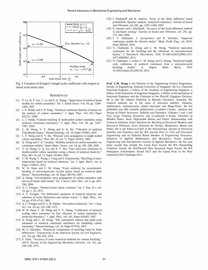
Fig. 3 Variation of Eringen’s length scale coefficient with respect to initial axial stress ratio

REFERENCES [1] P. Lu, H. P. Lee, C. Lu and P. Q. Zhang, “Application of nonlocal beam

models for carbon nanotubes,” Int. J. Solids Struct. Vol. 44, pp. 5289–5300, 2007.

[2] J. N. Reddy and S. D. Pang, “Nonlocal continuum theories of beams for the analysis of carbon nanotubes,” J. Appl. Phys. Vol 103, Paper 023511, 2008.

[3] L. J. Sudak, “Column buckling of multiwalled carbon nanotubes using nonlocal continuum mechanics,” J. Appl. Phys. Vol. 94, pp. 7281–7287, 2003.

[4] C. M. Wang, Y. Y. Zhang and X. Q. He, “Vibration of nonlocal Timoshenko beams,” Nanotechnology, vol. 18, Paper 105401, 2007.

[5] L. F. Wang and H. Y. Hu, “Flexural wave propagation in single-walled carbon nanotubes,” Phys. Rev. B, vol. 71, Paper 195412, 2005.

[6] Q. Wang and V. K. Varadan, “Stability analysis of carbon nanotubes via continuum models,” Smart Mater. Struct., vol. 14, pp. 281–286, 2005.

[7] Y. Q. Zhang, G. Q. Liu and X. Y. Xie, “Free transverse vibrations of double-walled carbon nanotubes using a theory of nonlocal elasticity,” Phys. Rev. B, vol. 71, Paper 195404, 2005.

[8] C. M. Wang, Y. Xiang, J. Yang and S. Kitipornchai, “Buckling of nano-rings/arches based on nonlocal elasticity,” Int. J. Appl. Mech., vol. 4, Paper 1250025, 2012.

[9] W. H. Duan and C. M. Wang, “Exact solutions for axisymmetric bending of micro/nanoscale circular plates based on nonlocal plate theory,” Nanotechnology, vol. 18, Paper 385704, 2007.

[10] Q. Wang, “Axi-symmetric wave propagation of carbon nanotubes with non-local elastic shell model,” Int. J. Struct. Stab. Dyn., vol. 6, pp. 285–296, 2006.

[11] A. C. Eringen, “Nonlocal polar elastic continua,” Int. J. Eng. Sci., vol. 10, pp. 1–16, 1972.

[12] A. C. Eringen, “On differential equations of nonlocal elasticity and solutions of screw dislocation and surface waves,” J. Appl. Phys., vol. 54, pp. 4703–4710, 1983.

[13] A. C. Eringen and D. G. B. Edelen, “On nonlocal elasticity,” Int. J. Eng. Sci., vol. 10, pp. 233–248, 1972.

[14] W. H. Duan, C. M. Wang and Y. Y. Zhang, “Calibration of nonlocal scaling effect parameter for free vibration of carbon nanotubes by molecular dynamics,” J. Appl. Phys., vol. 101, Paper 024305, 2007.

[15] Q. Wang and C. M. Wang, “The constitutive relation and small scale parameter of nonlocal continuum mechanics for modelling carbon nanotubes,” Nanotechnology, vol. 18, Paper 075702, 2007.

[16] M. G. Salvadori, “Numerical computation of buckling loads by finite differences,” Transactions of the American Society of Civil Engineers, vol. 116, pp. 590–624, 1951.

[17] P. Seide, “Accuracy of some numerical methods for column buckling,” ASCE Journal of the Engineering Mechanics Division, vol. 101, pp. 549–560, 1975.

[18] I. Elishakoff and R. Santoro, “Error in the finite difference based probabilistic dynamic analysis: analytical evaluation,” Journal of Sound and Vibration, vol. 281, pp. 1195–1206, 2005.

[19] R. Santoro and I. Elishakoff, “Accuracy of the finite difference method in stochastic setting,” Journal of Sound and Vibration, vol. 291, pp. 275–284, 2006.

[20] I. V. Andrianov, J. Awrejcewicz and D. Weichert, “Improved continuous models for discrete media,” Math. Probl. Eng., vol. 2010, Paper 986242, 2010.

[21] N. Challamel, Z. Zhang and C. M. Wang, “Nonlocal equivalent continuum for the buckling and the vibrations of microstructured beams,” J. Nanomech. Micromech., DOI: 10.1061/(ASCE)NM.2153-5477.0000062, 2013.

[22] N. Challamel, J. Lerbet, C. M. Wang, and Z. Zhang, “Analytical length scale calibration of nonlocal continuum from a microstructured buckling model,” Z. Angew. Math. Mech., DOI: 10.1002/zamm.201200130, 2013.

Prof. C.M. Wang is the Director of the Engineering Science Programme, Faculty of Engineering, National University of Singapore. He is a Chartered Structural Engineer, a Fellow of the Academy of Engineering Singapore, a Fellow of the Institution of Engineers Singapore, a Fellow of the Institution of Structural Engineers and the Chairman of the IStructE Singapore Division. He is also the Adjunct Professor in Monash University, Australia. His research interests are in the areas of structural stability, vibration, optimization, nanostructures, plated structures and Mega‐Floats. He has published over 400 scientific publications, co-edited 3 books: Analysis and Design of Plated Structures: Stability and Dynamics: Volumes 1 and 2 and Very Large Floating Structures and co‐authored 4 books: Vibration of Mindlin Plates, Shear Deformable Beams and Plates: Relationships with Classical Solutions, Exact Solutions for Buckling of Structural Members and Structural Vibration: Exact Solutions for Strings, Membranes, Beams and Plates. He is the Editor‐in‐Chief of the International Journal of Structural Stability and Dynamics and the IES Journal Part A: Civil and Structural Engineering and an Editorial Board Member of Engineering Structures, Advances in Applied Mathematics and Mechanics, Ocean Systems Engineering and International Journal of Applied Mechanics. He has won many awards that include the Lewis Kent Award, the IES Outstanding Volunteer Award, the IES/IStructE Best Structural Paper Award, the IES Prestigious Achievement Award 2013 and the Grand Prize in the Next Generation Port Challenge 2013.


ISBN: 978-1-61804-226-2 31

Abstract— In this work we consider a model for granular

medium. Reduced Cosserat Continuum is an elastic medium, which translations and rotations are independent, force stress tensor is asymmetric and couple stress tensor equal to zero. The main purpose of our work is to get system of thermodynamic equations for the CC.

Keywords— current configuration , energy coupling tensors, reduced Cosserat continuum, thermodynamic.

I. INTRODUCTION

IN this work we are aiming to establish a system of

thermodynamic equations for reduced Cosserat continuum. The idea of the reduced Cosserat continuum as an elastic medium is proposed as a model for granular medium as well. This type of medium and its behavior is very important in different branches of engineering and industrial applications such as mining, agriculture, construction and geological processes.

Most of the models suggest that the sizes of solid particles are negligible in comparison with typical distances between particles. Our model deals with granular materials where grain’s size and nearest-neighbour distance are roughly comparable. In contrast to solid bodies in granular materials there is no “rotational springs” that keep rotations of neighbouring grains. For example in the simplest case, solids can be modeled as an array of point masses connected by springs.

Originally an idea of an equal footing of rotational and translational degrees of freedom appeared in [1]. In that work authors obtained good correspondents between their theoretical results with experimental data. We used this work as in inspiration in our studies.

There are two well-known theories for described solids: moment theory of elasticity (Cosserat Continuum), moment theory of elasticity with constrained rotation (Cosserat

V. Lalin is with the Department of Structural mechanics, Saint Petersburg State Polytechnic University, Saint Petersburg, Russia (e-mail: vllalin@ yandex.ru).

E. Zdanchuk is with the Department of Structural mechanics, Saint Petersburg State Polytechnic University, Saint Petersburg, Russia (e-mail: [email protected]).

Pseudocontinuum). There exists a vast amount of literature on these models, such as [2], [3], [4], [5], [6]. A practical application of these models requires an experimental determination of a large number of additional constants in constitutive equations. These theories can still be applied to granular media although there are many other specific models describing this type of media [8], [9], [10], [11]. In recent papers [12], [13] more advanced Reduced Cosserat Continuum was suggested as possible model to describe granular materials. In this continuum translations and rotations are independent, stress tensor is not symmetric and couple stresses tensor equal to zero. A feature of this model that it has a classical continuum as its static limit. More advanced studies of this model were performed quit recently in the works [14], [15].

In this paper, we further develop results achieved in [17], [18], [19] for reduced Cosserat continuum as a suitable model for granular medium. In these works we have presented linear reduced Cosserat continuum equations, plane wave propagation and dispersion curves for an isotropic case. Here we present thermodynamic nonlinear reduced Cosserat continuum equations for the current configuration.

II. MATH In reduced Cosserat continuum each particle has 6 degrees

of freedom, in terms of kinematics its state is described by vector r and turn tensor P. The turn tensor is orthogonal tensor that is defined by 3 independent parameters with determinant equal to 1. Current position of the body at time t is called the current configuration (CC). Let us introduce a basis

ksk xtx ∂∂= /),( rr , a dual basis ),( txskr and a Hamiltonian

for the CC k

k

x∂∂

=∇ r.

A purpose of this work is to obtain thermodynamic equations for the nonlinear reduced Cosserat continuum as Eulerian description for the CC.

Here we list equations that are necessary to establish the system of equations for the CC:

a linear momentum balance equation

Nonlinear thermodynamic model for granular medium

Lalin Vladimir, Zdanchuk Elizaveta


ISBN: 978-1-61804-226-2 32

∫∫ ⋅=SV

dSdVdtd τnvρ

(1) a kinetic momentum balance equation

∫∫ ⋅×=×+⋅SV

dSdVdtd )()( τnrvrωJ ρρ

(2) an energy balance equation:

QdSdVdtd

SV

+⋅⋅=Π+⋅⋅+ ∫∫ vτnωJv )21

21( 2 ρρωρ

(3) and the Reynolds transport theorem

∫∫ =VV

dVAAdVdtd

ρρ (4)

where ρ is density for the CC, v - velocity vector )( rv = , r - radius vector for the CC, ω - angular velocity

vector )( PωP ×= , n - an outward unit normal to the surface S, J - mass density of an inertia tensor, Π - mass density of the

strain energy, (...)(...))...(

.∇⋅+

∂∂

= vt - material time

derivative, A - arbitrary scalar, vector or tensor field, V - volume limited by a surface S, Q - thermal power. To simplify calculations we assume that the body forces are equal to zero.

We shall combine equation (4), Gauss-Ostrogradskii theorem and equations (1) and (2). As a result we get motion equations for the CC:

vτ ρ=⋅∇ (5) )( ωJωJωτ ⋅+⋅×= ρx , (6)

where xτ denotes a vector invariant of tensor τ . A definition of this vector invariant was given by Lurie [20].

Equations (5) and (6) are the first two equations in our system describing CC.

Heat Q is sum of a heat coming into the volume V through its surface and a heat distributed in volume and can expressed as a following formula

∫∫∫ ⋅∇−=+⋅−=VVS

dVRRdVdSQ )( hhN ρρ. (7)

Here N is a unit normal vector to S, h is a heat flux vector, R is a heat source per unit mass.

After combining equations (3), (4), (7) and applying an

identity aAaAaA T ⋅∇⋅+⋅⋅∇=⋅⋅∇ )( we arrive at

∫ ∫ ⋅∇−+⋅∇⋅+⋅⋅∇=Π+⋅⋅+⋅V V

T dVRdV )()()( hvτvτωJωvv ρρ

. (8) Since volume V is an arbitrary volume, than using (8) and

equation (5) we obtain the following relation hωωJvτ ⋅∇−+⋅⋅−⋅∇⋅=Π RT ρρρ )(

(9) Now let us apply relation (6) for a second term in the right

hand side of an equation above. The latter combined with 0)( =⋅⋅× ωωω J results

)()( ωIτωτωωJ ×⋅⋅=⋅=⋅⋅− TTxρ .

The equality above was obtained with help of expression )()( aBAaBA ×⋅⋅=⋅⋅ x with B = I [21]. Now we can rewrite

the equation (9) in the following form hωIvτ ⋅∇−+×+∇⋅⋅=Π RT ρρ )(

. (10) A strain state for reduced Cosserat continuum is described

by a strain tensor ),( txke . We can define it for the CC as: TT PFIe ⋅−= −

, (11)

where F should satisfy a relationTRF ∇=−1

with R as a radius vector in the reference configuration.

Let us differentiate the expression (11) with respect to time,

using TT −− ⋅−∇= FvF and ωPP ×−= TT

to obtain rhe ωIvevωeee ×+∇=⋅∇+×+= D . (12)

From now we will use this short notation for hvhhh ⋅∇+×+= ωD for an arbitrary h. Value hD is shown

to be an objective derivative [11]. The equation (12) is the compatibility equation for the CC.

And its number 3 in our system of equations. After having introduced strain and stress, it is necessary to

establish a relation between them. This was done through constitutive equations. Let us substitute (12) in (10) and obtain

heτ ⋅∇−+⋅⋅=Π RDT ρρ (13) One can easily recognize the first law of thermodynamics in

(13). As we know from [20], the second law of thermodynamics

can be expressed as 0ln)( ≥∇⋅−⋅∇−− θρηρθ hhR , (14)

where ),( θηη e= is a unit entropy. Recombination of terms in the expression (13) gives us

eτh DR T ⋅⋅−Π=⋅∇− ρρ . Let us substitute this into (14) to get

0ln ≥∇⋅−⋅⋅+Π− θρηρθ heτ DT

Further, we use θη−Π=f - the Helmholtz free-energy

function, where θ is a temperature. With equation above this results in

0ln)( ≥∇⋅−+−⋅⋅ θηθρ heτ fDT. (15)

Applying a techniques describing in [21] we can get

θθ

∂∂

+⋅⋅∂

∂=

fDffT

ee . (16)

Substituting (16) into (15) we obtain

0ln)()( ≥∇⋅−+∂∂

−⋅⋅∂∂

− θθηθ

ρρ hee

τ

fDf T

. (17) It is shown in [20] that equation (17) holds only if

0=∂∂

−e

τ fρ,

0)( =+∂∂ ηθ

ρ f, 0ln ≥∇⋅− θh ,

which leads us to the following result


ISBN: 978-1-61804-226-2 33

eτ

∂∂

=fρ

(18)

ηθ

=∂∂

−f

(19) In our case a mass density Π is a function of two

arguments: a strain state e and a temperatureθ . A partial derivative of Π with respect to e can be transformed in the following way

eeeeeeee ∂∂

=∂∂

−∂∂

+∂∂

=∂∂

∂∂

+∂∂

+∂∂

=∂Π∂ ffff )( θθηθ

θθη

, (20)

Here we used definition of f and expression (19). Using this expression (20) and the equation (18) arrive at

eτ

∂Π∂

= ρ. (21)

The expression (21) is the constitutive equation for the CC. In order to obtain next equation for the CC we need to refer

back to the expression (13). For that we introduce )( ηθρϕ +−⋅⋅= fDT eτ - as unit energy dissipation.

In the elastic medium 0=ϕ , thus thermal conductivity equation has a following simple form

h⋅∇−= Rρηρθ . (22) Since we consider isotropic media θ∇−= kh , where k

denotes the coefficient of thermal conductivity.

Time derivative of ),( θηη e= in combination with technique describing in [21] results in

TD )( ee

⋅⋅∂∂

+∂∂

=ηθ

θηη

. And with help of formula (21) we arrive at

θρηρθθθηρθ ∇⋅∇+=⋅⋅

∂∂

+∂∂ kRD T)( e

e

. (23) Combining formulas (18) and (19) results in

θρη

∂∂

−=∂∂ τ

e1

. (24)

Now we introduce θηθχ

∂∂

= - the specific heat capacity of

constant deformation. After substitution of χ and (24) into (23) we arrive to the

following equation TDkR )( eτ

⋅⋅∂∂

+∇⋅∇+=θ

θθρθρχ . (25)

The last equation is a heat conductivity equation for the CC and it is the fifth equation in our system.

The system of equation for the CC will not be full without the mass conservation law [22]

0=⋅∇+ vρρ . (26)

III. RESULTS Here we gather all the equation in our system:

motion equations vτ ρ=⋅∇ ,

)( ωJωJωτ ⋅+⋅×= ρx , the compatibility equation

ωIvevωee ×+∇=⋅∇+×+ , the constitutive equation

eτ

∂Π∂

= ρ,

the heat conductivity equation TDkR )( eτ

⋅⋅∂∂

+∇⋅∇+=θ

θθρθρχ ,

the mass conservation law 0=⋅∇+ vρρ .

This system depends on the following unknown functions: 9 stresses τ , 9 strains e , 6 velocities v ,ω , temperature θ and density ρ. As a result we have 26 unknown functions. The problem becomes fully set after adding the boundary and initial conditions.

The main advantage of our work is that our description for the CC does not contain kinematic unknown r, P as well as strain gradient F. Although unknown r, P can be found by

integrating equations rv = , PωP ×= after solving the system of equation.

.

REFERENCES [1] Schwartz L.M., Johnson D.L., Feng S. “Vibrational modes in granular

materials” in Physical review letters, v. 52, 10, 1984. pp.831-834. [2] Neff P., Jeong J. “A new paradigm: the linear isotropic Cosserat model

with conformally invariant curvature energy” in ZAMM Zeitschrift fur Angewandte Mathematik und Mechanik. vol.89, 2, February 2009, pp 107-122.

[3] Jasiuk I., Ostoja-Starzewski M. “On the reduction of constants in planar cosserat elasticity with eigenstrains and eigencurvatures” in Journal of Thermal Stresses. 26 (11-12), 2003. pp.1221-1228.

[4] Khomasuridze N.G. “The symmetry principle in continuum mechanics” in Journal of Applied Mathematics and Mechanics. 71 (1), 2007. pp. 20-29.

[5] Arslan H., Sture S. “Finite element simulation of localization in granular materials by micropolar continuum approach” in Computers and Geotechnics. 35 (4), 2008. pp. 548-562.

[6] Jeong J., Neff P. “Existence, uniqueness and stability in linear cosserat elasticity for weakest curvature conditions” in Mathematics and Mechanics of Solids. 15 (1), 2010. pp. 78-95.

[7] Ieşan D. “Deformation of porous Cosserat elastic bars” in International Journal of Solids and Structures. 48 (3-4), 2011. pp. 573-583.

[8] Badanin A., Bugrov A., Krotov A. The determination of the first critical load on particulate medium of sandy loam foundation // Magazine of Civil Engineering. 9. 2012. Pp 29-34. (in Russian).

[9] Harris D. “Double-slip and Spin: A generalisation of the plastic potential model in the mechanics of granular materials” in International Journal of Engineering Science. Volume 47, Issues 11–12, 2009. pp.208-1215.

[10] Heinrich M. Jaeger, Sidney R. Nagel. “Granular solids, liquids, and gases” Reviews of modern physics. vol.68, 4, 1996. pp 1259-1273.


ISBN: 978-1-61804-226-2 34

http://www.scopus.com/source/sourceInfo.url?sourceId=27970&origin=recordpage



http://www.scopus.com/authid/detail.url?origin=resultslist&authorId=7003549031&zone=


http://www.scopus.com/record/display.url?eid=2-s2.0-0344271820&origin=resultslist&sort=plf-f&src=s&st1=reduced+Cosserat+Continuum&sid=B69A4977BF0C90A697DB4B3D023FD955.Vdktg6RVtMfaQJ4pNTCQ%3a40&sot=b&sdt=b&sl=41&s=TITLE-ABS-KEY%28reduced+Cosserat+Continuum%29&relpos=19&relpos=19&citeCnt=3&searchTerm=TITLE-ABS-KEY%28reduced+Cosserat+Continuum%29



http://www.scopus.com/source/sourceInfo.url?sourceId=20987&origin=resultslist

























[11] Kurbatskiy E.N., Golosova O.A.” Features of the propagation of stress waves in natural and artificial granular media” in Structural mechanics and calculation of structures. 2, 2011. pp. 45-50. (in rus).

[12] Grekova E.F., Herman G.C.” Wave propagation in rocks modelled as reduced Cosserat continuum” in proceedings of 66th EAGE conference, Paris, 2004.

[13] Grekova E.F., Kulesh M.A., Herman G.C. “Waves in linear elastic media with microrotations, part 2: Isotropic reduced Cosserat model” in Bulletin of the Seismological Society of America. 99 (2 B), 2009. pp. 1423-1428.

[14] Harris D. Douple-slip and Spin: Dilatant Shear in a Reduced Cosserat Model. Modern Trends in Geomechanics. Springer, 2006.

[15] Grekova E.F.” Linear reduced cosserat medium with spherical tensor of inertia, where rotations are not observed in experiment” in Mechanics of solids. vol 47, issue 5, 2012. pp538-543.

[16] Grekova E.F.”Nonlinear isotropic elastic reduced Cosserat continuum as a possible model for geomedium and geomaterials. Spherical prestressed state in the semilinear material” in Journal of seismology. vol 16, issue 4, 2012. pp695-707.

[17] Lalin V., Zdanchuk E. “On the Cauchy problem for nonlinear reduced Cosserat continuum” in Proceedings of the XXXIX Summer School – Conference ADVANCED PROBLEMS IN MECHANICS, Saint Petersburg. 2011.

[18] Lalin V., Zdanchuk E. “A model of continuous granular medium. Waves in the reduced Cosserat continuum” in Magazine of Civil Engineering. 5(31). 2012. Pp65-71. (in Russian).

[19] Zdanchuk E., Lalin V. “The theory of continuous medium with free rotation without coupled stresses” in Proceedings of the XXXVIII Summer School – Conference ADVANCED PROBLEMS IN MECHANICS, Saint Petersburg. 2010

[20] Lurie A.I. Nonlinear theory of elasticity. Amsterdam. 1990. [21] Lalin V. “Non-linear dynamics equations of the moment elastic

medium” in Scientific and Technical Sheets SPbGPU. 2007. (in Russian).

[22] Zhilin P.A. “A new approach to the analysis of free rotations of rigid bodies” in ZAMM-Z. angew. Math.Mech, 76, 4, 1996. pp187-204.


ISBN: 978-1-61804-226-2 35





Application of the bi-Helmholtz type nonlocal elasticity on the free vibration problem of carbon

nanotubes

C. Chr. Koutsoumaris and G. J. Tsamasphyros

Division of Mechanics School of Applied Mathematical and Physical Sciences

National Technical University of Athens Athens

e -mail: [email protected]

Abstract—Recent studies have shown that classical continuum theories are insufficient to accurately and meticulously describe deformation phenomena in the regime of small scales. Thus, enhanced or higher-grade continuum theories that account for lower-scale-driven processes have been proposed. Until now, all the studies on the dynamical response of single carbon nanotubes were based on Helmholtz-type nonlocal beam models. A study [1] on bars shows that the bi-Helmholtz model is more appropriate to fit molecular dynamics results (Born-Karman). In this study, we investigate the bi-Helmholtz type nonlocal elasticity for the free vibration problem of a single walled carbon nanotube, considering three different boundary conditions (cantilever, simply supported, clamped-clamped beam).

Keywords—Nonlocal Elasticity, Beams, Carbon Nanotubes, eigenfrequencies.

I. INTRODUCTION

Since the discovery of carbon nanotubes (CNTs) at the

beginning of the 1990s [2], extensive research related to nanotubes in the fields of chemistry, physics, materials science and electrical engineering has been reported. Mechanical behavior of CNTs, including vibration analysis, has been the subject of numerous studies [10,12–14]. Since controlled experiments at nanoscale are difficult and molecular dynamics simulations remain expensive and formidable for large-scale systems, continuum mechanics models, such as the classical Euler elastic-beam model, have been effectively used to study overall mechanical behavior of CNTs.

Τhe applicability of classical continuum models at very small scales is questionable, since the material microstructure at small size, such as lattice spacing between individual atoms, becomes increasingly important and the discrete structure of the material can no longer be homogenized into a continuum. Therefore, the modified continuum theories, such as nonlocal, may be an alternative to take into account the scale effect in the studies of nanomaterials.

The theory of nonlocal continuum mechanics and nonlocal elasticity was formally initiated by the papers of Eringen and Edelen [3 – 6]. Application of nonlocal continuum theory in nanomaterials was initially addressed by Peddieson et al. [7], in which they applied the nonlocal elasticity to formulate a nonlocal version of Euler–Bernoulli beam model, and concluded that nonlocal continuum mechanics could potentially play a useful role in nanotechnology applications.

Considering the study of the free vibration problem for carbon nanotubes, there exists significant literature in the framework of non-local theory (see for example [9,10,12]). Most approaches are based on the Helmholtz operator proposed by Eringen [3,6]. A study [1] on bars show that bi-Helmholtz model is more appropriate to fit molecular dynamics results (Born-Karman). Considering this study, we investigate the bi-Helmholtz type nonlocal elasticity for the free vibration problem of a single walled carbon nanotube considering three different boundary conditions (cantilever, simply supported, clamped-clamped beam)

II. GOVERNING EQUATIONS

A. General equations of Non Local Elasticity For homogeneous and isotropic solids the linear theory is

expressed by the following set of equations [3,6]

, ( ) 0kl k l lt f uρ+ − = (1)

( ) ( , ) ( ) ( )kl klVt K dτ σ υ′ ′ ′ ′= −∫x x x x x (2)

( ) ( ) 2 ( )kl rr kl kle eσ λ δ µ′ ′ ′= +x x x (3)

1 ( ) ( )( )

2k l

kl

l k

u ue

x x

′ ′∂ ∂′ = +

′ ′∂ ∂

x xx (4)


ISBN: 978-1-61804-226-2 36


where ,klt ,ρ lf and lu are, respectively, the components of the stress tensor, the mass density, the body force density vector components and the displacement vector components at a reference point x in the body at time t. Further, ( )klσ ′x is the

classical stress tensor at ′x which is related to the linear strain tensor ( )kle ′x at any point ′x in the body at time t via the Hooke law, with λ and μ being Lamé constants. It is readily observable that the only difference between (1) – (4) and the respective equations of classical elasticity is the expression of the stress tensor (2) which replaces Hooke’s Law (3). The volume integral in (2) is evaluated over the region V of the body.

The Equation (2) expresses the contribution of other parts

of the body in the stress at point x through the attenuation function (nonlocal modulus) ( , )K τ′ −x x . From the structure of (2), we conclude that the attenuation function [5,8] has the dimension of (length)-3. Therefore, it should depend on a characteristic length ratio /a , where a is an internal characteristic length i.e. lattice parameter/bond length and is an external characteristic length i.e. crack length, wave length. Consequently, the expression of K in a more appropriate form is ( , )K K τ′= −x x , 0 /e aτ = (5)

where 0e is a dimensionless constant. The nonlocal modulus has the following properties: i) When τ (or a ) 0→ , K must revert to the Dirac generalized function, so that classical elasticity limit is obtained in the limit of vanishing internal characteristic length.

0lim ( , ) ( )Kτ

τ δ→

′ ′− = −x x x x (6) (6)

ii) It acquires its maximum at ′ =x x , attenuating with ′ −x x . iii) If K is a Green’s function of a linear differential operator i.e. if

[ ]( , ) ( )L K τ δ′ ′− = −x x x x (7) (7)

then applying the operator L to eq.(2), we obtain:

kl klLt σ= (8) (8)

In this paper, we use the nonlocal modulus

( ) ( ) 2 2

1 2

1 21 21 1

( ) exp exp2

/ /BHK x c cc c

x c x c=−

− − −

(9) which is the Green’s function of the following bi Helmholtz operator [6,8]

2 2 2 42 2 2 2 2 2

1 2 1 2 1 22 2 2 41 1 1 ( )BH d d d d

L c c c c c cdx dx dx dx

= − − = − + +

2 4

2 4

2 41

d d

dx dxε γ= − + (10)

where 2 2 2

1 2c cε = + and 4 2 2

1 2c cγ = 1c and 2c are given by the expressions:

2 42

1 41 1 4

2c

ε γ

ε= + −

2 42

2 41 1 4

2c

ε γ

ε= − −

where 4

40 1 4

γ

ε≤ −

In the case of 4 4

1 24 , are real 2c cγ ε ε γ= = ⇒ = And the kernel has the following form [8]:

( ) ( )2

1 1( , ) exp /

2 2BHK x x xγ γ γγ

= + −

1

(0, )4BHK γγ

= (11)

In the case where 0

2

e aγ = the modulus (10) can be write as:

( )0 0

2

0

1 1( , ) exp

2 2 2/BH

e a e aK x x x

e aγ = + −

(12) the operator takes the form:

( ) ( )42 42 0

0 2 41 14

BH d e a dL e a

dx dx= − + (13)

A variant of the above operator is for 0e aγ =

( ) ( )2 4

2 4

0 02 42 1 2BH d dL e a e a

dx dx= − + (14)

We also used the classical Helmholtz nonlocal modulus to

make a comparison between the results obtained by each modulus.

The Helmholtz nonlocal modulus has the form:

( )0

0

1( , ) exp /

2HK x x e ae a

γ = − (15)

which is the Green’s function of the following operator [3,6]

( )2

2

0 21H d

L e adx

= − (16)

At this point it is useful to show the two kernels to comparing these.


ISBN: 978-1-61804-226-2 37

ea=0.1

ea=0.2

0.2 0.4 0.6 0.8 1.0s

1

2

3

4

5K0.5, s

Figure 1. The nonlocal modulus HK (dashed line),

( )1 2continuous line,BHK c c= at x = 0.5 for different values of e0a

B. Differential equation for Euler Bernoulli beam

The Euler Bernoulli beam theory (EBT) is based on the displacement field

( )1 ,w

u u x t zx

∂= −

∂ 2 0u = ( )3 ,u w x t= (17)

Where (u,w) are the axial and transverse displacements of the point (x,0) on the middle plane of the beam. In the EBT the only non zero strain is:

2

0

2xx xx

u wz z

x xε ε κ

∂ ∂= − ≡ +∂ ∂

(18)

Where 0

xxε is the extensional andκ is the curvature The equations of motion are given by

( )2

0 2,

N uf x t m

x t+

∂ ∂=

∂ ∂ (19)

and

2 2 4

0 22 2 2 2ˆM w w w

m m q Nx t t x x x

∂ ∂ ∂ ∂ ∂= − − +

∂ ∂ ∂ ∂ ∂ ∂

(20)

Where f(x,t), q(x,t) are the axial force per unit length and

transverse force per unit length, respectively. N is the axial force, M is the bending moment which are defined

asxx

A

N dAσ= ∫ , xx

A

M z dAσ= ∫ where xxσ is the classical

axial stress on the yz section in the direction of x. The mass inertias 0m and 2m are defined by

0

A

m dA Aρ ρ= =∫ and 2

2

A

m z dA Iρ ρ= =∫

where I denotes the second moment of area about y axis.

C. Differential equation for non local Euler Bernoulli beam Applying the operator (10) in equation (8) and considering

that xx xxEσ ε= ,where E is the Young’s modulus of the

material and 2

2

o

xx xx

uz z

x x

wε ε κ

∂ ∂= + = −

∂ ∂ (Euler Bernoulli

Theory - EBT), we obtain the following expressions:

,xx xx xx

BHxx

HL L tτ σ σ== (20a,b) or

22

21 xxxx E

xε τ ε

∂−

∂

=

(21)

2 4

2 4

2 41 xx xxE

x xtε γ ε

∂ ∂− +

∂ ∂=

(22)

where xxτ and xxt are the nonlocal stresses for the two modulus, respectively.

The non local axial force and bending moment defined as follow for each of the cases (21,22):

i) xx

A

HNLN dAτ= ∫ xx

A

HNLM z dAτ= ∫ (23a,b)

ii) xx

A

BHNLN dAt= ∫ xx

A

BHNLM zt dA= ∫ (24a,b)

The process for constructing the differential equation refers to the operator BHL . Integrating the (20b), we obtain:

(24 )

xx xx

A A

aBHL t dx dxσ= ⇒∫ ∫

2 4

2

2 4

4BH BH

oNL NLxx

BHNL

N NN EA

x xNε εγ∂ ∂

− + = =∂ ∂

(25)

(24 )

xx xx

A

bBH

A

L zt dx z dxσ= ⇒∫∫

2 4

2

2 4

4BH BH

NL NLBHNL

M MM EI M

x xε κγ∂ ∂

− + = =∂ ∂

(26)

Consider that


ISBN: 978-1-61804-226-2 38

2 2

0 02 2

BH BHNL NLN u N u

f m m fx t x t

or∂ ∂ ∂ ∂+ = = −

∂ ∂ ∂ ∂ (27)

And

2 2 4

0 22 2 2 2ˆ

BH

NLM w w wm m q N

x t t x x x

∂ ∂ ∂ ∂ ∂= − − +

∂ ∂ ∂ ∂ ∂ ∂

(28)

Substituting for the first and third derivative of N from (27) into (25), we obtain

3 2 32 4

0 02 2 2

BH

NL

u u f u fN EA m m

x t x x x t x xε γ

∂ ∂ ∂ ∂ ∂ ∂= + − − −

∂ ∂ ∂ ∂ ∂ ∂ ∂ ∂

(29)

Substituting N from (29) into the equation of motion (27) we obtain:

2

4 2

0 2 2 2

u u fEA f m

x x t x xε

∂ ∂ ∂ ∂+ + − −

∂ ∂ ∂ ∂ ∂

6 4 2

0 02 4 4 2

4 0u f u

m mt x x t

γ∂ ∂ ∂

− − − =∂ ∂ ∂ ∂

(30)

Similarly, substituting the second and fourth derivative of M from (28) into (26) we obtain:

2 2 42

0 22 2 2 2ˆBH

NLw w w w

M EI m m q Nx t t x x x

ε∂ ∂ ∂ ∂ ∂

= − + − − +∂ ∂ ∂ ∂ ∂ ∂

4 6 2 34

0 22 2 2 4 2 3ˆw w q w

m m Nt x t x x x x

γ∂ ∂ ∂ ∂ ∂

− − − +∂ ∂ ∂ ∂ ∂ ∂ ∂

(31)

Substituting M from (31) into (28) we obtain: 2 2 2 2 4

2

0 22 2 2 2 2 2

2 4 6 2 34

0 22 2 2 2 4 2 3

ˆ

ˆ

w w w wEI m m q N

x x x t t x x x

w w q wm m N

x t x t x x x x

ε

γ

∂ ∂ ∂ ∂ ∂ ∂ ∂− + − − +

∂ ∂ ∂ ∂ ∂ ∂ ∂ ∂

∂ ∂ ∂ ∂ ∂ ∂− − − +

∂ ∂ ∂ ∂ ∂ ∂ ∂ ∂

2 4

0 22 2 2ˆ

w w wq N m m

x x t t x

∂ ∂ ∂ ∂+ − = −

∂ ∂ ∂ ∂ ∂

(32)

In the case of pure bending (m2=0)

2 22

02 2ˆBH

NLw w w

M EI m q Nx t x x

ε∂ ∂ ∂ ∂

= − + − +∂ ∂ ∂ ∂

4 2 34

0 2 2 2 3ˆw q w

m Nt x x x x

γ∂ ∂ ∂ ∂

− − +∂ ∂ ∂ ∂ ∂

(33)

and the equation takes the form:

2 2 2 22

02 2 2 2

2 4 2 3

02 2 2 2 3

ˆ

ˆ

w w wEI m q N

x x x t x x

w q wm N

x t x x x x

ε

γ

∂ ∂ ∂ ∂ ∂ ∂− + − +

∂ ∂ ∂ ∂ ∂ ∂

∂ ∂ ∂ ∂ ∂− − +

∂ ∂ ∂ ∂ ∂ ∂

2

0 2ˆ w w

q N mx x t

∂ ∂ ∂+ − =

∂ ∂ ∂

(34)

The same equation arises from the principle of virtual displacements as shown below:

( ) ( )[ ]

0 0

2 2

0 2 0

2

2, , 0

T L

BHNL

BHNL

u u w w w wm m m

t t x t x t t t

u wN M f x t u q x t w dxdt

x x

δ δ δ

δ δδ δ

∂ ∂ ∂ ∂ ∂ ∂+ + −

∂ ∂ ∂ ∂ ∂ ∂ ∂ ∂

∂ ∂− + + + =

∂ ∂

∫ ∫

(35)

Taking into account the (29) and (31), we have:

3 5 32

0 02 2 3 3

2 2 42

0 22 2 2 2

2 2

0 2 00 0

0

4

T L

L u u f u fEA m mx t x x t x x

w w wEI m m qx t t x

u u w w w wm m m dxt t x t x t t t

u dxx

ε

ε

δ δ δ

δγ

∂ ∂ ∂ ∂ ∂ + − − − ∂ ∂ ∂ ∂ ∂ ∂ ∂

∂ ∂ ∂ ∂− + − − +

∂ ∂ ∂ ∂

∂ ∂ ∂ ∂ ∂ ∂+ + −∂ ∂ ∂ ∂ ∂ ∂ ∂ ∂

∂−∂

+

∫ ∫

∫

4 6 2 34

0 22 2 2 4 2 3

0

2

2

ˆ

ˆ

L wNx x

w w q wm m Nt x t x x x x

w dxx

γ δ

∂ ∂ ∂

∂ ∂ ∂ ∂ ∂ − − − + ∂ ∂ ∂ ∂ ∂ ∂ ∂

∂∂

∫

( ) ( )[ ]0

, , 0L

f x t u q x t w dx dtδ δ+ + =

∫ (36)

Neglected m2 [pure bending (m2=0)]and axial force N

2 2

0 2 00 0

3 5 32

0 02 2 3 30

2 2 42 4

0 02 2 2 2

4

T L

L

u u w w w wm m m dx

t t x t x t t t

u u f u f uEA m m dx

x t x x t x x x

w w wEI m q m

x t t x

δ δ δ

δε

ε γ

γ

∂ ∂ ∂ ∂ ∂ ∂+ + −

∂ ∂ ∂ ∂ ∂ ∂ ∂ ∂

∂ ∂ ∂ ∂ ∂ ∂− + − − −

∂ ∂ ∂ ∂ ∂ ∂ ∂ ∂

∂ ∂ ∂+ − + − −

∂ ∂ ∂ ∂

∫ ∫

∫

( ) ( )[ ]

2 2

2 20

0

, , 0 (37)

L

L

q wdx

x x

f x t u q x t w dx dt

δ

δ δ

∂ ∂−∂ ∂

+ + =

∫

∫

It can be verified that the Euler-Langrage equations associated with the variational statement in (37) are indeed the same as (30) and (34). Indicatively the bending equation is:

2 2 2 2

2

0 02 2 2 2

w w wm EI m q

t t x x x tε

∂ ∂ ∂ ∂ ∂ ∂− − + − −∂ ∂ ∂ ∂ ∂ ∂

( )2 4 2

4

02 2 2 2, 0

w qm q x t

x t x xγ

∂ ∂ ∂− − + =

∂ ∂ ∂ ∂

(38)

In addition the natural boundary conditions at x= 0,L are obtained:

Q =2

2

wEI

x x

∂ ∂−∂ ∂

22

0 2

wm q

x tε

∂ ∂+ −

∂ ∂


ISBN: 978-1-61804-226-2 39

4 2

4

0 2 2 2

w qm

x t x xγ

∂ ∂ ∂− −

∂ ∂ ∂ ∂

(39)

M =2

2

wEI

x−

∂

∂2

2

0 2

wm q

tε

∂+ −

∂

4 24

0 2 2 2

w qm

t x xγ

∂ ∂− −

∂ ∂ ∂

(40)

III. FREE VIBTRATION PROBLEMS In this section we study the free vibration problem for

three different boundary conditions. We assume constant material and geometric properties. The governing equation is obtained form (38).

For free vibration we suppose that q(x,t)=0. Equation (38) takes the form:

4 4 62 4

0 0 04 2 2 2 40

w w w wEI m m m

x t x t x t tε γ

∂ ∂ ∂ ∂ ∂− + + − =

∂ ∂ ∂ ∂ ∂ ∂ ∂

(41)

and the generalized forces become:

Q =3

3

wEI

x

∂−

∂

32

0 2

wm

t xε

∂+

∂ ∂

54

0 2 3

wm

t xγ

∂−

∂ ∂

(42)

M =2

2

wEI

x−

∂

∂

22

0 2

wm

tε

∂+

∂

44

0 2 2

wm

t xγ

∂−

∂ ∂

(43)

In order to calculate the eigenfrequencies, we seek periodic

solutions of the form ( ) ( ), i tw x t x e ωϕ= where ( )xϕ is the mode shape and ω is the natural frequency. After straightforward calculations, we obtain the following equations:

( ) ( )4 2

2 2 2

0 0 04 2

4 2 0d d

EI m m mdx dx

ϕ ϕγ ω ω ω ϕε− =+ − (44)

( )Q x =3

3

dEI

dx

ϕ− 2 2

0

dm

dx

ϕε ω−

34

0 3

2 dm

dx

ϕω γ+

(45)

( )M x =2

2

dEI

dx

ϕ− ( )2

0

2 mω ε ϕ−2

4

0 2

2 dm

dx

ϕω γ+

(46)

The general solution of (44) is:

( ) ( ) ( ) ( ) ( )1 2 3 4sin cos sinh coshx c ax c ax c x c xϕ β β= + + +

(47)

where:

( ) ( )( )2

0

2 2 2 4 2

0 04 2

0

14

2EI m

EI ma m mγ ω

γ ωε ω ω−

−= +

( ) ( )( )2

02

0

2 2 2 4 20 04

14

2EI m

EI mm mγ ω

γ ωβ ε ω ω−

−= − +

(48a,b)

A. Cantilever beam For this problem the boundary conditions are:

( )0 0ϕ = , ( )0 0ϕ′ = ( )ˆ 0M L = , ( )ˆ 0Q L = (49) Use of the boundary conditions leads to the condition:

1 40c c+ = ,

1 40c ca β+ =

( )( )( )

( )( )( )

2 2 2 2

0 0 1 2

2 2 2 2

0 0 3 4

4

4

sin cos

sinh cosh 0

EI m a m c aL c aL

EI m m c L c L

γ ω ε ω

γ ω β ε ω β β

− − +

− + + =

−

( )( )( )

( )( )( )

2 2 2 2

0 0 1 2

2 2 2 2

0 0 3 4

4

4

cos sin

cosh sinh 0

a EI m a m c aL c aL

EI m m c L c L

γ ω ε ω

β γ ω β ε ω β β

− − −

− + + =

−

(50)

To calculate the eigenfrequencies ωn, n=1,2,…N of a cantilever beam we have to set the determinant of the coefficient matrix in (50) to zero.

B. Simply supported beam For this problem the boundary conditions are:

( )0 0ϕ = ( ) 0Lϕ = ( ) ( )ˆ ˆ0 0, 0M M L= = (51)

To calculate the eigenfrequencies ωn, n=1,2,…N of simply supported beam we follow the same procedure as that in the case of the cantilever beam.

C. Clamped clamped beam For this problem the boundary conditions are

( )0 0ϕ = ( ) 0Lϕ = ( )0 0ϕ = ( ) 0Lϕ′ = (52)

Respectively the eigenfrequencies ωn, n=1,2,…N of clamped-clamped beam we follow the same procedure as that in the case of the cantilever beam and simply supported beam.

IV. RESULTS AND DISCUSSION

A. Results Numerical results are presented using the properties of carbon nanotubes. The following values of the parameters [10] are used E=1TPa, L=100nm, ρ=2300 kg/m,3 d= 91 10 m−× ,

A= 19 27.85 10 m−× ,4

38 44.91 1064

dI m

π −= = ×


ISBN: 978-1-61804-226-2 40

Table 1 The eigenfrequencies (ωn) of the cantilever beam

Table 2 The eigenfrequencies (ωn) of the simply supported beam

Table 3 The eigenfrequencies (ωn) of the Clamped – Clamped beam

The eigenfrequencies for each kind of boundary conditions (cantilever, simlpy supported and clamped-clapmed) are presented in table 1, 2 and 3. In the first column is the number of mode “n”, in the second column are the first nine eigenfrequencies corresponding to the classical ( )0 0e a = EBT. In the other three columns are the results from the nonlocal theory using three different operators HL and

1 2,BH BHL L . For all cases the nonlocal parameter 0e a has the

value of 80.1 10L m−× = .

The above results are presented in the following diagrams. The eigenfrequencies are dimensionless. In each problem, all the eigenfrequencies are divided by the fundamental eigenfrequency of the classical theory (EBT).

The conclusions of the study of the bi-Helmholtz nonlocal operator are summarized as follows:

For all cases of boundary conditions, almost all the eigenfrequencies are smaller than those of classical theory, but also from those yielded by the Helmholtz operator. This means that essentially our model presents lower stiffens response. The only exception is the fundamental natural frequency in the case of the cantilever beam.

The variation of results especially in high eigenfrequencies is quite large , exceeding 50 % for ω9 compared with this form the Helmholtz operator.

figure 1 The first nine Dimensionless eigenfrequencies of the cantilever beam

Figure 2 The first nine Dimensionless eigenfrequencies of the simply supported beam

Figure 3 The first nine dimensionless eigenfrequencies of the claped-clapmed beam

Mode Classic (GHz)

HL (GHz) 1

BHL (GHz) 2

BHL (GHz)

1 1.8335 1.8415 1.8412 1.8485 2 11.491 10.784 10.727 9.9857 3 32.174 26.629 25.801 21.226 4 63.048 44.686 41.075 29.913 5 104.63 63.288 54.106 35.961 6 156.45 81.733 64.333 40.001 7 217.75 99.904 70.214 42.795 8 289.51 118.24 78.083 44.746 9 371.86 135.47 82.631 46.174

Mode Classic (GHz)

HL (GHz) 1

BHL (GHz) 2

BHL (GHz)

1 5.1469 4.9102 4.9048 4.6865 2 20.587 17.432 17.194 14.763 3 46.322 33.710 32.076 24.531 4 82.350 51.277 46.017 31.929 5 129.21 69.100 57.605 37.109 6 185.42 86.835 66.733 40.695 7 252.42 104.74 73.784 43.213 8 329.12 122.29 79.215 45.021 9 417.75 139.42 83.426 46.351

Mode Classic (GHz)

HL (GHz) 1

BHL (GHz) 2

BHL (GHz)

1 11.667 11.008 10.947 10.243 2 32.162 26.587 25.763 21.160 3 63.049 44.699 41.086 29.940 4 104.24 63.281 54.102 35.947 5 156.73 81.738 64.335 40.010 6 217.42 99.900 72.145 44.751 7 290.18 118.61 78.084 46.170 8 372.14 135.72 82.631 47.227 9 464.50 153.46 86.154 48.0316


ISBN: 978-1-61804-226-2 41

From all the models (Classic, HL , 1 2,BH BHL L ) that were used in this study the bi-Helmholtz operator appear to be in better agreement comparing with results from selected studies [15] of the theory of molecular dynamics.

The choice of bi Helmholtz operator is more appropriate for the dynamical analysis of nanotubes, under the consideration that limitations are arising on possible values of the parameter 0e a .

The next step of the study is to develop computational molecular dynamics simulation to calculate the eigenfrequencies due to the strong dispersion of results in existing studies[12,13,14,15]

ACKNOWLEDGMENT This research has been co-financed by the European Union (European Social Fund—ESF) and Greek national funds through the Operational Program ‘Education and Lifelong Learning’ of the National Strategic Reference Framework (NSRF). Project title: “THALIS-NTUA-Development of self healing composite materials and innovative techniques for structural health monitoring on aerospace applications”

REFERENCES

[1] D.A. Fafalis, S.P. Filopoulos and G.J. Tsamasphyros, “On the capability of generalized continuum theories to capture dispersion characteristics at the atomic scale”, European Journal of Mechanics A/Solids, vol. 36 pp 25-37, 2012

[2] S. Iijima, “Helical microtubules of graphitic carbon”, Nature 354, p. 56, 1991.

[3] A.C. Eringen, “On differential equations of nonlocal elasticity and solutions of screw dislocation and surface waves”, J. Appl. Phys., 54, pp.4703 – 4709, 1983

[4] A.C. Eringen and D. G. B. Edelen, “On nonlocal elasticity”, Int. J. Engng. Sci. 10, pp. 233 – 248, 1972

[5] A.C. Eringen, “Theory of nonlocal elasticity and some applications”, Res. Mechan. 21, pp.313 – 342, 1987.

[6] A.C. Eringen, Nonlocal Continuum Field Theories, Springer – Verlag, New York , 2002

[7] Peddieson, J., Buchanan, R.G., McNitt, P.R. (2002), “Application of nonlocal continuum models to nanotechnology”, Int. J. Engng. Sci. 41,pp. 305 – 312.

[8] Lazar, M., Maugin, A.G., Aifantis, C. E., 2005. “On a theory of nonlocal elasticity of bi- Helmholtz type and some applications”, Int. J. Solids Struct. 43, 1404 – 1421.

[9] J. N Reddy, “Nonlocal theories for bending, buckling and vibration of beams”, International Journal of Engineering Science, vol. 45, pp. 288-307, June 2007.

[10] J. N Reddy and S.D. Pang,“Nonlocal continuum theories of beams for the analysis of carbon nanotubes”, Journal of Applied Physics, vol. 103, pp. 023511, 2008.

[11] M.A. Eltaher, Amal E. Alshorbagy and F.F. Mahmoud, “Vibration analysis of Euler-Bernoulli nanobeams by using finite element method”, Applied Mathematical Modelling, vol 37, pp 4784-4797, 2013

[12] R. Ansari and S. Sahmani ,“Small scale effect on vibrational response of singel walled carbon nanotubes with different boundary conditions based on nonlocal beam models”, Commun Nonlinear SciNumer Simulat, vol. 17, pp. 1965-1979, 2012

[13] W.H. Duan, C.M. Wang and Y.Y. Zhang, “Calibation of nonlocal scaling effect for free vubration of carbon nanotubes by molecular dynamics”, Journal of applied physics, vol. 101, 024305, 2007

[14] Y.Y. Zhang, C.M. Wang an V.B.C. Tan, “Assessment of Timoshenko Beam models for vibrational behavior of single walled carbon nanotubes using molecular dynamics”, Advances in Applied Mathematics and Mechanics, vol. 1, no.1, pp. 89-106

[15] I-LingChang, “ Molecular dynamics investigation of carbon nanotube resonance”, Modeling and Simulation in Materials Science and Engineering, vol. 21, pp. 045011, 2013.


ISBN: 978-1-61804-226-2 42

http://www.scopus.com/authid/detail.url?authorId=34972625700&eid=2-s2.0-84860537226

http://www.scopus.com/authid/detail.url?authorId=7006221145&eid=2-s2.0-84860537226

Abstract—In this work, the third of this study, numerical

simulations involving supersonic and hypersonic flows on an

unstructured context are analyzed. The Van Leer and the Radespiel

and Kroll schemes are implemented on a finite volume formulation,

using unstructured spatial discretization. The algorithms are

implemented in their first and second order spatial accuracies. The

second order spatial accuracy is obtained by a linear reconstruction

procedure based on the work of Barth and Jespersen. Several non-

linear limiters are studied using the linear interpolation based on the

work of Jacon and Knight. To the turbulent simulations, the Wilcox,

the Menter and Rumsey and the Yoder, Georgiadids and Orkwis

models are employed. The compression corner problem to the

supersonic inviscid simulations and the re-entry capsule problem to

the hypersonic viscous simulations are studied. The results have

demonstrated that the Van Leer algorithm yields the best results in

terms of the prediction of the shock angle of the oblique shock wave

in the compression corner problem and the best value of the

stagnation pressure at the configuration nose in the re-entry capsule

configuration. The spatially variable time step is the best choice to

accelerate the convergence of the numerical schemes, as reported by

Maciel. In terms of turbulent results, the Wilcox model yields the

best results, proving the good capacity of this turbulence model in

simulate high hypersonic flows. This paper is continuation of

Maciel’s works started in 2011 and treats mainly the influence of

turbulence models on the solution quality.

Keywords— Euler and Navier-Stokes equations; Menter and

Rumsey turbulence model; Radespiel and Kroll algorithm;

Unstructured spatial discretization; Van Leer algorithm; Wilcox

turbulence model; Yoder, Georgiadids and Orkwis turbulence

model.

I. INTRODUCTION

ONVENTIONAL non-upwind algorithms have been

used extensively to solve a wide variety of problems ([1]).

Conventional algorithms are somewhat unreliable in the

sense that for every different problem (and sometimes, every

different case in the same class of problems) artificial

dissipation terms must be specially tuned and judicially

chosen for convergence. Also, complex problems with shocks

and steep compression and expansion gradients may defy

Edisson S. G. Maciel teaches at the Federal University of Great Dourados,

Rodovia Dourados – Itahum, km 12 – Caixa Postal 364 – Dourados, MS, Brazil

– 79804-970 (corresponding author, phone number: +55 012 99174-3844; e-

mail: [email protected]).

solution altogether.

Upwind schemes are in general more robust but are also

more involved in their derivation and application. Some

upwind schemes that have been applied to the Euler equations

are, for example, [2-4]. Some comments about these methods

are reported below:

[2] suggested an upwind scheme based on the flux vector

splitting concept. This scheme considered the fact that the

convective flux vector components could be written as flow

Mach number polynomial functions, as main characteristic.

Such polynomials presented the particularity of having the

minor possible degree and the scheme had to satisfy seven

basic properties to form such polynomials. This scheme was

presented to the Euler equations in Cartesian coordinates and

three-dimensions.

[3] proposed a new flux vector splitting scheme. They

declared that their scheme was simple and its accuracy was

equivalent and, in some cases, better than the [5] scheme

accuracy in the solutions of the Euler and the Navier-Stokes

equations. The scheme was robust and converged solutions

were obtained so fast as the [5] scheme. The authors proposed

the approximated definition of an advection Mach number at

the cell face, using its neighbor cell values via associated

characteristic velocities. This interface Mach number was so

used to determine the upwind extrapolation of the convective

quantities.

[4] emphasized that the [3] scheme had its merits of low

computational complexity and low numerical diffusion as

compared to other methods. They also mentioned that the

original method had several deficiencies. The method yielded

local pressure oscillations in the shock wave proximities,

adverse mesh and flow alignment problems. In the [4] work,

a hybrid flux vector splitting scheme, which alternated

between the [3] scheme and the [2] scheme, in the shock

wave regions, was proposed, assuring that resolution of

strength shocks was clear and sharply defined.

The motivation of the present study is described in [6,7]

and the interesting reader is encouraged to read this reference

to become familiar with the equations and its applications.

In this work, the third of this study, numerical simulations

involving supersonic and hypersonic flows on an unstructured

context are analysed. The [2, 4] schemes are implemented on

Supersonic and Hypersonic Flows on 2D

Unstructured Context: Part III

Other Turbulence Models

Edisson S. G. Maciel

C


ISBN: 978-1-61804-226-2 43

a finite volume formulation, using unstructured spatial

discretization. The algorithms are implemented in their first

and second order spatial accuracies. The second order spatial

accuracy is obtained by a linear reconstruction procedure

based on the work of [8]. Several non-linear limiters are

studied using the linear interpolation based on the work of

[9]. To the turbulent simulations, the [10-12] models are

employed. The compression corner problem to the inviscid

simulations and the re-entry capsule problem to the

hypersonic viscous simulations are studied. The results have

demonstrated that the [2] algorithm yields the best results in

terms of the prediction of the shock angle of the oblique

shock wave in the compression corner problem and the best

value of the stagnation pressure at the configuration nose in

the re-entry capsule configuration. The spatially variable time

step is the best choice to accelerate the convergence of the

numerical schemes, as reported by [13-14]. In terms of

turbulent results, the [10] model yields the best results,

proving the good capacity of this turbulence model in


Maciel’s works started in 2011 and treats mainly the

influence of turbulence models on the solution quality.

II. NAVIER-STOKES EQUATIONS AND ALGORITHMS

The Navier-Stokes equations, defined by the two-equation

turbulence models treated herein, are presented in details in

[6], and are not repeated here. The interesting reader is

encouraged to read [6].

The employed algorithms in this study are also described in

[6], as also the linear reconstruction procedure to obtain high

resolution of [9], and are not repeated herein.

III. WILCOX TURBULENCE MODEL

In this work, the k- model of [10] is one of the studied

models, where s = (s is the second turbulent variable). To

define the turbulent viscosity in terms of k and , one has:

kReT . (1)

where: k is the turbulent kinetic energy, ω is the vorticity, is

the fluid density, Re is the Reynolds number, and T is the

turbulent viscosity.

The source term denoted by G in the governing equation

contains the production and dissipation terms of k and . To

the [10] model, the Gk and G terms have the following

expressions:

kkk DPG and DPG , (2)

where:

y

u

x

v

y

uP Tk

, RekD *

k ;

kkPP , and ReD 2 . (3)

The closure coefficients adopted to the [10] model assume the

following values: 9/5 ; 40/3 ; 09.0* ;

0.2k ; 0.2 ; PrdL = 0.72; PrdT = 0.9.

IV. MENTER AND RUMSEY TURBULENCE MODEL

The [11] model presents four variants: k- model of

Wilcox, k- of two layers, BSL model of [15], and SST (Shear

Stress Transport) model of [15]. They are defined as follows:

A. k- model of Wilcox

Constants of the k- model of [10]:

09.0*1 , 5.0*

1 , 41.01 , 9/51 , 5.01 and

*1

*1

21111

;

Constants of the standard k- model of [16]:

09.0C , 44.1C 1 , 92.1C 2 , k = 1.0, and =

1.17;

Constants of the equivalent k- model:

C*2 , k

*2 /1 , 41.02 , 2 = 0.1C 1 ,

/12 , and C0.1C 22 ;

Weighting function, F1:

F1 = 1.0;

Turbulent viscosity:

kReT ;

B. k- model of two layers


09.0*1 , 5.0*

1 , 41.01 , 9/51 , 4.01 and

*1

*1

21111

;



ISBN: 978-1-61804-226-2 44

09.0*2 , 0.1*

2 , 41.02 , 2 = 0.44, 857.02 ,

and *2

*2

22222

;


1 parameter:

2M1 n/500 , (4)

with: /MM and n = normal distance from the wall to

the cell under study;

Coefficient CDk-:

20

2k 10,Reyy

k/2MAXCD ; (5)

2 parameter:

k2

22 CDnk4 ; (6)

M parameter:

21M ,MIN ; (7)

4M1 TANHF ; (8)


kReT ;

C. Menter’s BSL model


09.0*1 , 5.0*

1 , 41.01 , 9/51 , 5.01 and

*1

*1

21111

;


09.0*2 , 0.1*

2 , 41.02 , 2 = 0.44, 857.02 ,

and *2

*2

22222

;


1 parameter:

2M1 n/500 ;

Coefficient CDk-:

20

2k 10,Reyy

k/2MAXCD ;

2 parameter:

k2

22 CDnk4 ;

3 parameter:

nk *13 ; (9)

M parameter:

231M ,,MAXMIN ; (10)

4M1 TANHF ;


Re/kT ;

D. Menter’s SST model


09.0*1 , 5.0*

1 , 41.01 , 9/51 , 5.01 and

*1

*1

21111

;


09.0*2 , 0.1*

2 , 41.02 , 2 = 44.0 , 857.02 ,

and *2

*2

22222

;


1 parameter:

2M1 n/500 ;

Coefficient CDk-:

20

2k 10,Reyy

k/2MAXCD ;


ISBN: 978-1-61804-226-2 45

2 parameter:

k2

22 CDnk4 ;

3 parameter:

nk *13 ;

M parameter:

231M ,,MAXMIN ;

4M1 TANHF ;


M parameter:

13M ,2MIN ; (11)

2M2 TANHF ; (12)

parameter:

yu ; (13)


ReF/ka,/kMIN 21T , (14)

where a1 = 0.31.

With these definitions, each model can determine the

following additional constants:

*211

*1

* F1F ; (15)

2111 F1F ; (16)

*

k /1 and /1 ; (17)

2111 )F1(F ; (18)

2111 )F1(F ; (19)

*211

*1

* )F1(F . (20)




expressions:

kkk DPG and DifDPG , (21)

where:

y

u

x

v

y

uP Tk

; Re/kD *

k ;

Tk /PP ; Re/D 2 ;

Reyy

k2)F1(Dif 2

1

, (22)

with: /TT .

V. YODER, GEORGIADIDS AND ORKWIS

The [12] turbulence model adopts the following closure

coefficients: Rs = 8.0, Rk = 6.0, R = 2.7, k = 1.0, = 0.0,

= 3/40, MT,0 = 0.0, 0 = 0.1, 3/*0 , 0.2k and

0.2 . The turbulent Reynolds number is specified by:

MT /kRe . (23)

The parameter * is given by:

kTkT*0

* RRe1RRe . (24)

The turbulent viscosity is specified by:

/kRe *T . (25)




expressions:

kkk DPG and DPG ,

where:

Pk is given by Eq. (3).

The turbulent Mach number is defined as:

2

T a/k2M . (26)

It is also necessary to specify the function F:

0.0,MMMAXF 20,T

2T . (27)

The * parameter is given by:

4

ST

4

ST* R/Re1R/Re18/509.0 (28)


ISBN: 978-1-61804-226-2 46

and the dissipation term of turbulent kinetic energy is

obtained:

Re/F1kD k*

k ; (29)

The production term of vorticity is defined by:

kkP/P , (30)

with:

*TT0 RRe1RRe9/5 . (31)

Finally, the vorticity dissipation term is determined by:

ReFD *2 . (32)

VI. UNSTRUCTURED TRIANGULATION

An unstructured discretization of the calculation domain is

usually recommended to complex configurations, due to the

easily and efficiency that such domains can be discretized

([17-19]). However, the unstructured mesh generation

question will not be studied in this work. The unstructured

meshes generated in this work were structured created and

posteriorly the connectivity, neighboring, node coordinates

and ghost tables were built in a pre-processing stage.

Figure 1. Triangulation in the Same Sense (SS).

A study involving two types of domain triangulation is

performed. In the first case, the mesh is generated with the

triangles created in the same sense (see Fig. 1). In the second

case, the triangles generated in one row is in a specific sense

and in the above row is in an opposite sense (see Fig. 2),

originating a mesh with more regular geometrical properties.

It is important to emphasize that in the second method, the

number of lines should be odd. These triangulation options

are studied in the inviscid and turbulent cases. As in [6-7] the

alternated generation provides excellent results in

symmetrical configurations. It is expected to be repeated in

this study.

Figure 2. Triangulation in Alternate Sense (AS).

VII. TIME STEP

As in [6-7] the spatially variable time step procedure

resulted in an excellent tool to accelerate convergence, it is

repeated in this study with the expectative of also improve the

convergence rate of the numerical schemes. For details of

such implementation the reader is encouraged to read [6], as

for the convective case as for the convective + diffusive case.

VIII. INITIAL AND BOUNDARY CONDITIONS

Freestream values, at all grid cells, are adopted for all flow

properties as initial condition, as suggested by [17,20]. This

initial condition is specified in [6].

The boundary conditions are basically of five types: solid

wall, entrance, exit, far field and continuity. These conditions

are implemented with the help of ghost cells and details of

such implementation are also described in [6].

IX. RESULTS

Simulations were performed using a personal notebook

with processor INTEL core i7 and 8GBytes of RAM memory.

The convergence criterion consisted of a reduction of four (4)

orders in the magnitude of the residual. The residual was

defined as the maximum value of the discretized equations.

As one have four (4) equations to the inviscid case and six (6)

equations to the turbulent case, each one should be tested to

obtain the value of the maximum discretized equation for

each cell. Comparing all discretization equation values, one

obtains the maximum residual in the field. The entrance or

attack angle in the present simulations was adopted equal to

0.0o. The value of was estimated in 1.4 for “cold gas” flow

simulations. Two problems were studied: the compression

corner (inviscid case) and the reentry capsule (turbulent case).


ISBN: 978-1-61804-226-2 47

A. Inviscid Solutions – Same Sense Mesh Generation

In the inviscid case, it was studied the supersonic flow

along a compression corner with 10o of inclination angle.

The freestream Mach number was adopted equal to 3.0, a

moderate supersonic flow. The compression corner

configuration and the corner mesh are show in Figs. 3 and 4.

Details of the same sense (SS) and alternated sense (AS)

mesh generations are presented in Figs. 5 and 6. This mesh is

composed of 6,900 triangular cells and 3,570 nodes, which

corresponds to a mesh of 70x51 points in a finite difference

context.

Figure 3. Compression corner configuration.

Figure 4. Compression corner mesh (70x51).

Figure 5. Detail of the SS mesh generation.

Figure 6. Details of the AS mesh generation.

Figure 7. Pressure contours (VL-BJ).

Figure 8. Pressure contours (VL-VL).

Figures 7 to 11 exhibit the pressure contours obtained by

the [2] scheme, in its five variants, to a second order high

resolution solution. The five variants were abbreviated as

follows: Barth and Jespersen (BJ), Van Leer (VL), Van

Albada (VA), Super Bee (SB) and -limiter (BL). All

variants of the [2] algorithm capture appropriately the shock


ISBN: 978-1-61804-226-2 48

wave at the corner. Oscillations are not present, which

indicates that the wall pressure distribution of each variant is

smooth and well defined.

Figure 9. Pressure contours (VL-VA).

Figure 10. Pressure contours (VL-SB).

Figure 11. Pressure contours (VL-BL).

In the second order solutions with the [2] algorithm none

of the variants present differences in terms of thickness width,

which is expected to the SB limiter, due to its improved

capability of capturing shock waves, as reported by [21].

Figure 12. Mach number contours (VL-BJ).

Figure 13. Mach number contours (VL-VL).

Figure 14. Mach number contours (VL-VA).


ISBN: 978-1-61804-226-2 49

Figure 15. Mach number contours (VL-SB).

Figure 16. Mach number contours (VL-BL).

Figure 17. Wall pressure distributions (VL).

Figures 12 to 16 present the Mach number contours

obtained by each variant of the [2] algorithm. The solutions

are, in general, of good quality, but some oscillations appear

in the SB and BL results. The shock wave is well captured by

the variants of the [2] algorithm in the Mach number

contours results too.

Figure 17 shows the wall pressure distributions of each

variant of the [2] scheme. They are compared with the

oblique shock wave theory results. They are plotted with

symbols to illustrate how many points are necessary to

capture the discontinuity. As can be observed, all solutions

capture the shock discontinuity with four (4) cells. The best

wall pressure distributions are due to BJ and VL non-linear

limiters. The other limiters present a pressure peak at the

discontinuity region, which damages its solution quality.

One way to quantitatively verify if the solutions generated

by each scheme are satisfactory consists in determining the

shock angle of the oblique shock wave, , measured in

relation to the initial direction of the flow field. [22] (pages

352 and 353) presents a diagram with values of the shock

angle, , to oblique shock waves. The value of this angle is

determined as function of the freestream Mach number and of

the deflection angle of the flow after the shock wave, . To

= 10º (corner inclination angle) and to a freestream Mach

number equals to 3.0, it is possible to obtain from this

diagram a value to equals to 27.5º. Using a transfer in

Figures 7 to 11, it is possible to obtain the values of to each

scheme, as well the respective errors, shown in Tab. 1. The

results highlight the [2] scheme, in its SB variant, as the most

accurate of the studied versions, with error of 0.00%.

Table 1. Shock angle and percentage errors ([2]).

Variant () Error (%)

BJ 28.0 1.82

VL 27.9 1.45

VA 28.0 1.82

SB 27.5 0.00

BL 27.6 0.36

Figure 18. Pressure contours (RK-BJ).

Figures 18 to 22 exhibit the pressure contours obtained


ISBN: 978-1-61804-226-2 50

with the [4] scheme, in its five variants. All figures present

pressure oscillations. The reasonable solution is that

generated by the VL variant. From the analysis

aforementioned, it is reasonable to predict pressure oscillation

at the wall pressure distributions.

Figure 19. Pressure contours (RK-VL).

Figure 20. Pressure contours (RK-VA).

Figure 21. Pressure contours (RK-SB).

The oscillations are more significant in the SB solution.

Figures 23 to 27 show the Mach number contours obtained

with the [4] algorithm in its five versions. All solutions

present oscillations. The reasonable solution is that presented

by the BL variant.

Figure 22. Pressure contours (RK-BL).

Figure 23. Mach number contours (RK-BJ).

Figure 24. Mach number contours (RK-VL).


ISBN: 978-1-61804-226-2 51

Figure 25. Mach number contours (RK-VA).

Figure 26. Mach number contours (RK-SB).

Figure 27. Mach number contours (RK-BL).

Figure 28 presents the wall pressure distributions obtained

by the [4] algorithm in their five versions. The solutions are

compared with the oblique shock wave theory results. All

algorithms capture the discontinuity in five cells,

characterizing this scheme as worse than the [2] scheme, to

the SS mesh generation. The pressure peak is present in all

solutions and the VL variant is the most reasonable result that

can be considered for comparison.

Figure 28. Wall pressure distributions (RK).

Again, the shock angle of the oblique shock wave can be

considered to quantitatively measure the level of accuracy that

each variant of the [4] scheme presents for. Noting that again

THEORETICAL = 27.5, using a transfer in Figs. 18 to 22, one

has in Tab. 2:



BJ 27.4 0.36

VL 27.4 0.36

VA 28.0 1.82

SB 27.4 0.36

BL 27.5 0.00

The results highlight the [4] scheme, in its BL variant, as

the most accurate of the studied versions. The percentage

error was 0.00%.

B. Inviscid Solutions – Alternated Sense Mesh Generation

To the alternated sense mesh generation, the same problem

was studied. A freestream Mach number of 3.0 (moderate

supersonic flow) was used to perform the numerical

simulation. This is the equal condition used in the same sense

mesh generation study.

Figures 29 to 33 show the pressure contours obtained by

the [2] algorithm in its five versions. It is a remarkable aspect

of these solutions that the thickness of the shock wave is very

thin as compared to the same results of the SS case. All

solutions present this aspect and their quality is significantly

improved. Moreover, the shock wave is well captured by the

[2] scheme in its variants.


ISBN: 978-1-61804-226-2 52

Figure 29. Pressure contours (VL-BJ).

Figure 30. Pressure contours (VL-VL).

Figure 31. Pressure contours (VL-VA).

Figures 34 to 38 exhibit the Mach number contours

obtained by the [2] scheme in its variants. The main feature

of reducing the thickness of the shock wave is again repeated.

Although the SB and BL present oscillations in their

solutions, which originates non-homogeneity in the Mach

number contours, the thickness is still thin. All variants

capture appropriately the shock wave.

Figure 32. Pressure contours (VL-SB).

Figure 33. Pressure contours (VL-BL).

Figure 34. Mach number contours (VL-BJ).


ISBN: 978-1-61804-226-2 53

Figure 35. Mach number contours (VL-VL).

Figure 36. Mach number contours (VL-VA).

Figure 37. Mach number contours (VL-SB).

Figure 39 shows the wall pressure distributions generated

by the five variants of the [2] algorithm. As can be observed,

the AS case presents a smoothing of the pressure plateau,

eliminating the oscillation and peaks presents in the SS case.

It is a remarkable feature of the AS case: due to its better

symmetry properties, the solution is far more improved and

better resolution is achieved. The best solution is obtained by

the [2] scheme using the BL non-linear limiter.

Figure 38. Mach number contours (VL-BL).

Figure 39. Wall pressure distributions (VL).



BJ 27.9 1.45

VL 27.5 0.00

VA 27.6 0.36

SB 27.2 1.09

BL 27.0 1.82





has in Tab. 3. The results highlight the [2] scheme, in its VL

variant, as the most accurate of the studied versions, with an


ISBN: 978-1-61804-226-2 54

error of 0.00%.

Figure 40. Pressure contours (RK-BJ).

Figure 41. Pressure contours (RK-VL).

Figure 42. Pressure contours (RK-VA).

Figures 40 to 43 exhibit the pressure contours obtained

with the [4] algorithm in its four variants. The SB non-linear

limiter did not present converged results. What is more

important to note in these figures, is the notable improvement

in the solution quality of the pressure contours. Oscillations

disappeared and shock wave thicknesses are thin. It is a very

surprising characteristic of this procedure to solve

unstructured Euler equations. As seen in [6,7], a great feature

of this procedure had been in the viscous turbulent

simulations, where the flow symmetry at the re-entry

capsule’s trailing edge had been guaranteed only because of

the alternated sense in the mesh generation process. Now, it

guarantees not only the homogeneity in the pressure and

Mach number contours, but also corrects and yields the

thinnest thickness of the shock wave, to both algorithms.

Figure 43. Pressure contours (RK-BL).

Figure 44. Mach number contours (RK-BJ).

Figures 44 to 47 present the Mach number contours

obtained by the algorithm of [4] in its four variants. As

notable, the shock wave thickness is far thinner than in the

respective solution in the SS case. A pre-shock oscillation

occurred at the corner beginning in the BL solution,

producing a non-homogeneity field close to the wall. All

variants capture appropriately the shock wave at the corner.

Figure 48 shows the wall pressure distributions obtained by


ISBN: 978-1-61804-226-2 55

the [4] scheme. All variant’s solutions are plotted. They are

compared with the oblique shock wave theory results. An

improvement is clear: the shock discontinuity was captured

using three cells, which is very significant. The best pressure

distribution is due to the VL variant.

Figure 45. Mach number contours (RK-VL).

Figure 46. Mach number contours (RK-VA).

Figure 47. Mach number contours (RK-BL).

Figure 48. Wall pressure distributions (RK).





has in Tab. 4:



BJ 27.4 0.36

VL 27.0 1.82

VA 27.6 0.36

BL 27.1 1.45

The results highlight the [4] scheme, in its BJ and VA

variants, as the most accurate of the studied versions. These

non-linear limiters obtained the best solutions with an error of

0.36%.

C. Inviscid Conclusions

In qualitative terms, the best solution was obtained by the

[2] scheme using the BL non-linear limiter due to its best

wall pressure distribution. In quantitative terms there are

three variants that present the exact solution: VL – SS – SB,

RK – SS – BL, and VL – AS – VL. As the qualitative results

were good as the AS simulation was performed, the VL – AS

– VL was chosen the best scheme to the quantitative results.

Therefore, the [2] scheme, in its BL and VL variants, is the

best scheme to the inviscid case studied in this work.

D. Turbulent Solutions – Same Sense Mesh Generation

In this work, three turbulence models were studied: the k-

model of [10], the k- and k- model of [11] and the k-

model of the [12]. It is important to remember that the [11]

turbulence model has four (4) variants: Wilcox, Two-Layers,

BSL and SST. All these variants are studied in this work.

Initially the SS case was considered.


ISBN: 978-1-61804-226-2 56

Re-entry capsule problem

The re-entry capsule configuration is shown in Fig. 49,

whereas the re-entry capsule mesh, generated in the SS case,

is exhibited in Fig. 50. Three freestream Mach numbers were

studied, each one related to the maximum value of this

parameter that each model was able to support.

Figure 49. Re-entry capsule configuration.

Figure 50. Re-entry capsule mesh (SS case).

Table 5. Freestream conditions to the re-entry capsule

problem.

Mach Re Mesh Stretching Model

7.0 1.66x106 65x51 7.5% W, MR, YGO

9.0 2.14x106 65x51 7.5% W, YGO

11.0 2.61x106 65x51 7.5% W

Hence, in Table 5 is presented the test cases that were

performed by the [2, 4] algorithms in the solution of this

turbulent problem. Only first order solutions were obtained.

The Reynolds number is also included in Tab. 5 to

characterize the flow. For instance, for M = 7.0, all

turbulence models simulated this problem; for M = 9.0, only

the [10] and the [12] simulated this problem; and for M =

11.0, only the [10] simulated this problem. [23] gives the

Reynolds number.

Case 1 – M = 7.0 (Low “cold gas” hypersonic flow)

Figures 51 and 52 exhibit the pressure contours obtained

by the [2] and the [4] algorithms as using the [10] turbulence

model. The pressure field generated by the [2] scheme is more

strength than the respective field in the [4] scheme. Good

symmetry properties are observed, even in the SS mesh

generation procedure. Figures 53 and 54 present the Mach

number contours obtained by each algorithm. As can be

observed, a wake is formed in both solutions at the

configuration trailing edge.

Figure 51. Pressure contours (VL-W).

Figure 52. Pressure contours (RK-W).

Non-symmetry is noted at the wake, which is an indicative

that the separation region behind the re-entry capsule

geometry presents an unsymmetrical behavior. This


ISBN: 978-1-61804-226-2 57

consideration implies that the pair of circulation bubbles that

is formed in this region is unsymmetrical too. In both

solutions the maximum freestream Mach number exceeded

the original freestream Mach number. It could be a problem

of the algorithm or of the turbulence model under study. This

aspect will be verified in the following sections.

Figure 53. Mach number contours (VL-W).

Figure 54. Mach number contours (RK-W).

Figure 55. Velocity field and streamlines (VL-W).

Figure 56. Velocity field and streamlines (RK-W).

Figures 55 and 56 exhibit the velocity vector field and the

streamlines around the re-entry capsule configuration. Both

solutions present good symmetry properties. The [4] solution

presents a small non-symmetry characteristic at the trailing

edge. Both solutions present a wake formed at the trailing

edge and this wake is not positioned at the body’s symmetry

line, indicating a non-symmetry zone. Afterwards it will be

shown that it is characteristic of the mesh generation process

and that the AS generation process eliminates this solution

aspect. In general, the solutions are good.

Figure 57. -Cp distributions at wall.

Figure 57 shows the wall pressure distributions obtained by

the [2, 4] schemes, in terms of -Cp distribution. The solutions

are very close, without meaningful differences. The -Cp

plateau equal to zero indicates that at the separation region

the pressure is constant and has its freestream value. In other

words, in a region of great exchange of energy, the pressure is

constant and equal to its freestream value. The Cp peak at the

re-entry capsule leading edge is approximately 1.92 for both

schemes. The variation of –Cp at the ellipse region is


ISBN: 978-1-61804-226-2 58

practically linear, without great variations. The Cp behavior,

hence, is characterized by a linear region at the ellipse zone

and by a constant region, with Cp = 0.0, at the linear zone of

the re-entry capsule. This Cp behavior is typical of blunt nose

bodies.

Figure 58. Turbulent kinetic energy.

Figures 58 and 59 exhibit the turbulent kinetic energy

profile and the turbulent vorticity profile captured by the [2,

4] algorithms at node 58. As can be seen, the kinetic energy

of the [4] scheme is bigger than the respective energy of the

[2] scheme. It means that the [4] scheme remove more kinetic

energy of the mean flow than the [2] scheme does. In terms of

vorticity, both schemes dissipate approximately the same

quantity of energy. Note that the vorticity is maximum close

to the wall.

Figure 59. Turbulent vorticity.

Figure 60 shows the u distribution along y, respectively.

The u profile presents a reverse flow close to y = 0.0 and

characterizes as turbulent profile because of the large width

close to the wall and a linear behavior approaching the

boundary edge.

Figure 60. u profile.

X. CONCLUSIONS

In this work, the third of this study, numerical simulations

involving supersonic and hypersonic flows on an unstructured

context are analysed. The [2, 4] schemes are implemented on

a finite volume formulation, using unstructured spatial

discretization. The algorithms are implemented in their first

and second order spatial accuracies. The second order spatial

accuracy is obtained by a linear reconstruction procedure

based on the work of [8]. Several non-linear limiters are

studied using the linear interpolation based on the work of

[9]. To the turbulent simulations, the [10-12] models are

employed. The compression corner problem to the inviscid

simulations and the re-entry capsule problem to the

hypersonic viscous simulations are studied. The results have

demonstrated that the [2] algorithm yields the best results in

terms of the prediction of the shock angle of the oblique

shock wave in the compression corner problem and the best

value of the stagnation pressure at the configuration nose in

the re-entry capsule configuration. The spatially variable time

step is the best choice to accelerate the convergence of the

numerical schemes, as reported by [13-14]. In terms of

turbulent results, the [10] model yields the best results,

proving the good capacity of this turbulence model in


Maciel’s works started in 2011 and treats mainly the

influence of turbulence models on the solution quality.

The forth part of this study will terminate the Mach

number 7.0 studies and perform the consecutive analyses.

REFERENCES

[1] P. Kutler, “Computation of Three-Dimensional, Inviscid Supersonic

Flows”, Lecture Notes in Physics, Vol. 41, pp. 287-374, 1975.

[2] B. Van Leer, “Flux-Vector Splitting for the Euler Equations”, Proceedings

of the 8th International Conference on Numerical Methods in Fluid

Dynamics, E. Krause, Editor, Lecture Notes in Physics, Vol. 170, pp. 507-

512, Springer-Verlag, Berlin, 1982.


ISBN: 978-1-61804-226-2 59

[3] M. Liou, and C. J. Steffen Jr., “A New Flux Splitting Scheme”, Journal of

Computational Physics, Vol. 107, pp. 23-39, 1993.

[4] R. Radespiel, and N. Kroll, “Accurate Flux Vector Splitting for Shocks and

Shear Layers”, Journal of Computational Physics, Vol. 121, pp. 66-78,

1995.

[5] P. L. Roe, “Approximate Riemann Solvers, Parameter Vectors, and

Difference Schemes”, Journal of Computational Physics, Vol. 43, pp.

357-372, 1981.

[6] E. S. G. Maciel, “Supersonic and Hypersonic Flows on 2D Unstructured

Context: Part I”, WSEAS Transactions on Fluid Dynamics, Vol. 6,

October, Issue 4, pp. 199-226, 2011.

[7] E. S. G. Maciel, “Supersonic and Hypersonic Flows on 2D Unstructured

Context: Part II”, WSEAS Transactions on Fluid Dynamics, Vol. 6,

October, Issue 4, pp. 227-256, 2011.

[8] T. J. Barth, and D. C. Jespersen, “The Design and Application of Upwind

Schemes on Unstructured Meshes”, AIAA Paper 89-0336, 1989.

[9] F. Jacon, and D. Knight, “A Navier-Stokes Algorithm for Turbulent Flows

Using an Unstructured Grid and Flux Difference Splitting”, AIAA Paper

94-2292, 1994.

[10] D. C. Wilcox, “Reassessment of the Scale-Determining Equation for

Advanced Turbulence Models”, AIAA Journal, Vol. 26, No. 11, pp. 1299-

1310, 1988.

[11] F. R. Menter, and C. L. Rumsey, “Assessment of Two-Equation

Turbulence Models for Transonic Flows”, AIAA Paper 94-2343, 1994.

[12] D. A. Yoder, N. J. Georgiadids, and P. D. Orkwis, “Implementation of a

Two-Equation k-omega turbulence model in NPARC”, AIAA Paper 96-

0383, 1996.

[13] E. S. G. Maciel, “Analysis of Convergence Acceleration Techniques Used

in Unstructured Algorithms in the Solution of Aeronautical Problems –

Part I”, Proceedings of the XVIII International Congress of Mechanical

Engineering (XVIII COBEM), Ouro Preto, MG, Brazil, 2005.

[14] E. S. G. Maciel, “Analysis of Convergence Acceleration Techniques Used

in Unstructured Algorithms in the Solution of Aerospace Problems – Part

II”, Proceedings of the XII Brazilian Congress of Thermal Engineering

and Sciences (XII ENCIT), Belo Horizonte, MG, Brazil, 2008.

[15] F. R. Menter, “Zonal Two Equation k- Turbulence Models for

Aerodynamic Flows”, AIAA Paper 93-2906, 1993.

[16] B. E. Launder, and B. I. Sharma, “Application of the Energy-Dissipation

Model of Turbulence to the Calculation of Flow Near a Spinning Disc”,

Letters in Heat and Mass Transfer, Vol. 1, No. 2, pp. 131-138, 1974.

[17] A. Jameson, and D. Mavriplis, “Finite Volume Solution of the Two-

Dimensional Euler Equations on a Regular Triangular Mesh”, AIAA

Journal, Vol. 24, No. 4, pp. 611-618, 1986.

[18] D. J. Mavriplis, “Accurate Multigrid Solution of the Euler Equations on

Unstructured and Adaptive Meshes”, AIAA Journal, Vol. 28, No. 2, pp.

213-221, 1990.

[19] S. Pirzadeh, “Structured Background Grids for Generation of Unstructured

Grids by Advancing Front Method”, AIAA Paper 91-3233-CP, 1991.

[20] E. S. G. Maciel, “Simulação Numérica de Escoamentos Supersônicos e

Hipersônicos Utilizando Técnicas de Dinâmica dos Fluidos

Computacional”, Ph.D. Thesis, ITA, CTA, São José dos Campos, SP,

Brazil, 2002.

[21] P. L. Roe, In Proceedings of the AMS-SIAM Summer Seminar on Large-

Scale Computation in Fluid Mechanics, edited by B. E. Engquist et al.,

Lectures in Applied Mathematics, (Amer. Math. Soc., Providence, R. I.,

1985), Vol. 22, p. 163, 1983.

[22] J. D. Anderson Jr., Fundamentals of Aerodynamics, McGraw-Hill, Inc.,

563p, 1984.

[23] R. W. Fox, and A. T. McDonald, Introdução à Mecânica dos Fluidos,

Ed. Guanabara Koogan, Rio de Janeiro, RJ, Brazil, 632 p, 1988.

Edisson S. G. Maciel (F’14), born in 1969, february, 25, in Recife,

Pernambuco. He is a Mechanical Engineering undergraduated by UFPE in 1992,

in Recife, PE, Brazil; Mester degree in Thermal Engineering by UFPE in 1995,

in Recife, PE, Brazil; Doctor degree in Aeronautical Engineering by ITA in

2002, in São José dos Campos, SP, Brazil; and Post-Doctor degree in

Aeronautical Engineering by ITA in 2009, in São José dos Campos, SP, Brazil.

He is Professor at the Federal University of Great Dourados. The last

researches are based on thermochemical reentry non-equilibrium simulations in

Earth and thermochemical entry non-equilibrium simulations in Mars. They are:

Maciel, E. S. G., and Pimenta, A. P., “Thermochemical Non-Equilibrium

Reentry Flows in Two-Dimensions – Part I’, WSEAS Transactions on

Mathematics, Vol. 11, Issue 6, June, pp. 520-545, 2012; Maciel, E. S. G., and

Pimenta, A. P., “Thermochemical Non-Equilibrium Entry Flows in Mars in

Two-Dimensions – Part I’, WSEAS Transactions on Applied and Theoretical

Mechanics, Vol. 8, Issue 1, January, pp. 26-54, 2013; and he has two published

books: Maciel, E. S. G., “Aplicações de Algoritmos Preditor-Corretor e TVD na

Solução das Equações de Euler e de Navier-Stokes em Duas Dimensões”,

Recife, PE, Editor UFPE, 2013. He is interested in the Magnetogasdynamic field

with applications to fluid dynamics and in the use of ENO algorithms.


ISBN: 978-1-61804-226-2 60

Abstract— This paper is concerned with the modeling of the behavior

of railway tracks under a dynamic load of wheel set taking into account the elastic, viscous-elastic and elastic-plastic properties of the interaction region between two solid bodies and elastic anisotropic properties of the mound, which differ in three main directions: along the rails, along the sleepers and vertically downwards.

Keywords— dynamic interaction, the condition of compatibility, railway embankment, engineering-geological factors, dynamic sag.

I. INTRODUCTION to explore in detail the process of dynamic loading of the track structure with subsequent establishment of dependencies for buckling (sag) and stresses it is necessary to simulate the dependencies of the force of interaction on different types of deformation (including bearing deformation) [1-12]. The main approaches that allow the detailed modeling of the interaction process between two rigid bodies differ from one another in the force acting in the contact area [1-5] and the nature of motion of the track (rail) points outside of the interaction region [6-12].

After the beginning of the interaction of the wheel set, which is represented by a solid body and the construction of the top ways, the contact area with the radius of r0 is formed in this construction and both the quasi-longitudinal and quasi-transverse waves, which fronts represent surfaces of strong discontinuity, start to propagate from its surface.

II. DEFINING EQUATIONS

The embankment of the railway is modeled by an elastic

orthotropic two-dimensional Uflyand-Mindlin element that exhibits a cylindrical anisotropy. In the polar coordinate system, the dynamic behavior of this element is described using equations which take into account the rotary inertia of the cross sections, deformation of the transverse shear and axial symmetry of the problem [4]:

2 2 22 2 3 2 3

2 2 2 2 21 1 1

1 1 1 rc c c c cr r c c r rr r r c r

ϕ ϕ ϕ σ ψ ϕϕθ θθ

∂ ∂ ∂ + ∂ + ∂+ + − + − +

∂ ∂ ∂ ∂∂ ∂

24

21

12,

c wc r

ϕϕτ

∂ ∂ + − = − ∂ ∂ (1)

2 2 24 4 4

12 2 2 21 1 1

,c c cw w w w qc r c r r r c rr r

ϕ ϕ ψθθ τ

∂ ∂ ∂ ∂ ∂ ∂ − + − + − = + ∂ ∂ ∂∂ ∂ ∂

2 2 2 23 2 3 2 32

2 2 2 2 2 21 11 1

1 ,rc c c c ccu u u u v v ur r c c r rr c r r c r

σθ θθ τ

+ +∂ ∂ ∂ ∂ ∂ ∂+ + − + − = ∂ ∂ ∂ ∂∂ ∂ ∂

2 2 2 23 3 2 32

2 2 2 2 2 21 11 1

1 ,c c c cc v v v v u u vc r r c r rc r r r c r

θσθ θθ τ

+ +∂ ∂ ∂ ∂ ∂ ∂+ + − + + = ∂ ∂ ∂ ∂∂ ∂ ∂

2 2 23 3 2 32

2 2 2 2 21 11 1

25

21

1

12 1 ,

c c c ccc r r c r rr r c r c r

c wc r

θσψ ψ ψ ψ ϕ ϕθ θθ

ψψθ τ

+ +∂ ∂ ∂ ∂ ∂+ − + + + + ∂ ∂ ∂ ∂∂ ∂

∂ ∂ + − = − ∂ ∂

where ( )

11, , , , , ,

1r

r

t c Ew u v rw u v r ch h h h h θ

τσ σ ρ

= = = = = =−

( )2 ,1 r

Ec θ

θσ σ ρ=

− 3 ,rG

c θ

ρ= 4 5, zrz KGKGc c θ

ρ ρ= = , 1

1

qhqcρ

= ,

3,

12r rhD B=

3,

12hD Bθ θ=

3,

12k khD B= ,r rC hB=

, ,k kC hB C hBθ θ= = 2 ,r r kD D Dθ θσ= + ,1

rr

r

EBθσ σ

=−

,1 r

EB θ

θθσ σ

=−

,k rB G θ= ,r rE Eθ θσ σ= 5 6,K = Dr, Dθ

and Сr, Сθ - the bending regidity and and tension-compresiion rigidity for r and θ directions, respectively; Dk – the torsional regidity; Сk – the shear stiffness; Еr, Еθ and σr, σθ - the coefficients of elastisity and Poisson's ratios for r and θ directions, respectively; Grz, Gθz – the shear modules for rz and θz planes, respectively; w(r,θ) – the normal displacement of the median plane, u(r,θ) and v(r,θ) – the tangential displacements of the medial surface with respect to r and θ coordinates; ϕ(r,θ) and ψ(r,θ) – the rotation angles of the normals in r and θ directions r,θ (fig.1), ρ - density, q – load, R1 – radius of spherical impactor, h – thickness of the plate.

Fig. 1 Model of the contact between wheel and rail

Modeling of work of a railway track at the dynamic effects of a wheel pair

Alexey A. Loktev, Anna V. Sycheva and Vladislav V. Vershinin


ISBN: 978-1-61804-226-2 61

III. METHOD OF SOLUTION To determine the unknown displacements in Eq. (1) the

following series expansion can be used [2,4,5,6]:

( ) /

1( , ) , ,!

k

k t s Gk o

s sZ s t Z t H tk G G

∞

==

= − − ∑ (2)

where Z – the required function, Z,(k) = kZ/tk, , the upper indices «+» and «-» of the derivative Z,(k) indicate that the value is found in front of and behind the wave surface, respectively, G – the normal velocity of the wave, Н(t-s/G) – the Heaviside step function, s – length of a curve, measured along the ray, t – time.

The proposed method is based on the applying the geometric and kinematic conditions of compatibility, suggested in reference [1] and developed for physical components in the paper [2] as follows:

,(k)(k)(k 1)

Z,Z,G Z,

s t

δ

δ+

∂ = − + ∂ (3)

where δ /δt - δ -time-derivative at the surface of the wavefront. To determine the coefficients of the series (2) for the

required functions it is necessary to differentiate the wave equations (1) k times with respect to time, calculate their difference at various sides of the wave surface and apply the compatibility condition (3). The found discontinuities allow one to write the expressions for the required functions in a view of an interval of the ray series within the accuracy of the coefficients, which are determined from the boundary conditions [2,4,5]. In order to determine the integration constants it is required to consider the problem of a dynamic contact between the wheel set and the track structure [9,10,11]. For the modelling of the contact the buffer is used, which can be represented as an elastic, visco-elastic and elastic-plastic element. For these three elements the dependencies of the arising contact force in the point of interaction on the rail displacement and mechanic characteristics of applied materials are determined [2,3,4,5,6]

1P t E t w t , (4)

( ) ( ) ( ) 111

1 0

t t tEP t E w w e dt ,τα ατ

− ′−= − − − ′∫ (5)

( ) ( )( )

2 3max 1

1 max 12 3 max 1max

, 0, ,1 1 , 0, ,

0, ,,f p

bP dP dt P Pc Pd dP dt P P

dP dt P Pb P P

α β β

α

> <= + + − > > < >+

(6)

where ( )( )( )1 32219 16b k k Rπ= + , ( )2

1 1 11k Eσ= − ,

( )21k Eσ= − , ( )( )21

31 43 kkRP += χ , λ=5.7,

( )( ) 321

31 43 kkRb ff += − , 1 1 1p fR R R− − −= − ,

( )( ) 1 2 3 21 max4 3fR k k P χ −= + , ( ) ( ) ( ) 1

max max1 2p pP P Rα β χ

−= − ,

( )1 21 13 8с k kχ= + , 0.33β = , 1 2d Rχ= , plkχ π λ= , plk –

the minimal plastic constant of the interacting bodies, σ 1, E1 – the Poisson's ratio and the module of rigidity of the wheel set, respectively, 1 1 1 ,Eτ η= τ1 – the relaxation time in the case of the visco-elastic model, t′ - the integration variable, η1 – the viscosity coefficient, α, w - displacements of the upper and lower ends of the rail, respectively.

For the determination of the integration constants it is necessary to write a system of equations that describes the behavior of the wheel set, the buffer and the rail contact area after the biginning of the interaction [4,5,8,9].

Taking into account the condition of a horizontal position of the tangent line towards the middle surface of the rail at the boundary points of the contact area with the wheel set, the system of equations defining the process of interaction between the wheel, rail and tie may be obtained [9,10]. This system is solved using the following initial conditions:

By solving the system of equations, which determine the

behavoir of the interacting bodies after the beginning of the contact, at equal times and based on Eq. (4) the expression for the interaction force between the wheel and the rail my be written as

( )( ) ( )( )1 2

3 411 0 1 2 3

0 0

1 26 6

E G Gt tP t E V t Em h r h rρ π ρ π

+ = − + + −

( ) ( )( )21 2 2 51

1 4 20 0

1 26 20

G G E tEmh r h rρ π ρ π

+ − − + +

( ) ( )( ) ( ) ( )( )31 2 1 21

1 3 2 50 0 0

4 41 2E G G G GE

mh r h r h rρ π ρ π ρ π

+ + + − + + −

( ) ( )( ) ( ) ( )( ) ( )

( ) ( )

1 3 2 3 1 3 2 3 2 2

5 3 2 1 2 2 20 0

1 124

G G G G G

h r h r G Gρ π ρ π

+ −− − +

−( ) ( )

( ) ( )

1 3 2 6

5 1 20

1 1 .360r

E G G tEh r G G

θ

ρ π

+ − −

IV. NUMERICAL INVESTIGATION

Figure 3 shows the time dependencies of the dimensionless

contact force for different interaction models: curve 1 – elastic contact (Eq. (4)), curve 2 – visco-elastic contact (Eq. (5)), curve 3 – elastoplastic contact (Eq. (6)). The dotted line depicts the results of the experimental tests, carried out using a geometry car (fig. 2). From Fig. 3 it can be seen that the elastic model (Eq. (4)) gives the best approximation to the experimentally obtained data in respect to the maximal force value, the contact time and type of a graphic dependence.


ISBN: 978-1-61804-226-2 62

Fig. 2 View testimony of the geometry car

Fig.3 The dependence of the force of interaction on time for different models of contact

The conducted investigations have shown that the elastic

model describes in the best way the behavior of the force in the point of interaction and by correctly choosing the stiffness properties (moduli of deformation and shear) of the superstructure and the main body of the embankment allows for the precise determination of the railway behavior with the dynamic loading. Operating by a kinematic parameter (sag) and a power parameter (interaction force) it is possible to find such a velocity and a cargo regime of the wagonage passing, at which the полотно would be less destroyed. On the contrary, by knowing the parameters of the velocity and the pressure on the axis one can determine the suitable materials for the embankment and the underlayer, as well as the parameters of armoring (reinforcement) of the grade level (foundation, earth

work, road base), at which the arising sag and stresses would not exceed the acceptable value.

REFERENCES [1] Thomas T.Y. Plastic Flow and Fracture in Solids. N.Y.; L.:Acad. Press,

1961. [2] Rossikhin Yu.A., Shitikova M.V. A ray method of solving problems

connected with a shock interaction//Acta Mechanica.1994, V.102, 1-4., Р. 103-121.

[3] Birukov, D.G., Kadomtsev, I.G.: Dynamic elastoplastic contact of an indenter and a spherical shell. Prikl. Mekh Tech. Phys. 43, 171–175 (2002) [in Russian]

[4] Loktev, A.A.: Elastic transverse impact upon round orthotropic plate. Pisma Zh. Tekh. Fiz. 31, 4–9 (2005) [in Russian]

[5] Loktev, A.A.: Dynamic contact of an indenter and an elastic orthotropic plate at the presence of propagating thermoelastic waves. Prikl. Mat. Mekh. 72, 652–658 (2008) [in Russian]

[6] Achenbach J.D., Reddy D.P. Note on wave propagation in linear viscoelastic media // Z. Angew. Math. Phys. 1967. V.18. – P.141-144.

[7] Abrate S. Modelling of impact on composite structures // Composite Structures. 2001. Vol. 51. P.129-138.

[8] Olsson R., Donadon M.V., Falzon B.G. Delamination threshold load for dynamic impact on plates // International Journal of Solids and Structures, 2006, V.43., Р.3124-3141.

[9] Tiberkak R., Bachene M. , Rechak S. , Necib B. Damage prediction in composite plates subjected to low velocity impact // Composite Structures. 2008. Vol.83. P.73-82.

[10] Agostinacchio M., Ciampa D., Diomedi M., Olita S. Parametrical analysis of the railways dynamic response at high speed moving loads // Journal of Modern Transportation, 2013, V. 21, 3, P. 169 – 181.

[11] Fang M., Cerdas S. F., Qiu Ya. Numerical determination for optimal location of sub-track asphalt layer in high-speed rails // Journal of Modern Transportation, 2013, V. 21, 2, P. 103 – 110.

[12] Loktev A.A. Dynamic contact of a spherical indenter and a prestressed orthotropic Uflyand-Mindlin plate // Acta Mechanica, 2011, V. 222, 1-2, P. 17-25.

Alexey A. Loktev Doctor of Physical and Mathematical Sciences, Professor, Head of Department of Structure Mechanics, Machines and Equipment, Moscow State University of Railway (МIIT), 22/2 Chyasovaya st., Moscow, 125993, Russia. +7 (495)799-95-78, [email protected].


ISBN: 978-1-61804-226-2 63

Anna V. Sycheva Senior Lecturer, Department of Buildings and structures in transport, Moscow State University of Railway (МIIT), 22/2 Chyasovaya st., Moscow, 125993, Russia. +7 (495)799-95-34, [email protected]. Vladislav V. Vershinin Postgraduate Student, Department of Structural Mechanics, Moscow State University of Civil Engineering (МSUCE), 26 Jaroslavskoe shosse, Moscow, 129337, Russia. +7 (499) 183-24-01, [email protected].


ISBN: 978-1-61804-226-2 64

Abstract— A model for the prediction of temperature profiles

inside particle reinforced composites of polymer matrix, during induction heating processes, is presented. The magnetic particles, that consist the filler of the composite, are stimulated by the applied electromagnetic field and act as heat sources during the induction heating procedure. Heat is generated inside the particles as a result of three distinct mechanisms namely magnetic hysteresis, the Joule phenomenon due to induced eddy currents and residual loss. In the following analysis a decoupling from the electromagnetic effects is adopted and the rate of heat generation per volume W/m3 inside the particles is assumed known. The main goal is a study on the uniformity of the temperature field generated when the heating source is a large number of spherical inclusions (the particles), stimulated by a driving electromagnetic field. The need for accurate prediction of the temperature profile stems from the applications of induction heating to the curing of polymer matrix (e.g. epoxy resin) composites, or bonding procedures involving epoxy resin adhesives. Utilizing the periodicity of the configuration studied, a unit cell analysis yields the approximate distance between successive particles. For obtaining closed form solutions of the resulting heat transfer problem, the particles are modeled as point sources with equivalent heat generating capacity. The singularities of the temperature field, induced by this model at the centre of the particles, are rapidly diminishing and do not affect in essence the temperature distribution outside the particles. A simplified model of heat transfer, based on effective parameters, is also derived. Several applications of the derived formulas are presented and the dependence of the temperature field on the volume fraction of the particles in the examined composite is studied through representative examples.

Keywords— Heat transfer, induction heating, particle reinforced composites, periodic structures.

This research has been co‐financed by the European Union (European

Social Fund – ESF) and Greek national funds through the Operational Program "Education and Lifelong Learning" of the National Strategic Reference Framework (NSRF) ‐ Research Funding Program: THALES. Investing in knowledge society through the European Social Fund.

T. K. Papathanasiou is with the Department of Mechanics, School of Applied Mathematical and Physical Science, National Technical University of Athens, Zografou Campus, 15773, Athens, Greece (phone: +30-210-7721371; e-mail: papathth@ gmail.com).

A. C. Christopoulos is with the Department of Mechanics, School of Applied Mathematical and Physical Science, National Technical University of Athens, Zografou Campus, 15773, Athens, Greece (e-mail: [email protected]).

G. J. Tsamasphyros is Professor Emeritus with the Department of Mechanics, School of Applied Mathematical and Physical Science, National Technical University of Athens, Zografou Campus, 15773, Athens, Greece (e-mail: [email protected]).

I. INTRODUCTION EMPEATURE field simulation, in particle reinforced composites of polymer matrix, during induction heating

processes, is a subject of both theoretical and industrial interest. The phenomenon comprises of a temperature field generated when the heating source inside a polymer matrix composite is a large number of spherical inclusions (the particles) that are stimulated by a driving electromagnetic field. From the analysis point of view, the periodicity of the structure (if an equidistribution of the filler particles inside the matrix is assumed) may favor the application of homogenization techniques or other advanced theoretical tools [1]. In addition, the posed problem in its full generality would require the coupling of the temperature with the electromagnetic field driving the induction heating process. From the applications point of view, we mention, for example, induction heating for the curing of polymer matrix (e.g. epoxy resin) composites, or bonding procedures involving epoxy resin adhesives. The strict specifications of the curing cycles for these applications, dictate uniform temperature distributions so as to ensure proper curing and consequently achieve the desired properties and structural integrity of the product.

Regarding the induction heating method, it is a non contact heating process of metallic materials, based on power loss in an alternating magnetic field. The total power loss is composed of three parts namely hysteresis, eddy current and residual loss [2], [3]. Hysteresis loss is due to the irreversible magnetization process in AC magnetic field. Eddy current loss is the Joule loss due to eddy current, induced by the alternating magnetic field, and hence depends much on the electrical resistivity of the material. The physical origin of residual loss is more complicated as it can be separated neither from eddy current nor from hysteresis loss in a straight forward manner. Residual loss originates from various relaxation effects of magnetization in a magnetic field.

Additionally, induction heating is applicable to non metallic materials, such as composites, for curing their thermosetting or thermoplastic matrix. Extensive research on this field has been conducted, ultimately establishing the feasibility of induction heating in polymer processing [4], [5], [6]. Existing polymer processing techniques are restricted by time and cost limitations that hysteresis heating could surmount. As the thermal requirements for the repair of high-performance

On the induction heating of particle reinforced polymer matrix composites

Theodosios K. Papathanasiou, Aggelos C. Christopoulos, and George J. Tsamasphyros

T


ISBN: 978-1-61804-226-2 65

polymer composites are stringent, self-controlled heating, based on the Curie temperature of the material, is ideal. Moreover, by using nanoparticles as additive fillers, one can easily adapt existing processing techniques for hysteresis-heating-based processing of polymers. Extensive research is required in order to quantify the heat-generation capabilities of various magnetic nanoparticle systems and the use of Curie temperature as a built-in "smart" thermal control system. Recently, techniques involving the use of magnetic particles as heating susceptors were proposed. The application of FeCo magnetic nanoparticles is mentioned, which has been investigated in curing polymer epoxy composites through radio-frequency heating [7]. The RF response of functionalized FeCo was shown to cure the epoxy uniformly, without parasitic heating.

In medical science, induction heating is used in cancer treatment. Hyperthermia is well established in terms of the required temperatures and dwell cycles for cellular thermal shock, thermotolerance buildup from heat shock proteins, apoptosis, and rapid thermoablation [8], [9], [10]. The most clinically effective and desirable means of imposing thermal energy for hyperthermia is to inject a susceptor material directly into the target cells. Hence, allowing localization of thermal energy into the target cells alone. In order to be acceptable for hyperthermia treatment in humans, the susceptor material must be injectable into the cellular structure, remain localized in the target cells for the subsequent treatment, and not cause clinical complications. In order to be effective, the susceptor material, or ferrofluid, must be energetically able to remain in suspension, capable of rapid heating up to the correct "process" temperature as to minimize electromagnetic radiation exposure time for the patient, have a Curie temperature that provides for precise control of temperature, and finally must have sufficient hysteretic properties such that the volumetric percentage of loading of particles is minimized.

The magnetic losses, utilized for heating, arise due to different processes of magnetization reversal in systems of magnetic nanoparticles. These processes depend on the applied magnetic AC field amplitude and frequency. Moreover, there is a strong correlation between particle magnetic and structural properties like mean size, width of size distribution, particle shape and crystallinity.

In the following analysis, a decoupling from the electromagnetic effects is adopted and the rate of heat generation per volume W/m3 inside the particles is assumed known. The paper is organized as follows: In section II, the attributes of the domain as a periodic structure and the geometry of a typical unit cell are studied. This analysis provides the distance between neighboring particles as a function of the percentage volume fraction of filler inside the composite. In sections III and IV, steady state and transient heat transfer analysis for the given configuration are presented respectively. A simplified model based on the law of mixtures to produce equivalent parameters for the heat transfer equation

is introduced in section V. Finally, in section VI, simulation results based on the proposed method are presented.

II. GEOMETRY OF THE DOMAIN

A. Periodicity and Unit Cell Characteristics Consider a continuum of density , thermal conductivity k

and Specific heat capacity under constant pressure P

C ,

occupying the Euclidian space 3 . Let this continuum

constitute the matrix of a particle reinforced composite (see figure 1). We introduce the following assumptions.

(A1) All particles are perfect spheres of radius

pR

(A2) The filler particles are uniformly distributed inside the matrix, thus forming a periodic configuration.

Let the reinforcing material concentration be % per

volume and assume that it comprises of a total of N particles (The actual number of particles is irrelevant as it actually does not appear in any of the subsequently derived formulas of practical interest).

Fig. 1 uniform distribution of particles inside the matrix and

characteristic cells. If

FV is the volume of the filler and

CV is the volume of the

whole composite, we have

34

100 3 100pF

C C

N RV

V V

. (1)

Let us now define the characteristic cell as a cube of edge

length , with a particle located at its centre. The characteristic cell volume is

3 CV

N . (2)

From equations (1) and (2) we get

1 1 3 1 3400 3 7 4822/ /( ) .

p pR R . (3)


ISBN: 978-1-61804-226-2 66

If the % per weight is to be used instead, one can derive a simple formula, of in terms of , provided that the

particle density p

is known.

We denote 1p

c . From the definition of we have

3

3

431

100 10043

p pF

CC p p

N RW

WV N R

. (4)

Equation (4), finally yields

1 1 1 1100 100

c

. (5)

For typical polymer matrix and metallic reinforcing particle

materials it is 5c .

B. Maximum Distance between two Neighboring Particles For two unit cells with one common face, the distance from

center two center is . For the configuration shown in figure 2, the distance between the centers of the cubes is

1 22 33

4 2

/

cd

. (6)

Combining eq. (6) with (3) we have 1 36 4798 /.

c pd R . (7)

Equation (7) is of extreme importance as it will be used in

order to determine the lowest temperature inside the composite, when the particles act as heat sources during induction heating. Figure 2 shows the geometry of the characteristic cell and the maximum distance between two particles

Fig. 2 characteristic cell geometry and maximum distance between

neighboring particles

C. Validity and Limitation of the Formulas Apart from the aforementioned assumptions (A1) and (A2),

which need to hold in order of the above analysis to be valid, it is evident that the characteristic length must be at least two times the particle radius

pR . The critical case, is when

2p

R . (8)

From (3) and (8) we have

400 52 324

. %criticaal

. (9)

This critical value, poses no practical limitations, as in most

realistic cases, the typical values for are significantly smaller.

Fig. 3 characteristic nondimensional cell edge length and maximum

half distance between neighboring particles as a function of .

Figure 3, shows the characteristic nondimensional cell edge length and maximum distance between neighboring particles as a function of .

III. STEADY STATE HEAT TRANSFER ANALYSIS Having defined the domain characteristics of the Induction

heating problem for particle reinforced composites, we now present a first approach for modeling heat transfer phenomena during the heating process itself. At this point, an assumption additional to (A1) and (A2), is introduced:

(A3) The particles are in perfect contact with the matrix and

the thermal contact resistance of the interface is zero.

A. Steady State Heat Transfer for a Single Particle Consider a single spherical particle of thermal conductivity

pk (W·m-1·K-1) inside the 3D matrix of thermal conductivity

k and fix the axes origin at the center of the sphere (Fig. 4). Inside the particle, a constant uniform heat generation rate of W/m3 is caused by induction heating, when the process has


ISBN: 978-1-61804-226-2 67

reached a plateau stage. The temperature of the configuration, as the distance r from the origin tends to infinity attains the constant value T

K. Due to the central symmetry, the respective boundary value problem of heat conduction becomes [11]:

2

2

2

p

d T dT

r dr kdr

, 0

pr R , (10)

2

2

2 0d T dT

r drdr ,

pr R , (11)

with continuity of temperature and heat flux as interface conditions

( ) ( ) ,p p

p p pr R r R

dT dTT R T R k k

dr dr

, (12)

and boundary conditions,

0( )T bounded and lim ( )

rT r T

. (13)

The solution of the above problem is

22

3

1 2 06

1 3

,( )

,

p p

pp p

p

p

R k rr R

k k RT r TR

r Rk r

(14)

The temperature at 0r , calculated from the first of (14)

is

2

0 0 1 26

( ) p p

p

R kT T T

k k

, (15)

while the temperature at the particle matrix interface is

2

3( ) p

p

RT R T

k

. (16)

Define the nondimensional radius 1

prR . Equations (14)

in nondimensional form become

1

2

10

1 1 2 0 1

12 1 2 1

,( )

,

p

p p

k

kT r T

T T k k

k k

. (17)

B. Steady State Heat Transfer for a Point Source The total amount of heat rate generated inside a particle is

3

0

4

3p

R Φ , W . (18)

If we replace the particle by a point source, located at point

0 0 0( , , )x y z , we have the solution

00 0 0( , , ) ( , , , , , )T x y z T G x y z x y z

k Φ

, (19)

where

0 0 0

2 2 20 0 0

1 4

( , , , , , )

( ) ( ) ( )

G x y z x y z

x x y y z x

, (20)

is the fundamental solution of the Laplace equation in 3

. We readily observe that if 0 0 0 0 0 0, , , ,x y z , equations (18),

(19) and (20) yield

3

13

( ) pR

T r Tk r

, (21)

which is the same as (14), for

pr R . Solution (21) has a

singularity at 0r , being in essence the fundamental solution, times a suitable constant. The use of equation (21) produces a singularity of the temperature field in the centre of the spherical particle. However, both solutions coincide outside the particle.

Fig. 4 nondimensional temperature distribution (Eq. (17)) for

different values of the thermal conductivity ratio /p

k k


ISBN: 978-1-61804-226-2 68

Figure 4 shows the nondimensional temperature distribution as predicted by Eq. (17) for different values of the thermal conductivity ratio /

pk k . Outside the spherical particle, the

temperature profile is actually of the form induced by a point source located at 0 . Inside the particle radius, the temperature is of quadratic form and becomes approximately constant for 10/

pk k .

Since the solution of the problem under consideration cannot be obtained analytically for a system of particles, in the following, we will approximate the solution, with the one for a system of point sources, disregarding the temperature field inside the particles.

C. Steady State Heat Transfer for a System of Point Sources The steady state heat transfer problem for the temperature

profile inside an infinite 3D medium of thermal conductivity k and a distribution of heat sources ( , , )x y zΦ is

2 2 2

2 2 2

T T T

kx y z

Φ . (22)

The general solution of problem (22) is [12]

2 2 2

1 4

( , , )

( , , )

( ) ( ) ( )

T x y z T

u v w dudvdw

x u y v z w

Φ . (23)

For the induction heating problem of the particle reinforced

composite, the heat source distribution, is a system of point heat sources located at points( , , )

i i ix y z , 1 2, ,..,i N

corresponding to the centers of the particles. In this case it is

01

( , , ) ( , , )N

i i ii

x y z x x y y z z

Φ Φ , (24)

and according to (23) the solution becomes

3

2 2 21

1 3

( , , )

( ) ( ) ( )

Np

ii i i

T x y z T

R

k x x y y z z

, (25)

IV. TRANSIENT HEAT TRANSFER ANALYSIS For reasons of completeness, the transient heat diffusion

problem inside a particle reinforced composite, where the particles act like point sources during induction heating processes, will be briefly discussed.

The transient heat transfer problem for the temperature profile inside an infinite 3D medium of density , thermal conductivity k , specific heat capacity under constant pressure C and initial temperature T

, occupying the Euclidian space 3

is

2 2 2

2 2 2

( , , , )

P

x y z tT T T Ta

t Cx y z

Φ , (26)

where 1( )a k C (m2/s) is the thermal diffusivity and

( , , , )x y z tΦ , 0t is the distribution of heat sources. The general solution of the above problem is [12]

0

( , , , )

( , , , , , , , )t

T x y z t T

A x y z t u v w dudvdwd

, (27)

where

( , , , , , , , )

( , , , ) ( , , , , , , )

A x y z t u v w

u v w G x y z u v w t

Φ

, (28)

and

2 2 2

3 2

1 48 /

( , , , , , , )

( ) ( ) ( )exp

( )

G x y z u v w t

x u y v z w

atat

, (29)

For the induction heating problem of the particle reinforced

composite, the heat source distribution, is a system of point heat sources located at points( , , )

i i ix y z , 1 2, ,..,i N ,

similarly to the steady state problem. In this case it is

3

1

4

3

( )( , , , ) ( , , )

Np

i i ii

R tx y z t x x y y z z

Φ . (30)

And according to (27), the solution becomes

3

3 23 2 01

6 //

( , , , )

( )( , , , , , , , )

( )

N tp

i i ii

T x y z t T

RB x y z x y z t d

ta

, (31)

with

2 2 2

4

( , , , , , , , )

( ) ( ) ( )exp

( )

i i i

i i i

B x y z x y z t

x x y y z z

a t

. (32)


ISBN: 978-1-61804-226-2 69

V. A SIMPLIFIED MODEL BASED ON EFFECTIVE MODULI The heat generation rate inside a unit cell is given by

equation (18). The heat generation rate per unit cell volume is thus

3

3

4

1003p

R

. (33)

A steady state heat transfer problem, based on effective

moduli, has the form

2 2 2

2 2 2eff

T T T

kx y z

, (34)

where

effk (W·m-1·K-1) is an equivalent thermal conductivity,

representative of the polymer matrix/particle reinforced composite. There exists an extensive literature on effective conductivity formulas, dating back to the work of Maxwell and Lord Rayleigh. Among them perhaps the simplest is the one based on the law of mixtures and reads

1100 100eff p

k k k

. (35)

More sophisticated approximations as for example in [13],

[14] and the references therein may also be incorporated. These approaches may be classified as flux law models, in the case that the temperature field is solved for a given geometry, or Ohm’s models, when based on an equivalent electrical system resistance formulation [15].

VI. NUMERICAL EXAMPLES AND DISCUSSION In this section, several applications of the above derived

formulas, for the induction heating process of a polymer matrix/magnetic particle reinforced composite, will be presented, the main goal being the study of the resulting temperature field.

As a first example, the temperature field generated inside a polymer matrix of infinite dimensions, with a small number of point sources will be studied by means of eq. (25). Three different numbers of point-sources (particles) are considered, namely 8N , 64N and 512N . The origin of the axes 0 0 0( , , ) ( , , )x y z is located at the common vertex of the eight central cells. The induced nondimensional temperature field for the three cases is shown in figures 5,6 and 7 respectively. All spatial coordinates are in the nondimensional form 1( , , ) ( , , )

pR x y z . The subfigures, show the

plane at deferent levels of . Level 0 is the most distant from the planes where point sources exist, as for example

2/ . As expected, the temperature field is smoother as

the distance from the planes where point sources exist increases. Furthermore, more uniform distributions in the central area occur and a highest maximum temperature is achieved as the number of point sources increases. It is mentioned here that the singularities of the temperature filed generated in any level of the form 2/n , n are an undesired result of this particular solution and do not exist in real applications. However, they are representative of the tendency of the temperature filed to increase as the heating particles are approached. Inside the particles, temperature distributions close to those predicted by eq. (14) are to be expected for low values of .

Fig. 5 plane nondimensional temperature contour plot in an infinite medium with 8N particles, at different levels: (a)

0 , (b) 4/ , (c) 0 9 4. / , (d) 0 95 4. /


0 , (b) 4/ , (c) 0 9 4. / , (d) 0 95 4. /


ISBN: 978-1-61804-226-2 70


0 , (b) 4/ , (c) 0 9 4. / , (d) 0 95 4. /

The area at the vicinity of the heating particle is of great importance itself. In cases of polymer matrix curing, particles will create ‘hot spots’ around them and the quality of the product material might be compromised. In addition, high temperature gradients at the aforementioned points might lead to increased thermal stresses.

Consider now the configuration shown in figure 8. A cube of the polymer matrix/magnetic particle reinforced composite composes the central part of a bulk of the same polymer material as the one of the matrix. The dimensions of the whole specimen are very large compared to that of the composite material cube specimen in the interior. This allows the modeling of the composite specimen as if it is located in an infinite space consisting of the polymer matrix.

Fig. 8 Infinite domain, containing a cube of volume 3h of the

particle reinforced composite, with internal heat generation at the particles

A system of coils is supposed to generate the appropriate electromagnetic field that induces the desired heat generation rate inside the particles. This theoretical configuration could be easily set up for the experimental validation of the analytical formulas.

In the following, Equation 25 has been used for the calculation of the temperature at points 0 and 300 . All calculations were performed with the size of the edge of the small cube 1h mm. For the particle radius, the value

0 1 μm.p

R was adopted. Five different values of the

volume fraction were used, namely 1, 2.5, 5, 7.5, 10 %. These values correspond to a total of particles 2.3846 109, 5.9691 109, 1.1915 1010, 1.7902 1010 and 2.3838 1010 respectively. Figure 9, shows the temperature as a function of . The temperature increase in the selected points is practically linear. Furthermore, the filed inside the body is almost uniform, at least not in the vicinity of the point sources.

Fig. 9 non dimensional temperature at selected points as a function

of . As a last application, a comparison of the derived results,

with the ones yielded by the model based on the effective moduli will be presented. If we instead of a cubic specimen of volume 1 mm3, assuming a spherical specimen of the same volume, its radius will be 0 6204.R mm. Inside this specimen, the thermal conductivity is given by eq. (35). Using now equation (15), we finally get

12

2

3 0 0 02 1 1

200 100( ( , , ) )

p pp

k T T R k

R kR

.

(36) Comparing the results of equation (36) with the analytical

solution (25), as shown in figure 10, it is seen that although the low of mixtures, although being a simple approximation when applied for the effective conductivity, yields results that are of the correct form of the temperature variation and within the same order of magnitude as the analytical solution. The


ISBN: 978-1-61804-226-2 71

approximation is better for low values of and the ratio /

pk k . In order to remedy this inconsistency more

sophisticated formulas for the effective modulus should be employed. We mention finally, that for typical magnetic particle and polymer matrix materials, the ratio /

pk k is

usually much higher than 10.

Fig. 10 results of formula (36) for different values of and the

conductivity ratio /p

k k .

In the above analysis, as far as the use of induction heating

for the matrix curing is employed, any effects of the cure reaction on the temperature field are not considered. A more detailed analysis would involve the coupled effects of cure reaction – heat diffusion. The corresponding analysis is typically nonlinear and advanced computational methods need to be employed.

VII. CONCLUSION The form of temperature fields generated inside a polymer

matrix/magnetic particle reinforced composite during induction heating processes, where the particles act as distributed heat sources, is studied with analytical techniques. Due to the periodicity of the configuration, a unit cell approach is adopted, through which all the problem parameters, are expressed as functions of the volume fraction of the particles inside the composite. Heat transfer analysis by means of analytic formulas for point sources and with the use of simplified equation of effective parameters is presented. The derived formulas are applied in a number of numerical results and comparisons are featured. The formulas based on the effective parameters calculated by the laws of mixtures are found to be in some agreement with the analytic formulas, especially for low values of the ratio /

pk k . The actual limits

of the two methods should be tested against experimental procedures, as described in the preceding section.

REFERENCES [1] L. Lacinski, “Numerical verification of two mathematical models for the

heat transfer in a laminated rigid conductor, ” J. Theor. Appl. Mech., vol 43, no. 2, pp. 367-384, Apr., 2005

[2] D. Stoppels, “Developments in soft magnetic power ferrites,” J. Magn. Magn. Mater.,vol 160, pp. 323-328, Jul. 1996.

[3] O. Inoue, N. Matsutani, and K. Kugimiya, “Low Loss Mn-Zn ferrites” IEEE Trans. on Magn., vol 29, pp. 3532-3534, Dec. 1993.

[4] B. K. Fink, R. L. McCullough, and J. W. Gillespie, Jr. “Heating of Continuous Carbon Fiber Thermoplastic Composites by Magnetic Induction,”in Proc. 3rd DOD/NASA Repair Technology Workshop, 1991.

[5] E. Karamuk, E. D. Wetzel, and J. W. Gillespie, Jr. “Modeling and Design of Induction Bonding Process for Infrastructure Rehabilitation with Composite Materials,” in Proc. 53rd ANTEC’95, 1995,pp 1239-1243.

[6] B. K. Fink, R. L. McCullough, and J. W. Gillespie, Jr. “A Local Theory of Heating in Cross-ply Carbon Fiber Thermoplastic Composites by Magnetic Induction,” Polymer Engineering and Science, vol. 32, no. 5, pp. 357-369, Mar. 1992.

[7] K. J. Miller, K. N. Collier, H. B. Soll-Morris, Raja Swaminathan, and M. E. McHenry, “Induction heating of FeCo nanoparticles for rapid rf curing of epoxy Composites”. J. Applied Physics, vol 105, iss. 7, pp. 07E714-07E714-3, Apr. 2009.

[8] A. Jordan, P. Wust, R. Scholz, H. Faehling, J. Krause, and R. Felix, “Magnetic Fluid Hyperthermia,” in Scientific and Clinical Applications of Magnetic Carriers, ed. by U. Hafeli et al., New York: Plenum Press, 1997, pp. 569-597.

[9] K. S. Sellins, and J. J. Cohen, “Hyperthermia Induces Apoptosis in Thymocytes,” Radiation Research, vol. 126, no. 1, pp. 88-95, Apr. 1991.

[10] J. J. Fairbairn, M. W. Khan, K. J. Ward, B. W. Loveridge, D. W. Fairbaim, and K. L. O'Neill, “Induction of Apoptotic Cell-DNA Fragmentation in Human-Cells After Treatment With Hyperthermia,” Cancer Letters, vol. 89, no. 2, pp. 183-188, Mar. 1995.

[11] M. D. Mikhailov and M. N. Özişik, Unified analysis and solutions of heat and mass diffusion. Dover Publications, INC., N. Y., 1984, pp 21-55.

[12] A. D. Polyanin, Handbook of linear partial differential equations for engineers and scientists. Chapman & Hall/CRC, 2002, sections 3.1.1 and 8.2.2.

[13] I. H. Tavman, “Effective thermal conductivity of granular porous materials,” Int. comm. Heat Mass Transfer, vol 23, no. 2, pp.169-176, Apr., 1996.

[14] I. H. Tavman, “Effective thermal conductivity of isotropic polymer composites,” Int. comm. Heat Mass Transfer, vol 25, no. 5, pp.723-732, Jul., 1998.

[15] F. P. Incropera, D. P. DeWitt, Fundamentals of heat and mass transfer. John Wiley & Sons, 5th edition, 2002, pp. 90-95.


ISBN: 978-1-61804-226-2 72

Abstract— Usually phase transitions in solids are described by

using the assumption about unstable constitutive law, containing a

decreasing segment. The present paper investigates the possibility of

obtaining such stress-strain relation through considering two-

component medium. The basic idea lies in the assumption that a

crystalline structure consists of two lattices connected by nonlinear

interaction force. This force depends on the relative displacement of

the lattices. When this value reaches its critical value the system

passes to the unstable branch of the interaction force leading to a

complicated dynamics. In this article the problem of static loading of

two-component medium is considered. The problem is limited to one

space dimension. The analytic solution obtained by applying the

Galerkin procedure is compared with results of numerical

calculations.

Keywords— Kinematic loading, structural conversion, unstable

constitutive law.

I. INTRODUCTION

recent papers on experimental study of a high-speed

deformation under a shock wave loading [1], [2] it was

found that inner structure can exert a serious impact on

material, resulting in increasing such important

characteristics such as yield stress and hardness. These

changes indicate an important role of structural

transformations, which are caused by a local loss of stability

by crystalline lattice leading to appearance of inclusions.

Obviously, the process of structural conversion make some

contribution in overall deformation, but despite a large number

of experimental data it is very difficult to estimate it. The

influence of microstructure on material properties still remains

unclear. Classical continuum mechanics doesn't take the

microstructure into consideration. The relation between the

conservation laws and the properties of material is established

only by the constitutive law, and the possibility of structural

transformations should be somehow reflected in it. For

instance, in many works devoted to phase transitions in solids

[3],[4],[5] it is accepted that description of this process is

.

D. A. Indeitsev is director of the Institute for Problems in Mechanical

Engineering (IPME), V.O., Bolshoj pr., 61, St. Petersburg, 199178. e-mail:

[email protected].

D.Yu. Skubov and L.V. Shtukin are with the St. Petersburg State

Polytechnical University, Polytechnicheskaya, 29, St.Petersburg, 195251. e-

mails: [email protected], [email protected].

D.S. Vavilov works in IPME, e-mail: [email protected]

based on a non-monotone stress-strain relation. In case of one-

dimensional problem the constitutive curve is often presented

with a piece-wise function including a decreasing segment that

separates two stable phases A and B (see Fig.1).

Fig. 1 Constitutive curve

The presence of decreasing branch means that after reaching

the critical value of deformation material can not resist to

external load, and after passing the unstable segment this

ability is recovered.

In the present paper we would like not to postulate the

non-monotone stress-strain relation but to obtain it as a result

of introducing new variable corresponding to structural

conversions and to point out the values of parameters, which

provide the existence of such constitutive law.

II. TWO-COMPONENT MEDIUM. BASIC EQUATIONS

Let us consider a 1D model of material with a complicated

crystalline structure which consists of two lattices. We suppose

that there is no mass production (or destruction). Then the

balance of momentum equations for each of the lattices are

given by [ 6]

1 11

2 22

σ

σ

dVQ

x dt

dVQ

x dt

ρ

ρ

∂− =

∂

∂+ =

∂

. (1)

Here ( 1, 2)k kσ = is the stress, kV denotes the mass

velocity and kρ is the density of each component. The

Two-Component Medium with Unstable

Constitutive Law

D. A. Indeitsev, D. Yu. Skubov, L.V. Shtukin, and D.S. Vavilov

IN


ISBN: 978-1-61804-226-2 73

interaction force is denoted by Q . The operatord

dt signifies

the material derivative kVkd

dt t x

∂ ∂= +

∂ ∂ . After introducing

the center of mass velocity 1 2 1 1 2 2( )V V Vρ ρ ρ ρ+ = + and

postulating 1 2σ σ σ= + , one can obtain a conventional form

of dynamic equation

,dV

dtσ ρ∇ ⋅ = (2)

where 1 2ρ ρ ρ= + . Considering small deformations we

assume the validity of Hooke's Law for both components and

we write time derivative instead of material one. In this case

the equations (1) take the form

2 2

1 11 012 2

2 2

2 22 022 2

u uE Q

x t

u uE Q

x t

ρ

ρ

∂ ∂− =

∂ ∂

∂ ∂+ =

∂ ∂

. (3)

Here ku denotes displacement of the components. kE is

Young's modulus and 0kρ is density in the equilibrium.

Equations (3) will be used for the further analysis. The form

of expression for interaction force depends on the properties

of medium which have a dominant role in the investigated

phenomena. The process of conversion of crystalline structure

during can be conceived by using a rheological model [7]

depicted in Fig. 2.

Fig. 2 Rheological Model

Suppose that as a result of the longitudinal displacement of

the chains with respect to each other material points can

occupy a new stable equilibrium position corresponding to

another phase. Taking into account the periodic structure of

the lattice, the simplest expression for interaction force can be

chosen as follows

( ) sinQ z K zλ= , (4)

where K defines its maximum value. The relative

displacement is denoted as 1 2z u u= − , and λ signifies the

reciprocal of the period in crystalline lattice. In essence,

function z plays the role of a latent degree of freedom, which

can't be measured during experiment. It can be revealed only

through its impact on the center of mass. Basing upon these

considerations [8] it is convenient to rewrite the equations (1)

with respect to the center of mass displacement U and relative

displacement z

2 2

2 2 2

1

2 2

2 2

1 1

(1 ) (1 )

(1 (1 )) 1 (1 )

(1 (1 )) 1( )

xx tt xx

xx tt tt

m mU U z

c m m

m mz z Q z U

c c

α α

α α

αβ

− −− =

− − − −

− − −− = +

. (5)

In these equations 1

2

cm

c= stands for the ratio of the sound

velocities

0

kk

k

Ec

ρ= . The coefficient 1 2

1 2

E E

E Eβ

+=

depends on rigidity of the components. If z is negligibly

small, the problem reduces to a linear wave equation with

respect to the center of mass.

III. KINEMATIC LOADING. STATEMENT OF THE PROBLEM

In the present paper we discuss the possibility of obtaining

the constitutive relation with decreasing segment (see Fig. 1).

For this purpose we consider a static loading of two-

component rod of length l , which is described by the system

of equations (5). It is obvious that the static problem reduces

to one equation with respect to z

( ) 0xxz Q zβ− = (6)

which should be supplemented by appropriate boundary

conditions. Suppose that one of the butts of the rod is fixed

and another one moves accordingly to the prescribed function

of time 0 ( )U t . These conditions can be written down in the

following form

01 1 02 21 2 00

01 02

0, ( )x

x l

u uu u U U t

ρ ρ

ρ ρ=

=

+= = = =

+ (7)

From the system of equations (3) it is clearly seen that three

boundary conditions are not enough to determine the solution.

So, we need an additional assumption which allows us to find

one more condition. Let us assume that the stress distribution


ISBN: 978-1-61804-226-2 74

among the components is proportional to their densities

0

01 02

k kk

uE

x

ρ σ

ρ ρ

∂=

∂ + . (8)

The assumption (8) is a moot point, but at least it doesn't

contradict to the postulate of stress summation. The equation

(6) and conditions (7) and (8) form a full problem of

kinematic loading. Of course, all boundary conditions should

be rewritten with respect to z . Our aim is to determine the

relation between σ and 0 ( )U t . After introducing

dimensionless variables:

0

0

1 2

, = , , Ux z

w Pl l E E l

σξ ε= = =

+ the problem can

be presented in the form :

( )

01 1 2 0

001

sin( ) 0

0, ,

.

xx

xx

x

z lz

z Prz

x E E

z Pr

γ λ

ρ

ρε

==

=

− =

∂= =

∂

= −

(9)

Here the following notation is used: 2 01 1 02r E Eρ ρ= − ,

Klγ β= , 0 01 02ρ ρ ρ= + . Eliminating P from equations

(9) one can obtain the problem with mixed-boundary

conditions. Note that parameter r corresponds to the

difference between the sound velocities of the components. If

dimensionless parameter lλ is small, the problem becomes a

linear one. Its analytical solution is given by

0 2

0 1 2

1,

tanh1

ef efP E Er

E E

εγ

ρ γ

= =

+

, (10)

where lγ γλ= The relation (10) can be regarded as

Hooke's law with equivalent Young modulus equal to efE ,

which depends on parameters r and γ . If the sound

velocities of the components are equal, we deal with spring's

parallel connection. The same situation happens, if the force

between the components becomes infinitely strong. The

function tanh( )

( )Fγ

γγ

=

tends to zero when the

argument γ goes to infinity.

IV. GALERKIN PROCEDURE. NUMERICAL SOLUTION.

For nonlinear problem we apply the Galerkin method, taking

for simplicity only one basic function ( )f x x= and

searching solution in the form z Ax= . After multiplying the

equation (9) by ( )f x and integrating it between the limits

0x = and 1x = we arrive at the following algebraic system

of equations

2

0

1 2 00

cos( ) sin( ) 0

( )( )

P rm m A

m m

E EA P

r

γ γ β

ρ

ρε

− − + =

+= −

. (11)

The first equation of the system can be written as

( , )F A P =0, where F is implicit function. Obtaining the

stress-strain relation analogous to the one shown in Fig. 1

requires that the derivative of stress with respect to the

prescribed elongation of the rod equals to zero at critical

points. Between these points the derivative should be

negative. Using the implicit function allows to present the last

requirement in the following form:

0

0

0

F A F

d A P PF AdP

A

ε

ε

∂ ∂ ∂+

∂ ∂ ∂= − <∂ ∂

∂ ∂

. (12)

At critical points the denominator is equal to zero. This

condition can be brought to the form

2

2 21 sin( ) cos( )

mm m

m m lλ γ

− − =

. (13)

The equation (13) has roots only if the inequality m lλ γ<

is fulfilled. On the other hand, the relation (12) leads us to

another inequality 2

2

1 2 0

2

lm

r

E E

γλ

ρ

>

+

. Thus, we have a strong

constraint on the roots of equation (13)

2

2

1 2 0

2

lm l

r

E E

γλγλ

ρ

< <

+

. (14)

Although the gap is rather narrow, it is not very difficult to

find the parameters, satisfying the inequality (14). One of the

examples is demonstrated in Fig. 3. The calculations are

performed with the following parameters:


ISBN: 978-1-61804-226-2 75

10 10 3

1 2 01 02

11 3 5 1

1 10 , E 5 10 , 3 10 / ,

5 10 / , 1 10 , =1 10 .

E N N kg m

K N m l m

ρ ρ

λ− −

= ⋅ = ⋅ = = ⋅

= ⋅ = ⋅ ⋅

These parameters do not correspond to any real material. They

were chosen arbitrarily to illustrate the solution. Dots in Fig. 3

indicate the results of numerical calculation performed by

using finite difference method with the same parameters.

Fig. 3 Constitutive relation

This method was used to verify the solution obtained by

Galerkin procedure. We see that two different approaches

correlate well with each other.

V. CONCLUSION

The present paper deals with the problem of structural

conversions of material. We consider the model of two-

component medium which implies introducing an additional

degree of freedom and writing a separate equation for it. We

demonstrate that in one-dimensional case this approach allows

to obtain a non-monotone stress-strain relation, which is

widely used for description of phase transitions in solids. One

of the controversial points here is the form of expression for

nonlinear force. It may depend on different factors and it is a

complicated problem to pick out the most important ones. The

boundary condition (8) also seems to be rather contentious.

There are many doubts about the restriction (14). Does it have

any physical sense or is it just a mathematical trick? We

assume that it is necessary to investigate dynamic equations

(5) to answer this question. Finally, it not clear yet whether it

is possible to extend this approach for two and three-

dimensional problems.

REFERENCES

[1] Garkushin G. V., Ignatova, O. N. Kanel, G. I. Meyer, L. W., and

Razorenov S. V. (2010). Submicrosecond strength of ultrafine-grained

materials. Mechanics of solids, 45(4), pp.624-632. [2] Razorenov S. V., Garkushin G. V., and Ignatova O. N. (2012).

Resistance to dynamic deformation and fracture of tantalum with

different grain and defect structures. Physics of the Solid State, 54(4),

pp. 790-797.

[3] Slepyan L. I. (2001). Feeding and dissipative waves in fracture and

phase transition: II. Phase-transition waves. Journal of the Mechanics

and Physics of Solids, 49(3), pp. 513-550.

[4] [1] Făciu C., and Molinari A. (2006). On the longitudinal impact of two

phase transforming bars. Elastic versus a rate-type approach. Part I: The

elastic case. International journal of solids and structures, 43(3), pp.

497-522.

[5] Gavrilov S. N., and Shishkina E. V. (2010). On stretching of a bar

capable of undergoing phase transitions. Continuum Mechanics and

Thermodynamics, 22(4), pp. 299-316.

[6] Zhilin P. A. (2006). Advanced problems in mechanics. St. Petersburg.

[7] Indeitsev D. A., Naumov V. N., Semenov B. N. (2007). Dynamic

effects in materials of complex structure. Mechanics of Solids, 42(5),

pp. 672-691.

[8] Aero E. L., and Bulygin A. N. (2008). The Nonlinear Theory of

Localized Waves in a Complex Crystalline Lattice as a Discrete

Continual Model. Vych. Mekh. Sploshn. Sred, 1(1), pp. 14-30.


ISBN: 978-1-61804-226-2 76

Abstract— In this paper, we reveal the research results on the

behaviour of the resistance structure of an overhead travelling crane which operates in the steelwork of an integrated iron and steel plant. This has been realised through theoretical analysis, based on the resistance structure modelling, using the finite element method, and by experimental measurements, based on electric resistance tensometry. The obtained results can be used to develop programs for monitoring the behaviour in time of the overhead travelling crane resistance structure, for its further optimal operation, in order to obtain lifelike physical models of the real resistance structure, for size optimisation at redesigning.

Keywords—crane, experimental, resistance, structure.

I. INTRODUCTION The resistance structures of the metallurgical equipment,

designed and tested using the classical methods of Strength of materials, lead in most cases to over sizing [1]. Due to the current trend of getting machines with lower weights, but without affecting the strength, rigidity and stability, it is necessary to optimize their size [2]. This leads to an optimum correlation between the deformed state of the structure and material consumption [3], [4].

The complex process of analyzing the behaviour of resistance structures of the metallurgical equipment under operating loads is achieved using theoretical and experimental methods of investigation [5]. The theoretical study methods are based on the resistance structure modelling, which in turn is based on the analysis using the finite element method. In order to validate the theoretical study, certain industrial experiments should be carried out to highlight the behaviour of the structure resistance in the assembly whose part it is [6]. The experimental analysis is performed to determine the stresses and deformations in the resistance structure of the equipment in operation, and their

C. Pinca-Bretotean Departament of Engineering and Management, University Politehnica of Timisoara, 331128RO (phone:+40732165956; fax: +40254207501; e-mail: camelia.bretotean@ fih.upt.ro).

A. Josan. Departament of Engineering and Management, University Politehnica of Timisoara 331128RO (phone:+40721268626; fax: +40254207501; e-mail: ana.josan@ fih.upt.ro).

A. Dascal Departament of Engineering and Management, University Politehnica of Timisoara, 331128RO (phone:+40728303875; fax: +40254207501; e-mail:amalia.dascal@ fih.upt.ro)

S. Ratiu Departament of Engineering and Management, University Politehnica of Timisoara, 331128RO (phone:+40732165956; fax:+ +40254207501; e-mail: sorin.ratiu@ fih.upt.ro)

distribution in the areas of stress concentrators. These are considered critical areas, which will be given special attention either in operation or in case of equipment redesigning [7], [8].

The metallurgical equipment design procedures are highly standardized and most effort and time are spent on interpreting and implementing the available design standards [9]. The research of the resistance structures stresses for the elevating and conveying plants, represents a very important stage for the design of some installations according to the reliability imposed by the norms and standards in the field [10]-[12]. DIN-Taschenbuch and F.E.M Rules offer design methods and empirical approaches and equations that are based on previous design experience. DIN norms generally state standards values of design parameters and F.E.M. rules are mainly an accepted collection of rules to guide metallurgical equipment designers. It includes criteria for deciding on the external loads to select the components [13], [14]. There are many published studies on structural and component stresses, safety under static loading and dynamic behaviour of cranes [15]-[17].

In this study, the calculations apply the F.E.M. rules and DIN standards, which are used for the cranes. A solid model of the metallurgical travelling crane is generated with the same dimensions as in the calculation results. Then static analysis is performed, using finite element method. Before starting the solutions, the boundary conditions are applied as in practice. Next, we are going to perform experimental measurements in static regime, to highlight the behaviour in operation of the structure, which involves determining the state of stresses and deformations by applying resistance tensometry methods. The complex process applied to analyse the behaviour of the metallurgical equipment resistance structures under operating loads, using theoretical and experimental methods of investigation, highlights the strength reserves of the structure, which can be taken into account for size optimization, in case of redesigning it. On the other hand, the modality to assess the structure response to operational actions, and the interpretation of its complex behaviour phenomenon under loading, are significant factors on which the further operation of the construction depends.

II. ANALYSIS PROCEDURE Based on the rules in force, in redesigning the resistance

structures of the metallurgical equipment it is accepted the semi-probabilistic computing concept, and the calculation method related to this concept is the Limit State Method [18].

Experimental determinations on the behaviour in operation of the resistance structure of an

overhead travelling crane, for size optimisation C. Pinca-Bretotean, A. Josan, A. Dascal, and S. Ratiu


ISBN: 978-1-61804-226-2 77

Principle, this method consists in providing reasonable elements and resistance structures strength as a whole, for reaching limit states. Reaching these limit states would involve either loss of ability to meet the operating conditions, or generate hazards for humans or property.

The use of this method in the calculation of metallurgical equipment resistance structure involves [19]:

• observance of the structure design and calculation rules (sizing and testing) applied to the resistance structures of the metallurgical equipment;

• proper execution of the structural elements, in accordance with the standards in force;

• proper operation of the resistance structure, consistent with the design conditions approved;

• periodic check of the resistance structure behaviour, according to the design-established rules.

Metallurgy industry develops certain technological processes whose features need the use of all equipments of the assemblies – these equipments belong to the hardware category [1]. The most appropriate equipments we use in this domain are the cranes, because they provide some advantages, such as: they could adjust according to the features of the technology process, they could lift up and transport a large range of weights, they do not need too much space, and are used for a large range of activities. The sub-installation is the most important element of the strength structure when assembling the cranes, because it should provide the lastingness, stiffness during transportation and assembling, easy maintenance during use, and its elements should adjust to the dynamic use of the equipment [5], [20].

In this paper, we checked the way of reaching the limit state at normal operation of the resistance structure of an overhead travelling crane which operates in the steelwork of an integrated iron and steel plant. The method allows resistance structure calculation for an overhead travelling crane in the design stage, and also after a certain period of construction operation, under the influence of various operating loads [5].

Adopting the limit state method to calculate the strength structures of the metallurgical equipment involves assessing their response to external stresses, both qualitatively and quantitatively. The qualitative aspect refers to the modalities used to assess the physical quantities corresponding to the analyzed strain state (displacements and stresses), and the quantitative one refers to the determination of their values.

In this regard, the quantitative characterization of the response received from the resistance structure of the overhead travelling crane subjected to study, that is the assessment of the stress state in one of its principal beams, was conducted in this paper in two modalities: theoretical studies about the resistance structure modelling, using the finite element calculation program COSMOS/M, [21], and experimental measurements based on electric resistance tensometry [22].

Taking into account the above-mentioned aspects, the study conclusions have been made by analysing the experimentally determined results compared with those obtained by modelling, using the finite element method. The goals have been reached by searching:

• the geometrical aspect of the principal beam behaviour, which is part of the resistance structure of the analysed overhead travelling crane, by interpreting the measured deformations comparatively with those calculated; • the physical aspect of the analysed principal beam

behaviour, by studying the correlations between the experimentally obtained stresses and those analytically determined.

III. CONSTRUCTIVE ANALYSIS OF THE OVERHEAD TRAVELLING CRANE

The crane we are analysing is able to lift up to 100 KN, and the items are lift up to 17.3 m. It is made up by the following main sub-installations: strength structure – 1, trolley - 2, the translation mechanism - 3, the electric installation and additional elements - 4, fig.1.

Fig.1 The assembly of the travelling crane

The design values used in the crane analysis from F.E.M

and DIN standards are given in I.

I. Crane property values

All the subassemblies are mounted on the resistance structure,

the mechanisms are electrically operated from the control room fixed on the resistance structure, and for lifting the loads, the crane trolley is equipped with a hook shank. The resistance structure is made of two symmetric, caisson-type main beams, and two cross beams (right end beam, left end beam). The connection between the main and cross beams is realised by welding, creating a closed, statically indeterminate structure. The caisson section is realised by welding the constituent elements. These are 8 mm-thick steel strips, for sides, and 6 mm-thick for the upper and lower flange, respectively. The main beams have, at the ends, dimensions reduced along the height, unlike the cross beams which are made with constant section. Looking


ISBN: 978-1-61804-226-2 78

from the point of view of construction, we found that the resistance structure of the overhead travelling crane represents about 75% of the total equipment weight, which represents a rather high percentage and requires dimensional optimization. In this paper, we analysed the possibility to obtain a size optimisation without losing the stability and rigidity of the resistance structure under the operation strains.

IV. THEORETICAL ANALYSIS OF THE RESISTANCE STRUCTURE The theoretical analysis of the studied overhead travelling

crane resistance structure dealt with the following problems: - structural composition of the overhead travelling crane in

terms of geometry of the structure and its elements; - analysis of the static load schemes of the resistance

structure; - modelling of the overhead travelling crane resistance

structure, for its spatial calculation; - analysis of the state of stresses and deformations in the

resistance structure elements; - presentation of the theoretical study results. The results of the performed theoretical analysis will allow

us to assess the behaviour under operation strains, in terms of optimization possibilities of the overhead travelling crane resistance structure.

In this study, the finite element modelling is carried out by means of the Cosmos package, [21], [23], which has shell type elements with three or four nodes per element and six degrees per node in the finite elements library, which secure a very good calculation accuracy, with deviations under 4% related to the exact methods of calculation, [24]- [26]. The solid model of the overhead travelling crane is presented in fig. 2.

The theoretical analysis of the overhead travelling crane resistance structure has been presented in detail in [26]-[30].

4,25 m

11 m

Longitudinal beam II

Longitudinal beam I

Right end beam

Left end beam

y

x z

The rolling system of rolling bridge assimilated to some supports which

block the linear displacement on two or

three direction

Fig. 2 Solid model of the strength structure of the travelling crane

The analysis of the strength structure of the crane using

finite elements have been calculated all the stresses and strains tensor from the structure nodes and from the centroids of the finite elements. Analyzing these data, it results a series of conclusions regarding the behavior of the strength structure of the crane. We have selected some values we have considered

important from amongst the analysis of the folders which contained the results. The beams of the strength structure of the rolling bridge are made of OL 37 then, the analysis of stresses and strains is more effective if we use the theory of the specific form modifying energy (stated by von Misses) as a determining factor for reaching the limit stages, [5].

The extreme values of the principal stresses σ1, σ2, σ3,

normal stresses σx, σy, σz, tangential stresses τxy, τzy , τzx and von Mises stresses σvon Mises are presented in II.

II. The extreme values of stresses, obtained from the analysis with finite element method

After a thorough analysis of results files, we selected several values we considered significant both for stresses because they generate critical areas within the strength structure of the crane bridge. Thus, the most requested areas are presented in fig.3.


ISBN: 978-1-61804-226-2 79

σ3, σy, τzx

σ2, σx σz, τzy, τxy

σ1, σVon Mises maximum positive

σ2, σ3, σz

σ1, σVon Mises maximum negative

Fig. 3 The critical areas of the resistance structure

In III we can see the minimum and maximum values of the displacements, considering four distinct values for the nominal load. Fig. 4 shows the image of the structure deformed under the action of the highest value of the rated load. III. Value of maximum and minimum displacement of main beam A

Fig. 4 Deformation of the resistance structure under the action of

the maximum rated load Also, the area of the right end beam near the global axis

system needs special attention in order to improve the product and to eliminate any possible tension peak.

The conclusion obtained after the analyzing using finite element method are:

- the mid area of the main beam A is critical for which action will be taken to improve the state of stress and deformation if the strength structure is redesigned;

- the main critical area of the travelling crane is represented by the connection between the main beam A and the right end beam;

- for the maximum value of the load, the maximum displacement is recorded in the middle of the principal beam A.

V. THE PROGRAM OF EXPERIMENTAL DETERMINATIONS

The program of experimental determinations by electric resistance tensometry aimed at determining the values of stresses and displacements corresponding to the stress state of the resistance structure of the overhead travelling crane in operation. This includes the following steps:

• preparation in laboratory of the measurements; • selection of equipment, materials and accessories needed

for the experimental determinations; • establishing the conditions for measurements inside the

steelwork where the analysed overhead travelling crane is working;

• selection of tensometric methods, preparation of the related operation and experimental determinations planes, according to the design of the resistance structure;

• carrying out the experimental determinations, based on electrotensometric measurements, followed by experimental data processing;

• preparation of the final table results; • critical analysis and interpretation of the obtained values.

VI. EXPERIMENTAL DETERMINATIONS The object if of experimental determinations consists in

determining the displacements corresponding to the stresses states, under the conditions of overhead travelling crane operation, and the maximum absolute values of stress for certain hypotheses considered, either at the level of the upper flange, or the lower flange of the caisson belonging to the principal beam “A”. The resistance structure scheme for experimental determinations, made using the electric resistance tensometry method, is presented in fig.5.

Fig. 5 The resistance structure scheme prepared for carrying out

experimental determinations

For loading the overhead travelling crane, we used steel ingots with known weight. So, the loads used for experimental measurements are presented in III. We neglected the tare weight of the metal construction and other mechanisms mounted on the crane, and the loads were considered to have the point of application in the geometric centre of the trolley. The positions of the geometric centre of the trolley were


ISBN: 978-1-61804-226-2 80

marked with P1, P2, P3, P4, and P5. The analysed resistance structure was subjected to stress in static regime, with the loads Qi (i = 1.3), applied increasingly up to exceeding the limit load. The investigated sections are noted with SIII, SII, SI, S1, S2, and S3 , fig. 6.

Fig. 6 Presentation of the caisson afferent to the principal beam A, the sections where the experimental determinations are carried out,

and the positions of the geometric centre of the trolley

The degrees of freedom imposed to the supports and the positions of those six sections on the main beam A, part of the resistance structure of the overhead travelling crane for which the experimental determinations were performed, are presented in fig. 7. It is stated that the sections SI* and S1*, located on the main beam B, have been explored as a witness. This is the reason for which the experimental determinations for the main beam B have been carried out only in two sections.

Fig. 7 The explored sections positions on the resistance structure of

the overhead travelling crane

Two strain gauges were placed within each of the six analysed sections, on the upper flange and, respectively, on the lower flange of the main beam A, at 120 mm from the ends of the side wings of the caisson, fig. 8.

Lower flange

Upper flange

Side caisson

2 1

3 4

Fig. 8 Positioning of the electrical strain gauges on the upper and, respectively, on the lower flange of the caisson afferent to the main

beam A The experimental determinations have been carried out in

the positions P1, P2, P3, P4, and P5, with successive application of the loads Q0, Q1, Q2, and Q3, every time making records in the sections SIII, SII, SI, S1, S2, and S3. These sections and the measurement points Pi (i = 1…5), during the experimental determinations, are presented in fig. 9.

a – marking of the section SII and

position P2 of the geometric centre of the trolley on the main

beam A

b – marking of the sections SI and, respectively, S1, and

position P1 of the geometric centre of the trolley

c - marking of the witness sections SI* and S1* on the main beam B

Fig. 9 Marking of the analysed sections and positions of the

geometric centre of the trolley on the resistance structure of the overhead travelling crane, in order to determine the industrial

experiments

In order to perform experimental determinations based on electrotensometric measurements, [31], we carried out tensometric apparatus balancing, as follows:

a. For static measurements with the load Q0, the trolley being empty, for the strain gauges placed within the sections S1, S2, S3 the balancing was realised in the position P1 of the Q0 load, and for the sections SIII, SII, SI the balancing has been realised in the position P5 of the load Q0.

b. For static measurements with the loads Q1, Q2, Q3, the balancing was realised with the load Q0 placed in the point where it was made the loading.

The experimental determinations led to: • plotting the stress variation diagrams in those six analysed

sections; • plotting the deformation variation diagrams along the main

beam A; • quantitative and qualitative study of the correlations

between the analytically obtained results and those determined experimentally.

• critical analysis of the experimental results compared with those obtained with the finite element program.

At each loading step, we measured the specific deformations to be used for calculating the normal stresses in the direction in which the measurements were carried out. So, on the upper flange and, respectively, on the lower flange of the caisson, we plotted the specific stresses, taking into account the quantities measured with the resistance strain gauges placed in the points 1and 2, respectively, 3 and 4, fig. 8. Laterally, we plotted the variation diagrams of the specific stresses in the lateral sections of the


ISBN: 978-1-61804-226-2 81

caisson, based on the results obtained from the arithmetic means of the measured stresses, for each of those six analysed sections.

The stress variation diagrams in the cross section are used to find the stress state in the upper and lower flanges of the main beam A.

Analysing all the diagrams, we found differences between the records afferent to the same section of the upper flange compared with the lower flange, but not significant. This is due to measurement errors, that is. the recording errors, inherent in any electrotensometric measurement.

Regarding the stress distribution in the cross sections, the worst loading case was recorded for the main beam A, towards the area of connection with the right end beam. In fig. 10, we presented the variation diagram of the specific stresses in the section S2, in the loading hypothesis Q3 in P4, this being the worst loading situation for which we obtain the maximum values of the specific stresses.

0

1 2 −

+ 4 3

−

+

0 σe

σe

σs

σi

Fig. 10 Variation diagram of the specific stresses in the side

sections of the caisson, hypothesis Q3 in P4

With the experimental data obtained, we plotted the variation diagrams for the deformations along the main beam A, using the Excel program. We realised the quantitative and qualitative study of the correlations among the analytically obtained results and those determined experimentally, in order to find:

• the geometric aspect of the principal beam A behaviour, by qualitative interpretation of the measured deformations compared with the calculated ones;

• the physical aspect of the main beam A behaviour, by studying the correlations among the stresses obtained experimentally and those determined analytically.

The comparative study of the above mentioned aspects has been conducted based on four loading hypotheses, considered to be significant: Q0 in P1 (Fig. 11), Q1 in P2 (Fig. 12), Q2 in P3

(Fig. 13), Q3 in P4 (Fig. 14). In these diagrams: - 1-2 E represents the variation diagram of deformation

for the upper flange, along the main beam A, plotted with the experimentally determined values, and 1-2 A for the analytically determined values;

- 3-4 E represents the variation diagram of deformation for the lower flange, along the main beam A, plotted with the experimentally determined values, and 3-4 A for the analytically determined values.

Fig. 11 The strength variation diagram along the main beam A, drawn up based on the analytically and experimentally obtained

results, hypothesis Q0 in P1


results, hiypothesis Q1 in P2


results, hiypothesis Q2 in P3

Fig.14. The strength variation diagram along the main beam A, drawn up based on the analytically and experimentally obtained

results, hiypothesis Q3 in P4.

As a common element of the diagrams determined analytically and experimentally, we found significant increases of the vertical displacements in the areas of concentrated force action, directly applied on the resistance structure. On the other hand, the displacement variation generally keeps the same shape. This shows that the calculation scheme is properly modelling the beam behaviour in terms of displacement rigidities. In the same sets of diagrams we found the existence, within the same cross sections, of certain differences between the records afferent to


ISBN: 978-1-61804-226-2 82

the upper flange (in the points marked with 1 and 2) and those afferent to the lower flange (in the points marked with 3 and 4). To explain these differences, we made the assumption that among the four components of the cross section, realised as a closed caisson, it was also manifesting the spatial collaboration phenomenon. The consequences of this phenomenon would be the mitigation of the adverse effect of twisting caused (due to the deviation from the vertical axis of symmetry) by the loading resulted from the load suspended in the hook, transmitted to the higher level in point 1.

Regarding the physical aspect of the principal beam A behaviour, some significant differences has been found in the following cases:

• On the cross section, in the upper flange, which confirms the collaboration between the hearts and flanges of the caisson section;

• In the longitudinal direction of the beam, where remarkable quantitative differences are seen towards the cross sections located in the surrounding areas of the supports, especially in the loading cases when concentrated forces are found in these sections.

In IV, we presented the comparative values of the maximum stresses obtained analytically and experimentally in the upper flange and, respectively, in the lower flange of the principal beam A.

IV. Comparative values of the maximum stresses obtained

analytically and experimentally in the upper and lower flanges of the principal beam A

The operation behaviour assessment for the resistance structure of the overhead travelling crane with the rated load of 100 KN and lifting height of 17.3 metres has been made after testing it at the limit state of normal operation, according to the standards in force, [10], [11], [14], [18] based on the analytical results presented in detail in [26]-[30] and the experimentally results presented in this paper. So, the limit state of normal operation of the overhead travelling crane resistance structure was tested in terms of stresses and displacements. The test results highlighted the fact that, in the loading situation considered for the analysed overhead travelling crane, which operates in the steelwork of an integrated iron and steel plant, the limit state conditions of normal operation are met, and the analysed resistance structure has significant reserves of strength. This makes possible further dimensional optimization.

VII. CONCLUSIONS All modeling revealed that the operation mode of the

structure varies according to the calculation pattern adopted from a quantitative point of view, and behave identically from a qualitative point of view. Different quantitative behavior revealed that the resistance structure has inseminated strength reserve, so it may be subject to dimensional optimization by reducing the thickness of plate beams without exceeding allowable material strength; the same qualitative behavior confirms the validity of the model calculation. In case of resistance structure, choosing a certain calculation pattern has a quantitative and qualitative influence on the structure components’ state of application, with direct implications on the process of optimization. All results of this study can be conducted as a basis for developing the software used for tracking down the travelling crane strength structure and for redesigning it.

Adopt a calculation model is quantitative and qualitative influence on the state of application components of the strength structure of travelling crane in use after a relatively long time.

The results of the undertaken studies and experimental research can be used as basis to develop programs for monitoring the behaviour in time of the overhead travelling crane resistance structure, and to realise lifelike physical models of the real resistance structure, aimed at redesigning it.

REFERENCES [1] M. Alămorean, L. Coman., S. Niculescu, “Machines and high

transports. Organ specific mechanism and high power cars”, Ed.Technical, Bucharest, 1996

[2] R. H. Gallanger, O.C. Zienkiewicz, “Optimum structural design.Theory and apllications”, New York, John Willey, 1977

[3] S. Timoshenko., J. Gere, “Theory of elastic stability”, Ed.Technical, Bucharest, 1967

[4] N. Neguţ. M., Hluşcu. C. Pinca Bretotean, “Analysis of tension and deformation state of the resistance structure of a rolling bridge to optimize dimensional”, 12th National Symphosium of Mechanical robots, Timişoara, pp.187-198, 1994

[5] C. Pinca Bretotean, “Optimization of a strength structure of a metallurgical aggregate”, PhD. Thesis, Politechnica University, Timişoara, Romania, 2002


ISBN: 978-1-61804-226-2 83

[6] C. Alkin, C.E. Imrak.,H. Kocabas., “Solid modelling and finite element avalysis of an overhead crane bridge”, Acta Polytechnica, Vol. 45 No. 3, 2005, pp. 61-67

[7] J. Errichello, “Crane design: Theory and calculations of reliability”, ASME Journal of Mechanical design, Vol.105, 1983, pp. 283-284

[8] J.Kogan, “Crane design: Theory and calculation of reliability”, John Wiley &Sons, 1976

[9] A. Erden, “Computer Automated Access to the F.E.M. rules for Crane Design”, Anadolu University Journal of Science and Technology, Vol. 3 (2002), No.1, pp.115-130.

[10] V. N. Democritov-“Selection of optimal system criteria for crane girders”, Russian Engineering Journal, Vol 54, No.4, pp.7, 1974

[11] M. Lemeur, C. Ritcher, L. Hesser, “Newest methods applied to crane wheel calculations in Europe”, Iron and Steel Engineer, Vol.51, No.9, pp.66, 1977

[12] F. P. McCaffety, “Designing overhead cranes for nonflat runways”, Iron and Steel Engineer, Vol.55, No.4,pp.52, 1978

[13] K.A. Moustafa, T.G. Abou-Elyazid, “Load sway control of overhead cranes with load hoisting via stability analysis”, JSME Int. Journal, Series C, Vol.39, No.1, pp.34-40, 1996

[14] DIN 18800 (Teil 1)- Allgemeine entwurfsgrrundlagen [15] C.D.Mladenova, I.M. Mladenov, “An experiment in increasing the

lifting capacity of the pouring side crane”, Journal of theoretical and applied mechanics, Vol.38, No.3, 2008, pp. 201-2002

[16] D.C.D.Oguamanam, J.S. Hanses, G.R. Heppler, “ Dynamic of a three-dimensional overhead crane system”, Journal of Sound and Vibration, vol. 242, No.3, pp.411-426, 2001

[17] A. Otani, K. Nagashima, J. Suzuki, “Vertical seismic response of overhead crane”, Nuclear Eng. And Design, vol.212, pp.211-220, 1996

[18] CTICM-EUROCOD No.3- Calcul des structures en cier. Regles generals et regles pour les batiments

[19] J. Baker, “Cranes in need of change”, Engineering, vol.211, No.3, p.298, 1971

[20] C.Pinca Bretotean, T. Babeu, “Analysis of the strength state from the main beam of a 50 kN-13,92m travelling crane” Scientific Buletin of Politehnica of Timisoara, 45(59), pp.1-8, 2000.

[21] COSMOS User`s guide, Structural research analysis corporation, Santa Monica, 1999

[22] D.R Mocanu, “Experimental analisys of stresses”, Technical Ed.Bucuresti, 1976

[23] O.C.Zienkiewicz , R.L.Taylor, La method des elements finis, AFNOR, Paris, 1991

[24] N.Faur., “The evolution and calculation accuracy fot the thin shell type finite element with moments”, Scientific Journal of University Politechnica of Timisoara, Vol. 45(59), 2000, pp. 15-25

[25] C. Alkin., “Solid modeling of overhead crane bridges and analysis with finite element method”, M. Sc. Thesis, Istanbul Technical University, Istanbul, Turkey, 2004

[26] C. Pinca-Bretotean, G. O. Tirian , “Research on increasing the lastingness of a rolling bridge”, Journal Wseas Transactions on Applied and Theoretical Mechanics, 4(3), pp.115-124, 2009

[27] C.Pinca-Bretotean,G. O.Tirian, A. Josan, „Application of Finite Element Method to an Overhead Crane Bridge”, Journal Wseas Transactions on Applied and Theoretical Mechanics, 4(2), pp.64-73, 2009

[28] C.Pinca-Bretotean, G.O. Tirian, A.Josan. G.,Cheţe, “Modeling effectiveness of stress and deformation state of strength structures”, Int. 2nd Wseas Last trends on Engineering Mechanics, Structures and Engineering Geology, Grece, pp.97-102, 2009

[29] C.Pinca-Bretotean, G.O. Tirian, V. Socalici, E.Ardelean, “The optimization of the main beam for the resistance structure of an over-size rolling bridge”, Proceedings of the 9nd WSEAS Int. Conf.on Simulation, modeling and optimization,Hungary, pp. 86-91, 2009

[30] C.Pinca-Bretotean, G.O. Tirian, A. Josan, „The analysis of the stresses and strains state of the strength structure of a rolling bridge for increasing its solidity”, Proceedings of the 2nd WSEAS International. Conference on Engineering mechanics, structures and engineering geology , Greece, pp.79-84, 2009

[31] N.I. Constantinescu, D.M. Stefănescu, „ Measurement of mechanical quantities using tensometry”, Technical Ed., Bucuresti, 1989


ISBN: 978-1-61804-226-2 84

Abstract—The heat transfer problems for critical regimes, e.g.

severe accidents at the nuclear power plants (NPP) are considered as a case of complex influence of many different real factors including change of the Navier-Stokes partial differential equations (PDE) to the equations with fractional derivatives both in time and space. An example of particle cooling (heating) in a flow of coolant (high-temperature medium) is analyzed. The models considered and the results obtained may be of interest for planning and decision making in the field of environmental and other research and for diverse practical applications with complex heat transfer processes.

Keywords—Computer simulation, flow, fractional derivatives, mathematical model, particle, heat transfer, non-linearity, severe accidents.

I. INTRODUCTION he considered problem has concern to one of the problems on system analysis for NPP in touch with modeling and

simulation of the melted fuel cooling and spreading during postulated severe accidents. Development and implementation of the complex mathematical models for analysis and computer simulation of the many unknown processes for such or similar critical conditions allow forecasting these processes for the needs of creation the passive protection systems against severe accidents.

Development of the new complex mathematical models for analysis and simulation of the different complex systems, where the traditional known models are too robust for their description, e.g. severe accidents at the nuclear power plants, when heat and flow of the melted materials reveal unknown features due to multiphase and multicomponent nature of the system, high temperature differences of components and intensive transformations of the flow and heat transfer conditions.

Such kind models are of paramount importance for scientists and engineers because of need for their computer modeling and simulation due to valuable prediction of any (1) Department of Energy Technology, Royal Institute of Technology (KTH), Brinellvägen, 68, Stockholm, 10044, Sweden, [email protected], http://www.kth.se/itm/inst?l=en_UK. (2) Department of Physics and Mathematics, Nizhyn Gogol State University, Kropyv’yans’koho 2, Nizhyn, Chernigiv region, 16602, Ukraine, http://en.wikipedia.org/wiki/Nizhyn_Gogol_State_University (3) Department of Heat and Power, National Technical University of Ukraine “KPI”, Polytekhnichna str. 37, 02056, Kyiv, Ukraine, http://inter.kpi.ua/

available negative environmental influence of these processes, revealing both positive as well as negative unknown properties of the complex systems, forecasting catastrophes, and the most important – development the preventive methods and tools against accidents and catastrophes.

One of the problems mentioned above has concern to spreading and cooling of particles of high-temperature nuclear melted fuel during hypothetic severe accidents [1-5]. For example, particle in a high-temperature melted fuel, or high-temperature particle of a solidified fuel in a coolant flow - both cases are interesting for detail modeling and simulation of peculiarities of the severe accident’s progression. Such complex phenomena predetermine physical features for development of the passive protection systems against severe accidents at the NPP. Certainly they are of interest for many other physical situations, which are waiting for an investigation.

II. HEAT TRANSFER FOR A PARTICLE IN A FLOW

A. Equation for the heat transfer of a particle.

Let us consider particle in a flow in a polar coordinate system , , where and are respectively dimensionless coordinates by radius and angle, =0 is the center of the moving particle and =1 is its surface, Fo is dimensionless time, Fourier number. Then two-dimensional energy equation is written as follows [6]:

2

2 3

2

2 2 2 3

2 3 1cos 12 2 2

sin 3 11 02 4 4

T T Pe TFo

T ctg Pe T

(1)

where are: rR

, 2

atFoR

and 2URPe

a - Peclet

number, T is a temperature, R is a radius of a particle, U , a - flow velocity and heat diffusivity coefficient in a fluid flow, respectively.

B. Physical domain The domain of fluid flow is considered as

Modeling of complex heat transfer processes with account of real factors and fractional

derivatives by time and space Ivan V. Kazachkov(1,2), Jamshid Gharakhanlou(3)

T


ISBN: 978-1-61804-226-2 85


http://www.kth.se/itm/inst?l=en_UK

http://en.wikipedia.org/wiki/Nizhyn_Gogol_State_University

http://inter.kpi.ua/

1 , 0 , 0 Fo . The next boundary and initial conditions for the partial

differential equation (1) are stated

00,Fo T T , (2)

1 , ( , )sT T Fo ; , 0T . (3)

Here in the initial condition (2) 0 ( , )T T is the known initial spatial temperature distribution in a particle and surrounding flow. The first boundary condition (3) determines a temperature distribution at the surface of a spherical particle as a function of the angle coordinate and time while the second boundary condition (3) expresses undisturbed conditions in a domain at the infinity (or just far from particle in a reality).

Thus, the boundary-value problem (1)-(3) for the heat transfer of a particle in a flow is one of the simplest two-dimensional problems for this physical situation. Dimensionless equation (1) contains two criteria, which determine completely the considered heat transfer process – Fourier and Peclet numbers. An analytical solution for this boundary-value problem has been done in [6] by the method of fractional differentiation with derivative by Letnikov.

In a reality heat conductivity coefficient depends on temperature, therefore some additional terms appear in the equation (1) due to this. And spatial temperature distribution may change equation to the three-dimensional case. Then equation (1) is written for the case when particle is just moving in a uniform flow, without considering the full Navier-Stokes equations for fluid flow and heat transfer. But there are actually more complex factors, which may sometimes change the physical situation dramatically.

III. EQUATION IN FRACTIONAL DERIVATIVES The problem for fractional heat conduction equation has

been considered by many researchers, e.g. solution for a space- and time-fractional heat conduction equation defined in a space (0,1) [7–10]. The space- and time-fractional derivatives are described in the Caputo sense. There are used also some other definitions for fractional differentials. The pulse boundary conditions are presented in [11] to show the application of the proposed method. Results show the transition from a pure diffusion process to a pure wave process.

The non-stationary second order partial differential equation (1) may be generalized for fractional differentiation case as follows

3

2 2 3

2 3 1cos 12 2 2

sin 3 11 02 4 4

T T Pe TFo

T ctg Pe T

.

(4)

Here are: 0< <2, 1< <2, 0< <1. The process of fractal thermal conductivity that is due to the sharp temperature heating of the border area [11] and many other processes were investigated during the last years. The solution depends continuously on the α, β and and varies from solution of the pure diffusion equation (α, β = = 2) to wave (α = 2 β = 2). The results can be used in the study of dynamic problems of fractal of thermal conductivity in the two- and three dimensional cases.

These results by fractional calculus have shown connection between fractional derivatives and fractal nature of the domains’ geometry of space and fractal properties of time in case of substantial unlocal dependence of functions in a space and time including equations with deviated arguments [1, 12, 13], which represent one case of unlocal time-dependent functions.

The above considered equations are based on the Fourier law q k T , which is linear correlation between heat flux q and temperature gradient T with proportionality coefficient k . In general heat conductivity is function of temperature ( )k T , which may cause local abnormal heat transfer processes [14] up to a blow-up regime. But many real heat transfer processes are even more complex and do not follow linear Fourier law or some similar non-linear law.

An example of the more complex energy equation corresponding to the dual phase lag model results from the generalized form of the Fourier law, in which the two ‘delay times’ (relaxation and thermalization time) are introduced was given in a literature, e.g. the problem of heat diffusion in the presence of volumetric internal heat sources Q(x,t) is described by the following PDE [15]:

2

2q T qT T T Qc T Qt t t t

This equation should be used in case of microscale heat

transfer analysis, in particular when thermal processes are characterized by extremely short duration (e.g. ultrafast laser pulse or severe accident at NPP).

IV. NUMERICAL ALGORITHM FOR SOLVING THE PROBLEM The finite-difference numerical algorithm for solution of the

boundary-value problem (1)-(3) may be proposed as follows. An algorithm starts with an appropriate grid generation in the numerical domain including the spherical particle in a flow:

( 1/ 2)i i , i=1,2,…,M,

max /( 1/ 2)M , j j ,

j=0,1,…,N-1, 2 / N , n n , n=0,1,2,…;

max ,h ,

where the variable Fo is introduced for simplicity of computations. Here the spatial and temporal steps of the


ISBN: 978-1-61804-226-2 86

numerical grid are chosen from the request stated by fidelity of calculation and temporal interval considered.

The approximation of spatial derivatives are performed inside the numerical domain by the known methods of discretization according to the specific boundary-value problem stated. For example most useful second-order central difference approximations for derivatives are:

xff

xf ji

nji

n

∆−

=∂∂ −+

2

,1,1

, 2

,1,,1

2

2

)(2

xfff

xf ji

nji

nji

n

∆+−

=∂∂ −+

where ( ,i j ) is a grid cell in a numerical domain, x∆ is a spatial step chosen on the numerical grid, n is a number for a temporal step, f is a function sought from numerical solution of the problem. On the boundary of the discrete numerical domain there no enough grid points for central difference approximation, therefore an approximation of the derivatives is considered for example as follows

xfff

xf j

nj

nj

n

∆+−

=∂∂

22 ,1,2,3

.

The index n here shows a corresponding value of the

function the temporal layer n . The above approximations written in a common form are

applied to the function T in our case and the independent variables , are implemented instead of the above-mentioned variable x .

Then the following data arrays are introduced in the numerical solution procedure:

0 ( , ), ( , ),sT T 1 2( , , ), ( , , ),...F F

The quantity of such data arrays depends on the stated number К, which means the order of a selected accuracy by time in the numerical solution. Here the first two arrays are representing the initial data by temperature distribution in the domain as stated in (2).

The arrays 1( , , )F represent the first order temperature derivatives by time at the grid cells in the numerical domain for the initial moment of time. Later on, for the current moment of time, it is computed according to the outgoing partial differential equation and according to the initial conditions stated at the numerical grid.

The arrays 2 ( , , )F represent the second order temperature derivatives by time at the grid cells in the numerical domain for the initial moment (and afterwards for the current time) computed by differentiation by time the outgoing partial differential equation with account of the functions 1( , , )F and the initial conditions at the numerical grid.

Afterwards 3 ( , , )F are the arrays representing the

third order temperature derivatives by time at the grid cells in the numerical domain first for the initial moment and afterwards for the current time, which are computed by second differentiation in time of the outgoing partial differential equation.

The above described numerical procedure is repeated up to the requested accuracy by time for the numerical solution sought.

With account of the procedure described, the following arrays are introduced

( , , ), ( , , ),..., ( , , )T DT DKT ,

which mean temperature distribution in the numerical domain, its derivatives in the numerical domain of all orders by time requested by the temporal accuracy stated.

For the partial differential equation (1) the above-mentioned functions are as follows:

2

1 2 3

2 3 1( , , ) cos (1 )2 2 2

T PeF

(5) 2

2 2 2 3

sin 3 1(1 )2 4 4

T T ctg Pe T

.

Then the function 2 1 1( , , ) ( )F F F is computed

according to the algorithm described above. In the expression

1 1( )F F the function 1F is substituted instead of the function

T , and so on as follows:

2 1 1( , , ) ( )F F F , 3 1 2( , , ) ( )F F F . Now the solution sought is sought in the following form of

a Taylor series by time steps :

1 0 1 0

0 0

01

( , , ) ( , ) ( , , ) ...1 ( , , )( ) ( , )!

1 ( , , )( ) ,!

nn

Kn

nn

T T F

F Tn

Fn

…………………………………………………… (6)

1 1 11

1( , , ) ( , , ) ( , , )( )!

Kn

m m m m n mn

T T Fn

,

1m m .

Thus, as seen from the equation array (6), the values ( , , )T and 1( / )T are computed according to the

time step chosen. Such computations are done for each temporal step in the way that the results of computations for the two consecutive numerical grids with m (k) and


ISBN: 978-1-61804-226-2 87

m /2 (k+1) differ less than it is requested by the fidelity

stated: 1k k

k

T TT

, where is a fidelity of computations.

With the equation array (5), (6) the computer computations are going until the fidelity stated is achieved. The calculations done according to the equations (6) with an accuracy up to have the first order of accuracy, then calculations with

accuracy up to ( )2- correspondingly second order accuracy, afterwards with accuracy ( )3- the third order accuracy, etc.

This numerical algorithm for solution of the general case non-stationary Navier-Stokes 3-D partial differential equation array applied here was developed in [16]. In a first order approach by , when only the terms up to are kept in computations, the numerical scheme coincides with a simple first order explicit scheme. Nevertheless afterwards these two methods are absolutely different.

It is widely known that the second order in time numerical schemes are time-consuming. On a contrast, in the strategy considered the numerical solution procedure in a second order by time (and in any higher order by time what is especially valuable) is nearly the same as in the first order by time. Then any numerical solution of a highest order is similarly obtained, it does not request substantially more computer resources than in a first order approach.

Solution of the boundary-value problem this way is comparably simple computations from the equations stated. The end of numerical procedure is substitution of the results obtained into the Taylor series expansions (6).

V. NUMERICAL SIMULATION OF THE HEAT TRANSFER

A. Uniform initial temperature distribution The first physical situation about particle in a fluid was

stated as follows. Initial temperature of fluid is supposed to be equal to 0.7 in a whole domain, while the temperature of particle is 1.0. The problem may be of interest for example in case of modeling hypothetic severe accidents at NPP when particles of melted or solidified fuel are moving inside coolant. Due to internal heat generation one can consider that particle keep constant temperature at the surface and simulate temperature distribution for such simple modeling case.

Fig. 1 initial temperature distribution inside the fluid

Thus, first the PDE (1) with the initial and boundary conditions (2), (3) was solved numerically by the method described above. The results of simulation are presented in figures 1-3:

Fig. 2 temperature distribution in particle and fluid, Fo=5 As seen from Fig. 2, temperature around particle for the

moment of time Fo=5 has grown substantially approximately until the distant of one particle radius and it has grown remarkably in front of moving particle while behind it not so much.

Fig. 3 temperature distribution at Fo=14

This tendency in non-uniform temperature distribution

around particle is kept with time as shown in Fig. 3, so that it looks like a feature for small Peclet numbers, which is here Pe=10.

B. Uniform initial temperature distribution The second physical situation about particle in a fluid was

stated for the case of sharply non-uniform temperature distribution in particle. The initial temperature of fluid is supposed to be uniformly zero in a whole domain. Particle has sinusoidal temperature distribution by angle coordinate on its surface. The results of computations are presented in figures 4-7 below:


ISBN: 978-1-61804-226-2 88

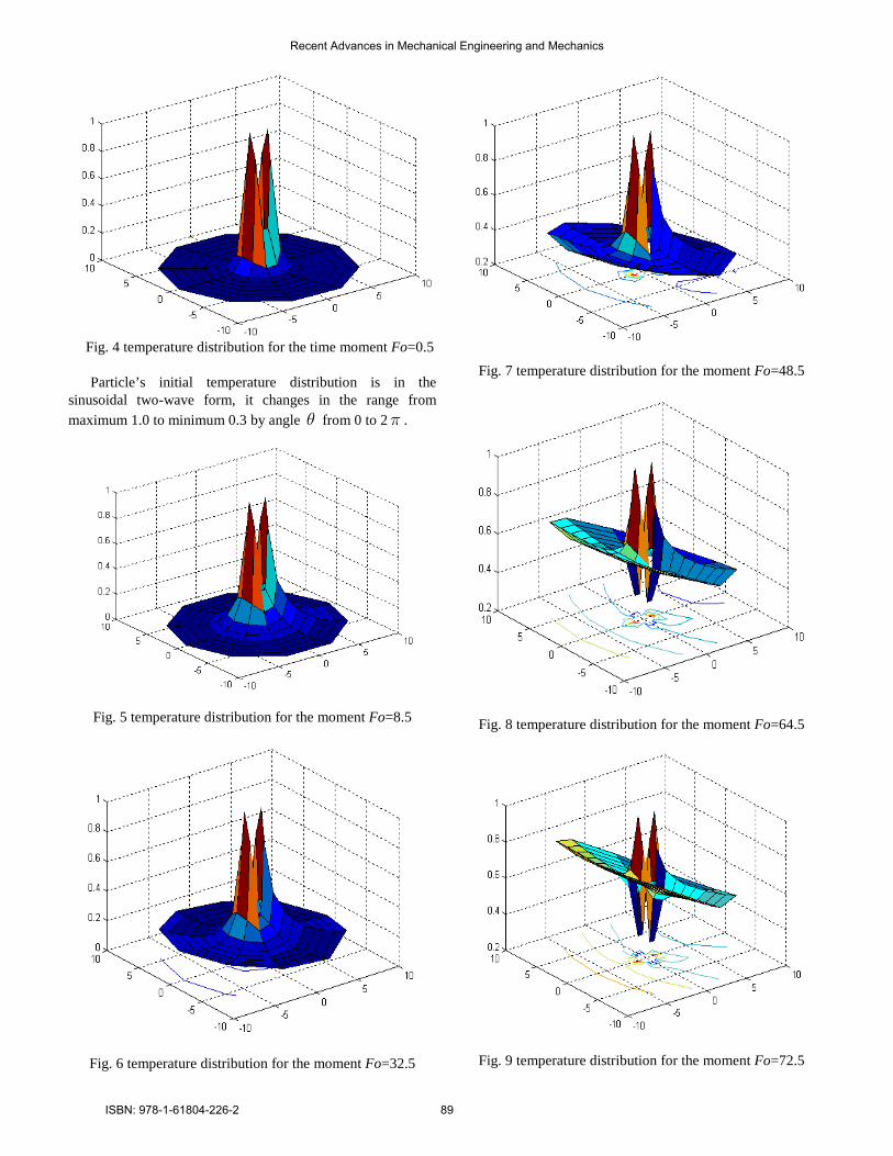
Fig. 4 temperature distribution for the time moment Fo=0.5 Particle’s initial temperature distribution is in the

sinusoidal two-wave form, it changes in the range from maximum 1.0 to minimum 0.3 by angle from 0 to 2 .

Fig. 5 temperature distribution for the moment Fo=8.5






ISBN: 978-1-61804-226-2 89

REFERENCES [1] Jamshid Gharakhanlou, I.V. Кazachkov. Mathematical modeling of

potentially hazardous nuclear power objects with shifted arguments// J. Nuclear and Radiation Safety.- 3 (55) .- 2012.- P. 21-26. (In Russian).

[2] I.V. Kazachkov and Ali Hasan Moghaddam. Modeling the thermal hydraulic processes by severe accidents at the NPPs.- Monograph.- Kyiv, NTUU “KPI”.- Zhytomyr.- Polissya.- 2008.- 170pp. (In Russian).

[3] I.V. Kazachkov. The mathematical models for penetration of a liquid jets into a pool// WSEAS Trans. on fluid mechanics.- 2011.- Issue 2.- Vol. 6, April.- P. 71-91.

[4] Kazachkov I.V., Paladino D., Sehgal B.R. Ex-vessel coolability of a molten pool by coolant injection from submerged nozzles // 9-th Int. Conf. Nucl. Energy Devel (April 8 - 12, 2001. Nice, France). - P. 43 - 49.

[5] H.S. Park, I.V. Kazachkov, B.R. Sehgal, Y. Maruyama and J. Sugimoto. Analysis of Plunging Jet Penetration into Liquid Pool in Isothermal Conditions/ ICMF 2001: 4th Int. Conference on Multiphase Flow, New Orleans, Louisiana, U.S.A., May 27 - June 1, 2001.

[6] Babenko Yu.I., Heat and mass transfer.- Leningrad.- Khimiya.- 1986.- 144pp. (In Russian).

[7] A. Kilbas, H.M. Srivastava, J.J. Trujillo. Theory and applications of fractional differential equations.- North-Holland Mathematics studies 204.- 2006.– 524 p.

[8] Povstenko Y.Z. Fractional heat conduction equation and associated thermal stresses// J. Thermal Stresses.– 2005.– 28.– P. 83-102.

[9] Momani Sh. General solutions for the space and time-fractional diffusion-wave equation// Journal of physical sciences.– 2006.– 10.– P. 30-43.

[10] Gorenflo R. Fractional calculus: integral and differential equations of fractional order /A. Carpinteri, F. Mainardi // Fractals and fractional calculus in continuum mechanics.– Springer Verlag, Wien and New York.– 1997.– P. 223-276.

[11] Fil’shtinskii L.А., Mukomel T.V., Kirichok T.A. One-dimensional initial-boundary-value problem for fractional heat conduction equation.- Zaporizhzhya National University.- Scientific Bulletin.- 2010.- 1.- P. 113-118.

[12] I.V. Kazachkov, Ye.V. Chesnokov and O.M. Kazachkova. Modelling of Potentially Hazardous Objects with Time Shifts// WSEAS Trans. on Business & Economics.- 2004.- Issue 3.- 1.- Р. 37-43.

[13] Jamshid Gharakhanlou, I.V. Кazachkov. Development and Investigation of Aggregate Models for Nuclear Objects with Time Shifts// J. Nuclear and Radiation Safety.- 2 (54).- 2012.- P. 36-41.

[14] Kazachkov I.V. and Konovalikhin M.J. A Model of a Steam Flow through the Volumetrically Heated Particle Bed// Int. J. of Thermal Sciences.- 2002.- Vol.41, 1077-1087.

[15] Bohdan Mochnacki. Estimation of relaxation and thermalization times in microscale heat transfer model// Journal of theoretical and applied mechanics.- Warsaw 2013.- 51.- 4.- P. 837-845.

[16] Kazachkov I.V. A combined space discrete algorithm with a Taylor series by time for CFD// WSEAS Тransactions on fluid mechanics.- Issue 1, Volume 6, January 2011.- P. 51-69.


ISBN: 978-1-61804-226-2 90

http://www.znu.edu.ua/eng/main

Non-linear Dynamics of Electromechanical System “Vibration Transport Machine – Asynchronous Electric Motors”

Sergey Rumyantsev, Eugeny Azarov, Andrey Shihov, Olga Alexeyeva

Abstract – In this paper we present some new results on the numerical simulation of dynamics of vibration transport machines (VTM) with independently rotating vibration ex-citers (VE). There are given the non-linear differential equa-tions for movement of “VTM – electric motors" system in case of an asynchronous motor drive with random quantity of poles’ pairs. The model describes an influence of the cur-rent displacement effect on the asynchronous driver rotor resistance. Key-words – Asynchronous electric motors, Dynamics, Non-linear Differential Equations, Self-synchronization, Vibration.

1 INTRODUCTION

Vibration transport machines (VTM) are intended for transporting and/or separating variable bulk mate-rials. Most of these machines are constructed as solid bodies (working elements, WE) fixed on springs or by means of other elastic elements that enable their plane-parallel motion (Fig. 1).

Fig. 1

The motion of working elements is excited by special devices called vibration exciters (VE). VE act as unba-lanced rotors driven by electric motors. This work was supported by RFBR, research projects No. 11-08-00053a and No. 14-08-00605a. Sergey Rumyantsev is with The Ural State University of Rail-way Transport, Ekaterinburg, RUSSIA, e-mail: [email protected]. Eugeny Azarov is with The Ural State University of Railway Transport, Ekaterinburg, RUSSIA. Andrey Shihov is with The Ural State University of Railway Transport, Ekaterinburg, RUSSIA. Olga Alexeyeva is with The Ural State University of Railway Transport, Ekaterinburg, RUSSIA.

Lately VTM with independent rotating VE have the increasing application. The concept of their action is based on active usage of physical phenomenon called self-synchronization (SS) of vibrators. In these ma-chines synchronism and relation of VE’ phases are achieved automatically due to characteristic properties of the vibration system [1]. The dynamics of VTM with independently rotating VE was observed in works of I. Blechman, B. Lavrov, K. Frolov, L. Sperling, A. Kosolapov and other re-searchers [1-6].

2 TRANSIENT DYNAMIC PROCESSES Most of above-mentioned authors’ works were de-noted to synchronous motions. We had stated the prob-lem of transient dynamic processes researching. These processes are accompanying the start of the machine from its stand still until its reaching (or not-reaching) stabled synchronous motion [7-9]. This approach al-lows evaluating the time until synchronization and the type of connections between this time and various fac-tors. The VTM dynamics with n independently rotating VE is given by the following system of differential equations:

42

1

42

1

2

1 ( sin cos ) ,

1 ( sin cos ) ,

1

( sin( ) cos

x x x x i i i i i ii

y y y y i i i i i ii

x y x y

i i i i i i i

x k x k c x c mM

y k y k c y c mM

k x k y k c x c y cJ

m r

ϕ ϕ=

ϕ ϕ=

ϕ ϕ ϕ ϕ ϕ ϕ

= − − ϕ− − ϕ+ ε ϕ ϕ +ϕ ϕ = − − ϕ− − ϕ+ ε ϕ ϕ −ϕ ϕ

ϕ = − − − ϕ− − − ϕ+

+ ε ϕ ϕ −δ −ϕ −ϕ

∑

∑

[ ] [

4

1

2

( )) ,

1 ( ) ( ) sin cos cos

cos( ) sin( ) ,

( 1,...,4).

i ii

i ii i i i i i i i i

i i

i i i i i i

mI L R x y gJ J

r r

i

=

ϕ −δ −ϕ ε ϕ = ϕ − ϕ + ϕ − ϕ − ϕ −

− ϕ ϕ −δ −ϕ − ϕ ϕ −δ −ϕ =

∑

(1)

Here x, y, φ, φi are generalized coordinates of the sys-tem, where x, y are the coordinates of the mass centre of VTM’s WE in some Cartesian coordinate system strictly connected to earth; φ is the angle of WE rota-tion about the axis passing through the mass centre perpendicular to the motion plane of the machine; φi is an angle of i-th eccentric weight rotation about the mo-


ISBN: 978-1-61804-226-2 91



tor axis; Li(φi) is the rotation moment of i-th eccentric weight; Ri(φi) is the moment of the rotating resistance for i-th eccentric weight; Ii are indicate of the rotation direction of i-th eccentric weight, where the value is taken equal to 1 for eccentric weights rotating counter-clockwise (positive direction) and -1 for eccentric weights rotating clockwise; M is the total VTM mass (of WE and eccentric weights); mi is the mass of the i-th eccentric weight; J is the second moment of VTM relative to the mass centre; Ji is the second moment of i-th eccentric weight relative to the rotative axis; εi is the radius of gyration of the i-th eccentric weight rela-tive to the rotative axis (Fig.2);

Fig.2

δi is the angle assigning the i-th eccentric weight posi-tion; ri is the distance from the mass centre to the axis of the i-th eccentric weight; cx, cy, cϕ, cxϕ, cyϕ are the generalized coefficients of elastic supporting elements’ hardness; kx, ky, kϕ, kxϕ, kyϕ are the viscous drag coeffi-cients; g is the free fall acceleration. 2.1 Electromechanical System “Vibration Transport

Machine – Asynchronous Electric Motors”

The model describes only non-stationary dynamics of VTM itself without taking into account transient dynamic processes in motors. However, by the start-up and impact loads affecting the machine, there may arise transient dynamic processes in electric motors, resulting in strong deviation of torque / angular speed dependence from the static characteristic. Accounting for these effects will allow describing more precisely not only the influence of motors on non-stationary VTM dynamics, but also influence of VTM dynamics on electromagnetic processes in the motor. The dynamics of “VTM – electric motors" system in case of an asynchronous motor drive with random quantity of poles’ pairs is given by the following sys-tem of differential equations [10]:

[ ]

[ ]

[

]

,),,1(:

;;)sin(;)cos(

,)sin(

)cos(coscossin

)()(1

,)cos()sin(

1

,)cossin(1

,)cossin(1

324434

414333

42212

32111

2

4132

уд2

1

1уд

2

1

2

)2(

nipKKpKK

KKtUKKtU

r

rgyxJ

m

RAIJ

Mrm

cycxckykxkJ

FmcyckykM

y

mcxckxkM

x

iiiiiiii

iiiiiiii

iiiimi

iiiimi

iii

iiiiiii

ii

iiiiiiiii

i

iiiiiii

n

iii

yxyx

n

iiiiiiiyyyy

n

iiiiiiixxxx

=ψϕ+ψ+ψ−=ψψϕ−ψ+ψ−=ψ

ψ+ψ−α+ω=ψψ+ψ−α+ω=ψ

ϕ−δ−ϕϕ−

−ϕ−δ−ϕϕ−ϕ−ϕ−ϕε

+

+ϕ−ψψ−ψψ=ϕ

+ϕ−δ−ϕϕ−ϕ−δ−ϕϕε+

+ϕ−−−ϕ−−=ϕ

−ϕϕ−ϕϕε+ϕ−−ϕ−−=

ϕϕ+ϕϕε+ϕ−−ϕ−−=

∑

∑

∑

=

ϕϕϕϕϕϕ

=ϕϕ

=ϕϕ

c

c

This system contains 3+5n differential equations de-scribing movement of VTM – asynchronous driven motors electromechanical system. The phase va-riables of this system are generalized coordinates x, y, φ, rotational angle φi of i motor, and magnetic-flux linkages of motors 4321 ,,, iiii ΨΨΨΨ . p is the number of pairs of poles. Coefficients Ai,Kij (j =1, … , 4) are calculated by formulas:

.;

;;

2423

2221

iiris

iiri

iiris

isiri

iiris

iisi

iiris

irisi

MLLMrK

MLLLrK

MLLMrK

MLLLrK

−=

−=

−=

−= (3)

.)(2

32

iiris

iii

MLLMpA−

= (4)

Mi, Lis , Lir are mutual inductance and complete induc-tances of stator and rotor windings. The research was carried out using the VTM dynam-ics mathematical model based on numerical solution of system (1) or (2).

3 PROBLEM FORMULATION The system (2) includes coefficients Ai and Ki1 – Ki4 that depend on the active and inductive resistances of stators and rotors of the motors. These values used to be considered constant and equal to the values of re-levant nominal rating resistances. The research, which was conducted using numerical experiment with the mathematical model [10, 12], has stated that differential equations of asynchronous mo-tors with constant coefficients, included in the system (2), can be applied well to the VTM working process during the operating mode, as well as to the transient processes that appear in the VTM when its vibration exciters are accelerated. However, this model gives inadequate results when describing the transient processes that occur during the startup of the VTM.


ISBN: 978-1-61804-226-2 92

It is obvious that startup transient processes modeling must take into account variability of the range of phys-ical parameters of motors, and, consequently, variabili-ty (i.e. dependence on the current angular speed of the rotors) of the coefficients Ai and Ki1 – Ki4. Thus the decision was taken to consider a non-linear model that would take into account the current displacement ef-fect in rotor winding bars of asynchronous drivers as the factor that has the greatest influence on the starting torque value.

4 INFLUENCE OF THE CURRENT DISPLACEMENT EFFECT ON THE ASYNCHRONOUS DRIVER ROTOR

RESISTANCE It is known [13] that in case when there is alternate current in the winding, conductors produce whirling currents that combine with the principal current and increase (or decrease) the current density in different areas of the conductor sections. The current density evenness is disturbed, which increases the active resis-tance of the conductor. The greatest current density will occur in upper parts of the conductor sections, i.e. in the areas that are lo-cated closer to the slot opening into the air gap (Fig.3). Because it looks as if the current has been displaced into the upper part of the conductor section, this phe-nomenon is called the current displacement, whereas the coefficient kr, which registers the active resistance change caused by this affect, is called the current dis-placement coefficient.

Fig.. 3 Current density allocation in the short-circuit motor

winding bar with deep-bar slots on the rotor

Calculations showed that it is less practical to de-fine directly the active and inductive bar resistance by the uneven current allocation, than to define their rela-tive change caused by the influence of the current dis-placement effect. These changes are measured with the use of coefficients kr and kd [14, 15]. Coefficient kr shows by how many folds the active resistance rcp of the slotted bar area by the uneven current density in the bar has increased in comparison with its resistance rc by equal density throughout all the bar section

ccpr rrk /= . The damping coefficient kd shows how the magnetic conductance ξλ′p of the slot area with the conductor under current has decreased in comparison with the

resistance of the same area by the even current density pλ′ in the bar pPDk λ′λ′= ξ / .

Rotor winding active resistance with account for the current displacement

RKrr 22 =ξ.

Overall rotor resistance increase coefficient caused by the current displacement effect 2c /)1(1 rrkK rR −+= . The current displacement coefficient kr is defined by the equation rr qqk /c= , where qc is the bar section area; qr is the section area constrained by the height hr (Fig. 4).

Fig. 4 Depth of current penetration into the bar

Current penetration depth )1/(c ξϕ+= hhr , where φξ

is the coefficient that depends [14] on ξ (Fig. 5).

Fig. 5 Dependence of φξ on ξ

The ξ value for the cast aluminum rotor winding is defined by the equation

ссс /)(15,65)( ωϕ−ω=ϕξ ph ,

where сω is the power-line frequency, ϕ is the rotor

angular speed, p is the number of poles pairs. Rotor winding inductive resistance with allowance for the current displacement effect:

,22 XKXX =ξ ./)1(1 2'п2 Σλλ−−= dX kK


ISBN: 978-1-61804-226-2 93

The damping coefficient dk is considered to be equal to

ξϕ′ , where ξϕ′ is the coefficient that depends [14] on

the ξ value (Fig. 6).

Fig. 6 Dependence of ξϕ′ on the ξ value

The differential VTM equation system with allowance for the current displacement effect in the rotors of dri-ven motors can be written in this case as

[ ]

[ ]

[ ]

),,,1(;)()()(;)()()(

;)()()sin()(;)()()cos()(

,)sin()cos(coscossin

)()()(1

,)cos()sin(

1

,)cossin(1

,)cossin(1

324434

414333

4221c2

3211c1

2

4132

2

1

1

2

1

2

)5(

nipKKpKK

KKtUKKtU

rrgyxJ

m

RAIJ

rm

cycxckykxkJ

mcyckykM

y

mcxckxkM

x

iiiiiiiiiii

iiiiiiiiiii

iiiiiimii

iiiiiimii

iiiiiiiiii

ii

iiiiiiiiii

i

iiiiiii

n

iii

yxyx

n

iiiiiiiyyyy

n

iiiiiiixxxx

=ψϕ+ψϕ+ψϕ−=ϕψψϕ−ψϕ+ψϕ−=ϕψ

ψϕ+ψϕ−α+ω=ϕψψϕ+ψϕ−α+ω=ϕψ

ϕ−δ−ϕϕ−ϕ−δ−ϕϕ−ϕ−ϕ−ϕε

+

+ϕ−ψψ−ψψϕ=ϕ

ϕ−δ−ϕϕ−ϕ−δ−ϕϕε+

+ϕ−−−ϕ−−=ϕ

ϕϕ−ϕϕε+ϕ−−ϕ−−=

ϕϕ+ϕϕε+ϕ−−ϕ−−=

∑

∑

∑

=

ϕϕϕϕϕϕ

=ϕϕ

=ϕϕ

where

;)(

)()(;

)(

)()(

;)(

)(;)(

)()(

2423

2221

iiiris

iiRiirii

iiiris

isiRiirii

iiiris

iisii

iiiris

iirisii

MLL

MKrK

MLL

LKrK

MLL

MrK

MLL

LrK

−ϕ

ϕ=ϕ

−ϕ

ϕ=ϕ

−ϕ=ϕ

−ϕ

ϕ=ϕ

;

))((2

3)(

2iiiris

iiii

MLL

MpA

−ϕ=ϕ

;/))(()( с212 ωϕ+=ϕ iXiiiiir KXXL

2c /)1)((1)( rrkK iriR −ξ+=ϕ ;

./)1(1 2'п2 Σλλ−−= dX kK

ссс /)(15,65)( ωϕ−ω=ϕξ ph .

In this differential equation system coefficients Ai and Ki1 – Ki4 are no longer constant and are nonlinearly dependant on the angular speed of the rotors in the dri-ven electric motors. Angular rotation rates of the i-th VE (the rotor of the motor) iϕ , or else their derivatives, are included into all these equations. On the other hand, the flux linkage rates of the i-th electric motor

4321 ,,, iiii ΨΨΨΨ , are included into the VE angular ac-celeration. Thus the system poses a rigidly bound diffe-rential equation system. It is impossible to solve some of its equations separately from the others, all the sys-tem must be integrated in unison. To calculate the currents of the real three-phase machine it is possible to take advantage of formulas of return transformations which are as follows for stator and rotor magnitudes:

;120sin120cos

);120sin()120cos(

;0sin0cos

00

00

βα

βα

βα

−=

−−−=

−=

ssC

ssB

ssA

iii

iii

iii (6)

).120sin()120cos(

);120sin()120cos(

);0sin()0cos(

00

00

+ϕ−−+ϕ−=

−ϕ−−−ϕ−=

ϕ−−ϕ−=

βα

βα

βα

rrc

rrb

rra

iii

iii

iii

The current isα will be correspondent to real phase current of the one of stator phases of three-phase ma-chine.

5 CONCLUSION

Therefore, a new differential equation system (5) has been deduced that describes non-stationary dynamics of VTM – electric motors electromechanical system, which is highly-nonlinear in the electrical as well as in the mechanical parts and allows a more precise mea-suring of the startup transient processes.

REFERENCES [1] Blechman I.I., Synchronization of Dynamics Systems, Moskow: Nauka, 1971 (in Russian). [2] Michalczyk J., Cieplok G., Generalized Problem of Syn-chronous Elimination, Machine Vibration, 1993. [3] Irvin R.A., “Large Vibrating Screen Design-Manufacturing and Maintenance Consideration”, Mining Engineering, 1984, Vol.36, 9, P.1341-1346. [4] Sperling L., “Selbstsynchronisation Statisch und Dyna-misch Unwuchtiger Vibratoren”, Technische Mechanic, 1994, 14, 1 und 2. [5] Gear C.W., “Simultaneous Numerical Solution of Diffe-rential/Algebraic Equation”, IEEE Trans. Circuit Theory, 1971, CT 18, pp.367-384.


ISBN: 978-1-61804-226-2 94

[6] Kosolapov A.N., “An Adaptive Property of Vibrational Machines with Self-Synchronized Vibration Exciters”, Iz-vestiya Vuzov: Gorniy Journal, No.11, 1989(in Russian). [7] Rumyantsev S.A., Dynamics of Transient Processes and Self-Synchronization of Vibrational Machines Motions, Eka-terinburg: Ural Department of RAS, 2003(in Russian). [8] Rumyantsev S., Tarasov D., “Non-linear Dynamics of Vibration Transport Machines in Cases of Three and Four Independently Rotating Vibration Exciters”, Recent Ad-vances in Continuum Mechanics, Proceedings of the 4th IASME/WSEAS International Conference on Continuum Mechanics, Cambridge, UK, February 24-26, 2009. pp. 132-135. [9] Rumyantsev S., Tarasov D., “Numerical Simulation of Non-linear Dynamics of Vibration Transport Machines in Case of Three Independently Rotating Vibration Exciters”, Recent Advances in Applied Mathematics, Proceedings of the American Conference on Applied Mathematics (AMERICAN-MATH ’10), Harvard University, Cambridge, USA, January 27-29, 2010, pp. 191-194. [10] Rumyantsev S.A., Azarov E.B., “The Mathematical Model of Non-stationary Dynamics of VTM – Driven Mo-tors System in Case of Cage Asynchronous Motors”, Transport Urala, No.1, 2005, pp. 2 – 7. [11] Rumyantsev S.A., Vasilyeva G.V., Alekseeva O.N., “Numerical Simulation of Dynamics of Two-mass VTM with Vibroexciters Mounted on the Lower Mass”, Herald of the Ural State University of Railway Transport, No. 3-4, 2009, pp. 87 – 91. [12] S.A. Rumyantsev, E.B. Azarov. ”Research of non-stationary dynamics of vibration transport machines by means of mathematical modeling”, Transport Urala, No.4, 2005. pp. 45 – 50. [13] A.V. Ivanov-Smolensky, Electrical machines, Moskow: Energia, 1980. – 928 p. [14] Electrical machines designing. / edit. I.P. Kopylov, Moskow: Energoatomizdat, 1993. [15] Y.S. Gurin, B.I. Kuznetsov. Designing of electrical machine ranges. Moskow: Energia, 1978, 480 p.


ISBN: 978-1-61804-226-2 95

Abstract- Changing the length of the arm leads us to a new approach; we name it multi-joint single actuator. To find out the control approach, the mechanism is described in this article. Using one actuator for lots of joints and each time connecting one of them to this actuator is required 2 issues. The first issue is to control the freedom of joint. Another is transferring the torque to the desired joint. In this article, a mechanism is proposed for satisfying both. For the second issue, two approaches are proposed and analyzed. Equations for both of are found.

Keywords—Robot, mechanism, joint, control, arm.

I. INTRODUCTION ECHANICAL arm [1] is a robot act like human arm and, is used in different functions like welding, painting,

assembling and rehabilitation [2]. In these robots each joint has its own actuator and controller. For controlling several degrees of freedom, same number of actuators is needed like snake robots [3, 4, 5] which have several actuators. Another kind of robots is continuous robot [6, 7] which consists of three actuators. They move a continuous arm like elephant nose. Joints are not controllable separately in continuous robots. Controlling several joints with one actuator is an issue, is investigated in this paper. Two mechanisms is proposed for this purpose. The first one is for selecting the desire joint and other one for transferring the torque to that joint. For transferring the force to the joints there is two ways. The first one is wire and some springs and the second one is using a series of gears. In this article mechanical design and dynamic analysis of both is proposed but gears is used for transferring. This robot can be used in many applications which there are several joints and each time one of them is moving. This mechanism helps us to reduce the number of actuators to 3 for several joints. The only factor that limits us in number of joints is the accuracy of our devises like our manufacturing machineries and our actuator. One of the application of this mechanism is in endoscopy [8] and Laparoscopic [9] since the robot can work in different workspaces. By improving this mechanism in future works we can use it in multi actuator robots like humanoid robots [10].

II. MECHANICAL DESIGN The proposed mechanism consists of two coaxial groups of joints, inner group and outer group. In the inner group, each

joint axis has a non zero angle with respect to the others, however, all joints axes of the outer group are in the same plane, i.e., each joint axis has a zero angle with respect to the others. If the inner group is rotated, the difference in its joints angles makes the mechanism to bend merely in the desired joint. For example, for bending the third joint, the inner group must rotate until the angle between the third inner joint axis and the third outer one becomes zero. On the other hand, it can’t bend in the other joints (e.g. in the fourth joint) because there is a non zero angle between the other inner joint axes and their corresponding outer ones.

For manufacturing this robot, one polyamide cylinder was located inside the other one. Then both of them were cut in the same length. The links were built and joined together, as shown in Fig.1. Then the inner joints were put inside the outer ones.

To rotate the desired joint by exerting the actuator force, we investigate two approaches. The first approach is based on using the wire and spring. A wire is along the robot and one of its ends is connected to the end of the robot and its other end is connected to the actuator. When the actuator pulls the wire, its length decreases and makes the robot to rotate. On the other side of the robot (the side with no wire), there are some springs. If the pulling force of the wire is removed then these springs release and the robot rotates to the other side. This is similar to the method used in some continuous robots.

Fig.1 angle of inner and outer axis

A Multi-Joint Single-Actuator Robot: Dynamic and Kinematic Analysis

A.Nouri, and M.Danesh.

M


ISBN: 978-1-61804-226-2 96

The second approach is based on using a series of gears which the last gear attached to the robot body and the first gear is connected to the actuator shaft. All of the other gears are free to turn and some of them are located on the joints (one gear on

Fig.2 Cartesian coordination

each joint).For example, if the third joint is allowed to move, the gear on this joint acts like a gear attached to the third link. When the actuator’s shaft rotates, only the gears before the third joint rotate. This leads to the arm movement in the third joint.

Returning the spring to its normal extension is not controllable, thus, the second approach is more accurate than the first approach. On the other hand, in the second approach the ratio of gears can be chosen by designer to control the velocity and the force of each joint.

III. DYNAMIC ANALYSIS A. ROBOT WITH WIRE AND SPRING

KINEMATIC

Consider Cartesian coordination defined in the plane that the robot turns in it, according to Fig.2.

In Fig.2, link i is the last movable link and n is the total number of robot links. is the angle between the movable link axis and horizontal axis, x. (x,y) shows the position of the end effecter. is limited by the structure. Due to the links structure in this prototype, the limit is 60 degree. The end effecter position is derived as

Fig.3. A 3D coordination

(1)

(2)

A 3D coordination is shown in Fig.3. x axes are the same in both recent figures, however, y axes are different in them. The end effecter position in this coordination is

(3)

(4)

(5)

The relationship between and other variables can be derived geometrically. Fig.4 shows the geometrical model of this robot.

a is the perpendicular distance between the wire and the link axis, and b is the half of the distance between two adjacent joints.c is the hypotenuse of the right-angled triangleabc. Fs shows the spring force of the joint i. Fc is the wire force supplied by the actuator. is the angle between the two adjacent c hypotenuses in the wire side. β is the same angle, however in the spring side. and β are calculated by the following equations.


ISBN: 978-1-61804-226-2 97

Fig.4. different angles in spring and wire

(7)

The spring and wire torques are

(8)

The joint torque is

(9)

There are three different kinds of springs, hard, soft and linear, and their typical characteristics are shown in Fig.5.

Fig.5. Typical characteristics of different kinds of springs

Spring force in each group of springs is calculated by the following equations.

hard Liner

soft (10) n>1

In this robot, xs is calculated by

To compute the moment of inertia in each mode of robot, a Catia model for each link is developed. Based on this model, the moment of inertia of each link around its z axis (Jn) and then the moment of inertia of all movable links around the movable joint are calculated as

M is the mass of movable joints and m is the mass of each link.

(11)

(12)


ISBN: 978-1-61804-226-2 98

Fig.6. forces and moments in robot

DYNAMICS

Dynamic analysis can be done with both Newton-Euler and Lagrangian.

NEWTON-EULER:

In the following formulation, the torque is calculated. We rewrite all of the formulation with ө.

(13)

LAGRANGIAN:

In this part, the robot dynamic relations are derived by Lagrangian.

(14)

In this robot, we have 2 kinds of potential energy, spring and gravity.

(15)

From the following equations

(16)

(17) Then,

(18)

(19)

(20)

(21)

Kinematic energy comes from the rotation of arm.

(22)

Then

(23)

At last Q is the generalized force.

(24)

From Lagrangian formula and its ingredients, we have

(25)


ISBN: 978-1-61804-226-2 99

B. ROBOT WITH GEARS

KINEMATICS:

Robot kinematic with gear is the same as that of with spring and wire.

Here, the potential energy includes only gravity term.

(29)

(30)

(31)

DYNAMIC ANALYSIS:

For gears, it is easier to find the desired arm torque. Because the actuator moment is directly transferred to the joint and can be used directly in the formulation, thus, we rewrite the equations as

Newton Euler:

(26)

(27)

Lagrangian:

(28)

Therefore, the dynamic equation is as

(26)

IV. THEORITICAL RESULTS

We simulate all the equations in MATLAB and get these plots as the result

(a)Torque(n.m) plot for joint 1

description Length Force Force Mass of each link Gravity Angle Links number Moment of inertia

symbol L FX FY m g i j

value 0.05 2 1 0.117 9.81 π/2 1 0.00004149

Table 1. Robot characteristics


ISBN: 978-1-61804-226-2 100

(b)Torque(n.m) plot for joint 2

(c)Torque(n.m) plot for joint 3

(d)Torque (n.m) plot for joint 4

Fig.6. Theoretical results, (0)=-pi/3, = (0) +t pi/10;

V. EXPERIMENTAL RESULTS

To find out the effectiveness of the proposed robot design, as it is depicted in fig.7, we made this robot and tested the mechanism. The robot parameters are mentioned in table 1.

All of the robots links are made of polyamide which is suitable for production procedure of this

Fig.7. the prototype of robot

prototype. Polyamides are very hard and need to be cooled in milling process.


ISBN: 978-1-61804-226-2 101

In this robot, a RX-64 motor is used for turning the arm in each case. This motor is controlled via MATLAB (software) and is commanded through USB2DYNAMIXEL connector (hardware interface). All of the feedback data are stored in a matrix and are plotted.

Fig.8. presents a comparison between the actual torque and theoretical torque for the same trajectory. Although we tried to consider all factors in the theoretical calculation, however, we can’t ignore the friction and some production faults effects. In this mechanism, manufacturing accuracy is very important. If inner and outer joints are not exactly coaxial then some difficulties appears in turning the inner joints. Also the axes of the inner joints and outer joints must be in the same plane. In the case, the angle between the axis of the 3rd inner joint and the axis of the 3rd outer joint becomes zero, if they do not coincide, they won’t move. If the joints have backlash or free space, it causes unwanted turn in other joints.

(a)Torque (n.m) plot for joint 1

(b)Torque (n.m) plot for joint 2

(c)Torque (n.m) plot for joint 3

(d)Torque (n.m) plot for joint 4

Fig.8. experimental results, (0) = -pi/3, = (0) +t pi/10;

V. 3BCONCLUSION In this paper, a novel mechanism is presented to robot design, manufactured and practically tested. This robot has the following contributions.

1) Several joints can be controlled with just one actuator and turned with only one actuator; however, in a simple arm an actuator is needed to move each joint.

2) The work space of a continuous arm or a simple robot arm is limited. In this robot, there is a work space for each mode.

3) The mechanism, used in this robot can be used in other robots, especially if there is a need for adjustable joints.

4) Changing the radiuses of gears in this robot can transfer different torques to the joints and it is useful


ISBN: 978-1-61804-226-2 102

when we want different torques in each link with the same actuator.

In this robot, the accuracy in the production process is very important. In comparison with a robot with the same number of joints, this robot costs less.

Acknowledgment

This study is partially supported by Isfahan University of Technology.

References

1. M. Hiromi, “Kinematics for the whole arm of a serial-chain manipulator,” Advanced Robotics, Volume 15, Number 2, pp. 255-275(21), 2001.

2. L. Wang, Z. Deng, L. Zhang and, Q. Meng, “Dynamic Analysis of Rehabilitative Arm Robot,” Mechatronics and Automation, Proceedings of the IEEE International Conference, Luoyang, Henan, 2006, pp. 1181 - 1185.

3. S. Ma, Li W.J., and, Y. Wang, “A Simulator to Analyze Creeping Locomotion of a Snake-like Robot,” Robotics and Automation, ICRA. IEEE International Conference, 2001, pp. 3656 - 3661 vol.4.

4. A. Akbarzadeh and, H. Kalani, “Design and Modeling of a Snake Robot Based on Worm-Like Locomotion,” Advanced Robotics, Volume 26, issue 5-6, pp. 537-560, 13 Apr 2012.

5. Y. Takita, M. Hasegawa and, M. Nunobiki“An investigation of climbing up stairs for an inchworm robot,” Advanced Robotics, Volume 15, issue 2, pp. 245-253, 2001.

6. M. W. Hannan, I. D. Walker, “Analysis and Initial Experiments for a Novel Elephant’s Trunk Robot,” IEEE Conf. on Intelligent Robots and Systems, pp. 330-337, Takamatsu, 2000.

7. K. Nakajima,T. Li, H. Sumioka, M. Cianchetti, R. Pfeifer, “Information theoretic analysis on a soft robotic arm inspired by the octopus,” Robotics and Biomimetics (ROBIO), IEEE International Conference, pp. 110 - 117,Karon Beach, Phuket, 2011.

8. H. Yamashita, k. Daeyoung, N.Hata, T. Dohi, “multi slider linkage mechanism for endoscopic forceps manipulator,” Intelligent Robots and Systems, (IROS 2003), IEEE/RSJ International Conference, 2003, pp. 2577 – 2582 vol.3.

9. B. F. Allen, B. Jordan,W. Pannell and, C. Lewis“Y. Takita, M. Hasegawa and, M. Nunobiki“Laparoscopic Surgical Robot for Remote In Vivo Training,” Advanced Robotics, Volume 24, pp. 1679–1694, 2010.

10. A. Karimi, M. Danesh, A. Tabibian, A. Nouri, “Dynamic analysis and path planning for a redundant actuated biped robot,” Control, Instrumentation and Automation (ICCIA), 2nd International Conference on, Shiraz, 2011, pp. 1074 - 1079.


ISBN: 978-1-61804-226-2 103

Abstract— Using the conservation laws in the form of the

Euler and Navier-Stokes equations, showing the occurrence of the instability of a tangential section rate in the nanoscale range of wavelengths, for certain parameters. This allows the hope that this approach will produce the parameterization of nanostructure formation.

Keywords — Kelvin-Helmholts instability, nanostructure, dispersion equation, viscous and viscous-potential fluid

I. INTRODUCTION When exposed to a heterogeneous plasma electrical

explosion of conductors formed on the metal surface characteristic graded structure mode electro explosive doping.Fibrewise studies performed constant electro microscopy methods (Y.F. Ivanov), revealed a layered structure as the distance from the surface treatment [1].

Fig. 1 Scheme four structural zones.

First nanostructured layer (I) of thickness ~ 1 μm contacts with plasma simulates the incoming flow. Second layer (II) with a honeycomb structure has a crystallization crystal cell sizes along the substantially vertical direction than along the horizontal (scheme in Fig 1). The third layer (III) with approximately equal longitudinal and transverse dimensions of the grains. The fourth inner layer nanostructured (IV) ~ 1 μm thick. These experimental facts, namely the presence of two nanolayers have been the subject of theoretical studies. First nanolayer able to describe in the development of Kelvin - Helmholtz instability - impinging plasma and molten metal (two semi-infinite layer). Second nanolayer - internal, was described by the Kelvin - Helmholtz instability char by finite layers. In the products of the rapid quenching of the melt on the high-speed drive (spinning) identified four structural zones

described A.M. Glaser [2]. Area adjacent to the quench surface area or freeze - microfine. It is believed that it is formed as a result of multiple nucleation. The second zone is columnar crystals. In the third zone is formed dendritic or dendritic-cellular structure. The fourth zone - the area of equiaxed randomly oriented nanograins. The resulting situation is similar to the above described case. Formation of nanoscale structures for large plastic deformations also occurs when two materials shear [2]. In a detailed microscopic examination in shear bands were observed nanostructures [3]. Creating volumetric structural nanomaterials under intensive plastic deformation described in [4]. Given set of experimental data suggests broader manifestations appearance nanostructures by shear flows. Therefore, an important task is to develop the physical mechanisms and mathematical models of nanostructure formation in the development of instability in shear flows in nanoscale scale.

In [5] proposed to explain the first nanolayer based on the mechanism of Kelvin - Helmholtz instability (KHI) in the nanoscale range. The relative motion of the two media waves appear. KHI study conducted over a hundred years. In the linear approximation of the evolution of the interface is obtained dispersion equation, as a rule, it is a transcendental algebraic equation relating the growth rate and wavelength. It depends on a large number of parameters, so analytical parameterization possible to carry out in rare cases. Therefore, the dispersion equation is solved numerically to obtain ix increment depending on the wavelength for certain values of the parameters. Maximums in this dependence for positive increment achieved at certain wavelengths – λmax. Hence the development of wave and get them generated eddies of size ~ λmax , and wavelengths, and therefore will not develop other scales. Dispersive equation for viscous fluids for KHI booked out in the early XX century, but analyze it in nanoscale wavelengths to explain the tour nanostructures in the liquid metal to our work in the literature did not occur. In [5], a dispersion equation for the semi-infinite layers of viscous and ideal fluids, simulating wind plasma interaction and molten metal, and the numerical analysis. Control parameter was the relative sliding velocity layers.

The idea of using this mechanism to a second internal nanolayer (Zone IV) was given in [6]. There was discharged corresponding mathematical model and show that under certain conditions, there are two possible scale of the instability in the nano-and micro-bands. In this case the control parameter is the thickness of the upper layer.

New mechanism of nanostructure formation by the development of hydrodynamic instabilities

Vladimir D. Sarychev, Aleks Y. Granovsky, Elena V. Cheremushkina, Victor E. Gromov


ISBN: 978-1-61804-226-2 104

II. MATHEMATICAL MODELS Consider two layers for liquid surface tension and

accelerating field, a tangential velocity on the surface of the gap section (Fig. 2). We will use the linear approximation in the equations and in the boundary conditions. We denote perturbations of the longitudinal and transverse velocities by Un and Vn , respectively, and the perturbation of pressures in

the nth fluid by Pn ; these perturbations satisfy the Navier-

Stokes and Euler differential equations.

Fig. 2 Two-dimension flow of a bilayer fluid.

The system of the Navier-Stokes equations for perturbations

in the first layer has the form 2 2

1 1 1 12 2

1

2 21 1 1 1 1 1

2 21

1

1 0

U P U Ut x x y

V P V V U Vt y x y x y

νρ

νρ

∂ ∂ ∂ ∂= − + + ; ∂ ∂ ∂ ∂

∂ ∂ ∂ ∂ ∂ ∂= − + + ; + = . ∂ ∂ ∂ ∂ ∂ ∂

(1)

The system of Euler equations for perturbations in the second layer has the form

2 2 2

02

2 2 2 2 20

2

1

1 0

U U Put x x

V V P U Vut x y x y

ρ

ρ

∂ ∂ ∂+ = − ;

∂ ∂ ∂∂ ∂ ∂ ∂ ∂

+ = − ; + = .∂ ∂ ∂ ∂ ∂

(2)

The boundary conditions are specified as follows: 020 01 1

0 0 2 12

12 ( )1 1 1 2 2 1 0 2

1 1 0.

y H V

y h U V

y u V Vt x t

VP P g

y xU V

y x

η η η

ηρ ν ρ ρ η σ

= : = ;

= − : = , = ;

∂ ∂ ∂= : + = ; = ;

∂ ∂ ∂∂ ∂

− + + = − + ;∂ ∂

∂ ∂+ =

∂ ∂

(3)

We will seek the solutions to system (1), (2) in the form of traveling waves:

( , , ) ( , , ) ( ( )).U V P U iV P exp i kx tn n n n n n ω= − Substituting this relation into Eqs. (1), (2), we obtain a

system of ordinary differential equations. Solving this system, we obtain the general solution depending on arbitrary

constants. Substituting the solution into boundary conditions (3), we obtain a system of homogeneous algebraic equations in these constants. To obtain a nontrivial solution to such a system, the determinant of this system must vanish. This condition leads to the basic dispersion equation

( ) ( ) ( )( )( )( ) ( )( )

( )( ) ( ) ( ) ( )

( ) ( ) ( )( )( ) ( )( )

21

42

2 2 21

2 2

1

( ) cth( ) 0

1 th th( )

th th

2 1 2 3sh ch sh ch

2 3 2 1 3 th th

th th

G z d kH W

z z zd dG z d

zd z d

z z z zzd d z d zd

z z z d zd

zd z d

µ

ν

ν νν

νν

, + Ω + = ,

− −, = +

−

− − ++ +

−

+ − ++

−

(5)

where the following notations has been introduced: 2 0 2

1 21

22 1 0

3 31 1

( 1)

( ) .

uz ik k

g kAWk k

ρν µρ

ρ ρ σρ ρ

ΩΩ = = − − , = ,

− −= =

(6)

When 1ν ν= , we obtain the dispersion equation for a

viscous fluid:

( ) ( ) ( ) ( )

2 2( ) cth( ) 01 124 ( 1)( )1 sh ch sh ch

4 2 4 2( 2 5) ( 6 1) th( ) th( ).

th( ) th( )

G z d kH W

z zG z dzd d z d zd

z z z z z d zdzd z d

ν µ, + Ω + = ,

− +, = +

−

+ + − + ++

−

(7)

For semi-infinite layers (i.e., for h→∞ and H →∞ ), we find that th( ), th( ),cth( ) 1d zd kH → and ch( ),sh( )d d →∞ , and Eq. (7) leads to the following dispersion equation:

( ) ( )22 4 21 2 1 ( ) 0.1z z Wν µ − − − + Ω + =

(8)

An analogous equation was obtained earlier in [5]. The

increment is the imaginary part of ω whose positive sign indicates instability. We denote it by

2 2Im( ) Im( ( 1))i k zα ω ν= = − . Numerical analysis of this equation revealed the peak of the increment in the nanometer range (Fig. 3). The resulting dependence on the wavelength increment indicates the fact that the instability occurs at wavelengths corresponding to the maximum λmax decrement. Unstable waves generate vortices that lead to the creation of nanostructures, continuing during solidification.


ISBN: 978-1-61804-226-2 105

Fig. 3 Plots of the KH instability increment α versus surface perturbation

wavelength λ for relative plasma-melt slip velocities U0=759 (1), 670(2), and 350 m/s (3).

For 0 01ν ν= , ≠ the limit transition from Eq. (5) leads to

dispersion equation for a viscous potential fluid in which viscosity 1ν is taken into account only at the interface:

( ) ( )

20( ) cth( ) 02 2

22( )2 12 4th th

kuG z d kH W

k

iG z d

d k k d

ωµ

ω ων

−, + + = ,

, = +

(9)

To explain an internal limb nanolayer were used in the upper layer part of a viscous fluid (7) and the viscosity of the liquid potential (9). Increment depending on the wavelength for these two models are shown in Figure 4, which show that these two models describe the existence of two maxima. The first maximum is in the nanoscale range, and the second - in the microwave. Parametric analysis comfortable visco-potential model, which is described in more simple dispersion equation.

Fig. 4. Dependence of increment α on wavelength λ upon variation of

thickness H of the upper layer for surface tension σ0=1.2 N/m. Solid and dashed curves correspond to the viscous and viscopotential models, respectively. Upper layer thickness H, nm: 6 (1), 10 (2), 20 (3), and 30 (4).

So are three models: viscous and visco-potential end layers and layers of semi-infinite model, which describe the existence of the instability in the nanoscale range. This allows the state to establish a new mechanism for the formation of nanostructures.

REFERENCES [1] A.Y. Bagautdinov, E.A. Budovskikh, Y.F. Ivanov, V.E. Gromov,

"Physical basis electroexplosive doping metals and alloys", Novokuznetsk: SibGIU, 2007.

[2] A.M. Glaser, V.E. Gromov, Y.F. Ivanov, Y.P. Sharkeev, "Nanomaterials: structure, properties and applications", Novokuznetsk: "Inter-Kuzbass", 2012.

[3] T.E. Konstantinova, “From the dislocation to nanostructures: a new look at the mechanism of fragmentation in terms of intensive plastic deformations”, Abstracts “First Moscow Readings of Strange of Materials”, 2009, p. 105.

[4] R.Z. Valiev, N.A. Enikeev, M.Y. Murashkin, F.Z. Utyashev, "Use of severe plastic deformation to obtain bulk nanostructured metallic materials", News RAS, Mechanics of Solids, 4, 2012, pp. 106-119.

[5] V.D. Sarychev, E.S. Vashuk, E.A. Budovskikh, V.E. Gromov, "Formation of nanosize structures in metals when exposed to pulsed plasma jets electrical explosion ", Letters JTP, vol. 36, no. 14, 2010

[6] A.Y. Granovskiy, V.D. Sarychev, V.E. Gromov, " Model of formation of inner nanolayers in shear flows of material", Journal Technical Physics, vol. 58, no. 10, 2013.


ISBN: 978-1-61804-226-2 106

Abstract—Optimization of injection molding process serves for

finding ideal conditions during production of plastic parts and observing their final dimensions, shapes and properties. It is possible to determine the appropriate injection pressure, velocity, value and time of packing pressure, etc. by optimization. The paper is dealing with description of Moldflow Plastics Xpert (MPX) system and its usage in optimization of injection molding process on real part during its production.

Keywords—Defect, Injection molding, Optimization, Polymer, Process.

I. INTRODUCTION NJECTION molding represents the most important process for manufacturing plastic parts. It is suitable for mass

producing articles, since raw material can be converted into a molding by a single procedure. In most cases finishing operations are not necessary. An important advantage of injection molding is that with it we can make complex geometries in one production step in an automated process. The injection molding technique has to meet the ever increasing demand for a high quality product (in terms of both consumption properties and geometry) that is still economically priced.

This is feasible only if the molder can adequately control the molding process, if the configuration of the part is adapted to the characteristics of the molding material and the respective conversion technique, and a mold is available which satisfies the requirements for reproducible dimensional accuracy and surface quality. Typical injection moldings can be found everywhere in daily life; examples include toys, automotive parts, household articles and consumer electronics goods.

This paper is supported by the internal grant of TBU in Zlin No.

IGA/FT/2014/016 funded from the resources of specific university research and by the European Regional Development Fund under the project CEBIA-Tech No. CZ.1.05/2.1.00/03.0089.

Michal Stanek is with the Tomas Bata University in Zlin, nam. T. G.

Masaryka 5555, 76001 Zlin, Czech Republic (phone: +420576035153; fax: +420576035176; e-mail: [email protected]).

David Manas is with the Tomas Bata University in Zlin, nam. T. G. Masaryka 5555, 76001 Zlin, Czech Republic (e-mail: [email protected]).

Miroslav Manas is with the Tomas Bata University in Zlin, nam. T. G. Masaryka 5555, 76001 Zlin, Czech Republic (e-mail: [email protected]).

II. MOLDFLOW PLASTICS XPERT (MPX) Moldflow Plastics Xpert (MPX) is a software and hardware

solution that interfaces directly with injection molding machine controllers on the shop floor. MPX combines process setup, real-time process optimization, and production control according to set process parameters in one system.

MPX is an advanced control solution for the automatic setup, optimization and monitoring of the process window of an injection molding machine. Unlike other control solutions, MPX can utilize the advanced simulation capabilities of Autodesk Moldflow Advisers (AMA) and Autodesk Moldflow Insight (AMI) software to provide an initial process configuration. MPX interfaces directly with the injection molding machine and provides on-line process correction with technology developed exclusively for the plastics injection molding industry. Nowadays, molding machine operators can consistently and systematically set up the process, perform an automated DOE (design of experiments) to determine a robust processing window, and automatically correct the process whether it should be drifted or go out of control during production.

The optimization process consists of three main parts: process setup, process optimization and process control.

Process setup allows users to automate the setup of the injection molding process through a series of velocity and pressure-phase setup routines designed to fix molded part defects systematically. The objective is to achieve a combination of processing parameters which results in one good molded part.

Process optimization easily allows users to run an automated design of experiments (DOE) to determine a robust, “good parts” processing window that will compensate for normal process variation and ensure that acceptable quality parts are produced consistently.

Process control is designed to maintain the optimized processing conditions determined with Process Optimization, resulting in reduced reject rates, higher part quality, and more efficient use of machine time. Process Control can automatically correct the process – either be drifted or go out of control and also can send relay signals to alarm operators or to divert suspect parts.

The optimization process consists of three main parts: • Process Setup allows users to automate the setup of

the injection molding process through a series of

SW Optimization Possibilities of Injection Molding Process

M. Stanek, D. Manas, M. Manas and A. Skrobak

I


ISBN: 978-1-61804-226-2 107

velocity and pressure-phase setup routines designed to systematically fix molded part defects. The objective is to achieve a combination of processing parameters which results in one good molded part.

• Process Optimization easily allows users to run an automated design of experiments (DOE) to determine a robust, “good parts” processing window that will compensate for normal process variation and ensure that acceptable quality parts are produced consistently.

• Process Control is designed to maintain the optimized processing conditions determined with Process Optimization, resulting in reduced reject rates, higher part quality, and more efficient use of machine time. Process Control can automatically correct the process should it drift or go out of control and also can send relay signals to alarm operators or to divert suspect parts.

Fig. 1 Scheme of MPX unit connection

A. Process setup (setup wizard) Setup Wizard automatically calculates initial profiles based

on tool or machine related parameters. Tender can choose from three Setup Wizard methods:

• Automated Setup - calculates initial profiles based on the material and the values operator enters for velocity stroke/injection volume, part thickness and mold layout. Operator can also calculate the optimal temperature, screw rotation, and back pressure settings for plastication.

• Assisted Setup - creates initial profiles using the values operator enters for velocity stroke, injection velocity, packing pressure, and cooling time.

• Manual Setup - creates initial profiles using the values you enter for velocity stroke, injection velocity, packing pressure, and cooling time. Velocity stroke, injection velocity and packing

pressure must be entered as a percentage of the maximum machine capability.

To use the Setup Wizard, operators need to provide some initial information on molding parameters or machine parameters, depending on the option their select. The Setup Wizard then calculates an initial velocity and pressure profile based on this information. The Setup Wizard makes initial adjustments to stroke length and cushion size to ensure a full shot and adequate cushion, and then develops a basic, un-optimized profile, which can be further refined with MPX Process Setup. Operators can also calculate the optimal temperature, screw rotation, and back pressure settings for plastication.

Fig. 2 Velocity profile example

B. Process optimization The purpose of MPX Process Optimization is to establish a

robust processing window that produces acceptable quality parts while minimizing scrap. This is done by carrying out an automated Design of Experiment (DOE) that traditionally took many hours that can now be done in a few minutes.

The MPX Process Optimization DOE produces a series of parts using many different profiles. The amount by which the profiles are altered is determined by producing a number of parts and measuring how the part quality varies with the processing conditions. MPX Process Optimization then moves the profile set points so that they are positioned in the most robust position in the process window. With the tolerance boundaries of the process window known, the profile set points can be modified if they occur outside of those boundaries. This means that the process is better able to handle changes in small variables, such as raw material variability and ambient temperature. Additionally, the process can be monitored so that the specifications for the DOE parameters are maintained.

During production, the processing conditions will vary slightly. With a good set of profiles, these small changes do not affect part quality. MPX Process Optimization uses a Design of Experiment (DOE) to ensure that typical process fluctuations do not affect part quality, by finding a window of processing conditions for which good parts will be produced. A DOE involves using a series of different profiles, which can


ISBN: 978-1-61804-226-2 108

be derived from MPX Process Setup profiles, or directly from the Profile Wizard. Each profile is changed a small amount. The operator creates a series of parts with these profiles, and records which of the parts have defects. MPX Process Optimization uses this information to adjust the profiles that were generated by MPX Process Setup, so that the profiles are positioned in the most robust position in the process window (Fig. 3.).

Fig. 3 The process window There is possible eliminate any combination of visual,

dimension, warpage and weight defects using MPX Process Optimization. Different processing conditions are systematically varied, depending on the DOE settings which have been chosen.

C. Process control

MPX Process Control helps to maintain optimal machine operating conditions during production. MPX Process Control graphically monitors variables specific to the injection molding process (Fig. 4.) and automatically determines acceptable quality control limits.

Once a robust set of processing conditions has been established, it is possible to use MPX Process Control to monitor the critical parameters that define the profiles during production. MPX Process Control detects any tendency of the process to drift away from the center of the window. It can then produce a warning with recommendations for corrective action or it can make corrections, depending upon the cause of the drift.

MPX Process Control has two main roles:

• It displays control charts of process parameters, monitoring any changes that occur. Control charts are a great benefit to process engineers, who want to know when and why part quality varies. For example, examination of the control charts may reveal steadily decreasing controller performance, an indicator that maintenance may be due. Alternatively, the material, tool, or environment variation may cause the process change.

• It can also automatically fine tune injection molding machine set points to compensate for any changes in process parameters. This ensures that gradual changes in processing conditions do not lead to bad parts or injection molding machine damage.

Fig. 4 Viewing the control charts


ISBN: 978-1-61804-226-2 109

III. INJECTION MOLDING PROCESS OPTIMIZATION There will be description of injection molding process

optimization procedure in the next chapters. It will be shown on the real chosen part usage MPX software and hardware directly connected to the injection molding machine Arburg Allrounder 420 C 1000-400.

A. Injection molded part – square piece The eight-cavity injection mold was used for production of

the molded part (electrical cover – Fig. 5). The electrical cover is a plastic part used in electrotechnical industry with the main dimensions 40 x 15 x 15 mm. The material of the product is PP (polypropylene) and its main properties are described in Table 1.

Tab. 1 Properties of injected material (PP)

Basic properties

Melt density 728,95 kg/m3

Solid density 915,42 kg/m3

Elastical modulus 1340 MPa

Melt flow index 21 g/10min

Shrinkage 1,3 %

Structure Crystalline

Recommended processing

Mold temperature 50°C

Melt temperature 240°C

Ejection temperature 98°C

Fig. 5 Injection molded part – electrical cover

B. Process settings taken from MPI analysis Injection molding process of the electrical cover has been

analyzed in Autodesk Moldflow Insight (AMI) software. The values (some of them are on Fig. 6 and Fig. 7) taken from this analysis has been used for comparison with optimized values and for upload to MPX software for next part of process optimization.

Fig. 6 Fill time – 0,765 s

Fig. 7 Pressure at end of fill – 18,56 MPa

C. Optimization of injection molding process Cooling of the injection mold has been made by circulating

water with temperature 50°C. Temperatures of the heating zones are described in Table 2.

Tab. 2 Temperatures of heating zones

Heating Zone Feed Transition Metering Nozzle

Temperature [°C] 205 210 220 230

D. Automated setup

Tab. 3 Automated setup - results Initial

Profile Final

Profile Difference

Velocity [mm/s] 40 97

Displacement (start - end) [mm]

9,0 - 44,8 10,6 - 54,2

Pressure [bar] 50 149

Fill Time [s] 0,90 0,45 -0,45


ISBN: 978-1-61804-226-2 110

Packing Pressure Time [s]

15 15 0,00

Cooling Time [s] 35 13,63 -21,37

Total Time [s] 50,9 29,08 -21,82

Velocity profile

0

10

20

30

40

50

60

70

80

90

100

0 10 20 30 40 50 60

Displacement [mm]

Velo

city

[mm

/s]

Initial profile Final profile

Fig. 6 Velocity profile – automated setup Pressure profile

0

20

40

60

80

100

120

140

160

0 2 4 6 8 10 12 14 16

Time [s]

Pres

sure

[bar

]


Fig. 6 Pressure profile – automated setup

E. Manual setup

Tab. 4 Manual setup - results Initial

Profile Final

Profile Difference


Displacement (start - end) [mm]

18,1 - 90,6 47,7 - 90,6


Fill Time [s] 1,09 0,57 -0,52

Packing Pressure Time [s]

6,43 6,43 0,00

Cooling Time [s] 15 10,39 -4,61

Total Time [s] 22,52 17,39 -5,13

Velocity profile

0

10

20

30

40

50

60

70

80

0 10 20 30 40 50 60 70 80 90 100

Displacement [mm]

Velo

city

[mm

/s]


Fig. 10 Velocity profile – manual setup

Pressure profile

0

200

400

600

800

1000

1200

0 1 2 3 4 5 6 7

Time [s]Pr

essu

re [b

ar]

Initial profile Final profile Fig. 11 Pressure profile – manual setup

F. Some defects on square piece appeared during optimization

Fig. 12 Defects on part – voiding marks

Fig. 13 Defects on part – sink marks

Fig. 13 Defects on part – sink marks


ISBN: 978-1-61804-226-2 111

Fig. 14 Defects on part – short shots on real part

Fig. 15 Defects on part – short shots by simulation Tab. 5 Summary of process parameters

Process setting Automated Setup

Manual Setup


Displacement (start - end) [mm] 10,6 - 54,2 47,7 - 90,6


Fill Time [s] 0,45 0,57

Packing Pressure Time [s] 15 6,43

Cooling Time [s] 13,63 10,39

Total Time [s] 29,08 17,39

IV. CONCLUSION This work deals with optimization of injecting cycle and

using software MPX. The MPX system enables very effective optimization of the injecting process and ensures optimum process parameters leading to eliminating possible product defects. The aim of optimization is not only correct process conditions setting and eliminating all defects made during production, but also minimizing the total time of the injecting cycle which has a great economical impact.

ACKNOWLEDGMENT This paper is supported by the internal grant of TBU in Zlin

No. IGA/FT/2014/016 funded from the resources of specific university research and by the European Regional Development Fund under the project CEBIA-Tech No. CZ.1.05/2.1.00/03.0089.

REFERENCES [1] Stanek, M, Manas, M., Manas, D., Sanda, S., “Influence of Surface

Roughness on Fluidity of Thermoplastics Materials”, Chemicke listy, Volume 103, 2009, pp.91-95

[2] Manas, D., Stanek, M., Manas, M., Pata V., Javorik, J., “Influence of Mechanical Properties on Wear of Heavily Stressed Rubber Parts”, KGK – Kautschuk Gummi Kunststoffe, 62. Jahrgang, 2009, p.240-245

[3] Stanek, M., Manas, M., Manas, D., Sanda, S., “Influence of Surface Roughness on Fluidity of Thermoplastics Materials”, Chemicke listy, Volume 103, 2009, p.91-95

[4] Stanek, M., Manas, M., Manas, D., “Mold Cavity Roughness vs. Flow of Polymer”, Novel Trends in Rheology III, AIP, 2009, pp.75-85

[5] J. Javorik, M. Stanek, “The Numerical Simulation of the Rubber Diaphragm Behavior,” in Proc. 13th WSEAS International Conference on Automatic Control, Modelling & Simulation, Lanzarote, Spain, 2011, pp. 117-120.

[6] J. Javorik, D. Manas, “The Specimen Optimization for the Equibiaxial Test of Elastomers,” in Proc. 13th WSEAS International Conference on Automatic Control, Modelling & Simulation, Lanzarote, Spain, 2011, pp. 121-124.

[7] J. Javorik, Z. Dvorak, “Equibiaxial test of elastomers,” KGK – Kautschuk Gummi Kunststoffe, issue 11, vol. 60, 2007, pp. 608-610.

[8] Z. Holik, M. Danek, M. Manas, J. Cerny, “The Influence of Cross-linking Agent on Mechanical Properties of Polyamide Modified by Irradiation Cross-linking”, in Proc. 13th WSEAS International Conference on Automatic Control, Modelling & Simulation, Lanzarote, Spain, 2011, pp.222-225.

[9] Z. Holik, K. Kyas, M. Krumal, J. Cerny, M. Danek, “Improvement of Polypropylene Properties”, 21st International DAAAM Symposium, 2010, Zadar, Croatia, pp. 1191-1192.

[10] H. Charvatova, D. Janacova, K. Kolomaznik, “Non-Stationary Temperature Field in a Plane Plate for Symmetric and Asymmetric Problem”, in Proc. 13th WSEAS International Conference on Automatic Control, Modelling & Simulation, Lanzarote, Canary Islands 2011.

[11] D. Janacova, H. Charvatova, K. Kolomaznik, V. Vasek, P. Mokrejs, “Solving of Non-Stationary Heat Transfer in a Plane Plate”, in Proc. 13th WSEAS International Conference on Automatic Control, Modelling & Simulation, Lanzarote, Canary Islands 2011

[12] D. Janacova, H. Charvatova, V. Vasek, K. Kolomaznik, P. Mokrejs, “Modeling of non-stationary heat field in a plane plate for assymetric problem”, in 14th WSEAS International Conference on Systems. Latest Trands on Systems, Volume II, Rhodos, 2010.

[13] M. Stanek, D. Manas, M. Manas, J. Javorik, “Simulation of Injection Molding Process,” in Proc. 13th WSEAS International Conference on Automatic Control, Modelling & Simulation, p.231-234.

[14] M. Stanek, D. Manas, M. Manas, O. Suba, “Optimization of Injection Molding Process by MPX,” in Proc. 13th WSEAS International Conference on Automatic Control, Modelling & Simulation, p.212-216.

[15] G. R. Faulhaber, “Design of service systems with priority reservation,” in Conf. Rec. 1995 IEEE Int. Conf. Communications, pp. 3–8.

[16] W. D. Doyle, “Magnetization reversal in films with biaxial anisotropy,” in 1987 Proc. INTERMAG Conf., pp. 2.2-1–2.2-6.

[17] G. W. Juette and L. E. Zeffanella, “Radio noise currents n short sections on bundle conductors (Presented Conference Paper style),” presented at the IEEE Summer power Meeting, Dallas, TX, June 22–27, 1990, Paper 90 SM 690-0 PWRS.

[18] J. G. Kreifeldt, “An analysis of surface-detected EMG as an amplitude-modulated noise,” presented at the 1989 Int. Conf. Medicine and Biological Engineering, Chicago, IL.

[19] J. Williams, “Narrow-band analyzer (Thesis or Dissertation style),” Ph.D. dissertation, Dept. Elect. Eng., Harvard Univ., Cambridge, MA, 1993.

[20] N. Kawasaki, “Parametric study of thermal and chemical nonequilibrium nozzle flow,” M.S. thesis, Dept. Electron. Eng., Osaka Univ., Osaka, Japan, 1993.

[21] J. P. Wilkinson, “Nonlinear resonant circuit devices (Patent style),” U.S. Patent 3 624 12, July 16, 1990.

[22] IEEE Criteria for Class IE Electric Systems (Standards style), IEEE Standard 308, 1969.


ISBN: 978-1-61804-226-2 112

Abstract— A comprehensive numerical study of the combustion

dynamics in a lean premixed swirl-stabilized combustor is described. The analysis treats the Reynolds Average Navier-Stokes Equations (RANS) in two dimensions and takes in to account the finite-rate chemical reactions. The combustor is operated with air and propane mixture under atmospheric pressure at swirl number and a global equivalence ratio of . The effect of inlet swirl on the flow development and combustion dynamics is presented. The flow field with inner and outer recirculation zones (IRZ and ORZ) is typical of swirl-stabilized flame and, a high temperature reaches is identified in the outer recirculation zone, also a high velocity field is identified from the converging/diverging nozzle to the shear layer of the inner recirculation zone. Detailed fields of axial velocity, temperatures and mass fractions, for deferent locations given by RANS are compared with experimental values measured by LDV, thermocouples and suction probes respectively. Moreover, the results indicate a good agreement between numerical and experimental values.

Keywords— Combustion, Premixed, RANS, Swirl, Vortex.

I. INTRODUCTION ODERN gas turbine (GT) combustors are operated under lean premixed or partially premixed conditions in

order to reduce emissions of NOx and CO [1,2]. The instabilities of the highly turbulent flames in GT combustors are treated aerodynamically by swirling motion. This leads to recirculation of hot burned gases, which enhances ignition of unburned gas and thus helps to operate the flames under the desired lean conditions [3]. These phenomena are generally referred to as “combustion dynamics”, and constitute one of the most challenging areas in combustion research. The swirling flows have been deeply investigated by researchers in the recent years in both non-reacting [4,5] and, as the current study, reacting flows [6,7]. Because of the intrinsic unsteadiness of this phenomenon, the burnt gas filled a recirculation zones (swirl-stabilized flames) which is a key issue for addressing lean premixed (LP) flame stability. In the shear layer between the recirculation zones and the inflow of fresh gas, a spectacular large scale structure named Precessing Vortex Core (PVC) has an important role in raising instabilities. Several works focus on PVC [8,9] and because of

F. A. Mansouri Zakaria is with the Mechanical Engineering Department,

Amar Thelidji University, Laghouat, Ghardaia Road - Laghouat 03000 Algeria (phone: +213-770-887-274; e-mail: zakaria.mans@ gmail.com).

S. B. Aouissi Mokhtar is with the Mechanical Engineering Department, Amar Thelidji University, Laghouat, Ghardaia Road – Laghouat 03000 Algeria, (e-mail: [email protected]).

the tow dimensional treatment of our study the PVC can’t appear so, we’ll focus on the flame-vortex interaction (the role of recirculation zones) that cause the stability. In the present paper, a numerical analysis of reacting flow in a swirl lean premixed combustor is proposed. The approach is based on two dimensional burner geometry, high swirl number, steady state, two equation eddy-viscosity model for turbulence and Finite-Rate/Eddy Dissipation model for chemical reactions. First objective of this work is to elucidate both inner recirculation zone (IRZ) and outer recirculation zone (ORZ) that appear as a result of the vortex breakdown. On the other hand their dependence on the flame stability. Second, to examine the impact of other key parameters on this problem, an analysis of both temperature and mass fraction fields are also presented. Finally, we have been employing comparisons of measurements and numerical results (e.g., axial velocity profiles) in order to relate our numerical results to physics.

II. COMPUTATIONAL METHOD AND MODELING In this step, The FLUENT solver is used as a CFD-tool to

solve the governing equations for the turbulent premixed combustion. As discussed in the introduction, the flow model considered in the present investigation is based on two dimensions situation, steady state and turbulence closure model for RANS. However, the utilized model for governing Turbulence-Chemistry Interaction is the Finite-Rate/Eddy Dissipation model.

A. RANS modeling

For the numerical prediction of flow properties in engineering practice RANS type turbulence models are state of the art. This is mostly motivated by reasonable computational costs required by this method. A review on the application of RANS models to swirl flows has been given by [8].

1) Governing equations

The mass and momentum Reynolds-averaged equations for a turbulent steady state flow can be written in the Cartesian tensor notation as follows:

• Mass conservation equation

Assessment of RANS in predicting vortex-flame stabilization in a model premixed combustor

A. Mansouri Zakaria, B. Aouissi Mokhtar

M


ISBN: 978-1-61804-226-2 113

• Momentum (Reynolds-averaged) equation

where the deviatoric stress tensor is given by

In (2) the velocity fluctuating tensors, , are generally identified as Reynolds stresses. The numerical solution of (1) and (2) for a turbulent flow can be obtained only by introducing additional equations for the Reynolds stresses. These equations contain other correlations of higher order which have to be modeled in order to close the system of Reynolds-averaged equations. The turbulence closure model employed in the present work is summarized briefly below.

2) k- model

In the model, the Reynolds stresses are linearly related to the mean rate of strain by a scalar eddy viscosity as follows [9]:

where and are the mean rate of strain tensor and the eddy viscosity which are given, respectively, as:

where and are the turbulent kinetic energy and dissipation rate, respectively, which are expressed as:

The model, consists of the following transport equations for and

The model constants, which are summarized in Table 1, are determined from experiments [10].

TABLE I THE K- MODEL COEFFICIENTS

0.09 1.44 1.92 1 1.3

B. Combustion modeling

The governing equation to solve for energy transport is given by

A usual assumption in turbulent premixed combustion modeling is to consider a single one-step, irreversible chemical reaction. For propane combustion the end products can be regarded as carbon dioxide and water in an ideal reaction at stoichiometric ratio

However, when temperatures in excess of are reached, and will dissociate into a number of species with light molecular weight due to strong thermal atomic vibration.

A Finite-Rate/eddy dissipation model is used to solve this global reaction. This approach is based on the solution of transport equations for species mass fractions. The reaction rates are assumed to be controlled by the turbulence instead of the calculation of Arrhenius chemical kinetics. The net rate of production for species i due to reaction r, is given by the smaller of the two expressions below [11]:

We notice that the eddy dissipation model assumes that reactions are fast and that the system is purely mixing limited. When that is not the case, it can be combined with finite-rate chemistry.

III. SWIRLED BURNER CONFIGURATION A schematic of the combustor operated at Lisbon Technical

University [12] is shown in Fig. 1. The premixed mixture flows from the left to the right. First it goes through a swirl generator with adjustable blade angles to give the flow the desired swirl. The swirling jet enters then a premixing pipe of m diameter. This tube is connected to the combustion chamber through a converging/diverging nozzle with minimum diameter . All the dimensions in this paper will be non-dimensionalised with respect to such contraction diameter.

Fig. 1 Schematic of the swirl burner and limits of the computational domain [14]. All dimensions are in mm.


ISBN: 978-1-61804-226-2 114

Because of the sudden expansion downstream of the contraction, vortex breakdown occurs and the flame is stabilized at the expansion. The model combustor is axisymmetric.

The computational domain covers a fraction of the experimental rig, as sketched in Fig. 1, and includes the premixing tube, the contraction and the combustion chamber. The swirler is not included in the domain. The flow enters the premixing tube through an annulus surrounding a conical bluff body. The premixing tube, including the annulus and the converging diverging nozzle, is long. The diameter of the premixing tube is and reduces to at the contraction. The conical bluff body is long. The cylindrical combustion chamber has a diameter of and a length of .

The reference frame is chosen such that is aligned along the symmetry axis and its origin is in the sudden expansion plane ( is the combustion chamber, is the premixing tube).

IV. OPERATING AND BOUNDARY CONDITIONS

A. Operating conditions

The operating conditions of the combustors are the same as [12]. The flame is operated with a perfect mixing of propane and air, for a global equivalence ratio at atmospheric pressure. The unburned gas temperature at the burner’s inlet is . The bulk velocity in the nozzle, , is used as reference. The corresponding Reynolds number at the throat of the converging/diverging nozzle is . The swirler configured at blade angle , which provides a swirl number , downstream the swirler. This later is defined as the ratio of the axial flux of the tangential momentum to the product of the axial momentum flux and a characteristic radius. The exact expression of swirl number depends on the injector geometry and flow profiles [13].

where and are the radii of the of the central body supporting blades and the outer chamber of the swirling device, respectively.

B. Boundary conditions

The boundary conditions are essential for all computational results and in particular for RANS. Zero gradient boundary conditions are applied at the outlet. The walls are assumed to be adiabatic and no-slip conditions are also applied. Swirling flames are rather compact therefore far from the walls. The effect of the adiabatic assumption is expected to be negligible, especially on the dynamics of the inner and outer recirculation zones, which are the zones where this work focuses on. At the inlet, in the unforced case the velocity vector is constant and it is imposed to ensure the mass flow rate of the mixture . It should be remarked that the inlet in

this work has been placed downstream the swirler, at the beginning of the premixing tube. At the outlet the temperature is about .

V. RESULTS AND DISCUSSIONS Many works performed using this setup (Experimental and

numerical investigations) both for reacting [12,14] and non-reacting [5] cases. They studied extensively the isothermal flow field and the swirling flame and reported velocity as well as temperature measurements.

The experimental measurements are summarized in [12]. They include laser Doppler anemometry LDA measurements and propane mass fraction and temperature measurements using intrusive techniques. We remark that the main scope of this work is to study the vortex-flame interaction. Therefore, we should present the axial velocity profiles and the fuel mass fraction as well as temperature fields that can be compared to the experiments.

A. Flow structure

The flow fields in the converging/diverging nozzle and the combustion chamber are illustrated in Fig. 2. The color of the streamline patterns represents the axial values of velocity.

Fig. 2 Streamline plots colored by axial velocity fields.

The flow field is typical of confined swirl flames and consists of a cone-shaped stream of burning gas in the inlet of the chamber .For sufficiently high swirl number , IRZ appears as a result of the vortex breakdown. The length of the IRZ is about . This recirculation region is deeply involved in the flame stabilization process as it constantly puts hot burnt gases in contact with fresh gases allowing permanent ignition. An outer recirculation zone (ORZ) comes out above the shear layer (SL) of the IRZ and takes it shape from the neighboring boundary walls. The length of the ORZ is about . Strong velocity gradients occur in the throat of the nozzle and, in the outer shear layer (OSL) between inflow and (ORZ) because of the strong turbulent mixing in those locations.

B. Thermochemical state

Distributions of temperature and mixture fraction fields, which were simulated in this study using Finite-Rate/Eddy Dissipation model, are presented in Fig. 3. For propane and air mixture, the stoichiometric value is , and the value for equivalence ratio is .

It is seen in Figure 3a, that in the IRZ the mixture composition is relatively lean , whereas in ORZ and


ISBN: 978-1-61804-226-2 115

when the mixture is completely burnet . This is due to sudden expansion which caused by the location of the converging/diverging nozzle. Figure 3b presents the temperature’s increasing within the jet flow region from at to at as a result of reaction progress. Those results indicate that the flame is stabilized both by the inner recirculation zone caused by the vortex breakdown and by the outer recirculation behind the expansion as previous discussed.

Fig. 3 Distributions of (a) mixture fraction and (b) temperature.

C. Comparison with experimental data

1) Axial velocity profiles

Fig. 4 Comparisons with experimental data: Axial velocity of radial profiles at several axial locations.

The axial velocity of radial profiles at several axial locations is shown in Fig.4. RANS simulation capture the LDA data of the axial velocity profiles quite well, and describes the same flow patterns. Near the expansion (upstream location ) agreement gives good results and shows that RANS captures the central recirculation zone as well as the weak outer recirculation accurately. Since the included it has got an advantage in predicting the swirl jet in the combustion chamber. Further downstream locations and RANS give unsatisfactory results (somewhat smaller) it can be explained by the estimation of LDA measurements of the velocity in this region about 15% lower than the one reported in the original paper [12].

2) Flame fields distribution

Figs. 5 and 6, display the numerical predicted flame fields (in terms of temperature and mass fraction fields, respectively) compared to the measurements in different locations.

Fig. 5 Comparisons with experimental data: Static temperature of radial profiles at several axial locations.

The overall agreement between the RANS results and the measurements is quite well. In addition, the two experimental variables fields ( and ) agree reasonably well and show similar tends. These trends are also captured by the RANS approach, except in a zone relatively close to the burner inlet . This lack of precision could be due to an insufficient mesh resolution in this region. Combustion is nearly finished at and no fresh gases are found, in this section agreement is exactly the same for both temperature and mass fraction. Obviously, these results suggest that more studies are required to clarify this issue and this is left for further work.


ISBN: 978-1-61804-226-2 116

Fig. 6 Comparisons with experimental data: Mass fraction of radial profiles at several axial locations.

VI. CONCLUSION Simulation of turbulent swirling flow in axisymmetric lean

premixed sudden expansion combustor has been performed. The approaches applied (RANS, Finite-Rate/Eddy Dissipation) are useful to capture the vortex-flame interaction. In other words we demonstrated the importance of the flow/flame dynamics for understanding flame stabilization. It was found that introduction of swirl flow greatly enhances the mixing of the fuel-air streams, leading to flame stability.

The measured properties (Axial velocity, Static temperature and Mass fraction) in four locations of the chamber compared to the present RANS numerical results are closely much and gives good agreement as well. These results suggest studying this burner more deeply, takes in to account three dimensional situations, other turbulence closure technique (e.g., Large-Eddy Simulation), introducing acoustic oscillations, studying pollutants formation (e.g., NOx) and many other parametric studies. All of this is left for further works.

REFERENCES [1] Y. Huang, H.G. Sung, S.Y. Hsieh and V. Yang, “Large-Eddy Simulation

of Combustion Dynamics of Lean-Premixed Swirl-Stabilized Combustor,” AIAA, J. Propulsion and Power, vol. 19, no.5, pp.782–794, Sept-Oct 2003.

[2] C. Fureby, F.F. Grinstein, G. Li and E.G. Gutmark, “An experimental and computational study of a multi-swirl gas turbine combustor,” Proceedings of the Combustion Institute, vol. 31, pp. 3107–3114, 2007.

[3] Y. Huang and V. Yang, “Effect of swirl on combustion dynamics in a lean-premixed swirl-stabilized combustor,” Proceedings of the

Combustion Institute, vol. 30, pp. 1775–1782, 2005.

[4] F. Flemming, C. Olbricht, B. Wegner, A. Sadiki, J. Janicka, F. Bake, U. Michel, B. Lehmann and I. Röhle, “Analysis of Unsteady Motion with Respect to Noise Sources in a Gas Turbine Combustor: Isothermal Flow Case,” Flow Turbulence and Combustion, vol. 75, pp. 3–27, 2005.

[5] S.I. Shtork, C.E. Cala and E.C. Fernandes, “Experimental characterization of rotating flow field in a model vortex burner,” Experimental Thermal and Fluid Science, vol. 31, pp. 779–788, 2007.

[6] D. Galley, S. Ducruix, F. Lacas and D. Veynante, “Mixing and stabilization study of a partially premixed swirling flame using laser induced fluorescence,” Combustion and Flame, vol. 158, pp.155–171, 2011.

[7] S. Roux, G. Lartigue, T. Poinsot, U. Meier and C. Bérat, “Studies of mean and unsteady flow in a swirled combustor using experiments, acoustic analysis, and large eddy simulations,” Combustion and Flame, vol. 141, pp.40–54, 2005.

[8] D. Sloan, P. Smith and L. Smoot, “Modeling of swirl in turbulent flow systems,” Progress in Energy and Combustion Science, vol. 12, pp.163–250, 1986.

[9] B.E. Launder and D.B. Spalding, “The numerical computation of turbulent flows,” Computer Methods in Applied Mechanics and

Engineering, vol. 03, pp.269–289, 1974. [10] B.E. Launder and D.B. Spalding, Lectures in Mathematical Models of

Turbulence. Academic Press, London, UK, 1972. [11] T. Furuhata, S. Tanno, T. Miura, Y. Ikeda and T. Nakajima,

“Performance of numerical spray combustion simulation,” Energy

Conversation and Management, vol. 38, pp. 1111–1122, 1997. [12] P.M. Anacleto, E.C. Fernandes, M.V. Heitor and S.I. Shtork, “Swirl

flow structure and flame characteristics in a model lean premixed combustor,” Combustion Science and Technology, vol. 175, pp.1369–1388, 2003.

[13] A.K. Gupta, D.G Lilley and N. Syred, Swirl flows. Abacus Press, Tunbridge Wells, London, UK, 1984.

[14] P. Iudiciani and C. Duwig, “Large Eddy Simulation of the Sensitivity of Vortex Breakdown and Flame Stabilisation to Axial Forcing,” Flow Turbulence and Combustion, Vol. 86, pp. 639–666, 2011.


ISBN: 978-1-61804-226-2 117

Abstract—Extensive research work has been carried out to identify

the suitable pattern wax formulation which can be recycled/reused

without blending any extra material. To find out the best pattern wax

formulation a statistical technique; Design of Experiment (DOE) has

been used. It was found that wax formulation comprising paraffin

wax 80%, with other coded waxes B,C,D having 8 %, 8 %, 4 % by

weight respectively is the best formulation that has maximum

recyclability.

Industrial trials of identified wax formulation resulted in

successful recyclability up to three times without adding any extra

material, the yield of pattern wax in each recycle is found to be in the

range of 89 to 93 %. Surface roughness parameters of the wax

pattern, inside portion of the sintered shell, as cast stainless steel

component, and sand blasted stainless steel component were

determined and found to be not varying much with each cycle.

Keywords—DOE, Investment Casting, Pattern Wax Formulation,

Recyclability.

I. INTRODUCTION

NVESTMENT casting or the Lost Wax process is the oldest

method of precision casting, it originated in China about

3500 years ago, and it was rediscovered in Italy 400 years ago.

During World War II, this technique was adapted to produce

castings which could not be fabricated by other casting

methods. Traditionally used for the creation of jewellery and

art objects, the need for mass production of near net shape

components during the 20th

century led to the industrial

development of the precision investment casting process.

Today this ancient process is more relevant than ever,

influencing and enhancing our daily lives, through leisure

pursuits, air travel, medical implants, power generation, and a

multitude of other diverse applications.

Today, the reclamation of spent investment casting wax

forms an integral part of most casting wax supplier's business

This work was supported by Visvesvaraya Technological University (VTU), Belgaum, Karnataka, India under R & D Projects grants, and Zircast

Limited, Bangalore India permitted to carryout shop floor trials

D.N. Shivappa is with the Sir M. Visvesvaraya Institute of Technology, Bangalore, India. (phone: +91-9448774650; fax: 91-080-28467081; e-mail:

[email protected]).

Harisha K. is with the Sir M. Visvesvaraya Institute of Technology, Bangalore, India. (phone: +91-9448774650; fax: 91-080-28467081; (phone:

+91-9448774650; e-mail: [email protected]).

A.J.K. Prasad is with the Sir M. Visvesvaraya Institute of Technology, Bangalore, India. (phone: +91-9448774650).

Manjunath R., was formerly Deputy General Manager, Zircast Limited,

Jigani, Bangalore. (e-mail: [email protected]).

activities. Historically, investment casting foundries used

reclaimed wax as a low-cost option for the production of

runners, gates and sprues. Today industries look for reclaimed

waxes that can be used for regular pattern making. The

recyclability of waxes brings in both environmental and

economic benefits. The focus of this research work is to

develop a pattern wax formulation(s) which can be reused or

recycled without reconditioning not only for gating systems

but more importantly for making patterns.

The research aims to develop the suitable pattern wax

formulation which will give greater results in all aspects such

as pattern wax properties, recyclability and flexibility for all

types of industrial components production without modifying

the pattern wax in each recycle. The recyclability aspect of

pattern wax is a major challenge for the industry and

researchers alike. The probable reasons for using virgin

pattern wax every time may be because of producing castings

with good surface finish. It is generally observed that

investment casting foundries procure wax formulations or

blends of waxes rather than producing themselves, so is the

case with reconditioning of the used wax. Recycled pattern

wax is though very much desirable for making patterns,

however, foundries use the recycled wax for making gating

systems. It is understood that presently about 20 % of the wax

could be reclaimed for its reuse. The technologies of wax

formulation presently available are proprietary in nature.

II. LITERATURE REVIEW

Fielder [1] in his work on reclamation of waxes explained

that the wax reclamation process involves the removal of the

contaminants from autoclaved wax to yield a clean and dry

wax with performance characteristics such that it can be

reused in the investment casting process. Pankaj Sharma et al

[2] in their paper work described how investment casting wax

was developed with a summary of structure categories of

investment casting wax available, properties and wax pattern

production and possibilities of improving the recyclability of

the wax. Chris Verta [3] describes factors that drove the

investment casting industry into wax recycling, how changes

in quality control processes affect the usage parameters of

recycled waxes, and how the methods of recycling have

improved to meet the needs of today’s foundries.

Charanjeet Singh Sandhu et al [4] describes about the

investment casting process. The investment casting process

gives good surface finish, high dimensional accuracy, and

complex shape. But due to some defects are like shrinkage,

Experimental Studies on Recyclability of

Investment Casting Pattern Wax

D.N. Shivappa, Harisha K., A.J.K. Prasad , and Manjunath R.

I


ISBN: 978-1-61804-226-2 118

inadequate surface finish, improper dimensional accuracy in

the wax patterns result in the poor quality of the final casting

product. The wax pattern handled during the melting, injecting

will reflect the quality of wax pattern produced for the

investment. They have suggested that to produce the good

quality wax pattern Paraffin wax, Beeswax, Montan wax,

Carnauba wax, China waxes are the preferred waxes.

From the literature it is learnt that pattern wax recyclability

is limited to making gating systems only, even for this used

pattern wax is sent to the supplier for reconditioning and used

further. It may be noted that researchers have reported

recyclability of pattern wax but such recycled wax

formulations were either further blended and used, or used

only for making gating systems. It is understood that

reclamation of used pattern wax is a lengthy and difficult

process; it has its own drawbacks. Therefore it is desirable to

find a suitable wax formulation which can be reused as pattern

wax at least 2 to 3 times without blending/reconditioning.

III. EXPERIMENTAL

From the literature and wisdom of Foundry experts it is

identified that four types of waxes namely Paraffin, Beeswax,

Montan, and Carnauba waxes are ideal for making the pattern

wax. Each of these waxes will be in solid state at room

temperature and melting temperatures of these waxes vary

between 640C to 87

0C. However pattern wax formulation

should ideally have melting and congealing temperature in the

range of 40 to 45°C. It has been experimentally observed that

formulation made from above four waxes will bring down the

melting and congealing temperatures due to interaction effect

of waxes. It is required to identify the appropriate levels of

each of these waxes such that melting and congealing

temperatures of wax formulation are in the required level.

Among these four waxes Paraffin wax is required in bulk

and other three waxes are required in small percentages,

however these three waxes are sensitive and very important in

the pattern wax formulation. In order to maintain the

confidentiality while identifying the suitable percentage of

three sensitive waxes they are indicated by code names such

as wax B, wax C, and wax D (not in order). Exhaustive

experimental trials were carried out to arrive at a wax

formulation that has lowest melting point (MP), lowest

congealing point (CP) and acceptable level of ash content. In

selecting the type of wax cost and availability were given

prime importance.

The proportions selected in the formation of different wax

blends are given in Table 1. The weight of each wax is

measured using electronic balance and ingredients of each

wax are mixed and melted at a range of 100 – 1200C in a

metal container with constant agitation to get homogeneous

blend of waxes. In order to identify the best pattern wax

formulation it was decided to test the formulation for MP and

CP temperatures, and ash content.

In Table 2 properties of individual waxes and wax

formulations are presented, from the table it may be observed

that individual waxes B and C are having higher MP and CP

where as paraffin and wax D are having low MP and CP. In

respect of formulations it was found that formulations 3 and 4

are having lowest MP and CP. Ash content of the Paraffin wax

is lowest and the ash content of wax C is highest and the

formulations 2 and 1 are having lowest and highest ash

content respectively.

Table 1 Types of Wax Formulations

Type of

wax

Formulat

ion-1

Wt%

Formu

lation-

2 Wt%

Formul

ation-3

Wt%

Formul

ation-4

Wt%

Paraffin

wax 60 65 73 84

Wax B 20 20 15 8

Wax C 15 10 8 5

Wax D 5 5 4 3

Total 100 100 100 100

Table 2 Properties of individual waxes and wax formulations

Wax and

Formulation

/ Property

Melting

Point ( °C)

Congeali-

ng Point

(°C)

Ash

Content

(%)

Paraffin wax 66 61 0.01

Wax B 86.6 79 0.046

Wax C 83.6 73.6 1.42

Wax D 64 60.6 0.081

Formulation-1 44 48 0.21

Formulation-2 46.5 43.2 0.042

Formulation-3 43.2 41.7 0.076

Formulation-4 42.6 40.3 0.16

Low MP and CP temperature are required for pattern wax

because it is preferably be injected to the mould at a lower

temperature; should solidify at a lower temperature; more

importantly during de-waxing stage wax formulation having

lower melting point will melt at the peripheral areas in a shell

and may help reduce the breakage of the green shell and

aiding in easy collection of the bulk wax. In order to identify

the best formulation with low melting and congealing

temperature it was decided to use Factorial Design of

Experiment technique. Brief description on concept of

Factorial Design is given in the following section.

IV. FACTORIAL DESIGN OF EXPERIMENT

Factorial design of experiment is one of the several

statistical technique used to analyze the experimental data.

Factorial experimental technique is used to analyze the data

when a number of variables are involved. These variables may

bring about changes in the value of a particular effect. This


ISBN: 978-1-61804-226-2 119

technique can be used in the areas like agricultural production,

metallurgy, foundry, etc., examples: yield patterns can be

studied with respect to the manure application, seeding

pattern, water feeding or rainfall etc., for a particular corp. The

variation in dimensions in an oven as a function of

temperature and fuel used. To determine the effects of various

alloying elements on the mechanical properties in an alloy

steel and interpret the results. To analyze the performance of a

bearing under various test conditions. To control the rejection

of component in a foundry.

In a factorial experiment individual variables (here

individual waxes) will be taken at different levels either

equally spaced or unequally spaced and experiment is

conducted for all variables at all levels in permutation and

combinations [5]. The number of variables of experimental

conditions in a factorial experiment increases multiplicatively

with the number of levels of each variable. Hence in the

present work the experimental conditions are restricted to a

maximum of 3 – variables taken at two levels only. And

normally analysis is carried out with minimum of two

replicates (repetition of experiments with same combination of

variables).

‘Factorial experiment’ earlier called as ‘complex

experiment’ was first adopted during the years 1843 to 1852 to

increase the yield of wheat and barley productions at

Broadbalk and Hoosefield respectively [6]. The work of V.P.

Gupta [7] on casting rejection control and the work of Durga

and Nayak [8] on optimization of molybdenite flotation also

indicates that the factorial experiment can be effectively used

where there are number of variables involved in an

experiment. Batra et al [9] describes the two level 3 factor full

factorial experiment pattern analysis using SPSS software.

Mark Anderson [10] explains the two level factorial design by

taking example of making microwave popcorn. Shivappa et al

[11] describes the 2m (m – number of variables at 2 level of

each variable) factorial design of experiment was used in their

study on chromite sand with different binders and accelerators

to study the effect on bond development and sand strength

properties. The analysis shows the possible significant levels

of binders and accelerator for bond and strength

developments.

In the present experiment since Paraffin wax is required in

bulk it is considered as base material and other three waxes are

taken as variables, and experiments are formulated varying

only these three waxes. The waxes B, C, and D are taken at 2

– Level as given below, these levels are fixed based on the

preliminary experimental results reported in Table 2.

Wax Code Level 1 Level 2

B 8 15

C 5 8

D 3 4

Three factors (B,C,D) taken at 2-Level, makes it total 8

experiments. These experiments are conducted to find the

response parameters such as MP and CP temperatures, and the

factorial analysis is made on the basis of the MP and CP

which are the important properties of a pattern wax. Here 2-

replicates of melting and congealing temperatures have been

considered as shown in Table 3.

Table 3 Melting point and Congealing point of BCD System

Levels

Treatment

Combinat-

ions

MP CP

Rep.1 Rep.2 Rep.1 Rep.2

1 B1C1D1 46 45.5 43 43

B B2C1D1 43 43.5 41 41

C B1C2D1 42 42 39.5 39

BC B2C2D1 42 42 39 40

D B1C1D2 44.5 44 42 41.5

BD B2C1D2 43.5 43 40.5 41

CD B1C2D2 44.5 45 42 42.5

BCD B2C2D2 44.5 44.5 42.5 42

It is required to get the best formulation which will yield

minimum values of MP and CP, outcome of ANOVA will be

based on higher property values of variables, but for the

pattern wax MP and CP values are to be at lower level. Hence

in order to get minimum values of MP and CP the reciprocal

of the experimental results given in Table 3 of MP and CP are

considered to compute ANOVA. Computed ANOVA results

are given in Tables 4 and 5, since these tables cannot be

accommodated in double column format they are presented in

the last page of the paper in single column.

V. OUTCOME OF FACTORIAL DESIGN

The ANOVA will result in optimal values of the

formulations leading to maximum values of Melting Point

(MP) and Congealing Point (CP) of the wax formulation. In

this system, three variables namely wax B, wax C, and wax D

are taken at two levels forms 23 factorial experiments. Hence

23=8, treatment combinations of variables with pattern wax

were tested for MP and CP. The inference of ANOVA on the

melting point and congealing point is described in following

sections.

A. Inference of ANOVA of Melting Point

Referring to F-Table (Table 4) of melting point ANOVA it

can be concluded that the independent effects of all individual

waxes such as wax B, C, and D are significant at both 99%

and 95% of confidence levels. The effects of 2 variable

interaction of wax C and D is more significant at 99%

confidence level, but the interaction of wax B and D is

insignificant. The effect of 3 variable interactions of waxes B,

C, and D is significant at 95% of confidence level. The

interaction of waxes C and D at higher level of their

composition bring down melting point of the wax formulation.

Since interaction of wax B at level 1 (8%), and waxes C (8%)

and D (4%) at level 2 giving highest F experimental value,


ISBN: 978-1-61804-226-2 120

that shows it is the best combination to get lower MP

temperature.

B. Inference of ANOVA of Congealing Point

Referring to ANOVA table (F-Table) of CP temperature

given in Table 5, it may be noted that the independent effects

of individual waxes C and D are significant at 99% with F

experimental values of 16.79 and 28.7 respectively where as

the interaction of waxes C and D has resulted in substantial

increase in F experimental value of 78. Whereas interaction

effect of waxes B and D as well as BCD is insignificant. With

this it is concluded that the wax formulation with wax B at

level 1 (8%) and waxes C and D at level 2 (8% and 4%

respectively) are found to be contributing for low congealing

temperature. Interestingly same levels of waxes BCD

combination are also resulted in lower MP temperature. Outcome of factorial experiment has clearly identified the

properties of waxes B, C, D in combination along with

Paraffin wax gives best melting and congealing temperatures.

With this it is concluded that pattern wax formulation with

Paraffin wax at 80%, and waxes B at 8%, C at 8% and D at

4% by weight is the best formulation.

VI. INDUSTRIAL TRIALS

After identifying the pattern wax formulation the

recyclability study of the developed pattern wax

formulation is done by using the same wax not only for

gating systems but more importantly for making patterns

without reconditioning after each recycle. Investment casting

foundry ‘Zircast Limited, Bangalore’ was identified for

carrying out shop floor trials. Pattern preparation, wax tree

preparation, shells preparation, dewaxing, sintering,

preheating, pouring, fettling, cutting and sand blasting

operations were carried out as per the industry practice.

Photographs of injection molding machine, typical wax tree

and autoclave used for dewaxing are presented in Fig. 1.

Fig. 1(a) Injection Molding Machine

Fig. 1(b) Typical Wax Tree

Fig. 1(c) Autoclave used for Dewaxing

Fig. 1 Photographs of Equipments used in Industry Trials

During shop-floor trials castings were marked appropriately

R0, R1, R2, and R3 for the castings obtained by using virgin

pattern wax, once recycled pattern wax, twice re-cycled, and

thrice recycled wax respectively. Surface roughness

parameters of the components namely wax pattern, inside

portion of the shell, as cast component and sand blasted

component were determined using Confocal Microscope

(Olympus make LEXT OLS4000). Photograph of wax pattern

obtained from thrice recycled wax (R3) is presented in Fig. 2.

From this figure it can be observed that the pattern is integral

and the dimensions were determined to be the same as those of

the pattern prepared using virgin wax (R0).


ISBN: 978-1-61804-226-2 121

Fig. 2 Photograph of Wax Pattern

In Fig. 3, photographs of (a) inside portion of the sintered

shell, (b) as cast steel component, and (c) sand blasted steel

component are presented (all components obtained from R3

wax). From the figures it can be seen that the components are

integral in shape and structure.

Fig. 3(a) Typical inside portion (after breaking) of the Sintered Shell

Fig. 3(b) As Cast Steel Casting

Fig. 3(c) Sand Blasted Steel Component

Fig. 3 Photographs of Casting Shell and Cast Components

In Table 6 yield of the pattern wax obtained after each

recycle is presented. From this table, it can be noted that the

yield of the de-waxed wax is not varying much. A difference

of 4 % in yield from R3 to R1 may be due to handling and

other losses.

Table 6 Yield of the Pattern Wax per Recycle

Recycle

Number Yield (%)

R1 93

R2 91

R3 89

In the Table 7 average surface roughness values of Line

Parameter (Ra) and Surface Parameter (Sa), and root mean

square values of Line Parameter (Rq) and Surface Parameter

(Sq) of the components obtained by using three times recycled

wax are presented. From the table it may observed that the

surface roughness of as cast stainless steel casting obtained


ISBN: 978-1-61804-226-2 122

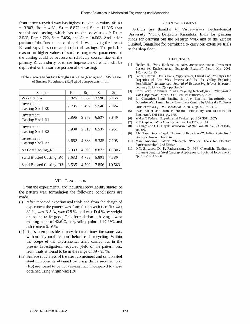
from thrice recycled wax has highest roughness values of; Ra

= 3.983, Rq = 4.89, Sa = 8.872 and Sq = 11.305 than

sandblasted casting, which has roughness values of; Ra =

3.535, Rq= 4.702, Sa = 7.856, and Sq = 10.563. And inside

portion of the Investment casting shell was having the lowest

Ra and Rq values compared to that of castings. The probable

reason for higher values of surface roughness parameters of

the casting could be because of relatively coarser size of the

primary Zircon slurry coat, the impression of which will be

duplicated on the surface portion of the casting.

Table 7 Average Surface Roughness Value (Ra/Sa) and RMS Value

of Surface Roughness (Rq/Sq) of components in µm

Sample Ra Rq Sa Sq

Wax Pattern 1.825 2.582 3.598 5.065

Investment

Casting Shell R0 2.735 3.497 5.548 7.024

Investment

Casting Shell R1 2.895 3.576 6.537 8.840

Investment

Casting Shell R2 2.908 3.818 6.537 7.951

Investment

Casting Shell R3 3.662 4.888 5.385 7.105

As Cast Casting_R3 3.983 4.890 8.872 11.305

Sand Blasted Casting R0 3.632 4.755 5.891 7.530

Sand Blasted Casting R3 3.535 4.702 7.856 10.563

VII. CONCLUSION

From the experimental and industrial recyclability studies of

the pattern wax formulation the following conclusions are

made.

(i) After repeated experimental trials and from the design of

experiment the pattern wax formulation with Paraffin wax

80 %, wax B 8 %, wax C 8 %, and wax D 4 % by weight

are found to be good. This formulation is having lowest

melting point of 42.60C, congealing point of 40.3°C, and

ash content 0.16 %.

(ii) It has been possible to recycle three times the same wax

without any modifications before each recycling. Within

the scope of the experimental trials carried out in the

present investigations recycled yield of the pattern wax

from trials is found to be in the range of 89 - 93 %. (iii) Surface roughness of the steel component and sandblasted

steel components obtained by using thrice recycled wax

(R3) are found to be not varying much compared to those

obtained using virgin wax (R0).

ACKNOWLEDGMENT

Authors are thankful to Visvesvaraya Technological

University (VTU), Belgaum, Karnataka, India for granting

funds for carrying out the research work and to the Zircast

Limited, Bangalore for permitting to carry out extensive trials

in the shop floor.

REFERENCES

[1] Fielder H., "Wax Reclamation gains acceptance among Investment

Casters for Environmental, Economic Reasons". Incast, Mar 2001,

14(2), pp. 12-15. [2] Pankaj Sharma, Doli Kasana, Vijay Kumar, Charat Goel, “Analysis the

Properties of Lost Wax Process and Its Use ability Exploring

Possibilities”. International Journal of Engineering Science Invention, February 2013, vol. 2(2), pp. 32-35.

[3] Chris Verta “Advances in wax recycling technologies”. Pennsylvania

Wax Corporation, Paper ID 113, Source Number72, 2005. [4] Er. Charanjeet Singh Sandhu, Er. Ajay Sharma, “Investigation of

Optimize Wax Pattern in the Investment Casting by Using the Different

Form of Waxes”, IOSR-JMCE, vol. 3, no. 9, pp. 01-06, 2012.

[5] Irwin Miller and John E Freund, “Probability and Statistics for

Engineers”, PHI 1981, pp. 375.

[6] Walter T Federer “Experimental Design”, pp. 166 (IBH 1967). [7] V.P. Guptha, Indian Foundry Journal, Jan 1977, pp. 14.

[8] S. Durga and U.B. Nayak. Transaction of IIM, vol. 40, no. 5, Oct 1987,

pp. 395. [9] P.K. Batra, Seema Jaggi. “Factrortial Experiment”’, Indian Agricultural

Statistics Research Institute.

[10] Mark Anderson, Patrick Whitcomb, ‘Practical Tools for Effective Experimentation’, 2nd Edition.

[11] D.N. Shivappa, Dr. K. Radhakrishna, Dr. M.P. Chowdiah. ‘Studies on

Chromite Sand for Steel Casting- Application of Factorial Experiment’, pp. A.5.2.1- A.5.2.8.


ISBN: 978-1-61804-226-2 123

Table 4 ANOVA Table for Melting Point

Source of

variation

Degrees of

freedom

Sum of

squares

Mean

Squares

F

Expt.

F

Tabulated

Replicates 1 3.73829E-09 3.74E-09 0.163523

F 1,7 = 5.59

at 95%

F 1,7 = 12.25

at 99%

Main effects

B 1 9.12976E-07 9.13E-07 39.93597

C 1 7.53022E-07 7.53E-07 32.93914

D 1 1.05993E-06 1.06E-06 46.36402

Interaction between

variables.

BC

1 6.89986E-07 6.9E-07 30.1818

BD 1 9.49168E-08 9.49E-08 4.151907

CD 1 3.13482E-06 3.13E-06 137.1254

BCD 1 1.87428E-07 1.87E-07 8.198591

Error 7 1.60027E-07 2.29E-08

Totals 15 6.99685E-06

Table 5 ANOVA Table for Congealing Point

Source of

variation

Degrees of

freedom

Sum of

squares

Mean Squares F

Expt.

F

Tabulated

Replicates 1 6.83549E-09 6.84E-09 0.114955

F 1,7 = 5.59 at

95%

F 1,7 = 12.25

at 99%

Main effects

B 1 6.11562E-07 6.12E-07 10.28485

C 1 9.98376E-07 9.98E-07 16.79005

D 1 1.70645E-06 1.71E-06 28.69791

Interaction between

variables.

BC 1 8.84074E-07 8.84E-07 14.86778

BD 1 3.77051E-08 3.77E-08 0.634099

CD 1 4.63975E-06 4.64E-06 78.02831

BCD 1 1.2419E-07 1.24E-07 2.088544

Error 7 4.16237E-07 5.95E-08

Totals 15 9.42517E-06


ISBN: 978-1-61804-226-2 124

Abstract - The analysis of the mechanical properties of cells is a field of great interest both in medicine and biology because it becomes fundamental each time it is necessary to recognize and prevent some diseases causing alterations in cellular behaviour and resistance. Biological Micro Electro-Mechanical Systems (Bio-MEMS) allow the application of extremely small and precise forces increasing, as a consequence, the number of results possible per experiment and the number of experiments that can be performed simultaneously. The aim of our work is to present an electro-thermally actuated microgripper for single-cell manipulation. Specifications and targets impose several limitations and difficulties in micro manipulators design and these obstacles are even more important when the target of microgripping are biological particles (e.g. living cells). The main parameters that have to be taken into account while designing a cell micromanipulator are, aside from its actuation principle, its kinematics, its fingertips shape, its releasing strategy and its material biocompatibility. Electro-thermal actuation strategy is investigated in order to understand its main advantages and limitations related, for example, to thermal stability, insulation and high temperatures; all these parameters have to be considered to ensure the cell’s integrity during its micromanipulation. Fabrication step and fabrication strategy is presented as the results of the realization procedure.

Keywords - Bio-MEMS, cell manipulation, cell microgripper, electro-thermal actuation

I. INTRODUCTION Cells are subjected to continuous stimulation inside the human body. For example, bone cells are subjected to compression; endothelium (inside blood vessels) cells to both stretching and shear stress; muscle cells to stretching; cardiac cells to both stretching and compression. Even though a lot is known with respect to their structure, there is only little information about cellular mechanics and cellular response to mechanical stimuli. The study of cells mechanical properties is of great interest because of the important implications it has for the comprehension of the cellular model and of the correlation between illness and genetic alterations; some diseases (e.g. many cardiovascular diseases, intracranial injury and hypertension) cause changes in cellular behaviour so the cellular resistance is modified in case of solicitations. In order to recognize and prevent some diseases, the quantification of the mechanical properties of cells becomes fundamental.

Corresponding author: *[email protected]

Rheology is a science that studies the balance achieved by a material that flows or deforms itself as a result of a state of solicitation. Its bases were laid by E.C. Bingham in 1928 with the aim of formulating appropriate analytical models able to describe the behavior of materials (both natural and for industrial production) in the most varied conditions of stress and the resulting deformation. In medicine, one of the most common rheological analysis is the hemorheology and it consists in determination of the characteristics of blood considered as a homogeneous fluid when flowing through the large arteries, veins and the heart; in case of both large and small vessels, however, the rheological properties of blood depend on the viscoelastic properties of its individual cells (mainly red blood cells, white blood cells and platelets) as well as on the properties of plasma considered as a Newtonian fluid whose viscosity is independent of its flow speed. In case of the great arteries and veins, the viscosity of blood is mainly dependent on the viscosity of plasma and on the concentration and on the properties of red blood cells (the volume of leukocytes and platelets is too small so they have little influence on the total blood viscosity). Hemorheology has important applications also from the diagnostic point of view: the alteration of the rheological parameters (e.g. viscosity and/or hematocrit variations, changes in the aggregation of red blood cells, etc.) may lead to a decrease in the blood flow and consequently to a lower contribution of nourishment to tissues. The problem of cell mechanics can be approached using two different techniques: the study of cell populations or of single cells. The dynamics of cell populations can be investigated using bioreactors. Silicone rubber and gels (e.g. poly-dimethyl siloxane (PDMS)) are commonly used as substrates for cell adhesion and stretching. This approach can provide information about the average mechanical properties of cells. One criticism of cell population studies is that, despite the ability of such studies to show that applied mechanical stress alters cell structure and function, the heterogeneity among cell responses is largely ignored. Furthermore, the response of a single cell to mechanical signals cannot be decoupled easily from the response of the entire population. As concerns the single cell approach, the existing techniques can be subdivided into two separate branches: local probes, used to stimulate a portion of the cellular membrane, and mechanical stimulation of the entire cell. In the first case, the probe can be, for instance, the Atomic Force Microscope (AFM) sharp tip located at the free end of a flexible cantilever

Design and building-up of an electro-thermally actuated cell microgripper

Aurelio Somà*, Sonia Iamoni, Rodica Voicu, Raluca Muller


ISBN: 978-1-61804-226-2 125

generating a local deformation on the cell surface; the resulting deflection of the cantilever tip can be calibrated to estimate the applied force. Magnetic Twisting Cytometry (MTC) is also a common method for the local stimulation of a cell; in this case, magnetic beads are attached to a cell and a magnetic field imposes a twisting moment on the beads, thereby deforming a portion of the cell. The mechanical stimulation of the entire cell can be performed mainly using optical tweezers or laser trap, micropipette aspiration, micro-plates or MEMS. In the case of optical tweezers or laser trap, an attraction force is created between a dielectric bead and a laser beam, pulling the bead towards the focal point of the trap. In micropipette aspiration, a cell is deformed by applying suction through a micropipette placed on the surface of the cell; by recording geometry changes of the cell, the elastic response of the cell is inferred, however it is not easy to take into account the friction between the cell membrane and the micropipette walls. Micropipette aspiration is a useful tool for the study of cells in suspension, like red blood cells, but not for the study of adherent cells in their physiological conditions. In micro-plates system, the single cell is seized between two glass micro-plates; one of the plates, being more flexible, serves as a sensor of the applied force. The micro-plates used to manipulate cells are very adhesive and thereby promote cell spreading. Cells are different in sizes and shape: an ostrich egg is a single cell with a diameter of more than 10 cm, while a human red blood cell is orders of magnitude smaller, with a diameter of approximately 8 μm. Most cells, however, are in the range of 10‐30 μm in diameter, so a fine cell mechanics analysis can be performed by means of Micro Electro-Mechanical Systems (MEMS) that give the possibility of carrying out studies on a single cell and not only on populations of a few million cells. MEMS devices realized in silicon-based technology have been largely used for several applications in military, satellite and communication fields, but only few works about the use of MEMS devices for the study of single cells have been reported up to now. Due to the great flexibility of MEMS in relation to the possible solicitation modes, a biaxial solicitation can also be applied; this load condition is common among the cells located in tissues which play a key role in the human body, for example, the pericardium. MEMS technology offers many advantages in the study of the mechanical properties of cells such us the compatibility of the device dimensions with the characteristics of the single cell, the possibility of applying forces in a wide range (pN÷μN), the possibility of carrying out studies on the single cell both adherent to the substrate and in suspension, the possibility of stimulating the entire cell and not only a local portion of its membrane and, finally, the possibility of working in a liquid medium; the ability to discriminate and move individual groups of living cells within or out of aqueous media is an important advantage since it can lead to the arrangement of cells in specific patterns, to the placement on surfaces of sensors or to the isolation of individual cell spheres from a culture.

II. CELL MICROMANIPULATION

The increased demands of microtechnical applications have led in the last twenty years to the development of new assembling technologies which enable handling of very small microoptical, microelectronical or micromechanical elements in nano or micrometer range. Specifications and targets impose several limitations and difficulties in micro manipulators design especially when the target of microgripping are biological particles (e.g. living cells). The actuation mechanism of cell microgrippers shall be suitable for operating in electrolytic aqueous media because of ionic environment of cells; this fact limits the application of high voltage in piezo actuated grippers since bubble formation, caused by electrolysis, occurs at 1.5-2 volts in water. Moreover, any exposure to magnetic or electrical fields may have some negative effects on biological cells limiting the application of electrostatic or electromagnetic actuated microgrippers. Shape memory alloy (SMA) actuators are not applicable in micro grippers because of the lack of reliability for a high number of cycles. Electro-thermal actuators are widely studied for cell manipulation even though they show many difficulties when are used as the maximum allowed temperature for manipulation of human cells in many applications is around 37 °C that is quite lower than the required high temperature (more than 100 °C for bare extended arms of gripper) in an electro-thermal gripper. Gripper’s materials biocompatibility places some restrictions in choosing of actuation method and fabrication process. A survey of the cells microgrippers state of art reveals that, whatever the actuation method is, there are many points that must be taken into consideration for microgripper design, such as:

- actuation principle - kinematics - fingertips shape - force feedback - releasing strategy

From a system engineering point of view all these aspects have to be taken into account in the preliminary design of a cell microgripper. A. Actuation principle

Talking about the actuation of a microgripper, two different strategies (internal and external) are possible. In case of internal actuation, it is possible to design a specific part of the gripper with piezoelectric (PZT) material in order to generate a localized force when an electric voltage is provided [3-4]. The electrostatic force [5-8] can be used as an actuation by applying a voltage difference on a capacitor with movable armature. The thermal actuation, widely used for both biological and non-biological manipulation, is based on the thermal expansion of the gripper arms due to the Joule effect in presence of electric currents [9-13]. A faster response of the arms can be achieved with shape memory alloys [14-16] that are able to restore almost immediately the memorized shape when a threshold temperature is passed. The electromagnetic


ISBN: 978-1-61804-226-2 126

actuation [17] is based on micro-coils and is able to generate weak confined magnetic fields. Hydraulic and pneumatic actuation can be used to manipulate bio-cells with micro-pipes integrated in small circuits including micro-pumps and valves. Each one of the described internal actuation strategies has its own limits. PZT actuators have strong nonlinear output, high supply voltage, small motion range, low resistance to creep and mechanical fatigue phenomena, hysteresis and biocompatibility problems. The electrostatic actuators are generally disadvantaged by the small dimensions of the capacitors; very complicated shapes of the gripper having many comb drives are necessary to increase the force, but, as a consequence, the motion range is strongly reduced by the small gaps between the armatures and the applied voltage easily causes electrolysis of watered environments. Thermal actuators may induce high temperature in the region close to the cells so long grippers dissipating the heat produced by the actuators need to be used. SMA materials present low fatigue resistance that causes very limited cycle time, small strain capability, strong nonlinearity, hysteresis and a fabrication process that is usually very complicated at the microscale. The limitations of electromagnetic actuators are related to the small dimensions of electromagnetic micro-actuators that imply fast heating of the coil due to the Joule effect and low allowable currents; the resulting magnetic field is generally weak and subjected to relevant leakages, giving small power per unit volume. Hydraulic and pneumatic actuators are limited to pipe based devices; they are not suitable for precision operations involving more than one cell and the hydraulic solution only works in wet environments. External actuators preserve the thermal insulation of the gripper and avoid contaminations or biocompatibility problems. Piezoelectric motors are the most promising solution for this application, due to their small size and high accuracy as they have very high response and wide speed range (from few micrometers/second to few millimeters/second); thermal heating is negligible in this kind of actuator, but there are problems related to the interface [18] between the motor and the microgripper, where interferences and frictions must be considered. A particular kind of external actuation strategy is the manual one; in this case [19] the manual rotation of a micrometer head is used to open the tips of the tweezer structure, whereas the closing of the device is due to elastic deformation.

III. PROPOSED ACTUATION STRATEGY AND RESULTS

The dimensional scaling [20,21] has consequences both for the mechanical design and for the actuation of microactuators; the choice of the actuation principle depends on the structural dimensions, the technology, the functioning and the purpose of the micro device. External forces can be generated using different effects such as the thermopneumatic, the electrochemical, the electrostatic and the magnetic ones; internal forces exploit the intrinsic actuation capability of some special materials including piezoelectric, thermomechanical, shape memory and electrostatic effects.

The presented work deals with the electro-thermal actuation strategy; a polymeric microgripper is used to catch a cell having a diameter up to 40 μm creating a micro chamber around the cell to insulate it from the other ones and provide cell rheological analyses. The polymer used as the base material of the microgripper is SU-8 having good mechanical and chemical properties (see Table I), biocompatibility, ease of fabrication and low cost. It is important to make a note: the presented results were obtained by means of Ansys 11.0 FEM (Finite Element Method) simulations; no experimental activity has been done up to now so the results were compared, in terms of orders of magnitude, to the ones found in the literature. Table I. SU-8 mechanical/thermal properties. [18,22]

Young’s Modulus (E) [GPa] 2 Poisson ratio (ν) 0.22

Tensile Strength (σm) [MPa] 70 Coeff. of Thermal Expansion (α) [1/K] 52·10-6

Thermal Conductivity (λ) [W/(m·K)] 0.3 Softening point [°C] 210

A. Thermal actuation

In Figure 1 it is possible to see a thermally driven microgripper where the Joule heating is produced via a thin gold metallic layer deposited and patterned on the top of SU-8.

Fig. 1 thermally driven microgripper geometry; the gripping zone and the clamped region for mechanical equilibrium are pointed out

To perform the simulation it was necessary to put thermal constraints on the device as it can be seen in Figure 2: the extreme cold arms of the gripper are at room temperature (supposed to be equal to 20 °C) whereas the central hot arm is subjected to different temperatures (from 30 °C to 100 °C) depending on the voltage applied so on the current flowing through it. Figure 3 shows a relationship between the temperature of the hot arm and the openings of the microgripper; temperatures higher than 100 °C but lower than 210 °C (the SU-8 softening point) weren’t taken into account in the FEM simulations but the values of the jaws openings corresponding to this range of temperatures were reported as well in the graph (see the continuity coloured lines in dashes) exploiting the linear relationship shown by the 30 °C÷100 °C range of temperatures coming from the simulations.

Fig. 2 thermally constrained arms of the microgripper


ISBN: 978-1-61804-226-2 127

Fig. 3 gripping site openings vs hot arm temperature

As it was previously said, the main problem related to thermal actuation of biological particles is the high temperature that could destroy or damage the cell, so it was necessary to study the temperature distribution (see Figure 5) along the microgripper giving it a particular geometry so that the temperature of the gripping zone (20 °C÷26.7 °C) was not higher than the maximum temperature (37 °C) a cell can withstand without changing its biological/mechanical properties and behaviour. Figure 4 shows the four opening zones considered in the gripping site; as it can be seen from the picture, “CD” and “GH” openings are the reference ones because a cell can enter without exiting the microgripper only if it has a diameter lower than “CD” distance and bigger than “GH” one. For example, heating the actuation hot arm until a temperature of 80 °C, a cell having a diameter from 37 μm to 41 μm can enter the microgripper to be analyzed.

Fig. 4 opening zones of the gripping site

Fig. 5 temperature distribution along the microgripper

IV. FABRICATION STEPS

The following photographs (taken under both optical and electron microscope) deal with the main building-up steps of the micromanipulator discussed until now; it was fabricated in the clean room of IMT in Bucharest (National Institute for

Research and Development in Microtechnologies). For the manufacturing process we used the surface micromachining techniques and 2 masks processes. The materials used were thermal silicon dioxide, used as sacrificial layer, SU-8 as structural layer and chromium/gold for the manufacturing of the resistors. The masks were designed using Clewin program: one mask for the metallic resistors configuration and one for the SU-8 configuration. The realized physical masks were analyzed using optical microscope (Fig. 6-7). After the masks manufacturing we proceeded with the technological steps for the manufacturing of the microgripper structures.

Fig. 6 SU-8 physical mask (optical microscope photo)

Fig. 7 gold physical mask (optical microscope photo) We used silicon wafers which were cleaned in piranha solution before starting the technological steps. Using thermal oxidation process we obtained a 1.7 µm thick layer of silicon dioxide, used as sacrificial layer. A Cr/Au layer was deposited using sputtering evaporation on the SiO2 layer. Thicknesses of 10nm/300nm were obtained for the Cr/Au layer which was patterned using the first mask. We spun the polymer SU-8 2025 at 3000 rpm on the wafer and obtained a thickness of around 20 µm. The wafer was soft baked at 65 oC and 95 oC and exposed using the second mask. After exposure, the wafer was baked again at 65 oC and 95 oC to obtain the latent image of the SU-8 layer geometry. In order to obtain the microgripper configuration (Fig. 8) the wafer was developed. The last thermal process of the polymer was the hard bake at 180 oC for 30 minutes in order to finalize the cross links of the SU-8 (Fig. 9-10).


ISBN: 978-1-61804-226-2 128

Fig. 8 SU-8 configured layer before hard bake treatment

Fig. 9 SU-8 configured layer (SEM photo)

Fig. 10 a chip with six SU-8 configured structures Figures 11 and 12 present the optical microscope images of the Cr/Au configured heating resistors on wafer. Figure 13 shows an individual microgripper structure of a chip with 6 structures (Fig. 14) after the final techonological processing step before the releasing of the chips.

Fig. 11 configured gold resistance on silicon substrate before the deposition/configuration of the SU-8 layer

Fig. 12 gold configured layer (optical microscope photo)

Fig. 13 one structure with configured SU-8 and gold layers (optical microscope photo)


ISBN: 978-1-61804-226-2 129

Fig. 14 one chip with six structures at the final step of fabrication (optical microscope photo) To release the microgripper structures we performed wet etching in a bath of buffered HF acid. In the same technological step of surface micromachining we obtained the chip with 6 structures (as presented in Fig. 8 where holes design, in order to have a faster removal of the sacrificial layer, can be seen). The final structures will be used for further tests and measurements.

V. CONCLUSIONS AND FUTURE PURPOSES In this paper a preliminary design of a cell microgripper and its fabrication are discussed by evaluating the system requirements. The electro-thermal strategy is proposed and optimized by means of the finite element method; the cylindrical shape of the fingertips not to have high pressures acting on the cell external surface, the thermo-mechanical design and the analysis of the thermically actuated gripper in order to have low temperatures in the cell gripping zone are all strengths that make this micro-device innovative, not conventional and especially suitable also in the bio-field and not only in the micro-mechanical one. Some biological cells have a diameter up to 50 μm so the use of a microgripper having a gripping zone not bigger than 40 μm generates interference and compression forces between each one of these cells and the jaws of the device; our purpose is the creation of a FEM contact model to evaluate the pressure acting on the external surface of the cell by varying the gripping zone shape and/or the cell shape. The mechanical and the material properties of the cell have to be introduced in the FEM simulation as if the cell were a micro mechanical component subjected to an external load. An other future purpose of our research activity is linked to the thermally actuated micro device proposed in this paper; we would like to compare the FEM simulations results with some future laboratory experimental ones to study the electro-thermal behaviour of the device and perform some cell rheological analyses.

REFERENCES [1] Darnell, Lodish, Baltimore, “Molecular Cell Biology”, Scientific

American Books, Distributed by W. H. Freeman and Company, New York, 1990, pp. 681-951.

[2] Darnell, Lodish, Baltimore, “Molecular Cell Biology”, Scientific American Books, Distributed by W. H. Freeman and Company, New York, 1990, pp. 617-638.

[3] Nah S.K., Zhong Z.W., “A microgripper using piezoelectric actuation for micro-object manipulation”, Sensors and Actuators A 133, pp. 218-224, 2007.

[4] Mohd Nashrul Mohd Zubir, Bijan Shirinzadeh, Yanling Tian, “A new design of piezoelectric driven compliant-based microgripper for micromanipulation”, Mechanism and Machine Theory 44, pp. 2248-2264, 2009.

[5] Beyeler F., Neild A., Oberti S., Bell D.J., Sun Y., Dual J., Nelson B.J., “Monolithically Fabricated Microgripper With Integrated Force Sensor for Manipulating Microobjects and Biological Cells Aligned in an Ultrasonic Field”, Journal of Microelectromechanical Systems 16(1), pp. 7-15, 2007.

[6] Volland B.E., Heerlein H., Rangelow I.W., “Electrostatically driven microgripper”, Microelectronic Engineering 61-62, pp. 1015-1023, 2002.

[7] Heng-Chung Chang, Julius Ming-Lin Tsai, Hsin-Chang Tsai, Weileun Fang, “Design, fabrication, and testing of a 3-DOF HARM micromanipulator on (111) silicon substrate”, Sensors and Actuators A 125, pp. 438-445, 2006.

[8] Tao Chen, Lining Sun, Liguo Chen, Weibin Rong, Xinxin Li, “A hybrid-type electrostatically driven microgripper with an integrated vacuum tool”, Sensors and Actuators A 158, pp. 320-327, 2010.

[9] Ivanova K., Ivanov T., Badar A., Volland B.E., Rangelow I.W., Andrijasevic D., Sümecz F., Fischer S., Spitzbart M., Brenner W., Kostic I., “Thermally driven microgripper as a tool for micro assembly”, Microelectronic Engineering 83, pp. 1393-1395, 2006.

[10] Volland B.E., Ivanova K., Ivanov Tzv., Sarov Y., Guliyev E., Persaud A., Zöllner J.P., Klett S., Kostic I., Rangelow I.W., “Duo-action electro thermal micro gripper”, Microelectronic Engineering 84, pp. 1329-1332, 2007.

[11] Deutschinger A., Schmid U., Schneider M., Brenner W., Wanzenböck H., Volland B., Ivanov Tzv., Rangelow I.W., “Characterization of an electro-thermal micro gripper and tip sharpening using FIB technique”, Microsyst Technol DOI 10.1007/s00542-010-1110-0, 2010.

[12] Andersen K.N., Carlson K., Petersen D.H., Mølhave K., Eichhorn V., Fatikow S., Bøggild P., “Electrothermal microgrippers for pick-and-place operations”, Microelectronic Engineering 85, pp. 1128-1130, 2008.

[13] Nam-Trung Nguyen, Soon-Seng Ho, Cassandra Lee-Ngo Low, “A polymeric microgripper with integrated thermal actuators”, J. Micromech. Microeng. 14, pp. 969-974, 2004.

[14] Huang W., “On the selection of shape memory alloys for actuators”, Materials and Design 23, pp. 11-19, 2002.

[15] Kohl M., Skrobanek K.D., “Linear microactuators based on the shape memory effect”, Sensors and Actuators A 70, pp. 104-111, 1998.

[16] Kohl M., Brevet B., Just E., “SMA microgrypper system”, Sensors and Actuators A 97-98, pp. 646-652, 2002.

[17] Giouroudi I., Hötzendorfer H., Kosel J., Andrijasevic D., Brenner W., “Development of a microgripping system for handling of microcomponents”, Precision Engineering 32, pp. 148-152, 2008.

[18] Mousavi M.M.S., De Pasquale G., Somà A., Brusa E., “A Novel SU-8 Microgripper with External Actuator for Biological Cells Manipulation”, Proc. DTIP, 2011, pp. 356-361.

[19] Bin-Da Chan, Farrukh Mateen, Chun-Li Chang, Kutay Icoz, Cagri A. Savran, “A Compact Manually Actuated Micromanipulator”, Journal of Microelectromechanical Systems 21(1), pp. 7-9, 2012.

[20] Thielicke E., Obermeier E., “Microactuators and their technologies”, Mechatronics 10, pp. 431-455, 2000.

[21] Ouyang P.R., Tjiptoprodjo R.C., Zhang W.J., Yang G.S., “Micro-motion devices technology: The state of arts review”, Int J Adv Manuf Technol 38, pp. 463-478, 2008.

[22] http://www.microchem.com/pdf/SU-8-table-of-properties.pdf.


ISBN: 978-1-61804-226-2 130

Abstract— The model of plasticity based on the ideas of deformed material as a two-phase heterogeneous medium is suggested. Within this approach the wave displacement is regarded as a shock transition in this medium. One of the phases which is an excited one is responsible for system restructuring, and another one is normal and unrelated to structural transformations. The plasticity wave is the result of these two phases interaction. The equations of a filtration model are obtained, that include the laws of pulse and mass conservation as well as filtration ratio between the phases.

Keywords— plastic deformation, the plasticity wave, filtration model, heterogeneous medium

.

I. INTRODUCTION ne of the problematic issues in the physics of strength and plasticity is the explanation of the observed inhomogeneities of plastic flow of materials as well as its

stages during the experiment [1, 2]. To date, methods of modern physical materials science such as scanning and transmission electron microscopy and double-exposure speckle-interferometry have shown that the process of plastic deformation is of wave nature [3 – 5]. It is proved by the stress distribution at the boundary “surface layer – substrate” in the “staggered” order (the “checkerboard” effect) [3, 4] and non-uniform distribution of displacement fields and deformations [5]. These facts indicate that there are zones in the material not involved into the plastic deformation. The characteristic scales of inhomogeneities according to [5] can be from ~ 1 µm to ~ 1 mm. Stages of plastic deformation are due to the changing nature of deformation localization, increase of the number of equidistant localization sites at the stages of linear and parabolic hardening, and at the stage of pre-fracture the collapse of plasticity wave occurs.

Studies of the dislocation substructures [6, 7] at various stages of plastic deformation showed that the transition from one stage to another is accompanied by a transformation of one type substructure to another and during the transition process two types of substructures can exist simultaneously.

This work was supported by the RFBR Grant 14-08-00506 А (sponsor

and financial support acknowledgment goes here). V. D. Sarychev is with the Siberian State University of Industry,

Novokuznetsk, Kirov Street 42, 654007, Russia (corresponding author to provide phone: +7(3843) 78-43-91; fax: +7(3843) 46-57-92; e-mail: [email protected]).

S. A. Nevskii, is with the Siberian State University of Industry, Novokuznetsk, Kirov Street 42, 654007, Russia (e-mail: [email protected]).

E. V. Cheremuskina, is with the Siberian State University of Industry, Novokuznetsk, Kirov Street 42, 654007, Russia (e-mail: [email protected]).

V. E. Gromov, is with the Siberian State University of Industry, Novokuznetsk, Kirov Street 42, 654007, Russia (e-mail: [email protected]).

The combination of these experimental facts leads to the conclusion that the cause of the observed regularities of plastic flow is the collective nature of the changes of the internal structure [8 – 12]. To describe plastic deformation the ideas of mechanics of heterogeneous media can be applied [13]. Such approach was used in [14] for the study of phase transformations, plastic deformation and other structural transformations of the solid. The peculiarity of this approach is the split of the entire ensemble of the structural elements of the medium (atoms, defects, etc.) into two subsystems: the excited one, responsible for the system restructuring and the normal one which is unexcited and not related to structural transformations. After splitting the resulting heterogeneous mixture is represented as a set of several continua-phases, each of which is described by the conservation laws and defining equations.

II. PROBLEM STATEMENT The proposed model in this paper provides an explanation of non-uniform distribution of displacements under uniaxial deformation [5] using the laws of momentum and mass conservation. As it is known [15], plastic deformation of polycrystals occurs due to the micro-and macroshifts that are presented in this model as a current of fast-moving phase in between the weakly deformable and inactive blocks, which can be seen as a current of two-phase heterogeneous mixture. The first component will be the microshifts, the second one – macroshifts. We will provide the conservation laws for each component. They will be:

2111 div Iwt

=+∂

∂

ρρ (1)

wIpdt

wd21211

11

~div −+= σρ

∇⋅+

∂∂

=

wtdt

d1

(2)

1222 div Iut

=+∂

∂

ρρ (3)

uIpdt

ud

121222

2~div −+= σρ

∇⋅+

∂∂

=

utdt

d2

(4)

where eαρρ =1 , sραρ )1(2 −= , σασ ~~

1 = , σασ ~)1(~2 −= , ρe

and ρs – the true densities of phases, α - the volume fraction of the first phase, σ~ – the voltage of the whole mixture,

1221 pp

−= , I21= -I12 – the exchange intensity of momentum and mass, respectively, between the phases, w and u – velocities of the first and the second phase, respectively. The intensity of pulse exchange between the phases can be represented as 21212121 uIRp

+= , where R21 – interphase

Model of Plasticity by Heterogeneous Media Vladimir D. Sarychev, Sergei A. Nevskii, Elena V. Cheremushkina, Victor E. Gromov

O


ISBN: 978-1-61804-226-2 131

force associated with the friction forces, the clutch phases, and 2121uI

‒ with phase transformations. We assume that the intensity of mass transfer is small compared to the intensity of the momentum exchange and the mixture components interact according to Rakhmatulin’s scheme [16]. Consequently, ,2121 Rp

= 2121 FpR

+∇−= α , where force

( )wuK

F e

−−= )1(121 ααρ is associated with high-speed non-

equilibrium phases, where K – constant. With regard to all of the above facts the system (1) – (4) takes the form:

;/))(1(~div11 Kwu

dtwd

e

−−+= ααρσαρ (5)

;0div111 =+ w

dtd

ρρ (6)

( ) ;/))(1(~div122 Kwu

dtud

e

−−−−= ααρσαρ (7)

,0div222 =+ u

dtd

ρρ (8)

In (5) assume that the inertial member 011 ≈

dtwd

ρ then adding

(5) with equation (7) leads to the following relation:

( ) Kwudiv e /)1(~

−−−= ραασα . (9)

Equation (9) is a consequence of the law of momentum conservation for the first phase and is analogous to Darcy’s law in the filtration theory [13]. Sense of the constant 1/K is that it is a factor of resistance to movement of the first phase from the second. System (5) – (8) must be closed by the equation of state. Since the second phase is a weakly deformable blocks, then ρs = const. For the first phase, we assume that ).(PFe =ρ Now let us consider the problem in the one-dimensional setting. As it is known the voltage in a heterogeneous mixture depends on the pressure P−=σ~ . As it is known the voltage in a heterogeneous mixture depends on the pressure. Then (5) – (8) with regard to (9) and equations of state will be as follows:

We seek a solution in the form )( 0tux −α , )( 0tuxu − , )( 0tuxw − , )( 01 tux −ρ , )( 0tuxP −

therefore

First integrals of the equations (13) – (15) are:

0

11uu

С−

−=α , (16)

( )uCCP sρ12 −= , (17)

30 )1(С

BPKuu

ee =

−

′−−

ρααρ . (18)

Transforming (18) with (16), (17) and 0uuu −= we get an equation containing the rate of the second phase:

1

13 )(CuCuC

dud e

−−−

=ρ

η, (19)

where sK

ddρξη = . Consider the case APe =ρ [17], then

1

21 ))((Cu

uuuud

ud−

−−=

η, (20)

Where 1u , 2u – velocities of the second phase on the border

focus localization. Integration of this equation leads to:

CduuuuuCuu

uuuС

+=−

−−

−−

−− η)ln()ln( 1

12

112

21

21 (21)

To determine the constants involved (20) and (21) we can

write the boundary conditions:

( ) 10 uu = , ( ) 2uLu = , ( ) 00 =′u , ( ) 0=′ Lu

1)0( αα = , 2)( αα =L (22) Then, by (22) the first integrals will take the form:

111)1( Cu =− α ,

1121 uCCP sρ−= ,

0)( 21312211

21 =−−++− CCCuCCCu ρρ , (23)

122 )1( Cu =− α ,

2122 uCCP sρ−= ,

0)( 21322211

22 =−−++− CCCuCCCu ρρ .

Returning in (21) and (23) to the variable u, we construct the speed plotted for the second phase of the case u1 > u2 и α1< α2 from the coordinates at various time points (Figure 1). The

;)1(

1xP

xuu

tu

s ∂∂

−−=

∂∂

+∂∂

ρα (10)

( ) ;1xu

xu

t ∂∂

−=∂∂

+∂∂ ααα (11)

011 =∂

∂+

∂∂

xw

tρρ (12)

( ) ( ) ;1

10 Puuu

s′

−−=−′

ρα (13)

( ) uuu ′−=−′ )1(0 αα (14)

0)( 110 =′+′− wu ρρ (15)


ISBN: 978-1-61804-226-2 132

analysis of this dependence shows that it has a kind of "shock transition." Consequently, there are the areas of the deformable material, which are not involved in the plastic deformation, which is confirmed by experimental facts [5]. Speed containment chamber is defined as:

21

22110

)1()1(αα

αα−

−+−=

uuu . If u1 = 0 and u2 = u*, where u* –

velocity of the traverse beam, the values of the marginal rate of localization focus on the order exceeds the rate of the traverse beam of the testing machine, which also corresponds to the experiment. The case u1 < u2 and α1 > α2 also allows the existence of "shock transition". Note that these relationships were obtained in [18] for fixed and dynamic structures and in [19], for a shock wave in an ideal gas.

Fig. 1. The velocity of the second phase from the coordinates

at various points of time: 1− t=0, 2 – t=1, 3 – t = 2.

We define the width of the "shock transition" with the formula,

which has the following form:

−

=

dxduuul

max

21 . The evaluation

of the magnitude shows that it has the value of ~ 10 µm, which coincides with the characteristic length scales of heterogeneity observed in the experiment. Note also that the path of dislocations in the materials are of the same order of magnitude [20].

III. CONCLUSIONS 1. The system of equations of filtration plasticity model is built. A solution is obtained in the form of "shock transition." Its width was defined, which coincides with the characteristic values of the scale of the inhomogeneity of deformation. 2. It is shown that the maximum speed of the focus on the localization of the order exceeds the rate of crosshead of the testing machine, which corresponds to the experimental data.

REFERENCES [1] V.E. Panin, V.E. Egorushkin, T.F. Elsukova “Physical mesomechanics

of grain boundary sliding in a deformed polycrystalline”, Physical mesomechanics, vol. 14, Issue 6, 2011, pp. 15 – 22.

[2] P.V. Yasniy, P. O. Marushak, S.V. Panin and others “The vicissitudes of deformation of the material and the kinetics of growth of fatigue cracks in steel 25Kh1M1Ph at low loading frequencies”, Physical mesomechanics, vol. 15, Issue 6, 2012, pp. 15 – 22.

[3] V.E. Panin, A.V. Panin “The effect of the surface layer in a deformable solid”, Physical mesomechanics, vol. 8, Issue 5, 2005, pp. 7 – 15.

[4] V.E. Panin “Surface Layers as Synergetic Activator of Plastic Yielding of Loaded Solid”, Metal Science and Heat Treatment, Volume 47, Issue 7-8, 2005, pp 312-318.

[5] L.B. Zuev, V.I. Danilov, S.A. Barannikova Physics of macrolocalization of plastic flow. Novosibirsk: Nauka, 2008, 328 p.

[6] E.V. Kozlov, L.I. Trishkina, N.A. Popova and others. “The place of dislocation physics in multi-level approach to plastic deformation”, Physical mesomechanics, vol. 14, Issue 3, 2011, pp. 95 – 110.

[7] N.A. Koneva, E.V. Kozlov “Physical nature of stages in plastic deformation”, Soviet Physics Journal, vol. 33, February 1990, pp 165-179.

[8] G.A. Malygin “Self-organization processes of dislocation and crystal plasticity”, UFN, vol. 181, 1999, pp. 1129 –1156. [in Russian]

[9] S.P. Kiselev “Dislocation structure of shear bands in single crystals”, Journal of Applied Mechanics and Technical Physics, vol. 47, November 2006, pp 857-866.

[10] J. Pontes, D. Walgraef, E.C. Aifantis “On dislocation patterning: Multiple slip effects in the rate equation approach”, International Journal of Plasticity, vol. 22, 2006, pp.1486 – 1505.

[11] P. P. Kaminskii, Yu.A. Khon “Kinetic theory of low-temperature microscopic crack nucleation in crystals”, Theoretical and Applied Fracture Mechanics, vol. 51, 2009, pp. 161-166.

[12] L.B. Zuev, Yu.A. Khon, S.A. Barannikova “Dispersion of autowaves in a localized plastic flow”, Technical physics, vol. 55, 2010, Issue 7, pp. 965 – 971.

[13] R.I. Nigmatulin The basics of mechanics of heterogeneous media. Moscow: Nauka, 1978. 336 p.

[14] E.C. Aifantis “On the Mechanics of Phase Transformations”, Phase Transformation. London, 1986.pp. 233 – 289.

[15] V.V.Rybin Large plastic deformation and fracture and the destruction of metals. Moscow: Metallurgy, 1986. 224 p.

[16] Kh. A. Rakhmatulin “The fundamentals of gas dynamics of interpenetrating motions of compressible media” Journal of Applied Mathematics and Mechanics, 1956, Issue 2, pp. 184 – 194 [in Russian]

[17] V.D. Sarychev, V.A. Petrunin “Filtration model of plastic deformation”, Izvestia VUZ Chernaya Metallurgiya, 1993, Issue 2, pp.29 – 33 [in Russian]

[18] V.G. Makaryan, N.E. Molevich, D.P. Porfiriev “Classification of gas-dynamic structures described by a nonlinear equation of acoustics of relaxing environment”, Vestnik of SamSU. The natural science series. 2009. Issue 6. pp. 92 – 104.

[19] B.L. Rozhdestvennskiy, N.N. Yanenko System of quasi-linear equations and their applications to gas dynamics. Moscow: Nauka, 1968. 686 p.

[20] J. Hirth, I. Lothe, Theory of dislocations. Moscow:: Atomizdat, 1972. 600 p.

1


ISBN: 978-1-61804-226-2 133

meltflow front

solidifying layer

wall

Abstract— Delivery of polymer melts into the mold cavity is the

most important stage of the injection molding process. This paper shows the influence of cavity surface roughness, polymer material (with different flow properties) and technological parameters on the flow length of polymers into mold cavity. Application of the measurement results may have significant influence on the production of shaping parts of the injection molds especially in changing the so far used processes and substituting them by less costly production processes which might increase the competitiveness of the tool producers and shorten the time between product plan and its implementation. Because the finishing operations of machining are very time and money consuming leading to high costs of the tool production.

Keywords— injection molding, mold, polymer, roughness, surface, fluidity.

I. INTRODUCTION NJECTION molding is one of the most extended polymer processing technologies. It enables the manufacture of final

products, which do not require any further operations. The tools used for their production – the injection molds – are very complicated assemblies that are made using several technologies and materials. Working of shaping cavities is the major problem involving not only the cavity of the mold itself, giving the shape and dimensions of the future product, but also the flow pathway (runners) leading the polymer melt to the separate cavities. The runner may be very complex and in most cases takes up to 40% volume of the product itself (cavity). In practice, high quality of runner surface is still very often required. Hence surface polishing for perfect conditions for melt flow is demanded. The stated finishing operations are very time and money consuming leading to high costs of the tool production.



Michal Stanek is with the Tomas Bata University in Zlin, nam. T. G. Masaryka 5555, 76001 Zlin, Czech Republic (phone: +420576035153; fax: +420576035176; e-mail: [email protected]).



Vojtech Senkerik is with the Tomas Bata University in Zlin, nam. T. G. Masaryka 5555, 76001 Zlin, Czech Republic (e-mail: [email protected]).

The fluidity of all polymers during injection molding cycle is affected by many parameters (mold design, melt temperature, mold temperature, injection rate, pressures, etc.) and by the flow properties of polymers. Results of the experiments carried out with selected types of polymer materials proved a minimal influence of surface roughness of the runners on the polymer melt flow. This considers excluding (if the conditions allow it) the very complex and expensive finishing operations from the technological process as the influence of the surface roughness on the flow characteristics does not seem to play as important role as was previously thought. A plastic nucleus is formed by this way of laminar flow, which enables the compression of the melt in the mold and consecutive creeping. A constant flowing rate given by the axial movement of the screw is chosen for most of the flows.

Fig. 1 Fountain flow During filling the mold cavity the plastic material does not

slide along the steel mold surface but it is rolled over. This type of laminar flow is usually described as a “fountain flow” (Fig.1).

II. INJECTION MOLDING The testing samples were prepared by injection molding

technology (injection molding cycle is shown on Fig. 2). The injection mold for was designed for the easiest possible manipulation both with the mold itself and during injection molding process while changing the testing plates, size of the mold gate, pressure and temperature sensors inside the cavity, etc. The cavity space of the mold is generated by the female mold part, called cavity, and a male mold part, called the core. It is necessary to fill the mold cavity fully during the injection molding process. The ability of cavity filling could be affected by the polymer properties and the properties of cavity walls.

How Surface Roughness Influence the Polymer Flow

M. Stanek, D. Manas, M. Manas and V. Senkerik

I


ISBN: 978-1-61804-226-2 134

http://slovnik.seznam.cz/search.py?lg=en_cz&wd=surface%20roughness

Fig. 2 Injection molding cycle

A. Testing plates The shaping part of the injection mold is composed of right

and left side. The most important parts of the injection mold concerning the measurements are: testing plate, cavity plate and a special sprue puller insert. There is possible to use pressure and temperature sensors in the mold cavity for the values progress evaluation.

Fig. 3 Cross section of mold cavity

The cavity (Fig. 4) of testing injection mold for is in a shape

of a spiral (Fig. 5) with the maximum possible length of 2000 mm and dimensions of channel cross-section: 6x1 mm. The cavity is created when the injection mold is closed, i.e. when shaping plate seals the testing plate in the parting plane of the mold. The mold cavity is cooling by flowing oil from tempering unit. [2]

Fig. 4 Cavity plate – shaping plate

Fig. 5 Testing sample – spiral

Testing Injection mold can operate with 5 easy exchangeable testing plates (Fig. 6) with different surface roughness.

testing plate

mold plate


ISBN: 978-1-61804-226-2 135

Fig. 6 Cavity plate – testing plate

The surface of the plates was machined by four different

technologies, which are most commonly used to work down the cavities of molds and runners in industrial production. These technologies are polishing, grinding, milling and two types of electro-spark machining – fine and rough design (Table 1). Table 1 Surfaces of testing plates

Plate surface Surface photo Polished plate (Ra = 0,102µm)

Grinded plate (Ra = 0,172µm)

Electro – spark machined plate with a fine design (Ra = 4,055µm)

Milled plate (Ra = 4,499µm)

Electro – spark machined plate with a rough design (Ra = 9,566µm)

The testing plates are made from tool steel (DIN 1.2325) whose are used for simple and fast changing the surface of the mold cavity. [7]

Injection molding machine ARBURG Allrounder 420C 1000 – 350 with oil tempering unit Regloplas 150 smart were used for testing samples production.

B. Sprue puller insert Special sprue puller insert enables the exchange of

differently sized gates. Size of the gate could be 1, 2, 4 or 6 mm.

Fig. 7 Sprue puller insert

C. Testing injection mold The testing injection mold is inserted into a universal frame

which was designed for use with many different injection molds that fit the size of the frame. This makes the change of the separate injection molds easier, because the frame remains clamped to the injection molding machine and only the shaping and ejection parts of the molds are changed. Attaching right and left sides of the frame to fixed and moving plates of the injection molding machine is done using four adjustable clamps on each side. [16, 17]

III. TESTED POLYMERS Six types of thermoplastic polymers with different flow

properties (MFI - Melt Flow Index) were tested: • polypropylen (PP) Mosten GB 003,

MFI = 3,3 • polyethylen (LDPE) Bralen VA 20-60,

MFI = 20 • termoplastic polyurethan (TPU) Ellastolan C 78 A,

MFI = 6,1 • akrylonitril-butadien-styren (ABS) Polylac PA 757,

MFI = 2,4


ISBN: 978-1-61804-226-2 136

polishedgrinded

electro-sparkmachined("fine")

milledelectro-spark

machined("rough")

injection rate 30 mm/s

injection rate 60 mm/s

injection rate 90 mm/s160

170

180

190

200

210

220

flow

leng

th [m

m]

surface of testing plate

injection rate 30 mm/sinjection rate 60 mm/sinjection rate 90 mm/s

• polypropylen filled by 20% of chalk Taboren PH 89 T20, MFI = 14,4

• polypropylen filled by 10% of chalk Keltan TP 7603, MFI = 16,9

IV. RESULTS The filling of mold cavity depends on material properties,

technological conditions and surface quality. The lower is the viscosity of polymer (measured by Melt Flow Index) the better cavity filling has been achieved (Fig. 8 and Fig. 9).

Rising injection rate and filling pressure have a result in better in mold cavity filling (Fig. 11) Above mentioned results of polymer melt behaviour during mold filling were expected. New and very important result rises from experiments which analyzed the influence of surface quality on injection mold filling. It could be generally said that the surface quality of flow pathway significantly affect flow of polymer melt. It was found that better quality of wall surface worsened the flow condition the length of injected sample spiral was shorter. This finding could have very important effect for tools producers. There is not necessary to use high precision cutting operation and it would be possible to exclude some very costly final operation as for example grinding or polishing.

Fig. 8 Influence of flow length on surface quality and type of polymer (injection pressure 8 MPa)

Fig. 9 Influence flow length on surface quality and type of polymer (injection pressure 6 MPa)

Fig. 10 Influence of flow length on surface quality and injection rate (Taboren, gate 6 mm, injection pressure 6 MPa)

Fig. 11 Influence of flow length on surface quality and injection pressure (Keltan, gate 6 mm, injection rate 30 mm.s-1)

polishedplate grinded

plate electro-spark

machined("fine")

milled plateelectro-spark

machined("rough")

Elastollan

Polylac

Mosten

Bralen

TaborenKeltan

50

70

90

110

130

150

170

190

210

230

flow

leng

th [m

m]

ElastollanPolylacMostenBralenTaborenKeltan

polishedplate grinded

plate electro-spark

machined("fine")

milled plateelectro-spark

machined("rough")

Elastollan

Polylac

Mosten

Bralen

TaborenKeltan

50

100

150

200

250

300

flo

w le

ng

th [

mm

]

ElastollanPolylacMostenBralenTaborenKeltan

polished grinded

electro-sparkmachined

("fine")

milled electro-spark

machined ("rough")

injection pressure 4 MPa

injection pressure 6 MPa

injection pressure 8 MPa0

50

100

150

200

250

300

flow

leng

th [m

m]

surface of testing plate

injection pressure 4 MPainjection pressure 6 MPainjection pressure 8 MPa


ISBN: 978-1-61804-226-2 137

Fig. 12 Influence of flow length on surface quality and gate size (Keltan, injection pressure 8 MPa, injection rate 90 mm.s-1)

Table 2. Increase of flow length in percentage against the polished plate for selected materials

V. CONCLUSION This research looked into the influence of technological

parameters on filling of the injection mold cavity and the flow length respectively. The differences in flow lengths at the testing cavity plates with different surface roughness were very small, rather higher in case of rougher surfaces. The measurement shows that surface roughness of the injection mold cavity or runners have no substantial influence on the length of flow. This can be directly put into practice. It also suggests that final working and machining (e.g. grinding and polishing) of some parts of the mold, especially the flowing pathways, are not necessary.

ACKNOWLEDGMENT This paper is supported by the internal grant of TBU in Zlin No. IGA/FT/2014/016 funded from the resources of specific university research and by the European Regional Development Fund under the project CEBIA-Tech No. CZ.1.05/2.1.00/03.

REFERENCES [1] V. Pata, M. Manas, D. Manas, M. Stanek: “3D Replication of Surface

Structures by Rapid Prototyping”, Chemicke listy, Volume 105, Issue 17, 2011, pp. S733-S734

[2] D. Manas, M. Manas, M.Stanek, S. Sanda, V. Pata, “Thermal Effects on Steels at Different Methods of Separation“, 2011, Chemicke listy, Volume 105, Issue 17, pp. S713-S715

[3] M. Stanek, D. Manas, M. Manas, O. Suba, “Optimization of Injection Molding Process“, International Journal of Mathematics and Computers in Simulation, Volume 5, Issue 5, 2011, p. 413-421

[4] Stanek, M., Manas, D., Manas, M., Kyas, K., Senkerik, V., Skrobak, A., Navratil, J., Polymer fluidity influenced by the percentage of filler, International Journal of Mathematics and Computers in Simulation 6 (6) , pp. 542-549.

[5] M. Manas, D. Manas, M. Stanek, S. Sanda, V. Pata, “Improvement of Mechanical Properties of the TPE by Irradiation“, 2011, Chemicke listy, Volume 105, Issue 17, pp. S828-S829

[6] M. Stanek, M. Manas, D. Manas, S. Sanda, “Influence of Surface Roughness on Fluidity of Thermoplastics Materials”, Chemicke listy, Volume 103, 2009, pp.91-95

[7] M. Manas, M. Stanek, D. Manas, M. Danek, Z. Holik, “Modification of polyamides properties by irradiation”, Chemicke listy, Volume 103, 2009, p.24-26.

[8] M. Stanek, M. Manas, D. Manas, V. Pata, S. Sanda, V. Senkerik, A. Skrobak, “How the Filler Influence the Fluidity of Polymer”, Chemicke listy, Volume 105, 2011, pp.303-305.

[9] D. Manas, M. Manas, M. Stanek, M. Danek, Archives of Materials Science and Engineering, Sci. Eng., 32 (2), 2008, pp. 69-76.

[10] D. Manas, M. Stanek, M. Manas, V. Pata, J. Javorik, “Influence of Mechanical Properties on Wear of Heavily Stressed Rubber Parts”, KGK – KautschukGummiKunststoffe, 62. Jahrgang, 2009, p.240-245.

[11] J. Javorik, M. Stanek, “The Shape Optimization of the Pneumatic Valve Diaphragms“, International Journal of Mathematics and Computers in Simulation, Volume 5, Issue 4, 2011, p. 361-369.

[12] M. Stanek et al., Simulation of Injection Molding Process by Cadmould Rubber, International Journal of Mathematics and Computers in Simulation, Vol.5, 2011, pp. 422-429.

[13] D. Manas, M. Manas, M. Stanek, M. Zaludek, S. Sanda, J. Javorik, V. Pata, “Wear of Multipurpose Tire Treads” Chemické listy, Volume 103, 2009, p.72-74.

[14] M. Manas, M. Stanek, D. Manas, M. Danek, Z. Holik, ”Modification of polyamides properties by irradiation”, Chemické listy, Volume 103, 2009, p.24-28

[15] M. Stanek, D. Manas, M. Manas, J. Javorik, “Simulation of Injection Molding Process by Cadmould Rubber“, International Journal of Mathematics and Computers in Simulation, Volume 5, Issue 5, 2011, p. 422-429

[16] S. Sanda, M. Manas, D. Manas, M. Stanek, V. Senkerik, Gate Effect on Quality of Injected Part”, Chemicke listy, Volume 105, 2011, pp.301-303

[17] M. Stanek, M. Manas, D. Manas, S. Sanda, “Influence of Surface Roughness on Fluidity of Thermoplastics Materials, Chemické listy, Volume 103, 2009, p.91-95

[18] M. Stanek, M. Manas, D. Manas, S. Sanda, “Plastics Parts Design Supported by Reverse Engineering and Rapid Prototyping”, Chemické listy, Volume 103, 2009, p.88-91

[19] Manas, M.; Manas, D.; Stanek, M.; Mizera, A.; Ovsik, M. Modification of polymer properties by irradiation properties of thermoplastic elastomer after radiation cross-linking. Asian Journal of Chemistry, 2013, Volume 25, Issue 9, s. 5124-5128. ISSN 09707077.

[20] D. Manas, M. Hribova, M. Manas, M. Ovsik, M. Stanek, D. Samek, “The effect of beta irradiation on morfology and micro hardness of polypropylene thin layers“, 2012, Thin Solid Films, Volume 530, pp. 49-52. ISSN 0040-6090.

[21] M. Ovsik, D. Manas, M. Manas, M. Stanek, M. Hribova, K. Kocman, D. Samek, “Irradiated Polypropylene Studied by Microhardness and WAXS“, 2012, Chemicke listy, Volume 106, pp. S507-510. ISSN 0009-2770

[22] Stanek, M., Manas, M., Manas, D., “Mold Cavity Roughness vs. Flow of Polymer”, Novel Trends in Rheology III, AIP, 2009, pp.75-85.

[23] M. Ovsik, D. Manas, M. Manas, M. Stanek, S. Sanda, K. Kyas:“ Microhardness of PA6 Influenced by Beta Low Irradiation Doses“, International Journal of Mathematics and Computers in Simulation, Volume 6, Issue 6, 2012, p. 575-583, ISSN 1998-0159.

polished

plate grinded

plate

electro-spark machined ("fine")

milled plate

electro-spark

machined ("rough")

Mosten - +0,4% +2,3% +3,5% +7,0% Taboren - -0,2% +0,6% +3,1% +5,2%


ISBN: 978-1-61804-226-2 138


http://www.scopus.com/authid/detail.url?origin=resultslist&authorId=26432047100















Application of hydraulic based transmission system in Indian locomotives- A Review

Mohd Anees Siddiqui

Department of Mechanical Engineering, Integral University Lucknow, INDIA E-mail: [email protected], Tel +91-09307263647

Abstract- This paper is basically a review of transmission system based on hydraulic applications that how the power is transmitted from engine to the axle. Hydraulic transmissions were introduced over Indian Railways way back in 1050s. Since then it has found wide range of application to meet the operational requirements. The use of hydraulic transmission has progressively changed from Mechanical to Hydro-mechanical to ultimately hydrodynamic system. Hydro-Mechanical transmission also known as Suri transmission used in WDS4 and ZDM3 class of locomotives consisting of one converter and hydro-mechanical clutch system. In this paper, loco characteristics are also discussed for WDP2 Loco of Indian Railways. Keywords—Hydraulic, Locomotive, Transmission

I. INTRODUCTION Unlike the steam engine, a diesel engine has certain inherent characteristics, which do not permit a direct drive to the loco wheels. One of the above is that it cannot start under load and it requires a certain minimum rotational speed, called firing speed, before it catches the cycle and continues to run. Secondly it is not allowed to run either below the idling speed or beyond the maximum rated speed as the reciprocating parts are balanced for a particular speed range only. The other important characteristic is that the direction of rotation for running, which cannot be changed at will. Over and above, a diesel locomotive must fulfill the following essential requirements: • It should be able to start a heavy load, hence it should

exert a very high starting torque at the axles. • It should be able to cover a wide speed range. • It should be able to run in either direction with much

ease. Considering the fundamental characteristics of diesel engine, to satisfy the above operating requirements of the loco, it becomes necessary to introduce a device between the prime mover and the loco wheels. This device is called Transmission.Any transmission device employed in a loco should be able to fulfill the following requirements: • It should transmit the power from engine to the wheels

with minimum loss.

• It should have the provision to connect and disconnect the diesel engine from axles for starting and stopping the loco at will.

• It must incorporate a mechanism to reverse the direction of travel.

• It must provide necessary permanent speed reduction, as the axle speed is normally much lower than the engine speed.

• It must provide a high torque multiplication at start which should gradually fall with the increase of vehicle speed and vice-versa.

II. MECHANICAL TRANSMISSION

In this system of transmission, a clutch and a multi-ratio gear box are employed. the gearbox consists of several gear trains, each designed to give a specific speed ratio, the engine power is transmitted through one gear pair at a time. as the engine is connected to the loco, wheels through a fixed gear ratio in each gear set, the loco speed directly varies with the engine speed. the change over from one gear train to another is through clutch. in case of mechanical transmission, through the efficiency is high, the power utilization factor is low.

Fig.1 Mechanical underfloor drive system of a diesel rail car(1)Engine, (2)Multidrive clutch, (3)Four-speed transmission, (4)Cardanshaft, (5)Reversing final drive.

III. HYDRAULIC TRANSMISSION

Hydraulic transmissions are of two types: • Fluid coupling • Hydraulic torque converter


ISBN: 978-1-61804-226-2 139

A. Fluid coupling A fluid coupling is a device employed in a power transmission system to transmit torque through a fluid medium. The principal members are Impeller or pump generally connected to the input side of the power transmission system and Turbine or runner connected to the output side. The impeller and turbine of the coupling are identical with respect to their inside and outside diameter, design and positioning of the blades etc. The kinetic energy and torque absorbed by the impeller is equal to that released in the turbine i.e., the torque conditions of both elements are identical. Hence, there can be no torque conversion in a fluid coupling and impeller torque is always equal to the turbine torque. B. Hydraulic torque converter

Fig.2 Constructional view of a hydraulic torque converter.

There are four components inside the very strong housing of the torque converter: • Pump: Impeller or pump, generally connected to input

side. • Turbine: Turbine or runner, connected to output side. • Stator: The third member is reaction wheel guide

wheel. It is placed in the fluid circuit to guide the fluid, coming from the turbine, into the impeller and is normally connected to the casing and remains stationary.

• Transmission fluid: The housing of the torque

converter is bolted to the fly wheel of the engine, so it turns at whatever speed the engine is running at. The fins that make up the pump of the torque converter are attached to the housing, so they also turn at the same speed as the engine.

C. Working of hydraulic torque converter The converter has three member i.e. impeller, turbine and reaction elements, where as turbine has impeller and turbine only.The principal members are not identical in construction and the blades (vanes) provided in them are shaped and positioned to from different angles with respect to the axis of rotation to obtain required performance. The torque condition of impeller and turbine are not same owing to the existence of reaction member in the fluid circuit. The impeller torque gets increased or decreased in turbine according to the speed of the two members.

Fig.3 Power transmission of a hydraulic torque converter.

Fig.4 Working of a hydraulic torque converter.

In transmitting power, a torque converter behaves like a gearbox having infinite gear ratio and hence provides step-less variation of torque at turbine end for constant input torque. This inherent characteristics suits very well with the output torque requirement of the locomotive. Owing to conversion of energy from mechanical to hydraulic in the impeller and hydraulic to mechanical in the turbine, there is loss of power and hence efficiency of the transmission poorer than mechanical transmission. However it compares well with electrical transmission. For a definite output speed, its transmission efficiency is superior while working under part load. So it is ideal for shunting locomotive. It does not transmit shocks and vibration due to hydraulic medium.


ISBN: 978-1-61804-226-2 140

IV. HYDRAULIC TRANSMISSION IN USE ON INDIAN RAILWAYS

Hydraulic transmissions were introduced over Indian Railways way back in 1950s. Since then it has found wide range of application to meet the operational requirements. The use of hydraulic transmission has progressively changed from Mechanical to Hydro-mechanical to ultimately hydrodynamic system. Hydro-Mechanical transmission also known as Suri transmission used in WDS4 and ZDM3 class of locomotives consisting of one converter and hydro-mechanical clutch system. In 1983, hydrodynamic turbo reversible transmissions were introduced over Indian Railway. They are: • L4r2U/U2: It has one converter for each direction of

travel. It is fitted in WDS4D shunting locomotives and ZDM4A NG locomotives.

• L4r4U/U2: It has two converters for each direction of

travel. Of the two one is for high torque low speed and the other for low torque and high speed. It is fitted in YDM2 locomotives.

A. Broad gauge locomotives

• WDS3 class locomotive

It is RDSO’s first diesel locomotive introduced over Indian Railways in 1968. It incorporates a large number of novel features like high efficiency and adhesion, which constitute major advances in diesel loco design. 650 hp diesel hydraulic shunting locomotive was designed with Suri hydro-mechanical Transmission. They have features for main line as well as shunting operation respectively. • WDS4 class locomotives Subsequently, WDS4 class locomotives were introduced on Indian Railway, Which are 700 hp upgraded version of WDS3 locomotives. They have features for main line as well as shunting operation at 65 and 27 km/h speed respectively. Main feature are: • Equipped with a single Mak model 6M282A (K)

turbocharged after cooled diesel engine, set to deliver at site a constant 700 hp in the speed range 700 to 1000 rpm by means of reverse governing for better fuel efficiency.

• Suri hydro-mechanical type transmission consisting of a Trilok converter coupling and synchronizing fluid coupling with plate clutch for higher efficiency

• Jack shaft gear box for operation in main line and shunting

• Electro pneumatic reversing system

• Provided with compressed air brakes system for locomotive with arrangement for operating vacuum brakes on the trailing stock.

Fig.5 WDS4 Claas Locomotive

• WDS4D class locomotives Successful introduction of Voith Hydrodynamic transmission in ZDM4 locomotives, prompted the introduction of Voith turbo reversible hydrodynamic transmission in WDS4 class locomotives. WDS4D is such locomotive. They have features for main line as well as shunting operation at 65 and 27 km/h speed respectively. B. Narrow gauge locomotives

• ZDM3 class locomotives For dieselization of the narrow gauge sections, it was decided to adopt a basically B-B design of 8.5t axle load with provision to modify the same to 1B’-B’1 design to reduce the axle load to 6t. First ZDM3 class locomotive was introduced in Kalka-Shimla section of Northern Railway. The design of power equipment is similar to that of WDS4 class locomotives. equipped with a single Mak model 6M282A (K) turbocharged after cooled diesel engine with voith governor • Fitted with Voith turbo-reversible transmission having

one converter for each direction of travel. • Complete elimination of mechanical reversing system, • Dynamic braking by emptying the filled converter and

filling opposite direction converter.


ISBN: 978-1-61804-226-2 141

Fig.6 ZDM3 Claas Locomotive

• ZDM4 class locomotives This overcome the recurring problem in electro-pneumatic reversing arrangement, these locomotives were designed with Voith turbo- reversing Hydrodynamic transmission. These locomotives were first introduced in 1983-84 in Kurudwadi section of Central Railway. The main features are: • equipped with a single Mak model 6M282A (K)

turbocharged after cooled diesel engine with voith governor

• Fitted with Voith turbo-reversible transmission having one converter for each direction of travel.

• Complete elimination of mechanical reversing system, • Dynamic braking by emptying the filled converter and


Fig.7 ZDM4 Claas Locomotive C. Metre gauge locomotives

• YDM2 class locomotives The development of design YDM2 class diesel hydraulic locomotive was further progress in introduction of Voith

transmission with Hydro-dynamic feature in passenger service application. It contains • equipped with a single Mak model 6M282A (K)

turbocharged after cooled diesel engine with voith governor

• Fitted with Voith turbo-reversible transmission having two converter for each direction of travel.

• Complete elimination of mechanical reversing system, • Dynamic braking by emptying the filled converter and


Fig.8 YDM3 Claas Locomotive

V. LOCO CHARACTERSTICS

TABLE:1 HAULAGE CAPACITY OF WDP2 LOCOMOTIVE HAULAGE CAPACITY (Passenger)

LOCO:-WDP2 GAUGE: B.G. WT OF LOCO: 117t

Trailing load in tonnes at km/h on tangent track, ICF stock (With 0.005 m/sec2 a acceleration reserve)

GRADE

SPEED (Km/h)

20 30 40 50 60 70 80 100 120 130 140 LEVEL

Above 1900t

2025 1245 815 640 530

500 1890 1500 1235 805 545 435 365

400 1700 1355 1125 735 500 400 335

200 1385 1115 900 755 500 345 275 230

150 1530 1110 900 725 610 405 280 220 -

100 1860 1545 1080 785 635 515 430 285 - - -

50 945 785 540 385 305 240 195 - - - -


ISBN: 978-1-61804-226-2 142

0

10000

20000

30000

40000

50000

0 20 40 60 80 100 120 140 160Speed(Km/h)

Trac

tive

Effo

rt (K

g)/R

ectif

ier O

utpu

t Cur

rent

/10(

Amps

)

PERFORMANCE OF 3100 HP WDP2 BG DE LOCOMOTIVE2750 HP INPUT TO TRACTION

1 - TA 10102 CW TRACTION ALTERNATOR6 - TM 5002 AZ TRACTION MOTOR

TE 6P FF

Alternator Current 6P FF

Alternator Current (2S-

Alternator Rectified

Adhesionµ =

Fig.9 Performance of 3100 HP WDP2 BG DE Locomotive

VI. CONCLUSION

Hydraulic transmissions were introduced over Indian Railways way back in 1950s. Since then it has found wide range of application to meet the operational requirements. In this paper, transmission system based on hydraulic applications are discussed that how the power is transmitted from engine to the axle. Hydraulic transmissions were introduced over Indian Railways way back in 1050s. Since then it has found wide range of application to meet the operational requirements. The use of hydraulic transmission has progressively changed from Mechanical to Hydro-mechanical to ultimately hydrodynamic system. Hydro-Mechanical transmission also known as Suri transmission used in WDS4 and ZDM3 class of locomotives consisting of one converter and hydro-mechanical clutch system. In this paper, loco characteristics are also discussed for WDP2 Loco of Indian Railways.

REFERENCES

[1] Diesel Hydraulic Textbook, RDSO Manual 2002. [2] Diesel Hydraulic Locomotives of the Western Region,

Brian Reed, David & Charles Publishers, England, 1974. [3] Review of Developments in Transport in Asia and the

Pacific 2007, Jose Antonio Ocampo, United Nations Publications, 2009

[4] Material Management in Indian Railway, Dr. C.L. Bansotra, University Science Press, 2010.

[5] Railway Track Engineering, Mundrey, Tata McGraw-Hill Education, 2000.

[6] Diesel Hydraulic Locomotive Model G.H. 700: Engine 700 H.P. Caterpillar D379 Series B., Transmission: Voith L4r4U2.

[7] Journal of the Institute of Rail Transport, Volume 14, Institute of Rail Transport (India), 1978

BIOGRAPHY Mohd Anees Siddiqui was born in Kanpur, India, in 1988. He received the B.Tech degree in Mechanical Engineering from Integral University, Lucknow, India, in 2011, and pursuing M.Tech in Production & Industrial Engineering from Integral University. In 2011, he joined the production

department, Technical Associates Ltd, Lucknow and worked in manufacturing sector for a period of one year. He worked as a Lecturer in Lucknow Institute of Technology, Lucknow. Presently, he is working as a Lecturer in Department of Mechanical Engineering, Integral University Lucknow. He has undergone internship and training programmes at Tata Motors Ltd, Hindustan Aeronautics Ltd. and Research Development & Standards Organisation. He is a member of International Association of Engineers, International Association of Computer Science & Information Technology, and International Association of Engineers & Scientists. His area of interest is Manufacturing, Production & Industrial engineering. He has published several papers in International journals. He has attended several national & international conferences on mechanical engineering. He received 2nd Award in model presentation Geothermal Energy Exploration Plant on celebration of Rajiv Gandhi Renewable Energy Day at Non-Conventional Energy Development Agency, Lucknow, in Aug, 2010.


ISBN: 978-1-61804-226-2 143

Abstract— In this study, we report results of a numerical

simulation the effect turbulence intensity on the NOx formation incombustion of methane in a turbulent diffusion piloted flame. Flowfield and temperature distribution using the k- turbulence model andeddy-dissipation concept (EDC) model for combustion. The focus ison assessing the performance of the chemical kinetics schemes forabout eight species (Hyer mechanism of oxidation methane) bycomparing predictions with experimental measurements. The NOx

concentrations were predicted through implementing the extendedZildovich mechanism and two transport equations model,respectively (Thermal NOx and Prompt NOx). It was found that theincrease of turbulence intensity of the air supply results in asignificant reduction in the NO formation of the flame. Thecombination with eddy dissipation concept model and Hyermechanism can be simulating local chemical non-equilibrium due tothe aerodynamic staining of the flame by the turbulent flow-field. Nox

can also be modeled with extended Zeldovich mechanism.

Keywords—Piloted flame, EDC, Methane, NOx formation.

I. INTRODUCTION

urbulent combustion is an important phenomenon inindustrial application, such as gas turbines, diesel engines,low NOx burners and furnaces. The numerical simulation

is a useful tool because it can easily employ various conditionsby simply changing the parameters. Oxidation of methane ismaybe the most important combustion reaction, because themain component of natural gas is methane and its combustionis of great economical importance. Several reactionmechanisms have been developed for the description ofmethane combustion. The combustion is now one of the majorprocesses to produce energy, whether it is starting from coal,oil or gas. Natural gas is the primary fuel for industrial gasturbines. Although Natural gas is mostly Methane, itscomposition varies. Methane is the simplest hydrocarbon fuelavailable; several studies have focused on methane-air flames.

A. Guessab, Ecole Nationale Polytechnique d’Oran, Département deGénie Mécanique, Oran, 31000. Algeria, (corresponding author; phone :00213. 560706424; e-mail: [email protected]).

A. Aris, Ecole Nationale Polytechnique d’Oran, Département de GénieMécanique, Oran, 31000. Algeria, (corresponding author; phone: 00213.41290284; e-mail: [email protected]).

A. Bounif, USTOMB, Département de Génie Mécanique, Oran, 31000.Algeria, (e-mail: [email protected]).

T. Baki, USTOMB, Département de Génie Mécanique, Oran, 31000.Algeria, (e-mail: [email protected] )

The oxidation of methane is understood quite well and variousdetailed reaction mechanisms are reported in literature [1, 2].They could be divided in to full mechanisms, skeletalmechanisms, and reduced mechanisms.The various mechanisms differ with respect to the consideredspecies and reactions. However, considering the uncertaintiesand simplifications included in a turbulent flame calculation,the various mechanisms agree reasonably well [3]. Inliterature, several mechanisms of methane combustion exist.

We can cite: for detailed mechanisms: Westbrook [4],Glarborg et al. [5], Miller and Bowman [6], and recently,Konnov v.0.5 [7], Huges et al. [8], LCSR [9], Leeds v.1.5[10], San- Diego [11] and the standard GRI-Mech v.3.0 andGRI-Mech v.1.2 [12]. For reduced mechanisms: Westbrookand Dryer [13], and Jones and Lindstedt [14]. For skeletalmechanisms: Kazakov and Frenklach [15], Yungster andRabinowitz [16], Petersen and Hanson [17], Hyer et al. [18]and Li and Williams [19].

Reduction of pollutant emissions is important task ofinterest in combustion technology. The accurate prediction ofpollutants of interest such as carbon monoxide, CO, nitricoxide, NO. Control of NOx emissions in the combustionprocess has become an important criterion that is achieved bychanging air conditions in a combustor. NOx (NO and NO2) isproduced in a combustor through four establishedmechanisms: the thermal NO, the prompt NO, the nitrousoxide mechanism and fuel NO. The latter two are of lessimportance for this study since they are little influenced byflame temperature or flame structure. The thermal NOmechanism is described by the oxidation of atmosphericnitrogen (N2) in high-temperature regions of the flame andpost flame gases through the Zeldovich reaction scheme [20].

The prompt NO mechanism describes the formation of NOunder fuel rich conditions, involving reactions betweenhydrocarbons radicals (CH) and N2. Prompt NO is usuallyfound early in the flame region, near the burner, where the CHfree radicals were just released from the main hydrocarbonchain.

The work is focused of investigate the effect turbulenceintensity on NOx formation in turbulent diffusion pilotedflame. Flow field and temperature a methane diffusion flameusing the k- turbulence and eddy-dissipation concept forcombustion model. The reduced chemical kinetics scheme ofHyer was used to describe the combustion process in terms ofeight chemical reaction and eight species using the commercial

The Effects Turbulence Intensity on NOx

Formation in Turbulent Diffusion Piloted Flame(Sandia Flame D)

Guessab A., Aris A., Baki T., and Bounif A.

T


ISBN: 978-1-61804-226-2 144





code Fluent. Some modifications of the usually adoptedmodels for the representation of the turbulence-kineticsinteraction are introduced. The results of this study canprovide good knowledge to better control the pollutants insuch combustor.

II. PROBLEM DESCRIPTION AND NUMERICAL PROCEDURE

The configuration used for the simulation the effectturbulence intensity is a piloted methane/air jet diffusion flame(Sandia Flame D). The flame is a turbulent diffusion pilotedmethane flame. A co-flowing air was placed around the flameto avoid the influence of air flow in radial direction. Thegeometrical configuration and sizes of the experimentalcombustor to be predicted are shown in Fig. 1. The boundaryconditions of the measurements are shown in Table I. Flamepilot is one in a series piloted jet flames operated using theSydney University Piloted Burner Geometry [20]. Because ofcylindrical isotropy, half of the cross section of the combustoris simulated. The pilot flame burns a pre-mixture of C2H2, H2,air, CO2, and N2gases having the same composition andenthalpy as a CH4/air mixture at 0.27 mixture fraction. Theexperiment was performed at room temperature. The flamehas been experimentally investigated by Hassel et al. [21],who provided data for the velocity field obtained by LDVmeasurements and by Barlow and Frank [22], who performedRayleigh measurements for the temperature, and Raman andLIF measurements to obtain mass fractions of chemical speciesand the mixture fraction. All of the details regarding this flameare provided and regularly updated in the web site [22]. Thereaction mechanism of Hyer adopted in this work containseight species (CH4, CO2, H2O, O2, CO, H2, C2H6 and N2) andeight reactions (Table II). All chemical models used incombustion share the same description of elementary chemicalreaction, based on an Arrhenius law. Table II shows theoptimized Arrhenius coefficients (Activation Energy Ek, Pre-Exponential factor Ak and temperature coefficient k) that areused in the 8-step reaction mechanism. In the present work, theturbulence (k-) model include a correction for round jetsperformed by using the Pope formulation (C3 =0.79) [23]turbulence closure model is adopted.

In the case of a jet flame, a correction is necessary toaccurately predict the spreading rate of the jet and unifiededdy-dissipation concept turbulence-chemistry model are usedto simulate turbulent flows, combustion and NO formation.The computation domain is 0-100 diameters in axial direction,0-18 diameters from jet centerline to outer stream. Geometryand grid generation is done using Gambit which is thepreprocessor bundled with Fluent. In the present study, it isfound that the grid size of 2000 cells for the geometry ensuresa grid-independent solution, Fig. 2.

Conservation equations for a steady state reacting flows areused in this paper. , the conservation equations of mass,momentum, energy and chemical species mass fraction, and iswritten as:

Sxx

Ux i iii

ii

(1)

Where is a general term dependent variable, representingtwo velocity components U, V, turbulent kinetic energy (k), itsdissipation (), enthalpy (h) and mass fraction (Yi), is the

corresponding exchange coefficient, S is the corresponding

source term in the conservation equations. 1 , representthe continuity equation.

Fig. 1: The geometrical configuration and sizes of theexperimental combustor.

(R1=3.6mm, R2=3.85mm, R3=9.1mm and R4=9.45mm)

Table I: Experimental and simulation conditions [22].

Fig. 2: The Quadrilateral grid for the combustor model.

The flow simulations are done using Fluent modified withUser Defined Functions (UDFs) in order to integrate thereaction rate formula proposed by Hyer [18].

In Fluent, the governing nonlinear equations together withthe boundary conditions are solved by an iterative numericalapproach using the Finite Volume Method (Versteeg andMalalasekera)[28].


ISBN: 978-1-61804-226-2 145

Table II: Hyer chemical kinetics mechanism and Arrheniusrate coefficients [18].

In the solution of the mean transport equations andturbulence model, a SIPMLE (Semi-Implicit-Method forPressure-Linked Equations) algorithm is used for pressure-velocity coupling. The second order discretization scheme isconsistently used for all the terms. The Standard scheme wasused for interpolation methods for pressure. This means thatthe solution approximation in each finite volume was assumedlinear. This saved on computational expense.

In order, to properly justify using a second order scheme, itwas necessary to show that the grid used in this work hadadequate resolution to accurately capture the physics occurringwithin the domain.

In other words, the results needed to be independent of thegrid resolution. This was verified by running simulations withhigher resolution grids.

In a reacting flow such as that studied in this work, there aresignificant time scale differences between the general flowcharacteristics and the chemical reactions. The criterion ofconvergence is the summation of residual mass sources lessthan 10-6 for the other terms of the transport equations and is10-4 for energy equation. The grid spacing increased in theradial and axial directions since gradients were small in the farfield. The radiative heat transfer of the diffusion flame iscalculated with the P1 model [25]. The density is obtainedfrom the incompressible ideal gas law. The interactionbetween turbulence and chemistry is often handled through theEddy-Dissipation Concept (EDC). The controlling rate isassumed the slower between the kinetic values and turbulentmixing rate. The options used in this work are presented inTable III.

III. EDDY DISSIPATION CONCEPT (EDC)

Fluent models mixing and transport of chemical species bysolving conservation equations for each component. One of themodels in Fluent that deal with the chemistry is the EddyDissipation Concept model (EDC). The Eddy-dissipationConcept model is an extension of the eddy-dissipation modelto include detailed chemical mechanisms in turbulent flows[24]. It assumes that the reactions occur in small turbulentstructures, called the fine scales. The length fraction of the finescales is modeled as [24]:

41

2k1377.2

(2)

Where () denotes fine-scale quantities and kinematicviscosity. In the EDC the total space is subdivided into areaction space, called the ‘fine structures’ and the ‘surroundingfluid’. All reactions of the gas phase components are assumedto take place within this reaction space which represents thesmallest turbulence scales where all turbulent energy isdissipated into heat. All reactions in the surrounding fluid areneglected. Thus in order to be able to treat the reactions withinthe fine structures, the volume fraction of the reaction space g*and the mass transfer rate M* between the fine structures andthe surrounding fluid have to be determined.

21

45.2M

(3)

Both quantities are derived from the turbulence behavior ofthe fluid. The expression for mean chemical source term in the

transport equation for the mean mass fraction iY~

, is obtained

as:

ii3

2

i Y~

Y1

R~

(4)

Where iY is the fine-scale species mass fraction after reacting

over the time. ( 5.0

4082.0 ) (5)

The EDC model can incorporate detailed mechanisms intoturbulent reacting flows. Details of the applied EDCimplementation are given in [24].

Table III: Under-relaxation factors and discretization modelstep (S.O.U =Second Order Upwind).


ISBN: 978-1-61804-226-2 146

IV. NOX FORMATION (EXTENDED ZELDOVICH MECHANISM)

The three primary sources of NOx in combustion processes:Thermal NOx, Fuel NOx and Prompt NOx. Thermal NOxformation, which is highly temperature dependent, isrecognized as the most relevant source when combustingnatural gas. Fuel NOx tends to dominate during the combustionof fuels, such as coal, which have significant nitrogen content,particularly when burned in combustors designed to minimisethermal NOx.

In Fluent, the three principal reactions (the extendedZeldovitch mechanism) producing thermal NOx is [25]:

NNOON1k

1k2

(6)

ONOON2k

2k2

(7)

In the first reaction di-nitrogen is attacked by O to form NOand a nitrogen radical. The nitrogen radical then attacks O2 toform another NO and regenerates the oxygen radical.

The overall reaction is given by,

NO2ON3k

3k22

(8)

Another reaction may be added to the mechanism of thermalNO formation is defined by:

NOHOHN (9)

Where the rate constants for these reactions are [29]:

k+1 = 1.8 108 exp -38,370/T (10)k-1 = 3.8 107 exp-425/T (11)k+2 = 1.8 104 T exp -4680/T (12)k-2 = 3.8 103 T exp-20,820/T (13)k+3 = 7.1 107 exp -450/T (14)k-3 = 1.7 108 exp-24,560/T (15)

The net rate of formation of NO via reactions (6), (7) and 8is given by

HNOkONOk

NNOkOHNk

ONkNOkdt

NOd

32

13

2221

(16)

All concentrations have units of [gmol/m3].

The Prompt NO formation rate is depicted by

RT

)g.Kcal(5.72expFuelNO107.6f

dt

NOd 1

226

c

(17)In which, is the order of reaction and fc is a correction

factor which depends on the fuel type and fuel air ratio.

In the flame front, this mechanism is through by the rapidreaction of hydrocarbon radicals with molecular nitrogen:

HNOOHN (18)

The Fuel NO mechanism is responsible for the formationof NOx from the nitrogen content in the fuel. This mechanismdepends mainly on the nitrogen content of the fuel. For certainfuels this mechanism is responsible for much of the formationof NOx. Generally N2O emission in the flame is low and themechanism of their formation is given by the followingreactions:

COOHNONCO 2 (19)

HOHNONH 2 (20)

More N2O reacts with H atoms by the reaction:

OHHHON 22 (21)

The amount of NO emission is conventionally quantifiedby the emission index EINOx [25], which is generally definedas the mass of pollutant emitted per unit mass of fuelconsumed, and can be obtained using the following equation.

3

VCHCH

VNOxNOx

10dvM

dvM

EINOx44

(22)

V. MODEL VALIDATION

The sensitivity of the predictions to the choice of k- model(with Cε3 = 0.79), chemical kinetic mechanism and the EDCmodel for turbulence-chemistry interaction is studied.

The reduced mechanism of Hyer (8-step) was previouslyvalidated on the base of diffusion flames. Then, the mechanismimplemented into the Fluent.

The mechanism was incorporated into the Fluent by themeans of a User-Defined Functions (UDFs) that uses thesubroutine (Define-Net-Reaction-Rates) to compute thespecies reaction rates, which are fed into the turbulence-combustion model (EDC).

User-defined functions (UDFs) are written in the Cprogramming language. UDFs are linked to Fluent through theargument macro. This macro is called by the EDC model andis used to compute the closed turbulent species reaction rates.The EDC uses the UDFs reactions rates as an input to theturbulent reaction rates (Fig. 3).

In this manner, the UDFs is a complement to the EDCmodel and does not by-pass the EDC model.

Once the reduced mechanism is constructed and executed,the subroutine that computes the chemical source terms isautomatically generated. This subroutine which is compatiblewith FLUENT is specified in the user defined function andreturns the molar production rates of the species given thepressure, temperature, and mass fractions.

The Under-relaxation factors are different for differentvariables varying from 0.3 to 0.9. The energy equation is very


ISBN: 978-1-61804-226-2 147

difficult to converge, so the factor is taken as 0.4. The inletturbulent specification method is ‘intensity and length scale’.

Fig. 3: Link between the UDFs file and the FLUENT.

The plots of the results contain axial profiles of thetemperature, mass fraction of CH4, CO2, H2O, O2 and NO,turbulent kinetic energy are calculated using the k-/EDC(turbulence/combustion model interaction) approach.

Results are then compared with experimental data for allaxial locations where data are available.

The calculated mean temperature along the centerline isshown in Fig 4.

Radial profiles of this quantity are provided in Fig. 5. Boththe mean temperature agree well with the experimental data.

The temperature is slightly overpredicted up to x/Djet=45.The model can well predict the location of the temperaturepeaks near the position of the experimental one: x/Dflame=47.

The averaged mean of temperature is presented for axiallocations x/Djet = 2, 15 and 30. At all locations the calculationsshow reasonable agreement with the experimental data(Fig. 5).

In Figure 5, the temperature profile indicates that thesimulated jet is spreading more rapidly than in the experiment.A possible reason for this is that the inlet perturbations to thesub-grid kinetic energy are too large causing the jet to be“more turbulent” than observed experimentally, thus causingthe jet to spread rapidly.

The following figures show centerlines for species massfractions of CH4, CO2, O2 and H2O (Fig.6), and NO (Fig.7).In general all profiles agree well with the experimental data.Small discrepancies at x/Djet > 40. In rich part of the flame atx/Djet < 40, H2O and CO2 are also slightly overpredicted, whileCH4 and O2 are under-predicted. The reason for this is thepartial premixing of the fuel with air.

Figure 7, show the axial profile of NO mass fractioncompared with experimental data.

Also in rich part of the flame at x/Djet <40 the measured NOmass fractions profile can be considered to be very good andvery accurately. Both at x/Djet> 40 position, NO mass fractionsprofile are under-predicted.

The reason for this, because of the computational limits, thedetailed chemistry of NOx formation cannot be used in theCFD codes and the chemical post-processor was adopted onthe basis of the flow, Thermal path and Prompt path fieldsobtained from the CFD calculations approximately 15%.

The formation of NO is thereby dominated by the promptpath.

In fact the NO mass fraction peak is located in the zonecharacterized by the highest temperature levels.

0 10 20 30 40 50 60 70 80 90 1000

200

400

600

800

1000

1200

1400

1600

1800

2000

2200

2400

Tem

pera

ture

(k)

x/Djet

Experiment present work

Fig. 4: Temperature comparison along the furnace axis (lines:calculation, symbols: experiments).

0 1 2 3 4 5 60

200

400

600

800

1000

1200

1400

1600

1800

2000Te

mpe

ratu

re (K

)

r/Rjet

Exp. x/Djet=2 Exp. x/Djet=15 Exp. x/Djet=30 present calcul x/Djet=2 present calcul x/Djet=15 present calcul x/Djet=30

Fig 5: Comparison of predicted temperature profiles withexperimental data (lines: calculation, symbols: experiments).

0 10 20 30 40 50 60 70 80 90 1000.00

0.02

0.04

0.06

0.08

0.10

0.12

0.14

0.16

0.18

0.20

H2O

O2

CO2

CH4

Mas

s Fr

actio

n

x/Djet

Fig. 6: Axial profiles of (CH4, CO2, H2O and O2) species massfraction (lines: calculation, symbols: experiments).


ISBN: 978-1-61804-226-2 148

0 10 20 30 40 50 60 70 800.00000

0.00001

0.00002

0.00003

0.00004

0.00005

0.00006

0.00007

0.00008

0.00009

Mas

s fra

ction

of N

O

x/Djet

Experimental data present work

Fig. 7: Axial NO mass fraction compared with experimentaldata (lines: calculation; symbols: experiments).

VI. SIMULATION RESULTS AND DISCUSSION

The effect turbulence intensity is examined, mainly becauseof the conclusion from thesis, “it is concluded that inletturbulence intensity affects the accuracy of simulations morethan any other parameter investigated. Accurate modeling ofinlet turbulence is therefore vital to accurate simulations” [26].

Here, three inlet turbulence intensities are used andcompared in the simulations: One is 20%, also used in CFD simulations by the

researchers. Another is 5%. It is estimated from the empirical

correlation derived for the intensity at the core of fully-developed pipe flows [25],

81

rmsturb

DHRe

16.0

U

'UI (22)

WhereHDRe is the Reynolds number based on the hydraulic

diameter.The turbulence intensity at the inlet was prescribed as 4.57

for the fuel. Based on this correlation, an intensity of 5% wasfinally used for the comparison with 10% and 20%.

The axial NO mass fraction for three radial location(2r/Djet=0, 5 and 10) are presented in Fig. 8, Fig. 9 and Fig.10. It is obvious that NO mass fraction significantly decreaseswith increasing turbulence intensity.

The reduction is notable when the turbulence intensityincreases from 5% to 10%, while the reduction is less for anincrease of turbulence intensity from 10% to 20%. Themaximum NO concentration decreases more than 20% for2r/Djet = 0 and more than 10% for 2r/Djet = 15 and 12% for2r/Djet=10.

It can be concluded from Fig. 8-10, that reduction in NOconcentration is proportional to turbulence intensity and theposition of minimum NO is located at the combustor outlet.

0 10 20 30 40 50 60 70 80 90 1000.00000

0.00002

0.00004

0.00006

0.00008

0.00010

0.00012

0.00014

0.00016

0.00018

0.00020

Mas

s fra

ction

of N

O

x/Djet

2r/Djet=0. Turb. intensity = 5 % Turb. intensity = 10 % Turb. intensity = 20 %

Fig. 8: Axial NO mass fraction profiles: comparison betweenthree turbulence intensity (2r/Djet = 0).

0 10 20 30 40 50 60 70 80 90 1000.00000

0.00002

0.00004

0.00006

0.00008

0.00010

0.00012

0.00014

0.00016M

ass f

racti

on o

f NO

x/Djet

2r/Djet=5 Turb. intensity= 5 % Turb. intensity=10 % Turb. intensity=20 %

Fig. 9: Axial NO mass fraction profiles at radial distance2r/Djet = 5, comparison between three turbulence intensity.

0 10 20 30 40 50 60 70 80 90 1000.00000

0.00001

0.00002

0.00003

0.00004

0.00005

0.00006

0.00007

Mas

s fra

ction

of N

O

x/Djet

2r/Djet=10 Turb. intensity = 5 % Turb. intensity = 10 % Turb. intensity = 20 %

Fig. 10: Axial NO mass fraction profiles at radial distance2r/Djet = 10, comparison between three turbulence intensity.


ISBN: 978-1-61804-226-2 149

VII. CONCLUSION

The main results are mainly:1. The 8-step reaction mechanism was successfully implantedinto the Fluent.2. The Eddy-Dissipation Concept Model, which has beensuccessfully used in RANS calculations of turbulent diffusionflames, has been formulated as a combustion model for RANSsimulations of turbulent jet diffusion flames. The model hasbeen applied in a simulation methane/air flame (Sandia flameD).3. The results are compared with experimental data for thetemperature and various chemical species (CH4, CO2, H2O andO2), including NO. The agreement is very reasonable for allquantities.4. Kinetically limited species, in particular NOx can bemodeled using reduced kinetic mechanisms.5. The analysis shows that the increasing air turbulence intensityresults in decreasing NO formation.6. Neither the inlet turbulence intensity nor the turbulence modelis found to make significant difference in the main resultspredicted by Fluent.7. Future research work will be concerned with : Using a reduced chemical kinetics mechanism for Nox

emission prediction in methane gas combustion. Adoption of more reasonable turbulence-chemistry modelinteraction for multi-step chemical reaction equations.

ACKNOWLEDGMENT

The authors would like to thank University of Oran USTO.MB and the“SONATRACH” company (Algeria) for the support regarding this researchProject.

REFERENCES

[1] J. M. Simmie, detailed chemical kinetic models for the combustion ofhydrocarbon fuels, Progress in Energy and Combustion Science, Vol.29, 2003, pp. 599-634.

[2] S. C. Li, F. A. Williams, Reaction mechanisms for methane ignition,Journal of Engineering for Gas Turbines andPower, Vol. 124 (2002), pp.471-480.

[3] D. M. Davidenko, I. Gökalp, E. Dufour, P. Magre, Numericalsimulation of supersonic combustion with CH4-H2 fuel, EuropeanConf. for Aero. Sci., Moscow, Russia, 4-7 July (2005).

[4] C. K.Westbrook, Applying Chemical Kinetics to Natural GasCombustion Problems, Report No. PB-86-168770/XAB, LawrenceLivermore National Laboratory, Livermore, Cal., USA, (1985).

[5] P. Glarborg, J. A. Miller, R. J. Kee, Kinetic Modeling and SensitivityAnal y sis of Nitrogen Oxide ormation in Well Stirred Reactors,Combustion and Flame, 65 (1986), 2, pp. 177-202

[6] J. A. Miller, C. T. Bowman, Mechanism and Modeling of NitrogenChemistry in Combustion, Progress in Energy and CombustionSciences, 15 (1989), 4, pp. 287-338.

[7] A. A. Konnov, Detailed Reaction Mechanism for Small HydrocarbonsCombustion, (2000) Release 0.5, http://homepages.vub.ac.be/~akonnov/

[8] K. J. Huges et al., Development and Testing of a ComprehensiveChemical Mechanism for the Oxidation of Methane, InternationalJournal of Chemical Kinetics, 33 (2001), 9, pp. 515-538.

[9] P. Dagaut, the kinetics of hydrocarbon oxidation from natural gas tokerosene and diesel fuel, Phys. Chem. Chem. Phys., Vol. 4 (2002), p.2079-2094.

[10] The Leeds methane oxidation mechanism, http://www.chem.leeds.ac.uk.[11] San Diego Mechanism,

http://maemail.ucsd.edu/~combustion/cermech/olderversions/sandiego.[12] GRI-Mech v.3.0, http://www.me.berke ley.edu/gri_mech.

[13] C. K. Westbrook, F. L. Dryer, Simplified Reaction Mechanisms for theOxidation of Hydrocarbon Fuels in Flames, Combustion Sciences andTechnologies, 27(1981), 1-2, pp. 31-43.

[14] W. P. Jones, R. P. Lindstedt, Global Reaction Schemes forHydrocarbon Combustion, Combustion and Flame, 73 (1988), 3, pp.233-249.

[15] A. Kazakov, M. Frenklach, Reduced Reaction Sets based on GRI-Mech1.2, http://www.me.berkeley.edu/drm/

[16] S. Yungster, M. J. Rabinowitz, Computation of shock-inducedcombustion using a detailed methane-air mechanism, Journal ofPropulsion and Power, Vol. 10 (1994), No. 5, p. 609-617.

[17] E. L. Petersen, R. K. Hanson, Reduced kinetics mechanisms for ramaccelerator combustion, Journal of Propulsion and Power, Vol. 15(2000), No. 4, p. 591-600.

[18] P. Hyer, D. Stocker, I. O. Clar, Gravitational Effects on LaminarDiffusion Flames, Creare. X Users’Group Meeting Proceedings, pp.345-372, (1991).

[19] M. H. Lewis, L. D. Smoot, Turbulent Gaseous Part I: Theory and LocalSpecies Concentration Measurements, J. of Propulsion and Power, Vol.42 (2001), pp. 183-196.

[20] Y. B. Zeldovich, “The oxidation of nitrogen in combustion explosions,”Acta Physicochim. URSS 21, 577-1946.

[21] Barlow R.S., (1998), TNF Website, International Workshop onMeasurement and Computation of Turbulent Non-premixed Flames,http://www.ca.sandia.gov/TNF/

[22] E. Hassel, www.ca.sandia.gov/tdf/Workshop.html, 1998.[23] S.B.Pope ”Turbulent Flows” Cambridge press (2000).[24] B.F. Magnussen, On the Structure of Turbulence and a Generalized

Eddy Dissipation Concept for Chemical Reaction in Turbulent Flow.Nineteenth AIAA Meeting, St. Louis, (1981).

[25] FLUENT Inc. , Theory Guide: Release 12.0, Last modified January 23,(2009).

[26] Johansen, L.C.R. “RANS Simulation of Oxy-Natural Gas Combustion”.Master Thesis, Board of Studies of Energy, Aalborg University, June(2010).

[27] Turns, S. R. and Lovett, J. A., Combust. Sci. Technol. 66:233–249(1989).

[28] Versteeg, H. K., and Malalasekera, W. (1995). An introduction tocomputational fluid dynamics: the finite volume method. AddisonWesley-Longman.

[29] Hanson, W. A. and Wendt, J. O. L. (1981). Nox formation in flat,laminar, opposed jet methane diffusion flames. InternationalSymposium on Combustion 18: 121-131.

Guessab Ahmed was born in Algeria, Planteurs City, Oran, in 1974. Hereceived his Bachelor degree in mathematics from Ibn Badiss School, Oran.Engineer degree in Mechanical Engineering from Oran University Algeria(USTOMB) in 2002, and he has Magister Degrees, in energetic frommechanical institute Oran University (USTOMB) in 2004. He was a teacherof some disciplines in National Polytechnic School from 2005 to present day.He focuses his research interests on the turbulent flow, models of turbulentcombustion and combustion CFD simulation.

Aris Abdelkader is an Assistant Professor of Mechanical Engineering at theNational Polytechnic School of Oran, Algeria. He received his Ph.D inMechanical Engineering from Oran University, USTO.MB (Algeria) in 2006.His researches focus on numerical and experimental combustion phenomenon(internal combustion engine, burners and furnaces), heat transfer andrenewable energy. He is responsible for the team's energy specialty inengineering school (ENP.Oran)

Baki Touhami is a researcher of Mechanical Engineering at the University ofScience and Technology of Oran (USTO.MB), Algeria. He received hisMaster's degree in 2011. His research interest is fluid dynamics, heat transferand combustion.

Bounif Abdelhamid is a Professor of Mechanical Engineering Department atthe University of Science and Technology of Oran (USTO.MB), Algeria. Hisresearch works concern numerical analysis and application of combustion andother areas of thermal and fluid sciences. Dr. Bounif has published manypapers in journal and conference in his research fields.


ISBN: 978-1-61804-226-2 150

http://homepages.vub.ac.be/~akonnov/

http://www.chem.leeds.ac.uk

http://maemail.ucsd.edu/~combustion/cermech/olderversions/sandiego

http://www.me.berke

http://www.me.berkeley.edu/drm/

http://www.ca.sandia.gov/TNF/

www.ca.sandia.gov/tdf/Workshop.html

Abstract— Reliability analysis for mobile robot system is

conducted by applying statistical techniques based on failure data.

Data collection from the robot and their analysis were valid over a

long time of thirty four months. Critical components of the mobile

robot with respect to failure frequency and reliability are identified

for taking necessary measures for enhancing availability of the

system. Reliability at component level and the entire mobile robot

were computed. They can potentially be useful tools to improve the

current generation of robots and to predict their designs of the next

generation.

Keywords—Reliability, applied statistics, failure data, mobile

robot.

I. INTRODUCTION

HE mobile robot is a complex system that consists of

numerous components. The reliability of the robot system

depends directly of the performance of each component. A

successful robot installation has to be safe and reliable; a

robot with poor reliability leads to many problems such as

high maintenance cost, unsafe conditions and inconvenience

[1]. The subject of robot reliability is very complex and there

are numerous interlocking variables in evaluating and

accomplishing various reliability levels [2]. The reliability

analysis of the failure data could be a useful tool to assess the

current situation, and to predict reliability for upgrading the

operation management of the mobile robot system.

In the literature there are several published articles and

books on reliability analysis [3-7]. On the other hand, Dhillon

[8] reported that despite the existence of a vast amount of

literature on robotic research, not much work has been done

on robot system reliability. Carlson and Murphy [9] proposed

a new approach and studied the reliability analysis of mobile

robots. Khodabandehloo [10] presented the use of systematic

techniques such as fault tree analysis (FTA) and event tree

analysis (ETA) to examine the safety and reliability of a given

This research is implemented through the Operational Program "Education

and Lifelong Learning" and is co-financed by the European Union (European

Social Fund) and Greek national funds. The work is part of the research project

entitled «DIAGNOR - Fault Diagnosis and Accommodation for Wheeled Mobile

Robot» of the Act "Archimedes III - Strengthening Research Groups in TEI of

Central Greece".

P. H. Tsarouhas, is with the Department of Supply Chain Management &

Logistics, Technological Educational Institute of Central Macedonia, Katerini

601 00, Greece, (phone: +30- 23510-47862; fax: +30-23510-47860; e-mail:

[email protected]).

G. K. Fourlas is with the Department of Informatics, Technological

Educational Institute (T. E. I.) of Central Greece, Lamia 35100, Greece, (phone:

+30-22310-60186; fax: +30-22310-33945; e-mail: [email protected])

robotic system. Dhillon and Fashandi [11] present

probabilistic analysis of a system consisting of a robot and its

associated safety mechanism. Expressions along with plots for

the robot system availability and state probabilities are

presented. Moreover, Carreras and Walker [12] used interval

method to chalk out the reliability analysis of robot. Hoshino

et al. [13] proposed an optimal maintenance strategy on the

basis of reliability engineering in fault-tolerant multi-robot

systems. Bererton and Khosla [14] quantified the gain in

productivity of a team of repairable robots compared to a team

without repair capabilities based on reliability theory.

The corresponding literature related to the reliability

analysis of failure data for mobile robots is quite limited.

Nourbakhsh [15] describes a set of four autonomous robots

used for a period of five years as full-time museum docents.

Their robots reached a mean time between failures (MTBF) of

72 to 216 hours. Carlson et al. [16] proposed a new approach,

where the reliability analysis of mobile robots was studied and

suggestions based on mean time between failures (MTBF),

mean time to repair and downtime, for system performance,

were given. In another study, Tomatis [17] maximized the

autonomy and interactivity of the mobile platform (with10

autonomous robots) while ensuring high robustness,

reliability and performance. The result pointed out that their

MTBF was around 7 hours. Stancliff et al. [18] estimated

mission reliability for a repairable robotic system and then

extended the approach to multi-robot system design and

presented the first quantitative support for the argument that

larger teams of less-reliable robots can perform certain

missions more reliably than smaller teams of more-reliable

robots. In other study, Starr et al. [19] surveyed failure and

maintenance reports from two large automotive plants. The

reports covered 200 robots representing five manufacturers

over a period of 21 weeks. The robots were found to be down

for repair or maintenance for 3.95 hrs per week per

manufacturing line in the first plant and 1.74 hrs in the

second.

In this study, reliability analysis is conducted for mobile

robot system by applying statistical techniques on field failure

data. Data collection from the robot and their analysis were

valid over a long time of thirty four months. Critical

components of the mobile robot with respect to failure

frequency and reliability are identified for taking necessary

measures for enhancing availability of the system. Reliability

at component level and the entire mobile robot were

computed. They can potentially be useful tools to improve the

Reliability analysis of mobile robot: a case study

Panagiotis H. Tsarouhas and George K. Fourlas

T


ISBN: 978-1-61804-226-2 151

current generation of robots and to predict their designs of the

next generation.

II. DESCRIPTION OF THE MOBILE ROBOT SYSTEM

A wheeled mobile robot is usually an embedded control

platform, which consists of an on-board computer, power,

motor control system, communications, sonars, cameras, laser

radar system and sensors such as gyroscope, encoders,

accelerometer etc., Fig. 1.

In this study, the mobile robot Pioneer 3-AT was used as a

robotic platform. This robot is a four wheel skid – steering

vehicle actuated by two motors, one for the left sided wheels

and the other for the right sided wheels. The wheels on the

same side are mechanically coupled and thus have the same

velocity. Also, they are equipped with two high resolution

optical quadrature shaft encoders mounted on reversible-DC

motors which provide rotational speeds of the left and right

wheels ωL and ωR respectively. Moreover the mobile robot is

equipped with an Inertial Measurement Unit (IMU) which

provides the forward linear acceleration and the angular

velocity as well as the angle θ between the mobile robot axle

and the x axis of the mobile robot.

As a fault, it can be considered any unpermitted deviation

from the normal behavior of the system. It is consider five

different types of faults: (a) fault in the encoder reading F1,

(b) gradual loss of tire pressure F2, (c) loss of wireless

communication between the robot on-board computer and the

base station F3, (d) gradual discharge of the battery F4, and

(e) malfunction of the motor F5.

III. FIELD FAILURE DATA

Failure and repair data of the robotic system were collected

from the files of the researchers by the end of each

experimental day. The mobile robot operates continuously

ten-hour during each day, five days per week. According to

the records, a total of 117 failures were determined for the

entire system. Thus, the failure and repair data cover a period

of 34 mounts. The records include the failures occurring per

day, the action taken to repair the failure, the down time, and

the exact time of failure. Therefore, there is the exact time

both for the component failure and the repair of this failure.

This means that the precision in computing the time-between-

failures (TBFs) and the time-to-repair (TTRs) of failures. The

TBFs are recorded in hours, whereas the TTRs in minutes.

In Fig. 2, the faults of the mobile robot with respect to

failures frequency were shown. The following observations

were made: (a) the encoder (F1) has the highest number of

failures 45%, (b) the second important is the tires (F2) that

has 30% of failures, and (c) the encoder (F1) and the tires

(F2) in diagram stand for the 75% of all the failures of

system. It is noteworthy that since the motor (F5) present only

two failures there is no need for further analysis.

In the reliability theory the main features are the mean time

between failure (MTBF) and the mean time to repair

(MTTR), and are given respectively by

1

1 N

i

i

MTBF TBFN

(1)

1

1 N

i

i

MTTR TTRN

(2)

where N is the total number of failures/repairs studied within

the frame of this investigation.

The availability of the mobile robot machine is defined as

MTBFAvailability

MTBF MTTR

(3)

Table1 presents the number of failures, the MTBF/MTTR,

and the availabilities of the faults for the mobile robot. The

following observations were made: (a) the lowest

availabilities are observed on the tire (F2) with 99.95% and

on the wireless communication (F3) with 99.96%. (b) The

MTBFs range from 138.7 hours to 936 hours, whereas the

MTTRs are between 2.26 to 8.15 minutes.

Table 1 Availabilities for the mobile robot at fault level

Fig. 1 The mobile robot Pioneer 3-AT

Fig. 2 The components with respect to failures frequency


ISBN: 978-1-61804-226-2 152

Faults Failures MTBF MTTR Availability

F1 53 138.7 2.264 0.999732977

F2 35 208 5.143 0.999599466

F3 20 356.6 8.15 0.999637329

F4 7 936 7.286 0.999886513

IV. DATA ANALYSIS

After collection, sorting and classification of the data, the

validation of the assumption for independent and identically

distributed (iid) nature of the TBF are verified using trend test

and serial correlation test. The trend test for TBFs is done

graphically by plotting the cumulative frequency of failure

against the cumulative TBF respectively. In case of trend test

of TBF, concave upward curve indicates that the system is

deteriorating and concave downward curve indicates the

system is improving. If the curve is approximately a straight

line, then the data is identically distributed and free from

trends.

800070006000500040003000200010000

60

50

40

30

20

10

0

Cum TBF C1

Cu

mN

F1

Scatterplot of CumN F1 vs Cum TBF C1

800070006000500040003000200010000

40

30

20

10

0

Cum TBF C2

Cu

mN

F2


800070006000500040003000200010000

25

20

15

10

5

0

Cum TBF C3

Cu

mN

F3


800070006000500040003000200010000

8

7

6

5

4

3

2

1

0

Cum TBF C4

Cu

mN

F4


Fig. 3 Trend Test plot for TBF of mobile robot

The serial correlation test can be performed graphically by

plotting the ith TBF against (i-1)th TBF for i = 1, 2... n, where

n is the total number of failures. If the points are scattered

without any clear pattern, then the data are independent i.e.

free from serial correlation. In case where the failure data is

dependent or correlated, the points should lie along a line.

7006005004003002001000

700

600

500

400

300

200

100

0

TBFi-1 C1

TB

Fi C

1

Scatterplot of TBFi C1 vs TBFi-1 C1

9008007006005004003002001000

900

800

700

600

500

400

300

200

100

0

TBFi-1 C2

TB

Fi C

2


2000150010005000

2000

1500

1000

500

0

TBFi-1 C3

TB

Fi C

3



ISBN: 978-1-61804-226-2 153

2000150010005000

2000

1500

1000

500

0

TBFi-1 C4

TB

Fi C

4


Fig. 4 Serial Correlation Test for TBF of mobile robot

In Fig. 3 and 4, the trend tests and serial correlation tests

plot for TBF data sets of the faults are shown, respectively.

Thus, from these tests it is obvious that the TBFs of the

mobile robot are free from the presence of trends and serial

correlations.

V. RELIABILITY ANALYSIS

Reliability is the probability that a system will perform a

required function, under stated conditions, for a stated period

of time t. Thus, reliability is the probability of non-failure in a

given period of time. Then, the reliability can be expressed as

[20],

( ) ( )R t P T t (4)

The mobile robot consists of five components in series, and

in a serial configuration, all the consisting components of the

system should be operating to maintain the required operation

of the robot. A failure of a single component of the robot will

cause failure of the whole system. Thus, the reliability of the

entire mobile robot can be calculated with the following

equation:

5

1 2 5

1

( ) ( ) * ( ) *...* ( ) ( )Robot i

i

R t R t R t R t R t

(5)

To identify the distributions of the trend-free failure data

between several theoretical distributions (i.e. Weibull,

lognormal, exponential, loglogistic, normal and logistic

distribution), the maximum likelihood estimation method was

used per candidate distribution and assessed its parameters by

applying a goodness-of-fit test Anderson-Darling. The results

of best-fit distributions and their estimated parameters for

TBF are shown in Table 2.

Table 2 Best–fit distribution for TBF data sets and estimated

parameters

Faults Best fit distribution Parameters

F1 Exponential β=0.007

F2 Lognormal β=4.6924 θ=1.2866

F3 Lognormal β=5.2634 θ=1.2721

F4 Weibull β=1.7603 θ=1171.72

In Fig. 5 the reliability diagram for TBF of the robotic

system are displayed. The following observations are made:

(a) the reliability of the mobile robot, in 5 hours of operation

is 94.60%, and in 40 hours of operation is 52.44%. (b) The

highest reliability is on the battery (F4), whereas the lowest is

observed on the encoder (F1).

Fig. 5 Reliability diagram for TBF of the mobile robot

VI. CONCLUSION

The main research findings can be summarized as follows:

(a) whereas the availabilities of the components for the

mobile robot are high, the reliabilities are low as well as the

entire system. (b) The MTBFs range from 138.7 hours (F1) to

936 hours (F4). (c) The failure data are free from the presence

of trends and serial correlations, meaning the TBFs are

independent and identically distributed. (d) The highest

reliability is on the battery (F4), whereas the lowest is

observed on the encoder (F1). (e) The reliabilities of the

components and their parameters are calculated.

Therefore, to avoid the inconvenient impact of the faults

on the mobile robot, it is strongly recommended to increase

the reliabilities of the encoder (F1) and then of the tires (F2),

as well as the entire system.

REFERENCES

[1] N. Kumar, J.-H. Borm, A. Kumar, “Reliability analysis of waste clean-up

manipulator using genetic algorithms and fuzzy methodology”, Computers

& Operations Research, Vol. 39, 2012, pp. 319-319.

[2] S.P. Sharma, N. Sukavanam, N. Kumar, A. Kumar, “Reliability analysis

of complex robotic system using Petri Nets and Fuzzy Lambda-Tau


ISBN: 978-1-61804-226-2 154

Methodology”, Engineering Computations, 2010;Vol. 27, No 3, 2010, pp.

54–364.

[3] B. Foucher, D. Das, J. Boulie, B. Meslet, “A review of reliability

prediction methods for electronic devices. Microelectronics Reliability”,

Vol. 42, No 8, 2002, pp. 1155-1162.

[4] S.E. Rigdon, A.P. Basu, Statistical methods for the reliability of repairable

systems. John Wiley and Sons, Inc, 2000, pp. 73-110.

[5] M. Rausand, and A. Høyland, System Reliability Theory, Models,

Statistical Methods, and Applications. Wiley Series in Probability and

Statistics, 2004, pp. 35-74.

[6] P. Tsarouhas, I. Arvanitoyannis, Z. Ampatzis, “A case study of

investigating Reliability and Maintainability in a Greek Juice bottling

Medium Size Enterprise (MSE)”, Journal of Food Engineering. Vol. 95,

2009, pp. 479-488.

[7] MIL-HDBK-338B, Electronic Reliability Design Handbook. Department

of Defense, USA, (1998), pp. 44-97.

[8] B.S. Dhillon, O.C. Anude, “Robot safety and reliability: a review.

Microelectronics Reliability”, Vol. 3, No 3, 1993,pp. 413–29.

[9] J. Carlson, and R.R. Murphy, “Reliability analysis of mobile robots”, In

Proceedings of the IEEE annual reliability and maintainability symposium,

Vol. 1, 2003, pp. 274–281.

[10] K. Khodabandehloo, “Analysis of robot systems using fault and event trees:

case studies”, Reliability Engineering and System Safety, Vol. 53, No3,

1996, pp.247–64.

[11] B.S. Dhillon, A.R.M. Fashandi, “Robotic system‟s probabilistic analysis”,

Microelectronics Reliability, Vol. 37, No2, 1997, pp. 211–224.

[12] C. Carreras, I.D. Walker, “On interval methods applied to robot reliability

quantification”, Reliability Engineering and System Safety, Vol. 70, No3,

2000, pp. 291–303.

[13] S. Hoshino, H. Seki, and J. Ota, “Optimal Maintenance Strategy in Fault-

Tolerant Multi-Robot Systems”, IEEE/RSJ International Conference on

Intelligent Robots and Systems September 25-30, 2011, pp. 2314-2320.

[14] C. Bererton, and P. Khosla, “An analysis of cooperative repair capabilities

in a team of robots”, Proc. 2002 IEEE Int. Conf Robotics and Automation,

2002, pp. 476-486.

[15] I. Nourbakhsh, “The mobot museum robot installations”, In Proceedings of

the IEEE/RSJ IROS 2002 Workshop on Robots in Exhibitions, 2002, pp.

14-19.

[16] J. Carlson, R.R. Murphy, and A. Nelson, “Follow-up analysis of mobile

robot failures”, Proceedings of the IEEE International Conference on

Robotics and Automation (ICRA‟ 04), Vol. 5, 2004, pp. 4987-4994.

[17] N. Tomatis, G. Terrien, R. Piguet, D. Burnier, S. Bouabdallah, and R.

Siegwart, “Design and system integration for the expo.02 robot”, In

Proceedings of the IEEE/RSJ IROS 2002 Workshop on Robots in

Exhibitions, 2002, pp. 67-72.

[18] S.B. Stancliff, J.M. Dolan, and A. Trebi-Ollenu, “Mission reliability

estimation for repairable robot teams”, International Journal of Advanced

Robotic Systems, Vol. 3 No2, 2006, pp. 155-164.

[19] A. Starr, R. Wynne, and I. Kennedy, “Failure analysis of mature robots in

automated production”, Proceedings of the Institution of Mechanical

Engineers-Part B (J. Eng. Manuf.), Vol. 213, 1999, pp. 813–824.

[20] P. Tsarouhas, “Reliability, Availability, and Maintainability (RAM)

analysis in food production lines: a review”, International Journal of Food

Science & Technology, Vol. 47, No11, 2012, pp. 2243-2251.

Dr Panagiotis Tsarouhas, Dipl. Eng., PhD is Assistant Professor at

Technological Educational Institute of Central Macedonia (Greece), Department

of Supply Chain Management & Logistics and a tutor in postgraduate course on

Quality Assurance in Hellenic Open University. He received his Diploma in

Mechanical Engineering from Universita degli studi di Napoli Federico II (Italy),

and both Ph.D. and M.Sc. from the Department of Mechanical and Industrial

Engineering from the University of Thessaly in Volos, Greece. For about 10

years he was at the Technical Department as production and maintenance

operation head in food industry „Chipita International SA‟ in Lamia, Greece. He

has about 23 years research/teaching experience, and more than 40 research

papers in international journals, book chapters and conference proceedings. He

has been involved in many research and practical projects in the field of

reliability analysis and maintenance engineering. His areas of interest are

reliability & maintenance engineering, quality engineering, and supply chain

management.

George K. Fourlas is an Assistant Professor at the Department of Informatics

of Technological Educational Institute (T.E.I.) of Central Greece, Lamia,

Greece. He received his BSc in Physics from the University of Patras, Greece in

1991, MS in Control of Industrial Processes from the University Paris XII – Val

de Marne, France in 1993 and PhD in Fault Diagnosis of Hybrid Systems from

School of Mechanical Engineering at National Technical University of Athens

(NTUA), Greece in 2003. His research interest is mainly focused on: fault

diagnosis and fault tolerance of hybrid systems, failure diagnosis, robotics, air

traffic management systems, hybrid control systems, embedded systems and

microcontrollers, power systems.


ISBN: 978-1-61804-226-2 155

Abstract — The experimental study deals with the effect of

modification of the surface layer by irradiation cross-linking on the microchanical properties of the high-density polyethylene (HDPE) tested using the instrumented nanohardness test. The surface layer of HDPE specimen made by injection technology was modified by irradiation cross-linking using beta irradiation, which significantly influences micromechanical properties of the surface layer. Compared to the heat and chemical-heat treatment of metal materials (e.g. hardening, nitridation, case hardening), cross-linking in polymers affects the surfaces in micro layers. These micromechanical changes of the surface layer are observed in the instrumented microhardness test. Our research confirms the comparable properties of surface layer of irradiated HDPE with highly efficient polymers. The subject of this research is the influence of irradiation dosage on the changes of micromechanical properties of surface layer of HDPE.

Keywords— HDPE, nanohardness, irradiation crosslinking, surface layer, β – radiation.

I. INTRODUCTION igh density polyethylene (HDPE) has a melting point of 120±130_C and latent heat of fusion is as high as

180±210 J/g. It has been reported that the melting point of HDPE is especially suitable for its use as a thermal energy storage material for solar absorption air conditioning [1]

HDPE can be crosslinked by chemical or irradiation methods [2].

Since crosslinked HDPE has a thermally stable form, it may be utilized as a thermal energy storage material in direct





Michal Stanek is with the Tomas Bata University in Zlin, nam. T. G. Masaryka 5555, 76001 Zlin, Czech Republic (e-mail: [email protected]).

Martin Ovsik is with the Tomas Bata University in Zlin, nam. T. G. Masaryka 5555, 76001 Zlin, Czech Republic (phone: +420576035062; e-mail: [email protected]).

contact with the heat transferred, ethylene glycol. This thermally stable form of HDPE does not require separate packaging which increases the cost of the thermal energy storage system. Thus HDPE has been recommended as an economical thermal energy storage material with its large heat of fusion, relatively low cost and congruent melting behavior [2].

Degradation is the major problem in the development of HDPE as a thermal energy storage material. Especially thermal oxidative degradation of HDPE produces low molecular weight products and oxygenated products, which have e€ects on melting point, heat of fusion and crystallinity. As thermal oxidative degradation proceeds, the amount of the degraded products becomes larger and the crystallinity of HDPE decreases, and hence the performance of the thermal energy storage system declines. In order to use HDPE as a thermal energy storage material, it should not be degraded during the period of application.

The irradiation cross-linking of thermoplastic materials via electron beam or cobalt 60 (gamma rays) proceeds is proceeding separately after the processing. The cross-linking level can be adjusted by the irradiation dosage and often by means of a cross-linking booster [1] [2].

The main deference between β- and γ- rays is in their different abilities of penetrating the irradiated material. γ- rays have a high penetration capacity. The penetration capacity of electron rays depends on the energy of the accelerated electrons.

Due to electron accelerators the required dose can be applied within seconds, whereas several hours are required in the γ-radiation plant.

The electron accelerator operates on the principle of the Braun tube, whereby a hot cathode is heated in vacuum to such a degree that electrons are released.

Simultaneously, high voltage is generated in a pressure vessel filled with insulating gas. The released electrons are accelerated in this vessel and made to fan out by means of a magnetic field, giving rise to a radiation field. The accelerated electrons emerge via a window (Titanium foil which occludes the vacuum) and are projected onto the product [3] [7] [9].

Effect of Beta Low Irradiation Doses on the Micromechanical Properties of Surface Layer of

HDPE

D. Manas, M. Manas, M. Stanek and M. Ovsik

H


ISBN: 978-1-61804-226-2 156


Cobalt 60 serves as the source of radiation in the gamma radiation plant. Many of these radiation sources are arranged in a frame in such a way that the radiation field is as uniform as possible. The palleted products are conveyed through the radiation field. The radiation dose is applied gradually, that is to say, in several stages, whereby the palleted products are conveyed around the Co – 60 radiation sources several times. This process also allows the application of different radiation doses from one product type to another. The dimensional stability, strength, chemical resistance and wear of polymers can be improved by irradiation. Irradiation cross-linking normally creates higher strength as well as reduced creep under load if the application temperature is above the glass transition temperature (Tg) and below the former melting point. Irradiation cross-linking leads to a huge improvement in resistance to most of the chemicals and it often leads to the improvement of the wear behaviour [2] [4].

The thermoplastics which are used for production of various types of products have very different properties. Standard polymers which are easy obtainable with favourable price conditions belong to the main class. The disadvantage of standard polymers is limited both by mechanical and thermal properties. The group of standard polymers is the most considerable one and its share in the production of all polymers is as high as 90%.

a) b)

Fig. 1 Design of Gamma rays (a) and Electron rays (b) a) 3 – secondary electrons, 4 – irradiated material, 5 – encapsulated

Co – 60 radiation source, 6 – Gamma rays b) 1 – penetration depth of electron, 2 – primary electron, 3 –

secondary electron, 4 – irradiated material The engineering polymers are a very important group of

polymers which offer much better properties in comparison to those of standard polymers. Both mechanical and thermal properties are much better than in case of standard polymers. The production of these types of polymers takes less than 1 % of all polymers [1] [6].

High performance polymers have the best mechanical and thermal properties but the share in production and use of all polymers is less than 1%.

Irradiation of HDPE by β-rays produces free radicals by kicking H-atoms, resulting in different chemical reactions, such as recrystallization, creation of hydroperoxides, cross-linking and degradation. The atmospheric oxygen diffusion in HDPE sample during β-irradiation would form hydroperoxides

at the polymer chains in the amorphous regions. By increasing the irradiation dose, cross-linking together with increasing of crystallinity in the amorphous regions is induced, and consequently the created hydroperoxides are predominant, resulting a reduction in the rate of degradation [3] [9].

The present experimental work deals with the influence of beta irradiation on the micromechanical properties of surface layer of HDPE.

II. EXPERIMENTAL

A. Nano-hardness according to Vickers Test of hardness according to Vickers is prescribed by

European standard CSN EN ISO 14577-1. The penetrating body – made of diamond shaped as a

regular tetragonal pyramid with the square base and with preset vertex angle (136°) between opposite walls – is pushed against the surface of testing body. Then, the diagonal size of the dint left after load removal is measured (Fig. 2).

Vickers´ nanohardness is then expressed as the ratio of the testing load applied to dint area in form of regular tetragonal pyramid with square base and the vertex angle equal to the angle of penetrating body (136°).

Fig. 2 The basic principle of hardness testing according to Vickers

B. Material samples For this experiment High Density Polyethylene HDPE

DOW – HDPE 25055E, DOW - Chemical company, USA (unfilled, HDPE) was used. The prepared specimens were irradiated with doses of 0, 33, 66 and 99 kGy at BGS Beta-Gamma Service GmbH & Co. KG, Germany.

C. Testing samples preparation The samples were made using the injection molding

technology on the injection moulding machine Arburg Allrounder 420C. Processing temperature 200–240 °C, mold


ISBN: 978-1-61804-226-2 157

temperature 40 °C, injection pressure 80 MPa, injection rate 55 mm/s.

D. Instrumented nanohardness tests Instrumented nanohardness tests were done using a

Nanoindentation Tester (NHT2) – Opx/Cpx , CSM Instruments (Switzerland) according to the CSN EN ISO 14577-1. Load and unload speed was 20 mN/min. After a holding time of 90 s at maximum load 10 mN the specimens were unloaded. The indentation hardness HIT was calculated as maximum load to the projected area of the hardness impression according to [3] [4] [6] [8] [9].

The indentation hardness HIT was calculated as maximum

load to the projected area of the hardness impression according to:

pIT A

FH max= with

SF

hhcmax

max ε−= (1)

where hmax is the indentation depth at Fmax, hc is contact depth. In this study the Oliver and Pharr method was used calculate the initial stiffness (S), contact depth (hc). The specimens were glued on metallic sample holders [5] [6].

The indentation modulus is calculated from the Plane Strain modulus using an estimated sample Poisson’s ratio:

)1(* 2

sIT vEE −⋅= (2) The deduced modulus is calculated from the following

equation:

)(2 cpr hA

SE⋅⋅

⋅=

βπ

(3) The Plane Strain Modulus E* is calculated from the

following equation:

i

i

r Ev

E

E 2111*

−−

=

(4) Where Ei is the Elastic modulus of the indenter, Er is the

Reduced modulus of the indentation contact, νi is the Poisson´s ratio of the indenter.

Determination of indentation hardness CIT:

1001

12 ⋅−

=h

hhCIT

(5)

Where h1 is the indentation depth at time t1 of reaching the test force (which is kept constant), h2 is the indentation depth at time t2 of holding the constant test force [1] [4] [5].

Fig. 3 Expression of indentation creep

III. RESULTS AND DISCUSSION The values measured during the nanohardness test showed

that the lowest values of indentation hardness were found for the non-irradiated HDPE. On the contrary, the highest values of indentation hardness were obtained for HDPE irradiated by a dose of 99 kGy (by 25% higher in comparison with the non-irradiated HDPE), as can be seen at Fig. 4.

Fig. 4 Hardness HIT of HDPE vs. irradiation doses

Higher radiation dose does not influence significantly the

microhardness value. An indentation hardness increase of the surface layer is caused by irradiation cross-linking of the tested specimen. A closer look at the microhardness results reveals that when the highest radiation doses are used, microhardness decreases which can be caused by radiation indusced degradation of the material.

According to the results of measurements of

nanohardness, it was found that the highest values of indentation modulus of elasticity were achieved at the HDPE irradiated with dose of 99 kGy (by 9% higher than compared


ISBN: 978-1-61804-226-2 158

with irradiated HDPE). On the contrary, the lowest values of the indentation modulus of elasticity were found for HDPE irradiated by a dose of 66 kGy as is seen at Fig. 5.

Fig. 5 Elastic modulus EIT of HDPE vs. irradiation doses

According to the results of measurements of nanohardness,

it was found that the lowest values of indentation creep were achieved at the HDPE irradiated with dose of 99 kGy (by 19% lower than compared with non-irradiated HDPE). On the contrary, the highest values of the indentation creep were found for non-irradiated HDPE as is seen on Fig. 6.

Fig. 6 Indentation creep CIT of HDPE vs. irradiation doses Interesting results were found for elastic and deformation

work. The lowest value of elastic work was measured for irradiated HDPE by a dose 33kGy while the lowest value of plastic deformation work was found at the radiation dose of 99 kGy. The highest value at both deformation works was found when the lowest value of radiation dose of 0 kGy was applied (Fig. 7). Also, the value of elastic part of indentation work ηIT which provides information about the relaxation of the indent created in HDPE was the smallest for non-irradiated HDPE.

Fig. 7 Deformation work of HDPE vs. irradiation doses

IV. CONCLUSION Very interesting results were obtained for irradiation

modified HDPE. When comparing the irradiated and non-irradiated HDPE it was apparent that the values of indentation hardness, elastic modulus considerably increased, in some cases even by 25% at the irradiation dose of 99kGy. Also different depths of indentation in the surface layer of tested specimen were significantly different. It also proved the fact that higher doses of radiation do not have very positive effects on the mechanical properties, on the contrary due to degradation processes the properties deteriorate.

The resistance of surface layer to wear makes its use suitable for the production of gears, friction parts of machinery and as alternative to some metal materials. Thanks to its low weight HDPE modified by beta radiation is a suitable alternative to commonly used materials in the car and electrical industry.

ACKNOWLEDGMENT This paper is supported by the internal grant of TBU in Zlin

No. IGA/FT/2014/016 funded from the resources of specific university research and by the European Regional Development Fund under the project CEBIA-Tech No. CZ.1.05/2.1.00/03.0089.

REFERENCES [1] Bradley, M., Phillips, E., 1991. Novel propylene for foaming in

conventional equipment. Plast. Eng., 82. [2] M. Stanek, D. Manas, M. Manas, O. Suba, “Optimization of Injection

Molding Process“, International Journal of Mathematics and Computers in Simulation, Volume 5, Issue 5, 2011, p. 413-421

[3] Pusz, A., Michalik, K., Creep damage mechanisms in gas pipes made of high density polyethylene,2009 Archives of Materials Science and Engineering 36 (2) , pp. 89-95

[4] M. Manas, D. Manas, M. Stanek, S. Sanda, V. Pata,Improvement of Mechanical Properties of the TPE by Irradiation“, 2011, Chemicke listy, Volume 105, Issue 17, pp. S828-S829

[5] M. Manas, M. Stanek, D. Manas, M. Danek, Z. Holik, “Modification of polyamides properties by irradiation”, Chemicke listy, Volume 103, 2009, p.24-26.

[6] M. Stanek, M. Manas, T. Drga, D. Manas, Testing Injection Molds for Polymer Fluidity Evaluation, 17th DAAAM International Symposium: Intelligent Manufacturing & Automation: Focus on Mechatronics and Robotics, Vienna, Austria, 2006, p.397-398.


ISBN: 978-1-61804-226-2 159



http://www.scopus.com/record/display.url?eid=2-s2.0-77952523788&origin=resultslist&sort=plf-f&cite=2-s2.0-79958839719&refeid=2-s2.0-77952502920&src=s&imp=t&sid=Nz5cajxRKlyguf9LH3djOYt%3a560&sot=cite&sdt=a&sl=0&relpos=4&relpos=4&searchTerm=











Abstract— In lifting equipment, risks due to failure of structures are magnified by the nature of components that are designed to operate in extreme environments. In addition, due to passage rates on equipment and successive decelerations and accelerations, the cables for hanging ponds and handling are considered among the most difficult and the most critical services in the field of construction and engineering civil. In this context, the wire ropes are a prime target of brutal damage, compared to conventional structures. More generally; the sudden failure is the major cause of cables degradation. Industrial experience shows that the failure of much of their hoisting ropes in use is most commonly due to cumulative damage of wires. This is particularly insidious due to its hidden nature; it can lead to significant reduction in strength capacity of wire ropes over time, which can sometimes lead to their total or partial rupture. Analysis to assess the effect of brutal damage affecting the performance of hoisting ropes in the long term is the essence of this work. This consists of developing a model to predict the strength capacity of a cable at various levels of damage of its components, and exposing a mechanical model describing the state of damage depending on the number of broken wires. In order to optimize the residual resistance loss of a lifting wire rope, we propose a study of rupture impact of its wires on the loss of residual strength elastic.

Keywords—Failure, accelerations, wire ropes, brutal damage, degradation, partial rupture, broken wires, residual strength elastic.

I. INTRODUCTION he base material of metal wires is typically a low alloy steel containing a carbon content close to eutectoid, with as main alloying elements manganese and silicon (Fig.1).

These steels are formed by a drawing process [1]. Other production processes also exist as the bainitic and martensitic hardened, but they are less used for wires [2].

To ensure the characterization of cables under optimal conditions, an analysis of its security must be combined with well-defined inspection procedures [3] [4] [5].

Unfortunately, many cables have never been subject to inspection or otherwise, only very partially, due to the limitations of inspection techniques.

The safety analysis is to connect the estimation of residual

strength of cable using inspection data, this link is difficult to establish, even if we admit that the concept of safety factor of cable is a little insufficient to characterize its present state [6]. The majority of works related to determining the bearing of a suspension cable capacity are statistical models that do not fit the complexity of mechanical description (non-linear behavior, the distribution of load, friction between the strands ....).

Fig.1.Component parts of a metal wire

The behavior of cable is multi-level; therefore, we can

distinguish two scales study: scale wires and wide strands. Systemic diagram of a suspended cable can be either a parallel series system: parallel (Number of wires) and series (number of strands) or a series parallel system: series (Number of wires) and parallel (Number of strand) [7] [8].

Estimated loss of residual strength of a flexible metal lifting wire rope: Case of artificial

damage

CHOUAIRI Asmâa1, EL GHORBA Mohamed1, BENALI Abdelkader1, HACHIM Abdelilah2

1Laboratory of Control and Mechanical Characterization of Materials and Structures, ENSEM, BP 8118 Oasis, Hassan II University, Casablanca, Morocco

2Higher Institute of Maritime Studies (ISEM), Department of Machinery,

7 km Road El Jadida, Casablanca, Morocco

T


ISBN: 978-1-61804-226-2 160

The choice of these scales is given that a relevant portion of a wire behavior governs the behavior of entire cable. The physico - chemical processes such as the rate of degradation, due to the environment (corrosion) are different for each layer, the outer layers is more exposed [9].

Indeed, when the wires are twisted and wound together, a broken wire has the ability to recover its strength in a specific length; this length defines the size of effective segment, its value is 1 to 2.5 times cast length.

II. DEGRADATION MECHANISMS OF CABLES

Cables suffer from continued aggression of environment (urban, industrial, marine…..). The effects of the aggression manifested through various events, including the direct effects are strong changes in geometrical and mechanical characteristics of the components, which indicate a significant reduction in the strength capacity of the cable over time, which can sometimes lead to partial rupture.

In general, the defects of the hoisting ropes are classified into four categories: 1- Reduction of the section by wear, corrosion or abrasion; 2 - Rupture of wires steel; 3 - Strains such as bird cages, shell, crush....; 4 - Fatigue.

This part presents a recall of main degradation mechanisms that affect the cables, their typical scenarios of accidents and losses they cause mechanical strength and discard criteria.

A. Breakage of wire ropes Wire break evolves disproportionately. This fact must be

taken into consideration when determining the control intervals (Fig.2).

Fig.2. Breakage of strand cables

The sudden termination of cables is often the result of

interactions between two contacting wires, subjected to relative displacements of low or high amplitude. Several phases can be distinguished in the behavior of cable breakage. First, a more or less significant degradation and rapid wires with the formation of wear debris (third body) part of which may be ejected from the contact. During the second phase, there is the appearance of microcracks initiated at the contacts which involved in the formation of larger debris thereby increasing degradation strands. The last phase is the crack of contact when toughness cable reaches a critical value.

Siegert [10] studied the fatigue mechanisms that are causing ruptures wires in the steel cables, used for bracing of structures. For this, he relied on many experimental results. He also proposed a criterion to predict the initiation and endurance of fatigue cracks in the interfilaires contacts cables. This criterion is based on the concept of critical facet amplitude maximum shear.

Contact materials which reduce the wear of cable and their strands cracking are wear materials such as zinc or aluminum alloy and lubricant materials such as high density polyethylene. Studies by Urvoy [11] were used to compare the change in wet or galvanized wires, strands of contact and mechanical stresses at interfilaires contacts subjected to friction between wires. These tests demonstrate that the 100 MPa fatigue endurance limit ( Δσ peak/peak ) obtained by Siegert [10] on uncoated dry wires is raised to 170 MPa for dry galvanized strands for 200 MPa on uncoated lubricated .

B. Friction interfilaire The study of interfilaire contacts is essential for modeling

the behavior of cables. In general, two types of contact exist in multilayer cables: the linear contact between the wires of a single layer and the point contact between two strands belonging to adjacent layers (Fig.3). The side contact is considered as a line contact when the initial contact area is a curve. This contact also exists between core wire and strand of first wire [12].

The other type of interfilaire contact is present between wires of successive layers which are extended in opposite directions. Therefore, wires in both layers cross at an angle, where a line contacts rather than point. The contact pressures are clearly higher in the case of a point contact as in the case of linear contact [13].

In general the behavior of the cable in axial load is characterized by a coupling between traction, torsion and bending. In the literature there are various models that describe the behavior of the cable tension. Costello [14] and Hruska [15] have modeled the behavior of strands subjected to different tensile forces. They confirmed that the Poisson effect, friction and geometric nonlinearities have a negligible influence on the overall behavior of cables in tension. Moreover, the radial contact between the core and outer wire are the only contacts that exist during an axial loading.

Yan Shen [16] studied the influence of applied loading and lubrication strands on characteristics of cable (18*6) analyzed.

The variations of the friction coefficient according to the movement of steel in relatively stable wires stage at different loads of contact are shown in the fig.4.

It can be seen that the coefficient of friction increased by the applied loads and gradually decreased with increasing amplitudes of displacement.


ISBN: 978-1-61804-226-2 161

Fig.3.Line contact

Fig.4.Point contact

C. Localized corrosion

Dissolving wires may also take the form of craters, in addition to bearing capacity, reduce the strain at break of strands and also promote fatigue cracking (Fig.5).

Fig.5. Crater dissolution (locally reduced by 50% of section)

Elachachi [17] developed a model to predict the load-

carrying capacity of a corroded cable, at various levels of damage to its components in order to estimate the residual life and the risk assessment of broken wires for a given level of stress.

The effect of corrosion on the behavior of a section of strand is presented with the average effort (1000 simulations) as a function of displacement which is given for 8 deadlines (the time increment is 20 years). It is found that the corrosion influences the initial stiffness of section and on the maximum resistive force which decreases with time (here 27% of 100 years).

III. MATERIAL, EXPERIMENTAL TECHNIQUES

In our study, we will look at tests to be performed on cables of type 19 * 7 (7 wires 19 strands) of non-rotating structures (1 * 7 + 6 * 7 + 12 * 7) 6 mm in diameter, composed of steel light greased, metal core, right cross, preformed, used especially in tower cranes and suspension bridges (Fig.6).

They are composed of two layers of strands wired in opposite directions, which avoids the rotation of the suspended load when the lift height is important and that the burden is not guided. Their use requires a certain amount of caution at rest and during operation. This construction, robust nature, is widely used for common applications and especially for lifting heights reduced.

The sample length of the cable is equal to 10 times the pitch of 20 mm reancrage more necessary to mooring. Therefore, the length of 700 mm was taken as the length of tests for these cables. The accuracy of measurement in a length of ± one millimeter for all samples studied.

The base material is steel from which wires are formed.

They are twisted to form the assembled strand. Then the strands are wound in spirals around describing core (type 1 +6). The cable is finally obtained from the strands with a structure of 19 x 7 (1 +6).

Table 1. Main features of the experimental rope study

Cable diameter (mm) Dc = 6 mm Design 19*7 (1 * 7 + 6 * 7 + 12 *

7) Nature and direction of wiring Steel, ordinary lay on the

right

Minimum breaking strength 23,2 KN Surface quality of the wires Galvanized steel Twisting direction Right Mass per unit length (kg/m) 0,153 kg/m Use Lifting and handling Young modulus of the wire (MPa)

E = 200 000 MPa

Poisson’s ratio ν = 0,3


ISBN: 978-1-61804-226-2 162

Fig. 6. Cross section of a 19*7 “antigiratoire” wire rope

IV. RESULTS AND RECOUNTS

A. Static tensile test on degraded cables (19*7) In order to calculate the damage of broken wire ropes, a

graphical interface is performed using a library destined especially to complex systems whose functional description can be translated into a block diagram that combines, in series or in parallel, components (or failure modes). The characteristics of the components (relative difference, endurance limit, loss of elastic resistance ….), are saved in a library.

Recall that our goal is to calculate the damage elastic and

ultimate through the unified theory and compare the results of damages to quantify the energy reserve between the two types of damage.

The curves of experimental trials of force in function of the elongation for cables at different number of broken thread are given in the (Fig.7) relatively to the cable of 6 mm.

A virgin cable has a residual ultimate force of 26, 35 KN

which fall gradually, as and when extent, that the number of thread broken increases, until the value of 13 KN, for a cable 90% of thread broken.

For broken wires at 30%, 50% and 70%, the maximum

force of break successively diminished from 20 KN to 17,50 KN and 14,33 KN at the end; this can be translated into a loss of resistance of the cable depending on number of thread broken (Fig.6).

Fig.7. Comparison of stress-strain curves at different levels of degradation of cable with different number of broken thread

B. Calculation of the conventional strength

According to the tensile curves of broken cables at different levels of degradation (Fig.7) we calculate the ultimate strength and the elastic strength conventional, and then we determine the standardized section to derive the residual stress of the cable studied (19 * 7). The ultimate conventional strength values of various cables broken simultaneously at 30%, 50%, 70% and 90% of threads are given in Table 2.

Table 2. Values of elastic and ultimate residual strength Number of

broken thread (%)

0%

30%

50%

70%

90%

Fer(0.2%) (KN)

24,75

19,27 16,50 14,06 11,79

Fur (KN)

26,10

20,57 18,00 15,35 13,10

The elastic force is calculated for a conventional elongation of the slope of traction. Force for different levels of artificially broken cable (virgin, experienced in 30%, 50%, 70%, 90%) successively diminished by 24.75 KN for a virgin cable, to 11.79 KN for a broken cable at 90% of its thread.

C. Calculation of the standardized section We use the following formula (1) to calculate the area

of the standardized section of wire rope 19 * 7:

2

4mdA f π= (7)


ISBN: 978-1-61804-226-2 163

Where: d is the diameter of the cable and f a coefficient equal to f = 0.55 for multi-strand cables. The wire rope 19 * 7 is a cable multiple strand therefore the standardized section will be equal to 15, 54 mm².

D. Loss of residual strength according to the number of broken wires The experimental results are shown in fig.8. This figure shows the change of the loss of tensile strength as a function of number of broken thread.

Fig. 8. Loss of residual strength based on the number of broken thread of the cable diameter 6 mm

The cable has an ultimate tensile strength of 1680 MPa and static yield strength of 1593MPa. The yield of residual degrades continuously as the number of cyclic loading amplitude σe believed to failure.

σua Represents the ultimate applied stress which reached 843 MPa σea is the elastic applied stress which attaint 759 MPa in our case. Furthermore, we note that the two curves have a decreasing pace, depending on the level of constraint imposed only for a number of relatively large broken threads (Fig.8).

V. CONCLUSION

Metal cables are primordial elements and should be

checked regularly by qualified personnel. The frequency of tests shall be chosen so as to detect the damage in time.

The failure criteria for the cable are more complex than those applied to continuous structures, where the measurement of crack length or the simple observation of the loss of integrity may suffice. Generally, these criteria are based on a mixture of past experience, personal preference and prejudice for each particular type of application. The occurrence of

unacceptable number of wire breaks is by the most common adopted for the assessment of damage to the cable action, which justifies our choice.

Analysis to assess the impact of factors affecting the reliability of hoisting ropes which constituted the essence of this work. It developed a model for predicting the reliability and dependability of a cable at various stages of his period in service. In this study , our contribution is essentially reliability engineer through a system based on a mathematical approach that determines the reliability of the cable , taking into account all its parameters and its physical and chemical characteristics model .

REFERENCES

[1] G. Simonnet, Steel Wire Drawing, Technical Engineer. Metallic materials, 1996 Vol.MC2, N.M645, p. M645.1-M645.12.

[2] Canadian Centre for Occupational Health and Safety "wire rope lifting" in February 2010.

[3] D.Siegert, P.Brevet, Fatigue of stay cables inside end fitting high frequencies of wind induced vibrations, OIPEEC Bulletin,2005, No.89, pp.43-51.

[4] D.K. Zhang, S.R. Ge, Y.H. Qiang, Research on fatigue behavior due to the fretting wear of steel wire in hoisting rope, Wear, 2003, Vol.255, pp.1233-1237.

[5] JR Urvoy, D.Siegert, L.Dieng, P.Brevet, Influence of metallic coatings and lubricants on the fatigue interfilances contacts cables, August 29-September 2 2005, the 17th French Congress of Mechanics, Troyes, France.

[6] R. E.Hobbs et M. Raoof , «Mechanism of fretting Fatigue in steel cables», Vol. 16, pp. 273-280, 1994.

[7] A. CHOUAIRI, M. EL GHORBA, A. BENALI « Reliability and maintenance analysis of complex industrial systems», LAP Lambert Academic Publishing AG & Co. KG, Mechanical engineering and manufacturing technology, paperback: 52 pages, ISBN-13: 978-3-659-24578-7, ISBN-10: 365924578X, EAN: 9783659245787, Germany (2013-06-02).

[8] A.CHOUAIRI Mr. EL Ghorba, A.BENALI, A. Maziri "Reliability and maintainability of complex preventive systems dedicated to lifting: applications to metallic cables offshore" International Workshop on Information and Communication (WOTIC'11), National School of Electricity and Mechanics (ENSEM), 13-15 October 2011.

[9] H.Zejli, Detection and localization of acoustic emission in broken anchors of work of art cables strands.

[10] D.Siegert, Mechanisms of fretting fatigue in the guy wires of Civil Engineering, June 1997, Thesis of Sciences Graduate School of Engineering Nantes.

[11] JR Urvoy, Fatigue interfilaire Contacts: Effect of coatings and lubricants, September 21, 2005, Technical Workshops Cables 2005 LCPC Nantes, France. [24] R. E.Hobbs and M. Raoof, «Mechanism of fretting Fatigue in steel cables», Vol. 16, pp. 273-280, 1994.

[12] CASTILLO E. and RUIZ-COBO, R. » Functional equation and Modelling in Science and Engineering», Marcel Dekker, 1992.

[13] R. E. Hobbs, M. Raoof, Behviour of cables under dynamic or repeated loading, Journal of constructional research, 1996, Vol. 68, pp. 31-50.

[14] G.A. Costello, Theory of wire rope, 1990, Theory of wire rope, Springer. [15] F. Hruska, calculation of stresses in wire ropes, Wire and wire products,

1957, Vol.26, pp.761-768. [16] Yan Shen , Dekun Zhang, Junjie Duan, Dagang Wang, Fretting wear

behaviors of steel wires under friction-increasing grease conditions, Journal of International Tribology, pp. 16-21, 2010.

[17] S. M. Elachachi, D. Breysse, S. Yotte, C. Cremona, Probabilistic modeling of the load-carrying capacity and the residual life of corroded structures, XXII nth Dating University of Civil Engineering cables - CITY & ENGINEERING, France, 2004.


ISBN: 978-1-61804-226-2 164

https://www.morebooks.de/store/gb/book/reliability-and-maintenance-analysis-of-complex-industrial-systems/isbn/978-3-659-24578-7



Design of a Hyper-flexible cell for handling 3D Carbon fiber fabric

R. Molfino, M. Zoppi, F. Cepolina, J. Yousef , E.E. Cepolina

Abstract— The paper presents the main design concepts of a

hyper-flexible cell for low-volume industrial aircraft manufacturers. The cell is served by two cooperative robots, each of them equipped with a simple and reliable adaptive prehensor, purposely developed for the robust handling of limp carbon-fiber preforms. Some details are given about the adopted picking technology and results obtained on a purposely developed test bench on the first physical prototype of the new picking module are presented.

Keywords—Flexible manufacturing cell, Dexterous handling, Soft material, Robotics.

I. INTRODUCTION Modern production systems have to be flexible to adapt

quickly to an increasing number and variety of products and fluctuating demands. In this highly volatile and dynamic environment, reconfigurable and flexible production systems have been suggested and partially realized during the last decade for industrial environments working on stiff, well defined shape parts and components. Indeed the level of flexibility of these systems has to be improved so that they should be able to adapt in real time to different changing scenarios and needs. The few dedicated systems that are available have high tool recovery cost and increased tool needs. On the other hand, the automation of processes dealing with limp, soft, porous material, such as carbon fiber, leather, fabric, and technical tissues, not only requires the development of a suitable reliable robotic device, but also of a highly flexible handling system for such difficult materials.

The paper deals with a new hyper-flexible cell for handling carbon fiber preforms, served by two cooperating robots, endowed with plug & produce capabilities, able to pick parts with different geometries from a cutting table and to place them on moulds with different 3D shapes. Both arms are endowed with a new smart modular hand/gripper adaptable to the handling of different carbon fiber textures in single and multi layers.

The manipulation of non stiff materials like carbon fiber

fabric allows new automation and robotization processes in other manufacturing sectors working on limp thin sheets like automotive, leather, textile/clothing, medical

This work was supported in part by the European Commission who funded

the Leapfrog (Leadership for European Apparel Production From Research along Original Guidelines) project under the grant n° 515810-2.

M. Zoppi, F. Cepolina, S. Jack, Authors are with the PMARlab at the University of Genova (R. Molfino corresponding author phone: 0039-010-3532837; fax: 0039-010-3532298; e-mail: author@ dimec.unige.it).

E.E. Cepolina is with SnailAid Technology for development, Genova. [email protected]

Eco-sustainability issues call for the design and manufacturing of less mass and more energy efficient products so, in the near future, wider and wider use of limp lightweight sheets will be applied not only in the transport sector but also in many other industrial sectors. The robotic manipulation of thin, near 2D, limp non-homogeneous and permeable parts is very difficult. Only a few dedicated and conventional systems, with a complex and time-consuming configuration and startup process, are available. For this reason, the handling operations today are made manually or, sometimes, by dedicated automated cells. Up to now viable robust, cost efficient, flexible robotic handling solutions are not yet working in industry.

II. STATE OF THE ART When talking about flexible manufacturing and assembly

cells, the central issue of an advanced robotic manipulation has recently been and is being extensively addressed and this offers advantages to many industrial sectors as demonstrated by the 4-year initiative to develop a robotic autonomous manipulator (ARM) that mimics the human hand and is able to handle flexible material fabric. “ARM Industry Day” was organized by DARPA in Arlington (US) on February 18 2010 to launch this initiative. In the last 30 years some researchers faced the problem and prototyped few reliable handling systems most of which very expensive and narrowly oriented to specific tasks (see pioneering work done within Hull University, The Charles Stark Draper Laboratory, Textile/Clothing Technology Corporation, MITI and WO/1984/000949, WO/1995/024974).

Basic research activities, in the context of fabric handling, were performed on the physical principles for adhesion of the gripper to the material at the areas of interaction for their manipulation. The leading work of Seliger on the analysis of the performance of different gripping methods was summarized in [1]. A radial outflow gripper developed at the University of Salford [2] was able to handle low permeability materials but it is unsuitable for porous materials. New interesting gripping principles, adaptable to a wide range of materials, were developed and patented like Coanda effect ejector [3] and dynamic fan originally proposed by researchers at DIMEC [4] and demonstrated on porous materials in different versions within the European projects EuroShoE


ISBN: 978-1-61804-226-2 165

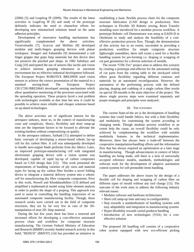
(2006) [5] and Leapfrog IP (2009). The results of the latest activities in LeapFrog IP [6] and study of the prototype definitely indicates the need to channelize efforts for developing new miniaturized solutions based on the same adhesion principles.

Development of innovative handling mechanisms has significantly complemented the above activities. Tsourveloudis [7], Acaccia and Molfino [8] developed modular and multi-fingers grasping devices with planar workspace. Dougeri and Fahantidis [9] demonstrated a soft finger gripper that grips limp materials but this device does not preserve the pinched part shape. In 1982 Salisbury and Craig [10] anticipated the use of sensors like tactile and vision to achieve intrinsic grasping robustness in uncertain environment but no effective industrial development followed. The European Project ROBOTEX BRE20958 used vision sensors to achieve the correct presentation of the material to a standard sewing-head. The European Project CR117391/BRE20643 developed sensing mechanisms which allow quantitative monitoring of the processes associated with the spreading operation. These projects faced a real problem with technologies available at that time but now it could be possible to achieve more reliable and cheaper solutions based on up-dated technologies.

The above activities are of significant interest for the

aerospace industry, more so, in the context of manufacturing costs and complexity. Hence, flexibility and short ramp-up time are the important factors to be focused to alleviate the existing burdens without compromising on quality.

In the aerospace industry, Sarhadi [11] attempted to define basic concepts of developing a sensor-based robotic lay-up cell for dry carbon fibre. A cell was subsequently developed to handle aero-engine blade preforms from dry fabrics. Later, an improved prototype-manufacturing cell with integrated electrostatic gripping device with a vision system was developed, capable of rapid lay-up of carbon composites based on CAD design data [12]. This work presented the requirements of handling varieties of ply sizes and material types for laying up dry carbon fiber besides a novel folding device to integrate a material delivery system into a robotic cell for manufacturing dry fibre composite components. Prior to this work, Newell and Khodabandehloo [13] defined and simplified a mathematical model using finite element analysis in order to predict the shape of a prepreg. This approach was used to assist in controlling the handling trajectories of an automated composite manufacturing facility. Though, these research works were carried out in the field of composite structures, they are by far very few in case of the 3D-manipulation of near 2D- limp material.

During the last few years there has been a renewed and increased efforts for developing a cost-effective automated process chain and workflow for composite structure manufacturing. The German Federal Ministry of Education and Research (BMBF) recently funded research activity in this field; “REDUX” (BMVIT) [14] has provided an initiative in

establishing a basic flexible process chain for the composite structure fabrication (CAD design to production). New techniques in Flexible 3D Robotic sewing, Resin Transfer moulding were introduced for a modular process workflow. A prototype Robotic cell Demonstrator was setup at EADS-D in Ottobrunn to study and analyze the feasibility of a cost-effective production process flow. Though, the demonstration of this activity has to an extent, succeeded in providing a production workflow for simple composite structure lightweight assemblies, there still exists a need for a flexible handling system for pre-forming i.e. draping or wrapping of cut part geometries for a diverse selection of moulds.

The recent “CFK-Tex” project aims to address this scenario by creating a prototype end-effector for the automated sorting of cut parts from the cutting table to the stockyard which offers great flexibility regarding different contours and materials by an automated reconfiguration. However, the automation of the performing process with the defined placing, draping and crabbing of a single carbon fiber textile on special 3D-moulds is the main objective of the project. The above single process steps were examined separately and proper strategies and principles were analyzed..

III. THE SCENARIO The current State-of-the art is the development of handling

systems that could handle fabrics, but with a little flexibility and modularity for customising the system according to changing needs. Though modular process workflow to an extent help the cause, an overall flexibility could be only achieved by complementing the workflow with suitable modularity features in the technical implementation. Moreover, there has always been a trade-off between the cooperative manipulation/handling efforts and the information flow that has always required an optimization at a later stage in manufacturing. Though advancements in context of fabric handling are being made, still there is a lack of universally accepted reference models, standards, methodologies and software tools for the development of adaptive automation control systems for soft permeable items handling.

The paper addresses the above issues by the design of a

flexible cell for draping and wrapping of carbon fiber on different types of mould without any tool change [15]. The outcome of the work aims to address the following industry relevant issues:

• Modular software and hardware architectures • Short cell ramp-up time and easy re-configurability • Step towards a standardization of handling systems with

easy adaptability and integration in manufacturing systems • Hyper-flexibility towards varied products handling • Introduction of new technologies (VSA) for a cost-

effective solution The proposed 3D handling cell consists of a cooperative

robot system equipped with new eco-efficient picking


ISBN: 978-1-61804-226-2 166

modules, able to grasp carbon-fiber fabrics, which are mounted on to a reconfigurable gripper capable of adapting the positions of picking points to the part geometry and stiffness.

Given the large size of the fabrics to be handled accurately, cooperating robots provide a greater flexibility in handling compared to a large single tool. The main advantage of this system, in comparison to a single handling unit, is that it enables to save workspace, tool manufacturing cost and the subsequent return of investment, besides the reusability of the system (robot and grasping device) with minimal or practically no reconfiguration for other customized application. Also, the ability to handle the part simultaneously in a geometrically coordinate fashion forms a significant feature and advantage of the cooperating system.

A lesson learnt from the current state of the art is that a balanced interaction between the information flow and the material flow have always determined the efficiency of a system. Our intelligent grasping device is conceived as a combination of complex kinematic structures and sensors with minimal data interaction. On the other hand, the simplicity of the hardware design can always be augmented by increased data interaction.

In the proposed scenario, the reconfigurable grasping device with the picking modules has a simple design with augmented control strategies for real time adaptation. The grasping device is endowed with a variable stiffness actuation, in order to have a “natural” soft interaction between the grasping device and the mould. This makes the device better adaptable to geometric features of the parts and the mould, such as curved surfaces, as well as the properties and requirements of the materials to be handled. The picking points, which depend on the part geometry, the mould type, and the material properties of the fabric, are transferred to the robot controller via a TCP/IP interface in order to inform the grasping device together with the robot system on the requested self-adapting needs.

IV. CELL LAYOUT In order to address the industry relevant issues previously

mentioned, a pre-defined scenario has been defined. The handling cell layout is sketched in the Figure 1. The task of the cell is to unload carbon fiber cut parts from a cutting table and to place them on different type of moulds through a cooperative handling system without tool changes and re-setup. The two grasping devices mounted on to each system have an ability to adapt the picking modules positions to the geometry and properties of the actual part to pick.

Figure 1 shows a layout that foresees two robots fixed on to an overhead linear rail performing the handling, draping/wrapping operation in cooperation. Another cell of the family, able to handle big carbon fiber parts, could include robots mounted on mobile platforms.

Fig.1 Sketch of the handling cell demonstrator

A. Handling strategy

The main workflow of the task is as follows: The two robots synchronously reach the part on the

cutting table and move the grasping devices in order to position the picking modules on the prescribed picking points;

The picking points are actuated and the part is lifted up through a collaborative synchronized task of the two robots.

The part is then transferred to the placing reference position on the mould through a collaborative task, by reducing a little bit the distance between the two TCPs (Tool Center Points) during the transport in order to avoid to introduce unwanted stresses into the carbon fiber tissue (see Figure. 2)

The part is then operated taking into account the shape of the mould, the wrap up rate and needs (see Figure 2)

The part is then released onto the mould with VSA small modifications.

Fig.2 Work sequence in mould draping and wrapping tasks of carbon fibre preforms on different moulds

During the above operations, an optical sensor (3D Laser

Measurement Scanner) is used to identify the mould and determine suitable placing strategies. The image processing in 3D is used to identify position and orientation of each


ISBN: 978-1-61804-226-2 167

handling device for achieving the different picking points. An algorithm determines optimal picking points and control strategies to drive the item on the mould, the points are transferred to the robot).

B. The new handling system

The multi points grasping philosophy, already successfully adopted for fabric handling in Leapfrog IP [4], has been adopted taking into account the lesson learnt in the previous research work. This approach allows developing a handling device working with near 2D limp porous parts with different shapes, sizes and materials, usable for different handling tasks and manufacturing environments. Taking into account the cooperative work of the two robots, the handling device is embedded with a suitable minimum number of picking modules and it will be able to reconfigure adapting the picking positions to the lifting-up/handling needs of the actual parts/tasks.

The proposed philosophy allows decoupling the adaptation to the part layers/material, in charge of the picking module, from the adaptation to the shape and size of the part to be handled, in charge of the hand architecture. In effect the picking modules guarantee the picking robustness versus material and surface properties and the handling device architecture guarantee the re-configurability range complying with the parts different sizes and shapes.

Picking modules have been designed mainly based on the previous experience and tests made on different physical picking principles. Mixed vacuum high flow and mechanical clamping technologies have been analyzed and picking devices implemented.

A new cheap, small size, efficient radial compressor has been designed that generate enough negative pressure. Although some radial micro compressors could be found in the market, because the relatively high price compared to the application and the difficulty of integration, a new, application oriented, low cost effective compressor was designed.

Figure 3 gives a summary of the picking module design, more details are in [16]

Fig.3 Picking module digital mock-up and reference performance chart

The handling mechanism has been designed, realized and

integrated with the picking modules, sensors, variable impedance actuation and motion control for re-configurability.

Modular cooperative adaptive control architecture have

been considered for the handling system. The two arms have to really cooperate during the carbon fiber preform handling [17]. In fact during this task the two kinematic chains (robot + gripper) close on the limp preform while exchanging generalized forces and the handling trajectories needs to perfectly comply with difficult tasks like mould wrapping.

Real time control logics [18] are defined and corresponding algorithms written for placing strategies and picking strategies enhancing the capability of the cell to quickly and robustly adapt to different carbon fiber aerospace components manufacturing.

The framework is expected to enable real time awareness of system status and reconfiguration potential so that the most appropriate adjustment of operating parameters can take place. The control logics ensure that all possible adaptation actions are accounted for at all handling task levels and therefore all flexibility/performance potential of the system can be assessed.

C. The cell control

The different components of the automation hardware are connected via adequate interfaces, standard if possible or purposely developed.

Figure 4 represents a physical layout of the cell together with the information control flow architecture

CuttingTable

Stressed skinfuselage

Pressure shells

Gantry Rails

Buffer

CooperatingHandling System

Pick and place control

Cell control Manager

Placing station control

Cooperating handling system

Fig.4 Sketch of the architecture of the cell layout information flow

Simple picking (from a table) and placing stations (moulds

for open carbon fiber components or for close wrapped components) are arranged within the cell mimicking the work done in the aerospace industry. The cell logistics and programming are defined and implemented, including the development of the human friendly interfaces and the criteria for the efficient management of the cell also against unexpected events.

A suitable Product Data Base includes Product Description and CAD files of the carbon fiber parts and moulds. Besides the logics for the cooperative tasks with mutual interaction and force exchange between the robots/part/ mould, the real time adaptation procedures at cell level are studied also with the aim of the possibility of 'auditing' the reconfigurations with regards to parts handled in the aerospace manufacturing environment. In fact, in aerospace, on one hand, reconfiguration of the production occurs very often due to


ISBN: 978-1-61804-226-2 168

product variants and volume changes while, on the other hand, it is common practice (also because of safety regulations) to keep track of the production layout/cycle used for the manufacturing of each part. 'Auditing' of adaptation changes can be done automatically as cell operations monitoring. The "configuration snapshots" of the cell will be further used as knowledge for suggesting autonomous adaptation in more complex handling cells of the same family.

V. EXPERIMENTS AND CONCLUSION One of the most critical design activity is the design of the

new eco-efficient picking module able to robust handling of carbon fiber fabric performs.

A test bench was purposely implemented and used at the PMAR laboratory with the purpose to test the picking module performances and to set its parameters: it is shown in Figure 5.

Fig.5 Test bench used in the early experiments

The early experiments and demonstration have been done

with reference to the following ranges: • carbon fiber materials (not restricted to): T700SC 12K

50C, 6K HR, HTA 5131 6K • geometry/size: from 100x500mm to 500x1800mm • layers number: 1-2 • mould shape: see Figure 6

Fig. 6 Example mould shapes

Many data were collected and results achieved during the experiment tests. As example are here reported some results on the behaviour of the new picking module used to handle samples of carbon fiber, see Figure 7 and Figure 8.

Actuator: 16V, 2.6A Diameter: 36mm

Actuator: 20V, 3,4A Diameter: 63.5mm

Pressure [mbar]

Suction force [N]

Pressure [mbar]

Suction force [N]

Max 21.7 2.2 17 5.3

Min 17.6 1.7 14.5 4.2

Mean 19.6 1.9 15.5 4.9

Fig.7 Comparative results on the picking module parameters

Pressure versus Flowrate

0

0,01

0,02

0,03

0,04

0,05

0,06

0,07

0 10 20 30 40 50

Fl owr a t e ( m3 / h)

16V, 2,6A

20V, 3,4A

Fig.8 Characteristic curve for carbon fiber from experiments on the test bench

The main result in these scenarios is to successfully enable

the robotic handling of difficult material that, till now, is mainly performed by human hands.

The new metamorphic hyper-redundant handling system with its 14 mobilities, equipped with the new picking modules and with the proprioceptive and exteroceptive sensors is able to adapt real time to different kind of carbon fiber materials, different geometry of the cut parts, different number of layers and different placing mould shapes.

Besides the hyper flexible cell here addressed, more sophisticated cells of the same family will allow handling largest parts, see Figure 9.

The hyper flexible intelligent cell will contribute to reduce the time to market for mass customized aircraft components.

A great added value is associated to the high level of flexibility of the cell. Carbon fiber components are used mainly in transport green production: in aerospace, automotive, bicycle. But new applications are foreseen in electronics (cases), in medical products, civil engineering, military, motorsports and other new sectors are showing interest day by day

Fig.9 Vision of the proposed cell family

ACKNOWLEDGMENT The authors thank the ROBOX company for the precious

discussion about the handling device motion control and AVIOSPACE company for the fruitful discussion on the design requirements and solution feasibility.


ISBN: 978-1-61804-226-2 169

REFERENCES [1] Seliger G., F. Szimmat, J. Niemeyer and J. Stephan, “Automated

Handling of Non-rigid Parts”, Annals of the CIRP 52/1 (2003), pp. 21–24

[2] Ozcelik Babur, Fehmi Erzincanli, “A non-contact end-effector for the handling of garments”, Robotica, Vol. 20, pp. 447-450, 2002

[3] Lien T. K., Davis P. G. G. “A novel gripper for limp materials based on lateral Coanda ejectors”, Annals of the CIRP 2008, vol. 57, no 1 pp. 33-36

[4] Molfino Rezia, Matteo Zoppi, Enrico Carca, “Robotic soft Material Handling”, in: Transforming Clothing Production into a Demand-Driven, Knowledge-Based, High-Tech Industry, The Leapfrog Paradigm Editor(s) name(s): Lutz Walter, George-Alexander Kartsounis, Stefano Carosio, Springer, 200

[5] Molfino R.M. and M. Zoppi. “Mass-customized shoe production: A highly reconfigurable robotic device for handling limp material”. Int. J. IEEE Robotics&Automation Magazine, 12(2):6676, 2006.

[6] R. Molfino, “Robotic handling of limp soft near 2D material”, Schunk International Expert Days, Hausen, February 24-25 2010

[7] Tsourveloudis N, Valavanis K, Kolluru R et al. ”Position and Suction Control of a Recon-figurable Robotic Gripper”. Machine Intelligence and Robotic Control, 1999, 11(2):53-62

[8] Acaccia G., L. Bruzzone, R. Molfino, M. Zoppi, “Modular SMA-based matrix gripper for grasping and handling of limp materials”, Int. Conf. on Intelligent Manipulation and Grasping IMG04, Genova, Italy, 2004, pp.266-269

[9] Dougeri Z. and N. Fahantidis, “Picking up Flexible Pieces out of a Bundle”, IEEE Robotics and Automation Magazine, vol. 9/2 (2002), pp. 9–19

[10] Salisbury J K, Craig J (1982) “Articulated Hands: Forces Control and Kinematic Issues”. The Int. J. of Robotics Research 1(1):4-17

[11] Sarhadi, M.: “Robotic handling and lay-up of advanced composite materials, an overview'', in Taylor, P.M. (Ed.), Nato ASI Series, Sensory Robotics for the Handling of Limp Materials(1990), Vol. F64, Springer-Verlag, Berlin, pp. 34-49

[12] Chestney, J.A. and Sarhadi, M., `”Control and integration techniques in a fully automated manufacturing cell for carbon composites” (1996), IEE Proc. Control Theory and Applications, Vol. 143 No. 2, pp. 159-63

[13] Newell, G.C. and Khodabandehloo, K., “Modeling flexible sheets for automatic handling and lay-up of composite components” (1995), Proceedings of Institute of Mechanical Engineers, Vol. 209, pp. 423-32

[14] BMVIT, Take off – First Aerospace Research Results, Bundesministerium für Verkehr, Innovation und Technologie : Journal (2007), pp. 20

[15] Reinhart Gunther, Gerhard Straßer and Claudia Ehinger, “Highly Flexible Automated Manufacturing of Composite Structures Consisting of Limp Carbon Fibre Textiles”, SAE Int. J. of Aerospace, Volume 2, Issue 1, pp. 181-187

[16] Yousef J, Zoppi M, Molfino R, “Pick and Place Vacuum Robotic Gripper for Flexible Material Manipulation”, 1st International Conference on Applied Bionics and Biomechanics: ICABB 2010, 14-16 October, Venice, Italy

[17] Mills, A.: “Automation of carbon fibre preform manufacture for affordable aerospace applications. Composites Part A” Applied Science and Manufacturing 32 (2001) 7, S. 955–962

[18] Taylor P.M., "The Automated Handling of Limp Materials, in Theory and Practice of Control and Systems," Edit. A. Tornambe, G. Conte, A.M. Perdon, World Scientific Press, (1999)


ISBN: 978-1-61804-226-2 170

Abstract—The present paper is dedicated to present the numerical simulation of thermal convection in a two dimensional vertical conical partially annular space. The constant properties and the Boussinesq approximation for density variation is used to solve the governing equations of mass, momentum and energy using the CFD FLUENT 12.0. The results of streamlines and the isotherms of the fluid are discussed for different annuli with various boundary conditions and Rayleigh numbers. Emphasis is placed on the height influences of the inner vertical cone on the flow and the temperature distribution. In more, the effects on the heat transfer are treated for deffirents values of physical parameters of the fluid in the annulus geometry. The heat transfer on the hot walls of the annulus is also computed in order to make comparisons the cylinder annulus for boundary conditions and several Rayleigh numbers. the results obtained of Nusselt number has been found between the present previsions and available data from the published literature data.

Keywords—Annular space, Conical partially, Natural convection, Heat transfer, Numerical simulation.

I. INTRODUCTION The heat transfer analysis by natural convection in an enclosure is an large research topic owing to its wide variety of engineering applications involving energy conversion, storage and transmission systems. Instances of using annulus geometry solar energy collection and nuclear reactor design [1]. A comprehensive review of natural convection in various cavity shapes has been documented in the open literature. Among the very first investigations, [2]has been analyzed numerically the heat transfer problem by natural convection in rectangular enclosure is filled by micropolar fluid, to studied the influence of the conductive vertical divider. The case of square and cubic cavities was reported by [3] and [4]. Other investigations [5] have been studied by cfd simulation the effect of the physical and geometrical parameters in two-

B. O. Author is with the Laboratory of Numerical and Experimental

Modeling of Mechanical phenomena, Department of Mechanical, University of Mostaganem Abdelhamid Ibn Badis, UMAB, BP300, Route Belhacel, Mostaganem (27000), Algeria; e-mail: kazemou@ yahoo.fr).

N. R. Author, was with Laboratory of Numerical and Experimental Modeling of Mechanical phenomena, Department of Mechanical, University of Mostaganem Abdelhamid Ibn Badis, UMAB, BP300, Route Belhacel, Mostaganem (27000), Algeria; e-mail: retieln@ yahoo.fr).

M. A. Author is with Associate Professor, Engineering College (l Research Chair in Quality & Productivity Improvement in Construction Industry, Université, Hail University, S.A. Saudi BinLaden); Faculty of engineering, University of Hail, Hail, PO Box 2440, Hail 43385, Saudi Arabia, (e-mail: [email protected]).

dimensional vertical enclosure by heat transfer with correlations generalized. The complex shapes such that inclined cavities with wavy walls by [6], and trapezoidal cavities by [7]. Natural convection and fluid flow was studied for triangular enclosures mostly with boundary conditions, see [8] and [9]. [10] Have carried investigations of heat transfer by protruding isothermal heater within an triangular enclosure. The study numerically of this phenomenon of natural convection flow in vertical concentric annular with isothermal inner and outer vertical walls. Several problems that have been extensively studied due to its several practical applications have received much attention. The studies conducted by [11] in a vertical cylindrical cavity, A parametric study numerically of the thermal convection in vertical annulus by the heat generation rod variation centrally vertically by [12]. The study the effect of tilted angle and diameter ratio on natural convection heat transfer in the case of horizontal cylindrical annulus by [13]. Investigation the transition effect and turbulence flows on natural convection along a horizontal annular cavity with local and mean Nusselt number were presented by [14] and recently by [15]. Few research works have been reported for the case of conical, have numerically solved the heat transfer by natural convection and radiation problem in a conical annular cylinder porous fixed is presented by [16].These studies were restricted to conduction heat transfer only. The present paper covers the laminar natural convection in a vertical conical cylinder partially annular space. On the other hand, the direct numerical simulation necessary for well resolved the study of heat transfer, (DNS) approach which requires computational resources well beyond actual capacities for the majority of real industrial problems. We will be concerned with the effect of the Rayleigh number and annulus radius ratio as well as the cavity geometry on the heat transfer.

II. PHYSICAL AND MATHEMATICAL FORMULATION

A. Physical Domain

In this present problem the geometry is schematized for studied the flow produced by natural convection in a vertical conical partial annulus; where the annulus is filled with air. The analysis domain is delimited by two concentric, conics with isothermal walls of the inner and outer axial height h, H respectively. The top and bottom walls of the outer cone are considered adiabatic, as shown in Fig. 1. The bottom radius of inner and outer conics are ri and ro and the inner and outer wall

Numerical Simulation of Natural Convection in a Two-Dimensional Vertical Conical Partially

Annular Space B. Ould said, N. Retiel, and M. Aichouni


ISBN: 978-1-61804-226-2 171


temperature are Ti and To, respectively. The horizontal walls of the outer cone are insulated. The buoyancy induced flow is assumed to be laminar, and the fluid studied is incompressible with constant fluid properties except the density variation. The Boussinesq approximation is used for calculated the density variation with the temperature. Then, the mathematical model used is based on the hypothesis of a two-dimensional (axisymmetric) flow.

Fig. 1Physical Model

B. Governing Equations The problem description and the assumptions application on

the fluid properties, the governing differential equations in vector form can be written as:

Continuity,

Momentum,

Energy,

In present study can be written as the governing

dimensionless equations in cylindrical coordinates in the following forms.

Continuity,

R momentum,

Z momentum with the Boussinesq approximation for the buoy-ancy term,

Energy

Where the dimensionless variables and numbers are defined as follows:

C. Boundary Conditions

The corresponding dimensionless boundary conditions for the radial and vertical velocity is equals to zero at all walls. The temperature boundary conditions are as follows. - At 0≤ Z≤ and Ro≤R≤Ro- cotδ: U= V= 0 and =0 for the isothermal cold tilted wall. -At 0≤ Z≤ and Ri≤R≤Ri- cotδ: U= V= 0 and =1 for the isothermal hot tilted wall. -At Z= and 0≤ R ≤Ri- cotδ: U= V= 0 and =1 for the isothermal hot horizontal wall. -At Z = and Z =0: U= V= 0 and 0 for the adiabatic walls.

III. NUMERICAL METHOD

To solve the governing equations using the finite volume method was used The FLUENT 12.0, CFD code, with first order formulation was solved the segregated implicit. The conservation governing equations was solved independently, by the segregated solver. The first order upwind differencing scheme is used the equations of momentum and energy. The discretization scheme used for pressure was body force weighted to take the density variations in consideration. The pressure–velocity coupling is ensured using the SIMPLE algorithm. The Gambit used for created and meshed the geometrical model with a simple quadrilateral cell. If necessary for correctly resolving the steep gradients in the thin buoyancy-driven boundary layer. A very fine spacing near the walls in conical partially annular grid. All the variables were calculated right up to the walls without using any wall function. on the wall boundary conditions, the radial and vertical velocity values were to zero. The dimensionless temperature of the active walls are set to 0 and 1 respectively. While meshing the domain, it is taken care that the mesh size does not influence the solution.

The residuals of continuity, momentum and energy equations are required to be lower 10-7 in order to achieved totally converging solution. The relaxation parameters have been adapted for every simulation in order to speed up convergence.

IV. NUMERICAL SOLUTIONS

A. Nusselt Number

The energy transmitted by the inner cylinder of the annulus are expressed in values to obtain the local and mean Nusselt numbers. The local Nusselt number for the annullus inner cylinder is obtained from temperature gradients by the following relationships:

z, v

ro

r, u

Adiabatic wall

Adiabatic wall

Incompressible Newtonian fluid

Cold wall To

H h

ri

Hot wall Ti

ro


ISBN: 978-1-61804-226-2 172

The mean Nusselt number is defined by

B. Validation Before continuing, it's required to ensure the dependability and the precision of the present numerical model and the FLUENT 12.0 CFD code. The heat transfer data computed for differentially heated of the conical annular, with different parameters which correspond to the cone angle δ = 90°, aspect ratio Ar = H / L, radius ratio K = ro / ri, height ratio h = X / L & Rayleigh number 104 ≤ Ra ≤ 105. The present problem is to numerically investigate the natural convection flow in a vertical cylinder annular space and the average Nusselt number variation is compared with those of reference from the literature data. Table 1 demonstrated the comparison between the current results and those of [17] and [18]. It is clearly demonstrated in Table 1 that, for several values of Rayleigh number. Was checked and ensured with the present results and those obtained by these authors. There is a satisfactory agreement.

Table 1

Values of the overall Nusselt number at the Isothermal Walls for Annulus Aspect ratio Ar=10 and K=2, =90°

V. RESULTS AND DISCUSSION

A. Effects of Rayleigh number Number

In this study The results obtained with respect to different parameters being Ar=1, K=2, X=0.5 and =45°. Fig.2 shows for Rayleigh number 103 ≤ Ra ≤ 104 that there is a logarithmic temperature distribution in the all-region of the annulus

illustrates that heat from the left wall toward the right wall is transferred by conduction regime for Rayleigh number Ra=5×104. The temperature gradient become slightly flatter at the core of the annulus which indicates that the conduction dominance is slashed in reason to a small quantity of convection established in the central part. The flow models show where convection promotes the transfer of heat. Fig. 2 shows the Rayleigh number Ra = 105 A vertical steep temperature gradient formed near the active wall. This confirms the increased in heat transfer rate due the existence of the cells models formed at interior annulus. This regime transition, wherein the boundary layer formed at the left and right active wall attain the central part of the annulus and merges all. Therefore, ago a rotational movement of the fluid, provoking mixing and ameliorate in heat transfer evaluation. However, for Rayleigh number Ra = 106, the nucleus was considered almost isothermal with the temperature gradient just about equal to zero. This indicate that the heat transfer in the annulus is mainly drawn by the moving boundary layers close by the walls and the fluid flow is in the regime of the laminar boundary layer. The heat transferred through the nucleus is negligible.

Vertical velocity profiles are presented in Fig. 3 for different Rayleigh numbers ranging from Ra = 103 to Ra =106. The profiles are plotted along the horizontal direction. Other geometric parameters were selected as Ar =1, K = 2, X = 0.5and =45°. As expected, the velocity is very low across wherever in the annulus at Ra ≤104. The fluid move is not effectual confirmed that the conductive regime is predominant effective under this condition. This means that the fluid is virtually stagnant in the annulus at 0 ≤ R ≤ 0.5 and 0.9 ≤ R ≤1.1. But, when the Rayleigh number is in the range of 5 × 104 ≤ Ra ≤ 105, the fluid entrained by the buoyancy-driven force in annulus is begins to accelerate from the base and forms the primary flow in the vertical direction to up. The velocity increases when the Rayleigh number is large enough Ra= 106, and the fluid flow is now confined adjacent at a time in the hot wall (0.37 ≤ R ≤ 0.67) and the cold wall (1, 09 ≤ R ≤ 1.33).

The Rayleigh number effects on streamlines (left) and isotherms (right) Fig. 4 (a) - (d) Present Ar = 1, K = 2, X = 0.5 and =45° visualizations are given from Ra = 103 to Ra = 106. The single cell is formed, shown from these figures, of all values of the Rayleigh numbers considered, which is in the direction of rotation clockwise. At lower Rayleigh number Ra ≤ 104 such that Fig. 4 a-b the isotherms are almost vertical at the active wall for most of the annulus, illustrating the mechanism of heat transfer flow by conduction dominated. For higher values of the Rayleigh number (i.e.105 ≤ Ra ≤ 106) as shown in Fig. 4 c-d, due to the increase of the mode of convection heat transfer, two thin boundary layers were formed vicinity of the hot and cold walls for 1 ≤ R ≤ 2. The isotherms are deformed and crowded adjacent the bottom left and upper right of the annulus and are stratified horizontally. The flow majority moves to upwardly right and top of the annulus in reason to the presence of the wall partly cooled and heated. because of adiabatic boundaries at the upper and the bottom of the annulus the Flow becomes motionless. However, the increased convection mode of heat transfer

Rayleigh number

[17] [18] Present

104 2.355 2.33 2.343 5104 3.718 3.758 3.755 105 4.558 4.568 4.564


ISBN: 978-1-61804-226-2 173

provoked by increasing the Rayleigh number and the virtually parallel distribution to the horizontal walls. It can also be seen from streamlines, the fluid velocity increases and the fluid direction and revolved towards the top right and bottom left of the annulus when the increase of the Rayleigh number.

Fig.2 Temperature profiles variation with horizontal distance for annulus Aspect ratio Ar=1, K=2, X=0.5 and =45° at Z=0.75.

Fig. 3 Axial velocity profiles variation with horizontal distance for annulus Aspect ratio Ar=1, K=2, X=0.5 and

=45° at Z=0.75.

Fig.4 Streamlines and isotherms for annulus Aspect ratio Ar=1, K=2, X=0.5 and =45°.

B. Effects of Aspect ratio The isotherms (on the right) and streamlines (on the left) are

depicted variations for aspect ratio Ar As can be seen from Fig. 5. The figure obtained for different aspect ratio values i.e. Ar=1, 1.5 & 2 and three different values of title angles =45°, 56.31°& 63.44°corresponding to K =2, X=0.5, 0.75 &1 and Ra = 105. The form of the isotherms show that increasing the aspect ratio provoked to the isotherms crowding at the bottom left and top right of the annulus. The temperature gradient in the hot wall, there is continuous variations low aspect ratio Fig. 5a indicates that the heat transfer rate continuously varies along the vertical height of the hot wall, which is not the case at higher aspect ratio Fig. 5c. The fluid flow center increased when aspect ratio increases.

The increase in the Nusselt number for different aspect ratio Ar = 1, 1.5 and 2, and height ratio X = 0.5, 0.75 and 1, and its linear variation with the Rayleigh number on a logarithmic scale are presented in Fig. 6. The other parameters are K = 2 and =45°, 56.31°& 63.44°. For the hot wall, the average heat transfer rate increases as the Rayleigh number is increased by the growing contribution of natural convection. And the heat transfer rate increases with increase in the annulus aspect ratio.

c) Ra=105

d) Ra=106

a) Ra=103

b) Ra=104

a) Ar=1, =45°

b) Ar=1.5, =56.31°


ISBN: 978-1-61804-226-2 174

Fig. 5 Streamlines and isotherms for different Annulus Aspect ratio at Ra=105 and K=2.

Fig. 6 Nusselt number variation with Rayleigh number and annulus Aspect ratio, Height ratio at K=2 and =45°,56.31°&63.44°.

C. Effects of Height ratio The isotherms (on the right) and streamlines (on the left) with different annulus height ratio X as demonstrated in Fig. 7. This figure corresponds to the several values Ra = 105, Ar=1, K = 2 and =45°. It's clearly noted from this figure that the isotherms move to the hot wall with a ratio of height increasing. This informs that increasing of the annulus height ratio provoked increasing the heat transfer from the hot wall of annulus. The temperature gradient hot wall can also be seen from the isothermal continuous decrease as the decrease in the ratio of the height. (The fluid flow is clearly visualized in the streamlines, The fluid flow is clearly visible in the streamlines). The complete cycle formed through the fluid circulation directed upward toward the hot wall falls then to the cold wall of the annulus . showing that the fluid flow concentrates of the circular cell at the entire annular space of small height ratio, but it moves half of the annular space (1 ≤ R ≤ 2), the height ratio increases. When the ratio of the height increases the orientation of the cell becomes parallel to the vertical inner cone.

The Nusselt number variation with aspect ratio X for several Rayleigh number. The figure corresponds to Ar = 1, K = 2 and

=45° are plotted in Fig. 8. As expected, the heat transfer rate is greater at the Rayleigh number is greater. It can be inferred from the figure that the growth rate effect is higher than the line for Ra ≤105 is stronger at higher Rayleigh number values and the line corresponding to Ra = 106. The height ratio does not influence the heat transfer rate when Ra ≤ 105, because the fluid move is very slow, and therefore the conductive regime prevails over convection regime, which explains the almost constant value the Nusselt number.

Fig. 7 Streamlines and isotherms for different annulus Height ratio at Ra=105, Ar=1 ,K=2 and =45°.

Fig.8 Nusselt number Variation with annulus Height ratio and Rayleigh number at Ar=1 and K=2, =45°.

a) X=0

b) X=0.25

d) X=0.75

e) X=1

c) Ar=2, =63.44°


ISBN: 978-1-61804-226-2 175

VI. CONCLUSION In this paper, the numerical study of natural convection in a

Two-Dimensional vertical conical partially annular space for steady-state regime with differentially heated walls has been analyzed. the effect of main parameters as Rayleigh number, Aspect ratio and Height ratio of annulus. concise summaries of the major results are reported in the following: -The heat transfer rate increases with increasing Rayleigh number. The heat transfer rate increasing is a function of the annulus Aspect ratio. -For lower Rayleigh number values we observed a dominance of conduction heat transfer. At higher values of Rayleigh number was observed that heat transfer rate increased and dominated by convection mode. -The natural convection regime has been bounded by Rayleigh number. When the Rayleigh number is weak, the fluid is practically stagnant. But for higher values of Rayleigh number the fluid entrained and begins to accelerate by the buoyancy-driven force in annulus from the base and forms the primary flow in the vertical direction to up. -It is finds that the annulus height ratio is one of the more important parameters on flow and temperature fields and heat transfer. The Nusselt number increase is a function of the annulus height ratio. -For high value of the annulus height ratio the cell orientation becomes parallel to the vertical inner cone i.e. The fluid motion is accelerated fully in the 1≤R≤2 and they is almost zero in the other side 0≤R≤1 at above the inner cone. But when height ratio decreases the fluid motion is accelerated increasingly in the zone 0≤R≤1 (the circular cell of the fluid motion is concentrated at the all in this zone).

ACKNOWLEDGMENT The authors acknowledge the partial support of the work

within the BinLaden Research Chair on Quality & Productivity Improvement in the Construction Industry, funded by Saudi BinLaden Group.

References

[1] A. Sridhar and K.S. Reddy, “Transient analysis of modified cuboid solar integrated-collector-storage system, ” Applied Thermal Engineering, vol. 27, pp.330-346, 2007. [2] S.G. Wang and T.Y. Li and P.T. Hsu and Kaohsiung and Taiwan, “Natural convection of micropolar fluid in a partially divided enclosure,” Acta Mechanica, vol. 136, pp. 41 – 53, 1999. [3] Y.L. He and W.W. Yang and W.Q. Tao, “Three-Dimensional Numerical Study of Natural Convective Heat Transfer of Liquid in a Cubic Enclosure,” Numerical Heat Transfer Part A Applications, vol. 47, pp.917-934, 2005. [4] HN. Dixit and V. Babu, “ Simulation of high Rayleigh number natural convection in a square cavity using the lattice Boltzmann method,” International Journal of Heat and Mass Transfer, vol. 49, pp. 727–739, 2006. [5] A.A. Ganguli and A.B. Pandit and J.B. Joshi, “ CFD simulation of heat transfer in a two-dimensional vertical enclosure,” Chemical Engineering Research and Design, vol. 87, pp. 711–727, 2009. [6] M. Aounallah and Y. Addad and S. Benhamadouche and O. Imine and L. Adjlout and D. Laurence, “Numerical investigation of turbulent natural convection in an inclined square cavity with a hot wavy wall,” International Journal of Heat and Mass Transfer, vol. 50, pp. 1683–1693, 2007. [7] Y. Varol and H.F. Oztop and I. Pop, “Natural convection in right-angle porous trapezoidal enclosure partially cooled from inclined wall,” International Communications in Heat and Mass Transfer, , vol. 36, pp.6–15, 2009.

[8] E. Fuad Kent and E. Asmaz and S. Ozerbay, “Laminar natural convection in right triangular enclosures", Heat and Mass Transfer, 2007, Vol. 44, pp. 187–200. [9] I. Hajri and A. Omri and S. Ben Nasrallah, “A numerical model for the simulation of double-diffusive natural convection in a triangular cavity using equal order and control volume based on the finite element method,” Desalination, vol. 206, pp. 579–588, 2007. [10] Y. Varol and H.F. Oztop and T. Yilmaz, “ Natural convection in triangular enclosures with protruding isothermal heater,”International Journal of Heat and Mass Transfer, vol. 50, pp. 2451–2462, 2007. [11] A. Hadjadj and S. Maamir and B. Zeghmati, “A new study of laminar natural convection in two concentric vertical cylinders,” Heat and Mass Transfer, vol. 35, pp. 113-121, 1999. [12] P. Venkata Reddy and G. S.V.L. Narasimhamn, “Natural convection in a vertical annulus driven by a central heat generating rod,” International Journal of Heat and Mass Transfer, vol. 51, pp.5024–5032, 2008. [13] F A. Hamad and M K. Khan, “Natural convection heat transfer in horizontal and inclined annuli of different diameter ratios", Energy Conversion and Management, 1998, Vol. 39, pp. 797-807. [14] E.L.M. Padilla and A. Silveira-Neto, “Large-eddy simulation of transition to turbulence in natural convection in a horizontal annular cavity,” International Journal of Heat and Mass Transfer, vol. 51, pp. 3656-3668, 2008. [15] M. Habibi Matin and I. Pop, “ Natural convection flow and heat transfer in an eccentric annulus filled by Copper nanofluid,” International Journal of Heat and Mass Transfer, vol. 61,pp. 353–364, 2013. [16] N.J.A. Salman and A.B. Irfan and Z.A. Zainal and H.M.T. Khaleed and K. Jeevan, “ Heat transfer in a conical cylinder with porous medium,” International Journal of Heat and Mass Transfer, vol. 52, pp. 3070–3078, 2009. [17] G. de Vahl Davis and R.W.Thomas, “ Natural Convection Between Concentric Vertical Cylinders High Speed Computing in Fluid Dynamics,” Physics of Fluids, vol. 2, pp. 198–207, 1969. [18] R. Kumar and M.A. Kalam, “Laminar Thermal Convection between Vertical Coaxial Isothermal Cylinders,” International Journal of Heat and Mass Transfer, vol. 34, pp. 513-524, 1991.


ISBN: 978-1-61804-226-2 176

http://www.tandfonline.com/action/doSearch?action=runSearch&type=advanced&searchType=journal&result=true&prevSearch=%2Bauthorsfield%3A(He%2C+Y.+L.)

http://www.tandfonline.com/action/doSearch?action=runSearch&type=advanced&searchType=journal&result=true&prevSearch=%2Bauthorsfield%3A(Yang%2C+W.+W.)

http://dx.doi.org/10.1016/j.icheatmasstransfer.2008.09.010



http://dx.doi.org/10.1016/j.desal.2006.03.581





http://dx.doi.org/10.1016/j.ijheatmasstransfer.2006.12.027




http://www.sciencedirect.com/science/journal/00179310/61/supp/C

Abstract--- In this paper study the flow behavior in horizontal wellbore with 60 and 150 perforations of perforation densities equivalent to 6 and 12 SPF respectively has been studied. The pressure drops in a perforated pipe that includes the influence of inflow through the pipe walls compares for two pipes that difference in perforation density. 3D numerical simulations for the pipe with two numbers of perforations were investigated by using ANSYS CFX modeling tool with Reynolds number ranging from 28,773 to 90,153 and influx flow rate ranging from 0 to 899 lit/hr to observe the flow through perforated pipe, measure pressure drops. The effect of density perforations on the flow through perforated pipe was conducted. CFD simulations yielded results that are reasonably close to experiments data. Keywords---perforation density, pressure, numerical, CFX.

I. INTRODUCTION In a horizontal well, depending upon the completion method, fluid may enter the wellbore at various locations and at various rates along the well length. The complex interaction between the wellbore hydraulics and reservoir flow performance depends strongly on the distribution of influx along the well surface and it determines the overall productivity of the well. Therefore, the optimization of well completion to improve the performance of horizontal wells is a complex but very practical and important problem.

The most commonly used assumptions in studying horizontal well production behavior are: infinite conductivity, and uniform influx. Infinite conductivity assumes no pressure drop along a horizontal well, and uniform influx assumes that the influx from the reservoir is constant along a horizontal well. It has been argued in the literature that the infinite conductivity wellbore assumption is adequate for describing flow behavior in horizontal wells. Although this may be a good assumption in situations where the pressure drop along the horizontal section of the wellbore is negligible compared to that in the reservoir, it is also reasonable to expect the friction and acceleration effects to cause noticeable pressure drops in long horizontal wellbores [1]. The petroleum industry started investigating horizontal wellbore was proposed by [2] which included acceleration pressure loss due to continuous fluid influx along the wellbore. They assumed that the injected fluid enters the main flow with no momentum in the axial direction. Kloster [3] performed experimental work and concluded

that the friction factor versus Reynolds number relationship for perforated pipes with no injection from the perforation does not show the characteristics of regular pipe flow. The friction factor values were 25-70% higher than those of regular commercial pipes. He also observed that small injections through perforations reduced the friction factor.

Dinkken [4] presented a simple isothermal model that links single phase turbulent well flow to stabilized reservoir flow. It was proposed that the pressure drop inside the horizontal wellbore was totally contributed by wall friction.

The flow in perforated tubes differs from conventional pipe flow as there is radial fluid inflow through the perforations. The injection disturbs the velocity profile and boundary layer [5] such that the pressure gradient along the length of the perforated tube is affected. Boundary layer injection reduces the friction of the surface the wetted surface. This effect was observed clearly in the transpiration experiments of [6], [7]. The reduction in friction for transpiration experiments was proportional for porous surfaces since the average diameters of the surface are sufficiently small.

Yuan et al. [1] the flow behavior in horizontal wells with a single perforation and with multiple perforations of perforation densities equivalent to 1, 2 and 4 shots per foot were investigated. Experiments were conducted with Reynolds numbers ranging from 5,000 to 60,000 and influx to main flow rate ratios ranging from 1/5 to 1/100 for the single injection case and from 1/100 to 1/2000 for the multiple injection case and for the no influx case. Horizontal well friction factor correlations were developed by applying experimental data to the general friction factor expressions. It was observed that the friction factor for a perforated pipe with fluid injection can be either smaller or greater than that for a smooth pipe, depending on influx to main flow rate ratios.

In this paper, the theoretical study of the pressure drop in partially perforated wellbore of the two pipes with different in perforation density. It incorporates not only frictional, accelerational pressure drops but also the pressure caused by inflow. The main difference between the two pipes is the number of perforations, the first one was 60 perforations but the other one 150 perforations with same diameter. The objective of the paper is the comparison between them for the values of total pressure drops, frictional, accelerational and additional pressure drops and etc.

A Comparison of the Density Perforations for the horizontal Wellbore

Mohammed Abdulwahid, Sadoun Dakhil, Niranjan Kumar


ISBN: 978-1-61804-226-2 177

II. MODEL DESCRIPTION Theoretical analysis was carried out to determine the total pressure drops, frictional, acceleration and additional pressure drops with different mass flow rate and density perforations. Fluid flow in a wellbore is considered as shown in Fig. 1 and assumed an incompressible, isothermal condition along a uniformly pipe. The test pipe is a partly perforated one and the rest is a plain pipe without perforation. Pipes and perforation geometry for theoretical study are listed in Table I. The first one was 60 perforations but the other one 150 perforations with same diameter. The computational domain taken up in this study is same as that of the dimensions considered in the experimental rigs [8], [9]. The geometry has been analyzed using 3D Computational Fluid Dynamics (CFD). Fig. 2 is the structured computational grids. The calculations were carried out with commercial finite volume code ANSYS FLUENT 14 CFX to solve Navier-Stokes equations, using a first scheme and turbulent with k epsilon model.

III. SIMULATION PARAMETERS The fluid considered for the simulations is water with constant density of 998.2 kg/m3 and dynamic viscosity of

0.001 kg/m s. Three tests were carried out with Reynolds number of the inlet flow ranging from 28,773 to 90,153. In each of the tests, flow rate through the perforations was increased from zero to maximum value. The roughness of the test pipe wall was 0.03 mm; the type of the test pipe was PVC. Test details are summarized in Table II. Uniform water mass flow is introduced at the inlet of a partially perforated pipe. Two boundary conditions are considered. At the inlet mass flow is taken into consideration both axially and radially where as at the exit outlet pressure is considered as the boundary condition. It is assumed that no-slip boundary conditions occur along the isothermal walls. Water enters at a uniform temperature (T) of 25˚C. For the symmetry lines both velocity and pressure is kept constant.

IV. FLUID FLOW MODEL FOR PERFORATED SECTION

The pressure drop of the fluid in the perforated section comprising: a pressure drop caused by the frictional resistance generated by fluid flow in the wellbore wallp∆ . Reservoir fluids flow into the well and confluence with the mainstream fluid, which causes the mixed pressure drop

.mixp∆ . Meanwhile, radial fluid inflow makes well section become variable mass flow, so the acceleration occurs and produces accelerated pressure drop .accp∆ , besides, there is a

pressure drop due to perforation roughness .perfop∆ should be taken into consideration. Divided the perforated section into the length of ΔL and the number of n perforation unit according to the number of holes, each the unit contains a hole. The pressure loss p∆of i unit is obtained from the sum of above several pressure loss.

... perfoiimixiaccwallii ppppp ∆+∆+∆+∆=∆ (1)

The last two terms in Eq. (1) combine into one term as

.addp∆


ISBN: 978-1-61804-226-2 178

Equation (1) can be written as:

.. addiacciwalili pppp ∆+∆+∆=∆ (2)

The total pressure loss of the horizontal wells perforated sections Tp∆ is stated as follows:

∑=

∆=∆n

iiT pp

1

(3)

Where n is the number of perforated holes. In perforated section, each unit of wall friction pressure drop algorithm is the same as the non-perforated section:

2

21

iiwalli vD

Lfp ∆=∆

ρ (4)

The friction factor if can be calculated

211.1

7.3Re9.6log8.1

−

+−=

Dfi

ε (5)

When the wall surface inflow and mainstream outflow ratio (the perforations radial flow and wellbore axial flow ratio) is less than the critical value, the radial fluid flow smooth the pipe flow, reduce the pressure drop. At this point, the mixing pressure drop caused by the perforations friction and radial inflow can be written as follows:

iiperfoimix Q

qxpp

−∆=∆ Re031.0.. (6)

Where q is radial flow of a single perforation, m3/s；Q is axial flow of horizontal wellbore; m3/s. Perforation friction pressure drop iperfop .∆ can be obtained by

perforation friction coefficient iperfof . shown below:

2.. 2

1iiperfoiperfo v

dLfp ∆

=∆ρ

(7)

Accelerated pressure drop is only associated with the density of the fluid, and the flow rate, it can be expressed as:

( )221. 2 iiiacc vvp +=∆ +

ρ (8)

V. RESULTS AND DISCUSSIONS In this paper, theoretically were carried out on the pipes that were simulated with the experimental pipe8, 9. Three tests with different pipe flow rate were carried out for the perforated pipe. Fig. 3 shows the acceleration pressure drop due to momentum for three tests. The pressure drop due to momentum change (acceleration pressure drop) was calculated from Eq. 8. The acceleration pressure drop increases with increase of the total flow rate ratio. We notice at the test 1 when the axial flow is large and the radial flow is low, there is a small difference between the acceleration pressure drop for the two pipes (60 & 150 perforations) with ranges from 2.95% at zero flow rate ratio to 0.039% at maximum flow rate ratio. For test 2 there is a difference in values of acceleration pressure drop with increases of the total flow rate ratio with ranges from 0.0192% at zero flow rates to 0.164% at maximum flow rate ratio. But for test 3 there is a difference with ranges from 0.989% at zero flow rate ratios to 0.0876% at maximum flow rate ratio. Because the pressure drop due to momentum depends upon the axial velocities at the inlet and the outlet of the pipe.

Fig. 4 presents the frictional pressure drop with total flow rate ratio for two pipes (60 & 150 perforations). The frictional pressure drop increases as the flow rate ratio increases for all tests and perforation density. For test 1 the frictional pressure drop is greater than tests 2 & test 3. Therefore, the frictional pressure drop increases as the axial flow increases. The friction pressure drop increases with decrease the perforation density i.e. the frictional pressure drop for pipe with 60 perforations greater than the frictional pressure drop for pipe with 150 perforations.

The total pressure drop in a perforated pipe section is contributed by the combined effect of fluid mixing and perforation roughness, ordinary frictional and accelerational pressure drops. The numerical results were examined in terms of the total pressure drop with total flow rate ratio, as shown in Fig. 5 for the tests conducted on pipe with different perforation density. The total pressure drop


ISBN: 978-1-61804-226-2 179

increases as the total flow rate ratio increases. The total pressure drop increases as increase of the perforation density.

The additional pressure drop, which is the combined effects of fluid mixing and perforation roughness with total flow rate ratio for 60 and 150 perforations pipes, as shown in Figs 6 and 7 respectively. The additional pressure drop decreases as the total flow rate ratio increases. This shows a lubrication (smoothing) effect to the pipe flow by inflow through perforations in the pipe wall. It is demonstrated that the additional pressure drop due to perforation roughness was reduced by the smoothing effect, and that the total pressure drop was reduced [10].

Effect of perforation density on the pressure drop coefficients of the total pressure drops is shown in Fig. 8. The pressure drop coefficients of pipe with 150 perforations were obviously larger than those of pipe with 60 perforations. This was because the perforation density of 150 perforations pipe was twice as larger that of 60 perforations pipe.


ISBN: 978-1-61804-226-2 180

VI. CONCLUSION Numerical simulations have been carried out on the flow in a partly perforated pipe with inflow through perforations. The geometry of the pipe used was similar to the pipe used in the experimental tests [8] - [10] with two perforation densities 60 and 150 perforations. The accelerational pressure drop for 60 & 150 perforations is small difference in the values for the three tests as shown above because it depends upon the axial velocities at the inlet and outlet of the pipe. The frictional pressure drop values for 60 perforations pipe are greater than 150 perforations pipe. The friction pressure drop increases with decrease the perforation density. The total pressure drop increases as the total flow rate ratio increases. The total pressure drop increases as increase of the perforation density. All the additional pressure drop values for 60 perforations are negative but some values of 150 perforations pipe are positive. The pressure drop coefficient of 150 perforations pipe is larger than 60 perforations pipe.

REFERENES [1] Yuan, H., Sarica, C. and Brill, J.P. “Effect of Perforation Density on Single Phase Liquid Flow Behavior in Horizontal Wells”. Paper SPE 37109, International Conference on Horizontal Well Technology, Calgary, Alberta, Canada, 18-20 November 1996. [2] Asheim, H. et al.: “A Flow Resistance Correlation for Completed Wellbore,” J. Petrol. Sci. Eng., 1992, 8 (2), pp. 97-104. [3] Kloster, J.: “Experimental Research on Flow Resistance in Perforated Pipe,” Master thesis, Norwegian Int. of Technology, Trondheim, Norway (1990). [4] Dikken, B.J.: “Pressure Drop in Horizontal Wells and its Effect on Production Performance,” JPT (November 1990) 1426. [5] Kato H., Fujii, Y., Yamaguchi, H. and Miyanaga, M. “Frictional Drag Reduction By Injection High-Viscosity Fluid into Turbulent Boundary Layer,” Fluid Engineering, June 1993, Vol. 115, pp. 207-212. [6] Kays, W.M. “Heat Transfer to the Transpired Turbulent Boundary Layer,” International Journal of Heat and Mass Transfer, 15: 1023-1044, 1971. [7] Eckert, E.R.G., Lomdardi, G., Sparrow, E.M. “Experiments on Heat Transfer to Transpired Pipe Flows,” International Journal of Heat and Mass Transfer, 17: 429-437, 1973. [8] Su, Z. and Gudmundsson, J.S. “Pressure Drop in Perforated Pipes,” PROFIT Projected Summary Reports, Norwegian Petroleum Directorate, Stavanger (1995). [9] Su, Z. and Gudmundsson, J.S.: “Pressure Drop in Perforated Pipes,” report, Department of Petroleum Engineering and Applied Geophysics, U. Trondheim, Norway (1995). [10] Su, Z. and Gudmundsson, J.S.: “Perforation Inflow Reduces Frictional Pressure Loss in Horizontal Wellbores,” J. Petrol. Sci. Eng., 1998, 19, pp. 223-232.


ISBN: 978-1-61804-226-2 181

Abstract— In this study, a 3D combustion chamber was simulated using FLUENT 6.32. Aims to obtain accurate information about the profile of the combustion in the furnace and also check the effect of oxygen enrichment on the combustion process. Oxygen enrichment is an effective way to reduce combustion pollutant. The flow rate of air to fuel ratio is varied as 1.3, 3.2 and 5.1 and the oxygen enriched flow rates are 28, 54 and 68 lit/min. Combustion simulations typically involve the solution of the turbulent flows with heat transfer, species transport and chemical reactions. It is common to use the Reynolds-averaged form of the governing equation in conjunction with a suitable turbulence model. The 3D Reynolds Averaged Navier Stokes (RANS) equations with standard k-ε turbulence model are solved together by Fluent 6.3 software. First order upwind scheme is used to model governing equations and the SIMPLE algorithm is used as pressure velocity coupling. Species mass fractions at the wall are assumed to have zero normal gradients. Results show that increase of AF ratio flow rate, decreases amount of CH4consumption.

Keywords—combustion chamber, Oxygen enrichment, Reynolds Averaged Navier- Stokes, AF.

I. INTRODUCTION

ue to increased demand for energy, clean cut fossil fuel resouresources, and growing concern over environmental pollution and global warming, mainly caused by the greenhouse effect is a urgent need for advanced energy systems to provide efficient power, with harmful consequences there is less environmental.

Oxy-fuel firing is more energy efficient and environmental friendly than conventional air-fuel firing and its application to reheating furnaces has begun since 1990s [1].

Combustion air can increase the oxygen in the exhaust gases and reduce energy loss and increase the efficiency of heating systems.

The main objective of this study was to compare the amount of air to fuel ratio of CH4 consumption, including and without oxygen enrichment.

Today, oxygen enrichment combines with oxidizer in the chemical reaction. The benefits of oxygen enrichment are: lower emissions, increase efficiency, increase productivity,

This work was supported in part by the Khuzestan Water and Power

Authority Z. O. Author is with the Khuzestan Water and Power Authority, Ahvaz,

Iran, on leave from the Sharif University of Technology, Kish Island, Iran (e-mail: [email protected]).

and improve temperature stability and heat transfer, and reduce costs of fuel consumption and pollutants [2].

II. GOVERNING EQUATION Combustion simulations typically involve the solution of

the turbulent flows with heat transfer, species transport and chemical reactions. FLUENT [3] uses finite volume to resolve physical equations (energy, continuity, momentum equations).

Continuity Equation

( ) ( ) mSVt

=∇+∂∂ ρρ . (1)

Momentum Equation

( ) ( ) ( )( ) FVVVVt t +∇+∇=∇+

∂∂ µµρρ .. (2)

Energy Equation

( ) ( ) ( )( ) ( ) ( )

hr

t

SS

pVVTkkVEEt

++

∇−∇+∇+∇=∇+∂∂ .... τρρ (3)

It is common to use the Reynolds-averaged form of the

governing equation in conjunction with a suitable turbulence model. The 3D Reynolds Averaged Navier Stokes (RANS) equations together with standard k turbulence model [4] are solved by Fluent 6.3. In finite volume method, integrated physical equations are used.

(4)

(5)

Where

Numerical Study of air and oxygen on CH4 consumption in a Combustion Chamber

Zohreh Orshesh

D


ISBN: 978-1-61804-226-2 182

III. COMBUSTION MODELING Before simulate the problem by FLUENT 6.32, the

geometry is modeled in GAMBIT. The computational domain is a cubic rectangle which is 60 cm wide, 90 cm high and 190cm long.

Fluent software uses two resolutions, namely pressure based and density based resolutions. In this study modeling is based on pressure. In order to resolve the chemical reaction and its modeling, species are selected from species transport in models menu.

Since the fuel and air inlets are quite distinct, this model can be used efficiently. In mixture material menu, methane-air is selected since methane-air reactions are involved. In reaction, volumetric option is selected. Then, inlet diffusion, diffusion energy source, full multi component diffusion, thermal diffusion options are all checked and eddy-dissipation is selected in turbulence-chemistry interaction menu. From Material menu, density option, incompressible gas is selected. Then, by clicking species, all components of reaction can be observed.

Independence and the turbulence model and the turbulence were investigated and finally with 83 320 grid cells were chosen as the computational grid (figure 1) and standard k-ε was decided to be used as the turbulence model.

Fig.1 Computational grid

The regions close to the burner were meshed into smaller

control volumes in order to enhance forecast accuracy (figure 2).

Fig.2 meshing of oxygen inlet

IV. 3BNUMERICAL CALCULATION

8BA standard k- ε as a simple perturbation model as a complete model of turbulence is widely used in the simulation of turbulent combustion. The pressure velocity coupling is resolved with SIMPLE algorithm. The descritization model is first order upwind scheme.

After writing chemical reaction of methane combustion in stoichiometric and use from thermodynamic tables, adiabatic flame temperature calculates 2320°k. When the residual comes down to near zero and reach convergence, solution will be finish.

V. 4BBOUNDARY CONDITION Flow conditions are steady, turbulent flow, heat transfer and

chemical reactions, also under flow a condition, Mach number is very low; hence, the flow in assumed incompressible. The inlet temperature is 300°K for all inlets.

Fig.3 Computational Mesh in solution domain

VI. 5BRESULT AND DISCUSSION

After numerical calculation, it is easy to see results. In 2005, M. Darbandi, A. Banaeizadeh and G. E. Schneider had been done numerical simulation on reacting flow [5] and compared their results with experimental data results and other numerical results which is gotten by Elkaim, D., Reggio, M., and Camarero, R and Smoot, J.L, and Lewis, H.M. Fig. 4 plotted those results and results of this study and shows comparison between them. According to this figure, there is good agreement between results.

Fig.4 Mixture fraction distribution of species and a comparison

between present study, Elkaim et al. [6] and experimental data [7]


ISBN: 978-1-61804-226-2 183

By plotting the CH4 mole fraction vs. X, according to figure 5, with the increase of AF ratio, CH4 decreases. It is obvious Minimum consumption CH4 mole fraction in combustion, happens at highest AF ratio (5.1).

The increase of incoming oxygen discharge, has a little effect on curve of CH4 mole fraction at state AF=1.3 and has approximately no effect on amount of CH4 in other states.

Fig.5 CH4 mole fraction vs. length of combustion chamber

Figure 6 show effects of AF ratio and oxygen enriched flow

rate on CH4 concentration along centerline of combustion.

(a)

(b)

(c)

Fig.6 CH4 concentration of combustion enriched combustion 54 lit/min, (a) AF = 1.3 (b) AF = 3.2, (c) AF =5.1

By comparison above three contours, it can be find another

result. Combustion process occurs earlier by increasing AF ratio.

Fig.7 compares temperature along the torch centerline with different

air-fuel inlets and oxygen enrichment

With the increase of air-fuel ratio, the maximum torch flame increases too. According to figure 7, this increase is very strict from air-fuel ratio of 1.3 to 3.2. The temperature becomes uniform along the torch centerline. With oxygen enrichment, variations are observed in maximum temperature of AF ratio of 1.3. As the oxygen inlet increases, the temperature decreases dramatically. However, with AF ratio of 3.2. Changes in oxygen enrichment are negligible in AF ratio of 3.2 and 5.1

VII. CONCLUSION Computational results for the pollutant emissions resulting

from combustion of fuel are evaluated. A 3D combustion chamber was simulated using FLUENT 6.32 software. Air/fuel ratio is flexible as 1.3, 3.2 and 5.1 and the oxygen enriched flow rates are 28, 54, 68 lit/min. Results show increase of AF flow rate ratio causes reduction CH4 consumption.

ACKNOWLEDGMENT I have some thanks from hydropower and dam research

office at Khuzestan water and power authority.

REFERENCES [1] Hamzeh Jafar Karimi, Mohammad Hassan Saidi, “Heat Transfer and Energy Analysis of a Pusher Type Reheating Furnace Using Oxygen Enhanced Air for Combustion,” Journal of Iron and Steel Research, International, Vol. 17, Issue 4, April 2010, Pages 12-17. [2] Industrial Technologies Program Energy Efficiency and Renewable Energy U.S.,” Energy Tips – Process Heating,” Department of Energy Washington, DC 20585-0121, Tip Sheet #3 www.eere.energy.gov/industry, September 2005. [3] Fluent Inc., Fluent 6.3 User's Guide, 2007. [4] B.E. Launder and D.B. Spalding, “The Numerical Computation Of Turbulent Flows,” Comp. Meth. Appl. Mech. Eng., Vol. 3, No. 2, 269–289, March 1974. [1] Y. Khazraii, K. Daneshvar, H. PoorkhademNamin, “Numerical Simulation on Nox Emission in Liquid Fuel Spray Flames,” Journal of Modeling and Optimization, International, Vol. 1, No. 4, October 2011. [5] M. Darbandi, A. Banaeizadeh and G. E. Schneider, “Implicit Finite Volume Method to Simulate Reacting Flow” 43rd AIAA Aerospace Sciences Meeting and Exhibit, Reno, Nevada, 10-13 Jan, 2005.


ISBN: 978-1-61804-226-2 184

[6] Elkaim, D., Reggio, M., and Camarero, R., “Control Volume Finite-Element Solution of a Confined Turbulent Diffusion Flame,” Numerical Heat Transfer, Vol. 23, 1993, pp.259-279. [7] Smoot, J.L, and Lewis, H.M., “Turbulent Gaseous Combustion: Part 1, Local Species Concentration Measurements,” Combustion and Flame, Vol. 42, 1981, pp.183-196.

Zohreh Orshesh (M’01–SM’04–F’11) of Khuzestan water and power authority has been born in Ahvaz, Iran 1978. Has graduated with BS in Solid Mechanical Engineering from Chamran University of Technology, Ahvaz, Iran in 2000, and then graduated with a Master of Science degree in Energy conversion from Sharif University of Technology, Kish Island, Iran, in 2012. She was working as a member of Department of Mechanical and electronically quality control in Khuzestan water and power authority Ahvaz, Iran from 2001-2004 and is working as an office manager of solid mechanic department at Khuzestan water and power authority, Ahvaz, Iran from 2004. She has four published papers, two are: Numerical Study on CO2 Pollution in an Ignition Chamber by oxygen enrichment (kuala lampur, Malaysia, Journal 68 of World Academy of Science, 2012), Numerical Study of oxygen enrichment on NO Pollution Spread in a Combustion Chamber (kuala lampur, Malaysia, Journal 69 of World Academy of Science, 2012), Effects of air to fuel ratio and enriched oxygen on O2 behavior in an Ignition Chamber (Pune, India, ICMIE, 2012), Numerical Study of air and oxygen on CH4 consumption in an Ignition Chamber (Pune, India, ICMIE, 2012). Ms Orshesh has all certificates of above papers.


ISBN: 978-1-61804-226-2 185

Abstract— One of the objectives of turbulent combustion models

is to determine the average rate of reaction. Because high nonlinearity of the reaction rate of the different species. The estimate of the reaction rate is not straightforward and should be based on a phenomenological approach. In this numerical investigation we have used two approaches of the probability density function PDF for a turbulent diffusion flame of fuel H2/N2 injected into coflow hot air at a temperature of 1045 K. A comparative study of the two approaches was conducted and validated with experimental data. It was found that the second model, transported PDF gives more reliable results than the PDF presumed. Keywords—- Combustion, coflow, PDF (presumed transported), chemical reaction rate, Turbulence.

.

I. INTRODUCTION Industrial systems involving combustion phenomena (ovens, automobile engines , aircraft , gas turbines ) are subject to constraints increasingly important economically ,

that is to say, cost reduction , performance improvement on the environmental plan (reduction of pollutant emissions , noise emissions , etc ... ). . All these considerations motivate many research related to turbulent combustion. Indeed, understanding, modeling and simulation allow not only the improvement of existing systems, but also the development of new technologies. Turbulent diffusion flames meet in the industry most often in the gas burners (fuel jet injected from a center of air flow in the same direction). The turbulence plays an important role to mix as quickly as possible in the gas presence. Position of the problem: The interaction between the turbulence and the combustion plays an important role in most industrial systems. The study of these flows leads to the characteristic equations derived

This work was supported in part by the Department of Mechanics, University of Science and Technology of Oran Mohamed Boudiaf Algeria. A.A.Larbi, Department of Mechanics, University of Science and Technology of Oran Mohamed Boudiaf Algeria (e-mail: [email protected]). A.Bounif, Department of Mechanics, University of Science and Technology of Oran Mohamed Boudiaf (e-mail: [email protected]).

from MDF, thermodynamics, chemistry. In view of the complexity of these equations and mathematical tools, analytical resolution is limited to very simple cases, the direct solution without simplifying assumption requires computing power (the computational power of current computer is not sufficient for this kind of calculation). In this case, we used the method (RANS) which consists in averaging equations phenomena. The equations for the average quantities that result from this approach show an unknown term that must déterminer.il is the average rate of reaction. Because of the high nonlinearity of the reaction rates of different species, its estimation is not straightforward and should be based on a phenomenological approach. Models of turbulent combustion based on the statistical phenomenological approach PDF, are of two different types. One of these goals is to determine the rate of reaction. In our study we opted and used both methods in order to know the advantages and disadvantages and make a comparative study between the two. The first model presumed PDF is to presume the form of the PDF. The second model, transports PDF is to solve equation transport for the PDF. These methods have the advantage to take into account precisely the chemistry and thus a priori be applicable to all combustion regimes. In particular, all the terms defined in a point, such as the average rate of chemical reaction, can be determined. Numerical simulation is a very important tool in the study of prediction of turbulent reactive flows. Indeed, it has several advantages (gain time, less expensive than the experience ...). It allows to consider several configurations of boundary conditions, for the same initial flow and in a short time. Also provides information on almost all of the area studied, simulating with real or ideal conditions to deepen the understanding of the phenomenon studied. The fluent code became a widely used tool for the simulation of all phenomena in the field of energy in industry for research. The construction of the geometric model, mesh and boundary conditions is generated with Gambit preprocessor.

II. THE GOVERNING EQUATIONS The flow that we have considered is a reactive flow, turbulent, multi species. The equations that govern this phenomenon are

Numerical study of a turbulent diffusion flame H2/N2 injected in a coflow of hot air.

Comparison between models has PDF presumed and transported

A.A. Larbi, A.Bounif.

I


ISBN: 978-1-61804-226-2 186



those of continuity, momentum, energy conservation, species conservation and the equation of state of the gas is supposed perfect [1]. The flow is turbulent. Dynamic equations were established in the two-dimensional stationary case. 2.1 Continuity equation: This equation expresses the conservation of mass

2.2. Equation of momentum: The momentum equation for an incompressible and Newtonian fluid is given by:

.................( ) ( ) (2)iki k i

k k i

pu u ut x x x

τρ ρ ∂∂ ∂ ∂+ = −

∂ ∂ ∂ ∂ Where ikτ is the viscous stress tensor:

.................2) 3).( (3

i k iik ik

k i l

u u ux x x

τ ρν ρν δ∂ ∂ ∂= + −

∂ ∂ ∂ Where ku represents the speed, p and ρ the pressure of the mixture density 2.3. Balance of species involved in the reaction: stock of the species is written as follows:

..( ) ( ) ( ) (4)..ii k i i i

k k k

YY u Y Dt x x x

ρ ρ ρ ω∂∂ ∂ ∂+ = +

∂ ∂ ∂ ∂ Where iω is the rate of chemical reactions i iω ρ= Ω iY is the mass fraction and Di is the binary diffusion coefficient of species i. 2.4. Enthalpy equation: After using the approximation Schved-zeldovitc (which calculates all species, enthalpy and temperature, based on a conservative mixture fraction variable and one variable reactive mass fraction of chemical species) . The energy balance leads to the equation for the specific enthalpy:

...........( ) ( ) ( ) (5. )k ik k k

u Dt x x x

ζρζ ρ ζ ρ∂ ∂ ∂ ∂+ =

∂ ∂ ∂ ∂ 2.5. Equation characterizing the state of the gas mixture: We will consider these gases as perfect ideal gas mixtures:

.................................................. . (6). .m

Rp TM

ρ=

III. AVERAGE EQUATIONS AND CLOSE PROBLEMS:

WE APPLIED THE AVERAGE OPERATOR ON EXACT EQUATIONS

CONTINUITY EQUATION:

...........................................( ) 0 (7).kk

ut xρ ρ∂ ∂

+ =∂ ∂

Equation of momentum:

" "( ) ( ) ( ) (8)i k i ik i kk k i

pu u u u ut x x x

ρ ρ τ ρ∂ ∂ ∂ ∂+ = − −

∂ ∂ ∂ ∂ Equation Evolution of the average fraction mixture:

" " .( ) ( ) ( ) (9)k kk k k

u D ut x x x

ζρζ ρ ζ ρ ρ ζ∂ ∂ ∂ ∂+ = −

∂ ∂ ∂ ∂ Equation of evolution of the average mass fraction:

" "

................................................................

( ) ( ) ( )

(. ). 1. 0

k kk k k

YY u Y D u Yt x x x

ρ ρ ρ ρ

ω

∂ ∂ ∂ ∂+ = −

∂ ∂ ∂ ∂

+

Equation average of state ........................................* * ..... (11. )T T cteρ ρ= =

We found new terms appear and separate equations of the initial equations, these terms represent the turbulent transport variables:

• The term of the Reynolds stress tensor of the form " "i ku uρ whose closure is due to the different

turbulence models

• Turbulent flow of mixture fraction " "kuρ ζ and

" "ku Yρ species, or terms of turbulent transport,

whose closure is due to the appropriate models of combustion.

• Source terms, such as chemical source terms iω .

These terms are problematic because of their non-linearity.

The particular problem of the closure of the reaction rate is one of the main objectives of our study and modeling turbulent combustion.

IV. MODELING OF TURBULENT COMBUSTION One of the objectives of turbulent combustion models is to determine the average rate of reaction. Because of the high non-linearity of the reaction rate of the different species, the estimated average rate of reaction is not straightforward [2] and should be based on a phenomenological approach. Three main approaches used to describe the turbulent flames: approach based on the geometrical analysis, based on the turbulent mixing and statistical analysis at a point. In our study we used the statistical analysis based on a point approach. This analysis allows for the statistical properties of the scalar field at a point of the mean flow by the probability density function (PDF). There are two PDF model, the first presumed PDF is to assume the form of the PDF. The second PDF transported consists to solve an equation transport the PDF. 4.1 Presumed PDF model: The basic approach is to link the instantaneous thermochemical properties of the fluid (temperature, density and mass fraction) to a conservative

.................................................0 (1)k

k

ut x

ρρ ∂∂+ =

∂ ∂


ISBN: 978-1-61804-226-2 187

scalar called mixture fraction.

,

, ,

...................................... (............ 12)j j ox

j c j ox

z zz z

ζ −=−

Where Zj is the elementary mass fraction of the element j. The advantage of the fraction of the mixture is that it can be calculated from a local value ζ of any other conservative

scalar φ a function of ζ , such as temperature, mass fraction etc.. In a turbulent regime, the mixture fraction can fluctuate chaotically. To model these fluctuations, we calculate the variance. If the average of the mixture fraction is given by the

above equation, the variance can be written 2'ζ :

( ) ( )

222

0

.............1' . (. .. 1. 3)t dtτ

ζ ζ ζ ζ ζτ

= − = − ∫

La forme de la PDF peut être calculée à partir des résultats expérimentaux ou bien on peut la présumer. C’est la dernière approche qui est généralement utilisée. La PDF la plus couramment utilisée est une fonction du type BETA :

( ) ( )( )

11

11

11

pd

βα

βα

ζ ζζ

ζ α ζ

−−

−−

−=

−∫ with

( )2

11

'

ζ ζα ζ

ζ

− = −

(14)

And ( ) ( )2

11 1

'

ζ ζβ ζ

ζ

− = − −

p(ζ ) is a temporal representation of fluctuations in a turbulent flow. It is used to calculate the average values dependent of ζ 4.2 Transported PDF model The composition model PDF transported is used when one wants to simulate the effects of chemical kinetics in a reactive turbulent flow. With appropriate chemical mechanism, this method can be provided. The kinetic-controlled species such as CO and NOx, as the extinction of flame and ignition. The simulation is computationally expensive PDF transported, and it is recommended to start the model with small grids, and preferably in 2D. in this method, the scalar is calculated by a Lagrangian method [3], followed by a representative fluid particle of a chemical species. The advantages are the accurate determination of the reaction rate as well as taking into account the temporal and spatial evolution of a chemical species. The operation is achieved by statistical averaging temporally through a sufficient number of instantaneous fields of particles (20 to100). The species transport equations are mathematically obtained from an equation of the PDF transport.

i k i

, .........................

( ) ( u ) ( S

.................

) u "

1 (15)

i k i

i k

k i

p p p py x x

jp

x

ψψ

ψψ

∂ ∂ ∂ ∂ ρ + ρ + ρ = − ρ ∂ ∂ ∂ ∂

∂∂+ ρ

∂ ρ ∂ In the equation, the terms on the left side were closed, while those on the right are not and require modeling. The first term on the left side is the rate of change of PDF unstable, the second term is the change due to the PDF by the convection of the mean velocity field, and the third term is the rate of reaction. The main strength of the PDF transport approach is that the reaction term highly nonlinear is completely closed and does not require modeling. The two terms on the right side represent the change in PDF due to scalar convection by turbulence (turbulent scalar flux), and the molecular / mixture distribution. The limit of turbulent scalar flux is open, and modeled in FLUENT by the claim diffusion gradient

iCt

.....u " ( .....) (16)S

.......t

i i i

u ppx x x

ψ∂ ∂ ∂ − ρ = ∂ ∂ ρ ∂

Sct : is the turbulent Schmidt number A model of turbulence or turbulence modeling is needed for the composition of simulated PDF transported, and this determines Ut. As the PDF is a single point and only the information on the neighboring points are missing and all the terms of gradient, such as the molecular mixing, are opened and should be modeled. The mixture model is essential because the combustion occurs at smaller scales when molecular reagents and diffuse heat together. Mixture modeling methods in the PDF is not simple, and is the weakest of the transported PDF approach.

V. PRESENTATION OF THE STUDY geometry considered is similar to the burner of CABRA (FIG. 1). The burner consists of a horizontal tube of internal diameter 4.57mm, 6.35mm and outside diameter, centered in a cross-section of internal diameter 210mm.

Fig1:Domaine calculation.


ISBN: 978-1-61804-226-2 188

Parameter Symbol Jet Coflow

Température T (°K) 305 1045 Flow velocity V (m/s) 107 3.5

hydraulic diameter DH(m) 2.285 10×

3105 10−×

The molar fraction of hydrogen XH2 0.02388 -

The molar fraction of oxygène XO2 - 0.17082

The molar fraction of H2O X H2O - 0.06453

The molar fraction of azote XN2 0.97612 0.76466

Reynolds number Re 23660 18600 According to the simplified map [4] modes and combustion regimes of different academic flames, measured in the TNF workshop. Our flame is that of (Berkeley / Sydney Lifted nonpremixed jet flames in vitiated coflow H2/Air). it is shown in (FIG. 2). The geometrical configuration is axisymmetric. FLUENT code uses a Cartesian coordinate system. On the mesh size, we opted for forms of quadrilateral meshes. it is 2530 meshes (Figure 3).

Fig3 Studied geometry after meshing the software GAMBIT A refining zones near the outlet of the burner has been considered to reflect the wide variations occurring in these areas including the velocity gradients. the definition of the geometry and the generation of the mesh were carried out using the GAMBIT.

VI. DISCUSSION OF RESULTS Study of the evolution of the temperature

Study of the evolution of oxygen mass fraction

Study of the evolution of hydrogen mass fraction:

Fig2 geometries burner

PDF présume

PDF présume

PDF présume

PDFtransport

PDFtransport

PDFtransport


ISBN: 978-1-61804-226-2 189

Profile of various developments in the application of the two methods of PDF. Experimental result (cabra 2002).

0 5 10 15 20 25 30 35 40

200

400

600

800

1000

1200

1400

1600

T

Z/D

expPDF transportPDF présumé

0 5 10 15 20 25 30 35 40

0,000

0,005

0,010

0,015

0,020

0,025

H2

Z/D


0 5 10 15 20 25 30 35 40-0,01

0,00

0,01

0,02

0,03

0,04

0,05

0,06

0,07

0,08

0,09

O2

Z/D


Note: According to the results, we can divide our computational domain into four areas: • The first zone (Z / D = 0 to 4) is the area of pure fuel. • The second zone (Z / D = 4 to 12.5) is the area of heterogeneous premix. • The third zone (Z / D = 12.5 to 25) is the reaction zone. • The last zone (Z / D = 25 to the end) is the area of the burned gas.

VII. CONCLUSION The objective of this thesis was to contribute to the development of models and simulation techniques to reproduce and predict phenomena resulting from the coupling between combustion and turbulence in diffusion flames. The complexity of the phenomena and the technical difficulties of experimental studies on real configurations in the field of combustion showed the interest of numerical approaches. The probability density function of proved a promising approach for the prediction of complex turbulent reactive flows. We have two models of probability density function, the first model presumed PDF and the second transported PDF. These two models do not have the same average and study conditions, and therefore the same results. It is in this context that fits our study, in order to apply both PDF approach and compare these results with experiment. The calculations were compared with detailed Berkeley Lab / Sydney, nonpremixed jet flames in vitiated Lifted H2/N2 coflow experimental data. Excellent agreement was obtained between the calculations and experience in both methods and especially with transported PDF. We found some anomalies between the results. These anomalies can be justified by several reasons:

• The mechanism used. • The mesh and the number of nodes: the presumed

PDF model, we can use a large tiller mesh. By against, with the second model can not use this network due to lack of computing means (requires a large memory capacity)

• The boundary conditions (adiabatic walls). • Model of turbulence. • Model mixture.

REFERENCES [1] Veynante .D, Turbulent combustion modeling , Prog. Energy Combust.

Sci,193-266 , 2002.W.-K. Chen, Linear Networks and Systems (Book style). Belmont, CA: Wadsworth, 1993, pp. 123–135.

[2] BORGHI .B , Modélisation Et Théorie Des Flammes, technip ;2000. [3] Masri .A.R , «PDF calculations of turbulent lifted flames of H2/N2 fuel

issuing into a vitiated co-flow». Combust. Theory Modelling . 1–22 , 2004.

[4] ROBIN. Vincent, Contribution à la Modélisation des Ecoulements Turbulents Réactifs Partiellement Prémélangés ,thèse pour l’obtention de doctorat, université de poitters 2007.

[5] Proceedings of the third international workshop on measurement and computation of turbulent nonpremixed flames ,boulder Colorado, 1998

[6] Cabra. R, Simultaneous Laser Raman-Rayleigh-LIF Measurements and Numerical Modeling Results of a Lifted Turbulent H2/N2 Jet Flame in a Vitiated Coflow . Turbulent Combustion , 1A03, 2002.

[7] R. Cabra, R.W. Dibble, http://www.me.berkeley.edu/ cal/VCB/ (2002).2, Aug. 1987, pp. 740–741 [Dig. 9th Annu. Conf. Magnetics Japan, 1982, p. 301].

[8] FLUENT Inc. Fluent 6.3.26 User Guide.J. U. Duncombe, “Infrared navigation—Part I: An assessment of feasibility (Periodical style),” IEEE Trans. Electron Devices, vol. ED-11, pp. 34–39, Jan. 1959.

Fig 3: Temperature profile through the application of two methods of PDF.

Fig 4: Profile of the fraction of hydrogen by applying the two methods PDF.

Fig 5: Profile of the oxygen fraction by applying the two methods PDF.


ISBN: 978-1-61804-226-2 190

http://www.me.berkeley.edu/

Authors Index

Abdelilah, H. 160 Manjunath, R. 118 Abdelkader, B. 160 Mohamed, E. G. 160 Abdulwahid, M. 177 Mokhtar, A. 113 Aichouni, M. 171 Molfino, R. 165 Alexeyeva, O. 91 Muller, R. 125 Aris, A. 144 Nevskii, S. A. 131 Asmâa, C. 160 Nouri, A. 96 Azarov, E. 91 Orshesh, Z. 182 Baki, T. 144 Ovsik, M. 156 Belibassakis, K. A. 17 Papathanasiou, T. K. 17, 65 Bounif, A. 144, 186 Pinca-Bretotean, C. 77 Cepolina, E. E. 165 Prasad, A. J. K. 118 Cepolina, F. 165 Ratiu, S. 77 Challamel, N. 25 Retiel, N. 171 Cheremushkina, E. V. 104, 131 Rumyantsev, S. 91 Christopoulos, A. C. 65 Said, B. O. 171 Dakhil, S. 177 Sarychev, V. D. 104, 131 Danesh, M. 96 Senkerik, V. 134 Dascal, A. 77 Shihov, A. 91 Duan, W. H. 25 Shivappa, D. N. 118 Fourlas, G. K. 151 Shtukin, L. V. 73 Gharakhanlou, J. 85 Siddiqui, M. A. 139 Granovsky, A. Y. 104 Skrobak, A. 107 Gromov, V. E. 104, 131 Skubov, D. Y. 73 Guessab, A. 144 Somà, A. 125 Harisha, K. 118 Stanek, M. 107, 134, 156 Iamoni, S. 125 Sycheva, A. V. 61 Indeitsev, D. A. 73 Tsamasphyros, G. J. 36, 65 Josan, A. 77 Tsarouhas, P. H. 151 Kazachkov, I. V. 85 Vavilov, D. S. 73 Koutsoumaris, C. C. 36 Vershinin, V. V. 61 Kumar, N. 177 Voicu, R. 125 Lalin, V. 32 Wang, C. M. 25 Larbi, A. A. 186 Yousef, J. 165 Loktev, A. A. 61 Zakaria, M. 113 Maciel, E. S. G. 43 Zdanchuk, E. 32 Manas, D. 107, 134, 156 Zhang, Z. 25 Manas, M. 107, 134, 156 Zoppi, M. 165


ISBN: 978-1-61804-226-2 191

RECENT ADVANCES in MECHANICAL ENGINEERING and ...

Documents

Transcript of RECENT ADVANCES in MECHANICAL ENGINEERING and ...