
International Conference on Advances in Civil Engineering
98
Interscience Research Network Interscience Research Network Interscience Research Network Interscience Research Network Conference Proceedings - Full Volumes IRNet Conference Proceedings 12-17-2011 International Conference on Advances in Civil Engineering International Conference on Advances in Civil Engineering Prof.Srikanta Patnaik Mentor IRNet India, [email protected] Follow this and additional works at: https://www.interscience.in/conf_proc_volumes Part of the Civil Engineering Commons, Construction Engineering and Management Commons, Environmental Engineering Commons, Geotechnical Engineering Commons, Hydraulic Engineering Commons, Structural Engineering Commons, and the Transportation Engineering Commons Recommended Citation Recommended Citation Patnaik, Prof.Srikanta Mentor, "International Conference on Advances in Civil Engineering" (2011). Conference Proceedings - Full Volumes. 66. https://www.interscience.in/conf_proc_volumes/66 This Book is brought to you for free and open access by the IRNet Conference Proceedings at Interscience Research Network. It has been accepted for inclusion in Conference Proceedings - Full Volumes by an authorized administrator of Interscience Research Network. For more information, please contact [email protected].
-
Upload
khangminh22 -
Category
Documents
-
view
0 -
download
0
Transcript of International Conference on Advances in Civil Engineering

Interscience Research Network Interscience Research Network
Interscience Research Network Interscience Research Network
Conference Proceedings - Full Volumes IRNet Conference Proceedings
12-17-2011
International Conference on Advances in Civil Engineering International Conference on Advances in Civil Engineering
Prof.Srikanta Patnaik Mentor IRNet India, [email protected]
Follow this and additional works at: https://www.interscience.in/conf_proc_volumes
Part of the Civil Engineering Commons, Construction Engineering and Management Commons,
Environmental Engineering Commons, Geotechnical Engineering Commons, Hydraulic Engineering
Commons, Structural Engineering Commons, and the Transportation Engineering Commons
Recommended Citation Recommended Citation Patnaik, Prof.Srikanta Mentor, "International Conference on Advances in Civil Engineering" (2011). Conference Proceedings - Full Volumes. 66. https://www.interscience.in/conf_proc_volumes/66
This Book is brought to you for free and open access by the IRNet Conference Proceedings at Interscience Research Network. It has been accepted for inclusion in Conference Proceedings - Full Volumes by an authorized administrator of Interscience Research Network. For more information, please contact [email protected].

Interscience Research Network (IRNet)
Bhubaneswar, India
Proceedings of International Conference on
Advances in Civil Engineering
(ICACE-2011) 17th –18th DECEMBER, 2011
BHUBANESWAR, India

Editorial
With an increasing sophistication and increasing luxury on the face of materialism, the human race
is striving for state of the art infrastructure for its every social institution. The role of civil
engineering is prominent in this context. Civil engineering is the oldest engineering discipline after
military engineering,[4]
and it was defined to distinguish non-military engineering from military
engineering. It is traditionally broken into several sub-disciplines including environmental
engineering, geotechnical engineering, structural engineering, transportation engineering, municipal
or urban engineering, water resources engineering, materials engineering, coastal engineering,[4]
surveying, and construction engineering.[6]
Civil engineering takes place on all levels: in the public
sector from municipal through to national governments, and in the private sector from individual
homeowners through to international companies. Civil engineering comprises many disciplines and
in the recent years many sub disciplines have been emerging. Civil engineering is concerned with
the overall interface of human created fixed projects with the greater world. General civil engineers
work closely with surveyors and specialized civil engineers to fit and serve fixed projects within
their given site, community and terrain by designing grading, drainage, pavement, water supply,
sewer service, electric and communications supply, and land divisions. General engineers spend
much of their time visiting project sites, developing community consensus, and preparing
construction plans. General civil engineering is also referred to as site engineering, a branch of civil
engineering that primarily focuses on converting a tract of land from one usage to another. Civil
engineers typically apply the principles of geotechnical engineering, structural engineering,
environmental engineering, transportation engineering and construction engineering to residential,
commercial, and industrial and public works projects of all sizes and levels of construction.
Structural engineering is concerned with the structural design and structural analysis of buildings,
bridges, towers, flyovers, tunnels, off shore structures like oil and gas fields in the sea, and other
structures. This involves identifying the loads which act upon a structure and the forces and stresses
which arise within that structure due to those loads, and then designing the structure to successfully
support and resist those loads. The loads can be self weight of the structures, other dead load, live
loads, moving (wheel) load, wind load, earthquake load, load from temperature change etc. Another
aspect of Civil engineering is materials science. Material engineering deals with ceramics such as
concrete, mix asphalt concrete, metals Focus around increased strength, metals such as aluminum
and steel, and polymers such as polymethylmethacrylate (PMMA) and carbon fibers. Geo technical
and environmental engineering also plays an important role in it. In dealing with the rise scarcity of
the natural resources like water Civil Engineering steer it in a different form called Water Resource
Engineering.

As the area is broad and requires cross functionally expert reviewers for technical scrutiny of the
papers, we have tried to impart justice to all the paper in its publication in the proceeding. In all
sense we have been transcendental in this field in developing the fauna of the conference.. In
meeting the professional commitments we maintained the sanctity by adhering to ethics, ontology
and semiotics. I beg apology for any inconveniency caused to the participants and delegates in the
journey of this conference. I have regards for the IRNet family members, reviewers, and support
staffs for their generous gifts of time, energy and effort. Specifically I owe indebtedness to the
authors for their intellectual contributions in this conference.
I wish this conference to become a grand success.
Thanks and Regards
Prof. R. K. PanigrahiProfessor & Head
Department of Civil Engineering
Synergy Institute of Engineering and Technology
Dhenkanal-759001, India

International Conference on Advances in Civil Engineering, 17th- 18th December, 2011, Bhubaneswar
1
An Experimental Approach to Free Vibration Response of Woven
Fiber Composite Plates under Free-Free Boundary Condition
Itishree Mishra & Shishir Kumar Sahu
Department of Civil Engineering, NIT, Rourkela, 769008, India
Abstract - The present study involves extensive experimental works to investigate the free vibration of woven fiber Glass/Epoxy
composite plates in free-free boundary conditions. The specimens of woven glass fiber and epoxy matrix composite plates are
manufactured by the hand-layup technique. Elastic parameters of the plate are also determined experimentally by tensile testing of
specimens using Instron 1195. An experimental investigation is carried out using modal analysis technique with Fast Fourier
Transform Analyzer, PULSE lab shop, impact hammer and contact accelerometer to obtain the Frequency Response Functions.
Also, this experiment is used to validate the results obtained from the FEM numerical analysis based on a first order shear
deformation theory. The effects of different geometrical parameters including number of layers, aspect ratio, and fiber orientation of
woven fiber composite plates are studied in free-free boundary conditions in details. This study may provide valuable information
for researchers and engineers in design applications.
Key words - Woven composite, Frequency Response function, Modal Analysis, Finite element Method.
I. INTRODUCTION
Woven fabrics as an attractive reinforcement provide
excellent integrity and conformability for advanced
structural composite applications. The reinforcement of
composites with industry driven woven fiber materials
lead to improved properties of composite structures in
terms of acoustical, elastical and thermal properties.
Glass fibers are the most commonly used ones in low to
medium performance composites because of their high
tensile strength and low cost. In woven fiber
composites, fibers are woven in both principal directions
at right angles to each other (warp and fill directions).
To better understand any structural vibration problem,
the resonant frequencies of a structure need to be
identified and quantified. Today due to the advancement
in computer aided data acquisition systems and
instrumentation, experimental modal Analysis has
become an extremely important tool in the hands of an
experimentalist. A number of researchers have been
developed numerous solution methods to analysis the
dynamic behavior of laminated composite laminates.
However experimental investigations on woven fabric
composite laminated Structures are still limited. There
have been few experimental investigations of the free
vibration of free-free anisotropic plates. Clary [1]
investigated theoretically and experimentally the effect
of the effect of fiber orientation on the first five flexural
modes of rectangular, unidirectional, boron-epoxy
panels. The agreement between theoretical and
experimental frequencies was generally good, though
there were large errors in some of the predictions of
thinner panels. Cawley and Adams [2] used finite
element method which included transverse shear
deformation to predict the natural modes of free-free
CFRP plates. This method produced improved accuracy
for the theoretical results for anisotropic plates. Dutt and
Shivanand [3] studied the free vibration response of C-
F-F-F and C-F-C-F woven carbon composite laminates
using a FFT analyzer and compared with FEM tool
ANSYS. This work presents an experimental study of
modal testing of woven fiber Glass/Epoxy laminated
composite plates using FFT analyzer. The main
objective of this work is to contribute for a better
understanding of the dynamic behavior of components
made from industry driven woven fiber composite
materials, specifically for the case of plates. The effects
of different geometrical parameters including number of
layers, aspect ratio and fiber orientation of industry
driven woven fiber composite plates in free-free
boundary condition are studied in details.
II. FINITE ELEMENT FORMULATIONS
The first order shear deformation theory is used to
develop a finite element approach for the prediction of
natural frequencies and modes of laminated composite
pates. The formulation is essentially similar to that of
chakraborty et al. [4]. Consider a laminate composite
plate of length ‘a’ and width ‘b’ consisting of N number
of thin homogenous arbitrarily oriented orthotropic
layers having a total thickness ‘h’ is considered as
shown in fig.1.T In the present investigation, an eight
noded two dimensional quadratic isoparametric element

An Experimental Approach to Free Vibration Response of Woven Fiber Composite Plates under Free-Free Boundary Condition
International Conference on Advances in Civil Engineering, 17th- 18th December, 2011, Bhubaneswar
2
having five degrees of freedom (u, v, w,θx, θy) per node
is used for analysis. A program for vibration analysis of
Laminated Composite plate is developed using the
formulation based on finite element method (FEM) for
free-free boundary conditions. Reduced integration
technique is adopted to avoid possible shear locking.
The overall stiffness and mass matrices are obtained by
assembling the corresponding element matrices, using
skyline technique.
Fig. 1 : Laminated Composite Plate
The displacement field is in the form of
( ) ( ) ( )0 Yu x , y , z u x , y + z x , yθ=
( ) ( ) ( )0 Xv x , y , z v x , y + z x , yθ=
( ) ( )0w x , y , z , t w x , y=
Where u, v, w and u0, v0 and w0 are displacement
components in the x, y and z directions anywhere in the
plate and at mid-plane respectively. θx and θy represent
rotations of the mid-plane normal about x and y axes
respectively. The associated strain components are:
εεγ
γγ
εεεεε
+z kkkkk
Where ε , ε and ε are the midplane strains and k , k and k are the curvatures of the laminated plate
A. Stress –Strain Relations: NxxNyyNxyMxxMyyMxyQxzQxz
A11 A12 A16 B11 B12 B16 0 0A12 A22 A26 B12 B22 B26 0 0A16 A26 A66 B16 B26 B66 0 0B11 B12 B16 D11 D12 D16 0 0B12 B22 B26 D12 D22 D26 0 0B16 B26 B66 D16 D26 D66 0 00 0 0 0 0 0 S44 S450 0 0 0 0 0 S45 S55
εxx0εyy0γxy0KxxKyyKxyγxz0γyz0
Aij, Bij, Dij, and Sij are the extensional, bending-
stretching coupling, bending and transverse stiffnesses.
They may be defind as
( ) ( )1
1
−=
−=∑ kk
n
kkijij zzQA
( ) ( )2
1
2
12
1−
=
−= ∑ kk
n
kkijij zzQB
( ) ( )3
1
3
13
1−
=
−= ∑ kk
k
n
k
ijij zzQD For ji, = 1, 2, 6
( ) ( )1
1
−=
−= ∑ kk
n
kkijij zzQS α For ji, = 4, 5
α = shear correction factor =5/6 (Assumed for the
numerical solutions)
zk, zk-1= top and bottom distance of lamina from mid-
plane.
B. Finite Element Matrices:
The element matrices are derived as given below
1) Element stiffness matrix:
T1 1
e1 1
K B D B J d dξ η+ +
− −
=⎡ ⎤ ⎡ ⎤ ⎡ ⎤ ⎡ ⎤⎣ ⎦ ⎣ ⎦ ⎣ ⎦ ⎣ ⎦∫ ∫
2) Element mass matrix or consistent mass matrix:-
T1 1
e1 1
M N P N J d dξ η+ +
− −
=⎡ ⎤ ⎡ ⎤ ⎡ ⎤ ⎡ ⎤⎣ ⎦ ⎣ ⎦ ⎣ ⎦ ⎣ ⎦∫ ∫
C. Governing Equations
The equations of equilibrium of a discretised elastic
structure undergoing small deformations can be
expressed as
For free undamped vibration, the equation reduces to
If modal co-ordinates are employed the equation
becomes
}
Where ω and {φ} represents the natural frequencies and
the corresponding Eigen vectors of the generalized
Eigen value problem.

An Experimental Approach to Free Vibration Response of Woven Fiber Composite Plates under Free-Free Boundary Condition
International Conference on Advances in Civil Engineering, 17th- 18th December, 2011, Bhubaneswar
3
III. EXPERIMENTAL PROGRAMME:
A. Materials Required for Fabrication of Plates:
The constituent materials used for fabricating the
epoxy/glass fiber plates are: E-glass woven roving as
reinforcement (from Owens corning), Epoxy as resin,
Hardener as catalyst (10% of the weight of epoxy),
Polyvinyl alcohol as a releasing agent.
B. Fabrication Procedure:
The composite plate specimens used in this research
were made from 0/90 woven glass fiber with epoxy
matrix. Specimens were fabricated by hand layup
technique. The percentage of fiber and matrix has taken
as 50:50 in weight for fabrication of the plates. A flat
plywood rigid platform is selected. A plastic sheet i.e. a
mould releasing sheet was kept on the plywood platform
and a thin film of polyvinyl alcohol is applied as a
releasing agent by use of spray gun. Laminating Starts
with the application of a gel coat (epoxy and hardener)
deposited on the mould by brush, whose main purpose
was to provide a smooth external surface and to protect
the fibers from direct exposure to the environment. Ply
was cut from roll of woven roving. Layers of
reinforcement were placed on the mould at top of the gel
coat and gel coat was applied again by brush. Any air
which may be entrapped was removed using steel
rollers. The process of hand lay-up was the continuation
of the above process before the gel coat had fully
hardened. After completion of all layer, again a plastic
sheet was covered the top of last ply by applying
polyvinyl alcohol inside the sheet as releasing agent.
Again one flat ply board and a heavy flat metal rigid
platform were kept top of the plate for compressing
purpose. The plates were left for a minimum of 48 hours
in room temperature before being transported and cut to
exact shape for testing.
Fig. 2 : Plate Casting
C. Determination of Material constants:
The material constants (i.e. of: E1, E2, E45) of woven
fiber Glass/Epoxy composite plate were determined
experimentally by performing tensile tests on specimens
cut in longitudinal and transverse directions, and at 45°
to the longitudinal direction using INSTRON 1195
machine as per ASTM standard : D 3039/D 3039M-
2008[5]. The shear modulus was determined using the
formula from Jones [6].
Table1. Material properties of composite plates:
Layer E1
GPa
E2
GPa
E45
GPa
G12
GPa ν12
8 7.4 7.4 5.81 2.15 0.17
D. Experimental Setup and Test Procedure for Free
Vibration Test:
To simulate free boundary conditions, all the four edges
of the plate are hanged in an iron frame using a flexible
string as shown in Figure 1. The connections of FFT
analyzer, laptop, transducers, modal hammer, and cables
to the system were done as per the guidance manual
shown in fig.2. The pulse lab shop software key was
inserted to the port of laptop. The plate was excited in a
selected point by means of Impact hammer (Model
2302-5), fixed on the hammer. The resulting vibrations
of the specimens on the selected point were measured by
an accelerometer (B&K, Type 4507) mounted on the
specimen by means of bees wax.
Fig. 3 : Iron Frame for making Free-Free B.C
Fig. 4 : Vibration test set up
For FRF, at each singular point the modal hammer
was struck five times and the average value of the
response was displayed on the screen of the display unit
At the time of striking with modal hammer to the points

An Experimental Approach to Free Vibration Response of Woven Fiber Composite Plates under Free-Free Boundary Condition
International Conference on Advances in Civil Engineering, 17th- 18th December, 2011, Bhubaneswar
4
on the specimen precaution were taken for making the
stroke to be perpendicular to the surface of the plates.
Then By moving the cursor to the peaks of the FRF the
frequencies are measured.
IV. RESULTS AND DISCUSSIONS:
Numerical results are carried out to determine the
capability of the present formulation to predict the
natural frequency of woven fiber composite plates.
A. Comparison with Previous Studies:
The present formulation is validated for vibration
analysis of composites panels in free-free boundary
conditions as shown in Table 2. The four lowest non-
dimensional frequencies obtained by the present finite
element are compared with numerical solution published
by Ju et al. [7].
Table. 2: Comparison of natural frequencies (Hz) of
vibration of 8 layer laminated composite plate
[0°/90°/45°/90°]s at free-free boundary conditions.
a=b=0.25m, t=0.00212, E1 = 132 Gpa, E2 = 5.35 Gpa
G12 = 2.79 Gpa, ν12=0.3, =1446.20 kg/m 3
Reference Natural frequencies at free-free
boundary conditions
Ju et al.[6]
Present
FEM
1 2 3 4
73.30
72.53
202.59
201.39
243.37
243.54
264.90
263.26
B. Experimental and Numerical Results:
Results:
After validating the formulation with the existing
literature, both the experimental and numerical results
for vibration study of laminated composite plates are
presented. Here for free vibration analysis, the study is
aimed upon the following parameters:
1) Effect of number of layers of a laminate
2) Effect of fiber orientations
3) Effect of aspect ratio
1) Effect of Number of layers of laminate:
To examine the effects of no. of layers of laminate,
three different types of laminate are fabricated, which
are made up of 8, 12 and 16 layers. The natural
frequencies for free vibration are obtained both
experimentally and numerically for free-free boundary
condition. The variation of natural frequencies with
increasing layer of laminate for both experimental
results and numerical results are shown graphically in
figure-5. All the geometrical dimensions of the
composite plates are same as described in table-3. From
figure 5 it is observed that as the number of layers
increases, the natural frequency also increases as
excepted. There is a considerable variation in the natural
frequency made up of 12 and 16 layers whereas for 8
layers of composite plates it is less.
Fig. 5 : Variation of natural frequency of Experimental
and numerical results with different no. of layers
2) Effect of fiber orientation:
In order to know the effect of fiber orientations on
natural frequencies of laminated plate, (8-layers) three
types of plates with fiber orientations i.e. [0]8, [30/-30]4,
[45/-45]4. are considered having thickness 0.0032m and
is taken as 1580 kg/m3. The variations of natural
frequency with fiber orientation are presented in fig.6
for free-free boundary condition. The results obtained
from free vibration of the plates of both experiment and
present FEM are in good agreement. As observed from
fig.6 the experimental results show a good agreement
with the FEM proving that the fiber angle has influence
on the dynamic behavior of the laminated plates. As the
fiber angle increases, the natural frequencies decrease. It
is observed that the maximum frequency occurs at θ =
00 and the minimum occurs at θ =300.
Fig. 6 : Variation of natural frequency of experimental
and numerical results with different fiber orientation

An Experimental Approach to Free Vibration Response of Woven Fiber Composite Plates under Free-Free Boundary Condition
International Conference on Advances in Civil Engineering, 17th- 18th December, 2011, Bhubaneswar
5
From the experimental results, it is observed that
increasing the angle of the fibers from 00 to 300 reduces
the natural frequency by about 13% (i.e. from 86 to 75
Hz) for the 1st mode and by about 11.5% (i.e. from 113
to 100 Hz) for the 2nd mode.
3) Effect of Aspect ratio:
To study the effect of aspect ratio, four different
types of aspect ratios for laminated composite plates are
considered i.e. for a/b value (1.0, 1.5 and 2.0).For
different aspect ratios, the plate dimension varies,
whereas the thickness of the plate i.e. (h=0.0031m)
remains unchanged. The Variations of natural
frequencies of Experimental results with present FEM
results of different aspect ratio of woven GFRP under
free-free boundary condition are shown in fig7
Fig. 7 : Variation of natural frequency of Experimental
and numerical results with different aspect ratio.
V. CONCLUSION:
In the present study, both experimental and
numerical study is conducted for woven roving G/E
composite plates. Quantitative results are presented to
show the effect of different Parameter like no. of layers,
aspect ratio and fiber orientation in free-free boundary
conditions. Based on the first order shear deformation
theory, a finite element formulation is presented for the
analysis of the free vibration of composite plates. The
percentage of difference between numerical results and
experimental results are due to non uniformity in the
specimens properties (Voids, variations in thickness,
non uniform surface finishing) and also positioning of
the accelerometers. This experimental method
represents to predict the dynamical behavior of woven
composite, in order to design panels or other similarly
structure used in different applications such as
automotive industry, aerospace, civil, marine and other
high performance structures.
PULSE REPORT:
Pulse report for 12-layer Woven Fiber Glass/Epoxy
Cantilever Composite Plate
Fig. 8 : Typical FRF of test specimen.
Fig. 9 : Typical coherence of test specimen.
Table 3. Geometrical dimensions of composite plate:
The plate dimensions are 24cmx24cm with different
thickness as the no. of layers varies.
Plate
no
Stacking
sequence
h (m) ρ(kg/m3)
1 [0]8
0.0031
1580
2 [0]12
0.0047
1650
3 [0]16
0.0056
1686
4 [0]8 (a/b=0.5)
0.0031
1523
5 [0]8 (a/b=1)
0.0031
1580
6 [0]8 (a/b=1.5)
0.0031
1512
VI. ACKNOWLEDGMENTS
The authors gratefully acknowledge the financial
support provided by the Department of science and

An Experimental Approach to Free Vibration Response of Woven Fiber Composite Plates under Free-Free Boundary Condition
International Conference on Advances in Civil Engineering, 17th- 18th December, 2011, Bhubaneswar
6
Technology (DST), New Delhi, India. (Project
No.SR/S3/MERC/009/2008).
NOMENCLATURE:
a, b, h Plate dimensions along x, y and z axes
respectively
1E ,2E Young’s moduli of a lamina along and across
the fibers, respectively
12G Shear moduli of a lamina with respect to 1 and 2
axis
[Ke] Elastic stiffness matrix
[Me] Element mass matrix of the plate
[B] Strain displacement matrix of the plate
[N] Shape function of the plate
12ν Poisson’s ratios
ρ Mass density
nω Natural frequency
REFERENCES:
[1] R.L.Clary, “Vibration characterstics of
Aluminium plates Reinforced with Boron-Epoxy
composite material”, Journal of Composite
Materials, Vol-7, 1975, pp-348-365.
[2] P.Cawley and R.D. Adams, “The Predicted and
experimental natural modes of free-free CFRP
plates”, Journal of Composite Materials, Vol.12,
1978, pp-336-347.
[3] K.M.Dutt and H.K.Shivanand, “An experimental
approach to free vibration response of carbon
composite laminates”, Journal of Advanced
Engineering & Applications, (2011), pp- 66-68.
[4] S. Chakraborty, M. Mukhopadhyay and A. R.
Mohanty, “Free Vibrational Responses of FRP
Composite Plates: Experimental and Numerical
Studies”, Journal of Reinforced Plastics and
Composite, Vol-19, 2000, pp- 535-551.
[5] ASTM D 3039/D 3039 M (2008), Standard test
method for tensile properties of polymer matrix
composite materials.
[6] Jones R. M., “Mechanics of Composite
Materials”, McGraw Hill, (1975), New York.
[7] F. Ju, H.P. Lee and K.H. Lee “Finite element
analysis of free vibration of delaminated
composite plate” Composite Engineering, vol.5,
1995, pp-195-209.

International Conference on Advances in Civil Engineering, 17th- 18th December, 2011, Bhubaneswar
7
Comparative Performance of
Elevated Isolated Liquid Storage Tanks (With Shaft Staging)
Pravin B.Waghmare, Atul M. Raghatate & Niraj D.Baraiya
Civil Engg. Dept, A.S. Polytechnic, Pipri (M), Wardha (MH)-India
Abstract - Liquid storage tanks are important components of lifeline and industrial facilities. They are critical elements in water supply scheme and fire fighting system, and extensively used for storage and processing of variety of liquid like material such as petroleum product, liquefied natural gas, chemical fluid and wastage of different forms. In this paper, the seismic response of base isolated cylindrical liquid storage tanks is investigated under real earthquake ground motion. The isolation systems considered is elastomeric bearings (without lead core), the specific objectives of the study are to carry out the comparative performance of the tanks with isolation and without isolation (i.e. Fixed tanks) also to investigate the response of the tanks for varying capacity with varying heights. For this study forty tanks of varying heights such as 8m,10m,11m,11.5m,12.5m,14m,16m with varying capacities of 500kl,265kl,200kl,100kl,50kl are considered. For this a time history analysis has been carried out by using a three time history of varying magnitude with varying peak ground acceleration. It is observed that the base shear of elevated liquid storage tanks supported on shaft is significantly reduced due to isolation. The drift of the tank relation to base of shaft is also significantly reduced due to isolation. The earthquake response of isolated short tanks is relatively more, i.e. Isolation is not effective for stiffer shafts, and however in general, the effectiveness of base isolation is achieved for tall tanks. Although the effectiveness of seismic isolation increases with the increase of bearing flexibility and damping these properties needs to be modified for desired response.
Keywords- liquid storage tanks, shaft, earthquake ground motion, elastomeric rubber bearing
I. INTRODUCTION
The tanks come under variety of configuration; it
may be ground supported, elevated or partly buried. In
recent years the number, the size and importantance of
these structure have been increased and there is need to
understand their seismic behavior and to formulate
rational and efficient method of their analysis and
design to resist earthquake ground motion. Over period
of times failure of large number of tanks has attributes
the need of more clear understanding and assessment of
behavior of tanks during an earthquake ground motion.
Reinforced concrete circular shafts type support
(staging) is widely used for elevated tanks of low to a
very high capacity for its ease of construction and more
solid form it provides compared to frame construction.
In recent past earthquakes Bhuj,Gujarat (2001)and
Jabalpur (1997)thin shell of circular shaft have perform
unsatisfactory, thin shaft shell when used as a column
(or pedestal)are vulnerable because they not only
possess a very low ductility but also lack redundancy
of alternate load path that are present in framed
structure. For structure in high Seismicity regions
earthquakes loading is considered the most significant
and possibly the most destructive external loads,
particularly for low to medium rise tanks. Seismic
isolation consist essentially the installation of
mechanism which decouple the tanks and or its content
from particularly damaging earthquakes induces ground
or support motion. This decoupling is achieved by
increasing the flexibility of the system, together with
providing appropriate damping to resist the amplitude of
the motion caused by the earthquakes. The advantages
of seismic isolation includes the ability to
significantly reduces structural and non structural
damage to reduce seismic design forces. The past
studies of the dynamics behavior. This includes (i) the
effect of aspect ratio on for further study of base isolated
liquid storage tanks to understand tanks reducing the
earthquake response of tanks. However, there is need.
Liquid storage tanks confirm the effectiveness of base
isolation in (ii) the effectiveness of isolation System for
liquid storage tanks.
II. MODEL OF SEISMIC ISOLATED LIQUID
STORAGE TANKS
For the presents study, a practical range of tanks is
considered. Five practical capacities of tanks viz, 50kl,
100kl, 250kl, 256kl, 500kl are considered for the
analysis’s height of the tanks is varied from 8m to
14m(various parameters of tanks are given in table
No.3.1).Thus 8 tanks for each capacities are considered.
Thus, in alls the performance of 40 tanks is examined
using time history for each fixed base and isolated tanks.

A
Each of 40
geometrical p
modeled as sh
i.e. laminated
tower to decou
A. Spring ma
It was obs
distinct pattern
tank behaves
tank wall, this
which acceler
impulsive hyd
similarly on b
tank undergoe
convective li
hydrodynamic
total liquid m
impulsive ma
model of tank-
to be suitab
convective ma
height [hc] an
shown by a ma
Fig.1.1 Mat
Comparat
International Co
tanks is de
parameters. Th
hell in SAP-20
rubber bearing
uple the structu
ass model for s
served that t
n[1] (a) The li
like a mass t
s mass is terme
rates along w
drodynamic p
ase (b) Liquid
es sloshing mo
iquid mass a
c pressure on
mass gets div
ss and convec
-liquid system,
bly represente
ass is shown b
nd impulsive m
ass at a height
thematical Mo
Mas
tive Performance
onference on Adv
esigned to e
he shaft and
000. The isol
gs (LRB) instal
ure from the gr
seismic analysi
tank liquid vib
iquid in the lo
that is rigidly
ed as impulsiv
with the wall
pressure on ta
mass in the up
otion, this mass
and it exert
tank wall and
vided into tw
ctive mass. In
, these two liqu
ed. In the p
by spring with
mass attach wi
[hi] of the cont
odel of Tank wi
sses
e of Elevated Iso
vances in Civil E
evaluate their
container is
lation system,
lled below the
round.
is
brates in two
ower region of
connected to
ve liquid mass
and induces
ank wall and
pper region of
s is termed as
ts convective
d base. Thus,
wo parts, i.e.,
n spring mass
uid masses are
present work
h a mass at a
ith the wall is
tainer.
ith Various
olated Liquid Sto
Engineering, 17t
8
f
f
F
Whediameter
Time pe
Wheof stagistiffness
Time
Wheof conve
Fig, 1.3
The
are expr
Design H
The Des
mode,[4
Where,
orage Tanks (Wi
th- 18th Decembe
ig, 1.2 Impulsiconvect
ere, S =H/D (i.er of the tank) [
Yc=mc/m
Yi=mi/m
m=π R3 H ρw
eriod of impuls
ere ms- masing, mi-impulss of staging.
e period of con
ere, mc- convecective mass
Heights of Imp
effective heigh
essed as [fig.1
Hc=µcH
Hi= µi H
Horizontal Seis
sign horizontal
7]
Ahi= (Z/2) (I/R
,
ith Shaft Staging
er, 2011, Bhuban
ive and Convective spring stiff
e. ratio of the li1]
ive mode [47].
ss of container sive mass of
nvective mode
ctive mass of li
pulsive and Co
hts Hc,Hi, in ter
.3].
(
(
smic Coefficie
seismic coeffi
R) (Sa /g)i (
g)
neswar
ctive Masses affness
iquid height to
(3.1)
(3.2)
(3.3)
.
(3.4)
and one third f liquid,Ks- L
[1].
(3.5)
quid, Kc- stiffn
onvective Mass
rms of liquid he
3. 6)
3. 7)
ent:-
icient for impu
3. 8)
and
o
mass Lateral
fness
ses
eight
ulsive

Z-zone fac
Damping 5
(Sa/g) i-spectra
Design horizo
mode,[47]
Ahc= (Z/2
Shaft is ccurtains both Response redu0.5% Tc-time p
A multiplfor 0.5% damp
Impulsive hyd
piw(y)=Qiw(y)
where,
Qiw(y)=0.866[
Maximum pre
y=0, Impulsiv
direction, on b
given by[1].
pib =0.866 (Ah
Where,
ρ = Mass d
angle, and
y = Vertica
bottom of tan
x=horizont
the direction o
Lateral Conve
pcw=Qcw(y) (A
Where,
Qcw(y) =0.562
Comparat
International Co
ctor=0.24, I-imp
5%,Ti-time per
al acceleration
ontal seismic
) (I/R) (Sa /g)c
considered to horizontally a
uction factor period of conv
ication factor oping from that
drodynamic pre
(Ah) i ρgh cosØ
1-(y/h)2] tanh(
essure will occ
ve hydrodyna
base slab (y=0
h) i ρgh sinh(1.7
density of liqui
al distance of a
nk wall.
tal distance of
of seismic force
ctive hydrodyn
Ah) c ρgD (1-1/3
5cosh (3.674y/
tive Performance
onference on Adv
portance factor
riod of impulsiv
coefficient.
coefficient fo
(3. 9)
have reinforcand verticallyis taken as 1
vective mode.
of 1.75 is usedof 5% dampin
essure on wall
Ø
(0.866D/h)
cur at φ=0, at
amic pressure
0) on a strip o
732 x/h)/cosh(0
d,φ = Circumf
a point on tank
a point on base
e, from centre o
namic pressure
cos2Ø) cosØ
/D)/cosh (3.67
e of Elevated Iso
vances in Civil E
r=1.5
ve mode.
or convective
ement in two . Hence, R –1.8. Damping
d to get (Sa /g)c
g.
[1].
(4. 0)
(4. 1)
t base of wall
in vertical
of length l',is
0.866l'/h) .
(4. 2)
ferential
wall from the
e of tank in
of tank
e on wall [1].
(4. 3)
4h/D) (4. 4)
olated Liquid Sto
Engineering, 17t
9
Convect
on base
pcb=Qcb(
Where
Qcb(x) =
Pressure
p-(wall i
thicknes
B. Gov
Stru
using S
elevated
earthqua
form as
Where {
[m]
[c]-
[k]-
üg -
The
by using
shaft is
appropri
masses l
(3.6) to
points ar
For
used, the
in horiz
equally d
C. Ear
The
is invest
recorded
earthqua
Country
Sanfraci
behavior
X-comp
(1952/07
Sanfraci
orage Tanks (Wi
th- 18th Decembe
tive hydrodyna
slab (y=0) [1].
(x) (Ah) c ρgD
=1.125[(x/D)-4/
e on tank wall d
inertia) = (Ah) i
ss
verning equatio
ucture has been
AP-2000 (vers
d liquid storage
ake ground mo
[3]
{x}-displaceme
-mass matrix
damping matri
stiffness matri
-earthquake ac
e convective an
g eq. (3.1) to
calculated au
iate nodal poin
lumped at appr
(3.7).For non
re given zero d
isolated tanks
e time period o
ontal motion.
divided among
rthquake groun
seismic respon
tigated for near
d on rock. For
ake ground
(1952/07/21),
isco (1957/03/2
r of the tanks,
onent. Records
7/21), Imperi
isco (1957/03/2
ith Shaft Staging
er, 2011, Bhuban
amic pressure in
/3(x/D)3] sech
due to inertia is
i x mass densit
on of motion
n model by fin
sion 9i).The eq
e tanks subject
otion are expr
ent vector,
ix
x
celeration
nd impulsive m
(3.3) the self
utomatically b
nts. The conve
ropriate height
n isolated tank
degrees of freed
L.R.B. types o
of isolation is
The total stiff
g all nodal poin
nd motion
nse of isolated
r fault earth qu
the present st
motions con
Imperial Valle
22). For the pu
ground motion
s of acceleratio
ial Valley
22) are as below
g)
neswar
n vertical direc
(4. 5)
[3.674 h/D] (
s given by[47]
ty of wall x wa
nite element m
quation of moti
ted to unidirec
ressed in the m
(4
masses are calcu
weight of tank
by the softwa
ective and impu
ts by using equ
ks the bottom
dom i.e. fixed.
of isolation has
considered as
fness of isolat
nts.
liquid storage
uake ground mo
tudy, three rec
nsidered are
ey (1979/10/15
urpose of the se
ns records are p
on for Kern Co
(1979/10/15),
w [2].
ction
(4.6)
.
all
method
ion of
ctional
matrix
4.7)
ulated
k and
are at
ulsive
uation
nodal
s been
2 sec
ion is
tanks
otions
corded
Kern
5) and
eismic
put in
ountry
and

Comparative Performance of Elevated Isolated Liquid Storage Tanks (With Shaft Staging)
International Conference on Advances in Civil Engineering, 17th- 18th December, 2011, Bhubaneswar
10
Earthquake Magnitude Record/Component PGA
Kern-
Country
(1952/07/21)
M(7.5) KERN/HOL-UP 0.022(g)
Imperial-
Valley
(1979/10/15)
M6.5) IMPAVAL/
H-AEP045
0.327(g)
Sanfracisco
(1957/03/22)
M(5.3) SANFRAN/GGP-
UP
0.112(g)
III. DESIGN OF ISOLATORS
A practical seismic isolation system should meet the
fallowing requirements.
1. Sufficient horizontal flexibility to increase the
structural periods and spectrum demands accepts
for very soft soil sites
2. Sufficient energy dissipitation capacity to limit the
displacement across the isolators to a practical
level.
3. Adequate rigidity to make the isolated structure not
much different from a fixed base structure under
general service loading.
Based on above mentioned requirements and codal
procedure, as per UBC -1997, LRB isolator design
properties like damping, hardness, modulus of rigidity,
and poissoins ratio for rubber are considered from UBC
1997.
Tanks under consideration here requires different
size of isolators, as gravity loads acting on the column
are different for different sizes of tanks, different sizes
of bearings are required.
The basic equation of LRB is as fallows [4].
The effective horizontal stiffness of the isolators is [4]
keff=(W/g)(2π/TD)2=GA/t (4.7)
Where W- total weight of the tank,
G-gravitational force and taken as 9.81m/s,2
TD- effective isolation period,
G- Shear modulus of the rubber,
A-cross sectional area of the bearing,
t- total thickness of rubber layer.
The design displacement DD of the isolation system
along each main horizontal axis at design basis
earthquake level is calculated according to the UBC97
[5]
DD=(g/4π2)(CVDTD)/BD (4.8)
CVD- Seismic coefficient CD as set forth in Table 16-R
[5],
BD - Numerical coefficient related to the effective
damping of the isolation system at the design
displacement ßD as set forth in Table A-16-C [5],
The total design displacement including additional
displacement due to accidental torsion is calculated
according to the UBC [5]
DTD =DD[1+(12ey/b2+d2)] (4.9)
e-actual eccentricity plus accidental eccentricity
which is taken as maximum tank direction perpendicular
to the direction of force under consideration,b-shortest
plan dimension, d -longest plan dimension, y- distance
between the center of rigidity of the isolation system[6].
The characteristics force Q is [7]
Q = (π/2)keffßDDD (5)
ßD – damping of the isolation system
The post yield horizontal stiffness k2 is [7]
k2=keff-(Q/DD) (5.1)
Post yield to pre yield stiffness ratio is taken as 0.1
i.e. k2 /k1 = œ
The yield displacement DY [7]
DY = Q/ ( k2- k1) (5.2)
The yield force FY [7]
FY=Q+k2DY (5.3)
The pre-yield horizontal stiffness k1 [7]
k1 =F Y / DY (5.4)
The vertical stiffness of the laminated rubber bearings is
expressed by
kv =ErA / t (5.5)
-0.05
0
0.05
AC
CE
LE
RA
TI
ON
(g) TIME(sec)
Fig.1.7 Accelerogram from Kren Country Earthquake
21 JULY 1952

Comparative Performance of Elevated Isolated Liquid Storage Tanks (With Shaft Staging)
International Conference on Advances in Civil Engineering, 17th- 18th December, 2011, Bhubaneswar
11
Er—compression modulus of elasticity of rubber [7],
A-c/s area of LRB, t- total thickness of LRB. [7],
Er=[1/(6GSH2)]+1.333K (5.6)
K- Bulk modulus. For circular LRB, shape factor is
taken as [7]
SH=Ø/(4tr) (5.7)
where Ø- diameter of LRB, tr- thickness of each rubber
layer in LRB.The details calculations of base isolators
are omitted here and final design parameters are listed in
table no 1.5-1.6. It is important to note that analysis and
design of all different types of base isolator was done
using excel spread sheet
Table1.1 (A) Geometric Properties of All Water Tank
. Geometry of
shaft support
Bottom slab Vertical slab
Sr
No
Capa
city
thickn
ess
height Diame
ter
thickn
ess
heig
ht
Dia
meter
thickn
ess
KL (m) (m) (m) (m) (m) (m) (m)
1
50 KL
2.628 0.175 8 4.38 0.1 3.285 4.38
2 2.628 0.175 10 4.38 0.1 3.285 4.38
3 2.628 0.175 10.5 4.38 0.1 3.285 4.38
4 2.628 0.175 11 4.38 0.1 3.285 4.38
5 2.628 0.175 11.5 4.38 0.1 3.285 4.38
6 2.628 0.175 12.5 4.38 0.1 3.285 4.38
7 2.628 0.175 14 4.38 0.1 3.285 4.38
8 2.628 0.175 16 4.38 0.1 3.285 4.38
Table1.1 (B) Geometric Properties Of All Water Tanks
. Geometry of
shaft support
Bottom slab Vertical slab
Sr
No
Capacity thickness height diameter thickness height diamet
er
thickn
ess
(KL) (m) (m) (m) (m) (m) (m) (m)
1
100 KL
3.312 0.15 8 5.52 0.2 4.14 5.52
2 3.312 0.15 10 5.52 0.2 4.14 5.52
3 3.312 0.15 10.5 5.52 0.2 4.14 5.52
4 3.312 0.15 11 5.52 0.2 4.14 5.52
5 3.312 0.15 11.5 5.52 0.2 4.14 5.52
6 3.312 0.15 12.5 5.52 0.2 4.14 5.52
7 3.312 0.15 14 5.52 0.2 4.14 5.52
8 3.312 0.15 16 5.52 0.2 4.14 5.52
Table1.1(C) Geometric Properties Of All Water Tanks . Geometry of
shaft support
Bottom slab Vertical slab
Sr.
No
Capacity thickness height diameter thickness height diameter thickn
ess
(KL) (m) (m) (m) (m) (m) (m) (m)
1
200 KL
4.176 0.16 8 6.96 0.2 5.22 6.96
2 4.176 0.16 10 6.96 0.2 5.22 6.96
3 4.176 0.16 10.5 6.96 0.2 5.22 6.96
4 4.176 0.16 11 6.96 0.2 5.22 6.96
5 4.176 0.16 11.5 6.96 0.2 5.22 6.96
6 4.176 0.16 12.5 6.96 0.2 5.22 6.96
7 4.176 0.16 14 6.96 0.2 5.22 6.96
8 4.176 0.16 16 6.96 0.2 5.22 6.96
Table1.1 (D) Geometric Properties Of All Water Tanks
. Geometry of
shaft support
Bottom slab Vertical slab
Sr. No
Capacity thickness height diameter thickness height diameter thickness
(KL) (m) (m) (m) (m) (m) (m) (m)
1
265 KL
4.59 0.16 8 7.65 0.23 5.737 7.65
2 4.59 0.16 10 7.65 0.23 5.737 7.65
3 4.59 0.16 10.5 7.65 0.23 5.737 7.65
4 4.59 0.16 11 7.65 0.23 5.737 7.65
5 4.59 0.16 11.5 7.65 0.23 5.737 7.65
6 4.59 0.16 12.5 7.65 0.23 5.737 7.65
7 4.59 0.16 14 7.65 0.23 5.737 7.65
8 4.59 0.16 16 7.65 0.23 5.737 7.65
Table 1.1 (E) Geometric Properties Of All Water Tanks
Geometry of
shaft support
Bottom slab Vertical slab
Capacity thickness height diameter thickness height diameter thickness
KL (m) (m) (m) (m) (m) (m) (m)
500 KL
5.676 0.2 8 9.46 0.2 7.095 9.46
5.676 0.2 10 9.46 0.2 7.095 9.46
5.676 0.2 10.5 9.46 0.2 7.095 9.46
5.676 0.2 11 9.46 0.2 7.095 9.46
5.676 0.2 11.5 9.46 0.2 7.095 9.46
5.676 0.2 12.5 9.46 0.2 7.095 9.46
5.676 0.2 14 9.46 0.2 7.095 9.46
5.676 0.2 16 9.46 0.2 7.095 9.46
Table 1.2 Time Period Of Convective Mass
Capacity
KL
Ec
(KN/m2)
ρs
(KN/m3)
kc
kg/m
Tc
sec
Hc
(m)
Hi
(m)
Mass of
container
(kg)
50KL
22.3
x106
25 121928 2.1
2.29
1.23
17.87
x103
100KL
22.3
x106
25 193680 2.4
2.8
1.55
47.80
x104
200KL
22.3
x106
25 307814 2.7
3.6
1.95
59.83
x104
265KL
22.3
x106
25 372240 2.9
4.01
2.14
71.93
x104
500KL
22.3
x106
25 567720 3.2
4.9
2.65
109.6
x104
Fig.1.9 Time Period Of Impulsive Mass
of All Tanks

Comparative Performance of Elevated Isolated Liquid Storage Tanks (With Shaft Staging)
International Conference on Advances in Civil Engineering, 17th- 18th December, 2011, Bhubaneswar
12
Table 1.4 Properties Of Lrb (As Per Ref. [7])
Capacity
(KL)
Height of
staging
(m)
keff
(KN/m)
DTD
(m)
Q
(KN)
k2
(KN/m)
k1
(KN/m)
FY
(KN)
DY
(mm)
50
KL
8m 989 0.2 46. 787.1 7871 51. 6
10m 1057.3 0.2 49. 841. 8415. 55.5 6
10.5m 1073.4 0.2 50. 854. 8543. 55.3 6.5
11m 1092.4 0.2 51. 865 8695. 56.3 6.5
11.5m 1107.5\\ 0.2 51. 881.5 8815. 57 6.5
12.5m 1134.7\ 0.2 53. 903 9031 59 6.5
14m 1190.9 0.2
0 255 947.9 9479 62 6.5
16m 1258.3 0.2 59. 1001. 1001 651 6.5
100
KL
8m 1826.1 0.26 85 1453. 1453 95.8 6.5
10m 1860. 0.2 87. 1480. 1480 97 6.5
10.5m 1878. 0.2 88. 1495. 1495. 99 6.5
11m 1900.5 0.26 89. 1512. 1512 99 6.5
11.5m 1915.6 0.26\ 89. 1524. 1524 99.4 6.5
12.5m 1947.7 0.26 91. 1550. 1550 101.5 6.5
14m 2007.0 0.26 94. 1597. 1597 107 6.5
16m 2079.4 0.26\\ 97.6 1655.0 16550 108 6.6
200
KL
8m 3001.0 0.2 140 2388 2388 152 6.5
10m 3108.6 0.26 145 2474 2474 162.1 6.5
10.5m 3120.6 0.26 146 2483 2483 162.7 6.5
11m 3156.8 0.26 148 2512. 2512 164.6 6.5
11.5m 3192.0 0.26 149 2540.5 25405 166.49 6.5
12.5m 3260.4 0.26 153 2594 2594 170.0 6.5
14m 3315.6 0.26 155 2638. 2638 172.9 6.5
16m 3415.1 0.26 160 2718 2718 178. 6.5
Table 1.4(B) Properties Of Lrb (As Per Ref. [7])
Capa
city
KL
Height of
staging
(m)
keff
(KN/m)
DTD
(m)
Q
(KN)
k2
(KN/m)
k1
(KN/m)
FY
(KN)
DY
(mm)
265
KL
8m 3827. 0.26 179 3046. 30461 199 6.5
10m 3935. 0.26 184 3132. 31325 205 6.5
10.5m 3962. 0.26 186 3154. 31541 206 6.5
11m 3991 0.26 187 3176. 31764 208 6.5
11.5m 4018. 0.26 188 3198 31980 209 6.5
12.5m 4072. 0.26 191 3241. 32412 212 6.5
14m 4153 0.26 194 3306 33060 216 6.5
16m 4235 0.26 198 3370. 33708 220 6.5
500
KL
8m 6782 0.26 318 5397. 53978 353. 6.5
10m 6954 0.26 326 5535. 55354 362. 6.5
10.5m 7044 0.26 330 5606. 56066 367. 6.5
11m 7051 0.26 330 5608 56088 367 6.5
11.5m 7065 0.26 331 5623. 56234 368 6.5
12.5m 7178 0.26 336 5713. 57130 374 6.5
14m 7278 0.26 341 5793. 57930 379 6.5
16m 6782 0.26 348 5913 59138 387 6.5
TABLE 1.5 Properties of LRB
Capacity
(KL)
Height Of
Staging
(m)
Kv
(KN/m)
SH
A
(m2)
t
(m)
tr
(m)
50
KL
8 131633 14 0.24725 0.25m 0.01
10 141758 14 0.26433 0.25m 0.01
10.5 144143 14. 0.26835 0.25m 0.01
11 146977 14. 0.273124 0.25m 0.01
11.5 149215 15 0.276893 0.25m 0.01
12.5 15324 15 0.28367 0.25m 0.01m
14 16160 15 0.29774 0.25m 0.01
16 17161 14 0.31458 0.25m 0.01
100
KL
8 256301 19 0.456547 0.25m 0.01
10 261405 19 0.46509 0.25m 0.01
10.5 264108 19. 0.469612 0.25m 0.01
11 267412 19. 0.47514 0.25m 0.01
11.5 269665 19 0.478909 0.25m 0.01
12.5 274471 19 0.48695 0.25m 0.01
14 283334 19 0.501774 0.25m 0.01
16 294153 20 0.519865 0.25m 0.01
200
KL
8 432082 24 0.750274 0.25m 0.01
10 448188 24 0.77716 0.25m 0.01
10.5 449994 25 0.780175 0.25m 0.01
11 455414 25 0.78922 0.25m 0.01
11.5 460683 25 0.798015 0.25m 0.01
12.5 470920 25 0.8151 0.25m 0.01
14 479200 25. 0.82892 0.25m 0.01
16 494106 26 0.853795 0.25m 0.01
265
KL
8 555848 27.600 0.956813 0.25m 0.01
10 572114 27.989 0.98395 0.25m 0.01
10.5 576180.6 28.085 0.990734 0.25m 0.01
11 580397.9 28.185 0.997769 0.25m 0.01
11.5 584464.6 28.28 1.004554 0.25m 0.01
12.5 592598.2 28.471 1.018122 0.25m 0.01
14 604798.9 28.754 1.038474 0.25m 0.01
16 617000.1 29.034 1.058827 0.25m 0.01
500KL
8 998822.8 36.741 1.69553 0.25m 0.01
10 1024745 37.206 1.738747 0.25m 0.01
10.5 1038158 37.445 1.761109 0.25m 0.01
11 1039123 37.123 1.761109 0.25m 0.01
11.5 1041323 37.501 1.766386 0.25m 0.01
12.5 1058203 37.798 1.794528 0.25m 0.01
14 1073275 38.062 1.819654 0.25m 0.01
16 1096033 38.457 1.857595 0.25m 0.01
IV. RESPONSE OF TANKS ISOLATED BY
ELASTOMERIC BEARINGS SUBJECTED TO
REAL EARTHQUAKES
The seismic response of isolated and fix base tanks
system is investigated for the three real earthquakes
excitation. The time history analysis is carried out by
giving excitation in lateral direction of tank (shaft).
A. Maximum Bearing Displacement
The bearing displacement increases with increase of
isolation period. It becomes more flexible leading to
more displacement. In the present study, time period of
isolation system (target period) is TD=2 sec, damping
ratio i.e. ßD=0.13and normalized yield strength i.e. FO=
FY/W is equal to 0.05.It is found that the maximum
displacement of the bearing depends upon the stiffness
properties of the bearing, in present work stiffness
properties of the bearings varies due to increase in the
total seismic weight of the structure. Also, the vertical to
horizontal stiffness ratio for 50kl, 100kl,200kl,
265kl,500kl,increase to 134,140,144,147,

Comparative Performance of Elevated Isolated Liquid Storage Tanks (With Shaft Staging)
International Conference on Advances in Civil Engineering, 17th- 18th December, 2011, Bhubaneswar
13
148 respectively, there is a slight difference in
maximum displacement in the bearing which is under
the permissible limits. The maximum permissible limits
for the lateral displacement of the bearing are equal to
the height of the bearing. All the bearing for all the
tanks did perform as desired i.e. the displacement of the
bearing are well controlled by the design of the bearing.
B. Maximum Acceleration Response
Response of both fixed base (non isolated tanks) and
isolated tanks are investigated for three different
earthquakes having different characteristics. The
normalized response gives a clear idea of effectiveness
of isolation for the given tanks in fig 2.4 to fig 2.6. It is
observed that tanks with fixed base attracted greater
ground acceleration. It is also found that all the isolated
tanks performed as desired i.e. they attracted lesser
ground acceleration as compared to fixed
base(normalized acceleration value below 1). Isolation
tanks especially the shorter height did not perform well
i.e. the ground acceleration were amplified after
isolation.
C. Base Shear Response
Each earthquake record considered for the time
history are having properties like peak ground
acceleration (PGA), frequency composition and duration
varying significantly so that the inherent variability of
earthquake can be accounted in the analysis. In the
present study, time period of isolation system (target
period) is TD=2 sec,damping ratio i.e. ßD=0.13 and
normalized yield strength i.e. FO= FY/W is equal to 0.05,
From above study it is observed that the percentage
reduction of base shear under Imperial Valley
(1979/10/15) earthquake for 50kl tank of height 8m,
10m, 10.5m, 11m, 11.5m, 12.5m, 14m,16m are
72,73,68,67,70,71, 78,77 which are less as compared to
base shear 81,81,79,82,80,82,82,87 under Kern-Country
(1952/07/21) and base shear 84,82,84,84,82,80,81,86
under Sanfracisco(1957/3/22) earthquake.
In 100kl tank the percentage reduction of base shear
under Imperial Valley (1979/10/15) earthquake for
8m,10m,10.5m,11m,11.5m,12.5m,14m,16m,are,64,68,7
0, 74,74,78,81,83 which are less as compared to base
shear,88,89,88,89,89,88,88,90,under,Kern-Country,
(1952/7/21)earthquake,and,base shear, 94,87,90,87,87,
87,91,95,under. Sanfracisco-(1957/03/7) earthquake.
In 200kl tank the percentage reduction of base
shear under Imperial Valley (1979/10/15) earthquake for
8m, 10m, 10.5m, 11m, 11.5m, 12.5m,14m,16m,are
71,66,66,78,78,78,77,80 which are less as compared to
base shear, 89, 89, 89, 87, 90, 90, 92,87under,Kern-
Country (1952/07/21)earthquake&base-shear, 85, 89,
85, 89 88,89,92,94 under Sanfracisco (1957/03/22)
earthquake.
In 265kl tank the percentage reduction of base
shear under Imperial Valley (1979/10/15) earthquake for
8m,10m,10.5m,11m,11.5m,12.5m,14m,16m,are,81,83,
83,85,83,83,81,75 which are less as compared to base
shear 90,93,86,84,90,91,91,94 under Kern-Country
(1952/07/21) earthquake and base shear 90,93,92, 93,95,
95, 95, 95 under Sanfracisco (1957/03/22) earthquake.
In 500kl tank the percentage reduction of base
shear under Imperial Valley (1979/10/15) earthquake for
8m,10m,10.5m,11m,11.5m,12.5m,14m,16m,are,81,88,
89,91,89.4,89.5,88.2,87.7which are less as compared to
base shear,93,94,95,95,94,94,94,95,under,Kern-Country
(1952/07/21)earthquake,and,base-shear,93,96, 96,
95,94, 95, 94, 95 under Sanfracisco(1957/03/22)
Earthquake.
Base shear values for all the tanks are
considerably reduced after isolation. It is found that all
the tanks behave satisfactory under Kern-Country
(1952/07/21) earthquake, and Sanfracisco (1957/03/22)
earthquake as compared to Imperial Valley (1979/10/15)
earthquake. It is also observed that the designed
isolation system decreases the base shear value as
damping of the isolation system maintains constant. In
fig. 2.7 to fig. 2.9 shows the comparative graphs with
height and normalized base shear for considered time
history.
In fig. 3 to fig.4.1 shows the comparative graphs
with time and base shear values of isolated and fixed
base tanks for considered time history.
V. CONCLUDING REMARKS
1. Comparative performance of elevated liquid storage
tanks supported on shafts by putting the base
isolation system at bottom of the supporting shaft is
investigated using real earthquake motions. The
earthquake response of isolated tanks is compared
with the non isolated (fixed base) tanks to measure
the effectiveness of the isolation.
2. It is observed that the base shear of elevated liquid
storage tanks supported on shaft is significantly
reduced due to isolation.
3. The drift of the tank relation to base of shaft is also
significantly reduced due to isolation.
4. The earthquake response of isolated short tanks is
relatively more, i.e. isolation is not effective for
stiffer shafts, and however in general, the
effectiveness of base isolation is achieved for tall
tanks.
5. Although the effectiveness of seismic isolation
increases with the increase of bearing flexibility and
damping these properties needs to be modified for
desired response.

Comparative Performance of Elevated Isolated Liquid Storage Tanks (With Shaft Staging)
International Conference on Advances in Civil Engineering, 17th- 18th December, 2011, Bhubaneswar
14
REFERENCES
[1] Jain S.K., Jaiswal O. R. IITK-GSDMA
Guidelines for seismic design of liquid storage
tanks.
[2] http://peer.berkeley.edu/research/motions
[3] Shrimali M. K. And Jangid R.S. Earthquake
response of isolated elevated liquid storage steel
tanks, Dept.Of Civil Engg. IIT, Bombay.
[4] 4.Cenk A. and Metin A. Performance of non
linear base isolation systems designed
according to uniform building code, 5th
international advanced technologies symposium
(IATS’09) May13-15, 2009, Karabuk, Turkey.
[5] International building code, UBC 1997
[6] IS 3370-1967-PART I, “Code of practice for
concrete structure for storage of liquids” Bureau
of Indian standards, New Delhi.
[7] Kelly, J.M., Earthquake resistant design with
rubber, Springer Publishers, New York, USA
(1997).
[8] SAP-2000 Version-9 COMPUTRS AND
STRUCTURES, INC, Berkeley, California
0
0.1
0.2
0.3
0.4
0.5
0.6
0.7
8m 10m 10.5m 11m 11.5m 12.5m 14m 16m
HEIGHT(m)
NO
RM
AL
IZE
D A
CC
EL
ER
AT
ION
TANK 50kl TANK 100klTANK 200kl TANK 265klTANK 500kl
Fig.2.4 Normalized Acceleration Response Spectra for
Imperial Valley (1979/10/15) Earthquake
Fig.2.5 Normalized Acceleration Response Spectra for
Kern Country (1952/7/21) Earthquake
Fig.2.6 Normalized Acceleration Response Spectra for
Sanfracisco (1957/03/22) Earthquake
Fig.2.7 Normalized Base Shear Response Spectra for
Imperial Valley (1979/10/15) Earthquake
Fig.2.8 Normalized Base Shear Response Spectra for
Kern Country (1952/7/21) Earthquake
Fig.2.9 Normalized Base Shear Response Spectra for
Sanfracisco (1957/03/22) Earthquake
0
0.005
0.01
0.015
0.02
0.025
0.03
0.035
8m 10m 10.5m 11m 11.5m 12.5m 14m 16mHEIGHT(m)
NO
RM
AL
IZE
D A
CC
EL
ER
AT
ION TANK 50kl TANK 100kl
TANK 200kl TANK 265klTANK 500kl
0
0.005
0.01
0.015
0.02
0.025
0.03
0.035
8m 10m 10.5m 11m 11.5m 12.5m 14m 16mHEIGHT(m)
NO
RM
AL
IZE
D A
CC
EL
ER
AT
ION TANK 50kl TANK 100kl
TANK 200kl TANK 265klTANK 500kl
0
0.1
0.2
0.3
0.4
8m 10m 10.5m 11m 11.5m 12.5m 14m 16m
HEIGHT (m)N
OR
MA
LIZ
ED
BA
SE
SH
EA
R
TANK 50kl TANK 100klTANK 200kl TANK 265klTANK 500kl
0
0.05
0.1
0.15
0.2
0.25
8m 10m 10.5m 11m 11.5m 12.5m 14m 16m
HEIGHT(m)
NO
RM
AL
IZE
D B
AS
E
SH
EA
R
TANK 50kl TANK 100klTANK 200kl TANK 265klTANK 500kl
0
0.05
0.1
0.15
0.2
0.25
8m 10m 10.5m 11m 11.5m 12.5m 14m 16m
HEIGHT(m)
NO
RM
AL
IZE
D B
AS
ES
HE
AR
TANK 50kl TANK 100klTANK 200kl TANK 265klTANK 500kl

Comparative Performance of Elevated Isolated Liquid Storage Tanks (With Shaft Staging)
International Conference on Advances in Civil Engineering, 17th- 18th December, 2011, Bhubaneswar
15
Fig.3 Variation of Base Shear Response Spectra against Time
of 50kl Tank (Height 8m) For Imperial Valley (1979/10/15)
Earthquake
Fig.3.1 Variation of Base Shear Response Spectra against
Time of 50kl Tank (Height 8m) For Kern Country (1952/7/21)
Earthquake
Fig.3.2 Variation of Base Shear Response Spectra against
Time of 50kl Tank (Height 8m) For Sanfracisco (1957/03/22)
Earthquake
Fig.3.3 Variation of Base Shear Response Spectra against
Time of 100kl Tank (Height 10m) For Imperial Valley
(1979/10/15) Earthquake
Fig.3.4 Variation of Base Shear Response Spectra against
Time of 100kl Tank (Height 10m) For Kern Country
(1952/7/21) Earthquake
Fig.3.5 Variation of Base Shear Response Spectra against
Time of 100kl Tank (Height 10m) For Sanfracisco
(1957/03/22) Earthquake
Fig.3.6 Variation of Base Shear Response Spectra against
Time of 200kl Tank (Height 11m) For Imperial Valley
(1979/10/15) Earthquake
Fig.3.7 Variation of Base Shear Response Spectra against
Time of 200kl Tank (Height 11m) For Kern Country
(1952/7/21) Earthquake
-100
-80
-60
-40
-20
0
20
40
60
80
100
120
0 1 2 3 4 5 6 7 8 9 10
TIME(sec)
BA
SE
SH
EA
R(K
N)
FIXED BASE
ISOLATED BASE
-100
-80
-60
-40
-20
0
20
40
60
80
100
120
0 1 2 3 4 5 6 7 8 9 10
TIME(sec)
BA
SE
SH
EA
R(K
N)
FIXED BASE
ISOLATED BASE
-10
-5
0
5
10
15
20
25
30
35
0 1 2 3 4 5 6 7 8 9 10
TIME(sec)
BA
SE
SH
EA
R(K
N)
FIXED BASE
ISOLATED BASE
-250
-200
-150
-100
-50
0
50
100
150
200
0 1 2 3 4 5 6 7 8 9 10
TIME(sec)
BA
SE
SH
EA
R(K
N)
FIXED BASE
ISOLATED BASE
-200
-150
-100
-50
0
50
100
150
200
0 1 2 3 4 5 6 7 8 9 10
TIME(sec)
BA
SE
SH
EA
R (
KN
)
FIXED BASE ISOLATED BASE
-15
-10
-5
0
5
10
15
20
0 1 2 3 4 5 6 7 8 9 10
TIME(sec)B
AS
E S
HE
AR
(K
N)
FIXED BASE
ISOLATED BASE
-300
-200
-100
0
100
200
300
400
0 1 2 3 4 5 6 7 8 9 10
TIME(sec)
BA
SE
SH
EA
R(K
N)
FIXED BASE
ISOLATED BASE
-250
-200
-150
-100
-50
0
50
100
150
200
250
300
0 1 2 3 4 5 6 7 8 9 10
TIME(sec)
BA
SE
SH
EA
R(K
N)
FIXED BASE
ISOLATED BASE

Comparative Performance of Elevated Isolated Liquid Storage Tanks (With Shaft Staging)
International Conference on Advances in Civil Engineering, 17th- 18th December, 2011, Bhubaneswar
16
Fig.3.8 Variation of Base Shear Response Spectra
against Time of 200kl Tank(Height 11m) For
Sanfracisco (1957/03/22) Earthquake
Fig.3.9 Variation of Base Shear Response Spectra
against Time of 265kl Tank (Height 12.5m) For
Imperial Valley (1979/10/15) Earthquake
Fig.4 Variation of Base Shear Response Spectra
against Time of 265kl Tank (Height 12.5m)For Kern
Country (1952/7/21) Earthquake
Fig4.1 Variation of Base Shear Response Spectra
against Time of 265kl Tank (Height 12.5m) For
Sanfracisco (1957/03/22) Earthquake
-60
-40
-20
0
20
40
60
0 1 2 3 4 5 6 7 8 9 10
TIME(sec)
BA
SE
SH
EA
R(K
N)
FIXED BASE
ISOLATED BASE
-400
-300
-200
-100
0
100
200
300
400
0 1 2 3 4 5 6 7 8 9 10
TIME(sec)
BA
SE
SH
EA
R(K
N)
FIXED BASE
ISOLATED BASE
-250
-200
-150
-100
-50
0
50
100
150
200
250
0 1 2 3 4 5 6 7 8 9 10
TIME(sec)
BA
SE
SH
EA
R(K
N)
FIXED BASE
ISOLATED BASE
-40
-30
-20
-10
0
10
20
30
40
50
60
0 1 2 3 4 5 6 7 8 9 10
TIME(sec)
BA
SE
SH
EA
R(K
N)
FIXED BASE
ISOLATED BASE

A
I
Abstract - Over
safely be used fo
of FRP material
parking garages
of FRP wrapped
the behavior in
studies to provi
response of FRP
Keywords-FRP;
I. INTROD
Externally
are now wide
means of repa
strength reinfo
most efficient
repair techn
(confinement)
increase both
members. Des
for repair and
wraps, and the
used in hundre
Despite the nu
technique, it h
buildings, due
with the FRP
results of an
investigating t
columns. The
strengthening
assembly stre
investigated w
II. FRP’S IN
All struc
steel, experie
properties and
of FRP’s. At e
the FRP’s p
properties det
International Co
FR
Infrastructure
r the past decad
for strengthening
ls, at high tempe
s and industrial s
d confined RC c
fire of these me
ide fire design g
P wrapped confin
; numerical prog
DUCTION
y bonded fiber
ely accepted a
airing and upgr
orced concrete
t and widely i
niques is
of RC colum
h axial streng
sign recomme
d upgrade of c
e technique ha
eds of field app
umerous advan
has yet to see
e in large part
materials duri
n ongoing nu
the behavior i
e current disc
applications, a
engthening ap
within the overa
N FIRE
tural material
ence some d
d elevated temp
elevated tempe
polymer matri
teriorate rapidl
onference on Adv
RP Confi
J
e Engineering,
de, research has
g and rehabilitati
erature and this i
structures. This
columns. The pr
embers; to inves
guidance. A num
ned RC columns
gram; thermal an
r reinforced po
s an effective
rading deterior
(RC) structure
implemented,
circumferentia
mns, which h
gth and ducti
ndations are n
concrete colum
as, in the last 1
plications arou
ntages of the F
widespread a
t to uncertaint
ing fire. This p
umerical resea
n fire of FRP
ussion focuse
although slab a
pplications are
all program.
ls, including
degradation in
perature, and th
eratures, beyon
ix component
ly, this results
vances in Civil E
Perfor
ined Con
Jivesh Kumar
University of P
shown that fibe
ion of reinforced
is a primary fact
paper presents t
rimary objective
stigate techniqu
merical model is
s under exposure
nd structural res
olymers (FRP)
and efficient
rated or under
es. One of the
of these FRP
al wrapping
has shown to
lity of these
now available
mns with FRP
10 years, been
und the world.
FRP wrapping
applications in
ies associated
paper presents
arch program
P wrapped RC
es on column
and beam slab
e also being
concrete and
n mechanical
his is true also
nd the GTT of
t, mechanical
s reduction in
Engineering, 17th
17
rmance o
ncrete Co
r & RamanshB
Petroleum and
er reinforced po
d concrete RC st
tor limiting the w
the results of a n
e of this research
es to improve th
s presented whic
e to standard fire
sponse.
f
the stren
extremel
exposure
and sev
resulting
effective
accompl
tests on
the litera
was fitte
analysis
strength
(CFRP)
included
steel and
0
20
40
60
80
100
% R
oo
m T
emp
. M
od
ulu
s
h- 18th Decembe
of
olumns In
Bajpai
d Energy Studie
olymers (FRP’s)
tructures. Howev
widespread appl
numerical progra
h paper is -: to d
heir behavior in
ch is capable of
e.
ngth and stiffn
ly-bonded FR
e to elevated t
vere deteriorat
g in delaminat
eness as tensil
lish this goal,
FRP at high
ature. For each
ed to the data
. As an exam
and stiffness d
with temper
d in fig1 are e
d concrete.
Fig. 1(a) R
0 200
concrete
er, 2011, Bhuban
n Fire
es, Dehradun, I
can be efficien
ver little is know
lication of FRP m
am to investigate
develop numeric
n fire; and to use
f predicting the t
fness of the F
RP application
temperatures w
tion of the F
tion of the FR
le or confining
a database of
temperature w
h type of FRP,
a using a least
mple, the resul
deterioration of
rature are sho
equivalent cur
Reduction of st
400 600Temp. C
Steel Yield
neswar
India
ntly, economical
wn about the beh
materials in buil
e the fire perform
cal models to sim
e data from num
thermal and stru
RP. In additio
s, it is likely
would lead to
FRP/concrete
RP and loss
g reinforcemen
results from t
was assembled
, a sigmoid fun
t squares regre
lting curves fo
f carbon/epoxy
own in fig.1.
rves for reinfo
trength.
800 10
d CFRP
ly and
haviour
ldings,
mance
mulate
merical
uctural
on, in
y that
rapid
bond,
of its
nt. To
ensile
from
nction
ession
or the
y FRP
also
orcing
000

Performance of FRP Confined Concrete Columns In Fire
International Conference on Advances in Civil Engineering, 17th- 18th December, 2011, Bhubaneswar
18
Fig 1(b) Reduction of stiffness of Carbon/Epoxy FRP at
elevated temperatures.
III. NUMERICAL MODEL
Fire resistance experiments on loaded full-scale
columns are relatively complex and costly to perform,
with the advent of powerful computing capabilities,
however, it is now possible to develop detailed
numerical models which, once verified by relatively few
full-scale experiments, can be used to conduct
parametric studies and examine the influence of various
factors on member behavior in a more cost effective
manner. For current study, a numerical model has been
developed to stimulate both the heat transfer and load
capacity of FRP wrapped RC columns.
A. Heat Transfer
The transfer of heat within the column during fire is
treated using an explicit finite difference methodology
wherein the column is divided into a series of ring
elements. For each ring, an energy balance is formulated
such that the heat entering into minus the heat going out
of the element (due to conduction) is equated to the
energy stored in the element during some finite time
interval. This allows the development of a series of
equations which, once programmed into a computer, can
be used to predict the temperature at any location within
an FRP-wrapped and insulated RC column during
exposure to fire following a known time- temperature
curve. The thermal analysis ignores the contribution of
the reinforcing steel to temperature propagation since its
effect is negligible due to the small cross-sectional area
of rebars.
B. Load Capacity
The load capacity of a structural member in fire can
be evaluated once the distribution of internal
temperatures is known (using heat transfer model
described above). The analysis tools developed in the
current program allow for the calculation of column
strength based on pure axial crushing or on buckling.
The buckling generally governs failure in fire for
column lengths that would be encountered in practice.
The analysis accounts for the thermal deterioration of
mechanical properties of all materials involved, except
for the insulation which is assumed to provide negligible
strength to the column. The output of the load capacity
analysis consists of curves showing the variation in axial
strength, buckling strength, or overall axial elongation,
with time during exposure to fire.
IV. RESULTS AND DISCUSSION
A. Temperatures
Figure 2 presents the temperature recorded at
various key locations. Included also in figure 2a are
equivalent temperatures as predicted by the numerical
model. For both columns, the temperature at the level of
the FRP is seen to increase fairly rapidly within the first
15-45 minutes of exposure, at which point the rate of
temperature rise decreases and a temperature plateau is
seen near 100 degree centigrade. The duration of this
plateau, which can be attributed to the evaporation of
both free and chemically combined moisture from the
insulation at temperature near the boiling point of water
is longer for column 2, which has greater insulation
thickness, as should be expected. Indeed the FRP
temperature in col. 2 remains less than 100 degree
centigrade for more than 3 hours under fire exposure.
Once all of the moisture has evaporated, the
temperatures at the level of the FRP increase more
rapidly until the end of the test. This behavior implies
that one way to significantly improve the fire
performance of the columns would be to increase the
GTT of the polymer matrix to even slightly above 100
degree centigrade. The temperature at the level of the
FRP remained less than the matrix ignition temperature
for the full duration of fire exposure for col.2. For
column 3, the ignition temperature was exceeded about
3 hours of exposure (a factor which may have
contributed to its sudden failure at slightly more than 4
hours). For all 3 columns, the thermal insulation
provided by the supplemental insulation was excellent,
and temperatures within the concrete and reinforcing
steel remained less than 350 degree centigrade for the
full duration of the fire (until failure). Thus, it is likely
that the columns retained essentially all of their
unwrapped strength till the insulation was lost late in the
fire exposure (beyond 4 hours for col.5 and beyond 5
hours for cols. 1 &2). Hence, the columns satisfied the
ASTM E119 fire endurance requirement for 4 or 5 hours
for the square and circular columns respectively.
Figures 2a and 2b show that, while the predictions
of the numerical model generally is in agreement with
test data, the model does not precisely capture the 100
degree centigrade temperature plateau exhibited in the
experimental thermal profiles. This can be attributed to
0
20
40
60
80
100
0 200 400 600 800 1000
% r
oo
m t
emp
. M
od
ulu
s
Temperture˚ C
concrete steel CFRP
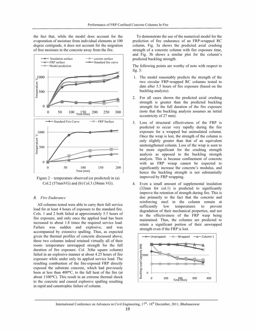
Performance of FRP Confined Concrete Columns In Fire
International Conference on Advances in Civil Engineering, 17th- 18th December, 2011, Bhubaneswar
19
the fact that, while the model does account for the
evaporation of moisture from individual elements at 100
degree centigrade, it does not account for the migration
of free moisture in the concrete away from the fire.
Figure 2 – temperature observed (or predicted) in (a)
Col.2 (57mmVG) and (b) Col.3 (38mm VG).
B. Fire Endurance
All columns tested were able to carry their full service
load for at least 4 hours of exposure to the standard fire.
Cols. 1 and 2 both failed at approximately 5.5 hours of
fire exposure, and only once the applied load has been
increased to about 1.8 times the required service load.
Failure was sudden and explosive, and was
accompanied by extensive spalling. Thus, as expected
given the thermal profiles of concrete discussed above,
these two columns indeed retained virtually all of their
room- temperature unwrapped strength for the full
duration of fire exposure. Col. 3(the square column)
failed in an explosive manner at about 4.25 hours of fire
exposure while under only its applied service load. The
resulting combustion of the fire-exposed FRP directly
exposed the substrate concrete, which had previously
been at less than 400*C, to the full heat of the fire (at
about 1100*C). This result in an extreme thermal shock
to the concrete and caused explosive spalling resulting
in rapid and catastrophic failure of column.
To demonstrate the use of the numerical model for the
prediction of fire endurance of an FRP-wrapped RC
column, Fig. 3a shows the predicted axial crushing
strength of a concrete column with fire exposure time,
and Fig. 3b shows a similar plot for the column’s
predicted buckling strength.
The following points are worthy of note with respect to
fig. 3:
1. The model reasonably predicts the strength of the
two circular FRP-wrapped RC columns tested to
date after 5.5 hours of fire exposure (based on the
buckling analysis).
2. For all cases shown the predicted axial crushing
strength is greater than the predicted buckling
strength for the full duration of the fire exposure
(note that the buckling analysis assumes an initial
eccentricity of 27 mm).
3. Loss of structural effectiveness of the FRP is
predicted to occur very rapidly during the fire
exposure for a wrapped but uninsulated column.
Once the wrap is lost, the strength of the column is
only slightly greater than that of an equivalent
unstrengthened column. Loss of the wrap is seen to
be more significant for the crushing strength
analysis as opposed to the buckling strength
analysis. This is because confinement of concrete
with an FRP wrasp cannot be expected to
significantly increase the concrete’s modulus, and
hence the buckling strength is not substantially
improved by FRP wrapping.
4. Even a small amount of supplemental insulation
(32mm for col.1) is predicted to significantly
improve the retention of strength during fire. This is
due primarily to the fact that the concrete and
reinforcing steel in the column remain at
sufficiently low temperatures to prevent
degradation of their mechanical properties, and not
to the effectiveness of the FRP warp being
maintained. Thus, the columns are predicted to
retain a significant portion of their unwrapped
strength even if the FRP is lost.
0
500
1000
0 50 100 150 200 250 300
Temperature
˚C
Time (min)
Insulation surface cocrete surface
FRP surface Standard fire curve
Model prediction
0
500
1000
0 50 100 150 200
Temperature
˚C
Time (min)
Standard Fire Curve FRP Surface
0
5000
0 100 200 300 400BucklingLoadCapacity
(kN)
Time (min)
Unwrapped Wrapped Column 1

Performance of FRP Confined Concrete Columns In Fire
International Conference on Advances in Civil Engineering, 17th- 18th December, 2011, Bhubaneswar
20
Fig.3 – Observed and predicted structural fire endurance
for various column configurations based on (a) crushing
strength and (b) buckling strength.
V. CONCLUSIONS
FRP materials used as externally – wounded
reinforcement for concrete structures are sensitive
to the effects of elevated temperatures.
FRP’s experience degradation in strength, stiffness,
and the bond at temperatures exceeding the GTT of
the polymer matrix.
Appropriately designed (and in the most cases
supplementally- insulated) FRP wrapped circular
RC columns can achieve satisfactory fire
endurances in excess of 5 hours.
The numerical models presented briefly herein can
be used to predict the heat transfer within, and load
capacity of, unwrapped and FRP wrapped and
insulated RC columns under exposure to a standard
fire.
Parametric studies conducted using the model (not
discussed here) indicate that the most important
factors influencing the fire endurance of FRP
wrapped RC columns are the thickness and thermal
conductivity of the insulation applied to the exterior
of the FRP wrap.
While no explicit requirement currently exists that
the temperature of an FRP wrap must remain below
its matrix GTT during fire, it is not known what
temperatures are allowable in the FRP such that it
retains sufficient residual properties to remain
effective after a severe building fire.
Further work is required in this area.
REFERENCES :
1. Apicella, F., &Imbrogno, M., “Fire performance
of CFRP-composites used for repairing and
strengthening concrete,” Materials and
Construction, Cincinnati, OH, USA, May, 1999,
pp 260-266.
2. Saadatmanesh, H.; Ehsani, M.R.; and Li, M.W,
“Repair of earthquake damaged RCC columns
with FRP wraps,” ACI Structural Journal, No. 94,
S-20,1996,pp. 206-214.
3. Benichou, N. “Results of Fire Resistance
Experiments on FRP-Strengthened Reinforced
Concrete Columns – Report No. 2”, Research,
Report, Institute for Reseach in Construction,
National Research Council Canada, pp. 39, 2007.
4. Benichou, N. “Fire Performance of FRP-
strengthened concrete systems”, short course,
Response of Materials and Structures to Fires,
Carleton University, Ottawa, Ontario, May 20-
22, 2009.
5. FOSTA PVT LMT, “FRP for Structural
Strengthening in Land and Marine Environment”,
Singapore.
6. Krishna Conchem Pvt. Ltd., http://
www.krishnaconchem.com/products.html
7. Mukherjee, Abhijeet, and Joshi, Mangesh.
“Recent Advances In Repair And Rehabilitation
of RCC Structures”. Department of Civil
Engineering, IIT Bombay.
8. Limaye.R.G., and KAMAT M.K., Experimental
studies on polymer modificationof cement
mortar, The Indian Concrete Journal,
March1992.
9. Sorathia, U., Dapp, T., & Beck, C., “Fire
performance of Composites,” Mat. Engrg., 9,
1992, pp. 10-12.
10. Lie, T., Structural Fire Protection, ASCE, New
York, NY, USA, 1992, pp. 241.
11. ISIS, Design Manual No. 4, ISIS Canada,
Winnipeg, MB, Canada, 2001.
0
1000
2000
3000
4000
5000
6000
0 60 120 180 240 300 360
Bucklingloadcapacity
(KN)
Time (min)
Unwrapped wrapped column 1
column2 service load

International Conference on Advances in Civil Engineering, 17th- 18th December, 2011, Bhubaneswar
21
System Identification with Noisy Data
U. K. Dewangan1 & S. V. Barai
2
1Dept. of Civil Engineering, National Institute of Technology, Raipur, India 2Dept of. Civil Engineering, IIT Kharagpur, Kharagpur -721 302, India
Abstract - System identification from the field obtained data is not successful till date because of the noise in the sensor or measured.
The unknown system parameter for any unknown damage is still a long way to move. In this paper finite element technique is
applied on the simulated damaged structures. The damage detection for the noise free data is extended and tried for the random noisy
sensor data. The proposed algorithm is used to predict the system parameter on static deflection data with introduction of some
random noisy data using simulated structure. The developed algorithm is applied on bridge truss structure for the identification of the
damaged system parameter prediction.
Key words - Damage, System identification; Noisy data; Finite element.
I. INTRODUCTION
The prediction of the damaged parameters from the
field data having noise is still an open challenge in the
field of structural identification. The Structural Health
Monitoring (SHM) of large space structures like
aerospace structure; satellite vehicles, where once the
damage had occurred cause the uncertainty due to
unknown damaged parameter. Finite element methods
are universally accepted as fast computation tools for
structural behavior prediction. Development in the field
of computational technology and sensing instruments
has also progressed a lot. Field data are usually noisy.
The damage detection, location and damage extent
prediction are among the important aspect of structural
behavior prediction. The main aim of researchers is
concentrated on the suitable identification algorithms
based on uncertain available sensor data which may be
linear or nonlinear, noisy or noise free sensor data.
There are two kinds of parameter identification
namely static and dynamic parameter identification. In
the dynamic parameter identification there are three
unknowns. They are mass, stiffness and damping. The
relationship between the dynamic coefficients (mass,
stiffness and damping) and also its sensitivity effects of
one property on another are still unknowns. Such a
system makes the analysis very complicated. For
uncertain damage with uncertain noisy data, no certain
techniques are available. The static identification
method seems to be better than dynamic identification
as it is having only one unknown (stiffness).
A brief review on damage detection mainly using
the static method or static combined with dynamic
method is presented here. The static damage parameter
identification approaches by the error term reduction
includes minimum deviation, sensitivity analysis, output
error optimization etc. were approached by [2] , [4], [7],
[12], [14] and [15]. Damage detection in composite
materials using system identification technique proposed
by [14]. The output error approach of system
identification was employed to determine the changes in
the analytical model in order to minimize the distance
between measured and predicted response. [2] Used
force error estimator and displacement error estimator
for static parameter grouping scheme to identify the
error by least squares minimization. Static strain
measurement from multiple loading models for
identification of the hole and cracks in linear anisotropy
elastic materials with nonlinear optimization was
presented by [4]. [15] applied a linear constrained
nonlinear optimization problem using the minimization
of error between the measured and computed
displacement to find damage.
Error sensitivity analysis is found to be a popular
method for finding the damage existence [9], [11], [13],
[1. On analyzing the sensitivity coefficients for natural
frequency, mode shapes and modal flexibility, [9] found
that modal flexibility is more sensitive as damage
indicator. Sensitivity with some other term approach
like orthogonal sensitivity, non-linearity, modal
updating were approached by[3], [16], [20] etc. The
orthogonal condition sensitivities was developed by [16]

System Identification with Noisy Data
International Conference on Advances in Civil Engineering, 17th- 18th December, 2011, Bhubaneswar
22
for the damaged and undamaged structure mode shapes
using FEM in laminated rectangular plate of composite
structures. [20] presented a sensitivity-based finite
element (FE) model updating for damage detection. The
modal flexibility residual formulation and its gradient
were used for formulation. The damage detection
procedure was illustrated on a simulated example with
noisy data and on a reinforced concrete beam model.
Dmage detection of cable-stayed bridges by
changes in cable forces, was optimized on cable force
error between measurement results and analytical model
by [17]. [10] developed a method used continuous
strain data from fiber optic sensor and neural network
model. [18] used sensitive characteristic of strain to
identify damage in structures for strain-based damage
identification. [8] Used conventional single-objective
optimization approach defines the objective function by
combining multiple error terms into a single one, for
weaker constraint in solving the identification problem.
The above literature review indicates that both
static as well dynamic methods were used in the system
parameter prediction of structure using simulated,
experimental and from the field data. Static methods
used either strain or displacement as measured data,
while in case of dynamic methods frequency and mode
shapes data were used popularly. Sensitivity method,
analyses the effect of parameter changes on the other
parameters. When the structural parameters are
unknown, the sensitivity analysis has no meaning. In
addition, noise in the measured data may completely
change the matrix property using matrix inversion. The
structural parameter identification from the field data
has no well-established solution, until now.
The paper is attributed to the static parameter
identification process with the noisy sensor data. The
objective of this paper is to develop a new modified
approach for the noisy sensor data with few
measurement. The initial parameter identification
algorithm has been taken from [13] but some noise were
introduced in the sensor data. This will lead to near
realistic field situation. Finite element method for
damage detection using static test data for smaller
subgroups of matrix was applied [3] for damage
existence prediction with only few measurements. The
noise values were varied between ± 4 % errors in the
sensor data. A finite element model of bridge truss
structure presented for the demonstration.
II. INITIAL AND DEDELOPED APPROACH
An algorithm to find the parameter extent for noise
free data was developed by [13]. Assuming the structure
behavior of structure is linear throughout the test, the
force displacement relationship in the static case for
undamaged structure is given by
]][[][ UKF (1)
and for damaged structure by
]][[][ UKF d (2)
Partitioning into measured and unmeasured
displacements
a daa dab a
b dab dbb b
f K K U
f K K U (3)
][[ aaa Kf – abK --1
bbK --1
abK aU
+ abK bbK --1
bf (4)
af , bf and aU are measured from test. The
difference between the measured and theoretically
calculated value will be the error term. If the stiffness
parameters are correct, then error matrix )( pE will
be zero, otherwise non-zero.
)( pE = ][[ aaK – abK --1
bbK --1
abK aU
+ abK bbK --1
bf – af (5)
)( pE )( pE + )( pS p (6)
The error sensitivity expression was calculated
using first order Taylor series expansion of error matrix
)( pE . The stiffness parameters were obtained by
minimization of error function with respect to unknown
parameter ( p) using the least square optimization.
The error sensitivity expression has been modified
for noisy sensor data as the displacement gets modified
due to sensor noise and unknown damaged. The
unknown parameters become the function of both
displacements. The sensitivity matrix was recalculated
with this new modified expression,
.

International Conference on Advances in Civil Engineering, 17th- 18th December, 2011, Bhubaneswar
23
.
The present method is able to predict the damage
existence in structure with only few measurements.
Using least square optimization technique, all the
unknown damaged parameters can be identified after
some iteration successfully with the noisy sensor data.
The finite element method revisited and a row-echelon
form of matrix developed for damage detection using
static displacement and force data, Dewangan U. K.
(2010) [4]. The row-echelon form has an advantage of
partitioning matrix into smaller subgroups.The noise
values were varied between ± 4 % errors in the sensor
data. A finite element model of bridge truss structure
presented for the demonstration. The modified algorithm
is implemented using MATLAB [21].
III. EXAMPLES
Based on the algorithm discussed in the above
section, the computer program was written in MATLAB
and tested Bridge Truss Structure Bridge Truss Structure
Structural Details: All elements are having the modulus
of elasticity 210E GPa and initial undamaged
cross sectional area 5 21.61 10A X mm . The
structural configuration is shown in Fig. 3.8. A single
concentrated load is applied at each joint. The
deflections at each joint are measured. The force matrix
[ ]F is found out and corresponding displacement
matrix [ ]U is measured.
For bridge truss structure, [1] as shown in Figure 1,
the modulus of elasticity of all elements was 206.8 GPa
and initial undamaged cross sectional area of all
members was 500 mm2. The noise was introduced up to
± 5 % error in the sensor data for sensor numbers 5, 6, 7
and 8 displacement d.o.f. Different load combinations
are considered and they are tabulated in the Table 2 with
sensor noise value. Previously discussed algorithms
were applied to this problem and results are given in
Table 2 and Figure 4 for typical cases. For the noisy
sensor data set combination on tower truss the computed
parameter values were compared with the actual
parameter value. From the plotted graph as shown in
Figure 2, it is clear that with the noisy sensor data, [13]
algorithm values are far away from the actual value of
the parameter. The modified proposed algorithm values
are nearly close to the actual value of the parameters.
The algorithm could identify the damage extent for
members away from the supports.
1 1
1 1 1
1 1 1
1 1 1
1
( ) [
*
*
aa ab ab
i bb ba ab bb
i i i
ab a
ab bb bb ba a aa ab bb ab
i i
ab bb
bb ab bb bb
i i
a aa ab bb ab a ab bb
ab bb b b a
k k kS p k k k k
p p p
k Uk k k k U k k k k
p p
k kk k k k
p p
f K K K K U K K
K k f f f1 1
1 1
*
* (7)
aa aa
bb aa a ab bb
i i
aa aa a
a bb aa ab bb
i i i
k kk K U K K
p p
k k Uf k K K K
p p p

System Identification with Noisy Data
International Conference on Advances in Civil Engineering, 17th- 18th December, 2011, Bhubaneswar
24
Figure 2 Railway bridge truss (Case 2)
2
8
U4U3
U2
U1
U14U13
U12
U11
3 4 51
2
9 106 7
12
Force degree of freedom
11
8
U4 U3
U2U1
U14
U13
U12U11
3 4 51
9 106 7
12
Displacement degree of freedom
11
Fig. 3 : Comparative study of damage extent prediction (Bridge truss Structure)
TABLE I: RESULTS OF NOISY SENSOR DATA WITH MODIFIED ALGORITHM ON BRIDGE TRUSS
Case Member
damaged
Applied
force d.o.f.
Measured
displacement d.o.f.
Noise in
Sensor
Members
Converged
Members
Diverged
1 All 1-20 1-20 8 up to 5% 1-4, 6-14, 17-20 5,16,15 and 21
2 All 7-10, 17-20 7-10, 17-20 1- 8 up to 5% 1-4, 6-14, 17-20 5,16,15 and 21
3 All 7-10, 17-20 1-4, 11-14 4 up to 5% 1-4, 6-14, 17-20 5,16,15 and 21
4 All 1-20 1-20 5,6,7 and, 8 1-4, 6-14, 17-20 5,16,15 and 21
00.5
11.5
22.5
33.5
44.5
1 3 5 7 9 11 13 15 17 19 21
Pa
ram
eter
Pre
dic
ted
Element Number
Sensor 7,8,9,10,17,18,19,20 all with 4% Noise
Actual
Sanayei and Onipede (1991)
Modified Proposed Algorithm

System Identification with Noisy Data
International Conference on Advances in Civil Engineering, 17th- 18th December, 2011, Bhubaneswar
25
up to 4%
.
IV. RESULTS
Considering the various multiple damaged member
combinations, the existence of damage is detected.
Different combinations of force DOF and
displacement DOF used are given in Table 1for various
cases.
From the plotted graph as shown in Figure 4, it is
clear that with the noisy sensor data, the modified
proposed algorithm values are nearly close to the actual
value of the parameters. The algorithm could identify
the damage extent for members away from the supports.
V. DISCUSSION
In this study, it was clearly observed from the
demonstrated examples that the modified algorithm
could predict damage extent in the presence of noise in
structural response. Further it was found that the
algorithms failed to predict damage extent in the
members, which were near to the support. Hence, the
present work is very well justified for the large space
structures where except the support connected members,
all other members, damage extent could be predicted.
The failure of the algorithm in identifying the damage
extent in members near support is a matter of further
investigation.
VI. CONCLUSION
The damage parameter identification with the noisy
sensor data was carried out for different random noise
value. Algorithm developed by [13] has been modified
for the noise in sensor value. Finite element method for
damage detection using static test data for smaller
subgroups of matrix was applied [3] for damage
existence prediction with only few measurements. The
noise values were varied between ± 4 % errors in the
sensor data. The algorithm works well for lower noise
level up to a value ± 4 % errors in the sensor data and
the unknown damaged parameter could be extracted
even from the noisy data set of structural response using
above technique for the members with only few
measurements. Hence the algorithm is useful for
damage prediction with noisy sensor data on large
structures for the members, which are away from the
supports.
NOTATION
d.o.f. = Degree of freedom
d.d.o.f. = Displacement degree of freedom
f.d.o.f. = Force degree of freedom
{E(p)} = Error function vector
[ Fa] = Applied force matrix at force d.o.f. at
measured d.o.f.
[Fb] = Unapplied force matrix at force d.o.f. for
unmeasured displacement d.o.f.
F.E.M. = Finite element method
[K] = Undamaged global stiffness matrix
[Kdaa] = Sub matrix of [K] corresponding to
measured d.o.f. and applied force d.o.f.
[Kdab] = Sub matrix of [K] corresponding to
measured d.o.f. and unapplied force d.o.f.
[Kdbb] = Sub matrix of [K] corresponding to
unmeasured d.o.f. and unapplied force d.o.f.
[Kdba] = Sub matrix of [K] corresponding to
unmeasured d.o.f. and applied force d.o.f.
[Kd] = Damaged global stiffness matrix
n = Number of elements
p = Unknown parameter’s values
r = Row number
[Sd] = Damaged global stiffness matrix
[S] = Undamaged global stiffness matrix
[Saa] = Sub matrix of [S] corresponding to
measured d.o.f. and applied force d.o.f.
[Sab] = Sub matrix of [S] corresponding to
measured d.o.f. and unapplied force d.o.f.
[Sbb] = Sub matrix of [S] corresponding to
unmeasured d.o.f. and unapplied force d.o.f.
[Sba] = Sub matrix of [S] corresponding to
unmeasured d.o.f. and applied force d.o.f.
{S(p)} = Sensitivity matrix
[ U ] = Transformation matrix
[Ua] = Measured displacements matrix
[Ub] = Unmeasured displacements matrix
REFERENCES
[1] S. R. Agrawal, “Steel Bridges In Indian
Railways. Advances in Steel Structures,” (Ed.) V.
Kalyanraman, Proc. of the National Symposium
on Advances in Steel Structures, Tata McGraw
Hill, Publishing Company Ltd., New Delhi,
,1990, pp. 227–243.
[2] M. R. Banan, M. R. Banan and K. D. Hjelmstad,
“ Parameter Estimation of Structures From Static
Response II: Numerical simulation studies,”

System Identification with Noisy Data
International Conference on Advances in Civil Engineering, 17th- 18th December, 2011, Bhubaneswar
26
Journal of Structural Engineering, vol. 120,
Nov,1994, pp. 3259–3283.
[3] U. K. Dewangan, “Structural Damage Existence
Prediction with Few Measurements” International
Journal of Engineering Science and Technology,
Vol. 3, 2011 No.10, pp. 7587–7597.
[4] C. Hwu and Y. C. Liang, “Hole Crack
Identification By Static Strains from Multiple
Loading Modes,” AIAA Journal, vol. 39, 2, 2001,
pp. 315–324.
[5] D. Bernal and B. Gunes, “Flexibility Based
Approach for Damage Characterization:
Benchmark Application,” Journal of Engineering
Mechanics, vol. 130, 1, 2004, pp. 61–70.
[6] E. Udwadia, “Structural Identification and
Damage Detection From Noisy Modal Data,”
Journal of Aerospace Engineering, vol. 18, 3,
2005, pp. 179–187.
[7] J. H. Jang, I. Yeo, S., Shin, and S. P. Chang,
“Experimental Investigation of System –
Identification – Based – Damage Assessment on
Structures,” Journal of Structural Engineering,
vo. 128, 3, 2002, pp. 390 – 399.
[8] J. Sungmoon et al., “Structural Damage
Identification Based on Multi–Objective
Optimization,” Conference Proceedings of the
Society for Experimental Mechanics Series, 12,
2011, pp. 1239–1244.
[9] J. Zhao and J. T. Dewolf, Sensitivity study for
vibrational parameters used in damage detection,
Journal of Structural Engineering, 125,4 ,1999,
pp. 410–416.
[10] J.W. Lee, C. kwang–Ho and Huh Y. C., “Damage
Detection Method For Large Structures Using
Static and Dynamic Strain Data From Distributed
Fiber Optic Sensor,” International Journal of
Steel Structures , vol. 10, 2010, pp. 91–97.
[11] L. H. Yam, Y.Y. Li, and W.O. Wong,
“Sensitivity Studies Of Parameters For Damage
Detection Of Plate – Like Structures Using Static
And Dynamic Approaches,” Engineering
Structures, vol. 24, 11, 2002, pp. 1465–1475.
[12] M. D. Paola and C. Bilello, “An Integral
Equation For Damage Identification Of Euler –
Bernoulli Beams Under Static Loads,” Journal of
Engineering Mechanics, vol. 130, 2, 2004, pp.
225–234.
[13] M. Sanayei and O. Onipede, “Damage
Assessment Of Structures Using Static Test
Data,” AIAA Journal, vol. 29, 7, 1991, pp. 1174–
1179.
[14] P. Hajela and F. J. Soerio, “Recent Developments
in the Damage Detection Based On System
Identification Methods,” Structural Optimization,
vol.2,1990, pp. 1–10.
[15] S. Shin, and H.M. Koh, “A Numerical Study on
Detecting Defects in a Plane – Stressed Body by
System Identification, Nuclear Engineering and
Design, vol. 190, 1999, pp. 17 – 28.
[16] V. Santos, M. Soares, and C, A. Pina, “Damage
Identification Numerical Model Based On The
Sensitivity Of Orthogonality Conditions And
Least Squares Techniques.” Computers and
Structures, vol. 78, 1, 2000, pp. 283–291.
[17] X. G. Hua, Y. Q. Ni, Z. Q. Chen, and J. M. Ko,
“Structural Damage Detection Of Cable–Stayed
Bridges Using Changes In Cable Forces And
Model Updating, J. Struct. Eng, vol. 135, 9, 2009,
pp. 1093–1107.
[18] Y. Y. Li, “Hypersensitivity of strain–based
indicators for structural damage identification: A
review,” Mechanical System and Signal
Processing, vol. 24,3, 2010, pp. 653–664.
[19] B. Vanlanduit, E. Parloo, and P. Guillaume,
“Combined Damage Detection Techniques,”
Journal of Sound and Vibration, 266, vol. 4,
2003, pp. 815–831.
[20] B. Jaishi, and W.X. Ren, “Damage Detection by
Finite Element Modal Updating Using Modal
Flexibility Residual.” Journal of Sound and
Vibration, vol. 290(1 – 2), 2006, pp. 369 – 387.
[21] R. Pratap, “Getting Started with MATLAB.” 3rd
Ed., 2001, Oxford University Press. New York.

International Conference on Advances in Civil Engineering, 17th- 18th December, 2011, Bhubaneswar
27
Accident Analysis and Prediction of Model
on National Highways
Rakesh Kumar Singh & S.K.Suman
Department of Civil Engineering, National Institute of Technology Patna, Patna, Bihar, India
Abstract - Rapid growth of population coupled with increased economic activities has favored in tremendous growth of motor
vehicles. This is one of the primary factors responsible for road accidents. It is observed that few works have been carried out on
statistical analysis of accidents particularly on two-lane National Highways.
For this paper stretch of NH-77 has been selected from Hajipur to Muzaffarpur. The accidental data was collected for last eleven
years, 2000-2010 from the Police Stations where FIR was lodged. The collected data were analyzed to evaluate the effect of
influencing parameters on accident rate. Heavy vehicles like truck are involved in maximum number of accidents on the selected
stretch. It is estimated that a heavy vehicles is involved in almost 48% accidents followed by two-wheelers 16%, car 12% and bus
10%. There is no definite trend for monthly variation in accident on a study section but the accidents in month of July and January
are generally higher. Accident rate in terms of number of accidents per km-year increases with traffic volume. But the accidents rate
in terms of number of accident per million-vehicle kilometer-year (MVKY) decreases with increase in traffic volume. Accident rate
per MVKY increases during the study year, whereas both injury and fatality rate per MVKY show a declining trend over the study
period. The developed model for accident prediction represents that the number of accidents per-km-year increases with AADT and
decreases with improvement in road condition.
Key word - FIR, Statistical analysis, Regression model
I. INTRODUCTION
The highway network is accelerated at a fast rate
and the safety of vehicular movements becomes a
concern for everybody due to reporting of loss of lives
and properties along with fatal injuries and periodical
obstruction of traffic flow. National highways provide
the efficient mobility and accessibility function. The
increasing road accidents have created social problems
due to loss of lives and human miseries. Road accidents
are essentially caused by interactions of the vehicles,
road users and roadway conditions. Each of these basic
elements comprises a number of sub elements like
pavement characteristics, geometric features, traffic
characteristics, road user’s behavior, vehicle design,
driver’s characteristics and environmental aspects.
Valli & Sarkar (1997) examined the possibility of
using the speeds formula on accidents rate estimation
for Indian condition and proposed a model for road
accidents in India based on that. Victor & Vasudeman
(1998) made a detail study and analysis on bus related
accident in Tamil Nadu taking data from fine bus
Transport Corporations. Chand (1999) made an attempt
to examine the accident frequently and trend of bus
related accidents with special references to public Road
Transport under takings in India.Baviskar (1999) studied
road accidents in Nashik Municipal corporation area and
highlighted the distribution and accidents pattern in the
city at micro level during the period 1980-1989.Saija et
al (2000) had made a detailed study on road accident
spectrum analysis of Gujrat.Singh & Misra (2000)
analyzed the road accident spectrum for the city of
Patna.Chakraborty et al (2001) studied the aggression to
risk taking behaviors that leads a threat to road safety.
Jenna et al (2001) developed a model for prediction of
accidents in Indian urban roads taking field data from
Ernakulum. Mohan Dinesh (2007) deals a sustainable
transport system that provide mobility and accessibility
to all urban residents in a safe and environment friendly
mode of transport.
A. NEED AND OBJECTIVES OF STUDY
As per the NATPAC number of road accidents in
India is three times higher than that prevailing in
developed countries. The number of accidents for 1000
vehicles in India is as high as 35 while the figure ranges
from 4 to 10 in developed countries.
The objectives of the present study are listed below:
1. To study the monthly and annual variation in
accident rate on selected stretch.
2. To study the effect of traffic volume on accident
rate.

Accident Analysis and Prediction of Model on National Highways
International Conference on Advances in Civil Engineering, 17th- 18th December, 2011, Bhubaneswar
28
3. To develop an accident prediction model based on
AADT and road condition.
II. DATA COLLECTION
The busiest NH-77 passing through two cities
namely Hajipur and Muzaffarpur, the stretch of this road
has length 70km is selected for data collection and
statistical analysis of accidents, as road shown in Bihar
Road Map [Fig. -1].With the prior permission of the
concerned Senior Superintendent of Police (S.S.P), the
accident data were collected from the six Police stations
situated along the NH-77. These Police stations are
Hajipur, Sarai, Bhagwanpur, Goraul, Kudhani and
Turki.The police stations have their own FIR records of
several years. Accident, Fatality and Injury data were
collected month wise in every year from each police
station records during year 2000 to 2010. The type of
vehicles involved in accidents as recorded in the FIR
was also noted down. The categories of vehicles include
Tuck, Bus, Tractor, Jeep, Car, Tempoo, Motorcycle and
Bicycle etc. Further, monthly-obtained data were sorted
out year wise, represented in percentage over the study
year as shown in Table-1.
Year Fatality
in %
Injury in % Total
Accident in
%
2000 6.15 2.33 3.15
2001 1.54 3.00 2.56
2002 7.69 8.33 8.27
2003 15.38 9.00 9.25
2004 15.38 10.00 10.43
2005 13.85 11.33 11.81
2006 10.77 12.00 12.00
2007 7.69 11.67 10.43
2008 6.15 14.00 13.58
2009 10.77 13.33 13.39
2010 4.62 5.33 5.31
Table -1: Accident, Injury & Fatality in % on NH-77
A. DATA COLLECTED FROM P.W.D.
RECORDS
P.W.D. (Public works Department) records are the
main source for traffic volume data & road map. In
addition to the above, road conditions information were
also obtained from PWD records. Traffic survey was
conducted at Sarai market on NH-77 at about 8km from
Hajipur. Traffic volume for the year of count 2008 was
extracted and represent in form of Commercial Vehicles
per day (CVPD) & PCU/day, shown in Table-2.It is
assumed that the traffic volume is uniform throughout
the study stretch.
As the yearly traffic census data was not available
for all the years, the available data were used to predict
traffic volume on a road in each year for the period
2000-2010 as shown in Table-3.A growth rate (r) of 7.5
% per year was assumed for this purpose. A formula
was used for forecasting as follows:
(1 )100
nrA P= ±
where A = Predicted year traffic volume, P = Present
year traffic volume, n = years of count and minus sign
indicates before the present year traffic count and plus
sign indicates after the present year traffic count.
Table -2: Traffic Volume Data
Name/No.
of the road
Year of
count
Traffic
Volume
CVPD PCU/day
NH-77 2005 9507 15128
Table-3: Predicted Traffic Volume
Year PCU/day
2000 7499.93
2001 8108.03
2002 8765.44
2003 9476.15
2004 10244.49
2005 11075.12
2006 11973.10
2007 12943.90
2008 13993.40
2009 15128.00
2010 16262.60
III. ANALYSIS OF DATA AND DISCUSSION OF
RESULTS
The data collected reflects the view of the reporting
Police Officer. According to the literature review
accidental data collected from the Police Station is not
the complete information because all accidents are not
recorded in their FIR (First information report).
Therefore, all accidental data may be increased by 25-
30%.
In this paper all accidental data are increased by
30%. All accidental data were analyzed, using the
software MS EXCEL. As per the pilot survey, accidents
cause has been recognized that occur due to (i) Driver’s
fault (ii) Failure of the motor vehicle (iii) Road
condition and, (iv) Environmental condition.

Accident Analysis and Prediction of Model on National Highways
International Conference on Advances in Civil Engineering, 17th- 18th December, 2011, Bhubaneswar
29
Fig.1: Map showing the study stretch
A. ANNUAL VARIATION IN ACCIDENTS
Fig.-2 shows the annual variation in accidents
during 2000-2010.It is observed that percentage
accidents are increasing relatively in most of the year. In
year 2010 accident rate fall down suddenly, this type of
situation occur may be due to the maintenance of the
road is executed in the same year.
3.152.56
8.279.25
10.4311.81 12
10.43
13.5813.39
5.31
02468
10121416
Accident,%
Year
Fig.2: Annual Variation in accidents during 2000-2010
on NH-77
B. MONTHLY VARIATION OF ACCIDENTS
Average monthly variation in accidents during year
2000-2010 on NH-77 road section is shown in bar chart;
Fig.-3.These results indicate that there is no definite
trend for monthly variation in accidents. Accidents in
the month of July are quite high. It may be due to rainy
season in this month. The earthen shoulder gets
deteriorated in rains and pavement surface becomes
slippery. Also, it is observed that accidents rate is
comparatively higher in the month of December –
January of the year. No definite reason can be attributed
to this trend but it might be due to poor or low visibility
(fog condition) in winter seasons
13.61
7.43 7.92 8.17
5.94
8.17
13.12
7.435.94
4.70
6.44
11.14
0.00
2.00
4.00
6.00
8.00
10.00
12.00
14.00
16.00
1 2 3 4 5 6 7 8 9 10 11 12
Month
Acc
ide
nt(
%)
Fig.3: Average monthly variation in accidents during
2000-2010 on NH-77
C. ANNUAL VARIATION IN FATALITY,
INJURY AND ACCIDENTS
Fig.-4 shows the comparison of Fatality, Injury and
Accidents in percentage. Fatality in the year 2003 and
2004 is quite high. Injury rate during the whole study
year are increasing relatively and the accident rate is as
mentioned in the fig-4. However, High fatality rate
gives the challenge to the Traffic Engineer to prevent
the casualty. Therefore, Traffic Engineer has to study
the cause of casualty and to suggest corrective treatment
at potential locations.
Fig.4: Yearly variation in fatality, injury & accident
during 2000-2010 on NH-77
D. VEHICLES INVOLVED IN ACCIDENTS
Fig.-5 shows the percentage accidents involving a
particular type of vehicle. It is observed that Truck are
involved in maximum number of accidents almost 48%.
It may be due to the most of the Truck driver are driving
their vehicles after drink of alcohol or they are not
aware about the condition /maintenance of their
vehicles. It is followed by Motorcycle (16%), Car
Yearly variation in Fatality,Injury & Accident during 1996-
2006 on NH-77
0.00
2.00
4.00
6.00
8.00
10.00
12.00
14.00
16.00
18.00
1 2 3 4 5 6 7 8 9
10
11
Year
Fata
lity
,In
jury
& A
ccid
en
t in
%
Fatality%
Injury%
Accident%

Accident Analysis and Prediction of Model on National Highways
International Conference on Advances in Civil Engineering, 17th- 18th December, 2011, Bhubaneswar
30
(12%), Bus (10%), Tempo (5%), Jeep & Tractor (3%),
cycle (2%) and Pedestrian (1%).
Fig.-5: Vehicles composition involved in accidents
E. ACCIDENTS AS RELATED TO TRAFFIC
VOLUME
To observe the relationship between accident rate
and traffic volume, accident rate is presented in two
forms. In first case, it was the number of accidents that
occurred in a road section per km per year and presented
as accident per km-year. In second case, it was the
number of accidents that occurred in a road section per
million vehicles (MV) taken in terms of PCU per
kilometer (k) per year (y), represented as accident per
MVKY (Accidents per million vehicles-km-years).
Fig.6: Accidents per km-year as related to traffic volume
It is observed that accident rate increases with
increase of AADT.The data supporting the linear trend
line relationships may be sensitive to the design and
operational feature of the Highway.
Fig.-7: Accident per MVKY as related to traffic volume
Figure-7 shows the accidents per million-vehicle-
kilometer –year decreases slowly with increase in the
AADT.It may again be due to design and operational
features of the highway and influence of other
parameters like roadside features, degree of side slope,
climate condition and operational environment.
F. TREND OF ACCIDENTS DURING 2000-2010
The annual trend of MVKY is shown in fig.8.Linear
variation means accident rate per MVKY increases in
each subsequent year. This increasing trend in accident
rate may be due to detoriation in road and shoulder
conditions and the road users did not adopt general
awareness. Even though the failures of the motor vehicle
are mainly driver’s fault, result the accidents.
y = 9.0636x ‐ 18082R² = 0.7326
0
50
100
150
1995 2000 2005 2010 2015
Accidents per MVKY
Year
Fig.-8: Trend of accidents during 2000-2010
Motarcycle 16%
Tractor
3%
Tempu 5%
Car 12%
Jeep
3% Bus 10%
Truck
48%
Cycle
2%
Pedestrian
1%
Accidents per km-year as re lated to traffic volume
y = 0.0846x - 0.2484
R2 = 0.7518
0.00
0.20
0.40
0.60
0.80
1.00
1.20
0.00 5.00 10.00 15.00 20.00
AADT(1000PCU)
Ac
cid
en
ts p
er
km
-ye
ar
Accidents per MVKY as related to traffic volume
y = -1.2468x + 83.935
R2 = 0.2909
0.00
10.00
20.00
30.00
40.00
50.00
60.00
70.00
80.00
90.00
0.00 5.00 10.00 15.00 20.00
AADT(1000PCU)
Ac
cid
en
ts p
er
MV
KY

Accident Analysis and Prediction of Model on National Highways
International Conference on Advances in Civil Engineering, 17th- 18th December, 2011, Bhubaneswar
31
Fig-9: Trend of injuries during 2000-2010
G. TREND OF INJURIES DURING 2000-2010
The annual trend of injuries is shown in
Fig.9.Scattered points do not show the definite trend,
this may be due to the insufficient relatively closer
values. A linear trend line is fitted to show the trend
because logically true but have coefficient of
determination/correlation is very less. It was found that
injuries per MVKY decrease over the period 2000-
2010.This trends may be attributed to incautiousness
driving of small sized vehicles and also priority goes to
motorcyclists.
H. TREND OF FATALITIES DURING 2000-2010
The observed values are not showing the definite
trend of fatalities. The fatality rate per MVKY has
decreased substantially over the years. Ref Fig.10.
Fig.10: Trend of fatalities during 2000-2010
IV. ACCIDENT PREDICTION MODEL
The portion of the Highways and shoulder, where
maintenance work was carried out in a particular year
were noted down from the PWD records. Chandra and
Dev Raj (1999) suggested that the section of a road and
its shoulder may be ranked on a 5-point scale as shown
below:
Excellent = 5, Good = 4, Average = 3,
Poor = 2 and Bad = 1
The excellent means road and shoulders was
maintained very recently and bad means road and
shoulders were not maintained within last four years and
these have deteriorated to the extent that vehicles cannot
use them. This decimal way of ranking is primarily due
to the maintenance works not being carried out in a
single year for the whole stretch of a road. The accidents
per km-year were regressed with AADT and road
shoulder conditions rank.
The general form of equation is represented as:
Accident /km-year =C0 + C1 (AADT) + C2 (Road
and Shoulder Condition Rank [CR])
Accidental data collected for the study stretch of
NH-77 was used to develop the Accident Model.
Regression analysis is used in the present study, for
finding out a best prediction model for accidents on
National Highways. The accident data collected from
different police stations were regressed against the
AADT and CR.
C0 =1.21, C1 = 4 x 10⁻⁶,
C2 = 0.183, R2 = 0.895
The prediction model for NH-77 may be represented as
Accident/km-year = 1.21 + 4 x 10⁻⁶
(AADT)
-0.183(CR)
The above equations indicate that the accident/km-
year increases with AADT, but decreases with
improvement in condition of road or shoulders or both.
A. VALIDATION OF THE MODEL
Using the AADT of the selected stretch of the road
and road and shoulder condition rank (CR) are assigned
as per site visit. The accident prediction model was
validated for the road stretches between Kudhani to
Sitamardhi road on NH-77.The estimated values from
the accident prediction model were tested by Chi-
squared test.
Table-4: Estimated accidents at 5 locations for
validation
Locations 1 2 3 4 5
Accidents
estimated from
prediction
model
0.87
0.70
0.70
0.51
0.69
y = ‐0.4585x + 925.35R2 = 0.1126
0.00
5.00
10.00
15.00
20.00
1999 2004 2009 2014 Year
Fatalities per MVKY
y = ‐1.9803x + 4002.7R 2 = 0.336
0.00
10.00
20.00
30.00
40.00
50.00
60.00
1998 2000 2002 2004 2006 2008 2010 2012
Year
Injuries per MVKY

Accident Analysis and Prediction of Model on National Highways
International Conference on Advances in Civil Engineering, 17th- 18th December, 2011, Bhubaneswar
32
Sum of the accidents rate =
0.87+0.70+0.70+0.51+0.69 =3.47, the expected number
of accidents rate = 3.47/5 =0.69, Chi-square = 0.87,
Degree of freedom, df = 5-1= 4 and H0 = it is a good fit,
Chi-square for df = 4 and 5% significance level = 9.488,
since 0.87 <<9.488
Hence,H0 is correct. Therefore, It was found that
estimated accident rate from accident prediction model
were significant at 5% level of significance.
V. CONCLUSIONS
The following conclusions are drawn:
1. There is no definite trend for monthly variation in
accident on a section of highway. But the accident
in months of July is generally higher. It may be due
to fast deterioration of earthen shoulder by rain in
these months. Accident in month of January has
relatively high value; it may be due to the foggy
weather.
2. Heavy vehicles like truck are involved in maximum
number of accidents on National Highways. It is
estimated that a heavy vehicles is involved in
almost 48 % accidents followed by two-wheelers
(motorcycle) 16%, car12% and Bus10%.
3. Accident rate in terms of number of accidents per
km-year increases with traffic volume. But the
accidents rate in terms of number of accident per
million-vehicle kilometer-year (MVKY) decreases
with increase in traffic volume.
4. Accidents rate per MVKY increases during the
study year, whereas, both injury and fatality rate per
MVKY show a declining in trend over time.
5. Accident prediction model developed in the present
study show that number of accidents per km-year
increases with AADT and decreases with
improvement in road/shoulder condition.
Accident prediction model was validated by Chi-
squared test and found to have a good linear relationship
between AADT and CR.
REFERENCES
[1] Bavikar, S.B. (1999), “Road Accidents in Nashik
Municipal Corporation Area: A Case Study,”
Indian Journal of Transport Management,
2319,pp543-555.
[2] Chandra, S and Dev. Raj (1999), “Role of
shoulders in Traffic operation,” Indian Highways,
27(11), Indian Roads Congress, New Delhi,
pp31-38.
[3] Chand M (1999), “An analytical study of bus –
related accidents in India,” Indian Highways,
(2799), 9-20.
[4] Chakraborty, S. et al (2001), “Accident
Characteristics of roadway Vehicles in
Kolkata,”ROTRAN, Vol.2, pp6.39-6.45
[5] Chandra, S et al (2004), “Accident Analysis on
two lane roads,” Highway research bulletin,
Highway research Board, IRC, pp77-92
[6] Kadiyali, L.R. et al (1983), “Effect of road
characteristics on accident rates on rural
highways in India,” Highway research bulletin,
IRC, 20, 1-38.
[7] Kadiyali L.R., “Traffic engineering and transport
planning,” Khanna publishers Delhi-110006,
ed1999, 411-483
[8] Mohan D., (2007),”Traffic safety and health in
Indian cities’, Research and Injury prevention
Programme,” IIT Delhi, New Delhi
[9] Saija, K.K. et al (2000), “Spectrum analysis of
road accidents a case study,” Indian highways,
28(9), 29-41.
[10] Singh S.K. (2004), “Road accident analysis: A
case study of Patna city,” Urban Transport
Journal, Vol.2, No.2, pp.60-75.
[11] Tula Dhār, S.B.S and Justo C.E.G. (1981),
“Analysis of accidents rates-A case study,”
Highway research bulletin’, Indian road
congress,(56),1-11.
[12] Victor, D.J. and Vasudenan, J (1998), “Factors
affecting bus related accidents case study of five
corporations in Tamilnadu,”HRB, IRC, 4088,
pp39-52.
[13] Valli P. and Sarkar P.K. (1997), “Models for road
accidents in India,” Highway research bulletin,
IRC 16

International Conference on Advances in Civil Engineering, 17th- 18th December, 2011, Bhubaneswar
33
Innovations in Concrete Technology
of High-Rise Buildings
Rinu Mary Abraham & B. S. Srinivasa Prabhu
Department of Civil Engineering, Manipal Institute of Technology (MIT), Manipal, India
Abstract - Skyscrapers and High-rise buildings are an increasingly common sight where land is expensive, as in the centers of big cities, because they provide such a high ratio of rentable floor space per unit area of land. Not only do they define the skyline, they help to define the city's identity. In this paper a brief history of the prominence of concrete in the construction of tall buildings is closely examined. We have attempted to bring out the merits of concrete and the usage of composites in concrete for high rise structures. Important advancements in concrete technology involved in high rises including high performance concrete and light weight concrete are described. In this connection, prominent concrete high rise structures like Ingalls Building, Marina City Towers and their crucial features are discussed. Through this paper an attempt is made to bring out the various advancements of concrete construction to enable futuristic construction for high rises with prospects of using appropriate concrete technology.
Keywords-skyscraper;concrete; high-rise construction;
I. INTRODUCTION
Development of tall buildings underlines and accentuates the prosperity of the urban communities all around the globe. They are built not just for economy of space; like temples and palaces of the past, skyscrapers are considered symbols of a city's economic power. The choice for construction material for high-rises has been strongly influenced by economical and structural stability factors which include the ability to withstand natural calamities such as windstorms. Traditionally, the primary concern of the structural engineer designing a building has been the provision of a structurally safe and adequate system to support the vertical loads. This is understandable since the vertical load-resisting capability of a building is its reason for existence. However, this is only true for the buildings involved if they are not too high, are not in seismic zones, or have been constructed with adequate built-in safety margins in the form of substantial nonstructural masonry walls and partitions. A structure must be designed to carry loads due to gravity, wind, equipment and snow; resist high or low temperatures and vibrations; protect against explosions; and absorb noises. Adding to this the human factor means considering rentable spaces, owner needs, aesthetics, cost, safety and comfort. Although one set is not mutually exclusive of the other, careful planning and consideration are essential in an attempt to satisfy and integrate both. Considering structure alone, there are two main categories for high-rise buildings - structures that resist gravity and lateral loads and those that carry primarily gravity loads. Since skyscrapers have the greatest need for resisting high magnitudes of wind, the lateral load resisting system becomes the most
important and hence, it is essential to also take into account the lateral forces such as wind loads, seismic inertia-forces, blast loads, etc. to ensure the stability of buildings.
Concrete, inspite of being a relatively recent construction material has become an indispensable part of the modern construction industry. Engineers are coming to realize how concrete can be utilized to build seemingly impossible structures with relative ease and efficiency. Ransome, Hennebique, Fazlur Khan initiated the emergence of concrete to the modern age. With the advent of concrete technology involving high- strength concrete, light weight concrete, slag cement and such, the presence of concrete in superstructures was established. From the Ingalls building, concrete skyscrapers have graced the skyline over the years. Johnson Wax Tower, Place Victoria, Lake Point Towers are but a few examples. The structural aspects of the Ingalls building, and modern skyscrapers such as the Burj Khalifa, provide insights into how far we’ve come from single storeyed stone structures and how we continue to dream on.
II. EMERGENCE OF CONCRETE AS A
SIGNIFICANT CONSTRUCTION MATERIAL
Concrete in its present form is the youngest of the three basic structural materials (steel, concrete and masonry materials) of construction. While steel has been much favored in the construction of high-rises, concrete is gaining fast popularity in the field. According to CEMBUREAU, in 1900, the total world production of cement was about 10 million tons; in 1998 it was 1.6 billion tons. If we suppose that on average 250kg of

Innovations in Concrete Technology of High-Rise Buildings
International Conference on Advances in Civil Engineering, 17th- 18th December, 2011, Bhubaneswar
34
cement are used to produce 1 m3 of concrete, in 1900 only 40 million m3 of concrete were used, whereas in 1997 the amount produced was about 6.4 billion m3.[4]
The baseline from which to measure the history and development of the skyscraper is the 1876 Centennial Exposition in Philadelphia. Specimens of reinforced concrete were exhibited at the Centennial as a usual curiosity in the field of specific possibilities, but as yet unrecognized for any general use, although a few obscure but adventurous leaders had begun to catch the vision [1].
Reinforced concrete started gaining popularity in construction from the late 1900s. The parallel development of reinforced concrete frame construction by Ernest L. Ransome in the United States, and by Francois Hennebique in France is a significant example. Ransome, first used reinforcing in 1877, and in 1884 he patented a system using twisted square rods to help the development of bond between the concrete and reinforcing. Between 1901 and 1902, Ransome first patented a system with an exterior belt course to hold up walls from stories above. The Ingalls Building, a landmark structure in Cincinnati, was built in 1904 using a variation of the Ransome system. Designed by the firm of Elzner and Henderson, it was the first concrete skyscraper, reaching 16 stories (210 feet). He also developed the first precast wall units that were placed integrally with cast-in-place floors and columns. Precast systems were initially popular making erection quicker and more efficient as well as avoiding cold weather problems [2]. These two innovations changed the exterior walls from ones that carried their own loads to ones that bore integrally with the rest of the system. This encouraged the use of concrete as framing with a curtain wall sealing the building from external forces.
On the other side of the Atlantic, Francois Hennebique, a successful mason turned contractor in Paris, had started to build reinforced concrete houses in the late 1870s. His method of construction involved integrating separate elements of construction, such as the column and the beam, into a single monolithic element. He took out patents in France and Belgium for the Hennebique system of construction and proceeded to establish an empire of franchises in major cities. He promoted the material by holding conferences and developing standards within his own company network. Most of his buildings were industrial. More than any other individual he was responsible for the rapid growth of reinforced concrete construction in Europe.
Frank Lloyd Wright declared the prime assets of reinforced concrete to be its formability and monolithic property of construction, but he did not take advantage of this until late in his career. He was the first to exploit the cantilever as a design feature made possible by the
continuous nature of reinforced concrete construction. The Kaufman House (Falling water), built in 1936, is a tour de force in the use of the cantilever.
The most significant contribution to concrete high- rise construction however, was made by Fazlur Rahman Khan with the introduction of the concept of tubular structures. The framed-tube structure has its columns closely spaced around the perimeter of the building, rather than scattered throughout the footprint, while stiff spandrel beams connect these columns at every floor level. This structural system was first implemented in 1964 in the construction of the DeWitt-Chestnut Apartments in Chicago, a 43-story reinforced concrete tower designed by Fazlur Khan and his colleagues at Skidmore, Owings & Merrill (SOM). Because of its great relative strength and stiffness, the tubular form immediately became a standard in high-rise design. Furthermore, crafting rational architecture in cooperation with Bruce J. Graham, chief design architect in SOM's Chicago office, Fazlur Khan united an exceptionally efficient "trussed-tube" structural system with an articulate, graceful form for Chicago's 100-story John Hancock Center. Another groundbreaking structural system, the "bundled tube", was later introduced by him. This structural design for Chicago's 110-story Sears Tower was structurally efficient and economic; at a height of 1,450 feet, it provided more space and rose higher than the Empire State Building, yet cost much less per unit area. Equally important, the new structure type was innovative in its potential for versatile formulation of architectural space. Efficient towers no longer had to be box-like; the tube-units could take on various shapes and could be bundled together in different sorts of groupings.
III. UNIQUE CHARACTERISTICS OF CONCRETE
Flexibility in mode of production as well as material properties of concrete enables various types of architectural structures.
Cast-in-place concrete reduces project start-up time and start-to-finish time as compared to steel. Concrete provides structural economy in many other ways too; including reduced material costs and improved cash flow. It can also maximize marketable space and increase Return on Investment (ROI).
During construction, the new generation of concrete admixtures and super plasticizers make concrete flow more easily. Today's concrete solutions set in lower temperatures. So, site-cast concrete construction can proceed year round. With super plasticizers high concrete strengths can be achieved rapidly, and pouring on successive floors can proceed more quickly. Cast-in-place concrete construction can finish off, and other trades can get on the floor sooner. Electrical,

Innovations in Concrete Technology of High-Rise Buildings
International Conference on Advances in Civil Engineering, 17th- 18th December, 2011, Bhubaneswar
35
mechanical, plumbing and HVAC (heating, ventilation, and air conditioning) systems as well as interior partitions can be installed while the frame is progressing upward.
High-strength mixtures and advanced reinforcing design technologies allow engineers and architects to design longer spans with fewer and smaller columns making more useable floor space available. Moreover, concrete has a shorter floor-to-floor height than steel by up to two feet per floor. Because concrete can withstand catastrophic loading and there is less movement with concrete structures, buildings have a longer life expectancy. Concrete constructions, also are weather-tight, require lower maintenance and have greater resale value than other structures. Concrete is naturally fire-resistant. Concrete buildings typically qualify for reduced fire insurance rates—up to 60 percent less on fire and extended coverage for warehouses and storage buildings. New coloring admixtures provide attractive, economical alternatives to exterior finishing. And concrete is adaptable to a variety of surface treatments and shapes resulting in structures that set graciously into any environment.
IV. ADVANCEMENTS IN CONCRETE
TECHNOLOGY
Today's concrete technologies provide innovative solutions for architectural interest and versatility in design. A few of the prominent are mentioned here.
High performance concrete (HPC): This type of concrete possesses high workability, high strength and high durability. ACI (American Concrete Institute) has defined HPC as a concrete in which certain characteristics are developed for a particular application and environment. HPC is a concrete made with appropriate materials combined according to a selected mix design; properly mixed, transported, placed, consolidated and cured so that the resulting concrete will give excellent performance in the structure in which it is placed, in the environment to which it is exposed and with the loads to which it will be subject for its design life. Mix proportions for high-performance concrete (HPC) are influenced by many factors, including specified performance properties, locally available materials, local experience, personal preferences, and cost. With today’s technology, there are many products available for use in concrete to enhance its properties. Under the ACI definition durability is optional and this has led to a number of HPC structures, which should theoretically have had very long services lives, exhibiting durability associated distress early in their lives. ACI also defines a high-strength concrete as concrete that has a specified
compressive strength for design of 6,000 psi (41 MPa) or greater.
Ready-mix concrete: It is defined as the type of concrete that is manufactured in a factory or batching plant, according to a set recipe, and then delivered to a work site, by truck mounted transit mixers. This results in a precise mixture, allowing specialty concrete mixtures to be developed and implemented on construction sites. The first ready-mix factory was built in the 1930s, but the industry did not begin to expand significantly until the 1960s, and it has continued to grow since then. Ready-mix concrete is sometimes preferred over on-site concrete mixing because of the precision of the mixture and reduced work site confusion.
Lightweight Concrete: One of the disadvantages of conventional concrete is the high self-weight of concrete. Density of normal concrete is in the order of 2200 to 2600 kg/m3. Light weight concrete however, has a density of 300-1850 kg/m3. The advantages of low density concrete include reduction of dead load, lower haulage and handling costs. Construction using light weight concrete results in considerable economy, especially in framed tall structure, where the beams and columns have to bear the weight of walls and floors. Another characteristic feature of this type of concrete is its relatively low thermal conductivity, a property which improves with decreasing density. In high rises, where extreme climatic conditions are encountered this comes as a considerable advantage.
Self-compacting Concrete: Shortage of skilled labour and savings in construction time were the main factors for development of self-compacting concrete. High fluidity and segregation resistance were obtained by the simultaneous use of a super plasticizing admixture and a viscosity-increasing admixture. In France, the ready-mixed concrete industry is using self-compacting concrete as a noise-free product that can be used around the clock in urban areas. Due to noise reduction, labour savings, and longer life of steel molds, the precast concrete products industry is also investigating the use of the material.
Cathodic protection of reinforced concrete: Cathodic protection techniques involve the suppression of current flow in the galvanic cell either by external supply of current in the opposite direction or by using sacrificial anodes. The externally applied current method is commonly used for corrosion protection in chloride-contaminated reinforced concrete structures. Researchers including Rasheduzzafar have reported the degradation of bond between steel and concrete probably due to a buildup of sodium and potassium ions which results in the softening of concrete at the steel-concrete interface [5]. The degradation of steel-concrete

Innovations in Concrete Technology of High-Rise Buildings
International Conference on Advances in Civil Engineering, 17th- 18th December, 2011, Bhubaneswar
36
bond was found to increase with the increase in the impressed current density and chloride content of concrete.
Slag cement: Ground granulated slag is often used in concrete in combination with Portland cement as part of blended cement. Ground granulated slag reacts with water to produce cementitious properties. Concrete containing ground granulated slag develops strength over a longer period, leading to reduced permeability and better durability. Since the unit volume of Portland cement is reduced, this concrete is less vulnerable to alkali-silica and sulfate attack. This previously unwanted recycled product is used in the manufacture of high performance concretes, especially those used in the construction of bridges and coastal features, where its low permeability and greater resistance to chlorides and sulfates can help to reduce corrosive action and deterioration of the structure. [6]
Another innovation that improved the utilization of concrete structures is the Hardy Cross Method for determination of indeterminate structures. Most concrete structures are highly statically indeterminate, which makes them difficult to analyze. In 1930, Hardy Cross, a professor of structural engineering at the University of Illinois, published a 10-page paper outlining a method of successive approximation called moment distribution. The Hardy Cross Method took ten years to develop and is noteworthy for its straightforwardness and elegance.
V. CONCRETE SKYSCRAPERS SINCE THE
20TH CENTURY
High-rise construction in concrete progressed slowly forward from the Ingalls Building in 1904. The giants and mid-giants of the 1930s were all of steel construction. The Johnson Wax Tower, however, provided the impetus for Bertrand Goldberg's twin towers of Marina City, though on a vastly different scale. The Chicago 60 storey high-rise, erected in 1962, heralded the beginning of the use of reinforced concrete in modern skyscrapers and with it, competition for the steel frame. Place Victoria in Montreal, constructed in 1964, reached a height of 624 ft. utilizing 6000 psi concrete in the columns. Concretes of higher strength proved to be the key to increased height, permitting as they do a reasonable column size on the floors below. One Shell Plaza in Houston topped out at 714 ft. in 1970 using 6000 psi concrete. The Chicago area, with its plentiful supply of high quality fly ash (which helps to achieve a more workable concrete at lower water/cement ratios), has spawned the greatest concentration of tall reinforced concrete buildings. The 70-story Lake Point Towers used 7500 psi concrete to reach 645 ft. in 1968. Water Tower Place reached 859 feet in 1973 with concrete strengths as high as 9000 psi
thanks to a super plasticizing admixture. Maybank Menara came up in 1988 incorporating concrete on an entirely new level of construction paved way for the construction of taller structures such as the Petronas towers (1998) in Kuala Lumpur. In 1989 the Scotia Plaza Building in Toronto was completed to a height of 907 ft. In 1990 two more towers in Chicago exceeded 900 ft. The taller of these is the building at 311 S. Wacker Drive which is located next to the Sears Tower. The latest jewel in the crown of concrete skyscrapers is the Burj Khalifa, a marvel in concrete, steel and glass.
VI. CASE STUDY OF A FEW CONCRETE HIGH-
RISE STRUCTURES
The Ingalls Building - This building was considered a daring engineering feat at the time, but its success contributed to the acceptance of concrete construction in high-rise buildings in the United States. Many people from both the public and the engineering community believed that a concrete tower as tall as the plan for the Ingalls Building would collapse under wind loads or even its own weight. Ingalls and engineer Henry N. Hooper were convinced, however, that Ernest L. Ransome's system of casting twisted steel bars inside of concrete slabs as reinforcement (patented in 1884) and casting slab, beams and joints as a unit allowed them to create a rigid structure. Hooper’s design consisted of a monolithic "concrete box of eight-inch [200 mm] walls, with concrete floors and roof, concrete beams, concrete columns, concrete stairs - no steel. It consisted merely of bars embedded in concrete, with the ends interlaced" [1]. The amount of concrete produced during construction - 100 cubic yards (76 m³) in each ten-hour shift was limited by the rate at which the builders could place it. An extra wet mix was used to insure complete contact with the rebars and uniform density in the columns. Floor slabs were poured without joints at the rate of three stories per month. Columns measured 30 by 34 inches (760 by 860 mm) for the first ten floors and 12 inches (300 mm) square for the rest. Three sets of forms were used, rotating from the bottom to the top of the building when the concrete had cured. Completed in eight months, the finished building measured 50 by 100 feet (15 by 30 m) at its base and rises 210 feet (64 m) tall. The exterior concrete walls are eight inches thick (200 mm) in unbroken slabs 16 feet (5 m) square with a veneer 4 to 6 inches (100 to 150 mm) thick. The Beaux Arts Classical exterior is covered on the first three stories with white marble, on the next eleven stories with glazed gray brick, and on the top floor and cornice with glazed white terra cotta.
Marina City Towers- The 60-story Marina Towers of 1962 in Chicago designed by Bertrand Goldberg, reached 588 ft. (180m). According to Schueller (1990), these towers may be considered the first true reinforced

Innovations in Concrete Technology of High-Rise Buildings
International Conference on Advances in Civil Engineering, 17th- 18th December, 2011, Bhubaneswar
37
concrete skyscrapers expressing the character of the material. The cylindrical forms of the twin towers offers a true tube geometry (although the structural tube concept was unknown at that time), providing three-dimensional structural action and making it highly efficient, aerodynamically [8]. A cylindrical building also has a smaller exposed projected surface or “sail” perpendicular to the wind direction and thus encounters lower magnitudes of wind forces as compared to other shapes [3].
Lake Point Tower -The race for height in concrete began in 1968, with the 70-story, 645-ft. (197-m) high Lake Point Tower apartment building in Chicago, which utilized the flat plate–shear wall principle [3]. Designed by Schipporeit-Henrich Architects with Graham, Anderson, Probst & White, the high-rise residential tower is based on a cloverleaf geometry that takes advantage of the unique plastic characteristics of concrete and its ability to be modeled into organic shapes. In a manner similar to Wright’s Johnson Wax Building, the floor plates of Lake Point Tower is cantilevered from a central core buried deep in the earth. The exterior is wrapped in a dark glass curtain wall emphasizing its monolithic form and curvilinear surfaces.
311 South Wacker Drive - Completed in 1990, the 75-story, 969-ft. (296-m) high 311 South Wacker Drive office tower in Chicago was officially acknowledged, at the time, the tallest concrete high-rise building. It is also a good example of the application of a shear wall and interactive frame structural system [8]. A basic requirement for such interaction is that the relative stiffness properties of each shear wall and each frame remain unchanged throughout the entire height of the building. In practice it is rarely possible to comply strictly with this requirement for various architectural and functional reasons. With the availability of sophisticated computer programs, which can simulate the actual interaction of the idealized elements, this is no longer a problem.
Burj Khalifa - Designers purposely shaped the structural concrete Burj Khalifa - ‘Y’ shaped in plan - to reduce the wind forces on the tower, as well as to keep the structure simple and foster constructability. The structural system can be described as a ‘buttressed’ core. Each wing, with its own high performance concrete corridor walls and perimeter columns, buttresses the others via a six-sided central core, or hexagonal hub. The result is a tower that is extremely stiff laterally and torsionally. Skidmore, Owings & Merrill (SOM) applied a rigorous geometry to the tower that aligned all the common central core, wall, and column elements. Each tier of the building sets back in a spiral stepping pattern up the building. The setbacks are organized with the
tower’s grid, such that the building stepping is accomplished by aligning columns above, with walls below to provide a smooth load path [7]. This allows the construction to proceed without the normal difficulties associated with column transfers. The setbacks are organized such that the tower’s width changes at each setback. The advantage of the stepping and shaping is to ‘confuse the wind’. The wind vortexes never get organized because at each new tier the wind encounters a different building shape.
VII. INFERENCES AND RECOMMENDATIONS
Skyscrapers and other high-rises are fast becoming part of our living environment thus influencing our living conditions, social well-being and health. Hence, it is important to explore sound and economical design and development techniques for buildings and infrastructure for them to be sustainable and affordable, and also which encourage innovation in construction. Shown in Fig. 1 are some of the prominent concrete high-rises since the 1950’s. The figure clearly indicates on the average the growth both in terms of height and number of floors for concrete high rises over the past five decades. This is indicative of the efforts taken in the direction of new concrete technologies over the years and the need to further it.
VII. CONCLUSIONS
Concrete is fast becoming an indispensible part for several concrete high rise construction projects. In this respect, it is crucial to understand its characteristics and capabilities. This paper has roughly covered the basic advantageous properties of concrete in the construction of concrete skyscrapers.
ACKNOWLEDGMENT
The authors would like to thank Dr. Sarath Chandra Rao Sanku and Dr. Ranjit Abraham for their assistance in the research work.
REFERENCES
[1] Mir M. Ali, “Evolution of Concrete Skyscrapers: from Ingalls to Jin Mao”, Electronic Journal of Structural Engineering, Vol. 1, No.1, pp. 2-14, 2001.
[2] Harries, K. A., "Reinforced Concrete at the Turn of the Century," Concrete International, January, 1995, pp. 58-62.
[3] Paul J. Armstrong, “Architectural Issues for Concrete Design and Construction”, CTBUH Review 3, Journal of the Council on Tall Buildings and Urban Habitat, 2001, Vol. 1, No. 3

Innovations in Concrete Technology of High-Rise Buildings
International Conference on Advances in Civil Engineering, 17th- 18th December, 2011, Bhubaneswar
38
[4] Pierre-Claude AõÈtcin, “Cements of yesterday and today, Concrete of tomorrow”, Cement and Concrete Research 30 (2000), pp 1349±1359
[5] Rasheeduzzafar; Ali, M. G.; and Al-Sulaimani, G. J., “Degradation of Bond Between Reinforcing Steel and Concrete Due to Cathodic Protection Currents,” ACI Materials Journal, V. 90, No. 1, January- February 1993, pp. 8-15.
[6] “High Performance Cement for High Strength and Extreme Durability” by Konstantin Sobolev, 2009.
[7] “Burj Dubai: Engineering The World’s Tallest Building”, William F. Baker, D. Stanton Korista and Lawrence .C. Novak, Skidmore, Owings & Merrill LLP, Chicago, Illinois, USA.
[8] Ali, M. ve Armstrong, P., Architecture of Tall Buildings, Council on Tall Buildings and Urban Habitat Committee (CTBUH), New York: McGraw-Hill Book Company, 1995.
.
…..

A
I
Abstract - Kark
first impoundm
reservoir-induce
observations. B
impoundment a
applied in orde
confirms a stron
Keywords - res
I. INTROD
Since the
at Lake Mead
have been ma
around the w
impoundment
water level
seismicity has
filling of the
years for R
earthquakes h
such as, Xinf
reservoir in Z
India, and the
caused loss
damages. By
and their poten
matters, RIS h
over the past
and numerica
reservoir induc
The scope
Karkheh dam
the largest dam
billion cubic
Karkheh dam
of 127 m and
Karkheh river,
river flow disc
the dam was s
and total rese
about 5.6 billi
International Co
Sta
Civ
kheh dam is the l
ment, increasing
ed seismicity (R
Based on the ass
nd their focal de
er to find the re
ng relationship b
ervoir-induced s
DUCTION
first case of r
d (Hoover Da
any reports of
orld. RIS cau
of artificial re
changes. In
been observed
reservoir, whi
RIS to occu
ad occurred at
fengjiang reser
ambia-Zimbab
e Kremasta res
of human li
increasing the
ntial hazards in
has attracted th
decades. Con
al models have
ced seismicity.
e of the current
site. Karkheh s
m in Iran due
meters at th
is an earth core
d a length of 3
, the third large
charge, in sout
started on Feb.
ervoir volume
on cubic meter
onference on Adv
tistical E
In
S. M. Mir
vil Engineering
largest dam in Ir
in seismic activ
RIS).In the prese
sessment of the
epths, it is conc
elationship betw
between fluctuati
seismicity (RIS);
reservoir induc
am) in the mi
f this phenome
used by not on
eservoir but als
many cases,
d immediately
le in others, it
ur[4, 5].There
t some large a
rvoir in China
bwe, the Koyn
ervoir in Gree
ife, injuries
number of la
n the economi
he attention of
nsequently, ma
e been develo
. [7, 8, 9]
t work is to stu
storage dam is
to its capacity
he maximum
e rock-fill dam
3030 m which
est river in Iran
thwest of Iran.
12, 2000. The
are more than
rs at the norma
vances in Civil E
Evaluatio
n Karkhe
r Mohammad
, AmirKabir U
ran with a capac
vity in the dam
ent work, a prel
number of ear
luded that RIS i
ween water level
ion of the water
; Karkheh dam;
ced seismicity
id-1930, there
enon from all
nly the initial
so by seasonal
changing in
y after the first
t took several
eafter, major
artificial dams
a, the Kariba
na reservoir in
ece [6], which
and property
arge reservoirs
ical and social
the scientists,
any analytical
oped to study
udy the RIS in
considered as
y of about 7.4
water level.
m with a height
is located on
n based on the
The filling of
e water height
n 100 m and
al water level,
Engineering, 17th
39
on of Indu
eh Dam,
d Hosseini &
University of Te
ity of about 7.4×
m area has been
liminary evaluat
rthquakes occurr
is happening in
l fluctuations an
level and the nu
dam impoundme
f
respectiv
Karkheh
belt who
basemen
[1]. The
km from
foredeep
thrust fa
Lohbari
fault at
and the D
Figu
h- 18th Decembe
uced Seis
Iran
& Pegah Raja
echnology, Teh
×109 cubic mete
n observed that
tion is conducte
red in equal tim
the dam site. Se
nd the variation
umber of seismic
ent; cross-correl
vely. From se
h dam is locat
ose deformatio
nt thrusts and
majority of th
m the dam rese
p (Dezful Emb
aults are prese
fault at the eas
the north, Dal
Dezful thrust a
ure 1 : Active fa
er, 2011, Bhuban
smicity
aei
hran, Iran
rs and height of
indicates the p
ed firstly in orde
me periods befo
econdly, a cross
ns of seismic ac
city events in the
lation method
eismo-tectonic
ted in the Zag
on appears to
a few transver
he project area
ervoir is locate
bayment unit).
ented at the d
st of the dam,
l-pari anticline
at the southeast
aults in the vic
reservoir
neswar
f 127 meters. Sin
ossible occurren
er to investigate
ore and after res
-correlation met
ctivities. This an
e dam area.
c point of view
gros fold and
be concentrate
rse strike-slip
a in a distance
d within the Z
Some revers
dam area, incl
Kabir-Kuh ant
e fault at the s
t, as seen in Fig
inity of Karkhe
nce the
nce of
e these
servoir
thod is
nalysis
w, the
thrust
ed on
faults
of 30
Zagros
se and
luding
ticline
south,
g1.
eh

Statistical Evaluation of Induced Seismicity In Karkheh Dam, Iran
International Conference on Advances in Civil Engineering, 17th- 18th December, 2011, Bhubaneswar
40
a) before impoundment
b) after impoundment
Figure 2. Seismic events before and after
impoundment whose epicenter were located with 100
kilometers from reservoir, The red circles represent
earthquake epicenters whereas earthquake magnitudes
are proportional with the diameters of the circles. (ISC
catalog)
Since insufficient efforts have been made to study
this phenomenon and also dam’s characteristics
augment the probability of causing RIS, in the current
work, a preliminary evaluation of RIS at the Karkheh
dam is conducted. And then, a statistical approach,
cross-correlation method, is applied for verification of
the rudimentary assessment.
II. DATA ANALYSIS
For primary analysis, the database has been
provided by using NEIC (National earthquake
Information Center), ISC (International Seismological
Center), USGS (U.S. Geological Survey), IRSC (Iranian
Seismological Center). A 10-year period before the
impoundment and a 10-year period after the
impoundment are considered. Furthermore, according to
the number of events before and after the impoundment,
the earthquakes whose epicenters are located within 100
kilometers from the reservoir have been included in the
database. For the second part of the investigation, data
which recorded by the Karkheh dam network station (5
station were installed) has been added to the database,
the sequence of seismic events between 2000 and 2008
with magnitude m>1 has been considered. The daily
water level fluctuation data in the reservoir, measured
by Mahab Ghods Consulting Engineering Co., has been
also used.
III. PRELIMINARY EVALUATION
According to Simpson et al. [10], two types of
respond to the large dams impoundment can be
observed, namely rapid and delayed seismic responses.
Two main mechanisms corresponding to these responses
are: a) the increase in stresses due to the load of the
reservoir and b) the diffusion of pore pressure. The
water weight stresses could lead to change the seismic
activity, also the active faults in the reservoir area (Fig.
1) are susceptible to lose their effective normal stresses
because of increase in pore pressure. Therefore it can be
concluded that both mechanisms could cause reservoir
induced earthquakes.
To roughly evaluate the mechanism which is
responsible for RIS in Karkheh dam site, the annual
cases of RIS have been shown in Fig. 3. It indicates that
the annual number of events has increased significantly
after the impoundment. As can be seen, despite the
effect of shear strength decrease, due to increased pore
pressure, the first mechanism (rapid increase in elastic
load) cannot be neglected. Moreover, for the case of
Karkheh dam, the maximum load from the reservoir
water is about 10 bars, whereas the already-developed
pressure at the hypocentral depth exceeds 2000 bar.
Thus, it can be concluded that the water load cannot
directly cause earthquake. As discussed by Beck [11],
reservoir water load only accounts for nearby faults
which are close to their critical stress to fail and cause
earthquake.
Fig. 3. The Number of earthquakes within 100 km around the reservoir
in a 10 year period before and after the reservoir filling

RIS is cha
[2]. To study
at the Karkheh
4 and 5 for
impoundment,
average earthq
about 30.5 km
after the impou
Figure 4. Eart
Figure 5. Mag
Since the
database have
catalogs, the re
to make them
2.5
3.0
3.5
4.0
4.5
5.0
5.5
6.0
6.5
7.0
Ma
gn
itu
de
ave
International Co
aracterized by
the behavior o
h dam, these pa
the periods
, respectively.
quake depth b
m, whereas it
undment.
thquake depth d
impoun
gnitude of earth
after impo
e earthquake
e been obtained
elationships pr
compatible w
i
e.
Statistical Eva
onference on Adv
shallow hypo
of RIS depth a
arameters are s
before and a
According to
before the imp
decreases to
distribution be
ndment
hquakes occurr
oundment
magnitudes o
d from differe
roposed by Uts
ith each other.
res
erv
oir
ave. magn
aluation of Induc
vances in Civil E
central depths
and magnitude
shown in Figs.
after reservoir
o Fig. 4, the
poundment is
about 22 km
efore and after
red before and
of the current
ent earthquake
su [3] are used
. Fig. 5 shows
itude=3.7
ced Seismicity In
Engineering, 17t
41
that the
4.5 and
respectiv
equation
frequenc
cumulati
equal to
within a
paramete
shows re
is repo
earthqua
To
dam, the
data afte
The
lower th
the wor
behavior
indicatin
RIS is n
Papazac
some ten
consider
IV. SEI
LEV
In p
very hig
RIS exis
the local
water le
level ach
maintain
Figur
K
n Karkheh Dam
th- 18th Decembe
average earthq
3.7 before and
vely. Gutenbe
n, Log10N= a-
cy of seismic
ive total numb
or greater tha
a certain time p
ers that depend
elatively high
orted that b
akes is increase
investigate the
e aforesaid equ
er the impound
e b value for th
han the values
rld. Therefore,
r of RIS at t
ng that the conc
not always true
hos [12], who
ndency to the
red as a discrim
ISMICITY AN
VEL
previous studie
gh correlation b
sts. There are m
l tectonic settin
evel increase,
hieved, and du
ned [13].
re 6. Gutenberg
Karkheh dam se
im
m, Iran
er, 2011, Bhuban
quake magnitud
d after the rese
erg and Rich
bM , which i
events. In this
ber of earthqua
an M that occu
period, and a
d on the region
b values comp
b values in
ed up to 1 or ev
e b value of R
uation is applie
dment.
he Karkheh da
observed in ot
, it may be
the Karkheh d
clusion about t
e. A similar res
o stated that th
larger values
minatory prope
ND RESERVO
es [2, 11], it ha
between reserv
more effective
ng of the dam
duration of
uration for wh
g-Richter (G-R
eismicity after
mpoundment
neswar
des in the regio
rvoir impound
hter presented
is applicable t
s equation, N
akes with magn
ur in a given r
and b are con
n. In most case
pared to non-R
reservoir-ind
ven more [2].
RIS at the Ka
d for the earthq
am is 0.61 wh
ther cases of R
concluded tha
dam is an exa
the high b valu
sult was report
he b for RIS s
but this cann
rty of RIS.
OIR WATER
as been shown
voir water leve
e factors in RIS
area, such as r
loading, max
hich high leve
R) relationship
the reservoir
on are
dment,
d the
to the
is the
nitude
region
nstant
es RIS
RIS. It
duced
arkheh
quake
hich is
RIS in
at the
ample
ues for
ted by
shows
not be
R
that a
el and
S than
rate of
imum
els are
for

Statistical Evaluation of Induced Seismicity In Karkheh Dam, Iran
International Conference on Advances in Civil Engineering, 17th- 18th December, 2011, Bhubaneswar
42
Fig. 7.Annual number of earthquakes with water level
fluctuations before and after the reservoir impoundment
To examine the effect of reservoir water load on the
RIS at the Karkheh dam, the daily fluctuations of
reservoir water level is presented along with annual
seismicity in Fig. 8. Overall, a strong correlation can be
seen between reservoir water level and seismicity.
Cross correlation method
Cross-correlation method is a standard approach for
estimating the correlation coefficient between two
different series, as follows:
ii
i
mydiymxix
mydiymxixdr
22 )))(()))((
])(())([)(
(1)
Where mx and my are the means of two series, x(i) and
y(i), respectively, and d is the time lag between the
corresponding series.
M. M. Selim et al. [9] carried out a cross-correlation
method to find out whether the fluctuation of water level
could influence the seismicity activities in the Aswan
dam area or not. For the first series, they took the
monthly average of daily reservoir’s water level into
account and calculated the deviations of these values
from moving average of a 13-month interval in order to
obtain the fluctuation data. For the second series, they
computed the daily average numbers of events for every
month and attained the fluctuation data via the same
methods as other series. Their computations involved
three principle parameters, namely the earthquake
depths, their location and the period in which the
earthquakes happened. In most of the cases they found
very low correlation between two series.
This method is applied in this context; however,
since 95 percent of rainfalls in the Karkheh dam area
occur in the first half of a year, a model based on
moving average of a 7 month interval is also used in
addition to the Selim model.
The correlation coefficients for the first model
are obtained for depths of 0-18km, 18-40 km and 0-
40km, the periods of 1 year to 8 years and within the
distances of 30, 50, 100 kilometers from the reservoir.
In the second model, time periods are considered from 6
months to 5 years at a 6 month step. Time lags for both
models are assumed in the range of 1 to 12 months by
an increment of one month.
The analysis results indicate that the best
correlation coefficients can be obtained via second
model in the distance up to 100 kilometers, with the
depth ranging from 0 to 40 km and in a 6-month period.
As seen in the table.1 and table.2, the correlation
coefficients for the second half of the year in all periods
are above 0.56 and in most of the years the maximum
coefficients are attained at a 0 month time lag. For the
first half of the year the correlation coefficients in some
periods are below 0.5 and the time lags are also
oscillated in the range of 0-4 months.
On the other hand, in the first model the maximum
correlation coefficient is 0.58. Moreover the results
show that even in the longer periods these coefficients
are lower in the first model.
In order to compare these two models in a typical
longer period, the cross-correlation coefficients are
plotted in Fig.8.
TABLE I. CORRELATION COEFFICIENT FOR THE FIRST HALF
OF THE YEARS
Year Cross-correlation
coefficient
Time Lag
2000 0.89 0
2001 0.4 0
2002 0.67 2
2003 0.59 1
2004 0.63 3
2005 0.53 0
2006 0.5 0
2007 0.37 4
2008 0.78 2
TABLE II. CORRELATION COEFFICIENT FOR THE SECOND
HALF OF THE YEARS
Year Cross-correlation
coefficient
Time Lag
2000 0.76 0
2001 0.68 0
2002 0.69 0
2003 0.56 0
2004 0.81 1
2005 0.56 0
2006 0.7 0
2007 0.71 1
2008 0.66 2

Statistical Evaluation of Induced Seismicity In Karkheh Dam, Iran
International Conference on Advances in Civil Engineering, 17th- 18th December, 2011, Bhubaneswar
43
Figure. 8. Correlation coefficients between fluctuation
of water level and number of earthquakes, which
happened in 2002-2003, versus time lag for the distance
of up to 100 km and depth of up to 40 km, between
these two series. The results for both models are shown
for comparison.
V. CONCLUSION
Investigating the RIS phenomenon is of great
interest because of the potential hazards that may cause.
Therefore, RIS in Karkheh dam due to impoundment is
studied. Based on the evaluation of seismicity in the
dam site, the number of earthquakes in a 10-years period
after the filling of the dam is 5 times greater in
comparison to an equal time interval before the
impoundment. Furthermore, the reservoir impounding
has changed the seismic behavior of the dam site so that
the region experiences more earthquakes with less
magnitudes.
As other case of RIS, strong correlation between the
fluctuation of water level and number of events can be
observed in Karkheh dam. For further investigation, a
cross-correlation method is applied. According to the
results, the correlation is better during the drawdown
phase of the reservoir.
REFERENCE :
[1] M. Berberian, Seismotectonic Map of Iran,
Geological and Mining Survey of Iran:, 1976, report
NO.39.
[2] H. K. Gupta, B. K. Rastogi, and H. Narain, “Earthquakes in the Koyna region and common
features of the reservoir-associated seismicity,”
Geophys. Monogr. Ser., vol. , edited by W. C.
Ackermann et al.,1973, pp. 455–467
[3] International Association of Seismology and
Physics of the Earth's Interior. Committee on
Education, International Association for Earthquake
Engineering, “International handbook of earthquake
and engineering seismology, Part2 ,”
Academic
Press, 2003
[4] H.K. Gupta and H.M. Iyer, “Are reservoir-induced
earthquakes of magnitude greater than or equal to
5.0 at Koyna, India, preceded by pairs of
earthquakes of magnitude greater than or equal to
4.0,” Bulletin of the Seismological Society of
America, vol. 74 (3), June. 1984, pp. 863- 873.
[5] D.W.Simpson,“Seismicity changes associated with
reservoir loading,”
Engineering Geology, vol. 10,
Jun. 1976, pp. 123-150,doi:10.1016/0013-
7952(76)90016-8
[6] H.K.Gupta, “A review of recent studies of triggered
earthquakes by artificial water reservoirs with
special emphasis on earthquakes in Koyna, India,”
Earth-Science Reviews, vol.58, July. 2002,pp. 279-
310,doi:10.1016/S0012-8252(02)00063-6
[7] E.A.Roeloffs,“Fault stability changes induced
beneath a reservoir with cyclicvariations in water
level,”
J. Geophys. Res, vol.93(B3), 1988,pp. 2107-
2124,doi: 10.1029/JB093iB03p02107.
[8] L. Telesca, “Analysis of the Cross-Correlation
between Seismicity and Water Leve l i n the Koyna
Area of India,”Bulletin of the Seismological Society
of America, vol. 100, october. 2010, pp. 2317-
2321,doi: 10.1785/0120090392.
[9] M. M. Selim,M.Imoto, and N.Hurukawa, “Statistical
investigation of reservoir-induced seismicity in
Aswan area, Egypt,”
Earth, Planets and Space, vol.
54, April. 2002, pp. 349-356,doi:
10.1785/0120090392
[10] D.W.Simpson,“Two types of reservoir induced
seismicity ,”Bulletin of the Seismological Society of
America, vol. 78, December. 1988, pp. 2025-2040.
[11] J. L. BECK, “Weight-induced stresses and the recent
seismicity at Lake Oroville, California,”
Bulletin of
the SeismologicalSociety of America, vol. 66,
August. 1976, pp. 1121-1131.
[12] B.C. Papazachos,“On the relation between certain
artificial lakes and the associated seismic
sequences,”
Engineering Geology, vol. 8, August.
1974, pp. 39-48, doi:10.1016/0013-7952(74)90010-
6
[13] H.K. Gupta, B.K. Rastogi,“Investigations of the
behaviour of reservoir-associated earthquakes,”
Engineering GeologyEngineering Geology, vol. 8,
August. 1974, pp. 29-38, doi:10.1016/0013-
7952(74)90009-X .

International Conference on Advances in Civil Engineering, 17th- 18th December, 2011, Bhubaneswar
44
Swell And Compressibility of
Fiber Reinforced Expansive Soils
Mona Malekzadeh & Huriye Bilsel
Department of Civil Engineering, Eastern Mediterranean University, Gazimagusa, Mersin 10, Turkey
Abstract - This paper presents an experimental study evaluating the effect of polypropylene fiber on swell and compressibility of
expansive soils. The initial phase of the experimental program includes the study of the effect of polypropylene fiber on maximum
dry density (MDD) and optimum moisture content (OMC) with different fiber inclusions. Static and dynamic compaction tests have
been conducted on an expansive soil sample with different percentages of 0%, 0.5%, 0.75%, and 1% polypropylene fiber additions
(by dry weight of the soil). The second phase of the experimental program focuses on the compressibility and hydraulic
characteristics of the soils. The unreinforced and reinforced specimens have been prepared statically and the swell and
compressibility behavior of the samples have been analyzed. Finally it is concluded that mitigation of expansive soils using
polypropylene fiber might be an effective method in reducing the swell potential and compressibility of subsoils on which roads and
light buildings are constructed.
Keywords: expansive soils, polypropylene, compaction, compressibility, swell potential.
I. INTRODUCTION
Expansive soils which include montmorillonite-rich
clays, over- consolidated clays and shales are
problematic soils found in many parts of the world
(Nelson and Miller, 1992). They may cause serious
problems in the behavior of light buildings associated
with the seasonal cycles of wetting and drying. Moisture
variations play important role in the swell-shrink
potential of soils, and are dependent on climate,
permeability of soil deposits, temperature, groundwater,
vegetation, drainage and manmade water sources
[9],[13].
There has been a growing interest in recent years in
the influence of chemical modification of soils which
upgrades and enhances the engineering properties. The
transformation of soil index properties by adding
chemicals such as cement, fly ash, lime, or combination
of these, often alter the physical and chemical properties
of the soil including the cementation of the soil
particles. Especially use of lime admixture has proved to
have a great potential as an economical method for
improving the geotechnical properties of expansive soils
[2],[3],[14],[10]. Rao, S. M and Shivananda, P. (2005)
has examined the compressibility behavior of lime-
stabilized soils [4]. According to Gordon and McKeen,
(1976), cement and lime show different behavior in soil
stabilization [6]. Cement contains the necessary
ingredients for the pozzolanic reactions, whereas lime
can be effective only if there are reactants in the soil.
Recently there is a growing attention to soil
reinforcement with different types of fiber. However,
there is limited research done on fiber reinforcement of
fine grained soils particularly its effect on swelling,
consolidation settlement, hydraulic conductivity, and
desiccation characteristics. In this experimental
investigation, the aim was to study the effect of
polypropylene fiber reinforcement on the improvement
of physical and mechanical properties of a clay sample
obtained from an expansive clay deposit in Famagusta,
North Cyprus. The experimental program was carried
out on compacted soil specimens with 0%, 0.5%, 0.75%,
and 1% polypropylene fiber additives, and the results of
one-dimensional swell and consolidation tests are
discussed. Despite the difficulties encountered in
representative specimen preparation due to random
distribution of fiber filaments, it is observed that there is
a future prospect in the use of this environmental
friendly additive for soil mitigation.
II. LITERATURE REVIEW
Reference [11] studied the behavior of lime-fiber
stabilized soils, concluding the improvement in
compression and shear strength, swelling and shrinkage.
The addition of fiber is observed to transfer the failure
characteristic of soil from brittle to ductile failure. Tang,
C., Shi, B., Gao, W., Chen, F., Cai, Y. (2007)
investigated on the effect of fiber and cement inclusions
on unconfined compressive strength, shear strength
parameters, stiffness and ductility of soil specimens. The

Swell And Compressibility of Fiber Reinforced Expansive Soils
International Conference on Advances in Civil Engineering, 17th- 18th December, 2011, Bhubaneswar
45
combined effect of fiber and cement have been observed
to improve these properties, and fiber usage to impede
the formation of dessication cracks [11]. Abdi,
Parsapajouh, and Arjoman (2008)’s work on fiber
reinforced soils substantiates the previous findings that
consolidation settlements, swelling and dessication
crack formation reduce substantially. They have also
concluded that the hydraulic conductivities increased
slightly by increasing fiber content and length [12].
Viswanadham, Phanikumar, and Mukherjee (2009)
examined swelling behavior of geofiber-reinforced soils,
using fibers of different aspect ratios and observed a
reduction in heave. The swelling pressure was the
maximum at low aspect ratios at both the fiber contents
of 0.25% and 0.50%. Finally, the mechanism by which
discrete and randomly distributed fibers restrain
swelling of expansive soil was explained with the help
of soil–fiber interaction [6]. Effect of freeze and thaw
cycles on the strength behavior of expansive soils
reinforced by polypropylene fiber has been studies by
Ghazavi and Roustaie (2010). In cold climates freezing
and thawing of the expansive soils is the main problem.
Once the soil freezes most of its properties including
permeability, water content, stress–strain behavior,
failure strength, elastic modulus, cohesion, and friction
angle will change accordingly. A method of static
compaction is used for preparing samples with different
percentages of polypropylene fiber to overcome the
difficulty in sample preparation Finally, they have
reported that an increase in the number of freeze–thaw
cycles results in the reduction of unconfined
compressive strength of clay samples by 20–25% [7].
III. MATERIALS AND METHODS
A. Soil
The soil that is used in this research has been
obtained from the Eastern Mediterranean University
campus in North Cyprus. The physical properties of the
soils are as depicted in Table I. The high plasticity index
indicates high swell potential, the most problematic soil
type under light structures. Identification, description,
and classification of this type of soils are based on
preliminary assessment of their mechanical properties
based on the Atterberg limits analysis. According to
Nelson and Miller (1992) the soil used in this study has
a high swell potential [1].
B. Polypropylene Fiber
The polypropylene fiber used in this study is the
most commonly used synthetic material due to its low
cost and hydrophobic and chemically inert nature which
does not allow the absorbtion or reaction with soil
moisture or leachate. The other properties are the high
melting point of 160°C, low thermal and electrical
conductivity, and high ignition point of 590°C. The
physical properties also include the specific gravity of
0.91, and an average diameter and length of 0.06 mm
and 20 mm respectively.
C. Sample Preparation
All the test specimens were compacted at their
respective maximum dry density (MDD) and optimum
moisture content (OMC), corresponding to the values
obtained in the Standard Proctor compaction tests in
accordance with ASTM D698-91. This is achieved by
statically compacting the reinforced and unreinforced
soil by applying the right amount of energy needed to
reach to MDD at OMC. The static compaction is applied
in a modified CBR instrument. To prepare unreinforced
samples, water is added and the soil is statically
compacted after 24 hours of mellowing. To obtain
reinforced samples, the fiber is added after the
mellowing time and blended in a mixer.
TABLE I. PHYSICAL PROPERTIES OF THE STUDIED
SOIL Property
Specific Gravity 2.56
Gravel (>2000 μm), (%) 0
Sand (75-2000 μm), (%) 8
Silt (2-75 μm), (%) 40
Clay (<2 μm), (%) 52
Liquid limit, (%) 57
Plastic limit, (%) 28
Plasticity index, (%) 29
Linear shrinkage, (%) 20
Optimum moisture content, (%) 24
Maximum dry density, (kg/m3) 1497
Soil classification(USCS) CH
IV. RESULTS AND DISCUSSIONS
In order to assess the effect of random fiber
inclusion on swelling, consolidation settlement, and
hydraulic conductivity, oedometer tests were conducted
according to ASTM D2435-96.
A. Effect of polypropylene fiber on swell potential
To investigate the swelling characteristics of
unreinforced and fiber reinforced specimens, one
dimensional swell tests were carried out. Samples were
statically compacted in consolidation rings at optimum
moisture obtained from Standard Proctor content in
consolidation rings of 50 mm inner diameter and 19 mm
of height. The samples were left under a low surcharge
of 7 kPa and full swell was measured. Specimens of

different fiber
increase in fre
1 presents th
(ΔH/H0) with
minutes for di
an increase of
and a sudde
According to
in swell perc
polypropylene
percent with 1
size is a factor
of the soil sa
(2000) pointe
reduction in
increase of fib
tested with di
increase in sw
Fig. 1 : Perce
with
Fig. 1 show
of time relati
primary swell
swell times (ts
reveal that the
potential with
secondary swe
the completion
with the increa
B. Compressi
The effect
properties of
use of one-dim
pressures up
applied during
of this experim
the compressi
with the increa
this study wit
compressible
International Co
r inclusions h
e swell with tim
he free swell
h respect to lo
fferent fiber pe
f swell with 0.5
en reduction
Ghazavi and R
centage has b
e fiber and a
% and 2% of p
r which can inf
amples [7]. A
ed out, samp
swell percent
ber content and
imension of 6
ell percent of t
nt swell of soil
h different poly
ws the swell p
ionship for di
(sw%), secon
s) are summari
ere is a marked
h the increas
ell, which is th
n of primary s
ase of fiber con
ibility Characte
of polypropyl
expansive soil
mensional cons
to a maximum
g the process. T
ment in which
on and reboun
ase in fiber con
th high swell
experiencing
Swell And C
onference on Adv
ave been swe
me became ma
response in p
ogarithm of ela
ercentages. The
5% and 0.75%
with 1% f
Roustaie (2009
been obtained
an enhancem
polypropylene
fluence the sw
As Loehr, Axt
ples of 10.2
tage versus ti
d, the same so
6.4 cm which
the soil specim
l specimens ve
ypropylene fib
percentage ver
ifferent fiber c
dary swell and
ized in Table I
d reduction in
e in fiber in
he amount of
swell, has also
ntent.
eristics
ene fiber on co
ls has been in
solidation test.
m of 1568 kP
Table III indica
a considerabl
nd indices can
ntent. Expansiv
potential, wa
a noticeable
Compressibility o
vances in Civil E
elled until the
arginal. Figure
percent swell
apsed time in
e results show
% fiber content
fiber content.
9), a reduction
with 3% of
ent of swell
fiber. Sample
well percentage
tell, Bowders
cm showed
ime with the
oils have been
indicated an
mens [8].
ersus log time
ers.
rsus logarithm
contents. The
d the primary
II. The results
primary swell
nclusion. The
swell beyond
been reduced
ompressibility
nvestigated by
Consolidation
Pa have been
ates the results
e reduction in
n be observed
ve soil used in
as also highly
reduction in
of Fiber Reinfor
Engineering, 17t
46
f
volume
consolid
versus l
can be o
has been
TABLE
Fibe
Conte
(%
0
0.
0.
1.
Fig.
C. Hydr
The
determin
under lo
stress ra
surface s
pavemen
and rein
Where k
coefficie
volume
The resu
with dif
Compari
reveals t
the hydr
apprecia
observed
ced Expansive S
th- 18th Decembe
change. Fig
dation tests on
logarithm of p
observed on the
n mixed with 1
II. PRIMAR
FIBER REI
er
ent
)
Primary
swell (%)
150
.5 80
.75 50
.0 6
2 : Void ratio
raulic Conduct
hydraulic con
ned indirectly f
ow stress ran
anges are impo
soil that is in c
nt. The hydrau
forced soils ha
k= cv mv γw
k is the saturate
ent of consoli
compressibilit
ults show var
fferent fiber co
ing the k obta
that the additio
raulic conducti
able increase
d. Despite the i
Soils
er, 2011, Bhuban
gure 2 give
increasing fib
pressure. A di
e compressibili
% polypropy
RY AND SECOND
INFORCED SPEC
y
)
Time of pri
swell, ts (m
4.4
4.6
6.3
1.6
versus effectiv
pressure.
tivity
nductivity of
from the conso
nges. In pavem
ortant for ana
ontact which th
ulic conductiv
as been obtaine
ed hydraulic co
idation, mv is
ty, γw is the un
riations of hyd
ontent, as pre
ained for 0-200
on of 0.5% an
ivity. With 0.7
in hydrauli
inconsistency i
neswar
es the result
ber contents as
istinct improve
ity of the soil w
lene fiber.
DRY SWELL OF
CIMENS
imary
min)
Secon
swell
0.9
0.8
0.6
0.4
ve consolidatio
the soil has
olidation test r
ment design,
lysis since it
he main layer
vity of unreinf
ed using Equati
(1)
onductivity, cv
the coefficie
nit weight of w
draulic conduc
sented in Figu
0 ranges of str
nd 1% fiber red
5% fiber conte
ic conductivit
in the results, d
ts of
s time
ement
which
THE
ndary
(%)
9
8
6
4
on
been
results
lower
is the
of the
forced
ion 1.
is the
ent of
water.
ctivity
ure 3.
resses
duced
ent an
ty is
due to

Swell And Compressibility of Fiber Reinforced Expansive Soils
International Conference on Advances in Civil Engineering, 17th- 18th December, 2011, Bhubaneswar
47
random distribution of fiber in soil matrix, there is a
tendency for hydraulic conductivity to increase with the
increase of fiber content.
Fig. 3 : Hydraulic conductivity of low range stresses
versus fiber content.
TABLE III. CONSOLIDATION PARAMETERS
Fiber
conte
nt
Compressi
on index
(Cc)
Reboun
d index
(Cr)
Preconsolidati
on pressure
Swell
pressu
re
0% 0.317 0.131 830 200
0.5% 0.265 0.088 199 80
0.75% 0.230 0.058 505 68
1% 0.186 0.046 120 40
V. CONCLUSIONS
This study demonstrates the influence of
polypropylene fiber on swelling, compressibility and
hydraulic conductivity of expansive soils. The results
indicate that primary swell and secondary swell
percentages decreased considerably with increase in
fiber addition. The time of primary swell, however
increased with 0.5% and 0.75% fiber, while a marked
reduction occurred with 1% fiber. The same behavior is
observed in compression index results. Hydraulic
conductivity shows another erratic behavior, increasing
with 0.75% fiber, whereas with 1% a reduction in three
fold occurs. It can be concluded that there is a potential
for use of polypropylene fiber to reinforce expansive
soils. 1% fiber content is suitable for the soil in this
study to have low amount of swell, compressibility, and
hydraulic conductivity. However, further research is
required to substantiate these conclusions.
REFERENCES
[1] Nelson, J. D., & Miller, D. J. (1992). Expansive
soils. New York: Wiley.
[2] Bilsel, H., Oncu, S. (2005). Soil-water
characteristics and volume change behavior of an
artificially cemented expansive clay. Proceedings
of an International Symposium on Advanced
Experimental Unsaturated Soil
Mechanics, Trento, Italy, 27-29 June, A.A.
Balkema Publishers, Taylor & Francis Group,
London, pp. 331-335.
[3] Nalbantoglu Z., Tuncer, E. R. (2001).
Compressibility and hydraulic conductivity of
chemically treated expansive clay. Can.Geotech,
38, 154-160.
[4] Rao, S. M.. , Shivananda, P. (2005).
Compressibility behaviour of lime-stabilized
clay. Geotechnical and Geological Engineering,
23, 309–319.
[5] McKeen, R. G. (1976). Design and construction
of airport pavements on expansive soils.
Washington, D.C.: U.S. Department of
Transportation, Federal Aviation Administration
Systems Research & Development Service.
[6] Viswanadham., B. V. S., Phanikumar, B.R.,
Mukherjee, R. V. (2009). Swelling behaviour of a
geofiber-reinforced expansive soil. Geotextiles
and Geomembranes, 27(1), 73-76.
[7] Ghazavi, M., Roustaie, M. (2010). The influence
of freeze and thaw cycles on the unconfined
compressive strength of fiber reinforced clay.
Cold Region science and technology, 61, 125-
131.
[8] Loehr. , J. E., Axtell, P. J., Bowders, J. J. (2000).
Reduction of soil swell potential with fiber
reinforcement. GeoEng2000.
[9] Hanafy E.A.D.E. (1991). Swelling/shrinkage
characteristic curve of dessicated expansive
clays. Geotech. Testing J. GTJODJ. Vol 14, 206-
211, 1991.
[10] Leroueil, S., and Vaughan, P.R. (1990). The
general and congruent effects of structure in
natural soils and weak rocks, Géotechnique, Vol
40, 467-488.
[11] Tang, C., Shi, B., Gao, W., Chen, F., Cai, Y.
(2007). Strength and mechanical behavior of
short polypropylene fiber reinforced and cement
stabilized clayey soil. Geotextiles and
Geomembranes 25 194–202.
[12] Abdi, M. R., Parsapajouh, A., Arjoman, M. A.
(2008) . Effects of Random Fiber Inclusion on
Consolidation, Hydraulic Conductivity, Swelling,
Shrinkage Limit and Desiccation Cracking of

Swell And Compressibility of Fiber Reinforced Expansive Soils
International Conference on Advances in Civil Engineering, 17th- 18th December, 2011, Bhubaneswar
48
Clays. International Journal of Civil Engineering,
Vol. 6, No. 4.
[13] Chen, F.H. and Ma, G.S. (1987). Swelling and
shrinkage behavior of expansive clays.
Proceedings of 6th International Conference on
Expansive Soils, New Delhi, pp. 127-129.
[14] Basma, A.,A., and Tuncer, E. R. (1991). Effect of
lime on volume change and compressibility of
expansive clays. Transportation Research Record,
Vol 1295, 52-61.
[15] McKeen, R.G. (1992). A model for predicting
expansive soil behavior, Proceedings of the 7th
International Conference on Expansive Soils,
Dallas, Texas, pp. th1-6, August 3-5.

International Conference on Advances in Civil Engineering, 17th- 18th December, 2011, Bhubaneswar
49
Synchronization of Traffic Signals
“A Case Study – Eastern Ring Road, Indore”
H. S. Goliya & Nitin Kumar Jain
CE-AMD, S.G.S.I.T.S., Indore, India
Abstract - During the past decade major cities have under gone haphazard growth of Industrialization, urbanization of country.
Consequently the urban population has to travel greater distances within minimum possible time. To manage travel demand the
intersection should be give least resistance to traffic flow so that the travel time can be minimized. The present requirement of
metropolitan cities is to absorb the growing traffic demand but within the same physical dimension at the intersection. These days all
around the globe efforts are being put forward to protect the environment to save earth. In this paper an attempt has been made to
study the various intersections, so as to minimize the delays at these intersections and consequently improve the level service. Traffic
signal can be synchronized so that a vehicle starting at one end of the Street and traveling at Preassigned speed can go to other end
without stopping for red light. At each intersection the existing traffic has been estimated and then signal designed. Improve the level
of service at intersections and to minimize delay, optimized signal has been synchronize and estimated the benefits.
I. INTRODUCTION
Transportation is involved with the movement of
people and material from one place to other i.e. from
origin to designation. Transportation creates place and
time utility for goods for both finished and raw, but also
ensuring that the right kinds of goods are available at the
right time. Doing this efficiently, in other words at the
least cost in the least time, also satisfies in the essence
of transportation, the relative facilities. The increasing
vehicular traffic on urban road in network demands
effective measure of traffic control on road –network,
especially at the intersection, where turning movement
of vehicle and mixed traffic creates congestion, traffic
jam. All the Metropolitan cities in India face this
problem in acute form. The provision of signal at the
intersection is one of the methods to control the traffic,
signal permits the leg wise movement of the traffic and
synchronization is the coordination between relative
signals.
In congested parts of the cities, traffic control at
road intersection in practical and economical only with
the help of traffic signals under the prevailing
conditions. A major objective of Traffic Signal
Synchronization at intersection is to clear maximum
number of vehicles through the intersection in a given
length and time with least number of accidents, at
maximum safe speed and with minimum delay. Indore
city having many heavy traffic corridors like Agra
bombay road, Mahatma gandhi road, Eastern ring road,
MR-10, Western ring road. In which Eastern ring road is
one of the most important roads having traffic 22716
PCU per day.
A. Need of Study
Due to mixed nature of traffic it becomes very
difficult to accommodate the traffic on road particularly
at intersection. The loss of time and fuel due to delay
and traffic congestion on urban road is phenomenon.
Traffic congestion is a severe problem at an intersection
in urban, having create many critical problems like
traffic jam, delay, pollution, accidents etc. It challenges
in major and most populated cities around the world.
Which can be solved by applying traffic signal
management and engineering measures?
At the time of heavy traffic condition, traffic jam
condition is developed on ring road. Due to more traffic
jam the delay of vehicles is more. Excessive fuel is loss
due to low running speed and delays. Excessive burned
fuel creates excessive smoke in nature which creates air
pollution. More traffic jam and delay is also reason of
the noise pollution which is the reason of many health
problems. Due to these traffic jams intersection traffic
handling capacity and road capacity will reduce. The
objectives of present study are to reduce the delay and
time saving due to synchronization of signal in series, to
reduce pollution produced by traffic and fuel loss due to
low running speed.

Synchronization of Traffic Signals “A Case Study – Eastern Ring Road, Indore”
International Conference on Advances in Civil Engineering, 17th- 18th December, 2011, Bhubaneswar
50
II. MATHADOLOGY
III. TRAFFIC SURVEY AND DATA
COLLECTION
Eastern ring road corridor having eleven
intersections between Devash naka to Rajeev gandhi
intersection. The traffic growth on this road is day by
day increase rapidly because new colony and town ship
developing along corridor. Now day’s problem facing at
various intersections due to rapid growth in this section.
A. Detail Information of Road
[Devesh naka Intersection (N) to Rajeev Gandhi
Intersection(S)]
Name of road : Eastern Ring Road Corridor.
Total Length of road: 14.6 km.
No of Intersection: 11No.
Rotary at Intersections: 08 No.
B. Geometry and Traffic at intersection survey
The detail measurements have taken for analysis of
road. Line diagram of ring road at fig.1, Video survey
have accuracy higher than the accuracy of manual data
collectors methods, this method has been used to
determine traffic survey at each intersection of road.
.
Fig. 1 : Line Diagram of Eastern Ring Road Devesh Naka to Rajeev Gandi intersection
Table 1 : Traffic Survey Data at Intersections of Eastern Ring Road (PCU)
Sr. No. Name of
Intersection
Distance
(m.)
From N E S W
To E S W S W N W N E N E S
1 Devash naka
Junction 800 - - - 225 146 - 621 - 195 - 89 612
2
Bombay
Hospital
Junction
2000 111 1135 191 192 229 70 409 757 296 228 370 378
3 M R -10
Junction 500 378 728 236 162 628 468 648 760 300 165 412 456
4 M R - 9
Junction 900 165 1462 232 114 107 63 357 1285 197 102 138 196
1.
�Reconnaissance Survey�Traffic Survey at intersection
2.
�Analysis of Survey data�Signal Design at Intersection
3.
�Synchronization of Signals�Results and Conclustion

5 Khajr
Juncti
6 Banga
Juncti
7 Pipliy
Juncti
8 Mush
Juncti
9
Nema
road
Juncti
10
Ashar
Bapu
Juncti
11
Rajee
Gandh
Juncti
Chart-
IV. RESULT
All interse
in table 2.
Mote
Cycl
44%
Three Wheelar
5%
App
Approach
Flow V
Green Ph
Green Ti
Amber T
Red Tim
Delay di
V/C R
Sync
International Co
rana
ion 1100
ali
ion 1400
ya
ion 1700
a khedi
ion 1800
aver
ion
1800
ram
ion
1400
v
hi
ion
2000
-1 Avg. Vehicl
TS
ection Signal D
Ta
er e
%
Cycle
8%
proach
h Width W
(PCU/hr.)
hase (sec.)
ime G (sec)
Time (sec.)
me (sec.)
(sec./veh.)
Ratio (X)
chronization of T
onference on Adv
0 311
0 247
0 152
0 100
0 267
0 382
0 -
le Flow N to S
Design based o
able.2. Traffic
Fig. 2
Truck (Multi Axle)
2%
Tractor 1%
N E
10.5 10
963 109
25 28
20 23
5 5
78 75
34.8 32
0.89 0.8
Traffic Signals “A
vances in Civil E
1231 327
938 227
927 549
828 388
1027 172
845 242
1109 -
(Veh/hr)
on webster’s si
Signal Design
: Timing Diagr
Car
32%
Bus
4%
Truck (Singal Axle)
4%
E S
.5 10.5
96 1041
8 27
3 22
5 5
5 76
.9 33.7
89 0.89
A Case Study –
Engineering, 17t
51
7 113 474
7 133 681
9 52 103
8 49 126
2 181 846
2 208 651
- -
Cha
gnal design me
at Intersection
ram of MR-10
T
W
Tractor
0%
W
10.5
864
23
18 D
5 Cr
80
36.3
0.90
Eastern Ring Ro
th- 18th Decembe
4 136 123
103 224
3 49 299
6 75 119
6 183 607
265 92
- -
art-2 Avg. Veh
ethod. Detail d
n of Eastern Rin
Intersection
Moter Cycle
49%
Three Wheelar
5%r
Optimum Cy
Effective Gre
Inter Sec
Determination o
ritical V/C Rat
Total Intersect
Intersection
oad, Indore”
er, 2011, Bhuban
663 46
4 1086 195
9 867 68
9 864 174
7 747 625
901 143
1046 -
hicle Flow S to
design One of t
ng Road
Truc
(Mu
Axle
2%
Cycle
8%
ycle Time Co (s
een Time GE (s
ction Capacity
of Critical lane
tio for Intersect
tion Delay DI (
Level of Serv
neswar
401 608
193 717
582 112
204 285
337 871
346 466
- -
o N (Veh/hr)
them is given b
Car
28%
Bus
5%
Truck (Singal Axle)
3%
ck lti e)
%
sec.) 10
sec.) 8
46
e group 0.7
tion Xc 0.8
(sec.) 34.
vice D
169
221
161
53
177
57
-
below
03
7
56
72
85
.37
D

Synchronization of Traffic Signals “A Case Study – Eastern Ring Road, Indore”
International Conference on Advances in Civil Engineering, 17th- 18th December, 2011, Bhubaneswar
52
.
Table. 4 : Different parameters of Signal Design
Sr.
No
Name of
Intersection
Distance
(m.)
Cycle
Time
V/C
Ratio
Delay
Sec/Veh LOS
1 Bombay
Hospital - 102 0.85 31.89 D
2 M R -10 500 103 0.85 34.37 D
3 M R - 9 900 101 0.85 27.59 D
4 Khajrana 1100 136 0.89 42.13 E
5 Bangali 1400 182 0.92 57.52 E
6 Pipliyahana 1700 65 0.73 19 C
7 Musha khedi 1800 65 0.74 20.26 C
8 Nemaver
Road 1800 185 0.92 58.4 E
9 Asharam
Bapu 1400 82 0.80 27.38 D
A. Synchronization of Signals
Traffic signal synchronization allows a series of
lights along a street to turn green based on synchronized
timers set and preassigned speed to current traffic
patterns and congestion levels. It is a cost effective way
to reduce overall stops and travel delays.
Synchronization of traffic Signals has been done and it‘s
detail is given in Figure 4 and Figure 5.
Table3. Signal Design Detail Intersections
Green Phase (sec.) Red Phase (sec.)
Sr.
No Name of Intersection
Distance
(m.)
Cycle
Time Co 1 2 3 4 1 2 3 4
1 Bombay Hospital
Intersection - 102 33 14 27 28 69 88 75 74
2 M R -10 Intersection
500 103 25 28 27 23 79 76 77 81
3 M R - 9 Intersection
900 101 41 10 36 15 61 92 65 86
4 Khajrana Intersection
1100 136 47 29 24 36 89 107 112 100
5 Bangali Intersection
1400 182 46 43 50 43 137 139 132 139
6 Pipliyahana Intersection
1700 65 28 8 19 11 37 57 46 54
7 Musha khedi Intersection
1800 65 24 9 21 12 42 56 44 53
8 Nemaver road Intersection
1800 185 48 41 54 42 137 144 131 143
9 Asharam Bapu
Intersection 1400 82 24 21 23 14 58 61 59 69

Synchronization of Traffic Signals “A Case Study – Eastern Ring Road, Indore”
International Conference on Advances in Civil Engineering, 17th- 18th December, 2011, Bhubaneswar
53
Bombay
MR-10
MR-9
Khajrana
Bangali
0.5km
0.9km
1.10km
1.4km
1.7 km
Pipliyahana
1.8 km
Mushakhedi
1.8 km
Namavar Road
1.4 km
AsharamBapu
Dis
tan
ce(k
m)
100 200 300 400 500 800700600 90000
Scale-1 km = 2m
2Sec=0.1mTime (sec)
Fig. 4 : Time and Distance Diagram Bombay Hospital
to Asharam Bapu Intersection (N to S)
Bombay
MR-10
MR-9
Khajrana
Bangali
0.5km
0.9km
1.10km
1.4km
1.7 km
Pipliyahana
1.8 km
Mushakhedi
1.8 km
Namavar
Road
1.4 km
AsharamBapu
Dis
tan
ce(k
m)
100 200 300 400 500
Scale-1 km = 2m
2Sec=0.1mTime (sec)
800700600 90000
Fig. 5 : Time and Distance Diagram Asharam Bapu to
Bombay Hospital Intersection (S to N)
B. Economic Analysis Details
After Applying Synchronization saving time per
hour per passenger is 210 sec. and 151 sec. As per Avg.
Traffic survey detail Converted into passenger per hour
3332 and 3211. By the report of Advance Estimation of
National income 2010-11 estimates at current prices Per
Capita income is Rs. 54,527, so per capita per sec.
income is Rs 0.00519. Peak traffic hours of the day is 6
hour, then benefits in terms of money is Rs 21,725 per
Day and Rs 15,052 per Day. Due to low running Speed
of vehicle the extra fuel has been burn, synchronization
of signal can save this loss from N-S & S-N, Petrol
627.02 Lit/Day and Diesel 911.44 Lit/Day. Cost of this
fuel is Petrol Rs.42,870 and Diesel Rs.41,115. Due to
Delay the vehicle burn extra fuel , this fuel loss is ideal
fuel consumption of vehicles, it can save loss of fuel
Petrol 34.32 Lit/Day and Diesel 20.90 Lit/Day, Cost of
fuel Rs.2347 and Rs.949. Detail of this data given below
in table 6 & table 7.
Table 6 : Results of Synchronization
N to S Time
Saving-
S to N Time
Saving-
Before After Before After
Journey time (sec) 986 776 995 844
Journey Speed (kmph) 38.70 49.14 38.352 45.19
Delay time (sec) 31 0 45 0
No of Passengers per hr 3332 3211
Time Saving
Sec/hr/pass. 210 151
Table 7:Benefits of peak hours traffic in terms of Money
Direction Bombay Hospital To
Asharam Bapu (N-S)
Asharam Bapu To
Bombay Hospital
(S-N)
Total
Save Time
(Sec./Day) 4188382 2901843
Time Saving
in Rs. (Per
Day)
21725 15052 36777
Low Running
Fuel
Loss(Lit/Day)
343.73 P 491.53 D 283.29 P 419.91D
Loss of fuel in
Rs. (Per Day) 45821 38436 84257
Delay Fuel
Loss (Lit./
Day)
15.01 P 9.37 D 19.31 P 11.53 D
Loss of Fuel in
RS. (Per Day) 1452 1844 3296
Total Rs. (Per
Day) 68997 55332 124392
Total Rs. (Per
Annum) 25184070 20196251 45380320
C. Carbon Dioxide (CO2) Emission
Now days Global Warming is very big problem in
front of us. One of the important cause of the global
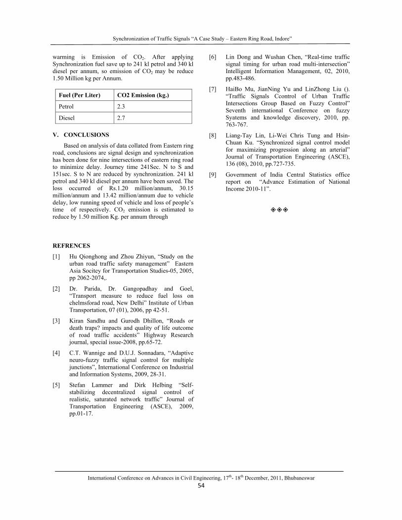
Synchronization of Traffic Signals “A Case Study – Eastern Ring Road, Indore”
International Conference on Advances in Civil Engineering, 17th- 18th December, 2011, Bhubaneswar
54
warming is Emission of CO2. After applying
Synchronization fuel save up to 241 kl petrol and 340 kl
diesel per annum, so emission of CO2 may be reduce
1.50 Million kg per Annum.
Fuel (Per Liter) CO2 Emission (kg.)
Petrol 2.3
Diesel 2.7
V. CONCLUSIONS
Based on analysis of data collated from Eastern ring
road, conclusions are signal design and synchronization
has been done for nine intersections of eastern ring road
to minimize delay. Journey time 241Sec. N to S and
151sec. S to N are reduced by synchronization. 241 kl
petrol and 340 kl diesel per annum have been saved. The
loss occurred of Rs.1.20 million/annum, 30.15
million/annum and 13.42 million/annum due to vehicle
delay, low running speed of vehicle and loss of people’s
time of respectively. CO2 emission is estimated to
reduce by 1.50 million Kg. per annum through
REFRENCES
[1] Hu Qionghong and Zhou Zhiyun, “Study on the
urban road traffic safety management” Eastern
Asia Socitey for Transportation Studies-05, 2005,
pp 2062-2074,.
[2] Dr. Parida, Dr. Gangopadhay and Goel,
“Transport measure to reduce fuel loss on
chelmsforad road, New Delhi” Institute of Urban
Transportation, 07 (01), 2006, pp 42-51.
[3] Kiran Sandhu and Gurodh Dhillon, “Roads or
death traps? impacts and quality of life outcome
of road traffic accidents” Highway Research
journal, special issue-2008, pp.65-72.
[4] C.T. Wannige and D.U.J. Sonnadara, “Adaptive
neuro-fuzzy traffic signal control for multiple
junctions”, International Conference on Industrial
and Information Systems, 2009, 28-31.
[5] Stefan Lammer and Dirk Helbing “Self-
stabilizing decentralized signal control of
realistic, saturated network traffic” Journal of
Transportation Engineering (ASCE), 2009,
pp.01-17.
[6] Lin Dong and Wushan Chen, “Real-time traffic
signal timing for urban road multi-intersection”
Intelligent Information Management, 02, 2010,
pp.483-486.
[7] HaiBo Mu, JianNing Yu and LinZhong Liu ().
“Traffic Signals Ccontrol of Urban Traffic
Intersections Group Based on Fuzzy Control”
Seventh international Conference on fuzzy
Syatems and knowledge discovery, 2010, pp.
763-767.
[8] Liang-Tay Lin, Li-Wei Chris Tung and Hsin-
Chuan Ku. “Synchronized signal control model
for maximizing progression along an arterial”
Journal of Transportation Engineering (ASCE),
136 (08), 2010, pp.727-735.
[9] Government of India Central Statistics office
report on “Advance Estimation of National
Income 2010-11”.

International Conference on Advances in Civil Engineering, 17th- 18th December, 2011, Bhubaneswar
55
Formulation of Equivalent Steel Section for Partially Encased
Composite Column under Concentric Gravity Loading
Debaroti Ghosh & Mahbuba Begum
Dept. of Civil Engineering, Bangladesh University of Engineering and Technology, Dhaka, Bangladesh
Abstract - Partially encased composite column (PEC) consists of thin walled welded H- shaped steel section with transverse links provided at regular intervals between the flanges to inhibit the occurrence of local buckling in the thin flange plates. The space between the flanges and the web plate are filled up with concrete. Extensive experimental investigations have been conducted by several research groups to understand the behavior of this relatively new composite column under both concentric and eccentric loading conditions along with sophisticated non-linear finite element analysis. But the separation between concrete and steel initiates the unstable condition in the finite element analysis near the ultimate point when flange plate buckles. To avoid the expensive and cumbersome modeling of the behavior at the interface of two dissimilar materials, an attempt has been made in this study to replace the composite section of PEC column with an equivalent steel section which can easily be incorporated in commercially available finite element softwares.
Key words - column: composite; concrete: encased: equivalent; steel.
I. INTRODUCTION
Steel-concrete composite columns can substantially improve the behavior and cost efficiency of steel-only columns used in the construction of mid-rise and high-rise buildings. A welded H–shaped steel section figures the partially encased composite (PEC) section with concrete infill between the flanges (Fig. 1). In Europe, in the early 1980s, PEC columns and beams were introduced using standard-sized rolled steel sections. In 1996, the Canam Group in North America proposed a PEC column section constructed from a thin–walled built–up steel shape with transverse links provided at regular intervals to restrain local buckling as shown in Fig.1. Extensive experimental research has been performed in Ecole Polytechnique de Montréal [1-3] on small-scale and large-scale PEC column specimens under various conditions of loading. The influences of high performance materials on the behavior of these columns have also been investigated experimental by Prickett and Driver [4] at the University of Alberta. The results of these experimental investigations indicated that the behavior of this composite column is significantly affected by the local instability of the thin steel flanges. Begum et al. [5] were able to overcome these challenges in the finite element model through the implementation of a dynamic explicit formulation along with a damage plasticity model for concrete and a contact pair algorithm at the steel-concrete interface. The developed model was applied successfully to reproduce the behavior of 34 PEC columns from five
experimental programs. However, despite of the accuracy, the composite finite element model developed by Begum et al. [5] is very sophisticated due to the presence of two dissimilar materials. Moreover, modeling of the interfacial behavior between steel and concrete requires extensive calculations as well as skilled and experienced users. Due to these complexities most of the structural analysis and design software do not handle such composite members. In this paper an attempt has been made to develop a fictitious steel section of the partially encased composite steel section. This equivalent steel section has added a new dimension to the analysis of partially encased composite column renovating the numerical procedure.
II. OBJECTIVES AND SCOPES
The main objective of this study is to formulate the methodology for the development of fictitious steel section for partially encased composite column built up with thin steel plates. The methodology is then used to simulate ten test PEC test columns from the published literature with variety of geometric properties subjected to concentric gravity loading only. The formulation of the fictitious steel section is based on the equivalence criteria of the basic geometric properties of the composite column. Linear elastic material behavior is assumed for steel as well as for concrete in the composite section.

Formulation of Equivalent Steel Section for Partially Encased Composite Column under Concentric Gravity Loading
International Conference on Advances in Civil Engineering, 17th- 18th December, 2011, Bhubaneswar
56
Fig. 1 : Partially Encased Composite Column with Thin-Walled Built-Up Steel Section, (a) Column Cross-Section and (b) 3D view of the Steel Configuration
III. REFERENCE TEST COLUMNS
Ten test PEC columns from the published literature are selected for current study. The lists of these specimens, along with their properties, are given in Table 1. Fig. 2 shows the cross-section and elevation of a typical test column. Specimens C-2 to C-7 were tested during the initial phase of the research program by Tremblay et al. [1] to study the behavior under concentric gravity loading which had square cross-sections of 300 mm × 300 mm and 450 mm × 450 mm, and a length equal to 5d, where d is the depth of the cross-section. Specimens C-8 to C-11, tested by Chicoine et al. [2] under axial compression, were larger in their cross–sectional dimensions (600 mm×600 mm) as compared to the previous test specimens.
All the test columns were fabricated from CSA-G40.21-350W grade steel plate. Normal strength concrete (nominally 30 MPa) was used in the test region of these columns. To strengthen the end regions of these test specimens, high strength concrete of 60 MPa nominal strength was used along with the closer link spacing provided in these zones.
Fig. 2 : Typical PEC Test Column, (a) Cross-section, (b) Elevation
IV. FORMULATION OF EQUIVALENT STEEL
SECTION
The fictitious steel cross-section consists of the actual steel cross-section and two additional pairs of plates, one perpendicular to the web at mid-height and one perpendicular to the flanges at mid-width as shown in Fig.3. The cross-sections of the fictitious and the actual column are equivalent in that they have the same:
1. Resistance in compression, and 2. Bending stiffness about the two principal
centroidal axes.
In order to produce the equivalent fictitious steel section, the dimensions of the two pairs of steel plates added to the initial cross-section is to be determined from the algebraic expressions of the three equivalence criteria: compression resistance and bending stiffness about the two principal axes.
.
TABLE I : PROPERTIES OF REFERENCE TEST SPECIMENS
Reference Speci
men
Plate size
bf x d x t
Link
spacing
s
Link
diameter
Φ
Length
L
Compressive
Strength of
concrete ′
Yield
strength of
plates
(mm) (mm) (mm) (mm) ( MPa) (MPa)
Tremblay et al. (1998
C-2 450x450x9.70 225 12. 7 2250 32. 7 370
C-3 450x450x9.70 337.5 12. 7 2250 32. 4 370
C-4 450x450x9.70 450 12. 7 2250 31. 9 370
C-5 450x450x9.70 225 22. 2 2250 34. 3 370
C-6 450x450x6.35 337.5 12. 7 2250 33. 1 374
C-7 300x300x6.35 300 12. 7 1500 31. 9 374

Formulation of Equivalent Steel Section for Partially Encased Composite Column under Concentric Gravity Loading
International Conference on Advances in Civil Engineering, 17th- 18th December, 2011, Bhubaneswar
57
Chicoine et al. (2002
C-8 600x600x12.88 600 15. 9 3000 34. 2 360
C-9 600x600x12.91 600 15. 9 3000 34. 2 360
C-10 600x600x12.81 300 15. 9 3000 34. 2 360
C-11 600x600x9.70 600 15. 9 3000 34. 2 345
.
(a) (b)
Fig. 3 : Equivalent steel section for PEC column, (a) Actual cross-section, (b) Equivalent steel section
A. Equivalence in compression resistance
The compression resistance of a composite steel-concrete cross section comprises of the plastic resistance of the steel cross-section, steel links and the concrete. The total area of the fictitious cross-section represents the area combining area of the initial steel cross-section and the additional plates.
(1)
Here, Ase = effective area of the steel shape including the I section and the links
Aa = total steel area of the additional steel plates in fictitious section
fs= design stress of steel= fy
fc= design stress of concrete
The effective area of a non-compact steel section can be defined as, 2 2 (2) Here, overall depth of the cross section Thickness of the steel plates Total effective width of the flange
Now,
12 1
0. 9/ / .2 / 2 .75 .5 / 1 Here, bf = full width of a flange plate
λp = Slenderness parameter
Es = Elastic modulus of steel
νs = Poisson’s ratio of steel
n = 1.5 as proposed by Chicoine et al. [3]
Considering the condition of equivalence in compression resistance and the relation in (1), it is obtained (3)
Here, design-stress ratio for concrete-to-steel
The total area of the composite cross-section comprises the equivalent steel cross section Ase and concrete section Ac. (4)
Dividing Eq. (2) by and introducing the non dimensional parameters ρse’ and a positive constant qx
2, " (5)
The total cross-secional area of the four additional plates in the fictitious section as shown in Fig.3 is, 2 2 (6)
Which after normalization by and introduction of normalized plate dimensions β, η, χ and γ becomes: 2 2 (7)
Since equation (4) and (6) are identical in left hand sides, the outcome is: 2 2 (8)
ca
ba
be
d ha
t

Formulation of Equivalent Steel Section for Partially Encased Composite Column under Concentric Gravity Loading
International Conference on Advances in Civil Engineering, 17th- 18th December, 2011, Bhubaneswar
58
Here the unknowns are β, η and χ on the left side and the combined geometric and material attributes of the actual cross-section enter through the constants and qx
2.
B. Equivalence in stiffness about the major axis
The flexural stiffness about the major axis y-y of the actual composite steel-concrete cross-section and its fictitious purely steel counterpart are given by:
, , , , , , (9)
Here, and are the effective elastic modulous of steel and concrete respectively. , , , and , are the moment of inertia about minor axis for actual steel section, concrete and additional steel plates respectively.
To enforce the condition of equivalence in major-axis stiffness, solving for Ia,y and introducing the concrete-to-steel ratio of elasticity moduli,
, , , 10
In reference to Fig.1(a)
12 , ,
, ,
Equation (9) may be written as:
, 12 , (11)
After normalization of (11) by dividing it with bfd
3/12 and using qy2 as a positive constant to sum up
the effects of the geometry and material properties of the actual cross section, the final equation is,
12 1 3 , (12)
Here, , 2 /
The additional major-axis flexural stiffness of the fictitious cross-section as a function of the dimensions of the additional plates is given by: 2 12 12 2
This, after normalization with (bfd3/12) and
introduction of the non-dimensional geometric properties β, η, χ, and γ, yields: 12 , 2 2 1 1 (13)
Since (12) and (13) have identical left-hand sides, 2 2 1 1 (14)
Here the unknowns are β, χ on the left side and the combined geometric and material attributes of the actual cross-section enter through the constants and qy
2 .
C. Equivalence in stiffness about minor axis
The treatment of major axis stiffness equivalence presented in the previous subsection is repeated here in shorthand for the minor-axis case.
First, minor-axis counterpart of (11):
, 12 ,
12 , (15)
After normalization of (15) by dividing it with bfd3/12
and using qz2 as a positive constant the obtained
equation is
12 , 1 3 , (16)
Here, , 2 /
Similarly for the additional elements of the fictitious steel cross-section, one obtains the counterpart of (13), 12 , 2 2 (17)
Since (16) and (17) have identical left-hand sides, the outcome is 2 2 (18)
Here the unknowns are β, χ on the left side and the combined geometric and material attributes of the

Formulation of Equivalent Steel Section for Partially Encased Composite Column under Concentric Gravity Loading
International Conference on Advances in Civil Engineering, 17th- 18th December, 2011, Bhubaneswar
59
actual cross-section enter through the constants γ and qz
2.
In order to transform the actual section in to fictitious section, three non-linear (8), (14) and (18) were developed. Three non-dimensional parameters, qx
2, qy2 and qz
2 describe the additional compression resistance major-axis stiffness, and minor-axis stiffness, respectively, due to concrete and links. These equations must be solved for the three non-dimensional unknowns’ β, χ and η to determine the dimensions of the additional steel plate’s ba, ha, and ca in the fictitious cross-section.
V. COMPARISION OF FICTITIOUS SECTION
WITH ACTUAL SECTION
The methodology described in the previous section is implemented to compute the equivalent steel sections
of the reference test PEC columns mentioned in Table I. The dimensions of the additional steel plates representing the concrete part of the composite section are provided in Table II. The geometric properties of the equivalent steel sections for columns C-2 to C-11 is calculated and compared to their actual composite cross-section. Table III presents the comparison between the cross-sectional area and moment of inertias of the composite and equivalent steel section of the column. The results show that the cross-sectional area and the moment of inertia about the major axis for equivalent steel section are in excellent agreement with the actual composite section. The moment of inertia about minor axis of the steel section is found to be around 4% lower than that of the composite section. This difference is within acceptable range.
.
Table II : Develpoment of Equivalent Steel Section for Partially Encased Composite Column
Composite steel section Equivalent steel section
Specimen bf d t s φ be ba ha ca t
C-2 450 450 9.7 225 12.7 368.08 304.90 21.46 196.36 9.7
C-3 450 450 9.7 337.5 12.7 371.48 304.91 21.45 196.36 9.7
C-4 450 450 9.7 450 12.8 375.89 309.98 20.42 196.36 9.7
C-5 450 450 9.7 225 22.2 368.08 295.48 23.54 196.36 9.7
C-6 450 450 6.35 337.5 12.7 265.46 303.64 23.19 259.36 6.35
C-7 300 300 6.35 300 12.7 247.74 223.58 12.18 142.27 6.35
C-8 600 600 12.88 600 15.9 503.43 382.01 33.51 258.57 12.88
C-9 600 600 12.91 600 15.9 503.97 382.00 33.50 258.15 12.91
C-10 600 600 12.81 300 15.9 491.82 382.00 33.58 259.57 12.81
C-11 600 600 9.7 600 15.9 420.41 382.21 35.09 312.89 9.7
Table III. Comparison between the properties of composite and fictitious section
Specimens Area Moment of inertia about of
major axis
Moment of inertia about
minor axis
CPS
*103
EQS
*103
CPS
*106
EQS
*106
,, CPS
*106
EQS
*106
,,C-2 16.76 16.90 0.99 410.13 410.63 1.00 443.14 425.22 1.04
C-3 16.76 16.89 0.99 410.13 410.63 1.00 443.14 425.06 1.04
C-4 16.35 16.47 0.99 410.13 410.57 1.00 443.14 424.86 1.04
C-5 17.58 17.72 0.99 410.13 410.77 1.00 443.14 425.22 1.04
C-6 17.17 17.38 0.99 432.84 433.47 1.00 455.13 446.56 1.02
C-7 7.20 7.25 0.99 91.40 91.47 1.00 98.61 94.67 1.04
C-8 32.03 32.27 0.99 1264.62 1267.01 1.00 1365.96 1309.64 1.04

Formulation of Equivalent Steel Section for Partially Encased Composite Column under Concentric Gravity Loading
International Conference on Advances in Civil Engineering, 17th- 18th December, 2011, Bhubaneswar
60
C-9 32.02 32.26 0.99 1264.15 1266.55 1.00 1365.71 1309.21 1.04
C-10 32.04 32.30 0.99 1265.69 1268.10 1.00 1366.54 1311.73 1.04
C-11 32.56 32.89 0.99 1314.18 1316.93 1.00 1392.22 1356.36 1.03
MEAN 0.99 1.00 1.04
SD 0.00 0.00 0.01
.
VI. CONCLUSIONS
The composite cross-section of thin walled partially encased composite column was replaced by an equivalent steel section. The formulation of the fictitious steel plates replacing the concrete part of the composite cross-section was presented in the paper. Linear elastic material behavior was considered during the formulation. The local buckling of the thin flange plates were incorporated by considering the effective width of the flange plates. The proposed methodology was used to calculate the equivalent steel section of ten PEC columns with a variety of geometric properties under concentric gravity loading only. The geometric properties of the actual composite section and the equivalent section were compared. The cross-setional area and moment of inertias for the equivalent steel section were found to be very close to properties of the actual composite section. The proposed methodology can reliably replace the composite section with an equivalent steel section.
VII. ACKNOWLEDGMENT
All assistance including laboratory, computing and financial supports from Bangladesh University of Engineering and Technology (BUET), Dhaka, Bangladesh are gratefully acknowledged
REFERRENCES
[1] Tremblay, R., Massicotte, B., Filion, I., and Maranda, R. “Experimental study on the behaviour of partially encased composite columns made with light welded H steel shapes under compressive axial loads.” Proc., Structural Stability Research Council Annual Technical Session and Meeting, Atlanta, 195–204, 1998.
[2] Chicoine, T., Tremblay,R., Massicotte, B., Ricles, J., and Lu, L.-W. “Behavior and strength of partially-encased composite columns with built up shapes.” J. Struct. Eng., 128(3), 279–287, 2002.
[3] Bouchereau, R., and Toupin, J.-D.. “Étude du comportement en compression-flexion des poteaux mixtes partiellement enrobés.” Rep.No. EPM/GCS-2003-03, Dept. of Civil, Geological, and Mining Engineering, cole Poly Technique, Montréal, 2003.
[4] Prickett, B. S. and Driver, R. G.: Behaviour of Partially Encased Composite Columns Made with High Performance Concrete.” Structural Engineering Report No 262, Dept. of Civil and Environmental Engineering, University of Alberta, AB, Canada, 2006.
[5] Begum, M., Elwi, A. E., and Driver, R. G. .” Finite-Element Modeling of Partially Encased Composite Columns Using the Dynamic Explicit Method.” Journal of Structural Engineering, ASCE, 133 (3), 326-334, 2007.

International Conference on Advances in Civil Engineering, 17th- 18th December, 2011, Bhubaneswar
61
Recommendations to Develop all-in-one ERP System
for Construction Industry
Sheetal Gogoi & S. S. Pimplikar
Civil Dept., MIT, Pune, India
Abstract - Because of involvement of uncertainty and high risk, it is challenging to complete the project in given time and budget.
Also, there are many channels of communication in a typical organization for the flow of information. It is necessary to properly
channelize and screen the information before it is passed to the respective authority, particularly when the information is to be passed
to higher level management for decision making. Because of inter-dependencies between various departments and business units,
(internal and external relationships) there are many chances of miss communication leading to failure of task. It is therefore
necessary to synchronize the flows of information for better productivity and to overcome the miss communication.
Enterprise Resource Planning software is one of the tools that can handle this problem effectively. It is software that encompasses all
functional departments of enterprise. It helps management for better analysis of data and acts as decision support systems (DSS) and
data retrieving, reducing the paperwork and errors.
The objective of this paper is to recommend strongly, the need of developing an all-in-one ERP software for construction industry as
a total quality management tool. The methodology employed is a mix of literature review & market studies in the form of
questionnaire survey, based on which analysis is done before making the recommendation as stated above.
Key Words - ERP, TQM, DSS, EC&O
I. INTRODUCTION
Enterprise resource planning (ERP) system is a
business management system that comprises integrated
sets of comprehensive software, which can be used,
when successfully implemented, to manage and
integrate all the business functions within an
organisation. These sets usually include a set of mature
business applications and tools for financial and cost
accounting, sales and distribution, materials
management, human resource, production planning and
computer integrated manufacturing, supply chain, and
customer information (Boykin, 2001; Chen, 2001; Yen
et al., 2002). These packages have the ability to
facilitate the flow of information between all supply
chain processes (internal and external) in an
organisation.
ERP packages touch many aspects of a company’s
internal and external operations. Consequently,
successful deployment and use of ERP systems are
critical to organizational performance and survival
(Markus et al., 2000b). Potential benefits include drastic
declines in inventory, breakthrough reductions in
working capital, abundant information about customer
wants and needs, along with the ability to view and
manage the extended enterprise of suppliers, alliances
and customers as an integrated whole (Chen, 2001). In
the manufacturing sector, ERP implementation has
reduced inventories anywhere from 15 to 35 per cent
(Gupta, 2000).
An overview of ERP systems including some of the
most popular functions within each module is shown in
fig. no. 1
II. NEED OF ERP IN CONSTRUCTION
INDUSTRY
ERP systems are being used by construction
companies to improve responsiveness in relations to
customers, strengthen supply chain partnerships,
enhance organizational flexibility, improve decision
making capabilities, and reduce project completion time
and lower costs. The goal of ERP is to support one time
entry of information at the point where it is created and
to make it available to all the participants within the
organization. The aim of this study is to investigate the
suitability and the importance of the ERP systems in
construction industry to improve the efficiency and
productivity.

Recommendations to Develop all-in-one ERP System for Construction Industry
International Conference on Advances in Civil Engineering, 17th- 18th December, 2011, Bhubaneswar
62
.
Fig1 ERP System modules
.
III. NECESSITY OF INTEGRATED APPROACH
Because the construction industry is capital-
intensive, construction companies need to be able to
manage all resources accurately in order to increase
profit while encouraging quality and business model
improvement. Companies from the construction industry
can take advantage of software solutions such as
enterprise resource planning (ERP) systems that
specialize in service delivery to support specific
construction project portfolio management (PPM) and
back-office operations, among other operations.
Integrated approach is the key to successful
implementation of ERP. Figure 2 explains the typical
relationship and connections between various major
processes / departments in a company.
Fig.2 ERP- Integrated approach
Although computers are widely used in the
construction projects, they are not generally used in an
integrative manner, and if so are specific to a single
company on projects comprised of many players. The
importance of managing projects in lesser funds and
time is immerging. This will require optimal utilization
of available resources. One cannot now allow heap of
material lying on site, spending money on non-
productive marketing exercises, allotting extra funds
than required, get into cash flow problems, so on and so
forth. As the construction industry is a highly
fragmented industry, it needs to communicate on a large
scale with other related businesses such as material and
equipment suppliers, vendors, sub-contractors and
clients.
ERP is available in various forms. On the basis of
its application, ERPs are basically categorized in to
customized package and readymade packages.
IV. MARKET SURVEY
Based on the suggestions received from the
software developers, some of the best clients were
selected those who are using ERP software for min. 2 to
3 years of time period. The impact of the use of software
was found out from the change in the turnover of the
company and the feedback from the users. Departmental
processes, organizational and departmental structure
play a vital role in the success of the ERP. In the

Recommendations to Develop all-in-one ERP System for Construction Industry
International Conference on Advances in Civil Engineering, 17th- 18th December, 2011, Bhubaneswar
63
survey, various departments are visited and ongoing
processes are observed to find out the mismatch
between requirement/ capabilities of ERP and the
processes/needs. Roles and responsibilities of major
posts are noted and software authorities are also cross
checked. Following feedback is received by two of the
companies viz. M/s Goel Ganga and M/s Amit
Enterprises that use readymade software – Highrise.
Readymade software has got its limitation based on the
development of the software. Following feedback is
received from the users of the software from various
departments-
V. PROBLEMS FACED BY USERS-
1) Documentation is found difficult.
2) Data analyzing is tedious and time consuming.
3) Training of site staff is a very tedious Job.
4) To assign computer on every site is a very
expensive job.
.
Figure 3 : Work process for readymade software

Recommendations to Develop all-in-one ERP System for Construction Industry
International Conference on Advances in Civil Engineering, 17th- 18th December, 2011, Bhubaneswar
64
5. Connectivity of internet connection is the major
problem on site due to which whatever the data
entries have to be done on site are kept pending.
Due to this problem whatever work is left requires
more time & this becomes a tedious job.
6. Estimate differs from actual expenditure.
7. Delays due to changes in the work at site in planned
activities.
8. Lack of technical staff at site and hence incapability
of solving technical problems while using software
VI. FEEDBACK BY USERS:
1) Easy on screen process is required to be
fulfilled by software.
2) Continuous good quality internet is required so
an alternative system is required to be given by
company to fulfill the same work of internet
connection.
3) Direct detailed estimation by drawings is
possible and found to be useful.
Application of software in construction industry
Information Technology plays a vital role in
Construction industry. Any project starts with site
surveying and goes through various stages such as
Estimation, Tendering, Bidding, Planning, Contracting,
Billing, etc. At every stage in the project, there is a need
of appropriate software to compile the available data,
process it and give output in desired manner. Various
software are developed by IT that has made various jobs
easy. Figure 4 explains the process of a typical
construction project.
Typical construction project undergoes various
phases from conceptual phase to close out and
maintenance. In absence of software, integrating
functions of all these phases is a challenging and tedious
job. But, every individual software has got its own
functional limitations. Because of which while
developing ERP system, one has to understand all
project phases, respective project processes,
organizational structure, interlinking between
departments, as-is and to-be reports, and the most
appropriate modules to be interlinked in ERP to assure
best coordination and communication of information
amongst the organization. In the context of TQM, no
single software is available. Also, within the individual
software, many important functions are not really
catered for.
Applications of individual software available in
market are –
- Financial software,
- Project Management Software,
- Personal Communication Software
- Client Communication Software
- Customer Relations Management Software
- Construction Project Management Tools
- Project Portfolio Management Software
- Integrated Construction Estimating Software
- Online Construction Management
Fig. 4 Process flow chart of a typical construction
project
Existing ERP systems: Table 1 summarizes the
application some of the existing ERP systems.
Construction Project
Project conception Feasibility Study
Conception Phase
Pre planning phase
Planning phase
Detailed Project
Report
Designing
Architectural
Structural
Detailing
Estimation,
Tendering
and Bidding
Financial Management
Resources Management
Quality Management
Time & Cost Management
Site
Execution
Safety Management
Claims Management and
Dispute Resolution
Communication and
Coordination

Recommendations to Develop all-in-one ERP System for Construction Industry
International Conference on Advances in Civil Engineering, 17th- 18th December, 2011, Bhubaneswar
65
.
Table no. 1 : Applications of the ERP systems
Sr.
No.
Name and
Manufacturer of
ERP Software
Cost of Software
Survival in
Market
(Yrs.)
Software applications
1
HIGHRISE
Make: Kanix
Infotec. Pvt. Ltd.,
Pune
15 Lakhs/
Professional
Module
14
Engineering, Materials, Management, Contract Management,
Marketing & Sales Management, Accounts & Finance
Management, Lease & Mall Management, Land & Legal,
Human Resource Management
2HITOFFICE
Make: EDSS Pune
1.50 Lakhs/ Per
User 25
Quotation, Planning, Master data, Purchase, ISO, Safety,
Staff-management, Correspondence, Trade, Builder, Address-
management, Accountancy, Equipment
3Oracle 11i
Make: Oracle Not available 33
Financials, Projects, Product Development, Lease
Management, Maintenance Management, Manufacturing,
Order Management, Procurement, Supply Chain Planning,
Payroll
4
ebuild
Make: IMT,
MUMBAI
Not available 11 Engineering, Purchase, Sales, Maintenance, Payroll,
Architecture, Finance, Administration, Legal, Accounting
5
Qudra suite
Make: Quadra
Software Solutions
Pvt. Ltd., Bangalore
Not available 20
Land Management, Legal Management, Liaison Management,
Tender Bid Management, Estimation, Material Management,
Contractors Billing, Labour Management, Plant & Machinery,
Fixed Asset Management, Enquiry Management, Client
Management, Marketing Financials, Financial Accounts,
Salary & Payroll, Employee Portal, Project Scheduling,
Vendor Portal, Contractor Portal, MIS, Lease & Rental, After
Sales
All-in-one ERP
In general or other readymade ERP systems,
company either has to adopt the practices in the ERP
system (which is not as per company’s current practice)
or has to customize the solution to its specific needs. An
attempt has been made to address all the project
management, financial and operational requirements of
executing construction and infrastructure projects. It
should help one to manage and control the construction
projects by giving complete and instant access to its
progress with full analysis of costs, revenues, liabilities
and subcontractor performance by easily entering the
data and getting the relevant reports.
A lot of construction companies use a variety of
software in their business, with different programs being
used for different tasks. The problem here is that these
different programs are usually not well integrated. This
can lead to inaccurate records as data entered by one
department is not reflected in the records kept by other
departments. The answer to these potential nightmares
in a construction company office is a fully integrated
suite of software which addresses the needs of
construction companies Information Technology plays a
vital role in Construction industry.
In project execution, bulk of time is taken up by
managing an enormous amount of data – site specs,
project plans, estimates, contracts, schedules and more.
Analysis by various construction software engineers
revealed that project managers in the construction
industry need software which can help them to manage
this data efficiently in order to streamline operations for
maximum efficiency and exceeding client expectations.
All in one construction software can give company the
edge it needs to stay ahead in this fast paced, severely
competitive industry.
Like most midsize engineering, construction, and
operations (EC&O) companies today, the organization
faces many challenges that characterize a volatile and
maturing market. These include increased competition,
client pressure to provide greater cost and project
transparency, slim margins, and demand for flawless
project execution. While one search for practical and

Recommendations to Develop all-in-one ERP System for Construction Industry
International Conference on Advances in Civil Engineering, 17th- 18th December, 2011, Bhubaneswar
66
affordable ways to meet these challenges, he is
constantly looking for new ways to improve the
operations and profitability.
To succeed, one must coordinate suppliers,
manage a diversified project portfolio, and deal with a
project value chain that may be poorly integrated and
fraught with manual business process. Plus, one needs to
satisfy customer demands for on-time completion,
competitive pricing, and innovative solutions.
Recommendations for all-in-one ERP software:
Following are the modules recommended for
development of all-in-one ERP system to overcome the
lacunas in existing ERP software:
Module of Conceptual Planning: To carry out
pre planning of project at conceptual stage to take
care of project risks – financial, market,
technological, business and other projected by
client based on the type of project.
Module of Feasibility study and Surveying: To
carry out detailed site survey, soil exploration etc.
needed to prepare Techno-economical feasibility
report to generate detailed project to minimize
errors at later stage in the successful completion of
project. Also it should cover various techno-legal
requirements and approval checks covering all
legal, environmental and other issues in the
module.
Module of Designing and engineering – Develop
and launch quality, innovative projects faster and
more cost-effectively including various functions
such as cost estimation, rate analysis from detailed
drawings to incorporate changes made in
designing at various stages of project. It will save
time required to do manual corrections in
estimation and tendering documents because of
change taken place in drawing and design.
Module of Project management with cost and
profit control – Plan and schedule projects and
compare project progress to contract cost-
effectively. Improve efficiency with a solution that
has the functionality to support your business
processes. Use of value engineering and
reengineering.
Module of Safety Management: ERP needs to
take care of safety issues of site, training,
punishment and rewards, accident prevention,
safety tools, records, to aim at zero accident
culture.
Module of Machinery Management: For right
selection of equipment for the project activity, best
match of equipment, routine and periodical
maintenance, life cycle assessment, rent/buy/lease
decision etc.
Module of Quality Management: Available ERP
systems only include quality checks for various
tasks in a project but fail to continual improvement
and assessment aiming at total quality
management. This module should support all
standards such as IS 1200 in Indian context for
estimation, IS 456 for RCC design, IS 800 for steel
design etc.
Module of Supply chain management and
Logistic: to coordinate and integrate resource flow
both within and among stake holders, to reduce
project inventory (with the assumption that
resources are available when needed) in the
pipeline.
Module of Project Maintenance: It is one of the
important but ignored areas in existing ERP
systems. Various processes such as project
performance after handover, recording of delays,
NRCs, penalties, project maintenance, follow ups,
etc. should be taken care of.
Module of Claims management & Dispute
resolution: Claims raising and recording, dispute
resolution and arbitration in context with tender
document needs to be covered in ERP system that
is missing from existing ERP modules. It will help
save time in dispute handling and claims
settlement.
Module of Project close out: For close out
planning, customer handover, demobilization of
resources and project learnings.
Module of Multi project at multi locations: The
system should provide the facility for handling
multiple projects from various locations for
projects spread over a vast geographic area to
easily tract the project status and to optimize the
resources.
VII. CONCLUSION
Though ERP has many advantages, there are few
disadvantages such as late return on investment, high
cost and skilled workforce requirement. Success or
failure depends on top management support, planning,
training, team contribution, right software selection to
suite the organizational structure and needs, and ERP
consultant support. Failures were not because the ERP
software were coded incorrectly, rather companies failed
to match the true organizational needs and systems
required to solve the business problems.

Recommendations to Develop all-in-one ERP System for Construction Industry
International Conference on Advances in Civil Engineering, 17th- 18th December, 2011, Bhubaneswar
67
It is understood that individual software as well as
available ERP software- whether tailor made or
readymade has got its own functional limitations.
Because of which while developing ERP system, one
has to understand all project phases, respective project
processes, organizational structure, interlinking between
departments and the most appropriate modules to be
interlinked in ERP to assure best coordination and
communication of information amongst the
organization. In the context of TQM, no single software
is available. Also, within the individual software, many
important functions such as project cost and time
control, project inception and closure etc. are not really
catered for.
ERP software was found useful as an effective
TQM tool subjected to availability of right information
such as estimation, quality checks etc. with minimal
changes in the due course of commencement of project.
Authorities and securities given in ERP help observe
better control on successful project progress.
There are lacunas in the existing ERP modules
studied, and recommendations were made to develop
all-in-one ERP software to best suite the construction
processes. It is suggested to develop all-in-one ERP
system to accommodate modules such as –Conceptual
planning, Feasibility and surveying, Designing,
Estimation and Rate analysis, Safety and Quality
management, Project maintenance, Claims and Dispute
resolution, cost and time control, Machinery
management, Multi project multi locations, Supply
chain as well as Project closer module.
REFERENCE :
[1] Alan R. Peslak, Enterprise resource planning
success An exploratory study of the financial
executive perspective, journal of Industrial
Management & Data Systems Vol. 106 No. 9,
2006, pp. 1288-1303
[2] Amarolinda Zanela Saccol, Cristiane Drebes
Pedron, Silvio Cesar Cazella, Marie Anne
Macadar, Guilherme Liberali Neto, University of
Vale do Rio Sinos, Sao Leopoldo, Rio Grande do
sul: “The impact of ERP systems on
organizational strategic variables in Brazilian
companies”, pp. 1-10
[3] Boo Young Chung, “An Analysis of success &
Failure Factors ERP Systems in Engineering &
Construction Firms, pp. 1-218
[4] Boo Young Chung, Miroslaw J. Skibniewski &
Young Hoon Kwak “Developing ERP Systems
Success Model for the Construction Industry”
Journal of Construction Engineering &
Management, ACSE, March 2009, pp. 207-216
[5] Boo Young Chung, Miroslaw J. Skibniewski,
Henry C. Lucas Jr. & Young Hoon Kwak:
“Analyzing Enterprise Resource Planning System
Implementation Success Factors in the
Engineering-Construction Industry”, Journal of
Computing in Civil Engineering, ASCE,
Nov/Dec 2008, pp. 373-282
[6] Carl Marnewick & Lessing Labuschange, “A
conceptual model for enterprise resource
planning (ERP)”, Information Management &
Computer Security
[7] Elbanna, Amany, “The Construction of the
relationship between ERP and the organization
through negotiation”, pp. 1-13
[8] Ike C. Ehie, Mogens Madsen: “Identifying
critical issues in enterprise resource planning
(ERP) implementation”, Science direct, pp. 545-
557
[9] Ike C. Ehie, Mogens Madsen: “Identifying
Critical issues in enterprise resource planning
(ERP) implementation”, Computers in Industry
56 (2005), pp. 545-557
[10] Jha V S and Joshi H. “Relevance of TQM or
Business Excellence Strategy Implementation for
ERP – A Conceptual Study”, pp. 1 to 11

International Conference on Advances in Civil Engineering, 17th- 18th December, 2011, Bhubaneswar
68
Transit Scheduling: “A Case Study of Eastern Ring Road
Corridor of BRTS Indore”
H. S. Goliya1 & Vikram Singh Patel
2
1CE-AMD, SGSITS Indore , MP, India 2ME Transportation Engineering, CE-AMD, SGSITS Indore, MP, India
E-mail : [email protected], [email protected]
Abstract - Indore is a fast growing industrial city of Madhya Pradesh. To meet the large demand and improve the capacity and
productivity of buses, ICTSL has proposed to plan, to develop and operate Bus Rapid Transit System (BRTS) in Indore. Bus Rapid
Transit System is a new form of public transportation which is an emerging approach to using buses as an improved high-speed
transit system. Bus Rapid Transit involves coordinated improvements in a transit system’s infrastructure, equipment, operations, and
technology that give preferential treatment to buses on urban roadways. We are selecting eastern ring road corridor for our case
study of transit scheduling now a day’s eastern area of Indore is developing rapidly. To provide faster and effective transit services, I
make schedule for transit units going to be run on that route. The schedule is made for 14 hours in a day (7:00 AM To 09 PM). For
finding out schedule of transit units, traffic data are collected at different road sections along the route. The traffic data is then
analyzed and traffic flow and passenger flow along the route is taken out. Transit units are provided on the basis of passenger flow at
different sections and at different time within a day.
Key words - BRTS, Scheduling, Transit Scheduling, Dwell Time.
I. INTRODUCTION
Indore is a fast growing industrial city of Madhya
Pradesh. It is the only metropolitan city in the state, with
a growth rate of 32.7% in the last decade. Its population
size was 1.6 million in 2001, 2.2 million in 2011 and is
projected to be 4.2 million by 2025. Planning,
development, operation and management of the
transport system of Indore to meet the increasing travel
demands of the city in an efficient, convenient, safe and
economical manner is important to sustain the economic
viability, productivity and competitiveness of Indore
City. To meet the large demand and improve the
capacity and productivity of buses, ICTSL has proposed
to plan, to develop and operate Bus Rapid Transit
System (BRTS) in Indore.
In the context of rapid growth of the city, increasing
mobility, high travel demand, increasing congestion,
delays, accidents, need for conservation of energy,
growing community consciousness towards
environmental quality and to address a host of such
other problems and objectives, public mass transport
system of the city stands out as the most critical
element. It needs to be rationally planned, efficiently
operated and diligently managed to be effective and
productive by itself and in turn enable the city to be
productive and competitive.
A. Concept of Bus Rapid Transit System
Bus Rapid Transit System is a new form of public
transportation which is an emerging approach to using
buses as an improved high-speed transit system. Bus
Rapid Transit involves coordinated improvements in a
transit system’s infrastructure, equipment, operations,
and technology that give preferential treatment to buses
on urban roadways
B. Need for Present Study
In the context of rapid growth of the Indore city,
increasing mobility, high travel demand, increasing
congestion, delays, accidents, need for conservation of
energy, growing community consciousness towards
environmental quality and to address a host of such
other problems and objectives, public mass transport
system of the city stands out as the most critical
element. It needs to be rationally planned, efficiently
operated and diligently managed to be effective and
productive by itself and in turn enable the city to be
productive and competitive.
USER
Rectangle

Fig. 1 : Easte
II. OBJECT
To fin
To fin
To sc
buses
To re
To im
To po
depen
III. METHOD
The case
eastern ring ro
traffic data are
is done to fi
sections on th
are taken out
hours. (07 AM
Transit
International Co
ern Ring Road
TIVES OF TH
nd out the traff
nd out number
chedule the ar
s at stops.
educe the traffic
mprove the traf
opularize publ
ndability over p
DOLOGY
study is carrie
oad corridor of
e collected from
ind out passe
he basis of wh
and schedulin
M TO 09 PM).
t Scheduling: “A
onference on Adv
Corridor of BR
HE STUDY
fic volume of s
r of buses.
rrival and depa
c congestion.
ffic managemen
lic transport an
private vehicle
d out on a pre
f BRTS Indore
m the field and
enger flow in
hich number o
ng is done for
A Case Study of
vances in Civil E
RTS Indore
selected route.
arture time of
nt in the city .
nd reduce the
es.
defined route,
e. In this case,
d then analysis
between the
f transit units
r them for 14
Eastern Ring Ro
Engineering, 17t
69
f
IV. EAS
IND
East
non-inte
Eastern
Pass roa
to Dewa
part of t
likely to
area nea
schemes
DETAIL
Name of
Total Le
Four arm
Rotary a
V. TRA
CO
Dat
secondar
primary
various
from som
such as C
The
case stu
location
primary
of prima
the prim
for the c
primary
for three
BRT sit
maps, pr
worldwi
case stud
VI. DA
Dat
and tran
useful
supporti
Prim
travel su
analyzed
oad Corridor of B
th- 18th Decembe
STERN RING
DORE
tern ring road
errupted transp
ring road lies
ad of Indore. S
as naka Square
traffic of easter
o be increased
ar it is very
s are going on.
L INFORMAT
f road : Eastern
ength of road: 1
m intersection o
at road intersec
AFFIC SURV
LLECTION
a collection c
ry data. Prim
surveys and
sources such a
me of the org
CEPT Ahmada
e Data collecti
udy BRT corrid
s of the majo
survey locatio
ary surveys co
mary surveys a
case study. Prim
surveys carrie
e days at eac
tuations. Seco
revious studies
ide, from vari
dies from journ
TA ANALYS
a analysis is a
nsforming dat
information,
ing decision m
mary data was
urveys along t
d with traffic e
BRTS Indore”
er, 2011, Bhuban
G ROAD COR
corridor of BR
portation facilit
in between th
Starting from R
e (Niranjanpur
rn part of Indo
in future. Th
high, and so
TION OF ROA
n Ring Road C
15.40 km.
of road: 10 No
ction: 09 No.
VEY AND DA
comprises of
mary data w
secondary dat
as libraries, int
ganizations con
abad, CRRI, TR
ion comprises
dor, basic deta
or intersection
ons on the corr
onducted, infe
and impact pa
mary data has b
ed out on the p
h section for
ondary data s
s, various BRT
ious literature
nals and intern
IS
a process of ga
ta with the go
suggesting
aking.
collected from
the proposed B
engineering par
neswar
RRIDOR OF
RTS offers a fa
ty to the road
he A.B. road a
Rajiv Gandhi
r). It carries a
ore. And the tra
he growth rate
many develo
AD
Corridor.
.
TA
primary data
was collected
ta is collected
ternet websites
ncerned with B
RB, HCM etc
of selection o
ails of the cor
ns on the cor
ridor route ma
erences drawn
arameters iden
been collected
pilot BRTS co
pre BRT and
such as litera
T studies carrie
s and interna
net are collecte
athering, mode
oal of highlig
conclusions,
m various traffi
BRTS corrido
rameters.
BRTS
ast and
d users.
and By
Square
a major
affic is
of the
opment
a and
from
from
s, and
BRTS
of the
rridor,
rridor,
ap, list
from
ntified
d from
rridor
d post
atures,
ed out
ational
ed.
elling,
ghting
and
ic and
or and

Traffic im
such as tr
characteristics
engineering t
sections of the
VII. TRAFFI
Here, tra
mid sections,
the corridor.
morning; noon
11:00am, 01pm
the numbers
Date : Averag
Location : Raj
Survey Carrie
Type of vehicle
Truck (multi
axel)
Truck
Tractor
Loading
Rikshaw/Picku
Bus
Omni/Magic
(Public Trans.)
Auto/Taxi
Four Wheeler
(Car/Jeep)
Two Wheeler
Total No .of
Vehicles
Transit
International Co
mpact paramete
raffic chara
s, etc and
techniques an
e corridor with
IC FLOW ST
affic flow study
located betwee
The surveys
n and evening
m to 03pm and
in peak hour
Table 1 : Sho
e Traffic 02-0
iv Gandhi Squ
ed By : Rajiv G
e08 to 09
AM
11
24
2
up52
10
12
9
139
657
916
t Scheduling: “A
onference on Adv
ers were ident
cteristics, sp
analyzed as
nd compared
h the present an
UDY
y was carried
en all major in
s were cond
g hours betwe
d 05pm to 08p
rs are represe
owing Traffic F
04 May
uare TO Khand
Gandhi Square
09 To 10
AM
10
23
57
8
88
14
19
17
195
853
1274
Fig
A Case Study of
vances in Civil E
tified in broad
peed, travel
per traffic
at different
nd past study.
out for at ten
ntersections of
ducted during
en 9:00am to
pm and finally
nted. Manual
RAJIV GAN
Flow From Ra
dwa Naka Squa
TO Khandwa
0 To 11
AM
01 T
PM
32 48
73 70
6 4
75 63
9 15
14 1
21 19
181 16
777 59
1188 96
g. 2 : Showin
Eastern Ring Ro
Engineering, 17t
70
f
Count an
video c
corridor
out for t
composi
hours
composi
traffic
variation
below t
Square
ring road
.
NDHI SQUAR
ajiv Gandhi Sq
are
o 02
M
02 To 0
PM
8 35
0 58
4 2
3 51
5 12
1 7
9 13
61 143
90 545
61 866
ng Traffic Com
oad Corridor of B
th- 18th Decembe
nd Video Grap
cameras focus
from the appr
the traffic flow
ition of all mo
traffic, PCU
ition, hourly tr
flow, traffic
n of passenger
ables, charts a
to Khandawa
d corridor of B
RE:
quare To Khand
3 05 To 06
PM
64
70
2
52
21
9
17
142
588
965
mposition
BRTS Indore”
er, 2011, Bhuban
phic technique
sing the runn
ropriate level.
w characteristi
des types, peak
Us, etc. Traf
raffic volume,
comparison
r flow on BRT
and graphs of
Naka Square
BRTS.
dawa Naka Squ
06 To 07
PM
0
75
82
4
64
27
7
15
157
645
1076
neswar
e was applied,
ning traffic on
Analysis is ca
cs, vehicular t
k hour and off
ffic Data, t
hourly variati
chart, and h
S etc. are show
f the Rajiv G
e section of ea
uare
07 To 08
PMTo
52 34
83 51
3 3
37 48
17 12
10 8
24 13
167 12
540 51
933
using
n the
arried
traffic
f-peak
traffic
ion of
hourly
wn on
Gandhi
astern
otal
40
17
31
82
25
89
35
285
195

Fi
Total Goods Transp
Total Public Transpo
Provision for Pu
Required Flow
Remaining Traf
Transit
International Co
ig. 5 : Compari
portation
ort
ublic Transportation
(60%) For BRTS
ffic Flow
t Scheduling: “A
onference on Adv
Fig.
Fig. 4 :
ison Chart
99 19
817 108
490.2 65
326.8 43
A Case Study of
vances in Civil E
. 3 : Showing
Showing Hour
90 195
84 993
50.4 595.8
33.6 397.2
Eastern Ring Ro
Engineering, 17t
71
Hourly Traffic
rly Variation o
Fig
200
781
468.6 42
312.4 28
oad Corridor of B
th- 18th Decembe
c Volume
f Traffic Flow
g. 6 : Showing
158 209
708 756
24.8 453.6
83.2 302.4
BRTS Indore”
er, 2011, Bhuban
g Shifted Traffi
252
824
494.4 4
329.6 2
neswar
ic
192 1
741 6
444.6 4022.4
296.4 2681.6
495
6704

Table 2. Show
.
The traffic
only. In the s
flow is taken o
data, traffic co
variation of tr
hourly variati
shown on tab
road sections
gives us the
intersections,
number of bu
eastern ring ro
Passenger Flow
No. of Passenger
Omni/ Magic (Public
Auto/ Taxi
Four Wheeler (Car/ J
Two Wheeler
Total No. Of Passeng
Passenger Flow on B
Transit
International Co
wing Passenger
F
c data shown
same manner,
out at each int
omposition, ho
raffic flow, tra
ion of passen
bles, charts an
of eastern rin
peak hour p
which is requ
uses to be run
oad corridor of
08 t
Trans.)
Jeep)
9
ger
BRTS (60%) 8
t Scheduling: “A
onference on Adv
Fig. 7 :
Flow From Ra
Fig. 8 : Showin
here is of on
traffic flow a
tersection. The
ourly traffic vo
affic comparis
nger flow on
nd graphs of
ng road corrid
passenger flow
uired by us for
n at different
f BRTS.
to 09 AM 09 To 10 A
48 76
22.5 42.5
417 585
985.5 1279.5
1473 1983
883.8 1189.8
A Case Study of
vances in Civil E
Showing Hour
ajiv Gandhi Sq
ng Hourly Var
ne intersection
and passenger
e above traffic
olume, hourly
son chart, and
n BRTS etc.
the different
dor of BRTS,
w at different
r deciding the
t time on the
AM 10 To 11 AM 01
56
52.5
543
1165.5
1817
1090.2
Eastern Ring Ro
Engineering, 17t
72
rly Variation o
quare To Khand
riation of Passe
With
composi
traffic f
intersect
above d
and pass
nodes on
A. Peak
The
graph (F
at the pa
the spec
of this w
transpor
To 02 PM 02 To 03
44 28
47.5 32.5
483 429
885 817.5
1459.5 1307
875.7 784.2
oad Corridor of B
th- 18th Decembe
f Traffic Flow
dawa Naka Squ
enger Flow on
h the help of
ition at differe
flow at road s
tions, at differ
data we get the
senger flow in
n the BRTS co
k Hour and Off
peak hour an
Figure 09 and
articular inters
cified time inte
we can find out
rtation on the B
3 PM 05 To 06 PM 0
36
42.5
426
5 882
7 1386.5
2 831.9
BRTS Indore”
er, 2011, Bhuban
uare
BRTS
f this graph
ent sections, h
section in bet
rent time perio
e hourly varia
n between the s
orridor.
f-Peak Graphs
nd off-peak ho
10) shows the
ection at the sp
erval within a
t number of bu
BRTS corridor
06 To 07 PM 07 To 0
28 40
37.5 60
471 50
967.5 81
1504 141
902.4 846
neswar
we get the t
hourly variati
tween the diff
od of day. From
ation of traffic
sections of dif
our passenger
e flow of pass
pecified time a
day. With the
uses required f
.
08 PM Total
0 356
0 337.5
1 3855
0 7792.5
11
6.6 7404.6
traffic
on of
fferent
m the
c flow
fferent
flow
senger
and at
e help
for the

Peak Hour Pas
- Betw
- Betw
Off-Peak hour
- Betw
Table 3 : Sh
Flow
Table 4 : Sho
Flow
VIII. THE S
Schedulin
sequencing th
the utilization
criterion. Sc
statically, off-
information fr
made is dyna
decisions shou
Transit
schedules. A s
transit unit ar
time. It is also
Location
Name Of Intersec
Rajiv Gandhi Squa
Khandawa Naka S
Teenimli Square
Musakhedi Square
Pipliyapala Square
Bengali Square
Khazarana Square
MR-9 Square
Bombay Hospital
Dewas naka Squa
Niranjanpur Squar
Location
Name Of Intersec
Rajiv Gandhi Squa
Khandawa Naka S
Teenimli Square
Musakhedi Squar
Pipliyapala Square
Bengali Square
Khazarana Square
MR-9 Square
Bombay Hospital
Dewas naka Squa
Niranjanpur Squar
Transit
International Co
ssenger Flow
ween 10am – 11
ween 06 pm – 0
r Passenger Flo
ween 02 pm – 0
howing Peak a
owing Peak a
SCHEDULING
ng a set o
hem on one or
n of resources
cheduling is
f-line, while in
rom which sch
amic, suggestin
uld be made dy
system run
schedule is a s
rrives at partic
o the statemen
Rajiv
ction 10 T
are 1
Square 1
1
e 1
e 1
2
e 2
2
Square 1
are
re
Rajiv
ction 10 T
are 1
Square 1
1
e 1
e 1
2
e 2
2
Square 1
are
re
t Scheduling: “A
onference on Adv
1 am
7 pm
ow
03 pm
and Off peak
and Off peak
G
of processes
r more process
optimizes som
traditionally
n an operating
heduling decis
ng that the be
ynamically.
on specified
statement of ti
cular stop ove
nt of time at w
Gandhi To Dewas Na
To 11 AM 02 TO 03
1090 784
1712 1303
1374 835
1061 850
1471 942
2082 1525
2822 1899
2766 1746
1017 702
679 538
v Gandhi To Dewas Na
To 11 AM 02 TO 03
1090 784
1712 1303
1374 835
1061 850
1471 942
2082 1525
2822 1899
2766 1746
1017 702
679 538
A Case Study of
vances in Civil E
Hour Traffic
Hour Traffic
consists of
sors such that
me scheduling
y performed
g system, the
sions must be
est scheduling
d routes and
imes at which
er a period of
which a single
aka
PM 06 To 07 PM
902
1455
1267
1347
1251
1792
2348
1388
600
443
aka
PM 06 To 07 PM
902
1455
1267
1347
1251
1792
2348
1388
600
443
Eastern Ring Ro
Engineering, 17t
73
f
f
transit u
its route
once the
stops are
A. Sch
For
necessar
applicati
impleme
able to m
advantag
B. Th
An
transit s
(say bus
routes, o
and dep
or effic
waiting
of resou
Fig
Fig.
oad Corridor of B
th- 18th Decembe
unit of a given
e. The later in
e schedule of
e known.
heduling Polic
r a practical r
ry to provide
ion-defined s
ent our schedu
modify these p
ge of the flexib
e Transit Sche
nother optimiz
system design
ses). The prob
one needs to d
artures at all t
cient schedule
time of passen
urce and service
. 9 : Showing P
Passenger
10 : Showing
Passenger
BRTS Indore”
er, 2011, Bhuban
route arrives a
nformation can
arrivals and d
ies
real-time oper
e a mechanis
scheduling po
uling model; th
policies at runt
bility of the mo
eduling
zation proble
is the schedul
blem here is t
develop schedu
the stops of th
e is one whi
ngers while op
e related const
Peak Hour and
r Flow at Inters
Peak Hour and
r Flow At Inter
neswar
at different sto
n always be de
departures of a
rating system,
sm to expres
olicies neede
he system shou
ime in order to
odel.
em related to
ling of transit
that given a s
ules for bus ar
he network. A
ich minimize
perating within
traints.
d Off Peak Hou
section
d Off Peak Hou
rsection
ops on
erived
all the
, it is
s the
ed to
uld be
o take
o the
units
set of
rrivals
good
s the
n a set
ur
ur

Transit Scheduling: “A Case Study of Eastern Ring Road Corridor of BRTS Indore”
International Conference on Advances in Civil Engineering, 17th- 18th December, 2011, Bhubaneswar
74
IX. DWELL TIME
Dwell time is the single most important factor
affecting vehicle capacity. It is the time required to
serve passengers at the busiest door, plus the time
required to open and close the doors.
Dwell times may be governed by boarding
demand and the alighting demand or by total
interchanging passenger demand (e.g., at a major
transfer point on the system). In all cases, dwell time is
proportional to the boarding and/or alighting volumes
times the service time per passenger.
X. SCHEDULE DETERMINATION OF
EASTERN RING ROAD CORRIDOR FOR
BUS TRANSIT RAPID SYSTEM:
Table 5. For Schedule Determination
- Total Length Of The Route 15.5 km
- Round Trip Time Of Transit Unit 90 minute
- Running Speed Of Transit Unit 50 km/hr
- Journey Speed Of Transit Unit 35km/hr
- The Peak hour headway between the buses is 4
minute
- Off Peak hour headway between the buses is 6
minute
The Schedule of off- peak hour and -peak hour is
given below in the tables for the buses travelling from
Rajiv Gandhi Square to Niranjanpur Square. The
schedule is developed from 07 am to 09 pm along the
route.
Some buses are introduced into the route from other
routes at the time of peak hours, to accommodate the
passenger traffic at the stop and to maintain the BRTS
facility.
XI. CONCLUSION:
The route is analyzed and transit units are
provided on the basis of passenger traffic flow
along sections on the route.
Schedule is developed on the bases of their
departure time.
16 transit units are required to run along the route,
continuously throughout the day.
Additional 34 transit units are required to
accommodate the peak hour traffic at some
specified sections of the route.
60 % of passenger traffic is travelling through the
BRTS.
Traffic congestion is reduced on the route, as two
wheeler and four wheeler traffic is getting shifted
on BRTS.
Well managed traffic system has been designed
along the route.
Public transport get popularize and reduce the
dependability over private vehicles.
REFERENCES:
[1] E. Douglas Jensen, C. Douglass Locke, Hideyuki
Tokuda (1985): “A Time-Driven Scheduling Model
for Real-Time Operating Systems”, CH2220-
2/85/OOOO/011, 1985 (IEEE)
[2] Liping Fu, Qing Liu, and Paul Calamai (2003):
“Real-Time Optimization Model for Dynamic
Scheduling of Transit Operations”, Transportation
Research Record 1857, Paper No. 03-3697
[3] Michael G. H. Bell (2004): “Games, Heuristics, and
Risk Averseness in Vehicle Routing Problems”,
Vol. 130, No. 1, March 1, 2004 J. URBAN
PLANNING & DEVELOPMENT, ASCE
[4] Liqun Xu (2005): “A Decision Support Model
Based on GIs for Vehicle Routing”, 0-7803-897 1 -
9/05, 2005 (IEEE)
[5] Qiang Meng, Der-Horng Lee and Ruey Long Cheu
(2005): “Multiobjective Vehicle Routing and
Scheduling Problem with Time Window
Constraints in Hazardous Material Transportation”,
Vol. 131, No. 9, September 1, 2005. Journal of
Transportation Engineering, ASCE,
[6] Jian Sun, Shikui Zhai, Shuying Wang (2010):
“Research and Application of Solution of Vehicle
Routing Problem Based on GIS”, 2010 Sixth
International Conference on Natural Computation
(ICNC 2010), 978-1-4244-5961-2/10, 2010 IEEE
Sr. No Name Of Stop Distance (km) Dwell Time Travel Time Required
1 Rajiv Gandhi Square --- 2 min --
2 Bholaram Ustad Marg Square 0.6 2 min 0 min 40 sec
3 Khandawa Naka Square 1.4 2 min 1 min 40 sec
4 Teenimli Square 1.8 2 min 1 min 40 sec
5 Musakhedi Square 1.8 2 min 2 min 10 sec
6 Pipliyapala Square 1.7 2 min 2 min 10 sec
7 Bengali Square 1.4 3 min 2 min 00 sec
8 Khazarana Square 1.1 3 min 1 min 40 sec
9 MR-9 Square 0.9 3 min 1 min 20 sec
10 MR-10 Square 2 2 min 1 min 00 sec
11 Bombay Hospital Square 0.5 2 min 0 min 40 sec
12 Dewas naka Square 2 2 min 2 min 20 sec
13 Niranjanpur Square 0.9 2 min 1 min 00 sec

Transit Scheduling: “A Case Study of Eastern Ring Road Corridor of BRTS Indore”
International Conference on Advances in Civil Engineering, 17th- 18th December, 2011, Bhubaneswar
75
[7] Gong Yancheng (2010): “Vehicle Scheduling
Problems of Military Logistics Distribution Based
on Improved Genetic Algorithm”, International
Conference on Computer Application and System
Modeling (ICCASM), 2010
[8] Ming Wei, Wenzhou Jin, Weiwei FU, HAO Xiao-ni
(2010): “Improved Ant Colony Algorithm for
Multi-depot Bus Scheduling Problem with Route
Time Constraints”, World Congress on Intelligent
Control and Automation, 978-1-4244-6712-9/10,
2010 IEEE
[9] Transit cooperative Research Program “TCRP
REPORT 90” Bus Rapid Transit Volume 1: Case
Studies In Bus Rapid Transit
[10] Transit Cooperative Research Program “TCRP
REPORT 90” Bus Rapid Transit Volume 2:
Implementation Guidelines
[11] Parth Chakroborty and Animesh Das “Principles of
Transportation Engineering”
[12] “Traffic Engineering and Transportation Planning”
Dr. L.R. Kadiyali.
[13] Indore Muncipal Corporation, indore
[14] Indore city transport service limited, indore
[15] CEPT Ahamdabad.
.
Table 6 : Showing Schedule From 07 AM To 09 AM Travelling Direction from Rajiv Gandhi Square To Niranjanpur Square.
Table 7 : Showing Schedule From 09 AM To 10 AM Travelling Direction from Rajiv Gandhi Square To Niranjanpur Square.
07 AM TO 09 AM
Sr. No. 1 2 3 4 5 6 7 8 9 10 11 12 13
Time Required 00:00:40 00:01:40 00:01:40 00:02:10 00:02:10 00:02:00 00:01:40 00:01:20 00:01:00 00:00:40 00:02:20 00:01:00
Dwell Time 00:02:00 00:02:00 00:02:00 00:02:00 00:02:00 00:03:00 00:03:00 00:03:00 00:02:00 00:02:00 00:02:00 00:02:00
Bus No. 01 07:00:00 07:02:40 07:06:20 07:10:00 07:14:10 07:18:20 07:23:20 07:28:00 07:32:20 07:35:20 07:38:00 07:42:20 07:45:20
Bus No. 02 07:06:00 07:08:40 07:12:20 07:16:00 07:20:10 07:24:20 07:29:20 07:34:00 07:38:20 07:41:20 07:44:00 07:48:20 07:51:20
Bus No. 03 07:12:00 07:14:40 07:18:20 07:22:00 07:26:10 07:30:20 07:35:20 07:40:00 07:44:20 07:47:20 07:50:00 07:54:20 07:57:20
Bus No. 04 07:18:00 07:20:40 07:24:20 07:28:00 07:32:10 07:36:20 07:41:20 07:46:00 07:50:20 07:53:20 07:56:00 08:00:20 08:03:20
Bus No. 05 07:24:00 07:26:40 07:30:20 07:34:00 07:38:10 07:42:20 07:47:20 07:52:00 07:56:20 07:59:20 08:02:00 08:06:20 08:09:20
Bus No. 06 07:30:00 07:32:40 07:36:20 07:40:00 07:44:10 07:48:20 07:53:20 07:58:00 08:02:20 08:05:20 08:08:00 08:12:20 08:15:20
Bus No. 07 07:36:00 07:38:40 07:42:20 07:46:00 07:50:10 07:54:20 07:59:20 08:04:00 08:08:20 08:11:20 08:14:00 08:18:20 08:21:20
Bus No. 08 07:42:00 07:44:40 07:48:20 07:52:00 07:56:10 08:00:20 08:05:20 08:10:00 08:14:20 08:17:20 08:20:00 08:24:20 08:27:20
Bus No. 09 07:48:00 07:50:40 07:54:20 07:58:00 08:02:10 08:06:20 08:11:20 08:16:00 08:20:20 08:23:20 08:26:00 08:30:20 08:33:20
Bus No. 10 07:54:00 07:56:40 08:00:20 08:04:00 08:08:10 08:12:20 08:17:20 08:22:00 08:26:20 08:29:20 08:32:00 08:36:20 08:39:20
Bus No. 11 08:00:00 08:02:40 08:06:20 08:10:00 08:14:10 08:18:20 08:23:20 08:28:00 08:32:20 08:35:20 08:38:00 08:42:20 08:45:20
Bus No. 12 08:06:00 08:08:40 08:12:20 08:16:00 08:20:10 08:24:20 08:29:20 08:34:00 08:38:20 08:41:20 08:44:00 08:48:20 08:51:20
Bus No. 13 08:12:00 08:14:40 08:18:20 08:22:00 08:26:10 08:30:20 08:35:20 08:40:00 08:44:20 08:47:20 08:50:00 08:54:20 08:57:20
Bus No. 14 08:18:00 08:20:40 08:24:20 08:28:00 08:32:10 08:36:20 08:41:20 08:46:00 08:50:20 08:53:20 08:56:00 09:00:20 09:03:20
Bus No. 15 08:24:00 08:26:40 08:30:20 08:34:00 08:38:10 08:42:20 08:47:20 08:52:00 08:56:20 08:59:20 09:02:00 09:06:20 09:09:20
Bus No. 16 08:30:00 08:32:40 08:36:20 08:40:00 08:44:10 08:48:20 08:53:20 08:58:00 09:02:20 09:05:20 09:08:00 09:12:20 09:15:20
Bus No. 01 08:36:00 08:38:40 08:42:20 08:46:00 08:50:10 08:54:20 08:59:20 09:04:00 09:08:20 09:11:20 09:14:00 09:18:20 09:21:20
Bus No. 02 08:42:00 08:44:40 08:48:20 08:52:00 08:56:10 09:00:20 09:05:20 09:10:00 09:14:20 09:17:20 09:20:00 09:24:20 09:27:20
Bus No. 03 08:48:00 08:50:40 08:54:20 08:58:00 09:02:10 09:06:20 09:11:20 09:16:00 09:20:20 09:23:20 09:26:00 09:30:20 09:33:20
Bus No. 04 08:54:00 08:56:40 09:00:20 09:04:00 09:08:10 09:12:20 09:17:20 09:22:00 09:26:20 09:29:20 09:32:00 09:36:20 09:39:20
Bus No. 05 09:00:00 09:02:40 09:06:20 09:10:00 09:14:10 09:18:20 09:23:20 09:28:00 09:32:20 09:35:20 09:38:00 09:42:20 09:45:20
09 AM To 10 AM
Stop No. 1 2 3 4 5 6 7 8 9 10 11 12 13
Transfer Time 00:00:40 00:01:40 00:01:40 00:02:10 00:02:10 00:02:00 00:01:40 00:01:20 00:01:00 00:00:40 00:02:20 00:01:00
Dwell Time 00:02:00 00:02:00 00:02:00 00:02:00 00:02:00 00:03:00 00:03:00 00:03:00 00:02:00 00:02:00 00:02:00 00:02:00
Bus No. 831 09:18:00 09:22:20 09:25:20
Bus No. 731 09:15:20 09:20:00 09:24:20
Bus No. 631 09:14:20 09:19:20 09:24:00
Bus No. 05 09:00:00 09:02:40 09:06:20 09:10:00 09:14:10 09:18:20 09:23:20 09:28:00 09:32:20 09:35:20 09:38:00 09:42:20 09:45:20
Bus No. 832 09:30:00 09:34:20 09:37:20
Bus No. 06 09:04:00 09:06:40 09:10:20 09:14:00 09:18:10 09:22:20 09:27:20 09:32:00 09:36:20 09:39:20 09:42:00 09:46:20 09:49:20
Bus No. 07 09:08:00 09:10:40 09:14:20 09:18:00 09:22:10 09:26:20 09:31:20 09:36:00 09:40:20 09:43:20 09:46:00 09:50:20 09:53:20
Bus No. 131 09:16:20 09:20:00 09:24:10 09:28:20 09:33:20 09:38:00 09:42:20 09:45:20
Bus No. 08 09:12:00 09:14:40 09:18:20 09:22:00 09:26:10 09:30:20 09:35:20 09:40:00 09:44:20 09:47:20 09:50:00 09:54:20 09:57:20
Bus No. 732 09:37:20 09:42:00 09:46:20 09:49:20
Bus No. 09 09:16:00 09:18:40 09:22:20 09:26:00 09:30:10 09:34:20 09:39:20 09:44:00 09:48:20 09:51:20 09:54:00 09:58:20 10:01:20
Bus No. 632 09:36:20 09:41:20 09:46:00 09:50:20 09:53:20
Bus No. 10 09:20:00 09:22:40 09:26:20 09:30:00 09:34:10 09:38:20 09:43:20 09:48:00 09:52:20 09:55:20 09:58:00 10:02:20 10:05:20
Bus No. 833 09:50:00 09:54:20 957:20:00
Bus No. 12 09:24:00 09:26:40 09:30:20 09:34:00 09:38:10 09:42:20 09:47:20 09:52:00 09:56:20 09:59:20 10:02:00 10:06:20 10:09:20
Bus No. 132 09:32:20 09:36:00 09:40:10 09:44:20 09:49:20 09:54:00 09:58:20 10:01:20
Bus No. 13 09:28:00 09:30:40 09:34:20 09:38:00 09:42:10 09:46:20 09:51:20 09:56:00 10:00:20 10:03:20 10:06:00 10:10:20 10:13:20
Bus No. 14 09:32:00 09:34:40 09:38:20 09:42:00 09:46:10 09:50:20 09:55:20 10:00:00 10:04:20 10:07:20 10:10:00 10:14:20 10:17:20
Bus No. 834 10:02:00 10:06:20 10:09:20
Bus No. 15 09:36:00 09:38:40 09:42:20 09:46:00 09:50:10 09:54:20 09:59:20 10:04:00 10:08:20 10:11:20 10:14:00 10:18:20 10:21:20
Bus No. 733 10:01:20 10:06:00 10:10:20 10:13:20
Bus No. 16 09:40:00 09:42:40 09:46:20 09:50:00 09:54:10 09:58:20 10:03:20 10:08:00 10:12:20 10:15:20 10:18:00 10:22:20 10:25:20
Bus No. 835 10:10:00 10:14:20
Bus No. 01 09:44:00 09:46:40 09:50:20 09:54:00 09:58:10 10:02:20 10:07:20 10:12:00 10:16:20 10:19:20 10:22:00 10:26:20 10:29:20
Bus No. 133 09:52:20 09:56:00 10:00:10 10:04:20 10:09:20 10:14:00 10:18:20
Bus No. 02 09:48:00 09:50:40 09:54:20 09:58:00 10:02:10 10:06:20 10:11:20 10:16:00 10:20:20 10:23:20 10:26:00 10:30:20 10:33:20
Bus No. 836 10:18:00 10:22:20 10:25:20
Bus No. 03 09:52:00 09:54:40 09:58:20 10:02:00 10:06:10 10:10:20 10:15:20 10:20:00 10:24:20 10:27:20 10:30:00 10:34:20 10:37:20
Bus No. 734 10:17:20 10:22:00 10:26:20
Bus No. 04 09:56:00 09:58:40 10:02:20 10:06:00 10:10:10 10:14:20 10:19:20 10:24:00 10:28:20 10:31:20 10:34:00 10:38:20 10:41:20
Bus No. 837 10:25:00 10:29:20 10:32:20
Bus No. 633 10:16:20 10:21:20 10:26:00 10:30:20 10:33:20
Bus No. 05 10:00:00 10:02:40 10:06:20 10:10:00 10:14:10 10:18:20 10:23:20 10:28:00 10:32:20 10:35:20 10:38:00 10:42:20 10:45:20

Transit Scheduling: “A Case Study of Eastern Ring Road Corridor of BRTS Indore”
International Conference on Advances in Civil Engineering, 17th- 18th December, 2011, Bhubaneswar
76
Table 8 : Showing Schedule From 01 PM To 03 PM Travelling Direction from Rajiv Gandhi Square To Niranjanpur Square
.
01 PMTO 03 PM
Sr. No. 1 2 3 4 5 6 7 8 9 10 11 12 13
Time Required 00:00:40 00:01:40 00:01:40 00:02:10 00:02:10 00:02:00 00:01:40 00:01:20 00:01:00 00:00:40 00:02:20 00:01:00
Dwell Time 00:02:00 00:02:00 00:02:00 00:02:00 00:02:00 00:03:00 00:03:00 00:03:00 00:02:00 00:02:00 00:02:00 00:02:00
Bus No. 09 01:00:00 01:02:40 01:06:20 01:10:00 01:14:10 01:18:20 01:23:20 01:28:00 01:32:20 01:35:20 01:38:00 01:42:20 01:45:20
Bus No. 10 01:06:00 01:08:40 01:12:20 01:16:00 01:20:10 01:24:20 01:29:20 01:34:00 01:38:20 01:41:20 01:44:00 01:48:20 01:51:20
Bus No. 11 01:12:00 01:14:40 01:18:20 01:22:00 01:26:10 01:30:20 01:35:20 01:40:00 01:44:20 01:47:20 01:50:00 01:54:20 01:57:20
Bus No. 12 01:18:00 01:20:40 01:24:20 01:28:00 01:32:10 01:36:20 01:41:20 01:46:00 01:50:20 01:53:20 01:56:00 02:00:20 02:03:20
Bus No. 13 01:24:00 01:26:40 01:30:20 01:34:00 01:38:10 01:42:20 01:47:20 01:52:00 01:56:20 01:59:20 02:02:00 02:06:20 02:09:20
Bus No. 14 01:30:00 01:32:40 01:36:20 01:40:00 01:44:10 01:48:20 01:53:20 01:58:00 02:02:20 02:05:20 02:08:00 02:12:20 02:15:20
Bus No. 15 01:36:00 01:38:40 01:42:20 01:46:00 01:50:10 01:54:20 01:59:20 02:04:00 02:08:20 02:11:20 02:14:00 02:18:20 02:21:20
Bus No. 16 01:42:00 01:44:40 01:48:20 01:52:00 01:56:10 02:00:20 02:05:20 02:10:00 02:14:20 02:17:20 02:20:00 02:24:20 02:27:20
Bus No. 01 01:48:00 01:50:40 01:54:20 01:58:00 02:02:10 02:06:20 02:11:20 02:16:00 02:20:20 02:23:20 02:26:00 02:30:20 02:33:20
Bus No. 02 01:54:00 01:56:40 02:00:20 02:04:00 02:08:10 02:12:20 02:17:20 02:22:00 02:26:20 02:29:20 02:32:00 02:36:20 02:39:20
Bus No. 03 02:00:00 02:02:40 02:06:20 02:10:00 02:14:10 02:18:20 02:23:20 02:28:00 02:32:20 02:35:20 02:38:00 02:42:20 02:45:20
Bus No. 04 02:06:00 02:08:40 02:12:20 02:16:00 02:20:10 02:24:20 02:29:20 02:34:00 02:38:20 02:41:20 02:44:00 02:48:20 02:51:20
Bus No. 05 02:12:00 02:14:40 02:18:20 02:22:00 02:26:10 02:30:20 02:35:20 02:40:00 02:44:20 02:47:20 02:50:00 02:54:20 02:57:20
Bus No. 06 02:18:00 02:20:40 02:24:20 02:28:00 02:32:10 02:36:20 02:41:20 02:46:00 02:50:20 02:53:20 02:56:00 03:00:20 03:03:20
Bus No. 07 02:24:00 02:26:40 02:30:20 02:34:00 02:38:10 02:42:20 02:47:20 02:52:00 02:56:20 02:59:20 03:02:00 03:06:20 03:09:20
Bus No. 08 02:30:00 02:32:40 02:36:20 02:40:00 02:44:10 02:48:20 02:53:20 02:58:00 03:02:20 03:05:20 03:08:00 03:12:20 03:15:20
Bus No. 09 02:36:00 02:38:40 02:42:20 02:46:00 02:50:10 02:54:20 02:59:20 03:04:00 03:08:20 03:11:20 03:14:00 03:18:20 03:21:20
Bus No. 10 02:42:00 02:44:40 02:48:20 02:52:00 02:56:10 03:00:20 03:05:20 03:10:00 03:14:20 03:17:20 03:20:00 03:24:20 03:27:20
Bus No. 11 02:48:00 02:50:40 02:54:20 02:58:00 03:02:10 03:06:20 03:11:20 03:16:00 03:20:20 03:23:20 03:26:00 03:30:20 03:33:20
Bus No. 12 02:54:00 02:56:40 03:00:20 03:04:00 03:08:10 03:12:20 03:17:20 03:22:00 03:26:20 03:29:20 03:32:00 03:36:20 03:39:20
Bus No. 13 03:00:00 03:02:40 03:06:20 03:10:00 03:14:10 03:18:20 03:23:20 03:28:00 03:32:20 03:35:20 03:38:00 03:42:20 03:45:20

International Conference on Advances in Civil Engineering, 17th- 18th December, 2011, Bhubaneswar
77
4D Modeling and Virtual Prototyping in Construction
Col. S. Gopikrishnan
Military Engineer Services, Commander Works Engineers (Army), Colaba, Mumbai, India
Abstract - 3D modeling has been in vogue for decades. Development in hardware and software continue to bring better and less expensive 3D computing capabilities to designers, architects and constructors. A fourth dimension is added to animate the construction sequence and produce 4D computer modeling. It integrates three dimensional CAD drawings with a fourth dimension, time to improve co ordination, communication and development of construction projects. This process enhances the capabilities of engineers to visualize the problem areas and iron out kinks. It also reduces the co ordination problems at ground level between the executive staff and the contractors. 4D modeling can be used for new construction projects as well as retrofitting/reconstruction.
Virtual Prototyping is a computer aided design process concerned with construction of digital project modules (virtual prototypes) and realistic graphic simulations that addresses the issues of physical layout, operational concepts, functional specifications and dynamic analysis under various operating environments. Virtual Prototyping technology is the latest and effective way of envisaging real circumstances that enhance effective communication of design and ideas. Whereas a large number of digital technologies have been developed to visualize innovative architectural design, very few have been developed to facilitate integral planning and visualization of construction plans of building projects. The construction virtual prototyping (CVP) system allows the project teams to check constructability, safety and to visualize 3D models for a facility before commencement of construction. Virtual prototyping makes a 4D model more complete by visualizing variables.
This paper analyzes 4D modeling and construction visual prototyping (CVP) system for their application in planning and execution of large scale and complex construction projects.
Key words - 4D Modeling, Virtual Prototyping, Building Information model.
I. INTRODUCTION
During the formulation of a complete construction
schedule, planners and site managers are required to
simulate various construction processes, required to
build the project. Computer-based decision support tools
have provided the construction planner with the ability
to plan construction tasks efficiently using techniques
such as 3D- CAD, Prima Vera and MS Projects. The
basis of these Project Management techniques is the
construction activity, which concentrates mainly on the
temporal aspect of construction planning. Emerging
research efforts are currently focused in the provision of
project planners and managers with computer-based
advisory tools to visualize the construction plan in a 4-
dimensional (3D computer model + time) environment.
4D CAD is a natural progression from 3D CAD models,
as it adds a further dimension, time. Commercial 4D
CAD applications are becoming more accessible and the
use of this technology allows the construction planner to
produce more efficient construction schedules.
II. CONSTRUCTION SCHEDULE
GENERATION
a. Construction Schedule
A construction schedule is a sequencing document
that defines when construction activities will occur and
may also provide information on when resources,
materials and previously completed work will be
utilized. Schedule generation is an important part of the
construction planning process. Scheduling is generally
carried out several times during the life of a construction
project from preliminary schedules at the project
feasibility phase to detailed short interval schedules
during field construction. Most planning efforts in
construction use the schedule and the design documents
as the primary planning tools supported by estimating
packages and other aids.
b. Current Schedule Generation Processes
In current practice, construction schedules (baseline
schedules) are usually generated during the pre-
mobilization phase, ( Figure 1). During this stage, and

based on an
including des
(3D) of the fa
activities req
common know
on available r
relationships a
and project d
construction
maintaining th
and develops
tasks involvin
Short-Interval
project person
Schedule gen
scheduler’s in
including 2D
translating suc
These activiti
knowledge o
availability. T
understanding
is time consum
c. Disadvant
Schedule
pre-constructio
with no seriou
the design p
schedule, on t
construction
perform the w
International Co
understanding
ign drawings
acility, the sch
quired to con
wledge of cons
resources, the
among the activ
duration to ge
starts, the
he schedule p
short interval
ng schedule m
schedules ge
nnel other th
neration is m
nterpretation o
drawings and
ch interpretati
es are manual
of constructi
This process
of the project
ming and may l
tages in the cur
generation is
on phase as we
us considerati
hase. There
the method tha
planner envis
work. This res
4D Mod
onference on Adv
g of the desig
(2D) and/or
heduler determ
nstruct the pr
struction metho
scheduler crea
vities and calc
enerate the sc
person resp
performs sched
schedules. In
maintenance an
eneration are p
han the origin
mainly depen
of the contrac
d/or 3D CAD
on into a list
lly linked tog
ion methods
of translatin
t documents in
lead to schedul
rrent schedule
only thought
ell as the const
on to its gene
is no inform
at the designer
saged would
sults in the sc
deling and Virtu
vances in Civil E
gn documents,
CAD models
mines a list of
roject. Using
ods and based
ates sequential
ulates activity
chedule. Once
ponsible for
dule updating
n many cases,
nd/or detailed
performed by
nal scheduler.
dent on the
ct documents
and manually
of activities.
gether through
and crew
ng the visual
nto a schedule
le errors.
generation
of during the
truction phase
eration during
mation, in the
r, estimator or
be used to
chedule being
ual Prototyping in
Engineering, 17t
78
f
built w
producti
recogniz
Compute
simulatio
of const
schedule
problem
d. ActCon
The
virtual c
activitie
in Figur
facility,
re-assem
construc
construc
element,
model w
Fig. 2
To
select on
element
in the pr
selected
relations
between
will be
lags, an
virtual c
n Construction
th- 18th Decembe
with little con
ion issues. T
zed by those
er-interpretable
on was tried in
truction metho
es. But they w
ms to the contra
ivity Generationstruction
e proposed sch
construction fo
s and their seq
re 2, using a pr
the user can m
mbling the 3D
ction window
ction. The user
, or a group
window and pla
: The Virtual C
generate activ
ne or more gr
or group of e
roject activity l
graphical elem
ship among
n the activities
possible for t
nd other relatio
onstruction pro
er, 2011, Bhuban
nsideration of
This problem
involved in
e models an
n the late 90s fo
ods and autom
were found ina
ctor’s perform
on and Sequen
heduling proces
or automatic ge
quential relatio
reliminary 3D
manually cons
graphical elem
w in the pe
r can click an
of elements,
ace it into the v
Construction G
vities of the pr
raphical eleme
elements will r
list. The seque
ments will all
the activities
s requires furth
the user to sp
onships betwe
ocess.
neswar
f construction
m has long
field constru
nd discrete
or the represen
mated generati
adequate and p
mance.
ncing using V
ss involves uti
eneration of p
onships. As dep
CAD model o
struct the proje
ments in the v
erceived orde
nd drag a grap
from the 3D
virtual window
Generation Proc
roject, the use
ents. Each grap
represent an ac
ence of draggin
ow for creatin
. The relatio
her specificati
pecify concurr
een activities i
n and
been
uction.
event
ntation
on of
posed
Virtual
ilizing
project
picted
of the
ect by
virtual
er of
phical
CAD
w
cess
r will
phical
ctivity
ng the
ng the
onship
on. It
rency,
in the

4D Modeling and Virtual Prototyping in Construction
International Conference on Advances in Civil Engineering, 17th- 18th December, 2011, Bhubaneswar
79
Fig. 3 : The proposed VCE model
As depicted in Figure 3, modules defining knowledge about resources, space and construction methods will help guide the user in constructing the schedule during the virtual construction session. The virtual construction system will utilize a Petri Net based tool (Wakefield and Sears 1997) to record information developed during the virtual session. Information recorded will include construction methods selected, resource utilization, and space decisions made. This will allow for carrying further checks on resources, space and construction methods following the virtual session.
III. 4D MODELING
a. 4D Modeling
4D modeling uses the virtual construction environment to integrate a 3D model and the corresponding construction schedule in order to create a “virtual” construction simulation. 4D simulation is a 3D interface to the construction process model, with an ability to visualize progress of the construction phase, by linking units of work to the work tasks on the construction schedule.
A 3D model of a construction project is generated using the existing commercial software like 3D Max etc. Construction schedules are generated for these projects using the existing commercial software like prima vera and MS Project. These two are then linked with the interface software that has been developed to integrate the 3D model with the schedules. The available software for integration of 3D models with the construction schedules are as under. 2
(a) Bentley Schedule Simulator
(b) Common Point 4D
(c) Smart Plant Review
(d) Project Navigator
(e) Four Dviz
(f) Visual Project Scheduler
(g) Synchro project constructor
b. Advantages of 4D modeling
Major advantages of 4D modeling3 are
Schedule creation - 4D models help visualize schedule constraints and opportunities for schedule improvements through re sequencing of activities or reallocation of workspace.
Schedule analysis - 4D models help analyze the schedule and visualize conflicts that are not apparent in the Gantt charts and CPM diagrams.
Communication – In a project team, many members join the team in midstream of the project. 4D modeling is a very useful tool to bring the new members abreast with the latest state on the project.
Team building - 4D modeling is an effective team building tool that also facilitates creation of a conducive team atmosphere where the planning, design, executive and contract staff solves problems together.
Certain significant advantages of 4D modeling during various stages in construction of a project are as under.
Planning phase - 4D modeling allows the construction teams to focus on the planning aspects instead of the traditional focus in constructability. It helps in optimizing the project scope/schedule and will validate the planning for the project by assessing its feasibility.
Design phase - It will enable the designers and constructors to co ordinate activities where they can visualize the construction in the virtual environment and improve upon their design.
Contract phase - 4D modeling facilitates contract with realistic timeframe for construction of the project by visualizing and linking it with the scheduling. It will immensely help the contractor to plan his execution in a more practicable manner which will improve on site performance, enhance productivity and better utilization of resources.
Construction phase - The field engineers can visualize the schedule, the sequence of erection, and the equipment logistics and look for potential interference in

4D Modeling and Virtual Prototyping in Construction
International Conference on Advances in Civil Engineering, 17th- 18th December, 2011, Bhubaneswar
80
the construction plan. They can rehearse the construction plan in the virtual environment to ensure the construction plan is most cost-efficient. Problems associated with logistics and layout such as work execution space can be solved. It will also help in resolving safety issues during construction.
Post construction phase – It will enable flawless documentation of the project, visualize post construction operation and maintenance and also dispute resolution and litigation.
Reduction in time - Rehearsals of construction process using 4D modeling will result in most effective scheduling of the project reducing the duration of the project as a whole.
Reduction in cost - Effective planning of project, proper scheduling, effective utilization of resources results in minimization of errors, wastage etc and culminates in reduction of costs.
Quality of construction – 4D modeling enables optimization of design suiting the project requirements. It provides various alternatives without investment. Choice of most appropriate design accommodating project scope, user aspirations and most suitable aesthetics will result in improved quality of construction.
User satisfaction – It will be beneficial to the user if he is involved during planning stage to visualize the end product during interaction with project team. It enables any midcourse corrections to be effected to suit user requirement.
Trg - 4D simulation is a useful training tool for inexperienced planners.
c. Case Study - Use of 4D CAD on Renovation of a Hospital4
The project involved demolition, renovation, remodeling, and new construction on an existing old hospital. The hospital had to be functional at all times and the disruptions to hospital operations had to be minimized. This motivated the project manager of the project to accept the assistance from the researchers to develop a 4D model for construction planning.
The project team created 3D AutoCAD models from the 2D AutoCAD drawings obtained from the architect of the project. The entire site and all the buildings, including 27,000 sq. meters of old, new, and soon-to-be-remodeled buildings ranging in size from 1,800 sq. meters to over 10,000 sq. meters were modeled in 3D. The model contained over 25,000 objects. The Primavera schedule obtained from the project manager was used to generate the 4D model. A detailed 4D model was then generated by linking the 3D
model to the schedule using Jacobus Technology’s Construction Simulation Toolkit software. The 4D model of this $10 million central utility plant incorporated 100 design drawings and 600 schedule activities totaling 14 months. The 4D models animated the schedule in different colors to highlight objects under construction during that time frame. For example, red was used when critical path activities were under construction and green was used when non-critical path activities were under construction. The time frame can be viewed on the screen and is illustrated in weekly or monthly intervals, or any other interval the viewer selects. A video of the animation of the construction schedule was also generated. Everyone involved in the project was able to view these videos at the same time without being in front of a computer. The audiences included subcontractors, suppliers, owner representatives, neighborhood groups, and donors. The hospital management, doctors, nurses, and the technical staff were one of the most important groups that viewed the videos. The hospital personnel were able to understand the impact of the planned construction on their department, office, and daily operations.
4D models resulted in reducing coordination problems between on-going operations and construction, improve subcontractor coordination and improve the acceptance of the construction project by concerned individuals.
d. Challenges Encountered while Building 4D Models
Inconsistencies: Often, the geometry is defined in ways that conflict with the schedule. For example, the architect defined the geometry by building elements, but the constructor places concrete and steel not by element, but rather according to steel sequence. The geometry had to be broken down and recombined a great deal to get a geometrical configuration to match the schedule.
Other Data: Cranes, laydown and staging areas, scaffolding, etc. are not part of the architect’s design model, but these elements play a large role on the construction site. These geometries need to be added in the 3D model.
e. Representation of activities with no geometry:
A 4D modeler has to be sensitive as to the best way to communicate any activity. e.g. Ductwork, by perhaps attaching the activity to a floor slab or ceiling framing
f. Lacunae in 4D Modeling
The current 4D models do not convey all the information required to evaluate the schedule. For example, building components and construction equipment are usually modeled in the 3D images and linked with schedule. These 4D CAD systems lack

4D Modeling and Virtual Prototyping in Construction
International Conference on Advances in Civil Engineering, 17th- 18th December, 2011, Bhubaneswar
81
construction-specific components such as scaffolding and other temporary works integrated in the 3D model. Such 4D models do not show the space needs and corresponding potential congestion of temporary works. However, temporary works are a critical element of the overall construction plan. Failure in planning appropriate temporary structures affects safety, quality, and productivity adversely. Virtual prototyping obviates the above problems.
IV. CONSTRUCTION VIRTUAL PROTOTYPING
a. Virtual Prototyping (VP)
Virtual Prototyping is a computer aided design process concerned with construction of digital project modules (virtual prototypes) and realistic graphic simulations that addresses the issues of physical layout, operational concepts, functional specifications and dynamic analysis under various operating environments. Virtual Prototyping technology is the latest and effective way of envisaging real circumstances that enhance effective communication of design and ideas. Large number of digital technologies has been developed to visualize innovative architectural design; very few have been developed to facilitate integral planning and visualization of construction plans of building projects. Virtual prototyping makes a 4D model more complete by adding environment and site factors as also temporary works. It aids the planners to review construction process planning and analyze the work-space layout more effectively. Some of course rightly call it Building Information Modeling (BIM)
b. Construction Virtual Prototyping5
Though the VP system is being effectively used in manufacturing of various products, it is in its stage of infancy in construction Industry. The construction virtual prototyping (CVP) system is one of the virtual prototyping systems which is developed for modeling, simulation, analysis and virtual prototyping of construction processes from digital design. It allows the project teams to check constructability, safety and to visualize 3D models for a facility before commencement of construction.
DELMIA of Dassault Systemes (DS) has developed software for CVP. The system can easily generate, reuse and modify 3D models of building components, construction equipment, temporary works as well as labour force. The proposed system will make 4D models more complete by adding temporary works and their activities to set them and dismantle them. It will aid planners to review the construction process planning and analyze the work space layout more efficiently. CVP helps to provide rapid prototyping of projects and present the feasibility of construction methods. The
CVP system can also assist in developing a detailed or improved construction programme during the construction phase. Both constructability and safety can be evaluated in the virtual experiment.
V. BIM
Building Information Modeling (BIM)6 is the process of generating and managing building data during its life cycle. Typically it uses three-dimensional, real-time, dynamic building modeling software to increase productivity in building design and construction. It encompasses building geometry, spatial relationships, geographic information, and quantities and properties of building components. BIM can be used to demonstrate the entire building life cycle including the processes of construction and facility operation. Quantities and shared properties of materials can easily be extracted. Scopes of work can be isolated and defined. Systems, assemblies, and sequences are able to be shown in a relative scale with the entire facility or group of facilities.
The interoperability requirements of construction documents include the drawings, procurement details, environmental conditions, submittal processes and other specifications for building quality. It is anticipated by proponents that BIM can be utilized to bridge the information loss associated with handing a project from design team, to construction team and to building owner/operator, by allowing each group to add to and reference back to all information they acquire during their period of contribution the BIM model. For example, a building owner may find evidence of a leak in his building. Rather than exploring the physical building, he may turn to his BIM and see that a water valve is located in the suspect location. He could also have in the model the specific valve size, manufacturer, part number, and any other information ever researched in the past, pending adequate computing power.
a. Advantages of CVP5
(a) The CVP system can convert 2D engineering design to a 3D construction model, and finally to a model with erection sequences.
(b) The CVP system produces a precise and detailed planning and scheduling prior to the execution of real construction work giving the ability to observe potential risks and foresee possible problems.
(c) CVP system provides the planner an opportunity to improve the resource utilization.
(d) In the visualization module, users can view the construction activities at a particular time, and their interrelationship with other activities.

4D Modeling and Virtual Prototyping in Construction
International Conference on Advances in Civil Engineering, 17th- 18th December, 2011, Bhubaneswar
82
(e) CVP increases the accuracy of the project schedule and their ability to predict and plan construction tasks.
(f) The most important benefits of virtual prototyping in tendering process are its ability to impress client and well define the project scope.
(g) Use of CVP in construction stage will help to reduce rework and change orders, and improve coordination and communication effectiveness
VI. CONCLUSION
The use of 4D modeling has significant potential for the construction industry. 4D simulations can have a positive impact on both pre-construction and the construction phases, whilst having the power to assist planners in producing improved planned projects, allowing them to see how their plan will unfold. In addition, 4D technology enables planners to predict potential problems at the construction stage, 4D simulations results in considerable savings in construction projects by identifying problems prior to construction and avoiding re-work during the project. The fundamental attributes required by 4D models vary depending on construction project planning practice. Whilst the use and application of this technology is increasing, further research will be required to incorporate GIS, cost estimation and safety.
Construction Virtual Prototyping (CVP) enables the users to rehearse and simulate construction process virtually prior to the commencement of a real construction project. It enables visualization of the constructability of the proposed construction approach. The CVP system also assists the project team to design a precise construction schedule so as to remove any potential unproductive activities. The rapid prototyping of the CVP system can be enhanced by improving the existing process and resource optimization, constructability and safety evaluation.
Both technologies put together with BIM added during the currency of the project have the potential to revolutionize the way we visualize, plan, manage, operate and maintain and ultimately demolish building projects. In fact these can be rightly described as Womb to Tomb solutions.
REFERENCES
[1] Virtual construction for automated schedule generation by W.Y. THABET, R.R. WAKEFIELD, and A.F. WALY, Department of Building Construction, 122 Burruss Hall, Virginia Tech, Blacksburg, VA 24061-0156, USA.
[2] Trends of 4D CAD applications for construction planning by DAVID EESOM(1) and LAMINE MAHDJOUBI(2) - (1) School of Engineering and the Built Environment, University of Wolverhampton, Wulfruna Street, Wolverhampton, WV1 1SB, UK and (2)Faculty of the Built Environment, University of the West of England, Bristol, UK
[3] Using 4 D CAD and Immersive Virtual Environments to Improve Construction Planning by Sai Yerrapathruni, © 2003 Sai Yerrapathruni
[4] A virtual environment for building construction by Norman Murray (1) , Terrence Fernand (1) , Ghassan Aouad (2)
(1) Centre for Virtual Environments, Business House, University of Salford, Salford, M5 4WT, U.K. [email protected] (2). School of Construction and Property Management, Bridgewater Building, University of Salford, Salford, M7 9NU, U.K.
[5] A virtual prototyping system for simulating construction processes by Ting Huang a, C.W. Kong a, H.L. Guo a, Andrew Baldwin b, Heng Li a (a) Department of Building and Real Estate, The Hong Kong Polytechnic University, Hong Kong, (b)
[6] Faculty of Construction and Land Use, The Hong Kong Polytechnic University, Hong Kong, September 2006
[7] Journal of Building Information Model (BIM) - www.wbdg.org

International Conference on Advances in Civil Engineering, 17th- 18th December, 2011, Bhubaneswar
83
Analysis And Design of Flat Slab And Grid Slab
And Their Cost Comparison
Amit A. Sathawane & R.S. Deotale
Department of Civil Engineering, Yeshwantrao Chavhan College of Engineering Nagpur, India
Abstract - The FLAT slab system of construction is one in which the beam is used in the conventional methods of construction done
away with the directly rests on column and the load from the slabs is directly transferred to the columns and then to the foundation.
Drops or columns are generally provided with column heads or capitals. Grid floor systems consisting of beams spaced at regular
intervals in perpendicular directions, monolithic with slab. They are generally employed for architectural reasons for large rooms
such as auditoriums, vestibules, theatre halls, show rooms of shops where column free space is often the main requirement. The aim
of the project is to determine the most economical slab between flat slab with drop, Flat slab without drop and grid slab. The
proposed construction site is Nexus point apposite to Vidhan Bhavan and beside NMC office, Nagpur. The total length of slab is
31.38 m and width is 27.22 m. total area of slab is 854.16 sqm. It is designed by using M35 Grade concrete and Fe415 steel. Analysis
of the flat slab and grid slab has been done both manually by IS 456-2000 and by using software also. Flat slab and Grid slab has
been analyzed by STAAD PRO. Rates have been taken according to N.M.C. C.S.R
It is observed that the FLAT slab with drop is more economical than Flat slab without drop and Grid slabs.
Keywords- Flat slab with drop, Flat slab without drop, grid slab, drop, column capital.
I. INTRODUCTION
A. FLAT SLAB
A reinforced concrete flat slab, also called as
beamless slab, is a slab supported directly by columns
without beams. A part of the slab bounded on each of
the four sides by centre line of column is called panel.
The flat slab is often thickened closed to supporting
columns to provide adequate strength in shear and to
reduce the amount of negative reinforcement in the
support regions. The thickened portion i.e. the
projection below the slab is called drop or drop panel. In
some cases, the section of column at top, as it meets the
floor slab or a drop panel, is enlarged so as to increase
primarily the perimeter of the critical section, for shear
and hence, increasing the capacity of the slab for
resisting two-way shear and to reduce negative bending
moment at the support. Such enlarged or flared portion
of and a capital. Slabs of constant thickness which do
not have drop panels or column capitals are referred to
as flat plates. The strength of the flat plate structure is
often limited due to punching shear action around
columns, and consequently they are used for light loads
and relatively small spans.
METHODS
DESIGN OF FLAT SLAB
Methods of Design:
Two approximate method methods are adopted by
the codes for the design of flat slab or flat plate .These
method can be used provided the limitations specified
therein are satisfied. The two design methods are a) The
direct design method. (b) The equivalent frame method

Analysis And Design of Flat Slab And Grid Slab And Their Cost Comparison
International Conference on Advances in Civil Engineering, 17th- 18th December, 2011, Bhubaneswar
84
1.2 GRID SLAB
Grid floor systems consisting of beams spaced at
regular intervals in perpendicular directions, monolithic
with slab. They are generally employed for architectural
reasons for large rooms such as auditoriums, vestibules,
theatre halls, show rooms of shops where column free
space is often the main requirement.The rectangular or
square void formed in the ceiling is advantageously
utilized for concealed architectural lighting. The sizes of
the beams running in perpendicular directions are
generally kept the same. Instead of rectangular beam
grid, a diagonal.
ANALYSIS OF GRID SLAB
1) Approximate Methods
2) Analysis of grid Floor by Plate Theory
II. DESIGN OF FLAT SLAB WITH DROP
INTERIOR PANEL OF SIZE 10.6 × 8.86 M
Size of columns = L1/16 or H/8=500mm
Estimate size of column capital= D = L2 /5=1772
Length of drop=1/3 span = 3.5 x 3.0 m
slab thickness= Ln = L1-b=300 mm.
thickness of drop H=1.25 to 1.5 h=450mm
Size of external column =500 mm square
Size of edge beam= 300 × 600 mm
fck 35 ; fy = 415 ;
Load Calculations:
(a) Dead Load: bDγ = 1×0.3×25 = 7.5 KN/m
(b) Floor Finish = 1 kN/m
(c) Live Load = 4 kN/m
Total Design Load = 18.75 KN/m
Analyze the Interior X frame:
M0=wL2Ln2 / 8 = 1618.34 kNm
DISTRIBUTION FACTORS:
longitudinal distribution Inter span
Support (-ve) = 0.65, Span (+ve) = 0.35
End spans: Interior –ve = 0.75-0.1R= 0.69
Span +ve =.63-0.28R = 0.45; Exterior –ve = 0.65
R= 0.42
Transverse distribution
Interior –ve : 75% to column strip;25% to mid
Span +ve : 60% to column strip;40%to mid-strip
Exterior –ve : 100% to column strip
Table-1
Item X Y
c to c span 10.6 8.86
Clear span(Ln) 10.6-1.772= 8.828 7.088
Width of
span(L2)
8.86 10.6
Width of column
strip (BS)
4.43 4.43
Width of mid
strip
4.43 6.17
L2/L1 0.836 1.20
Table-2
Type of
moments
Longitudinal
Direction
Factors Transverse
Direction
Factor Moment CS MS
Negative 0.65 1051.92 0.75 788.9 262.98
0.25
Positive 0.35 566.41 0.6 339.8 226.5
0.4
End span analysis (IS 456)
Interior (-
ve)
0.685 1108.77 0.75 831.5 277.19
0.25
Span(+ve) 0.448 725.62 0.6 435.3 290.24
0.4
Exterior 0.422 682.34 1 682.3
Check for shear:
Effective depth of slab = 270 mm,
Effective depth of slab = 270 mm,
Weight of drop projection below slab=25 × (0.3 –
0.24)×1.5 = 2.25 kN/m2
Design shear at critical section around capital
Vud =16.125( 10.6 ×8.8 6 - ( π ×(2.26 2/4))+2.25 (3.6 ×
3 - π ×(2.26 2/4))
= 1450.0 + 15.0 = 1936.5 KN.
Design Shear strength of concrete:
τc = k. τc where, τc = 0.25√fck
τc= 0.25√35 = 1.48 N/ m2

Analysis And Design of Flat Slab And Grid Slab And Their Cost Comparison
International Conference on Advances in Civil Engineering, 17th- 18th December, 2011, Bhubaneswar
85
k =(0.5+β) τc but ≤ 1.0
k= 1.0 ; τuc = 1.48 N/mm2
Shear resistance of concrete
v uc = τuc × p × d = 1.48 × ( π ×2260 ) × 0.260
=4723.42 KN > v ud (= 1936 )
check for shear around the drop: The critical section is
at a distance d/2 = 270/2 = 135 mm from the periphery
of the drop
Design shear at critical section:
v ud = 18.125 {( 10.6 × 8.8 6 ) - ( 3.6+0.20) × ( 3.6 +
0.270 ) } = 1480.4 KN.
Shear resistance of concrete,
v uc = 1.48 × 2(3800+3800) × (270/1000)
= 6185 KN > v ud
.
LOCATION
MOMENTS (per m width)
AREA OF STEEL
DIAMETER OF BARS Spacing ( mm c/c ) (mm2)
Longitudinal
direction
Transverse
Longitudinal Transverse
Longi-
tudinal
Transverse Longi-
tudinal
Transverse direction
Column Middle Column Middle Column Middle Column Middle
Interior
support
-ve support 237.453 178.09 59.363 2775.30 2004.19 626.50 20 20 16 110 175 175
+ve support 127.85 76.72 51.143 1398.10 816.643 537.59 20 16 12 220 150 125
End span
ACI METHOD
Interior 255.71 191.79 63.929 3026.87 2176.40 676.21 20 20 16 100 140
165
( -ve )
Span + ve 182.656 109.59 73.062 2061.24 1186.63 776.33 20 16 16 150 260 145
Exterior 109.594 82.195 27.398 1186.63 877.40 284.75 20 16 12 260 355 395
( -ve )
End span
IS 456
Interior 250.28 187.72 62.572 2951.28 2124.86 661.40 20 20 16 105 145 170
( -ve )
Span + ve 163.797 98.278 65.518 1827.81 1057.79 693.56 20 16 16 170 295 160
Exterior -ve 154.028 154.03 1709.10 1709.10 20 20 12 180 180
Table-III
.
III. COMPARISION
3.1 Comparison of Maximum Moments obtained
Manually and by Software for Flab Slab
Maximum
Moments
Manually Software
Column strip
positive kNm
76.72 73
Column strip
negative kNm
178.1 177
Middle strip
positive kNm
51.14 54.06
Middle strip
negative kNm
59.36 61.66
3.2 Comparison of Maximum Moments obtained
Manually and by Software of Grid Slab
MANUALLY SOFTWARE
MAXIMUM
MOMENT kNm
1020 1163
MAXIMUM
SHEAR FORCE
kN
625 618

3.3 Flat Slab WSPAN (m) 7 ×6
CONCRETE (m3)
88.2
AMOUNT (Rs)
8533
3.4 Rate Comp
CONCRETE
( m 3)
STEEL ( KG )
TOTAL
AMOUNT (Rs)
RATE PER
Sqm
RATE PER Sqft
4. GRAPHS
260270280290300310320
0
10000
20000
30000
40000
50000
Ana
International Co
With Drop: 6 8 × 7
2 137.52
360 1348540
parison:
FLAT SLAB
WITH DROP
293.01
29800
3009660
3524
327
S:
CONCRE
STEEL
alysis And Desig
onference on Adv
9 × 8 10 × 9
190.696 270.1
2052690 29726
FLAT SLAB
WITHOUT
DROP
281.87
38125
3292650
3855
358
ETE( cum )
CON
L( KG)
S
gn of Flat Slab A
vances in Civil E
9 10.6 × 8.86
293.01
681 3009600
GRID
SLAB
314.63
36500
3420780
4005
372
NCRETE( cum )
STEEL( KG)
And Grid Slab A
Engineering, 17t
86
CONCL
1) Dro
stren
2) Enh
junc
3) By
rigid
4) The
resi
mom
supp
5) Con
to F
6) Stee
com
7) Flat
slab
8) Rate
was
with
9) Rate
foun
drop
280290300310320330340350
300
320
340
360
380
And Their Cost C
th- 18th Decembe
LUSION :
ops are importa
ngth of the slab
hance resistan
ction of concre
incorporating
dity of slab.
e negative mom
st the larger o
ments for th
ports.
ncrete required
Flat slab with D
el required in F
mpared to Flat s
t slab with dro
b without Drop
e per square m
s found to be
hout drop (385
e per square fe
nd to be more
p (358) and gri
0000000000000000000000000000000000000000
AM
Comparison
er, 2011, Bhuban
ant criteria in i
b.
nce to punchi
ete slab & colum
heads in slab
ment’s section
f the two inter
he span fram
d in Grid slab i
Drop and Flat s
Flat slab witho
slab with Drop
op is more ec
and Grid slab
meter of flat sla
more econom
5) and grid sla
eet of flat slab w
economical th
id slab (372).
MOUNT (RS
Rate/sqft
neswar
increasing the
ing failure a
mn.
, we are incre
shall be design
rior negative d
ming into com
s more as com
lab without Dr
out Drop is mo
p and Grid slab
conomical than
.
ab with drop (
mical than flat
ab (4005).
with drop (327
han flat slab w
S)
AMOUNT
(RS)
Rate/sq
shear
at the
easing
ned to
design
mmon
mpared
rop.
ore as
.
n Flat
3524)
t slab
7) was
ithout
T
qft

Analysis And Design of Flat Slab And Grid Slab And Their Cost Comparison
International Conference on Advances in Civil Engineering, 17th- 18th December, 2011, Bhubaneswar
87
REFERENCES
Papers:
[1] Vemuri Venkata Rangarao, Naraparaju, Venkata
Ramanarao FLAT STRIP SLAB SYSTEM,
International Classes: E04B1/16; ( 03-04-2010)
[2] Gowda N Bharath; Gowda S. B. Ravishankar;
A.V Chandrashekar; Review and Design of Flat
Plate/Slabs Construction in India .
[3] Ahmed Ibrahim, , , Hani Salim and Hamdy Shehab
El-Din; Moment coefficients for design of
Flat slabs with and without openings. ( 11-06-
2011)
[4] Dario Coronelli; 'Grid Model for For Flat Slab
Structures
[5] Lawson,Patrick D; STRUCTURAL GRID
FOR SLAB FACING MATERIALS; (03-28-
1972)
P. C Books:
P. C. Varghese- Advanced Reinforced Concrete Design
Ramachandra , vijay Gehlot –Limit state of Design
concrete structure S. N. Sinha - Reinforced Concrete
Design IS: 456 – 2000 – Plain and Reinforced
Concrete – Code of Practice
S.Ramamrutham - Design of Reinforced concrete
structure Dr.V.L. Shah , Late Dr. S.r. kurve - Limit
state theory & Design of Reinforced concrete

International Conference on Advances in Civil Engineering, 17th- 18th December, 2011, Bhubaneswar
88
Slope Stability Analysis for High Embankment with Metacomputing
Technique “A Case Study of NATRAX High Speed Track”
H. S. Goliya & Priyesh Gour
Department of Civil Engineering, SGSITS Indore, MP, India
Abstract - In the present study an attempt has been made for find out the reason of slope failure on the basis of site investigations,
experimental and design analysis to provide the standard geotechnical properties of materials with the suitable side slope. Some
geotechnical characteristics of soil as Grain size, Optimum moisture content and Cohesive strength has been taken in consideration
to design and construct the high embankment up to 20m. The optimization of side slope with required factor of safety as per IRC
guideline has been also attempted in the present study. Treatment of embankment slopes for erosion control is considered to prevent
from damage due erosion from rain and wind.
Key words - Stability analysis, Geotechnical property improvement, Advance methods.
I. INTRODUCTION
The evolution of slope stability analysis in
geotechnical engineering has followed closely the
developments in soil and rock mechanics as a whole.
Slopes either occur naturally or are constructed by
humans. Slope stability problems have been faced
throughout history when men or nature has disrupted the
delicate balance of natural soil slopes. Furthermore, the
increasing demand for engineered cut and fill slopes on
construction projects has only increased the need to
understand analytical methods, investigative tools, and
stabilization methods to solve slope stability problems.
A case study carried out for NATRAX High Speed
Track, Pithampur in Dhar District, about 45km from
Indore, MP India. The proposed embankment will be the
oval High Speed Track for vehicle testing purpose, at
which the vehicle with speed up to 350 km/hr will be
tested.
About the site
NATRAX (National Automotive Test Track) is a
up leading test centre of NATRIP (National Automotive
Testing and R&D Infrastructure Project). NATRAX will
be the world class automotive proving ground set up on
4123 acres with digital testing infrastructure capable of
sensing fine nuance of an automobile. The proving
ground will have all verities of structure types to test
vehicles against varying terrains and stringencies. The
heart of the proving ground will be oval High Speed
Track which is 13.28 km in length where vehicle with
natural speed up to 350 kmph would be tested. A large
part of test load relating to speed, noise, vibration,
handling, stability etc. is expected to shift to India from
abroad once this infrastructure is complete. Once ready,
it will be world’s largest providing ground.
NATRAX will be the CoE for vehicle dynamic.
NATRiP has planned an expenditure of Rs 900 carores
to create world-class facilities at NATRAX
Need for present study
The project has to recognize a need for consistent
understanding and application of slope stability analysis
for construction and remediation projects across the
India and abroad. These analysis are generally carried
out at the beginning, and sometimes throughout the life,
of projects during planning, design, construction,
improvement, rehabilitation, and maintenance. Planners,
engineers, geologists, contractors, technicians, and
maintenance workers become involved in this process.
This body of information encompasses general slope
stability concepts, engineering geology principles,
groundwater conditions, geologic site explorations, soil
and rock testing and interpretation, slope stability
concepts, stabilization methods, instrumentation and
monitoring, design documents, and construction
inspection.
Objective of the study
• Identification of significant parameter those
affect the system.
• To establish a simplified method of monitoring
the performance of system to avoid the practical
complexity.

Slope Stability Analysis for High Embankment with Metacomputing Technique “A Case Study of NATRAX High Speed Track”
International Conference on Advances in Civil Engineering, 17th- 18th December, 2011, Bhubaneswar
89
• To improve the cohesion of soil with respective
angle of internal friction (Ø) as required
condition.
• To develop an appropriate system by using
advance method with enhancing accuracy.
Scope of the study
With the present study it is possible to remove the
geotechnical deficiencies in the existing ground set-up.
High embankment (up to 20m) has been design with
proper and safe side slope, optimization of slope with
necessary safety factor has been kept in mind to enhance
the proper land use. Safety provisions are considered for
road users. Treatment of embankment slopes for erosion
control is considered to prevent from damage due
erosion from rain and wind. Drainage from road and
side slopes is also considered to prevent damage in rainy
seasons.
II. COMPUTER PROGRAMS
For more sophisticated analysis and complex slope,
soil, and loading conditions, computer programs are
generally used to perform the computations. Computer
programs are available that can handle a wide variety of
slope geometries, soil stratigraphies, soil shear strength,
pore water pressure conditions, external loads, and
internal soil reinforcement. Most programs also have
capabilities for automatically searching for the most
critical slip surface with the lowest factor of safety and
can handle slip surfaces of both circular and noncircular
shapes. Most programs also have graphics capabilities
for displaying the input data and the results of the slope
stability computations.
Types of computer programs
Two types of computer programs are available for
slope stability analysis: The first type of computer
program allows the user to specify as input data the
slope geometry, soil properties, pore water pressure
conditions, external loads, and soil reinforcement, and
computes a factor of safety for the prescribed set of
conditions. These programs are referred to as analysis
programs. They represent the more general type of
slope stability computer program and are almost always
based on one or more of the procedures of slices.
The second type of computer program is the design
program. These programs are intended to determine
what slope conditions are required to provide one or
more factors of safety that the user specifies. Many of
the computer programs used for reinforced slopes and
other types of reinforced soil structures such as soil
nailed walls are of this type. These programs allow the
user to specify as input data general information about
the slope geometry, such as slope height and external
loads, along with the soil properties.
Different methods for computing factor
of safety
Different methods of stability analysis indicating
equilibrium conditions, forces and factor of safety
considered. Almost all computer programs employ one
or more schemes for searching for a critical slip surface
with the minimum factor of safety
S. N
o
Met
hod
s
Mo
men
t
Eq
uil
ibri
um
Fo
rce
Eq
uil
ibri
um
Inte
r S
lice
No
rma
l ce
s
Inte
r S
lice
Sh
ear F
orc
es
Mom
en
t F
act
or
of
safe
ty
Fo
rce
Facto
r
Of
Sa
fety
Inte
r S
lice
Fo
rce
Fu
nct
ion
1
Fellenius,
Swedish
circle or
ordinary
Method
(1936)
Yes No No No Yes No No
2
Bishop
Simplified
method
(1955)
Yes No Yes No Yes No No
3
Janbu
Simplified
method
(1954)
No Yes Yes No No Yes No
4
Morgenster
n -Price
method
(1965)
Yes Yes Yes Yes Yes Yes
Const
ant
Half
-Sine
III. METHODOLOGY
The study has been carried out by collecting
information of project site from Rites Ltd. and study the
re-usability of the excavated material. Laboratory
investigation of sub surface material and embankment
fill materials have been collected from site. The
conventional Limit Equilibrium method is used to
analyze the high embankment slope stability. Program
Geo-Studio (SLOPE/W) is formulated in terms of
moment and force equilibrium factor of safety
equations. Analysis provides a factor of safety, defined
as a ratio of available shear resistance (capacity) to that
required for equilibrium.

Slope Stability Analysis for High Embankment with Metacomputing Technique “A Case Study of NATRAX High Speed Track”
International Conference on Advances in Civil Engineering, 17th- 18th December, 2011, Bhubaneswar
90
IV. TESTS AND SIMULATION RESULTS
4.1 Test results of Excavated Fill Materials collected
from site.
Sr.
No.
Sam
ple
Proctor
Compaction
Test
Grain Size Analysis
Triaxial
Compaction
Quick Test
OMC
%
MDD
gm/cc
Gravel
%
Sand
%
Silt
%
Clay
%
C
kg/cm2 Ø0
1 Fil
l
mat
eria
l I
6 1.82 23.21 24.51 41.82 10.46 0.07 15
2 Fil
l
mat
eria
l II
16 1.8 18.64 17.96 42.48 20.92 0.7 7
3 Fil
l
mat
eria
l II
I
22 1.87 34.81 39.59 21.76 3.84 0.7 10
4 Fil
l
mat
eria
l IV
9 1.94 69.71 12.53 16.33 1.42
5 Fil
l
mat
eria
l V
22 1.27 32.43 60.79 5.36 1.42
6 Fil
l
mat
eria
l V
I
10 1.79 61.86 32.2 5.69 0.24
7 Fil
l
mat
eria
l V
II
21 1.83 46.84 26.23 16.56 10.37 0.82 13
The tests mentioned above has been done for different
types of material to enhance the check the geotechnical
suitability of the material for high embankment side slope
with required factor of safety. The excavated material has
been collected from site perform the tests to ensure that
whether this material is suitable for embankment fill or not,
the test results are shown in table 4.1. The results of
Borrowed Fill Materials collected from local area near site
are shown in table 4.2.
Gravel and sand contain of some material is much
higher that so that the triaxial test not possible for that kind
of materials, to overcome from this problem it is possible to
processing the soil in terms of altering its grain size
distribution.
Some modifications have been done with the materials
by mechanical blending to perform the triaxial test and can
find out the cohesive strength of material. The test results of
the altered grain size distribution of the soil samples are
shown in table 4.3.
4.2 Test results of Borrowed Fill Materials collected
from site
Sr.
No.
Sam
ple
Proctor
Compaction
Test
Grain Size Analysis
Triaxial
Compaction
Quick Test
OMC
%
MDD
gm/cc
Gravel
%
Sand
%
Silt
%
Clay
%
C
kg/cm2 Ø0
8
Yel
oow
ish
Murr
um
17 1.66 9 40 30 21 0.26 20
9
Bro
wnis
h
Murr
um
14 1.9 40 41 19 0.21 32
10 SM
20 1.76 3 58 29 0.13 36
11
Sil
t C
lay
CH
26 1.62 1 11 48 40 0.69 10
12
Sil
t C
lay
CH
25 1.62 6 9 41 44 0.66 10
13
Sil
ty S
and
SP
8 1.81 0 98 2
14
San
dy
Gra
vel
GP
7 2.2 95 1 4

Slope Stability Analysis for High Embankment with Metacomputing Technique “A Case Study of NATRAX High Speed Track”
International Conference on Advances in Civil Engineering, 17th- 18th December, 2011, Bhubaneswar
91
The materials with some grain size alteration (table
4.3) have been denoted by the coding as Fill material V
with Gravel 20% (FV g20%) is denoted by M1, Fill
Material V with Gravel 30% (FV g30%) is denoted by
M2, Fill Material V with Gravel 40% (FV g40%) is
denoted by M3, Fill Material V with Gravel 50% (FV
g50%) is denoted by M4. Similarly some borrowed
materials ware mixed together with some particular fixed
percentage (as shown in Table 4.3) to check the change
of geotechnical property of the materials, as the
borrowed material 14 (Sandy Gravel GP) 60% and
borrowed material 11 (Silt Clay CH) 40% is coded by
M5, the same materials ware again altered with various
percentage mix to verify the effect of gravel and silt
quantity variations. The borrowed material 14 (Sandy
Gravel GP) 40% and borrowed material 11 (Silt Clay
CH) 60% is denoted by M6, again the borrowed material
13 (Sandy Gravel GP) and borrowed material 11 (Silt
Clay CH) is added in same quantity (50% + 50%) which
is coded by M7. Then the four borrowed materials 11,
12, 13, 14 were mixed together with same quantity i.e.
25% of all four materials, which is denoted by M8. All
these materials test results is shown in Table 4.3.
4.3 Test results of Borrowed Fill Materials collected
from site with some grain size alteration
Sr.
No.
Sam
ple
Proctor
Compaction
Test
Grain Size Analysis
Triaxial
Compaction
Quick Test
OMC
%
MDD
gm/cc
Gravel
%
Sand
%
Silt
%
Clay
%
C
kg/cm2 Ø0
1 F V
(g2
0%
)
18 1.79 21.87 31.32 41.95 4.86 0.74 14
2 F V
(g3
0%
)
17 1.84 30.79 28.98 37.09 3.14 0.7 15
3 F V
(g4
0%
)
16 1.88 40.83 20.97 36.76 1.44 0.64 16
4 F V
(g5
0%
)
14 1.9 50.12 15.61 32.82 1.45 0.6 16
5
F14+
F11
(60%
+40%
)
18 1.86 48.14 20.43 15.13 16.3 0.82 10
6
F14 +
F11
(40
%+
60%
)
19 1.88 38.23 6.13 31.14 24.5 0.84 8
7
F14 +
F11
(50
%+
50
%)
18 1.85 45.43 7.12 26.71 20.74 0.83 11
8
F11+
F12+
F13+
F14
(All
25%
)
17 1.8 26.33 30.15 39.52 4 0.79 15
V. ANALYSIS AND FINDINGS
The analysis of collected data and test results will
serve to identify the deficiencies in slope stability for
high embankment and suggest for overcoming the
deficiencies.
The conventional limit equilibrium methods
investigate the equilibrium of the soil mass tending to
slide down under the influence of gravity. Transitional
or rotational movement is considered on assumed or
known potential slip surface below soil mass. All
methods are based on comparison
of forces (moments or stresses) resisting instability of
the mass and those that causing instability (disturbing
forces). Two-dimensional sections are analyzed
assuming plain strain conditions. These methods assume
that the shear strengths of the materials along the
potential failure surface are governed by linear (Mohr-
Coulomb) or non-linear relationships between shear
strength and the normal stress on the failure
surface. Analysis provides a factor of safety, defined as
a ratio of available shear resistance (capacity) to that
required for equilibrium.
Functional slope design considers calculation with
the critical slip surface where is the lowest value of
factor of safety. Locating failure surface can be made
with the help of computer programs using
search optimization techniques. Program SLOPE/W is
formulated in terms of moment and force equilibrium
factor of safety equations. Limit equilibrium methods
include Morgenstern-Price,
Spencer, Bishop, Ordinary, Janbu etc. This program
allows integration with other applications.
Analysis modeling
Modeling of the continuum is suitable for the
analysis of soil slopes, massive intact rock or heavily
jointed rock masses. This approach includes the finite
difference and finite element methods that discretize the
whole mass to finite number of elements with the help
of generated mesh. Various types of models ware
analyse for different soil properties and heights of

Slope Stability Analysis for High Embankment with Metacomputing Technique “A Case Study of NATRAX High Speed Track”
International Conference on Advances in Civil Engineering, 17th- 18th December, 2011, Bhubaneswar
92
embankment with their respective side slope. These
models are analysed on axis symmetry geometry.
The typical cross sections of the embankment of
20m height with side slope of 1:2 without any berm is
shown in figure 5.1.
Fig. 5.1 : Typical cross sections of the embankment of
20m height with side slope of 1:2
The above cross section of the embankment defines
different type of materials by different colours. Red
colour shows the critical slip surfaces or the critical
area. The hatched area shows the slice which divides the
potential sliding soil mass into sections, the calculation
of forces on slice will estimate the total sliding soil
mass.
Table 5.3 : Stability Analysis by SLOPE/W for
Excavated Fill Materials at side slope of 1:1.7
S n
o.
Em
ban
km
ent
Hei
gh
t (m
)
Sid
e S
lop
e
Material properties Factor of Safety
(calculated by different
methods)
Mate
rial
Ind
ex
Fill Material
γ
kN/m3
C
kN/m2
Ø0
Ordin-
ary
Bisho-
ps Janbu M. P.
1 20
1:1
.75
F I
17 123 4 2.618 2.664 2.659 2.665
2 20
1:1
.75
F I
I 15 68 7 2.121 2.141 2.066 2.418
3 20
1:1
.75
F I
II
16 68 10 2.22 2.288 2.175 2.302
4 20
1:1
.75
F V
II
17 80 13 2.277 2.368 2.245 2.377
Table 5.2: Stability Analysis by SLOPE/W for Excavated Fill
Materials at side slope of 1:2
5 20 1:2
F I
17 123 4 2.605 2.679 2.627 2.674
6 20 1:2
F I
I
15 68 7 2.246 2.185 2.168 2.305
7 20 1:2
F I
II
16 68 10 2.304 2.334 2.263 2.405
8 20 1:2
F V
II
17 80 13 2.303 2.428 2.259 2.237
Table 5.3: Stability Analysis by SLOPE/W for
Borrowed Fill Materials collected from site with some
modifications
S n
o.
Em
ban
km
ent
Hei
gh
t (m
)
Sid
e S
lop
e
Material properties Factor of Safety
(calculated by different
methods)
Ma
teri
al
Ind
ex
Fill Material
γ
kN/m3
C
kN/m2
Ø0
Ordin-
ary
Bisho-
ps Janbu M. P.
1 20
1:1
.75
M 1
14 72 14 2.003 2.074 2.02 2.074
2 20
1:1
.75
M 2
15 68 15 1.883 1.963 1.886 1.96
3 20
1:1
.75
M 3
15 62 16 1.838 1.925 1.837 1.922
4 20
1:1
.75
M 4
16 58 16 1.723 1.815 1.714 1.81
5 20
1:1
.75
M 5
15 80 10 1.929 1.984 1.952 1.958
6 20
1:1
.75
M 6
15 82 8 1.92 1.969 1.946 1.971
7 20
1:1
.75
M 7
15 81 11 1.954 2.011 1.986 2.012
8 20
1:1
.75
M 8
14 77 15 2.07 2.141 2.098 2.14
Effect of Grain size on Cohesion

Slope Stabilit
Factor of Saf1:1.75
Factor of saf
methods
Grav
Sand
Silt %
Clay
Gra
in S
ize
in %
1.6
1.7
1.8
1.9
2
2.1
2.2
58 60 6
Factor of Safty
0
0.5
1
1.5
2
2.5
M1
Factor o
f Safety
ty Analysis for H
International Co
fety V/s Cohe
fety of modi
0.6
vel % 450.12
d % 215.61
% 332.82
% 1.45
C
62 64 66 68 70C (kN/
M2 M3 M4Mate
High Embankme
onference on Adv
esion of soil
fied material
0.70.64
30.7940.83
28.9820.97
37.0936.76
3.141.44
C (kN/m^2)
0 72 74 76 78/m^2)
M5 M6 M7erial
ent with Metacom
vances in Civil E
of side slope
by different
0.74
21.87
31.32
41.95
4.86
0102030405060
80 82
M8
Ordinary
Bishops
Janbu
Morgestern and Price
mputing Techniq
Engineering, 17t
93
VI. CO
The
since the
mechani
observat
study fo
1. The
estim
thre
Janb
2. For
shou
shou
emb
limi
the
3. For
of t
kN/
be 1
4. Proc
size
criti
be a
the
5. Nor
San
suit
with
6. Trea
be
emb
REFER
[1] W
R
fa
G
14
[2] W
(1
Jo
1
[3] M
“S
an
G
80
[4] Z
em
que “A Case Stu
th- 18th Decembe
NCLUSION A
e selection of s
e accuracy of t
ics of the
tions, theoreti
llowing points
e Ordinary S
mate lower fa
ee methods lik
bu Method and
embankment
uld be homog
uld be ensure
bankment mate
it and that is
soil prior the r
safe embankm
the soil or the
/m2 and the ang
150 – 200.
cessing the so
e distribution
ical cases mec
adopt to achie
soil regarding
rmally 40% –
nd, 30% - 35%
able for fill m
h the side slope
atment of emb
done by s
bankment.
RENCE
Werneck, L.
Ramalho-Ortiga
ailure on clay
Geotechnical
479.
Wu, H.T., Ran
1993). “Stabi
ournal of G
19(1), 127-146
Manzari M.T
Significance o
nalysis.” Jou
Geoenvironmen
0.
Zaretskii, Yu.k.
mbankment
udy of NATRAX
er, 2011, Bhuban
AND RECOM
slope stability
the analysis res
failure. Bas
ical analysis
s are concluded
Swedish Circl
actor of safety
ke Bishop’s S
d Morgenstern
of height up-t
geneous and
e that the wa
erial should be
uniformly dis
rolling.
ment side slop
e fill material
gle of internal
oil in terms o
is rarely pos
chanical blend
eve the geotec
withstanding t
45% of Grav
% of Silt and 1
material of 20m
e of 1:1.75 to 1
bankment for e
stone pitchin
G. M., Lace
ao J.A., (198
near Rio de J
Engineering,
ndolph, W.B.,
ility of sha
Geotechnical
6.
., and Nou
of soil dilatanc
urnal of G
ntal Engineerin
., (2001). “Prov
stability.” J
X High Speed Tr
neswar
MMENDATIO
methods is cr
sults depends o
ed on the
and experim
d:
le Method al
compared to
Simplified Me
and Price Met
o 20m, the ma
well compact
ater content o
e within the sp
tributed throu
pe the cohesio
should be 72
friction (Ø) s
of altering its
ssible but in
ding procedur
chnical proper
the side slope.
vel, 15% - 20
1% - 5% of C
m high embank
1:2.
erosion control
ng from top
erda A. W.,
83). “Embank
Janeiro.” Journ
vol.109(11),
, and Huang
le embankm
Engineering,
ur M.A., (2
cy in slope sta
Geotechnical
ng, vol. 126(1
vision for slop
Journal of
rack”
ON
ritical
on the
field
mental
lways
other
ethod,
thod.
aterial
ed, it
of the
pecific
ughout
on (C)
– 80
hould
grain
some
e can
rty of
0% of
lay is
kment
l shall
p of
and
kment
nal of
1460-
C.S.,
ents.”
vol.
2000).
ability
and
), 75-
pe and
soil

Slope Stability Analysis for High Embankment with Metacomputing Technique “A Case Study of NATRAX High Speed Track”
International Conference on Advances in Civil Engineering, 17th- 18th December, 2011, Bhubaneswar
94
Mechanics and Foundation Engineering, vol.
38(6), 2-6.
[5] Ashford, S.A., and Sitar, N., (2002). “Simplified
method for evaluating seismic stability of steep
slopes.” Journal of Geotechnical and
Geoenvironmental Engineering, vol. 128(2),
119-128.
[6] Irsyam,M., Susila,E., and Himawan,A., (2006).
“Slope failure of an embankment on clay shale at
Km 97+500 of the Cipularang toll road and the
selected solution.” Int. Conf., on Geotechnical
Engineering, Ground Improvement and
Geosynthetics 2006, HSEP Bangkok, Thailand.
[7] Sinha, B.N. (2007). “Advance methods of Slope-
Stability Analysis for Economical Design of
Earth Embankment.” IRC Journal, vol. 68(3),
201-222.
[8] Batog, A., and Stilger-Szydlo, E., (2009). “New
Approach to Assessment of road embankment
Stability.” Studia Geotechnica et Mechanica,
vol. 31(3) 27-46.
[9] Saha, S., (2009). “Control of landslide hazards
through Slope Stability Analysis – Case
Studies.” IRC Journal, vol. 37(12), 23-31.
[10] Behera, J., (2009). “Slope SStabilization in hill
roads using Bio-Engineering works: A case
study of Mizoram state road projects.” IRC
Journal, vol. 37(10), 31-37.
[11] Zhang, J., Tang W.H., and Zhang, L.M., (2010)
“Efficient probabilistic Back-Analysis of Slope
Stability model parameters.” Journal of
Geotechnical and Geoenvironmental
Engineering, vol.136(1), 99-109.
[12] Collins, B.D., and Sitar, N., (2011). “Stability of
steep slopes in Cemented Sands.” Journal of
Geotechnical and Geoenvironmental
Engineering, vol.137(1), 43-51.