Civil Engineering` 15. 5th International Scientific Conference ...
188
5 th International Scientific Conference PROCEEDINGS Volume 5 Jelgava, 2015 Latvia University of Agriculture ISSN 2255-7776 ISSN 2255-8861 (online)
-
Upload
khangminh22 -
Category
Documents
-
view
0 -
download
0
Transcript of Civil Engineering` 15. 5th International Scientific Conference ...

5th International Scientific Conference
PROCEEDINGS
Volume 5
Jelgava, 2015
Latvia University of Agriculture
ISSN 2255-7776ISSN 2255-8861 (online)
llufb
Sticky Note
©Latvia University of Agriculture All rights reserved. Copyright of the Proceedings of the Latvia University of Agriculture "Civil Engineering" is the property of Faculty of Rural Engineers of the Latvia University of Agriculture and authors.

_________________________________________________________________________
_________________________________________________________________________
International Scientific Conference and Proceedings “CIVIL ENGINEERING 15” – dedicated to the 40th anniversary of civil engineering education in
Latvia University of Agriculture
The 5th International Conference “CIVIL ENGINEERING 15” held on May 14-15, 2015 is a continuation of a well-established tradition of organizing scientific conferences every second year, thus providing regular publication of scientific articles. This year the scientists and civil engineering professionals are presenting their reports at four conference sections. Alongside with the scientists and civil engineering professionals from the Latvia University of Agriculture and Riga Technical University, scientists from the universities of Lithuania, Estonia, Russia and Poland have made a great contribution to the conference. The main research directions represented at the conference are: structural engineering, building materials, heat engineering, landscape, environment and land management.
The conference’s “CIVIL ENGINEERING 15” international scientific committee is represented by civil engineering experts and academic staff from Latvia, Lithuania, Estonia, Poland, Russia, Sweden and Norway.
The 5th International Scientific Conference “CIVIL ENGINEERING 15” and proceedings are dedicated to the 40th anniversary of the civil engineering education in Latvia University of Agriculture. Over the period of 40 years, the sector of building and the fields closely related to it – landscape, environment and land management have strengthened their positions and have become internationally acknowledged and appreciated. Thanks to the support through different EU projects, an opportunity has been created in recent years to considerably strengthen the scientific basis, as a result of which laboratories (acoustic, thermal, structural engineering, fire, etc. research laboratories) were established, which facilitate new and qualitative research, promoting international cooperation and obtaining irreplaceable experience at the European level. It is very important to advance the research in the aforementioned fields by using both the existing qualitative scientific basis and the international contacts for further research in this very significant field of science.
It is important to note that scientific papers from the previous International Scientific Conference “CIVIL ENGINEERING 11” Proceedings were included in the SCOPUS, EBSCO Central & Eastern European Academic Source, AGRIS, CAB ABSTRACTS databases. This conference proceedings also will be sent for submission for SCOPUS, AGRIS, CAB Abstracts and EBSCO Academic Search Complete databases.
The international scientific collection of publications “CIVIL ENGINEERING 15” dedicated to the 40th anniversary of civil engineering education in Latvia, and it is a contribution to the civil engineering sector not only in Latvia but also on a wider scale. It is a successful tool for further strengthening of international cooperation with foreign colleagues in this particular field of science.
Dr. arch., asoc. prof. Daiga Zigmunde
ORGANIZING COMMITTEE
Chairpersons: Dr. sc. ing. Jānis Kreilis, Latvia University of Agriculture, Latvia Dr. arch. Una Īle, Latvia University of Agriculture, Latvia Co-chairperson: Mg. sc. ing. Silvija Štrausa, Latvia University of Agriculture, Latvia Members: Dr. arch. Daiga Zigmunde, Latvia University of Agriculture, Latvia Dr. oec. Anda Jankava, Latvia University of Agriculture, Latvia Mg. sc. ing. Ilmārs Preikšs, Latvia University of Agriculture, Latvia Dr. sc. ing. Reinis Ziemeļnieks, Latvia University of Agriculture, Latvia Dr. sc. ing. Andris Šteinerts, Latvia University of Agriculture, Latvia Mg. sc. ing. Silvija Rubene, Latvia University of Agriculture, Latvia Dr. arch. Aija Ziemeļniece, Latvia University of Agriculture, Latvia Dr. oec. Vivita Baumane, Latvia University of Agriculture, Latvia Mg. sc. ing. Inga Grīnfelde, Latvia University of Agriculture, Latvia Dr. oec. Sandra Gusta, Latvia University of Agriculture, Latvia Dr. sc. ing. Ulvis Skadiņš, Latvia University of Agriculture, Latvia

_________________________________________________________________________
_________________________________________________________________________
LATVIA UNIVERSITY OF AGRICULTURE
CIVIL ENGINEERING '15 5th International Scientific Conference
PROCEEDINGS
Volume 5
Jelgava 2015
ISSN 2255-7776ISSN 2255-8861 (online)

_________________________________________________________________________
_________________________________________________________________________
Civil Engineering ’15 5th International Scientific Conference Proceedings, Vol. 5 Jelgava, Latvia University of Agriculture, 2015, 186 pages ISSN 2255-7776 ISSN 2255-8861 (online) SCIENTIFIC COMMITTEE
Chairperson: Dr. arch. Daiga Zigmunde, Latvia University of Agriculture, Latvia Co-chairpersons: Dr. phil. Simon Bell, Estonian University of Life Science, Estonia Dr. sc. ing. Andris Šteinerts, Latvia University of Agriculture, Latvia Dr. sc. ing. Juris Skujāns, Latvia University of Agriculture, Latvia Members: Dr. sc. ing. Jaan Miljan, Estonian Agricultural University, Estonia Dr. habil. sc. ing. Jānis Brauns, Latvia University of Agriculture, Latvia Dr. sc. ing. Gintaras Stauskis, Vilnius Gediminas Technical University, Lithuania Dr. sc. ing. Ralejs Tepfers, Chalmers University of Technology, Sweden Dr. sc. ing. Arturs Lešinskis, Latvia University of Agriculture, Latvia Dr. oec. Velta Paršova, Latvia University of Agriculture, Latvia Dr. arch. Uģis Bratuškins, Riga Technical University, Latvia Dr. sc. ing. Lilita Ozola, Latvia University of Agriculture, Latvia Dr.sc.ing. Raimondas Sadzevicius, Aleksandras Stulginskis University, Lithuania Prof. Jerzy Sobota, Wroclaw University of Environmental of Life Sciences, Poland Dr. habil. sc. ing. Uldis Iljins, Latvia University of Agriculture, Latvia Dr. sc. ing. Anatolijs Borodiņecs, Riga Technical University, Latvia Dr. sc. ing. Natalia Liba, Estonian University of Life Science, Estonia Dr. arch. Valeriy Nefedov, St. Petersburg State University of Architecture and Civil Engineering, Russia Dr. scient. Karsten Jorgensen, Norwegian University of Life Sciences, Norway Dr. arch. Aija Ziemeļniece, Latvia University of Agriculture, Latvia Dr.sc.ing. Ainārs Paeglītis, Riga Technical University, Latvia Dr. sc. ing. Vilda Grybauskiene, Aleksandras Stulginskis University, Lithuania Dr. sc. ing. Leonīds Pakrastiņš, Riga Technical University, Latvia REVIEWERS J. Skujāns, A. Lešinskis, E. Tīlgalis, F. Mikuckis, G. Stauskis, J. Miljan, J. Brauns, J. Kreilis, J. Zapomel, L. Ozola, P. Makelainen, S. Bell, D. Zigmunde, R. Tepfers, U. Bratuškins, U. Iļjins, S. Štrausa, G. Andersons, S. Gusta, A. Ziemeļniece, A. Borodiņecs, R. Ziemeļnieks, K. Zaleckis, U. Īle, M. Urtāne, R. Misius, I. Niedzwiecka-Filipiak, E. Navickiene, N. Liba, J. Kaminskis, I. Bīmane, A. Jankava, V. Paršova, A. Šteinerts, A. Lešinskis, R. Sadzevicius, J. Sobota, K. Jorgensen, V. Nefedov, A. Paeglītis, V. Grybauskiene, L. Pakrastiņš Every scientific paper was reviewed by two independent reviewers. Published scientific papers will be submitted in SCOPUS, Agris, CAB Abstracts and EBSCO Academic Search Complete databases. The data bases select the articles from the proceedings for including them in their data bases after individual qualitative and thematic examination. Every author is responsible for the quality and the information of his article. EDITORS
Editor of language Diana Svika, Mg.paed. Technical editor Madara Markova, Dr.arch.
Latvia University of Agriculture Printed by SIA DRUKĀTAVA

5th International Conference CIVIL ENGINEERING`15 Proceedings CONTENT
_____________________________________________________________________________________________________________
_______________________________________________________________________________________
3
Structural Engineering ........................................................................................................ 6 Janis Brauns, Janis Kreilis ANALYSIS OF BASE FIXED STEEL FRAME BY PLASTIC METHOD ......................... 6 Ilze Paeglīte, Juris Smirnovs DYNAMIC EFFECTS CAUSED BY THE VEHICLE-BRIDGE INTERACTION ................................................................................................................... 11 Ainārs Paeglītis, Andris Freimanis MODELING OF TRAFFIC LOADS FOR BRIDGE SPANS FROM 200 TO 600 METERS .............................................................................................................................. 15 Janis Brauns, Guntis Andersons, Ulvis Skadiņš OPTIMUM DESIGN OF TANKS FOR SEASONAL THERMAL ENERGY STORAGE ............................................................................................................................ 24 Building Materials .............................................................................................................. 29 Raitis Brencis, Juris Skujans, Uldis Iljins, Imants Ziemelis, Juozas Navickas HEMP SHIVES REINFORCEMENT INFLUENCE ON THERMAL CONDUCTIVITY AND PHYSICAL-MECHANICAL PROPERTIES OF FOAM GYPSUM ........................ 29 Radosław Tatko, Maciej Orzechowski, Mateusz Kozok APPLICATION OF DIGITAL REFLECTION PHOTOELASTICITY METHOD FOR EARLY DETECTION OF CRACKS IN CONCRETE ELEMENTS ................................. 37 Vincas Gurskis, Rytis Skominas INVESTIGATION OF PHYSICAL AND MECHANICAL PROPERTIES OF STRAW AS A BUILDING MATERIAL ........................................................................................... 43 Maris Manins, Aina Bernava, Guntis Strazds COMPOSITES WITH HEMP FIBRE WOVEN REINFORCEMENTS ............................. 52 Siim Kallau, Regino Kask, Harri Lille, Alexander Ryabchikov IMPACT OF WETTING/OVEN-DRYING CYCLES ON THE MECHANICAL AND PHYSICAL PROPERTIES OF ORIENTED BOARD ........................................................ 59 Raitis Brencis, Martins Andzs, Ramunas Tupciauskas, Prans Brazdausks, Janis Rizhikovs, Maris Puke, Aigars Paze, Kristine Meile, Nikolajs Vedernikovs ACOUSTIC PROPERTIES OF BINDERLESS PANEL MADE FROM PRETREATED HEMP (CANNABIS SATIVA L.) SHIVES ........................................................................ 64
CONTENT

5th International Conference CIVIL ENGINEERING`15 Proceedings CONTENT
_____________________________________________________________________________________________________________
_______________________________________________________________________________________
4
Heating Engineering ........................................................................................................... 71 Mārtiņš Ruduks, Arturs Lešinskis GENERATION OF A TYPICAL METEOROLOGICAL YEAR FOR ALŪKSNE, LATVIA ............................................................................................................................... 71 Maija Krizmane GREEN BUILDING STRATEGIES AND ACHIEVEMENTS IN LEED ZERO NET ENERGY BUILDINGS ....................................................................................................... 79 Jurģis Zemītis, Anatolijs Borodiņecs INDOOR AIR QUALITY IN MULTI-STOREY APARTMENT BUILDINGS AFTER REFURBISHMENT ............................................................................................................. 84 Dainius Ramukevičius, Petras Milius INVESTIGATION OF SOIL TEMPERATURE VARIATION ON COWSHED STRUCTURE GROUND ..................................................................................................... 90 Abdellah Zerroug, Khaled Zehar, Egils Dzelzitis, Anatolijs Borodinecs
ANALYSIS OF ENERGY CONSUMPTION IN ALGERIA ............................................. 94 Abdellah Zerroug, Egils Dzelzitis ANALYSIS OF RESULTS OF ENERGY CONSUMPTION SIMULATION WITH EQUEST AND ENERGYPLUS ........................................................................................ 102 Aleksandrs Zajacs, Jekaterīna Nazarova, Anatolijs Borodinecs REVIEW OF GEOTHERMAL ENERGY POTENTIAL IN EUROPE ............................ 108 Landscape, Environment and Land management ....................................................... 116 Una Ile LANDSCAPE SPATIAL STRUCTURE OF THE LARGE-SCALE RESIDENTIAL AREAS ............................................................................................................................... 116 Madara Markova, Natalija Ņitavska CHURCH LANDSCAPES IDENTITY IN THE COASTLINE OF SOUTH KURZEME .......................................................................................................... 126 Aija Ziemeļniece TRANSFORMATION OF THE LANDSCAPE SPACE OF DRIKSA IN THE URBAN ENVIRONMENT OF JELGAVA ...................................................................................... 138 Olga Pasko THE INFLUENCE OF ANTHROPOGENIC IMPACTS ON THE WATER REGIME OF THE RIVER TOM ............................................................................................................. 147 Igors Gusarevs, Dagnija Lazdiņa ALTERNATIVE TREATMENTS FOR UTILIZATION OF DEHYDRATED SEWAGE

5th International Conference CIVIL ENGINEERING`15 Proceedings CONTENT
_____________________________________________________________________________________________________________
_______________________________________________________________________________________
5
WASTE WATER SLUDGE .............................................................................................. 151 Kristīne Valujeva, Inga Straupe, Inga Grīnfelde THE USE OF PHYTOREMEDIATION METHOD IN LATVIA .................................... 155 Anda Jankava, Ilze Jankava ANALYSIS OF LAND INTER-AREAS IN LATVIA ...................................................... 163 Vivita Baumane LAND QUALITY ASSESSMENT OF THE IMPACT OF REAL PROPERTY CADASTRAL VALUE IN LATVIA................................................................................. 169 Aivars Ratkevičs, Armands Celms, Reiner Jäger GEODETIC INSTRUMENT CALIBRATION POLYGON ELEMENT STRUCTURE AND CONSTRUCTION .................................................................................................... 174 Eriks Tilgalis, Reinis Ziemelnieks CALCULATION OF MAXIMUM RAINSTORM FLOW RATE IN AREAS OF LATVIA ....................................................................................................................... 182

5th International Conference CIVIL ENGINEERING`15 Proceedings STRUCTURAL ENGINEERING
_____________________________________________________________________________________________________________
_______________________________________________________________________________________
6
ANALYSIS OF BASE FIXED STEEL FRAME BY PLASTIC METHOD
Janis Brauns, Janis Kreilis Latvia University of Agriculture, Department of Structural Engineering
[email protected], [email protected]
ABSTRACT
By using an elastic design it is possible to analyse several combinations of loading conditions for which the structure must be designed. However, the rules of superposition are not valid in plastic design. Each possible loading combination has a different failure mechanism and each combination has to be considered separately. The location of plastic hinges in the frame varies with the type of loading, shape and physical properties of the frame. To determine the location and minimum number of plastic hinges needed for a mechanism with the given loading, various analytical procedures may be applied to the frames. The most widely used is the energy and equilibrium method. The main task of this study is to discover which mechanism requires the least load, establishing the limiting capacity of the frame. According to the analysis performed it was determined that the real ultimate load carrying capacity of a frame by the combined or beam mechanism method can be fixed. The frame structure designed by using the ultimate strength analysis resulted in weight savings of the steel framework from 4 to 10 %
Key words: Bending moment, equilibrium method, mechanism method, plastic deformations, ultimate load INTRODUCTION
Frames can be made of rolled shapes or built-up members, with welded, bolted, or riveted connections. With careful design, attractive and economical structures may be obtained for spans varying from 12 to 60 m. In some instances rigid-frame construction may require a slightly greater amount of steel than a truss-column frame, but the simplicity and speed of erection usually result in appreciable savings (Bresler et al., 1960). Also, the use of welding and the plastic method of design may achieve further savings, so that the use of a rigid base fixed frame becomes economically advantageous. For a rigid frame, with known loads and support conditions, determination of reactions, internal forces, and bending moments is a statically indeterminate problem. The solution to this problem requires consideration of the stress-deformation relations of the frame components. If the stress-deformation relations are linear, the internal forces and bending moments can be determined by using methods based on the theory of elasticity. Elastic solution is based on the conditions of continuity and equilibrium, and the assumption that Mmax < My , where bending moment My corresponds to the yield stress fy. If plastic deformation takes place, i.e. local deformation increase without an increase in local stress, forces and moments can be determined by using methods based on the theory of plasticity. Plastic solutions are based on the conditions of local plastification, forming of a
collapse mechanism, and conditions of equilibrium. When full plastification occurs at certain critical sections of a frame, it leads to the development of plastic hinges, i.e. when Mmax = Mp at these sections. The plastic moment Mp corresponds to the moment at which the deformation begins to increase rapidly. The ultimate load is usually defined as the load which produces a sufficient number of plastic hinges to convert the structure into a mechanism allowing instantaneous hinge rotation without developing an increased resistance. In order to determine the location and minimum number of plastic hinges needed for the mechanism with the given loading, various analytical procedures may be applied to frames. The most widely used is the energy or mechanism method and equilibrium method. Many investigations of statically determinate and indeterminate steel frames have been performed and have solved different problems. The pin-supported statically indeterminate frames of the first degree have been studied in textbooks (McCormac, 1992; Salmon and Johnson, 1990; Crawley and Dillon, 1977). Some approaches for steel frame analysis have been published in journal articles: numerical method in elastic and large deflection analysis of steel frame with non-linear flexible joint connections (Chiorean, 2009), an approach for the modelling of joint flexibility in the nonlinear analysis of steel moment frames (Hjelmstad and Haikal, 2006), and the effects of connection flexibility and material
STRUCTURAL ENGINEERING

5th International Conference CIVIL ENGINEERING`15 Proceedings STRUCTURAL ENGINEERING
_____________________________________________________________________________________________________________
_______________________________________________________________________________________
7
yielding on the behaviour of plane steel frame subjected to static (monotonic) loads (Sekulović and Nefovska-Danilović 2004). This paper aims to develop a simplified method for strength analysis of the base fixed rigid portal frame and to clarify which mechanism requires the least load establishing the limiting capacity of the frame. DESCRIPTION OF THE METHODS
Mechanism method
The mechanism (energy) method involves an energy theory where each plastic hinge is assumed to have a virtual rotation such that the total internal work can be equated to external work. The external work is represented by the displacement of the supported loads. Let us examine the method in reference to a simple base fixed rigid frame. The frame is assumed to have just reached a mechanism state and each plastic hinge, developing a plastic moment Mp, goes through a rotation ɵ so small that it is referred to as virtual. The internal work at each plastic hinge can be represented as the product of
Mp and ɵ. The sum of all the work at each plastic hinge, required for mechanism, represents the total internal work Wi. The external work We is represented by the sum of the products of loads and their displacements. According to the law of conservation of energy it is possible to permit equating of the external work to the internal one. The considered base fixed rigid frame, bent with a single concentrated vertical (gravity) load Fv = cgF at mid span of the girder and equivalent horizontal load Fh = cwF (Fig. 1a), where coefficients cg and cw can be selected depending on the loading variant and fixed load F. Since the shear is uniform and the bending moment varies as a straight inclined line, the plastic hinges can form only in cross sections 1-5. In order to determine the bending moments by using the given loads, let us present the frame by an equivalent system (Fig. 1b). For such purpose the frame is divided into - two half parts and the interaction of both halves is replaced by shear Q, axial force N, and bending moment M3.
Figure 1. Base fixed frame (a) and equivalent analysis scheme (b) Considering the loaded frame shown in Fig. 1, three separate analyses are required: beam-type, panel-type, and the combined mechanism. The main task is to discover which mechanism requires the least load, thereby establishing the limiting capacity of the frame, i.e., its ultimate strength. Because the frame has six reaction components and is thus indeterminate to the third degree, it requires four plastic hinges to create a mechanism. However, in some cases it can require only three plastic hinges for the mechanism. The beam-type mechanism requires three plastic hinges in cross sections 2, 3, and 4. The kinematically possible state is shown in Fig. 2a. Involving the principle of virtual work and equating external work to internal work We = Wi we can get the expression
,04 pgw MlFcc
from which follows the formula for the ultimate load Fu in the case of the beam-type mechanism
lccM
Fgw
pu
4 . (1)
The panel-type mechanism requires four plastic hinges in cross sections 1, 2, 4, and 5. Virtual displacements of the frame at ultimate load are shown in Fig. 2b. Taking into account that the displacement of the member 2-3-4 in the vertical direction is negligible, the expression of the full energy of system is
,04 pg MlFkc where k = H/2l.

5th International Conference CIVIL ENGINEERING`15 Proceedings STRUCTURAL ENGINEERING
_____________________________________________________________________________________________________________
_______________________________________________________________________________________
8
Figure 2. Mechanism method analysis: beam-type (a) and panel-type (b) The ultimate load for panel-type mechanism is
lkcM
Fg
pu
4 . (2)
Assuming that the plastic hinges form in cross sections 1, 3, 4, and 5 (Fig. 3), the ultimate load can be determined according to the combined mechanism. On the basis of the principle of virtual displacements follows that
06 pgwg MFlccFlkc and the ultimate load for the combined mechanism is
lckcM
Fgw
pu
6. (3)
Figure 3. Combined mechanism Equilibrium method
By using internal forces in cross section 3 and external loads, the expressions for moments Mi (i = 1,2,4,5) can be expressed as follows
FlckckNlQlMM gw 31 ,
QlMM 32 , (4)
FlccQlMM gw 34 ,
FlcckNlQlMM gw 35 . By eliminating Q and N in equations (4) the following expressions can be written:
FlccMMM gw 4232 , (5)
FlckcMMMM gw )(22 1235 (6) Transforming expressions (5) and (6) and eliminating M2 or M3, we obtain
FlkcMMMM g 4125 , (7)
FlckcMMMM gw )(22 1435 . (8) In the case of the beam mechanism the bending moments are
ppp MMMMMM 432 ;; . On the basis of formula (5) and the foregoing values of moments, the expression for the beam-type mechanism follows. According to the panel-type mechanism (lateral displacement) bending moments in cross sections 1, 2, 4, and 5 are
pppp MMMMMMMM 5421 ;;; . By using equation (7) and moments M1, M2, M3, and M5 we can get the expression (2). Assuming the combined mechanism (Fig. 3) ultimate moments form in cross sections 1, 3, 4, and 5
pppp MMMMMMMM 5431 ;;; .

5th International Conference CIVIL ENGINEERING`15 Proceedings STRUCTURAL ENGINEERING
_____________________________________________________________________________________________________________
_______________________________________________________________________________________
9
Substituting values of moments in equation (8) we can get formula (3) for the ultimate load in the case of the combined mechanism. FEM Analysis
For the purpose of analysis the frame is divided into linear finite elements and joints. A joint is defined as the junction of two elements. The joints have been placed along the horizontal and vertical members of the frame. The geometry of the coordinates of the joints is relative to a set of coordinate axes which are referred to as structure axes. An element is uniquely defined by specifying its number and the numbers of the joints to which it is connected. The structural characteristics of the elements are described in terms of moment of inertia, cross-sectional area, and modulus of elasticity. NUMERICAL RESULTS AND DISCUSSION
A separate investigation is performed for each possible mechanism caused by any variation in loading. Each solution is based upon the fact that the maximum bending moment is limited to Mp i.e. plastic hinge. This permits a redistribution of other moments until the next hinge is formed. The process continues until a sufficient number of hinges have been formed to create a mechanism. The analysis is performed on the basis of a frame with the span of 2l = 24 m and a different height H. Uniform rolled cross-section along the frame is assumed (W30). Steel with a yield limit fy = 235 MPa is specified. The plastic moment based upon the actual frame cross-section and steel properties is Mp = 99.94 kNm. In Fig. 4 the variation of ultimate vertical load with ratio cw at different frame geometry is shown. It is determined that for a high frame and large lateral load the load carrying capacities are established by the combined mechanism but in the case of a small lateral load by the beam-type mechanism. By using FEM analysis it is determined that at k = 1 in order to form the plastic moment Mp the least load is in the case of the combined mechanism (Fc). It is shown in Fig. 5 that after reaching of the plastic moments in three cross-sections of frame Mi
c (i = 3, 4, 5), the redistribution of moments performs until a fourth hinge in the cross section 1 occurs (M1
c). In the case of the beam-type mechanism the ultimate load (Fb) is higher and the values of the moments Mi
b (i = 1, 2, 3) are very close to each other. However, some redistribution of the moments is performed until the collapse of the frame takes place.
Figure 4. Ultimate load analysis at cg =1: 1 − beam-type mechanism; combined mechanism: k = 1(2),
0.75(3), 0.5(4), 0.25(5); panel-type mechanism: k = 1(6), 0.75(7), 0.5(8)
Depending on the ratio of H to 2l either the mid span plastic hinge, or the two corner plastic hinges, will occur first. For small values of height to span ratio the positive moment plastic hinge forms first in the middle of span and the structure remains stable until the corner plastic hinges form. If, however, the height/span ratio is large, the corner plastic hinges occur first and the structure has reached its collapse condition only when the third hinge forms. Depending on the choice of the load combination and frame geometry the plastic design method yields slightly higher economical results. The savings of steel depending on particular case can reach 4-10%.
Figure 5. Mechanism type FEM analysis at k = 1 and cg = 1; M1
c (1), M2
b = M4
b (2), M3
b = M3c (3),
M4c (4), M5
c (5)

5th International Conference CIVIL ENGINEERING`15 Proceedings STRUCTURAL ENGINEERING
_____________________________________________________________________________________________________________
_______________________________________________________________________________________
10
A member subjected to a plastic moment Mp could also sustain a small axial load. However, as the axial load increases, the plastic moment has to be reduced and the design of the frame performed according to Eurocode (EN 1993-1-1, 2005). Note that it is assumed that for profiles used in the analysis, their stability limit states (lateral-torsional buckling, local flange buckling and local web buckling) are controlled. CONCLUSIONS
The investigation shows that the ultimate load of the base fixed rigid portal frame depends on the frame geometry and the combination of gravity and wind load. It is determined that for high frame and
large lateral load, the load carrying capacity is established by the combined mechanism but in the case of the small lateral load by the beam-type mechanism. Depending on the height to span ratio either the mid span plastic hinge, or the two corner plastic hinges, form first. By using FEM analysis it is determined that for the frame with k = 1 and cw = 0.6 the load carrying capacity is established by the combined mechanism because after the formation of the plastic moments in three cross sections the redistribution of moments takes place. The structure remains stable until the base plastic hinge occurs that results in steel savings of 4-10%.
REFERENCES
Bresler B., Lin T.Y., Scalzi J.B. (1960) Design of Steel Structures. New York: John Wiley & Sons, 830 p.
Chiorean C.G. (2009) A computer method for nonlinear inelastic analysis of 3D semi-rigid steel frameworks Engineering Structures Vol. 31, p. 3016-3033. Crawley S.W., Dillon R.M. (1977) Steel Buildings: Analysis and Design. New York: John Wiley & Sons, 591 p.EN 1993-1-1 (2005) Eurocode 3: Design of Steel Structures: Part 1.1 - General Rules and Rules for Buildings.
Hjelmstad K.D., Haikal G. (2006) Analysis of steel moment frames with deformable panel zones. Steel Structures, Vol. 6, p. 129-140.
McCormac J.C. (1992) Structural Steel Design: ASD Method. New York: Harper Collins Publishers, 726 p.
Salmon Ch.G., Johnson J.E. (1990) Steel Structures: Design and Behaviour. New York: Harper Collins Publishers, 1086 p.
Sekulović M. Nefovska-Danilović M. (2004) Static inelastic analysis of steel frames with flexible connections. Theoret. Appl. Mech., Vol.31, p. 101-134.

5th International Conference CIVIL ENGINEERING`15 Proceedings STRUCTURAL ENGINEERING
_____________________________________________________________________________________________________________
_______________________________________________________________________________________
11
DYNAMIC EFFECTS CAUSED BY THE VEHICLE-BRIDGE INTERACTION <insert two empty lines 10pt here>
remove all grey instructions Ilze Paeglīte
Riga Technical University, Department of Roads and Bridges E-mail: [email protected]
Juris Smirnovs
Riga Technical University, Department of Roads and Bridges E-mail: [email protected]
one empty line 10pt here> ABSTRACT
This paper presents research on the interaction between a bridge and a vehicle moving over it. A vehicle moving over a bridge causes dynamic effects that can be indicated by different dynamic parameters like – natural frequency, bridge logarithmical decrement, bridge acceleration and dynamic amplification factor (DAF). The dynamic amplification factor is the most widely used parameter included in design codes, because it shows amplification of the static effects on a bridge structure. The results show that a bridge carriageway’s condition significantly influences DAF.
Key words: bridge, vehicle-bridge interaction, dynamic amplification factor <insert two empty lines 10pt here>
INTRODUCTION
Dynamic force induced by vehicle-bridge interaction plays a significant role in the design of a bridge. Dynamic vehicle-bridge interaction results in an increase of bridge deformations that are described by DAF, it shows how many times static load should be increased to cover additional dynamic effect (Fryba 1996). Dynamic vehicle load on a bridge depends on the dynamic properties of the vehicle, dynamic properties of the bridge, vehicle speed and bridge surface roughness. Although additional dynamic load usually does not lead to major bridge failures, dynamic vehicle load can cause problems that later contribute to fatigue, surface wear rapid deterioration and cracking of concrete that leads to reinforcement corrosion (Cebon 1999). It decreases bridge lifetime and increases the cost of maintenance for the structure. This paper presents 4 composite bridge dynamic load test results performed from 2009 to 2014.
<insert one empty line 10pt here> MATERIALS AND METHODS
Loads
To evaluate bridge dynamic response it is very important to know the moving load and bridge parameters. Evaluation methods of the moving load over bridges and possible solutions have been analysed by Fryba (1999), Law, Chan and Zeng (1997). The dynamic load is time varying and depends on various criteria like: vehicle type, vehicle weight, vehicle axle configuration, bridge material, bridge span length and road roughness. EN 1991-2 (2003) does not exactly indicate how dynamic load should be evaluated in the design, but the dynamic effect is accounted by multiplying the static live load by the DAF or is a built-in value of a
live load model. In general codes, the DAF is given as a function of the bridge span length. However, the obtained load test results showed the DAF dependence on the road surface conditions, vehicle weight and passing speed. In the EN 1991-2 (2003) Actions on structures, Part 2 Traffic loads on bridges, the load models have built-in DAF values, which depend only on the shape of the influence line and bridge length (Cantero, Gonzalez, O`Brien 2009). The DAF values used in the EN 1991-2 (2003) for a 2-lane bridge roadway are presented in Fig.1.
Figure 1. DAF – dynamic amplification factor
built- in values in the EN 1991-2 (2003) (Bruls, Calgaro 1996)
Vehicle – bridge interaction
Two sets of equations can be used to express the bridge-vehicle interaction: one for the vehicle and another for the bridge. The two systems interact with each other through contact forces - the forces induced at the contact points between the wheels and the pavement surface of the bridge. This problem is non-linear and time-dependent due to the

5th International Conference CIVIL ENGINEERING`15 Proceedings STRUCTURAL ENGINEERING
_____________________________________________________________________________________________________________
_______________________________________________________________________________________
12
fact that the contact forces may move from time to time, while their magnitudes do not remain constant as a result of the relative movement of the subsystems (Anon 1992). Because of the nonlinearity of the problem, the mathematical calculation of the dynamic response is very complex, hence a live scale load testing is used to find the dynamic properties of the bridge structure.
<insert one empty line 10pt here> Dynamic load testing
The national standard LVS 190-11 “Bridge inspection and load testing" in Latvia requires a new bridge with non-standard structure to be tested with live load. This testing also includes the dynamic testing of the bridge. The dynamic load tests give information about the natural frequency and damping of the bridge including the variations of the DAF. As a dynamic load a loaded truck with an approximate weight of 30 t is used. The passage of the loaded truck creates the most real dynamic effect on the structure, hence giving reasonably accurate dynamic results. Dynamic properties of the bridge were found in the vibration response diagrams. The vibration responses were obtained by the vibration sensor Noptel PSM-200. Examples of the obtained vibration responses are given in Fig. 2. The transmitter can be at a distance from 1 to 350 meters from the receiver, depending on the environmental conditions. As a vibration inducer vehicles passing the bridge roadway with speeds of 20km/h and 40 km/h are used.
Figure 2. The Vibration response diagram obtained
by the Noptel PSM-200
The dynamic load test includes the vehicle driving over two different roadway conditions - an even and uneven pavement. The uneven pavement is used to model damages (damaged pavement or ice caused bumps) on the bridge pavement surface. The bumps in the pavement surface will be formed with timber planks approximately 5 cm high and 10 cm wide installed on the path of the vehicles. The length of the planked roadway depends on the length of the span and could cover approximately 2/3 of it. The distance between the planks is approximately 3 to 3.5 m.
<insert one empty line 10pt here>
Dynamic effects
The dynamic effects on the bridge can be indicated by different dynamic parameters. Most common dynamic parameters are the DAF, bridge natural frequency and bridge span acceleration. Bridge design codes like EN 1991-2 and AASHTO (1996) consider the DAF as the most useful parameter for design purposes; hence DAF is introduced in the bridge design codes. The DAF for a bridge is defined as the maximum total load (including dynamic part) effect divided by the maximum static load effect (Brady, O’Brien, Znidaric 2006):
where ε (stat) – maximum static response (stress, strain or deflection), ε (dyn) – maximum dynamic response (stress, strain or deflection) . Another important parameter is a bridge’s natural frequency that strongly depends on the span structural system, cross section type and material, construction type, bearing conditions and other parameters. A natural frequency for two to three span structures can be found if the stiffness and mass of the structure is given (Beards 1996): where, L is – span length, EI is – structure stiffness, m is – mass of the span. For considered bridges natural frequency and period was calculated using FEM software LIRA model.
RESULTS AND DISCUSSION
Four new composite bridge’s dynamic parameters designed according to EN 1991-2 (2003) load model LM1 are discussed in this paper. Bridge parameters are given in Table 1.
Natural frequency
Natural frequency for structures was calculated using FEM software LIRA and calculated results for the first mode shape are given in Table 1. Fig. 3 shows natural frequency correlation with bridge span length. For all bridges measured the natural frequency is between 2 and 4 Hz that is the recommended value. Moreover, for all bridges except the bridge in Valmiera, the measured natural frequency exceeds the calculated first mode shape frequency but does not exceed the second mode shape. It can be noted, that the bridge in Valmiera has non uniform cross section beams and hence the structure is more slender and can perform in a more elastic mode.
(1)
22EIf
L m
(2)

5th International Conference CIVIL ENGINEERING`15 Proceedings STRUCTURAL ENGINEERING
_____________________________________________________________________________________________________________
_______________________________________________________________________________________
13
Table 1 Composite bridge parameters
Nr. Bridge Span length (m) Bridge width(m) Natural
frequency measured, Hz
1st mode Natural frequency calculated, Hz
1. Bridge over Venta (transport channel) in Ventspils
19.5 12.11 2.9 2.62
2. Bridge over Venta in Ventspils (span 8-9) 40 19.2 3.5 3.1 3. Bridge over Gauja in Valmiera 36.27 13.00 3.6 2.95 4. Bridge over Mūsa in Bauska 43.5 15.00 2.83 2.95
Figure 3. Calculated and measured natural frequency dependence on span length
Figure 4 shows first and second mode shape of bridge over Gauja in Valmiera.
Figure 4. 1st and 2nd mode shape of bridge over
Gauja in Valmiera Dynamic amplification factor
Figure 5 shows DAF values for selected composite bridges. The values that were measured when the vehicle was driving over an even pavement are inside the range 1 and 1.4 used in EN 1991-2 (2003), however DAF values that were obtained for vehicle driving with speed 20km/h over uneven surface were much higher than recommended.
Figure 5. DAF dependence on span length
Figure 5 also shows that the span length is not the only parameter that influences the DAF values for a bridge and that there are many other factors that need to be considered when the DAF is being determined.
Figure 6. DAF dependence on natural frequency
Figure 6 shows that for composite bridges there is no correlation between the DAF and natural frequency, but there is a tendency for vehicles passing a bridge with 20 km/h over an uneven surface to increase the DAF. Fig. 5 and fig.6 show that for an uneven pavement the DAF values increase, also this value significantly depends on the vehicle’s speed. For lower speeds the DAF values are higher, hence it has much more of an influence on the bridge load carrying capacity.

5th International Conference CIVIL ENGINEERING`15 Proceedings STRUCTURAL ENGINEERING
_____________________________________________________________________________________________________________
_______________________________________________________________________________________
14
Figure 7. DAF dependence on vehicle weight
Figure 7 shows that for vehicles with a weight up to 40 t there is not much correlation with the DAF values. However for vehicles with a weight over 35 t, DAF tends to decrease.
empty line 10pt here> CONCLUSIONS 1) Results show that for the bridge dynamic
response, the carriageway surface condition is a very important factor. Deteriorated bridge
surfaces and heavy vehicles can significantly increase the DAF values thus accelerating the deterioration process of the structure.
2) Results also show that natural frequency correlated with the DAF - for higher natural frequency values the DAF values increased for the vehicle speed of 20km/h over an uneven pavement surface.
3) Overall the DAF values for an even pavement were within 1.0 and 1.4 and are in the range proposed in the EN 1991-2 (2003). Hence the proposed values are reasonable for good pavement condition.
ACKNOWLEDGMENT
The research leading to these results has received funding from the Latvia state research programme under the grant agreement "INNOVATIVE MATERIALS AND SMART TECHNOLOGIES FOR ENVIRONMENTAL SAFETY, IMATEH".
<insert two empty lines 10pt here>
REFERENCES
AASHTO (1996) Standard Specification for Highway bridges, American Association of State Highway and Transportation, Washington, D.C.
Anon, A. (1992) Report of the OECD Working group IR2 on the Dynamic Loading of Pavements, OECD, Paris, France.
Beards, C. F. (1996) Structural vibration: analysis and damping, Butterworth – Heinemann publications, p. 150–152.
Brady, S. P.; O'Brien, J. O.; Znidaric, A. (2006) Effect of vehicle velocity on the dynamic amplification of a vehicle crossing a simply supported bridge, Journal of Bridge Engineering 11(2): 241–249. http://dx.doi.org/10.1061/(ASCE)1084-0702(2006)11:2(241)
Bruls, A.; Calgaro, J. A.; Mathieu, H.; Prat, M. (1996) ENV1991 – Part 3: the main models of traffic loads on bridges: background studies. IABSE Colloquim, Delft. The Delft: IABSE, 215–228.
Cantero, D.; González, A.; O'Brien, E. J. (2009) Maximum dynamic stress on bridges traversed by moving loads, Proceedings of the ICE – Bridge Engineering 162(BE2): 75–85. http://dx.doi.org/10.1680/BREN.2009.162.2.75
Cebon, D.(1999). Handbook of vehicle-road interaction, London: Taylor & Francis.
European standard. Eurocode 1991-2. (2003) Actions on structures - Part 2: Traffic loads on bridges. EN 1991-2:2003.
Fryba, L. (1996). Dynamics of Railway Bridges. 2-nd ed., London: Thomas Telford. http://dx.doi.org/10.1680/dorb.34716
Fryba, L. (1999). Vibrations of Solids and Structure Under Moving Loads, 3-rd.ed., London: Thomas Telford.
LVS 190-11:2009 "Bridge inspection and load testing"(in Latvian)
S. S. Law, T. H. T. Chan, and Q. H. Zeng. (1997) Moving force identification: a time domain method, Journal of Sound and Vibration, vol. 201, no. 1, pp. 1–22.

5th International Conference CIVIL ENGINEERING`15 Proceedings STRUCTURAL ENGINEERING
_____________________________________________________________________________________________________________
_______________________________________________________________________________________
15
MODELLING OF TRAFFIC LOADS FOR BRIDGE SPANS FROM 200 TO 600 METERS
Ainārs Paeglītis Riga Technical University, Institute of Transport Infrastructure Engineering
E-mail: [email protected] Andris Freimanis
Riga Technical University, Institute of Transport Infrastructure Engineering E-mail: [email protected]
ABSTRACT
Traffic load models available in building codes are most often developed for short or medium span bridges, but the most unfavorable traffic situations for the long span bridges are very different from the ones considered in them. For this reason funds may be used irrationally, if inappropriate traffic load models are used for long span bridge design. Weigh – in – Motion (WIM) data from a WIM station installed on 72 kilometers of highway A1, have been used in this thesis. First data cleaning was performed and then the data were split into two lanes. Long span bridge loads were calculated by using information about vehicles found in the traffic flow from the cleaned WIM data. Load calculations were done for 200, 300, 400, 500 and 600 meter long spans, traffic flow was simulated using seven different traffic scenarios, out of which the first six simulate traffic with a varying percentage of trucks, the seventh scenario simulates traffic flow consisting entirely of cars. For each lane, span, traffic scenario combination Gumbel’s distributions were fitted to the highest 30% of the calculated loads, by using the maximum likelihood estimate for the left truncated data; loads were extrapolated to the probability of the exceedance of 10% in a one hundred year period. Results show that Eurocode 1 part 2 load model 1 loads are too conservative for use in a long span bridge design even when the very unlikely scenario of only trucks in the leftmost lane is considered.
Keywords: Bridge load, WIM, Weigh-In-Motion, Load modeling, Long span brides INTRODUCTION
Since short and medium span bridges are by far the largest percent of all bridges, transport load models given in building standards and regulations are usually meant for traffic load modeling on those kind of bridges. But the governing traffic situation isn’t the same on those bridges as on long span bridges. Since accurate modeling of loads expected in the work life of a construction is an important condition for a successful design, it is then necessary to develop traffic load models just for long span bridges. Too high of a probability of exceedance of traffic loads in a bridge’s work life can lead to the collapse of the structure, on the other hand loads must not be too conservative, as that can make the construction of the bridge unnecessarily expensive. Traffic scenarios, each with a different amount of truck traffic were designed using data from WIM systems installed on highways A1 and A3. The authors calculated uniformly distributed loads for bridge spans from 200 to 600 meters based on the developed traffic scenarios. Using the maximum likelihood method for left truncated data Gumbel’s distributions were fitted to the highest 30% of loads for each lane, span and traffic scenario combinations. The results were compared to Eurocode 1 load model 1 (LM1).
Although high speed WIM systems are the most popular tools for gathering traffic data, they still have some flaws. To gather accurate data, devices must be regularly calibrated and even then WIM data should be cleaned of unreasonable values. Data cleaning when vehicles are grouped by their number of axles is described in (Getachew 2003). WIM data filtering without designing filters for each class is described in (Sivakumar and Sheikh Ibrakhim 2007), (Enright and OBrien 2011) and (Paeglitis and Paeglitis 2014) the same filters are set for all vehicles, but it has to be noted that WIM data without any trucks are used in these three studies. Effects of truck permitting policy on US bridges are studied (OBrien, Enright and Leahy 2013). Five different filters to distinguish and filter out permit vehicles are proposed. Live load models for long span bridges have been of interest for a couple of the authors over the years. (Getachew 2003) calculates loads by forming vehicles in WIM data and data simulated with the Monte-Carlo method in queues, splitting the queue in the spans of chosen length and dividing the total weight of vehicles in one segment by the length of it. Another approach is described in (Lutomirska 2009) and (Nowak, Lutomirska and Sheikh Ibrahim 2010). Loads are calculated with a similar approach to the one described before, except that the vehicles in queue are put on a “span” when loads are

5th International Conference CIVIL ENGINEERING`15 Proceedings STRUCTURAL ENGINEERING
_____________________________________________________________________________________________________________
_______________________________________________________________________________________
16
calculated the first vehicle is removed and the next one in queue is added. Influence lines for different elements from two existing bridges in Korea together with 4 artificially made traffic scenarios are used to calculate loads in (Hwang, Lee and Kim 2012). Different traffic simulations are used (Chen and Wu 2011), (Hayrapetova, O.Connor and OBrien 2012), (Enright, Carey and Caprani 2013) to calculate traffic loads for long span bridges. In all of them traffic data are simulated from real WIM data and loads are calculated in each time step. Traffic measurements are usually done for a much shorter period than bridge design life, but it is necessary to predict the maximum loads that a bridge will have to carry during its life, therefore the probability distributions are fitted to the calculated loads and they are extrapolated to the chosen probabilities of exceedance. In (Getachew 2003) bimodal normal and lognormal distribution were used for load description. Normal distributions were used for tail fitting in both (Lutomirska 2009) and (Nowak, Lutomirska and Sheikh Ibrahim 2010). Proposes for the use of the semi parametric approach to distribution fitting. (OBrien, Enright and Getachew 2010). This approach is compared to the parametric and non-parametric method for simulating gross vehicle weight (GVW) described by Gumbel’s distribution with normal parent distribution. The moving average is used to smooth out histograms of bending moments and shear forces in the bridge structure caused by traffic (Žnidarič, et al. 2012). WIM DATA CLEANING
WIM system and raw data
Traffic weight data used in this study were collected from two WIM systems installed on highway A1 and A3 in Latvia - where truck traffic is one of the highest in the country. Vehicles were measured with piezo-electric sensors installed in the surface of the pavement. Data from 14.07.2014 till 15.01.2014 were available from highway A1 and from 05.09.2013 till 15.01.2014 from highway A3 WIM data contained 2 127 403 vehicles from A1 and 542 941 from A3. WIM systems automatically distributed each vehicle in one of 27 vehicle classes. It was noticed that not all the data were reasonable, Python programming language scripts were used to apply various filters. Filtering based on error messages
Both WIM systems included error messages in the data about the conditions that might have influenced measurements, there were 18 different error messages in total. There were 4 messages that indicated an error in sensor, upon checking the vehicles containing them, it was obvious that values were not reasonable. All
the vehicles containing these messages were deleted. “Temperature Error” was given for some vehicles with unreasonable temperatures, but not all. Since unreasonable temperatures were examined at a later stage of data cleaning, vehicles containing this message were kept. Two different error messages were given depending on the vehicle’s position in the lane, the first one if the vehicle was driving in the wrong direction and second one if it was driving in the middle of the road. Vehicles containing any of these two messages were deleted as the first message meant that the vehicles could not be used to form queues for load calculations and the second that only one wheel of each axle was weighed. Vehicles that had any of the rest of 11 messages were kept in the data as it was assumed that these errors would not influence the calculations. Adjustment for influence of temperature
In the whole period of measurements, temperatures ranging from -32.768°C to +85°C were recorded on highway A1. 93.02% of all the vehicles were recorded with temperatures from -26°C to +42°C. Temperatures within this interval were considered to be reasonable for the weather in Latvia. From 14.07.2014 till 15.01.2014 all the vehicles were recorded with the temperature of -32.768°C. No connection between vehicle characteristic values or the time of day and measured unreasonable temperatures were found. It is the authors’ opinion that these temperatures were caused by some measuring device’s malfunction. All the vehicles with unreasonable temperatures were deleted, a total of 148 370 or 6.98%. WIM system on highway A3 had registered temperatures from -32.768°C to +74°C. Only 10 vehicles were registered with temperatures outside the interval from -15°C to +35°C, which would be in the normal temperature range for Latvia’s weather. All 10 vehicles were deleted. WIM systems are installed in the pavement of the road and their measurements depend on the ambient temperature, since the thermal expansion coefficient of asphalt, concrete and the materials that WIM systems are made of are different, the results are influenced by changes in temperature, another author’s research (Gajda, et al. 2013) suggests that inaccuracies in gross vehicle weight measurements can reach up to 40% from the true weight of the vehicle. Data were adjusted by changes in the weight of class 55 vehicles (two axle tractors + 3 axle semi-trailers) depending on the ambient temperature. Class 55 vehicles with GVW between 50% and 95% percentiles were selected, it was assumed that this interval describes vehicles with cargo. All the selected vehicles were ordered in chronological order and divided into 3 hour intervals, then the

5th International Conference CIVIL ENGINEERING`15 Proceedings STRUCTURAL ENGINEERING
_____________________________________________________________________________________________________________
_______________________________________________________________________________________
17
mean GVW in each interval was calculated. Adjustment coefficients were calculated by dividing the mean GVW of the whole, selected vehicle population with each interval’s mean GVW. Calculated adjustment coefficients for each 3 hour interval were then plotted against the interval’s mean temperature and a 3rd degree curve was fitted to the coefficients by using least squares. Temperatures with less than 10 calculated adjustment coefficients were omitted from the fitting as they were considered unreliable. Calculated adjustment coefficients and fitted function are shown in Figure 1 for A1 data and in Figure 2 for A3 data. GVW and each axle load of every vehicle were then multiplied by the coefficient obtained from the fitted function. Class 55, 52 (2 axle tractor + 2 axle semi-trailer) and 41 (2 axle rigid truck + 1 or 2 axle trailer) were chosen to assess the impact of the adjustment, as those were the largest truck classes. The mean GVWs in different months before the adjustment for A1 data are shown in Figure 3, after adjustment – in Figure 4, for A3 data in Figure 5 and Figure 6 respectively.
Figure 1. Adjustment coefficients and describing function for A1 data
Figure 2. Adjustment coefficients and describing function for A3 data
Figure 3 and Figure 4 shows that there is a large jump in GVWs from A1 data at the end of measurement period even after adjustment. Since there has been no increase in legally allowed maximum GVWs, it is assumed that the increase was caused by the lack of calibration of the WIM system. Fluctuations in GVWs of ±10% from the mean value were considered as reasonable. Data with mean values outside these bounds were deleted and calculations and adjustment were performed again with the methods described above. The calculated coefficients and fitted function are shown in Figure 7.
Figure 7. Adjustment coefficients and describing function. A1 data
Table 1
Mean GWVs' coefficients of variation before and after adjustment. A1 data
Vehicle class Coefficients of variation
Before After
55 0.057 0.048
52 0.059 0.051
41 0.047 0.042
Table 2
Mean GWVs' coefficients of variation before and after adjustment. A3 data
Vehicle class Coefficients of variation
Before After
55 0.008 0.013
52 0.023 0.018
41 0.015 0.013 Figure 8 shows the mean GVWs in the first 13 months before adjustment, Figure 9 – after adjustment. The coefficients of variation for the mean GVWs are shown in Table 1 for A1 data and in Table 2 for A3 data. It can be seen that they are lower after the adjustment for the influence of temperature, except for class 55 data.

5th International Conference CIVIL ENGINEERING`15 Proceedings STRUCTURAL ENGINEERING
_____________________________________________________________________________________________________________
_______________________________________________________________________________________
18
Figure 3. Mean GVWs of class 55, 52 and 41 vehicles from A1 data before adjusting for temperature
Figure. 4. Mean GVWs of class 55, 52 and 41 vehicles from A1 data after adjusting for temperature
Figure 5. Mean GVWs of class 55, 52 and 41 vehicles from A3 data before adjusting for temperature
Figure 6. Mean GVWs of class 55, 52 and 41 vehicles from A3 data after adjusting for temperature
Figure 8. Mean GVWs of class 55, 52 and 41 vehicles in first 13 months before adjusting for temperature

5th International Conference CIVIL ENGINEERING`15 Proceedings STRUCTURAL ENGINEERING
_____________________________________________________________________________________________________________
_______________________________________________________________________________________
19
Figure 9. Mean GVWs of class 55, 52 and 41 vehicles in first 13 months after adjustment for influence of temperature
Other filters used
In the next two filtering steps general filters for all the vehicles and different filters for each class were applied. General filters used (vehicles were excluded if): speed was lower than 40 km/h; number of axles were not equal to number of
axle loads; difference between length and wheelbase
was negative; number of axle spacings is equal or greater
than number of axles; the sum of axle spacings is greater than
length of vehicle; any axle spacing is less than 70 cm.
Class filters were used because cars weren’t excluded from the data and the same filters for trucks and cars would not clean the unreasonable cars. Motorcycles and mopeds were deleted from the data. Filters for the car vehicle classes were based on 5% and 95% percentiles of their lengths, GVWs and axle loads. Maximum GVW was set to 3.5 t. For trucks (and buses) legal limits were used were applicable. 2 t was set as the lowest limit for all axle loads, first axle was limited by legally allowed 10 t, the rest of the axle loads were limited by 10 × 1.75 = 17.5 t, to allow for overloading. Minimum GVW was set to 3.5 t. There were filters set up to ensure that two and three axle groups are at the rear of the truck. Permit vehicles, identified here as any vehicle with more axles than 6, were excluded from the data. Data after filtering
After all the cleaning steps only the data between 08.08.2012 and 31.08.2013 were retained and used for load calculations from A1 data. Raw data contained 2 127 403 vehicles out of which 1 212 550 were kept after cleaning, a total of 914 853 or 43% were deleted, the lions share was (452 179 vehicles) after exclusion of data from 01.09.2013 till 15.01.2014. The amount of vehicles in A1 WIM data after each cleaning step is shown in Figure 10. After cleaning of A3 data 468 821 out of 542 941 vehicles in the raw data, or 86%
remained. The amount of vehicles after each cleaning step is shown in Figure 11.
Figure 10. Amount of vehicles in A1 data after each data cleaning step
Figure 11. Amount of vehicles in A3 data after each data cleaning step
After cleaning the minimum GVW of vehicle increased multiple times, the maximum GVW had decreased from 1.05 to 1.6 times, the mean GVW had increased slightly. Since the effect of a single very heavy vehicle on a bridge construction decreases with an increase in span length, it can be assumed that data cleaning had a conservative impact. To show the effect of data cleaning the same three vehicle classes as before were used, maximum, minimum and mean GVWs of those classes are shown in Table 3 and Table 4 below.

5th International Conference CIVIL ENGINEERING`15 Proceedings STRUCTURAL ENGINEERING
_____________________________________________________________________________________________________________
_______________________________________________________________________________________
20
Table 3 Maximum, minimum and mean GVWs of class 55, 52, 41 vehicles from A1 data before and after
cleaning
Vehicle class
Gross vehicle weight (kg)
Minimum Mean Maximum
Before After Before After Before After
55 737 11 224 27 506 27 544 81 420 59 299
52 410 8 975 18 253 18 337 64 529 48 223
41 302 9 615 19 663 20 642 72 984 46 476
Table 4
Maximum, minimum and mean GVWs of class 55, 52, 41 vehicles from A3 data before and after cleaning
Vehicle class
Gross vehicle weight (kg)
Minimum Mean Maximum
Before After Before After Before After
55 246 12 173 19 365 32 904 62 870 59 373
52 613 9 992 16 767 17 861 53 373 43 274
41 302 10 212 19 365 21 079 62 870 44 207
LOAD CALCULATIONS
Traffic scenarios
Since WIM systems used in this study are installed on a 2 lane bidirectional highways, accurate data about truck distribution in lanes on highway with more than a single lane in each direction are not available. Also it cannot be said that available data represent any real traffic flow because vehicles were deleted in data cleaning. For these reasons it was decided to create 7 different traffic scenarios. Only one lane of traffic was simulated by these scenarios. The first traffic scenario simulates flow consisting only of trucks. The second to sixth scenarios simulate traffic with, respectively 10%, 20%, 30%, 40% and 50% cars in the traffic flow. The seventh scenario consists only of cars.
Calculation of uniformly distributed loads
In this study uniformly distributed loads (UDL) from 7 different traffic scenarios for 200, 300, 400, 500 and 600 m long bridge spans were calculated. The traffic jam situation is the most unfavorable as the bridge span increases as shown in other authors’ works (Getachew 2003), (Leonardo Da Vinci Pilot Project 2005), (Sedlacek, et al. 2008), (Lutomirska 2009), (Nowak, Lutomirska and Sheikh Ibrahim 2010) and (Hwang, Lee and Kim 2012). Vehicles from WIM data from both highways were divided into two lanes, hereafter referred to as Lane 1 and Lane 2. There were 388 days of
data available. The data were further divided into days and each day’s vehicles were formed into a queue with a constant spacing of 5 m between vehicle wheelbases. Calculation of loads was done in similar fashion as in (Lutomirska 2009) and Python programming language scripts were used for calculations. The following parameters were assigned to each vehicle: vehicle weight, kN:
required space for vehicle, m:
(1)
where di – wheelbase of a i –th vehicle, m; 5 m – assumed distance between two vehicle wheelbases. Then the weight and the required space of the vehicles in queue following the first one will be added to the weight and the required space of the first vehicle (summed vehicles will be considered “on span”),
(2)
(3) where Ai – total weight of vehicles on span, kN; Li – total required space by the vehicles on span, m. When Li exceeded chosen span length B a uniformly distributed load qi was calculated by

5th International Conference CIVIL ENGINEERING`15 Proceedings STRUCTURAL ENGINEERING
_____________________________________________________________________________________________________________
_______________________________________________________________________________________
21
dividing total weight of the vehicles on span Ai by total required space by the vehicles on span Li.
(4)
where Li – total required space by the vehicles on span, m; B – chosen span length, m; qi – calculated uniformly distributed load, kN/m. This process was repeated by removing the first vehicle from the span.
(5)
(6) The required space was then once again compared to the chosen span length, if the chosen span was longer then the next vehicle in queue was added and the check was performed again,
(7)
(8) if the required space Li+1 was longer than the chosen span length, the calculation was repeated
(9)
This process was repeated till there were no more vehicles in queue. Then daily maximum UDL was chosen from days’ data:
(10) where Qi – daily maximum UDL. These calculations were repeated until loads for all the days were calculated. When all the daily maximum UDLs for all the spans, traffic scenarios and lanes were obtained, Gumbel’s distributions were fitted to the upper 30% of the loads from each span, traffic scenario and lane combination as described in (Faber, Kohler and Sorensen 2004). Loads were then extrapolated to the probability of exceedance of 5% in 50 year period.
Figure 12. Calculated loads for highway’s A1 Lane1
Figure 13. Calculated loads for highway’s A1 Lane2
Figure 14. Calculated loads for highway’s A3 Lane1
Figure 15. Calculated loads for highway’s A3 Lane2
RESULTS
35 loads were calculated for each highway and lane combination. Loads calculated from A1 data are presented in Figure 13 and Figure 14, loads from A3 – in Figure 15 and Figure 16, also Table 5 shows all of the loads. Scenario 7 was omitted from all the figures due to visibility reasons.

5th International Conference CIVIL ENGINEERING`15 Proceedings STRUCTURAL ENGINEERING
_____________________________________________________________________________________________________________
_______________________________________________________________________________________
22
Table 5 Loads calculated, in kN/m
Span length
Traffic scenario Highway and lane 1 2 3 4 5 6 7
200 m 24.31 24.04 23.50 22.94 22.69 22.59 3.22
A1 lane 1
300 m 22.78 22.13 21.84 21.57 20.99 20.71 3.15
400 m 21.94 21.42 20.87 20.55 20.17 19.57 3.12
500 m 21.17 21.01 20.44 19.94 19.77 19.31 3.10
600 m 20.67 20.35 19.77 19.16 19.19 18.60 3.08
200 m 24.59 24.07 23.86 23.22 22.87 22.89 3.17
A1 lane 2
300 m 23.69 23.27 22.40 21.58 21.71 21.28 3.06
400 m 23.10 22.29 21.58 21.44 21.25 21.03 3.04
500 m 22.31 21.70 20.98 20.94 20.69 20.38 3.00
600 m 21.95 21.45 20.85 20.34 20.14 19.93 2.97
200 m 23.25 23.67 23.34 22.26 21.94 21.73 3.01
A3 lane 1
300 m 22.67 22.42 21.07 20.46 20.6 19.18 2.99
400 m 21.98 21.63 20.74 20.44 19.42 19.49 2.93
500 m 21.41 20.69 19.63 19.49 19.14 18.74 2.9
600 m 20.67 19.53 19.23 18.56 18.24 17.58 2.88
200 m 23.25 23.67 23.34 22.26 21.94 21.73 3.01
A3 lane 2
300 m 22.67 22.42 21.07 20.46 20.6 19.18 2.99
400 m 21.98 21.63 20.74 20.44 19.42 19.49 2.93
500 m 21.41 20.69 19.63 19.49 19.14 18.74 2.9
600 m 20.67 19.53 19.23 18.56 18.24 17.58 2.88
CONCLUSIONS
In this study a comprehensive WIM data cleaning was performed based on four different types of filters. Then the cleaned data were used to calculate uniformly distributed loads for 200, 300, 400, 500 and 600 meters long bridges spans were calculated. Load values decrease with an increase in bridge span and a decrease in the amount of trucks in traffic flow, although there are some exceptions. They could have arisen because the cars that were included in the traffic flow were selected randomly but chronological order was preserved, it is therefore possible that cars have been included in the middle of a long truck platoon, that has been preserved in other scenarios. If compared to UDL of the most loaded lane in LM1, even the loads calculated from the first traffic scenario where traffic flow consists of only trucks in traffic flow are lower than 27 kN/m, the only exception here is A3 Lane 1 200 meter span, but that has been addressed in conclusion 2. But it has to be noted that calculated loads have not been increased to provide room for future increase in truck weights. If the load calculated from the 7th traffic scenario that simulates traffic flow with only
cars in it is compared to the load model’s 1 remaining lane loads (7.5 kN/m), it can be seen that calculated load is much lower than the ones currently used, however it would be unreasonable to assume that there would be a lane without any trucks. These calculated loads still must be compared to loads calculated from specific bridge’s influence lines as currently they are only for a case when maximum stresses are achieved with the whole deck. ACKNOWLEDGMENTS
The authors would like to thank Aleš Žnidarič from ZAG (Slovenian National Building and Civil Engineering Institute) for providing the method for WIM data adjustment for the influence of temperature and invaluable advice and the Latvian Road Administration for providing the WIM data. The research leading to these results has received funding from the Latvia state research programme under the grant agreement "Innovative materials and smart technologies for environmental safety, IMATEH".

5th International Conference CIVIL ENGINEERING`15 Proceedings STRUCTURAL ENGINEERING
_____________________________________________________________________________________________________________
_______________________________________________________________________________________
23
REFERENCES
Chen, S. R., and J. Wu. 2011. "Modeling stochastic live load for long-span bridge based on microscopic traffic." Computers and Structures (Elsevier) 89 (9-10): 813 - 824. doi:10.1016/j.compstruc.2010.12.017.
Enright, B., and E. J. OBrien. 2011. "Cleaning Weigh-in-Motion Data: Techniques and Recommendations." Accessed 13 06, 2014. http://iswim.free.fr/doc/wim_data_cleaning_ie.pdf
Enright, B., C. Carey, and C. Caprani. 2013. "Microsimulation Evaluation of Eurocode Load Model for American Long-Span Bridges." Journal of Bridge Engineering 18 (SPECIAL SECTION: Eurocodes and Their Implications for Bridge Design: Background, Implementation, and Comparison to North American Practice): 1252 - 1260. doi:10.1061/(ASCE)BE.1943-5592.0000546.
Faber, M. H., J. Kohler, and J. D. Sorensen. 2004. "Probabilistic modeling of graded timber material properties." Structural Safety 26 (3): 295 - 309. doi:10.1016/j.strusafe.2003.08.002.
Gajda, J., R. Sroka, T. Zeglen, and P. Burnos. 2013. "The influence of temperature on errors of wim systems employing piezoelectric sensors." Metrology and Measurement Systems 20 (2): 171 - 182. doi:10.2478/mms-2013-0015.
Getachew, Abraham. 2003. "Traffic Load Effects on Bridges. Statistical Analysis of Collected and Monte Carlo Simulated Vehicle Data." PhD thesis. Stockholm: Royal Institute of Technology. 50 - 62.
Hayrapetova, A. A., A. J. O.Connor, and E. J. OBrien. 2012. "Traffic load models for long span bridges." Bridge Maintenance, Safety, Management, Resilience and Sustainability - Proceedings of the Sixth International Conference on Bridge Maintenance, Safety and Management. Stresa, Lake Maggiore; Italy: Taylor & Francis. 2589 - 2596.
Hwang, E. -S., K. -T. Lee, and D. -Y. Kim. 2012. "Modelling of truck traffic for long span bridges." 6th International Conference on Bridge Maintenance, Safety and Management, IABMAS 2012. Stresa, Lake Maggiore; Italy: Taylor & Francis Group. 1100 - 1107.
Leonardo Da Vinci Pilot Project. 2005. "Handbook4. Design of bridges. Guide to basis of bridge design related to Eurocodes supplemented by practical examples." I-6 - I-10. Accessed 12 06, 2014. eurocodes.jrc.ec.europa.eu/show_Entity.php?file_id=EC_00000046.
Lutomirska, Marta. 2009. "Live Load Models for Long Span bridges." PhD Thesis. Lincoln. University of Nebraska. 49 - 76.
Nowak, A. S., M. Lutomirska, and F. I. Sheikh Ibrahim. 2010. "The development of live load for long span bridges." Bridge Structures 6 (1-2): 73 - 79. doi:10.3233/BRS-2010-006.
OBrien, E. J., B. Enright, and C. Leahy. 2013. "The effect of truck permitting policy on US bridge loading." Safety, Reliability, Risk and Life-Cycle Performance of Structures and Infrastructures - Proceedings of the 11th International Conference on Structural Safety and Reliability, ICOSSAR 2013. New York, NY; United States: Taylor & Francis. 3761 - 3766.
OBrien, E., B. Enright, and A. Getachew. 2010. "Importance of the Tail in Truck Weight Modeling for Bridge Assessment." Journal of Bridge Engineering 15 (2): 210 - 213. doi:10.1061/(ASCE)BE.1943-5592.0000043.
Paeglitis, A, and A Paeglitis. 2014. “Traffic load models for Latvian road bridges with span length up to 30 meters.” The Baltic Journal of Road and Bridge Engineering 2 (9): 139 - 145. doi:doi:10.3846/bjrbe.2014.18.
Sedlacek, G., G. Merzenich, M. Paschen, A. Bruls, L. Sanpaolesi, P. Croce, J. A. Calgaro, et al. 2008. Background document to EN 1991- Part 2 - Traffic loads for bridges - and consequences for the design. Scientific and Technical Reports, JRC European Commission.
Sivakumar, Bala, and Firas I. Sheikh Ibrakhim. 2007. "Enhancement of bridge live loads using weigh-in-motion data." Bridge Structures 3 (3-4): 193 - 204. doi:10.1080/15732480701515386.
Žnidarič, A., M. Kreslin, I. Lavrič, and J. Kalin. 2012. "Modeling Traffic Loads on Bridges, A Simplified Approach Using Bridge-WIM Measurements." Proceedings of the International Conference on Weigh-In-Motion (ICWIM 6). Dallas, Texas, USA: John Wiley & Sons. 418 - 428.

5th International Conference CIVIL ENGINEERING`15 Proceedings STRUCTURAL ENGINEERING
_____________________________________________________________________________________________________________
_______________________________________________________________________________________
24
OPTIMUM DESIGN OF TANKS FOR SEASONAL THERMAL ENERGY STORAGE
Janis Brauns, Guntis Andersons, Ulvis Skadiņš Department of Structural Engineering, Latvia University of Agriculture [email protected]; [email protected]; [email protected]
ABSTRACT
Energy demands in buildings vary on a daily, weekly and seasonal basis. These demands can be matched with the help of thermal energy storage systems (TES). TES systems have the potential of making the use of thermal equipment more effective, and they are important means of offsetting the mismatch between thermal energy availability and demand. The peaking power problem arising in the case of a discrepancy between energy supply and expenditure can be resolved by using energy accumulation. The construction costs for energy accumulation can be lower than those for special peak energy equipment. The performance and design problems of an advanced type of reinforced concrete thermal energy storage tank with a “hot” inner steel liner have been studied. In the case of the system with a thin steel liner the thermal buckling optimisation problem of a steel lining shell has to be solved. By using the linear theory of cylindrical shells in the case of thermal action only, a critical temperature interval is determined depending on the shell geometry and the stiffness of the basic reinforced concrete structure. On the basis of multi-objective optimisation, the design methods for optimum weight and fastening of the lining shell to the basic structure are derived. Key words: Critical temperature, elastic foundation, multivariable optimization, steel liner, thermal buckling INTRODUCTION
Demands for thermal energy vary on a seasonal basis. These demands can be matched with the help of Thermal Energy Storage (TES) systems that operate synergistically and are carefully matched to each specific application. TES systems have the potential of making the use of thermal equipment more effective, and are important means of offsetting the mismatch between thermal energy availability and demand. Well-designed systems can reduce initial and maintenance costs and improve energy efficiency (Dincer et al., 1997). A variety of TES techniques for heating and cooling applications have been developed over the past decades. Increasing energy demands, shortages of fossil fuels and environmental concerns are increasing the interest in the development of economically competitive and reliable means of seasonal storage of thermal energy. Different examples about the efficient utilization of natural and renewable energy sources, cost savings and increased efficiency achievable through the use of seasonal TES can be considered (Dincer and Rosen, 2011). Any system providing energy consists of the source of primary energy, a subsystem of transformation and consumers of the transformed energy. In such systems, discrepancies can arise in time and space between energy supply and expenditure. The peaking power problem can be resolved by using energy accumulation. The construction costs for energy accumulation can be lower than those for special peak energy equipment (Beckmann and Gilli, 1984).
This study examines an advanced type of thermobattery with a “hot” inner steel liner (Fritz and Nemet, 1983). In order to prevent the penetration of vapour, gas and liquid into the base structure formed as a reinforced concrete structure, a thin steel liner is used. Between the liner and reinforced concrete vessel there is a thermal insulation layer (Fig. 1). The vessel acts in a plane stress state and must be resistant to normal inner pressure and its design has to be performed according to building codes (EN 1992-1-1, 2004). During transient regimes with low inner pressure and high temperature, the steel liner is in a state of thermal deformation as a result of thermal expansion (Beckmann and Gilli, 1984). Thermal stresses can cause buckling of the lining shell. During repeated buckling processes of the facing shell, permanent deformation can occur, which causes deterioration of shell stiffness and durability of the structure. In Fig. 1 the cross section of layered tank is shown and the inner steel layer is depicted in the post-buckling form. By using fasteners in definite places along the circumference, it is possible to force the steel liner to buckle with the predefined form. In general, the buckling form of the lining shell resting on the elastic support depends on the shell geometry, stiffness of basic structure or the interlayer of the thermal insulation, as well as on the type of fastening to the basic structure. To regulate the distribution of buckling waves along the length of the shell and around its circumference, and to improve the load carrying capacity of the steel shell during thermal action, a definite system of fasteners is needed. For a given length and radius

5th International Conference CIVIL ENGINEERING`15 Proceedings STRUCTURAL ENGINEERING
_____________________________________________________________________________________________________________
_______________________________________________________________________________________
25
of a lining shell, the critical temperature interval depends on the thickness of the shell and the stiffness of the basic structure and parameters of the buckling form. The purpose of this study is to develop an analytical method for optimization of a steel liner and the determination of an optimum system for fastening the liner to the basic structure.
Figure 1. Scheme of thermal energy storage tank and cross section with buckled liner
STEEL LINER BEHAVIOUR UNDER THERMAL ACTION
Analytical solution to the thermal buckling problem
The objective of this research is to study the thermal buckling problem of a steel shell resting on an elastic foundation. It is assumed that the temperature of the outer “cool” basic construction is fixed and that there is no temperature gradient throughout the thickness of the steel shell. For the given temperature interval, the modulus of elasticity of the shell does not change. Both ends of the shell are pinned. In-plane and out-of-plane (lateral) displacements are not possible (Fig. 2). The steel shell is considered as a cylinder of length L and radius R resting on an elastic foundation. It is assumed that the reaction offered by the basic construction to the thermal lateral deflection w of the steel shell is proportional to the deflection. Thus, the reaction per unit area of the shell is Kw, where K is constant, called the modulus of foundation. According to the linear theory of cylindrical shells in the case of thermal action only, the equilibrium equation is given by
2
2
2
2
2
2
24
)1(12
1
Ehyw
xw
xRw
hD
yx (1)
and the deformation compatibility equation is
Txw
RE2
2
24 11
, (2)
where – effective value of thermal moment (Volmir, 1963; Brauns, 1988); T – average temperature along thickness of the shell; – coefficient of thermal expansion; – Poisson’s ratio of steel; h – thickness of shell. Cylindrical stiffness D is determined in the following way:
)1(12 2
3
EhD . (3)
Figure 2. Analysis scheme of cylindrical part of lining shell resting on elastic foundation
The coordinates x and y are oriented in a lengthways and circumferential direction, respectively. Elimination Airy stress function in Eqs (1) and (2), and taking into account the reaction of the basic structure to thermal expansion of the shell yields the result
,042
24
2
24
4
4
28
whK
yw
xw
xw
REw
hD
y
x
(4)
where x and y - normal stresses in direction; x and y, respectively; K – modulus of foundation in post-buckling stage. Differential operators in expressions (1), (2), and (4) are expressed in the following forms:
4
4
22
4
4
44 2
yyxx
; 448 . (5)
The following function is assumed for the radial deflection of lining shell:
Rny
Lxmyxw si nsi n),(
, (6)

5th International Conference CIVIL ENGINEERING`15 Proceedings STRUCTURAL ENGINEERING
_____________________________________________________________________________________________________________
_______________________________________________________________________________________
26
where m and n – numbers of half waves in the lengthways direction of the shell and waves in the circumferential direction of the shell, respectively. Equation (6) satisfies boundary conditions on the x = 0, L. By substituting representation of the lateral deflexion (6) into the governing differential equation (4) the following result is obtained:
.02
2
2
2
22
2
22
2
2
2
22
2
222
2
2
2
22
4
44
2
4
2
2
2
22
Rn
Lm
hK
Rn
Rn
Lm
Rm
Rn
Lm
Lm
RE
Rn
Lm
hD
y
x
(7)
The thermal stress component y is defined by
,)1( 22
0
00
ERT
TRKhR
wKhR
y
y
(8)
where w0 is deflection of the lining shell and K0 is modulus of foundation in the pre-buckling stage, respectively. The temperature increase is determined as
0TTT , where T0 is initial temperature. By solving Eqs (5) and (8) for 0T , the critical
temperature interval crT is determined. Structural optimization of lining shell
If the system to be optimized does not yet exist, or if experimentation on an existing system is not feasible, due to high costs or for other practical reasons, the only approach is through an analytical model. The structural optimization problem considered consists of the weight )(W minimization of a steel shell lining including fastening to the basic structure. The design variables i are the length )( 1 L and radius
)( 2 R of the shell at the given tank volume and design temperature interval T , shell thickness
)( 3 h , stiffness )( 04 K of support (interlayer) in pre-buckling stage and wave numbers
).,( 65 nm The entire problem can be
expressed in terms of the design variables as follows: find a vector ξ such that
min)
2()(
f as t
t opbot
V
VVRLhW ξ (9)
Subject it to behavioural constraints
RUjj QjggG ,0)()( ξξ (10)
and side constraints
Uii
Li ξξξ . (11)
Here QR denotes the set of retained constraints:
Ujg – the upper bond to a response quantity )(ξjg ;
Ui
Li ξ andξ – the lower and upper limit of the
independent design variables i , respectively; – the specific gravity of steel;
f astt opbot VVV and, – volumes of the steel liner in the bottom and top part of the battery and the volume of fasteners, respectively. One important feature of constrained optimization is the difficulty in showing that a local optimum is in fact a global value. In general, however, starting from different base points, and if all searches lead to the same solution, it is likely that this is the global optimum. These procedures can be used freely in unconstrained problems. With restrictions, however, it is not so easy to obtain valid alternative starting points that satisfy all the constraints and which are significantly different. Numerical results and discussion
The problem is solved with a linear elastic statement. The multi-objective optimization by applying Optimization Toolbox used together with MATLAB is performed. By applying the conjugate gradient-type minimizer, the optimum fastening system, depending on temperature interval and lining shell geometry as well as stiffness of the basic structure, according to Eq. (11) is performed. In practical cases, it is important not only to locate the optimum, but also to examine the nature of function in this neighbourhood, since it is unlikely that we can exactly maintain the optimal conditions. Certainly, each adjacent point should have a worse value of the objective function than that at the optimum, but this is not enough. It is also necessary to know the sensitivity of the designed system. The purpose of the investigations is not only to find the local or global optimum but also to carry out analysis and perform the design of the structure. An algorithm and PC programme have been developed

5th International Conference CIVIL ENGINEERING`15 Proceedings STRUCTURAL ENGINEERING
_____________________________________________________________________________________________________________
_______________________________________________________________________________________
27
for drawing isolines in sections )( jiji with all the factors fixed except two. After determination of buckling form, i.e. m and n, providing the given critical temperature interval at fixed length L, radius R and thickness h (Fig. 3), graphs for the practical design of the lining shells according to the given conditions are derived (Fig. 4). Note that, in order to prevent the thermal buckling below critical temperature for the given stiffness of the basic structure or insulation layer, a fixed thickness of lining shell is needed. To increase the critical temperature at the given stiffness of support structure and shell thickness n – 1 or n – 2, rows of fasteners in a circumferential direction can be used. The fasteners fix the shell at determined points along the circumference against the radial displacement resulting in buckling form with decreased number of waves.
Figure 3. Isolines of critical temperature interval
(◦C) of lining shell: m = 1, K0 0.75 MPa, L = 20 m, R = 2.5 m
Figure 4. Critical temperature interval (◦C) isolines of lining shell: m = 1, n = 5, L = 20 m, R = 2.5 m
Fig. 5 shows the isolines of the lining shell weight with shell length and radius. Line 1 shows the weight variation in the cylindrical part of the liner at a fixed volume of thermal energy storage tank V = 400 m3 and liner thickness 1.0 cm. The weight difference between tank with length L = 5 m and L = 20 m is a factor of two. Taking into account the weight of the liner in semi-spherical bottoms, the difference is approximately 30%, i.e. 33 and 24 tons, respectively. Because the construction of the cover (top) is complicated in the case of large diameter, a tank with a length to diameter ratio of 3-5 is more preferable.
Figure 5. Isolines of lining shell weight (tons); 1 – cylindrical part of liner at tank volume V = 400 m3
and liner thickness h = 1.0 cm On the basis of multi-variable optimization (Beveridge and Schechter, 1970) for the designed thermal energy storage tank of volume V, the minimum weight problem of the lining shell, including fastening system, can be solved by taking into account the behavioural and side constraints as well as the given degree of safety (Malmeister et al., 1980) for thermal buckling. CONCLUSIONS
An analytical method for the thermal buckling of a lining steel shell in a holder has been developed. On the basis of multi-objective optimization, the design methods for optimum weight and fastening system of the lining shell, depending on temperature interval, have been derived. By using fasteners, the lining shell is fixed to base structure at determined points along the circumference against radial displacement and buckling form with n – 1 or n – 2 waves realized, and the degree of safety for thermal buckling of the liner for a given geometry has been increased.

5th International Conference CIVIL ENGINEERING`15 Proceedings STRUCTURAL ENGINEERING
_____________________________________________________________________________________________________________
_______________________________________________________________________________________
28
REFERENCES
Beckmann G., Gilli P.V. (1984) Thermal Energy Storage: Basics-design-applications to Power Generation and Heat Supply. New York: Springer-Verlag, 232 p.
Beveridge G.S.G., Schechter R.S. (1970) Optimization: Theory and Practice. New York: McGraw-Hill, 773 p.
Brauns J. (1988) Thermal buckling of isotropic cylindrical shell with outer stiffening by elastic layer. In: Design and Optimization of Engineering Structures (in Russian). Riga: Riga Technical University, p. 57-62.
Dincer I., Dost S. and Li X. (1997) Performance analyses of sensible heat storage systems for thermal applications. Int. J. Energy Res., Vol. 21, p. 1157-1171.
Dincer, I., Rosen M.A. (2011) Thermal Energy Storage: Systems and Applications. 2nd ed., New York: John Wiley & Sons, Ltd., 620 p.
EN 1992-1-1: (2004) Eurocode 2: Design of concrete structures – Part 1-1: General rules and rules for buildings.
Fletcher R. (2000) Practical Optimization Methods. New York: Academic Press,456 p.
Fritz K., Nemet J.A. (1983) PCPV with elastic hot liner. In: Proceedings of International Symposium on Gas-cooled Reactors Today. London: BNES, Vol. 4, p. 39-48.
Malmeister A.K. Tamuzs V.P., Teters G.A. (1980) Strength of Polymeric and Composite Materials (in Russian). Riga: Zinatne, 571 p.
Volmir A.S. (1963) Theory of Elastic Stability (in Russian). Moscow: Phys-math. Lit. Publ., 984 p.

5th International Conference CIVIL ENGINEERING`15 Proceedings BUILDING MATERIALS
_____________________________________________________________________________________________________________
_______________________________________________________________________________________
29
HEMP SHIVES REINFORCEMENT INFLUENCE ON THERMAL CONDUCTIVITY AND PHYSICAL-MECHANICAL PROPERTIES OF FOAM
GYPSUM
Raitis Brencis*, Juris Skujans*, Uldis Iljins**, Imants Ziemelis***, Juozas Navickas****
*Latvia University of Agriculture, Department of Architecture and Building, E-mail: [email protected]; [email protected]
**Latvia University of Agriculture, Department of Physics E-mail: [email protected]
***Latvia University of Agriculture, Institute of Mechanics E-mail: [email protected]
****Aleksandras Stulginskis University, Institute of Studies of Fundamental Sciences, Department of Physics E-mail: [email protected]
ABSTRACT
Nowadays when energy reserves in the world are becoming limited, saving fossil energy resources and reducing CO2 emissions have become important issues. These issues are important in the building materials industry and their use in energy saving. The research presents thermal, mechanical and acoustic properties of foam gypsum with hemp shives reinforcement. The thermal conductivity of the material was determined by the company’s LASERCOMP gauge FOX200 FOX600, which measures the samples according to ASTM C518-91 and the MBox RF1 equipment. The sound absorption coefficient was measured by the two-microphone method according to the standard ISO 10534-2 and the average sound absorption coefficient in the range of frequencies from 250Hz till 4400Hz was determined according to the standard EN ISO 11654. Bending and pressure parameters were obtained with the equipment Zwick Roell 2.5 TS provided with computer and software Test Xpert V9.01. It was determined that the main factor increasing thermal conductivity and mechanical strength of foam gypsum with hemp reinforcement was the volume density. The mechanical strength and sound absorption properties of the foam gypsum with hemp reinforcement depend on the length of hemp pieces in the composite. The sound absorption coefficient at an equal volume density value is higher for foam gypsum with short hemp reinforcement, but long shives reinforcement increases the foam gypsum absorption coefficient even more than short shives reinforcement. Our research shows that foam gypsum with hemp reinforcement in the range of volume density 250 - 450 kg m-3 can be used as heat and sound insulation material.
Key words: thermal insulation, heat transfer coefficient, foam gypsum, hemp shives reinforcement
INTRODUCTION
Energy saving for the production of housing and building materialsof is an important issue in Latvia and other countries. Huge primary energy consumption and CO2 emissions are characteristic of production of various modern insulation materials. Natural resources have been widely used for the production of building materials in many countries all over the world (Mathur, 2006; Akthar, Evans, 2010). The use of local materials, for example, gypsum in building materials and insulating building constructions, would be a significant contribution to Latvia’s national economy. Gypsum is a local resource and its usage in Latvia’s national economy is economically advantageous. Foam gypsum is one of the possible gypsum types for which it is possible in a wide range to vary the volume density and also such important parameters of building materials and
composites as mechanical properties, sound absorption (Grubliauskas, Butkus, 2009; Laukaitis, Fiks, 2006), heat conductivity (Kymäläinen, Sjöberg, 2008; Skujans, Iljins et al., 2010) etc. Previous research (Skujans, Vulans et al., 2007) on foam gypsum showed that foam gypsum could be similar to other popular thermal and sound insulation materials such as mineral cotton, polystyrene, perlite, clay, etc. Gypsum obtains a high fire-resistance – the fire reactions class A in accordance with the European regulations (Ministry..., 2008). Fragility of the material could be mentioned as a certain disadvantage, which is why reinforcement of the material is needed (Chen, Sucech et al., 2010). Natural fibrous plants growing in the region could be used as a reinforcement. For example, palm plants in southern regions (Bacellar, D’Almeida, 2009) and hemp in Europe (Allin, 2005). Fibrous plants are relatively widely
BUILDING MATERIALS

5th International Conference CIVIL ENGINEERING`15 Proceedings BUILDING MATERIALS
_____________________________________________________________________________________________________________
_______________________________________________________________________________________
30
used in building, production of industrial products, in the sphere of vehicle production, agriculture and other fields (Yuanjian, Isaac, 2007). The research on this topic has been developed in Germany, France and Great Britain (Ulme, Freivalde, 2009). A lot of research has been carried out on the improvement of mechanical properties of compositions using different shives (Duval, Bourmaud et al., 2011; Khan, Chen et al., 2010; Khan, Chen et al., 2011; Yuanjian, Isaac, 2007). Nilsson (Nilsson, Gustafsson, 2007) and Duval (Duval, Bourmaud et al., 2011) have carried out research on the influence of shives diameter on their compressive and flexure strength. From the research it was observed that hemp fiber properties are highly dependent on the harvest year. Special attention is paid to the use of fibrous hemp in various sectors of the national economy, especially with the increase of hemp plants in Europe (Kymäläinen, Sjöberg, 2008). Composite material hemp concrete’s grey energy is 90 kWh m-3 and it is very small by comparing with 430 kWh m-3 of normal concrete (Tran, Maalouf et al., 2010). Using cheaper gypsum instead of cement has to provide an economic benefit and increase energy efficiency. So far the usage of various fibrous plants in foam gypsum production as well as the production costs and ecological efficiency has not been evaluated. The purpose of the research is – using hemp processing residues (hemp shives) to produce building material of foam gypsum composite (foam gypsum modified with hemp shives reinforcement) and determine the physical and mechanical properties of hemp shives and foam gypsum composite.
MATERIALS AND METHODS
Production technology of foam gypsum samples
The foam gypsum samples were produced using the dry mineralization method (Skujans, Vulans et
al., 2007), mixing water, gypsum, a surface active substance (SAS) STAMEX F-15 FFFP 5%, and adding hemp reinforcement. As a foam producer the surface active substance is used in fire extinguishers. Foam gypsum binder – CaSO40.5H2O was used in the experiments. In order to compare the indicators of thermal conductivity and mechanical strength, the former research results with high strength gypsum – CaSO40.5H2O were used. The concentration of hemp shives used in foam gypsum is the amount of shives in grams per 1 kg dry gypsum binder (c, g kg-1). The hemp shives concentration was varied within the limits of 15÷50 g kg-1. Shive pieces of two lengths were used in the sample production, and they were added to the foam gypsum during its production process. Shives were prepared by chopping them into pieces and sifting in order to get pieces of two different lengths – 2.5÷5.0 mm (hereinafter – short shives) and with a length of 5÷10 mm (hereinafter – long shives). Beams of size 40×40×160 mm were produced from the foam gypsum and used for the bending and pressure resistance testing, pressing the material to the maximum breaking point. Foam gypsum beams for testing in an acoustic tube were processed using a round shape knife and a cylinder type sample with a 40 mm and a length of 160 mm. In order to obtain the heat transfer coefficient, samples with the dimensions of 300×300×40 mm were made.
Measurements of heat conductivity
The foam gypsum sample’s heat conductivity was determined by heat flux method using the company’s LASERCOMP measurement instruments FOX200 and FOX600. These instruments were designed according to ASTM C518-91 “Standard Test Method for Steady-State Heat Flux Measurements and Thermal Transmission Properties by Means of the Heat Flow Meter Apparatus”.
Figure 1. Block scheme of two-canal wireless heat flow and electronic measuring system MBox; ACP – analog-to-digital converter; RF – 2.4 GHz transmitter sending data to receiver module

5th International Conference CIVIL ENGINEERING`15 Proceedings BUILDING MATERIALS
_____________________________________________________________________________________________________________
_______________________________________________________________________________________
31
A part of the thermal conductivity measurements was done with the two-canal wireless heat flow and electronic measuring system MBox RF1, developed at the University of Latvia. The block scheme of the measuring system is shown in Fig. 1. The equipment was used for long term temperature and heat flow measurements with a fixed time step and accumulating the acquired data in the computer. The measuring equipment ensures a total of eight thermo couples and two flow sensors connection to two measurement modules Fig. 1. A wireless connection data transfer was ensured between the sensor modules and base module which was connected to the computer. The main components of the receiver module were a receiver (RF), which registers the data sent by the sensor modules, and a signal transformer for the computer input, using a USB port. 24 samples of every kind of foam gypsum (with and without shives) were made for heat conductivity measurements. Each sample was measured four times turning it 90 degrees after each measurement and repeating the measurement. Research methodology of the foam gypsum sound absorption measurements
The sound absorption measurements were carried out using impedance tube (Sinus) by the two microphone method. With the tube it was possible to measure the sound absorption coefficient in the range of frequencies from 250 Hz up to 4000 Hz, when the sound is reflected from the sample. The sound muffle coefficient (α) was determined by the formula:
fal
abs
II
, (1)
where: Iabs – intensity of absorbed sound, W m-2; Ifal – sound intensity falling on the sample, W m-2. For all range of frequencies the mean value of the absorption coefficient was determined according to the standard of the European Union (International..., 1997).
30 samples of every kind of foam gypsum (without shives and with short and long shives) were made for sound absorption measurements. Each sample was measured three times.
Foam gypsum bending and compressive strength
Research on bending and pressure resistance of the composite material (foam gypsum + hemp shives) was carried out using the device Zwick Roell 2.5 TS. The results were processed by the computer programme Test Xpert V9.01. As a result of the research, the maximum bending and pressure stresses of the material were determined depending
on the length of the shives and the concentration in the composite. Samples were tested at three points- bending with 100 mm distance between supports. 30 samples of every kind of foam gypsum (with short and long shives) were made for bending strength measurements. Each sample was measured three times. For the pressure resistance measurement, the same samples from the bending strength measurements were divided into halves and used. The results for bending and pressure resistance, sound absorption and heat conductivity were obtained using a qualitative research method. Processing of the data used an economically mathematical method - multivariated correlation calculation (using software SPSS-15 with p<0.001).
RESULTS AND DISCUSSION
By varying the composite production technology (ratio of water, gypsum and surface active substance), it is possible to obtain a foam gypsum of volume density from 250 kg m-3 to 1100 kg-3 (Skujans, Iljins et al., 2010), which significantly influences the entire foam gypsum and its composite materials’ properties. Fig. 3 shows the foam gypsum heat transfer coefficient dependency on the material volume density. The figure shows heat conductivity for two types of foam gypsum. Marking the (Foam (α) alfa gypsum) data were taken from the corresponding publication (Skujans, Vulans et al., 2007) for foam gypsum, which is produced from calcium sulphate hemihydrates ( CaSO40.5H2O). The second series of measurements (Foam () beta gypsum) were obtained by the authors with calcium sulphate hemihydrates ( CaSO40.5H2O). At a volume density of 250 – 325 kg m-3 the measurements were made using the equipment FOX200, but at a volume density range of 375 – 425 kg m-3, using the equipment MBox RF1 and FOX600. The differences between the measurement series can be explained by the fact that different and modification foam gypsum compositions were used. Thermal conductivity for hemp concrete where hemp shives with the density of 413 kg m-3 were used for reinforcement obtained by Tran (Tran, Maalouf et al., 2010) is 0.1 W (m K)-1. For foam gypsum it is a better reason of thermal conductivity of matrix. After processing the dependencies of the heat transfer coefficient by programme SPSS15, it was established that the volume density of the samples in a process of measurements and the concentration of hemp shives in foam gypsum were statistically significant (p 0.001), and the volume density of the samples to the average heat transfer coefficient value was more important than the concentration of hemp shives in the foam gypsum.

5th International Conference CIVIL ENGINEERING`15 Proceedings BUILDING MATERIALS
_____________________________________________________________________________________________________________
_______________________________________________________________________________________
32
Hemp shives in foam gypsum at the concentration used in the research do not relevantly affect the thermal conductivity Fig. 2. It does not correspond to the hemp concrete investigations by Arnaud (Arnaud & Gourlay, 2012), where Thermal conductivity is between 0.6 W (m K)-1and 0.12 W m K)-1 depending on the mix formulation. For this phenomenon the authors have the opinion that thermal conductivity of foam gypsum matrix is
better than cement paste matrix and for that reason cement paste matrix needs less hemp additives to change thermal conductivity. The common sound absorption coefficient tendency depending on the volume density is that increases if the foam gypsum volume density decreases (Skujans, Iljins et al., 2010).
l = 0.0003r + 0.0174R2 = 0.9954
l = 0.0002r + 0.013R2 = 0.9651
l = 0.0002r + 0.0283R² = 0.9821
0.06
0.07
0.08
0.09
0.10
0.11
0.12
0.13
0.14
0.15
150 200 250 300 350 400 450 500
Hea
t con
duct
ivity
(l)
Volume density (r)
W (m K)-1
kg m-3
- Foam alfa gypsum (Skujans, Vulans et al., 2007), - Foam - Fogypsum, - Foam gypsum with hemp, - Alfa foam gypsum
Figure 2. Foam gypsum thermal conductivity dependence on the volume density. The data marked with (Foam gypsum) have been taken from the corresponding publication (Skujans, Vulans et al., 2007) for
foam gypsum, produced from calcium sulphate hemihydrate ( CaSO40.5H2O). The second series of measurements (Foam gypsum) were obtained by the authors with calcium sulphate
hemihydrate ( CaSO40.5H2O)
= -0.0012r + 0.9267R² = 0.783
= -0.0014r + 1.1047R² = 0.8872
= -0.0014r + 1.0528R² = 0.8426
= -0.0011r + 0.9762R² = 0.5368
0
0.1
0.2
0.3
0.4
0.5
0.6
0.7
0.8
0.9
1
150 250 350 450 550 650 750 850
kg m-3
Soun
d ab
sorb
tion
coef
ficie
nt
Volume density (r)
- Short shives, - Long shives, - Without shives (Beta foam gypsum), - Alfa foam gypsum
Figure 3. The value of sound absorption depending on the volume density

5th International Conference CIVIL ENGINEERING`15 Proceedings BUILDING MATERIALS
_____________________________________________________________________________________________________________
_______________________________________________________________________________________
33
This tendency has been observed also when modifying foam gypsum with hemp reinforcement. It is possible to obtain a better sound absorption coefficient of the material at equal foam gypsum volume density (Fig. 3). This index is better for the foam gypsum with long shives. The foam gypsum sound absorption coefficient with short shives is higher compared to the composition without shives, but lower compared to the foam gypsum with the long shives at equal volume density value. When the material is compared with hemp concrete developed by Gle (Gle, Gourdon et al., 2011) it has been established that the increase in hemp concentration increases sound absorption coefficient, but this material has a different binder.
The sound absorption coefficient within the limits of 0.75 – 0.30 is equal to the European standard (EN ISO 11654:1997) C, D class requirements (International..., 1997), and that is why the foam gypsum with hemp reinforcement within the volume density value of 250 – 450 kg m-3 can be used as a sound absorbing material. In order to specify the shives’ length and quantity impact on mechanical properties within the volume density value of 380 – 550 kg m-3, samples with two types of hemp shives with lengths 2.5÷5 mm and 5÷10 mm were produced. Increasing short shives’ concentration in the foam gypsum, its volume density value increases, but this coherence is opposite when producing foam gypsum with long shives’ reinforcement (Figure 4).
r = -1.1468c + 442.92R² = 0.645
r = 0.7093c + 398.7R² = 0.3676
350
370
390
410
430
450
470
0 10 20 30 40 50 60
kg m-3
g kg-1
Vol
ume
dens
ity (r
)
Hemp concentration (c)
- Short shives, - Long shives
Figure 4. The volume density of the composite material depending on long and short shives
s = -0.0037c + 0.4188R² = 0.629
s = 0.0003c + 0.3185R² = 0.0413
0.150
0.200
0.250
0.300
0.350
0.400
0 5 10 15 20 25 30 35 40 45 50 55
MPa
g kg-1
Ben
ding
stre
sess
(s)
Hemp concentration (c)
- Short shives, - Long shives
Figure 5. The value of bending stress in the composite material depending on concentration of long and short shives
Figure 5 reflects the bending stress of samples with long and short shives. Increasing short shives’ concentration, the bending stress prevalently increases. Increasing long shives’ concentration, the
bending stress decreases. This coherence correlates with the volume density influence on material strength (Fig. 4), where increasing short shives concentration, the volume density increases, but in

5th International Conference CIVIL ENGINEERING`15 Proceedings BUILDING MATERIALS
_____________________________________________________________________________________________________________
_______________________________________________________________________________________
34
the foam gypsum with long shives the volume density value decreases. For comparison, bending resistance of foam gypsum with gypsum CaSO40.5H2O at r=400 kg m-3 equals to 0.30 MPa, and pressure resistance of 0.45 MPa. Using the composition with hemp shives of 35 g kg-1 equals to a bending resistance of 0.35 MPa, but a pressure resistance of 0.45 MPa. Using high strength foam gypsum CaSO40.5H2O this bending measurement is proportionately at 0.90 MPa and pressure 1.15 MPa. Using hemp shive (1÷10 mm long) reinforcement
with fibres content 7 % (in our investigations from 1.5÷5.0 %) in hemp concrete bending test results was 5.0 MPa (Sedan, Pagnoux et al., 2008). Lower compressive results are for lime-hemp concrete where using hemp shives with volume density 98 kg m-3 and hemp binder ratio 0.22÷0.33 (in our case 0.015÷0.05) composite with compressive strength from 0.22÷0.55 MPa was obtained (Bruijn, Jeppsson, et al., 2009). Higher results are obtained because of stronger matrix used in composite of concrete.
s = -0.0067c + 0.6287R² = 0.6348
s = 0.0006c + 0.4111R² = 0.0331
0.15
0.25
0.35
0.45
0.55
0.65
0 10 20 30 40 50 60
MPa
g kg-1Pres
sure
stre
sess
(s)
Hemp concentration (c)
- Short shives, - Long shives
Figure 6. The value of pressure stress in the composite material depending on concentration of long and short shives
A similar bending stress is observed in research on pressure strength Fig. 6. By increasing hemp reinforcement concentration the pressure strength of the foam gypsum with short shives increases, but the pressure strength of the foam gypsum with long shives decreases. It correlates with Arnaud and Gourlay (Arnaud & Gourlay, 2012) researches where short hemp shives (average length 3.1 mm) are recommended to use in lighter concretes whose mechanical properties evolve more slowly due to reduction of macropores size but finally have higher modulus and compressive strength. Investigating thermal conductivity dependence on volume density Fig. 2, the authors are of the opinion that one of the main foam gypsum components – the gypsum binding material, which makes walls of pores, leaves a significant effect on the coefficient of heat conductivity. As and foam gypsum binding materials differ in crystal structure and volume density, 2760 kg m-3 gypsum and 2630 kg m-3 gypsum (Vorobjev, 1983) (in our research 2670 kg m-3 gypsum and 2550 kg m-3 gypsum), then using gypsum at the same volume density we obtain an increased strength together with increased thermal conductivity. Foam gypsum and hemp shives reinforcement volume density dependence on shives concentration
Fig. 3 is still an unclear and disputable issue. It is possible that hemp shives influence the growth of pores in foam gypsum, and the foam gypsum volume density value is changed when modified with hemp shives. The issue of hemp shives and foam gypsum structure correlation will be developed by further research on pore structure in foam gypsum modified with hemp shives. Differences in the sound absorption coefficient for the samples with hemp shives and without them at equal volume density value, is still an unanswered issue. It is possibly connected with the fact that hemp shives have the ability to transfer sound waves deeper into the material, thus increasing the sound absorption ability. CONCLUSIONS
1. Foam gypsum reinforced by hemp shives at the volume density of 250 – 350 kg m-3 can be used as a heat insulation material l=0.07-0.10 W (mK)-1. 2. Foam gypsum with hemp reinforcement of the volume density within 250 – 450 kg m-3 by its acoustic qualities corresponds to the standard EN ISO 11654:1997 C, D level requirements, and it can be used as a sound absorbing material. 3. The sound absorption coefficient at equal volume density value is higher for foam gypsum with short

5th International Conference CIVIL ENGINEERING`15 Proceedings BUILDING MATERIALS
_____________________________________________________________________________________________________________
_______________________________________________________________________________________
35
hemp reinforcement, but long shives reinforcement increases the foam gypsum absorption coefficient more than short shives reinforcement. 4. Increasing the concentration of short piece (2.5÷5.0 mm) shives reinforcement in the foam gypsum increases its volume density, but decreases the volume density for the foam gypsum with long piece (5÷10 mm) shives. The change of the volume
density, in its turn, determines the bending and pressure stresses. ACKNOWLEDGEMENTS
The work was supported by ESF project No. 2009/0180/1DP/1.1.2.1.2/09/ IPIA/VIAA/017, contract No.04.4-08/EF2.D2.37.
REFERENCES
Akthar, F.K. & Evans, J.R.G. (2010) High porosity (> 90%) cementitious foams. Cement and Concrete Research, 40(2), p. 352-358.
Allin, S. (2005). Building with Hemp. Kenmare, Ireland: Seed Press Rusheens. 151 p.
Arnaud, L. & Gourlay, E. (2012) Experimental study of parameters influencing mechanical properties of hemp concrete. Constructions and building materials, 28(1), p. 50-56.
Bacellar, R.S. & D’Almeida, J.R.M. (2009) Mechanical properties of pupunha (Bactris gasipaes) Palm. In: 9th International Conference on Chemical and Process Engineering, 10-13 May 2009, Rome, Italy: The Italian Association of Chemical Engineering. p. 1771-1776.
Bruijn, P.B., Jeppsson, K.H., Sandin, K. & Nilsson, C. (2009) Mechanical properties of lime – hemp concrete containing shives and fibres. Biosystems Engineering, 103(4), p. 474-479.
Chen, Z., Sucech, S. & Faber, K.T. (2010) A hierarchical study of the mechanical properties of gypsum. Journal of Materials Science, 45(16), p. 4444-4453.
Duval, A., Bourmaud, A., Augier, L. & Baley C. (2011) Influence of the sampling area of the stem on the mechanical properties of hemp fibers. Materials Letters, 65(4), p. 797-800.
Gle, P., Gourdon, E., Arnaud, L. (2011) Acoustical properties of materials made of vegetable particles with several scales of porosity. Applied Acoustics, 72(5), p. 249-259.
Grubliauskas, R. & Butkus, D. (2009) Chamber investigation and evaluation of acoustic properties of materials. Journal of Environmental Engineering and Landscape Management, 17(2), p. 97-105.
International Organization for Standardization. (1997) Acoustics, Sound absorbers for use in buildings, Rating of sound absorption, EN ISO 11654.
Khan, M.R., Chen, Y., Belsham, T., Laguë, C., Landry, H., Peng, Q. & Zhong, W. (2011) Fineness and tensile properties of hemp (Cannabis sativa L.) fibres. Biosystems Engineering, 108(1), p. 9-17.
Khan, M.R., Chen, Y., Laguë, C., Landry, H., Peng, O. & Zhong, W. (2010) Compressive properties of Hemp (Cannabis sativa L.) stalks. Biosystems Engineering, 106(3), p. 315-323.
Kymäläinen, H.R. & Sjöberg, A.M. (2008) Flax and hemp fibres as raw materials for thermal insulations. Building and Environment, 43(7), p. 1261-1269.
Laukaitis, A. & Fiks, B. (2006) Acoustical properties of aerated autoclaved concrete. Applied Acoustics, 67(3), p. 284-296.
Mathur, V.K. (2006) Composite materials from local resources. Construction and Building Materials, 20(7), p. 470-477.
Ministry of Economics of the Republic of Latvia (2008) Ieteikumi par ģipša plākšņu, konstrukciju, ģipša apmetumu un plātņu lietošanu ugunsaizsardzības konstrukcijās. [online] [accessed on February 3, 2011]. Available: http:www.em.gov.lv/images/modules/items/iet280710.pdf. (In Latvian)
Nilsson, T. & Gustafsson, P.J. (2007) Influence of dislocations and plasticity on the tensile behaviour of flax and hemp fibres. Composites Part A: Applied Science and Manufacturing, 38(7), p. 1722-1728.
Sedan, D., Pagnoux, C., Smith, A. & Chotard, T. (2008) Mechanical properties of hemp fibre reinforced cement: Influence of the fibre/matrix interaction. Journal of the European Ceramic Society, 28(1), p. 183-192.

5th International Conference CIVIL ENGINEERING`15 Proceedings BUILDING MATERIALS
_____________________________________________________________________________________________________________
_______________________________________________________________________________________
36
Skujans, J., Iljins, U., Ziemelis, I., Gross, U., Ositis, N., Brencis, R., Veinbergs, A. & Kukuts, O. (2010) Experimental research of foam gypsum acoustic absorption and heat flow. In: 4th International Conference on Safety & Environment in Process Industry, 14-17 March 2010 Florence, Italy: The Italian Association of Chemical Engineering, p. 79-84.
Skujans, J., Vulans, A., Iljins, U. & Aboltins, A. (2007) Measurements of Heat Transfer of Multi-Layered Wall Construction with Foam Gypsum. Applied Thermal Engineering, 27(7), p. 1219-1224.
Tran, Le A.D., Maalouf, C., Mai, T.H., Wurtz, E. & Collet, F. (2010) Transient hygrothermal behaviour of a hemp concrete building envelope. Energy and Buildings, 42(10), p. 1797-1806.
Ulme, A. & Freivalde, L. (2009) Atjaunojamo izejvielu attīstība Latvijas teritorijā. RTU zinātniskie raksti, 9, Materiālu zinātne, 4, p. 63-67. (in Latvian).
Vorobjev, H. S. (1983). Gypsum binders and compositions. Moscow: Building Publication. (in Russian)
Yuanjian, T. & Isaac, D.H. (2007) Impact and fatigue behaviour of hemp fibre composites. Composites Science and Technology, 67(15-16), p. 3300-3307.

5th International Conference CIVIL ENGINEERING`15 Proceedings BUILDING MATERIALS
_____________________________________________________________________________________________________________
_______________________________________________________________________________________
37
APPLICATION OF DIGITAL REFLECTION PHOTOELASTICITY METHOD FOR EARLY DETECTION OF CRACKS IN CONCRETE ELEMENTS
Radosław Tatko
Wroclaw University of Environmental and Life Sciences, Institute of Building Engineering E-mail: [email protected]
Maciej Orzechowski
Wroclaw University of Environmental and Life Sciences, Institute of Building Engineering E-mail: [email protected]
Mateusz Kozok
Wroclaw University of Environmental and Life Sciences, Institute of Building Engineering
ABSTRACT
Concrete is a material of diverse structure, for which it is usually impossible to predict a certain behaviour. Of course, there are well developed methods used for engineering calculation of concrete or RC elements. However none of the so far known models provides the possibility to predict the exact location and propagation of cracks in concrete elements. Obviously, once a crack appears it is fairly easy to detect it; however, its appearance makes a permanent change in the material structure. So there is the fundamental question that instantly arises: is it possible to find weak spots in the concrete element before a permanent change actually happens? This article describes the preliminary results of ongoing research aimed at the development of a method for early detection of cracks in concrete elements. The conducted experiment shows that by using special materials of photoelastic properties it is possible to observe local concentration of strain on an element’s surface. Those spots can be considered as the weakest, most likely locations for the cracks to form. The method gives a unique possibility to detect locations that are mostly eligible for the appearance of cracks in concrete elements. In order to conduct the experiment a test station, including custom-made equipment and custom-developed image-processing software, had to be prepared. This setup allowed the researches to register, process and analyse collected image data in real time. This article consists of three main parts. Firstly, some background information regarding the methods is provided, including a short literature review. Secondly, the test station is described. In the final section, the results are presented and conclusions are drawn.
Key words: digital reflection photoelasticity method, early detection of crack, concrete
INTRODUCTION
Photoelasticity methods belong to the oldest and most commonly used empirical techniques used for the measurement of deformation propagation and, eventually, for the determination of stress in structures with the use of mathematical dependencies. A synthesis of these and other contemporary laboratory methods of deformation analysis is presented in the work by Szala (Szala et al., 2007). Photoelasticity can be used in cases when difficulties in calculations are encountered in the analysis of designed or tested structural elements. It is widely used in the mechanical industry, where the degree of complexity of the designed elements is the highest. Boeing has been successfully using the photoelastic coating method, which is one of variations of the discussed techniques, for years, for the analysis of the manner of stress propagation and to identify the locations most exposed to stress in the landing gear elements of designed aircrafts. Photoelastic tests are conducted on structural elements or two- or three-dimensional models of
such elements made from materials characterized by birefringent properties. The photoelastic method is a visual method and the image obtained in the course of tests is directly visible to the human eye. This is particularly important, as it appeals to the human imagination, being both convincing and suggestive. Additionally, the form and colour scheme of the emerging images is very similar to those of deformation or stress maps obtained in FEM analyses. This enables one to find direct analogies between the images obtained in experiments on models and the results of computer analyses. In the era of dynamic development of software and information technology, empirical methods such as the photoelastic method continue to play an important role, as they allow for the observation and verification of assumptions and results obtained in the course of theoretical analyses of complex design and research issues.

5th International Conference CIVIL ENGINEERING`15 Proceedings BUILDING MATERIALS
_____________________________________________________________________________________________________________
_______________________________________________________________________________________
38
BASIC PRINCIPLES OF PHOTOELASTIC TESTS
For a typical model photoelastic method, tests are carried out on models of actual structural elements made from birefringent materials, characterised by high uniformity, isotropy and elasticity. Test results obtained on the model are then translated to the actual structural element in compliance with the model similarity principle. This method is suitable for structural elements made from uniform, isotropic materials such as metals. In the case of anisotropic or heterogeneous materials such as concrete, it is not always possible to transfer the results from the model to the actual element. In such cases another experimental method is used, i.e. the photoelastic coating method, pursuant to which tests are conducted directly on the structural element made from the actual material and a photosensitive coating is applied directly onto the surface of the element. It is essential to provide a very good bond between the photoelastic coating and structural element, as the deformations of the structural element have to be transferred 1:1 to the photoelastic coating. The photoelastic effect resultant in the tests reflects the propagation of deformations and stress on the surface of the analysed element. The photosensitive materials commonly used in both methods are epoxy resins, used for the first time by Fleury and Zandman in the 1950s. After a certain decrease in the popularity of photoelastic methods, they have become increasingly popular in recent years, mainly due to the development of digital image recording and analysis techniques (Remesh, 2000, Chang at al. 2008). They are used both in photoelastic tests on two- and three-dimensional models and in the photoelastic coating method. The concept of the photoelastic coating method used in the tests presented herein has been widely discussed in literature (e.g. by Vishay, 2011). The image created in the course of photoelastic tests shows two types of interference stripes, which determine certain values characterising the state of strain and deformation. These stripes are called isochromes (fringes) and isoclines. Fringes are the geometric positions of points characterised by constant differences between principal stress and maximum tangential stress. The relations between the fringe orders and the difference in deformations are expressed by the Wertheim law:
l Nf
chN
221 (1)
where: ε1, ε2 – values of principal deformations; N – fringe order;
λ – length of light wave; h – thickness of the photoelastic coating; c – Strain-optical coefficient; fε – fringe value:
chf
2l
(2)
If monochromatic light is used for analysis, full fringes are visible in the form of dark lines. If white light is used, a multi-colour image emerges, with visible full and fraction fringes. Figure 1, presenting the sequence of colours to the third fringe order (Vishay, 2011), may be used for approximate identification of fringes.
Figure 1. Sequence of fringe colours
The image of higher order fringes becomes harder to identify, due to a similar repetitive colour sequence. Isoclines are the second type of interference stripes. They are the geometrical loci of points of constant directions of principal stress. In white light, isoclines are dark lines visible on the background of coloured fringes. Each of the isoclines is described by the value of an angle called the "isocline parameter". This angle is measured in the counter clockwise direction, between the optical axis of the polariser and the axis of the assumed reference system. One of the features of isoclines is the fact that only one of them may cross a given point. Isoclines are possible to observe only in linearly polarised light. Circular polarisation enables to eliminate isoclines so that only fringes remain visible.
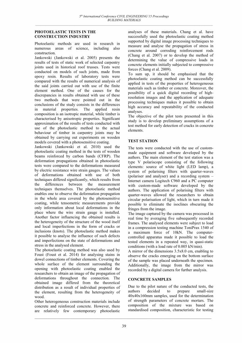
5th International Conference CIVIL ENGINEERING`15 Proceedings BUILDING MATERIALS
_____________________________________________________________________________________________________________
_______________________________________________________________________________________
39
PHOTOELASTIC TESTS IN THE CONSTRUCTION INDUSTRY
Photoelastic methods are used in research in numerous areas of science, including also construction. Jankowski (Jankowski et al. 2005) presents the results of tests of static work of selected carpentry joints used in historical roof trusses. Tests were conducted on models of such joints, made from epoxy resin. Results of laboratory tests were compared with the results of numerical analysis of the said joints carried out with use of the finite element method. One of the causes for the discrepancies in results obtained with use of these two methods that were pointed out in the conclusions of the study consists in the differences in material properties. The applied resin composition is an isotropic material, while timber is characterised by anisotropic properties. Significant approximation of the results of tests conducted with use of the photoelastic method to the actual behaviour of timber in carpentry joints may be obtained by carrying out experiments on wooden models covered with a photosensitive coating. Jankowski (Jankowski et al. 2010) used the photoelastic coating method in the tests of wooden beams reinforced by carbon bands (CFRP). The deformation propagations obtained in photoelastic tests were compared to the deformations measured by electric resistance wire strain gauges. The values of deformations obtained with use of both techniques differed significantly, which results from the differences between the measurement techniques themselves. The photoelastic method enables one to observe the deformation propagation in the whole area covered by the photosensitive coating, while tensometric measurements provide only information about local deformations in the place where the wire strain gauge is installed. Another factor influencing the obtained results is the heterogeneity of the structure of the wood itself and local imperfections in the form of cracks or inclusions (knots). The photoelastic method makes it possible to analyse the influence of such defects and imperfections on the state of deformations and stress in the analysed element. The photoelastic coating method was also used by Foust (Foust et al. 2014) for analysing stains in dowel connections of timber elements. Covering the whole surface of the element surrounding the opening with photoelastic coating enabled the researchers to obtain an image of the propagation of deformations throughout the connection. The obtained image differed from the theoretical distribution as a result of individual properties of the element, resulting from the heterogeneity of wood. Other heterogeneous construction materials include concrete and reinforced concrete. However, there are relatively few contemporary photoelastic
analyses of these materials. Chang et al. have successfully used the photoelastic coating method supported by digital image processing techniques to measure and analyse the propagation of stress in concrete around corroding reinforcement rods (Chang et al. 2007) or to develop the method of determining the value of compressive loads in concrete elements initially subjected to compressive forces (Chang et al. 2009). To sum up, it should be emphasised that the photoelastic coating method can be successfully applied in tests of the properties of heterogeneous materials such as timber or concrete. Moreover, the possibility of a quick digital recording of high-resolution images and the application of adequate processing techniques makes it possible to obtain high accuracy and repeatability of the conducted analyses. The objective of the pilot tests presented in this study is to develop preliminary assumptions of a test method for early detection of cracks in concrete elements. TEST STATION
The tests were conducted with the use of custom-made equipment and software developed by the authors. The main element of the test station was a type V polariscope consisting of the following elements: source of white light (LED lamp), a system of polarising filters with quarter-waves (polariser and analyser) and a recording system – Internet camera Logitech C960 and a PC computer with custom-made software developed by the authors. The application of polarising filters with quarter-waves allowed the researchers to obtain circular polarisation of light, which in turn made it possible to eliminate the isoclines obscuring the fringes from the image. The image captured by the camera was processed in real time by averaging five subsequently recorded frames. The analysed elements were subject to load in a compression testing machine ToniPrax 1540 of a maximum force of 10kN. The computer-controlled apparatus made it possible to load the tested elements in a repeated way, in quasi-static conditions (with a load rate of 0.005 kN/min). A mirror of the dimensions 3.5x8.0 cm, enabling to observe the cracks emerging on the bottom surface of the sample was placed underneath the specimen. Additionally, the image from the mirror was recorded by a digital camera for further analysis. CONCRETE SAMPLES
Due to the pilot nature of the conducted tests, the authors decided to prepare small-size 40x40x160mm samples, used for the determination of strength parameters of concrete mortars. The composition of the mixture was based on standardised composition, characteristic for testing

5th International Conference CIVIL ENGINEERING`15 Proceedings BUILDING MATERIALS
_____________________________________________________________________________________________________________
_______________________________________________________________________________________
40
concrete mortars. Additionally, each sample was reinforced with steel wire of a diameter of 1mm, with a characteristic strength of 250MPa, leaving 3mm of cover. All irregularities on the surface of samples in locations where the photoelastic coating was to be adhered were polished, cleaned and prepared for the installation of photoelastic sheet plates as recommended by the manufacturer. Two types of photoelastic plates (hereinafter referred to as Type A and Type B plates) manufactured by Vishay Micro-Measurements, made from epoxy resin and characterised by the same optical coefficient k=0.15 but of different thickness were used in the experiment. Type A plate (PS-1D) of a thickness of 0.508 ± 0.0508 mm, Type B plate (PS-1B) of a thickness of 2.0828 ± 0.0508 mm were used.
Figure 2. Samples with attached photoelastic plates
Figure 3. Sample B1 – element without applied load
COURSE OF THE EXPERIMENT
The course of the experiment has been analysed basing on sample B1. In the initial stage of the experiment, permanent photoelastic effects were recorded. The distortions visible in Figure 3 occurred during the cutting of the photoelastic plate. No other effects were observed. Figure 4 presents phase I of the work of a beam at the moment of occurrence of the photoelastic effect, but before the element cracked. This took place at a load of 1.72kN, in the 172nd second from the moment of
application of load. Transition from phase I to phase II (cracked phase) occurred as late as in the 264th second. The crack on the bottom of the sample, visible in Figure 5 appeared at the load of 2.64 kN. Then, in seconds 240 and 333, cracks 2 and 3 appeared, subsequently (Figure 6).
Figure 4. Sample B1 – phase I, moment of occurrence of photoelastic effect in the tensile zone
of the beam
Figure 5. Beam B1 – phase II – cracked beam
Figure 6. Beam B1 – phase II – beam with three cracks
Figure 6 shows fringes of the compressed zone (just under point where the load was applied) separated by a zone with zero stress, which allows for the determination of the location of the neutral axis of the cross-section. Additionally, in the tensile zone,

5th International Conference CIVIL ENGINEERING`15 Proceedings BUILDING MATERIALS
_____________________________________________________________________________________________________________
_______________________________________________________________________________________
41
three overlapping zones of large-order fringes are visible. They appear in the places where the three cracks appeared. The beam was destroyed at a load of 6.48 kN in the 648 second of the experiment. The destroying crack was crack No. 1 (Figure 7), signalled by the photoelastic effect that occurred at the force of 1.72kN. After the end of the experiment, both parts of the beam were used to determine the compression strength of concrete. Tensile strength of concrete was determined during typical strength tests as in the case of mortars, carried out on non-reinforced beams the size of 40x40x160mm.
Figure 7. Destroyed sample ANALYSIS OF THE TEST RESULTS
Basing on the values of tensile strength of the concrete and the transverse dimensions of the elements, the theoretical cracking moment was determined, along with the theoretical cracking force for each of the beams, treated as working concrete elements in phase I (without cracks). The results of these calculations, together with the observed values of forces at which the photoelastic effects occurred and a crack on the bottom of the beam was noticed, are presented in Table 1.
Table 1
Presentation of forces
Beam Type of plate
Theoretical cracking
force
Force at which
photoelastic effect was
noticed
Force at which a
crack was noticed at the bottom of the beam
No. [-] [kN] [kN] [kN] 1 A 1.879 1.600 - * 2 A 1.879 1.500 - * 3 A 1.906 2.200 - * 1 B 2.103 1.720 2.640 2 B 1.985 1.780 2.840 3 B 1.934 1.880 2.420
* - value omitted due to very low resolution of photographic documentation, which made it impossible to read the moment of occurrence of the crack. Two types of photoelastic plates of different thickness were used in the experiment. The aim of this procedure was to test the influence of plate thickness on the quality of the obtained interference images. The conducted tests confirmed the connection between the thickness of the plates of
identical optical coefficient and the obtained images of the deformation state. During the experiment, the image on plates marked with letter A (0.5 mm thick) showed a less clear depiction of fringes in comparison to the image on B type plates (2.1 mm thick). On thinner plates a high-number fringes became visible nearly instantly after the occurrence of the photoelastic effect, which made it impossible to unambiguously determine the order of specific fringes. On the other hand, both types of plates made it possible to capture the moment of occurrence of the photoelastic effect in a similar way. CONCLUSIONS
The conducted tests demonstrated that the photoelastic coating method makes it possible to notice locations that are particularly vulnerable to structural changes in a material subjected to applied load. One may conclude that such spots are particularly prone to the occurrence of a stress concentration and thus, these are locations where the continuity of the material may be disrupted. The tests also confirmed that due to low values of concrete deformation the selection of thickness of the photosensitive coating is essential. The result analysis showed, in five cases out of six, that the force at which the occurrence of photoelastic effect was noticed was significantly lower than the cracking force determined theoretically for a concrete element, pursuant to the principles of material strength. Thus, one can conclude that the photoelastic method provides the possibility to determine the location of the occurrence of a crack before it actually appears (mean percentage relation of force at which photoelastic effect was observed to the force at which a crack on the bottom of the beam was noticed equals 68.5%). This is interesting, because the use of suitable photosensitive materials and the application of an assumed, small load may make it possible to detect the weakest points in the cross-section and thus to determine which locations are particularly prone to damage. It should be noted that the conducted tests are of a pilot nature and that they require additional laboratory experiments, in which the influence of external factors that may affect the presented results could be further limited. Currently, the authors are unable to determine the influence of effect of the adhesion of a photoelastic plate on the additional bearing capacity of the element. The plate adhered to the surface of the beam may carry some of the internal forces (here bending momentum), thus strengthening the cross-section of the tested element. Such strengthening might have delayed the moment of occurrence of the crack, resulting in incorrect outcomes. Further tests in this aspect are required.

5th International Conference CIVIL ENGINEERING`15 Proceedings BUILDING MATERIALS
_____________________________________________________________________________________________________________
_______________________________________________________________________________________
42
REFERENCES
Chang C.W., Chen P.H., Lien H.S. (2009) Evaluation of residual stress in pre-stressed concrete material by digital image processing reflection photoelastic coating and hole drilling method. Measurement, Vol. 42, No. 4, p. 552–558.
Chang C.W., Lien H.S. (2007) Expansion stress analysis of ferroconcrete corrosion by digital reflection photoelasticity. NDT & E International, Vol. 40, No. 4, p. 309–314.
Chang C.W., Lien H.S., Lin J.H. (2008) Determination of reflection photoelasticity fringes analysis with digital image-discrete processing. Measurement, Vol. 41, No. 8, p. 862–869.
Foust B.E., Lesniak J.R., Rowlands R.E. (2014) Stress analysis of a pinned wood joint by grey-field photoelasticity. Composites Part B: Engineering, Vol. 61, p. 291–299.
Jankowski L., Engel L.J., Jasieńko J. (2005) Praca statyczna wybranych połączeń występujących w drewnianych obiektach historycznych. Wiadomości Konserwatorskie, Vol. 18, p. 29–41.
Jankowski L., Jasieńko J., Nowak T.P., (2010) Experimental assessment of CFRP reinforced wooden beams by 4-point bending tests and photoelastic coating technique. Materials and Structures, Vol. 43, p. 141–150.
Ramesh K. (2000) Digital Photoelasticity: Advanced Techniques and Applications, Berlin: Springer, 410 p.
Szala J., Boroński D. (2007) Analiza odkształceń lokalnych w obszarach nieciągłości geometrycznych i niejednorodności materiałowych. Acta mechanica et automatica, Vol. 1, No. 1, p. 103–124;
Vishay Micro-Measurment (2011) Introduction to Stress Analysis by the PtotoStress® Method [online] [accessed on 10.05.2014.]. Available: http://www.vishaypg.com/docs/11212/11212_tn.pdf

5th International Conference CIVIL ENGINEERING`15 Proceedings BUILDING MATERIALS
_____________________________________________________________________________________________________________
_______________________________________________________________________________________
43
INVESTIGATION OF PHYSICAL AND MECHANICAL PROPERTIES OF STRAW AS A BUILDING MATERIAL
Vincas Gurskis, Aleksandras Stulginskis University, Institute of Hydraulic Engineering, Lithuania
E-mail: [email protected] Rytis Skominas
Aleksandras Stulginskis University, Institute of Hydraulic Engineering, Lithuania E-mail: [email protected]
ABSTRACT
This article analyses how straw and straw buildings pass the Basic requirements given in Regulation (EU) No 305/2011 of the European Parliament and of the Council. The research was performed by analysing the various scientific works and test results carried out at accredited laboratories. The analysis reveals that perfectly prepared straw as well as buildings insulated with it can pass the Basic requirements. During the test of required pressure of rye, triticale and oat straw it was estimated that the type of straw and humidity have not influenced the compression. During the experiment, the following aspects were also estimated: the pressure to obtain an optimal density of 90...140 kg∙m–3, the dependency between straw density and pressure deformations. The research of thermal conductivity confirmed the results of other scientific works, which state that increasing the straw’s humidity increases the thermal conductivity coefficient as well. The thermal conductivity coefficient of dry straw is about 0.01...0.02 W∙m–1∙K–1 smaller than that of straw with 20 % of humidity.
Key words: straw, Basic requirements, density, pressure, thermal conductivity. INTRODUCTION
Straw as barriers for thermal insulating and roofing material has been used for a long time. The usage greatly increased when the production of straw bale was started. In these latter years, straw has been used as a soundproofing and structural material. The increasing cost of traditional insulation materials, willingness to live in healthier ambience, environmental problems while producing energy-intensive building materials as well as access to information distributed over the Internet determined the wider use of pressed straw in Lithuania. The straw bales compared with traditional building materials, are ecological due to a low requirement for production energy and utilization. Recently, the considerable interest is being paid to straw bale, not only in popular literature but also on the internet and in the scientific publications (Ashour et al, 2011; Bainbridge, 2000, 2003; Czachor, 2002; Drack et al., 2004; Goodhew et al., 2004; Henderson, 2006; Korjenic et al, 2011; Lawrence, 2009; Simonsen, 1996; Sodagar et al, 2011; Taylor et al., 2006; Wieland et al., 2002). In a theme of construction from straw there are patents of inventions (Patent..., 2004, 2006, 2007 ir kt.), books (Hodge, 2006; Hollis, 2005; Karen, 2005, Bingham, 2007, King, 2006, Corum, 2005, Magwood, 2005). “The Last Straw Journal“ has been published in USA since 1993. The PhD thesis about the use of renewable building materials in construction process was prepared (Ashour, 2003; Krick, 2008, Vejeliene, 2012; Milutiene, 2013). The material about construction from pressed straw is placed on
the internet by associations, unions and corporations in many countries. All this suggests that the pressed bales of straw as a building material in the future should be used more widely. The usage of straw as a building material is connected with the estimation of how buildings and their structures constructed from straw pass the Basic requirements stated in Regulation (EU) No 305/2011 of the European Parliament and the Council (Regulation..., 2011). When using straw it is important to know the thermal conductivity dependence on straw density, moisture content as well as their compression pressure. The aim of this work is to evaluate if the straw buildings pass the Basic requirements or not; to determine the pressure and density dependenc; to estimate the dependency between thermal conductivity and straw density, humidity. MATERIALS AND METHODS
Evaluating straw as a building material the scientific works about the suitability to use pressed straw in construction were analyzed. During the analysis the pressed straw as a building material was reviewed according to the Basic requirements stated in Regulation (EU) No 305/2011 of the European Parliament and the Council (Regulation..., 2011). For the pressing test - three types of straw (rye, triticale and oat) were used. The test was performed using a reinforced steel box. The box shape was rectangular with a cross-section area of 0.1 m2. During the test, samples cut from straw bales

5th International Conference CIVIL ENGINEERING`15 Proceedings BUILDING MATERIALS
_____________________________________________________________________________________________________________
_______________________________________________________________________________________
44
according to the dimensions of box were used. For pressing a universal testing machine (Fig. 1) was used. The pressure to straw was transmitted through a rigid steel plate. The humidity was estimated according to the mass.
Figure 1. Straw pressure test with universal testing machine
Figure 2 Straw sample for thermal conductivity test
and „LaserComp“ FOX200 test apparatus
The thermal conductivity was estimated using shredded 50 mm long and differently pressed
triticale straw according to standard methods (EN12667, ASTM C 518, ISO 8301) with „LaserComp“ FOX200 test apparatus. The straw was tested under dry and wet conditions. The heat flow was vertical to the straw’s length (Fig. 2).
RESULTS AND DISCUSSION
Requirements for pressed straw bales as a building material, analysis of recently made investigations
The frequent usage of straw as abuilding material is associated with some distrust and fear: the building will burn, rot, mice or rats will attack it. In this article we will try to answer the above-mentioned fears by analyzing the scientific works: articles in refereed scientific journals, conformity assessment data carried out in independent laboratories. Recently in the European Union there are undivided requirements for construction products. Each product, which is available on the market, shall have a declaration of performance. This is being performed according to standard methodology. Straw and manufactured construction products validation is possible after the establishment of the National Technical Assessment (NTA) or European Technical Assessment (ETA). In Germany in 2006 according to the Building from Pressed Straw Union order, a technical assessment was prepared and in 2014 Construction from Straw Directive (Strohbaurichtlinie..., 2014) and certificate (Allgemeine..., 2014) were prepared as well. These documents refer to particular requirements for pressed straw bales: dimensions, density, thermal conductivity, humidity, reaction to fire and others. The requirements for the construction process are given as well. Technical assessment describes the test methods, standards and periodicity of straw bales testing. Similar requirements for pressed straw are prepared in the USA and Belarus. Assessing pressed straw bales and building structures from the basic requirement of mechanical strength and stability viewpoint, mechanical properties, particularly strength, are very important. The pressed straw is usually used for the frame building construction as insulation material for walls, roof, ceiling and loft. In this case, the load bearing structures are wooden frames, ceiling beams or rafters. In Germany, (Strohbaurichtlinie..., 2014) the length between the posts must not be longer than 1 m. The mechanical tests show that walls with wooden frames sustain quite great vertical and horizontal loads. An analogous test was carried out in Lithuania for legalization of wooden frames with external board filled with straw (straw shades (Fig. 3)) (National..., 2013). The test results proved that straw shades can be used for construction. According to this, it can be seen that straw is a suitable material for thermal insulation in wooden frame and shade buildings, where load bearing structures are wooden elements. Frameless
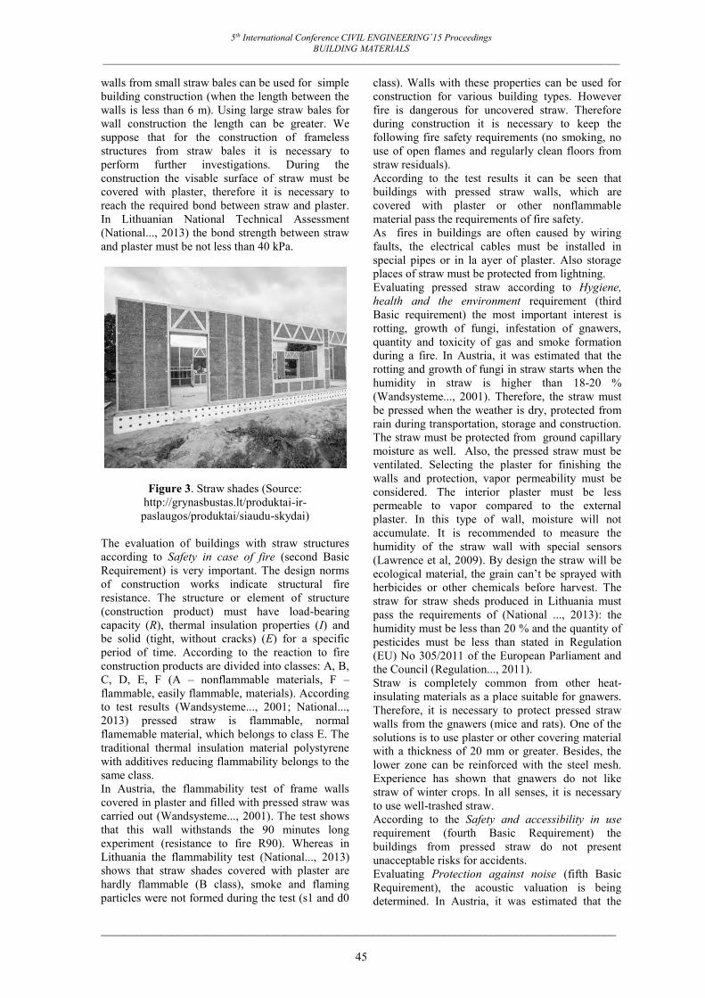
5th International Conference CIVIL ENGINEERING`15 Proceedings BUILDING MATERIALS
_____________________________________________________________________________________________________________
_______________________________________________________________________________________
45
walls from small straw bales can be used for simple building construction (when the length between the walls is less than 6 m). Using large straw bales for wall construction the length can be greater. We suppose that for the construction of frameless structures from straw bales it is necessary to perform further investigations. During the construction the visable surface of straw must be covered with plaster, therefore it is necessary to reach the required bond between straw and plaster. In Lithuanian National Technical Assessment (National..., 2013) the bond strength between straw and plaster must be not less than 40 kPa.
Figure 3. Straw shades (Source: http://grynasbustas.lt/produktai-ir-paslaugos/produktai/siaudu-skydai)
The evaluation of buildings with straw structures according to Safety in case of fire (second Basic Requirement) is very important. The design norms of construction works indicate structural fire resistance. The structure or element of structure (construction product) must have load-bearing capacity (R), thermal insulation properties (I) and be solid (tight, without cracks) (E) for a specific period of time. According to the reaction to fire construction products are divided into classes: A, B, C, D, E, F (A – nonflammable materials, F – flammable, easily flammable, materials). According to test results (Wandsysteme..., 2001; National..., 2013) pressed straw is flammable, normal flamemable material, which belongs to class E. The traditional thermal insulation material polystyrene with additives reducing flammability belongs to the same class. In Austria, the flammability test of frame walls covered in plaster and filled with pressed straw was carried out (Wandsysteme..., 2001). The test shows that this wall withstands the 90 minutes long experiment (resistance to fire R90). Whereas in Lithuania the flammability test (National..., 2013) shows that straw shades covered with plaster are hardly flammable (B class), smoke and flaming particles were not formed during the test (s1 and d0
class). Walls with these properties can be used for construction for various building types. However fire is dangerous for uncovered straw. Therefore during construction it is necessary to keep the following fire safety requirements (no smoking, no use of open flames and regularly clean floors from straw residuals). According to the test results it can be seen that buildings with pressed straw walls, which are covered with plaster or other nonflammable material pass the requirements of fire safety. As fires in buildings are often caused by wiring faults, the electrical cables must be installed in special pipes or in la ayer of plaster. Also storage places of straw must be protected from lightning. Evaluating pressed straw according to Hygiene, health and the environment requirement (third Basic requirement) the most important interest is rotting, growth of fungi, infestation of gnawers, quantity and toxicity of gas and smoke formation during a fire. In Austria, it was estimated that the rotting and growth of fungi in straw starts when the humidity in straw is higher than 18-20 % (Wandsysteme..., 2001). Therefore, the straw must be pressed when the weather is dry, protected from rain during transportation, storage and construction. The straw must be protected from ground capillary moisture as well. Also, the pressed straw must be ventilated. Selecting the plaster for finishing the walls and protection, vapor permeability must be considered. The interior plaster must be less permeable to vapor compared to the external plaster. In this type of wall, moisture will not accumulate. It is recommended to measure the humidity of the straw wall with special sensors (Lawrence et al, 2009). By design the straw will be ecological material, the grain can’t be sprayed with herbicides or other chemicals before harvest. The straw for straw sheds produced in Lithuania must pass the requirements of (National ..., 2013): the humidity must be less than 20 % and the quantity of pesticides must be less than stated in Regulation (EU) No 305/2011 of the European Parliament and the Council (Regulation..., 2011). Straw is completely common from other heat-insulating materials as a place suitable for gnawers. Therefore, it is necessary to protect pressed straw walls from the gnawers (mice and rats). One of the solutions is to use plaster or other covering material with a thickness of 20 mm or greater. Besides, the lower zone can be reinforced with the steel mesh. Experience has shown that gnawers do not like straw of winter crops. In all senses, it is necessary to use well-trashed straw. According to the Safety and accessibility in use requirement (fourth Basic Requirement) the buildings from pressed straw do not present unacceptable risks for accidents. Evaluating Protection against noise (fifth Basic Requirement), the acoustic valuation is being determined. In Austria, it was estimated that the

5th International Conference CIVIL ENGINEERING`15 Proceedings BUILDING MATERIALS
_____________________________________________________________________________________________________________
_______________________________________________________________________________________
46
sound absorption coefficient of the frame wall insulated with pressed straw and covered with plaster, was 55 dB (Wandsysteme..., 2001). Similar results were obtained in Lithuania by testing straw sheds: the sound reduction index was 54 dB (National ..., 2013). These results show that external pressed straw walls insulate against noise well and are suitable for the highest acoustic comfort class A. For buildings, where the interior temperature must be positive, Energy economy and heat retention requirement (sixth Basic requirement) is very important. According to this requirement, the amount of energy used to heat, depending on the local climate and the needs of the population, should not be greater than necessary. This depends on the parameters of barriers (heat transfer coefficient U, thermal resistance Rt). These parameters depend on the thermal conductivity coefficient λ of the material. In Austria, Denmark, USA, Germany and other countries it was estimated that the thermal conductivity coefficient λ of pressed straw (density 70-150 kg∙m–3) is equal to 0.045-0.06 W/(m∙K) when they are dry and equal to 0.054-0.072 W/(m∙K) and when they are air-dry (Wandsysteme..., 2001; Ashour et al., 2003; 2011). The German Construction from Pressed Straw Directive states that the thermal conductivity the coefficient λ of pressed straw is 0.052 W/(m∙K) (Strohbaurichtlinie..., 2014). In this case, the heat transfer coefficient of a wooden frame (evaluating influence of wood) wall filled with pressed straw
and covered with plaster on both sides will be 0.13-0.14 W/(m2∙K) (total thermal resistance Rt = 7.7-7.1 m2∙K/W). These results show us that the heat transfer coefficient is less than required (till 2016 UN = 0.2 W/(m2∙K) for residential buildings) by 43-54 %. The 40 cm thickness straw sheds (the density of straw 98...127 kg∙m–3) produced in Lithuania also have small thermal conductivity. The heat transfer coefficient is U = 0.15 W/(m2∙K) (total thermal resistance Rt = 6.65 m2∙K/W). Besides, it is possible to reduce this coefficient by additionally insulating the walls with wood fibre panels and getting energy effective buildings or passive buildings. The requirement of Sustainable use of natural resources (seventh Basic Requirement) states that buildings must be designed, built and demolished in such a way that the use of natural resources is sustainable and, in particular, ensures the following: (a) reuse or recyclability of the buildings, their materials and parts after demolition; (b) durability of the buildings; (c) use of environmentally compatible raw and secondary materials in the buildings. Straw and others renewable raw materials mostly suit this requirement due to low energy required for production (Fig. 4), use and utilization (Sodagar et al., 2011; Vom..., 2014). Properly constructed and exploited buildings with pressed straw can be used for a long time. The longevity of straw sheds produced in Lithuania is 50 years (National..., 2013). In the world, there are straw buildings that were built more than 100 years ago.
Figure 4. Required energy for material production, when heat transfer coefficient U = 0,2 W∙m–2∙K-1
(Vom..., 2014)
The Numbers Above do not look proper Summarizing the test results of scientific works on pressed straw usage in construction and having compared them with requirements stated in Regulation (EU) No 305/2011 of the European
Parliament and the Council (Regulation..., 2011), it can be stated that pressed straw as a natural thermal insulation material can be used for construction of buildings as it passes the Basic requirements.

5th International Conference CIVIL ENGINEERING`15 Proceedings BUILDING MATERIALS
_____________________________________________________________________________________________________________
_______________________________________________________________________________________
47
Straw pressing test
When using pressed straw for building wall thermal insulation it should be properly pressed, so that the wall will be tight and the straw will not settle in the wall. During the pressing test of rye, triticale and oat straw, dependencies between deformations and pressure (Fig. 5, 6, 7), pressure and density (Fig. 8), deformations and density (Fig. 9, 10, 11) were estimated.The test results show that at the beginning of the test compression deformations run faster. The
logarithmic equation characterizes this dependency. The dependency between the density and the pressure of different straw states that the highest density are oat straw with 24.1 % of humidity and rye straw with 19.2 % of humidity. It is estimated that in order to get the rye straw density to 120 kg∙m–3 it is necessary to press them with 30 kPa of pressure. While triticale and oat straw must be pressed with 50 kPa and 55 kPa of pressure, respectively.
Figure 5. Dependency between deformations and pressure of triticale straw
Figure 6. Dependency between deformations and pressure of rye straw

5th International Conference CIVIL ENGINEERING`15 Proceedings BUILDING MATERIALS
_____________________________________________________________________________________________________________
_______________________________________________________________________________________
48
Figure 7. Dependency between deformations and pressure of oat straw
Figure 8. Dependency between density and pressure: 1 and 2 – oat straw, with 24.1 % and 15.4 % of humidity; 3 and 4 – triticale straw, with 13.4 % and 13.8 % of humidity; 5 – rye straw, with 19.2% of
humidity
Figure 9. Dependency between compression deformation and density of triticale straw

5th International Conference CIVIL ENGINEERING`15 Proceedings BUILDING MATERIALS
_____________________________________________________________________________________________________________
_______________________________________________________________________________________
49
Figure 10. Dependency between compression deformation and density of rye straw
Figure 11. Dependency between compression deformation and density of oat straw
The polynomial equations characterize dependency between deformations and density. According to these equations the required density can be calculated. For example, to get 120 kg∙m–3 of density triticale and oat straw, the compression deformation must be 35 % and for rye straw – 25 %.
Straw thermal conductivity test
Nowadays, as it was mentioned before, generally straw is used as a thermal insulation material. The thermal conductivity of straw was estimated using shredded 50 mm long and differently pressed triticale straw. The straw was dry and with a particular humidity. The results of the test are given in Table 1.
Table 1 Test results of thermal conductivity
Sample
Air-dry samples Wet samples
Humidity %
Density kg∙m–3
Thermal conductivity W∙m–1∙K–1
Humidity %
Density kg∙m–3
Thermal conductivity W∙m–1∙K–1
1 1-1.5 46 0.048 22.1 57 0.058 2 1-1.5 63 0.048 18.8 79 0.067 3 1-1.5 53 0.046 44.3 91 0.071 4 1-1.5 128 0.048 21.6 151 0.057 5 1-1.5 139 0.049 13.0 209 0.061 6 1-1.5 134 0.053 - - - 7 1-1.5 425 0.061 3.6 694 0.081

5th International Conference CIVIL ENGINEERING`15 Proceedings BUILDING MATERIALS
_____________________________________________________________________________________________________________
_______________________________________________________________________________________
50
The test results show that the thermal conductivity of dry straw depends on the density. This tendency is typical for other thermal insulation materials as well. The wet straw had a greater density and thermal conductivity coefficient. The increased humidity by 1 % increases the thermal conductivity coefficient by 0.0005...0.0011 W∙m–1∙K–1. Therefore, the maximum humidity (20 %) of straw increases the thermal conductivity up to 0.01...0.02 W∙m–1∙K–1 or by 19...42 %. It is also can be stated that in the range between 50 and 130 kg∙m–3 there is a negligible influence of the density of air-dry straw on thermal conductivity. After this range the increasing density of straw weight increases the thermal conductivity.
CONCLUSIONS
Based on the obtained results the following conclusions can be drawn: 1. Wooden frame and shed walls insulated with pressed straw pass the Basic requirements. 2. The pressure of straw depends on the type and humidity of straw. In order to get 120 kg∙m–3 of density of straw it is necessary to press rye straw with 30 kPa, triticale – with 50 kPa and oat – with 55 kPa of pressure; triticale and oat straw compression deformation must be 35 % and rye – 25 %. 3. Humidity of straw has a negative effect on the thermal conductivity coefficient: increasing humidity increases the value of the thermal conductivity coefficient. The maximum humidity (20 %) of straw increases the thermal conductivity to 0.01...0.02 W∙m–1∙K–1 or by 19...42 %.
REFERENCES Allgemaine Bauaufsichtliche Zulassung. (2014) Wärmedämstoff aus Strohballen „Baustrohballen“. 9 p. [Previewed 10-05-2014.]. Access in internet: https://fasba.de/images//z-23.11-1595%203.6.2014kl.pdf Ashour T; Georg H, Wuc W. (2011) Performance of straw bale wall: A case of study. Energy and Buildings, Volume 43, Issue 8, August. p. 1960-1967.
Ashour, T. (2003) The use of renewable agricultural by-Products as building materials. Ph. D Thesis. Benha University Moshtohor, Toukh, Kaliobia, Egypt. p. 348.
ASTM C518: 2004. Standard Test Method for Steady-State Heat Flux Measurements and Thermal Transmission Properties by Means of the Heat Flow Meter Apparatus
Bainbridge D.A. (2003) High performance low cost buildings of straw. Agriculture, Ecosystems & Environment, Vol. 16, No 3-4, p. 281-284.
Bainbridge, D. A. (2000) Straw bales stack up for buildings. A lost art resurfaces in the modern world. Resource, Engineering & Technology for a Sustainable World, Vol. 7, No 3, p. 9-10.
Bingham W.J., Pfeffer J. (2007) Natural timber frame homes: building with wood, stone, clay, and straw. Salt Lake City, Utah: Gibbs Smith. 146 p.
Corum, N. (2005) Building a straw bale house: the red feather construction handbook. Foreword by Jane Goodall. New York: Princeton Architectural Press. 195 p.
Czachor H. (2002) Application of straw bales to construction of farm building walls. Problemy Inzynierii Rolniczej, Vol. 10, No 4, p. 85-92.
DIRECTIVE 98/8/EC OF THE EUROPEAN OPEAN PARLIAMENT AND OF THE COUNCIL of 16 February 1998 concerning the placing of biocidal products on the marke.
Drack M., Wimmer R., Hohensinner H. (2004) Treeplast Screw – a device for mounting various items to straw bale constructions. The Journal of Sustainable Product Design. Vol. 4, No 1-4, p. 33-41.
EN 12667:2001. Thermal performance of building materials and products - Determination of thermal resistance by means of guarded hot plate and heat flow meter methods - Products of high and medium thermal resistance.
Goodhew S., Griffiths R., Woolley, T. (2004) An investigation of the moisture content in the walls of a straw-bale building. Building and Environment, Vol. 39, No. 12, p. 1443-1451.
Henderson K. (2006) Ethics, Culture, and Structure in the Negotiation of Straw Bale Building Codes. Science, Technology & Human Values, Vol. 31, No 3, p. 261-288.
Hodge, B. G. (2006) Building your straw bale home: from foundations to the roof. CSIRO Publishing; Collingwood; Australia, 260 p. http://www.rivendellvillage.org/Building-Your-Straw-Bale-Home.pdf
Hollis, M. (2005) Source: Practical straw bale building. Landlinks Press; Collingwood; Australia, 98 p.

5th International Conference CIVIL ENGINEERING`15 Proceedings BUILDING MATERIALS
_____________________________________________________________________________________________________________
_______________________________________________________________________________________
51
ISO 8301:1991/Amd.1:2010. Thermal insulation - Determination of steady-state thermal resistance and related properties - Heat flow meter aparatus.
Karen E. (2005) Building a Straw Bale House: The Red Feather Construction Handbook. Princeton Architectural, dist. by Chronicle. 192 p.
King B. (2006) Design of straw bale buildings: the state of the art. With contributing authors: Aschheim M.et al. San Rafael, Calif. Green Building Press. 296 p.
Korjenic A., Petránek V., Zach J, Hroudová J. (2011) Development and performance evaluation of natural thermal-insulation materials composed of renewable resources. Energy and Buildings, Volume 43, Issue 9, September, Pages 2518-2523.
Krick. B. (2008) Untersuchung von Strohballen und Strohballenkonstruktionen hinsichtlich ihrer Anwendung für ein Energie sparendes Bauen unter besonderer Berücksichtigung der Lasttragenden Bauweise. (Dissertation). [Previewed 12-05-2014]. Access in internet: http://www.uni-kassel.de/upress/online/frei/978-3-89958-422-6.volltext.frei.pdf
Lawrence M., Heath A., Walker P. (2009) Determining moisture levels in straw bale construction. Construction and Building Materials, Volume 23, Issue 8, August, Pages 2763-2768.
Magwood Ch., Mack P., Therrien T. (2005) More straw bale building: a complete guide to designing and building with straw. New Society Publishers. Repr. 2008. 288 p.
Milutiene E. (2013) Environmental performance improvement possibilities of a building using renewable aterialsand energy. Summary of doctoral dissertation. Kaunas, 37 p.
National technical approval (2013) NTĮ-01-061:2013 (original Lithuanian language version). Wooden frame external panels with insulation straw core.
Patent CN1844016-A. Method for manufacturing non-bearing heat-preserving building block by sorghum straw. Wang, B., Sun, Y., 2007.
Patent US2004172900-A1. Building wall moisture controlling system, has foundation wall for supporting straw bales, step extending downwardly and away from foundation wall, and vent pipes that communicate plenum space with airspace exterior to wall. Black, R. G., 2004.
Patent DE102005020557-A1. Wooden frame walls for building with compacted straw bale filling and covered by water inhibiting clay rendering. Krupinski, M, 2006.
Regulation (EU) No 305/2011 of the European Parliament and of the Council of 9 March 2011 laying down harmonised conditions for the marketing of construction products and repealing Council Directive 89/106/EEC.
Simonsen, J. (1996) Utilizing straw as a filler in thermoplastic building materials. Construction and Building Materials. Vol. 10, No 6, p. 435-440.
Sodagar B., Rai D, Jones B.; Wihan J., Fieldson R. (2011) The carbon-reduction potential of straw-bale housing. Journal: Building Research & Information. Volume 39, Issue 1, February, pages 51-65.
Strohbaurichtlinie SBR-2014 (2014) Fachverband Strohballenbau Deutschland e.V. 37 p. [Previewed 10-12-2014]. Access in internet: https://fasba.de/images/sbr%202014-11-22-download.pdf
Taylor, B., Vardy, S., MacDougall C. Compressive Strength Testing of Earthen Plasters For Straw Bale Wall Application. Solid Mechanics and Its Applications, Vol. 140, Advances in Engineering Structures, Mechanics & Construction, 2006, P. 175-183.
Vejeliene J. (2012) Processed straw as effective thermal insulation for building envelope constructions. Journal: Engineering Structures and Technologies. Volume 4, Issue 3, September, pages 96-103.
Vom Halm zum Haus (2014) [Previewed 10-12-2014]. Access in internet:
http://www.baubiologie-regional.de/strohballenbau.pdf
Wandsysteme aus nachwachsenden Rohstoffen. Wirtschaftliche Grundlagenstudie. Endbericht. TU Wien, 2001, S.99. [Previewed 30-03-2004] Access in internet: http://www.grat.at/Publikationen/Wandaufbau_aus_NWR.pdf
Wieland, H., Ashour, T., Bockisch, F. J. (2002) Straw - renaissance for an old building material? Landtechnik, Vol. 57, No 4, 2002, p. 222-223.

5th International Conference CIVIL ENGINEERING`15 Proceedings BUILDING MATERIALS
_____________________________________________________________________________________________________________
_______________________________________________________________________________________
52
COMPOSITES WITH HEMP FIBRE WOVEN REINFORCEMENTS
Maris Manins *, Aina Bernava**, Guntis Strazds ***
Forest Industry Competence Centre E-mail: * [email protected], ** [email protected], *** [email protected]
ABSTRACT
The research focuses on hemp yarn activity in the woven reinforcements, depending on the production method as well as production of reinforcement of natural yarns and thermoplastic yarns as a matrix in one woven product for the production of composites of building materials. The reinforcements of hemp yarns (100 tex), polypropylene yarns (100 tex) and polyethylene yarns (220 tex) were produced using a plain weaving technique on a craftsman’s loom. The measurements of the fabric thickness and physical-mechanical properties of reinforcements were carried out according to ISO 5084:1996 and LVS EN ISO 13934-1-2001 standards. Fabric thickness of the hemp yarn reinforcement was 0.61-0.69 mm and density 91-100 g/m2. Tensile strength of the hemp reinforcement in the warp direction was 241 N-279 N and in the weft direction 249 N -302 N; tensile modulus- 218 MPa-271 MPa and 189 MPa-196 MPa. The Laboratory Press LP_S_50/SASTM) was used for the production of composites. The mechanical properties of the composite were established according to ISO 527-5:2009 standard and thickness swelling in water was conducted in accordance to EN 622-2: 2004 standard. Composite thickness depending on the reinforcement layers in the composites was from 0.34 mm to1.1mm; the density of the composites varied from 311 g/m2 to 1040 g/m.2 Tensile strength of the composites varied from 303 N (one layer) to 2019 N (five layers) and the elastic modulus of the same composites was 908 MPa and 1809MPa.
Key words: hemp yarns, woven reinforcements, thermoplastic matrix, composites
INTRODUCTION
Research on natural fibre composites has existed since the early 20th century, but it received more attention in the late 1980s. Composites, primarily glass but including natural reinforced composites are found in countless consumer products including boats, skis, agricultural machinery and cars (Dammer L., et al., 2013). The usage of textiles for the reinforcement of concrete is a flexible and efficient technology which can be used for repairing and strengthening existing structures, as well as for the production of load-bearing for façade constructions or non-load-bearing precast parts (Funkea H., et al., 2013; Hartig J et al., 2010; Hausding J, et.al., 2006; Hegger J., et al., 2008; Lepenies I., et al.; 2007). Due to the worldwide emphasis on environmental awareness recent studies have pointed out hemp fibre composites as a promising option for applications that are currently using glass fibre composites and other materials with similar mechanical properties (Bernava A. et.al.; 2011; Bernava A., et.al., 2012; Manins. M. et.al., 2011; Westman M.P. et. al.,2010). The largest advantages of using natural fibres in composites are the cost of materials, their sustainability and density (Dammer L. et al., 2013). The share of natural fibres in the fibre market has decreased over the last 20 years and in the year 2013 the amount of produced natural fibres was 33% of the fibre market. In 2012 the largest share of the European Union (EU) composites’ market (total
volume 150 000 t) of natural fibre 30 000 t, including hemp fibres 4 000 t were used for the automotive industry (De Vasconcellos D. S., et. al., 2012.). Jute and allied fibres gained interest as a reinforcing material in the composite industry to produce new and alternate building materials for low cost housing application, including: building panels, roofing sheets, boards’ partitions, doors and windows, tiles etc. (Singh B., et. al., 2011). The addition of natural fibres to concrete was found helpful in producing cost-effective and sustainable building constructions and to improve various mechanical performances including flexural properties, impact resistance, fracture toughness, etc. even for glass and carbon fibres (Parveen S. et. al.,2012). The interest in natural fiber-reinforced polymer composite materials in industrial applications is because they are renewable, cheaper, completely or partially recyclable (Manins M., et.al. 2015), they have low weight, good heat and sound insulation properties, and could offer an eco-friendly alternative to glass fibres (Bernava A. et.al., 2012). Over the last decades, natural fibres grown as a raw material for industrial and household use have proved their popularity, economic viability and processing perspective in Latvia (Adamovics A., et. al. 2014; Strazds G., et.al. 2012). Our pervious researches were focused on the comparison of the production method for woven reinforcement production and the mechanical properties. This research focuses on hemp yarn activity in woven reinforcements, depending on the

5th International Conference CIVIL ENGINEERING`15 Proceedings BUILDING MATERIALS
_____________________________________________________________________________________________________________
_______________________________________________________________________________________
53
production method, as well as the fabrication of the reinforcement of natural and thermoplastic fibre as a matrix in one woven product for production composites of building materials.
MATERIALS AND METHODS
Materials and Techniques For the production of reinforcements the hemp yarns with a density of 100 tex, polypropylene (100 tex) and polyethylene (220 tex) yarns were used. Before weaving they were tested according to LVS EN ISO 5079:2001 standard (Table 1). For the production of the reinforcements an industrial loom СТБ-175 and a craftsman’s loom in plain weaving technique was used.
Table 1
Parameters of the yarns used
The measurements of fabric thickness were carried out with the ATLASS thickness meter according to ISO 5084:1996 standards. The physical-mechanical properties of hemp and hybrid reinforcements in the warp direction were tested with the INSTRON
dynamometer corresponding to LVS EN ISO 13934-1-2001 standard. The mechanical properties of the polypropylene and polyethylene yarns were not tested, because their task was to act as the composite matrix.
Composite Production and Testing
Before the production of the composite the reinforcements were held in a vacuum for 24h at a temperature of 25ºC. For the production of laminate composites unidirectional lay- up method (Figure 1) with the change of the reinforcements warp direction (0°), the Laboratory Press LP_S_50/SASTM at a temperature of 190°C was used. The technological parameters for producing of composites were noted in table 3.
Figure1. Composites production method
The mechanical properties of the composite were established according to ISO 527-5:2009 standard. The composites thickness swelling (TS) in water was conducted in accordance to EN 622-2: 2004 standard after 24, 48 and 72 hours.
a)
b)
c)
Woven reinforcement of hemp yarns
Woven reinforcement of hemp yarns and polypropylene yarns
Composite of hemp and polypropylene yarn reinforcement
Figure 2. Woven reinforcements and composite (size of sample 1.5* 2.0 cm)
RESULTS AND DISCUSSION
Woven reinforcements of hemp yarns were produced on a craftsman’s and industrial loom while hybrid reinforcements of hemp and polypropylene or polyethylene yarns were produced on a craftsman’s loom (Figure 2 A, B). The mechanical properties of the reinforcement of hemp yarns were compared
since both looms have different thread feeders that affect the mechanical characteristics of the produced structure. As can be seen in Table 2, the tensile strength in the warp direction is by 14% higher for the industrially made reinforcement, while in the weft direction it is higher for a handmade reinforcement (by 18%).
Des
igna
tion
Yar
n de
nsity
, tex
Max
imum
lo
ad, N
Tens
ile
exte
nsio
n,
mm
Hemp HA 100 15.4 17.3 Glass fibres GF 136 97.4 4.1 Polypropylene PP 100 - - Polyethylene PE 220 - -

5th International Conference CIVIL ENGINEERING`15 Proceedings BUILDING MATERIALS
_____________________________________________________________________________________________________________
_______________________________________________________________________________________
54
The tensile stress in both directions is higher for the handmade reinforcement by 3% (warp direction) and by 14% (weft direction). The tensile extension in both directions is lower (by 2%-4%) for the industrially made reinforcement. The tensile modulus in the warp direction is higher for the handmade reinforcement (by 20%), but in the weft direction for the industrially made reinforcement (by 14%).
The hybrid reinforcements with polypropylene or polyethylene yarns and glass fibres addition were not tested before the composite production, because the most prominent influence on the mechanical properties of reinforcements came from the polypropylene or polyethylene yarns, which act as the composite matrix. However, the influence of the glass fibre addition in reinforcements is insignificant due to the damage of the glass fibres during the weaving process.
Table 2
Reinforcement surface parameter, physical- mechanical properties
Reinforcement Fabric
thickness, mm
Surface density,
g/m2
Tensile strength,
N
Tensile stress, MPa
Tensile Extension,
%
Tensile Modulus,
MPa
HA_industrial 0.61 91 Warp 279 6.7 2. 56 218 Weft 249 7.5 3.44 196
HA_handmade 0.69 100 Warp 241 6.9 2. 60 271 Weft 302 8.7 3.55 169
HA/PP 0.83 203 - - - - HA/PE 0.99 235 - - - -
Table 3
The technological parameters for composite production and surface parameters
Fibre used, layer count Pre heating contact
Pressing+ cooling
Composite thickness, mm
Surface density, g/m2
C_1 HA/PP_1 10 sec 6 min 0.34 311 C_2 HA/PP_2 10 sec 6 min 0.59 608 C_3 HA/PP_3 10 sec 6 min 0.90 880 C_4 HA/PP_4 2 min 6 min 1.10 1040 C_5 HA/GF/PP_2 10 sec 6 min 0.59 480 C_6 HA/GF/PP_3 2 min 6 min 0.90 840 C_7 HA/GF/PP_5 10 sec 6 min 1.28 1220 C_8 HA/PE_1 7 min 5 min 0.26 213 C_9 HA/PE_2 7 min 5 min 0.47 424
C_10 HA/PE_3 7 min 5 min 0.67 692
Preheating time for the production of composites was from 10 sec to 10 min. The pressing + cooling time was about 5-6 min. The average thickness of the composites, depending on the reinforcement and the number of layers, varied from 0.26 to0.34 mm (1 layer composite); 0.47-0.59 mm (2 layers); 0.67-0.9 mm (3 layers); 1.1 mm (4 layers) and 1.28 mm (5layer composite). The composite’s density for one layer composite varied from 213 to 311 g/m2; for 2 layer composite - from 424 g/m2 to 608g/m2 ; for 3 layer composite from 692 g/m2 to 880 g/m2; for 4 layer composite 1 040 g/m2 and 1 220 g/m2 for 5 layer composite. Composite’s tensile strength (Figure 3; Table 4) is closely related to the number of reinforcement layers, regardless of the material and matrix used in the development of the composites. For one layer, the composite’s tensile strength is 264 N- 303 N; for two layer composite it varies from 573 N to 652
N; for three layer composite - from 911 N to 999 N. For composites of 4 and 5 layers the tensile strength is respectively 1 459 N and 2 019 N. It means that with increasing the reinforcement layers, the increase of composite strength is by 29% (HA/PP composites) to 41% (HA/GF/PP composites). However, the influence of adding glass fibres in the reinforcement the warp direction is not significant. In the case of the elastic modulus (Figure 3; Table 4) of composites the number of layers does not always produce tangible influence. The difference between the elastic modulus of 2, 3 and 4 layer composites is 2%-7%. The tensile stress (Table 4; Figure 4) increases by 6% for HA/GF/PP composites as well as about 17% with the increasing of HA/PP reinforcement layers in the composites. While the use of PE matrix gives an improvement of tensile stress of about 19% compared with PP matrix in the case of
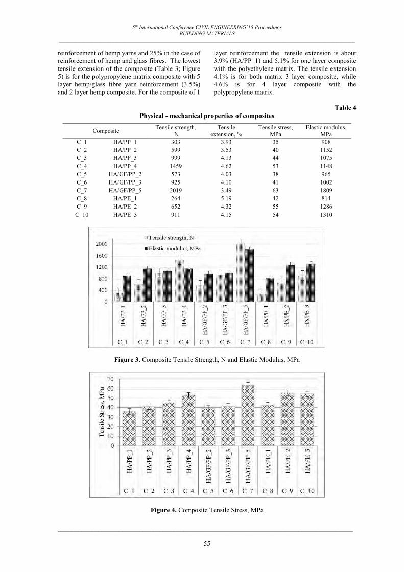
5th International Conference CIVIL ENGINEERING`15 Proceedings BUILDING MATERIALS
_____________________________________________________________________________________________________________
_______________________________________________________________________________________
55
reinforcement of hemp yarns and 25% in the case of reinforcement of hemp and glass fibres. The lowest tensile extension of the composite (Table 3; Figure 5) is for the polypropylene matrix composite with 5 layer hemp/glass fibre yarn reinforcement (3.5%) and 2 layer hemp composite. For the composite of 1
layer reinforcement the tensile extension is about 3.9% (HA/PP_1) and 5.1% for one layer composite with the polyethylene matrix. The tensile extension 4.1% is for both matrix 3 layer composite, while 4.6% is for 4 layer composite with the polypropylene matrix.
Table 4
Physical - mechanical properties of composites
Composite Tensile strength, N
Tensile extension, %
Tensile stress, MPa
Elastic modulus, MPa
C_1 HA/PP_1 303 3.93 35 908 C_2 HA/PP_2 599 3.53 40 1152 C_3 HA/PP_3 999 4.13 44 1075 C_4 HA/PP_4 1459 4.62 53 1148 C_5 HA/GF/PP_2 573 4.03 38 965 C_6 HA/GF/PP_3 925 4.10 41 1002 C_7 HA/GF/PP_5 2019 3.49 63 1809 C_8 HA/PE_1 264 5.19 42 814 C_9 HA/PE_2 652 4.32 55 1286
C_10 HA/PE_3 911 4.15 54 1310
Figure 3. Composite Tensile Strength, N and Elastic Modulus, MPa
Figure 4. Composite Tensile Stress, MPa

5th International Conference CIVIL ENGINEERING`15 Proceedings BUILDING MATERIALS
_____________________________________________________________________________________________________________
_______________________________________________________________________________________
56
0
1
2
3
4
5
HA
/PP_
1
HA
/PP_
2
HA
/PP_
3
HA
/PP_
4
HA
/GF/
PP_2
HA
/GF/
PP_3
HA
/GF/
PP_5
HA
/PE
_1
HA
/PE
_2
HA
/PE
_3
C_1 C_2 C_3 C_4 C_5 C_6 C_7 C_8 C_9 C_10
Tens
ile e
xten
sion
, %
Figure 5. Composite tensile extensions, %
0
10
20
30
40
50
60
HA
/PP_
1
HA
/PP_
2
HA
/PP_
3
HA
/PP_
4
HA
/GF/
PP_2
HA
/GF/
PP_3
HA
/GF/
PP_5
HA
/PE
_1
HA
/PE
_2
HA
/PE
_3
HA
/PE
_4
C_1 C_2 C_3 C_4 C_5 C_6 C_7 C_8 C_9 C_10 C_11
Thic
knes
s Sw
ellim
g, T
S, %
24h 48h 72h
Figure 6. Composite thickness swelling TS, %
For one layer composite with the polypropylene matrix, thickness swelling (Figure 6) was 10.6%-11.8%; for 2 layer composite it was 14.9%-24.4%; for 3 layer composite thickness swelling was 8.1%-16.5% and for 4 layer composite it was 7.5%-12.3%. The most significant thickness swelling was observed for the composites with the reinforcement of polypropylene with glass fibres addition past 48h -33% - 52% and 30% -37% past 72h, while for 5 layer composite thickness swelling was 5.9%-8.7%. For one layer composite with the polyethylene matrix thickness swelling was 11.1%-16.5%; for 2 layer composite it was 7.9%-18.0% and for 3 layer composite 10.9%- 12.9% and 9.5% - 10.1% for 4 layer composite. From the results of the tests that were carried out the water absorption in the
composites and thickness changes, it can be concluded that with the hemp yarn water uptake as well as by the hemp yarn damage with glass fibresin weaving process (C_6) a larger water uptake in the composite was observed. CONCLUSION
2D woven structures depending on the application and composite processing were executed using the plain weaving technique. Woven reinforcement production methods have a strong impact on mechanical properties. Such property as the tensile strength in the warp direction of the reinforcement is 14% higher for industrially made reinforcement, while in the weft direction it is 18% higher for a handmade reinforcement. The

5th International Conference CIVIL ENGINEERING`15 Proceedings BUILDING MATERIALS
_____________________________________________________________________________________________________________
_______________________________________________________________________________________
57
tensile stress is higher for handmade reinforcement on the weft direction (14%) and in the warp direction (3%) compared to the industrial made reinforcement. The tensile extension in both directions is lower for the industrial made reinforcement (2%- 4%). The tensile modulus in the warp direction is 20% higher for handmade reinforcement but in the weft direction for industrially made reinforcement - 14%. For composites of hemp and polypropylene or polyethylene yarns the increase of composite tensile strength (19%-41%) and tensile stress (6%- 17%) depending on the number of reinforcement layers, compared to the previous number of layers was observed.
Composite tensile extension (3.5-5.1%) and elastic modulus (814.85N-1809.64N) depend on the reinforcement used , matrix properties as well as the method of composite production. The changes in thickness from 8.74% (5 layer HA/GF composite) to 37.53% (3 layer HA/GF composite) by immersion in water for 72h were observed depending on the hemp yarn quality in the composite. The composites of hemp and polypropylene or polyethylene yarns are applicable for wall covering panels, because this is a stable and low weight material with predictable fibre and matrix proportions in reinforcement and changeable composite design as well as properties.
REFERENCES
Adamovičs A.et. al. (2014) Development of Farming and Removing Technology for Production of High Value Products of Industrial Hemp (CANNABIS SATIVA L) Report of the Ministry of Agriculture of Latvia, Latvia University of Agriculture, p.1-78, http://lathemp.lv
Bernava, A., Manins, M., Kukle, S. (2012), Natural Fibers Woven Structures for Composites Reinforcements, Journal of Biobased Materials and Bioenergy, Vol.6, No.4, p. 449-455.
Bernava A., Manins M., Kukle S. (2012), Mash Type Woven Structures for Composites Reinforcements, Book of Proceedings 12th Autex World Textiles Conference, Innovative Textile for High Future Demands: Croatia, Zadar, p.1623-1628.
Dammer L., Carus M., Raschka A., Scholz L.(2013), Market Developments of and Opportunities for biobased products and chemicals, Final report of nova-Institute for Ecology and Innovation, p. 1-67.
De Vasconcellos D. S., Touchard F., Chocinski-Arnault1 L. (2012) Cyclic Fatique Behavior of Woven Hemp Epoxy Composite Damage Analysis, Author manuscript published in: ECCM15 - 15TH European Conference on Composite Materials, Venice, Italy, p.1-8.
Funkea H., Gelbricha S., Ehrlicha A.(2013), Development of a new hybrid material of textile reinforced concrete and glass fibre reinforced plastic, Procedia Materials Science 2, p.103 – 110.
Hartig J., Jesse F., Häußler- Combe U. (2010), Evaluation of Experimental Setups for Determining the Tensile Strength of Textile Reinforced Concrete, Proceedings: International RILEM Conference on Material Science - 2nd ICTRC - Textile Reinforced Concrete - Theme 1, p. 117 – 127.
Hausding J., Engler T., Franzke G., Köckritz U., Cherif C. (2006), Plain Stitch –bonded Multi-Plies for Textile Reinforced Concrete, AUTEX Research Journal, Vol. 6, No 2, p. 81-90.
Hegger J., Zell M. & Horstmann M. (2008), Textile Reinforced Concrete – Realization in applications, Tailor Made Concrete Structures: New Solutions for our Society, Taylor & Francis Group, London, p. 357-362.
Lepenies I., Meyer C., Schorn H., and Zastrau B. (2007 ) Modeling of Load Transfer Behavior of AR-Glass-Rovings in Textile Reinforced Concrete, International Concrete Abstracts Portal, Special Publication, 244, p. 109-124, www.concrete.org/.../internationalconcreteabstractsportal?
Manins M., Bernava A., Strazds G. (2015), 2DWoven Reinforcements of Natural Fibers, Advanced Materials Research Vol. 1064, p. 77-82.
Manins, M., Kukle, S., Strazds, G., Bernava, A. (2011), Renewable Resource Integration in Biodegradable Composites, Environment. Technology. Resources: Proceedings of the 8th International Scientific and Practical Conference. Vol.2, p.139-144.
Nam G., Wu N., Okubo K., Fujii T. (2014) Effect of Natural Fiber Reinforced Polypropylene Composite Using Resin Impregnation, Agricultural Sciences, Vol. 5, p.1338-1343.
Parveen S., Rana S., Fangueiro R. ( 2012) Natural Fibre Composites for Structural Applications, Post conference book Mechanics of Nano, Micro and Macro Composite Structures, Torino, Italy, p.1-2.

5th International Conference CIVIL ENGINEERING`15 Proceedings BUILDING MATERIALS
_____________________________________________________________________________________________________________
_______________________________________________________________________________________
58
Singh B., Gupta M., Tarannum H., Randhawa A. (2011) Natural Fiber- Based Composite Building Materials, Cellulose Fibers Bio- Nano Polymer Composites, Springer –Verlag Berlin Heidelberg, p. 701-719.
Strazds G., Stramkale V., Laizāns T. (2012) Recommendations for Industrial Hemp Growers and Processors, Ieteikumi rūpniecisko kaņepju audzētājiem un pārstrādātājiem, Biznesa augstskola Turība, Ltd., Riga, Latvia, p.1-52 .
Westman M.P., Fifield L.S., Simmons K.L., Ladha S.G., Kafentris T.A. (2010) Natural Fiber Composites: A Review prepared for the U.S. Department of Energy, Contract DE-AC05-76RL01830, p.1-10. https://hal.inria.fr/file/index/docid/796853/filename/487.pdf

5th International Conference CIVIL ENGINEERING`15 Proceedings BUILDING MATERIALS
_____________________________________________________________________________________________________________
_______________________________________________________________________________________
59
IMPACT OF WETTING/OVEN-DRYING CYCLES ON THE MECHANICAL AND PHYSICAL PROPERTIES OF ORIENTED BOARD
Siim Kallau, Regino Kask, Harri Lille, Alexander Ryabchikov Estonian University of Life Sciences, Institute of Forestry and Rural Engineering
Address: Fr. R. Kreutzwaldi 5, 51014, Tartu, Estonia Phone: +372 731 3181
E-mail: [email protected]
ABSTRACT
The objective of this study was to explore some physical and mechanical properties and the dimensional stability of oriented strand board OSB/3 after 10 cycles of soaking/oven-drying. The properties to be determined were BS (bending strength), MOE (modulus of elasticity in bending), JH (Janka hardness) and thickness swelling (TS). The moisture content of the samples was altered by soaking for 24 hours and drying in a ventilated drying box. The study consisted of carrying out 3-point bending tests and static hardness tests with the INSTRON Universal Testing System 3369, deflection was measured by an optical gauge (Advanced Video Extensometer 2663-821). The sensitivity of the measured data was studied and the expanded uncertainties of the computed mean values are presented. An analytical equation was used for approximation of the change in the physical and mechanical properties of the samples depending on the number of cycles. It was shown that BS and MOE were affected by the number of soaking and drying cycles and they decreased significantly. The values of thickness, swelling and JH of the test pieces decreased significantly faster after the first three cycles and afterwards the values stabilized. The final values of BS, MOE, JH and TS after 10 cycles were 51-56%, 46%, 43% and 133% from the initial values, respectively. Key words: oriented strand board, bending strength, modulus of elasticity, static hardness, thickness swelling INTRODUCTION
The oriented strand board (OSB) should be according to EVS EN 300:2006 Grade OSB/3 moisture resistant. The mechanical properties of OSB are generally similar to those of particleboard, but it has a greater thickness swelling and poorer surface smoothness. Particleboards are used for cladding wall and ceiling indoors or outdoors as a floor decking material and a wind barrier. This kind of material is also applied in load bearing structures as the rigidity material and is also used as the formwork of concrete casting. The classifications of the OSB and the requirements of its mechanical properties are presented in EVS-EN 300:2006. The goal of this study was to explore two OSB/3 panels with the thickness of 12 mm (produced by the manufacturer ‘’KRONOSPAN Riga’’ SIA, former Bolderaja Ldt, Latvija). The OSB/3 panel as a wood-based sheet is a hygroscopic material and its dimensional stability and the mechanical and physical properties are dependent on the moisture content, number of soaking/oven-drying cycles and the ambient temperature. Changes in bending strength (BS), modulus of elasticity in bending (MOE), Janka hardness (JH), thickness swelling (TS) at different soaking/oven-drying cycles were investigated (Kallau, 2014). The basic method is to soak the samples in water during a fixed period of time (24 h), to dry them in a ventilated drying box a certain number of cycles
and then test them using the computer-controlled mechanically actuated universal test machine INSTRON 3369. After these procedures, output of data and analysis of the obtained results take place. The sensitivity of the measured data was studied and the expanded uncertainties of the computed mean values are presented. An analytical expression was used to approximate the experimental data for the investigated BS, MOE and JH depending on their soaking/oven-drying cycles. Experimental procedure and methods
The BS and the MOE were found by a three-point bending arranged in accordance with EN 310 (1993b) using the test machine INSTRON 3369 (Fig. 1). Deflection for calculating the modulus of elasticity was measured by an optical gauge (Advanced Video Extensometer 2663-821).
a)
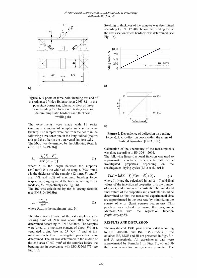
5th International Conference CIVIL ENGINEERING`15 Proceedings BUILDING MATERIALS
_____________________________________________________________________________________________________________
_______________________________________________________________________________________
60
b)
Figure 1. A photo of three-point bending test and of the Advanced Video Extensometer 2663-821 in the
upper right corner (a); schematic view of three-point bending test; location of testing area for
determining static hardness and thickness swelling (b)
The experiments were made with 11 series (minimum numbers of samples in a series were twelve). The samples were cut from the board in the following directions: one in the longitudinal (major) axis and the other in the transversal (minor) axis. The MOE was determined by the following formula (see EN 310 (1993b))
( )
( )
31 2 1
32 1
,4m
l F FE
bt a a
(1)
where l1 is the length between the supports, (240 mm); b is the width of the sample, (50±1 mm); t is the thickness of the sample, (12 mm); F1 and F2 are 10% and 40% of maximum bending force, respectively; a1, a2 are deflections according to the loads F1, F2, respectively (see Fig. 2b). The BS was calculated by the following formula (see EN 310 (1993b))
max 12
3 ,2mF lfbt
(2)
where Fmax, is the maximum load, N. The absorption of water of the test samples after a soaking time of 24 h was about 40% and was determined according to EN 322:2002. The samples were dried to a moisture content of about 8% in a ventilated drying box at 65 °C± 1º and at this moisture content all investigated properties were determined. The JH was determined in the middle of the end area 50×50 mm2 of the samples before the bending test in accordance with ISO 3350:1975 (see Fig. 1 b).
Swelling in thickness of the samples was determined according to EN 317:2000 before the bending test at the cross section where hardness was determined (see Fig. 1 b).
a)
b)
Figure 2. Dependence of deflection on bending force a); load-deflection curve within the range of
elastic deformation [EN 310] b) Calculation of the uncertainty of the measurements was done according to EN 326-1:2002. The following linear-fractional function was used to approximate the obtained experimental data for the investigated properties depending on the soaking/oven-drying cycles (Lille et al., 2014)
( ) ( )( ) ,/)( ffi YdcxYYdxY (3) where Yi, Yf are the calculated initial (x = 0) and final values of the investigated properties, x is the number of cycles, and c and d are constants. The initial and final values of the properties and constants should be determined so that the measured experimental data are approximated in the best way by minimizing the square of error (least squares regression). This problem was solved by using the programme Mathcad 15.0 with the regression function genfit(vx,vy,vg,F). RESULTS AND DISCUSSION
The investigated OSB/3 panels were tested according to EN 310:2002 and ISO 3350-1975 (E); the obtained BS, MOE and JH are presented in Figs. 3, 4 and 5, respectively. All experimental data were approximated by Formula 3. In Figs. 3b, 4b and 5b the mean values for one cycle are presented. The
Deflection a1
Load F
2
1
0250500750
1000
0 2 4 6 8Deflection, mm
Ben
ding
forc
e, N
– real curve 2 – approximation line

5th International Conference CIVIL ENGINEERING`15 Proceedings BUILDING MATERIALS
_____________________________________________________________________________________________________________
_______________________________________________________________________________________
61
experimental data of all properties fluctuated to a great extent. According to EN 300, the minimum allowed value of BS for the major axis was 20 N/mm2, the experimentally obtained mean after the third cycle was 18.7 N/mm2. The corresponding values for the minor axis was 10 N/mm2 and after the second cycle was 8.99 N/mm2. The BS after the first soaking cycle (24 h) at a moisture content of 40% was 52% and 54% of the values determined for air-dry samples (8%) for the major axis and for the minor axis, respectively (Kask et al., 2011). This value is below the valid minimum for the standard (EN 300:2006).
a)
b)
Figure 3. Dependence of BS on soaking/oven-
drying cycles: a) bar chart; b) mean values of the experimental data and the curves of approximation: major axis fm,i =24.6 N/mm2 and fm,f =2.4 N/mm2; minor axis fm,i =12.2 N/mm2 and fm,f =2.8 N/mm2
a)
b)
Figure 4. Dependence of MOE on soaking/oven-drying cycles: a) bar chart; b) mean values of the
experimental data and the curves of approximation: major axis Em,i =5233 N/mm2 and Em,f =2482
N/mm2; minor axis Em,i =2334 N/mm2 and Em,f =785 N/mm2
a)
b)
Figure 5. Dependence of JH on soaking/oven-drying cycles: a) bar chart; b) mean values of the
experimental data and the curves of approximation: major axis H8c,i =34.2 N/mm2 and H8c,f
=15.3 N/mm2
The gradient of the investigated properties was greater after the first soaking/oven-drying cycle: 24% for BS for the major axis and 17% for minor axis; for MOE, 18% for both axes, for JH as high as 40% and for TS, 15%. After ten soaking/oven-drying cycles all properties significantly lost their
0 2 4 6 8 100
10
20
30
40
50
60
C1y
C1 t( )
Cx t,
60
50
40
30
20
10
0 0 2 4 6 8 10 M
odul
us o
f ela
stic
ity, N
/mm
2
Number of soaking/oven-drying cycles
■ c=0.350 cycle-1 d=0.180
0 2 4 6 8 100
1200
2400
3600
4800
6000
7200
B1y
B2y
B1 t( )
B2 t( )
Bx Bx, t, t,
7200
6000
4800
3600
2400
1200
0 0 2 4 6 8 10 M
odul
us o
f ela
stic
ity, N
/mm
2
Number of soaking/oven-drying cycles
■ c=0.090 cycle-1 d=0.472 ▲ c=0.090 cycle-1 d=0.459
0 2 4 6 8 100
10
20
30
40
A1y
A2y
A1 t( )
A2 t( )
Ax Ax, t, t,
40
30
20
10
0 0 2 4 6 8 10
Ben
ding
stre
ngth
, N/m
m2
Number of soaking/oven-drying cycles
■ c=0.059 cycle-1 d=0.458 ▲ c=0.064 cycle-1 d=0.352

5th International Conference CIVIL ENGINEERING`15 Proceedings BUILDING MATERIALS
_____________________________________________________________________________________________________________
_______________________________________________________________________________________
62
initial values: for MOE less, 44%, for the major axis and for JH more, 57%. The BS and MOE decreased continuously with the increasing number of cycles. In air-dry conditions, also BS and MOE were more than two times greater for the major axis than for the minor axis. We can see that the proposed Formula (3) approximated the experimental data satisfactorily; constants c and d are close for BS and MOE.
a)
b)
Figure 6. Dependence of TS on soaking/oven-drying cycles: a) bar chart, b) diagram of thickness
change
The TS of the board did not change significantly after three soaking/oven-drying cycles, i.e. 21-22% (according to EN 300, the maximum allowed value is 15%). This has been observed in the case of wood. Swelling in wood takes place below the fibre saturation point (about 30%) at which the total amount of the water is present within the cell wall (Hiziroglu) and regardless of the number of soaking/oven-drying cycles, the dimensions do not change. This kind of phenomenon was observed to a certain extent in our experiments in the case of hardness (see Fig. 5). CONCLUSIONS
1. The final mean values determined at a moisture content of 8% after ten soaking/oven-drying cycles were: for MOE, 51% for the minor axis and 56% for the major axis, for BS 46%, for both axis, for JH, 43% and for TS, 133% of the respective initial values. 2. The maximum gradient of the investigated properties was recorded after the first soaking/oven-drying cycle: for BS, 24% for the major axis and 17% for the minor axis; for MOE, 18% for both axes, for JH, as much as 40% and for TS, 15%. 3. The proposed analytical function approximated the experimental data of BS, MOE and JH, depending on the number of soaking/oven-drying cycles, satisfactorily and allowed to predict to a certain extent the mechanical and physical properties of the samples when their values after applying a small number of soaking/oven-drying cycles were known. The presented analysis is limited to the data obtained from the experiments described above.
REFERENCES
EN 300:2006 E. Oriented Strand Boards (OSB) - Definitions, classification and specifications. Brussels. Management Centre. 20 p.
EN 310:1993. Wood-based panels - Determination of modulus of elasticity in bending and bending strength. Brussels. Central Secretariat. 7 p.
EN 317:1993. Particleboards and fibreboards - Determination of swelling in thickness after immersion in water. Brussels. Central Secretariat. 5 p.
EN 322:1993. Wood-based panels – Determination of moisture content. Brussels. Central Secretariat. 4 p.
EVS-EN 326-1:2002. Wood-based panels. Sampling, cutting and inspection. Part 1: Sampling and cutting of test pieces and expression of results. Tallinn. Eesti Standardikeskus. (in Estonian). 14 p.
Hiziroglu, S. Dimensional Changes in Wood. Oklahoma Cooperative Extension Service. Avaible oneline at http://pods.dasnr.okstate.edu/docushare/dsweb/Get/Rendition-3624
ISO 3350-1975 (E). Wood – Determination of static hardness. International Standard. 2 p.
Kallau, S. (2014). Impact of Wetting and Drying Cycles on Mechanical and Physical Properties of Oriented Strand Board Depending on the Cycle Count. M. Eng. Thesis. Tartu: Estonian University of Life Sciences. 96 p.

5th International Conference CIVIL ENGINEERING`15 Proceedings BUILDING MATERIALS
_____________________________________________________________________________________________________________
_______________________________________________________________________________________
63
Kask, R., Lille, H., Siim, K., Paabo, P., Sillaste, K. (2011). Study of Physical and Mechanical Properties of Oriented Board Depending on Moisture Content. In: 3rd International Conference CIVIL ENGINEERING`11 Proceeding, Jelgava, Latvia, pp 91-94
Lille, H., Kõo, J., Ryabchikov, A., Reitsnik, R., Veinthal, R., Mikli, V., Sergejev, F. (2013). Investigation of Residual Stresses and Some Elastic Properties of Brush-Plated Gold and Silver Coatings, Key Engineering Materials, Engineering Materials and Tribology, 527, pp 125–130.

ACOUSTIC PROPERTIES OF BINDERLESS PANEL MADE FROM PRETREATED HEMP (CANNABIS SATIVA L.) SHIVES
Raitis Brencis* Martins Andzs*; **, Ramunas Tupciauskas**, Prans Brazdausks**; ***, Janis Rizhikovs**, Maris Puke**, Aigars Paze**; ***, Kristine Meile**, Nikolajs Vedernikovs**
*Latvia University of Agriculture E-mail: [email protected]
**Latvian State Institute of Wood Chemistry E-mail: [email protected]
***Riga Technical University E-mail: [email protected]
ABSTRACT
In Latvia industrial hemp cultivation is rapidly growing. A study of binderless panel made from hemp (Cannabis sativa L.) shives after hydrothermal pretreatment and steam explosion treatment is reported. The acoustic properties of the panels were determined by means of the sound absorption coefficient (αw) determined according to standards ISO 10534-2:2001 and 11645:2000. The average sound absorption coefficient (αw) of the panels reached between 0.10 ÷ 0.15 and varies in all frequency ranges (250 – 4000 Hz) between 0.05 ÷ 0.90 depending on the raw material treatment and hot-pressing conditions. According to the standard EN ISO 11645:2000, the obtained sound absorption coefficients of binderless panels conform to Class E absorbent, which is the lowest rate.
Key words: hemp (Cannabis sativa L.) shives, hydrothermal pretreatment, steam explosion treatment, binderless panel, acoustic properties.
INTRODUCTION
Today renewable resources of biomass (wood and agricultural residues, shrubs, etc.) are a real alternative to oil as a raw material for the production of chemicals and motor fuel. However, biomass pretreatment is needed to obtain such products. The biomass pretreatment process most commonly means hydrolysis of biomass components such as hemicelluloses, lignin and cellulose. The pretreatment process is one of the most important stages further in the biomass processes, where the mechanical and chemical structure of the biomass cell wall is changed, as well as making it easier to convert to other valuable products (boards, bioethanol, levoglucosane, etc.) in further processing (Yang et al., 2012). The increasing demand for platform chemicals derived by the chemical industry increases the demand for furfural, which is exclusively obtained from biomass containing hemicelluloses. It is used for the production of a wide range of important non-petroleum derived chemicals such as furan, tetrahydrofuran and furfuryl alcohol (Lange et al., 2012). One of the biomass examples is the hemp plant consisting of long (bast) fibres and woody part of the stem with short fibres called shives. The main utilization of hemp as a crop is for its bast fibres until now (Shahzad, 2012). However, the high content of hemicelluloses of the shives (Table 1) shows its great potential for furfural production. Also, this valuable raw material is concentrated in one place at the fibre production manufacturer’s site. The hemp species have been approved and are a rapidly expanding crop in Latvia with a yield from 150 ha in 2009 to 1200 ha in 2013.
The hemp shives make up to 75% of the oven dry stalk. The high content of such chemical components of the hemp shives as cellulose and lignin, like a relatively low content of minerals (Table 1), confirm that the crop also has a potential for production of binderless panels.
Table 1 Chemical Components of Shives of Hemp Species
“Bialobrzeskie”
Chemical component Percentage Cellulose 43.7 ± 0.4 Hemicelluloses 31.8 ± 0.7 Lignin 22.0 ± 0.6 Minerals (ash) 1.6 ± 0.1
To utilize leftover lignocellulose after obtaining furfural, binderless panels could be made by using no additional adhesives at all during the panels’ production process. The panels made from shives after catalyzed pretreatment may have improved water resistance because the hemicelluloses are the most water absorbing component (Garrote et al., 2001) and after the pretreatment its content is significantly diminished. Furthermore, steam explosion (SE) treatment transforms the lignin structure in the plant matrix and promotes the binderless composite moulding in the following hot-pressing process (Okuda et al., 2006; Shao et al., 2009; Tupciauskas et al., 2011). Materials obtained from secondary feedstock, such as glass, rubber (Pastor 2014), industrial residues
_______________________________________________________________________________________ 64

(Garcia-Valles et al., 2008), tyres (Maderuelo-Sanz et al., 2012) etc. can be developed to produce acoustic absorbents. Analysing typical absorption materials and their ability to muffle the sound in different frequency ranges has a situation where the panel absorbents are highly adept in the low frequency range. The Helmholtz resonator absorber in the average frequency range with a very pronounced absorption in narrow frequency range and porous absorbers are efficient in the high frequency range (Fig 1. Fahy, 2005).
00.10.20.30.40.50.60.70.80.9
125 1000
Figure 1. Typical sound absorption coefficient of materials in various frequency ranges: porous absorber, Helmholtz resonator, panel
absorber.
A wide range of biomaterials has been used for production of acoustic panels, for example, kenaf, sunflower, maize, Jerusalem artichoke, miscanthus (Balduci et al., 2008) coir (Fouladi, 2010; Fouladi, 2011) etc. On average, the highest values of the absorption coefficient of these materials can be reached in the region above 2000 Hz. They are not applicable as separate panels for finishing or shielding operations, since they are loose, porous or soft materials. Previous studies about hemp shives acoustic absorption ability depending on the fractional composition and binder content (Gle, 2011; Gle, 2012) showed that satisfactory results can be obtained if about 26% of the binder was used for moulding of the panels. If a lower amount of binder was used, the absorption coefficients of the panels were close to those of raw material. Binderless panels are thin (6÷8 mm) and are classified as a panel absorber in an efficient absorption low frequency range. Previous investigations concerning the ability of natural fiber to be employed as a sound absorber have been carried out (Putra et al., 2013). However, according to our knowledge acoustic absorption of binderless panels made of hemp shives has not been previously investigated. The objective of
the study was to investigate acoustic properties of binderless panels as an absorption material.
MATERIALS AND METHODS
The study of binderless panels from pretreated hemp (Cannabis sativa l.) shives is a part of the biorefinery concept illustrated in Fig. 2. Raw material
The shives of the hemp variety “Bialobrzeskie” (Poland, code 893) was chosen as a raw material. The chemical and elemental composition given in Table 1 was determined as described in Gandofi et al., 2013. The raw material was fractionated by a MUOTOTERA OY classifier using 5 screens according to SCAN-CM 40:01, 2013. For further processing the fraction 3–12 mm, which comprises 77% of the residues of hemp fibre production, was used to homogenize the raw material and to avoid the presence of undesirable compounds such as sand and long fibres.
Figure 2. Complex utilization of hemp shives obtaining value added products.
Hydrothermal pretreatment
Lignocellulosic residue for the panels moulding was obtained by the hydrothermal pretreatment process of hemp shives, carried out in a specially constructed 13.7 L bench scale laboratory reactor equipped with a steam jacket in continuous steam flow (200 mL/min) conditions described elsewhere (Brazdausks et al., 2013; 2014). Temperatures of 160°C, 170°C and 180°C were chosen and the duration of the process was 90 min. Before the process, the raw material was mixed with a calculated amount of the catalyst Al2(SO4)3 – 5 wt% of the oven dry sample. Further in the paper the hemp shives samples after the hydrothermal pretreatment are defined as H160, H170 and H180. Steam explosion (SE) treatment
A part of each pretreated lignocellulosic leftover was additionally steam-exploded in a 0.5 L batch reactor (Tupciauskas et al., 2011) to liberate lignin from the cell
_______________________________________________________________________________________
65 65
Hemp shives
Hydrothermal pretreatment
Lignocellulose
Steam explosion
Moulding of panels
Binderless panels
Furfural Frequency, Hz
Soun
d ab
sorp
tion
coef
ficie
nt

wall to the fibre surface since the lignin is the most important component relevant to binderless panel production (Okuda et al., 2006; Shao et al., 2009). The SE treatment conditions for all pretreated samples were the same: temperature 235°C and time 5 s. Further in the paper the hemp shives samples after the pretreatment and SE treatment are defined as H160SE, H170SE and H180SE. Panel manufacture
After the pretreatment and SE treatment hemp shives were air dried (25±2°C) and hot-pressed at one stage press under 3 MPa pressure (p) by four regimes for each pretreatment temperature and SE treatment samples, varying the temperature (T), time (t) and moisture content (MC) as shown in Table 2. Further in the paper the panel samples indicating the manufacture regime given in Table 2 are defined as e.g. H160_2, H170SE_1, etc. Precisely weighed lignocellulosic materials were pre-pressed under 2±1 MPa for 7±3 s using a frame. Untreated hemp shives were used as reference material (Ref in Table 2) pressing under 5 MPa pressure because of the material non pretreated structure. The set density of all samples was 1000 kg m-3 and the set panel dimensions 100×100×7 mm.
Table 2 Panel manufacturing conditions
No T, °C t, min MC, % p, MPa 1 150±2 15 10±2 3±0.2 2 160±2 15 10±2 3±0.2 3 160±2 15 5±2 3±0.2 4 170±2 10 5±2 3±0.2 Ref 200±2 15 7±2 5±0.2
Determination of panel acoustic absorption
Determination procedure for the panel’s acoustic absorption properties was carried out for 3 parallel samples from each panel and obtained values were averaged, and the relative error of measurements was less than ±5%. The measurements of the sound absorption coefficient (αw) in frequency ranges 250; 500; 1000; 2000; 4000 Hz were performed for binderless panel samples in an impedance tube (Ø 40 mm) by applying two microphone transfer function method according to ISO 10534-2:2001 and ISO 11645:2000. RESULTS AND DISCUSSION
Binder-less panels made from hemp shives after pretreatment and steam explosion (SE) have an average sound absorption coefficient (αw) between 0.10 ÷ 0.15 and vary in all frequency range between 0.05 ÷ 0.90. The highest absorption coefficient was observed in the
frequency range of 2000 ÷ 4000 Hz with the highest value at 4000 Hz (Table 3), which is logical due to the material's ability to absorb higher frequencies. The sound absorption coefficient at low-frequency region (250 ÷ 1000 Hz) is almost similar for all samples, and it is below 0.15.
Table 3 Average sound absorption coefficients of panel
sample groups
Sample group
250 Hz
500 Hz
1 kHz
2 kHz
4 kHz αW
H160 0.05 0.05 0.10 0.55 0.90 0.10 H170 0.10 0.10 0.15 0.25 0.40 0.10 H180 0.05 0.10 0.15 0.20 0.25 0.15
H160SE 0.10 0.10 0.15 0.20 0.25 0.10
H170SE 0.10 0.10 0.20 0.30 0.40 0.15
H180SE 0.10 0.10 0.10 0.15 0.20 0.10 Ref 0.05 0.05 0.10 0.45 0.30 0.10
Sample Ref. results of the highest sound absorption value were achieved at 2000 Hz. The sample is made of hemp shives without pretreatment and then the surface formed roughness and open cavities which discharge sound material and muffles it, turning it into heat energy. The sample Ref. curve of sound absorption coefficient in the frequency range (Fig. 4) is characterized by Helmholtz resonator type absorbents (Fig. 1), but not the type of absorbent panels. The results obtained showed that in the low frequency range (below 2000 Hz) there is no direct impact of the panels manufacture conditions on the acoustic absorption coefficients, but indirectly they are affected by changing physical properties of the pretreated and steam-exploded hemp shives (Fig. 3). The highest sound absorption coefficients were reached in the frequency range of 4 kHz for panel samples made from pretreated shives at 160°C and 170°C and then steam-exploded one. (H160, H170, H170SE, Table 3). Assessing the impact on raw material treatment, the panels obtained from pretreated and then steam-exploded materials did not have significant differences on average value of αw; however, there were significant differences in some frequency ranges (samples H160 and H160SE, H170 and H170SE in Table 3). The αw significantly increases in all frequency range almost for all obtained panel samples except of Reference sample (Fig. 3). Maximal value of αw of sample made from raw shives (Ref) was achieved at 2000 Hz. After the pretreatment of shives at 160°C the maximal value of αw increases from 0.45 to 0.90 at the highest frequency (samples Ref and H160, Table 3). Increasing the raw material pretreatment temperature up to 180°C, the αw tends to decrease in the frequency range between 2000 ÷4000 Hz but in the frequency range between 500 ÷ 1000 Hz the αw tends to increase, however, the average value did not improve (samples H160, H170, H180, Table 3).
_______________________________________________________________________________________ 66

R² = 0.9588
R² = 0.6704
R² = 0.7635R² = 0.4955
R² = 0.4184R² = 0.7955
R² = 0.7821
0.00.10.20.30.40.50.60.7
0.80.91.0
0 1000 2000 3000 4000 5000
Soun
d A
bsor
ptio
n C
oefic
ient
Frequency, Hz
H160
H170
H180
Ref 2
H160_SE
H170_SE
H180_SE
Figure 3. Panel sound absorption coefficient depending on hemp shives treatment.
0.00
0.10
0.20
0.30
0.40
0.50
0.60
0.70
0.80
0.90
0 500 1000 1500 2000 2500 3000 3500 4000
Soun
d ab
sorb
tion
coef
fieci
ent
Frequency, Hz
Ref
H160_2
H160_SE_1
H160_SE_2
H160_SE_3
H160_SE_4
Figure 4. Panel sound absorption coefficient depending on the manufacture conditions from shives pretreated
at 160°C.
0.00
0.10
0.20
0.30
0.40
0.50
0.60
0 500 1000 1500 2000 2500 3000 3500 4000
Soun
d ab
sorb
tion
coef
fieci
ent
Frequency, Hz
H170_1H170_3H170_4H170_SE_1H170_SE_2H170_SE_3H170_SE_4
Figure 5. Panel sound absorption coefficient depending on manufacture conditions from shives pretreated at
170°C. _______________________________________________________________________________________ 67
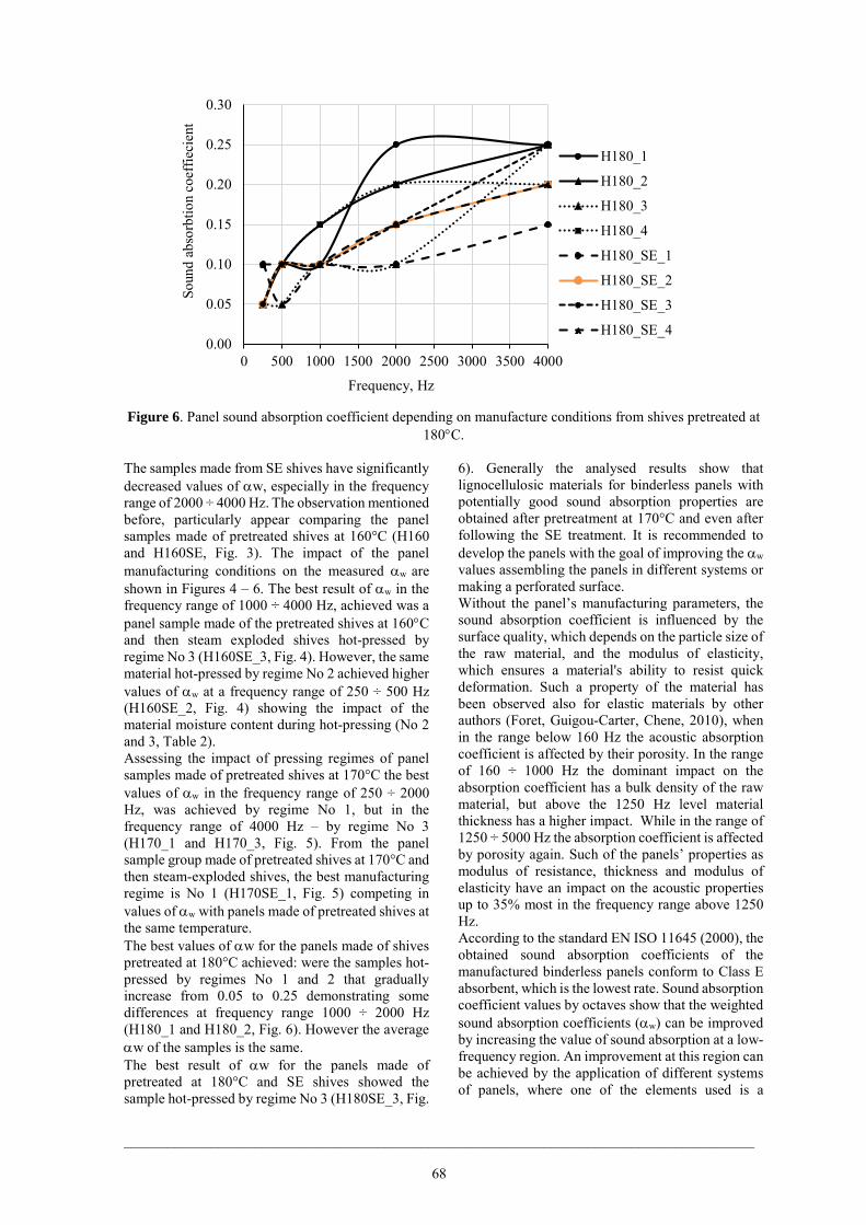
0.00
0.05
0.10
0.15
0.20
0.25
0.30
0 500 1000 1500 2000 2500 3000 3500 4000
Soun
d ab
sorb
tion
coef
fieci
ent
Frequency, Hz
H180_1
H180_2
H180_3
H180_4
H180_SE_1
H180_SE_2
H180_SE_3
H180_SE_4
Figure 6. Panel sound absorption coefficient depending on manufacture conditions from shives pretreated at
180°C.
The samples made from SE shives have significantly decreased values of αw, especially in the frequency range of 2000 ÷ 4000 Hz. The observation mentioned before, particularly appear comparing the panel samples made of pretreated shives at 160°C (H160 and H160SE, Fig. 3). The impact of the panel manufacturing conditions on the measured αw are shown in Figures 4 – 6. The best result of αw in the frequency range of 1000 ÷ 4000 Hz, achieved was a panel sample made of the pretreated shives at 160°C and then steam exploded shives hot-pressed by regime No 3 (H160SE_3, Fig. 4). However, the same material hot-pressed by regime No 2 achieved higher values of αw at a frequency range of 250 ÷ 500 Hz (H160SE_2, Fig. 4) showing the impact of the material moisture content during hot-pressing (No 2 and 3, Table 2). Assessing the impact of pressing regimes of panel samples made of pretreated shives at 170°C the best values of αw in the frequency range of 250 ÷ 2000 Hz, was achieved by regime No 1, but in the frequency range of 4000 Hz – by regime No 3 (H170_1 and H170_3, Fig. 5). From the panel sample group made of pretreated shives at 170°C and then steam-exploded shives, the best manufacturing regime is No 1 (H170SE_1, Fig. 5) competing in values of αw with panels made of pretreated shives at the same temperature. The best values of αw for the panels made of shives pretreated at 180°C achieved: were the samples hot-pressed by regimes No 1 and 2 that gradually increase from 0.05 to 0.25 demonstrating some differences at frequency range 1000 ÷ 2000 Hz (H180_1 and H180_2, Fig. 6). However the average αw of the samples is the same. The best result of αw for the panels made of pretreated at 180°C and SE shives showed the sample hot-pressed by regime No 3 (H180SE_3, Fig.
6). Generally the analysed results show that lignocellulosic materials for binderless panels with potentially good sound absorption properties are obtained after pretreatment at 170°C and even after following the SE treatment. It is recommended to develop the panels with the goal of improving the αw values assembling the panels in different systems or making a perforated surface. Without the panel’s manufacturing parameters, the sound absorption coefficient is influenced by the surface quality, which depends on the particle size of the raw material, and the modulus of elasticity, which ensures a material's ability to resist quick deformation. Such a property of the material has been observed also for elastic materials by other authors (Foret, Guigou-Carter, Chene, 2010), when in the range below 160 Hz the acoustic absorption coefficient is affected by their porosity. In the range of 160 ÷ 1000 Hz the dominant impact on the absorption coefficient has a bulk density of the raw material, but above the 1250 Hz level material thickness has a higher impact. While in the range of 1250 ÷ 5000 Hz the absorption coefficient is affected by porosity again. Such of the panels’ properties as modulus of resistance, thickness and modulus of elasticity have an impact on the acoustic properties up to 35% most in the frequency range above 1250 Hz. According to the standard EN ISO 11645 (2000), the obtained sound absorption coefficients of the manufactured binderless panels conform to Class E absorbent, which is the lowest rate. Sound absorption coefficient values by octaves show that the weighted sound absorption coefficients (αw) can be improved by increasing the value of sound absorption at a low-frequency region. An improvement at this region can be achieved by the application of different systems of panels, where one of the elements used is a
_______________________________________________________________________________________ 68

binderless panel with an additional perforation or by increasing the panel thickness (Schmidt 1969).
CONCLUSIONS
It is possible to obtain binderless panels from untreated hemp shives and from pretreated ones and also from steam-exploded ones. The weighted sound absorption coefficient (αw) for the investigated binderless panels is 0.10 ÷ 0.15 and varies in all frequency ranges (250 ÷ 4000 Hz) between 0.05 ÷ 0.90 depending on the raw material treatment and hot-pressing conditions. According to the standard EN ISO 11645 (2000) the obtained sound absorption coefficients of the binder-less panels conform to Class E absorbent, which is the lowest rate. Binder-less panels from pretreated hemp shives can be used as acoustic absorbent in the frequency region above 2 000 Hz. Generally the analysed results show that lignocellulosic materials for binder-less panels with potentially good sound absorption properties are
obtained after pretreatment at 170°C and even after following SE treatment. The best sound absorption coefficients for the panels achieved by hot-pressing regimes No 1, 2 and 3 indicated the pressing temperature of 150°C and 160°C, time 15 min and moisture content of lignocellulosic material between 5 and 10%. However the moisture content was found to be too high threatening the delamination of the panels after opening the press. It is recommended developing the panels with the goal of improving the αw values assembling the panels in different systems or making a perforation.
ACKNOWLEDGEMENTS
The study was implemented within the Europe Social Fund framework “Innovative technology for complex processing of fibrous crop residues to products with high added value” No. 2013/0044/1DP/1.1.1.2.0/13/APIA/VIAA/022.
REFERENCES Balduci F., Charles H., Meinlschmidt P., Dix B., Sanasi A. (2008) Development of Innovative Particleboard Panels. Drvna Industrija, Vol. 59, No. 3, p. 131–136.
Brazdausks P, Puke M, Vedernikovs N, Kruma I. (2014) Effect of the amount of the catalyst on the formation of furfural and acetic acid from birch wood in the biomass pretreatment process. Baltic Forestry, Vol. 20, No.1, p. 106–114.
Brazdausks P, Puke M, Vedernikovs N, Kruma I. (2013) Influence of biomass pretreatment process time on furfural extraction from birch wood. Scientific Journal of Riga Technical University. Environmental and Climate Technologies, Vol. 11, p. 5–11.
Fahy F., (2005) Foundation of engineering acoustics, London, Academic press, Elsevier, 465 p.
Foret R., Guigou-Carter C., Chene J.B. (2010) Porous material parameters influencing the acoustic performances of building construction systems. In: International sceintific conference „Internoise 2010, noise and sustainability”, 13-16 June 2010 Lisbon Portugal, p. 1-10. CD
Fouladi M.H., Ayub Md., Mohd Nor M. J. (2011) Analysis of coir fiber acoustical characteristics. Applied Acoustics, Vol. 72, p. 35–42.
Fouladi M.H., Mohd Nor M. J., Ayub Md., Leman Z.A. (2010) Utilization of coir fiber in multilayer acoustic absorption panel. Applied Acoustics, Vol. 71, p. 241–249.
Gandofi S., Gianluca O., Riva S., Fantoni G.P., Patel I. (2013) Complete chemical analysis of Carmagnola hemp hurds and structural features of its components. BioResources, Vol. 8, No. 2, p. 2641–2656.
Garcia-Valles M., Avila G., Martinez S., Terradas R., Nogués J.M. (2008) Acoustic barriers obtained from industrial wastes. Chemosphere, Vol 72, p. 1098–1102.
Garrote G., Domínguez H., Parajó J.C. (2001) Study on the deacetylation of hemicelluloses during the hydrothermal processing of Eucalyptus wood. Holz als Roh- und Werkstoff, Vol. 59, No. 1–2, p. 53–59.
Gle P., Gourdon E., Arnaud L. (2011) QAcoustical properties of materials made of vegetable particles with several scales of porosity. Applied Acoustics, Vol. 72, p. 249–259.
Gle P., Gourdon E., Arnaud L. (2012) Modeling of the acoustical properties of hemp particles. Construction and building materials, Vol. 37, p. 801–811.
ISO 10534-2:2001. Acoustic-Determination od sound absorption coefficient and impedance tubes Part 2: Transfer function method. ISO 11645:2000. Acoustics - Sound absorbers for use in buildings - Rating of sound absorption.
_______________________________________________________________________________________ 69

Lakra R., Kiran M.S., Usha R., et al. (2014) Enhanced stabilization of collagen by furfural. International Journal of Biological Macromolecules, Vol. 65, p. 252–257.
Lange J.-P., Van Der Heide E., Van Buijtenen J., Price R. (2012) Furfural - A promising platform for lignocellulosic biofuels. ChemSusChem, Vol. 5, No. 1, p. 150–166.
Maderuelo-Sanz R., Nadal-Gisbert A.V., Crespo-Amorós J.E., Parres-García F. (2012) A novel sound absorber with recycled fibers coming from end of life tires (ELTs). Applied Acoustics, Vol. 73, p. 402–408. Okuda N., Hori K., Sato M. (2006) Chemical changes of kenaf core binderless boards during hot pressing (I): influence of the pressing temperature condition. Journal of wood science, Vol. 52, No. 3, p. 244–248.
Pastor J.M., Garcia L.D., Quintana S., Pena J. (2014) Glass reinforced concrete panels containing recycled tyres: Evaluation of the acoustic properties of for their use as sound barriers. Construction and building materials, Vol. 54, p. 541–549.
Putra A., Abdullah Y., Efendy H., Farid W.M., Ayob Md R, Py M. S., (2013) Utilizing Sugarcane Wasted Fibers As A Sustainable Acoustic Absorber. Procedia Engineering,Vol. 53, p. 632–638;
SCAN-CM 40:01 (2001) Wood chips for pulp production. Size distribution. Scandinavian pulp, paper and board testing committee.
Schmidt L.M. (1969) Acoustic materials. Moscow: Stroyizdat, 175 p.
Shahzad A. (2012) Hemp fiber and its composites - A review. Journal of Composite Materials, Vol. 46, No. 8, p. 973–986.
Shao S., Jin Z., Wen G., Iiyama K. (2009) Thermo characteristics of steam-exploded bamboo (Phyllostachys pubescens) lignin. Wood Science and Technology, Vol. 43, No. 7–8, p. 643–652.
Tupciauskas R., Gravitis J., Veveris A., Tuherm H. (2009) Self-binding fibreboard made of steam exploded wood. In: Proceedings of the 5th meeting of the Nordic-Baltic network in wood material science and engineering (WSE), October 1-2, 2009, Copenhagen, Denmark. A. Bergstedt (ed.). Forest & Landscape Working Paper, No. 43, p. 141–146.
Yang W., Li P., Bo D., et al. (2012) The optimization of formic acid hydrolysis of xylose in furfural production. Carbohydrate. Research, Vol. 375, No. 1, p. 53–61. Zeitsch K. J. (2000) The chemistry and technology of furfural and its many by-products. Amsterdam: Elsevier Science, 376 p. ______________________________________________________________________________________ 70

5th International Conference CIVIL ENGINEERING`15 Proceedings HEAT ENGINEERING
_____________________________________________________________________________________________________________
_______________________________________________________________________________________
71
GENERATION OF A TYPICAL METEOROLOGICAL YEAR FOR ALŪKSNE, LATVIA
Mārtiņš Ruduks Latvia University of Agriculture, Department of Architecture and Building
Email: [email protected] Arturs Lešinskis
Riga Technical University, Institute of Heat, Gas and Water Technology Email: [email protected]
ABSTRACT
Meteorological conditions vary significantly from year to year. For this reason, there is a need to create a typical meteorological year (TMY) data model, to represent the long term weather conditions over a year. TMY data is one of the main sources for successful building energy simulations. Two different typical meteorological data models were generated and compared: TMY and TMY-2. Both models where created by analysing every 3-hour weather data for a 30-year period (1984–2013) in Alūksne, Latvia, provided by the Latvian Environment Geology and Meteorology Centre (LEGMC). TMY model was created using statistical approach, but to create second model - TMY-2, 30 year average data were applied. In the TMY model creation representative typical meteorological months (TMM) were selected. TMM for each of the 12 calendar months were selected by choosing the one with the smallest deviation from the long-term average weather data. The 12 TMMs, selected from the different years, were used to create a TMY for Alūksne. The data gathered from TMY and TMY-2 models where compared with the climate data from the Latvian Cabinet of Ministers regulation No. 379, Regulations Regarding Latvian Building Code LBN 003-01. Average monthly temperature values in LBN 003-01 were lower than the TMY and TMY-2 values. TMY selection process should include the most recent meteorological observations and should be periodically renewed to reflect the long term climate change.
Key words: Typical meteorological year; climate change, building energy simulations INTRODUCTION
In Latvian legislation long-term climate data are reflected in the Latvian Building Code (LBN) 003-01 „Būvklimatoloģija” (23.08.2001, Riga), where various climatic indicators are shown that represents the climatic situation in the territory of Latvia, providing information about the average monthly and yearly meteorological parameters. But this information is not sufficient to fully describe the region’s climatic conditions, because there is a necessity to define the daily and hourly meteorological data values. The need of such meteorological data worldwide led to the development of methodologies for generating the typical meteorological year (TMY). TMY is data set that contains a sequence of 8 760 hourly values of chosen meteorological quantities. The requirement of TMY is that it has to correspond to an average year (Skeiker, 2004). TMY provides hourly climatic parameter values, enabling one to use these parameters for heating, ventilation and air conditioning (HVAC) device management and capacity optimisation.
Creation of the TMY was introduced in 1978 by Hall et al. (Hall et al., 1978). For a network of stations in the United States, a representative database consisting of weather data was created. Hall’s method has been used to successfully generate TMYs for a number of locations across the globe (Chan et al., 2006; Guggenberger et al., 2013; Hall et al., 1978; Jiang, 2010; Kalogirou, 2003; Lee et al., 2010; Skeiker, 2007; Skeiker, 2004; Yang, et al., 2007; Zang et al., 2012; Zariņš, 2001; Zhang, 2006).
Figure 1. Location of Alūksne
HEAT ENGINEERING

5th International Conference CIVIL ENGINEERING`15 Proceedings HEAT ENGINEERING
_____________________________________________________________________________________________________________
_______________________________________________________________________________________
72
LBN 003-01 describes climate parameters for ten cities in Latvia. These parameters have been calculated using data from 1961-1990. The aim of this research is to generate a representative climate database for one of these cities – Alūksne, by employing the method that has been proposed by Hall et al. (Hall et al., 1978) and adapted in Latvia by Zariņš (Zariņš, 2001). Generation of The TMY of Alūksne would provide hourly climate data that LBN 003-01 does not provide. Geographical data for Alūksne: latitude 57°26’ N; longitude 27°02’ E; on a relatively flat surface, elevated 193 m above sea level, located 160 km from the Gulf of Riga (Fig.1).Average temperature is 4.5 °C. The TMY is generated by using the available weather data obtained from the station of Alūksne by the Latvian Environment Geology and Meteorology Centre (LEGMC), covering the period from 1984–2013. LEGMAC database provides 3-hour weather data values for temperature and relative humidity. This is the first time in Latvia when 30 year weather data have been used to create a TMY. MATERIALS AND METHODS
The TMY models where created applying two different TMY creation methods. TMY model was created by using method that was described by Hall et al. (Hall et al., 1978) and adapted in Latvia by Zariņš (Zariņš, 2001). The second TMY model – TMY-2 was created by applying the average meteorological year method (Skeiker, 2007). The TMY model consists of weather data that have been observed in one of the 30 year periods. This method includes temperature peaks that can be used to determine the appropriate power for HVAC systems. The TMY-2 model consists of the averaged 30 year weather data, this method does not show the temperature peaks, but it shows the most precise average monthly temperatures. The TMY-2 model is best used for calculating average long-term building energy consumptions for HVAC systems. TMY creation
Climate data for TMY creation were obtained from the LEGMC database from 1984–2013. LEGMC provides climate data with 3 hour intervals, but TMY needs hourly climate data. The necessary data for TMY were calculated by linear interpolation. In February there may be 28 or 29 days, and it is not possible to compare years with a different count of days, e.g. the 29th day. February was excluded from the TMY creation. The rest of the days where rearranged in ascending order starting with the first hour of January till the last hour of December (8 760 values).
For each month the temperature distribution was calculated – how many hours per month each of the temperatures (in the range from –35 °C to 35 °C) was observed. This procedure was used for each month of the 30 year period. Each month can be included in the TMY, but before it is determined it is called a candidate month. Adapted Halls TMY creation method (Hall et al., 1978) tries to find the most typical month – typical meteorological month (TMM), for each of the 12 months (January–December), from the observed time period (1984–2013). To determine the TMM for each of the 12 calendar months, each month’s temperature distribution was compared with the temperature distribution from a 30 year period. The sum of the square error (SSE) parameter was used (equation 1) to compere months. When all 30 year SSE values were compared the month that had the lowest value of SSE (equation 2) was chosen as the TMM and was included in the TMY. This action was applied for all 12 calendar months.
n
iii xxSSE
1
2)( (1)
where ix - temperature distribution value in a candidate month;
ix - temperature distribution value from 30 year average data
min)(1
2
n
iii xxSSE (2)
where ix - temperature distribution value in a candidate month;
ix - temperature distribution value from 30 year average data
All the TMMs were combined and TMY was generated, but as TMM where from different years and there was mismatch of values at the connecting point of two TMM. Last 6 hours of the preceding month and the first 6 hours of the following month were smoothened by replacing them with the average values. The TMY model includes temperature and relative humidity values, temperature values are selected as described, but relative humidity values for the TMY are determined according to the selected TMM. Relative humidity values are smoothened at the connecting point of two TMM like with the temperature.
TMY-2 creation
The TMY-2 model was created with average meteorological year method (Skeiker, 2007). In this method the same climate data were used as it was in

5th International Conference CIVIL ENGINEERING`15 Proceedings HEAT ENGINEERING
_____________________________________________________________________________________________________________
_______________________________________________________________________________________
73
TMY model creation. And they were arranged starting from the first hour of January till the last hour of December. Each of the TMY-2 model 8 760 temperature and relative humidity values was calculated by averaging this value from 30 year data.
RESULTS AND DISCUSSIONS
TMY was created combining TMMs that are determined based on their ability to follow the long
term distribution. Selected month/year combinations from which the TMY was created are shown in Fig. 2. Two months (November, and December) were selected from one year (1989), but other months were selected from different years. This displays that TMMs are selected from all ranges of the observed period.
Figure 2. The Month/Year combinations for the composition of TMY
Figure 3. Temperature fluctuation in TMY

5th International Conference CIVIL ENGINEERING`15 Proceedings HEAT ENGINEERING
_____________________________________________________________________________________________________________
_______________________________________________________________________________________
74
After TMMs were connected and the TMY was created, temperature fluctuation (Fig. 3), temperature distribution (Fig. 5), relative humidity fluctuation (Fig. 4) and relative humidity distribution (Fig. 6) was displayed. When TMY and TMY-2 temperature distribution values are compared with the 30 year average data (long term data) (Fig. 5), TMY shows good
agreement with the long term data. TMY value deviation from long term data is a maximum 100 hours per year at 3 °C, but TMY-2 deviation at –5 °C is more than 470 hours per year. The difference between TMY and TMY-2 models can be explained by the fact that TMY-2 is made averaging climate data and it does not contain the maximum and minimum temperature values.
Figure 4. Relative humidity fluctuation in TMY
Figure 5. Hourly temperature distribution for TMY, TMY-2 and 30 year average data
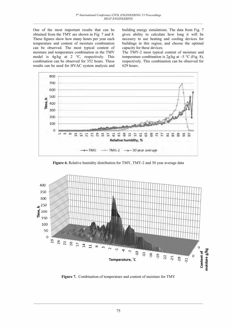
5th International Conference CIVIL ENGINEERING`15 Proceedings HEAT ENGINEERING
_____________________________________________________________________________________________________________
_______________________________________________________________________________________
75
One of the most important results that can be obtained from the TMY are shown in Fig. 7 and 8. These figures show how many hours per year each temperature and content of moisture combination can be observed. The most typical content of moisture and temperature combination in the TMY model is 4g/kg at 2 °C, respectively. This combination can be observed for 352 hours. These results can be used for HVAC system analysis and
building energy simulations. The data from Fig. 7 gives ability to calculate how long it will be necesery to use heating and cooling devices for buildings in this region, and choose the optimal capacity for these devices. The TMY-2 most typical content of moisture and temperature combination is 2g/kg at –5 °C (Fig. 8), respectively. This combination can be observed for 629 hours.
Figure 6. Relative humidity distribution for TMY, TMY-2 and 30 year average data
Figure 7. Combination of temperature and content of moisture for TMY

5th International Conference CIVIL ENGINEERING`15 Proceedings HEAT ENGINEERING
_____________________________________________________________________________________________________________
_______________________________________________________________________________________
76
Figure 8. Combination of temperature and content of moisture for TMY-2
Table 1
Average monthly temperature values (°C)
Month Jan Feb Mar Apr May Jun Jul
30 year average –5.4 –6.0 –1.5 5.4 11.3 14.9 17.3
TMY –2.8 –6.2 –1.1 4.8 11.6 14.3 16.7
TMY-2 –5.4 –6.0 –1.5 5.4 11.3 14.9 17.3
LBN 003-01 –7.6 –6.8 –2.5 4.0 11.0 14.8 16.1
Month Aug Sep Oct Nov Dec Average
30 year average 15.7 10.8 5.4 –0.2 –4.0 5.3
TMY 15.4 9.7 4.8 –1.3 –4.6 5.2
TMY-2 15.7 10.8 5.4 –0.2 –4.0 5.3
LBN 003-01 15.0 10.2 5.2 –0.4 –4.9 4.5
The TMY and TMY-2 average year temperature value difference is 0.1 °C, but the differences of the LBN 003-01 value are 0.7 and 0.8 °C, respectively (Table 1). The difference of the LBN 003-01 values can be explained by the fact that they were obtained from 1961–1990, but the TMY and TMY-2 values were obtained from 1984–2013. Climate change can be a factor for the difference. The TMT and TMY-2 average year relative humidity value difference is 2 % (Table 2), but the difference of the LBN 003-01 value for the TMY and TMY-2 is 1%. Comparing TMY, TMY-2, the long term average and LBN 003-01 values (Table 3) the LBN 003-01
has the longest duration of a heating period, the lowest average temperature in a heating period and also it has the most number of degree days.
Comparing the results in table 1 with the results that were obtained by Zariņš (Zariņš, 2001) for the city of Riga, they show a similar tendency that the average monthly temperatures in LBN 003-01 are lower than the TMY values. The results can be explained by the fact that data in LBN 003-01 were obtained from 1961–1990, but for the TMY from 1984–2013. Due to global changes the average monthly temperatures have risen.
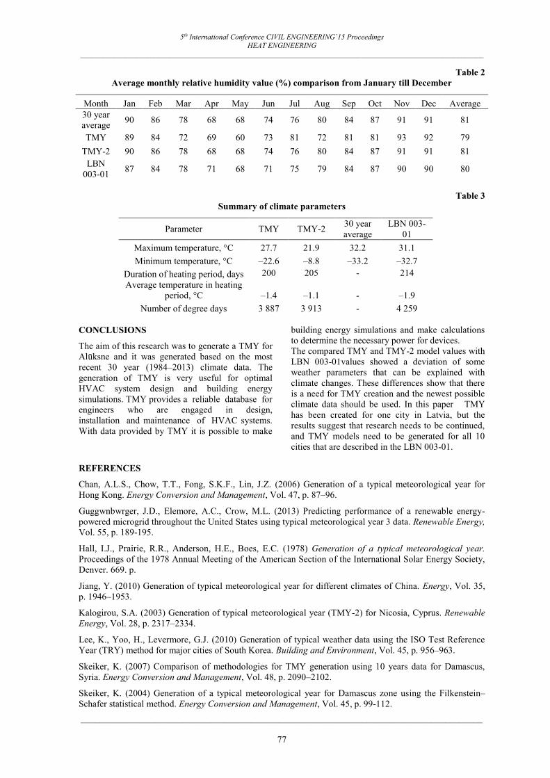
5th International Conference CIVIL ENGINEERING`15 Proceedings HEAT ENGINEERING
_____________________________________________________________________________________________________________
_______________________________________________________________________________________
77
Table 2 Average monthly relative humidity value (%) comparison from January till December
Table 3
Summary of climate parameters
Parameter TMY TMY-2 30 year average
LBN 003-01
Maximum temperature, °C 27.7 21.9 32.2 31.1 Minimum temperature, °C –22.6 –8.8 –33.2 –32.7
Duration of heating period, days 200 205 - 214 Average temperature in heating
period, °C –1.4 –1.1 - –1.9 Number of degree days 3 887 3 913 - 4 259
CONCLUSIONS
The aim of this research was to generate a TMY for Alūksne and it was generated based on the most recent 30 year (1984–2013) climate data. The generation of TMY is very useful for optimal HVAC system design and building energy simulations. TMY provides a reliable database for engineers who are engaged in design, installation and maintenance of HVAC systems. With data provided by TMY it is possible to make
building energy simulations and make calculations to determine the necessary power for devices. The compared TMY and TMY-2 model values with LBN 003-01values showed a deviation of some weather parameters that can be explained with climate changes. These differences show that there is a need for TMY creation and the newest possible climate data should be used. In this paper TMY has been created for one city in Latvia, but the results suggest that research needs to be continued, and TMY models need to be generated for all 10 cities that are described in the LBN 003-01.
REFERENCES
Chan, A.L.S., Chow, T.T., Fong, S.K.F., Lin, J.Z. (2006) Generation of a typical meteorological year for Hong Kong. Energy Conversion and Management, Vol. 47, p. 87–96.
Guggwnbwrger, J.D., Elemore, A.C., Crow, M.L. (2013) Predicting performance of a renewable energy-powered microgrid throughout the United States using typical meteorological year 3 data. Renewable Energy, Vol. 55, p. 189-195.
Hall, I.J., Prairie, R.R., Anderson, H.E., Boes, E.C. (1978) Generation of a typical meteorological year. Proceedings of the 1978 Annual Meeting of the American Section of the International Solar Energy Society, Denver. 669. p.
Jiang, Y. (2010) Generation of typical meteorological year for different climates of China. Energy, Vol. 35, p. 1946–1953.
Kalogirou, S.A. (2003) Generation of typical meteorological year (TMY-2) for Nicosia, Cyprus. Renewable Energy, Vol. 28, p. 2317–2334.
Lee, K., Yoo, H., Levermore, G.J. (2010) Generation of typical weather data using the ISO Test Reference Year (TRY) method for major cities of South Korea. Building and Environment, Vol. 45, p. 956–963.
Skeiker, K. (2007) Comparison of methodologies for TMY generation using 10 years data for Damascus, Syria. Energy Conversion and Management, Vol. 48, p. 2090–2102.
Skeiker, K. (2004) Generation of a typical meteorological year for Damascus zone using the Filkenstein–Schafer statistical method. Energy Conversion and Management, Vol. 45, p. 99-112.
Month Jan Feb Mar Apr May Jun Jul Aug Sep Oct Nov Dec Average 30 year average 90 86 78 68 68 74 76 80 84 87 91 91 81
TMY 89 84 72 69 60 73 81 72 81 81 93 92 79 TMY-2 90 86 78 68 68 74 76 80 84 87 91 91 81
LBN 003-01 87 84 78 71 68 71 75 79 84 87 90 90 80

5th International Conference CIVIL ENGINEERING`15 Proceedings HEAT ENGINEERING
_____________________________________________________________________________________________________________
_______________________________________________________________________________________
78
Yang, L., Lam, J.C, Liu, J. (2007) Analysis of typical meteorological years in different climates of China. Energy Conversion and Management, Vol. 48, p. 654–668.
Zang, H., Xu, Q., Biang, H. (2012) Generation of typical solar radiation data for different climates of China. Energy, Vol. 38, p. 236-248.
Zariņš, M. (2001) Klimata datu izvēle gaisa kondicionēšanas jaudas aprēķinam. Jelgava: Latvia University of Agriculture. 59 p.
Zhang, Q. (2006) Development of the typical meteorological database for Chinese locations. Energy and Buildings, Vol. 38, p. 1320–1327.

5th International Conference CIVIL ENGINEERING`15 Proceedings HEAT ENGINEERING
_____________________________________________________________________________________________________________
_______________________________________________________________________________________
79
GREEN BUILDING STRATEGIES AND ACHIEVEMENTS IN LEED ZERO NET ENERGY BUILDINGS
Maija Krizmane
Riga Technical University, Department of Gas Heat and Water Technology E-mail: [email protected]
ABSTRACT
Zero Net Energy (ZNE) buildings are those that are striving for sustainable development for the future. The energy use of the building in these projects is met by onsite renewable energy technologies, in some cases producing excess energy to supply it to the grid. When looking at the basis of sustainability – environmental, social and economical benefits, ZNE buildings contribute to all of those. By using renewable sources, ZNE buildings protect the legacy of scarce natural resources and contribute to the global goal of climate change limitation. ZNE buildings allow energy savings this way, providing economical benefits not only to the owners and tenants but also to the system as a whole – reducing the need for a large energy supply infrastructure in the future. Additionally ZNE buildings contribute to the reputation of the owners and residents. When considering social benefits ZNE buildings provide synergies between energy security, safety and resilience as well as serve as demonstration projects and provide a sustainability educational platform. New Buildings Institute ZNE 2014 Status Update identifies 32 verified ZNE buildings in the US. 15 out of those are LEED (Leadership in Energy and Environmental Design) gold and platinum buildings http://www.gbig.org/collections/14147. In this research the submittal documents, profiles and case studies of these 15 buildings were assessed. (NBI, 2014) This paper assesses a relatively small dataset of LEED ZNE buildings therefore it seeks to find a trend and an idea of how such buildings perform not only in terms of energy but also with regard to other sustainable building criteria under the LEED rating system. The main focus is on analyzing renewable energy generation and its share in the total energy consumption and comparing EUI values to various benchmarks. Additionally, the paper seeks synergies of high performance across LEED categories. The main results show the following pattern – when a building has higher energy consumption, the share of renewable energy is higher, meaning that a high energy demand can be met with renewable energy, which is a signal for a sustainable building market. Energy savings not only reach and exceed the LEED ceiling but also show exceptional scores in terms of national average values. When looking beyond energy, most projects fall in the highest or 2-3 point short of the highest scores in terms of all LEED credit categories. Slightly worse results are found in materials and resources category. That means there is room for development however the conclusions also state that further research on this is required within a larger dataset. Key words: Zero Net Energy, LEED, EUI, sustainable building, NBI 2014
INTRODUCTION
ZNE buildings are those that operate with zero net energy consumption and zero carbon emissions. Over a one year period, 100% of a building’s energy use can be met with onsite renewable energy technologies. Design features may include solar panels, heat pumps, heat recovery, efficient building envelopes, green roofs, high efficiency lighting and appliances, multi-glazed windows, control systems and other technologies and design features that contribute to operational energy efficiency. The development of ZNE buildings allows a change of mind set in the construction environment. The concept of 100% on-site energy on a yearly basis is a new way of thinking and designing. It goes further than just building a building. It corresponds to the integrated development – infrastructure, education and energy systems. At the moment ZNE buildings are already moving from the state-of-the-art status
to common practices in the modern world. There are still many challenges to overcome, but it becomes more and more clear, that ZNE buildings and the kind of thinking those represent is the future and it provides benefits far beyond energy savings. New Buildings Institute ZNE 2014 Status Update identifies 32 verified ZNE buildings in the US. (NBI, 2014) 15 out of those are LEED gold and platinum buildings. (http://www.gbig.org/collections/14147) The submittal documents, profiles and case studies of these 15 buildings were assessed. Zero Net Energy certification provides unique opportunity to showcase high-performance LEED buildings and to verify the design strategies with ongoing high performance achievements - this way recognizing the leadership of these buildings from a third party perspective. Energy efficiency has a high importance in terms of

5th International Conference CIVIL ENGINEERING`15 Proceedings HEAT ENGINEERING
_____________________________________________________________________________________________________________
_______________________________________________________________________________________
80
the green building industry. In developed countries, buildings account for 20–40% of total energy use (Lombard, Ortiz, Pout, 2008; http://www.oee.nrcan.gc.ca/corporate/statistics/neud/dpa/, 2008). For example, the main source of energy for buildings – power plants – account for 39% of all carbon dioxide emissions. (Goodman, Walker, 2006) In order to benchmark green building designs and projects, as well as define the current state of the industry in terms of energy efficiency and create strategies, incentives and policies on different levels, building assessment tools play a huge role. In terms of LEED, these buildings by far exceed the ceiling of the design energy savings for the maximum available points for the ‘’Optimize Energy Performance’’ credit. Therefore this paper seeks to recognize those achievements as well. Since all the LEED ZNE projects are New Construction projects, the relevant metrics are from LEED Design and Construction rating system - the goal is to create a design that improves energy efficiency relative to an ASHRAE 90.1 compliant baseline and points are awarded according the energy savings relative to this baseline. A paper on the current status in the green building research (Jian, Zhen-Yu, 2014) points out three major areas of green building research – searching for definitions of green building, ideas, strategies, examples on how to achieve the green building performance as well as analysis on costs and benefits. Topics as potential transformations due to population growth, adequate policy making in terms of energy supply and energy use and economic, environmental consequences as well as social acceptance challenges are opened subjects in green building research environment (Mustafa, 2008; Wedding, Crawford-Brown, 2007). This paper however strives to dive deeper into the profiles of ZNE buildings and to identify the common strategies and common achievements in terms of LEED. MATERIALS AND METHODS
In order to analyse and compare the achievements of these buildings, several metrics are to be used. In order to compare buildings of different sizes, energy use intensity (EUI) is used. Energy Use Intensity (EUI) is a metric of total building energy use commonly used in benchmarking. A number of studies have been done to evaluate LEED buildings in terms of EUI and in comparison with national mean values. (Turner, Frankel, 2008; Newsham, Mancini, Birt, 2009; GSA Public Buildings Service, 2008; Torcellini, et al., 2006; Diamond, et al., 2006) EUI is the sum of all fuels used in the building per year divided by the building’s floor space and is expressed in kilowatt-hours per square meter of occupied space per year (i.e. 25 kWh/m2/yr). This study relies solely on site EUI, as opposed to source
EUI that includes energy from transmission and production. National average EUIs for commercial building energy use are from CBECS5. (NBI, 2014) Additional measures in order to assess the scale are used – for example the total renewable energy production in kWh per year and the percentage of total energy consumption. In order to compare various versions of this rating system, all savings have been aligned to match the ASHRAE 90.1- 1999 baseline that is the reference standard of LEED 2.1 version. Dataset overview
LEED Dataset consists of 16 buildings - 14 out of those are platinum, one gold and one registered Buildings. The size varies from 261 m2 up to 19 639 m2 with an average of around 2372 m2. Energy Savings
In order to assess the energy savings of ZNE LEED buildings, EUI values of LEED buildings were compared to the values of other ZNE buildings as well as national average values. Additionally LEED buildings were compared by a common LEED baseline (ASHRAE 1999). Renewable Energy
In order to see the trends of renewable energy production this paper compares the percentage of renewable energy out of the total energy consumption whilst also earmarking the total renewable energy produced. In this way the paper investigates if there is an urge to produce more renewable energy if the demand is higher. Beyond Energy
In terms of sustainable building and development in general an efficient and resilient building goes far beyond being energy efficient and even beyond zero net energy. This paper seeks to take advantage of the LEED scores of these buildings in order to sketch the achievements in different areas - indoor air quality, materials and resources, water efficiency, sustainable sites as well as innovation and design. The hypothesis is that these buildings show leadership in all the categories. In order to assess that, the paper reviews the points achieved for each credit category to identify the possible gaps in performance in categories beyond energy.
RESULTS AND DISCUSSION
Energy Savings
Whilst the ZNE verified buildings in NBI Status Report 2014 has an average EUI of 67 kWh/m2/yr the 13 LEED buildings show an average of 82 kWh/m2/yr and range between 35 and 290 kWh/m2/yr. National average meanwhile is 289

5th International Conference CIVIL ENGINEERING`15 Proceedings HEAT ENGINEERING
_____________________________________________________________________________________________________________
_______________________________________________________________________________________
81
kWh/m2/yr according to Commercial Buildings Energy Consumption Survey (CBECS). That said, in terms of energy consumption, the average consumption is far below national average. The performance in terms of EUI was not influenced by the building’s size meaning that not only small, but also large buildings are ready to be ZNE. Within LEED system points for energy savings are awarded for projects under the “Optimize Energy Performance” credit. Depending on the rating system version the maximum points are awarded for up to 46 - 60% energy savings relative to baseline
(adjusted to ASHRAE 1999). However the average design achievement of 92% by far exceeds this ceiling. And even more – the highest achievement is 132 % below the baseline. One of the significant features in this dataset is that the project with the highest EUI - meaning large energy consumption - has achieved high levels of design energy savings. That shows that buildings, which are highly occupied and equipped with energy-sensitive technologies can be leaders of the market and show significant reductions in energy consumption.
Table 1 Energy savings of LEED zero NET energy buildings
No. Project LEED Version Certification Level
Energy Savings (ASHRAE 1999), % Size, m2 EUI,
kWh/m2/year
1 LEED NC 2.0 Platinum N/A 466 54 2 LEED NC 2.1 Platinum 113 1 237 50 3 LEED NC 2.1 Platinum N/A 520 88 4 LEED NC 2.2 Platinum 100 793 57 5 LEED NC 2.2 Platinum 66 637 N/A 6 LEED NC 2.2 Gold 63 416 41 7 LEED NC 2.2 Platinum 111 300 66 8 LEED NC 2.2 Platinum 51 19 639 104 9 LEED NC 2.2 Platinum 82 3 143 47
10 LEED NC 2009 Platinum 132 368 290 11 LEED NC 2009 Platinum 132 368 76 12 LEED NC 2009 Platinum 86 1 420 85 13 LEED NC 2009 Platinum N/A 261 88 14 LEED for Schools 2007 Platinum 109 640 85 15 LEED for Schools 2007 Registered 111 7 197 57 16 LEED for Schools 2007 Platinum 93 548 35
Figure 1. Renewable energy production

5th International Conference CIVIL ENGINEERING`15 Proceedings HEAT ENGINEERING
_____________________________________________________________________________________________________________
_______________________________________________________________________________________
82
Renewable Energy
In order to assure net ZERO energy consumption, the energy demand must be produced on site with renewable technologies. Across LEED rating system the points for producing renewable energy on site are awarded in Renewable Energy credit. Depending on the rating system projects can earn a maximum amount of points for renewable energy production of 12.5% to 20% out of the energy demand. These buildings however use from 23 to 117% renewable energy produced on site – by far exceeding the LEED ceiling. Also within this
relatively small dataset the total production of renewables follows the trend of % of renewables (as shown in the figure 1).
Beyond Energy
The LEED net ZERO building are Platinum and Gold which demonstrates their leadership in other sustainability criteria on top of their high energy performance. Other credit categories – Indoor Air Quality, Sustainable Sites, Innovation and Design, Materials and Resources and Water Efficiency - show a wide range of achievement levels.
Figure 2. Shortage of maximum LEED credit achievements across credit categories
Figure 2 represents the achievements of net ZERO LEED projects in all LEED credit categories. In most categories, the majority of projects show high performance and are awarded either the maximum number of points available or they end up short of 1-3. Materials and Resources category shows a room for development. By reaching the highest scores in other categories, these achievements leave a question mark in terms of materials category. With the further development of more LEED net ZERO energy buildings, this trend can be researched further and into more detail.
CONCLUSIONS
Out of 15 LEED Certified Zero Net Energy Buildings 14 are Platinum and 1 Gold Level. That points out the leadership of these buildings in LEED credit categories – Sustainable Sites, Water Efficiency, Energy and Atmosphere, Materials and Resources, Indoor Environmental Quality and Innovation and Design. The ZNE Emerging and Ultra-Low Energy buildings are highly efficient assets striving for further energy savings and targeting ZNE status. Through clear benchmarking
tools and publicly available data, future projects are able to benefit from the lessons learned by the existing ones. In sharing this information openly, the energy efficiency leaders of today will continue pulling the market even further in the direction of net zero energy buildings. The leadership in these buildings extends to high quality Indoor Air, Sustainable Sites and Innovation and Design. Materials and Resources do not show particularly advanced levels of achievement. Some explanations have been introduced for this trend for example each team focuses on different measures that can be or not be related to one or the other credit category. For that reason it is not accurate to say that ZNE buildings did not show results in the Materials and Resources category in an aggregated way, but rather to see what the technologies and strategies are that ensured the energy achievements. Materials and Resources in this dataset show room for development with respect to the LEED rating system. ZNE LEED buildings contribute to energy savings and show very high achievements compared with the national average. Only one Retail project

5th International Conference CIVIL ENGINEERING`15 Proceedings HEAT ENGINEERING
_____________________________________________________________________________________________________________
_______________________________________________________________________________________
83
exceeds the national average, however with the highest renewables EUI, it shows a negative net EUI. Reduced plug loads, high efficiency building components, passive systems and efficient technologies contribute to low EUI values in these ZNE buildings. Additionally LEED ZNE buildings with larger energy demand have shown
significantly higher energy savings than buildings with smaller energy demands whilst also producing the largest proportion of renewables on-site. Such trends allow buildings with the highest footprint to emerge as leaders and provide a substantial positive impact.
REFERENCES
2005 Natural resources Canada. National Energy Use Database. [Online] [assessed: September 09, 2008.] http://www.oee.nrcan.gc.ca/corporate/statistics/neud/dpa/.
2014 Getting to Zero Status Update: A look at the projects, policies and programs driving zero net energy performance in commercial buildings. (2014) New Buildings Institute (NBI) status report.
Diamond R., et al. (2006) Evaluating the Energy Performance of the First Generation of LEED-Certified Commercial Buildings in: ACEEE Summer Study on Energy Efficiency in Buildings. American Council for an Energy- Efficient Economy. p. 3-41-3-52.
Goodman S. and Walker M. (2006) Benchmarking Air Emissions. E3 Ventures; Natural Resources Defense Council; Ceres; PSEG.
GSA Public Buildings Service. (2008) General Services Administration, Assessing Green Building Performance. Washington, DC, USA: Office if Applied Science and Applied Research.
Newsham R.G. and Mancini S., Birt B.J. (2009) Do LEED-certified buildings save energy? Yes, but.. Energy and Buildings, 41, p. 897 - 905.
Omer, Abdeen Mustafa. (2008) Energy, environment and sustainable development. Renewable and Sustainable Energy Reviews, 12, p. 2265 - 2300.
Pe´rez-Lombard, L., Ortiz, J. and Pout, C. (2008) A review on buildings energy consumption information. Energy and Buildings, 40 (3), p. 394 - 398.
Research Highlights: Zero net energy LEED buildings. [online] Available: http://www.gbig.org/collections/14147
Torcellini P.A., et al. (2006) Lessons Learned from Case Studies of Six High-Performance Buildings. Technical Report. Turner C., and Frankel M. (2008) Energy Performance of LEED for New Construction Buildings. Washington, DC, USA: New Buildings Institute.
Wedding G.C. and Crawford-Brown D. (2007) An Analysis of Variation In the Energy-Related Environmental Impacts of LEED Certified Buildings. Journal of Green Building, Vol. 2, p. 151 - 170.
Zuo, Jian and Zhao, Zhen-Yu. (2014) Green building research–current status and future agenda: A review. Renewable And sustainable Energy Reviews, 30, p. 271 - 281.

5th International Conference CIVIL ENGINEERING`15 Proceedings HEAT ENGINEERING
_____________________________________________________________________________________________________________
_______________________________________________________________________________________
84
INDOOR AIR QUALITY IN MULTI-STOREY APARTMENT BUILDINGS
AFTER REFURBISHMENT
Jurģis Zemītis*, Anatolijs Borodiņecs**
* Riga Technical University Institute of Heat, Gas and Water Technology
E-mail: [email protected] **ITMO University
ABSTRACT
The paper presents a study on existing building stock energy consumption for the country of Latvia and researches the renovation potential of multi-storey apartment buildings and its influence on indoor air quality. The study analyses IAQ parameters and the energy consumption in renovated and non-renovated buildings and presents practical examples of Latvian and Estonian case studies as well. The possible reduction of energy consumption after thermal insulation of apartment buildings and renovation of ventilation systems has been estimated at the state level. Different insulation scenarios and efficiencies of various types of ventilation systems have been evaluated.
Key words: Multi apartment buildings, refurbishment, ventilation and energy consumption INTRODUCTION
The majority of Latvian as well as European residential buildings were constructed within the period from 1965 to 1990. In general the total energy consumption due to the building sector is about 40% of all the energy while up to 75% of heating energy is consumed by residential buildings, therefore making them the largest and most essential heat consumers during the heating season. This is caused by the fact that the old buildings did not have any insulation and on average the heat transfer coefficient of a typical homogeneous single layer external wall of an old non-renovated Latvian multi apartment building was 1.20 W/m2K which is at least 3.5 times higher than the values specified in the current Latvian Building Code. The major part of the energy is lost in heating the old non-renovated buildings which consume up to 4 times more energy than new buildings. This provides the opportunity for large energy savings and has caused rising interest in building retrofitting, especially in countries with a cold climate like Latvia, Estonia, Finland, etc. However, the retrofitting process must be done correctly and understanding that these buildings after refurbishment must serve for the next 30 years. As the existing examples show, a particular attention must be paid to proper installation of the ventilation systems, the correct choice of insulation material and thickness as well as proper balancing of the heating systems. Especially great attention must be paid to the buildings’ ventilation systems, since the old buildings constructed before the 90s were equipped only with natural ventilation systems. The fresh air in such buildings uncontrollably flows in through
the gaps between the window frame and window carcass while the exhaust air leaves through the vents located in the kitchens and bathrooms (Borodinecs et. al., 2007). However, during the renovation process it is a common practice to replace the old wooden windows with new PVC ones due to their lower U values. This combined with adding extra insulation on the walls drastically reduces the natural infiltration leading to reduced ventilation rates. In a lot of cases this has caused mould problems on inner walls as well as complaints of bad IAQ. Therefore a solution for the best ventilation system must be looked for in each situation. METHODOLOGIES
In order to estimate the energy saving potential at the Latvian level the typical Latvian housing stock and different renovation scenarios were analysed. Practical measurements of IAQ and analysis of energy consumption were performed. Renovation scenarios include different thicknesses of insulation, various air exchange rates and additional maintenance works of building engineering systems. During calculations it is taken into account that in general the Latvian climate can be described by moderate temperatures with all year round high relative humidity. According to the outdoor air temperature, the number of degree days in Latvia is relatively high and can vary from 3744 to 4687 with the winter design temperatures of -18.30C down to -25.10C. The indoor temperature according to the existing legislation is accepted at 180C. For indoor air quality measurements data loggers with the following parameters were used: temperature: -200C to 700C (±0.350C); relative

5th International Conference CIVIL ENGINEERING`15 Proceedings HEAT ENGINEERING
_____________________________________________________________________________________________________________
_______________________________________________________________________________________
85
humidity: 10% to 90% (±2.5%); CO2 level: 0 to 2 500 ppm (±50 ppm or 5% of reading). Energy consumption and different air exchange rates
The calculations to determine the optimal insulation thicknesses are based on the potential of reducing heat losses through the building envelope and therefore saving money compared to the necessary investments. Generally the yearly energy consumption for heating needs in kWh/m2 is determined according to the following equation: Qyearly = (Dheat · 24 · (Qenvel. + Qbridges + Qinfil. + Qvent.) – Qsolar – Qint.) / A (1) where Qyearly – yearly heat losses (kWh/m2/year), Qenvel. – heat losses through the building envelope (kW), Qbridges – heat losses through thermal bridges (kW), Qinfilt. – heat losses through infiltration (kW), Qvent. – heat losses through ventilation (kW), Qsolar – yearly heat gains from passive solar energy (kW/year), Qint.– yearly heat gains from internal gains (kW/year), A – floor area of the building (m2), Dheat – days of heating per year. As seen from the equation above, overall energy consumption is not only dependent on heat losses through the building envelope but also from the heat necessary for the ventilation system. Knowing that by the refurbishment process the infiltration part of ventilation decreases, a conscious effort must be made to increase the controlled ventilation. However, there are a number of different opinions and norms on how to determine the right amount of ventilation air. In Latvia the local norms regulate the minimum air exchange depending on the room
type and area (LBN 211-08, 2008) and the minimum air volume for one person (LBN 231-03, 2003). Sometimes a generalized air exchange of 1 time per hour is applied as this was usually the case for old Soviet period buildings. However, it is also possible to determine the air exchange based on the CO2 concentration. In general, good air quality is when the CO2 concentration does not exceed 700 ppm above the outdoor concentration (ASHRAE Standard 62.1., 2004). The dynamic change of the CO2 concentration can be determined by using the mass balance formula, see equation 2 (Zemitis J., Borodinecs A., 2012).
inpersoutin cVnqncVn
dtdcV
******
. (2)
where V – room volume, m3; n – air exchange rate, cout – outdoor air CO2 concentration, kg/m3, npers. – number of persons in a room; q – CO2 production by one person, kg/h, cin – indoor air CO2 concentration, kg CO2/m3. Assuming that the CO2 concentration reaches a steady state throughout the building the equation can be simplified to the following (Seppänen, 2008):
ohih
hh CC
GQ
.. (3)
where Qh – the airflow needed for selected air quality in respect to any contaminant in the air, Gh. – the generation of contaminant, Ch,i – acceptable contaminant concentration in indoor air (kW), Ch,o. – the contaminant concentration of intake air
0.00
10.00
20.00
30.00
40.00
50.00
60.00
70.00
80.00
90.00
kwh/m2/year
Building type (storeys)
Acording to LBN 231-03
CO2<1000 ppm
According to LBN 211-08
Air exchange rate 1h-1
Figure 1. Necessary yearly heating energy for different ventilation volumes
The importance of the appropriate selection of the correct ventilation rate can be seen in Figure 1. It
shows that the energy consumption for ventilation air heating is strongly related to the applied

5th International Conference CIVIL ENGINEERING`15 Proceedings HEAT ENGINEERING
_____________________________________________________________________________________________________________
_______________________________________________________________________________________
86
calculation method. The old Soviet period air exchange rate of one air change per hour along with the most commonly used method calculating the ventilation depending on the type of room and its area requires the largest need for heating of about 60-70 kWh/m2/year. However, if the ventilation rate is chosen so it ensures the CO2 level of 1 000 ppm for all the time which is close to 700 ppm above the average outside concentration, the energy consumption can be reduced by about 30% to 40 kWh/m2/year. To demonstrate the influence on the total energy consumption of ventilation for heating - Figure 2
shows both the necessary energy for compensating heat losses that occur throughout the building envelope if the building is renovated to reach the local building codes together with heat needed for ventilation if it is chosen to ensure the CO2 level of 1000 ppm. A case of no heat recovery systems for ventilation is assumed, as this is the usual case in Latvia. The figure shows that the heat for ventilation can reach up to 80% or sometimes even more than 100% compared to the heat for transition losses.
0.00
10.00
20.00
30.00
40.00
50.00
60.00
70.00
kwh/m2/year
Building type (storeys)
Heat for ventilation
Heat loses through envelope
Figure 2. Necessary annual heating energy for optimal ventilation volume and heat losses through building envelope
Case studies of Multi-storey apartment building refurbishments
Until February of the year 2013 the total number of already renovated multi-storey buildings in Latvia had reached 156 while overall there are 1 217 applications of projects and contracts for 700 renovations. These numbers show the high interest in the refurbishment process which is stimulated by the possibility of attracting European funds. To apply for the renovation process each building needs to have an energy audit. This audit is standardized in Latvia and contains the main information about the building size, area, date of construction, engineering systems, actual energy consumption and possible measures to reduce it and also the predicted benefits. For the purpose of the study we analysed 44 building audits, from which we chose three buildings which have already been renovated and have had energy consumption measurements both before and after renovation. Two of these buildings are typical kindergartens and one is a multi-storey apartment building. The presented buildings are showcases of a typical Soviet period construction with high air leakage, no insulation and poor quality of construction work.
Table 1 shows the different types of renovation works and their influence on the total energy consumption. Not all of the suggested works were done during the renovation phase therefore the theoretically predicted energy consumption after the refurbishment is the following: for Kindergarten ,,Zīlīte” 121 kWh/m2/year, for Kindergarten ,,Pasaulīte” 117 kWh/m2/year and for the Multi storey residential building 78 kW/h/year. The measured energy consumption after the renovation however is as follows: for Kindergarten ,,Zīlīte” 150 kWh/m2/year, for Kindergarten ,,Pasaulīte” 145 kWh/m2/year and for the multi-storey residential building 75 kWh/m2/year. As the results show there are some differences between the predicted and measured energy consumptions, especially for the kindergartens. The differences in the data can be partly explained by the increase of indoor temperature after refurbishment. In the calculations it was assumed to be 180C but the performed measurements showed that it was actually around 200C. The increase in temperature is observed mostly in the kindergartens due to fact that the temperature is regulated by the schools’ nurses and they do not get any financial benefit for trying to save energy. In most cases this can be considered as

5th International Conference CIVIL ENGINEERING`15 Proceedings HEAT ENGINEERING
_____________________________________________________________________________________________________________
_______________________________________________________________________________________
87
a good thing because the indoor temperature before the renovation was too low and by increasing it, the indoor climate quality is improved. However, if the temperature rise is unwanted, the heating system needs to be rebalanced after renovation, or an
automation system for heating boiler must be installed. For multi-apartment buildings it is different because the residents can lower the temperature, thus saving money.
Table 1
Renovation measures performed in chosen objects and predicted energy savings in supplied specific energy in kWh/m2/year
Additional insulation of
heating systems pipeline
Renovation of heating
system
Extra insulation of
exterior walls
Extra insulation of
slab on ground
Extra insulation of basements
ceilings
Extra insulation
of roof
New windows to PVC with
U=1.8 W/(m²K)
Total savings in energy in
kWh/m2/year
Kindergarten ,,Zīlīte”, Plūdoņa street 60, Bauska
7.20 10.80 45.01 (100
mm material)
19.80 (100 mm
material) - - - 82.81
Multi- storey residential building, Kareivju street 3, Bauska
1.6 4.7
36.0 (for facades)
24.2 (for end walls)
- 13.7
(40 mm material)
32 (150 mm material)
38 87.2
Kindergarten ,,Pasaulīte”, Saules street 8, Bauska
- 6.33 82.72 (100
mm material)
23.36 (100 mm
material) - - - 113.69
Unfortunately none of the analysed buildings or energy audits involved installation of a new mechanical ventilation system. In most cases the audits only recommended cleaning the existing natural ventilation exhaust shafts and/or introducing additional air supply openings in the walls or windows. However, the existing research (Dimdina et al., 2011) shows that this is not sufficient and the natural ventilation air velocity in the shafts is lower than it is necessary to provide enough fresh air. On average the air velocity in the measured buildings was under 1 m/s, but to provide the necessary air volume it should be about 1.44 m/s. Also the research (Borodinecs et. al., 2011) shows that there is a large difference in air exchange depending on the storey and height of the building and this can cause a serious increase in relative humidity and bad IAQ in the uppermost storeys of high rise buildings. The following Estonian experience (Borodinecs et al. 2013) shows a possible solution for the ventilation system. The building is located in Estonia in the district of Mustamäe, Tallin, Sõpruse Street 244. The building has five floors with a heated area of 2968 m2 and 60 apartments. Renovation works included the insulation of the entire façade and roof. The insulation used for the façade was polystyrene EPS 150. For the roof insulation polystyrene EPS50 with a thickness of 250mm was used. During the renovation of the building the old wooden windows were replaced with new PVC windows with U = 1.1 W/m2K. Also the balcony panels were replaced and new balcony
glass railings were installed. Additionally 3 new water–to-water heat pumps taking the heat from the mechanical ventilation exhaust were added to the existing heating unit. The heat from the exhaust air of the apartments and stairwells is utilized in preparation of domestic hot water and preheating of heating systems. The existing natural ventilation shafts were used for mechanical exhaust. Supply air modules connected with radiators were installed under the heaters in living rooms, bedrooms and kitchens to compensate for the extracted air. Before the renovation the energy consumption was 150kWh/m2/year. The energy saving measures resulted in 50.6% decrease of building heating energy need leading to a consumption of 75.9kWh/m2/year. However, the electricity consumption increased by a staggering 729% from 2.4 to 17.5 kWh/m2 as the result of installing the exhaust air heat pumps. Nevertheless, the total measured energy consumption of the building including heat, electricity and domestic hot water as of now is 93.4 kWh/m2 per year which is 38.8% compared to the situation before the renovation.
Measurements of IAQ in refurbished buildings
As the energy consumption for the heating of buildings’ ventilation air after renovation can vary between 40-50% of the total heat consumption it can be very tempting to reduce it. This can lead to unsatisfactory indoor air quality. To check this, measurements in two kindergartens were performed that have had renovation works (Stankevica, 2012).

5th International Conference CIVIL ENGINEERING`15 Proceedings HEAT ENGINEERING
_____________________________________________________________________________________________________________
_______________________________________________________________________________________
88
As seen from the results presented in Table 2 in both kindergartens the CO2 value exceeds the suggested 1000 ppm. Nevertheless, the excess is relatively small and does not pose any threat to the children’s safety. A higher CO2 concentration was registered in Renovated No. 2 daycare center, which has a natural ventilation system as opposed to the other daycare centers with mechanical systems installed. This proves that in longer periods during the daytime a better indoor air quality is achieved in mechanically ventilated spaces with a constant supply of fresh air compared to a naturally ventilated system, even taking into account that additional ventilation is achieved by opening windows.
Table 2 Measured data on the CO2 concentration in
renovated daycare centers
Daycare center
Area [m2]
Type of venti-lation system
Mean CO2 concentra- tion in ppm (95% CI)
Max CO2 concentra- tion in ppm
Reno-vated 1
2152 Mechani-cal 743 (604-882)
1140
Reno-vated 2
2112 Natural 864 (651-1077)
1356
RESULTS AND DISCUSSION
As the performed research results show, it is economically feasible to apply the thermal insulation on the building envelope, thus vastly reducing heat losses. However, meanwhile in order to achieve better energy efficiency, the ventilation rate is significantly lowered which results in leading to an unsatisfactory IAQ. This is usually due to the lack of mechanical ventilation which is caused by the high installation costs. The practical installation of air handling units with heat recovery also is often limited by room space and lack of existing
ventilation shafts. Another main disadvantage of installing heat recovery units is the increase in electricity consumption. In the Baltic States the price of one MWh of electricity is approximately 2 times higher than the price of a MWh of district heating therefore increasing the payback time. The results show that in a typical situation it is possible to decrease the overall heat consumption by approximately 50% from 150-180 to 75-100 kWh/m2. To achieve this it is necessary to apply wall insulation with a thickness of 150 mm, roof insulation with 200 mm, ground slab insulation with 50 mm as well as renovating the heating system and replacing or adding insulation to old piping. Also ventilation rates must be chosen accordingly, taking into account the occupancy load of the building, and which can often be reduced in half compared to how it is usually calculated. This leads to a significant reduction in heat consumption while preserving good indoor air quality. CONCLUSIONS
The heat consumption after applying thermal insulation during the refurbishment process of buildings can be realistically reduced down to 70 kWh/m2 under typical Latvia’s climate conditions. The optimal U-values of walls after thermal insulations are 0.25 – 0.30 W/(m∙K), while for roofs 0.17 – 0.20 W/(m∙K). On average the share of the energy consumption for ventilation needs in the renovated buildings without heat recovery is 50% of the total heat consumption for space heating and ventilation. The IAQ measurements in renovated buildings have shown a slightly unsatisfactory situation with an increased CO2 concentration higher relative humidity, while energy consumption can almost be reduced to the level of the energy efficient buildings.
REFERENCES
ASHRAE Standard 62.1. (2004) Ventilation for acceptable indoor air quality. American Society of Heating, Refrigerating and Air Conditioning Engineers, Atlanta.
Borodinecs A., Gaujena B., Zemitis J., Kreslins A. (2011). The stack effect influence on air exchange rate and IAQ in dwelling buildings. Paper presented at the 12th International Conference on Indoor Air Quality and Climate 2011, 2 973-978.
Borodinecs A., Kreslins A., Dzelzitis E., Krumins, A. (2007). Introduction of hybrid ventilation systems of dwelling buildings in Latvia. Paper presented at the IAQVEC 2007 Proceedings - 6th International Conference on Indoor Air Quality, Ventilation and Energy Conservation in Buildings: Sustainable Built Environment, pp. 361-368.
Borodinecs A., Zemitis J., Rodriguez-Gabriel A. et al. (2013) Handbook on Building Renovation in Central Baltic Region, Riga: Riga Technical University, pp. 92
Dimdina I., Lesinskis A., Krumins et al (2011) Indoor Air Quality and Energy Efficiency in Multi-Apartment Buildings before and after Renovation: a Case Study of Two Buildings in Riga. Civil Engineering '11: 3rd International Scientific Conference: Proceedings, Latvia, Jelgava, 12.-13. May, pp. 1-6.

5th International Conference CIVIL ENGINEERING`15 Proceedings HEAT ENGINEERING
_____________________________________________________________________________________________________________
_______________________________________________________________________________________
89
Latvian Building Code LBN 211-08 (2008) Multi-storey residential buildings.
Latvian Building Code LBN 231-03 (2003) Heating and ventilation of residential and public buildings.
Seppänen O. (2008) Ventilation Strategies for Good Indoor Air Quality and Energy Efficiency, International Journal of Ventilation, Vol. 6, No. 4, 297-306.
Stankevica G., Lesinskis A. (2012) Indoor Air Quality and Thermal Comfort Evaluation in Latvian Daycare Centers with Carbon Dioxide, Temperature and Humidity as Indicators. Journal of Civil Engineering and Architecture, pp.633-638.
Zemitis J., Borodiņecs A. (2012) IAQ as a Function of Air Exchange Rate. Recent Researches in Energy, Environment and Sustainable Development: 6th WSEAS International Conference on Waste Management, Water Pollution, Air Pollution, Indoor Climate (WWAI '12), Portugal, Porto, 1.-3. July, pp. 107.-112.

5th International Conference CIVIL ENGINEERING`15 Proceedings HEAT ENGINEERING
_____________________________________________________________________________________________________________
_______________________________________________________________________________________
90
INVESTIGATION OF SOIL TEMPERATURE VARIATION ON COWSHED STRUCTURE GROUND
Dainius Ramukevičius*, Petras Milius** Aleksandras Stulginskis University
Institute of Hydraulic Constructional Engineering Address: Universiteto str. 10, LT53361, Akademija, Kaunas, Lithuania
E-mail: *[email protected], **[email protected]
ABSTRACT
Intensive heat interchanges pass through constructive elements of the animal breeding building. The cost of keeping the animals healthy and productive depends on the temperature surface regime of the building floor on the soil, because most of their time big animals rest, and the incorrect ground surface temperature influences their metabolism, heat production and feed consumption. While trying to improve good economical rates of the farm, the floor surfaces of constructions should be improved while evaluating the ground soil. The influence of the ground soil of the cowshed building over the temperature regime of the surface of a traditional floor is analysed in the study. The experimental 80-place cowshed has been used for that purpose. Three temperature fixing borings have been arranged outside and also inside the room of the building. Temperature variation curves (of various seasons) of the ground surface of the cowshed building have been made. The investigation of temperature variation of an all year round floor surface has been carried out. The character of variation of outside temperature (during the whole year) of the ground of cowshed building and soil in its surroundings was produced. Keywords: cows, cowshed, soil, temperature INTRODUCTION
Intensive heat interchanges go through the construction elements of the barriers of animal breeding buildings. While evaluating the temperature state of the building, the main attention is paid to the walls and overlays. The floor construction of the exploited animal breeding building together with the ground soil influence the microclimate of the lodgment as well (Johannesson, 2000; Hilty, et al., 2002). From the thermodynamic point of view the animal, like all living organisms, is an open energy system with an internal heat source. The energy system openness indicates that the animal’s body performs a continuous energy exchange with its surroundings. The animal's body uses the energy resulting from food and the environment for the maintenance of vital functions, synthesis of organic and inorganic compounds, safeguard of muscle contraction, etc. (Gebremedhin, et al., 2003; Sallvik,1998). Finally, the energy received by the animal is converted into heat energy, which must be placed in the environment of the organism to maintain the status of thermostability. If the animal gives off too much heat from the body, it feels cold. The building’s floor on the ground has an impact on such kind of animal's well-being (Ehrlemark, 1996). With the cattle lying on the floor, a lot of heat is lost through conduction, because the contact with the floor area covers 1/5-1/6 part of the skin surface. Heat transfer from the animal's body through the
floor of the bearing housing can increase by up to 40 % of the total heat transfer (Sirvydas, et al., 2009; Kavolėlis et al., 2004). Physical characteristics of the floor influence the animal's body locally. When the animal is lying, one side of the body is cooled and the body is unable to fully adapt to its dual affecting conditions so that one side of the body attracts blood vessels, detracts warm blood from the skin and at the same time the normal function of blood vessels occurs in other body areas. Cooling of the individual parts of the skin temporarily reduces their temperature, because in such places dishes of arterial circulation shrink reducing blood flow. The drop or rise of the local temperature changes temperature not only in symmetric, but also in remote parts of the body Bleizgys, et al. 2010; Daanen, et al., 2003). In order to protect the animals from the harmful effects of low temperatures of the bearing housing, it is important to identify the environmental factors that affect heat transfer through the floor. One such factor is the ground of the building and the soil in its surroundings. As the floors of livestock buildings usually are installed on the ground and do not have direct contact with the outside world, the flow of heat through the floor depends not only on the thermal properties of the floor, but also on the ground soil temperature regime of the building, because the soil as well as any building material is influenced by the heat exchange patterns (Hansen, 2000; Phillips, 1992).

5th International Conference CIVIL ENGINEERING`15 Proceedings HEAT ENGINEERING
_____________________________________________________________________________________________________________
_______________________________________________________________________________________
91
It is also necessary to assess the influence of the surrounding soil’s temperature regime, which is directly influenced by the weather conditions on the ground soil temperature field of the building. In order to evaluate (under the climatic conditions of Lithuania) the impact of the soil of the livestock building surroundings, which in turn depends in part on the heat transfer through the floor of the building and which affects the temperature of the floor, first it is necessary to carry out experimental tests. MATERIALS AND METHODS
While selecting the place in the object for the measuring of ground temperature, the building configuration, lodgment layout, windows and doors
arrangement, animal resting and standing areas have been taken into account as well as the potential influence of outdoor factors. Temperature measurements of the ground were carried out in the cowshed in 80 places. The cowshed lodgment measures 66.6 m in length, 12.5 m, in width and 2.4 m in height. Constructions of the cowshed are the following: foundations – concrete strip, width – 40 cm, deepening – 1.1 m. Floor construction: concrete – 5 cm; gravel – 15 cm; ground – clay. There are 80 cows in two roped rows in the cowshed. The cowshed plan is shown in Figure 1. It is very important that the borings must be arranged very close to the foundation from the indoor as well as from the outdoor areas.
Figure 1. Plan of the cowshed: I-VI – borehole numbers
Inside the cowshed 3 borings I, II, III with a diameter of 4 cm were made for the ground temperature investigation, from the outside of the foundation up to the middle of the cowshed. Semiconductor transistor sensors were placed in order to measure the temperature in every boring in a vertical direction at a distance of 0.25 m, 0.5 m, 1.0 m, 2.0 m and 3.0 m from the land’s surface. Also outside of the building at a distance of 0.6 m, 2.0 and 5.0 m from the outdoor wall and in IV, V, VI borings, the above mentioned sensors were placed into duplicate depths in the land surface. All borings up to the land surface were filled up with a mixture of sand and gravel. For the measurement of the soil and floor surface temperature of the cowshed ambient surroundings, thermometers to measure the temperature, adjusted to measure solid surfaces, were used. The measurements were carried out 1-2 times a week. The computer program “Surfer” was used for the graphical presentation of temperature spreading in the cowshed base and in its surroundings (Fig. 2). The heat transmission from higher to lower temperature zones are displayed by pointers.
RESULTS AND DISCUSSION
The cowshed basement and the surrounding soil temperature fluctuations had a seasonal nature, as the Lithuanian climate is characterized by temperature changes in individual seasons. During the study period, the highest monthly average temperature (10.3C) was fixed in October. And the lowest (-6.9C) – in January. The same year the cowshed environment soil surface temperature in October 13.6 and in January -2.3 was higher than the average air temperature 12.6C and -6.1C, respectively. As one can see from the graphs (Fig. 2), the soil temperature fluctuations in the cowshed environment are quite complex. Ultra sharp temperature fluctuations occur in the soils of the building’s environment (IV-VI borehole numbers). Not so sharp, temperature fluctuations of a much lower amplitude were fixed in the soils underlying under the building (I-III borehole numbers). The sharpest cowshed environment soil temperature fluctuations (IV-VI borehole numbers) were fixed in the upper layers. These fluctuations depend on the plant layer as well as on the snow during the

5th International Conference CIVIL ENGINEERING`15 Proceedings HEAT ENGINEERING
_____________________________________________________________________________________________________________
_______________________________________________________________________________________
92
cold season. The sharpest were soil surface temperature fluctuations as well as of the soils at a depth of 0.25 m, the amplitude of which reached 10C and 5C, respectively. Not so sharp temperature variations of lower amplitude were fixed at a depth of 0.5 m (1°-3C) and in deeper soil layers. With deepening the amplitude decreased. The soil temperature changed up to the researched soil depth. Especially intensive heat exchange between the outside air and the soil of the building through the foundation occurs during the coldest period of the year. The lowest temperature of the cowshed ground soil was fixed near the foundation. This temperature variation is mainly caused by the atmospheric climate and seasons. It can be seen in the data of the research period (III borehole
number). During the cold period the outside air temperature fell below zero reduced the soil temperature of the cowshed at the building foundation. At the beginning of the indoor period the outdoor temperature decreased (0.5°-1°C / per week), the ground soil temperature under the animal bearing decreased as well (II borehole number, sensor depth – 0.25 m). When the outdoor air temperature is close to 0°C, the cowshed ground soil temperature starts to decrease (0.5°-1°C / per week) and in the deeper layers (I borehole number, sensor depth 1.0 m). Therefore, it can be said that to some extent, the ground soil temperature of the cowshed depends on the impact of atmospheric climate.
Figure 2. Distribution of the cowshed building base and environmental ground temperature during the period of the coldest indoor months

5th International Conference CIVIL ENGINEERING`15 Proceedings HEAT ENGINEERING
_____________________________________________________________________________________________________________
_______________________________________________________________________________________
93
During the cold period livestock spent more time in the pits of the cowsheds, lying down and resting. This increased the animal's contact with the bearing housing on the floor. The floor and ground soil temperature relationship of the bearing housing and the cowshed is especially evident during the indoor period. The cowshed experimental studies show that the animal radiated heat, that transmits not only into the air, but also into the ground soil through the floor, has a significant influence on the ground soil temperature field. This is clearly seen in Figure 2, where the highest soil temperature during the cold season is under the floor of the bearing housing (II borehole number). The increased temperature of the bearing housing floor increased soil temperature. It can be seen in the data of the selected characteristic periods of December and February. When the floor surface temperature of the cowshed bearing housing reaches 14°-20°C during the cold period, the ground soil temperature starts to rise (0.2°-0.5°C /per week) and the increase goes on up to the depth of 1.5 m. This process lasted until the end of the indoor period. Some of the animal radiant heat comes back into the room through the floor of the bearing housing into the ground because of the temperature difference between the ground soil and space air in the next floor area, i.e. not through the floor of the animal bearing housing. This thermal movement in the ground soil occurs only during the cold season,
and when the outside air temperature is significantly lower than -5C. With the rising temperature of the outdoor air, distribution of the soil temperature of the building ground and its surroundings become more even in depth. CONCLUSIONS
The cowshed floor and surrounding soil temperature measurements showed that the soil temperature field is in a constant dynamic state. Between the outside of the building and the soil under the building as well as between the floor arranged over them – the occurring heat transfer is influenced by the external temperature regime. The lowest temperature of the cowshed ground soil was fixed near the foundation. This temperature variation is mainly caused by the atmospheric climate and seasons. At the beginning of the indoor period the accumulated heat in the cowshed ground soil comes in different directions during the cold season, as well as through the floor, i.e. it comes back into the room. So, in some measure, the ground soil affects the floor temperature of the bearing housing. The fixed ground temperatures in the boring (which is 5 metres away from the building) showed that most of all the temperature distribution is influenced by the climate.
REFERENCES Bleizgys R., Kavolėlis B., Čėsna J. (2010) Emission of Water Vapour in Uninsulated Cowshed. Annals of Animal Science. Vol. 10, No 1 p. 57-65.
Daanen A., Vliert E. (2003) Driving performance in cold, warm and thermoneutral environments // Applied Ergonomics, N. 34, p. 597-602.
Ehrlemark A. G., Sallvik K. G. (1996) Model of Heat and Moisture Dissipation from Cattle Based on Thermal Properties. Transaction of the ASAE, N39(1), 187-194;
Gebremedhin K. G., Wu B. X. (2003) Characterization of Flow Field in a Ventilated Space And Simulation of Heat Exchange Between Cows and Their Environment. Journal of Thermal Biology, Vol. 28, p. 301-319.
Hansen K., Storm J. S. (2000) Characterization of Artificial Bedding Materials for Cow Cubicles. Danish Institute of Agricultural Science, Department of Agricultural Engineering, Research Center Bygholm. Denmark, 78 p.
Hilty R., Kaufmann R., Van Canegem L. (2002) Building for Cattle Husbandry. Yearbook Agricultural Engineering, VDMA Landtechnik, No.14, p. 163-170.
Johannesson T. (2000) Welfare Assessment in a Dairy Cattle Herd. The Royal Veterinary & Agricultural University, Department of Animal Science and Animal Health. Copenhagen, 136 p.
Kavolėlis В., Šateikis I. (2004) Effective Cowshed Insulating and Ventilation System Parameters // Energy and Buildings, No.36 (9), p. 969-973.
Phillips C, Piggins D. (1992) Farm Animals and the Environment. Wallingford C. A. B. International cop., 54 p.
Sallvik K. (1998) Environment for Animals. CIGR Hanbook of Agricultural Engineering / Animal Production. Volume II. Publisher by: American Society of Agricultural Engineers, p. 32-54.
Sirvydas A., Nadzeikienė J., Stepanas A., Teresciuk V. (2009) Temperature Measurements in Research of Thermal Weed Extermination. Proceedings of the International Conference, Development of Agricultural Technologies and Technical Means in Ecological and Energetic Aspects, No. 16, p. 257-262.

5th International Conference CIVIL ENGINEERING`15 Proceedings HEAT ENGINEERING
_____________________________________________________________________________________________________________
_______________________________________________________________________________________
94
ANALYSIS OF ENERGY CONSUMPTION IN ALGERIA
Abdellah Zerroug
Riga Technical University, Institute of Heat, Gas and Water Technology E-mail: [email protected]
Khaled Zehar University of Bahrein,
E-mail: [email protected] Egils Dzelzitis
Riga Technical University, Institute of Heat, Gas and Water Technology E-mail: [email protected] Anatolijs Borodinecs
Riga technical University, Institute of Heat, Gas and Water Technology E-mail: [email protected]
ABSTRACT
This paper analyses the total final energy consumption (TFC) for industry, transport and agriculture sectors in Algeria during the decade of 1998-2008, the total final energy by activity sector and fuel type, the total energy intensity evolution and the impact of energy consumption in Algeria on the environment. The total final energy consumption (TFC) in 2007 reached 20 million TOE, for 34.4 million inhabitants occupying 2 393 367 square km of land, and with a Gross Domestic Product (GDP) equal to 9 389.70 million DA (Algerian Dinars). The consumption per capita in Algeria is 1 058.0 kilograms of oil equivalent (kgOE) per person, while in Morocco, which has nearly the same number of inhabitants it is 458 (kgOE) and in Tunisia the figure is 843 (kgOE). The total gas emission is equal to 46 million tonnes of CO2 with an average of 3 TECO2/TOE. The GDP is equal to 3 232.2 million DA. Detailed information on different industrial sectors, different transport means sector, as well as the agriculture sector have been presented and discussed in the paper. The final energy intensity in Algeria has stabilized at around $ 0.53 TOE/1000 between the years 2000 and 2003. It has been improved by 2% between 2003 and 2007, exceeding 0.41 TOE /1000, which indicates an elasticity of about 1.23 .This performance is due to an optimization of the rate of capacity utilization (TUC) of the production system. The energy intensity reflects the degree of dependence of an economy with respect to the energy factor. The higher the energy intensity, the more vulnerable the economy is to the fluctuations in energy cost. Energy intensity is also a relevant indicator according to the obligations taken in the Kyoto Protocol. Emissions of greenhouse gases due to the final energy consumption reached 46 million TCO2.
Key words: Energy consumption, Fuel type, Activity sector, Environment
INTRODUCTION
The total final consumption (TFC) of energy in 2007 reached 20 million TOE for 34.4 million inhabitants occupying 2 393 367 square km and with a Gross Domestic Product (GDP) equal to 9 389.70 million DA (Algerian Dinars). The consumption per capita in Algeria is 1058.0 Kilograms of oil equivalent (kgOE) per person, while in Morocco which has nearly the same number of inhabitants it is 458 (kgOE) whereas in Tunisia the figure is 843 (kgOE) (Earthtrends.wri.org 2012). The total gas emission is equal to 46 million tonnes of CO2 with an average of 3 TECO2/TOE. The GDP is equal to 3 232.2 million DA. This is firstly due to fuel prices in Algeria, and probably due to the level of average living standard and purchasing power, which is greater in Algeria than in its neighbouring countries. When writing this paper and according to the World Bank data
the percentage of the population having access to electricity was: 99.3 % in Algeria and 97% in Morocco, which accounts for nearly the same number of inhabitants (W.B.O. 2013).
Figure 1. Energy consumption by fuel type
Thus, allowing the access of Algerian citizens to more electrical appliances such as air conditioning units, refrigerators, TVs, natural gas appliances such as gas boilers for central heating and hot

5th International Conference CIVIL ENGINEERING`15 Proceedings HEAT ENGINEERING
_____________________________________________________________________________________________________________
_______________________________________________________________________________________
95
water, gas stoves, gas cookers, etc. The percentage of the population connected to electric power is 99.5% in Tunisia, but the consumption of natural gas in megajoules per capita for the year 2006 was 17 287 while in Algeria it was 33 353 and in Morocco it was 776 for (Energy data yearbook 2009). The total energy consumption distribution by fuel type shows that oil is the most consumed fuel, shares are as follows: 48% share for oil products, 29 % share for natural gas, 12% for electricity, and 11% for LPG, the GDP per inhabitant is equal to 93 959 DA with an average consumption of 0.581 TOE per inhabitant. Meanwhile the final gas emission is 1.83 teCO2 and the primary emission is 2.222 TECO2 per inhabitant. Sector shares in total energy consumption are 7% for agriculture and hydraulics, 33% for transportation, 19% for industry (without hydrocarbons) and building construction, 41% for the residential and tertiary sector. The final energy consumption by type of fuel and by the activity sector is shown in Table 1. The percentage of CO2
emissions in Algeria between 2009 and 2010 according to the global energy statistical yearbook (Energy data year book 2011) was 4.2% of the global emissions, which was less than the African emissions percentage for the same period at 5.8%. The average annual growth rate in the petroleum industry is 5.93%, and in the gas industry it is 4.84%. For this recorded rate the average annual growth of agriculture and water resources, industry-building construction, residential - tertiary and finally transport are shown in the Table 1. As it is shown in table 1, the percentage of the average growth in the residential and tertiary sector is merely the same as in the petroleum industry, the transport has an average less than in the petroleum industry, whereas, both industries - building construction, and agriculture –water resources illustrate a percentage value more than that of the petroleum industry. The total energy annual growth consumption accounts for 27 665.6 TOE, therefore producing an annual amount of 76.45 TCO2.
Table 1
Average annual consumption growth in percentage
Agriculture and water resources
yr teudni l orteP srni l orteP
Industry and building construction
Residential and tertiary building
Transport
8.7% 5.93% 4.84% 6.46% 5.9% 5.76%
In this paper, the total energy consumption by activity and by type of fuel is analysed, starting with the industrial sector, the transport sector, and finally the agriculture sector. Afterwards conclusions were made. MATERIALS AND METHODS
Total energy consumption by activity and fuel type
For an average annual growth rate of 8.7% in the agriculture and water resources sector, 6.46% in
industrial and construction sector, 5.9% in residential and tertiary sector, and finally 5.76% in transportation sector, the recorded average annual growth rate in the petroleum industry was 5.93%, and 4.84% in gas industry. Energy industry sector consumption amounts to 5680.4 TOE and the consumption of non-energy industry sector is equal to 1 994.24 TOE. The global consumption is equal to 27 665.6 TOE with a CO2 emission of 76 446 653 TECO2. The energy consumption by type of fuel and by sectors is represented in table 2.
Table2
Energy consumption by type pf fuel and by sector
kToe Solids Petrol Diesel Heavy fuel
Light fuel
LPG Natural gas Elect. Total
Industry and construction
477 0 669.63 0 0 74.28 2438 5580.67 4339.63
Residential 0 0 1421.80 0 20.46 1611.58 2747.7 769.9 6571.45 Tertiary 0 0 122.94 0 0 55.23 376.04 635.71 1189.91
Transport 0 2350.73 3030.80 595.87 0 379.20 0 2.67 6539.23
Consumption trends analysis by sector and product between the years 2000 and 2007 shows that the national final energy consumption registered an annual average growth rate of about 6.32%. The final energy intensity in 2007 reached 6 TOE/MDA, which means 0.411 per 1000 dollars of GDP and twice that in OECD countries. Thus, the economy consumes twice as much energy as required to
create the same unit added value, with a primary energy intensity of 3.82TOE/MDA (or 0.27 Toe/$1000). The evolution from 1971 to 2008 of the world’s total final consumption by fuel (MTOE) has doubled compared to 1973, reaching 4676 MTOE and in 2008 reaching 8428 MTOE according to the key world energy statistics (International Energy Agency 2010). The fuel

5th International Conference CIVIL ENGINEERING`15 Proceedings HEAT ENGINEERING
_____________________________________________________________________________________________________________
_______________________________________________________________________________________
96
shares of total final consumption are 15.6% for gas, 41.6% for oil, 9.8% for coal/peat, 17.2% for electricity, 12.7% as combustible renewable and finally 3.1% for others. Total energy consumption distribution by fuel type shows that oil is the most consumed combustible. This is due to the growing industry demand and transport. The consumption of natural gas for industrial purposes, such as electricity production by thermal stations using natural gas, comes in second place because of the increasing demand in residential and tertiary, as well, as in the energy-industry and non-energy industry. The increasing demand for electricity represents 12%. Liquefied propane gas consumption is increasing and this due to the encouragement by the government for the use of this clean fuel for transport vehicles and private cars, thus exempting them from pollution taxes, as well as installing more centrals (central transportation/stations) ? for cities not served by natural gas. RESULTS AND DISCUSSION
Total energy consumption analysis in the industrial sector
The final energy consumption in the industrial sector has attained the value of 3.3 million of TOE.
The building materials industry is the first energy consumer with a share of 60%; steel, metallurgy, mechanics, electrical and electronics (ISMME) industries share 15% of the final consumption, basic chemicals 3%, food industry 9%, manufacturing 11%, and finally mines and quarries with 2%. Natural gas consumption in the sector exceeds 76% of the energy in the industrial sector, 6% is consumed as petroleum products and 17% in the form of electricity. Steel industry, metallurgy, mechanics, electrical and electronics represent a total budget of 46 705MDA (mil of Algerian dinars, 1USD = 77.92 AD), building materials 64 304MDA, basic chemicals 29 050MDA, Food Industry 152 132MDA. Industry manufactures 31 761MDA, and various industries 44 779MDA. The relationship between changes in energy consumption in industrial sector and the evolution of the added value (in constant dinars) shows a growth of 2.45% per annum of the energy intensity sector, which recorded 10 kTOE per kDA in 2007. However the added value rose by 6% while energy consumption grew by 6.2%. The consumption of 3.2TOE per employee has declined by a rate of 4.3% per year during the same period. Figure 2 illustrates the industry energy consumption by type of fuel from the year 2000 to 2007.
Figure 2. Energy consumption in industrial sector Total energy consumption analysis in transport sector
The energy consumption in the transport sector reached 6.5 million TOE, 46% of this energy consumed is in the form of diesel, and 48% is in the form of petrol, 6% in the form of LPG (liquefied propane gas) and 0.04% in the form of electricity. The length of road network: 109 452 km for a total number of 3.655 million vehicles, 45% of these vehicles use diesel, 12 0000 were converted to LPG, the railway length is equal to 4 200 km, the main fuel used is diesel and the railway fleet has
220 locomotives and 460 cars. The maritime fleet has 38 vessels, with 10commercial ports and 35 fishing ports. The air fleet have 55 aircraft, with a total number of 35 airports. During the period of 2000 - 2007, petrol consumption registered a growth of 4%, compared with that of diesel which recorded a rate of growth of 7.3%, while the consumption of LPG recorded a growth rate of 9.6%, which represents a consumption of 1.80 TOE/vehicle. Figure 3 illustrates the transport energy consumption by type of fuel from the year 2000 to 2007.

5th International Conference CIVIL ENGINEERING`15 Proceedings HEAT ENGINEERING
_____________________________________________________________________________________________________________
_______________________________________________________________________________________
97
Figure 3. Energy consumption in transport sector Air Algérie is the national air transport company, In 2009, an international tender to purchase eleven aircraft (seven medium-haul Airbuses A320 or Boeings 737, four regional turboprop ATR or Bombardiers DASH-type) for a value of $ 111 million (agreement of the Algerian state) has been offered. In July 2011, the official website of the company gives the number of 43 aircraft in operation, including15 as cargo, all with an average age of 7 years. Air Algeria has a network of 96 400 km. More than three million passengers and nearly 20 000 tonnes of freight operations are transported by the company each year. In 2010 Air Algeria carried 3.5 million passengers. With more than 3 million vehicles, according to the latest statistics available, Algeria has the largest fleet in North Africa and the second largest in Africa. This is mainly due to the starting of vehicle loans in 2001. The measures adopted in 2005, prohibiting the import of used vehicles and introducing compulsory roadworthiness tests, the vehicle fleet has been considerably renewed The average age of the vehicles remains high with 77% of older vehicles that are more than ten years old and only 17% less than five years old. The Algerian Minister of Transportation recently estimated the Algerian automobile fleet of up to 5.5 million, with less than 10% of these vehicles run on LPG (Finances mediterranee 2013). By 2014, the length of the national railway network will be 10 400 km. The Transport Minister, confirms, from Batna, where he was inaugurated, the first link-propelled M'sila Ain Touta-Constantine, that, once all projects are finished, Algeria will be among one of the "greatest countries in Africa". With this length of the network Algeria will be in second place, behind South Africa with more than 20 000 km network (Algerie360.2012). The development programme of railway transport in Algeria gave priority to the continued expansion and modernization of the network in terms of doubling rail (east-west), and, the creation of a new rail (north-south), signaling and electrification of
the entire network and the acquisition and renewal of rolling stock. Since 2009, the construction and the renovation of 1 383 km of roads, the reactivation of 767 km, and the electrification of nearly 400 km of track, have been realized. Between the lines reactivated (767 km, in total whole during the year 2009) and the new built lines (1 383 km from the year 2009), the Algerian rail network totals 3 919 km of the exploited rail up until the first quarter of 2011, compared with 1 769 km to the end of 2008. During the last few years, an expansion and modernization programme of the rail network was launched. This was accompanied by the acquisition and commissioning of 64 electric driven trains for Algiers suburbs, which have already reached 100 000 passengers a day, 17 railcars serving the main northern lines of Algeria and 30 diesel electric locomotives. 1 551.5 km of new lines have already been realized and 5 900 km are planned for construction, and should be completed by the end of 2014 (Algerie 360. 2012). During the 80s, Algeria had an enviable fleet, one of the largest in the third world. It was ranked among the top 50 worldwide. The Algerian Fleet was then composed of more than 80 vessels of all types (bulk carriers, tankers, chemical tankers, gas carriers, tankers, Multipurpose, RORO and car ferries). The whole fleet was operated by CNAN (National maritime transport company). CALTRAM Algerian-Libyan company operated four vessels during the 80s and 90s. The CNAN ensured with its own capabilities a share of about 35% of foreign trade of Algeria with a target of 50%. Transportation demand has been increasing over the past 30 years; It has literally exploded in the last decade through the import of 19 million tonnes in 2001 to 37 million tonnes in 2011. The domestic supply of maritime transport of general cargo is reduced to its simplest expression; its evolution was inversely proportional to the increasing demand. The national fleet now consists of 16 units distributed among eight bulk carriers, four ships and two Multipurpose RO-RO vessels

5th International Conference CIVIL ENGINEERING`15 Proceedings HEAT ENGINEERING
_____________________________________________________________________________________________________________
_______________________________________________________________________________________
98
belonging to CNAN and RO-RO and a bulk carrier owned by NOLIS, a subsidiary of CEVITAL (Algerian private company for food products). The average age of the CNAN fleet is 30 years, (between 30 and 35) corresponding to the age of demolition. In fact, only five ships are operating between Europe (Marseille, Barcelona, Laspezia, Antwerp and Hamburg) and Algeria, covering an insignificant general merchandise transport. The two private ships are used to cover the needs of the group CEVITAL transportation. We actually arrived at a stage where we can objectively consider that Algeria has more equipment for shipping general cargo (Cooperation économique et commerciale 2013). Total energy consumption analysis in agriculture sector
The energy consumption in the agriculture sector reached 1.1 million TOE, 94% of the energy
consumed in agriculture sector is in the form of diesel, and 6% is in the form in electricity. The total agriculture surface area is equal to 8 389 640 ha, only 0.0095 % is irrigated with a total surface of 803.871 ha. The number of pumps and motor pumps used for irrigation is 161 772, the number of agriculture farm machines (all types) is 226 724 units, and the number of drilling operations is 7 464 at a rate of 4 242 HM3 of water flow. Diesel is the most used fuel, with a rate of consumption at 94% of the energy balance in agriculture, and 17% of the national balance sheet, while the consumption of electricity for irrigation represents 3% of the national balance sheet. During the period of 2000 to 2007, the energy consumption in the sector increased by 9% at an average of 8% for diesel and 12% for electricity. Figure 4 illustrates the agriculture energy consumption by type of fuel from year 2000 to 2007.
Figure 4. Energy consumption in agriculture Total energy intensity evolution
The final energy intensity in Algeria had stabilized at around $ 0.53 TOE/1000 between the years 2000 and 2003. It had been improved by 2% between 2003 and 2007, passing 0.41 TOE /$1000, which indicate an elasticity of about 1.23. This performance is due to an optimization of the rate of capacity utilization (TUC) (Energy and mine ministry, APRUE National Agency for Promotion and Rationalization of the use of energy, key 2007, edition 2009) of the production system. The energy intensity reflects the degree of dependence of an economy with respect to the energy factor. The higher the energy intensity, the more vulnerable the economy is to the fluctuations in energy cost. Energy intensity is also a relevant indicator according to the obligations taken in the Kyoto Protocol. Figure 5 illustrates a comparison between energy intensity in Algeria, Africa, and in the rest of the world.
The evolution of energy intensity from 2000-2007 is shown in Table 3 for agriculture, industry, petroleum, gas industry, tertiary, and transport.
Figure 5. Energy intensity
Agriculture is an important element of rural development in Algeria and is considered one of the major components of the national economy. Agriculture represents 25% of the labor force and contributes approximately 10% of the GDP [Laoubi

5th International Conference CIVIL ENGINEERING`15 Proceedings HEAT ENGINEERING
_____________________________________________________________________________________________________________
_______________________________________________________________________________________
99
and Yamao, 2009]. However, Algeria’s arable land (useful agricultural area) is limited to less than 3% of its total area, approximately 8.7 million ha (cash crops, forest, pasture, rangelands, scrub and alfalfa land). As it can be seen in Table 3, agriculture energy intensity was fluctuating between 1.649 and 1.893 between the years 2000 and 2004, it decreased during the year 2001 and increased in 2002, then it decreased again in 2003 and 2004. From 2005 it increased. This may be due to the national programme launched in 2000 for the development of agriculture PNDA (National
Agricultural Development Programme), The PNDA evolved to include a rural dimension in 2002 and became the National Agricultural and Rural Development Programme (PNDAR). This programme included the development and modernization of farms, the intensification and expansion of irrigated areas, thendevelopment of agricultural production and productivity through substantial investments and appropriate and sustainable use of natural resources.
Table 2
Evolution of energy intensity by sectors Energy intensity by sector Toe/MDA 2000 2001 2002 2003 2004 2005 2006 2007 TCAM% Agriculture 1.774 1.671 1.893 1.677 1.649 1.774 1.792 1.992 1.15 Industry 8.842 8.759 8.683 8.814 9.517 9.924 10.646 10.477 2.45 Petroleum Industry 3.555 4.145 4.146 3.905 2.681 1.970 1.818 1.904 -8.53 Tertiary 1.116 1.058 1.071 1.109 1.068 1.040 1.042 1.020 -1.27 Transport 26.848 23.967 24.052 22.493 19.832 17.620 14.806 15.906 -7.21 Global Toe/MDA tax included 5.464 5.733 5.831 5.523 4.793 4.092 3.728 3.819 -5 Global Toe/MDA free of taxes 7.252 6.910 7.020 6.814 6.643 6.539 5.957 5.920 -3 Global Toe/1000$ taxes included 0.411 0.443 0.465 0.427 0.345 0.300 0.271 0.265 -6 Global Toe/1000$ free of taxes 0.546 0.534 0.559 0.527 0.479 0.480 0.433 0.411 -4
The PNDA was accompanied by supporting measures such as supervision, follow up, evaluation, and technical guidance from extension services (Ministry of Agriculture and Rural Development 2012). The PNDAR was designed to be a comprehensive and coherent response to the primary challenges and constraints of the natural, technical, organizational and institutional problems responsible for weakening the basics of the national food security, degrading natural resources and reducing cohesion and social peace in rural areas, which are essential for Algerian society (Ministry of Agriculture and Rural Development, 2007). Under the Support Plan for Economic Recovery (PSRE), $1.7 billion during 2001-2004 and $7.1 billion (under the Complementary Plan for Economic Growth Support (PCSC)) during 2005-2009 were allocated to the agricultural sector. The PNDAR programmes have yielded mixed results. Since the application of the PNDA, Algeria’s agricultural sector has recorded significant growth of 6.5% on average, whereas the growth rate between 1990 and 2000 was only 4%. Equivalent programme to support small and medium companies could be behind this energy intensity increase. The government put different support programs to strengthen the investment, among these organizations supporting investment, we find the National Investment Council (CNI). The CNI is created with the Minister responsible for investment promotion, who provides the secretariat, and which is placed under the authority of the Head of Government who holds the presidency. The National Agency for Intermediation and Regulation (ANIREF) to facilitate the emergence of a land
market economy and the National Agency for Investment and Development (ANDI) should also be mentioned. Energy and environment
Emissions of greenhouse gases due to the final energy consumption reached 46 million TCO2. The structure of consumption emissions by sector is given in table 4.
Table 3 CO2 Gas emissions by activity sector and fuel
type
Total products
Petroleum products
Gaseous products
Electri-city
TCO2/Toe
13.329 2.826 10.369 0.133 Agriculture 2.454 0.658 1.526 0.269 Residential 2.372 0.310 0.834 1.229 Tertiary 2.343 0.184 1.762 0.397 Industrial 2.352 0.225 2.021 0.107 Petroleum
industry 2.959 2.825 0.133 0.001 Transport 3.034 1.176 1.161 0.238 Total
sectors The total emissions balance sheet is 76 MTCO2. 19 MTCO2 is produced by transport and represents 25% of the emission, 16 MTCO2 is produced by industry and represents 21% of the emission, whereas 15 MTCO2 is the result of agriculture activities and it is about 19% of the total emission. Oil industry has a share of 18% with a production of 13.5 MTCO2, and finally the tertiary participates with 10% of total production of 7.6 MTCO2. According to the AIEA (Agence International de l’Energie Atomique) report for the year 2000, the

5th International Conference CIVIL ENGINEERING`15 Proceedings HEAT ENGINEERING
_____________________________________________________________________________________________________________
_______________________________________________________________________________________
100
annual total emission for an Algerian inhabitant is less than 1 TCO2/inhabitant/year, and for African average is 3TCO2/habitant/year, 6 for the French, 9 for the European, and 20 for the American. Emissions from final energy consumption are 46 million TCO2 with a 1.830 of TCO2 per capita, 3.235 of TCO2 emissions for one tonne of oil equivalent consumed. For one thousand Algerian dinars consumed, only 0.020 tonnes of CO2 emission is produced. Total emissions due to primary energy amount to 82.6 million TCO2. 30% of this production is due to electricity generation, 35% is due to the gaseous products, and 35% due to petroleum products. The province of Setif which has a central position with six thousand five hundred and fifty square kilometres (6550 km2), and with a population of one million and six hundred thousand inhabitants, consume more than 5.4 % of the national production, and participates with 4.70% of National CO2 emission. CONCLUSIONS
The percentage of the average growth in the residential and tertiary sector is merely the same as in petroleum industry, the transportation has an average less than in the petroleum industry, Whereas, both industry - building construction, and agriculture –water resources illustrate a percentage value more than that of the petroleum industry. The total energy annual growth consumption accounts for 27 665.6 TOE, therefore producing annual amount of 76 446 653 TCO2. For an average annual growth rate of 8.7% in the agriculture and water resources sector, 6.46% in industrial and construction sector, 5.9% in residential and tertiary sector, and finally 5.76% in transportation sector, the recorded average annual growth rate in the petroleum industry was 5.93%, and 4.84% in gas industry. The energy industry sector consumption amounts to 5 680.4 TOE and the consumption of non-energy industry sector is equal to 1 994.24 TOE. The global consumption is equal to 27 665.6 TOE with a CO2 emission of 76 446 653 TECO2. The consumption trends analysis by sector and product between the years of 2000 and 2007 shows that the national final energy consumption
registered an annual average growth rate of about 6.32%. The final energy intensity in 2007 reached 6 TOE/MDA, which means 0.411 per 1000 dollars of GDP and twice that in the OECD countries. Thus, the economy consumes twice as much energy as required to create the same unit added value, with a primary energy intensity of 3.82TOE / MDA (or 0.27 Toe/1000$). The evolution from 1971 to 2008 of the world’s total final consumption by fuel (MTOE) has doubled; it was in 1973, 4676 MTOE and it reached 8428 MTOE in 2008. The fuel shares of total final consumption are 15.6% for gas, 41.6% for oil, 9.8% for coal/peat, 17.2% for electricity, 12.7 as combustible renewable and finally 3.1% for others. The total energy consumption distribution by fuel type shows that oil is the most combustible consumed, this is due to the growing industry demand and transportation. The consumption of natural gas for industrial purposes, such as electricity production by thermal stations using natural gas, comes in second place because of the increasing demand in residential and tertiary, as well, as in energy-industry, and non-energy industry. The increasing demand for electricity represents 12%. Liquefied propane gas consumption is increasing, and this is due to the encouragement of the government for use of this clean fuel for transportation vehicles and private cars, by exempting them from pollution taxes, as well as installing more central stations? for cities not served by natural gas. The relationship between changes in energy consumption in industrial sector and the evolution of the added value (in constant dinars) shows a growth of 2.45% per annum of the energy intensity sector, which recorded 10 kToe per kDA, in 2007. However the added value rose by 6% while energy consumption grew by 6.2%. The consumption of 3.2TOE per employee has declined at a rate of 4.3% per year during the same period. Figure 2 illustrates the industry energy consumption by type of fuel from the year 2000 to 2007. The energy consumption in the transport sector reached 6.5 million TOE, 46% of this energy consumed is in the form of diesel, and 48% is in the form of gasoline, 6% in the form of LPG (liquefied propane gas) and 0.04% in the form of electricity.
REFERENCES Algérie 360 (2010) Deuxiéme réseau ferroviaire d’afrique. online accessed [20/11/2012].Available: http://www.algerie360.com/algerie/algerie-deuxieme-reseau-ferroviaire-dafrique-en-2014
Comité Permanent pour la Coperation économique et commercial (2010). Rapport sur l’Algérie. online accessed [20/11/2012].Available: http://www.comcec.org/UserFiles/File/ulastirma/%C3%9CLKE%20RAPORLARI.rnic R. (1999)
Energy and mine ministry 2009, APRUE National Agency for Promotion and Rationalization of the use of energy, key 2007, edition 2009.

5th International Conference CIVIL ENGINEERING`15 Proceedings HEAT ENGINEERING
_____________________________________________________________________________________________________________
_______________________________________________________________________________________
101
Finances Méditerranée (2009). Annual Report Transport Activities. online accessed [23/9/2013]. Available: http:// www.financesmediterranee.com/images/stories/Fichiers- FCM/Missions_FCM/ME-secteur_auto.pdf.
International Energy Agency (2010), Enerdata Yearbook 2011. online accessed [11/8/2013] Available: (http://unstats.un.org/unsd/energy/yearbook/2011/2011_125.pdf).
Laoubi and Yamao, 2009. Algerian Irrigation in Transition; Effects on Irrigation Profitability in Irrigation Schemes: The Case of the East Mitidja Scheme. International journal of agriculture, biosystems, science and engineering vol2 N°12, 2008.
Ministry of agriculture and rural development, (2007) Annual report.
United Nation Statistics (2009), Enerdata Yearbook 2009. online accessed [11/8/2013] Available: (http://unstats.un.org/unsd/energy/yearbook/2009/2009_395.pdf).
United Nation Statistics (2011), Key World Energy Statistics. Available: (http://unstats.un.org/unsd/energy/yearbook/2011/2011_125.pdf).
The World Bank, Energy statistics, (2013). Access to electrical energy and population percentage. online accessed [1/1/2013] Available: http://donnees.banquemondiale.org/indicateur/EG.ELC.ACCS.ZS
World Resources Institute, (2012) Earth trends publication [online] [accessed on 10.05.2012.]. Available: http://www.wri.org/our-work/project/earthtrends-environmental-information

5th International Conference CIVIL ENGINEERING`15 Proceedings HEAT ENGINEERING
_____________________________________________________________________________________________________________
_______________________________________________________________________________________
102
ANALYSIS OF RESULTS OF ENERGY CONSUMPTION SIMULATION WITH EQUEST AND ENERGYPLUS
Abdellah Zerroug
Riga Technical University, Institute of Heat, Gas and Water Technology E-mail: [email protected]
Egils Dzelzitis
Riga Technical University, Institute of Heat, Gas and Water Technology E-mail: [email protected]
ABSTRACT
This paper is an attempt to analyse some of the features of the whole building energy simulation most commonly used programmes, eQUEST and EnergyPlus, using data from previous researchers. The whole building energy simulation programmes are increasingly being employed in the first step in the design process to help architects and engineers to take the best decision and to choose which alternative designs are more energy efficient and cost effective. To achieve this the whole building energy simulation programmes are more and more employed in the first step of the design process to help architectures and engineers to make the best decision, and to choose which alternatives design are more energy efficient and cost effective. The united state department of energy develops both programmes studied. Earlier they launched a DOE programme, the most popular program used for whole energy building simulation. The programme DOE 2.1e uses as interface EnergyPro or visual DOE, The second version of DOE 2.2 engine uses Autodesk GBS5 (ecoTect), and eQUEST. Meanwhile EnergyPlus uses the interfaces, Bentely Hevacomp, Design Builder and open studio. Comparisons of the simulation results given by eQUEST and EnergyPlus, for annual energy consumption, using previous researcher’s work have been done. Using some utility data from literature, to check the closeness of the simulation programme with real heat and energy flows in building. This theoretical study confirms the previous researchers’ conclusions that eQuest is the easiest programme to use and the quickest in producing results that help architects and engineers make the most energy efficient design during the preparation phase.
Key words: Modeling, eQUEST, EnrgyPlus, Consumption, Energy.
INTRODUCTION
With the increasing cost of energy in general, and in buildings in particular, this leads to an increasing interest in energy efficient building design. To achieve this, the whole building energy simulation programmes are increasingly being employed in the first step of the design process to help architects and engineers to make the best decisions, and to choose which alternative designs are more energy efficient and cost effective. Designing sustainable buildings that also fulfill all operational requirements of the users is an unprecedented challenge of our times. Researchers, practitioners and other stakeholders are faced with enormous challenges due to the need to recognize and take account of various dynamic processes around us, such as global climate change, depletion of fossil fuel stocks, increasing flexibility of organizations, growing occupant needs and comfort expectation; increasing awareness of the relation between indoor environment and the health and wellbeing of the occupants, and consequently their productivity (J.L.M.Hensen, and Roberto Lamberts, 2011). Whole building energy simulation tools are increasingly used for analysis of energy performance of buildings and the thermal comfort
of their occupants. Nowadays, there are many building simulation programmes with different user interfaces and different simulation engines that are capable of these analyses. Because of the very wide and significant variety of these simulation tools, it is more important to understand the limitations of the tools and the complexity of simulations. The reliability of data exchange and straightforward, user-friendly interfaces are major aspects of the practical usage of these tools. Due to the huge amount of data that is to be input and the availability of rich 3D geometry rendering engines, effective data exchange and software interfaces are crucial to enable faster and reliable performance of the simulation tools (Drury, B. & al 2005) The eQUEST software is one of the most popular programmes used by the building simulation community. Simulation can be performed within a few minutes using a computer. The DOE-2 energy model takes less than a minute or a couple of minutes in case of a tertiary building to complete an annual simulation run. eQUEST efficiency results from its hour-by-hour calculations, and the sequential structure of LOADS-SYSTEMS-PLANT-ECONOMICS which does not solve the thermal dynamics of a building envelope with the HVAC system operating performance

5th International Conference CIVIL ENGINEERING`15 Proceedings HEAT ENGINEERING
_____________________________________________________________________________________________________________
_______________________________________________________________________________________
103
simultaneously ( eQUEST 2013). EnergyPlus is a new generation of simulation programmes built upon the best features of DOE- 2 and BLAST, and adds new modeling features beyond the two programmes. With DOE-2’s limitations in modeling emerging technologies, more modelers, especially in the academia and research community, have begun using EnergyPlus for their simulation needs. EnergyPlus does sub-hourly calculations and integrates the load and system dynamic performance into the whole building energy balance calculations, which can provide more accurate simulation results, but runs much slower compared with DOE-2. (DOE 2013). Both programmes offer their own set of advantages and disadvantages. Other programmes can be more or less close to one or another of these two major software, eQUEST and EnergyPlus. The purpose of this study is to perform a theoretical analysis of some of these programmes by using previous researchers’ works in the building energy simulation comparison field (Drury, B. & al 2005), (Hema Sree Rallapalli,2010), and (Joana Sousa 2011). MATERIALS AND METHODS
Statistical results from previous researchers’ works have been used in this building energy consumption analysis. Both electrical and gas real consumption were compared to the results of simulation by both eQUEST and EnergyPlus. The core tools in the building energy field are the whole-building energy simulation programmes that provide users with key building performance indicators such as energy use and demand, temperature, humidity, and costs. Drury, B. and al, listed a number of comparative surveys of energy programmes, which have been published. In his work, the author hopes to elaborate a platform which will become a living document that will evolve over time to reflect the evolution of tools and evolution of the language the community uses to discuss the facilities within tools. This task is beyond the resources of three or four authors. This report first provides a brief overview of each of the programmes. This is followed by 14 tables which compare the capabilities for each of the twenty simulation programmes in the following areas: General Modeling Features, Zone Loads, Building Envelope and Daylighting, Infiltration, Ventilation and Multizone Airflow, Renewable Energy Systems, Electrical Systems and Equipment, HV AC Systems, HV AC Equipment, Environmental Emissions, Economic Evaluation, Climate Data Availability, Results Reporting, Validation, and User Interface, Links to Other Programmes, and Availability. In their report, Drury, B. Crawley, Jon W. Hand, Michaël Kummert, and Brent T. Griffith, (Drury, B. & al 2005) they provide an up-to-date comparison
of the features and capabilities of twenty major building energy simulation programmes: BLAST, BSim, DeST, DOE- 2.1E, ECOTECT, Ener-Win, Energy Express, Energy-10, EnergyPlus, eQUEST, ESP-r, IDA ICE, IES <VE>, HAP, HEED, PowerDomus, SUNREL, Tas, TRACE and TRNSYS. They used the information provided by the programme developers in the following categories: general modeling features; zone loads; building envelope, daylighting and solar; infiltration, ventilation and multizone airflow; renewable energy systems; electrical systems and equipment; HVAC systems; HVAC equipment; environmental emissions; economic evaluation; climate data availability; results reporting; validation; and user interfaces, links to other programmes, and availability. After giving a brief overview on each of the twenty simulation programmes investigated, on the basis of the information published by the software developer’s site, they then started a comparison among the tools. The remainder of this report contains 14 tables, which compare the capabilities and features of the 20 programmes, that are listed alphabetically. Table 1, general modeling features, Table 2, zone loads, Table 3, Building Envelope and Daylighting, Table 4, Infiltration, Ventilation and multi-zone Airflow, Table 5, Renewable Energy Systems, Table 6, Electrical Systems and Equipment, Table 7, HVAC Systems, table 8, HVAC Equipment, Table 9, Environmental Emissions, Table 10, Economic Evaluation, Table 11, Climate Data Availability, Table 12, Results Reporting, Table 13, Validation, Table 14, User Interface, Links to Other Programmes, and Availability. Then, the authors arrived at the following conclusions: First: There was not a common language to describe what the tools could do. There was a lot of ambiguity which will continue to require additional work to resolve in the future. Second: There are many nuances of ‘capability’ that the developers found difficult to communicate. The authors attempt to clarify this by providing more depth than a simple X (has capability) by including P (partially implemented), O (optional), R (research use), E (expert use), or I (difficult to obtain input data) or through extensive explanatory footnotes. Third: They found that there was a relatively new level of attention and interest in publishing validation results. Fourth: There is also the issue of trust: Do the tools really perform the capabilities indicated? What level of effort and knowledge is required by the user? How detailed is the model behind a tick in the table? For open source tools, everyone can check the model and adapt it. For the other tools, only very detailed BESTEST-like procedures can give the answer. We may need a way for users to provide feedback and ratings for these in the future. And Fifth: they suggested that this report should be used and
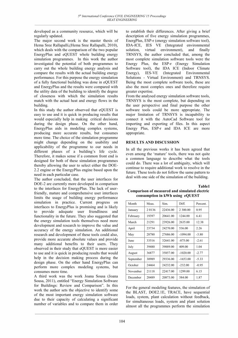
5th International Conference CIVIL ENGINEERING`15 Proceedings HEAT ENGINEERING
_____________________________________________________________________________________________________________
_______________________________________________________________________________________
104
developed as a community resource, which will be regularly updated. The major second work is the master thesis of Hema Sree Rallapalli,(Hema Sree Rallapalli, 2010), which deals with the comparison of the two popular EnergyPlus and eQUEST whole building energy simulation programmes. In this work the author investigated the potential of both programmes to carry out the whole building energy analysis and compare the results with the actual building energy performance. For this purpose the energy simulation of a fully functional building was done in eQUEST and EnergyPlus and the results were compared with the utility data of the building to identify the degree of closeness with which the simulation results match with the actual heat and energy flows in the building. In this study the author observed that eQUEST is easy to use and it is quick in producing results that would especially help in making critical decisions during the design phase. On the other hand, EnergyPlus aids in modeling complex systems, producing more accurate results, but consumes more time. The choice of the simulation programme might change depending on the usability and applicability of the programme to our needs in different phases of a building’s life cycle. Therefore, it makes sense if a common front end is designed for both of these simulation programmes thereby allowing the user to select either the DOE-2.2 engine or the EnergyPlus engine based upon the need in each particular case. The author concluded, that the user interfaces for DOE-2 are currently more developed in comparison to the interfaces for EnergyPlus. The lack of user-friendly, mature and comprehensive user interfaces limits the usage of building energy performance simulation in practice. Current progress on interfaces to EnergyPlus is promising and is likely to provide adequate user friendliness and functionality in the future. They also suggested that the energy simulation tools themselves need more development and research to improve the value and accuracy of the energy simulation. An additional research and development of these tools could also, provide more accurate absolute values and provide many additional benefits to their users. They observed in their study that eQUEST is more easier to use and it is quick in producing results that would help in the decision making process during the design phase. On the other hand EnergyPlus can perform more complex modeling systems, but consumes more time. A third work was the work Joana Sousa (Joana Sousa, 2011), entitled “Energy Simulation Software for Buildings: Review and Comparison”. In this work the author sets the objective to identify some of the most important energy simulation software due to their capacity of calculating a significant number of variables and to compare them in order
to establish their differences. After giving a brief description of five energy simulation programmes, EnergPlus, ESP-r (energy simulation software tool), IDA-ICE, IES VE (Integrated environmental solution, virtual environment), and finally TRNSYS, the author concluded that, among the most complete simulation software tools were the Energy Plus, the ESP-r (Energy Simulation Software tool), the IDA ICE (Indoor Climate Energy), IES-VE (Integrated Environmental Solutions - Virtual Environment) and TRNSYS. Being the most complete software tools, these are also the most complex ones and therefore require greater expertise. From the analysed energy simulation software tools, TRNSYS is the most complete, but depending on the user perspective and final purpose the other software tools could be more appropriate. The major limitation of TRNSYS is incapability to connect it with the AutoCad Software tool for importing and exporting of files. In this aspect Energy Plus, ESP-r and IDA ICE are more appropriate. RESULTS AND DISCUSSION
In all the previous works it has been agreed that even among the ‘mature’ tools, there was not quite a common language to describe what the tools could do. There was a lot of ambiguity, which will continue to require additional work to resolve in the future. These tools do not follow the same pattern to deal with one side of the simulation of the building.
Table1 Comparison of measured and simulated electric
consumption in kWh using eQUEST
Month Meas. Sim. Diff. Percent.
January 2 0136 22436.00 2 300.00 0.95
February 19397 20641.00 1244.00 6.41
March 21291 23926.00 2635.00 12.38
April 23734 24270.00 536.00 2.26
May 28780 27686.00 -1094.00 -3.80
June 33516 32641.00 -875.00 -2.61
July 39480 39889.00 409.00 1.04
August 36877 35857.00 -1020.00 -2.77
September 30989 29336.00 -1653.00 -5.33
October 24464 24232.00 -232.00 -0.95
November 21118 22417.00 1299.00 6.15
December 20489 20873.00 384.00 1.87
For the general modeling features, the simulation of the BLAST, DOE2.1E, TRACE, have sequential loads, system, plant calculation without feedback, for simultaneous loads, system and plant solution almost all the programmes perform the simulation
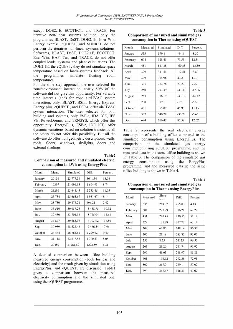
5th International Conference CIVIL ENGINEERING`15 Proceedings HEAT ENGINEERING
_____________________________________________________________________________________________________________
_______________________________________________________________________________________
105
except DOE2.1E, ECOTECT, and TRACE. For iterative non-linear systems solution, only the programmes BLAST, DeST, DOE2.1E, Ener-Win, Energy express, eQUEST, and SUNREL do not perform the iterative non-linear systems solutions. Softwares, BLAST, DeST, DOE2.1E, ECOTECT, Ener-Win, HAP, Tas, and TRACE, do not offer coupled loads, systems and plant calculations. The DOE2.1E, the eQUEST, they do not simulate space temperature based on loads-systems feedback. All the programmes simulate floating room temperatures. For the time step approach, the user selected for zone/environment interaction, nearly 50% of the software did not give this opportunity. For variable time intervals (and) for zone air/HVAC system interaction, only, BLAST, BSim, Energy Express, Energy plus, eQUEST , and ESP-r, offer air/HVAC system interaction. The user selected for both building and systems, only ESP-r, IDA ICE, IES VE, PowerDomus, and TRNSYS, which offer this opportunity. EnergyPlus, ESP-r, IDE ICE, offer dynamic variations based on solution transients, all the others do not offer this possibility. But all the software do offer full geometric descriptions, walls, roofs, floors, windows, skylights, doors and external shadings.
Table2
Comparison of measured and simulated electric consumption in kWh using EnergyPlus
Month Meas. Simulated Diff. Percent.
January 20136 23 777.34 3641.34 18.08
February 19397 21 091.93 1 694.93 8.74
March 21291 23 644.45 2 353.45 11.05
April 23 734 25 665.67 1 931.67 8.14
May 28 780 29 476.21 696.21 2.42
June 33 516 30 057.25 -3 458.75 -10.32
July 39 480 33 704.96 -5 775.04 -14.63
August 36 877 30 683.08 -6 193.92 -16.80
Sept. 30 989 28 522.46 -2 466.54 -7.96
October 24 464 26 763.62 2 299.62 9.40
Nov. 21 118 22 818.53 1 700.53 8.05
Dec. 20489 21781.59 1292.59 6.31
A detailed comparison between office building measured energy consumption (both for gas and electricity) and the result given by simulation using EnergyPlus, and eQUEST, are discussed. Table1 gives a comparison between the measured electricity consumption and the simulated one, using the eQUEST programme.
Table 3 Comparison of measured and simulated gas
consumption in Therms using eQUEST
Month Measured Simulated Diff. Percent.
January 535 579.8 -44.8 -8.37
February 604 528.45 75.55 12.51
March 451 511.88 -60.88 -13.50
April 329 341.51 -12.51 -3.80
May 309 304.98 4.02 1.30
June 305 282.78 22.22 7.29
July 250 293.39 -43.39 -17.36
August 263 306.19 -43.19 -16.42
Sept. 290 309.1 -19.1 -6.59
October 401 355.07 45.93 11.45
Nov. 507 540.78 -33.78 -6.66
Dec. 694 606.42 87.58 12.62
Table 2 represents the real electrical energy consumption of a building office compared to the simulated consumption using EnergyPlus. The comparison of the simulated gas energy consumption using eQUEST programme, and the measured data in the same office building is shown in Table 3. The comparison of the simulated gas energy consumption using the EnrgyPlus programme, and the measured data in the same office building is shown in Table 4.
Table 4 Comparison of measured and simulated gas consumption in Therms using EnergyPlus
Month Measured Simu-lated Diff. Percent.
January 535 269.97 265.03 4.13
February 604 227.79 376.21 62.29
March 451 220.45 230.55 51.12
April 329 121.28 207.72 63.14
May 309 60.86 248.14 80.30
June 305 21.18 283.82 93.06
July 250 8.75 24125 96.50
August 263 21.26 241.74 91.92
Sept. 290 41.03 248.97 85.85
October 401 108.62 292.38 72.91
Nov. 507 217.9 289.1 57.02
Dec. 694 367.67 326.33 47.02

5th International Conference CIVIL ENGINEERING`15 Proceedings HEAT ENGINEERING
_____________________________________________________________________________________________________________
_______________________________________________________________________________________
106
Table 5 Detailed difference percentage between eQUEST
and EnergyPlus
Electricity consumption Gas consumption
Month eQUEST% EP% eQUEST
% EP%
January 0.95 18.08 -8.37 4.13
February 6.41 8.74 12.51 62.29
March 12.38 11.05 -13.50 51.12
April 2.26 8.14 -3.80 63.14
May -3.80 2.42 1.30 80.30
June -2.61 -10.32 7.29 93.06
July 1.04 -14.63 -17.36 96.50
August -2.77 -16.8 -16.42 91.92
Sep. -5.33 -7.96 -6.59 85.85
October -0.95 9.4 11.45 72.91
Nov. 6.15 8.05 -6.66 57.02
Dec. 1.87 6.31 12.62 47.02
CONCLUSIONS
The results of comparison of the two major whole building simulation programmes show that, when we are dealing with annual energy consumption, the eQUEST results are much closer than those of the EnergyPlus results. The difference between the measured annual electrical energy consumption, and the simulated one using eQUEST programme, are +/- 0.95% for January and October, the highest difference percentage registered is 12.38% for the month of March, The others fluctuate between +/- 6%, and +/- 1%. The EnergyPlus programme shows a difference of 18% and 8%. Table 5 shows the detailed difference percentage between eQUEST and EnergyPlus, and it shows clearly that the results obtained when using eQUEST are closer than when using EnergyPlus. The difference between the simulated results, using EnergyPlus and the real values for annual gas consumption, shows a very large percentage of difference than when using eQUEST programme.
REFERENCES
Aprile A., Spacone E., Limkatanyu S. (2001) Role of bond in RC beams strengthened with steel and frp plates. Journal of Structural Engineering, Vol. 127, No. 12, p. 1445-1454.
Ashton I. E., Halpin I. C., Petit P. H. (1969) Primer on Composite Materials: Analysis. Stanford, 134 p.
Bergmeister K. (1999) Vorspannung von Kabeln und Lamellen aus Kohlenstoffasern. Beton- und Stahlbetonbau, Vol. 94, No. 1, p. 20-26.
Eurocode 8. (1996) Design provisions for earthquake resistance of structures. Part 1-4: General rules Strengthening and repair of buildings. ENV 1998-1-4.
Malek A.M., Patel K. (2002) Flexural strengthening of reinforced concrete flanged beams with composite laminates. Journal. of Composites in Construction, ASCE, Vol. 6, No. 2, p. 97-103.
Zarnic R. (1999) Strengthening of RC by fiber reinforced plastics. In: Urban Heritage, Building Maintenance, Concrete. Proceedings of International Congress on Building Maintenance. The Netherlands: Delft University of Technology, p. 91-100.
Drury B. Crawley, John W. Hand, Michael Kummert, Brent T. Griffith July (2005) Contrasting the capabilities of building energy performance simulation programs. page 7.
Drury B. Crawley, John W. Hand, Michael Kummert, Brent T. Griffith (2005) Contrasting the capabilities of building energy performance simulation programs Page 11.
Drury B. Crawley, John W. Hand, Michael Kummert, Brent T. Griffith (2005) Contrasting the capabilities of building energy performance simulation programs Page 13.
Hensen Jan L.M. and Roberto Lamberts (2011) Introduction to building performance simulation” Building performance simulation for design and operation Spon Press 2011.
Hema Sree Rallapalli (2010), A comparison of EnergyPlus and eQUEST whole building energy simulation results for a medium sized office building, Arizona state university 2010.
DOE (2013), EnergyPlus Graphical Interfaces. online accessed 14/02/2014, Available on http://apps1.eere.energy.gov/buildings/energyplus/ep_interfaces.cfm.( accessed the 14th of February 2014)
AECOsim (2014) Interdisciplinary building design, analysis and simulation, online accessed 5/3/2014 Available : http://www.bentley.com/enUS/Promo/AECOsim/aecosim+energy+simulator.htm

5th International Conference CIVIL ENGINEERING`15 Proceedings HEAT ENGINEERING
_____________________________________________________________________________________________________________
_______________________________________________________________________________________
107
eQUEST (2012)……. The Quick energy simulation tool, online acces 7/3/2014, available at: http://www.doe2.com/download/equest/eQUESTv3-Overview.pdf.
Berkely Natinonal Laboratory, Simulation Research Group, online access (2/2/2014) available at: https://simulationresearch.lbl.gov .
Joana Sousa, (2012), Energy Simulation Software for Buildings: review and comparison, University of Porto, Portugal. Online access 15/10/2014. available at: http://ceur-ws.org/Vol-923/paper08.pdf

5th International Conference CIVIL ENGINEERING`15 Proceedings HEAT ENGINEERING
_____________________________________________________________________________________________________________
_______________________________________________________________________________________
108
REVIEW OF GEOTHERMAL ENERGY POTENTIAL IN EUROPE
Aleksandrs Zajacs*, Jekaterīna Nazarova**, Anatolijs Borodinecs***
Riga Technical University, Institute of Heat, Gas and Water technology *E-mail: [email protected]
**E-mail: [email protected] ***E-mail: [email protected]
ABSTRACT
Geothermal energy worldwide is the most extensively used renewable energy besides hydro-power. In 2000 about 52,000 GWh of geothermal energy were extracted worldwide for direct use for space heating, process heat, thermal spas or greenhouses. Geothermal energy can be exploited with various technologies, although it generally, albeit not exclusively, involves drilling and pumping water from a certain depth. It feeds a great diversity of applications, alone or in combination with other sources of energy. Over 25% of the EU population live in areas directly suitable for Geothermal District Heating There are 237 Geothermal Distict Heating plants (including cogeneration systems) in Europe representing the total installed capacity of 4.3 GWth and production of some 12883 GWh or 1107 ktoe in 2012. In order to increase awareness, GEODH, an IEE project co-financed by the EU - has assessed and presented for the first time the potential of geothermal energy in Europe on an interactive map. In the EU there are 27 countries which have 3550 DH systems providing heat for 2160 cities and towns for over 5000 inhabitants, thus satisfying 12% of total heat demand of the population. The majority of the systems are fed by gas and only 1% by renewables (mostly biomass). Despite the favorable geothermal conditions in Europe, geothermal energy contributes only 0.001% of the district heating systems. The major markets are in France, Iceland, Germany and Hungary, however most of the European countries foresee a significant growth by 2020, also in line with their NREAP (National Renewable Energy Action Plans) targets. By 2020, nearly all the countries in Europe will have GeoDH.
Key words: geothermal energy, geothermal district heating, renewable energy,
INTRODUCTION
A large portion of the global energy supply is used for electricity generation and space heating, with the majority derived from fossil fuels. Fossil fuels are finite resources and their combustion is harmful to the environment through the emission of greenhouse gases and contribute to climate change and other pollutants. The use of renewable energy sources leads to the reduction of the environmental pollution which is well described in a similar study (Shipkovs, 2012). The demand for energy is increasing and future fossil fuel shortages are predicted (Ediger, 2007). A variety of different renewable energy sources are presented on the energy market and some of them have a potential to substitute or partly replace fossil fuels, thus contributing energy independence for countries which are geographically deprived of fossil energy sources. The use of solar potential for sustainable development is well evaluated in a similar study (Shipkovs, 2009), however an additional study is needed on geothermal potential as another promising renewable energy source. Geothermal energy worldwide is the most extensively used renewable energy besides hydro-power. By the end of 2000, geothermal power plants amounted worldwide to an installed capacity of about 8,000 MWel. They produced electrical energy of roughly
50,000 GWh per year. Besides this, about 52,000GWh of geothermal energy per year were extracted worldwide for direct use for space heating, process heat, thermal spas or greenhouses. Compared to other renewable energies, geothermal heat is advantageous since it is available all day and during all seasons. This and its great resource make geothermal energy an attractive option for a sustainable energy supply in the future. Geothermal energy can be exploited with various technologies, although it generally, albeit not exclusively, involves drilling and pumping water from a certain depth. It feeds a great diversity of applications, alone or in combination with other sources of energy. Geothermal energy is stored in the subsurface in certain concentrations and modes, which influence the type of application and extraction method that can be adopted. Over 25% of the EU population live in areas directly suitable for Geothermal District Heating (GeoDH) (Aalborg University, 2013). There is a large potential in Central and Eastern Europe, with GeoDH systems in operation in 22 European countries including Hungary, Poland, Slovakia, Slovenia, the Czech Republic, and Romania, where existing heat networks are well developed. Leading countries by GeoDH capacity installed are Iceland, Hungary, France, Germany, Italy. There are 237 Geothermal Distict Heating plants (including

5th International Conference CIVIL ENGINEERING`15 Proceedings HEAT ENGINEERING
_____________________________________________________________________________________________________________
_______________________________________________________________________________________
109
cogeneration systems) in Europe representing the total installed capacity of 4.3 GWth and production of some 12883 GWh or 1107 ktoe in 2012 (GeoDH, 2014). Additionally it would be useful to mention the relevance and potential of geothermal energy within the development of smart cities (Zajacs, 2014), where steps are being taken to improve the energy efficiency of the residential sector by the renovation of multi-apartment buildings (Borodinecs, 2015) and decrease the consumption of thermal energy, in this case the use of geothermal energy for heating and hot water preparation sees promising and feasible measure.
GEOTHERMAL BENEFITS AND POTENTIAL IN EUROPE
Geothermal generation has its roots in Europe. In the EU, 180 geothermal district heating systems
have a total capacity of 1.1 GWth installed, producing some 4256 GWh of thermal power, (i.e. 366 ktoe in 2012). The main benefits of geothermal heating and cooling are the provision of a local base load and flexible renewable energy, diversification of the energy mix and protection against volatile and rising fossil fuels prices. Using geothermal resources can provide economic development opportunities for countries in the form of taxes, royalties, technology export, and jobs. The geothermal potential is recognised by some EU Member States in their National Renewable Energy Action Plans. However, the actual potential is significantly larger. In order to increase awareness, GEODH, an IEE project co-financed by the EU - has assessed and presented for the first time the potential in Europe on an interactive map: http://loczy.mfgi.hu/flexviewer/geo_DH/.
Figure 1. Heat flow density; >90mW/m2 (MFGI, 2014)
From the map we can conclude that: GeoDH can be developed in all 28 EU countries; Geothermal can be installed with existing DH systems during extension or renovation, replacing fossil fuels; New GeoDH systems can be built in many regions of Europe at competitive costs; The Pannonian basin is of particular interest when looking at potential development in Central and Easter Europe. According to Eurostat, about one third of the EU's total crude oil (34.5%) and natural gas (31.5%) imports in 2010 originated from Russia. Of this, 75% of the gas is used for heating (2/3 in
households and 1/3 in the industry). Geothermal DH technology has the potential to replace a significant part of that fuel (GeoDH, 2014). Geothermal resources are defined as that part of the geothermal energy which can be extracted economically and legally in the near future. (Muffler and Cataldi, 1978). In order to quantify these resources, it is necessesary to define the amount of heat available in the rock (geothermal reservoir) and the characteristics of the reservoir with respect to the extraction of this heat. There are numerous methods and models that can be used to quantify geothermal resources. The assessment of geothermal resources is based on a volumetric heat content model for porous reservoirs assuming

5th International Conference CIVIL ENGINEERING`15 Proceedings HEAT ENGINEERING
_____________________________________________________________________________________________________________
_______________________________________________________________________________________
110
exploitation of geothermal energy by a doublet (Muffler and Cataldi, 1978). The resource H1 (in Joules), is given by
H1 = H0 · R0 (1) where H0 represents the heat in place (in J) in the reservoir under a surface area A. The fraction of this heat that can be extracted is R0, a recovery factor that depends on the extraction technology used. H0 comprises the heat stored in the rock matrix (index m) and in the water filling the pores (index w):
H0 = [(1 - P) · ρm · cm + P · ρw · cw] · [ Tt - T0] · S · ∆z (2)
where ρm, ρw are the density of the rock matrix and water, respectively in kg/m3, cm, cw are the specific heat capacity of the rock matrix and water, respectively, in J/(kg*K), P is effective porosity, dimensionless, Tt is the temperature at the top of the aquifer, in °C, T0 is the temperature at the surface, in °C, S is the surface area under consideration, in m2, and ∆z net aquifer thickness, in m. In a doublet system, where there is a production borehole and an injection borehole used to reinject the fluid after use, it can be shown that (Lavigne, 1978):
R0 = 0,33 · (Tt - Tr) / (Tt - T0) (3) where Tr is the reinjection temperature. A group of experts from the European Commission (EC) recommended a value of 25 °C for Tr. Reinjection avoids a pressure decline in the aquifer during exploitation and prevents environmental pollution of superficial water and soil as a result of disposing of highly saline geothermal water (Hurter, 2003). The geothermal gradient of temperatures through the crust is 25–30 °C (77–86 °F) per kilometer of depth in most of the world. The conductive heat flux averages 0.1 MW/km2. These values are much higher near tectonic plate boundaries where the crust is thinner. With knowledge of surface temperature (T0) in °C, heat production (A) in µW/m3, thermal conductivity (K) in W/m/°K, and heat flow (Q) in mW/m2, the temperature at any depth (Tz) can be approximated by:
Tz = T0 + Q / K · (z – z0) – A / 2K · (z – z0)2 (4) Temperature distribution at depths of 1000 m (Figure 2) and 2000 m provide a large scale view of the thermal field, while maps depicting the cities of presently operating geothermal installations (red dots) and the areas for which more detailed resources assessment can be found in specific national contributions.
Figure 2. Temperature distribution at depths of 1000m T>50°C (blue) and 2000m T>90°C (red) (MFGI, 2014)

5th International Conference CIVIL ENGINEERING`15 Proceedings HEAT ENGINEERING
_____________________________________________________________________________________________________________
_______________________________________________________________________________________
111
The map is not a tool to determine drilling sites for geothermal installations. Rather, it should be employed in activities preceding the targeting of drilling for geothermal purposes. It serves as a guide to set priorities for future investments in local studies and auxiliaries in delineating target areas for these investments. Geological Structure of Latvia’s territory
The utilization of geothermal energy in the territory of Latvia can be classified in the following groups: - Geothermal resources of low temperature <20°C; applicable for heating small objects and individual buildings and for preparing hot water with heat pumps; - Geothermal resources of medium temperature 20°C - 30°C; applicable for heating buildings and for preparing hot water with heat pumps; - Geothermal resources of high temperature >30°C; applicable for heating small residential areas and for preparing hot water with heat pumps, for direct heating as well as in combined electric power stations; - Petrothermal energy resources >100°C; applicable for electricity production, heating and preparing hot water. An average geothermal gradient varies within the interval of 0.8°C/100m – 1.9°C/100m in the north and east part of Latvia, but on average the geothermal gradient reaches 3.5°C /100m in the central and southwest part of Latvia. The change of geothermal gradient in the cross section happens in
the point where a blocking layer meets the water horizon. The graphs of rocks’ temperature measurements carried out in the boreholes reflect it as the change of an angle between a vertical axis and a temperature graph. Three lithological stratigraphical structures with different geothermal gradients are apparent in the geological cross section of Latvia: 1. Devonian terrigenic Carboniferous rocks, 2. Silurian and Ordovician Carboniferous clay deposits, 3. Cambrian and Venda terrigennic rocks. In the Cambrian and Venda cross section, gradients vary from 0.6°C/100m to 3.1°C/100m. The maximum value is reached in the southwest of Latvia. The analysis of the changes in an average temperature of Cambrian structure in the territory of Latvia is based on the observation data from measurements of temperature conditions in 72 boreholes that are scattered unevenly. There are 2 geothermal zones in the Cambrian structure with an increased temperature: 1. the zone in the direction to the south, southeast of Liepaja, where the temperature in Cambrian deposits reaches 38°C – 62°C in the depth of 1,281 – 1,714m. 2. From the borders of Jurmala to the Lithuanian border (Eleja geothermal anomalous zone), where the water temperature of the Cambrian reservoir is 33°C – 55°C in the depth of 1,100 – 1,436m (Pshenichnaya, 2011).
Figure 3. An average temperature map in the Cambrian underground water horizon (LNGA, 2014)

5th International Conference CIVIL ENGINEERING`15 Proceedings HEAT ENGINEERING
_____________________________________________________________________________________________________________
_______________________________________________________________________________________
112
GEOTHERMAL TECHNOLOGY FOR RESIDENTIALS
GHPs (Geothermal Heating Plants) exploit the relatively constant temperature in the ground, which is warmer than the ambient air during winter and cooler in summer. The ground temperature remains nearer to the desired temperature inside a building. When there is a large variation between inside and outside temperatures, as is the case for air source heat pumps, more work is required to provide the same degree of heating, which reduces the COP. If an excessive temperature difference exists, heat pump systems do not operate as intended. In the case of using of geothermal energy, temperature of the uderground aquifier remains constant and realtively high, depending on the area and depth of the geothermal borehole. The system principles are the same for residential building heating or for district heating plant changing only the scale and depth of facilities (Self, 2013).
Closed loop systems
In closed loop systems, which are commonly utilized, the heat transfer fluid is enclosed in a circulating loop and has no direct contact with the ground; heat transfer with the ground occurs through the piping material. There are four classes of closed loop heat exchange systems: vertical, horizontal, spiral, and pond. For residential buildings and private houses it is possible to apply all of these system types, but for industrial plants vertical loop systems are applied (Fig. 4). Vertical closed loop
A vertical closed loop system includes a loop field consisting of vertically oriented heat exchange pipes. A hole is bored into the ground, typically ranging from 45 to 75 m deep for residential and over 150 m for larger industrial applications. Pairs of pipes, connected at the bottom by a U-shaped connector, are fed into the hole (Fig. 5).
Figure 4. Horizontal loop heat exchange system configurations for geothermal heat pump from the left basic, in series, parallel (Self, 2013)
Figure 5. Vertical closed loop heat exchange system for geothermal heat pump (Self, 2013)
To enhance heat transfer, the gaps between the pipes and the borehole wall are filled with a pumpable grout material. The borehole diameter is approximately 102 mm for a typical residential home. For a typical residential application the spacing between boreholes is around 5–6 m in order to prevent adjacent boreholes from affecting one another and changing ground conditions. To ensure equal flows for multiple borehole systems a manifold system is used, which can be located in the building or buried in the loop field. An advantage of the vertical loop configuration is a reduced installation area, making them advantageous where land is limited. Another
incentive for these systems is low landscape disturbance, since drilling has a reduced impact compared to trenching. Also, locating the piping deep in the ground, where the temperature is constant year round, allows consistent heat pump performance and reduces overall loop length. The main disadvantage of using a vertical system is the installation costs, since drilling is normally more costly than horizontal trenching. Consequently the vertical loop systems are normally more economic for larger applications. The main advantage of geothermal heat pumps is their ability to utilize soil and ground water temperatures between 5 °C and

5th International Conference CIVIL ENGINEERING`15 Proceedings HEAT ENGINEERING
_____________________________________________________________________________________________________________
_______________________________________________________________________________________
113
30 °C, which is common at reasonable depths around the world (Self, 2013). GEOTHERMAL DISTRICT HEATING
District heating (DH) is a system which distributes heat from a centralized generation plant to users, connected via a heating grid and substations. DH achieves higher energy, economic and environmental performance compared to the traditional central heating systems, as heat supply is best adjusted to users demand. Last but not least, it reduces greenhouse gas emissions and excess heat losses, thus significantly contributes to the climate and energy policy targets. In the EU there are 27 countries which have 3550 DH systems providing heat for 2160 cities and towns for over 5000 inhabitants, thus satisfying 12% of the total heat demand of the population. The majority of the systems are fed by gas and only 1% by renewables (mostly biomass). Despite the favorable geothermal conditions in Europe, geothermal energy contributes only 0.001% of the district heating systems. Nevertheless geothermal district-heating (Geo-DH) dates back to the Roman ages, when city homes and baths were heated via natural hot water catchments and piping. In 2011 there were 212 Geo-DH systems operating in Europe with a total installed capacity of ~ 4700 MWt capacity. The major markets are in France, Iceland, Germany and
Hungary, however most of the European countries foresee a significant growth by 2020, also in line with their NREAP (National Renewable Energy Action Plans) targets (GeoDH, 2014). Geothermal District Heating (GeoDH) is the use of geothermal energy (i.e. the energy stored in the form of heat below the earth’s surface) to heat individual and commercial buildings, as well as for industry, through a distribution network. The first regions to install GeoDH, were those with the best hydrothermal potential, however with new technologies and systems, there is an ever increasing batch of regions that are developing geothermal technology for heating & cooling. Systems can be small (from 0.5 to 2 MWth), and larger with a capacity of 50 MWth. There are some new District heating schemes that utilise shallow geothermal resources, assisted by large heat pumps (GeoDH, 2014). The ‘hot’ GeoDH markets in Europe are in France (Paris, and renewed activity in the Aquitaine basin), Germany (Munich) and Hungary, but it is important to always note that geothermal DH systems can be installed in all European countries. In recent times, there have been new entrants to the market: The Netherlands, Spain (Madrid), UK (Newcastle) etc. By 2020, nearly all the countries in Europe will have GeoDH.
Figure 6. Geothermal doublet system for district heating (GeoDH, 2014)

5th International Conference CIVIL ENGINEERING`15 Proceedings HEAT ENGINEERING
_____________________________________________________________________________________________________________
_______________________________________________________________________________________
114
Many GeoDH systems (such as in the Paris Basin) are based on a dependable sedimentary resource environment, and on the doublet concept of heat extraction. Modern doublet designs include two wells drilled in deviation from a single drilling pad. Bottom hole spacings are designed to secure a minimum twenty year span, before cooling of the production well occurs. Well depths (deviated) of 2,000m to 3,500m are not uncommon; and these are often located in sensitive, densely populated urban environments, therefore requiring heavy duty silent rigs (up to 350 ton hook loads, diesel electric drive) Figure 6. The installation for systems with a lower temperature assisted by heat pumps is also possible. In several instances (Denmark, Germany, Iceland) absorption heat pumps, often associated with geothermal Combined Heat & Power plants (CHP), have been successfully installed and operated. Additionally, the installation of GeoDH systems becomes more economical close to areas with a higher urban density, as both resources and demands need to be geographically matched. One considerable challenge in the current economic crisis concerns the financing and the development of new heat grid infrastructures. Retrofitting is an alternative for developing the GeoDH market. Oradea, in Western Romania, is an example of the insertion of a geothermal heating system into the existing city: a coal fired/back pressure system, combined heat and power (CHP) network, typical of previous Central/Eastern Europe district heating practice is being used. Geothermal district cooling is actually poorly developed in Europe, with merely 30 MWth of installed cold power. This development issue should be challenged by geothermal operators (and users), as it could provide additional summer loads to GeoDH systems. In the Paris Basin, for instance, absorption chillers can be placed in grid substations and the primary hot fluid supplied by the geothermal heat plant. The chilled water can be piped to consumers via the same flow circuit used for heating (GeoDH, 2014). CONCLUSIONS
Geothermal heat pumps are highly efficient heating technologies that allow for reductions in CO2
emissions, the potential avoidance of fossil fuel usage and economic advantages. Heat pumps utilize significantly less energy that is harmful to the environment to heat a building than alternative heating systems. Many variations of geothermal systems for heating exist, with different configurations suitable in different situations and most locations around the world. In deciding among heating options it is important to determine the benefits for different ground heat pump options, typically in terms of efficiency, emissions and economics. Exploitation of geothermal resources is critically determined by the transmissivity of the aquifer, which constrains production rates. Transmissivity data and pumping test results are only available for specific areas. It would not be possible to obtain assessments for most of Europe based on such data. Furthermore, permeability may vary over several orders of magnitude within short distances, with almost unpredictable consequences for the exploitation. With the increased interest in geothermal heat pumps, geothermal energy can now be developed anywhere, for both heating and cooling. Low-to-moderate temperature geothermal resources are also being used in cogeneration heating plants (CHP). CHP projects certainly maximize the use of the resources and improve the economics, as has been shown in Iceland, Austria and Germany. Using low-to-moderate temperature geothermal resources in the direct heat applications, given the right conditions, is an economically feasible business and can make a significant contribution to a country’s or region’s energy mix. As oil and gas supplies dwindle and increase in price, geothermal energy will become an even more economically viable alternative source of energy. With geothermal energy becoming increasingly more competitive with fossil fuels and the environmental benefits associated with renewable energy resources better understood, development of this natural “heat from the earth” should accelerate in the future. An important task for all of us in the geothermal community is to spread the word on geothermal energy, its various applications, and the many environmental benefits that can accrue from its use (John, 2011).
REFERENCES
Aalborg University, Halmstad University, Ecofys Germany, Plan Energi (2013) Heat Roadmap 2050. Second Pre-Study for the EU-27, p. 50.
Borodinecs A., Zemitis J., Zajacs A., Nazarova J. (2015) Renovation of Multi-apartment Building in Latvia. Applied Mechanics and Materials, Vol.725-726, p. 1177.-1181.
Ediger V.S., Hosgor E., Surmeli A.N., Tatlidil H. (2007) Fossil fuel sustainability index: an application of resource management. Energy Policy, Vol. 35, p. 2969–2977.

5th International Conference CIVIL ENGINEERING`15 Proceedings HEAT ENGINEERING
_____________________________________________________________________________________________________________
_______________________________________________________________________________________
115
Geothermal District Heating in Europe (2014) About Geothermal District Heating [accessed on 02.08.2014.]. Available: http://geodh.eu/about-geothermal-district-heating/
Hurter S., Schellschmidt R. (2003) Atlas of geothermal resources in Europe. Geothermics, Vol. 32, p. 779–787.
John W.L., Derek H.F. (2011) Direct utilization of geothermal energy 2010 worldwide review. Geothermics, Vol. 40, p. 159–180.
Latvijas Nacionālā Ģeotermālā Asociācija (2014) Ģeotermija Latvijā [accessed on 02.08.2014.]. Available: http://lnga.lv./
Magyar Foldtani es Geofizikai Intezet (2014) Geothermal District Heating [accessed on 02.08.2014.]. Available: http://loczy.mfgi.hu/flexviewer/geo_DH/
Pshenichnaya Y., Kreslins A. (2011). The potential of geothermal energy usage in Latvia. 12th International Conference on Indoor Air Quality and Climate “Indoor Air 2011”, p. 2414–2419.
Self S.J., Reddy B.V., Rosen M.A. (2013) Geothermal heat pump systems: Status review and comparison with other heating options. Applied Energy, Vol. 101, p. 341–348.
Shipkovs P., Kashkarova G., Lebedeva K., Vanags M., Snegirjovs A., Migla L. (2009) Solar Energy Use for Sustainable Development // ISES Solar World Congress 2009: Renewable Energy Shaping Our Future: CD Proceedings, p. 1881.-1888.
Shipkovs P., Kashkarova G., Lebedeva K., Purina I., Migla L. (2012) Renewable Energy Resources Use for Environmental Pollutions Reduction // The Fourth IASTED African Conference on Power and Energy Systems (AfricaPES 2012) : Proceedings, p. 79.-85.
Zajacs, A., Zemitis, J., Tihomirova, K., Borodinecs, A. (2014) Concept of Smart City: First Experience from City of Riga. Journal of Sustainable Architecture and Civil Engineering, Vol 7, No 2, p. 54.-59.
5th International Conference CIVIL ENGINEERING`15 Proceedings LANDSCAPE, ENVIRONMENT AND LAND MANAGEMENT
_____________________________________________________________________________________________________________
_______________________________________________________________________________________
116
LANDSCAPE SPATIAL STRUCTURE OF THE LARGE-SCALE RESIDENTIAL AREAS
<insert two empty lines 10pt here> remove all grey instructions
Una Ile
Latvia University of Agriculture, Department of Architecture and Construction E-mail: [email protected]
one empty line 10pt here> ABSTRACT
The research is based on the authors’ previously performed researches on the landscape space quality in the large-scale residential areas in the Baltic Sea region and also on the researches about solutions for residential outdoor territory planning for the 21st century residential areas and their courtyards. Applying the comparative method in the research, several residential outdoor spaces were analysed according to their compositional planning solutions and their elements in Scandinavian countries. Consequently, the research studies the relation between landscape spatial structure and modern development tendencies of the large-scale residential areas in scale of Scandinavian countries.
Key words: landscape spatial structure, large-scale residential environment, development tendencies.
<insert two empty lines 10pt here> INTRODUCTION
Free landscaped spatial structures in Europe started to develop in the end of 19th century and in the beginning of the 20th century. They were planned and built as opposite to the sharply developing industrial cities, where exaggerated and unarranged planning structure created unfavorable social, working and recreation conditions. The slogan “Closer to nature!” got its embodiment in structural solutions of the differentiated nature building harmonious linking, mainly in suburb natural environment geographic ranges (Briņķis, Buka, 2008). Seeing from the point of view of modern urban planning theory, one of the large-scale residential environment development possibilities is functional differentiation of the courtyard space, which resulting main task is a perception and exponentiation of its recreativity potential. As Danish urban planner Jan Gehl pointed, there can be pointed three main directions in the functional and aesthetic spectrum of the public outdoor territory: necessary activities, possible activities and social activities. Recreation function by this division corresponds with the second category, where the processes of included functions are directly dependent on adequate outdoor territory conditions – „if there is a wish … and if one has time and place allows” (Treija, Bratuškins, 2003). How do they do in other cities? Referring to the north states, which are in our climate zone and in similar maritime conditions (Ilgtspējīgas lietusūdeņu apsaimniekošanas ..., 2006). North states have already been working for a long time in the politics for creating successful dialog with society in the urban planning process. It can be noted here the experience of not only the large cities
(Helsinki, Oslo, Stockholm), but also of the small cities (Tamper, Tapiola, Malmö), where urban planners emphasize the importance of society implication in planning processes (Liepa−Zemeša, 2008). From practical researches for objective determination of the situation it is necessary to get objective information about experience of other European states in planning, maintainance, to research and to reconstruct successfully the large-scale residential area territory. Therefore, its importance, role and expected consequences must be understood (Mansbach, 2006). In the research rationally planned and improved courtyards were established in the city of Finland – Tapiola and in Sweden in the new large-scale residential area of Hammarby Sjöstad. Such courtyards were created on the basis of progressive functional, economic and aesthetical factors, whose solve the matters of inhabitants’ living space quality in the widest urban building aspect (Mansbach, 2006; Rotzler Krebs Partner, 2005; Hammarby Sjöstad – Stockholm ..., 2009). Consequently, the aim of this research is to obtain new findings from the analysed territories in this research.
<insert one empty line 10pt here> MATERIALS AND METHODS
The methodological and informative basis of the paper is composed of modern analytical overview of the large-scale residential areas in the Scandinavian countries. In order to reach the set goal, the following scientific research literature was studied – publications, documents and electronic resource analyses. The literature sources used comprise material on the large-scale residential areas and their development tendencies. The inductive
LANDSCAPE, ENVIRONMENT AND LAND MANAGEMENT

5th International Conference CIVIL ENGINEERING`15 Proceedings LANDSCAPE, ENVIRONMENT AND LAND MANAGEMENT
_____________________________________________________________________________________________________________
_______________________________________________________________________________________
117
method was applied in the research process that was based on the analysis of the large-scale residential areas in the Scandinavian countries. For successful interpretation and establishing results, a monographic (descriptive) method was applied, which is based on the scientific findings, theory gained during the research and author research “The Landscape Quality of the Residential Area Courtyards in the Cities of Latvia”, what has been developed from September 2008 till August 2011. RESULTS AND DISCUSSION
In the context of balanced development ideas the whole world is increasingly thinking about the intensive use of existing resources. Therefore, increasing attention in urban planning is focused on the restoration of the degraded territories (Treija, 2001; Western Docks ..., 2001). The new structure plan of Stockholm, where sustainability is a central purpose, in addition draws the attention to the recurrent exploitation of the land for not creating new urban green zones (Beatley, 2000), visually illustrated in the Figures 1 and 2. Planning system in Sweden is marked as “comminuty planning”, which is a system focused on society production and consumption processes changing and improving, which otherwise is left to the market competence. Planning means strategy formulation, which would improve the quality of Swedish life and natural environment, visually illustrated in Figures 3 and 4. Planning and environmental policy focuses on this dual purpose model of urban development and green zone preservation-creation guide lines, whose provide possibilities for people to be closer to nature and that natural theories save their ecological functions (Nelson …). Large-scale urban reconstruction project is implemented in the other city of Sweden – Malmö.
Figure 1. Residential area of Hammarby Sjöstad in Sweden (1996)
(Source: http://www.hammarbysjostad.se/glashusett/)
Former industrial territory created close to the straits in connection of new Sweden and Denmark – Øresund near the bridge, has been rebuilt into new
residential and bargain area. In the basis of area development there are clearly defined principles of balanced development, in such way pointing at the full readiness of responsibility to undertake the main role in materialization of balanced development principles into (Treija, 2001).
Figure 2. Residential area of Hammarby Sjöstad
in Sweden (2009) (Source:http://www.hammarbysjostad.se/glashusett/) Linking with the other part of Malmö is affected by existing industrialized landscape with unequal urban development. The development of the other West port, which part has to be Bo01, still is only in the beginning stage, though, today more active building works have been started in the northern part of the area. It will be about 10 years required for Bo01 to become a part of greater interest to the city and to get wide local social and commercial service exposure, which usually also is expected from the new city. Only then the development of the new city can be precisely evaluated. But it is possible today already to make some conclusions (Gronlund, 2005). One of the basic ideas of Sweden European housing exhibition at the turn of the millennium was the idea that had to touch the theme of ecology, ecocycle and resources preservation. When Malmö was chosen as the place for exhibition process and after West port was chosen as a development place, the processes of ideas specification for ecological urban area had began.
Figure 3. Natural environment in residential area of Hammarby Sjöstad in Sweden
(Source: photo from author private archive, 2012)

5th International Conference CIVIL ENGINEERING`15 Proceedings LANDSCAPE, ENVIRONMENT AND LAND MANAGEMENT
_____________________________________________________________________________________________________________
_______________________________________________________________________________________
118
Figure 4. Natural environment in residential area of Hammarby Sjöstad in Sweden
(Source: photo from author private archive, 2012)
Figure 5. Example of the residential area in Malmö, Sweden (Source: http://www.bing.com/maps)
Figure 6. Examples of planning designs of residential courtyards of Malmö, Sweden
(Source: http://www.bing.com/maps)
Purposes were high and main idea the result to be applicable in the whole world, for it to be able to inspire the global urban environment initiative in the largest cities. Not all purposes were achieved, but Bo01 proved itself, and it still is a remarkable example (Nilsson, 2005), visually illustrated in the Figures 5, 6. Some of Malmö municipality officials, who helped to plan new region, were skeptical about conscious environmental perception of incoming population.
Figure 7. Designed shallow pond with rocky bed in Malmö, Sweden (Source: from project
LV2003/005−876/VAPF/0029 materials)
Figure 8. Example of rainwater design in Malmö, Sweden
(Source: photo from K. Siļķe private archive)
But this preconceived conception, that affluent people are not interested in environmental procedures, can be contravene. There are people, who, on the contrary, believe that conscious environment perception and prevention correspond with the higher class level. This point of view that most frequently occurs in environmental research proves that people, who are wealthy, try to be more educated and, thereby, try to take more interest about environmental problems (Ost, 2005). Malmö came to the solutions for soil pollution purification, ecocycle, and green structure and traffic problems. Developers prepared individual designs for the building. Bo01 plan attracted the attention of planners and architects; it became a good example of the long-term urban development. Created plan hoped to optimize constructing perspectives of compact and vivacious region; the region, which would protect from drafts and would give possibility for ecological, social, economic and human sustainability. For creating human sustainability, in order to reach high life quality in sustainable society, there was a new dimension of sustainable development concept. Bo01 green initiatives results showed wide interest in many courtyards, they were widely used also in other new projects, both in Malmö, and in Europe

5th International Conference CIVIL ENGINEERING`15 Proceedings LANDSCAPE, ENVIRONMENT AND LAND MANAGEMENT
_____________________________________________________________________________________________________________
_______________________________________________________________________________________
119
(Nilsson et al., 2005; Nilsson, 2005). The upkeep of rainwater in Malmö is closely connected with the planning process. Rainwater was one of the most important Bo01 external environment themes. Important environment matter was that, how appropriately to get rid of this water. In the same time rainwater was often used purposely to create different pleasant effects and different courtyards, streets spaces and park environment (Persson, 2005), visually illustrated in the Figures 7 and 8. Rainwater is an important aspect in urban planning process; therefore, in places, where it is impossible to solve rainwater upkeep matter or where the territories are very sensitive, building is not permitted. On working out detailed plannings as an obligatory the requirements are included: for rainwater accumulation and / or purification, on planning territory open rainwater system arrangement, to create topography of the area, the location of buildings and the greenery, taking into consideration rainwater drainage (Cilinskis, Zaloksnis, 1996.; Ilgtspējīgas lietusūdeņu apsaimniekošanas ..., 2006). If accurately created, then open rainwater systems take important place and progressively affect urban environment. Detalized design and type, as equipment are integrated in the urban landscape, are of great importance in this respect. Even such renewables as water has to be exploited rationally to provide enough stocks for future generations (Bolund, Hunhamma, 1999; Stahre, 2006; Ilgtspējīgas lietusūdeņu apsaimniekošanas ..., 2006; A lively and liveable ..., 2009). One of the biggest Bo01 problems was a creation of modern, resources effective and densely developed urban area that would remain close to nature. To achieve that the system design for wide urban area was created. Therefore, system design was created for local rainwater upkeep either that prescribed to invest resources in overground channel creation, as well as in introduction with water saving system, which would be used as a convenience in compact urban structure (Nilsson et al., 2005). Qualitative courtyards evaluation was made in the summer of 2002 and it was made by the landscape architect Sabina Jallow. Sabina Jallow described the plannings, vegetation and ecology of all residential courtyards. In total there were evaluated 18 features by three-point evaluation scale. The most characteristic ang higher evaluated features refer to the feeling for the place – it is well-tended and looks fresh, and it has development potential and sustainability, as well as it can give shelter. Such features as possibility to play, recreation places for sitting, impression of green zones, were evaluated a little higher of average level. In turn, the variety of plant materials, cultivated biological variety, insects amount, experience diversity, possibilities for inhabitants to develop and to create residential outdoor territory, evaluation was lower than the standard (Persson, 2005). Therefore, it was established in the
research that there are some failures in so far accepted harmoniously created and rationally planned courtyards. In the last decades the system of housing development, when municipality implements considerable apartment building and is the largest housing fund builder in the state, is one of the reasons, why Helsinki today is one of the sharply growing cities in Europe. As the tendency of population number increase has still going on, in new development plan provision with qualitative housing is among main priorities. 65 % of urban territory is municipal property; therefore, Helsinki is not restricted to plan new residential areas both in the central part of the city, and in the suburbs (Treija, 2000), visually illustrated in the Figures 9 and 10.
Figure 9. The design of the outdoor territory in the residential area of Helsinki (Source: photo from
V. Nefedov private archive, 2014)
Figure 10. The desing of children playground, example of Helsinki (Source: photo from V. Nefedov
private archive, 2012)
Helsinki determined strong policy to develop residential function in already existing urban territory. It has more reasons – working places are concentrated in the central part of the city, inner city has developed infrastructure.

5th International Conference CIVIL ENGINEERING`15 Proceedings LANDSCAPE, ENVIRONMENT AND LAND MANAGEMENT
_____________________________________________________________________________________________________________
_______________________________________________________________________________________
120
Figure 11. Bird's-eye view of residential areas of Helsinki (Source: http://www.bing.com/maps)
Helsinki is a port city and ports are located straight close to the center of the city. In the middle of the 80’s the municipality of Helsinki took a decision to change the exploitation of land in wide territories of ports and storages to the residential territories with mixed character. West port is about 200 ha large area, created in the west egde of Helsinki peninsula in pedestrian walk apart from urban business center. According to the development plan of Helsinki West port was planned as urban part with more than 22 000 inhabitants. Planned area consists of three regions – RuoKolahti, Jatkasaari and Munkkisaari (Treija, 2001), visually illustrated in the Figures 11 and 12.
Figure 12. Residential area of Jatkasari, Helsinki (Source: http://www.bing.com/maps)
Helsinki is also a very green city, because 35 % of the urban land territory is an open green space, moreover, green territories bind the whole urban structure. Therefore Helsinki used to call itself as garden city (Rīgas pilsētas attīstības ..., 2004). Helsinki, as well as many other Scandinavian cities, has compact urban form and large greening areas, whose line through the center of the city. Therefore, the compact urban form gives possibility for the existence of the pedestrian life style (Beatley, 2000). In Helsinki in the beginning of the 20th century there had already marked the transfer from the structural amorphous building to the purposeful its decentralization. This tendency was
corroborated by worked out in the middle of the century the general layout/plan of Helsinki. Therefore, in consequence of started at the turn of the century decentralization new, wide residential complexes were developed both in north, and in west directions. They are architectonically structurally tightly connected to the landscaped environment and embody progressive garden cities building principles. One of the more known Finnish garden cities is Tapiola, in development of which harmonious interaction of the building and nature environment has been achieved. One of the main priorities there is an effective, comprehensive structure of landscaped spatial environment (Briņķis, Buka, 2006). Values of Tapiola, to maintain environmental quality and to find the future success guide lines of Tapiola – not forgetting about the structural, social, economic and visual sustainability (Tapiola projects review, 2009), visually illustrated in the Figures 13 and 14.
Figure 13. Example of the large-scale residential area in Tapiola (Source: http://www.bing.com/maps)
Figure 14. Residential area structure in Tapiola (Source: http://www.bing.com/maps)
In the practise of Danish territorial planning it is widely used the method of restricting large cities with green planting belts and linearly arranging in their surrounding territory satelitte towns. In the planning project of Copenhagen suburbs it is envisaged to locate inhabitants along radial transport main roads, preserving among housing

5th International Conference CIVIL ENGINEERING`15 Proceedings LANDSCAPE, ENVIRONMENT AND LAND MANAGEMENT
_____________________________________________________________________________________________________________
_______________________________________________________________________________________
121
complexes green planting blocks (Briņķis, Buka, 2006). The main task of the year 1993 in the municipal plan of Copenhagen is to create comprehensive development in integrated city, where different urban activities are joined together, if it is allowed based on the principles of urban planning, environment and transport planning. In 1975–1990 the population number in Copenhagen decreased for 58 000 inhabitants, while in the other part of the state the amount increased. As one of the reasons urban planners of Copenhagen consider unattractive living conditions. In 1993 one of the main tasks of the municipal plan of Copenhagen was to provide high quality development possibilities for the housings. Therefore, on bringing forward as priority attractive territories in the wate quays, accessible with social services and public transport (Treija, 2000). In future it is planned to develop new residential areas in such way to improve the situation in the housing sphere in Copenhagen. Examples of the residential area courtyard are visually illustrated in the Figures 15, 16 and 17.
Figure 15. Example of the residential courtyards in Copenhagen (Source: http://www.bing.com/maps)
Figure 16. Landscape space of the courtyard in the example of Copenhagen
(Source: http://www.bing.com/maps) The development of new areas is first of all supported along the existing transport corridors to
accordingly provide good possibilities of approachability. Modern urban environmental policy in Europe rather follows the tendencies of urban development, than determines guide lines for urban development. There are big differences between the cities of West Europe and the cities of post-socialism states, which have to get over fast changes processes in many life domains (Rīgas pilsētas attīstības ..., 2004; Treija, 2001). Kevin Lynch asserted that it is possible to project built environment in such way for people to be able to fit fully into the surrounding conditions, to orientate themselves and to keep in mind ways and routes. He wrote that successful environmental sight gives its owner important feeling of emotional safety (Biddulph, 2007). Functionally designed courtyard planning is visually illustrated in the scheme of the Figure 18. The residential outdoor territory is rationally isolated from the parking lots. Building intensification still can’t be implemented at the expense of the limitation or decrease of the public outdoor territory functional diversity. Every outdoor territory users group has typical specific needs, which have to be respected, creating both active, and passive recreation zones, as well as places for entertainment for different age interested individuals, visually illustrated in the Figures 19, 20 and 21.
Figure 17. Landscape space of the courtyard in the example of Copenhagen (Source: photo from
V. Nefedov private archive, 2014)

5th International Conference CIVIL ENGINEERING`15 Proceedings LANDSCAPE, ENVIRONMENT AND LAND MANAGEMENT
_____________________________________________________________________________________________________________
_______________________________________________________________________________________
122
It must be found the possibility to implement other activities connected with residential environment, for example, walking with pets. Important role in the improvement of the public outdoor territory must be turned to the improvement of the surrounding landscaped quality, which was purposefully implemented; it is a vital increasing factor of environment recreativity level (Treija, Bratuškins, 2003). Urban planning is not only a science and art, but also economics and politics. Therefore, for taking into consideration the succession it is necessary to work out strict guide lines for urban spatial structure development. The development of the theories, which are important in the urban landscape and which are important part of the public outdoor territory, as well as where the large-scale development is planned, has to happened according to the plan accepted by all the interested parties (Liepa−Zemeša, 2008; A lively and liveable ... , 2009). One of the basis matters touching the urban planners today is how to make understandable projects of urban planning to the inhabitants and politicians, showing the city, which does not exist today, creating democratic dialog (Liepa−Zemeša, 2008). Therefore, wide practise and basis about different architectonic and ideological searches has been formed in foreign states over the decades. Once in a while designs occur, whose purpose is to accent principles and tendencies of modern architecture, not only to create comfortable or prestige housings for a definite society group. In Sweden and in a number of other European states
processes of housing architecture and technical organization were protractedly going on differently from processes in Latvia (Antenišķe, 2000). Even though building simplicity and comfortable functional organization have been practiced for a long time in Latvian building either. As surrounding building, which image and architectonic design is an important indicator of the public outdoor territory expression degree, which is mostly depressingly uniform in the large-scale residential area, one of the possible ways for environmental recreativity increase is purposeful building intensification with a purpose to optimize environment spatial space and to widen its functional spectrum. Depending on the relations of the existing in environment determinant elements scales to free courtyard area scale, building intensification could be implemented with the methods of both multi-storey, and low rise building. In current large-scale monofunctional residential areas the processes diversity could considerably increase the quality of the residential outdoor territory, and in this sphere the priority is given to the different inhabitants’ services oriented activities (Treija, Bratuškins, 2003). Residential area project should not be isolated from the other land exploitation methods, because many people live close to the schools, recreation possibilities, shops and other local institutions. Unfortunately, often residential areas are built not paying attention to the environment.
Figure 18. Example of the residential area spatial building planning in Copenhagen, where 1-existing large-scale building; 2-large-scale residential courtyards; 3-parking lots in the
residential area; 4-traffic zone; 5-low rise building; 6-view point in the courtyard territory (Source: author construction)
It has many reasons. The first and the main reason is the increasing people dependence of the personal transport. Today many people use cars to do the things that just some decades ago were done going by foot, riding a bicycle or using public transport (Biddulph, 2007; Rogers, 1997). Therefore, traffic is the one of our biggest environment problems. To
prevent its negative consequences, urban planning has to propose alternative that would allow people to refrain from driving in many daily situations and encourage using other transports kinds in place of cars. As a result it is necessary to optimize road network planning, to increase its exploitation effectivity (Ryden et al., 2005; Bertaud, 2002).

5th International Conference CIVIL ENGINEERING`15 Proceedings LANDSCAPE, ENVIRONMENT AND LAND MANAGEMENT
_____________________________________________________________________________________________________________
_______________________________________________________________________________________
123
Figure 19. Recreation area for adults in the courtyard of Helsinki (Source: photo from A. Ermolinskiy
private archive, 2014)
Figure 20. Recreation area design in the courtyard of Helsinki, Ruoholahti (Source: photo from
V. Nefedov private archive, 2014)
Figure 21. Recreation area design in the courtyard of Copenhagen (Source: photo from V. Nefedov
private archive, 2014)
Sustainable city does not mean only problem solutions for energy acquisition, pollution reduction, mianteinance of fauna and flora natural environment, green zones and simiral matters – even though some decades, beginnning with 1960, there was big necessity to focus straight to these points. There are many other important factors for the attention. It is a matter not only of aesthetics and
outdoor territory, it is important for city to be of great economic vitality, and to employ inhabitants and to be democtratic in daily working process (Gronlund, 2005). The interaction of nature and arranged environment constattly express bigger pressure in the urban development to the surrounding lanscape. Among the most important international factors and development trends affecting the development of population structure is the globalization of the economy. Increase of interrelations and competition, as well as the increase of knowledge-based economic activities. These changes substantially affect the states of the Baltic Sea region either. Main beneficiaries of them are areas of the capitals and other metropolises that have become magnets for the rapidly growing business services, communication industry, investitions flow (Vides aizsardzības un reģionālās ..., 2001; Лусе, 1978), it is necessary to determine equivalent residential area perspective development.
<insert one empty line 10pt here> CONCLUSIONS
There were established in the research different spatial spaces for urban environment courtyards in the Baltic Sea region. In the territory of Scandinavian states, where is functional improvement and splendid greenery formed for inhabitants residential outdoor territory, it can provide qualitative courtyard territory. The emphasis in these territories is placed on the raising of the courtyard spatial potential for recreativity development. The large-scale courtyards territories are formed to the green, environment friendly landscaped spaces that are suitable for different types of recreation possibilities. There are no more unreclaimed territories for development in Stockholm, therefore, there is defined the reconstruction of existing territories in the city that promotes the higher potential development of these territories. Scandinavian states think more and more about the intensive use of existing resources, therefore, greater attention is put to the reiterative exploitation and renovation of degraded territories. Consequently, achieving harmonious building with landscaped space, courtyard development in urban environment is balanced. Increase of pedestrian traffic and bikeways network potential by decreasing the transport traffic, prevention of environment pollution, the maximum exploitation of green structure and rainwater potential, implementation of garbage sorting system, flora natural environment maintainance in green plantations blocks provide viable courtyard territory for every inhabitants needs in daily life.
<insert two empty lines 10pt here>

5th International Conference CIVIL ENGINEERING`15 Proceedings LANDSCAPE, ENVIRONMENT AND LAND MANAGEMENT
_____________________________________________________________________________________________________________
_______________________________________________________________________________________
124
REFERENCES
A lively and liveable Singapore: strategies for sustainable growth (2009) [online] [accessed on 10.10.2014]. Available: http://app.mewr.gov.sg/web/Contents/ContentsSSS.aspx?ContId=1299
Antenišķe A. (2000). Divi mazstāvu dzīvojamie rajoni Somijā. Latvijas Arhitektūra, Nr. 6, 96.−99. lpp.
Beatley T. (2000). Green urbanism. Washington: Island Press, p. 30–41. Bertaud A. (2002). Note on Transportation and Urban Spatial Structure [online] [accessed on 20.10.2014.]. Available: http://www.alain-bertaud.com/images/AB_Transportation_and_Urban_Spatial_Structure_ revised2.pdf
Biddulph M. (2007). Introduction to Residential Layout. Amsterdam: Elsevier, 241 p. Bolund P., Hunhamma S. (1999). Ecosystem services in urban areas. Ecological Economics. The Transdisciplinary Journal of the International Society for Ecological Economics. Netherlands: Elsevier, Vol. 29, p. 293−301.
Briņķis J., Buka O. (2006). Pilsētu un lauku apdzīvoto vietu kompleksu arhitektoniski telpiskās plānošana. Rīga: Rīgas Tehniskās universitāte, 235 lpp.
Briņķis J., Buka O. (2008). Zemes īpašumu vērtēšana un taksācija pilsētplānošanā. Rīga: Rīgas Tehniskās universitāte, 50 lpp.
Cilinskis E., Zaloksnis J. (1996). Solid-Waste Management in the City of Riga, Latvia: Objectives and Strategy. Royal Swedish Academy of Sciences, Vol. 25, p. 103−107.
Gronlund B. (2005). Urban planning for good urban living. In: Sustainable city of tomorrow. Stockholm: Vasteras, p. 31−40.
Hammarby Sjöstad – Stockholm, Sweden (2009) [online] [accessed on 10.10.2014.]. Available: http://urbantheory-hammarbysjostad.blogspot.com/
Ilgtspējīgas lietusūdeņu apsaimniekošanas sistēmas izveide Latvijas pašvaldībās (2006). Projekta (LV2003/ 005−876/VAPF/0029) ietvaros. Jelgava: Jelgavas Tipogrāfija, 56 lpp.
Liepa−Zemeša M. (2008). Topical Dimensional Planning in Cities of Baltic Sea Region. Scientific Journal of Riga Technical University: Architecture and Urban Planning, Vol. 2, Series 10, p. 170−179.
Mansbach S. A. (2006). Modernist Architecture and Nationalist Aspiration in the Baltic: Two Case Studies. Journal of the Society of Architectural Historians, No. 1(65), p. 92−111.
Nelson A. City of Water [online] [accessed on 05.10.2014.]. Available: http://depts.washington.edu/ open2100/Resources/1_OpenSpaceSystems/Open_Space_Systems/Stockholm_Case_Study.pdf
Nilsson D. (2005). The LIP programme – a prerequisite for the environmental initiatives. In: Sustainable city of tomorrow. Stockholm: Vasteras, p.11−15.
Nilsson P., Andersson J., Hallin P. etc. (2005). A model for the future? In: Sustainable city of tomorrow. Stockholm: Vasteras, p.19−21.
Ost T. (2005). Sustainable urban district for (un)interested residents? In: Sustainable city of tomorrow. Stockholm: Vasteras, p. 81−87.
Persson B. (2005). What is sustainable urban drainage? In: Sustainable city of tomorrow. Stockholm: Vasteras, p.132−139.
Rīgas pilsētas attīstības perspektīvas starptautiskā kontekstā (2004). Rīgas domes Pilsētas attīstības departaments [online] [accessed on 10.10.2014.]. Available: http://www.rdpad.lv/uploads/rpap /att_plan_izpetes/12_rigas_attistiba_starptautiskaja_konteksta.pdf
Rogers W. (1997). The Professionals Practice of Landscape Architecture. Canada: John Wiley & Sons, p. 10−16.
Rotzler Krebs Partner (2005). Schonaustrasse Courtyard. Ultimate Landscape design. New York: Publishing Company, p. 392−397.
Ryden C., Fridh R., Nilsson R. etc. (2005). Towards a sustainable transport system. In: Sustainable city of tomorrow. Stockholm: Vasteras, p. 125−128.
Stahre P. (2006). Sustainability in urban storm drainage. Stockholm: Svenskt Vatten, 81 p.

5th International Conference CIVIL ENGINEERING`15 Proceedings LANDSCAPE, ENVIRONMENT AND LAND MANAGEMENT
_____________________________________________________________________________________________________________
_______________________________________________________________________________________
125
Tapiola projects review 2009. Espoo [online] [accessed on 05.10.2014.]. Available: http://www.espoo.fi/Tapiola
Treija S. (2000). Development of Housing Area in Riga. Scientific Journal of Riga Technical University: Architecture and Urban Planning, Vol. 1 , Series 2 p. 58−62.
Treija S. (2001). Contemporary Urban Renewal. Scientific Journal of Riga Technical University: Architecture and Urban Planning, Vol. 2, Series 2, p. 70−75.
Treija S., Bratuškins U. (2003). Development Problems of Large Scale Housing Estates in Riga. Scientific Journal of Riga Technical University: Architecture and Urban Planning, Vol. 4, Series 2, p. 77−83.
Vides aizsardzības un reģionālās attīstības ministrija (2001). Latvijas apdzīvojuma struktūra. Rīga: Jumava, 57.−80. lpp.
Western Docks. Public space (2001) [online] [accessed on 05.10.2014.]. Available: http://www.publicspace. org/en/works/b004-western-docks
Лусе M. (1978). Oзеленение малых городов Латвия. Pига: Зинатне, 103 c.
5th International Conference CIVIL ENGINEERING`15 Proceedings LANDSCAPE, ENVIRONMENT AND LAND MANAGEMENT
_____________________________________________________________________________________________________________
_______________________________________________________________________________________
126
CHURCH LANDSCAPES IDENTITY IN THE COASTLINE OF SOUTH KURZEME
Madara Markova, Natalija Ņitavska
Latvian University of Agriculture, Department of Architecture and Building E-mail: [email protected]; [email protected]
ABSTRACT
Church buildings are visually expressive dominants of the landscape; however, the sacral landscapes have not been extensively researched. In order to reveal the character of church landscapes and its elements, a thorough appraisal of the selection of indicators, of their scale. A particular method of research has been employed for characterisation of the church landscape in Kurzeme, on the shore of the Baltic Sea and along the bay, synthesized by a way of such specific research method as imageability
Key words: church landscape, identity, character, Kurzeme coastline
INTRODUCTION
The historical development and architecture of the landscape of Kurzeme
A traditional coastal building unit is a fisherman's homestead, which consisted of several buildings group – a dwelling house, a barn, a fish cellar, a pigsty, a net shack, a fish smokehouse, a cattle-shed, a bath-house, a root cellar, and a summer kitchen. As a typical features it should be noted that fishermen lived in individual farms in the coast of Vidzeme, but they formed small villages in the coast of Kurzeme. These coastal fishermen’s villages are a particular part of the coastal landscape identity and culture-historical objects of the national importance. The homesteads of the South Kurzeme and Vidzeme are characterized with the two-yards planning principle, which is divided into a “pure” yard with a barn and a “dirty” yard with a cattle-shed, a stable and a shed. Trees, bushes are planted in the “pure” yard; splendid flower-beds associated with fruit and bee garden are formed (Piekrastes apbūves…, 2011; Kultūrvēstures avoti…, 2008). Until the 19th century dwelling houses were built of wood – logs of fir or pine. One-storey houses were built both for living and farming. The most popular was a log structure construction or pillar construction with a sill filling. A cladding of vertical planks or hewn beam was used to protect the wall from the weather conditions, reeds were also used for the cladding near the lakes. Boulders were used for foundations and in ovens. Gabled (ridged) roofs or multigabled roofs were covered with rye straw, reeds or wooden lath, less with the boards. In the 19th century, when economic freedom was gotten, stone building started to build, but strong traditions of wooden architecture still maintained. In the second half of the 19th century boulders started to be used for the construction of a cattle-sheds and stables, but bricks were used for a dwelling house building, woods were mostly used for barns. Livonian fishermen built smoke-houses –
summer kitchens, which were called small houses, out of the sawed boats. They were also also also frequently used as a warehouse or a net shack – this building had become a sign of coastal recognition. Fishermen of Kurzeme formed so-called berth on the coast – boats were placed at the seashore, net shacks and fishing tools shacks were built, stake lines for fishing nets drying were formed (Piekrastes apbūves…, 2011; Kultūrvēstures avoti…, 2008). Ancient Latvian traditions are associated with archaeological sites – Sacred Hill, Sacred Grove, Sacred Cave, Sacred Spring – these are not buildings, but these are landscapes that bear the symbolic meaning. The oldest sacred / holy place is located in the coastal zone – in the camp of Sarnate swamp, not far from Užava. Another cult places found in Kurzeme are Idols Mountains and Church Mountains. Sacred springs, where the water attributed to strength, should be mentioned as well. The coast is rich with cultural monuments at the moment – including archaeological, historical, architectural, urban and industrial objects, as well as art objects. There are 338 national cultural monuments and 413 cultural monuments of local importance in total located on the coast (Valsts kultūras…; Piekrastes telpiskās…, 2010). One of the integral parts of the culture-historical heritage is churches and church landscapes of the coast of Kurzeme, which have a special landscape identity.
The genesis of the architectural structure of Latvian church landscape
The development of architecture in Europe and around the world was very dynamic and various. On time changing, people again and again rebuild and build new churches, wishing to show their faith (Kaminska, Bistere, 2011). Each era discovers its own evidences that make humanity's living space culture-historically richer (Zilgalvis, 2012).

5th International Conference CIVIL ENGINEERING`15 Proceedings LANDSCAPE, ENVIRONMENT AND LAND MANAGEMENT
_____________________________________________________________________________________________________________
_______________________________________________________________________________________
127
The beginning of the church building is dated with the beginning of the 13th century, when the Romanesque ruled in the beginning and then the Gothic style of the subsequent (Krastiņš, u.c., 1998). Starting with the middle ages, Latvia joined the Western Europe professional art scene. On conversion of the population of Latvia to the Christian religion churches started to build in its territory. These were wooden churches in the beginning, later stone churches. Wooden churches continued to develop next to the stone churches, which appeared later. Church architecture and construction on the general influence of the historical events was formed with deep rooted traditions. Wooden churches building, in spite of different historical events, blossomed again and again (Kaminska, Bistere, 2011; Krūmiņš, 2003). In the middle ages churches were the buildings in which artistic styles were most clearly readable. At the end of the 13th century the early territories of the Libyans, Latgalians, Courses, Selonians and Semigallians formed the confederation of feudal kingdoms, called Livonia. The dominant style in the end of the 19th century and in the beginning of the 20th century was historism. This is reflected in the various buildings of that time, whereas the churches of the different confessions were made in different historical styles. This connection principle of styles and confessions, certainly, is not consistent, but the trend is very explicit: Protestant churches in neo-gothic style; Catholic churches mostly in neo-baroque, but also found churches created in neo-gothic and neo-Romanesque styles; Orthodox Churches in the Russian Byzantine style. In the period of Classicism major changes took place in the Latvian church architecture. Columns, pilasters, pediments and other elements brought them closer to the image of the ancient temple, changing the medieval appearance preserved for centuries. Latvian architectural heritage of the second half of the 19th century till the beginning of the 20th century is rich and varied. This largely forms the culture-historical environment in which we reside daily. (Zilgalvis, 2012). Along with the rapid rise of economic and cultural levels in the second half of the 19th century eclectic entered in the architecture, intensive building of different types of buildings took place, followed by the beginning of the social 20th century with Art Nouveau (Avotiņa, u.c., 2004), churches a lot less were raised within this period. Within the period from 1918 to 1940 the attention in architecture was mainly focused on the school building and solving of apartments and urban issues (Avotiņa, u.c., 2004). Latvian cultural church environment is rich not only with churches of different architecture styles, but also with the fact that its forming was strongly influenced by
architects such as – F.B. Rastrelli, K. Hāberlands, J.D. Felsko, V. Neimanis, V. Bokslafs, P. Kundziņš (Levina, 1999).
Landscape identity and religion
Church landscape with its dominant elements church and church garden is a multidisciplinary research object. On the influence of the modern globalization processes changes in the landscape are perceived as a threat in the whole world, it is noted in the European Landscape Convention, as well as geographer, who explore the holistic nature of the landscape, Mark Antrop’s research (Antrop, 2005; European Landscape …, 2000). On considering that church landscapes have been studied a little, it is important to carry out their fixation and characterization of today's situation. A detailed research of the current situation not only provides an insight into the genesis of the processes, but also helps to recognize the visual aesthetic qualities of the modern church landscape. Cultural environment, including landscape, is a factor influencing the quality of life that is not only an integral part of the identity, but also the spatial development resource. Landscape and each of its elements is a reflection of the cultural heritage (General…, 1999; Mücher, 2010; Peirce, 1979; Penning-Rowsell, 1981; Schama, 1995; Siliņš, 2008; Ziemeļniece, 1998) present cultural manifestation. Landscape is the part of society identity; therefore it has to be researched in the context with the society. There is a causal link that between the regional or national scale and local scale the same landscapes may change their perception and understanding of the identity. Landscape changes for people living in a particular landscape are important because on changing the landscape the part of their daily lives disappears, places associated with emotions and memories vanish (Arnesen, 1998). Mihaels Houghs (Houghs, 1990). in his research uses the connection between geology and landscape identity. He considers that the landscape geology clearly shows close connection with culture expressions in the landscape – one of such landscape elements is architecture. The landscape geology is a reflection of the landscape identity in a longer time period – religions, objects generated under the influence of military and political events, different use of materials and symbolic meaning of objects (Houghs, 1990). Different society groups and their cultural identity have a direct connection with the landscape, as it is confirmed by scientists from different fields (Gray, 2003; Hay, 1998; Stephenson, 2008; Stokowski, 1996). Landscape is characterized by a spatial expressiveness, as weel as it contains social relations. Gatherings and performance of ritual activities promotes a sense of belonging to the place and society (Williams, 2012). The more important

5th International Conference CIVIL ENGINEERING`15 Proceedings LANDSCAPE, ENVIRONMENT AND LAND MANAGEMENT
_____________________________________________________________________________________________________________
_______________________________________________________________________________________
128
are the measures of mental activities, the greater number of people it attracts. Therefore, the social meaning of the landscape expands. Besides, if the landscape is distinguishing, it reflects the region, as well as diferences of the society (Peirce, 1979). Changes of the landscape structure influence local population. The thing that is so valuable in the landscapes and gives the inhabitants the sense of place and identity is its local nature and uniqueness (distinctiveness) (Rippon, 2012). The foreign experience enters the landscape planning in rapid steps, as well as foreign law is implemented and adapted to the landscape planning system. Therefore, in order to ensure the conservation and development of the landscape local nature and distinctiveness, a fixing, inventory and exploration of this nature is as a starting point.
Religion and churches in Kurzeme
Christianity originally came in Kurzeme peacefully and gradually. A number of changes in the landscape and the culture as a whole started along with the arrival of the Christianity, for example, in North Kurzeme cremations that had previously been typically here had disappeared. Each region in Latvia developed differently. Kurzeme was hardly affected during the time of the Livonian and Polish-Swedish wars, therefore in the second half of the 16th century the pronounced formation of differences had already started in the Duchy of Kurzeme (Courland) (Avotiņa, u.c., 2004; Feldmanis, 2010). It should be noted that in the Duchy of Kurzeme (Courland) Latvian and Livonian cultures with before the Christian traditions stood close to the Western culture. Although there were little churches in the beginning, then in the second half of the 16th century the decision was accepted to establish in Kurzeme 70 church congregations and build or rebuild churches there (Avotiņa, u.c., 2004; Feldmanis, 2010). Many of these churches have survived to the present day and are the national cultural monuments. In Kurzeme, unlike other Latvian culture-historical districts, Christianity was not the only one that was more pronounced in common. During the time of the Duchy of Kurzeme (Kurland) Christian church was represented by Catholics, Lutherans, reformists (Calvin's teachings followers), Orthodoxies and Old Believers (Feldmanis, 2010). In the beginning of the 17th century paganism still had a major role in the Latvian spiritual life. Around the middle of the 17th century the uplift of the spiritual life was observed (Feldmanis, 2010). Latvians of Kurzeme tightly clung to the religion of their forefathers. The period of Baroque is very pronounced in the Latvian church landscape, but still it had left the most vivid features in Latgale with the really gorgeous, white baroque pearls. But there are found churches of baroque in Kurzeme – in Kuldīga, Liepāja,
Ventspils. The baroque of Kurzeme is characterized by the simple, ponderous external presentation appearance. In the beginning of the 18th century fever epidemic made a great distress to Kurzeme (Avotiņa, u.c., 2004; Feldmanis, 2010). In the 18th century Latvia was not still a united territory and different development continued in various different spheres of life in each of the culture-historical districts, including religion. The next important step in the development of the religion life after innumerable political changes was the law adopted in the twenties of the 20th century on Latvian church to be separated from the state. During the Soviet period the restriction of the Christian traditions and atheistic propaganda took place. As a result of globalization and population migration in the 21st century not only sacred architectures significantly changed, but also the importance and function of its ambient territories and elements. Churches transformed from everyday landscape elements into spatial development resource in the sector of the economy such as tourism. The church as a cult building and landscape space around it in the beginning of the 21st century had started a new form of synthesis, in bringing a new additional value based on cultural traditions, craftsmanship and historical evidence storage and cognition. In the period of the last half century church landscapes diminishing and equalization had not yet fully destroyed architecturally distinctive spatial characteristics of the local cultural landscape. Landscape visual protection on the European level has become current along with an implementation of the European Landscape Convention. Ever since the middle ages the feature of populated area is the buildings of public nature, designed for people gathering, buildings for living and church along with the burial area – as the local religious focal point (Aston, Batsford, 1995) both in the visual aspect and in the spiritual and planning form. The variety of church landscape in Latvia forms in total due to different circumstances of natural basis, as well as in formation of culture-historical stratification in the different history of each region. One of such examples is aizjomi of Jurmalciems which form a specific landscape. Known as an aizjomi landscape, it consists of small, humanly made tilths on the seashore. These features are both physical elements and repositories of historical and cultural meaning. In one sense, through hard labor humans created the aizjomi landscape, adjusting the morphological and dynamic elements of the landscape and continually maintaining them. These human efforts made agriculture possible in the dunes, and in so doing they fashioned a means for producing a livelihood and, indeed, for sustaining life. The aizjomi landscape became a materialization of the people's

5th International Conference CIVIL ENGINEERING`15 Proceedings LANDSCAPE, ENVIRONMENT AND LAND MANAGEMENT
_____________________________________________________________________________________________________________
_______________________________________________________________________________________
129
day-to-day life in the middle and late 19th century. (Stūre, 2009; 2012). It is limited information available about church landscapes; therefore the determination of the landscape character is included in the fixation of the current state. In turn, determined indicators have been used relatively recently in the research. One indicator provides a little information so it is valuable to use of a system of indicators, where each of them would be representative, available, reliable and efficient (Bottero, 2011; Gabrielsen, 2003). More common use of indicators is for large-scale landscapes (European…, 2005; Stupariu, u.c., 2011; Swanwick, 2002), however, they can also be used in smaller areas (Swanwick, 2002; 2006).
MATERIALS AND METHODS
Objects
The research area is the South Kurzeme – from Lithuanian border to the city of Ventspils. The objects of research are located in the research area the Lutheran, Catholic and Orthodox churches, as well as a Baptist prayer houses, hereinafter referred to as churches. The research includes 16 churches (Figure 1).
Figure 1. Research territory and objects
Starting with the Lithuanian border the landscape of Kurzeme seaside consists of territories included in
the districts of Rucava, Nica, Pāvilosta, Ventspils, as well as the territories of republican cities of Liepaja and Ventspils which are not discussed in this research. The landcape of churches of large populated areas are observed separately, because they include regional differences, but the clearest dominance, however, is the city building structure and its created space. Building tradition and styles in the city context are also diversed and multicultural as large settlements are more closely involved in trading and cultural network than the other regions of the territory. This research examines the part of Kurzeme till Ventspils.
Methods
Monographic or descriptive method, based on the existing as well as scientific knowledge and theory acquired during the research, was used for the theoretical foundation for the development, as well as for the compilation, the identification and interpretation of the results. Several landscape research methods were used to characterize the church landscape of the coastline of Kurzeme:
Imegability method; Descriptive inventory; Definition of the perception criterias of the
landscape visual overall image.
Imageability method
The characterization of church landscape of the coastline of Kurzeme was carried out by the imegability method. After Kevin Lynch’s thoughts imegability is a quality of a physical object, which creates a possibility to cause a strong impression in any observer (Lynch, 1960). This is a form, color or an arrangement, which contributes the formation of the widely recognizable, powerfully created, widely used mental image of the environment. Lynch admits that imageability could also be called as imegability or visibility, but in the sense that objects could not only be seen in a landscape, but also could be felt the environment. The term “imageability” is being used with the meaning of “legibility” (Markova, 2014). Indicators of imegability in church landscape were defined during field surveys in 2012 and 2014 within the framework of the expedition, using aerial photographs as reference. An aerial photograph of the surveyed church landscape was prepared before going to the particular place. A detailed survey of each place was made on scouring the area and all access roads to analyze all the available view points. The place imegability schemes of the landscape of particular churches where this metode was used were made on the basis of aerial photograph to be able to clearly define the scope. On the other hand notably objects in the imegability schemes differ in which elements form the nature of the church landscape and landscape borders.

5th International Conference CIVIL ENGINEERING`15 Proceedings LANDSCAPE, ENVIRONMENT AND LAND MANAGEMENT
_____________________________________________________________________________________________________________
_______________________________________________________________________________________
130
Imegability schemes are made in „AutoCad 2012” programm, using a variety of graphical tools, as well as inserting there the aerial photo of particular church landscape.
Descriptive inventory
A fixation of church garden elements of the coastline of Kurzeme, consolidation of the results and transformation to visual patterns were made by tying a quantitative method with a qualitative method. A descriptive inventory was used in the research of the garden landscape space and elements, which is widely used in the evaluation of visual resources (Arthur, et.al., 1977). Descriptive inventory includes a combination of quantitative and qualitative landscape evaluation methods on analyzing and describing their components. The method of synthesis is used in the field research for the broadest possible collection of data, when separate elements of the research object are combined into a single whole, in order to study their interrelationships. The synthesis method is also used to interpret the data. Quantitative and qualitative indicators of the landscape are collected in the matrix used in the field research (Markova, 2014). Based on the experience of the previous research a matrix of survey and cartographic materials had been already prepared before the expedition using an electronic card system kurtuesi.lv. Survey matrix includes all the most anticipated parameters of the church landscape and elements of the church garden that would be useful for further research. On surveying the church gardens in the coastline of Kurzeme, there were fixed elements existing in every church garden. Later data obtained in matrixes were summarized in the "Microsoft Office Excel 2007" program. Landscape characterization is identification of essential and distinctive characteristics and qualities. This is still a relatively new approach to display and interpretation of the landscape. Landscape characterization approach rooted in England (Clark, et. al., 2004; Swanwick, 2002), later it developed in Scotland, Ireland and in other places in Europe. Landscape characterization is considered as an effective tool in forming the comprehension of the importance of the landscape (Herring, 2009). It is possible to use it for variety of scales, from the international up to the local (Swanwick, 2002; 2006). The reading of the landscape using the landscape indicators. The physical components of the landscape, related activities, its importance and symbolism are basic formative elements of landscape identity (Herring, 2009; Swanwick, 2002; 2006). The research focuses on the visible physical identity.
Perceptual criterias for the visual overall image of the landscape
Visual formative elements of the landscape identity are closely related with the human subjective perception where are separated several levels of perception – visual availability, scale, natural landscape, use intensity, diversity, consistency or harmony. Based on these theoretical visual perception levels of the landscape identity the visual survey matrix of the the landscape was designed, which served as the data collection, surveying the the research area. The survey matrix includes the total subjective visual evaluation of the landscape (Melluma, 1992; Krause, 2001; Forest landscape…, 1989; Swanwick, 2002; Ode, 2003; Nikodemus, Rasa, 2005; Hunziker, Kienast, 1999; Fisher, 1996; Ziemeļniece, 1998; Visual Resource…, 1984; 1986; 2008). There were determined following parameters for the subjective evaluation of the landscape: the visual availability, scale, topography, color, materials, texture, diversity, rarity, senses, movement, and natural landscape. Based on the theoretical group of criterias determined to define the identity of visual landscape, each landscape type specifies the possible criterias that may be slightly different in the urban and rural environment. Determination of the perception criterias of the landscape overall image is described in the detail in the authors’ previous researches (Ņitavska, 2012).
RESULTS AND DISCUSSION
In general churches in the coast are distributed irregularly, differently, both clustering around the populated areas, and locating in a rural landscape. Churches are not found in the coastal landscape in the district of Rucava. In the district of Nica there are five churches located in the coastal area – Baptist and Lutheran churches of Jurmalciems, Lutheran church of Muitnieki and Baptist and Lutheran churches of Skatre. There are six churches in the district of Pāvilosta – Lutheran church of Saraiķi, Lutheran church of Ziemupe, Catholic church, Lutheran and Baptist churches of Pāvilosta, Baptist church of Ulmale. There are five churches in the district of Ventspils – Lutheran church of Labraga, Catholic church of Jūrkalne, Baptist church of Sārnate and Baptist and Lutheran churches of Užava. There are 16 churches in the survey territory in total, 8 of them are Lutheran churches, 2 Catholic churches, 6 Baptist churches. Most of observed churches are located in even though small, but still populated areas. Accordingly, other churches are located in the rural landscape, because large populated areas are not included in this reserach (Table 1). There are observed church landscapes outside the large populated areas in the research, in this case, therefore, excluding Liepaja and Ventspils.

5th International Conference CIVIL ENGINEERING`15 Proceedings LANDSCAPE, ENVIRONMENT AND LAND MANAGEMENT
_____________________________________________________________________________________________________________
_______________________________________________________________________________________
131
Table 1 Churches of the sea coast of the South Kurzeme
Nr. District of
Kurzeme coast
Church
Church location place
1 Nīca Baptist church of Jurmalciems
Rural populated area
2 Lutheran church of Jurmalciems
Rural populated area
3 Lutheran church of Muitnieki
Rural landscape
4 Baptist church of Skatre
Rural landscape
5 Lutheran church of Skatre
Rural landscape
6 Pāvilosta Lutheran church of Saraiķi
Rural landscape
7 Lutheran church of Ziemupe
Rural populated area
8 Catholic church of Pāvilosta
Rural populated area
9 Lutheran church of Pāvilosta
Rural populated area
10 Baptist church of Pāvilosta
Rural populated area
11 Baptist church of Ulmale
Rural landscape
12 Ventspils Lutheran church of Labraga
Rural populated area
13 Catholic church of Jūrkalne
Rural populated area
14 Baptist church of Sārnate
Rural landscape
15 Baptist church of Užava
Rural populated area
16 Lutheran church of Užava
Rural populated area
The research area is divided into: •“rural landscape” – territory outside populated areas, not excluding that there might be individual residential or non-residential buildings located next to the church, “rural populated area” – villages and small populated areas, small towns.
Imageability
Imageability is essential characteristic aspect of the church landscape. Factor that affects the visibility of the church is the height of the church building and expressiveness of the church building bell tower as a dominant in the landscape. 6 of 16 churches are till 6 metres high and others mostly are only marginally above this height, thus do not exceed the height of the low-rise building. Church towers are not expressive component of the landscape. Perhaps church towers are not typical for these areas for not to mislead the shippers. Churches are typically located in the flat places and at the roadsides. Both of these factors contribute the poor visibility of the church landscape, because expressed distant view lines do not form. The church landscape of the South Kurzeme coast differs markedly with miniatures church landscape spaces, where the church is not an expressive dominant, but often groups in the common building of the populated area, creating a single fishermens’ village landscape.
Figure 2. Baptist church of Jurmalciems
dominant point – church; aizjomi; viewpoints;
tree structure; main road axis; dwelling house

5th International Conference CIVIL ENGINEERING`15 Proceedings LANDSCAPE, ENVIRONMENT AND LAND MANAGEMENT
_____________________________________________________________________________________________________________
_______________________________________________________________________________________
132
Figure 3. Baptist and Lutheran churches of Užava
dominant point – church; low-rise building territory; viewpoints;
tree structure; main road axis; dwelling house; industrial building
Figure 4. The Catholic church of Jūrkalne
dominant point – church; viewpoints; tree structure;
main road axis For example, the landscape of the Baptist church of Jurmalciems, where the longest view line, which is
formed, is about 200 m. This culture-historical church landscape is complemented by some unique cultural elements – aizjomi (Stūre, 2009; 2012). The landscape of Baptist and Lutheran churches of Užava is a bit more away from the sea as the rest of the church landscapes examined in the research and radical differences are felt here. Churches are considered for the dominants of this landscape which compete with closely neighboured industrial and warehouse buildings. The combination of low-rise buildings and the woody creates a peaceful backstage in the landscape. Both roadside plantings and private gardens greenery form the dense overgrown of the trees. In spite of the large quantities of small church landscapes met on the coast, there are also church landscapes with a long viewlines in the South Kurzeme. Bright landscape dominant is the Catholic church of Jūrkalne. The church is both visible from a distance only from the south; it is hidden by crowns of mature trees from the rest of the building. Trees are both in the church garden and in the neighboured cemetery. Viewline from the south is about 700 m long.
Occurrence of elements in the church gardens
Church landscapes and church gardens in the Latvian regions are formed according to different principles. These differences reproduce regionally different historical development and traditions. In general church gardens of the South Kurzeme have

5th International Conference CIVIL ENGINEERING`15 Proceedings LANDSCAPE, ENVIRONMENT AND LAND MANAGEMENT
_____________________________________________________________________________________________________________
_______________________________________________________________________________________
133
highly economic nature. There are household buildings, sheds and outdoor toilets in the church gardens. Symbolic elements are met a little in these gardens. And burials are only in one of the observed gardens (Table 2). The same situation is with the decorative plants. Perennials and in only minimal amounts are only in two of 16 observed church gardens. Garden structures are all asymmetric.
Table 2 The occurrence of elements in church gardens in
the coast of the South Kurzeme
Nr. Element Occurrence of the element in the
church garden, % 1 Outdoor toilet 75 2 Fence 62 3 Household building 62 4 Well 31 5 Small benches 25 6 Woody perimeter 19 7 Flgpole 13 8 Crucifix 13 9 Burials next to the territory of
the church garden 6 10 Burials inside the territory of
the church garden 6 11 Free-standing bell tower 6 12 Bicycle racks 6 The results of the percentage distribution of the occurrence of the elements in church gardens are rounded to the whole numbers to obtain greater transparency.
Occurred trees
There are mostly lilac shrubs in church gardens (Table 3). Pine-trees are also much used in church gardens and regarded as a typical element of the coastal church landscapes.
Table 3
Trees ocuured in the church gardens of the coast of South Kurzeme
Nr. Trees Occurrence of the tree in the
church garden, % 1 lilac 69 2 pine 62 3 linden 44 4 thuja 38 5 birch 38 6 maple 31 7 rowan 31 8 oak 13 9 fir 13 10 willow 6 11 elm 6 12 juniper 6 13 chestnut 6
Trees such as linden, birch, maple are considered as a typical for the whole Latvian landscape. Thujas are often used in Church gardens, as weel as in cemeteries. An interesting is application of the rowan in the church garden, which is placed at the entrance of the territory. It is considered for reverberation of sacred pagan traditions in a sacral garden area. Other trees are used only in certain cases – willow, elm, juniper and chestnut. The results of the percentage distribution of the occurrence of the trees in church gardens are rounded to the whole numbers to obtain greater transparency.
Criterias of the perception of the visual landscape overall image
The visual availability of the coastal church garden landscape of the South Kurzeme after the results of the research is narrow (43,75 %) and partly available (37,5 %), more rarely open and restricted (Figure 5). It is based on a coastal mosaic structures in rural areas or on a fully enclosed areas formed by coastal forests, as well as the small scale of the churches, and also that they mainly do not have a tower associated with coastal specifics, where high towers were not located not to mislead the shippers. It is proved by the landscape scale after the results of the research which in 50% of cases is small and in common in ~ 40% intimate (18,75 %) and close (18,75 %) (Figure 6). In addition this visual limitation is also explained by the churches located in flat areas rather than a flat hill tops that elsewhere in Latvia - ~ 70% of cases the terrain is flat and ~ 20% flat with some rolling hills. Landscape colors are also estimated as nuanced (43,75 %) and neutral (18,75 %). The color gamut of the coastal church landscape is also closely connected with the used materials, which here is represented by a brick (in 8 cases), wood (in 7 cases), plaster (in 6 cases) and stone (in 3 cases). The texture of the landscape is generally fine (75 %) and more rarely rough (25 %). The coastal church landscapes fundamentally are natural landscapes with some human-made elements (87,5 %), because they are mainly located in rural landscape (Table 1). Thus the landscape movement is also explained, which at the results of the research is defined as pacific (75 %) or dead (25 %). The prevalence of the natural landscapes and a distance of a people and civilization community created neutral (43,75 %) and pleasant (25 %) feelings. Comparing the church landscapes in other places of Latvia the coastal church landscapes in the South Kurzeme are relatively simple (68,75 %), that is in generally connected with traditions and self-restraint of the coastal population (Figure 7).
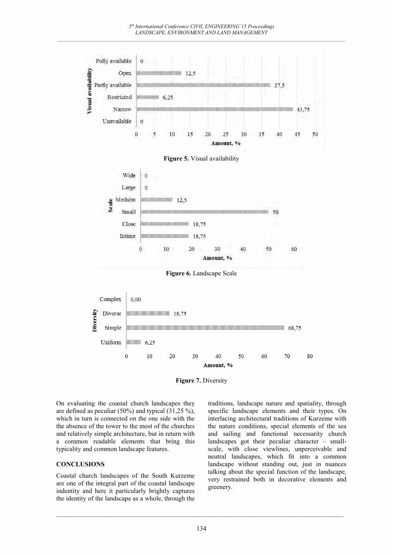
5th International Conference CIVIL ENGINEERING`15 Proceedings LANDSCAPE, ENVIRONMENT AND LAND MANAGEMENT
_____________________________________________________________________________________________________________
_______________________________________________________________________________________
134
Figure 5. Visual availability
Figure 6. Landscape Scale
Figure 7. Diversity
On evaluating the coastal church landscapes they are defined as peculiar (50%) and typical (31,25 %), which in turn is connected on the one side with the the absence of the tower to the most of the churches and relatively simple architecture, but in return with a common readable elements that bring this typicality and common landscape features. CONCLUSIONS
Coastal church landscapes of the South Kurzeme are one of the integral part of the coastal landscape indentity and here it particularly brightly captures the identity of the landscape as a whole, through the
traditions, landscape nature and spatiality, through specific landscape elements and their types. On interlacing architectural traditions of Kurzeme with the nature conditions, special elements of the sea and sailing and functional necessarity church landscapes got their peculiar character – small-scale, with close viewlines, unperceivable and neutral landscapes, which fit into a common landscape without standing out, just in nuances talking about the special function of the landscape, very restrained both in decorative elements and greenery.

5th International Conference CIVIL ENGINEERING`15 Proceedings LANDSCAPE, ENVIRONMENT AND LAND MANAGEMENT
_____________________________________________________________________________________________________________
_______________________________________________________________________________________
135
REFERENCES
Antrop, M. Sustainable landscapes: contradiction, fistion or utopija? Landscape and Urban Planing, Elsevier, 2005, No.75, p. 187–197.
Arnesen, T. (1198) Landscapes lost. Landscape Research, Vol. 23, No. 1, p. 39–50. ISSN 1469-9710.
Arthur, L.M., Daniel, T.C., Boster, R.S. (1977) Scenic assessment: an overview. Landscape Planning, No.4, p. 109–129. Aston, M., Batsford B.T. Interpreting the landscape Landscape archaeology in Local Studies. London, 1985, 168 p.
Avotiņa, A., Blūma, D., Līdaka, A., u.c. (2004) Latvijas kultūras vēsture. 2. Izdevums. Rīga: Apgāds Zvaigzne ABC, 507 lpp.
Bottero, M. Indicators Assessment Systems (2011) Landscape Indicators. In: Assessing and Monitoring Landscape Quality, Cassatella, C., Peano, A. (ed.). Dordrecht: Springer, p. 15–29.
Briņķis, J., Buka, O. Reģionālā attīstība un prognostika pilsētplānošanas kontekstā. Rīga: RTU izdevniecība, 2008, 195 lpp. ISBN 978-9984-32-255-1.
Clark, J., Darlington, J., Fairclough, G.J. (2004) Using Historic Landscape Characterisation. English Heritage’s review of HLCA aplications 2002 - 03. Preston: English Heritage, Lancashire County Council, 72p. European Council. Recommendation of the European Parliament and 15. of the European Council of 30 may. Concerning the implementation of Integrated Coastal Zone Management in Europe (2002). Official Journal of the European Communities, Vol.148, p. 24–27.
European Landscape Character Areas – Typologies, Cartography and Indicators for the Assessment of Sustainable Landscapes. Landscape Europe (2005) [online] [accessed on 20.02.2012.]. http://www.paesaggiopocollina.it/paesaggio/dwd/lineeguida/elcai_projectreport.pdf European Landscape Convention. Counsile of Europe [tiešsaite]. 2000 [skatīts 10.09.2012.]. Pieejams: http://conventions.coe.int/Treaty/EN/Treaties/Html/176.htm
Feldmanis, R. (2010) Latvijas baznīcas vēsture. Rīga: Luterisma mantojuma fonds, 423. lpp. ISBN 978-9984-753-62-1.
Fisher, P.F. (1996) Extending the applicability of viewsheds in landscape planning. Photogrammetric Engineering and Remote Sensing, Vol. 62, p. 1297–1302. ISSN 1939-1404.
Forest landscape Analysis and Design (1989) Forestry Commission, USDA Forest Service Pacific Northwest region. USDA: Edinburgh, 114 p. ISBN 01692046.
Gabrielsen, P., Bosch, P. (2003) Environmental indicators: typology and use in reporting. European Environment Agency, 20 p.
General Guidelines for Identifying and Evaluating Historic Landscapes, environmental program, California. California department of transportation Sacramento (1999) [online] [accessed on 10.10.2011.]. www.dot.ca.gov/ser/downloads/cultural /languide.pdf
Gray, J. (2003) A rural sense of place: intimate experience in planning a countryside for life. Planning Theory and Practice, Routledge, No.4 (1), p. 93–96.
Hay, R. (1998) A rooted sense of place in crocc-cultural perspective. The Canadian Geographer, No.42(3), p. 245–266.
Herring, P.C. (2009) Framing perceptions of the historic landscape: historic landscape characterization (HLC) nad historic land-use assessment (HLA). Scottish Geographical Journal, Routledge, Vol.125, No.1, p. 61–77.
Hough, M. (1990) Out of Place, Restoring Identity to the Regional Landscape, New Haven. London: Yale University Press, 230 p. ISBN 0-300-04510-7.
Hunziker, M., Kienast, F. (1999) Potential impacts of changing agricultural activities on scenic beauty – a prototypical technique for automated rapid assessment. Landscape Ecology, Vol. 14, p. 161–176. ISSN 1572-9761.
Kaminska, R., Bistere, A. (2011) Sakrālās arhitektūras un mākslas mantojums Rēzeknes pilsētā un rajonā. Rīga: Neputns, 335 lpp. Kaminska, R., Bistere, A. Sakrālās arhitektūras un mākslas mantojums Rēzeknes pilsētā un rajonā. Rīga:
5th International Conference CIVIL ENGINEERING`15 Proceedings LANDSCAPE, ENVIRONMENT AND LAND MANAGEMENT
_____________________________________________________________________________________________________________
_______________________________________________________________________________________
136
Neputns, 2011, 335 lpp.
Krastiņš, J., Strautmanis, I., Dripe, J. (1998) Latvijas arhitektūra no senatnes līdz mūsdienām. Rīga: SIA Izdevniecība Baltika, 312 lpp.
Krause, C.L. (2001) Our visual landscape managing the landscape under special consideration of visual aspects. Landscape and Urban planning, Vol. 54, p. 239–254. ISSN 01692046. Krūmiņš, A. Latgales koka baznīcas Romas katoļu draudzēs 18. Gadsimtā. Rīga: Jumava, 2003, 192 lpp.
Latvijas Zinātņu Akadēmija. (2008) Kultūrvēstures avoti un Latvijas piekraste. Letonika, otrais kongress: rakstu krājums. Rīga: Latvijas Zinātņu Akadēmijas Vēstis, 381 lpp.
Laumane, B. (2013) Jūra latviešu valodā un folklorā: etnolingvistiskais aspekts. Liepāja: LiePA, 403 lpp. ISBN 978-9984-864-89-1. Lenz, R., Malkina-Pykh, I.G., Pykh, Y. Introduction and overwiev. Ecological modeling, Elsevier, 2000, No.130, p. 1–11.
Levina, M., Tipāne, A., Silkāne, L.u.c. (1999) Eiropa - kopīgs mantojums. Baznīcas Latvijā : Eiropas kultūras mantojuma dienas Latvijā, 1999. g. 11. -12. Sept. Rīga: Valsts Kultūras pieminekļu aizsardzības inspekcija, 100 lpp.
Lynch, K. (1960) The Image of the City. Cambridge: MIT Press & Harvard University Press, 194 p.
Markova M., (2014) Latgales dievnamu ainava. Promocijas darbs. Jelgava, 155. lpp.
Markova, M. (2012 a) Characterization guidelines for churchyard in Latgale Upland. Peer reviewed proceedings of ECLAS 2012 Conference – The Power of Landscape at Warsaw University of Life Sciences – SGGW, Warsaw: Warsaw University of Life Sciences. lpp. 59–64, ISBN 9788393588404.].
Markova, M. (2012 b) Churchyard elements in Latgale upland. Research for rural development 2012. Annual 18th international scientific conference proceedings, volume 2, Jelgava: LLU, lpp. 122–129, ISSN 1691-4031.
Markova, M. (2013) Latgale Upland Church landscape reading though spatial indicators. Landscape Architecture and Art, Volume 2, Number 2, Jelgava, Latvia: Latvia University of Agriculture, lpp. 12–21, ISSN 2255-8632
Melluma, A., Leinerte, M. Ainava un cilvēks. Rīga: Avots, 1992, 176 lpp. ISBN 5-401-00772-8.
Mücher, C.A., Klijn, J.A., Wascher, D.M. u.c. (2010) A new European landscape classification (LANMAP): a transparent, flexible and user-oriented methodology to distinguish landscapes. Ecological indicators, Elsevier, No.10, p. 87–103.
Nikodemus, O., Rasa, I. (2005) Gaujas Nacionālā parka ainavu estētiskais vērtējums [tiešsaiste]. [skatīts 07.03.2010.]. Pieejams: http://www.daba. gov.lv/upload/File/Publikacijas/ZIN_P_GNP_Ainavu_est–vert.pd.
Nitavska N. (2011) The Method of Landscape Identity Assessment. Research for Rural Development 2011, 175- 182 pp.
Ode, Å. Visual Aspects in Urban Woodland Management and Planning: doctoral thesis.Alnarp: Swedish University of Agricultural Sciences, 2003,41p.
Peirce, F.L. (1979) Axioms for reading the landscape. Some guides to the American scene. The interpretation of ordinary landscapes, Meinig, D.W. (ed.) New York, Oxford: Oxford university press, p. 11–32.
Penning-Rowsell, E.C. (1981) Fluctuating fortunes in gauging landscape value. Progress in Human Geography, No.5, 1, p. 25 – 41.
Piekrastes apbūves vadlīnijas. Latvijas Lauku tūrisma asociācija: Lauku ceļotājs [tiešsaiste]. 2011 [skatīts 19.04.2012.]. Pieejams: http://www.celotajs .lv/cont/prof/proj/PolProp/Dokumenti/Apbuves_vadlinijas_web.pdf
Piekrastes telpiskās attīstības pamatnostādnes 2011.-2017.gadam. (2010) Stratēģiskais ietekmes uz vidi novērtējums [tiešsaiste]. [skatīts 11.10.2012.]. Pieejams: http://www.mk.gov.lv/doc/2005/RAPLMpamn_230410_piekr.502.doc
Rippon, S., Clark J. (2012) Historic landscape analysis: deciphering the countryside. Practical handbooks in archaeology. York: Council for British Archaeology, No.16, 173 p.
Schama, S. (1995) Landscape and memory. London: Vintage Books, 1995, 672 p.
Siliņš, E.I. (2008) Lielo patiesību meklējumi. Rīga: Jumava, 2008, 512 lpp.

5th International Conference CIVIL ENGINEERING`15 Proceedings LANDSCAPE, ENVIRONMENT AND LAND MANAGEMENT
_____________________________________________________________________________________________________________
_______________________________________________________________________________________
137
Stephenson, J. (2008) The cultural value model: an integrated approach to value in landscape. Landscape and Urban Planning, Amsterdam: Elsevier, No.84, p. 127–139.
Stokowski, P. (1996) Riches and Regrets: Betting on gambling in two Colorado mountain towns. Colorado: University Press of Colorado, 338 p.
Stupariu, I.P., Stupariu, M.S., Cuculici, R., u.c. (2011) Application of the global indicators to landscape change modelling on Prahova Valley Romanian Carpathians and Subcarpathians. International Journal of the Physical Sciences, Vol. 6 (3), p. 534–539.
Stūre, I. (2009) Jūrmalciema aizjomu ainavas stāsts. Rīga: LU Akadēmiskais apgāds, 112 lpp. ISBN 978-9984-45-143-5.
Stūre, I. (2012) The rise and the fall of the aizjomi landscape. Geographical Review, 102: 427–445.
Swanwick, C. (2002) Landscape Character Assessment. Guidance for England and Scotland. The Countryside Agency: John Dower House, p.84.
Swanwick, C. (2006) The Role of Landscape Character Assessment. In: Farming, Forestry and the National Heritage – Towards a more Integrated Future, Davison, R., Galbraith, C. (ed.). Edinburgh: The Stationery Office, p. 133– 146.
Taylor, K. (2008) Landscape and Memory: cultural landscapes, intangible values and some thoughts on Asia. Quebec, Canada[online] [accessed on 10.06.2011.]. http://openarchive.icomos.org/139/1/77-wrVW-272.pdf
Teritorijas attīstības plānošanas likums. Latvijas Republikas likums (2011) [online] [accessed on 10.02.2012.]. http://likumi.lv/doc.php?id=238807
Valsts kultūras pieminekļu aizsardzības inspekcija [tiešsaiste]. [skatīts 04.01.2013.]. Pieejams: http://www.mantojums.lv/?lang=lv&cat=576
Visual Resource Contrast Rating [tiešsaiste]. BLM Manual Handbook H_8431_1. U.S. Department of Interior, Washington, DC, 1986 [skatīts 18.03.2011.]. Pieejams: http://www.blm.gov:80/nstc/VRM/8431.html, Date accessed: April 4, 2008.
Visual Resource Management [tiešsaiste]. BLM Manual, 1984 [skatīts 16.03.2011.]. Pieejams: http://www.blm.gov:80/nstc/VRM/8400.html
Visual Resource Management U.S. Department of Interior [tiešsaiste]. Washington, DC, 2008 [skatīts 18.03.2011.]. Pieejams: http://www.blm.gov:80 /nstc/VRM/index.html, Date accessed: May 9, 2008.
Visual Resource Manual [tiešsaiste]. BLM Manual, 1984 [skatīts 17.03.2011.]. Pieejams:http://www.blm.gov/nstc/VRM/8410.html
Williams, A. (2012) Spiritual therapeutic landscapes and healing: a case study of St. Anne de Beaupre, Quebec, Canada. Social science & medicine, Elsevier, No.70, p. 1633–1640.
Ziemeļniece, A. (1998) Estētiskā kvalitāte ainaviskajā telpā. Jelgava: Latvijas Lauksaimniecības universitāte, 97 lpp. Zilgalvis, J. (2012) Jaunākās atziņas Latvijas arhitektūras mantojuma izpētē. Latvijas Zinātņu Akadēmijas Vēstis A daļa, Rīga, 66.sējums, ½.Numurs, 95.

5th International Conference CIVIL ENGINEERING`15 Proceedings LANDSCAPE, ENVIRONMENT AND LAND MANAGEMENT
_____________________________________________________________________________________________________________
_______________________________________________________________________________________
138
TRANSFORMATION OF THE LANDSCAPE SPACE OF DRIKSA IN THE URBAN ENVIRONMENT OF JELGAVA
<insert two empty lines 10pt here> remove all grey instructions
Aija Ziemeļniece Latvia University of Agriculture, Department of Architecture and Construction
E-mail: aija@k_projekts.lv one empty line 10pt here>
ABSTRACT
As a popular walking place for the townspeople, the bank of the Driksa River was already characterized a hundred years ago, when the city had not yet been devastated by wars and their misery. Dozens of postcards with nice recreational areas of Old Jelgava have toured the world. Currently, it is only possible to compare Jelgava with what it has once been in the memories. New view points, building scale, architectural stylistics, street widths, adapted to the technological requirements and comfort of the 21st century. However, the functional meaning and the German name of the Driksa bank has not changed - promenade – for a city which brings overlaying of a very dense urban space from the beginning of the 16th century. A hundred years away from the period, when the city was ravaged by the Bermontian venturers, the time cycle is particularly acutely delineated, which has wiped out unique artistic values of the urban construction into the rubbish of history. Also, along the waterfront of the Driksa River. Reconstruction of the promenade - a small fragment of the middle reach of the Driksa River, which vividly demonstrates a good cooperation result between the municipality, architects, landscape architects and engineers that can give an aesthetically valuable contribution to the urban space.
Key words: urban structure, urban landscape, visual and aesthetic quality, contextualism, harmony, space transformation INTRODUCTION In awarding Jelgava with the name of the best European city, it is worth noting that the urban constructed space has rapidly progressed over the last decade in terms of the quality of the environment. Several post-Soviet “bastions” have fallen that visually have degraded the city - low-value warehouse building, overgrown trees, functionally awkward green areas, crossed by narrow muddy walkways, traffic systematization, rainwater systematization. Particularly problematic is the issue of the discharge of the surface water, as the flat terrain of Jelgava and the height marks of 2.0-4.5 m above the sea level are the cause of high groundwater, creating extensive flood zones.
Figure 1. The place of the perspective promenade of the upper reach (Source: photo by author, 2014)
The huge difference in water levels of the seasons is an indicator, which gives the city a strange character of uniqueness in different seasons. The pulsating character of the Lielupe River and the Driksa River in July, when during hot summers the banks are exposed and the water flow in the river is not even noticeable - until ice piles in spring, which swirling across the flood plains, carry away broken tree and shrub fragments. The moments of observation of the uniqueness of these natural moments are a great advantage. In particular, if the sight lines are located on the high suspension bridge, right next to a residential building. Balancing the architectural composition of the bridge in the urban space with the natural pictorial values, a very high functioning and aesthetic contribution is made to the urban constructed space. The aim of the research is to assess the green, recreational space of the Driksa River and the scale, density of the adjacent building, conservation opportunities of the cultural and historical landscape space as well. The assignment of the research is based on the study of the historical materials about the city, which is associated with the transformation processes of the urban constructed space. It is mainly based on time periods, which have brought both world wars and the post-Socialism period in half a century. The left bank of the Driksa River of 2.7 km in length is chosen as a separate study area, focusing on searches of synthesis of the cultural and historical space and the ecological values.

5th International Conference CIVIL ENGINEERING`15 Proceedings LANDSCAPE, ENVIRONMENT AND LAND MANAGEMENT
_____________________________________________________________________________________________________________
_______________________________________________________________________________________
139
MATERIALS AND METHODS
The research includes the study of two parts of the city’s urban space for the left bank of the Driksa River: -The upper reach of the Driksa River – in the section between the railway embankment and Raiņa Street (700 m section, Figure 2); - The lower reach of the Driksa River between the Palace Bridge and the Northern Bridge under design (2 km section, Figure 3).
Figure 2. The existing production area and perspektive promenade of the upper reach of Driksa
(Source: drawing by author, 2014)
Both areas are evaluated in an approximately 20-40 m wide band that outlines the perspective construction zone of the promenade, so forecasting the landscape space of the urban constructed space. The first waterfront area is characterized by a distant sight line (400 m) from Palīdzības Street on the right bank of the Lielupe River, which is highlighted by the building area of the manufacturing zone, the Science Center, as well as the recreational zone and a beach place. The serene flow of the Lielupe River and the silhouette of the thin building create harmony and peace of the landscape space for the plain area (Īle, 2013). After dismantling of the building volume of the sugar refining factory, the silhouette of Pārlielupe has won a more attractive appearance. Of course, we can discuss the mindless “wiping away” of the historical building, for which reconstruction of the building volume and integration of the architectural appearance of the building into a new production zone have been possible. Unfortunately, the conditions of the funding of the European Union are
harsh and narrow from the point of view of the heritage conservation. The silhouette of the opposite bank in the northern part is somewhat hidden by the tree growth of Pasta Island and elements of the improvements on the island.
Figure 3. The existing functional territory of the lower reach bank of the Driksa River (Source:
drawing by author, 2014) The second area of the research is the lower reach of the Driksa River that is characterized by closer and further sight lines to the floodplain meadows of Palace Island. Palace Island is a closed area with birds nesting in the wild, wild horses grazing and where a rare plant vegetation can be found. In the plain area, the lower reach of the Driksa River is marked as being the base of the natural area, while the upper reach of the river is characterized as an urban landscape with a more or less dense building, load. There are only a few cities in Latvia that can boast of such a long bank line of the river that enters the urban environment. Such structure of the geomorphological urban construction creates not only an aesthetically high-quality living space, but also a serious search for engineering solutions to ensure easy operation of the street and underground communications. This is attributable to the fact that Jelgava is situated approximately 4.0 m above the sea level where the river flow to the sea is relatively long (70 km). At the same time, it is linked with the evaluation of the city's historical and cultural building, the existing elements of the natural base and the architectural space of the new architectural building.

5th International Conference CIVIL ENGINEERING`15 Proceedings LANDSCAPE, ENVIRONMENT AND LAND MANAGEMENT
_____________________________________________________________________________________________________________
_______________________________________________________________________________________
140
By overlaying of the urban environment – from the city’s protective canal and the construction of the ramparts in the middle of the 17th century up to the construction of new blocks of houses through the old burial areas in the middle of the 20th century and the beginning of the 21st century (Jāņa Cemetery, Literātu Cemetery), a new structure, building density and scale of the urban constructed space are created.
Figure 4. The landscape of the lower reach bank of the Driksa River near the promenade. The market building in the distance (Source: photo by author,
2014) The research includes the summary of the information of the archaeological and architectural and historical study. The research is based on the comparative method, evaluating the historical and the current transformation processes of the landscape space for the building of the left bank of the Driksa River. The material of the study through the comparative method describes separate functional and green areas along the waterfront in a more detailed way.
Figure 5. The Boat moorage to market. end of the 19 century (Source: Jelgava History and Art Museum) The methodology is based on the research findings, which are summarized in the scientific works of Prof. Briņķis and Prof. O. Buka (Brinkis, Buka, 2008) when evaluating the models of the development of the urban constructed space. Regionally, in the planning of the spatial, balanced and sustainable urban development processes, an important role is played by prognostics, which by
scientific and analytical methods determines the ways of attaining the goals of the development of the regional settlement and their optimization in a specific time period. In the planning practice, the first short-term phase of the development forecasts includes the immediate transparent 12 years. The second, long-term or distant phase includes a relatively transparent prognostic period of 20-25 years. Two main methodological approaches are used in the prognostics: 1) The genetic and descriptive method – the forecast of the territorial unit under the development is based on the description of the historical and the current situation, and the analysis the processes within a specific period of time;
Figure 6. The garden of the Villa Medem (end of the 19 century (Source: Jelgava History and Art
Museum)
Figure 7. Villa Medem. View from the Uzvaras street (end of the 19 century) (Source: Jelgava
History and Art Museum)
2) The target predictability method is based on the result of a specific project development program and the expected conceptual setting, which should be provided in the process of the development perspective. When planning the attainment of the forecasted goals, the specifics, time and tempo of the structural, spatial development of the already existing environment should not be ignored. When predicting the development processes of the structural construction of the modern architecture and spatial planning, such as integration, differentiation, transformation, reconstruction, regeneration, etc. - a balanced and sustainable or threshold development of

5th International Conference CIVIL ENGINEERING`15 Proceedings LANDSCAPE, ENVIRONMENT AND LAND MANAGEMENT
_____________________________________________________________________________________________________________
_______________________________________________________________________________________
141
these processes must be ensured. The forecasted development of Jelgava in the 21st century perspective must be linked not only with the regional-spatial and socioeconomic cooperation settings of the countries of the European Union and the Baltic Sea Basin, but also with the urban construction potential of the Jelgava agglomeration region. In forecasting the development potential, it is important to take into account the population growth rates, specifics of the demographic structure and optimization.
Figure 8. Villa Medem (55 Uzvaras street). Instead of the historical fencing there is a new masonry
fence. The Westermann and Dӧring flax-spinning mill in the rear (Source: photo by author, 2014)
Forecasting is one of the main components of the professional activities of architects-urban planners in the processes of the spatial development of the environment. It is associated with a responsible decision making, working on plannings of various settlements being different in the spatial scale, as well as on the implementation of projects. But the urban development processes must not only be forecasted by architects, it should be done in a close cooperation with ecologists, economists, transport planners, engineering specialists, etc.. It generally makes the urbanization process prognostic for a closer and perspective period.
Figure 9. After the disappearance of the historic wooden building, the land properties are surrounded by a seamless fence line (Source: photo by author,
2014) Consequently, the research includes several criteria: -The evaluation of the changes of the landscape space of the Driksa River and the urban environment over the next 12 years;
- The study of the current and the forecasted functional load (the Northern Bridge, the forecasted building and transport load); - Visually aesthetic quality transformation in the next few years (building intensity, the green area of the area changes, infrastructures). - The current degraded industrial landscapes and their change (or transformation) options; - High-quality view lines and points, their availability and the context in the development of the urban constructed space. The total area of Jelgava is 6032 ha, of which 293 ha - in open water areas. The city's territory has very low height marks as the lowland itself: up to + 2.0 m above the sea level - 523h, from + 2.0 to + 3.5 m above the sea level -1257h, from + 3.5 to + 4.5 m above the sea level - 2825h, but higher than 4.5 m - 1427h or ¼. (Information of Municipal institutions of Pilsetsaimnieciba Jelgava, 2014).
Figure 10. Uzvaras street opposite Villa Medem. The tree, shrub overgrowth along the Driksa River,
which hides its picturesque bank. (Source: photo by author, 2014)
Thus, 5% of the territory of the city is covered by water. But following the statistical data, the flood areas are so huge that the building foundation height mark is not permissible less than 4.00 m above the sea level. Hence, a half of the city's area is under the flood threat. It has been vividly demonstrated by the rains of October 14, 2014, which within 24-hour time has paralyzed the collection of the city's surface water, washing out the slope of the left bank of the Driksa River that fits tight to the city’s streets. Such geomorphological feature of the city seems to devote particular attention to the consistency of the infrastructural utilities, without undermining the visual and aesthetic quality of the urban space. Besides, the high water area ratio against the total building area of the city should be evaluated. These features of the natural base should be synthesized in the overall context of the building of the urban space. This is especially true for the landscape space of the recreational holidays.

5th International Conference CIVIL ENGINEERING`15 Proceedings LANDSCAPE, ENVIRONMENT AND LAND MANAGEMENT
_____________________________________________________________________________________________________________
_______________________________________________________________________________________
142
Figure 11. The former flax-spinning mill. The expression of the masonry architecture.
(Source: photo by author, 2014)
Figure 12. The former flax-spinning mill. The opportunities of transformation
of the industrial heritage in creating the functional application of new buildings.
(Source: photo by author, 2014) Thanks to the successful stabilization and development of the city's economic policy, an enormous contribution has been made in the regeneration of the green recreational area of the urban constructed space. This is attributable to the creation of the pedestrian area along the right bank of the Lielupe River and the left bank of the Driksa River, as well as the improvements of the island separating the two rivers (The spatial plan of Jelgava city, 2009). Of course, in order to escape from the flooding of the island and not to reduce its recreational significance, the geomorphological form of Pasta Island is changed - i.e., its artificial raising has been done by raising the bottom in the height of 3-5 m. Thus, the level difference and the slopes of both banks of the Driksa River are visually balanced. The nature of the bed of the Driksa River in the north-south direction and 5.4 km in length – is repeated by Zemgale prospectus - Akadēmijas street - Uzvaras street, observing the distance parallelism between the bank and the street within one block of houses, which is 50 m (in the lower reach) to 300 m (in the upper reach of the river near the railway embankment). Carefully studying the current building and the green wedge-type areas along the left bank of the river in the direction of the city center or in the westerly direction, it is possible to divide the left embankment
of the Driksa River into several urban construction spaces: - The landscape space near Sporta-Palīdzības streets and the adjacent cultural and historical building; - The section between Palīdzības and Raiņa streets marks a dense production and warehouse area of 400 m in length with a solid cover for the areas up to the river slope; - The area from Raiņa street up to Aspāzijas street that creates a landscaped and aesthetically attractive promenade; - From Ausekļa street to Lapskalna street - the market warehouse building with a large solid surface cover area; - From Lapskalna street up to the perspective Northern Bridge (900 m) – an expressive landscape space with the cultural and historical building. Currently, the area is deserted and it “hides” the likelihood of restoration of the historic building in itself, in the perspective obtaining architectural and landscaped spaces of very high quality. - The floodplain meadows of the Driksa River and the Lielupe River.
Figure 13. The floodplain meadow in a 50 m narrow band along Uzvaras street to the perspective
Northern Bridge. (Source: photo by author, 2014) RESULTS AND DISCUSSION
The upper reach of the left bank of the Driksa River –within the section of 700 m from the railway embankment up to Raiņa street. The upper reach of the Driksa River is characterized as a an area of manufacturing and warehouse building between Sporta street and Raiņa street. The last post-war “bastions” (a prison, warehouses of the construction base, power supply facilities, etc.), which takes around 200 m wide band of the bank with a dense building. Among the current industrial building volumes, the values of the cultural and historical heritage are “hidden” - the Red Cross buildings and the brick architecture of the old prison building, a wooden residential building and the former Reijers shelter (Ziemeļniece,2014). For the functional provision of the adjacent city railway terminal near the railway embankment, not
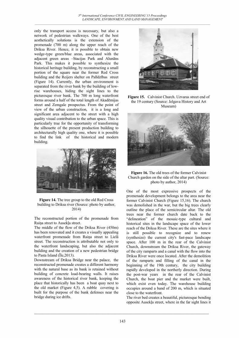
5th International Conference CIVIL ENGINEERING`15 Proceedings LANDSCAPE, ENVIRONMENT AND LAND MANAGEMENT
_____________________________________________________________________________________________________________
_______________________________________________________________________________________
143
only the transport access is necessary, but also a network of pedestrian walkways. One of the best aesthetically solutions is the extension of the promenade (700 m) along the upper reach of the Driksa River. Hence, it is possible to obtain new wedge-type green/blue areas, associated with the adjacent green areas –Stacijas Park and Alunāns Park. This makes it possible to synthesize the historical heritage building, by reconstructing a small portion of the square near the former Red Cross building and the Reijers shelter on Palīdzības street (Figure 14). Currently, the urban environment is separated from the river bank by the building of low-rise warehouses, hiding the sight lines to the picturesque river bank. The 700 m long waterfront forms around a half of the total length of Akadēmijas street and Zemgale prospectus. From the point of view of the urban construction, it is a long and significant area adjacent to the street with a high quality visual contribution to the urban space. This is particularly true for the opportunity of transforming the silhouette of the present production building to architecturally high quality one, where it is possible to find the link of the historical and modern building.
Figure 14. The tree group to the old Red Cross building to Driksa river (Source: photo by author,
2014) The reconstructed portion of the promenade from Raiņa street to Ausekļa street. The middle of the flow of the Driksa River (450m) has been renovated and it creates a visually appealing waterfront promenade from Raiņa street to Lielā street. The reconstruction is attributable not only to the waterfront landscaping, but also the adjacent building and the creation of a new pedestrian bridge to Pasta Island (Īle,2013). Downstream of Driksa Bridge near the palace, the reconstructed promenade creates a different harmony with the natural base as its bank is retained without building of concrete load-bearing walls. It raises awareness of the historical river bank, keeping the place that historically has been a boat quay next to the old market (Figure 4,5). A rubble covering is built for the purpose of the bank defenses near the bridge during ice drifts.
Figure 15. Calvinist Church. Uzvaras street end of the 19 century (Source: Jelgava History and Art
Museum)
Figure 16. The old trees of the former Calvinist Church garden on the side of the altar part. (Source:
photo by author, 2014)
One of the most expressive prospects of the promenade development belongs to the area near the former Calvinist Church (Figure 15,16). The church was demolished in the war, but the big trees clearly outline the place of the semicircular altar. The old trees near the former church date back to the “delineation” of the mosaic-type cultural and historical sites in the landscape space of the lower reach of the Driksa River. These are the sites where it is still possible to recognize and to renew (synthesize) the current city's fast-pace landscape space. After 100 m in the rear of the Calvinist Church, downstream the Driksa River, the gateway of the city ramparts and a canal with the flow into the Driksa River were once located. After the demolition of the ramparts and filling of the canal in the beginning of the 19th century, the city building rapidly developed in the northerly direction. During the post-war years in the rear of the Calvinist Church, the boat pier and the market were built, which exist even today. The warehouse building occupies around a band of 200 m, which is situated close to the waterfront. The river bed creates a beautiful, picturesque bending opposite Ausekļa street, where in the far sight lines it

5th International Conference CIVIL ENGINEERING`15 Proceedings LANDSCAPE, ENVIRONMENT AND LAND MANAGEMENT
_____________________________________________________________________________________________________________
_______________________________________________________________________________________
144
is possible to enjoy both the floodplain meadows on Palace Island and the river bed. The tree growths from the waterfront up to the intersection of Lapskalna street and Uzvaras street create the “green” bridge or a wedge (1.0 h) and its coming up to the old pre-war building site (1.4 ha of the area) between these streets. The building on Uzvaras street in the section from 49 Uzvaras street up to the former flax-spinning mill (a 300 m long band). The street section, which retains the most vivid cultural and historical building – a wooden residential building at 49 Uzvaras street, a masonry residential building at 8b Uzvaras street and at 62/64 Uzvaras street, Villa Medem and the former building of the flax-spinning mill. In the postwar years, Uzvaras street (the former Ezera or Lilienfeld street) has kept only a
Figure 17. Building on Uzvaras street 49 (Source: photo by author, 2014)
Figure 18. Building on Uzvaras street(Lilienfeld street) 51 end of the 19 century (Source: Jelgava
History and Art Museum) few buildings and the former street width. With the disappearance of the seamless building of the street along the river bank, a chaotic household and warehouse building zone has been created in the post-war years, which concludes with a seamless fence line, surrounding the land areas with tree and shrub growths and hiding the banks of the Driksa River.
After the demolition of the ramparts and backfilling of the canal (the start of the 19th century), in 1835/1836 near the Lake gate Count Johann Christoph Friedrich von Medem (1763-1838) Medem finished the Classical-style recreational palace Villa Medem designed in 1818 by the architect Johann Georg Berlitz (1753-1837), creating a recreation park near it. The sculpture of the beautiful Dorothea created by the sculptor Eduard Schmidt von der Launitz (1797-1869) from Paris was located in the park (Tomašūns,2014)). Villa Medem is a Classical-style building where both sides of the building are surrounded by exaggerated large-scale ionic four column porticos. In the center of the building, there is the hall characteristic to the Classicism (Krastiņš, 2014). Historically, opposite Villa Medem there has had an access to the river that visually has united the building volume with the expressiveness of the river. Currently, the double fence on both sides of the street (along the property at 62/63 Uzvaras street and Villa Medem) does (Figure 6,7) not allow the bank meadow to come into the urban environment. The positive fact is that at present, between the river and the villa, there is no building created in the post-war years. This enables the municipality to acquire privately owned green areas, thus connecting the perspective promenade band with the cultural and historical building. Close to Villa Medem (12 m) in the northern part, the former Westermann and Dӧring flax-spinning mill was built (1889), which gave a good contribution to the city's industrial boom at the end of the 19th century (Asaris, 1938; Figure 8). By no means, its location in the lower reach of the river was cost-effective and convenient for loading of the mill’s products and raw material in ships. The river dredging or cleaning was done regularly because of the slow flow of the Driksa River and the spring debris overgrowing in a fast way (Figure 9,10). The brick architecture of the 4-storey building volume of the flax-spinning mill beside Villa Medem - highlights the dual perception of the second half of the 19th century about the nature of the urban constructed space (Figure 11,12) beside the luxurious villa with a beautiful garden for walking, a production building of a huge building volume has been built. Currently, the building of the flax-spinning mill is abandoned, but its uniqueness consists of brick architecture and small window panes. As an industrial heritage, in the perspective it is to be reconstructed both as a public character and a multi-flat residential building. In particular, this applies to the nearest ten years, when the Northern Bridge will be built. Uzvaras (Ezera) street by the end of the 19th century is characterized by one-storey wooden building with tiled roofs, which during the war has been burned down (Figure 17,18). Part of the street building has been lost during World War I as the city's liberation

5th International Conference CIVIL ENGINEERING`15 Proceedings LANDSCAPE, ENVIRONMENT AND LAND MANAGEMENT
_____________________________________________________________________________________________________________
_______________________________________________________________________________________
145
from the Bermontians started in the direction from Ložmetējkalns to the city center, where exactly here severe street battles continued. After the liberation of the city in 1919, Ezera street was renamed into Uzvaras street. The cultural and historical building of the street in the length of 200 m, hides a good perspective of the urban construction, the economic growth of which will be brought by a new traffic infrastructure around the year 2020. The area of the historical heritage under the reconstruction is located in a geographically advantageous position between the two overpasses of the Lielupe River, the connection of which is possible through the connection with Uzvaras street. Parallel to the transport streams, the pedestrian and bicycle path along the Driksa River will play an important role. The waterfront of the lower reach of the river comes closest to the historical building (40 m), thus making it possible to create linking of the public outdoor spaces with water. Here starts the floodplain meadow about 600 min in length, which goes up to the perspective location of the Northern Bridge. After 2.5 km down the Lielupe River, its mouth into the Lielupe River starts and the city's administrative boundary closes. In the sight point of the place of the Northern Bridge in the upper reach of the Driksa River, the city’s building silhouette is readible (Figure 19,20). The solutions of the development problems of the urban constructed space lie also in the fact that the new overpass crosses the ornithological closed area, which must be protected from noise of the transport, thus seeking opportunities for construction of noise damping barriers. The opposite side of the river is an island that is formed between the beds of the Lielupe River and the Driksa River. The previously discussed building zones of the upper reach waterfront of the Driksa River and the green areas form a wedge in the direction from the river to the city, in turn, in the lower reach of the Driksa River – the floodplain meadows are seamlessly connected to the city in the area of several hectares. Here, in the 20th century a new high-rise residential building was created – the building of Dzilnas – Satiksmes and Ganību streets, which forms the extra-urban closing ring. Predicting the situation in the next few years after the construction of the Northern Bridge, undoubtedly, the extra-urban green areas will form the infrastructure of a new character. Downstream along the Driksa River between Villa Medem and the bypass of the Northern Bridge a natural base is formed - meadows with overgrowth (6 ha), thus creating a protective zone along the city's water treatment plant and the prospective transport artery. In the sight lines from the Northern Bridge, entering the city from the side of Riga, this will form a symbolic “green gate”.
Figure 19. The city's skyline in the lower reach of the Driksa River(end of the 19 century) (Source:
Jelgava History and Art Museum)
Figure 20. The city's skyline in the lower reach of the Driksa River (Source: photo by author, 2014)
Between the new Northern Bridge bypass and the end of the 19th century wooden building along Kazarmes street, in the post-war years there has been built a low-rise residential building with gardens and the street network that is broken apart by the scale of separate infrastructure units - the school and the production zones between Kārļa street and Meiju Road, creating multi-rings in the urban construction plan, which repeat the line of the old city ramparts. These functional zones mark the periods of the political and economic development of the urban space, which is particularly well readable in the northern and western part of the city’s building. This is true for the building height, density and the functional role: -The historic center of the urban construction from the end of the 17th century to the end of the 19th century, - The construction period before World War I from the end of the 19th century to the start of the 20th century, - The free state period building from the start of the 20th century to 1940, - The post-war building from ‘60-80s of the 20th century, - The period of the start of the 21st century.

5th International Conference CIVIL ENGINEERING`15 Proceedings LANDSCAPE, ENVIRONMENT AND LAND MANAGEMENT
_____________________________________________________________________________________________________________
_______________________________________________________________________________________
146
The dynamic growth of the elements of the urban planning and their inter-weighted spatial correlation is akin to a living organism — its ability to purposefully grow and structurally
Figure 21. The flow of the Driksa River –a river of the lowland, to the sea
emerge, develop through self-regulation. In the elements of the urban planning, the developmental stages specific of a living organism are also visible - birth, youth, maturity and old age. In the process of self-regulation of the urban construction of the region, the interaction of the urban space with the surrounding natural environment, the range of settlements, transport, as well as the transformation processes with all of these factors in space and time
is important. The basis of the regional spatial environment is generally created by single, structurally complex systems of the local settlements. CONCLUSIONS
Sawing out of the overgrown huge trees in the post-war years and the creation of a new promenade on the left bank of the Driksa River has given a fresh breath to the city and a symbolic fullstop to the elimination of the war devastations in the city's skyline. It gives a new impetus to the organization of the waterfront on the southern and the northern directions. The task of the next phase is more difficult because of the need to seek synthesized solutions, where the scale of the cultural and historical building, the contemporary modernist requirements and the avant-garde of the engineering solutions should be considered. In addition, it is made more difficult by the fact that the city is characterized by a high level of the groundwater, threatening the city during spring floods and summer and autumn rainfalls. Balance, equilibrium and harmony both in the architectural and functional expression, it all means to create important conditions for the acquisition of aesthetically high-quality public spaces.
References Asaris H. (1938) Latvijas pilsētas valsts 20 gados. Latvijas pilsētu savienības izdevums, p. 219.-242.
Briņķis J., Buka O. (2008) Reģionālā attīstība un prognostiska pilsētplānošanas kontekstā. Rīga: RTU, p. 154.-155.
Grosmane E. (2010) Senā Jelgava. Rīga: Neputns, p. 33-72.
Īle U. (2013) The silhouette of the east side of the Jelgava city. Proceedings of the Latvia University of Agriculture, Landscape Architecture and Art, vol.3, number 3, p. 14-22.
Jelgavas pilsētas pašvaldības iestādes ”Pilsētsaimniecība” dati. Jelgava, 2014.
Jelgavas pilsētas teritorijas plānojums 2009.-2021.gadam. Jelgava, 2009.
Krastiņš J. Arhitektūras stili Latvijā. [online] [accesed 01.11.2014.] Available: e.znet.lv/arhitekt_stili_Latvija_Text.pdf
Skujenieks M. (1927) Latvija. Zeme un iedzīvotāji. Rīga:, p. 167.-172.
Tomašūns A. (2014) Mana Jelgava, [online] [accesed 01.11.2014.] Available: http://www.jelgavniekiem.lv/pict/res/mana_jelgava.pdf
Ziemeļniece A. (2014) Transformation of the landscape space in the post years. Jelgava example. Proceedings of the Latvia University of Agriculture, Landscape Architecture and Art, volume 4, p. 67-76.

5th International Conference CIVIL ENGINEERING`15 Proceedings LANDSCAPE, ENVIRONMENT AND LAND MANAGEMENT
_____________________________________________________________________________________________________________
_______________________________________________________________________________________
147
THE INFLUENCE OF ANTHROPOGENIC IMPACTS ON THE WATER REGIME OF THE RIVER TOM
Olga Pasko National Research Tomsk Polytechnic University, Institute of Natural Resources
E-mail: [email protected]
ABSTRACT
Intensive extraction of sand-and-gravel material is often the reason for the shallowing process of rivers and seas, and the change of their hydrological regime is irreversible within several centuries. Easy profit from sand-and-gravel extraction results in great losses with regard to bottom dredging, problems with vessel’s capacity and cargo delivery.
Key words: ecosystems, river sand-and-gravel extraction, economic and social consequences INTRODUCTION
Today in Russia there is a dynamic growth in the volume of capital and road construction. This requires an appropriate market development of the non-metallic materials - sand, gravel, granite macadam and crushed limestone (Lopatnikov, 2006 ; Butkevich, 2006). Market growth rates of non-metallic materials in Russia make 10-15% per year, and more than half of the volume is formed by crushed stones and gravel (Kharo, Levkova, 2005). Their cost-effective extraction is due to technical floating equipment and water transportation (Pasko, Kovyazin, 2013). Unfortunately, intensive extraction of sand-and-gravel material is often the reason for the shallowing process of rivers and seas and changes in their hydrological regime that is irreversible within several centuriesas well (Tsupikova , 2003). The ecosystems’ function is damaged, species composition of plants and animals is depleted (Litvin, Tsupikova, 1999; Tsupikova, 1999).
The object of the study was the river Tom. The aim of this work was the scientific analysis of the effects of anthropogenic impact on the river Tom. Task 1: to identify the causes and degree of reduction for the possibilities of shipping. Task 2: to consider alternative ways of gravel extraction. MATERIALS AND METHODS
The research methods used were analytical, historical and comparative .The information for publication was obtained by the author in the archives of OAO "Tomsk shipping company" and JSC "Subrechprojectt". RESULTS AND DISCUSSION
This work is devoted to the investigation of sand-and-gravel extraction impact on the hydrographic features of the Tom river and the resulting economic and social consequences. Тom – is a river in western Siberia, a large tributary of the Ob, it flows into the Ob 68 km north of the center of Tomsk city (Fig.1).
Figure 1. Map of Tom river

5th International Conference CIVIL ENGINEERING`15 Proceedings LANDSCAPE, ENVIRONMENT AND LAND MANAGEMENT
_____________________________________________________________________________________________________________
_______________________________________________________________________________________
148
The river’s length is 827 km, the flood plain is up to 3 km, vertical drop from the source up to mouth is 185 m, the flood basin is 62 000 km², the average annual flow is:1100 m³/sec, 35.0 km³/year (Yevseyeva, 2001). The average depth in Tomsk area is — 2.5 m, stream speed into low water is up to 1.0 m/sec. Long-time average annual water turbidity is 95 g/m³. Observations on the Tom river have been carried out since the year 1918.The water flow rate from that time had practically not changed till 1950.The water level began to decrease in 1950 when large scale gravel extraction started there.
In the Tom, in the area of Tomsk city the extraction of large volume of sand-and-gravel materials which was out of control exceeding many times the natural flow of the accumulated drift, has caused the vertical deformation of the river bed and the changes of hydraulic characteristics flow (water levels regimes, free surface slope, stream speed and etc.) (Dubrovskaya, Zemtsov, 1997; Popov, 1990; Vershinin, 2005). The water level in the river in the area of Tomsk city has fallen by 2.1 meters (Fig.2).
a)
b)
Figure 2. Tom River: а) in the area of Kolarovo village; b) in the area of municipal bridge. The distance between the objects is 16 km (Source: photo from authors private archive)
According to experts’ opinion it is due to the fact that after gravel extraction the river "went" into the ground. The ground water level of the flood plain in the area of Tomsk city has accordingly fallen. Moreover, at the river bottom there was no slope from the Semilujki relief to the flat relief, crests of
sand bar appeared to be removed. All these facts led to stream slowdown (Reports, 2006-2011). From the middle of the 50s up to the middle of the 80s of the 20th century approximately 70 million m3 of sand-and-gravel material had been extracted (with the maximal annual volume of extraction 6.9

5th International Conference CIVIL ENGINEERING`15 Proceedings LANDSCAPE, ENVIRONMENT AND LAND MANAGEMENT
_____________________________________________________________________________________________________________
_______________________________________________________________________________________
149
million m3 per year) (Fig. 3). Development of Tom’s river bed deposits was made for satisfying the demands for constructional of non-metallic materials of plants located in Tyumen, Omsk and Tomsk areas, where other actual sources of
commercial extraction were not available. The fall in the water level required reconstruction of water intake facilities, relaying of inverted siphon and reinforcement of bridge.
Figure 3. Extraction of sand-and-gravel material on the Tom river (Source: photo from authors private
archive)
With the development of the West-Siberian oil and gas complex in the 80s of the 20th century the demands for sand-and-gravel material increased. The State Committee for Construction and Housing and Utility Complex (Gosstroy) of the Russian Soviet Federated Socialistic Republic took the decision on rational management of natural resources of non-metallic constructional materials river bed deposits on the Tom river and maintenance of river stage. The research work on the impact of the development of river bed deposits on the state of the Tom river state was started. Alongside with the development of Verkhni (Upper) Tomsk and Nishni (Lower) Kemerovo sand-and-gravel material deposits on the Tom river with an extraction volume of about 3 million m3 per year was planned. During the restructuring period in Russia (Perestroika) the construction speed and demands for sand-and-gravel material decreased sharply. According to the decision of local government authorities the sand-and-gravel material extraction on river bed deposits on the Tom river was utterly forbidden in 1993, but in 2002 the extraction was partially permitted. Today due to multi-bucket dredger and merchant marine the processing of extracted sand-and-gravel material into valuable construction material enriched coarse-grained sand (with fineness modulus from 2.3 up to 3 mm), that is not found in natural quarries has been successfully managed Such material is used in all kinds of construction works, in manufacturing of heavy and light aggregate concrete, precast reinforced concrete, for the forming of the filter layer by well infrastructure development of water supply, also in manufacturing of foundation blocks, floor slabs and so on. Extraction of enriched coarse-grained mortar sand and crushed stones with proven reserves of 2.086
million tons is made by OJSC “Tomsk Shipping Company” (OAO Tomskaya sudokhodnaya kompaniya). This company is dealing also with goods transport on the rivers of Ob-Irtysh basin to areas of Tomsk and Novosibirsk regions, the Khanty-Mansijsk and Yamalo-Nenets Auton-omous Districts. Now the company’s marine fleet includes more than 400 vessels, and about 270 among them were bought in the winter of 2011-2012. Lowering of the water level as a result of excess volume extraction of sand-and-gravel material worsened by the rainless summer in 2012 has caused acute problems. Firstly, the works were performed in extreme conditions, because the water level on the sand bars (max.180 cm) was by 50 per cent less than the estimated transportation capacity of our marine vessels and shallow waters trapped the vessels capacity. Marine vessels loading by less than 50 per cent of the transportation capacity was known to be unprofitable. Secondly, the company failed to use its own quarries on sand-and-gravel extraction and to provide road construction complexes of the Tomsk region with required materials (usually the “Tomsk Shipping Company” provided 90-95% of these industries demands for a year ahead). On the other hand, that year the company had to transport 6.3 million tons (mainly – non-metallic construction materials, reinforced concrete coal, etc.), and collect the 1.2 million tons of cargo under the contracts with the oil companies – “Surgutneftegas”, “LUKOIL”, Rosneft”, “TNK”, “Yuganskneftegas” and others. In the middle of summer, from 1.200 thousand t 300 thousand t were collected. The company suffered heavy losses due to force majeure because shallow waters are not specified in the contract.

5th International Conference CIVIL ENGINEERING`15 Proceedings LANDSCAPE, ENVIRONMENT AND LAND MANAGEMENT
_____________________________________________________________________________________________________________
_______________________________________________________________________________________
150
Thirdly, river transport for goods delivery to the north of the region is the cheapest means of transport. The cargo which is not handled is delivered by other means of transport and for the final customer it is much more expensive. An alternative to sand-and-gravel material extraction in the Tom river bed was the start-up of the up-to-date crushing and grading complex of Shaghai Shibang Machinery Co., Ltd (China) at the cost of 1 million USD in the territory of Kandinka sand-and gravel deposits, on May 25th, 2012. According to the experts estimation the deposit output makes 73 million cubic meters. When extracting 1 million cubic meters per year the estimated length of time is73 years without the damaging of river beds (Sand-and-gravel deposit, 2013). The full-flowing navigable Siberian river has been shallowed during its life of just one
generation, and in the area of the municipal bridge by the end of the summer you can wade in it. Easy profit from sand-and-gravel extraction has resulted in problems connected with bottom dredging vessels’ capacity and cargo delivery. The “boomerang” carelessly started half a century ago has turned back. CONCLUSIONS
1. Significant anthropogenic impact on the river Tom in the production of large quantities of gravel led to a strong deformation of the riverbed, causing the deterioration of shipping and large economic losses. 2. An alternative less hazardous options for the extraction of gravel at the moment is gravel extraction on Kandinsky Deposit of peat.
REFERENCE Butkevich G.R. (2006). Non-metallic construction materials industry. Current state and special features, magazine. Mining Industry (Gornaya Promyshlennost),V. 6 (68), p. 46-62.
Dubrovskaya L.I., Zemtsov V.A. (1997). Water level change of Tom river and ground waters of flood plain in the area of Tomsk city, Siberia geography issues, Tomsk, p. 100-106.
Kharo O.E., Levkova N.S. (2005). Nomenclature of non-metallic construction materials and perspectives of its expansion. Construction materials, V. 12, p. 81.
Litvin V.M., Tsupikova N.A. (1999). Ecological consequence of construction materials extraction from the bottom of Baltic Sea. Regional ecology, V. 3, p. 69 -72.
Lopatnikov M.I. (2006). Raw materials base for production of non-metallic construction materials of Russian Federation. Construction materials, V. 8, p. 42–43.
Map of Tom river. [online] [accessed on 10.02.2013.].
Available: http://images.yandex.ru/#!/yandsearch?p=2&text=томь река мост томск&img_url=etceterini.gorod.tomsk.ru%2Fuploads%2F23868%2F1313930845%2FSev01.jpg&pos=88&rpt=simage
Pasko O. A. Workshop on the basics of environmental management : textbook / O. A. Pasko, V. F. Kovyazin; National research Tomsk Polytechnic University (TPU), Institute of natural resources (IPR), Department of General Geology and land (were).- Tomsk: Publishing house of TPU, 2013. - 240 p.
Popov V.A. (1990). Gravel extraction on Tom river, Man and water, Tomsk, p. 46-48.
Reports on survey works / Sibgiprorechtrans, Tomsk, 2006-2011.
Sand-and-gravel deposit in Kandinka village will provide TDSK with gravel for 50-70 years [online] [accessed on 10.02.2015] Available: http://www.70rus.org/more.php?UID=18475
Tsupikova N.A. (2003). Impact of sand and gravel underwater mining on the geo-ecological situation in Baltic Sea. Dissertation for the degree of Cand. Sc., work subject of candidate of geological and mineralogical sciences according to State Commission for Academic Degrees and Titles. 25.00.36. - Ecogeology, Moscow, 343 p.
Tsupikova N.A. (2009). Impact of sand-and-gravel underwater mining on the geo-ecological situation in Baltic Sea, Integrated study of the Atlantic Ocean basin, Abstracts of 9-th regional conference. Kaliningrad, p. 70.
Vershinin D.A. (2005). Man-made impact on vertical deformations of river bed and stream hydraulics by the example of Tom river, Dissertation for the degree of Cand. Sc. (Geography), Tomsk : Tomsk State University, 188 p.
Yevseyeva N.S. (2001). Geography of Tomsk region. Tomsk : Tomsk State University, p. 223.

5th International Conference CIVIL ENGINEERING`15 Proceedings LANDSCAPE, ENVIRONMENT AND LAND MANAGEMENT
_____________________________________________________________________________________________________________
_______________________________________________________________________________________
151
ALTERNATIVE TREATMENTS FOR UTILIZATION OF DEHYDRATED SEWAGE WASTE WATER SLUDGE
Igors Gusarevs Latvian State Forest Research Institute Silava
E-mail: [email protected] Dagnija Lazdiņa
Latvian State Forest Research Institute Silava E-mail: [email protected]
ABSTRACT
The main aim of the study was to evaluate utilization options of dehydrated waste water sludge (WWS) as fuel and fertilizer. Changes in quality of the final product of three WWS treatment methods were compared – drying, pasteurization and incineration. This paper analyses potential risks and benefits of using waste water sludge as fertilizer and the suitability of using dehydrated and incinerated material as fertilizer. Technological and energy consumption aspects of all three options were analysed. The barriers for implementation of these technologies into common practice are more political than technical. For waste water sludge containing a low content of heavy metals, drying or incineration are more sustainable after-treatment methods. Key words: drying, sludge, heavy metals, ash content, compaction
INTRODUCTION
Waste water sludge (WWS) is one waste material that could be used for nutrient recycling in agriculture, plantation forestry or recultivated areas, thus reducing the amount of material required to be stored in waste polygons. Before reuse or storage it is important to pretreat the material using the most effective and adequate method. The use of waste water sludge in Latvia is regulated by the Rule of Cabinet of Ministers No 362 (Rules of Cabinet of Ministers, 2006). There are several studies on the problems of waste material utilization and methods, including measurement and simulation of the contact drying of sewage sludge in a Nara-type paddle dryer (Deng et al., 2009), solar drying in sludge management in Turkey for more sunny countries (Salihoglu et al., 2007), and other studies on the dewatering of industrial waste sludge by drying (Ohm et al., 2009; Font et al., 2011; Zhu et al.ab, 2012; Bennamoun et al., 2013). Wakerman (2007) studied separation technologies for sludge dewatering. A more complicated method reported is wastewater sludge gasification (Lumley et al., 2014). Other studies describe carbon mineralization in an arid soil amended with thermally-dried and compost of sewage sludge (Fernández et al., 2007), fertilization of willows (Lazdina, 2009; Heinsoo & Dimitriou, 2014) and other potential reuse possibilities such as incineration (European Commission, 2006). But those solutions are for large scale industry. Small scale treatment plants need small scale devices and simple solutions for after treatment of sludge before reuse or storage by reduction of the amount and water content in waste material.
The aim of the study was to compare three WWS treatment methods – drying, pasteurization and incineration and to assess changes in the quality of the final product.
MATERIALS AND METHODS
Material and instruments used
Waste water sludge from Salaspils waste water treatment plant passive drying fields was used. The material was collected ten days after placement on drying fields. The temperature of sludge at the beginning of experiments-treatments was +21°C, moisture content was 87%. The following equipment was used for the analyzed parameter determination: scales – “KERN” EMB 6000, Max. – 6000 g, d=0,1 g; for temperature - thermometer; pH Meter 3305 “JENWAY”; furnace - MLW WS 100 “VEB MLW MEDIZINISCHE”, tip 117-0100, temperature max 300°C.
Treatment
The temperature in the laboratory during experimental procedures was +25°C. A sample of waste water sludge “paste” (approximately 240/140/40 mm) was placed on a steel plate. Samples were pasteurized at 700C for 30 minutes, and then dried at 100°C. Incineration was modeled on the steel plate by heating the WWS with an open flame.
Analysis of materials
Chemical analyses and determination of moisture content were done in the Environmental laboratory

5th International Conference CIVIL ENGINEERING`15 Proceedings LANDSCAPE, ENVIRONMENT AND LAND MANAGEMENT
_____________________________________________________________________________________________________________
_______________________________________________________________________________________
152
of the Latvian Research Institute “Silava” according to ISO standards and Rules of Cabinet of Ministers (Rules of Cabinet of Ministers, 2006).
RESULTS AND DISCUSSION
Power consumption and temperature changes of waste water mass during pasteurization and drying are given in Table 1.
Table 1
Changes of temperature in WWS “paste” during drying
T in furnace °C
T of material
°C
Consumption of energy,
kW
Time, hh:mm:ss
100 71 1.6 01:00:00 110 79 1.6 02:00:00 110 72 1.7 01:00:00 110 72 1.7 01:00:00
Total 6.6 05:00:00
Table 2 Changes of temperature in WWS “paste” during
pasteurization
T in furnace
°C
T of material °C
consumption of electric y, kW
Time
temperature sensor set on 75°C 46 - 0.2 0 71 - 0.1 00:06:00 75 32 0.1 00:10:00 77 47 0.1 00:10:00 75 52 0.1 00:10:00 75 55 0.1 00:10:00 75 59 0.1 00:10:00 75 56 0.1 00:10:00 74 55 0.2 00:20:00
temperature sensor set on 85°C 85 61 0.2 00:20:00 85 66 0.2 00:20:00 85 68 0.2 00:20:00 84 68 02 00:20:00
temperature sensor set on 95°C
94 72 03 00:20:00
temperature sensor set on 85°C
85 70 0.3 00:30:00
Total 2.5 03:36:00 To reach 70% of the dry mass in the WWS material during drying 6.6 kW of energy were consumed and it took 5 hours. Pasteurization was started at 75°C
and then continued at 85°C and 95°C. Air and sludge sample temperature and consumption of energy are shown in table 2. The entire process of reaching 70% of dry mass in sample consumed 2.5 kW taking 3.5 hours (Table2). Shortening the process of pasteurization reduces energy consumption, but there is a risk that some pathogens could survive. In addition, pasteurization was less effective from the perspective of compaction of waste water sludge mass. The most effective method for decreasing volume is burning or incineration, but it leads to a decrease of the quality of material to be used for nutrient recycling, because the amounts of heavy metals become more concentrated (Table 3, Table 4).
Table 3
Mass and volume loss of WWS “paste” after treatment
Loss of mass Loss of volume Drying 70.25% 56.10%
Pasteurization 42.95% 36.59% Incineration/ burning 96.92% 89.27%
The WWS material used in the experiment contained heavy metals in concentrations which are characteristic for waste water sludge or compost quality class II (Rules of Cabinet of Ministers, 2006).
Table 4
Concentration of heavy metals and quality class of WWS “paste” after treatment
WWS treatment method
Incinera-rtion Drying Pasteuri-
sation Control
Cr mg kg-1 215 270 382 169
Quality class II III III II
Cu mg kg-1 740 204 322 350
Quality class IV I I I
Ni mg kg-1 69 14 12 17
Quality class II I I I
Pb mg kg-1 70 3 5 9
Quality class I I I I
Zn mg kg-1 2457 730 852 790 Quality class IV I II I

5th International Conference CIVIL ENGINEERING`15 Proceedings LANDSCAPE, ENVIRONMENT AND LAND MANAGEMENT
_____________________________________________________________________________________________________________
_______________________________________________________________________________________
153
Heavy metal content in waste water sludge after different treatments is shown in Table 4. According to the existing regulation, the material obtained after pasteurization and drying could be used for re-cultivation of degraded areas, but the ash formed after burning is not usable for recycling because the content of heavy metals is too high. The most problematic elements are Zn and Cu, which probably enter waste water from companies dealing with metalworking and construction.
Table 5 Concentration of NPK and pH of WWS after
treatment
pHCaCl2 pHKCl Ntot, gkg-1
P, gkg-1
K, gkg-1
Incineration 9.7 10.0 7.9 71.2 22.9 changes,% 31.4 29.4 -87.8 257.4 191.5
Drying 6.9 6.8 61.4 22.0 7.7 changes,% -7.6 -12.5 -5.2 10.2 -1.5
Pasteurization 7.3 7.4 60.7 21.7 8.9 changes,% -1.9 -4.0 -6.3 8.8 13.1
Control 7.4 7.7 64.7 19.9 7.8 During processing, not only the concentration of metals is increasing, but also the concentration of the main plant nutrient elements and the pH of the
final product are different compared to untreated waste water sludge (Table 5). There were minor changes in pH and concentration of N and P after pasteurization. After drying only P concentration increased. The largest changes in concentrations were after incineration. It will be necessary to solve the problems with heavy metals to utilize WWS ash as a liming material with a reasonable content of P and K. CONCLUSIONS
Pasteurization is a less energy consuming and faster after-treatment method of waste water sludge. Concentration of phosphorus and potassium increases and pH decreases after pasteurization of waste water sludge. Drying decreases the mass and volume of treated waste water and increases concentration of phosphorus in final product and decreases pH of the product. Incineration is the most effective method for decreasing mass and volume, but it increases the concentration of heavy metals in the final product. Waste water sludge ash is 30% more alkaline than WWS and contains twice the amount of phosphorus and potassium than in non-treated material. Ash produced from WWS with low heavy metal content has good liming and autumn fertilizer properties.
REFERENCES
Bennamoun L., Arlabosse P., Léonard A. (2013) Review on fundamental aspect of application of drying process to wastewater sludge. Renewable and Sustainable Energy Reviews Vol.2,8 p. 29–43.
Deng W.Y., Yan J.H., Li X.D., Wang F., Lu S.F., Chi Y., Cen K.F. (2009) Measurement and simulation of the contact drying of sewage sludge in a Nara-type paddle dryer. Chemical Engineering Science Vol. 64, p. 5117 – 5124.
EUROPEAN COMMISSION (2006) Integrated Pollution Prevention and Control Reference Document on the Best Available Techniques for Waste Incineration, 602 p. [online] [accessed on 01.11.2014.] Available: http://eippcb.jrc.ec.europa.eu/reference/BREF/wi_bref_0806.pdf
Fernández J.M., Plaza C., Hernández D., Polo A. (2007) Geoderma Vol.137, p. 497 – 503.
Font R., Gomez-Rico M.F., Fullana A. (2011) Skin effect in the heat and mass transfer model for sewage sludge drying. Separation and Purification Technology Vol.77, p.146–161.
Heinsoo K., Dimitriou I., 2014. Growth performance of willow clones in short rotation coppice after sewage sludge application. Baltic Forestry Vol. 20(1), p. 70-77.
Lazdiņa D. (2009) Using of wastewater sewage sludge in short rotation willow coppice. Summary of thesis Notekūdeņu dūņu izmantošanas iespējas kārklu plantācijās in Latvian), Jelgava, 2009 p. 58. [online] [accessed on 01.11.2014.]. Available: http://llufb.llu.lv/dissertation-summary/forest/Dagnija_Lazdina_promocijas-darba-kopsavilkums-2009-LLU-MF.pdf
Lumley N.P.G., Ramey D.F., Prieto A.L., BraunR.J., Cath T.Y., Porter J.M. (2014) Techno-economic analysis of wastewater sludge gasification: A decentralized urban perspective. Bioresource Technology Vol.161, p. 385–394.
Ohm T.I., Chae J.S., Kim J.E., Kim H.K., Moon S.H. (2009) A study on the dewatering of industrial waste sludge by fry-drying technology. Journal of Hazardous Materials Vol.168, p.445–450.

5th International Conference CIVIL ENGINEERING`15 Proceedings LANDSCAPE, ENVIRONMENT AND LAND MANAGEMENT
_____________________________________________________________________________________________________________
_______________________________________________________________________________________
154
Rules of Cabinet of Ministers No 362 (2006) Ministru kabineta noteikumi Nr.362, Rīgā 2006. gada 2. maijā “Noteikumi par notekūdeņu dūņu un to komposta izmantošanu, monitoringu un kontroli” "Latvijas Vēstnesis", 73 (3441), 11.05.2006. (Rules of waste water sludge and compost use, monitoring and control in Latvian)[online] [accessed on 01.11.2014.]. Available: http://likumi.lv/doc.php?id=134653
Salihoglu N.K., Pinarli V., Salihoglu G. (2007) Solar drying in sludge management in Turkey. Renewable Energy Vol. 32, p.1661–1675.
Wakeman R.J. (2007) Separation technologies for sludge dewatering. Journal of Hazardous Materials Vol. 144, p. 614–619.
Zhu F.b a, Zhang Z., Jiang H., Luyao ZhaoL. (2012) The study of sewage sludge thermo-drying efficiency. [online] [accessed on 01.11.2014.] Available: http://eippcb.jrc.ec.europa.eu/reference/BREF/wi_bref_0806.pdf Procedia Environmental Sciences Vol.16, p.363 – 367.

5th International Conference CIVIL ENGINEERING`15 Proceedings LANDSCAPE, ENVIRONMENT AND LAND MANAGEMENT
_____________________________________________________________________________________________________________
_______________________________________________________________________________________
155
THE USE OF PHYTOREMEDIATION METHOD IN LATVIA
Kristīne Valujeva
Latvia University of Agriculture, Department of Environment and Water Management E-mail: [email protected]
Inga Straupe
Latvia University of Agriculture, Department of Forestry E-mail: [email protected]
Inga Grīnfelde
Latvia University of Agriculture, Department of Environment and Water Management E-mail: [email protected]
ABSTRACT
Human activities and a growing economic development have resulted in increased pollution of soil, for instance in Latvia there are more than 2650 territories with historically contaminated soil. There are organic or inorganic pollutants including various heavy metals. This review summarizes phytoremediation process and gives an appropriate list of plants which can be used for phytoremediation under the Latvian climate conditions to remediate petroleum products and heavy metals. Additionally a description and characterization of habitat is given for each plant.
Key words: phytoremediation, pollution, heavy metals, oil pollution
INTRODUCTION
Protractedly science and technologies have allowed human beings to use natural resources. Because of the anthropogenic effect with various chemicals, high-speed progress in manufacturing and artificially made use of raw materials the planet’s ecosystem has eroded the ability of self-purification, for its part, the accumulated pollution affects humans’ health as well as the whole ecosystem in general (Susarlaa et al., 2002, Kļaviņa un Zaļokšņa red, 2010,). The term phytoremediation consists of two words: phyto (from Ancient Greek meaning – plant) and remedium (from Latin meaning – restoring balance). Plants have a characteristic feature to imbibe polluted substances and to manage environmental detoxification with diverse mechanisms. Phytoremediation is the use of plants and related soil microorganisms to decrease the concentration of pollution or toxic consequences in the environment (EPA, 2001; Ashraf et al, 2010). It is comparatively recent technology, and it is considered as advantageous, efficient, original, environmentally friendly and direct solar energy technology. Its research started in the 90s. It is suitable for large polluted areas where other methods of purification are not cost-effective or practical. Compared to different methods of recovery, phytoremediation has low implementation and maintenance costs, for example – less than five percent from alternative purification methods (Ali
et al., 2013). In addition, the establishment of vegetation in the polluted areas relieve soil erosion and pollution leaching. Phytoremediation is a new method, within the framework of which plants are used to remove and convert toxic and chemical substances, which are located in the soil, groundwater, surface water and even in the atmosphere, into less harmful compounds. The aim of research is to develop a list of usable plants for phytoremediation in Latvia. MATERIALS AND METHODS
The phytoremediation method for the rehabilitation of the soil, polluted with heavy metals and petroleum products has been analysed using the monographic method. To develop a list of plants which can be used for phytoremediation in Latvia, a logical test was developed. It is shown in Figure 1. As a result of the study, a list of common plants in Latvia, capable of accumulating heavy metals, splitting them into various petroleum products and converting them into less harmful compounds was created. On the basis of the scientific studies on phytoremediation carried out abroad, a list of plants, plant growth conditions and substances, which they can accumulate or split, has been made. The list of plants is divided in five parts: herbaceous native plants in Latvia; herbaceous introduced plants in Latvia; herbaceous cultivated plants in Latvia; scrubs and trees; water and wetland plants.

5th International Conference CIVIL ENGINEERING`15 Proceedings LANDSCAPE, ENVIRONMENT AND LAND MANAGEMENT
_____________________________________________________________________________________________________________
_______________________________________________________________________________________
156
Figure 1. Flowchart of plant selection for the list
RESULTS AND DISCUSSION
Currently the phytoremediation method is used to purify the environment from various polluting substances, among them, petroleum products, chlorinated solvents, pesticides, explosives, heavy metals and radionuclides (Morel et al., 2006). It is known that 80% of the polluted ground extends up to 20 meters deep (Best et al., 1997). Consequently a significant number of polluted areas are potentially suitable for phytoremediation, which has lower costs than traditional methods (Susarlaa et al., 2002). In recent years there has been a rapid increase in use of phytoremediation in polluted soil and groundwater purification throughout the world. Chang and Corapcioglu (1998) describe that plants can enable environmental rehabilitation in chemical and toxic waste dumps. Recovery can be carried out due to the following plant functions and properties: 1) The ability to change the physical and chemical properties; 2) The ability of the roots to release organic oxygen; 3) The ability to increase the porosity of upper soil area and, thereby, improve soil aeration; 4) The ability to intercept and detain chemical substances, thereby reducing the pollution in the groundwater;
5) The ability to perform chemical degradation by metabolic processes of microorganisms and plant enzymes. Many environmental restoration projects use phytoremediation after the initial pollution treatment. If the levels of pollution are low, phytoremediation can be a very economical and effective remediation technique (Bell and Failey, 1991). In places where pollution is less toxic, phytoremediation is suitable as a long-term solution to the problem (Susarlaa et al., 2002). Plant species are selected taking into account their capacity to adapt to climatic conditions and different soils in Latvia. The list includes plant species that grow in wet and damp soils and even those which are suitable for dry and sandy soils. Each species tear down polluted substances by only its inherent plant ongoing biochemical processes. Future studies should be aimed at finding out how each of these species evolve and better adapt to the polluted area, as well as – what kind of phytoremediation methods plants use as a treatment in a polluted place. Plants are divided in 5 tables by the method which is shown in Figure 1. The tables are sorted in alphabetical order by Latin plant names.

5th International Conference CIVIL ENGINEERING`15 Proceedings LANDSCAPE, ENVIRONMENT AND LAND MANAGEMENT
_____________________________________________________________________________________________________________
_______________________________________________________________________________________
157
Table 1 Native herbaceous plants usable for phytoremediation in Latvia
Plant species Habitat’s description Inorganic or
organic compound
References
Armeria maritima (Mill.) Willd. Sea Thrift
Different size of groups in dry, salty meadows and in sandy places with thin vegetation. Pollution and fertilization are endangering the species.
Pb Fiegl et.al., 2003
Artemisia campestris L. Field Wormwood
Often different sizes of groups in dry soils with thin vegetation: in sands, dunes, weedy places, meadows, also in pine forests, on roadsides, along railways, in fallow lands and bushes.
Heavy crude oil
Liužinas et.al., 2003
Calamagrostis epigeios (L.) Roth Wood Small-reed
Often found in dry and rocky places along railways, on roadsides, in dry meadows, forests and in weedy places.
Heavy crude oil
Liužinas et.al., 2003; Madzhugina et.al. 2008.
Carex arenaria L. Sand Sedge
Often found on sea shores or close to them. Form different sizes of groups in thin dry meadows, dunes and dune forests, beach sands.
Heavy crude oil
Liužinas et.al., 2003
Carex hirta L. Hairy Sedge
Often found as individual plants and different sizes of groups in meadows, fallow lands, dry forests and bushes, on roadsides and along railways.
Diesel fuel Dzhura et.al., 2009; Liužinas et.al., 2003
Cirsium arvense (L.) Scop. Creeping Thistle
Often found as individual plants and different sizes of groups in gardens, fields, near houses, roadsides and along railways and also in weedy places.
Heavy crude oil
Liužinas et.al., 2003
Convolvulus arvensis L. Field Bindweed
Often found, form groups on edges of gardens and roadsides, in weedy places, along railways, in dunes and in bushes by rivers.
Heavy crude oil
Liužinas et.al., 2003
Elytrigia repens (L.) Nevski Common Couch
Often found in different habitats, which have been affected by humans’ activities. Weed that is difficult to destroy in gardens and fallow lands, the reason is strong rhizomes.
Heavy crude oil
Liužinas et.al., 2003
Equisetum arvense L. Field Horsetail
Often found in dry fallow lands, meadows, on roadsides and different beds.
Heavy crude oil
Liužinas et.al., 2003
Festuca arundinacea Schreb. Tall Fescue
Often grows in the western part of Latvia in meadows of river valleys, fallow land, roadsides and gravel soils.
Cd, Pb, N, P, K, Zn, PAH ,
TPH
Christensen-Kirsh, 1996; Byrne-Kelly et.al., 2001; Banks, Schwab, 1998; Flathman, Lanza, 1998; Leewis et.al., 2013; Pivetz, 2001
Festuca ovina L. Sheep‘s fescue
Different size of groups in dry soils. Found in meadows, fallow land, forests, on roadsides, along railways.
Pb Fiegl et.al., 2003
Festuca rubra L. Red Fescue
Often found in dry soils in meadows, fallow land, thin forests, bushes, on roadsides, along railways, in deciduous woods. One of the valuable grassland species.
Cs, N, P, K, diesel fuel, crude oil
McCutcheon, Schnoor, 2003; Christensen-Kirsh (1996); Leewis et.al., 2013
Leymus arenarius (L.) Hochst. Lyme - grass
Not infrequently form quite large groups on sandy sea shores and dunes on the sea shore of the Baltic Sea and The Gulf of Riga.
Heavy crude oil
Liužinas et.al., 2003
Lolium multiflorum Lam. Italian Rye-grass
Cultivated species. Form groups on roadsides, along railways, in dry fallow lands and weedy places.
Cs, Sr, PAH McCutcheon, Schnoor, 2003; Flathman, Lanza, 1998; Leewis et al., 2013
Lolium perenne L. Perennial Rye-grass
Common species, grow in trampled and compatcted soils on roadsides, in quarries, dry fallow lands, cultivated grassland and weedy places.
Ba, Cd, Cu, Pb, P, Al,
PAH
Otabbong, 1990; Oyler, 2004; Flathman, Lanza, 1998; Pivetz, 2001; Leewis et.al., 2013
Poa compressa L. Flattened Meadow-grass
Often form thin groups in dry forests, bushes, fallow lands, quarries and roadsides.
Heavy crude oil
Liužinas et.al., 2003
Poa pratensis L. Smooth Meadow-grass
Often found in moderately wet meadows in different Cl. Molinio-Arrhenatheretea communities, in fallow lands, forests, bushes, on
PAH Leewis et.al., 2013; Bizecki, 2003

5th International Conference CIVIL ENGINEERING`15 Proceedings LANDSCAPE, ENVIRONMENT AND LAND MANAGEMENT
_____________________________________________________________________________________________________________
_______________________________________________________________________________________
158
Plant species Habitat’s description Inorganic or
organic compound
References
roadsides and along railways. Silene vulgaris (Moench) Garcke Bladder Campion
Often found in meadows, bushes, edges of the forests, weedy places.
Zn, Cd
Oyler, 2004
Trifolium pratense L. Red Clover
Common grassland species in Latvia. Also found in crop lands, pastures, on roadsides, rarely in forests.
Zn McCutcheon, Schnoor, 2003
Trifolium repens L. White Clover
Often found in meadows, fallow lands, weedy places, grasslands, on roadsides, rarely in bushes and thin forests.
Pb, B, Cu, As, PAH
Speir et al., 1992; McCutcheon, Schnoor, 2003
Tanacetum vulgare L. Tansy
Often found in different size of groups in dry, moderately wet meadows, by riversides, in weedy places, fallow places and along railways.
Heavy crude oil
Dazy, et all. 2009; Liužinas et.al., 2003
Tussilago farfara L. Colt’s - foot
Often found from some individual plants to large groups in different meadows, on roadsides, fallow lands and coasts of waterbodies. Usually grows in places with thin vegetation. Typical for new rural areas.
AS; SB Pb; Heavy crude
oil
Liužinas et.al., 2003; Robinson et.al., 2008; Vaculík et.al. 2013
Table 2
Introduced herbaceous plants usable for phytoremediation in Latvia
Plant species Habitat’s description Inorganic or
organic compound
References
Amaranthus retroflexus L. Common Amaranth
Individual plants and small groups in weedy places, on roadsides, along railways, in gardens, fields close to houses.
Cd, Cs, Ni, Zn
McCutcheon, Schnoor, 2003
Ambrosia artemisiifolia L. Ragweed
Infrequent along railways and in weedy places. Pb McCutcheon, Schnoor, 2003
Avena strigosa Schreb. Bristle Oat
Individual plants and thin groups in cornfields, weedy places, on roadsides and along railways.
Cd Uraguchi, 2006
Kochia scoparia (L.) Schrad. Summer-cypress
Decorative plant in gardens and green areas. In some places became wild. Individual plants and small groups grow on roadsides and in weedy places.
Se McCutcheon, Schnoor, 2003
Sorghum halepense (L.) Pers. Sorghum
Individual plants and groups in dry weedy places and along railways.
Al, As, Cs, Cu, Mn, Ni,
U, Zn
McCutcheon, Schnoor, 2003
Table 3
Cultivated herbaceous plants usable for phytoremediation in Latvia
Plant species Habitat’s description Inorganic or
organic compound
References
Brassica juncea (L.) Czern. Chinese Mustard
Individual plants and small groups in weedy places and along railways. Rare plant in Latvia.
Cd, Cs, Au, Pb, Ni, Pu,
U, Zn
McCutcheon, Schnoor, 2003; Kumar et.al., 1995
Brassica napus L. s.l. Rape
Often cultivated in crop areas. Individual plants in weedy places, on roadsides, along railways and landfills.
Ba, Cu, Pb, Zn
Groom, Halasz et al.,2002; Fiegl et al. 2003; Kumar et al., 1995
Hordeum vulgare L. Common Barley
Often cultivated in crop areas. Individual plants in weedy places, on roadsides, along railways.
Al, Ca McCutcheon, Schnoor, 2003; Cipollini, Pickering, 1986
Medicago sativa L. Alfalfa Cultivated in crop fields. In some places have become wild – in meadows, borders of the forest, edges of fields, weedy places, on roadsides and along railways.
Ba, Cs, Pb, Zn, Cu, Cd, Cr, Ni, PAH
McCutcheon, Schnoor, 2003; EPA, 2005; Tiemann et al. 1998; Pradhan et al., 1998; Pivetz, 2001
Pisum sativum L. Garden Pea
Cultivated species in gardens, crop fields, often with oats. Individual plants rarely found in weedy places near locality and in landfills.
PAH Pivetz, 2001
Triticum aestivum L. Wheat
Cultivated in crop areas. Individual plants in weedy places, on roadsides, along railways.
Ba, Cu, Pb, Zn, Cs
Bell et al., 1988; Fiegl et al., 2003
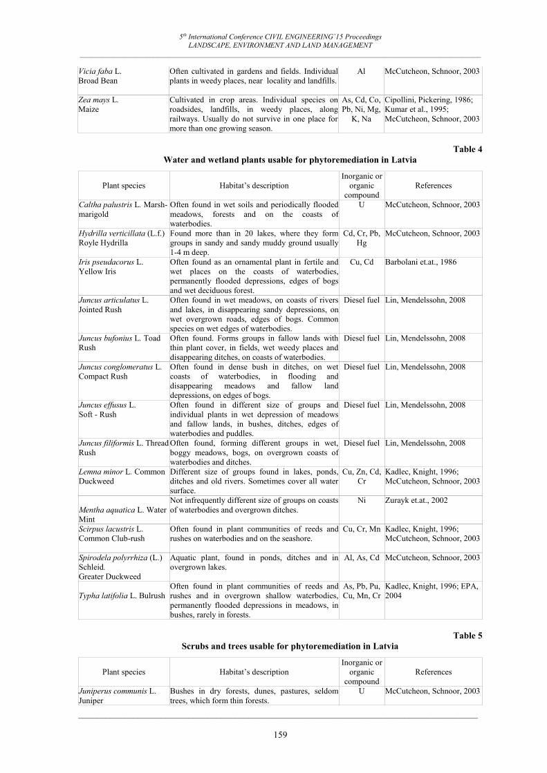
5th International Conference CIVIL ENGINEERING`15 Proceedings LANDSCAPE, ENVIRONMENT AND LAND MANAGEMENT
_____________________________________________________________________________________________________________
_______________________________________________________________________________________
159
Table 4
Water and wetland plants usable for phytoremediation in Latvia
Plant species Habitat’s description Inorganic or
organic compound
References
Caltha palustris L. Marsh-marigold
Often found in wet soils and periodically flooded meadows, forests and on the coasts of waterbodies.
U McCutcheon, Schnoor, 2003
Hydrilla verticillata (L.f.) Royle Hydrilla
Found more than in 20 lakes, where they form groups in sandy and sandy muddy ground usually 1-4 m deep.
Cd, Cr, Pb, Hg
McCutcheon, Schnoor, 2003
Iris pseudacorus L. Yellow Iris
Often found as an ornamental plant in fertile and wet places on the coasts of waterbodies, permanently flooded depressions, edges of bogs and wet deciduous forest.
Cu, Cd Barbolani et.at., 1986
Juncus articulatus L. Jointed Rush
Often found in wet meadows, on coasts of rivers and lakes, in disappearing sandy depressions, on wet overgrown roads, edges of bogs. Common species on wet edges of waterbodies.
Diesel fuel Lin, Mendelssohn, 2008
Juncus bufonius L. Toad Rush
Often found. Forms groups in fallow lands with thin plant cover, in fields, wet weedy places and disappearing ditches, on coasts of waterbodies.
Diesel fuel Lin, Mendelssohn, 2008
Juncus conglomeratus L. Compact Rush
Often found in dense bush in ditches, on wet coasts of waterbodies, in flooding and disappearing meadows and fallow land depressions, on edges of bogs.
Diesel fuel Lin, Mendelssohn, 2008
Juncus effusus L. Soft - Rush
Often found in different size of groups and individual plants in wet depression of meadows and fallow lands, in bushes, ditches, edges of waterbodies and puddles.
Diesel fuel Lin, Mendelssohn, 2008
Juncus filiformis L. Thread Rush
Often found, forming different groups in wet, boggy meadows, bogs, on overgrown coasts of waterbodies and ditches.
Diesel fuel Lin, Mendelssohn, 2008
Lemna minor L. Common Duckweed
Different size of groups found in lakes, ponds, ditches and old rivers. Sometimes cover all water surface.
Cu, Zn, Cd, Cr
Kadlec, Knight, 1996; McCutcheon, Schnoor, 2003
Mentha aquatica L. Water Mint
Not infrequently different size of groups on coasts of waterbodies and overgrown ditches.
Ni
Zurayk et.at., 2002
Scirpus lacustris L. Common Club-rush
Often found in plant communities of reeds and rushes on waterbodies and on the seashore.
Cu, Cr, Mn
Kadlec, Knight, 1996; McCutcheon, Schnoor, 2003
Spirodela polyrrhiza (L.) Schleid. Greater Duckweed
Aquatic plant, found in ponds, ditches and in overgrown lakes.
Al, As, Cd McCutcheon, Schnoor, 2003
Typha latifolia L. Bulrush
Often found in plant communities of reeds and rushes and in overgrown shallow waterbodies, permanently flooded depressions in meadows, in bushes, rarely in forests.
As, Pb, Pu, Cu, Mn, Cr
Kadlec, Knight, 1996; EPA, 2004
Table 5
Scrubs and trees usable for phytoremediation in Latvia
Plant species Habitat’s description Inorganic or
organic compound
References
Juniperus communis L. Juniper
Bushes in dry forests, dunes, pastures, seldom trees, which form thin forests.
U McCutcheon, Schnoor, 2003
Vicia faba L. Broad Bean
Often cultivated in gardens and fields. Individual plants in weedy places, near locality and landfills.
Al McCutcheon, Schnoor, 2003
Zea mays L. Maize
Cultivated in crop areas. Individual species on roadsides, landfills, in weedy places, along railways. Usually do not survive in one place for more than one growing season.
As, Cd, Co, Pb, Ni, Mg,
K, Na
Cipollini, Pickering, 1986; Kumar et al., 1995; McCutcheon, Schnoor, 2003

5th International Conference CIVIL ENGINEERING`15 Proceedings LANDSCAPE, ENVIRONMENT AND LAND MANAGEMENT
_____________________________________________________________________________________________________________
_______________________________________________________________________________________
160
Plant species Habitat’s description Inorganic or
organic compound
References
Larix decidua Mill. European Larch
Cultivated in dry mineral soils in forest stands and in green areas.
Cs McCutcheon, Schnoor, 2003
Picea abies (L.) Karst. Norway Spruce
Boreal coniferous forest species. Constitute a fifth of Latvian total forest area. Grows in unmixed forests or mixed forests in moderately fertile soils and in wet soils mainly in mineral soils.
Cs McCutcheon, Schnoor, 2003
Pinus sylvestris L. Scots Pine
Main tree species in Latvian forests. Grows in unmixed forests and mixed forests. The dominant species in dry and wet mineral soil and marsh soil in different pine forests.
Diesel fuel Palmroth et.al., 2002
Populus deltoides x Wettstein; Populus x canadensis Hybrid Aspen
Selectively for forestry needs. Cultivated in hybrid aspen plantations.
BTEX, PAH ITRC, 2009
Quercus robur L. Pedunculate Oak
Often found in European broadleaf forests by riversides, in glens and individual plants in agricultural land.
U McCutcheon, Schnoor, 2003
Salix schwerinii x viminalis Hybrid Willow, Tora
Selectively for forestry needs. Cultivated in willow plantations.
Heavy crude oil
Pivetz, 2001
Salix viminalis L. Osier
Quite often as individual plants and groups by waterbodies, in overgrown ditches and sand dunes.
Cd, Cr, Cu, Pb, K, Ag,
Sr, U, Zn, As
Hinchman et al., 1997; Schmidt, 2003; McCutcheon & Schnoor, 2003
CONCLUSIONS
The phytoremediation research method is at an early stage in the world and also in Latvia, and it opens up a wide range of opportunities for further research. Currently, most studies have been performed in laboratories under experimental conditions and temporarily, therefore it is necessary to extend field studies about the effectiveness of
pollution purifying plant species from the above mentioned in the climatic conditions in Latvia. Since the plant movement is limited, many species have developed unique biochemical systems for feeding process security, as a result of which they determine and affect the local geochemical soil conditions and play a significant role in reducing the pollution in the soil.
REFERENCES
Ali H., Khan E., Sajad M.A., (2013). Phytoremediation of heavy metals—Concepts and applications. 91(7), 869-881. DOI: 10.1016/j.chemosphere.2013.01.075
Ashraf, M., Ozturk, M., Ahmad, M. S. A., (2010). Plant Adaptation and Phytoremediation. Springer (pp. 481).
Banks K., Schwab P., (1998). Phytoremediation in the Field: Craney Island Site. 3rd Annual International Conference on Phytoremediation, Houston
Barbolani E.; Pantani F.; Gellini R.; Clauser M., (1986). Residual heavy metal (Cu and Cd) removal by Iris pseudacorus. Water, Air & Soil Pollution, 28(3-4), 277-282.
Bell J. N. B., Minski M. J., Grogan H. A., (1988). Plant Uptake of Radionuclides. Soil Use Management, 4, 76–84.
Bell R.M., Failey R.A., (1991). Plant uptake of organic pollutants. In Organic contaminants in the environment. Ed. K.C. Jones. Elsevier Applied Science, Essex, U.K., pp 189-206.
Best P.H., Zappi M.E., Fredrickson H.L., Sprecher S.L., Larson S.L., Ochman M., (1997). Screening of aquatic and wetland plant species for phytoremediation of explosives-contaminated groundwater for the Iowa Army Ammuntion Plant. Annals of the New York Academy Sciences, 829, 179-194. DOI: 10.1111/j.1749-6632.1997.tb48574.x

5th International Conference CIVIL ENGINEERING`15 Proceedings LANDSCAPE, ENVIRONMENT AND LAND MANAGEMENT
_____________________________________________________________________________________________________________
_______________________________________________________________________________________
161
Bizecki D., (2003). Phytoremediation of hydrocarbon-contaminated soil using plants adapted to the western canadian climate. Soil Science, University of Saskatchewan, pp 235.
Byrne-Kelly D., Cornish J., Gordon R., Licis I., (2001). Revegetation of Mining Waste Using Organic Soil Amendments and Evaluation of the Potential for Creating Attractive Nusiances for Wildlife. Abstract. 2001. Proceedings of the 2001 Conference on Environmental Research, pp 119-147.
Chang Y., Corapcioglu M.Y., (1998). Plant-enhanced subsurface bioremediation of nonvolatile hydrocarbons. Journal of Environmental Engineering, 124(1), 162-169.
Christensen-Kirsh, K.M (1996). Phytoremediation and wastewater effluent disposal: Guidelines for landscape planners and designers. Master’s Project, Department of Landscape Architecture. University of Oregon.
Cipollini M. L., Pickering J. L., (1986). Determination of the Phytotoxicity of Barium in Leach-Field Disposal of Gas Well Brines. Plant and Soil, 92, 159–69.
Dazy, M., Béraud, E., Cotelle, S., Grévilliot, F., Férard, J.-F., Masfaraud, J.-F. Changes in plant communities along soil pollution gradients: Responses of leaf antioxidant enzyme activities and phytochelatin contents (2009) Chemosphere, 77 (3), 376-383.
Dzhura N.M., Romanyuk O.I., Oshchapovsky I.V., Gasior J., Tsvilynyuk O.M., Terek O.I. (2009). Using plants for recultivation of oil polluted soils.
Fiegl J. L., McDonnell B. P., Kostel J. A., Finster M. E., Gray K. (2003). A Resource Guide: The Phytoremediation of Lead to Urban, Residential Soils. New Jersey, John Wiley & Sons.
Flathman P. E, Lanza G. R., (1998). Phytoremediation: Current Views on an Emerging Green Technology. Journal of Soil Contamination, 7, 415–32.
Groom, Halasz C.A, A., Paquet L., Morris N., Olivier L., Dubois C. and Hawari J. (2002). Accumulation of HMX (Octahydro-1,3,5,7-tetranitro-1,3,5,7-tetrazocine) in Indigenous and Agricultural Plants Grown in HMX- Contaminated Anti-Tank Firing-Range Soil. Environmental Science & Technology, 36(1), 112-118. DOI: 10.1021/es0110729
Hinchman, R. R., Negri M. C., Gatliff E. G., (1997). Phytoremediation: Using Green Plants to Clean Up Contaminated Soil, Groundwater, and Wastewater. Submitted to the U.S. Department of Energy, Assistant Secretary for Energy Efficient and Renewable Energy under Contract W-31-109-Eng-38.
Interstate Technology & Regulatory Council (ITRC), (2009). Phytotechnology Technical and Regulatory Guidance and Decision Trees, Revised. PHYTO-3. Washington, D.C.: Interstate Technology & Regulatory Council, Phytotechnologies Team, Tech Reg Update.
Kadlec, R. H., Knight R. L.. (1996). Treatment Wetlands. Boca Raton, Fla.: CRC Press, Lewis Publishers.
Kļaviņa M., Zaļokšņa J. redakcija (2010). Vide un ilgtspējīga attīstība. (97. – 116. lpp). Rīga: LU akadēmiskais apgāds.
Kumar P. B. A. N., Dushenkov V., Motto H., Raskin I., (1995). Phytoextraction: The Use of Plants to Remove Heavy Metals from Soils. Environmental Science and Technology. 29:1232–38
Kumar P. B. A. N., Dushenkov V., Motto H., Raskin I., (1995). Phytoextraction: The Use of Plants to Remove Heavy Metals from Soils. Environmental Science and Technology. 29:1232–38
Leewis M.C., Reynolds C.M., Leigh B.M., (2013). Long-term effects of nutrient addition and phytoremediation on diesel and crude oil contaminates soils in subarctic Alaska. ScienceDirect, Cold Regions Science and Technology, 96, 129-137. DOI: 10.1016/j.coldregions.2013.08.011
Lin Q., Mendelssohn I.A., (2008). Potential of restoration and phytoremediation with Juncus roemerianus for diesel-contaminated coastal wetlands. ScienceDirect, Ecological Engineering, 35(1), 85-91. DOI: 10.1016/j.ecoleng.2008.09.010
Liužinas R., Jankevičius K., Šalkauskas M., Rašomavičius V., Gudžinskas Z., Sinkevičiene Z., (2003). Phytoremediation of polluted soil at sites in the district of Klaidepa (Lithuania), pp 12.
Madzhugina, Yu.G., Kuznetsov, Vl.V., Shevyakova, N.I. Plants inhabiting polygons for megapolis waste as promising species for phytoremediation. (2008) Russian Journal of Plant Physiology, 55 (3), pp. 410-419.
McCutcheon S.C., Schnoor I.L., (2003). Phytoremediation: Transformation and Control of Contaminants. Hoboken, New Jersey: Wiley-Interscience, Inc.
5th International Conference CIVIL ENGINEERING`15 Proceedings LANDSCAPE, ENVIRONMENT AND LAND MANAGEMENT
_____________________________________________________________________________________________________________
_______________________________________________________________________________________
162
Morel J.L., Echevarria G., Goncharova N., (eds.), (2006). Phytoremediation of Metal-Contaminated Soils. NATO Science Series. IV. Earth and Environmental Sciences (pp 345).
Otabbong E., (1990). Chemistry of Cr in Some Swedish Soils. Plant and Soil 123, 89–93.
Oyler, J., (2004). Blue Mountain Superfund Remediation Project. Palmerton, PA, ITRC Phytotechnologies conference.
Palmroth M.R.T., Pichtel J., Puhakka J.A., (2002). Phytoremediation of subarctic soil contaminated with diesel fuel. Bioresource Technology, 84(3), 221-228. DOI: 10.1016/S0960-8524(02)00055-X
Pivetz B.E., (2001). Phytoremediation of Contaminates Soil and Ground Water at Hazardous Waste Sites. U.S. Environmental Protection Agency (EPA), Office of Research and Development, Office of Solid Waste and Emergency Response, Washington, DC.
Pradhan S. P., Conrad J. R., Paterek J. R., Srinistava V. J., (1998). Potential of Phytoremediation for Treatment of PAHs in Soil at MGP Sites. Journal of Soil Contamination, 7, 467–80.
Robinson, B.H., Bischofberger, S., Stoll, A., Schroer, D., Furrer, G., Roulier, S., Gruenwald, A., Attinger, W., Schulin, R. Plant uptake of trace elements on a Swiss military shooting range: Uptake pathways and land management implications (2008) Environmental Pollution, 153 (3), pp. 668-676.
Salt, D. E., Blaylock M., Kumar P. B. A. N., Dushenkov V., Ensley B. D., Chet I., Raskin I., (1995). Phytoremediation: A Novel Strategy for the Removal of Toxic Metals from the Environment Using Plants. Biotechnology 13: 468–74.
Schmidt U., (2003). Enhancing Phytoextraction: The Effect of Chemical Soil Manipulation on Mobility, Plant Accumulation, and Leaching of Heavy Metals (pp. 1939-1954). Journal of Environmental Quality.
Speir, T. W., August J. A., Feltham C. W., (1992). Assessment of the Feasibility of Using CCA (Copper, Chromium and Arsenic)–Treated and Boric Acid–Treated Sawdust as Soil Amendments, I. Plant Growth and Element Uptake. Plant and Soil, 142, 235–48.
Susarlaa S, Medinab V. F., McCutcheon S. C., (2002). Phytoremediation: An ecological solution to organic chemical contamination. Ecological Engineering. 18(5), 647-658. DOI: 10.1016/S0925-8574(02)00026-5
Tiemann, K. J., Gardea-Torresdey J. L, Gamez G., Dokken K.. (1998). Interference Studies for Multi-Metal Binding by Medicago sativa (Alfalfa), p. 42 (Abstract 67) in Proceedings, Conference on Hazardous Waste Research, Snow Bird, Utah.
U. S. Environmental Protection Agency (EPA), (2005). Road Map to Understanding Innovative Technology Options for Brownfield’s Investigation and Cleanup. (Fourth ed.). Washington, DC: U.S. Environmental Protection Agency, Office of Solid Waste and Emergency Response, Office of Superfund Remediation and Technology Innovation.
U.S Environmental Protection Agency (EPA), (2004). Phytoremediation field studies database for chlorinated solvents, pesticides, explosives, and metals. Office of Superfund Remediation and Technology Innovation, Washington, DC.
U.S. Environmental Protection Agency (EPA), (2001). Brownfields Technology Primer: Selecting and Using Phytoremediation for Site Cleanup. Office of Solid Waste and Emergency Response, Washington, DC.
Uraguchi S., Watanabe I., Yoshitomi A., Kiyono M., Kuno K., (2006). Characteristics of cadmium accumulation and tolerance in novel Cd accumulating crops, Avena strigosa and Crotalaria juncea. Journal on Experimental Botany, 57(12), 2955-2965.
Vaculík, M., Jurkovič, A., Matejkovič, P., Molnárová, M., Lux, A. Potential risk of arsenic and antimony accumulation by medicinal plants naturally growing on old mining sites (2013) Water, Air, and Soil Pollution, 224 (5), art. no. 1546
Zurayk R., Sukkariyah B., Baalbaki R., Ghanem D. A., (2002). Ni Phytoaccumulation in Mentha aquatica L. and Mentha sylvestris L. American University of Beirut, Water Air and Soil Pollution, 139(1-4), 355-364.

5th International Conference CIVIL ENGINEERING`15 Proceedings LANDSCAPE, ENVIRONMENT AND LAND MANAGEMENT
_____________________________________________________________________________________________________________
_______________________________________________________________________________________
163
ANALYSIS OF LAND INTER-AREAS IN LATVIA
Anda Jankava Latvia University of Agriculture, Department of Land Management and Geodesy
E-mail: [email protected] Ilze Jankava
„Latvijasmernieks.lv”, Ltd. E-mail: [email protected]
ABSTRACT
As a result of land reform the problem of land inter-areas is described in the article. “Land inter-area” is a land parcel owned by public persons. Its area is smaller than the minimum size of a land parcel defined in the binding regulations of a municipality or configuration of which does not allow the use of the parcel according to the approved territorial planning or access is not provided. According to the data of the Land report of January1st,,2014 from the State Land Service of the Republic of Latvia the number of land inter-areas is 11 307 and the total area occupied by land inter-areas is 10 624.1 ha. In the current study land inter-areas by ownership, size and structure in recent years are analysed. In the presented examples the territorial distribution of land inter-areas has been analysed and the solutions to this problem are sought after.
Key words: land inter-area, land use, land parcel, public person <insert two empty lines 10pt here>
INTRODUCTION Both in the theory and practice of land use planning, one of the main shortcomings in land use land inter-area is mentioned. In accordance with the Land Survey Act (Land Use Planning Law, 2006) the land inter-area is “a separately situated land parcel which is separated from the main land parcel by land owned by another person.” The existence of land inter-areas result in land fragmentation. Increasing the distances between these separate land plots, conditions of land management are made worse. The costs of of transportation and time spent to cover the distances increase. Extra capital investments increase and, in addition, it results in the necessity to cross over other farm land. This failure of land use and its evaluation, as well as the necessity of avoiding it has been researched by various authors and scientists (Demetriou, 2014; Platonova, 2010; Maasikamäe, 2005; Thomas, 2012
et. al.). Avoiding land fragmentation and land inter-areas is one of the main challenges of land management and has always been included in the legislation of the Republic of Latvia. In our previous study (Jankava, Jankava, 2013) the analysis of the concept of land inter-area in various laws and regulations of the Republic of the Latvia according to ownership, size and other factors (Table 1) was carried out. As can be seen, in the first three established regulations, the land inter-area is defined as a land plot owned or used by natural person or juridical person that is separate from the main land plot with other owners’ (or users’) land plot. This concept is also used in a number of textbooks in Latvia and abroad (Butane, Lasteniece, 2000; Locmers, 1999; Волков, 2013) and studies (Platonova, 2010).
Table 1
Provided aspects in definitions of inter-area by various Latvia laws and regulations (Jankava, Jankava, 2013)
No. Regulation, date of establishment Provided aspects Regulation,
law in force ownership area configuration Access 1. Regulations of Land use planning
(1924) individual and legal person
more into small parcels
string-shaped, wedge-shaped
not specified
null and void
2. Cabinet Regulation No.52 „Regulations regarding Cadastral Assessment of Rural Area Land”(05.03.1996)
individual and legal person
unlimited
unlimited
not
specified
null and void
3. Land Use Planning Law (2006). individual and legal person
unlimited unlimited not specified
in force
4. Law on Expropriation of the Public Person Property (edition of 21.10.2010.)
state or municipality
less than area provided by municipality
do not conform to proper use
do not have
access to
in force

5th International Conference CIVIL ENGINEERING`15 Proceedings LANDSCAPE, ENVIRONMENT AND LAND MANAGEMENT
_____________________________________________________________________________________________________________
_______________________________________________________________________________________
164
Nonetheless, at the moment in Latvia there are two different existing interpretations of the concept of land inter-areas with different meanings. This situation has been in existence since 2007, when the Amendments to the Law on Expropriation of the State and Local Government Property (currently - Law on Expropriation of the Public Person Property) were adopted where a different explanation of land inter-area was given, defining it as “a land plot owned by public person, whose area: a) in cities is less than a minimum area of a building plot approved by the municipality in Building Regulations or whose configuration does not allow the use of the land for a building, or which can not be provided with access to a public road. b) in rural areas is less than a minimum area of a land plot in the Binding Regulations approved by the municipality or whose configuration does not allow the use of the land according to the approved land use plan, or which can not be provided with access to a public road. (Publiskas personas mantas..., 2010). Obviously, the main difference in definitions in these two laws (Land Use Planning Law, 2006; Law on Expropriation of the State and Local Government Property, 2010) is connected with land ownership and some other aspects. Land inter-areas owned by public persons have mostly been developed during the land reform, as a result of shortcomings in land formation. These land inter-areas are registered in the State Land Service National Real Estate Cadastre Information System and every year their number increases. MATERIALS AND METHODS
Public person in this country is the Republic of Latvia as an initial public law legal person and municipality as a derived public person. The aim of the study is to carry out an analysis on the land inter-areas owned by a public person in the Republic of Latvia. In accordance with the Law on the Expropriation of the Public Person Property inter-area is a land plot owned by a public person, that is not assigned as a property to natural person or juridical persons. For the analysis of land inter-area and data from The State Land Service of National Real Estate Cadastre Information System on 01.01.2014 were used. For the evaluation of the placement of separate land inter-areas, orthophoto maps with connected cadastral land boundaries as well as other materials were used. Analysis and synthesis, induction and deduction methods, document analysis, as well as other methods were used in the study. RESULTS AND DISCUSSION
According to the data of the Cadastre Information System of 01.01.2014 in the Republic of Latvia there are 11 307 land inter-areas owned by public
person with a total area of 10 624.1 ha, inter-area agricultural land of 4 976.6 ha. 7 032 inter-areas with a total area of 8 334.1 ha are land cognizable to municipalities, but 4 275 inter-areas (total area of 2 290.0 ha) are included in the reserve land fund of Latvia (Table 2).
Table 2
The count and total area of land inter-areas in Latvia as of 01.01.2014
Indicators
Land inter-areas land cognizable to municipalities
reserve land fund
total
Number 7032 4275 11 307 Total area, ha. 8 334.1 2 290.0 10 624.1 Agricultural land, ha.
4 285.0 691.6 4 976.6
The total area of land cognizable to municipalities registered in the National Real Estate Cadastre Information System of Land is 220 169.4 ha and land inter-areas of this makes only 3.8 %. As shown in Table 3, the greatest part of the count of land-parcels cognizable to municipalities (57.8 %) and its total area (69.2 %) has the group named “Land for Agriculture”, the average area of this land parcel is 1.4 ha. 5 % of the count and 14.8 % of area of the land parcels makes up Forestry land (average area 3.5 ha).
Figure1. Land inter-area in the city of Jurmala between two building land plots with accessibility,
land area 0.0151 ha Another significant amount of land parcels (1 247 land parcels or 18.7%) cognizable to the municipalities occupy inter-areas on individual dwelling houses’ land. Since these parcels are small (average 0.1 ha), they do not take up much area (only 1.4%) from the total area of the land of municipality. Figure 1 and 2 show that as a result of land surveying in the territories of individual

5th International Conference CIVIL ENGINEERING`15 Proceedings LANDSCAPE, ENVIRONMENT AND LAND MANAGEMENT
_____________________________________________________________________________________________________________
_______________________________________________________________________________________
165
dwelling houses, between surveyed properties there developed land plots - land inter-areas, whose areas are less than the minimum area of the building plot approved by the municipality building regulations and sometimes they are not provided with access. (Figure 2).
Figure 2. Land inter-area in the city of land area 0.0110 ha
Also in the reserve land fund, the number of such land inter-areas located in on individual dwelling houses’ lands is relatively high (754 parcels or 17.6%) (Table 4). The analysis shows that leading position in the structure of inter-areas in the reserve land fund according to groups of use of real property by the count of inter-areas and total area is held by the group of purpose of use of real property - Engineering Communications object utilization land. The area the group occupies makes 46.9% of the total area of inter-area and count of inter-areas cognizable to the state makes 38.2% of total count. The average area of inter-area is 0.7 ha (Table 4). This group could include forest land under high voltage power lines, which in accordance with the regulation at the beginning of the land reform was included in the territory assigned for use by the power lines holder, but later the Stock Company "Latvenergo" refused to formulate these lands on the property. Therefore, these lands were included in the reserve land fund. Thus a situation has occurred that in the rural areas a part of this land under the power lines is the property of farmsteads, but the other part is recognised as a reserve fund land. This situation has arisen in a number of the parishes in the Vidzeme region, as an example on the property of land for agriculture in Kocēni parish (Figure 3). Inter-areas in the reserve land fund whose purpose of use of real property is Land for agriculture are slightly behind the previous group (respectively 34.6% of the total count of inter-areas cognizable to the state and 39.8 % of total area). From the 129 land inter-areas cognizable to the municipalities and reserve land fund the purpose of
the use of real property for 33 inter-areas is “ Water object land”. A part of these are lakes in rural areas, which have a boundary along the coastline (Figures 4 and 5). As shown in Figure 4 and 5, when land properties and boundaries were formed near lakes, lakes were separate land parcels.
Figure 3. The placement of the reserve land fund in
Kocēni parish: on top – on the cadastral map, on the bottom – the cadastral map is connected with
orthophoto map
In addition, if these parcels which are occupied by a lake are registered as a land owned by municipality, the problem is not solved, because access to these lakes are provided only by the border line landowners. The illustrations show only a few examples of this problem which emerged during the land reform by the formatting and surveying of land property boundaries. As shown in Table 3 and 4 the land inter-areas developed on different types of land, both in rural areas and cities. According to the types of land use, more than half (51%) of the land inter-areas in Latvia are agricultural land, which are almost not used (Table 5). The existence of land inter-area as such is not related to the rational use of land, so it has to be avoided. It means that every case of more than 11 thousand of land inter-areas will have to be solved in the future.
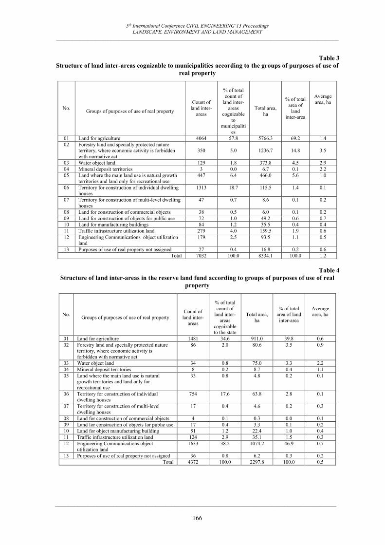
5th International Conference CIVIL ENGINEERING`15 Proceedings LANDSCAPE, ENVIRONMENT AND LAND MANAGEMENT
_____________________________________________________________________________________________________________
_______________________________________________________________________________________
166
Table 3 Structure of land inter-areas cognizable to municipalities according to the groups of purposes of use of
real property
No. Groups of purposes of use of real property
Count of land inter-
areas
% of total count of
land inter-areas
cognizable to
municipalities
Total area,
ha
% of total area of
land inter-area
Average area, ha
01 Land for agriculture 4064 57.8 5766.3 69.2 1.4 02 Forestry land and specially protected nature
territory, where economic activity is forbidden with normative act
350
5.0
1236.7
14.8
3.5
03 Water object land 129 1.8 373.8 4.5 2.9 04 Mineral deposit territories 3 0.0 6.7 0.1 2.2 05 Land where the main land use is natural growth
territories and land only for recreational use 447 6.4 466.0 5.6 1.0
06 Territory for construction of individual dwelling houses
1313 18.7 115.5 1.4 0.1
07 Territory for construction of multi-level dwelling houses
47 0.7 8.6 0.1 0.2
08 Land for construction of commercial objects 38 0.5 6.0 0.1 0.2 09 Land for construction of objects for public use 72 1.0 49.2 0.6 0.7 10 Land for manufacturing buildings 84 1.2 35.5 0.4 0.4 11 Traffic infrastructure utilization land 279 4.0 159.5 1.9 0.6 12 Engineering Communications object utilization
land 179 2.5 93.5 1.1 0.5
13 Purposes of use of real property not assigned 27 0.4 16.8 0.2 0.6 Total 7032 100.0 8334.1 100.0 1.2
Table 4
Structure of land inter-areas in the reserve land fund according to groups of purposes of use of real property
No. Groups of purposes of use of real property
Count of
land inter-areas
% of total count of
land inter-areas
cognizable to the state
Total area,
ha
% of total area of land inter-area
Average area, ha
01 Land for agriculture 1481 34.6 911.0 39.8 0.6 02 Forestry land and specially protected nature
territory, where economic activity is forbidden with normative act
86 2.0 80.6 3.5 0.9
03 Water object land 34 0.8 75.0 3.3 2.2 04 Mineral deposit territories 8 0.2 8.7 0.4 1.1 05 Land where the main land use is natural
growth territories and land only for recreational use
33 0.8 4.8 0.2 0.1
06 Territory for construction of individual dwelling houses
754 17.6 63.8 2.8 0.1
07 Territory for construction of multi-level dwelling houses
17 0.4 4.6 0.2 0.3
08 Land for construction of commercial objects 4 0.1 0.3 0.0 0.1 09 Land for construction of objects for public use 17 0.4 3.3 0.1 0.2 10 Land for object manufacturing building 51 1.2 22.4 1.0 0.4 11 Traffic infrastructure utilization land 124 2.9 35.1 1.5 0.3 12 Engineering Communications object
utilization land 1633 38.2 1074.2 46.9 0.7
13 Purposes of use of real property not assigned 36 0.8 6.2 0.3 0.2 Total 4372 100.0 2297.8 100.0 0.5
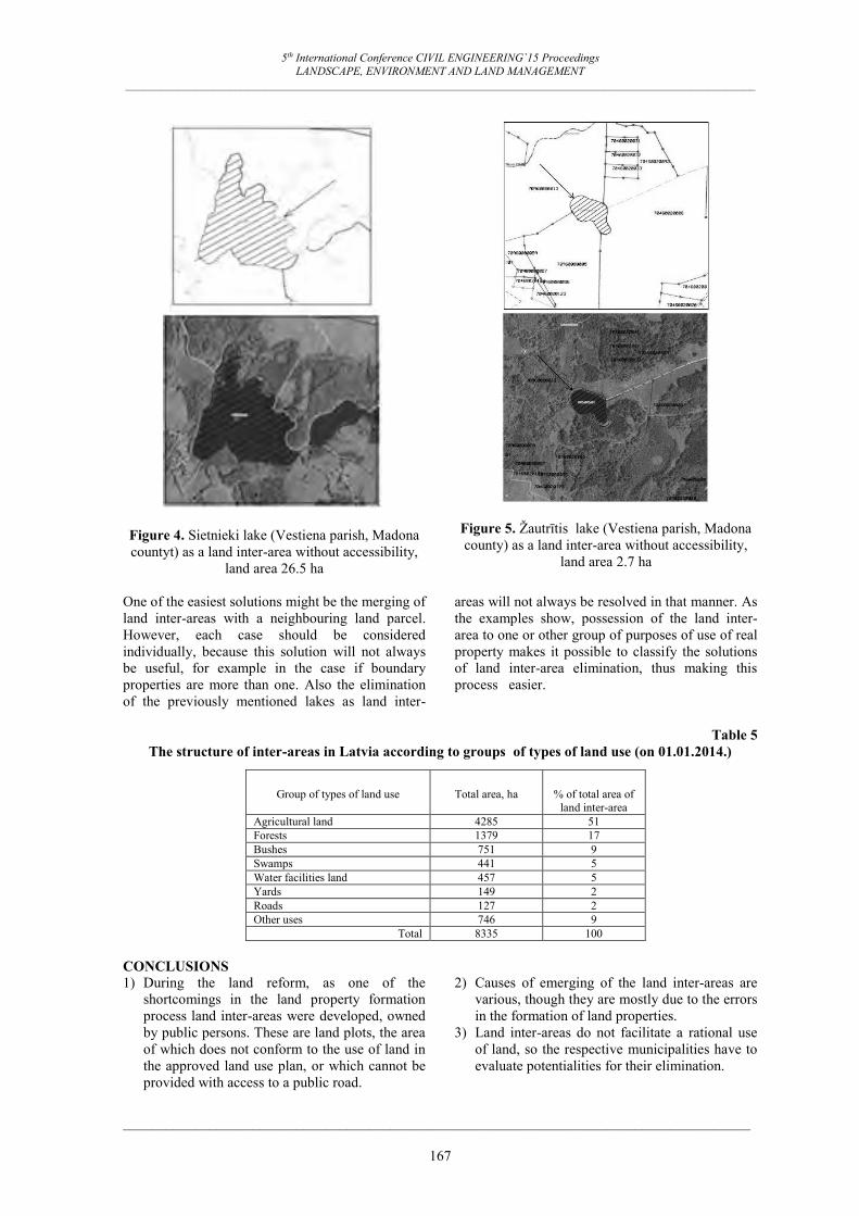
5th International Conference CIVIL ENGINEERING`15 Proceedings LANDSCAPE, ENVIRONMENT AND LAND MANAGEMENT
_____________________________________________________________________________________________________________
_______________________________________________________________________________________
167
Figure 4. Sietnieki lake (Vestiena parish, Madona countyt) as a land inter-area without accessibility,
land area 26.5 ha
Figure 5. Žautrītis lake (Vestiena parish, Madona county) as a land inter-area without accessibility,
land area 2.7 ha
One of the easiest solutions might be the merging of land inter-areas with a neighbouring land parcel. However, each case should be considered individually, because this solution will not always be useful, for example in the case if boundary properties are more than one. Also the elimination of the previously mentioned lakes as land inter-
areas will not always be resolved in that manner. As the examples show, possession of the land inter-area to one or other group of purposes of use of real property makes it possible to classify the solutions of land inter-area elimination, thus making this process easier.
Table 5 The structure of inter-areas in Latvia according to groups of types of land use (on 01.01.2014.)
Group of types of land use Total area, ha % of total area of land inter-area
Agricultural land 4285 51 Forests 1379 17 Bushes 751 9 Swamps 441 5 Water facilities land 457 5 Yards 149 2 Roads 127 2 Other uses 746 9
Total 8335 100
CONCLUSIONS 1) During the land reform, as one of the
shortcomings in the land property formation process land inter-areas were developed, owned by public persons. These are land plots, the area of which does not conform to the use of land in the approved land use plan, or which cannot be provided with access to a public road.
2) Causes of emerging of the land inter-areas are various, though they are mostly due to the errors in the formation of land properties.
3) Land inter-areas do not facilitate a rational use of land, so the respective municipalities have to evaluate potentialities for their elimination.

5th International Conference CIVIL ENGINEERING`15 Proceedings LANDSCAPE, ENVIRONMENT AND LAND MANAGEMENT
_____________________________________________________________________________________________________________
_______________________________________________________________________________________
168
REFERENCES
Butane A., Lasteniece V. (2000) Lauku saimniecību formēšana un konsolidācija. – Jelgava: LLU. 77 lpp.
Demetriou D. (2014) The Development of an Integrated Planning and Decision Support System (IPDSS) for Land Consolidation: Doctoral Thesis accepted by the University of Leeds, UK. Springer International Publishing Switzerland. 340 p.
Jankava A., Jankava I. (2013) The Problem of Land Inter-area in Latvia. In: Baltic Surveying 2013: Proceedings of the International Scientific Methodical Conference. Kaunas, Akademija, p. 76 – 82.
Land Use Planning Law: (2006) [online] [accessed on 14.10.2014.]. Available: http://www.likumi.lv/doc.php?id=144787.
Locmers M. (1999) Zemes ierīcības uzdevumi, saturs un nozīme. Jelgava: LLU. 100 lpp.
Maasikamäe S. (2005) Assesment of Land Fragmentation. In: VAGOS: Research papers 67 (20), 1, LUA, p. 75 – 82.
Platonova D. (2010) Analysis of Land Fragmentation in Rural Areas. In: Research for Rural Development: Proceedings of the International Scientific Conference. Jelgava: Latvia University of Agriculture, p. 110 – 114.
Publiskas personas mantas atsavināšanas likums (Law on Expropriation of the State and Local Government Property): (2010). [accessed on 14.10.2014.]. Available: http://www.likumi.lv/doc.php?id=68490.
Thomas J. (2012) Verfahrensablauf der Flurbereinigung. In: Kummer K., Frankenberger (Hrsg.) Das deutsche Vermessungs- und Geoinformationswesen. Berlin: Wichmann, S. 437 – 521.
Волков С.Н. (2013) Землеустройство. Учебники и учебные пособия для студентов высших учебных заведений. Москва: ГУЗ. – 992 с.

5th International Conference CIVIL ENGINEERING`15 Proceedings LANDSCAPE, ENVIRONMENT AND LAND MANAGEMENT
_____________________________________________________________________________________________________________
_______________________________________________________________________________________
169
LAND QUALITY ASSESSMENT OF THE IMPACT OF REAL PROPERTY CADASTRAL VALUE IN LATVIA
Vivita Baumane, asociate professor, Dr.oec. Latvia University of Agriculture, Department of Land Management and Geodesy
e-mail: [email protected] ABSTRACT
Land quality assessment is one of the most important characteristics that affect the real property cadastral value, which is used in the base value of the rural cadastral evaluation. The study evaluated soil quality assessment in territory of municipality of Latvia. The study analyzed the agricultural land area. Study evaluated the course of county real property expert survey results. The study concluded that the land quality assessment is important data of cadastral value. Main conclusion of the study is that the country need complex of state measure to update the land quality assessment, as a result of the development of real property cadastral value.
Key words: real property, agriculture land, land quality assessment, cadastral value. INTRODUCTION
Latvia gaining independence, the country began a rapid political, social and economic restructuring based on private property, as well as the decentralized market-oriented farming system, resulting in 1990 on 13th June adopted a resolution "On the agrarian reform of the Latvian Republic" (Par agrāro reformu.., 1990), as well as the 1990 on 21th November - the Law on Land Reform in the Latvian Republic in rural areas” (Par zemes reformu ..., 1990). Cadastral valuation of Latvian, since independence, began with the land valuation of the land reform provision. Therefore, maintained the pre-developed, scientifically based land quality assessment system, which included all agricultural land in the assessment of individual village councils and districts. The law "On Land Privatization in Rural Areas” also included the fact that the valuation of land in cash should be based on: • the land evaluation points; • weighting of holding the position; • one ground points in the assessment (above)
equaling 70 kg of rye value of the purchase price;
• growing tree stand assessment. In view of the land reform and the new land owners number, as well as assessing the Soviet years, developed land-use projects and carry out a soil mapping results, it was decided to support the new agricultural land cadastral valuation methods, the application of the 1957 - 1959 years developed soil fertility evaluation, the essentials of the 20th century Vidzeme and inventories, experience, and the Soviets during the second round of improvements to the methodology developed (Boruks, 1991; Boruks, 2004). Land quality assessment of all land users were defined on the basis of each type of land use and climatic conditions. On the natural conditions have
changed, or substantially changing a little, and their impact on crop yields and total crop production estimates are stable and long-term basis, regardless of land ownership or use of state, was the essential decisions to use land reform and land tax estimates of land quality indicators. More to 1992 year the actual land evaluation was carried out, a survey of certain land uses in the field, through the Soviet period created the situation survey plans and maps of soils and soil agrochemical survey maps and descriptions. Land appraisers found naturally in soil properties of all the complex data, marked the boundaries and the land valuation tables set rating and assessment of the points - the soil quality assessment. Real property cadastral valuation methodology is continuously evolving, but the soil quality assessment is a key factor in determining the rural cadastral value of bases indicators (Nekustamā īpašuma valsts…, 2005; Kadastrālās vērtēšanas noteikumi, 2006). The study hypothesis is Agricultural land quality assessment have the significant impact on property values. Consequently, the study aims to assess agricultural land quality assessment need to update, and its impact on the cadastral value. The study addressed the following objectives: • to evaluate the real property cadastral value of
determining characteristics and analysis of agricultural land;
• to evaluate the average municipalities land quality assessment;
• take local expert survey analysis; • provide conclusions and recommendations. Scientific literature, laws, the data of State Land Service are used in this research.

5th International Conference CIVIL ENGINEERING`15 Proceedings LANDSCAPE, ENVIRONMENT AND LAND MANAGEMENT
_____________________________________________________________________________________________________________
_______________________________________________________________________________________
170
MATERIALS AND METHODS
In the study were used a regulatory acts, where determine indicators for cadastral assessment. (Kadastrālās..., 2006). Monoghraphic method, questionnaires method, descriptive statistics analysis method is used in the particular research. In the data analysis were used SPSS. RESULTS AND DISCUSSION
To any objective property of certain cadastral value, it is necessary to get and keep pressing the cadastral data in the cadastral information system. One is a qualitative assessment of land used for the base value of the rural cadastral evaluation. The indicators of the basis of cadastral values for rural land shall be: the base value for the utilised agricultural land
soil for each quality group of the utilised agricultural land;
the base value for wooded land for each quality group of wooded land.
Utilised agricultural land depending on the quality assessment in points of the utilised agricultural land by the regulatory productivity (one land value point – 70 kg of rye units) shall be divided in 7 quality groups (Kadastrālās vērtēšanas noteikumi, 2006; Baumane, 2009): I quality group – less than 10 points II quality group – from 10 up to 19 points; II quality group – from 20 up to 30 points; III quality group – from 31 up to 40 points; IV quality group – from 41 up to 50 points; V quality group – from 51 up to 60 points; and
VI quality group – more than 60 points. The following main factors affecting the value shall be assessed in respect to the rural land (Baumane, 2010): the land quality, the content of the use types of land, the area, the location, the building effect and encumbrances. Analyzing 512 territorial units for the average agricultural land quality assessment a trend showed that mainly soil quality assessment of the range of 30 to 41 points (Figure 1). The lowest assessment is only 17 points in Kolka and Engure parishes, 19 points in Lapmežciems parish, where the basis of studies of the agricultural land capability, crop area, with no improvers, there is no practical use, therefore they are include in the I quality group. By contrast, highest rating is 67 points Svitene parish and 65 points Sesava parish, which includes in the VI quality group. Average parishes of Latvia soil quality assessment is 37 points, corresponding to the III quality group. However, clearly soils in Latvia has not been studied at the state level 20 years, and those estimates are based on the 1989 – 1991 year materials of soil mapping. Currently, each unit of land is fixed weighted average of the agricultural land quality assessment in points, and it is registered in the Cadastral Information System at each property. At the average indicator can’t determine soil types, different degrees of cultivation, drainage condition and the degree of erosion. Today is not united Land Policy in Latvia. Only a few laws have affected soil protection, and clearly do not identify the institution which exactly does soil protection aspects.
Figure 1. Distribution of soil quality assessment
In 2006 for the European Commission approved the Soil Protection Thematic Strategy. On this basis, the EC has prepared a draft Framework Directive on soil protection. EC is currently no common laws,
which ensure the protection of soil, and the political agreement of the Member States have not reached as part of the opinion that the Directive is not necessary, since everything is sufficiently regulated

5th International Conference CIVIL ENGINEERING`15 Proceedings LANDSCAPE, ENVIRONMENT AND LAND MANAGEMENT
_____________________________________________________________________________________________________________
_______________________________________________________________________________________
171
at the national level. While in Latvia, since the independence years of soil conservation has been neglected, acknowledged that the directive could serve as guidelines in this area. In 2007, the Ministry of Agriculture set up a Steering Group of the measure - Soil maps and databases, digitization and updating. In 2008, the Cabinet approved the national policy framework, which was to prepare an informative report about the land degradation in the development and implementation, including the issue of land re-cultivation / renewal possible economic instruments, to develop a methodology for determining soil quality assessment, to establish a land information system based on the current geo-spatial information in order to obtain complete and current information about any ground unit and its processes. Theoretical basis and prerequisites for improving the situation is, but still there are soil maps in use that containing the information which is outdated. As well as the currently used soil classification differs significantly from the international classification of soils, including the Food and Agriculture Organization (FAO) developed. It is therefore necessary to prepare the soil map, corresponding to FAO standards. Soil mapping is also necessary to obtain systematic information on the state of the soil to determine soil degradation risk areas, calculate the carbon balance, as well as business planning and to provide fertilizer and plant protection products used wisely, certain less-favored areas, so that the real estate would establish an objective and cadastral value.
The main indicators characterizing the soil quality of agricultural land is a state of agricultural land (arable land, meadows, pastures and orchards) area and its drainage situation. This is justified by several scientists (Boruks, Sumarakovs, 1972; Boruks, 2004; Aleknavicius, Gurklys, 2003) carried out a study finding that each country needed good quality, timely data on the drainage condition of the turn depends on the soil quality assessment. After Cadastral Information System data (on 01.01.2014.) occupies the largest area of land use types of forest with an area of 2,955,491.8 ha (46%) and agricultural land area of 2,429,774.7 ha (38%) (Figure 2.). After the land records of land use type distribution is stable and on January 1, 2013 did not change significantly. In recent years, maintained a downward trend of arable land and increase forest cover. In comparison with 2008 has decreased agricultural land of 4142 ha and the proportion of 0.1% of the cadastral information system established in the area, while forest area increased by 6,243 ha or 0.1% increase in the proportion of forest cover. State Land Service of the land accounts of the drained agricultural area data were published by 2007. In Cadastre Information System registration of real property were recorded in the drained area, but an area that they can perform the appropriate function is unknown. Therefore, in order to identify the actual extent of the area in the country, as well as to learn the views of specialists was carried out 109 local real property expert survey, referred to by the 79 local professionals.
38%
46%
2%4%
4%4%2% 2%
agricultural land
forest
underbrush
swamp
land of water object
countryard area
roads
orher land
Figure 2. Distribution area of land use types (01.01.2014.)
The questionnaire's first question was "What is your local municipality area of agricultural land, agricultural land drained area, including the operating system of drainage area?” This question was received only four responses from Stopini, Auce, Adazi and Balvi counties. And also the response was incomplete, as was indicated in the
approximate area drained except Adazi county of the total agricultural land 1935.4 ha of drained agricultural lands up 1064.7 ha. But as a functioning drainage systems, land only Adazi county indicated an approximate area of 200 ha. Some counties in the questionnaires were accompanied by commentary that the information

5th International Conference CIVIL ENGINEERING`15 Proceedings LANDSCAPE, ENVIRONMENT AND LAND MANAGEMENT
_____________________________________________________________________________________________________________
_______________________________________________________________________________________
172
on the agricultural area has still not been assembled counties, but access to its constituent parishes. However, the current state of agricultural land drainage or parishes, or counties is not available. The next question of the soil quality assessment was - "Do set your local parish average agricultural land quality assessment in points, in your opinion, is it consistent with the current situation?"
Total respondents were split as follows (Figure 3). – 19 believe that the agricultural land quality assessment is appropriate, 29 believes that the decreased but not more than 5 points, 18 believes that the reduction of the 5-10 points, 13 believes that declined by more than 10 points. None of the respondents answered that their municipality qualitative assessment should be increased.
Figure 3. Respondents' assessment about compliance of land quality assessment (n=87)
Respondents’ of statistical regions of the matter was marked by both common and different trends. Most respondents, 42% in Vidzeme, 46% in Latgale and 33% in Kurzeme region have recognized that the assessment is reduced, but not more than 5 points. Also, such an assessment reduction in some cases may significantly affect the cadastral value of land. For example, if the unit is located on agricultural land values in the first zone and the qualitative assessment of 52 points, then the base value is 1409 EUR/ha, and if not currently a qualitative assessment of 52 points, but has fallen by 5 points, so there are 47 points, then the base value of 1252 EUR/ha. Cadastral value is reduced by 156 EUR/ha. By contrast, in another case, if the unit is located in the agricultural land value in the first zone and the qualitative assessment of 58 points, then the base value is 1409 EUR/ha, and a decrease in a qualitative assessment of 5 points, the assessment is 53 points, as a result of quality assessment group remains constant and does not change the basic value of the remaining 1409 EUR/ha. Therefore, this change is examined in detail. Zemgale region characterized by high quality agricultural land and asset evaluation and development of agricultural production, therefore 43% of respondents in the region observes that the qualitative assessment of their local government is appropriate. By contrast, the Latgale region, where these conditions, the response "appropriate" is given only 8% of respondents, while 46% say that a qualitative assessment has decreased by 5 points and 31%, that a reduction of 5 to 10 points.
Therefore, the questionnaire was followed by the next question - "Is it necessary to raise agricultural land quality assessment?" In this matter the respondents’ opinion can say that it was ambiguous. Total 74 respondents said that the soil quality assessment has been updated with complex of state measures. In assessing respondents division into regions, It may be noted that the Vidzeme and Zemgale regions, there is 100% consensus that the agricultural land quality assessment is updated with complex of state measures. The difference is in Latgale respondents' opinion, the 18% notes that must be updated after the property owner initiative, while 82% support the need for updating with complex of state measures. By contrast, in the Kurzeme region of 8% and 5% in Riga region argues that soil quality assessment does not appreciate the update. The study showed that the data used in the real property cadastral value in some cases not reflect the true situation. This requires significant research to improve data quality and streamline the real property cadastral valuation CONCLUSIONS 1) Soil quality assessment is one of the most
important indicators of the rural land value bases of cadastre development as well as in the calculation of the cadastral value.
2) According to the State cadastral information system of real property which is based on 1989 – 1991 year materials of soil mapping, parish

5th International Conference CIVIL ENGINEERING`15 Proceedings LANDSCAPE, ENVIRONMENT AND LAND MANAGEMENT
_____________________________________________________________________________________________________________
_______________________________________________________________________________________
173
average soil quality assessment is 37 points, which in currently farming conditions are not suitable.
3) In order to obtain systematic information about soil position and consequently there would be determine objective cadastral value of real property there should be carry out soil mapping which accord to FAO rules
4) On the issue of soil quality assessment analysis results of the municipal staff of real property showed that only in 17% of Latvian municipalities this assessment is appropriate
5) According to the research and questionnaire results of the municipal staff of real property, can be concluded, that in the state should be done voluminous event complex, which result would be updated soil quality assessment.
REFERENCES
Aleknavicius P., Gurklys V., Maziliauskas, Aleknavicius A. (2003) Assessment of consequences resulting from abolishing the obstacles on land Transactions. Estonian Agricultural University. Baltic Surveying’03. Tartu – pp. 12.-22.
Baumane V. (2009) Improvement of cadastral valuation models. In: Proceedings of the International Scientific methodical Conference: Baltic Surveying 2009. Tartu: Estonia University of Life Sciences, pp. 11.-15
Baumane V. (2010) Cadastral valuations models. Proceedings of the International Scientific Conference: Economic science for rural development, No 22. Jelgava: LLU, pp. 68.-75
Boruks A. (1991) Zemes vērtēšanas metodika. LR LM Zinātniski tehniskās informācijas un propagandas centrs. 116 lpp
Boruks A. (2004) Dabas apstākļi un to ietekme uz agrovidi Latvijā. Rīga: LR VZD. 166 lpp
Boruks A., Sumarokovs G. (1972) Zemes kvalitātes nozīme lauksaimniecībā. Rīga: Liesma. 225 lpp.
Nekustamā īpašuma valsts kadastra likums (2005). LR likums (15.12.2005.) Latvijas Vēstnesis Nr.205 (3363) 22.12.2005.
Kadastrālās vērtēšanas noteikumi (2006). Ministru kabineta 2006. gada 18. aprīļa noteikumi Nr. 305. Latvijas Vēstnesis, Nr. 72, 2006. gada 10. maijs.
Par agrāro reformu Latvijas Republikā (1993). Latvijas Republikas Augstākās Padomes 1990. gada 13. jūnija lēmums. Latvijas Republikas zemes līkumošanas akti, I daļa. Rīga: Baltika. 86 lpp.
Par zemes reformu Latvijas Republikas lauku apvidos (1993). Latvijas Republikas 1990. gada 21. novembra likums. Latvijas Republikas zemes likumdošanas akti, II sadaļa. Rīga: Baltika. 120 lpp.

5th International Conference CIVIL ENGINEERING`15 Proceedings LANDSCAPE, ENVIRONMENT AND LAND MANAGEMENT
_____________________________________________________________________________________________________________
_______________________________________________________________________________________
174
GEODETIC INSTRUMENT CALIBRATION POLYGON ELEMENT STRUCTURE AND CONSTRUCTION
Aivars Ratkevičs
Latvia University of Agriculture, Department of Land Management and Geodesy E-mail: [email protected]
Armands Celms
Latvia University of Agriculture, Department of Land Management and Geodesy E-mail: [email protected]
Reiner Jäger Karlsruhe University of Applied Sciences, Institute of Applied Research
E-mail: [email protected] ABSTRACT
Geodetic instrument calibration polygon major components, elements structure and constructions of corresponding to different meanings, configuration and objectives of geodetic instruments calibration polygons establishments and exploitation, they are complex elements and elements that are tailored to the practical tasks of the user. Most important role of elements is support to ensure that the measurement results comply with the requirements. It is also associated with certain elements design and construction, as well as their mutual combination, which provide the best and most reliable measurements performance and stability. Research task was to prepare the initial theoretical justification for geodetic instruments calibration of polygon project to build a sound information base for elements creation, selection, design and structure. In Latvia is currently not available in full study, which covers of calibration polygon design and choice of element, which can be adapted to the local situation in Latvian, as here, there is not functional or maintained calibration polygon elements. Result of the study is defined in the basic principles of polygon structure and design elements for selecting the future course of study. It is prescribed the basic positions of polygon development and gives insight into the content for further research and for filing in accordance with the objectives and quality requirements (including accuracy, stability and utilization). The proposed polygon structures comparison in accordance with the polygons of uses and construction elements of choice positions and justifications. The study results include recommendations and conditions for use of the state geodetic grid of elements (centers), the adaptation and development of developing a new model of polygon. Main objective of the study is to provide preliminary information and conditions to continue to organize the research and development to create project of new geodetic instrument calibration polygons elements structure and built it for use of the Latvia conditions.
Key words: geodetic instrument calibration polygon design elements, construction elements, geodetic quality laboratory’s. INTRODUCTION
In any type of technical operations - where are used measuring devices or technical equipment is always confronted with two major problems: 1. Is instrument correctly/accurately and credibly presented measured variables? 2. How reliable the measurement results are from used instruments? Also, to the geodetic instruments application scope of fully attributable this essential problem effect when need find the answers to this questions – whether in surveying used instrument properly and accurately (according to the criteria set) be able to show the measured parameters and how relevant of importance to obtained measurement results with this specific instrument. In addition to these classical criteria, which apply only to a particular instrument and its technical
peculiarities, there are other effects of the factors who also have influence to obtained measurement results – for example for certain works (expected results) selected instruments usage and technologies together with measurer qualifications or training level as a specific instrument proper for user operation and correct selected technology of work application. Here already more emphasis is placed on human factors – such as specialist training and experience. Geodetic instrument quality indicators response is usually given of the instrument technical documentation - which provides the instrument manufacturer. Traditionally, in order quality determine manufactured instruments depending on requirements, appliances manufacturers use: Different types of tests (calibration) stands. In Quality laboratories – by instrument manufacturing which checks can be carried out both

5th International Conference CIVIL ENGINEERING`15 Proceedings LANDSCAPE, ENVIRONMENT AND LAND MANAGEMENT
_____________________________________________________________________________________________________________
_______________________________________________________________________________________
175
on specially constructed stands checks and without them. In Quality or control polygons. Instrument manufacturers choose a specific product quality necessary testing procedures and sites for using all procedures fully or partially (at the specific need). In special cases, manufacturers can be ordered, regardless of their own internal testing procedure, quality of research or calibration services (where need for an external instrument quality certificate - mandatory) which lead to an independent quality assurance. Users of instruments answers to these questions are usually obtained by relying on the information provided by the manufacturer, or applying to institutions/authorities - whose behavior is equipped inspection/calibration stands, laboratories, etc., with available appropriate training staff. But despite the above-mentioned user's expectations against the manufacturer, however situation is often formed, which indicates that user need to be carried out in the same instrument or instrument measuring results checks of evaluations finished or performed works. In this case, instrument user requires access to take measurements or appropriate control or test, to polygon or in laboratory calibration stands. With the need for clear and some form of independent from manufacturers answers on the above lists of the geodetic instrument major problems need to face practical use of the most direct tool users as well – of the results measuring the work principles. The probability of necessary begins with purchasing the instrument, continues with starting new jobs and ends with the discontinuation of the instrument. The instrument often can be discontinued after founding the facts about impossibility to obtain results with satisfactory answers in future exploitation of the instrument. The finding of this fact can be obtained while using all available options of quality testing – available polygons, benchmarks, etc. services. The specification of instrument manufacturer may prove to be inadequate after obtaining highly accurate measurements, because the carefulness of how the technology of serial manufacturing in a highly precise measuring instrument should be developed and implemented doesn’t matter. Each instrument, however, has its own unique, individual /different qualities where every of them alone or in various combinations can affect the accuracy of results differently. When we speak of the measurements of high accuracy, it is considered that each individual instrument has its own only and unique properties which are formed from the impact of several elements, for example: the each different manufactured indicator of accuracy differs from the same indicators in other similarly manufactured products (instruments);
the assembly or the adjustment and the calibration of components also has the potential to affect obtained results differently; during the operations of each individual instrument there are many different external and internal factors which, in general, creates different and individual changes in the sizes of calibration, accuracy and stability. The fact that during each operation of instrument may change its basic attributes differently has to be taken into account as well. These attributes are, for example: the interval between divisions in cylindrical bubble (level) tube; optical properties of telescope; operation parameters of compensator/s; the mutual position between axis of rotation and properties of rotation/aiming mechanisms; unit values of reference system or parameters of electronic systems measurement; the relationship of angles between the telescope optical axis and the axis of cylindrical bubble (level) tube (angle „i”); and others. The overall quality of instrument operation also may affect equipment elements which are used along with instrument. For example, these are elements, such as – rods, tripods and connection quality to them, quality of distance measuring, the relationship between pins and pads with the placement on surface structure. And at the end there is the human factor – with all the individual characteristics, which can affect the quality of measurement results directly. The influence of above mentioned facts provides that every surveying instrument (or a set of equipment) for high precision measurement requires careful and detailed inspection, research, examination, but not only prior the operation, but also systematically throughout the work process. The research and testing of surveying instruments divides into laboratory trials/tests and field tests. Laboratory trials/tests are considered to be with the most quality and the most valuable, but they are more expensive and more complex, because contrary the organization of field testing methods they require more funds for investment in technical equipment, exploitation and maintenance of personnel, facility and premise. But need to be aware that these tests have good quality only to determine technical parameters, but they do not provide the quality assessments of instrument in a real work environment, they have limited application for evaluation of various technological solutions and from experience and training of personnel and its skills to evaluate the individual measuring acquirement. Field tests can be simplified performed or performed in special dedicated geodetic instrument fields (polygons) of testing and calibration.

5th International Conference CIVIL ENGINEERING`15 Proceedings LANDSCAPE, ENVIRONMENT AND LAND MANAGEMENT
_____________________________________________________________________________________________________________
_______________________________________________________________________________________
176
The performers of simplified performance usually can do it in any work area – in the territory without specially prepared and tested workplace. They are widely used when it is suspected to receive the loss of measuring quality with any of operational factors or in order to ensure about the functional adequacy of the instrument or the whole equipment set before, during or after the work (the performance often is governed by the requirements of chosen measurement technological cycle). These tests are called self–calibration or self–control. The field tests of geodetic instruments or set are completed in the specially formed geodetic instrument calibration and test polygons. Tests in polygons are performed in specially designed topical fields (according to the specifics of instruments or sets or their technical or technological methods of usage), which are equipped with a set of specific structural elements (pylons, centers, tripods, racks, benchmarks, objectives, supports etc.), which have interconnected high precision measurement that are completed, verified and documented multiple times. Also, tests in polygons are performed when an authoritative high precision and verification of compliance with the prescribed measuring instrument is necessary (regardless of the manufacturer guarantees), the adequacy assessment of the chosen instrument and the chosen measurement technology to raised quality requirements and the work quality assessments of specialists that are to be or already are involved in the work. In this kind of polygons new technological and technical solutions for development testing and adaptation work are performed, to ensure that instrument is capable to accomplish raised quality requirements, as well as for technical documentation and recommendation processes. They also serve as scientific research and development or practical examination workplace and as a highly qualified specialist field of training and testing skills. It is considered that a field calibration and testing polygons do not provide the sterility of precise geodetic instrument and geodetic grid calibration processes – which are performed in laboratories on special precision stands or other specialized equipment for detecting accuracy, but the advantages of field testing polygons are related with instruments, instrument sets and their use in quality tests with selected technological solutions in regions with real conditions and scales that are close to the maximum with environment for practical application of work. Considering that field testing and calibration polygons are not the best substitute of opportunities in laboratories, but they are good to continue unfinished tests and examinations from there in a real work environment, where at the same time ensures the
options of high quality and accurate instrument parameters and their examination of used technologies and calibration. In order to provide the options of checking the instrument and calibration capability processes, it is necessary to build special peculiar benchmarks or measuring devices for calibration or measurement, which at the same time cannot be special laboratory work tables or stands. Then forms a situation in which the polygon with the established elements serve as the benchmark (or its substitute) of calibration or testing. Solutions can be achieved with building installation site (pylons, work tables, poles, circles, stands, tripods, etc.) elements for each group of instruments or for appropriate end-use measuring location. They need to be able to alter long /save their individual spatial position and the position of mathematical relationships to other similar elements that are contained in the usage target system of polygon. The construction of malleable elements is attributable with the deployment of specific instruments and the measuring process specifics of usage, as well as with the quality of calibration and test processes. However, the amount of elements, mutual spatial arrangement and the sequence of deployment depends on the intended/desired technology specific instruments of field test or calibration, as well as the practical application of the technology requirements of work performance standards – this position can be called a polygon element structure. An important condition – that all elements created and involved in the process must be surveyed with precision that exceeds the planned accuracy of calibrated test instrument. Both polygon element construction and element structure are directly attributable to the specific instrument and its application technologies. That is why the same polygon may consist of one or more topical polygons or polygon groups. They can be made only for purposes of some specific instruments or groups of calibration and test, but also may be combined in groups of various instruments or in systems of various test or calibration elements and structures. Multi-functional test and calibration polygons are also possible. In geodesy industry most often are found polygons with individual instruments or their systems for field tests and calibration – for example: gravimetric polygons, magnometric polygons, distance measuring polygons, Invar wire calibration polygons (comparators), levelling instrument or elevation measuring polygons, angle measuring instrument (theodolite, tacheometer, etc.) polygons, GNSS receiver test polygons (Fig. 1.), photogrammetry (aerotriangulation) polygons, etc. Polygons with two or three instruments and performance technologies are frequent, but multi-fuctional or nearly full profile geodetic instrument

5th International Conference CIVIL ENGINEERING`15 Proceedings LANDSCAPE, ENVIRONMENT AND LAND MANAGEMENT
_____________________________________________________________________________________________________________
_______________________________________________________________________________________
177
an technology calibration and test polygons are very rare.
Figure 1. The scheme/structure of GPS instrument test polygon in Germany,
Landesvermessung Rheinland-Pfalz
Despite the above discussed field polygon functionality association with instruments and technologies in all cases as option is considered to use polygons for training specialists, for determining and improving qualification and for a realization of scientific research process and events. MATERIALS AND METHODS
Within the set research tasks were researched documents and information about existing and functioning geodetic instrument calibration and test polygons in the Baltic States and in the region of the Baltic Sea countries. As well, within the set tasks were researched publications related to the questions about geodetic instrument calibration. Particular attention was paid to the polygons established in Finland and to some polygons established in Estonia. In addition to those, experience of Poland and Sweden was studied as well. Experience in other countries has been reviewed with a relatively generalized view just to complement and confirm the results of analyzes of the polygon element structures and the practice of elements structure. In parallel were evaluated the designs of geodetic reference grid elements (centers) used in territory of Latvia, their solutions in different periods of history, the guidelines to design construction, to its stability and spatial positions for the interest of preservation. As a special position is reviewed view of practical use and suitability of national geodetic reference points for equipping geodetic calibration and test fields. (National Geodetic Reference Grid classifier) As good example connected with field calibration polygons, can be mentioned The Finnish Geodetic Institute: In Geodetic metrology – The Finnish Geodetic Institute maintains standards for geodetic
and photogrammetric measurements and acts as a National Standards Laboratory of length and acceleration of free fall (Law no. 581/2000). Standards in geodetic measurements include quartz meters, geodetic baselines, precision tacheometers and other high precision electronic distance measurement (EDM) instruments, laser interferometers and comparators for levelling rods. They take care of the traceability of these, and perform high precision measurements and calibrations in various geodetic applications. In 2002 the Finnish Geodetic Institute joined the Mutual Recognition Arrangement (MRA) of national measurement standards and of calibration and measurement certificates issued by national metrology institutes. New quality system meets the requirements of the standards ISO/IEC 17025 and ISO 9001 (Jokela J., 2014). In the 21st century the Väisälä interference comparator is the most accurate instrument to measure lengths less than 1 km. The Nummela Standard Baseline (Fig. 2.), 40 km north-west of Helsinki, is the most famous baseline measured with the method developed by the academician Yrjö Väisälä in the 1920s. Use Standard and calibration baselines. A baseline is a permanently marked distance, the length of which is known and traceable to the definition of the meter with a known (small) uncertainty. Baselines are used as measurement standards e.g. in length transfer to electronic distance measurement (EDM) instruments and measurement wires and tapes. Standard baselines are established as national or international length standards. These and other calibration baselines serve in various tasks of geodetic metrology (Jokela J., 2014).
Figure 2. The Nummela standart baseline elements
Baselines in Finland: Nummela Standard Baseline (Fig. 2.), Nummela Calibration Baseline, Jämijärvi Calibration Baseline, HUT Väisälä Baseline. Similares Baselines around the world: Since 1947 the FGI has measured standard and calibration baselines around the world. Many of them now belong to the history of geodesy; some of them still are of great importance in maintaining and

5th International Conference CIVIL ENGINEERING`15 Proceedings LANDSCAPE, ENVIRONMENT AND LAND MANAGEMENT
_____________________________________________________________________________________________________________
_______________________________________________________________________________________
178
developing national measurement standards. (Poutanen M., Rouhiainen, P., 2014). The Gödöllö Standard Baseline in Hungary (Fig. 3.), 30 km north-east of Budapest, was founded in 1938.
Figure 3. Sight on base line in polygon at Godollo (Hungary)
The Chengdu Standard Baseline in Sichuan, China, was founded in 1998. This old calibration baseline was measured The Chang Yang Standard Baseline in China (Fig. 4.), 35 km south-west of Beijing was constructed in 1984. The Taoyuan Standard Baseline in Hsinchu, Taiwan, China.
Figure 4. The look of calibration base pylon in China
Since then seismic activity has caused deformations. The high precision EDM instruments used in the monitoring of stability were calibrated at the Nummela Standard Baseline in 1997 by the Center for Measurement Standards of the Industrial Technology Research Institute. High precision EDM is a much simpler method to measure baselines than the interference measurements. The 1320-m Kyviskes Calibration Baseline, 25 km east of Vilnius, Lithuania, was established for calibration of EDM instruments in 1996. The baseline was extended to a triangle-shaped test field in 2000, and remeasured in 2001. The results confirm the good stability of the baseline, which
now can be used in calibration of EDM instruments and testing of tacheometer and GPS measurement equipment. A similar scale transfer project was performed in 2000 to the old Vääna baseline (1728 m) in Estonia, in co-operation with the Maa-amet, Estonian Land Survey (Jokela J., 2014). The calibration of a measurement instrument in Finland compare the results given by the instrument with the more accurate values represented by the measurement standard. In geodesy the measurement standards include e.g. baselines (for EDM instruments) and laser interferometers (for levelling rods). Angle measurement instruments are not calibrated in the FGI. Facts related in calibrations in gravimetry can be found at the web-site of our National Standards Laboratory of acceleration of free-fall. In the calibration of EDM instruments the observed values are compared with the known values. Refraction and geometric corrections are needed before further computation. Adjustments of observations produce the instrument errors, necessary corrections and accuracy estimates. (Poutanen M., Rouhiainen P., 2014) The Nummela Standard Baseline (Fig. 2.) is the right place for calibration of high precision EDM instruments and for scientific research. As actual measurements are usually performed in field conditions, instruments should be calibrated in real field conditions, too. The medium always have an impact on the propagation of measurement signal. Correct air temperature, pressure and humidity values are of great importance, and must be determined with calibrated weather observation instruments. Self–service calibration facilities are available at the Nummela Calibration Baseline and at the Jämijärvi Calibration Baseline. National Standards Laboratory of acceleration of free-fall serves in the calibration of gravimeters too (Jokela J., 2014). Exploitation of electronic distance meters (EDM) in surveying practice, their rapid development in terms of construction, especially to range and accuracy of measured distance, brings a solution of new tasks in the area of measurement processing. One of the main characteristics is accuracy parameters of EDM. Low variance of the measurements when using EDM can often lead to a deep trust in the measurement results and factor of change of EDM parameters is often neglected. To the fore appears the reproducibility of distances when repeating measurement at different time intervals (Jezko J., 2012) (Micuda J., Korcik P., 2001). During the long-term exploitation is necessary to verify stated parameters in the field conditions. EDM user role is therefore check the reliability and accuracy of EDM before its exploitation, what should become the norm when using all instruments in surveying practice. One of the possibilities of verification of the EDM parameters is hence its calibration on the field length baseline. Such length

5th International Conference CIVIL ENGINEERING`15 Proceedings LANDSCAPE, ENVIRONMENT AND LAND MANAGEMENT
_____________________________________________________________________________________________________________
_______________________________________________________________________________________
179
comparative baseline – baseline Hlohovec, was built by the Department of Theoretical Geodesy of Faculty of Civil Engineering in collaboration with then IGHP n.p. Žilina, plant Bratislava in 1978 (Jezko J., 2012) (Micuda J., Korcik P., 2001). RESULTS AND DISCUSSION
The main components of geodetic instrument calibration polygon element structure and construction correspond to different meaning, configuration and target calibration instrument polygon designing and exploiting, they are elements and element complexes, which are formed in accordance with clearly defined tasks and role of practical use. The most important role of polygon elements is to ensure that the measurement results comply with the requirements and are attributable with design and construction of certain elements and their mutual layout – structure, which provides the best and the most reliable adequacy with the high precision measurement tasks and stability. Geodetic polygon element structure usually is adjusted to either a specific instrument or group of instruments to perform field tests or to perform standardize measurement procedures for interests of technological cycle performed activities within planned targeted tasks in firmly modeled/designed and prepared polygon system. With the purpose to accomplish each technological cycle of instruments or works there can be made multiple separate and independent polygons. For example, the distance measuring instruments and their application technologies (laser rangefinder and similar instruments are usually different from the measuring tapes, measuring wires or optical rangefinder systems) may be formed its own polygon (Fig. 3. sight on base line in polygon at Godollo (Hungary)). Levelers and levelling equipment sets have completely different polygons, etc. The structure of polygon (Fig. 1.) usually forms from the polygon elements that are accordingly to the specificity of the task constructed and arranged in strictly deliberated, reasoned order or shapes which provide that scheduled calibration or test task results are obtained when measuring with the instrument. For example, in polygons designed for rangefinders (Fig. 3.; Fig. 4.) the most common structure consists of elements which are located in one or more straight lines formed in strict order and distances between them. Line or line lengths (between the furthest line elements) usually reaches the distance that is maximal possible for rangefinder to reach, in some cases it may be less, but then there is an adequate justification. Elements in levelling polygon structure can be arranged either on the same straight line or on broken ones, where the total length of polygon often
corresponds to one complete cycle (loop) of levelling measurement line length. The next question is – how many and what design elements are placed in each individual polygon – but always need to remember that even polygon of one type and task can be supplied and equipped with elements of various difficulties. In dealing with geodetic polygon element structures – as the first raises the question of the stability of the spatial structure. Position to preserve the stability is achieved by considering a number of engineering-kind conditions – the first one is the importance about the placement of the polygon and elements, in geological meaning. For example, if the selected polygon’s placement is in Finland and Sweden on the bedrock of granite (Fig. 5.) and other continental plates of solid rock where in some places they reach the earth’s surface – the polygon element construction can be easily created without complex and massive additional buildings, deeply immersed pylons, etc. – here the main guarantor of stability is the base. If the stable bedrock is deeper – then when designing elements in most occasions need to sustain it (link) to the bedrock with constructing pylons – whose base is based on the bedrock and the upper part is at least at same level as earth’s surface (Fig. 2.; Fig. 3.; Fig. 4.; Fig. 5). If the link with bedrock becomes unrealistic (bedrock is very deep, almost unreachable), then for the construction of elements should be given more attention and resources – which would allow spatial stability (at least between elements in the same polygon).
Figure 5. Measurement of baseline at Olkiluoto
As the next position of impact sets the possible quality usage of specific geodetic instruments when using polygon elements – in which again as the first position is stability, associated with the opportunities to create uniform and stable placement for instrument in measurement process,

5th International Conference CIVIL ENGINEERING`15 Proceedings LANDSCAPE, ENVIRONMENT AND LAND MANAGEMENT
_____________________________________________________________________________________________________________
_______________________________________________________________________________________
180
for example – the options to of the installation location stability and uniform installation (uniform and precise alignment or fixed installation) for the instrument and its set of elements (Giniotis V., Rubokas M., 2010). The solution of problems associates with a well-considered creation of geodetic benchmarks and other places of centering and alignment and in the simplest cases with a practical, convenient instrument collocation capabilities in the element construction itself, as in more difficult cases a forced manufacture of centering devices and use of elements in exploitation processes (Fig. 4.; Fig. 5.; Fig. 6.).
Figure 6. Total station on the baseline in Hlohovec Next position of impact is associated with mitigating the effects of climatic and environmental factors on the polygon element construction dimensions and parameters (including spatial positioning) in long-term and in short-term processes during the using of geodetic instrument. Such positions of climatic impact as frost, temperature, solar radiation and wind effects in different combinations are capable of changing both the spatial position of the element itself and the mathematical size of the element – thereby changing the position of the measuring spot. The long-term solution is associated with overall stable placement (on the bedrock), or taking in account the subsurface freezing winters border in our climatic zone (when the element is not sustained to bedrock), the soil composition in the territory of interest and climate impacts on its stability – providing the already in engineering construction mentioned effects of compensation, prevention or at least minimization. Part of element above the surface is exposed to the effects of temperature – which can affect its mathematical parameters and as a consequence will change the centering spot position of instrument, both in the measurement process and in long-term, so in practice are used different screens and pylon insulation techniques from the environment (Fig. 5.). Since the primary issues are related to the stability and positioning of the polygon elements and are solved, there follows the next challenge – linked to
the efficacy of the polygon element practical use where main positions are collocation and convenient operating of instruments. This line is one of the factors that contribute to both the quality of completed work processes and the opportunity to reduce term times in polygon. Initially during the development of geodetic polygons as element constructions often are used the centers and benchmarks of national geodetic reference grid points, which usually according to the requirements for local climatic and geological situation have necessary stability. The designs of these points are usually developed and classified according to the increasing stability requirements - from the level of local grid to the highest geodetic grid’s reference points. Thereby when forming a geodetic polygon - the construction of elements originally is applied to existing point designs. But this original design has a number of lacks for practical use, where the first is simple and easy access to the instrument centering place on a daily basis - because the central element of the work is beneath the earth’s surface (and thereby protected from a variety of negative effects) and on each time of using the elements need to do additional activities to gain access to it. Then need to be able to perform instrument setup and alignment procedures - which are above the excavation pits but not very comfortable and have threats to center the instrument and to determinate accurate height and uniformity. Considering the facts that the geodetic reference grid measurement activities are carried out in the country with an average frequency not more than once a year, that outweigh the inconvenience of creating the complex surface center construction (who would guarantee its position and physical preservation). In case of use intensity of polygon elements, usually it is much larger and too frequent access (frequent digging up) may even damage the position of centering, not mentioning the increase of centering errors that possibly appear after uncomfortable activities. That is why some significant changes are introduced to polygon element constructions – firstly, lifting the centering points (without changing the placement depth of elements below the surface) to the surface or higher (often to the height of tripod), while making additional measures to ensure the stability of the position against the effects of climate and other mechanical damage (Fig. 2.; Fig. 3.; Fig. 4.; Fig. 5.; Fig. 6.). Also around the polygon elements can be created special work fields (Fig. 5.) which provides not only comfortable working to staff, but also provides accurate and uniform installation options for instrument in horizontal and vertical planes. In many cases the constructions of elements in polygons are created deeper than the classical geodetic points to locate their base on solid bedrock (whichever is deeper) or existing massive underground construction or to increase stability

5th International Conference CIVIL ENGINEERING`15 Proceedings LANDSCAPE, ENVIRONMENT AND LAND MANAGEMENT
_____________________________________________________________________________________________________________
_______________________________________________________________________________________
181
with the weight of construction and reference square in ground. As final questions of creating polygon elements are related to the possibility of creating exclusions or minimization of selective different external and internal factors of influence or registration of their size in measurement processes. These constructive options are made to elements of superior quality by incorporating special accurate centering or deployment devices in their constructions. For example, excluding the necessary to use tripods with the attributable effects – the pylon is created on same height as instrument, and it is placed as an installation table of instrument. After excluding the centering errors of instrument there are formed compulsory centering /installing devices, etc. These and similar improvements and developments in the list can be continued for each individual polygon and in process of development its elements can be added variety of different shifts, movement registrations and measurement accessories, which helps with the obtained information to get very high accuracy and reliability of the processed measurement results. CONCLUSIONS
The major components of element structure and constructions in geodetic instrument calibration polygons corresponds to them defined meanings,
configuration and targeted calibration polygon creation and exploitation. They consist of elements and element sets which are designed in accordance with clearly defined tasks and practical use of the role. The most important role of polygon elements is to ensure that the measurement results comply with the requirements of particular elements, constructions, as well as with their mutual placement – the structure, which provides the best and the most reliable compliance with the high-precision measurement tasks and stability. The structure of specific geodetic instrument calibration and test polygons is designed according to realize two basic tasks: the possibility and the technical quality of testing specific instruments and instrument sets; the possibility of the quality requirements and the ability to work for applicable instruments while processing specific works and technologies. The choice of the geodetic instrument calibration and test element polygon constructions is based on: the supported stability (constancy) of the spatial position during long periods of time; the suitability for intensive use (easy instrument installation and workplace); the possibility to selectively exclude influence of various external and internal factors, minimize them or register them after performed measurement.
REFERENCES
Giniotis V., Rubokas M. Creation of the p angle standard for the flat angle measurements. 13th IMEKO TC1-TC7 Joint Symposium, IOP Publishing, Journal of Physics: Conference Series 238. 2010, pp. 1-6.
Jezko J. Testing and calibration of surveying instruments and tools-means to the quality increase of surveying works in construction. Published within the frame of VEGA project, registration number of project 1/0481/12 „Monitoring and Analysis of Spatial Changes of the Building Structures and Natural Environment Using Terrestrial, Photogrammetric and Satellite Technologies”. Journal of interdisciplinary reserch Department of Surveying of FCE of SUT, Radlinského, Bratislava, 2012, pp. 128-131.
Jokela J. Baselines and distance meters. Finnish Geodetic Institute, Geodesy and geodynamics. Finland, Masala 2014, pp.74-79.
Micuda J., Korcik P. Methodology for Calibration of Electronic Distance Meters on the Length Baseline Hlohovec. In: Proceedings „Metrology in Geodesy”. Department of Theoretical Surveying FCE SUT Bratislava , 2001, pp. 101-105.
Poutanen M., Rouhiainen P. Rod and system calibration. In: Finnish Geodetic Institute, Geodesy and geodynamics, Finland, Masala 2014, pp.72-73.

5th International Conference CIVIL ENGINEERING`15 Proceedings LANDSCAPE, ENVIRONMENT AND LAND MANAGEMENT
_____________________________________________________________________________________________________________
_______________________________________________________________________________________
182
CALCULATION OF MAXIMUM RAINSTORM FLOW RATE IN AREAS OF LATVIA
Eriks Tilgalis, Reinis Ziemelnieks
Latvia University of Agriculture Department of Architecture and Building
E-mail: [email protected] ABSTRACT
Rainstorm water flow rate is highly variable and it is difficult to do accurate calculations of runoff and the flow rate, that result in periodic flooding of streets and squares disturbing traffic and causing material damages. The developed rainwater system calculation method is capable of determining the rainfall maximum flow rates of different surfaces with the probability of 300-10% in the entire territory of Latvia. A method for calculating rain flow probability of different recurrence was developed in the 2010 thesis for the city of Riga (R.Ziemelnieks). The aim of this paper is to develop a method for determining the rain flow for other major Latvian cities and populated areas. The improvement of the existing rainwater flow calculation method is given in Latvian Building Normative LBN 223-99, which is partly borrowed from the former Soviet Union improved building standards and regulations СНиП 2.04.03-85 (SNIP)(Строительные нормы..,1985), which are based on the promotion work thesis by Soviet scientist Kurganov (Курганов) in 1978(Курганов, 1984). Key words: rainwater, rain flow, surface runoff, intensity
INTRODUCTION
The effects of global warming each year causes intense unpredictable rain storm water, flooding the streets, rivers, newly built villages, destroying dams and causing financial losses for people. Laws are less able to quickly adapt to today's modern availability of materials and the rapid nature of human life. The situation is becoming worse by the connection of the old rainwater sewerage collectors to the sewerage networks, thus creating an additional load to the sewerage networks of the co-systems and pumping stations during the rain. Media news shows that heavy downpours in Riga and other Latvian cities are becoming more intensive year after year. In Latvia, the Latvian Building Normative LBN 223-99 is used as the official calculation method which does not give the correct results in practical life. The problem is that there has not been a method developed of correct calculation for the necessary distance in-between rainwater gully traps. MATERIALS AND METHODS
This study makes use of the rain observation data from different inhabited locations and towns using the publicly accessible information from the agency of Latvia environment, geology and meteorology (LVGMA) (Tables of Meteorological Observations.., Meteorological and hydrological..). The rain observation data rows were summed up and supplemented in order to improve the existing calculation method of maximum rainwater discharge in towns of Latvia by means of the new
k-coefficient. The data of rain intensity during the warm period from April till September were chosen and used when the downpours with the maximum intensity are observed in Latvia causing flooding of territories and streets. Rainwater discharge calculation methods
In order to be able to calculate the rain water discharge according to the data obtained with a larger possibility, some improvements were already made of the existing adopted calculations, thus by improving the drawn up formula with k-coefficient of the rainwater maximum discharge by A.Zīverts (Zīverts, 1997). Maximum storm water flow rates are determined according to the following expression Qmax = qF. [m3 s-1] (1) Qmax - max 20 minutes rainfall flow rate, m3 s-1; q – runoff module l (s ha)-1 calculated using the formula by E.Tilgalis; depending on the probability of calculation 300;200;100;50 and 10%, in accordance with LBN 223-99, 1 table and Fig.1-4); F – the surface run-off area, ha; – surface runoff coefficient (0.1-0.95% depending on the surface (Table 2); The rainwater diversion gravity self-flow collector internal diameters were calculated assuming full pipe filling and a minimum allowable internal pipe diameter of 200-250 mm for the inside section nets to calculate the minimum pipe slope (LBN 223-99),

5th International Conference CIVIL ENGINEERING`15 Proceedings LANDSCAPE, ENVIRONMENT AND LAND MANAGEMENT
_____________________________________________________________________________________________________________
_______________________________________________________________________________________
183
which will challenge the self-cleaning process of the pipe systems: Q=ω·υ, m3s-1 (2) Imin=τ(ρgR)-1 (3) where: ω- cross sectional flow area, m2; υ- flow speed, ms-1; τ – flow traction, N m-2; ρ – specific gravity of waste water, kg m-3; g - acceleration of free fall m s-2; R- filler of pipe hydraulic radius, m; The kind of material used for the surface cover may be different in the location of use of a conformable area, therefore the rainwater discharges change. In Latvia the coefficients of surface discharge have not been summed up in scientific literature.
Table 1 Runoff coefficients
Use of areas or type of Covering material
of surface area Coefficient,
Town office 0.70 - 0.95
Commercial premises 0.50 - 0.70
Detached house 0.30 - 0.50
Flat in a dwelling house 0.40 - 0.60
Flat(apartments) 0.60 - 0.80
Inhabited suburb district 0.25 - 0.40
Light industry 0.50- 0.80
Heavy industry 0.60 - 0.90
Parks, green areas, cemeteries 0.10 - 0.30 Street, pavement covering by
asphalt or concrete 0.70-0.95
Concrete area 0.80-0.95
Concrete cobble stone covering 0.70-0.80 Pedestrian pavements and
part for transport 0.75-0.85
House roof covering material (depending on material) 0.75-0.95
Sandy soil with 2% decline or less 0.05-0.10
Sandy soil with 2%-8% decline 0.10-0.16 Sandy soil with 8% decline or
more(precipice, slope) 0.16-0.20
Grassland having clayey soil composition
Decline 2% or less 0.10 - 0.16
Decline 2%-8% 0.17 - 0.25 Decline 8% and more
(precipice, slope) 0.26 - 0.36
Source: Computer applications in hydraulic engineering (basic hydrology-rainfall) (translation report by R.Ziemelnieks)
The coefficients of rainwater discharge surface for the present surface cover areas have been studied in the world and their values are shown in Table 1. The data in the table show clearly that it is possible to reduce the rainwater discharge several times by using the low density surface covering materials RESULTS AND DISCUSSION
By determining the values of the precipitation intensity of maximum minutes and by specifying the coefficients of surface runoff for different kind of covering materials, the calculation method of the existing discharge has been improved. The existing calculations in the Latvian building normative LBN 223-99 envisage the precipitation discharge having the repetition period once a year (100%), twice (200%) or three times a year (300%). Moreover, the calculation given by the LBN and recommendations partly adopted and improved from the building norms and regulations of the USSR СНиП 2.04.03-85 (SniP) were based on the USSR scientist Kurganov’s promotion paper elaborated in 1978 and improved in the course of time and later shown in the handbooks of different kinds and number table materials (Kurganov, 1984). The calculations have been specified and around 1986 Snip projecting materials were officially accessible (Metodiskie norādījumi lietus.., 1983).
Table 2 Runoff different sewage
collector location conditions
Sewarage system location conditions of pipe collectors
Recurrence intensity (once per given period) of rainwater
exceedance period P(years) in living areas, if q20
Small streets/Main streets
till 60
over 60-80
over 80-120
Over 120
Favorable and environmentally
friendly/Favorable 0.33-0.5 0.33-1 0.5-1 1-2
Unfavorable/ Medium favorable 0.5-1 1-1.5 1-2 2-3 Super unfavorable/
Unfavorable 2-3 2-3 3-5 5-10
.../Super unfavorable 3-5 3-5 5-10 10-20
Source:„Regulations about Latvian building normative LBN 223-99”Outer networks and buildings of sewerage” The existing method of rainwater calculation amount according to Latvian building normative „Cabinet regulations No.214” „Regulations about Latvian building normative LBN 223-99 “Outer networks and buildings of sewerage” ("LV",198/199 (1658/1659), 18.06.1999.) came into force on 01.10.1999 with the alterations

5th International Conference CIVIL ENGINEERING`15 Proceedings LANDSCAPE, ENVIRONMENT AND LAND MANAGEMENT
_____________________________________________________________________________________________________________
_______________________________________________________________________________________
184
(regulations on LBN 223-99., 2010), and it is complicated. Some parts for rainwater calculations in the normative which are given in the table or formulas are useful as coefficients of rainwater
discharge surface for street runoff designing Recurrence intensity of rainwater excess period in different sewage collector location has been shown in Table 2.
Figure 1. Maximum stormwater runoff module q20 with the probability of 100%; l(s*ha)-1
Figure 2. Maximum stormwater runoff module q20 with the probability of 50%; l(s*ha)-1 The method elaborated provides the possibility to calculate the maximum rainwater discharges in inhabited locations with a different possibility. In the result of the investigation it is possible to conclude that in Latvia it is advisable to use the calculations with the repetition possibility of 50 or 25% (frequency of repetition once in 2 or 4 years) and less. According to the table drawn up by A.Zīverts (Zīverts, 1997) several improvements
were carried out, values of k-coefficients were determined and the runoff module was calculated at different provisions for the inhabited locations of Latvia. Data calculations are moved to make practical isoanmale line drawings of the runoff module with the probabilities of 10, 25, 50, 100% in 20min (figures 1, 2, 3, 4). In the result of the investigation it is possible to conclude that in Latvia it is advisable to use the calculations with the

5th International Conference CIVIL ENGINEERING`15 Proceedings LANDSCAPE, ENVIRONMENT AND LAND MANAGEMENT
_____________________________________________________________________________________________________________
_______________________________________________________________________________________
185
repetition possibility 50 or 25% (frequency of repetition once in 2 or 4 years).
Figure 3. Maximum stormwater runoff module q20 with the probability of 25%; l(s*ha)-1
Figure 4. Maximum stormwater runoff module q20 with the probability of 10%; l(s*ha)-1
CONCLUSIONS
Calculations from given expressions of results criteria probabilities can be practically shown in map of Latvia for each town. The calculation method of maximum rainwater discharge elaborated shows that LBN 223-99 method is imperfect and gives incorrect results in the rainwater system calculation, it is proved by the fact that during heavy downpours many Latvian streets are flooded.
In the future the work must be continued on the improvement of calculation methods of more accurate maximum rain water discharges as well as on different kinds of calculation methods in the territory of Latvia. The newly formed formula and the values given offer an accurate calculation of the rainwater discharge.

5th International Conference CIVIL ENGINEERING`15 Proceedings LANDSCAPE, ENVIRONMENT AND LAND MANAGEMENT
_____________________________________________________________________________________________________________
_______________________________________________________________________________________
186
REFERENCES
Ziemeļnieks R., Tilgalis E. (2009) „Calculation method of rainfall flow rate”, LUA Annual 15th International Scientific Conference Proceedings, Research for Rural Development 2009. Jelgava, Latvia University of Agriculture, pp. 315-319.
Ziemelnieks R., Tilgalis E., Juhna V. (2008) „Rainfall effect on sewage co-system activity in Riga”, LUA Annual 14th International Scientific Conference Proceedings, Research for Rural Development 2008. Jelgava, Latvia University of Agriculture, pp.194-199.
Строительные нормы и правила (1985) СНиП2.04.03-85"Канализация. Наружные сети и сооружения" (утв. постановлением Госстроя СССР от 21 мая 1985 г. N 71)(с изменениями от 20 мая 1986 г.). Москва: Госстроем СССР. 129 c.
Курганов А.М. (1984) Таблицы паpaметров предельной интенсивность дождя для определения расходов в системах водоотведения: толковый справочник. Москва: Стройиздат. 108 c.
Tilgalis Ē. (2004) Notekūdeņu savākšana un attīrīšana: mācību grāmata. Jelgava: LLU, LVAF. 239 lpp.
Zīverts A. (1997) Ievads hidroloģijā: mācību palīglīdzeklis, Jelgava: LLU. 111 lpp.
Meteoroloģisko un hidroloģisko novērojumu dati [online] [accessed on 04.01.2010.]. Available: http://www.meteo.lv/public/hidrometeo_dati.html
Noteikumi par LBN 223-99 Kanalizācijas ārējie tīkli un būves: MK noteikumi Nr.214 [online] [accessed on 07.05.2010.]. Available: http://www.likumi.lv/doc.php?id=19996