Eindhoven University of Technology

MASTER

Wind power integration into the Costa Rican electricity system

van Houtert, R.Y.J.J.

Award date:2009

Link to publication

DisclaimerThis document contains a student thesis (bachelor's or master's), as authored by a student at Eindhoven University of Technology. Studenttheses are made available in the TU/e repository upon obtaining the required degree. The grade received is not published on the documentas presented in the repository. The required complexity or quality of research of student theses may vary by program, and the requiredminimum study period may vary in duration.

General rightsCopyright and moral rights for the publications made accessible in the public portal are retained by the authors and/or other copyright ownersand it is a condition of accessing publications that users recognise and abide by the legal requirements associated with these rights.

• Users may download and print one copy of any publication from the public portal for the purpose of private study or research. • You may not further distribute the material or use it for any profit-making activity or commercial gain

The faculty of Electrical Engineering of the Eindhoven University of Technology

disclaims any responsibility for the contents of this report

Electrical Power Systems

Faculty of Electrical Engineering

Den Dolech 2, 5612 AZ Eindhoven

P.O. Box 513, 5600 MB Eindhoven

The Netherlands

www.tue.nl

Author

R.Y.J.J. van Houtert

Supervisors:

Prof.ir. W.L. Kling

Dr.ir. J.M.A. Myrzik

Dr. A. Ishchenko

Energy research Centre

of the Netherlands (ECN):

Dr.ir. A.J. Brand

Instituto Costarricense

de Electricidad (ICE):

Ing. F. Rodríguez Madriz

Ing. R. Jiménez Valverde

Reference

EPS.09.A.199

Date

February 2009

Wind power integration into the Costa Rican electricity system

Master thesis report by R.Y.J.J. van Houtert

Abstract

Within an electricity system the supply and demand always needs to bebalanced. The transmission system operator has the task to provide therequested electricity demand. To achieve this balance, power plants aredispatch according to the expected load.

The dependency on wind makes wind power a highly fluctuating energysource. These fluctuations are often fully reflected in the electricity producedby the wind turbines, which is fed into the electricity system. To optimallyintegrate wind power into an existing system, the fluctuations should beeither reduced or described, such that the system operator can anticipateon the varying wind power generation.

Wind power prediction is a cost efficient method to describe the fluctuationsof wind power. This report presents the results of a study on wind powerprediction for the Costa Rican system operator. This study initiates thedevelopment of a prediction method for the Costa Rican environment.

It is shown that simple statistical methods can achieve reasonable results,because of the special weather conditions in Costa Rica. For advanced meth-ods, the hysteresis effect around turbine cut-off wind speed is a major errorsource.

Furthermore, an expansion of the wind power generation is analysed. Inthis part the power flows between Central American countries (caused bywind power imbalance) are investigated. Simulation results reveal that thelimited transport capacity between countries is a bottleneck for further windpower expansion.

2

Contents

Abstract 2

1 Introduction 71.1 System operator’s point of view on wind power integration . . 71.2 System reserves and wind power . . . . . . . . . . . . . . . . 71.3 Increasing the value of wind power . . . . . . . . . . . . . . . 81.4 Necessity of wind power predictions . . . . . . . . . . . . . . 91.5 Requirements on wind power forecasting . . . . . . . . . . . . 91.6 Project goal and hypothesis . . . . . . . . . . . . . . . . . . . 101.7 Report outline . . . . . . . . . . . . . . . . . . . . . . . . . . 11

2 Existing Models 132.1 Wind Power Prediction Tool (WPPT) . . . . . . . . . . . . . 132.2 Prediktor and equivalents . . . . . . . . . . . . . . . . . . . . 14

2.2.1 Prediktor . . . . . . . . . . . . . . . . . . . . . . . . . 142.2.2 Previento . . . . . . . . . . . . . . . . . . . . . . . . . 152.2.3 Aanbod voorspeller duurzame energie (AVDE) . . . . 15

2.3 LocalPred and RegioPred . . . . . . . . . . . . . . . . . . . . 152.4 EU funded projects . . . . . . . . . . . . . . . . . . . . . . . . 16

2.4.1 MORE-CARE . . . . . . . . . . . . . . . . . . . . . . 162.4.2 ANEMOS . . . . . . . . . . . . . . . . . . . . . . . . . 17

2.5 Conclusions . . . . . . . . . . . . . . . . . . . . . . . . . . . . 18

3 Error Measures 213.1 Definitions . . . . . . . . . . . . . . . . . . . . . . . . . . . . . 21

3.1.1 Single wind turbine forecasts . . . . . . . . . . . . . . 213.1.2 Clustered wind turbine forecasts . . . . . . . . . . . . 233.1.3 Normalisation . . . . . . . . . . . . . . . . . . . . . . . 263.1.4 Additional evaluation methods . . . . . . . . . . . . . 26

3.2 Conclusions . . . . . . . . . . . . . . . . . . . . . . . . . . . . 26

3

4 Wind farm data filtering 274.1 Data filtering . . . . . . . . . . . . . . . . . . . . . . . . . . . 27

4.1.1 Data representing time values . . . . . . . . . . . . . . 274.1.2 Output power measurements . . . . . . . . . . . . . . 284.1.3 Nacelle wind speed measurements . . . . . . . . . . . 294.1.4 Meteorological mast measurements . . . . . . . . . . . 29

4.2 Turbine state . . . . . . . . . . . . . . . . . . . . . . . . . . . 304.3 Conclusions . . . . . . . . . . . . . . . . . . . . . . . . . . . . 33

5 Wind Resources 355.1 Wind direction distribution . . . . . . . . . . . . . . . . . . . 355.2 Wind speed distribution . . . . . . . . . . . . . . . . . . . . . 355.3 Wind power distribution . . . . . . . . . . . . . . . . . . . . . 385.4 Diurnal variations . . . . . . . . . . . . . . . . . . . . . . . . 405.5 Conclusions . . . . . . . . . . . . . . . . . . . . . . . . . . . . 41

6 Time series forecast model 456.1 Generalised Moving Average model . . . . . . . . . . . . . . . 45

6.1.1 Model variations . . . . . . . . . . . . . . . . . . . . . 466.2 Persistence model results . . . . . . . . . . . . . . . . . . . . 46

6.2.1 Power output forecast of single wind turbines . . . . . 466.2.2 Clustering forecasts . . . . . . . . . . . . . . . . . . . 476.2.3 Comparison with literature . . . . . . . . . . . . . . . 48

6.3 Mean model results . . . . . . . . . . . . . . . . . . . . . . . . 486.3.1 Clustered forecast results . . . . . . . . . . . . . . . . 48

6.4 Combining mean and persistence model . . . . . . . . . . . . 506.4.1 Clustered forecast results of the combined model . . . 52

6.5 Conclusions . . . . . . . . . . . . . . . . . . . . . . . . . . . . 54

7 Physical forecast model 557.1 Weather Forecasting . . . . . . . . . . . . . . . . . . . . . . . 55

7.1.1 Numerical weather prediction systems . . . . . . . . . 567.1.2 Downscaling of weather predictions . . . . . . . . . . . 567.1.3 Recommendations . . . . . . . . . . . . . . . . . . . . 58

7.2 Power Forecasting . . . . . . . . . . . . . . . . . . . . . . . . 597.2.1 Simulation conditions . . . . . . . . . . . . . . . . . . 607.2.2 Model 1: Theoretical power curve referred to the me-

teorological mast . . . . . . . . . . . . . . . . . . . . . 607.2.3 Model 2: Global measured power curve referred to the

meteorological mast . . . . . . . . . . . . . . . . . . . 637.2.4 Model 3: Individual power curves referred to the na-

celle wind speeds . . . . . . . . . . . . . . . . . . . . . 647.2.5 Comparison of power curve models . . . . . . . . . . . 70

7.3 Confidence Interval . . . . . . . . . . . . . . . . . . . . . . . . 717.3.1 Determination of Confidence Interval bounds . . . . . 717.3.2 Validation of Confidence Intervals . . . . . . . . . . . 73

7.4 Conclusions . . . . . . . . . . . . . . . . . . . . . . . . . . . . 76

4

8 Impact of wind power imbalance 798.1 Characteristics of the Costa Rican electricity system . . . . . 79

8.1.1 Grid model . . . . . . . . . . . . . . . . . . . . . . . . 828.2 Simulation conditions . . . . . . . . . . . . . . . . . . . . . . 838.3 Background theory . . . . . . . . . . . . . . . . . . . . . . . . 85

8.3.1 Load flow equations . . . . . . . . . . . . . . . . . . . 858.3.2 Solution load flow equations . . . . . . . . . . . . . . . 868.3.3 Frequency deviations . . . . . . . . . . . . . . . . . . . 878.3.4 Primary control action . . . . . . . . . . . . . . . . . . 90

8.4 Case 1: Loss of wind power generation up to -200 MW . . . . 928.4.1 Generation dispatch . . . . . . . . . . . . . . . . . . . 928.4.2 Results . . . . . . . . . . . . . . . . . . . . . . . . . . 93

8.5 Case 2: Increase of wind power generation up to 200 MW . . 978.5.1 Generation dispatch . . . . . . . . . . . . . . . . . . . 978.5.2 Results . . . . . . . . . . . . . . . . . . . . . . . . . . 98

8.6 Conclusions . . . . . . . . . . . . . . . . . . . . . . . . . . . . 101

9 General Conclusions and Recommendations 1039.1 Wind power forecasting . . . . . . . . . . . . . . . . . . . . . 1039.2 Expanding installed wind power capacity . . . . . . . . . . . 105

A VGCS Database Structure 111A.1 Database tables . . . . . . . . . . . . . . . . . . . . . . . . . . 111A.2 Table fields . . . . . . . . . . . . . . . . . . . . . . . . . . . . 112

B Base cases grid study 115B.1 2008 Base case . . . . . . . . . . . . . . . . . . . . . . . . . . 115

B.1.1 Generation dispatch . . . . . . . . . . . . . . . . . . . 115B.1.2 Spinning reserves allocation . . . . . . . . . . . . . . . 116

B.2 2010 Base Case . . . . . . . . . . . . . . . . . . . . . . . . . . 118B.2.1 Case differences . . . . . . . . . . . . . . . . . . . . . . 118B.2.2 Spinning reserves . . . . . . . . . . . . . . . . . . . . . 119

C List of Symbols 121C.1 List of frequently used symbols . . . . . . . . . . . . . . . . . 121C.2 List of subscripts and superscripts . . . . . . . . . . . . . . . 122

5

6

Chapter 1

Introduction

1.1 System operator’s point of view on wind powerintegration

The integration of a large share of wind power in any electricity system leadsto several important challenges on the field of energy balancing.

Within an electricity system the supply of electricity needs to match thedemand at any time instant. From experience and measurements, the vari-ations within the load are generally known up to some level and describedby certain load profiles [1]. In the traditional closed market system, thetransmission system operator (TSO) has the task to provide the requestedelectricity demand. For this purpose, the TSO can influence the generationof electricity by power plants to equal the demand and bring the system inbalance.

The dependency on wind makes wind power a highly fluctuating energysource. These fluctuations are often fully reflected in the electricity producedby the wind turbines, which is fed into the system. Output of wind turbinesis difficult to control and in principle unknown. And thus, from the pointof view of the TSO, the production of wind turbines can be classified asnegative loads, i.e. loads which supply an unknown amount of energy to thesystem [2].

1.2 System reserves and wind power

To handle unforeseen short-term variations in generation or consumption,the electricity system has a certain amount of standing and spinning re-serve allocated [1]. The standing reserve can be put into operation duringe.g. maintenance, while the spinning reserve is usually allocated within the

7

actively producing units and is able to react quickly on imbalance. Theeffort made to keep these spinning reserves in ’stand-by mode’ decreases theoverall efficiency of the system. Minimising the amount of reserve usuallyreduces this effort and increases the efficiency.

The amount of spinning reserve is determined by several factors such as theuncertainty in the generation and load profiles. A typical load profile has arepetitive pattern. Considering wind turbine production as a negative loadleads to a heavily disturbed load profile. Figure 1.1 illustrates the influenceof wind power on the load profile for a region in Denmark with a largecapacity of wind power installed.4 1 Introduction

information. They are designed to produce a reliable forecast of the power output ofwind farms in the near future so that wind energy can be efficiently integrated intothe overall electricity supply.

Despite having rather different tasks and aims, the players on the liberalised en-ergy market need to know about the anticipated consumption and production of elec-tricity over a period of about 3 days in advance. Hence, energy traders, transmissionsystem operators and power plant operators depend on forecasts of load as well asproduction, e.g., to make bids on the energy exchange or to schedule conventionalpower plants. Consequently, for them reliable wind power predictions are one im-portant piece of information that leads to a cost-efficient energy supply with a largeshare of renewable energies. .

In order to assess the benefits of wind power predictions in more detail and derivethe boundary conditions for their operational use, some aspects of the electricitysupply system will now be further explained from the point of view of a transmissionsystem operator (TSO).

A secure electricity supply requires that at each point of time the electricity pro-duction match the demand as exactly as possible. It is the task of the TSO to carefullykeep this~balance. The load, i.e. the total consumption of electric power of householdsand industry, and its variations over the day are rather well known from experienceand are expressed by the so-called load profiles. These daily load patterns are usedto estimate the electricity demand of the next day with a relatively high accuracy.

In a world without wind energy the load profiles are sufficient for the TSO towork out a rather precise plan of how to satisfy the demand on a day-ahead basis. Ina liberalised market environment the TSO basically has two options: produce elec-tricity using its own power plants or buy electricity on the market. In the case of ownproduction a schedule forthe conventional power plants is made today that definesthe number and type of power plants to be in operation tomorrow. Hence, the timehorizon for the scheduling is about 48 h. This timetable considers the special char-acteristics of the different kinds of power plants, such as time constants to come intooperation or fuel costs. If electricity is bought or sold on a day-to-day basis on theenergy market, bids also have to be made about 48 h in advance. How the two optionsare combined depends on technical as well as economical considerations, e.g. thosedescribed by Poll et al. [94].

However, large shares of wind energy spoil this nicely established scheme to acertain degree, especially if wind power is unexpectedly fed into the system. Fromthe point of view of the TSO, wind power acts as a negative load because the de-mand of electricity that has to be met by conventional power plants is reduced by theproportion of wind power available in the grid. This can be quite substantial in areaswith high grid penetration of wind energy where the installed wind power is of theorder of magnitude of the minimum load, which is, e.g., the case for certain areas in

1.3 Motivation for Wind Power Prediction 5

1.2

0.8

0.6

0.4

0.2

load including wind powerload without wind power

-0.2 ~ ~ ~ ~ ~20 21 22 23 24 26 27

time [days]

Fig. 1.1. Electrical load with and without wind power for a TSO with high grid penetration ofwind energy for a period of 1 week. If no wind power is fed into the grid, the daily load patternis very regular, reflecting the electricity demand of consumers and industry. In contrast to this,the contribution of wind power as a negative load leads to a rather fluctuating behaviour. Insituations with high wind speeds the combined power output of wind farms can exceed thedemand for a certain period of time (day 25)

northern Germany or Denmark. Figure 1.1 illustrates the effect of large amounts ofwind power being fed into the electrical grid.

In Germany TSOs mainly deal with this situation by using additional balancingpower (e.g. described by Tauber [109] and Dany [15]). Balancing power is generallyapplied to compensate for sudden deviations between load and production and canalso be used to balance the fluctuating behaviour of wind power in the electrical grid.Keeping balancing power aims at being prepared for surprising situations, e.g. due toan unexpected drop in the power output of wind farms, which can be rather dramaticif many wind farms in a supply area switch themselves off for security reasons duringa storm and the production decreases considerably. As surprises are not the kind ofthing that are highly appreciated by TSOs, the amount of balancing power relatedto wind energy is relatively high and, therefore, expensive--a fact that is constantlypointed out by the TSOs; see e.g., [109]. Moreover, balancing power diminishes theenvironmental benefits of wind energy as it is technically realised by either makingpower plants operate with a reduced degree of efficiency or activating additional

Figure 1.1: Electrical load with and without wind power for an area in Denmarkwith a high penetration of wind energy. The contribution of wind power as a negativeload leads to irregular fluctuations in energy demand. [2]

This graph clearly shows the negative impact that wind power generationcan have on the increase of uncertainty of the load profiles and resultingincrease in reserves. This need for extra spinning reserves reduces the eco-nomical value of wind power and can diminish the positive effect of renewablewind power. The integration of a large share of wind power into the grid istherefore not simply ’plug-and-play’.

1.3 Increasing the value of wind power

The economical value of wind power could be increased, if the reserves aredecreased. As noted, this is accomplished by decreasing the uncertainty.Predicting the expected amount of wind power can contribute to this objec-tive. This requires a power prediction of all installed wind turbines/farmsand is often the primary motivation for using wind power predictions.

8

Furthermore, forecasting wind power makes it possible to trade in windpower on the energy market for a better price [2]. Trading of power is cur-rently minimal in Central America. With the extension of the internationalconnections and changing market conditions, the development is expected toboost in coming decade. Due to its variability, the competitive advantage ofwind power on the trade market compared to conventional power is limited.A higher price for wind energy can be obtained if the reliability of tradingpower is higher. Otherwise, wind power has to be traded on the spot marketon which prices can substantially fluctuate. Wind power forecasts increasethe reliability of the foreseen amount of trading power.

1.4 Necessity of wind power predictions

How to determine the need for a wind power prediction is not often ques-tioned. From previous discussion, it can be concluded that wind power fore-casts can be justified if the reserves are strongly affected by the installationof wind power within the system.

The variation of supply caused by a small number of wind turbines canusually be handled by the already available spinning reserves. In such acase, the wind power has a minor influence on the overall system. In lit-erature [3], two ratios are frequently taken as threshold. First, the ratiobetween installed wind power and overall installed capacity. If this reachesabout 10 to 15%, a wind power prediction system is justified. Second, theratio between installed wind power and minimum demand can be taken asa rule-of-thumb. If these are comparable a wind power forecast method isjustified. However, these guidelines do not consider the characteristics ofthe grid, the kind of generation plants installed, the objective of the windpower predictions, etc.

1.5 Requirements on wind power forecasting

The requirements on the wind power forecast system are mainly determinedby its function [4]. For trading a one-day ahead prediction of the totalamount of wind power is typically sufficient. Scheduling of maintenanceusually requires a longer lead time, increasing also the forecast horizon.

A secure, reliable and optimal operation of the electricity grid depends ongrid simulations. These simulations require knowledge of the load and pro-duction at each grid connection. This makes wind power predictions foreach grid connection necessary.

In all cases, the time resolution depends on the dispatch time of the elec-tricity system, typically ranging from 15 minutes to 1 hour.

9

1.6 Project goal and hypothesis

To expand the amount of wind power in Costa Rica and make optimal useof this power in scheduling of generation and maintenance, the unknown offluctuations should be decreased. The fluctuations of interest are in the sametime scale as the dispatch time. Wind power prediction is a cost efficientsolution to accomplish this, in comparison with e.g. electricity storage.

This leads to the hypothesis:

Are wind power forecasts applicable under Costa Rican wind condi-tions?

Questions related to the above hypothesis are:

What performance can be expected from statistical wind power forecastmethods?

How does a physical modelling approach perform in Costa Rica?

The work is directed towards a system as shown in Figure 1.2. This sys-tem is a mix of physical and statistical elements. It uses numerical weatherpredictions and downscaling methods based on physical models. Statisti-cal components convert the wind prediction to a power output. Numericalweather predictions are extensive models, which are run at national meteo-rological offices. The output of these models are assumed to be available.

Measurements

from met stations

Numerical

Weather

Prediction

Wind turbine

power curve

Downscaling

wind prediction

Power output

prediction

Model Output

Statistics

Tmeas, pmeas,

Umeas, ...Test, pest,

Uest, ...

Pest Pest

Test,

pest,

Uest

Wind farm

SCADA system

Pmeas

*

*

*

*

Figure 1.2: Diagram of the wind power forecasting system.

10

Due to the absence of an open energy market in Costa Rica, the system willmainly be used for scheduling of maintenance and secure operation of thegrid. The TSO wishes to achieve a forecast horizon of 7 days with a 1 hourresolution.

The amount of wind power integrated into the Costa Rican grid is limited bythe system operator, because of its variability. The limits on installed windpower capacity are under stress, as the economical development is causinga sharp increase in energy demand, while the potential for wind energy ishigh in Costa Rica. As such, the influence of an increase in installed windcapacity on the power flows through the Central American grid and gridconditions within Costa Rica is being examined in this report.

Related to this, is the hypothesis:

What are the limits on wind power capacity under normal grid condi-tions?

1.7 Report outline

First, the results of a study into existing literature on the topic of windpower forecasting are presented in the following Chapter 2. Next, to judgethe performance of prediction methods, a set of error measures are described.

Within the project a vast amount of data is used, originating from the Tejonawind farm and weather forecasts. This raw data is in inconvenient formatand contains a large number of irregularities, making it necessary to convertand filter it. This topic is discussed in Chapter 4 on data filtering.

In Chapter 5, a wind resource assessment is performed to get better insightinto the special climate conditions at the Tejona wind farm.

Subsequently, statistical time series models are presented in Chapter 6. Thissimple but powerful model is used in every performance comparison.

An advanced forecast method based partly on physical models is expectedto increase performance. Several elements of this method are described inChapter 7.

In Chapter 8, two power flow case studies are discussed. Assuming a windpower capacity of 200 MW in 2010, a step-wise imbalance is simulated.The voltages and line loadings within the Costa Rican grid and power flowsthrough the interconnected Central American grid are analysed.

Project conclusions and recommendation can be found in the final Chapter 9.

11

12

Chapter 2

Existing Models

Wind power has gained a significant popularity as a renewable energy source.The gradual increase of wind power within electricity systems has led to theawareness of the challenges related to the large integration of wind powerwithin a system. To optimally use the fluctuating wind power, the develop-ment of forecasting systems was initiated in the early nineties.

The wide variety of approaches to this topic has led to numerous short-termwind power forecast methods over the past decades. Within this chapterseveral models and projects are highlighted and compared:

Wind Power Prediction Tool

Prediktor and equivalents

LocalPred and RegioPred

More-Care

Anemos

2.1 Wind Power Prediction Tool (WPPT)

As a pioneer on the field of wind power, the first wind power forecast modelsfind their origin within Denmark. The Wind Power Prediction Tool is oneof them. The development of WPPT started at the Technical University ofDenmark (DTU) in 1992 and has been operationally running at Denmark’ssystem operators since 1994 [5].

The central part of this system is a mix of statistical models. In the minimalsetup the system requires online measurements of the wind power. Howeverdepending on the configuration, more variables can be included, such as

13

meteorological forecasts of wind speed and direction. Measurements of localwind speed, stability, number of active turbines can be used if available. [6]

WPPT is used for predicting the total wind power production in a regionwith a horizon of up to 120 hours. To achieve this, the predicted poweroutput from selected wind farms are scaled up.

2.2 Prediktor and equivalents

2.2.1 Prediktor

In contrast to WPPT, the Prediktor tool uses physical models to achieve anestimation of wind power output [7]. This method has been developed atthe Risø National Laboratory for Sustainable Energy (Denmark).

The tool is based on methods from the European Wind Atlas [8]. It com-bines the output of numerical weather prediction (NWP) models with theWAsP model to obtain local predictions of the wind. Subsequently, thePARK model converts the wind predictions to wind power output predic-tions. Several statistical operations increase the performance. The outlineof the system is displayed in Figure 2.1

In the analysis that follows, only the submodels based on physical reasoning will be studied, i.e. theMOS 1 and MOS 2 submodels are left out. The two model output statistics modules take into accountonly a linear correction of the predictions.

Analysis of Model

The meteorological input to the model is the forecast wind from an NWP model. This wind is taken asrepresenting the geostrophic wind ~G.

To transform ~G to the surface, two equations are used: the geostrophic drag law (for a neutrally stableatmosphere)

G u*k

ln

u*

fz0

ÿ A

2B2

s1

and the logarithmic wind pro®le

uz u*kln

z

z0

2

where G is the magnitude of ~G, u*is the friction velocity, k is the von Ka rma n constant, f is the Coriolis

parameter, z0 is the aerodynamic roughness length, A and B are constants and u(z) is the wind speed atheight z.

We collapse the two equations by writing the surface wind us as

us G; y; z 3

since the roughness z0 is a function of direction y.

Figure 1. Flow chart outlining the model. The input is a large-scale wind (HIRLAM wind) and the output is the powerproduction of a speci®c wind farm at a speci®c time. From Reference 7

# 1998 John Wiley & Sons, Ltd. Wind Energ., 1, 23±28 (1998)

24 L. Landberg

Figure 2.1: Outline of the Prediktor model with input from (among others) theHirlam numerical weather prediction model. [7]

Prediktor’s output is the expected wind power every 3 hours over a horizonof 48 hours.

14

2.2.2 Previento

Within Germany, the University of Oldenburg developed Previento [9]. Thismodel uses a similar approach as Prediktor, but also takes the atmosphericstability into account. A detailed analysis of different aspects of this researchmodel is given in [2]. The forecast horizon on Previento is 48 hours.

Previento- A Wind Power Prediction Systemwith an Innovative Upscaling Algorithm

Ulrich Focken, Matthias Lange, Hans-Peter Waldl

Department of Energy and Semiconductor Research, Faculty of Physics,Carl von Ossietzky University of Oldenburg, D-26111 Oldenburg,

Fax ++49-441-798-3326, email: office@ehf.uni-oldenburg.de, www.physik.uni-oldenburg.de/ehf

Previentois an operational forecast system which provides a prediction of the expected power output for a timehorizon up to 48 hours. It is based on an physical approach with input from a large scale weather prediction modellike Lokalmodellof the German Weather Service.In this paper we focus on the forecast of power output of regional distributed wind farms. Due to spatial smoothingeffects the fluctuations of the combined power output of distributed wind farms are damped, which results indecrease of fluctuations of the regional power output compared to the forecast for single sites. These effects arealready covered with the forecast of a small numbers of turbines. Therefore a detailed forecast for each turbineis not necessary and a linear upscaling from a small number of turbines is possible. As an example we make aforecast for whole Germany and show how this method works practicaly and which data is needed. Keywords:Forecastin Methods, Utility Integration, Dispersed Turbine Systems, Uncertainty Analysis

1 Introduction

The development of wind energy use has led to a noticeablecontribution to the energy supply in Germany. At themoment, for some regional utilities the installed capacityof wind turbines is of the order of magnitude of theminimal load (approx. 30 % of max. load). The feed in ofelectricity by wind energy acts as a negative load leadingto an increase in fluctuations of net load patterns. Theinsecurity of the temporal development of wind speedmay have consequences for the operation of conventionalpower plants or load management, respectively. For a timescale from some hours to two days additional conventionalreserves have to be kept ready to replace the wind energyshare in case of decreasing wind speeds.

3UHGLFWLRQV

3UHYLHQWR3UHGLFWLRQ6\VWHP

&DOFXODWLRQ0RGXOH

5HILQHPHQW

&RUUHFWLRQV 026

8QFHUWDLQW\

8SVFDOLQJ

5DZ 'DWD

3UHG 6LWHV

7XUELQH 6LWHV '(

0HDVXUHPHQWV

T

Figure 1:

Previentois an operational wind power prediction systemfor a time horizon up to 48 hours which is based on anphysical approach. Input is the forecast of any weatherprediction model e.g theLokalmodell of the German

Weather Service. Previentomodels the boundary layerwith regard to roughness, orography and wake effects.Important for the calculation of the windspeed at hubheightis the daily variation of the thermal stratification of theatmosphere which is used to change the logarithmic profile.Using the specific power characteristic of the turbinethe expected power output for single sites is calculated.The method and principle we use is described in detailin [1,2]. Due to a needed aggregated power output ofwind farms of a region we developed an innovativeupscaling method to forecast the expected power outputof a whole region. Previentoruns operational at Olden-burg and can be used everywhere with small adaption effort.

In this paper we concentrate on a method of generating aregional forecast. The problem occurs that it is not possi-ble to forecast the power output of each single turbine. Wedivide the region in sub-regions. For each sub-region onerepresentative sites is determined. Afterwards the forecastfor this site is upscaled to the summarized power of the sub-region. Two aspects have to be considered in this process.Due to spatial smoothing effects the prediction error for thecombined power output will decrease compared to a singlesite. The dependency of the prediction error on the region-size and the number of turbines is described in [3]. Notonly the error of the prediction but also the statistical char-acteristic, for example the fluctuation of the expected poweroutput is a measure for the quality of the prediction. Withlinear upscaling the fast fluctuations of the expected poweroutput of a single site are shifted to the regional forecast.But due to spatial correlation of the power output of singlesites smoothing effects can be expected. The power gradi-ents for the regional forecast are lower than for single sites[4]. The extent of the smoothing effects depends mainly onthe spatial correlation of the power output of single sites, the

Figure 2.2: Components of the Previento model [9]

2.2.3 Aanbod voorspeller duurzame energie (AVDE)

Based on the same principles as Prediktor and Previento, the Energy re-search Centre of the Netherlands (ECN) has developed a wind power forecastmodel for the Dutch market. This method is part of the Aanbod voorspellerduurzame energie (AVDE), which also forecasts solar power.

The method can predict wind as well as wind power, while taking localinfluences of roughness, obstacles and stability into account. If wind speedor wind power measurements are available, the output statistics module canbe employed in order to compensate for systematic errors in the forecasts.

2.3 LocalPred and RegioPred

LocalPred and RegioPred are a set of models developed by Martı Perez [10].As previous models, LocalPred uses a physical approach to predict the out-put of a wind farm.

This tool has been designed especially for complex terrain. One of thelimitations of the application of numerical weather prediction models forwind power forecasting is the low resolution of the NWP output. Effects

15

with a smaller dimension than the grid resolution are not well reflected.Especially in complex terrain local effects (such as topography and thermaleffects) can influence the wind flow significantly.

For the spatial downscaling of the low resolution NWP forecasts, LocalPreduses the mesoscale model MM5 [11]. This physical model increases thespatial resolution up to 1×1 km2. To achieve an even higher resolution (inthe scale of meters), a computational fluid dynamics model is incorporated.The application of these models implies a high computational time. Forforecast horizons up to 10 hours, a time series based model is applied. Themodel setup is given in Figure 2.3improves even more the wind forecasts detecting and

removing the systematic errors through a powerful

Figure 3. CENER prediction model structure.

Time series based

forecasts

Numerical Weather Predictions

High resolution physical modeling

(MM5, Fluent)

Wind farm power curve

Forecast horizon: +10 hours +48 hours (up to 5 days)

Local adaptation MOS

Win

d fo

reca

sts

Pow

er

fore

cast

s

statistical process that is based on historical wind predictions and simultaneous data. Finally, the wind forecasts are transformed into power forecasts through the wind farm power curve module. In parallel, the time series module generates a forecasts based only on wind and power productions measurements.

independent forecast based on wind and power measurements of the wind farm; this statistical forecast reduces the errors for the first hours taking advantage of the persistence of the wind. Figure 3 shows CENER prediction model structure.

3.1 MM5

MM5 is a numerical short-time prediction model; it is a well known model amongst meteorological modellers. The version used corresponds to the Fifth-Generation of the known Mesoscale Model, it was developed between the University Pennsylvania State (PSU) and the National Center for Atmospheric Research (NCAR) from United States. The main aspects that can be relevant for the generation of wind forecasts are:

Capability of multiple nesting with up to nine domains running at the same time and completely interacting in two-way. Two-way interaction means that the nest’s input from the coarse mesh comes via its boundaries, while the feedback to the coarse mesh occurs over the nest interior.

Non-hydrostatic Dynamic Formulation,

which adds vertical acceleration that contributes to the vertical pressure gradient. This characteristic is especially important for wind simulations in complex terrain, where the vertical acceleration of the wind plays an important role.

Automatic initialization with bucket meteorological datasets (AVN global model, ECMWF global model, HIRLAM, etc.). And also MM5 allows four-dimensional data assimilation (FDDA) while the model is executed. Essentially FDDA makes the model run with forcing terms that “nudge” it towards the observations or analysis.

This model incorporates the recently

developed parameterizations schemes for the physics process related with: atmospheric radiation, clouds, precipitation, turbulence, cumulus, convection and surface fluxes.

The conditions used for the test case are:

The wind farm’s topography is represented in a terrain file generated at NCAR using a USGS (United States Geological Survey) database for terrain and land use. The resolution of the source terrain and land use data are: 111 Km, 56 Km, 19Km, 9Km, 4km and 1Km.

Boundary conditions such as horizontal

winds, temperature, pressure and moisture fields depend on a global model used to initialize MM5. In this case, the AVN global

Figure 2.3: Structure of LocalPred model [12]

2.4 EU funded projects

Driven by the target to increase renewable energy sources, the EuropeanUnion co-finances a number of projects related to wind power integration.Within each project several partners are collaborating. Two of these projectsare worth mentioning in relation to this project.

2.4.1 MORE-CARE

The MORE-CARE project is a continuation of the CARE project [13]. Bothprojects do not focus solely on wind power. The main objective is to createan advanced Energy Management System (EMS), such that the penetrationof renewable energy sources (e.g. hydro, PV etc.) in isolated systems (e.g.Crete, Ireland, Madeira, etc.) can be increased in a secure and reliableway. [14]

16

Wind power forecast is just one of the tools to achieve this, see Figure 2.4 fora complete overview. In the More-Care system, four wind power forecast-ing modules are integrated. These modules are mostly based on statisticalmethods with input from a NWP model and a SCADA system. The firstmodule is based on the persistence model. The second module contains anadaptive fuzzy neural network. The third module is following a same ap-proach as Prediktor. An artificial neural network is the basis of the fourthmodule. These modules predict wind power output up to 48 hours.

2

OPERATOR

SCADA system

DATA-BASE

SCHEDULER

SECURITYASSESSMENT

RENEWABLESFORECASTING

MAN-MACHINEINTERFACE

SECURITYMONITORING

ECONOMICDISPATCH

UNIT COMMITMENT

LOAD FORECASTING

• Improved wind power forecasting modules for short-term (0-8 h) and medium time (4-48 h) horizons.

• Hydro power forecasting functions. • Unit Commitment and Economic Dispatch modules

that take into account the availability of hydro-storage, liberalized market conditions and increased security conditions.

• On-line security modules that provide both preven-tive and remedial advice in case of predetermined disturbances.

• Installation of the enhanced and new forecasting, op-erational planning and security modules on Crete, in order to face the new operating conditions.

• Installation of the enhanced and new forecasting, op-erational planning and security modules on Madeira, in order to face effectively the operating conditions with very high wind power penetration.

• Development of wind power forecasting modules for the power system of Ireland. Fig. 1: The CARE system architecture.

In this paper a general description of the software, includ-ing functionalities, general constraints, the characteristics of the user, operational environment, etc. are provided. Algo-rithmic details about the developed functions are provided in the accompanying papers in this Conference.

Economic Dispatch

Set-Points of Power Units

Every t2 minutes

Load & renewable power forecasts (h hours ahead)

Dynamic Security Monitoring

Unit Commitment hD

hours ahead

START

Load & renewable power forecasts ( H

D hours ahead)

Unit Commitment (H1

hours ahead)

Dynamic Security Assessment

Every t1 hours

( )

II. THE CARE SYSTEM ARCHITECTURE The MORE CARE system aims to assist the operators of

island systems by proposing optimal operating scenarios for the various power units, as well as the various actions needed to avoid dangerous situations, which might result from a poor prediction of load or weather or pre-selected disturbances. The insurance of increased security and reli-ability of the system will allow maximization of renewable penetration. The product under development includes vari-ous modules of forecasting, operational planning and secu-rity assessment. Due to the diverse needs of targeted me-dium and large scale systems, the software under develop-ment is highly modular, allowing integration of the options that are best suited to the particularities of each system.

Fig. 1 shows the general CARE system architecture, also retained in the MORE CARE system and the various func-tions that will be implemented. Figure 2 shows the execu-tion cycles and the succession of the MORE CARE mod-ules to generate the power system operation schedules. This flow-chart is appropriate for relatively larger systems com-prising steam and diesel or gas units. The power system of Crete is typical of such island systems. Units requiring both longer and shorter scheduling times characterize these sys-tems, therefore both longer and shorter horizon forecasts and unit commitment functions are included. For island systems comprising only diesel units or gas turbines, e.g. the Madeira system, it is possible to simplify these execu-tion cycles.

Fig. 2 : Main operations of the MORE CARE system algorithm. (For the pilot control installation of Crete it will be :H=48 hours, h=4 hours, t1=1 hour, t2=20 minutes.)

Unit commitment has an horizon of 8 hours ahead (mov-ing window) but tests showed that an outer cycle of 48 hours was needed to define guidelines that take into account the daily cycle of the load.

Security assessment follows the unit commitment and dispatch modules, leaving to the operator the decision whether or not he wants to activate the module for valida-tion of the proposed dispatch (or pre-dispatch resulting from the unit commitment). In this case, another solution will be presented to the operator, if the first is considered insecure.

Figure 2.4: Structure of Care system (similar to More-Care) [13]

2.4.2 ANEMOS

With all major European key players involved, the Anemos project set animportant step forward in wind power forecasting. The objective was toachieve an accurate short-term forecasting platform up to 2-3 days ahead,especially for complex terrain, extreme weather conditions and offshore ap-plication. In addition, the economical and technical benefits from the use of

17

wind power predictions were to be demonstrated.

Research within this project followed two approaches; the statistical mod-els and physical models, with an emphasis on uncertainties in predictions.The project contributed to the standardisation of wind power forecasts andcomparison of prediction models.

The developers of WPPT, Prediktor, Previento and LocalPred are amongthe institutes which have contributed to the Anemos project. Therefore,the general outline of the Anemos wind forecast platform is very similar toprevious described models, see Figure 2.5.

7

Fig. 14: RMSE of ECMWF wind power forecasts. Thin lines: all single 22 sites. Red triangles: Average of single sites. Pink stars: Aggregated 25GW offshore forecast. Green circles: Aggregated 50GW on-&offshore forecast.

A study was performed on the regional forecast for a total capacity of 25GW in the German Bight which showed an RMSE of 9-17%, credited to spatial smoothing effects that reduce the error by a factor of 0.73 compared to a single site. Hence, a combined regional forecast for all offshore sites would show an RMSE of 12% at 36h forecast time, i.e. an absolute RMSE of 3GW. It was then of interest to estimate the respective spatial error smoothing for the sum of onshore and offshore wind farms in Germany. An aggregated forecast for a situation with 25GW installed offshore capacity and 25GW onshore for the year 2004 was calculated. As a reference, it was used the sum of the offshore wind power time series calculated from the weather analysis and the real German onshore wind power production time series from 2004 that was scaled from 17GW to 25GW. The resulting RMSE ranges from 5% to 10% (Fig. 14), i.e. the area size of 800km leads to an error reduction In a dedicated task, the contribution of satellite data in offshore prediction was studied. Finally, various physical (i.e. MM5) and statistical (i.e. neural networks) models were calibrated on power data from two offshore wind farms: Tunoe and Middelgrunden in Denmark [41].

2.6 The ANEMOS forecasting platform. Today wind power prediction is an operational, commercial task which must fit into the requirements of ambitious customers like utilities, TSOs and operators of large wind farms. Although being operational, many approaches for power forecasting are originated in a research environment. In the framework of the ANEMOS project, a professional, flexible platform was developed for operating wind power prediction models, laying the main focus on state-of-the-art IT techniques, inter-platform operability, availability and safety of

operation. Currently, several plug-in prediction models from all over Europe are able to work on this platform. They cover a wide range of end-user requirements such as short-term prediction (0-6 hours) by statistical approaches, medium term prediction (0-48/72 hours) by statistical and physical approaches, combined approaches, regional/national forecasting through upscaling techniques, on-line uncertainty estimation, probabilistic forecasts, risk assessment, multiple numerical weather predictions as input and others. The flexibility of the platform permits simple settings for single wind farm prediction up to more complex ones corresponding to large wind power capacities. It can run at a remote mode by the ANEMOS Consortium as a prediction service or installed to run as a stand alone application. All interfaces, data formats and data base structures are well-defined and well-documented. For the actual prediction models, different ways of data retrieval and sending are available, starting with simple but standardized file exchange up to web service interfaces. Following this approach, the integration of different models was made easy and effective for the modellers. Also, for safe operation, an option for operation on multiple servers was implemented. By this way, it is possible to operate two ore more servers at different physical locations for the same prediction tasks, independent concerning power supply and network infrastructure. These servers will automatically mutually overtake the tasks of data retrieval, production and delivery if any problem occurs at one place. With this approach, we could reach an 100 % availability of our services in the last 18 months. The advantages of this platform approach for wind power prediction customers are quite obvious: safe operation, high availability, easy integration in own IT structures and access to a variety of forecasting models with only one starting infrastructure investment and a single user interface. More information is given in [43].

Fig. 15: General architecture of the ANEMOS prediction platform.

Figure 2.5: Structure of Anemos forecast platform [13]

2.5 Conclusions

Within the past two decades, wind power forecast methods have experienceda continuous development. A selection of models has been presented in thischapter. A comparison between the input variables and forecast horizon ofthese models can be found in Table 2.1.

The individual models have mainly been developed for local conditions. EUco-funded projects made the exchange of knowledge and standardisationpossible.

18

Forecast method NWP Mesoscale Observations Horizon (h)Persistence X ∗

WPPT X X 48 – 120Prediktor X X 48LocalPred/RegioPred X X X 48More-Care X X 36

Table 2.1: Comparison of discussed models [15]∗ The persistence model has an arbitrary forecast horizon.

The early models could clearly be categorised into statistical and physicalmethods. Although this is still true for a class of models, there is a cleartrend towards a mixed approach. Physical models are used to scale theweather predictions down to local conditions and mostly statistical modelsare used for conversion of wind to wind power.

19

20

Chapter 3

Error Measures

Defining a set of error measures will allow the evaluation of model quality.As error evaluation is based on statistical methods and not only limited towind power forecasting, most textbooks on statistics (such as [16]) give alarge number of ways to describe the produced error.

Within the framework of the EU funded Anemos project (see Chapter 2)a standardised evaluation protocol for wind power prediction methods hasbeen set up. This protocol is described in [17] and [18] and frequently usedwithin this report. A summary of this evaluation set and additional methodsare given in this chapter.

3.1 Definitions

3.1.1 Single wind turbine forecasts

If a single wind turbine is considered, the prediction error is defined as thedifference between the measured and predicted value at each point in time,

∆P (ti+k|ti) = P (ti+k)−P (ti+k|ti) i ∈ (1, . . . , F ), k ∈ (1, . . . , N) , (3.1)

where ∆P (ti+k|ti) is the prediction mismatch at time t = ti+k of the forecastinitiated at time t = ti, F is the total number of forecast runs and Nrepresents the forecast horizon. Each run of the forecast model leads to anerror set. These error sets can be interpreted in two different ways.

Set 1: Error measures with respect to the forecast horizon

This first interpretation has been proposed as standard evaluation protocolin the ANEMOS project and makes it possible to assess the development of

21

the error over the forecast horizon. The average error (BIAS ) and variance(V ) for each time point within the horizon (tk) are defined as,

BIASk = µk =1F

F∑i=1

∆P (ti+k|ti) , (3.2)

V k = σ2k =

1F − 1

F∑i=1

(∆P (ti+k|ti)− µk)2 . (3.3)

The average error does contain little information about the momentaneouserror, as positive and negative errors may compensate one another. Two ba-sic measures to analyse error behaviour are the mean absolute error (MAE )and root mean square error (RMSE ),

MAEk =1F

F∑i=1

|∆P (ti+k|ti)| , (3.4)

RMSEk =

√√√√ 1F

F∑i=1

∆P (ti+k|ti)2 . (3.5)

Set 2: Error measures with respect to the forecast run

Certain literature (such as [2]) calculates errors per forecast. This allows aquality assessment between different forecast methods or conditions. Withinthis project this evaluation set is adapted when errors are not related to theforecast horizon, e.g. in Chapter 7. In general, this error measures cannotbe compared with the previously defined evaluation set. The average error,variance, mean absolute error and root mean square error are defined as,

BIAS i = µi =1N

N∑k=1

∆P (ti+k|ti) , (3.6)

V i = σ2i =

1N − 1

N∑k=1

(∆P (ti+k|ti)− µi)2 , (3.7)

MAE i =1N

N∑k=1

|∆P (ti+k|ti)| , (3.8)

RMSE i =

√√√√ 1N

N∑k=1

∆P (ti+k|ti)2 . (3.9)

Subsequently, these error measures are averaged over the forecast runs togive a single error quantity.

22

3.1.2 Clustered wind turbine forecasts

Combining forecasts of multiple wind turbines has a positive effect on theerror measures due to spatial smoothing effects [3]. By integrating over aregion with multiple turbines, the fluctuations in the errors of single turbinescancel out partly. This is mathematically supported in this paragraph forthe first evaluation set.

First, the notation of Equation 3.1 needs to be extended to multiple windturbines. The prediction error at turbine j of forecast run i

∆P (ti+k|ti, j) = P (ti+k, j)− P (ti+k|ti, j) j ∈ (1, . . . ,M) . (3.10)

This notation is short-handed for reasons of clarity. Omitting k such thatthe result is valid for an arbitrary point t = tk in the forecast horizon, theerror of turbine j of forecast run i, average error and variance in the errorfor turbine j can be expressed as,

∆P (i, j) = P (i, j)− P (i, j) , (3.11)

µ(j) =1F

F∑i=1

∆P (i, j) , (3.12)

σ2(j) =1F

F∑i=1

(∆P (i, j)− µ(j))2 . (3.13)

Introducing the ensemble average of the forecast error of forecast run i asdefined in [19],

∆Pe(i) =1M

M∑j=1

∆P (i, j) , (3.14)

where M is the total number of turbines considered and subscript (·)e de-notes the ensemble. The systematic forecast error of the clustered turbinesis

µe =1F

F∑i=1

∆Pe(i)

=1F

F∑i=1

1M

M∑j=1

∆P (i, j)

=1M

M∑j=1

1F

F∑i=1

∆P (i, j)

=1M

M∑j=1

µ(j) = µ , (3.15)

(3.16)

23

where µ is the average of the individual systematic forecast errors at t = tk.The variance in the ensemble forecast is

σ2e =

1F

F∑i=1

(∆Pe(i)− µe)2

=1F

F∑i=1

1M

M∑j=1

∆P (i, j)− 1M

M∑j=1

µ(j)

2

=1F

F∑i=1

1M

M∑j=1

(∆P (i, j)− µ(j))

2

=1F

F∑i=1

1M2

M∑j=1

(∆P (i, j)− µ(j))2 + . . .

2M2

M−1∑j1=1

M∑j2=j1+1

(∆P (i, j1)− µ(j1)) (∆P (i, j2)− µ(j2))

=

1M2

M∑j=1

(1F

F∑i=1

(∆P (i, j)− µ(j))2

)+ . . .

2M2

M−1∑j1=1

M∑j2=j1+1

(1F

F∑i=1

(∆P (i, j1)− µ(j1)) (∆P (i, j2)− µ(j2))

).

Introducing the covariance σ(j1, j2) and correlation coefficient ρ(j1, j2) ofthe errors between turbine j1 and j2,

σ(j1, j2) =1F

F∑i=1

(∆P (i, j1)− µ(j1)) (∆P (i, j2)− µ(j2)) ,

ρ(j1, j2) =σ(j1, j2)σ(j1)σ(j2)

,

the above expression can be reduced to

σ2e =

1M2

M∑j=1

σ2(j) +2M2

M−1∑j1=1

M∑j2=j1+1

σ(j1, j2)

=1M2

M∑j=1

σ2(j) +2M2

M−1∑j1=1

M∑j2=j1+1

ρ(j1, j2)σ(j1)σ(j2) .

Characteristic values of the (continuous) correlation coefficient ρ(j1, j2) are-1, 0 and 1, which are related to anti-correlated, uncorrelated and correlated

24

errors, respectively. The standard deviation of the ensemble forecast erroris therefore bounded between,

σe = 0 for ρ(j1, j2) = −1 (3.17)

σe =1M

M∑j=1

σ(j) = σ for ρ(j1, j2) = 1 (3.18)

However, in practice the uncorrelated situation will define the lower bound-ary [19],

σe =1M

√√√√ M∑j=1

σ2(j) for ρ(j1, j2) = 0 (3.19)

The mean absolute error of the clustered forecast is

MAE e =1F

F∑i=1

|∆Pe(i)|

=1F

F∑i=1

∣∣∣∣∣∣ 1M

M∑j=1

∆P (i, j)

∣∣∣∣∣∣≤ 1

F

F∑i=1

1M

M∑j=1

|∆P (i, j)|

=1M

M∑j=1

1F

F∑i=1

|∆P (i, j)|

=1M

M∑j=1

MAE (j) = MAE .

The mean absolute error of the clustered forecast is therefore equal or smallerthan the average of the individual turbine mean absolute errors.

Expanding the variance σ2e it can be shown that the root mean square error

is equal to,

RMSE 2e = σ2

e + µ2e . (3.20)

Substituting from Equation 3.15, 3.17 and 3.18 yields

RMSE 2e = σ2

e + µ2e

≤ σ2 + µ2

= RMSE 2

25

As RMSE e ≥ 0 and RMSE ≥ 0,

RMSE e ≤ RMSE . (3.21)

As such, the root mean square error of the ensembled forecast is thereforeequal or smaller than the average of the individual turbine root mean squareerrors.

3.1.3 Normalisation

In this project, results are normalised by the installed capacity to be ableto compare them with observations found in literature. In addition, it hasthe advantage that forecasts can easily be scaled up.

3.1.4 Additional evaluation methods

In addition to the above defined error quantities, scatter plots and his-tograms are used to indicate the relation between variables and distributionof a variable, respectively. Wind roses are a special class of histograms,which are particular useful to visualise the distribution of the wind direc-tion.

3.2 Conclusions

The defined bias, mean absolute and root mean square error measures willallow the evaluation of model performance. The error is expected to reduceif multiple forecasts are clustered. To be able to compare the errors withliterature, the outcome will be normalised to the installed capacity. Scatterplots and histograms are a visual aid to assess errors and data.

26

Chapter 4

Wind farm data filtering

Within this project large amounts of measurement data are used. Thisdata originates from the Tejona wind farm, which is owned by the ICE.Before this data can be utilised, it needs to be filtered and corrected. Thischapter describes the process to make the data ready for further analysisand calculations.

At the Tejona wind farm measurements are recorded in a database. Thedatabase system is part of the Vestas Graphic Control System (VGCS),provided with the wind turbines. A copy of this database with over 2.5years of data (January 2005 – August 2007) was available for this project. Adetailed description of various tables in this database is given in Appendix A.

4.1 Data filtering

The data provided by the system operator are raw measurements. Twomajor problems are incompleteness and inconsistency. Inconsistency is de-fined here as either data out of physical bounds or data contradicting othermeasurements.

An example of both phenomena is given in Figure 4.1, which shows therecorded average wind power of wind turbine 1 during 5 days in June 2006.No measurements were recorded during several hours. Furthermore, afterresuming the measurement recordings an output power of about 1.3 MWwas registered, clearly above the maximum capacity (660kW).

Depending on the kind of data different corrections are performed.

4.1.1 Data representing time values

The database tables contain several fields with values representing amountsof seconds. Most of these fields are indicating the condition of the wind

27

23 24 25 26 27 28

0

200

400

600

800

1000

1200

1400

Time (days)

Ave

rage

pow

er o

utpu

t (kW

)

Figure 4.1: Output power of wind turbine 1 during the period 23 – 28 June 2006,with missing data and outliers.

turbine during the 10 minute measuring period. Logically, these time valuesare limited between their physical bounds, 0 and 600 seconds (10 minutes).No interpolation is done on non-available data.

As will become clear in later chapters, the (foreseen) state of the windturbines is a useful parameter for wind power forecasting and has shown tobe necessary for correct filtering of outliers. The state is not fully recordedin the database. In the next paragraph, a method to approximate the stateis described.

4.1.2 Output power measurements

The average output power is limited to the physical bounds,

−3 ≤ P ≤ G

600· Pnom , (4.1)

where P is the average output power in kW , G is the number of seconds thatthe generator is active during the 10 minute interval, Pnom is the nominaloutput power of the turbine in kW . Note that the lower bound is chosennegative, due to the fact that the turbine is consuming electricity duringnon-producing periods.

No interpolation is done on non-available data.

28

4.1.3 Nacelle wind speed measurements

An observation of the time series data shows that the recorded wind speedsby the nacelle anemometer is often incorrect during maintenance intervals.An example can be found in Figure 4.3 in the next paragraph. Therefore, thenacelle wind speed measurements are rejected during maintenance periods.

The resulting data set still contains a small amount of outliers and incorrectdata. These could be removed by using more restrictive rejection conditions,but it was found that this also reduces a large amount of possible correctdata points.

No interpolation is done on non-available data.

4.1.4 Meteorological mast measurements

Various weather conditions are measured at the meteorological mast (metmast). For this project, the 10 minute average values of air temperature,air pressure and wind direction are used.

The met mast wind speed can show strong deviations from the neighbour-ing nacelle wind speeds. A comparison between met mast wind speed andnacelle wind speed of wind turbine 10 is given in Figure 4.2. As a result ithas been decided to replace the met mast wind speed measurements by theaverage nacelle wind speeds.

10/04 15/04 20/04 25/04 30/04 05/050

5

10

15

20

25

Time (days)

Ave

rage

win

d sp

eed

(m/s

)

met mastWT 10

Figure 4.2: Comparison between recorded meteorological mast (met mast) windspeeds and neighbouring nacelle speeds of WT10 during April/May 2006.

29

The air temperature data is accepted if

T − 3σT ≤ T ≤ T + 3σT , (4.2)

where T is the air temperature in °Celcius, T is the time average over allsamples of T and σT is the standard deviation of T . Outliers and non-available data points are replaced by the average temperature, T .

The air pressure data is less fluctuating and is accepted if

p− 2σp ≤ p ≤ p+ 2σp , (4.3)

where p is the air pressure in hPa, p and σp are the time averaged andthe standard deviation of the air pressure. Outliers and non-available datapoints are replaced by the average value of the pressure, p.

The wind direction is not filtered and no interpolation is done on non-available data.

4.2 Turbine state

Power forecasts should anticipate on the turbine state. For this project,the state of the turbine is either classified as ’normal operation’ or ’ser-vice/maintenance’ state. The maintenance state contains the unavailabilitydue to foreseen service of the turbine. Normal operation includes all otherpossible states. The exact state is not being recorded in the database andneeds to be estimated.

It is assumed that all service on a wind turbine is foreseen. Referring toFigure A.1, the following relations can be derived,

LineSeconds− LineOKSeconds = Service state + Grid error . (4.4)

Assuming that service is given in intervals of 10 minutes, then

LineSeconds− LineOKSeconds = x =

Service state if x = 600sGrid error if x < 600s

However, this assumption is not sufficient. Figure 4.3 gives an example of anadditional challenge. The turbine has been out-of-order for several months,while the recorded conditions show no malfunction. The reason for thiscannot be determined from the database.

The following observation about the dataset of the example in Figure 4.3can be made,

TurbOkSeconds− RunSeconds= Grid error + Ambient error + User error = 600s . (4.5)

30

0

10

20

30

Win

d sp

eed

(m/s

)

0

200

400

600

Pow

er (

kW)

0

500

Line

Sec

onds

0

500

Line

OkS

econ

ds

0

500

Tur

bOkS

econ

ds

Jan Feb Mar Apr May Jun Jul Aug Sep Oct Nov Dec0

500

Run

Sec

onds

Time (month)

Figure 4.3: 2005 measurement data from wind turbine 15. The turbine was out-of-service until the end of November, while conditions showno obvious malfunction.

31

Furthermore,

LineSeconds−LineOKSeconds = Service state + Grid error = 0s (4.6)

implies that

Service state = 0s and Grid error = 0s . (4.7)

The nacelle measurements from neighbouring towers show that the 10 minuteaverage wind speed are not extreme, such that it is assumed that

Ambient error = 0s . (4.8)

These observations lead to the conclusion that the turbine is out-of-orderbecause of a ”User error”, such that

User error = 600s . (4.9)

Within this project, it is assumed that ”User error” is also a service state.Due to the fact that the ”Ambient OK” field are not registered in thedatabase, again an assumption is necessary.

If

TurbOkSeconds− RunSeconds = 600s and (4.10)LineSeconds− LineOKSeconds = 0s and (4.11)

AvgWindSpeed < 20m/s , (4.12)

then

User error = 600s . (4.13)

The wind speed limit of 20m/s instead of 25m/s is chosen, to avoid exclud-ing the turbine dynamics around the cut-off wind speed of 25m/s. This isfurther discussed in Chapter 7, but implies that the wind turbine can haltwhile the average 10 minute wind speed is below 25m/s.

To discriminate ”User errors” from ”Ambient errors” for wind speeds above20m/s a more dynamic approximation is deployed:

If

TurbOkSeconds(k)− RunSeconds(k) = 600 s andLineSeconds(k)− LineOKSeconds(k) = 0 s and

AvgWindSpeed(k) ≥ 20m/s andUser error(k − 1) = 600 s ,

32

then

User error(k) = 600s , (4.14)

where k denotes the point in time.

This will allow the ”User error” to propagate as long as previous conditions4.10 and 4.11 are being met.

Running the described algorithm on the example of Figure 4.3 leads to anavailability displayed in Figure 4.4. The results are reasonable in this case.The majority of the errors are concentrated around time intervals where nodata was available, which leads to a reset of the state approximation.

0

10

20

30

Win

d sp

eed

(m/s

)

0

200

400

600

Pow

er (

kW)

Jan Feb Mar Apr May Jun Jul Aug Sep Oct Nov Dec

service

normal

Sta

tus

Time (month)

Figure 4.4: Approximated state (normal operation or service/maintenance) of WT15during 2005.

4.3 Conclusions

In this chapter the data filtering for each data type has been discussed. Thisresults a better representation of the measured variables.

Determining the foreseen turbine state from the historical data has been achallenging task, with a solution approximating the reality. The exact stateof the wind turbines could not be determined, due to missing data withinthe database.

It is recommended to keep the wind farm database up-to-date and performdaily checks. The data within the database can be very valuable for future

33

research if correctly recorded. If all information would have been registeredproperly, then the only missing data in this project would have been the’expectation’ of the wind turbine state. This needs to be recorded separately.From this information a proper prediction of the wind turbine state can bederived.

34

Chapter 5

Wind Resources

Located near the equator between the Atlantic and Pacific oceans, CostaRica is experiencing substantially different atmospheric conditions comparedto Europe and North America. The tropic climate results in a two seasonsystem. The dry season starts at the beginning of November and lasts untilApril. In May the transition to the rainy season takes place. The intensityof the cloudbursts usually increases to the end of the rainy seasons.

This chapter summaries the climate conditions at the Tejona wind farm.Two years of measurement data (2005 and 2006) are used to analyse thewind resources.

5.1 Wind direction distribution

Costa Ricans location between two oceans leads to a very constant winddirection. A large low pressure system in front of the coast of Panamacauses dominating winds from the east north-eastern direction. The windrose in Figure 5.1 clearly shows the constant wind direction.

5.2 Wind speed distribution

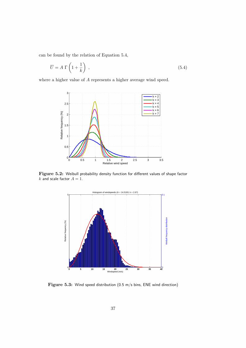
Illustrated in Figure 5.3 and 5.4 are the distributions of wind speeds forthe 2 major wind directions, East Northeast (ENE) and West Southwest(WSW).

It is common practice to fit a Weibull distribution to the wind distribu-tion [20]. The parameters of the Weibull distribution can be used to describeand compare the wind regime. This Weibull probability density function is

35

10 20 30 40 50

30

210

60

240

90270

120

300

150

330

180

0

Figure 5.1: Wind rose visualises the distribution of the wind direction (10°bins).

given by,

f(U) =k

A

(U

A

)k−1

exp

[−(U

A

)k], (5.1)

where A is the scale factor (m/s), k is the shape factor (dimensionless) andU is the wind speed (m/s).

The scale factor A and shape factor k can be determined in several ways,such as the use of special Weibull paper, standard deviation analysis orenergy pattern factor analysis [21]. Here the standard deviation analysis isused. The ratio between the standard deviation and average wind speedscan be related to the shape factor k by,

σ2U

U2 =

Γ(1 + 2

k

)Γ2(1 + 1

k

) − 1 , (5.2)

with σ2U the variance of U , U the time average wind speed and Γ(·) the

gamma function, a standard integral defined by,

Γ(x) =∫ ∞

0yx−1e−ydy . (5.3)

A higher value of k corresponds to a smaller distribution, as illustrated inFigure 5.2. Once the shape factor has been determined, the scale factor A

36

can be found by the relation of Equation 5.4,

U = A Γ(

1 +1k

), (5.4)

where a higher value of A represents a higher average wind speed.

0 0.5 1 1.5 2 2.5 3 3.50

0.5

1

1.5

2

2.5

3

Rel

ativ

e fr

eque

ncy

(%)

Relative wind speed

k = 2k = 3k = 4k = 5k = 6k = 7

Figure 5.2: Weibull probability density function for different values of shape factork and scale factor A = 1.

0 5 10 15 20 25 30 35 400

5

Rel

ativ

e fr

eque

ncy

(%)

Windspeed (m/s)

Histogram of windspeeds (A = 14.5193, k = 2.67)

0 5 10 15 20 25 30 35 400

0.1

Wei

bull

freq

uenc

y di

strib

utio

n

Figure 5.3: Wind speed distribution (0.5 m/s bins, ENE wind direction)

37

0 5 10 15 20 25 30 35 400

5

10

15

Rel

ativ

e fr

eque

ncy

(%)

Windspeed (m/s)

Histogram of windspeeds (A = 4.6591, k = 2.4)

0 5 10 15 20 25 30 35 400

0.1

0.2

0.3

Wei

bull

freq

uenc

y di

strib

utio

n

Figure 5.4: Wind speed distribution (0.5 m/s bins, WSW wind direction)

The ENE wind speed distribution shows a high scale factor (A = 14.5m/s),which is typical for trade wind regions. To get a better impression of thewind regime throughout the year, the Weibull distribution has been fit tothe wind data of each month. Considering only the east-northeastern winddirection, the calculated Weibull parameters in each month are shown inFigure 5.5.

This figure clearly shows the large differences between dry (November untilApril) and rainy (May until October) season. During the dry season, thewinds are stronger (higher scale factor) and more constant (higher shapefactor is equivalent to a smaller distribution). This makes wind power anexcellent renewable energy source to be used in combination with hydropower, which generation is reduced during the dry season.

5.3 Wind power distribution

The energy contained in the wind passing the rotor has a quadratic relationwith the wind speed according to [20,22],

Ew =12mU2 , (5.5)

with m the air mass and U the uniform constant wind speed. The power isdefined as the energy per second,

Pw =d

dt

(12mU2

)=

12U2dm

dt. (5.6)

38

Figure 5.5: Weibull scale factor A and shape factor k fit on monthly ENE winddata. During the dry season (coloured yellow) the winds are stronger and more constantcompared to the wet season (coloured blue).

The air mass can be defined as m = ρV , where ρ is the density and V is thevolume. The assumption of a constant air density leads to

Pw =12U2d ρV

dt=

12ρU2 dV

dt. (5.7)

dVdt is the volume of air passing the rotor disk per second. This volume per

second can be expressed as the rotor disk area A multiplied by the windspeed U . Substitution of dV

dt = AU reveals the cubic relation between windspeed and wind power,

Pw =12ρU2 dV

dt=

12ρAU3 . (5.8)

The wind power density per unit area is given by

PwA

=12ρU3 . (5.9)

The available measurement data contains the ten minute average values ofthe wind speed. The relation between the ten minute average wind powerand wind speed is similar to above equations, but requires a correction factor,

PwA

=12ρU3 =

12ρU3 = ke

12ρU

3,with ke =

U3

U3 . (5.10)

39

The correction factor ke can be derived from the Weibull shape factor kas [20]

ke =Γ(1 + 3

k

)Γ3(1 + 1

k

) . (5.11)

The previous paragraph showed a strong wind from the dominating ENEdirection. As such, it is no surprise that all power contained within thewind is coming from this direction (Figure 5.6). This is also reflected in thegrowth of the vegetation around Tejona.

The Tejona wind farm has been built nearly perpendicular to this winddirection, as shown in Figure 5.7. Wake effects are therefore minimal.

20 40 60 80

30

210

60

240

90270

120

300

150

330

180

0

Figure 5.6: Wind power rose (10°bins)

5.4 Diurnal variations

Diurnal variations (daily or twice-daily cycles) are common in temperature,wind speed, air pressure. The variations are mostly generated by periodicalheating of the atmosphere by the sun [23].

The variation in average wind speed is largely due to the fact that tempera-ture differences between the sea and the land surface tend to be larger during

40

Figure 5.7: Tejona wind farm layout and dominating wind direction

the day than at night. This effect is strongest near the coast. Although theTejona site is located about 100km from the Pacific coast line and 150kmfrom the Carribean coast, these variations are still noticeable as can be seenin Figure 5.8.

The twice-daily cycle of air pressure is caused by global atmospheric tides.Figure 5.9 shows these cycles in air pressure. The temperature follows adaily cycle related to the length of the common solar day, Figure 5.10. Theair pressure and temperature observations do not only reveal a clear diurnalvariation, but also a very constant climate.

5.5 Conclusions

This chapter illustrated general observations about the weather conditionsat the Tejona wind farm.

The weather conditions in the Tejona area have shown to be very constant,especially during the dry season. Variations in temperature and air pressureare small all year round, while in the dry season also the wind shows anarrow distribution with a high average wind speed and dominating east-northeastern wind direction throughout the year. The Tejona wind farmmakes optimal use of this fact as it has been built perpendicular to this

41

0 1 2 3 4 5 6 7 8 9 10 11 12 13 14 15 16 17 18 19 20 21 22 23 240.85

0.9

0.95

1

1.05

1.1

1.15

1.2

Time (hour)

Win

d sp

eed

(nor

mal

ised

to d

aily

ave

rage

)

Hourly averageStandard deviation

Figure 5.8: Diurnal variations in wind speeds

0 1 2 3 4 5 6 7 8 9 10 11 12 13 14 15 16 17 18 19 20 21 22 23 24929

930

931

932

933

934

935

936

Time (hour)

Air

pres

sure

(hP

a)

Hourly averageStandard deviation

Figure 5.9: Diurnal variations in air pressure

wind direction. Another advantage is that a wind power forecasting methoddoes not need to take wind farm layout into account, as turbine wakes donot occur. The analysis shows also the high potential of wind power withinthis region. Currently, all operational wind farms are situated in the vicinityof Tejona.

.

42

0 1 2 3 4 5 6 7 8 9 10 11 12 13 14 15 16 17 18 19 20 21 22 23 2419

20

21

22

23

24

25

26

27

Time (hour)

Tem

pera

ture

(° C

elsi

us)

Hourly averageStandard deviation

Figure 5.10: Diurnal variations in temperature

43

44

Chapter 6

Time series forecast model

Time series models are statistical models which depend only on observa-tions. The moving average model is a simple time series model with a broadapplication. This chapter presents the generalised moving average modeland two variations, the persistence model and global mean model.

Application of the persistence model for wind power forecasting is based onthe observation that average wind speeds change slowly. Therefore it oftenperforms well for very short forecast horizons. And due to the unambiguousimplementation, it has been used in most performance comparisons betweenwind power forecasting methods.

On the contrary, the (global) mean model performs better for long forecasthorizons. This model is justified by the observation that the best guess foran unknown variable with unknown distribution is its mean.

In this chapter both models are applied to the Tejona wind farm and resultsare analysed.

6.1 Generalised Moving Average model

The moving average model takes the average over the Q most recent mea-surements as a prediction for the entire forecast horizon,

P (ti+k|ti) =1Q

Q−1∑j=0

P (ti−j) ∀ k ∈ [1, . . . , N ] , (6.1)

where P is the estimated value, P the observations and N represents theforecast horizon.

Because it only depends on recent observations and requires a learning pe-riod of Q samples, the model is suitable in any situations in which a sufficientnumber of measurements are available.

45

For wind power forecasting, either wind power output or wind speed can betaken as forecast value. The latter requires the predicted wind speed to beconverted to wind power by the turbine power curve and an (optional) modelto predict the wind turbine state. As this conversion step can introduceadditional errors, the turbine power output is taken as forecast value.

6.1.1 Model variations

For Q = 1 the model becomes the persistence model,

P (ti+k|ti) = P (ti) . (6.2)

This model often performs well for very short forecast horizons, due to thetypically slow changes of average wind speed and atmospheric conditions.

For Q→∞ the prediction value approaches the global mean,

P (ti+k|ti) = P . (6.3)

Compared to persistence, the performance is expected to be poor for shorthorizons but better for longer horizons [24].

6.2 Persistence model results

The persistence model is applied on two years of measurement data from theTejona wind farm (January 2005 – December 2006). Per day one forecastper wind turbine is being made at noon (12:00pm). The model predicts10-minute average wind power output for a forecast horizon of 7 days.

6.2.1 Power output forecast of single wind turbines

Running the persistence model on the wind power output of each windturbine results in the average normalised errors as displayed in Figure 6.1.Normalisation is performed according to the nominal power of the turbines.

A clear periodic pattern can be detected in the bias, which is also reflectedin the mean absolute and root mean square errors. This systematic errorwith an amplitude of 5% results from diurnal variations in the wind speed,described in Chapter 5.

Both the mean absolute error as well as the root mean square error showan increasing behaviour. The MAE and RMS error reach their peak valueof 30% and 45%, respectively. This performance is expected, due to thenature of the model. However, the model performs reasonably well for shortforecast horizons.

46

−10

−5

0

5

NB

IAS

(%

)

0

10

20

30

NM

AE

(%

)

24 48 72 96 120 144 1680

1020304050

NR

MS

E (

%)

Forecast horizon (hours)

Figure 6.1: Performance of persistence model on turbine power output with respectto the forecast horizon. The presented error measures are averages over the number ofturbines and normalised to the nominal power.

6.2.2 Clustering forecasts

As the output of a cluster of wind turbines is less fluctuating, the error isexpected to increase less if the wind farm output is predicted instead of windturbine output, as discussed in Chapter 3. Figure 6.2 supports this theory.Both the average errors as well as the error of the clustered wind turbinesare displayed. A reduction of 5% is observed in the peak mean absoluteerror and a 10% improvement of the maximum root mean square error isachieved.

47

−10

−5

0

5

NB

IAS

(%

)

0

10

20

30

NM

AE

(%

)

24 48 72 96 120 144 1680

1020304050

NR

MS

E (

%)

Forecast horizon (hours)

Figure 6.2: Comparison between the average performance of single persistenceforecasts (blue line) and the performance of the persistence model on clustered windturbine output (brown line)

6.2.3 Comparison with literature

In literature [18], persistence model results can be found for a wind farmin Ireland, see Figure 6.3. The results from Tejona, redrawn in Figure 6.4to match the axes, are better at each point in the forecast horizon. Thedifference can be explained by the climate. Especially during the dry season,the wind turbines in Tejona are frequently running on nominal output power(or they are switched-off). Also the long maintenance periods contribute toa low error in the persistence model.

6.3 Mean model results

The mean model is applied under the same conditions as the persistencemodel.

6.3.1 Clustered forecast results

The global mean value of a variable is only a theoretical value, usuallyapproximated by the sample mean. Within the moving average model, Qrepresents the number of samples that are considered within the samplemean. Running the moving average model for different values of Q leads todifferent errors (Figure 6.5).

48

that for this case study, the model does not make any significant systematic error. This is

a desired property when using a prediction model. Nowadays, both statistical and

physical models enhanced with Model Output Statistics (MOS) are able to provide unbiased

forecasts.

Figure 5 illustrates the performance evaluation by the use of both the NMAE and the

NRMSE. The two error measures are computed for the advanced model and for the reference

one (Persistence is used here), for every prediction horizon. The NMAE can be interpreted:

straightforwardly; for instance, the advanced model made an average error representing 13%

WIND ENGINEERING VOLUME 29, NO. 6, 2005 483

0.02

0

–0.02

–0.04

–0.06

–0.08

µ (%

of i

nsta

lled

pow

er)

–0.1

–0.12

–0.14

–0.160 5 10 15 20 25

look-ahead time (hours)

30 35 40 45

Figure 4: Prediction model bias as a function of the lead time.

45

NMAE advanced modelNRMSE advanced modelNMAE PerisistenceNRMSE Perisistence

40

Err

or (

% o

f Pin

st)

35

30

25

20

15

10

55 10 15 20 25 30 35 400 45

Look-ahead time (hours)

Figure 5: Use of the NMAE and the NRMSE for assessing the performance of the advanced prediction

approach, and for comparison with a reference predictor (Persistence is used here).

01_S372.qxd 28/2/06 4:31 pm Page 483

Figure 6.3: Comparison of the NMAE and NRMSE between the persistence modeland an advanced prediction approach (not further specified), applied to a wind farm inIreland. [18]

0 5 10 15 20 25 30 35 40 450

5

10

15

20

25

30

35

40

45

Err

or (

% o

f ins

talle

d ca

paci

ty)

Forecast horizon (hours)

NMAE persistenceNRMSE persistence

Figure 6.4: NMAE and NRMSE of the persistence model applied to the Tejonawind farm for the same time horizon as Figure 6.3.

49

−5

0

5

NB

IAS

(%

)

10

20

30

NM

AE

(%

)

24 48 72 96 120 144 1680

10

20

30

40

NR

MS

E (

%)

Forecast horizon (hours)

Figure 6.5: Error performance of the mean model, which has been applied to windfarm output for three values for Q: Q = 1 day (blue), Q = 7 days (brown) andQ = 30 days (green).

For increasing values of Q the MAE and RMSE errors flatten out. Thisindependence of the forecast horizon is expected, as the average value isloosely related to instantaneous power output. Various simulations haveshown that the long-term prediction error improves slightly for each valueof Q, up to Q = 30 days.

For this value of Q, the error profile varies between 25% and 30% of the nom-inal installed capacity. Compared to the persistence model (Figure 6.6), themean absolute error does not significantly improve, while the mean modeloutperforms the persistence RMSE for horizons above 36 hours.

6.4 Combining mean and persistence model

By combining the persistence and mean model the performance can be fur-ther improved. Properly weighing both models leads to a model whichfollows the persistence model for short time horizons and approaches themean model for longer horizons. The eventual model is given by,

P (ti+k|ti) = ak P (ti) + (1− ak)P (ti) + bk , (6.4)

where P (ti) resembles the persistence model, P (ti) is the time average valueof the Q most recent observations (mean model), ak are weighing factorsand bk is an off-set.

50

−5

0

5

NB

IAS

(%

)

0

10

20

30

NM

AE

(%

)

24 48 72 96 120 144 1680

10

20

30

40

NR

MS

E (

%)

Forecast horizon (hours)

Figure 6.6: Comparison of errors between persistence model (blue) and mean model(brown). The mean model takes the average wind power output over the past month(Q = 30 days) as prediction forecast. The mean model outperforms the persistencemodel (measured in RMSE) for horizons over 30 hours.

In literature on wind power forecasting, the application of this model hasbeen proposed by Nielsen [24], however without off-set bk. This off-set isproposed here to account for diurnal variations, which are reflected in theturbine output and forecast error. It will be shown in the next paragraphthat the bk parameter can be substantial.

Linear regression model

Re-writing Equation 6.4 and short-handing notation leads to,

P (ti+k|ti) = P (ti) + ak(P (ti)− P (ti)

)+ bk (6.5)

Pi+k − P i = ak(Pi − P i

)+ bk (6.6)

∆Pi+k = ak ∆Pi + bk . (6.7)

In statistics, this model is known as a linear regression model with regressorvariable x = ∆Pi, response variable Y = ∆Pi+k and ak and bk regressioncoefficients [16]. Note that for each k a pair of (ak, bk) values is required.From this point onwards an arbitrary value of k is assumed.

Suppose n pairs of observations deducted from a training set are available,(x1, y1), . . . , (xn, yn). Each observation can be described by the model,

yj = axj + b+ εj j = 1, . . . , n , (6.8)

51

where a and b are the coefficients of the regression line and ε is a random errorwith mean zero and variance σ2. The sum of the squares of the deviationsof the observation from the regression line is,

L =n∑j=1

ε2j =n∑j=1

(yi − b− ax)2 (6.9)

The least squares estimators of a and b (a and b) must satisfy,

∂L

∂a

∣∣∣∣a,b

= −2n∑j=1

(yi − b− ax)x = 0 , (6.10)

∂L

∂b

∣∣∣∣a,b

= −2n∑j=1

(yi − b− ax) = 0 . (6.11)

Simplifying these equations yields,

nb+ an∑j=1

xj =n∑j=1

yj , (6.12)

b

n∑j=1

xj + a

n∑j=1

x2j =

n∑j=1

xjyj . (6.13)

(6.14)

The solution of these equations leads to the least square estimates of a andb,

b = y − ax , (6.15)

a =∑xjyj − 1

n (∑xj∑yj)∑

x2j −

1n (∑xj)

2 , (6.16)

where each summation is over the complete set of observations (j = 1, . . . , n).

6.4.1 Clustered forecast results of the combined model

The regression coefficients ak and bk are determined for a training set, whichcomprehends the year 2005. The resulting estimates with respect to theforecast horizon are displayed in Figure 6.7. As expected, there is a negativetrend in weighing factor ak, such that ak ≈ 1 for low values of k and akdecreases for higher values of k. The diurnal variations also shows up inboth the ak as well as the bk parameters.

Figure 6.8 illustrates the resulting error of the combined model in relationto the errors of the persistence and mean model.

52

0

0.5

1

a k

24 48 72 96 120 144 168−60

−40

−20

0

20

40

b k (kW

)

Forecast horizon (hours)

Figure 6.7: Estimated regression coefficients ak and bk with respect to the forecasthorizon.

−5

0

5

NB

IAS

(%

)

0

10

20

30

NM

AE

(%

)

24 48 72 96 120 144 1680

10

20

30

40

NR

MS

E (

%)

Forecast horizon (hours)

Figure 6.8: Comparison of errors between persistence model (blue), mean model(brown) and combined model (green). The combined model approaches performanceof the persistence model for short horizons, while for longer horizons the performanceis comparable to the mean model.

53

The combined model follows the persistence model for forecast horizons lessthan 30 hours, while the performance for longer horizons is comparable tothe mean model. However, the RMS error is not minimal for each point ofthe horizon. This is partly explained by the different validation sets. Thecombined model has been run on a validation set (year 2006), while thepersistence and mean model results are based on two years of simulations(year 2005 and 2006). Furthermore, the regression coefficients are assumedto be constant throughout the validation period, while in reality these varyslightly over time.

6.5 Conclusions

In this chapter the performance of the moving average model for the Tejonawind farm has been demonstrated. Two model variations and their combi-nation have been applied to measurements of the wind farm.

The persistence model takes the most recent observation as forecast for theentire horizon. As the average wind speeds are typically changing slowly,this model performs well for short horizons, while deteriorating for longertime horizons. The errors are reduced if multiple forecasts are combined.These cluster forecasts can achieve a 10% decrease in RMSE.

The mean model takes the average value of the most recent observations asforecast. A number of simulations showed that averaging over more than7 days of observations does not improve results. On the contrary to thepersistence model, the mean model has a relatively constant performanceover the forecast horizon and outperforms the persistence model for horizonsabove 30 hours.

A further improvement is obtained by properly combining both models. Theresulting linear regression model follows the performance of the persistencemodel for short horizons and the mean model for longer horizons. However,this model does require a substantial training set to determine the weighingfactors.

The obtained results are fairly satisfying in comparison to the simplicity ofthe model. In comparison to European wind farms, these models performconsiderably better due to the different wind regime. The models provide abasis for comparison with more advanced (physical) models.

54

Chapter 7

Physical forecast model

Following the development of the European research programmes, the use ofa physical method for short-term wind power forecasting is expected to resultin better performance compared to statistical models [5]. Especially forlonger time horizons, physical models have shown to outperform statisticalmethods.

Physical models utilise physical weather models to obtain local weather pre-dictions. Additional (mostly statistical) models are used to obtain a predic-tion of the turbine power output. The different elements are discussed andanalysed within this chapter.

7.1 Weather Forecasting

Wind turbines extract power out of the wind and transform this wind powerto electrical power. The wind power is related to the wind speed as shownin Chapter 5. Therefore, forecasting the wind turbine output starts withforecasting the wind.

Winds are mainly driven by global pressure systems [23]. As such, a globalmodel needs to be used in predicting the wind. Due to the scale and com-plexity of these models, numerical solving methods are used. These numer-ical weather prediction models have a finite resolution due to the limitedcomputer capacity.

The local wind conditions are greatly influenced by local spatial and tem-poral effects. The down scaling of the wind to local conditions requires anadditional model. Above topics are discussed in subsequent paragraphs. Asan operational weather forecast model is not present in Costa Rica at themoment, the discussion concludes with a number of recommendations onimplementing such models.

55

7.1.1 Numerical weather prediction systems

In general, physical modelling of the dynamics within the atmosphere leadsto a large complex nonlinear system of differential equations with a largenumber of states. This system describes the expected evolution of theweather over time. Due to their complexity, it is solved numerical andis therefore known as numerical weather prediction system (NWP).

The current atmospheric state is taken as a starting point for solving theNWP model. This state is derived from measurements at meteorologicalstations on various places. As weather is affected by global phenomena,NWP systems usually cover the complete Earth. Due to limited computercapacity the resolution of the numerical grid has to be finite. Typically, theoutput of NWP models is given at various vertical pressure levels, whichare related to the altitude above sea or ground level. The horizontal dis-tance between the grid points is in the range of 50 – 100+ kilometres forglobal models [15]. Processes on smaller scale are not directly simulated,but their influence on the evolution of the large scale weather conditions isparameterised.

The NWP output is usually calculated with a time step between 1 – 6 hoursup to 48 hours after initiation. Due to the complexity of the models, 2 – 5hours is normally needed for computing the output. These models requiresupercomputers and are run at national weather offices.

Costa Rica can benefit from the NWP models run by the US NationalWeather Service. This US governmental institute has an operational GlobalForecast System (GFS) model and provides output of this model for theCaribbean region. To spatially refine this output, the Costa Rican InstitutoMeteorologico Nacional (IMN) has been using Workstation Eta (WS-Eta).This model predicts the weather conditions on a horizontal spatial resolu-tion of 12 km with a time step of 6 hours up to an horizon of 48 hours.Especially the low temporal resolution limits the application of this data forwind power forecasting.

7.1.2 Downscaling of weather predictions

The output of NWP models has a coarse spatial and temporal resolution.NWP models are good in predicting the large scale weather systems. Forwind power forecast purposes, local wind speed predictions in the lowerregions of the planetary boundary layer are required.

European Wind Atlas method

Geostrophic wind predicted by the NWP model is the main driving forcefor the air flow in the planetary boundary layer (PBL). The wind in the

56

boundary layer is greatly influenced by the friction of the Earth’s surface.This friction causes turbulence and leads to transport of momentum, whichresults in a neglectable wind speed at ground level. For neutral situations a(vertical) logarithmic wind profile can be derived,

U(z) =u∗k

ln(z

z0

), (7.1)

which is characterised by a certain roughness length z0 (depending on thevegetation/terrain type) and surface friction velocity u∗. k is the von Kar-man constant with k = 0.4.

The relation between the geostrophic wind and surface friction velocity isgiven by the geostrophic drag law. For neutral situations this law is,

|G| = u∗k

√(ln(u∗fz0

)−A

)2

+B2 , (7.2)

where f is the Coriolis parameter and A and B are empirically determinedconstants. To account for thermal effects such as buoyancy, a correctionshould be performed. Details and a further derivation can be found inliterature [2, 20].

These models have been used in Europe to construct the European WindAtlas [8] and are the basis of the physical wind power forecast programPrediktor [7], discussed in Chapter 2.

Downscaling in complex terrain - Mesoscale model MM5

The logarithmic wind profile applies only if the upwind terrain is reasonablyhomogeneous [25]. In complex terrain local orographic and thermal effectsplay an important role that is not reflected completely by the models usedfor the European Wind Atlas. Pennsylvania State University and NationalCenter for Atmospheric Research (NCAR) have developed an open-sourceregional mesoscale modelling system MM5 [11], which has successfully beenapplied to obtain local wind predictions in complex terrain [12].

The MM5 system has the capability to nest multiple domains with increasingspatial resolution up to 1 km, which makes it possible to include local effects.This idea is illustrated in Figure 7.1. Four domains are used to obtain a highresolution forecast around San Jose, the capital of Costa Rica. The domainshave a horizontal resolution ranging from 90 km to 3.3 km.

Another important property for application in complex terrain wind fore-cast are the nonhydrostatic dynamics. This implies that vertical pressuregradient forces are also taken into account, which play an important role incomplex terrain.

57

Figure 7.1: Example of nested domains centred around San Jose. The domains d1to d4 have a resolution of 90, 30, 10 and 3.3km respectively. This configuration ofMM5 has been used for a study of NASA to the origin of tropical hurricanes. [26]

Judging from the specifications [11] and literature references (e.g. [12, 27]),the MM5 model is expected to be able to give local wind predictions at theTejona wind farm.

7.1.3 Recommendations

The currently at the ICE available weather forecasts from the WS-Eta modelhave very limited application for wind power forecasting. Forecasts aremainly used for analysing precipitation, as the energy production is highlydependent on hydro power stations (see Chapter 8). The output of the WS-Eta model is available at a spatial resolution of 12 km with a time step of6 hours up to an horizon of 48 hours.

A finer spatial and temporal resolution is necessary for wind power predic-tion purposes. This can be achieved by a mesoscale model. Although therehas been an intention in the past to run the MM5 model at the meteorologicoffice of the ICE, there is no active work done on this matter. Therefore,the performance of this model cannot be verified and this section is limitedto a theoretical discussion.

58

Before spending resources on implementing the MM5 model, the perfomanceshould be investigated. The Centro de Investigaciones Geofısicas (CIGEFI)of the University of Costa Rica has an experimental setup of the MM5model. [26] This knowledge can be used to explore the possibilities of themesoscale model and evaluate its performance for the Tejona wind farm.

The nested domain with the highest spatial resolution domain can be limitedto the Tejona region, where currently all wind farms are located. To coverthe whole of Costa Rica in fine resolution seems to be abundant and onlyincreases computer load.

Even more important than a high spatial resolution is a high temporal res-olution. Wind speeds have a very fluctuating behaviour over time, whichis reflected in the power output of wind turbines. The temporal resolutionof the currently available NWP model (3 hours) is far too low for makingaccurate wind power predictions. Typically, an internal integration step-sizeof 3∆X (in seconds, with ∆X the spatial resolution in kilometres) is rec-ommended for MM5 [28]. It should be possible to output (a subset of) thepredicted variables in this small step size as well. For the purpose of windpower predictions the minimum temporal resolution of the MM5 output isrecommended to be 1 hour. For this time step the power curve can be ap-plied without making a too big error. Smaller step sizes can have a positiveeffect on power prediction error and can be used to predict extreme windspeeds.

The time horizon of the model depends on the horizon of the NWP model,which is needed to initiate the MM5 model and supplies the boundary con-ditions. The GFS output available on the internet reaches up to 7.5 days.It should be possible to have wind power prediction for a 7 day horizon, asdesired by the system operator.

7.2 Power Forecasting

When weather forecasts are available, the foreseen output power can beobtained through a model for wind turbine output. This model consistsof the power curve and a state model for the estimated state of the windturbine. As concluded in Chapter 5, no model is needed for the wind turbinewake effects, because these do not appear. As the power curve is a staticmodel of a dynamic process and the state model is a simplified discretepresentation of the turbine, the conversion from wind speed to wind turbinepower output is an additional error source.

After clarifying the simulation conditions, several models for the power curveare investigated:

Model 1: Theoretical power curve referred to the meteorological mast.

59

Model 2: Global measured power curve referred to the meteorologicalmast.

Model 3: Individual power curves referred to the nacelle wind speeds.

7.2.1 Simulation conditions

As actual wind prediction are not available, the wind speed measurementscan be used as fictitious wind speed predictions. As a consequence thisparagraph focusses only on the error introduced by the wind speed to powerconversion. This also implies that the error is no longer dependent on theforecast horizon, instead the overall error is addressed.

The proposed models are tested on measurement data from 2006. A 10 minuteaverage forecasted output power is compared to the measured output power.For models 2 and 3, a training period is needed to determine the powercurves. Data from 2005 is taken as a training set for these models, such thattraining and validation data sets do not overlap.

The state as determined in Chapter 4 is used for the model of wind turbinestate. This model has outputs 0 and 1, which are related to ’maintenance’and ’normal operation’ state respectively.

The power curve models are determined for an air density of ρ0 = 1.08 kg/m3.To achieve this, the available temperature and air pressure measurementsof the meteorological mast are used to calculate the actual air density, ρair.The wind speeds are corrected with a factor C according to IEC 61400-12standard [29],

C = 3

√ρairρ0

, (7.3)

such that the wind speed is normalised to an air density of ρ0 = 1.08 kg/m3.Due to the constant air pressure the correction factor C has a very smallvariation of (0.0024)2 around a mean of 1.0064 with minimum and maxi-mum values of 0.9969 and 1.0142 respectively. The influence is thereforeneglectable and is omitted for the validation of the power curves.

7.2.2 Model 1: Theoretical power curve referred to the me-teorological mast

An initial model for the power curve is given by the wind turbine data sheet.This data sheet specifies the wind turbine output under standardised testconditions. The obvious advantage is that such a model is available out-of-the-box. But, the model does not account for deviating conditions at

60

the site (different turbulence intensities, etc.) and time varying influences(gearbox wear, etc.).

The turbine power curve of the V42/660 defined by Vestas is shown inFigure 7.2 and is valid for 10 minute average wind speeds with an air densityof ρ0 = 1.08 kg/m3 [30]. The cut-in, rated and cut-out wind speed are 4m/s,18.5m/s and 25m/s respectively.

0 5 10 15 20 25 30−100

0

100

200

300

400

500

600

700

Wind speed (m/s), ρ = 1.08 kg/m3

Pow

er o

utpu

t (kW

)

Figure 7.2: Data sheet power curve Vestas V42/660. Valid for 10-minute averagewind speed with an air density of ρ0 = 1.08 kg/m3. [30]

The power curve model is applied for predicting the output of the wind farmas shown in Figure 7.3.

Power curve

modelX ∑Uest

Aest Pmeas

Pest Perror

+

–

Figure 7.3: Power forecast setup of models 1 and 2. In this figure Uest is the esti-mated wind speed at the met mast, Aest is the estimated number of normal operatingwind turbines, Pest is the estimated total power output of the wind farm, Pmeas is themeasured wind farm output and Perror the resulting error in power forecast.

This model leads to an output as visualised by the scatter plot of Figure 7.4.In this figure, the estimated and measured wind farm power output (nor-malised to the total installed capacity) are presented as function of the wind

61

speed. The distinctive levels in the power prediction are a consequence ofthe varying availability of the turbines. Figure 7.5 gives the general patternof the error in relation to the wind speed.

Figure 7.4: Realised wind power output and wind farm output predictions based onthe data sheet power curve with respect to predicted meteorological mast wind speeds.Both measurements as well as predictions are scaled to the total installed capacity.

These graphs illustrate the major short-coming of the formal data sheetpower curve. First, due to the recommendations in the IEC 61400-12 stan-dard [29], the data sheet power curve is determined only on data sets forwhich the turbine has ran for the complete 10-minute interval. If, for cer-tain bins, no data is available the power curve is inter- or extrapolated. Thisrecommendation neglects the practical cut-off behaviour of the wind speed.Vestas V42 turbines are halted when the 100 second average wind speedis above the cut-off wind speed level (vcut-off = 25m/s) [31]. This impliesthat 10-minute average wind speeds can be below 25m/s, while a wind gustmight cause the running 100-second average to cross the cut-off wind speedlevel and cause the turbine to automatically switch off.

Second, the wind speed measurements at the met mast do not representthe wind speed at every turbine equally well. This can be concluded fromthe fact that the output of the wind farm is nonzero for wind speeds above25m/s. As a consequence of the cut-off behaviour, individual turbines shutdown if wind speeds cross the stop wind speed and therefore have a (close to)zero output for 10-minute average wind speeds above 25m/s. The nonzerowind farm output for wind speeds above cut-off is a consequence of the local(complex) terrain, which distorts wind flow considerably. While observed

62

Figure 7.5: Error in wind power prediction with respect to predicted wind speed,normalised to the total installed capacity. The large negative error is due to the cut-offbehaviour of wind turbines.

wind speeds at the met mast are above 25m/s, turbine X might face a windspeed below cut-off and is still producing.

7.2.3 Model 2: Global measured power curve referred to themeteorological mast

To overcome the previously mentioned short-comings, the power curve canbe based on actual on-site measurements. This requires a minimum setof met mast wind speed and wind farm power output observations. Thepower curve is determined on the 2005 wind farm output and wind speedmeasurement at the meteorological mast. The measurements are groupedinto wind speed bins of 0.5m/s-width. For each bin, the average output iscalculated according to

Pi =1Ni

Ni∑j=1

Pi,j , (7.4)

where Pi is the average power output in bin i, Pi,j is the power outputof data set j in bin i (only normal operating wind turbines are taken intoaccount) and Ni is the number of 10 minute data sets in bin i.

The measured average power curve is presented in Figure 7.6. Compared todata sheet power curve, this model does take some of the cut-off and terrain

63

effects into account. The output decreases closer to cut-off wind speed andis nonzero for wind speeds above cut-off wind speed level. Using this powercurve in a similar setup as previous model (see Figure 7.3) yields the resultsof Figure 7.7 and Figure 7.8.

0 5 10 15 20 25 30−100

0

100

200

300

400

500

600

700

Wind speed (m/s), ρ = 1.08 kg/m3

Pow

er o

utpu

t (kW

)

Figure 7.6: Global measured average power curve referred to the meteorologicalmast. Valid for 10-minute average wind speed with an air density of ρ0 = 1.08 kg/m3.

The graphs indicate a considerable improvement. Model errors are centeredaround zero. The error between wind speeds of 20 and 25m/s can be ex-plained by the hysteris effect around cut-off wind speeds. In addition to theautomatic shut-down of wind turbines for 100-second average wind speedsabove 25m/s (see previous paragraph 7.2.2), wind turbines are restartedautomatically. This happens only when the 100-seconds mean wind speedis below the restart wind speed (vrestart = 20m/s) and stays below the stopwind speed for 1 minute [31]. The hysteris effect is visualised in Figure 7.9.This dynamic effect is not included in the static power curve model.

7.2.4 Model 3: Individual power curves referred to the na-celle wind speeds

Errors are expected to reduce, when individual power curves for each turbineare used. Although these power curves are still static, they are expected torepresent individual turbine characteristics better.

The individual power curves are computed in a similar way as the globalpower curve, see Model 2. For each individual wind turbine the measured

64

Figure 7.7: Realised wind power output and wind farm output predictions basedon the global measured power curve with respect to the met mast wind speed (inpercentage of the total installed capacity).

Figure 7.8: Error in wind power prediction with respect to the predicted wind speed,normalised to the total installed capacity. Cut-off behaviour leads to notable errors forhigher wind speeds.

65

18 19 20 21 22 23 24 25 26 27

Off

On

100−second average wind speed (m/s)

stat

us w

ind

turb

ine

(on/

off)

Figure 7.9: Hysteresis effects around cut-off wind speed. A turbine stops when the100 second average wind speed is above the stop wind speed level (vcut-off = 25m/s)and only restarts when the 100 seconds mean wind speed is below the restart windspeed (vrestart = 20m/s) and stays below the cut-off wind speed for 1 minute. [31]

output during normal operation is grouped into wind speed bins of 0.5m/s-width. Subsequently, the average power output of each bin is determined.The results are shown in Figure 7.10.

5 10 15 20 25 30

0

10

20

300

100

200

300

400

500

600

700

Wind turbineWind speed (m/s)

Pow

er o

utpu

t (kW

)

Figure 7.10: Individual measured power curves referred to the nacelle anemometer.Power curves are valid for a 10-minute average wind speeds with air density ρ0 =1.08 kg/m3.

Most power curves are following the expected shape. For wind turbines 8,11, 15, 19, 24, 26 and 27 this is not the case. Especially for higher windspeed their curves deviate from the data sheet/global measured models.

66

This can partly be explained by the insufficient number of samples in thetraining data set due to long maintenance periods. Wind turbines 8, 11, 15,19, 26 have ran between 10% and 30% of the time in 2005, while 14 (outof 30) turbines have operated normally over 80% of the year. This greatlyreduces the number of samples in each bin, as such the average may notbe representative for the true behaviour. Additionally, the poor availabilityestimation outlined in Chapter 4 leads to deformed curves. The power curvesare applied as shown in Figure 7.11.

Power curve

model WT1X ∑Uest

AestPmeas

Pest Perror

∑Power curve

model WTiX ∑Uest

AestPmeas

Pest

Power curve

model WT30X ∑Uest

Aest Pmeas

Pest

Perror

Perror

Perror

WT1

WTi

WT30

+

+

+

–

–

–

+

+

+

Figure 7.11: Power forecast setup of model 3. In this figure Uest, Aest and Pest

are the estimated wind speed at hub height, availability of the wind turbine and poweroutput, respectively. Pmeas is the measured wind farm output and Perror the resultingerror in power forecast.

Typical results obtained from applying individual power curves are given inFigure 7.12 and 7.13. The first figure displays the estimated and measuredwind power prediction of wind turbine 2 in percent of the nominal powerwith respect to the predicted wind speed. The second graph is a scatter plotof the estimation error in percent of the nominal power with respect to thepredicted wind speed.

The figures show the characteristic error of individual wind turbine powerpredictions. A part of this error is concentrated around zero and is relatedto the steepness of the power curve. Furthermore, there is a distinctiveerror, which shows up as a power curve mirrored with respect to the windspeed axes. This error is related to errors in the estimation of wind turbinestate. If wind turbines are out of operation, due to an unforeseen event,

67

Figure 7.12: Realised wind power output and power output prediction of windturbine 2 based on the individual measured power curve with respect to nacelle windspeeds (in percentage of the nominal capacity). Only normal operating conditions areincluded in this scatter plot.

Figure 7.13: Error in wind power prediction with respect to predicted wind speed,normalised to the nominal capacity. Three different error classes are distinguished;centered around zero, negative power curve and errors related to hysteris in the cut-offwind speed region.

68

the error follows the negative power curve. A third part is related to cut-offbehaviour. For 10-minute average wind speeds between 20 and 25m/s, thestate of the wind turbines are not uniquely determined by the wind speed,as discussed in previous paragraphs.

Another observation is the time variation of the wind turbine power curve.Figure 7.14 illustrates a part of the predicted and measured wind poweroutput of wind turbine 1. Two different observation sets can be noticed.The measurements from January 2006 till end of October 2006 follow thepower curve (based on the training set of 2005), a second set with datafrom November and December 2006 (after a revision at the end of Octo-ber) shows a structural higher output. This is caused by a change of thegearbox/generator.

Figure 7.14: Two datasets of realised wind power output and power output pre-diction of wind turbine 1 between wind speeds of 5 – 15 m/s. Data set 1 coversthe months Jan – Oct 2005, set 2 are observations of Nov – Dec 2005. Only normaloperating conditions are included.

In addition to the analysis of the individual power curve errors, the globalerror is briefly examined. In Figure 7.15 the root-mean-square error (nor-malised to the installed capacity) is illustrated with respect to the monthsin the validation period (2006). This RMSE shows a strong correlation withthe two seasons. The error is substantial for the dry season (November –April) and has a lower level in the rainy season (May – October). This canbe related to the high wind speeds in the dry season. The wind turbines arefrequently operating above rated wind speeds (v ≥ 18.5m/s), as discussedin the wind resource assessment (Chapter 5). In this wind range the errors

69

are dominated by the cut-off behaviour and show a large variation, leadingto a high RMSE.

Figure 7.15: Root-mean-square error in wind power forecast (normalised to theinstalled capacity) with respect to the month. A strong relation between the RMSEand dry (yellow) and wet (blue) seasons is noticeable.

7.2.5 Comparison of power curve models

In this section, three power curve models have been examined. The useof each model is conditioned on the availability of data. The data sheetpower curve in combination with one wind speed prediction fails to captureaverage cut-off behaviour and terrain influences, but has the advantage thatit is applicable out-of-the-box. A global measured power curve requirestraining data but does reflect the average cut-off and terrain effects.

Individual power curves show interesting error characteristics. The error canbe divided into several classes. Two dominant classes are a result of the stateestimation of wind turbines and the hysteresis effects around cut-off windspeeds. Reduction of errors of the former class requires more informationand an in-depth study on the reliability of the wind turbines. Performanceimprovement of the latter case needs local wind predictions of the 100-secondaverage wind speed, which can be provided by the MM5 model.

Another source of errors is the static nature of the power curve. Withinthe models, the power curve has been determined on one year of trainingdata. As illustrated, the power curve can vary considerably, especially dueto revision/replacement of mechanical components such as the gearbox and

70

generator. These effects are noticeable in the error between cut-in and ratedwind speeds of individual wind turbines and can be accounted for by usingadaptive curves. This implies that the introduced error is mainly noticeableduring the rainy season when wind speeds are in this range. As shown, thehysteresis effect has a much large impact on RMS error and should be apriority in future research.

Table 7.1 summarises the model performance measured as RMSE. Thisclearly shows the benefits of using individual power curves on the perfor-mance of the power forecast.

Model Training Validation NRMSEperiod period (%)

Theoretical power curve – Jan – Dec 13.412006

Global measured power curve Jan – Dec Jan – Dec 4.482005 2006

Individual measured power curve Jan – Dec Jan – Dec 3.842005 2006

Table 7.1: Comparison of NRMSE (in % of the installed capacity)

7.3 Confidence Interval

The realised wind power output often differs from the predicted power. Sev-eral error sources for the mismatches can be identified, such as the windforecasts, turbine power curves, turbine availability, turbine switch-off dueto extreme wind conditions, etc.

To indicate the reliability of the estimated wind power production, a con-fidence interval can be added around the prediction. The upper (V ) andlower (L) limits of a 100α%-confidence interval, bound the interval in which100α% of the realised wind power is expected to be,

Pr (L < U < V ) = α . (7.5)

In this paragraph a possible method to construct such an interval is demon-strated. A set of confidence intervals (of different α-levels) are determinedand validated.

7.3.1 Determination of Confidence Interval bounds

The confidence levels can be related to various variables. Lange [32] showeda special interest in the relation between meteorological situations and the

71

uncertainty in the wind forecast. Another method is the use of a neural net-work with a correction depending on the weather stability [33]. These mightbe feasible methods, if the meteorological classification is easier to predictthan the actual uncertainty. Ernst [4] proposed a multimodel approach toderive uncertainty in the forecast.

In the setup as defined in this project, it is an apparent choice to relatethe predicted wind speed and wind power forecast uncertainty. As windmeasurements are used as forecasts, the uncertainty in predicted outputis caused by the uncertainty in the turbine power curve, availability andswitch-off behaviour for extreme wind speeds.

Wind turbine 28 is taken as an example for constructing the confidenceintervals around the 10 m/s wind speed. For this 10 m/s wind speed bin(9.75 < v ≤ 10.25m/s), the measured output power is shown in Figure 7.16.As before, the training set has been used to create the power curve andconfidence intervals. The best estimate of the power output is 329 kW .The histogram in Figure 7.17 gives a visual picture of the distribution of themeasured power. For this wind speed, the measurements approach a normaldistribution.

07/02 29/03 18/05 07/07 26/08 15/10 04/12260

280

300

320

340

360

380

400

Time (dd/mm)

Pow

er (

kW)

Figure 7.16: Measured power output of wind turbine 28 for wind speeds around10m/s

The data can also be represented by a cumulative distribution, as illustratedin Figure 7.18. From this distribution the limits of the confidence intervalscan be determined. One example of the 95%-confidence level is illustratedin Figure 7.19. In this project, the choice has been made to use the 10, 50,70, 80, 90 and 95%-confidence levels.

72

260 280 300 320 340 360 380 4000

20

40

60

80

100

120

Power (kW)

Num

ber

of o

bser

vatio

ns

Figure 7.17: Histogram of measured power output of wind turbine 28 for windspeeds around 10m/s

260 280 300 320 340 360 380 4000

0.1

0.2

0.3

0.4

0.5

0.6

0.7

0.8

0.9

1

Power (kW)

Cum

ulat

ive

freq

uenc

y

Figure 7.18: Cumulative probability distribution of measured power of wind turbine28 for wind speeds around 10m/s

7.3.2 Validation of Confidence Intervals

A typical wind power forecast with confidence intervals is displayed in theupper graph of Figure 7.20, which shows the predicted wind power in red,the confidence levels are given by different tints of blue and the measuredoutput is drawn in black. The confidence intervals are clearly dependent onthe wind speed.

The computed confidence levels can be validated. The upper and lower

73

260 280 300 320 340 360 380 4000

0.1

0.2

0.3

0.4

0.5

0.6

0.7

0.8

0.9

1

Power (kW)

Cum

ulat

ive

freq

uenc

y

95% Confidence Interval

Figure 7.19: 95%-confidence interval for wind speeds around 10m/s of wind turbine28

1 2 3 4 5 6 7 8 9 10 11 12 13 14580

600

620

640

660

Pow

er o

utpu

t (kW

)

15

17

19

21

23

Win

d sp

eed

(m/s

)

Wind speedPredicted wind powerMeasured wind power

95% 90% 80% 70% 50% 10%

Figure 7.20: Typical predicted and measured wind power output of wind turbine28 with confidence intervals, with the time in hours on the horizontal axis.

limits of each confidence level are computed for the validation set. Next,the time (in percent of the total time) for which the measured output is inbetween these limits is determined. This is repeated for each wind turbine.The results are given in Figure 7.21.

74

5 10 15 20 25 300

10

20

30

40

50

60

70

80

90

100

Wind turbine

Val

idat

ed c

onfid

ence

inte

rval

s (%

)

10% 50% 70% 80% 90% 95%

Figure 7.21: Validated confidence intervals, which indicates the percentage of timefor which each wind turbine output has been within the 10, 50, 70, 80, 90 and 95%confidence interval.

This figure can be interpreted as follows. Take the 95%-confidence levelas an example. The power output of wind turbine 28 lies about 90% ofthe time between the upper and lower limits of the 95%-confidence level.Ideally, this should be 95% of the time, as is the case for e.g. wind turbine5. To conclude, the 95%-confidence interval for WT28 is too optimistic inthis specific case and should be wider.

In general, the validation shows that the confidence intervals as determinedfor the training set do not represent the confidence intervals of the validationset. Only for turbines 23, 24, 25, 27 and 30 each confidence level holds.

Several explanations can be found for the large deviations.

First of all, the amount of data in the training set is very limited for anumber of wind turbines due to long periods of maintenances. In such acase, the computed confidence intervals and power curves are not a properrepresentation of their true values. This reason also applies on the validationset.

Second, confidence intervals have a static characteristic as they are fixed forthe validation set. This has proven to be undesirable, because the poweroutput varies over time as a result of aging of equipment, changing of gear-box or generator, cleaning of the blades, differences in turbulence intensity,etc. Shown in Figure 7.22 are the cumulative distributions of observed power

75

output of wind turbine 20 for 10m/s wind speeds for the training and vali-dation sets. This turbine had a 6 month revision at the end of the trainingperiod and the beginning of the validation period. The shifted cumulativedistribution indicates that the output in the validation set is substantiallyhigher. In future implementations, the interval limits should be updatedregularly to incorporate these time varying effects.

220 240 260 280 300 320 340 360 380 400 4200

0.1

0.2

0.3

0.4

0.5

0.6

0.7

0.8

0.9

1

Power output (kW)

Cum

mul

ativ

e pr

obab

ility

Training setValidation set

Figure 7.22: Cumulative frequency distributions of observed power output of windturbine 20 for 10m/s wind speeds for the training and validation sets

7.4 Conclusions

Within this chapter different elements of a physical forecast method havebeen analysed. Physical wind power forecast models rely on complex weatherprediction models. Therefore, the implementation of such a system requiresmore effort, but results in higher performance, especially for longer horizons.

The currently available weather forecasts in Costa Rica are not suitable forapplication in wind power prediction methods. A refinement in spatial andtemporal domain is needed to obtain usable local wind predictions.

Subsequently, if local wind predictions are available, static power curve mod-els have shown to perform reasonably well for normal wind speeds. In gen-eral, the more data is included in determining these curves, the better.Further research is required for extreme wind speeds, for which automaticshut-down and start-up hysteresis effects cause large prediction mismatches.

76

Finally, in addition to the best point-estimate of the wind power output,an interval can be constructed around the point-estimate that indicates thereliability of the estimated power. Confidence levels around forecasted poweroutput have an added value in interpretating the quality of wind powerpredictions. However, the confidence levels are rather sensitive to systematictime variations in turbine output. Time adaptive or frequent updating ofthese levels should therefore be considered. Future research should also focuson the optimal integration of this information into the power productionscheduling.

77

78

Chapter 8

Impact of wind powerimbalance

The fluctuating behaviour of wind power causes a constantly varying im-balance in the electricity system. For this reason, the electricity utility isallowing not more than 130 MW of wind power connected to the grid. Sev-eral imbalance conditions have been simulated and analysed for the year2008, 2009 and 2010, which led to similar results and conclusions.

In this chapter two case studies are presented to analyse the effect of a worstcase imbalance in 2010, if this limit is increased up to 200 MW. Taking thetypical development time of projects into account, projects initiated todaywill probably not affect the system before the dry season of 2010.

First, a detailed picture is given of the electricity system of Costa Rica andthe grid model is summarised together with the theoretical background ofthe load flow simulations.

8.1 Characteristics of the Costa Rican electricitysystem

The Costa Rican electricity system is characterised by a large amount ofrenewable energy sources. Hydro power stations provide a large share of theproduced electricity. Since the early nineties, geothermal and wind powergeneration have an increasing role in the energy production.

The fast economical development of Costa Rica has caused an exponentialincrease in energy demand and consequently energy production, as illus-trated in Figure 8.1. As the construction of large scale renewable powerplants takes several years, several thermal plants have been installed in re-cent years to meet the growing demand. A number of these thermal plants

79

have been rented temporarily, while new renewable plants (geothermal, windand hydro) are being built. In Figure 8.2 the installed capacity of each typeof energy source is shown.

0

1 000

2 000

3 000

4 000

5 000

6 000

7 000

8 000

9 000

10 000

1971 1976 1981 1986 1991 1996 2001 2006

GW

h

Coal/peat Oil Gas Nuclear Hydro Comb. renew. & waste Geothermal/solar/wind

Electricity generation by fuel

IEA Energy Statistics

Costa Rica

Statistics on the Web: http://www.iea.org/statist/index.htm

For more detailed data, please consult our on-line data service at http://data.iea.org.© OECD/IEA 2008

Figure 8.1: Evolution of total production of energy in Costa Rica from 1971 to2006 [34].

Costa Rican electricity system The fluctuating behaviour of wind power requires a flexible electricity system. We will simulate a number of situations

and study the effects on spinning reserve, international interchange and grid status in subsequent chapters. In this

chapter a detailed picture is given of the electricity system of Costa Rica and the grid model is summarised.

Characteristics of the Costa Rican electricity system The Costa Rican electricity system is characterised by a large amount of renewable energy sources. Hydro power stations

provide a large share of the produced electricity. Since the early nineties, geothermal and wind power generation have

an increasing role in the energy production.

The fast economical development of Costa Rica has caused an exponential increase in energy demand. As the

construction of large scale renewable power plants takes several years, a number of thermal plants have been installed

in recent years to meet the growing demand. A number of these thermal plants have been rented temporarily, while

new renewable plants (geothermal and wind) are being built.

In Figure 1 the installed capacity of each type of energy source is shown.

Figure 1: Installed capacity per energy source (2008) * Rental thermal plants

The power plants are not dispatched proportionally to their capacity. The geothermal units are operating at their full

capacity throughout the year, while the generation at wind farms depends on the wind conditions. The annual

production of each energy source is displayed in Figure 2.

[Fig 2: Annual production per energy source]

The Costa Rican grid is divided into four zones, North, Central, East and Atlantic. Taking a closer look to the distribution

of generation and load, reveals that the Central zone demands the majority of the energy. This zone accommodates the

capital San José and the surrounding major industrial areas. To illustrate this, the 2008 distribution is given in Figure 3.

1%

14%

11%

7%

64%

3%

Bio-mass

Fuel

Fuel*

Geothermal

Hydro

Wind

Figure 8.2: Installed capacity per energy source (dry season 2008)* Rental thermal plants

80

The Costa Rican grid is divided into four zones: North, Central, East andAtlantic. Taking a closer look to the distribution of generation and load,reveals that the Central zone demands the majority of the energy. This zoneaccommodates the capital San Jose and the surrounding major industrialareas. To illustrate this, the 2008 distribution of the peak load and thegeneration capacity during the dry season are given in Figure 8.3.

Figure 2: Load and generation capacity in MW distribution (2008)

Most generation capacity is installed in the North. The Lake Arenal is an artificial reservoir, providing water to three

hydro plants. Geothermal and wind power generation can be found in the same region. The East and Atlantic zone also

contains several large scale hydro and thermal plants. The production capacity in the Central zone has a large ratio of

thermal units. In Figure 4 the distribution of installed capacity per energy source per zone is illustrated.

Figure 3: Installed capacity per energy source per zone (2008) * Rental thermal plants

The tropical climate in Costa Rica results in two seasons, a dry and a rainy season. Due to the large amount of hydro

units, there are sufficient resources available to meet the energy demand during the rainy season. Most problems within

energy production are during the dry season. Especially at the end of the dry season, the level of the reservoirs can

become critical.

To make optimal use of the reservoirs, the system operator dispatches hydro units in the East and Atlantic zones to their

full capacity during the rainy season. The production at the hydro plants around Lake Arenal is reduced to accumulate

water in the reservoir. The plants connected to this reservoir are dispatched during the dry season.

The spinning reserve is allocated within a limited number of hydro units in the North and East/Atlantic zones. Above

dispatch practice implies that the reserve is located in the East/Atlantic during the dry season and in the North during

the rainy season.

17%

60%

15%8%

48%

18%

13%

21% North

Central

East

Atlantic

0

100

200

300

400

500

600

Bio

-mas

s

Fuel

Fuel

*

Geo

ther

mal

Hyd

ro

Win

d

Fuel

Fuel

*

Hyd

ro

Hyd

ro

Fuel

Hyd

ro

North Central East Atlantic

Inst

alle

d c

apac

ity

(MW

)

Figure 8.3: Peak demand (left) and generation capacity (right) per zone (dry season2008)

Most generation capacity is installed in the North around Lake Arenal. Thisis a large artificial reservoir, providing water to three hydro plants. Geother-mal and wind power generation can be found in the same region. The Eastand Atlantic zone also contains several large scale hydro and thermal plants.The production capacity in the Central zone has a large share of thermalunits. In Figure 8.4 the distribution of installed capacity per energy sourceper zone is illustrated.

Figure 2: Load and generation capacity in MW distribution (2008)

Most generation capacity is installed in the North. The Lake Arenal is an artificial reservoir, providing water to three

hydro plants. Geothermal and wind power generation can be found in the same region. The East and Atlantic zone also

contains several large scale hydro and thermal plants. The production capacity in the Central zone has a large ratio of

thermal units. In Figure 4 the distribution of installed capacity per energy source per zone is illustrated.

Figure 3: Installed capacity per energy source per zone (2008) * Rental thermal plants

The tropical climate in Costa Rica results in two seasons, a dry and a rainy season. Due to the large amount of hydro

units, there are sufficient resources available to meet the energy demand during the rainy season. Most problems within

energy production are during the dry season. Especially at the end of the dry season, the level of the reservoirs can

become critical.

To make optimal use of the reservoirs, the system operator dispatches hydro units in the East and Atlantic zones to their

full capacity during the rainy season. The production at the hydro plants around Lake Arenal is reduced to accumulate

water in the reservoir. The plants connected to this reservoir are dispatched during the dry season.

The spinning reserve is allocated within a limited number of hydro units in the North and East/Atlantic zones. Above

dispatch practice implies that the reserve is located in the East/Atlantic during the dry season and in the North during

the rainy season.

17%

60%

15%8%

48%

18%

13%

21% North

Central

East

Atlantic

0

100

200

300

400

500

600

Bio

-mas

s

Fuel

Fuel

*

Geo

ther

mal

Hyd

ro

Win

d

Fuel

Fuel

*

Hyd

ro

Hyd

ro

Fuel

Hyd

ro

North Central East Atlantic

Inst

alle

d c

apac

ity

(MW

)

Figure 8.4: Installed capacity per energy source per zone (2008)* Rental thermal plants

As previously noted (see Chapter 5), the tropical climate in Costa Ricaresults in two seasons, a dry and a rainy season. Due to the large amountof hydro units, there are sufficient resources available to meet the energydemand during the rainy season. Most problems within energy balancing

81

are during the dry season. Especially at the end of the dry season, the levelof the reservoirs can become critically low.

To make optimal use of the reservoirs, the system operator dispatches hydrounits in the East and the Atlantic zones to their full capacity during therainy season. The production at the hydro plants around Lake Arenal isreduced to accumulate water in the reservoir. The plants connected to thisreservoir are dispatched during the dry season.

The spinning reserve is allocated within a limited number of hydro unitsin the North and the East/Atlantic zones. Above dispatch practice impliesthat the reserve is located in the East/Atlantic during the dry season andin the North during the rainy season.

8.1.1 Grid model

The used grid model comprises the whole Central American high voltagegrid. This grid spans from Guatemala to the Panama Canal and connectsGuatemala, El Salvador, Honduras, Nicaragua, Costa Rica and Panama inseries. The grid model originates from a regional study of several yearsago [35]. Within the model only the Costa Rican grid has been updatedto the current status. The lack of up-to-date information about the othersystems is preventing to draw specific conclusions on these systems, buttheir effect is included. Within Costa Rica, the grid model includes the230 kV and 138 kV voltage levels. An outline of the 2007 grid is displayedin Figure 8.5.

Figure 8.6 gives the Central American grid. The limits on power interchangehave been determined in a study by Sistema de Interconexion Electrica delos Paises America Central (SIEPAC) and can be found in Table 8.1.

Interconnection Interchange limit (MW)Guatemala - El Salvador 80El Salvador – Honduras 80Honduras – Nicaragua 80

Nicaragua – Costa Rica 80Costa Rica – Panama 30

Table 8.1: Current interchange limits in MW. [38]

The international interconnections are mainly used for frequency support.Trade between countries in a development stage and only occurs sporad-ically. Since 2001 the Central American countries have been started tointegrate their infrastructure, with the goal to increase security of supplyand reduce the cost of electricity. Driven by political motivations, the coun-tries are working towards a regional energy market, the Mercado Electrico

82

Fig

ure 2

-1: T

ran

smissio

n g

rid o

f Co

sta R

ica - la

yo

ut

Figure 8.5: Costa Rica HV transmission grid. [36]

Regional (MER). To make energy trade possible, the grid needs to be en-forced to be able to handle higher power flows. The SIEPAC is currentlyconstructing a new transmission line to achieve this goal [38]. However, theSIEPAC line is not included in the simulations described in this report.

Unlike Europe, the economical development (and population) of the CentralAmerican countries differs strongly. This is reflected in the energy consump-tion of each country per capita, Figure 8.7.

8.2 Simulation conditions

In the grid simulations performed in this chapter, the focus is on the peakdemand in the dry season (6:30pm). The steady-state system is disturbedby an imbalance, caused by a sudden change in wind power generation. Theprimary control brings the system to a new steady-state situation, in whichgeneration and load are again equal. For this new state the bus voltages,line loadings, interchange limits and grid frequency are checked against theirallowable values.

83

Figure 8.6: Central American grid outline with interconnections. [37]

5019% 632

12%56110%

3647%

180934%

148128% Guatemala

El Salvador

Honduras

Nicaragua

Costa Rica

Panama

Figure 8.7: Electrical energy consumption 2005 in kWh per capita [34, 39]

84

The underlying base case of 2008 (as obtained from the system operator [35,40]) and modifications for the year 2010 are discussed in Appendix B. Thekey figures from these cases are given in Table 8.2.

Year 2008 2010Season Dry DryTime 18:30 18:30Total load 1561 MW 1751 MWWind power capacity 66.6 MW 131.6 MWSpinning reserve 89.6 MW 89.5 MW

Table 8.2: Key figures of 2008 and 2010 simulation cases

8.3 Background theory

In this section the theory is developed to calculate the state of the grid andchanges in this state.

8.3.1 Load flow equations

The state of a network is uniquely determined by the node voltages (magni-tude and phase angles). The relation between the bus voltages and injectedcurrents are given by Kirchhoff’s current law [1],

Ii = Yi1V1 + Yi2V2 + . . .+ YinVn =n∑j=1

YijVj , (8.1)

where Ii is the injected current at bus i and Vj are the bus voltages. Yij iseither the admittance between nodes i and j (for j 6= i) or the sum of theadmittances connected to bus i (for j = i). The voltages and admittancescan be expressed in polar form,

Vi = |Vi|∠δi , (8.2)Yij = |Yij |∠θij , (8.3)

such that Equation 8.1 becomes,

Ii =n∑j=1

|Yij ||Vj |∠(θij + δj) . (8.4)

However, in a power system, powers are usually defined. The injected buspower at bus i can be formulated as,

Si = Pi + jQi = Vi I∗i , (8.5)

85

with (·)∗ the complex conjugate.Substituting Equation 8.2 – 8.4 into 8.5 yields

Pi − jQi = |Vi|∠(−δi) ·n∑j=1

|Yij ||Vj |∠(θij + δj) , (8.6)

with

Pi =n∑j=1

|Vi||Vj ||Yij | cos(θij − δi + δj) , (8.7)

Qi = −n∑j=1

|Vi||Vj ||Yij | sin(θij − δi + δj) . (8.8)

Above equations are known as loadflow or powerflow equations. If busvoltages Vj are known, the injected bus power Sj can be determined fora network specified by the admittances Yij . Subsequently, the power flowsthrough the lines and line losses can be calculated.

Within power systems, buses can be classified into three types:

Load buses (P-Q buses). The active and reactive powers are speci-fied for these buses and the voltage magnitude and phase angle areunknown.

Regulated/Generator buses (P-V buses). At these buses the voltagemagnitude and active power are specified, while the phase angles andreactive power need to be determined.

Swing/Slack bus. This bus is taken as reference with a specified volt-age magnitude and phase angle. This bus is needed to balance outdifferences between supply and demand.

Depending on the bus type, either P and Q, P and |V | or |V | and ∠δ areknown. This turns the loadflow equations (Equation 8.7 and 8.8) into aset of nonlinear algebraic relations. From the given quantities, the voltageat each bus can be computed by iterative methods. One popular solutionmethod is discussed in next paragraph.

8.3.2 Solution load flow equations

Most commonly used solving techniques are the Gauss-Seidel and Newton-Raphson methods. Although Newton-Raphson requires more functionalevaluations per iteration, it has a quadratic convergence, which typicallyresults in only a few iterations [41]. This method is used as solving tech-nique in this project and briefly explained here.

86

Newton-Raphson power flow solution

Expanding Equation 8.7 and 8.8 in Taylor’s series about the voltage mag-nitudes and angles and neglecting all higher order terms results in a set oflinear equations [41],

∆P2...

∆Pn∆Q2

...∆Qn

=

∂P2∂δ2

. . . ∂P2∂δn

∂P2∂|V2| . . . ∂P2

∂|Vn|...

......

...∂Pn∂δ2

. . . ∂Pn∂δn

∂Pn∂|V2| . . . ∂Pn

∂|Vn|∂Q2

∂δ2. . . ∂Q2

∂δn∂Q2

∂|V2| . . . ∂Q2

∂|Vn|...

......

...∂Qn

∂δ2. . . ∂Qn

∂δn∂Qn

∂|V2| . . . ∂Qn

∂|Vn|

∆δ2...

∆δn∆|V2|

...∆|Vn|

, (8.9)

or, (∆P∆Q

)= J

(∆δ

∆|V|

), (8.10)

where J the so-called Jacobian matrix with the linearised relationship be-tween small changes in voltage magnitudes and angles and the small changesin real and reactive power. Bus 1 is assumed to be the swing bus.

The unknown voltage magnitudes |V | and angles ∠δ at the load buses andunknown voltage phase angles ∠δ at the regulated buses need to be deter-mined. Therefore, only these variables are included.

From an initial guess for the voltage magnitudes and phase angles, the initialguess for the active and reactive power at the load buses and active powerat generator buses can be determined with Equation 8.7 and 8.8. The dif-ferences between the scheduled powers and the estimated powers leads topower residuals ∆P and ∆Q. A new estimate for the bus voltages can beobtained through Equation 8.10,

δk+1i = δki + ∆δki (8.11)

|V k+1i | = |V k

i |+ |∆V ki | (8.12)

where subscript k refers to kth-iteration. The process is repeated until thepower residuals are within a specified margin.

8.3.3 Frequency deviations

The loadflow equations determine the state of a network under the assump-tion of steady-state conditions. If an imbalance between supply and demandoccurs, the grid frequency is affected and primary control regulates generatorpower at certain units to reach a new steady state condition. The frequencychange can be determined by the swing equation discussed next.

87

Swing equation

If losses are neglected, the Newton’s law for rotating masses relates theimbalance in the torques acting on the rotor and mechanical angular accel-eration of the rotor according to [41,42],

Jdωmdt

= Tm − Te , (8.13)

where J is the combined moment of inertia of the turbine and generator inkgm2, ωm is the mechanical angular velocity of the rotor with respect tothe stationary stator in rad/s, Tm the driving mechanical torque and Te isthe electromagnetic torque in Nm.

The moment of inertia J is usually expressed in terms of the inertia constantH in per unit value, which is the ratio between the kinetic energy stored inthe machine at synchronous speed in MJ and base power in MVA,

H =12Jω

20m

Sbase⇒ J =

2Hω2

0m

Sbase , (8.14)

with ω0m the synchronous mechanical angular velocity in rad/s. Substitu-tion of Equation 8.14 into 8.13 yields,

2Hω2

0m

Sbasedωmdt

= Tm − Te . (8.15)

Rewriting above expression leads to,

2Hd

dt

(ωmω0m

)=

Tm − TeSbase/ω0m

. (8.16)

The relation between mechanical and electrical angles of the rotor is givenby,

ωmω0m

=ωr/p

ω0/p=ωrω0

= ω∗r , (8.17)

where p is the number of poles, ωr is the angular velocity of the rotor inelectrical rad/s, ω0 is the rated angular velocity of the rotor in electricalrad/s, ω∗r is the per unit value of the angular velocity.

Noting that Tbase = Sbase/ω0m [42], Equation 8.16 becomes

2Hdω∗rdt

= T ∗m − T ∗e , (8.18)

where T ∗m and T ∗e are the per unit values of the mechanical and electromag-netic torque, respectively.

88

The angular position of the rotor in electrical radians relative to the syn-chronously rotating reference frame (with angular velocity ω0) is given by,

δ(t) = ωrt− ω0t+ δ(0) . (8.19)

Taking the time derivatives results in

dδ

dt= ωr − ω0 = ∆ωr , (8.20)

d2δ

dt2=

dωrdt

= ω0dω∗rdt

. (8.21)

Furthermore, the relation between torque and power is given by,

ωmT = P (8.22)ωmT

Sbase/ω0m=

P

Sbase/ω0m(8.23)

ωmT∗ = ω0mP

∗ (8.24)

T ∗ =ω0m

ωmP ∗ =

ω0

ωrP ∗ (8.25)

Substition of Equation 8.21 and 8.25 into 8.18 leads to,

2Hωrω2

0

d2δ

dt2= P ∗m − P ∗e . (8.26)

For ∆ωr ω0 (see Equation 8.20), this relation becomes

2Hω0

d2δ

dt2= P ∗m − P ∗e , (8.27)

which describes the relative motion of the rotor with respect to the syn-chronously rotating reference frame due to a disturbance. Equation 8.27 isknown in literature as the swing equation [41].

89

PSS/E implementation

PTI PSS/E is used as software tool to simulate the grid model. The effect ofa sudden imbalance can be estimated with the inertial and governor responsepower flow activity (INLF) [43].

The inertial power flow solution indicates the system conditions that wouldexist half a second after an event on the steady-state system conditions.These steady-state system conditions are determined by solving the loadflowequations with the Newton-Raphson method. In the half second time frame,governor effects are minimal and the rate of change of frequency is assumedto be linear.

The frequency is estimated by taking Equation 8.18 and substituting 8.25,

2Hdω∗rdt

=ω0

ωr(P ∗m − P ∗e ) . (8.28)

With ωr = ω0ω∗r this becomes,

2Hdω∗rdt

=P ∗m − P ∗e

ω∗r. (8.29)

Noting that ω∗r = 1 + ∆ω∗r and dω∗rdt = d∆ω∗r

dt leads to,

2Hd∆ω∗rdt

=P ∗m − P ∗e1 + ∆ω∗r

, (8.30)

which is used by PSS/E to estimate the frequency of each machine. Thegrid frequency is estimated by the average of the dispatchable machine fre-quencies.

8.3.4 Primary control action

The primary control of units (governor) reacts on the frequency deviationscaused by imbalance situations. It regulates the setpoint of the generatorsuch that balance between supply and demand is achieved.

A model for the generator can be deducted from combining Equation 8.27with 8.21 and dω∗r

dt = d∆ω∗rdt ,

d∆ω∗rdt

=1

2H(∆P ∗m −∆P ∗e ) . (8.31)

The Laplace transform leads to

∆Ω(s) =1

2Hs(∆Pm(s)−∆Pe(s)) , (8.32)

where the (·)∗ per unit notation has been omitted.

90

A simple first-order model for the turbine is given by [41]

∆Pm(s) =1

1 + τT s∆Pv(s) . (8.33)

The turbine obtains its setpoint from a governor, which also can be describedby a first-order model,

∆Pv(s) =1

1 + τgs∆Pg(s) . (8.34)

The governor takes as input the difference between a setpoint and the pro-portional primary controller,

∆Pg(s) = ∆Pref (s)− 1R

∆Ω(s) , (8.35)

where R is the so called droop.

Combining the models leads to Figure 8.8, where the transfer function be-tween frequency changes ∆Ω(s) and load changes ∆Pe(s) is given by,

∆Ω(s)∆Pe(s)

=−R(1 + τgs)(1 + τT s)

1 + 2HRs(1 + τgs)(1 + τT s). (8.36)

∑ ∑

ΔPe

ΔPref ΔPg ΔΩΔPmΔPv

–

–

1R

11 + τg s

11 + τT s

12Hs

Figure 8.8: Model of power system with primary control action [41]

The eventual frequency difference as a result of a step change in the load∆Pe can be calculated with the final value theorem,

limt→∞

∆ωr(t) = lims→0

s∆Ω(s) = −R∆Pe , (8.37)

which is also used in PSS/E to estimate the frequency of each machine.

91

8.4 Case 1: Loss of wind power generation up to-200 MW

This case study takes the expected Costa Rican grid, load and generationconditions in 2010 as a starting point. The amount of installed wind poweris scaled up to 200 MW and it is assumed that the wind farms are operatingat their full capacity. The amount and allocation of the spinning reserve isequal to the base case (approx. 90MW within the southern hydro units).

In this case a series of distinct events are simulated and the relation betweenthem are analysed. Starting each time from a balanced situation a successivedrop of wind power generation in incremental amounts of 20 MW (e.g. -20,-40, -60, ..., -200 MW imbalance) is simulated.

The reaction of spinning reserve units, interchanges and grid losses withinCentral America are examined. The voltages and line rates within CostaRica are also checked for possible over/under voltages and line overloadingrespectively.

8.4.1 Generation dispatch

The 2010 base case contains an amount of 131.6 MW of installed windpower, producing at its full capacity. To attain a production of 200 MW,the present wind farms are scaled up according to Table 8.3.

Wind farm Base case capacity Assumed capacityTejona 20 MW 40 MWPesa 20 MW 30 MWMovasa 20 MW 30 MWAeroenergia 6.6 MW 35 MWMogote 50 MW 50 MWSanta Ana 15 MW 15 MWTotal 131.6 MW 200 MW

Table 8.3: Case study wind power capacity distribution

A number of units are re-dispatched to balance the supply and demand.The dispatch is performed according to the priority as given by the systemoperator. This implies that several thermal units are taken out of the system,maximising the use of hydro power (Table 8.4).

Above dispatch results in minor changes in the amount and allocation ofspinning reserve. Figure 8.9 gives a detailed overview of all units withinCosta Rica assigned as spinning reserve.

92

Unit Type Base case Current case(MW) (MW)

COR-U1 Hydro (swing) 60.2 60.8ALS-PMX2 Thermal (rental) Gen. off line 3.2SAN-U3 Thermal 18.0 Gen. off lineSAN-U4 Thermal 18.0 Gen. off lineANG-U1 Hydro (spin res.) 36.8 37.0ANG-U2 Hydro (spin res.) 36.8 37.0ANG-U3 Hydro (spin res.) 36.8 37.0MOI-U5 Thermal 33.0 Gen. off line

Table 8.4: Differences in dispatch of generators between 2010 base case and currentcase

Figure 4: Spinning reserve allocation in Costa Rica

Results

We have performed a series of 10 simulations. In each simulation started with the steady-state situation as outlined in

the previous paragraph. Subsequently the wind power production has proportionally been scaled down in multiples of

20 MW, e.g. in the first simulation this results in a loss of 20 MW, in the tenth simulation the full production of 200 MW

is disconnected.

In none of these simulations we have found voltage problems or line overloadings within Costa Rica. Examining the line

loading within other Central American countries shows that a number of lines are overloaded due to the power flow

through Nicaragua. Table 5 gives an overview of overloaded lines in percent according to rating set A (normal

operations). Not included are the lines which have a lower overloading in the simulated situations in comparison to the

base case.

From Bus To Bus Rating (MVA)

Wind power loss (MW)

0 -20 -40 -60 -80 -100 -120 -140 -160 -180 -200

SKL-69 YGA-69 6 107,7 107,7 107,8 107,9 107,9 108 108,2 108,3 108,4 108,6 108,8

ACY-138 GAT-138 7 120,3 120,3 120,4 120,5 120,6 120,7 120,8 121 121,3 121,4 121,7

BZN-69 TCP-69 19 105,4 105,5 105,6 105,8 106,1 106,3 106,7 107 107,5 107,8 108,3

BTH-138 LBS-138 85.5 101,3 101,7 102,1 102,5 103 103,4 103,9 104,4 105 105,5 106,1

AMF-230 PNI-230 54 100,8 100,8 100,9 101 101,2 101,4 101,6 102 102,3 102,7 103,3

MGA-138 PTZ-138 90 100,1 101,5 103 104,5 106,1 107,8 109,6 111,3 113,2

EST-138 YGA-138 15 100,1 100,2 100,3 100,4 100,5 100,7

LBS-230 TCP-230 143.1 105,3 111,7 119

LBS-230 PNI-230 225 101,7 106,3

Table 5: Line overloading in percent of rating set A in Nicaragua

If the line loading within the base case is allowable, then the observed (additional) line overloadings do not seem to be

too extreme. The percent increase in over loading is in most cases within 5%. Three lines show a higher increase; MGA-

138 to PTX-138, LBS-230 to TCP-230 and LBS-230 to PNI-230. The latter two connections are loaded to 95.7% and

107.1% of the emergency rating (in the -200MW case), which does not seem too hot. For the former transmission line

no emergency rating is specified.

COR-U1

COR-U2

COR-U3

ARE-U1

ARE-U2

ARE-U3

GAR-U3

GAR-U4

RMA-U3

RMA-U4

RMA-U5

CAC-U1

CAC-U2

CAC-U3

ANG-U1

ANG-U2

ANG-U3

Reserve 0,2 0 0 0 0 0 0 0 2,5 2,5 0 6 6 2 23 23 23

PGEN 60,8 61 0 52 52 0 50 0 27,5 27,5 0 30 30 30 37 37 37

0

10

20

30

40

50

60

70

Ge

ne

rati

on

an

d

rese

rve

(M

W)

Figure 8.9: Spinning reserve allocation in Costa Rica (88.2MW)

8.4.2 Results

A series of 10 simulations are performed. Each simulation starts with thesteady-state situation as outlined in the previous paragraph. Subsequentlythe wind power production is proportionally scaled down in multiples of 20MW, e.g. in the first simulation this results in an imbalance of -20 MW, inthe tenth simulation the full capacity of 200 MW is lost.

In none of these simulations voltage problems or line overloadings withinCosta Rica occur. The average grid frequency after each primary controlaction is shown in Figure 8.10

The primary control action of every spinning reserve unit in the CentralAmerican grid reacts to imbalance within Costa Rica. The diagram of Fig-ure 8.11 gives a detailed picture of the net contribution of each country toeach event. The net contribution is the difference between the increase ingeneration of spinning reserve units and the increase in losses.

The ratio of the net contribution of each country is presented in Figure 8.12.As spinning reserve units have a linear response to frequency deviations,

93

59,75

59,8

59,85

59,9

59,95

60

60,05

0 -20 -40 -60 -80 -100 -120 -140 -160 -180 -200

Ave

rage

gri

d f

req

ue

ncy

(H

z)

Imbalance (MW)

59,94

59,96

59,98

60

60,02

60,04

60,06

60,08

60,1

60,12

0 20 40 60 80 100 120 140 160 180 200

Ave

rage

gri

d f

req

ue

ncy

(H

z)

Imbalance (MW)

Figure 8.10: Grid frequency after the primary control action caused by each imbal-ance event

The spinning reserve in each of the Central American countries reacts to imbalance within Costa Rica. The diagram in

Figure 5 (below) gives a detailed picture of the net contribution of each country to each event. The net contribution is

the difference between the increase in generation of spinning reserve units and the increase in losses.

Figure 5: Net contribution in MW to the loss of wind power in Costa Rica

The ratio of the net contribution of each country is presented in Figure 6. As spinning reserve units have a linear

response to frequency deviations, the ratio is quite stable. Small difference between simulations can be explained by the

saturation of some units, which implies a larger share of other units with a possible different droop. The four larger

electricity systems (Guatemala, Honduras, Panama and Costa Rica) balancing out approximately 90% of the loss.

Figure 6: Net contribution in percent to the loss of wind power in Costa Rica

0 -20 -40 -60 -80 -100 -120 -140 -160 -180 -200

PANAMA 0 4 8,3 12,2 15 17,8 20,6 23,7 27,3 30,9 33,4

COSTA RICA 0 4,3 8,8 13,1 18,2 23,1 28 31,9 36,5 41,4 46,3

NICARAGUA 0 1 2,1 3,3 4,9 6,6 8,3 10,3 12,2 13,6 14,2

HONDURAS 0 4 7,2 10,3 14,1 18 22 26,4 31,3 36,8 43,6

EL SALVADOR 0 1,1 2,3 3,6 5,3 7,2 9,1 11,2 13,9 16,6 19,9

GUATEMALA 0 5,4 11,3 17,4 22,3 27,1 31,9 36,3 38,7 40,4 42,5

0

20

40

60

80

100

120

140

160

180

200

Ne

t co

ntr

ibu

tio

n (

MW

)

0%

10%

20%

30%

40%

50%

60%

70%

80%

90%

100%

-20 -40 -60 -80 -100 -120 -140 -160 -180 -200

Ne

t co

ntr

ibu

tio

n (

%)

Imbalance (MW)

PANAMA

COSTA RICA

NICARAGUA

HONDURAS

EL SALVADOR

GUATEMALA

Figure 8.11: Net contribution in MW to an imbalance caused by a drop of windpower in Costa Rica

the ratio is quite stable. Small differences between simulations can be ex-plained by the saturation of some units, which implies a larger share of otherunits with a possible different droop. The four larger electricity systems(Guatemala, Honduras, Panama and Costa Rica) balancing out approxi-mately 90% of the loss.

94

The spinning reserve in each of the Central American countries reacts to imbalance within Costa Rica. The diagram in

Figure 5 (below) gives a detailed picture of the net contribution of each country to each event. The net contribution is

the difference between the increase in generation of spinning reserve units and the increase in losses.

Figure 5: Net contribution in MW to the loss of wind power in Costa Rica

The ratio of the net contribution of each country is presented in Figure 6. As spinning reserve units have a linear

response to frequency deviations, the ratio is quite stable. Small difference between simulations can be explained by the

saturation of some units, which implies a larger share of other units with a possible different droop. The four larger

electricity systems (Guatemala, Honduras, Panama and Costa Rica) balancing out approximately 90% of the loss.

Figure 6: Net contribution in percent to the loss of wind power in Costa Rica

0 -20 -40 -60 -80 -100 -120 -140 -160 -180 -200

PANAMA 0 4 8,3 12,2 15 17,8 20,6 23,7 27,3 30,9 33,4

COSTA RICA 0 4,3 8,8 13,1 18,2 23,1 28 31,9 36,5 41,4 46,3

NICARAGUA 0 1 2,1 3,3 4,9 6,6 8,3 10,3 12,2 13,6 14,2

HONDURAS 0 4 7,2 10,3 14,1 18 22 26,4 31,3 36,8 43,6

EL SALVADOR 0 1,1 2,3 3,6 5,3 7,2 9,1 11,2 13,9 16,6 19,9

GUATEMALA 0 5,4 11,3 17,4 22,3 27,1 31,9 36,3 38,7 40,4 42,5

0

20

40

60

80

100

120

140

160

180

200

Ne

t co

ntr

ibu

tio

n (

MW

)

0%

10%

20%

30%

40%

50%

60%

70%

80%

90%

100%

-20 -40 -60 -80 -100 -120 -140 -160 -180 -200

Ne

t co

ntr

ibu

tio

n (

%)

Imbalance (MW)

PANAMA

COSTA RICA

NICARAGUA

HONDURAS

EL SALVADOR

GUATEMALA

Figure 8.12: Net contribution in percent to the loss of wind power in Costa Rica

Due to the fact that the electricity grids in Central America are connectedin series, there is a snowball effect in the power flow. The countries closerto Costa Rica will need to transport an increasing amount of power overtheir grid. Figure 8.13 gives the increase in losses (in MW) within each gridrelative to the steady-state situation.

Due to the fact that the electricity grids in Central America are connected in series, there is a snowball effect in the

power flow. The countries closer to Costa Rica will need to transport an increasing amount of power over their grid.

Figure 2 gives the increase in losses within each grid relative to the steady-state situation of previous paragraph.

Figure 7: Net grid losses in percent (relative to the steady-state situation) as a result of imbalance in Costa Rica

Due to the topology, the losses in two smaller grids of El Salvador and Nicaraguan grid increase sharply. This has also

been observed in previous case studies. The power flow caused by the interchanges is relatively large in comparison

with nominal power flows in the Nicaraguan grid. With a large additional power flow, the losses in the grid also increase

rapidly. But, as seen before, the Nicaraguan grid is still able to transport these amounts of power. However, it is

recommendable to recover the loss of wind power by standing reserve within Costa Rica to bring interchanges back to

zero.

Figure 8 gives a closer look to the power flow between Costa Rica and neighbouring countries Nicaragua and Panama. As

expected, the import depends linearly on the imbalance.

Figure 8: Active power flow over the border connections

Taking the limits on interchanges between Central American countries, see Table 4. If there is no nominal interchange

between countries, the given limits are reached for an imbalance of approximately -130 MW in Costa Rica.

-20,00

-10,00

0,00

10,00

20,00

30,00

40,00

50,00

60,00

70,00

0 -20 -40 -60 -80 -100 -120 -140 -160 -180 -200

Dif

fere

nce

in g

rid

loss

es

(%)

Imbalance (MW)

GUATEMALA

EL SALVADOR

HONDURAS

NICARAGUA

COSTA RICA

PANAMA

ACANAL

0 -20 -40 -60 -80 -100 -120 -140 -160 -180 -200

NICARAGUA 0 11,5 22,9 34,6 46,6 58,9 71,3 84,2 96,1 107,4 120,2

PANAMA 0 4 8,3 12,2 15 17,8 20,7 23,8 27,4 31 33,5

0

20

40

60

80

100

120

140

Po

we

r fl

ow

(M

W)

Figure 8.13: Net grid losses in percent (relative to the steady-state situation) as aresult of imbalance in Costa Rica

Due to the topology, the losses in two smaller grids of El Salvador andNicaraguan grid increase sharply. The power flow caused by the interchangesis relatively large in comparison with nominal power flows in the Nicaraguangrid. With a large additional power flow, the losses in the grid also increaserapidly. The time of the imbalance should be limited by e.g. activatingstanding reserve or shedding load. The simulation contains a number of

95

hydro and thermal plants running at reduced capacity, which could be usedas standing reserve. A selection of these plants with their unused capacityis given in Table 8.5. The actual capacity available as standing reserve inthe hydro plants depends on the level of the reservoirs.

Plant Type Unused capacity (MW)Moin Thermal 119.9Corobici Hydro 61Arenal Hydro 52Garita Hydro 50Toro Hydro 45Cariblanco Hydro 40Baranca Thermal 36

Table 8.5: Selection of plants with unused capacity, which could be used as back-upsource for wind power imbalance. The actual reserves available at hydro plants dependon the level of the reservoirs.

Figure 8.14 gives a closer look to the power flow between Costa Rica andneighbouring countries Nicaragua and Panama. As expected, the importdepends approximately linearly on the imbalance. If there is no nominalinterchange between countries, the given interchange limits of Table 8.1 arereached for an imbalance of approximately -130 MW in Costa Rica. Thiscorresponds to the current limit of installed wind power capacity

Due to the fact that the electricity grids in Central America are connected in series, there is a snowball effect in the

power flow. The countries closer to Costa Rica will need to transport an increasing amount of power over their grid.

Figure 2 gives the increase in losses within each grid relative to the steady-state situation of previous paragraph.

Figure 7: Net grid losses in percent (relative to the steady-state situation) as a result of imbalance in Costa Rica

Due to the topology, the losses in two smaller grids of El Salvador and Nicaraguan grid increase sharply. This has also

been observed in previous case studies. The power flow caused by the interchanges is relatively large in comparison

with nominal power flows in the Nicaraguan grid. With a large additional power flow, the losses in the grid also increase

rapidly. But, as seen before, the Nicaraguan grid is still able to transport these amounts of power. However, it is

recommendable to recover the loss of wind power by standing reserve within Costa Rica to bring interchanges back to

zero.

Figure 8 gives a closer look to the power flow between Costa Rica and neighbouring countries Nicaragua and Panama. As

expected, the import depends linearly on the imbalance.

Figure 8: Active power flow over the border connections

Taking the limits on interchanges between Central American countries, see Table 4. If there is no nominal interchange

between countries, the given limits are reached for an imbalance of approximately -130 MW in Costa Rica.

-20,00

-10,00

0,00

10,00

20,00

30,00

40,00

50,00

60,00

70,00

0 -20 -40 -60 -80 -100 -120 -140 -160 -180 -200

Dif

fere

nce

in g

rid

loss

es

(%)

Imbalance (MW)

GUATEMALA

EL SALVADOR

HONDURAS

NICARAGUA

COSTA RICA

PANAMA

ACANAL

0 -20 -40 -60 -80 -100 -120 -140 -160 -180 -200

NICARAGUA 0 11,5 22,9 34,6 46,6 58,9 71,3 84,2 96,1 107,4 120,2

PANAMA 0 4 8,3 12,2 15 17,8 20,7 23,8 27,4 31 33,5

0

20

40

60

80

100

120

140

Po

we

r fl

ow

(M

W)

Figure 8.14: Active power flow over the border connections

96

8.5 Case 2: Increase of wind power generation upto 200 MW

The previous experiments are repeated in reverse order, i.e. starting froma steady-state situation with a zero amount of wind power generation, theamount is increased in steps of 20MW. This requires a different dispatchof units in the system, discussed in the next paragraph. The amount andallocation of the spinning reserve is equal to the 2010 base case (approx.90MW within the southern hydro units).

As before, the reaction of spinning reserve units to the change in frequency,interchanges and grid losses within Central America is assumed. The volt-ages and line rates within Costa Rica are also checked for possible over/undervoltages and line overloading respectively.

8.5.1 Generation dispatch

The 2010 base case contains an amount of 131.6 MW of installed wind power,producing at its full capacity. This case starts from a total installed windpower capacity of 200 MW at a zero production level in balanced situation.The present wind farms are scaled up according to Table 8.3 of the previouscase.

To balance the generation and demand a number of units are re-dispatched.Compared to the base case, an additional 131.6 MW needs to be dispatchedover the hydro and thermal units. The dispatch is performed accordingto the priority as given by the system operator. This implies that severalthermal units are put into operation (Table 8.6).

Above dispatch results in minor changes in the amount and allocation ofspinning reserve. The total amount of reserves in Costa Rica is 89.3 MW. Adetailed overview of all units within Costa Rica assigned as spinning reservecan be found in Figure 8.15.

Figure 9: Spinning reserve allocation (89.3 MW)

Results

Each simulation is initiated from the steady-state situation as outlined in the previous paragraph (0 MW wind power).

Subsequently, the wind power production is proportionally scaled up in multiples of 20 MW.

In none of these simulations we have found voltage problems or line overloadings within Costa Rica. Examining the line

loading within other Central American countries shows that a number of lines are overloaded. However, none of these

lines have a significantly higher line loading than in the base case. If we assume that base case loadings are within

allowable limits, then we foresee no line loading problems.

The spinning reserve in each of the Central American countries decreases their production due to the imbalance within

Costa Rica. Figure 10 illustrates the net contribution of each country to each imbalance condition. This net contribution

is the difference between decrease in generation at spinning reserve units and increase in losses.

Figure 10: Net contribution in MW to the increase of wind power in Costa Rica

The ratio of the net contribution of each country is presented in Figure 11. In comparison to previous case we observe a

more stable ratio in decreased generation. The spinning reserve units do not reach their minimum power generation. As

such, for each case, the same units (with same linear frequency response) decrease their generation. Again, the four

COR-U1

COR-U2

COR-U3

ARE-U1

ARE-U2

ARE-U3

GAR-U3

GAR-U4

RMA-U3

RMA-U4

RMA-U5

CAC-U1

CAC-U2

CAC-U3

ANG-U1

ANG-U2

ANG-U3

Reserve (MW) 1,3 0 0 0 0 0 0 0 2,5 2,5 0 6 6 2 23 23 23

PGEN (MW) 59,7 61 0 52 52 0 50 0 27,5 27,5 0 30 30 30 37 37 37

010203040506070

Ge

ne

rati

on

an

dre

serv

e (

MW

)

0 20 40 60 80 100 120 140 160 180 200

PANAMA 0 -3,2 -6,4 -9,5 -12,6 -15,6 -18,6 -21,6 -24,5 -27,4 -30,2

COSTA RICA 0 -5,3 -10,7 -16,2 -21,7 -27,4 -33 -38,6 -44,4 -50,2 -56,1

NICARAGUA 0 -0,7 -1,4 -2,1 -2,8 -3,6 -4,5 -5,3 -6,2 -7,2 -8,1

HONDURAS 0 -5 -9,9 -14,9 -19,8 -24,7 -29,6 -34,5 -39,5 -44,4 -49,3

EL SALVADOR 0 -1,1 -2,2 -3,3 -4,4 -5,5 -6,7 -7,8 -9 -10,1 -11,3

GUATEMALA 0 -4,7 -9,4 -14,1 -18,7 -23,2 -27,7 -32,1 -36,4 -40,7 -44,9

-200-180-160-140-120-100

-80-60-40-20

0

Figure 8.15: Spinning reserve allocation (89.3 MW)

97

Unit Type Base case Current case(MW) (MW)

COR-U1 Hydro (swing) 60.2 60.8ALS-MTU Thermal (rental) Gen. off line 60.3ALS-PMX1 Thermal (rental) Gen. off line 4.5*ALS-PMX2 Thermal (rental) Gen. off line 3.2*SAN-U3 Thermal 18.0 Gen. off lineSAN-U4 Thermal 18.0 Gen. off lineANG-U1 Hydro (spin res.) 36.8 37.0ANG-U2 Hydro (spin res.) 36.8 37.0ANG-U3 Hydro (spin res.) 36.8 37.0MOI-U8 Thermal Gen. off line 20MOI-U9 Thermal Gen. off line 40MOI-U10 Thermal Gen. off line 40

Table 8.6: Differences in dispatch of generators between base case and current case* The ALS-PMX1 and PMX2 plants consist of a large number of units, of which severalwere off line in the base case. The figure given here is the additional production bythese plants

8.5.2 Results

Each simulation is initiated from the steady-state situation as outlined in theprevious paragraph (0 MW wind power, 89.3 MW spinning reserve). Subse-quently, the wind power production is proportionally scaled up in multiplesof 20 MW.

In none of these simulations voltage problems or line overloadings have beenfound within Costa Rica. The estimated grid frequency is displayed in Fig-ure 8.16. Compared to the grid frequencies after a negative imbalance, thedeviation is smaller due to the larger inertia in the steady-state condition. Inboth cases, the frequency deviations are extremely modest and not expectedto cause serious problems.

The spinning reserve in each of the Central American countries reacts to theincreased frequency by decreasing their production. Figure 8.17 illustratesthe net contribution of each country to each imbalance condition. This netcontribution is the difference between decrease in generation at spinningreserve units and increase in losses.

The ratio of the net contribution of each country is presented in Figure 8.18.In comparison to previous case (see Figure 8.12) a more stable ratio indecreased generation is observed. The spinning reserve units do not reachtheir minimum power generation. As such, for each case, the same units(with same linear frequency response) decrease their generation. Again, thefour larger electricity systems (Guatemala, Honduras, Panama and Costa

98

59,75

59,8

59,85

59,9

59,95

60

60,05

0 -20 -40 -60 -80 -100 -120 -140 -160 -180 -200

Ave

rage

gri

d f

req

ue

ncy

(H

z)

Imbalance (MW)

59,94

59,96

59,98

60

60,02

60,04

60,06

60,08

60,1

60,12

0 20 40 60 80 100 120 140 160 180 200

Ave

rage

gri

d f

req

ue

ncy

(H

z)

Imbalance (MW)

Figure 8.16: Grid frequency after the primary control action caused by each imbal-ance event

Figure 9: Spinning reserve allocation (89.3 MW)

Results

Each simulation is initiated from the steady-state situation as outlined in the previous paragraph (0 MW wind power).

Subsequently, the wind power production is proportionally scaled up in multiples of 20 MW.

In none of these simulations we have found voltage problems or line overloadings within Costa Rica. Examining the line

loading within other Central American countries shows that a number of lines are overloaded. However, none of these

lines have a significantly higher line loading than in the base case. If we assume that base case loadings are within

allowable limits, then we foresee no line loading problems.

The spinning reserve in each of the Central American countries decreases their production due to the imbalance within

Costa Rica. Figure 10 illustrates the net contribution of each country to each imbalance condition. This net contribution

is the difference between decrease in generation at spinning reserve units and increase in losses.

Figure 10: Net contribution in MW to the increase of wind power in Costa Rica

The ratio of the net contribution of each country is presented in Figure 11. In comparison to previous case we observe a

more stable ratio in decreased generation. The spinning reserve units do not reach their minimum power generation. As

such, for each case, the same units (with same linear frequency response) decrease their generation. Again, the four

COR-U1

COR-U2

COR-U3

ARE-U1

ARE-U2

ARE-U3

GAR-U3

GAR-U4

RMA-U3

RMA-U4

RMA-U5

CAC-U1

CAC-U2

CAC-U3

ANG-U1

ANG-U2

ANG-U3

Reserve (MW) 1,3 0 0 0 0 0 0 0 2,5 2,5 0 6 6 2 23 23 23

PGEN (MW) 59,7 61 0 52 52 0 50 0 27,5 27,5 0 30 30 30 37 37 37

010203040506070

Ge

ne

rati

on

an

dre

serv

e (

MW

)

0 20 40 60 80 100 120 140 160 180 200

PANAMA 0 -3,2 -6,4 -9,5 -12,6 -15,6 -18,6 -21,6 -24,5 -27,4 -30,2

COSTA RICA 0 -5,3 -10,7 -16,2 -21,7 -27,4 -33 -38,6 -44,4 -50,2 -56,1

NICARAGUA 0 -0,7 -1,4 -2,1 -2,8 -3,6 -4,5 -5,3 -6,2 -7,2 -8,1

HONDURAS 0 -5 -9,9 -14,9 -19,8 -24,7 -29,6 -34,5 -39,5 -44,4 -49,3

EL SALVADOR 0 -1,1 -2,2 -3,3 -4,4 -5,5 -6,7 -7,8 -9 -10,1 -11,3

GUATEMALA 0 -4,7 -9,4 -14,1 -18,7 -23,2 -27,7 -32,1 -36,4 -40,7 -44,9

-200-180-160-140-120-100

-80-60-40-20

0

Figure 8.17: Net contribution in MW to the increase of wind power in Costa Rica

Rica) absorb approximately 90% of the Costa Rican over production.

Figure 8.19 gives the difference in losses (in MW) within each grid relativeto the steady-state situation of previous paragraph.

In previous studies (see paragraph 8.4) a sharp increases in grid losses inNicaragua could be noticed. In these experiments the different power flow

99

larger electricity systems (Guatemala, Honduras, Panama and Costa Rica) absorb approximately 90% of the Costa Rican

over production.

Figure 11: Net contribution in percent to the increase of wind power in Costa Rica

Figure 12 gives the difference in losses within each grid relative to the steady-state situation of previous paragraph.

Figure 12: Net grid losses in percent (relative to the steady-state situation) as a result of imbalance in Costa Rica

In previous studies we have seen sharp increases in grid losses in Nicaragua. In these experiments the different power

flow and generation in the Nicaraguan grid seem to result in a more efficient use of the grid (as can be concluded from

the lower losses), in contrast to the losses within Costa Rica, which show a moderate increase.

Figure 3 gives a closer look to the power flow between Costa Rica and neighbouring countries Nicaragua and Panama. As

expected, also the export depends linearly on the imbalance.

-100%

-90%

-80%

-70%

-60%

-50%

-40%

-30%

-20%

-10%

0%

20 40 60 80 100 120 140 160 180 200

Ne

t co

ntr

ibu

tio

n (

%)

Imbalance (MW)

PANAMA

COSTA RICA

NICARAGUA

HONDURAS

EL SALVADOR

GUATEMALA

-30,0

-20,0

-10,0

0,0

10,0

20,0

30,0

0 20 40 60 80 100 120 140 160 180 200

Dif

fere

nce

in g

rid

loss

es

(%)

Imbalance (MW)

GUATEMALA

EL SALVADOR

HONDURAS

NICARAGUA

COSTA RICA

PANAMA

ACANAL

Figure 8.18: Net contribution in percent to the increase of wind power in CostaRica

larger electricity systems (Guatemala, Honduras, Panama and Costa Rica) absorb approximately 90% of the Costa Rican

over production.

Figure 11: Net contribution in percent to the increase of wind power in Costa Rica

Figure 12 gives the difference in losses within each grid relative to the steady-state situation of previous paragraph.

Figure 12: Net grid losses in percent (relative to the steady-state situation) as a result of imbalance in Costa Rica

In previous studies we have seen sharp increases in grid losses in Nicaragua. In these experiments the different power

flow and generation in the Nicaraguan grid seem to result in a more efficient use of the grid (as can be concluded from

the lower losses), in contrast to the losses within Costa Rica, which show a moderate increase.

Figure 3 gives a closer look to the power flow between Costa Rica and neighbouring countries Nicaragua and Panama. As

expected, also the export depends linearly on the imbalance.

-100%

-90%

-80%

-70%

-60%

-50%

-40%

-30%

-20%

-10%

0%

20 40 60 80 100 120 140 160 180 200

Ne

t co

ntr

ibu

tio

n (

%)

Imbalance (MW)

PANAMA

COSTA RICA

NICARAGUA

HONDURAS

EL SALVADOR

GUATEMALA

-30,0

-20,0

-10,0

0,0

10,0

20,0

30,0

0 20 40 60 80 100 120 140 160 180 200

Dif

fere

nce

in g

rid

loss

es

(%)

Imbalance (MW)

GUATEMALA

EL SALVADOR

HONDURAS

NICARAGUA

COSTA RICA

PANAMA

ACANAL

Figure 8.19: Net grid losses in percent (relative to the steady-state situation) as aresult of imbalance in Costa Rica

and generation in the Nicaraguan grid seem to result in a more efficient useof the grid (as can be concluded from the lower losses), in contrast to thelosses within Costa Rica, which show a moderate increase.

Figure 8.20 gives a closer look to the power flow between Costa Rica andneighbouring countries Nicaragua and Panama. As expected, also the exportdepends linearly on the imbalance.

Taking the limits as set by the SIEPAC (see Table 8.1) the maximum allow-able imbalance in Costa Rica is 140 MW under the assumption that thereis no nominal interchange between countries.

100

Figure 13: Active power flow over the border connections to neighbouring countries

Taking the limits as set by the DPC study the maximum allowable imbalance in Costa Rica is 140 MW under the

assumption that there is no nominal interchange between countries.

Conclusions

In this case study we have analysed a sudden gain of wind power in steps of 20 MW. The simulations confirm previous

studies partly. The over production within Costa Rica is mainly absorbed by spinning reserve units in Guatemala and

Honduras (on the north side), Panama (on the south) and units within Costa Rica.

Grid problems are less severe when having a sudden over production. The Costa Rican grid can handle imbalances

without problems. The previous observed problems in Nicaragua do not appear in this study. The reduced generation at

the spinning reserve units and different power flow have a positive effect on the line loadings and losses within the

Nicaraguan grid.

If no interchange is taken place between countries in the steady-state situations, the current interchange limits are

reached for an imbalance of +140MW of wind power. If interchange is taking place, either due to power trade or earlier

imbalance, the direction of interchange determines the maximum imbalance.

Conclusions 2010 load flow cases

0 20 40 60 80 100 120 140 160 180 200

NICARAGUA 0 11,5 22,9 34,4 45,7 57 68,5 79,7 91,1 102,4 113,6

PANAMA 0 3,2 6,4 9,5 12,6 15,6 18,6 21,6 24,5 27,5 30,3

0

20

40

60

80

100

120

Po

we

r e

xpo

rt (

MW

)

Figure 8.20: Active power flow over the border connections to neighbouring coun-tries

8.6 Conclusions

A further expansion of the wind power capacity from 66.6 MW in 2008 to131.6MW in 2010 is foreseen. This chapter showed that the power exchangebetween Central American countries caused by the worst-case imbalance iswithin the allowable limits and no problems are expected in the Costa Ricanelectricty grid.

In Chapter 5, it has been shown that the wind resources are substantial andtherefore the potential for wind power in Costa Rica is high. Furthermore,wind power complements hydro power. Combining these observations withthe fact that energy demand is rapidly growing, leads to the conclusion thatwind power can play an important role in fulfilling the future energy needs.As such, a fictitious increase of wind power capacity up to 200 MW withinthe electricity system has been investigated.

Under the conditions of zero interchange between Central American coun-tries, the limits on interchange are reached for a sudden imbalance of 130MW.If imbalanced is only caused by fluctuating wind power generation, a con-servative and strict rule would be to limit the amount of wind power to130MW, such that a drop in generation from maximum to zero could becompensated.

Of course, the probability of this situation should also be considered. Asudden loss of the full capacity of wind power could theoretically be causedby a wind gust, actions of the security devices in the grid and human errors.All causes are feasible. For the year 2010, 5 of the 6 wind farms (90% ofthe total wind power capacity) are located in the same geographical region,wind gusts can cause simultaneous turbine switch off. 3 wind farms (35%

101

of the capacity) are connected to the HV grid at the Arenal bus. Local gridconditions determine the actions of safety devices, and therefore affecting asignificant share of wind power (and hydro power) capacity. Future researchshould include a study on the probability of wind power imbalance.

102

Chapter 9

General Conclusions andRecommendations

9.1 Wind power forecasting

The project has been a first step in the development of a wind power forecastmethod for the Costa Rican electricity utility, the Instituto Costarricensede Electricidad (ICE). The ICE will need to make a decision on continuingthe development of wind power forecasting tool or acquiring a commercialavailable solution. The project conclusions in this chapter can contribute inthe decision process.

Based on a literature research of the European research on wind powerforecasting, the performance of prediction methods for complex terrain siteswill benefit from the use of physical models. The development of a physicalmodel has also been set as ultimate goal for the wind power forecast methodof the ICE.

Time series model

Due to the constant weather conditions as discussed in Chapter 5, purestatistical time series models perform substantially better in Costa Ricacompared to European sites, as illustrated in Chapter 6. These time seriesmodels have been developed in this project for comparison with the eventualphysical forecast model. But, based on the performance, simplicity and lowcomputational effort, an operational time series model is a good alternativefor power forecasting.

Operational time series models requires a minimum amount of measure-ment data from the wind farm. Daily data sets with 10-minute averagepower output are sufficient. Setting up a reliable communication channel

103

between the SCADA system of the wind farm and the system operator willundoubtely lead to several new challenges, but similar data sets are usuallyalso required for more advanced physical models and commercial solutions.Therefore, making time series models operational requires very little addi-tional effort/costs and is highly recommended.

Physical forecast method

Still, a physical model is expected to improve performance considerably,especially for longer horizons. These models consist of several modules, suchas global weather forecast, downscaling method, power curve model, turbinestatus model and optional intermediate model output statistic methods.In Chapter 7 several elements are discussed in greater detail, which aresummarised here.

Global weather forecast models (NWP) are complex numerical models, whichare typically run on super computers of national weather institutes. Themodels supply the input and the boundary conditions for downscaling meth-ods to obtain local weather predictions. The US National Weather Serviceprovide operational NWP output for the Caribbean region, which can alsobe used for wind power forecasting in Costa Rica.

For downscaling weather predictions in the complex terrain, specialised toolshave been developed. A well-known model is the mesoscale model MM5.Although, there is an intention at the ICE to implement this model, it isnot yet available and therefore no complete physical forecast method couldbe demonstrated.

For the implementation of the MM5 model, the following considerationsshould be taken into account:

The output should be at a high temporal resolution output, as windcan be highly fluctuating. A 1-hour to 10-minute average wind speedforecast is considered to be sufficient for turbine output prediction,while a higher resolution can be useful to predict turbine shutdownfor extreme wind conditions.

A high spatial resolution domain limited to the Tejona area will in-clude all current wind farms and reduce computational time. Havinga fine spatial grid covering entire Costa Rica is not necessary and willincrease computer load.

Wind speed predictions at hub height is the most important output.Wind direction, air temperature and pressure are not required in aninitial method, because of the low variability in these quantities inCosta Rica.

104

With local wind prediction available, static power curve models have provento be capable of predicting wind farm output adequately for normal windspeeds. For high wind speeds (U ≥ 20m/s) the turbine control algorithmhalts and restarts turbines automatically. The resulting hysteresis effect isnot reflected in data sheet power curves and causes large prediction errors,especially in the dry season when wind regimes are often extreme. Futureresearch should primarily focus on the prediction of turbine shutdown as aresult of these extreme wind regimes.

General turbine state is another important subject, which can improve windpower forecasts. Within this project, insufficient data was available to de-termine the exact turbine state (’normal operation’ or ’maintenance’) andits predictability.

The SCADA system offers the possibility to resolve the turbine state. How-ever, as noted in Chapter 4, the SCADA system is not registering the keyvariables to make a unique distinction. To be able to use the turbine statefor research purposes, the SCADA system must be revised to record allpossible quantities.

In addition, for wind forecast purpose, the foreseen turbine state is im-portant. This is not recorded by the SCADA system and should be kept inadditional (digital) diaries. Furthermore, the SCADA system is not designedto relate events, a separate diary system could fulfil this role.

Actual wind farm data is not only valuable for this project, but can also beused for future economical and reliability analyses and can strengthen thecompetitive position in a future open energy market.

To conclude, the in-house development of a wind power forecast tool has alarge potential. Statistical models can be operated at small additional costs,while an additional physical method is being created to improve forecastsfor longer time horizons.

9.2 Expanding installed wind power capacity

The Costa Rican electricity system is characterised by a large share of hy-dro power and other renewable energy sources, as illustrated in Chapter 8.The steady increase in energy demand has led to the installation of (partlyrented) thermal plants in recent years, while the potential for wind energy inCosta Rica is substantial. In addition, wind energy is an excellent renewableenergy source to complement hydro power, as shown in Chapter 5.

Due to the fluctuating behaviour and resulting imbalance, the amount ofinstalled wind power capacity is currently limited to 130 MW. This limit isexpected to be reached within 2 years. On the basis of a number of loadflow

105

simulations, the power flow in the 2010 Central American grid caused by amaximum wind power imbalance has been investigated.

It can be conclude that the 130 MW limit is a conservative limit. For a130 MW imbalance, no voltage or line loading problems are foreseen, whilepower interchange between Nicaragua and Costa Rica reaches its limits.Increasing the allowable wind power capacity (and maximum imbalance) upto 200 MW does not lead to problems in the national grid.

The grid study can be expanded with voltage stability analysis, contingencystudies for different time points and imbalance probability calculations. Anup-to-date grid model is a necessity to draw conclusions on future grid ex-pansion.

Further research is also required on the relation between confidence intervalsof wind power predictions and the dispatch of generators, spinning reservesand standing reserves. This relation is not evident as system operators andcontrollers within the system constantly minimise the effects of imbalance,while confidence levels are fixed once a prediction has been made.

106

Bibliography

[1] W. L. Kling. Planning en bedrijfsvoering van elektriciteitsvoorzien-ingsystemen, 2007. Lecture notes.

[2] Matthias Lange and Ulrich Focken. Physical approach to short-termwind power prediction. Springer, 2006.

[3] Ulrich Focken, Matthias Lange, Kai Monnich, Hans-Peter Waldl,Hans Georg Beyer, and Armin Luig. Short-term prediction of the aggre-gated power output of wind farms–a statistical analysis of the reductionof the prediction error by spatial smoothing effects. Journal of WindEngineering and Industrial Aerodynamics, 90(3):231 – 246, 2002.

[4] Bernhard Ernst, Brett Oakleaf, Mark L. Ahlstrom, Matthias Lange,Corinna Moehrlen, Bernhard Lange, Ulrich Focken, and Kurt Rohrig.Predicting the wind. IEEE Power and Energy Magazine, 5:78–89, 2007.

[5] Gregor Giebel. The state-of-the-art in short-term prediction of windpower. Technical report, Project ANEMOS, 2003.

[6] Wind power prediction tool website, 2008. http://www.enfor.eu/.

[7] Lars Landberg. A mathematical look at a physical power predictionmodel. Wind Energy, 1:23–28, 1998.

[8] Ib Troen and Erik Lundtang Petersen. European Wind Atlas. RisøNational Laboratory, Roskilde, 1989.

[9] Ulrich Focken, Matthias Lange, and Hans-Peter Waldl. Previento - awind power prediction system with an innovative upscaling algorithm.In Proceedings of the 2001 European Wind Energy Conference, 2001.

[10] Ignacio Martı, Daniel Cabezon, Javier Villanueva, Maria JesusSanisidro, Yolanda Loureiro, Elena Cantero, Javier Sanz, JorgeNavarro, and Antonio Roldan. Localpred and regiopred. advanced toolsfor wind energy prediction in complex terrain. In Proceedings of the2003 European Wind Energy Conference, 2003.

107

[11] Penn State/UCAR. MM5 community model homepage, 2008.http://www.mmm.ucar.edu/mm5/.

[12] I. Martı, M. J. San Isidro, D. Cabezon, Y. Loureiro, J. Villanueva,E. Cantero, and I. Perez. Wind power prediction in complex terrain:from the synoptic scale to the local scale. In Proceedings of the 2004EAWE Conference, 2004.

[13] MORE-Care workshop proceedings, 2002.

[14] More-care project website, 2008. http://www-cenerg.cma.fr/more-care/.

[15] Lars Landberg, Gregor Giebel, Henrik Aalborg Nielsen, Torben Nielsen,and Henrik Madsen. Short-term prediction - an overview. Wind Energy,6:273–280, 2003.

[16] Douglas C. Montgomery and George C. Runger. Applied statistics andprobability for engineers. John Wiley and Sons, 2002.

[17] H. Madsen, G. Kariniotakis, H.Aa. Nielsen, T.S Nielsen, and P. Pinson.A protocol for standardizing the performance evaluation of short-termwind power prediction models. Technical report, Project ANEMOS,2004.

[18] Henrik Madsen, Pierre Pinson, George Kariniotakis, Henrik Aa.Nielsen, and Torben S. Nielsen. Standardizing the performance evalu-ation of short-term wind power prediction models. Wind Engineering,29:475–489, 2005.

[19] Arno J. Brand. Wind power forecasts, 2006. Lecture notes.

[20] J.F. Manwell, J.G. McGowan, and A.L. Rogers. Wind energy explained: theory, design and application. Wiley, 2002.

[21] E.H. Lysen. Introduction to wind energy - basic and adcanced intro-duction to wind energy with emphasis on water pumping windmills.Technical report, Consultancy services wind energy developing coun-tries, 1983.

[22] Johanna M.A. Myrzik. Decentral power generation. Lecture notes, May2008.

[23] Michael Pidwirny. Fundamentals of physical geography.http://www.physicalgeography.net/, March 2008.

[24] Torben Skov Nielsen, Alfred Joensen, Henrik Madsen, Lars Landberg,and Gregor Giebel. A new reference for wind power forecasting. WindEnergy, 1:29–34, 1998.

108

[25] Erik L. Petersen, Niels G. Mortensen, Lars Landberg, Jørgen Højstrup,and Helmut P. Frank. Wind power meteorology. part i: Climate andturbulence. Wind Energy, 1:2–22, 1998.

[26] Centro de investigaciones geofısicas website, 2008.http://www.cigefi.ucr.ac.cr/ tc4/.

[27] I. Martı, G. Kariniotakis, P. Pinson, I. Sanchez, T. S. Nielsen, H. Mad-sen, G. Giebel, J. Usaola, A.M. Palomares, R. Brownsword, J. Tambke,U. Focken, M. Lange, G. Sideratos, and G. Descombes. Evaluation ofadvanced wind power forecasting models results of the anemos project.In Proceedings of the 2006 European Wind Energy Conference, 2006.

[28] Mei Xu, Jian-Wen Bao, Thomas T. Warner, and David J. Stensrud.Effect of time step size in mm5 simulations of a mesoscale convectivesystem. Monthly Weather Review, 129:502–516, March 2001.

[29] IEC. IEC 61400-12-1: Power performance measurements of electricityproducing wind turbines. IEC, 2005.

[30] Juan Carlos Quesada Lacoya and Alonso Alvarado Alvarado. Calculode las curvas de potencia para el parque eolico tejona. Technical report,Instituto Costarricense de Electricidad, 2007.

[31] Vestas. Datasheet Vestas V47-660 kW, 2000.

[32] Matthias Lange and Detlev Heinemann. Relating the uncertainty ofshort-term wind speed predictions to meteorological situations withmethods from synoptic climatology. In Proceedings of the 2003 Eu-ropean Wind Energy Conference, 2003.

[33] P. Pinson and G. Kariniotakis. On-line assessment of prediction riskfor wind power production forecasts. Wind Energy, 7:119–132, 2004.

[34] Energy Information Administration. International energy annual, 2008.

[35] Anabelle Zaglul Fiatt. Private communication, August – October 2008.

[36] Fabian Rodrıguez Madriz. Private communication, January – December2008.

[37] Leonardo Montealegre Lobo. Private communication, August – October2008.

[38] Siepac website, 2008. http://www.eprsiepac.com/.

[39] Population reference bureau website, 2008. http://www.prb.org/.

[40] Alonso Alvarado Alvarado. Private communication, August – October2008.

109

[41] Hadi Saadat. Power system analysis. McGraw-Hill, 2004.

[42] Prabha Kundur. Power System Stability and Control. McGraw-Hill,1994.

[43] Power Technologies. PSS/E 29 Program operation manual, Volume 1.Power Technologies Inc., October 2002.

[44] Juan Carlos Montero Quiros. Private communication, August – Octo-ber 2008.

110

Appendix A

VGCS Database Structure

The measurements from the Tejona wind farm are stored in a databasesystem provided by Vestas. This appendix clarifies the structure of thedatabase and the database tables.

A.1 Database tables

Table DescriptionUnit relation between the unit id numbers and the con-

ventional unit namesVMETShortHist 10 minute values of all variables measured at the

meteorologic mastWTShortHist 10 minute values of all variables measured at all

wind turbines

Table A.1: Database tables

111

A.2 Table fields

Field Units DescriptionTotRain mm PrecipitationAvg, Max, Min, Std Temp average, maximum, mini-

mum and standard devia-tion of air temperature

Avg, Max, Min, Std AirPress hPa average, maximum, mini-mum and standard devia-tion of air pressure

Avg, Max, Min, Std WinDir1 ° average, maximum, mini-mum and standard devia-tion of wind direction

Avg, Max, Min, Std WinSpeed1 m/s average, maximum, mini-mum and standard devia-tion of wind speed

Table A.2: Fields in VMETShortHist (measured at hub height during 10 minuteintervals)

Field Units DescriptionAvg, Max, Min, Std WindSpeed m/s average, maximum, mini-

mum and standard devia-tion of nacelle wind speed

Avg, Max, Min, Std Power kW average, maximum, mini-mum and standard devia-tion of output power

Table A.3: Fields in WTShortHist (measured during 10 minute intervals)

112

Controller off

Service state

Grid error

Ambient error

Turbine error

Idle

User error

Generator

To

tal

Lin

eS

eco

nd

s

Lin

eO

kS

eco

nd

s

Am

bO

kS

eco

nd

s*

Tu

rbO

kS

eco

nd

s

Ru

nS

eco

nd

s

Ge

n1S

eco

nd

s

ServOnSeconds*

Figure A.1: Principle counter hour registration [44]. * not registered in database

113

114

Appendix B

Base cases grid study

In this Appendix the 2008 and 2010 base cases for the grid studies areoutlined.

B.1 2008 Base case

The base case 2008 has been provided by the system operator. Its charac-teristics are discussed in this paragraph. A summary is given in Table B.1.

Year 2008Season DryTime 18:30Total load 1561 MWWind power capacity 66.6 MWWind power generation 22.8 MWSpinning reserve 89.6 MW

Table B.1: Base case 2008 summary

B.1.1 Generation dispatch

To meet the demand of 1561 MW and grid losses of 18.4 MW, the generatorsare dispatched according to Table B.2.

Figure B.1 points out the distribution of the generation over the differentenergy sources. The high dependence on hydro power is clearly reflected inthis graph.

115

Subtation Bus Name Type Generation (MW)Angostura ANG Hydro 110,4Arenal ARE Hydro 104Barranca BAR-MTU Fuel* 0Barranca BAR-PMX1 Fuel* 0Barranca BAR-PMX2 Fuel* 44,8Barranca BAR Fuel 0Cach CAC Hydro 90Cariblanco CAR Hydro 40Colima COL Fuel 8Corobici COR Hydro 121Garita GAR Hydro 88,6General GEN Hydro 40La Joya JOY Hydro 42Miravalles MIR Geothermal 155Moin MOI Fuel 99Peas Blancas PBL Hydro 36San Antonio PMX1 Fuel* 0San Antonio PMX2 Fuel* 35,2Ro Macho RMA Hydro 65Sandillal SAD Hydro 32San Antonio SAN-ENE Fuel* 40,5San Antonio SAN Fuel 36Toro TOR Hydro 45El Viejo VIE Bio-mass 0Tejona Wind 7Pesa Wind 7Aeroenergia Wind 1,8Movasa Wind 7Private Hydro 324,1Total 1579,4

Table B.2: Generation dispatch, base case 2008* Rental thermal plants

B.1.2 Spinning reserves allocation

The diagram in Figure B.2 gives an overview of the dispatched generationand available spinning reserve at each of the units. As noted in Chapter 8,the hydro plants around Lake Arenal (Corobici (COR) and Arenal (ARE))are operating at full capacity during the dry season. Therefore the spinningreserve is located in the plants of Rio Macho (RMA), Cachi (CAC) andAngostura (ANG), situated in the East and Atlantic zones. Garita (GAR)

116

Subtation Bus Name Type Generation (MW)

Private Hydro 324,1

Total 1579,4

Table 2: Generation dispatch, base case 2008 * Rental thermal plants

Figure 1 points out the distribution of the generation over the different energy sources. The high dependence on hydro

power is clearly reflected in this graph.

Figure 1: Distribution of production over the types of generators, base case 2008 * Rental thermal plants

Spinning reserves

The diagram in Figure 2 gives an overview of the dispatched generation and available spinning reserve at each of the

units. As noted before, Corobici (COR) and Arenal (ARE) are operating at full capacity during the dry season. Therefore

the spinning reserve is located in the plants of Rio Macho (RMA), Cachi (CAC) and Angostura (ANG), situated in the East

and Atlantic zones. Garita (GAR) is a plant located in the central zone.

Figure 2: Spinning reserve allocation (89.6 MW), base case 2008

The COR-U3, ARE-U3 and GAR-U4 units are out-of-service in this base case. The fifth unit at Rio Macho (RMA-U5) is

operating as synchronous condensers.

0%

9%8%

10%

72%

1%

Bio-mass

Fuel

Fuel*

Geothermal

Hydro

Wind

COR-U1

COR-U2

COR-U3

ARE-U1

ARE-U2

ARE-U3

GAR-U3

GAR-U4

RMA-U3

RMA-U4

RMA-U5

CAC-U1

CAC-U2

CAC-U3

ANG-U1

ANG-U2

ANG-U3

Reserve (MW) 1 0 0 0 0 0 0 0 2,5 2,5 0 6 6 2 23,2 23,2 23,2

PGEN (MW) 60 61 0 52 52 0 50 0 27,5 27,5 0 30 30 30 36,8 36,8 36,8

0

10

20

30

40

50

60

70

Ge

ne

rati

on

an

d

rese

rve

(M

W)

Figure B.1: Distribution of production over the types of generators, base case 2008* Rental thermal plants

is a plant located in the central zone.

Subtation Bus Name Type Generation (MW)

Private Hydro 324,1

Total 1579,4

Table 2: Generation dispatch, base case 2008 * Rental thermal plants

Figure 1 points out the distribution of the generation over the different energy sources. The high dependence on hydro

power is clearly reflected in this graph.

Figure 1: Distribution of production over the types of generators, base case 2008 * Rental thermal plants

Spinning reserves

The diagram in Figure 2 gives an overview of the dispatched generation and available spinning reserve at each of the

units. As noted before, Corobici (COR) and Arenal (ARE) are operating at full capacity during the dry season. Therefore

the spinning reserve is located in the plants of Rio Macho (RMA), Cachi (CAC) and Angostura (ANG), situated in the East

and Atlantic zones. Garita (GAR) is a plant located in the central zone.

Figure 2: Spinning reserve allocation (89.6 MW), base case 2008

The COR-U3, ARE-U3 and GAR-U4 units are out-of-service in this base case. The fifth unit at Rio Macho (RMA-U5) is

operating as synchronous condensers.

0%

9%8%

10%

72%

1%

Bio-mass

Fuel

Fuel*

Geothermal

Hydro

Wind

COR-U1

COR-U2

COR-U3

ARE-U1

ARE-U2

ARE-U3

GAR-U3

GAR-U4

RMA-U3

RMA-U4

RMA-U5

CAC-U1

CAC-U2

CAC-U3

ANG-U1

ANG-U2

ANG-U3

Reserve (MW) 1 0 0 0 0 0 0 0 2,5 2,5 0 6 6 2 23,2 23,2 23,2

PGEN (MW) 60 61 0 52 52 0 50 0 27,5 27,5 0 30 30 30 36,8 36,8 36,8

0

10

20

30

40

50

60

70

Ge

ne

rati

on

an

d

rese

rve

(M

W)

Figure B.2: Spinning reserve allocation in hydro stations (89.6 MW), base case2008

The COR-U3, ARE-U3 and GAR-U4 units are out-of-service in this basecase. The fifth unit at Rio Macho (RMA-U5) is operating as synchronouscondensers. There is no nominal interchange assumed between the countries.

117

B.2 2010 Base Case

The base case of 2010 is an extrapolation of the 2008 case. It simulatesthe peak daily demand as expected in the dry season. A comparison of thecurrent case with the 2008 case is shown in the Table B.3.

Year 2008 2010Season Dry DryTime 18:30 18:30Total load 1561 MW 1751 MWWind power capacity 22.8 MW 131.6 MWWind power generation 22.8 MW 131.6 MWSpinning reserve 89.6 MW 89.5 MW

Table B.3: Base case 2010 summary and comparison with 2008

B.2.1 Case differences

Applying an annual load increase of +6% results in a demand increase of 190MW compared to 2008. All positive loads within the 2008 case are scaledup with 6%/a with a constant P/Q-ratio. The negative loads are simplifiedmodels of (privately owned) generators, which are kept unchanged.

At the end of 2008, a new 230kV transmission line comes into operationbetween Lindora, Tarbaca and Parrita. This transmission line is added tothe simulation case. Except for the topology changes of the grid, it alsocauses some rearrangements of loads. Table B.4 gives the change in loadvalues at the affected busses.

Bus name Before activation (2008) After activation (2008)MW MVAR MW MVAR

GAR34.5A 28 10,7 18,7 7,9GAR34.5B 26,4 10,1 19,5 7,5DES34.5A 49,9 12,4 39,1 10,2DES34.5B 37,6 9,3 33,7 8,2COV34.5A 80,8 7,6 58,9 6,1COV34.5B 29,3 8,5 23,5 6,8TAR34.5 0 0 47,7 10,4PAR34.5 0 0 19,0 5,8SIS34.5A 35,9 7,4 28,7 5,9Total 287,9 66 288,8 68,8

Table B.4: Rearrangement of loads due to LIN-TAR-PAR line

118

Furthermore, for 2009 a new wind farm near Santa Ana (Central zone) isexpected to start production. This farm is modelled as a negative load of15 MW at a new 13.8kV bus connected to the Escazu 138kV substation.

During 2009 the completion of the Mogote wind farm, with a capacity of 50MW, is expected. This farm (situated around Lake Arenal) is connected tothe 230kV grid between Miravalles and Liberia. The current transmissionline between those two busses is being tapped and a new 230kV bus isinserted. This is already indicated in the grid outline of Figure 8.5. TheMogote wind farm is modelled as a negative load of 50 MW and connectedto this new 230kV bus by a 13.8-230kV transformer.

Generators are dispatch to cover the increased demand. The thermal rentalplants at La Caja are dispatched to their maximum capacity. The finaldifference between generation and load is balanced out by including severalthermal units at Moin to produce 20.8 MW.

As no information is available of other countries, the grid conditions inother Central American countries are not altered. This also implies thatthe amount and distribution of spinning reserve within these countries isequal to 2008. Furthermore, no nominal power interchange between CentralAmerican countries is assumed.

B.2.2 Spinning reserves

The spinning reserve is allocated in the same hydro units as in 2008. Exceptfor the swing bus (COR-U1), their dispatched generation is unaffected. Fig-ure B.3 gives an overview of the dispatched generation and available spinningreserve at each of the units.

Figure 1: Spinning reserve allocation (89.5 MW), base case 2010

Case 1: Disconnection of 131.6 MW of wind power As before, the first case study assumes expected normal conditions and focuses on the worst-case situation, in which

maximum wind power generation is disconnected instantaneously. For 2010, this implies an amount of 131.6 MW. The

amount of spinning reserve of the base case is unchanged (about 90 MW). These amounts of wind power and reserve

are already included in the base case and as such no re-dispatch needs to be done.

Results

As a result of disconnecting the wind power plants, the interchanges between Central American countries increase. To

cover the loss, units within Costa Rica increase production with 29.1 MW and 102.5 MW is imported from neighbouring

countries. The active power flows between countries are given in Table 2.

From \ To Guatemala Salvador Honduras Nicaragua Costa Rica Panama

Guatemala 35

Salvador -35 46

Honduras -46 70

Nicaragua -70 80

Costa Rica -80 -23

Panama 23

Table 2: International power exchange in MW after an imbalance of 66.6 MW in Costa Rica

A detailed picture of the governor responses and resulting interchange and losses differences are given in the following

diagram. Similar to previous case studies, a major contribution is coming from generation units in Guatemala, Honduras

and Panama.

COR-U1

COR-U2

COR-U3

ARE-U1

ARE-U2

ARE-U3

GAR-U3

GAR-U4

RMA-U3

RMA-U4

RMA-U5

CAC-U1

CAC-U2

CAC-U3

ANG-U1

ANG-U2

ANG-U3

Reserve (MW) 0,8 0 0 0 0 0 0 0 2,5 2,5 0 6 6 2 23,2 23,2 23,2

PGEN (MW) 60,2 61 0 52 52 0 50 0 27,5 27,5 0 30 30 30 36,8 36,8 36,8

0

10

20

30

40

50

60

70

Ge

ne

rati

on

an

d

rese

rve

(M

W)

Figure B.3: Spinning reserve allocation (89.5 MW), base case 2010

119

120

Appendix C

List of Symbols

C.1 List of frequently used symbols

A - Weibull scale factor [m/s]H - intertia constant [s]I - current [A]J - moment of inertia [kg m2]k - Weibull shape factorp - air pressure [hPa]P - power [W]Q - reactive power [VAr]S - apperent power [VA]t - time [s]T - temperature [K]T - torque [Nm]V - voltage [V]µ - bias of a signalσ2 - variance of a signalρ - correlation coefficientρ - air density [kg/m3]δ - voltage angle [deg]ω - angular velocity [rad/s]

121

C.2 List of subscripts and superscripts

(·), (·)est - estimate(·)meas - measurement(·) - mean(·)e - ensemble(·)m - mechanical(·)e - electrical(·)0 - fundamental(·)r - rotor(·)∗ - per unit, complex conjugate(·)base - base

122

Acknowledgements

This thesis project would not have been possible without the help and sup-port of many people.

I am very grateful to prof.ir. Wil Kling for giving me the opportunity toperform this project under his supervision. His lectures (in and outsidethe lecture room) are an example of how to inspire new generations. Thefeedback and reflections from dr.ir. Johanna Myrzik are greatly appreciated.She challenged me to stop thinking as a student and start thinking as anengineer. The many valuable advices of my coach Anton Ishchenko haveimproved my work and development to a great extent.

The guidance and support of dr.ir. Arno Brand from Energy Research Cen-tre of the Netherlands (ECN) have helped me to gain necessary knowledgeof wind power forecasting. I would also like to express my gratitude toFabian Rodgrıguez and Ronald Jimenez from the Instituto Costarricense deElectricidad (ICE), who have trusted me with this project assignment andsupported me throughout this work.

In addition, I would like to thank all my colleagues for their contribution tothis project. I would especially like to mention my co-workers at the ICE:Alonso Alvarado, Anabelle Zaglul, Dylana Vargas, Juan Carlos Montero,Leonardo Montealegre, Juan Carlos Quesada. Furthermore, a big thanksfor my office mates at the TU/e Frank Beckers, Wouter Bos, Jan Willemvan Bree and Jackie Lava for the pleasant atmosphere during the projectand for keeping my plant alive during my time in Costa Rica.

Also, I thank my parents for their unconditional support throughout myyears at university. Finally, I am very grateful to Fabiola and Elena. Even-though our relationship has asked a lot of patience during the past years,they have always been by my side and have provided me love, care, encour-agement and a warm home. I sincerely thank you.

123