
INTERFÉROMÉTRIE OPTIQUE AVEC LE VLT APPLICATION ...
172
OBSERVATOIRE EUROPÉEN AUSTRAL UNIVERSITÉ PARIS VII - DENIS DIDEROT OBSERVATOIRE DE PARIS-MEUDON - DESPA THESE présentée pour obtenir le diplôme de DOCTEUR DE L'UNIVERSITÉ PARIS VII - DENIS DIDEROT SPÉCIALITÉ: ASTROPHYSIQUE ET TECHNIQUES SPATIALES par PIERRE KERVELLA INTERFÉROMÉTRIE OPTIQUE AVEC LE VLT APPLICATION AUX ETOILES CÉPHÉIDES VOLUME II: DOCUMENTS Soutenue le 14 Novembre 2001 devant le Jury composé de: M. Daniel ROUAN, Président M. Pierre LÉNA, Co-Directeur de thèse M. Andreas GLINDEMANN, Co-Directeur de thèse M. Denis MOURARD, Rapporteur M. Stephen RIDGWAY, Rapporteur M. Vincent COUDÉ DU FORESTO, Examinateur
-
Upload
khangminh22 -
Category
Documents
-
view
4 -
download
0
Transcript of INTERFÉROMÉTRIE OPTIQUE AVEC LE VLT APPLICATION ...

OBSERVATOIRE EUROPÉEN AUSTRAL UNIVERSITÉ PARIS VII - DENIS DIDEROT
OBSERVATOIRE DE PARIS-MEUDON - DESPA
THESEprésentée pour obtenir le diplôme de
DOCTEUR DE L'UNIVERSITÉ PARIS VII - DENIS DIDEROTSPÉCIALITÉ: ASTROPHYSIQUE ET TECHNIQUES SPATIALES
par
PIERRE KERVELLA
INTERFÉROMÉTRIE OPTIQUE AVEC LE VLTAPPLICATION AUX ETOILES CÉPHÉIDES
VOLUME II: DOCUMENTS
Soutenue le 14 Novembre 2001 devant le Jury composé de:
M. Daniel ROUAN, Président
M. Pierre LÉNA, Co-Directeur de thèse
M. Andreas GLINDEMANN, Co-Directeur de thèse
M. Denis MOURARD, Rapporteur
M. Stephen RIDGWAY, Rapporteur
M. Vincent COUDÉ DU FORESTO, Examinateur

2
Photo de couverture: Observatoire de Paranal, depuis le "NTT Peak" (mars 2001).

3
Table des Matières
1. Introduction ____________________________________________________ 4
2. LdV Software User Requirements ___________________________________ 5
3. LISA Test Report ________________________________________________ 7
4. LdV Precision and Sensitivity ______________________________________ 9
4
1. Introduction
Ce volume regroupe trois documents en langue anglaise écrits lors de mon travail de thèse,
et qui ont été référencés dans le volume principal. Ils présentent une approche plus détaillée et
plus technique de l'instrument. De manière à ne pas alourdir le document principal du
mémoire de thèse, ils sont reproduits séparément dans ce second volume.
Les deux premiers documents (Sections 2 et 3) présentent le fonctionnement de
l'instrument VINCI. Le premier, "VINCI Software User Requirements" (Section 2), donne les
spécifications utilisées pour la programmation du logiciel de contrôle de VINCI. Il s'agit du
document de référence pour comprendre le fonctionnement pratique de l'instrument, ainsi que
ses possibilités d'évolution.
Le second document, "LISA Test Report" (Section 3), porte sur les résultats des tests
effectués sur la caméra infrarouge de VINCI lors de son intégration à Garching. Il présente les
caractéristiques techniques de la caméra, son principe de fonctionnement ainsi que ses
performances.
Le dernier document concerne la précision de l'instrument VINCI. Déterminer la précision
de mesure d'un instrument interférométrique est un exercice particulièrement délicat. Je
présente dans la Section 4 une estimation de la contribution des différentes sources de bruit
sur les mesures VINCI, ainsi que la précision résultante sur la visibilité. Ce document ayant
été rédigé avant les premières observations de VINCI, le lecteur est invité à consulter le
Volume I pour les résultats obtenus en conditions réelles.

5
2. LdV Software User Requirements

6
E U R O P E A N S O U T H E R N O B S E R V A T ORY
Organisation Européenne pour des Recherches Astronomiques dans l'Hémisphère Austral
Europäische Organisation für astronomische Forschung in der südlichen Hemisphäre
VERY LARGE TELESCOPE
LEONARDO da VINCI
Software User Requirements
Doc. No.: VLT-SPE-ESO-15810-1852
Issue: 1.11
Date: 16 September, 1999
Prepared: P. Kervella. . . . . . . . . . . . . . . . . . . . . . . . . . . . . . . . . . . . . . . . . . . . . . . . . . . . . . . . . . . . . . .
Name Date Signature
Approved: A. Glindemann. . . . . . . . . . . . . . . . . . . . . . . . . . . . . . . . . . . . . . . . . . . . . . . . . . . . . . . . . . . . . . .
Name Date Signature
Released: M. Tarenghi. . . . . . . . . . . . . . . . . . . . . . . . . . . . . . . . . . . . . . . . . . . . . . . . . . . . . . . . . . . . . . .
Name Date Signature
VLT PROGRAMME * TELEPHONE: (089) 3 20 06-0 * FAX: (089) 3 20 23 62

LEONARDO da VINCI
Software User Requirements
Doc:IssueDatePage
VLT-SPE-ESO-15810-18521.116 September, 1999i
CHANGE RECORD
Issue Date Section/Page affected Reason/Initiation/Remarks1.0 6 July, 1999 All First release (v6.0 draft)
1.1 2 August, 1999 List of numbered reqs (2.19) GUI display parameters (2.18) Templates overview (2.17)
Includes corrections after theLdV FDR
1.11 16 September,1999
Maintenance and engineeringmodes precised (2.7, 2.18)
Some numbered reqs added(2.19)
Includes comments from J.-P.Dupin and A. Longinotti.
LEONARDO da VINCI
Software User Requirements
Doc:IssueDatePage
VLT-SPE-ESO-15810-18521.116 September, 1999ii
TABLE OF CONTENTS
1 INTRODUCTION 1
1.1 Scope 1
1.2 Applicable Documents 1
1.3 Reference Documents 1
1.4 Abbreviations, Acronyms and Typographic Conventions 2
1.5 Glossary 2
2 LEONARDO DA VINCI SOFTWARE USER REQUIREMENTS 5
2.1 Instrument Concept 5
2.2 LdV System Overview 7
2.2.1 Interferometry Room 7
2.2.2 Optical System 7
2.2.3 LISA Camera 7
2.2.4 Mechanical System 7
2.3 LdV Units 8
2.3.1 Combiner Unit 8
2.3.1.1 Manually Movable Devices 8
2.3.1.2 Computer Controled Devices 8
2.3.2 Alignment Toolkit Unit 9
2.3.2.1 Manually Movable Devices 9
2.3.2.2 Computer Controled Devices 9
2.3.3 Artificial Star Unit 9
2.3.3.1 Manually Movable Devices 9
2.3.3.2 Computer Controled Devices 10
2.3.4 Infrared Camera Unit 10
2.4 Movable Hardware Description 10
2.4.1 BSA, BSB 10
2.4.2 ALI1, ALI5 11
2.4.3 ALI Slide 11
2.4.4 TCCD Assembly (head and lens) 12
2.4.5 INB Slide 12
2.4.6 INA1, INB1 12
2.4.7 OUT1 13
2.4.8 Polarization Controllers 13
2.4.9 LISA Filter Wheel 14
2.4.10 Piezo Mirror INA3 14
2.5 Summary of LdV Movable Hardware Positions 14
2.6 Instrument States 15
2.7 LdV Engineering and Maintenance Modes 17
LEONARDO da VINCI
Software User Requirements
Doc:IssueDatePage
VLT-SPE-ESO-15810-18521.116 September, 1999iii
2.8 LdV Instrument Modes 17
2.8.1 Autotest 17
2.8.2 Autocollimation 18
2.8.3 Stellar Interferometer 19
2.8.4 Pupil Check 20
2.8.5 Image Check 22
2.8.6 Artificial Star 23
2.9 Data Acquisition aspects of LdV 24
2.9.1 Description 24
2.9.2 Terminology and typical values 25
2.9.3 Chronology of data acquisition 27
2.9.4 Real-time considerations 28
2.9.5 Delay Line Control 29
2.9.6 Quick Look Fringe Detection Algorithm 30
2.9.6.1 Construction of the Combined Interferometric Signal 30
2.9.6.2 Frequency Filtering 30
2.9.6.3 Fringes Detection and OPD Offset 30
2.9.6.4 Alternative Algorithm for Fringe Detection and OPD Offset 30
2.9.7 Synchronized Data Acquisition Parameters (SYNC) 30
2.9.8 Signal Check Parameters (NOT SYNC) 31
2.9.9 LISA Full Frame Readout (FULL FRAME) 32
2.9.10 Engineering Mode Data 33
2.10 Data flow from LdV 34
2.11 LdV Data Structure 34
2.11.1 Workstation Localized Data 34
2.11.2 Archived Data 34
2.11.2.1 Data Hierarchy 34
2.11.2.2 Data Sources 34
2.11.2.3 Data Time Scales 37
2.11.2.3.1 Frame 38
2.11.2.3.2 Scan 38
2.11.2.3.3 Observation 38
2.11.2.4 Data Format 40
2.12 Description of the Observation Procedure 41
2.12.1 Observation Procedure with VINCI 41
2.12.2 LEONARDO Interface with the VLTI Instruments 44
2.12.3 Alignment Toolkit Interface with the VLTI instruments 45
2.13 Instrument User Manual 45
2.14 Settings Database 45
2.15 TCCD Procedures 46
2.15.1 TCCD focusing 46
2.15.2 TCCD Calibrations 46
2.15.3 Pupil Check 46
2.15.4 Image Check 47
2.15.5 Star Image Centering 48
2.15.6 Off-line use of TCCD images and LISA full frames 49
2.16 Injection and Output Optimization Procedures 49
2.16.1 Refined Injection Optimization 49
2.16.2 Output Alignment Procedure 50
2.17 Templates 51

LEONARDO da VINCI
Software User Requirements
Doc:IssueDatePage
VLT-SPE-ESO-15810-18521.116 September, 1999iv
2.17.1 Autotest Mode Observations Standard Template : 51
2.17.2 Autocollimation Mode Observations Standard Template : 51
2.17.3 Pupil check Standard Template 51
2.17.4 Image Check Standard Template 52
2.17.5 Stellar Interferometer Mode Observations Standard Template : 52
2.18 Graphical User Interface 52
2.18.1 Online Modes Interface 53
2.18.2 List of Parameters displayed by the Autotest / Autocollimation Modes GUI 55
2.18.3 List of Parameters displayed by the Pupil / Image Check Modes GUI 56
2.18.4 List of Parameters displayed by the Artificial Star Mode GUI 56
2.18.5 List of Parameters displayed by the Stellar Interferometer Mode GUI 57
2.18.6 Interface for the Engineering and Maintenance Modes 58
2.18.7 Setting up the Instrument Parameters 58
2.19 List of Numbered Requirements 59
2.20 Second Generation Upgrades 61
2.20.1 Automated Injection Optimization 61
2.20.1.1 Fast image scan algorithm 61
2.20.1.2 Slow image scan algorithm 61
2.20.2 Automated Output Alignment 62
2.20.3 Spectral Dispersion 62
2.20.4 Sensors 62
2.20.5 Photometric Calibrations for the TCCD 64

LEONARDO da VINCI
Software User Requirements
Doc:IssueDatePage
VLT-SPE-ESO-15810-18521.116 September, 19991
1 INTRODUCTION
The VLT Interferometer Near-Infrared Commissioning Instrument, LEONARDO da VINCI (LdV) iscomposed of three subsystems with separate functions :- two beams combiner (VINCI)- alignment toolkit (ALIU )- artificial star light source (LEONARDO )
ALIU and LEONARDO are intended to be facilities of the VLTI infrastructure for the otherinstruments and for alignment. VINCI will be used first to debug the VLTI and obtain the firstfringes, and then as a fiducial point for fringe recovery after changes in the VLTI or its instruments.It will also be an important pedagogical tool, particularly as it can obtain interference fringesautonomously in Autotest mode.
The design of VINCI is based on the FLUOR beam recombiner (Fiber Linked Unit for OpticalRecombination), which is currently routinely operated at the Mount Hopkins Observatory, Arizona.
The conception and design of LdV are provided by the Observatoire de Paris (Meudon), and it isbuilt as an ESO instrument. The HAWAII based infrared camera is built by the MPE Garching.
1.1 SCOPE
This document defines the software user requirements specific to LEONARDO da VINCI.
1.2 APPLICABLE DOCUMENTS
1. "LdV Technical Specifications", VLT-SPE-MEU-15810-0002, v1.0, 11/07/992. "Interface Control Document between the VLTI and its Instruments", VLT-ICD-ESO-15000-
1826, v1.0, 23/04/99
1.3 REFERENCE DOCUMENTS
3. "LdV Optical Definition", VLT-SPE-MEU-15810-1000, v1.0, 11/06/994. "LdV Mechanical Design", VLT-SPE-MEU-15810-2000, v1.0, 12/07/995. "LdV Sources and Guided Optics", VLT-SPE-MEU-15810-1001, v1.0, 10/07/996. "LdV Electronics Design", VLT-SPE-MEU-15810-3000, v1.0, 13/07/997. “Reference, alignment sources and waveguides in LEONARDO/VINCI”, Vincent Coude du
Foresto, 27/02/998 . “Data Acquisition in VINCI : Terminology and Chronology”, Vincent Coude du Foresto ,
28/04/999. "VLT Software Management Plan", VLT-PLA-ESO-00000-0006, v2.0, 21/05/9210. "Technical report on Image Processing Algorithms for TCCD systems", VLT-TRE-ESO-17240-
1689, 23/10/9811. "VLTI Software Requirements Specification", VLT-SPE-ESO-15400-0866, 18/12/96

LEONARDO da VINCI
Software User Requirements
Doc:IssueDatePage
VLT-SPE-ESO-15810-18521.116 September, 19992
1.4 ABBREVIATIONS , ACRONYMS AND TYPOGRAPHIC CONVENTIONS
[goal, min] Numerical requirement (goal value, minimum value)[Req. #] Numbered requirement (see section 2.19)ADJ AdjustableADU Analog Digital UnitALIU The Alignment UnitDCS Detector Control SoftwareDP Data PipelineDL Delay LineDLCS Delay Line Control SystemFSU Fringe Sensor UnitGUI Graphical User InterfaceGEI Graphical Engineering InterfaceHW HardwareICS Instrument Control SoftwareIN InsertedIWS Instrument WorkstationLCU Local Control UnitLdV LEONARDO da VINCI, the whole instrumentLEONARDO The artificial star subsystemLISA The HAWAII-based infrared cameraLISA WS The LISA LCU (workstation)MONA The fibered recombinerN.A. Not applicableOPD Optical Path DifferenceOS Observation SoftwareOUT RemovedSNR Signal to Noise RatioSW SoftwareTBC To Be ConfirmedTBD To Be DefinedTCCD ESO Technical CCDTCS Telescope Control SoftwareVCM Variable Curvature MirrorVINCI The main optical table of LdVVLT Very Large TelescopeWS Workstation
1.5 GLOSSARY
Batch : a hundred to a thousand scansIn order to decrease the statistical noise, many interferograms are acquired in a row. The termbatch designates this collection of scans.
LEONARDO da VINCI
Software User Requirements
Doc:IssueDatePage
VLT-SPE-ESO-15810-18521.116 September, 19993
Detector Control Software (DCS) : the DCS is responsible to control one detector system. Itresides partly on the LCU (for the direct interface to hw and real-time issues), partly on theInstrument Workstation, for not real-time issues. For LdV we have 2 DCSs, one for the IR sciencecamera (LISA) and one for the TCCD.
Frame : 4 pixel valuesA frame is a set of four numbers which are elementary values of the four signals coming out ofLISA : 2 interferometric flux values and 2 photometric flux values (dt acquisition~1 millisecond ).They are the basic information elements provided by LISA.
Instrument Control Software (ICS) : it is responsible to control the whole instrument hw, exceptthe detectors. It resides partly on the LCU (for the direct interface to hw and real-time issues),partly on the Instrument Workstation, for not real-time issues.
Instrument modesLdV is designed both as an engineering and observing instrument. The instrument modesforeseen for LdV are :• Autotest• Autocollimation• Stellar Interferometer• Pupil Check• Image Check• Artificial Star (LEONARDO alone)
Instrument setupThe term "setup" designates the hardware setting of the different optical and mechanical elementson LdV. All the LdV setups are associated with an instrument mode. The setups are subsets of theinstrument modes. Several setups are associated with a single instrument mode.
Instrument statusThe current setup of LdV.
Observation : four batches (on source, off source, beam A, beam B)During an observation (dt acquisition~1 to 10 minutes ), four batches are obtained :
- off source (about a hundred scans),- on source (about a thousand scans),- beam A only (about a hundred scans),- beam B only (about a hundred scans).
A pointer to the relevant calibrators observation files is included in the header of the file. This is thelargest self-consistent data set, and thus it has to be stored in a single, separated file.
Observation block : a few (star observation+calibrators observation) An observation block consists of interferograms obtained on a science star (the astronomicalobject of interest) on one hand, and on a calibrator star on the other hand (which is used as areference to calibrate the science data). The calibrator data is mandatory to produce scientificallysignificant visibility values from the science target raw data. The calibrator star gives a reference for the evaluation of the transfer function of the instrument.During an observation block, a few observation pairs (star+calibrator) are acquired to sample thetransfer function variation (dt acquisition ~15 minutes to 1 hour ). The final estimation of the
LEONARDO da VINCI
Software User Requirements
Doc:IssueDatePage
VLT-SPE-ESO-15810-18521.116 September, 19994
transfer function variations takes into account all the calibrators used during the night, by linearlyinterpolating between the transfer function values. Still, each observed object is associatedspecifically with one or several calibrators, to which references should be included in the savedfile.
Observation Software (OS) : it coordinates the activities of DCSs, ICS and VLTI and interfaceswith the VLT Data Flow System. It runs only on the Instrument Workstation. This implies that itcannot deal with any real-time issue, for which DCS and/or ICS must be responsible.
Optical Path Difference (OPD) : this is the difference in the physical length traveled by the stellarlight between one arm of the interferometer (i.e. from one telescope) and the other.
Scan : a few hundred framesThe interferogram itself covering a few hundred microns OPD with ~ thousand frames (sampling :~ 5 pixels / fringe). It shows fringes on the interferometric channels and the photometric variations(dt acquisition~0.1 to 1 second ).
LEONARDO da VINCI
Software User Requirements
Doc:IssueDatePage
VLT-SPE-ESO-15810-18521.116 September, 19995
2 LEONARDO DA VINCI SOFTWARE USER REQUIREMENTS
2.1 INSTRUMENT CONCEPT
LdV is at the same time an interferometric beam combiner, designed to coherently add the lightcoming from two telescopes (either test siderostats, auxiliary telescopes or unit telescopes), areference source system for the VLTI and an alignment toolkit.
The key element of the instrument is the fibered triple coupler MONA, which uses single-mode (inthe K-band) fluoride glass fibers to guide and mix the stellar light coming from the two telescopes.It will provide four signals: two interferometric outputs and two photometric calibration signals. Theinterferometric outputs carry the scientific information, the fringes visibility, while the calibrationsignals are used to compensate for the perturbations introduced by the atmosphere.
LdV is made physically of two optical tables, separated by a distance of 10 to 15 meters typically:
• LEONARDO : a small optical table bearing the reference sources unit (also called artificialstar), which can be operated without the main VINCI table. This is the first table in the opticallaboratory, just after the telescopes light beams entrance. In this document, LEONARDO willbe considered as a single source, but it consists of several distinct light sources (Visible Laser,thermal source, K-band Laser,…),on which a fiber is connected manually to send the light tothe other parts of the instrument.
• VINCI / ALIU : the main instrument (VINCI), with the fiber injection optics and the alignmenttools, including the Technical CCD detector and optics (for ALIU). It is the last optical along thelight beams path before the Fringe Sensor Unit (FSU). It is located just before the FSU on thewest side of the laboratory. MONA and LISA : the fibered beam combiner (MONA), the outputoptics and the infrared camera (LISA) are located on the VINCI table.

LEONARDO da VINCI
Software User Requirements
Doc:IssueDatePage
VLT-SPE-ESO-15810-18521.116 September, 19996
Figure 1. Optical layout of VINCI
LEONARDO da VINCI
Software User Requirements
Doc:IssueDatePage
VLT-SPE-ESO-15810-18521.116 September, 19997
2.2 LDV SYSTEM OVERVIEW
2.2.1 Interferometry Room
LdV is located in the VLT interferometry laboratory. The two LdV optical tables LEONARDO andVINCI/ALIU are separated by about 10 to 15 meters. LEONARDO is the first optical table after thebeam compressors. The laboratory layout is not yet frozen and the precise positions ofLEONARDO and VINCI/ALIU are still TBD.
2.2.2 Optical System
The most recent version of the optical design of LdV is presented p.5. The beam diameter whichwill be accepted by LdV is 18 mm, corresponding to the diameter produced by the beamcompressors.
LdV is divided in four functional units:
- COMBINER (COMU) : it groups the fiber injection optics (INA, INB), the MONA fiber combinerbox, the fiber output optics (OUT) and the filter wheel of LISA (FILT),
- ALIGNMENT TOOLKIT (ALIU) : the Technical CCD head and associated optics, thebeamsplitter cubes (ALI1 and ALI5), the ALI slide (bearing ALI3 and ALI4),
- ARTIFICIAL STAR (ARTU) : the LEONARDO artificial star optics and light sources (lasers,thermal light).
- INFRARED CAMERA (LISA) : the main HAWAII based infrared camera of LdV, including itscontroler.
2.2.3 LISA Camera
The infrared detector of LdV is a HAWAII 1024x1024 array, enclosed in a liquid nitrogen cryostat,with a filter wheel, a cold stop and a lens. Only a quadrant (512x512 pixels) will be used by LdV.The four outputs of the optical fibers from the combiner are imaged on four windows (of one or afew HAWAII detector pixels each) of the detector: two for the interferometric outputs and two forthe photometric calibration signals. For simplicity, these windows are refered to as 'pixels' in thisdocument. The camera measures the flux on each pixel while the optical path difference ismodulated by the fast scan mirror INA3.
2.2.4 Mechanical System
The optomechanics of LdV need a main table (VINCI/ALIU) surface of 2.4x1.5 meters, plusanother optical table, 1.8x0.9 meters large for the LEONARDO artificial star.

LEONARDO da VINCI
Software User Requirements
Doc:IssueDatePage
VLT-SPE-ESO-15810-18521.116 September, 19998
2.3 LDV UNITS
Some setup change is required to switch from one instrument mode of LdV to another. In thefollowing section, both manually movable and locally controlled motorized parts are described. Theintensity setting of the fibered K-band laser is preset manually in the laboratory by offsetting theattached fiber head. The LdV division in units is [Req. 55] .
2.3.1 Combiner Unit
2.3.1.1 Manually Movable Devices
Element Controltype
Comments
Stellar Beams Folding MirrorsCOMA3, COMB3
Manual
Folding Mirror for Output BeamALI9
Manual
Injection A Flat MirrorINA2
Manual
Injection B Flat MirrorINB2
Manual
Injection B Flat MirrorINB3
Manual
Output Optics Flat MirrorOUT2
Manual
2.3.1.2 Computer Controled Devices
Element Controltype
Comments
LISA Filter WheelFILT
Motor 6 positions
Output Fiber HeadOUT1
Motor 3 translations + 1 rotation
Injection A Fast Scan MirrorINA3
Piezo Provides fast OPD modulation (~10Hz)
Injection B SlideINB
Motor 1 translation
Injection B On-axis ParabolaINB1
Motor 3 micromotors : tip, tilt and focus
Injection A On-axis ParabolaINA1
Motor 3 micromotors : tip, tilt and focus
LEONARDO da VINCI
Software User Requirements
Doc:IssueDatePage
VLT-SPE-ESO-15810-18521.116 September, 19999
Polarization MotorsPOLA A, POLA B
Motor Two rotating motors : one for eachbeam
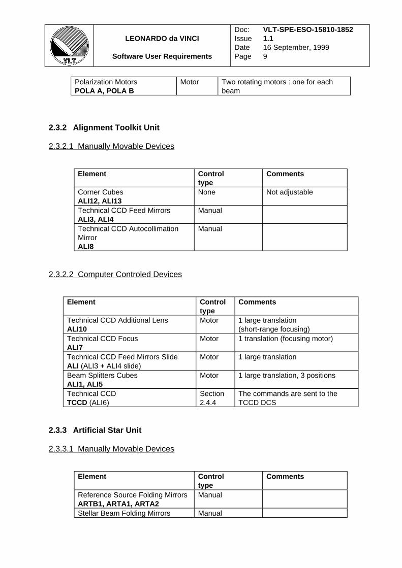
2.3.2 Alignment Toolkit Unit
2.3.2.1 Manually Movable Devices
Element Controltype
Comments
Corner CubesALI12, ALI13
None Not adjustable
Technical CCD Feed MirrorsALI3, ALI4
Manual
Technical CCD AutocollimationMirrorALI8
Manual
2.3.2.2 Computer Controled Devices
Element Controltype
Comments
Technical CCD Additional LensALI10
Motor 1 large translation(short-range focusing)
Technical CCD FocusALI7
Motor 1 translation (focusing motor)
Technical CCD Feed Mirrors SlideALI (ALI3 + ALI4 slide)
Motor 1 large translation
Beam Splitters CubesALI1, ALI5
Motor 1 large translation, 3 positions
Technical CCDTCCD (ALI6)
Section2.4.4
The commands are sent to theTCCD DCS
2.3.3 Artificial Star Unit
2.3.3.1 Manually Movable Devices
Element Controltype
Comments
Reference Source Folding MirrorsARTB1, ARTA1, ARTA2
Manual
Stellar Beam Folding Mirrors Manual

LEONARDO da VINCI
Software User Requirements
Doc:IssueDatePage
VLT-SPE-ESO-15810-18521.116 September, 199910
ARTB2, ARTA3Artificial Star Injection On-axisParabolaART1
Manual/LocalMotor
Adjustment normallynot necessary
Artificial Star Injection Flat MirrorART2
Manual/LocalMotor
adjustment normallynot necessary
Reference Source Glass CubeART4
Manual Transmissive at 2.2and 10 microns
2.3.3.2 Computer Controled Devices
Element Controltype
Comments
Artificial Star Light SourceART3
On/Off Light switches, K Laser
Reference Source Beam SplittersBSA, BSB
Motor 1 large translation, 3 positions
2.3.4 Infrared Camera Unit
Element Controltype
Comments
Main Infrared CameraLISA / OUT3
SeeSection 2.9
The commands are sent to theLISA DCS
2.4 MOVABLE HARDWARE DESCRIPTION
The following sections give the list of the commands related to the opto-mechanical elements[Req. 56] , the TCCD and the LISA camera of LdV. For every Element, the current status, as wellas the last setup value should be accessible to the user through the GUI (in online modes) or theGEI (in engineering mode) [Req. 1] .
In general, any failure when performing setup actions should be reported to the user immediately,through the GUI or GEI [Req. 2] .
2.4.1 BSA, BSB
These beam splitter cubes are movable in and out of the light beams, in order to clear the stellarlight paths of any obstruction during the interferometric observations. The cubes have to be movedin translation to insert or remove them from the beams. Three positions are available :- Beamsplitter cube sending the light directly to the instruments (BSA1, BSB1) for autotest
mode.

LEONARDO da VINCI
Software User Requirements
Doc:IssueDatePage
VLT-SPE-ESO-15810-18521.116 September, 199911
- Beamsplitter cube sending the light to the telescopes (BSA2, BSB2) for autocollimation mode.- Without any optical element in the beam (OUT), for stellar interferometer mode.
The BSA and BSB slides shall be positioned always in the same direction [Req. 3] , in order toavoid any backlash in the mechanical motion.
Element Range/Values
BSA BSA1, BSA2, OUT
BSB BSB1, BSB2, OUT
2.4.2 ALI1, ALI5
ALI1 and ALI5 are beam splitter cubes used to redirect the stellar beams to the technical CCDassembly. The cubes have to be moved in translation to insert or remove them from the beams.Three positions are available:- Beamsplitter cube directing the light to the Technical CCD assembly (ALI1, ALI5), for
alignment purposes.- Shutter blocking the light from the telescopes (ALI1S, ALI5S). In the current definition, the
shutter positions will be used in engineering mode only.- Without any optical element in the beam (OUT), for stellar interferometer mode.
The ALI1 and ALI5 slides shall be positioned always in the same direction [Req. 4] , in order toavoid any backlash in the mechanical motion.
Element Range/Values
ALI1 ALI1, ALI1S, OUT
ALI5 ALI5, ALI5S, OUT
2.4.3 ALI Slide
The two mirrors ALI3 and ALI4 are on the same moving slide. They are used to redirect either theA or the B beam to the technical CCD assembly, after the ALI1 and ALI5 cubes. An intermediateposition allows to see the output of MONA after reflection on ALI9 (mirror movable by hand). TheALI slide has to be moved in translation to insert ALI3, ALI4 or no mirror in the beam.
The ALI slide shall be positioned always in the same direction [Req. 5] , in order to avoid anybacklash in the mechanical motion.
LEONARDO da VINCI
Software User Requirements
Doc:IssueDatePage
VLT-SPE-ESO-15810-18521.116 September, 199912
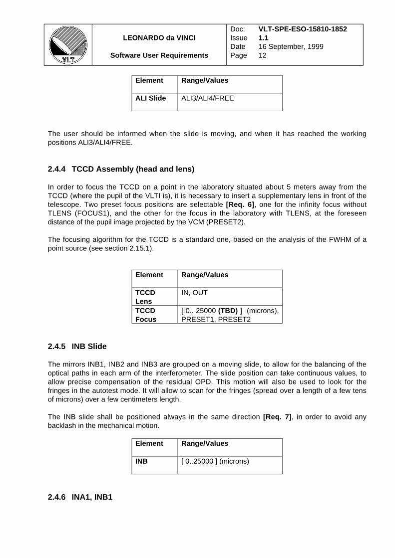
Element Range/Values
ALI Slide ALI3/ALI4/FREE
The user should be informed when the slide is moving, and when it has reached the workingpositions ALI3/ALI4/FREE.
2.4.4 TCCD Assembly (head and lens)
In order to focus the TCCD on a point in the laboratory situated about 5 meters away from theTCCD (where the pupil of the VLTI is), it is necessary to insert a supplementary lens in front of thetelescope. Two preset focus positions are selectable [Req. 6] , one for the infinity focus withoutTLENS (FOCUS1), and the other for the focus in the laboratory with TLENS, at the foreseendistance of the pupil image projected by the VCM (PRESET2).
The focusing algorithm for the TCCD is a standard one, based on the analysis of the FWHM of apoint source (see section 2.15.1).
Element Range/Values
TCCDLens
IN, OUT
TCCDFocus
[ 0.. 25000 (TBD) ] (microns),PRESET1, PRESET2
2.4.5 INB Slide
The mirrors INB1, INB2 and INB3 are grouped on a moving slide, to allow for the balancing of theoptical paths in each arm of the interferometer. The slide position can take continuous values, toallow precise compensation of the residual OPD. This motion will also be used to look for thefringes in the autotest mode. It will allow to scan for the fringes (spread over a length of a few tensof microns) over a few centimeters length.
The INB slide shall be positioned always in the same direction [Req. 7] , in order to avoid anybacklash in the mechanical motion.
Element Range/Values
INB [ 0..25000 ] (microns)
2.4.6 INA1, INB1
LEONARDO da VINCI
Software User Requirements
Doc:IssueDatePage
VLT-SPE-ESO-15810-18521.116 September, 199913
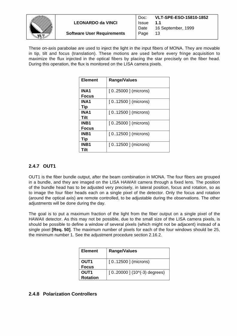
These on-axis parabolae are used to inject the light in the input fibers of MONA. They are movablein tip, tilt and focus (translation). These motions are used before every fringe acquisition tomaximize the flux injected in the optical fibers by placing the star precisely on the fiber head.During this operation, the flux is monitored on the LISA camera pixels.
Element Range/Values
INA1Focus
[ 0..25000 ] (microns)
INA1Tip
[ 0..12500 ] (microns)
INA1Tilt
[ 0..12500 ] (microns)
INB1Focus
[ 0..25000 ] (microns)
INB1Tip
[ 0..12500 ] (microns)
INB1Tilt
[ 0..12500 ] (microns)
2.4.7 OUT1
OUT1 is the fiber bundle output, after the beam combination in MONA. The four fibers are groupedin a bundle, and they are imaged on the LISA HAWAII camera through a fixed lens. The positionof the bundle head has to be adjusted very precisely, in lateral position, focus and rotation, so asto image the four fiber heads each on a single pixel of the detector. Only the focus and rotation(around the optical axis) are remote controlled, to be adjustable during the observations. The otheradjustments will be done during the day.
The goal is to put a maximum fraction of the light from the fiber output on a single pixel of theHAWAII detector. As this may not be possible, due to the small size of the LISA camera pixels, isshould be possible to define a window of several pixels (which might not be adjacent) instead of asingle pixel [Req. 50] . The maximum number of pixels for each of the four windows should be 25,the minimum number 1. See the adjustment procedure section 2.16.2.
Element Range/Values
OUT1Focus
[ 0..12500 ] (microns)
OUT1Rotation
[ 0..20000 ] (10^(-3) degrees)
2.4.8 Polarization Controllers

LEONARDO da VINCI
Software User Requirements
Doc:IssueDatePage
VLT-SPE-ESO-15810-18521.116 September, 199914
In order to compensate for differential polarization states between the two beams, the MONA boxincludes rotative polarization controlers, one for each beam. They are rotated by two motors,whose range has to be defined (about 1 turn).
Element Range/Values
POLA A [ 0..360 (TBD) ] (degrees)
POLA B [ 0..360 (TBD) ] (degrees)
2.4.9 LISA Filter Wheel
The LISA filter wheel carries four different filters for operation at different wavelengths (K band, K'band, H band, 2.3 microns narrow band) a free position (open) and an obstructed position(closed). The filters, and the associated software names, may change during the life of theinstrument. The filter names are fixed arbitrarily for the moment, but should eventually comply withthe ESO filter naming system.
Element Range/Values
FILT K, KPRIME, H, NARROW,OPEN, CLOSED
2.4.10 Piezo Mirror INA3
This is a flat mirror mounted on a piezo stack, which is moved quickly back and forth (0.1-20 Hz) inorder to modulate the optical path difference between the two beams. This is done to scan thefringes, while they are recorder by the LISA infrared detector. The synchronization of the motion ofINA3 with the LISA detector is a critical real-time process, which is described in the section 2.9.
2.5 SUMMARY OF LDV MOVABLE HARDWARE POSITIONS
Unit Element Range/Values
ARTU BSA BSA1, BSA2, OUT
ARTU BSB BSB1, BSB2, OUT
ARTU ART3 ON/OFF (See section 2.8.6)

LEONARDO da VINCI
Software User Requirements
Doc:IssueDatePage
VLT-SPE-ESO-15810-18521.116 September, 199915
ALIU ALI1 ALI1, ALI1S, OUT
ALIU ALI5 ALI5, ALI5S, OUT
ALIU ALI Slide ALI3/ALI4/FREE
ALIU TCCDLens
IN, OUT
ALIU TCCDFocus
[ 0.. 25000 (TBC) ] (microns),PRESET1, PRESET2
COMU INB [ 0..25000 ] (microns)
COMU INA1Focus
[ 0..25000 ] (microns)
COMU INA1Tip
[ 0..12500 ] (microns)
COMU INA1Tilt
[ 0..12500 ] (microns)
COMU INB1Focus
[ 0..25000 ] (microns)
COMU INB1Tip
[ 0..12500 ] (microns)
COMU INB1Tilt
[ 0..12500 ] (microns)
COMU OUT1Focus
[ 0..12500 ] (microns)
COMU OUT1Tip
[ 0..12500 ] (microns)
COMU OUT1Tilt
[ 0..12500 ] (microns)
COMU OUT1Rotation
[ 0..20000 ] (10^(-3) degrees)
COMU INA3 See section 2.9
COMU POLA A [ 0..360 (TBD) ] (degrees)
COMU POLA B [ 0..360 (TBD) ] (degrees)
COMU FILT K, KPRIME, H, NARROW,OPEN, CLOSED
2.6 INSTRUMENT STATES
From the user point of view, the instrument shall be in one of the four states specified in thisparagraph [Req. 57] .

LEONARDO da VINCI
Software User Requirements
Doc:IssueDatePage
VLT-SPE-ESO-15810-18521.116 September, 199916
Number Name Power Moving Functions Reference
Sources
LISA,
TCCD
Status
logging
1 Off Off Motors and encoders off Off Off Off
2 Loaded On Motors and encoders off Off On Active
3 Standby On Motors and encoders on Off On Active
4 Online On Some motors off after
reaching position,
encoders on
Any On Active
Transition possibilities between instrument states:1 → 22 → 1,33 → all4 → all
Power up/down (from/to state 1 or 2) of the whole instrument, including CCD, will be donemanually. Transitions between conditions 2 - 4 will be performed under SW control.
When LdV is set to state 'Online', the motors whose positions are monitored by differentialencoders are initialized by sending them to their references.
The instrument has achieved the 'Loaded' state only when all the real motor positions areavailable to the ICS (either read from absolute encoders, or set to the reference). The switchingfrom 'Loaded' to 'Online' can then be done. No particular starting position is required by theinstrument design in the 'Online' mode. The user has the possibility to choose any setup once theinstrument is 'Online'. A default starting setup for the 'Online' state could be chosen (a goodstarting point could be the 'Stellar Interferometer Idle' setup), but this is not mandatory.
Power up following a power failure may leave the instrument in a hazardous condition so there area number of hardware interlocks for protection of the LISA camera. The motion of the motors andother mechanical systems should be stopped after a power failure.
The commands issued to the ICS and DCS and the corresponding replies from the ICS are loggedwhen the instrument power is on [Req. 60] .
The mechanical design of the functions is such that the positions will be kept due to friction. Toreduce dissipation of motors, the mechanical devices will be positioned and then the motorsswitched off. The only remaining dissipation is that of the encoders. They will be left on if theposition of the related moving device has to be known to a high precision and if it is moved duringthe observations. Which encoders will have to be left on has to be checked.
In the OFF, LOADED and STANDBY states, LdV is not directly operational. The BSA and BSBcubes of LEONARDO are placed in positions OUT, where they do not block the light beams, asthe other instruments may need to access them. The optical elements on the VINCI table do notrequire particular positioning, and should be left in the last on-line state setup used.
LEONARDO da VINCI
Software User Requirements
Doc:IssueDatePage
VLT-SPE-ESO-15810-18521.116 September, 199917
2.7 LDV ENGINEERING AND MAINTENANCE MODES
The need for these modes is only to have direct access to all the hardware parameters of theinstrument. The normal state for LdV during Engineering and Maintenance operation is "Online".
In the Engineering mode, the user can access and monitor individually the hardware devices(motors, TCCD,…) through the part of the GUI related directly to the ICS and DCS [Req. 61] . It isthen possible to adjust all the hardware parameters individually (encoders ranges, motor speeds,voltages,…).
2.8 LDV INSTRUMENT MODES
Here are described the different modes and the associated hardware setups while LdV is in OnlineState. Setups are assumed to be particular settings of the movable devices of LdV associated withan instrumental mode. The LdV setups allow the user to move the many LdV optical andmechanical elements at the same time as a whole, by entering the corresponding request.
Generally speaking, there is no critical time constraint on the motion of the LdV hardware devices(except for the piezo mirror, see section 2.9.4). No particular hardware incompatibilities areforeseen on the VINCI table.
The software system should then aim at moving the devices as quickly as possible [Req. 52] (goal5 seconds, minimum 15 seconds), in parallel, in order to spare observing time. But there is nocritical time limit driven by the conception of the instrument.
The following tables give the setups for each LdV mode.
The setups are named by their function, for example “Autotest Injection Adjust” designates thehardware setup used to make the adjustment of the light injection in the fiber heads, in theautotest mode. The “Idle” setup, which is found in all the instrument modes, is used forengineering purposes or during observations for special needs. It is the default starting setup if nosetup is specified by the user when switching to a mode/setup, including the engineering andmaintenance modes [Req. 54] . In the “Idle” setup, the instrument in online and ready to switch toanother setup in the same mode or in another mode.
“IN” = in the optical beam, “OUT” = off the optical beam, N.A. = not applicable, ADJ = adjustable.
2.8.1 Autotest
In this mode, LdV can observe fringes without any other VLTI system involved. The LEONARDOartificial star is used to produce the light which is sent directly to the VINCI table.

LEONARDO da VINCI
Software User Requirements
Doc:IssueDatePage
VLT-SPE-ESO-15810-18521.116 September, 199918
Unit Element Autotest
Idle
Autotest
Output Adjust
Autotest
InjectionAdjust
Autotest
FringeSearch
Autotest
DataAcquisition
COMU INB SLIDE
MOTOR
OFF OFF OFF ADJ
(steps)
OFF
COMU INB1 MOTORS(TIP/TILT/FOCUS)
OFF OFF ADJ OFF OFF
COMU INA1 MOTORS
(TIP/TILT/FOCUS)
OFF OFF ADJ OFF OFF
COMU INA3 FAST SCAN
PIEZO
OFF OFF OFF ON ON
COMU OUT1 MOTORS(TIP/TILT/FOCUS/
ROTATION)
OFF ADJ OFF OFF OFF
COMU POLA A, POLA BMOTORS
OFF OFF OFF OFF OFF
COMU LISA Filter Wheel N.A. OPEN OPEN ADJ ADJ
ALIU ALI1 POSITION OUT OUT OUT OUT OUT
ALIU ALI5 POSITION OUT OUT OUT OUT OUT
ALIU ALI SLIDE
POSITION
N.A. N.A. N.A. N.A. N.A.
ALIU TCCDLENS POSITION
N.A. N.A. N.A. N.A. N.A.
ALIU TCCD FOCUS N.A. N.A. N.A. N.A. N.A.
ARTU BSA POSITION BSA1 BSA1 BSA1 BSA1 BSA1
ARTU BSB POSITION BSB1 BSB1 BSB1 BSB1 BSB1
ARTU LEONARDO light
source
ON ON ON ON ON
LISA LISA Acquisition OFF FULLFRAME
4 PIX,NOT
SYNC
4 PIX,SYNC
4 PIX,SYNC
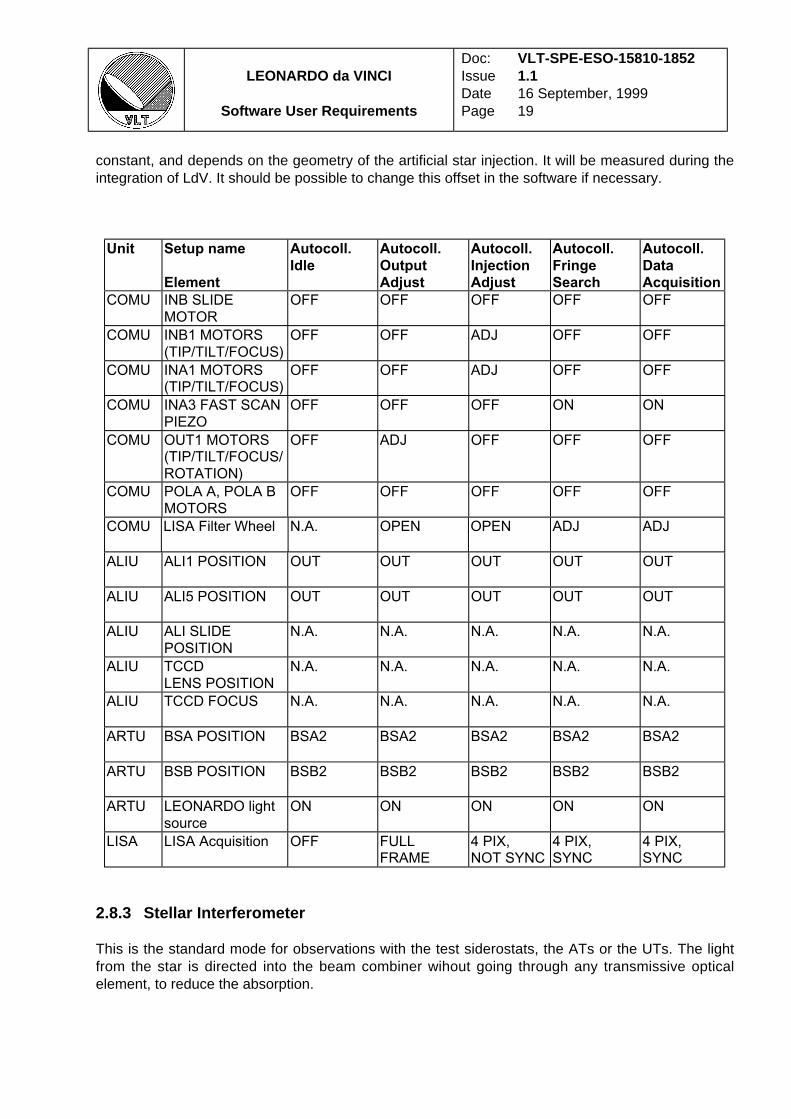
2.8.2 Autocollimation
This mode give the capability to send light in the whole VLTI optical system up to the telescopes.This light is then retroreflected to VINCI and fringes are measured. This requires to inject light fromLEONARDO, using the BSA2 and BSB2 beamsplitter cubes positions. This mode will be availableon-line, without requiring any manual operation in the laboratory. No external access (from theother instruments) is foreseen.
The switching to the autocollimation mode requires to send an OPD offset value to the delay line[Req. 8] , compared to the Stellar Interferometer or Autotest modes. The value of this offset is
LEONARDO da VINCI
Software User Requirements
Doc:IssueDatePage
VLT-SPE-ESO-15810-18521.116 September, 199919
constant, and depends on the geometry of the artificial star injection. It will be measured during theintegration of LdV. It should be possible to change this offset in the software if necessary.
Unit Setup name
Element
Autocoll.
Idle
Autocoll.
Output
Adjust
Autocoll.
Injection
Adjust
Autocoll.
Fringe
Search
Autocoll.
Data
Acquisition
COMU INB SLIDE
MOTOR
OFF OFF OFF OFF OFF
COMU INB1 MOTORS
(TIP/TILT/FOCUS)
OFF OFF ADJ OFF OFF
COMU INA1 MOTORS(TIP/TILT/FOCUS)
OFF OFF ADJ OFF OFF
COMU INA3 FAST SCAN
PIEZO
OFF OFF OFF ON ON
COMU OUT1 MOTORS(TIP/TILT/FOCUS/
ROTATION)
OFF ADJ OFF OFF OFF
COMU POLA A, POLA B
MOTORS
OFF OFF OFF OFF OFF
COMU LISA Filter Wheel N.A. OPEN OPEN ADJ ADJ
ALIU ALI1 POSITION OUT OUT OUT OUT OUT
ALIU ALI5 POSITION OUT OUT OUT OUT OUT
ALIU ALI SLIDE
POSITION
N.A. N.A. N.A. N.A. N.A.
ALIU TCCD
LENS POSITION
N.A. N.A. N.A. N.A. N.A.
ALIU TCCD FOCUS N.A. N.A. N.A. N.A. N.A.
ARTU BSA POSITION BSA2 BSA2 BSA2 BSA2 BSA2
ARTU BSB POSITION BSB2 BSB2 BSB2 BSB2 BSB2
ARTU LEONARDO light
source
ON ON ON ON ON
LISA LISA Acquisition OFF FULLFRAME
4 PIX,NOT SYNC
4 PIX,SYNC
4 PIX,SYNC
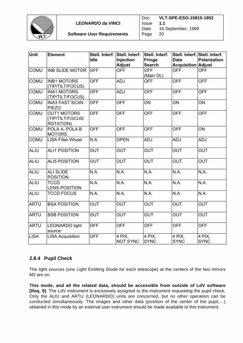
2.8.3 Stellar Interferometer
This is the standard mode for observations with the test siderostats, the ATs or the UTs. The lightfrom the star is directed into the beam combiner wihout going through any transmissive opticalelement, to reduce the absorption.
LEONARDO da VINCI
Software User Requirements
Doc:IssueDatePage
VLT-SPE-ESO-15810-18521.116 September, 199920
Unit Element Stell. Interf.
Idle
Stell. Interf.
InjectionAdjust
Stell. Interf.
FringeSearch
Stell. Interf.
DataAcquisition
Stell. Interf.
PolarizationAdjust
COMU INB SLIDE MOTOR OFF OFF OFF
(Main DL)
OFF OFF
COMU INB1 MOTORS(TIP/TILT/FOCUS)
OFF ADJ OFF OFF OFF
COMU INA1 MOTORS
(TIP/TILT/FOCUS)
OFF ADJ OFF OFF OFF
COMU INA3 FAST SCAN
PIEZO
OFF OFF ON ON ON
COMU OUT1 MOTORS(TIP/TILT/FOCUS/
ROTATION)
OFF OFF OFF OFF OFF
COMU POLA A, POLA BMOTORS
OFF OFF OFF OFF ON
COMU LISA Filter Wheel N.A. OPEN ADJ ADJ ADJ
ALIU ALI1 POSITION OUT OUT OUT OUT OUT
ALIU ALI5 POSITION OUT OUT OUT OUT OUT
ALIU ALI SLIDE
POSITION
N.A. N.A. N.A. N.A. N.A.
ALIU TCCDLENS POSITION
N.A. N.A. N.A. N.A. N.A.
ALIU TCCD FOCUS N.A. N.A. N.A. N.A. N.A.
ARTU BSA POSITION OUT OUT OUT OUT OUT
ARTU BSB POSITION OUT OUT OUT OUT OUT
ARTU LEONARDO light
source
OFF OFF OFF OFF OFF
LISA LISA Acquisition OFF 4 PIX,NOT SYNC
4 PIX,SYNC
4 PIX,SYNC
4 PIX,SYNC
2.8.4 Pupil Check
The light sources (one Light Emitting Diode for each telescope) at the centers of the two mirrorsM2 are on.
This mode, and all the related data, should be accessible from outside of LdV software[Req. 9] . The LdV instrument is exclusively assigned to the instrument requesting the pupil check.Only the ALIU and ARTU (LEONARDO) units are concerned, but no other operation can beconducted simultaneously. The images and other data (position of the center of the pupil,…)obtained in this mode by an external user instrument should be made available to this instrument.

LEONARDO da VINCI
Software User Requirements
Doc:IssueDatePage
VLT-SPE-ESO-15810-18521.116 September, 199921
No real-time constraint is foreseen in this mode.
The pupil check is done by imaging the pupil of the two telescopes on the TCCD. During normaloperation, the pupil is situated on the VINCI table, on the parabolae INA1 and INB1. After thisimage has been saved, the image of the artificial star provided by LEONARDO (star image atinfinity) is obtained. By comparing the positions of the pupil and artifial star, the user can evaluatethe quality of the pupil alignment.
The LdV TCCD will be used in this mode during the alignment of the pupil of the VLTI, but thecontrol of the mirrors of the optical train is not part of LdV SW, but of VLTI software. It will onlyprovide the coordinates of the pupil and artificial source images to the VLTI alignment software,which will adjust the relevant mirrors. The corresponding interface is TBD.
The TCCD can image the pupil from 1 meter to infinity. It is necessary to insert an additional lens(TLENS achromat lens, focal length = 2000 mm) in front of the TCCD in order to focus to pupildistances (to the TCCD refractor lens center) of less than 3900 mm. The focal length of the TCCDrefractor is 300 mm. The pupil longitudinal positioning question is adressed in the document [2]section 4.2.4. The detailed description of the optical design for pupil check can be found in thedocument [3], p 14.
The size of the pupil image on the TCCD will be 6 mm for INA (magnification 0.3) and 8 mm forINB (magnification 0.4), when it is at its nominal position on the on-axis parabolae INA1 (distancefrom the autocollimator = 2000 mm) and INB1 (distance from the collimator = 1500 mm).
Pupil position Additional lens position1320 mm to 3900 mm Inserted
3900 mm to infinity Removed
Two preset focus positions are selectable [Req. 6] , one for the infinity focus without TLENS(PRESET1) (this is used in the PupilCheck.ArtificialStar* setups) and the other for the focus in thelaboratory with TLENS, at the foreseen distance of the pupil image projected by the VCM(PRESET2).
After the rough focus has been achieved, the fine focus procedure can be done if necessary.
Unit Element Pupil CheckIdle
Pupil CheckTelescope A
Pupil CheckTelescope B
PupilCheck
Artificial
Star A
PupilCheck
Artificial
Star B
COMU INB SLIDEMOTOR
N.A. N.A. N.A. N.A. N.A.
COMU INB1 MOTORS
(TIP/TILT/FOCUS)
N.A. N.A. N.A. N.A. N.A.
LEONARDO da VINCI
Software User Requirements
Doc:IssueDatePage
VLT-SPE-ESO-15810-18521.116 September, 199922
COMU INA1 MOTORS
(TIP/TILT/FOCUS)
N.A. N.A. N.A. N.A. N.A.
COMU INA3 FAST SCANPIEZO
N.A. N.A. N.A. N.A. N.A.
COMU OUT1 MOTORS
(TIP/TILT/FOCUS/
ROTATION)
N.A. N.A. N.A. N.A. N.A.
COMU POLA A, POLA B
MOTORS
N.A. N.A. N.A. N.A. N.A.
ALIU ALI1 POSITION IN IN IN IN IN
ALIU ALI5 POSITION IN IN IN IN IN
ALIU ALI SLIDE
POSITION
NOMIRROR ALI3 ALI4 ALI3 ALI4
ALIU TCCDLENS POSITION
OUT IN IN OUT OUT
ALIU TCCD FOCUS N.A. ADJ
PRESET2
ADJ
PRESET2
ADJ
PRESET1
ADJ
PRESET1
ARTU BSA POSITION OUT OUT OUT IN IN
ARTU BSB POSITION OUT OUT OUT IN IN
ARTU LEONARDO light
source
N.A. N.A. N.A. ON ON
ARTU LISA Filter Wheel N.A. N.A. N.A. N.A. N.A.
LISA LISA Acquisition N.A. N.A. N.A. N.A. N.A.
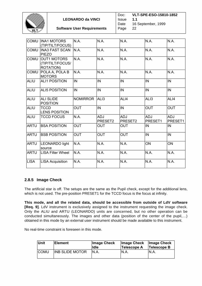
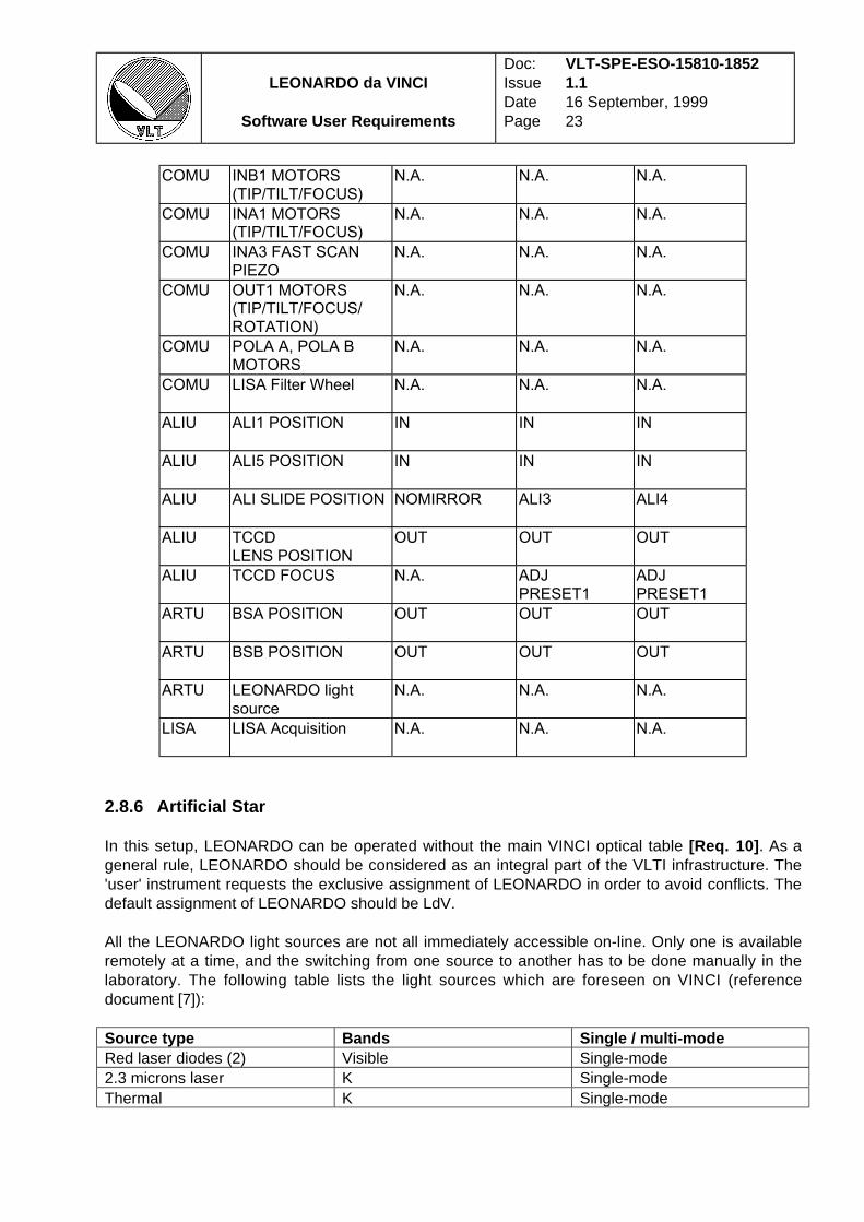
2.8.5 Image Check
The artificial star is off. The setups are the same as the Pupil check, except for the additional lens,which is not used. The pre-position PRESET1 for the TCCD focus is the focus at infinity.
This mode, and all the related data, should be accessible from outside of LdV software[Req. 9] . LdV instrument is exclusively assigned to the instrument requesting the image check.Only the ALIU and ARTU (LEONARDO) units are concerned, but no other operation can beconducted simultaneously. The images and other data (position of the center of the pupil,…)obtained in this mode by an external user instrument should be made available to this instrument.
No real-time constraint is foreseen in this mode.
Unit Element Image Check
Idle
Image Check
Telescope A
Image Check
Telescope B
COMU INB SLIDE MOTOR N.A. N.A. N.A.
LEONARDO da VINCI
Software User Requirements
Doc:IssueDatePage
VLT-SPE-ESO-15810-18521.116 September, 199923
COMU INB1 MOTORS
(TIP/TILT/FOCUS)
N.A. N.A. N.A.
COMU INA1 MOTORS(TIP/TILT/FOCUS)
N.A. N.A. N.A.
COMU INA3 FAST SCAN
PIEZO
N.A. N.A. N.A.
COMU OUT1 MOTORS(TIP/TILT/FOCUS/
ROTATION)
N.A. N.A. N.A.
COMU POLA A, POLA B
MOTORS
N.A. N.A. N.A.
COMU LISA Filter Wheel N.A. N.A. N.A.
ALIU ALI1 POSITION IN IN IN
ALIU ALI5 POSITION IN IN IN
ALIU ALI SLIDE POSITION NOMIRROR ALI3 ALI4
ALIU TCCD
LENS POSITION
OUT OUT OUT
ALIU TCCD FOCUS N.A. ADJ
PRESET1
ADJ
PRESET1
ARTU BSA POSITION OUT OUT OUT
ARTU BSB POSITION OUT OUT OUT
ARTU LEONARDO light
source
N.A. N.A. N.A.
LISA LISA Acquisition N.A. N.A. N.A.
2.8.6 Artificial Star
In this setup, LEONARDO can be operated without the main VINCI optical table [Req. 10] . As ageneral rule, LEONARDO should be considered as an integral part of the VLTI infrastructure. The'user' instrument requests the exclusive assignment of LEONARDO in order to avoid conflicts. Thedefault assignment of LEONARDO should be LdV.
All the LEONARDO light sources are not all immediately accessible on-line. Only one is availableremotely at a time, and the switching from one source to another has to be done manually in thelaboratory. The following table lists the light sources which are foreseen on VINCI (referencedocument [7]):
Source type Bands Single / multi-modeRed laser diodes (2) Visible Single-mode2.3 microns laser K Single-modeThermal K Single-mode

LEONARDO da VINCI
Software User Requirements
Doc:IssueDatePage
VLT-SPE-ESO-15810-18521.116 September, 199924
Thermal K Multi-modeThermal N Single-modeThermal N Multi-modeThermal Visible Multi-mode
This mode will be used mainly after the commissioning phase, when the science instrumentsAMBER and MIDI are operational. The electronic racks of LdV will be on, as well as the WS sw,thus allowing normal operation of the motors and light switches of LEONARDO. The light sourcecan be turned ON without being injected in the optical beams in order to pre-heat it. It can also beturned OFF with the cubes IN to check for the effect of the cubes on the optical transmission. Thismode, and all the related data, should be accessible from outside of LdV software [Req. 11] .
There is no remote intensity adjustment foreseen for any of the sources on LEONARDO.
The external instruments should access LEONARDO only through the predefined modes(described in the following table) [Req. 12] . No low-level command is foreseen to be accessiblefrom outside of LdV software.
Unit Element ArtificialStarOffRemoved
ArtificialStarOnInserted
ArtificialStarOnRemoved
ArtificialStarOffInserted
AutocollimationOnInserted
ARTU BSA OUT BSA1 OUT BSA1 BSA2
ARTU BSB OUT BSB1 OUT BSB1 BSB2
ARTU LEONARDO
Light source
OFF ON ON OFF ON
2.9 DATA ACQUISITION ASPECTS OF LDV
2.9.1 Description
The piezo mirror INA3 is used to quickly modulate the optical path difference between the twobeams, in order to scan over the fringes. The frequency of its motion is adjustable from 0.1 Hz to20 Hz [Req. 13] . The most common frequency which will be used is 10 Hz. The scan length isalso adjustable, from 1 micron to 360 microns [Req. 14] . The wave used to control the piezo has a“smooth triangle” shape, which is intermediate between a triangle and a sinusoid. Thecorresponding factor for the softening ratio is the wave shape factor, whose range will be between0 (triangle) and 1 (sinusoid) [Req. 15] . The generation of this curve is made at the LCU level,based on the defined parameters.
LEONARDO da VINCI
Software User Requirements
Doc:IssueDatePage
VLT-SPE-ESO-15810-18521.116 September, 199925
The most important difficulty for the piezo is that it has to be precisely synchronized with the LISAacquisition during the scanning of the fringes, at a submillisecond precision (goal 0.5 ms, minimum1 ms) [Req. 16] . The synchronization does not have to be done at the frame level, but only at thebeginning of the scan. This scheme assumes that the internal clockings of the two LCUs (piezoLCU and LISA WS) are accurate enough to guarantee no significant deterioration of thesynchronization during the scan duration.
2.9.2 Terminology and typical values
There are four fiber outputs in LdV, named I1, I2, P1, P2. The four fibers are arranged (through afiber bundle) in a square which forms the optical output imaged on the LISA focal plane array.Ideally, each fiber core is imaged onto a single pixel. In case the light cannot be put on a singlepixel, it will have to be collected in a window of 1 to 25 pixels [Req. 50] (that might not beadjacent). The LISA DCS reads out only those pixels located in the four windows. It then returnsfour numbers which correspond to the total energy output of I1, I2, P1 and P2 respectively. Thisoperation (readout and sommation) is called a "frame". Frame rates range between a few Hz anda few kHz, a typical value is 1500 Hz.
A "scan " is a collection of frames. While observing the astronomical source, they are obtainedwhile the optical path difference (OPD) is modulated by the fast scan mirror INA3. There are real-time issues related to the acquisition of successive scans, which are detailed below.
A "batch " is the collection of a number of scans (from about a hundred to a thousand), obtained toreduce the stastical noise. During the batches off-source and with only one of the beams, thepiezo mirror could be stopped, as OPD modulation is not relevant, but the data produced is thesame as on-source (four series of numbers : I1, I2, P1, P2).
An "observation " is a collection of four batches:- On-source : the target is centered in the field and fringes are observed. A few thousand
scans are obtained during this phase.- Off-source : the telescopes are offset from the source in order to measure the sky
background signal. The number of scans Off-source is aproximately the same as On-Source (but they are acquired faster as no synchronization is need between the piezomirror and the LISA camera).
- Beam A : the beam B is obstructed (by a shutter or by offsetting the telescope B), and aseries of about a hundred scans are obtained.
- Beam B : the beam A is obstructed (by a shutter or by offsetting the telescope A), and aseries of about a hundred scans are obtained.
The order in which these batches will be acquired is not necessarily the one given here. Anobservation represents 5-10 mm of observing time and its end product is the fundamental VINCIdata unit to be saved in the VLTI archive. No time-critical operation is expected to occur betweentwo successive observations.
The fast scan mirror INA3 is mounted on a piezo device which is controled through a commandvoltage Uc. The following table lists the different scales that relate the command voltage to theOPD generated. The gain factor g takes into account geometric considerations, sign conventions,and the stiffness of the piezo support blades. Its absolute value is typically 1.5 but it has to becalibrated during integration.

LEONARDO da VINCI
Software User Requirements
Doc:IssueDatePage
VLT-SPE-ESO-15810-18521.116 September, 199926
Piezo command voltage Uc -5 V (or 0 V) +5 V (or +10 V)Piezo input voltage Uin 0 1000 VPiezo mechanical extension 0 micron +180 micronsOPD generated 0 micron 180 x g microns
The voltage ramp that generates the scan is of "smooth triangle" type. The OPD modulation rate vis called the OPD velocity, or fringe velocity. The data are collected only when v is stabilized, i.e.during the linear part of the ramp. Fringe velocity range from 0 to 2500 microns/s. For eachobservation, the user requests (via the OS) a given velocity and DAQ OPD (typical values are 660microns/s and 200 microns respectively). Depending on those parameters, the total duration ofdata collection in a scan ∆tDAQ = OPDDAQ/v can range between 0.05 s and several minutes. Weshall adopt 0.1 s as a nominal (and most common) value. The user also choses a "sampleinterval", i.e. the OPD interval between two successive frames. This is translated by the OS into aframe rate. The combination of DAQ OPD length, fringe velocity and frame rate determines thenumber of frames recorded per scan.
After acquisition, a "quick look" analysis is performed by LdV DCS (at the LCU level). Each scan isrearranged in four 1D arrays (synchronous time sequences) that record the intensity evolution ateach of the fiber outputs I1, I2, P1, P2. An algorithm (see section 2.9.6) is performed on the arraysI1 and I2 to determine whether fringes have been observed [Req. 17] and, if yes, what is the timetZOPDobs of the observed location of the center of the fringe packet (corresponding to zero totalOPD). This time is compared to the expected time tZOPDexp of zero OPD occurrence, and thequantity OPDOFFSET=(tZOPDexp - tZOPDobs ) x v is sent to the VLTI delay line OPD controler as an OPDoffset.
For the information of the observer, it would be very interesting to compute a simple estimation ofthe instrumental visibility as a complement to the OPD offset, and to send it to the LdV WSsoftware. The software should display one computed visibility to the user at a frequency of [2 Hz,1 Hz] [Req. 18] .
Under normal observing conditions, the OPD offset should be smaller than 100 microns. Note thatthe quick look analysis requires that also reside in memory :
- A dark scan, or a small series of scans acquired off source- The quick look data reduction parameters
These parameters are updated at the end of each individual observation.
In the current implementation of VINCI it has only one spectral channel (one window for eachsignal I1, I2, P1, P2). With a typical number of frames per scan of 512, we can estimate thequantity of data contained in one scan : if the data from LISA are coded on 16 bits, one typicalscan represents 4 kbytes of data. Only 2 kbytes (256 frames centered on tZOPDexp) per scan aresaved.
In a seond generation upgrade of the instrument, it is foreseen to insert a dispersive element infront of LISA to disperse the four output signals. This will result in an increase of the data quantityproduced at each scan, by a factor which could be up to 50 (see section 2.20.3). The softwaresystem should be able to manage about 100 kbytes per scan [Req. 19] , but the associatedelectronics hardware should not be considered for the first phase of LdV.
LEONARDO da VINCI
Software User Requirements
Doc:IssueDatePage
VLT-SPE-ESO-15810-18521.116 September, 199927
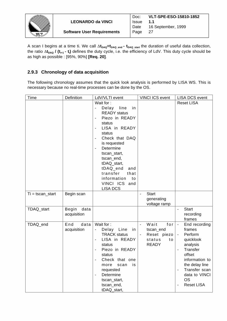
A scan I begins at a time ti. We call ∆tDAQ=tDAQ_end - tDAQ_start the duration of useful data collection,the ratio ∆tDAQ / (t i+1 - ti) defines the duty cycle, i.e. the efficiency of LdV. This duty cycle should beas high as possible : [95%, 90%] [Req. 20] .
2.9.3 Chronology of data acquisition
The following chronology assumes that the quick look analysis is performed by LISA WS. This isnecessary because no real-time processes can be done by the OS.
Time Definition LdV/VLTI event VINCI ICS event LISA DCS eventWait for :- Delay l ine in
READY status- Piezo in READY
status- LISA in READY
status- Check that DAQ
is requested- Determine
tscan_start,tscan_end,tDAQ_start,tDAQ_end andt rans fe r t ha tinformation toVINCI ICS andLISA DCS
Reset LISA
Ti = tscan_start Begin scan - Startgeneratingvoltage ramp
TDAQ_start Begin dataacquisition
- Startrecordingframes
TDAQ_end End da taacquisition
Wait for :- Delay Line in
TRACK status- LISA in READY
status- Piezo in READY
status- Check that one
more scan isrequested
- Determinetscan_start,tscan_end,tDAQ_start,
- W a i t f o rtscan_end
- Reset piezos t a t u s t oREADY
- End recordingframes
- Performquicklookanalysis
- Transferoffsetinformation tothe delay line
- Transfer scandata to VINCIOS
- Reset LISA
LEONARDO da VINCI
Software User Requirements
Doc:IssueDatePage
VLT-SPE-ESO-15810-18521.116 September, 199928
tDAQ_end andt rans fe r t ha tinformation toVINCI ICS andLISA DCS
Tscan_end End of piezomotion
Ti+1 =tscan_start
Begin scan - Startgeneratingvoltage ramp
The time intervals [Tscan_start, tDAQ_start] and [tDAQ_end, Tscan_end] are used to accelerateand decelerate the piezo mirror. These intervals are not compressible, as they are defined by thehysteresis curve of the piezo itself.
2.9.4 Real-time considerations
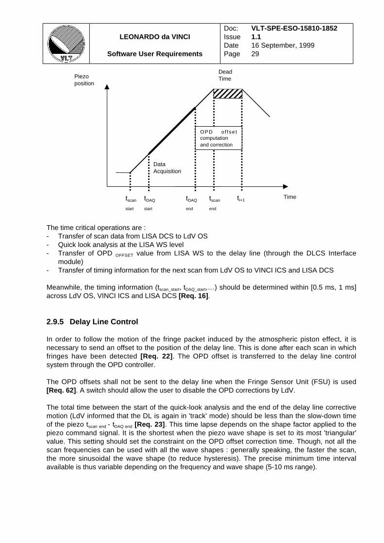
The critical time interval is ti+1 - tscan end, which corresponds to the 'dead time' during which VINCI isnot acquiring data. The software architecture should be designed to, ideally, make it zero or atleast minimal [Req. 21] : this is the time interval (after the end of the scan) during which the piezomirror is stopped to wait for the OPD offset computation and correction to finish. After that, thepiezo goes backwards to start the next scan in the other direction.
This means that the software system should compute the fringe position quickly enough ('quicklook' algorithm), and correct the delay line position, so that it is possible not to waste any time bystopping the piezo at its extremal position (to wait for the computation to end). This puts aconstraint on the computation time tOPD offset which is : tOPD offset < tscan end - tDAQ end. In any case, the'dead time' ti+1 - tscan end should be minimized in order to obtain the maximum efficiency of LdV, butthe delay line has to be in the 'track' status before starting the next data acquisition.
LEONARDO da VINCI
Software User Requirements
Doc:IssueDatePage
VLT-SPE-ESO-15810-18521.116 September, 199929
The time critical operations are :- Transfer of scan data from LISA DCS to LdV OS- Quick look analysis at the LISA WS level- Transfer of OPD OFFSET value from LISA WS to the delay line (through the DLCS Interface
module)- Transfer of timing information for the next scan from LdV OS to VINCI ICS and LISA DCS
Meanwhile, the timing information (tscan_start, tDAQ_start,…) should be determined within [0.5 ms, 1 ms]across LdV OS, VINCI ICS and LISA DCS [Req. 16] .
2.9.5 Delay Line Control
In order to follow the motion of the fringe packet induced by the atmospheric piston effect, it isnecessary to send an offset to the position of the delay line. This is done after each scan in whichfringes have been detected [Req. 22] . The OPD offset is transferred to the delay line controlsystem through the OPD controller.
The OPD offsets shall not be sent to the delay line when the Fringe Sensor Unit (FSU) is used[Req. 62] . A switch should allow the user to disable the OPD corrections by LdV.
The total time between the start of the quick-look analysis and the end of the delay line correctivemotion (LdV informed that the DL is again in 'track' mode) should be less than the slow-down timeof the piezo tscan end - tDAQ end [Req. 23] . This time lapse depends on the shape factor applied to thepiezo command signal. It is the shortest when the piezo wave shape is set to its most 'triangular'value. This setting should set the constraint on the OPD offset correction time. Though, not all thescan frequencies can be used with all the wave shapes : generally speaking, the faster the scan,the more sinusoidal the wave shape (to reduce hysteresis). The precise minimum time intervalavailable is thus variable depending on the frequency and wave shape (5-10 ms range).
DataAcquisition
tscan
start
tscan
end
tDAQ
start
tDAQ
end
ti+1
DeadTime
OPD of fse tcomputationand correction
Time
Piezoposition
LEONARDO da VINCI
Software User Requirements
Doc:IssueDatePage
VLT-SPE-ESO-15810-18521.116 September, 199930
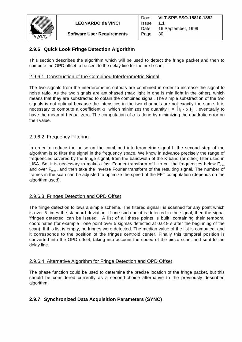
2.9.6 Quick Look Fringe Detection Algorithm
This section describes the algorithm which will be used to detect the fringe packet and then tocompute the OPD offset to be sent to the delay line for the next scan.
2.9.6.1 Construction of the Combined Interferometric Signal
The two signals from the interferometric outputs are combined in order to increase the signal tonoise ratio. As the two signals are antiphased (max light in one is min light in the other), whichmeans that they are substracted to obtain the combined signal. The simple substraction of the twosignals is not optimal because the intensities in the two channels are not exactly the same. It isnecessary to compute a coefficient α which minimizes the quantity I = I1 - α.I2, eventually tohave the mean of I equal zero. The computation of α is done by minimizing the quadratic error onthe I value.
2.9.6.2 Frequency Filtering
In order to reduce the noise on the combined interferometric signal I, the second step of thealgorithm is to filter the signal in the frequency space. We know in advance precisely the range offrequencies covered by the fringe signal, from the bandwidth of the K-band (or other) filter used inLISA. So, it is necessary to make a fast Fourier transform of I, to cut the frequencies below Fmin
and over Fmax, and then take the inverse Fourier transform of the resulting signal. The number offrames in the scan can be adjusted to optimize the speed of the FFT computation (depends on thealgorithm used).
2.9.6.3 Fringes Detection and OPD Offset
The fringe detection follows a simple scheme. The filtered signal I is scanned for any point whichis over 5 times the standard deviation. If one such point is detected in the signal, then the signal'fringes detected' can be issued. A list of all these points is built, containing their temporalcoordinates (for example : one point over 5 sigmas detected at 0.019 s after the beginning of thescan). If this list is empty, no fringes were detected. The median value of the list is computed, andit corresponds to the position of the fringes centroid center. Finally this temporal position isconverted into the OPD offset, taking into account the speed of the piezo scan, and sent to thedelay line.
2.9.6.4 Alternative Algorithm for Fringe Detection and OPD Offset
The phase function could be used to determine the precise location of the fringe packet, but thisshould be considered currently as a second-choice alternative to the previously describedalgorithm.
2.9.7 Synchronized Data Acquisition Parameters (SYNC)
LEONARDO da VINCI
Software User Requirements
Doc:IssueDatePage
VLT-SPE-ESO-15810-18521.116 September, 199931
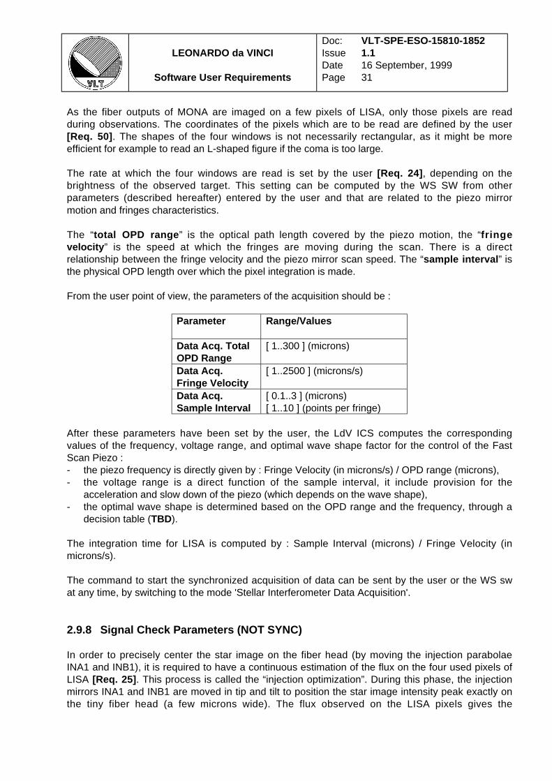
As the fiber outputs of MONA are imaged on a few pixels of LISA, only those pixels are readduring observations. The coordinates of the pixels which are to be read are defined by the user[Req. 50] . The shapes of the four windows is not necessarily rectangular, as it might be moreefficient for example to read an L-shaped figure if the coma is too large.
The rate at which the four windows are read is set by the user [Req. 24] , depending on thebrightness of the observed target. This setting can be computed by the WS SW from otherparameters (described hereafter) entered by the user and that are related to the piezo mirrormotion and fringes characteristics.
The “total OPD range ” is the optical path length covered by the piezo motion, the “fringevelocity ” is the speed at which the fringes are moving during the scan. There is a directrelationship between the fringe velocity and the piezo mirror scan speed. The “sample interval ” isthe physical OPD length over which the pixel integration is made.
From the user point of view, the parameters of the acquisition should be :
Parameter Range/Values
Data Acq. TotalOPD Range
[ 1..300 ] (microns)
Data Acq.Fringe Velocity
[ 1..2500 ] (microns/s)
Data Acq.Sample Interval
[ 0.1..3 ] (microns)[ 1..10 ] (points per fringe)
After these parameters have been set by the user, the LdV ICS computes the correspondingvalues of the frequency, voltage range, and optimal wave shape factor for the control of the FastScan Piezo :- the piezo frequency is directly given by : Fringe Velocity (in microns/s) / OPD range (microns),- the voltage range is a direct function of the sample interval, it include provision for the
acceleration and slow down of the piezo (which depends on the wave shape),- the optimal wave shape is determined based on the OPD range and the frequency, through a
decision table (TBD).
The integration time for LISA is computed by : Sample Interval (microns) / Fringe Velocity (inmicrons/s).
The command to start the synchronized acquisition of data can be sent by the user or the WS swat any time, by switching to the mode 'Stellar Interferometer Data Acquisition'.
2.9.8 Signal Check Parameters (NOT SYNC)
In order to precisely center the star image on the fiber head (by moving the injection parabolaeINA1 and INB1), it is required to have a continuous estimation of the flux on the four used pixels ofLISA [Req. 25] . This process is called the “injection optimization”. During this phase, the injectionmirrors INA1 and INB1 are moved in tip and tilt to position the star image intensity peak exactly onthe tiny fiber head (a few microns wide). The flux observed on the LISA pixels gives the

LEONARDO da VINCI
Software User Requirements
Doc:IssueDatePage
VLT-SPE-ESO-15810-18521.116 September, 199932
information to know if we are getting close to this maximum: if it rises, we are getting closer, if itfalls, we are going the wrong way. Moreover, the atmospheric turbulence causes the flux to varyerratically during this process. Basically, this optimization has to be done before each starobservation, that is every 5 to 10 minutes.
The injection optimization is a hard point for the control software if it is intended to be doneautomatically. The necessity for an operator to do it manually may not be possible to avoid. Apossible algorithm for the automatic injection optimization is described in the section 2.20.1. It isforeseen to achieve the complete automatization of the LdV operations, and this possibility shouldbe left open in the software design.
From the user point of view, the parameters are the same as for the synchronized mode, exceptthat the signals are displayed in a continuous loop. The only difference is that the piezo mirrormight not be moving effectively (if simpler from the SW point of view). Only the computed pixelreadout frequency (also called frame rate) is used effectively as a parameter. The difference withsynchronized mode is that the camera is read continuously, without the need to wait for thesynchronization of the piezo, thus resulting in higher data rate. The parameters used are the sameas for the synchronized mode in order to check that they are good with respect to the flux comingfrom the star (i.e. that the star is not saturating the detector for example).
Parameter Range/Values
Data Acq. TotalOPD Range
[ 1..300 ] (microns)
Data Acq.Fringe Velocity
[ 1..2500 ] (microns/s)
Data Acq.Sample Interval
[ 0.1..3 ] (microns)[ 1..10 ] (points per fringe)
Once the parameters are set, the user or the WS sw can send the starting command for notsynchronized acquisition (for example START NOTSYNC).
The possibility to use the synchronized mode for the injection optimization has to be checked,depending on the gain in terms of software development.
2.9.9 LISA Full Frame Readout (FULL FRAME)
The positions of the fiber outputs on the HAWAII chip have to be very precisely known andadjusted if necessary. The mount on which the fibers are mounted can drift with time ortemperature, and so require a realignment of the outputs on the desired pixels. This is done bytaking a full quadrant image (512x512 pixels x 16 bits) from the LISA chip, and fitting the pixelpositions with centroids. The position of maxima, together with the FWHM of the pixels are theinformations needed to make the necessary adjustements.
In a first implementation, the output optimization will be done manually during daytime, relying onthe stability of the camera and fiber mounts to ensure the correct alignment of the fibers on the
LEONARDO da VINCI
Software User Requirements
Doc:IssueDatePage
VLT-SPE-ESO-15810-18521.116 September, 199933
LISA pixels. The operator actions will be based on the (maximum, FWHM) informations displayedin near real-time by the system, with a computed value of the percentage of light in a single pixel[Req. 26] . The full-frame image should also be available on the display [Req. 27] . Checking of theoutput pixels should be available online during the observations [Req. 28] . Eventually, the outputoptimization could be done before every observation to maximize the effectiveness of theinstrument, but this requires that the output optimization process be automatic.
The output optimization automatization is potentially difficult for the control software. Though, as itis foreseen to eventually achieve the complete automatization of the LdV operations, thispossibility should be left open in the software design.
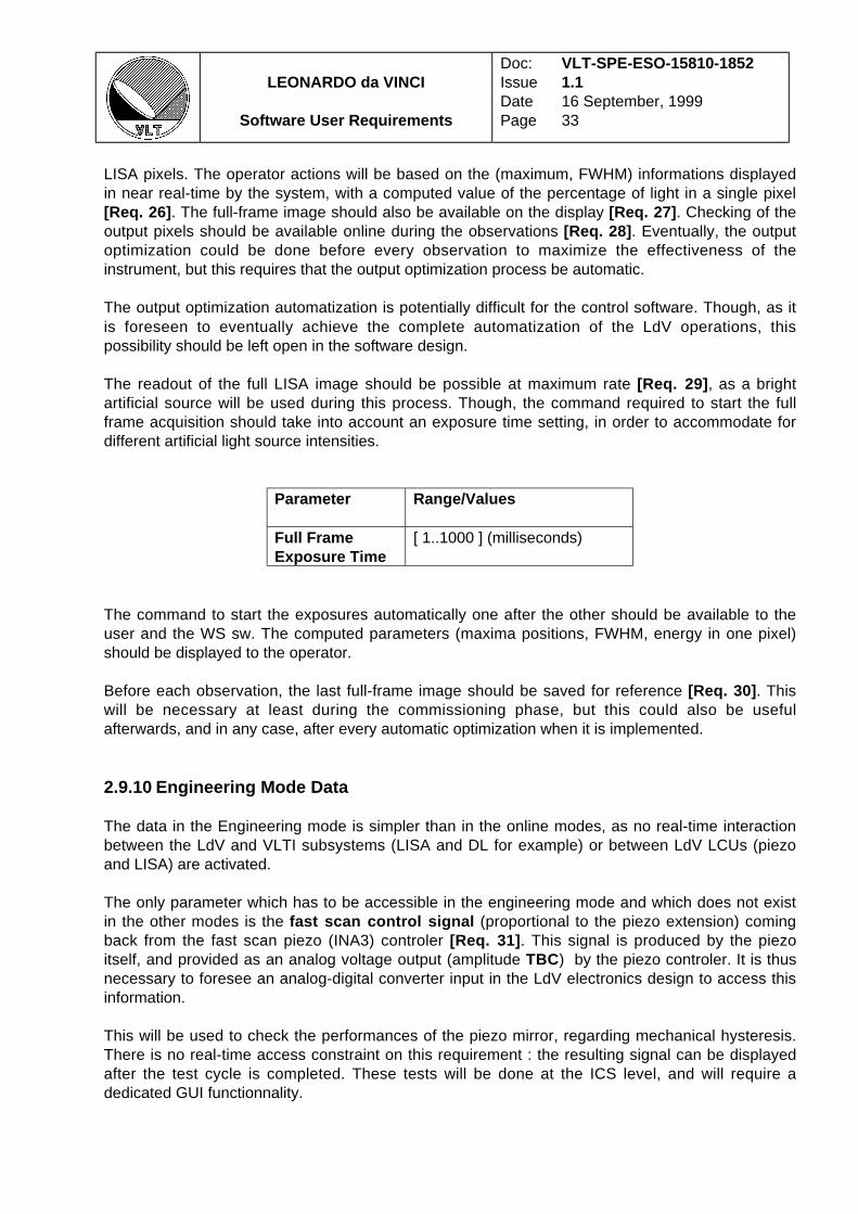
The readout of the full LISA image should be possible at maximum rate [Req. 29] , as a brightartificial source will be used during this process. Though, the command required to start the fullframe acquisition should take into account an exposure time setting, in order to accommodate fordifferent artificial light source intensities.
Parameter Range/Values
Full FrameExposure Time
[ 1..1000 ] (milliseconds)
The command to start the exposures automatically one after the other should be available to theuser and the WS sw. The computed parameters (maxima positions, FWHM, energy in one pixel)should be displayed to the operator.
Before each observation, the last full-frame image should be saved for reference [Req. 30] . Thiswill be necessary at least during the commissioning phase, but this could also be usefulafterwards, and in any case, after every automatic optimization when it is implemented.
2.9.10 Engineering Mode Data
The data in the Engineering mode is simpler than in the online modes, as no real-time interactionbetween the LdV and VLTI subsystems (LISA and DL for example) or between LdV LCUs (piezoand LISA) are activated.
The only parameter which has to be accessible in the engineering mode and which does not existin the other modes is the fast scan control signal (proportional to the piezo extension) comingback from the fast scan piezo (INA3) controler [Req. 31] . This signal is produced by the piezoitself, and provided as an analog voltage output (amplitude TBC) by the piezo controler. It is thusnecessary to foresee an analog-digital converter input in the LdV electronics design to access thisinformation.
This will be used to check the performances of the piezo mirror, regarding mechanical hysteresis.There is no real-time access constraint on this requirement : the resulting signal can be displayedafter the test cycle is completed. These tests will be done at the ICS level, and will require adedicated GUI functionnality.

LEONARDO da VINCI
Software User Requirements
Doc:IssueDatePage
VLT-SPE-ESO-15810-18521.116 September, 199934
2.10 DATA FLOW FROM LDV
The data quantity coming out of LdV is not very large. On a very successful observing night, onecan expect to observe during 8 hours. This means 60 targets observed 10 minutes each plus 2minutes to switch from one target to the other and acquire fringes. Over these 10 minutes of dataacquisition, about 5000 scans are obtained, 4 kbytes each. This gives a total science data quantityover one night of : 60x5000x4 kbyte = 1.2 Gbyte. The technical data, instrument parameters andcalibration data should a few hundred megabytes at most. This gives a maximum data rate ofabout 1.5 Gbyte per night. Most probably, the “real life” data rate will be half of this figure, that is~800 Mbyte [Req. 32] .
It is important to keep in mind that an upgrade of VINCI to dispersed fringes mode will increase thedata flow from VINCI up to 50 times the previous figure (with a dispersion on 50 pixels taken as abasis). The effective data rate could then theoretically be 60 Gb per night (usually ~30 Gb/night).See section 2.20.3 for further details.
2.11 LDV DATA STRUCTURE
The data from LdV will be in two forms : the WS localized data, and the archived data.
2.11.1 Workstation Localized Data
The structure of the data on the LdV dedicated WS depends mainly on the design of the softwareitself, and thus will be defined later more precisely.
2.11.2 Archived Data
The general requirement reference for the archived data is [Req. 59] .
2.11.2.1 Data Hierarchy
The interferometric data can be divided in frame , scan , batch , observation and observationblock , from the most basic information element to the star and calibrator homogeneous data set,which provides the final visibility measurement. These terms are defined page 2.
2.11.2.2 Data Sources
This section gives a list of the data which has to be stored in the final raw data files, sorted bysource. The aproximate frequency (frame, scan, observation) at which this data has to be acquiredis indicated. All these parameters are available from the LdV LCUs or WS, unless otherwiseindicated.
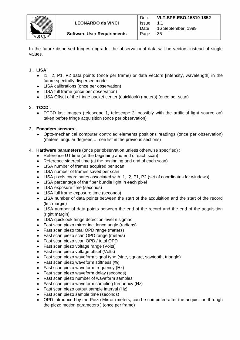
LEONARDO da VINCI
Software User Requirements
Doc:IssueDatePage
VLT-SPE-ESO-15810-18521.116 September, 199935
In the future dispersed fringes upgrade, the observational data will be vectors instead of singlevalues.
1. LISA :♦ I1, I2, P1, P2 data points (once per frame) or data vectors [intensity, wavelength] in the
future spectrally dispersed mode.♦ LISA calibrations (once per observation)♦ LISA full frame (once per observation)♦ LISA Offset of the fringe packet center (quicklook) (meters) (once per scan)
2. TCCD :♦ TCCD last images (telescope 1, telescope 2, possibly with the artificial light source on)
taken before fringe acquisition (once per observation)
3. Encoders sensors :♦ Opto-mechanical computer controled elements positions readings (once per observation)
(meters, angular degrees,… see list in the previous sections)
4. Hardware parameters (once per observation unless otherwise specified) :♦ Reference UT time (at the beginning and end of each scan)♦ Reference sidereal time (at the beginning and end of each scan)♦ LISA number of frames acquired per scan♦ LISA number of frames saved per scan♦ LISA pixels coordinates associated with I1, I2, P1, P2 (set of coordinates for windows)♦ LISA percentage of the fiber bundle light in each pixel♦ LISA exposure time (seconds)♦ LISA full frame exposure time (seconds)♦ LISA number of data points between the start of the acquisition and the start of the record
(left margin)♦ LISA number of data points between the end of the record and the end of the acquisition
(right margin)♦ LISA quicklook fringe detection level n sigmas♦ Fast scan piezo mirror incidence angle (radians)♦ Fast scan piezo total OPD range (meters)♦ Fast scan piezo scan OPD range (meters)♦ Fast scan piezo scan OPD / total OPD♦ Fast scan piezo voltage range (Volts)♦ Fast scan piezo voltage offset (Volts)♦ Fast scan piezo waveform signal type (sine, square, sawtooth, triangle)♦ Fast scan piezo waveform stiffness (%)♦ Fast scan piezo waveform frequency (Hz)♦ Fast scan piezo waveform delay (seconds)♦ Fast scan piezo number of waveform samples♦ Fast scan piezo waveform sampling frequency (Hz)♦ Fast scan piezo output sample interval (Hz)♦ Fast scan piezo sample time (seconds)♦ OPD introduced by the Piezo Mirror (meters, can be computed after the acquisition through
the piezo motion parameters ) (once per frame)

LEONARDO da VINCI
Software User Requirements
Doc:IssueDatePage
VLT-SPE-ESO-15810-18521.116 September, 199936
♦ Piezo / camera user settings (OPD range, fringe velocity, sample interval)♦ FSU usage (with / without)
5. Object reference data :This section describes the data which should be stored as a reference for the data reduction andanalysis. The different fields to be stored will depend on the definition of the VLTI referencecatalog of sources and calibrators which is TBD . As a general rule, it is important to store anyinformation which influenced the choices the observer has made for his observations (type ofvariability, brightness, spectral energy distribution,…). This will be necessary in order to build aposteriori an image of what was the knowledge of the observer about the target at the time theobject was observed.
♦ Names (as taken from Simbad for example, HD, SAO, HR, HIP,…)♦ Type : target, calibrator, type of artificial source♦ Calibrator quality rating (from 1 (best) to 5 (worse))♦ RA, Dec, taken from the Hipparcos catalog or the FK5 (epoch J2000.0)♦ Proper motion with uncertainties♦ Parallax measurements (Hipparcos,…)♦ Separated magnitude estimations in K [min, mean, max], V [min, mean, max]♦ All available bands magnitudes (U, B, V, K, L, IRAS, IUE…), [min, mean, max]♦ All available color indexes (B-V, J-K,…), with uncertainties♦ All available angular diameter estimations (theoretical models, lunar occultations,…) with
publications references♦ Computed angular diameters, through different methods (spectral type+distance,
bolometric flux,…) with uncertainties (in milliarcsec and in radians)♦ Variability flag♦ Binarity or multiplicity flag♦ Variability type (if applicable), code taken from the GCVS for example♦ Spectral type(s) determination(s), with publications references♦ Period (seconds and days), epoch (julian date), wavelength of measurement (meters),
reference publication (for periodic variables)♦ Expected amplitude of the angular diameter variation (if applicable) (in milliarcsec and
radians)♦ Comments entered by the observer
6. Software parameters (once per observation, unless otherwise specified) :♦ Reference code of the observation (can be sequential, allows to quickly retrieve the data)♦ LdV mode name or code♦ LdV setup name or code♦ Projected baseline length (meters) (once per scan)♦ Baseline vector coordinates (u,v,w) (once per scan)♦ OPD velocity (meters/second) (once per scan)♦ Hour angle (seconds) (once per scan)♦ Theoretical RA, Dec♦ Theoretical Altitude, Azimuth (once per scan)♦ Wavelength range [mini, mean, maxi], coupled to the LISA filter wheel position (meters).
This will be replaced by a vector of wavelength ranges (one [min, mean, max] triplet perspectral channel) for spectrally dispersed data.
♦ Observed internal OPD (meters) (once per scan)
LEONARDO da VINCI
Software User Requirements
Doc:IssueDatePage
VLT-SPE-ESO-15810-18521.116 September, 199937
♦ LdV OPD offset (meters)♦ Expected visibility on the current baseline (mean over the observation), with uncertainty
(dimensionless)♦ Technical CCD extracted parameters (position, brightness of the object) (once per
observation)♦ Universal time of the beginning and end of the scans (once per scan)♦ Number of data points saved in each scan (once per observation)♦ Number of scans saved (once per observation)♦ Number of scans on source (once per observation)♦ Number of scans off source (once per observation)♦ Number of scans beam A (once per observation)♦ Number of scans beam B (once per observation)♦ Name of calibrator(s) and reference code of calibrator files used for this target (once per
observation)♦ Name of the original file of the observations (once per observation)♦ Refraction parameters : air mass, refraction correction applied by the VLTI (beginning and
end of each observation)
7. Delay Line (once per scan) parameters read from the DL system:♦ Delay line position (meters)♦ Delay line velocity (meters per second)♦ Delay line piezo relative position (meters)♦ Delay line piezo velocity (meters per second)♦ Delay line VCM curvature (curvature radius)♦ Delay line relative pupil position (meters)♦ Delay line error signal (meters)
8. FSU parameters read from the FSU system:♦ Piston RMS value measured bu the FSU (once per scan)♦ Residual FSU error signal (once per scan)
9 . Telescopes (once per observation, unless otherwise specified) parameters read from thetelescopes system :♦ VLTI setup (baseline used, telescope types, UT names)♦ Name of the delayed telescope♦ RA, Dec (beginning and end of each observation)♦ Altitude, Azimuth (beginning and end of each observation)♦ Mean tracking error (RA and Dec) over the observation
10. Observatory (once per observation, unless otherwise specified) parameters read from theobservatory environment monitoring system :♦ Environmental parameters:seeing, isoplanetic angle, correlation time, air pressure, air temperature, ground temperature, humidity, wind
velocity and direction, seismic activity, seismic flag
2.11.2.3 Data Time Scales

LEONARDO da VINCI
Software User Requirements
Doc:IssueDatePage
VLT-SPE-ESO-15810-18521.116 September, 199938
In this section, the data produced by LdV is sorted by time scale. The data which is not availablelocally in the LdV LCUs and WS is indicated.
2.11.2.3.1 Frame
♦ I1, I2, P1, P2 data points (data vectors in the future dispersed mode)♦ OPD introduced by the Piezo Mirror (meters, can be computed after the acquisition through
the piezo motion parameters )
2.11.2.3.2 Scan♦ Reference UT time (at the beginning and end of each scan)♦ Reference sidereal time (at the beginning and end of each scan)♦ LISA Offset of the fringe packet center (quicklook) (meters) this value is the one sent the
the OPD controller in order to recenter the fringe packet.♦ Projected baseline length (meters)♦ Baseline vector coordinates (u,v,w)♦ OPD velocity (meters/second)♦ Hour angle (seconds)♦ Theoretical Altitude, Azimuth♦ Number of data points saved in each scan♦ Observed internal OPD (meters)
Available from the FSU (TBD):♦ Piston RMS value measured bu the FSU (once per scan)♦ Residual FSU error signal (once per scan)
Available from the DL system:♦ Delay line position (meters)♦ Delay line velocity (meters per second)♦ Delay line piezo relative position (meters)♦ Delay line piezo velocity (meters per second)♦ Delay line VCM curvature (curvature radius)♦ Delay line relative pupil position (meters)♦ Delay line error signal (meters)
2.11.2.3.3 Observation♦ Reference code of the observation (can be sequential, allows to quickly retrieve the data)♦ Names (as taken from Simbad for example, HD, SAO, HR, HIP,…)♦ Name of calibrator(s) and reference code of calibrator files used for this target♦ Type : target, calibrator, type of artificial source♦ Calibrator quality rating (from 1 (best) to 5 (worse))♦ Name of the original file of the observations♦ Theoretical RA, Dec♦ LISA Calibrations♦ TCCD last images (telescope 1, telescope 2, possibly with the artificial light source on)
taken before fringe acquisition (once per observation)

LEONARDO da VINCI
Software User Requirements
Doc:IssueDatePage
VLT-SPE-ESO-15810-18521.116 September, 199939
♦ Opto-mechanical computer controled elements positions readings (meters, angulardegrees,… see list in the previous sections)
♦ LISA number of frames acquired per scan♦ LISA number of frames saved per scan♦ LISA pixel coordinates associated with I1, I2, P1, P2 (set of coordinates for windows)♦ LISA percentage of the fiber bundle light in each pixel♦ LISA exposure time (seconds)♦ LISA number of data points between the start of the acquisition and the start of the record
(left margin)♦ LISA number of data points between the end of the record and the end of the acquisition
(right margin)♦ LISA quicklook fringe detection level n sigmas♦ LISA full frame♦ LISA full frame exposure time (seconds)♦ Fast scan piezo mirror incidence angle (radians)♦ Fast scan piezo total OPD range (meters)♦ Fast scan piezo scan OPD range (meters)♦ Fast scan piezo scan OPD / total OPD♦ Fast scan piezo voltage range (Volts)♦ Fast scan piezo voltage offset (Volts)♦ Fast scan piezo waveform signal type (sine, square, sawtooth, triangle)♦ Fast scan piezo waveform stiffness (%)♦ Fast scan piezo waveform frequency (Hz)♦ Fast scan piezo waveform delay (seconds)♦ Fast scan piezo number of waveform samples♦ Fast scan piezo sampling waveform sampling frequency (Hz)♦ Fast scan piezo sample interval (meters)♦ Fast scan piezo sample time (seconds)♦ Piezo / camera user settings (OPD range, fringe velocity, sample interval)♦ RA, Dec, taken from the Hipparcos catalog or the FK5 (epoch J2000.0)♦ Proper motion with uncertainties♦ Parallax measurements (Hipparcos,…)♦ Separated magnitude estimations in K [min, mean, max], V [min, mean, max]♦ All available bands magnitudes (U, B, V, K, L, IRAS, IUE…), [min, mean, max]♦ All available color indexes (B-V, J-K,…), with uncertainties♦ All available angular diameter estimations (theoretical models, lunar occultations,…) with
publications references♦ Computed angular diameters, through different methods (spectral type+distance,
bolometric flux,…) with uncertainties (in milliarcsec and in radians)♦ Variability flag♦ Variability type (if applicable), type code taken from the GCVS for example♦ Binarity or multiplicity flag♦ Spectral type(s) determination(s), with publications references♦ Period (seconds and days), epoch (julian date), wavelength of measurement (meters),
reference publication (for periodic variables)♦ Comments entered by the observer♦ LdV mode name or code♦ LdV setup name or code♦ Wavelength range [mini, mean, maxi] (meters) (vector for dispersed fringes)
LEONARDO da VINCI
Software User Requirements
Doc:IssueDatePage
VLT-SPE-ESO-15810-18521.116 September, 199940
♦ LdV OPD offset (meters)♦ Expected visibility on the current baseline (mean over the observation), with uncertainty
(dimensionless)♦ Technical CCD extracted parameters (position, brightness of the object)♦ Technical CCD refined optimization intensity map♦ Number of scans saved♦ Number of scans on source♦ Number of scans off source♦ Number of scans beam A (with one telescope off source)♦ Number of scans beam B (with one telescope off source)♦ Refraction parameters : air mass, refraction correction applied by the VLTI (beginning and
end of each observation)
Available from the telescopes or observatory systems:♦ VLTI setup (baseline used, telescope types, UT names)♦ Name of the delayed telescope♦ RA, Dec (beginning and end of each observation)♦ Altitude, Azimuth (beginning and end of each observation)♦ Mean tracking error (RA and Dec) over the observation♦ Environmental parameters:seeing, isoplanetic angle, correlation time, air pressure, air temperature, ground temperature, humidity, wind
velocity and direction, seismic activity, seismic flag
2.11.2.4 Data Format
After a meeting with representatives of the AMBER and MIDI teams (the two science instrumentsof the VLTI), and ESO Data Management Division, it has been agreed that the FITS binary tableformat was the most suitable for the storage of the data. The exact internal formatting andkeywords of these files are currently under definition .
The header of the FITS file contains all the parameters which are defined less often than everyscan (i.e night, observation block, observation). The interferometric data itself is stored in the bodyof the FITS file. The TCCD images are stored in the body of the data file, before or after theinterferometric data.
The following figure shows the typical data acquisition during an observing night, and what isstored in the data files.

LEONARDO da VINCI
Software User Requirements
Doc:IssueDatePage
VLT-SPE-ESO-15810-18521.116 September, 199941
2.12 DESCRIPTION OF THE OBSERVATION PROCEDURE
2.12.1 Observation Procedure with VINCI
This section gives an overview of a typical observing session.
1. Observations Scheduling: the observations scheduling is conducted off-line from the real-timeoperating system. The creation of a formatted observing list should be possible before on-sitearrival through a “front page” software. This system could help the observer determine:
• which sources are visible• the previous observations of his targets• the magnitudes (including the K magnitude, if necessary computed from the other
bands measurements)• the estimated visibility• the calibrators used so far• the baselines used so far on this target…
The querying of this database is possible through every field, and it is possible to use thedatabase while on the observing site. The calibrators, selected by the observer with the help ofdedicated software, are integrated in the list of the observations to be conducted. Their nature
Obs. parameters
Scans
Obs. parameters
Scans
Block 1
Block 2
Block 3
Block ...
OObbsseerrvv ii nngg NN iigghh tt OObbsseerrvvaa tt ii oonn FF ii ll eess
#1
#2
#n
(1 hour)
(10 min.)
DDeettaa ii ll eedd CCoonn tteenn tt
Star parametersInstrument configuration
VLTI configurationTCCD images pointersLISA full frame pointerSoftware parametersHardware parametersEnvironmental data
...
Scan reference codeStarting delay line position
Scan start timeI1, I2, P1, P2 frames
Scan end timeOPD Offset
...
TCCD images
TCCD images
Obs. parameters
Scans
TCCD imagesLISA Full Frame
LISA Full Frame
LISA Full Frame
LEONARDO da VINCI
Software User Requirements
Doc:IssueDatePage
VLT-SPE-ESO-15810-18521.116 September, 199942
of calibrators should be apparent in the list. The database is a key element of the VLTI SW.The definition of this database is a point to discuss with the other instruments and the VLTI.
The observation scheduling SW tools are not part of the VINCI SW, but rather part of thegeneral VLTI SW (since they will be used by all the instruments).
2. LdV Initialization: the instrument status is changed to “online”.
3 . Short-term Observations Scheduling: in order to fine-tune the observing program of theinstrument, the observer has access to the observing list, and can modify it by hand. Thepossibility remains of having an automated system to optimize the observing schedule for thenight.
4. Telescopes Pointing: position the telescopes at the target coordinates.
5. Telescopes Focusing: focus the telescopes in order to feed a collimated beam in the Coudetrain.
6. Delay Line positioning: the delay line is sent to the position required for optical path lengthequalization between the two beams, and it is moved at the computed rate for the observedtarget.
7. Technical CCD Images Acquisitions: images of the target are obtained by the technical CCDon both beams to check for the positioning of the pupil and the image quality. This requires themotion of the LdV mirrors ALI2/ALI3 and ALI4/ALI6.
8. Positioning of the fiber input: this is done by maximizing the flux on the camera pixels. Thesetting of the injection parabolae is motorized, and the flux maximization is done on the starsduring the observations. This first setting during the initialization phase will help finding themaximum light position on the scientific targets by giving a reference point. As an upgrade ofthe system, it should be possible to do this process automatically.
9. Acquisition of a LISA full frame: this will enable the observer to check for the quality of theimages of the fibers on the HAWAII detector, and track any systematic problem. If thecentering of the fiber heads is bad, then an output optimization procedure can be started.
10. Off source and mixed batches: In order to compute the transfer matrix of the system, it isnecessary to obtain three small batches (about a hundred scans) :
- off-source : the telescopes are pointed to the background sky,- beam A only,- beam B only.
11. Fringes Finding (long scan) and Scanning (fast scan): [Req. 51] during the fringes findingphase, the optical path difference is slowly modulated by moving the delay line while scanningwith the fast scan mirror INA3. By doing this motion, a segment of optical path difference isscanned for the presence of fringes. The delay line motion is superimposed to the siderealspeed. The algorithm is simple :
LEONARDO da VINCI
Software User Requirements
Doc:IssueDatePage
VLT-SPE-ESO-15810-18521.116 September, 199943
- while fringes are not found, increase the internal OPD by a fixed ammount X (entered bythe observer, can be positive or negative)
- once the fringes are found by the quicklook algorithm, the delay line motion speed is set tothe sidereal rate, in order to have the fringes at a fixed position.
The fringes are then repeatedly measured and the scans are stored. The duration of theobservation is selected by the observer (as a number of 'good' scans for example). At the endof each fringe scan, while on source, a quick look analysis is performed which results in anupdated value for the internal OPD, to be communicated to the delay line.
12. On-line Data Quality Control: the LdV operating system provides the user with an on-linedisplay of the data acquired [Req. 18] . This enables the observer to check the quality of thevisibility measurements, and gives an estimation of the atmospheric perturbations evolutionduring the night. The display of these values can be done with a delay of [0.5 s, 1 s] and/or bypackets (several scans displayed simultaneously) to reduce the real-time constraints on thesystem. The basic data reduction should be done by the DCS (quick reduction, in real-time onthe LISA WS, but displayed every [0.5 s, 1 s] to the user) and the fine data reduction by the OS(in a near-line regime, after each observation). This implies that the fine data reductionalgorithm should be resident on the LdV WS. Since the LdV WS will be essentially idle duringan observation, one can expect that the fine reduction can be done during the observationsthemselves [Req. 33] .
The scenario would be:
OS ICS / DCSObservation n Request obj. pointing
Check TCCD, LISA, etc…Request DAQ
Receive data from DCS
Get small batch off-sourceGet small batch beam AGet small batch beam BGet batch on-source: loop on:- Wait for DL in track- Get one scan- Quick look- Transmit internal OPD
value- Quick data reduction- Display scan + visGet batch off-sourceTransfer data to OS
Observation n+1 Request obj. pointingCheck TCCD, LISA etc.Request DAQ
Pipeline observation nStore data in archiveDisplay results obs. n
Receive data from DCS
Wait for DAQ requestGet small batch off-sourceGet small batch beam AGet small batch beam BGet batch on-sourceGet batch off-sourceTransfer data to OS
LEONARDO da VINCI
Software User Requirements
Doc:IssueDatePage
VLT-SPE-ESO-15810-18521.116 September, 199944
If observation n+1 is terminated before observation n is fully pipelined, then observation n is storedin a buffer to be pipelined at the end of the night [Req. 34] .
13. During the routine operation of LdV, many targets (~50) are observed during the night.
14. LdV End of the Night: after the last target has been observed, the termination procedure isstarted. This includes:
• saving the opened files, saving the observing log• performing a final detector calibration• creating a summary of the observations of the night: a summary of the measurements
obtained during the observing session is displayed to the observer, and possiblyprinted or sent by e-mail to the interested users. The final environmental parameterscould also be added to the saved data. A summary of all the technical problems andimportant error messages from the operating system could also be displayed andsaved to disk.
• switching off the instrument: the status of LdV is changed to “off”.
15. Reduction Pipeline: the automated data reduction process is started after the end of the night.It reduces all the data obtained during the night, which is not already reduced, and saves theresulting files to the LdV night data set.
16. Off-line Data Analysis: using standard (MIDAS, IDL,…) or specific data analysis tools, theastronomer processes and combines the data.
2.12.2 LEONARDO Interface with the VLTI Instruments
The VLTI scientific instruments AMBER and MIDI should have access to LEONARDO artificial starmode [Req. 11] .
All the setups of the Artificial Star mode (see desctiptions section 2.8.6) should be available to theVLTI instruments through the VLTI CS :
- Artificial Star Off Removed- Artificial Star On Inserted- Artificial Star On Removed- Artificial Star Off Inserted- Autocollimation On Inserted
The switching between these setups will require a few seconds, in order for the motors to achievethe necessary motions. The 'user' instruments should access LEONARDO only through thesepredefined modes [Req. 12] . No low-level command is foreseen to be accessible from outside ofLdV software.

LEONARDO da VINCI
Software User Requirements
Doc:IssueDatePage
VLT-SPE-ESO-15810-18521.116 September, 199945
The thermal light source can be turned off during normal operations, but if it is required to switch iton again, the preheating will take a few minutes in order to achieve a good stability [Req. 53] . Thisdoes not apply to laser sources.
The commands issued by the instruments should follow the same format as the commands for theother systems of the VLTI (telescopes, delay lines,…). Generally speaking, LEONARDO should beintegrated in the VLTI infrastructure as much as possible and follow the same control procedure[Req. 35] . This means that it will act independently from VINCI and the alignment toolkit ALIU.
The user instrument should request the allocation of LEONARDO before sending commands to it,in order to avoid conflicts with the other instruments. By default, LEONARDO should be assignedto LdV. LEONARDO should be automatically allocated to the master observing instrument, so asto avoid the accidental insertion of the LEONARDO cubes in the beams.
2.12.3 Alignment Toolkit Interface with the VLTI instruments
The VLTI instruments AMBER and MIDI as well as the alignment software of the VLTI should haveaccess to the Pupil Check and Image Check modes and setups [Req. 9] . All the data acquiredshould be available on request from any system to the VLTI CS (but no real-time constraints areforeseen). The interface requirements are currently under definition (TBD).
Generally speaking, the alignment toolkit should be integrated in the VLTI infrastructure as muchas possible and follow the same control procedure [Req. 36] . The allocation of ALIU (alignmenttoolkit) to the alignment software or the other instruments should be done by request. By default,it should be assigned to LdV software.
2.13 INSTRUMENT USER MANUAL
As LdV will be operated in several ways as a facility for the other VLTI instruments, it is importantto foresee a complete User's Manual for this instrument. This will enable the science instruments'teams to have a reference for the proper use of LEONARDO, the alignment unit (those twosystems will be used directly by the other instruments) and VINCI.
2.14 SETTINGS DATABASE
The operation of LdV on different baselines will require a database of settings (internal OPD, INBslide position, TCCD focus positions,…) to quickly find the fringes after a baseline change. Thisdatabase should be available on-line on Paranal. It is not part of the VINCI software, and belongsto the VLTI system.
As a general rule for LdV, there is no particular order in which the various functions should be set,and the settings can be done in parallel.

LEONARDO da VINCI
Software User Requirements
Doc:IssueDatePage
VLT-SPE-ESO-15810-18521.116 September, 199946
2.15 TCCD PROCEDURES
2.15.1 TCCD focusing
The focusing of the TCCD is done in a standard way. The image of a point source is obtained,then fitted with a gaussian bidimensional curve, and a correction is computed from the width of thisgaussian. Is is iterated a few times if necessary.
In Pupil Check mode, the focus will be achieved on the red LED which is at the center of mirrorM2, or on the artificial star image. In Image Check mode, it will be done on the stellar image (eitherartificial or from the sky). The focusing might be needed from time to time, as a maintenanceprocedure
In the following sub-sections, the TCCD is supposed focused.
2.15.2 TCCD Calibrations
It is necessary to obtain an image of the fiber inputs on the TCCD. This is done by injecting light inthe MONA box from one the outputs, and illuminating the fiber input head. Via the ALI1 and ALI5beamsplitter cubes, the resulting “artificial stars” are imaged on the TCCD. Once the image hasbeen acquired, the precise position of the fiber input is computed by a gaussian fit. Thesecoordinates are the reference on which all the star light has to be concentrated during theobservations.
2.15.3 Pupil Check
This section refers to the optical configuration described in the reference document [2], section3.9.2.
At the beginning of the night, and to avoid any loss of stellar light, it is important to check that thelight beam arrives unobstructed (= unvignetted) to the instruments. This is done by imaging thepupils of the telescopes on the TCCD chip. The pupils are the images of the secondary mirrors ofthe feeding optical systems (either siderostats, UTs or ATs). The delay lines system is built so asto keep the beam B pupil plane in the laboratory (this allows an extended field of view for theimaging applications).
Normally, the image of the pupil is obtained by turning on the light source at the center of thesecondary mirror. The image obtained on the TCCD is then a point, which has to be centeredrelatively to the axis of the technical CCD optics. The refractor in front of the TCCD defines theoptical axis of the VLTI.
The pupil alignment is expected to occur once per night, or before any observation depending onthe stability of the VLTI.
The location of the pupil planes for the two beams will be on the injection parabolae INA1 andINB1. This means that for imaging the pupil, it is necessary to focus at their distance with theTCCD. As it is used also for viewing the stellar images, it is normally focused at infinity.

LEONARDO da VINCI
Software User Requirements
Doc:IssueDatePage
VLT-SPE-ESO-15810-18521.116 September, 199947
In order to focus at a few meters, this requires the addition of a converging lens in front of theTCCD. Once this is done, the TCCD can focus on the pupil image which is situated on INA1/INB1.
The OS should get the expected pupil position from VLTI OS [Req. 37] and from then:- insert the bonnette if the pupil is less than 3m away,- preset the TCCD focus to the expected pupil position.
Once the focusing has converged on the pupil LED, from the focus motor readout the softwareshould derive a measured pupil longitudinal position [Req. 38] (which can be compared to theexpected pupil position provided by the VLTI OS).
The necessary setups have been described in the section 2.8.4. The focusing of the TCCD isdone the same way as for the Image Check, only the starting position (rough focusing) changes.
In the current design, the role of LdV is not to provide the commands to set the mirrors of theoptical train to align the pupil. Only the display and shape measurements of the pupil are arequirement for the LdV software. But this has TBC when a clear alignment procedure has beendefined.
The procedure to obtain and measure the pupil with the TCCD is the following:
1. Obtain an image with the TCCD in the Pupil Check setup, with the Secondary Mirror redLEDs switched on.
2. Provide the image to the user , together with information on the quantity of light available,
and the position of the spot. 2.15.4 Image Check This section refers to the optical configuration described in the reference document [2], section3.9.3.
As a part of the alignment procedure, VINCI's TCCD will be used to measure the alignment of theVLTI regarding the position of the image. It will be done by reimaging a light source (multimodefiber connected to a laser diode) located at the Nasmyth focus of the selected telescope, on theTCCD located in the interferometric laboratory. Then, the position of the image of the source canbe modified by tilting a mirror in the VLTI optical train (TBD preferably located in a pupil plane orclose to it, to limit cross coupling between tilt and OPD).
The image alignment is expected to occur once per night, or before any observation depending onthe stability of the VLTI. The procedure to obtain and measure the image of the Nasmyth light source with the TCCD is thefollowing:
3. Obtain an image with the TCCD in the Image Check setup, with the Nasmyth multimodelaser diode switched on.

LEONARDO da VINCI
Software User Requirements
Doc:IssueDatePage
VLT-SPE-ESO-15810-18521.116 September, 199948
4. Provide the image to the user , together with information on the quantity of light available,
and the position of the spot.
In the current design, the role of LdV is not to provide the commands to set the mirrors of theoptical train to align the pupil. Only the display and shape measurements of the image are arequirement for the LdV software. But this has TBC when a clear alignment procedure has beendefined.
2.15.5 Star Image Centering
The Technical CCD is used to check the star image quality and position. During observations inthe stellar interferometer mode, the TCCD is used in the following sequence after the telescopesare tracking on the target. The alignment of the VLTI is supposed to be good enough, so as tobring the stellar light up to the VINCI table and on the TCCD chip. The following procedure isforeseen [Req. 39] :
1. The star image is acquired . The exposure time is computed based on the brightness ofthe source in the optical wavelengths. It is taken from the observing template or the onlinecatalogs database.
2. Measurement of the source(s) : the resulting image shows the source, and possibly otherobjects, with a calibrated intensity in ADUs. The sources are then measured by fitting twodimensional gaussian curves to the intensity profiles present in the image. This fit could bedone via a fast Fourier transform of the image, or other numerical method. The resultingdata is a set of coordinates, intensities and profile widths. This information, and the TCCDimage will be saved in the observations data.
3. Identification of the target : in the observing template, a flag should indicate if a closebright source is expected to be in the same field.
- In case this flag is up, the identification could be done based on the expectedrelative brightness of the target compared to the other object(s), or visually by theoperator of the instrument.- In case this flag is down, the identification is normally unambiguous, though avery slight risk of confusion exists with an unexpected source (other very close star,asteroid,…). This risk should not be taken into account for the design of thesoftware.
4. Computation of the position error : once the target is identified, its coordinates arecompared to the fiber head input coordinates as measured during the calibration phase.The alignment of the optical train up to the laboratory is supposed to be good, and only theinjection optics will be moved to precisely position the star image on the fiber input.
5. Computation of the tip-tilt mirrors required motions : the difference is computed andconverted to tip-tilt positions of the injection mirrors. The coefficients for this conversion(two for each injection mirror) have been estimated during the commissionning of LdV. Itwill be also necessary to include an offset coefficient in the parameters, due to the differentpositions of the star images in the visible and in the infrared. This offset varies with respect
LEONARDO da VINCI
Software User Requirements
Doc:IssueDatePage
VLT-SPE-ESO-15810-18521.116 September, 199949
to the altitude of the star in the sky. At zenith, this is zero, while near the horizon it isseveral arcsec (projected on the sky), but a direct mathematical relation allows itscomputation based on the altitude of the object, the TCCD sensitivity curve meanwavelength and the mean wavelength of the LISA infrared band.
6. Motion of the INA1 and INB1 mirrors : commands are sent to the INA1 and INB1 motorsto move in order to position the image of the star in the infrared at the same position as thefiber head as measured at the beginning of the night. It is necessary to inject the light at aposition offset from the visible outputs of the fibers (as seen on the TCCD), due todifferential refraction of the atmosphere. The computed offset will have to take into accountthe differential refraction, which requires input from VLTI environmental parameters(humidity, temperature...). It is foreseen that the VLTI collecting telescopes send theinfrared light directly on-axis, while guiding on the optical image off-axis. This means thatthe differential diffraction offset has to be taken into account directly at the telescope level.This would make this procedure simpler as no variable offset would have to be applied tothe INA1 and INB1 mirrors.
7. Refined optimization : At this stage, the star should be positioned on the fiber head,sending light into the MONA box up to the HAWAII detector. The refined injectionoptimization can then be conducted, see next paragraph.
2.15.6 Off-line use of TCCD images and LISA full frames
At least one image of the object (from each telescope) obtained with the TCCD during theacquisition procedure should be saved in the data [Req. 40] . This will enable the user during post-processing to check visually the quality of the seeing, the postion of the object relatively to thefiber heads during pre-acquisition,…
As a complement to the TCCD image(s), the computed data on the positions of the sources in theimage as well as the refined injection optimization data should be stored in the observation of thestar.
The same comments apply to the LISA full frame images, which will help during the data reductionprocess to track misalignments of the fiber outputs. They should be saved before eachobservation, and in any case after every output alignment procedure.
2.16 INJECTION AND OUTPUT OPTIMIZATION PROCEDURES
2.16.1 Refined Injection Optimization
The principle for this optimization is that we are looking for the very precise position of the stellarimage peak intensity. The stellar Airy disk size is 0.065 arcsec in FWHM for UT and 0.290 arcsecfor AT, and the fiber head projected size on the sky is the same (but the speckle cloud, whichreplaces the Airy disk without adaptive optics, is about 0.5 to 1 arcsec in size for both). The starimage and the fiber head transmissivity have gaussian profiles.

LEONARDO da VINCI
Software User Requirements
Doc:IssueDatePage
VLT-SPE-ESO-15810-18521.116 September, 199950
The precision required for the superposition of the two gaussian curves is of the order of 7milliarcsec for the UTs. It will not be possible to center the images using the TCCD, because thestar detection precision is not sufficient. This is a critical point, because all the light which is notinjected in the fiber is lost.
As the automation of this procedure is very demanding for the software system, the operatorshould manually search for the optimum injection in the first phase of the operations of LdV [Req.41]. The main drawback is a slow down of the observations, and the interruption of the automatedtemplate observing session.
Refined injection optimization is a second generation upgrade at this point, but this is veryimportant since as long as we do not have automated injection optimization it will not be possibleto implement and test fully automated observation templates which is the target operating modefor the VLTI instrumentation. See section 2.20.1 for description of possible algorithms.
2.16.2 Output Alignment Procedure
The four fiber outputs have to be precisely positioned on four pixels of the LISA camera (to afraction of a HAWAII pixel). This means that the position of the fiber bundle output has to beprecisely adjusted with respect to the HAWAII detector pixels. This is done via the OUT1 fiberbundle output, which is adjustable in translation (3 directions) and rotation. Only the focus androtation aroud the optical axis are remotely controlled. The alignment is checked on the HAWAIIcamera by acquiring full frames (which cover a quarter of the chip surface, i.e. 512x512 pixels)while light is sent into the fiber bundle with the artificial star light source LEONARDO.
The output alignment is normally done before the observing night, using the Autotest orAutocollimation setups. However, it is possible to do refocusing or rotational adjustment during thenight if necessary, as it is remote controlled.
A possible scheme for the output alignment procedure is [Req. 42] :
1. Obtain quick exposures from the LISA camera in full frame mode. 2. Monitor nearly continuously (frequency of a few Hz) values for :
- the total flux arriving on the HAWAII detector- the parameters of the four images of the fibers outputs : position of the maximum
light, FWHM. This is obtained by fitting gaussian curves to the image.- the percentage of the flux (in ADU) concentrated in each maximum light pixels.- the global percentage of the light concentrated in the four maximum light pixels.
The maximization of this value is the goal of the output alignment procedure.
3. Adjust OUT1 through paddle control on the WS (z,rotation) , to move the four fiberoutputs on the HAWAII detector. This adjustement is done by the operator. During thismotion, the positions of the fiber outputs are adjusted so as to put them on the desiredcolumns of the detector. The precise adjustment of the positions is done using thecomputed light concentration percentage. The image of the fiber outputs is continuouslydisplayed to the operator. The look-up table for this image is not dynamic, but can be
LEONARDO da VINCI
Software User Requirements
Doc:IssueDatePage
VLT-SPE-ESO-15810-18521.116 September, 199951
adjusted by the user. Only focus (z direction) and rotation can be adjusted remotely, whilethe x and y settings are done by the observer before the observing night and are supposedfixed.
Once this is done, the fiber outputs are well aligned on the detector pixels. The coordinates of thepixels used, as well as the percentages of the light concentrated in each pixel are stored in the WSsw, in order to be added to the data files headers [Req. 43] .
A LISA full frame image is stored after this process for reference during the data reduction [Req.30].
Automated output focus and rotation alignment is a second generation upgrade at this point, but itwill be mandatory in order to implement fully automated observation templates. See section2.20.2 for description of a possible algorithm.
2.17 TEMPLATES
The control software shall allow to build up templates which will carry out in a semi-automated wayan observation or a group of observations and use them to measure astronomical, astmosphericor instrumental parameters [Req. 44] . The observations with LdV based on templates are not yetcompletely defined.
The sequencing of LdV modes includes the intervention of the observer for some critical tasks,such as injection optimization and output alignment. The steps requiring the operator action aremarked with [operator].
2.17.1 Autotest Mode Observations Standard Template :
• mode Autocollimation Injection Adjust [operator]• mode Autocollimation Output Adjust [operator]• mode Autocollimation Fringe Search• mode Autocollimation Data Acquisition• archival of the data
2.17.2 Autocollimation Mode Observations Standard Template :
• mode Autotest Injection Adjust [operator]• mode Autotest Output Adjust [operator]• mode Autotest Fringe Search• mode Autotest Data Acquisition• archival of the data
2.17.3 Pupil check Standard Template

LEONARDO da VINCI
Software User Requirements
Doc:IssueDatePage
VLT-SPE-ESO-15810-18521.116 September, 199952
• mode Pupil Check Artificial Star A• mode Pupil Check Artificial Star B• mode Pupil Check telescope A• mode Pupil Check telescope B• TCCD images are made available to LdV and the external instruments
2.17.4 Image Check Standard Template
• mode Image Check telescope A• mode Image Check telescope B• TCCD images are made available to LdV and the external instruments
2.17.5 Stellar Interferometer Mode Observations Standard Template :
The Pupil Check and Image Check steps require a call to the corresponding standard templates.
• pointing of the telescopes• initial positioning of the Delay Lines• standard template Pupil Check• standard template Image Check• mode Stellar Interferometer Injection Adjust [operator]• mode Stellar Interferometer Fringe Search• mode Stellar Interferometer Data Acquisition• archival of the data
2.18 GRAPHICAL USER INTERFACE
The user of LdV shall normally interact with the instrument via the Instrument Workstation and theLdV graphical user interface (GUI) [Req. 58] . The user will first have to select the way to operateamong three options:
Standard Observing: for astronomical targets observations, in the stellar interferometer setup. Inthis option, the operator will use the GUI to control the observations. LdV will also be used as ameasurement tool for internal seeing, optical alignments, internal OPD measurements. This willmake use of the standard operating modes defined Section 2.8.
Maintenance: to check periodically the performances of LdV at the OS level. The GUI shoulddisplay the series of tests to be performed, and either perform them automatically or under theuser's control. The results of the maintenance tests are then logged for statistical analysis andpreventive maintenance.
Engineering: to carry out detailed tests or settings regarding the instrument hardware devices,during improvements of the system or in-depth analysis of hardware problems. This is done at theICS level.
LEONARDO da VINCI
Software User Requirements
Doc:IssueDatePage
VLT-SPE-ESO-15810-18521.116 September, 199953
In the first two options, the possibility shall be given to change the instrument state between on-line, stand-by and off [Req. 45] . Via the GUI, it shall then be possible to select the instrumentmode either [Req. 46] :
• Individually via typed commands from the WS sw• Via the GUI, by form-filling• Via the GUI, using pre-stored files• Via a template sequence
The GUI should also display the status information provided by the LdV and TCCD control andacquisition electronics and other relevant data (e.g. meteo and telescope data). The GUI will alsogenerate warnings of hazards or error conditions (e.g. mirrors bad positioning or failure,…)whenever power is on.
The automated operation of LdV, via a template sequence, is a very demanding goal to achieve.Interferometers are very complex technical systems and it is important to realize that no currentlyworking interferometer is completely automated. The option to operate the instrument in a manualor semi-automated way (the first three bullets of the above list) should not be discarded.
2.18.1 Online Modes Interface
The LdV WS sw in Stellar Interferometer Mode should be able to [Req. 47] :
• Interact with the VLTI Control System, controlling the telescopes and gathering positional andenvironmental data. The pointing instructions are sent to the VLTI Control System.
• Interact with the LdV Instrument Control System. This allows the automatic or semi-automaticsetting and monitoring of the:
- light switches- motor commands- encoders readout- piezo fast scan parameters
• Control the LISA DCS. All the acquisition parameters (duration, frequency) are defined by theobserver and sent to the camera through the operating system.
• Control the Technical CCD DCS. During the acquisition procedure, the WS sw controls thesettings of the exposure as well as displays the resulting images and performs the relevantparameters extraction as described in section 2.15. These parameters and data should bedisplayed in real-time to the operator for quality check.
• Monitor real-time information about the status of LdV and the VLTI, including error and warningmessages. For example, the position of the delay line, the pointing direction of the telescopes,the status of the movable mirrors, the readings of the encoders and the status of the lightswitches.
• Provide the observer with software control over every computerized element relevant for theStellar Interferometer Mode, such as the movable mirrors and white light sources.

LEONARDO da VINCI
Software User Requirements
Doc:IssueDatePage
VLT-SPE-ESO-15810-18521.116 September, 199954
• Read and modify the observing list, to allow for real-time tuning of the observing schedule. Theobserving conditions can influence the selection of the sources, for example the faint sourceswill not be observable during bad turbulence periods.
• Perform basic observational data pre-processing, such as averaging multiple scans values.The raw data shall be kept safe during these steps and saved together with pre-processeddata in the archive.
• Real-time display the observational data. This is the key point to allow for a real-timeappreciation of the quality of the data, and to check for possible malfunctions. The visibilitiescould be displayed in chronological order, as well as in the form of an histogram.
• Allow the user to perform near-line visibility data processing. To check for unexpectedvariability in the targets visibilities, and possibly trigger extended observation on the mostinteresting objects.
• Access the VLTI archive system. In order to check for any previous observation of theinstrument. To reliably save the observational data, the operating system should access theVLTI Archive at the end of the night, to write the files of the data obtained during the night. Itwould also be interesting to be able to read in the archive during the observations to check forthe previous measurements on the targets.
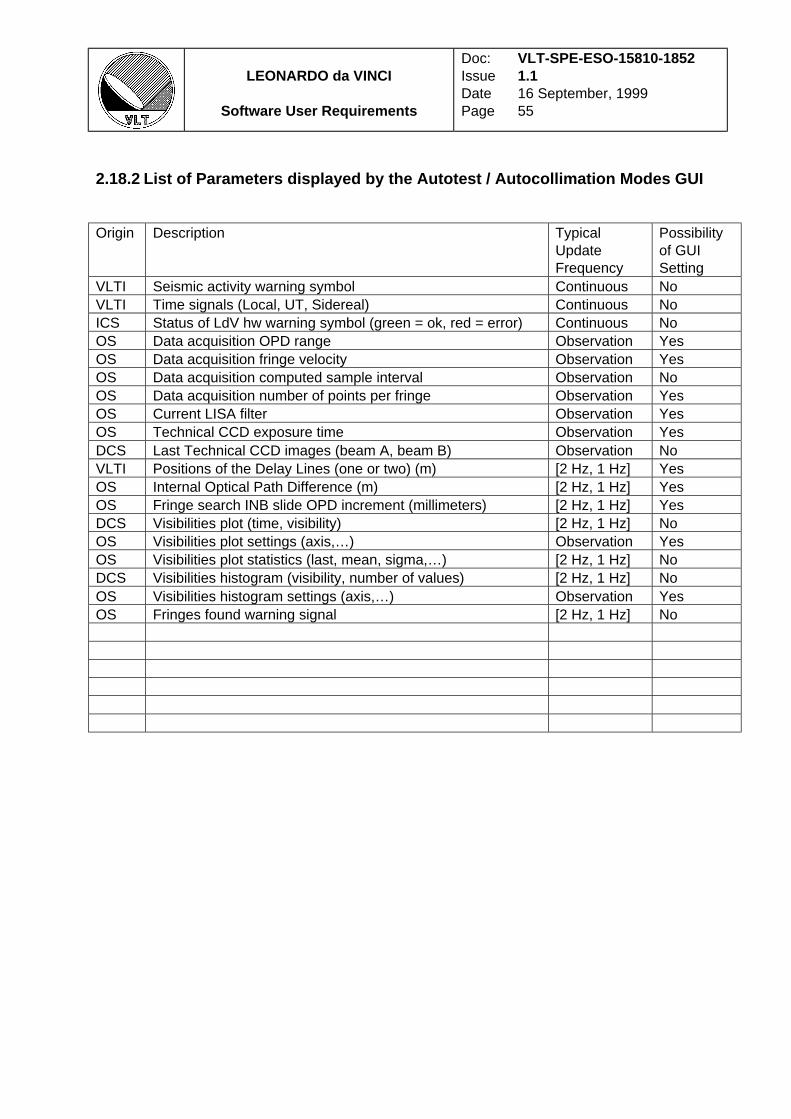
LEONARDO da VINCI
Software User Requirements
Doc:IssueDatePage
VLT-SPE-ESO-15810-18521.116 September, 199955
2.18.2 List of Parameters displayed by the Autotest / Autocollimation Modes GUI
Origin Description TypicalUpdateFrequency
Possibilityof GUISetting
VLTI Seismic activity warning symbol Continuous NoVLTI Time signals (Local, UT, Sidereal) Continuous NoICS Status of LdV hw warning symbol (green = ok, red = error) Continuous NoOS Data acquisition OPD range Observation YesOS Data acquisition fringe velocity Observation YesOS Data acquisition computed sample interval Observation NoOS Data acquisition number of points per fringe Observation YesOS Current LISA filter Observation YesOS Technical CCD exposure time Observation YesDCS Last Technical CCD images (beam A, beam B) Observation NoVLTI Positions of the Delay Lines (one or two) (m) [2 Hz, 1 Hz] YesOS Internal Optical Path Difference (m) [2 Hz, 1 Hz] YesOS Fringe search INB slide OPD increment (millimeters) [2 Hz, 1 Hz] YesDCS Visibilities plot (time, visibility) [2 Hz, 1 Hz] NoOS Visibilities plot settings (axis,…) Observation YesOS Visibilities plot statistics (last, mean, sigma,…) [2 Hz, 1 Hz] NoDCS Visibilities histogram (visibility, number of values) [2 Hz, 1 Hz] NoOS Visibilities histogram settings (axis,…) Observation YesOS Fringes found warning signal [2 Hz, 1 Hz] No
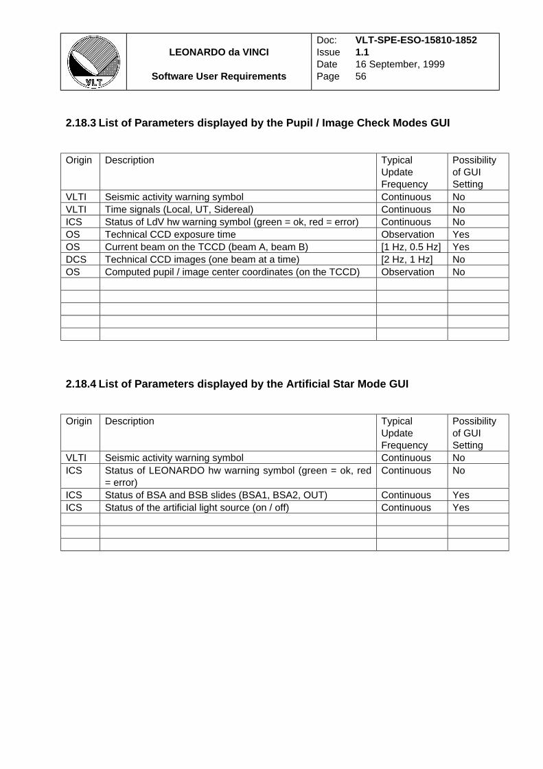
LEONARDO da VINCI
Software User Requirements
Doc:IssueDatePage
VLT-SPE-ESO-15810-18521.116 September, 199956
2.18.3 List of Parameters displayed by the Pupil / Image Check Modes GUI
Origin Description TypicalUpdateFrequency
Possibilityof GUISetting
VLTI Seismic activity warning symbol Continuous NoVLTI Time signals (Local, UT, Sidereal) Continuous NoICS Status of LdV hw warning symbol (green = ok, red = error) Continuous NoOS Technical CCD exposure time Observation YesOS Current beam on the TCCD (beam A, beam B) [1 Hz, 0.5 Hz] YesDCS Technical CCD images (one beam at a time) [2 Hz, 1 Hz] NoOS Computed pupil / image center coordinates (on the TCCD) Observation No
2.18.4 List of Parameters displayed by the Artificial Star Mode GUI
Origin Description TypicalUpdateFrequency
Possibilityof GUISetting
VLTI Seismic activity warning symbol Continuous NoICS Status of LEONARDO hw warning symbol (green = ok, red
= error)Continuous No
ICS Status of BSA and BSB slides (BSA1, BSA2, OUT) Continuous YesICS Status of the artificial light source (on / off) Continuous Yes
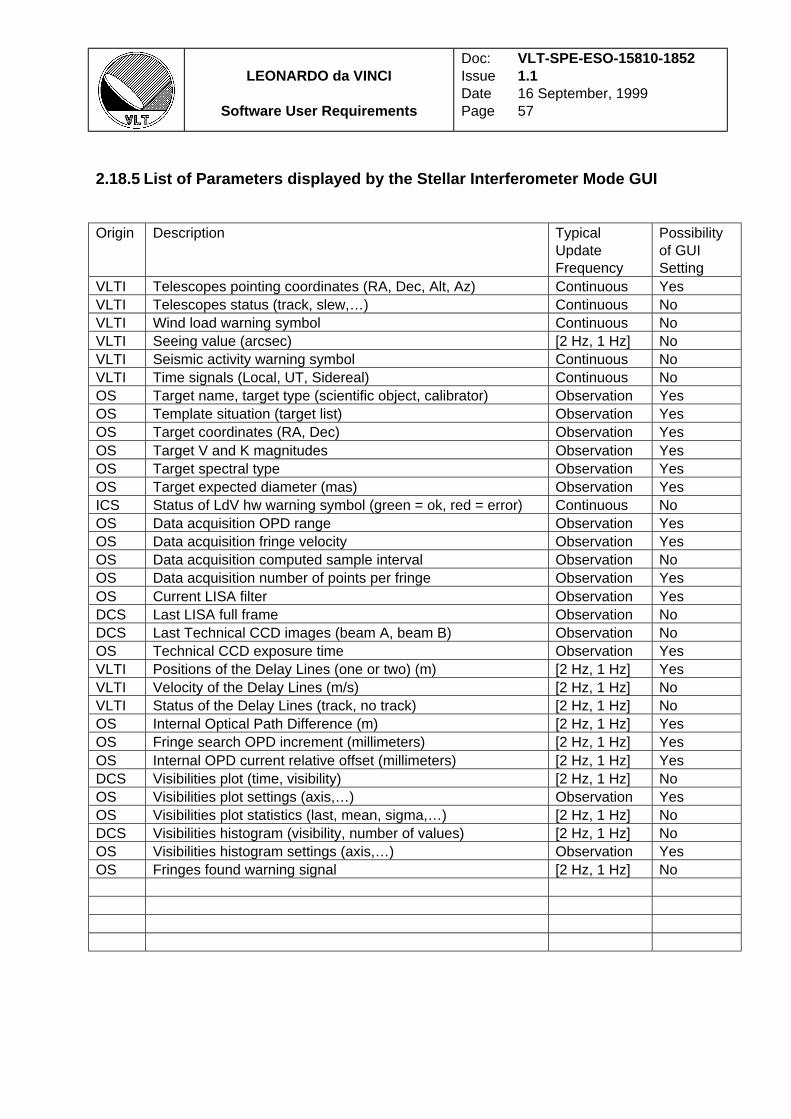
LEONARDO da VINCI
Software User Requirements
Doc:IssueDatePage
VLT-SPE-ESO-15810-18521.116 September, 199957
2.18.5 List of Parameters displayed by the Stellar Interferometer Mode GUI
Origin Description TypicalUpdateFrequency
Possibilityof GUISetting
VLTI Telescopes pointing coordinates (RA, Dec, Alt, Az) Continuous YesVLTI Telescopes status (track, slew,…) Continuous NoVLTI Wind load warning symbol Continuous NoVLTI Seeing value (arcsec) [2 Hz, 1 Hz] NoVLTI Seismic activity warning symbol Continuous NoVLTI Time signals (Local, UT, Sidereal) Continuous NoOS Target name, target type (scientific object, calibrator) Observation YesOS Template situation (target list) Observation YesOS Target coordinates (RA, Dec) Observation YesOS Target V and K magnitudes Observation YesOS Target spectral type Observation YesOS Target expected diameter (mas) Observation YesICS Status of LdV hw warning symbol (green = ok, red = error) Continuous NoOS Data acquisition OPD range Observation YesOS Data acquisition fringe velocity Observation YesOS Data acquisition computed sample interval Observation NoOS Data acquisition number of points per fringe Observation YesOS Current LISA filter Observation YesDCS Last LISA full frame Observation NoDCS Last Technical CCD images (beam A, beam B) Observation NoOS Technical CCD exposure time Observation YesVLTI Positions of the Delay Lines (one or two) (m) [2 Hz, 1 Hz] YesVLTI Velocity of the Delay Lines (m/s) [2 Hz, 1 Hz] NoVLTI Status of the Delay Lines (track, no track) [2 Hz, 1 Hz] NoOS Internal Optical Path Difference (m) [2 Hz, 1 Hz] YesOS Fringe search OPD increment (millimeters) [2 Hz, 1 Hz] YesOS Internal OPD current relative offset (millimeters) [2 Hz, 1 Hz] YesDCS Visibilities plot (time, visibility) [2 Hz, 1 Hz] NoOS Visibilities plot settings (axis,…) Observation YesOS Visibilities plot statistics (last, mean, sigma,…) [2 Hz, 1 Hz] NoDCS Visibilities histogram (visibility, number of values) [2 Hz, 1 Hz] NoOS Visibilities histogram settings (axis,…) Observation YesOS Fringes found warning signal [2 Hz, 1 Hz] No
LEONARDO da VINCI
Software User Requirements
Doc:IssueDatePage
VLT-SPE-ESO-15810-18521.116 September, 199958
2.18.6 Interface for the Engineering and Maintenance Modes
The Engineering Mode is generally speaking less complex than the Stellar Interferometer Mode.The user interface for this mode is basically the same as for the online modes, with access to allthe instrument parameters [Req. 48] , either via a GUI or a command line.
During the maintenance and setup procedures, the needs of the user are mainly to have fullcontrol on every element, possibly at the expense of the ease of use. The user interface for thismode is basically the same as for the engineering mode, with access to all the instrumentparameters, either via a GUI or a command line.
2.18.7 Setting up the Instrument Parameters
The instrument parameters for each standard setup, listed in the section 2.6, should be loadedafter the choice of the mode and optical setup of LdV (Autotest, Stellar Interferometer, PupilAlignment, Image Alignment). They will define the position of each hardware element (motor, lightswitches, piezos,…) for each mode. The operator should have access via the GUI to the differentparameters settings and be able to change them, even after a setup has been loaded [Req. 49] .
Use of encoder values to set the functions shall be possible via a dedicated “Hardware Setup”interface.
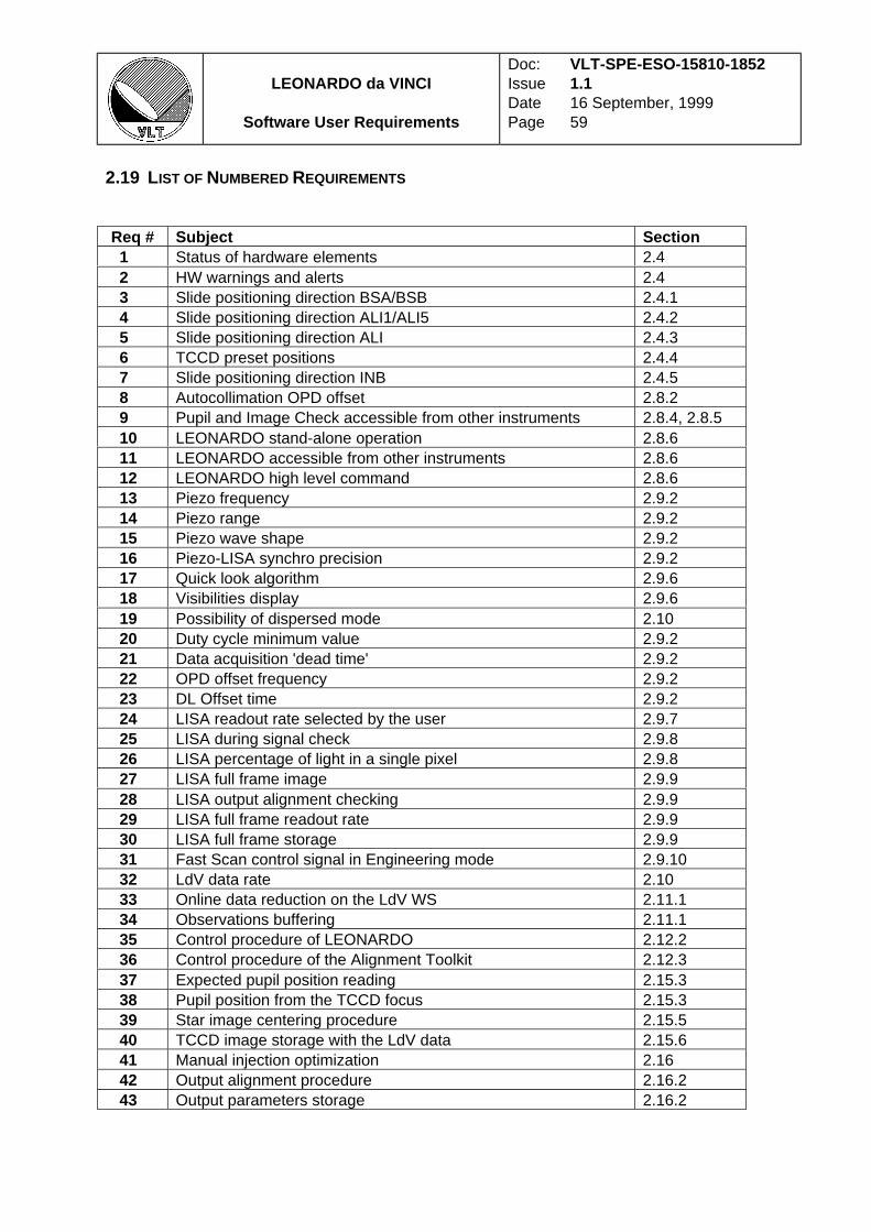
LEONARDO da VINCI
Software User Requirements
Doc:IssueDatePage
VLT-SPE-ESO-15810-18521.116 September, 199959
2.19 LIST OF NUMBERED REQUIREMENTS
Req # Subject Section1 Status of hardware elements 2.42 HW warnings and alerts 2.43 Slide positioning direction BSA/BSB 2.4.14 Slide positioning direction ALI1/ALI5 2.4.25 Slide positioning direction ALI 2.4.36 TCCD preset positions 2.4.47 Slide positioning direction INB 2.4.58 Autocollimation OPD offset 2.8.29 Pupil and Image Check accessible from other instruments 2.8.4, 2.8.510 LEONARDO stand-alone operation 2.8.611 LEONARDO accessible from other instruments 2.8.612 LEONARDO high level command 2.8.613 Piezo frequency 2.9.214 Piezo range 2.9.215 Piezo wave shape 2.9.216 Piezo-LISA synchro precision 2.9.217 Quick look algorithm 2.9.618 Visibilities display 2.9.619 Possibility of dispersed mode 2.1020 Duty cycle minimum value 2.9.221 Data acquisition 'dead time' 2.9.222 OPD offset frequency 2.9.223 DL Offset time 2.9.224 LISA readout rate selected by the user 2.9.725 LISA during signal check 2.9.826 LISA percentage of light in a single pixel 2.9.827 LISA full frame image 2.9.928 LISA output alignment checking 2.9.929 LISA full frame readout rate 2.9.930 LISA full frame storage 2.9.931 Fast Scan control signal in Engineering mode 2.9.1032 LdV data rate 2.1033 Online data reduction on the LdV WS 2.11.134 Observations buffering 2.11.135 Control procedure of LEONARDO 2.12.236 Control procedure of the Alignment Toolkit 2.12.337 Expected pupil position reading 2.15.338 Pupil position from the TCCD focus 2.15.339 Star image centering procedure 2.15.540 TCCD image storage with the LdV data 2.15.641 Manual injection optimization 2.1642 Output alignment procedure 2.16.243 Output parameters storage 2.16.2
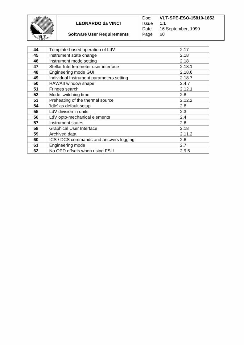
LEONARDO da VINCI
Software User Requirements
Doc:IssueDatePage
VLT-SPE-ESO-15810-18521.116 September, 199960
44 Template-based operation of LdV 2.1745 Instrument state change 2.1846 Instrument mode setting 2.1847 Stellar Interferometer user interface 2.18.148 Engineering mode GUI 2.18.649 Individual Instrument parameters setting 2.18.750 HAWAII window shape 2.4.751 Fringes search 2.12.152 Mode switching time 2.853 Preheating of the thermal source 2.12.254 'Idle' as default setup 2.855 LdV division in units 2.356 LdV opto-mechanical elements 2.457 Instrument states 2.658 Graphical User Interface 2.1859 Archived data 2.11.260 ICS / DCS commands and answers logging 2.661 Engineering mode 2.762 No OPD offsets when using FSU 2.9.5
LEONARDO da VINCI
Software User Requirements
Doc:IssueDatePage
VLT-SPE-ESO-15810-18521.116 September, 199961
2.20 SECOND GENERATION UPGRADES
In this section are described the functions and capabilities that are not necessary for VINCI towork, but which would improve its productivity and ease of use. They could be implemented as animprovement to the current concept after the first fringes have been obtained.
It is important to keep the necessary options opened in the software design.
2.20.1 Automated Injection Optimization
In this section, two possible algorithms for automatically peaking the alignment of the star into thefiber are described.
2.20.1.1 Fast image scan algorithm
This algorithm will work only if the motors of the INA1 and INB1 mirrors are replaced by piezos,which is not the case in the current implementation of LdV. It is taken from a proposal by SteveRidgway (NOAO).
The idea is to scan the image rapidly across the fiber in order to freeze the seeing. But then ittakes multiple scans to build up signal to noise. This is not a problem, because you really wantthe measurement to average over the seeing fluctuations.
Since you have a piezo control, it is possible to put a ramp signal on the piezo and scanrepeatedly the fiber head over a range of +/-1 arcsec. Synchronized with the scans, the signal iscoadded into a vector. When finished, you should have a peak in the vector which corresponds tothe nominal position. You can then move the piezo to the correct position. Then repeat in the otherdirection. This should be faster, more accurate and more sensitive than alignment by hand.
2.20.1.2 Slow image scan algorithm
Another possible scheme for the automated optimization of the injection in the fibers is :
1. Obtain quick exposures from the LISA camera in not synchronized mode , in order toobtain a nearly continuously (frequency of a few Hz) monitored value for the flux arriving onthe HAWAII detector. The maximization of this value will be the goal of the optimization.
2. Start a slow spiral motion of one of the injection mirrors, say INA1, to slowly move the
stellar image disk in front of the fiber head. During this motion, the intensity on the LISAcorresponding photometric and interferometric pixels is continuously monitored, as well asthe position of the tip and tilt motors. After the spiral motion has reached a radius of onespeckle cloud (~ 0.5-1 arcsec projected on the sky), the data acquired is an array of tip andtilt positions (in mm) associated with intensity values (in ADUs).
LEONARDO da VINCI
Software User Requirements
Doc:IssueDatePage
VLT-SPE-ESO-15810-18521.116 September, 199962
3. Do the same thing with the other injection mirror INB1, which gives you another arrayof (tip, tilt, intensity) values.
4. Fit the measured (tip, tilt, intensity) data with a 2 dimensional gaussian curve , inorder to find the precise position of the maximum intensities for the two beams. This givesthe offsets to apply to the injection optics to maximize the injected flux. The main source ofnoise is the intensity variations due to turbulence.
5. Correct the position with the tip-tilt mirrors : finally, the computed offsets are sent to theINA1 and INB1 mirrors.
6. Fringe search : At this stage, the injection should be optimized, and the fringe search canbegin.
2.20.2 Automated Output Alignment
This algorithm is TBD, but will be, for the focusing part, very similar to the TCCD focus algorithm.
For this procedure, LEONARDO artificial star is on (thermal light source).
The focus setting of the fiber output is remotely adjustable. The precise focusing of the four fiberoutputs on the LISA detector requires to monitor precisely their FWHM on LISA full frame images,and then to apply the necessary focus motion on the fiber bundle head OUT1.
To set the rotation of the fiber bundle, it is possible to monitor the light concentrated in the fourpixels corresponding to the light maxima, and to compare it with the flux in the surrounding pixels.The target here is to have as much of the incoming light concentrated on a single pixel of thedetector. This could result is positioning the four output pixels on four different lines and columns(i.e. on a square with non horizontal and vertical sides).
2.20.3 Spectral Dispersion
The optical design of LdV makes it possible to disperse the light from the four fiber outputs beforeit enters the LISA camera. This feature is very interesting, because it would greatly extend thecapabilities of LdV, in the field of stellar and extrasolar planets observations. It is thus important tokeep in mind that the LdV software has to be able to accommodate for four lines readout of LISAinstead of four pixels.
The dispersion would cover about 50 pixels. This would mean for the LdV software a proportionalincrease in the quantity of raw data produced. The LdV software should be able to read 200 (50x4)individual windows on the HAWAII detector. The fiber output alignment procedure would also beaffected in this configuration of the instrument.
2.20.4 Sensors

LEONARDO da VINCI
Software User Requirements
Doc:IssueDatePage
VLT-SPE-ESO-15810-18521.116 September, 199963
A number of optical elements are moved manually. If they are forgotten in a wrong position, thiscould cause data to be lost. The monitoring of their position, with the possibility to send alerts tothe user in case of mispositioning, might be required in order to ensure the reliable operation ofthe instrument.
The particular question of the fiber type sensors is adressed here with respect to the referencedocument [7]. They are not essential for the operation of the instrument, but they could make theoperation of LdV easier and more straightforward. In the following table, the name of each fiberconnector to be monitored is indicated in the column 'Measured Physical Parameter' (for example,the ART3 connector on the artificial source,…). The names of the fibers that can be plugged oneach connector are listed in the column 'value' (for example, it is possible to plug WG1X1,
WG1X2, WG2X1, WG2F1, WG2F2,… on the ART3 connector). Each fiber is designated by itscoded name (for example WG1X2 means WaveGuide 1 connected to the X coupler number 2 onone end).
Measured Physical
ParameterMeasuredevery…
Range/Values Comments
ART3 FIBER Observation WG1X1, WG1X2,WG2X1, WG2F1,
WG2F2, WG2F3,
WG2F4, WG2F5,WG2F6, WG2F7,
WG3F1, WG3F2,
WG3F3, WG3F4,
WG3F5, WG3F6,WG3F7, WG4F1,
WG4F2
The main light source fiberfeed
ART2 FIBER Observation WG1X2, WG2X1,WG3F1, WG4F1,
WG5F1
Focus of parabola ART1
INA2 FIBER Observation WG1X1, WG2F2 Focus of parabola INA1
INB2 FIBER Observation WG2F6, WG3F6 Focus of parabola INB1
MONA IN 1 FIBER
(A BEAM)
Observation WG1X2, WG2F4,
WG3F2
Injection of light from the “in”
side of MONA, beam A
MONA IN 2 FIBER(B BEAM)
Observation WG1X2, WG2F5,WG3F3
Injection of light from the “in”side of MONA, beam B
MONA OUT 1 FIBER (A
BEAM)
Observation WG2X1, WG3F4 Injection of light from the
“out” side of MONA, beam A
MONA OUT 2 FIBER (BBEAM)
Observation WG2X1, WG3F5 Injection of light from the“out” side of MONA, beam B
OUT1 FIBER Observation WG2F6, WG2F7,
WG3F6, WG3F7
Output of the MONA box (4
fibers bundle)
COMA3 POSITION Night IN, OUT Present in normal operations
COMB3 POSITION Night IN, OUT Present in normal operations
LEONARDO da VINCI
Software User Requirements
Doc:IssueDatePage
VLT-SPE-ESO-15810-18521.116 September, 199964
ALI9 POSITION Night IN, OUT Used only for engineering
2.20.5 Photometric Calibrations for the TCCD
At the beginning of the night, it would be interesting to obtain flat field images of the bright skywith the TCCD in order to calibrate the images obtained during the night. Once the objectimage has been acquired, a dark field should be acquired, of the same exposure duration asthe object exposure, to be substracted from the object image.
Moreover, it is desirable to obtain once or twice per night the image of a photometric reference,in order to estimate broadband magnitudes of the targets. The procedure to obtain thesemeasurements is not different from the pointing of the science targets. The desired magnitudeprecision is 0.1 mag. It is understood that this magnitude is not directly comparable to thestandard systems magnitudes, as it is a broadband integration, based on the sensitivity curveof the TCCD. This measurement could be useful to estimate the parameters for the infraredcamera exposures.

Page laissée vierge intentionnellement

7
3. LISA Test Report

8
E U R O P E A N S O U T H E R N O B S E R V A T ORY
Organisation Européenne pour des Recherches Astronomiques dans l'Hémisphère Austral
Europäische Organisation für astronomische Forschung in der südlichen Hemisphäre
VERY LARGE TELESCOPE
LEONARDO da VINCI
LISA Test Report
Doc. No.: VLT-TRE-ESO-15810-2330
Issue: 1.0
Date: 5 October, 2000
Prepared: P. Kervella. . . . . . . . . . . . . . . . . . . . . . . . . . . . . . . . . . . . . . . . . . . . . . . . . . . . . . . . . . . . . . .
Name Date Signature
Approved: A. Glindemann. . . . . . . . . . . . . . . . . . . . . . . . . . . . . . . . . . . . . . . . . . . . . . . . . . . . . . . . . . . . . . .
Name Date Signature
Released: M. Tarenghi. . . . . . . . . . . . . . . . . . . . . . . . . . . . . . . . . . . . . . . . . . . . . . . . . . . . . . . . . . . . . . .
Name Date Signature
VLT PROGRAMME * TELEPHONE: (089) 3 20 06-0 * FAX: (089) 3 20 23 62
LISA Test ReportDoc:IssueDatePage
VLT-TRE-ESO-15810-2330
1.0
5 October, 2000i
CHANGE RECORD
Issue Date Section/Page affected Reason/ Initiation/Remarks1.0
draft
1.2
draft
2.0
draft
1.0
7 August, 2000
6 September, 2000
21 September, 2000
5 October, 2000
All
All
Sections 5, 6, 10, 11
Sections 6-9
First draft, alignment procedure.
Includes first tests with the windowed
readout mode.
Detector tests using the 64x64 pixels
and windowed readout modes.
The results obtained with the
chopping device (memory effect) are
included, and the filter wheel order is
corrected. Readout noise level error
corrected.
LISA Test ReportDoc:IssueDatePage
VLT-TRE-ESO-15810-2330
1.0
5 October, 2000ii
TABLE OF CONTENTS
1. INTRODUCTION ......................................................................................................................................... 3
1.1 SCOPE ...................................................................................................................................................... 3
1.2 GENERAL PHILOSOPHY ........................................................................................................................... 3
1.3 APPLICABLE DOCUMENTS ....................................................................................................................... 3
1.4 REFERENCE DOCUMENTS ........................................................................................................................ 3
1.5 ABBREVIATIONS AND ACRONYMS.......................................................................................................... 3
2. DEWAR GENERAL CHARACTERISTICS ............................................................................................ 5
2.1 COLD TEMPERATURE AUTONOMY........................................................................................................... 5
2.2 NITROGEN FILLING.................................................................................................................................. 5
2.3 VACUUM TIGHTNESS ............................................................................................................................... 5
3. MECHANICAL ALIGNMENT .................................................................................................................. 6
3.1 DESCRIPTION ........................................................................................................................................... 6
3.2 ALIGNMENT PROCEDURE ........................................................................................................................ 6
4. DOUBLET FOCUSING ............................................................................................................................... 8
4.1 ALIGNMENT PROCEDURE ........................................................................................................................ 8
4.2 FOCUSING PROCEDURE............................................................................................................................ 9
4.3 EXPERIMENTAL RESULTS ........................................................................................................................ 9
4.4 FOCUS CORRECTION TO APPLY TO THE DOUBLET................................................................................. 11
4.5 RESULT OF THE FOCUSING .................................................................................................................... 11
4.5.1 Procedure .................................................................................................................................... 11
4.5.2 Intensity profiles .......................................................................................................................... 12
4.5.3 Energy in the target pixel............................................................................................................ 12
4.5.4 Optical efficiency......................................................................................................................... 13
4.6 PROBLEMS ............................................................................................................................................. 13
4.6.1 Clamping of the camera mount................................................................................................... 13
4.6.2 Sign of the ADU counts ............................................................................................................... 13
4.6.3 Filters order in the filter wheel................................................................................................... 13
4.6.4 Connector surface ....................................................................................................................... 14
4.6.5 Camera mount stability ............................................................................................................... 14
5. OPTICAL AND BASIC DETECTOR TESTS ........................................................................................ 15
5.1 FIELD OF VIEW....................................................................................................................................... 15
5.1.1 Description .................................................................................................................................. 15
5.1.2 Procedure .................................................................................................................................... 15
5.1.3 Diffuse illumination..................................................................................................................... 15
5.1.4 Focused saturated spot ............................................................................................................... 15
5.1.5 To be checked: Usable detector area ......................................................................................... 16
5.2 BACKGROUND LEVEL ............................................................................................................................ 18
5.3 DETECTOR READOUT NOISE IN FULL FRAME MODE .............................................................................. 20
5.3.1 Aproximate gain factor ............................................................................................................... 21
5.3.2 Readout noise in full quadrant mode (512x512 pixels) ............................................................. 21
5.4 READOUT MODES .................................................................................................................................. 21
5.4.1 List of modes................................................................................................................................ 21
5.4.2 Off-line windows generator ........................................................................................................ 22
5.4.3 Full quadrant, double correlated................................................................................................ 22
5.4.4 64x64 window, double correlated............................................................................................... 22
5.4.5 Windowed readout, double correlated ....................................................................................... 225.4.5.1 Beampix data..........................................................................................................................................23
5.4.5.2 Flux data .................................................................................................................................................24
5.4.5.3 Quicklook data .......................................................................................................................................24
6. READOUT FREQUENCIES..................................................................................................................... 25
6.1 INTRODUCTION...................................................................................................................................... 25
LISA Test ReportDoc:IssueDatePage
VLT-TRE-ESO-15810-2330
1.0
5 October, 2000iii
6.2 EFFECTIVE MAXIMAL READOUT FREQUENCIES .................................................................................... 25
7. BEST PHOTOSITES SELECTION ......................................................................................................... 26
7.1 PRINCIPLE.............................................................................................................................................. 26
7.2 PIXEL GAINS .......................................................................................................................................... 26
7.2.1 Measurement procedure.............................................................................................................. 26
7.2.2 Examples of gain curves.............................................................................................................. 26
7.2.3 Gain map ..................................................................................................................................... 28
7.2.4 Histogram of pixel gains ............................................................................................................. 29
7.3 PIXEL READOUT NOISES ........................................................................................................................ 29
7.3.1 Measurement procedure.............................................................................................................. 29
7.3.2 Readout noise map ...................................................................................................................... 30
7.3.3 Histogram of pixel readout noises.............................................................................................. 30
7.3.4 Readout noise at the highest frame frequency............................................................................ 31
7.4 PIXEL NOISE POWER SPECTRAL DENSITY ............................................................................................ 31
7.4.1 Low frequency (0–3.33 Hz)......................................................................................................... 327.4.1.1 Data analysed .........................................................................................................................................32
7.4.1.2 Examples of individual pixels PSD.......................................................................................................32
7.4.1.3 Median low frequency PSD over the 64x64 pixels ..............................................................................33
7.4.2 High frequency (0–828 Hz)......................................................................................................... 347.4.2.1 Data analysed .........................................................................................................................................34
7.4.2.2 Example of pixel [33,38] .......................................................................................................................34
7.4.3 Maximum frequency (0–1223 Hz)............................................................................................... 357.4.3.1 Data analysed .........................................................................................................................................35
7.4.3.2 Example of pixel [33,38] .......................................................................................................................35
7.5 DISCUSSION ........................................................................................................................................... 36
8. INDIUM LAYER STABILITY ................................................................................................................. 37
9. MEMORY EFFECT ................................................................................................................................... 38
9.1 DESCRIPTION ......................................................................................................................................... 38
9.2 MEASUREMENT PROCEDURE................................................................................................................. 38
9.3 GEOMETRY OF THE CHOPPING SYSTEM................................................................................................. 38
9.4 DATA REDUCTION ................................................................................................................................. 39
9.5 DISCUSSION ........................................................................................................................................... 40
10. SUMMARY OF PROBLEMS............................................................................................................... 41
11. APPENDIX: IDL SIGNAL PROCESSING PROCEDURES........................................................... 42
11.1 READ DATA....................................................................................................................................... 42
11.2 PROCESS 64X64 DATA ...................................................................................................................... 43
11.3 PROCESS SCANS ................................................................................................................................ 44
11.4 PLOT 64X64 DATA ............................................................................................................................ 46
11.5 PLOT SCAN DATA .............................................................................................................................. 47
11.6 TRANSFER FUNCTION COMPUTATION............................................................................................... 48
11.7 MODEL GENERATION........................................................................................................................ 49
11.8 TRANSFER FUNCTION PLOT .............................................................................................................. 50
LISA Test ReportDoc:IssueDatePage
VLT-TRE-ESO-15810-2330
1.0
5 October, 20001
Figures
Figure 1. LISA Nitrogen consumption 5Figure 2. LISA installed on its support. 6Figure 3. Example of a focusing done by moving the fiber (test #7, X scale in tens of microns, Y in ADUs). 10Figure 4. Direction of the applied focus motion 11Figure 5. Image of the OUT fiber as seen on the detector of LISA. The fiber core (bright, saturated point near
center, should be dark if not saturated) is surrounded by the envelope (dark), and the surface of theconnector (brighter halo). The scale being inverted, the connector appears in reality darker than thebackground. 14
Figure 6. The HAWAII array. LISA detector uses quadrant IV (picture from Rockwell). The X axis of the LISAcamera is along the fast shift register (positive direction), and the Y axis is along the slow shift register(positive direction). 17
Figure 7. LISA Hawaii detector usable part 17Figure 8. Zoom on the usable part of the array. 18Figure 9. Variation of the background due to stray light from a soldering iron about 25 degrees off axis. The
curves correspond to three different test sequences. 19Figure 10. Background with cold shutter closed (Mean = 19.28, RMS = 2.07 ADUs) . 19Figure 11. LISA cold mechanics and baffling, seen from the front (photo MPE). 20Figure 12. LISA detector support and baffling, seen from the back (photo MPE). 20Figure 13. Variance as a function of signal for LISA. The slope is 0.1182, giving a gain factor of 2.9
electrons/ADU. X axis is the mean signal in ADU. Y axis is the observed variance of the temporal sequencein ADU2. 21
Figure 14. LISA windowed mode readout order. 23Figure 15. Gain plot for pixel [31,38] (G=5.1096) 27Figure 16. Gain plot for pixel [32,38] (G=6.8939) 27Figure 17. Gain plot for pixel [33,38]. (G=6.9652) 28Figure 18. Gain map over the 64x64 pixels lower left area. Pixel [0,0] is in the lower left corner, X axis is to
directed the right, Y to the top. 29Figure 19. Histogram of the 64x64 lower left pixels gains (measured at 6.66 Hz frame frequency). 29Figure 20. Readout noise map of the lower left 64x64 area, at 6.66 Hz frame frequency. The image grey scale is
linear between 0 and 30 electrons. 30Figure 21. Histogram of pixel readout noises at 6.66 Hz frame frequency. The median value is 20.18 e-, and the
maximum number of pixels is found at 18 e-. There are still a number of pixels at less than 15 e-. 31Figure 22. Power spectral density for pixel [31,38] from 0 to 3.33 Hz (X=128). Y scale arbitrary. 32Figure 23. PSD for pixel [32,38] from 0 to 3.33 Hz (X=128). Y scale arbitrary. 33Figure 24. PSD for pixel [33,38] from 0 to 3.33 Hz (X=128). Y scale arbitrary. 33Figure 25. Median Power Spectral Density for the 64x64 pixels, from 0 to 3.33 Hz (X=128). The Y scale is
arbitrary. 34Figure 26. Overview of the PSD for pixel [33,38] read at 1656 Hz frame rate (frequencies between 0 and 828
Hz). The shutter was open (background light present), but the fiber spot was not illuminated. The largepeak on the left is precisely in the bin containing the 100 Hz frequency. (mean over 20 scans). 35
Figure 27. Power spectral density at maximum acquisition frequency for pixel [33,38], with cold shutter closed.Notice the overall very low level compared to the previous case (1656 Hz frequency). Ths frequencies of thepeaks are mostly multiples of 50 Hz, therefore suspected to be associated with power supply pickups(grounding problems ?). 36
Figure 28. Chopper geometrical configuration. 39Figure 29. Modulation transfer function of the LISA camera (spikes) compared to a perfect integrator (solid
line). 40
Tables
Table 1. Fiber head motion to obtain the focus on the Hawaii array. 9Table 2. Result of the in-focus test on LISA. 13Table 3. Filters positions in the filter wheel. 13Table 4. LISA readout modes 22Table 5. Maximum readout frequencies for LISA 25

LISA Test ReportDoc:IssueDatePage
VLT-TRE-ESO-15810-2330
1.0
5 October, 20002
Table 6. Modulation transfer function of LISA 40Table 7. Apparent problems in the LISA system during the tests in Garching. 41Table 8. Points to be clarified 41

LISA Test ReportDoc:IssueDatePage
VLT-TRE-ESO-15810-2330
1.0
5 October, 20003
1. INTRODUCTION
1.1 SCOPE
This document describes both the procedures and results of the tests conducted on the LISA camera inGarching, using the collimated light source provided by the Observatoire de Paris-Meudon.
1.2 GENERAL PHILOSOPHY
VINCI makes a particular use of the HAWAII detector of LISA, reading only a few of its pixels at a highfrequency. The tests described here aim at validating both the optical concept and performances of thecamera.
These tests are preliminary to the acceptance of LISA in Garching and also to the AIV of the wholeLEONARDO da VINCI instrument.
1.3 APPLICABLE DOCUMENTS
1. LISA Maintenance Manual (Draft), MPE 06/2000
2. LISA User’s Manual (Draft), MPE 06/2000
3. LISA Acceptance Plan (Draft), MPE 06/2000
4. LISA Drawings, MPE 06/2000
5. LISA Statement of Work VLT-SOW-ESO-15810-1xxx v.1.0 28/07/1999
6. LISA Technical Specifications VLT-SPE-ESO-15810-1xxx v.1.0 31/08/1999
7. OUT Alignment Procedure, DESPA 17/07/2000
8. ICD between VLTI and Instruments VLT-ICD-ESO-15000-1826 v.1.0 16/11/1999
1.4 REFERENCE DOCUMENTS
1.5 ABBREVIATIONS AND ACRONYMS
ADU Analog Digital UnitAIV Assembly, Integration and VerificationALIU The Alignment UnitDCS Detector Control SoftwareDP Data Pipeline
LISA Test ReportDoc:IssueDatePage
VLT-TRE-ESO-15810-2330
1.0
5 October, 20004
GUI Graphical User InterfaceGEI Graphical Engineering InterfaceGOL Garching Optical LaboratoryHW HardwareICS Instrument Control SoftwareIRTD Infrared Real Time DisplayIWS Instrument WorkstationLCU Local Control UnitLdV LEONARDO da VINCI, the whole instrumentLEONARDO The artificial star subsystemLISA The HAWAII-based infrared cameraLISA WS The LISA LCU (workstation)MONA The fibered recombinerN.A. Not applicableOPD Optical Path DifferenceOS Observation SoftwareROF Raw Observation FileSNR Signal to Noise RatioSW SoftwareTBC To Be ConfirmedTBD To Be DefinedTCCD ESO Technical CCDVINCI The main optical table of LdVWS Workstation
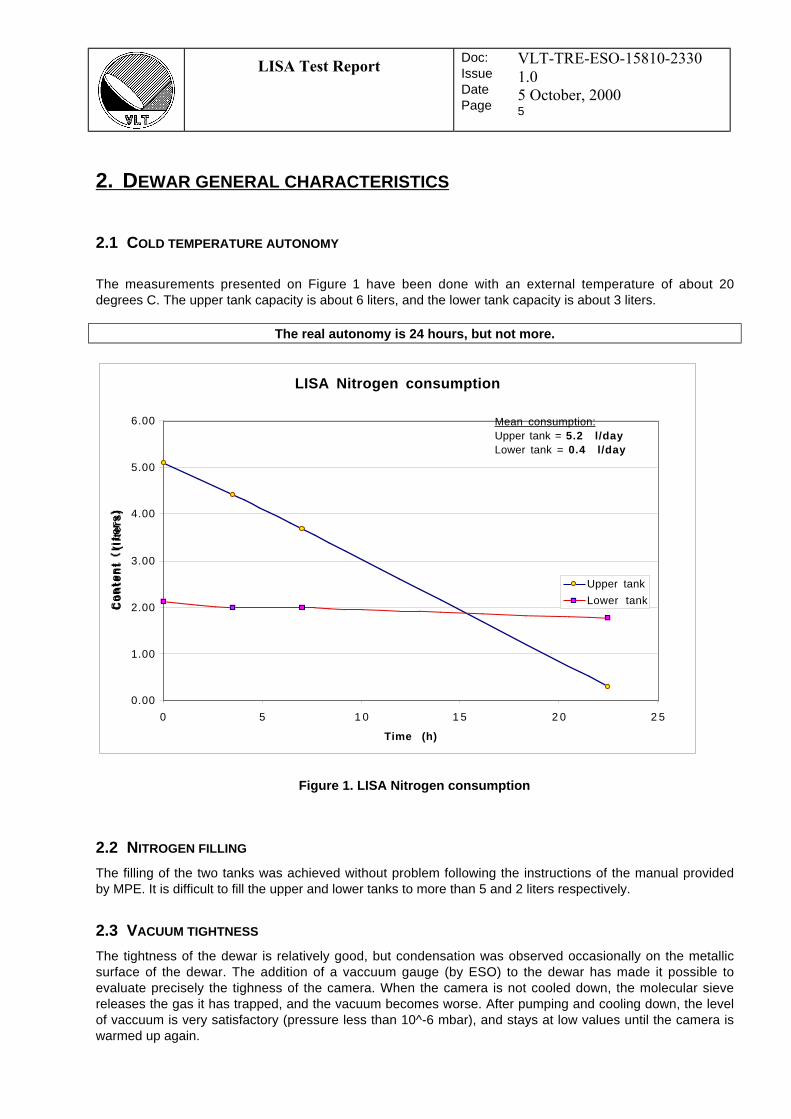
LISA Test ReportDoc:IssueDatePage
VLT-TRE-ESO-15810-2330
1.0
5 October, 20005
2. DEWAR GENERAL CHARACTERISTICS
2.1 COLD TEMPERATURE AUTONOMY
The measurements presented on Figure 1 have been done with an external temperature of about 20degrees C. The upper tank capacity is about 6 liters, and the lower tank capacity is about 3 liters.
The real autonomy is 24 hours, but not more.
LISA Nitrogen consumption
0.00
1.00
2.00
3.00
4.00
5.00
6.00
0 5 1 0 1 5 2 0 2 5
Time (h)
Co
nte
nt
(lit
ers
)
Upper tank
Lower tank
Mean consumption:Upper tank = 5.2 l/dayLower tank = 0.4 l/day
2.2 NITROGEN FILLING
The filling of the two tanks was achieved without problem following the instructions of the manual providedby MPE. It is difficult to fill the upper and lower tanks to more than 5 and 2 liters respectively.
2.3 VACUUM TIGHTNESS
The tightness of the dewar is relatively good, but condensation was observed occasionally on the metallicsurface of the dewar. The addition of a vaccuum gauge (by ESO) to the dewar has made it possible toevaluate precisely the tighness of the camera. When the camera is not cooled down, the molecular sievereleases the gas it has trapped, and the vacuum becomes worse. After pumping and cooling down, the levelof vaccuum is very satisfactory (pressure less than 10^-6 mbar), and stays at low values until the camera iswarmed up again.
Figure 1. LISA Nitrogen consumption
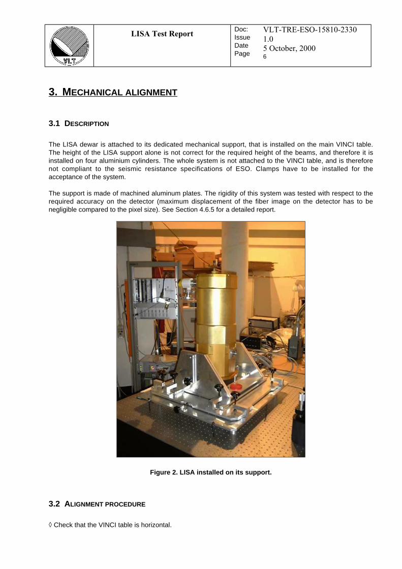
LISA Test ReportDoc:IssueDatePage
VLT-TRE-ESO-15810-2330
1.0
5 October, 20006
3. MECHANICAL ALIGNMENT
3.1 DESCRIPTION
The LISA dewar is attached to its dedicated mechanical support, that is installed on the main VINCI table.The height of the LISA support alone is not correct for the required height of the beams, and therefore it isinstalled on four aluminium cylinders. The whole system is not attached to the VINCI table, and is thereforenot compliant to the seismic resistance specifications of ESO. Clamps have to be installed for theacceptance of the system.
The support is made of machined aluminum plates. The rigidity of this system was tested with respect to therequired accuracy on the detector (maximum displacement of the fiber image on the detector has to benegligible compared to the pixel size). See Section 4.6.5 for a detailed report.
3.2 ALIGNMENT PROCEDURE
◊ Check that the VINCI table is horizontal.
Figure 2. LISA installed on its support.

LISA Test ReportDoc:IssueDatePage
VLT-TRE-ESO-15810-2330
1.0
5 October, 20007
◊ Set all the mechanical adjustments of the LISA camera to central position.
◊ Check that the LISA support bottom plate is horizontal, relatively to the VINCI table. For this, use a slidecaliper to measure the height of the four corners of the support relatively to the VINCI optical table.
◊ Check that the upper plate of the dewar is horizontal (with a bubble level). Pay special attention to thesetting of:- the “cradle” part of the support,- the direction pointed by the dewar window.These two settings directly impact the position of the beam on the detector.
◊ Measure the height of the entrance window of LISA and of the output mirror of the artificial light sourceOUT relatively to the VINCI table surface. This can be done directly by using a square and measuring theheight from the table surface, or by using a slide caliper to measure the heights of all the supports. Thecenter of the dewar window is located aproximately 149 mm above the bottom surface of the dewar.
◊ Adjust if necessary of the height of LISA, by using the three pads below the dewar. Be careful to maintainthe same height for all pads. The height of the center of the entrance window of the dewar should be 320mm.
◊ Check precisely the horizontality of the off-axis parabola using the two reference pods on the back of itssupport. This can be done with a micrometric comparator or, as an alternative, with a precise slide caliper.The reference for the measurement should be the optical table itself, but as a second choice, the base plateof the OUT source can also be used.

LISA Test ReportDoc:IssueDatePage
VLT-TRE-ESO-15810-2330
1.0
5 October, 20008
4. DOUBLET FOCUSING
4.1 ALIGNMENT PROCEDURE
◊ Collimate roughly the artificial light source following the Meudon procedure (on a distant wall for example).The adjustement is done by moving the fiber head itself. The image produced by the laser should be a tinyspot of light less than 1 mm across, with round shape and sharp edge. Two small, fainter dots on each sideof the main spot should be visible (they are due to the microgrooves of the off axis parabola). Turn back thesource in the correct direction.
◊ Measure the relative positions of the two benches on the VINCI table. The references are the center of theLISA dewar window and the center of the OUT2 flat mirror. The precision required depends on the distancebetween the source and the dewar (the further, the lower the required precision). A precision better than 1mm (relatively to the table edge) should be sufficient assuming a distance of 1 or 2 m between LISA andOUT2.
◊ Send the laser in the OUT system and adjust the OUT2 mirror only to have the red dot centered on theentrance window of the LISA camera. This will set the reference for the alignment of the optical axis of theautocollimator. Be careful to switch off the laser after use.
◊ Install the autocollimator and adjust its height precisely. For that it is necessary to have a correcthorizontality of the autocollimator optical axis. There is an integrated bubble level for that purpose. Theheight of the center of the input lens should be set at 320 mm above the table surface.
◊ Position the axis of the autocollimator between the OUT2 mirror and the LISA camera window (mmprecision). This part is not very easy, as there is no reference to set the direction of the refractor. Onepossible method is to use the laser of the OUT source:
- send the laser light into the OUT source,- check that the laser dot is at the center of the entrance lens of the autocollimator, but do not look
into the eyepiece ,- be careful to switch the laser off and plug in the thermal light source,- do a first rough autocolimation of the refractor by using a flat mirror in front of the entrance lens.
The goal here is to focus the image of the cross.- while looking into the eyepiece, move the back of the autocollimator until you can see the fiber
head near the center of the autocollimator,
◊ Do a second autocollimation to focus precisely the autocollimator to infinity.
◊ Move the OUT2 mirror to center the fiber image on the cross of the autocollimator.
◊ Adjust finely the fiber position to have a focused, aberration-free fiber image in the autocollimator. Theaberration-free field of the off-axis parabola is only of the size of the fiber core , so the precision ofpositioning must be very good. The image should be a small yellowish disk of light, with round shape andclean edge. If the fiber is moved vertically or laterally, use the OUT2 mirror to center the image back on thecenter of the autocollimator field of view.
◊ Note the exact focus position of the micrometric knob used to move the fiber in focus (and also in otherdirections). This measurement can be done to a precision of 1 micron on the adjustment knob. Be careful tohave a precise reading.
◊ Remove the autocollimator from the beam. There should be a somewhat fuzzy image on the LISAdetector.
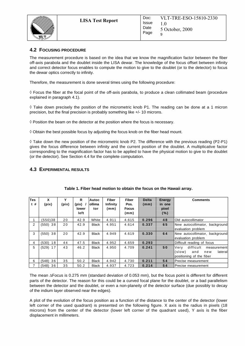
LISA Test ReportDoc:IssueDatePage
VLT-TRE-ESO-15810-2330
1.0
5 October, 20009
4.2 FOCUSING PROCEDURE
The measurement procedure is based on the idea that we know the magnification factor between the fiberoff-axis parabola and the doublet inside the LISA dewar. The knowledge of the focus offset between infinityand correct detector focus enables to compute the motion to give to the doublet (or to the detector) to focusthe dewar optics correctly to infinity.
Therefore, the measurement is done several times using the following procedure:
◊ Focus the fiber at the focal point of the off-axis parabola, to produce a clean collimated beam (procedureexplained in paragraph 4.1).
◊ Take down precisely the position of the micrometric knob P1. The reading can be done at a 1 micronprecision, but the final precision is probably something like +/- 10 microns.
◊ Position the beam on the detector at the position where the focus is necessary.
◊ Obtain the best possible focus by adjusting the focus knob on the fiber head mount.
◊ Take down the new position of the micrometric knob P2. The difference with the previous reading (P2-P1)gives the focus difference between infinity and the current position of the doublet. A multiplicative factorcorresponding to the magnification factor has to be applied to have the physical motion to give to the doublet(or the detector). See Section 4.4 for the complete computation.
4.3 EXPERIMENTAL RESULTS
Test #
X(pix)
Y(pix)
R(pix) /lowerleft
Autocollima
tor
FiberInfinity(mm)
FiberPos.
Focus(mm)
Delta(mm)
Energyin onepixel(%)
Comments
1 (550)38 2 0 42.9 White 4.911 4.615 0.296 4 8 Old autocollimator2 (550) 3 8 2 0 42.9 Black 4.951 4.614 0.337 6 5 New autocollimator, background
evaluation problem3 (550) 3 8 2 0 42.9 Black 4.949 4.619 0.330 6 4 New autocollimator, background
evaluation problem4 (530) 1 8 4 4 47.5 Black 4.952 4.659 0.293 Difficult reading of focus5 (529) 1 7 4 3 46.2 Black 4.950 4.709 0.241 5 0 Very di f f icul t measurement
(s low) and n e w lateralpositioning of the fiber
6 (548) 3 6 3 5 50.2 Black 4.942 4.730 0.211 5 4 Precise measurement7 (548) 3 6 3 5 50.2 Black 4.937 4.723 0.214 5 4 Precise measurement
The mean ∆Focus is 0.275 mm (standard deviation of 0.053 mm), but the focus point is different for differentparts of the detector. The reason for this could be a curved focal plane for the doublet, or a bad parallelismbetween the detector and the doublet, or even a non-planeity of the detector surface (due possibly to decayof the indium layer observed near the edges).
A plot of the evolution of the focus position as a function of the distance to the center of the detector (lowerleft corner of the used quadrant) is presented on the following figure. X axis is the radius in pixels (18microns) from the center of the detector (lower left corner of the quadrant used), Y axis is the fiberdisplacement in millimeters.
Table 1. Fiber head motion to obtain the focus on the Hawaii array.

LISA Test ReportDoc:IssueDatePage
VLT-TRE-ESO-15810-2330
1.0
5 October, 200010
Delta focus
0.000
0.050
0.100
0.150
0.200
0.250
0.300
0.350
0.400
42.0 43.0 44.0 45.0 46.0 47.0 48.0 49.0 50.0 51.0
Delta (millimeters) = -0.01408 R(pixels of 18 microns) + 0 .924
Using this formula, it is possible to compute the focus correction to give to the doublet (or to the detector),depending on the part of the detector that will be used for the actual observations. Though, it is necessary toevaluate the usable area of the detector to determine the best focus to apply.
Intensity
-12000
-11000
-10000
-9000
-8000
-7000
-6000
-5000
1 5 2 0 2 5 3 0
Intensity
The direction of the focus motion necessary is towards the off axis parabola (See Figure 4 ).
Figure 3. Example of a focusing done by moving the fiber (test #7, X scale in tens of microns, Y inADUs).
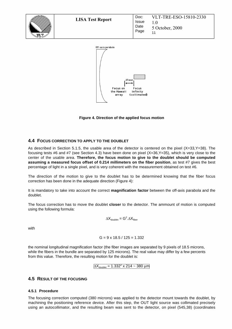
LISA Test ReportDoc:IssueDatePage
VLT-TRE-ESO-15810-2330
1.0
5 October, 200011
4.4 FOCUS CORRECTION TO APPLY TO THE DOUBLET
As described in Section 5.1.5, the usable area of the detector is centered on the pixel (X=33,Y=38). Thefocusing tests #6 and #7 (see Section 4.3) have been done on pixel (X=36,Y=35), which is very close to thecenter of the usable area. Therefore, the focus motion to give to the doublet should be computedassuming a measured focus offset of 0.214 millimeters on the fiber position , as test #7 gives the bestpercentage of light in a single pixel, and is very coherent with the measurement obtained on test #6.
The direction of the motion to give to the doublet has to be determined knowing that the fiber focuscorrection has been done in the adequate direction (Figure 4):
It is mandatory to take into account the correct magnification factor between the off-axis parabola and thedoublet.
The focus correction has to move the doublet closer to the detector. The ammount of motion is computedusing the following formula:
∆Xdoublet = G2.∆Xfiber
with
G = 9 x 18.5 / 125 = 1.332
the nominal longitudinal magnification factor (the fiber images are separated by 9 pixels of 18.5 microns,while the fibers in the bundle are separated by 125 microns). The real value may differ by a few percentsfrom this value. Therefore, the resulting motion for the doublet is:
∆Xdoublet = 1.3322 x 214 ~ 380 µm
4.5 RESULT OF THE FOCUSING
4.5.1 Procedure
The focusing correction computed (380 microns) was applied to the detector mount towards the doublet, bymachining the positioning reference device. After this step, the OUT light source was collimated preciselyusing an autocollimator, and the resulting beam was sent to the detector, on pixel (545,38) (coordinates
Figure 4. Direction of the applied focus motion

LISA Test ReportDoc:IssueDatePage
VLT-TRE-ESO-15810-2330
1.0
5 October, 200012
(33,38) from the lower left corner of the detector, corresponding to the center of the usable field. The beamposition was adjusted at sub-pixel precision to maximize the flux in the target pixel.
4.5.2 Intensity profiles
The resulting profiles in the X and Y directions are presented in the following figures (measurement #10). Inthis measurement, the 64x64 window readout mode was used at the maximum frequency. The spot was notsaturated on the detector.
4.5.3 Energy in the target pixel
The energy contained in the target pixel is 56 % (see Table 2), for test #10 (the most significant). This resultis about the same as for the best focus obtained previously (tests #6 and #7). It is suspected that theprevious tests were done with the detector in the saturated regime, on the strongly non linear part of thesensitivity curve, but the focusing could (fortunately) still be achieved correctly in this regime.
Intensity (ADU) along column X=33
-7000
-5000
-3000
-1000
1000
36 37 38 39 40
Y
Intensity (ADU), along line Y=38
-7000
-5000
-3000
-1000
1000
3 1 3 2 3 3 3 4 3 5
X
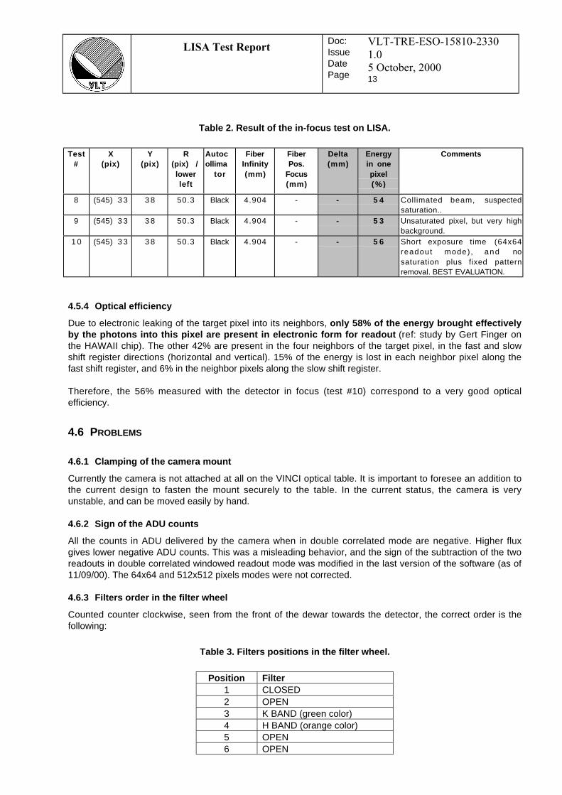
LISA Test ReportDoc:IssueDatePage
VLT-TRE-ESO-15810-2330
1.0
5 October, 200013
Test#
X(pix)
Y(pix)
R(pix) /lowerleft
Autocollima
tor
FiberInfinity(mm)
FiberPos.
Focus(mm)
Delta(mm)
Energyin onepixel(%)
Comments
8 (545) 3 3 3 8 50.3 Black 4.904 - - 5 4 Collimated beam, suspectedsaturation..
9 (545) 3 3 3 8 50.3 Black 4.904 - - 5 3 Unsaturated pixel, but very highbackground.
1 0 (545) 3 3 3 8 50.3 Black 4.904 - - 5 6 Short exposure time (64x64readout mode), and nosaturation plus fixed patternremoval. BEST EVALUATION.
4.5.4 Optical efficiency
Due to electronic leaking of the target pixel into its neighbors, only 58% of the energy brought effectivelyby the photons into this pixel are present in electronic form for readout (ref: study by Gert Finger onthe HAWAII chip). The other 42% are present in the four neighbors of the target pixel, in the fast and slowshift register directions (horizontal and vertical). 15% of the energy is lost in each neighbor pixel along thefast shift register, and 6% in the neighbor pixels along the slow shift register.
Therefore, the 56% measured with the detector in focus (test #10) correspond to a very good opticalefficiency.
4.6 PROBLEMS
4.6.1 Clamping of the camera mount
Currently the camera is not attached at all on the VINCI optical table. It is important to foresee an addition tothe current design to fasten the mount securely to the table. In the current status, the camera is veryunstable, and can be moved easily by hand.
4.6.2 Sign of the ADU counts
All the counts in ADU delivered by the camera when in double correlated mode are negative. Higher fluxgives lower negative ADU counts. This was a misleading behavior, and the sign of the subtraction of the tworeadouts in double correlated windowed readout mode was modified in the last version of the software (as of11/09/00). The 64x64 and 512x512 pixels modes were not corrected.
4.6.3 Filters order in the filter wheel
Counted counter clockwise, seen from the front of the dewar towards the detector, the correct order is thefollowing:
Position Filter1 CLOSED2 OPEN3 K BAND (green color)4 H BAND (orange color)5 OPEN6 OPEN
Table 2. Result of the in-focus test on LISA.
Table 3. Filters positions in the filter wheel.
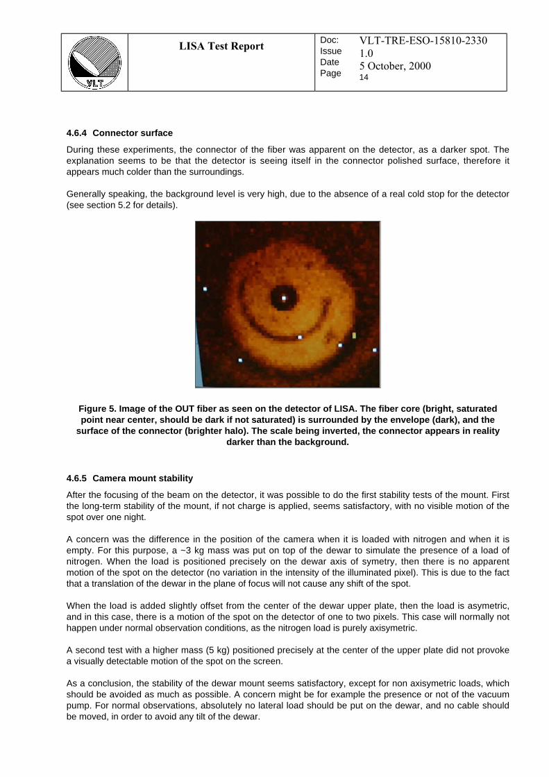
LISA Test ReportDoc:IssueDatePage
VLT-TRE-ESO-15810-2330
1.0
5 October, 200014
4.6.4 Connector surface
During these experiments, the connector of the fiber was apparent on the detector, as a darker spot. Theexplanation seems to be that the detector is seeing itself in the connector polished surface, therefore itappears much colder than the surroundings.
Generally speaking, the background level is very high, due to the absence of a real cold stop for the detector(see section 5.2 for details).
4.6.5 Camera mount stability
After the focusing of the beam on the detector, it was possible to do the first stability tests of the mount. Firstthe long-term stability of the mount, if not charge is applied, seems satisfactory, with no visible motion of thespot over one night.
A concern was the difference in the position of the camera when it is loaded with nitrogen and when it isempty. For this purpose, a ~3 kg mass was put on top of the dewar to simulate the presence of a load ofnitrogen. When the load is positioned precisely on the dewar axis of symetry, then there is no apparentmotion of the spot on the detector (no variation in the intensity of the illuminated pixel). This is due to the factthat a translation of the dewar in the plane of focus will not cause any shift of the spot.
When the load is added slightly offset from the center of the dewar upper plate, then the load is asymetric,and in this case, there is a motion of the spot on the detector of one to two pixels. This case will normally nothappen under normal observation conditions, as the nitrogen load is purely axisymetric.
A second test with a higher mass (5 kg) positioned precisely at the center of the upper plate did not provokea visually detectable motion of the spot on the screen.
As a conclusion, the stability of the dewar mount seems satisfactory, except for non axisymetric loads, whichshould be avoided as much as possible. A concern might be for example the presence or not of the vacuumpump. For normal observations, absolutely no lateral load should be put on the dewar, and no cable shouldbe moved, in order to avoid any tilt of the dewar.
Figure 5. Image of the OUT fiber as seen on the detector of LISA. The fiber core (bright, saturatedpoint near center, should be dark if not saturated) is surrounded by the envelope (dark), and the
surface of the connector (brighter halo). The scale being inverted, the connector appears in realitydarker than the background.

LISA Test ReportDoc:IssueDatePage
VLT-TRE-ESO-15810-2330
1.0
5 October, 200015
5. OPTICAL AND BASIC DETECTOR TESTS
5.1 FIELD OF VIEW
5.1.1 Description
The Hawaii array is illuminated by the cold doublet lens in front of the camera. It is necessary to evaluate thefield of view seen by the detector, in order to position the fiber images in an unvignetted part of the field.
5.1.2 Procedure
◊ First roughly evaluate the LISA detector field of view by putting a diffuse, extended light source just in frontof the camera window while running the full-frame acquisition.
◊ Evaluate the uniformity of the light on the dectector.
◊ Make a focused image of the fiber head on the LISA detector (see Section 4.2).
◊ Measure the peak intensity of the spot as it is moved over the detector (by turning the knobs on the flatmirror of the OUT source).
The center of the field is located at the lower left corner of the detector (as seen on the RTD screen), inorder to have the best possible readout speed. Though, there are a number of dead or bad pixels in thatregion, that should be avoided.
5.1.3 Diffuse illumination
The illumination of the detector with a diffused source gave a uniformly decreasing intensity from the centerto the edge of the detector (radial). The decrease is nearly perfectly linear, and the noise level seems to beapproximately constant. It is difficult to estimate the impact of this effect on the fringe measurements, beforethe noise tests have been conducted on the system.
5.1.4 Focused saturated spot
As a second step, the focused light source spot was moved over the array, in order to estimate what fractionof the detector is usable to image the fiber head. The problem here is that the beam is easily vignetted bythe window of the dewar if its direction is too much tilted. The practical experiment was done by measuringthe intensities across one line and one column.
A problem was identified after the measurement: the spot was heavily saturated due to a too longexposure time (more than 2 seconds). Therefore, the usable area defined in this section will have tobe checked with a lower intensity beam and the LdV four fibers bundle.
It is important to bring the spots as close as possible to the lower left corner of the array to optimizethe readout frequency.

LISA Test ReportDoc:IssueDatePage
VLT-TRE-ESO-15810-2330
1.0
5 October, 200016
Intensity along the column #36 ( X=548)
-20000
-18000
-16000
-14000
-12000
-10000
-8000
-6000
-4000
-2000
0
0 2 0 4 0 6 0 8 0 100 120
Pixel along the Y axis
Inte
nsi
ty
(AD
U)
Intensity along the line #29 (Y=29)
-18000
-16000
-14000
-12000
-10000
-8000
-6000
-4000
0 2 0 4 0 6 0 8 0 100 120
Pixel along the X axis
Inte
nsi
ty
(AD
U)
The structure of the array is nearly symetric relatively to the diagonal of the quadrant, with the first lines andcolumns not as reactive as the others. The explanation for this behavior may be the same as for thepresence of dead pixels around the outer edges of the detector (indium layer decay ?).
The best area for the positioning of the four scientific spots seems therefore to be approximately [20 < X <45, 25 < Y < 50], intersected with a quarter disc of radius ~ 45 (centered on the lower left corner).
5.1.5 To be checked: Usable detector area
In the following figures, the usable part of the Hawaii detector is indicated on the quadrant (“OK” squarearea). The size of this area is small, but this is the best location with the current optical design.
This zone has to be verified using a non saturated spot moved across the detector.
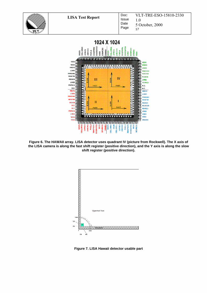
LISA Test ReportDoc:IssueDatePage
VLT-TRE-ESO-15810-2330
1.0
5 October, 200017
Figure 6. The HAWAII array. LISA detector uses quadrant IV (picture from Rockwell). The X axis ofthe LISA camera is along the fast shift register (positive direction), and the Y axis is along the slow
shift register (positive direction).
Figure 7. LISA Hawaii detector usable part
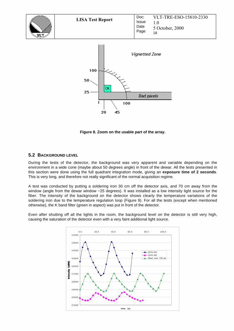
LISA Test ReportDoc:IssueDatePage
VLT-TRE-ESO-15810-2330
1.0
5 October, 200018
5.2 BACKGROUND LEVEL
During the tests of the detector, the background was very apparent and variable depending on theenvironment in a wide cone (maybe about 50 degrees angle) in front of the dewar. All the tests presented inthis section were done using the full quadrant integration mode, giving an exposure time of 2 seconds .This is very long, and therefore not really significant of the normal acquisition regime.
A test was conducted by putting a soldering iron 30 cm off the detector axis, and 70 cm away from thewindow (angle from the dewar window ~25 degrees). It was installed as a low intensity light source for thefiber. The intensity of the background on the detector shows clearly the temperature variations of thesoldering iron due to the temperature regulation loop (Figure 9). For all the tests (except when mentionedotherwise), the K band filter (green in aspect) was put in front of the detector.
Even after shutting off all the lights in the room, the background level on the detector is still very high,causing the saturation of the detector even with a very faint additional light source.
-21000
-20000
-19000
-18000
-17000
-16000
-15000
-14000
-13000
-12000
0.0 20.0 40.0 60.0 80.0 100.0
time (s)
Inte
nsi
ty
(AD
U)
(535,46)
(545,38)
Mean over 728 pix
Figure 8. Zoom on the usable part of the array.
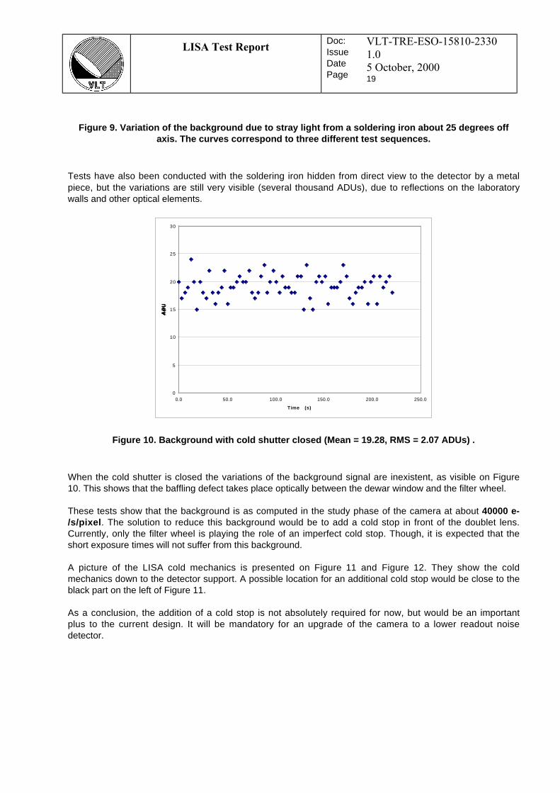
LISA Test ReportDoc:IssueDatePage
VLT-TRE-ESO-15810-2330
1.0
5 October, 200019
Tests have also been conducted with the soldering iron hidden from direct view to the detector by a metalpiece, but the variations are still very visible (several thousand ADUs), due to reflections on the laboratorywalls and other optical elements.
0
5
10
15
20
25
30
0.0 50.0 100.0 150.0 200.0 250.0
Time (s)
AD
U
When the cold shutter is closed the variations of the background signal are inexistent, as visible on Figure10. This shows that the baffling defect takes place optically between the dewar window and the filter wheel.
These tests show that the background is as computed in the study phase of the camera at about 40000 e-/s/pixel . The solution to reduce this background would be to add a cold stop in front of the doublet lens.Currently, only the filter wheel is playing the role of an imperfect cold stop. Though, it is expected that theshort exposure times will not suffer from this background.
A picture of the LISA cold mechanics is presented on Figure 11 and Figure 12. They show the coldmechanics down to the detector support. A possible location for an additional cold stop would be close to theblack part on the left of Figure 11.
As a conclusion, the addition of a cold stop is not absolutely required for now, but would be an importantplus to the current design. It will be mandatory for an upgrade of the camera to a lower readout noisedetector.
Figure 9. Variation of the background due to stray light from a soldering iron about 25 degrees offaxis. The curves correspond to three different test sequences.
Figure 10. Background with cold shutter closed (Mean = 19.28, RMS = 2.07 ADUs) .
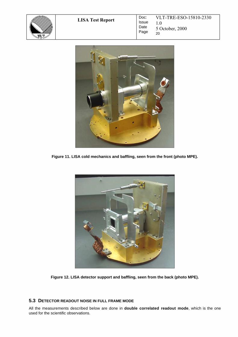
LISA Test ReportDoc:IssueDatePage
VLT-TRE-ESO-15810-2330
1.0
5 October, 200020
5.3 DETECTOR READOUT NOISE IN FULL FRAME MODE
All the measurements described below are done in double correlated readout mode , which is the oneused for the scientific observations.
Figure 11. LISA cold mechanics and baffling, seen from the front (photo MPE).
Figure 12. LISA detector support and baffling, seen from the back (photo MPE).

LISA Test ReportDoc:IssueDatePage
VLT-TRE-ESO-15810-2330
1.0
5 October, 200021
5.3.1 Aproximate gain factor
The gain factor is computed from the slope of the Signal vs. Noise curve. It is expressed in ADU/electron.The measurements were done in full quadrant, double correlated readout mode. The light source used wassimply the background light (it is nearly saturating the detector, see section 5.2 for discussion). The intensitywas varied by (very) slightly opening the cold shutter in front of the doublet lens. Temporal series of a fewtens of values were obtained for each light level.
The gain is given by the inverse square root of the slope of the linear fit (shown on Figure 13):
g ~ 2.9 electrons/ADU.
0
2 0 0
4 0 0
6 0 0
8 0 0
1 0 0 0
1 2 0 0
1 4 0 0
1 6 0 0
1 8 0 0
2 0 0 0
0 2 0 0 0 4 0 0 0 6 0 0 0 8 0 0 0 1 0 0 0 0 1 2 0 0 0 1 4 0 0 0 1 6 0 0 0 1 8 0 0 0
- Mean Signal (ADU)
Va
ria
nce
(A
DU
)
The overall distribution of the points on the curve may not be linear. It seems that a plateau occurs at leastfrom -4000 to -12000 ADUs. This point will be checked more thoroughly in the 64x64 and windowed readoutmodes (fast readout). Please see Section 7 for a much more precise study.
5.3.2 Readout noise in full quadrant mode (512x512 pixels)
The shutter being closed, a time sequence of pixel values is acquired. The graph presented on Figure 10shows that the signal mean value is 19.18 ADU (inverted scale in double correlated mode: the higher valuesvalues are negative), and the standard deviation is 2.06 ADU. Using the gain factor computed in section5.3.1, the resulting read-out noise in double correlated mode is ~ 6 electrons.
This value is a very rough first estimate of the effective readout noise of the array. Please refer to Section 0for precise measurements.
5.4 READOUT MODES
5.4.1 List of modes
The useful modes for the camera operation are listed in the following table. They include the possibility toswitch from one windowed readout mode to another, to adapt the size of the read windows to the brightnessof the star for example. This list is likely to be updated.
Figure 13. Variance as a function of signal for LISA. The slope is 0.1182, giving a gain factor of 2.9electrons/ADU. X axis is the mean signal in ADU. Y axis is the observed variance of the temporal
sequence in ADU 2.
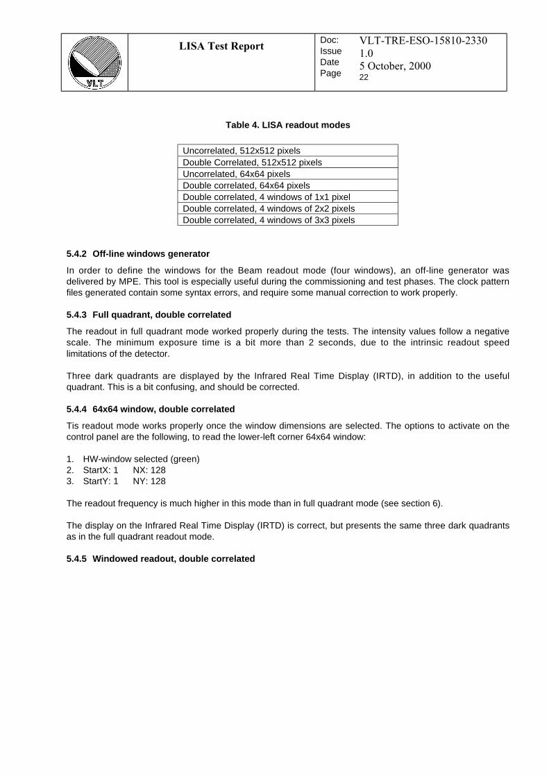
LISA Test ReportDoc:IssueDatePage
VLT-TRE-ESO-15810-2330
1.0
5 October, 200022
Uncorrelated, 512x512 pixelsDouble Correlated, 512x512 pixelsUncorrelated, 64x64 pixelsDouble correlated, 64x64 pixelsDouble correlated, 4 windows of 1x1 pixelDouble correlated, 4 windows of 2x2 pixelsDouble correlated, 4 windows of 3x3 pixels
5.4.2 Off-line windows generator
In order to define the windows for the Beam readout mode (four windows), an off-line generator wasdelivered by MPE. This tool is especially useful during the commissioning and test phases. The clock patternfiles generated contain some syntax errors, and require some manual correction to work properly.
5.4.3 Full quadrant, double correlated
The readout in full quadrant mode worked properly during the tests. The intensity values follow a negativescale. The minimum exposure time is a bit more than 2 seconds, due to the intrinsic readout speedlimitations of the detector.
Three dark quadrants are displayed by the Infrared Real Time Display (IRTD), in addition to the usefulquadrant. This is a bit confusing, and should be corrected.
5.4.4 64x64 window, double correlated
Tis readout mode works properly once the window dimensions are selected. The options to activate on thecontrol panel are the following, to read the lower-left corner 64x64 window:
1. HW-window selected (green)2. StartX: 1 NX: 1283. StartY: 1 NY: 128
The readout frequency is much higher in this mode than in full quadrant mode (see section 6).
The display on the Infrared Real Time Display (IRTD) is correct, but presents the same three dark quadrantsas in the full quadrant readout mode.
5.4.5 Windowed readout, double correlated
Table 4. LISA readout modes

LISA Test ReportDoc:IssueDatePage
VLT-TRE-ESO-15810-2330
1.0
5 October, 200023
The order of the data in the IRTD and in the data file is presented in the following sections.
5.4.5.1 Beampix data
During the tests of the windowed readout mode (four beams each of 2x2 pixels), the system behavedcorrectly, showing the intensity of the light in the 16 pixels at the first and second reads of the detector (32data points). The waterfall display on the IRTD was correct. To ascertain that the correct pixels were listed atthe correct positions, the fiber spot was moved from one pixel to the other in the same window (fourthwindow).The pixel showing the spot was always correct in the Beampix data submode.
The order in which the data is output is the following, using the naming convention of the Figure 14, with[A2,2] meaning the second read of the A2 pixel:
Figure 14. LISA windowed mode readout order.

LISA Test ReportDoc:IssueDatePage
VLT-TRE-ESO-15810-2330
1.0
5 October, 200024
[A1,1] [A1,2] [A2,1] [A2,2] [A3,1] [A3,2] [A4,1] [A4,2] [B5,1] [B5,2] [B6,1] [B6,2]…
On the IRTD, these values are displayed as a temporal sequence starting from the bottom of the screen tothe top, in a kind of “reversed waterfall” display.
To obtain the fluxes in ADU (positive sign) for example on pixel A1:
Flux A1 = [A1,1] – [A1,2]
The actual fluxes from the DCS are computed using this formula, and therefore have the correct sign.
5.4.5.2 Flux data
In this data submode, the fluxes in each of the four windows (first read minus second read to give a positivevalue) is summed to give one value per window. The result is a series of four numbers, plus two additionalnumbers containing the total flux in all windows and TBC. The display in the RTD shows the following values(as displayed on the screen):
Line # Name Order
6 [?] O(t1) O(t2) O(t3)…5 [Total flux] F(t1) F(t2) F(t3)…4 [Flux beam D] D(t1) D(t2) D(t3)…3 [Flux beam C] C(t1) C(t2) C(t3)…2 [Flux beam B] B(t1) B(t2) B(t3)…1 [Flux beam A] A(t1) A(t2) A(t3)…
5.4.5.3 Quicklook data
A vector containing the processed scans (TBC) is also produced. In the tests we have conducted, thequicklook algorithm was not implemented, and therefore the data produced was not meaningful.
LISA Test ReportDoc:IssueDatePage
VLT-TRE-ESO-15810-2330
1.0
5 October, 200025
6. READOUT FREQUENCIES
6.1 INTRODUCTION
The readout of the camera in double correlated mode is based on five steps:
1. Reset of the four windows2. Optional wait time3. First readout of the four windows4. Exposure time5. Second readout of the four windows
The execution of these five steps produces two numbers for each pixel corresponding to the first and secondreads. Both numbers are accessible in the Beampix data submode for each pixel of each window. In theFlux output mode, the fluxes are summed over each window. The order of the pixels in the data output fromthe camera is explained in section 5.4.5.
The minimum exposure time Min DIT is computed automatically, and displayed on the control panel. Thisminimum time corresponds to the time needed to complete a single scan, with the specified number offrames. It does not include the overhead time necessary to compute the delay line offset, and therefore it isstrictly the time necessary to acquire one frame multiplied by the number of frames. From this number, it iseasy to compute the effective frame frequency through:
Frequency = [Number of Frames in Scan] / [Min DIT]
6.2 EFFECTIVE MAXIMAL READOUT FREQUENCIES
The maximal frequency reachable by the detector depends on the position of the four windows on thedetector and on their size. The smaller and the closer to the lower left corner, the faster the readout. Theselected pixel windows for the windowed readout tests were centered (for the 1x1 or 3x3 pixels) or had theirlower left corner (for the 2x2 pixels windows) on the pixels [29,26], [25,34], [33,38], [37,30] . The distancebetween these pixels was chosen to be 9 pixels, to mimic as much as possible the behavior of the real spotsreadouts.
Mode Maximal frequency (Hz)4 windows 1x1 pixel each 25454 windows 2x2 pixels each 16564 windows 3x3 pixels each 106264x64 double correlated 28.664x64 uncorrelated 54.1512x512 double correlated 0.48512x512 uncorrelated 0.95
The maximum frequency reachable with the 1x1 pixel mode is better than 2.5 kHz, therefore fulfilling therequirements stated in the ‘LISA Technical Specifications’ document.
For information, the pixel readout rate in 64x64 mode was 117 kHz. This means that 4 windows of 1x1 pixellocated in the lower left corner of the array ([0,0] [0,1] [1,1] [1,0]) could theoretically be read at a maximumframe rate of 29 KHz.
Table 5. Maximum readout frequencies for LISA
LISA Test ReportDoc:IssueDatePage
VLT-TRE-ESO-15810-2330
1.0
5 October, 200026
7. BEST PHOTOSITES SELECTION
7.1 PRINCIPLE
To select the best possible photosites for the light detection, it is necessary in principle to measure the noiselevel of all the pixels in the frequency range used by the DCS. The detector useful readout frequency rangeis about 2 - 2000 Hz.
It is possible to use the special 64x64 readout mode of LISA to have a sampling rate of about 30 Hz onevery pixel in the selected window, in double correlated mode. It is reasonable to assume that the noiselevel of the LISA camera does not depend on the readout frequency of the detector (this assumption waschecked a posteriori and is valid). The selection can therefore be done in two steps:
1) first construct a map of the lower left corner 64x64 region indicating the bad and noisy pixels. Using the64x64 readout mode gives access to the power spectral density up to a frequency of 14.3 Hz.
2) do a finer selection of the best pixels in this area, by acquiring a series of scans at the highest possiblefrequency. In this case, the maximum reachable frequency in the power spectral density can be of morethan 1000 Hz.
For these tests, the data was acquired using the control panel of the camera, and saved into standard FITSformat data files. The data processing was done using the IDL software (including the ASTRON package).
7.2 PIXEL GAINS
7.2.1 Measurement procedure
To obtain the values of the gains for all the pixels, the detector was exposed to an increasing light level byopening slightly the cold shutter. Cubes of 500 frames of 64x64 pixels were recorded (150 ms exposuretime), of which 256 were processed (adequate number for fast Fourier transform computation). This test wasconducted at seven different light levels, of which six were kept for processing (the seventh contained somesaturated pixels).
σ σ σ
σ
total photons RON
ADURON
ADUS
G
S
G
2 2 2
2
= +
= + ≈
The gain was estimated as the inverse of the slope of the linear regression of the Variance = f(Signal) curve.
All the processing was done using IDL. The listing of the procedures is included in the Appendix.
7.2.2 Examples of gain curves
The following curves show the fits achieved for three typical pixels.
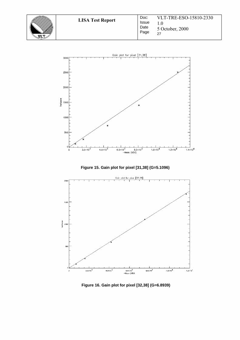
LISA Test ReportDoc:IssueDatePage
VLT-TRE-ESO-15810-2330
1.0
5 October, 200027
Figure 15. Gain plot for pixel [31,38] (G=5.1096)
Figure 16. Gain plot for pixel [32,38] (G=6.8939)

LISA Test ReportDoc:IssueDatePage
VLT-TRE-ESO-15810-2330
1.0
5 October, 200028
7.2.3 Gain map
The gains are available numerically for all the pixels in the lower left 64x64 area of the detector. Figure 18shows a graphical plot of the gains over the array (linear scale). Typical values are between 5 and 10.
Figure 17. Gain plot for pixel [33,38]. (G=6.9652)
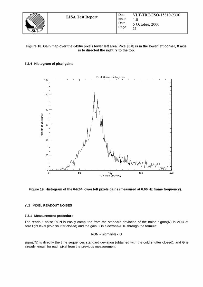
LISA Test ReportDoc:IssueDatePage
VLT-TRE-ESO-15810-2330
1.0
5 October, 200029
7.2.4 Histogram of pixel gains
7.3 PIXEL READOUT NOISES
7.3.1 Measurement procedure
The readout noise RON is easily computed from the standard deviation of the noise sigma(N) in ADU atzero light level (cold shutter closed) and the gain G in electrons/ADU through the formula:
RON = sigma(N) x G
sigma(N) is directly the time sequences standard deviation (obtained with the cold shutter closed), and G isalready known for each pixel from the previous measurement.
Figure 18. Gain map over the 64x64 pixels lower left area. Pixel [0,0] is in the lower left corner, X axisis to directed the right, Y to the top.
Figure 19. Histogram of the 64x64 lower left pixels gains (measured at 6.66 Hz frame frequency).
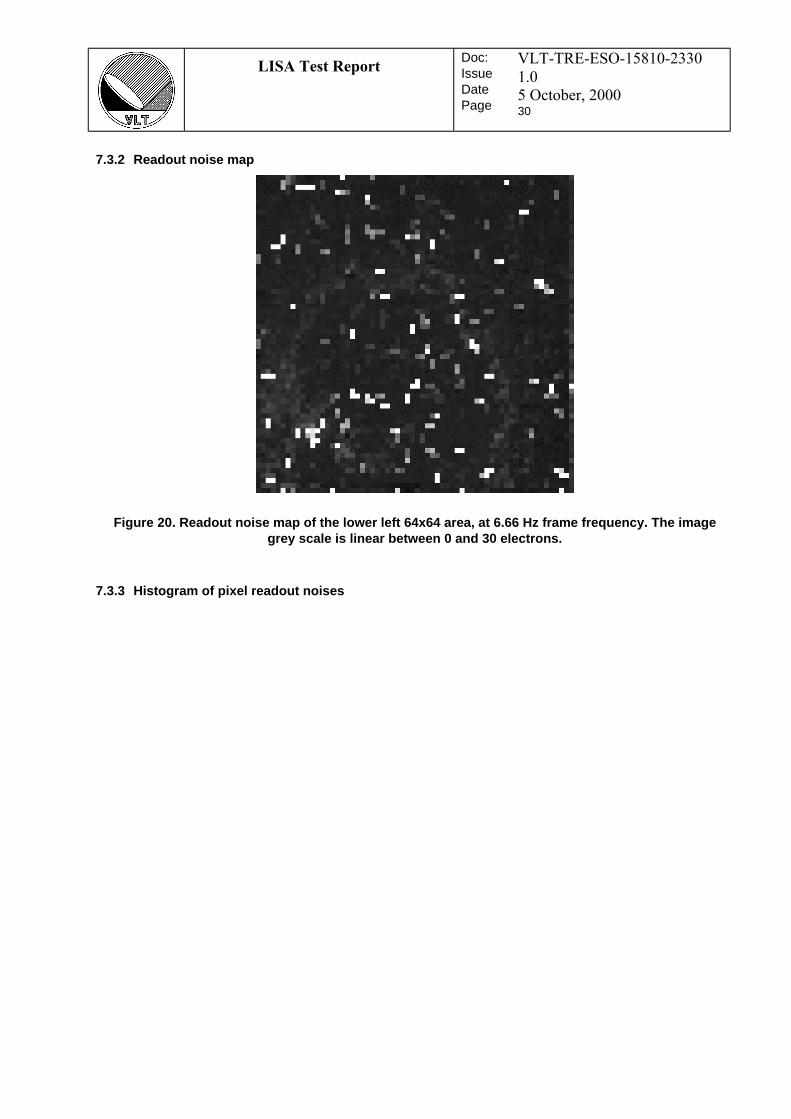
LISA Test ReportDoc:IssueDatePage
VLT-TRE-ESO-15810-2330
1.0
5 October, 200030
7.3.2 Readout noise map
7.3.3 Histogram of pixel readout noises
Figure 20. Readout noise map of the lower left 64x64 area, at 6.66 Hz frame frequency. The imagegrey scale is linear between 0 and 30 electrons.
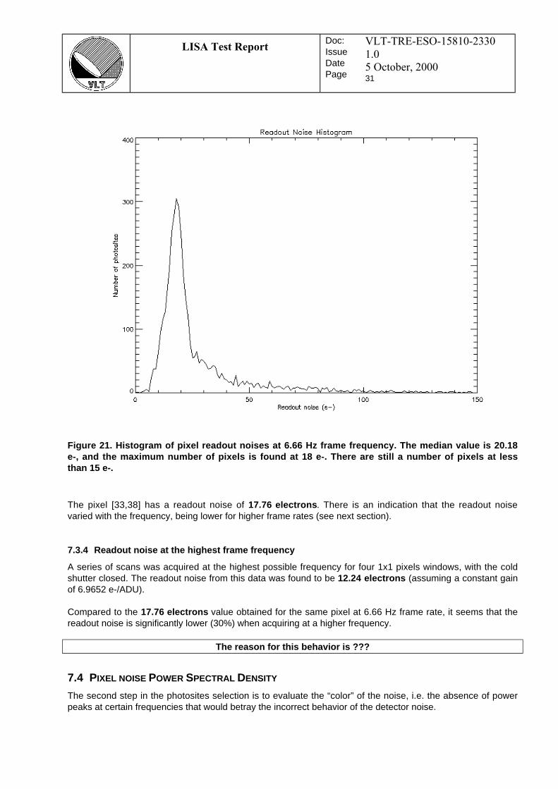
LISA Test ReportDoc:IssueDatePage
VLT-TRE-ESO-15810-2330
1.0
5 October, 200031
The pixel [33,38] has a readout noise of 17.76 electrons . There is an indication that the readout noisevaried with the frequency, being lower for higher frame rates (see next section).
7.3.4 Readout noise at the highest frame frequency
A series of scans was acquired at the highest possible frequency for four 1x1 pixels windows, with the coldshutter closed. The readout noise from this data was found to be 12.24 electrons (assuming a constant gainof 6.9652 e-/ADU).
Compared to the 17.76 electrons value obtained for the same pixel at 6.66 Hz frame rate, it seems that thereadout noise is significantly lower (30%) when acquiring at a higher frequency.
The reason for this behavior is ???
7.4 PIXEL NOISE POWER SPECTRAL DENSITY
The second step in the photosites selection is to evaluate the “color” of the noise, i.e. the absence of powerpeaks at certain frequencies that would betray the incorrect behavior of the detector noise.
Figure 21. Histogram of pixel readout noises at 6.66 Hz frame frequency. The median value is 20.18e-, and the maximum number of pixels is found at 18 e-. There are still a number of pixels at lessthan 15 e-.
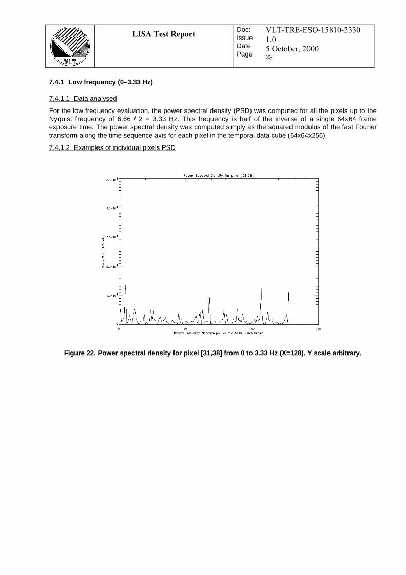
LISA Test ReportDoc:IssueDatePage
VLT-TRE-ESO-15810-2330
1.0
5 October, 200032
7.4.1 Low frequency (0–3.33 Hz)
7.4.1.1 Data analysed
For the low frequency evaluation, the power spectral density (PSD) was computed for all the pixels up to theNyquist frequency of 6.66 / 2 = 3.33 Hz. This frequency is half of the inverse of a single 64x64 frameexposure time. The power spectral density was computed simply as the squared modulus of the fast Fouriertransform along the time sequence axis for each pixel in the temporal data cube (64x64x256).
7.4.1.2 Examples of individual pixels PSD
Figure 22. Power spectral density for pixel [31,38] from 0 to 3.33 Hz (X=128). Y scale arbitrary.
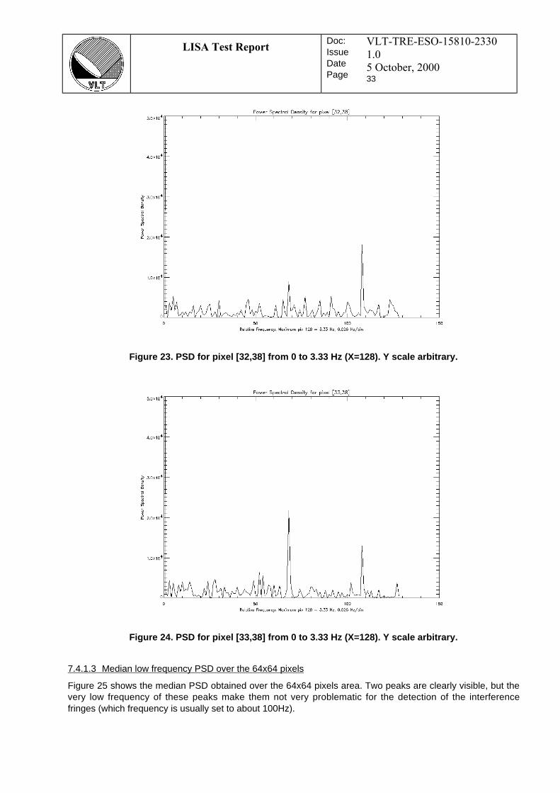
LISA Test ReportDoc:IssueDatePage
VLT-TRE-ESO-15810-2330
1.0
5 October, 200033
7.4.1.3 Median low frequency PSD over the 64x64 pixels
Figure 25 shows the median PSD obtained over the 64x64 pixels area. Two peaks are clearly visible, but thevery low frequency of these peaks make them not very problematic for the detection of the interferencefringes (which frequency is usually set to about 100Hz).
Figure 23. PSD for pixel [32,38] from 0 to 3.33 Hz (X=128). Y scale arbitrary.
Figure 24. PSD for pixel [33,38] from 0 to 3.33 Hz (X=128). Y scale arbitrary.

LISA Test ReportDoc:IssueDatePage
VLT-TRE-ESO-15810-2330
1.0
5 October, 200034
When using LdV with a fringe tracker, it will be necessary to decrease the fringe frequency down to very lowvalues for faint objects, possibly interfering with these peaks. In this case they could become an importantproblem.
7.4.2 High frequency (0–828 Hz)
7.4.2.1 Data analysed
This second type of measurements is done using the windowed readout mode of LISA. This is necessarybecause the readout frequency of the camera in the 64x64 pixels mode is limited to less than 30 Hz, whichis too low for the study of the behavior of the detector at the frequencies used for the detection of the fringes.
The windows used were 2x2 pixels in size, giving 16 pixels. For each pixel, a series of 20 scans of each1024 frames was analysed. The frame frequency was set to the maximum possible value (at the selectedconfiguration, see Section 6 for details), e.g. 1656 Hz. Therefore, the frequencies investigated by computingthe PSD of the sequences were in the range 0-828 Hz.
7.4.2.2 Example of pixel [33,38]
Figure 25. Median Power Spectral Density for the 64x64 pixels, from 0 to 3.33 Hz (X=128). The Y scaleis arbitrary.

LISA Test ReportDoc:IssueDatePage
VLT-TRE-ESO-15810-2330
1.0
5 October, 200035
7.4.3 Maximum frequency (0–1223 Hz)
7.4.3.1 Data analysed
This measurement is done using the windowed readout mode of LISA. The windows used were 1x1 pixel insize, giving 4 pixels. For each pixel, a series of 20 scans of each 1024 frames was analysed. The framefrequency was set to the maximum possible value (at the selected configuration, see Section 6 for details),e.g. 2545 Hz. Therefore, the frequencies investigated by computing the PSD of the sequences were in therange 0-1223 Hz.
7.4.3.2 Example of pixel [33,38]
Figure 26. Overview of the PSD for pixel [33,38] read at 1656 Hz frame rate (frequencies between 0and 828 Hz). The shutter was open (background light present), but the fiber spot was not illuminated.
The large peak on the left is precisely in the bin containing the 100 Hz frequency. (mean over 20scans).
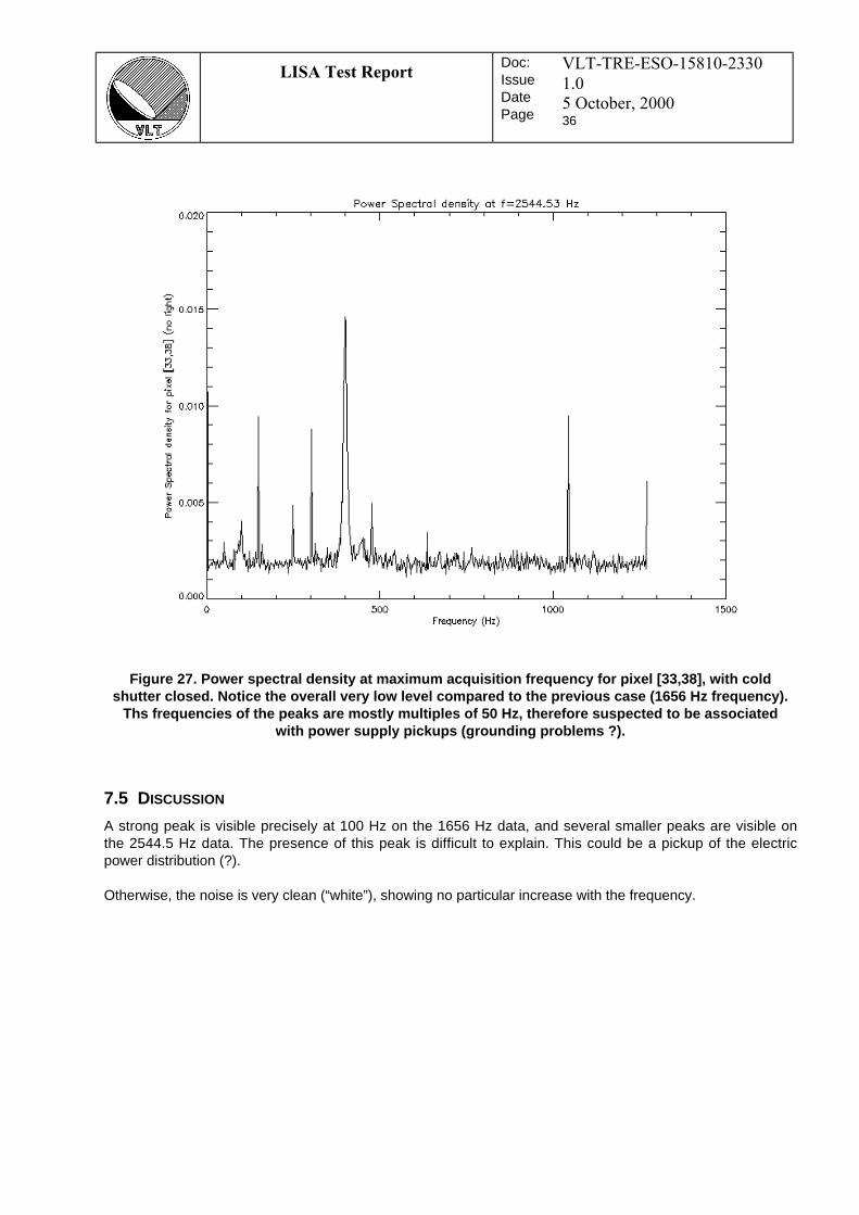
LISA Test ReportDoc:IssueDatePage
VLT-TRE-ESO-15810-2330
1.0
5 October, 200036
7.5 DISCUSSION
A strong peak is visible precisely at 100 Hz on the 1656 Hz data, and several smaller peaks are visible onthe 2544.5 Hz data. The presence of this peak is difficult to explain. This could be a pickup of the electricpower distribution (?).
Otherwise, the noise is very clean (“white”), showing no particular increase with the frequency.
Figure 27. Power spectral density at maximum acquisition frequency for pixel [33,38], with coldshutter closed. Notice the overall very low level compared to the previous case (1656 Hz frequency).
Ths frequencies of the peaks are mostly multiples of 50 Hz, therefore suspected to be associatedwith power supply pickups (grounding problems ?).

LISA Test ReportDoc:IssueDatePage
VLT-TRE-ESO-15810-2330
1.0
5 October, 200037
8. INDIUM LAYER STABILITY
The array used in LISA is an engineering grade detector and suffers from dead pixels at the external edgesof the array. This is caused by the destruction of the indium layer connecting the photosites. The evolution ofthis defect has to be followed carefully, as it may evolve after each cooling of the camera.
The procedure is simply to save an full frame image produced by the array after cooling it down. Thedetection of possible dead pixels can be done by subtracting the images obtained from a reference image,and by adjusting the display levels to check for the pixels having no evolution between the two frames (nonoise associated with them).
During the tests of the camera, a series of images of the full 512x512 quadrant have been saved for futurereference. No obvious variation of the dead pixels positions have been observed visually during the tests.
LISA Test ReportDoc:IssueDatePage
VLT-TRE-ESO-15810-2330
1.0
5 October, 200038
9. MEMORY EFFECT
9.1 DESCRIPTION
As stated in the LISA User’s Manual, the Hawaii detector may be subject to a memory effect, which couldaffect the visibility measurements and even the observational procedure.
The symptom of the detector memory is that after a bright illumination of the photosite (causing or not asaturation of the pixel), a residual signal is kept for a while and affects the readouts for the following cycles.
Three kinds of behaviors are tested:
• Minute timescale : Saturation of the detector followed by closure of the cold shutter. This testensure that the array does not need a rest time between a bright source and a faint sourceobservation. The effect of the saturation should disappear completely in a short time. The tests werenot conducted on the LISA camera, but measurements have already been obtained by Gert Fingeron the HAWAII detector. His measurements show that the signal intensity is divided by 100 in 150seconds.
• Millisecond timescale : Array response to a chopped signal stimulus cut very quickly to zero (inless than 1 integration time). This measurement makes it possible to evaluate if the fringe visibilitycould be degraded by a memory effect of the detector. The only delicate point in this test is that theshut-off of the light intensity has to be very fast. This is achieved easily by masking quickly the fiberhead with an opaque material on the light injection side. The very small diameter of the fiber coreallow to achieve sub millisecond closing times. A chopping device was used for that purpose.
9.2 MEASUREMENT PROCEDURE
◊ Align the light source in order to have a good quality, point-like source on the detector.
◊ Adjust the intensity of the light source to obtain an intensity on the detector just below saturation.
◊ Close the cold mask of the detector for a while, in order to avoid contamination by a possible long-termmemory effect.
◊ Open the cold mask and select the K band filter.
◊ Start the chopper wheel, in front of the fiber injection.
◊ Start the data acquisition at the maximum data rate on a four windows set containing the illuminated pixel.
◊ Acquire two sets of data shutter open and shutter closed to have the top and bottom levels.
9.3 GEOMETRY OF THE CHOPPING SYSTEM
The geometry of the chopping system determines the shape of the input signal sent to the camera. Figure28 shows the geometrical configuration of the chopper used to modulate the signal sent to the camera. Thissystem is installed at the injection side of the artificial light source. This allows to have a sharper cutting ofthe beam than in the collimated part after the off-axis parabola.
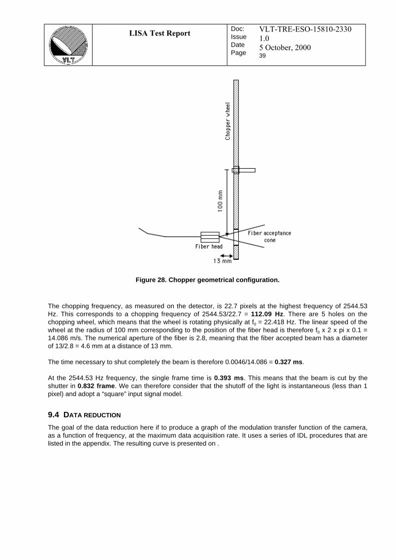
LISA Test ReportDoc:IssueDatePage
VLT-TRE-ESO-15810-2330
1.0
5 October, 200039
The chopping frequency, as measured on the detector, is 22.7 pixels at the highest frequency of 2544.53Hz. This corresponds to a chopping frequency of 2544.53/22.7 = 112.09 Hz. There are 5 holes on thechopping wheel, which means that the wheel is rotating physically at f0 = 22.418 Hz. The linear speed of thewheel at the radius of 100 mm corresponding to the position of the fiber head is therefore f0 x 2 x pi x 0.1 =14.086 m/s. The numerical aperture of the fiber is 2.8, meaning that the fiber accepted beam has a diameterof 13/2.8 = 4.6 mm at a distance of 13 mm.
The time necessary to shut completely the beam is therefore 0.0046/14.086 = 0.327 ms .
At the 2544.53 Hz frequency, the single frame time is 0.393 ms . This means that the beam is cut by theshutter in 0.832 frame . We can therefore consider that the shutoff of the light is instantaneous (less than 1pixel) and adopt a “square” input signal model.
9.4 DATA REDUCTION
The goal of the data reduction here if to produce a graph of the modulation transfer function of the camera,as a function of frequency, at the maximum data acquisition rate. It uses a series of IDL procedures that arelisted in the appendix. The resulting curve is presented on .
Figure 28. Chopper geometrical configuration.
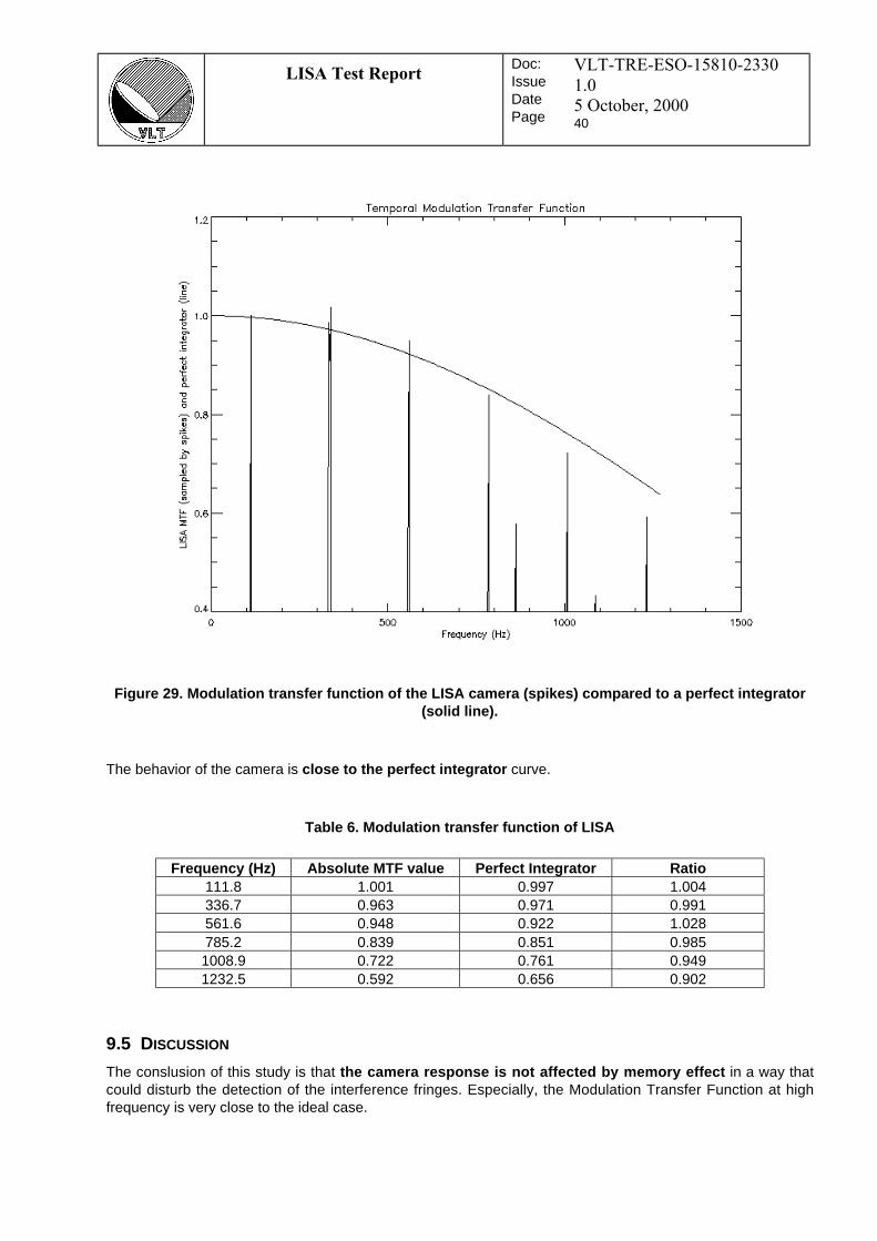
LISA Test ReportDoc:IssueDatePage
VLT-TRE-ESO-15810-2330
1.0
5 October, 200040
The behavior of the camera is close to the perfect integrator curve.
Frequency (Hz) Absolute MTF value Perfect Integrator Ratio111.8 1.001 0.997 1.004336.7 0.963 0.971 0.991561.6 0.948 0.922 1.028785.2 0.839 0.851 0.9851008.9 0.722 0.761 0.9491232.5 0.592 0.656 0.902
9.5 DISCUSSION
The conslusion of this study is that the camera response is not affected by memory effect in a way thatcould disturb the detection of the interference fringes. Especially, the Modulation Transfer Function at highfrequency is very close to the ideal case.
Figure 29. Modulation transfer function of the LISA camera (spikes) compared to a perfect integrator(solid line).
Table 6. Modulation transfer function of LISA

LISA Test ReportDoc:IssueDatePage
VLT-TRE-ESO-15810-2330
1.0
5 October, 200041
10. SUMMARY OF PROBLEMS
The following table lists the major problems encountered during the installation and tests of LISA in stand-alone mode in Garching. The mention “NA” (not applicable) in the “Solved” column means that the problemwas not solved but is not a concern in the actual status of the camera.
# Problem Suspected Cause Solved
1. Negative values for increasing incomingflux in double correlated mode
Wrong sign in the subtraction of the tworeadouts for the double correlated mode.
Yes
2. Filters in the filter wheel are not in thedocumented order
Wrong mounting of the filters Yes
3. Blurred image of the collimated lightsource on the detector
Incorrect focusing of the doublet relatively to theHAWAII array.
Yes
4. Impossible to mount the cryogenicsecurity device for the upper nitrogen tank
Damage to the threading on the dewar. NA
5. Insecure fastening of the camera supporton the table
No briddling currently available. No
6. Very high level and variable background Improper cold stop. NA
7. Three dark quadrants displayed togetherwith the useful one
Data is not discarded early enough in thecomputer system (only for 64x64 and 512x512).
No
8. Dark stripes in the widowed readout mode(missing data)
Program code problem Yes
9. First few pixels of a frame are brighterthan the others
Reset before the scan (removed) Yes
10. Generation of the windows for the fourbeams mode is tedious
Off-line generator has bugs (see Section 5.4.2) No
11. Data content in the “flux” data mode is notcorrect for the two additional channels
(the four windows total fluxes are correct) No
12. Presence of a strong frequency peak inthe noise at a frequency of ~ 100 Hz
Interference with electroluminescent light tubesthrough power supply?
Yes(TBC)
13. Presence of low frequency peaks in thecamera noise
Ground loops producing “waves” on thedetector?
Yes(TBC)
# Question Suggested solution Solved
1. Structure of the data produced by IRACEnot clear
The DCS to IRACE SW interface documentshould be completed
Yes
2. Possibility to save a data cube of 64x64images for photosites selection
Yes
3. Effective exposure time and frame timeare not available in the keywords
Modify dictionnary Yes
4. 3x3 windows generation and readout Generate and check clock paterns Yes(still pb)
Table 7. Apparent problems in the LISA system during the tests in Garching.
Table 8. Points to be clarified
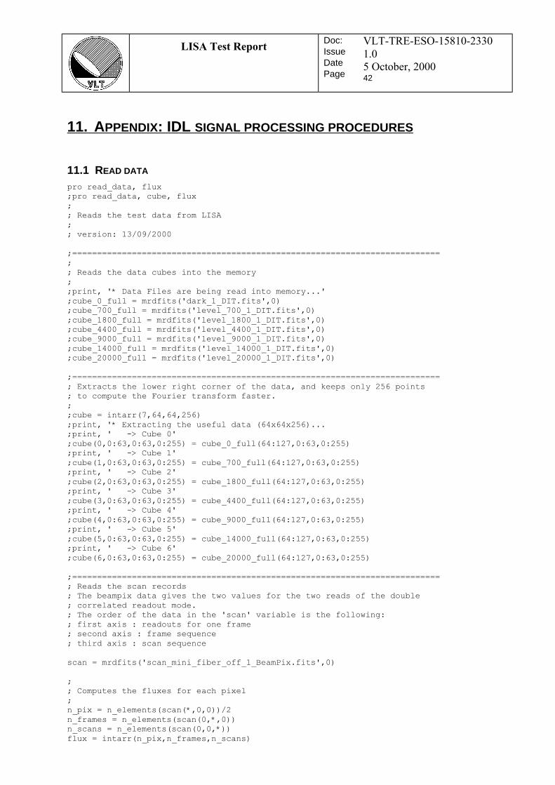
LISA Test ReportDoc:IssueDatePage
VLT-TRE-ESO-15810-2330
1.0
5 October, 200042
11. APPENDIX: IDL SIGNAL PROCESSING PROCEDURES
11.1 READ DATA
pro read_data, flux;pro read_data, cube, flux;; Reads the test data from LISA;; version: 13/09/2000
;==========================================================================;; Reads the data cubes into the memory;;print, '* Data Files are being read into memory...';cube_0_full = mrdfits('dark_1_DIT.fits',0);cube_700_full = mrdfits('level_700_1_DIT.fits',0);cube_1800_full = mrdfits('level_1800_1_DIT.fits',0);cube_4400_full = mrdfits('level_4400_1_DIT.fits',0);cube_9000_full = mrdfits('level_9000_1_DIT.fits',0);cube_14000_full = mrdfits('level_14000_1_DIT.fits',0);cube_20000_full = mrdfits('level_20000_1_DIT.fits',0)
;==========================================================================; Extracts the lower right corner of the data, and keeps only 256 points; to compute the Fourier transform faster.;;cube = intarr(7,64,64,256);print, '* Extracting the useful data (64x64x256)...;print, ' -> Cube 0';cube(0,0:63,0:63,0:255) = cube_0_full(64:127,0:63,0:255);print, ' -> Cube 1';cube(1,0:63,0:63,0:255) = cube_700_full(64:127,0:63,0:255);print, ' -> Cube 2';cube(2,0:63,0:63,0:255) = cube_1800_full(64:127,0:63,0:255);print, ' -> Cube 3';cube(3,0:63,0:63,0:255) = cube_4400_full(64:127,0:63,0:255);print, ' -> Cube 4';cube(4,0:63,0:63,0:255) = cube_9000_full(64:127,0:63,0:255);print, ' -> Cube 5';cube(5,0:63,0:63,0:255) = cube_14000_full(64:127,0:63,0:255);print, ' -> Cube 6';cube(6,0:63,0:63,0:255) = cube_20000_full(64:127,0:63,0:255)
;==========================================================================; Reads the scan records; The beampix data gives the two values for the two reads of the double; correlated readout mode.; The order of the data in the 'scan' variable is the following:; first axis : readouts for one frame; second axis : frame sequence; third axis : scan sequence
scan = mrdfits('scan_mini_fiber_off_1_BeamPix.fits',0)
;; Computes the fluxes for each pixel;n_pix = n_elements(scan(*,0,0))/2n_frames = n_elements(scan(0,*,0))n_scans = n_elements(scan(0,0,*))flux = intarr(n_pix,n_frames,n_scans)

LISA Test ReportDoc:IssueDatePage
VLT-TRE-ESO-15810-2330
1.0
5 October, 200043
for pix=0,(n_pix-1) do begin flux(pix,*,*) = scan(2*pix,*,*) - scan(2*pix+1,*,*)endfor
end
11.2 PROCESS 64X64 DATA
pro process_64, cube, means, variances, gain, readout_noise, fourier, psd, median_psd,mean_psd_per_pix, median_RON, median_gain; SYNTAX:; process_64, cube, means, variances, gain, readout_noise, fourier, psd, median_psd,mean_psd_per_pix, median_RON, median_gain;; Processes the test data acquired with the LISA camera in order to; extract the best possible pixels for the VINCI beams. This procedure; makes the computations for the 64x64 windows data cubes and produces; the power spectral density for all pixels, at different lighting levels.;; This is the first step of the best pixels selection, as described in the; document 'LISA tests in Garching';; It also computes the gain factor and the read-out noise for every pixel; at the frequency used for the tests.;; version: 28/09/2000
;; Computes the mean value and variance of each pixel over the sequence; It excludes the last acquisition (partly saturated).;print, '* Means and variances...'means = fltarr(6,64,64)variances = fltarr(6,64,64)for n=0,5 do begin
print, '+++'for i=0,63 do begin
for j=0,63 do beginmeans(n,i,j) = mean(cube(n,i,j,*))variances(n,i,j) = variance(cube(n,i,j,*))
endforendfor
endfor;;==========================================================================; Computes the gain factor and the read-out noise for each pixel;weights = replicate(1.0,n_elements(means(*,0,0)))results = fltarr(64,64,2)gain = fltarr(64,64)readout_noise = fltarr(64,64)print, '* Computing gains and readout noises for each pixel...'for i=0,63 do begin
for j=0,63 do beginresults(i,j,*) = regress(transpose(-
means(*,i,j)),variances(*,i,j),weights,$yfit,const,/RELATIVE_WEIGHT)
gain(i,j) = 1/(results(i,j,0))readout_noise(i,j) = sqrt(variances(0,i,j))*gain(i,j)
endforendforprint, 'Gains'print, gain(1:10,1:10)print, 'RON'print, readout_noise(1:10,1:10)median_RON = median(readout_noise)
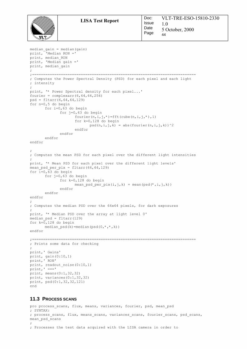
LISA Test ReportDoc:IssueDatePage
VLT-TRE-ESO-15810-2330
1.0
5 October, 200044
median_gain = median(gain)print, 'Median RON ='print, median_RONprint, 'Median gain ='print, median_gain;;==========================================================================; Computes the Power Spectral Density (PSD) for each pixel and each light; intensity;print, '* Power Spectral density for each pixel...'fourier = complexarr(6,64,64,256)psd = fltarr(6,64,64,129)for n=0,5 do begin
for i=0,63 do beginfor j=0,63 do begin
fourier(n,i,j,*)=fft(cube(n,i,j,*),1)for k=0,128 do begin
psd(n,i,j,k) = abs(fourier(n,i,j,k))^2endfor
endforendfor
endfor
;; Computes the mean PSD for each pixel over the different light intensities;print, '* Mean PSD for each pixel over the different light levels'mean_psd_per_pix = fltarr(64,64,129)for i=0,63 do begin
for j=0,63 do beginfor k=0,128 do begin
mean_psd_per_pix(i,j,k) = mean(psd(*,i,j,k))endfor
endforendfor;; Computes the median PSD over the 64x64 pixels, for dark exposures;print, '* Median PSD over the array at light level 0'median_psd = fltarr(129)for k=0,128 do begin
median_psd(k)=median(psd(0,*,*,k))endfor
;==========================================================================; Prints some data for checking;print,' Gains'print, gain(0:10,1)print,' RON'print, readout_noise(0:10,1)print,' ==='print, means(0:1,32,32)print, variances(0:1,32,32)print, psd(0:1,32,32,121)end
11.3 PROCESS SCANS
pro process_scans, flux, means, variances, fourier, psd, mean_psd; SYNTAX:; process_scans, flux, means_scans, variances_scans, fourier_scans, psd_scans,mean_psd_scans;; Processes the test data acquired with the LISA camera in order to

LISA Test ReportDoc:IssueDatePage
VLT-TRE-ESO-15810-2330
1.0
5 October, 200045
; extract the best possible pixels for the VINCI beams. This procedure; makes the computations for the ***scans*** data cubes and produces; the power spectral density for all the pixels used.;; This is the second step of the best pixels selection, as described in the; document 'LISA tests in Garching';; Version: 13/09/2000; Author: P. Kervella
; Computes the mean value and variance of each pixel over the sequence; It excludes the last acquisition (partly saturated).;n_pix = n_elements(flux(*,0,0))n_frames = n_elements(flux(0,*,0))n_scans = n_elements(flux(0,0,*))
print, '* Means and variances...'means = fltarr(n_pix)variances = fltarr(n_pix)print, '+++'
for n=0,(n_pix-1) do beginmeans(n) = mean(flux(n,*,*))variances(n) = variance(flux(n,*,*))
endfor
print, flux(0:5,0:20,2)
;==========================================================================; Computes the Fourier Transform for each pixel and each scan;print, '* Fourier transform for each pixel and each scan...'fourier = complexarr(n_pix,n_frames,n_scans)psd = fltarr(n_pix,n_frames/2+1,n_scans)
for i=0,(n_pix-1) do beginfor j=0,(n_scans-1) do begin
fourier(i,*,j)=fft(flux(i,*,j))endfor
endfor
;==========================================================================; Computes the Power Spectral Density (PSD) for each pixel and each scan;print, '* Power Spectral density for each pixel and each scan...'
psd = fltarr(n_pix,n_frames/2+1,n_scans)
for i=0,(n_pix-1) do beginfor j=0,(n_scans-1) do begin
for k=0,(n_frames/2) do beginpsd(i,k,j) = abs(fourier(i,k,j))^2
endforendfor
endfor
;==========================================================================; Computes the mean Power Spectral Density (PSD) for each pixel; over the scansmedian_psd_scans = fltarr(n_pix,(n_frames/2 +1))print, '* Mean PSD over the scans'for i=0,(n_pix-1) do begin
for j=0,(n_frames/2) do beginmean_psd(i,j)=mean(psd(i,j,*))
endfor
LISA Test ReportDoc:IssueDatePage
VLT-TRE-ESO-15810-2330
1.0
5 October, 200046
endforend
11.4 PLOT 64X64 DATA
pro data_plot, means, variances, gain, readout_noise, fourier, psd, median_psd; SYNTAX:; data_plot, means, variances, gain, readout_noise, fourier, psd, median_psd;; Plots the processing results for the selection of the best pixels for; the LISA camera.;; This ends the first step of the best pixels selection, as described in the; document 'LISA tests in Garching';; version: 12/09/2000;;==========================================================================; Variance of the pixel as a function of flux (gain plot) for one good pixel;window, 0, title='Gain plot for pixel 33,38', xsize=800, ysize=600plot, -means(*,33,38), variances(*,33,38), psym=2, xtitle='-Mean (ADU)',$
ytitle='Variance', title='Gain plot for pixel [33,38]'x_fit_gain = [0,20000]y_fit_gain = fltarr(2)y_fit_gain(*) = x_fit_gain(*)/gain(33,38)^2$
+variances(0,33,38)oplot, x_fit_gain, y_fit_gainwrite_bmp, 'gain_plot_X33_Y38.bmp',tvrd();; Variance of the pixel as a function of flux (gain plot) for one good pixel;window, 0, title='Gain plot for pixel 32,38', xsize=800, ysize=600plot, -means(*,32,38), variances(*,32,38), psym=2, xtitle='-Mean (ADU)',$
ytitle='Variance', title='Gain plot for pixel [32,38]'x_fit_gain = [0,20000]y_fit_gain = fltarr(2)y_fit_gain(*) = x_fit_gain(*)/gain(32,38)^2$
+variances(0,32,38)oplot, x_fit_gain, y_fit_gainwrite_bmp, 'gain_plot_X32_Y38.bmp',tvrd()
; Variance of the pixel as a function of flux (gain plot) for one good pixel;window, 0, title='Gain plot for pixel 31,38', xsize=800, ysize=600plot, -means(*,31,38), variances(*,31,38), psym=2, xtitle='-Mean (ADU)',$
ytitle='Variance', title='Gain plot for pixel [31,38]'x_fit_gain = [0,20000]y_fit_gain = fltarr(2)y_fit_gain(*) = x_fit_gain(*)/gain(31,38)^2$
+variances(0,31,38)oplot, x_fit_gain, y_fit_gainwrite_bmp, 'gain_plot_X31_Y38.bmp',tvrd()
; Power Spectral Density;window, 0, title='PSD for pixel 33,38', xsize=800, ysize=600plot, psd(0,33,38,*), xrange=[0,128], yrange = [0,50000], xtitle='Relative Frequency.Maximum pix 128 = 3.33 Hz, 0.026 Hz/bin',$
ytitle='Power Spectral Density', title='Power Spectral Density for pixel [33,38]'write_bmp, 'psd_X33_Y38.bmp',tvrd()
; Power Spectral Density;
LISA Test ReportDoc:IssueDatePage
VLT-TRE-ESO-15810-2330
1.0
5 October, 200047
window, 0, title='PSD for pixel 32,38', xsize=800, ysize=600plot, psd(0,32,38,*), xrange=[0,128], yrange = [0,50000], xtitle='Relative Frequency.Maximum pix 128 = 3.33 Hz, 0.026 Hz/bin',$
ytitle='Power Spectral Density', title='Power Spectral Density for pixel [32,38]'write_bmp, 'psd_X32_Y38.bmp',tvrd()
; Power Spectral Density;window, 0, title='PSD for pixel 31,38', xsize=800, ysize=600plot, psd(0,31,38,*), xrange=[0,128], yrange = [0,50000], xtitle='Relative Frequency.Maximum pix 128 = 3.33 Hz, 0.026 Hz/bin',$
ytitle='Power Spectral Density', title='Power Spectral Density for pixel [31,38]'write_bmp, 'psd_X31_Y38.bmp',tvrd()
;; Histogram of the noises of the pixels;window, 0, title='Histogram of the pixel readout noises', xsize=800, ysize=600plot, histogram(readout_noise, min=0, max=30, bin=1,/nan),$
title='Readout Noise Histogram', xtitle='Readout noise (e-)',$ytitle='Number of photosites'
write_bmp, 'Noise_histogram.bmp',tvrd();; Histogram of the gains of the pixels;window, 0, title='Histogram of the pixel gains', xsize=800, ysize=600plot, histogram(gain, min=0, max=5, bin=0.1,/nan),$
title='Pixel Gains Histogram', xtitle='10 x Gain (e-/ADU)',$ytitle='Number of photosites'
write_bmp, 'Gain_histogram.bmp',tvrd()
;; Gain factors image;window, 0, xsize=64, ysize=64tv, gainwrite_bmp, 'gain_map.bmp', tvrd();; Readout noises image;window, 0, xsize=64, ysize=64tv, readout_noisestretch, 0, 60write_bmp, 'readout_noise_map.bmp', tvrd();; Median PSD for all pixels;window, 0, title='Median PSD over the 64x64 pixels', xsize=800, ysize=600plot, median_psd(*), xrange=[0,128], yrange = [0,30000], xtitle='Relative Frequency.Maximum pix 128 = 3.33 Hz, 0.026 Hz/bin',$
ytitle='Power Spectral Density', title='Median Power Spectral Density over the64x64 array (dark)'write_bmp, 'median_psd.bmp',tvrd()
end
11.5 PLOT SCAN DATA
pro scan_data_plot, frequency, mean_psd; SYNTAX:; scan_data_plot, frequency, mean_psd_scans;; Plots the processing results for the selection of the best pixels for; the LISA camera.;
LISA Test ReportDoc:IssueDatePage
VLT-TRE-ESO-15810-2330
1.0
5 October, 200048
; This ends the first step of the best pixels selection, as described in the; document 'LISA tests in Garching';; version: 12/09/2000;; Power Spectral Density;set_plot, 'X';set_plot, 'PS';device,/inches, xsize=7.0, ysize=7.0!p.position=[0.15,0.1,0.9,0.9]
n_pix = n_elements(mean_psd(*,0))n_frames = 2*(n_elements(mean_psd(0,*))-1)
window, 0, xsize=800, ysize=600
plot, frequency, mean_psd(12,*), yrange = [0,1], $xtitle='Frequency (Hz)',$ytitle='Power Spectral Density', title='Power Spectral Density for pixel [33,38]'
write_bmp, 'psd_scan_X33_Y38_overview.bmp',tvrd()
plot, frequency, mean_psd(12,*), yrange = [0,0.2], $xtitle='Frequency (Hz)',$ytitle='Power Spectral Density', title='Power Spectral Density for pixel [33,38]'
write_bmp, 'psd_scan_X33_Y38.bmp',tvrd()
plot, frequency, mean_psd(12,*), yrange = [0,0.05], $xtitle='Frequency (Hz)',$ytitle='Power Spectral Density', title='Power Spectral Density for pixel [33,38]'
write_bmp, 'psd_scan_X33_Y38_zoom.bmp',tvrd()wdelete, 0end
11.6 TRANSFER FUNCTION COMPUTATION
pro transfer, fft_model, fft_chop, transfer_function, transfer_function_table; SYNTAX: transfer, fft_model, fft_chop, transfer_function, transfer_function_table; ;,fft_const_mean;; Computes the modulation transfer function of the camera. fft_chop contains; the individual ffts of each scan;; version: 21/09/2000;; Identification of the frequencies sampled;table_freq=fltarr(1024)
limit = 180limit2 = 130limit3 = 80
for i=0,100 do beginif abs(fft_model(i)) GT limit then begin
; if (((i*2.48486) mod 112.09) LE 0.05) then begintable_freq(i)=1.0
endif else begintable_freq(i)=0.0
endelseendfor
for i=100,300 do beginif abs(fft_model(i)) GT limit2 then begin
; if (((i*2.48486) mod 112.09) LE 0.05) then begintable_freq(i)=1.0
LISA Test ReportDoc:IssueDatePage
VLT-TRE-ESO-15810-2330
1.0
5 October, 200049
endif else begintable_freq(i)=0.0
endelseendfor
for i=300,513 do beginif abs(fft_model(i)) GT limit3 then begin
; if (((i*2.48486) mod 112.09) LE 0.05) then begintable_freq(i)=1.0
endif else begintable_freq(i)=0.0
endelseendfor
transfer_function_table = complexarr(1024,100)
for i=0,1023 do beginfor j=0,99 do begintransfer_function_table(i,j) = (fft_chop(i,j)/fft_model(i))
; Normalization to the noise of the open shutter...; transfer_function_table(i,j) = (fft_chop(i,j)/fft_model(i))$; /fft_const_mean(i)
endforendfor
for i=0,512 do begintransfer_function(i)=mean(abs(transfer_function_table(i,*)$
*table_freq(i)))endforplot, transfer_function, xrange=[0,600], yrange=[0.5,1.5]
end
11.7 MODEL GENERATION
pro gen_model, period, size, min_level, max_level, rise, model; SYNTAX: gen_model, period, size, min_level, max_level, rise, model;; generates a model of the chopping, with a defined rise time, period, and size.;; version: 21/09/2000;
for n=0,(fix(size/period)-2) do begini = period*nfor j=fix(i),fix(i+rise/2) do $
model(j)=max_level/2 - $(max_level-min_level)*(j-fix(i))/rise
for j=fix(i+rise/2),fix(i+period/2-rise/2) do model(j) = min_levelfor j=fix(i+period/2-rise/2),fix(i+period/2+rise/2) do $
model(j)=min_level + $(max_level-min_level)*(j-fix(i+period/2-rise/2))/rise
for j=fix(i+period/2+rise/2),fix(i+period-rise/2) do model(j)=max_levelfor j=fix(i+period-rise/2),fix(i+period) do $
model(j)=max_level - $(max_level-min_level)*(j-fix(i+period-rise/2))/rise
endforplot, modelend

LISA Test ReportDoc:IssueDatePage
VLT-TRE-ESO-15810-2330
1.0
5 October, 200050
11.8 TRANSFER FUNCTION PLOT
pro memory_plot, transfer_function, frequency, model_transfer; SYNTAX: memory_plot, transfer_function, frequency, model_transfer;; Plots the processing results for the study of the memory effect.;; version: 21/09/2000;; for i=1,511 do model_transfer(i)=sin(!pi*frequency(i)/2544.5)$; /(!pi*frequency(i)/2544.5)
set_plot, 'X';set_plot, 'PS';device,/inches, xsize=7.0, ysize=7.0!p.position=[0.15,0.1,0.9,0.9]
window, 0, title='Temporal MTF compared to perfect integrator', xsize=800, ysize=600
;device, file='transfer_compare.ps'
plot, frequency, transfer_function(0:512), yrange=[0.5,1.2], xrange=[0,1300],$xtitle='Frequency (Hz)',$ytitle='LISA MTF (sampled by spikes) and perfect integrator (line)',$title='Temporal Modulation Transfer Function'
oplot, frequency, model_transferwrite_bmp, 'transfer_compare.bmp', tvrd()
wdelete, 0
;device, /close;set_plot, 'X'end

9
4. LdV Precision and Sensitivity

10

E U R O P E A N S O U T H E R N O B S E R V A T ORY
Organisation Européenne pour des Recherches Astronomiques dans l'Hémisphère Austral
Europäische Organisation für astronomische Forschung in der südlichen Hemisphäre
VERY LARGE TELESCOPE
LEONARDO da VINCI
LdV Precision and Sensitivity
Doc. No.: VLT-TRE-ESO-15810-2177
Issue: 1.0
Date: 12 July 2000
Prepared: P. Kervella. . . . . . . . . . . . . . . . . . . . . . . . . . . . . . . . . . . . . . . . . . . . . . . . . . . . . . . . . . . . . . .
Name Date Signature
Approved: A. Glindemann. . . . . . . . . . . . . . . . . . . . . . . . . . . . . . . . . . . . . . . . . . . . . . . . . . . . . . . . . . . . . . .
Name Date Signature
Released: M. Tarenghi. . . . . . . . . . . . . . . . . . . . . . . . . . . . . . . . . . . . . . . . . . . . . . . . . . . . . . . . . . . . . . .
Name Date Signature
VLT PROGRAMME * TELEPHONE: (089) 3 20 06-0 * FAX: (089) 3 20 23 62

LdV Precision and SensitivityDoc:IssueDatePage
VLT-TRE-ESO-15810-2177
1.0
12 July 20001 of 2
CHANGE RECORD
Issue Date Section/Page affected Reason/ Initiation/Remarks
1.0 Error! Referencesource not found.
All first issue

LdV Precision and SensitivityDoc:IssueDatePage
VLT-TRE-ESO-15810-2177
1.0
12 July 20002 of 3
TABLE OF CONTENTS
Table of Contents
1. INTRODUCTION ......................................................................................................................................... 4
1.1 SCOPE ...................................................................................................................................................... 4
1.2 REFERENCE DOCUMENTS ........................................................................................................................ 4
2. PRECISION AND SENSITIVITY LIMITING FACTORS.................................................................... 5
3. OPTICS........................................................................................................................................................... 6
3.1 AREA OF THE COLLECTORS OPTICS......................................................................................................... 6
3.2 TRANSMISSION OF THE OPTICAL TRAIN .................................................................................................. 6
3.2.1 Photometry..................................................................................................................................... 6
3.2.2 Vibrations and polarization contrast losses................................................................................. 6
3.2.3 Static wavefront distortion due to the optical train ..................................................................... 7
3.2.4 Pupil lateral jitter.......................................................................................................................... 7
3.3 FIBER INJECTION STATIC LOSSES ............................................................................................................ 7
3.4 FRESNEL LOSSES ..................................................................................................................................... 7
3.5 FIBER INJECTION DYNAMIC LOSSES ........................................................................................................ 8
3.6 EFFICIENCY OF THE TRIPLE COUPLER ..................................................................................................... 8
3.7 IMAGING OF THE FIBER HEADS ON THE DETECTOR................................................................................. 8
4. DETECTION ................................................................................................................................................. 9
4.1 DETECTOR QUANTUM EFFICIENCY.......................................................................................................... 9
4.2 READOUT NOISE ...................................................................................................................................... 9
4.3 THERMAL BACKGROUND NOISE .............................................................................................................. 9
4.3.1 Temperature................................................................................................................................... 9
4.3.2 Emissivity....................................................................................................................................... 9
4.3.3 Beam etendue................................................................................................................................. 9
4.4 SAMPLING LOSSES ................................................................................................................................. 10
4.5 DETECTOR DEFECTS .............................................................................................................................. 10
5. ATMOSPHERE........................................................................................................................................... 11
5.1 PISTON NOISE ........................................................................................................................................ 11
5.1.1 Theoretical aspects...................................................................................................................... 11
5.1.2 FLUOR / IOTA experimental results.......................................................................................... 12
5.1.3 Fringe Sensor Unit ...................................................................................................................... 13
5.2 STREHL RATIO ....................................................................................................................................... 13
5.3 PHOTOMETRIC NOISE ............................................................................................................................ 13
5.4 INTERNAL TURBULENCE........................................................................................................................ 13
5.5 ATMOSPHERIC TRANSMISSION IN THE K BAND .................................................................................... 14
5.6 TRANSVERSAL ATMOSPHERIC DISPERSION........................................................................................... 15
5.6.1 Between the K band and the visible:........................................................................................... 15
5.6.2 Inside the K band: ....................................................................................................................... 15
5.7 NON STATIONARITY OF THE ATMOSPHERIC CONTRAST LOSS............................................................... 15
5.8 CORRELATION OF THE TWO INTERFEROMETRIC CHANNELS................................................................. 15
5.9 STATISTICAL PHOTON SHOT NOISE ....................................................................................................... 16
6. GLOBAL PARAMETERS......................................................................................................................... 17
6.1 OVERALL PHOTOMETRIC EFFICIENCY................................................................................................... 17
6.2 OVERALL INTERFEROMETRIC EFFICIENCY............................................................................................ 17
7. STATISTICAL VISIBILITY PRECISION CURVES........................................................................... 18
7.1 SIGNAL TO NOISE RATIO........................................................................................................................ 18
7.2 OPTIMAL OPD SCAN SPEED .................................................................................................................. 18
7.3 CURVES WITH THE DIFFERENT LIGHT COLLECTORS, WITHOUT FSU.................................................... 18

LdV Precision and SensitivityDoc:IssueDatePage
VLT-TRE-ESO-15810-2177
1.0
12 July 20003 of 4
8. ASTROPHYSICS ........................................................................................................................................ 20
8.1 UNCERTAINTY ON THE CALIBRATOR ANGULAR SIZE ........................................................................... 20
8.1.1 Precision of the transfer function estimation ............................................................................. 20
8.1.2 Multiple calibration..................................................................................................................... 21
8.1.3 Refinement of the calibrator catalogue ...................................................................................... 21
8.2 KNOWLEDGE OF THE TARGET SPECTRUM SHAPE.................................................................................. 21
9. CALIBRATED VISIBILITIES ................................................................................................................. 23
9.1 LIGHT COLLECTORS .............................................................................................................................. 23
9.2 PRECISION CURVES AND EXPOSURE TIME CALCULATOR TOOL ............................................................ 23
9.3 CALIBRATORS, BASELINE AND SHAPE FACTOR .................................................................................... 24
9.4 EXAMPLE: THE CASE OF ZETA GEMINORUM ........................................................................................ 24
9.5 CALIBRATED VISIBILITY PRECISION CURVES FOR 40 M AND 195 M BASELINES .................................. 25
9.6 ATMOSPHERIC TURBULENCE AND FRINGE SENSOR IMPORTANCE ...................................................... 27
10. APPENDIX: SIGNAL AND NOISE FORMULAE............................................................................ 28
10.1 USEFUL VALUES ............................................................................................................................... 28
10.2 SIGNAL.............................................................................................................................................. 28
10.3 THERMAL NOISE ............................................................................................................................... 29
10.4 PISTON NOISE.................................................................................................................................... 29
10.5 DETECTOR NOISE .............................................................................................................................. 30
10.6 PHOTON NOISE .................................................................................................................................. 30
10.7 UNCERTAINTY ON THE VISIBILITY ................................................................................................... 30
11. APPENDIX: MATLAB ROUTINES ................................................................................................... 31
11.1 EXECUTION BATCH ........................................................................................................................... 31
11.2 MAIN PROGRAM (ABAQUE) ........................................................................................................... 31
11.3 SNR COMPUTATION (SNR_VINCI)................................................................................................ 32
11.4 NOISES CONTRIBUTIONS (NOISES_CONT).................................................................................... 34
LdV Precision and SensitivityDoc:IssueDatePage
VLT-TRE-ESO-15810-2177
1.0
12 July 20004 of 5
1. INTRODUCTION
1.1 SCOPE
This document gives estimates of the precision and sensitivity that will be achievable with VINCI in its stellarinterferometer mode using the different VLTI light collectors. It gives the limiting magnitudes in each case,the statistical visibility precisions that will be achievable, and finally the calibrated visibilities accuracy. Theimpact of the use of a fringe tracker and adaptive optics is also described briefly.
1.2 REFERENCE DOCUMENTS
1. Interface control document between VLTI and its Instruments – VLT-ICD-ESO-15000-1826 v.1.0 – 16/11/1999
2. Functional description of the VLTI – VLT-ICD-ESO-15000-1918 v.1.0 – 16/11/1999
3. Test Siderostat Optical design, Pupil Shape and Sky Coverage – VLT-TRE-ESO-15000-1616 v.1.0 –
08/06/1998
4. Filtrage modal et recombinaison de grands telescopes. Contributions à l’instrument FLUOR – C. Ruilier –
1999
5. LdV Optical Definition – VLT-MEM-MEU-15810-1000 v.2.0 – 21/06/1999
6. LdV Sources and Guided Optics – VLT-SPE-MEU-15810-1001 v.1.0 – 10/07/1999
7. Transversal atmospheric dispersion in the VLTI – VLT-TRE-ESO-15000-1989 v.1.0 – 25/01/2000
8. Factors affecting the performance of stellar interferometers – B. Koehler
9. Specifications for the feasibility study of PRIMA – VLT-SPE-ESO-15800-1652 v.1.0 – 28/08/1998
10. PRIMA/FSU Final report – F. Cassaing et al., ONERA – 16/08/1999
11. LdV Optical Definition – VLT-SPE-MEU-15810-1000 v.2.0 – 21/06/1999
12. LISA Final Design Review – Hardware – R. Hofmann – 10/11/1999

LdV Precision and SensitivityDoc:IssueDatePage
VLT-TRE-ESO-15810-2177
1.0
12 July 20005 of 6
2. PRECISION AND SENSITIVITY LIMITING FACTORS
VINCI is designed to be a test instrument. Though, because of its particular optical fiber beam combiner, itcan achieve very high precisions in the measurement of visibilities. FLUOR has demonstrated remarkablecapabilities using this combination principle.
Table 1 give the list of all known sensibility and precision limiting factors that will affect VINCI. Precision andsensitivity are the two sides of the same problem, and are considered simultaneously. Though, not all of thelisted factors will cause both a precision and sensitivity degradation. The factors limiting mostly theprecision, without affecting the sensitivity are in italic.
Optics Detection Atmosphere AstrophysicsArea of the lightcollectors optics
Detector overallquantum efficiency
Piston noise (direct skyor FSU residuals)
Uncertainty on thecalibrator angular size
Photometrictransmissivity of the
optical train
Detector read-out noise(Hawaii array RON)
Strehl ratio fluctuations(photometric noise)
Knowledge of the targetspectrum shape
Stability of the opticaltrain (vibrations)
Thermal backgroundnoise seen by the
detector
Internal turbulence (nonAO corrected)
Statistical photon shotnoise (photon noise)
Stability of the contrastloss (polarization)
Sampling losses (nonblocking sampler)
Atmospherictransmission in the K
bandWavefront distortion due
to the optical trainPossible additional
detector noise (arraydefects)
Differential longitudinaldispersion
Fiber injection losses(coupling efficiency <
0.8)
Transversal dispersionbetween visible and
infraredPhotometric efficiency ofthe fibered triple coupler
Non stationarity of theatmospheric contrast
lossInterferometric efficiency
of the fibered triplecoupler
Correlation of the twochannel visibilities
Bad imaging of the fiberson the detector pixels
Table 1. Precision and sensitivity limiting factors in VINCI
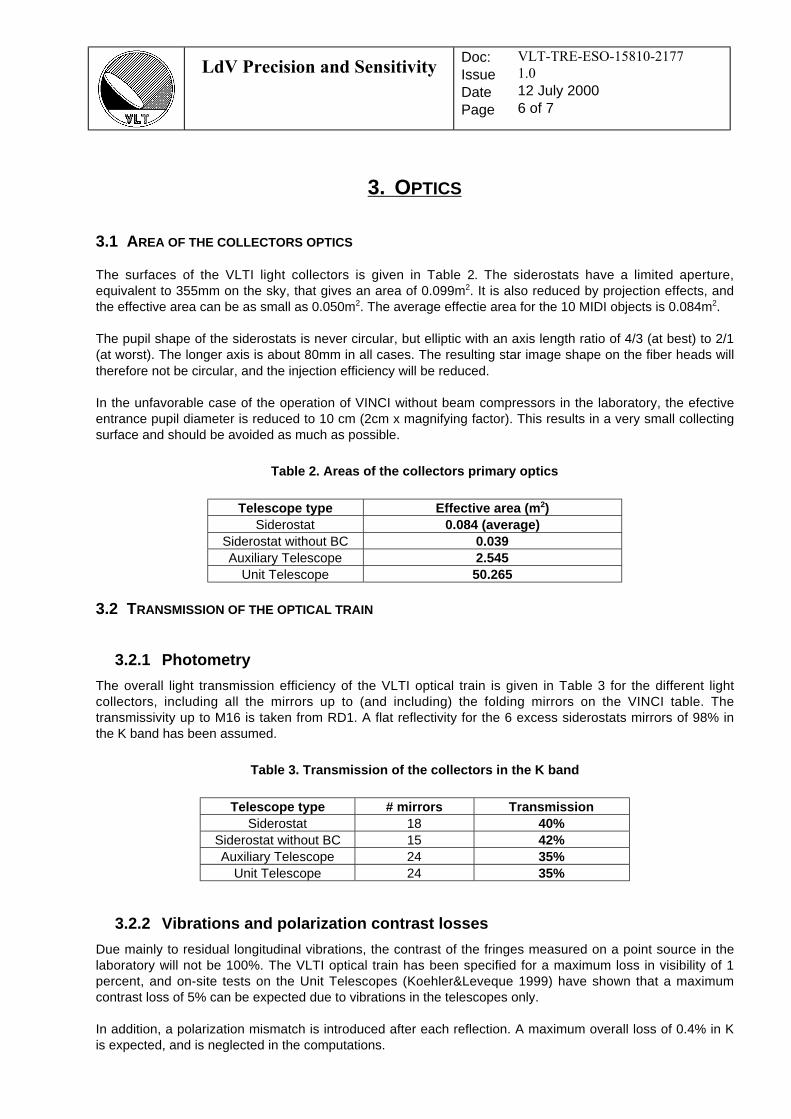
LdV Precision and SensitivityDoc:IssueDatePage
VLT-TRE-ESO-15810-2177
1.0
12 July 20006 of 7
3. OPTICS
3.1 AREA OF THE COLLECTORS OPTICS
The surfaces of the VLTI light collectors is given in Table 2. The siderostats have a limited aperture,equivalent to 355mm on the sky, that gives an area of 0.099m2. It is also reduced by projection effects, andthe effective area can be as small as 0.050m2. The average effectie area for the 10 MIDI objects is 0.084m2.
The pupil shape of the siderostats is never circular, but elliptic with an axis length ratio of 4/3 (at best) to 2/1(at worst). The longer axis is about 80mm in all cases. The resulting star image shape on the fiber heads willtherefore not be circular, and the injection efficiency will be reduced.
In the unfavorable case of the operation of VINCI without beam compressors in the laboratory, the efectiveentrance pupil diameter is reduced to 10 cm (2cm x magnifying factor). This results in a very small collectingsurface and should be avoided as much as possible.
Telescope type Effective area (m 2)Siderostat 0.084 (average)
Siderostat without BC 0.039Auxiliary Telescope 2.545
Unit Telescope 50.265
3.2 TRANSMISSION OF THE OPTICAL TRAIN
3.2.1 Photometry
The overall light transmission efficiency of the VLTI optical train is given in Table 3 for the different lightcollectors, including all the mirrors up to (and including) the folding mirrors on the VINCI table. Thetransmissivity up to M16 is taken from RD1. A flat reflectivity for the 6 excess siderostats mirrors of 98% inthe K band has been assumed.
Telescope type # mirrors TransmissionSiderostat 18 40%
Siderostat without BC 15 42%Auxiliary Telescope 24 35%
Unit Telescope 24 35%
3.2.2 Vibrations and polarization contrast losses
Due mainly to residual longitudinal vibrations, the contrast of the fringes measured on a point source in thelaboratory will not be 100%. The VLTI optical train has been specified for a maximum loss in visibility of 1percent, and on-site tests on the Unit Telescopes (Koehler&Leveque 1999) have shown that a maximumcontrast loss of 5% can be expected due to vibrations in the telescopes only.
In addition, a polarization mismatch is introduced after each reflection. A maximum overall loss of 0.4% in Kis expected, and is neglected in the computations.
Table 2. Areas of the collectors primary optics
Table 3. Transmission of the collectors in the K band

LdV Precision and SensitivityDoc:IssueDatePage
VLT-TRE-ESO-15810-2177
1.0
12 July 20007 of 8
The expected interferometric efficiency of the VLTI is therefore 0.95.
3.2.3 Static wavefront distortion due to the optical train
The static planeity of the wavefront produced by the optical train of the VLTI will impact on the quantity offlux injected into the fibers. The quality of the wavefront will be evaluated using the end-to-end modeldeveloped at ESO. Detailed beam propagation simulations are currently produced by Rainer Wilhelm.
3.2.4 Pupil lateral jitter
The pupil lateral positioning effect on the injection in a fiber is given in RD4. For the VLTI, the stability of thepupil lateral position depends on the bases used. The worst case is for the station located the farthest fromthe laboratory (e.g. the J6 station). Table 4 lists the pupil lateral jitter as given in RD1.
Timewindow
AT without beamexpanders
Siderostats, UT and ATwith beam expander
0.1 s 400 µm RMS 90 µm RMS1 s 600 µm RMS 135 µm RMS10 s 730 µm RMS 165 µm RMS
30 min 790 µm RMS 180 µm RMS
The mean time to acquire a scan in VINCI on a faint star is about 0.2 seconds, but the time between twooptimizations will be of the order of 5 minutes. The figure to take into account is here the latter, as the fluxloss will not be checked afterwards. The resulting flux loss is computed using the following formula (takenfrom RD4):
ρρ
δ
max
≈ −e p22 561 2.
with δp the lateral misalignment as a fraction of the pupil size. In any case, the pupil size is 18mm at theentrance of the instruments.
Light collector Lateral relativeRMS jitter
Flux loss
AT without beamexpander
750/18000=4.2%
3.9%
Siderostats, UT, ATwith beam expander
170/18000=0.94%
0.2%
3.3 FIBER INJECTION STATIC LOSSES
The maximum fraction of the light injected into the optical fibers is 78%. This is due to the fact that the modeon which the telescope diffraction pattern is projected has a gaussian shape (and not an Airy pattern).
3.4 FRESNEL LOSSES
Fresnel losses happen at the surface of the fiber, both at the entrance and output of the fiber. Thetheoretical maximum eficiency is 96%. Four fiber interfaces are foreseen on VINCI between the fiber input
Table 4. VLTI Pupil lateral jitter (worst case, J6 station)
Table 5. RMS flux loss due to lateral jitterof the pupil
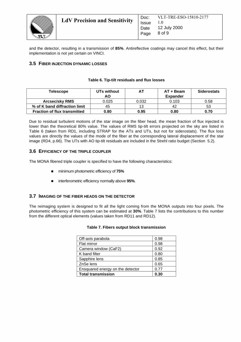
LdV Precision and SensitivityDoc:IssueDatePage
VLT-TRE-ESO-15810-2177
1.0
12 July 20008 of 9
and the detector, resulting in a transmission of 85%. Antireflective coatings may cancel this effect, but theirimplementation is not yet certain on VINCI.
3.5 FIBER INJECTION DYNAMIC LOSSES
Telescope UTs withoutAO
AT AT + BeamExpander
Siderostats
Arcsec/sky RMS 0.025 0.032 0.103 0.58% of K band diffraction limit 45 13 42 53Fraction of flux transmitted 0.80 0.95 0.80 0.70
Due to residual turbulent motions of the star image on the fiber head, the mean fraction of flux injected islower than the theoretical 80% value. The values of RMS tip-tilt errors projected on the sky are listed inTable 6 (taken from RD1, including STRAP for the ATs and UTs, but not for siderostats). The flux lossvalues are directly the values of the mode of the fiber at the corresponding lateral displacement of the starimage (RD4, p.66). The UTs with AO tip-tilt residuals are included in the Strehl ratio budget (Section 5.2).
3.6 EFFICIENCY OF THE TRIPLE COUPLER
The MONA fibered triple coupler is specified to have the following characteristics:
minimum photometric efficiency of 75%
interferometric efficiency normally above 95%.
3.7 IMAGING OF THE FIBER HEADS ON THE DETECTOR
The reimaging system is designed to fit all the light coming from the MONA outputs into four pixels. Thephotometric efficiency of this system can be estimated at 30%. Table 7 lists the contributions to this numberfrom the different optical elements (values taken from RD11 and RD12).
Off-axis parabola 0.98Flat mirror 0.98Camera window (CaF2) 0.92K band filter 0.80Sapphire lens 0.85ZnSe lens 0.65Ensquared energy on the detector 0.77Total transmission 0.30
Table 6. Tip-tilt residuals and flux losses
Table 7. Fibers output block transmission
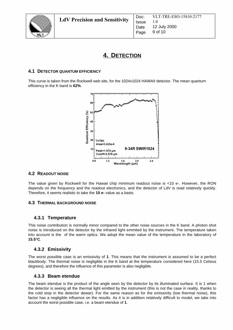
LdV Precision and SensitivityDoc:IssueDatePage
VLT-TRE-ESO-15810-2177
1.0
12 July 20009 of 10
4. DETECTION
4.1 DETECTOR QUANTUM EFFICIENCY
This curve is taken from the Rockwell web site, for the 1024x1024 HAWAII detector. The mean quantumefficiency in the K band is 62%.
4.2 READOUT NOISE
The value given by Rockwell for the Hawaii chip minimum readout noise is <10 e-. However, the RONdepends on the frequency and the readout electronics, and the detector of LdV is read relatively quickly.Therefore, it seems realistic to take the 10 e- value as a basis.
4.3 THERMAL BACKGROUND NOISE
4.3.1 Temperature
This noise contribution is normally minor compared to the other noise sources in the K band. A photon shotnoise is introduced on the detector by the infrared light emmited by the instrument. The temperature takeninto account is the of the warm optics. We adopt the mean value of the temperature in the laboratory of15.5°C.
4.3.2 Emissivity
The worst possible case is an emissivity of 1. This means that the instrument is assumed to be a perfectblackbody. The thermal noise is negligible in the K band at the temperature considered here (15.5 Celsiusdegrees), and therefore the influence of this parameter is also negligible.
4.3.3 Beam etendue
The beam etendue is the product of the angle seen by the detector by its illuminated surface. It is 1 whenthe detector is seeing all the thermal light emitted by the instrument (this is not the case in reality, thanks tothe cold stop in the detector dewar). For the same reason as for the emissivity (low thermal noise), thisfactor has a negligible influence on the results. As it is in addition relatively difficult to model, we take intoaccount the worst possible case, i.e. a beam etendue of 1.

LdV Precision and SensitivityDoc:IssueDatePage
VLT-TRE-ESO-15810-2177
1.0
12 July 200010 of 11
4.4 SAMPLING LOSSES
The HAWAII detector is used as a non blocking sampler. The maximum efficiency in the transmission of thefringe contrast is reached for a sampling of 5 points per fringe, corresponding to an efficiency of 80%.
4.5 DETECTOR DEFECTS
The HAWAII array of VINCI is an engineering grade detector. This means that the possibility exists that thedetector presents some discrepancies from the mentioned characteristics, either in readout noise, frequencyresponse, or other parameters. No defect has been taken into account here.
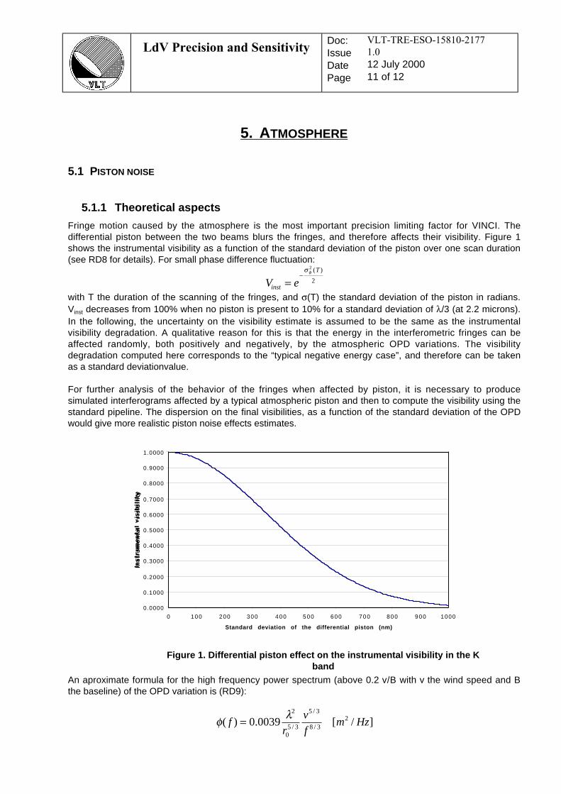
LdV Precision and SensitivityDoc:IssueDatePage
VLT-TRE-ESO-15810-2177
1.0
12 July 200011 of 12
5. ATMOSPHERE
5.1 PISTON NOISE
5.1.1 Theoretical aspects
Fringe motion caused by the atmosphere is the most important precision limiting factor for VINCI. Thedifferential piston between the two beams blurs the fringes, and therefore affects their visibility. Figure 1shows the instrumental visibility as a function of the standard deviation of the piston over one scan duration(see RD8 for details). For small phase difference fluctuation:
V einst
T
=−σ φ
2
2
( )
with T the duration of the scanning of the fringes, and σ(T) the standard deviation of the piston in radians.Vinst decreases from 100% when no piston is present to 10% for a standard deviation of λ/3 (at 2.2 microns).In the following, the uncertainty on the visibility estimate is assumed to be the same as the instrumentalvisibility degradation. A qualitative reason for this is that the energy in the interferometric fringes can beaffected randomly, both positively and negatively, by the atmospheric OPD variations. The visibilitydegradation computed here corresponds to the “typical negative energy case”, and therefore can be takenas a standard deviationvalue.
For further analysis of the behavior of the fringes when affected by piston, it is necessary to producesimulated interferograms affected by a typical atmospheric piston and then to compute the visibility using thestandard pipeline. The dispersion on the final visibilities, as a function of the standard deviation of the OPDwould give more realistic piston noise effects estimates.
0.0000
0.1000
0.2000
0.3000
0.4000
0.5000
0.6000
0.7000
0.8000
0.9000
1.0000
0 100 200 300 400 500 600 700 800 900 1000
Standard deviation of the differential piston (nm)
Inst
rum
en
tal
visi
bil
ity
An aproximate formula for the high frequency power spectrum (above 0.2 v/B with v the wind speed and Bthe baseline) of the OPD variation is (RD9):
φλ
( ) . [ / ]/
/
/fr
v
fm Hz= 0 0039
2
05 3
5 3
8 32
Figure 1. Differential piston effect on the instrumental visibility in the Kband
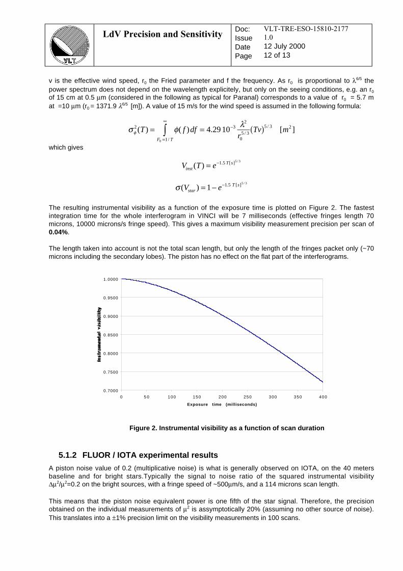
LdV Precision and SensitivityDoc:IssueDatePage
VLT-TRE-ESO-15810-2177
1.0
12 July 200012 of 13
v is the effective wind speed, r0 the Fried parameter and f the frequency. As r0 is proportional to λ6/5 thepower spectrum does not depend on the wavelength explicitely, but only on the seeing conditions, e.g. an r0
of 15 cm at 0.5 µm (considered in the following as typical for Paranal) corresponds to a value of r0 = 5.7 mat =10 µm (r0 = 1371.9 λ6/5 [m]). A value of 15 m/s for the wind speed is assumed in the following formula:
σ φλ
φ2 3
2
05 3
1
5 3 24 29 100
( ) ( ) . [ ]//
/T f dfr
Tv mF T
= = ( )−
=
∞
∫which gives
V T einstT s( ) . [ ] /
= −1 5 5 3
σ ( ) . [ ] /
V estarT s= − −1 1 5 5 3
The resulting instrumental visibility as a function of the exposure time is plotted on Figure 2. The fastestintegration time for the whole interferogram in VINCI will be 7 milliseconds (effective fringes length 70microns, 10000 microns/s fringe speed). This gives a maximum visibility measurement precision per scan of0.04%.
The length taken into account is not the total scan length, but only the length of the fringes packet only (~70microns including the secondary lobes). The piston has no effect on the flat part of the interferograms.
0.7000
0.7500
0.8000
0.8500
0.9000
0.9500
1.0000
0 5 0 100 150 200 250 300 350 400
Exposure time (milliseconds)
Inst
rum
en
tal
visi
bil
ity
5.1.2 FLUOR / IOTA experimental results
A piston noise value of 0.2 (multiplicative noise) is what is generally observed on IOTA, on the 40 metersbaseline and for bright stars.Typically the signal to noise ratio of the squared instrumental visibility∆µ2/µ2=0.2 on the bright sources, with a fringe speed of ~500µm/s, and a 114 microns scan length.
This means that the piston noise equivalent power is one fifth of the star signal. Therefore, the precisionobtained on the individual measurements of µ2 is assymptotically 20% (assuming no other source of noise).This translates into a ±1% precision limit on the visibility measurements in 100 scans.
Figure 2. Instrumental visibility as a function of scan duration

LdV Precision and SensitivityDoc:IssueDatePage
VLT-TRE-ESO-15810-2177
1.0
12 July 200013 of 14
This value is of the same order of magnitude as the 12% precision of the theoretical computations (for thesame scan duration, i.e. with a fringe speed of 500µm/s) presented in Section 5.1.1, which is lower becausethe seeing conditions considered are for Paranal (hence with a better seeing than Mount Hopkins).
5.1.3 Fringe Sensor Unit
The role of the FSU is to reduce the piston sufficiently to have a maximum OPD error of 30 nm up tomagH=13 (UTs) or 10 (ATs) as specified in RD9. When used with the FSU, the theoretical minimumprecision with VINCI considering this residual piston only is 0.37% (up to the limiting magnitude of the FSU,H~ 4 with the siderostats). For the brightest stars (K~ -2 on the siderostats), the theoretical OPD residual isabout 1nm (taken from RD10), which translates into a theoretical visibility loss of 0.0004% (4e-6). Such anumber should not be considered reliable, as no experiment has ever demonstrated this kind of capabilities.Moreover, this is not the final precision, as it only takes into account the piston noise.
The PFSU can theoretically provide the same accuracy, but for stars about 2 magnitudes brighter (i.e. up toH~ 2). The parameters for the upgraded version FINITO should be close to the FSU values.
5.2 STREHL RATIO
The mean values of the Strehl ratios (apart from the quasi-static wavefront errors introduced by the opticaltrain, see Section 3.2.3) expected for the different light collectors are listed in Table 8. The values withoutAO assume an r0 of 1 meter in the K band at Paranal, and do not take into account the residual tip-tilt errors(see Section 3.5), except fo the UTs with AO.
Telescope type Strehl without AO in K Strehl with AOSiderostat wihout BC ~100% -
Siderostat with BC ~100% -AT 30.8% -UT 1.56% 48% (K=12)
Shaklan (Applied Optics, 27, 2334, 1988) has shown that the optimal injection is obtained for a value of D/r0
of 4 (with D the telescope diameter and r0 the Fried parameter). It could therefore be interesting to foreseepupil stops for the first observations with the UTs not equipped with AO systems.
5.3 PHOTOMETRIC NOISE
The adaptive optics and/or tip-tilt correction systems will leave some residual star motion on the fiber head.This will cause a degradation in the quantity of light coupled into the fibers, and random variations of the fluxmeasured on the detector. From time to time, the flux injected in the fibers can drop to zero (or smallvalues). As the interferometric signals are divided by the photometric signals, this causes a decrease in theSNR of the photometrically corrected fringes.
In the case of VINCI, this effect is equivalent to a random photometric loss. The single-mode fibers filter outcompletely the tip-tilt and high order wavefront errors, and the output wavefront is only affected by fluxvariations. These variations inject some power in the frequency range of the fringes, and therefore can affectthe fringe visibility. To reduce this effect, the photometric signals are used to calibrate the interferometricoutputs during the data reduction.
Further simulations are required to estimate the impact of this kind of noise on the measurements.
5.4 INTERNAL TURBULENCE
Table 8. Strehl ratios for different telescope configurations
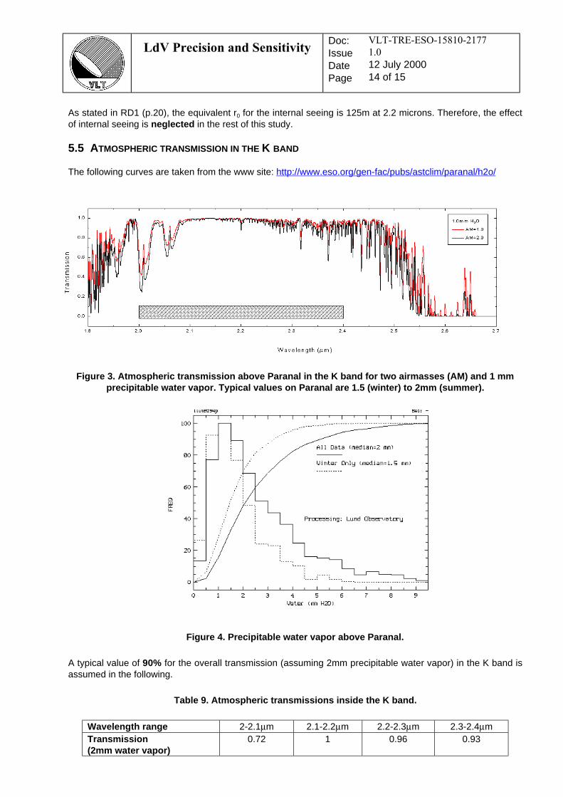
LdV Precision and SensitivityDoc:IssueDatePage
VLT-TRE-ESO-15810-2177
1.0
12 July 200014 of 15
As stated in RD1 (p.20), the equivalent r0 for the internal seeing is 125m at 2.2 microns. Therefore, the effectof internal seeing is neglected in the rest of this study.
5.5 ATMOSPHERIC TRANSMISSION IN THE K BAND
The following curves are taken from the www site: http://www.eso.org/gen-fac/pubs/astclim/paranal/h2o/
A typical value of 90% for the overall transmission (assuming 2mm precipitable water vapor) in the K band isassumed in the following.
Wavelength range 2-2.1µm 2.1-2.2µm 2.2-2.3µm 2.3-2.4µmTransmission(2mm water vapor)
0.72 1 0.96 0.93
Figure 3. Atmospheric transmission above Paranal in the K band for two airmasses (AM) and 1 mmprecipitable water vapor. Typical values on Paranal are 1.5 (winter) to 2mm (summer).
Figure 4. Precipitable water vapor above Paranal.
Table 9. Atmospheric transmissions inside the K band.
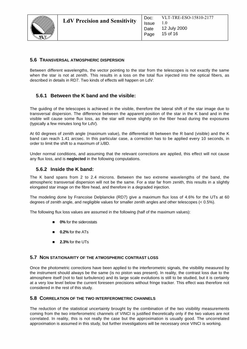
LdV Precision and SensitivityDoc:IssueDatePage
VLT-TRE-ESO-15810-2177
1.0
12 July 200015 of 16
5.6 TRANSVERSAL ATMOSPHERIC DISPERSION
Between different wavelengths, the vector pointing to the star from the telescopes is not exactly the samewhen the star is not at zenith. This results in a loss on the total flux injected into the optical fibers, asdescribed in details in RD7. Two kinds of effects will happen on LdV:
5.6.1 Between the K band and the visible:
The guiding of the telescopes is achieved in the visible, therefore the lateral shift of the star image due totransversal dispersion. The difference between the apparent position of the star in the K band and in thevisible will cause some flux loss, as the star will move slightly on the fiber head during the exposures(typically a few minutes long for LdV).
At 60 degrees of zenith angle (maximum value), the differential tilt between the R band (visible) and the Kband can reach 1.41 arcsec. In this particular case, a correction has to be applied every 10 seconds, inorder to limit the shift to a maximum of λ/8D.
Under normal conditions, and assuming that the relevant corrections are applied, this effect will not causeany flux loss, and is neglected in the following computations.
5.6.2 Inside the K band:
The K band spans from 2 to 2.4 microns. Between the two extreme wavelengths of the band, theatmospheric transversal dispersion will not be the same. For a star far from zenith, this results in a slightlyelongated star image on the fibre head, and therefore in a degraded injection.
The modeling done by Francoise Delplancke (RD7) give a maximum flux loss of 4.6% for the UTs at 60degrees of zenith angle, and negligible values for smaller zenith angles and other telescopes (< 0.5%).
The following flux loss values are assumed in the following (half of the maximum values):
0% for the siderostats
0.2% for the ATs
2.3% for the UTs
5.7 NON STATIONARITY OF THE ATMOSPHERIC CONTRAST LOSS
Once the photometric corrections have been applied to the interferometric signals, the visibility measured bythe instrument should always be the same (is no piston was present). In reality, the contrast loss due to theatmosphere itself (not to fast turbulence) and its large scale evolutions is still to be studied, but it is certainlyat a very low level below the current foreseen precisions without fringe tracker. This effect was therefore notconsidered in the rest of this study.
5.8 CORRELATION OF THE TWO INTERFEROMETRIC CHANNELS
The reduction of the statistical uncertainty brought by the combination of the two visibility measurementscoming from the two interferometric channels of VINCI is justified theoretically only if the two values are notcorrelated. In reality, this is not really the case but the approximation is usually good. The uncorrelatedapproximation is assumed in this study, but further investigations will be necessary once VINCI is working.

LdV Precision and SensitivityDoc:IssueDatePage
VLT-TRE-ESO-15810-2177
1.0
12 July 200016 of 17
5.9 STATISTICAL PHOTON SHOT NOISE
Due to the statistics of the individual photons arriving on the detector, a noise proportional to the square rootof the number of photons (or power) is introduced in the measurements. The contribution of this noisedepends on the integration time. RElated formulae are given in the Appendix.

LdV Precision and SensitivityDoc:IssueDatePage
VLT-TRE-ESO-15810-2177
1.0
12 July 200017 of 18
6. GLOBAL PARAMETERS
6.1 OVERALL PHOTOMETRIC EFFICIENCY
Telescopes Siderostatswithout BC
Siderostatswith BC
ATs + BE UTswithout AO
UTs withAO
Atmospheric transmission 0.90 0.90 0.90 0.90 0.90Strehl ratio 1.00 1.00 0.31 0.016 0.48Transversal dispersion 1.00 1.00 1.00 0.98 0.98Optical train 0.42 0.40 0.35 0.35 0.35Pupil lateral jitter 1.00 1.00 0.96 1.00 1.00Fiber injection 0.78 0.78 0.78 0.78 0.78Fresnel losses 0.85 0.85 0.85 0.85 0.85Fiber injection tip-tilt residuals 0.70 0.70 0.80 0.80 1.00Triple coupler 0.75 0.75 0.75 0.75 0.75Outputs imaging 0.30 0.30 0.30 0.30 0.30Signal splitting 0.25 0.25 0.25 0.25 0.25Quantum efficiency 0.62 0.62 0.62 0.62 0.62TOTAL 0.00612 0.00582 0.00173 0.0000914 0.00342
6.2 OVERALL INTERFEROMETRIC EFFICIENCY
Telescopes Siderostats ATs UTs withoutAO
UTs withAO
Sampling losses 0.80 0.80 0.80 0.80Telescopes and optical train 0.95 0.95 0.95 0.95Triple coupler 0.95 0.95 0.95 0.95TOTAL 0.722 0.722 0.722 0.722
Table 10. Photometric transmission coefficients
Table 11. Interferometric transmission coefficients
LdV Precision and SensitivityDoc:IssueDatePage
VLT-TRE-ESO-15810-2177
1.0
12 July 200018 of 19
7. STATISTICAL VISIBILITY PRECISION CURVES
7.1 SIGNAL TO NOISE RATIO
The signal to noise ratio Ω is given by the following formula:
Ω =+ + +
S
thermal photonϖ ϖ ϖ ϖ4 4 4 4detector piston
the fourth power on the NEP come from the fact that the signal is the squared visibility of the fringes.
7.2 OPTIMAL OPD SCAN SPEED
The effective precision attainable with VINCI will depend on the exposure time used on each star. Theoptimized parameter is the OPD scan speed v (in optical path difference, which is twice the piezo mirrormotion speed). As a general rule, VINCI will sample the fringes at a fixed n = 5 points per fringe (optimalvalue), gives directly the readout frequency of the detector through the formula : f = n.v/λ. This means thatthe readout frequency of the detector (and therefore the exposure time) is completely defined by the fringespeed.
As the star is brighter, the exposure time can be shorter, and therefore the piston noise impact on the fringescan be reduced. It is important though to have a sufficient number of photons in each OPD bin, so as not tobe limited by the detector readout noise, but still not too large to avoid the photon shot noise. Thedetermination of the optimal exposure time is therefore a trade-off between the piston noise, the photonnoise and the detector noise, in order to minimize the total noise on the flux measurement. For the faintstars, the problem is the same, but the photon shot noise will be negligible compared to the readout noise ofthe detector and the piston noise.
The formulae for the different noise sources are given in the Appendix (Section 10). The minimization isdone on the total signal to noise ratio Ω (as given in Section 7.1), assuming that only the OPD scan speedis variable. The piston has an effect on ly on the fringes part of the acquired interferograms. This means thatthe time used to compute the fringes blurring is the the time necessary to scan the 70 microns of the fringepacket (see Section 5.1 for details).
7.3 CURVES WITH THE DIFFERENT LIGHT COLLECTORS , WITHOUT FSU
For 100 scans and combining the two interferometric outputs. From left to right:
Siderostats without beam compressors
Siderostats with beam compressors
ATs and UTs without Adaptive Optics (same curve)
UTs with Adaptive Optics

LdV Precision and SensitivityDoc:IssueDatePage
VLT-TRE-ESO-15810-2177
1.0
12 July 200019 of 20
0.001
0.01
0 .1
1
1 0
- 3 - 2 - 1 0 1 2 3 4 5 6 7 8 9 1 0 1 1 1 2 1 3
K Magnitude
Precision on the v is ib i l i ty (%)
The maximum statistical precision theoretically attainable is about 0.002 % for the brightest stars. Thelimitation for the UTs comes from the photon noise, and is due to the limited maximum speed of the piezomirror (vmax(OPD) = 1 cm/s). A practical limit for the observations can be set at 2% limiting precision (in 100scans). After this limit, the calibration of the observation can be problematic, but the system can be usableup to a 5% precision. This gives the limiting magnitudes listed in Table 12. It should be stressed that thefigures given in this table are for the statistical uncertainties only. They are useful to prepare an observation,as they give an estimate of the limiting magnitude of a single star observation, but the final calibratedvisibilities will have a lower precision, due to the uncertainties on the calibrator angular size or other factors(see Section 9 for details).
Collector Limitingmagnitude 2%
precision
Limitingmagnitude 5%
precisionSiderostats without beam compressors 4.6 6.1Siderostats with beam compressors 6.0 7.5Auxiliary Telescopes 8.3 9.8Unit Telescopes without Adaptive Optics 8.3 9.8Unit Telescopes with Adaptive Optics 12.3 13.8
Table 12. VINCI statistical limiting magnitudes
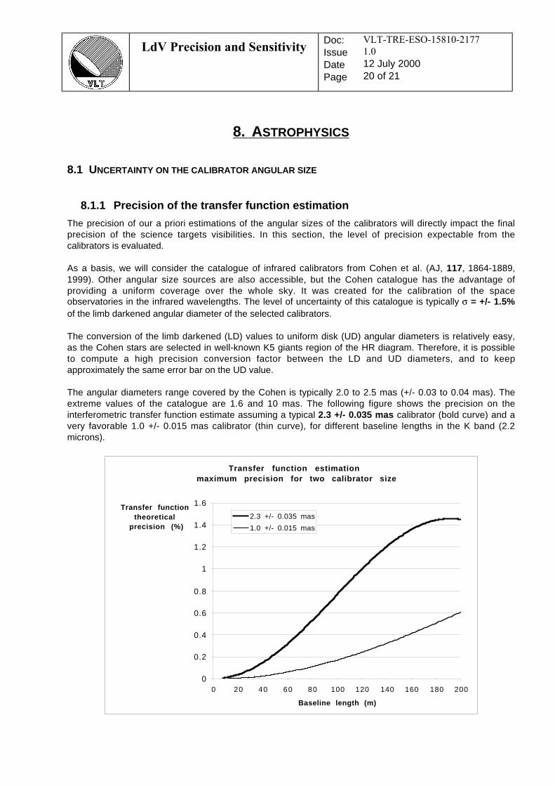
LdV Precision and SensitivityDoc:IssueDatePage
VLT-TRE-ESO-15810-2177
1.0
12 July 200020 of 21
8. ASTROPHYSICS
8.1 UNCERTAINTY ON THE CALIBRATOR ANGULAR SIZE
8.1.1 Precision of the transfer function estimation
The precision of our a priori estimations of the angular sizes of the calibrators will directly impact the finalprecision of the science targets visibilities. In this section, the level of precision expectable from thecalibrators is evaluated.
As a basis, we will consider the catalogue of infrared calibrators from Cohen et al. (AJ, 117, 1864-1889,1999). Other angular size sources are also accessible, but the Cohen catalogue has the advantage ofproviding a uniform coverage over the whole sky. It was created for the calibration of the spaceobservatories in the infrared wavelengths. The level of uncertainty of this catalogue is typically σ = +/- 1.5%of the limb darkened angular diameter of the selected calibrators.
The conversion of the limb darkened (LD) values to uniform disk (UD) angular diameters is relatively easy,as the Cohen stars are selected in well-known K5 giants region of the HR diagram. Therefore, it is possibleto compute a high precision conversion factor between the LD and UD diameters, and to keepapproximately the same error bar on the UD value.
The angular diameters range covered by the Cohen is typically 2.0 to 2.5 mas (+/- 0.03 to 0.04 mas). Theextreme values of the catalogue are 1.6 and 10 mas. The following figure shows the precision on theinterferometric transfer function estimate assuming a typical 2.3 +/- 0.035 mas calibrator (bold curve) and avery favorable 1.0 +/- 0.015 mas calibrator (thin curve), for different baseline lengths in the K band (2.2microns).
Transfer function estimation maximum precision for two calibrator size
0
0.2
0.4
0.6
0.8
1
1.2
1.4
1.6
0 20 40 60 80 100 120 140 160 180 200
Baseline length (m)
Transfer function theoretical
precision (%)2.3 +/- 0.035 mas
1.0 +/- 0.015 mas
LdV Precision and SensitivityDoc:IssueDatePage
VLT-TRE-ESO-15810-2177
1.0
12 July 200021 of 22
On the brightest stars, VINCI is able to reach a statistical precision of 0.002 %. This means that the finalvisibility estimation will be limited mainly by the calibrator size knowledge for baselines larger than a fewtens of meters meters. It is important to realize that it will not be possible to increase this precision byobserving the calibrator for a longer time, as it is a fundamental uncertainty (not of statistical origin).
One should also mention that the error on the transfer function measurement impacts the final calibratedprecision in a way that is not multiplicative, but by division. This means that usually, if the observations onthe target are very good and the calibrator is bad, then the final precision on the target will be substanciallybetter than for the calibrator.
8.1.2 Multiple calibration
A way to solve this problem is to use several calibrators for the same science star. Assuming that theangular diameters are not biased, we can reduce the final uncertainty on the transfer function substantially.
If we consider the standard 2.3 +/- 0.035 mas calibrator case, observed with the 200 meters baseline, it isnecessary to reduce the uncertainty from 1.45% to 0.04% to be limited only by the statistical uncertainty ofVINCI (bright star). This means a factor 36, and more than 1300 calibrators to observe. Of course, this isimpossible to achieve.
By using 10 calibrators (which is a reasonable maximum number for a single star), we can go to a transferfunction precision of 0.43% on the transfer function for the 200 meters baseline. This is still a factor 200above the VINCI maximum precision, but this is probably the best we will be able to achieve on a singleobservation by using the “raw” Cohen calibrators catalogue.
8.1.3 Refinement of the calibrator catalogue
During the course of one night, and assuming that we observe a number of targets and calibrators together,it will be possible to cross calibrate the calibrators. The observations with the longest baselines are able toresolve almost completely the ~2 mas calibrators of Cohen. This means that we will have the possibility tomeasure all the angular diameter of each calibrator by comparing it to the other observed known stars. Thiscomparison can only be done in a limited segment of time, as the transfer function of the whole VLTI+VINCIsystem must not evolve between the measurements.
As the catalogue of the observed sources will grow, so will the “cross-calibrated” calibrators catalogue. Afirst step could be to check the internal consistency of the whole southern sky Cohen catalogue (~ 300stars). This would require to observe each star of the catalogue together with two other Cohen (or otherexternal reference) stars (the number three is chosen to stay in a short time segment).
Each set of three stars will provide the calibrated diameters for two of them, while the third star can be usedas a link to the rest of the catalogue. The total number of single star observations would therefore be:
(3 stars) x (2 observation per star) x (Ntotal / 2) = 900 observations.
Assuming 80 observations per night (~one every 6 minutes), this could be completed in 12 nights.
It will also be possible to extend the Cohen catalogue by observing stable stars down to smaller sizes, andcalibrating them with Cohen stars.
8.2 KNOWLEDGE OF THE TARGET SPECTRUM SHAPE
The spectral distribution of the energy received from the star can be far from beeing perfectly flat over the Kband. Depending on the spectral type of the star, the mean slope of the star spectrum can be either nearlyflat (hot stars) or rising steeply with wavelength (cold stars). During the data reduction process, it isimportant to know the effective mean wavelength of the observations, in order to locate correctly the peak ofthe fringe power in the Fourier transform of the corrected interferomtetric signals.

LdV Precision and SensitivityDoc:IssueDatePage
VLT-TRE-ESO-15810-2177
1.0
12 July 200022 of 23
If no shape factor correction is applied on the data, the error on the visibility estimation can be as large as+/- 1% for extreme cases. This is especially important when the star and calibrator have significantlydifferent spectral types.
It is possible to assemble a database of the shape factor corrections based on the spectral type, andtherefore to cancel the difference between the science targets and calibrators. Though, for peculiar targets,for which the spectral type is not comparable to a standard type, is will be necessary to acquire a lowresolution K band spectrum to compute the proper correction.
Eventually, the coupling of a low resolution spectrograph to the VLTI would be interesting to have a fullcalibration capability.

LdV Precision and SensitivityDoc:IssueDatePage
VLT-TRE-ESO-15810-2177
1.0
12 July 200023 of 24
9. CALIBRATED VISIBILITIES
9.1 LIGHT COLLECTORS
The first fringes will be obtained with VINCI using the siderostats. It is still unclear whether the beamcompressors will be present or not. There is a 1.4 limiting magnitude difference between the twoconfigurations, but the limiting precision will not be reached for both types of collectors on the brightest stars(the photon noise will never be dominating).
In the present section all the light collector cases (including the siderostats with and without beamcompressors) are examined.
9.2 PRECISION CURVES AND EXPOSURE TIME CALCULATOR TOOL
An Excel sheet (the graphical user interface is presented Figure 5) was created in order to estimate theimpact of the variations of the numerous observational parameters on the precision obtainable with VINCI.
It takes as input parameters:• the baseline length,• all the statistical errors tables computed with Matlab as listed in Section 7,• the magnitude of the calibrator,• the angular diameter (uniform disk) of the calibrator,• the uncertainty on the a priori angular diameter of the calibrator.
and specifically for the exposure time calculator:• science target magnitude,• science target estimated angular diameter,• requested precision.
A short macro is used to adjust the observation duration to match the requested precision. It alwaysconsiders the optimal scan as the actual acquisition rate. The precisions curves are plotted in real time asthe user enters the parameters values.

LdV Precision and SensitivityDoc:IssueDatePage
VLT-TRE-ESO-15810-2177
1.0
12 July 200024 of 25
9.3 CALIBRATORS , BASELINE AND SHAPE FACTOR
The calibrators available in the first weeks will not benefit from the accuracy improvement procedureproposed in Section 8.1.3. Therefore, the transfer function measurement accuracy will be limited for thelongest baselines to about 1%. For the short baselines (up to 20 meters), the uncertainty will be less than0.05%.
The shape factor will be derived from the catalogued spectral types, and is not expected to be a limitingparameter for the final precision, as no very peculiar sources are foreseen during this first period.
9.4 EXAMPLE : THE CASE OF ZETA GEMINORUM
In order to have a realistic case for the observation simulations, the case of the Cepheid Zeta Gem with thecalibrator star HD 49968 is considered. Zeta Gem is a 1.98 magnitude star in K (angular diameter ofaproximately 1.8 mas). HD 49968 is a 2.2 magnitude calibrator from the Cohen list, with a uniform diskangular diameter of 1.87 +/- 0.030 mas.
Considering the longest baseline of 195 meters, it will be necessary to observe for about 1300 seconds oneach Zeta Gem and HD 49968 with the siderostats to get to a 2% accuracy on the visibilities. This resultsfrom the fact that the correlated visibility of this star is high (as it is resolved), but the uncertainty on thecalibrator also adds to the difficulty of the observation.
Figure 5. Exposure time calculator graphical user interface
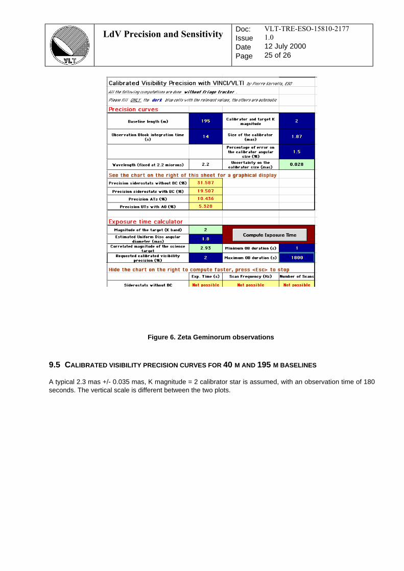
LdV Precision and SensitivityDoc:IssueDatePage
VLT-TRE-ESO-15810-2177
1.0
12 July 200025 of 26
9.5 CALIBRATED VISIBILITY PRECISION CURVES FOR 40 M AND 195 M BASELINES
A typical 2.3 mas +/- 0.035 mas, K magnitude = 2 calibrator star is assumed, with an observation time of 180seconds. The vertical scale is different between the two plots.
Figure 6. Zeta Geminorum observations

LdV Precision and SensitivityDoc:IssueDatePage
VLT-TRE-ESO-15810-2177
1.0
12 July 200026 of 27
Figure 7. Precision on the calibrated visibility for a 40 m baseline

LdV Precision and SensitivityDoc:IssueDatePage
VLT-TRE-ESO-15810-2177
1.0
12 July 200027 of 28
9.6 ATMOSPHERIC TURBULENCE AND FRINGE SENSOR IMPORTANCE
The atmospheric turbulence introduces random corrugation of the incoming wavefront, both in shape(perpendicular to the propagation direction) and longitudinal delay (along the direction of propagation, alsocalled differential piston effect). The adaptive optics allows the flattening of the wavefront in theperpendicular direction. Once corrected, the wavefront can be injected much more efficiently in single-modeoptical fibers. This results in a higher flux used for beam combination, and increased sensitivity.
The role of the fringe sensor unit (FSU) is to stabilize the fringes longitudinally, to allow for longer integrationtimes with the science instrument. Normally, the piston effect limits the scan time to a few tens ofmilliseconds. The FSU removes it by quickly adjusting the internal OPD by means of a delay line. The FSUcould become available for the testing period with the siderostats. The effect of the FSU is important on theprecision of the visibility measurements (reduced or canceled piston noise), but not primarily on the limitingmagnitude of the instrument. With a FSU, the maximum measurement accuracy can be reached on allreachable stars, but the observable targets number will not be significantly larger than without FSU. AsVINCI and the FSU will supposedly have the same limiting magnitude, fainter stars will not be accessiblebefore the arrival of PRIMA and its dual-beam capability. With PRIMA though, the limiting magnitude willbecome much higher (Mag K ~ 19).
The Fringe Sensor Unit is absolutely essential for the most demanding observation programs, such as theexoplanets, and the efforts should be concentrated on having it available on Paranal as soon as possible.The limiting precision reachable with the FSU is not yet certain, but could be as low as 0.001 % (10^-5) forall observable stars.
Figure 8. Precision on the calibrated visibility for a 195 m baseline
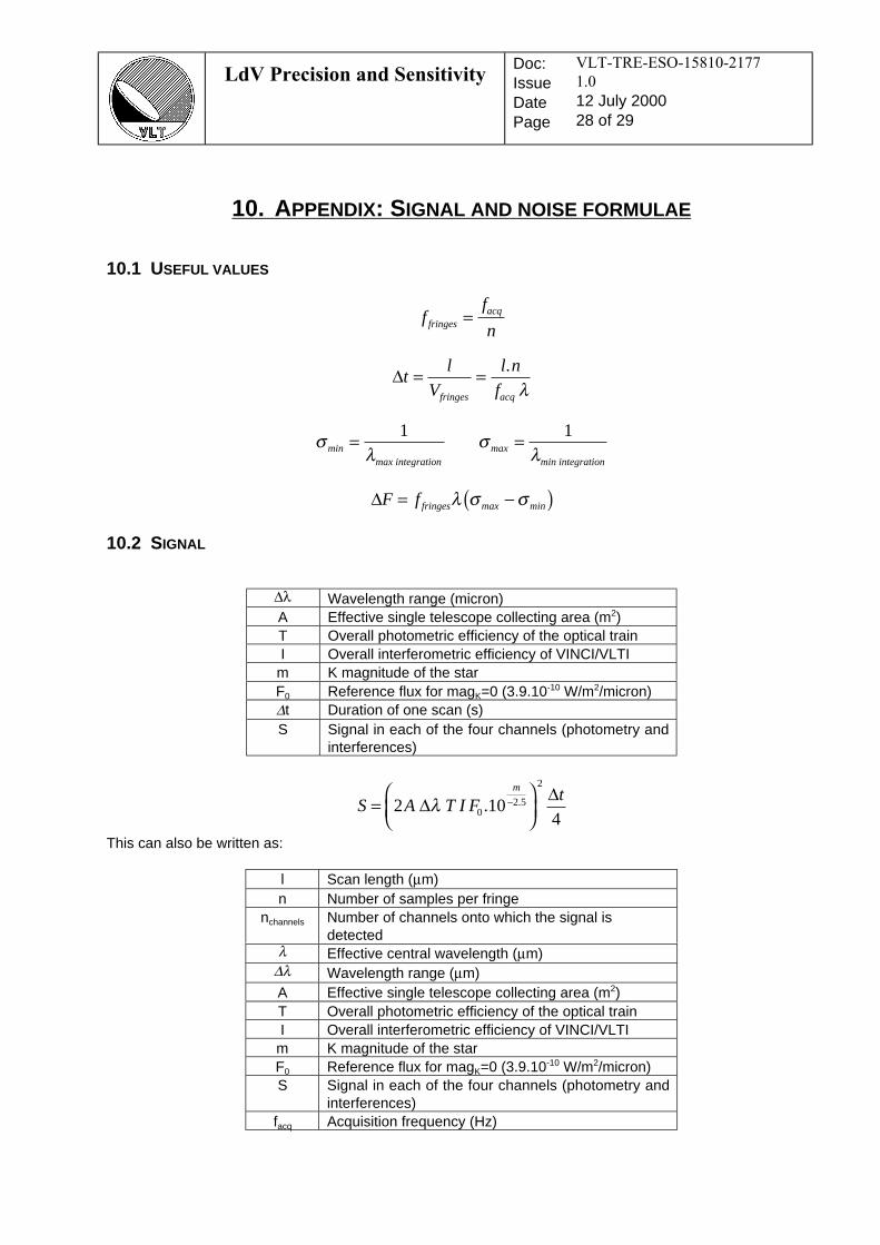
LdV Precision and SensitivityDoc:IssueDatePage
VLT-TRE-ESO-15810-2177
1.0
12 July 200028 of 29
10. APPENDIX: SIGNAL AND NOISE FORMULAE
10.1 USEFUL VALUES
ff
nfringesacq=
∆tl
V
l n
ffringes acq
= =.λ
σλ
σλmin
max integrationmax
min integration
= =1 1
∆F f fringes= −( )λ σ σmax min
10.2 SIGNAL
∆λ Wavelength range (micron)A Effective single telescope collecting area (m2)T Overall photometric efficiency of the optical trainI Overall interferometric efficiency of VINCI/VLTI
m K magnitude of the starF0 Reference flux for magK=0 (3.9.10-10 W/m2/micron)∆t Duration of one scan (s)S Signal in each of the four channels (photometry and
interferences)
S A TI Ftm
=
−2 10
402 5
2
∆∆
λ . .
This can also be written as:
l Scan length (µm)n Number of samples per fringe
nchannels Number of channels onto which the signal isdetected
λ Effective central wavelength (µm)∆λ Wavelength range (µm)A Effective single telescope collecting area (m2)T Overall photometric efficiency of the optical trainI Overall interferometric efficiency of VINCI/VLTI
m K magnitude of the starF0 Reference flux for magK=0 (3.9.10-10 W/m2/micron)S Signal in each of the four channels (photometry and
interferences)facq Acquisition frequency (Hz)
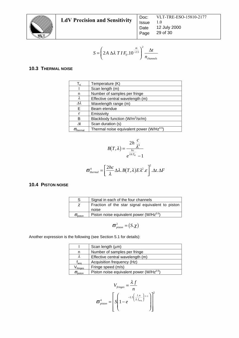
LdV Precision and SensitivityDoc:IssueDatePage
VLT-TRE-ESO-15810-2177
1.0
12 July 200029 of 30
S A TI Ft
n
m
channels
=
−2 1002 5
2
∆∆
λ . .
10.3 THERMAL NOISE
TK Temperature (K)l Scan length (m)n Number of samples per fringeλ Effective central wavelength (m)∆λ Wavelength range (m)E Beam etendueε EmissivityB Blackbody function (W/m2/sr/m)∆t Scan duration (s)
ϖthermal Thermal noise equivalent power (W/Hz0.5)
B Th
c
ehc
kTK
,λ λλ
( ) =−
2
1
3
ϖλ
λ λ λ εthermal
hcB T E t F4 2
22= ( )
∆ ∆ ∆. , . . .
10.4 PISTON NOISE
S Signal in each of the four channelsχ Fraction of the star signal equivalent to piston
noiseϖpiston Piston noise equivalent power (W/Hz0.5)
ϖ χpiston S2 = ( ).
Another expression is the following (see Section 5.1 for details):
l Scan length (µm)n Number of samples per fringeλ Effective central wavelength (m)
facq Acquisition frequency (Hz)Vfringes Fringe speed (m/s)ϖpiston Piston noise equivalent power (W/Hz0.5)
Vf
nfringes =λ
ϖ λpiston
l n
fS e acq4
1 5
2
15 3
= −
−
.
. /

LdV Precision and SensitivityDoc:IssueDatePage
VLT-TRE-ESO-15810-2177
1.0
12 July 200030 of 31
10.5 DETECTOR NOISE
facq Acquisition frequency (Hz)ffringes Fringe frequency (Hz)
n Number of samples per fringeφ Read out noise (e-)η Quantum efficiency
ϖdetector Detector noise equivalent power (W/Hz0.5)
ϖ φη λdetector
4
2 2
2=
. .hc
n f t Fpixels acq ∆ ∆
10.6 PHOTON NOISE
λ Effective central wavelength (m)∆λ Wavelength range (µm)A Effective single telescope collecting area (m2)T Photometric transmission of the optical trainm K magnitude of the starF0 Reference flux for magK=0 (3.9.10-10 W/m2/µm)
ϖphoton Photon noise equivalent power (W/Hz0.5)
ϖλ
λphoton
mhcA TF t F4
02 5
2
22 10=
−∆ ∆ ∆. .
10.7 UNCERTAINTY ON THE VISIBILITY
By combining the visibilities of the two interferometric channels, and assuming that they are not correlated,the resulting uncertainty ϑ on the visibility for one scan is (for N interferograms, with Ω the SNR):
ϑ =2N.Ω

LdV Precision and SensitivityDoc:IssueDatePage
VLT-TRE-ESO-15810-2177
1.0
12 July 200031 of 32
11. APPENDIX: MATLAB ROUTINES
11.1 EXECUTION BATCH
The files are written in wk1 spreadsheet format for use in Excel.
table_siderostats_without_bc=abaque(0);wk1write('table_sids_witout_bc',table_siderostats_without_bc);table_siderostats=abaque(1);wk1write('table_sids',table_siderostats);table_ats=abaque(2);wk1write('table_ats',table_ats);table_uts_without_ao=abaque(3);wk1write('table_uts_without_ao',table_uts_without_ao);table_uts_with_ao=abaque(4);wk1write('table_uts_with_ao',table_uts_with_ao);
11.2 MAIN PROGRAM (ABAQUE)
function table_results=abaque(telescope);
% table_results contains the following data:% 1- magnitude of the star% 2- resulting SNR per channel per scan% 3- resulting precision for 1 scan and 1 channel% 4- optimal frequency for acquisition% 5- required piezo speed% 6- precision for 100 scans and the two channels (supposed decorrelated)% 7- fraction of noise due to the piston;% 8- fraction of noise due to the detector;% 9- fraction of noise due to the photon;
l = 51.2*2.2e-6; % Total length of the scan in mlambda = 2.2e-6; % Wavelength in mn = 5; % Points per fringemax_speed = 0.01; % Maximum scan speed in m/s
% Siderostat without Beam Compressorsif telescope==0,
max_loop=85+31;end% Siderostat with BCif telescope==1,
max_loop=85+31;end% ATif telescope==2,
max_loop=110+31;end% UT without AOif telescope==3,
max_loop=110+31;end% UT with AOif telescope==4,
max_loop=150+31;end
for i=1:max_loop,magnitude = (i-31)/10;scan_speed=fmins('snr_vinci',5e-4,foptions,[],magnitude,telescope);
% If the scan speed is larger than the maximum speed of the piezo, then% take the maximum value.if scan_speed>0.01,
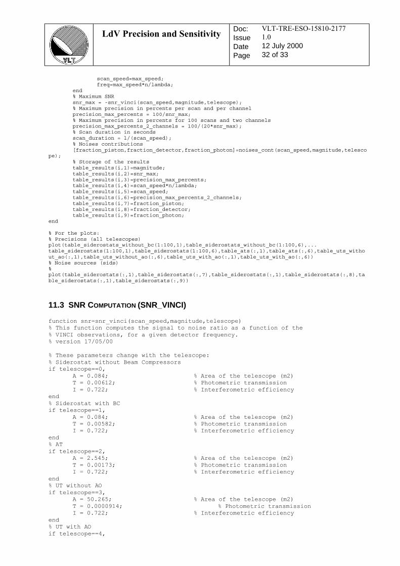
LdV Precision and SensitivityDoc:IssueDatePage
VLT-TRE-ESO-15810-2177
1.0
12 July 200032 of 33
scan_speed=max_speed;freq=max_speed*n/lambda;
end% Maximum SNRsnr_max = -snr_vinci(scan_speed,magnitude,telescope);% Maximum precision in percents per scan and per channelprecision_max_percents = 100/snr_max;% Maximum precision in percents for 100 scans and two channelsprecision_max_percents_2_channels = 100/(20*snr_max);% Scan duration in secondsscan_duration = l/(scan_speed);% Noises contributions[fraction_piston,fraction_detector,fraction_photon]=noises_cont(scan_speed,magnitude,telesco
pe);% Storage of the resultstable_results(i,1)=magnitude;table_results(i,2)=snr_max;table_results(i,3)=precision_max_percents;table_results(i,4)=scan_speed*n/lambda;table_results(i,5)=scan_speed;table_results(i,6)=precision_max_percents_2_channels;table_results(i,7)=fraction_piston;table_results(i,8)=fraction_detector;table_results(i,9)=fraction_photon;
end
% For the plots:% Precisions (all telescopes)plot(table_siderostats_without_bc(1:100,1),table_siderostats_without_bc(1:100,6),...table_siderostats(1:100,1),table_siderostats(1:100,6),table_ats(:,1),table_ats(:,6),table_uts_without_ao(:,1),table_uts_without_ao(:,6),table_uts_with_ao(:,1),table_uts_with_ao(:,6))% Noise sources (sids)%plot(table_siderostats(:,1),table_siderostats(:,7),table_siderostats(:,1),table_siderostats(:,8),table_siderostats(:,1),table_siderostats(:,9))
11.3 SNR COMPUTATION (SNR_VINCI)
function snr=snr_vinci(scan_speed,magnitude,telescope)% This function computes the signal to noise ratio as a function of the% VINCI observations, for a given detector frequency.% version 17/05/00
% These parameters change with the telescope:% Siderostat without Beam Compressorsif telescope==0,
A = 0.084; % Area of the telescope (m2)T = 0.00612; % Photometric transmissionI = 0.722; % Interferometric efficiency
end% Siderostat with BCif telescope==1,
A = 0.084; % Area of the telescope (m2)T = 0.00582; % Photometric transmissionI = 0.722; % Interferometric efficiency
end% ATif telescope==2,
A = 2.545; % Area of the telescope (m2)T = 0.00173; % Photometric transmissionI = 0.722; % Interferometric efficiency
end% UT without AOif telescope==3,
A = 50.265; % Area of the telescope (m2)T = 0.0000914; % Photometric transmissionI = 0.722; % Interferometric efficiency
end% UT with AOif telescope==4,
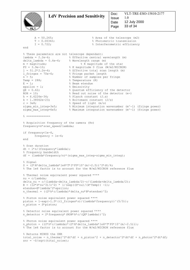
LdV Precision and SensitivityDoc:IssueDatePage
VLT-TRE-ESO-15810-2177
1.0
12 July 200033 of 34
A = 50.265; % Area of the telescope (m2)T = 0.00342; % Photometric transmissionI = 0.722; % Interferometric efficiency
end
% These parameters are not telescope dependant:lambda = 2.2e-6; % Effective central wavelength (m)delta_lambda = 0.4e-6; % Wavelength range (m)m = magnitude; % K magnitude of the starF0 = 3.9e-10; % K magnitude 0 flux (W/m2/MICRON)l = 51.2*2.2e-6; % Effective total scan length (m)l_fringes = 70e-6; % Fringe packet lengthn = 5; % Number of samples per fringeTemp = 288; % Temperature (K)E = 1; % Beam etendueepsilon = 1; % EmissivityQE = 0.62; % Quantum efficiency of the detectorRON = 10; % Read out noise of the detector (e-)h = 6.6226e-34; % Planck constant (J.s)k = 1.38062e-23; % Boltzmann constant (J/s)c = 3e8; % Speed of light (m/s)sigma_min_integ=3e5; % Minimum integration wavenumber (m^-1) (fringe power)sigma_max_integ=6e5; % Maximum integration wavenumber (m^-1) (fringe power)
% ==============
% Acquisition frequency of the camera (Hz)frequency=n*scan_speed/lambda;
if frequency<1e-6,frequency = 1e-6;
end
% Scan durationdt = l*n/(frequency*lambda);% Frequency bandwidthdf = (lambda*frequency/n)*(sigma_max_integ-sigma_min_integ);
% SignalS = (2*A*delta_lambda*1e6*T*I*F0*10^(m/-2.5))^2*dt/4;% The 1e6 factor is to account for the W/m2/MICRON reference flux
% Thermal noise equivalent power squared ****nu = c/lambda;delta_nu = c/(lambda-delta_lambda/2)-c/(lambda+delta_lambda/2);B = ((2*h*nu^3)/c^2) * 1/(exp((h*nu)/(k*Temp)) -1);etendue=E*lambda^2*epsilon;n_thermal = ((2*h*c/lambda)*delta_nu*B*etendue)^2;
% Piston noise equivalent power squared ****piston = 1-exp(-1.5*((l_fringes*n)/(lambda*frequency))^(5/3));n_piston = S*piston;
% Detector noise equivalent power squared ****n_detector = 2*frequency*(RON*h*c/(QE*lambda))^2;
% Photon noise equivalent power squared ****n_photon = ((2*h*c/lambda)*(2*A*delta_lambda*1e6*T*F0*10^(m/-2.5)));% The 1e6 factor is to account for the W/m2/MICRON reference flux
% Returns MINUS the SNRtotal_noise = n_thermal^2*dt*df + n_piston^2 + n_detector^2*dt*df + n_photon^2*dt*df;snr = -S/sqrt(total_noise);
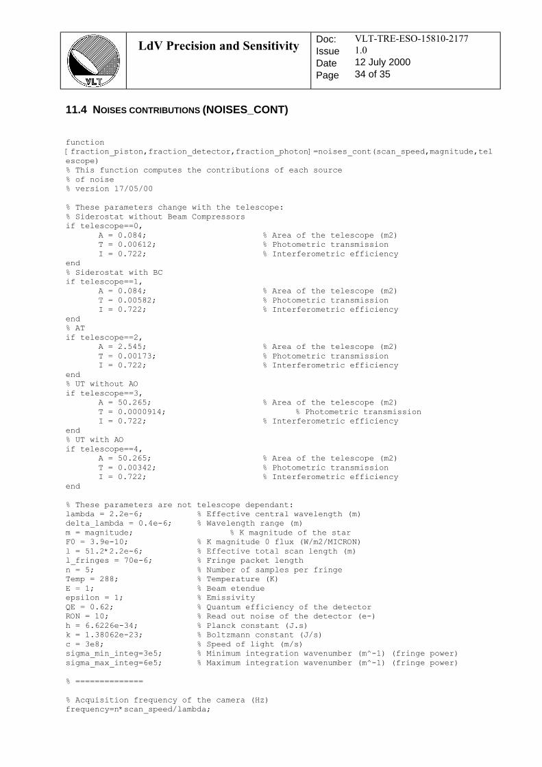
LdV Precision and SensitivityDoc:IssueDatePage
VLT-TRE-ESO-15810-2177
1.0
12 July 200034 of 35
11.4 NOISES CONTRIBUTIONS (NOISES_CONT)
function[fraction_piston,fraction_detector,fraction_photon]=noises_cont(scan_speed,magnitude,telescope)% This function computes the contributions of each source% of noise% version 17/05/00
% These parameters change with the telescope:% Siderostat without Beam Compressorsif telescope==0,
A = 0.084; % Area of the telescope (m2)T = 0.00612; % Photometric transmissionI = 0.722; % Interferometric efficiency
end% Siderostat with BCif telescope==1,
A = 0.084; % Area of the telescope (m2)T = 0.00582; % Photometric transmissionI = 0.722; % Interferometric efficiency
end% ATif telescope==2,
A = 2.545; % Area of the telescope (m2)T = 0.00173; % Photometric transmissionI = 0.722; % Interferometric efficiency
end% UT without AOif telescope==3,
A = 50.265; % Area of the telescope (m2)T = 0.0000914; % Photometric transmissionI = 0.722; % Interferometric efficiency
end% UT with AOif telescope==4,
A = 50.265; % Area of the telescope (m2)T = 0.00342; % Photometric transmissionI = 0.722; % Interferometric efficiency
end
% These parameters are not telescope dependant:lambda = 2.2e-6; % Effective central wavelength (m)delta_lambda = 0.4e-6; % Wavelength range (m)m = magnitude; % K magnitude of the starF0 = 3.9e-10; % K magnitude 0 flux (W/m2/MICRON)l = 51.2*2.2e-6; % Effective total scan length (m)l_fringes = 70e-6; % Fringe packet lengthn = 5; % Number of samples per fringeTemp = 288; % Temperature (K)E = 1; % Beam etendueepsilon = 1; % EmissivityQE = 0.62; % Quantum efficiency of the detectorRON = 10; % Read out noise of the detector (e-)h = 6.6226e-34; % Planck constant (J.s)k = 1.38062e-23; % Boltzmann constant (J/s)c = 3e8; % Speed of light (m/s)sigma_min_integ=3e5; % Minimum integration wavenumber (m^-1) (fringe power)sigma_max_integ=6e5; % Maximum integration wavenumber (m^-1) (fringe power)
% ==============
% Acquisition frequency of the camera (Hz)frequency=n*scan_speed/lambda;

LdV Precision and SensitivityDoc:IssueDatePage
VLT-TRE-ESO-15810-2177
1.0
12 July 200035 of 36
if frequency<1e-6,frequency = 1e-6;
end
% Scan durationdt = l*n/(frequency*lambda);% Frequency bandwidthdf = (lambda*frequency/n)*(sigma_max_integ-sigma_min_integ);
% SignalS = (2*A*delta_lambda*1e6*T*I*F0*10^(m/-2.5))^2*dt/4;% The 1e6 factor is to account for the W/m2/MICRON reference flux
% Thermal noise equivalent power squared ****nu = c/lambda;delta_nu = c/(lambda-delta_lambda/2)-c/(lambda+delta_lambda/2);B = ((2*h*nu^3)/c^2) * 1/(exp((h*nu)/(k*Temp)) -1);etendue=E*lambda^2*epsilon;n_thermal = ((2*h*c/lambda)*delta_nu*B*etendue)^2;
% Piston noise equivalent power squared ****piston = 1-exp(-1.5*((l_fringes*n)/(lambda*frequency))^(5/3));n_piston = S*piston;
% Detector noise equivalent power squared ****n_detector = 2*frequency*(RON*h*c/(QE*lambda))^2;
% Photon noise equivalent power squared ****n_photon = ((2*h*c/lambda)*(2*A*delta_lambda*1e6*T*F0*10^(m/-2.5)));% The 1e6 factor is to account for the W/m2/MICRON reference flux
% Returns the SNRtotal_noise = n_thermal^2*dt*df + n_piston^2 + n_detector^2*dt*df + n_photon^2*dt*df;snr = S/sqrt(total_noise);
fraction_thermal = n_thermal^2*dt*df/total_noise;fraction_piston = n_piston^2/total_noise;fraction_detector = n_detector^2*dt*df/total_noise;fraction_photon = n_photon^2*dt*df/total_noise;