Interannual variability of the tropical Atlantic independent of and associated with ENSO: Part I....

INTERNATIONAL JOURNAL OF CLIMATOLOGY

Int. J. Climatol. 26: 1957–1976 (2006)

Published online 4 May 2006 in Wiley InterScience

(www.interscience.wiley.com) DOI: 10.1002/joc.1342

INTERANNUAL VARIABILITY OF THE TROPICALATLANTIC INDEPENDENT OF AND ASSOCIATED WITH ENSO:

PART II. THE SOUTH TROPICAL ATLANTIC

ITSUKI C. HANDOH,a,* GRANT R. BIGG,b ADRIAN J. MATTHEWSa,c and DAVID P. STEVENSc

a School of Environmental Sciences, University of East Anglia, Norwich, UKb Department of Geography, University of Sheffield, Sheffield, UKc School of Mathematics, University of East Anglia, Norwich, UK

Received 26 April 2005Revised 8 February 2006Accepted 3 March 2006

ABSTRACT

Two dominant ocean–atmosphere modes of variability on interannual timescales were defined in part I of this work,namely, the North Tropical Atlantic (NTA) and South Tropical Atlantic (STA) modes. In this paper we focus on the STAmode that covers the equatorial and sub-tropical South Atlantic. We show that STA events occurring in conjunction withENSO have a preference for the southern summer season and seem to be forced by an atmospheric wave train emanatingfrom the central tropical Pacific and travelling via South America, in addition to the more direct ENSO-induced changein the Walker Circulation. They are lagged by one season from the peak of ENSO. These events show little evidence forother-than-localised coupled ocean–atmosphere interaction.

In contrast, STA events occurring in the absence of ENSO favour the southern winter season. They appear to betriggered by a Southern Hemisphere wave train emanating from the Pacific sector, and then exhibit features of a self-sustaining climate mode in the tropical Atlantic. The southward shift of the inter tropical convergence zone that occursduring the warm phase of such an event triggers an extra tropical wave train that propagates downstream in the SouthernHemisphere. We present a unified view of the NTA and STA modes through our observational analysis of the interannualtropical Atlantic variability. Copyright 2006 Royal Meteorological Society.

KEY WORDS: tropical Atlantic variability; ENSO; ocean–atmosphere interaction; teleconnections; Equatorial Atlantic Oscillation

1. INTRODUCTION

Co-variability of sea surface temperature (SST) and zonal wind stress (τx) is indicative of ocean–atmospherecoupled modes. The relative importance of internal and remotely forced variability in the tropical Atlantichas been intensively debated (e.g. Servain et al., 1982; Carton and Huang, 1994; Curtis and Hastenrath,1995; Klein et al., 1999; Huang et al., 2002; Liu et al., 2004; Xie and Carton, 2004). In the companion paper(Handoh et al., 2006), we have shown through singular value decomposition (SVD) analysis that there are twodominant modes in the tropical Atlantic: the North Tropical Atlantic (NTA) and South Tropical Atlantic (STA)modes. Each mode was sub-divided into two types of events: ones associated with ENSO (ENSO-associatedevents) and others independent of ENSO (ENSO-independent events). The causal mechanism of warm/coldevents in the NTA appears to be a Pacific–North America (PNA) like wave train emanating from the Pacificbasin, with a passive oceanic response to the induced changes in the overlying trade; local wind-evaporation-SST (WES) feedback (Xie and Philander, 1994) was not confirmed. This wave train appears to be the crucial

* Correspondence to: Dr Itsuki C. Handoh, Department of Applied Mathematics, The University of Sheffield, The Hicks Building,Hounsfield Road, Sheffield S3 7RH, UK; e-mail: [email protected]

Copyright 2006 Royal Meteorological Society

1958 I. C. HANDOH ET AL.

mechanism for both ENSO-associated and ENSO-independent events; the latter cannot be entirely generatedwithin the NTA sector. Hereafter we focus on the STA (second) mode.

The equatorial Atlantic exhibits a quasi-biennial oscillation of SST anomalies (Tourre et al., 1999; Tsengand Mechoso, 2001). In the STA, SST anomalies co-vary with those of the surface wind and convectionon this same timescale (Ruiz-Barradas et al., 2000). The patterns of the SST and surface wind anomaliesare reminiscent of ENSO in the Pacific. The heat flux anomalies associated with the equatorial events tendto locally damp the initial SST anomalies over the eastern Atlantic basin (Sutton et al., 2000; Mo andHakkinen, 2001). In fact, what maintains the equatorial SST anomalies is the Bjerknes (1969) feedback thatis characterised by the westward propagation of coupled ocean–atmosphere anomalies. However, from thetheory of unstable ocean–atmosphere coupled modes in tropical basins, self-sustaining warm–cold cyclescan exhibit both westward and eastward propagation (Hirst, 1988). In a modelling study, CabosNarvaez et al.(2002) showed that there are two ways in which SST anomalies can be developed over the Gulf of Guinea:one is an eastward propagation in response to the atmospheric anomalies and the other is as a standingoscillation.

Handoh and Bigg (2000) proposed that the equatorial Atlantic could exhibit a self-sustaining climate mode.The mode was hypothesised to involve equatorial and off-equatorial wave dynamics: an oceanic downwellingKelvin wave, excited by equatorial westerly anomalies at the western Atlantic, propagates eastwards; this isreflected from the African coast and becomes a slow westward propagating wave of warm SST anomalies onand off the equator. The westward propagation was only one-third the expected phase speed of an oceanicRossby wave along the equator. This suggests ocean–atmosphere interaction through SST, surface wind, andatmospheric convective anomalies. Handoh and Bigg (2000) therefore called the westward propagating wavea coupled-mode wave. The arrival of the westward propagating, convective anomalies and their associatedwind stress anomalies at the western equatorial Atlantic were hypothesised to force an eastward-propagatingoceanic upwelling Kelvin wave to cross back to Africa, followed by a slow westward propagating wave ofnegative SST anomalies. The overall dynamics of the equatorial Atlantic climate variability is consistent withthe fundamental unstable mode of the tropical basin of Hirst’s (1986, 1988) model II. This warm–cold cyclecan be repeated a number of times, and is a self-sustaining oscillation. The periodicity of the oscillationover the equator is in good agreement with that of the quasi-biennial oscillation of the equatorial Atlantic(Tseng and Mechoso, 2001), although propagating events of such equatorial anomalies seem to be very rare(Handoh and Bigg, 2000). This Equatorial Atlantic Oscillation (EAO) includes off-equatorial anomalies overthe STA. A model experiment of the equatorial Atlantic coupled mode was studied by Zebiak (1993). Heshowed that the oscillation cannot be self-sustained over a decade or two, in contrast to Hirst (1986, 1988),probably because this unstable mode prefers the basin size of the tropical Pacific to that of the tropicalAtlantic.

However, a few cases of eastward propagating SST anomalies in the tropical Atlantic can be found in theevents of 1983–1984 and 1997–1998, which seem to have been associated with the Pacific El Nino events of1982–1983 (Philander, 1986; Delecluse et al., 1994) and 1997–1998 (Latif and Grotzner, 2000), respectively.The former displayed some ocean–atmosphere interaction (see e.g. Horel et al., 1986). Latif and Grotzner(2000) studied an ‘EAO’. They showed that ENSO-associated equatorial events in the Atlantic display sloweastward-propagating anomalies (Philander, 1986), in contrast to a slow westward-propagating co-variabilityof SST and atmospheric anomalies during the type of event that is independent from ENSO (Handoh andBigg, 2000). Extrapolating from the dynamics of Hirst’s (1988) unstable mode, however, external forcingsuch as ENSO does not necessarily determine the direction of propagation of the coupled equatorial Atlanticanomalies; rather, the eastward-propagating SST anomalies may be just a passive oceanic response to theENSO-induced change in the overlying trades (Latif and Grotzner, 2000).

A brief description of the STA climate mode is presented in Section 2. Details of the methodology weregiven by Handoh et al. (2006). Section 3 summarises and discuss the composite analysis of selected climatevariables and the global significance of ENSO-associated and ENSO-independent events. The implicationsof these analyses are considered in Section 4, and we will discuss the possibility of a purely internal climateoscillation of the equatorial Atlantic, pulling together this work with that of Handoh et al. (2006).

Copyright 2006 Royal Meteorological Society Int. J. Climatol. 26: 1957–1976 (2006)DOI: 10.1002/joc

INTERANNUAL VARIABILITY OF THE SOUTH TROPICAL ATLANTIC 1959

2. DATA AND ANALYSIS

2.1. Data

We used monthly mean SST, surface zonal (τx) and meridional (τy) wind stresses, and sea-level pressure(SLP) in order to examine the surface structure of the climate variability, and zonal and meridional windcomponents, horizontal divergence and streamfunction at three different pressure levels: 1000, 850, and200 hpa. The pressure coordinate vertical velocity at 500 hpa is also used. SST was from the UK MetOffice Global Ice and Sea Surface Temperature (GISST) dataset and the remaining variables were from theNCEP–NCAR re-analysis products (Kistler et al., 2001). We used the period from January 1948 to December1999.

We have shorter sets of monthly data of outgoing longwave radiation (OLR), surface shortwave radiationflux, surface longwave radiation flux, and latent heat flux. OLR was used as a proxy for deep tropicalconvection (Liebmann and Smith, 1996), for the period 1974–1999. The latent heat flux was calculated usingthe TOGA–COARE bulk flux algorithm (Fairall et al., 1996) with SST and surface atmospheric datasets asinput parameters from July 1983 to June 1999. We employed the International Satellite Cloud ClimatologyProject (ISCCP) D2 monthly data in order to calculate surface shortwave and longwave radiation fluxes. Thealgorithms for surface shortwave and longwave radiation estimates are adapted from Bishop and Rossow(1991) and Gupta et al. (1992), respectively (and references therein). Owing to the limited vertical pressurelevels of the TIROS Operational Vertical Sounder (TOVS) data in ISCCP D2 products, we used linearinterpolation (Darnell et al., 1983) to estimate TOVS-derived temperature and water burden at each 50 hpainterval. SST, and heat flux data were interpolated onto a 2.5° × 2.5° grid, to match the spatial resolution ofthe NCAR–NCEP re-analysis datasets.

We removed the long-term linear trend and annual cycle from each data set, and then applied an order 12Butterworth filter to derive inter-annual fluctuations in the 12–72 month band. Owing to the filtering effect,the first and last 12 months of data were removed.

2.2. Composite analysis

We have discussed the SVD analysis of these data and the two leading modes it produces in Handoh et al.(2006). Note that the outcome of SVD analysis of SST and τx will be somewhat different from previousstudies, which used empirical orthogonal function analysis (or equivalent analysis) of SST anomalies (e.g.Enfield and Mayer, 1997; Sutton et al., 2000). Both methods have different merits, but the SVD analysisprovides more information about possible coupled ocean–atmosphere modes. Here we concentrate on thesecond mode, the STA mode, which described 30% of the variance in co-variability of SST and τx . Thisinevitably involves some repeat of material.

The spatial structure of the STA mode (Figure 1(a) and (b)) covers both the equatorial Atlantic and STA.It displays the largest, organised signals in both SST and τx anomalies over the STA (Figure 1(a) and (b),respectively), consistent with the STA pattern found in previous work (Enfield and Mayer, 1997; Dommengetand Latif, 2000; Mo and Hakkinen, 2001). However, this spatial organisation of the STA pattern may bea manifestation of equatorial and sub-tropical modes combining (Florenchie et al., 2004; Huang, 2004; Wuet al., 2004). We would like to stress, however, that neither (rotated) empirical orthogonal function analysisof SST anomalies, nor SVD analysis of SST and surface zonal wind stress anomalies, picks up the so-calledBenguela mode, unless the analysis is geographically restricted.

In addition, modest, isolated anomalies exist over the eastern tropical North Atlantic basin. The largestpositive τx anomalies are located west of those of SST, with weak, negative anomalies of τx to the east of theSST anomaly maximum. This pattern over the equatorial region was found in previous work (Zebiak, 1993;Handoh and Bigg, 2000; Ruiz-Barradas et al., 2000; Tseng and Mechoso, 2001).

ENSO-associated events can be distinguished from ENSO-independent events, in the manner presented byHandoh et al. (2006). The coupling index defined there, A2, is weakly correlated with the tropical Pacificthrough a range of leads and lags, but it correlates well with the equatorial Atlantic index, ATL3 (r = 0.85,p < 0.05) without lags. The maximum correlation with ENSO occurs with a 1-month lag (r = 0.24, p < 0.05).



0.2

0.2

0.2

0.2

0.4

0.4

0.4

0.4

0.6

0.8

0

0

100°W 80°W 60°W 40°W 20°W 0° 20°E 100°W 80°W 60°W 40°W 20°W 0° 20°E30°S

20°S

10°S

0°

10°N

20°N

30°N

30°S

20°S

10°S

0°

10°N

20°N

30°N(a) (b)

50 55 60 65 70 75 80 85 90 95−4

−3

−2

−1

0

1

2

3

4

Year

Nor

mal

ised

(c)

SVD mode 2Nino 3 (1 mon)ENSO–associated ENSO–independent

0.2

0.2

0.2

0.4

0.4

0.6

0.6

0.6

0

0 0

0

0

00.2

0.20.8

Figure 1. Anomaly correlation maps of SVD 2 over the Atlantic domain (30 °S–30 °N): (a) SST anomaly; (b) zonal wind stress anomaly.Contour interval is 0.2. Negative contours are dotted, and zero contour is omitted. (c) Time series of A2 (solid line) and NINO3 (dashedline, lagged by 1 month). Months included in the ENSO-associated (ENSO-independent) composites are indicated by stars (diamonds).

Reproduced from Handoh et al. (2006)

This indicates that our STA mode is essentially independent from ENSO. However, some events seem to beinduced by ENSO signals, and the sign of the correlation coefficient could vary with season (Saravanan andChang, 2000). The lag time of 1 month is shorter than that previously reported between the tropical Pacificand STA SST anomalies (4 months; Enfield and Mayer 1997) and between the tropical Pacific and equatorialAtlantic (∼6 months; Latif and Grotzner, 2000), but consistent with the surface wind anomalies (1 month;Enfield and Mayer, 1997). We will examine this further in Section 3.4. The occurrence of ENSO-associatedand ENSO-independent events shows a preference in the seasonal cycle for October–March and April–July,respectively; they are approximately out of phase.

Composites for the STA mode were constructed by selecting months in which A2 > 1 (warm events) andthose in which A2 < −1 (cold events). Those are then further sub-divided into events that were classed asoccurring in conjunction with ENSO, called ENSO-associated events, when the 1-month lagged NINO3 indexwas above 1 for the warm events and below −1 for the cold events. The remaining selected months wereclassed as ENSO-independent events, with no associated ENSO signal (Figure 1(c)). Warm and cold eventcomposites (both events) had similar patterns, but with opposite sign, and are summarised here as an averageof the warm minus cold pattern. This linearity occurs because in our composite method the primary criterionis the tropical climate variability (A2). Previous studies report that the global response to ENSO signals isessentially non-linear (e.g. Pozo-Vazquez et al., 2001; Wu and Hsieh, 2004; Mariotti et al., 2005), but ENSOhere is used as a secondary criterion, reducing the importance of its non-linearity. Note that because of theshort lag, and weak correlation between ENSO and STA, the drawback of this statistical analysis is that a few



events that were considered to be induced by ENSO (e.g. 1983–1984; Philander, 1986) are now classified asENSO-independent events (Figure 1(c)).

A re-sampling technique was used to examine the statistical significance of the composite maps. FollowingMatthews and Kiladis (1999), 10 000 paired synthetic time-series for A2 and the 1-month lagged NINO3 indexwere created, with the same auto-correlation and cross-correlation characteristics as the original time-series.The local significance of the composite patterns at each grid point was then tested at the 95% level againstthe distribution function calculated from the synthetic time-series.

Since the seasonal phase-locking for ENSO-associated and -independent events is relatively weak (Handohet al., 2006), we have also constructed lag composites in order to examine the origin and evolution of warmand cold events. For each warm (cold) event, the month with a temporal maximum (minimum) of A2 isdefined as month 0. Then, 3-month means centred over months −9, −6, −3, 0, +3, +6, +9 were calculatedin order to compute a series of lag/lead composite maps. It should be stressed that the mean atmospheric statecould vary significantly over the period for which the peaks of an ENSO-associated or -independent eventcould last. This will affect parts of the global atmospheric response to the tropical SST anomalies. However,there is still a robust part of the response that does not depend sensitively on the season. Our re-samplingtechnique was used to examine the statistical significance of the composited anomalies, and identified thisrobust response (see Section 3.4).

3. RESULTS

3.1. Sea surface temperature, wind stress and convection

Global SST and wind stress anomaly vectors for the STA mode occurring in conjunction with ENSO areshown in Figure 2(a). Positive SST anomalies between 0.1 and 0.4 °C and northwesterly wind stress anomaliescover the equatorial and South Tropical Atlantic. This is accompanied by a band of weaker positive SSTanomalies over the tropical North Atlantic, which is not seen in the composite map of Mo and Hakkinen (2001).In our analysis the STA mode contains SST anomalies in the equatorial and off-equatorial (15–30 °S) regions,and that the former co-exists with weaker wind anomalies than does the latter. Part of this is consistent withprevious work, which suggests that the STA consists of a few modes (Huang, 2004; Wu et al., 2004). NegativeSST anomalies are found in the extra-tropical South Atlantic, with southeasterly wind stress anomalies extend-ing from the mid-latitudes. Together with the sub-tropical westerly anomalies, they form a cyclonic anomaly.

Other significant positive SST anomalies are found in the Indian Ocean, and more markedly in the central-eastern tropical Pacific, consistent with an El Nino. Negative SST anomalies are present in the South Pacificover the sub-tropical latitudes, but the spatial extent is much smaller than for mode 1 (Handoh et al., 2006),and so is the North Pacific counterpart. Positive SST anomalies are also found along the west coast of NorthAmerica.

Similar to the ENSO-associated events, ENSO-independent events show significant year-round SSTanomalies over the STA (Figure 2(b)). Again, the STA exhibits both equatorial and off-equatorial peaks inSST anomalies. These are associated with northwesterly wind stress anomalies. To some extent, the ENSO-independent warm events show northerly cross-equatorial winds, and are similar to those of Ruiz-Barradaset al. (2000). There are no significant and organised SST anomalies in other ocean basins.

Composites of OLR were constructed using the data from 1974 to 1999. Although over this period therewere only 1 warm and 2 cold ENSO-associated events, our re-sampling technique confirmed the statisticalsignificance of the composite maps. However, it should be stressed that our ENSO-associated results for theOLR analysis may be strictly applicable only to 1995–2000, because there is inter-decadal variability in theENSO teleconnection (Compo et al., 2001; Diaz et al., 2001).

Consistent with the positive SST anomalies over the equatorial central and eastern Pacific, deep convectionwas enhanced (negative OLR anomalies) in these regions and suppressed over Indonesia (Figure 3(a)) duringthe ENSO-associated events. This was also found for the NTA mode (mode 1; Figure 5(a) in Handoh et al.,2006); it is essentially the El Nino signal. Over the Atlantic sector, convection in the intertropical convergencezone (ITCZ) and over the Amazon was suppressed. As with the NTA mode (Handoh et al., 2006), the latter is



−180 −150 −120 −90 −60 −30 0 60 120 150 180−90

−70

−50

−30

−10

10

30

50

70

90

−90

−70

−50

−30

−10

10

30

50

70

90

(a)

(b)

0.01

30 90

−180 −150 −120 −90 −60 −30 0 60 120 150 18030 90

0.01

Figure 2. Global composite anomaly maps for mode 2 (average of warm minus cold events) of SST anomalies and wind stress vectors,(a) ENSO-associated events, (b) ENSO-independent events. SST contour interval is 0.1 °C, and anomalies significant at the 95% levelare shaded. Positive and negative anomalies are contoured by solid, and dotted lines, respectively. The zero contour is omitted. Thereference surface wind stress vector is 0.01 N/m2, and vectors are only plotted (every 10°) where either the x or y-component is

significant

indicative of suppressed convective rainfall, which suggests that in these cases the link between the Amazonianrainfall and tropical Atlantic warm events is induced by ENSO. However, the spatial pattern is different fromthat of the NTA mode (Handoh et al., 2006). Negative OLR anomalies over the northern sub-tropical Atlanticindicate an enhancement of low-level stratocumulus that may be associated with a decrease in the subsidingbranch of the Hadley Cell, confirmed by diagnosis of vertical velocity anomalies (not shown). Even thoughthere are positive SST anomalies above 0.5 °C over much of the equatorial and South Tropical Atlantic, thereare no negative OLR anomalies over this region, implying that the convective anomalies during these eventsare controlled by the Pacific region. Thus, although there is a tendency for the ITCZ to shift south, since thetropical north and south Atlantic are warm, the cross equatorial SST gradient is small and the ITCZ tends to



(a)

(b)

0.01

0.01

−90

−70

−50

−30

−10

10

30

50

70

90

−90

−70

−50

−30

−10

10

30

50

70

90

−180 −150 −120 −90 −60 −30 0 60 120 150 18030 90

−180 −150 −120 −90 −60 −30 0 60 120 150 18030 90

Figure 3. Same as Figure 2 but for OLR anomalies. Contour interval is 2.5 W/m2, and significant anomalies are shaded. Positive andnegative anomalies are contoured by solid, and dotted lines, respectively. The zero contour is omitted

stay in its climatological position. Thus, only the direct ENSO effect weakens the ITCZ (Chiang et al., 2002;Giannini et al., 2004).

By contrast, the enhanced convection over the equatorial strip is a distinctive feature of the ENSO-independent events (Figure 3(b)). This indicates a southward enhancement of the ITCZ, consistent withHandoh and Bigg (2000). The suppressed convection over the tropical Pacific is not statistically significant.

The similar spatial distribution of SST anomalies between the ENSO-associated and ENSO-independentevents, but with different OLR and wind anomalies, suggest some differences in atmosphere–ocean interactionin the tropical Atlantic between the different types of events. Noting that both events show two distinctequatorial and off-equatorial zonal bands of SST anomalies, we will explore the dynamics that distinguishesENSO-associated from ENSO-independent events in Sections 3.3 and 3.4.



120W 90W 60W 30W 0 30E 60E

40S

30S

20S

10S

0

10N

20N

30N

40N

120W 90W 60W 30W 0 30E 60E

40S

30S

20S

10S

0

10N

20N

30N

40N

(a)

(b)

0.01

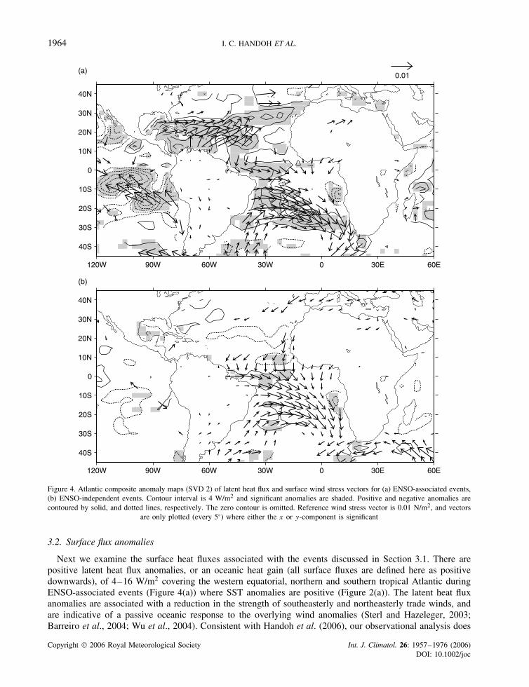
Figure 4. Atlantic composite anomaly maps (SVD 2) of latent heat flux and surface wind stress vectors for (a) ENSO-associated events,(b) ENSO-independent events. Contour interval is 4 W/m2 and significant anomalies are shaded. Positive and negative anomalies arecontoured by solid, and dotted lines, respectively. The zero contour is omitted. Reference wind stress vector is 0.01 N/m2, and vectors

are only plotted (every 5°) where either the x or y-component is significant

3.2. Surface flux anomalies

Next we examine the surface heat fluxes associated with the events discussed in Section 3.1. There arepositive latent heat flux anomalies, or an oceanic heat gain (all surface fluxes are defined here as positivedownwards), of 4–16 W/m2 covering the western equatorial, northern and southern tropical Atlantic duringENSO-associated events (Figure 4(a)) where SST anomalies are positive (Figure 2(a)). The latent heat fluxanomalies are associated with a reduction in the strength of southeasterly and northeasterly trade winds, andare indicative of a passive oceanic response to the overlying wind anomalies (Sterl and Hazeleger, 2003;Barreiro et al., 2004; Wu et al., 2004). Consistent with Handoh et al. (2006), our observational analysis does



−180 −150 −120 −90 −60 −30 300 60 90 120 150 180

−180 −150 −120 −90 −60 −30 300 60 90 120 150 180 −180 −150 −120 −90 −60 −30 300 60 90 120 150 180

−180 −150 −120 −90 −60 −30 300 60 90 120 150 180−90

−70

−50

−30

−10

10

30

50

70

90

−90

−70

−50

−30

−10

10

30

50

70

90

−90

−70

−50

−30

−10

10

30

50

70

90

−90

−70

−50

−30

−10

10

30

50

70

90

(a) (b)

(c) (d)

1 1

1 1

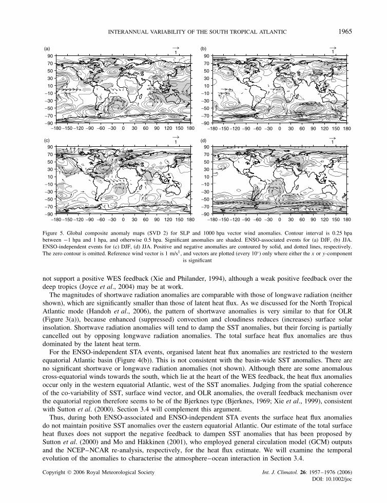
Figure 5. Global composite anomaly maps (SVD 2) for SLP and 1000 hpa vector wind anomalies. Contour interval is 0.25 hpabetween −1 hpa and 1 hpa, and otherwise 0.5 hpa. Significant anomalies are shaded. ENSO-associated events for (a) DJF, (b) JJA.ENSO-independent events for (c) DJF, (d) JJA. Positive and negative anomalies are contoured by solid, and dotted lines, respectively.The zero contour is omitted. Reference wind vector is 1 m/s1, and vectors are plotted (every 10°) only where either the x or y-component

is significant

not support a positive WES feedback (Xie and Philander, 1994), although a weak positive feedback over thedeep tropics (Joyce et al., 2004) may be at work.

The magnitudes of shortwave radiation anomalies are comparable with those of longwave radiation (neithershown), which are significantly smaller than those of latent heat flux. As we discussed for the North TropicalAtlantic mode (Handoh et al., 2006), the pattern of shortwave anomalies is very similar to that for OLR(Figure 3(a)), because enhanced (suppressed) convection and cloudiness reduces (increases) surface solarinsolation. Shortwave radiation anomalies will tend to damp the SST anomalies, but their forcing is partiallycancelled out by opposing longwave radiation anomalies. The total surface heat flux anomalies are thusdominated by the latent heat term.

For the ENSO-independent STA events, organised latent heat flux anomalies are restricted to the westernequatorial Atlantic basin (Figure 4(b)). This is not consistent with the basin-wide SST anomalies. There areno significant shortwave or longwave radiation anomalies (not shown). Although there are some anomalouscross-equatorial winds towards the south, which lie at the heart of the WES feedback, the heat flux anomaliesoccur only in the western equatorial Atlantic, west of the SST anomalies. Judging from the spatial coherenceof the co-variability of SST, surface wind vector, and OLR anomalies, the overall feedback mechanism overthe equatorial region therefore seems to be of the Bjerknes type (Bjerknes, 1969; Xie et al., 1999), consistentwith Sutton et al. (2000). Section 3.4 will complement this argument.

Thus, during both ENSO-associated and ENSO-independent STA events the surface heat flux anomaliesdo not maintain positive SST anomalies over the eastern equatorial Atlantic. Our estimate of the total surfaceheat fluxes does not support the negative feedback to dampen SST anomalies that has been proposed bySutton et al. (2000) and Mo and Hakkinen (2001), who employed general circulation model (GCM) outputsand the NCEP–NCAR re-analysis, respectively, for the heat flux estimate. We will examine the temporalevolution of the anomalies to characterise the atmosphere–ocean interaction in Section 3.4.



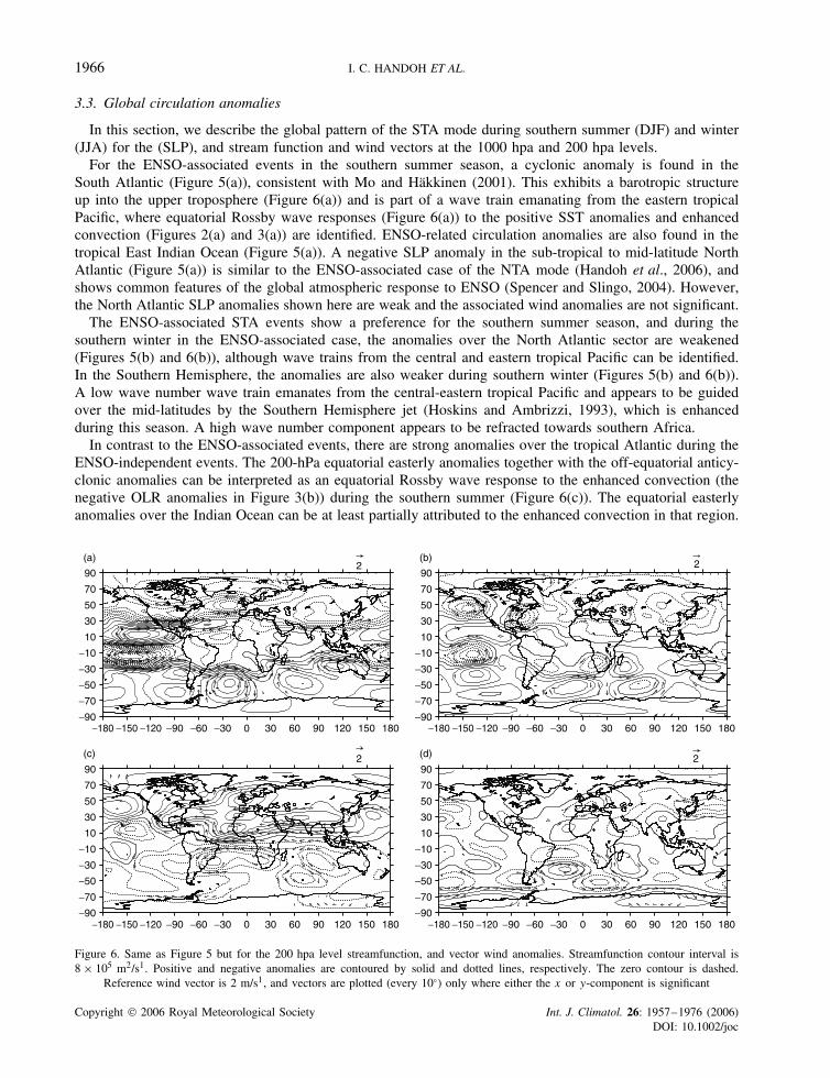
3.3. Global circulation anomalies

In this section, we describe the global pattern of the STA mode during southern summer (DJF) and winter(JJA) for the (SLP), and stream function and wind vectors at the 1000 hpa and 200 hpa levels.

For the ENSO-associated events in the southern summer season, a cyclonic anomaly is found in theSouth Atlantic (Figure 5(a)), consistent with Mo and Hakkinen (2001). This exhibits a barotropic structureup into the upper troposphere (Figure 6(a)) and is part of a wave train emanating from the eastern tropicalPacific, where equatorial Rossby wave responses (Figure 6(a)) to the positive SST anomalies and enhancedconvection (Figures 2(a) and 3(a)) are identified. ENSO-related circulation anomalies are also found in thetropical East Indian Ocean (Figure 5(a)). A negative SLP anomaly in the sub-tropical to mid-latitude NorthAtlantic (Figure 5(a)) is similar to the ENSO-associated case of the NTA mode (Handoh et al., 2006), andshows common features of the global atmospheric response to ENSO (Spencer and Slingo, 2004). However,the North Atlantic SLP anomalies shown here are weak and the associated wind anomalies are not significant.

The ENSO-associated STA events show a preference for the southern summer season, and during thesouthern winter in the ENSO-associated case, the anomalies over the North Atlantic sector are weakened(Figures 5(b) and 6(b)), although wave trains from the central and eastern tropical Pacific can be identified.In the Southern Hemisphere, the anomalies are also weaker during southern winter (Figures 5(b) and 6(b)).A low wave number wave train emanates from the central-eastern tropical Pacific and appears to be guidedover the mid-latitudes by the Southern Hemisphere jet (Hoskins and Ambrizzi, 1993), which is enhancedduring this season. A high wave number component appears to be refracted towards southern Africa.

In contrast to the ENSO-associated events, there are strong anomalies over the tropical Atlantic during theENSO-independent events. The 200-hPa equatorial easterly anomalies together with the off-equatorial anticy-clonic anomalies can be interpreted as an equatorial Rossby wave response to the enhanced convection (thenegative OLR anomalies in Figure 3(b)) during the southern summer (Figure 6(c)). The equatorial easterlyanomalies over the Indian Ocean can be at least partially attributed to the enhanced convection in that region.

(d)(c)

(b)(a)2 2

2 2

−90

−70

−50

−30

−10

10

30

50

70

90

−90

−70

−50

−30

−10

10

30

50

70

90

−90

−70

−50

−30

−10

10

30

50

70

90

−180 −150 −120 −90 −60 −30 300 60 90 120 150 180

−180 −150 −120 −90 −60 −30 300 60 90 120 150 180

−180 −150 −120 −90 −60 −30 300 60 90 120 150 180

−90

−70

−50

−30

−10

10

30

50

70

90

−180 −150 −120 −90 −60 −30 300 60 90 120 150 180

Figure 6. Same as Figure 5 but for the 200 hpa level streamfunction, and vector wind anomalies. Streamfunction contour interval is8 × 105 m2/s1. Positive and negative anomalies are contoured by solid and dotted lines, respectively. The zero contour is dashed.

Reference wind vector is 2 m/s1, and vectors are plotted (every 10°) only where either the x or y-component is significant



Significant SLP and circulation anomalies are found in the Northern Hemisphere (Figures 5(c) and 6(c)).Cross-equatorial flow over the tropical Atlantic occurs only during the southern summer (Figure 5(c), (d)),but it is strong enough to appear in the composite annual map (Figure 2(b)). This is associated with thesouthern part of the anti-cyclonic anomaly extending from the sub-tropical Atlantic to Europe. This is anotable difference from the ENSO-associated events, which show a cyclonic anomaly of similar magnitude.The sub-tropical cyclonic anomaly in the South Atlantic during the northern winter (Figure 5(c)) is weakerthan in the ENSO-associated events (Figure 5(a)). Recall that the preferred season for ENSO-independentevents is April–July (see also Cabos Narvaez et al., 2002).

A strong negative SLP anomaly is found over the high-latitudes in the Southern Hemisphere during thesouthern winter, part of which has a barotropic structure up to 200 hpa (Figures 5(d) and 6(d)). A wavetrain emanating from the western tropical Pacific is similar to the Pacific-South-America (PSA) pattern (Moand Paegle, 2001; Huang, 2004). Another wave train departing from the tropical Atlantic has two majorcomponents: the high and low wave-number components reach the southwestern Indian Ocean, and theeastern Pacific, via the Indian Ocean section of Antarctica, respectively. The latter wave train may influencethe tropical Pacific.

3.4. Dynamic evolution of the anomalies

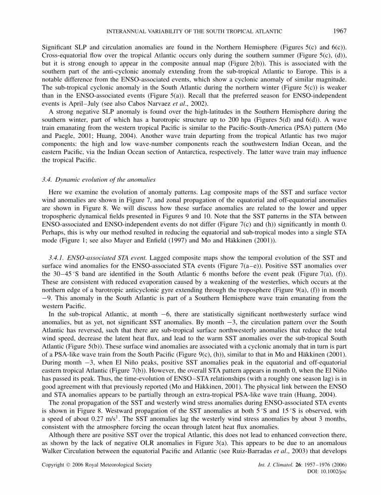
Here we examine the evolution of anomaly patterns. Lag composite maps of the SST and surface vectorwind anomalies are shown in Figure 7, and zonal propagation of the equatorial and off-equatorial anomaliesare shown in Figure 8. We will discuss how these surface anomalies are related to the lower and uppertropospheric dynamical fields presented in Figures 9 and 10. Note that the SST patterns in the STA betweenENSO-associated and ENSO-independent events do not differ (Figure 7(c) and (h)) significantly in month 0.Perhaps, this is why our method resulted in reducing the equatorial and sub-tropical modes into a single STAmode (Figure 1; see also Mayer and Enfield (1997) and Mo and Hakkinen (2001)).

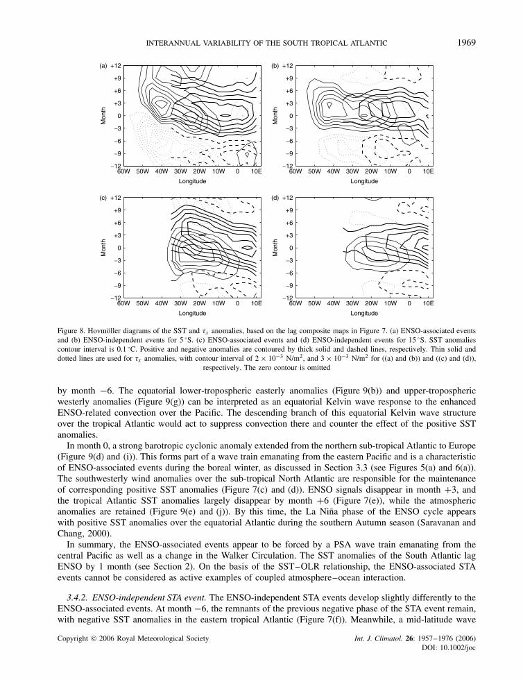
3.4.1. ENSO-associated STA event. Lagged composite maps show the temporal evolution of the SST andsurface wind anomalies for the ENSO-associated STA events (Figure 7(a–e)). Positive SST anomalies overthe 30–45 °S band are identified in the South Atlantic 6 months before the event peak (Figure 7(a), (f)).These are consistent with reduced evaporation caused by a weakening of the westerlies, which occurs at thenorthern edge of a barotropic anticyclonic gyre extending through the troposphere (Figure 9(a), (f)) in month−9. This anomaly in the South Atlantic is part of a Southern Hemisphere wave train emanating from thewestern Pacific.

In the sub-tropical Atlantic, at month −6, there are statistically significant northwesterly surface windanomalies, but as yet, not significant SST anomalies. By month −3, the circulation pattern over the SouthAtlantic has reversed, such that there are sub-tropical surface northwesterly anomalies that reduce the totalwind speed, decrease the latent heat flux, and lead to the warm SST anomalies over the sub-tropical SouthAtlantic (Figure 5(b)). These surface wind anomalies are associated with a cyclonic anomaly that in turn is partof a PSA-like wave train from the South Pacific (Figure 9(c), (h)), similar to that in Mo and Hakkinen (2001).During month −3, when El Nino peaks, positive SST anomalies peak in the equatorial and off-equatorialeastern tropical Atlantic (Figure 7(b)). However, the overall STA pattern appears in month 0, when the El Ninohas passed its peak. Thus, the time-evolution of ENSO–STA relationships (with a roughly one season lag) is ingood agreement with that previously reported (Mo and Hakkinen, 2001). The physical link between the ENSOand STA anomalies appears to be partially through an extra-tropical PSA-like wave train (Huang, 2004).

The zonal propagation of the SST and westerly wind stress anomalies during ENSO-associated STA eventsis shown in Figure 8. Westward propagation of the SST anomalies at both 5 °S and 15 °S is observed, witha speed of about 0.27 m/s1. The SST anomalies lag the westerly wind stress anomalies by about 3 months,consistent with the atmosphere forcing the ocean through latent heat flux anomalies.

Although there are positive SST over the tropical Atlantic, this does not lead to enhanced convection there,as shown by the lack of negative OLR anomalies in Figure 3(a). This appears to be due to an anomalousWalker Circulation between the equatorial Pacific and Atlantic (see Ruiz-Barradas et al., 2003) that develops



−120−100 −80 −60 −40 −20 0 20 40 60 80 100−60

−30

0

30

−120−100 −80 −60 −40 −20 0 20 40 60 80 100

−120−100 −80 −60 −40 −20 0 20 40 60 80 100

−60

−30

0

30

−60

−30

0

30

−120−100 −80 −60 −40 −20 0 20 40 60 80 100−60

−30

0

30

−120−100 −80 −60 −40 −20 0 20 40 60 80 100−60

−30

0

30

−120−100 −80 −60 −40 −20 0 20 40 60 80 100−60

−30

0

30

−120−100 −80 −60 −40 −20 0 20 40 60 80 100−60

−30

0

30

−120−100 −80 −60 −40 −20 0 20 40 60 80 100−60

−30

0

30

−120−100 −80 −60 −40 −20 0 20 40 60 80 100−60

−30

0

30

−120−100 −80 −60 −40 −20 0 20 40 60 80 100−60

−30

0

30

(a) Month -6

(b) Month -3

(c) Month 0

(d) Month +3

(e) Month +6

(f) Month -6

(g) Month -3

(h) Month 0

(i) Month +3

(j) Month +6

ENSO-independent STAENSO-associated STA0.01 0.01

Figure 7. Lag composite maps for SST and surface wind vectors anomalies. (a) −6, (b) −3, (c) 0, (d) +3, and (e) +6 months forENSO-associated events. (f) −6, (g) −3, (h) 0, (i) +3, and (j) +6 months for ENSO-independent events. SST anomalies contour intervalis 0.1 °C, and significant anomalies are shaded. Positive and negative anomalies are contoured by solid and dotted lines, respectively.The zero contour is omitted. The reference surface wind stress vector is 0.01 N/m2, and vectors are plotted (every 7.5°) only where

either the x or y-component is significant



60W 50W 40W 30W 20W 10W 0 10E−12

−9

−6

−3

0

+3

+6

+9

+12

−12

−9

−6

−3

0

+3

+6

+9

+12

−12

−9

−6

−3

0

+3

+6

+9

+12

Mon

thM

onth

−12

−9

−6

−3

0

+3

+6

+9

+12

Mon

thM

onth

Longitude

60W 50W 40W 30W 20W 10W 0 10E

Longitude

60W 50W 40W 30W 20W 10W 0 10E

Longitude

60W 50W 40W 30W 20W 10W 0 10E

Longitude

(b)

(c) (d)

(a)

Figure 8. Hovmoller diagrams of the SST and τx anomalies, based on the lag composite maps in Figure 7. (a) ENSO-associated eventsand (b) ENSO-independent events for 5 °S. (c) ENSO-associated events and (d) ENSO-independent events for 15 °S. SST anomaliescontour interval is 0.1 °C. Positive and negative anomalies are contoured by thick solid and dashed lines, respectively. Thin solid anddotted lines are used for τx anomalies, with contour interval of 2 × 10−3 N/m2, and 3 × 10−3 N/m2 for ((a) and (b)) and ((c) and (d)),

respectively. The zero contour is omitted

by month −6. The equatorial lower-tropospheric easterly anomalies (Figure 9(b)) and upper-troposphericwesterly anomalies (Figure 9(g)) can be interpreted as an equatorial Kelvin wave response to the enhancedENSO-related convection over the Pacific. The descending branch of this equatorial Kelvin wave structureover the tropical Atlantic would act to suppress convection there and counter the effect of the positive SSTanomalies.

In month 0, a strong barotropic cyclonic anomaly extended from the northern sub-tropical Atlantic to Europe(Figure 9(d) and (i)). This forms part of a wave train emanating from the eastern Pacific and is a characteristicof ENSO-associated events during the boreal winter, as discussed in Section 3.3 (see Figures 5(a) and 6(a)).The southwesterly wind anomalies over the sub-tropical North Atlantic are responsible for the maintenanceof corresponding positive SST anomalies (Figure 7(c) and (d)). ENSO signals disappear in month +3, andthe tropical Atlantic SST anomalies largely disappear by month +6 (Figure 7(e)), while the atmosphericanomalies are retained (Figure 9(e) and (j)). By this time, the La Nina phase of the ENSO cycle appearswith positive SST anomalies over the equatorial Atlantic during the southern Autumn season (Saravanan andChang, 2000).

In summary, the ENSO-associated events appear to be forced by a PSA wave train emanating from thecentral Pacific as well as a change in the Walker Circulation. The SST anomalies of the South Atlantic lagENSO by 1 month (see Section 2). On the basis of the SST–OLR relationship, the ENSO-associated STAevents cannot be considered as active examples of coupled atmosphere–ocean interaction.

3.4.2. ENSO-independent STA event. The ENSO-independent STA events develop slightly differently to theENSO-associated events. At month −6, the remnants of the previous negative phase of the STA event remain,with negative SST anomalies in the eastern tropical Atlantic (Figure 7(f)). Meanwhile, a mid-latitude wave



200 hPa(f) Month -9

180 135W 90W 45W 0 45E 90E 135E 18090S

60S

30S

0

30N

60N

90N

(g) Month -6

180 135W 90W 45W 0 45E 90E 135E 18090S

60S

30S

0

30N

60N

90N

(h) Month -3

180 135W 90W 45W 0 45E 90E 135E 18090S

60S

30S

0

30N

60N

90N

(i) Month 0

180 135W 90W 45W 0 45E 90E 135E 18090S

60S

30S

0

30N

60N

90N

(j) Month +6

180 135W 90W 45W 0 45E 90E 135E 18090S

60S

30S

0

30N

60N

90N

850 hPa(a) Month -9

180 135W 90W 45W 0 45E 90E 135E 18090S

60S

30S

0

30N

60N

90N

(b) Month -6

180 135W 90W 45W 0 45E 90E 135E 18090S

60S

30S

0

30N

60N

90N

(c) Month -3

180 135W 90W 45W 0 45E 90E 135E 18090S

60S

30S

0

30N

60N

90N

(d) Month 0

180 135W 90W 45W 0 45E 90E 135E 18090S

60S

30S

0

30N

60N

90N

(e) Month +6

180 135W 90W 45W 0 45E 90E 135E 18090S

60S

30S

0

30N

60N

90N

21

Figure 9. Lag composite maps for 850 and 200 hpa streamfunction, and vector wind anomalies for ENSO-associated events. (a), (f) −9,(b), (g) −6, (c), (h) 3, (d), (i) 0, and (e), (j) +6 months for 850 and 200 hPa level, respectively. Stream function contour intervals are 6and 12 × 105 m2/s1 for 850 and 200 hPa levels, respectively. Positive and negative anomalies are contoured by solid and dotted lines,respectively. The zero contour is omitted. Reference wind vectors are shown on the top of (a) and (f). Vectors are plotted (every 7.5°)

only where either the x or y-component is significant



200 hPa(f) Month -9

(g) Month -6

(h) Month -3

(i) Month 0

(j) Month +6

850 hPa(a) Month -9

180 135W 90W 45W 0 45E 90E 135E 18090S

60S

30S

0

30N

60N

90N

180 135W 90W 45W 0 45E 90E 135E 18090S

60S

30S

0

30N

60N

90N

180 135W 90W 45W 0 45E 90E 135E 180

180 135W 90W 45W 0 45E 90E 135E 180 180 135W 90W 45W 0 45E 90E 135E 180

180 135W 90W 45W 0 45E 90E 135E 180 180 135W 90W 45W 0 45E 90E 135E 180

90S

60S

30S

0

30N

60N

90N

90S

60S

30S

30N

60N

90N

180 135W 90W 45W 0 45E 90E 135E 18090S

60S

30S

0

30N

60N

90N

180 135W 90W 45W 0 45E 90E 135E 18090S

60S

30S

0

30N

60N

90N

180 135W 90W 45W 0 45E 90E 135E 18090S

60S

30S

0

30N

60N

90N

(b) Month -6

(c) Month -3

(d) Month 0

0

90S

60S

30S

30N

60N

90N

0

90S

60S

30S

30N

60N

90N

0

90S

60S

30S

30N

60N

90N

0

(e) Month +6

21

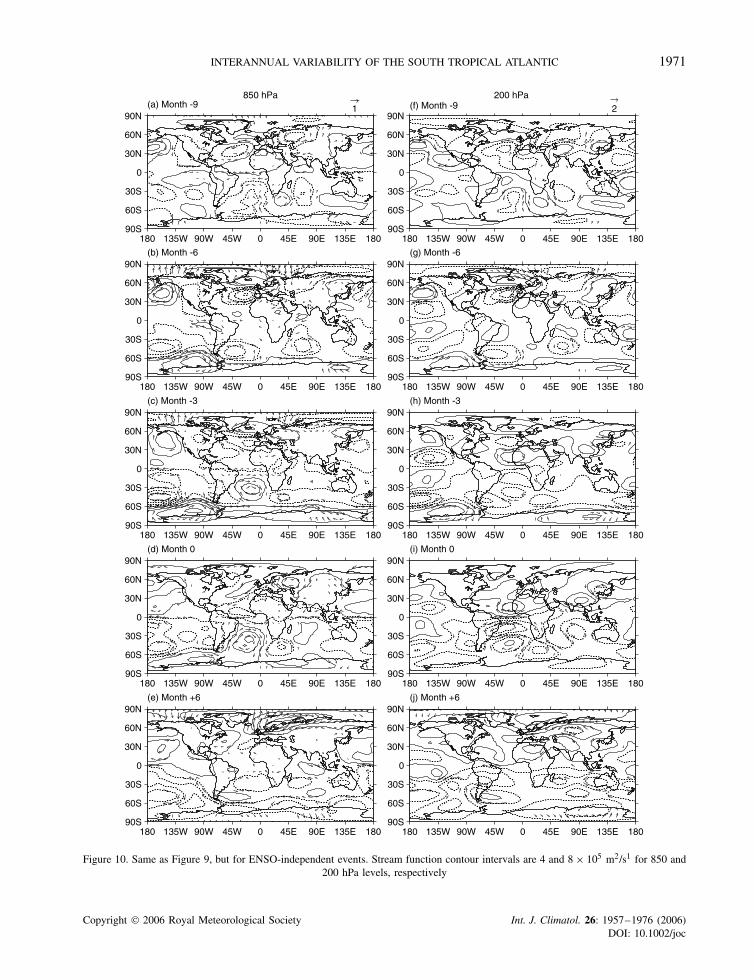
Figure 10. Same as Figure 9, but for ENSO-independent events. Stream function contour intervals are 4 and 8 × 105 m2/s1 for 850 and200 hPa levels, respectively



train emanates from the western tropical Pacific and propagates over the Southern Ocean before recurvingnorthwards over the South Atlantic (Figure 10(b), (g)). This wave train seems to have a higher wave numberthan that found by Mo and Hakkinen (2001). The equatorward extension of this wave train has surfacenorthwesterly anomalies which then develop together with positive SST anomalies over the eastern SouthAtlantic at month −3 (Figure 7(g)).

By month +6, the positive SST anomalies have largely disappeared and the event is over (Figure 7(j)).This can be compared with the longer lasting ENSO-associated STA events, where there is still a significantpositive SST anomaly at month +6 (Figure 7(e)).

The SST anomalies in the ENSO-independent event do not appear to just arise as a passive response tothe atmospheric forcing. They lead to enhanced convection (negative OLR anomalies) along the equator(Figure 3(b)), representing a southward shift of the ITCZ. Part of the atmospheric anomalies at and followingthe peak of the STA event can be interpreted as a response to this enhanced convection. At month 0,lower-tropospheric equatorial westerly anomalies and a cyclonic anomaly in the sub-tropical North Atlantic(Figure 10(d)), and upper-tropospheric equatorial easterly anomalies together with a pair of sub-tropicalanticyclonic anomalies (Figure 10(i)) can be interpreted as an equatorial Rossby wave response to the enhancedconvection. These appear to force an extra-tropical wave train in the Southern Hemisphere (Ruiz-Barradaset al., 2000), which propagates over the Southern Ocean into the Indian Ocean sector (Figure 10(i)). In theNorthern Hemisphere, a wave train leads to a cyclonic anomaly over Europe at month 0 (Figure 10(d)).This cyclonic anomaly persists well after the tropical Atlantic SST anomalies have decayed in month 6(Figure 10(e)), and extends further eastward over Asia. Within the North Atlantic these atmospheric anomaliesare consistent with those in the quasi-biennial equatorial mode of Tourre et al. (1999).

The westward propagation speed of the Atlantic SST and surface wind stress anomalies is much faster inENSO-independent events (Figure 8(c), (d)) compared to the ENSO-associated events. In month −6, negativeSST anomalies are found along the equatorial Atlantic. This occurs at the end of the negative phase of suchan ENSO-independent event (Figure 7(f)). The first indication of the positive phase of the STA event in thetropics is the weakening of the surface trades over the Gulf of Guinea in month −6 (westerly anomalies at0 °E in Figure 8(b)). This would excite an eastward propagating, oceanic downwelling Kelvin wave. Thus theinitiation of such Kelvin wave propagation does not necessarily come from the western equatorial Atlantic,unlike those previously reported (Servain et al., 1982; Huang and Shukla, 1997; Handoh and Bigg, 2000).The arrival of the Kelvin wave at the African coast would then excite a number of westward-propagatingRossby waves, consistent with the positive SST anomalies that propagate westwards from the coast, bothnear (Figure 8(b)) and off the equator (Figure 8(d)). These SST anomalies would then induce an atmosphericcirculation with westerly and easterly anomalies to the west and east, respectively, of the maximum SSTanomalies, consistent with the observations in Figure 8(b), (d). Near the equator, the arrival of positive SSTanomalies off the coast of Brazil is accompanied by surface westerly anomalies. The westward propagatingSST anomalies induce surface easterly anomalies, east of the SST maximum, which in turn would excite aneastward-propagating oceanic upwelling Kelvin wave, the trigger of the negative phase of the event. Thus, theENSO-independent STA events can display self-sustaining warm–cold cycles. The westward propagation ofSST, wind, and OLR anomalies is consistent with Hirst’s (1988) theoretical model II, although this unstablemode would favour the size of the tropical Pacific basin rather than that of the tropical Atlantic.

4. CONCLUSIONS

Following the methodology presented in Handoh et al. (2006), we have analysed the global patterns associatedwith inter-annual coupled ocean–atmosphere variability of the STA. There is a clear difference between thetwo cases with and without ENSO influence, as expected from our analysis of the NTA mode (Handoh et al.,2006). For the ENSO-associated case, peak SST and zonal wind stress anomalies in the STA lag ENSO by1 month. However, this correlation appears to be dominated by the equatorial anomalies. The overall SSTanomalies lag ENSO by one season, consistent with previous reports (Enfield and Mayer, 1997; Latif andGrotzner, 2000; Mo and Hakkinen, 2001). Our analysis suggests that the ENSO-associated events are forcedby a wave train emanating from the central Pacific in addition to a change in the Walker circulation due to



the atmospheric equatorial Kelvin wave response to ENSO. By contrast, the ENSO-independent case showedthat the tropical Atlantic anomalies could be forced by a Southern Hemisphere wave train that originated overthe western Pacific (e.g. Mo and Paegle, 2001). This suggests that tropical Atlantic warm/cold events can becaused by non-ENSO stochastic forcing, consistent with Handoh et al. (2006).

Interestingly, for both ENSO-associated and -independent events, the equatorial and off-equatorial com-ponents of the STA mode seem to behave independently. The two components can then be considered asindependent modes as in previous studies (Huang et al., 2004; Wu et al., 2004). However, our method is nec-essarily of limited value in defining the modes comparable with previous work that includes the Benguela Nino(Florenchie et al., 2004), as we have emphasised the co-variability of the SST and surface wind anomalies,and clear separation between ENSO-associated and -indepedendent events. In fact, the dynamical behavioursare proven to be different for the equatorial and sub-tropical components only when the ENSO-associatedevents are separated from ENSO-independent events.

Ocean–atmosphere coupling processes are identified whichever season is examined (Section 3.2). The WESfeedback (Xie and Philander, 1994) is not a plausible mechanism for locally maintaining the mode over theoff-equatorial regions during the ENSO-associated events. Rather, the off-equatorial SST anomalies appearto be a passive oceanic response to the induced change in the overlying trade winds (Sterl and Hazeleger,2003; Barreiro et al., 2004). The nature of this mechanism is very similar to that of the NTA mode (Handohet al., 2006). By contrast, the feedback mechanism for ENSO-independent events is attributed to off-equatorialwestward-propagating oceanic Rossby-like waves.

The westward propagation of equatorial and off-equatorial SST anomalies is the main characteristic ofthe STA mode. Interestingly, we have not confirmed slow eastward-propagating SST anomalies from thewestern to central equatorial Atlantic previously identified (Philander, 1986; Delecluse et al., 1994; Latif andGrotzner, 2000; CabosNarvaez et al., 2002). ENSO-independent events display westward-propagating coupledocean–atmosphere behaviour similar to Hirst’s (1986, 1988) model II. Handoh and Bigg (2000) consideredthat the initiating mechanism of the 1995–1997 EAO was a westerly wind burst in the western tropicalAtlantic. However, our analysis suggests that, more typically, westerly wind anomalies over the easternequatorial Atlantic, are precursors of the EAO, and that STA ENSO-independent events are an internal self-sustaining oscillation of the equatorial Atlantic, supporting the hypotheses proposed by Handoh and Bigg,(2000) and Tseng and Mechoso (2001). Our analysis also supports the idea that such events are independentof ENSO signals.

Together with the companion paper (Handoh et al., 2006), our observational analysis of the inter-annualcoupled tropical Atlantic modes allows us to develop a unified view of NTA and STA modes. The events,and their causal and ocean–atmosphere feedback mechanisms, are summarised in Table 1. Broadly speaking,most of their characteristics are consistent with previous work (Enfield and Mayer, 1997; Saravanan andChang, 2000; Sutton et al., 2000; Ruiz-Barradas et al., 2000; Mo and Hakkinen, 2001; Huang, 2004). Whatwe have shown, however, is the clear separation of processes in the presence and absence of ENSO in thePacific. These differences between ENSO-associated and ENSO-independent events are not only in spatialextent but also in how the event develops. Stochastic atmospheric wave trains from the Pacific basin appear tobe important forcing mechanisms for the excitation of off-equatorial ENSO-independent events in the Atlantic(both NTA and the off-equatorial component of STA). The nature of the ocean–atmosphere interaction alsodiffers between the events. The extent of tropical ocean–atmosphere coupling that generates diabatic heatingis very limited during ENSO-associated events, while the heating anomaly generated in ENSO-independentevents results in wave trains that propagate towards mid- and high-latitudes.

A major question is whether or not these dynamical links are found in ocean–atmosphere coupled GCMs.As the evolution of ENSO-associated events could be considered as a linear superposition of the STA modeand the remote influence of ENSO, we are currently pursuing this question through a modelling study, to bereported in the future.

ACKNOWLEDGEMENTS

The NCEP–NCAR re-analysis and OLR data were obtained from the Climate Diagnostics Center (http://www.cdc.noaa.gov). SST data were provided by the British Atmospheric Data Centre. Satellite-derived data



Table I. Summary of the inter-annual tropical Atlantic modes. The corresponding causal and local ocean–atmosphereinteractions are discussed in the main text. Suggested operating feedback mechanisms are passive oceanic response to theoverlying wind anomalies (Passive; no feedback), potentially Wind-Evaporation-SST (WES), and Bjerknes feedbacks.The preferred peak seasons are given for both warm (W) and cold (C) events. Note that the STA mode consists of the

equatorial (EQ) and off-equatorial (OEQ) components

Mode Event type Causal mechanism Operating feedback Peak seasons

1: NTA ENSO-associated PNA-like wave train Passive W: Mar–JunC: Feb–May

ENSO-independent PNA-like wave train(stochastic origin)

Passive or potentiallyWES. A NH wave trainexcited at the westCaribbean

W: Sep–DecC:?

2: STA ENSO-associated EQ: Change in WalkerCirculationOEQ: PSA-like wavetrain

EQ: NoneOEQ: Passive

W: Nov–MarC: Oct–Mar

ENSO-independent EQ: Self-sustainingOEQ: PSA-like wavetrain (stochastic origin?).

EQ: Bjerknes. NH andSH wave trains excitedfrom equator.OEQ: Passive, butoff-equatorialwestward-propagatingoceanic Rossby-likewave

W: Apr–JulC: Apr–Jun

to estimate shortwave and longwave radiations were provided by the ISCCP (http://isccp.giss.nasa.gov).We thank the two anonymous reviewers and COAPEC colleagues for constructive criticisms and usefuldiscussions, respectively, that helped to improve the manuscript. ICH has been financially supported by theNERC COAPEC programme (NER/T/S/2000/00295).

REFERENCES

Barreiro M, Giannini A, Chang P, Saravanan R. 2004. On the role of the South Atlantic atmospheric circulation in tropical Atlanticvariability. In Earth Climate: The Ocean-Atmosphere Interaction, Wang C, Xie SP, Carton JA (eds). Geophysical Monograph. AGU:Washington, DC.

Bishop JKB, Rossow WB. 1991. Spatial and temporal variability of global surface solar irradiance. Journal of Geophysical Research96: 16839–16858.

Bjerknes J. 1969. Atmospheric teleconnection from the equatorial Pacific. Monthly Weather Review 97: 163–172.CabosNarvaez W, Alvarez Garcıa F, Ortizbevıa MJ. 2002. Generation of equatorial Atlantic warm and cold events in a coupled general

circulation model simulation. Tellus 54A: 426–438.Carton JA, Huang B. 1994. Warm events in the tropical Atlantic. Journal of Physical Oceanography 24: 888–903.Chiang JCH, Kushnir Y, Giannini A. 2002. Deconstructing Atlantic ITCZ variability: influence of the local cross-equatorial

SST gradient, and remote forcing from the eastern equatorial Pacific. Journal of Geophysical Research 107: 4004, DOI:10.1029/2000JD000307.

Compo GP, Sadeshmukh PD, Penland C. 2001. Changes of subseasonal variability associated with El Nino. Journal of Climate 14:2256–3374.

Curtis S, Hastenrath S. 1995. Forcing of anomalous sea surface temperature evolution in the tropical Atlantic during Pacific warmevents. Journal of Geophysical Research 100: 15835–15847.

Darnell WL, Gupta SK, Staylor WF. 1983. Downward longwave radiation at the surface from satellite measurements. Journal of Climateand Applied Meteorology 22: 1956–1960.

Delecluse P, Servain J, Levy C, Arpe K, Bengtsson L. 1994. On the teleconnection between the 1984 Atlantic warm event and the1982–83 ENSO. Tellus 46: 448–464.

Diaz H, Hoerling M, Eischeid J. 2001. ENSO variability, teleconnections and climate change. International Journal of Climatology 21:1845–1862.

Dommenget D, Latif M. 2000. Interannual to decadal variability in the tropical Atlantic. Journal of Climate 13: 777–792.Enfield DB, Mayer DA. 1997. Tropical Atlantic sea surface temperature variability and its relation to El Nino-Southern Oscillation.

Journal of Geophysical Research 102: 929–945.



Fairall CW, Bradley EF, Rogers DP, Edson JB, Young GS. 1996. Bulk parameterization of air-sea fluxes for tropical ocean-globalatmosphere coupled-ocean atmosphere response experiment. Journal of Geophysical Research 101: 3474–3764.

Florenchie P, Reason CJC, Lutjeharms JRE, Rouault M, Roy C, Masson S. 2004. Evolution of interannual warm and cold events in theSoutheast Atlantic Ocean. Journal of Climate 17: 2318–2334.

Giannini A, Chiang JCH, Cane MA, Kushnir Y, Seager R. 2001. The ENSO teleconnection to the tropical Atlantic Ocean: contributionsof the remote and local SSTs to rainfall variability in the tropical Americas. Journal of Climate 14: 4530–4544.

Gupta SK, Darnell WL, Wilber AC. 1992. A parameterization for longwave surface radiation from satellite data: Recent improvements.Journal of Applied Meteorology 31: 1359–1367.

Handoh IC, Bigg GR. 2000. A self-sustaining climate mode in the tropical Atlantic, 1995–1997: Observations and modelling. QuarterlyJournal of the Royal Meteorological Society 126: 807–821.

Handoh IC, Matthews AJ, Bigg GR, Stevens DP. 2006. Interannual variability of the tropical Atlantic independent of and associatedwith ENSO: Part I. The North tropical Atlantic. International Journal of Climatology DOI:10.1002/joc1343.

Hirst AC. 1986. Unstable and damped equatorial modes in simple coupled Ocean-atmosphere models. Journal of the AtmosphericSciences 43: 606–632.

Hirst AC. 1988. Slow instabilities in tropical Ocean basin-global atmosphere models. Journal of the Atmospheric Sciences 45:830–852.

Horel JD, Kousky VE, Kagano MT. 1986. Atmospheric conditions in the Atlantic sector during 1983 and 1984. Nature 322:240–243.

Hoskins BJ, Ambrizzi T. 1993. Rossby wave propagation on a realistic longitudinally varying flow. Journal of the Atmospheric Sciences50: 1661–1671.

Huang B. 2004. Remotely forced variability in the tropical Atlantic Ocean. Climate Dynamics 23: 133–152.Huang B, Shukla J. 1997. Characteristics of the interannual and decadal variability in a general circulation model of the tropical Atlantic

Ocean. Journal of the Atmospheric Sciences 27: 1693–1712.Huang BH, Schopf PS, Pan ZQ. 2002. The ENSO effect on the tropical Atlantic variability: A regionally coupled model study.

Geophysical Research Letters 29: 2039, DOI: 10.1029/2002GL014872.Huang BH, Schopf PS, Shukla J. 2004. Intrinsic ocean-atmosphere variability of the tropical Atlantic Ocean. Journal of Climate 17:

2058–2077.Joyce TM, Frankignoul C, Yang JY. 2004. Ocean response and feedback to the SST dipole in the tropical Atlantic. Journal of Physical

Oceanography 34: 2525–2540.Kistler R, Kalnay E, Collins W, Saha S, White G, Woollen J, Chelliah M, Ebisuzaki W, Kanamitsu M, Kousky V, van den Dool H,

Jenne R, Fiorino M. 2001. The NCEP-NCAR 50-year reanalysis: Monthly means CD-ROM and documentation. Bulletin of theAmerican Meteorological Society 82: 247–267.

Klein SA, Soden BJ, Lau NC. 1999. Remote sea surface temperature variations during ENSO: Evidence for a tropical atmosphericbridge. Journal of Climate 12: 917–932.

Latif M, Grotzner A. 2000. The equatorial Atlantic oscillation and its response to ENSO. Climate Dynamics 16: 213–218.Liebmann B, Smith CA. 1996. Description of a complete (interpolated) outgoing longwave radiation dataset. Bulletin of the American

Meteorological Society 77: 1275–1277.Liu Z, Zhang Q, Wu L. 2004. Remote impact on tropical Atlantic climate variability: statistical assessment and dynamic assessment.

Journal of Climate 17: 1529–1549.Mariotti A, Ballabrera-Poy J, Zeng N. 2005. Tropical influence on Euro-Asian autumn rainfall variability. Climate Dynamics 24:

511–521.Matthews AJ, Kiladis GN. 1999. Interactions between ENSO, transient circulation, and tropical convection over the Pacific. Journal of

Climate 12: 3062–3086.Mo KC, Hakkinen S. 2001. Interannual variability in the tropical Atlantic and linkages to the Pacific. Journal of Climate 14:

2740–2762.Mo KC, Paegle JN. 2001. The Pacific-South American modes and their downstream effects. International Journal of Climatology 21:

1211–1229.Philander SGH. 1986. Unstable conditions in the tropical Atlantic ocean in 1984. Nature 322: 236–238.Pozo-Vazquez D, Esteban-Parra MJ, Rodrigo FS, Castro-Diez Y. 2001. The association between ENSO and winter atmospheric

circulation and temperature in the North Atlantic region. Journal of Climate 14: 3408–3420.Ruiz-Barradas A, Carton JA, Nigam S. 2000. Structure of interannual-to-decadal climate variability in the tropical Atlantic sector.

Journal of Climate 13: 3285–3297.Ruiz-Barradas A, Carton JA, Nigam S. 2003. Role of the Atmosphere in climate variability of the tropical Atlantic. Journal of Climate

16: 2052–2065.Saravanan R, Chang P. 2000. Interaction between tropical Atlantic variability and El Nino-Southern Oscillation. Journal of Climate 13:

2177–2194.Servain J, Picaut J, Merle J. 1982. Evidence of remote forcing in the equatorial Atlantic Ocean. Journal of Physical Oceanography 12:

457–463.Spencer H, Slingo JM. 2003. The simulation of peak and delayed ENSO teleconnections. Journal of Climate 16: 1757–1774.Sterl A, Hazeleger W. 2003. Coupled variability and air-sea interaction in the South Atlantic Ocean. Climate Dynamics 21: 559–571.Sutton RT, Jewson SP, Rowell DP. 2000. The elements of climate variability in the tropical Atlantic region. Journal of Climate 13:

3261–3284.Tourre YM, Rajagopalan B, Kushnir Y. 1999. Dominant patterns of climate variability in the Atlantic Ocean during the last 136 years.

Journal of Climate 12: 2285–2299.Tseng L, Mechoso CR. 2001. A quasi-biennial oscillation in the equatorial Atlantic Ocean. Geophysical Research Letters 28: 187–190.Wu L, Zhang Q, Liu Z. 2004. Toward understanding tropical Atlantic variability using coupled modeling surgery. In Earth Climate:

The Ocean-Atmosphere Interaction, Wang C, Xie SP, Carton JA (eds). Geophysical Monograph. AGU: Washington, DC.



Wu AM, Hsieh WW. 2004. The nonlinear association between ENSO and the Euro-Atlantic winter sea level pressure. Climate Dynamics23: 859–868.

Xie SP, Carton JA. 2004. Tropical Atlantic variability: Patterns, mechanisms, and impacts. In Earth Climate: The Ocean-AtmosphereInteraction, Wang C, Xie SP, Carton JA (eds). Geophysical Monograph. AGU: Washington, DC.

Xie SP, Philander SGH. 1994. A coupled ocean-atmosphere model of relevance to the ITCZ in the central Pacific. Tellus 46A: 340–350.Xie SP, Tanimoto Y, Noguchi H, Matsuno T. 1999. How and why climate variability differs between the tropical Atlantic and Pacific.

Geophysical Research Letters 26: 1609–1612.Zebiak SE. 1993. Air-sea interactions in the equatorial Atlantic region. Journal of Climate 6: 1567–1586.


Interannual variability of the tropical Atlantic independent of and associated with ENSO: Part I....

Documents

Transcript of Interannual variability of the tropical Atlantic independent of and associated with ENSO: Part I....