Tropical extra-tropical thermocline water mass exchanges in the Community Climate Model v.3 Part I:...

OSD3, 55–84, 2006

Tropical extra-tropicalinteraction in the

CCSM

I. Wainer et al.

Title Page

Abstract Introduction

Conclusions References

Tables Figures

J I

J I

Back Close

Full Screen / Esc

Printer-friendly Version

Interactive Discussion

EGU

Ocean Sci. Discuss., 3, 55–84, 2006www.ocean-sci-discuss.net/3/55/2006/© Author(s) 2006. This work is licensedunder a Creative Commons License.

Ocean ScienceDiscussions

Papers published in Ocean Science Discussions are underopen-access review for the journal Ocean Science

Tropical Extra-tropical thermocline watermass exchanges in the communityclimate model v.3 Part I: the AtlanticOceanI. Wainer1, A. Lazar2, and A. Solomon3

1Department of Physical Oceanography, University of Sao Paulo, Sao Paulo, Brazil2 Laboratoire d’Ocanographie Dynamique et de Climatologie (LODYC), Paris, France3 National Oceanic Atmospheric Administration-Cooperative Institute Research EnvironmentalSciences (NOAA-CIRES) Climate Diagnostics Center, Boulder, CO, USA

Received: 12 December 2005 – Accepted: 21 January 2006 – Published: 10 May 2006

Correspondence to: I. Wainer ([email protected])

55

http://www.ocean-sci-discuss.net

http://www.ocean-sci-discuss.net/3/55/2006/osd-3-55-2006-print.pdf

http://www.ocean-sci-discuss.net/3/55/2006/osd-3-55-2006-discussion.html

http://www.copernicus.org/EGU/EGU.html

OSD3, 55–84, 2006


CCSM

I. Wainer et al.

Title Page



Tables Figures

J I

J I

Back Close

Full Screen / Esc



EGU

Abstract

The NCAR CCSM numerical coupled model is used to understand the tropical-extra-tropical pathways of thermocline waters in the Atlantic Ocean. Climatological annualmean simulation results from three numerical experiments are analyzed. Two are fullycoupled runs with different spatial resolution (T42 and T85) for the atmospheric com-5

ponent. The third numerical experiment is an ocean-only run forced by NCEP windsand fluxes. Results show that the different atmospheric resolutions have a significantimpact on the subduction pathways in the Atlantic because of how the wind field isrepresented. These simulation results also show that the water subducted at the sub-tropics reaching the EUC is entirely from the South Atlantic. The coupled model ability10

to simulate the STCs is discussed.

1 Introduction

Perhaps one of the most interesting characteristics of the tropical-extra-tropical circu-lation in the Tropical Atlantic Ocean is the fact that most of the water reaching theequator has Southern Hemisphere origin, in particular within the Equatorial Undercur-15

rent (EUC) i.e. Zhang et al. (2003); Molinari et al. (2003). This is accomplished due tothe equatorward flow at the depth of the thermocline by the Subtropical Cells (STC).This shallow overturning cell (confined to the upper 500 m, according to Schott et al.,1998; Snowden and Molinari, 2003; Zhang et al., 2003) is characterized by polewardEkman flow at the surface, associated upwelling and a return flow which is associated20

with the subduction processes that transfer interior ocean water into the thermocline.In other words, Ekman pumping injects surface water into intermediate depths alongisopycnal surfaces in the subtropics that ventilate the tropics.

Zhang et al. (2003), using geostrophic velocities derived from hydrographical data,describe the mean pathways in the interior and surface ocean for tropical-extra-tropical25

water exchange. They show that in the North Atlantic, water pathways go around the

56





OSD3, 55–84, 2006


CCSM

I. Wainer et al.

Title Page



Tables Figures

J I

J I

Back Close

Full Screen / Esc



EGU

potential vorticity ridge located under the Intertropical Convergence Zone convergingon the western boundary. In the Southern Hemisphere the ventilation pathways arespread throughout the interior and include a western boundary route. Their obser-vational analysis will serve as comparison basis for the model simulations analyzedin this work. Their work is described in Snowden and Molinari (2003) who provide a5

comprehensive review of the Atlantic STC. They point out that in general there is stillmuch to be learned about its variability and structure mostly because of the unevendata distribution and lack of quantitative errors surrounding them. Grodsky and Carton(2002), attempt to look at the near-surface pathways of the Atlantic STC using drifterdata. They discuss that the small number of drifters along with their inhomogeneous10

spatial and temporal distribution, are not enough to quantify the relative importance ofthe four major pathways they identified. In their study the water exiting the cold tongueregion does not lead directly back to the subduction regions.

The modeling studies that have been carried out; i.e. (Lazar et al., 2002; Malanotte-Rizzoli et al., 2000; Blanke et al., 1999) are ocean only numerical experiments that15

provide a global description of the pathways associated with the STC circulation. Lazaret al. (2002), and Malanotte-Rizzoli et al. (2000) based their study on the evaluation ofthe Bernoulli function on isopycnal surfaces, showing that for the South Atlantic STC,nearly all the thermocline flow from the subtropics into the equator passes through thewestern boundary. In a high resolution modeling study, Harper (2002) using particle20

trajectories, shows that the subducted water reaching the EUC is entirely from South-ern Hemisphere origin. Results of these numerical simulations show considerable dif-ferences in the mean pathways within the STCs. These differences can be attributedto differences in model configurations, differences in the simulated MOC (because theSTC can be superimposed on its return northward branch and hard to distinguish one25

from the other) and the wind forcing chosen (see for example, Inui et al., 2002).In this qualitative study, the annual subduction rate, upwelling and Lagrangian (sub-

surface) trajectories at different isopycnals are examined in order to quantify the STCpathways similar to Lazar et al. (2002).

57





OSD3, 55–84, 2006


CCSM

I. Wainer et al.

Title Page



Tables Figures

J I

J I

Back Close

Full Screen / Esc



EGU

2 The numerical model

Coupled models used in climate change studies have undergone a rapid developmentin recent years and have in several respects obtained a considerable degree of real-ism. The CCSM3 (Community Climate System Model) is a numerical coupled model,composed of 4 components: atmosphere, ocean, land surface and sea-ice. The on-5

line description can be found at: www.ccsm.ucar.edu/models/ccsm3.0. The CCSM3system includes new versions of all the component models. The atmosphere is CAMversion 3.0 (Collin et al., 20051), the land surface is CLM version 3.0 (Oleson et al.2004; Dickinson et al. 2005), the sea ice is CSIM version 5.0 (Briegleb et al., 2004),and the ocean is based upon POP version 1.4.3 (Smith and Gent, 2002). New features10

in each of these components are described in Collin et al., 20051. Each componentis designed to conserve energy, mass, total water, and fresh water in concert with theother components.

The dynamical atmosphere model is the Community Atmosphere Model (CAM3,Collins et al., 20052), a global atmospheric general circulation model developed from15

the NCAR CCM3. In this work, two horizontal resolutions are used both have 26 ver-tical levels. One has triangular truncation at 42 wave numbers (T42) and the other85 (T85) which roughly corresponds to a horizontal resolution of 3.75◦ and 1.4◦, re-spectively. The hybrid vertical coordinate merges a terrain-following sigma coordinateat the bottom surface with a pressure-level coordinate at the top of the model.20

The ocean component solves the primitive equations in general orthogonal coordi-nates in the horizontal with the hydrostatic and Boussinesq approximations. The grid

1Collins, W., Blackmon, M., Bitz, C., Bonan, G. B., Bretherton, C. S., Carton, J. A., Chang,P., Doney, S., Hack, J. J., Kiehl, J. T., Henderson, T., Large, W. G., McKenna, D., Santer, B. D.,and Smith, R.: The Community Climate System Model: CCSM3, J. Clim., submitted, 2005.

2Collins, W., Rasch, P. J., Boville, B. A., Hack, J. J., McCaa, J. R., Williamson, D. L., Briegleb,B. P., Bitz, C. M., Lin, S.-J., and Zhang, M.: The Formulation and Atmospheric Simulation of theCommunity Atmosphere Model: CAM3, J. Clim., submitted, 2005.

58





www.ccsm.ucar.edu/models/ccsm3.0

OSD3, 55–84, 2006


CCSM

I. Wainer et al.

Title Page



Tables Figures

J I

J I

Back Close

Full Screen / Esc



EGU

uses spherical coordinates in the Southern Hemisphere, but in the Northern Hemi-sphere the pole is displaced into Greenland at 80◦ N, 40◦ W. The horizontal grid has320 (zonal) ×384 (meridional) grid points, and the resolution is uniform in the zonal,but not in the meridional, direction. In the Southern Hemisphere, the meridional res-olution is 0.27◦ at the equator, gradually increasing to 0.54◦ at 33◦ S, and is constant5

at higher latitudes. There are 40 levels in the vertical, whose thickness monotonicallyincreases from 10 m near the surface to 250 m in the deep ocean. The minimum depthis 30 m, and the maximum depth is 5.5 km. The surface fresh water flux is convertedinto an implied salt flux using a constant reference salinity. Therefore, although the seasurface height varies locally, the ocean volume remains fixed. The domain is global,10

which includes Hudson Bay, the Mediterranean Sea, and the Persian Gulf. The timestep used is one hour, which is small enough that no Fourier filtering is required aroundthe displaced Greenland pole.

The horizontal viscosity is a Laplacian operator that is anisotropic following the for-mulation of Smith and McWilliams (2003), and uses different coefficients in the east-15

west and north-south directions. Both coefficients are spatially and temporally variable,depending on the local rates of shear and strain, and the minimum background hor-izontal viscosity is 1000 m2 s−1. The vertical mixing scheme is the KPP scheme ofLarge et al. (1994). In the ocean interior, the background diffusivity varies in the verti-cal from 0.1×10−4 m2 s−1 near the surface to 1.0×10−4 m2 s−1 in the deep ocean. The20

background viscosity has the same vertical profile, but is a factor of ten larger. Theparameterization of the effects of mesoscale eddies is that of Gent and McWilliams(1990), with a constant coefficient of 600 m2 s−1. Further details on the ocean compo-nent of the CCSM3 can be found in Smith and Gent (2002).

The Community Land Model, CLM (Dickinson et al., 20053), is the result of a collab-25

orative project between scientists in the Terrestrial Sciences Section of the Climate and

3Dickinson, R. E., Oleson, K. W., Bonan, G. B., Hoffman, F., Vertenstein, P. T. M., Yang,Z.-L., and Zeng, X.: The Community Land Model and Its Climate Statistics as a Component ofthe Community Climate System Model, J. Clim., submitted, 2005.

59





OSD3, 55–84, 2006


CCSM

I. Wainer et al.

Title Page



Tables Figures

J I

J I

Back Close

Full Screen / Esc



EGU

Global Dynamics Division (CGD) at NCAR and the CCSM Land Model Working Group.Other principal working groups that also contribute to the CLM are Biogeochemistry,Paleoclimate, and Climate Change and Assessment. The land model grid is identicalto the atmosphere model grid.

The sea-ice component of CCSM is the Community Sea-Ice Model (CSIM, Briegleb5

et al., 2004). The sea-ice component includes the elastic-viscous-plastic (EVP) dynam-ics scheme, an ice thickness distribution, energy-conserving thermodynamics, a slabocean mixed layer model, and the ability to run using prescribed ice concentrations. Itis supported on high- and low-resolution Greenland Pole grids, identical to those usedby the POP ocean model.10

The coupled model data analyzed consists of annual averages of temperature, salin-ity and current velocity from 50 years of two 400 year runs of the NCAR CCSM wherethe atmosphere has different spatial resolution (T42, T85). The ocean only (POP3)data analyzed is theannual mean average of a 43 year run forced by NCEP/NCARwinds and fluxes. The South Atlantic is defined by the region between the Equator and15

55◦ S and between 65◦ W and 20◦ E.The uncoupled NCAR CCSM Ocean Model (POP3) is forced in a similar manner as

when it is coupled to an atmospheric model. The open-ocean surface boundary con-ditions are fluxes of momentum, heat, and freshwater. The open-ocean turbulent heatfluxes are computed from a prescribed atmospheric state using traditional, bulk formu-20

las. The required surface winds, air temperature, and air humidity are obtained fromthe National Centers for Environmental Prediction (NCEP) global reanalysis dataset;see E. et al. (1996).

The numerical results are compared to the Levitus (Levitus et al., 2000) climatology.Although this is the standard climatology for ocean model versus data intercomparison,25

caution should be exercized in the equatorial region (where meridional gradients arelarge) considering the broad smoothing used.

60





OSD3, 55–84, 2006


CCSM

I. Wainer et al.

Title Page



Tables Figures

J I

J I

Back Close

Full Screen / Esc



EGU

3 Results

3.1 The tropical annual mean circulation

An important feature of the tropical-extratropical dynamics is the Tropical Cell (TC)which is even shallower than the STC and confined to the tropics. As described inMolinari et al. (2003) they are associated with downwelling driven by the decrease of5

the poleward Ekman transport just a few degrees off the equator. STCs interact withthe TCs. Figure 1 shows at 30◦ W the mean meridional versus vertical velocity circu-lation vectors superimposed on the zonal velocity field characterizing the TC for thethree numerical experiments. Black contours with selected isopycnal surfaces are alsosuperimposed on Fig. 1. The common feature is the surface Ekman divergence and as-10

sociated equatorial upwelling through the upper 50 m. The compensating geostrophicsubsurface convergence is not so clear in the coupled runs (hereafter referred to asT42 and T85, respectively): there is a clear reversal of the surface poleward flow southof the equator below 100 meters which is not observed north of the equator. There,the flow is significantly reduced, but not convergent. As a matter of fact, there is a15

maximum in the northward flow for these runs, at 80-m depth, centered exactly at theequator. The forced ocean result (hereafter referred to as POP3) shows the expectedconvergence associated with the TC at approximately 100 m. The Ekman-driven, di-vergent flow, at the equator, forces equatorial upwelling and poleward surface flow toform a closed shallow subtropical cell.20

In the coupled models, centered at about 8◦ S there is unrealistic upwelling whichcan be related to an unrealistic wind field. In fact, examination of the mean wind stressfield in Fig. 4 shows that there is a sign reversal in the wind stress curl at 8◦ S (positivein POP3 (Fig. 4c) and negative for the coupled model runs (Figs. 4a, b). The wind fielditself is predominantly zonal at that latitude for POP3. In fact, the weak upwelling in the25

coupled models are a direct result of the too-weak winds. These also account for theabsence of a better defined northern SEC and the surfacing of the EUC.

The mean zonal velocity at 30◦ W (color shading), with the main isopycnals super-61





OSD3, 55–84, 2006


CCSM

I. Wainer et al.

Title Page



Tables Figures

J I

J I

Back Close

Full Screen / Esc



EGU

imposed in Fig. 1 shows the eastward flowing Equatorial Undercurrent (EUC) charac-terized by a strong velocity core around 100m depth. Note that the core of the EUClies in the density range between the 24.5 kg m−3<σθ<26.5 kg m−3 isopycnal surfacesconsistent with Schott et al. (2004) and Molinari et al. (2003). However, for each simu-lation the core is located on a different isopycnal surface (24.3 kg m−3 for T42, Fig. 1 left5

panel; 24.5 kg m−3 for T85, Fig. 1 right panel and 25.0 kg m−3 for POP3, bottom panel).Only waters less or near the 26.5 kg m−3 isopycnal reaches the equator. Denser waterscannot reach the EUC.

The core of the EUC for the coupled numerical experiments has a maximum of ap-proximately 40 cm/s. For the forced case the maximum value of the EUC is at 112m and10

approximately 10 cm/s stronger. It should be noted that the core is displaced slightlysouthward (and upward, at 83-m depth) in the coupled runs corresponding to an upperlimit of the eastward flow at σθ=23.0 kg m−3 for the T85 and 22.5 kg m−3 for the T42run which reaches the surface. The maximum EUC velocity for T42 and T85 occursfurther west, at 34◦ W, reaching approximately 45 cm/s at 83-m depth. The depth of15

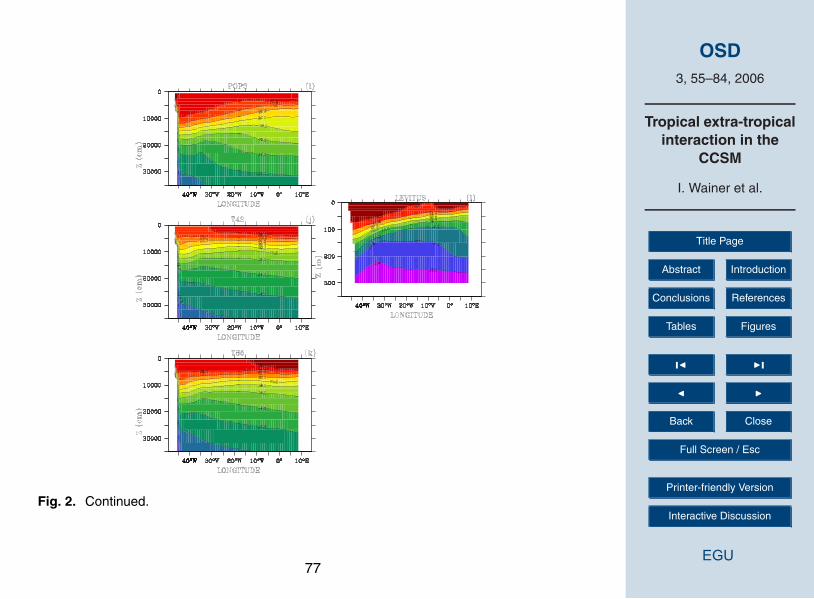
the EUC core coincides with the depth of the thermocline of the tropical Atlantic. Themean climatological temperature structure is shown in Fig. 2 for all three runs (b–d),together with the Levitus et al. (2000) climatological field (Fig. 2a) and their differences(Figs. 2e- h) at 30◦ W. Equatorial cross-sections can be seen in Figs. 2i–k.

A significant difference between the forced numerical experiment (POP3) and the20

Levitus et al. (2000) climatology seen in Fig. 2e is right at the equator at the core level(around 100-m depth) showing a 5◦C difference. A difference of 4◦C at 80-m depth,at the latitude where the eastward flowing North Equatorial Counter Current (NECC)encounters the westward flowing North Equatorial Current (NEC) is also noted. Differ-ences between POP3 and the two coupled runs (Figs. 2f, g) show a model bias in the25

thermocline in the tropics descending to 300 m in the subtropics. Differences in bothcases are significantly larger for the Northern Hemisphere subtropics with maximumvalues close to 8◦C at approximately 18◦ N (within the region of the NEC). Small differ-ences (compared to POP3) in the temperature profiles between the coupled runs show

62





OSD3, 55–84, 2006


CCSM

I. Wainer et al.

Title Page



Tables Figures

J I

J I

Back Close

Full Screen / Esc



EGU

that T85 is warmer than T42 in the southern subtropics, the thermocline and the regionpoleward of 20◦ N.

The core of the EUC has temperatures around 20◦C, which is about 4–5◦C coolerthan the surface waters in the equatorial region. From the equatorial temperature sec-tions (Figs. 2i–l) it is evident that the thermocline shoals eastward only in the POP35

run. It is actually almost flat for the coupled runs where there is a reverse east-westtemperature gradient with warmer waters in the east. POP3 temperature distributionis closer to the Levitus et al. (2000) Climatology albeit warmer in the surface. In thewest (Figs. 2i–l) the thermocline is more diffuse and the 26◦C isotherm is very flat withrespect to the observations. In Levitus et al. (2000) (Fig. 2l), this isotherm surfaces be-10

tween 20◦ W and 0◦ W and is confined more to the west. At some points (e.g., 25◦ W)it is locally steeper. The warm bias in the coupled model could also be a result of thetoo-weak equatorial upwelling.

With respect to the salinity structure, along the EUC poleward boundaries, relativelyfresher waters are found (not shown), which can indicate that lower salinity waters may15

also feed the EUC and recirculate within the South Equatorial Current (SEC). HighSouth Atlantic Water (SAW) salinity values (greater than 36.6 psu) present within thePOP3 EUC core agree with the discussion of Bonhoure et al. (2003) about the directSAW supply to the tropics through the North Brazil Current (NBC) retroflection.

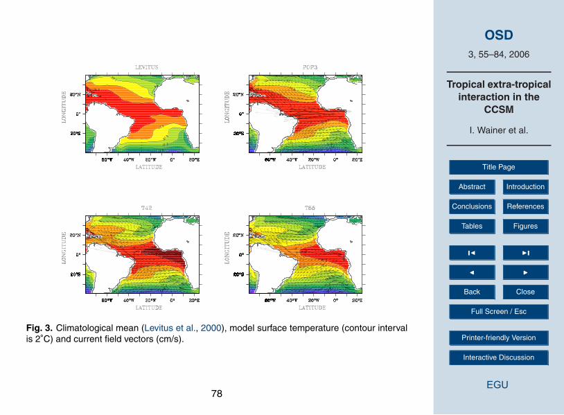
The annual mean surface horizontal temperature distribution for the three runs (con-20

tour interval is 2◦C) with the surface current velocity field superimposed can be seenin Fig. 3. The most realistic temperature field is that of POP3 (upper right panel) verysimilar to Levitus et al. (2000) (Fig. 4, upper left panel), except for the absence ofthe eastern Atlantic upwelling off Africa, which is an already known bias. The marinestratus regions off the western coasts of North and South America and off Africa are25

too warm by 2–3 K, resulting from a bias in cloud simulation. According to Norris andWeaver (2001) the atmospheric component of the CCSM overestimates shortwave andlong wave cloud radiative forcing when vertical motion is upward (negative omega) andunderestimates shortwave and long wave cloud radiative forcing compared to observa-

63





OSD3, 55–84, 2006


CCSM

I. Wainer et al.

Title Page



Tables Figures

J I

J I

Back Close

Full Screen / Esc



EGU

tions when vertical motion is downward. The coupled model present a reverse gradientin the equatorial region (noted by Davey et al. (2002) in an intercomparison study of 23different coupled models). Warmer temperatures are found in the eastern equatorialAtlantic rather than in the west as in observations.

The annual mean horizontal current velocity field for all three runs has overall sim-5

ilarities where one can delineate the two tropical gyres and major equatorial (Northand South Equatorial Currents, Guyana Current) and western boundary currents (i.e.the North and South Brazil currents are very similar in magnitude for the three runs).The flow is less realistic in the coupled runs. In T42 (left bottom panel) the zonal cur-rent is predominantly westward south of the equator but reverses right at the equator10

extending for the whole width of the Atlantic. This can be interpreted as a southwarddisplacement of the NECC that does not appear in the forced case (Fig. 3, lower panel).In T85 the flow at the equator is also eastward but weaker. In both cases this is dueto the surfacing of the EUC. At this latitude the largest zonal current velocity differencebetween POP3 and the coupled runs occurs at approximately 10◦–12◦ W and is about15

–45 cm/s for POP3 minus T42 and –30 cm/s for POP3 minus T85. Another differencein the annual mean velocity field between the coupled runs and the forced case is offSouthern Africa in the eastern basin where there seems to be a spurious southwardflowing current from approximately 5◦ S to 25◦ S in the coupled runs that merges withthe southern branch of the South Equatorial current whereas in POP3 this does not20

occur.In order to appreciate some of the differences described, it is important to turn to the

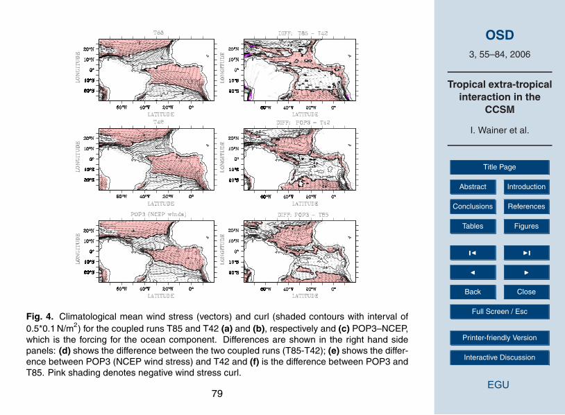
forcing. Since STCs are largely influenced by the winds, they are compared, togetherwith the curl, between the three runs and shown in Fig. 4.

The zonal winds are too weak at the equator which accounts wor the weak upwelling25

in the coupled model noted earlier. Weaker winds are also responsible for the absenceof a better defined Northern SEC and the surfacing of the EUC. Furthermore, theequatorial winds (off South Africa) are also too weak which accounts for the lack ofcoastal upwelling and the ill direction of the ocean currents there (i.e. Fig. 3).

64





OSD3, 55–84, 2006


CCSM

I. Wainer et al.

Title Page



Tables Figures

J I

J I

Back Close

Full Screen / Esc



EGU

It can be seen that the broad-scale spatial characteristics are very similar betweenthe coupled (Figures 4a,b) and forced run (POP3 – Fig. 4c) which is actually the NCEPwind stress. However, more detailed examination reveals that the largest differencesare between POP3 and T42 (Fig. 4e). Overall, the curl (and consequently the associ-ated Ekman-pumping velocity field) is significantly stronger in POP3 than in the coupled5

runs. However, the curl in T42 is stronger compared to POP3 north of the equator withthe maximum difference off the African coast of about 1.5 N/m2 off Mauritania (Fig. 4e).The same difference between POP3 and T85 is 1.0 N/m2 (Fig. 4f). The other regionwith big differences is also off the African coast but further south, between 15◦–25◦ S.Differences between POP3 and T42 are also the largest reaching 1.5 N/m2 off the coast10

of Namibia (Fig. 4e). It is interesting to note that in this region, the difference betweenPOP3 and T85 is significantly less (Fig. 4f, between 0.5–1 N/m2). Comparison of theclimatological mean wind stress curl between the coupled runs indeed shows that theydiffer largely in the south-eastern part of the domain. In T85 (Fig. 4d) the negative windstress curl is stronger but confined to a narrow region hugging the coast of Namibia15

and Angola (much like the NCEP winds in POP3, Fig. 4c) whereas in T42 the same re-gion is broader and extends further northwest. Note also that the zero line is displaceda few degrees west in T42 as compared to POP3 and T85. The importance of thesedifferences becomes evident once the pathways of tropical extra-tropical exchange ofthermocline waters, that are highly dependent on the wind distribution (e.g. Liu and20

Philander, 1995; Inui et al., 2002) are examined.

3.2 The subtropical cells

The STC can be viewed as an extension of the ventilated thermocline theory (i.e.Snowden and Molinari (2003); Malanotte-Rizzoli et al. (2000); Hazeleger et al. (2003);Luyten et al. (1983), etc.) where subtropical thermocline waters that are subducted25

along specified isopycnals conserve potential vorticity (PV) and are transported to theEquator. At the equator the wind forced upwelling and associated poleward flow arealso part of the STC. The equatorward path of the STC is still subject of investigation

65





OSD3, 55–84, 2006


CCSM

I. Wainer et al.

Title Page



Tables Figures

J I

J I

Back Close

Full Screen / Esc



EGU

and is complicated in the South Atlantic due to, among other factors, the superpositionof the northward flowing branch of the basin-wide meridional overturning circulation(MOC) that underlies the STC return flow at the western boundary.

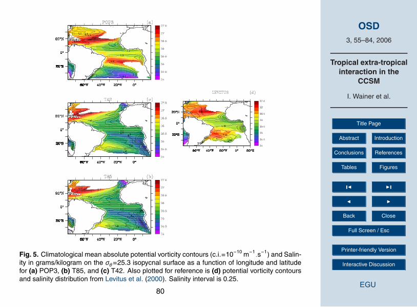
One way to look at the characteristics of tropical-extra-tropical exchanges in theCCSM3 and to understand the pathways by which the STC feeds the EUC, is to ex-5

amine the planetary potential vorticity distribution (PV). Since water that upwells at theequator will originate from 24.5<σθ<26.8 kg/m3 and in order to compare with Zhanget al. (2003), PV contours are plotted on the σθ=25.3 surface for POP3 and can beseen in Fig. 5 overlaying the salinity distribution on the same surface. PV and salinityfor the coupled runs are also displayed in Fig. 5 but at σθ= 24.3 kg/m3 for T42 and σθ=10

24.0 kg/m3 for T85. The reason for using different isopycnal surfaces is the fact that thecore of the EUC is at a different depth for each run. The isopycnals chosen are exactlythe ones that cross the EUC core at 30◦ W, as seen in Fig. 1.

The PV calculations follows the formulation of Cushman-Roisin (1987) as in Lazaret al. (2002) where PV can be approximated by:15

P V =fρ0

∂ρ∂z

(1)

where f=Coriolis parameter and ρ=density.The flow streamlines for each run, calculated at the isopycnal surfaces representing

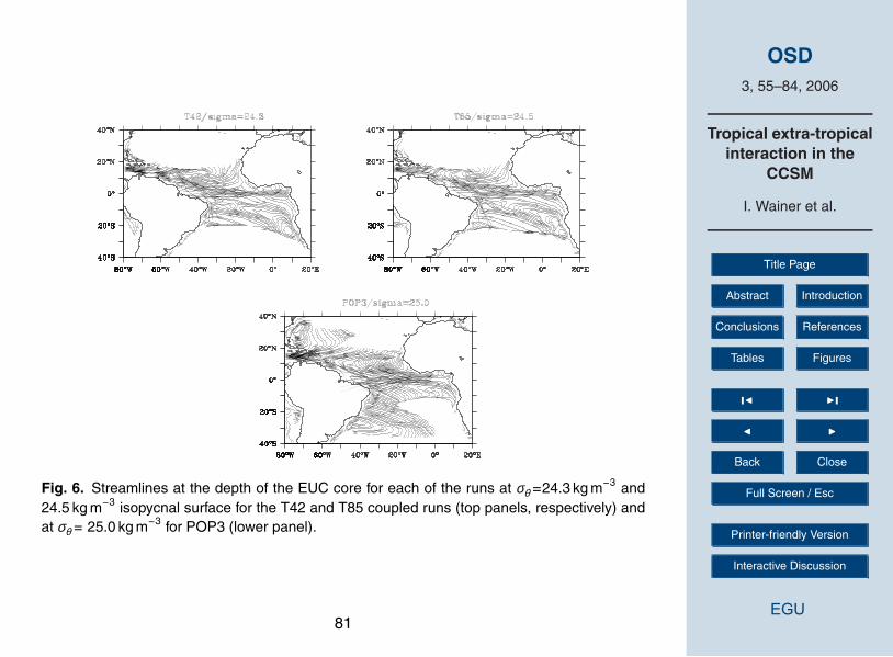
the depth of the EUC core (σθ=25, 24.5, 24.3 for POP3, T85 and T42, respectively)and shown in Figs. 6. The streamlines, show a distinct asymmetry between hemi-20

spheres. For POP3 (lower panel), the interior pathways are observed only in the SouthAtlantic together with the western boundary route. There is a closed streamline regionnortheast of the equator (between approximately 10◦ N and 20◦ N induced by the posi-tive Ekman pumping (e.g. Fig. 4) which is a result of the PV ridge seen in Fig. 5. Thisimplies that the subducted waters cannot cross the region towards the equator in order25

to conserve PV. Instead they are advected westward. Depth of the σθ=25.3 surface in-creases toward the western side of the basin (not shown) consistent between all threeruns and in agreement with Lazar et al. (2002).

66





OSD3, 55–84, 2006


CCSM

I. Wainer et al.

Title Page



Tables Figures

J I

J I

Back Close

Full Screen / Esc



EGU

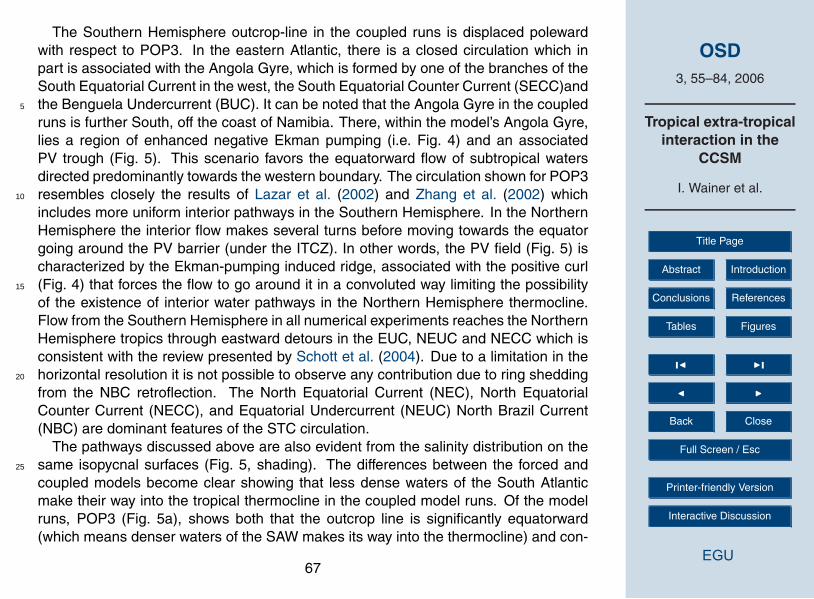
The Southern Hemisphere outcrop-line in the coupled runs is displaced polewardwith respect to POP3. In the eastern Atlantic, there is a closed circulation which inpart is associated with the Angola Gyre, which is formed by one of the branches of theSouth Equatorial Current in the west, the South Equatorial Counter Current (SECC)andthe Benguela Undercurrent (BUC). It can be noted that the Angola Gyre in the coupled5

runs is further South, off the coast of Namibia. There, within the model’s Angola Gyre,lies a region of enhanced negative Ekman pumping (i.e. Fig. 4) and an associatedPV trough (Fig. 5). This scenario favors the equatorward flow of subtropical watersdirected predominantly towards the western boundary. The circulation shown for POP3resembles closely the results of Lazar et al. (2002) and Zhang et al. (2002) which10

includes more uniform interior pathways in the Southern Hemisphere. In the NorthernHemisphere the interior flow makes several turns before moving towards the equatorgoing around the PV barrier (under the ITCZ). In other words, the PV field (Fig. 5) ischaracterized by the Ekman-pumping induced ridge, associated with the positive curl(Fig. 4) that forces the flow to go around it in a convoluted way limiting the possibility15

of the existence of interior water pathways in the Northern Hemisphere thermocline.Flow from the Southern Hemisphere in all numerical experiments reaches the NorthernHemisphere tropics through eastward detours in the EUC, NEUC and NECC which isconsistent with the review presented by Schott et al. (2004). Due to a limitation in thehorizontal resolution it is not possible to observe any contribution due to ring shedding20

from the NBC retroflection. The North Equatorial Current (NEC), North EquatorialCounter Current (NECC), and Equatorial Undercurrent (NEUC) North Brazil Current(NBC) are dominant features of the STC circulation.

The pathways discussed above are also evident from the salinity distribution on thesame isopycnal surfaces (Fig. 5, shading). The differences between the forced and25

coupled models become clear showing that less dense waters of the South Atlanticmake their way into the tropical thermocline in the coupled model runs. Of the modelruns, POP3 (Fig. 5a), shows both that the outcrop line is significantly equatorward(which means denser waters of the SAW makes its way into the thermocline) and con-

67





OSD3, 55–84, 2006


CCSM

I. Wainer et al.

Title Page



Tables Figures

J I

J I

Back Close

Full Screen / Esc



EGU

tribution from both the north and south Atlantic to the equatorial circulation, althoughthe contribution from the Southern Hemisphere is significantly larger. The salinity dis-tribution and PV contours for Levitus et al. (2000) can be seen in Fig. 5d for reference.It is clear that the salinity distribution in POP3 (Fig. 5a) most resembles observations inLevitus et al. (2000). The salinity field is characterized by regions of high salinity (salin-5

ity maximum waters) in the North and South subtropical Atlantic ocean. In betweenthese two regions of maximum salinity lies tropical low salinity waters. The coupledruns (Figs. 5b, c) exhibit a significantly different structure. The Northern Hemispheresalinity maxima region, for example, is displaced poleward and is confined to the westof 40◦ W with a maximum value of approximately 37.5 psu. The equivalent high salin-10

ity waters of the Southern Hemisphere in the coupled runs is considerably less densethan in POP3 (approximately 1 psu difference). It is spatially confined to the westernboundary, hugging the southeast coast of Brazil with its maximum value of approxi-mately 36 psu centered around 22–23◦ S. In POP3 the region of maximum salinity inthe Southern Hemisphere has a maximum of approximately 37 psu that extends zonally15

across the whole basin centered around 10◦ S. Basically this spatial distribution trans-lates into a salinity front in the northwest corner of the basin along the trajectory of thecoupled model’s NBC (i.e. Fig. 3) while the equivalent for the forced model seems tofollow the NEC (as in Zhang et al., 2002).

In summary, from the salinity distribution in Fig. 5 it can be clearly seen for POP320

that the high salinity subtropical waters does reach the EUC from both northern andsouthern Atlantic resulting in a high salinity tongue that extends eastward along theequator. For the coupled runs the equator is not marked by the high salinity subtropicalwaters and contribution from the Northern Hemisphere subtropics is not evident.

68





OSD3, 55–84, 2006


CCSM

I. Wainer et al.

Title Page



Tables Figures

J I

J I

Back Close

Full Screen / Esc



EGU

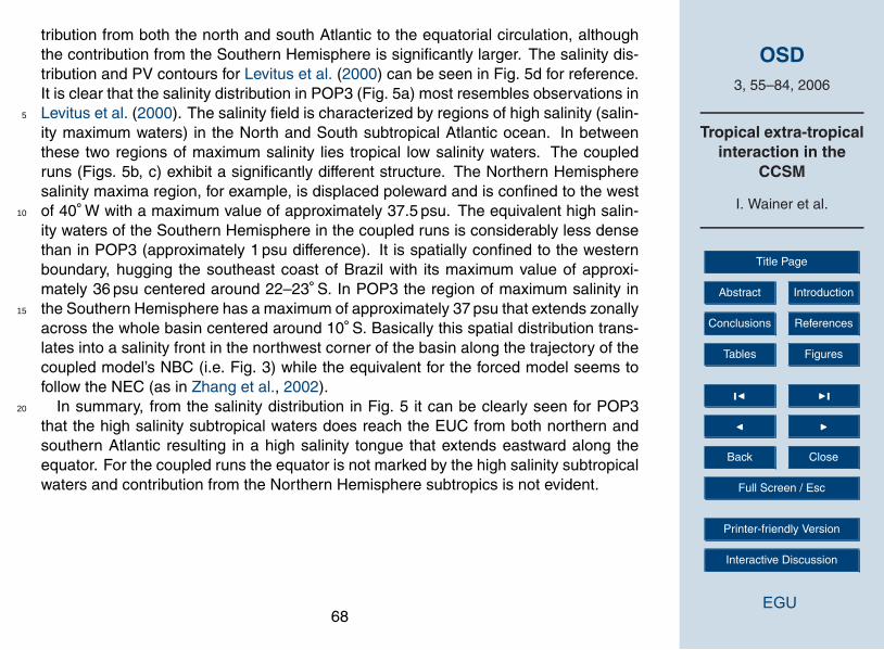
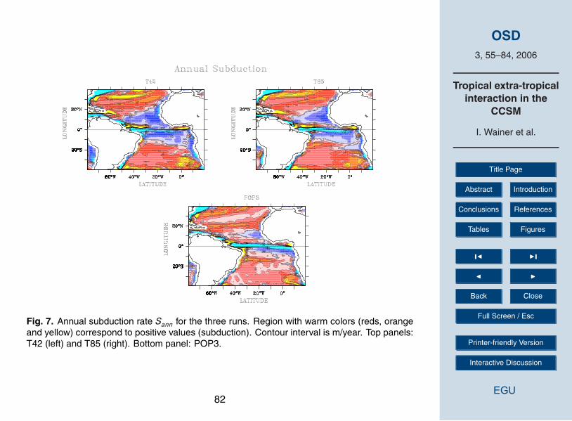
3.3 Annual Subduction

Next, the annual subduction is calculated as in Cushman-Roisin (1987), following Lazaret al. (2002), given by:

Sann = −(VH .∇H + wH ), (2)

where VH and wH are the climatological annual mean horizontal and vertical velocity5

at the depth H . H is the maximum climatological mean mixed layer depth. Sann forthe three runs can be seen in Fig. 8. Warm color (reds) shading represents positivecontours associated with downwelling. Negative values (blues) indicate entrainmentinto the mixed layer. The overall general structure is similar between the runs, howeverthere are some distinct differences, particularly between the coupled runs (T42 and10

T85) and the forced case (POP3). The common feature between T42 and T85, and tosome extent POP3 is the broad entrainment region (negative contours) particularly inthe high positive PV region in the east, in the Northern Hemisphere. In the west, be-tween 5◦ N–10◦ N, at the NECC retroflection region, there is a strong region of positivevalues that are confined to the west of 30◦ W in the T42 run (Fig. 7, upper left panel)15

and spreads towards the east in T85 (Fig. 7, upper right panel) and POP3 (Fig. 7, lowerpanel). Similar to the the numerical study of Lazar et al. (2002), which would comparewith POP3 in this study, the Southern Hemisphere shows a more regular distributionwith respect to the Northern Hemisphere.

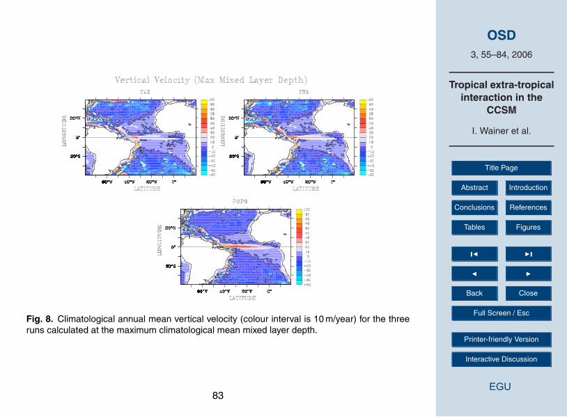
Compared to POP3, the equatorial upwelling signature in T42 is weak and confined20

to the west. At T85 a more basin-wide signal is observed. These characteristics arebest observed in the vertical velocity field at the climatological mean maximum mixedlayer depth shown in Fig. 8. Regional differences of upwelling/downwelling can be ob-served which imply that the atmospheric model resolution seems to affect the strengthand spatial features of the STC/TC system. Considering that the annual subduction25

rate is largely affected by the strength and distribution of the wind fields (e.g. Inui et al.,2002; Lazar et al., 2002; Liu and Philander, 1995) the response is expected to be differ-ent. Using the forced case as a realistic base for comparison, i.e. the POP3 results are

69





OSD3, 55–84, 2006


CCSM

I. Wainer et al.

Title Page



Tables Figures

J I

J I

Back Close

Full Screen / Esc



EGU

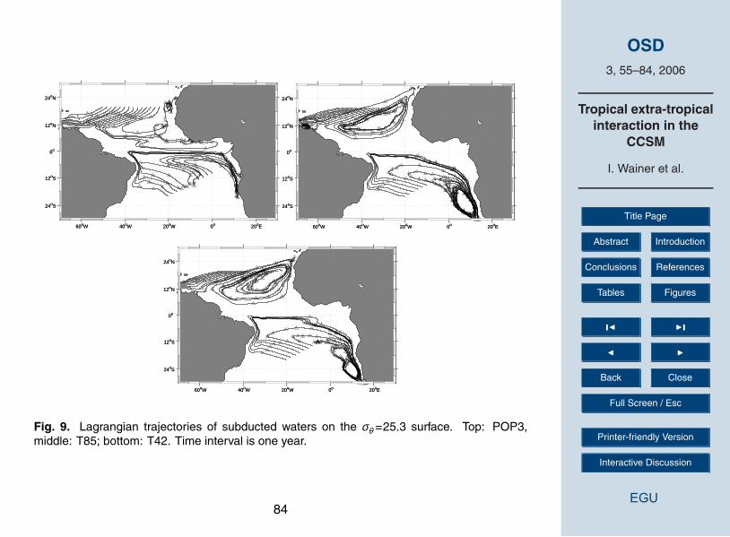
in good agreement with the observation analysis of Zhang et al. (2003), examinationof the coupled runs reveals that T85 has a better representation of the Atlantic STC.To confirm these results we examine the Lagrangian trajectories of floats released atthe σθ=25.3 surface (Fig. 9) partly reproduced from Alexander et al., 20054. The inter-val between floats is one year. What is clear from the Lagrangian analysis is the fact5

that regardless of the atmospheric model resolution (and its impact on the wind fieldstructure), there seems to be no Northern Hemisphere contribution to the STC/TC cir-culations in the coupled models. The trajectories on this single isopycnal surface seenin Fig. 9 do not capture all the complexity of the flow that was shown in Fig. 6 for thedensity layers averaged between 24.5 kg m−3<σθ<26.5 kg m−3. It should also be noted10

that the Lagrangian trajectory analysis takes into account the projection of the velocityfield onto an isopycnal surface, so that it does not account for possible diapycnal flow.

4 Conclusions

Tropical-extra-tropicalinteractions can be a key element in the low-frequency sea sur-face temperature (SST) variability. Many stand alone modeling studies have been per-15

formed to understand subduction and transport pathways in the upper circulation of theAtlantic Ocean. However, little is known about these tropical extra-tropical exchangeswithin a coupled GCM framework.

The most significant results of the intercomparison of the STC pathways in the threedifferent numerical experiments (two coupled and one stand-alone ocean simulation),20

seen in both the float trajectories (Fig. 8) and the salinity projected onto the 25.3σθsurface (Fig. 5), is the fact that for the coupled runs all subtropical waters that feed theEUC is from Southern Hemisphere waters. The EUC in POP3 reaches the equatorfrom the Northern Hemispher after going around the PV ridge created by the upward

4Alexander, M., Yin, J., Branstator, G., Capotondi, A., Cassou, C., Cullather, R., Kwon, Y.,Norris, J., Scott, J., and Wainer, I.: Extratropical Ocean-Atmosphere Variability in CCSM3, J.Clim., submitted, 2005.

70





OSD3, 55–84, 2006


CCSM

I. Wainer et al.

Title Page



Tables Figures

J I

J I

Back Close

Full Screen / Esc



EGU

Ekman pumping. In other words, in all three runs north of the equator, the circulationis characterized by a closed region with upward Ekman pumping directly related tothe wind stress distribution. The predominant Southern Hemisphere contribution tothe Atlantic EUC is in fact mentioned in Hazeleger et al. (2003) and has already beenshown in part by Metcalf and Stalcup (1967), Fratantoni et al. (2000) and Malanotte-5

Rizzoli et al. (2000). What is different in the coupled runs is a closed cyclonic circulationfound in the southeastern edge of the Tropical Atlantic that forces the interior flowtowards the west. This anomalous circulation arises from known biases in the coupledmodel and is much more evident in T42 than in T85. When compared to POP3, T85seems to capture more of the STC/TC dynamics. It should be noted that these warm10

SST bias in the eastern basin is not unique to the CCSM and has been noted to occurin several other coupled climate models (Davey et al. (2002)).

Although the literature gives a good idea in of how the STC behaves, there is stillmuch discussion on how the transport is partitioned between the western boundaryand the interior of the basin. In the CCSM there is no debate on the contribution of15

water masses from each hemisphere since all the waters originate from the SouthernHemisphere.

Acknowledgements. The authors wish to thank P. Gent and W. Large from NCAR for veryuseful discussions and M. Goes for helping with the lagrangean tracers algorithm. This workwas supported in part by grants FAPESP-00/02958-7, CNPq 300223/93-5, CNPq 300561/91-1.20

and CNPq 300040/94-6. I. Wainer thanks NCAR, SGER and WISC from the National ScienceFoundation for additional travel support.

References

Blanke, B., M., A., Madec., G., and Roche, S.: Warm water paths in the equatorial Atlantic asdiagnosed with a general circulation model, J. Phys. Oceanogr., 29, 2753–2768, 1999. 5725

Bonhoure, D., Rowe, E., Mariano, A., and Ryan, E.: The South Equatorial Current System,www.oceancurrents.rsmas.miami.edu/atlantic/south-equatorial.html, 2003. 63

71





www.oceancurrents.rsmas.miami.edu/atlantic/south-equatorial.html

OSD3, 55–84, 2006


CCSM

I. Wainer et al.

Title Page



Tables Figures

J I

J I

Back Close

Full Screen / Esc



EGU

Briegleb, B. P., Bitz, C. M., Hunke, E. C., Lipscomb, W. H., Holland, M. M., Schramm, J. L.,and Moritz, R. E.: Scientific description of the sea ice component in the Community ClimateSystem Model, Version Three, NCAR Tech. Note NCAR/TN- 463+STR, 70, 2004. 58, 60

Cushman-Roisin, B.: Dynamics of the Oceanic Surface Mixed Layer, Hawaii Inst. of Geophys.,181–196, 1987. 66, 695

Davey, M., Huddleston, M., Sperber, K., Braconnot, P., Bryan, F., Chen, D., Colman, R., Cooper,C., Cubasch, U., Delecluse, P., DeWitt, D., Fairhead, L., Flato, G., Gordon, C., Hogan, T., Ji,M., Kimoto, M., Kitoh, A., Knutson, T., Latif, M., Treut, H. L., Li, T., Manabe, S., Mechoso, C.,Meehl, G., Power, S., Roeckner, E., Terray, L., Vintzileos, A., Voss, R., Wang, B., Washington,W., Yoshikawa, I., Yu, J., Yukimoto, S., Zebiak, S., and Danabasoglu, G.: STOIC: a study of10

coupled model climatology and variability in tropical ocean regions., Climate Dynamics, 18,403–420, 2002. 64, 71

Fratantoni, D. W. J., Townsend, T., and Hurlburt, H.: Low-Latitude Circulation and Mass Trans-port Pathways in a Model of the Tropical Atlantic Ocean, J. Phys. Oceanogr., 30, 1944–1966,2000. 7115

Gent, P. and McWilliams, J.: Isopycnal mixing in ocean circulation models, J. Phys. Oceanogr.,20, 150–155, 1990. 59

Grodsky, S. A. and Carton, J.: Surface drifter pathways originating in the equatorial Atlanticcold tongue, Geophys. Res. Lett., 29(23), 2147–2151, 2002. 57

Harper, S.: Thermocline ventilation and pathways of tropical-subtropical water mass exchange,20

Tellus, 52A, 330–345, 2002. 57Hazeleger, W., de Vries, P., and Friocourt, Y.: Sources of the Equatorial Undercurrent in the

Atlantic in a High-Resolution Ocean Model, J. Phys. Oceanogr., 33, 677–693, 2003. 65, 71Inui, T., Lazar, A., Malanotte-Rizzoli, P., and Busalacchi, A.: Wind stress effects on the Atlantic

subtropical-tropical circulation, J. Phys. Oceanogr., 32(8), 2257–2276, 2002. 57, 65, 6925

Kalnay, E., Kanamitsu, M., Kistler, M., Collins, K. W., Deaven, D., Gandin, L., Iredell, M., Saha,S., White, G., Woollen, J., Zhu, Y., Leetmaa, A., Reynolds, R., Chelliah, M., Ebisuzaki, W.,Higgins, W., Janowiak, J., Mo, K. C., Ropelewski, C., Wang, J., Jenne, R., and Joseph, D.:The NCEP/NCAR 40-year reanalysis project, Bull. Am. Meteorol. Soc., 77, 437–471, 1996.6030

Large, W., McWilliams, J., andDoney, S. C.: Oceanic vertical mixing: A review and a modelwith a nonlocal boundary layer parameterization, Rev. Geophys., 32, 363–403, 1994. 59

Lazar, A., Inui, T., Busalacchi, A., Malanotte-Rizzoli, P., and Wang, L.: Seasonality of the

72





OSD3, 55–84, 2006


CCSM

I. Wainer et al.

Title Page



Tables Figures

J I

J I

Back Close

Full Screen / Esc



EGU

ventilation of the tropical Atlantic thermocline., J. Geophys. Res., 107, 181–187, 2002. 57,66, 67, 69

Levitus, S., Antonov, J., Boyer, T., and Stephens, C.: Warming of the world ocean., Science,287, 2225–2229, 2000. 60, 62, 63, 68, 76, 78, 80

Liu, Z. and Philander, S.: How different wind stress patterns affect the tropical-subtropical5

circulations of the upper ocean, J. Phys. Oceanogr., 25, 449–462, 1995. 65, 69Luyten, J., Pedlosky, J., and Stommel, H.: The ventilated thermocline, J. Phys. Oceanogr., 13,

292–309, 1983. 65Malanotte-Rizzoli, P., Hedstrom, K., Arango, H., and Haidvogel, D.: Water mass pathways

between the subtropical and tropical ocean in a climatological simulation of the North Atlantic10

ocean circulation., Dyn. Atmos. Oceans, 32, 331–371, 2000. 57, 65, 71Metcalf, W. G. and Stalcup, M.: Origin of the Atlantic Equatorial Undercurrent, J. Geophys.

Res., 72, 4959–4875, 1967. 71Molinari, R., Bauer, S., Snowden, D., Johnson, G., Bourles, B., Gouriou, Y., and Mercier, H.:

A Comparison of kinematic evidence for tropical cells in the Atlantic and Pacific oceans,15

Elsevier Oceanographic Series, 269–286, 2003. 56, 61, 62Norris, J. R. and Weaver, C. P.: Improved techniques for evaluating GCM cloudiness applied to

the NCAR CCM3., J. Climate, 2540–2550, 2001. 63Schott, F., Fischer, J., and Stramma, L.: Transports and pathways of the upper-layer circulation

in the western tropical Atlantic, J. Phys. Oceanogr., 28, 1904–1918, 1998. 5620

Schott, F. A., McCreary, J. P., and Johnson, G. C.: Shallow overturning circulations of thetropical-subtropical oceans, Ocean-Atmosphere Interaction and Climate Variability, AGUGeophys. Monogr., edited by: Wang, C., Xie, S.-P., and Carton, J. A., in press, 2004. 62, 67

Smith, R. and McWilliams, J.: Anisotropic horizontal viscosity for ocean models, Oc. Model, 5,129–156, 2003. 5925

Smith, R. and Gent, P. R.: Reference manual for the Parallel Ocean Program (POP): Oceancomponent of the Community Climate System Model (CCSM2.0 and CCSM3.0), Los AlamosNational Laboratory Technical Report LA-UR-02-2484, 2002. 58, 59

Snowden, D. and Molinari, R.: Subtropical cells in the Atlantic Ocean: An observational sum-mary, Elsevier Oceanography Series, 68 (ISBN 0-444-51267-5), 2003. 56, 57, 6530

Zhang, D., McPhaden, M. J., and Johns, W. E.: Interior Pycnocline Transports in the AtlanticSubtropical Cells, Exchanges, 25, 1–3, 2002. 67, 68

Zhang, D., McPhaden, M. J., and Johns, W. E.: Observational evidence for flow between the

73





OSD3, 55–84, 2006


CCSM

I. Wainer et al.

Title Page



Tables Figures

J I

J I

Back Close

Full Screen / Esc



EGU

Subtropical and Tropical Atlantic: the Atlantic Subtropical Cells, J. Phys. Oceanogr., 33,1783–1797, 2003. 56, 66, 70

74





OSD3, 55–84, 2006


CCSM

I. Wainer et al.

Title Page



Tables Figures

J I

J I

Back Close

Full Screen / Esc



EGU

1

1

Fig. 1. mean meridional versus vertical velocity (x1e3) circulation vectors superimposed onthe zonalvelocity field (contour interval is 5 cm/s for T85 and T42 – upper panels, and 10 cm/sfor POP3 – bottom panel). Thick white horizontal curves are selected isopycnals at 5 kg m−3

contour intervals. Note that for each run a different isopycnal surface crosses the core of theEUC. Thick black line is the zero contour for zonal velocity (in color shading).

75





OSD3, 55–84, 2006


CCSM

I. Wainer et al.

Title Page



Tables Figures

J I

J I

Back Close

Full Screen / Esc



EGU

Fig. 2. Climatological mean temperature (◦C) at 30◦ W down to 300 m between 30◦ S–30◦ N forthe (a) Levitus et al. (2000) Climatology, (b) POP3, (c) T42 (d) T85; their differences (e) POP3– Levitus et al. (2000) Climatology, (f) POP3 – T42, (g) POP3 – T85 and (h) T85 – T42; andthe equatorial sections for (i) POP3, (j) T42 (k) T85 (l) Levitus et al. (2000) Climatology .

76





OSD3, 55–84, 2006


CCSM

I. Wainer et al.

Title Page



Tables Figures

J I

J I

Back Close

Full Screen / Esc



EGU

Fig. 2. Continued.

77





OSD3, 55–84, 2006


CCSM

I. Wainer et al.

Title Page



Tables Figures

J I

J I

Back Close

Full Screen / Esc



EGU

1

1

1

1

1

1

1

1

1

1

Fig. 3. Climatological mean (Levitus et al., 2000), model surface temperature (contour intervalis 2◦C) and current field vectors (cm/s).

78





OSD3, 55–84, 2006


CCSM

I. Wainer et al.

Title Page



Tables Figures

J I

J I

Back Close

Full Screen / Esc



EGU

11

11

Fig. 4. Climatological mean wind stress (vectors) and curl (shaded contours with interval of0.5*0.1 N/m2) for the coupled runs T85 and T42 (a) and (b), respectively and (c) POP3–NCEP,which is the forcing for the ocean component. Differences are shown in the right hand sidepanels: (d) shows the difference between the two coupled runs (T85-T42); (e) shows the differ-ence between POP3 (NCEP wind stress) and T42 and (f) is the difference between POP3 andT85. Pink shading denotes negative wind stress curl.

79





OSD3, 55–84, 2006


CCSM

I. Wainer et al.

Title Page



Tables Figures

J I

J I

Back Close

Full Screen / Esc



EGU

Fig. 5. Climatological mean absolute potential vorticity contours (c.i.=10−10 m−1.s−1) and Salin-ity in grams/kilogram on the σθ=25.3 isopycnal surface as a function of longitude and latitudefor (a) POP3, (b) T85, and (c) T42. Also plotted for reference is (d) potential vorticity contoursand salinity distribution from Levitus et al. (2000). Salinity interval is 0.25.

80





OSD3, 55–84, 2006


CCSM

I. Wainer et al.

Title Page



Tables Figures

J I

J I

Back Close

Full Screen / Esc



EGU

Fig. 6. Streamlines at the depth of the EUC core for each of the runs at σθ=24.3 kg m−3 and24.5 kg m−3 isopycnal surface for the T42 and T85 coupled runs (top panels, respectively) andat σθ= 25.0 kg m−3 for POP3 (lower panel).

81





OSD3, 55–84, 2006


CCSM

I. Wainer et al.

Title Page



Tables Figures

J I

J I

Back Close

Full Screen / Esc



EGU

Fig. 7. Annual subduction rate Sann for the three runs. Region with warm colors (reds, orangeand yellow) correspond to positive values (subduction). Contour interval is m/year. Top panels:T42 (left) and T85 (right). Bottom panel: POP3.

82





OSD3, 55–84, 2006


CCSM

I. Wainer et al.

Title Page



Tables Figures

J I

J I

Back Close

Full Screen / Esc



EGU

Fig. 8. Climatological annual mean vertical velocity (colour interval is 10 m/year) for the threeruns calculated at the maximum climatological mean mixed layer depth.

83





OSD3, 55–84, 2006


CCSM

I. Wainer et al.

Title Page



Tables Figures

J I

J I

Back Close

Full Screen / Esc



EGU

60oW 40oW 20oW 0o 20oE

24oS

12oS

0o

12oN

24oN


24oS

12oS

0o

12oN

24oN


24oS

12oS

0o

12oN

24oN


24oS

12oS

0o

12oN

24oN


24oS

12oS

0o

12oN

24oN


24oS

12oS

0o

12oN

24oN

Fig. 9. Lagrangian trajectories of subducted waters on the σθ=25.3 surface. Top: POP3,middle: T85; bottom: T42. Time interval is one year.

84





Tropical extra-tropical thermocline water mass exchanges in the Community Climate Model v.3 Part I:...

Documents

Transcript of Tropical extra-tropical thermocline water mass exchanges in the Community Climate Model v.3 Part I:...