Interaction of a solitary wave with an externalforce in the extended Korteweg-de Vries

equation

Roger Grimshaw1, Efim Pelinovsky2,

1 Department of Mathematical Sciences,Loughborough University, Loughborough, UK

2 Laboratory of Hydrophysics and Nonlinear Acoustics,Institute of Applied Physics, Nizhny Novgorod, Russia,

November 27, 2001

AbstractThe interaction of a strongly nonlinear solitary wave with an external

force is studied using the extended Korteweg-de Vries equation as a model.This equation has several different families of nonlinear wave solutions:solitons, the so-called ”thick” solitons, algebraic solitons, and breathers,depending upon the sign of the cubic nonlinear term. A simple nonlineardynamical system of the second order for the amplitude and position of thesolitary wave is dervived, and used to study the interaction. Its solutionsare investigated in the phase plane. The conditions for the capture orreflection of a solitary wave by a single isolated external force are obtained,with an emphasis on the role of the cubic nonlinear term.

1 Introduction

The forced Korteweg-de Vries (KdV) equation is a canonical model for theresonant generation of solitary waves by an external force moving with a speedclose to the speed of linearised long waves. In non-dimensional form it is,

∂u∂t

+ ∆∂u∂x

+ 6u∂u∂x

+∂3u∂x3 =

∂f∂x

, (1)

where u(x, t) is the wave function, x is the spatial coordinate in the referenceframe moving with an external force, t is the time, ∆ is the linear long-wavespeed and the speed of the moving force), and f(x) is a representation of theexternal force. Explicit asymptotic derivations of the forced Korteweg-de Vriesequation have been carried out for several situations in the ocean and atmo-sphere (see, for instance, the review papers by Grimshaw (2001a,b)).

At the next order a perturbation theory in the wave amplitude the extendedforced Korteweg-de Vries equation can be obtained, and in the general case itshould include cubic nonlinearity, fifth-order linear dispersion, and nonlineardispersion. The contribution of the various high-order terms depends on theparameters of the model (e.g. in the oceanic, or atmospheric, applications, onthe density stratification and shear flow). For instance, for internal waves ina two-layer fluid, the quadratic nonlinear term vanishes when the pycnoclinelies in the middle of the fluid (in the Boussinesq approximation), and the cubicnonlinear term is then the most important higher-order term; in this case, theextended Korteweg-de Vries equation coincides with the modified Korteweg-deVries equation, which like the KdV equation, is integrable. More generally,when the quadratic nonlinear term is small, the cubic nonlinear term shouldalso be taken into account, and the corresponding equation is,

∂u∂t

+ 6u∂u∂x

+ βu2 ∂u∂x

+∂3u∂x3 =

∂f∂x

. (2)

In the absence of forcing, this is the extended Korteweg-de Vries (eKdV) equa-tion, or Gardner equation. It is often used as a model for strongly nonlinear

1

internal waves in the ocean (Holloway et al, 2001). The coefficient β of the cubicnonlinear term may have either sign depending on the oceanic (or atmospheric)stratification. For the classical two-layer model it is always negative, but forcertain three-layer models, it was recently shown that it may be as negative, orpositive, (Grimshaw et al, 1997).

The solutions of the extended Korteweg-de Vries equation describe variouskinds of nonlinear waves (solitons, breathers, dissipationless shock waves) forvarious signs of the coefficients of the quadratic and cubic nonlinear terms. Fur-ther, although the unforced equation (2) is integrable, like the Korteweg-de Vriesequation, the number of explicitly solved problems is quite small. In particular,soliton interactions have been investigated by Slunyaev & Pelinovsky (1999) andSlunyaev (2001) for both signs of the cubic nonlinear term. Instability of alge-braic solitons in the framework of the extended Korteweg-de Vries equation hasbeen studied by Pelinovsky & Grimshaw (1997), who showed that any small dis-turbance leads either to transformation to a ”normal” soliton, or to a breather.Interesting examples of the soliton transformation when the quadratic nonlinearterm changes its sign (this situation may be realised for internal waves in thecoastal zone with an inclined pycnocline) were given by Grimshaw et al (1999).The influence of all high-order terms on soliton dynamics was investigated nu-merically by Marchant & Smyth (1990, 1996). This paper is concerned withsoliton dynamics in the framework of the forced extended Korteweg-de Vriesequation (2) when the forcing has the form of a single impulse. Numerical sim-ulations of this equation shown that the imposition of a forcing on an initiallyquiescent state generates various forms of nonlinear wave packets, as well assolitary waves (Choi et al, 1996, Grimshaw et al, 2001a). Here we suppose thatthe wave field consists of just one solitary wave, and we will study its interactionwith an external force. Our analysis will use an asymptotic method for solitonperturbations, similar to that used by Grimshaw et al (1994) for the analogousproblem for the forced KdV equation (1). Indeed, our main objective here is todetermine how the cubic nonlinear term in equation (2) will affect the resultsobtained in Grimshaw et al (1994) in their study of an interaction of a solitarywave with an isolated external force in the KdV model (1).

2 Forced extended Korteweg - de Vries equation

First, we observe that equation (2) can be written in the Hamiltonian form

∂u∂t

= − ∂∂x

δHδu

, (3)

where the Hamiltonian H is

H =∫ (

12∆u2 + u3 +

β12

u4 − 12

{

∂u∂x

}2

− uf)

dx. (4)

2

Consequently equation (2) (or (3)) conserves both the mass

M =∫

udx (5)

and the Hamiltonian. However, the momentum

P =∫

u2

2dx, (6)

is not conserved, although we note that equation (2) can be re-written as

∂∂t

δPδu

+∂∂x

δHδu

= 0. (7)

It is important to note that the mass is constant for any disturbance in the fieldof an isolated force f(x), where we assume that f → 0 as x → ±∞.

We will study the case when the forcing is weak, and so, in the zero (leadingorder) approximation, the waves are free. Our focus is on solitary waves (soli-tons), and first we need to describe their properties. When f ≡ 0, it followsfrom equation (7) that a solitary wave of speed c satisfies the equation

cδPδu

=δHδu

. (8)

The analytical expression for the soliton shape can be obtained for either signof the coefficient of the cubic nonlinear term as

u(x, t) =γ2

1 + B cosh(γ(x− ct), (9)

B2 = 1 +βγ2

6, c = ∆ + γ2,

where γ is a parameter characterising the inverse width of the solitary wave.The wave amplitude (peak value) is

a =γ2

1 + B=

6β

(B − 1). (10)

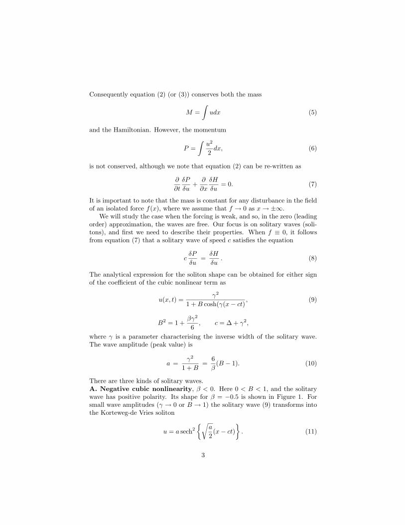
There are three kinds of solitary waves.A. Negative cubic nonlinearity, β < 0. Here 0 < B < 1, and the solitarywave has positive polarity. Its shape for β = −0.5 is shown in Figure 1. Forsmall wave amplitudes (γ → 0 or B → 1) the solitary wave (9) transforms intothe Korteweg-de Vries soliton

u = a sech2{√

a2(x− ct)

}

. (11)

3

As the wave amplitude increases, it approaches the limiting value

alim =6|β|

. (12)

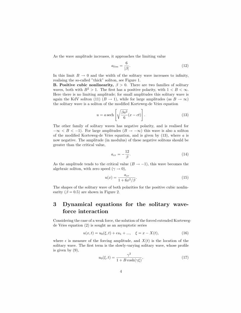
In this limit B → 0 and the width of the solitary wave increases to infinity,realising the so-called ”thick” soliton, see Figure 1.B. Positive cubic nonlinearity, β > 0. There are two families of solitarywaves, both with B2 > 1. The first has a positive polarity, with 1 < B < ∞.Here there is no limiting amplitude; for small amplitudes this solitary wave isagain the KdV soliton (11) (B → 1), while for large amplitudes (as B → ∞)the solitary wave is a soliton of the modified Korteweg-de Vries equation

u = a sech

[√

βa2

6(x− ct)

]

. (13)

The other family of solitary waves has negative polarity, and is realised for−∞ < B < −1). For large amplitudes (B → −∞) this wave is also a solitonof the modified Korteweg-de Vries equation, and is given by (13), where a isnow negative. The amplitude (in modulus) of these negative solitons should begreater than the critical value,

acr = −12β

. (14)

As the amplitude tends to the critical value (B → −1), this wave becomes thealgebraic soliton, with zero speed (γ → 0),

u(x) =acr

1 + 6x2/β. (15)

The shapes of the solitary wave of both polarities for the positive cubic nonlin-earity (β = 0.5) are shown in Figure 2.

3 Dynamical equations for the solitary wave-force interaction

Considering the case of a weak force, the solution of the forced extended Korteweg-de Vries equation (2) is sought as an asymptotic series

u(x, t) = u0(ξ, t) + εu1 + ..., ξ = x−X(t), (16)

where ε is measure of the forcing amplitude, and X(t) is the location of thesolitary wave. The first term is the slowly-varying solitary wave, whose profileis given by (9),

u0(ξ, t) =γ2

1 + B cosh(γξ), (17)

4

wheredXdt

= c = ∆ + γ2. (18)

Due to the effect of the forcing, the solitary wave amplitude and position willchange, so that the inverse-width parameter, γ is a function of time (and hencealso the amplitude, etc.). We will not describe here the asymptotic methodwhich allows us to obtain the equations for the solitary wave parameters, as themethod is well-known, in this context see, for instance, Grimshaw et al (1994).At the first order of the asymptotic theory, the amplitude variation can be foundfrom the momentum equation

dPdt

=∫

u∂f∂x

dx, (19)

which is readily obtained from equation (2) and the definition (5) of P . Indeed,using the leading order term (17) of the asymptotic series (16) we get

dP0

dt=

∫ ∞

−∞u0(x−X(t))

∂f∂x

dx, (20)

where P0 =∫ ∞

−∞

12u2

0 dx. (21)

Since P0 is a function of γ(t), the system of ordinary differential equations (18)and (20) form a dynamical system for the wave amplitude a and the positionX.

To simplify the right-hand side of (20) we next suppose that the force hasa large width compared to the solitary wave, the so-called “broad” forcing caseof Grimshaw et al (1994). In this case (20) reduces to

dP0

dt= M0

df(X)dX

. (22)

where M0 =∫ ∞

−∞u0 dx, (23)

is the mass of the solitary wave. This reduced system has a Hamiltonian K0

given by

K0 = V (P0) − f(X), where∂V∂P0

=c

M0. (24)

This Hamiltonian is conserved, and hence all the orbits of the dynamical systemare given by the curves K0 = constant in the X−a plane. Using equation (18)we see that the orbits are given by

f(X) = ∆F1(a) + F2(a) + constant , (25)

where F1(a) =∫

dP0

M0, and F2(a) =

∫

γ2dP0

M0. (26)

5

Both functions, F1(a) and F2(a) are monotonic functions of the wave amplitudea.

In general, when a solitary wave deforms there is the accompanying gen-eration of a trailing shelf (see, for instance, Grimshaw and Mitsudera, 1993).However, in the present case of broad forcing it can be shown that these shelvesare absent here to leading order. Indeed, their absence allows us to obatin thenext-order correction to the solitary wave speed, and replace equation (18) with

dXdt

= ∆ + γ2 − ∂M0

∂P0f(X) . (27)

The simplest demonstration of this is to note that if no shelves are generated,the interaction of the solitary wave with the force retains a Hamiltonian char-acter, and the Hamiltonian is just the expression (4) evaluated at leading order,denoted here by K and given by

K = H0(P0) − M0f(X), where∂H0

∂P0= c = ∆ + γ2. (28)

Here H0 is the Hamiltonian H evaluated for the solitary wave u0 and with f ≡ 0.Then, with the canonical variables X and P0, we see that the dynamical systemconsisting of (22) and(27) is just

dP0

dt= −∂K

∂X,

dXdt

= − ∂K∂P0

. (29)

The additional term in equation (27) can be shown to be significant only forsmall amplitudes, and since our main interest here is in large-amplitude soli-tary waves, we shall not consider the extended equation (27) further in thispaper, and instead use only the reduced equation (18). We also note that theHamiltonians K and K0 are proportional, K = K0M0.

4 Interaction of weak-amplitude solitary waveswith an external force

First, let us demonstrate the main features of the dynamics of weak-amplitudesolitary wave (i.e. the KdV approximation). In this case all integrals can beobtained in explicit form,

M = 2√

2a1/2, P =2√

23

a3/2, γ2 = 2a, (30)

and F1(a) =a2, F2(a) =

a2

2.

6

These expressions were obtained by Grimshaw et al (1994). We recall that theforce is isolated, that is, f(x) → 0 as x → ±∞. The soliton dynamics nowdepends on the sign of ∆.

If ∆ > 0 (”subcritical” forcing motion) the solitary wave has a speed greaterthan the speed of the external force for all amplitudes. In this case an exactresonance between the force and the solitary wave is impossible. The phaseportrait for this case is shown in Figure 3 for a positive disturbance (f > 0).The parameters of are

f(x) = b exp(−x2), b = 0.5, ∆ = 0.1. (31)

The main regime here is the passage of fast-moving solitary wave through theexternal force. The solitary wave takes momentum from the force (it is evidentfrom equation (22)), and its amplitude increases as

a(x) =

√

∆2

4+ 2f(x) + ∆a∞ + a2

∞ − ∆2

, (32)

(a∞ is the amplitude of the ”free” soliton) when the solitary wave passes throughthe forcing area. There is no net change in the solitary wave amplitude duringpassage, but the solitary wave has an additional phase shift due to the interac-tion.

In addition to this passage regime we have also the regime of birth/decay. Aweak solitary wave is generated behind the force, increases up to the momentof overtaking and then decays to zero in front of the force. Maximal amplitudeof this virtual wave can be found from (32) at a∞ = 0

amax =

√

∆2

4+ 2fmax −

∆2

. (33)

We should mention that the stage of birth/decay cannot be described by (18),(22), because the weak solitary wave has a very large width, and the approx-imation of broad forcing is not valid in this case. A more detailed analysis ofall possible wave regimes was done by Grimshaw et al (1994). For instance, ifthe force has negative polarity, (f(x) < 0), the solitary waves pass through theforcing area, but the trajectories on the phase plane are shifted in the directionof weak amplitudes.

A more interesting situation is realised for ∆ < 0 (”supercritical” forcingmotion), when the solitary wave can be in resonance with the force. The exactresonant condition is

2a = |∆|, (34)

obtained from (18). The system (18), (22) has an equilibrium state

X = 0, 2a0 + ∆ = 0, (35)

7

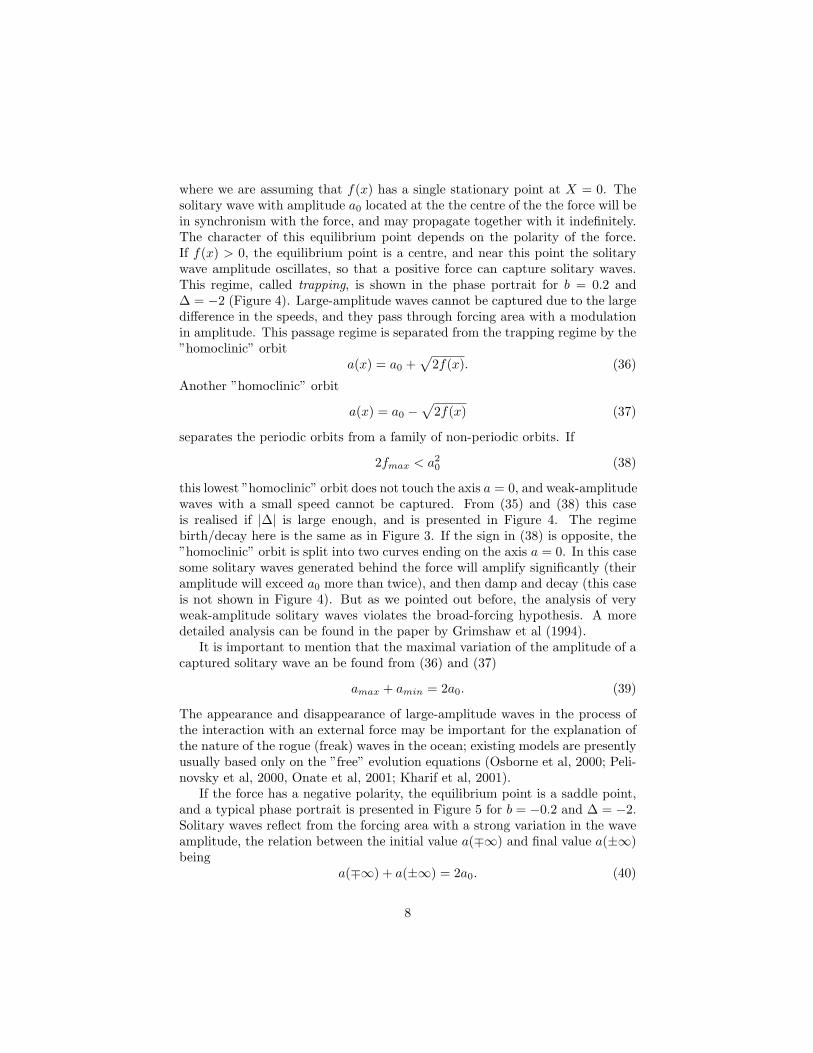
where we are assuming that f(x) has a single stationary point at X = 0. Thesolitary wave with amplitude a0 located at the the centre of the the force will bein synchronism with the force, and may propagate together with it indefinitely.The character of this equilibrium point depends on the polarity of the force.If f(x) > 0, the equilibrium point is a centre, and near this point the solitarywave amplitude oscillates, so that a positive force can capture solitary waves.This regime, called trapping, is shown in the phase portrait for b = 0.2 and∆ = −2 (Figure 4). Large-amplitude waves cannot be captured due to the largedifference in the speeds, and they pass through forcing area with a modulationin amplitude. This passage regime is separated from the trapping regime by the”homoclinic” orbit

a(x) = a0 +√

2f(x). (36)

Another ”homoclinic” orbit

a(x) = a0 −√

2f(x) (37)

separates the periodic orbits from a family of non-periodic orbits. If

2fmax < a20 (38)

this lowest ”homoclinic” orbit does not touch the axis a = 0, and weak-amplitudewaves with a small speed cannot be captured. From (35) and (38) this caseis realised if |∆| is large enough, and is presented in Figure 4. The regimebirth/decay here is the same as in Figure 3. If the sign in (38) is opposite, the”homoclinic” orbit is split into two curves ending on the axis a = 0. In this casesome solitary waves generated behind the force will amplify significantly (theiramplitude will exceed a0 more than twice), and then damp and decay (this caseis not shown in Figure 4). But as we pointed out before, the analysis of veryweak-amplitude solitary waves violates the broad-forcing hypothesis. A moredetailed analysis can be found in the paper by Grimshaw et al (1994).

It is important to mention that the maximal variation of the amplitude of acaptured solitary wave an be found from (36) and (37)

amax + amin = 2a0. (39)

The appearance and disappearance of large-amplitude waves in the process ofthe interaction with an external force may be important for the explanation ofthe nature of the rogue (freak) waves in the ocean; existing models are presentlyusually based only on the ”free” evolution equations (Osborne et al, 2000; Peli-novsky et al, 2000, Onate et al, 2001; Kharif et al, 2001).

If the force has a negative polarity, the equilibrium point is a saddle point,and a typical phase portrait is presented in Figure 5 for b = −0.2 and ∆ = −2.Solitary waves reflect from the forcing area with a strong variation in the waveamplitude, the relation between the initial value a(∓∞) and final value a(±∞)being

a(∓∞) + a(±∞) = 2a0. (40)

8

The forcing thus introduces an anisotropy into the solitary wave field: solitarywaves behind the force have weak amplitudes, and the waves in front of theforce have large amplitudes.

Additionally to the repulsion regime there are again two passage regimes,large-amplitude solitary waves overtake the force, and weak-amplitude wavesbecome detached from the force. In the area of very small amplitudes there isagain a regime birth/decay which as we mentioned cannot be described correctlyhere.

5 Influence of a negative cubic nonlinearity onthe solitary wave-force interaction

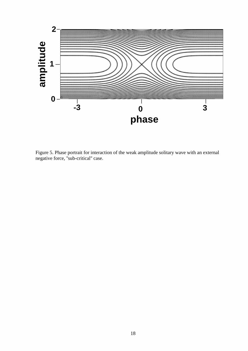
When the cubic nonlinear term in the forced extended Korteweg-de Vries equa-tion (2) is taken into account, we should consider the more general case forequations (18) and (22). Qualitatively, the phase portrait is the same as forweak-amplitude solitary waves described above, with the one important remarkthat wave amplitude is bounded by the limiting value (12). This affects theresonant condition obtained from (18)

∆ + γ2 = 0. (41)

Due to this amplitude limitation, the parameter γ is bounded (γ2 ≤ 6/|β|), andresonance is possible only when

6/β ≤ ∆ ≤ 0. (42)

To plot the phase portrait, we need to evaluate the integrals (21) and (23). Themass and momentum of the solitary wave are given by the parametric curves

M0 = 4

√

6|β|

atanh

√

1−B1 + B

, a =6|β|

(1 + B),

P0 =3|β|

(M0 − 2γ), B =

√

1 +βγ2

6. (43)

The functions M0(a), normalised by 4√

6/|β|; P0(a), normalised on (6/|β|)3/2;F1(a), normalised by 3/2|β|, and F2(a), normalised by 9/β2 are displayed inFigure 6. For very small wave amplitudes these expressions coincide with theKorteweg-de Vries limit (30). In the vicinity of the limiting solitary wave am-plitude, all these functions tend to infinity, having the asymptotic behaviour,

M0 ∼√

alim|ln(1− a/alim)|; P0 ∼alim

2M ;

F1 ∼alim

2lnM ; F2 ∼

a2lim

2lnM. (44)

9

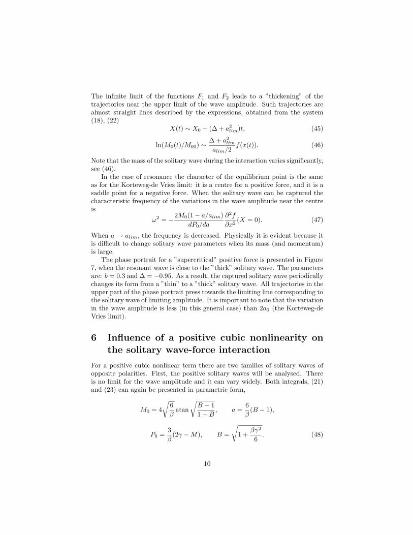
The infinite limit of the functions F1 and F2 leads to a ”thickening” of thetrajectories near the upper limit of the wave amplitude. Such trajectories arealmost straight lines described by the expressions, obtained from the system(18), (22)

X(t) ∼ X0 + (∆ + a2lim)t, (45)

ln(M0(t)/M00) ∼∆ + a2

lim

alim/2f(x(t)). (46)

Note that the mass of the solitary wave during the interaction varies significantly,see (46).

In the case of resonance the character of the equilibrium point is the sameas for the Korteweg-de Vries limit: it is a centre for a positive force, and it is asaddle point for a negative force. When the solitary wave can be captured thecharacteristic frequency of the variations in the wave amplitude near the centreis

ω2 = −2M0(1− a/alim)dP0/da

∂2f∂x2 (X = 0). (47)

When a → alim, the frequency is decreased. Physically it is evident because itis difficult to change solitary wave parameters when its mass (and momentum)is large.

The phase portrait for a ”supercritical” positive force is presented in Figure7, when the resonant wave is close to the ”thick” solitary wave. The parametersare: b = 0.3 and ∆ = −0.95. As a result, the captured solitary wave periodicallychanges its form from a ”thin” to a ”thick” solitary wave. All trajectories in theupper part of the phase portrait press towards the limiting line corresponding tothe solitary wave of limiting amplitude. It is important to note that the variationin the wave amplitude is less (in this general case) than 2a0 (the Korteweg-deVries limit).

6 Influence of a positive cubic nonlinearity onthe solitary wave-force interaction

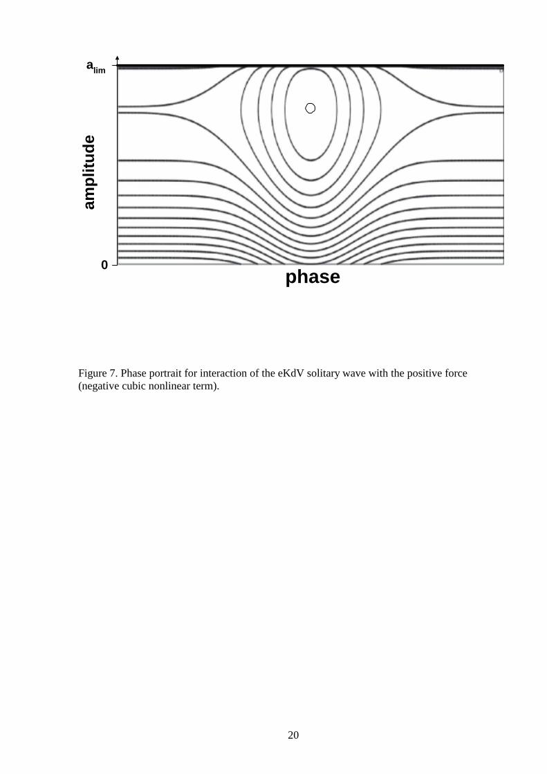
For a positive cubic nonlinear term there are two families of solitary waves ofopposite polarities. First, the positive solitary waves will be analysed. Thereis no limit for the wave amplitude and it can vary widely. Both integrals, (21)and (23) can again be presented in parametric form,

M0 = 4√

6β

atan

√

B − 11 + B

, a =6β

(B − 1),

P0 =3β

(2γ −M), B =

√

1 +βγ2

6. (48)

10

These functions (with the same normalisation as in Figure 6) are displayed inFigure 8. For weak amplitudes all expressions coincide with Korteweg de Vrieslimit (30), while for the large amplitudes they coincide with the expressionsobtained for the extended modified Korteweg-de Vries equation (Pelinovsky,2000)

M0 = π√

6β

, P0 = a√

6β

, γ2 =βa2

6. (49)

F1(a) =aπ

, F2(a) =βa3

18π. (50)

Phase portraits of these positive solitary wave dynamics in the field of an exter-nal force are similar to the Korteweg-de Vries limit, see Figures (3) - (5), andwill not discussed here in detail. The maximal variation of the solitary waveamplitude in the process of the interaction with an external ”super-critical”force (when the solitary wave can be captured for a positive force, or reflectedfor negative force) in this general case is less than the Korteweg - de Vries limit(39). In particular in the limit of the modified Korteweg-de Vries solitary waves,the maximal and minimal values of the wave amplitude satisfy to equation

amax = −amin

2+

√

3− 3a2min

4, (51)

and the sum amin + amax varies from√

3 to 2.The next case is the interaction of a negative solitary wave with an external

force. All integrals can be evaluated in the parametric form

M0 = −4√

6β

atan

√

|B|+ 1|B| − 1

, a =6β

(B − 1),

P0 =3β

(2γ −M0), B = −√

1 +βγ2

6. (52)

and are displayed in Figure 9. The main feature of this solitary wave is itsnegative mass. Also its mass (in modulus) decreases an increase of the waveamplitude (in modulus). Formally, changing the sign of the mass in the system(18), (22) is equivalent to changing the polarity of the external force. As a result,the phase portrait in the case of a resonance with an ”supercritical” externalforce is changed significantly. For instance, a negative solitary wave cannot becaptured by a positive ”supercritical” forcing (as in the previous cases), and theequilibrium point is a saddle point. A phase portrait for this situation is shownin Figure 10 for b = 80 and ∆ = −30.

The next important comment here relates to the limitation of the solitarywave amplitude, that it should be more (in modulus) than acr, see (14). All

11

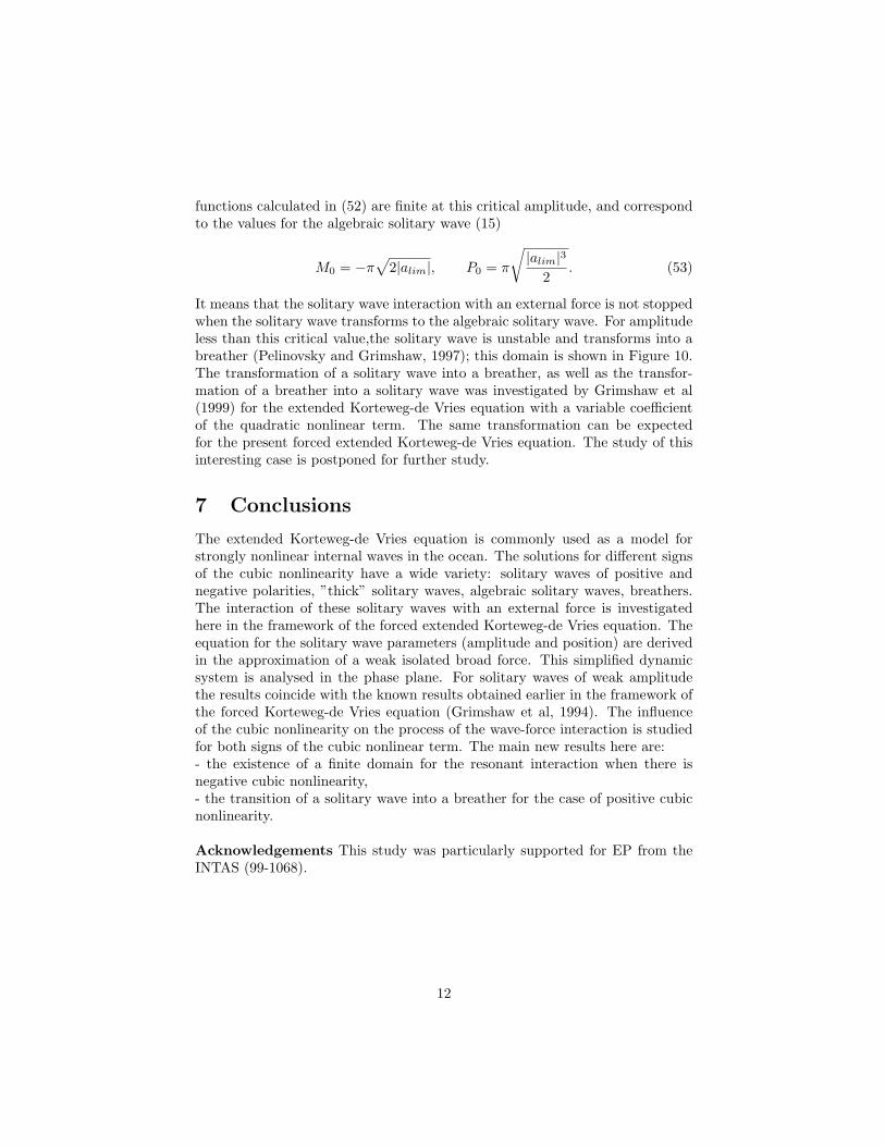
functions calculated in (52) are finite at this critical amplitude, and correspondto the values for the algebraic solitary wave (15)

M0 = −π√

2|alim|, P0 = π

√

|alim|32

. (53)

It means that the solitary wave interaction with an external force is not stoppedwhen the solitary wave transforms to the algebraic solitary wave. For amplitudeless than this critical value,the solitary wave is unstable and transforms into abreather (Pelinovsky and Grimshaw, 1997); this domain is shown in Figure 10.The transformation of a solitary wave into a breather, as well as the transfor-mation of a breather into a solitary wave was investigated by Grimshaw et al(1999) for the extended Korteweg-de Vries equation with a variable coefficientof the quadratic nonlinear term. The same transformation can be expectedfor the present forced extended Korteweg-de Vries equation. The study of thisinteresting case is postponed for further study.

7 Conclusions

The extended Korteweg-de Vries equation is commonly used as a model forstrongly nonlinear internal waves in the ocean. The solutions for different signsof the cubic nonlinearity have a wide variety: solitary waves of positive andnegative polarities, ”thick” solitary waves, algebraic solitary waves, breathers.The interaction of these solitary waves with an external force is investigatedhere in the framework of the forced extended Korteweg-de Vries equation. Theequation for the solitary wave parameters (amplitude and position) are derivedin the approximation of a weak isolated broad force. This simplified dynamicsystem is analysed in the phase plane. For solitary waves of weak amplitudethe results coincide with the known results obtained earlier in the framework ofthe forced Korteweg-de Vries equation (Grimshaw et al, 1994). The influenceof the cubic nonlinearity on the process of the wave-force interaction is studiedfor both signs of the cubic nonlinear term. The main new results here are:- the existence of a finite domain for the resonant interaction when there isnegative cubic nonlinearity,- the transition of a solitary wave into a breather for the case of positive cubicnonlinearity.

Acknowledgements This study was particularly supported for EP from theINTAS (99-1068).

12

References

[1] Choi, J.W., Sun, S.M., and Shen, M.C. Internal capillary-gravitywaves of a two-layer fluid with free surface over an obstruction - Forcedextended KdV equation. Physics Fluids, 1996, v. 397 - 404.

[2] Grimshaw, R. Internal solitary waves. In “Environmental StratifiedFlows”, ed. R. Grimshaw, Kluwer, Boston, 2001a, Chapter 1, 1-28.

[3] Grimshaw, R Nonlinear effects in wave scattering and generation. In:Proceedings of the IUTAM Symposium on Diffraction and Scattering inFluid Mechanics and Elasticity, Manchester, 2001b, (to appear).

[4] Grimshaw, R., Chan, K.H., and Chow K.W. Transcritical flow of astratified fluid: the forced extended Korteweg - de Vries model. Departmentof Mathematical Sciences, Phys. Fluids. (to appear).

[5] Grimshaw, R. and Mitsudera, H. Slowly-varying solitary wave solu-tions of the perturbed Korteweg-de Vries equation revisited. Stud. Appl.Math., 1993, v. 90, 75-86.

[6] Grimshaw, R., Pelinovsky, E., and Bezen, A. Hysteresis phenomenonin the interaction of a damped solitary wave with an external force. WaveMotion, 1997, v. 26, 253 - 274.

[7] Grimshaw, R., Pelinovsky, E., and Sakov, P. Interaction of a solitarywave with an external force moving with variable speed. Stud. Appl. Math., 1996, v. 97, 235 - 276.

[8] Grimshaw, R., Pelinovsky, E. and Talipova,T. The modifiedKorteweg-de Vries equation in the theory of the large-amplitude internalwaves. Nonlinear Processes in Geophysics, 1997, v. 4, 237 - 250.

[9] Grimshaw, R., Pelinovsky, E., and Talipova, T. Solitary wave trans-formation in a medium with sign-variable quadratic nonlinearity and cubicnonlinearity. Physica D, 1999, v. 132, 40 - 62.

[10] Grimshaw, R., Pelinovsky, E., and Tian, X. Interaction of a solitarywave with an external force. Physica D, 1994, v. 77, 405 - 433.

[11] Holloway, P., Pelinovsky, E., and Talipova, T. Internal tide trans-formation and oceanic internal solitary waves. In “Environmental StratifiedFlows”, ed. R. Grimshaw, Kluwer, Boston, 2001, Chapter 2, 29-60.

[12] Kharif, C., Pelinovsky, E., Talipova, T., and Slunyaev, A. Focusingof nonlinear wave groups in deep water. JETP Letters, 2001, v. 73, N. 4,170 - 175.

13

[13] Marchant, T.R. and Smyth, N.F. The extended Korteweg-de Vriesequation and the resonant flow over topography. J. Fluid Mech. 1990, v.221, 263 - 288.

[14] Marchant, T.R. and Smyth, N.F. Soliton interaction for the extendedKorteweg - de Vries equation. J. Appl. Math., 1996, v. 56, 157 - 176.

[15] Onarato, M., Osborne, A.R., Serio, M., and Bertone, S. Freakwaves in random oceanic sea states. Physical Review Letters, 2001, v. 86,5831 - 5834

[16] Osborne, A.R., Onorato, M., and Serio, M. The nonlinear dynamicsof rogue waves and holes in deep-water gravity wave train. Phys. LettersA, 2000, v. 275, 386-393.

[17] Pelinovsky, D., and Grimshaw, R. Structural transformation of eigen-values for a perturbed algebraic soliton potential. Phys. Lett., 1997, v. A229,165 - 172

[18] Pelinovsky, E.N. Autoresonance processes under interaction of solitarywaves with external fields. Applied Hydromechanics (Ukraine), 2000, v. 2(74), 67 - 72.

[19] Pelinovsky, E., Talipova, T., and Kharif, C. Nonlinear dispersivemechanism of the freak wave formation in shallow water. Physica D, 2000,v. 147, 83-94.

[20] Slyunyaev, A., Pelinovskii, E. Dynamics of large-amplitude solitons.JETP, 1999, v. 89, N. 1, 173 - 181.

[21] Slyunyaev, A.V. Dynamics of localized waves with large amplitude in aweakly dispersive medium with a quadratic and positive cubic nonlinearity.JETP, 2001, v. 119, 606-612.

14

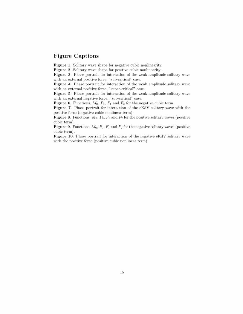
Figure Captions

Figure 1. Solitary wave shape for negative cubic nonlinearity.Figure 2. Solitary wave shape for positive cubic nonlinearity.Figure 3. Phase portrait for interaction of the weak amplitude solitary wavewith an external positive force, ”sub-critical” case.Figure 4. Phase portrait for interaction of the weak amplitude solitary wavewith an external positive force, ”super-critical” case.Figure 5. Phase portrait for interaction of the weak amplitude solitary wavewith an external negative force, ”sub-critical” case.Figure 6. Functions, M0, P0, F1 and F2 for the negative cubic term.Figure 7. Phase portrait for interaction of the eKdV solitary wave with thepositive force (negative cubic nonlinear term).Figure 8. Functions, M0, P0, F1 and F2 for the positive solitary waves (positivecubic term).Figure 9. Functions, M0, P0, F1 and F2 for the negative solitary waves (positivecubic term).Figure 10. Phase portrait for interaction of the negative eKdV solitary wavewith the positive force (positive cubic nonlinear term).

15

16

-6 -3 0 3 6coordinate

0

4

8

12

wav

e sh

ape

Figure 1. Solitary wave shape for negative cubic nonlinearity.

-0.8 -0.4 0 0.4 0.8coordinate

-80

-60

-40

-20

0

20

40

60

wav

e sh

ape

Figure 2. Solitary wave shape for positive cubic nonlinearity.

17

0 3-3phase

0

1

2am

plitu

de

G

Figure 3. Phase portrait for interaction of the weak amplitude solitary wave with an external positive force, ''sub-critical'' case.

0 3-3phase

0

1

2

ampl

itude

G

Figure 4. Phase portrait for interaction of the weak amplitude solitary wave with an external positive force, ''super-critical'' case.

18

0 3-3phase

0

1

2am

plitu

de

G

Figure 5. Phase portrait for interaction of the weak amplitude solitary wave with an external negative force, ''sub-critical'' case.

19

0 0.5 1a/alim

0

2

4F(a)

F1

F2

0 0.5 1a/alim

0

1

2

3M0

0 0.5 1a/alim

0

4P0

Figure 6. Functions, M0, P0, F1 and F2 for the negative cubic term.

20

0

alim

ampl

itude

phase

Figure 7. Phase portrait for interaction of the eKdV solitary wave with the positive force (negative cubic nonlinear term).

21

0 5 10aβ/6

0

100

200F(a)

F1

F2

0 5 10aβ/6

0

0.4

0.8M0

0 5 10aβ/6

0

10P0

Figure 8. Functions, M0, P0, F1 and F2 for the positive solitary waves (positive cubic term).

22

-15 -10 -5 0a(β/6)1/2

-400

0

F(a)F1

F2

-15 -10 -5 0a(β/6)1/2

-2

-1

0

M0

-15 -10 -5 00

5

10

15P0

Figure 9. Functions, M0, P0, F1 and F2 for the negative solitary waves (positive cubic term).

23

G

phase

ampl

itude

|acr|breather zone

Figure 10. Phase portrait for interaction of the negative eKdV solitary wave with the positive force (positive cubic nonlinear term).