Generation of solitons and breathers in the extended Korteweg–de Vriesequation with positive cubic nonlinearity

R. Grimshaw,1 A. Slunyaev,2,a� and E. Pelinovsky2

1Department of Mathematical Sciences, Loughborough University, Loughborough LE11 3TU,United Kingdom2Department of Nonlinear Geophysical Processes, Institute of Applied Physics,Russian Academy of Sciences, Nizhny Novgorod 603950, Russia

�Received 23 October 2009; accepted 2 December 2009; published online 5 January 2010�

The initial-value problem for box-like initial disturbances is studied within the framework of anextended Korteweg–de Vries equation with both quadratic and cubic nonlinear terms, also known asthe Gardner equation, for the case when the cubic nonlinear coefficient has the same sign as thelinear dispersion coefficient. The discrete spectrum of the associated scattering problem is found,which is used to describe the asymptotic solution of the initial-value problem. It is found that whileinitial disturbances of the same sign as the quadratic nonlinear coefficient result in generation ofonly solitons, the case of the opposite polarity of the initial disturbance has a variety of possibleoutcomes. In this case solitons of different polarities as well as breathers may occur. The bifurcationpoint when two eigenvalues corresponding to solitons merge to the eigenvalues associated withbreathers is considered in more detail. Direct numerical simulations show that breathers and solitonpairs of different polarities can appear from a simple box-like initial disturbance. © 2010 AmericanInstitute of Physics. �doi:10.1063/1.3279480�

Internal solitary waves in the stratified coastal ocean areubiquitous and are commonly observed. They may reachan amplitude of 100 m and be comparable to the waterdepth. The solitary waves preserve their shape andpropagate for long distances unchanged, thus they play avery important role in the distribution of energy in theocean interior. Another kind of nonlinear internal wave,bounded nonlinear wave packets or breathers, are alreadyknown as exact solutions of certain model nonlinear waveevolution equations, such as the modified Korteweg–deVries (KdV) equation. In the stratified ocean, the exis-tence of breathers needs a specific kind of stratification(quite distinct from the popular two-layer model). Thepossibility of internal breathers in a stratified fluid wasonly recently confirmed by fully nonlinear numericalsimulations. In general breathers are more complicatednonlinear waves compared with solitary waves and havebeen much less investigated. The Gardner equation (GE)(the KdV equations with an extra term with cubic non-linearity) is a simple nonlinear wave model which gov-erns the dynamics of internal wave breathers. Getting thebenefit from the integrability of the GE by means of theinverse scattering technique (IST), we study the initial-value problem for a box-shaped initial perturbation indetail, analytically and numerically. We show that whenthe perturbation is of the opposite sign than the usualKdV solitary waves, a complicated scenario occurs.Single solitary waves, pairs of solitary waves, and inter-nal breathers may be born from this simple initial distur-bance, depending on its amplitude and width.

I. INTRODUCTION

Internal solitary waves have often been modeled as soli-tons of the KdV type �see reviews in Refs. 1–3�. These mod-els can provide for an accurate description of internal solitarywave propagation and their interactions. In particular, thesolitary waves in the KdV equation can be found as theasymptotic outcome from a localized initial disturbance �seeRef. 4, for instance�. Moreover, KdV solitons are often con-venient for a qualitative description of nonlinear wave dy-namics. Hence the KdV model is popular in many physicalapplications.

For the case of internal waves, the coefficients in theKdV equation are defined by the density stratification, whichmay be quite variable in the ocean, and can lead to differentsigns of the coefficient of the quadratic nonlinear term in theKdV equation. Indeed, this coefficient can be quite small andmay even vanish. In this scenario the quadratic and cubicnonlinear terms appear at the same order in an asymptoticperturbation theory, and the outcome is an extended KdVequation �or the GE�, with both quadratic and cubic nonlin-ear terms. Although it is slightly more complicated than theKdV equation, in many cases it can describe large-amplitudeinternal solitary waves rather better, showing dynamicswhich can look quite different from the KdV case.5,6 The GEis also integrable, and thus allows the analysis using theIST.4

The associated scattering problem for the KdV equationis defined by the stationary Schrödinger equation, whichplays a fundamental role in quantum physics. Thus, theinitial-value problem for the KdV equation is very well es-tablished and understood. In contrast, the initial-value prob-lem for the GE is less well developed. An example of its

a�Author to whom correspondence should be addressed. Electronic mail:slunyaev@hydro.appl.sci-nnov.ru.

CHAOS 20, 013102 �2010�

1054-1500/2010/20�1�/013102/11/$30.00 © 2010 American Institute of Physics20, 013102-1

rather more complicated dynamics was shown by Grimshawet al.;7 the solution becomes more intricate due to the com-petition between the two nonlinear terms. In the case of apositive coefficient of the cubic nonlinear term relative to thesign of the coefficient of the linear dispersive term, as well assolitons, there are allowed exact breather solutions. The co-efficients of the equation are determined by the densitystratification;3,8 the cubic nonlinear coefficient is positive, forexample, in the case of a three-layer fluid, when the densityjumps are situated close to the bottom and to the surface, seeGrimshaw et al.8 A breather is essentially a nonlinear wavepacket, and its dynamics can be quite complicated.6,9–11 Thepossibility of the presence of breather waves in realistic con-ditions in a continuously stratified ocean was shown recentlythrough fully nonlinear numerical simulations by Lambet al.12

Our concern in this paper is to examine which kind ofinitial conditions can generate breathers. Internal solitarywaves can become coupled due to weak dispersion or dissi-pation effects,13,14 which is one possible mechanism for theformation of internal breathers. Breather-type waves mayalso appear due to the modulational instability of intenseshort-scale waves,11,15 through perturbations of solitarywaves,9 or through variations in the waveguidecharacteristics.16 However, steepening of internal tides is themost common mechanism for the generation of internal soli-tary waves in the ocean, and so here we shall study thegeneration of intense internal breathers from initial distur-bances of rather simple shapes.

We have already noted that the initial-value problem forthe GE is more complicated than for the KdV equation7 �seealso the discussion in Sec. II�. The initial-value problem inthe large-amplitude limit �using then the framework of themodified KdV equation� coincides with that for the focusingnonlinear Schrödinger �NLS� equation, which is widely usedin nonlinear optics, and we note the long but still incompletelist of the papers studying the initial value problem for thefocusing NLS equation.17–27 It is significant that the KdV-like evolution equations describe real-valued wave fields,while the NLS equation governs evolution of complex wavefields. Therefore not all the initial-value problems treatedwithin the framework of the NLS equation have physicalsense in our case.

Although NLS envelope solitons on a pedestal are oftencalled breathers, in this paper we shall call breathers onlysolitary solutions of modified KdV equation �or the GE� cor-responding to a pair of complex conjugate eigenvalues. Oneeigenvalue of the scattering problem for the NLS equationalways corresponds to one envelope soliton. A pair of com-plex conjugate eigenvalues of the scattering problem for theNLS equation corresponds to two envelope solitons. Theinitial-value problem for disturbances composed of two ad-joining box-like profiles was studied by Clarke et al.25 andalso by Kaup et al.22 and Kaup and Malomed.23 It was foundthat single eigenvalues appear when the boxes have similarpolarities, while coupled complex conjugate pairs are fa-vored by asymmetric initial pulses. Takahashi and Konno21

and Desaix et al.27 showed that complex conjugate pairs ofeigenvalues can arise from two separated pulse disturbances.

In this paper we shall show that breathers of the GE, andalso solitons of opposite polarities can be generated from asingle box-shaped initial disturbance. Section II is introduc-tory, where we formulate the associated scattering system forthe GE, discuss its relation to the KdV and modified KdVequations, and present the soliton and breather solutions. InSec. III the exact solution of the scattering problem for abox-like initial disturbance is obtained and discussed forboth possible signs. In Sec. IV some results of the directnumerical simulations of the initial-value problem for the GEare presented. Our results are summarized in Sec. V.

II. EXACT SOLUTIONS OF THE GARDNER EQUATION

The GE with a positive coefficient of the cubic nonlinearterm is written here in the usual dimensionless form

ut + 6uux + 6u2ux + uxxx = 0. �1�

For the case when internal waves in a stratified ocean areconcerned, the function u�x , t� has the sense of the displace-ment of the isopycnals, x is the horizontal coordinate, and t istime �more details may be found, for example, in Ref. 3�.The coefficients of the evolution equation are defined by thebackground density stratification and current. When the cu-bic nonlinear coefficient has the same sign as the linear dis-persion coefficient, then the equation may always be reducedto the form �1� with the help of the scaling and Galileantransformations.

Equation �1� belongs to the important class of integrableequations. The long-time asymptotics of its solution may befound with the help of the IST. This method consists of thesolution of the associated linear scattering problem. Thelatter may be given in the form �AKNS approach, see Refs.28 and 4�

�� = ��, where � = ��1

�2�, � = � − �x u

u + 1 �x� . �2�

Here � is the complex-valued vector eigenfunction, and � isthe complex-valued eigenvalue. In addition to Eq. �2�, tem-poral evolution of the eigenfunctions is also prescribed bythe IST �see Ref. 4�, but is not used in this study. The eigen-value problem in a similar form was first suggested in Ref.29 for the GE with negative coefficient of the cubic nonlin-ear term.

It is well known that the linear transformation

q�x,t� = u�x − 32 t,t� + 1

2 �3�

reduces solutions of GE �1� to the solutions of the modifiedKdV �mKdV� equation

qt + 6q2qx + qxxx = 0. �4�

The mKdV equation �4� has its own scattering system:30

�� = ��, � = �− �x q

q �x� . �5�

With the use of transformation �3� this eigenvalue problem�5� may be directly applied for solving the GE, by seekingthe solutions of the mKdV equation on a pedestal, similar tothe approach of Romanova.31 However, since the transforma-

013102-2 Grimshaw, Slunyaev, and Pelinovsky Chaos 20, 013102 �2010�

tion �3� links the initial-value problem for the GE with a zerobackground to an initial-value problem for the modified KdVequation on a pedestal, it has not received much attention inthe literature.

It may be shown that

�2� = ��2 − 14�� = ��2 − 1

4�� = �2� , �6�

where q is changed to u+1 /2 in Eq. �5�. Then the eigenval-ues of the two scattering problems, Eqs. �2� and �5�, areconnected by

�2 = �2 − 14 . �7�

The eigenvalue problem for the GE with negative cubicnonlinearity was reduced in Ref. 7 to the eigenvalue problemof the KdV equation, which is a classic one, and thus, ismore convenient for qualitative analysis. Solutions of the GEwith positive cubic nonlinearity �1� may be transformedthrough the relation

v�x,t� = u�1 + u� + i�u

�x, �8�

similar to the well-known Miura transformation, to solutionsof the KdV equation

�v�t

+ 6v�v�x

+�3v�x3 = 0. �9�

The associated scattering problem for the KdV equation �9�follows from Eq. �2�,

� �2

�x2 + v�x��� = �2�, � = �1 + i�2. �10�

But although the eigenvalue problem �10� has the classicalform, the change �8� makes the field v complex-valued.Hence the scattering problem �10� corresponds to an unusualcase, when the potential is complex, and simple analogs can-not be drawn.

It is useful to introduce the change in variable

� = �1 + i�2, � = �1 − i�2, �11�

so that the system �2� becomes

−��

�x+ i�u +

1

2�� = �� −

i

2�� ,

�12�

−��

�x− i�u +

1

2�� = �� +

i

2�� .

This more symmetrical form allows the elimination of eithervariable to yield the equivalent second order equations

�2�

�x2 + �u�u + 1� − �2�� − iux� = 0,

�13��2�

�x2 + �u�u + 1� − �2�� + iux� = 0.

Note that the second equation here is just Eq. �10� recoveredby a different approach. We note from Eq. �2� or Eq. �13�that if � is an eigenvalue, then so are −� and ��, and so the

eigenvalues typically occur as a quartet, and only one quad-rant of the eigenvalue plane may be considered without lossof generality. It is convenient hereafter to restrict our interestto eigenvalues Re����0. The discrete spectrum of the scat-tering problem corresponds to solutions which decay at in-finity; solitary waves �solitons� correspond to real-valued ei-genvalues, and breathers to complex-valued eigenvalues.Next, from Eq. �13� it follows that for the discrete spectrum,we can obtain the integral identities

�−

��x�2 + ��2 − u�u + 1�����2 + iux���2dx = 0,

�14�

�−

��x�2 + ��2 − u�u + 1�����2 − iux���2dx = 0.

Taking the imaginary part of these expressions yields

2�R�I�−

���2dx = − �−

ux���2dx ,

�15�

2�R�I�−

���2dx = �−

ux���2dx ,

where �=�R+ i�I. Note that for a real eigenvalue when �I=0,both integral terms on the right-hand side �RHS� must bezero.

Returning to the system in the form �2� we can constructthe equation set for the squared eigenfunctions,

Ix = 2uQ2 − 2�u + 1�Q1 − 2�IJ, Jx = 2�II ,

�16�Q1x = uI − 2�RQ1, Q2x = − �u + 1�I + 2�RQ2,

where

I = �1�2� + �2�1

�, J = i��1�2� − �2�1

�� ,

�17�Q1 = ��1�2, Q2 = ��2�2.

Here Q1, Q2 are real and non-negative, and I, J are realvalued. Note that ���2=Q1+Q2+J, ���2=Q1+Q2−J, and thenthe relations �16� can be used to give an alternative deriva-tion of Eq. �15�.

There are several consequences which can now bedrawn. In particular if u�u+1�0 �that is −1u0� foraxb where u=0 for x�a, x�b where either or both ofa, b may be infinite, then the real and imaginary parts of Eq.�14� may be considered separately which leads to the condi-tion �R

2 �I2 where �=�R+ i�I. It follows that there are no

real eigenvalues, and hence only breathers can occur.For the GE a soliton is given by

013102-3 Generation of solitons and breathers Chaos 20, 013102 �2010�

uS�x,t� =4�2

1 1 + 4�2 cosh�2��x − x0 − 4�2t��, �18�

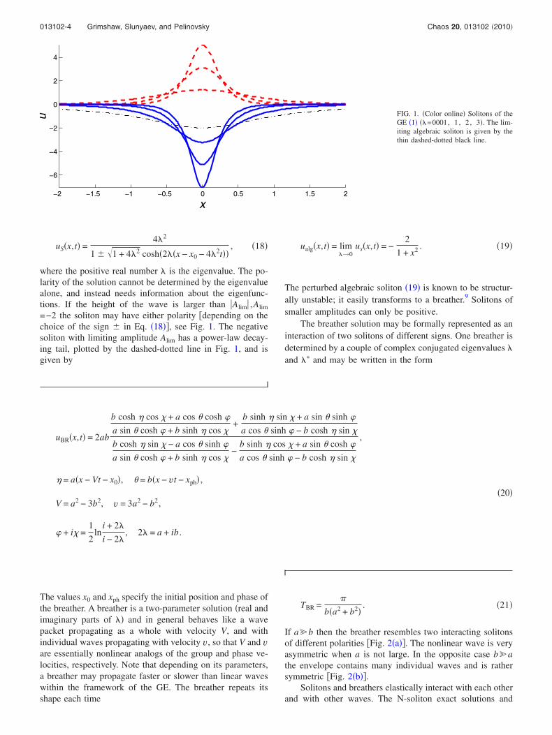
where the positive real number � is the eigenvalue. The po-larity of the solution cannot be determined by the eigenvaluealone, and instead needs information about the eigenfunc-tions. If the height of the wave is larger than �Alim� ,Alim

=−2 the soliton may have either polarity �depending on thechoice of the sign in Eq. �18��, see Fig. 1. The negativesoliton with limiting amplitude Alim has a power-law decay-ing tail, plotted by the dashed-dotted line in Fig. 1, and isgiven by

ualg�x,t� = lim�→0

us�x,t� = −2

1 + x2 . �19�

The perturbed algebraic soliton �19� is known to be structur-ally unstable; it easily transforms to a breather.9 Solitons ofsmaller amplitudes can only be positive.

The breather solution may be formally represented as aninteraction of two solitons of different signs. One breather isdetermined by a couple of complex conjugated eigenvalues �

and �� and may be written in the form

uBR�x,t� = 2ab

b cosh � cos � + a cos � cosh �

a sin � cosh � + b sinh � cos �+

b sinh � sin � + a sin � sinh �

a cos � sinh � − b cosh � sin �

b cosh � sin � − a cos � sinh �

a sin � cosh � + b sinh � cos �−

b sinh � cos � + a sin � cosh �

a cos � sinh � − b cosh � sin �

,

� = a�x − Vt − x0�, � = b�x − vt − xph� ,

�20�V = a2 − 3b2, v = 3a2 − b2,

� + i� =1

2ln

i + 2�

i − 2�, 2� = a + ib .

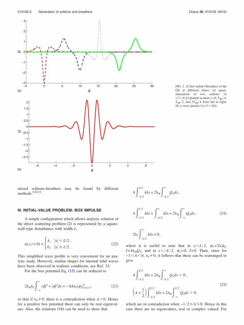
The values x0 and xph specify the initial position and phase ofthe breather. A breather is a two-parameter solution �real andimaginary parts of �� and in general behaves like a wavepacket propagating as a whole with velocity V, and withindividual waves propagating with velocity v, so that V and vare essentially nonlinear analogs of the group and phase ve-locities, respectively. Note that depending on its parameters,a breather may propagate faster or slower than linear waveswithin the framework of the GE. The breather repeats itsshape each time

TBR =�

b�a2 + b2�. �21�

If a�b then the breather resembles two interacting solitonsof different polarities �Fig. 2�a��. The nonlinear wave is veryasymmetric when a is not large. In the opposite case b�athe envelope contains many individual waves and is rathersymmetric �Fig. 2�b��.

Solitons and breathers elastically interact with each otherand with other waves. The N-soliton exact solutions and

−2 −1.5 −1 −0.5 0 0.5 1 1.5 2

−6

−4

−2

0

2

4

x

u FIG. 1. �Color online� Solitons of theGE �1� ��=0001, 1 , 2 , 3�. The lim-iting algebraic soliton is given by thethin dashed-dotted black line.

013102-4 Grimshaw, Slunyaev, and Pelinovsky Chaos 20, 013102 �2010�

mixed solitons-breathers may be found by differentmethods.6,10,32

III. INITIAL-VALUE PROBLEM: BOX IMPULSE

A simple configuration which allows analytic solution ofthe direct scattering problem �2� is represented by a square-wall-type disturbance with width L,

u�x,t = 0� = A , �x� L/2,

0, �x� � L/2.� �22�

This simplified wave profile is very convenient for an ana-lytic study. However, similar shapes for internal tidal waveshave been observed in realistic conditions, see Ref. 33.

For the box potential Eq. �15� can be reduced to

2�R�I�−

���2 + ���2dx = − 8A�I��2�x=L/22 , �23�

so that if �I�0, there is a contradiction when A�0. Hencefor a positive box potential there can only be real eigenval-ues. Also, the relations �16� can be used to show that

A�−L/2

L/2

Idx = 2�R�−L/2

Q1dx ,

A�−L/2

L/2

Idx + �−L/2

Idx = 2�R�−

Q2dx , �24�

2�I�−L/2

Idx = 0,

where it is useful to note that in x�L /2, �1=2��2,I=4�RQ2, and in x−L /2, �1=0, I=0. Then, since for−1A0, �I�0, it follows that these can be rearranged togive

A�−L/2

L/2

Idx = 2�R�−L/2

Q1dx � 0,

�25�

�A +1

2��

−L/2

L/2

Idx = 2�R�−

L/2

Q2dx � 0,

which are in contradiction when −1 /2�A�0. Hence in thiscase there are no eigenvalues, real or complex valued. For

−5 0 5 10 15 20 25 30−3

−2

−1

0

1

2

3

x

u

−6 −4 −2 0 2 4 6

−2.5

−2

−1.5

−1

−0.5

0

0.5

1

1.5

2

x

u

(a)

(b)

FIG. 2. �Color online� Breathers of theGE at different times: �a� quasi-interaction of two solitons ��=3 0.2i� plotted at times t=0, TBR /4,TBR /2, and 3TBR /4 from left to right;�b� a wave packet ��=3 10i�.

013102-5 Generation of solitons and breathers Chaos 20, 013102 �2010�

the case −1�A−1 /2 when only complex eigenvalues mayoccur, our numerical simulations of the GE and a perturba-tion analysis described below indicate that complex-valuedeigenvalues do indeed exist, and so we infer that the nonex-istence proof made above for −1 /2�A�0 cannot be ex-tended into the range −1�A−1 /2.

Then the localized discrete eigenfunctions for the eigen-value problem �2�, or equivalently, for any of Eqs. �12� and�13�, corresponding to the discrete spectrum, may be definedfor each interval of the constant potential �22�, and thenmatched at the boundaries. As a result the discrete spectrumis determined by

exp�2L�2 − A�1 + A�� =

A

2��2 − A�1 + A�−

�

�2 − A�1 + A�+ 1

A

2��2 − A�1 + A�−

�

�2 − A�1 + A�− 1

, �26a�

or alternatively by

tan s =2sG − s2

U − 2�G − s2�, �26b�

where s2=G�1−�2�, �L=�G, U=AL2, G=U�1+A�, andA�1+A��0.

Some other forms of the solution �26� are given in theAppendix. In Eq. �26b� � is the normalized eigenvalue,which is complex valued in the general case, and s is anauxiliary variable, which may also be complex valued.

The real parameter G is a convenient parameter, definingthe strength of nonlinear effects, and generalizes the Ursellnumber U, defined here as U=AL2, which is a commonlyused similarity parameter for the KdV equation. Note that Gtends to U when �A� is small. In the opposite case, when �A�is large, G→A2L2. It is important to note that the RHS of Eq.�26� does not depend on L. This fact allows us to expressvalue G1/2 via the normalized eigenvalue � and amplitude Aof the disturbance,

G =1

1 − �2��k + atan �1 − �2

U

2G− �2�� ,

�27�

G = LA�1 + A�, � =�

A�1 + A�,

U

2G=

1

2�1 + A�.

In Eq. �27� the domain of the atan function lies within theinterval �−� /2,� /2�; many branches of the solution existdue to the term �k, where k is an integer number.

In the sequel, two different cases corresponding to thesign of the disturbance are considered in detail.

A. Positive initial disturbance

When A�0, then all the eigenvalues � or � are real andonly solitary waves arise. This is an immediate consequenceof Eq. �23�, since if �I�0 there is a contradiction whenA�0. Since here G�0 it can be shown that the auxiliaryvariable s must also be real and positive, and so 0�1.The solution of Eq. �26b� can now be analyzed qualitatively

by plotting the curves of the left-hand side �LHS� and RHSas functions of real s. For this case of positive A it is moreconvenient to plot the inverse values of RHS and LHS of Eq.�26b�. While the function cot s on LHS becomes infinite ats=�k, where k is integer, the inverse RHS of Eq. �26b� be-comes infinite when s=0 or s=G1/2. Thus, at least one solu-tion �one soliton� always exists for A�0 for any L�0. Anew soliton branch appears when G1/2=��Ns−1�, where Ns

is the number of solitons given by

Ns = �G

�� + 1, �28�

where �f� is the maximum integer not exceeding f .When the KdV limit A→0 is concerned, the number of

solitons Ns depends on the Ursell parameter only �G→U�. Inthe case of large amplitudes, Ns depends on parameter L2A2.

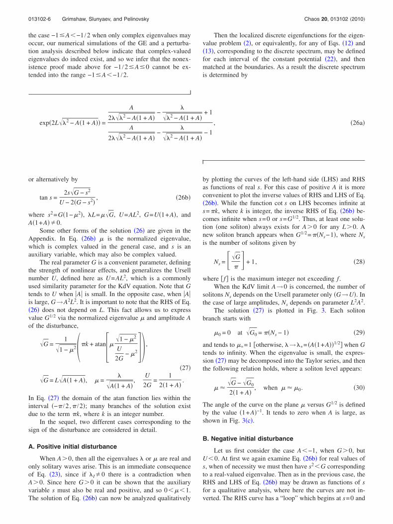
The solution �27� is plotted in Fig. 3. Each solitonbranch starts with

�0 = 0 at G0 = ��Ns − 1� �29�

and tends to ��=1 �otherwise, �→��= �A�1+A��1/2� when Gtends to infinity. When the eigenvalue is small, the expres-sion �27� may be decomposed into the Taylor series, and thenthe following relation holds, where a soliton level appears:

� �G − G0

2�1 + A�, when � � �0. �30�

The angle of the curve on the plane � versus G1/2 is definedby the value �1+A�−1. It tends to zero when A is large, asshown in Fig. 3�c�.

B. Negative initial disturbance

Let us first consider the case A−1, when G�0, butU0. At first we again examine Eq. �26b� for real values ofs, when of necessity we must then have s2G correspondingto a real-valued eigenvalue. Then as in the previous case, theRHS and LHS of Eq. �26b� may be drawn as functions of sfor a qualitative analysis, where here the curves are not in-verted. The RHS curve has a “loop” which begins at s=0 and

013102-6 Grimshaw, Slunyaev, and Pelinovsky Chaos 20, 013102 �2010�

ends at s=G1/2. The RHS and LHS curves do not intersect ifG is small. When G is close to, but less than the value

G0 = �n, n = 1,2, . . . , �31�

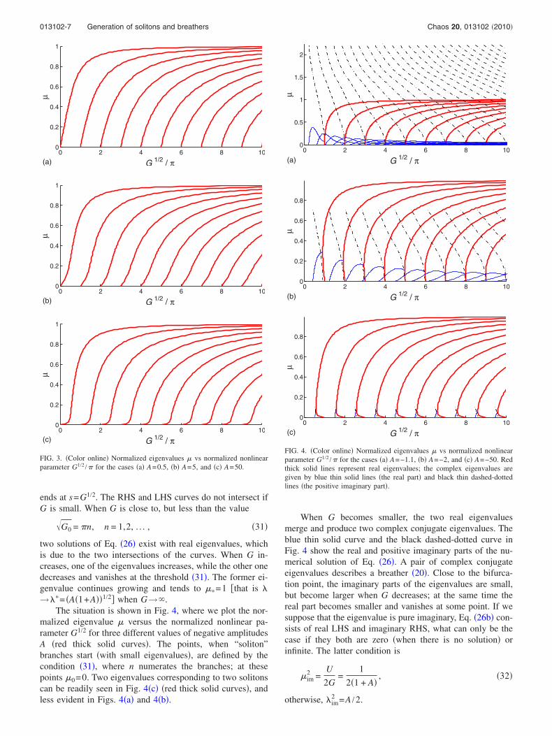
two solutions of Eq. �26� exist with real eigenvalues, whichis due to the two intersections of the curves. When G in-creases, one of the eigenvalues increases, while the other onedecreases and vanishes at the threshold �31�. The former ei-genvalue continues growing and tends to ��=1 �that is �→��= �A�1+A��1/2� when G→.

The situation is shown in Fig. 4, where we plot the nor-malized eigenvalue � versus the normalized nonlinear pa-rameter G1/2 for three different values of negative amplitudesA �red thick solid curves�. The points, when “soliton”branches start �with small eigenvalues�, are defined by thecondition �31�, where n numerates the branches; at thesepoints �0=0. Two eigenvalues corresponding to two solitonscan be readily seen in Fig. 4�c� �red thick solid curves�, andless evident in Figs. 4�a� and 4�b�.

When G becomes smaller, the two real eigenvaluesmerge and produce two complex conjugate eigenvalues. Theblue thin solid curve and the black dashed-dotted curve inFig. 4 show the real and positive imaginary parts of the nu-merical solution of Eq. �26�. A pair of complex conjugateeigenvalues describes a breather �20�. Close to the bifurca-tion point, the imaginary parts of the eigenvalues are small,but become larger when G decreases; at the same time thereal part becomes smaller and vanishes at some point. If wesuppose that the eigenvalue is pure imaginary, Eq. �26b� con-sists of real LHS and imaginary RHS, what can only be thecase if they both are zero �when there is no solution� orinfinite. The latter condition is

�im2 =

U

2G=

1

2�1 + A�, �32�

otherwise, �im2 =A /2.

0 2 4 6 8 100

0.2

0.4

0.6

0.8

1

G 1/2 / π

µ

0 2 4 6 8 100

0.2

0.4

0.6

0.8

1

G 1/2 / π

µ

0 2 4 6 8 100

0.2

0.4

0.6

0.8

1

G 1/2 / π

µ

(a)

(b)

(c)

FIG. 3. �Color online� Normalized eigenvalues � vs normalized nonlinearparameter G1/2 /� for the cases �a� A=0.5, �b� A=5, and �c� A=50.

0 2 4 6 8 100

0.5

1

1.5

2

G 1/2 / π

µ0 2 4 6 8 10

0

0.2

0.4

0.6

0.8

G 1/2 / πµ

0 2 4 6 8 100

0.2

0.4

0.6

0.8

G 1/2 / π

µ

(a)

(b)

(c)

FIG. 4. �Color online� Normalized eigenvalues � vs normalized nonlinearparameter G1/2 /� for the cases �a� A=−1.1, �b� A=−2, and �c� A=−50. Redthick solid lines represent real eigenvalues; the complex eigenvalues aregiven by blue thin solid lines �the real part� and black thin dashed-dottedlines �the positive imaginary part�.

013102-7 Generation of solitons and breathers Chaos 20, 013102 �2010�

The expression �32� defines the upper limit of imaginaryparts of �, shown in Fig. 4. Since the LHS of Eq. �26b� isinfinite, then s=� /2+�k, where k is an integer. Thus, withthe use of Eq. �32�, we get that

Gim =2�1 + A��1 + 2A���

2+ �n − 1���2

, �33�

where the integer n�0 numerates the branches. This nonlin-ear parameter corresponds to the case when the eigenvalues�� and �� are purely imaginary. It then follows from Eqs.�32� and �33� that complex solution exists when A−1.

When �A� is large, Eq. �33� becomes

Gim1/2 �

�

2+ �n − 1��, − A � 1. �34�

Thus, the real parts of the complex eigenvalues in Fig. 4�c�cross the abscissa axis at Eq. �34�, which is in the middlebetween the points where the real eigenvalues are born�G0

1/2�. This limit corresponds to the case of the modifiedKdV equation. It is seen from Fig. 4 that the curves of realeigenvalues �thick lines� become close to the point definedby Eq. �34�, when �A� is large. It is well known that therelation �34� defines the birth of solitons within the frame-work of the mKdV equation. The large-amplitude limits forpositive and negative values of A have similar solutions,compare Fig. 4�c� and Fig. 3�c�.

For small values of �1+A� the coefficient �1+A� / �1+2A� in formula �33� becomes smaller, and hence the curvesof complex eigenvalues become dense, see Figs. 4�a� and4�b�. This coefficient tends to zero when A→−1. The bifur-cation point, when two solitons tend to a breather, may befound approximately under certain assumptions �see the de-tails in the Appendix� as

Gbif1/2 � n� −

2

n��1 + A�2, �bif � − 2

1 + A

�n. �35�

It may be seen in Fig. 4 that for small values of �1+A� thereal parts of the normalized complex eigenvalues corre-sponding to the bifurcation points become smaller as thebranch number increases, but the bifurcation eigenvalue �bif,

�bif � − 2�1 + A��1 – 2�1 + A

�n�2� , �36�

slightly grows with the branch number n.Let us now examine the case −1�A−1 /2, when

G0, and U0. We notice first that the reference solutioncorresponding to purely imaginary eigenvalues still exists,since formulas �32� and �33� remain valid and provide �im

and Gim. In the present case −1�A−1 /2 the values �im areimaginary, but sim and �im are real. Moreover, it followsfrom Eq. �26� that purely imaginary eigenvalues �im existeven for the case A=−1. Indeed in this case, the expression�26a� collapses to

exp�− 2�L� = 1 + 4�2. �37�

It readily follows that Eq. �37� possesses purely imaginarysolutions

�im = i

2, Lim =

12

�� + 2�n�, n � 0, �A = − 1� ,

�38�

which agrees with Eqs. �32� and �33�. A perturbation ap-proach may now be used to prove the existence of the solu-tion of Eq. �37� in the vicinity of �im. Let us seek a solutionin the form

� = �im + �R� + i�I�, L = Lim + l , �39�

where �R� , �I�, and l are real and small; �R� �0. Then a solu-tion of Eq. �37� at the leading order is

�R� �2

8 + Lim2 l, �I� � −

12

Lim

8 + Lim2 l, �A = − 1� . �40�

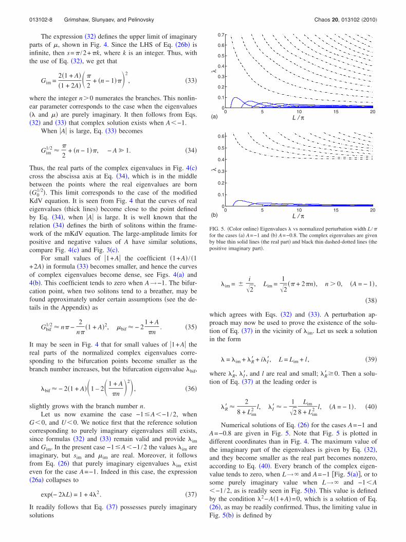
Numerical solutions of Eq. �26� for the cases A=−1 andA=−0.8 are given in Fig. 5. Note that Fig. 5 is plotted indifferent coordinates than in Fig. 4. The maximum value ofthe imaginary part of the eigenvalues is given by Eq. �32�,and they become smaller as the real part becomes nonzero,according to Eq. �40�. Every branch of the complex eigen-value tends to zero, when L→ and A=−1 �Fig. 5�a��, or tosome purely imaginary value when L→ and −1A−1 /2, as is readily seen in Fig. 5�b�. This value is definedby the condition �2−A�1+A�=0, which is a solution of Eq.�26�, as may be readily confirmed. Thus, the limiting value inFig. 5�b� is defined by

0 5 10 15 200

0.1

0.2

0.3

0.4

0.5

0.6

0.7

L / π

λ0 5 10 15 20

0

0.1

0.2

0.3

0.4

0.5

0.6

L / πλ

(a)

(b)

FIG. 5. �Color online� Eigenvalues � vs normalized perturbation width L /�for the cases �a� A=−1 and �b� A=−0.8. The complex eigenvalues are givenby blue thin solid lines �the real part� and black thin dashed-dotted lines �thepositive imaginary part�.

013102-8 Grimshaw, Slunyaev, and Pelinovsky Chaos 20, 013102 �2010�

�� = i− A�1 + A� . �41�

When A=−1, then ��=0, as seen in Fig. 5�a�. WhenA→−1 /2, then �� tends to �im, and the solution vanishes.

IV. NUMERICAL SIMULATIONS

In this section the initial-value problem within theframework of the GE is solved by direct numerical integra-tion of Eq. �1�. The box-like disturbance �22� is used as theinitial condition. From Sec. III, a disturbance of positive po-larity will evolve in a qualitatively simple manner, producingsequences of solitary waves, which are similar to the solitonsof the KdV equation, when their amplitudes are small, andsimilar to solitons of the modified KdV equation, when theyare large. Negative disturbances, in contrast, can give birth toboth solitons and breathers.

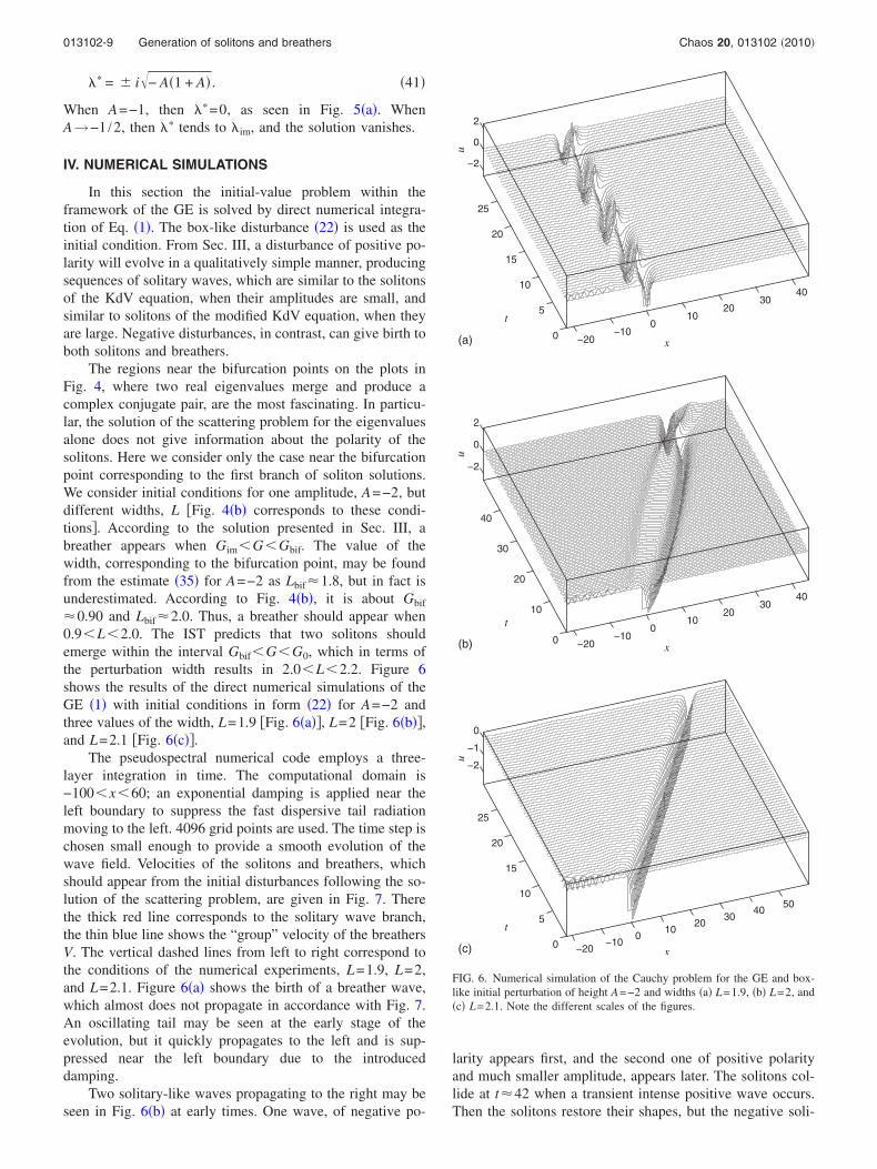
The regions near the bifurcation points on the plots inFig. 4, where two real eigenvalues merge and produce acomplex conjugate pair, are the most fascinating. In particu-lar, the solution of the scattering problem for the eigenvaluesalone does not give information about the polarity of thesolitons. Here we consider only the case near the bifurcationpoint corresponding to the first branch of soliton solutions.We consider initial conditions for one amplitude, A=−2, butdifferent widths, L �Fig. 4�b� corresponds to these condi-tions�. According to the solution presented in Sec. III, abreather appears when GimGGbif. The value of thewidth, corresponding to the bifurcation point, may be foundfrom the estimate �35� for A=−2 as Lbif�1.8, but in fact isunderestimated. According to Fig. 4�b�, it is about Gbif

�0.90 and Lbif�2.0. Thus, a breather should appear when0.9L2.0. The IST predicts that two solitons shouldemerge within the interval GbifGG0, which in terms ofthe perturbation width results in 2.0L2.2. Figure 6shows the results of the direct numerical simulations of theGE �1� with initial conditions in form �22� for A=−2 andthree values of the width, L=1.9 �Fig. 6�a��, L=2 �Fig. 6�b��,and L=2.1 �Fig. 6�c��.

The pseudospectral numerical code employs a three-layer integration in time. The computational domain is−100x60; an exponential damping is applied near theleft boundary to suppress the fast dispersive tail radiationmoving to the left. 4096 grid points are used. The time step ischosen small enough to provide a smooth evolution of thewave field. Velocities of the solitons and breathers, whichshould appear from the initial disturbances following the so-lution of the scattering problem, are given in Fig. 7. Therethe thick red line corresponds to the solitary wave branch,the thin blue line shows the “group” velocity of the breathersV. The vertical dashed lines from left to right correspond tothe conditions of the numerical experiments, L=1.9, L=2,and L=2.1. Figure 6�a� shows the birth of a breather wave,which almost does not propagate in accordance with Fig. 7.An oscillating tail may be seen at the early stage of theevolution, but it quickly propagates to the left and is sup-pressed near the left boundary due to the introduceddamping.

Two solitary-like waves propagating to the right may beseen in Fig. 6�b� at early times. One wave, of negative po-

larity appears first, and the second one of positive polarityand much smaller amplitude, appears later. The solitons col-lide at t�42 when a transient intense positive wave occurs.Then the solitons restore their shapes, but the negative soli-

−20−10

010

2030

40

0

5

10

15

20

25

−2

0

2

x

t

u

−20−10

010

2030

40

0

10

20

30

40

−2

0

2

x

t

u

−20−10

010

2030

4050

0

5

10

15

20

25

−2

−1

0

x

t

u

(a)

(b)

(c)

FIG. 6. Numerical simulation of the Cauchy problem for the GE and box-like initial perturbation of height A=−2 and widths �a� L=1.9, �b� L=2, and�c� L=2.1. Note the different scales of the figures.

013102-9 Generation of solitons and breathers Chaos 20, 013102 �2010�

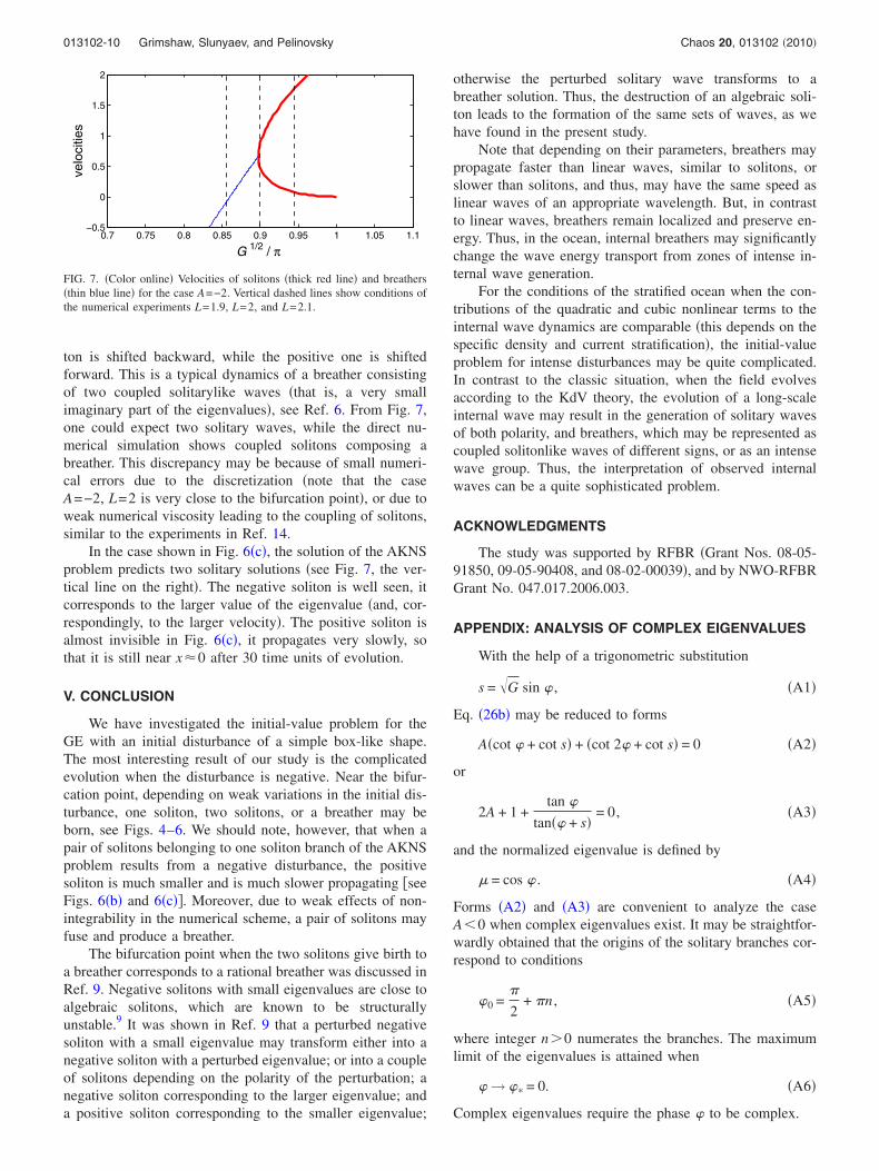
ton is shifted backward, while the positive one is shiftedforward. This is a typical dynamics of a breather consistingof two coupled solitarylike waves �that is, a very smallimaginary part of the eigenvalues�, see Ref. 6. From Fig. 7,one could expect two solitary waves, while the direct nu-merical simulation shows coupled solitons composing abreather. This discrepancy may be because of small numeri-cal errors due to the discretization �note that the caseA=−2, L=2 is very close to the bifurcation point�, or due toweak numerical viscosity leading to the coupling of solitons,similar to the experiments in Ref. 14.

In the case shown in Fig. 6�c�, the solution of the AKNSproblem predicts two solitary solutions �see Fig. 7, the ver-tical line on the right�. The negative soliton is well seen, itcorresponds to the larger value of the eigenvalue �and, cor-respondingly, to the larger velocity�. The positive soliton isalmost invisible in Fig. 6�c�, it propagates very slowly, sothat it is still near x�0 after 30 time units of evolution.

V. CONCLUSION

We have investigated the initial-value problem for theGE with an initial disturbance of a simple box-like shape.The most interesting result of our study is the complicatedevolution when the disturbance is negative. Near the bifur-cation point, depending on weak variations in the initial dis-turbance, one soliton, two solitons, or a breather may beborn, see Figs. 4–6. We should note, however, that when apair of solitons belonging to one soliton branch of the AKNSproblem results from a negative disturbance, the positivesoliton is much smaller and is much slower propagating �seeFigs. 6�b� and 6�c��. Moreover, due to weak effects of non-integrability in the numerical scheme, a pair of solitons mayfuse and produce a breather.

The bifurcation point when the two solitons give birth toa breather corresponds to a rational breather was discussed inRef. 9. Negative solitons with small eigenvalues are close toalgebraic solitons, which are known to be structurallyunstable.9 It was shown in Ref. 9 that a perturbed negativesoliton with a small eigenvalue may transform either into anegative soliton with a perturbed eigenvalue; or into a coupleof solitons depending on the polarity of the perturbation; anegative soliton corresponding to the larger eigenvalue; anda positive soliton corresponding to the smaller eigenvalue;

otherwise the perturbed solitary wave transforms to abreather solution. Thus, the destruction of an algebraic soli-ton leads to the formation of the same sets of waves, as wehave found in the present study.

Note that depending on their parameters, breathers maypropagate faster than linear waves, similar to solitons, orslower than solitons, and thus, may have the same speed aslinear waves of an appropriate wavelength. But, in contrastto linear waves, breathers remain localized and preserve en-ergy. Thus, in the ocean, internal breathers may significantlychange the wave energy transport from zones of intense in-ternal wave generation.

For the conditions of the stratified ocean when the con-tributions of the quadratic and cubic nonlinear terms to theinternal wave dynamics are comparable �this depends on thespecific density and current stratification�, the initial-valueproblem for intense disturbances may be quite complicated.In contrast to the classic situation, when the field evolvesaccording to the KdV theory, the evolution of a long-scaleinternal wave may result in the generation of solitary wavesof both polarity, and breathers, which may be represented ascoupled solitonlike waves of different signs, or as an intensewave group. Thus, the interpretation of observed internalwaves can be a quite sophisticated problem.

ACKNOWLEDGMENTS

The study was supported by RFBR �Grant Nos. 08-05-91850, 09-05-90408, and 08-02-00039�, and by NWO-RFBRGrant No. 047.017.2006.003.

APPENDIX: ANALYSIS OF COMPLEX EIGENVALUES

With the help of a trigonometric substitution

s = G sin � , �A1�

Eq. �26b� may be reduced to forms

A�cot � + cot s� + �cot 2� + cot s� = 0 �A2�

or

2A + 1 +tan �

tan�� + s�= 0, �A3�

and the normalized eigenvalue is defined by

� = cos � . �A4�

Forms �A2� and �A3� are convenient to analyze the caseA0 when complex eigenvalues exist. It may be straightfor-wardly obtained that the origins of the solitary branches cor-respond to conditions

�0 =�

2+ �n , �A5�

where integer n�0 numerates the branches. The maximumlimit of the eigenvalues is attained when

� → �� = 0. �A6�

Complex eigenvalues require the phase � to be complex.

0.7 0.75 0.8 0.85 0.9 0.95 1 1.05 1.1−0.5

0

0.5

1

1.5

2

G 1/2 / π

velo

c itie

s

FIG. 7. �Color online� Velocities of solitons �thick red line� and breathers�thin blue line� for the case A=−2. Vertical dashed lines show conditions ofthe numerical experiments L=1.9, L=2, and L=2.1.

013102-10 Grimshaw, Slunyaev, and Pelinovsky Chaos 20, 013102 �2010�

If one supposes the eigenvalue to be complex with asmall imaginary part, solution �A3� may be written in Taylorseries in the form

T1 + iT2 Im��� + O�Im���2� , �A7�

where T1 and T2 are real functions of Re���. Thus, conditionT1=0 defines the leading order of the solution �considerablereal part of the eigenvalue� and is equivalent to Eq. �A3�, andT2=0 defines the condition, when this situation �small imagi-nary part of the eigenvalue� occurs, what reads

1 + G cos � +1 + 2A

1 + 4A�1 + A�cos2 �= 0, �A8�

otherwise

Z3 + Z2 +G

4A�1 + A�Z +

G

2A= 0, Z = �G . �A9�

Equation �A9� defines the bifurcation points jointly with Eq.�26�. The solution of Eq. �A9� may be found, but Eq. �26�remains transcendental.

It may be shown through differentiation that Eq. �A3�results in Eq. �A8� when condition

�G

��= 0 �A10�

is employed. It follows from the graphical solution of Eq.�26b� that near the bifurcation points s��n, Nr��2n2, andthus, ��� /2. Then, the RHS of solution �27� may be de-composed in the Taylor series for ��� /2 as

G = �n − 2�1 + A��� −�

2� +

�n

2�� −

�

2�2

+ O��� −�

2�3� . �A11�

The first three terms on the RHS of Eq. �A11� represent aparabola with the minimum corresponding to the condition�A10�, which therefore corresponds to the bifurcation point,

�bif ��

2+ 2

1 + A

�n, �A12�

which gives formula �35�.

1L. A. Ostrovsky and Yu. A. Stepanyants, Chaos 15, 037111 �2005�.2K. R. Helfrich and W. K. Melville, Annu. Rev. Fluid Mech. 38, 395�2006�.

3Solitary Waves in Fluids, edited by R. H. J. Grimshaw �WIT, Southamp-ton, 2007�.

4P. G. Drazin and R. S. Johnson, Solitons: An Introduction �CambridgeUniversity Press, Cambridge, England, 1996�.

5A. V. Slyunyaev and E. N. Pelinovskii, Sov. Phys. JETP 89, 173 �1999�.6A. V. Slyunyaev, Sov. Phys. JETP 92, 529 �2001�.7R. Grimshaw, D. Pelinovsky, E. Pelinovsky, and A. Slunyaev, Chaos 12,1070 �2002�.

8R. Grimshaw, E. Pelinovsky, and T. Talipova, Nonlinear Processes Geo-phys. 4, 237 �1997�.

9D. Pelinovsky and R. Grimshaw, Phys. Lett. A 229, 165 �1997�.10K. W. Chow, R. H. J. Grimshaw, and E. Ding, Wave Motion 43, 158

�2005�.11R. Grimshaw, E. Pelinovsky, T. Talipova, M. Ruderman, and R. Erdélyi,

Stud. Appl. Math. 114, 189 �2005�.12K. G. Lamb, O. Polukhina, T. Talipova, E. Pelinovsky, W. Xiao, and A.

Kurkin, Phys. Rev. E 75, 046306 �2007�.13S. V. Dmitriev and T. Shigenari, Chaos 12, 324 �2002�.14D. N. Ivanychev and G. M. Fraiman, Theor. Math. Phys. 110, 199 �1997�

�in Russian, Teoreticheskaya i Matematicheskaya Fizika 110, 254 �1997��.15R. Grimshaw, D. Pelinovsky, E. Pelinovsky, and T. Talipova, Physica D

159, 35 �2001�.16R. Grimshaw, E. Pelinovsky, and T. Talipova, Physica D 132, 40 �1999�.17S. V. Manakov, Zh. Eksp. Teor. Fiz. 65, 505 �1973� �Sov. Phys. JETP 38,

248 �1974��.18J. Satsuma and N. Yajima, Suppl. Prog. Theor. Phys. 55, 284 �1974�.19Z. V. Lewis, Phys. Lett. A 112, 99 �1985�.20J. Burzlaff, J. Phys. A 21, 561 �1988�.21H. Takahashi and K. Konno, J. Phys. Soc. Jpn. 58, 3085 �1989�.22D. J. Kaup, J. El-Reedy, and B. A. Malomed, Phys. Rev. E 50, 1635

�1994�.23D. J. Kaup and B. A. Malomed, Physica D 84, 319 �1995�.24M. Desaix, D. Anderson, M. Lisak, and M. L. Quiroga-Teixeiro, Phys.

Lett. A 212, 332 �1996�.25S. Clarke, R. Grimshaw, P. Miller, E. Pelinovsky, and T. Talipova, Chaos

10, 383 �2000�.26M. Klaus and J. K. Shaw, Phys. Rev. E 65, 036607 �2002�.27M. Desaix, D. Anderson, L. Helczynski, and M. Lisak, Phys. Rev. Lett.

90, 013901 �2003�.28M. J. Ablowitz, D. J. Kaup, A. C. Newell, and H. Segur, Stud. Appl. Math.

53, 249 �1974�.29J. W. Miles, Tellus 31, 456 �1979�.30M. Wadati, J. Phys. Soc. Jpn. 34, 1289 �1973�.31N. N. Romanova, Theor. Math. Phys. 39, 415 �1979� �in Russian, Teoret-

icheskaya i Matematicheskaya Fizika 39, 205 �1979��.32Y. Chen and P. L.-F. Liu, Wave Motion 24, 169 �1996�.33J. Small, T. C. Sawyer, and J. Scott, Ann. Geophys. 17, 547 �1999�.

013102-11 Generation of solitons and breathers Chaos 20, 013102 �2010�