Economic Modelling 50 (2015) 27–39

Contents lists available at ScienceDirect

Economic Modelling

j ourna l homepage: www.e lsev ie r .com/ locate /ecmod

Enhancing the forecasting power of exchange ratemodels by introducingnonlinearity: Does it work?☆

Kelly Burns a,⁎, Imad A. Moosa b

a Curtin University, Australiab RMIT, Australia

☆ We are grateful to the editor of this journal and twocomments on the original, shorter version of this paper.⁎ Corresponding author.

E-mail address: kelly.burns@curtin.edu.au (K. Burns).1 For an extensive survey of these issues, see Moosa an

http://dx.doi.org/10.1016/j.econmod.2015.06.0030264-9993/© 2015 Elsevier B.V. All rights reserved.

a b s t r a c t

a r t i c l e i n f o

Article history:Accepted 6 June 2015Available online xxxx

Keywords:ForecastingRandom walkExchange rate modelsNonlinearity

It is demonstrated that the forecasting power of the flexible price monetary model of exchange rates can beenhanced by introducing dynamics through the use of a linear error correction specification. However, theintroduction of nonlinearity, by using a polynomial in the error correction term, does not lead to any furtherimprovement in forecasting accuracy and may even lead to deterioration. The results provide evidence againstthe proposition that the Meese–Rogoff puzzle can be explained in terms of failure to account for nonlinearity.It is also shown that the introduction of dynamics boosts the forecasting accuracy (in terms of the magnitudeof the forecasting error) of the model relative to the static specification because dynamic specifications involvea random walk component. The empirical results lead to the conclusion that accounting for nonlinearity doesnot resolve the Meese–Rogoff puzzle.

© 2015 Elsevier B.V. All rights reserved.

1. Introduction

Since the publication of the highly-cited paper of Meese and Rogoff(1983), it has become something like an undisputable fact of life thatconventional exchange rate determination models cannot outperformthe naïve random walk model in out-of-sample forecasting. Meeseand Rogoff (1983) attributed the failure of exchange rate models tooutperform the randomwalk to simultaneous equations bias, samplingerrors, stochastic movements in the true underlying parameters,misspecification and nonlinearity.1 In this paper we consider one ofthese possible explanations for the Meese–Rogoff “puzzle”: failure toaccount for nonlinearity.

Taylor et al. (2001) point out that “the idea that there may be non-linearities in real exchange rate adjustment dates at least fromHeckscher (1916)”. If a nonlinear relation exists between the exchangerate and macroeconomic variables, any attempt to fit a linear model tothe data and generate forecasts with smaller errors compared to therandomwalk will invariably fail. This sounds logical but it does not nec-essarily mean that any attempt to fit a nonlinear model to the data andgenerate forecasts with smaller errors compared to the random walkwill invariably succeed. Chinn (1991) emphasises nonlinearity as an ex-planation for theMeese–Rogoff puzzle, arguing that “theory provides usthe set of ‘fundamentals’, but not the form of the relationships wherebythe fundamentals determine the exchange rate”. Hence, he argues, “the

anonymous referees for useful

d Burns (2015).

superiority of the random walk in forecasting exercises such as Meeseand Rogoff ..... may not be so much an indictment of structural models,as much as one of linear structural models”.

In this paperwe provide evidence on the role played by nonlinearityin exchange rate forecasting.We start with the static version of the flex-ible price monetary model, which we compare, in terms of forecastingaccuracy, with the corresponding linear, nonlinear and asymmetricerror correction models. Both conventional and recently developedmeasures of forecasting accuracy are used. Apart from the use of aneconometric methodology that allows us to compare three versions ofan error correction model with the static version of the flexible pricemonetary model, this study makes other contributions that makes itdifferent from existing studies.

Unlike almost all of the other studies, we challenge the very notionof theMeese–Rogoff puzzle and demonstrate that it cannot be resolvedby the introduction of nonlinearity and that a more straightforward ex-planation for the puzzle does exist. We must also emphasise that ourmain objective is to find out if nonlinearity has any value added as faras forecasting accuracy is concerned. Conversely, the primary objectiveofmost of the studies surveyed in the following section is to detect non-linearity. Yet another distinguishing feature of our study, comparedwith the existing literature, is that we use a larger number of exchangerates (including some cross rates that are rarely used) and a data samplespanning the modern era of floating exchange rates (1973–2014).

1.1. The literature on nonlinearity in exchange rates

Interest in nonlinearity in exchange rates stems from the observa-tion that linear models are unable to explain a number of important

28 K. Burns, I.A. Moosa / Economic Modelling 50 (2015) 27–39

features that are common to nonlinear time series, such asleptokurtosis, volatility clustering and leverage effects (Brooks, 2005).Nonlinear models are used when the underlying theory suggests thatthe relation between the dependent and explanatory variables cannotbe represented by a linear model. More often, however, theory cannottell us much about whether the underlying functional relation is linearor nonlinear, inwhich case choice between linear and nonlinearmodelsbecomes an empirical issue. In this case choice can bemade on the basisof non-nested model selection tests or by using other validation toolssuch as forecasting accuracy, which is what we do in this study.

Interest in nonlinear exchange rate models was initially motivatedby the desire to explain deviations from purchasing power parity. Forexample, Leon and Najarian (2003) attribute nonlinear exchange rateadjustment to transaction costs in international arbitrage. They alsosuggest other possible reasons for nonlinearity, including heterogeneityin the expectations of market participants and local-currency pricing.For the purpose of this paper, interest in nonlinearity is attributed tothe possibility that the poor performance of conventional exchangerate models (which are typically linear in parameters) may explaintheMeese–Rogoff puzzle. However, whilst it is valid to warn of the haz-ard of using a linear model when the underlying relation is nonlinear,there is no guarantee that the use of nonlinear models brings about adefeat of the random walk, notwithstanding the observation thatsome economists have made such a claim.

Nonlinearity can be accounted for in several ways and by usingmodels of various specifications. Taylor et al. (2001) suggest thatESTAR models are predominant in the (exchange rate) literature fortwo reasons: (i) they have the attractive property of allowing for“smooth transition between regimes and symmetric adjustment of thereal exchange rate for deviations above and below the equilibriumlevel”; and (ii) they are relatively simplistic. Markov-switching modelsare popular because they capture the exchange rate adjustment processthrough a transition probability that is a function of the lagged deviationof the exchange rate from its equilibrium level (Hamilton, 1989). Kempaand Riedel (2013) estimate a Markov switching model for the bilateralCanadian-U.S. dollar exchange rate and find that an active monetarypolicy stance may account for nonlinearity in the exchange rate-fundamentals nexus and that nonlinearity confirms the notion thatexchange rate movements cannot be explained exclusively in terms ofany one particular exchange rate model. Kruse et al. (2012) criticisethe disproportionately large body of literature in which ESTAR modelsare used whilst neglecting competing nonlinear models, such as theMarkov switching AR model. Diaz et al. (2002) use an ARFIMA modeland find that this model is not always able to capture all of the nonlin-earity in the data. Iovino and Sitzia (2008) use a double thresholdEGARCHmodel and conclude that “the proposed model is both feasibleand of wide applicability to the analysis of exchange rate volatility”.

Nonlinear models are used to ascertain whether or not the weakexplanatory power of the monetary model is associated with the prop-osition that exchange rates are insensitive to macroeconomic variablesclose to equilibrium values but exhibit greater predictability the greaterthe deviation from equilibrium (Kilian and Taylor, 2003; Taylor andPeel, 2000; Taylor et al., 2001). Taylor and Peel (2000) use an ESTARmodel to predict monthly changes in the dollar exchange rates of thepound and German mark from 1973 to 1996. They conclude that ex-change rates are almost unpredictable when macroeconomic variablesare close to equilibrium values, but when they deviate from equilibriumby a large amount, the predictive power of themodel improves becauseof strong reversion towards equilibrium.

Mark (1995) uses a simple monetary model that incorporates anonlinear error correction term to forecast a range of exchange ratesvis-à-vis the U.S. dollar. The error term measures the deviation of theactual exchange rate from the long-run equilibrium value. Using theDiebold–Mariano test, he demonstrates that the random walk can beoutperformed in terms of the magnitude of error for the French francand Japanese yen at the 1, 4, 8, 12 and 16-quarter horizons, as well as

the German mark at the 12 and 16-quarter horizons. For the Canadiandollar, however, the random walk outperforms the model at all butthe one-quarter horizon. Overall, Mark (1995) concludes that the“out-of-sample point predictions generally outperform the driftless ran-dom walk at longer horizons”. Perhaps, but this performance is due todynamics, not nonlinearity. Likewise, Lopez-Suarez and Rodriguez-Lopez (2011) use a nonlinear error correction model and find evidenceof nonlinear predictability of the nominal exchange rate and of nonlin-earmean reversion of the real exchange rate. They base their conclusionon Theil's U-statistics which indicate “a higher forecast precision of thenonlinear model than the one obtained with a random walk specifica-tion”. However, they fail to test for the significance of the difference inTheil's U-statistics.

Junttila and Korhonen (2011) account for nonlinearity by using anonlinear error correction model. The results, they conclude, “stronglysupport the non-linear connection between exchange rates and mone-tary fundamentals”. However, this study focuses on identifying the exis-tence of a nonlinear relation rather than forecasting. Hence, no evidenceis reported on whether or not forecasting accuracy can be enhanced byincorporating nonlinearity. They conclude that nonlinearmodel specifi-cations are relevant, suggesting that “traditional macroeconomicfundamentals play a crucial role in the determination of the short-runexchange rate dynamics”. They argue that nonlinearity can be impor-tant but only under some conditions, suggesting that “non-linear errorcorrection mechanism operates only when the inflation differential issufficiently high” and that for low relative inflation differentials theerror correction process is linear. Furthermore, they suggest thattraditional macroeconomic variables are important determinants of ex-change rates although their impact depends on the inflation differential,which should be incorporated into themodel as a nonlinear effectwhenthis differential is high. We have to remember, however, that when theinflation differential is high (as when one country experiences hyperin-flation) themonetary model works very well, irrespective of whether itis linear or nonlinear (see, for example, Moosa, 2000).

This brief survey of the literature reveals some support for the prop-osition that the use of nonlinear models pays off and that nonlinearmodels are better at forecasting exchange rates than linear models.However, this evidence is based on inference without testing and/orthe use of dynamic models. The literature fails to distinguish betweenthe effect of dynamics and nonlinearity, attributing improvement inforecasting accuracy to nonlinearity when it should be attributed tothe introduction of dynamics. This is why the nonlinear models thatare claimed to outperform the random walk are invariably dynamic.The literature does not produce a nonlinear static model that is claimedto be superior to the random walk. In this paper we provide systematicevidence showing that it is dynamics that makes nonlinear models lookgood. This is yet another contribution of this paper.

1.2. The models

The basic flexible price monetary model, which is one of the threemodels used by Meese and Rogoff (1983), is specified as

st ¼ α0 þ α1 ma;t−mb;t� �þ α2 ya;t−yb;t

� �þ α3 ia;t−ib;t� �þ εt ð1Þ

where s is the log of the exchange rate,m is the log of themoney supply,y is the log of industrial production, i is the interest rate, and a and brefer to the countries having a and b as their currencies, respectively(the exchange rate is measured as the price of one unit of b—thatis, a/b). Eq. (1) represents the static version of the model, which westart with because, apart from the fact that it was used by Meese andRogoff (1983), we will demonstrate that improvement in forecastingpower can be achieved by introducing dynamics and that introducingnonlinearity has no value added.

29K. Burns, I.A. Moosa / Economic Modelling 50 (2015) 27–39

The corresponding linear error correction model is

Δst ¼ α0 þX‘j¼0

β jΔ ma;t− j−mb;t− j� �þX‘

j¼0

γ jΔ ya;t− j−yb;t− j

� �þX‘j¼0

δ jΔ ia;t− j−ib;t− j� �þ ϕεt−1 þ ξt

ð2Þ

where the error correction term is the residual of the static model.Dynamics is introduced through the error correction term and laggedexplanatory variables.

Although nonlinearity in exchange rate models take many shapesand forms we choose to follow the approach suggested by Hendry andEriccson (1991) by using a polynomial of degree three in the errorcorrection term as it appears in Eq. (2). The nonlinear error correctionmodel is specified as

Δst ¼ α0 þX‘j¼0

β jΔ ma;t− j−mb;t− j� �þX‘

j¼0

γ jΔ ya;t− j−yb;t− j

� �þX‘j¼0

δ jΔ ia;t− j−ib;t− j� � þ

X3i¼1

ϕiεit− j þ ξt :

ð3Þ

If the introduction of nonlinearity has any implication for forecastingaccuracy, as some economists seem to suggest, the nonlinear errorcorrection model (3) should produce more accurate forecasts than thelinear model (2).

As a related exercise we also investigate the possibility thatintroducing asymmetry, which can be thought of as some kind of non-linearity, leads to improvement in forecasting accuracy. Narayan andGupta (2015) suggest that predictability is nonlinear when negativechanges in the explanatory variable(s) affect the dependent variablemore or less than the positive values.2 In an error correction modelasymmetry can be captured by splitting the error correction term intopositive and negative values, signifying positive and negative deviationsfrom the long-run equilibrium condition. The asymmetric ECM isspecified as

Δst ¼ α þ βΔ ma;t−mb;t� �þ γΔ ya;t−yb;t

� �þ δΔ ia;t−ib;t� �þ ϕþεþt−1

þ ϕ−ε−t−1 þ ξt ð4Þ

where εt − 1+ = εt − 1 if εt − 1 N 0 and εt − 1

+ = 0 if εt − 1 b 0. Conversely,εt − 1− = εt − 1 if εt − 1 b 0 and εt − 1

− = 0 if εt − 1 N 0.The four models are estimated using data on 14 exchange rates and

the related explanatory variables. The currencies include the U.S. dollar(USD), Japanese yen (JPY), British pound (GBP), Canadian dollar (CAD),Swiss franc (CHF) and Swedish kroner (SEK). The exchange rates in-clude those of every currency against the dollar as well as all possiblecross rates, with the exception of the SEK/CHF rate because it is so stablethat it looks as if it is fixed. The use of dollar rates and cross rates is mo-tivated by the desire to find out if there is such a thing as a “dollarphenomenon”—that is, the tendency of the results to differ when themodels are estimatedwith the dollar rates from those when themodelsare estimated for the cross rates. The data sample, which was obtainedfrom the IMF's International Financial Statistics, covers the periodJanuary 1973 to September 2014. The reason why the sample starts inJanuary 1973 is that this date is generally taken to be the point in timewhen floating becamewidespread following the collapse of the BrettonWoods system of fixed exchange rates in August 1971 and the failure ofthe Smithsonian agreement to save the system.

2 Narayan and Gupta (2015) make a valid point but some economists distinguish be-tween nonlinearity and asymmetry. For example, Leon and Najarian (2003) distinguishbetween “asymmetric adjustment” and “nonlinear dynamics”. They refer to deviationsfromPPP in thepresence of nonlinearity and adjustment andwonderwhether adjustmenttowards PPP is symmetric from above and below.

1.3. In-sample forecasting

Although Meese and Rogoff (1983) conducted their forecastingexercise on an out-of-sample basis, there is no consensus view in theliterature on whether forecasting accuracy should be assessed onan in-sample or out-of-sample basis. The literature suggests thatexchange rate models have greater explanatory power in sample,as opposed to out of sample, when compared to the random walk(Sarno and Taylor, 2002). However, this finding has been questionedon several grounds. Concern about the apparent superiority of in-sample performance stems from four main propositions: structuralbreaks in the time series, data mining, reliability of hypothesistesting and sample size.

Engel et al. (2007) argue that in-sample forecasting is an unreliablebenchmark because of the possibility of over-fitting or data miningand that the out-of-sample forecasting power is a higher hurdle andthe standard by which exchange rate models should be judged.Tashman (2000) suggests that in-sample errors are likely to understateforecasting errors and that over-fitting and structural changes mayaggravate the divergence between in-sample and out-of-sample errors.Thus, a model performs better in sample, which makes in-sampleforecasting an unreliable benchmark.

In terms of the reliability of hypothesis testing, Kilian and Taylor(2003) provide evidence indicating that for a small sample, out-of-sample tests may have considerably lower power than in-sampletests. As a result, there may be a tendency to reject incorrectly the nullof no predictability. The proposition that the sample size is importantin the outcome of hypothesis testing, both in sample and out of sample,is further illustrated by Inoue and Killian (2002) who argue that stron-ger in-sample predictability results from sample splitting and loss ofinformation. Consequently, an out-of-sample test may fail to detectpredictability that exists in the population whereas the in-sample testdetects it correctly.

Clark andMcCracken (2002) draw attention to the impact of param-eter instability on in-sample and out-of-sample predictability. In-sample predictability does not imply out-of-sample predictability inthe presence of parameter instability, which (together with structuralbreaks) make out-of-sample predictability much harder to demon-strate. Hence, out-of-sample predictability is a higher and moreappropriate benchmark for assessing forecasting accuracy.

Despite the evidence supporting in-sample predictability, andconcerns about the reliability of hypothesis testing out-of-sample, themajority of economists suggest that forecasting accuracy should beassessed out of sample. For instance, Tashman (2000) states that “fore-casters generally agree that forecasting methods should be assessed foraccuracy using out-of-sample tests”. Fildes and Makridakis (1995) con-tend that “the performance of a model on data outside that used in itsconstruction remains the touchstone for its utility in all applications”.Ashley et al. (1980) point out that assessing predictive power out-of-sample is the “sound and natural approach”. Likewise, Moosa andBurns (2013) consider it more appropriate to use out-of-sampleforecasting. Regardless, Moosa (2013) argues that the choice betweenin-sample and out-of-sample forecasting may not matter because“if out-of-sample forecasting is conducted on a one-step-ahead basis(as per the Meese and Rogoff approach), there is no reason why thein-sample forecasting performance will be necessarily superior to theout-of-sample performance”. Furthermore, he shows that it is difficultto outperform the random walk in terms of the magnitude of theforecasting error, irrespective of whether the exercise is conducted insample or out of sample.

In this exercise we choose to follow the proposition put forward byNarayan and Gupta (2015) and generate both in-sample and out-of-sample forecasts. They point out that “there is a pendulumof argumentssupporting and similarly chastising out-of-sample tests, just like in-sample tests”. They also suggest that “there is no theory to guide appliedresearchers on this”. In fact they consider the desire for robustness as a

30 K. Burns, I.A. Moosa / Economic Modelling 50 (2015) 27–39

motivation for conducting both in-sample and out-of-sample forecast-ing (see also Narayan et al., 2014). Therefore, it is a good idea to findout if the results of an in-sample exercise are different from thoseobtained from an out-of-sample exercise.

To generate in-sample forecasts, the models are estimated over thewhole sample period, t = 1, 2, … n, then forecasts are generated fromthe estimated equation.3 For the static model, the forecast log exchangerate is

st ¼ α0 þ α1 ma;t−mb;t� �þ α2 ya;t−yb;t

� �þ α3 ia;t−ib;t� � ð5Þ

where αi is the estimated value of αi. Hence the forecast level of theexchange rate is

St ¼ exp stð Þ: ð6Þ

Once we have corresponding time series for the actual, St, andforecast, Ŝt, exchange rates for the period t=1, 2,… n, we can calculatemeasures of forecasting accuracy based on the forecasting error. Theroot mean square error (RMSE) is calculated as

RMSE ¼

ffiffiffiffiffiffiffiffiffiffiffiffiffiffiffiffiffiffiffiffiffiffiffiffiffiffiffiffiffiffiffiffiffiffi1n

Xnt¼1

St−StSt

!2vuut : ð7Þ

Meese and Rogoff (1983), and most of the subsequent studies,reached a conclusion on the superiority or otherwise of the randomwalk by comparing the numerical values of the RMSEs and similar met-rics, without testing for the statistical significance of the difference.Some studies, however, use the Diebold and Mariano (1995) test. As arobustness check, we opt to use a different test—the AGS test suggestedby Ashley et al. (1980). This test requires the estimation of the linearregression

Dt ¼ a0 þ a1 Mt−M� �þ ut ð8Þ

where Dt ¼ w1t−w2t ;Mt ¼ w1t þw2t ;M is the mean of M, w2t is theforecasting error at time t of the model with the higher RMSE, w2t isthe forecasting error at time t of the model with the lower RMSE. Ifthe samplemean of the errors is negative, the observations of the seriesmust bemultiplied by−1 before running the regression. The estimatesof the intercept term (a0) and the slope (a1) are used to test thestatistical difference between the RMSEs of two different models. Ifthe estimates of a0 and a1 are both positive, then a test of the jointhypothesis H0 : a0 = a1 = 0 is appropriate. However, if one of theestimates is negative and statistically significant then the test is incon-clusive. But if one of the coefficients is negative and statistically insignif-icant the test remains conclusive, in which case significance isdetermined by the upper-tail of the t-test on the positive coefficientestimate.

It has been suggested that the use of the RMSE and similar criteria tomeasure forecasting accuracy may not be entirely appropriate. Someeconomists argue that a correct prediction of the direction of changecan be more important than the magnitude of the error, whilst othershave suggested that the ultimate test of forecasting power is the abilityto make profit by trading on the basis of the forecasts.

We use the conventional measure of direction accuracy

DA ¼ 1n

Xnt¼1

zt ð9Þ

3 This illustration pertains to the static model (1). Forecasts are generated in a similarmanner from the linear ECM (2), nonlinear ECM (3) and asymmetric ECM (4).

where

zt ¼ 10

�if

Stþ1−St� �

Stþ1−Stð Þ N 0

Stþ1−St� �

Stþ1−Stð Þ b 0

8<: : ð10Þ

A conventional test of the significance of a proportion is used to findout if direction accuracy is significantly different from 0. A rejection ofH0 : DA=0means that the underlyingmodel is superior to the randomwalk in predicting direction.

Moosa and Burns (2012) suggest a measure of forecasting accuracy,the adjusted root mean square error (ARMSE), which combines themagnitude of the error and the ability of the model to predict directioncorrectly. The ARMSE is calculated as follows

ARMSE ¼

ffiffiffiffiffiffiffiffiffiffiffiffiffiffiffiffiffiffiffiffiffiffiffiffiffiffiffiffiffiffiffiffiffiffiffiffiffiffiffiffiffiffiffiffiffiffiffiffi1−DAð Þ

n

Xnt¼1

St−StSt

!2vuut ð11Þ

which means that it is obtained by adjusting the RMSE to take intoaccount the ability or otherwise to predict the direction of change. Iftwo models have equal RMSEs, the model with the lower DA shouldhave a higher ARMSE.

We examine the profitability of two alternative trading strategies:pure carry trade and forecasting-based trading. Under the randomwalk (without drift), the forecast change in the exchange rate is alwayszero, whichmeans that a profitable strategywould be to go short on thelow interest currency and long on the high interest currency. Thisoperation represents the common carry trade, which in effect is also aforecasting-based strategy except that the forecasts are provided bythe random walk (without drift). Under this trading strategy, theperiod-to-period return is calculated as

π ¼ ib−iað Þ þ S�

tþ1

ia−ibð Þ−S�

tþ1

(if ib N ia

ib b iað12Þ

where ia is the interest rate on currency a, ib is the interest rate oncurrency b and Ṡt + 1 is the percentage change in the exchange rate.On the other hand, if forecasts are used for trading, the decision rulewill be based on whether the forecast return, π, is positive or negative.In this case the realised return is calculated as

π ¼ ib−iað Þ þ S�

tþ1

ia−ibð Þ−S�

tþ1

(if π N 0

π b 0ð13Þ

where π ¼ ib−iað Þ þ bS� tþ1 andbS�

tþ1 is the forecast percentage change inthe exchange rate. Profitability is assessed in terms of mean return,standard deviation and the Sharpe ratio. The mean and standarddeviation are calculated as

π ¼ 1n

Xnt¼1

πt ð14Þ

σ ¼ffiffiffiffiffiffiffiffiffiffiffiffiffiffiffiffiffiffiffiffiffiffiffiffiffiffiffiffiffiffi1n

Xnt¼1

πt−πð Þ2vuut : ð15Þ

The Sharpe ratio is used to measure risk-adjusted return. FollowingBurnside et al. (2010) and Gynelberg and Remolona (2007), the Sharperatio is calculated as the ratio of the mean to the standard deviation ofthe rate of return

SR ¼ πσ: ð16Þ

Table 3In-sample adjusted root mean square error.

Exchangerate

RW Static LinearECM

NonlinearECM

AsymmetricECM

JPY/USD 0.032 0.242 0.021 0.021 0.021GBP/USD 0.029 0.097 0.021 0.021 0.021CAD/USD 0.019 0.083 0.014 0.014 0.014CHF/USD 0.035 0.171 0.023 0.024 0.023SEK/USD 0.032 0.121 0.022 0.021 0.021JPY/GBP 0.034 0.261 0.022 0.022 0.022JPY/CAD 0.037 0.319 0.025 0.026 0.025JPY/CHF 0.033 0.234 0.022 0.021 0.022JPY/SEK 0.036 0.315 0.001 0.024 0.024GBP/CAD 0.030 0.086 0.021 0.020 0.021GBP/CHF 0.029 0.120 0.019 0.019 0.019GBP/SEK 0.026 0.084 0.017 0.017 0.017CAD/CHF 0.037 0.158 0.025 0.025 0.025CAD/SEK 0.031 0.082 0.021 0.020 0.020

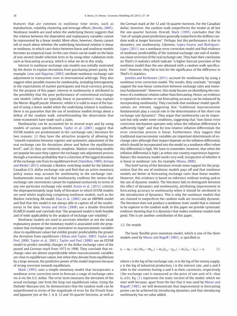
Table 1In-sample root mean square error.

Exchangerate

RW Static LinearECM

NonlinearECM

AsymmetricECM

JPY/USD 0.032 0.352⁎ 0.031⁎ 0.031⁎ 0.031⁎

GBP/USD 0.029 0.134⁎ 0.029 0.029 0.029CAD/USD 0.019 0.106⁎ 0.019 0.019 0.019CHF/USD 0.035 0.230⁎ 0.034⁎ 0.034⁎ 0.034⁎

SEK/USD 0.032 0.173⁎ 0.032 0.031 0.032JPY/GBP 0.034 0.396⁎ 0.033⁎ 0.033⁎ 0.033⁎

JPY/CAD 0.037 0.452⁎ 0.036⁎ 0.036⁎ 0.036⁎

JPY/CHF 0.033 0.333⁎ 0.033 0.033 0.033JPY/SEK 0.036 0.448⁎ 0.035⁎ 0.035⁎ 0.035⁎

GBP/CAD 0.030 0.124⁎ 0.030 0.030 0.030GBP/CHF 0.029 0.174⁎ 0.028 0.028 0.028GBP/SEK 0.026 0.126⁎ 0.026 0.026 0.026CAD/CHF 0.037 0.223⁎ 0.036 0.036 0.036CAD/SEK 0.031 0.121⁎ 0.030⁎ 0.030⁎ 0.030⁎

⁎ Significantly different from the RMSE of the randomwalk at the 5% level as indicatedby the AGS test.

31K. Burns, I.A. Moosa / Economic Modelling 50 (2015) 27–39

A model producing a higher Sharpe ratio than that of the randomwalk implies superior risk-adjusted profitability.

The results of in-sample forecasting are presented in Tables 1–4. InTable 1 we find the root mean square errors of the models, togetherwith an indication of whether or not the RMSE of the model is signifi-cantly different from the RMSE of the random walk as indicated by theAGS test. We can see that the random walk outperforms the staticmodel by a big margin for all exchange rates. This result is consistentwith the finding of Meese and Rogoff (1983) that exchange ratemodels cannot outperform the random walk. However, the linearerror correction model outperforms the random walk for six exchangerates (JPY/USD, CHF/USD, JPY/GBP, JPY/CAD, JPY/SEK and CAD/SEK)—forthe others the linear ECM performs just as well as the random walkbecause the difference in RMSEs is statistically insignificant. Notice,however, that there is no improvement whatsoever as we movefrom the linear ECM to the nonlinear ECM and the asymmetricECM. We reach the same conclusion by looking at other measuresof forecasting accuracy where we find that even the static model out-performs the random walk in terms of direction accuracy andprofitability.

The results show that improvement in the predictive power over thestatic model (measured by the reduction in RMSE) is due to dynamicsrather than nonlinearity or asymmetry. The introduction of dynamicsreduces the RMSE because it produces a randomwalk term representedby the lagged dependent variable. This proposition can be verified by

Table 2In-sample direction accuracy.

Exchangerate

Static LinearECM

Non linearECM

AsymmetricECM

JPY/USD 0.53⁎ 0.53⁎ 0.54⁎ 0.53⁎

GBP/USD 0.47⁎ 0.48⁎ 0.48⁎ 0.49⁎

CAD/USD 0.39⁎ 0.43⁎ 0.43⁎ 0.42⁎

CHF/USD 0.45⁎ 0.53⁎ 0.52⁎ 0.53⁎

SEK/USD 0.51⁎ 0.52⁎ 0.54⁎ 0.56⁎

JPY/GBP 0.56⁎ 0.57⁎ 0.58⁎ 0.58⁎

JPY/CAD 0.50⁎ 0.51⁎ 0.49⁎ 0.50⁎

JPY/CHF 0.51⁎ 0.54⁎ 0.57⁎ 0.54⁎

JPY/SEK 0.50⁎ 0.54⁎ 0.54⁎ 0.53⁎

GBP/CAD 0.52⁎ 0.52⁎ 0.53⁎ 0.53⁎

GBP/CHF 0.53⁎ 0.54⁎ 0.54⁎ 0.55⁎

GBP/SEK 0.55⁎ 0.56⁎ 0.55⁎ 0.56⁎

CAD/CHF 0.50⁎ 0.51⁎ 0.52⁎ 0.52⁎

CAD/SEK 0.54⁎ 0.52⁎ 0.55⁎ 0.55⁎

⁎ Significantly different from zero at the 5% level.

simplifying the linear error correction model (2) such that the threeexplanatory variables are replaced with a vector,xt, whilst imposingthe restriction ℓ = 1. By re-writing the static model (2) as st =a + bxt + εt and since Δst = st − st − 1 and Δxt = xt − xt − 1, Eq. (2)becomes

st−st−1 ¼ α0 þ α1 xt−xt−1ð Þ þ α2 xt−1−xt−2ð Þþ ϕ st−1−a−bxt−1ð Þ þ ξt

ð17Þ

which gives

st ¼ α0−ϕað Þ þ 1þ ϕð Þst−1 þ α1xt þ −α1 þ α2−ϕbð Þxt−1−α2xt−2 þ ξt :

ð18Þ

The process st = (α0 − ϕa) + (1+ ϕ)st − 1 + ξt represents randomwalk without drift if (α0 − ϕa) = 0 and (1 + ϕ) = 1.

In Fig. 1 we can see clearly how the linear error correction modelproduces a significantly lower RMSE than that of the static model butthe nonlinear and asymmetric models add nothing. Figs. 2–4 show acomparison of other measures of forecasting accuracy. It remains tosay that even if a dynamic model outperforms the random walk, thisamounts to beating the random walk with a random walk, which is adodgy proposition.

1.4. Out-of-sample forecasting

In out-of-sample forecasting the model is estimated over part ofthe sample period, t= 1, 2,… k, then a one-period-ahead forecast is

Table 4In-sample Sharpe ratio.

Exchangerate

RW Static LinearECM

NonlinearECM

AsymmetricECM

JPY/USD 0.03 0.04 0.06 0.06 0.06GBP/USD 0.09 0.11 0.07 0.07 0.10CAD/USD 0.04 0.11 0.10 0.10 0.05CHF/USD 0.10 0.10 0.18 0.19 0.15SEK/USD 0.08 0.10 0.12 0.12 0.10JPY/GBP 0.05 0.23 0.06 0.06 0.06JPY/CAD 0.08 0.08 0.05 0.05 0.06JPY/CHF 0.12 0.06 0.15 0.15 0.16JPY/SEK 0.04 −0.01 0.06 0.06 0.05GBP/CAD 0.08 0.12 0.11 0.11 0.10GBP/CHF 0.02 0.16 0.05 0.05 0.05GBP/SEK 0.09 0.12 0.14 0.12 0.14CAD/CHF 0.07 0.08 0.08 0.06 0.09CAD/SEK 0.10 0.12 0.11 0.13 0.13

Fig. 1. In-sample RMSE.

32 K. Burns, I.A. Moosa / Economic Modelling 50 (2015) 27–39

generated for the point in time k + 1.4 The forecast log exchangerate is

skþ1 ¼ α0 þ α1 ma;kþ1−mb;kþ1� �þ α2 ya;kþ1−yb;kþ1

� �þ α3 ia;kþ1−ib;kþ1

� �εt : ð19Þ

Hence the forecast level of the exchange rate is

Skþ1 ¼ exp skþ1ð Þ: ð20Þ

The process is then repeated by estimating the model over theperiod t = 1, 2, … k + 1 to generate a forecast for the point in timek + 2, ŝk + 2, and so on until we get to ŝn, where n is the total sample

4 As in the case of in-sample forecasting, this illustration pertains to the staticmodel (1).

size. This process, therefore, involves recursive regression, which is inline with what is recommended by Marcellino (2002) and Marcellinoet al. (2001) who make it explicit that their forecasts are generated byusing a “fully recursive methodology”. The same measures of forecast-ing accuracy are calculated over the forecasting period t = k + 1, … n.

The results of the out-of-sample forecasting exercise with a samplesplit point of December 1993 are reported in Tables 5–8.5 They are qual-itatively similar to the results obtained from the in-sample exercise,showing that the nonlinear model is not superior to the linear modeland that it can be worse. In Table 5 we find the RMSEs and the associat-ed AGS test results. The static model is always worse than the randomwalk, but we observe improvement resulting from the introduction of

5 A split point in December 1993 represents 50% of the sample, which is recommendedbyWesterlund and Narayan (2012).

Fig. 2. In-sample direction accuracy.

33K. Burns, I.A. Moosa / Economic Modelling 50 (2015) 27–39

dynamics, although the improvement is not sufficient to outperform therandomwalk. Comparedwith the nonlinear ECM, the linear ECM showsa better performance relative to the random walk as the difference be-tween the RMSEs is insignificant in 8 out of 14 cases (6 out of 14 forthe nonlinear model). The direction accuracy results are reported inTable 6, showing that the linear ECMhas a higher DA than the nonlinearECM in seven cases. The linear ECM also outperforms the nonlinearmodel in terms of the ARMSE and the Sharpe ratio.

1.5. Out-of-sample forecasting with a different sample split point

It has been suggested that the out-of-sample forecasting resultsmaybe affected by the choice of the sample split or break point—that is, thepoint in time dividing the total sample period into an estimation period

and a forecasting period. Studies suggest that the length of the estima-tion period is important in that using additional historical observationsenhances forecasting performance (Kirikos, 2000). The literature alsopoints towards the selection of the forecasting period as influencingforecasting performance, because a model that performs well for onecurrency at one point in time may not work well for that currencyover time (Cheung et al., 2005). Some evidence indicates that changingthe sample split point is consequential for forecasting performance(Cheung et al., 2005; Kirikos, 2000). Other studies suggest that a smallsample size has an adverse effect on the ability of exchange ratemodelsto outperform the random walk in terms of the magnitude of error(Anaraki, 2007; Cheung et al., 2005; Engel and West, 2005; Kirikos,2000). Kirikos (2000), for example, finds that the forecasting perfor-mance of the random walk varies with the length of the forecasting

Fig. 3. In-sample ARMSE.

34 K. Burns, I.A. Moosa / Economic Modelling 50 (2015) 27–39

period and that model performance improves as the forecasting periodis shortened. Cheung et al. (2005) also find that the use of short out-of-sample periods enhances forecasting accuracy.

Narayan and Gupta (2015) consider the choice of the split point tobe “an issue at the heart of out-of-sample forecasting evaluations,which has implications for robustness test outcomes”. In the absenceof any theoretical guidance on how to determine the split point,Westerlund and Narayan (2012) argue that using split points at 25, 50and 75% of the sample is sufficient for a robustness test of out-of-sample. In the light of these arguments we choose another split point(December 2003, which is a 75% split) and conduct the analysis oncemore.

The results of out-of-sample forecasting with a sample split point atDecember 2003 are reported in Tables 9–12. There is hardly any differ-ence in terms of the RMSE between the linear and nonlinear models. In

terms of direction accuracy the linear ECM produces a higher DA inseven cases. In one case (CAD/SEK) the linear ECM produces the highestDA of 0.6, compared with 0.5 for the nonlinear ECM. In terms of theARMSE (Table 11) the results are hardly distinguishable. In Table 12we observe that the nonlinear ECM is slightly better than the linearECM in terms of the Sharpe ratio—however, the static model is far supe-rior to both of the dynamic models. Hence, even the static model canoutperform the random walk in terms of profitability, which is a betterforecast evaluation criterion than the RMSE. The Meese–Roof puzzle isonly a puzzle because they based their conclusion on the RMSE andsimilar magnitude-only metrics.

The last point to discuss in this section is that of structural breaks andregime shifts. Kilian (1999) and Groen (1999) show that using datafrom the 1990s to forecast exchange rates into the 2000s weakens theforecasting accuracy and performance of the models. This finding

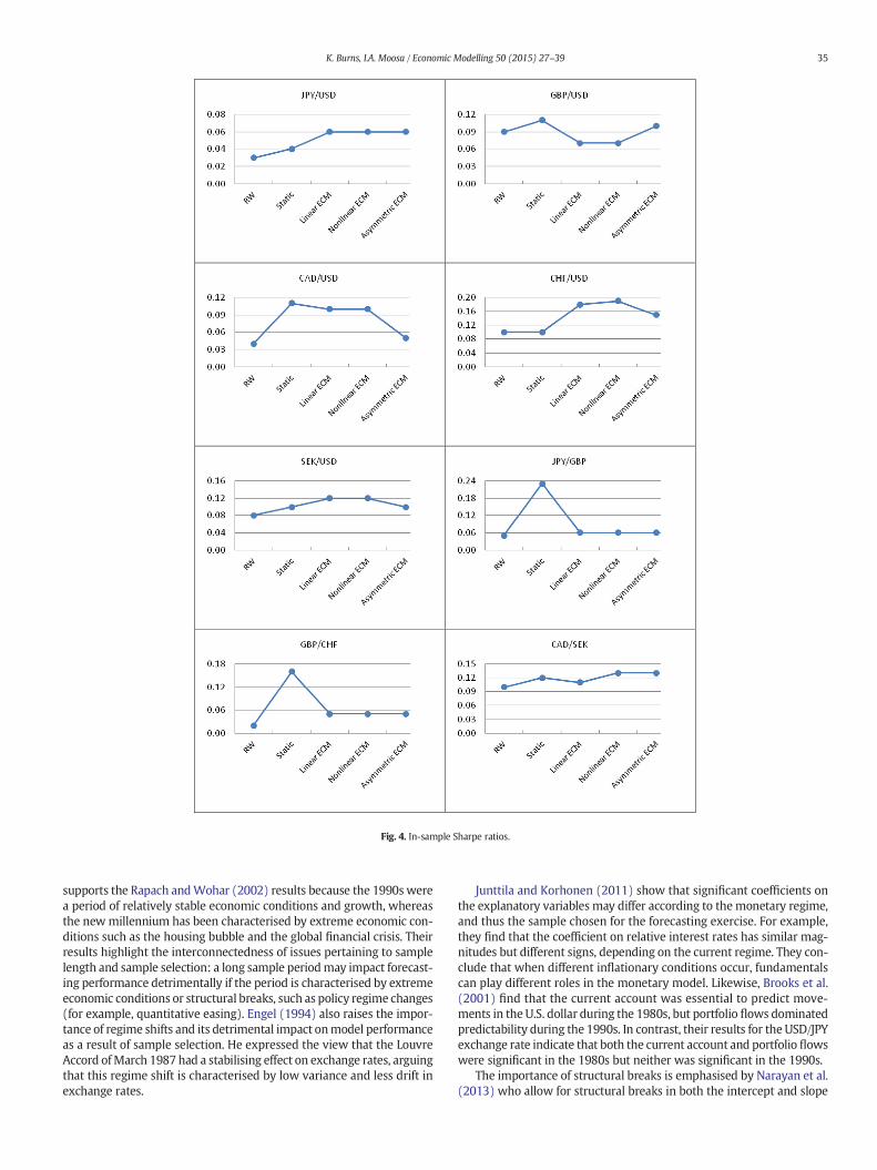
Fig. 4. In-sample Sharpe ratios.

35K. Burns, I.A. Moosa / Economic Modelling 50 (2015) 27–39

supports the Rapach andWohar (2002) results because the 1990s werea period of relatively stable economic conditions and growth, whereasthe newmillennium has been characterised by extreme economic con-ditions such as the housing bubble and the global financial crisis. Theirresults highlight the interconnectedness of issues pertaining to samplelength and sample selection: a long sample periodmay impact forecast-ing performance detrimentally if the period is characterised by extremeeconomic conditions or structural breaks, such as policy regime changes(for example, quantitative easing). Engel (1994) also raises the impor-tance of regime shifts and its detrimental impact onmodel performanceas a result of sample selection. He expressed the view that the LouvreAccord ofMarch 1987 had a stabilising effect on exchange rates, arguingthat this regime shift is characterised by low variance and less drift inexchange rates.

Junttila and Korhonen (2011) show that significant coefficients onthe explanatory variables may differ according to themonetary regime,and thus the sample chosen for the forecasting exercise. For example,they find that the coefficient on relative interest rates has similar mag-nitudes but different signs, depending on the current regime. They con-clude that when different inflationary conditions occur, fundamentalscan play different roles in the monetary model. Likewise, Brooks et al.(2001) find that the current account was essential to predict move-ments in the U.S. dollar during the 1980s, but portfolio flows dominatedpredictability during the 1990s. In contrast, their results for the USD/JPYexchange rate indicate that both the current account and portfolio flowswere significant in the 1980s but neither was significant in the 1990s.

The importance of structural breaks is emphasised by Narayan et al.(2013) who allow for structural breaks in both the intercept and slope

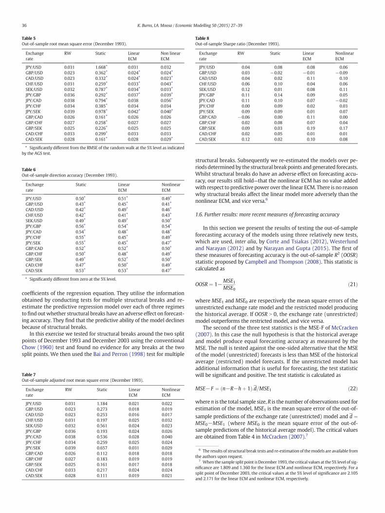
Table 5Out-of-sample root mean square error (December 1993).

Exchangerate

RW Static LinearECM

Non linearECM

JPY/USD 0.031 1.668⁎ 0.031 0.032GBP/USD 0.023 0.362⁎ 0.024⁎ 0.024⁎

CAD/USD 0.023 0.332⁎ 0.024⁎ 0.023⁎

CHF/USD 0.031 0.259⁎ 0.033⁎ 0.043⁎

SEK/USD 0.032 0.787⁎ 0.034⁎ 0.033⁎

JPY/GBP 0.036 0.292⁎ 0.037⁎ 0.039⁎

JPY/CAD 0.038 0.794⁎ 0.038 0.056⁎

JPY/CHF 0.034 0.385⁎ 0.034 0.034JPY/SEK 0.039 0.978⁎ 0.042⁎ 0.040⁎

GBP/CAD 0.026 0.161⁎ 0.026 0.026GBP/CHF 0.027 0.258⁎ 0.027 0.027GBP/SEK 0.025 0.226⁎ 0.025 0.025CAD/CHF 0.033 0.299⁎ 0.033 0.033CAD/SEK 0.028 0.161⁎ 0.028 0.029⁎

⁎ Significantly different from the RMSE of the randomwalk at the 5% level as indicatedby the AGS test.

Table 6Out-of-sample direction accuracy (December 1993).

Exchangerate

Static LinearECM

NonlinearECM

JPY/USD 0.50⁎ 0.51⁎ 0.49⁎

GBP/USD 0.43⁎ 0.45⁎ 0.41⁎

CAD/USD 0.42⁎ 0.49⁎ 0.46⁎

CHF/USD 0.42⁎ 0.41⁎ 0.43⁎

SEK/USD 0.49⁎ 0.49⁎ 0.50⁎

JPY/GBP 0.56⁎ 0.54⁎ 0.54⁎

JPY/CAD 0.54⁎ 0.48⁎ 0.48⁎

JPY/CHF 0.55⁎ 0.45⁎ 0.49⁎

JPY/SEK 0.55⁎ 0.45⁎ 0.47⁎

GBP/CAD 0.52⁎ 0.52⁎ 0.50⁎

GBP/CHF 0.50⁎ 0.48⁎ 0.49⁎

GBP/SEK 0.49⁎ 0.52⁎ 0.50⁎

CAD/CHF 0.47⁎ 0.50⁎ 0.49⁎

CAD/SEK 0.53⁎ 0.53⁎ 0.47⁎

⁎ Significantly different from zero at the 5% level.

Table 8Out-of-sample Sharpe ratio (December 1993).

Exchangerate

RW Static LinearECM

NonlinearECM

JPY/USD 0.04 0.08 0.08 0.06GBP/USD 0.03 −0.02 −0.01 −0.09CAD/USD 0.04 0.02 0.11 0.10CHF/USD 0.06 0.10 0.04 0.06SEK/USD 0.12 0.01 0.08 0.11JPY/GBP 0.11 0.14 0.09 0.05JPY/CAD 0.11 0.10 0.07 −0.02JPY/CHF 0.00 0.09 0.02 0.03JPY/SEK 0.09 0.09 0.01 0.07GBP/CAD −0.06 0.00 0.11 0.00GBP/CHF 0.02 0.08 0.07 0.04GBP/SEK 0.09 0.03 0.19 0.17CAD/CHF 0.02 0.05 0.01 0.01CAD/SEK 0.12 0.02 0.10 0.08

36 K. Burns, I.A. Moosa / Economic Modelling 50 (2015) 27–39

coefficients of the regression equation. They utilise the informationobtained by conducting tests for multiple structural breaks and re-estimate the predictive regression model over each of three regimesto find outwhether structural breaks have an adverse effect on forecast-ing accuracy. They find that the predictive ability of the model declinesbecause of structural breaks.

In this exercise we tested for structural breaks around the two splitpoints of December 1993 and December 2003 using the conventionalChow (1960) test and found no evidence for any breaks at the twosplit points. We then used the Bai and Perron (1998) test for multiple

Table 7Out-of-sample adjusted root mean square error (December 1993).

Exchangerate

RW Static LinearECM

NonlinearECM

JPY/USD 0.031 1.184 0.021 0.022GBP/USD 0.023 0.273 0.018 0.019CAD/USD 0.023 0.253 0.016 0.017CHF/USD 0.031 0.197 0.025 0.032SEK/USD 0.032 0.561 0.024 0.023JPY/GBP 0.036 0.193 0.024 0.026JPY/CAD 0.038 0.536 0.028 0.040JPY/CHF 0.034 0.259 0.025 0.024JPY/SEK 0.039 0.657 0.031 0.029GBP/CAD 0.026 0.112 0.018 0.018GBP/CHF 0.027 0.183 0.019 0.019GBP/SEK 0.025 0.161 0.017 0.018CAD/CHF 0.033 0.217 0.024 0.024CAD/SEK 0.028 0.111 0.019 0.021

structural breaks. Subsequently we re-estimated the models over pe-riods determined by the structural breakpoints and generated forecasts.Whilst structural breaks do have an adverse effect on forecasting accu-racy, our results still hold—that the nonlinear ECM has no value addedwith respect to predictive power over the linear ECM. There is no reasonwhy structural breaks affect the linear model more adversely than thenonlinear ECM, and vice versa.6

1.6. Further results: more recent measures of forecasting accuracy

In this section we present the results of testing the out-of-sampleforecasting accuracy of the models using three relatively new tests,which are used, inter alia, by Corte and Tsiakas (2012), Westerlundand Narayan (2012) and by Narayan and Gupta (2015). The first ofthese measures of forecasting accuracy is the out-of-sample R2 (OOSR)statistic proposed by Campbell and Thompson (2008). This statistic iscalculated as

OOSR ¼ 1−MSE1MSE0

ð21Þ

where MSE1 and MSE0 are respectively the mean square errors of theunrestricted exchange rate model and the restricted model producingthe historical average. If OOSR N 0, the exchange rate (unrestricted)model outperforms the restricted model, and vice versa.

The second of the three test statistics is the MSE-F of McCracken(2007). In this case the null hypothesis is that the historical averageand model produce equal forecasting accuracy as measured by theMSE. The null is tested against the one-sided alternative that the MSEof the model (unrestricted) forecasts is less than MSE of the historicalaverage (restricted) model forecasts. If the unrestricted model hasadditional information that is useful for forecasting, the test statisticwill be significant and positive. The test statistic is calculated as

MSE−F ¼ n−R−hþ 1ð Þ:d=MSE1 ð22Þ

where n is the total sample size, R is the number of observations used forestimation of the model, MSE1 is the mean square error of the out-of-

sample predictions of the exchange rate (unrestricted) model and d ¼MSE0−MSE1 (where MSE0 is the mean square error of the out-of-sample predictions of the historical average model). The critical valuesare obtained from Table 4 in McCracken (2007).7

6 The results of structural break tests and re-estimation of themodels are available fromthe authors upon request.

7 When the sample split point isDecember 1993, the critical values at the 5% level of sig-nificance are 1.809 and 1.360 for the linear ECM and nonlinear ECM, respectively. For asplit point of December 2003, the critical values at the 5% level of significance are 2.105and 2.171 for the linear ECM and nonlinear ECM, respectively.

Table 13The OOSR statistic.

Exchange rate Split: December 1993 Split: December 2003

Linear ECM Non linear ECM Linear ECM Non linear ECM

JPY/USD 0.01 −0.05 0.03 0.02GBP/USD −0.06 −0.07 −0.05 −0.06CAD/USD 0.48 0.48 0.46 0.46CHF/USD −0.12 −0.94 0.03 0.05SEK/USD −0.15 −0.05 0.03 0.02JPY/GBP 0.03 −0.17 −0.01 0.00JPY/CAD 0.02 −1.09 0.01 0.01JPY/CHF −0.01 0.00 0.01 0.01JPY/SEK −0.15 −0.01 0.00 0.03

Table 9Out-of-sample root mean square error (December 2003).

Exchange rate RW Static LinearECM

NonlinearECM

JPY/USD 0.027 0.504⁎ 0.027 0.027GBP/USD 0.026 0.182⁎ 0.026 0.026CAD/USD 0.028 0.396⁎ 0.028 0.028CHF/USD 0.032 0.316⁎ 0.031⁎ 0.031⁎

SEK/USD 0.035 0.301⁎ 0.035 0.035JPY/GBP 0.037 0.207⁎ 0.037 0.037JPY/CAD 0.040 0.606⁎ 0.040 0.040JPY/CHF 0.035 0.292⁎ 0.035 0.035JPY/SEK 0.042 0.615⁎ 0.042 0.042GBP/CAD 0.027 0.358⁎ 0.027 0.027GBP/CHF 0.028 0.296⁎ 0.027 0.027GBP/SEK 0.027 0.132⁎ 0.027 0.027CAD/CHF 0.034 0.244⁎ 0.034 0.034CAD/SEK 0.030 0.090⁎ 0.030 0.030

⁎ Significantly different from the RMSE of the randomwalk at the 5% level as indicatedby the AGS test.

Table 10Out-of-sample direction accuracy (December 2003).

Exchange rate Static LinearECM

NonlinearECM

JPY/USD 0.47⁎ 0.52⁎ 0.54⁎

GBP/USD 0.48⁎ 0.46⁎ 0.42⁎

CAD/USD 0.39⁎ 0.48⁎ 0.48⁎

CHF/USD 0.38⁎ 0.52⁎ 0.55⁎

SEK/USD 0.51⁎ 0.55⁎ 0.54⁎

JPY/GBP 0.58⁎ 0.53⁎ 0.55⁎

JPY/CAD 0.52⁎ 0.48⁎ 0.48⁎

JPY/CHF 0.49⁎ 0.56⁎ 0.48⁎

JPY/SEK 0.56⁎ 0.43⁎ 0.50⁎

GBP/CAD 0.48⁎ 0.52⁎ 0.51⁎

GBP/CHF 0.54⁎ 0.52⁎ 0.50⁎

GBP/SEK 0.56⁎ 0.54⁎ 0.53⁎

CAD/CHF 0.50⁎ 0.48⁎ 0.50⁎

CAD/SEK 0.59⁎ 0.60⁎ 0.50⁎

⁎ Significantly different from zero at the 5% level.

Table 12Out-of-sample Sharpe ratio (December 2003).

Exchange rate RW Static LinearECM

NonlinearECM

JPY/USD −0.03 0.06 −0.05 −0.01GBP/USD −0.05 0.06 −0.15 −0.16CAD/USD −0.06 −0.04 0.04 0.08CHF/USD 0.07 −0.03 0.19 0.09SEK/USD −0.02 0.01 −0.01 0.07JPY/GBP 0.05 0.15 −0.01 0.03JPY/CAD −0.05 0.11 −0.02 0.05JPY/CHF −0.07 −0.05 0.00 0.00JPY/SEK 0.06 0.06 0.01 0.14GBP/CAD −0.15 −0.04 −0.16 −0.13GBP/CHF −0.06 0.11 −0.04 −0.02GBP/SEK −0.02 0.04 0.05 0.05CAD/CHF −0.01 0.15 0.00 −0.02CAD/SEK 0.08 0.21 0.07 0.03

Table 11Out-of-sample adjusted root mean square error (December 2003).

Exchange rate RW Static LinearECM

NonlinearECM

JPY/USD 0.027 0.368 0.019 0.018GBP/USD 0.026 0.132 0.019 0.020CAD/USD 0.028 0.309 0.020 0.020CHF/USD 0.032 0.250 0.022 0.021SEK/USD 0.035 0.211 0.023 0.024JPY/GBP 0.037 0.135 0.025 0.025JPY/CAD 0.040 0.422 0.029 0.029JPY/CHF 0.035 0.208 0.023 0.025JPY/SEK 0.042 0.407 0.032 0.030GBP/CAD 0.027 0.259 0.019 0.019GBP/CHF 0.028 0.201 0.019 0.019GBP/SEK 0.027 0.087 0.018 0.018CAD/CHF 0.034 0.172 0.024 0.024CAD/SEK 0.030 0.058 0.019 0.022

37K. Burns, I.A. Moosa / Economic Modelling 50 (2015) 27–39

The third test statistic is the ENC–NEW proposed by Clark andMcCracken (2001). In this case the null hypothesis, that the modeland historical average have equal predictive accuracy, is tested againstthe alternative hypothesis that the unrestricted model has greater fore-casting accuracy (because of the additional information contained in theexplanatory variables). If the unrestricted model embodies additionalinformation that is useful for forecasting, the test statistic will be signif-icantly positive. The test statistic is calculated as

ENC−NEW ¼ P:c

MSE1ð23Þ

where P is the number of one-step-ahead predictions andc is the covari-ance between the forecasting error terms u0,t + 1 and u0,t + 1 − u1,t + 1

such that subscripts 0 and 1 refer to the exchange rate (unrestricted)model and the historical average, respectively, and MSE1 is the meansquare error of the out-of-sample predictions of the exchange ratemodel. The critical values are obtained from Table 3 in Clark andMcCracken (2000).8

The results obtained by carrying out these additional tests are re-ported in Tables 13–15 for the linear and nonlinear models. InTable 13 we report the estimated OOSR for all of the exchange rates

8 For a split point of December 1993, the critical values at the 5% level of significance are3.007 and 3.586 for the linear ECM and nonlinear ECM, respectively. When the split pointis December 2003, the critical values at the 5% level of significance are 1.8354 and 2.152 forthe linear ECM and nonlinear ECM, respectively.

using the two split points of December 1993 and December 2003. Theresults show that, if anything, the linear ECM model is superior to thenonlinear ECMmodel. When the split point is December 1993, the line-ar ECM is better than the historical average for six out of the 14 ex-change rates whereas the nonlinear model outperforms the historicalaverage in three cases only. When the sample split point is December2003, the linear ECM outperforms the historical average in ten out ofthe 14 cases whereas the nonlinear ECM beats the historical averagein seven cases only.

The results presented in Table 14 tell a similar story. According to theMSE–F statistic, the linear ECM outperforms the historical average for 6of the 14 exchange rates, whereas the nonlinearmodel is superior to the

GBP/CAD −0.03 −0.02 0.01 0.00GBP/CHF 0.02 0.01 0.02 0.00GBP/SEK −0.01 −0.01 −0.01 −0.01CAD/CHF 0.00 0.01 0.02 −0.01CAD/SEK 0.01 −0.03 0.02 −0.02

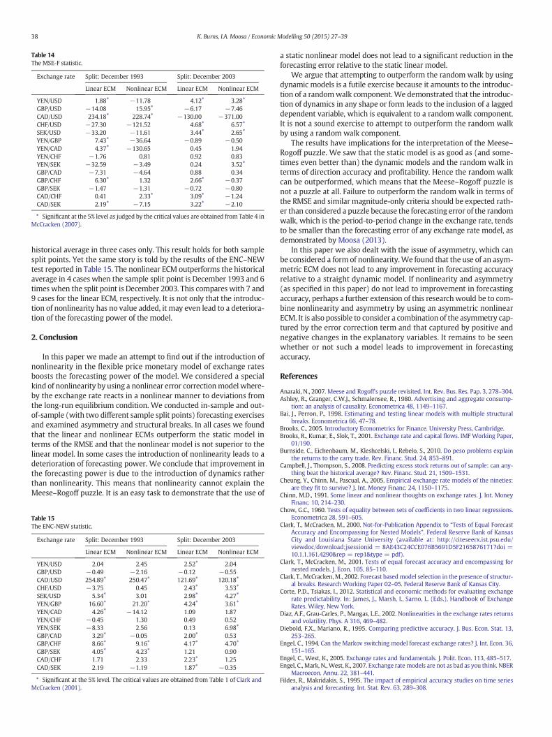
Table 14The MSE-F statistic.

Exchange rate Split: December 1993 Split: December 2003

Linear ECM Nonlinear ECM Linear ECM Nonlinear ECM

YEN/USD 1.88⁎ −11.78 4.12⁎ 3.28⁎

GBP/USD −14.08 15.95⁎ −6.17 −7.46CAD/USD 234.18⁎ 228.74⁎ −130.00 −371.00CHF/USD −27.30 −121.52 4.68⁎ 6.57⁎

SEK/USD −33.20 −11.61 3.44⁎ 2.65⁎

YEN/GBP 7.43⁎ −36.64 −0.89 −0.50YEN/CAD 4.37⁎ −130.65 0.45 1.94YEN/CHF −1.76 0.81 0.92 0.83YEN/SEK −32.59 −3.49 0.24 3.52⁎

GBP/CAD −7.31 −4.64 0.88 0.34GBP/CHF 6.30⁎ 1.32 2.66⁎ −0.37GBP/SEK −1.47 −1.31 −0.72 −0.80CAD/CHF 0.41 2.33⁎ 3.09⁎ −1.24CAD/SEK 2.19⁎ −7.15 3.22⁎ −2.10

⁎ Significant at the 5% level as judged by the critical values are obtained from Table 4 inMcCracken (2007).

38 K. Burns, I.A. Moosa / Economic Modelling 50 (2015) 27–39

historical average in three cases only. This result holds for both samplesplit points. Yet the same story is told by the results of the ENC–NEWtest reported in Table 15. The nonlinear ECM outperforms the historicalaverage in 4 cases when the sample split point is December 1993 and 6times when the split point is December 2003. This compares with 7 and9 cases for the linear ECM, respectively. It is not only that the introduc-tion of nonlinearity has no value added, it may even lead to a deteriora-tion of the forecasting power of the model.

2. Conclusion

In this paper we made an attempt to find out if the introduction ofnonlinearity in the flexible price monetary model of exchange ratesboosts the forecasting power of the model. We considered a specialkind of nonlinearity by using a nonlinear error correctionmodel where-by the exchange rate reacts in a nonlinear manner to deviations fromthe long-run equilibrium condition. We conducted in-sample and out-of-sample (with two different sample split points) forecasting exercisesand examined asymmetry and structural breaks. In all cases we foundthat the linear and nonlinear ECMs outperform the static model interms of the RMSE and that the nonlinear model is not superior to thelinear model. In some cases the introduction of nonlinearity leads to adeterioration of forecasting power. We conclude that improvement inthe forecasting power is due to the introduction of dynamics ratherthan nonlinearity. This means that nonlinearity cannot explain theMeese–Rogoff puzzle. It is an easy task to demonstrate that the use of

Table 15The ENC-NEW statistic.

Exchange rate Split: December 1993 Split: December 2003

Linear ECM Nonlinear ECM Linear ECM Nonlinear ECM

YEN/USD 2.04 2.45 2.52⁎ 2.04GBP/USD −0.49 −2.16 −0.12 −0.55CAD/USD 254.89⁎ 250.47⁎ 121.69⁎ 120.18⁎

CHF/USD −3.75 0.45 2.43⁎ 3.53⁎

SEK/USD 5.34⁎ 3.01 2.98⁎ 4.27⁎

YEN/GBP 16.60⁎ 21.20⁎ 4.24⁎ 3.61⁎

YEN/CAD 4.26⁎ −14.12 1.09 1.87YEN/CHF −0.45 1.30 0.49 0.52YEN/SEK −8.33 2.56 0.13 6.98⁎

GBP/CAD 3.29⁎ −0.05 2.00⁎ 0.53GBP/CHF 8.66⁎ 9.16⁎ 4.17⁎ 4.70⁎

GBP/SEK 4.05⁎ 4.23⁎ 1.21 0.90CAD/CHF 1.71 2.33 2.23⁎ 1.25CAD/SEK 2.19 −1.19 1.87⁎ −0.35

⁎ Significant at the 5% level. The critical values are obtained from Table 1 of Clark andMcCracken (2001).

a static nonlinear model does not lead to a significant reduction in theforecasting error relative to the static linear model.

We argue that attempting to outperform the random walk by usingdynamic models is a futile exercise because it amounts to the introduc-tion of a randomwalk component. We demonstrated that the introduc-tion of dynamics in any shape or form leads to the inclusion of a laggeddependent variable, which is equivalent to a random walk component.It is not a sound exercise to attempt to outperform the random walkby using a random walk component.

The results have implications for the interpretation of the Meese–Rogoff puzzle. We saw that the static model is as good as (and some-times even better than) the dynamic models and the random walk interms of direction accuracy and profitability. Hence the random walkcan be outperformed, which means that the Meese–Rogoff puzzle isnot a puzzle at all. Failure to outperform the random walk in terms ofthe RMSE and similar magnitude-only criteria should be expected rath-er than considered a puzzle because the forecasting error of the randomwalk, which is the period-to-period change in the exchange rate, tendsto be smaller than the forecasting error of any exchange rate model, asdemonstrated by Moosa (2013).

In this paper we also dealt with the issue of asymmetry, which canbe considered a form of nonlinearity.We found that the use of an asym-metric ECM does not lead to any improvement in forecasting accuracyrelative to a straight dynamic model. If nonlinearity and asymmetry(as specified in this paper) do not lead to improvement in forecastingaccuracy, perhaps a further extension of this research would be to com-bine nonlinearity and asymmetry by using an asymmetric nonlinearECM. It is also possible to consider a combination of the asymmetry cap-tured by the error correction term and that captured by positive andnegative changes in the explanatory variables. It remains to be seenwhether or not such a model leads to improvement in forecastingaccuracy.

References

Anaraki, N., 2007. Meese and Rogoff's puzzle revisited. Int. Rev. Bus. Res. Pap. 3, 278–304.Ashley, R., Granger, C.W.J., Schmalensee, R., 1980. Advertising and aggregate consump-

tion: an analysis of causality. Econometrica 48, 1149–1167.Bai, J., Perron, P., 1998. Estimating and testing linear models with multiple structural

breaks. Econometrica 66, 47–78.Brooks, C., 2005. Introductory Econometrics for Finance. University Press, Cambridge.Brooks, R., Kumar, E., Slok, T., 2001. Exchange rate and capital flows. IMF Working Paper,

01/190.Burnside, C., Eichenbaum, M., Kleshcelski, I., Rebelo, S., 2010. Do peso problems explain

the returns to the carry trade. Rev. Financ. Stud. 24, 853–891.Campbell, J., Thompson, S., 2008. Predicting excess stock returns out of sample: can any-

thing beat the historical average? Rev. Financ. Stud. 21, 1509–1531.Cheung, Y., Chinn, M., Pascual, A., 2005. Empirical exchange rate models of the nineties:

are they fit to survive? J. Int. Money Financ. 24, 1150–1175.Chinn, M.D., 1991. Some linear and nonlinear thoughts on exchange rates. J. Int. Money

Financ. 10, 214–230.Chow, G.C., 1960. Tests of equality between sets of coefficients in two linear regressions.

Econometrica 28, 591–605.Clark, T., McCracken, M., 2000. Not-for-Publication Appendix to “Tests of Equal Forecast

Accuracy and Encompassing for Nested Models”. Federal Reserve Bank of KansasCity and Louisiana State University (available at: http://citeseerx.ist.psu.edu/viewdoc/download;jsessionid = 8AE43C24CCE076B5691D5F2165876171?doi =10.1.1.161.4290&rep = rep1&type = pdf).

Clark, T., McCracken, M., 2001. Tests of equal forecast accuracy and encompassing fornested models. J. Econ. 105, 85–110.

Clark, T., McCracken, M., 2002. Forecast basedmodel selection in the presence of structur-al breaks. Research Working Paper 02–05. Federal Reserve Bank of Kansas City.

Corte, P.D., Tsiakas, I., 2012. Statistical and economic methods for evaluating exchangerate predictability. In: James, J., Marsh, I., Sarno, L. (Eds.), Handbook of ExchangeRates. Wiley, New York.

Diaz, A.F., Grau-Carles, P., Mangas, L.E., 2002. Nonlinearities in the exchange rates returnsand volatility. Phys. A 316, 469–482.

Diebold, F.X., Mariano, R., 1995. Comparing predictive accuracy. J. Bus. Econ. Stat. 13,253–265.

Engel, C., 1994. Can the Markov switching model forecast exchange rates? J. Int. Econ. 36,151–165.

Engel, C., West, K., 2005. Exchange rates and fundamentals. J. Polit. Econ. 113, 485–517.Engel, C., Mark, N.,West, K., 2007. Exchange rate models are not as bad as you think. NBER

Macroecon. Annu. 22, 381–441.Fildes, R., Makridakis, S., 1995. The impact of empirical accuracy studies on time series

analysis and forecasting. Int. Stat. Rev. 63, 289–308.

39K. Burns, I.A. Moosa / Economic Modelling 50 (2015) 27–39

Groen, J., 1999. Long horizon predictability of exchange rates: is it for real? Empir. Econ.24, 451–469.

Gynelberg, J., Remolona, E.M., 2007. Risk in carry trades: a look at target currencies in Asiaand the Pacific. BIS Q. Rev. 73–82 (December).

Hamilton, J., 1989. A new approach to the economic analysis of nonstationary time seriesand the business cycle. Econometrica 57, 357–384.

Heckscher, E., 1916. Vaxelkursens Grundval vid Pappersmyntfot. Ekon. Tidsk. 18,309–312.

Hendry, D.F., Ericcson, N., 1991. An econometric analysis of UK money demand in mone-tary trends in the United States and the United Kingdom by Milton Friedman andAnna J Schwartz. Am. Econ. Rev. 81, 8–38.

Inoue, A., Killian, L., 2002. In-sample or out-of-sample tests of predictability: which oneshould we use? European Central Bank Working Paper Series, No.195

Iovino, D., Sitzia, B., 2008. Nonlinearities in exchange rates: double EGARCH thresholdmodels for forecasting volatility. MPRA Papers, No 8661.

Junttila, J., Korhonen, M., 2011. Nonlinearity and time-variation in the monetary model ofexchange rates. J. Macroecon. 33, 288–302.

Kempa, B., Riedel, J., 2013. Nonlinearities in exchange rate determination in a small openeconomy: some evidence for Canada. N. Am. J. Econ. Financ. 24, 268–278.

Kilian, L., 1999. Exchange rates andmonetary fundamentals: what dowe learn from long-horizon regressions? J. Appl. Econ. 14, 491–510.

Kilian, L., Taylor, M., 2003. Why is it so difficult to beat the random walk forecast ofexchange rates? J. Int. Econ. 60, 85–107.

Kirikos, D., 2000. Forecasting exchange rates out-of-sample: random walk vs Markovswitching regimes. Appl. Econ. Lett. 7, 133–136.

Kruse, R., Frommel, M., Menkhoff, L., Sibbertsen, P., 2012. What do we know about realexchange rate nonlinearities? Empir. Econ. 43, 457–474.

Leon, H., Najarian, S., 2003. Asymmetric adjustment and nonlinear dynamics in realexchange rates. IMF Working Papers, No WP/03/159.

Lopez-Suarez, C.F., Rodriguez-Lopez, J.A., 2011. Nonlinear exchange rate predictability.J. Int. Money Financ. 30, 877–895.

Marcellino, M., 2002. Instability and non-linearity in the EMU. Working Paper.IEP-Universita Bocconi.

Marcellino, M., Stock, J., Watson, M., 2001. Macroeconomic forecasting in the Euro area:country specific versus area-wide information. Working Paper. Innocenzo GaspariniInstitute for Economic Research, p. 201.

Mark, N., 1995. Exchange rates and fundamentals: evidence on long horizon predictabil-ity. Am. Econ. Rev. 85, 201–218.

McCracken, M., 2007. Asymptotics for out of sample tests of granger causality. J. Econ.140, 719–752.

Meese, R., Rogoff, K., 1983. Empirical exchange rate models of the seventies: do they fitout of sample? J. Int. Econ. 14, 3–24.

Moosa, I.A., 2000. A structural time series test of the monetary model of exchangerates under the german hyperinflation. J. Int. Financ. Mark. Inst. Money 10,213–223.

Moosa, I.A., 2013. Why is it so difficult to outperform the random walk in exchange rateforecasting. Appl. Econ. 23, 3340–3346.

Moosa, I.A., Burns, K., 2012. Can exchange rate forecasting models outperform therandom walk? Magnitude, direction and profitability as criteria. Econ. Int. 65,473–490.

Moosa, I.A., Burns, K., 2013. A reappraisal of the Meese–Rogoff puzzle. Appl. Econ. 46,30–40.

Moosa, I.A., Burns, K., 2015. Demystifying the Meese–Rogoff Puzzle. Palgrave, London.Narayan, P.K., Gupta, R., 2015. Has oil price predicted stock returns for over a century.

Energy Econ. 48, 18–23.Narayan, P.K., Narayan, S., Sharma, S.S., 2013. An analysis of commodity markets: what

gain for investors? J. Bank. Financ. 37, 3878–3889.Narayan, P.K., Sharma, S.S., Thuraisamy, K., 2014. An analysis of price discovery from

panel data models of CDs and equity returns. J. Bank. Financ. 41, 167–177.Rapach, D., Wohar, M., 2002. Testing the monetary model of exchange rate determina-

tion: new evidence from a century of data. J. Int. Econ. 58, 359–385.Sarno, L., Taylor, M., 2002. The Economics of Exchange Rates. Cambridge University Press,

Cambridge.Tashman, L., 2000. Out-of-sample tests of forecasting accuracy: an analysis and review.

Int. J. Forecast. 16, 437–450.Taylor, M., Peel, D., 2000. Non-linear adjustment long-run equilibrium and exchange rate

fundamentals. J. Int. Money Financ. 19, 22–54.Taylor, M., Peel, D., Sarno, L., 2001. Nonlinear mean-reversion in real exchange rates:

toward a solution to the purchasing power parity puzzles. Int. Econ. Rev. 42,1015–1042.

Westerlund, J., Narayan, P.K., 2012. Does the choice of estimator matter when forecastingreturns? J. Bank. Financ. 36, 2632–2640.