PERMIS-2007

FOREWORDSPONSORS

PerMIS 2008

PERFORMANCE METRICSFOR

INTELLIGENT SYSTEMS (PERMIS) WORKSHOPNational Institute of Standards and Technology, Gaithersburg, Maryland USA

August 19 - 21, 2008

Edited byR. MadhavanE.R. Messina

NIST SpecialPublication 1090

FOREWORDThe 2008 Performance Metrics for Intelligent Systems (PerMIS'08) Workshop will be the eighth in the series that started in 2000, targeted at defining measures and methodologies of evaluating performance of intelligent systems. The workshop has proved to be an excellent forum for discussions and partnerships, dissemination of ideas, and future collaborations in an informal setting. Attendees usually include researchers, graduate students, practitioners from industry, academia, and government agencies.

PerMIS’08 aims at identifying and quantifying contributions of functional intelligence towards achieving success. Our working definition of functional intelligence is “the ability to act appropriately in an uncertain environment, where appropriate action is that which increases the probability of success”, and success is “the achievement of behavioral goals” (J. Albus, 1991). In addition to the main theme, as in previous years, the workshop will focus on applications of performance measures to practical problems in commercial, industrial, homeland security, and military applications. Topic areas include, but are not limited to:

Defining and measuring aspects of a system:

• The level of autonomy

• Human-robot interaction

• Collaboration & coordination

• Taxonomies

• Biologically inspired modelsEvaluating components within intelligent system

• Sensing and perception

• Knowledge representation, world models, ontologies

• Planning and control

• Learning and adaption

• Reasoning

Infrastructural support for performance evaluation

• Testbeds and competitions for intercomparisons

• Instrumentation and other measurement tools

• Simulation and modeling supportTechnology readiness measures for intelligent systems

Applied performance measures in various domains, e.g.,

• Intelligent transportation systems

• Emergency response robots (search and rescue, bomb disposal)

• Homeland security systems

• De-mining robots

• Defense robotics

• Hazardous environments (e.g., nuclear remediation)

• Industrial and manufacturing systems

• Space/Aerial robotics

• Medical Robotics & assistive devices

PerMIS 2008

PerMIS’08 will feature five plenary addresses and seven special sessions. The plenary speakers are world-class experts in their own field and we are confident that the attendees will be able to benefit from their presentations. This year, there is a special session for every (parallel) general session. Over the course of three days, there will be twelve sessions related to performance of intelligent systems covering an array of topics from medical systems to manufacturing, mobile robotics to virtual automation, human-system interac-tion to biologically inspired models, and much more.

Special thanks are due to the Program Committee for publicizing the workshop, the special session organiz-ers for proposing interesting topics and bringing together researchers related to their sessions, and the reviewers who provided feedback to the authors, and helped us to assemble an excellent program. We much appreciate the authors submitting their papers to this workshop and for sharing their thoughts and experi-ences related to their research with the workshop attendees.

PerMIS’08, is sponsored by NIST with technical co-sponsorship of the IEEE Washington Section Robotics and Automation Society Chapter and in-cooperation with the Association for Computing Machinery (ACM) Special Interest Group on Artificial Intelligence (SIGART). As in previous years, the proceedings of PerMIS will be indexed by INSPEC, Compendex, ACM’s Digital Library, and are released as a NIST Special Publication. Springer Publishers are back again this year to raffle off some of the books that will be displayed at their booth during the course of the workshop. Selected papers from this workshop will be considered for inclusion in an edited book volume by Springer. We gratefully acknowledge the support of our sponsors.

We sincerely hope that you enjoy the presentations and the social programs!

Raj Madhavan Elena MessinaProgram Chair General Chair

SPONSORS

PerMIS 2008

PROGRAM COMMITTEE

General Chair:

Elena Messina (Intelligent Systems Division, NIST, USA)

Program Chair:

Raj Madhavan (Oak Ridge National Laboratory/NIST, USA)

S. Balakirsky (NIST USA)

R. Bostelman (NIST USA)

F. Bonsignorio (Heron Robots Italy)

G. Berg-Cross (EM & I USA)

J. Bornstein (ARL USA)

P. Courtney (PerkinElmer UK)

J. Evans (USA)

D. Gage (XPM Tech. USA)

J. Gunderson (GammaTwo USA)

L. Gunderson (GammaTwo USA)

S. K. Gupta (UMD USA)

A. Jacoff (NIST USA)

S. Julier (Univ. College London UK)

M. Lewis (UPitt USA)

R. Lakaemper (Temple Univ USA)

T. Kalmar-Nagy (Texas A & M USA)

A. del Pobil (Univ. Jaume-I Spain)

S. Ramasamy UALR USA)

L. Reeker (NIST USA)

C. Schlenoff (NIST USA)

M. Shneier (NIST USA)

E. Tunstel (JHU-APL USA)

PerMIS 2008

Table of Contents Foreword . . . . . . . . . . . . . . . . . . . . . . . . . . . . . . . . . . . . . . . . . . . . . . . . . . . . . . . . . . . . . . . . . . . vii Sponsors . . . . . . . . . . . . . . . . . . . . . . . . . . . . . . . . . . . . . . . . . . . . . . . . . . . . . . . . . . . . . . . . . . . viii Program Committee . . . . . . . . . . . . . . . . . . . . . . . . . . . . . . . . . . . . . . . . . . . . . . . . . . . . . . . . . . . ix Plenary Addresses . . . . . . . . . . . . . . . . . . . . . . . . . . . . . . . . . . . . . . . . . . . . . . . . . . . . . . . . . . . . . x Workshop Program . . . . . . . . . . . . . . . . . . . . . . . . . . . . . . . . . . . . . . . . . . . . . . . . . . . . . . . . . . . xiii Author Index . . . . . . . . . . . . . . . . . . . . . . . . . . . . . . . . . . . . . . . . . . . . . . . . . . . . . . . . . . . . . . . . xix Acknowledgements . . . . . . . . . . . . . . . . . . . . . . . . . . . . . . . . . . . . . . . . . . . . . . . . . . . . . . . . . . . xxi

Technical Sessions TUE-AM1 Performance Evaluation

Evolution of the SCORE Framework to Enhance Field-Based Performance Evaluations of Emerging Technologies [Brian Weiss, Craig Schlenoff] . . . . . . . . . . . . . . . . . . . . . . . . . . . . . . . . . . . . . . . . . . . . . 1 Reliability Estimation and Confidence Regions from Subsystem and Full System Tests via Maximum Likelihood [James Spall] . . . . . . . . . . . . . . . . . . . . . . . . . . . . . . . . . . . . . . . . . . . . . . . . . . . . . . . . . . 9 Fuzzy-Logic-Based Approach for Identifying Objects of Interest in the PRIDE Framework [Zeid Kootbally, Craig Schlenoff, Raj Madhavan, Sebti Foufou] . . . . . . . . . . . . . . . . . . 17

Identifying Objects in Range Data Based on Similarity Transformation Invariant Shape Signatures [Xiaolan Li, Afzal Godi, Asim Wagan] . . . . . . . . . . . . . . . . . . . . . . . . . . . . . . . . . . . . . . 25 Stepfield Pallets: Repeatable Terrain for Evaluating Robot Mobility [Adam Jacoff, Anthony Downs, Ann Virts, Elena Messina] . . . . . . . . . . . . . . . . . . . . . . 29 Potential Scaling Effects for Asynchronous Video in Multirobot Search [Prasanna Velagapudi, Paul Scerri, Katia Sycara, Huadong Wang, Michael Lewis]. . . 35

TUE-AM2 Special Session I: Cognitive Systems of EU Cognition Programme

Cognitive Systems of EU Cognition Programme* [Patrick Courtney]

i

The Rat’s Life Benchmark: Competing Cognitive Robots [Olivier Michel, Fabien Rohrer] . . . . . . . . . . . . . . . . . . . . . . . . . . . . . . . . . . . . . . . . . . . 43 The iCub Humanoid Robot: An Open Platform for Research in Embodied Cognition [Giorgio Metta, Giulio Sandini, David Vernon, Lorenzo Natale, Francesco Nori] . . . . 50 An Open-Source Simulator for Cognitive Robotics Research: The Prototype of the iCub Humanoid Robot Simulator [Vadim Tikhanoff, Angelo Cangelosi, Paul Fitzpatrick, Giorgio Metta, Lorenzo Natale, Francesco Nori] . . . . . . . . . . . . . . . . . . . . . . . . . . . . . . . . . . . . . . . . . . . . . . . . . . . . . . . . 57 Symbiotic Robot Organisms: REPLICATOR and SYMBRION Projects [Serge Kernbach, Eugen Meister, Florian Schlachter, Kristof Jebens, Marc Szymanski, Jens Liedke, Davide Laneri, Lutz Winkler, Thomas Schmickl, Ronald Thenius, Paolo Corradi, Leonardo Ricotti] . . . . . . . . . . . . . . . . . . . . . . . . . . . . . . . . . . . . . . . . . . . . . . . .62 Virtual Agent Modeling in the RASCALLI Platform [Christian Eis, Marcin Skowron, Brigitte Krenn] . . . . . . . . . . . . . . . . . . . . . . . . . . . . . . 70

TUE-PM1 Human-System Interaction

Evaluation Criteria for Human-Automation Performance Metrics [Birsen Donmez, Patricia Pina, Mary Cummings] . . . . . . . . . . . . . . . . . . . . . . . . . . . . . .77

Assessing Measures of Coordination Demand Based on Interaction Durations [Michael Lewis, Jijun Wang] . . . . . . . . . . . . . . . . . . . . . . . . . . . . . . . . . . . . . . . . . . . . . . 83

The Gestural Joystick and the Efficacy of the Path Tortuosity Metric for Human/Robot Interaction [Richard Voyles, Jaewook Bae, Roy Godzdanker] . . . . . . . . . . . . . . . . . . . . . . . . . . . . . .91

Modeling of Thoughtful Behavior with Dynamic Expert System [Vadim Stefanuk] . . . . . . . . . . . . . . . . . . . . . . . . . . . . . . . . . . . . . . . . . . . . . . . . . . . . . . . 98

TUE-PM2 Special Session II: Architectures for Unmanned Systems UAV Architectures* [George Vachtsevanos]

Architectures for Unmanned Systems* [James Albus] Levels-of-Autonomy of the ASTM F41 Unmanned Maritime Vehicles Standard* [Mark Rothgeb]

ii

Ontological Perspectives for Autonomy Performance [Hui-Min Huang, Elena Messina, Tsai Hong, Craig Schlenoff] . . . . . . . . . . . . . . . . . . 101

WED-AM1 Metrics & Measures

Robotic Systems Technical and Operational Metrics Correlation [Jason Schenk, Robert Wade] . . . . . . . . . . . . . . . . . . . . . . . . . . . . . . . . . . . . . . . . . . . . .108 Survey of Domain-Specific Performance Measures in Assistive Robotic Technology [Katherine Tsui, Holly Yanco, David Feil-Seifer, Maja Mataric] . . . . . . . . . . . . . . . . . 116 Refining the Cognitive Decathlon [Robert Simpson, Charles Twardy] . . . . . . . . . . . . . . . . . . . . . . . . . . . . . . . . . . . . . . . . 124 Using Metrics to Optimize a High Performance Intelligent Image Processing Code [Scott Spetka, Susan Emen, George Ramseyer, Richard Linderman] . . . . . . . . . . . . . 132 Measurement Techniques for Multiagent Systems [Robert Lass, Evan Sultanik, William Regli] . . . . . . . . . . . . . . . . . . . . . . . . . . . . . . . . . 134 RoboCupRescue Robot League: 2008 Overview* [Adam Jacoff, Andreas Birk, Johannes Pellenz, Ehsan Mihankhah, Raymond Sheh, Satoshi Tadokoro]

WED-AM2 Special Session III: Performance Metrics for Perception in Intelligent Manufacturing

Performance of Super-Resolution Enhancement for Flash LADAR Data [Shuowen Hu, Susan Young, Tsai Hong] . . . . . . . . . . . . . . . . . . . . . . . . . . . . . . . . . . . . 143 Performance Evaluation of Laser Trackers [Bala Muralikrishnan, Daniel Sawyer, Christopher Blackburn, Steven Phillips, Bruce Borchardt, Tyler Estler] . . . . . . . . . . . . . . . . . . . . . . . . . . . . . . . . . . . . . . . . . . . . . . . . . 149 Preliminary Analysis of Conveyor Dynamic Motion for Automation Applications [Jane Shi] . . . . . . . . . . . . . . . . . . . . . . . . . . . . . . . . . . . . . . . . . . . . . . . . . . . . . . . . . . . . 156 3D Part Identification Based on Local Shape Descriptors [Xiaolan Li, Afzal Godil, Asim Wagan] . . . . . . . . . . . . . . . . . . . . . . . . . . . . . . . . . . . . . 162 Calibration of a System of a Gray-Value Camera and an MDSI Range camera [Tobias Hanning, Aless Lasaruk] . . . . . . . . . . . . . . . . . . . . . . . . . . . . . . . . . . . . . . . . . 167 Dynamic 6DOF Metrology for Evaluating a Visual Servoing System [Tommy Chang, Tsai Hong, Mike Shneier, German Holguin, Johnny Park, Roger Eastman]. . . . . . . . . . . . . . . . . . . . . . . . . . . . . . . . . . . . . . . . . . . . . . . . . . . . . . .173

iii

WED-PM1 Autonomous Systems

Integrating Reification and Ontologies for Mobile Autonomous Robots [James Gunderson, Louise Gunderson] . . . . . . . . . . . . . . . . . . . . . . . . . . . . . . . . . . . . .181 Quantification of Line Tracking Solutions for Automotive Applications [Jane Shi, Rick Rourke, Dave Groll, Peter Tavora] . . . . . . . . . . . . . . . . . . . . . . . . . . . .189 Mobile Robotic Surveying Performance for Planetary Surface Site Characterization [Edward Tunstel] . . . . . . . . . . . . . . . . . . . . . . . . . . . . . . . . . . . . . . . . . . . . . . . . . . . . . . 200 Evaluating Situation Awareness of Autonomous Systems [Jan Gehrke] . . . . . . . . . . . . . . . . . . . . . . . . . . . . . . . . . . . . . . . . . . . . . . . . . . . . . . . . . 206

WED-PM2 Special Session IV: Results from a Virtual Manufacturing Automation Competition

NIST/IEEE Virtual Manufacturing and Automation Competition: From Earliest Beginnings to Future Directions [Stephen Balakirsky, Raj Madhavan, Chris Scrapper] . . . . . . . . . . . . . . . . . . . . . . . . . .214 Analysis of a Novel Docking Technique for Autonomous Robots [George Henson, Michael Maynard, Xinlian Liu, George Dimitoglou] . . . . . . . . . . . . 220 Partitioning Algorithm for Path Determination of Automated Robotic Part Delivery System in Manufacturing Environments [Payam Matin, Ali Eydgahi, Ranjith Chowdary] . . . . . . . . . . . . . . . . . . . . . . . . . . . . . .224 Algorithms and Performance Analysis for Path Navigation of Ackerman-Steered Autonomous Robots [George Henson, Michael Maynard, George Dimitoglou, Xinlian Liu] . . . . . . . . . . . .230

THU-AM1 Model-based Performance Assessment

Wireless Communications in Tunnels for Urban Search and Rescue Robots [Kate Remley, George Hough, Galen Koepke, Dennis Camell, Robert Johnk, Chriss Grosvenor] . . . . . . . . . . . . . . . . . . . . . . . . . . . . . . . . . . . . . . . . . . . . . . . . . . . . . . . . . . . 236 A Performance Assessment of Calibrated Camera Networks for Construction Site Monitoring [Itai Katz, Nicholas Scott, Kam Saidi] . . . . . . . . . . . . . . . . . . . . . . . . . . . . . . . . . . . . . . 244 A Queuing-Theoretic Framework for Modeling and Analysis of Mobility in WSNs [Harsh Bhatia, Rathinasamy Lenin, Aarti Munjal, Srini Ramaswamy, Sanjay Srivastava] . . . . . . . . . . . . . . . . . . . . . . . . . . . . . . . . . . . . . . . . . . . . . . . . . . . . . 248

iv

Towards Information Networks to Support Composable Manufacturing [Mahesh Mani, Albert Jones, Junho Shin, Ram Sriram] . . . . . . . . . . . . . . . . . . . . . . . . 254 3D Reconstruction of Rough Terrain for USARSim using a Height-map Method [Gael Roberts, Stephen Balakirsky, Sebti Foufou] . . . . . . . . . . . . . . . . . . . . . . . . . . . . 259

THU-AM2 Special Session V: Quantitative Assessment of Robot-generated Maps

Characterizing Robot-Generated Maps: The Importance of Representations and Objective Metrics* [Chris Scrapper, Raj Madhavan, Stephen Balakirsky] Using Virtual Scans to Improve Alignment Performance in Robot Mapping [Rolf Lakeamper, Nagesh Adluru] . . . . . . . . . . . . . . . . . . . . . . . . . . . . . . . . . . . . . . . . . 265 The Role of Bayesian Bounds in Comparing SLAM Algorithms Performance [Andrea Censi] . . . . . . . . . . . . . . . . . . . . . . . . . . . . . . . . . . . . . . . . . . . . . . . . . . . . . . . . 271 Map Quality Assessment [Asim Wagan, Afzal Godil, Xiaolan Li] . . . . . . . . . . . . . . . . . . . . . . . . . . . . . . . . . . . . . 278 Discussion: Roadmap for Map Evaluation Frameworks

THU-PM1 Special Session VI: Biologically Inspired Models of Intelligent Systems Introduction to Biological Inspiration for Intelligent Systems [Gary Berg-Cross] . . . . . . . . . . . . . . . . . . . . . . . . . . . . . . . . . . . . . . . . . . . . . . . . . . . . . 283 Overview of Biologically Inspired Cognitive Architectures (BICA)* [Alexei Samsonovich] Recent modeling and Rapid Prototyping Experience Aimed at Building Architectures of Cognitive Agents* [Giorgio Ascoli] Applying Developmental-Inspired Principles to the Field of Developmental Robotics [Gary Berg-Cross] . . . . . . . . . . . . . . . . . . . . . . . . . . . . . . . . . . . . . . . . . . . . . . . . . . . . . 288 Discussion of Biologically Inspired Models [Panel]

THU-PM2 Special Session VII: Medical Robotics

Overcoming Barriers to Wider Adoption of Mobile Telerobotic Surgery: Engineering, Clinical and Business Challenges [Gerald Moses, Charles Doarn, Blake Hannaford, Jacob Rosen] . . . . . . . . . . . . . . . . 293

v

Calibration of a Computer Assisted Orthopaedic Hip Surgery Phantom [Daniel Sawyer, Nick Dagalakis, Craig Shakarji, Yong Kim] . . . . . . . . . . . . . . . . . . . 297 HLPR Chair – A Novel Patient Transfer Device [Roger Bostelman, James Albus, Joshua Johnson] . . . . . . . . . . . . . . . . . . . . . . . . . . . 302 Robotic Navigation in Crowded Environments: Key Challenges for Autonomous Navigation Systems [James Ballantyne, Salman Valibeik, Ara Darzi, Guang-Zhong Yang] . . . . . . . . . . . .306 Note: * Presentation Only

vi

FOREWORDThe 2008 Performance Metrics for Intelligent Systems (PerMIS'08) Workshop is the eighth in the series that started in 2000, targeted at defining measures and methodologies of evaluating performance of intelligent systems. The workshop has proved to be an excellent forum for discussions and partnerships, dissemination of ideas, and future collaborations in an informal setting. Attendees usually include researchers, graduate students, practitioners from industry, academia, and government agencies.

PerMIS’08 aims at identifying and quantifying contributions of functional intelligence towards achieving success. Our working definition of functional intelligence is “the ability to act appropriately in an uncertain environment, where appropriate action is that which increases the probability of success”, and success is “the achievement of behavioral goals” (J. Albus, 1991). In addition to the main theme, as in previous years, the workshop focuses on applications of performance measures to practical problems in commercial, industrial, homeland security, and military applications. Topic areas include, but are not limited to:

Defining and measuring aspects of a system:

• The level of autonomy

• Human-robot interaction

• Collaboration & coordination

• Taxonomies

• Biologically inspired modelsEvaluating components within intelligent system

• Sensing and perception

• Knowledge representation, world models, ontologies

• Planning and control

• Learning and adaption

• Reasoning

Infrastructural support for performance evaluation

• Testbeds and competitions for intercomparisons

• Instrumentation and other measurement tools

• Simulation and modeling supportTechnology readiness measures for intelligent systems

Applied performance measures in various domains, e.g.,

• Intelligent transportation systems

• Emergency response robots (search and rescue, bomb disposal)

• Homeland security systems

• De-mining robots

• Defense robotics

• Hazardous environments (e.g., nuclear remediation)

• Industrial and manufacturing systems

• Space/Aerial robotics

• Medical Robotics & assistive devices

PerMIS 2008vii

PerMIS’08 features five plenary addresses and seven special sessions. The plenary speakers are world-class experts in their own field and we are confident that the attendees will be able to benefit from their presentations. This year, there is a special session for every (parallel) general session. Over the course of three days, there will be twelve sessions related to performance of intelligent systems covering an array of topics from medical systems to manufacturing, mobile robotics to virtual automation, human-system interac-tion to biologically inspired models, and much more.

Special thanks are due to the Program Committee for publicizing the workshop, the special session organiz-ers for proposing interesting topics and bringing together researchers related to their sessions, and the reviewers who provided feedback to the authors, and helped us to assemble an excellent program. We much appreciate the authors submitting their papers to this workshop and for sharing their thoughts and experi-ences related to their research with the workshop attendees.

PerMIS’08, is sponsored by NIST with technical co-sponsorship of the IEEE Washington Section Robotics and Automation Society Chapter and in-cooperation with the Association for Computing Machinery (ACM) Special Interest Group on Artificial Intelligence (SIGART). As in previous years, the proceedings of PerMIS will be indexed by INSPEC, Compendex, ACM’s Digital Library, and are released as a NIST Special Publication. Springer Publishers was back again this year to raffle off some of the books that were displayed at their booth during the course of the workshop. Selected papers from this workshop are being included in an edited book volume by Springer. We gratefully acknowledge the support of our sponsors.

We sincerely hope that you enjoy the presentations and the social programs!

Raj Madhavan Elena MessinaProgram Chair General Chair

SPONSORS

PerMIS 2008viii

PROGRAM COMMITTEE

General Chair:

Elena Messina (Intelligent Systems Division, NIST, USA)

Program Chair:

Raj Madhavan (Oak Ridge National Laboratory/NIST, USA)

S. Balakirsky (NIST USA)

R. Bostelman (NIST USA)

F. Bonsignorio (Heron Robots Italy)

G. Berg-Cross (EM & I USA)

J. Bornstein (ARL USA)

P. Courtney (PerkinElmer UK)

J. Evans (USA)

D. Gage (XPM Tech. USA)

J. Gunderson (GammaTwo USA)

L. Gunderson (GammaTwo USA)

S. K. Gupta (UMD USA)

A. Jacoff (NIST USA)

S. Julier (Univ. College London UK)

M. Lewis (UPitt USA)

R. Lakaemper (Temple Univ USA)

T. Kalmar-Nagy (Texas A & M USA)

A. del Pobil (Univ. Jaume-I Spain)

S. Ramasamy UALR USA)

L. Reeker (NIST USA)

C. Schlenoff (NIST USA)

M. Shneier (NIST USA)

E. Tunstel (JHU-APL USA)

PerMIS 2008ix

ABSTRACTWe hypothesize that adding compu-tational cognitive reasoning compo-nents to intelligent systems will result in three benefits:Most if not all intelligent systems must interact with humans, who are the ultimate users of these systems. Giving the system cognitive models can enhance the human-system in-terface by allowing more common ground in the form of cognitively plausible representations and qualita-tive reasoning. By using cognitive models, reasoning mechanisms and representations, we believe that we can yield a more effective and effi-cient interface that accommodates the user.

Since the resulting system in interact-ing with the human, giving it behav-iors that are more natural to the hu-man can also result in more natural interactions between the human and the intelligent system. For example,

mobile robots that must work collabora-tively with humans can actually result in less effective interac-tions if its behaviors are alien or non-intuitive to the human. By incorporating cognitive models, we can develop systems whose behavior is more expected and natural.

One key interest is in measuring the performance of intelligent systems. We propose that an intelligent system that is cognitively enhanced can be more directly compared to human level per-formance. Further, if cognitive models of human performance have been developed in creating the intelligent system, we can directly compare the intelligent systems behavior and perform-ance in the task to the human subject behavior and performance.

In this talk, I will present several instantiations of developing cognitively enhanced intelligent systems.

BIOGRAPHY Alan C. Schultz is the Director of the Navy Center for Applied Research in Artificial Intelligence at the Naval Research Labora-tory in Washington, DC. His research is in the areas of human-robot interaction, cognitive robotics, evolutionary robotics, learn-ing in robotic systems, and adaptive systems. He is the recipient of an Alan Berman Research Publication Award, and has pub-lished over 90 articles on HRI, machine learning and robotics. Alan is currently the co-chair of the AAAI Symposia Series, and chaired the 1999 and 2000 AAAI Mobil Robot Competition and Exhibitions.

PLENARY SPEAKER

Mr. Alan Schultz

Navy Center for Applied

Research in Artificial

Intelligence (NCARAI), USA

Cognitively Enhanced Intelligent Systems

Tues. 8:30 am

ABSTRACT Haptics is the science and technol-ogy of experiencing and creating touch sensations. This talk will exam-ine the role of haptics in three types of medical systems: surgical robotics, surgical simulators, and rehabilitation robotics. Robot-assisted surgery can improve the outcomes of medical procedures by enhancing accuracy and minimally invasive access, thereby reducing patient trauma and recovery time. However, the current lack of force and tactile information is hypothesized to compromise system performance. With approaches rang-ing from psychophysical studies to control systems engineering, we are designing teleoperated robots capa-ble of providing haptic feedback in challenging surgical environments. Haptic information is also needed for accurate surgical simulation. Surgical simulators present a safe and poten-tially effective method for surgical training, and can also be used in

robot-assisted surgery for pre- and intra-operative planning. I will describe experiments to determine the mechanics of interaction between surgical instruments and tissues, as well as techniques for accurate patient-specific mod-eling. Finally, rehabilitation through robotically enabled orthotics and prosthetics inherently requires understanding and appropri-ate generation of haptic interactions. Our recent work in this area includes motor control augmentation with an exoskeleton robot, and studies of the role of haptic proprioception in prosthetic limb use.

BIOGRAPHYAllison M. Okamura received the BS degree from the University of California at Berkeley in 1994, and the MS and PhD degrees from Stanford University in 1996 and 2000, respectively, all in mechanical engineering. She is currently an associate professor of mechanical engineering and the Decker Faculty Scholar at Johns Hopkins University. She is associate director of the Laboratory for Computational Sensing and Robotics and a thrust leader of the NSF Engineering Research Center for Computer-Integrated Surgical Systems and Technology. Her awards include the 2005 IEEE Robotics Automation Society Early Academic Career Award, the 2004 US NSF CAREER Award, the 2004 JHU George E. Owen Teaching Award, and the 2003 JHU Diversity Recognition Award. Her research interests are haptics, teleoperation, medical robotics, virtual environments and simulators, prosthetics, rehabilitation engineering, and engineering education.

PLENARY SPEAKER

Prof. Allison Okamura

The Johns Hopkins

University, USA

Haptics in Medical

Robotics: Surgery,

Simulation, and

Rehabilitation

Tues. 2:00 pm

PerMIS 2008 x

ABSTRACTIn industrial robotics, system integration is a rather common business. Robot manufacturers typically team up with a number of so-called system integrators, which design robot cells, assembly lines and entire manufacturing plants out of “standardized” components, such as manipulators, sensors, tools, and conveyor systems.

In service robotics the situation is in no way comparable. Service robots are typically considered as mass products, which are designed like dish washers or play stations. System integration is simply part of the regular product design.

It would be rather irrelevant to discuss this issue any further, if the design of a service robot for

some specific application was a task like the design of a dish washer. As a matter of fact, the two tasks have not much if anything at all in common.

The design of a service robot is more the result of the ingenuity of an engineer rather of established procedures or methodologies or even technologies. Typically every new service robot is design from scratch. Not too seldom, the service task itself and the operational constraints are not too well understood, neither is the business model under which the automation of a service could become an economic success. A plenitude of components such as sensors, actuators, operating systems, algorithms are available but no common recipe for integrating and compiling them into a competitive product.

Service robotics today is in a situation very much comparable to the situation of the car industry in 1885, when Carl Benz built the first car. The industry is virtually not existing. Potential players and investors are skeptical because not only a realistic market but also a realistic technology assessment gives them a rather fuzzy picture.

This situation has motivated the German Ministry for Education and Research to invest into a so-called technology platform for service robotics. Other funding agencies such as the European Commission are implementing similar initiatives.

In my presentation I will talk about the German Service Robotics Initiative, which as a major activity pushes the development of such a technology platform. The platform is considered as a vehicle for understanding and managing the requirements for system integration in service robotics. I will talk about a first

approach of this Initiative to incrementally integrate, evaluate and harmonize available off the shelf components and their interfaces to simplify and accelerate the development of new service robots. I will also talk about the lessons learned in this Initiative and how they are currently being picked up in other initiatives to promote the development of harmonized and/or standardized building blocks for service robots.

BIOGRAPHYErwin Prassler received a master's degree in Computer Science from the Technical University of Munich in 1985 and a Ph.D. in Computer Science from the University of Ulm in March 1996. For his doctoral dissertation he received the AKI dissertation award in September 1997. Between 1986 and 1989, Dr. Prassler held positions as a member of the scientific staff at the Technical University of Munich and as a guest researcher in the Computer Science Department at the University of Toronto. In fall 1989, he joined the Research Institute for Applied Knowledge Processing (FAW) in Ulm, where he headed a research group working in the field of mobile robots and service robotics between 1994 and 2003. In 1999, Dr. Prassler entered a joint affiliation with Gesellschaft fur Produktionssysteme (GPS) in Stuttgart, where directed the department for Project Management and Technology Transfer. In this function, Dr. Prassler coordinated the MORPHA project (Interaction and Communication between Humans and Intelligent Robot Assistents, www.morpha.de) one of six national research projects in the field of Human Machine Interaction funded by the German Ministry for Education and Research. In March 2004, Dr. Prassler was appointed as an Associate Professor at the Bonn-Aachen International Center for Information Technology. Together with Prof. Rolf Dieter Schraft, director of Fraunhofer IPA in Stuttgart, he is currently co-ordinating the German Service Robotice Initiatve DESIRE (www.service-robotik-initiative.de), a joint national research project involving 7 academic and 6 industrial partners.

PerMIS 2008

PLENARY SPEAKER

Prof. Erwin Prassler

Applied Science Institute, Germany

Incremental Integration,

Evaluation, and Harmonization of Components of a Reference

Platform for Service

Robotics

Wed. 8:30 am

xi

ABSTRACTA mature systems engineering discipline is exemplified by aerospace engineering where purpose-built vehicles are designed while regularly consulting system level performance models to help guide the design optimization process. Robotics has not yet identified such rich and universal performance models but useful performance models do arise naturally in the performance of the work. This talk will discuss a large number of field robotic systems in an attempt to identify some system level constraints, tradeoffs and metrics which seem to be valuable in formulating the quest for an optimal system. Examples include the hard constraints of safe real-time replanning, the optimal update rate of a visual servo, the related tradeoff between systematic and random error accumulation in mapping, and

the relative completeness of planning search spaces and its affect on winning robot races.

BIOGRAPHYDr. Alonzo Kelly is an associate professor at the Robotics Insti-tute of Carnegie Mellon University. He has also worked as a member of the technical staff at MD Robotics, Canada and at NASA's Jet Propulsion Laboratory. His research typically con-cerns wheeled mobile robots operating in both structured and unstructured environments. His work spans many sub-specialties of mobile robots including control, position estimation, mapping, motion planning, simulation, and human interfaces. It also spans many application areas including outdoor unmanned ground ve-hicles, agricultural and mining vehicles, planetary rovers, and indoor automated guided vehicles.

ABSTRACTRobotics is emerging as a promising tool for training of human functional movement. The current research in this area is focused primarily on upper extremity movements. This talk describes novel designs of three lower extremity exoskeletons, in-tended for gait assistance and train-ing of motor-impaired patients. The design of each of these exoskele-tons is novel and different. Force and position sensors on the exo-skeleton provide feedback to the user during training. The exoskele-tons have undergone tests on healthy and chronic stroke survivors to assess their potential for treadmill training. These results will be pre-sented. GBO is a Gravity Balancing un-motorized Orthosis which can alter the gravity acting at the hip and knee joints during swing. ALEX is an Actively driven Leg Exoskeleton

which can modulate the foot trajectory using motors at the joints. SUE is a bilateral Swing-assist Un-motorized Exoskeleton to propel the leg during gait. This research was supported by NIH through a BRP program.

BIOGRAPHYProf. Agrawal received a Ph.D. degree in Mechanical Engineering from Stanford University in 1990. He is currently the Director of Mechanical Systems Laboratory. He has published close to 200 journal and conference papers and 2 books in the areas of controlled mechanical systems, dynamic optimization, and robotics. Dr. Agrawal is a Fellow of the ASME and his other honors include a Presidential Faculty Fellowship from the White House in 1994, a Bessel Prize from Germany in 2003, and a Humboldt US Senior Scientist Award in 2007. He has served on editorial boards of numerous journals published by ASME and IEEE.

PerMIS 2008

PLENARY SPEAKER

Prof. Sunil Kumar Agrawal

University of Delaware, USA

Robotic Exoskeletons

for Gait Assistance

and Training of the Motor

Impaired

Thurs. 8:30 am

PLENARY SPEAKER

Prof. Alonzo Kelly

Carnegie Mellon University, USA

Various Tradeoffs and

Metrics of Performance

for Field Robots

Wed. 2:00 pm

xii

PerMIS 2008

TUES

DAY 1

9August

08:15 Welcome & Overview

08:30 Plenary Presentation: Alan Schultz Cognitively Enhanced Intelligent Systems

09:30 Coffee Break

10:00 TUE-AM1 Performance EvaluationChairs: James Spall & Craig Schlenoff• Evolution of the SCORE Framework to Enhance Field-Based

Performance Evaluations of Emerging Technologies[Brian Weiss, Craig Schlenoff]

• Reliability Estimation and Confidence Regions from Subsystem and Full System Tests via Maximum Likelihood [James Spall]

• Fuzzy-Logic-Based Approach for Identifying Objects of Interest in the PRIDE Framework[Zeid Kootbally, Craig Schlenoff, Raj Madhavan, Sebti Foufou]

• Identifying Objects in Range Data Based on Similarity Transformation Invariant Shape Signatures[Xiaolan Li, Afzal Godil, Asim Wagan]

• Stepfield Pallets: Repeatable Terrain for Evaluating Robot Mobility[Adam Jacoff, Anthony Downs, Ann Virts, Elena Messina]

• Potential Scaling Effects for Asynchronous Video in Multirobot Search [Prasanna Velagapudi, Paul Scerri, Katia Sycara, Huadong Wang, Michael Lewis]

12:30 Lunch

14:00 Plenary Presentation: Allison OkamuraHaptics in Medical Robotics: Surgery, Simulation, and Rehabilitation

15:00 Coffee Break

15:30 TUE-PM1 Human-System InteractionChairs: Michael Lewis & Birsen Donmez• Evaluation Criteria for Human-Automation Performance Metrics

[Birsen Donmez, Patricia Pina, Mary Cummings]• Assessing Measures of Coordination Demand Based on Interaction

Durations [Michael Lewis, Jijun Wang]• The Gestural Joystick and the Efficacy of the Path Tortuosity Metric for

Human/Robot Interaction[Richard Voyles, Jaewook Bae, Roy Godzdanker]

• Modeling of Thoughtful Behavior with Dynamic Expert System [Vadim Stefanuk]

19:00 Reception

PROGRAM PERMIS

xiii

PerMIS 2008

August

08:15 Welcome & Overview

08:30 Plenary Presentation: Alan Schultz Cognitively Enhanced Intelligent Systems

09:30 Coffee Break

10:00 TUE-AM2 Special Session I: Cognitive Systems of EU Cognition ProgrammeOrganizer: Patrick Courtney• Cognitive Systems of EU Cognition Programme* [Patrick Courtney]• The Rat’s Life Benchmark: Competing Cognitive Robots

[Olivier Michel, Fabien Rohrer]• The iCub Humanoid Robot: An Open Platform for Research in Embodied

Cognition [Giorgio Metta, Giulio Sandini, David Vernon, Lorenzo Natale, Francesco Nori]

• An Open-Source Simulator for Cognitive Robotics Research: The Prototype of the iCub Humanoid Robot Simulator [Vadim Tikhanoff, Angelo Cangelosi, Paul Fitzpatrick, Giorgio Metta, Lorenzo Natale, Francesco Nori]

• Symbiotic Robot Organisms: REPLICATOR and SYMBRION Projects [Serge Kernbach, Eugen Meister, Florian Schlachter, Kristof Jebens, Marc Szymanski, Jens Liedke, Davide Laneri, Lutz Winkler, Thomas Schmickl, Ronald Thenius, Paolo Corradi, Leonardo Ricotti]

• Virtual Agent Modeling in the RASCALLI Platform[Christian Eis, Marcin Skowron, Brigitte Krenn]

12:30 Lunch

14:00 Plenary Presentation:Allison OkamuraHaptics in Medical Robotics: Surgery, Simulation, and Rehabilitation

15:00 Coffee Break

15:30 TUE-PM2 Special Session II: Architectures for Unmanned SystemsOrganizers: Roger Bostelman & James Albus • UAV Architectures*

[George Vachtsevanos]• Architectures for Unmanned Systems*

[James Albus]• Levels-of-Autonomy of the ASTM F41 Unmanned Maritime Vehicles

Standard*[Mark Rothgeb]

• Ontological Perspectives for Autonomy Performance[Hui-Min Huang, Elena Messina, Tsai Hong, Craig Schlenoff]

19:00 Reception

PROGRAMPERMIS

TUES

DAY 1

9

*Presentation Onlyxiv

PerMIS 2008

WED

NESD

AY 20

August

08:15 Overview

08:30 Plenary Presentation: Erwin PrasslerIncremental Integration, Evaluation, and Harmonization of Components of a Reference Platform for Service Robotics

09:30 Coffee Break

10:00 WED-AM1 Metrics & MeasuresChairs: Scott Spetka & Robert Wade• Robotic Systems Technical and Operational Metrics Correlation

[Jason Schenk, Robert Wade] • Survey of Domain-Specific Performance Measures in Assistive Robotic

Technology [Katherine Tsui, Holly Yanco, David Feil-Seifer, Maja Mataric]• Refining the Cognitive Decathlon [Robert Simpson, Charles Twardy]• Using Metrics to Optimize a High Performance Intelligent Image

Processing Code [Scott Spetka, Susan Emeny, George Ramseyer, Richard Linderman]

• Measurement Techniques for Multiagent Systems[Robert Lass, Evan Sultanik, William Regli]

• RoboCupRescue Robot League: 2008 Overview*[Adam Jacoff, Andreas Birk, Johannes Pellenz, Ehsan Mihankhah, Raymond Sheh, Satoshi Tadokoro]

12:30 Lunch

14:00 Plenary Presentation:Alonzo KellyVarious Tradeoffs and Metrics of Performance forField Robots

15:00 Coffee Break

15:30 WED-PM1 Autonomous SystemsChairs: James Gunderson & Edward Tunstel• Integrating Reification and Ontologies for Mobile Autonomous

Robots [James Gunderson, Louise Gunderson] • Quantification of Line Tracking Solutions for Automotive

Applications [Jane Shi, Rick Rourke, Dave Groll, Peter Tavora]• Mobile Robotic Surveying Performance for Planetary Surface Site

Characterization [Edward Tunstel]• Evaluating Situation Awareness of Autonomous Systems

[Jan Gehrke]

18:30 Banquet

PROGRAM PERMIS

*Presentation Onlyxv

PerMIS 2008

August

08:15 Overview

08:30 Plenary Presentation: Erwin PrasslerIncremental Integration, Evaluation, and Harmonization of Components of a Reference Platform for Service Robotics

09:30 Coffee Break

10:00 WED-AM2 Special Session III: Performance Metrics for Perception in Intelligent ManufacturingOrganizers: Tsai Hong & Roger Eastman• Performance of Super-Resolution Enhancement for Flash LADAR Data

[Shuowen Hu, Susan Young, Tsai Hong ]• Performance Evaluation of Laser Trackers [Bala Muralikrishnan, Daniel Sawyer,

Christopher Blackburn, Steven Phillips, Bruce Borchardt, Tyler Estler]• Preliminary Analysis of Conveyor Dynamic Motion for Automation Applications

[Jane Shi] • 3D Part Identification Based on Local Shape Descriptors

[Xiaolan Li, Afzal Godil, Asim Wagan]• Calibration of a System of a Gray-Value Camera and an MDSI Range camera

[Tobias Hanning, Aless Lasaruk]• Dynamic 6DOF Metrology for Evaluating a Visual Servoing System

[Tommy Chang, Tsai Hong, Mike Shneier, German Holguin, Johnny Park, Roger Eastman]

12:30 Lunch

14:00 Plenary Presentation: Alonzo KellyVarious Tradeoffs and Metrics of Performance for Field Robots

15:00 Coffee Break

15:30 WED-PM2 Special Session IV: Results from a Virtual Manufacturing Automation CompetitionOrganizers: Stephen Balakirsky, Raj Madhavan & Chris Scrapper• NIST/IEEE Virtual Manufacturing and Automation Competition:

From Earliest Beginnings to Future Directions[Stephen Balakirsky, Raj Madhavan, Chris Scrapper]

• Analysis of a Novel Docking Technique for Autonomous Robots[George Henson, Michael Maynard, Xinlian Liu, George Dimitoglou]

• Partitioning Algorithm for Path Determination of Automated Robotic Part Delivery System in Manufacturing Environments [Payam Matin, Ali Eydgahi, Ranjith Chowdary]

• Algorithms and Performance Analysis for Path Navigation of Ackerman-Steered Autonomous Robots [George Henson, Michael Maynard, George Dimitoglou, Xinlian Liu]

18:30 Banquet

PROGRAMPERMIS

WED

NESD

AY 20

xvi

PerMIS 2008

THUR

SDAY

21August

08:15 Overview

08:30 Plenary Presentation: Sunil Kumar AgrawalRobotic Exoskeletons for Gait Assistance and Training of the Motor Impaired

09:30 Coffee Break

10:00 THU-AM1 Model-based Performance AssessmentChairs: Kate Remley & Kam Saidi• Wireless Communications in Tunnels for Urban Search and Rescue

Robots [Kate Remley, George Hough, Galen Koepke, Dennis Camell, Robert Johnk, Chriss Grosvenor]

• A Performance Assessment of Calibrated Camera Networks for Construction Site Monitoring [Itai Katz, Nicholas Scott, Kam Saidi]

• A Queuing-Theoretic Framework for Modeling and Analysis of Mobility in WSNs [Harsh Bhatia, Rathinasamy Lenin, Aarti Munjal, Srini Ramaswamy, Sanjay Srivastava]

• Towards Information Networks to Support Composable Manufacturing [Mahesh Mani, Albert Jones, Junho Shin, Ram Sriram]

• 3D Reconstruction of Rough Terrain for USARSim using a Height-map Method [Gael Roberts, Stephen Balakirsky, Sebti Foufou]

12:30 Lunch

14:00 THU-PM1 Special Session VI: Biologically Inspired Models of Intelligent Systems Organizer: Gary Berg-Cross• Introduction to Biological Inspiration for Intelligent Systems

[Gary Berg-Cross]• Overview of Biologically Inspired Cognitive Architectures (BICA)*

[Alexei Samsonovich]• Recent modeling and Rapid Prototyping Experience Aimed at

Building Architectures of Cognitive Agents*[Giorgio Ascoli]

• Applying Developmental-Inspired Principles to the Field of Developmental Robotics[Gary Berg-Cross]

• Discussion of Biologically Inspired Models [Panel]

16:00 Coffee Break

16:30 Adjourn

PROGRAM PERMIS

*Presentation Onlyxvii

PerMIS 2008

August

08:15 Overview

08:30 Plenary Presentation: Sunil Kumar AgrawalRobotic Exoskeletons for Gait Assistance and Training of the Motor Impaired

09:30 Coffee Break

10:00 THU-AM2 Special Session V: Quantitative Assessment of Robot-generated MapsOrganizers: Chris Scrapper, Raj Madhavan & Stephen Balakirsky • Characterizing Robot-Generated Maps: The Importance of

Representations and Objective Metrics*[Chris Scrapper, Raj Madhavan, Stephen Balakirsky]

• Using Virtual Scans to Improve Alignment Performance in Robot Mapping [Rolf Lakeamper, Nagesh Adluru]

• The Role of Bayesian Bounds in Comparing SLAM Algorithms Performance [Andrea Censi]

• Map Quality Assessment [Asim Wagan, Afzal Godil, Xiaolan Li]• Discussion: Roadmap for Map Evaluation Frameworks

12:30 Lunch

14:00 THU-PM2 Special Session VII: Medical RoboticsOrganizer: Ram Sriram• Overcoming Barriers to Wider Adoption of Mobile Telerobotic

Surgery: Engineering, Clinical and Business Challenges[Gerald Moses, Charles Doarn, Blake Hannaford, Jacob Rosen]

• Calibration of a Computer Assisted Orthopaedic Hip Surgery Phantom[Daniel Sawyer, Nick Dagalakis, Craig Shakarji, Yong Kim]

• HLPR Chair – A Novel Patient Transfer Device[Roger Bostelman, James Albus, Joshua Johnson]

• Robotic Navigation in Crowded Environments: Key Challenges for Autonomous Navigation Systems [James Ballantyne, Salman Valibeik, Ara Darzi, Guang-Zhong Yang]

16:00 Coffee Break

16:30 Adjourn

PROGRAMPERMIS

THUR

SDAY

21

*Presentation Onlyxviii

AUTHOR INDEXAlbus, J. ..................THU-PM2Adluru, N. ................THU-AM2Ascoli, G. ................THU-PM1Bae, J. .....................TUE-PM1Balakirsky, S. ..........WED-PM2.................................THU-AM1.................................THU-AM2Ballantyne, J. ..........THU-PM2Berg-Cross, G. ........THU-PM1.................................THU-PM1Bhatia, H. ................THU-AM1Birk, A. ...................WED-AM1Blackburn, C. .........WED-AM2Borchardt, B. ..........WED-AM2Bostelman, R. .........THU-PM2Camell, D. ...............THU-AM1Cangelosi, A. ...........TUE-AM2 Censi, A. .................THU-AM2Chang, T. ................WED-AM2Chowdary, R. .........WED-PM2Corradi, P. ................TUE-AM2Courtney, P. .............TUE-AM2Cummings, M. .........TUE-PM1Dagalakis, N. ...........THU-PM2Darzi, A. ..................THU-PM2 Dimitoglou, G. ........WED-PM2 ................................WED-PM2Doarn, C. ................THU-PM2Donmez. B. .............TUE-PM1Downs, A. ................TUE-AM1Eastman, R. ............WED-AM2Eis, C. ......................TUE-AM2Emeny, S. ...............WED-AM1Estler, T. ..................WED-AM2Eydgahi, A. .............WED-PM2Feil-Seifer, D. ..........WED-AM1Fitzpatrick, P. ...........TUE-AM2Foufou, S. ................TUE-AM1.................................THU-AM1Gehrke, J. ...............WED-PM1Godil, A. ..................TUE-AM1................................WED-AM2.................................THU-AM2Godzdanker, R. .......TUE-PM1Groll, D. ..................WED-PM1

Grosvenor, C. ..........THU-AM1Gunderson, J. ........WED-PM1Gunderson, L. ........WED-PM1Hannaford, B. ..........THU-PM2Hanning, T. .............WED-AM2Henson, G. .............WED-PM2................................WED-PM2Holguin, G. .............WED-AM2Hong, T. ...................TUE-PM2................................WED-AM2................................WED-AM2Hough, G. ...............THU-AM1Hu, S. .....................WED-AM2Huang, H-M. ............TUE-PM2Jacoff, A. .................TUE-AM1................................WED-AM1Jebens, K. ...............TUE-AM2Johnk, R. .................THU-AM1Johnson, J. .............THU-PM2Jones, A. .................THU-AM1Katz, I. .....................THU-AM1Kernbach, S. ...........TUE-AM2Kim, Y. .....................THU-PM2Koepke, G. ..............THU-AM1Kootbally, Z. ............TUE-AM1Krenn, B. .................TUE-AM2Lakeamper, R. .........THU-AM2Laneri, D. .................TUE-AM2Lasaruk, A. .............WED-AM2Lass, R. ..................WED-AM1Lenin, R. ..................THU-AM1Lewis, M. .................TUE-AM1.................................TUE-PM1Li, X. ........................TUE-AM1................................WED-AM2.................................THU-AM2Liu, X. .....................WED-PM2................................WED-PM2Liedke, J. .................TUE-AM2Linderman, R. .........WED-AM1Madhavan, R. ..........TUE-AM1................................WED-PM2.................................THU-AM2Mani, M. ..................THU-AM1Mataric, M. .............WED-AM1Matin, P. .................WED-PM2Maynard, M. ...........WED-PM2................................WED-PM2

Meister, E. ...............TUE-AM2Messina, M. .............TUE-AM1.................................TUE-PM2Metta, G. .................TUE-AM2.................................TUE-AM2Michel, O. ................TUE-AM2Mihankhah, E. ........WED-AM1Moses, G. ...............THU-PM2Munjal, A. ................THU-AM1Muralikrishnan, B. ..WED-AM2Natale, L. .................TUE-AM2.................................TUE-AM2Nori, F. .....................TUE-AM2.................................TUE-AM2Park, J. ...................WED-AM2Pellenz, J. ..............WED-AM1Phillips, S. ..............WED-AM2Pina, P. ....................TUE-PM1Ramaswamy, S. ......THU-AM1Ramseyer, G. ..........WED-AM1Regli, W. .................WED-AM1Remley, K. ...............THU-AM1Ricotti, L. .................TUE-AM2Roberts, G. .............THU-AM1Rohrer, F. .................TUE-AM2Rosen, J. .................THU-PM2Rothgeb, M. ............TUE-PM2Rourke, R. ..............WED-PM1Saidi, K. ..................THU-AM1Samsonovich, A. .....THU-PM1Sandini, G. ...............TUE-AM2Sawyer, D. ..............WED-AM2.................................THU-PM2Scerri, P. ..................TUE-AM1Schenk, J. ..............WED-AM1Schlachter, F. ...........TUE-AM2Schlenoff, C. ............TUE-AM1.................................TUE-AM1.................................TUE-PM2Schmickl, T. .............TUE-AM2Scott, N. ..................THU-AM1Scrapper, C. ...........WED-PM2.................................THU-AM2Shakarji, C. .............THU-PM2Sheh, R. .................WED-AM1Shi, J. .....................WED-AM2................................WED-PM1Shin, J. ....................THU-AM1

PerMIS 2008 xix

Shneier, M. .............WED-AM2Simpson, R. ...........WED-AM1Skowron, M. ............TUE-AM2Spall, J. ...................TUE-AM1Spetka, S. ..............WED-AM1Sriram, R. ................THU-AM1Srivastava, S. ..........THU-AM1Stefanuk, V. .............TUE-PM1Sultanik, E. .............WED-AM1Sycara, K. ................TUE-AM1Szymanski, M. .........TUE-AM2Tadokoro, S. ..........WED-AM1Tavora, P. ................WED-PM1Thenius, R. ..............TUE-AM2Tikhanoff, V. .............TUE-AM2Tsui, K. ...................WED-AM1Tunstel, E. ..............WED-PM1Twardy, C. ..............WED-AM1Vachtsevanos, G. ....TUE-PM2Valibeik, S. ..............THU-PM2Velagapudi, P. ..........TUE-AM1Vernon, D. ...............TUE-AM2Virts, A. ....................TUE-AM1Voyles, R. ................TUE-PM1Wade, R. ................WED-AM1Wagan, A. ................TUE-AM1................................WED-AM2.................................THU-AM2Wang, H. .................TUE-AM1Wang, J. ..................TUE-PM1Weiss. B. .................TUE-AM1Winkler, L. ................TUE-AM2Yanco, H. ................WED-AM1Yang, G-Z. ...............THU-PM2Young, S. ................WED-AM2

PerMIS 2008xx

ACKNOWLEDGMENTSThese people provided essential support to make this event happen. Their ideas and efforts are very much appreciated.

Website and Proceedings

Debbie Russell

Local ArrangementsJeanenne Salvermoser

Conference and Registration

Mary Lou Norris

Kathy KilmerAngela Ellis

Teresa Vicente

PerMIS 2008

Intelligent Systems Division Manufacturing Engineering Laboratory

National Institute of Standards and Technology100 Bureau Drive, MS-8230

Gaithersburg, MD 20899 http://www.isd.mel.nist.gov/

Thank you PerMIS

attendees!

xxi

Evolution of the SCORE Framework to Enhance Field-Based Performance Evaluations of Emerging

TechnologiesBrian A. Weiss and Craig Schlenoff

National Institute of Standards and Technology 100 Bureau Drive, MS 8230

Gaithersburg, Maryland 20899 USA +1.301.975.4373, +1.301.975.3456

brian.weiss@nist.gov, craig.schlenoff@nist.gov

ABSTRACTNIST has developed the System, Component, and Operationally-Relevant Evaluations (SCORE) framework as a formal guide for designing evaluations of emerging technologies. SCORE captures both technical performance and end-user utility assessments of systems and their components within controlled and realistic environments. Its purpose is to present an extensive (but not necessarily exhaustive) picture of how a system would behave in a realistic operating environment. The framework has been applied to numerous evaluation efforts over the past three years producing valuable quantitative and qualitative metrics. This paper will present the building blocks of the SCORE methodology including the system goals and design criteria that drive the evaluation design process. An evolution of the SCORE framework in capturing utility assessments at the capability level of a system will also be presented. Examples will be shown of SCORE’s successful application to the evaluation of the soldier-worn sensor systems and two-way, free-form spoken language translation technologies.

Categories and Subject DescriptorsC.4 [Performance of Systems]: measurement techniques, modeling techniques, performance attributes.

General TermsMeasurement, Documentation, Performance, Experimentation, Verification.

KeywordsSCORE, DARPA, ASSIST, TRANSTAC, performance evaluation, elemental tests, vignette tests, task tests, speech translation, soldier-worn sensor.

1. INTRODUCTIONAs intelligent systems emerge and take shape, it is important to understand their capabilities and limitations. Evaluations are a means to assess both quantitative technical performance and qualitative end-user utility. System, Component and Operationally Relevant Evaluations (SCORE) is a unified set of criteria and software tools for defining a performance evaluation approach for intelligent systems. It provides a comprehensive evaluation

blueprint that assesses the technical performance of a system and its components through isolating and changing variables as well as capturing end-user utility of the system in realistic use-case environments. SCORE is unique in that:

It is applicable to a wide range of technologies, from manufacturing to defense systems Elements of SCORE can be decoupled and customized based upon evaluation goals It has the ability to evaluate a technology at various stages of development, from conceptual to full maturation It combines the results of targeted evaluations to produce an extensive picture of a systems’ capabilities and utility

Section 2 introduces the SCORE framework and its initial evaluation design structure. Section 3 presents SCORE’s first applications in evaluating technologies developed under the Defense Advanced Research Projects Agency’s (DARPA) Advanced Soldier Sensor Information System and Technology (ASSIST), Phase I and II program along with DARPA’s Spoken Language Communication and Translation System for Tactical Use (TRANSTAC) Phase II program. Section 4 discusses the evolution of the framework necessitated by the advancing goals of the ASSIST and TRANSTAC programs. Section 5 describes some future efforts (outside of the above military-based programs) that are expected to use the SCORE framework. Section 6 concludes the paper.

2. BACKGROUND2.1 SCORE Development Intelligent systems tend to be complex and non-deterministic, involving numerous components that are jointly working together to accomplish an overall goal. Existing approaches to measuring such systems often focus on evaluating the system as a whole or individually evaluating some of the components under very controlled, but limited, conditions. These approaches do not comprehensively and quantitatively assess the impact of variables such as environmental variables (e.g, weather) and system variables (e.g., processing power, memory size) on the system’s overall performance. The SCORE framework, with its comprehensive evaluation criteria and software tools, is developed to enhance the ability to quantitatively and qualitatively evaluate intelligent systems at the component level -- and the system level -- in both controlled and operationally-relevant environments. SCORE leverages the multi-level Steves/Scholtz evaluation framework that defines metrics and measures in the context of

This paper is authored by employees of the United States Government and is in the public domain. PerMIS’08, August 19–21, 2008, Gaithersburg, MD, USA. ACM ISBN 978-1-60558-293-1/08/08.

1

system goals and evaluation objectives, and combines these assessments for an overall evaluation of a system [1]. SCORE takes the framework a step further by identifying specific system goals and areas of interest. It is built around the premise that, in order to get a comprehensive picture of how a system performs in its actual use-case environment, technical performance should be evaluated at the component and system levels [2]. Additionally, system level utility assessments should be performed to gain an understanding of the value the system provides to the end-users. SCORE defines three evaluation goal types:

Component Level Testing – Technical Performance – This evaluation type involves decomposing a system into components to isolate those subsystems that are critical to system operation. Ideally, all of the components together, should include all facets of the system and yield a complete evaluation. System Level Testing – Technical Performance – This evaluation type is intended to assess the system as a whole, but in an ideal environment where test variables can be isolated and controlled. The benefit is that tests can be performed using a combination of test variables and parameters, where relationships can be determined between system behavior and these variables and parameters based upon the technical performance analysis. System Level Testing – Utility Assessments – This evaluation class assesses a system’s utility, where utility is defined as the value the application provides to the end-user. In addition, usability is assessed which includes effectiveness, learnability, flexibility, and user attitude towards the system. The advantage of this evaluation mode is that system’s utility and value can still be addressed even when the system design and user-interface are not yet finalized (i.e. the working version in place is not perfected).

For each of these three goal types, the following evaluation elements are pertinent:

Identification of the system or component to be assessed Definition of the goal/objective(s)/metrics/ measures o Goal – For a particular assessment, the goal is

influenced by whether the intent of the evaluation is to inform or validate the system design. The state of system maturity also weighs heavily on the goal specification

o Objectives – Evaluation objectives are used to separate evaluation concerns. These evaluation concerns also include identifying how different variables impact system performance and determining which should be fixed and which should be modified during testing.

o Metrics/measures – Depending upon the type of evaluation, either technical performance metrics or utility metrics would be employed.

Specification of the testing environment(s) – Selecting a testing environment is influenced by a range of aspects including system maturity, intended use-case environments, physical issues, site suitability, etc. Identification of participants – The system users, whether they are the technology developers and/or end-users needs to be determined. Actors that will be indirectly interacting with the system through role-playing within the environment also need to be identified.

Specification of participant training – Technology users must be properly instructed (and have time to practice) on how to appropriately interact/engage the systems. Likewise, the environmental actors require guidance as to how they should perform throughout the test(s). Specification of data collection methods – As measures and metrics are specified, data capture methods must be formulated.Specification of the use-case scenarios – The evaluation architect must devise the use scenario(s) under which the system (or component) will be tested.

Considering each of these evaluation elements, SCORE takes a tiered approach to measuring the performance of intelligent systems. At the lowest level, SCORE uses component level tests to isolate specific components and then systematically modifies variables that could affect the performance of that component to determine those variables’ impact. Typically, this is performed for each relevant component within the system. At the next level, the overall system is tested in a highly structured environment to understand the performance of individual variables on the system. Lastly, the technology is immersed in a richer scenario that evokes typical situations and surroundings in which the end-user is asked to perform an overall mission or procedure in a highly-relevant environment which stresses the overall system’s capabilities. Formal surveys and semi-structured interviews are used to assess the usefulness of the technology to the end-user.

3. INITIAL APPLICATIONS SCORE was initially applied to intelligent systems developed under the DARPA ASSIST and TRANSTAC programs. The SCORE-based evaluations also provided the researchers and end-users with the information needed to determine if and when the technology will be ready for actual use. The SCORE framework identified various key components of the system and evaluated them both independently and as a whole, thus helping to determine the impact of the individual components on the performance of the overall system. This detailed analysis allowed the evaluation team, and the sponsor, to more accurately target the aspects of the systems that were shown to provide the greatest benefit to the overall advancement of the technology. Prior to adopting SCORE, DARPA did not have this level of necessary detail about system and component performance.

3.1 ASSIST – Phase I and II The DARPA ASSIST program is an advanced technology research and development program whose objective is to exploit soldier-worn sensors to augment a Soldier’s mission recall and reporting capability to enhance situational knowledge within Military Operations in Urban Terrain (MOUT) environments [3]. This program is split into two tasks with the NIST Independent Evaluation Team (IET) focused on evaluating task 2 technology. This task stresses passive collection and automated activity/object recognition capabilities in the form of algorithms, software, and tools that will undergo system integration in future efforts. The process of applying the SCORE framework to the ASSIST evaluations begins with identifying the specific technologies. The technologies were developed by three different research teams. It should be noted that there is no single, fully-integrated ASSIST system, so each team focused their attention on some unique and/or overlapping technologies. The Phase I and Phase II capabilities are broken out as follows:

2

Image/Video Data Analysis Capabilities o Object Detection/ Image Classification (Phase I) o Arabic Text Translation (Phase I) o Face Recognition and Matching (Phase II) Audio Data Analysis Capabilities o Sound Recognition/Speech Recognition (Phase I) o Shot Localization/Weapon Classification (Phase I) Soldier Activity Data Analysis Capabilities o Soldier State Identification/Localization (Phase I and II)

Further explanation of these technologies can be found in [3] and [4]. The next crucial step is to determine the evaluation goals/ objectives and metrics/measures. As outlined by DARPA, at a high level, they are: 1. The accuracy of object/event/activity identification and

labeling.2. The system’s ability to improve its classification

performance through learning. 3. The utility of the system in enhancing operational

effectiveness.

Guided by the SCORE framework, component and system level technical performance tests are developed to handle metrics 1 and 2, while system level utility assessments are designed to address the third metric. The quantitative performance tests are accomplished through elemental tests, while the qualitative tests are done through vignette tests. 3.1.1 Elemental Tests This test type was used to measure technical performance at both the component and system levels [4]. Specifically, this test type afforded the designer the ability to place tight controls on the testing environment including modifying specific test variables in order to measure their impact on a technology’s performance. The elemental tests that were developed across the ASSIST Phase I and II evaluations include:

Arabic text translation – This test was designed to evaluate the Arabic text translation ability at both the component and system levels. Component level elemental tests include specific measurements of the technology’s ability to 1) Identify Arabic text in an image, 2) Extract Arabic text from an image, and 3) Translate Arabic text to English text. The system level elemental test measured the technology’s start-to-finish ability from capturing an image of Arabic text and to successfully translating the text into English. Face recognition and matching – Likewise, this elemental test evaluated the face recognition technology at the component and system levels. The component level test occurred in the form of an offline evaluation where test images of faces were directly fed into a computer running the matching algorithm and compared against a preloaded watchlist of images. Accuracy measures were calculated based upon the system’s output as compared to the ground truth. The system level test evaluated the full hardware/software technology package in a controlled environment by measuring the time and accuracy for the system to capture a person’s image and match them against a watchlist. Object detection/image classification – This elemental test evaluated these technologies at the system level. The test began with end-users capturing feature/object-laden images of the environment with the evaluation team analyzing their

output of the number of objects detected/images classified. Shot localization/weapon classification - A system level elemental test was designed to evaluate the accuracy of this technology’s ability to detect gunshots, calculate a shot’s trajectory, localize a shot’s origin, identify the caliber of bullet fired and classify the weapon that fired the shot (see Figure 1 for an example output). Soldier state/localization – A system level elemental test was created to assess the ASSIST system’s ability to characterize a Soldier’s actions within indoor and outdoor environments. Sound/speech recognition – A system level elemental test was devised to evaluate the technology’s ability to detect specific sounds within the environment.

Figure 1: Shot localization/weapon classification output Once the technologies and their respective elemental tests were ascertained, the next step was to define the specific metrics and measures. This step also included identifying the influential variables that impact performance, specifically highlighting which variables should be fixed along with those that should be altered during the test(s). More information on this step with respect to the ASSIST evaluations can be found in [2] [4]. It was now time to identify a suitable testing environment for each of these elemental tests. It was determined that the system-level elemental tests would be conducted at a MOUT site at the Aberdeen Proving Grounds in Maryland. The only exception to this was the shot localization/weapon classification test. Since live gunfire was necessary to accurately assess this technology and safety restrictions were in place at the MOUT site, this technology was evaluated at a live fire range adjacent to the MOUT site. Locating a test environment for the component level elemental tests was less taxing since these could be run practically anywhere since they were run on common personal computers (PCs).

Choosing participants was the next step, specifically those that will use the technology (whether it be the members of the end-user population or the technology developers) and those that will indirectly interact with the systems (including those playing roles within the environments). Per DARPA’s instructions, Phase I evaluations had the technology developers use/wear their ASSIST systems and shadow the movements of partner Soldiers. This restriction was reduced as both researchers and end-users (Soldiers) used/wore the systems throughout the Phase II evaluations.

Training of these personnel played a critical role in the evaluations. For Phase I that called for the developers to use their own systems, the training consisted of familiarizing these

3

personnel with the scope of the elemental tests, not the technology (since they were the ones that created the systems). However, when the Soldiers stepped in to use the technology during later evaluations, they had to be trained not only on the scope of the elemental tests, but also on how to use the technology. Likewise, the actors in the environment (e.g. the people whose faces were captured to support the face recognition technology, the shooters who fired the weapons to test the shot localization/weapon classification technology, etc.) all had to be trained on their roles.

Additionally, it was necessary to determine how data was to be collected from the ASSIST technologies (and the environment, where necessary). Successfully undertaking this task required that the technology outputs are known (which, according to the SCORE framework, are highlighted as the technologies for evaluation are identified) along with realizing what critical data could be captured from the environment. Data collection can be as simple as measuring the amount of time it takes for the face recognition/matching algorithm to return a match. It can also require more complex actions such as an IET member noting specific actions of the system-wearer into a voice-recorder and then comparing those actions with corresponding times (from their audible notes) to that of a technology system-output log file. For each of the described elemental tests, data collection methods were determined based upon the available output data and the metrics necessary for each evaluation.

Going hand-in-hand with determining the data collection methodology and the required personnel were the scenarios in which the components/systems were tested. These use-case scenarios were developed based upon the expected concept(s) of operation (CONOPS) while keeping in mind the technology’s current state of maturity. Specifically, CONOPS is a “formal document that employs users' terminology and a specific, prescribed format to describe the rationale, uses, operating concept, capabilities and benefits of a system” [5]. The challenge in this step is that CONOPS do not often exist for emerging technologies. To surmount this obstacle, the IET developed use-case scenarios with end-user and technology developer input. These test scenarios are presented in great detail in [2] [4].

Going through these SCORE-prescribed steps in order to assess technical performance at the component and system levels produced comprehensive evaluations for the above mentioned ASSIST technologies. SCORE was also applied to develop system level utility assessments in the form of vignette tests.

3.1.2 Vignette Tests This test type was used to perform System Level Testing – Utility Assessment of the ASSIST technologies [6]. In this case, utility is defined as the value that a technology or piece of equipment provides to an end-user. Utility assessments were uniquely designed given the technology’s state of maturity. Typically, a system’s utility can still be evaluated prior to its full development where the intent of the assessment is to inform on the system design. Assessments done at the end of a technology’s development cycle are intended to validate the value of the system. The former evaluation type is known as formative while the latter is defined as summative.

Since the ASSIST technologies were young in development, these formative vignette tests took the form of several operationally-relevant, mini-mission scenarios where end-users employed the technology in use-case situations to accomplish their mission

objectives. Informing the developers about the capabilities of the ASSIST technology became the goal in the design and execution of the SCORE-driven utility evaluations. It should be noted that all of the ASSIST Phase I and II technologies were evaluated under vignette tests with the exception of the shot localization/weapon classification due to safety considerations.

Measures were identified in the form of end-user surveys and semi-structured interviews. The end-users (Soldiers in the case of the ASSIST evaluations) were presented with a suite of survey questions that they answered with respect to their recent experiences with the technology. Furthermore, the Soldiers were interviewed (without the technology developers being present) to gain further insight into what features/capabilities they liked, what they didn’t like, and what improvements should be made. The responses were rolled up into technology utility assessments. The Aberdeen MOUT site presented a small-scale, middle-Eastern-like village where Soldiers frequently train. This test environment provided over a dozen single-story and two-story buildings that challenged the ASSIST technology-laden end-users.

The participants selected to use the technology and to interact with the end-users in the environment were chosen in an identical manner to that of the individuals selected for the elemental tests. Phase I started with the researchers wearing their own technologies and shadowing the Soldiers during the elemental and vignette tests while Phase II put the technology directly on the Soldiers. In both phases, extras/environmental actors were employed to bring about more realism in the vignette test environment. Training for these participants is similar for what was done in support of the elemental tests. When the Soldiers were wearing the technology, they were provided specific training by the research teams so they would be competent in the systems’ basic operations.

Some of the data collection methods are already presented in the form of survey instruments and semi-structured interviews. Additionally, several evaluation team members were strategically placed within the environment to observe the Soldiers, the researchers (when they wearing the technology during Phase I), and the extras acting within the environment.

In parallel, the specific vignette mission scenarios were created. After considering the various SCORE-prescribed factors and interviewing subject matter experts, the following mission-scenarios were used throughout the various evaluations in Phase I and II included:

Presence patrol with deliberate search Presence patrol leading to a cordon and search Presence patrol and improvised explosive device site reconnaissanceAssessment of local village with respect to an upcoming election Presence patrol leading to checkpoint operations

Prior to the execution of each mission, the Soldiers were briefed on their specific objectives and told to react accordingly to the environment based upon their tactical training. The Soldiers were also reminded of the available ASSIST technologies at their disposal and instructed to use them as they see fit to accomplish their mission objectives. Using the SCORE framework, elemental and vignette tests were designed and executed to provide the program sponsor with the

4

requested data in addition to informing the researchers on the state of their technologies. The next subsection will show how SCORE has been applied to evaluate another technology.

3.2 TRANSTAC – Phase II TRANSTAC is another DARPA advanced technology and research program whose goal is to demonstrate capabilities to rapidly develop and field free-form, two-way speech-to-speech translation systems enabling English and foreign language speakers to communicate with one another in real-world tactical situations where an interpreter is unavailable [7]. Several prototype systems have been developed under this program for numerous military applications including force protection and medical screening. The technology has been demonstrated on PDA (personal digital assistant) and laptop platforms. DARPA asked NIST to assess these systems starting in Phase II of this program (another team evaluated these systems during Phase I). Five different research teams presented systems for evaluations during this phase. The NIST IET applied the SCORE framework to this program because this approach would scale well as the systems continued to mature and DARPA wanted both technical performance and utility assessments of the technology. Specifically, the following test types were conducted during the Phase II evaluations: 1. System usability testing – providing overall scores to the

capabilities of the whole system. 2. Software component testing – evaluating components of a

system to see how well they perform in isolation.

The IET implemented a two-part test methodology to produce these metrics. Metric 1 was evaluated through the use of structured scenarios within live evaluations, while metric 2 was evaluated through the use of pre-recorded utterances within offline evaluations.

3.2.1 Offline Evaluations The offline evaluations, which represent the Component Level Testing – Technical Performance aspect of the TRANSTAC evaluation, were designed to test the TRANSTAC systems with exactly the same set of data so comparison among the systems would truly be “apples-to-apples.” Identical speech utterances, both English and foreign language, were fed into each developer’s system. These utterances were collected from audio recordings from data gathering events. First, an audio file was fed into each system to test the systems’ speech-to-text (S to T) capabilities. Then a text format to test their systems’ text-to-text (T to T) capabilities was fed into each technology. Since the system outputs include translated text and speech, metrics were extracted through comparison of the system outputs to ground truth. A range of metrics including low-level concept transfer and automated metrics were extracted from the offline outputs [8]. Since this evaluation focused on inputting utterances into each development teams’ system, choosing the appropriate test site was trivial. For simplicity, the offline evaluation was conducted at the same site as the live evaluations since there were tighter venue constraints for these tests. Additionally, participant selection and training is very straight forward. An offline evaluation specialist worked with a member of each research team to ensure that each system accepted the offline utterances without incident. The use-case scenarios under which the utterances (both audible and text speech) were generated stemmed from the supporting

data collections (and their respective scenarios) that took place months in advance of the evaluation. This scenario development process began with the IET meeting with the technology’s potential end-users, both English-speaking military personnel and foreign language experts, to determine the representative use-cases in which this type of technology would be most beneficial. Once those situations were established, the IET developed scenarios that were used in the data collections. The data collections brought together English and foreign language speakers to talk/role-play through the data collection scenarios that produced 10 to 20 minute data collection dialogues. Each of the audio dialogues were transcribed and translated. A majority of the data was provided to the developers to train their systems while the remainder was held out by the IET to create the evaluation scenarios. Utterances from the evaluation set were selected to be used in the offline evaluation.

3.2.2 Live Evaluations The live evaluations were performed in two different venues, the lab and the field (both containing facets of System Level Testing – Technical Performance and System Level Testing – Utility Assessment) and were conducted with structured scenarios. This scenario type provided a set of questions to the English speaker that they needed to find answers, while the foreign language speaker was given the answers to those questions in paragraph format. A dialogue occurred between the two speakers and the number of questions that the English speaker was able to get answered were noted. In addition, surveys were provided to the English and foreign language speakers to gauge their perception of the TRANSTAC systems. Lab evaluations were designed to test the TRANSTAC systems in an idealistic environment, with no background noise and the participants being stationary. The TRANSTAC systems were placed on a table as opposed to being worn by the speakers. This idealistic environment gave the IET and the developers an idea of the best that the systems can do at this stage in their development. The purpose of the field evaluations was to test the TRANSTAC systems in a more realistic environment. This included well-controlled background noise, the English-speakers carrying the TRANSTAC systems, and both the English and foreign language speakers being mobile during the evaluation. Twenty structured scenarios (ten in the lab and ten in the field) were designed to foster the evaluation dialogues. These scenarios were derived from the same held back scenarios that the offline scenarios originate. The system users for these evaluations were chosen to be potential TRANSTAC system end-users including both English-speaking military personnel and representative foreign language speakers. Training and preparation of these individuals was critical. These individuals had to be both trained on the proper usage of the TRANSTAC systems, but also had to be educated on the procedures and flow of the structured scenarios. This training was done sequentially to enable the IET the ability to isolate and address any areas of concern. Selecting a site for these evaluations required the consideration of numerous factors including a location that could support the offline, lab, and field evaluations, a spot that could accommodate 50+ personnel, a site that was available for six consecutive days, etc. Ultimately, the NIST campus was selected after extensive exploration.

5

3.3 Initial Findings using SCORE The ASSIST Phase I and II and TRANSTAC Phase II evaluations were successful events that provided DARPA with the necessary and detailed results desired by the programs. SCORE is viewed as a contributor to this success due to the extensive nature in which it laid out these evaluations. Following its prescribed steps and addressing each evaluation component ensured that comprehensive and relevant evaluations were generated. The following section will show how SCORE has evolved to produce innovative evaluations as the ASSIST and TRANSTAC programs further advance.

4. EVOLUTION of the FRAMEWORK Both the ASSIST and TRANSTAC programs have since moved into Phase III. To date, two ASSIST Phase III evaluations have been performed while a single TRANSTAC Phase III evaluation has already occurred with each program having one more Phase III evaluation to go. Since these programmatic goals have changed from the previous phases, the SCORE framework has evolved to produce the desired metrics. One major innovation is the addition of a fourth evaluation goal type, described below:

Capability Level Testing – Utility Assessments – This evaluation group is proposed to assess the utility of an individual capability (where the complete system is made up of multiple capabilities), where utility is defined as the value the application provides to the system end-user (just as it is System Level Testing – Utility Assessments). The benefit of this evaluation type is that specific capability utility and usability to the end-user can still be addressed even when the system and user-interface are still under development.

This goal type can be inserted into the tiered approach either after the Component Level Testing – Technical Performance or the System Level Testing – Technical Performance goal types. Each of the evaluation elements described in section 2.1 are applied to this new goal type. This new SCORE addition will be presented within the following discussion of the ASSIST Phase III evaluation design whereas further applications of SCORE will be discussed in TRANSTAC Phase III evaluation plan.

4.1 ASSIST – Phase III As the ASSIST program moved into Phase III, the program evaluation focus was altered to place more emphasis on end-user utility assessments as opposed to technical performance. With the technologies further along in their development cycles (as compared to their status in earlier phases), it was becoming more important to gain insight into the end-users’ value of specific capabilities. In addition to emphasizing utility assessments, the program is now more focused on real-time capabilities as opposed to those that support after-mission reporting. Three separate research teams produced Phase III evaluation technologies that included the following capabilities:

Face recognition/matching o Face image collection using commercial off-the-shelf

(COTS) hardware o Face image matching displayed on COTS wearable

interface Real-time information collection and sharing o Automatic capture of image, audio, and GPS data o End-user viewing own-captured data on wearable,

COTS visual display (see Figure 2) o Transmit/receive image and GPS data to/from other

ASSIST units After-mission reporting o Retrieving mission data at specific times and locations o Locating field-marked significant actions o Observing soldier state analytics

Figure 2: Soldier using real-time data collection ASSIST system To satisfy the program goals, only technical performance evaluations were designed for the face recognition/matching technology at both the component and system levels. This took the form of elemental tests, similar to those outlined in section 3.1.1. Additionally, system level utility assessments were collected for the real-time information sharing and after-mission reporting technologies through additional vignettes (comparable to those presented in section 3.1.2.). However, the need to gather further utility assessments, especially of the face recognition/matching technology which was not evaluated in the vignette tests during this phase, spawned the SCORE evaluation goal type of Capability Level Testing – Utility Assessment. This inspired the development of task tests whose intent was to assess end-user utility of specific capabilities within the various ASSIST technologies. After determining the objective of the task evaluations, the IET continued down the path of identifying the remainder of the SCORE evaluation elements by identifying the necessary measures and metrics. The measures extracted from this test include IET observer notes (made while following the end-users with the technology during the tasks) along with surveys presented to the end-users at the conclusion of each task (similar to those given at the end of the vignette tests). The data collection methods used to gather the observer notes include the use of hand-held PDA note-taking devices while the surveys were administered via PC. The survey results and observer notes were combined to produce the necessary metrics (similar to what was done to produce the metrics from the vignette tests). These task tests, in addition to the elemental and vignette tests, took place at the same Aberdeen MOUT site that supported the Phase I and II evaluations. Multiple participants were required for the task tests. Soldiers, the ultimate end-users, were selected to use/wear the systems throughout the task tests. For the task tests (like the other test types), training was a critical component. Specific time was set up for the research teams to brief the Soldiers on their technology along with allowing them an opportunity to have hands-on practice with the various systems. Additionally, training time was also allocated for the Soldiers to become competent with the specific task tests (both, the test objectives and flow). Prior to the Soldiers running these tasks,

6

they were briefed on the specific task objectives (both with respect to using the technology and the tactical goals). Following the briefing, the end-users and the IET practiced each of the task runs (without the technology) to ensure everyone was competent with the tests when it became time to run them with the technology. The task test scenarios were created in parallel to addressing the numerous steps presented above. Tasks were developed to specifically address all of the Phase III technology capabilities including the following:

Street observation and interaction – This task was developed to specifically test real-time image sharing across multiple ASSIST systems. Presence Patrol – This task was designed to evaluate personnel tracking, GPS positioning and map annotation capabilities. Insurgent Surveillance – This test was created to assess the capability of image and map transfer between the laptop-based systems and ground-based wearable ASSIST technologies. Insurgent Surveillance and Ambush – This task was created to test the ASSIST technology’s ability to calculate soldier state analytics. Base/entry checkpoint – This task was developed to test the face recognition/matching system’s ability to capture images in the field and present matches in real-time on the system-wearer’s personnel interface.

These tasks were designed to be between 10 to 15 minutes in length where each was run twice. The runs were also set up to have three end-users use the relevant ASSIST technology with an emphasis on the specified capabilities. Two Soldiers used the portable, wearable technology while the other user interacted with the laptop-based system. Addressing each one of the SCORE framework elements with respect to the task tests enhanced the effectiveness of this series of evaluations at the most recent ASSIST events. Comprehensive utility assessments were collected from the task tests which enabled the IET to produce an extensive picture of the current state of the ASSIST technologies when combined with the elemental and vignette test data. This additional Capability Level Testing – Utility Assessment is an advancement in the SCORE framework. Additional improvements will be shown in the following section discussing the latest phase of the DARPA TRANSTAC program.

4.2 TRANSTAC – Phase III Phase III of the DARPA TRANSTAC program continues to present the same overall evaluation objectives as presented in Phase II. Additionally, this phase brought about additional technical performance and utility assessments of several specific TRANSTAC technologies including a ruggedized, portable hardware platform (known as the Lynx system) and the systems’ ability to handle the translation of names, streets, and places (simply stated as “names” throughout the rest of this paper) from a specific foreign language to English. Keeping these goals in mind, offline and live formats (lab venue, only) were conducted similar to those run in Phase II to accomplish the primary evaluation goals. The SCORE framework

played a critical role in defining the testing scopes for evaluating the Lynx system and the systems’ capability to address names. The Lynx evaluation was designed under the System Level Testing – Technical Performance and System Level Testing – Utility Assessment evaluation goal types. The design of this evaluation closely mirrored that of the live lab evaluations. Recall that the main TRANSTAC systems were evaluated with both speakers sitting at a table interacting with the laptop-based system which was placed on the table (as opposed to being worn). To that end, the Lynx systems were evaluated in a similar manner where they were placed on a table where the English speaker sat on one side of the table and the foreign language speaker on the opposite. The Lynx test tasked the speakers with transferring as many concepts as possible within a ten minute timeframe while adhering to the structured scenario format. For the sake of comparison, the same structured scenarios that were used in the main evaluation were selected for the Lynx evaluation. As in the main test, the evaluation team was able to extract technical performance metrics through the number of concepts transfer. Additionally, the end-users were administered specific surveys to assess their utility of the Lynx technology. Because the Lynx platform was different from that of the laptop-based systems, additional training was provided to the end-users before this evaluation. This was particularly important so that the end-users did not confuse this system’s operation with that of the technology they had used earlier (the main laptop system evaluations were conducted immediately prior to the Lynx system testing). The names capability was evaluated under the Component Level Testing – Technical Performance and Capability Level Testing – Utility Assessment evaluation goal types. This test was conducted in both the live lab and offline settings and used the main evaluation laptop-based platforms. The only other similarity to the main live lab evaluations include the fact that the speakers were sitting across from one another at a table and did not have to wear the system. Since the goal of this evaluation was to isolate the systems’ ability to translate names, the SCORE elements directed the IET to design unique scenarios to support both the offline and live lab venues. This specialized scenario design stemmed back to the data collection scenarios. Three unique, names-laden scenarios were created as scripted dialogues and recorded by unique speaker-pairs. These dialogues were crafted such that there was at least one name in each foreign language utterance where it was noted whether this name appeared in the names lexicon (a list of names that the research teams have access) or if it did not along with whether each name was unique (the name can only mean a name) or whether it was a “double” (the name can also mean an object, etc). This recorded data was used to create the offline names evaluation set where all of the recordings were kept by the IET (no names data was released to the developers since the intent was to prevent the out of lexicon names from being known by the researchers ahead of time). The scenarios used in the live names evaluations were identical to those scripted ones used in the names data collections. The offline names evaluation ran similarly to that of the main offline evaluation. Specific utterances are selected and fed directly into the TRANSTAC systems. However, the measures and metrics from this test focused on how the systems specifically handled the translations of the names.

7

The live names evaluation ran in a different manner than that of the live main (lab) evaluation. The speakers were provided with the scripted names scenarios (as opposed to the standard structured scenarios) and instructed to read them verbatim. The English speaker began each utterance by stating the number of the utterance they were about to read (which alerts the foreign language speaker to the current utterance) and then spoke the utterance. Since the focus of this evaluation was on the translation of names from the foreign language into English, the English speaker did not speak into the TRANSTAC system. After hearing the English utterance, the foreign language speaker responded with their scripted utterance which they spoke into the TRANSTAC system. If the English speaker was able to understand the name that was communicated, they noted that and moved on to the next utterance. If the English speaker was unable to ascertain a name from the TRANSTAC output, then they were able to rephrase their utterance in any manner they saw fit. Likewise, the foreign language speaker, upon hearing the English speaker rephrase their utterance, rephrased theirs accordingly to convey the desired name. The output of this evaluation produced both technical performance and utility assessment data. This took the form of measuring the number of names successfully transferred and collecting survey responses from the end-users regarding their specific names interactions. The SCORE framework was successfully employed to address additional evaluation goals including the Lynx system and names translation capabilities. Likewise, the framework further evolved to address progressing needs in the ASSIST program.

5. FUTURE EFFORTS SCORE is still being used to design the remaining ASSIST and TRANSTAC Phase III evaluations which will both take place before the end of the calendar year. If these programs continue, it is envisioned that SCORE will be used to design their successive evaluations. The SCORE framework is applicable to domains beyond emerging military technologies and those solely dealing with intelligent systems. Personnel at NIST are applying the SCORE framework to the virtual manufacturing automation competition (VMAC) and the virtual RoboRescue competition (within the domain of urban search and rescue). Their intent is to develop elemental tests and vignette scenarios to test complex system capabilities and their component functions. Likewise, personnel in NIST’s construction metrology group have expressed interest in the SCORE framework with respect to designing evaluations within the automated construction domain.

It is envisioned that SCORE will be applied to a broad range of technologies, both to design evaluations of emerging components and systems along with enhancing evaluation procedures of pre-existing technologies. This framework is highly adaptable and capable of meeting most any evaluation requirement.

6. CONCLUSION SCORE has proven to be an invaluable evaluation design tool of the NIST IET and was the backbone of eight (five for ASSIST and three for TRANSTAC) evaluations. Further, it is expected to

play a critical role in the remaining Phase III ASSIST and TRANSTAC evaluations. The NIST IET will continue to apply the SCORE framework in future evaluations (including those outside of the military community) and will support other members in the technology evaluation community who wish to leverage it.

7. DISCLAIMER Certain commercial products and software are identified in this paper in order to explain our research. Such identification does not imply recommendation or endorsement by NIST, nor does it imply that the products and software identified are necessarily the best available for the purpose.

8. ACKNOWLEDGMENTS The authors would like to acknowledge the DARPA ASSIST/ TRANSTAC program manager, Dr. Mari Maeda, and the members of the NIST IET for their continued support.

9. REFERENCES [1] Steves, M. and Scholtz, J. 2005. A Framework for Evaluating

Collaborative Systems in the Real World. In Proceedings of the 48th Hawaii International Conference of System Sciences(HICSS-38), Hawaii.

[2] Schlenoff, C., Steves, M., Weiss, B.A., Shneier, M., and Virts, A. 2006. Applying SCORE to Field-based Performance Evaluations of Soldier Worn Sensor Technologies. Journal of Field Robotics, Volume 24, (8-9), pp. 671-698.

[3] Schlenoff, C., Weiss, B.A., Steves, M., Virts, A., Shneier, M. and Linegang, M. 2006. Overview of the First Advanced Technology Evaluations for ASSIST, In Proceedings of the 2006 Performance Metrics for Intelligent Systems (PerMIS) Conference, Gaithersburg, Maryland.

[4] Weiss, B.A., Schlenoff, C., Shneier, M., and Virts, A. 2006. ASSIST: Technology Evaluations and Performance Metrics for Soldier-Worn Sensor Systems. In Proceedings of the 2006 Performance Metrics for Intelligent Systems (PerMIS) Conference, Gaithersburg, Maryland.

[5] CONOPS, http://en.wiktionary.org/wiki/CONOPS,(Definition retrieved on 07/10/08)

[6] Steves, M. P. 2006. Utility Assessments for ASSIST Systems. In Proceedings of the 2006 Performance Metrics for Intelligent Systems (PerMIS) Conference, Gaithersburg, Maryland.

[7] Weiss, B.A., Schlenoff, C., Sanders, G., Steves, M., Condon, S., Phillips, J., and Parvaz, D. 2008. Performance Evaluation of Speech Translation Systems, In Proceedings of the 6th edition of the Language Resources and Evaluation Conference. Marrakech, Morocco.

[8] Sanders, G., Bronsart, S., Condon, S., and C. Schlenoff. 2008. Odds of successful transfer of low-level concepts: A key metric for bidirectional speech-to-speech machine translation in DARPA’s TRANSTAC program. In Proceedings of LREC 2008.

8

Reliability Estimation and Confidence Regions fromSubsystem and Full System Tests

via Maximum Likelihood James C. Spall

The Johns Hopkins University Applied Physics Laboratory 11100 Johns Hopkins Road

Laurel, Maryland 20723-6099 U.S.A. james.spall@jhuapl.edu

ABSTRACT This paper develops a rigorous and practical method for estimating the reliability—with confidence regions—of a complex system based on a combination of full system and subsystem (and/or component or other) tests. It is assumed that the system is composed of multiple processes (e.g., the subsystems and/or components within subsystems), where the subsystems may be arranged in series, parallel (i.e., redundant), combination series/parallel, or other mode. Maximum likelihood estimation (MLE) is used to estimate the overall system reliability based on this fusion of multiple sources of information. Interestingly, for a given number of subsystems and/or components, the performance metric (likelihood function) does not change with the system configuration; rather, only the optimization constraints change, leading to an appropriate MLE. The MLE approach is well suited to providing asymptotic or finite-sample confidence bounds through the use of Fisher information or Monte Carlo sampling (bootstrap). The paper establishes formal conditions for the convergence of the MLE to the true system reliability.

Categories and Subject Descriptors G.3 Probability and statistics I.3 Simulation and modeling J.2 Physical sciences and engineering

General Terms Algorithms, design, experimentation, measurement, performance, reliability, theory.

Keywords Reliability, parameter estimation, optimization, bootstrap, maximum likelihood, likelihood performance metric, Fisher information matrix, data fusion.

1. INTRODUCTION This paper considers the problem of estimating the

reliability for a complex system based on a combination of information from tests on the subsystems, components, or other aspects of the system, and, if available, tests on the full system. A key motivation for this setting comes from the fact that it is often difficult or infeasible to directly evaluate the reliability of complex systems through a large number of full system tests alone. Such a difficulty may arise, for example, when the full system is very costly (or dangerous) to operate and/or when each full system test requires the destruction of the system itself. Nevertheless, it is also often the case that there are at least a few tests of the full system available; it is obviously desirable to include such information in the overall reliability assessment. Such full systems tests are often critical to help guard against possible mismodeling of the relationship between the subsystems and full system in calculating overall reliability. This paper develops a method based on principles of maximum likelihood for estimating the overall system reliability from a combination of full system and subsystem or other tests.1

Certainly, other approaches exist for estimating system reliability when the subsystems are independent (see, e.g., Hwang et al., 1981; Tang et al., 1997; and Ramírez-Márquez and Jiang, 2006). However, these approaches do not allow for easy inclusion of limited full system tests (when available), and do not generalize to include systems where the subsystems may be statistically dependent. (Note that the inequality-based reliability method of Hill and Spall, 2007, does allow for such dependence in producing a bound to the full system reliability, but this method requires certain pairwise subsystem tests that may not be feasible in practice.)

A key part of the approach here is the calculation of uncertainty (confidence) bounds on the estimates. We discuss the Fisher information matrix as a basis for asymptotic bounds and also discuss a bootstrap-based method for computing confidence regions when the asymptotic bounds are inappropriate. This

Permission to make digital or hard copies of all or part of this work for personal or classroom use is granted without fee provided that copies are not made or distributed for profit or commercial advantage and that copies bear this notice and the full citation on the first page. To copy otherwise, or republish, to post on servers or to redistribute to lists, requires prior specific permission and/or a fee.

1To avoid the cumbersome need to repeatedly refer to tests on subsystems, components, and other aspects of the system as the key source of information other than full system tests, we will usually only refer to subsystem tests; “subsystem tests” in this context should be considered a proxy for all possible test information short of full system tests.

PerMIS’08, August 19–21, 2008, Gaithersburg, MD, USA. Copyright 2008 ACM 978-1-60558-293-1…$5.00.

9

bootstrap approach deals with the inadequacies of traditional methods based on the asymptotic normality of the MLE.

Several other approaches have been proposed to deal with the inadequacy of asymptotic normality in the context of using subsystem tests to estimate full system reliability. For example, Myhre and Saunders (1968) use the asymptotic chi-squared distribution of the log-likelihood ratio to deal with the problem of having confidence intervals outside the unit interval [0, 1]. Easterling (1972) treats the system reliability (derived from subsystem estimates) as an estimate from data having a binomial distribution and then uses standard results on the exact distribution of the binomial estimate to get the confidence interval; this yields an exact solution in the special case where the system is composed of one subsystem (i.e., system = subsystem), and an intuitively appealing approximation when there are two or more subsystems. Coit (1997) considers the case where there are a “large” number of subsystems in either a series or parallel configuration; in the series configuration, the logarithm of the system reliability is approximately normally distributed by central limit theorem effects. Hence, a log-normal distribution is assumed for the system reliability, providing the basis for the confidence interval. Ramírez-Márquez and Jiang (2006) focus on methods for estimating the variance of the reliability estimates, and then use these variance estimates together with normal or binomial approximations to the distribution of the estimates to form confidence intervals. There are also a large number of Bayesian methods for forming estimates and uncertainty bounds (e.g., Tang et al., 1997); we do not consider these here due to the difficulties in specifying reliable prior distributions.

Section 2 of this paper gives the general MLE formulation, showing that one likelihood function (the objective function for optimization) applies across all problem settings, with only the constraints changing to accommodate the different settings. Section 3 considers the case of systems with subsystems that are statistically dependent while the system is operating. Section 4 establishes that the MLE for the full system reliability is stochastically (almost surely) convergent to the true system reliability as the amount of test data gets large. Section 5 discusses the Fisher information matrix and gives explicit forms in the special cases of fully series and fully parallel systems. This matrix is critical in determining whether there is sufficient information to estimate the reliability (the identifiability) and in forming asymptotic confidence regions for the MLE. Section 6 describes a bootstrap-based method for constructing confidence intervals that is useful when the asymptotic bounds do not apply. Section 7 is a numerical study and Section 8 offers some concluding remarks.

2. THE LIKELIHOOD FUNCTION AND MLE FORMULATION 2.1 General Formulation

Consider a system composed of p processes, typically subsystems and/or components of subsystems. The subsystems may be arranged in series, parallel (i.e., redundant), combination series/parallel, or other form (e.g., standby systems), subject to being able to write down a probabilistic characterization of the system that leads to a likelihood function (Leemis, 1995, Chap. 2, includes a thorough discussion of the many types of systems frequently encountered in practice). While we assume that the testdata for estimating the reliability are statistically independent, we

do not, in general, require that the processes be statistically independent when operating as part of the full system. (In principle, it is also possible to formulate a likelihood function based on test data that are statistically dependent. That is, the testing outcome for process j may be statistically dependent on the outcome for process i, for some i j. We do not pursue that extension here.) In the discussion below, the term “operationally [in]dependent” is used to refer to the case where the processes are statistically independent or dependent (as relevant) when operating as part of the full system.

The general MLE formulation involves a parameter vector , representing the parameters to be estimated, together with an associated log-likelihood criterion L( ). Let and j represent the reliabilities (success probabilities) for the full system and for process j, respectively, j = 1, 2, ..., p. The vector = [ 1, 2 ,…, p]T; is not included in because it will be uniquely determined (or bounded) from the j and possibly other information via relevant constraints. Note that when is uniquely determined by a function of , then the estimate ˆ , as determined

from applying this function to the MLE of (say ˆ ), is the MLE of . This invariance of MLE applies even though the mapping from to is not generally one-to-one and may not be continuous (see, e.g., Zehna, 1966).

Ultimately, we are interested in an estimate (with confidence bounds) for (derived from the MLE for ). The specific definition of will depend on the details of the system. Interestingly, for a given definition of , the definition of L( ) will not depend on how the subsystems are arranged in the full system (i.e., L( ) is the same regardless of whether, say, the subsystems are in series or parallel). However, the MLE will change as a function of the system arrangement. This is a consequence of the constraints in the optimization problem that is solved to produce the MLE, as illustrated below.

It is generally assumed, at a minimum, that success/failure data are available on the p processes within the full system. As mentioned above, it is also generally assumed that success/failure data are available directly on the full system. In cases involving dependent subsystems, it may be desirable that the information from the p processes include some data other than direct subsystem success/failure data in order to obtain the information needed for characterizing the nature of the dependence (we say “desirable” because it may be possible to estimate bounds to the system reliability in the absence of such information). For example, in the dependent-subsystem case discussed in Section 3, obtaining data on one critical component appearing within multiple subsystems allows for an MLE of ; the absence of such data allows the analyst to estimate a lower bound to .

We now present the general MLE optimization problem. Let represent the feasible region for the elements of . To ensure that relevant logarithms are defined and that the appropriate derivatives exist, it is assumed, at a minimum, that the feasible region includes the restriction that 0 < j < 1 for all j(other restrictions may be included as appropriate). The general MLE formulation is:

10

ˆ arg max ( )

subject to ( , ) 0,f

L (2.1)

where f ( ) is some function reflecting the constraints associated with the operation of the full system. In some common cases (e.g.,fully series and fully parallel cases, with the processes corresponding to the subsystems as in Subsection 2.2), the inequality in the constraint can be replaced with an equality.

Let X represent the number of successes in n independent, identically distributed (i.i.d.) experiments with the full system and Xj represent the number of successes in nj i.i.d. experiments with process j, j = 1, 2, ..., p. Note that in the discussion below there is no notational distinction between a random variable (vector) and its realization, with the expectation that the distinction should be clear from the context. Let Y represent the full set of data {X, X1, X2,…, Xp}. From the assumption of independence of all test data, the probability mass function, say p(Y | , ), is:

1 1 1

( )

( )1 ( )11

1

system

processes

( | , ) (1 )

(1 ) (1 ) ,p p

X n X

p X n XX n Xp p

p

p

np

X

nnX X

Y

p

(2.2)

leading to the log-likelihood function L( ) log p(Y | , ):

1

( ) log log(1 )

log log constant,

( )

( ) (1 )p

j j j j jj

X n X

X n X

L (2.3)

where the constant is not dependent on . Note that the generic forms for the above likelihood and log-likelihood apply regardless of the specific layout of the subsystems (series, parallel, combination series/parallel, or operationally dependent). However, the relationship between and the j differs according to the layout of the processes. In finding the MLE of , say ˆ , this relationship manifests itself as constraints in an optimization problem.

Typically, the MLE is determined via finding a root of the score equation ( )L = 0 (or a normalized form of this equation in the asymptotic sample size case), where the score vector is

1

2

p

LLL

L

. (2.4)

The elements of the score vector depend on the constraints. A common special case is where the constraints lead to a unique differentiable function h ( ) that relates to : = h( ). In that case, (2.3) leads to the following form of the score vector in (2.4):

1 1 1

1 11

1

1p p p

p p

X n X

X h n X h

X n X

L . (2.5)

We will see several illustrations of the form in (2.5) in the examples and theoretical results below.

2.2 Fully Series and Fully Parallel Cases To illustrate the general formulation of Subsection 2.1,

we consider here the two most common “extreme” cases of fully series systems and fully parallel systems with the p processes corresponding to p operationally independent subsystems. The results below can extend readily to common cases of mixed (operationally independent) series/parallel systems (see, e.g., Leemis, 1995, Sect. 2.1, for a description of such general systems). The results here illustrate the setting mentioned in the context of (2.5) above, where there exists a differentiable function

= h( ). From (2.1), the MLE in the series-subsystem case is

found according to

ˆ arg max ( )L

1subject to

p

jj

,

while the MLE in the parallel-subsystem case is found according to

ˆ arg max ( )L

1subject to 1 (1 )

p

jj

.

In the above series and parallel cases cases, it is straightforward to determine the score vector using (2.5).

Making the substitution = 1p

jj in eqn. (2.5), the

j = 1, 2, ..., p elements of the score vector in (2.4) (or (2.5)) for the series case are:

(1 ) 1( )( )( )

j j j

j j j j

X X nn XL X. (2.6)

Likewise, making the substitution 1 ) = 1 1(pjj in eqn.

(2.5) (i.e., = h( ) = 1 1 1(p )jj ), the elements of the

score vector in (2.4) (or (2.5)) for the parallel case are:

11

(1 )( )

( )p

j ji

j j jii j

jX n n X XXL . (2.7)

Except for the degenerate settings of X = n in the series case and X = 0 in the parallel case, the solution to ( )L = 0 must generally be found by numerical search methods. (The two degenerate cases yield ˆ j = ( ) ( )j jn X n n and ˆ j =

11

( )j jX n n , respectively, both of which are the natural—intuitively obvious—solutions.)

3. DEPENDENT SUBSYSTEMS There are obviously innumerable ways in which

subsystems can interact while operating as part of a full system. The reliability analysis for each such system must be handled separately based on the information available. While the reliability analysis with operationally dependent subsystems is usually more difficult than with operationally independent subsystems, the MLE may still be available if the problem can be cast in the form of (2.1) with an appropriate constraint. For example, in systems that may be represented as a series of m p (generally dependent) subsystems, the following expression relates the full system reliability to conditional subsystem reliabilities:

1 2 1 3 1 211

1| 1 1 1 1

1 1 ,

( ) { } {

{ }mm jj

P S S P S S S

P S S

} (3.1)

where Sj = 0 or 1 is the indicator of whether subsystem j is, respectively, a failure or success and 1 = P(S1 = 1). Hence, the analyst may have the information needed to implement (2.1) with an equality constraint that uniquely defines if data and/or prior information are available to characterize the conditional probabilities on the right-hand side of (3.1).

We illustrate here an application of (3.1) in the relatively common setting where dependence gets introduced through shared components. That is, it is assumed that two or more subsystems share at least one piece of hardware or software while the system is operating (e.g., a battery may provide power to more than one subsystem). Note that this setting differs from that in Jin and Coit (2001), which assumes that multiple subsystems share the same type of component, but not the same specific component.

Let us consider the example of m = p 1 2 subsystems illustrated in Figure 3.1, with C1, C2, ...., Cp representing p independent components within the subsystems, but with component Cp appearing in all subsystems. With the possible exception of tests on this shared component (see the discussion on constraints below), it is assumed that testing can only be done at the subsystem level (i.e., it is not feasible to test each component separately).

Figure 3.1. Series system with dependent subsystems. Dependence follows from shared component Cp in all p 1subsystems.

It is necessary to formulate the constraint f ( ) 0 in (2.1) in order to produce the MLE for the setting of Figure 3.1 (recall that the test data are assumed to satisfy the standard independence assumptions associated with the likelihood function in (2.2) as appears in the top line of (2.1)). We now show two methods by which the constraint can be implemented, with the two methods depending on the level of information available.

Analogous to the indicator variable Sj = 0 or 1 in (3.1), let Cj = 0 or 1 indicate the failure or success of component j (so the notationCj represents both a label for the jth component and the associated indicator variable). Let j = P(Sj = 1), j = 1, 2, ..., p 1, and p = P(Cp = 1).

To derive the constraints via the two methods, we see from (3.1) that

1132

1 11

1 ,p

pjp

p p p p j (3.2)

where we have used the independence of the components. Note also that (3.2) is analogous (at the component level) to the standard series subsystem formulation. That is, =

1 1( )pjj P C , but that this component-series equality is not

directly usable in (2.1) due to the above-mentioned restriction that it is not feasible to test each component separately. The form in (3.2), however, is implementable subject to obtaining information about the reliability for the shared component Cp .

The preferred method for estimation is based on separate testing of the common component. Here = [ 1, 2 ,…,

p]T, as usual, implying that the estimation involves the p 1 subsystems and the shared component. Then, from (3.2), the formulation in (2.1) applies directly with constraint f ( , )

111 pp

p jj = 0 and associated log-likelihood (2.3) and score vector (2.5) (with = h( ) = 11

1pp

p j

p

j The second method by which the constraint can be formulated applies when it is not possible to isolate the shared component for separate testing. Here, one simply sets p = 1 in (3.2), yielding a lower bound to . That is, (2.1) involves the maximization of L( ) subject to 1

).

1jj (i.e., f ( , )

11p

jj 0), where the definition of is modified to remove p

(so is now a vector of dimension p 1). Note that this method is most appropriate when the reliability of Cp is high, especially if p is large (so that the inequality is at least moderately tight).

4. THEORETICAL PROPERTIES This section summarizes the convergence properties associated with the MLE formulation above. Note that standard i.i.d. MLE theory (e.g., Serfling, 1980, Sect. 4.2) does not apply because of the different success/failure probabilities associated with the different subsystems. Nevertheless, the structure associated with (2.1) and (2.3) allows us to show that the MLE for

will converge to the true full system reliability under reasonable conditions. First, however, we present a result giving conditions under which there is a unique function h( ) relating to .

Lemma 1. Suppose that the constraint in problem statement (2.1) can be represented as an equality f ( , ) = 0 with f being a continuously differentiable function in both and 0 < < 1. For a fixed , suppose ( , )f 0 almost surely (a.s.) at such that ,( )f = 0. Then there exists an open neighborhood of and a unique continuously differentiable function h such that for all in this neighborhood, = h( ) and

Subsystem 1

C1System out

Subsystem p 1

CpCCp 1p put

12

1( ) ( , ) ( , )f fh (4.1)

Proof. From the fact that the constraint in (2.1) can be represented as an equality f ( , ) = 0 and the fact that ( , )f 0 for a given , the implicit function theorem (e.g., Apostol, 1974, Sect. 13.4) ensures that there exists an open neighborhood of and one, and only one, continuously differentiable function h such that for all in this neighborhood, = h( ). Further, h is as shown in (4.1) in this neighborhood (e.g., Trench and Kolman, 1972, p. 483). Q.E.D.

We now present the following strong (a.s.) convergence result for the MLE of . Let be the true value of the full system reliability and = 1 2 be the corresponding true value of . Further, let AN =

, , ,[ Tp ]

1 2diag var var var( ), ( ), , ( )pL L L be a diagonal matrix used to normalize for the variability of the elements in L , where N = {n, n1, n2, ..., np} is the collective sample

size. Proposition 1 below establishes conditions for ˆ = + o(1) being a root of the normalized score equation, 1

N LA = 0, where o(1) is a term going to zero as N gets large in the sense described below. As usual when working with score vectors, however, the Proposition does not guarantee that this solution is unique and/or a global maximum of L( ).

Proposition 1. For constants 0 < C C+ < 1, suppose the feasible region is such that = { : C j C+ for all j} and that C C+. Further, suppose that the constraint in problem statement (2.1) can be represented as an equality f ( , ) = 0 with f being a continuously differentiable function in both and C

C+. For some strictly positive constants C and C and all and C C+, suppose C < ( , )f C and C

( , ) jf C for all j. Then, for the problem described in (2.1) and (2.3), = + o(1) is an a.s. solution to ˆ 1

N LA = 0 as n + n1 , n + n2 , ..., n + np , where, for each j, one of the following three possibilities holds: (i) jn n = o(1), (ii)

jn n = o(1), or (iii) jn n = O(1) and jn n = O(1).

Comment. The multiple limits n + n1 , n + n2 , ..., n + np are true if and only if one of the following three (mutually

exclusive) possibilities occur: (a) n and nj < for all j, (b) n < and nj for all j, or (c) n and nj for at least one j. The proof considers these three cases in turn subject to the additional constraints (i) (iii) in the Proposition statement.

Proof. Note that the conditions of the Proposition are stronger than those of Lemma 1. Hence, there exists a differentiable function h such that for all in an open neighborhood of ˆ , = h( ) with derivative given by (4.1). Thus, the score vector is given by (2.5).

As stated in the comment following the Proposition statement, there are three cases to consider: (a), (b), and (c). In case (a) (n and nj < for all j), it is apparent from (4.1), (2.5), and the fact that the definition of implies that the terms inside the square brackets on the right-hand side of (2.5) are bounded (independent of n) and that var( )jL grows at rate

proportional to n for any fixed and . Hence, in solving for the MLE of = h( ), we know that

1 1lim lim (1) a.s.1

0n n

X h n X hO

n nL

(i.e., 1limn N LA = 0 a.s. according to (2.3) and the assumptions in the Proposition statement), leading to the MLE,

1ˆ XO

n n a.s., (4.2)

where we have used the fact that ( ) jh C(C ) 1 > 0, as

follows by (4.1) and the assumptions ( , )f C and

( , ) jf C.

The second case (b) (n < and nj for all j) follows a pattern analogous to the above. Namely, for the jth component, var( )jL grows at rate proportional to nj for any fixed and

, and, therefore, the MLE of each j can be found as the solution to

1 1lim lim (1)1

0j j

j j j

n nj j j j j

X n XO

n nL ,

where the O(1) term follows from C C+ and the fact that ( ) jh C 1C < . This yields

1ˆ jj j

j j

XO

n a.s. (4.3)

From Lemma 1 and the fact that = 0, there exists an open neighborhood of

,(f ) and a unique continuously

differentiable function h such that for all in this neighborhood, = h( ) and = ( )h . Hence, because (4.3) holds for all j, we know that for all nj sufficiently large, can be made sufficiently close to

ˆ to guarantee that lies in this open neighborhood

a.s., implying, by the continuity of h( ) at , ˆ

ˆ = ˆ( )h a.s. when n < and nj for all j. Finally, for the third case (c) (n and nj for at least one j), consider a j with nj (the case (a) results above apply for those j with nj < ). From (2.5), it is known that var( )jL grows at rate proportional to n + nj . Hence, the

normalized gradient (score vector) with respect to j is as follows:

1 11

1.

1

j j j j

j j j j j

j j j

n X n h X n hn n n n

n X n X n

n n

L

j (4.4)

When jn n = o(1) (see the assumption in the Proposition statement), the first ( ) term on the right-hand side of (4.4) dominates as n and nj . Because ( ) jh C(C ) 1 > 0 (see below (4.2)) and because X n a.s. as n , we know that

1j jn n L 0 a.s. as n + nj if ˆ .

13

When jn n = o(1), the second ( ) term in (4.4) dominates as n and nj because ( ) jh C 1C < . By the fact that

j jX n j a.s. as nj , it is known that 1j jn n L

0 a.s. as n + nj if ˆ j j a.s. If this jn n = o(1) setting applies for all j, then, as below (4.3), we know that ˆ =

because h( ) is continuous at and ˆ( )h = ( )h ; if jn n o(1) for at least one j, then the case (a) analysis for (4.2) shows that a.s. directly when n and nj < or the analysis to follow (

ˆ

jn n and jn n are O(1)) applies. That is, when n and nj grow proportionally in the sense that both of jn n and jn n are O(1), then both ( ) terms in the right-hand side of (4.4) are significant as n and nj . From the above arguments, therefore, we know that

1j jn n L 0 a.s.

as n + nj if a.s., as desired. Because the case (a) analysis applies to those j such that n and nj < , we know that a.s. as n and nj for at least one j.

ˆ ˆ,[ j ] ],[ j

ˆThe above establishes that = + o(1) is an a.s.

solution to

ˆ1

N LA = 0, completing the proof of convergence for the three cases associated with n + nj for all j. Q.E.D.

5. THE FISHER INFORMATION MATRIX The Fisher information matrix is helpful in at least two respects in the reliability estimation problem: (i) It can be used to determine when the estimation problem in Section 2 is well posed (i.e., when is identifiable) through an evaluation of the conditions ensuring that the FIM is positive definite (e.g., Goodwin and Payne, 1977, pp. 104 and 139) and (ii) the inverse (average) information matrix is the covariance matrix appearing in the asymptotic distribution of the appropriately normalized MLE. Hence, when combined with the asymptotic normal distribution, the information matrix may be used in constructing confidence regions for the MLE when the sample size is sufficiently large. More generally, the information matrix provides a summary of the amount of information in the data relative to (e.g., Spall, 2003, Sect. 13.3). We restrict our attention below to the fully series and fully parallel subsystems cases (Subsection 2.2), but the analysis can be modified in a straightforward manner for certain other cases, including hybrid series-parallel subsystems cases.

The p p Fisher information matrix F( ) for a twice-differentiable log-likelihood function is given by

2( ) TE EL L LF = T , (5.1)

where 2 TL appearing after the last equality above corresponds to the Hessian matrix of the log-likelihood function.

Let us first compute F( ) for the series case using the Hessian-based form appearing after the second equality in (5.1). Because = {0 < j < 1 for all j}, it is known that the Hessian matrix is continuous and, consequently, symmetric. From (2.6), the elements of the negative Hessian for the series case of interest are:

2

2 2 2 22

2

when ,(1 ) 1

when .(1 )

( )( )( )

( )

j j j

j j j

j k

j k

X X n Xn Xj k

n X j k

L

Then, the corresponding elements of the information matrix F( ) = ( )jkF are:

2

2 2 when ,1(1 )

( )when .

(1 )

( )j j j

jj jjk

j k

n n nnj k

Fn

j k (5.2)

Likewise, the Hessian can be used to compute F( ) in the parallel subsystem case. From (2.7), the elements of the negative Hessian in the parallel case are:

2

2 2 2 22

2

2

(1 ) when ,1 1

(1 )( ) when ,1 1

( )( ) ( )

( )( )

j j j

j j j

j k

j k

X n n X X Xj k

X Xj k

L

leading to the following elements of the information matrix:

2

(1 ) (1 )when ,

1( )

(1 )( ) when .1 1

( )

( )( )

j j j

j jjk

j k

n n nj k

Fn n

j k (5.3)

One can use the expression above to determine if the information matrix is positive definite, thereby characterizing the identifiability of . It is clear that both n and the nj can contribute to the positive definiteness of F( ). For example, if the nj dominate n, then increasing all nj at the same rate (in the sense that j kn n = O(1) and k jn n = O(1) for all j, k) is sufficient to achieve the positive definiteness for sufficiently large sample sizes. It is also possible to have n subject to the nj growing sufficiently rapidly as well. In a practical application, one will have to assume values for prior to carrying out the estimation in order to evaluate F( ); these values may be chosen conservatively or as “typical” values in determining identifiability.

The other main interest for application of the information matrix is determining approximate confidence regions. However, one of the complications in using the standard asymptotic normality results is that there are multiple samples sizes, n, n1,..., np . Fortunately, the form for F( ) provides clarification with respect to this mix of sample sizes. Recall that the standard generic form for the asymptotic distribution of MLEs is,

dist 1sample size MLE true value ,( ) ( )0N F (5.4)

where dist denotes convergence in distribution and F is the limit of the mean information matrix (i.e., the limit of the information matrix averaged over the sample size) (e.g., Hoadley,

14

1971; Rao, 1973, pp. 415 417). In well-posed problems, F is a finite-magnitude positive definite matrix. Hence, to within slower growth terms, the magnitude of the unaveraged Fisher information matrix (à la F( ) above) must grow linearly with the increase in the relevant sample size. In the context of the form for F( ) above, it is clear that both n and the nj can contribute to the growth in magnitude for F( ) (for the “proper” asymptotic normality for ). For example, as above, if the nj dominate n, then increasing all nj at the same rate (in the sense that

ˆ

j kn n =

O(1) and k jn n = O(1) for all j, k) is sufficient to achieve the

necessary growth in the magnitude of F( ). It is also possible to have n subject to the nj growing sufficiently rapidly as well.

6. BOOTSTRAP CONFIDENCE INTERVALS It is well known that the traditional asymptotic normality-based methods are often inadequate in constructing confidence intervals for reliability estimates. Two factors contribute to this inadequacy: (i) sample sizes that are too small to justify the asymptotic normality and (ii) confidence intervals from the asymptotic normality that fall outside of the interval [0, 1] as a consequence of the need to approximate the true asymmetric distribution with the symmetric normal distribution (this is exacerbated by the fact that practical reliability estimates are often very near unity). We now present a bootstrap-based method for constructing confidence intervals for the full system reliability estimate under the assumption that is uniquely determined

from . Lemma 1 presented sufficient conditions for such a function via the implicit function theorem.

ˆ ˆˆ

Bootstrap methods are well-known Monte Carlo procedures for creating important statistical quantities of interest when analytical methods are infeasible (e.g., Efron and Tibshirani, 1986; Ljung, 1999, pp. 304 and 334; and Aronsson et al., 2006). The steps below describe a “parametric bootstrap” approach to constructing confidence intervals for (parametric bootstrap methods sample from a specified distribution based on using the estimated parameter values; a standard bootstrap method would sample from the raw data).

ˆ

Step 0: Treat the MLE , and associated , as the true value of and .

ˆ ˆ

Step 1: Generate (by Monte Carlo) a set of bootstrap data of the same collective sample size N = {n, n1, n2, ..., np} as the real data Y using the assumed probability mass function in (2.2) and the value of and from Step 0.

Step 2: Calculate the MLE of , say bootˆ , from the bootstrap

data Y in Step 1, and then calculate the corresponding full system reliability MLE, bootˆ .

Step 3: Repeat Steps 1 and 2 a large number of times (perhaps 1000) and rank order the resulting bootˆ values; one- or two-sided confidence intervals are available by determining the appropriate quantiles from the ranked sample of bootˆ values.

7. EXAMPLE: DEPENDENT SUBSYSTEMS To illustrate the generality of the approach above, let us

consider an example from Jin and Coit (2001), where the

subsystems are arranged in series, but where they have shared components. The shared components introduce dependencies between the subsystems when the full system is operating. The system of interest is illustrated in Figure 3.1 above. This study is not included here due to space limitations; results are available from the author upon request.

8. CONCLUDING REMARKS We have described above an MLE-based approach for

estimating the reliability of a complex system by combining data from full system reliability tests and subsystem (or other) tests. The method applies in general systems, where the subsystems may be arranged in series, parallel (i.e., redundant), combination series/parallel, or other mode.

This MLE approach provides a means of estimating the reliability of systems with relatively few (or even no) full system tests while maintaining stated requirements for statistical confidence in the full system estimates through the knowledge obtained via subsystem tests. By appropriately formulating constraints in an optimization problem, the approach accommodates general relationships between the subsystems and full system, including statistical dependencies among subsystems operating within the full system. Interestingly, the MLE objective function (i.e., the likelihood or log-likelihood function) has the same general form across all settings; only the constraints in the optimization problem change.

We also provided conditions under which the MLE will be almost surely (a.s.) convergent to the true system reliability. The method includes asymptotic (Fisher information-based) and finite-sample (bootstrap) methods for characterizing the uncertainty via confidence regions.

9. ACKNOWLEDGEMENTS This work was supported by the JHU/APL IRAD

Program. The author thanks Dr. Coire Maranzano for helpful discussions and for verifying some of the calculations.

10. REFERENCES [1] Apostol, T. M. (1974), Mathematical Analysis (2nd ed.),

Addison-Wesley, Reading, MA. [2] Aronsson, M., Arvastson, L. Holst, J., Lindoff, B., and

Svensson, A. (2006), “Bootstrap Control,” IEEE Transactions on Automatic Control, vol. 51(1), pp. 28 37.

[3] Coit, D. W. (1997), “System-Reliability Confidence-Intervals for Complex-Systems with Estimated Component Reliability,” IEEE Transactions on Reliability, vol. 46(4), pp. 487 493.

[4] Easterling, R. G. (1972), “Approximate Confidence Limits for System Reliability,” Journal of the American Statistical Association, vol. 67, pp. 220 222.

[5] Efron, B. and Tibshirani, R. (1986), “Bootstrap Methods for Standard Errors, Confidence Intervals, and Other Measures of Statistical Accuracy” (with discussion), StatisticalScience, vol. 1, pp. 54 77.

[6] Goodwin, G. C. and Payne, R. L. (1977), Dynamic System Identification: Experiment Design and Data Analysis, Academic Press, New York.

15

[7] Hill, S. D. and Spall, J. C. (2007), “Variance of Upper Bounds in Inequality-Based Reliability,” Proceedings of the American Control Conference, 11 13 July 2007, New York, NY, pp. 2320 2321 (paper ThA07.1).

[8] Hoadley, B. (1971), “Asymptotic Properties of Maximum Likelihood Estimates for the Independent Not Identically Distributed Case,” Annals of Mathematical Statistics, vol. 42, pp. 1977 1991.

[9] Hwang, C. L., Tillman, F. A., and Lee, M. H. (1981), “System-Reliability Evaluation Techniques for Complex/Large Systems—A Review,” IEEE Transactions on Reliability, vol. R-30, pp. 416 423.

[10] Jin, T. and Coit, D. (2001), “Variance of System-Reliability Estimates with Arbitrarily Repeated Components,” IEEETransactions on Reliability, vol. 50(4), pp. 409 413.

[11] Leemis, L. M. (1995), Reliability: Probabilistic Models and Statistical Methods, Prentice-Hall, Englewood Cliffs, NJ.

[12] Ljung, L. (1999), System Identification—Theory for the User (2nd ed.), Prentice-Hall PTR, Upper Saddle River, NJ.

[13] Myhre, J. M. and Saunders, S. C. (1968), “On Confidence Limits for the Reliability of Systems,” Annals of Mathematical Statistics, vol. 39(5), pp. 1463 1472.

[14] Ramírez-Márquez, J. E. and Jiang, W. (2006), “On Improved Confidence Bounds for System Reliability,” IEEETransactions on Reliability, vol 55(1), pp. 26 36.

[15] Rao, C. R. (1973), Linear Statistical Inference and Its Applications (2nd ed.), Wiley, New York.

[16] Serfling, R. J. (1980), Approximation Theorems of Mathematical Statistics, Wiley, New York.

[17] Spall, J. C. (2003), Introduction to Stochastic Search and Optimization: Estimation, Simulation, and Control, Wiley, Hoboken, NJ.

[18] Tang, J., Tang, K., and Moskowitz, H. (1997), “Exact Bayesian Estimation of System Reliability from Component Test Data,” Naval Research Logistics, vol. 44(1), pp. 127 146.

[19] Trench, W. F. and Kolman, B. (1972), MultivariableCalculus with Linear Algebra and Series, Academic, New York.

[20] Zehna, P. W. (1966), “Invariance of Maximum Likelihood Estimators,” Annals of Mathematical Statistics, vol. 37, p. 744.

16

Fuzzy-Logic-Based Approach for Identifying Objects ofInterest in the PRIDE Framework

Zeid Kootbally, Craig Schlenoff and Raj Madhavan∗

National Institute of Standards and Technology100 Bureau Drive

Gaithersburg, MD, USA{zeid.kootbally, craig.schlenoff}@nist.gov, raj.madhavan@ieee.org

Sebti FoufouUniversity of Burgundy

Laboratoire LE2i, UMR CNRS 5158Dijon, France

sebti.foufou@u-bourgogne.fr

ABSTRACTOn-road autonomous vehicle navigation requires real-timemotion planning in the presence of static and moving ob-jects. Based on sensed data of the environment and thecurrent traffic situation, an autonomous vehicle has to plana path by predicting the future location of objects of in-terest. In this context, an object of interest is a movingor stationary object in the environment that has a reason-able probability of intersecting the path of the autonomousvehicle within a predetermined time frame. This paper in-vestigates the identification of objects of interest within thePRIDE (PRediction In Dynamic Environments) framework.PRIDE is a multi-resolutional, hierarchical framework thatpredicts the future location of moving objects for the pur-poses of path planning and collision avoidance for an au-tonomous vehicle. Identifying objects of interest is an aspectof situation awareness and is performed in PRIDE using adangerous zone, i.e., a fuzzy-logic-based approach represent-ing a hazardous space area around an autonomous vehicle.Once objects of interest are identified, the risk of collisionbetween the autonomous vehicle and each object of inter-est is then evaluated. To illustrate the performance of adangerous zone within PRIDE, preliminary results are pre-sented using a traffic scenario with the high-fidelity physics-based framework for the Unified System for Automation andRobot Simulation (USARSim).

Keywords4D/RCS, autonomous vehicle, dangerous zone, fuzzy logic,

∗R & D Staff Member, Computational Sciences and En-gineering Division, Oak Ridge National Laboratory, OakRidge, TN 37831, USA.

(c) 2008 Association for Computing Machinery. ACM acknowledges thatthis contribution was authored or co-authored by a contractor or affiliateof the U.S. Government. As such, the Government retains a nonexclusive,royalty-free right to publish or reproduce this article, or to allow others todo so, for Government purposes only.PerMIS’08, August 19-21, 2008, Gaithersburg, MD, USA.ACM ISBN 978-1-60558-293-1/08/08.

fuzzy space, long-term prediction, moving object prediction,object of interest, PRIDE, situation awareness

1. INTRODUCTIONRoad traffic driving for autonomous vehicles (AVs) is con-

tinuing to gain traction both with researchers and practi-tioners. Funding for research in AVs has continued to growover the past few years, and recent high profile funding op-portunities have started to push theoretical research effortsinto worldwide development of the most advanced projects.A leading example of the state of the art in autonomousdriving is the Defense Advanced Research Projects Agency’s(DARPA) series of grand challenges. In 2007, DARPA pre-sented the Urban Challenge [1] (Victorville, CA, USA), aresearch and development program on AVs with the goalof developing technology that will keep warfighters off thebattlefield and out of harm’s way. This event required eachparticipating team to build an AV capable of executing sim-ulated military supply missions while merging into movingtraffic, navigating traffic circles, etc.

As demonstrated by the DARPA challenges, one of themain goal of AVs is to reduce the number of casualties intraffic accidents. The National Highway Traffic Safety Ad-ministration (NHTSA) [12] reported 42 642 killed peopleand 2 575 000 injured in motor vehicle crashes for the year2006. It was also reported that one cause (after speeding)of these accidents is misjudgment due to carelessness. Toreduce fatalities, many efforts have led to the enhancementsof road designs, imposition of laws and regulations, and im-provement of situation awareness (SAw) of the drivers.

Consequently, much effort has been directed towards try-ing to understand the “human factors” component in vehicleaccidents. As pointed out by Sukthankar [20], a primarychallenge to create an AV that can competently drive intraffic is the task of tactical reasoning, i.e., the AV shouldbe able to decide which actions to perform in a particulardriving situation, in real-time, given incomplete informationabout the rapidly changing traffic configuration. Humansare able to understand highly dynamic and complex envi-ronments via their cognitive capabilities. One componentof these cognitive capabilities is SAw, namely, the human’sability to perceive the environment, comprehend the situa-

17

tion, project that comprehension into the near future, anddetermine the best action to execute [5, 6]. Researchers’hypothesis is that an AV with human-like SAw capabilitiesshould improve the mission success of future AV systems [2].Research has shown that poor SAw is an important cause ofdriving accidents [22], hence, an AV should have good capa-bility of early recognition of obstacles and danger prediction.Adopting the idea that SAw is a key component in drivingsafety, the AV community has given considerable amount ofattention on this topic.

The research interest of this paper bears upon a level ofSAw of how other vehicles in the environment are expectedto behave considering their situation. When humans drive,they need to understand how each object in the environmentmoves according to the situation they find themselves in. Toaddress this need, PRIDE (PRediction in Dynamic Environ-ments), a multi-resolution hierarchical framework has beendeveloped. This framework provides an AV planning systemwith information that it needs to perform path planning inthe presence of moving objects [16]. PRIDE supports theprediction of the future location of moving objects at variouslevels of resolution, thus providing prediction information atthe frequency and level of abstraction necessary for plannersat different levels within the hierarchy.

This paper presents a fuzzy-logic-based methodology toidentify objects of interest within a dangerous zone for anAV. A dangerous zone is defined as a space with a potentialof hazard. Once objects of interest have been identified, therisk of collision is then evaluated for an AV with each objectof interest inside the dangerous zone. A simulated scenariousing the Unified System for Automation and Robot Simu-lation (USARSim) [4] shows preliminary results and demon-strates the performance of a dangerous zone within PRIDEfor identifying objects of interest.

The remainder of this paper is organized as follows: sec-tion 2 gives an overview of the PRIDE framework. Sec-tion 3 describes SAw within PRIDE and goes into detailabout objects of interest. Section 4 describes the conceptof dangerous zone used to identify objects of interests inthe environment. Section 5 discusses the performance of adangerous zone and section 6 concludes this paper.

2. THE PRIDE FRAMEWORKPRIDE is a multi-resolutional hierarchical framework that

provides an AV planning system with information requiredto perform path planning in the presence of moving objects.This framework supports the prediction of the future loca-tion of moving objects at various levels of resolution. PRIDEis based on the 4D/RCS architecture [8], which provides areference model for unmanned vehicles on how their softwarecomponents should be identified and organized.

The PRIDE framework provides moving object predic-tions to planners running at any level of the 4D/RCS hier-archy at an appropriate scale and resolution. The underly-ing concept of PRIDE lies in the incorporation of multipleprediction algorithms into a single, unifying framework.

At the higher levels of the framework, the prediction ofmoving objects needs to occur at a much lower frequencyand a greater level of inaccuracy is tolerable. At these lev-els, moving objects are identified as far as the sensors candetect and a long-term (LT) prediction algorithm predictswhere those objects will be at various time steps into thefuture. Higher-level reasoning processes need a global rep-

resentation of the environment to compute the future loca-tion of an AV. PRIDE uses the road network database [14](RND) to access different information about the road net-works, including individual lanes, lane markings, intersec-tions, legal intersection traversability, etc. The lower levelsof the framework use estimation theoretic short-term (ST)predictions based on an extended Kalman filter (EKF) topredict the future location of moving objects with an as-sociated confidence measure. Complete details on the LTand ST prediction algorithms can be found in previous ef-forts [11,16].

PRIDE currently integrates the Mobility Open Architec-ture Simulation and Tools (MOAST) framework along withUSARSim [17]. This integration provides predictions incor-porating the physics, kinematics and dynamics of AVs in-volved in traffic scenarios. MOAST is a framework that pro-vides a baseline infrastructure for the development, testing,and analysis of autonomous systems1. MOAST implementsa hierarchical control technique which decomposes the con-trol problem into a hierarchy of controllers with each echelon(or level) of control adding additional capabilities to the sys-tem. USARSim is a high-fidelity physics-based simulationsystem that provides the embodiment and environment forthe development and testing of autonomous systems. US-ARSim utilizes high-quality 3D rendering facilities to cre-ate a realistic simulation environment that provides the em-bodiment of a robotic system. The system architecture onthe integration of PRIDE with the MOAST and USARSimframeworks is described in previous work [11].

PRIDE also handles drivers’ aggressivity. In this context,the aggressivity represents the style and driving preferencesof a driver. For example, one would likely assume that aconservative driver will remain in his lane whenever possi-ble and will keep a gap between his vehicle and the lead-ing vehicle. Conversely, an aggressive driver would have ahigher probability of changing lanes and would be more aptto tailgate the leading vehicle. One may also find that theaggressivity of the driver may change over time, e.g., thedriver can be very aggressive when trying to get to a cer-tain lane, but become more passive when he gets there. ThePRIDE framework addresses all the driver types and sit-uations mentioned above. Experiments and correspondingresults performed on aggressivity can be found in previouswork [15].

3. SITUATION AWARENESSTo make assumptions of the future positions of moving

objects, PRIDE has access to a level of SAw of how othervehicles in the environment are expected to behave consider-ing the road traffic situation. An AV should be able to plana path while avoiding any collision with obstacles or othermoving objects on the road. The AV also requires knowledgeof the environment and knowledge on the status of other ob-jects in the environment to be able to drive tactically. Themodeling of other vehicles is the most important aspect oftactical driving [20]. It is straightforward to model speedand relative positions, however, it is a challenging task tomodel the future behavior of the drivers.

SAw was first discussed in connection with pilot perfor-

1Autonomous systems in this context refer to embodied in-telligent systems that can operate fairly independently fromhuman supervision.

18

mance in air-to-air combat and was seen as the critical differ-ence between fighter aces and ordinary pilots [7, 10]. Sinceits original conception, numerous definitions of SAw havebeen proposed. The work presented in this paper uses theformal definition from Endsley [6] where SAw is described as[An expert’s] perception of the elements in the environmentwithin a volume of time and space, the comprehension oftheir meaning and the projection of their status in the nearfuture.

3.1 Situation Awareness ModelThe model of SAw within the PRIDE framework is being

developed based on a three-level model provided by Endsley[6], as sketched in Figure 1.

Figure 1: Endsley’s model of situation awareness(from [19]).

• Perception: this level of awareness is achieved if AVsare able to perceive different elements (e.g., vehicles,roads) in the environment as well as their characteris-tics (e.g., size, color, location).

• Comprehension: not only the AVs must perceive rel-evant information in the environment, they also mustcombine the perceived data to interpret the situationcorrectly.

• Projection: at this level, the AVs have the ability toanticipate the actions of other vehicles and predict thefuture states of the environment.

The perception level for an AV in PRIDE is addressedthrough the MOAST/USARSim framework [17] and the RND[14]. MOAST queries USARSim to retrieve the character-istics of the AVs, such as the speed, the cartesian coordi-nates, the orientation, and the speed rotation of the wheels.PRIDE then compares the collected information to the RNDto determine the position of the AV in the environment. Thequery returns the type of the road where the AV is posi-tioned, the ID of the lane, the speed limit, and the trafficflow on the lane.

At the comprehension level, PRIDE combines the ele-ments from the perception level to present a situation forthe AV. For example, a vehicle with high speed (as com-pared to the speed limit of the road) and high accelerationcould be considered as aggressive for example. Likewise, avehicle driving at high speed toward the same uncontrolled

intersection as the AV has a higher probability of collisionthan if its speed was lower. Hereby, PRIDE has the ability tounderstand the situation by gathering different informationfrom different sources.

At the projection level, the LT prediction algorithm com-putes the future position of each AV by first computing allrealistic action sequences. Then, based on a final cost forperforming each action sequence, the LT algorithm choosesthe action with the lowest cost, i.e., the one with the highestprobability (see [16] for more details). The selected actionsequence is based on the actions of other moving objectsand on the situation of the AV itself. The output of the LTprediction algorithm is a collision-free path for the AV.

3.2 Object of InterestThe goal of PRIDE is to emulate human drivers’ behav-

iors for AVs. As such, to achieve autonomous driving withhuman-like SAw capabilities in the presence of moving ob-jects, the AVs have first to identify objects of interest in theenvironment. This section establishes the idea of identifica-tion of objects of interest, which is part of the state of theenvironment step, as depicted in Figure 1.

At its current state, PRIDE first takes into account allmoving objects in the environment and then tests if any fu-ture collision is likely possible. It is obvious here that thereis a need for identifying only specific objects (moving orstatic) and then evaluating the danger caused by each ob-ject. In real world, a driver pays attention to only a fewobjects around him, and obviously not to all of them. Sincetime constraints prevent processing all of this informationat every time instant, the driver must intelligently select theinformation most critical to the immediate task. Focusingon some moving vehicles or static obstacles first reduces thecomputation time for collision, especially for a large numberof vehicles and obstacles in the environment. Furthermore,identifying these specific objects constitutes a step furthertowards the simulation of a typical driving behavior. TheAV should first focus on objects of interest in the environ-ment that most constrain its available actions [13]. For ex-ample, when approaching an intersection with a STOP sign,the AV can safely ignore the trajectories of the vehicles be-yond the intersection, since the STOP sign forces the AV tocome to a halt. The AV should also make strong assump-tions about objects in the environment. While observing anoncoming vehicle, the AV could note its position and ve-locity, then “forget” about the oncoming vehicle for sometime interval, knowing that the vehicle would not be ableto close the distance in that time. The AV focuses on par-ticular objects at particular time in particular situations.These objects are termed “objects of interest” and can bedefined as a moving or stationary object in the environmentthat has a reasonable probability of intersecting the path ofthe autonomous vehicle within a predetermined time frame.The identification of objects of interest is performed withthe methodology presented in the next section.

4. METHODOLOGY TO IDENTIFY OBJECTSOF INTEREST

The methodology for the identification of objects of inter-est consists of two steps:

1. Building a dangerous zone around an AV to identifyobjects of interest.

19

2. Evaluating the risk of collision of the AV (called driv-ing risk level) with any object of interest.

4.1 Dangerous ZoneMoving vehicles are subject to physical hazards coming

from any direction, e.g., lateral impacts from the non-respectof rights-of-way at intersections or from a non-detected ve-hicle in the blind spot, and rear-end crashes usually dueto inattention, following too closely, or both. Some of theseaccidents occur when the driver fails to maintain a safe head-way from the leading car because of a perceptual inadequacyin estimating headways [21].

To effectively model the importance of an object on theroad, PRIDE relates to the concept of dangerous zone (DZ)[18] to identify objects of interest in the space area aroundthe AV. A DZ is defined as a space with a potential of hazard.Within the DZ, objects of interest have a different degreeof risk according to different criteria such as the distancebetween an object of interest and an AV.

In conventional methods, the classical definition of “mem-bership”puts an object either inside our outside a zone. Theapproach proposed in this paper tries to evaluate the degreeof severity of an object within the DZ by classifying thisobject based on several criteria. One criterion would be forexample, the closeness of an object of interest to the AV,which could be interpreted as close, very close, far, very far.As such, the effort of this paper describes a DZ by apply-ing multi-dimension fuzzy sets to model gradual changes incollision severity. The concept of fuzzy space (FS) is usedto present the spatial consideration fuzzy sets in two dimen-sions.

4.1.1 Fuzzy SpaceThe concept of FS is based on fuzzy logic and fuzzy sets.

Fuzzy logic is a superset of conventional (Boolean) logic thathas been extended to handle the concept of partial truth.In 1965, Zadeh introduced fuzzy sets as an extension of theclassical notion of a set to represent uncertain and impre-cise knowledge [23]. Fuzzy sets and fuzzy logic are used toheuristically quantify the meaning of linguistic variables, lin-guistic terms, and linguistic rules that are specified by theexpert.

Fuzzy logic uses graded statements rather than ones thatare strictly true or false. Fuzzy logic attempts to incorpo-rate the “rule of thumb”2 approach generally used by humanbeings for decision making. Thus, fuzzy logic provides anapproximate but effective way of describing the behavior ofsystems that are not easy to describe precisely.

Definitions.To define a FS, the universe of discourse is in the form

of R2. The work proposed in this paper considers the lon-

gitudinal distance x and the lateral distance y as linguisticvariables from the relative coordinates of the AV. A typicallinguistic variable is expressed as:

Linguistic Variable(term 1, term 2,. . . , term n)

where n is the number of terms in the linguistic variable.To define a FS, let X ⊂ R, and x, y ∈ X. Ax and Ay are

the fuzzy sets for the degree of risk as defined below:

2A method of procedure based on experience and commonsense.

Ax = (x, μAx)|x ∈ X, X → [0, 1]Ay = (y, μAy )|y ∈ X, X → [0, 1]

Figure 2 depicts a trapezoidal membership function forthe longitudinal direction as defined by Equation 1.

μAx(x) = max(min(x − a

b − a, 1,

d − x

d − c), 0) (1)

Figure 2: Longitudinal dangerous zone.

The parameters a and d correspond to the “feet” of thefunction μAx(x). The parameter d represents the safe dis-tance headway of the AV. This headway is typically definedin terms of time rather than distance, and a commonly rec-ommended minimum safe headway is 2 s. That way, if alead driver initiates a braking action, the following driverhas 2 s to initiate a braking response to the slowing downof the vehicle ahead. Using several parameters (e.g., currentvelocity of an AV, aggressivity, and weather), PRIDE con-verts the safe time headway into the corresponding distanceheadway.

Being able to modify the headway is an interesting pointfor the LT prediction algorithm. The LT algorithm com-putes the future location of moving objects at n secondsin the future [16]. So far, the time of prediction was es-tablished before running the simulation and could not bechanged thereafter. With the ability to change the head-way regarding the situation of the AV and the environment,the time of prediction is also modified in real-time. Thissubjects is further discussed in the rest of this paper.

The parameters b and c represent the range of the mem-bership function for which the degree of risk is the highest,i.e., where the x values are closest to the AV. It is reasonableto use the length of the AV (information from USARSim)to define b and c.

For an object far from the AV, the risk of collision is low.Conversely, for an object closer to the AV, the risk of colli-sion increases to its maximum. The function increases fasterin the rear of the AV, thus describing a greater danger for avehicle too close to the leading AV.

Figure 3 shows the bell shape membership function forthe lateral distance as defined by Equation 2.

μAy (y) =1

1 + | x−ca

|2b (2)

The parameter b is linked to the width of the lane and isdefined using the RND. The risk of collision grows for any

20

Figure 3: Lateral dangerous zone.

point approaching the AV on its sides. The parameter c lo-cates the center of the curve (0 in this case). The value ofa determines the membership values of the extreme points(0,1) of the universe when the crisp value, c, coincides withthe center of the universe (0 in this case). The member-ship function μAy (y) shows an increasing risk of danger forany object coming closer to the sides of the AV. Similar tothe definition of the longitudinal distance, the membershipfunction for the lateral distance has the ability to includethe dimension of the AV. In this case, the width of the laneis taken into account, and thus the width of the AV withinthe lane.

Construction of the Fuzzy Space.Different methods exist for the construction of FSs to de-

scribe DZs, such as the minimum intersection, the multipli-cation intersection, the rotational extension, and the cylin-drical extension (see [9] for an exhaustive list).

In this paper, the construction of the FS Axy is per-formed with the multiplication intersection method. The al-gebra multiplication μAx(x) μAy (y) is preferred to the fuzzylogic multiplication min(μAx(x), μAy (y)). As pointed out byShahrokhi and Bernard [18], the minimum intersection fuzzyspace is not sufficient to demonstrate all DZs. Furthermore,the algebra multiplication is more efficient for risk detection.The multiplication intersection fuzzy space Axy for the lon-gitudinal and lateral distances is defined by Equation 3 andis depicted in Figure 4.

Axy = μAxμAy (3)

It is important to understand that the fuzzy sets definedpreviously are not a standard for all road structures. Thefuzzy sets are tuned according to the type of the road. Themembership functions defined by Equations 1 and 2 are ap-propriate for a straight road. For a AV approaching an in-tersection for example, the fuzzy space can be spread over alarger area and can be represented by a semi-spherical shapeincorporating some parts of the intersection.

4.2 Fuzzy Expert SystemAs discussed previously, the membership functions depend

on different parameters, e.g., the aggressivity of the driverto compute the safe distance headway d in Equation 1 (Fig-ure 2). The designer has to intelligently choose relevantparameters so that the FS could adapt to different situa-

−20

24

68

10 −4

−2

0

2

4

0

0.5

1

Y [m]

X [m]

Fuzzy Space for an autonomous vehicle

Deg

ree

of ri

sk

0

0.1

0.2

0.3

0.4

0.5

0.6

0.7

0.8

0.9

1

Figure 4: Fuzzy space Axy.

tions. A fuzzy expert system is used with these parametersto compute the appropriate FS.

Fuzzy expert systems are rule based controllers where theinference mechanism is grounded on fuzzy logic. The generalarchitecture of a fuzzy expert system is depicted in Figure 5.

Figure 5: Architecture of a fuzzy expert system.

• The fuzzification module takes real input values (crispvalues) and maps them to the terms by assigning adegree of membership. For continuous variable, thedegree of membership is expressed by a membershipfunction. There is a degree of membership for eachlinguistic term that applies to the linguistic input vari-able.

• The rule base holds the knowledge in the form of aset of rules, of how best to control the system. Ingeneral, fuzzy controllers are based on control rulesof the type “IF condition” THEN “control” wherecondition and control are always fuzzy propositions(formula of fuzzy logic) of the type “x is A”, wherex is a linguistic variable and A is a linguistic term.

21

condition tells when the rules should be applied andcontrol describes the action to apply.

• The inference mechanism is the kernel of the fuzzycontroller. The inference mechanism evaluates whichcontrol rules are relevant at the current time and thendecides the fuzzy commands to apply to the process.

• The defuzzification module is needed to translate thefuzzy output of a fuzzy controller to a numerical rep-resentation. Intuitively, defuzzification can be doneusing an averaging technique. The work described inthis paper uses the center of gravity method [9], whichis the same method employed to calculate the centerof gravity of a mass.

4.2.1 Linguistic VariablesIn this paper, PRIDE uses the aggressivity, the speed, the

weather, and the acceleration as input linguistic variablesand the safe distance headway as the output. The linguisticvariables and the linguistic terms are presented in Table 1.

Variables

Input Output

Speed Aggressivity Weather Acceleration Headway

Term

s

Zero Passive Rainy Zero Very Low

Small Normal Snowy Small Low

Medium Aggressive Stormy Medium Medium

Big Sunny Big Big

Very Big

Table 1: Linguistic variables used by the fuzzy ex-pert system.

Once the linguistic variables are established, a set of rulesfor the inference mechanism has to be defined. Example ofrules are shown below:

1. IF“Speed is Small”AND“Aggressivity is Normal”AND“Weather is Sunny”AND“Acceleration is Zero”THEN “Headway is Low”.

2. IF “Speed is Medium” AND “Aggressivity is Nor-

mal” AND “Weather is Snowy” AND “Accelerationis Small” THEN “Headway is Medium”.

4.3 Evaluation of Driving Risk LevelAny object of interest is likely to lead to a potential col-

lision. To evaluate the driving risk level (DRL) of the AV,the distribution of the objects of interest within the DZ istaken into account. Each object of interest is representedby its position Oxi,yi in the environment. The DRL for eachobject of interest Oxi,yi is computed by maximizing the FSAxiyi as shown by Equation 4 [3].

DRL = max(Axiyi) (4)

Since the time of prediction coincides with the headway,the LT cost-based approach computes the cost for an AV toperform an action sequence. When an object of interest isidentified in the DZ, the LT algorithm computes the cost ofcollision of the AV with the object of interest. At this point,this cost is modified by the value of the DRL computed usingEquation 4.

5. PRELIMINARY RESULTS AND DISCUS-SION

This section describes a traffic scenario and demonstratesthe performance of the DZ for an AV. In the following sce-nario, the dimension of the AV is Length× Width=3.686m×1.799 m (from USARSim). According to the RND, thewidth of the lane is 3.75 m. Finally, the weather is set to“snowy”.

The chosen scenario is a lane-change maneuver over anobstacle. The AV and the static obstacle are in lane L1 asshown in Figure 6.

Figure 6: Vehicle avoiding a static obstacle.

Figure 7 shows the current positions of the AV and thestatic obstacle. The negative values for the Y coordinatesare due to the coordinates of this particular road network inUSARSim.

During its trajectory, the AV starts to switch to the leftlane L2 at X=103.6 m and Y=-220 m. At this time, thedistance between the AV and the static obstacle is approx-imately 5.5 m. The average speed of the AV on this trackwas 4 m/s. Since the weather is snowy for this scenario,the headway is greater (about 6.6 m) than it would be for asunny weather.

40 60 80 100 120 140 160 180−221.5

−221

−220.5

−220

−219.5

−219

−218.5

X [m]

Y [m

]

Current Positions

ObstacleVehicle

X: 109.1Y:−220.1X: 103.6

Y: −220

Figure 7: Current positions of the autonomous ve-hicle and the static obstacle.

Figure 8 depicts the variation of the DRL computed usingEquation 4 with the static obstacle as object of interest. Thenegative values refer to the distance while the AV drivestoward the obstacle (before reaching the obstacle), and thepositive values indicate the distance when the AV drivesaway from the obstacle.

It can be seen that the DRL is null while the AV is faraway from the obstacle, before and after passing the obsta-cle. During this time period, no object of interest is detected

22

−60 −40 −20 0 20 40 600

0.1

0.2

0.3

0.4

0.5

0.6

0.7

0.8

0.9

1Risk of collision and distance

Distance [m]

Driv

ing

Ris

k Le

vel (

DR

L)

Distance: 6.586 m Distance: 6.27 m

Distance: 3.536 m Distance: 3.32 m

Figure 8: Driving risk level compared to the dis-tance from the obstacle.

by the AV. However, at a distance of 6.586 m from the ob-stacle, the DRL starts to increase when the object of interestis identified within the DZ of the AV. The closer the AV isto the obstacle, the faster the DRL increases, meaning thehigher is the risk of collision. The AV starts to graduallymove to L2 as soon as the value of the DRL is high enoughfor a possible danger of collision. The DRL starts to increaseat a distance of 6.5 m from the obstacle, however, the AVstarts to switch to L2 only at a distance of 5.5 m from theobstacle, i.e., when the DRL is in [0.6 - 0.7] (Figure 8). TheDRL value within this range modifies the cost associatedto the straight path of the AV and thus the LT algorithmchooses a less expensive action, i.e., swerving to L2 in thatcase.

The DRL reaches its highest level (0.9982) for the AVbeing at around 3.5 m from the obstacle. While the AV ismoving to L2, the value of the DRL decreases and reaches0 at 6.27 m away from the obstacle. At this point, sinceno object of interest is identified within the DZ, the LTalgorithm modifies the cost associated to the AV driving inlane L2. A penalty is given to the AV for not being in theright-most lane, hence the lane switching to L1 at X=120 mand Y=-218.7 m as depicted in Figure 7.

6. CONCLUSIONThe work presented in this paper enhances situation aware-

ness within the PRIDE framework by identifying objects ofinterest in the environment. Autonomous driving requireshuman-like situation awareness capabilities. Consequently,autonomous vehicles (AVs) must consider objects of interestin the environment in order to plan a collision-free trajec-tory. Identifying objects of interest can be assimilated to adriver who only focuses on some objects that most constrainhis available actions.

The identification of objects of interest is performed bya dangerous zones (DZs). In this context, a DZ is a fuzzyspace which represents a hazard area for an AV. The DZ isbuilt by first assembling relevant parameters, which are thenprocessed through a fuzzy expert system to adapt the fuzzyspace to different situations. Any object that falls insidethe DZ is identified as object of interest. Once the objectsof interest are identified, the risk of collision of the AV is

evaluated.The fuzzy space has the advantages in considering the

dimension of the AVs, thus improving collision avoidance.Another advantage is the modifications of the time of pre-diction for the LT prediction algorithm in real-time. Thissecond point is useful to emulate driving tasks taking intoaccount the current forecast and the variation of the ag-gressivity for example. Lastly, by first identifying objectsof interest, and only then evaluating the danger pertinentto these objects, the time of computation of the LT algo-rithm is theoretically reduced, as compared with the formerversion of the LT algorithm.

The concept of DZ has demonstrated reasonable resultswith a new way to identify any danger in the environment.However, the preliminary results were obtained for a singleAV on a simple straight road with a static obstacle. Identify-ing objects of interest in more complex traffic situations is achallenge and should be developed in the near future. Sincethe concept of DZ was first introduced in industrial systems,PRIDE already has the capacity of considering DZs beforemoving towards simulation in industrial facilities.

7. REFERENCES[1] DARPA Urban Challenge 2007.

http://www.darpa.mil/GRANDCHALLENGE/, 2007.

[2] J. A. Adams. Unmanned Vehicle Situation Awareness:A Path Forward. In Proceedings of the 2007 HumanSystems Integration Symposium, 19–21 March 2007.

[3] H. Cai and Y. Lin. A Preliminary Study on a FuzzyDriving Risk Model. In Proceedings of the IEEEInternational Conference on Systems, Man andCybernetics, volume 2, pages 1785–1790, 10–12October 2005.

[4] S. Carpin, M. Lewis, J. Wang, S. Balakirsky, andC. Scrapper. USARSim: a Robot Simulator forResearch and Education. In Proceedings of the 2007IEEE International Conference on Robotics andAutomation (ICRA), pages 1400–1405, 10–14 April2007.

[5] M. R. Endsley. Design and Evaluation for SituationAwareness Enhancement. In Proceedings of the HumanFactors Society 32 nd Annual Meeting, volume 1,pages 97–101, 1988.

[6] M. R. Endsley. Toward a Theory of SituationAwareness in Dynamic Systems. Human Factors: TheJournal of the Human Factors and ErgonomicsSociety, 37(1):32–64, March 1995.

[7] K. Harwood, B. Barnett, and C. Wickens. SituationalAwareness: A Conceptual and MethodologicalFramework. In F.E. McIntire, editor, Proceedings ofthe 11 th Biennial Psychology in the Department ofDefense Symposium, pages 23–27, 1988.

[8] J. Albus et al. 4D/RCS Version 2.0: A ReferenceModel Architecture for Unmanned Vehicle Systems.Technical Report NISTIR 6910, National Institute ofStandards and Technology, 2002.

[9] R. Jager. Fuzzy Logic in Control. PhD thesis,Technische Universiteit Delft, The Netherlands, June1995.

[10] S. Kass, D. Hershler, and M. Companion. Are TheyShooting at Me: An Approach to Training SituationalAwareness. In Proceedings of Human Factors Society

23

34 th Annual Meeting, pages 1352–1356, 1990.

[11] Z. Kootbally, C. Schlenoff, and R. Madhavan. A BriefHistory of PRIDE. In Proceedings of the PerformanceMetrics for Intelligent Systems (PerMIS) Workshop,NIST SP 1073, pages 40–47, August 2007.

[12] NHTSA. Traffic Safety Facts 2006: A Compilation ofMotor Vehicle Crash Data from the Fatality AnalysisReporting System and the General Estimates System.Technical Report DOT HS 810 818, U.S. Departmentof Transportation, National Center for Statistics andAnalysis, U.S. Department of Transportation,Washington, DC 20590, September 2007.

[13] D. A. Reece. Selective Perception for Robot Driving.PhD thesis, Carnegie Mellon University, May 1992.

[14] C. Schlenoff, S. Balakirsky, A. Barbera, C. Scrapper,and J. Ajot. The NIST Road Network Database:Version 1.0. Technical Report NISTIR 7136, NationalInstitute of Standards and Technology, July 2004.

[15] C. Schlenoff, Z. Kootbally, and R. Madhavan. DriverAggressivity Analysis within the Prediction InDynamic Environments (PRIDE) Framework. InProceedings of the 2007 SPIE Defense and SecuritySymposium, volume 6561, page 65611O, May 2007.

[16] C. Schlenoff, R. Madhavan, and Z. Kootbally. PRIDE:A Hierarchical, Integrated Prediction Framework forAutonomous On-Road Driving. In Proceedings of the2006 International Conference on Robotic Applications(ICRA), pages 2348–2353, 15–19 May 2006.

[17] C. Scrapper, S. Balakirsky, and E. Messina. MOASTand USARSim: A Combined Framework for theDevelopment and Testing of Autonomous Systems. InProceedings of the 2006 SPIE Defense and SecuritySymposium, volume 6230, 17–21 April 2006.

[18] M. Shahrokhi and A. Bernard. A Fuzzy Approach forDefinition of Dangerous Zone in Industrial Systems. InProceedings of the IEEE International Conference onSystems, Man and Cybernetics, volume 7, pages6318–6324, 10–13 October 2004.

[19] P. R. Smart, A. Bahrami, D. Braines,D. McRae-Spencer, J. Yuan, and N. R. Shadbolt.Semantic Technologies and Enhanced SituationAwareness. In 1st Annual Conference of theInternational Technology Alliance (ACITA), 25–27September 2007.

[20] R. Sukthankar. Situation Awareness for TacticalDriving. PhD thesis, Robotics Institute, CarnegieMellon University, January 1997.

[21] M. Taieb and D. Shinar. Minimum and ComfortableDriving Headways: Reality versus Perception. HumanFactors, 43:159–172, 2001.

[22] J. R. Treat, N. S. Tumbas, S. T. McDonald,D. Shinar, R. D. Hume, R. E. Mayer, R. L. Stanisfer,and N. J. Castellan. Tri-Level Study of the Causes ofTraffic Accidents. Technical report, National HighwayTraffic Safety Administration, 1979.

[23] L. A. Zadeh. Fuzzy sets. Information and Control,8:338–353, 1965.

24

Identifying Objects in Range Data Based on Similarity Transformation Invariant Shape Signatures

Xiaolan Li1,2 Afzal Godil1 Asim Wagan1 1 National Institute of Standard and Technology, Gaithersburg, MD 20899, U.S.A.

2 Zhejiang Gongshang University, Hangzhou, Zhejiang 310018, China Contact: lixlan@nist.gov

ABSTRACT Identification and recognition of three dimensional (3D) objects in range data is a challenging problem. We propose a novel method to fulfill the task through two steps: 1) construct the feature signatures for the objects in the scene and the models in a 3D database; 2) based on the feature signature, find out the most similar model which decides the class of the corresponding object in the scene. We also evaluate the accuracy, robustness of the recognition method with several configurations. Our experimental results validate the effectiveness of our method.

Categories and Subject Descriptors I.2.10 [Vision and Scene Understanding]: Shape, Representations, data structures, and transforms.

General Terms Algorithms, Performance, Reliability.

Keywords Object recognition, accuracy evaluation. 1. INTRODUCTION With the development of sensor technology, laser scanners along with digital color cameras, sonar sensors and other sensors share the role of being “perception organs” of a robot. The action of the robot is highly dependent on the information obtained from the data collected by the “perception organs”. Here is a search and rescue example. When there is a gas leak in a dark factory, the robot enters as a rescuer. However, color cameras cannot capture images because of the darkness. Laser scanning becomes the preferred method for the acquisition of the information. Having obtained the range data, the robot first differentiates people from other objects, and then, carries on different strategies according to the recognition results: helping the people, and avoiding other objects.

Besides the advantage in applications, such as robot localization and strategy choice, object recognition in a cluttered scene is an interesting and challenging problem in its own right. The problem is defined as follows: given a 3D point cloud produced by a laser scanner observing a 3D scene, the goal is to

identify objects in the scene by comparing them to a set of candidate objects. This is closely related to 3D shape retrieval.

The main difference between 3D shape retrieval and the recognition problem here is that, for range data, only part of the object is captured by the scanner because of the limitation of the view angle and the occlusion. The situation of occlusion is complicated. For simplicity, we only focus on the case that the occlusion does not destroy the silhouette of the objects. As a result, a complete outline is preserved, which is used as a source to construct the shape representation of the object in the scene.

For the range data, we start by segmenting it into several regions. Then each region’s data is projected into a plane perpendicular to the view direction of the scanner to get a silhouette. As for the candidate objects in a 3D shape repository, their silhouettes are captured from several views. Then Fourier Mellin Transform is performed on those images to extract similarity transform invariant 2D features. After that, a comparison is done between regional range data and the models in the database to get the most similar one. The regional range data is labeled after the chosen model.

The rest of this paper is organized as follows. Section 2 describes some of the related work to our proposed approach for identifying 3D objects in range data. The procedures of feature extraction and similarity comparison are described in Section 3. In Section 4, we provide the recognition results for simulated range data and evaluate the accuracy and robustness of the approach. Section 5 provides some conclusions. 2. RELATED WORKS There exists extensive literature addressing 3D object recognition [Bustos05]. For simple scenes, it is straightforward to use several basic geometries to represent them, such as generalized cylinders [Binford71], superquadrics [Solina90], geons [Wu94], and so on. Unfortunately, this kind of representation is too abstract to describe complicated real 3D objects. Other sophisticated methods have been put forth, including visual similarity-based [Chen03] [Vranic03], geometric similarity-based [Osada02] [Papadakis07], topologic similarity-based [Biasotti04], and local region similarity-based [Frome04]. Our approach is closely related to the visual similarity-based methods. In this section, we give a brief description about this kind of approach.

(c) 2008 Association for Computing Machinery. ACM acknowledges that this contribution was authored or co-authored by a contractor or affiliate of the U.S. Government. As such, the Government retains a nonexclusive, royalty-free right to publish or reproduce this article, or to allow others to do so, for Government purposes only. PerMIS’08, August 19-21, 2008, Gaithersburg, MD, USA ACM ISBN 978-1-60558-293-1/08/08.

Orthogonal projected silhouette image is the most popular when researchers are thinking about using the collection of 2D images to represent the 3D shape [Chen03] [Vranic03]. Chen et al. [Chen03] first captured 100 silhouettes with 10 different configurations of cameras mounted on 10 dodecahedrons. Then 35 Zernike moments coefficients and 10 Fourier coefficients calculated from one image are concatenated as one descriptor. After that, the similarities between objects are measured using a

25

particular metric. Vranic [Vranic03] only use 6 silhouettes, which is comparably less than that in [Chen03], because of the pre-alignment procedure (PCA). Actually, the recognition power of visual similarity-based methods is strongly dependent on the 2D shape descriptors and the view direction used to capture the image.

(a) A scene. (b) The corresponding range data. (c) segmented scene. Figure 1. The scene.

Several approaches exist to describe the shape of an image, including geometric moments, complex moments, Legendre moments, Zernike moments, Fourier descriptors, etc. [Liao96]. Fourier and Zernike, which are a contour shape descriptor and a region shape descriptor respectively, are superior to the others according to the research of Zhang et al [Zhang02]. Nevertheless, they do not completely satisfy the invariance requirement with respect to similarity transformations (i.e. rotation, translation and scale). Under the Fourier-Mellin transform framework, which is widely used in image reconstruction and image retrieval, complete invariant descriptors can be derived [Yu07].

In this paper, we investigate a new method for 3D object recognition based on orthogonally projected silhouettes under the Fourier-Mellin transform framework. 3. IDENTIFICATION PROCEDURE The whole identification procedure is divided into 2 main parts: constructing the 3D descriptors, and computing the similarity between the range data and the candidate objects in the database. However, a scene usually includes several objects. In order to figure out what each object is, we should segment the range data.

Actually, for the range data captured from a certain view direction, it can be regarded as an image whose resolution is equal to the scanner’s resolution and whose pixel values record the depth from the surface of the objects to the scanner. Thus thousands of image segmentation methods can be used [Sezgin04]. A threshold approach is applied here to segment the range data. Figure 1(a) shows a scene, while figure 1(b) is the corresponding range data, and figure 1(c) displays the segmented result in which different color refers different object. 3.1. 3D descriptor construction For each object in the scene, after the segmentation phrase, a silhouette is obtained. Three steps of Fourier-Mellin transform are performed on the silhouette to extract a similarity invariant feature vector, which is shown in figure 2.

1) A 2D FFT

dxdyeyxfvuF vyuxj )(2),(),(

is applied to the silhouettes.

Figure 2. The procedure of FMT.

2) A log polar transform is performed on the images

composed of the magnitudes of the Fourier coefficients. In this step, the resolution of the image can be changed, which defines the size of the final descriptor. The resolution is denoted as M*M.

3) Another 2D FFT is carried out on the log polar images to obtain the Fourier Mellin coefficients.

Because of the symmetry property of FFT, we choose the magnitudes of the Fourier Mellin coefficients located in the first quadrant as the descriptor, that is

FV= ( c1,c2,…,cK ) (1) where K=M*M/4.

To decrease the size of the feature vector, there is another solution to construct it. The coefficients in the first quadrant are summed up along x and y directions. Therefore, the form of feature vector keeps the same form as in equation (1), in which K=M*2.

Figure 3. The demonstration for capturing several silhouettes from defined positions on the surface of bounding sphere.

26

For the candidate models, the construction of descriptor is similar to that of the objects in the scene. Nevertheless, more than one such descriptor is needed to give a complete description for the model. Several cameras are placed on the surface of a sphere to fulfill this goal, whose center is the center of the model and whose radius equals to the model’s max radius (shown in figure 3). The positions are defined by the longitude and latitude:

jiji 0,20),,( , (2) where i,j=1,2,…,N. As a result, the descriptor for one candidate model is denoted as an array:

FA=NN

KNNNN

K

K

fff

ffffff

**2

*1

222

21

112

11

(3)

3.2. Similarity computation To compare descriptor FV eq. (1) with descriptor FA eq. (3), L1 distance measurement is used. The similarity is evaluated based on it:

)(min1

1

K

ii

jijl cfsim , (4)

where j=1,2,…,N. The smaller the value is for equation (4), the more similar the object is to the candidate model. 4. RESULTS AND EVALUATION The recognition power of the method is tested on a set of reference 3D shapes made up of 15 models taken from the PSB 3D model library [Shilane04]. Figure 4 shows all of them. The point clouds used in our experiments were generated using a simulation program with resolution 256 by 256, which is regarded as query data. It is composed of one car (m1518), one person (m168) and one two-story house (m443) from the reference 3D model sets, which are all scaled to the normal size as in the real world in order to be reasonable.

The recognition results are shown in figure 5 with N=10, M=64. The X axis represents all the reference models in the data set, while the Y axis indicates the distance between the query object and the models.

How the noise level affects the recognition results is discussed here. Take one object –house – in the query scene as an example, we add Gaussian noise to it and get the result with

different noise levels. The recognition curves for different noise level are shown in figure 5. From the plot, we know that the noise will change the distance value a little bit, but the appearance of the curve keeps similar to the original one (the dark blue curve), which shows the robustness of our method.

m168 m145 m224 m1518 m1519 m1522 m1337 m1388

m437 m443 m453 m82 m103 m1051 m1055

In the reference data set, m168, m145, m224 belong to class “human”; m1518, m1519, m1522 belong to class “sedan”; m437, m443, m453 belong to class “two story house”; the others belong to different classes.

Figure 4. The reference data set.

Since the range data can be extracted from different directions, the robustness of the algorithm related to the extracting directions should be evaluated. The 3D range scanner is placed on the surface of the bounding sphere of the scene. And the positions are defined by the longitude and latitude (eq. 2) with N=15, which means the amount of the range data from different directions is 225. The configuration guaranteed the differences between the shooting direction of the camera and the scanning direction of the range scanner. Taking the model of a person (m168) as an example, figure 6 shows the effect of the scanning directions, in which the x axis shows the name of the model and the y axis shows how many times the object is recognized as the model. It shows the accuracy is 87%.

(a) Recognition result for “human”.

(b) Recognition result for “Car”.

27

We would like to thank the SIMA program and the IDUS program for supporting this work.

(c) Recognition result for “House”.

(d) Recognition result with different noise level for “House”.

Figure 5. The recognition results (a)(b)(c) for all the objects in the scene. The X axis records the shapes from the reference set. (d) represents the recognition results for “House” with different noise level.

Figure 6. The effect of the shooting directions.

REFERENCES [Biasotti04] S. Biasotti. Reeb graph representation of surfaces with boundary. Proc. of the Shape Modeling International 2004 (SMI’04), 2004. [Binford71] T.O. Binford. Visual perception by computer. IEEE Conf. on Systems and Control, Miami, FL, 1971. [Bustos05] B. Bustos, D. A. Keim, D. Saupe, T. Schreck, D. V. Vranic. Feature-based similarity search in 3D object databases. ACM Computing Surveys (CSUR), 37(4):345-387, 2005. [Chen03] D.Y. Chen, M. Ouhyoung, X.P. Tian, Y.T. Shen. On visual similarity based 3D model retrieval. Computer Graphics Forum (Eurographics ‘03), 03: 223-232, 2003. [Frome04] A. Frome, D. Huber, R. Kolluri, T. Bulow, J. Malik. Recognizing objects in range data using regional point descriptors. Proc. of European Conference on Computer Vision (ECCV), Prague, Czech Republic, 2004. [Liao96] S. X. Liao, M. Pawlak. On image analysis by moments. IEEE Trans. Pattern Analysis and Machine Intelligent, 18(1996): 254-266, 1996. [Osada02] R. Osada, T. Funkhouser, B. Chazelle, D. Dobkin. Shape distributions. ACM Transaction on Graphics, 21(4):807-832, 2002. [Papadakis07] P. Papadakis, I. Pratikakis, S. Perantonis, T. Theoharis. Efficient 3D shape matching and retrieval using a concrete radicalized spherical projection representation. Pattern Recognition, 40(2007):2437-2452, 2007. [Sezgin04] M. Sezgin, B. Sankur. Survey over image thresholding techniques and quantitative performance evaluation. Journal of Electronic Imaging, 13(1), 146-165, Jan. 2004. [Shilane04] P. Shilane, P. Min, M.Kazhdan, T. Funkhouser. The Princeton shape benchmark. Proc. of the Shape Modeling International 2004 (SMI'04), 04(00): 167-178, 2004. [Solina90] F. Solina, R. Bajcsy. Recovery of parametric models from range images: the case for superquadrics with global deformations. IEEE Trans. On Pattern Analysis and Machine Intelligence (PAMI), Feb. 1990. [Vranic03] D.V. Vranic. 3D model retrieval. Ph. D. Dissertation, 2003. [Wu94] K. Wu, M. Levine, Recovering parametric geons from multiview range data. CVPR, June, 1994. [Yu07] H. Yu, M. Bennamoun. Complete invariants for robust face recognition. Pattern Recognition, 40(2007):1579-1591, 2007. [Zhang02] D. S. Zhang, G. Lu. An integrated approach to shape based image retrieval. Proc. of 5th Asian Conf. on Computer Vision (ACCV), 02: 652-657, January 2002.

5. CONCLUSION In this paper, we presented a novel procedure for 3D object recognition using the Fourier-Mellin transform. Although FMT is widely used in 2D image retrieval and reconstruction, it has not been used in 3D shape recognition. We have applied it to 3D shape recognition, and the experimental results show its effectiveness. Furthermore, how the noise level and the scanning direction affect the recognition result is investigated. Nevertheless, to guarantee the recognition accuracy, the completeness of the silhouette should be kept, which is rare in a cluttered and clustered scene. In future work, more stable local feature signatures will be introduced to alleviate the effect of cluttering and clustering.

ACKNOWLEDGEMENT

28

Stepfield Pallets: Repeatable Terrain for Evaluating Robot Mobility

A. Jacoff, A. Downs, A. Virts, E. Messina

Intelligent Systems Division, National Institute of Standards and Technology (NIST) Gaithersburg, MD 20899-8230, USA

Email: {adam.jacoff, anthony.downs, ann.virts, elena.messina}@nist.gov

ABSTRACT Stepfield pallets are a fabricated and repeatable terrain for evaluating robot mobility. They were developed to provide emergency responders and robot developers a common mobility challenge that could be easily replicated to capture statistically significant robot performance data. Stepfield pallets have provided robot mobility challenges for the international RoboCupRescue Robot League competitions since 2005 and have proliferated widely for qualification and practice. They are currently being proposed as a standard test apparatus to evaluate robot mobility. This paper describes the origin and design of stepfield pallets, and discusses their use in several proposed standard test methods for response robots.

Keywords Stepfield, step field, robot mobility, robot test method, broken terrain, rough terrain, artificial rubble, urban search and rescue, RoboCupRescue.

1. INTRODUCTION The National Institute of Standards and Technology (NIST) is developing standard test methods for emergency response robots as part of an ongoing effort sponsored by the Department of Homeland Security and the National Institute of Justice. A series of workshops with subject matter experts from urban search and rescue (US&R) task forces and other emergency response organizations defined thirteen robot categories and over a hundred specific robot performance requirements [1, 2]. Many of these requirements address robot mobility in complex terrains, which necessitated repeatable test methods to capture statistically significant robot performance data. Our approach toward developing mobility test methods has relied upon well-defined apparatuses to differentiate robot capabilities, and typically use the time to negotiate a specified obstacle or path, or the total distance traversed, to measure performance. These mobility tests are lways conducted with a remote operator station, out of sight

and sound of the robot but within communications range, to emphasize the overall system performance.

Stepfield pallets were developed to represent complex terrain or rubble that is describable, reproducible, and repeatable for robot testing. Each pallet consists of a grid of square wood posts cut to assorted cubic unit lengths (a unit is the actual post width when using metric dimensional lumber) and assembled into either symmetric or random topographies tending toward flat, perpendicular hill, or diagonal hill patterns. Multiple stepfield pallets have been assembled into configurations such as the stepfield “dash,” a sequential series of five specific pallets in a straight line that has proliferated widely for qualification in the international RoboCupRescue Robot League competitions [3]. A stepfield “figure-8” has also been fabricated using thirteen stepfield pallets and surrounding walls to provide a well-defined continuous path with turns for robot endurance tests. Dozens of stepfield pallets have been configured into a “field” apparatus that allows unconstrained negotiation of stepfield terrain features. Robot developers and purchasers can replicate these common configurations to compare robot performance, improve designs, and support operator training.

2. BIOLOGICALLY INSPIRED TESTS The concept of using stepfield pallets to evaluate robot mobility in rough terrain derived from researchers investigating biologically inspired mechanisms and control systems. Researchers at the PolyPEDAL Laboratory at the University of California at Berkeley who evaluated cockroaches as effective legged mobility systems noted that they appeared to negotiate relatively rough terrain for their size with almost no loss in speed when compared to negotiation of flat surfaces [4]. They constructed terrain approximating a fractal surface consisting of 1 cm (0.4 in) posts of random height with a variance of 0.5 cm (0.2 in), the height of the insect’s center of mass. Extremes of height and depth of the terrain surface reached three times the height of the insect’s center of mass (see Figure 1A). Researchers in the Biomimetics Robotics Laboratory at Stanford University built a 16 cm (6 in) hexapod robot that emulated the movement of cockroaches. They used strips of wood equal to the robot’s “hip” height as obstacles along the robot’s path (see Figure 1B) [5].

a 

This paper is authored by employees of the United States Government nd is in the public domain. a

PA

 

erMIS'08, August 19-21, 2008, Gaithersburg, MD, USA CM ISBN 978-1-60558-293-1/08/08.

29

  

QuickTime™ and a decompressor

are needed to see this picture

QuickTime™ and a decompressor

are needed to see this picture.

Figure 1: A) A cockroach running over a fabricated fractal surface at the University of California – Berkeley. (Photo courtesy of Full et al.) B) A 16 cm (≈ 6 in) long hexapedal robot named Sprawlita

modeled after cockroach mobility being tested on hip-height obstacles at Stanford University. (Photo courtesy of Clark et al.) C

& D) A 53 cm (≈ 21 in) long hexapedal robot named RHex, with 17.5 cm (≈ 7 in) legs, being tested on a scaled up experimental

“broken terrain” made of wood posts at the University of Michigan and McGill University. (Photos courtesy of Saranli et al.)

Researchers at the University of Michigan and McGill University scaled up these experimental terrains using an array of wood posts cut to various lengths to test their RHex hexapedal robot, which itself was inspired from the research noted above [6]. They performed extensive mobility experiments in this “broken terrain” and others in an effort to quantify their robot’s mobility. Their experimental terrain used clusters of four posts of similar heights ranging from 10 cm (≈ 4 in) to 30 cm (≈ 12 in) with random height variations up to approximately 20 cm (8 in).

Stepfield pallets essentially combine the ideas noted above to form uneven terrains with elevated ridges as obstacles rising to heights roughly relative to the robot dimensions. Several inexpensive materials were considered before choosing the same simple wood posts used by Saranli et al. to form the square flat surfaces. Wood posts provide ruggedness and reasonable cost, thought they limit the scale of the discretized surfaces to typically available post sizes. However, they are easily fabricated and inexpensive enough to allow researchers and emergency responders to assemble many stepfield pallets into large test apparatuses for practice, evaluation, and training.

Three different scales of pallets provide proportional testing for a variety of robot sizes (see Figure 2). Given that emergency response robots can be wheeled, tracked, or legged, stepfield pallet sizes and the associated ridge heights are more generally correlated to overall robot dimensions rather than to “hip” height, axle height, or other single dimension. To be appropriately proportional to the stepfield

terrain, a given robot’s footprint should be no larger than 1/4 to 1/3 the area of a single stepfield pallet.

Figure 2: Three different scales of random stepfields for testing

different size robots. In each scale, similar pallet topographies are shown using flat, perpendicular hill, and diagonal hill pallets. The hill pallets have posts that randomly tend toward the elevated ridges

(shown in red) while following a few rules for continuity.

3. STEPFIELD PALLET FABRICATION Stepfield pallets are fabricated with a 10x10 grid of square wood posts standing on end to form the terrain with a containment perimeter on all sides made of similar wood post material. The pallet base is made from oriented strand board (OSB) plywood with a thickness of at least 16 mm (≈ 0.675 in) to support the weight of the stepfield when lifted. The containment perimeter is fastened to the plywood base using screws, but the interior grid of cut posts are free to jostle against one another and can be removed and reconfigured as necessary. Blocks can be fastened underneath the plywood base to allow forklift access for easier reconfiguration of test apparatuses made from many stepfield pallets.

The interior posts that form the terrain for each stepfield pallet are cut into four different cubic unit lengths based on defined step heights for each scale of stepfield. Each successive scale increases the step size by a factor of two in length, width, and height. The three different scales of stepfield pallets are described below. Note that each pallet’s containment perimeter adds two unit lengths in each direction to the overall assembly:

• Small size stepfield pallets have overall dimensions of 60 cm (≈ 24 in) on a side and are made of a 10x10 grid of 5 cm (≈ 2 in) cubic steps plus a containment perimeter. Each step is made of a single square wood post cut into unit lengths of 5 cm (≈ 2 in), 10 cm (≈ 4 in), 15 cm (≈ 6 in), and 20 cm (≈ 8 in) according to the layouts in Figure 3.

30

     Figure 3: Images and sample designs of random stepfield pallets showing cubic unit post heights. Post heights specified as 0 units are filled

with 5 cm (~2 in) posts to maintain grid spacing. (Left-Right) A) Flat square stepfield pallet. B) Flat cross stepfield pallet. C) Perpendicular hill stepfield. D) Diagonal hill stepfield pallet.

• Medium size stepfield pallets have overall dimensions of 120 cm (≈ 48 in) on a side and are made of a 10x10 grid of 10 cm (≈ 4 in) cubic steps. Each step is made of a single square wood post cut into unit lengths of 10 cm (≈ 4 in), 20 cm (≈ 8 in), 30 cm (≈ 12 in), and 40 cm (≈ 16 in) according to the layouts in Figure 3.

• Large size stepfields have overall dimensions of 240 cm (≈ 96 in) on a side and are made of four individual 120 cm (≈ 48 in) pallets with a terrain pattern that spans all four pallets. The terrain is made of a 10x10 grid of 20 cm (≈ 8 in) cubic steps. Each step is made with a cluster of four 10 cm (≈ 4 in) posts cut into unit lengths of 20 cm (≈ 8 in), 40 cm (≈ 16 in), 60 cm (≈ 24 in), and 80 cm (≈ 32 in) according to the layouts in Figure 3.

These dimensions work well with metric wood found in Europe, Asia, and elsewhere. But typical wood posts sizes in the United States are actually ≈ 4 cm (1.5 in) and ≈ 9 cm (3.5 in) square. This reduces the overall dimensions of the stepfield terrains though the ridge elevations can still be cut to the metric dimensions. Non-metric stepfield pallets are

ood for practice, but the standard apparatus will likely be he metric version.

gt 

3.1 Random Pallet Designs To make random stepfield pallets easy to proliferate, only four different general topographies have been generated: flat square, flat cross, perpendicular hill, and diagonal hill (see

Figure 3). Within a given stepfield pallet, the individual post heights are randomly generated using a few rules applied and are shown graphically in the cubic unit lengths mentioned previously. The following rules are used to maintain some continuity in slopes tending toward the elevated ridges:

1. There cannot be a step height difference of more than 2 cubic units between any two adjacent steps.

2. For the two generally flat pallet configurations, there are 4 locations that are 3 cubic units tall. These are the tallest steps on the pallet. The rest of the steps are generated randomly while following rule 1.

3. For the perpendicular hill configurations, the ridge is made of 4 cubic unit step heights and extends across the entire pallet. Two rows on either side of the ridge can range between 2 to 3 cubic units. The remaining rows range between 0 to 2 while following rule 1.

4. For the diagonal hill configurations, the ridge is made of 4 cubic unit step heights and extends across the entire pallet. Three diagonal rows on either side of the ridge can range between 2 to 3 cubic units. The remaining rows range between 0 to 2 while following rule 1.

3.2 Half-Cubic Stepfield Pallets All of the stepfield pallets discussed so far have been full-cubic stepfields. These are often called red stepfields due to

31

their placement in the RoboCupRescue competition’s red arena for advanced mobility. Half-cubic stepfields have also been fabricated which conform to the same general overall dimensions but have half step heights.

Figure 4: An arrangement of half-cubic (orange) stepfield pallets. These so-called orange stepfields provide for complexity in robot orientation without challenging mobility for properly scaled robots. They are used to make robotic tasks such as mapping, directed perception, and mobile manipulation more challenging than on simple flat flooring.

4. ROBOT TEST METHODS A suite of mobility and other test methods for emergency response robots are emerging through the ASTM International standards committee on Homeland Security Applications; Operational Equipment; Robots (E54.08.01) [7]. Stepfields play a prominent role in several of the test methods both to provide challenging and repeatable terrain to evaluate robot mobility and to provide complex flooring for robotic tasks other than mobility. These test methods are always conducted with a remote operator station, out of sight and sound of the robot but within communications range, to emphasize the overall system performance. Several of the test methods that use stepfield pallets are discussed below.

4.1 Stepfield Dash The Stepfield Dash is a sequential series of five specific pallet types in a straight line: flat square, perpendicular hill, flat cross, diagonal hill, flat square (see Figure 5). It has proliferated widely for qualification in the international RoboCupRescue Robot League competitions, which requires new teams to show a video of the robot traversing this test method along with submission of a team description paper.

The Stepfield Dash was first introduced into the competition arenas at the 2005 German Open. Robots initially had difficulty traversing them but the researchers recognized the challenge. Later that year, at the 2005 RoboCupRescue Championship in Osaka, Japan, several Stepfield Dashes were sequenced together to additionally require turning on pallets. Only a few robots could finish the course. The robot with the fastest time won the best-in-class mobility award. Since then, stepfield pallets have been one of the main mobility challenges in the competition.

   

  BA

Figure 5: A, B) The Stepfield Dash is used for robot qualification for the RoboCupRescue Robot League competitions. C) The 2005

Championship arenas in Osaka, Japan.

4.2 Endurance The Endurance test method was designed to measure the performance of robots traversing various terrain types within a constrained figure-8 course [8]. The advanced mobility configuration includes a sequential series of stepfield pallets bounded by walls to provide a continuous path with turns (see Figure 6). Robots are timed for average lap speeds and the total numbers of pallets traversed during a single battery cycle.

32

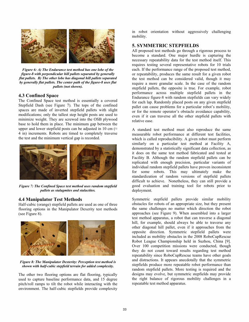
    Figure 6: A) The Endurance test method has one lobe of the

figure-8 with perpendicular hill pallets separated by generally flat pallets. B) The other lobe has diagonal hill pallets separated by generally flat pallets. The center path of the figure-8 uses flat

pallets (not shown). 

4.3 Confined Space The Confined Space test method is essentially a covered Stepfield Dash (see Figure 7). The tops of the confined spaces are made of inverted stepfield pallets with slight modifications; only the tallest step height posts are used to minimize weight. They are screwed into the OSB plywood base to hold them in place. The minimum gap between the upper and lower stepfield posts can be adjusted in 10 cm (≈ 4 in) increments. Robots are timed to completely traverse the test and the minimum vertical gap is recorded.

 

Figure 7: The Confined Space test method uses random stepfield pallets as stalagmites and stalactites.

4.4 Manipulator Test Methods Half-cubic (orange) stepfield pallets are used as one of three flooring options in the Manipulator Dexerity test methods (see Figure 8).

Figure 8: The Manipulator Dexterity: Perception test method is

shown with half-cubic stepfield terrain for added complexity.

The other two flooring options are flat flooring, typically used to capture baseline performance data, and 15 degree pitch/roll ramps to tilt the robot while interacting with the environment. The half-cubic stepfields provide complexity

in robot orientation without aggressively challenging mobility.

5. SYMMETRIC STEPFIELDS All proposed test methods go through a rigorous process to become a standard. One major hurdle is capturing the necessary repeatability data for the test method itself. This requires testing several representative robots for 10 trials each. If the performance range of the proposed test method, or repeatability, produces the same result for a given robot the test method can be considered valid, though it may require a more granular scale. In the case of the random stepfield pallets, the opposite is true. For example, robot performance across multiple stepfield pallets in the Endurance figure-8 with random stepfields can vary widely for each lap. Randomly placed posts on any given stepfield pallet can cause problems for a particular robot’s mobility, or for the remote operator’s obstacle avoidance capability, even if it can traverse all the other stepfield pallets with relative ease.

A standard test method must also reproduce the same measurable robot performance at different test facilities, which is called reproducibility. A given robot must perform similarly on a particular test method at Facility A, demonstrated by a statistically significant data collection, as it does on the same test method fabricated and tested at Facility B. Although the random stepfield pallets can be replicated with enough precision, particular variants of individual random stepfield pallets have proven inconsistent for some robots. This may ultimately make the standardization of random versions of stepfield pallets difficult to achieve. Nonetheless, they can still provide a good evaluation and training tool for robots prior to deployment.

Symmetric stepfield pallets provide similar mobility obstacles for robots of an appropriate size, but they present the same challenges no matter which direction the robot approaches (see Figure 9). When assembled into a larger test method apparatus, a robot that can traverse a diagonal hill, for example, should always be able to traverse any other diagonal hill pallet, even if it approaches from the opposite direction. Symmetric stepfield pallets were included as mobility obstacles in the 2008 RoboCupRescue Robot League Championship held in Suzhou, China [9]. Over 100 competition missions were conducted, though they do not count toward results regarding test method repeatability since RoboCupRescue teams have other goals and distractions. It appears anecdotally that the symmetric stepfields produce more repeatable robot performance than random stepfield pallets. More testing is required and the designs may evolve, but symmetric stepfields may provide the right balance of rigorous mobility challenges in a repeatable test method apparatus. 

33

 

 Figure 9: Symmetric stepfield pallets fabricated in Suzhou, China. 

(Left-Right) A) Flat cross pallet. B) Flat square pallet. C) Diagonal hill pallet. D) New center peak pallet.

6. CONCLUSIONS 8. REFERENCES Stepfield pallets, in both their full-cubic and half-cubic variants, have become a central part of several proposed NIST/ASTM test methods for response robots. They have also proliferated around the world as mobility challenges for international competitions. While they provide repeatable terrain to challenge and evaluate robot mobility and a remote operator’s situational awareness, they have proven to be difficult to standardize as a mobility test method. Random stepfields can continue to play a key role in helping robots move from the laboratory toward practice deployments and even to support operator training. But as a standard test method apparatus, a more repeatable version of the stepfields is necessary. More experimentation is required, but initial tests using symmetric stepfield pallets suggest that repeatability in robot performance and reproducibility of the test apparatus can be achieved.

[1] Messina, E., "Performance Standards for Urban Search and Rescue Robots," ASTM International Standardization News, August 2006.

[2] Statement of Requirements for Urban Search and Rescue Robot Performance Standards, May 2005. http://www.isd.mel.nist.gov/US&R_Robot_Standards/Requirements%20Report%20(prelim).pdf As accessed August 2008.

[3] RoboCupRescue Robot League competitions. http://www.isd.mel.nist.gov/projects/USAR/competitions.htm       As accessed August 2008.

[4] Full, R. J., Autumn, K., Chung, J. I., Ahn, A., “Rapid negotiation of rough terrain by the deathhead cockroach,” American Zoologist, 38:81A, 1998.

[5] Clark, J., Cham, J., Bailey, S., Froehlich, E., Nahata, P., Full, R., Cutkosky, M., “Biomimetic Design and Fabrication of a Hexapedal Running Robot,” Proceedings of the IEEE 2001 International Conference on Robotics and Automation, May 2001.

7. ACKNOWLEDGMENTS The authors would like to thank all the emergency responders involved in the NIST/DHS Response Robot Evaluation Exercises and other supporting events. Their initial set of robot requirements provided tangible goals to work toward and their ongoing feedback on test method designs has been much appreciated. Similarly, thanks to all the robot developers who have provided robot practice and training opportunities within prototype test methods and ongoing collaborations toward developing meaningful and challenging test methods for the community. And finally, we would like to thank the participants of the RoboCupRescue Robot League competitions for their enthusiastic robot testing, proliferation of apparatuses, and constructive ideas for new test methods.

[6] U. Saranli, M. Buehler, and D. E. Koditschek, "RHex: A Simple and Highly Mobile Hexapod Robot," Int. J. Robotics Research, 20(7):616-631, July 2001.

[7] ASTM International Standards Committee on Homeland Security Applications; Operational Equipment; Robots (E54.08.01). http://www.astm.org/COMMIT/SUBCOMMIT/E5408.htm As accessed August 2008.

[8] Response Robots Pocket Guide: Test Methods and Robots, 25 July 2008. http://www.isd.mel.nist.gov/US&R_Robot_Stndards/montgomery_county/pocketguide.htm As accessed August 2008.

[9] RoboCup World Championship, Suzhou, China, 14-20 July 2008. http://www.robocup-cn.org./en/index.php As accessed August 2008.

34

Potential Scaling Effects for Asynchronous Video in Multirobot Search

Prasanna Velagapudi Paul Scerri, Katia Sycara

Robotics Institute Carnegie Mellon University

Pittsburgh, PA 15213 001-412-268-8825

pkv@cs.cmu.edu

Huadong Wang, Michael Lewis School of Information Sciences

University of Pittsburgh Pittsburgh, PA 15260

001-412-624-9426

ml@sis.pitt.edu

ABSTRACT Camera guided teleoperation has long been the preferred mode for controlling remote robots with other modes such as asynchronous control only used when unavoidable. Because controlling multiple robots places additional demands on the operator we hypothesized that removing the forced pace for reviewing camera video might reduce workload and improve performance. In an initial experiment we evaluated the usefulness of asynchronous operation for a four robot search task. Participants operated four robot teams performing a simulated urban search and rescue (USAR) task using conventional streaming video plus a map interface or an experimental interface without streaming video but with the ability to store panoramic images on the map to be viewed at leisure. Search performance was somewhat better using the conventional interface; however, ancillary measures suggest that the asynchronous interface succeeded in reducing temporal demands for switching between robots. Because the advantages hypothesized for the asynchronous interface are due to reduction in time stress and workload, the four robot condition may have simply been too easy to observe this advantage. This view is at least partially supported by the reduced switching found in the panoramic condition. We have recently collected data for the streaming video condition for 4, 8, and 12 robots. In this data we found a marked deterioration in performance for the 12 robot condition, suggesting that at this level of difficulty asynchronous video might have an advantage. In this paper we present data for the four robot case comparison and discuss the implications of the recent data from larger teams.

Categories and Subject Descriptors

I.2.9 [Artificial Intelligence]: Robotics—operator interfaces

General Terms

Human Factors, Measurement, Experimentation

Keywords

Human-robot interaction, metrics, evaluation, multi-robot system

1. INTRODUCTION Practical applications of robotics can be classified by two distinct modes of operation. Terrestrial robotics in tasks such as surveillance, bomb disposal, or pipe inspection has used synchronous realtime control relying on intensive operator interaction usually through some form of teleoperation. Interplanetary and other long distance robotics subject to lags and intermittency in communications have used asynchronous control relying on labor intensive planning of waypoints and activities that are subsequently executed by the robot. In both cases planning and decision making are performed primarily by humans with robots exercising reactive control through obstacle avoidance and safeguards. The near universal choice of synchronous control for situations with reliable, low latency communication suggests a commonly held belief that experientially direct control is more efficient and less error prone. When this implicit position is rarely discussed it is usually justified in terms of “naturalness” or “presence” afforded by control relying on teleoperation. Fong and Thorpe [10] observe that direct control while watching a video feed from vehicle mounted cameras remains the most common form of interaction. The ability to leverage experience with controls for traditionally piloted vehicles appears to heavily influence the appeal for this interaction style.

Control based on platform mounted cameras, however, is no panacea. Wickins & Hollands [31] identify 5 viewpoints used in control, three of them, immersed, tethered, and “plan view” can be associated with the moving platform while 3rd person (tethered) and plan views require fixed cameras. In the immersed or egocentric view (A) the operator views the scene from a camera mounted on the platform. The field of view provided by the video feed is often much narrower than human vision, leading to the experience of viewing the world through a soda straw from a foot or so above the ground. This perceptual impairment leaves

Permission to make digital or hard copies of all or part of this work for personal or classroom use is granted without fee provided that copies are not made or distributed for profit or commercial advantage and that copies bear this notice and the full citation on the first page. To copy otherwise, or republish, to post on servers or to redistribute to lists, requires prior specific permission and/or a fee. PerMIS’08, August 19–21, 2008, Gaithersburg, MD, USA. Copyright 2008 ACM 978-1-60558-293-1…$5.00.

35

the operator prone to numerous, well-known operational errors, including disorientation, degradation of situation awareness, failure to recognize hazards, and simply overlooking relevant information [8, 15]. A sloped surface, for example, gives the illusion of being flat when viewed from a camera mounted on a platform traversing that surface [11]. For fixed cameras the operator’s ability to survey a scene is limited by the mobility of the robot and his ability to retain viewed regions of the scene in memory as the robot is maneuvered to obtain views of adjacent regions. A pan-tilt-zoom (ptz) camera resolves some of these problems but introduces new ones involving discrepancies between the robots heading and the camera view that frequently lead to operational mishaps [6]. A tethered “camera” (B,C) provides an oblique view of the scene showing both the platform and its 3D environment. A 3rd person fixed view (C) is akin to an operator’s view controlling slot cars and has been shown effective in avoiding roll-overs and other teleoperation accidents [4] but can’t be used anywhere an operator’s view might be obstructed such as within buildings or in rugged terrain. The tethered view (B) in which a camera “follows” an avatar (think Mario Brothers©) is widely favored in virtual environments [16,26] for its ability to show the object being controlled in relation to its environment by showing both the platform and an approximation of the scene that might be viewed from a camera mounted on it. This can be simulated for robotic platforms by mounting a camera on a flexible pole giving the operator a partial view of his platform in the environment [32]. Because of restriction in field of view and the necessity of pointing the camera downward, however, this strategy is of little use for surveying a scene although it can provide a view of the robot’s periphery and nearby obstacles that could not be seen otherwise. The exocentric views show a 2 dimensional version of the scene such as might be provided by an overhead camera and cannot be obtained from an onboard camera. This type of “overhead” view can, however, be approximated by a map. For robots equipped with laser range finders, generating a map and localizing the robot on that map provides a method for approximating an exocentric view of the platform. If this view rotates with the robot (heading up) it is a type D plan view. If it remains fixed (North up) it is of type E.

An early comparison at Sandia Laboratory between viewpoints for robot control [15] investigating accidents focused on the most common of these: (A) egocentric from onboard camera and (C) 3rd person. The finding was that all accidents involving rollover occurred under egocentric control while 3rd person control led to bumping and other events resulting from obstructed or distanced views. In current experimental work in remotely controlled robots for urban search and rescue (USAR) robots are typically equipped with both a ptz video camera for viewing the environment and a laser range finder for building a map and localizing the robot on that map. The video feed and map are usually presented in separate windows on the user interface and intended to be used in conjunction. While Casper and Murphy [5] reporting on experiences in searching for victims at the World Trade Center observed that it was very difficult for an operator to handle both navigation and exploration of the environment from video information alone, Yanco et al. [32] found that first responders using a robot to find victims in a mock environment made little use of the generated map. One possible explanation is that video is simply more attention grabbing than other presentations leading operators to control primarily from the

camera while ignoring other information available on their interface. A number of recent studies conducted by Goodrich, Neilsen, and colleagues [2,6,19,23,32] have attempted to remedy this through an ecological interface that fuses information by embedding the video display within the map. The resulting interface takes the 2D map and extrudes the identified surfaces to derive a 3D version resembling a world filled with cubicles. The robot is located on this map with the video window placed in front of it at the location being viewed. This strategy uses the egocentric camera view and the overhead view from the map to create a synthetic tethered view of the sort found most effective in virtual environments and games [16,26]. The anticipated advantages, however, have been difficult to demonstrate with ecological and conventional interfaces trading advantages across measures. Of particular interest have been comparisons between control based exclusively on maps or videos. In complex environments with little opportunity for preview maps were superior in assisting operators to escape from a maze [19]

When considering such potential advantages and disadvantages of viewpoints it is important to realize that there are two, not one, important subtasks that are likely to engage operators [26]. The escape task and the accidents reviewed at Sandia involved Navigation, the act of explicitly moving the robot to different locations in the environment. In many applications search, the process of acquiring a specific viewpoint—or set of viewpoints—containing a particular object may be of greater concern. While both navigation and search require the robot to move, an important distinction is the focus of the movement. Navigation occurs with respect to the environment at large, while search references a specific object or point within that environment. Switching between these two subtasks may play a major role in undermining situation awareness in teleoperated environments. For example, since search activities move the robot with respect to an object, viewers may lose track of their global position within the environment. Additional maneuvering may be necessary to reorient the operator before navigation can be effectively resumed. Because search relies on moving a viewpoint through the environment to find and better view target objects, it is an inherently egocentric task. This is not necessarily the case for navigation which does not need to identify objects but only to avoid them.

Search, particularly multi-robot search, presents the additional problem of assuring that areas the robot has traversed have been thoroughly searched for targets. This requirement directly conflicts with the navigation task which requires the camera to be pointed in the direction of travel in order to detect and avoid objects and steer toward its goal. When the operator attempts to compromise by choosing a path to traverse and then panning the camera to search as the robot moves he runs both the risk of hitting objects while he is looking away and missing targets as he attends to navigation. For multirobot control these difficulties are accentuated by the need to switch attention among robots multiplying the likelihood that a view containing a target will be missed. In earlier studies [29,30] we have demonstrated that success in search is directly related to the frequency with which the operator shifts attention between robots over a variety of conditions. An additional issue is the operator’s confidence that an area has been effectively searched. In our natural environment we move and glance about to construct a representation of our environment that is informed by planning and proprioception that

36

knit together the sequence of views. In controlling a robot we are deprived of these natural bridging cues and have difficulty recognizing as we pan and tilt whether we are resampling old views or missing new ones. The extent of this effect was demonstrated by Pausch [21] who found that participants searching for an object in a virtual room using a headmounted display were twice as fast as when they used a simulated handheld camera. Since even the handheld camera provides many ecological cues we should expect viewing from a moving platform through a ptz camera to be substantially worse.

1.1 Asynchronous Imagery To combat these problems of attentive sampling among cameras, incomplete coverage of searched areas, and difficulties in associating camera views with map locations we are investigating the potential of asynchronous control techniques previously used out of necessity in NASA applications as a solution to multi-robot search problems. Due to limited bandwidth and communication lags in interplanetary robotics camera views are closely planned and executed. Rather than transmitting live video and moving the camera about the scene, photographs are taken from a single spot with plans to capture as much of the surrounding scene as possible. These photographs taken with either an omnidirectional overhead camera (camera faces upward to a convex mirror reflecting 360 ) and dewarped [20,21] or stitched together from multiple pictures from a ptz camera [22] provide a panorama guaranteeing complete coverage of the scene from a particular point. If these points are well chosen, a collection of panoramas can cover an area to be searched with greater certainty than imagery captured with a ptz camera during navigation. For the operator searching within a saved panorama the experience is similar to controlling a ptz camera in the actual scene, a property that has been used to improve teleoperation in a low bandwidth high latency application [23].

1.2 Controlling Multiple Robots Because some functions of a MrS such as identifying victims among rubble depend on human input, evaluating the operator’s span of control as the number of controlled entities scale is critical for designing feasible human-automation control systems.

Controlling multiple robots substantially increases the complexity of the operator’s task because attention must constantly be shifted among robots in order to maintain situation awareness (SA) and exert control. In the simplest case an operator controls multiple independent robots interacting with each as needed. A search task in which each robot searches its own region would be of this category although minimal coordination might be required to avoid overlaps and prevent gaps in coverage. Control performance at such tasks can be characterized by the average demand of each robot on human attention [4]. Under these conditions increasing robot autonomy should allow robots to be neglected for longer periods of time making it possible for a single operator to control more robots.

Established methods of estimating MrS control difficulty, the neglect tolerance model, NT, [4] and the Fan-out measure [5] are predicated on the independence of robots and tasks. In the NT model the period following the end of human intervention but preceding a decline in performance below a threshold is considered time during which the operator is free to perform other tasks. If the operator services other robots over this period the

measure provides an estimate of the number of robots that might be controlled. Fan-out refers to maximum number of robots that can advantageously controlled under particular conditions. Fan-out can be determined empirically as in [5] by adding robots and measuring performance until a plateau without further improvement is reached or indirectly by predicting the maximum number of robots using parameters from the NT model [4].

Multi-robot control appears to impact the human operator’s workload in three distinct ways: (1) building and maintaining awareness, (2) making decisions, and (3) controlling the system. Increasing the autonomy level in robotic system, whether providing decision support or individual robot autonomy, allows us to shift the decision-making and robot control workload from the human to the robotic system. On the other hand, increased robot autonomy may cause an increase in perception and decision-making workloads. Thus, there is a trade-off between the autonomy level of the robotic system and the level of human intervention.

Current estimates of human span of control limitations are severe. Miller [17], for example, showed that under expected target densities, a controller who is required to authorize weapon release for a target identified by a UCAV, could control no more than 13 UAVs even in the absence of other tasks. A similar breakpoint of 12 was found by [7] for retargeting Tomahawk missiles. Smaller numbers (3-9) [6] have typically been found for ground robots depending upon task and level of automation. By most estimates, however, a team of four robots should be well within an operator’s span of control. Two experiments are reported in this paper. The first experiment compares a user interface supplying streaming video with one in which operators must rely on static panoramas for performing a USAR task with a four robot team. The second experiment investigates performance at the same task for the streaming video interface as the number of robots is increased from 4 to 8 to 12 to identify the operators’ limits of control.

2. METHOD 2.1 USARSim and MrCS The reported experiments were performed using the USARSim robotic simulation with simulated UGVs performing Urban Search and Rescue (USAR) tasks. USARSim is a high-fidelity simulation of urban search and rescue (USAR) robots and environments we developed as a research tool for the study of HRI and multi-robot coordination. USARSim supports HRI in ways lower fidelity simulations cannot by accurately rendering user interface elements (particularly camera video), accurately representing robot automation and behavior, and accurately representing the remote environment that links the operator’s awareness with the robot’s behaviors. USARSim can be downloaded from www.sourceforge.net/projects/usarsim and serves as the basis for the Virtual Robots Competition of the RoboCup Rescue League. The current version of USARSim includes detailed replicas of NIST USAR Arenas, as well as large-scale indoor and outdoor hypothetical disaster scenarios, and a large outdoor area along the Chesapeake Bay. USARSim complements these maps with high fidelity models of commercial (pioneer P2-DX, P2-AT, iRobot’s ATRV Jr., Foster-Miller’s Talon, and Telerob’s Telemax) and experimental (PER from CMU, Zerg from University of Freiburg, Kurt 3D from University

37

of Osnabruk) robots, including a snake (Soyu from Tohoku University), air (Air-robot helicopter) and a large Ackerman-steered UGV (Hummer) and sensor models for many common robotic sensing packages. USARSim uses Epic Games’ UnrealEngine2 [14] to provide a high fidelity simulator at low cost. Validation studies showing agreement for a variety of feature extraction techniques between USARSim images and camera video are reported in Carpin et al. [3]. Other sensors including sonar and audio are also accurately modeled. Validation data showing close agreement in detection of walls and associated Hough transforms for a simulated Hokuyo laser range finder are described in [13]. The current UnrealEngine2 integrates MathEngine’s Karma physics engine [14] to support high fidelity rigid body simulation. Validation studies showing close agreement in behavior between USARSim models and real robots being modeled are reported in [13,22,27,33].

MrCS (Multi-robot Control System), a multirobot communications and control infrastructure with accompanying user interface developed for experiments in multirobot control and RoboCup competition [1] was used. MrCS provides facilities for starting and controlling robots in the simulation, displaying camera and laser output, and supporting inter-robot communication through Machinetta a distributed mutiagent system. Figure 1 shows the elements of the MrCS involved in this experiment. In the standard MrCS the operator selects the robot to be controlled from the colored thumbnails at the top of the screen that show a slowly updating view from the robot’s camera. Streaming video from the in focus robot which the operator now controls is displayed on the Image Viewer. To view more of the scene the operator uses pan/tilt sliders (not shown) to control the camera. Robots are tasked by assigning waypoints on a heading-up map on the Mission Panel (not shown) or through a

Figure 1. MrCS components for Streaming Video Mode teleoperation widget (not shown). The current locations and paths of the robots are shown on the Map Data Viewer.

2.1.1 Panorama Mode Our USAR application which requires finding victims and locating them on a map needs to use both map and camera views [32]. In Panorama mode the operator directs navigation from the map being generated with panoramas being taken at the last

Figure 2. MrCS components for Asynchronous Panorama Mode

waypoint of a series. The panoramas are stored and accessed through icons showing their locations on the map. The operator can find victims by asynchronously panning through these stored panoramas as time becomes available. When a victim is spotted the operator uses landmarks from the image and corresponding points on the map to record the victim’s location. By changing the task from a forced paced one with camera views that must be controlled and searched on multiple robots continuously to a self paced task in which only navigation needs to be controlled in realtime we hoped to provide a control interface that would allow more thorough search with lowered mental workload. The reductions in bandwidth and communications requirements [1] are yet another advantage offered by this approach.

Although the experimental panoramic interface (Fig. 2) looks much the same it behaves quite differently. Robots are again selected for control from the colored thumbnails which now lack images. Panoramic images are acquired at the terminal point of waypoint sequences. Icons conveying the robot’s location and orientation at these points are placed on the map for accessing the panoramas. The operator can then view stored panoramas by selecting an icon and dragging a mouse over the Image Viewer to move the image around or using the mouse’s scroll wheel to zoom in and out of the image. The associated icon on the Map Data Viewer changes orientation in accordance with the part of the scene being viewed.

2.2 Experiment 1 Asynchronous vs. Streaming Video 2.2.1 Method Two equivalent search environments previously used in the 2006 RoboCup Rescue Virtual Robots competition [1] were selected for use in the experiment. Each environment was a maze like hall with many rooms and obstacles, such as chairs, desks, cabinets, and bricks. Victims were evenly distributed within the environments. A third simpler environment was used for training. The experiment followed a repeated measures design with participants searching for victims using both panorama and streaming video modes. Presentation orders for mode were counterbalanced. Test environments were presented in a fixed order confounding differences between the environments with learning effects. Because the environments were closely matched we will discuss these differences as transfer of training effects.

38

2.2.1.1 Participants and Procedure 21 paid participants, 9 male and 12 female old recruited from the University of Pittsburgh community. None had prior experience with robot control although most (15) were frequent computer users. Six of the participants (28%) reported playing computer games for more than one hour per week.

2.2.1.2 Procedure After collecting demographic data the participant read standard instructions on how to control robots via MrCS. In the following 15~20 minute training session, the participant practiced control operations for panorama and streaming video modes (both were enabled) and tried to find at least one victim in the training environment under the guidance of the experimenter. Participants then began two testing sessions in which they performed the search task using the panorama and streaming video modes.

2.2.2 Results Only one participant failed to find any victims under the most lenient criterion of marking the victim within 2 m of the actual location. This occurred in the panorama mode on the initial trial. Overall participants were successful in searching the environment in either mode finding as many as 9 on a trial. The average across conditions using the 2 m radius was 4.5 falling to 4.1 for a 1.5 m radius, 3.4 at 1 m and 2.7 when they were required to mark victims within .75 m. Repeated measures ANOVAs found differences in accuracy of location favoring the streaming video mode at the 1.5 m radius F(1,19) = 8.038, p=.01), and 2.0 radius F(1,19)=9.54, p=.006. Figure 3 shows these differences.

Victims Found

0

1

2

3

4

5

6

rad .75 rad 1 rad 1.5 rad 2

marking accuracy

panoramastreaming

Figure 3. Effects of display modes

No significant order effect (learning) was observed. As in earlier studies we found a positive relation, F(1,19)=3.86, p=.064, between the number of times the operator switched between robots and the victims that were found (Figure 4). In accord with our hypothesis that this is due to the forced pace of performing the task using streaming video no relation was found between the frequency of switching and victims for the panorama mode.

Switching in Streaming mode

0

2

4

6

8

10

12

0 20 40 60 80 100 120

N switches

N v

ictim

s

Series1Linear (Series1)

Figure 4. Finding victims was related to switches only in Streaming

mode

2.3 Experiment 2 Scaling in N Robots 2.3.1 Method A large USAR environment previously used in the 2006 RoboCup Rescue Virtual Robots competition [1] was selected for use in the experiment. The environment was a maze like hall with many rooms and obstacles, such as chairs, desks, cabinets, and bricks. Victims were evenly distributed within the environment. A second simpler environment was used for training. The experiment followed a repeated measures design with participants searching for victims using 4, 8, and finally 12 robots. Robot starting points were varied over the three trials. Because our primary concern was with changes in performance as N robots increased, trials were presented in a fixed order. This design confounding learning effects and starting points with N of robots was adopted because the randomly selected starting points were sufficiently comparable not to bias results and any learning effect would attenuate rather than accentuate the expected decrements.

2.3.1.1 Participants 15 paid participants, 8 male and 7 female were recruited from the University of Pittsburgh community. None had prior experience with robot control although most were frequent computer users.

2.3.1.2 Procedure After collecting demographic data the participant read standard instructions on how to control robots via MrCS. In the following 20 minute training session, the participant practiced control operations and tried to find at least one victim in the training environment under the guidance of the experimenter. Participants then began three testing sessions (15 minute each) in which they performed the search task using 4, 8, and finally 12 robots. After each task, the participants were asked to file the NASA-TXL workload survey immediately.

2.3.2 Results Overall participants were successful in searching the

environment in all conditions finding as many as 12 victims on a trial. The average number of victims found was 4.80 using 4 robots, 7.06 for 8 robots, but only 4.73 when using 12 robots. A paired t-test shows that in the 8 robots condition (R8) participants explored larger regions, t (15) = -10.44, p = 0.000, while finding

39

more victims, t (15) = -3.201, p = 0.003, than using a 4 robot team (R4). On the other hand, adding four addition robots degraded performance with participants in the 8 robot condition (R8) exploring larger regions, t (15) = -1.19, p = 0.059, as well as finding more victims, t (15) = -3.014, p = 0.005, than they did using a 12 robot team (R12).

Explored Regions

Median 25%-75% Non-Outlier Range

R4 R8 R120

50

100

150

200

250

300

350

400

450

Figure 5. Explored Regions

Victims Founded

Median 25%-75% Non-Outlier Range

R4 R8 R120

2

4

6

8

10

12

14

Figure 6. Victims Found

Figure 7 shows that as the number of robots is increased, fewer victims were found per robot. This measure should remain constant if robots were controlled to the same level of effectiveness. However, these differences were not significant. With increasing numbers of robots operators tended to neglect some robots either entirely or after an initial movement as shown in Table 2. A paired t-test indicates that participants neglected more robots in the 12 robot condition, t (15) = -1.922, p = 0.064, than under 4 robots team (R4). More robots were neglected after an initial move in the 8 robot (R8) condition t (15) = -2.092, p = 0.046, than for 4 robots (R4); and still more comparing a 12 robot team (R12) to the 8 robot (R8) condition t (15) = -3.761, p = 0.001. With increasing numbers of robots operators tended to neglect some robots either entirely or after an initial movement as shown in Table 2. A paired t-test indicates that participants neglected more robots in the 12 robot condition, t (15) = -1.922, p = 0.064, than under 4 robots team (R4).

Victims per Robotic

Median 25%-75% Non-Outlier Range

V/R_4 V/R_8 V/R_120.0

0.2

0.4

0.6

0.8

1.0

1.2

1.4

1.6

1.8

2.0

2.2

Figure 7. Victims Found per Robot

more robots in the 12 robot condition, t (15) = -1.922, p = 0.064, than under 4 robots team (R4). More robots were neglected after an initial move in the 8 robot (R8) condition t (15) = -2.092, p = 0.046, than for 4 robots (R4); and still more comparing a 12 robot team (R12) to the 8 robot (R8) condition t (15) = -3.761, p = 0.001.

Table 1. Neglected Robots

Number of Robots R4 R8 R12

Totally 0.00 0.13 0.80

After the Initial Move 0.00 0.33 1.87

As in earlier studies we found a positive relation between the number of times the operator switched between robots and the victims that were found. Higher switching rates are an indicator of shortened ITs or more efficient use of NT to service additional robots and hence should improve team performance. Figure 6 shows the number of switches observed under each of the three conditions. There were significant differences in number of switches between robots for the 4 robot and 8 robot conditions (t= -2.914, P<0.007) and the 4 robot and 12 robot conditions (t= -2.620, P<0.014). Similar results were found for numbers of missions (waypoint assignments) between the 4 robot and 8 robot condition (t= -3.079, P<0.005) and the 4 robot and 12 robot condition (t= -2.118, P<0.043). The result of the workload assessment indicates that workload increased with increasing numbers of robots to be controlled. This difference in workload was significant between the 4 robot and 12 robot conditions (P<0.0146). Our results show that we have successfully bounded the number of directly controllable robots for a realistic USAR task at between 8-12. This can be seen for both the number of victims found and the regions explored which improve between the four robot and eight robot conditions but decline again between 8 and 12 robots. Determining Fan-out empirically as in [20] the Fan-out plateau (point at which performance is no longer improved by

40

Switch Times

Median 25%-75% Non-Outlier Range

S4 S8 S1210

20

30

40

50

60

70

80

90

Figure 8. Number of Switches

Workload

Median 25%-75% Non-Outlier Range Outliers

R4 R8 R1220

30

40

50

60

70

80

90

100

110

Figure 9. NASA-TLX Measurement of Mental workload

adding additional robots) lies somewhere within this region. The point at which operator capabilities become saturated can be estimated more closely by observing the number of robots that are either completely neglected or neglected after the first move. This number is approximately 2.7 for the 12 robot condition suggesting that the actual limit for this experiment is approximately 9 robots. An examination of the number of switches between robots supports this estimate because the number of switches is essentially the same in both the 8 and 12 robot conditions. This means that operators have reached their limit for interactions and are neglecting the robots for slightly longer times to accommodate the additional robot they are actively controlling. With this initial experiment we are establishing a baseline for exploring the effects of robot team size on human performance. Even these early results suggest that the navigation component of the operator’s task and the perceptual tasks involved in search may be somewhat differently impacted by increases in team size. We hope to be able to use such results to guide system designers in allocating functions statically or dynamically between the operator and robot (team) autonomy.

3. DISCUSSION Our original motivation for developing a panorama mode for MrCS was to address restrictions posed by a communications server added to the 2007 RoboCup Rescue competition to simulate bandwidth limitations and drop-outs due to attenuation

from distance and obstacles. Although the panorama mode was designed to drastically reduce bandwidth and allow operation despite intermittent communications our system was so effective we decided to test it under conditions most favorable to a conventional interface. Our first experiment showed that under conditions allowing uninterrupted, noise free, streaming video a conventional interface lead to somewhat better (5 vs. 4 victims) search performance. The switching results, however, suggest that asynchronous panoramas do overcome the forced pace switching needed to avoid missing unattended targets in realtime interfaces. We would expect this advantage to grow as the number of robots increases with performance approaching or surpassing streaming video at some point. The second experiment demonstrates that for this USAR task control of four robots lies well within the cognitive capabilities of an operator. Our data show that the operators had sufficient reserve capacity to effectively control twice as many robots. These results suggest that if advantages are to be found for panorama-based search they are likely to be found in the 8-12 robot range. It is also important to note that while victims were marked more accurately in the streaming video mode, the greater accuracy may simply reflect advantages for marking locations rather than actual improvement in search performance. Because participants in the streaming video mode were able to drive their robots in close proximity to victims, their ability to mark locations with greater accuracy may have simply resulted from being nearer their targets than in the panorama condition where the target must be marked from the location at which the panorama had been taken. Just as [19] have demonstrated that maps may be better than cameras for navigation we hope that asynchronous video and related strategies may play a role in improving multirobot search capabilities. Coupled with the ability to control robots under poor communication conditions such as are expected in USAR and other field work we believe that interface innovations of this sort have an important role to play in making control of robot teams a reality.

4. ACKNOWLEDGMENTS This research has been sponsored in part by AFOSR FA9550- 07-1-0039, AFOSR FA9620-01-1-0542, ONR Grant N00014-03-1-0580 and L3-Communications (4500257512)

5. REFERENCES [1] S. Balakirsky, S. Carpin, A. Kleiner, M. Lewis, A. Visser, J.

Wang, and V. Zipara, “Toward hetereogeneous robot teams for disaster mitigation: Results and performance metrics from RoboCup Rescue,” Journal of Field Robotics, in press.

[2] D. J. Bruemmer, D. A. Few, M. C. Walton, R. L. Boring, J. L. Marble, C. W. Nielsen, and J. Garner. Turn off the television: Real-world robotic exploration experiments with a virtual 3-D display. Proc. HICSS, Kona, HI, 2005.

[3] S. Carpin, T. Stoyanov, Y. Nevatia, M. Lewis and J. Wang. Quantitative assessments of USARSim accuracy". Proceedings of PerMIS 2006 [ir-13] S. Carpin, J. Wang, M. Lewis, A. Birk and A. Jacoff. High fidelity tools for rescue robotics: Results and perspectives, Robocup 2005 Symposium, 2005.

41

[4] S. Carpin, M. Lewis, J. Wang, S. Balakirsky, C. Scrapper. (2006b). Bridging the gap between simulation and reality in urban search and rescue. Robocup 2006: Robot Soccer World Cup X, Springer, Lecture Notes in Artificial Intelligence, 2006.

[5] J. Casper and R. R. Murphy. Human-robot interactions during the robot-assisted urban search and rescue response at the world trade center. IEEE Transactions on Systems, Man, and Cybernetics Part B, 33(3):367–385, June, 2003

[6] J. W. Crandall, M. A. Goodrich, D. R. Olsen, and C. W. Nielsen. Validating human-robot interaction schemes in multitasking environments. IEEE Transactions on Systems, Man, and Cybernetics, Part A, 35(4):438–449, 2005.

[7] Cummings, M. and Guerlain, S. An interactive decision support tool for real-time in-flight replanning of autonomous vehicles, AIAA Unmanned Unlimited Systems, Technologies, and Operations, 2004.

[8] R. Darken, K. Kempster, and B. Peterson, “Effects of streaming video quality of service on spatial comprehension in a reconnaissance task,” in Proc. Meeting I/ITSEC, Orlando, FL, 2001.

[9] M. Fiala, “Pano-presence for teleoperation,” Proc. Intelligent Robots and Systems (IROS 2005), 3798-3802, 2005.

[10] T. Fong and C. Thorpe, “Vehicle teleoperation interfaces,” Autonomous. Robots, no. 11, pp. 9–18, 2001.

[11] M. Lewis and J. Wang, “Gravity referenced attitude display for mobile robots : Making sense of what we see, ” Transactions on Systems, Man and Cybernetics Part A, 37(1), 94-105, 2007.

[12] M. Lewis, J. Wang, and S. Hughes, “USARsim : Simulation for the Study of Human-Robot Interaction,” Journal of Cognitive Engineering and Decision Making, 1(1), 98-120, 2007.

[13] M. Lewis, S. Hughes, J. Wang, M. Koes, and S. Carpin. Validating USARsim for use in HRI research, Proceedings of the 49th Annual Meeting of the Human Factors and Ergonomics Society, Orlando, FL, 2005, 457-461

[14] Mathengine, MathEngine Karma User Guide, http://udn.epicgames.com/Two/KarmaReference/KarmaUserGuide.pdf, accessed May 3, 2005.

[15] D. E. McGovern, “Experiences and Results in Teleoperation of Land Vehicles,” Sandia Nat. Labs., Albuquerque, NM, Tech. Rep. SAND 90-0299, 1990.

[16] P. Milgram and J. Ballantyne, “Real world teleoperation via virtual environment modeling,” in Proc. Int. Conf. Artif. Reality Tele-Existence, Tokyo, 1997.

[17] Miller, C. Modeling human workload limitations on multiple UAV control, Proceedings of the Human Factors and Ergonomics Society 47th Annual Meeting, 526-527, 2004.

[18] J.R. Murphy, “Application of Panospheric Imaging to a Teleoperated Lunar Rover,” in Proceedings of the 1995 International Conference on Systems, Man, and Cybernetics, 1995.

[19] C. Nielsen and M. Goodrich. Comparing the usefulness of video and map information in navigation tasks. In Proceedings of the 2006 Human-Robot Interaction Conference, Salt Lake City, Utah, March 2006.

[20] D.R Olsen and S.B. Wood, Fan-out: measuring human control of multiple robots, in Proceedings of the SIGCHI conference on Human factors in computing systems. 2004, ACM Press: Vienna, Austria. p. 231-238.

[21] R. Pausch, M. A. Shackelford, and D. Proffitt, “A user study comparing head-mounted and stationary displays,” IEEE Symposium on Research Frontiers in Virtual Reality, October 25-26, 1993, San Jose, CA.

[22] C. Pepper, S. Balakirsky, and C. Scrapper. Robot Simulation Physics Validation, Proceedings of PerMIS’07, 2007.

[23] B. W. Ricks, C. W. Nielsen, and M. A. Goodrich. Ecological displays for robot interaction: A new perspective. In International Conference on Intelligent Robots and Systems IEEE/RSJ, Sendai, Japan, 2004.

[24] P. Scerri, Y. Xu, E. Liao, G. Lai, M. Lewis, and K. Sycara, “Coordinating large groups of wide area search munitions,” In D. Grundel, R. Murphey, and P. Pandalos (Ed.), Recent Developments in Cooperative Control and Optimization, Singapore: World Scientific, 451-480.

[25] N. Shiroma, N. Sato, Y. Chiu, and F. Matsuno, “Study on effective camera images for mobile robot teleoperation,” In Proceedings of the 2004 IEEE International Workshop on Robot and Human Interactive Communication, Kurashiki, Okayama Japan, 2004

[26] D. S. Tan, G. G. Robertson, and M. Czerwinski, “Exploring 3D navigation: Combining speed-coupled flying with orbiting,” in CHI 2001 Conf. Human Factors Comput. Syst., Seattle, WA, 2001.

[27] B. Taylor, S. Balakirsky, E. Messina and R. Quinn. Design and Validation of a Whegs Robot in USARSim, Proceedings of PerMIS’07, 2007.

[28] R. Volpe, “Navigation results from desert field tests of the Rocky 7 Mars rover prototype,” in The International Journal of Robotics Research, 18, pp.669-683, 1999.

[29] J. Wang, and M. Lewis, “Human control of cooperating robot teams”, 2007 Human-Robot Interaction Conference, ACM, 2007a.

[30] J. Wang, and M. Lewis, “Assessing coordination overhead in control of robot teams,” Proceedings of the 2007 International Conference on Systems, Man, and Cybernetics, 2007b

[31] C. Wickens and J. Hollands, Engineering Psychology and Human Performance, Prentice Hall, 1999.

[32] H. Yanco, M. Baker, R. Casey, B. Keyes, P. Thoren, J. Drury, D. Few, C. Nielsen, D. Bruemmer. “Analysis of human-robot interaction for urban search and rescue, Proceedings of PERMIS, 2006.

[33] M. Zaratti, M. Fratarcangeli and L. Iocchi. A 3D Simulator of Multiple Legged Robots based on USARSim. Robocup 2006: Robot Soccer World Cup X, Springer, LNAI, 2006.

42

The Rat’s Life Benchmark:Competing Cognitive Robots

Olivier MichelCyberbotics Ltd.PSE C - EPFL

CH-1015 Lausanne, SwitzerlandOlivier.Michel@cyberbotics.com

Fabien RohrerCyberbotics Ltd.PSE C - EPFL

CH-1015 Lausanne, SwitzerlandFabien.Rohrer@cyberbotics.com

ABSTRACTThis paper describes Rat’s Life: a complete cognitive roboticsbenchmark that was carefully designed to be easily repro-ducible in a research lab with limited resources. It relieson two e-puck robots, some LEGO bricks and the Webotsrobot simulation software. This benchmark is a survivalgame where two robots compete against each other for re-sources in an unknown maze. Like the rats in cognitiveanimal experimentation, the e-puck robots look for feederswhich allow them to live longer than their opponent. Once afeeder is reached by a robot, the robot draws energy from itand the feeder becomes unavailable for a while. Hence, therobot has to further explore the maze, searching for otherfeeders while remembering the way back to the first ones.This allows them to be able to refuel easily again and againand hopefully live longer than their opponent.

Keywordsbenchmark, SLAM, navigation, autonomy, vision

1. WHY WE NEED COGNITIVE ROBOTICSBENCHMARKS

1.1 IntroductionMost scientific publications in the area of robotics research

face tremendous challenges: comparing the achieved resultwith other similar research results and hence convincing thereader of the quality of the research work. These challengesare very difficult because roboticists lack common tools al-lowing them to evaluate the absolute performance of theirsystems or compare their results with others. As a result,such publications often fail at providing verifiable results,either because the studied system is unique and difficult toreplicate or they don’t provide enough experimental detailsso that the reader could replicate the system accurately.

Nevertheless, some of these publications become the de

Permission to make digital or hard copies of all or part of this work forpersonal or classroom use is granted without fee provided that copies arenot made or distributed for profit or commercial advantage and that copiesbear this notice and the full citation on the first page. To copy otherwise, torepublish, to post on servers or to redistribute to lists, requires prior specificpermission and/or a fee.PerMIS’08, August 19-21, 2008, Gaithersburg, MD, USACopyright 2008 ACM 978-1-60558-293-1 ...$5.00.

facto state of the art and this makes it extremely difficult tofurther explore these research areas, and hence to demon-strate advances in robotics research.

This matter of fact is unfortunately impairing the credi-bility of robotics research. A number of robotics researchersproposed to develop series of benchmarks to provide a meansof evaluation and comparison of robotics research results [1,3, 4, 9, 19].

Although a few robotics benchmarks already exist, theonly robotics benchmarks that are widely known and prac-ticed are implemented as robot competitions.

1.2 Existing Robot Competitions and Bench-marks

Several popular robot competitions are organized on aregular basis, usually once a year. The Robocup soccer[6] and FIRA [16] is a robot soccer tournament with sev-eral categories (small size league, middle size league, stan-dard platform league, simulation league, etc.). The RobocupRescue is based on the Urban Search And Rescue (USAR)benchmark developed by the NIST [7] where robots have tosearch and rescue the victims of a disaster in a urban envi-ronment. MicroMouse [11], involves wheeled robots solvinga maze. The FIRST [12], Eurobot [13] and Robolympics[14] are robot competitions more focused on education thanresearch in various disciplines (often inspired from sports).The AAAI Robot Competition [15] proposes different sce-narios each year during the AAAI conference, but often lacksa clear performance metrics. The DARPA Grand Challengeand Urban Challenge [17] and the European Land-RobotTrial [18] focus on unmanned ground and sometimes aerialvehicles racing against each other.

Although some of these competitions clearly focus on ed-ucation and are more intended to students and childrenrather than researchers (FIRST, Eurobot), others compe-titions (Robocup, FIRA, AAAI) are more intended to re-searchers. Such competitions are useful as they can provideelements of comparison between different research results.However one of the major problem is that the rules oftenchange across the different editions of the same competition.Hence it is difficult to compare the progress achieved overtime. Also these competitions are very specific to particularproblems, like Robocup is focused mostly on robot soccerand has arguably a limited interest for cognitive robotics[5]. Moreover, in most cases, and especially in the Robocupcase, installing a contest setup is expensive and takes a lotof resources (many robots, robot environment setup, room,

43

maintenance, controlled lighting conditions, etc.).

1.3 Going Further with Cognitive Robotics Bench-marks

Among all the benchmarks we reviewed which are mostlyrobot competitions, none of them provides both stable ruleswith advanced cognitive robotics challenges and an easysetup. This paper proposes a new robotics benchmark called”Rat’s Life” that addresses a number of cognitive roboticschallenges while being cheap and very easy to setup for anyresearch lab. The aim of this benchmark is to foster ad-vanced robotics and AI research.

Comparing to soccer playing contests (RoboCup, FIRA),the Rat’s Life benchmark is more bio-inspired as it focuseson foraging and survival. Also, it is more likely to con-tribute to scientific advances in Learning and Self Localiza-tion And Mapping (SLAM) as mazes are initially unknownto the robots. Moreover, it allows the researchers to focus ona single agent (competiting against another) rather than awhole team of agents, making the problem somehow simplerto handle. Finally, it is cheaper.

2. BENCHMARK REQUIREMENTSIn order to be useful a benchmark has to be practiced

by a large number of the best researchers trying to pushfurther the current state of the art. This can be achievedby proposing a scientifically and practically appealing seriesof benchmarks that will convince researchers to invest theirtime with these tools. Hence the Rat’s Life benchmark istrying to achieve a number of objectives:

2.1 Scientifically appealingTo be scientifically interesting, a benchmark has to ad-

dress a number of difficult challenges in robotics. The Rat’sLife benchmark focuses on cognitive robotics and addressesadvanced research topics such as image processing, learning,navigation in an unknown environment, landmark recogni-tion, SLAM, autonomy management, game strategies, etc.

2.2 Cheap and easy to setupThe benchmark should be easily practicable by any re-

searcher. Hence it has to be cheap and easy to setup. Allthe components should be easily available. The Rat’s Lifebenchmark costs no more than EUR 2000, for two e-puckrobots and many LEGO components (including a LEGONXT unit and four LEGO distance sensors). It requiresonly a table to setup a LEGO maze of 114x114 cm.

2.3 AccurateAccuracy is a very important aspect of a benchmark. The

environment, robots and evaluation rules should be definedvery carefully in an exhaustive manner. This way, the bench-mark is accurately replicable and hence different results ob-tained with different instances of the setup in different re-search lab can be compared to each others.

2.4 ComparableFinally, a benchmark is useful if users can compare their

own results to others and thus try to improve the state ofthe art. Hence a benchmark should keep a data base ofthe solutions contributed by different researchers, includingbinary and source code of the robot controller programs.These different solutions should be ranked using a common

performance metrics, so that we can compare them to eachother.

3. STANDARD COMPONENTSThe Rat’s Life benchmark is based on three standard af-

fordable components: the e-puck mobile robot, LEGO bricksand the Webots robot simulation software (free version).

3.1 The e-puck mobile robot

Figure 1: The e-puck robot

The e-puck mini mobile robot was originally developedat the EPFL for teaching purposes by the designers of thesuccessful Khepera robot. The e-puck hardware and soft-ware is fully open source, providing low level access to everyelectronic device and offering unlimited extension possibil-ities. The robot is already equipped with a large numberof sensors and actuators (figure 1). It is well supported bythe Webots simulation software with simulation models, re-mote control and cross-compilation facilities. The officiale-puck web site [23] gathers a large quantity of informationabout the robot, extension modules, software libraries, usersmailing lists, etc. The robot is commercially available fromCyberbotics [21] for about EUR 570.

3.2 LEGO bricksThe LEGO bricks are used to create an environment for

the e-puck robot. This environment is actually a maze whichcontains ”feeder” devices (see next sections) as well as visuallandmarks made up of patterns of colored LEGO brick inthe walls of the maze (see figure 2). These landmarks areuseful hints helping the robot to navigate in the maze. SinceLEGO models are easily demountable, the maze is easily re-configurable so that the users can create different instancesof the maze according to the specifications of the bench-mark.All the maze, landmarks and the feeder devices are properlydefined in a LEGO CAD file in LXF format using the LEGOdigital designer software freely available from the LEGO fac-tory web site [20]. The corresponding LXF files are freelyavailable on the Rat’s Life web site [10].

Thanks to the LEGO factory system, users can very easilyorder a box containing all the LEGO bricks necessary tobuild the environment of the robots.

3.3 The Webots robot simulation software

44

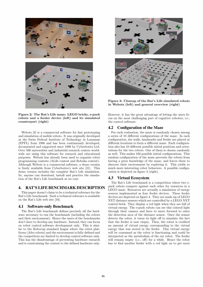
Figure 2: The Rat’s Life maze: LEGO bricks, e-puckrobots and a feeder device (left) and its simulatedcounterpart (right)

Webots [8] is a commercial software for fast prototypingand simulation of mobile robots. It was originally developedat the Swiss Federal Institute of Technology in Lausanne(EPFL) from 1996 and has been continuously developed,documented and supported since 1998 by Cyberbotics Ltd.Over 500 universities and industrial research centers world-wide are using this software for research and educationalpurposes. Webots has already been used to organize robotprogramming contests (ALife contest and Roboka contest).Although Webots is a commercial software, a demo versionis freely available from Cyberbotics’s web site [21]. Thisdemo version includes the complete Rat’s Life simulation.So, anyone can download, install and practice the simula-tion of the Rat’s Life benchmark at no cost.

4. RAT’S LIFE BENCHMARK DESCRIPTIONThis paper doesn’t claim to be a technical reference for the

Rat’s Life benchmark. Such a technical reference is availableon the Rat’s Life web site [10].

4.1 Software-only BenchmarkThe Rat’s Life benchmark defines precisely all the hard-

ware necessary to run the benchmark (including the robotsand their environment). Hence the users of the benchmarksdon’t have to develop any hardware. Instead, they can focuson robot control software development only. This is simi-lar to the Robocup standard league where the robot plat-forms (Aibo robots) and the environment is fully defined andthe competitors are limited to develop control software only.This has the disadvantage of preventing hardware researchand is constraining the contest to the defined hardware only.

Figure 3: Closeup of the Rat’s Life simulated robotsin Webots (left) and general overview (right)

However, it has the great advantage of letting the users fo-cus on the most challenging part of cognitive robotics, i.e.,the control software.

4.2 Configuration of the MazeFor each evaluation, the maze is randomly chosen among

a series of 10 different configurations of the maze. In eachconfiguration, the walls, landmarks and feeder are placed atdifferent locations to form a different maze. Each configura-tion also has 10 different possible initial positions and orien-tations for the two robots. One of them is chosen randomlyas well. This makes 100 possible initial configurations. Thisrandom configuration of the maze prevents the robots fromhaving a prior knowledge of the maze, and forces them todiscover their environment by exploring it. This yields tomuch more interesting robot behaviors. A possible configu-ration is depicted on figure 3 (right).

4.3 Virtual EcosystemThe Rat’s Life benchmark is a competition where two e-

puck robots compete against each other for resources in aLEGO maze. Resources are actually a simulation of energysources implemented as four feeder devices. These feederdevices are depicted on figure 4. They are made up of LEGONXT distance sensors which are controlled by a LEGO NXTcontrol brick. They display a red light when they are full ofvirtual energy. The e-puck robots can see this colored lightthrough their camera and have to move forward to enterthe detection area of the distance sensor. Once the sensordetects the robot, it turns its light off to simulate the factthat the feeder is now empty. Then, the robot is creditedan amount of virtual energy corresponding to the virtualenergy that was stored in the feeder. This virtual energywill be consumed as the robot is functioning and could beinterpreted as the metabolism of the rat robot. The feederwill remain empty (i.e., off) for a while. Hence the robothas to find another feeder with a red light on to get more

45

Figure 4: A full feeder facing an e-puck robot (left)and an empty one (right)

energy before its energy level reaches 0. When a robot runsout of virtual energy (i.e., its energy level reaches 0), theother robot wins.

4.3.1 Biological ComparisonThis scenario is comparable to an ecosystem where the

energy is produced by feeders and consumed by robots. Thefeeders could be seen as plants, slowy growing from the en-ergy of the sun, water and ground and producing fruitswhereas the robots could be seen as rats, foraging fruits.Since the fruits produced by a single plant are not sufficientto feed a rat, the rat has to move around to find more plants.

4.3.2 Electronics ComparisonAlthough the e-puck robots and feeder devices used in

the Rat’s contest are electronic devices, the energy is actu-ally simulated for convenience reasons. However, it couldbe possible to deal with real electrical energy: the feederwould correspond to photovoltaic solar docking stations ac-cumulating electrical energy over time and the robots couldrecharge their actual battery from these stations. However,such a system would be more complex to setup from a prac-tical and technological point of view. This is why we decidedto use virtual energy instead.

4.4 Robotics and AI ChallengesSolving this benchmark in an efficient way requires the

following cognitive capabilities:

• Recognize a feeder (especially a full one) from a camera

image.

• Navigate to the feeder and dock to it to grab energy.

• Navigate randomly in the maze while avoiding to getstuck.

• Remember the path to a previously found feeder andget back to it.

• Optimize energy management.

• Try to prevent the other robot from getting energy.

This translates into a number of control software techniques,namely image processing, motor control, odometry, land-mark based navigation, SLAM, autonomy management, gametheory. Most of these techniques are still open research areaswhere new progress will benefit directly to robotics and AIapplications. Both bio-inspired (neural networks, generic al-gorithms, learning) and traditional approaches (control the-ory, environment mapping) are concerned as no assumptionis made on the technologies used to implement the con-trollers. Moreover, because of its similarities with exper-iments with rodents, the Rat’s Life contest may be a veryinteresting benchmark for testing different bio-inspired mod-els, such as place cells, grid cells, spatial learning, condition-ing, etc.The best robots are expected to be able to somehow fullymemorize the maze they explore with the help of the land-marks, to rapidly find their way to the feeders, to maintainan estimation of the status of every feeder and to develop astrategy to prevent the opponent from recharging.

4.5 Online Contest

4.5.1 Real World and SimulationThe Rat’s Life contest is defined both as a real environ-

ment and a simulation. However, the same control pro-grams, written in C or Java programming language, canrun on both the simulation and the real robots. To run thecontrol program on the real robots, there are actually twooptions. The user can either execute the controller programon a computer remote controlling the robot or cross-compileit and execute it on the real robot. In the first case, theprogram running on the computer remote controls the realrobot by reading the sensor values from and sending the mo-tor commands to the Bluetooth connection with the robot.In the second case, the control program is executed directlyon the real robot. All the necessary software tools for remotecontrol and cross-compilation are integrated within the We-bots software, making the transfer from the simulation tothe real robot a very easy process. This way, the same con-troller program can control both the real and the simulatedrobot.

4.5.2 Participation to the ContestIn order to participate in the online contest, the competi-

tors can download the free version of Webots from Cyber-botics’ web site [21]. They can program the simulated e-puck robots to perform in the simulated maze. Then, theyhave to register a contestant account on the contest’s website [10]. Once open, this account allows the competitors toupload the controller programs they developed with the freeversion of Webots. Participation to the contest is totallyfree of charge.

46

4.5.3 Ranking SystemEvery business day (i.e., Monday to Friday) at 12 PM

(GMT) a competition round is started in simulation andcan be watched online from the Rat’s Life web site [10]. Ahall of fame displays a table of all the competitors registeredin the data base and who submitted a robot controller pro-gram. If there are N competitors in the hall of fame, thenN − 1 matches are played. The first match of a round op-poses the last entry, i.e., number N at the bottom of the hallof fame, to the last but one entry, i.e., number N − 1. If therobot number N wins, then the position of these two robotsin the hall of fame are switched. Otherwise no change occursin the hall of fame. This procedure is repeated with the newrobot number N − 1 (which may have recently changed dueto the result of the match) and robot number N−2. If robotnumber N − 1 wins, then it switches its position with robotnumber N − 2, otherwise nothing occurs. This is repeatedwith robots number N − 3, N − 4, etc. until robots number2 and 1, thus totaling a number of N − 1 matches.This ranking algorithm is similar to the bubble sort. Itmakes it possible for a newcomer appearing initially at thebottom of the ranking, to progress until the top of the rank-ing in one round. However, any existing entry cannot loosemore than one position in the ranking during one round.This prevents a rapid elimination of a good competitor (whichcould have been caused by a buggy update of the controllerprogram for example).

4.5.4 And The Winner Is...The contest is open for a fixed period of time. During this

period of time, new contestants can register and enter thecontest. The contestants can submit new versions of theircontroller program any time until the closing date. Once theclosing date is reached, new entry and submissions of newversions are disabled. Then, seven final rounds are run. Thefinal ranking for each competitor is computed as the aver-age ranking over these seven final rounds. The competitorranked at the top position is declared to be the ”winner ofthe simulated Rat’s Life benchmark” and its authors receivea prize for this: a Webots PRO pack. Moreover the top 3competitors are selected for a real world series of 3 rounds(i.e., 6 matches). The winner of these real world roundsis declared to be the ”winner of the real world Rat’s Lifebenchmark” and receives a prize: an e-puck robot.The real world rounds should however occur during an inter-national conferences or robotics competition to ensure thata large number of people, including a scientific committee,attends the event and can check that nobody is cheating thebenchmark.The contest will run continuously over years so that we canmeasure the progress and performances of the robot con-trollers over a fairly long period of robotics and AI research.

5. EVOLUTION OF THE COMPETITION OVERTIME

5.1 Movie DatabaseObserving the evolution of the competition over days was

very interesting and we decided to store all the simulationmovies in a data base to be able to analyse this evolutionafterwards. The movie database contains more than 2500movies (totalling more than 50 GB of data) and is freely

available online at http://www.cyberbotics.com/ratslife/movies/.

5.2 Participation to the ContestThe competition started on January 7th, 2008 with one,

then two competitors. Table 1 summarizes the evolution ofthe participation to the contest over time.

Table 1: Evolution of the participation to the Rat’sLife contest

Date Number of Competitors

January 31st 6

February 29th 15

March 31st 23

April 30th 26

May 31st 36

June 30th to be completed

5.3 Evolution of BehaviorsThe behavior of the robot controllers evolves in a similar

fashion as a genetic algorithm. Competitors are upload-ing new versions of their robot controller fairly frequently.Sometimes, a new version brings a significant performancebreakthrough and drives the competitors’ robot on the topof the hall of fame. This performance breakthough is thenimmediately analysed by the other competitors seeing thesimulation movies. They take inspiration from it to improvetheir own robot controller and submit their new improvedversion to the contest. Rapidly, a large number of com-petitors can replicate this winning behavior on their robotand most of the robots in the contest adopt this new ef-ficient behavior. This co-evolution dynamics is similar towhat happens in genetic algoritm where the behavior of effi-cient individuals spreads rapidly across the population. If wecould plot a fitness function over time, such breakthroughswould correspond to suddent increase of the fitness valuemaking steps in the evolutionary process.

5.4 Major breakthroughsDuring the contest, several major performance breakthroughs

could be observed simply by analysing the behavior of therobots in the simulation movies. One could identify five ma-jor breakthroughs which happened chronologically one afterthe other, bringing each time an improved performance:

5.4.1 Random WalkersThe random walkers came actually from the very first ver-

sion of the sample source code included with the contestsoftware development kit, made available to all the competi-tors. This simple control algorithm similar to Braitenbergvehicles [2] let the robots move randomly while avoiding theobstacles. By chance some of them met a feeder from timetime, but this behavior is very inefficient are rely mostly onluck. Also, this very first version was not very efficient atnavigating and often caused the robot to get stuck in someunexpected situations, like facing a corner.

5.4.2 Vision-Enabled Random Walkers

47

Figure 5: Rat’s Life Hall Of Fame, on June 6th, 2008

The so called vision-enabled random walkers are an im-proved version of the original random walker making an ex-tensive use of vision to recognize the feeders and adjust thetrajectory of the robot to reach the feeder instead of sim-ply moving randomly. This results in slightly more efficientrobots who won’t pass in front of a feeder without gettingenergy from it. A vision-enabled random walker is includedin the sample code currently distributed to the competitors.This sample version has however been largely improved bydifferent competitors over time.

5.4.3 Right Hand ExplorersOne of the problems with the random walkers is that a

Braitenberg vehicle behavior is not very efficient at explor-ing extensively a maze and hence at finding the feeders.Maze exploration algorithms exist and are much more ef-ficient. The right hand algorithm is one of the simplestand best known maze exploration algorithms. It consistsin simply following the first wall found on the right handside of the robot (this also works with the left hand side ofcourse). Using this algorithm combined with some vision toreach efficiently the feeders, a significant performance break-through was reached. The first right hand explorer appearedon February 22nd, with a robot named Tony (which reachedrank #1 of the hall of fame on February 22th very rapidly)and was rapidly copied by many other competitors as thisbehavior is both easy to understand and to re-program.

5.4.4 Energy-aware robots

Getting the energy from the feeder as soon as you find thefeeder is nice, but there is an even better strategy: Once arobot finds a feeder, it can simply stop and sit in front ofthe feeder, thus preventing the other robot from reachingthis feeder. In the meanwhile the robot sitting in front ofthe feeder should watch its energy level and decide to moveto the feeder once its energy level reached a very low value,just enough to make that move to the feeder and refuel.During this waiting time, the other robot may be strugglingto find a feeder and possibly loose the game if it runs outof energy. This kind of energy-aware robots appeared onFebruary 28th, with a robot named Ratchou (which reachedrank #1 thanks to this breakthrough). Similarly to the righthand explorer, it was rapidly copied by other competitors asit was easy to understand and to re-program as well.

5.4.5 SLAMersSLAM stands for Self Localization And Mapping. Com-

paring to other techniques mentioned above, it involves amuch more complicated algorithm and requires an efficientimage processing. SLAMer robots actually seems to use theright hand algorithm on a first stage to explore extensivelythe maze, but they build dynamically a map of this mazewhile exploring it and eventually don’t use the right handalgorithm at all. Their internal representation of the envi-ronment contains the walls, the feeders and likely the land-marks. This map is then used by the robot to get back topreviously found feeders. It turned out to be very efficientand clearly outperformed the simpler reactive controllers.The first SLAMer robot is Ratatouille who implemented afirst version of visual SLAM-based navigation on April 6thand reach rank #1. This first version was however proba-bly not well tuned (or somehow buggy) and it happened toloose in rare occasions against lucky and efficient right-handexplorers. However, the author of Ratatouille continued toimprove the performance of his SLAMer robot and finallysat steadily on the very top of the hall of fame for more thantwo months. The other competitors, including Tony amongothers, tried hard to implement such an efficient SLAM-based navigation controller, they were not very successfuluntil June 5th. At this point a competitor with a robot con-troller named gollum developed a pretty efficient SLAMerrobot able to challenge Ratatouille. Golum reached rank#2 on June 5th and had a really disputed and very inter-esting match against Ratatouille, but was not successful.

(to be continued)

5.4.6 Super-SLAMersThe author of Ratatouille actually never stopped from

April 6th to improve his SLAM-based robot controller. Amajor improvement was probably the estimation of the sta-tus of the feeders, combined with an estimation of the timeneeded to travel the maze to reach the feeder. From the mostrecent simulation movies, Ratatouille seems to be able to an-ticipate that a mapped feeder will become available again:when the feeder is still red, Ratatouille starts to navigate to-wards this feeder and about one second before it reaches thefeeder, the feeder becomes green again. This makes Rata-touille the most efficient robot controller currently on theRat’s Life benchmark (see figure 5). At this point, it is diffi-cult to imagine a better behavior than the one exhibited byRatatouille.

48

6. TRANSFER TO THE REAL WORLDAt the time of writting, the competition occured only in

simulation. We plan to run a series of rounds in the realworld, using the same robot controller as the ones used insimulation for the top three robots. We are currently work-ing to fix wireless communication speed issues to allow areliable and real time remote control of real robots allowingto test the best Rat’s Life controllers in the real world. Webelieve that some calibrations of the sensors, motors and im-age processing algorithms might be necessary to be able totransfer the best control algorithms from the simulation tothe real world. This issue will be discussed in an upcomingpublication.

7. CONCLUSIONThanks to the Rat’s Life benchmark, it becomes possi-

ble to evaluate the performance of various approaches torobot control for navigation in an unknown environment,including various SLAM and bio-inspired models. The per-formance evaluation allow us to make a ranking between thedifferent control programs submitted, but also to comparethe progresses achieved over a short period of time of re-search on this problem. However, this period of time couldbe extented and we could, for example, compare the top 5controller programs developed in 2008 to the top 5 controllerprograms developed in 2012 to evaluate how much the stateof the art progressed.The control program resulting from the best robot con-trollers could be adapted to real world robotics applica-tions in the areas of surveillance, mobile manipulators, UAV,cleaning, toys, etc. Also, interesting scientific comparisonswith biological intelligence could be drawn by opposing thebest robot controllers to a real rat (or a rat-controlled robot)in a similar problem. Similarly, we could also oppose thebest robot controllers to a human (possibly a child) remotecontrolling the robot with a joystick and with limited sen-sory information coming only from the robot sensors (mainlythe camera).We hope that this initiative is a step towards a more generalusage of benchmarks in robotics research. By its modestrequirements, simplicity, but nevertheless interesting chal-lenges it proposes, the Rat’s Life benchmark has the poten-tial to become a successful reference benchmark in cognitiverobotics and hence open the doors to more complex andadvanced series of cognitive robotics benchmarks.

AcknowledgementsThe authors of this paper would like to express their ac-knowledgments to the IST Cognitive Systems Unit of theEuropean Commission which funds the ICEA European project[22] within which the Rat’s Life benchmark and contest weredeveloped. ICEA stands for Integrating Cognition, Emo-tion and Autonomy and is focused on brain-inspired cogni-tive architectures, robotics and embodied cognition, bring-ing together cognitive scientists, neuroscientists, psycholo-gists, computational modelers, roboticists and control en-gineers. It aims at developing a cognitive systems archi-tecture integrating cognitive, emotional and bioregulatory(self-maintenance) processes, based on the architecture andphysiology of the mammalian brain.

8. REFERENCES

[1] Baltes, J.: ”A benchmark suite for mobile robots”,IROS 2000 conference proceeding (2000), 1101-1106vol.2, ISBN: 0-7803-6348-5

[2] Braitenberg, V.: ”Vehicles: Experiments in SyntheticPsychology” Cambridge, MA: MIT Press (1984)

[3] Serri, A.: ”A Lego robot for experimental benchmarkingof robust exploration algorithms”, Circuits and Systems(2004), iii - 163-6 vol.3, ISBN: 0-7803-8346-X

[4] Eaton, M., Collins, J. J., and Sheehan, L.: ”Toward abenchmarking framework for research into bio-inspiredhardware-software artefacts”, Artificial Life andRobotics, Springer Japan, 40-45 Vol.5 number 1 /March 2001, ISSN: 1433-5298

[5] Collins, J.J., Eaton, M., Mansfield, M., Haskett, D.,

OaAZSullivan, S.: ”Developing a benchmarkingframework for map building paradigms”, Proceedings ofthe 9th International Symposium on Artificial Life andRobotics, January 2004, Oita, Japan, pp. 614-617

[6] Kitano, H., Asada, M., Kuniyoshi, Y., et al: ”RoboCup:the robot world cup initiative”, IJCAI-95 workshop onentertainment and AI/ALife (1995)

[7] Jacoff, A., Weiss, B., Messina, E.: ”Evolution of aPerformance Metric for Urban Search and RescueRobots”, Proceedings of the 2003 Performance Metricsfor Intelligent Systems (PerMIS) Workshop,Gaithersburg, MD, September 16-18, 2003

[8] Michel, O. ”Webots: Professional Mobile RobotSimulation”, Journal of Advanced Robotics Systems,39-42 Vol.1 number 1 / 2004http://www.ars-journal.com/International-Journal-of-Advanced-Robotic-Systems/Volume-1/39-42.pdf

[9] Dillmann, R.: ”Benchmarks for Robotics Research”,EURON, April 2004.http://www.cas.kth.se/euron/eurondeliverables/ka1-10-benchmarking.pdf

[10] Rat’s Life contest. http://www.ratslife.org

[11] Micromouse contest. http://www.micromouseinfo.com

[12] FIRST Robotics competition. http://www.usfirst.org

[13] Eurobot Robotics competition.http://www.eurobot.org

[14] ROBOlympics. http://www.robolympics.net

[15] AAAI Robot Competition and exhibition.http://palantir.cs.colby.edu/aaai07

[16] The Federation of International Robot-soccerAssociation (FIRA). http://www.fira.net

[17] DARPA Grand Challenge.http://www.darpa.mil/grandchallenge

[18] European Land-Robot Trial ELROB.http://www.elrob.org/

[19] EURON Benchmarking Activities.http://www.euron.org/activities/benchmarks/index.html

[20] LEGO factory. http://factory.lego.com

[21] Cyberbotics Ltd. http://www.cyberbotics.com

[22] ICEA European Project (IST 027819)http://www.iceaproject.eu

[23] e-puck web site. http://www.e-puck.org

49

The iCub humanoid robot: an open platform for research in embodied cognition

(Special Session on EU-projects)

Giorgio Metta Giulio Sandini

Italian Institute of Technology and University of Genoa

Via Morego, 30 16163 Genoa, Italy +39 010 71781411

{giorgio.metta,giulio.sandini}@iit.it

David Vernon Khalifa University

P.O. Box 573 Sharjah

david@vernon.eu

Lorenzo Natale Francesco Nori

Italian Institute of Technology Via Morego, 30

16163, Genoa, Italy +39 010 71781420

{lorenzo.natale,francesco.nori}@iit.it

ABSTRACTWe report about the iCub, a humanoid robot for research in embodied cognition. At 104 cm tall, the iCub has the size of a three and half year old child. It will be able to crawl on all fours and sit up to manipulate objects. Its hands have been designed to support sophisticate manipulation skills. The iCub is distributed as Open Source following the GPL/FDL licenses. The entire design is available for download from the project homepage and repository (http://www.robotcub.org). In the following, we will concentrate on the description of the hardware and software systems. The scientific objectives of the project and its philosophical underpinning are described extensively elsewhere [1].

Categories and Subject DescriptorsI.2.9 [Artificial Intelligence]: Robotics – Commercial robots and applications, Kinematics and dynamics, Manipulators, Operator interfaces, Sensors.

General TermsExperimentation, Standardization.

KeywordsHumanoid robotics, cognitive systems, open source, software modularity.

1. INTRODUCTIONRobotCub is a collaborative project funded by the European Commission under the sixth framework programme (FP6) by Unit

E5: Cognitive Systems, Interaction and Robotics. It has the two-fold goal of: i) creating an open hardware/software humanoid robotic platform for research in embodied cognition, and ii) advancing our understanding of natural and artificial cognitive systems by exploiting this platform in the study of the development of cognitive capabilities. The RobotCub stance on cognition posits that manipulation plays a fundamental role in the development of cognitive capability [1-4]. As many of these basic skills are not ready-made at birth, but developed during ontogenesis [5], RobotCub aims at testing and developing this paradigm through the creation of a child-like humanoid robot: the iCub. This “baby” robot will act in cognitive scenarios, performing tasks useful for learning while interacting with the environment and humans. The small (104cm tall), compact size (approximately 22kg and fitting within the volume of a child) and high number (53) of degrees of freedom combined with the Open Source approach distinguish RobotCub from other humanoid robotics projects developed worldwide. In this paper, we focus on the description of the iCub, both in terms of hardware and software. In particular, we will briefly discuss the rationale of the hardware design, the modularity and reuse of software components, and the consequences of the Open Source distribution policy. RobotCub has, in parallel, the goal of advancing the science and engineering of cognitive systems. This part of the research has been discussed elsewhere in greater detail [4, 6] and will not be reported here.

The hardware of iCub has been specifically optimized and designed somewhat holistically: modularity in this case had to be traded for functionality and overall size. Software, on the other hand, has been designed with modularity and component reuse in mind [7]. Both the hardware and software of the iCub have been released under the GPL and FDL licenses. The mechanical drawings, the electronics, schematics and documentation are available from the RobotCub website. The iCub software is available as well from the same repository together with a basic dynamical simulator of the robot.

Additional initiatives are aiming at promoting the iCub as the platform of choice for research in embodied cognition. Fifteen

Permission to make digital or hard copies of all or part of this work for personal or classroom use is granted without fee provided that copies are not made or distributed for profit or commercial advantage and that copies bear this notice and the full citation on the first page. To copy otherwise, or republish, to post on servers or to redistribute to lists, requires prior specific permission and/or a fee. PerMIS’08, August 19–21, 2008, Gaithersburg, MD, USA.Copyright 2008 ACM 978-1-60558-293-1…$5.00.

50

robots are expected to be delivered by the end of the project (end of 2009) as part of RobotCub and of other EU funded projects.

2. THE ICUB The iCub has been designed to allow manipulation and mobility. For this reason 30 degrees of freedom (DOF) have been allocated to the upper part of the body. The hands, in particular, have 9 DOF each with three independent fingers and the fourth and fifth to be used for additional stability and support (only one DOF). They are tendon driven, with most of the motors located in the forearm. The legs have 6 DOF each and are strong enough to allow bipedal locomotion. From the sensory point of view, the iCub is equipped with digital cameras, gyroscopes and accelerometers, microphones, andforce/torque sensors. A distributed sensorized skin is under development using capacitive sensor technology. Each joint is instrumented with positional sensors, in most cases using absolute position encoders. A set of DSP-based control cards, designed to fit the iCub, take care of the low-level control loop in real-time. The DSPs talk to each other via CAN bus. Four CAN bus lines connect the various segments of the robot. All sensory and motor-state information is transferred to an embedded Pentium based PC104 card that handles acquisition and reformatting of the various data streams. Time consuming computation is typically carried out externally on a cluster of machines. The communication with the robot occurs via a Gbit Ethernet connection. The overall weight of the iCub is 22kg. The umbilical cord contains both an Ethernet cable and power to the robot. At this stage there is no plan for making the iCub fully autonomous in terms of power supply and computation (e.g. by including batteries and/or additional processing power on board). The mechanics and electronics were optimized for size, starting from an evaluation and estimation of torques in the most demanding situations (e.g. crawling). Motors and gears were appropriately sized according to the requirements of a set of typical tasks. The kinematics was also defined following similar criteria. The controllers were designed to fit the available space. Figure 5 shows the prototype of the iCub.

2.1 MechanicsThe kinematic specifications of the body of the iCub, the definition of the number of DOF, their actual locations as well as the actual size of the limbs and torso were based on ergonomic data and x-ray images. The possibility of achieving certain motor tasks is favored by a suitable kinematics and, in particular, this translates into the determination of the range of movement and the number of controllable joints (where clearly replicating the human body in detail is impossible with current technology). Kinematics is also influenced by the overall size of the robot which was imposed apriori. The size is that of a 3.5 years old child (approximately 100cm high). This size can be achieved with current technology. QRIO1 is an example of a robot of an even smaller size although with less degrees of freedom. In particular, our task specifications, especially manipulation, require at least the same

1 http://www.sony.net/Fun/design/history/product/2000/sdr-4x.html

kinematics of QRIO with the addition of the hands and moving eyes. Also, we considered the workspace and dexterity of the arms and thus a three degree of freedom shoulder was included. This was elaborated into a proper list of joints, ranges, and sensory requirements at the joint level. Considering dynamics, the most demanding requirementsappear in the interaction with the environment. Impact forces, for instance, have to be considered for locomotion behaviors, but also and more importantly, developing cognitive behaviors such as manipulation might require exploring the environment erratically. As a consequence, it is likely that high impact forces need to be sustained by the robot mechanical structure. This requires strong joints, gearboxes, and more in general powerful actuators and appropriate elasticity (for absorbing impacts). In order to evaluate the range of the required forces and stiffness, various behaviors were simulated in a dynamical model of the robot. These simulations provided the initial data for the design of the robot. The simulations were run using Webots2 and were later cross-checked by traditional static analysis. At a more general level, we evaluated the available technology, compared to the experience within the project consortium and the targeted size of the robot: it was decided that electric motors were the most suitable technology for the iCub, given also that it had to be ready according to the very tight schedule of the overall project. Other technologies (e.g. hydraulic, pneumatic) were left for a “technology watch” activity and were not considered further for the design of the iCub. From the kinematic and dynamic analysis, the total number of degrees of freedom for the upper body was set to 38 (7 for each arm, 9 for each hand, and 6 for the head). For the legs the simulations indicated that for crawling, sitting and squatting a 5 DOF leg is adequate. However, it was decided to incorporate an additional DOF at the ankle to support standing and walking. Therefore each leg has 6 DOF: these include 3 DOF at the hip, 1 DOF at the knee and 2 DOF at the ankle (flexion/extension and abduction/adduction). The foot twist rotation was not implemented. Crawling simulation analysis also showed that for effective crawling a 2 DOF waist/torso is adequate. However, to support manipulation a 3 DOF waist was incorporated. A 3 DOF waist provides increased range and flexibility of motion for the upper body resulting in a larger workspace for manipulation (e.g. when sitting). The neck has a total of 3 DOF and provides full head movement. The eyes have further 3 DOF to support both tracking and vergence behaviors. The actuation solution adopted for the iCub is based on a combination of a harmonic drive reduction system (CSD series, 100:1 ratio for all the major joints) and a brushless frameless motor (BLM) from the Kollmorgen frameless RBE series (Figure 1). The harmonic drive gears provide zero backlash, high reduction ratios on small space with low weight while the brushless motors exhibit the desired properties of robustness, high power density, and high torque and speed bandwidths (especially when compared with conventional DC brushed motors). The use of frameless motors permits integration of the motor and gears in an endoskeletal structure that minimizes size,

2 http://www.cyberbotics.com/products/webots/webots5.pdf

51

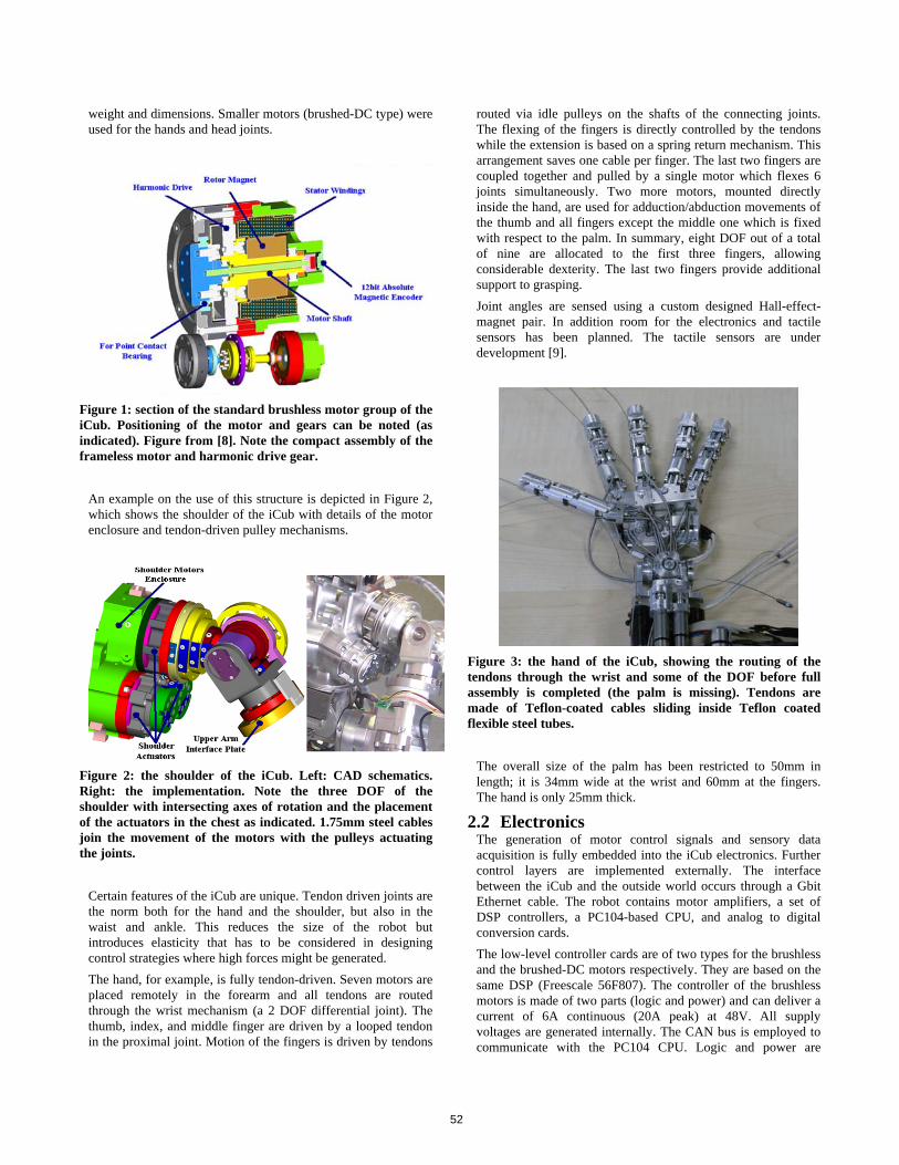
weight and dimensions. Smaller motors (brushed-DC type) were used for the hands and head joints.

Figure 1: section of the standard brushless motor group of the iCub. Positioning of the motor and gears can be noted (as indicated). Figure from [8]. Note the compact assembly of the frameless motor and harmonic drive gear.

An example on the use of this structure is depicted in Figure 2, which shows the shoulder of the iCub with details of the motor enclosure and tendon-driven pulley mechanisms.

Figure 2: the shoulder of the iCub. Left: CAD schematics. Right: the implementation. Note the three DOF of the shoulder with intersecting axes of rotation and the placement of the actuators in the chest as indicated. 1.75mm steel cables join the movement of the motors with the pulleys actuating the joints.

Certain features of the iCub are unique. Tendon driven joints are the norm both for the hand and the shoulder, but also in the waist and ankle. This reduces the size of the robot but introduces elasticity that has to be considered in designing control strategies where high forces might be generated.The hand, for example, is fully tendon-driven. Seven motors are placed remotely in the forearm and all tendons are routed through the wrist mechanism (a 2 DOF differential joint). The thumb, index, and middle finger are driven by a looped tendon in the proximal joint. Motion of the fingers is driven by tendons

routed via idle pulleys on the shafts of the connecting joints. The flexing of the fingers is directly controlled by the tendons while the extension is based on a spring return mechanism. This arrangement saves one cable per finger. The last two fingers are coupled together and pulled by a single motor which flexes 6 joints simultaneously. Two more motors, mounted directly inside the hand, are used for adduction/abduction movements of the thumb and all fingers except the middle one which is fixed with respect to the palm. In summary, eight DOF out of a total of nine are allocated to the first three fingers, allowing considerable dexterity. The last two fingers provide additional support to grasping. Joint angles are sensed using a custom designed Hall-effect-magnet pair. In addition room for the electronics and tactile sensors has been planned. The tactile sensors are under development [9].

Figure 3: the hand of the iCub, showing the routing of the tendons through the wrist and some of the DOF before full assembly is completed (the palm is missing). Tendons are made of Teflon-coated cables sliding inside Teflon coated flexible steel tubes.

The overall size of the palm has been restricted to 50mm in length; it is 34mm wide at the wrist and 60mm at the fingers. The hand is only 25mm thick.

2.2 ElectronicsThe generation of motor control signals and sensory data acquisition is fully embedded into the iCub electronics. Further control layers are implemented externally. The interface between the iCub and the outside world occurs through a Gbit Ethernet cable. The robot contains motor amplifiers, a set of DSP controllers, a PC104-based CPU, and analog to digital conversion cards. The low-level controller cards are of two types for the brushless and the brushed-DC motors respectively. They are based on the same DSP (Freescale 56F807). The controller of the brushless motors is made of two parts (logic and power) and can deliver a current of 6A continuous (20A peak) at 48V. All supply voltages are generated internally. The CAN bus is employed to communicate with the PC104 CPU. Logic and power are

52

58x42mm each and can control up to two motors. The power stage mounts also a metal heatsink that is then connected to the external shell of the robot for dissipation. Similarly the controller of the brushed-DC motors is made of two parts. One card acts as power supply; the other contains the CPU and amplifiers to control up to four motors. In this case the maximum continuous current is limited to 1A at 12V.

Figure 4: the brushless motor control logic and power amplifier of the iCub. Transistors and heatsinks are not shown. The size of the two PCBs is 58x42mm.

More development is in progress to interface tactile and force/torque sensors as discussed in [8].

2.3 SensorsGiven the size of the iCub, sensors were evaluated for performance but also weight and interface standards. The following table contains the list of available sensors and their status of maturity (i.e. integration into the robot hardware):

Component Model/type Notes

Cameras PointGrey Dragonfly 2 640x480 30fps

Firewire cameras, support also higher resolution

Microphones MICRO POM-2746L

Condenser electrect type

Inertialsensors

XSenseMTx

3 gyroscopes, 3 linear accelerometers, compass

Force/torquesensors

Custom Mechanically compatible with the ATI Mini-45

Positionsensors

AS5045 12bit, absolute magnetic encoder

Positionsensors

Faulhaber Integrated position sensing for DC motors

Positionsensors

Honeywell SS495A

Finger position sensing

Tactilesensors

Custom Based on the AD7147, capacitive sensing

All sensors are fully integrated apart from the force/torque sensor whose control electronics is still under development and the skin whose entire technology is under testing. More information can be found in [8, 9].

3. SOFTWAREThe iCub software was developed on top of Yarp [7]. RobotCub supported a major overhaul of the Yarp libraries to adapt to a more demanding collaborative environment. Better engineered software and interface definitions are now available in Yarp. Yarp is a set of libraries that support modularity by abstracting two common difficulties in robotics: namely, modularity in algorithms and in interfacing with the hardware. Robotics is perhaps one of the most demanding application environments for software recycling where hardware changes often, different specialized OSs are typically encountered in a context with a strong demand for efficiency. The Yarp libraries assume that an appropriate real-time layer is in charge of the low-level control of the robot and instead takes care of defining a soft real-time communication layer and hardware interface that is suited for cluster computation. Yarp takes care also of providing independence from the operating system and the development environment. The main tools in this respect are ACE [10] and CMake3. The former is an OS-independent communication library that hides the quirks of interprocess communication across different OSs. CMake is a cross-platform make-like description language and tool to generate appropriate platform specific project files. Yarp abstractions are defined in terms of protocols. The main Yarp protocol addresses inter-process communication issues. The abstraction is implemented by the port C++ class. Portsfollow the observer pattern by decoupling producers and consumers. They can deliver messages of any size, across a network using a number of underlying protocols (including shared memory when possible). In doing so, ports decouple as much as possible (as function of a certain number of user-defined parameters) the behavior of the two sides of the communication channels. Ports can be commanded at run time to connect and disconnect. The second abstraction of Yarp is about hardware devices. The Yarp approach is to define interfaces for classes of devices to wrap native code APIs (often provided by the hardware manufactures). Change in hardware will likely require only a change in the API calls (and linking against the appropriate library). This easily encapsulates hardware dependencies but leaves dependencies in the source code. The latter can be removed by providing a “factory” for creating objects at run time (on demand). The combination of the port and device abstractions leads to remotable device drivers which can be accesses across a network: e.g. a grabber can send images to a multitude of listeners for parallel processing. Overall, Yarp’s philosophy is to be lightweight and to be “gentle” with existing approaches and libraries. This naturally excludes hard real-time issues that have to be necessarily addressed elsewhere, likely at the OS level.

3 http://www.cmake.org

53

Figure 5: the complete iCub prototype.

3.1 Yarp example For the purposes of YARP, communication takes place through connections between named entities called ports. These form a directed graph, the YARP Network, where ports are the nodes, and connections are the edges. Each port is assigned a unique name, such as “/icub/camera/right”. Every port is registered by name with a “name server”. The goal is to ensure that if you know the name of a port, that is all you need in order to be able to communicate with it from any machine. The YARP name server converts from symbolic names to all the details necessary to make a connection with a specific resource. The YARP name server is designed to be easily used by clients who are not themselves using the YARP libraries or executables. The purpose of ports is to move data from one thread to another (or several others) across process and machine boundaries. The flow of data can be manipulated and monitored externally (e.g. from the command-line) at run-time. It can also be accessed without using the YARP libraries or executables, since the relevant protocols are documented. A port can send data to any number of other ports. A port can receive data from any number of other ports. Connections between ports can be freely added or removed, and may use different underlying transports. The use of several different transports and protocols allows us to exploit their best characteristics. TCP is reliable; it can be used to guarantee the reception of a message. UDP can be faster than TCP, but without guarantees. Multicast is efficient for distributing the same information to large numbers of targets. Shared memory can be employed for local connections. Figure 6 shows a very simple network of ports for a visual tracking application. Machine 1, in this example, grabs images which are sent to another application (the tracker proper). The

output of the tracker consists of two parts: the image coordinates of the tracked object and an image with a graphic overlay showing how good the tracker is doing. The output is sent to a control process on another machine (Machine 2) and for visualization to yet another machine. Different protocols can be used for reasons of efficiency.

Figure 6: example of a YARP network for a simple visual control loop.

4. OPEN SOURCE ROBOTICS RobotCub is Open Source both for software and hardware. While the phrase “Open Source software – OSS” is clear, “Open Source hardware” might sound strange, but in fact it is a plain transfer of the open source philosophy to the entire design of the RobotCub platform. The design of the robot started from the preparation of specifications (e.g. estimation of torque, speed, etc.), a typical 3D CAD modeling, and eventually in the preparation of the executive files which are used to fabricate parts and for assembly. Without good documentation it is very complicated to build and assemble a full robot. This means that documentation (as for software) is particularly important. The CAD files, in some sense, can be seen as the source code, since they are the “preferred form of the work for making modifications to it”, in the language of the GPL. They get “compiled” into 2D drawings which represent the executive drawings that can be used by any professional and reasonably well-equipped machine shop either to program CNC machines or to manually prepare the mechanical parts. This compilation process is not fully automated and requires substantial human intervention. There is a clear dependency of the 2D drawings on the original 3D CAD model. To enable the same type of virtuous development cycle as occurs in open source software, the 3D CAD is required, since changes happen in 3D first and get propagated to 2D later. In addition, assembly diagrams, part lists, and all the material produced during the design stage should be included to guarantee that the same information is available to new developers. One difference between software and the hardware design is that there are currently no effective formats for interchange of 3D models. Proprietary systems such as SolidWorks and Pro/E can import and export a range of formats, but going from one to another is lossy, destroying the information needed for production

54

and leaving just the basic geometrical shape. So in practice, designs are tied to tools produced by a particular vendor, and interoperability between hardware design tools is limited. In RobotCub we were forced to choose a specific set of tools for mechanical and electronic CAD and future upgrades will have to strictly adhere to these standards. Due to the absence of open source professional design tools, RobotCub uses proprietary products. This is an unfortunate situation, but there is no practical alternative at the moment. The “C++” and “gcc” of CAD do not exist yet. As a practical matter, the simple duplication of RobotCub parts does not require the use of any of these tools since we provide all executive drawings and production files (e.g. Gerber files for the PCBs). For modification, the design tools are somewhat expensive (although educational discounts or educational releases exist). Free of charge viewers are currently available for all file types in question. For RobotCub, we decided to license all the CAD sources under the GPL which seems appropriate given their nature. Associated documentation will be licensed under the FDL. These will be made available through the usual source code distribution channels (e.g. repositories, websites).

5. CONCLUSIONThe design process of RobotCub has been a distributed effort as for many open source projects. Various groups developed various subcomponents and contributed in different ways to the design of the robot including mechanics, electronics, sensors, etc. In particular, a whole design cycle was carried out for the subparts (e.g. head, hand, legs) and the prototypes that have been built and debugged. The final CAD and 2D drawings were discussed and then moved to the integration stage. Clearly, communication was crucial at the initial design stage to guarantee a uniform design and a global optimization. The distributed design broke down at the integration stage where the industrial partner (Telerobot Srl. – Genoa) stepped in to carry out integration, verification and consistency checks. The design and fabrication of the control electronics was also subcontracted to a specialized company. It is important to stress the collaboration with industry for a project of this size and with these goals and requirements. For many reasons building a complete platform involves techniques and management that is better executed following industrial standards. One example that applies to RobotCub is the standardization of the documentation. A further strategy used in RobotCub is that of building early. Each subsystem was built and copied as soon as possible. In several cases debugging happened either because the copies of the robot did not work as expected or because easy-to-fix problems were spotted. Sometimes the documentation had to be improved. Unfortunately, this strategy was applied less extensively to some of the subparts which are or were still under design and debugging. The design stage will be completed with the realization of the fifteen copies of the iCub. This will further test the documentation and in general the reliability of the overall platform including software, debugging tools, electronics, etc. The first release of the iCub will be consolidated after this final fabrication stage.

The actual design of the robot had to incorporate manipulation by providing sophisticated hands, a flexible oculomotor system, and a reasonable bimanual workspace. On top of this, the robot has to support global body movements such as crawling, sitting, etc. These many constraints were considered in preparing the specifications of the robot and later on during the whole design process.Both the iCub design and its software architecture are distributed as Open Source. This is not enough to guarantee success. Additional initiatives are required. RobotCub is giving away six copies of the iCub to the winners of an Open Call for proposals to use the iCub (recently concluded). In addition a structure called the Research and Training Site (RTS) has being created to support visiting researchers to work on the iCub prototypes in Genoa.

6. ACKNOWLEDGMENTSThe authors would like to thank the RobotCub Consortium. The authors were supported by European Union grant RobotCub (IST-2004-004370) and by euCognition (FP6 Project 26408). Paul Fitzpatrick is gratefully acknowledged for the continuous support to Yarp.

7. REFERENCES[1] L. Fadiga, L. Craighero, and E. Olivier, "Human motor

cortex excitability during the perception of others' action," Current Biology, vol. 14 pp. 331-333, 2005.

[2] L. Fadiga, L. Craighero, G. Buccino, and G. Rizzolatti, "Speech listening specifically modulates the excitability of tongue muscles: a TMS study," European Journal of Neuroscience, vol. 15, pp. 399-402, 2002.

[3] G. Rizzolatti and L. Fadiga, "Grasping objects and grasping action meanings: the dual role of monkey rostroventral premotor cortex (area F5)," in SensoryGuidance of Movement, Novartis Foundation Symposium, G. R. Bock and J. A. Goode, Eds. Chichester: John Wiley and Sons, 1998, pp. 81-103.

[4] D. Vernon, G. Metta, and G. Sandini, "A Survey of Cognition and Cognitive Architectures: Implications for the Autonomous Development of Mental Capabilities in Computational Systems," IEEE Transactions on Evolutionary Computation, special issue on AMD, vol. 11, 2007.

[5] C. von Hofsten, "On the development of perception and action," in Handbook of Developmental Psychology, J. Valsiner and K. J. Connolly, Eds. London: Sage, 2003, pp. 114-140.

[6] G. Sandini, G. Metta, and D. Vernon, "RobotCub: An Open Framework for Research in Embodied Cognition," presented at IEEE-RAS/RJS International Conference on Humanoid Robotics, Santa Monica, CA, 2004.

[7] P. Fitzpatrick, G. Metta, and L. Natale, "Towards Long-Lived Robot Genes," Journal of Robotics and Autonomous Systems, Special Issue on Humanoid Technologies, vol. 56, 2008.

[8] N. G. Tsagarakis, G. Metta, G. Sandini, D. Vernon, R. Beira, F. Becchi, L. Righetti, J. Santos-Victor, A. J. Ijspeert, M. C. Carrozza, and D. G. Caldwell, "iCub – The Design and Realization of an Open Humanoid

55

Platform for Cognitive and Neuroscience Research," Advanced Robotics, vol. 21, 2007.

[9] M. Maggiali, G. Cannata, P. Maiolino, G. Metta, M. Randazzo, and G. Sandini, "Embedded Distributed Capacitive Tactile Sensor," presented at The 11th

Mechatronics Forum Biennial International Conference 2008, University of Limerick, Ireland, 2008.

[10] S. D. Huston, J. C. E. Johnson, and U. Syyid, The ACE Programmer's Guide: Addison-Wesley, 2003.

56

An Open-Source Simulator for Cognitive Robotics Research: The Prototype of the iCub Humanoid Robot

Simulator V. Tikhanoff, A. Cangelosi

University of Plymouth Plymouth PL4 8AA

UK

vadim.tikhanoff@plymouth.ac.uk; acangelosi@plymouth.ac.uk

P. Fitzpatrick Lira-lab University of Genova

Viale F. Causa, 13 Genova Italy

paulfitz@liralab.it

G. Metta, L. Natale, F. Nori Italian Institute of Technology

Via Morego 30 Genova Italy

giorgio.metta@iit.it lorenzo.natale@iit.it francesco.nori@iit.it

ABSTRACT This paper presents the prototype of a new computer simulator for the humanoid robot iCub. The iCub is a new open-source humanoid robot developed as a result of the “RobotCub” project, a collaborative European project aiming at developing a new open-source cognitive robotics platform. The iCub simulator has been developed as part of a joint effort with the European project “ITALK” on the integration and transfer of action and language knowledge in cognitive robots. This is available open-source to all researchers interested in cognitive robotics experiments with the iCub humanoid platform.

Keywords Open-Source, Simulator, iCub humanoid robot, cognitive robotics.

1. INTRODUCTION Computer simulations play an important role in robotics research. Despite the fact that the use of a simulation might not provide a full model of the complexity present in the real environment and might not assure a fully reliable transferability of the controller from the simulation environment to the real one, robotic simulations are of great interest for cognitive scientists [18]. There are several advantages of robotics simulations for researchers in cognitive sciences. The first is that simulating robots with realistic physical interactions permit to study the behavior of several types of embodied agents without facing the problem of building in advance, and maintaining, a complex hardware device. The computer simulator can be used as a tool for testing algorithms in order to quickly check for any major problems prior to use of the physical robot. Moreover, simulators also allow researchers to experiment with robots with varying morphological characteristics without the need to necessarily

develop the corresponding features in hardware [1]. This advantage, in turn, permits the discovery of properties of the behavior of an agent that emerges from the interaction between the robot’s controller, its body and the environment. Another advantage is that robotic simulations make it possible to apply particular algorithms for creating robots’ controllers, such as evolutionary or reinforcement learning algorithms [12]. The use of robotics simulation permits to drastically reduce the time of the experiments such as in evolutionary robotics. In addition, it makes it possible to explore research topics like the co-evolution of the morphology and the control system [1]. A simulator for the iCub robot magnifies the value a research group can extract from the physical robot, by making it more practical to share a single robot between several researchers. The fact that the simulator is free and open makes it a simple way for people interested in the robot to begin learning about its capabilities and design, with an easy "upgrade" path to the actual robot due to the protocol-level compatibility of the simulator and the physical robot. And for those without the means to purchase or build a humanoid robot, such small laboratories or hobbyists, the simulator at least opens a door to participation in this area of research.

The iCub simulator is currently being used by both the RobotCub and the ITALK project partners for preliminary experiments on the simulator robot, and subsequent testing with the physical robots.

2. ICUB SIMULATOR DEVELOPMENT The iCub simulator has been designed to reproduce, as accurately as possible, the physics and the dynamics of the robot and its environment. The simulated iCub robot is composed of multiple rigid bodies connected via joint structures. It has been constructed collecting data directly from the robot design specifications in order to achieve an exact replication (e.g. height, mass, Degrees of Freedom) of the first iCub prototype developed at the Italian Institute of Technology in Genoa. The environment parameters on gravity, objects mass, friction and joints are based on known environment conditions.

2.1 Open-Source Approach The iCub simulator presented here has been created using open source libraries in order to make it possible to distribute the

Permission to make digital or hard copies of all or part of this work for personal or classroom use is granted without fee provided that copies are not made or distributed for profit or commercial advantage and that copies bear this notice and the full citation on the first page. To copy otherwise, or republish, to post on servers or to redistribute to lists, requires prior specific permission and/or a fee. PerMIS’08, August 19–21, 2008, Gaithersburg, MD, USA. Copyright 2008 ACM 978-1-60558-293-1…$5.00.

57

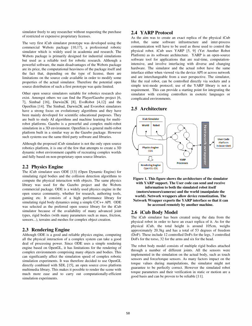
simulator freely to any researcher without requesting the purchase of restricted or expensive proprietary licenses.

The very first iCub simulator prototype was developed using the commercial Webots package [10,17], a professional robotic simulator which is widely used in academia and research. The Webots package is primarily designed for industrial simulations but used as a reliable tool for robotic research. Although a powerful software, the main disadvantages of the Webots package are its price, the computational heaviness of the package itself and the fact that, depending on the type of license, there are limitations on the source code available in order to modify some properties of the actual simulator. Therefore the potential open source distribution of such a first prototype was quite limited.

Other open source simulators suitable for robotics research also exist. Amongst others we can find the Player/Gazebo project [6, 7], Simbad [16], Darwin2K [8], EvoRobot [4,12] and the OpenSim [14]. The Simbad, Darwin2K and Evorobot simulators have a strong focus on evolutionary algorithms and they have been mainly developed for scientific educational purposes. They are built to study AI algorithms and machine learning for multi-robot platforms. Gazebo is a powerful and complex multi-robot simulation in a 3D environment. OpenSim is a general multi-robot platform built in a similar way as the Gazebo package. However such systems use the same third party software and libraries.

Although the proposed iCub simulator is not the only open source robotics platform, it is one of the few that attempts to create a 3D dynamic robot environment capable of recreating complex worlds and fully based on non-proprietary open source libraries.

2.2 Physics Engine The iCub simulator uses ODE [13] (Open Dynamic Engine) for simulating rigid bodies and the collision detection algorithms to compute the physical interaction with objects. The same physics library was used for the Gazebo project and the Webots commercial package. ODE is a widely used physics engine in the open source community, whether for research, authoring tools, gaming etc. It consists of a high performance library for simulating rigid body dynamics using a simple C/C++ API. ODE was selected as the preferred open source library for the iCub simulator because of the availability of many advanced joint types, rigid bodies (with many parameters such as mass, friction, sensors...), terrains and meshes for complex object creation.

2.3 Rendering Engine Although ODE is a good and reliable physics engine, computing all the physical interaction of a complex system can take a good deal of processing power. Since ODE uses a simple rendering engine based on OpenGL, it has limitations for the rendering of complex environments comprising many objects and bodies. This can significantly affect the simulation speed of complex robotic simulation experiments. It was therefore decided to use OpenGL directly combined with SDL [15], an open source cross platform multimedia library. This makes it possible to render the scene with much more ease and to carry out computationally-efficient simulation experiments.

2.4 YARP Protocol As the aim was to create an exact replica of the physical iCub robot, the same software infrastructure and inter-process communication will have to be used as those used to control the physical robot. iCub uses YARP [5, 9] (Yet Another Robot Platform) as its software architecture. YARP is an open-source software tool for applications that are real-time, computation-intensive, and involve interfacing with diverse and changing hardware. The simulator and the actual robot have the same interface either when viewed via the device API or across network and are interchangeable from a user perspective. The simulator, like the real robot, can be controlled directly via sockets and a simple text-mode protocol; use of the YARP library is not a requirement. This can provide a starting point for integrating the simulator with existing controllers in esoteric languages or complicated environments.

2.5 Architecture

Figure 1. This figure shows the architecture of the simulator with YARP support. The User code can send and receive

information to both the simulated robot itself (motors/sensors/cameras) and the world (manipulate the

world). Network wrappers allow device remotization. The Network Wrapper exports the YARP interface so that it can

be accessed remotely by another machine.

2.6 iCub Body Model The iCub simulator has been created using the data from the physical robot in order to have an exact replica of it. As for the physical iCub, the total height is around 105cm, weighs approximately 20.3kg and has a total of 53 degrees of freedom (DoF). These include 12 controlled DoFs for the legs, 3 controlled DoFs for the torso, 32 for the arms and six for the head.

The robot body model consists of multiple rigid bodies attached through a number of different joints. All the sensors were implemented in the simulation on the actual body, such as touch sensors and force/torque sensors. As many factors impact on the torque values during manipulations, the simulator might not guarantee to be perfectly correct. However the simulated robot torque parameters and their verification in static or motion are a good basis and can be proven to be reliable [11].

58

(a)

(b)

(c)

(d)

Figure 2. Photo of real iCub (a), of simulated iCub and the binocular view (b) The simulated iCub moving all four limbs as part of a demo (c) and the simulated iCub looking at and

manipulating an object in its environment.(d)

All the commands sent to and from the robot are based on YARP instructions. For the vision we use cameras located at the eyes of the robot which in turn can be sent to any workstation using YARP in order to do develop vision analysis algorithms.

The system has full interaction with the world/environment. The objects within this world can be dynamically created, modified and queried by simple instruction resembling those that YARP uses in order to control the robot.

3. ICUB SIMULATOR AND COGNITIVE ROBOTICS RESEARCH PROJECTS This section presents a research initiative on embodied cognition and developmental cognitive robotics based on the two EU projects RobotCub (robotcub.org) and ITALK (italkproject.org). Various robotics experiments in these two projects will rely on the use of the iCub simulator.

The RobotCub project aims at the development of an open humanoid robotic platform (iCub) and simultaneously the advancement of our understanding of cognitive systems by exploiting this platform in the study of the development of cognitive capabilities in humanoid robots. The idea is that, by creating a common platform, this will enable many laboratories to join this effort without having to invest themselves in developing

yet another robotic platform. The second aim of RobotCub is to investigate the development of these cognitive skills in natural and artificial cognitive systems. The project will carry out a plan of empirical research including neuroscience, developmental psychology, and robotics. This plan is centered on manipulation behavior, ranging from the direct aspects of reaching and grasping for objects to the use of gestures for communication. Aspects that will be touched along the way are—for instance—looking and overt attention, reaching, the detection and discovery of affordances, learning through imitation, and interaction. The emergent approach naturally encompasses the study of ontogenic development and, in fact, a comparatively large effort will be devoted to its study. The RobotCub project roadmap for this investigation includes the study of the starting point in terms of core abilities, the motivation of the system to explore and gather data, and new studies on a few research areas such as looking, reaching and manipulation, posture, locomotion, and social interaction. For each of these areas, issues of prospective use of information, motivation, and the mechanisms of exploration have to be experimentally investigated. The RobotCub agenda aims at covering—through targeted empirical investigation—most if not all of these issues.

The ITALK project intends to develop cognitive robotic agents, based among others on the iCub humanoid platform, that learn to handle and manipulate objects and tools autonomously, to cooperate and communicate with other robots and humans, and to adapt their abilities to changing internal, environmental, and social conditions. The main theoretical hypothesis behind the project is that the parallel development of action, conceptualisation and social interaction permits the bootstrapping of language capabilities, which on their part enhance cognitive development. This is possible through the integration and transfer of knowledge and cognitive processes involved in sensorimotor learning and the construction of action categories, imitation and other forms of social learning, the acquisition of grounded conceptual representations and the development of the grammatical structure of language.

The undergoing research falls into five main research themes: (i) action development, (ii) conceptualisation, (iii) social interaction, (iv) language emergence, and (v) integration and bootstrapping of cognition.

The study of the development of complex action manipulation capabilities will –in contrast to existing approaches– be based on synchronous development of motor, social and linguistic skills. For this it is fundamental to identify the characteristics of action development that are compatible with this scenario and reject those that are mere engineering solutions. Two core properties of biological motor control systems will be considered: compositionality, the construction of hierarchically ordered gesturing and manipulation, and generalization. We will study how action development can be guided by individual exploration by the robot and by imitating humans.

A fundamental skill of any cognitive system is the ability to produce a variety of behaviours and to display the behaviour that is appropriate to the current individual, social, cultural and environmental circumstances. This will require agents (1) to reason about past, present and future events, (2) to mediate their motor actions based on this reasoning process and (3) to communicate using a communication system that shares

59

properties with natural language. For this agents will need to develop and maintain internal categorical states, i.e. ways to store and classify sensory information. We term such internal states embodied concepts and we understand them as representations grounded in sensory-motor experiences that identify crucial aspects of the environment and/or of the agent/environmental interaction.

Another essential component of the ITALK research project is to look at the role of social learning and social interaction to support the development of a shared linguistic communication system. In particular, new research will consider (i) the role of imitation and human-robot interaction for the acquisition of shared communication systems based on deixis, gestures and reference, (ii) the role of users’ expectation in human-robot interaction and (iii) the emulation of actions and gestures in the learning of multimodal task-oriented behavior. Such research will be based on a series of human-robot interaction (HRI) experiments and on observational studies on parent-child dyads which will inform robot-robot and human-robot experiments. We expect to extend the expertise and methodologies in dialog systems for HRI studies to new studies on social interaction and communication where the robot’s linguistic communication system develops through interaction with its environment and other robots and humans.

The ITALK project will follow a cognitive linguistics approach. As it is centred on the interaction between action and language development, it provides the ideal testbed to investigate the emergence of linguistic constructions in close interaction with the development of action, social and grounded conceptual capabilities. We will focus on the emergence of linguistic structure. Among the research issues include (i) generalisation as the basis of the emergence of symbolic systems, (ii) the role of speech and “acoustic packaging”: speech or sound signals which serve as a cue to aid the learning of action sequences, (iii) the role of constructional grounding: the acquisition of linguistic construction and how one construction become favoured over another, (iv) the ontogenetic emergence of compositional lexicons, and (v) evolutionary studies on language emergence.

In the coming years the ITALK project aims to achieve a series of scientific and technological objectives such as providing new scientific explanations of the integration of action, social and linguistic skills and in particular on the hypothesis that action, social and linguistic knowledge co-develop and further bootstrap cognitive development. Another main aim deals with developing sets of methods for analyzing the interaction of language, action and cognition in humans and artificial cognitive agents using robot learning experiments, computer simulations, cognitive linguistic analysis, and experimental investigations from developmental linguistics, the neuroscience of language and action, and human-robot interaction experiments. Furthermore the project will develop innovative and cognitively plausible engineering principles, techniques and approaches for the design of communicative and linguistic capabilities in cognitive robots able to interact with their physical and social world and to manipulate entities, artefacts and other agents including humans.

All of the above aims would be demonstrated through the use of robotic experiments on the acquisition of object manipulation, social skills and linguistic capabilities in simulated and physical cognitive robots. In particular, robotic agents will be able to (a) acquire complex object manipulation capabilities through social

interaction; (b) develop an ability to create and use embodied concepts; (c) develop social skills that allow flexible interaction with other agents or people; (d) develop linguistic abilities to communicate about their interaction with the world.

4. CONCLUSION The current version of the iCub simulator has been used for preliminary testing by partners in the RobotCub and ITALK projects. In addition to being used for experiments on the development of controllers for the iCub robot, some groups have used the simulator to create a mental model [2] used by the robot to represent the current state of the environment.

Future plans on the simulator development will mostly involve the design of functionalities to model and interact with the physical environment. For example, this will allow the users to modify the objects in the world where the iCub resides, in order to allow different types of experiments. Finally, further work will focus on the systematic testing and replication of simulation studies with the physical robot.

5. ACKNOWLEDGEMENTS This work was supported by the European Commission FP6 Project RobotCub (IST-004370) and FP7 Project ITALK (ICT-214668) within the Cognitive Systems and Robotics unit (FP7 ICT Challenge 2). The authors also acknowledge the support of the FP6 euCognition Coordinated Action project funded under the same Cognitive Systems and Robotics unit.

6. REFERENCES [1] J.C. Bongard & R. Pfeifer (2003). Evolving complete agents

using artificial ontogeny. In Hara, F. & R. Pfeifer, Eds., Morpho-functional Machines: The New Species (Designing Embodied Intelligence) Springer-Verlag, pp. 237-258

[2] PF Dominey (2007) Sharing Intentional Plans for Imitation and Cooperation: Integrating Clues from Child Developments and Neurophysiology into Robotics, Proceedings of the AISB 2007 Workshop on Imitation.

[3] European commission, unit e5, home page. http://cordis.europa.eu/ist/cognition/index.html, 2007.

[4] Evorobot http://laral.istc.cnr.it/evorobot/simulator.html

[5] P. Fitzpatrick, G. Metta, L. Natale: Towards Long-lived Robot Genes, Robotics and Autonomous Systems, 56(1):29-45, 2008

[6] B. Gerkey, R. T. Vaughan and A. Howard. The Player/Stage Project: Tools for Multi-Robot and Distributed Sensor Systems. Proceedings of the 11th International Conference on Advanced Robotics, 2003.

[7] N. Koenig and A. Howard. Design and Use Paradigms for Gazebo, An Open-Source Multi-Robot Simulator. IEEE/RSJ International Conference on Intelligent Robots and Systems (IROS), Sendai, Japan, 2004.

[8] C. Leger, Darwin2K: An Evolutionary Approach to Automated Design for Robotics. Kluwer Academic Publishers, Aug 2000.

60

[9] G. Metta, P. Fitzpatrick & L. Natale. YARP: Yet Another Robot Platform. International Journal on Advanced Robotics Systems, 3(1):43–48, 2006.

[10] O. Michel, “Webots: Professional mobile robot simulation,” International Journal of Advanced Robotic Systems, vol. 1, no. 1, pp.39–42, 2004.

[11] N. Nava,V. Tikhanoff, G. Metta, G Sandini, Kinematic and Dynamic Simulations for The Design of RoboCub Upper-Body Structure ESDA 2008

[12] S. Nolfi & D. Floreano (2000). Evolutionary Robotics: The Biology, Intelligence and Technology of Self-Organizing Machines Cambridge, MA: MIT Press/Bradford Books

[13] Open Dynamics Engine http://opende.sourceforge.net/.

[14 OpenSim Simulator http://opensimulator.sourceforge.net/.

[15 SDL – Simple DirectMedia Layer http://www.libsdl.org/

[16] Simbad Simulator - http://simbad.sourceforge.net

[17] Webots - http://www.cyberbotics.com/

[18] Ziemke T. (2003). On the role of robot simulations in embodied cognitive science, AISB Journal, 1(4), 389-99

61

Symbiotic Robot Organisms:

REPLICATOR and SYMBRION ProjectsSpecial Session on EU-projects

Serge Kernbach∗

Eugen MeisterFlorian

SchlachterKristof Jebens

University of StuttgartUniversitätsstr. 38,D-70569 Stuttgart,

Germany

Marc SzymanskiJens Liedke

Davide LaneriLutz Winkler

University ofKarlsruhe

Engler-Bunte-Ring 8D-76131 Karlsruhe,

Germany

Thomas SchmicklRonald Thenius

Karl-Franzens-University

GrazUniversitatsplatz 2

A-8010 Graz, Austria

Paolo CorradiLeonardo RicottiScuola Superiore

Sant’AnnaViale Rinaldo Piaggio

3456025 - Pontedera

(PI), Italy

ABSTRACTCooperation and competition among stand - alone swarmagents can increase the collective fitness of the whole system.An interesting form of collective system is demonstrated bysome bacteria and fungi, which can build symbiotic organ-isms. Symbiotic communities can enable new functional ca-pabilities which allow all members to survive better in theirenvironment. In this article we show an overview of twolarge European projects dealing with new collective roboticsystems which utilize principles derived from natural sym-biosis. The paper provides also an overview of typical hard-ware, software and methodological challenges arose alongthese projects, as well as some prototypes and on-going ex-periments available on this stage.

Keywords: collective robotics, swarms, artificial evolu-tion, reconfigurable systems

1. INTRODUCTIONNature shows several interesting examples for cooperation

of individuals. Most prominent examples of cooperation arefound in social insects [1], where specialized reproductiveschemes (in most cases just a few out of thousands of colonymembers are able to reproduce) and the close relationshipsof colony members favoured the emergence of highly coop-erative behaviours [2]. However, also non-eusocial forms ofcooperative communities evolved, like the collective hunt-ing in predatory mamals [3] (e.g., lions, whales, ...) or thetrophallactic altruism in vampire bats. Such cooperative be-

∗Corresp. author: Serge.Kernbach@ipvs.uni-stuttgart.de

Permission to make digital or hard copies of all or part of this work forpersonal or classroom use is granted without fee provided that copies arenot made or distributed for profit or commercial advantage and that copiesbear this notice and the full citation on the first page. To copy otherwise, torepublish, to post on servers or to redistribute to lists, requires prior specificpermission and/or a fee.PerMIS 08, August 19-21, 2008, Gaithersburg, MD, USACopyright 2008 ACM 978-1-60558-293-1 ...$5.00.

haviours are mostly explained by reciprocal advantages dueto the cooperative behaviours and/or by the close relation-ship among the community members. In contrast to that,cooperation sometimes arises also among individuals thatare not just very distant in a gene pool, sometimes they donot even share the same gene pool: Cooperative behavioursbetween members of different species is called ’Symbiosis’.A non-exhaustive list of prominent examples are the polli-nation of plants by flying insects (or birds), the cooperationbetween ants and aphids. Also lichens, which are a closeintegration of fungi and algae and the cooperation betweenplant roods and fungi represent symbiotic interactions.

A common pattern in all these above-mentioned forms ofcooperation is that single individuals perform behaviours,which - on the first sight - are more supportive for the collec-tive of the group than for themselves. However, as these be-haviours have emerged through natural selection, we can as-sume that these cooperative behaviours have their ultimatereasoning in a sometimes delayed and often non-obvious in-dividual egoistic advantage.

Symbiotic forms of organization emerge new functional ca-pabilities which allow aggregated organisms to achieve bet-ter fitness in the environment. When the need of aggregationis over, symbiotic organism can dis-aggregate and exists fur-ther as stand-alone agents, thus an adaptive and dynamicalform of cooperation is often advantageous.

Lately, technical systems mimic natural collective systemsin improving functionality of artificial swarm agents. Col-lective, networked or swarm robotics are scientific domains,dealing with a cooperation in robotics [4]. Current researchin these domains is mostly concentrated on cooperation andcompetition among stand-alone robots to increase their com-mon fitness [5]. However, robots can build a principally newkind of collective systems, when to allow them to aggregateinto a multi-robot organism-like-forms. This ”robot organ-ism” can perform such activities that cannot be achievedby other kind of robotic systems and so to achieve betterfunctional fitness.

To demonstrate this idea, we consider a collective en-ergy foraging scenario for micro-robots Jasmine [6]. Swarmrobots can autonomously find an energy source and recharge.

62

The clever collective strategy can essentially improve the ef-ficiency of energy foraging, but nevertheless a functional fit-ness of a swarm is limited. For instance, if the rechargingstation is separated from a working area by a small barrier,robots can never reach the energy source. However, if robotsaggregate into more complex high-level organism which canpass the barrier, they will reach the docking station. Inthis way a cooperative organization of robotic system al-lows an essential increase of functional capabilities for thewhole group. The large integrated project ”REPLICATOR”(www.replicatores.eu), funded by the European commission,within the work programme ”Cognitive systems, interactionand robotics”, deals with such issues as reconfigurability ofsensors and actuators, adaptive control and learning strate-gies as well as working in real environments.

The cooperative (swarm-based or symbiotic) organizationof the robotic system provides essential plasticity of usedhardware and software platforms. The robot organism willbe capable of continuously changing its own structure andfunctionality. Such an evolve-ability opens many questionsabout principles and aspects of long- and short-term ar-tificial evolution and controllability of artificial evolution-ary processes. The large integrated project ”SYMBRION”(www.symbrion.eu), funded by European commission, withinthe work programme ”Future and Emergent Technologies”,is focused on evolve-ability, dependability and artificial evo-lution for such robot organisms based on bio-inspired andcomputational paradigms. Both projects are open-scienceand open-source.

Both projects, consortia and the European commissionare closely cooperating to achieve the targeted goals. It isexpected that results of both projects create new technologyfor making artificial robotic organisms self-configured, self-healing, self-optimizing and self-protecting from a hardwareand software point of view. This leads not only to extremelyadaptive, evolve-able and scalable robotic systems, but alsoenables the robot organisms to reprogram themselves with-out human supervision, to develop their own cognitive struc-tures and, finally, to allow new functionalities to emerge.

The rest of this paper is organized in the following way:In Section 2 we discuss a new paradigm of symbiotic sys-tems. Section 3 gives an example of the energy foragingscenario. Sections 4 and 5 briefly mention the hardware andsoftware challenges, where as Section 6 introduces severalideas towards evolve-ability of the robot organisms. Finally,in Section 7 we conclude this work.

2. NEW PARADIGM IN COLLECTIVEROBOTIC SYSTEMS

Collective intelligence is often associated with macroscopiccapabilities of coordination among robots, collective decisionmaking, labor division and tasks allocation in the group [7].The main idea behind this is that robots are achieving betterperformance when working collectively and so are capableof performing such activities which are not possible for in-dividual robots. The background of collective intelligence isrelated to the capability of swarm agents to interact jointlyin one medium. There are three different cases of such in-teractions:

1. In the first case agents communicate through a digitalchannel, capable for semantic messages exchange. Due toinformation exchange, agents build different types of com-

mon knowledge [8]. This common knowledge in fact underliecollective intelligence.

2. The second case appears when macroscopic capabilitiesare defined by environmental feedback. The system builds aclosed macroscopic feedback-loop, which works in a collec-tive way as a distributed control mechanisms. In this casethere is no need of complex communication, agents inter-act only by kinetic means. This case if interaction is oftendenoted as a spatial reasoning, or spatial computing.

3. The third case of interactions we encounter in na-ture, when some bacteria and fungi (e.g. dictyostelium dis-coideum) can aggregate into a multi-cellular organism whenthis provides better chances of survival [9]. In this way,they interact not only through information exchange or spa-tial interactions, they build the closest physical, chemicaland mechanical interconnections, through the agents stillremain independent from each other.

The first two cases of interactions are objects of extensiveresearch in many domains: robotics, multi-agents systems,bio-inspired and adaptive community and so on. Howeverthe practical research in the last case represents essentialtechnological difficulties and therefore is not investigatedenough. Despite the similarities between a robot swarm andmulti-robot organism, such as a large number of robots, fo-cus on collective/emergent behavior, a transition betweenthem is a quite difficult step due to mechanical, electricaland, primarily, conceptual issues [10]. In the following sec-tions we introduces corresponding challenges in more detail.

Now, we believe that research around the third case ofinteractions is concentrated on four important questions:

1. Reconfigurability, adaptability and learn-ability of thesymbiotic systems. These issues include flexible and multi-functional sensors and actuators, distributed computation,scalability, modelling, control and other issues, which areclosely related to the reconfigurable robotic research. TheREPLICATOR project is focused on these points.

2. Evolve-ability of the symbiotic systems, which includesprinciples and aspects of long- and short-term artificial evo-lution and adaptivity as well as exploring and analogies tobiological systems. The SYMBRION project is focused onthese points.

3, 4 Embodiment of evolutionary systems for different en-vironments and medias as well as investigation of informa-tion properties of such systems. These points are covered byother research initiatives and projects.

In this way, the next step in a further research withinthe collective robotic community can consist in investiga-tion multi-robot organisms or, in other words, a transitionfrom robot swarm to a multi-robot organisms. All furthersections are devoted to demonstrate diverse aspects of sucha transition.

3. EXAMPLE: ENERGY FORAGING SCE-NARIO

In this section we will demonstrate the advantages of sym-biotic organization of autonomous robotic systems. We choosefor this purpose an example of energy homeostasis, becauseit is applicable to both living and robotic organisms and sowe can draw several analogies between them.

The distinctive property of any living organism is the en-ergy homeostasis and, closely connected, foraging behav-ior and strategies [3]. The robots, equipped with on-board

63

recharging electronics, can also possess its own energy home-ostasis. In this way, when swarm robots get ”hungry”, theycan collectively look for energy resources and execute dif-ferent strategies in a cooperative energy foraging [11]. Incritical cases robots can even decide to perform individualforaging, competing with other robots for resources.

The need of energy is a perfect example of natural fit-ness. If robots that are performing individual strategies findenough energy, they can survive in the environment. Inturn, this means that these strategies were sufficient enoughto balance these robots energetic budgets. Simultaneously,other energetically die if their behavioral strategy was poor.Based on such energy foraging, many of evolutionary ap-proaches for different robotic species can be developed, com-pared and tested.

However, if there are many robots foraging in the environ-ment, several undesired effects can emerge: (1) the dockingstation can become a ”bottleneck” resource that essentiallydecreases the swarm efficiency; (2) robots with a high-energylevel can occupy the docking station and block low-energeticrobots. These robots can energetically die (and so decreasethe swarm efficiency); (3) many robots can create a ”crowd”around a docking station and essentially hinder a dockingapproach. This can increase the total recharging time andmakes worse the energetic balance of the whole swarm.

Robots, in pursuing their energetic homeostasis, have onlytwo possible decisions to make: (1) to execute a currentcollective task or (2) to move for recharging. In balancingthese two behaviours, a cooperative strategy may find theright timing and the right combination between these in-dividual decisions of all robots. Lately, several strategies ofenergy foraging for a robot swarm up to 70 swarm agents areimplemented, see Fig. 1. These cover different bio-inspiredapproaches [12], [13] and hand-coded strategies [14].

In one of these experiments, a few robots died close tothe docking station and blocked the recharge area (we ”sim-ulated” this in the Fig. 1(b)). Robots that were in frontof this barrier (away from the docking station) finally alsodied. This is the limit of functional fitness of swarm robots.There is no strategy, that allow swarm robots to overpass thebarrier. Only when swarm robots would collectively emergenew functionality, like ”pass the barrier”, they would solvethe ”barrier problem”.

Thus, an ideal solution for the ”barrier problem” can bethe aggregation of many single robots into one cooperativemulti-robot organism. This way, they can reach the dockingstations by ”growing legs” and stepping over the barrier. Inthat case, the robots are helping each other in a cooperativemanner, see Fig. 1(c).

Obviously, such a robotic behaviour is extremely challeng-ing from many viewpoints: Cooperative (symbiotic) robotsystems have many similarities with known robotic researchas e.g. mechanical self-assembling [15] or reconfigurablerobotics [16]. However, the symbiotic form, show in Fig. 1,essentially differs from this robotic research, namely: (1)Robots should be capable for autonomous aggrega-tion and disaggregation; (2) Robots in the disaggre-gate state should possess individual locomotion; (3)There is no central control neither for disaggregatedstate (swarm) nor for the aggregate state (organ-ism); (4) Stand-alone robots should profit from theaggregation into organism.

The swarm-based approaches, which is underlying the ag-

(a)

(b)

(c)

Figure 1: (a) Docking of a few robots for recharg-ing. Shown is the two-line approach: the first line -recharging robots, the second line - robots waitingfor recharging; (b) The ”barrier problem” - robotsare separated form docking stations by a barrier; (c)A possible solution to the ”barrier problem”: swarmrobots form a symbiotic multi-robot organism andcollective pass the barrier.

64

gregation processes, differs primarily from aggregated sys-tems which are studied in the field of ”reconfigurable robotics”.In the following we consider on-going work with aggregated(symbiotic) robot organisms.

4. HARDWARE CHALLENGESThe main feature of a modular robot consists in being

composed of several potentially independent modules, withlimited complexity and capabilities, which are able to con-nect to each other in different configurations, in order toform a robot with greater capabilities. The global knowl-edge and the functionalities of the assembled robot generateby sharing of information and of resources between modulesand by the fundamental capability of self-reconfiguration,in order to meet the demands of different tasks or differentworking environments. As a consequence, the overall func-tionalities and capabilities of a robotic modular organismare deeply related to the hardware structure and functionsof its basic composing modules.

At the current stage of development of the projects (bothprojects started in 2008), the development of the hardwarerepresents one of the hardest issues. In general, the conceptof hardware design is as follows:

1. Independence for separate robots, this includes capa-bilities for communication, computation and sensing as astand-alone robot, as well as individual locomotion and en-ergy management.

2. Large computational power of the organism, requiredfor performing on-line and on-board evolutionary approaches.

3. Heterogeneity of individual robots, which allows theirlater specialization within the organism.

4. Rich sensing and communication capabilities of theorganism. The more robots are joined in the organism, themore functional diversity the organism can demonstrate.

5. Possible higher independency from human in term ofenergy, support and maintenance.

The consortia considered many state-of-the-art reconfig-urable solutions, such as superBot [17], M-Tran [18], Poly-Bot [19], molecube [20], HYDRA/ATRON [21] and oth-ers, even visited some of these labs for exchange of expe-rience. Currently, we follow three different developmentallines, which will be later fused into one or two first proto-types.

4.1 Mechanical ChallengesThe mechanical design of a robot, which is working to-

gether with other robots inside a swarm, differs in severalpoints from the design of a robot being a part of an organism.In the first case, criteria like small size, simple kinematics,simple casing, high mobility and low price define the designof the robot. On the other hand, a robot inside of a self-reconfigurable organism needs docking elements, high-powermotors to produce enough torque, depending on the designof the organism one or more independent degrees of free-dom and a casing with high stiffness to handle reaction be-tween robots. Within the REPLICATOR and SYMBRIONprojects, one of the challenges will be to combine the char-acteristics of both kinds of robots into one.

In the beginning, there seems to be a few major prob-lems that need to be solved. First of all the robot musthave a docking element capable of handling the stress of sev-eral robots docked to it while applying all their forces (e.g.gravity, reaction, inertia force). Additionally, the docking

element needs to assure the automatic coupling of severalelectric contacts needed for information exchange and powerdistribution between the robots inside an organism. Besidetechnical requirements the docking element should supportthe self aggregation of the robots. No matter how the po-sition of two robots to each other is, the docking procedureshould work. Therefore the docking element needs to bal-ance misalignment and displacement to a certain degree. Toincrease the amount of possible structures for the organismand to simplify docking for the robots, all docking elementswill be unisex and there will be at least four docking ele-ments on each robot. Another problem is the mobility ofthe robot requested by the swarm based requirements. Inorder to guarantee local communication between robots, areasonable velocity (i.e. a contacting rate) is needed. Thekind of suitable locomotion is under evaluation.

The general approach in the state of art of modular roboticsis the development of ”cube-like” robotic modules with in-ternal motors, batteries and control. The docking ports areusually placed on the sides and both locomotion and liftingabilities are provided mechanically separating the module intwo blocks, able to bend reciprocally. This bending allowsthe lifting of attached modules, but often represents the onlylocomotion strategy for the robot, that can be quite slow andcomplex to control in accuracy and resolution of movement.Hence, as a new feature in modular robotics, we are cur-rently considering to introduce higher locomotion capabili-ties, for instance integrating wheels in the modules, givingmore independency to each module. The aim is to fabricatemodules that are firstly conceived as independent robotsrather than ”just” modules to be assembled in a robotic or-ganism. The increase in independency for what concernslocomotion allows in this way single modules, now roboticunits, to move and explore the environment, rapidly acquir-ing information about the environment. Subsequently, theycan rapidly reach their neighbours and, as a last process,engage assembly. Furthermore, wheeled modules could beused by the robotic organism as ”wheeled feet” in order tohave a faster global locomotion. As advanced feature, thewheels themselves could be an actuation mechanism (i.e., arotational degree of freedom), considering to integrate intothe wheels the docking mechanism. A wheeled-locomotionapproach is characterized by a very high-energy efficiencyon smooth surfaces, but it could show limitation on sandyor pebbly surfaces and even in facing small obstacles (likeelectrical cables, grass, etc.). The first concept in order tosolve this issue consists in moving from a basic mini-roverconfiguration with four wheels to a caterpillar-based roboticunit, able to provide locomotion even on challenging surfacesand environments.

A differential drive is easy to implement and to control.However, not every movement is possible. The docking oftwo robots in the orientation of their wheel axis is only pos-sible with a non trivial motion sequence. A non-holonomicdrive is capable of positioning the robot everywhere and inany orientation to another robot, but is difficult to imple-ment in design as well as in control. With at least twodegrees of freedom a movement by crawling is also possi-ble. Unfortunately, this is done by use of the main actu-ators which consume a lot of power. The optimal solutiondepends therefore on the scenario for the robots. At the mo-ment, a crawling like locomotion is likely for the replicatorrobot while a mixture between non-holonomic and differen-

65

tial drive is more suitable for the SYMBRION robot.These are only two challenges out of many which need

to be solved within the REPLICATOR and SYMBRIONprojects, but in the end we will know much more aboutsuitable design of self aggregating robots.

4.2 Electronic ChallengesThe electronic design is a huge challenge due to strong

restrictions of the size of the robot and the complexity ofthe hardware design. Each stand-alone robot is equippedwith two processors, one main microcontroller (MCU) andone shadow microprocessor (CPU, see Fig. 2). The break-down in microcontroller and microprocessor was deliberatelyintended to separate computational tasks within the singlecell.

CoreMCU

ShadowCPU

RAM+Flash

Sensors

/PC

/Cam

era

Upper board

CANcells cells

I²C

USB

(SPI)

Embedded Linux,Evolutionary Algorithms,ANN...

RTOS, Sensor pre-processing,AIS...

SPI

I²C

SPI

Sensors

/PC

/Zig

Bee

USB

Upper board

CELL

HDD

Figure 2: Functional electronic design of modules.

The core microcontroller performs basic functionality (e.g.sensor pre-processing, running artificial immune system) andkeeps the robot alive. The shadow microprocessor is mainlyresponsible for bio-inspired approaches like the genetic al-gorithms, sensor fusion, ANNs etc. and is more powerfulin comparison to the core processor. Due to higher compu-tational power results in higher energy consumption, theshadow processor is able to run at different power-downmodes when computational power isn’t needed.

One of the biggest challenges during the electronic designis the development of the shadow processor module in atiny size as well as finding solutions for shared resources likememory, power and communication capabilities.

5. SOFTWARE CHALLENGESBeside the hardware challenges, the project is faced with

many software requirements. Because robots can either runindependently, as a swarm, as an organism, or even as aswarm of organisms, the interaction has to be managed inan organized and efficient way.

The different layers of software development are shown inFig. 3. On the bottom layer there are two different proces-sors, which are able to communicate with each other andhave to be coordinated at the robot level. To cope withthe additional difficulties a swarm or an organism causes, amiddleware-like system is necessary. On top of this abstrac-tion layer high-level control mechanisms and distributed ap-plications can be integrated.

Figure 3: Different layers for software development.

5.1 Robot OSOn the robot level it is necessary to adopt mechanisms

to coordinate data and data flow in a suitable way, and atthe same time it is essential to predict and organize the be-haviour of the multitasking system. It is also critical forthe project to deal with the event driven architecture ofthe robot especially in respect to the real-time sensor sys-tem. For this reason a Real-Time Operating System (RTOS)builds the base of the software structure. The software ar-chitecture of the robot is modular and provides basic func-tionalities such as creation and termination of tasks andthreads, inter-task communication, inter-processor commu-nication, external event management, and memory alloca-tion. Additionally the robot runtime system has to providethe middleware system with appropriate interfaces.

5.2 MiddlewareOnce the robots are aggregated into a more advanced

multi-cellular organism it is essential to have an efficient con-trolling and coordinating mechanism. Therefore a middle-ware layer is introduced which defines unified interfaces andcommunication services according to the individual robotcapabilities. The distributed middleware controls synchro-nization processes between nodes, configures and handle thecommunication bus (CAN) and manages distributed mem-ory and energy resources. Furthermore it has to provide therobots with an abstraction layer between the operationalsystem functions and the high-level controller domain.

5.3 High-level control conceptsOur projects will evaluate and test a variety of different

control-concepts for the single robots as well as for the aggre-gated high-level robotic organism. Example can be given byartificial immune and artificial neuronal networks, differentlearning mechanisms as well as classical model-based con-trollers. In the following we describe one of these controllers- a bio-inspired controller concept which we call ”Hormone-Driven Robot Controller” (HDRC). A data-structure thatwill hold configuration information for the robot, especiallyfor the used software controllers of the robotic node, is called”Genome” in our constortia’s terminology. This Genome willcontain also a set of rules that link the degradation and thesecretion of hormones to the local levels of other hormones.The secretion of hormones can be triggered by other hor-mones or by receptors that get activated by receiving en-vironmental stimuli. Hormones can alter the sensitivity ofreceptors, trigger activities, modulate certain controllers oreven activate/deactivate whole (sub-)controllers. This waywe expect that a variety of systems can easily evolve:

1. Homeostatic systems: These hormone systems can

66

allow the organism to regulate a variety of internal proper-ties around a homeostatic set point. For example, an robot”hungry” for light but located in the dark, can increase itsmotion level, thus will increase its chance to find a light spot.

2. Adaptive behaviours: Hormones can reflect a changeof state of the environment, thus they can modulate con-trollers to respond to these environmental changes.

3. Target-oriented behaviours: Hormones with veryfast dynamics (short-term acting hormones) can be evenused to steer robots autonomously towards certain targetsor to actively avoid areas or objects. This can be used inthe previously mentioned foraging-for-energy scenarios.

3. Signal propagation and timing: As hormones arepassed also among the robotic nodes in an aggregated or-ganism, hormones can be used for signal propagation alongthe body of this organism. In nature, such systems showfrequently the ability to perform rather well working tim-ing tasks (see for example the synchronization of firefliesin [2]). We can expect to evolve such signal-propagationmechanisms also in our aggregated robotic organisms, pos-sibly synchronizing the movement patterns of legs or otherbody parts.

To allow the HDRC to evolve the above-mentioned tasksand to evolve the needed functionality to perform such tasks,we have to implement a separate hormone controller. Thiscontroller is created from the evolved information in theGenome and frequently simulates hormone secretions (addi-tions), degradations and diffusion within each robotic node.Using the available communication capabilities of the robots,the hormones are exchanged also between the robotic nodes,thus allowing a diffusion of virtual hormones within thewhole higher-level organism.

Fig. 4 shows two distinct ways how the HDRC can be usedin two different swarm states:

State 1: Fig. 4a shows that each robot is contains severalvirtual compartments, which associated with different realrobot ”body parts”. In the case depicted here, each robotcontains 2 lateral, one frontal and one terminal compart-ment. In the center, there is a fifth (central) compartmentlocated. Sensors can trigger excretion of hormones into theircorresponding local compartment and actuators can be mod-ulated/affected only by hormone concentrations which arepresent in their corresponding compartment. Hormones arediffused to neighboring compartments and to to the centralcompartment. In the depicted case, a light sensor senses anobstacle to the left of the robot. It triggers the secretion(addition) of a hormone into this segment, which enhancesthe speed of the associated left motor. By diffusion, thesame hormone reaches also the right compartment, whereit can decrease the rotation speed of the right motor: Therobot turns to the right. A central luminance sensor (centralcompartment) can trigger the secretion of another hormone,which generally increases motor speed on both sides: Therobot drives (forages) faster in brighter illuminated areas.

State 2: Fig. 4b shows a totally different usage of theHDRC: One robot started to call other robots for aggrega-tion. It secrets a specific ”head-marking” hormone. Thishormone is secreted only in the first robot that starts theaggregation. Due to the diffusion process and the increasingchain length, the concentration of this hormone decreases,as the robotic organism gets larger. By using this gradientas a source of information for the ”tail robots”, the organismcan be limited to certain sizes and there is always a gradient

Figure 4: (a) Schematic drawing of a hormone-driven robot controller (HDRC) performing anobstacle-avoidance behaviour. Receptors can trig-ger hormone secretions. these hormones can differthrough several virtual body compartments inside ofa single robot. Hormones can switch on or off actu-ators, modulate actuator function or interfere withother hormones; (b) Several robotic nodes are cou-pled together to a higher-level organism. Simulatedhormones are floating through the ”body”, form-ing hormone gradients. In the picture, a dedicated”head”-hormone is shown. These hormone gradientscan support the formation of aggregated organismsout from the ”fuzzy” swarm state, which is formedby many free-driving or free-walking robots.

inside of the organism that points towards the ”head”. Thisgradient information can also be important for coordinatingbody movements.

5.4 Simulation FrameworkTo test, compare and verify different robot designs, dif-

ferent organism configuration and the controllers in a quickand cheap way, a simulation environment needs to be im-plemented. The simulation should offer an easy and fastway to create a test environment and to design some basicrobot architectures to test the availabilities the robot mighthave. Later the simulation can be used to test different or-ganism configurations and to verify the different controllers.Furthermore, the simulation can be applied in long term sce-narios to explore biologic mechanisms like evolutionary andgenetic algorithms, collective and symbiotic behaviour andneuronal networks.

In the REPLICATOR and SYMBRION projects we willuse Delta-3D for the simulation framework, see Fig. 5. It of-fers lots of interfaces and has already successfully been usedin other simulations. The aim is to simulate the physics ofthe single robots, as well as that one of a whole organism.

67

Figure 5: Screenshot of the Simulation EnvironmentUsing Delta 3D.

3D-models from CAD-programs can easily be loaded intothe environment and without any effort a robot model canbe created in the simulation. Different robot configurationslike form, size and the position and orientation of the jointsof the robot can be easily created and tested within the envi-ronment. Additionally the simulation needs to integrate thecontroller into the environment without modifying it withthe aim that the robot will behave in the simulation nearlythe same as in the real environment. Therefore a hardwareabstraction layer (HAL) needs to be strictly specified, whichwill offer the same functionality for the actual robot and thesimulated one. A robot controller will only use the function-ality of the HAL, so that a robot, developed in a simulationenvironment, will run on a real robot and vice versa.

As the requirements to the simulation will grow with thecomplexity of the controller, running the simulation on justone computer or even just on a single core won’t be suf-ficient enough. Therefore a distributed simulation will bemandatory. For this purpose Delta-3D offers an interface tothe High Level Architecture (HLA), a general purpose archi-tecture for distributed computing. Using this architecturethe simulation can be executed on several computers havingdifferent platforms located within a local area network orconnected through the internet as well.

6. TOWARDS EVOLVE-ABILITY OF THEROBOT ORGANISM

Within the projects, the creation of evolvable or otherwiseadaptive software and hardware is the main focus. However,from the conceptual point of view, achievement of evolve-ability for the robot organism is planned in two complemen-tary ways, which we call bio-inspired (or bio-mimicking) andengendering-based approaches.

6.1 Bio-inspired/bio-mimicking approachAny bio-inspired approach is based on analogies to living

organisms and is carried out by the biological partners inour consortia. Our bio-inspired control algorithms use nei-ther any global point of information nor any form of complexknowledge. Our algorithms are stable to a wide range of en-vironmental conditions and are extremely robust. Therefore,the bio-inspired strategies in projects are going to draw ad-vantage from the well-known robustness/simplicity as wellas from the plasticity/adaptability derived from natural sys-tems. Our goal is to create stable, robust and adaptable

robotic organisms. Here we will investigate a variety of con-cepts, such as:

1. Genome: All robotic organisms will carry one orseveral Genomes. A Genome is a collection of genes, whichcarry information about controller structure and controllerdynamics. A gene can be a simple part of a blueprint, which”depicts” a part of the final controller. But a gene can alsowork as a rule, which is used to ”construct” parts of thefinal controller. In the latter case, there can be interferencesbetween different genes, thus competition or cooperation canarise also on the genetic level. A self-organized process canbe established which will be able to create a flexible, butrobust controller structure.

2. Controller: We will investigate several controllertypes, ranging from rules-based controllers, to EvolvableArtificial Neural Networks (EANN), to hormone-based con-trollers and to even hand-coded controllers that execute hand-optimized (modular) parts of the whole organism’s behaviouralrepertoire.

3. Sexuality/Reproduction: We plan to enhance andto speed-up the dynamics of artificial evolution by imple-menting virtual-reproduction of robots. A separate processwill allow to remove controllers from the least fit robots andto re-initialize them with mixtures (interbreeds) of the con-trollers of more fit robots. We will also investigate the ad-vantages of sexual reproduction in such scenarios.

4. Embryology: To allow well-ordered controllers toemerge from the information stored in the Genome, we willmimic embryological processes, driven by a virtual hormonesystem.

6.2 Engineering-based approachThe engineering-based approach is complementary to the

bio-inspired one and focuses in such issues as learning, dis-tributed decision making, navigation and so on. Generally,consortium focuses on three following approaches (these ap-proaches are closely connected so that finally it will be akind of hybrid framework):

1. On-line learning. On-line learning is based on thebehavior level and uses automatically generated feedback.The feedback comes from internal, external and virtual sen-sors. Some direct feedback can be sensed through vision-based subsystem, by using FRID-based identification or lo-calization technologies, by using smart laser scanner, sound,light, humidity, temperature, internal energy sensor and othersensors. It is intended to use middleware and sensor-fusionapproach to generate complex non-direct feedbacks throughvirtual sensors. Since off-line mechanisms can hardly be ap-plied to real robots, the challenge of the proposed approachis to perform non-supervised learning without any off-linemechanisms (or at least with a minimum of them). Thiscan be achieved by combining evolving computation withrewards/feedback/fitness calculated on-line. Therefore thewhole approach can be named ”on-line learning”.

2. Evolutionary computation. High computationalpower of the system allows running on-line and on-boardsuch well-known approaches as genetic programming (GP)(e.g. [22]), Genetic Algorithms (GA) (e.g. [23]). To avoidthe problems posed by a huge search space, we intend tointegrate limitations, originating from hardware platform.Another set of problems we are aware of are the fitnessfunctions required for these algorithms. These fitness func-tions are very difficult to calculate based only on local sensor

68

data. Moreover these functions are evaluated extremely de-layed because the organism mostly assess their fitness afteraccomplishing the task.

3. Approaches from the domain of DistributedArtificial Intelligence (DAI). On-line learning as well asGA/GP include diverse aspects of DAI such as a distributedknowledge management, semantic information processing,navigation and actuation in the environment, planning, sen-sor fusion and others. Development and implementation ofthese approaches is an important step towards evolve-abilityof the robot organisms.

7. CONCLUSIONIn this short paper we made on overview of two large

European projects, dealing with a new paradigm in collec-tive systems, where the swarm robots get capable of self-assembling into a single symbiotic multi-robot organism. Weintroduced an energy foraging scenario for both robot speciesand demonstrated that a transition between collective andsymbiotic robot forms represents a very hard problem. It in-volves not only hardware and software issues, but also verybasic questions being also open not only in biological but alsoin engineering sense. We demonstrated the main hardwareand software challenges and the road-map how to achievethe evolve-ability of the robot organisms.

8. ACKNOWLEDGEMENTREPLICATOR and SYMBRION projects are funded by

European Commission within the 7th framework programm.We want to thank ”euCognition”1 for supporting your in-volvement in the conference.

9. REFERENCES[1] E. Bonabeau, M. Dorigo, and G. Theraulaz. Swarm

intelligence: from natural to artificial systems. OxfordUniversity Press, New York, 1999.

[2] S. Camazine, J-L. Deneubourg, N.R. Franks, J. Sneyd,G. Theraulaz, and E. Bonabeau. Self-Organization inBiological Systems. Princeton University Press,Princeton, NJ, USA, 2003.

[3] D.W. Stephens and J.R. Krebs. Foraging Theory.Princeton University Press, 1987.

[4] E. Sahin. Swarm Robotics: From sources of inspirationto domains of application. Springer-Verlag,Heidelberg, Germany, 2004.

[5] S. Kornienko, R. Thenius, O. Kornienko, andT. Schmickl. Re-embodiment of honeybee aggregationbehavior in artificial micro-robotic system. AdaptiveBehavior (accepted for publication).

[6] S. Kornienko, O. Kornienko, and P. Levi. Ir-basedcommunication and perception in microroboticswarms. In Proc. of the IROS 2005, Edmonton,Canada, 2005.

[7] G. Weiss. Multiagent systems. A modern approach todistributed artificial intelligence. MIT Press, 1999.

[8] J.Y. Halpern and Y. Mosesi. Knowledge and commonknowledge in a distributed environment. J. of theAssociation for Computer Machinery, 37(3):549–587,1990.

1http://cordis.europa.eu/ist/cognition/index.html

[9] H. Haken. Synergetics: An introduction, third edition.Springer-Verlag, New York, 1983.

[10] S. Kornienko, O. Kornienko, A. Nagarathinam, andP. Levi. From real robot swarm to evolutionarymulti-robot organism. In Proc. of the CEC2007,Singapure, 2007.

[11] S. Kornienko and O. Kornienko. Collective energyhomeostasis in a large-scale micro-robotic. Roboticsand Autonomous Systems (under resubmitting).

[12] D. Habe. Bio-inspired approach towards collectivedecision making in robotic swarms. Master Thesis,University of Stuttgart, Germany, 2007.

[13] T. Kancheva. Adaptive role dynamics in energyforaging behavior of a real micro-robotic swarm.Master Thesis, University of Stuttgart, Germany,2007.

[14] A. Attarzadeh. Development of advanced powermanagement for autonomous micro-robots. MasterThesis, University of Stuttgart, Germany, 2006.

[15] A. Ishiguro and T. Maegawa. Self-assembly throughthe interplay between control and mechanical systems.In Proc. of IEEE/RSJ06 Int. Conf. on IntelligentRobots and Systems, pages 631–638, Beijing, China,2006. IEEE.

[16] S. Murata, K. Kakomura, and H. Kurokawa. Dockingexperiments of a modular robot by visual feedback. InProc. of IEEE/RSJ06 Int. Conf. on Intelligent Robotsand Systems, pages 625–630, Beijing, China, 2006.IEEE.

[17] Wei-Min Shen, Maks Krivokon, Harris Chiu, JacobEverist, Michael Rubenstein, and Jagadesh Venkatesh.Multimode locomotion for reconfigurable robots.Autonomous Robots, 20(2):165–177, 2006.

[18] Haruhisa Kurokawa, Kohji Tomita, Akiya Kamimura,Shigeru Kokaji, Takashi Hasuo, and Satoshi Murata.Distributed self-reconfiguration of m-tran iii modularrobotic system. Int. J. Rob. Res., 27(3-4):373–386,2008.

[19] Alex Golovinsky, Mark Yim, Ying Zhang, CraigEldershaw, and David Duff. Polybot andpolykinetic/spl trade/ system: a modular roboticplatform for education. In ICRA, pages 1381–1386.IEEE, 2004.

[20] V. Zykov, E. Mytilinaios, B. Adams, and H. Lipson.Self-reproducing machines. Nature, 435(7039):163–164,2005.

[21] David Johan Christensen, Esben HallundbokOstergaard, and Henrik Hautop Lund. Metamodulecontrol for the atron self-reconfigurable roboticsystem. In Proc. of the IAS-8, pages 685–692,Amsterdam, 2004.

[22] J. Koza. Genetic programming: on the programming ofcomputers by means of natural selection. MIT Press,Cambridge, Massacgusetts, London, England, 1992.

[23] M. Srinivas and Lalit M. Patnaik. Genetic algorithms:A survey. Computer, 27(6):17–26, 1994.

69

Virtual Agent Modeling in the RASCALLI Platform

(Special Session on EU-projects)

Christian EisResearch Studios Austria

Vienna, Austriachristian.eis@

researchstudio.at

Marcin SkowronAustrian Research Institute for

Artificial IntelligenceVienna, Austria

marcin.skowron@ofai.at

Brigitte KrennAustrian Research Institute for

Artificial Intelligence,Research Studios Austria

Vienna, Austriabrigitte.krenn@ofai.at

ABSTRACTThe RASCALLI platform is both a runtime and a develop-ment environment for virtual systems augmented with cog-nition. It provides a framework for the implementation andexecution of modular software agents. Due to the underly-ing software architecture and the modularity of the agents,it allows the parallel execution and evaluation of multipleagents. These agents might be all of the same kind or ofvastly different kinds or they might differ only in specific(cognitive) aspects, so that the performance of these aspectscan be effectively compared and evaluated.

Categories and Subject DescriptorsI.2.11 [Distributed Artificial Intelligence]: Intelligentagents; D.2.11 [Software Architectures]: Domain-specificarchitectures; K.6.3 [Software Management]: Softwaredevelopment

General TermsDesign, Experimentation, Measurement

KeywordsCognitive agents, Agent modeling, Agent evaluation, Opensource software

1. INTRODUCTIONThis paper gives an overview of the architecture and func-

tionality of the RASCALLI platform, developed as part ofthe RASCALLI project1. In this project, the platform isused as the underlying software environment for the devel-opment and execution of so called RASCALLI (ResponsiveArtificial Situated Cognitive Agents that Live and Learn onthe Internet). It provides the facilities for user-agent and

1European Commission Cognitive Systems Project FP6-IST-027596-2004 RASCALLI.

Permission to make digital or hard copies of all or part of this work forpersonal or classroom use is granted without fee provided that copies arenot made or distributed for profit or commercial advantage and that copiesbear this notice and the full citation on the first page. To copy otherwise, torepublish, to post on servers or to redistribute to lists, requires prior specificpermission and/or a fee.PerMIS’08, August 19–21, 2008, Gaithersburg, MD, USA.Copyright 2008 ACM 978-1-60558-293-1 ...$5.00.

agent-agent communication and serves as a testbed for theevaluation of various incarnations of the agents that use dif-ferent sets of action-perception tools, action selection mech-anisms and knowledge resources. The platform supportsa modular development style, where agents are assembledfrom small re-usable building blocks. Agents of differentkinds and configurations can run simultaneously within asingle platform environment. This enables the evaluationand comparison of different agents as well as the evaluationof whole agent communities.

The paper is organized as follows: Section 2 describes thegeneral objectives of the RASCALLI project to the extentthat they are relevant for the design and implementation ofthe RASCALLI platform. Section 3 gives a brief overviewof related platforms and methodologies. The RASCALLIplatform itself is then described in section 4, and section 5gives an overview of the agent components implemented inthe RASCALLI project. Finally, section 6 explains how theRASCALLI platform can be used for agent evaluation.

2. PROJECT OBJECTIVESThe project RASCALLI aims at the development of vir-

tual agents that perform tasks related to accessing and pro-cessing information from the Internet and domain-specificknowledge bases. RASCALLI agents, further referred toas Rascalli, represent a growing class of cooperative agentsthat do not have a physical presence, but nevertheless areequipped with major ingredients of cognition including sit-uated correlates of physical embodiment to become adap-tive, cooperative and self improving in a virtual environ-ment, given certain tasks.

The project objectives cover the following topics: devel-opment of a computational framework for the realizationof cognitive agents providing intelligent assistance capabil-ities; cognitive architecture and modeling; perception andaction; reasoning; learning; communication; agent-to-agentand agent-to-user interfaces. The Rascalli answer questionsof their users, learn the users’ preferences and interests, anduse this knowledge to present the users with new, interest-ing information. The agents exist in an environment con-sisting of external knowledge sources on the Internet, suchas search engines and RSS feeds, and domain-specific knowl-edge bases. They communicate with their users as well aswith other Rascalli.

Rascalli are developed in a modular fashion, which allowsindividual agents to be built from different sets of compo-nents. This enables e.g. the creation of agents which are“ex-

70

perts” in different knowledge domains. During its life-time,each agent adapts to its user’s interests and thus further spe-cializes in a certain sub-domain and evolves in accordancewith the user’s preferences. This results in a community ofspecialized agents, which can communicate with each otherto provide requested information to their users.

The modular approach enables the evaluation and com-parison of different sets of components, including differentcognitive aspects (e.g. different learning strategies) by exe-cuting multiple Rascalli in the same environment and eval-uating their performance (e.g. by means of user tests).

For the realization of these objectives, system integrationturned out to be a major roadblock, due to the followingreasons:

• Even though Java was chosen as the main implemen-tation language for the project, some project partnershave no or little experience with Java development.

• In order to avoid re-implementation, we had to in-tegrate existing components from previous projects.These components are based on a wide range of tech-nologies, such as different programming languages (e.g.Perl, Java, Lisp) and even native binaries for differentoperating sytems (Linux and Windows).

• Initial attempts at providing a development environ-ment that integrates all of these components and canbe replicated on each developer’s machine proved tobe difficult to use and keep up-to-date.

Based on the project objectives and constraints outlinedabove, we arrived at the following set of requirements forour software platform:

• Support the execution of various agents, belonging todifferent users.

• Support agent-to-agent and agent-to-user communica-tion.

• Allow developers to implement diverse agents based onshared components (this also means that multiple ver-sions of each component can exist at the same time).

• Integrate external and legacy components with mini-mal effort.

• Build agents in a modular, component-based fashion.

• Build the platform itself in a component-based, exten-sible fashion.

3. RELATED WORKResearch into related work has been conducted in mul-

tiple directions, including multi-agent platforms, as well asplatforms and development methodologies for cognitive sys-tems. While many such platforms and methodologies exist,none of them meets the requirements set for the RASCALLIplatform.

3.1 Multi-Agent PlatformsWe have investigated FIPA2 compliant agent platforms,

such as JADE3 [1], which is a Java-based middleware formulti-agent systems. However, these systems mostly focuson distributed systems and communication issues. Also, theRASCALLI platform is not a multi-agent system in the tra-ditional sense, where agents are independent componentsof a larger application, working for a common goal. In-stead, Rascalli are complete individual entities that simplyhappen to share the same environment and may communi-cate with each other, if they wish. Furthermore, none ofthe investigated agent platforms supports the developmentstyle targeted by the RASCALLI platform, where multipleagent architectures and agent definitions, as well as multipleversions of agent components co-exist in a single platforminstance.

It might be interesting future work to implement or inte-grate some of the FIPA standards (such as the Agent Com-munication Language) with the RASCALLI platform.

3.2 Agent Development Methodologies andFrameworks

As an example of an agent development methodology, Be-havior Oriented Design (BOD)4 [2] supports the implemen-tation of agents based on an iterative development processand a modular design. However, it does not provide muchof a runtime environment. Therefore, BOD does not re-ally compare to the RASCALLI platform, even though bothadvocate a modular approach. It would, however, be inter-esting to implement an agent architecture based on BODwithin the RASCALLI platform and thus use the platformas a runtime environment for BOD agents.

As for development frameworks, AKIRA5 [7] aims to cre-ate a C++ development framework to build cognitive archi-tectures and complex artificial intelligent agents. However,like the FIPA multi-agent platforms, it targets different re-quirements than the RASCALLI platform. It might be in-teresting to consider exploiting some of AKIRA’s conceptswithin the RASCALLI platform.

4. RASCALLI PLATFORMThis section provides an overview of the RASCALLI plat-

form. We start with a set of features supported by the plat-form in order to fulfill the requirements listed above. Thenwe describe the software architecture of the platform andexplain how this architecture supports the various platformfeatures.

4.1 Platform Features

Multi-Agent: The platform supports the concurrent exe-cution of multiple agents, including agents of the samekind, as well as agent of different kinds, ranging fromvery similar to vastly different.

Multi-User: Each agent has a single user (but one usermay have several agents).

2http://www.fipa.org/3http://jade.tilab.com/4http://www.cs.bath.ac.uk/ai/AmonI-sw.html5https://sourceforge.net/projects/a-k-i-r-a/

71

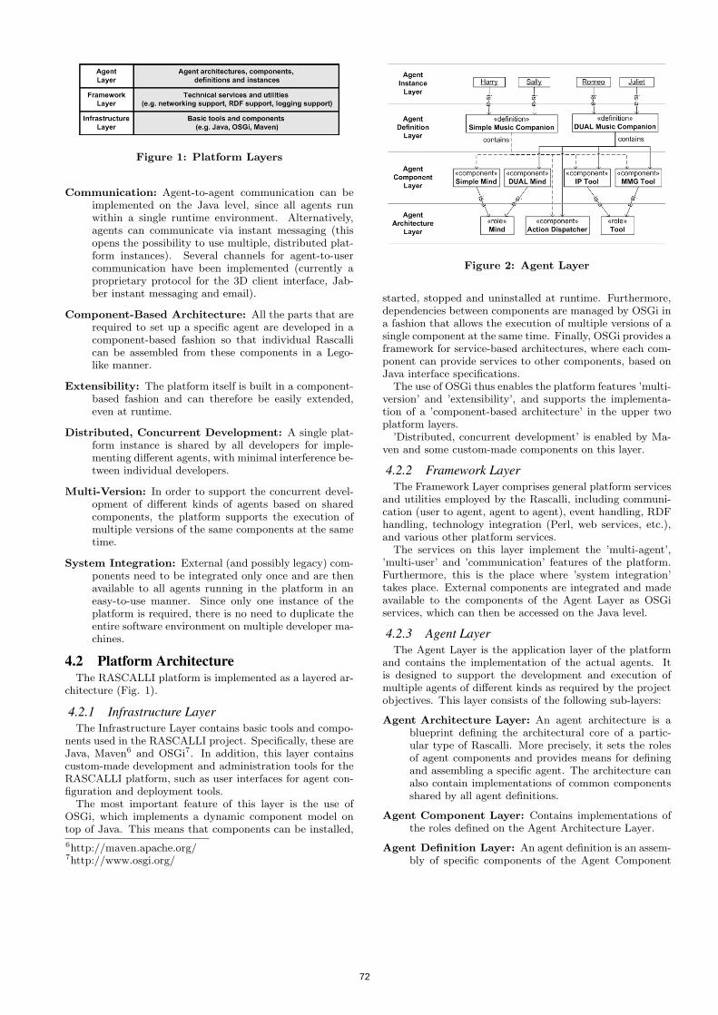
Figure 1: Platform Layers

Communication: Agent-to-agent communication can beimplemented on the Java level, since all agents runwithin a single runtime environment. Alternatively,agents can communicate via instant messaging (thisopens the possibility to use multiple, distributed plat-form instances). Several channels for agent-to-usercommunication have been implemented (currently aproprietary protocol for the 3D client interface, Jab-ber instant messaging and email).

Component-Based Architecture: All the parts that arerequired to set up a specific agent are developed in acomponent-based fashion so that individual Rascallican be assembled from these components in a Lego-like manner.

Extensibility: The platform itself is built in a component-based fashion and can therefore be easily extended,even at runtime.

Distributed, Concurrent Development: A single plat-form instance is shared by all developers for imple-menting different agents, with minimal interference be-tween individual developers.

Multi-Version: In order to support the concurrent devel-opment of different kinds of agents based on sharedcomponents, the platform supports the execution ofmultiple versions of the same components at the sametime.

System Integration: External (and possibly legacy) com-ponents need to be integrated only once and are thenavailable to all agents running in the platform in aneasy-to-use manner. Since only one instance of theplatform is required, there is no need to duplicate theentire software environment on multiple developer ma-chines.

4.2 Platform ArchitectureThe RASCALLI platform is implemented as a layered ar-

chitecture (Fig. 1).

4.2.1 Infrastructure LayerThe Infrastructure Layer contains basic tools and compo-

nents used in the RASCALLI project. Specifically, these areJava, Maven6 and OSGi7. In addition, this layer containscustom-made development and administration tools for theRASCALLI platform, such as user interfaces for agent con-figuration and deployment tools.

The most important feature of this layer is the use ofOSGi, which implements a dynamic component model ontop of Java. This means that components can be installed,

6http://maven.apache.org/7http://www.osgi.org/

Figure 2: Agent Layer

started, stopped and uninstalled at runtime. Furthermore,dependencies between components are managed by OSGi ina fashion that allows the execution of multiple versions of asingle component at the same time. Finally, OSGi provides aframework for service-based architectures, where each com-ponent can provide services to other components, based onJava interface specifications.

The use of OSGi thus enables the platform features ’multi-version’ and ’extensibility’, and supports the implementa-tion of a ’component-based architecture’ in the upper twoplatform layers.

’Distributed, concurrent development’ is enabled by Ma-ven and some custom-made components on this layer.

4.2.2 Framework LayerThe Framework Layer comprises general platform services

and utilities employed by the Rascalli, including communi-cation (user to agent, agent to agent), event handling, RDFhandling, technology integration (Perl, web services, etc.),and various other platform services.

The services on this layer implement the ’multi-agent’,’multi-user’ and ’communication’ features of the platform.Furthermore, this is the place where ’system integration’takes place. External components are integrated and madeavailable to the components of the Agent Layer as OSGiservices, which can then be accessed on the Java level.

4.2.3 Agent LayerThe Agent Layer is the application layer of the platform

and contains the implementation of the actual agents. Itis designed to support the development and execution ofmultiple agents of different kinds as required by the projectobjectives. This layer consists of the following sub-layers:

Agent Architecture Layer: An agent architecture is ablueprint defining the architectural core of a partic-ular type of Rascalli. More precisely, it sets the rolesof agent components and provides means for definingand assembling a specific agent. The architecture canalso contain implementations of common componentsshared by all agent definitions.

Agent Component Layer: Contains implementations ofthe roles defined on the Agent Architecture Layer.

Agent Definition Layer: An agent definition is an assem-bly of specific components of the Agent Component

72

Figure 3: MBE agent architecture

Layer of a specific agent architecture. Different agentdefinitions for the same agent architecture might con-tain different components for certain roles.

Agent Instance Layer: Contains the individual agent in-stances. Each Rascallo is an instantiation of a specificagent definition.

Fig. 2 gives a (simplified) example of an agent architec-ture (the Mind-Body-Environment architecture, see section5). The Agent Architecture Layer defines two roles, Mindand Tool, and implements an agent component (Action Dis-patcher) shared by all agent definitions. The Agent Compo-nent Layer contains two implementations of the Mind role,as well as two Tools. Based on this architecture, two agentdefinitions combine each of the Mind implementations withthe available Tools and the Action Dispatcher into differentkinds of agents. Finally, a number of agent instances areshown on the Agent Instance Layer.

5. AGENT COMPONENTSThis section gives an overview of the agent components

which have been implemented in the RASCALLI project(for more detailed information see [10]). RASCALLI agentsare currently based on a reactive agent architecture witha perception-action loop. This agent architecture is calledMind-Body-Environment architecture, because each agenthas a central control unit (Mind), which perceives and actson the Environment via a set of sensor and effector tools(Body), as shown in Fig. 3.

The Environment comprises the agent’s user, other agents,Internet services and domain-specific knowledge bases. Theagent perceives its environment (via a set of perception sen-sors, implemented as software tools) as a set of virtual en-tities with their own characteristics and properties. Theseinclude strings of written language originating from the useror extracted from HTML documents, markup tags, infor-mation about the accessibility of various Internet and localtools and resources, user feedback, etc. Therefore, the agenthas to deal with a dynamic environment i.e. evolving con-tent of the websites, permanent or temporary inaccessibilityof Internet services, appearance of new content or services,changes in the user preferences and interests, as well as thenatural language input from the user and the web-pages.Similarly, all actions of an agent in its environment are per-formed on the above introduced set of entities.

The Body contains components called Tools, which serveas sensors (Perception Layer) and effectors (Actuator Layer).A specific agent definition may contain an arbitrary subsetof the available Tools, but of course, the chosen Mind com-ponent must be able to deal with the selected Tools. Someof the available Tools are:

• T-IP4Dual, T-IP4Simple and T-IP4Adaptive,Input Processing Tools transform natural language anduser feedback inputs into categorized information use-able by the respective Mind components, and serve asa Perception Layer of an agent.

• T-MMG, for generating multi-modal output to theuser. The Multi-Modal Generation Component pro-vides a middle-ware functionality between generatedagent output and the user interfaces. The generationcomponent implements a template-based approach (inform of Velocity templates) by encoding vocabulary,phrases, gestures etc., which can be combined withthe output of the RASCALLI Tools and context data.The use of Velocity8, a template generation engine, al-lows templates to be designed and refined separatelyfrom the application code.

• T-QA, a general purpose open-domain question an-swering system (based on the work described in [8],[9]) is used in the RASCALLI platform to provide an-swers to the user factoid-type questions expressed innatural language.

• T-Nalqi, a natural language database query interface.The Tool is used in the RASCALLI platform for query-ing the databases accessible to the Rascalli, in a searchfor instances and concepts that can provide answers tothe user questions. The component analyses naturallanguage questions posed by the user and retrieves an-swers from the system’s domain-specific databases.

• T-RSS, provides a mechanism for Rascalli to retrievecurrent information that might be of interest for theuser.

• T-Wikipedia, an interface and analysis Tool for Wiki-pedia.

The Mind component performs action selection, based onthe current input from the environment and the agent in-ternal state. It can also make use of supporting services, forexample a user/agent modeling service. The following Mindcomponents are being developed in the RASCALLI project:

• Simple Mind, which performs action selection witha simple rule-based mechanism. These rules match tospecific cues in the input data arriving from sensorchannels. ’Simple Mind’ extracts relevant informationand passes this information on to the appropriate effec-tor tool. Even though seemingly non-trivial behaviorcan be accomplished through a series of interactions ofthe Simple Mind and the available tools, the SimpleMind does not contain any cognitive aspects such asmemory or learning.

8http://velocity.apache.org

73

• DUAL Mind, which incorporates the DUAL/AMBR([5], [6]) cognitive architecture for action selection. Itincludes a long term memory (LTM) where generaland episodic knowledge is stored, and a working mem-ory (WM) constituted by the active part of LTM, per-ceptual input and goals. The DUAL mind operatesonly on represented knowledge and has only a me-diated connection to the body and the environment.Thus it contains a partial, selected representation ofthe environment at an abstract conceptual level andexperiential memories related to specific episodes likeorganization of the interaction of an agent with its en-vironment.

• Adaptive Mind, a machine learning based classifi-cation driven action selection mechanism. Based onthe available knowledge, including the perception ofan input situation, the agent finds a set of actionsthat can be applied to a given input situation. Theselection of a particular action is based on the simi-larities with other actions the agent had successfullyperformed in the past, i.e. received positive feedbackfrom the user. The action selection classifiers are im-plemented as Maximum Entropy models [4]. The dataused for training the classifiers represents an input sit-uation in terms of entities from the environment per-ceived by the agent, an action applied to this situationand the feedback obtained from the user.

RASCALLI agents come with a variety of user interfacescomprising a 3D client featuring an embodied conversationalcharacter [3] (ECA-UI, see Fig. 4 and 5), a Jabber instantmessaging integration, a web-based user interface (Web-UI)and two domain-specific, special purpose interfaces whichallow the user the explore in a playful way the domain-specific knowledgebases accessible to the currently imple-mented Rascalli. The Web-UI9 mainly serves for user reg-istration, download of the 3D-client and specification of In-ternet resources (URLs and RSS-feeds) that are consideredby the user as important to be monitored by the agent.The agents use the Web-UI to present list-like informationto the user, and more generally all information not wellsuited for presentation by means of synthesized speech. TheECA-UI, on the contrary, specializes on virtual human-to-human dialogue. In order to avoid the bottelneck imposedby speech recognition, user input is restrained to utterancestyped into a small text window and to pressing buttons inorder to praise or scold the agent. The user is expectedto ask domain-specific questions but may also engage in achatterbot-type of conversation with the ECA. To do thisthe Rascalli make use of ALICE chat bot technology.10

The knowledge sources are a music database featuringsongs and albums of more than 60,000 singers/musiciansand a database providing background information on mu-sical artists such as their family relations, religion, trackrecord, band membership etc.11

Based on these components, multiple agent definitionshave been conceptualized and developed, including the ini-tial implementation of an agent with a basic set of tools

9http://intralife.researchstudio.at/rascalli/10http://www.alicebot.org/downloads/programs.html11See http://rascalli.researchstudio.at/ andhttp://rascalli.dfki.de/ontology/ for browsing the data.

(sandbox for testing the system components and their inte-gration), an agent utilizing an implementation of the DUALcognitive architecture as central control unit, and a SmartMusic Companion. Using those various incarnations of theagents implemented in the RASCALLI platform the perfor-mance (in terms of user satisfaction) can be compared andevaluated.

6. AGENT EVALUATIONIn the following, we first give an overview of evaluation

scenarios supported by the RASCALLI platform in generaland the currently implemented Rascalli in particular. Wethen give a more detailed account of an evaluation scenariothe goal of which is to investigate how the use of cognitiveaspects in an agent can improve the user experience.

6.1 Evaluation ScenariosWe distinguish three kinds of scenarios:

1. Automated performance measures: The high modular-ity of the platform eases the integration of automatedperformance measures with existing and future agentarchitectures. For example, one could easily measurethe time an agent needs to fulfill a given task, as wellas the accuracy with which an agent performs certaintasks.

2. Data mining from user activity logs: All user activitiesare logged in the platform including user id, agent id,timestamp and activity type. These data can then beevaluated employing data mining techniques and otherquantitative evaluation methods, in order to identifyprevalent usage patterns of individual users and acrossdifferent users, as well as different kinds of agents.

3. User testing: We distinguish two kinds of user test-ings. The one are studies where users interact withan agent for a short time to fulfill a certain, narrowlydefined task. The other one are studies where usersinteract with their agents more freely for a longer pe-riod of time. While with the former the focus lies ontesting specific aspects of the system and the relatedhuman-computer interaction, the latter address moregeneral questions about what makes an agent a suit-able companion for its user, which interfaces supportwhich tasks and how the interaction of the user withthe agent and his/her attitude towards, his/her lik-ing and understanding of the companion changes overtime.

As there are currently no automated performance mea-sures built into the RASCALLI platform, and the platformhas not yet been made accessible to a broader public andthus we still lack suffient amounts of usage data for applyingdata mining techniques, we will concentrate in the followingon user testing. Due to its modularity, the platform allowsus to experiment with agents being placed in the same en-vironment, but assembled from different internal buildingblocks and therefore are equipped with different perceptionand action capabilities as well as decision making strategies.

A male (Fig. 4) and a female (Fig. 5), human-like versionof the 3D character have been implemented. Both charac-ters are built on the basis of the same body model and areequipped with a similar set of gestures and facial expressions.

74

Figure 4: ECA user interface (male)

Figure 5: ECA user interface (female)

They are also comparable as regards their appearance, bothare designed to fit a pop-rock scenario. The identity of thecharacters except for gender related optical features allowsus to study effects that may be attributed to different per-ception of gender by simply switching between the male andfemale character whereas all other parameters in the sys-tem are kept the same. The RASCALLI system enables us,without further programming, to experiment with all kindsof settings where we let a user interact with or train his/heragent making use of either the male or the female version ofthe 3D character and then switch to the opposite sex.

The availability of two conceptually different, complemen-tary UIs for user-agent communication, i.e., the Web-UI forstandard windows and menu-based human-computer inter-action and the ECA-UI for interaction closely related to hu-man multimodal dialogue, is a valuable prerequisite to in-vestigate user preferences for different modes of interactionand social implications of human-computer interfaces.

At the time of writing two user studies are completed: theone (S1) concerning the liking and evaluation of individualusers engaging in a prescripted question-answer communi-cation with the male Rascalli character, the other one (S2)is a study concerning the usability of the interface to themusic data. Two further user studies are under prepara-tion. The one (S3) is a replication of the question-answer

study employing the female character instead of the maleone. Whereas the previously mentioned studies are all one-time encounters with the system, the second one (S4) ofthe studies under preparation is a longer-term study wherethe users interact with and train their agents over a longerperiod of time, with user assessments at the beginning, atseveral intermediate stages and at the end of the agent-usercollaboration period. Amongst others, we are interested inchanges over time of the users’ liking of their agents, theirexpectations on the performance of their agents, their ac-counts of trust, and their strategies to adapt to their agentsin order to achieve/satisfy their information requirements incollaboration with their agents.

In particular, we prepare two variants (narrow and broad)of the longer-term study. In the narrow study (S4.1), thetask is to train the agent as good as possible to monitorRSS-feeds for a specific topic of interest. To do so, the usersare asked to identifiy and sharpen a topic of interest suchas artist, group, genre, song, album etc. by exploring themusic-related knowledge of their agent utilizing the agent’sdomain-specific interfaces. In addition, they are asked toinform the agent about preferred Internet sources by speci-fying respective RSS feeds through the Web-UI. The agentwill then monitor the feeds and alert the user when encoun-tering relevant information making use of a Jabber client.

In the broad study (S4.2) the users are left much more un-guided. Other than in S4.1 where the users are confined tothe two domain-specific interfaces and the Web-UI, in S4.2they have access to all UIs. The users are more generallyinformed that the agents have some domian-specific knowl-edge about popular music and besides can access the Inter-net. Depending on what information the users frequentlyaccess, which Internet sources they specify, and which feed-back (praise, scolding) they give to their agents, the agentswill adapt to the users’ interests and aim at providing morerelated information. The more effort the users invest intraining their agents, the better the agents should becomein providing the users with new information relevant to theusers’ interests.

6.2 Evaluation Example: Use of Cognitive As-pects in an RSS Feed Filtering Scenario

We make use of a simple scenario for RSS feed filtering toillustrate the platform’s capability to augment the agents’abilities by incorporating cognitive aspects into processing.Since the different agents can exist at the same time in thesame environment and thus be subject to the same externalinfluences, they can be reliably compared and evaluated.

Recall: In the RSS Feed Filtering scenario, the agents’task is to provide their users with (potentially) interestinginformation gathered from music-related RSS feeds on theInternet. The users train their agents according to theirinterests, thus creating an agent profile containing relevantkeywords such as artist names, song names and genre names.The users also provide RSS feed URLs to their agents, whichthe agents then query for new information.

The research question for this simple scenario is whethercertain properties of an agent improve the overall user satis-faction (as measured by the rate of false positives and neg-atives). Therefore, in addition to the basic keyword-basedfiltering of RSS feeds, the following elements can be addedto a particular agent:

• The ability to find similar agents (agents with a similar

75

agent profile) and consider those agents’ RSS feeds inaddition to the ones provided by its own user. Thisessentially extends the agent’s search space.

• The ability to find items (artists, songs, etc.) similarto the ones specified in the agent profile. These itemsare then added to the filter keywords, thus extendingthe agent’s search criteria.

The services required to perform these tasks (finding sim-ilar agents, finding similar artists, etc.) are provided by theRASCALLI framework and made available to the agents asadditional Tools in the action and perception layers.

This setup allows us to create and compare four agent def-initions, containing neither of the two features, one of them,or both. For the evaluation, different users are equippedwith one of the available types of agents. The users canthen identify false positives and negatives.

Obviously, this example could be implemented without acomplex system such as the RASCALLI platform. However,even in this simple case the platform has some advantagesto offer:

• Components can be shared between agents. For exam-ple, the service to find similar agents is an external webservice, which is made available within the platform asa simple OSGi/Java service.

• The platform provides a single runtime environmentfor all the agents (there would be multiple agents ofeach kind), so that inter-agent communication (for ex-changing RSS feed URLs) can be easily implemented.

7. CONCLUSIONSThe RASCALLI platform meets a unique set of require-

ments, that is not targeted by any of the investigated plat-forms or methodologies. In particular, it supports the devel-opment and execution of multiple agents of different kinds.Furthermore, it supports the evaluation and comparison ofsuch different agents within a single environment.

Future work includes the completion of the developmentenvironment (e.g. the integration with development toolssuch as the Eclipse IDE), as well as the possible integrationof certain aspects of other projects, such as BOD, AKIRAor JADE.

The RASCALLI platform and selected system compo-nents will be made available to the research community bythe end of 2008 via the project homepage.12 In particu-lar, the project partners Research Studios Austria (SAT)and the Austrian Research Institute for Artificial Intelli-gence (OFAI) will provide an open source version of theplatform and Tools, respectively. In addition, SAT will makeavailable their other system components and user interfacesas managed services with limited support and data volumefree of charge for the research community. The German Re-search Center for Artificial Intelligence (DFKI) will makeavailable their data sources via an open research license andprovide their system components as webservices. The com-panies Ontotext and Radon Labs will make available theirSwiftOWLIM semantic repository and the 3D client, respec-tively. The New Bulgarian University (NBU) will conributetheir DUAL-inspired implementation of an agent’s mind.

12http://www.ofai.at/rascalli

8. ACKNOWLEDGMENTSThis research is supported by the EC Cognitive Systems

Project FP6-IST-027596-2004 RASCALLI, by the nationalFFG program ’Advanced Knowledge Technologies: Ground-ing, Fusion, Applications’ (project SELP), and by the Fed-eral Ministry of Economics and Labour of the Republic ofAustria. The work presented here builds on joint workwithin the RASCALLI project. In particular the authorswould like to thank our collegues from the following institu-tions: SAT, OFAI, Radon, NBU, Ontotext and DFKI. Fi-nally, our participation in the PerMIS’08 workshop is sup-ported by the European Network for the Advancement ofArtificial Cognitive Systems (euCognition, European Com-mission, Unit E5 - Cognition, FP6 Project 26408).

9. REFERENCES[1] F. Bellifemine, A. Poggi, and G. Rimassa. JADE: a

FIPA2000 compliant agent development environment.In AGENTS ’01: Proceedings of the fifth internationalconference on Autonomous agents, pages 216–217,New York, NY, USA, 2001. ACM.

[2] J. Bryson. Intelligence by Design: Principles ofModularity and Coordination for Engineering ComplexAdaptive Agents. PhD thesis, MIT, Department ofEECS, Cambridge, MA, 2001. AI Technical Report2001-003.

[3] J. Cassell, J. Sullivan, S. Prevost, and E. Churchill,editors. Embodied Conversational Agents. MIT Press,2000.

[4] E. Jaynes. Information theory and statisticalmechanics. Physical Review, 106(4):620–630, 1957.

[5] B. Kokinov. A hybrid model of reasoning by analogy.In K. Holyoak and J. Barnden, editors, AnalogicalConnections, volume 2 of Advances in Connectionistand Neural Computation Theory, pages 247–320.Ablex, 1994.

[6] B. Kokinov and A. Petrov. Integration of memory andreasoning in analogy-making: the AMBR model. InD. Gentner, K. Holyoak, and B. Kokinov, editors,Analogy: Perspectives from Cognitive Science. MITPress, in press.

[7] G. Pezzulo and G. Calvi. Designing modulararchitectures in the framework AKIRA. MultiagentGrid Syst., 3(1):65–86, 2007.

[8] M. Skowron. A Web Based Approach to Factoid andCommonsense Knowledge Retrieval. PhD thesis,Hokkaido University, Sapporo, Japan, 2005.

[9] M. Skowron and K. Araki. Effectiveness of combinedfeatures for machine learning based questionclassification. Special Issue of the Journal of theNatural Language Processing Society Japan onQuestion Answering and Automatic Summarization,12(6):63–83, 2005.

[10] M. Skowron, J. Irran, and B. Krenn. Computationalframework for and the realization of cognitive agentsproviding intelligent assistance capabilities. InProceedings of the Cognitive Robotics Workshop at the18th European Conference on Artificial Intelligence,2008.

76

Evaluation Criteria for Human-Automation Performance Metrics

Birsen Donmez MIT

Dept. of Aero-Astro Cambridge, MA, USA

1(617)258-5046

bdonmez@mit.edu

Patricia E. Pina MIT

Dept. of Aero-Astro Cambridge, MA, USA

1(617)258-5046

ppina@mit.edu

M. L. Cummings MIT

Dept. of Aero-Astro Cambridge, MA, USA

1(617)252-1512

missyc@mit.edu

ABSTRACT Previous research has identified broad metric classes for human-automation performance to facilitate metric selection, as well as understanding and comparison of research results. However, there is still lack of an objective method for selecting the most efficient set of metrics. This research identifies and presents a list of evaluation criteria that can help determine the quality of a metric in terms of experimental constraints, comprehensive understanding, construct validity, statistical efficiency, and measurement technique efficiency. Future research will build on these evaluation criteria and existing generic metric classes to develop a cost-benefit analysis approach that can be used for metric selection.

Categories and Subject Descriptors C.4 [Performance of Systems]: Measurement Techniques J.7 [Computers in Other Systems]

General Terms Measurement, Performance, Experimentation, Human Factors, Standardization, Theory.

Keywords Metric Quality, Human Supervisory Control, Validity, Statistics, Experiments.

1. INTRODUCTION Human-automation teams are common in many domains, such as military operations, process control, and medicine. With intelligent automation, these teams operate under a supervisory control paradigm. “Supervisory control means that one or more human operators are intermittently programming and continually receiving information from a computer that itself closes an autonomous control loop through artificial effectors and sensors to the controlled process or task environment [1].” Example applications include robotics for surgery, rock sampling for

geology research, and military surveillance with unmanned vehicles.

A popular metric used to evaluate human-automation performance in supervisory control is mission effectiveness [2, 3]. Mission effectiveness focuses on performance as it relates to the final output produced by the human-automation team. However, this metric fails to provide insights into the process that leads to the final mission-related output. A suboptimal process can lead to a successful completion of a mission, e.g., when humans adapt to compensate for design deficiencies. Hence, focusing on just the mission effectiveness makes it difficult to extract information to detect design flaws and to design systems that can consistently support successful mission completion.

Measuring multiple human-computer system aspects, such as the situational awareness of the human, can be valuable in diagnosing performance successes and failures, and identifying effective training and design interventions. However, choosing an efficient set of metrics for a given experiment still remains a challenge. Many researchers select their metrics based on their past experience. Another approach to metric selection is to collect as many measures as possible to supposedly gain a comprehensive understanding of the human-automation team performance. These methods can lead to insufficient metrics, expensive experimentation and analysis, and the possibility of inflated type I errors. There appears to be a lack of a principled approach to evaluate and select the most efficient set of metrics among the large number of available metrics.

Different frameworks of metric classes are found in the literature in terms of human-autonomous vehicle interaction [4-7]. These frameworks define metric taxonomies and categorize existing metrics into high level metric classes that assess different aspects of the human-automation team performance and are generalizable across different missions. Such frameworks can help experimenters identify system aspects that are relevant to measure. However, these frameworks do not include evaluation criteria to select specific metrics from different classes. Each metric set has advantages, limitations, and costs, thus the added value of different sets for a given context needs to be assessed to select the set that maximizes value and minimizes cost.

Permission to make digital or hard copies of all or part of this work for personal or classroom use is granted without fee provided that copies are not made or distributed for profit or commercial advantage and that copies bear this notice and the full citation on the first page. To copy otherwise, or republish, to post on servers or to redistribute to lists, requires prior specific permission and/or a fee. PerMIS’08, August 19–21, 2008, Gaithersburg, MD, USA. Copyright 2008 ACM 978-1-60558-293-1…$5.00.

77

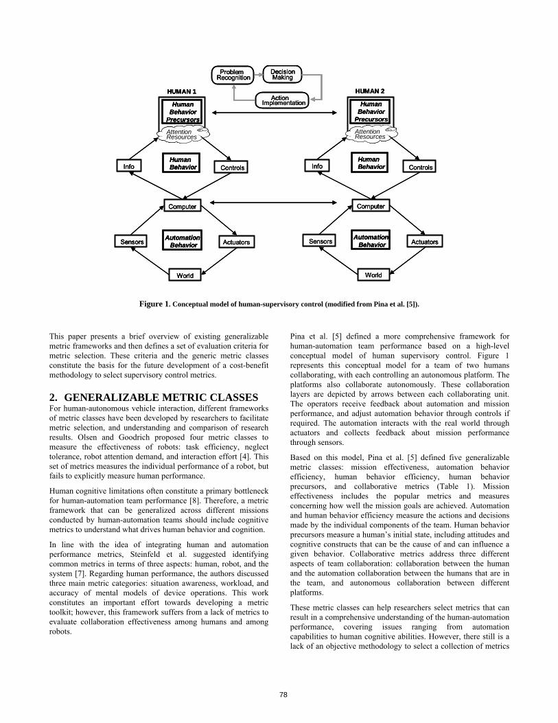
AutomationBehavior

Human Behavior

Precursors

HUMAN 1

Attention Resources

World

ControlsInfo

ActuatorsSensors

Computer

Human Behavior

AutomationBehavior

Human Behavior

Precursors

HUMAN 2

Attention Resources

World

ControlsInfo

ActuatorsSensors

Computer

Human Behavior

Action Implementation

DecisionMaking

Problem Recognition

AutomationBehavior

Human Behavior

Precursors

HUMAN 1

Attention Resources

World

ControlsInfo

ActuatorsSensors

Computer

Human Behavior

AutomationBehavior

Human Behavior

Precursors

HUMAN 2

Attention Resources

World

ControlsInfo

ActuatorsSensors

Computer

Human Behavior

AutomationBehavior

Human Behavior

Precursors

HUMAN 1

Attention Resources

World

ControlsInfo

ActuatorsSensors

Computer

Human Behavior

AutomationBehavior

Human Behavior

Precursors

HUMAN 2

Attention Resources

World

ControlsInfo

ActuatorsSensors

Computer

Human Behavior

Action Implementation

DecisionMaking

Problem Recognition

Action Implementation

DecisionMaking

Problem Recognition

Figure 1. Conceptual model of human-supervisory control (modified from Pina et al. [5]). This paper presents a brief overview of existing generalizable metric frameworks and then defines a set of evaluation criteria for metric selection. These criteria and the generic metric classes constitute the basis for the future development of a cost-benefit methodology to select supervisory control metrics.

2. GENERALIZABLE METRIC CLASSES For human-autonomous vehicle interaction, different frameworks of metric classes have been developed by researchers to facilitate metric selection, and understanding and comparison of research results. Olsen and Goodrich proposed four metric classes to measure the effectiveness of robots: task efficiency, neglect tolerance, robot attention demand, and interaction effort [4]. This set of metrics measures the individual performance of a robot, but fails to explicitly measure human performance.

Human cognitive limitations often constitute a primary bottleneck for human-automation team performance [8]. Therefore, a metric framework that can be generalized across different missions conducted by human-automation teams should include cognitive metrics to understand what drives human behavior and cognition.

In line with the idea of integrating human and automation performance metrics, Steinfeld et al. suggested identifying common metrics in terms of three aspects: human, robot, and the system [7]. Regarding human performance, the authors discussed three main metric categories: situation awareness, workload, and accuracy of mental models of device operations. This work constitutes an important effort towards developing a metric toolkit; however, this framework suffers from a lack of metrics to evaluate collaboration effectiveness among humans and among robots.

Pina et al. [5] defined a more comprehensive framework for human-automation team performance based on a high-level conceptual model of human supervisory control. Figure 1 represents this conceptual model for a team of two humans collaborating, with each controlling an autonomous platform. The platforms also collaborate autonomously. These collaboration layers are depicted by arrows between each collaborating unit. The operators receive feedback about automation and mission performance, and adjust automation behavior through controls if required. The automation interacts with the real world through actuators and collects feedback about mission performance through sensors.

Based on this model, Pina et al. [5] defined five generalizable metric classes: mission effectiveness, automation behavior efficiency, human behavior efficiency, human behavior precursors, and collaborative metrics (Table 1). Mission effectiveness includes the popular metrics and measures concerning how well the mission goals are achieved. Automation and human behavior efficiency measure the actions and decisions made by the individual components of the team. Human behavior precursors measure a human’s initial state, including attitudes and cognitive constructs that can be the cause of and can influence a given behavior. Collaborative metrics address three different aspects of team collaboration: collaboration between the human and the automation collaboration between the humans that are in the team, and autonomous collaboration between different platforms.

These metric classes can help researchers select metrics that can result in a comprehensive understanding of the human-automation performance, covering issues ranging from automation capabilities to human cognitive abilities. However, there still is a lack of an objective methodology to select a collection of metrics

78

that most efficiently measure a system’s human-automation performance. The following section presents a preliminary list of evaluation criteria that can help researchers evaluate the quality of a set of metrics.

Table 1. Human supervisory control metric classes and

subclasses [9]

3. METRIC EVALUATION CRITERIA The proposed metric evaluation criteria for human supervisory control systems consist of five general categories that are listed in Table 2. These categories focus both on the metrics, which are constructs, and on the associated measures, which are mechanisms for expressing construct sizes. There can be multiple ways of measuring a metric. For example, situational awareness, which is a metric, can be measured based on objective or subjective measures [10]. Different measures for the same metric can generate different benefits and costs. Therefore, the criteria presented in this section evaluate a metric set by considering the metrics (e.g., situational awareness), the associated measures (e.g., subjective responses), and the measuring techniques (e.g., questionnaires given at the end of experimentation).

These proposed criteria target human supervisory control systems, with influence from the fields of systems engineering, statistics, human factors, and psychology. These fields have their own flavors of experimental metric selection including formal design of experiment approaches such as response surface methods and factor analyses, but often which metric to select and how many are left to heuristics developed through experience.

Table 2. Metric evaluation criteria

1) Experimental Constraints (e.g., time required to analyze a metric)

2) Comprehensive Understanding (e.g., causal relations with other metrics)

3) Construct Validity (e.g., power to discriminate between similar constructs)

4) Statistical Efficiency (e.g., effect size) 5) Measurement Technique Efficiency (e.g., intrusiveness

to subjects)1) Mission Effectiveness (e.g., key mission

performance parameters) 2) Automation Behavior Efficiency (e.g., usability,

adequacy, autonomy, reliability) 3) Human Behavior Efficiency

a) Attention allocation efficiency (e.g., scan patterns, prioritization)

b) Information processing efficiency (e.g., decision making)

4) Human Behavior Precursors a) Cognitive precursors (e.g., situational awareness,

mental workload) b) Physiological precursors (e.g., physical comfort,

fatigue) 5) Collaborative Metrics

a) Human/automation collaboration (e.g., trust, mental models)

b) Human/human collaboration (e.g., coordination efficiency, team mental model)

c) Automation/automation collaboration (e.g., platforms’ reaction time to situational events that require autonomous collaboration)

3.1 Experimental Constraints Time and monetary cost associated with measuring and analyzing a specific metric constitute the main practical considerations for metric selection. Time allocated for gathering and analyzing a metric also comes with a monetary cost due to man-hours, such as time allocated for test bed configurations. Availability of temporary and monetary resources depends on the individual project; however, resources will always be a limiting factor in all projects.

The stage of system development and the testing environment are additional factors that can guide metric selection. Early phases of system development require more controlled experimentation in order to evaluate theoretical concepts that can guide system design. Later phases of system development require a less controlled evaluation of the system in actual operation. For example, research in early phases of development can assess human behavior for different automation levels, whereas research in later phases can assess the human behavior in actual operation in response to the implemented automation level.

The type of testing environment depends on available resources, safety considerations, and the stage of research development. For example, simulation environments can enable researchers to have high experimental control, and manipulate and evaluate different system design concepts accordingly. In simulation environments, researchers can create off-nominal situations and measure operator responses to such situations without exposing them to risk. However, simulation creates an artificial setting and field testing is required to assess system performance in actual use. The types of measures that can be collected are constrained by the testing environment. For example, the responses to rare events are more applicable for research conducted in simulated environments, whereas observational measures can provide better value in field testing.

3.2 Comprehensive Understanding It is important to maximize the understanding gained from a research study. However, due to the limited resources available, it is not possible to collect all required metrics. Therefore, each metric should be evaluated based on how much it explains the phenomenon of interest and how much it helps explain the underlying reasons for what other metrics measure.

The most important aspect of a study is finding an answer to the primary research question. The proximity of a metric to answering the primary research question defines the importance of that metric. For example, a workload metric may not tell much

79

without a mission effectiveness metric. However, this does not mean that the workload metric fails to provide additional insights into the human-automation performance. Another characteristic of a metric that is important to consider is the amount of additional understanding gained using a specific metric when a set of metrics are already collected. For example, rather than having two metrics that measure mission effectiveness, having one metric that measures mission effectiveness and another metric that measures human behavior can provide a better understanding on the team performance.

In addition to providing additional understanding, another desired metric quality is its causal relations with other metrics. A better understanding can be gained, if a metric can help explain the underlying reasons to what the other metrics measure. For example, operator response to an event, hence human behavior, will often be dependent on the conditions and/or operator’s state when the event occurs. The response to an event can be described in terms of three set of variables [11]: a pre-event phase that defines how the operator adapts to the environment; an event-response phase that describes the operator’s behavior in accommodating the event; and an outcome phase that describes the outcome of the response process. The underlying reasons for the operator’s behavior and the final outcome for an event can be better understood if the initial conditions and operator’s state when the event occurs is also measured. When used as covariates in statistical analysis, the initial conditions of the environment and the operator can help explain the variability in other metrics of interest. Thus, in addition to human behavior, experimenters are encouraged to measure human behavior precursors and automation behavior in order to assess the operator state and environmental conditions which may influence human behavior.

3.3 Construct Validity Construct validity refers to how well the associated measure captures the metric or construct of interest. For example, subjective measures for situational awareness ask subjects to rate the amount of situational awareness they had on a given scenario or task. These measures are proposed to help in understanding subjects’ situational awareness [10, 12]. However, self-ratings assess meta-comprehension rather than comprehension of the situation: it is unclear whether or not operators are aware of their lack of situational awareness. Therefore, subjective responses on situational awareness are not valid to assess the actual situational awareness but rather the awareness of lack of situational awareness.

Good construct validity requires a measure to have high sensitivity to changes in the targeted construct. That is, the measure should reflect the change as the construct moves from low to high levels [13]. For example, the primary task performance starts to break down only when the workload reaches higher levels [13, 14]. Therefore, primary task performance measures are not sensitive to changes in the workload at lower workload levels, since with sufficient spare processing capacity the operators are able to compensate for the increase in workload.

A measure with high construct validity should also be able to discriminate between similar constructs. The power to discriminate between similar constructs is especially important for abstract constructs that are hard to measure and difficult to define, such as human workload or attentiveness. An example measure

that fails to discriminate two related metrics is galvanic skin response. Galvanic skin response is the change in electrical conductance of the skin attributable to the stimulation of the sympathetic nervous system and the production of sweat. Perspiration causes an increase in skin conductance, thus galvanic skin response has been proposed and used to measure workload and stress levels (e.g., Levin et al. [15]). However, even if workload and stress are related, they still are two separate metrics. Therefore, galvanic skin response cannot alone suggest a change in workload.

Good construct validity also requires the selected measure to have high inter- and intra-subject reliability. Inter-subject reliability requires the measure to assess the same construct for every subject, whereas intra-subject reliability requires the measure to assess the same construct if the measure were repeatedly collected from the same subject under identical conditions.

Intra- and inter-subject reliability is especially of concern for subjective measures. For example, self-ratings are widely utilized for mental workload assessment [16, 17]. This technique requires operators to rate the workload or effort experienced while performing a task or a mission. Self-ratings are easy to administer, non-intrusive, and not expensive. However, different individuals may have different interpretations of workload, leading to decreased inter-subject reliability. For example, some participants may not be able to separate mental workload from physical workload [18], and some participants may report their peak workload whereas others may report their average workload. Another example of low inter-subject reliability is for subjective measures of situational awareness. Vidulich & Hughes [10] found that about half of their participants rated situational awareness by gauging the amount of information to which they attended; while the other half of the participants rated their SA by gauging the amount of information they thought they had overlooked. Participants may also have recall problems if the subjective ratings are collected at the end of a test period, raising concerns on the intra-subject reliability of subjective measures.

High correlation between different measures, even if they are intended to assess different metrics, is another limiting factor for metric selection. A high correlation can be indicative of the fact that multiple measures assess the same metric or the same phenomenon. Hence, including multiple measures that are highly correlated with each other can result in wasted resources.

3.4 Statistical Efficiency There are three metric qualities that should be considered to ensure statistical efficiency: total number of measures collected, frequency of observations, and effect size.

Analyzing multiple measures that are correlated with each other would inflate type I error. That is, as more dependent variables are analyzed, finding a significant effect when there is none becomes more likely. The inflation of type I error due to multiple dependent variables can be handled with multivariate analysis techniques, such as Multivariate Analysis of Variance (MANOVA) [19]. It should be noted that multivariate analyses are harder to conduct as researchers are more prone to include irrelevant variables in multivariate analyses, possibly hiding the few significant differences among many insignificant ones. The best way to avoid failure to identify significant differences is to

80

design an effective experiment with the most parsimonious metric/measure set that is expected to produce differences, and excluding others that are not expected to show differences among many treatments.

Another metric characteristic that needs to be considered is the number of observations required for statistical analysis. Supervisory control applications require humans to be monitors of automated systems, with intermittent interaction. Because humans are poor monitors by nature [20], human monitoring efficiency is an important metric to measure in many applications. The problem with assessing monitoring efficiency is that, in most domains, errors or critical signals are very rare, and operators can go through an entire career without encountering them. For that reason, in order to have a realistic experiment, such rare events cannot be included in a study with sufficient frequency. Therefore, if a metric requires response to rare events, the associated number of observations may not enable the researchers to extract meaningful information from this metric. Moreover, small frequency of observed events cannot be statistically analyzed unless data is obtained from a very large number of subjects, such as in medical studies on rare diseases. Conducting such large scale supervisory control experiments is generally cost-prohibitive.

The number of subjects recruited for a study is especially limited when participants are domain experts such as pilots. The power to identify a significant difference, when there is one, depends on the differences in the means of factor levels and the standard errors of these means. Standard errors of the means are determined by the number of subjects. One way to compensate for limited number of subjects in a study is to use more sensitive measures that will provide a large separation between different conditions, that is, a high effect size. Experimental power can also be increased by reducing error variance by collecting repeated measures on subjects, focusing on sub-populations (e.g., experienced pilots), and/or increasing the magnitude of manipulation for independent variables (low and high intensity rather than low and medium intensity). However, it should also be noted that increased control on the experiment, such as using sub-populations, can lead to less generalizable results, and there is a tradeoff between the two.

3.5 Measurement Technique Efficiency The data collection technique associated with a specific metric should not be intrusive to the subjects or to the nature of the task. For example, eye trackers are used for capturing operator’s visual attention [21, 22]. In particular, head-mounted eye trackers can be uncomfortable for the subjects, and hence influence their responses. Wearing an eye-tracker can also lead to an unrealistic situation that is not representative of the task performed in the real world.

Eye trackers are an example of how a measurement instrument can interfere with the nature of the task. The measuring technique itself can also interfere with the realism of the study. For example, off-line query methods are used to measure operator’s situational awareness [23]. These methods are based on briefly halting the experiment at randomly selected intervals, blanking the displays, and administering a battery of queries to the operators. This situational awareness measure then assesses global situational awareness metric by calculating the accuracy of operator’s

responses. The collection of the measure requires the interruption of the task in a way that is unrepresentative of the reality generating an artificial setting. The interruption may also interfere with other metrics such as operator’s performance and workload, as well as other temporal-based metrics.

4. DISCUSSION Supervisory control of automation is a complex phenomenon with high levels of uncertainty, time-pressure, and a dynamically-changing environment. The performance of human-automation teams depend on multiple components such as human behavior, automation behavior, human cognitive and physical capabilities, team interactions, etc. Because of the complex nature of supervisory control, there are many different metrics that can be utilized to assess performance. However, it is not feasible to collect all possible metrics. Moreover, collecting multiple metrics that are correlated can lead to statistical problems such as inflated type I errors.

This paper presented a preliminary list of evaluation criteria for determining a set of metrics for a given research question. These criteria were populated under five major headings: experimental constraints, comprehensive understanding, construct validity, statistical efficiency, and measurement technique efficiency. It should be noted that there are interactions between these major categories. For example, the intrusiveness of a given measuring technique can affect the construct validity for a different metric. In one such case, if the situational awareness is measured by halting the experiment and querying the operator, then the construct validity for the mission effectiveness or human behavior metrics become questionable. Therefore, the evaluation criteria presented in this paper should be applied to a collection of metrics rather than each individual metric alone, taking the interactions between different metrics into consideration. The list of evaluation criteria presented in this paper is a guideline for metric selection. It should be noted that there is not a single set of metrics that are the most efficient across all applications. The specific research aspects such as available resources and the questions of interest will ultimately determine the relative metric quality. Future research will identify a methodology based on a cost-benefit analysis approach, which will objectively identify the best set of metrics for classifications of research studies.

5. ACKNOWLEDGMENTS This research is funded by the US Army Aberdeen Test Center.

6. REFERENCES [1] Sheridan, T.B., Telerobotics, automation, and human

supervisory control. 1992, Cambridge, MA: The MIT Press. [2] Scholtz, J., et al., Evaluation of human-robot interaction

awareness in search and rescue, in Proceedings of the IEEE International Conference on Robotics and Automation (ICRA). 2004: New Orleans.

[3] Cooke, N.J., et al., Advances in measuring team cognition, in Team cognition: understanding the factors that drive process and performance, E. Salas and S.M. Fiore, Editors. 2004, American Psychological Association: Washington, D. C. p. 83-106.

[4] Olsen, R.O. and M.A. Goodrich, Metrics for evaluating human-robot interactions, in Proceedings of NIST

81

Performance Metrics for Intelligent Systems Workshop. 2003.

[5] Pina, P.E., et al., Identifying generalizable metric classes to evaluate human-robot teams, in Proceedings of Metrics for Human-Robot Interaction Workshop at the 3rd Annual Conference on Human-Robot Interaction. 2008: Amsterdam, The Netherlands.

[6] Crandall, J.W. and M.L. Cummings, Identifying predictive metrics for supervisory control of multiple robots. IEEE Transactions on Robotics - Special Issue on Human-Robot Interaction, 2007. 23(5): p. 942-951.

[7] Steinfeld, A., et al., Common metrics for human-robot interaction, in Proceedings of the 1st Annual IEEE/ACM Conference on Human Robot Interaction (Salt Lake City, Utah). 2006, ACM Press: New York, NY.

[8] Wickens, C.D., et al., An Introduction to Human Factors Engineering. 2nd ed. 2004, Upper Saddle River, New Jersey: Pearson Education, Inc.

[9] Pina, P.E., B. Donmez, and M.L. Cummings, Selecting metrics to evaluate human supervisory control applications. 2008, MIT Humans and Automation Laboratory: Cambridge, MA.

[10] Vidulich, M.A. and E.R. Hughes, Testing a subjective metric of situation awareness, in Proceedings of the Human Factors Society 35th Annual Meeting. 1991, The Human Factors and Ergonomics Society: Santa Monica, CA. p. 1307-1311.

[11] Donmez, B., L. Boyle, and J.D. Lee, The impact of distraction mitigation strategies on driving performance. Human Factors, 2006. 48(4): p. 785-804.

[12] Taylor, R.M., Situational awareness rating technique (SART): the development of a tool for aircrew systems design, in Proceedings of the NATO Advisory Group for Aerospace Research and Development (AGARD) Situational Awareness in Aerospace Operations Symposium (AGARD-CP-478). 1989. p. 17.

[13] Eggemeier, F.T., C.A. Shingledecker, and M.S. Crabtree, Workload measurement in system design and evalution, in

Proceeding of the Human Factors Society 29th Annual Meeting. 1985: Baltimore, MD. p. 215-219.

[14] Eggemeier, F.T., M.S. Crabtree, and P.A. LaPoint, The effect of delayed report on subjective ratings of mental workload, in Proceedings of the Human Factors Society 27th Annual Meeting. 1983: Norfolk, VA. p. 139-143.

[15] Levin, S., et al., Tracking workload in the emergency department. Human Factors, 2006. 48(3): p. 526-539.

[16] Wierwille, W.W. and J.G. Casali, A validated rating scale for global mental workload measurement applications, in Proceedings of the Human Factors Society 27th Annual Meeting. 1983: Santa Monica, CA. p. 129-133.

[17] Hart, S.G. and L.E. Staveland, The subjective workload assessment technique: a scaling procedure for measuring mental workload, in Human Mental Workload, P. Hancock and N. Meshkati, Editors. 1988, North Holland B. V.: Amsterdam, The Netherlands. p. 139-183.

[18] O'Donnell, R.D. and F.T. Eggemeier, Workload assessment methodology, in Handbook of perception and human performance: vol. II. Cognitive processes and performance, K.R. Boff, L. Kaufmann, and J.P. Thomas, Editors. 1986, Wiley Interscience: New York. p. 42-1 - 42-49.

[19] Johnson, R.A. and D.W. Wichern, Applied multivariate statistical analysis. Fifth ed. 2002, NJ: Pearson Education.

[20] Sheridan, T.B., Humans and automation: system design and research issues. 2002, New York, NY: John Wiley & Sons Inc.

[21] Janzen, M.E. and K.J. Vicente, Attention allocation within the abstraction hierarchy. International Journal of Human-Computer Studies, 1998. 48: p. 521-545.

[22] Donmez, B., L. Boyle, and J.D. Lee, Safety implications of providing real-time feedback to distracted drivers. Accident Analysis & Prevention, 2007. 39(3): p. 581-590.

[23] Endsley, M.R., B. Bolte, and D.G. Jones, Designing for situation awareness: an approach to user-centered design. 2003, Boca Raton, FL: CRC Press, Taylor & Francis Group.

82

Assessing Measures of Coordination Demand Based on Interaction Durations

Michael Lewis School of Information Sciences

University of Pittsburgh Pittsburgh, PA 15260 USA

ml@sis.pitt.edu

Jijun Wang Quantum Leap Innovations, Inc.

3 Innovation Way, Suite 100 Newark, DE 19711 USA

jijunwang.cn@gmail.co

ABSTRACT Controlling multiple robots substantially increases the complexity of the operator’s task because attention must constantly be shifted among robots in order to maintain situation awareness (SA) and exert control. In the simplest case an operator controls multiple independent robots interacting with each as needed. Control performance at such tasks can be characterized by the average demand of each robot on human attention. In this paper we present several approaches to measuring, coordination demand, CD, the added difficulty posed by having to coordinate as well as operate multiple robots. Our initial experiment compares “equivalent” conditions with and without coordination. Two subsequent experiments attempt to manipulate and measure coordination demand directly using an extension of the Neglect Tolerance model.

Categories and Subject Descriptors I.2.9 [Artificial Intelligence]: Robotics—operator interfaces

General Terms Human Factors, Measurement, Experimentation

Keywords Human-robot interaction, metrics, evaluation, multi-robot System

1. INTRODUCTION Borrowing concepts and notation from computational complexity, control of robots by issuing waypoints, could be considered O(n) because demand increases linearly with the number of robots to be serviced. Another form of control such as designating a search region by drawing a box on a GUI (Graphical User Interface), being independent of the number of robots, would be O(1). From this perspective the most complex tasks faced in controlling teams are likely to be those that involve choosing and coordinating subgroups of robots. Simply choosing a subteam to perform a task (the Permission to make digital or hard copies of all or part of this work for personal or classroom use is granted without fee provided that copies are not made or distributed for profit or commercial advantage and that copies bear this notice and the full citation on the first page. To copy otherwise, or republish, to post on servers or to redistribute to lists, requires prior specific permission and/or a fee. PerMIS’08, August 19–21, 2008, Gaithersburg, MD, USA. Copyright 2008 ACM 978-1-60558-293-1…$5.00.

iterated role assignment problem), for example, has been shown to be O(mn) [6]. The three experiments presented in this paper develop methods to assess the operator effort required to coordinate robots in tasks representative of expected application areas.

1.1 Coordination Demand Despite the apparent analogy between command complexity and the workload imposed by a command task there is no guarantee that human operators will experience difficulty in the same way. The performance of human-robot teams is complex and multifaceted reflecting the capabilities of the robots, the operator(s), and the quality of their interactions. Recent efforts to define common metrics for human-robot interaction [11] have favored sets of metric classes to measure the effectiveness of the system’s constituents and their interactions as well as the system’s overall performance. In this paper we present new measures of the demand coordination places on operators of multirobot systems and three experiments evaluating our approach and the usefulness of these measures.

Controlling multiple robots substantially increases the complexity of the operator’s task because attention must constantly be shifted among robots in order to maintain situation awareness (SA) and exert control. In the simplest case an operator controls multiple independent robots interacting with each as needed. A search task in which each robot searches its own region would be of this category although minimal coordination might be required to avoid overlaps and prevent gaps in coverage. Control performance at such tasks can be characterized by the average demand of each robot on human attention [5]. Under these conditions increasing robot autonomy should allow robots to be neglected for longer periods of time making it possible for a single operator to control more robots.

For more strongly cooperative tasks and larger teams, individual autonomy alone is unlikely to suffice. The round-robin control strategy used for controlling individual robots would force an operator to plan and predict actions needed for multiple joint activities and be highly susceptible to errors in prediction, synchronization or execution. Estimating the cost of this coordination, however, proves a difficult problem. Established methods of estimating multirobot system, MRS, control difficulty, neglect tolerance, and fan-out [5] are predicated on the independence of robots and tasks. In neglect tolerance, the period following the end of human intervention but preceding a decline in performance below a threshold is considered time during which the operator is free to perform other tasks. If the operator services other robots over this period, the measure provides an estimate of the number of robots that might be controlled. Fan-out, when measured

83

empirically, works from the opposite direction, adding robots and measuring performance until a plateau without further improvement is reached. Both approaches presume that operating an additional robot imposes an additive demand. These measures are particularly attractive because they are based on readily observable aspects of behavior: the time an operator is engaged controlling the robot, interaction time (IT), and the time an operator is not engaged in controlling the robot, neglect time (NT).

2. COORDINATION DEMAND To separate coordination demand (CD) from the demands of interacting with independent robots we have extended Crandall et al.’s (2005) neglect tolerance model by introducing the notion of occupied time (OT) as illustrated in Figure 1.

The neglect tolerance model describes an operator’s interaction with multiple robots as a sequence of control episodes in which an operator interacts with a robot for period IT raising its performance above some upper threshold after which the robot is neglected for the period NT until its performance deteriorates below a lower threshold when the operator must again interact with it. To accommodate

NT IT

OT FT FT

NT: Neglect Time; IT: Interaction Time; FT: Free Time, time off task; OT: Occupied Time IT+OT: time on task

Time

Team Effectiveness

Figure 1. Extended neglect tolerance model

dependent tasks we introduce occupied time, OT, to describe the time spent controlling other robots in order to synchronize their actions with those of the target robot. The episode depicted in Figure 1 starts just after the first robot is serviced. The ensuing free time ( FT ) preceding the interaction with a second dependent robot, the OT for robot-1 (that would contribute to IT for robot-2), and the FT following interaction with robot-2 but preceding the next interaction with robot-1 together constitute the neglect time for robot-1. Coordination demand, CD, is then defined as:

NTOT

NTFT

CD 1 (1)

Where, CD for a robot is the ratio between the time required to control cooperating robots and the time still available after controlling the target robot, i.e.; the portion of a robot’s free time that must be devoted to controlling cooperating robots. Note that OTn associated with robotn is less than or equal to NTn because OTn covers only that portion of NTn needed for synchronization.

Most MRS research has investigated homogeneous robot teams where additional robots provide redundant (independent) capabilities.

Differences in capabilities such as mobility or payload, however, may lead to more advantageous opportunities for cooperation among heterogeneous robots. These differences among robots in roles and other characteristics affecting IT, NT, and OT introduce additional complexity to assessing CD. Where tight cooperation is required as in box-pushing, task requirements dictate both the choice of robots and the interdependence of their actions. In the more general case requirements for cooperation can be relaxed allowing the operator to choose the subteams of robots to be operated in a cooperative manner as well as the next robot to be operated. This general case of heterogeneous robots cooperating as needed characterizes the types of field applications our research is intended to support. To accommodate this more general case, the Neglect Tolerance model must be further extended to measure coordination between different robot types and for particular patterns of activity.

The resulting expression [13] measures the way in which the team’s capabilities or resources are combined to accomplish the task without reference to the operation or neglect of particular robots. So, for example, it would not distinguish between a situation in which one robot of type, X, was never operated while another was used frequently from a situation in which both robots of type, X, were used more evenly. The incorporation of action patterns further extends the generality of the approach to accommodate patterns of cooperation that occur in episodes such as dependencies between loading and transporting robots. When an empty transporter arrives, its brief IT would lead to extended OTs as the loaders do their work. When the transporter has been filled the dependency would be reversed.

3. SIMULATION ENVIRONMENT The reported experiments were performed using the USARSim robotic simulation with 2-6 simulated robots performing Urban Search and Rescue (USAR), experiments 1 & 3, or box pushing (experiment 2) tasks. USARSim is a high-fidelity simulation of USAR robots and environments developed as a research tool for the study of Human Robot Interaction (HRI) and multi-robot coordination. Validation studies showing agreement for a variety of feature extraction techniques between USARSim images and camera video are reported in [3], showing close agreement in detection of walls and associated Hough transforms for a simulated Hokuyo laser range finder [2] and close agreement in behavior between USARSim models and the robots being modeled [4,8,9,12,15].

3.1 MrCS – The Multirobot Control System A multirobot control system (MrCS) was developed to conduct these experiments. The system was designed to be scalable to allow of control different numbers of robots, reconfigurable to accommodate different human-robot interfaces, and reusable to facilitate testing different control algorithms.

The user interface of MrCS is shown in Figure 2. The interface is reconfigurable to allow the user to resize the components or change the layout. Shown in the figure is a configuration that used in the RoboCup 2006 competition in which a single operator controls six robots. On the upper and center portions of the left-hand side are the robot list and team map panels, which show the operator an overview of the team. The destination of each of robot is displayed on the map to help the user keep track of current plans. Using this display, the operator is also able to control regional priorities by drawing rectangles on the map. On the center and lower portions of the right-hand side are the camera view and mission control panels,

84

which allow the operator to maintain situation awareness of an individual robot and to edit its exploration plan. On the mission panel, the map and all nearby robots and their destinations are represented to provide partial team awareness so that the operator can switch between contexts while moving control from one robot to another. The lower portion of the left-hand side is a teleoperation panel that allows the operator to teleoperate a robot.

3.2 Experiments

One approach to investigating coordination demand is to design experiments that allow comparisons between “equivalent” conditions

Figure 2. MrCS GUI

with and without coordination demands. The first experiment and one comparison within the third experiment follow this approach. The first experiment compares search performance between a team of autonomously coordinating robots, manually (waypoint) controlled robots, and mixed initiative teams with autonomously coordinated robots that accepted operator inputs. The impact of coordination demand was observable through the difference in performance between the manually controlled teams and the mixed initiative ones. The fully automated teams provided a control ensuring that the benefits in the mixed initiative condition were not due solely to the superior performance of the automation.

While experiment 1 examines coordination demand indirectly by comparing performance between conditions in which it was filled either manually or through automation, experiments 2 & 3 attempt to manipulate and measure coordination demand directly. In experiment 2 robots perform a box pushing task in which CD is varied by control mode and robot heterogeneity. By making the actions of each robot entirely dependent on the other, this choice of task eliminates the problem of distinguishing between interactions intended to control a target robot and those needed to coordinate with another. The third experiment attempts to manipulate coordination demand in a loosely coordinated task by varying the proximity needed to perform a joint task in two conditions and by automating coordination within subteams in the third. Because robots must cooperate in pairs and interaction for control needs to be distinguished from interaction for coordination for this task, CD is computed between robot types (equation 2) rather than directly

between robots (equation 1) as done in experiment 2.

All three experiments used paid participants from the University of Pittsburgh and lasted approximately one and a half hours. All used repeated measures designs and followed a standard sequence starting with collection of demographic data. Standard instructions for the experiment were presented followed by a 10 minute training session during which the participant was allowed to practice using the MrCS. Participants then began their first trial followed by a second with a short break in between. Experiments 2 and 3 included a third trial with break. At the conclusion of the experiment participants completed a questionnaire.

4. EXPERIMENT 1 Participants were asked to control 3 P2DX robots simulated in USARsim to search for victims in a damaged building. Each robot was equipped with a pan-tilt camera with 45 degrees Field of View (FOV) and a front laser scanner with 180 degree FOV and resolution of 1 degree. When a victim was identified, the participant marked its location on NIST Reference Test Arena, Yellow Arena [7]. Two similar testing arenas were built using the same elements with different layouts. In each arena, 14 victims were evenly distributed in the world. We added mirrors, blinds, curtains, semitransparent boards, and wire grid to add difficulty in situation perception. Bricks, pipes, a ramp, chairs, and other debris were put in the arena to challenge mobility and SA in robot control.

Presentation of mixed initiative and manual conditions were counterbalanced. Under mixed initiative, the robots analyzed their laser range data to find possible exploration paths. They cooperated with one another to choose execution paths that avoided duplicating efforts. While the robots autonomously explored the world, the operator was free to intervene with any individual robot by issuing new waypoints, teleoperating, or panning/tilting its camera. The robot returned back to auto mode once the operator’s command was completed or stopped. While under manual control robots could not autonomously generate paths and there was no cooperation among robots. The operator controlled a robot by giving it a series of waypoints, directly teleoperating it, or panning/tilting its camera. As a control for the effects of autonomy on performance we conducted “full autonomy” testing as well. Because MrCS doesn’t support victim recognition, based on our observation of the participants’ victim identification behaviors, we defined detection to have occurred for victims that appeared on camera for at least 2 seconds and occupied at least 1/9 of the thumbnail view. Because of the high fidelity of the simulation, and the randomness of paths picked through the cooperation algorithms, robots explored different regions on every test. Additional variations in performance occurred due to mishaps such as a robot getting stuck in a corner or bumping into an obstacle causing its camera to point to the ceiling so no victims could be found. Sixteen trials were conducted in each area to collect data comparable to that obtained from human participants.

4.1 Results All 14 participants found at least 5 of a possible 14 (36%) victims in each of the arenas. These data indicate that participants exploring less than 90% of the area consistently discovered 5 to 8 victims while those covering greater than 90% discovered between half (7) and all (14) of the victims. Within participant comparisons found wider regions were explored in mixed-initiative mode, t(13) = 3.50, p < .004, as well as a marginal advantage for mixed-initiative mode, t(13) = 1.85, p = .088, in number of victims found. Comparing with

85

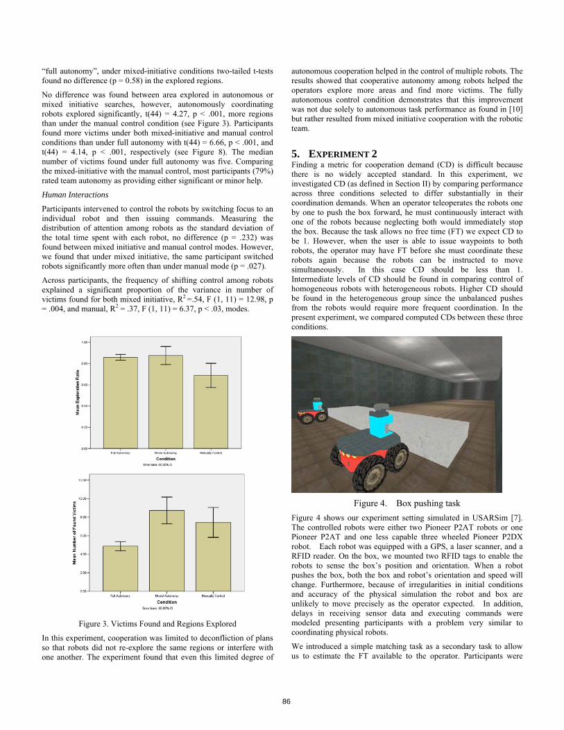
“full autonomy”, under mixed-initiative conditions two-tailed t-tests found no difference (p = 0.58) in the explored regions.

No difference was found between area explored in autonomous or mixed initiative searches, however, autonomously coordinating robots explored significantly, t(44) = 4.27, p < .001, more regions than under the manual control condition (see Figure 3). Participants found more victims under both mixed-initiative and manual control conditions than under full autonomy with t(44) = 6.66, p < .001, and t(44) = 4.14, p < .001, respectively (see Figure 8). The median number of victims found under full autonomy was five. Comparing the mixed-initiative with the manual control, most participants (79%) rated team autonomy as providing either significant or minor help.

Human Interactions

Participants intervened to control the robots by switching focus to an individual robot and then issuing commands. Measuring the distribution of attention among robots as the standard deviation of the total time spent with each robot, no difference (p = .232) was found between mixed initiative and manual control modes. However, we found that under mixed initiative, the same participant switched robots significantly more often than under manual mode (p = .027).

Across participants, the frequency of shifting control among robots explained a significant proportion of the variance in number of victims found for both mixed initiative, R2 =.54, F (1, 11) = 12.98, p = .004, and manual, R2 = .37, F (1, 11) = 6.37, p < .03, modes.

Figure 3. Victims Found and Regions Explored

In this experiment, cooperation was limited to deconfliction of plans so that robots did not re-explore the same regions or interfere with one another. The experiment found that even this limited degree of

autonomous cooperation helped in the control of multiple robots. The results showed that cooperative autonomy among robots helped the operators explore more areas and find more victims. The fully autonomous control condition demonstrates that this improvement was not due solely to autonomous task performance as found in [10] but rather resulted from mixed initiative cooperation with the robotic team.

5. EXPERIMENT 2 Finding a metric for cooperation demand (CD) is difficult because there is no widely accepted standard. In this experiment, we investigated CD (as defined in Section II) by comparing performance across three conditions selected to differ substantially in their coordination demands. When an operator teleoperates the robots one by one to push the box forward, he must continuously interact with one of the robots because neglecting both would immediately stop the box. Because the task allows no free time (FT) we expect CD to be 1. However, when the user is able to issue waypoints to both robots, the operator may have FT before she must coordinate these robots again because the robots can be instructed to move simultaneously. In this case CD should be less than 1. Intermediate levels of CD should be found in comparing control of homogeneous robots with heterogeneous robots. Higher CD should be found in the heterogeneous group since the unbalanced pushes from the robots would require more frequent coordination. In the present experiment, we compared computed CDs between these three conditions.

Figure 4. Box pushing task

Figure 4 shows our experiment setting simulated in USARSim [7]. The controlled robots were either two Pioneer P2AT robots or one Pioneer P2AT and one less capable three wheeled Pioneer P2DX robot. Each robot was equipped with a GPS, a laser scanner, and a RFID reader. On the box, we mounted two RFID tags to enable the robots to sense the box’s position and orientation. When a robot pushes the box, both the box and robot’s orientation and speed will change. Furthermore, because of irregularities in initial conditions and accuracy of the physical simulation the robot and box are unlikely to move precisely as the operator expected. In addition, delays in receiving sensor data and executing commands were modeled presenting participants with a problem very similar to coordinating physical robots.

We introduced a simple matching task as a secondary task to allow us to estimate the FT available to the operator. Participants were

86

asked to perform this secondary task as possible when they were not occupied controlling a robot. Every operator action and periodic timestamped samples of the box’s moving speed were recorded for computing CD .

A within subject design was used to control for individual differences in operators’ control skills and ability to use the interface. To avoid having abnormal control behavior, such as a robot bypassing the box bias the CD comparison, we added safeguards to the control system to stop the robot when it tilted the box. 5.1 Participants and Procedure 14 paid participants, 18-57 years old were recruited from the University of Pittsburgh community. None had prior experience with robot control although most were frequent computer users. Participants performed three testing sessions in counterbalanced order. In two of the sessions, the participants controlled two P2AT robots using teleoperation alone or a mixture of teleoperation and waypoint control. In the third session, the participants were asked to control heterogeneous robots (one P2AT and one P2DX) using a mixture of teleoperation and waypoint control. The participants were allowed eight minutes to push the box to the destination in each session. At the conclusion of the experiment participants completed a questionnaire. 5.2 Results Figure 5 shows a time distribution of robot control commands recorded in the experiment. As we expected no free time was recorded for robots in the teleoperation condition and the longest free times were found in controlling homogeneous robots with waypoints. The box speed shown on Figure 5 is the moving speed along the hallway that reflects the interaction effectiveness (IE) of the control mode. The IE curves in this picture show the delay effect and the frequent bumping that occurred in controlling heterogeneous robots revealing the poorest cooperation performance.

None of the 14 participants were able to perform the secondary task while teleoperating the robots. Hence, we uniformly find TAD=1 and CD=1 for both robots under this condition. Within participants comparison found that under waypoint control the team attention demand in heterogeneous robots is significantly higher than the demand in controlling homogeneous robots, t(13)=2.213, p=0.045 (Figure 5). No significant differences were found between the homogeneous P2AT robots in terms of the individual cooperation demand (P=0.2). Since the robots are identical, we compared the average CD of the left and right robots with the CDs measured under heterogeneous condition. Two-tailed t-test shows that when a participant controlled a P2AT robot, lower CD was required in homogeneous condition than in the heterogeneous condition, t(13)=-2.365. p=0.034. The CD required in controlling the P2DX under heterogeneous demand (CD) condition is marginally higher than the CD required in controlling homogenous P2ATs, t(13)=-1.868, p=0.084 (Figure 5). Surprisingly, no significant difference was found in CDs between controlling P2AT and P2DX under heterogeneous condition (p=0.79). This can be explained by the three observed robot control strategies: 1) the participant always issued new waypoints to both robots when adjusting the box’s movement, therefore similar CDs were found between the robots; 2) the participant tried to give short paths to the faster robot (P2DX) to balance the different speeds of the two robots, thus we found higher CD in P2AT; 3) the participant gave the same length paths to both robots and the slower robot needed more interactions because it

trended to lag behind the faster robot, so lower CD for the P2AT was found for the participant. Among the 14 participants, 5 of them (36%) showed higher CD for the P2DX contrary to our expectations.

Figure 5 The time distribution curves for teleoperation (upper) and waypoint control (middle) for homogeneous robots, and waypoint control (bottom) for heterogeneous robots 6. EXPERIMENT 3 To test the usefulness of the extended CD measureme for a weakly cooperative MRS, we conducted an experiment assessing coordination demand using an Urban Search And Rescue (USAR) task requiring high human involvement and of a complexity suitable to exercise heterogeneous robot control. In the experiment, participants were asked to control explorer robots equipped with a laser range finder but no camera and inspector robots with only cameras. Finding and marking a victim required using the inspector’s camera to find a victim to be marked on the map generated by the explorer. The capability of the robots and the cooperation autonomy level were used to adjust the coordination demand of the task.. 6.1 Experimental design Three simulated Pioneer P2AT robots and 3 Zergs [1], a small experimental robot were used. Each P2AT was equipped with a front laser scanner with 180 degree FOV and resolution of 1 degree. The Zerg was mounted with a pan-tilt camera with 45 degree FOV. The robots were capable of localization and able to communicate with other robots and control station. The P2AT served as an explorer to build the map while the Zerg could be used as an inspector to find victims using its camera. To accomplish the task the participant must coordinate these two types robot to ensure that when an inspector robot finds a victim, it is within a region mapped by an explorer robot so the position can be marked.

Three conditions were designed to vary the coordination demand on the operator. Under condition 1, the explorer had 20 meters detection range allowing inspector robots considerable latitude in their search. Under condition 2, scanner range was reduced to 5 meters requiring closer proximity to keep the inspector within mapped areas. Under condition 3, explorer and inspector robots were paired as subteams in which the explorer robot with a sensor range of 5 meters followed its inspector robot to map areas being searched. We hypothesized that CDs for explorer and inspector robots would be more even distributed under condition-2 (short range sensor) because explorers would need to move more frequently in response to inspectors’ searches than in condition-1 in which CD should be more asymmetric with explorers exerting greater demand on inspectors.

87

We also hypothesized that lower CD would lead to higher team performance. Three equivalent damaged buildings were constructed from the same elements using different layouts. Each environment was a maze like building with obstacles, such as chairs, desks, cabinets, and bricks with 10 evenly distributed victims. A fourth environment was constructed for training. Figure 6 shows the simulated robots and environment. A within subjects design with counterbalanced presentation was used to compare the cooperative performance across the three conditions. 6.2 Results Overall performance was measured by the number of victims found, the explored areas, and the participants’ self-assessments. To examine cooperative behavior in finer detail, CDs were computed from logged data for each type robot under the three conditions. We compared the measured CDs between condition 1 (20 meters sensing range) and condition 2 (5 meters sensing range), as well as condition 2 and condition 3 (subteam). To further analyze the cooperation behaviors, we evaluated the total attention demand in robot control and control action pattern as well. Finally, we introduce control episodes showing how CDs can be used to identify and diagnose abnormal control behaviors. 6.2.1 Overall performance Examination of data showed two participants failed to perform the task satisfactorily. One commented during debriefing that she thought she was supposed to mark inspector robots rather than victims. After removing these participants a paired t-test shows that in condition-1 (20 meters range scanner) participants explored more regions, t(16) = 3.097, p = 0.007, as well as found more victims, t(16) = 3.364, p = 0.004, than under condition-2 (short range scanner). In condition-3 (automated subteam) participants found marginally more victims, t(16) = 1.944, p = 0.07, than in condition-2 (controlled cooperation) but no difference was found for the extent of regions explored. In the posttest survey, 12 of the 19 (63%) participants reported they were able to control the robots although they had problems in handling some interface components, 6 of the 19 (32%) participants thought they used the interface very well, and only one participant reported it being hard to handle all the components on the user interface but still maintained

Figure 6 Scout and Explorer robots

she was able to control the robots. Most participants (74%) thought it was easier to coordinate inspectors with explorers with long range

scanner. 12 of the 19 (63%) participants rated auto-cooperation between inspector and explorer (the subteam condition) as improving their performance, and 5 (26%) participants though auto-cooperation made no difference. Only 2 (11%) participants judged team autonomy to make things worse.

6.2.2 Coordination effort During the experiment we logged all the control operations with timestamps. From the log file CDs were computed for each type robot according to equation 2 in section 2. Figure 7 shows a typical (IT,FT) distribution under condition 1 (20 meters sensing range) in the experiment with a calculated CD for the explorer of 0.185, a CD for the inspector of 0.06. The low CDs reflect that in trying to control 6 robots the participant ignored some robots while attending to others. The CD for explorers is roughly twice the CD for inspectors. After the participant controlled an explorer, he needed to control an inspector multiple times or multiple inspectors since the explorer has a long detection range and large FOV. In contrast, after controlling an inspector, the participant needed less effort to coordinate explorers.

Figure 8 shows the mean of measured CDs. We predicted that when the explorer has a longer detection range, operators would need to control the inspectors more frequently to cover the mapped area. Therefore a longer detection range should lead to higher CD for explorers. This was confirmed by a two tailed t-test that found higher coordination demand, t(18) = 2.476, p = 0.023, when participants controlled explorers with large (20 meters) sensing range.

We did not find a corresponding difference, t(18)=.149, p=0.884, between long and short detection range conditions for the CD for inspectors. This may have occurred because under these two conditions the inspectors have exactly the same capabilities and the difference in explorer detection range was not large enough to impact inspectors’ CD for explorers. Under the subteam condition, the automatic cooperation within a subteam decreased or eliminated the coordination requirement when a participant controlled an inspector. Within participant comparisons shows that the measured CD of inspectors under this condition is significantly lower than the CD under condition 2 (independent control with 5 meters detection range), t(18) = 6.957, p < 0.001. Because the explorer always tries to automatically follow an inspector, we do not report CD of explorers in this condition.

As auxiliary parameters, we evaluated the total attention demand, i.e. the occupation rate of total interaction time in the whole control period, and the action pattern, the ratio of control times between inspector and explorer, as well. Paired t-test shows that under long sensing conditions, participants interacted with robots more times than under short sensing

IT distribution

0 200 400 600 800 1000

Time (s)

R13 R22 R12 R21 R13 R23

Figure 7 Typical (IT,FT) distribution (higher line indicates the interactions of explorers).

88

which implies that more robot interactions occurred. The mean action patterns under long and short range scanner conditions are 2.31 and 1.9 respectively. This means that with 20 and 5 meters scanning ranges, participants controlled inspectors 2.31 and 1.9 times respectively after an explorer interaction. Within participant comparisons shows that the ratio is significantly larger under long sensing condition than under short range scanner condition, t(18) = 2.193, p = 0.042.

Figure 8 CDs for each robot type

6.2.3 Analyzing Performance

As an example of applying CDs to analyze coordination behavior, the performance over explorer CD and total attention demand under the 20 meters sensing range condition reveals three abnormal cases A, B, and C low on both CD and TAD. Associating these cases with recorded map snapshots, we observed that in case A, one robot was entangled by a desk and stuck for a long time, for case B, two robots were controlled in the first 5 minutes and afterwards ignored, and in case C, the participant ignored two inspectors throughout the entire trial.

7. CONCLUSIONS We proposed an extended Neglect Tolerance model to allow us to evaluate coordination demand in applications where an operator must coordinate multiple robots to perform dependent tasks. Results from the first experiment that required tight coordination conformed closely to our hypotheses with the teleoperation condition producing CD=1 as predicted and heterogeneous teams exerting greater demand than homogenous ones. The CD measure proved useful in identifying abnormal control behavior revealing inefficient control by one participant through irregular time distributions and close CDs for P2ATs under homogeneous and heterogeneous conditions (0.23 and 0.22), a mistake with extended recovery time (41 sec) in another, and a shift to asatisficing strategy between homogeneous and heterogeneous conditions revealed by a drop in CD (0.17 to 0.11) in a third. As most target applications such as construction or search and rescue require weaker cooperation among heterogeneous platforms the second experiment extended NT methodology to such conditions. Results in this more complex domain were mixed. Our findings of increased CD for long sensor range may seem counter intuitive. Our data show, however, that this effect is not substantial and provide an argument for focused metrics of this sort which measure constituents of the human-robot system directly. Moreover, this experiment also shows how CD can be used to guide us to identify and analyze aberrant control behaviors.

We anticipated a correlation between performance (found victims) and process (measured CDs) measures. However, we did not find the expected relationship in this experiment. From observation of participants during the experiment we believe that high level strategies, such as choosing areas to be searched and path planning,

had a significant impact on the overall performance. The participants had few problems in learning to jointly control explorers and inspectors but needed time to figure out effective strategies for performing the task. Because CD measures control behaviors not strategies these effects were not captured. These experiments have demonstrated the utility of measuring the process of human-robot interaction as well as outcomes to diagnosing operator performance and identifying aspects of the task, particularly for multiple robots, that might benefit from automation. While our approach to measuring CD was supported in the last two experiments the third experiment suggests the need for more sophisticated measures that can take into account strategies and patterns of actions as well as their durations. 8. ACKNOWLEDGEMENTS This work was supported in part by the Air Force Office of Scientific Research under Grant FA9550-07-1-0039 and Office of Naval Research Grant N00014-03-1-0580.

9. REFERENCES [1] Balakirsky, S., Carpin, S., Kleiner, A., Lewis, M., Visser, A.,

Wang, J., and Zipara, V. Toward hetereogeneous robot teams for disaster mitigation: Results and performance metrics from RoboCup Rescue, Journal of Field Robotics, 2007, 24(11-12): p. 943-967.

[2] Carpin, S., Wang, J., Lewis, M., Birk, A., and Jacoff, A. (2005). High fidelity tools for rescue robotics: Results and perspectives, Robocup 2005 Symposium.

[3] S. Carpin, T. Stoyanov, Y. Nevatia, M. Lewis, M.,J. Wang, (2006a). Quantitative assessments of USARSim accuracy". Proceedings of PerMIS 2006

[4] Carpin, S., Lewis, M., Wang, J., Balakirsky, S., Scrapper, C. (2006b). Bridging the gap between simulation and reality in urban search and rescue. Robocup 2006: Robot Soccer World Cup X, Springer, Lecture Notes in Artificial Intelligence

[5] J. W. Crandall, M. A. Goodrich, D. R. Olsen, and C. W. Nielsen. Validating human-robot interaction schemes in multitasking environments. IEEE Transactions on Systems, Man, and Cybernetics, Part A, 35(4):438–449, 2005

[6] B. Gerkey and M. Mataric. A formal framework for the study of task allocation in multi-robot systems. International Journal of Robotics Research, 23(9):939–954, 2004.

[7] A. Jacoff, E. Messina and J. Evans, Experiences in deploying test arenas for autonomous mobile robots. In Proceedings of the 2001 Performance Metrics for Intelligent Systems (PerMIS) Workshop, Mexico City, Mexico, September 2001.

[8] M. Lewis, S. Hughes, J. Wang, M. Koes and S. Carpin, Validating USARsim for use in HRI research, Proceedings of the 49th Annual Meeting of the Human Factors and Ergonomics Society, Orlando, FL, 457-461, 2005.

[9] C. Pepper, S. Balakirsky and C. Scrapper. Robot Simulation Physics Validation, Proceedings of PerMIS’07, 2007.

[10] N. Schurr, J. Marecki, M. Tambe, P. Scerri, N. Kasinadhuni, and J. Lewis, The future of disaster response: Humans working with multiagent teams using DEFACTO, In AAAI Spring Symposium on AI Technologies for Homeland Security, 2005.

[11] A. Steinfeld, T. Fong, D. Kaber, M. Lewis, J. Scholtz, A. Schultz and M. Goodrich, M. (2006). Common Metrics for Human-Robot Interaction, 2006 Human-Robot Interaction Conference, ACM, March, 2006.

89

[12] B. Taylor, S. Balakirsky, E. Messina and R. Quinn. Design and Validation of a Whegs Robot in USARSim, Proceedings of PerMIS’07.

[13] Wang, J. Human Control of Cooperating Robots, dissertation, University of Pittsburgh, http://etd.library.pitt.edu/ETD/available/etd -01072008-135804/unrestricted/Wang_EDC_2007-final2.pdf (accessed 7/22/2008), 2007.

[14] J. Wang and M. Lewis (2007) Human control of cooperating robot teams, 2007 Human-Robot Interaction Conference, ACM.

[15] M. Zaratti, M. Fratarcangeli and L. Iocchi. A 3D Simulator of Multiple Legged Robots based on USARSim. Robocup 2006: Robot Soccer World Cup X, Springer, LNAI, 2006.

90

The Gestural Joystick and the Efficacy of the Path Tortuosity Metric for Human/Robot Interaction

Richard Voyles University of Denver 2390 S. York Street Denver, CO USA 1 (303) 871-2481

rvoyles@du.edu

Jaewook Bae Samsung Corp.

1st 75 W. Plumeria Drive San Jose, CA USA

baex0021@umn.edu

Roy Godzdanker University of Denver 2390 S. York Street Denver, CO USA

roygod@gmail.com

ABSTRACT This paper describes the design and evaluation of the “gestural joystick,” a wearable 2-D pointing controller for mobile robots in hazardous environments that uses hand gestures. Hazardous environments, such as that of a collapsed building search, require operators to wear a significant amount of protective clothing. This protective clothing, which may include hard hats, suits, gloves, goggles, etc., reduces comfort, mobility, dexterity, load capacity, and ability to interact with conventional computer input devices. The gestural joystick, which is embedded in protective clothing, mitigates some of these impacts, but at the cost of lesser familiarity for the user and, therefore, potentially lesser performance. Effective performance metrics are required to evaluate this interface mechanism. Path tortuosity has been proposed as a performance metric for the evaluation of teleoperation of a robot, but has not been proven to be distinct from time-to-complete metrics. By injecting controlled uncertainty between the user and robot, we show, for the first time, that path tortuosity is a useful and distinct metric for the evaluation of robot teleoperation.

Categories and Subject Descriptors B.4.2 [Input/Output Devices]

General Terms Human Factors

Keywords Human/robot interaction, path tortuosity, gestures.

1. INTRODUCTION Urban search and rescue (USAR) has received much interest, recently, from robotics researchers around the world. Robots have a great deal to offer in that they are more expendable than humans, can be made smaller than

humans to enter confined spaces, and can tolerate harsher conditions. Robots are routinely deployed during emergency response exercises and are increasingly being deployed during actual emergencies. For instance, after the September 11th attack on the World Trade Center, robot scientists contributed to USAR teams to search for trapped victims [1]. USAR robots are currently controlled exclusively via teleoperation but traditional input devices have proven inappropriate due to the protective clothing required [2]. Traditional human/computer interaction (HCI) devices are hampered by protective clothing including safety glasses, hard hats, respirators, and, most importantly, gloves. Gloves have been found to reduce operator effectiveness in many tasks [3]. Since emergency responders are required to wear heavy gloves to insulate themselves from the hazardous environment, we have been investigating ways to embed wearable human/robot interfaces into the bulky clothing itself -- exploiting it as an asset, rather then a liability.

The prototype wearable glove-based input interface was

Permission to make digital or hard copies of all or part of this work for personal or classroom use is granted without fee provided that copies are not made or distributed for profit or commercial advantage and that copies bear this notice and the full citation on the first page. To copy otherwise, or republish, to post on servers or to redistribute to lists, requires prior specific permission and/or a fee. PerMIS’08, August 19–21, 2008, Gaithersburg, MD, USA. Copyright 2008 ACM 978-1-60558-293-1…$5.00.

Figure 1: Using the Gestural Joystick to operate a commercial Inuktun robot.

91

presented in [13] (and shown in Figure 1) for our USAR robot, TerminatorBot [4], which is a miniature robot for core-bored inspection tasks. This interface paradigm grew from the burdens of providing an intuitive interface and controller for the TerminatorBot with conventional interaction devices (Figure 2). Conventional input devices, such as touch screen, mouse, keyboard and joystick, are cumbersome to operators wearing safety gears, even though they are small enough to carry conveniently. Conventional glove-based interfaces, such as the Power Glove, CyberGlove, MIT LED glove and others [5], have shown to be highly accurate for the recognition of various hand gestures [6], [7], [8], [9]. However, these glove interfaces require complex and fragile sensor structures and wires and are not suitable for use in rugged environments. We are developing a new paradigm of gestural joysticking for USAR tasks that reduces encumbrances, yet remains intuitive to non-technical operators. Evaluating novel paradigms is challenging, however, and requires great care.

1.1 HRI Performance Metrics In the evaluation of user efficacy, metrics are necessary to measure how well a rescuer can control the robot under specified tasks [10], [11]. The development of metrics for USAR robots is still in its infancy, though the standard “time-to-complete” metric is commonplace. Steinfeld [11] tried to generalize common metrics for task-oriented HRI and built a standardized framework in HRI. However, the framework is difficult to apply to such a specific domain as that represented by USAR and development is still in progress.

The time required to complete a specified, closed-ended task is a common metric for the efficacy of user interfaces. This metric is simple to implement, it results in a single, quantitative value that is easily compared, and it applies to

many types of tasks and interfaces. If one interface requires the user to spend more time in completing a standardized, relevant task than another interface, it is reasonable to conclude that the former interface is inferior to the latter.

More recently, researchers have begun to examine other metrics that relate more specifically to the robot teleoperation task. It has been suggested that the degree of smoothness of resulting motion of a human-directed robot control task is a good indicator of the quality of the human/robot interface [10]. Voshell et al termed this metric “path tortuosity” [10] and quantified it through fractal dimension [12]. They used the 2-D projection of a mobile robot’s motion on the ground to show that path tortuosity correlated well with user subjective opinions and time-to-complete. However, to our knowledge, nobody has clearly demonstrated that path tortuosity is actually distinct from time-to-complete. Until now, the question has been left unanswered as to whether or not path tortuosity adds information or merely confirms time-to-complete measurements (which are easier to gather). In fact, path tortuosity often provides similar results to the easier to measure time-to-complete metric.

In this paper, we employ two different metrics to evaluate the human/robot interface for a specific task: time-to-complete and path tortuosity. In a test of non-technical users, we introduced varying degrees of uncertainty between the operator console and the robot, unknown to the operator. In effect, we were varying the quality of control they had over the robot in a controlled way, independent of the interface device. Our results provide evidence that path tortuosity is distinct from time-to-complete and provides a complimentary measure of efficacy in human/robot interaction.

2. SYSTEM CONFIGURATION Figure 2: The initial PDA-based interface for the TerminatorBot is too confusing for non-technical users. The gestural input system (see Figure 3), which we call

“WRIST” for Wearable Responder Interface for Search Tasks, forgoes the complex gestural capabilities of other glove interfaces, but also eliminates the encumbrances of these other interfaces such as wires, batteries, and active components. By simplifying the interface to only the pointing task, a robust, wearable, wire-free solution results that is suitable for hazardous environments with none of the difficulties of a complex alphabet to memorize. Based on permanent magnets and sensitive Giant Magnetoresistive (GMR) detectors, analog forward/backward and right/left gestures are encoded into commands that can be relayed to a robot, personal computer, or other device requiring pointing information.

Calibration of the sensitive but highly nonlinear GMR detectors is described in [15]. User evaluation tests are presented below for a simulated search and rescue task to compare controllability to a conventional joystick. These

92

tests employ not only the standard metric of time-to-complete, but add a metric for path tortuosity based on the fractal dimension of the robot's traced path. Possibly for the first time, we demonstrate the independence of the path tortuosity metric from the time-to-complete metric for pointing controllability.

WRIST provides unencumbered wearability that can be easily equipped on many styles of traditional gloves with minimal modifications. Moreover, the hardware structure of the system should permit intuitive and robust operation.

The embedded rare-earth permanent magnets (Figure 4) have relatively small size and consume no power. The sensor pad is integrated with eight GMR sensors and is worn on the wrist or embedded in the fringe of the sleeve. The magnets and sensors interact with no interconnecting wires allowing the glove to be easily removed.

The signal strength of each magnetic sensor changes with

wrist motion. The redundant sensor signals are continually monitored by the CPU where they are translated into the four directional components as described later. The sensor pad contains 8 GMR sensors (AA004, NVE Co., Eden Prairie, Minnesota, USA) and 8 op-amps on a flexible printed circuit board (PCB). The sensor pad can be completely wrapped around the wrist. The PCB is about the thickness of a piece of paper making it easy to embed into a sleeve.

The CPU module is built around the Atmel Corporation's 8-bit AtMega128 RISC microprocessor. Its Analog/Digital converters can process eight analog signals from the eight magnetic sensors. Each Analog/Digital converts a signal into a 10-bit digital output. The glove of WRIST includes nothing but four rare-earth magnets. Therefore, it is washable and virtually unbreakable.

Figure 3: The WRIST system consists of an array of magnets on the glove, an array of sensors on the sleeve, and

a data processor.

Figure 5: Usability tests based on the NIST gate model. Top is a virtual robot driven through a single gate to a goal

position. Bottom is the trace of a physical Inuktun robot driven through a single gate to a goal position. Figure 4: Configuration of the magnets and GMR sensors.

93

3. USABILITY EVALUATION A variety of usability tests were developed to test operator performance with WRIST in comparison to a conventional joystick and a mouse in two different modes (position and velocity mode). Fitz’ Law tests were performed as well as physical mobility tests and virtual and physical robot control tests based on the NIST “gate” model. The focus of this paper will be on the virtual and physical robot control tests.

In the NIST gate model, a single robot is teleoperated to navigate through a narrow gate, as shown in Figure 5. While the tests by NIST have used multiple gates, we use only one, for simplicity.

While the path tortuosity metric has been proposed before [10], it has not been proven to provide information that is independent of the time-to-complete metric. Although it is intuitive to use such a metric, many tests show close correspondence between the two. For example, in Figure 6, we show the results of five separate trials for the WRIST system and a conventional joystick. (Time to complete is on the top while fractal dimension is on the bottom.) Both metrics trend downward as gap width increases, meaning that the quality of control increases (task time gets shorter and the path gets smoother) for each interface device as the course gets easier. This is the expected result and shows that path tortuosity is consistent with intuition and time-to-complete, but it does not demonstrate path tortuosity is

actually providing new information.

3.1 Verification of the Uniqueness of Path Tortuosity In an effort to validate the independence of the metric, we deliberately introduced random error into the control software of certain test subjects without the test subject's knowledge. This error manifested itself in the form of a random angular offset in the motion direction of the cursor commanded by the user. In effect, this error controlled the degree of inaccuracy with which the user could control the cursor for the devices tested.

The distribution of the angular error was Gaussian and we made no modification to the commanded magnitude. For our operator pool, we used over one hundred non-engineering undergraduate students in a laboratory class that introduces them to technology. The task was explained to them and they were given one practice trial with each of five different interface devices. The interface devices included the WRIST system, a joystick, a trackball, a mouse in position mode and a mouse in velocity mode. Only a small subset of the data is presented here.

In comparing these "perturbed" runs to normal runs across several users, we found that time-to-complete was not reliably correlated with the actual inaccuracy of the trial, which is assumed to be dictated by the introduced error. The path tortuosity, as computed through Fractal

Figure 6: Top set of plots show the time-to-complete metric for five trials each of the WRIST and a conventional joystick as gate width increases. The bottom set of plots show path tortuosity for the same devices and gate tasks. The two metrics trend the

94

dimension, was a more reliable predictor of the introduced error.

The data are difficult to interpret as a pronounced learning effect is evident in the results (Figure 7). The subjects are not particularly tech savvy so many of the interface devices were new to them and they were only given one practice trial. As they moved through the five trials with each device, negative slopes are apparent as time-to-complete and path tortuosity both decrease with practice. Furthermore, the gate width was varied for many of the test subjects, which varies the difficulty of the task. This introduces a negative or positive slope depending on whether the width is increasing or decreasing.

Group 1: Normal then Noise - Shrinking Gap

0

5000

10000

15000

20000

25000

1 2 3 4 5 6 7 8 9 10

Tim

e (m

s)

0.88

0.9

0.92

0.94

0.96

0.98

1

1.02

1.04

Frac

tal D

imen

sion

21072 Time 23058 Time 24085 Time

21072 Frac Dim 23058 FD 24085 FD

Group 2: Noise then Normal - Shrinking Gap

0

5000

10000

15000

20000

25000

30000

1 2 3 4 5 6 7 8 9 10

Tim

e (m

s)

0.820.84

0.860.88

0.90.92

0.940.96

0.981

1.021.04

Frac

tal D

imen

sion

22075 Time 24062 Time 25090 Time

22075 FD 24062 FD 25090 FD

Figure 7: Group 1, top, and Group 2, bottom, indicating the trend over two devices and noise conditions for both time-to-

complete metric and path tortuosity. Test subjects are denoted by number.

To counteract these effects, we look at complementary test suites that reverse the effects. For example, we took two groups of test subjects and had them use devices in the same order; in this case, mouse in velocity mode followed by the joystick. (Five trials with each device are completed.) Over the five trials, the gate width is gradually

reduced, making the task more difficult and offsetting the learning effect. The complementary tests groups had noise injected at different times, however. By examining the slope and intercept of the trends, we can spot significant artifacts in the metrics.

Group 1 had noise introduced into the mouse tasks but not the joystick tasks while group 2 had noise introduced into the joystick tasks but not the mouse tasks. With the offsetting effects of learning and increasing difficulty, the slopes are near zero.

With the slope near zero, we can focus on the intercept to see which is higher or lower in relation to the device and noise. The intercepts are tabulated below and we see that path tortuosity is a more reliable predictor of the introduced noise than time-to-complete. (Erroneous cases are highlighted in Table 1.)

Table 1: Regression statistics of groups of user data.

Group Device/Noise Time Intercept

Fractal Dimension Intercept

Group 1 Mouse/No 17310 0.988 Group 1 Joystick/Yes 20150 0.979 Group 1 Mouse/No 18680 0.992 Group 1 Joystick/Yes 22220 1.000 Group 1 Mouse/No 13960 0.942 Group 1 Joystick/Yes 18790 0.966 Group 2 Mouse/Yes 18950 0.964 Group 2 Joystick/No 22830 0.919 Group 2 Mouse/Yes 22810 0.945 Group 2 Joystick/No 18070 0.919 Group 2 Mouse/Yes 12790 0.959 Group 2 Joystick/No 14620 0.938

MouseVel Joystick

MouseVel Joystick To further demonstrate the independence of path tortuosity, we gathered another set consisting of two groups of data: a "Noisy" group of 6 test subjects with random error introduced and a "Normal" group of 22 test subjects. Since it is meaningless to directly compare the performance of individual test subjects, we exhaustively compared the average performance (both time-to-complete and path tortuosity) of every subgroup of four test subjects from each group. This resulted in 15 Noisy subgroups (6C4 – 6-choose-4) and 7315 Normal subgroups (22C4).

Comparing every Noisy subgroup to every other Normal subgroup involved over 100,000 comparisons. Of these comparisons, the fractal dimension of the noisy subgroup was greater than the fractal dimension of the normal

95

subgroup 99.5% of the time while the time-to-completion of the noisy subgroup was greater than the time-to-completion of the normal subgroup 49.4% of the time (essentially chance).

Figure 8: Random sampling of group comparisons with

time-to-complete, top, and path tortuosity, bottom, for robot teleoperation tasks with and without noise introduced.

4. CONCLUSION A large number of tests have been conducted on both technical and non-technical users to determine the usefulness of the WRIST system in human/robot interaction. Over 120 users were tested with various input devices, including the WRIST system, a mouse, a joystick, and a trackball on both simulated robots and physical robots. We gathered both quantitative results and qualitative results. Our quantitative user test results indicate users were not as proficient, in either time-to-complete or path tortuosity, in using the WRIST as compared to the joystick or mouse. This is not surprising as nearly all users had some familiarity with these devices. In fact, learning rates were extrapolated from the data and the WRIST, indeed, shows a much higher improvement rate over the trials. In qualitative evaluations from non-technical users who had little prior exposure to use of a joystick, users preferred the WRIST system for its more intuitive nature. Coupling this result with the portability of the device and other unmeasured benefits of its wire-free nature leads us

to believe it will be a successful interface when fully developed.

The discrimination between the time-to-complete and path tortuosity metrics is highly meaningful. It seems intuitive that the two metrics would be distinct, but we believe this is the first result that demonstrates they are, in fact, distinct and separably valuable.

5. ACKNOWLEDGMENTS Partial funding for this work was provided by the NSF Safety, Security and Rescue Research Center and by NSF through grant 0719306. Thanks to Robin Murphy and the NSF R4 program for the loan of the Inuktun robot.

6. REFERENCES [1] R. Murphy, “Human-robot interaction in rescue robotics,”

IEEE Systems, Man and Cybernetics, vol. 34, no. 2, May 2004.

[2] K. Newman, “The open interface: Beyond keyboards and mice,” e.nz Magazine, May 2002.

[3] G. I. of Technology, “Real-time cooperative behavior for tactical mobile robot teams,” Georgia Tech College of Computing and Georgia tech research Institute: Final Report, vol. A003, 2001.

[4] R. M. Voyles, A. C. Larson, M. Lapoint, and J. Bae, “Core-bored search and rescue applications for an agile limbed robot,” in Proceedings of the 2004 IEEE/RSJ International Conference on Intelligent Robots and Systems, vol. 1, 2004, pp. 58–66.

[5] D. Sturman and D. Zeltzer, “A survey of glove-based input,” in IEEE Computer graphics and Applications, 1994.

[6] G. Kessler, L. Hodges, and N. Walker, “Evaluation of the cyberglove as a whole-hand input device,” in ACM Transactions on Computer-Human Interaction, vol. 2, no. 4, 1995, pp. 263–283.

[7] B. H. Thomas and W. Piekarski, “Glove based user interaction techniques for augmented reality in an outdoor environment,” Virtual Reality, vol. 6, pp. 167–180, 2002.

[8] B. Thomas and W. Piekarski, “Glove based user interaction techniques for augmented reality in an outdoor environment,” Virtual Reality, vol. 6, no. 3, pp. 167–180, 2002.

[9] R. Voyles and P. Khosla, “A multi-agent system for programming robots by human demonstration,” Integrated Computer-Aided Engineering, vol. 8, no. 1, pp. 59–67, 2001.

[10] M. Voshell, D. Woods, and F. Phillips, “Overcoming the keyhole in human-robot coordination: simulation and evaluation,” in Proceedings of the Human Factors and Ergonomics Society, pp. 26–30, 2005.

[11] A. Steinfeld, T. Fong, D. Kaber, M. Lewis, J. Scholtz, A. Schultz, and M. Goodrich, “Common metrics for human-robot interaction,” in Human-Robot Interaction Conference, March 2006.

96

[12] Mandelbrot, B., “How Long is the Coast of Britain? Statistical Self-Similarity and Fractional Dimension,” Science, v. 156, n. 3775, pp. 636-638, 1967.

[13] J. Bae and R. Voyles, “Wearable joystick for gloves-on human/computer interaction,” in Proceedings of the SPIE Defense and Security Symposium, Orlando, FL, April 2006.

[14] M. Goldstein, D. Chincholle, and M. Backstrom, “Assessing two new wearable input paradigms: The finger-joint-gesture palm-keypad glove and the invisible phone clock.” Personal and Ubiquitous Computing, vol. 4, no. 2/3, 2000.

[15] J. Bae, A. Larson, R.M. Voyles, R. Godzdanker, J. Pearce, "Development and User Testing of the Gestural Joystick for Gloves-On Hazardous Environments," in Proc. of the IEEE Intl. Symp. on Robot & Human Interactive Communication, Jeju, Korea, Aug. 2007, pp. 1096-1101.

97

Modeling of Thoughtful Behavior with Dynamic Expert System

Vadim Stefanuk Institute for Information Transmission Problems,

Russian Academy of Science, Bolshoy Karetny per. 19 127051 Moscow, Russia

7 495 6504679 stefanuk@iitp.ru

ABSTRACT The concept of Dynamic Expert System, used in this paper to cope with changing data and knowledge, was introduced at the start of 1990th.

Implemented via a quasi-static approach, the Dynamic Expert System presents a certain step forward in the modeling of intelligent behavior, which reminds that of human beings. There are two reasons for such a claim. First, in general case Dynamic Expert System never interrupts its activity, occasionally interrogating the user if it suspects that some of the previously entered data are obsolete or become unsatisfactory in some other way. This mode reminds the behavior of an alive, as it was discussed in a number of our previous publications.

The present paper considers a second important reason. It shows that Dynamic Expert System in certain sense resolves the Frame Problems of AI, demonstrating the level of reasoning, which is very close to that of human beings. A simple example of a rule-based traffic light control illustrates this property.

Keywords Dynamic Expert System, Frame Problem, Artificial alive creature, Thoughtful Behavior, traffic lights.

1. INTRODUCTION Recently there was a new wave of interest to the AI systems working in realistic surroundings as the ideas of data accumulation and the knowledge evolution were recognized as their important characteristics. In this paper it is proposed to treat corresponding problems via the concept of Dynamic Expert System. This term and the concept were introduced at the start of 1990th when a quasi-static approach to the system dynamics has been proposed [5]. The quasi-static approach provides a smooth combination of static and Permission to make digital or hard copies of all or part of this work for personal or classroom use is granted without fee provided that copies are not made or distributed for profit or commercial advantage and that copies bear this notice and the full citation on the first page. To copy otherwise, or republish, to post on servers or to redistribute to lists, requires prior specific permission and/or a fee. PerMIS’08, August 19–21, 2008, Gaithersburg, MD, USA. Copyright 2008 ACM 978-1-60558-293-1 $5.00.

change, when during certain time the knowledge used considered to be stable allowing for an inference to be made. However over larger time intervals some drastic modifications of the knowledge are allowed.

The implemented system found its first application in the seismology domain [5-7]. The Dynamic Expert System in this application never stops reacting to any new information on the various seismic predecessors arriving to the system. From time to time the system itself interrogates the user if it suspects that previously entered data are obsolete. In this respect the system behaves itself as an alive. In the present paper we will try to develop further this observation and to show that its behavior may be considered also as a thoughtful one.

The results of this paper supplement the paper [8], where it was shown that the concept of Dynamic Expert System is tightly related to the area of Empirical Bayesian Schemes and to the modern area of Modeling Field Theory Dynamic [4].

2. CLASSIC FRAME PROBLEM The proposed concept of Dynamic Expert System is not only useful in applications as described in [6]. There are some grounds to expect it may be a new step in the development of the whole area of Artificial Intelligence as it leads to the design of an artifact system, which is alive and has the intellectual behavior in a real sense of the word.

The reason for so ambitious statement lies in the fact that our Dynamic Expert System resolves the Frame Problems first mentioned by J.McCarthy and P.Heyes in [3], which was considered to be the main obstacle on the way of further progress in Artificial Intelligence.

The original formulation of the problem is the following one. Let in the situational calculus [3] it is asserted that

Holds (Situation_0, Black (Block A))

Holds (Situation_0, Separate (Block A))

Holds (Situation_0, Separate (Block B))

98

Is the following statement correct?

Holds (Result (Put-on (Block A, Block B), Situation_O),

Black (Block A))

In other words if one puts the Block A on the Block B, is it true that the color of the Block A would remain black? It turned out that rather obvious for a human being positive answer is not automatically obtainable in the Situation Calculus Certain additional statements have to be made to arrive to such an answer, like the following one [3]:

Holds (Situation_O, Black(Block A))

à Result (Put_On(Block A, Block B), Situation_0), Black(Block A)) ,

which explicitly shows that the Block A does not change its color.

The Frame Problem became a tough problem for AI due to the fact that the number of additional frame statements may be enormous one to be realistic in applications. There were many attempts to overcome the problem by the proper choice of logic formalisms, which have created actually some other equivalent problems (see the information on WWW).

One practical solution was to use ‘a natural law of inertia’ or ‘do not touch sleeping dog’ which roughly admits that things do not change if the change was not mentioned explicitly in the system. The Frame Problem was solved to some extend in the system STRIPS to control a robot, where the objects to be moved were real things shifted around research laboratory, which obviously ‘do not change their colors’.

The other important side of the Frame Problem was stressed by Marvin Minsky: it is not clear at all how to find and remove from the memory of a robot all the consequences of an action if the situation changed and this action was not performed (see also [1]).

Such situations are quite natural for a human, who has to reconsider his actions many times a day when he comes across with new situations. He understands clearly, what has preserved and what changed in transition form one situation to another. It looks like the problem does not really exist for a human being.

It must be especially difficult for an intelligent computer controlled robot due to the fact that even if some data and knowledge were fixed initially, the inferences from those may combine with the inferences obtained from the knowledge, which is modifiable, and the total result of the inferences becomes unclear.

3. PHILOSOPHICAL ASPECTS

For the purpose of our paper it is important to note that the Frame Problem obtained also a philosophical interpretation, which demonstrates that this problem distinguishes the behavior of an alive from that of an ordinary computer program. In other words, if one finds an adequate solution for the Frame Problem he probably deals with an artificial creature, which may be referred to as an alive.

Dannett in [1] formulated an Epistemological Frame Problem, how ‘a cognitive creature … with many beliefs about the world” can update those beliefs when it performs an act so that they remain “roughly faithful to the world” ’?

Fodor puts a similar question [2]: ‘How does the machine's program determine which beliefs the robot ought to re-evaluate given that it has embarked upon some or other course of action?’

Almost the same is said in the publication [9], where an importance of limited time and adaptation to changes are stressed: ‘A more intricate problem in the notion of adaptiveness, how can we expect to reuse results from earlier proofs when the circumstances change? The author plans to investigate these questions for the particular application domain of intelligent help’.

Concluding the paragraph we have to say that the logic is ‘quite correct’ at this point: the color of a block may change when the situation changes, for example due to a subtle change in the illumination or something similar. The Frame Problem should not be resolved by changing the logical formalism used. It is the problem that must be recognized and taken into account in the design of an advanced computer system. For us it is important to note that the system taking this problem into consideration should be recognized as a new step in creation of artificial intellectual entity, similar to the intelligent things existing in Nature.

In our Dynamic Expert System some modification of any property is possible only when a certain rule in the Knowledge Base admits such a modification or the rule being brought into the system by the user from outside. Then, it is the responsibility of our system to modify accordingly the believes, which currently exist in the system. Thus, the Dynamic Expert System resolves the Frame Problem in a way it is done by a human.

4. QUASI-STATIC ARCHITECTURE The quasi-static mode we described in [5,6] and elsewhere. It results from a certain modification of our static ES ZNATOK and a recursive use of this shell during one session of interaction with the user. At each recursive step practically all the data and all involved rules may be modified. Of course, if there are reasons for such modifications in the original KB or they are forced by the interaction with the system user.

99

Our quasi-static architecture resolves the classic problem – how to remove all the consequences, which follows from a certain fact if the fact is not true any more. At least it is achieved in “a pure ES shell” with only pure rules [6].

When the static shell ZNATOK is used in the dynamic mode, the Knowledge Engineer should take special care for the possible side effects in order to obtain an appropriate behavior of the system. This requires from the Knowledge Engineer a deep understanding both system architecture and the problem domain.

By the way, as it was mentioned in [6], the total number of possible side effects is doubled in a quasi-static mode with respect to the static mode. For each relative side effect, created by the form F1 for form F2 in static case, in the dynamic mode one has to consider the possibility to have a side effect of the form F2 for the Form F1. However, the side effects are the most powerful way to achieve a flexibility and effectiveness of the system performance and we want to keep them.

One of the important tasks for the Knowledge Engineer is to achieve an operational coherence when the side effects are used. Partially, operational coherence may be tested if one tries the shell in a number of static environments.

To achieve the operational coherence and the effectiveness the types for the system attributes were introduced in the system such as dynamic, static, fuzzy, and etc. The dynamic type restricts the number of attributes that may be reconsidered. The fuzzy type reduces the required computational efforts by distinguishing ordinary attributes from the fuzzy ones [7].

5. TRAFFIC LIGHTS CONTROL Our Dynamic Expert System, which is originally “tuned to” modification of the data and rules of the system on the run, naturally solves the Frame Problem in this application.

In this application the data considered are to be either of static or dynamic type. Based on the Dynamic Expert System Shell “Seismo” [5,7] the traffic system is designed in such a way that new dynamic value automatically causes a proper change to all other values involved in the inference. Due to this and other important properties we avoid the difficulty that was referred to as the Frame Problem.

This property will be illustrated here with an example of the traffic light control, which looks a bit more practical in comparison to the Block Word models of AI.

In case of pedestrian controlled traffic light, if the variable color is announced to be static one the light would behave itself incorrectly. Either it would not change the color, or the color would change itself accordance with a rule stored in the Knowledge Base of the Dynamic Expert System. If the type of the variable color were said to be dynamic one, the

pedestrian traffic light would work quite correctly.

Indeed, normally the pedestrian controlled traffic light will be in the state of ‘green‘ towards approaching cars, thus creating no obstacle for the traffic. It changes its color for the yellow and then for the red one, if a person wants to cross the street and pushes the corresponding button.

6. CONCLUSION The Dynamic Expert System presents a certain step forward in the modeling of intelligent behavior, which reminds that of human beings. There are several reasons for such a claim. In the present paper it is shown that Dynamic Expert System resolves the Frame Problems of AI in a certain sense, thus demonstrating the level of reasoning, which is very close to that of a human. A simple example of a rule-based traffic light control illustrates this property. In this example the Dynamics of our system becomes quite essential.

7. ACKNOWLEDGEMENTS This research was partially supported by the Russian Fond for Basic Research and with the Fundamental research program by Presidium of Russian Academy of Science.

8. REFERENCES [1] Dennett, D. Brainstorms. Cambridge, MIT Press, 1978.

[2] Fodor, J.A. The Modularity of Mind. Cambridge, MIT Press, 1983.

[3] McCarthy, J. & Hayes, P.J. “Some Philosophical Problems from the Standpoint of Artificial Intelligence”, in Machine Intelligence 4, ed. D.Michie and B.Meltzer, Edinburgh: Edinburgh University Press, pp. 463-502, 1969.

[4] Perlovsky L.I., Neural networks and intellect: Using model based concepts, Oxford University Press, New York (2001).

[5] Stefanuk V.L. The Behavior of Quasi-static Shell in Changing Fuzzy Environment, The Proceedings of the IY National Artificial Intelligence conference KII'94, Rybinsk, V.1, pp.199-203, 1994, (in Russian)

[6] Stefanuk V.L., Dynamic expert systems. KYBERNETES, The International Journal of Systems & Cybernetics. V.29, Issue 5, pp. 702-709, MCB University Press: 2000.

[7] Stefanuk V., Intellectual Performance using Dynamical Expert Knowledge in Seismic Environment. Proceedings of the Workshop “Performance Metrics for Intelligent Systems (PerMIS'06)”, http://www.isd.mel.nist.gov/PerMIS_2006/proceedings/ PerMIS_Program.pdf

[8] Stefanuk V.. Dynamic Knowledge Processing – Practical Approach. In Proceedings of 2007 International Conference on Integration of Knowledge Intensive Multi-Agent Systems (KIMAS’07), Copyright © IEEE, Prining House, Inc., Stoughton: 2007, pp. 22-27.

[9] Wern, A., Reactive Abduction. Proceedings of ECAI-92, pp.159-163.

100

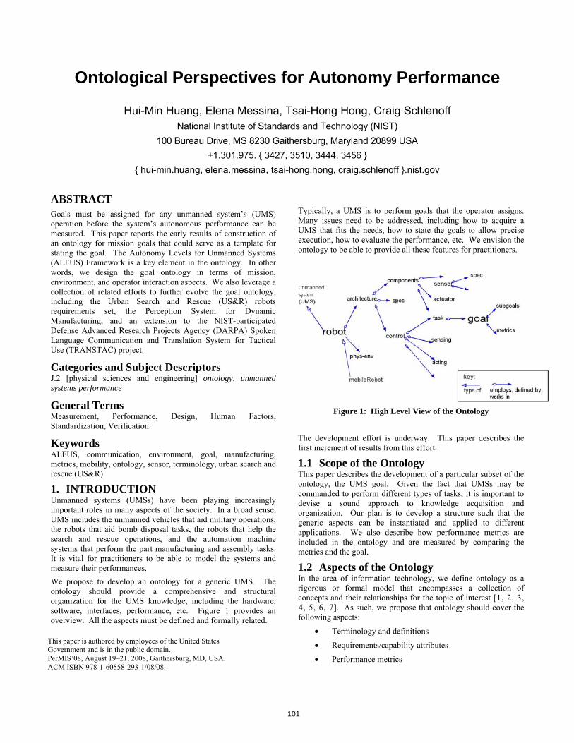
Ontological Perspectives for Autonomy Performance

Hui-Min Huang, Elena Messina, Tsai-Hong Hong, Craig Schlenoff National Institute of Standards and Technology (NIST)

100 Bureau Drive, MS 8230 Gaithersburg, Maryland 20899 USA +1.301.975. { 3427, 3510, 3444, 3456 }

{ hui-min.huang, elena.messina, tsai-hong.hong, craig.schlenoff }.nist.gov

ABSTRACT Goals must be assigned for any unmanned system’s (UMS) operation before the system’s autonomous performance can be measured. This paper reports the early results of construction of an ontology for mission goals that could serve as a template for stating the goal. The Autonomy Levels for Unmanned Systems (ALFUS) Framework is a key element in the ontology. In other words, we design the goal ontology in terms of mission, environment, and operator interaction aspects. We also leverage a collection of related efforts to further evolve the goal ontology, including the Urban Search and Rescue (US&R) robots requirements set, the Perception System for Dynamic Manufacturing, and an extension to the NIST-participated Defense Advanced Research Projects Agency (DARPA) Spoken Language Communication and Translation System for Tactical Use (TRANSTAC) project.

Categories and Subject Descriptors J.2 [physical sciences and engineering] ontology, unmanned systems performance

General Terms Measurement, Performance, Design, Human Factors, Standardization, Verification

Keywords ALFUS, communication, environment, goal, manufacturing, metrics, mobility, ontology, sensor, terminology, urban search and rescue (US&R)

1. INTRODUCTION Unmanned systems (UMSs) have been playing increasingly important roles in many aspects of the society. In a broad sense, UMS includes the unmanned vehicles that aid military operations, the robots that aid bomb disposal tasks, the robots that help the search and rescue operations, and the automation machine systems that perform the part manufacturing and assembly tasks. It is vital for practitioners to be able to model the systems and measure their performances. We propose to develop an ontology for a generic UMS. The ontology should provide a comprehensive and structural organization for the UMS knowledge, including the hardware, software, interfaces, performance, etc. Figure 1 provides an overview. All the aspects must be defined and formally related.

Typically, a UMS is to perform goals that the operator assigns. Many issues need to be addressed, including how to acquire a UMS that fits the needs, how to state the goals to allow precise execution, how to evaluate the performance, etc. We envision the ontology to be able to provide all these features for practitioners.

Figure 1: High Level View of the Ontology

The development effort is underway. This paper describes the first increment of results from this effort.

1.1 Scope of the Ontology This paper describes the development of a particular subset of the ontology, the UMS goal. Given the fact that UMSs may be commanded to perform different types of tasks, it is important to devise a sound approach to knowledge acquisition and organization. Our plan is to develop a structure such that the generic aspects can be instantiated and applied to different applications. We also describe how performance metrics are included in the ontology and are measured by comparing the metrics and the goal.

1.2 Aspects of the Ontology In the area of information technology, we define ontology as a rigorous or formal model that encompasses a collection of concepts and their relationships for the topic of interest [1, 2, 3, 4, 5, 6, 7]. As such, we propose that ontology should cover the following aspects:

Terminology and definitions This paper is authored by employees of the United States Government and is in the public domain. PerMIS’08, August 19–21, 2008, Gaithersburg, MD, USA. ACM ISBN 978-1-60558-293-1/08/08.

Requirements/capability attributes

Performance metrics

101

Engineering specifications

Standards

In other words, to develop an ontology for a topic, the engineer should:

identify the key concepts from the terms and definitions used in the domain,

identify the user, capability, and performance requirements for the program, and

utilize engineering specifications and applicable standards for the UMS and its subsystems and components.

In this first increment for development of a UMS ontology, we begin with the terminology, metrics, and requirements aspects and leave the others for future development.

1.3 Performance Metrics—ALFUS Framework Overview The performance of UMS must be measured in terms of the assigned goals. It is desirable to have a generic and standard structure for stating the goal. There are multiple concerns in the goal statement, including operation (or mission), environment, and operator interactions. These lead us to apply the Autonomy Levels for Unmanned Systems (ALFUS) Framework that NIST has been developing [8]. The ALFUS Framework describes that the autonomy of a UMS can be characterized with Contextual Autonomous Capability (CAC). The CAC model is composed of the following three aspects (or axes), Mission Complexity (MC), Environmental Complexity (EC), and Human Independence (HI), as shown in Figure 2. Each axis is further decomposed into a set of performance metrics.

Figure 2: The ALFUS Framework

The ALFUS Framework was developed originally by the ad hoc ALFUS Working Group (WG) that was lead by NIST. The group has later joined the Society for Automotive Engineers (SAE), a standards development organization, as the UMS Performance Measures Subcommittee. During the first ALFUS workshop, it was determined that the first objective of the group should be terminology [9]. This is because the ALFUS WG decided to take a definition-based approach. The fundamental terms, including autonomy and UMS were defined. The key words and their relationships were further developed into

additional terms, sub-relationships, as well as metrics. This fits well with the ontology concept. Figure 3 illustrates this construct. The MC metrics correspond to, among other aspects, the accuracy and repeatability aspects of a goal. The EC metrics correspond to the spatial and temporal aspects of the goal statement. Human interaction may be critical in assisting the robot to reach a safe state or to reach the goal.

Figure 3: ALFUS Framework Structure

1.4 The Involved Use Cases and Concepts In the three project activities that we use to further evolve this ontology, the US&R robots project has generated a comprehensive requirements set through intense interactions with the user community. The perception system for dynamic manufacturing project also derived a set of requirements from a workshop attended by the industry. We use these results to iterate the goal ontology. The TRANSTAC project uses a System, Component, and Operationally-Relevant Evaluation (SCORE) approach to evaluate the candidate systems. We began to apply some of the key concepts of SCORE in formulating the ontology [10, 11].

2. PERFORMANCE CHARACTERISTICS AND REQUIREMENTS The performance characteristics or requirements of various UMS systems were analyzed and pertinent elements were extracted for the development of the ontology, namely, the ontological model of the mission goal for UMS. The following described two use cases.

2.1 Teleoperation Requirements for US&R Federal Emergency Management Agency (FEMA) US&R Task Force personnel would be among the users who would teleoperate the robots for search and rescue operations. Figure 4 provides an example of the types of terrain which the US&R robots might have to traverse [11, 12]. The users conveyed to the NIST project team how they anticipate the robotic technology could help them. This typifies the interaction between users and technologists who may be implementing the requirements. The entire set of the requirements can be seen in [13]. The existent ontology work in this area includes [14, 15].

102

Figure 4: Rubble Pile that Robots Might have to Traverse

For this development effort, we examine a subset of the requirements and attempt to restructure them to facilitate the ontology implementation. We also apply engineering disciplines to attempt to explore further details of Requirements. Table 1 illustrates our analysis effort, with the left column stating a subset of the Requirements and the right column listing the robotic functions or subsystems that are involved to fulfill the requirements. The intent is to organize the robotic knowledge through the ontology.

Requirement Involved UMS Functions

To project remote situational awareness (SA), beyond line of sight, into compromised or collapsed structures or to convey other types of information; or be able to operate around corners of buildings; as such, SA for near, far, and field of view are required

Video, command and control signals in tight space

To enable use of video in confined spaces and for short-range object identification, which can wash out from excessive illumination of the scene; therefore, adjustability is required

Variable illumination

To support the SA, the robot should be able to ingress a specified number of meters into the worst case collapse, a reinforced steel structure

Maneuver within tight space

To use this system in sensitive public situations where maintaining control of remote systems is imperative and limiting access to video images and other communications to authorized personnel is prudent; should be shielded from jamming interference and encrypted for security

Security

To project remote situational awareness or to convey other types of information down range within line of sight

Video, command and control over long range

Table 1: Mapping of Requirements to US&R UMS Functions

Beyond this example, we reviewed several other Requirements observing that, overall, the following features are keys to the US&R robotic operations:

Situation awareness facilitation

Maneuvering in tight space

Radio link for video and command and control data

Usability to the operator

Minimum training

System monitoring

Sufficient power supply

Compatible with current logistics system These are to be reflected in the ontology work.

2.2 Requirements for Next Generation Manufacturing An impediment to advancing manufacturing to its next level is lack of adequate sensors and perception systems, because the involving environments would be dynamic and unstructured. Therefore, dynamic metrology is a key technology. Those perception systems must be comprehensive, pervasive and providing redundancy. In scenarios such as a robot grasping a moving part off an assembly line, a single, narrowly focused sensor will not be sufficient. The sensor may fail, may not be robust enough for the task, may not sense other objects that could become obstacles, or may not be able to adequately sense humans in the workspace to prevent accidents. Perception for such scenarios would require sensor fusion and control logic to facilitate arbitrations among multiple subsystems. To further discuss the roles and requirements of advanced sensor and perception for the future manufacturing, a workshop was held in October, 2007, which brought together people from Government, industry and academia [16]. A number of the participants indicated that the ability to measure the positions and orientations (6DOF) of components in dynamic environment would result in considerable cost savings in applications such as automobile manufacturing. The installations with more intelligent combinations of sensing and automation will better enable US manufacturers to compete globally. They also called for reference standards, as those would assist the community in establishing clear performance metrics for systems and algorithms. All these requirements were collected and will be incorporated into a comprehensive robotic ontology. One section of the ontology deals with sensors. A generic sensor includes major attributes of sensing function, sensing target, and sensor specification. Figure 5 provides an illustration of this model using the Protégé tool1. Each of the attributes is further elaborated. For example, sensing targets include the properties of spatial- 1 Disclaimer: Certain trade names and company products are mentioned in

the text or identified in certain illustrations to facilitate communication. In no case does such an identification imply recommendation or endorsement by the NIST, nor does it imply that the products are necessarily the best available for the purpose

103

temporal, chemical, climate, kinematic, etc. This effect is illustrated in Figure 6, using the same tool. Specifications may include speed, drift, resolution, etc. The generic structure, as represented in an ontology, allows the information for specific sensors to be recorded. This ontology will serve as a knowledge base or as a tool for a sensory requirements analysis. It will also be useful in standardizing terminology for robots and sensors and in understanding the application of metrics and standards.

Figure 5: Ontological Model for Sensor Definition

Figure 6: Ontological Model for Sensing Targets

3. ONTOLOGY: ELEMENTARY FEATURES The previous sections have described the project requirements and the metrics model. Now we will focus on developing the ontology that encompasses those aspects. We first defined sets of fundamental references and relationships that are used to develop the UMS ontology.

3.1 Relationships Two types of fundamental relationships are defined to associate the ontological entities. These relationships are further subtyped and instantiated to form hierarchical structures.

Part-whole: partOf This relationship can be further instantiated to specific needs. The following are two subsets:

Physical Subtypes: enclosedBy, boundedBy, composedOf Logical Subtypes: controlledBy, integratedIn, boundedBy, composedOf

These can be further instantiated for particular applications. There are also issues of mapping of numbers (a car is composed of auto parts), complementary active and passive relationships (composedOf and consistOf).

Peer: associatedWith Physical Subtypes: connectedWith

Logical Subtypes: interfaceWith, integratedWith

Generalization/specialization: typeOf

Requirement: required, optional; and, or

3.2 Spatial Aspect 3.2.1 References

distance, pose, area, tolerance typeOf spatial_feature

o position partOf pose

o orientation partOf pose

coordinate partOf position

angle partOf orientation

o coordinate partOf area

range typeOf distance

3.2.2 Environmental Features object_class typeOf spatial_feature

o ground_ object_class typeOf object_class

o maritime_object_class typeOf object_class

o aerial_ object_class typeOf object_class

3.3 Temporal Aspect time, tolerance typeOf temporal_feature

duration typeOf temporal_feature

3.4 Spatial and Temporal speed typeOf temporal_feature and spatial_feature

acceleration typeOf temporal_feature and spatial_feature

4. GOAL FOR UMS We began to generate an ontology for the concept of mission goal for the UMS. The identification of the goal attributes is facilitated through the project requirements as described in Section 3. The hierarchical layout of the section headings reflects the structure of the ontology. The mission goal is composed of the subgoals for the subsystems. The subgoals cover operational, environmental, and operator aspects. Given the fact that UMSs may be commanded to perform vastly different types of tasks, our bottom-up approach is to develop a structure and ontological attributes that might be generic to certain applications. As such, the following subsections describe what is equivalent to an illustrative goal ontology suitable for a particular

104

set of applications. Different types of applications may need separate sets of the ontology.

4.1 Subgoal for Mobility Subsystem A UMS includes a mobility system. Therefore, the following is modeled:

mobility subsystem integratedWith UMS

The subsystem’s goal can be modeled as:

mobility_goal partOf UMS_goal

o pose partOf mobility_goal

o object_class partOf mobility_goal

o time partOf mobility_goal

o duration partOf mobility_goal

o speed partOf mobility_goal

o acceleration partOf mobility_goal

o mobility_goal boundedBy tolerance

4.2 Subgoal for Sensor Subsystem A UMS typically includes a sensor system. Therefore, the following is modeled:

sensor subsystem integratedWith UMS

The subsystem’s goal can be modeled as:

sensory_goal partOf UMS_goal

o range partOf sensory_goal

o frequency partOf sensory_goal

4.3 Subgoal for Communication Subsystem A UMS typically includes a communication system. Therefore, the following is modeled:

communication subsystem integratedWith UMS

The subsystem’s goal can be modeled as:

comm_goal partOf UMS_goal o cover_range partOf comm_goal

o set_bandwidth partOf comm_goal

o receive_send_line_of_sight partOf comm_goal

4.4 Subgoal for Power Subsystem A UMS typically includes a power system. Therefore, the following is modeled:

power subsystem integratedWith UMS The subsystem’s goal can be modeled as:

power_subgoal partOf UMS_goal

o set_peak_power_output partOf power_subgoal

o save_min_power partOf power_subgoal

4.5 Subgoal for Mission Package Subsystem A robot typically carries additional subsystems beyond the platform. They may be manipulators, tools, special sensors, weapon, etc. Subgoals must be developed for them.

mission package integratedWith UMS

The subsystem’s goal can be modeled as:

mission_subgoal partOf UMS_goal

o identify_victim partOf mission_subgoal

o assemble_door partOf mission_subgoal

o establish_observation_post partOf mission_subgoal

o translate_text partOf mission_subgoal

4.6 Subgoal for Chassis Subsystem A UMS includes a chassis system. Therefore, the following is modeled:

chassis subsystem integratedWith UMS The subsystem’s goal can be modeled as:

chassis_goal partOf UMS_goal

o set_illumination_intensity partOf chassis_goal

4.7 Subgoal for Human-Robot Interaction (HRI) Subsystem A UMS includes a HRI system. Therefore, the following is modeled:

HRI subsystem integratedWith UMS The subsystem’s goal can be modeled as:

HRI_goal partOf UMS_goal o sound_alarm partOf HRI_goal o display_health_status partOf HRI_goal

4.8 Collaboration A UMS goal may be to collaborate with other systems. The subsystems of a UMS may need to collaborate among themselves.

collaboration_subgoal partOf UMS_goal

The subsystem’s goal can be modeled as: o wait_until partOf collaboration_subgoal o synchronize_with partOf collaboration_subgoal

Note that the performance metrics for the collaboration will be described later in this paper.

4.9 Prioritization and Management The UMS entities may be given multiple goals. The entities may receive multiple goals from their collaborators.

manage_goals partOf UMS_goal

o multi-tasking partOf manage_goals

o prioritize_goals partOf manage_goals

105

value partOf prioritize_goals

o costs partOf prioritize_goals

Note that being able to prioritize the goals would enhance the autonomous performance of the UMS.

4.10 Additional Subgoals Additional subsystems may be employed and the subgoals should be identified.

5. ALFUS METRICS As described earlier, the definition of performance metrics is an important aspect of the UMS knowledge and, therefore, it is a part of the ontology. We have developed the autonomous performance of UMS using the ALFUS metrics.

Autonomy_performance partOf UMS_performance

o MC partOf Autonomy_performance { subtasks_structure, precision, repeatability,

uncertainty, safety_level, risk_level } partOf MC { control_echelon, interoperability,

knowledge_shared } partOf MC { situation_analysis, replans } partOf MC { perception } partOf MC

o EC partOf Autonomy_performance

solution ratios partOf EC Scale: No impediment, one impediment out of

N possibilities, (N-1) out of N, n out of N, N out of N

solution_difficulty_levels partOf EC { energy consumption levels, computation load

levels, look-ahead ability } partOf solution_difficulty_levels

o HI partOf autonomy_performance

{ % of plan generated by UMS, % of plan pre-generated, % of plan execution that operator is involved, % of robot vs. operator initiated interactions, required training, workload } partOf HI

6. GOAL STATE-METRICS ASSOCIATIONS Various aspects of the ontology should be related. In this section, we illustrate how the requirements, goal, and autonomous performance aspects fit together, focusing on the US&R application example.

The goal model is driven by the Requirements, which state that the robot “should be able to ingress a specified number of meters into the worst case collapse” and “project remote situational awareness or to convey other

types of information down range.” These are reflected in the mobility and communication subgoals in the ontology.

The US&R Requirements call for the operator control unit (OCU) displays to be clear and legible in outdoor situations and under ambient light conditions. This is to facilitate UMS control and to reduce the stress level of the user, one of the autonomous performance metrics in the ALFUS Framework.

The US&R Requirements further call for “enable use of video in confined spaces and for short-range object identification.” This corresponds to the solution_difficulty and situation_analysis metrics in ALFUS.

7. SUMMARY An ontological approach is used to model certain aspects of UMS. The objective is to facilitate the investigation of the performance of UMSs. In particular, we represented the goal of a UMS in the ontology, followed by representing the autonomous performance. We further identified several cases illustrating that the two are integrated. Our ultimate goal is to expand on this work for a broad scope ontology that can be helpful to a large audience in the community.

8. REFERENCES

[1] Vujasinovic, M., “An Industrial Validation of a Semantic Mediation Architecture,” IEEE Internet Computing, October 2007

[2] Fiorentini, X. et al., “An Ontology for Assembly Representation,” NIST Interagency/Internal Report (NISTIR) 7436, Gaithersburg, MD, July 2007

[3] Obrst, L., et al., “The 2006 Upper Ontology Summit Joint Communique,” Applied Ontology Journal 2006

[4] Deshayes, L. et al., “An Ontology Architecture for Standards Integration and Conformance in Manufacturing,” Proceedings of the IDMME 2006 Grenoble, France, May 17-19, 2006

[5] Schlenoff, C. I., et al., “ An Intelligent Ground Vehicle Ontology for Multi-Agent System Integration,” Proceedings of the 2005 Knowledge Intensive Multi-Agent Systems (KIMAS) Conference, Waltham, MA, April 18-21, 2005

[6] Schlenoff, C. I., et al., “A Standard Intelligent System Ontology,” 2005 SPIE Defense and Security Symposium, March 2005, Florida

[7] Schenk, J.R. and Wade, R.L., “Robotic Systems Technical and Operational Metrics Correlation,” PerMIS’08 Workshop, Gaithersburg, Maryland, October 2008

[8] Autonomy Levels for Unmanned Systems (ALFUS) Framework, Volume II: Framework Models Version 1.0, NIST Special Publication 1011-II-1.0, Huang, H. et al., Ed., National Institute of Standards and Technology, Gaithersburg, MD, December 2007

[9] Autonomy Levels for Unmanned Systems Framework, Volume I: Terminology, Version 1.1, Huang, H. Ed., NIST

106

Special Publication 1011, National Institute of Standards and Technology, Gaithersburg, MD, September 2004

[10] Weiss, B.A. and Schlenoff, C., “Evolution of the SCORE Framework to Enhance Field-Based Performance Evaluations of Emerging Technologies,” PerMIS’08, Gaithersburg, MD, October 2008

[11] Schlenoff C, et al., Applying SCORE to Field-Based Performance Evaluations of Soldier Worn Sensor Technologies. Journal of Field Robotics 2007 September;24(8/9):671-98

[12] Messina, E., Jacoff, A., “Performance Standards for Urban Search and Rescue Robots,” Proceedings of the SPIE Defense and Security Symposium, Orlando, FL, April 2006

[13] Messina, E. R., et al., Statement of Requirements for Urban Search and Rescue Robot Performance Standards, NIST Draft Report, May 2005

[14] Schlenoff, C. I., et al., “ Test Methods and Knowledge Representation for Urban Search and Rescue Robots,” Chapter in the Climbing and Walking Robots Book, August 2007

[15] Schlenoff, C. I. and Messina, E. R., “A Robot Ontology for Urban Search and Rescue,” 2005 CIKM Conference: Workshop on Research in Knowledge Representation for Autonomous Systems, Bremen, Germany, October 2005

[16] Draft Proceedings of the Dynamic Measurement and Control for Autonomous Manufacturing Workshop, To Be Published as a NIST Internal Report, Gaithersburg, MD, October 2008

107

Robotic Systems Technical and Operational Metrics Correlation

Jason R. Schenk, Ph.D. DeVivo AST

2225 Drake Ave Suite 2 Huntsville Al 35805

256-489-4614jasonschenk@devivoast.com

Robert L. Wade US Army Aviation and Missile Research,

Development and Engineering Center Software Engineering Directorate (SED)

Redstone Arsenal, AL 35898 256-842-6174

robert.l.wade@us.army.mil

ABSTRACT As unmanned systems become more prevalent, so does the emphasis on quantifying their performance using standard measures. Several research efforts have attempted to elicit important attributes associated with unmanned systems performance, with limited applicability and success. We identify several reasons for this, including the lack of adherence to a strict ontology and taxonomy, the use of means-based rather than goal-based tests, and the lack of a clear correlation between tests and predicted performance. This paper provides a conceptual framework for the development of correlations between technical characteristics and operational performance. These correlations provide a foundation for generating predictive performance test standards.

Categories and Subject Descriptors B.8.2 [Hardware]: Performance and Reliability – performance analysis and design aids

General Terms Algorithms, Measurement, Performance, , Human Factors, Standardization

Key Words Analytic Hierarchy Process (AHP), Explosive Ordinance Disposal (EOD), unmanned systems, correlation, performance metrics

1. Introduction A multiplicity of technical performance measures have been developed for requirements documents, system performance specifications, and research analysis of current Department of Defense (DoD) robotic systems. None are standardized or widely accepted. Furthermore, their

correlation to operational performance is not known or well-understood within the robotics community. In fact, operational performance and technical characteristics are often ill-defined, mixed, or applied inconsistently. The establishment of a set of consistent normative technical and operational metrics based on a strict and logical ontology is critical to informing the design, comparison, and selection of unmanned systems [1]. The Robotic Systems Technical and Operational Metrics Correlation (RSTOMC) project aims to develop a methodology for establishing testable quantitative measures that correlate with unmanned systems performance. This project is sponsored by the United States Army and the Joint Robotics Ground Enterprise (JGRE), Office the Undersecretary of Defense (OUSD). Explosive ordinance disposal (EOD) is a current pressing need for the Army, so the focus of the current RSTOMC project is on tele-operated EOD platform domain analysis. This focus adds the benefit of working systems and operators with a significant historical experience. The RSTOMC project will develop a preliminary model for technical to operational correlation using quantitative and qualitative information from this domain. Based on these correlations, the project allows for the development of a method for selecting a set of technical performance tests and metrics for evaluating systems. Standardized robotic system metrics will enable the DoD to define, specify, distinguish, evaluate, and test robotic systems in a more systematic manner. This project will attempt to derive more reliable correlations between the technical and operational characteristics of robotic systems. This correlation has the potential to simplify and reduce the cost of analysis. Successful execution of this effort will provide the foundation for a project manager or user to objectively predict the impact of technical changes on operational performance, or the operational performance of a proposed system, to an accuracy of 80% by performing a set of low cost technical tests. While the creation of specific tests may be left to future work, the RSTOMC effort will produce a model for predicting operational performance based on a set of technical measures. We will refine the model based on the data available from within the EOD robotics community and develop a software based system that allows for the continued maturation of the model as well as the incorporation of

108

that this contribution was authored or co-authored by a contractor oraffiliate of the U.S. Government. As such, the Government retains anonexclusive, royalty-free right to publish or reproduce this article, or toallow others to do so, for Government purposes only.PerMIS’08, August 19-21, 2008, Gaithersburg, MD, USA

(c) 2008 Association for Computing Machinery. ACM acknowledges

ACM ISBN 978-1-60558-293-1/08/08.

additional domains. Finally, we propose a method for test creation and near-optimal set selection.

2. RSTOMC Plan The overall goal for this project is to improve the ability to objectively assess robotic systems by developing a tool that, through simple tests and measures, can predict the mission-specific operational performance to at least 80% accuracy. To reach this goal, a methodology for robotic systems performance measurement will be developed to identify and assess both technical measures and the operational performance of the systems in application specific usage scenarios. Technical measures are defined here as a quantitative assessment of a characteristic in a controlled environment. A technical characteristic is a physical ability of a system. This is different from operational performance measures, which are defined relative to mission goals or tasks. Correlations between the technical and performance measures will be determined. The resulting correlations will be captured in a software tool to be distributed to appropriate agencies. The RSTOMC project consists of the following tasks: Task 1) Collect and Analyze Operational Scenario.

Subtask 1) Select the method of analysis. Subtask 2) Select the data source and domain.

Task 2) Define Technical Performance Characteristics. Subtask 3) Identify relevant technical

characteristics (TC) of EOD systems. Task 3) Define Operational Score (Os). This task may

include defining mission-specific criteria which we call operational measures (Om). Subtask 4) Identify operational requirements and

their relative importance for successful EOD system performance.

Task 4) Establish Correlations between Operational Performance and TC. Operational performance may be defined as the Os or Om. Subtask 5) Identify the correlation between TC

and operational performance. Subtask 6) (Future work) Design technical

performance metrics. and measures (TPM), validating results where possible.

Subtask 7) (Future work) Create a method for selecting a near-optimal set of tests. Incorporate and document the results within a software product.

2.1 Subtask 1: Select Method Broadly speaking, efforts to measure robotic systems quality fall into two main categories. The first is based on task decomposition, such as [2], where each mission-specific task is broken down into its most fundamental subtasks and the physical requirements or resources required to accomplish them. The overall performance is assumed to be the sum of a systems ability to complete each subtask. These efforts generally start with subject

matter experts listing tasks or functions that a system must perform, and their frequency or importance. Such decomposition is often limited by experts’ ability to quantify the relative relationships of functions to performance. This becomes difficult or impossible in high complexity systems with multiple interaction effects and high order dependencies [3]. Further, such analyses risk focusing on means rather than ends, limiting its relevance back to overall system performance. One effort based on task decomposition to create a set of prioritized and measureable requirements for urban search and rescue robot performance comes from the National Institute of Standards and Technology (NIST) [4]. The study used subject matter experts to identify 103 requirements across 13 robotic platform categories from aerial to land to aquatic. There were 21 requirements that were most widely applicable across the 13 robot categories. Tests and measures were developed for each of these requirements, such as “communication range – beyond line of sight”. The National Institute of Justice has also used task decomposition to determine metrics for assessing unmanned system in law enforcement [5]. In their study, they used a focus group to obtain nine key attributes critical to system selection. These attributes were: purchase cost, platform speed, ability to complete its mission, minimal weight, minimal down time, minimal maintenance cost and maintenance requirements, manipulator lift capacity, and operating range. A survey was then conducted to determine acceptable values for each. An effort by the Air Force Research Laboratory (AFRL) attempts to link technical measures to operational requirements for explosive ordinance disposal (EOD) robotic vehicles [6][7]. This project used Quality Function Deployment (QFD) to elicit requirements from subject matter experts, as well as one-on-one interviews to gain detailed insight into requirements. The results of their most recent project are used in the current research, and are discussed in greater detail in the following sections. Task decomposition allows for a complete enumeration of expected task requirements. However, decomposition is platform and strategy dependent, meaning different designs or solution strategies cannot be tested as effectively or without bias. Secondly, decomposition of tasks does not test interaction effects, unless explicitly enumerated during the decomposition. Unmanned systems are complex and as such have complex interactions between component parts or capabilities. These interactions may form the basis for important emergent behaviors or qualities that allow the system to function or fail in surprising ways [8]. A second class of research efforts takes a gestalt approach, starting with the systems-level requirements of a system. The assumption is that complex systems have complex, inseparable interactions that produce emergent behavior. These emergent properties cannot be captured except by looking at the system as a whole. For example, Steinfeld et al. list five features that are required of a task-oriented human-robot system [9]. These are: navigation, manipulation, perception, management, and social, which are further broken down into more specific measurable

109

tasks. These tasks remain relatively generic and mission independent. It is again up to the subject matter expert to determine the relative importance of each of these tasks to the specific mission profile. Cummings et al. generated five sets of metrics classes using a separate ontological framework, based on human robot interaction (HRI) theory [10]. These classes are human behavior efficiency, human behavior precursors, Unmanned Vehicle (UV) behavior efficiency, collaboration, and mission effectiveness. Systems-level approaches are useful in that they include the complex and emergent properties of a system in its analysis. However, it is often difficult to create a set of technical tests to measure the top-level requirements a system. Additionally, such tests do not provide much specific information about a system. On the other hand, they are much more goal oriented, allowing for fair comparison of different platform designs or solution strategies. Such high-level tests are often very expensive, approaching the cost and complexity of full-blown field trials. Finally, the authors are not aware of any top-down approach that has generated specific weights for the importance of each of the proposed high-level requirements to overall performance. Another distinction one must consider is the ontology used in the approach. Two common ontologies are illustrated by the Architecture Framework for Unmanned Systems (AFUS), which standardizes a set of terms, definitions, and attributes common across all domains of unmanned systems [11]. The two ontologies are the Conceptual View (means-oriented) and the Capabilities View (goal-oriented). The Conceptual View describes unmanned systems in terms of component structure, knowledge store, and gross actions. The Capabilities describes capabilities and behaviors a system is able to perform. For example, a laser range-finder is a concept used to describe the composition of a system, while object-detection and tracking (which may use a laser range-finder) is a capability of the platform. The ontology chosen drives the development of the criteria, tests, and measures that are chosen to predict system performance.

2.1.1 Analytic Hierarchy Process Ideally, technical as well as operational performance data would be available from rigorous lab and field experimentation, and real-world observation across a wide range of platforms. Due to cost and logistics limitations, it is often more practical to obtain data through the elicitation of expert opinions. There are several ways in which to accomplish this, including Quality Function Deployment (QFD) and Analytic Hierarchy Process (AHP). The fundamental mathematics of the RSTOMC project comes from the AHP, which provides a systematic approach to correlating low level features with high level system requirements [12]. The raw data comes from a QFD and interviews performed by AFRL. The following is a brief description of the proposed mathematical relationships. These equations represent an idealized, hierarchical, and theoretical model of the relationships. The actual manifest structure of our analysis will depend on the specifics of the data.

Figure 2 Conceptual hierarchy of EOD unmanned systems analysis

Operational requirements, Om, include all the important criteria that may arise during an EOD mission. Examples might include probability of successful disarming or average time to disarm. In addition, their frequency or relative importance to the completion of the mission provides the basis for weighting. The weighted sum of these requirements yields the operational performance score of the system, sO .

(1) Technical characteristics refer to the physical systems and their interactions, such as end-effector lift capacity or screen resolution. These characteristics each have a unique impact on the set of operational requirements. The nature of this impact provides e g factors: the w ightin

(2) To further complicate matters, available metrics and derived tests may not correspond 1:1 to technical characteristics, which would require another set of weights,

. However, if a 1:1 correspondence can be established (that is, each test measures only one technical characteristic), then this weighting matrix is equal to the identity, I. These tests and metrics, which we call technical performance metrics, or TPM, may be related back to the operational perfo c in the following manner: rman e score,

(3) As an alternative, TPM may be directly related to operational requirements, or even operational performance scores, using weights derived from a separate survey. In this way, only one set of weights are needed, indifferent to the relationship of operational requirements and technical characteristics:

(4)

W2

W1

Os

W

Om Om

TC TC TC TC

TPM

...

...

TPM ...

110

This holds true only if the TPM are a minimum necessary and sufficient measure of the operational score (no zero rows or columns in the weighting matrix, ). In either case, the relationship is linear. Therefore, there are no interaction terms between TPM. This assumption is unlikely for complex systems, especially if each TPM corresponds to about one TC. For example, it would be difficult to design a TPM measuring manipulator reach and a TPM measuring lift capacity that are independent of one another, since lift capacity is relative to the extension of the arm. We are motivated to develop TPM based on some other criteria besides decomposition to the most fundamental tasks.

2.2 Subtask 2: Select Data Source and DomainWe chose the AFRL analysis to provide the raw data for the project, because it is one of the few analyses that quantify the relationships between characteristics and performance. The analysis uses Quality Function Deployment and significant domain expert input to formulate operational requirements, technical characteristics, and their relationship to one another. The inclusion of this relational data makes it ideal for our analysis. This analysis draws from interviews and focus groups with 270 DOD unit-level EOD technicians from 45 different organizations across the four United States armed forces services. The goal of the analysis was to generate requirements for the combat variant of the Next Generation EOD Remote Control Vehicle (NGEODRCV). The report identified and ranked, using QFD, 67 “technical characteristics” based on 79 “customer needs.” The expert interviews provided details to the technical characteristics, breaking them down further into approximately 271 stated needs, preferences, tasks, design elements, features, etc. The set of roughly 271 failure modes, design preferences, tasks, features, specifications, and customer requirements that make up the responses do not represent a clear and consistent ontology for use in our analysis. In order to be applicable to the RSTOMC project, they must be organized in such a way that a small set of valid technical metrics can be derived to be predictive of operational performance. By creating a set of technical tests and metrics, and using a set of weights derived from the domain expert interviews, we can use the AHP methodology to generate a first order linear model of operational performance.

2.3 Subtask 3: Identify TC Technical characteristics were established by the TSWG NGEODRCV Common Systems Architecture dated 14 January 2003. These characteristics were placed in a three-tiered hierarchy. For example, Navigation is broken into “path planning” and “path execution”. Each of these is further broken down. For example, path execution is broken down into “obstacle detection” and “obstacle avoidance”.

Table 2 Sample of Technical Characteristics from the QFD

Navigation PayloadPath Planning

PathExecution

SensorIntegration

ToolIntegration

Pos

ition

cap

abili

ty (D

-1-a

)

Map

ping

cap

abili

ty (D

-1-b

)

Way

poin

t nav

igat

ion

(D-1

-c)

Obs

tacl

e av

oida

nce

(D-2

-a)

Obs

tacl

e D

etec

tion

(D-2

-b)

Log

ical

(E-1

-a)

Ele

ctric

al (E

-1-b

)

Phy

sica

l (E

-1-c

)

Ele

ctric

al (E

-2-b

)

Phy

sica

l (E

-2-c

)

These characteristics were further broken down and defined in surveys. For example, “Tether Durability” was described as the ability to resist being run over by the platform (51%), resist tensile forces (25%), resist rough terrain (9%), and resist both rough terrain and being run over (15%). In a QFD, these characteristics are of the same level of scope, type, and fidelity. In other words, the ontology should be consistent. Typically, these are measurable characteristics with a possible range, such as “battery life: 0-24 hours”. However, in the present QFD, characteristics are a mixture of resistance to failure modes (e.g. tether resistance against being run over, prevention of dirt clogging treads), design modality preferences (e.g. joystick vs. keyboard), tasks (e.g. ability to place counter-measures on a vehicle, ability to reach into a 55-gal drum), typical customer requirements (e.g. fine/smooth motor control, “observability” of platform orientation), specifications (e.g. 12-hour battery life, maximum arm lift of 25-50 lbs.), and features (e.g. rangefinder). The experts’ reasoning generally appears within the interview responses. Therefore, this feature of the analysis may be addressed by (and provides further motivation for) goal-based tests. As a result of trying to fit all of the needs into the pre-determined hierarchy, several of the 271 needs are the same under multiple headings (e.g. depth perception appears under Visual (B-2-a) as well as Displays (C-2-d)). Therefore, the ranked list may be skewed, since some important needs may be diffused among multiple technical characteristics, while other characteristics represent aggregates of several important needs that could be broken-up further. In an effort to tighten the taxonomy, we re-sort and re-classify the needs into new technical characteristics categories. Each listed need maintains its constituent weight (the weight of the characteristic it belonged to times the percent of respondents citing it for that characteristic). The result is a list of approximately twenty-five new technical characteristics categories. Under each of these categories, the same 271 TC remain (condensed to 96 by combining duplicate and redundant TC), only in a more useful way for the RSTOMC project.

111

2.4 Subtask 4: Identify Operational RequirementsIn a QFD, user requirements in the form of qualities are listed along the left side of the table [13][14][15]. These requirements might include general qualities such as “ease of deployment” or “mobility”. Note that the emphasis is on general goals, rather than specific means or tactics. In the present case, the requirements represented possible tasks that a system would need to perform during operations, as determined by a joint service focus group of combat experienced EOD technicians. These included tasks such as “offload robot” and “negotiate terrain”, along with the subtasks required to accomplish these. The subtasks were weighted via survey as to their importance to the overall mission. As discussed previously, tests based on task decomposition methods tend to dictate the solution strategy, limiting its ability to compare innovative design or operational strategies [16]. More general goal-oriented requirements allow comparison of disparate designs over ordinal measures. At the least, the sum total of these requirements provides Os. The derivation of a more goal-focused set of operational measures, Om, may result from a separate survey. The formulation of tests based on these results will be discussed further in section 2.6.

Table 1 Sample of User Requirements from the QFD

Requirement

Off-load Robot

Unsecure robot

Power-up robot

Remove robot from vehicle

Pick up robot

Drive robot off vehicle

Off-load OCU

Remove OCU from vehicle

Set up OCU

Attach tether to OCU

2.5 Subtask 5: Identify the correlation The body of the QFD matrix represents the correlation between customer requirements and technical characteristics. Since we are reorganizing the data, the correlations must be carried along with the lowest level TC as they move to our new taxonometric structure. Since the operational analysis interview results cite the rationale and the relative number of respondents citing each rationale, we are able to carry that response over to the new parent category without losing that response’s relative contribution to overall system performance.

2.6 Subtask 6: Generate TPM Tests This section details the important considerations associated with test selection. Although this and the following section are identified as future works, it is important to mention here. This is because the present work is intended to ultimately facilitate the creation of standard tests, so preliminary work must be cognizant of this goal. The level of testing selected is based on cost, resources, the desired number and complexity of tests, and the required level of specificity and “predictiveness” of tests. Since each TC has its own weighting, tests may be devised that measure the each independently, collectively, across categories, or some variation of the three. The type of tests selected depends on 4 factors: 1. The natural grouping of the technical requirements.

Some sets of requirements are coupled or difficult to segregate. Interactions and emergent properties may also exist that cannot be measured if TC are measured in isolation. A solid taxonomy and ontology will facilitate this.

2. Cost or difficulty of the test. A set of tests that measure individual components separately may be more or less difficult or expensive than a single aggregate test. Cost is also impacted by interaction effects, as it may be more difficult to isolate TC that are naturally coupled.

3. The “informativeness” of the test. More atomic tests provide more specific information, while aggregate tests may be more predictive of actual operational performance, due to interaction effects and their goal rather than means focus.

4. The number of tests. A smaller set of tests are preferable to a large battery of tests.

Overall, the goal is to provide a small set of informative tests that together predict performance to the highest accuracy possible. Below are three levels of tests along the spectrum of aggregation. The weights included in the tables are estimated from the results of the operational analysis and our effort to re-sort the results for our purpose.

2.6.1 Atomic tests A large number of very specific “atomic” tests designed to measure each TC separately provide very specific information about a given platform. It provides clear evidence of what specific features or abilities are strong or weak in a platform, but the correlation to real world operational performance may not be as high. This is because individual tests would only provide for a first order linear model where interactions between components are ignored. Also, specific tests of “means” dictate a solution strategy and limit the possibility for innovation. For example, if system performance for a hypothetical mission is defined as the ability to cross a bridge, then tests of waypoint sensors, the drive train, stability, distance sensors and obstacle avoidance might be devised to see if the robot could cross the bridge. However, a system designed to bypass the bridge altogether and fjord the river might accomplish the

112

mission objective equally well, but score poorly on these atomic, “means” tests. Further, due to unmeasured interactions, the system that scores well on such tests might still be unable to accomplish the mission objectives, for example if its extra features make it too heavy or wide to cross the bridge.

Table 5 Examples of "atomic" level tests Test Details

Light board

Tests the manual dexterity of the robot, the controllability of the system, and the visual feedback of the device

~4%

Lift strength

Tests the strength of arm, effector, and the stability of the platform

~4%

Reach Tests the range of motion (solid angle or volume) of the arm

~3%

Climb Tests the maximum grade of stairs, curbs, and slopes scalable

~3%

2.6.2 Aggregate tests Alternatively, higher level “aggregate” tests are designed to measure sets of technical characteristics that are naturally coupled. These types of tests tend to be fewer in number, but more complex. As a result, interactions are captured and the subsequent model can be more predictive of operational performance. The tradeoff is that the information provided by the results of tests is less specific. The determination of specific deficiencies in the platform requires follow-up analysis. Using our river-crossing example, the test would measure how well (quickly, reliably, etc.) the robot could cross a bridge, rather than the individual systems that provide that affordance. As with the atomic tests, this level still risks measuring means rather than goals.

Table 6 Examples of "aggregate" level tests Test Details

Advanced Visual Acuity

Tests the ability to detect various types and levels of signals

~15%

Signal Strength

Tests the ability to maintain a strong signal across distance and with physical and electronic interference

~23%

Manual dexterity

Tests the ability to access and manipulate objects of various types, sizes despite possible obstructions

~15%

2.6.3 Task level tests A third design philosophy might be to create tests that are “task” or “goal” based. These tests are also very aggregate in that they test many components and the interactions in concert. The overall performance on a task represents a

system-level emergent capability, thereby allowing for multiple robot design types or strategies to be compared. Task outcomes (such as the ability to get to the other side of a river) are measured rather than means (bridge crossing, swimming, etc.). This method has the potential for being the most predictive of operational performance and best able to compare disparate robotic systems, because its tests more closely approximate the real world. As with all more aggregate tests, however, insight into specifics require post hoc analysis. In addition, the results of these tests will most likely not be independent, so the sum weightings may not be equal to 1. Finally, the resource and time costs associated with these tests approach those of full-blown field trials, the current method with which this effort is intended to improve upon.

Table 7 Examples of "task" level tests Test Details

Retrieve Enter a room and retrieve an object. There may be other objects in room, doors, stairs/slopes, and other obstacles, variable lighting, target object may be obstructed, buried, or inside a container, object may be large, small, fragile, slippery, or heavy.

~25-75%

Arrange Move objects to a predetermined arrangement. Specific tasks might include stacking, clearing an area, manipulating small objects (Chess, Perfection, Toy Ball), etc.

~25-75%

Regardless of the level of testing, tests must be correlated back to overall operational performance. The AFRL study provides a basis for this, as the previous section detailed. Verification may be conducted through additional surveys or interviews, using AHP or another method.

2.7 Subtask 7: TPM Test Set Selection Given the sheer number of alternative performance test combinations, an empirical method of test selection should be derived. This method is fundamentally a combination of two classical problems. First, it is a cost benefit-analysis. Each proposed test has a unique cost associated with it, in terms of resource requirements, time requirements, and costs associated with the difficulty of testing and measurement. The goal is to find a set of tests that can predict with the requisite level of accuracy at the minimum cost. To achieve this accuracy, the set of tests must span the relevant system characteristics that correlate with overall performance. This is a set covering problem. The solution must cover characteristics that account for at least 80% of the variability. In other words the overall test selection problem becomes: minimize the cost of the selected tests, such that the sum of of the TC covered by the selected tests 80%. This problem is NP-hard, and therefore we propose future work use a solution derived

113

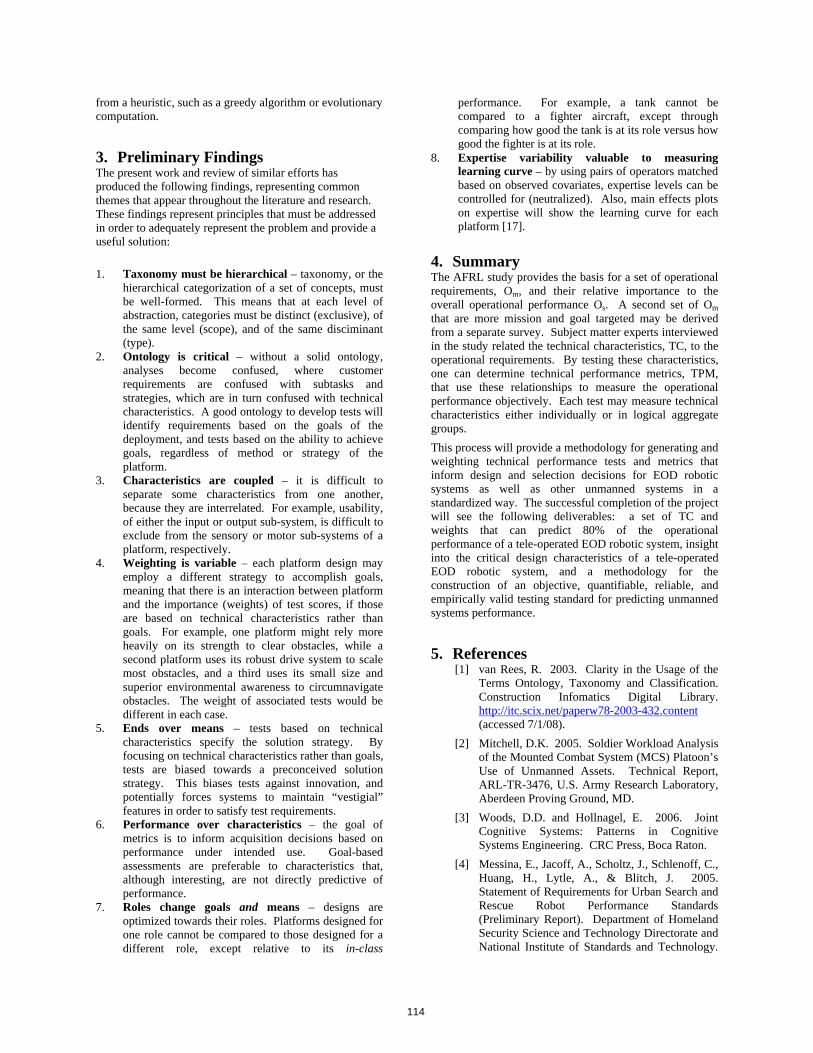
from a heuristic, such as a greedy algorithm or evolutionary computation.

3. Preliminary Findings The present work and review of similar efforts has produced the following findings, representing common themes that appear throughout the literature and research. These findings represent principles that must be addressed in order to adequately represent the problem and provide a useful solution:

1. Taxonomy must be hierarchical – taxonomy, or the hierarchical categorization of a set of concepts, must be well-formed. This means that at each level of abstraction, categories must be distinct (exclusive), of the same level (scope), and of the same disciminant (type).

2. Ontology is critical – without a solid ontology, analyses become confused, where customer requirements are confused with subtasks and strategies, which are in turn confused with technical characteristics. A good ontology to develop tests will identify requirements based on the goals of the deployment, and tests based on the ability to achieve goals, regardless of method or strategy of the platform.

3. Characteristics are coupled – it is difficult to separate some characteristics from one another, because they are interrelated. For example, usability, of either the input or output sub-system, is difficult to exclude from the sensory or motor sub-systems of a platform, respectively.

4. Weighting is variable – each platform design may employ a different strategy to accomplish goals, meaning that there is an interaction between platform and the importance (weights) of test scores, if those are based on technical characteristics rather than goals. For example, one platform might rely more heavily on its strength to clear obstacles, while a second platform uses its robust drive system to scale most obstacles, and a third uses its small size and superior environmental awareness to circumnavigate obstacles. The weight of associated tests would be different in each case.

5. Ends over means – tests based on technical characteristics specify the solution strategy. By focusing on technical characteristics rather than goals, tests are biased towards a preconceived solution strategy. This biases tests against innovation, and potentially forces systems to maintain “vestigial” features in order to satisfy test requirements.

6. Performance over characteristics – the goal of metrics is to inform acquisition decisions based on performance under intended use. Goal-based assessments are preferable to characteristics that, although interesting, are not directly predictive of performance.

7. Roles change goals and means – designs are optimized towards their roles. Platforms designed for one role cannot be compared to those designed for a different role, except relative to its in-class

performance. For example, a tank cannot be compared to a fighter aircraft, except through comparing how good the tank is at its role versus how good the fighter is at its role.

8. Expertise variability valuable to measuring learning curve – by using pairs of operators matched based on observed covariates, expertise levels can be controlled for (neutralized). Also, main effects plots on expertise will show the learning curve for each platform [17].

4. Summary The AFRL study provides the basis for a set of operational requirements, Om, and their relative importance to the overall operational performance Os. A second set of Om that are more mission and goal targeted may be derived from a separate survey. Subject matter experts interviewed in the study related the technical characteristics, TC, to the operational requirements. By testing these characteristics, one can determine technical performance metrics, TPM, that use these relationships to measure the operational performance objectively. Each test may measure technical characteristics either individually or in logical aggregate groups. This process will provide a methodology for generating and weighting technical performance tests and metrics that inform design and selection decisions for EOD robotic systems as well as other unmanned systems in a standardized way. The successful completion of the project will see the following deliverables: a set of TC and weights that can predict 80% of the operational performance of a tele-operated EOD robotic system, insight into the critical design characteristics of a tele-operated EOD robotic system, and a methodology for the construction of an objective, quantifiable, reliable, and empirically valid testing standard for predicting unmanned systems performance.

5. References [1] van Rees, R. 2003. Clarity in the Usage of the

Terms Ontology, Taxonomy and Classification. Construction Infomatics Digital Library. http://itc.scix.net/paperw78-2003-432.content (accessed 7/1/08).

[2] Mitchell, D.K. 2005. Soldier Workload Analysis of the Mounted Combat System (MCS) Platoon’s Use of Unmanned Assets. Technical Report, ARL-TR-3476, U.S. Army Research Laboratory, Aberdeen Proving Ground, MD.

[3] Woods, D.D. and Hollnagel, E. 2006. Joint Cognitive Systems: Patterns in Cognitive Systems Engineering. CRC Press, Boca Raton.

[4] Messina, E., Jacoff, A., Scholtz, J., Schlenoff, C., Huang, H., Lytle, A., & Blitch, J. 2005. Statement of Requirements for Urban Search and Rescue Robot Performance Standards (Preliminary Report). Department of Homeland Security Science and Technology Directorate and National Institute of Standards and Technology.

114

http://www.isd.mel.nist.gov/US&R_Robot_Standards/Requirements%20Report%20(prelim).pdf (accessed 7/1/08).

[5] National Institute of Justice. 2000. Final Report on Law Enforcement Robot Technology Assessment. TSWG Task T-150B2. http://www.nlectc.org/jpsg/robotassessment/robotassessment.html (accessed 7/1/08).

[6] AFRL. 2006. Next Generation EOD Remote Controlled Vehicle: Military Combat Operational Analysis (DRAFT). Combating Terrorism Technology Support Office Technical Support Working Group.

[7] AFRL. 2003. Next Generation EOD Remote Controlled Vehicle: Operational Analysis. Combating Terrorism Technology Support Office Technical Support Working Group.

[8] Hollnagel, E., Woods, D.D., & Leveson, N. 2006. Resilience Engineering: Concepts and Precepts. Ashgate; Burlington, VT.

[9] Steinfeld, A., Fong, T., Kaber, D., Lewis, M., Scholtz, J., Schultz, A., and Goodrich, M. 2006. Common metrics for human-robot interaction. In Proceedings of the 1st ACM SIGCHI/SIGART Conference on Human-Robot interaction (Salt Lake City, Utah, USA, March 02 - 03, 2006). HRI '06. ACM, New York, NY, 33-40.

[10] Donmez, B., Pina, P., & Cummings, M. 2008. Evaluation Criteria for Human-Automation Performance Metrics. PerMIS conferece proceedings; August 19-21, 2008, Gaithersburg.

[11] Society of Automotive Engineers AS-4A. 2008. Architecture Framework for Unmanned Systems. Architecture Framework Subcommittee, Society of Automotive Engineers.

[12] Saaty, T.L. 1980. The Analytic Hierarchy Process. McGraw-Hill, New York, NY.

[13] Kolarik, W.J. 1999. Creating Quality. McGraw-Hill, Boston.

[14] Kusiak, A. 1999. Engineering Design – Products, Processes, and Systems. Academic Press, San Diego.

[15] Lowe, A.J. 2000. QFD-HOQ tutorial. http://www.gsm.mq.edu.au/cmit/qfd-hoq-tutorial.swf (accessed 5/5/08).

[16] Saaty, T.L. 1999. Fundamentals of the Analytic Network Process. ISAHP; August 12-14, Kobe, Japan.

[17] Allen, T.T. 2006. Introduction to Engineering Statistics and Six Sigma: Statistical Quality Control and Design of Experiments and Systems. Springer-Verlag, London.

115

Survey of Domain-Specific Performance Measures inAssistive Robotic Technology

Katherine M. Tsui and Holly A. YancoUniversity of Massachusetts LowellDepartment of Computer Science

1 University AvenueLowell, MA, USA

{ktsui, holly}@cs.uml.edu

David J. Feil-Seifer and Maja J. MataricUniversity of Southern CaliforniaDepartment of Computer Science

941 West 37th PlaceLos Angeles, CA, USA

{dfseifer, mataric}@usc.edu

ABSTRACTAssistive robotics have been developed for several domains,including autism, eldercare, intelligent wheelchairs, assistiverobotic arms, external limb prostheses, and stroke rehabil-itation. Work in assistive robotics can be divided into twolarger research areas: technology development, where newdevices, software, and interfaces are created; and clinicalapplication, where assistive technology is applied to a givenend-user population. Moving from technology developmenttowards clinical applications is a significant challenge. De-veloping performance metrics for assistive robots can unveila larger set of challenges. For example, what well establishedperformance measures should be used for evaluation to lendcredence to a particular assistive robotic technology from aclinician’s perspective? In this paper, we survey several ar-eas of assistive robotic technology in order to demonstratedomain-specific means for evaluating the performance of anassistive robot system.

Categories and Subject DescriptorsA.1 [Introductory and Survey]

General TermsPerformance measures

KeywordsAssistive technology, human-robot interaction, robotics, end-user evaluation

1. INTRODUCTIONAssistive robotics may have therapeutic benefits in do-

mains ranging from autism to post-stroke rehabilitation toeldercare. However, it can be challenging to transition anassistive device developed in the lab to the target domain.This problem can occur even when the device was designed

Permission to make digital or hard copies of all or part of this work forpersonal or classroom use is granted without fee provided that copies arenot made or distributed for profit or commercial advantage and that copiesbear this notice and the full citation on the first page. To copy otherwise, torepublish, to post on servers or to redistribute to lists, requires prior specificpermission and/or a fee.PerMIS’08 August 19–21, 2008, Gaithersburg, MD, USA.Copyright 2008 ACM 978-1-60558-293-1 ...$5.00.

with a specific end user in mind. Romer et al. providedguidelines for compiling a technical file for an assistive de-vice for transfer from academic development to manufac-turing [52]. Their guidelines state that documentation ofan assistive device must include its “intended use, designspecifications, design considerations, design methods, designcalculations, risk analysis, verification of the specifications,validation information of performance of its intended use,and compliance to application standards” [52]. Academicand industrial research labs are the piloting grounds for newconcepts. However, due to the institutional separation be-tween the research environment and end-users, special caremust be taken so that a finished project properly addressesthe needs of end-users. As such, it is imperative for thedevelopment of assistive robotic technologies to involve theend-user in the design and evaluations [28]. These end-userevaluations, with the proper performance measures, can pro-vide the basis for performance validation needed to begin thetransition from research pilot to end product.

Does there exist a ubiquitous set of performance mea-sures for the evaluation of assistive robotic technologies?Time to task completion or time on task are common mea-sures. Romer et al. propose an absolute measure for time totask completion, where the time is normalized with an able-bodied person’s performance [52]. Task completion time fitsmany robotic applications, such as retrieving an object witha robotic manipulator. However, it may not suit other appli-cations, such as a range of motion exercise in the rehabilita-tion of an upper limb. Romer et al. also acknowledge otherfactors in determining performance measures, namely “userfriendliness, ease of operation, [and] effectiveness of inputdevice” [52].

Aside from the very general metrics described above, shouldthere even be a ubiquitous set of performance metrics? Thislack of a ubiquitous set has occurred in part because each do-main has very specific needs in terms of performance. Mostmetrics do not translate well between domains or even sub-domains. The field of assistive robotics technology has useda wide variety of performance measures specific to domainsfor end-user evaluations. However, there are observable sim-ilarities between various employed metrics and how they aredevised. In order to evaluate an assistive robotic technologywithin a particular domain, clinical performance measuresare needed to lend validity to the device.

Clinical evaluation is the mechanism used to determinethe clinical, biological, or psychological effects of an evalu-ated intervention. Clinical evaluations use The Good Clin-

116

ical Practice Protocol, which requires clearly stated objec-tives, checkpoints, and types and frequency of measurement[68]. Well established domains can have well establishedperformance measures. For example, the Fugl-Meyer motorassessment, created in 1975 [25], is commonly used whenevaluating upper limb rehabilitation for patients post-stroke.FIM [42] is popular when measuring the function indepen-dence of a person with respect to activities of daily living(ADLs). The two evaluations have little correlation, if any,to each other because they are domain-specific. However,they are both used for studying potential end-users that donot use assistive technology, and can serve as an effectivemethod for assessing performance relative to the establishedbaseline.

In this paper, we explore contemporary end-user evalua-tions and the performance measures used in evaluating assis-tive robotic technology. We detail the performance measuresand discuss for which evaluations and contexts they wouldbe appropriate.

2. ASSISTIVE ROBOTIC TECHNOLOGIESHaigh and Yanco surveyed assistive robotics in 2002 [30].

A historical survey of rehabilitation robotics through 2003can be found in Hillman [32]. Simpson surveyed intelligentwheelchairs through 2004 [57]. We present a contemporarysurvey of assistive technologies that have been evaluated byend-users. We believe that the primary focus of end-userevaluations should be on the human performance measure-ments, and secondarily on the performance of the robot.This section highlights six areas of assistive technology de-velopment: autism; eldercare; intelligent wheelchairs, assis-tive robotic arms; prosthetic limbs; and post-stroke reha-bilitation. For each area, we describe a few examples ofperformance metrics and how they are employed/applied.

2.1 Autism Spectrum DisorderAn increasing number of research institutions are inves-

tigating the use of robots as a means of interaction withchildren with autism spectrum disorder (ASD), includingthe National Institute of Information and CommunicationsTechnology [37], University of Hertfordshire [49, 50, 48],Universite de Sherbrooke [43, 53], University of SouthernCalifornia [21], University of Washington [60], and Yale Uni-versity [55, 56]. The goal of these systems is to use robots asa means of affecting the social and communicative behaviorof children with autism for either assessment or therapeuticpurposes.

2.1.1 End-user EvaluationsThe University of Hertfordshire has conducted several ob-

servation studies with children with ASD [49]. In one study,four children interacted with Robota, a robot doll, over a pe-riod of several months. Post-hoc analysis of video footage ofinteraction sessions yielded eye gaze, touch, imitation, andproximity categories. Performance measures included fre-quency of the occurrence of the categories. Another studyused the hesitation and duration of a drumming session as atask-specific measure of engagement with a drumming robot[50]. In addition, measures for observing social behaviorwere taken from existing work from the autism researchcommunity regarding methods for using video coding forobserving social behavior [64] to determine if a robot was anisolator or mediator for children with autism [48].

The Universite of Sherbrooke conducted an observationstudy of four children with autism spectrum disorder overseven weeks [43]. The children interacted with Tito, a human-character robot, three times per week for five minutes. Videowas collected during the interactions. In post-hoc analy-sis, the interactions were categorized into shared attention,shared conventions, and absence of shared attention or con-ventions; all video data were coded using twelve-second win-dows. Performance measures included frequency of the oc-currence of categories. Other work involved the use of au-tomated interaction logs in order to model a user’s play be-havior with the robot [53]. Performance measures includedcorrelation of recognized play with observed behavior.

The National Institute of Information and Communica-tions Technology (NICT) conducted a longitudinal observa-tion study in a day-care setting [37]. Groups of childreninteracted with a simple character robot, Keepon, in twentyfive three-hour sessions over five months. Each session wasa free-play scenario that was part of the regular day-careschedule. Children were given the opportunity to interactwith the robot, or not, and children were allowed to interactwith the robot in groups. Video of these interactions wasrecorded and analyzed in a qualitative fashion. In particu-lar, they observed changes in dyadic interaction between thechild, the robot, and peers.

The University of Southern California (USC) conducted astudy with children with autism interacting with a bubble-blowing robot [20]. This research uses a repeated-measuresstudy to compare two types of robot behavior, contingent(the robot responds to the child’s actions) and random (therobot executes an action after a random amount of time haspassed). The scenario involved the child, the robot, anda parent observed for forty-five minutes. Post-hoc analysisof video data was used to identify joint-attention, vocaliza-tions, social orienting, and other forms of social interaction,identified by target (parent, robot, or none). These behav-iors were taken from a diagnostic exam, the Autism Diagnos-tic Observation Schedule (ADOS) [40], which uses a similarscenario to the one used in the experiment, providing a keyfor identifying relevant evaluative behavior. Results fromthis work supported the hypothesis that a robot behavingcontingently provoked more social behavior than a robot be-having randomly. Performance measures included frequencyand richness of the interaction observed between sessions.

The University of Washington developed a study thatcompared a robot dog, AIBO, to a simple mechanical stuffeddog [60]. After a brief introductory period, the participants,parent and child, interacted with the one of the artifacts for aperiod of thirty minutes. The sessions were videotaped, andcoded for behavior. The behavior coding included verbalengagement, affection, animating artifact, reciprocal inter-action, and authentic interaction. The data were comparedbetween sessions with each dog. The performance measureused was the amount of coded social behavior observed.

Yale University has been developing robots for diagnos-tic and therapeutic applications for children with autism.Specifically, they are developing passive sensing techniquesalong with robots designed to exhibit social “presses” in or-der to provoke and observe the behavior of children withautism [55]. One example of this approach was the useof observing gaze behavior as a means for providing diag-nostic information [56]. In one study, children were outfit-ted with eye-tracking equipment and their gaze was tracked

117

with various visual and auditory stimuli. This experimenttested both children with autism and typically developingchildren. The performance measure for this study was todetermine if the gaze tracker could identify significant dif-ferences between the gaze patterns of children with autismand typically developing children. Another study comparedaffective prosody given from either a human or robot speechtherapist [36].

2.1.2 AnalysisOne common technique for measuring performance in the

ASD domain is coding, followed by a post-hoc analysis tocreate keywords, phrases, or categories from video data [51].Categories and definitions are defined from these units. Thedata, such as open ended responses to questions or recorded,can be annotated with the categories. To ensure reliabil-ity, multiple coders are trained on the units and definitions.When multiple coders are used, inter-rater reliability needsto be established, usually assessed using Cohen’s kappa [12].However, in each case, the basic unit of time for behaviordata could be vastly different, ranging from tenths of a sec-ond [49], to twelve seconds [43], to assessments of the entiresession [37]. The resulting performance measures use thenumber of occurrences within the categories.

While these assessments are in most cases driven by exist-ing tools used in developmental or autism-specific settings,there is little evidence shown so far that the measures usedtranslate well to real-world improvements in learning, socialskill development, and psychosocial behavior. It is impor-tant to note that autism is considered a spectrum disorderand that there is a great deal of heterogeneity to the popula-tion [24]. While studies can show effects for a small subgroupof children, it is important to analyze how generalizable theresults are. One strategy for ensuring that the observeddata are somewhat grounded in the field of autism researchis to draw the analysis metrics from existing communities[51, 20].

2.2 EldercareStudies show that the elderly population is growing world-

wide [6]. Roboticists from research institutions, such asNICT [70], USC [63], and University of Missouri [72] areinvestigating robots for use as minders, guides, and com-panions.

2.2.1 End-user EvaluationsThe University of Missouri in conjunction with Tiger-

Place, an eldercare facility, studied assistive technology foraging in place [72], where residents who would otherwise berequired to have full-time nursing-home care are able to livein their current residence and have health services brought tothem instead. As part of this effort, they developed a fuzzy-logic augmentation of an existing day-to-day evaluation, theShort Physical Performance Battery (SPPB) [29]. This testmeasures the performance for balance, gait, strength, andendurance.

NICT conducted a five-week study of twenty three elderlywomen interacting with Paro, the therapeutic care robotseal, in an eldercare facility. Interaction occurred one tothrees times per week [70]. Performance measures includedself assessment of the participant’s mood (pictorial Likertscale [39] of 1 (happy) to 20 (sad)) before and after theinteraction with Paro; questions from the Profile of Mood

States questionnaire [41] to evaluate anxiety, depression, andvigor (Likert scale of 0 (none) to 4 (extremely)); and urinaryspecimens to measure stress.

Researchers at the USC are currently developing a robotfor exercise therapy in adults suffering from dementia [63].Exercise therapy was part of the regular care regiment pro-vided by the staff at the nursing home location of the ex-periment, but keeping the elders engaged in the task wasa challenge for the staff. The experiment scenario involvesusing a robot to demonstrate, coach, and monitor exercises.The real-world performance measure for success is compli-ance to the exercise regimen, measured by time on task (fromrecorded video data post-hoc), or overall health of the res-idents. Initial studies involved using a focus group to as-sess resident’s reactions to the robot. For the focus groupinteraction, performance was measured by the number ofresidents showing willingness to interact with the robot.

2.2.2 AnalysisMost of the above systems are currently at the feasibility

stage of implementation, an important stage of evaluationfor determining if the technology is ready for deploymentin a real-world environment. User and behavior studies ofeldercare systems, such as with Paro, serve to describe theeffects that such systems have on users and their environ-ment. By emphasizing social interaction and fitness, theseperformance measures implicitly measure changes in qualityof life (QoL).

Current evaluations of eldercare systems occur over a pe-riod of days or weeks. As these systems become more per-manent fixtures in eldercare environments, the assessmentof QoL becomes more important. There exist standardizedquestionnaires for observing QoL at multiple points of time.Therefore, QoL can be a good method of observing the long-term effectiveness of a change in the eldercare environment[76]. For example, the SF-36 survey [1] is used to assesshealth-related QoL, while the 15-D [59] survey is used tomeasure QoL along several elements of a subject’s lifestyle.

2.3 Intelligent WheelchairsIntelligent wheelchairs can potentially improve the qual-

ity of life for people with disabilities. Research has focusedon autonomous and semi-autonomous collision-free naviga-tion and human-robot interaction (i.e., novel input devicesand intention recognition) and has been conducted by bothresearch institutions and companies.

2.3.1 End-user EvaluationsIn 2005, MobileRobots (formerly ActivMedia) and the

University of Massachusetts Lowell evaluated the Indepen-dence – Enhancing Wheelchair (IEW) [45, 46] with severalend-users at a rehabilitation center. The original testing de-sign planned to use of a maze-like obstacle course made ofcardboard boxes. However, this scenario did not work wellwith the participants. They were frustrated by a maze thatwas not like their regular driving environments and viewedboxes as moveable objects.

Instead, the participants operated the IEW as they wouldtypically use a wheelchair in their everyday lives (e.g., goingto class which entailed moving through corridors with otherpeople and passing through doorways). The performancemeasure, number of hits/near misses and time on task, wasnot modified. The results have not yet been published.

118

End-user trials have also been completed by intelligentwheelchair companies, such as DEKA [16] and CALL Centre[8], seeking government approval to prove the safety of thesesystems. The University of Pittsburgh has conducted anevaluation of DEKA’s iBOT with end-users [13].

2.3.2 AnalysisIn the domain of intelligent wheelchairs, the majority of

user testing has been in the form of feasibility studies withable-bodied participants. As noted in Yanco [77], able-bodiedparticipants are more easily able to vocalize any discomfortsand stop a trial quickly. These pilot experiments pave theway for end-user trials.

One barrier to end-user trials of robotic wheelchair sys-tems is the need for the use of a participant’s seating onthe prototype system. While seating can be moved from theparticipant’s wheelchair to the prototype system (if compat-ible) and back, this seating switch can take thirty to sixtyminutes in each direction, making multiple testing sessionsprohibitive.

We discuss performance measures commonly used thus farin feasibility studies. One of the most common tests of anautonomous intelligent wheelchair is passing through a door-way [58]. Passing through a doorway without collision is oneof seven “environmental negotiations” that a person mustperform in order to be prescribed a power wheelchair formobility [67]. Other tasks include changing speed to accom-modate the environment (e.g., cluttered = slow), stoppingat closed doors and drop offs (e.g., stairs and curbs), andnavigating a hallway with dynamic and stationary objects(e.g., people and furniture).

In the case of these power mobility skills, the user is ratedbased on his/her ability to safely complete the task. Incontrast, robotic performance measures are not binary. Per-formance measures include time to completion (i.e., timeto pass through the doorway), number of interactions, andnumber of collisions. Recent performance measures includeaccuracy, legibility, and gracefulness of the motion used topass through the doorway [9, 62].

2.4 Assistive Robotic ArmsRobotic arms can improve the quality of life by aiding

in activities of daily living (ADLs), such as self-care andpick-and-place tasks. Robotic arms can be used in fixedworkstations, placed on mobile platforms, or mounted towheelchairs. Research focuses both on building robot armsand the design of human-robot interaction. One topic of in-terest is retrieving an object from a shelf or floor (i.e., pick-and-place task), one of the most common ADLs [61]. Insti-tutions investigating assistive robotic arms include ClarksonUniversity [26], Delft University [65], Stanford University[71], University of Massachusetts Lowell [66], University ofPittsburgh [11], and TNO Science & Industry [65].

2.4.1 End-user EvaluationsStanford University conducted an experiment with twelve

spinal cord injury patients on two user interfaces for ProVAR,a vocational workstation [71]. After using each interface,each participant answered an evaluation questionnaire. Per-formance measures included open-ended responses to posi-tive and negative questions on the robot’s appearance, nav-igation, ease of use, error messages, complexity, usefulness,and functionality, and also on the participant’s satisfaction.

The University of Pittsburgh evaluated the effects of aRaptor arm, a commercially available wheelchair-mountedrobotic arm, on the independence of eleven spinal cord in-jury patients [11]. Participants first completed sixteen ADLswithout the Raptor arm, then again after initial training,and once more after thirteen hours of use. At each session,the participants were timed to task completion and classifiedas dependent, needs assistance, or independent.

Clarkson University evaluated eight multiple sclerosis pa-tients over five ADLs with and without the Raptor arm [26].The participants in this study all required assistance withself-care ADLs. Participants were evaluated before and af-ter training on the Raptor arm. At each session, the partici-pants were timed to task completion and interviewed. Theyalso rated the level of difficulty of task performance andthe Psychosocial Impact of Assistive Devices Scale (PIADS)[15].

University of Massachusetts Lowell conducted an experi-ment of a new visual human-robot interface for the ManusAssistive Robotic Manipulator (ARM), a commercially avail-able European robot arm. Eight individuals who used wheel-chairs and had cognitive impairments participated in aneight week controlled experiment to control the robot arm ina pick-and-place task. Performance measures included timeto task completion (i.e., object selection time), level of atten-tion, level of prompting (based on measurement of functionalindependence [42]), and survey responses (i.e., preference ofinterface, improvements).

TNO Science & Industry and Delft University conducteda four person case study [65]. The end-users were peo-ple who use power wheelchairs and have weak upper limbstrength and intact cognition. TNO Science & Industryevaluated their alternative graphical user interface for theManus ARM. The performance measures included numberof mode switches, task time, Rating Scale of Mental Effort(RSME) [78], and survey responses.

2.4.2 AnalysisAs demonstrated by Tsui et al. [66], Tijsma et al. [65],

and Fulk et al. [26], it is also important to account forthe user’s experience with respect to cognitive workload andmental and emotional state. The basis for the user’s experi-ence performance measure must be derived or adapted froman existing clinical measure.

In Tsui et al. [66] and Tijsma et al. [65], the partici-pants were rated or rated themselves with respect to cog-nitive workload. In Tsui et al. [66], the level of promptingduring a trial was a cognitive measure based on FIM, whichis a scale that measures functional independence [42]. A per-son is rated on a Likert scale (1 = needs total assistance to7 = has complete independence) on a variety of ADLs. FIMmay also be applied as a cognitive measure to activities suchas “comprehension, expression, social interaction, problemsolving, and memory” [42]. In Tijsma et al. [65], RSME wasused as a cognitive performance measure. RSME is a 150point scale measuring the mental effort needed to completea task, where 0 = no effort and 150 = extreme effort. TheStandardized Mini-Mental State Examination [47] is anothercognitive performance measures used in older adults.

In Fulk et al. [26], participants explicitly ranked the per-ceived difficulty of the task and their mental and emotionalstate were recorded using PIADS. PIADS is a twenty sixitem questionnaire in which a person rates their perceived

119

experience after completing a task with an assistive technol-ogy device [14]. It measures the person’s feelings of com-petence, willingness to try new things, and emotional state.PIADS is well established and significantly used in the USand Canada [14]. An alternative emotional performancemeasure is the Profile of Mood States [41] used in Wadaet al. [70].

2.5 External Limb ProsthesesRobotic prostheses can serve as limb replacements. Re-

search institutions, such as Hong Kong Polytechnic Univer-sity [38], Massachusetts Institute of Technology [3], North-western University [44], and the Rehabilitation Institute ofChicago [44], have investigated creating new robotic pros-thetics and control strategies.

2.5.1 End-user EvaluationsThe Rehabilitation Institute of Chicago (RIC) and North-

western University conducted a clinical evaluation of sixindividuals who underwent targeted muscle reinnervationsurgery [44]. After the upper limb prosthetic device was op-timally configured for each patient’s electromyography sig-nals (EMG), functional testing occurred after the first month,third month, and sixth month. The functional testing wascomprised of a series of standard tests: box and blocks,clothespin relocation, Assessment of Motor and Process Skills(AMPS) [23], and the University of New Brunswick pros-thetic function [54]. Performance measures included time tocomplete task, accuracy, and AMPS score.

Researchers at the Massachusetts Institute of Technol-ogy conducted a clinical evaluation with three unilateral,transtibial amputees [3]. Data collection included oxygenconsumption, carbon dioxide generation, joint torque, andjoint angle. Kinematic and kinetic data were collected usinga motion capture system for the ankle-foot prosthesis andunaffected leg. The resulting performance measures weremetabolic cost of transport (using oxygen consumption as aparameter), gait symmetry between the legs, vertical groundreaction forces, and external work done at the center of massof each leg.

Hong Kong Polytechnic University conducted a clinicalevaluation with four transtibial amputees over the course ofthree consecutive days [38]. Data collected included motioncapture and open-ended responses about the participant’scomfort and the prosthesis’ stability, ease of use, perceivedflexibility, and weight. Stance time, swing time, step length,vertical trunk motion, and average velocity were derivedfrom the motion capture data. Performance measures in-cluded ranking of the prostheses used (with respect to com-fort, stability, ease of use, perceived flexibility, and weight),gait symmetry, and ground force reactions.

2.5.2 AnalysisPerformance measures involving ADLs can be used in

evaluating prostheses because ADLs include functions sucha locomotion and self-care activities. Locomotion includeswalking and climbing stairs, and self-care activities involvea high level of dexterity. Heinemann et al. [31] proposed theOrthotics and Prosthetics Users’ Survey (OPUS). Burger etal. [7] in turn evaluated the Upper Extremity FunctionalStatus of OPUS with sixty one users with unilateral, up-per limb amputations and found that the scale was suitablefor the measuring functionality of the population. The Up-

per Extremity Function Status is comprised of twenty threeADLs, rated in a Likert scale fashion (0 = unable to com-plete, 3 = very easy to complete. Similarly, AMPS is alsocomprised of ADLs but in a more flexible fashion; thereare eighteen categories of ADLs with up to eleven choiceswithin a category [2]. Another measure of quality of life isFIM, which is comprised of eighteen ADLs.

2.6 Stroke RehabilitationRobots are being investigated for gait training at Ari-

zona State University [73], upper-limb recovery at RIC andNorthwestern University [33], and wrist rehabilitation atHong Kong Polytechnic University [34]. It is well docu-mented that stroke patients regain most of their mobilitythrough repetitions of task training [35]. Many researchersare investigating the use of robots as a way to augment cur-rent rehabilitation strategies for post-stroke patients.

2.6.1 End-user EvaluationsAn example of a typical rehabilitation robot study using

stroke patients was conducted by RIC and NorthwesternUniversity of the Therapy Wilmington Robotic Exoskele-ton (T-WREX). The team conducted a clinical evaluation oftwenty three stroke survivors over sixteen weeks comparingrobot-assisted therapy to a traditional rehabilitation ther-apy regimen [33]. The researchers observed functional armmovement, quality of affected arm use, range of motion, gripstrength, a survey of patient satisfaction of therapy, andthe use of the affected arm in the home when not undergo-ing therapy. Performance assessments with or without therobot included Fugl-Meyer [25] and Rancho Functional Testfor Upper Extremity [74] to measure ability to use the arm.In addition, they measured use of the arm outside of the ex-perimental setting by using the Motor Activity Log [69], aself-report, to determine how the arm was used in the home.Finally, to assess the costs of using the robot, they measuredthe amount of time that the user needed assistance in orderto use the T-WREX.

The early stages of rehabilitation robot development in-volves evaluations of the performance of the robot in a pilotsetting. Some evaluations are users studies, where the robotis used with small number of users to determine what needsto be altered [73]. Performance measures used involve satis-faction surveys, measures of robustness, and analyses of thequantifiability of sensor data for clinical purposes. Thesemeasures are specific to the robot being evaluated, and ingeneral cannot be used in the field in general.

The primary assessment of post-stroke rehabilitative ro-botics involves the use of clinical assessments of patient func-tion. Discussed above was the Fugl-Meyer and Rancho Func-tional Test. However, there are many others used. At atNorthwestern University and RIC, Ellis et al. [18] supple-mented the Fugl-Meyer with several other measures, includ-ing the Chedokee McMaster Stroke Assessment, the Reach-ing Performance Scale, and the Stroke Impact Scale. AtHong Kong Polytechnic University, Hu et al. [34] used fourother measures: the Motor Status Score (MSS, used to assessshoulder function) [22], the Modified Ashworth Scale (MAS,used to measure of increase of muscle tone) [4], the ActionResearch Arm Test (ARAT, used to assess grasp, grip, pinch,and gross movement) [17], and FIM (used to asses function-ality in ADLs) [42]. These performance measures providethe picture of the clinical definition of effectiveness.

120

2.6.2 AnalysisStroke rehabilitation is an established medical domain.

Thus, the evaluations of these experiments use relevant clin-ical evaluations to determine the effectiveness of the robot-augmented therapy. The scope of rehabilitative robotics forpatients post-stroke is quite large, ranging from upper-limbrecovery to gait training and wrist rehabilitation. Evenwithin a domain, the specific performance measures differdepending on the therapy and may not translate well toanother sub-domain. For example, the MSS is applicableto the T-WREX [33] upper-arm rehabilitative aid, but notevaluating gait rehabilitation.

Functional evaluations, such as the Fugl-Meyer [27] andWolf Motor Function [75], are crucial to comparing the ef-fectiveness of robot-augmented therapies to one another inaddition to comparing them with non-robot augmentationsfor current therapies. It is through these comparisons thatrobots can truly be evaluated as a rehabilitative device.

3. CONCLUSIONSWe believe that performance measures should be specific

to the domain and relevant to the task. Domains with clear,well-established medical or therapeutic analogs can leverageexisting clinical performance measures. For example, theFugl-Meyer motor assessment, founded in 1975 [25], is popu-lar when evaluating upper limb rehabilitation of post-strokepatients. Domains without strong therapeutic analogs canappropriately borrow clinical performance measures. Alter-natively, they may draw inspiration from a clinical perfor-mance measure to create a new one or augment an existingone if none of the existing measures are appropriate [29].

Further, we believe that evaluations conducted with end-users should focus at least as highly on human performancemeasures as they do on system performance measures. Byplacing the emphasis on human performance, it becomespossible to correlate system performance with human per-formance. Celik et al. has taken the important first stepsfor stroke-rehabilitation by examining trajectory error andsmoothness of motion with respect to Fugl-Meyer [10]. Sim-ilarly, Brewer et al. has used machine learning techniqueson sensor data to predict the score of a person with Parkin-son’s disease on the Unified Parkinson Disease Rating Scale(UPDRS) [5, 19].

Existing performance measures for most of assistive robotictechnologies do not provide sufficient detail for experimentaland clinical evaluations. We provide a summary of perfor-mance measures used (see Table 1) and offer guidelines asto choosing appropriate and meaningful performance mea-sures:

• Consult a clinician who specializes in the particulardomain, if possible.

• Choose an appropriate clinical measure for the domain.A domain’s “gold standard” will provide the best va-lidity to clinicians.

• Choose an appropriate method to capture a partici-pant’s emotional and mental state.

• Consider an appropriate quality of life measurement.

• Administer the human performance measures at leastbefore and after the experiment.

• Consider coding open ended responses, comments,and/or video.

• Concretely define each enumeration in a Likert scale.

By choosing meaningful performance measures, robotics re-searchers provide a common ground for interpretation andacceptance by the clinical community. In addition, the re-searchers of a given system are also given clear guidelines forhow to observe and define performance of a given system.

Through this survey, we seek other well-established per-formance measures to apply to assistive robotic technologies.Common performance measurements will allow researchersto both compare the state of the art approaches within spe-cific domains and also to compare against the state of thepractice within the field outside of the robotics community.

4. ACKNOWLEDGMENTSThis work is funded in part by the National Science Foun-

dation (IIS-0534364, CNS-0709296) and the Nancy LaurieMarks Family Foundation.

5. REFERENCES[1] N. K. Aaronson, C. Acquadro, J. Alonso, G. Apolone,

D. Bucquet, M. Bullinger, K. Bungay, S. Fukuhara,B. Gandek, S. Keller, D. Razavi, R. Sanson-Fisher,M. Sullivan, S. Wood-Dauphinee, A. Wagner, and J. E.Ware Jr. Intl. Quality of Life Assessment (IQOLA) Project.Quality of Life Research, 1(5):349–351, 2004.

[2] AMPS.com. Assess of Motor and Process Skills. Inhttp://www.ampsintl.com/tasks.htm, 2008.

[3] S. Au. Powered Ankle-Foot Prosthesis for the Improvementof Amputee Walking Economy. PhD thesis, MIT, 2007.

[4] R. Bohannon and M. Smith. Interrater reliability of amodified Ashworth scale of muscle spasticity. PhysicalTherapy, 67(2):206–7, 1987.

[5] B. R. Brewer, S. Pradhan, G. Carvell, P. Sparto,D. Josbeno, and A. Delitto. Application of MachineLearning to the Development of a Quantitative ClinicalBiomarker for the Progression of Parkinson’s Disease. InRehab. Eng. Society of North America Conf., 2008.

[6] J. Brody. Prospects for an ageing population. Nature,315(6019):463–466, 1985.

[7] H. Burger, F. Franchignoni, A. Heinemann, S. Kotnik, andA. Giordano. Validation of the orthotics and prostheticsuser survey upper extremity functional status module inpeople with unilateral upper limb amputation. J. of Rehab.Medicine, 40(5):393–399, 2008.

[8] CALL Centre. Smart wheelchair. In http://callcentre.education.ed.ac.uk/Smart WheelCh/smart wheelch.html, 2008.

[9] T. Carlson and Y. Demiris. Human-wheelchaircollaboration through prediction of intention and adaptiveassistance. In IEEE Intl. Conf. on Robotics andAutomation, 2008.

[10] O. Celik, M. K. O’Malley, C. Boake, H. Levin, S. Fischer,and T. Reistetter. Comparison of robotic and clinical motorfunction improvement measures for sub-acute strokepatients. In IEEE Intl. Conf. on Robotics and Automation,2008.

[11] E. Chaves, A. Koontz, S. Garber, R. Cooper, andA. Williams. Clinical evaluation of a wheelchair mountedrobotic arm. Technical report, Univ. of Pittsburgh, 2003.

[12] J. A. Cohen. A coefficient of agreement for nominal scales.Educational and Psychological Measurement, 20:37–46,1960.

[13] R. Cooper, M. Boninger, R. Cooper, A. Dobson, J. Kessler,M. Schmeler, and S. Fitzgerald. Use of the Independence3000 IBOT Transporter at home and in the community. J.of Spinal Cord Medicine, 26(1):79–85, 2003.

121

Table 1: Summary of Performance Measures Used in Assistive Robotic Technology Domains

Domain Performance Measures Used

Autism Behavior coding, correlate sensor modeling of behavior to human-rated behavior

Eldercare Activities of daily living (SBBP, etc.), mood, stress (Standardized Mini-Mental State), quality oflife (SF-36, 15-D, etc.)

Intelligent Wheelchairs Number of hits/near misses, time on task, accuracy, gracefulness

Assistive Robotic Arms Activities of daily living, time to task completion, mental state (RSME, Profile of Mood States),attention, level of prompting

Prostheses Functional tests (AMPS, OPUS, FIM, etc.), measures of effort (oxygen consumption, etc.), accuracy,time to complete task, comfort, ease of use

Post-Stroke Rehabilitation Functional measures (Fugl-Meyer, MSS, ARAT, FIM, Chedokee McMaster, Reaching PerformanceScale, MAS, Wolf Motor, etc.), use of affected limb in home (Motor Activity Log, etc.)

[14] H. Day and J. Jutai. Piads in the world. Inhttp://www.piads.ca/worldmapshtm/worldmap.asp, 2008.

[15] H. Day, J. Jutai, and K. Campbell. Development of a scaleto measure the psychosocial impact of assistive devices:lessons learned and the road ahead. Disability and Rehab.,24(1–3):31–37, 2002.

[16] DEKA Research and Development Corporation. DEKAEvolved Thinking. In http://www.dekaresearch.com, 2008.

[17] W. DeWeerdt and M. Harrison. Measuring recovery ofarm-hand function in stroke patients: a comparison of theBrunnstrom-Fugl-Meyer test and the Action Research ArmTest. Physiother Can, 37(2):65–70, 1985.

[18] M. D. Ellis, T. Sukal, T. DeMott, and J. P. A. Dewald.ACT3D exercise targets gravity-induced discoordinationand improves reaching work area in individuals with stroke.In IEEE Intl. Conf. on Rehab. Robotics, 2007.

[19] S. Fahn, R. Elton, et al. Unified Parkinson’s Disease RatingScale. Recent developments in Parkinson’s disease,2:153–163, 1987.

[20] D. J. Feil-Seifer and M. J. Mataric. Robot-assisted therapyfor children with autism spectrum disorders. In Conf. onInteraction Design for Children: Children with SpecialNeeds, 2008.

[21] D. J. Feil-Seifer and M. J. Mataric. Toward sociallyassistive robotics for augmenting interventions for childrenwith autism spectrum disorders. In Intl. Symposium onExperimental Robotics, 2008.

[22] M. Ferraro, J. Demaio, J. Krol, C. Trudell, K. Rannekleiv,L. Edelstein, P. Christos, M. Aisen, J. England, andS. Fasoli. Assessing the Motor Status Score: A Scale for theEvaluation of Upper Limb Motor Outcomes in Patientsafter Stroke. Neurorehabilitation and Neural Repair,16(3):283, 2002.

[23] A. Fisher. AMPS: Assessment of Motor and Process SkillsVolume 1: Development, Standardisation, andAdministration Manual. Ft Collins, CO: Three Star PressInc, 2003.

[24] B. Freeman. Guidelines for Evaluating InterventionPrograms for Children with Autism. J. of Autism andDevelopmental Disorders, 27(6):641–651, 1997.

[25] A. Fugl-Meyer, L. Jaasko, I. Leyman, S. Olsson, andS. Steglind. The post-stroke hemiplegic patient. 1. amethod for evaluation of physical performance.Scandinavian J. of Rehab. Medicine, 7(1):13–31, 1975.

[26] G. Fulk, M. Frick, A. Behal, and M. Ludwig. A wheelchairmounted robotic arm for individuals with multiple sclerosis.Technical report, Clarkson Univ., 2005.

[27] D. Gladstone, C. Danells, and S. Black. The Fugl-MeyerAssessment of Motor Recovery after Stroke: A CriticalReview of Its Measurement Properties. Neurorehabilitationand Neural Repair, 16(3):232, 2002.

[28] D. Greenwood, W. Whyte, and I. Harkavy. ParticipatoryAction Research as a Process and as a Goal. HumanRelations, 46(2):175–192, 1993.

[29] J. Guralnik, E. Simonsick, L. Ferrucci, R. Glynn,L. Berkman, D. Blazer, P. Scherr, and R. Wallace. A shortphysical performance battery assessing lower extremityfunction: association with self-reported disability andprediction of mortality and nursing home admission. J. ofGerontology, 49(2):M85–94, 1994.

[30] K. Haigh and H. A. Yanco. Automation as caregiver: Asurvey of issues and technologies. In AAAI-2002 Workshopon Automation as Caregiver: The Role of IntelligentTechnology in Elder Care, 2002.

[31] A. W. Heinemann, R. K. Bode, and C. O’Reilly.Development and measurement properties of the orthoticsand prosthetics users’ survey (opus): a comprehensive setof clinical outcome instruments. Prosthetics and OrthoticsIntl., 27(3):191–206, 2003.

[32] M. Hillman. Rehabilitation robotics from past to present -a historical perspective. In IEEE 8th Intl. Conf. on Rehab.Robotics, 2003.

[33] S. J. Housman, V. Le, T. Rahman, R. J. Sanchez, and D. J.Reinkensmeyer. Arm-training with t-wrex after chronicstroke: Preliminary results of a randomized controlled trial.In IEEE Intl. Conf. on Rehab. Robotics, 2007.

[34] X. L. Hu, K. Y. Tong, R. Song, X. j. Zheng, I. F. Lo, andK. H. Lui. Myoelectrically controlled robotic systems thatprovide voluntary mechanical help for persons after stroke.In IEEE Intl. Conf. on Rehab. Robotics, 2007.

[35] W. Jenkins and M. Merzenich. Reorganization ofneocortical representations after brain injury: aneurophysiological model of the bases of recovery fromstroke. Progress in Brain Research, 71:249–66, 1987.

[36] E. S. Kim, E. Newland, R. Paul, and B. Scassellati. ARobotic Therapist For Positive, Affective Prosody inHigh-Functioning Autistic Children. In Poster Pres. at theIntl. Meeting for Autism Research, 2008.

[37] H. Kozima and C. Nakagawa. Longitudinal child-robotinteraction at preschool. In AAAI Spring Symposium onMultidisciplinary Collaboration for Socially AssistiveRobotics, pages 27–32, 2007.

[38] W. Lee, M. Zhang, P. Chan, and D. Boone. Gait Analysisof Low-Cost Flexible-Shank Trans-Tibial Prostheses. IEEE

122

Trans. on Neural Systems and Rehab. Eng., 14(3):370–377,2006.

[39] R. Likert. A technique for the measurement of attitudes.Archives of Psychology, 140(5):1–55, 1932.

[40] C. Lord, S. Risi, L. Lambrecht, E. H. C. Jr., B. L.Leventhal, P. C. DiLavore, A. Pickles, and M. Rutter. Theautism diagnostic observation schedule-generic: A standardmeasure of social and communication deficits associatedwith the spectrum of autism. J. of Autism andDevelopmental Disorders, 30(3):205–223, 2000.

[41] D. M. McNair, M. Lorr, and L. F. Droppleman. Profile ofmood states. In Educational and Industrial Testing Service,1992.

[42] MedFriendly.com. Functional independence measure. Inhttp://www.medfriendly.com/functionalindependencemeasure.html, 2007.

[43] F. Michaud, T. Salter, A. Duquette, H. Mercier, M. Lauria,H. Larouche, and F. Larose. Assistive technologies andchild-robot interaction. In AAAI Spring Symposium onMultidisciplinary Collaboration for Socially AssistiveRobotics, 2007.

[44] L. Miller, K. Stubblefield, R. Lipschutz, B. Lock, andT. Kuiken. Improved Myoelectric Prosthesis Control UsingTargeted Reinnervation Surgery: A Case Series. IEEETrans. on Neural Systems and Rehab. Eng., 16(1):46–50,2008.

[45] MobileRobots Inc. Independence-enhaning wheelchair. Inhttp://www.activrobots.com/RESEARCH/wheelchair.html,2008.

[46] MobileRobots Inc. Robotic chariot. Inhttp://activrobots.com/robots/robochariot.html, 2008.

[47] D. Molloy and T. Standish. A Guide to the StandardizedMini-Mental State Examination. Intl. Psychogeriatrics,9(S1):87–94, 2005.

[48] B. Robins, K. Dautenhahn, and J. Dubowsky. Robots asIsolators or Mediators for Children with Autism? ACautionary Tale. In AISB05: Social Intelligence andInteraction in Animals, Robots and Agents, 2005.

[49] B. Robins, K. Dautenhahn, R. te Boekhorst, andA. Billard. Robots as assistive technology – doesappearance matter? In IEEE Int. Workshop on Robot andHuman Interactive Communication, 2004.

[50] B. Robins, K. Dautenhahn, R. te Boekhorst, andC. Nehaniv. Behaviour Delay and Robot Expressiveness inChild-Robot Interactions: A User Study on InteractionKinesics. In Intl. Conf. on Human-Robot Interaction, 2008.

[51] R. Robins, C. Fraley, and R. Krueger. Handbook ofResearch Methods in Personality Psychology. GuilfordPress, 2007.

[52] G. Romer and H. Stuyt. Compiling a Medical Device Fileand a Proposal for an Intl. Standard for RehabilitationRobots. IEEE Intl. Conf. on Rehab. Robotics, pages489–496, 2007.

[53] T. Salter, F. Michaud, D. Letourneau, D. Lee, andI. Werry. Using proprioceptive sensors for categorizinginteractions. In Human-Robot Interaction, 2007.

[54] E. Sanderson and R. Scott. UNB test of prosthetic function:a test for unilateral amputees [test manual]. Fredericton,New Brunswick, Canada, Univ. of New Brunswick, 1985.

[55] B. Scassellati. How Social Robots Will Help Us to Diagnose,Treat, and Understand Autism. Robotics Research: Resultsof the 12th Intl. Symposium ISRR, 28:552–563, 2007.

[56] F. Shic, B. Scassellati, D. Lin, and K. Chawarska.Measuring context: The gaze patterns of children withautism evaluated from the bottom-up. Intl. Conf. onDevelopment and Learning, pages 70–75, 2007.

[57] R. Simpson. Smart wheelchairs: A literature review. J. ofRehab. Research Development, 42(4):423–36, 2005.

[58] R. C. Simpson. Improved automatic adaption through thecombination of multiple information sources. PhD thesis,Univ. of Michigan, Ann Arbor, 1997.

[59] H. Sintonen. The 15-d measure of health related quality oflife: Reliability, validity and sensitivity of its health statedescriptive system. Working Paper 41, Center for HealthProgram Evaluation, 1994.

[60] C. Stanton, P. Kahn, R. Severson, J. Ruckert, and B. Gill.Robotic animals might aid in the social development ofchildren with autism. In Intl. Conf. on Human RobotInteraction, pages 271–278, 2008.

[61] C. Stranger, C. Anglin, W. S. Harwin, and D. Romilly.Devices for assisting manipulation: A summary of user taskpriorities. IEEE Trans. on Rehab. Eng., 4(2):256–265, 1994.

[62] T. Taha, J. V. Miro, and G. Dissanayake. Pompdp-basedlong-term user intention prediction for wheelchairnavigation. In IEEE Intl. Conf. on Robotics andAutomation, 2008.

[63] A. Tapus, J. Fasola, and M. J. Mataric. Socially assistiverobots for individuals suffering from dementia. InHuman-Robot Interaction Intl. Conf., Workshop onRobotic Helpers: User Interaction, Interfaces andCompanions in Assistive and Therapy Robotics, 2008.

[64] C. Tardif, M. Plumet, J. Beaudichon, D. Waller,M. Bouvard, and M. Leboyer. Micro-analysis of socialinteractions between autistic children and normal adults insemi-structured play situations. Intl. J. of BehavioralDevelopment, 18(4):727–747, 1995.

[65] H. Tijsma, F. Liefhebber, and J. Herder. Evaluation of newuser interface features for the manus robot arm. In IEEEIntl. Conf. on Rehab. Robotics, pages 258–263, 2005.

[66] K. Tsui, H. Yanco, D. Kontak, and L. Beliveau.Development and evaluation of a flexible interface for awheelchair mounted robotic arm. In Intl. Conf. on HumanRobot Interaction, 2008.

[67] Univ. of Illinois Chicago. Power mobility skills checklist. Inhttp://internet.dscc.uic.edu/forms/0534.pdf, 2008.

[68] US Food and Drug Administration. Guidance for industry,E6 good clinical practice: consolidated guidance. FederalRegister, 10:691–709, 1997.

[69] G. Uswatte, E. Taub, D. Morris, K. Light, andP. Thompson. The Motor Activity Log-28: Assessing dailyuse of the hemiparetic arm after stroke. Neurology,67(7):1189, 2006.

[70] K. Wada, T. Shibata, T. Saito, and K. Tanie. Effects ofrobot-assisted activity for elderly people and nurses at aday service center. IEEE, 92(11):1780–1788, 2004.

[71] J. Wagner and H. Van der Loos. Training strategies for theuser interface of vocational assistive robots. Intl. Conf. onEng. in Medicine and Biology Society, EMBC, 2, 2004.

[72] S. Wang, J. Keller, K. Burks, M. Skubic, and H. Tyrer.Assessing Physical Performance of Elders Using FuzzyLogic. IEEE Intl. Conf. on Fuzzy Systems, pages2998–3003, 2006.

[73] J. A. Ward, S. Balasubramanian, T. Sugar, and J. He.Robotic gait trainer reliability and stroke patient casestudy. In IEEE Intl. Conf. on Rehab. Robotics, 2007.

[74] D. Wilson, L. Baker, and J. Craddock. Functional test forthe hemiparetic upper extremity. American J. ofOccupational Therapy, 38(3):159–64, 1984.

[75] S. Wolf, P. Thompson, D. Morris, D. Rose, C. Winstein,E. Taub, C. Giuliani, and S. Pearson. The EXCITE Trial:Attributes of the Wolf Motor Function Test in Patientswith Subacute Stroke. Neurorehabilitation and NeuralRepair, 19(3):194, 2005.

[76] S. Wood-Dauphinee. Assessing quality of life in clinicalresearch: From where have we come and where are wegoing? J. of Clinical Epidemiology, 52(4):355–363, 1999.

[77] H. Yanco. Evaluating the performance of assistive roboticsystems. Performance Metrics for Intelligent Systems(PerMIS) Workshop, pages 21–25, 2002.

[78] F. Zijlstra. Efficiency in work behaviour: A designapproach for modern tools. PhD thesis, Delft Univ., 1993.

123

Refining the Cognitive Decathlon Robert L. Simpson, Jr.

Applied Systems Intelligence, Inc. 3650 Brookside Parkway, Suite 500

Alpharetta, Georgia, USA

bsimpson@asinc.com

Charles R. Twardy OnLine Star, Inc.

2515 Red Cedar Dr. Bowie, Maryland, USA

ctwardy@onlinestarinc.com

ABSTRACT We argue that cognitive tests of intelligent agents should use modern intelligence theory to help ensure the test battery covers key aspects of cognition and decomposes them as diagnostically as possible. To this end we assess the recent BICA cognitive decathlon proposal [15] on the Cattel-Horn-Carrol (CHC) factor model of human intelligence [11], and suggest tests to fill the gaps. Some of those tests come from cognitive performance software developed by NTI [17 & 18]. Appealing again to CHC theory, we note remaining gaps and suggest known tests which can fill them.

Categories and Subject Descriptors I.2.0 [Artificial Intelligence]: General – cognitive simulation

General Terms Measurement, Performance, Experimentation, Human Factors

Keywords Cognitive decathlon, Integrated cognitive agents, Intelligence theory, Cattel-Horn-Carrol Model (CHC), BICA

1. INTRODUCTION The idea of a cognitive decathlon dates back at least to the early 1990s when: “Vere proposed creating a “Cognitive Decathlon” to create a sociological environment in which work on integrated cognitive systems can prosper. Systems entering the Cognitive Decathlon are judged, perhaps figuratively, based on a cumulative score of their performance in each cognitive “event.” The contestants do not have to beat all of the narrower systems in their one specialty event, but compete against other well-rounded cognitive systems.” [23, p. 460]. In Newell [16] as well as Anderson and Lebiere [1], the goal is to resist specialization, and return AI to a broad vision of integrated intelligence. Anderson and Lebiere said their article could be viewed as a proposal for events in the decathlon, with initial scores provided by ACT-R and classical connectionism. Recognizing that goal, DARPA’s

Information Processing Technology Office (IPTO) has been looking for a “Cognitive Grand Challenge” to rival the highly-successful vehicle Grand Challenge. In January 2005, IPTO held a Grand Challenge workshop. They commissioned MITRE to prepare a report [2] detailing why previous Grand Challenge proposals had failed. Participants at the workshop were given copies of the report. It concluded that a Grand Challenge must meet these criteria:

Clear and compelling demonstration of cognition Clear and simple measurement Decomposable and diagnostic Ambitious and visionary, but not unrealistic Compelling to the general public Motivating for researchers

These in turn were explained in some detail. For example, to be “clear and compelling”:

a. The test should be a proxy for a range of problems requiring cognitive capabilities.

b. The test should not be “game-able” or solvable by “cheap tricks”

c. It should not be solvable by brute force computation, alone, and it should not lend itself to idiot savant solutions.

d. It should require integration of multiple cognitive capabilities. The best general categories were “Physical Activity”, like RoboCup, and “Take a Test”. The MITRE review placed a Cognitive Decathlon into the “Take a Test” camp. But what sort of test?

2. RIGHT IDEA, WRONG TEST RPI’s Selmer Bringsjord [2, 4 &5] proposed that AI agents simply be given the Wechsler Adult Intelligence Scale (WAIS), a popular IQ test. Others proposed the New York Regent’s exams, or the California STAR tests, which are performance tests, not aptitude tests. Bringsjord calls the general approach “Psychometric AI”. Unlike the all-or-none Turing Test, failure on a broad test like WAIS is diagnostic – the pattern of successes and failures on the questions will tell us what the agent does well and poorly. Furthermore, intelligence tests have been used for clinical diagnosis, opening up intriguing possibilities for “diagnosing” agents – which we expect will show a great many deficits when compared with humans, perhaps in characteristic patterns. For example, Paul Harrison [12] argues that statistical methods based on the Gaussian distribution react “autistically” to outliers.

Permission to make digital or hard copies of all or part of this work for personal or classroom use is granted without fee provided that copies are not made or distributed for profit or commercial advantage and that copies bear this notice and the full citation on the first page. To copy otherwise, or republish, to post on servers or to redistribute to lists, requires prior specific permission and/or a fee. PerMIS’08, August 19–21, 2008, Gaithersburg, MD, USA. Copyright 2008 ACM 978-1-60558-293-1…$5.00.

However, the choice of test matters. WAIS and other standard tests are deficient because they cover mainly memory and attention, things which computers are very good at [9]. Indeed,

124

Sanghi and Dowe [21] claim to have written a simple 960-line Perl program that gets average human scores on various IQ tests1, which is clearly a reductio for those tests, since the program earns its scores on arithmetic, logical, and pattern questions, not language or semantic ones. We argue that this is a problem with the particular tests, not the general idea. As we discuss in the next section, modern CHC theory holds that human intelligence factors into at least 10 broad aptitudes, only 2 or 3 of which are exercised by standard IQ tests. Flanagan et al. [10, p.54] claim, “The Wechsler verbal/nonverbal model does not represent a theoretically or empirically supported model of the structure of intelligence.” Our proposal, in a nutshell, is to make sure that all are covered. We want the individual tasks to map fairly cleanly onto cognitive “modules” – cohesive units of cognitive function. So we need to know what those units are.

3. CHC: MODERN PSYCHOMETRIC THEORY The underlying model of intelligence has changed in the hundred years since psychometric testing began. Flanagan et al. [10 & 11] describe the progression of intelligence theories & tests from single-factor theories to modern theories. They argue that the most well-supported theory of cognitive factors is “modern Gf-Gc” theory. Their version is CHC theory, so called because it merges Carroll’s 8-factor model based on an exhaustive review of the factor analysis literature2 with the Horn-Cattell 10-factor model. CHC theory has 10 broad cognitive abilities, each of which subsumes between 2 and 14 more narrow abilities. The most common intelligence tests (Stanford-Binet, and the Wechsler tests, including WAIS) do not match up with modern CHC theory. They were originally designed for single-factor or dichotomous theories of intelligence, and later revisions – the SB:IV and WISC-III or WAIS-III – have only been slightly updated: they do not correspond to the current consensus on the most likely cognitive factor/ability boundaries. Indeed, according to a new study, the recently-updated WISC-IV “measures [only] crystallized ability (Gc), visual processing (Gv), fluid reasoning (Gf), short-term memory (Gsm), and processing speed (Gs); some abilities are well-measured, others are not” [13].

3.1 The CHC Factors The factors are [17], pp.30-31, 42-45): Gf – fluid intelligence: what we use when faced with a novel task; inductive and deductive reasoning. Gc – crystallized intelligence: acquired knowledge; “the sage” Gq – quantitative knowledge, esp. arithmetical

1 They did not attempt the Wechsler tests or the Stanford-Binet tests, presumably because they are not publicly available. Nor should we expect their program to do well on them. As we see later, those tests have heavy language and semantic components. Sanghi and Dowe used the ACE, Eysenck tests 1—8, I.Q. Test Labs, test Testedich.de, and an I.Q. test from Norway. They scored poorly on the last 3 (59, 84, and 60) respectively. See their Table 1 (p.4) and references.

2 Carroll reviewed 1500 studies covering 461 data sets.

Grw – reading/writing ability; basic written comprehension & expression Gsm – short-term memory; storage for a few seconds; working memory Gv – visual processing: including spatial orientation Ga – auditory processing: “the ability to perceive, analyze, and synthesize patterns among auditory stimuli, and discriminate subtle nuances in patterns of sound” (p.42) Glr – long-term storage and retrieval: long-term memory performance (not content) Gs – processing speed: “attentive speediness”; on the order of 2-3 minutes (p.44) Gt – decision/reaction time or speed: on the order of seconds or parts thereof To get a good measure of human cognitive abilities, CHC theory suggests at least two independent tests for each of these 10 broad abilities, preferably using relatively unrelated “narrow” abilities from within the broad ability. For example, a measure of Fluid Intelligence, Gf, might include a test on “General Sequential Reasoning” and on “Induction”. Mueller et al. [15] present a cognitive decathlon they designed for DARPA’s Biologically Inspired Cognitive Architecture program, BICA. BICA sought to “develop comprehensive biological embodied cognitive agents that could learn and be taught like a human.” Mueller et al. developed three complex Challenge Scenarios, 23 Cognitive Decathlon3 tasks, and a Biovalidity Assessment. We are concerned with the Decathlon tasks. In Table 1, we have labeled the BICA decathlon tests according to the CHC abilities we think they measure. Unsurprisingly, the Visual tests measure Visual Processing, Gv. Some of the more challenging ones may also measure long-term memory, Glr, given that they involve remembering and recognizing places previously visited. Likewise, the advanced Search tasks involve Processing Speed (Gs), Memory (Glr & Gsm), and possibly some Fluid Intelligence (Gf ) when the agent must learn hiding patterns. Language and Knowledge areas test long-term memory (Glr) and Crystallized Intelligence (Gc) and possibly Short-term Memory (Gsm). Part II of Flanagan et al. [10] is basically a how-to guide for constructing a minimal but sound cross-battery test to measure CHC abilities. Since we will see the cross-battery approach again with the NTI “Armory”, we should consider Flanagan et al.’s core design ideas (pp.210-213) • Use good theory (e.g. CHC) so you have good factors. That way we are more likely to cut at the joints, getting scores for each separate cognitive faculty, which is especially important in clinical settings, such as diagnosing learning difficulties. • Use relatively pure indicators. Ideally, each task should measure a single factor, otherwise our indicator (the task score) contains reliable variance that is associated with another CHC construct, leading to confusion and misdiagnosis. • Conversely, Use at least two distinct, qualitatively different narrow abilities to measure a broad ability. Otherwise you’re not

3 No one interprets decathlon literally to mean 10 tasks.

125

measuring Gc, but just VL or LD or LS, etc. (The Wechsler Verbal Comprehension Index is actually quite good in this regard.) CHC theory describes a relative complete taxonomy of cognitive functions, but does not directly test abilities like attention, kinesthetic ability, causal understanding, tracking & timing, etc.

Table 1: Our Assessment of CHC Abilities Measured by the BICA Decathlon

Manual Control and Simple Motor Control tasks test abilities outside the scope of CHC theory. However, some of the manual control tasks involve integrating a series of visual actions (part of Gv) and remembering short sequences (Gsm).

The BICA materials suggest that task instructions are presented verbally, in which case they also test auditory processing (Ga) extensively. Nevertheless, if we are looking for more complete tests of cognitive ability in artificial agents, then CHC theory suggests we may want to supplement these decathlon entries with some that exercise other abilities: Gf – fluid intelligence Grw – reading/writing ability Gt – decision/reaction time Gs – processing speed Gq – quantitative knowledge Of these, perhaps the hardest to measure is Gf. But we can make some progress with the others. We might also be less interested in innate aptitudes than in cognitive performance. After all, cognitive systems are supposed to learn, so we might assess their capabilities at a specific time. For such repeated testing, it would be helpful to have a large “armory” of tests which can be composed on the fly. That armory idea comes from O’Donnell et al [17 & 18] at NTI.

4. THE NTI ARMORY In this section, we look at a cognitive performance evaluation “armory” developed and computerized by NTI, Inc. of Fairborn, OH; see O’Donnell et al. [17 & 18]. The original goal of this effort was to permit researchers to generate unique test batteries from the armory that would be tailored to the performance demands of specific jobs for people. NTI reviewed existing taxonomies including the CHC, and created a list of 18 broad “performance attributes” or cognitive functions such as Sustained Attention, Working Memory, Decision Making, Spatial Visualization, and Time/Velocity estimation. The creation of an armory of tests that have been described in terms of a single defined set of performance and cognitive skills is noteworthy for our Cognitive Decathlon purposes. The NTI report summarizes a vast literature, and took a big step towards applying that literature to cognitive metrics. Their idea was to rate each potential test/task against all of the 18 cognitive functions, creating a characteristic signature vector. The NTI software then creates an “optimal” test battery on the fly to match the skills needed by a particular job. According to O’Donnell4, “Since the armory was developed as a cognitive performance assessment tool, it has been used as a state measure, and has never been validated or compared to trait measures [such as CHC]. Some of the tests in the armory may have some history in the area of intelligence testing, but this was not our focus.” However, we can use CHC categories even to guide performance assessments. We envision a future Cognitive Decathlon web site where researchers could test the capabilities of their integrated cognitive agents by having their agents examined via administration of all or a subset of these and perhaps other tests. The advantage of this type of Decathlon is fairly straightforward. First, like CHC-based tests, these performance tests have a built-in comparison to human performance. Second, the tests are well understood within the

4 Personal communication.

Task Level CHC* Vision Invariant Object Identification Gv Object ID: Size discrimination Gv Object ID with rotation Gv Visual Action/Event Recognition Gv, Glr

Visual Search Gv Search & Navigation

Simple Navigation Gv, Gs Travelling Salesman Problem Gv, Gs, Glr Embodied Search Gv, Gs, Glr

Reinforcement Learning Gv, Gs, Glr, Gf, Gsm

Motor Mimicry --, Gsm, Gv Manual Control & Learning Simple (1-hand) Manipulation --, Gsm, Gv Two-hand manipulation --, Gsm, Gv Device Mimicry --, Gsm, Gv Intention Mimicry --, Gsm, Gv

Knowledge Learning Episodic Recognition Memory Glr, Gsm? Semantic Memory/Categorization Glr, Gf, Gsm?

Object-Noun Mapping Gc, Glr Language & Concept Learning Property-Adjective Gc, Glr Relation-Preposition Gc, Glr Action-Verb Gc, Glr Relational Verb-Coordinated

Action Gc, Glr

Eye Movements -- Simple Motor Control Aimed manual Movements --

* If presented verbally, all tasks also involve some auditory processing Ga, and language, Gc.

126

psychological testing community. Third, the average “man on the street” can understand the intuition of administering the same test to natural and artificial intelligent systems. The NTI Armory is not sufficient for BICA’s goals, particularly because someone could use a collection of subroutines each of which was optimized and specialized for a particular test, rather than an integrated cognitive agent. But our goal is to refine the BICA Decathlon, not replace it. CHC theory has led us to look for diagnostic tests that fill the gaps, and decompose relatively cleanly. The specific tests in the NTI Armory are listed in Table 2. We provide a short description of some of these tests below. Some tests – Dichotic Listening, Stroop Visual, and Visual Vigilance – depend on fine details of human cognition that we do not expect to see duplicated in machine cognition. For example, the famous Stroop test presents a color word like “red” in another color (as we did here, for those viewing this in color). The participant must try to name the color of the word, but humans find that difficult, and are prone to mistakenly say the conflicting color name from the word itself. (There is no difficulty with non-color words like “car”.)

Table 2: The NTI Armory Tests

In fact, a CMU-led team [8] showed that a simple neural net would generate human-like Stroop results so long as you trained it with more word-naming than color-naming tasks, so that word-naming was relatively automatic. That matched MacLeod and Dunbar’s [14] showing that color naming itself was relatively automatic when paired with the even less well-trained task of shape naming, and that sufficient training on shape naming reversed that effect. So tests like the Stroop task are very good candidates for systems that learn like humans do. Understanding the instructions may well be harder than taking the test itself. We do not want special-purpose agents that already know the task, so we must be able to describe the task to a general-purpose agent. The BICA proposal presumes a fair bit of verbal natural language processing (NLP). At minimum, agents would need to parse a formal language which can say, “You will get a task like this, and must remember x. Then you will get a distracter task where you have to do y, after which you will be asked to compare u and v to x.” Many of the NTI tasks put a lot of effort into directing human attention. As BICA imitation tasks like “do this” acknowledge, the ability to manage attention and indexical reference so the agent can have its attention directed is itself already a major

achievement. The first round is likely to present tasks as the full set of percepts. Let us now consider a few of the NTI tests. As our goal is not necessarily to exactly duplicate human performance, we should be prepared to use “staircase” techniques (e.g. [22]) to quickly find the system’s limits, and then explore them. We recommend adding such features to almost all of the tests.

5. SOME NTI TESTS 5.1 Test 1: Continuous Memory The continuous memory test consists of a random series of visual presentations of numbers which the operator must encode in a sequential fashion. As each number in the series is presented for encoding, a probe number is presented simultaneously. The operator must compare this probe number to a previously presented item at a pre-specified number of positions back in the series. Once the operator has made the appropriate recall, he or she must decide if that item is the same as, or different from, the probe number. Thus, the task exercises working memory functions by requiring operators to accurately maintain, update, and access a store of information on a continuous basis. Task difficulty is manipulated by varying the length of the series which must be maintained in memory in order to respond to recall probes. Continuous Memory

Dichotic Listening Digit Span Manikin (Low/High) Match to Sample Math Processing Motion Inference Novascan C (1 + 7) Precision Timing Peripheral Information-Processing Rapid Decision Making

Reaction Time - Choice Reaction Time - Simple Relative Motion (Join-Up) Sternberg - Letters Sternberg - Symbols Stroop - Visual Tower of Hanoi (Low /High) Tracking - Pursuit Tracking - Unstable Visual Vigilance Wisconsin Card Sorting

Potential for Cog Decathlon: Obviously this is easy for a special-purpose program. However, it may still be a challenge for cognitive architectures like ACT-R which deliberately have a very limited working memory. For example, a recurrent neural net model will have a Markov horizon because computational constraints limit the chain depth. Also, any system operating “in the loop” with rich perceptions will be forced to limit attention and recall. We may have to bar some systems based on architecture, unless we can rely on a system gaming this test to fail another. Presenting the input “visually” (as images or feature vectors) is harder for “honest” systems, but still simple for special-purpose programs: just pipe the output of a trained digit classifier to a simple list processor, for example.

5.2 Test 4 and 5: Manikin The Manikin Test as described here is a derivative of a task originally developed by [3] and popularized by the UTC-PAB [20]. The test is designed to index ability to mentally manipulate objects and determine orientation of a given stimulus. In this version, the test shows a vehicle such as an aircraft or a car. To one side is a male figure, and to the other side is a female figure. These figures and the object are lined up horizontally. Below the object and figures is a single query figure (male or female). The agent must determine whether the figure matching the query figure is to the right or the left of the vehicle, in the vehicle’s frame of reference . The figures may appear either upright or upside down and facing either toward or away from the subject. The 16 combinations of orientation, stimuli and side are pseudo-randomly ordered. The number of trials selected for a given training or test session is under experimenter control. The NTI software uses stock images of the front or back of a sports car, and schematic man or woman figures (as you might see on restrooms, but in uniform). Unpracticed humans find most of the trials to be easy, but not when the vehicle is presented upside down and backwards. This test is considered to have two states in

127

which somewhat different cognitive skills are measured. In the LOW TRAINING condition, the subject is familiar with the task, but has not reached a level of “automaticity.” In the HIGH TRAINING condition, the subject is so practiced that a different group of cognitive skills, such as procedural and working memory, are used to process the task. Potential for Cog Decathlon: This requires visual presentation and an understanding of handedness. It is likely a test that machines would find difficult to do as fast as humans, since it involves a lot of image rotation, an understanding of “front/back/side”, spatial awareness, and typical shapes of people and vehicles. It is still possible for a special-purpose program, but less so if the objects are chosen from a very large (and possibly unknown) set, and if we can apply obscurations to the image. Presuming a time limit, we can adapt this easily to test machines by reducing the time limit using a binary search. The metric for humans and machines could be the time-limit where they get 50% wrong.

5.3 Test 8: Motion Inference (Time/Velocity Estimation) During the task, the subject sees a moving stimulus traversing a curved path. Approximately half way to a hash mark, the stimulus disappears. The subject’s task is to determine when the stimulus, moving at a constant speed, would have reached a hash mark located in a random position along the curved path. The hash mark range of positions is set in the test’s configuration program and can be anywhere between the beginning and end of the curve, but typically located in the last third of the path. The subject must infer how long the stimulus would take to reach the hash mark. The response required is a button press when the subject believes the stimulus would have reached the mark. The distracter is a simple “semantic” task. When the stimulus disappears, a series of four letters of the alphabet appear on the screen. The subject must immediately decide whether any of the letters are vowels. This decision is indicated with a response using a designated button on the response device (e.g., mouse). In effect, this interpolated task acts as a distracter to the subject in estimating the inferred motion. In this way, the subject is precluded from using methods such as counting, tapping, or singing to infer the motion. Once the response to the letters is made, the subject is required to estimate when the stimulus would have reached the stop point, and is to indicate this by pressing the designated button. This task really seems to require some practice. Potential for Cog Decathlon: In addition to an interesting tracking task in itself, the distraction task forces us to consider how we present the directions to the cognitive agent. This is a good test, because it requires division and direction of attention between different tasks demanding different capacities. The distraction task could easily be gamed (if x in vowels: …), but once again, we seek other ways to prevent gaming. The visual tracking task should provide a challenge, and any agent capable of doing the visual tracking (given, say, a series of pixel planes) should be able to do visual inference of letters, which will make the task somewhat less trivial.

5.4 Test 9: NovaScan C This test represents a special adaptation of the "multi-tasking" approach. Generally, in multi-tasking efforts the subject is free to

adopt any strategy he or she wishes in order to achieve a final composite performance. This introduces some degree of difficulty in analyzing the task, particularly in diagnosing the nature of any decrements observed. NovaScan attempts to eliminate this ambiguity by using what has been called a "directed attention" rather than a "divided attention" paradigm. In the directed attention approach, the subject is still required to multiplex between two or more skill requirements. However, instead of being free to attend to each one whenever he/she wishes, the test directs the person to the test that must be attended to at any given time. This is done by having only one test appear on the screen at a time. In effect, the person has to keep one test's requirements in memory, while actively performing another test. In this way, the subject's strategy is highly constrained, and it is easier to determine where a cognitive decrement or improvement has occurred. Of course, it is still possible to introduce more than one task requirement at a time, as long as the demands of the tasks can be controlled. NovaScan is a generic paradigm. There are many tests that can be introduced into it, just as there are many tests that can be used in the traditional divided attention approach. The present application of NovaScan, (C) uses two of the individual tests described elsewhere in the armory (Manikin and Continuous Memory). In each, a task appears on the screen (e.g., Manikin) and the subject must perform it for some period of time. At irregular intervals, this task is replaced by another task (e.g., Continuous Memory), and the subject must process this for some period of time. When that task is again replaced with the first (Manikin) task, the subject must remember the demands of the second task (Continuous Memory) while again performing the first. This alternation continues for some defined period of time or number of presentations. In addition to these demands, the subject typically must monitor a dial in which the pointer is moving at a constant rate, but in an inconsistent manner (the Dial Task). The subject must detect when the dial has gone into a "danger" zone. To do this, the subject must establish a scan rate for the dial that optimizes the opportunity to detect a danger indication, while allowing time to optimally process the other tests. This paradigm therefore approximates complex real-world tasks where two or more basic cognitive or psychomotor requirements must be attended to, and an optimal multiplexing strategy must be adopted based on current experience. Potential for Cog Decathlon: The NovaScan paradigm offers a very flexible way to help prevent spoofing, since the agent must not only be able to do single tests, but switch between them. We should expect agents to have to learn the new combination, and then improve. Consider, for example, that learning to drive involves this kind of sequential directed attention, where subtasks are gradually automated. In fact, such considerations drove some of the early rule-generating systems. The instructions may still be the hardest part.

5.5 Test 12: Rapid Decision Making The basic concept of this test is to present the subject with a display containing three "areas" that represent three levels of unspecified "danger". These areas are clearly marked with respect to the level of danger. At various times, symbols appear on the display indicating that a "vehicle" has entered into one of the areas. The vehicle appears as one of three types of symbol. One type clearly indicates that the vehicle poses minimal threat;

128

another indicates that the vehicle is a clear threat, and third type indicates that it is uncertain whether the vehicle is friend or foe. The subject's task is to decide on the level of threat, based on the type of vehicle and the area of the display in which it is located, and to make a differential response based on that decision. This is to be done as rapidly as possible. The test is paced so that only a short period of time is available to make the decision before the next stimulus appears, and this interval may be adjusted by the experimenter. In essence, this test is a complex choice reaction time test where higher level cognitive processes must be used to determine what the stimulus means, and where there is a complex response selection. Potential for Cog Decathlon: This is obviously useful for a missile defense scenario. It naturally suggests a game where score is determined by a payoff matrix, where the values can be chosen at the start of the test. The main control variable is pacing. Other possibilities include number of locations and/or vehicle types. The uncertain vehicle is a nice touch, because optimal reward will require some utility calculations based on degree of certainty. The degree of uncertainty could be made to vary in a clear way, such as merging shape, or fading the image, or even just tagging it as uncertain and at what level.

5.6 Test 24: Wisconsin Card Sorting In the armory’s computerized version of this test, four groups of figures (called "key cards”) are shown to the subject on the screen. Each card shows different shapes, and a different number of shapes. Also, the shapes on each card are a different color. They are typically arranged as shown in Figure 1, and this pattern of colors, shapes, and number is the default option.

Figure 1: Example shapes for the four "key" cards

The participant is then presented a series of "test cards" containing various combinations of the shapes, colors, and number of objects shown in the key cards. The task is to decide which key card "matches" the presented test card. Since there are three different ways a test card can match a key card (by color, shape, or number) the subject must decide which sorting criterion to use. No rule is given to the subject for matching cards. However, feedback is given for each attempted match on whether it was “right” or “wrong”. This is based on a pre-established sorting criterion. Once the subject discovers the correct criterion and answers "correctly" six consecutive times, the criterion is switched to one of the other two. If the subject appears to be answering correctly for any number lower than six, and then makes an error, the count starts over (i.e., the subject must answer correctly six consecutive times). Normally, the types of shift in criterion are specified in the default condition. Among many dependent measures that may be collected, the number of matching categories completed and the number of “perseverative” errors (i.e., the number of matches attempted in which the same incorrect matching criterion was used) are perhaps most common. Perseverative errors indicate difficulty in changing approaches to problem solving, or inhibiting previously learned approaches. The task measures first the ability of the subject to conclude that there are 3 possible criteria by which to match the cards, and then

assesses cognitive flexibility by requiring the subject to switch criteria to continue being successful at the task. The test is a good measure of adaptability and avoidance of perseveration. Potential for Cog Decathlon: This card sorting task is a good test of a cognitive agent’s ability to perform rule induction. It has the added twist that the rule has to be revised under some executive control when the rule is changed. An important control for comparison to human performance is the degree that the human has had prior experience with rule learning. This can be controlled somewhat with the prior knowledge that the cognitive agent has about the card representations. Like some of the other tests, e.g., the “join up” and “pursuit” tasks, if the agent has the appropriate learning mechanism this task should be easy and the advantage should be with the cognitive agent. Noise in the representation or other distracters could be added but then the difficulty goes up for the human subject perhaps beyond performance.

6. GAPS IN THE NTI ARMORY The NTI Armory offers only partial coverage of all the potential dimensions of cognition. NTI’s expert panel rated each test across all 18 of their defined cognitive functions. At least four dimensions of cognition are not well represented: Problem Sensitivity, Math Functioning, Language/Semantics, and Declarative Memory. Problem sensitivity is the ability to recognize that a problem exists, not necessarily the ability to solve it. It is valued among emergency responders. Math functioning and language/semantics are self-explanatory. Declarative memory is memory of things from more than 20 minutes ago, hence a form of LTM but distinct from procedural LTM. So it would include both episodic (time-based) memory and other declarative (fact-based) memory. We have identified several potential supplementary tests. To cover fact-based declarative memory, we could include the California Verbal Learning Test (CVLT). Also, using Table 5.1 from Flanagan et al. [10], the following items from common intelligence batteries are strong tests of LTM (Glr): Tests of Associative Memory

• WJ-R Memory for Names • WJ-R Delayed Recall Memory of Names • WJ-R/III Visual-Auditory Learning • WJ-R/III Delayed Recall Visual-Auditory Learning • KAIT Rebus Learning • KAIT Delayed Recall Rebus Learning

Tests of Ideational Fluency, Naming, or Declarative Memory • WJ-III Retrieval Fluency (Ideational Fluency) • WJ-III Rapid Picture Naming (Naming Facility) • Visual paired-comparison (Declarative Memory)

Specific tests of language/semantics include the California Verbal Learning Test (CVLT) or any number of tests of crystallized intelligence from the WAIS and other intelligence batteries5:

• DAS Similarities 5 List based on Flanagan et al. 2000a, Table 5.1.

129

• SB:IV Verbal relations • SB:IV Comprehension • SB:IV Absurdities • WJ-III Verbal Comprehension • WAIS Verbal Comprehension

To remedy the shortcomings in the Math Functioning dimension, we could include either the Wechsler-Arithmetic which contains 14 mental arithmetic brief story problems, the WJ-R/III Calculation and Applied Problems tests, or any number of similar tests of basic arithmetic. Story problems will require some language ability of course, while straight calculation tests could be trivial, if the agent can encode them directly into parseable code. We have been unable to identify a suitable test for problem sensitivity. An incident commander we spoke with suspects that this ability is usually assumed for emergency responders: training exercises will often require the responder to say, “Scene survey” and wait for the instructor to say “The scene is secure” or else fail, but no actual survey is performed.6

7. EPISODIC MEMORY Episodic memory is declarative long-term memory (Glr) specifically associated with times or events – episodes – in an agent’s history. It is a form of associative memory. Our ability to organize memories by events, such as yesterday’s meeting or our last summer vacation, depends on (or exemplifies) episodic memory. The NTI test armory is weak here, especially because tests of long-term memory require, on their interpretation, 20-minute intervals. One of these tests would have to be paired with other tests that ran in the interval. However, the BICA tests are relatively strong. For example, one task requires the agent to remember which objects they have already encountered in which rooms. There are some dedicated episodic memory tests. One is the University of Southern California Repeatable Episodic Memory Test [19]. It consists of: …seven different lists, each co mposed of 15 semantically unrelated, high-frequency nouns. The words are presented in a different order on three study-test trials. After each study trial the subject recalls the words in any order. The test takes about 10 min to administer and score. The recall protocol can be scored for (a) global mnemonic efficiency, ( b) primary and secondary memory, ( c) subjective organizati on, ( d) recall consistency and (e) recall as a function of serial position. It has been applied in several clinical papers (for example, to Alzheimer’s patients) to determine the pattern of memory deficiencies. Although it does not specifically require a 20-minute delay, it could. It is designed to be repeatable, and could be made even more so by using WordNet to generate lists of the required type on demand. However, it requires a fair bit of semantic knowledge. Participants are expected to recall things by category, for example. Eventually, we want agents to be able to do this. In the meantime, however, we need a non-linguistic test of episodic memory. Several researchers in animal behavior (ethology) have been working on the problem.

6 Bob Koester, personal communication.

Figure 2: Western Scrub-Jay caching or retrieving food.

Scenery provides context for "episodic" memory. From N.S. Clayton, http://www.psychol.cam.ac.uk/cplcl/. Used with

permission.

Figure 2

Researchers at Cambridge have been investigating food-cache storing in corvids, especially scrub-jays [6 & 7]. The design, as shown in the photo ( ), involves a set of cache locations cued by features of the environment. The experimenters then compare the performance of caching birds, observing birds, and naïve birds on retrieval, attempting to control for various efficient search strategies. A similar experiment could be set up as a software task (like those in the NTI armory), using successive still images or video. A simpler version could use very “cartoon” locations and stimuli. The agent being tested can then be asked where agent Green placed the items, or agent Blue. This would allow us to test episodic memory for agents that do not yet meet all of the BICA presumptions. (Of course, with cognitive agents it need not be food caching!)

8. CONCLUSION In this paper we have reviewed the history of the idea of a cognitive decathlon as a methodology for testing the capabilities of an intelligent agent. We argued that the CHC criteria summarized by Flanagan et al.’s [10] presentation of modern intelligence theory – the Cattel-Horn-Carrol model lead nicely to specific cognitive categories for a decathlon. We also looked at a specific set of tests, the “NTI Armory,” as candidates for a potential battery of tests. Admittedly, the NTI Armory offers only partial coverage of all the potential dimensions of cognition. We still need to complete the battery of tests for missing dimensions of cognition and describe how the tests would be administered to agent subjects.

9. ACKNOWLEDGMENTS This paper is partially based upon work funded by DARPA and any opinions, findings, conclusions or recommendations expressed in this material are those of the authors and do not necessarily reflect the views of the U.S. Government.

10. REFERENCES [1] Anderson & Lebiere 2003. The Newell Test for a theory of

cognition. BBS 26:6, p.5.

130

[2] Bayer, S., Damianos, L., Hirschman, L. & Strong, G. A Summary of Previous Grand Challenge Proposals for Cognitive Systems. The MITRE Corporation. Prepared for DARPA IPTO, September 2004 Version 1.4 http://www.mitre.org/work/tech_papers/tech_papers_05/05_0947/index.html

[3] Benson, A. J., Gedye, J.L. and Jones, G. M. Disorientation in flight due to a covert vestibular disorder, with associated generalised, muscular tension. Aerosp Med. 1963 Jul;34:649–654.

[4] Bringsjord, S. & Schimanski. B. 2003. “What is Artificial Intelligence? Psychometric AI as an Answer,” Proceedings of the 18th International Joint Conference on Artificial Intelligence (IJCAI-03) (San Francisco, CA: Morgan Kaufmann), pp. 887-893.

[5] Bringsjord, S. & B. Schimanski 2004. “ ‘Pulling It All Together’ via Psychometric AI,” Achieving Human-Level Intelligence Through Integrated Systems and Research Technical Report FS- 04-01 (Menlo Park, CA: AAAI Press), pp. 9-16.

[6] Clayton, N. S. and A. Dickinson. 1998. Episodic-like memory during cache recovery by scrub jays. Nature 295, 272—278.

[7] Clayton, N. S. and J. M. Dally and J. D. Gilbert and A. Dickinson. 2005. Food caching by Western scrub-jays (Aphelocoma Californica): a case of prospective cognition. J. Exp. Psychol: Anim. Behav. Proc. 31, 115—124.

[8] Cohen, J.D., Servan-Schreiber, D. and McClelland, J. 1992. A parallel distributed processing approach to automaticity. American Journal of Psychology, 105(2), 239—269.

[9] Cohen, P. R. 2005. If Not Turing’s Test, Then What? AI Magazine 26(4): Winter 2005, 61–67

[10] Flanagan, D. P., McGrew, K. S. & Ortiz, S.O. 2000a. The Wechsler Intelligence Scales & Gf-Gc Theory: A Contemporary Approach to Interpretation. Allyn & Bacon, Boston.

[11] Flanagan, D. P., Ortiz, S.O., & McGrew, K. S. 2000b. Contemporary issues in intellectual assessment. Powerpoint presentation.

[12] Harrison, P. F. 2005. Is Autism a sensitivity to outliers? http://www.logarithmic.net/pfh/autism

[13] Keith, T., Fine, J., Taub, G., Reynolds, M. & Kranzler, J. 2006. Higher-Order, Multi-Sample, Confirmatory Factor Analysis of the Wechsler Intelligence Scale for Children—Fourth Edition: What Does it Measure? School Psychology Review, 35 (1), 108-127. (From a review posted on McGrew’s website, http://intelligencetesting.blogspot.com/2006/04/what-does-wisc-iv-measure-chc.html).

[14] MacLeod, C. M. & Dunbar, K. 1988. Training and Stroop-like interference: Evidence for a continuum of automaticity. Journal of Experimental Psychology: Learning, Memory, and Cognition, 14, 126—135.

[15] Mueller, M. S., Jones, M., Minnery, B. S. and Hiland, J. M. H. 2007. The BICA Cognitive Decathlon A Test Suite for Biologically-Inspired Cognitive Agents. BRIMS 2007, Norfolk, VA. http://obereed.net/docs/MuellerBRIMS2007.pdf

[16] Newell, A. (1990). Unified Theories of Cognition. Cambridge, MA: Harvard University Press.

[17] O’Donnell, R. D., Moise, S. and Schmidt, R. 2004. Comprehensive computerized cognitive assessment battery. Arlington, VA: Office of Naval Research; 2004. Contract No. N00014–01-C-0430. NTI, Inc.

[18] O’Donnell, R. D., Moise, S. and Schmidt, R. Generating performance test batteries relevant to specific operational tasks. Aviation, Space, and Environmental Medicine 2005; 76(7, Suppl.):C24–30. http://www.ingentaconnect.com/content/asma/asem/2005/00000076/A00107s1/art00007

[19] Parker, E. S., Eaton, E. M., Whipple, S.C., Heseltine and Bridge. 1995. J Clin Exp Neuropsychol. Dec;17(6):926-36. University of Southern California Repeatable Episodic Memory Test.

[20] Perez, W. A., Masline, P. J., Ramsey, E. G. and Urban, K. E. Unified Tri-Services Cognitive Performance Assessment Battery: Review and Methodology, Technical Report Apr 1984-Feb 1987. Systems Research Labs Inc., Dayton Ohio.

[21] Sanghi, P. and. Dowe, D. L. 2003. A Computer Program Capable of Passing I.Q. Tests, in P P Slezak (ed), Proceedings of the Joint International Conference on Cognitive Science, 4th ICCS International Conference on Cognitive Science & 7th ASCS Australasian Society for Cognitive Science (ICCS/ASCS-2003), 13-17 July 2003, Sydney, NSW, Australia, pp 570-575. http://www.csse.monash.edu.au/~sanghi/iq.html

[22] Watson, A. B. & Pelli, D. G. (1983) QUEST: a Bayesian adaptive psychometric method. Percept Psychophys, 33 (2), 113-20. http://www.psych.nyu.edu/pelli/pubs/watson1983quest.pdf

[23] Vere S. 1992. Planning, Encyclopedia of AI, Shapiro (ed.), Second Ed.

131

Using Metrics to Optimize a High Performance Intelligent Image Processing Code

Scott Spetka SUNY Institute of Technology

and ITT Corp. Utica and Rome, NY, USA

scott@cs.sunyit.edu

Susan Emeny ITT Corp.

775 Daedalian Drive Rome, NY, USA

Susan.Emeny@rl.af.mil

George O. Ramseyer Richard Linderman

Air Force Research Laboratory Rome, NY, USA

George.Ramseyer@rl.af.mil

Abstract— Optimizing the execution of intelligent codes on high performance computer’s (HPC’s) has become more challenging as the numbers of processors increases. Single processors in many HPC’s have been replaced with dual processors, and more recently multiprocessors. This, combined with the inherent complexities of multi-core processors, has made the processing of intelligent codes even more complex on the latest HPC’s. The coming availability of thousands of processors in more affordable medium sized HPC’s offers the potential for improved performance for codes that can scale sufficiently to take advantage of hundreds of teraflops. Additionally, techniques for harnessing the performance potential of multi-code processors require the appropriate location of data in shared memories, or even shared level-2 caches, and can afford additional orders of magnitude performance increases. The key to designing code that uses the available teraflops wisely is an understanding of the application’s behavior. For intelligent systems, whose behavior may depend on heuristics evaluated at runtime, measurements and profiling runs provide the basis for system design decisions, regarding distribution of data and processing. This paper focuses on the metrics needed to optimize intelligent codes, and how a specific image processing code was instrumented to produce the required metrics. Keywords: HPC, Latency, Performance, PCID, Optimization, FFT

I. INTRODUCTION

Because of recent developments in high performance computing, many codes that were optimized for older HPC systems need to be optimized again to take advantage of

current HPC technologies. In addition, intelligent codes require techniques for dynamically adapting to changes in system behavior to optimize performance. This leads to variations in processing approaches, depending on the inputs to the executing code. In these cases, the selection of a processing technique can depend not only on the approach taken, but also on how well it would scale across available processing resources. It would also depend on the underlying system architecture and configuration. Distribution of processing on an HPC Linux cluster, built from SONY Playstation IIIs, would be different from a cluster of dual quad-core Xeon systems.

At a lower level, improvements in networking and multi-core processors have introduced the possibility of remote DMA for networks [1] and shared level-2 cache, in addition to shared memory. Codes that were optimized for 100Mb Ethernet or even gigabit Ethernet can benefit from rethinking algorithms for Infiniband, where network latency can be as little as 10 usec. Shared cacheing on dual-core and quad-core processors are being implemented to allow limited sharing of level-2 cache [2].

To study tradeoffs and optimization techniques, we started with a multiple frame blind deconvolution algorithm, called PCID (Physically Constrained Image Deconvolution) [3]. We profiled and measured the code to develop optimization techniques that could be used for improving its performance. We used a suite of test cases, representative of a broad range of inputs that we expect to find for real situations. In section 2, we introduce the test systems. In section 3, higher level measurements help to determine the percentage of peak performance that is currently being achieved by the code and the parts of the code that offer the best potential rewards for optimization. Section 4 focuses on lower level code behavior of networking and cache performance. Section 5 presents our conclusions.

Permission to make digital or hard copies of all or part of this work for personal or classroom use is granted without fee provided that copies are not made or distributed for profit or commercial advantage and that copies bear this notice and the full citation on the first page. To copy otherwise, or republish, to post on servers or to redistribute to lists, requires prior specific permission and/or a fee. PerMIS’08, August 19–21, 2008, Gaithersburg, MD, USA. Copyright 2008 ACM 978-1-60558-293-1…$5.00.

II. TEST HARDWARE AND SOFTWARE

This project is focused on two test HPC systems and the PCID software. The test systems both run the Linux operating system. One of the test systems is Jaws, a 5,120 processor

132

Dell PowerEdge 1955. Each node contains two dual-core Xeon 3.0 GHz 64-bit Woodcrest CPUs, 8GB of RAM, and 72GB of local disk space. The nodes are connected via Cisco Infiniband, running at 10Gbits/sec (peak).

The other HPC system has 12 head nodes, each with two quad-core Xeon 3.0 GHz 64-bit processors and 32GB of RAM. The head nodes are interconnected with Infiniband. Each head node has 24 SONY Playstation III backnodes connected through their gigabit Ethernet ports. Each of the 288 Playstations has a Cell processor [4] with a PowerPC and 6 Synergistic Processing Elements (SPEs).

The PCID software is used for image deblurring. It uses a sequence of frames to compute a deblurring function that can be applied to input images to create a corrected image. The code is processor intensive, and offers choices for processing that allow users to select processing approaches to adapt the algorithm to their inputs. Optimizing PCID for out test environments requires determining appropriate test cases to exercise the PCID code, especially for cases that currently require longer executions. These cases may show the biggest improvement if our optimization succeeds.

III. HIGH LEVEL MEASUREMENTS

We measure the high level behavior of the system, running the PCID software, to determine the amount of time that is spent in key, processor intensive computation. The time is measured, both as a percentage of total execution time and as a measured elapsed time spent in each of the computationally complex functions. We expect that Fast Fourier Transforms (FFTs) will account for a high percentage of the processing time for an image processing algorithm that does a lot of matrix multiplication. The gprof profiling tool [5] was used to generate call graphs and percentages of time spent executing each of the PCID functions. In addition, we used the Multi-Processing Environment (MPE) [6] to create graphical displays for communications between processors for the parallel execution of the PCID code.

We also instrumented the PCID code with time measurement software to measure the elapsed time for each of the computationally intensive parts of the software. In particular, we measured the time spent in each of the FFT functions and also broke the times down according to the calling function for the FFT. Measuring the number of FFTs processed and the total processing time for FFTs allowed us to create a baseline performance metric for gigaflops/Sec. The number of floating point operations (flops) required to process FFTs in the code, based on the formula for the number of flops needed to perform a 1-D complex FFT of length n: 5n*log(n). High level measurements helped to determine where there was the most potential for improvement in the code and to identify communication problems, for example, cases where processors were idle, while processes waited for communication from other processes. It also helped to identify metrics to evaluate our success in optimizing the code, by establishing initial baseline metrics. Figure 1. Jaws at MHPCC.HPC.MIL.

IV. LOW LEVEL MEASUREMENTS

After identifying the functions that accounted for a large percentage of processing time, we proceeded to explore possible approaches to optimization at the lower level. Two basic approaches were used at this level. We implemented tests to verify that processor cores could share level-2 cache on quad-core processors. Some of the new processors keep track of cache hit rates and allow software to query the values. Also, performance measurements can reflect a relative lack of cache if performance degrades.

We also tried alternative libraries for FFT implementation, including Intel’s Integrated Performance Primitives (IPP) [7] and our own custom FFT implementation. The PCID code initially used the FFTW library [8]. Understanding the advantages and disadvantages of each FFT implementation would be difficult analytically. Developing metrics that suggest which code is best suited for each situation leads to improved overall optimization. A combination of fine-tuning a particular FFT code and having alternative implementations to select for specific situations seems to be a successful approach to optimize this important class of HPC image processing codes.

IV. CONCLUSION

We are currently performing ongoing system measurements and optimizations of PCID. An advantage of using metrics for continual optimization of an HPC code is that, as new challenging uses of the system emerge, they can be addressed in the context of the previous optimizations. We do not have to wait for a complete analysis of the system, because we expect it to be changing with increased use. Another advantage of using metrics for performance is that bugs in the system can be uncovered when unexpected results are produced. This is particularly useful when the code is

133

under active development, as many intelligent systems are, since the system is always adapting to new knowledge. Our approach works well, since it determines at an early stage in the optimization process, whether there is reason to expect a significant improvement in performance. It also helps find appropriate points to attack inefficiency for improved performance. New techniques will be developed and generalized for application to all HPC implementations, based on an improved understanding of the behavior of multi-core processors networked with Infiniband or the next generation of lower latency gigabit Ethernet.

REFERENCES [1] Understanding Infiniband – Cisco White Paper, http://www.cisco.com/en/US/prod/collateral/ps6418/ps6419- /ps6421/prod_white_paper0900aecd8043ba1d.html. [2] Quad-Core Intel Xeon Processor 5400 Series ftp://download.intel.com/products/processor/xeon/dc54kprodbrief.pdf

[3] Parallelization and Automation of a Blind Deconvolution Algorithm http://ieeexplore.ieee.org/iel5/4134019/4134020/04134075.pdf [4] The Cell project at IBM Research - http://www.research.ibm.com/cell/ [5] GNU Profiler - http://sourceware.org/binutils/docs-2.16/gprof/ [6] Multi-Processing Environment (MPE) http://www-unix.mcs.anl.gov/mpi/www/www4/MPE.html [7] IPP http://www.intel.com/cd/software/products/asmo-na/eng/302910.htm [8] FFTW – Fastest Fourier Transform in the West – www.fftw.org

134

Measurement Techniques for Multiagent Systems

Robert N. Lass, Evan A. Sultanik, William C. RegliDrexel University

Department of Computer ScienceCollege of Engineering3141 Chestnut Street

Philadelphia, PA 19104{urlass, eas28, regli}@cs.drexel.edu

ABSTRACTMultiagent Systems (MAS) are a software paradigm for build-ing large scale intelligent distributed systems. Increasingly,these systems are being deployed on handheld computingdevices, or on non-traditional networks such as mobile ad-hoc networks and satellite links. These systems present newchallenges for computer scientists in describing the perfor-mance of a system and analyzing competing systems. Thispaper surveys existing metrics that can be used to describeMASes and related components, and provides a frameworkfor analyzing MASes with a case study using DCOPolis, adistributed constraint reasoning system.

1. INTRODUCTIONAn agent is a situated computational process with one

or more of the following properties: autonomy, pro-activityand interactivity. A multiagent system (MAS) is a systemwith one or more agents. MASes are a software paradigmfor building large scale intelligent distributed systems. In-creasingly, these systems are being deployed on handheldcomputing devices, or on non-traditional networks such asmobile ad-hoc networks and satellite links. These systemspresent new challenges for computer scientists in describ-ing the performance of a system and analyzing competingsystems.

Much of the research in this area is entirely theoretical,in the sense that no examples of large-scale systems of thistype exist. As a result, most work utilizes simulators or met-rics that have not been validated against real-world results.Furthermore, there is a lack of standard terminology or evenan agreed upon set of functions that a MAS must provide.Hopefully the recently published Agent Systems ReferenceModel [7] will provide this in the same way that the OSIreference model has for the field of computer networking.

This is not to say that the simulators or metrics haveno value. So many variables exist that comparing a fieldedsystem of this type against another fielded system is nota straightforward task. In some cases the researchers may

Permission to make digital or hard copies of all or part of this work forpersonal or classroom use is granted without fee provided that copies arenot made or distributed for profit or commercial advantage and that copiesbear this notice and the full citation on the first page. To copy otherwise, torepublish, to post on servers or to redistribute to lists, requires prior specificpermission and/or a fee.PerMIS ’08 August 19–21, 2008, Gaithersburg, MD, USACopyright 2008 ACM 978-1-60558-293-1 ...$5.00.

not even have access to hardware or enough experience tosuccessfully run experiments with real systems [43].

Problems with current methods of evaluating decentral-ized systems are discussed at length in [23]. Specifically, theauthors claim that current practices have a tendency to beinappropriately generalized, to use technically inappropri-ate but “standard” evaluation techniques, and to focus tooheavily on feasible systems. Generalization is caused by onlyevaluating the performance of the system in a small portionof the environmental and workload space. Standard evalua-tion techniques bias research towards systems that performwell with regard to those techniques. The difficulty of estab-lishing new methods may cause systems to be evaluated atpoints that are not commensurate with their intended use.As a result of these three points, research may become os-sified: increasing the difficulty of making new discoveries.Lastly, the authors discuss robustness: focusing on a fewevaluation points may not uncover behavior that may occurin a more dynamic environment.

The main contributions of this paper are a procedurefor developing and testing frameworks and procedures forMASes to avoid these problems, and to present results froman example application of this procedure to a framework fordistributed constraint optimization. As advocated in [23],the framework separates the implementation of the algo-rithms being studied from the platform (simulator, real 802.11network, etc.) to allow code to be written once and thentested in the simulator or run as part of a real system. Thelatter also allows the simulation data, as well as algorithmmetrics to be verified.

2. MULTIAGENT SYSTEM MODELModels describe relationships between components of a

system to facilitate reasoning about the system. Many ab-stract models of MASes have been written. In this paper,we use the model derived in the Agent Systems ReferenceModel (ASRM), and classify metrics based on the layer ofthis model to which they are applied. We believe that thismodel is more relevant than others for applied researchersbecause the various components of the model were informedby reverse engineering of existing multiagent systems, ratherthan theories about how multiagent systems ought to op-erate. In addition, the ASRM was not written by a singleresearch group, but a collection of people from industry, gov-ernment and academia.

2.1 Abstract Model of a MASAn abstract representation of a MAS is shown in Fig. 1,

135

and is taken from the Agent Systems Reference Model (ASRM) [7].At the top of the diagram are agents, represented as tri-angles. Conceptually, an agent is a process with a sensorinterface that determines the state of the world. It givesinformation about the world to a controller, performs somecomputation, and may result in the effector taking some ac-tion to modify the world. A thermostat could be taken assimple example: the sensor consists of a thermometer, thecontroller decides whether or not to turn the air-conditioneror heater on, and the effector is the air conditioner or heaterinterface.

The agent is supported by an agent framework. An agentframework is the software components that support agentexecution. In some agent systems, the agent framework maybe trivial, if the agents run natively on the platform (as op-posed to in a virtual machine or some other local executionenvironment). Most agent systems, however, are based on aframework that supports key functionality agents commonlyuse, such as services for migration, agent messaging, andmatchmaking. Examples of such systems are JADE [27],Cougaar [14], and A-Globe [22].

Under the framework is the platform. The platform con-sists of all non-agent software present, such as the operat-ing system, databases, networking software or window man-agers. As depicted in Figure 1, each platform may havemultiple frameworks on top.

The platform executes on a computing device, or a host.This is the physical computing platform on which the soft-ware is executing. A host may have multiple platforms ex-ecuting on it. These hosts are distributed in the physicalworld, which is the bottom layer in the figure.

To summarize, measurement can take place at four lay-ers in the model: agent, framework, platform, and environ-ment/host. In addition, system measurements that coverthe whole system (i.e. all of the components functioning to-gether) can be taken. Within each of these layers, thereare different levels and classifications of components to bemeasured, such as:

• Framework: The OSI [52] layer 7 application pro-tocol could be analyzed, the memory footprint, cpuusage, and other framework related metrics.

• Platform: Except for in the trivial case where theagents run directly on the platform, the OSI [52] layers2–6 occur within the platform. Measurement could oc-cur at any of these levels. This means the performanceof 802.11, Internet Protocol (IP), Transmission Con-trol Protocol (TCP), Session Initiation Protocol (SIP),and Secure Sockets Layer (SSL) may all be measured,each of which is at a different OSI layer.

• Environment: This layer is primarily composed ofthe OSI layer one.

3. METRICS SURVEY

3.1 Meta-MetricsThere are a number of types of metrics that can be applied

at each layer of the model. They are generally classifiedbased on their purpose, or based on the domain of the valuesthey may take on.

Figure 1: An abstract representation of a multia-gent system. This diagram shows all of the differ-ent agents, frameworks, platforms (along with theirnon-agent software), and hosts needed to deliver thefunctionality of the system. Different colored cir-cles represent different types of frameworks. Theframework layer links show the logical connectionsthat exist between hosts, the platform layer showsthe communications connections that exist betweenhosts, and the environment layer shows the stateof the physical medium (in this case, radio signals)used for communications between hosts.

136

3.1.1 Effectiveness vs PerformanceMeasures of Effectiveness (MoE) quantify the system’s

ability to complete its task in a given environment. In somecases this could be a binary value (the system succeeds or itfails) while in other cases it could be a range of values (thesystem saved x% of the hostages).

Measures of Performance (MoP) are quantitative mea-sures of some system characteristic, such as bandwidth re-quired, power consumed, communications range or time toperform some task. They do not describe the quality of thesolution, but the quality of obtaining the solution.

Often, these two types of measures will be combined tosay something about the performance required to achieve alevel of effectiveness with a system. For example, one mightproduce a graph showing the trade off between time andsolution quality for a certain system.

3.1.2 Data ClassificationThe most widely adopted method of data classification di-

vides data into one of four different categories [47]. Nominalmeasurements are labels that are assigned to data. Ordinalmeasurements are rankings; greater than and less than canbe applied to the measurements, but meaningful arithmetictransformations are not possible. Interval measurements arealso numbers, but the difference between them has meaning.Ratio measurements are the same as interval measurements,except that there is a known zero point.

3.2 Agents and FrameworksAn agent is a situated computational process, and for our

purposes agents are the components that achieve the de-sired functionality of the system at the highest level. Theframework is a part of the system that provides functional-ity to the agents. Depending on the system, due to the wayin which agents and frameworks are differentiated, metricsthat are relevant for the agents in one system may be rel-evant to the framework in another system, and vice versa.Therefore, such metrics are categorized together herein.

A method for comparing ontology matching algorithmsthat is compatible with the accepted criteria of recall andprecision is proposed in [17]. The author states that this ismore accurate as it takes into account semantics, not justsyntax.

Quantifiable measures for autonomy are described in [5].The autonomy metric is a number between 0 and 1, and isalways defined with respect to a goal and an agent. Thenumber is calculated by determining the percentage of de-cisions that are made by the agent to reach the goal. Forexample, consider an agent a1 working to achieve goal g1. Ifone out of every four decisions used to reach g1 were madeby a1, the autonomy metric with respect to a1 and g1 is 0.25.If the agents vote on decisions, then the metric is the weightthat this agents vote has on the final decision. For exam-ple, if five agents each cast votes of equal weight for eachdecision, each agent’s autonomy metric is 0.2.

For conflict resolution, metrics such as those used by thedistributed constraint reasoning community may be used.Cycle-based runtime (CBR) [16], NCCC [36] and ENCCC [42]are three popular metrics based on logical clocks that maybe extended to measure virtually any asynchronous decisionprocess.

3.3 Platform

3.3.1 Distributed SystemsMany MAS are distributed systems, and it follows that

techniques for analyzing distributed systems can be appliedto MAS analysis. Hollingsworth summarized metrics [25]and techniques for evaluating the performance of distributedsystems [24]. Lynch gives an overview of many widely useddistributed algorithms, along with their analysis in [34]. Thereader is referred to these three publications.

3.3.2 NetworkingNetworking is major component of most realistic MASes,

and very diverse and active research in networking metrics isongoing. First is a brief overview of two types of networkingmetrics, connectivity and capacity, followed by a discussionof MANETs.

Connectivity.Connectivity refers to the state of the communications

links between computers in a network. Often, this is repre-sented as a graph with the nodes representing the computersand the edges representing communications links. If a com-puter can communicate with another computer, there is acommunications link between them.

The volatility of these links depends on the type of net-work. On traditional wired networks, the communicationslinks between computers are relatively static. On a MANET,the links between nodes change as the nodes move spatially.

The performance of the network at OSI layer three, specif-ically the routing protocol, is also critical. In [28], three dif-ferent ad-hoc routing protocols are each tested under threedifferent scenarios. In these experiments, the scenarios dif-fered in terms of the network load.

Capacity.There are several ways of measuring cross-layer network

performance. First, by using a program such as netperf [29],throughput can be measured for a given network topologyand configuration.

MANET.Various metrics specifically for evaluating MANETs are

described by [15], mainly at the four lowest layers of theOSI model. End-to-end throughput and delay, route acqui-sition time, percentage out-of-order delivery and efficiency.The latter is a general term describing the overhead involvedin sending data. Three example efficiency ratios are given:bits transmitted to bits delivered, control bits transmittedto data bits delivered and control and data packets trans-mitted to data packets delivered. It also describes differentcontexts under which a MANET may operate. These con-texts include network size, connectivity, topological rate ofchange, link capacity, fraction of unidirectional links, trafficpatterns, mobility and the fraction and frequency of sleep-ing nodes. When evaluating the performance of a MANETsystem, it is important to note the context under which theresearcher performs the evaluation.

3.4 Environment / HostThese metrics describe some aspect of the environment in

which the system was tested are environmental measures.In the case of a robot, this might be the physical world. Inthe case of a software agent, this is the services, users, andother agents with which it interacts.

137

In [1], the quantification of the complexity of a test envi-ronment is proposed. The intent is to allow one to measurethe task performance of an agent with respect to the tests’complexities. A more specific example of the complexity ofa test environment is given in [38], which describes threemetrics for describing the “traverseability” of terrain by arobot. Two are for roughness and one is for “crossability.”

Since humans can be part of the environment in whichagents operate, it may be useful to describe the level ofinteraction agent(s) have with them. A classification sys-tem for autonomous systems is proposed in [26], based onthe complexity of the mission, independence from humansand difficulty of the operational environment. Terms andother metrics for autonomous systems are also defined inthis work.

3.5 SystemSystem metrics are overall metrics that measure some-

thing about the system as a whole. When comparing dif-ferent systems for a task, often the evaluator wants a briefsummary they can present to others on the overall perfor-mance or effectiveness of the system, making these metricssome of the most relevant.

An approach to evaluating performance in surveillancesystems is presented in [20], along with domain specific met-rics are also proposed.

There is much research in the literature on evaluating theeffectiveness of robots, which have many similarities withMAS. A brief overview of metrics related to human-robotinteraction is provided by [46]. The robots’ performanceusually cannot be measured in terms of optimality, as theyhave to deal with a messy environment, making it difficultto objectively assess them. Often this means that the robotsare given a number of tasks that are taken to be representa-tive and evaluated based on how well they are able to com-plete these tasks. For example, [4] deals with autonomousrobots in a disaster scenario. The authors propose metricsthat award points based on how well the robots are able tomap their environment and find disaster victims. In a hybridhuman-robot system, one method of analysis is to measurethe effect of the robot on the human user’s effectiveness ata task [9]. Other works on evaluating human-robot interac-tion include [21], which presents a framework for evaluatingperformance and testing procedures for human-robot teams,and [39] which evaluates a number of metrics for how wellrobots help humans complete tasks.

Another human-machine hybrid system is the integratedautomobile crash warning system, presented in [18]. Threemetrics describing effectiveness were given based on the warn-ings the system gave: percent true, percent false and per-cent missed. A measure of performance (see next section)was also used describing how far before an area of danger adriver will be able to stop.

A discussion of endurance testing for robots and a recom-mendation for all safety, security and rescue (SSR) robots toundergo endurance testing is given in [31]. Using WEKA[50],statistical analysis was performed on the failure data col-lected to determine the causes of fault.

The results of a long term experimental use of robots in ajoint effort between Swedish academic and military organiza-tions was described in [33]. It included a qualitative analysisof the users attitude towards the robots before, during andafter the study.

When the optimal or actual solution is known, one wayto evaluate effectiveness is to compare the optimal or actualsolution to the solution produced by the MAS. In [19], theauthors present a new approach to analysis of road recog-nition algorithms. In this approach, the feature extractionresults are compared to actual features from a National In-stitute of Standards and Technology (NIST) database. Thefeature search trees were also used to describe the computa-tional complexity of the search.

When it’s not clear what the optimal solution is, or whenthere are many ways to describe the effectiveness of the sys-tem’s solution, several metrics may be needed. In [45], theexperimenters set up a slalom course, and wanted to mea-sure the performance of a hybrid human-robot system atnavigating the course. There is no single metric that de-scribes how well the system performed, so a number of per-formance measures were recorded such as time to navigatethe course, gates passed through, symbols seen, and the re-sults of a human user’s survey. The latter covered efficiency,effectiveness and user satisfaction.

Some of this work is more general. For example, in [30],the authors proposes a general effectiveness metric P =A − B, where A is the success metric, B is the failure met-ric and P is the combined performance metric. This typeof metric works with a wide variety of systems that havesome notion of success and failure. Similarly, in [11], theauthors proposes an information theoretic metric for evalu-ating the quality of the amount of information processed byan intelligent system.

If a single performance metric is desired, a number of met-rics can be combined. In [49], the authors propose a numberof performance metrics for the Mars Rover and a formula forgenerating a composite performance score. The scores arecombined using a technique inspired by information theory,described in [41].

A definition of performance, scalability and stability interms of multiagent systems, and an example of analyzinga MAS for these factors is presented in [32]. In general,performance is computational cost and throughput (compu-tational complexity and message complexity), scalability isthe rate at which the overhead increases as the agent popu-lation increases, and stability is whether or not there is anequilibrium point that the system will return to after per-turbations. An example of analyzing these factors is givenfor a MAS that solves a standard contract net [44] problem.

In many cases, a number of different metrics are neededto get a sense of the performance of the system. An exam-ple of this is [13], which investigates benchmarks for UGVsin terms of reconfiguration, communications and adaptationand learning. Another is [8], in which four metrics (2 MOE,2 MOP) are used to evaluate an algorithm for transformingdisparate data sets to a common coordinate system: conver-gence (MOP), speed (MOP), translation error (MOE) androtation error (MOE).

4. ANALYSIS FRAMEWORK FOR MULTI-AGENT SYSTEMS

This section presents a framework for applying these met-rics to a decision making task. There are three main compo-nents: selection, collection, and application. First the eval-uator decides which metrics to use, which must be groundedin some overall goal for the system. Next, the metrics are

138

collected by performing experiments. Finally, the metricsare applied to the original goals to determine if the systemmeets the goal or perhaps if one system performs better thananother.

4.1 SelectionThere are an infinite number of metrics that could be ap-

plied to a system, and an infinite number of ways to applythem. How does a researcher go about deciding which met-rics need to be measured for his or her system?

The Goal, Question, Metric (GQM) [6] approach for evalu-ation was developed during a series of projects at the NASASoftware Engineering Lab. This technique is intended toprovide a focus to investigation and evaluation of systems.

In this approach the evaluator first chooses goals for differ-ent products, processes, and / or resources. There are fourparts to a goal: the purpose, the issue, the object and theviewpoint. The example given in [6] is “Improve (purpose)the timeliness of (issue) change request processing (object)from the managers viewpoint (viewpoint).”

Next, the evaluator selects questions, usually with quan-tifiable answers, that must to be answered to understand ifthe system meets the goal. Each goal may need multiplequestions.

Finally, the metric is a set of data associated with thequestions that can be subjective (depends on the point ofview, such as ease of use of a UI) or objective (independentof the point of view, such as program size). This data is usedto answer the questions, which in turn informs the evaluatorabout the goals.

As an example scenario to illustrate how the GQM ap-proach works, consider evaluating two systems for solvinga Distributed Constraint Reasoning (DCR) problem [51] ona MANET. First, we must decide on a goal, such as “Se-lect (purpose) the system (object) providing the lowest av-erage runtime in a bandwidth constrained environment (is-sue) from the point of view of the last agent to converge ona solution (viewpoint).” There is still some fuzziness to thestatement, but the scope is narrower. For example, this goalis not concerned with the networking cost of a system, theamount of information an algorithm leaks to other agents,or memory utilization. There are usually multiple goals in areal evaluation, but for the rest of this example we will onlylook at this single goal.

The next step is to select questions that allow to charac-terize the object with respect to the goal, such as “How longdoes the system take to converge with test data A?”“Howlong does the system take to converge with test data B?”

Alternatively, there may be metrics or tests that are com-monly used in the domain in which the system operates.For example, [31], describes a specific type of test that theauthors recommend performing on a certain class of robots.

4.2 CollectionFrom the questions chosen in the previous section we need

to select a set of metrics to collect that will allow us toanswer them. In the example questions we selected we wereonly concerned with time to completion. So, we need tocollect runtime information for the system. This could bea sophisticated solution, such as instrumenting the code torecord timing information, or it could be something moreinformal such as having the user time it with a stopwatch.

Papers describing practices for conducting research, meth-

ods for analyzing data are classified here as “empirical meth-ods.” Some of them are general, such as [3] which providessome “rules of thumb” to keep in mind when comparing al-gorithms, and an example of the application of each of thoserules. One widely cited resource for empirical methods forMASes is [12].

4.3 ApplicationIn our example scenario, we asked the questions “How

long does the system take to converge with test data A?”and “How long does the system take to converge with thetest data B?” to help us meet the goal ”Select the systemproviding the lowest average runtime from the point of viewof the last agent to converge on a solution.” Al, all that isleft is to compare the runtime of each system to determinewhich is the lowest. If the runtime using both sets of testdata is lower for one system, clearly that is the system toselect. If one system has a lower runtime for test data Aand another has a lower runtime for test data B, then wehave to either decide which data set is most similar to theuse the system will see once deployed, or we need to createnew goals and re-assess the system.

5. CASE STUDY: DCOPOLISA large class of multiagent coordination and distributed

resource allocation problems can be modeled as distributedconstraint reasoning (DCR) problems. DCR has generated alot of interest in the constraint programming community anda number of algorithms have been developed to solve DCRproblems [37, 35, 40, 10]. A formal treatment of DCOP isoutside of the scope of this paper, and the reader is referredto [51] for an introduction to the topic.

Informally, DCR is a method for agents to collaborativelysolve constraint reasoning problems distributedly with onlylocal information. The four main components of a DCRproblem are variables, domains, agents and constraints. Eachagent has a set of variables, to which it must assign values.Each variable has an associated domain, which is the set ofall possible value assignments to the variable. Constraintsare a set of functions that specify the cost of any set ofpartial variable assignments. Finally, each agent is assignedone or more variables for which it is responsible for value as-signment. DCOP algorithms work by exchanging messagesbetween agents, who give each other just enough informa-tion to allow each agent to make a globally optimal variableassignment.

DCOPolis [48] is a framework for comparing and deployingDCR software in heterogeneous environments. DCOPolishas three key points:

1. The communications platform, DCR algorithm, andproblems instances are all modular and may be swappedfor a truly comprehensive analysis of algorithmic per-formance;

2. DCOPolis contributes to comparative analysis of DCRalgorithms by allowing different state-of-the-art algo-rithms to run in the same simulator under the sameconditions or to be deployed on “real” hardware in“real” scenarios; and

3. DCOPolis introduces a new form of distributed algo-rithm simulation that shows promise of accurate pre-diction of real-world runtime.

139

DCOPolis has three primary abstract components: prob-lems, algorithms, and platforms. The main function of DCOPo-lis is to provide an interface through which the three com-ponents can interact. By writing a new instance of any ofthese components that properly adheres to DCOPolis’ API,any algorithm should be able to solve any instance of anyproblem while running on any platform—even without priorknowledge of such. This makes implementation and testingof new algorithms and platforms trivial.

In keeping with the example given in Section 4 (“Select(purpose) the system (object) providing the lowest aver-age runtime in a bandwidth constrained environment (is-sue) from the point of view of the last agent to convergeon a solution (viewpoint).”), let us apply the framework toDCOPolis running two different algorithms.

• Agent: DCOPolis agents are instantiated with a lo-cal view of the problem and then assign values to theirvariables, send messages to other agents, and changethe assigned values based on the messages they re-ceived from other agents. Here, we need to record thetime each agent takes to converge upon a solution.

• Framework: In this case, the framework is what theASRM refers to as a “NULL framework.” The func-tionality is contained within the agents, which inter-act directly with the platform through the Java VirtualMachine. There is nothing to be measured here.

• Platform: Any of the metrics in Section 3.3.2 canmeasure the performance of the network at the plat-form layer. Then an estimation of the system’s per-formance were the bandwidth to drop below our testenvironment’s could be made. Also at this level, themetric in [2] could also be used to determine whichbottlenecks could be optimized, if we were interestedin improving as well as comparing the systems.

• Environment: Our goal stated that we must be con-cerned with bandwidth constrained environment. Themain thing to measure here is available bandwidth.

6. CONCLUSIONMAS are complicated systems made up a number of inter-

connected components. Measuring these systems presentsnew challenges, especially when these systems are deployedin dynamic environments such as mobile ad-hoc networks.This paper surveyed a number of metrics that can be used tomeasure these types of systems, as well as a general frame-work for analyzing MASes and its application to an exampleMAS, DCOPolis.

7. REFERENCES[1] Michael L. Anderson. A flexible approach to

quantifying various dimensions of environmentalcomplexity. In 2004 Performance Metrics forIntelligent Systems Workshop, 2004.

[2] Thomas E. Anderson and Edward D. Lazowska.Quartz: a tool for tuning parallel programperformance. In Proceedings of the 1990 ACMSIGMETRICS conference on measurement andmodeling of computer systems, pages 115 – 125, NewYork, NY, USA, 1990. ACM Press.

[3] S. Balakirsky and T. R. Kramer. Comparingalgorithms: Rules of thumb and an example. In 2004Performance Metrics for Intelligent SystemsWorkshop, 2004.

[4] S. Balakirsky, C. Scrapper, S. Carpin, and M. Lewis.Usarsim: Providing a framework for multi-robotperformance evaluation. In 2006 Performance Metricsfor Intelligent Systems Workshop, 2006.

[5] KS Barber and CE Martin. Agent autonomy:Specification, measurement, and dynamic adjustment.Proceedings of the Autonomy Control SoftwareWorkshop at Autonomous Agents (Agents2019 99),pages 8–15, 1999.

[6] V. Basili, G. Caldiera, , and H.D. Rombach. The GoalQuestion Metric Approach, pages 528–532. John Wileyand Sons, Inc., 1994.

[7] Brandon Bloom, Christopher J. Dugan, Tedd Gimber,Bernard Goren, Andrew Hight, Moshe Kam,Joseph B. Kopena, Robert N. Lass, Israel Mayk,Spiros Mancoridis, Pragnesh Jay Modi, William M.Mongan, William C. Regli, Randy Reitmeyer, Jeff K.Salvage, Evan A. Sultanik, and Todd Urness. AgentSystems Reference Model. Drexel University,Philadelphia, PA, 2006.http://gicl.cs.drexel.edu/people/regli/reference model-v1a.pdf.

[8] Bruce Brendle. 3d data registrnation based on humanperception. In 2006 Performance Metrics forIntelligent Systems Workshop, 2006.

[9] Jennifer L. Burke, Robin R. Murphy, Dawn R. Riddle,and Thomas Fincannon. Task performance metrcis inhuman-robot interaction: Taking a systems approach.In 2004 Performance Metrics for Intelligent SystemsWorkshop, 2004.

[10] Anton Chechetka and Katia Sycara. No-commitmentbranch and bound search for distributed constraintoptimization. In AAMAS ’06: Proceedings of the fifthinternational joint conference on Autonomous agentsand multiagent systems, pages 1427–1429, New York,NY, USA, 2006. ACM Press.

[11] Rama Chellappa and Amit K. Roy Chowdhury. Aninformation theoretic evaluation criterion for 3dreconstruction algorithms. In 2004 PerformanceMetrics for Intelligent Systems Workshop, 2004.

[12] Paul R. Cohen. Empirical methods for artificialintelligence. MIT Press Cambridge, MA, USA, 1995.

[13] Sesh Commuri, Yushan Li, Dean Hougen, and RafaelFierro. Evaluating intelligence in unmanned groundvehicle teams. In 2004 Performance Metrics forIntelligent Systems Workshop, 2004.

[14] BBN Corporation. Cognitive Agent Architecture(Cougaar). http://www.cougaar.org/.

[15] S. Corson and J. Macker. Mobile Ad hoc Networking(MANET): Routing Protocol Performance Issues andEvaluation Considerations. RFC 2501, January 1999.

[16] John Davin and Pragnesh Jay Modi. Impact ofproblem centralization in distributed constraintoptimization algorithms. In AAMAS ’05: Proceedingsof the fourth international joint conference onAutonomous agents and multiagent systems, pages1057–1063, New York, NY, USA, 2005. ACM Press.

[17] Jerome Euzenat. emantic precision and recall for

140

ontology alignment evaluation. In IJCAI ’07:Proceedings of the 21st International Joint Conferenceon Artificial Intelligence, 2007.

[18] Jack J. Ference, Sandor Szabo, and Wassim G. Najm.Performance evaluation of integrated vehicle-basedsafety systems. In Performance Metrics for IntelligentSystems Workshop, pages 85 – 89. NIST SpecialPublication, 2006.

[19] M. Foedisch, C. Schlenoff, and R. Madhavan.Performance analysis of symbolic road recognition foron-road driving. In 2006 Performance Metrics forIntelligent Systems Workshop, 2006.

[20] Michael Freed, Robert Harris, and Michael Shafto.Measuring autonomous uav surveillence. In 2004Performance Metrics for Intelligent SystemsWorkshop, 2004.

[21] A. Freedy, J. McDonough, R. Jacobs, E. Freedy,S. Thayer, and G. Weltman. A mixed initiativehuman-robots team performance assessment systemfor use in operational and training environments. In2004 Performance Metrics for Intelligent SystemsWorkshop, 2004.

[22] Agent Technology Group. A-globe.http://agents.felk.cvut.cz/aglobe/.

[23] Andreas Haeberlen, Alan Mislove, Ansley Post, andPeter Druschel. Fallacies in evaluating decentralizedsystems.

[24] Jeffrey K. Hollingsworth, James Lumpp, andBarton P. Miller. Techniques for performancemeasurement of parellel programs. In ParallelComputers: Theory and Practice. IEEE Press, 1995.

[25] Jeffrey K. Hollingsworth and Barton P. Miller.Parallel program performance metrics: A comparisonand validation. In Proceedings of the 1992 ACM/IEEEconference on Supercomputing, pages 4 – 13, LosAlamitos, CA, USA, 1992. IEEE Computer SocietyPress.

[26] Hui-Min Huang. The autonomy levels for unmannedsystems alfus framework. In Performance Metrics forIntelligent Systems Workshop, pages 47 – 51. NISTSpecial Publication, 2006.

[27] Telocom Italia. Java Agent DEvelopment Framework(JADE). http://jade.tilab.com/.

[28] Per Johansson, Tony Larsson, Nicklas Hedman,Bartosz Mielczarek, and Mikael Degermark.Scenario-based performance analysis of routingprotocols for mobile ad-hoc networks. In MobiCom’99: Proceedings of the 5th annual ACM/IEEEinternational conference on Mobile computing andnetworking, pages 195–206, New York, NY, USA,1999. ACM Press.

[29] Rick Jones. Netperf.http://www.netperf.org/netperf/NetperfPage.html.

[30] Balajee Kannan and Lynne E. Parker. Fault tolerancebased metrics for evaluating system performance inmulti-robot teams. In 2006 Performance Metrics forIntelligent Systems Workshop, 2006.

[31] Jeffrey A. Kramer and Robin R. Murphy. Endurancetesting for safety, security and rescue robots. InPerformance Metrics for Intelligent SystemsWorkshop, pages 247 – 254. NIST Special Publication,2006.

[32] Lyndon Lee, Hyacinth Nwana, Divine Ndumu, andPhillipe De Wilde. The Stability, Scalability andPerformance of Multi-agent Systems. BT TechnologyJournal, 16(3):94–103, 1998.

[33] C. Lundberg, H.I. Christensen, and R. Reinhold.Intellectual performance using dynamical expertknowledge in seismic environments. In 2006Performance Metrics for Intelligent SystemsWorkshop, 2006.

[34] Nancy A. Lynch. Distributed Algorithms. MorganKaufmann, 1996.

[35] Roger Mailler and Victor Lesser. Solving distributedconstraint optimization problems using cooperativemediation. In AAMAS ’04: Proceedings of the ThirdInternational Joint Conference on Autonomous Agentsand Multiagent Systems, pages 438–445, Washington,DC, USA, 2004. IEEE Computer Society.

[36] A. Meisels, E. Kaplansky, I. Razgon, and R. Zivan.Comparing performance of distributed constraintsprocessing algorithms, 2002.

[37] Pragnesh Jay Modi, Wei-Min Shen, Milind Tambe,and Makoto Yokoo. An asynchronous completemethod for distributed constraint optimization. InAAMAS ’03: Proceedings of the second internationaljoint conference on Autonomous agents andmultiagent systems, pages 161–168, New York, NY,USA, 2003. ACM Press.

[38] V. Molino, R. Madhavan, E. Messina, T. Downs,A. Jacoff, and S. Balakirsky. Treversability metrics forurban search and rescue robots on rough terrain. In2006 Performance Metrics for Intelligent SystemsWorkshop, 2006.

[39] Dan R. Olsen. and Michael A. Goodrich. Metrics forevaluating human-robot interactions. Proceedings ofPERMIS, 2003, 2003.

[40] Adrian Petcu and Boi Faltings. A distributed,complete method for multi-agent constraintoptimization. In CP 2004 - Fifth InternationalWorkshop on Distributed Constraint Reasoning(DCR2004), Toronto, Canada, September 2004.

[41] Guillermo Rodriguez and Charles R. Weisbin. A NewMethod to Evaluate Human-Robot SystemPerformance. Autonomous Robots, 14(2):165–178,2003.

[42] Marius Silaghi, Robert N. Lass, Evan Sultanik,William C. Regli, Toshihiro Matsui, and MakotoYokoo. Constant Cost of the Computation-Unit inEfficiency Graphs. In The Tenth Annual Workshop onDistributed Constraint Reasoning, May 2008.

[43] Emin Gun Sirer. Sextant deployment (accessed10/31/2007).http://www.cs.cornell.edu/People/egs/sextant/deployment.php.

[44] Reid G. Smith. The contract net protocol: High levelcommunication and control in a distributed problemsolver. In IEEE Transactions on Computers, volumeC-29 12, pages 1004 – 1113, december 1980.

[45] Brian Stanton, Brian Antonishek, and Jean Scholtz.Development of an evaluation method for acceptableusability. In Performance Metrics for IntelligentSystems Workshop, pages 263 – 267. NIST SpecialPublication, 2006.

[46] Aaron Steinfeld, Terrance Fong, David Kaber, Michael

141

Lewis, Jean Scholtz, Alan Schultz, and MichaelGoodrich. Common metrics for human-robotinteraction. ACM SIGCHI/SIGART Human-RobotInteraction, pages 33–40, 2006.

[47] S. S. Stevens. On the theory of scales of measurement.Science, 1946.

[48] Evan A. Sultanik, Robert N. Lass, and William C.Regli. DCOPolis: A framework for simulating anddeploying distributed constraint optimizationalgorithms. In The Ninth Annual Workshop onDistributed Constraint Reasoning, September 2007.

[49] Edward Tunstel. Performance metrics for operationalmars rovers. In Performance Metrics for IntelligentSystems Workshop, pages 69 – 76. NIST SpecialPublication, 2006.

[50] Ian H. Witten and Eibe Frank. Data Mining:Practical Machine Learning Tools and Techniques.Morgan Kaufmann, 2005.

[51] M. Yokoo, E.H. Durfee, T. Ishida, and K. Kuwabara.The distributed constraint satisfaction problem:formalization and algorithms. IEEE Transactions onKnowledge and Data Engineering, 10(5):673–685,1998.

[52] Herbert Zimmerman. OSI reference model—the ISOmodel of architecture for open system interconnection.IEEE Transactions on Communications,28(4):425–432, April 1980.

142

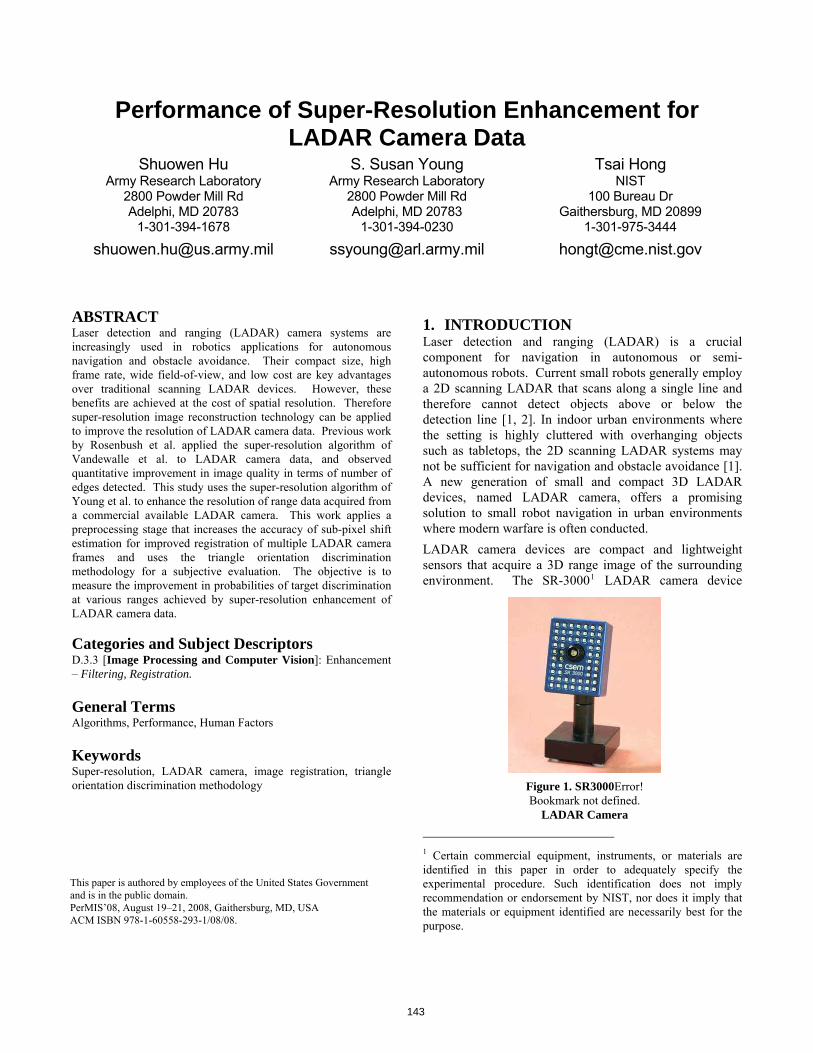
Performance of Super-Resolution Enhancement for LADAR Camera Data

Shuowen Hu Army Research Laboratory

2800 Powder Mill Rd Adelphi, MD 20783

1-301-394-1678

shuowen.hu@us.army.mil

S. Susan Young Army Research Laboratory

2800 Powder Mill Rd Adelphi, MD 20783

1-301-394-0230

ssyoung@arl.army.mil

Tsai Hong NIST

100 Bureau Dr Gaithersburg, MD 20899

1-301-975-3444

hongt@cme.nist.gov

ABSTRACT Laser detection and ranging (LADAR) camera systems are increasingly used in robotics applications for autonomous navigation and obstacle avoidance. Their compact size, high frame rate, wide field-of-view, and low cost are key advantages over traditional scanning LADAR devices. However, these benefits are achieved at the cost of spatial resolution. Therefore super-resolution image reconstruction technology can be applied to improve the resolution of LADAR camera data. Previous work by Rosenbush et al. applied the super-resolution algorithm of Vandewalle et al. to LADAR camera data, and observed quantitative improvement in image quality in terms of number of edges detected. This study uses the super-resolution algorithm of Young et al. to enhance the resolution of range data acquired from a commercial available LADAR camera. This work applies a preprocessing stage that increases the accuracy of sub-pixel shift estimation for improved registration of multiple LADAR camera frames and uses the triangle orientation discrimination methodology for a subjective evaluation. The objective is to measure the improvement in probabilities of target discrimination at various ranges achieved by super-resolution enhancement of LADAR camera data.

Categories and Subject Descriptors D.3.3 [Image Processing and Computer Vision]: Enhancement – Filtering, Registration.

General Terms Algorithms, Performance, Human Factors

Keywords Super-resolution, LADAR camera, image registration, triangle orientation discrimination methodology

1. INTRODUCTION Laser detection and ranging (LADAR) is a crucial component for navigation in autonomous or semi-autonomous robots. Current small robots generally employ a 2D scanning LADAR that scans along a single line and therefore cannot detect objects above or below the detection line [1, 2]. In indoor urban environments where the setting is highly cluttered with overhanging objects such as tabletops, the 2D scanning LADAR systems may not be sufficient for navigation and obstacle avoidance [1]. A new generation of small and compact 3D LADAR devices, named LADAR camera, offers a promising solution to small robot navigation in urban environments where modern warfare is often conducted. LADAR camera devices are compact and lightweight sensors that acquire a 3D range image of the surrounding environment. The SR-30001 LADAR camera device

Figure 1. SR3000Error! Bookmark not defined.

1 Certain commercial equipment, instruments, or materials are identified in this paper in order to adequately specify the experimental procedure. Such identification does not imply recommendation or endorsement by NIST, nor does it imply that the materials or equipment identified are necessarily best for the purpose.

LADAR Camera

This paper is authored by employees of the United States Government and is in the public domain. PerMIS’08, August 19–21, 2008, Gaithersburg, MD, USA ACM ISBN 978-1-60558-293-1/08/08.

143

(Figure 1) used in this study weighs 162 g and measures (5.0 x 6.7 x 4.23) cm [3]. LADAR camera devices emit diffuse modulated near-infrared light and measure the subsequent phase shift between the original emitted light and the reflected light. The phase measurements are combined to calculate the range data based on the time-of-flight principle [3]. The detector utilized by LADAR camera devices is a focal plane array (FPA), which is typically limited to a maximum size of (256 x 256) detectors. Consequently, these devices cannot achieve the resolution of scanning LADAR systems. This disadvantage of LADAR camera systems may be rectified by the application of super-resolution image reconstruction. Super-resolution algorithms utilize a series of low-resolution frames containing sub-pixel shifts to generate a higher resolution image. These algorithms are typically composed of two major stages: registration stage and reconstruction stage. During the registration stage, the shift with respect to a reference frame (usually the first frame of the series) is computed to sub-pixel (i.e. decimal pixel) accuracy. The second stage utilizes this sub-pixel information to interpolate the low-resolution frames onto a higher resolution grid. A necessary condition for successful super-resolution enhancement is the presence of differing shifts between the frames in the series. The differing shifts of each frame provide additional information from which to reconstruct the super-resolved imagery. Previous work by Rosenbush et al. [4] applied a super-resolution algorithm [5] to LADAR camera data, and observed improvement in image quality in terms of number of edges detected. In this work, the super-resolution algorithm of Young et al. [6] is applied to LADAR camera imagery. This algorithm separates the registration stage into a gross shift (i.e. integer pixel shift) estimation stage and a sub-pixel shift (i.e. decimal pixel shift) estimation stage for improved registration accuracy. Both sub-stages use the correlation method in the frequency domain to estimate shifts between the frame series and the reference image. The reconstruction stage of Young et al.’s algorithm applies the error-energy reduction method with constraints in both spatial and frequency domains to generate a high-resolution image [6]. Because LADAR camera imagery is inherently smoother than visible light imagery (LADAR camera data does not capture the texture or color of the scene), this work develops a preprocessing stage for improved image registration. Specifically, a wavelet edge filtering method [7] and a Canny edge detection method [4] are investigated and compared against the accuracy achieved with no preprocessing. The wavelet edge filtering method provided

more accurate shift

per-resolution enhancement of the LADAR camera data.

ection algorithm to generate binary edge frame

her frequency components as depicted in red in Figure

estimation for LADAR camera data. To assess the improvement in super-resolution enhanced LADAR camera data, the authors conducted perception experiments to obtain a human subjective measurement of

quality. The triangle orientation discrimination (TOD) methodology [8,9] was used to measure the improvement achieved with super-resolution. The TOD task is a four-alternative forced-choice perception experiment where the subject is asked to identify the orientation of a triangle (apex up, down, right, or left) [9]. Results show that the probability of target discrimination as well as the response time improves with su

2. METHODOLOGY 2.1 Preprocessing Stage The purpose of the preprocessing stage is to emphasize LADAR camera image edges for improved frame registration. One investigated method was the use of multi-scale edge-wavelet transforms [10] to calculate the horizontal and vertical partial derivatives of the input image at the second wavelet scale for each frame of the series. The two derivatives were then combined using sum of squares to produce a wavelet edge enhanced frame series. Another investigated method was the use of Canny edge detseries. To assess the benefit of preprocessing, the following procedure was followed. A synthetic frame series was generated with known sub-pixel shifts. First, an oversampled non-aliased scanning LADAR reference image (204 x 204) pixels was interpolated by an upsampling factor of eight (1632 x 1632) pixels using a Fourier windowing method [10]. Then, the simulated high-resolution image was sub-sampled at different factors to produce several low-resolution frame series, each with a different degree of aliasing. Figure 2 shows the un-aliased spectrum of a discrete space signal (e.g. scanning LADAR image) produced by oversampling a continuous space signal at a sampling frequency greater than the Nyquist frequency. If the sampling frequency is below Nyquist (simulated by sub-sampling the oversampled image), the spectrum of the sampled signal is aliased with distorted hig2. Synthetic frame series was generated by sub-sampling every m pixels in both dimensions of the simulated high-resolution image, where m = 4, 8, 12, 16, 20, 28, 36, 48, 56. Therefore the undersampling factors are m/8 (i.e., 0.5, 1, 1.5, 2, 2.5, 3.5, 4.5, 6, 7), simulating different degrees of aliasing. For each undersampling factor, the sub-pixel shifts for each frame of the synthetic series were generated by varying the starting pixel position of sub-sampling according to a uniform random distribution (30 frames for each series). Then preprocessing using either the wavelet or Canny method was performed. Sub-pixel shift estimates from the preprocessed and no preprocessing series were compared to the known shifts. Let i = ( xi , yi) denote

144

the registration error vector of the ith frame where xi and

yi are the registration errors in the x and y directions. A mean absolute error (MAE) can be calculated for the frames of each synthetic series using the following equation:

ii nn 11

where 30n . The registration errors of the wavelet preprocessing method was compared to that of Canny andno preprocessing metho

n

yixi

n

iE 2211

ds to assess the accuracy at each

undersampling factor.

2.2 Triangle Orientation Discrimination

Probabilities of target discrimination at different ranges can

(TOD) Methodology The TOD methodology, developed by Netherlands TNO Physics and Electronics Laboratory (TNO-FEL), is a perception study that allows human subjects to provide a measure of image quality at various target ranges [9]. The test pattern is an equilateral triangle in one of four possible orientations (apex up, down, left, or right), and the measurement process is a four-alternative forced-choice psychological procedure that requires the observer to indicate the orientation. Variation of triangle contrast/size by changing target ranges results in a correct discrimination percentage between 25 % (pure guess) and 100 %.

then be calculated to measure the quality of both the original and super-resolved data. The TOD method is suitable for electro-optical and optical imaging systems, and has been widely used in thermal and visual domain imagers. This methodology provides a simple task that has a close relationship to real target acquisition, and the results are free from observer bias [8,9]. The TOD methodology was adapted to LADAR camera data by using a target consisting of a square white foam board target (50 x 50) cm with an equilateral triangular hole (7.5 cm per side) cut into the board as shown in Figure 3. The triangular hole provides the necessary depth contrast against the board.

Figure 3. TOD setup 2.3 LADAR Camera The device utilized in this study is the SwissRanger SR-3000Error! Bookmark not defined. LADAR camera. The camera emits diffuse 850 nm near-infrared light modulated at a default frequency of 20 MHz from a bank of 55 light emitting diodes. The non-ambiguity range achieved at this modulation frequency is 7.5 m. The SR-3000Error! Bookmark not defined. has a pixel array of 176 x 144 with a field-of-view of 47.5o x 39.6o, and can capture images at a maximum rate of 50 frames/s (variable with respect to the integration time setting).

Figure 2. (Top) Un-aliased spectrum of signal sampled above y, (mid) at Nyquist, and (boNyquist frequenc ttom) aliased at

2.4 Data Collection Data collection for the experiment was conducted at a laboratory in the National Institute of Standards and Technology. The SR-3000Error! Bookmark not defined. LADAR camera was placed 6.5 m from a beige wall as depicted in Figure 3. The target was positioned at (3, 3.5, 4, 4.5, 5, 5.5, and 6) m from the camera. The investigated ranges were limited to between (3 and 6) m because inaccurate behavior of LADAR cameras was observed at very close and very far target distances [11]. At each range, the triangle was positioned at one of four possible orientations (apex up, down, left, right) with the center approximately 1 m high. For each orientation at each

below Nyquist frequency.

145

range, four trials were conducted. Each trial consisted of a sequence of 32 frames acquired by holding the camera. The natural motion of the hand while holding the camera provided the shifts required for the super-resolution algorithm. Motion is assumed to be limited to translations in the x (horizontal) and y (vertical) planes. Though slight rotation and translation in the z-plane (depth) might have occurred from holding the camera, these parameters were not considered in the current study.

2.5 Data Processing For each series of 32 frames, the first 25 frames are utilized for super-resolution image reconstruction. The first frame was used as the reference frame from which pixel shifts were calculated for successive frames. The use of 25 frames resulted in a resolution improvement factor of five in each direction for the super-resolved image. To ensure that the monitor modulation transfer function (MTF) was not a limiting factor in the experiment, the super-resolved images (250 x 250 pixels) were bilinearly interpolated by a factor of two to 500 x 500 pixels. The original imagery (50 x 50 pixels) was bilinearly interpolated to 500 x 500 pixels for consistency between the baseline and super-resolved imagery.

2.6 Perception Experiment The perception experiment was a four-alternative forced-choice procedure (up, down, left, right). The imagery in this experiment was organized in the image cells and their naming convention is shown in Table 1. As shown in the row of original images in Table 1, the grayscale baseline range imagery was grouped into seven cells corresponding to the seven different target ranges. Each cell consisted of 16 original low-resolution LADAR camera images (4 orientations x 4 trials). Similarly, the grayscale super-resolved range imagery was grouped into seven cells consisting of 16 images each as shown in the row of super-resolved images in Table 1. The experiment therefore consisted of 14 cells with a total of 224 images. Range m

A 3.0

B 3.5

C 4.0

D 4.5

E 5.0

F 5.5

G 6.0

Original Image

AA

BA CA DA EA FA GA

Super-resolved image

AB BB CB DB EB FB GB

Table 1. Image cell format and naming convention

Nine subjects participated in the experiment in July 2008. The subjects were shown one image at a time with randomized presentation of cells and randomized presentation of images within each cell. The display was a 19 inch flat panel (Dell 1908FPError! Bookmark not defined.) with a resolution of 1280 x 1024 pixels.

3. RESULTS AND DISCUSSION 3.1 Assessment of Registration Accuracy

0.5 1 1.5 2 2.5 3.5 4.5 6 7

0

0.05

0.1

0.15

0.2

Undersampling Factor

Mea

n A

bsol

ute

Erro

r

Mean Absolute Error vs Undersampling Factor

Wavelet PreprocessingCanny PreprocessingNo Preprocessing

Figure 4. Mean absolute registration error with standard deviation for each undersampling factor.

Figure 4 shows the mean absolute error of registration at each undersampling factor for the generated synthetic experiments. The unit of error is fraction of a pixel. Wavelet preprocessing outperformed both the Canny method and no preprocessing method for undersampling factors of less than 6. Wavelet preprocessing was especially effective at low and moderate degrees of aliasing (undersampling factor of less than 3.5). If the imagery contained severe aliasing (undersampling factor greater than 6), then no preprocessing resulted in higher registration accuracy. The observed trend is expected. LADAR camera data is characteristically smooth due to the lack of texture information, so edge filtering with the wavelet method will improve registration. But if the data is severely undersampled that its mid to high frequency components are corrupted by aliasing, then wavelet edge filtering (which uses these severely corrupted frequency components) will result in poorer registration. The degree of aliasing in the imagery acquired with the SR-3000Error! Bookmark not defined. is expected to be in the moderate range as super-resolved imagery using wavelet preprocessing yields fewer artifacts than imagery produced without preprocessing.

146

3.2 Triangle Orientation Discrimination Perception Experiment Figure 5 shows grayscale and color images (color-coded to distance) of the TOD target oriented up at a distance of 5 m from the camera. The orientation of the equilateral triangular hole is difficult to discern in the original images at this distance as the triangular hole appears like a blurred circle. By contrast, the orientation is clear in the super-resolution enhanced imagery. For imagery with target distances greater than 5 m, the orientation, as expected, was still more difficult to discern using the original LADAR camera imagery. But super-resolution at these greater distances proved to be effective.

Figure 6 shows grayscale and color images of the TOD target oriented left at a distance of 4 m from the camera. As the target distance decreases, the orientation of the triangular hole becomes more visible in the original imagery, though the triangular hole still appears distorted. In the super-resolved image, the triangular hole does not appear distorted, and is shaped more like a triangle. Figure 7 shows the group-averaged chance-corrected probability of target discrimination at each target range. At all ranges, super-resolved imagery produced a higher probability of target discrimination with smaller inter-subject variability. At a target distance of 3 m, the original imagery had a 77 % of the probability of target discrimination, while the super-resolved imagery reached 100 %. The target discrimination performance is increased by 30 % using the super-resolution algorithm. As the target distance increased, subjects had more difficulty to

discriminate the target orientation. At a target distance of 6 m, the original imagery had a 20 % of the probability of target discrimination, while the super-resolved imagery reached 90 %. That is a 350 % improvement in target discrimination performance. In summary, the probability of target discrimination is increased by 30 % to 350 % for the target ranges from 3 m to 6 m using the super-resolution algorithm.

.

3 4 5 60

0.2

0.4

0.6

0.8

1

Ensemble Probability of Target Discrimination

Range (m)

Pro

babi

lity

Original ImagerySuper-resolved Imagery

(a) original (b) super-resolved

Figure 5. Grayscale (top) and color-coded (bottom) LADAR camera imagery for (a) original image and (b) super-resolved image of TOD target at 5 m.

Figure 6. Grayscale (top) and color-coded (bottom) LADAR camera imagery for (a) original image and (b) super-resolved image of TOD target at 4 m.

Figure 7. Chance-corrected probability of target discrimination at each target range.

(a) original (b) super-res lvedo

147

Not only were subjects able to achieve higher accuracy at all ranges with super-resolved imagery, but the response times were also faster with less variability for super-resolved imagery at all ranges. Figure 8 shows the group-averaged response times at each range with standard error bars representing inter-subject variability. At a range of 6 m, subjects responded in an average time of 1.58 s using the super-resolved imagery, 23 % faster than the response time using original imagery.

4. CONCLUSION Super-resolution image reconstruction is complemented by a wavelet preprocessing stage for improved image registration, yields significant benefits for LADAR camera imagery. In the triangle orientation discrimination experiment, subjects achieved higher accuracy at all investigated target ranges with faster response times and reduced inter-subject variability for super-resolved imagery. Complemented by super-resolution image reconstruction, the high frame rate, small size, and light-weight LADAR camera sensors will be ideal for autonomous or semi-autonomous robot navigation in urban indoor environments. In semi-autonomous robot navigation, super-resolution enhancement will provide human operators with increased target discrimination. In fully autonomous mode, super-resolved imagery will allow guidance software to improve obstacle avoidance. The incorporation of super-resolution into the US Army’s

robotic applications will improve small robot performance, contributing to the soldier’s survivability and lethality.

3 4 5 60

0.5

1

1.5

2

2.5

3

Ensemble Average Response Times

Range (m)

Ave

rage

resp

onse

tim

e (s

)

Original ImagerySuper-resolved Imagery

5. ACKNOWLEDGMENTS The authors would like to thank Dr. Joe Reynolds and Dr. Keith Krapels at US Army’s Night Vision and Electronic Sensors Directorate for their insights and helpful discussions. We thank Tommy Chang at NIST for helping the data in the NIST vision lab.

6. REFERENCES [1] Ng, T. C. 2005. SIMTech technical reports, Vol. 6, No. 1,

13-18, 2005. [2] Committee on Army Unmanned Ground Vehicle Technology

2002. “Technology development for Army unmanned ground vehicles”, Sandia Report.

Figure 8. Response times at each target range with standard error bars showing inter-subject variability.

[3] MESA Imaging, 2006. SwissRanger SR-3000 Manual. http://www.mesa-imaging.ch/.

[4] Rosenbush, G., Hong, T. H., Eastman, R. D. 2007. Super-resolution enhancement of flash LADAR range data. In Proceedings of the SPIE, Vol. 6736, 67314.

[5] Vandewalle P., Susstrunk S., Vetterli, M. 2005. A frequency domain approach to registration of aliased images with application to super-resolution. EURASIP Journal on Applied Signal Processing, 71459

[6] Young, S. S., Driggers, R. G. 2006. Super-resolution image reconstruction from a sequence of aliased imagery. Applied Optics, Vol. 45, 5073-5085.

[7] Devitt, N., Moyer, S., Young, S. S. 2006. Effect of image enhancement on the search and detection task in the urban terrain. In Proceedings of SPIE, Vol. 6207, 62070D 1-13.

[8] Driggers, R. G., Krapels, K., Murrill, S., Young, S., Thielke, M., Schuler, J. 2005. Super-resolution performance for undersampled imagers. Optical Engineering, Vol. 44(1), 14002.

[9] Bijl, P., Valeton, J. M. 1998. Triangle orientation discrimination: the alternative to MRTD and MRC. Optical Engineering, Vol. 37(7), 1976-1983.

[10] Young, S. S., Driggers, R. G., Jacobs, E. L. 2008. Signal Processing and Performance Analysis for Imaging Systems. Artech House, Norwood, MA.

[11] Anderson, D., Herman H., Kelly A. 2005. Experimental characterization of commercial flash LADAR devices. In Proceedings of the International Conference of Sensing and Technology.

148

Performance Evaluation of Laser TrackersB. Muralikrishnan, D. Sawyer, C. Blackburn, S. Phillips, B. Borchardt, W. T. Estler

Precision Engineering Division National Institute of Standards and Technology

Gaithersburg, MD 20899

ABSTRACTThe American Society for Mechanical Engineers (ASME) recently released the ASME B89.4.19 Standard [1] on performance evaluation of spherical coordinate instruments such as laser trackers. At the National Institute of Standards and Technology (NIST), we can perform the complete set of tests described in the Standard, and have done so for a variety of laser trackers. We outline the tests described in the Standard, discuss our capabilities at the large-scale coordinate metrology group, and present results from B89.4.19 tests conducted on a few trackers. We also outline an analysis approach that may be used to evaluate the sensitivity of any measurement, including the tests described in the B89.4.19 Standard, to different geometric misalignments in trackers. We discuss how this approach may be useful in determining optimal placement of reference lengths to be most sensitive to different geometric misalignments.

Keywords ASME B89.4.19, large-scale metrology, laser tracker, performance evaluation, sensitivity analysis

1. INTRODUCTIONSpherical coordinate measurement systems such as laser trackers, scanners and other devices are increasingly used in manufacturing shop floors for inspection, assembly, automation etc. These instruments are also sometimes used in the calibration of other lower-accuracy instruments such as industrial robots and even certain Cartesian coordinate measuring machines (CMMs). The spherical coordinate systems provide high accuracy at relatively low cost (in comparison to more conventional Cartesian CMMs ), and are portable and convenient to use. Because of the proliferation of such devices in recent years, there has been an increasing need for a uniform set of performance tests so that users and manufacturers share a common understanding of the capabilities of the instrument.

In 2007, the American Society for Mechanical Engineers (ASME) published the ASME B89.4.19 Standard titled “Performance

Evaluation of Laser-Based Spherical Coordinate Measurement Systems”. This Standard, for the first time, defined a common set of tests that can be performed by both the user and the manufacture to establish if an instrument meets the manufacturer’s performance specifications (MPE). This Standard, although limited to instruments that use a cooperative target such as retro-reflector, represents a significant step forward. It is the first and to date, the only performance evaluation Standard for spherical CMMs and establishes a framework for testing and evaluation of laser trackers and related devices.

In this paper, we present an overview of the B89.4.19 Standard and highlight the different tests described in it. We discuss capabilities of the large-scale coordinate metrology group at NIST where a complete set of B89.4.19 tests may be performed. We show examples of laser trackers tested at NIST that meet the manufacture’s performance specifications and others that do not. Systematic errors due to geometrical and optical misalignments within a tracker are a major source of uncertainty in tracker measurements. An ideal performance evaluation test has high sensitivity to all misalignment parameters in a tracker’s error model. Given the error model, it is possible to numerically determine the sensitivity of each of the B89.4.19 tests to different misalignment parameters. We have performed such analysis and briefly discuss our method and results.

2. THE ASME B89.4.19 STANDARD The ASME B89.4.19 Standard describes three types of tests to be performed on trackers to evaluate their performance. These are the ranging tests, the length measurement system tests and two-face system tests.

This paper is authored by employees of the United States Government and is in the public domain. PerMIS’08, August 19–21, 2008, Gaithersburg, MD, USA ACM ISBN 978-1-60558-293-1/08/08.

Figure 1. The ASME B89.4.19 Standard.

149

2.1 Ranging Tests Ranging tests assess the distance (or displacement) measurement capability of the instrument. The ranging system (an interferometer or an absolute distance measurement (ADM) system) establishes the unit of length and is therefore a critical component of the system. The tests as described in the Standard require the tracker to measure several calibrated lengths aligned along the line-of-sight of the tracker. The reference lengths employed may be calibrated artifacts, realized by free standing targets, or a laser-rail system.

2.2 Length Measurement System Tests The length measurement system tests are similar to volumetric length tests on Cartesian CMMs. A calibrated reference length is placed at different positions and orientations in the measurement volume and is measured by the tracker. The error in the measured length is compared against the MPE to determine conformance to specification. There are several sources of mechanical and optical misalignments within the construction of a tracker that produce systematic errors in the measured angle and range readings and therefore in measured lengths. The length measurement system tests are designed to be sensitive to these misalignments. Again, the reference lengths employed may be calibrated artifacts, realized by free standing targets, or a laser-rail system.

Figure 2. The NIST 60 m laser rail facility viewed from the tracker under test end; note the movable

carriage with retroreflector.

Laser tracker

Referenceinterferometer

Carriage with targets

2.3 Two-face System Tests RailSome geometric misalignments are such that the errors in the

measured angles of a fixed target change in sign when the same target is measured in the backsight of the instrument. Such frontsight-backsight measurements of a single target are called two-face tests. These tests are extremely useful because they capture a large number of geometric misalignments and they do not require a calibrated reference length. The Standard requires two-face tests to be performed at different positions within the work volume of the instrument. More details on the test positions may be found in [1,2].

Figure 3. The LARCS laser rail.

3. LARGE-SCALE METROLOGY AT NIST The large-scale coordinate metrology group at NIST has the capability of performing the complete set of B89.4.19 tests.

The ranging tests are performed in the 60 m long-length test facility where a laser-rail and carriage system is operational (see Figure 2). The carriage has two opposing retro-reflectors. One

retro-reflector is used for the tracker under test while the other is used for the reference interferometer on the other end of the rail. The expanded uncertainty (k = 2) of reference length L is U(L) = 5 m + 0.3 10-6L.

The length measurement and two-face system tests are performed in the large-scale laboratory. Currently, the reference length for the length measurement tests is realized using the laser-rail and carriage system (LARCS) [3] (see Figure 3). The LARCS (different from the 60 m laser-rail facility used for range calibration) employs a reference interferometer mounted on a rail (about 3 m long) that can be oriented in different ways (horizontal, vertical, inclined) to meet the B89.4.19 requirements. A carriage with two retro-reflectors rides on the rail. The tracker uses one retro-reflector while the reference interferometer utilizes the other. The expanded uncertainty (k = 2) of a nominal reference length L is U(L) = 3.4 m + 0.5 10-6 L for the LARCS system. We are now evaluating different artifacts that may be used as the reference length instead of the LARCS system [4].

4. TRACKER CALIBRATION EXAMPLES We have performed the B89.4.19 tests on different trackers at our facility at NIST. Some trackers that were tested met the manufacture’s specifications while others did not. We show results of ranging test performed on Tracker A in Figure 4. The data were recorded in the ADM mode of the tracker and substantially more points were recorded than required by the Standard. The errors in the measured lengths were within the manufacturer’s specifications and therefore acceptable.

0 20 40 60−0.1

−0.05

0

0.05

0.1

Distance (m)

Err

or (μ

m)

Run #1Run #2Run #3MPE

Figure 4. Ranging test results for Tracker A.

150

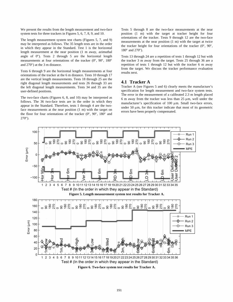
Tests 5 through 8 are the two-face measurements at the near position (1 m) with the target at tracker height for four orientations of the tracker. Tests 9 through 12 are the two-face measurements at the near position (1 m) with the target at twice the tracker height for four orientations of the tracker (0 , 90 ,180 and 270 ).

We present the results from the length measurement and two-face system tests for three trackers in Figures 5, 6, 7, 8, 9, and 10.

The length measurement system test charts (Figures 5, 7, and 9) may be interpreted as follows. The 35 length tests are in the order in which they appear in the Standard. Test 1 is the horizontal length measurement at the near position (1 m away, azimuthal angle of 0 ). Tests 2 through 5 are the horizontal length measurements at four orientations of the tracker (0 , 90 , 180and 270 ) at the 3 m distance.

Tests 13 through 24 are a repetition of tests 1 through 12 but with the tracker 3 m away from the target. Tests 25 through 36 are a repetition of tests 1 through 12 but with the tracker 6 m away from the target. We discuss the tracker performance evaluation results next. Tests 6 through 9 are the horizontal length measurements at four

orientations of the tracker at the 6 m distance. Tests 10 through 17 are the vertical length measurements. Tests 18 through 25 are the right diagonal length measurements and tests 26 through 33 are the left diagonal length measurements. Tests 34 and 35 are the user-defined positions.

4.1 Tracker A Tracker A (see Figures 5 and 6) clearly meets the manufacture’s specification for length measurement and two-face system tests. The error in the measurement of a calibrated 2.3 m length placed 6 m away from the tracker was less than 25 m, well under the manufacturer’s specification of 100 m. Small two-face errors, under 50 m, for this tracker indicate that most of its geometric errors have been properly compensated.

The two-face charts (Figures 6, 8, and 10) may be interpreted as follows. The 36 two-face tests are in the order in which they appear in the Standard. Therefore, tests 1 through 4 are the two-face measurements at the near position (1 m) with the target on the floor for four orientations of the tracker (0 , 90 , 180 and 270 ).

1 2 3 4 5 6 7 8 9 10 11 12 13 14 15 16 17 18 19 20 21 22 23 24 25 26 27 28 29 30 31 32 33 34 35

−100

−50

0

50

100

Test # (In the order in which they appear in the Standard)

Err

or (μ

m)

0 90 180

270

0 90 180

270

0 90 180

270

0 90 180

270

0 90 180

270

0 90 180

270

0 90 180

270

0 90 180

270

Hor

Min

Hor

3m

Hor

6m

Ver

3m

Ver

6m

RD

3m

RD

6m

LD 3

m

LD 6

m

Use

r Def

ined

1U

ser D

efin

ed 2

(a)

Run 1Run 2Run 3MPE

Figure 5. Length measurement system test results for Tracker A.

1 2 3 4 5 6 7 8 9 10 11 12 1314 15 16 17 1819 20 21 22 2324 25 26 2728 29 30 31 3233 34 35 360

20

40

60

80

100

120

140

160

180

Test # (In the order in which they appear in the Standard)

Err

or (μ

m)

0 90 180

270

0 90 180

270

0 90 180

270

0 90 180

270

0 90 180

270

0 90 180

270

0 90 180

270

0 90 180

270

0 90 180

270

1m, L

ow

1m, M

ed

1m, H

igh

3m, L

ow

3m, M

ed

3m, H

igh

6m, L

ow

6m, M

ed

6m, H

igh

(b) Run 1Run 2Run 3MPE

Figure 6. Two-face system test results for Tracker A.

151

4.2 Tracker B Figures 7 and 8 show the results of length measurement and two-face system tests for Tracker B. This tracker appears to have satisfactory length measurement performance, but demonstrates large two-face errors.

Notice that the two-face error (Figure 8) demonstrates periodicity that is a function of the azimuth. In addition, the average two-face error (approximately 1.2 mm in Figure 8) does not change with distance of the target from the tracker. The average two-face error with increasing distance may arise from an offset in the beam from its ideal position (Tracker B does not have a beam steering mirror. Rather, the source is located directly in the head). Such an offset will result in decreasing error in the measured angle farther away from the tracker; consequently, the two-face error will be independent of range.

An explanation for the periodicity in the measured two-face data involves some subtlety. An eccentricity in the horizontal angle encoder will result in two-face errors showing periodicity that is a function of the azimuth. A least-squares fit of the data will

therefore provide an estimate of the eccentricity. However, it turns out that when the two-face error, which is a convolved distance from horizontal and vertical angle error, is isolated into its constituent angle errors, the periodicity is in the vertical angle error. The vertical angle encoder has no functional relationship with the horizontal angle and therefore, the periodicity does not appear to be due to a geometric misalignment. The observed periodicity may be the result of stressing and relaxation of tension in cables within the tracker, or other such causes that are not considered in a geometric error model.

Although Tracker B did have large two-face errors, the B89.4.19 length measurement system test results (Figure 7) do not seem to be adversely affected by the large beam offsets. A careful consideration of the beam offset misalignment reveals that this term does not impact symmetrically placed lengths with respect to the tracker because the error at ends of the reference length cancel each other. Almost every B89.4.19 position is symmetrically placed with respect to the tracker. Asymmetrically positioned lengths will demonstrate large errors and may be used as the user-defined positions during the test.

1 2 3 4 5 6 7 8 9 10 11 12 13 14 15 16 17 18 19 20 21 22 23 24 25 26 27 28 29 30 31 32 33 34 35−200

−150

−100

−50

0

50

100

150

200

Test # (In the order in which they appear in the Standard)

Err

or (μ

m)

0 90 180

270

0 90 180

270

0 90 180

270

0 90 180

270

0 90 180

270

0 90 180

270

0 90 180

270

0 90 180

270

Hor

Min

Hor

3m

Hor

6m

Ver

3m

Ver

6m

RD

3m

RD

6m

LD 3

m

LD 6

m

Use

r Def

ined

1U

ser D

efin

ed 2

(a)

Run 1Run 2Run 3MPE

Test # Figure 7. Length measurement system test results for Tracker B.

2000

Figure 8. Two-face system test results for Tracker B.

1 2 3 4 5 6 7 8 9 10 11 12 1314 15 16 17 1819 20 21 22 2324 25 26 2728 29 30 31 32 33 34 35 360

500

1000

1500

Err

or (μ

m)

0 90 180

270

0 90 180

270

0 90 180

270

0 90 180

270

0 90 180

270

0 90 180

270

0 90 180

270

0 90 180

270

0 90 180

270

1m, L

ow

1m, M

ed

1m, H

igh

3m, L

ow

3m, M

ed

3m, H

igh

6m, L

ow

6m, M

ed

6m, H

igh

(b)

Run 1Run 2Run 3MPE

Test # (In the order in which they appear in the Standard)Test #

152

Several interesting points raised in this section are worth summarizing:

Large length measurement or two-face system test errors typically suggest that geometric misalignments have not been properly compensated. Two-face errors as reported in the B89.4.19 Standard are the convolved errors in both the horizontal and vertical angles, and scaled by the range. Raw horizontal and vertical angle errors from a two-face test contain more diagnostic information.The purpose of extracting the magnitude of physical misalignments from B89.4.19 tests is to estimate the error in other length measurements made within the work volume of the tracker.

4.3 Tracker C Tracker C shows large errors in the length measurement system tests. The periodicity of the errors for Tracker C (Figure 9) may be the result of an eccentricity in the horizontal angle encoder, as well as a tilt in the beam as it emerges from its source. This tracker has the source located in the base and a beam steering

mirror directs the beam to the target. Therefore, any tilt in the beam will also be a function of the azimuth. A least-squares best-fit may be performed to determine the magnitude of the eccentricity and tilt.

The two-face error (Figure 10) shows increasing error farther away from the tracker. A tilt in the beam as it emerges from the source will produce a constant angle error that when amplified by the range results in larger two-face error farther away from the tracker. We do not have the manufacturer’s specification for two-face error for this tracker. The errors in Figure 10 are comparable to those of Tracker A and may therefore be acceptable, but nevertheless, there is evidence of improper compensation for geometric errors.

In this section, we have suggested that the B89.4.19 test results may be employed in a diagnostic mode where physical misalignments are determined. A geometric error model is required for this purpose. Error models are also useful in performing sensitivity analysis where the sensitivity of any given test to any geometric misalignment is determined through numerical simulation. We describe sensitivity analysis next.

1 2 3 4 5 6 7 8 9 10 11 12 13 14 15 16 17 18 19 20 21 22 23 24 25 26 27 28 29 30 31 32 33 34 35

−300

−200

−100

0

100

200

300

Test # (In the order in which they appear in the Standard)

Err

or (μ

m)

0 90 180

270

0 90 180

270

0 90 180

270

0 90 180

270

0 90 180

270

0 90 180

270

0 90 180

270

0 90 180

270

Hor

Min

Hor

3m

Hor

6m

Ver

3m

Ver

6m

RD

3m

RD

6m

LD 3

m

LD 6

m

Use

r Def

ined

1U

ser D

efin

ed 2

(a)

Run 1Run 2Run 3MPE

Test #Figure 9. Length measurement system test results for Tracker C.

4.4

1 2 3 4 5 6 7 8 9 10 11 12 1314 15 16 17 1819 20 21 22 2324 25 26 2728 29 30 31 3233 34 35 360

50

100

150

200

250

300

Test # (In the order in which they appear in the Standard)

Err

or (μ

m)

0 90 180

270

0 90 180

270

0 90 180

270

0 90 180

270

0 90 180

270

0 90 180

270

0 90 180

270

0 90 180

270

0 90 180

270

1m, L

ow

1m, M

ed

1m, H

igh

3m, L

ow

3m, M

ed

3m, H

igh

6m, L

ow

6m, M

ed

6m, H

igh

(b) Run 1Run 2Run 3MPE

Test #Figure 10. Two-face system test results for Tracker C.

153

5. SENSITIVITY ANALYSIS A spherical coordinate instrument such as a laser tracker is a mechanical assembly of different components and therefore subject to misalignments such as offsets (offset in the beam from ideal position, offset between the standing and transit axes etc),tilt (tilt in the beam, tilt in the transit axis etc) and eccentricity (encoder eccentricity with respect to axis) during construction and assembly. It is general practice to correct for these misalignments by software compensation. A geometric error model [5] is required for this purpose that relates the corrected (true) range and angles to measured range and angles, and geometric misalignments within the tracker.

The corrected range (Rc) and angles (horizontal angle: Hc,vertical angle: Vc) of any coordinate in space are functions of several misalignment parameters within the construction of the tracker and also of the measured coordinate values at that location (Rm, Hm, Vm). The corrections Rm, Hm and Vm in Rm, Hmand Vm respectively may be expressed as (linear models may be sufficient as a first approximation),

),,(

),,(

),,(

1

1

1

VmHmRmwxVmVmVc

VmHmRmvxHmHmHc

VmHmRmuxRmRmRc

i

n

ii

i

n

ii

i

n

ii

where x is any misalignment parameter (eccentricity in encoder, beam offset, transit axis offset from standing axis, beam tilt, etc),and u, v and w are functions of measured range and angles.

Because different commercially available laser trackers have different mechanical constructions, an error model applicable to one tracker may not necessarily be applicable to another. At NIST, we have modeled three broad classes of trackers: a) tracker with a beam steering mirror for which the Loser and Kyle [5] model is applicable, b) tracker with the laser source in the rotating head and c) scanner with source mounted on the transit axis with a rotating prism mirror that steers the beam to the target.

As an example, an error model for a tracker with the source located in the head is given by

).cos().sin()sin(

)cos()cos(

).cos().sin()sin(

)cos()tan()sin()sin(.

)sin(.

997

7321

996

6541

82

Vmmx VmmxVm x

VmxxRm

VmxRmx

VmVc

Hmmx HmmxHmx

HmxVm

xVm

xVmRm

xHmHc

xVmxRmRc

dcz

nm

bay

xtt

where x1t and x1m are beam offsets along the transit axis and its normal, x2 is the transit offset, x3 is the vertical index offset, x4t is the beam tilt, x5 is the transit tilt, x6x and x6y are the horizontal angle encoder eccentricities, x7x and x7y are the vertical angle encoder eccentricities, x8 is the bird-bath error, and x9a, x9b, x9c and

x9d are the components of the mth order scale error in the encoder (1st order is not distinguishable from encoder eccentricity. Higher orders beyond 2nd order may be neglected).

This error model may now be used to numerically estimate the sensitivity of any given test to geometric misalignments that are included in the model. As an example, consider the beam offset terms. We describe how the coefficients for the parameters in the error model were obtained, and then discuss the sensitivity of different B89.4.19 tests to this misalignment.

x1t

x1mA

OT

MP

N

Z

Vm

Y

X

Hm

Rm

Figure 11. Schematic of beam offset in a tracker where the beam originates from the head (there is no beam steering

mirror). Axes OT, ON and OM are fixed to the tracker’s head and therefore rotate with the head about the Z axis.

5.1 Error Model Coefficients The beam originating from the source (at O) may be displaced from its ideal position by a constant offset (OA in Figure 11) to emerge from A, a misalignment parameter referred to as beam offset. The offset can be resolved into components along two orthogonal axes, M and T (x1m and x1t). In Figure 11, OT is the transit axis, P is the target, ON is the projection of the beam to the target on the XY plane, and OM is the normal to both the transit axis and beam to the target. XYZ is a fixed Cartesian coordinate system with origin at O. TNZ is Cartesian coordinate system, also with origin at O, but attached to the tracker head so that it can rotate about the Z axis. TPM is also a Cartesian system with origin at O and attached to the tracker so that it can rotate about the transit axis OT. The offset component along the transit (x1t)produces an error in the measured horizontal angle. The

correction for the beam offset is given by )sin(.

1VmRm

xHm t .

The component along its normal (x1m) produces an error in the measured vertical angle, and its correction is given

byRmx

Vm m1 .

154

5.2 Sensitivity to Two-face System Tests 7. CONCLUSIONSThe effect of beam offset on two-face tests described in the B89.4.19 Standard can be determined as follows. The corrections for the measured horizontal and vertical angles of a target placed distance Rm away from the front face of the tracker are given above. These corrections reverse in sign when the tracker is in the backsight mode. The apparent distance E in a two-face test is therefore given by for offset

along the transit axis and for offset along OM. Both beam offset parameters are therefore sensitive to every two-face test described in the Standard by the same sensitivity factor of 2.

txVmRmHmE 12)sin(..2

mxRmVmE 12.2

The recently released ASME B89.4.19 Standard provides a common set of performance evaluation tests that may be performed by both the manufacturer and the user to evaluate if the instrument meets the manufacture’s specifications.

The Standard contains three types of tests. The ranging tests assess the instrument’s distance (or displacement) measuring capability. The length measurement and two-face system tests identify any systematic errors within the instrument’s construction, such as mechanical and optical misalignments. The length measurement system tests require a calibrated reference length (typically 2.3 m long) realized either as an artifact or using laser-rails, or between free standing targets calibrated by other means. The ranging tests require a reference interferometer and a laser-rail and carriage system where long lengths may be calibrated or some other means to independently measure long lengths reliably. The two-face tests require no reference lengths. They are simple and easy to perform, and capture a large number of geometric misalignments.

5.3 Sensitivity to Length Measurement System Tests Systematic errors in measured range and angles lead to an error in the determination of the coordinates of each end of the reference length. This however does not necessarily imply an error in the calculated length between the two ends because the error vectors (vector between true coordinate and measured coordinate) at the two ends may simply result in translation and/or rotation of the length, but not a change in its magnitude. Sensitivity to length tests is achieved primarily if the error vectors at the two ends produce components along the length with non-zero sum. Components perpendicular to the length are generally not sensitive.

The B89.4.19 test results provide valuable diagnostic information as well. Using geometric error models of the tracker, it may be possible to estimate magnitudes of misalignments in the construction of the tracker. Such information may then be used in determining errors in other length measurements made within the work volume of the tracker.

Geometric error models also serve a more general role. They may be used to determine the sensitivity of any given test to any geometric misalignment within the tracker. Such sensitivity analysis is useful in determining if a given set of performance evaluation tests effectively captures the misalignments, or if any modifications in the placement of reference lengths are necessary.

Any symmetrically placed reference length (such as the horizontal, vertical or diagonal length tests in the Standard) is not sensitive to beam offset because it only serves to translate and rotate the length. The default position for the first user-defined test (asymmetrical vertical length test) is sensitive to beam offset along the M axis because the asymmetrical positioning of the reference length creates unequal error components at the two ends of the reference length which do not completely cancel each other.

8. REFERENCES[1] ASME B89.4.19-2006 Standard – Performance Evaluation of

Laser-Based Spherical Coordinate Measurement Systems, www.asme.org.

6. SUMMARY [2] W.T.Estler, D.S.Sawyer, B.Borchardt, and S.D.Phillips, Laser-scale metrology instrument performance evaluations at NIST, The Journal of the CMSC, Vol. 1, No. 2, pp 27-32, 2006.

The complete set of B89.4.19 tests may be numerically simulated and the sensitivity of each test to every parameter in the error model can be determined. The results, tabulated as a two-dimensional matrix with B89.4.19 tests in one axis and misalignment parameters in the other, is a “sensitivity matrix.” We have created such sensitivity matrices for the three classes of trackers for which we have developed error models. Such matrices are useful in assessing the capabilities and limitations of any set of performance evaluation tests.

[3] D. Sawyer, B. Borchardt, S.D.Phillips, C. Fronczek, W.T.Estler, W. Woo, and R.W. Nickey, A laser tracker calibration system, Proceedings of the Measurement Science Conference, Anaheim, CA, 2002.

[4] D. Sawyer, NIST progress in the development of a deployable high-accuracy artifact for laser tracker performance evaluation per ASME B89.4.19, Proceedings of the CMSC conference, Charlotte, NC, July 21-25, 2008.

Analysis of such sensitivity matrices further leads to the identification of optimal length positions that are sensitive to specific geometric misalignments. For example, we mentioned that the beam offset misalignment parameter was not sensitive to horizontal, vertical, or diagonal length tests because of the symmetrical nature of the positioning of the reference length with respect to the tracker. Sensitivity analysis indicated that asymmetrical positioning is advantageous, and therefore may be considered as a user-defined test.

[5] Raimund Loser and Stephen Kyle, Alignment and field check procedures for the Leica Laser Tracker LTD 500, Boeing Large Scale Optical Metrology Seminar, 1999.

155

Preliminary Analysis of Conveyor Dynamic Motion for Automation Applications

Jane Shi, Ph.D. GM R&D Center

30500 Mound Road Warren, MI, USA

Jane.Sh@gm.com

ABSTRACTIn order to eliminate the automation stop stations in automotive general assembly (GA) and enable robotic automation on continuous moving conveyors, it is essential that the conveyors’ dynamic motion behaviors at the assembly plant floor are characterized and quantified. A six degree of freedom (DOF) accelerometer with embedded data logging capability has been utilized to collect the conveyor dynamic motion data from several assembly plants. This paper summarizes conveyor dynamic motion data collected from several assembly plants, analyzes these dynamic motion data using simple statistical analysis to quantify the conveyor motion’s stability in the main direction of travel, and identify any frequency pattern of the conveyor dynamic motion data with the Fast Fourier Transformation (FFT) frequency analysis.

Categories and Subject DescriptorsC.4 [Performance of Systems]: Performance attributes. C.3 [Special-Purpose and Application-Based Systems]: Process control systems; Real-time and embedded systems.

General TermsMeasurement, Verification.

KeywordsMotion quantification, Statistical analysis, FFT

1. INTRODUCTION

In automotive general assembly (GA), vehicle bodies are being carried on a continuous moving assembly line. The vehicle bodies are moving through hundreds of workstations where a variety of parts are being assembled together, typically by human operators as shown in Figure 1.

Current automation of assembly tasks are implemented in stop

stations, i.e. the vehicle body stops and remains stationary for the entire time when the robotic assembly is being performed. A stop station in GA requires a long section of high speed conveyors before the stop station for job accumulation, then again a long section of high speed conveyors after the stop station for synchronizing with a slow moving conveyor and manual workstations. The GA automation stop stations are expensive: one stop station takes up an equivalent floor space of 7 manual workstations.

Figure 1 Automotive General Assembly Conveyors Transport Vehicle Bodies for

Assembly Operations

One of the solutions to eliminate the automation stop stations in general assembly is to automate assembly operations on a moving line. Line tracking is the fundamental enabler for robotic automation on a continuous moving line. In order to develop adequate line tracking capabilities, the conveyor’s motion need to be characterized. This paper presents the method to collect the conveyor motion data, summarizes the collected data, and presents the motion frequency analysis results and basic statistical analysis results for both linear acceleration and computed linear speed.

2. CONVEYOR MOTION DATA COLLECTION METHOD

Permission to make digital or hard copies of all or part of this work for personal or classroom use is granted without fee provided that copies are not made or distributed for profit or commercial advantage and that copies bear this notice and the full citation on the first page. To copy otherwise, or republish, to post on servers or to redistribute to lists, requires prior specific permission and/or a fee.

Line tracking of a moving vehicle body for assembly is mainly concerned with the vehicle body moving speed in the 3D space with respect to a fixed reference frame as shown in Figure 2. Given that OwXwYwZw is the fixed frame and OXYZ is the moving frame attached to the moving vehicle body, Xw is the PerMIS’08, August 19–21, 2008, Gaithersburg, MD, USA.

Copyright 2008 ACM 978-1-60558-293-1…$5.00.

156

main direction of conveyor motion. The goal of conveyor motion data collection is to record the frame OXYZ position or motion speed (Vx,Vy,Vz,Rx,Ry,Rz) or its acceleration with respect to the stationary frame for a coverage of an entire workstation.

Figure 2 Line Tracking Reference Frames

An ideal method and its associated instrument to collect the vehicle body motion data should be simple to set up, easy to initiate for data recording, and non-intrusive to operators on the production line since the instrument has to be riding with the vehicle body on the conveyors for a number of repeated data sampling. In addition, minimum secondary processing of recorded raw data is desired. Many of high speed camera or laser tracking systems are complex to set up, require line of sight, and are intrusive to the natural production environment on the assembly plant floor. After investigating several available motion sensors, the six degree of freedom (DOF) accelerometer, EDR3D-6DOF [1], as shown in Figure 3, is chosen based on its capabilities of embedded simultaneous data logging of all 6 axes data: three linear accelerations and three angular velocities. EDR3D-6DOF allows about 30 minute data logging of linear acceleration and angular velocity at 500 Hz rate of 10 bit to fill up 4 megabytes of embedded flash memory. An external toggle switch simply turns on or off the data logging. In addition magnets provide convenient way of mounting the instrument to any steel surface.

Table 1 below summarizes the measurement range and the resolution for all six axes.

Table 1 Accelerometer Measurement Range and Resolution

ParameterMeasurement

RangeResolution

XAcceleration

2.23g 0.005g1.93

in/sec^2Y

Acceleration2.28g 0.005g

1.93in/sec^2

LinearAcceleration

ZAcceleration

2.30g 0.005g1.93

in/sec^2

X Rotation 78.5 deg/sec 0.0766 deg/sec

Y Rotation 77.3 deg/sec 0.075488 deg/sec AngularVelocity

Z Rotation 79.6 deg/sec 0.077734 deg/sec

When placed with X direction aligned with conveyor main travel direction, the EDR3D-6DOF is used to collect three linear accelerations and three angular velocities of conveyors from the assembly plants.

3. RAW MOTION DATA COLLECTED

Raw conveyor motion data have been collected from a total of five different types of conveyor at four different assembly plants from late June through early September of 2007. For each conveyor type, the accelerometer was placed on the conveyor to ride through a workstation or a section of multiple workstations. Conveyor motion data are repeatedly sampled five times so that the randomness of conveyor motion can be studied. During the active data recording period, any external disturbances to the natural conveyor movement, such as an operator stepping on the conveyor carriers or a heavy machine loading onto the vehicle body, were noted so that any exceptional signal in the raw data can be detected. In this paper, only representative samples of data are illustrated for two types of conveyors: a platform type of conveyor with stable and smooth motion, a chain type of conveyor with rough and jerky motion.

Figure 4 shows three linear accelerations for a platform type of conveyor with stable and smooth motion.

For a conveyor that exhibits rough and jerky motion, Figure 5 is an example graph of three linear accelerations.

X

YZ

oXw

YwZw

Ow

Figure 3 An Accelerometer with Embedded Data Logging Capabilities

Figure 4 Raw Linear Accelerations of a Stable Conveyor

157

Figure 5 Raw Linear Accelerations for a Jerky Conveyor

Figure 8 Third Run of a Jerky Conveyor

Please note that the scale of Figure 5 is significantly larger than the scale of Figure 4.

The linear acceleration in X direction (main conveyor motion direction) exhibits significant jerky motion (blue) that is of short duration with big changes in X acceleration. Figure 6 through 9 are four samples of the same workstation with jerky motion.

Figure 9 Fourth Run of a Jerky Conveyor

Figure 7 Second Run of a Jerky Conveyor

Figure 6 First Run of a Jerky Conveyor

During the data collection period, the vehicle body stops at a random time for a time period and then starts again. Depends on the specific production activity, the stop and re-start occurs randomly. Figure 10 and 11 are two examples of captured stop and/or start of a conveyor.

Figure 10 Normal Start of A Jerky Conveyor

158

This section illustrates several representative data samples only. Given the multiple data sets for each of five types of conveyors, statistical analysis can identify the stability of each conveyor and allow the comparison of different types of conveyor. Signature motion of a conveyor can be identified so that the emulation of the representative motion can be rendered by other motion devices, such as a robot [2].

4. STATISTICAL ANALYSIS OF CONVEYORLINEAR ACCELERATIONS

Basic statistical analysis of three linear accelerations, the mean, the standard deviation, maximum and minimum value, has been performed and the results are summarized in Table 2.

Table 2 Three Linear Acceleration Statistics

As it is expected, the mean, as listed in column B,C,D, for three linear accelerations is zero. This means that there is no net acceleration for the linear motion even though the instant value of the acceleration can be quite large in either positive or negative direction as shown by the maximum and minimum values.

The range of acceleration distribution is measured by one standard deviation, as listed in column E,F,G.. So the conveyor motion’s stability can be evaluated simply by the value of standard derivation. The smaller the standard deviation value, the more stable the conveyor motion. Although Conveyor 5 moves at lower average speed, it is most unstable conveyor with the widest range of speed and highest magnitude of jerk (change rate of

acceleration).The next unstable conveyor is Conveyor 4. Stability of Conveyor 3 is similar to Conveyor 4. Conveyor 6 has better stability than previous two types of conveyor. Both Conveyor 1 and 2 are significantly stable as shown by their standard derivation as well as maximum and minimum values.

More sophisticated statistical analysis can be performed, possibly in future, to further analyze the dynamic motion data for detection of any relationships among the sample sets.

5. FAST FOURIER TRANSFORMATION ANALYSISOF CONVEYOR LINEAR ACCELERATION

In order to detect any frequency patterns of the collected acceleration data, Fast Fourier Transformation (FFT) analysis has performed for all linear acceleration data. Sample graph of FFT analysis results are illustrated for a smooth conveyor, Figure 12 and 13, and for a jerky conveyor by Figure 14 and Figure 15. The horizontal X axis is the frequency in Hz and the vertical Y axis is the power spectrum distribution at a particular frequency. The peaks are the frequency concentration of the acceleration.

Figure 11 Normal Stop and Start of A Smooth Conveyor

Figure 12 FFT Results of First Run of a Smooth Conveyor

Figure 13 FFT Results of Second Run of a Smooth Conveyor

159

Figure 14 FFT Results of First Run of a Jerky Conveyor

Figure 15 FFT Results of Fifth Run of a Jerky Conveyor

Table 3 is the summary of the frequencies for the first three highest peaks of FFT analysis results for a total of six conveyors.

Table 3 FFT Frequency of Three Linear Accelerations

When the highest dominant peak occurs at zero frequency, it means that zero acceleration is dominant as it is in Conveyor 1 case, and the conveyor motion speed is constant. When multiple and equally strong peaks occur at different frequencies, it means that the conveyor acceleration varies at combined multiple

frequencies as it is in Conveyor 5 case. Based on the FFT analysis results, it can be concluded that all jerky motion along the conveyor main travel direction is of random nature, i.e. they do not occur at a fixed frequency or fixed multiple frequencies with a regular pattern.

6. COMPUTED SPEED AND POSITION DATA

Given conveyors’ three linear acceleration data sampled at 500Hz, conveyors linear speed can be computed with a numerical integration method. It has turned out that the computed speed and position can not reliably reflect the accurate stop and start scenarios. Any small linear trend or nonzero mean in acceleration data will cumulate over time and it will lead to significant error in computed speed and position. After several attempts and experiments, it is discovered that the following pre-processing and necessary filtering can yield good speed and position data.

First, the linear trend of the linear acceleration within every 10 second period is removedSecond, the acceleration data is filtered at 5 Hz since high frequency vibration is of no interest for speed computation. Third, the mean is set to zero since it is assumed no net acceleration of the conveyor motion. Finally, the speed and position are computed using the first order linear integration with 0.002 second interval.

Sample graphs of computed conveyor speed and the 3D position are illustrated for a smooth conveyor, Figure 16 and 17, and for a jerky conveyor by Figure 18 and Figure 19. The horizontal X axis is the time in seconds and the vertical Y axis is the speed (inches/sec) for the speed chart.

Figure 17 Computed 3D Position of First Run of a Smooth Conveyor

Figure 16 Computed Speed of First Run of a Smooth Conveyor

160

Basic statistical analysis of three linear speeds, the mean, the standard deviation, maximum and minimum value, has been performed and the results are summarized in Table 4.

The range of speed distribution is measured by one standard deviation, as listed in column E,F,G.. So the conveyor motion’s stability can be similarly evaluated by the value of standard derivation. The smaller the standard deviation value, the more stable the conveyor motion. Although Conveyor 5 moves at lower average speed, it is most unstable conveyor with the widest range of speed and highest magnitude of acceleration (change rate of speed).The next unstable conveyor is Conveyor 4. Stability of Conveyor 3 is similar to Conveyor 4. Conveyor 6 has better stability than previous two types of conveyor. Both Conveyor 1 and 2 are significantly stable as shown by their standard derivation as well as maximum and minimum values. The same conclusion of the conveyor motion stability has been determined using the acceleration standard deviation in Section 4.

7. CONCLUSION AND SUMMARY

This paper presented a method of sampling conveyor motion data, illustrated raw linear acceleration data for two representative conveyors. Standard statistical analysis has been performed for both linear acceleration and computed linear speed to evaluate the conveyor motion stability. The Fast Fourier Transformation (FFT) has been performed on linear acceleration data to identify frequency pattern of the conveyer acceleration. The FFT analysis has shown that all jerky motion along the conveyor main travel direction is of random nature, i.e. they do not occur at a fixed frequency or multiple frequencies and do not have magnitude of regular pattern.

Based on the actual conveyor motion data collected from the assembly plants, the dynamic motion profile library has been built for each of conveyor type that is commonly used in the general assembly. These motion profiles can be used in laboratory experiments for developing new line tracking solutions and validating vendor supplied black box line tracking solutions that are targeted for plant floor deployment.

8. ACKNOWLEDGMENTS

The author would like to acknowledge Bob Scheuerman, Rick F. Rourke Dave Groll Jim W. Wells Thomas McGraw, Charles W. Wampler, Neil McKay, and Roland Menassa. Their contributions of data collection, inputs, and consultations have made this project a success compfrom its initial concept to the final results.

9. REFERENCES

[1] “EDR3D 6DOF Motionmaster User’s Manual”, IST, Inc. 2005

[2] J. Shi, R. Rourke, D. Groll, P. Tavora,“Qunatification of Line Tracking Solutions for Automotive Applications”, PreMIS’08, 2008

Table 4 Three Linear Speed Statistics

Figure 19 Computed 3D Position of First Run of a Jerky Conveyor

Figure 18 Computed Speed of First Run of a Jerky Conveyor

161

3D Part Identification Based on Local Shape Descriptors

Xiaolan Li1,2 Afzal Godil1 Asim Wagan1

1 National Institute of Standards and Technology, Gaithersburg, MD 20899, U.S.A. 2 Zhejiang Gongshang University, Hangzhou, Zhejiang 310018, China

Contact: lixlan@nist.gov

ABSTRACT This paper explores 3D object recognition based on local shape descriptor. 3D object recognition is becoming an increasingly important task in modern applications such as computer vision, CAD/CAM, multimedia, molecular biology, robotics, and so on. Compared with general objects, CAD models contain more complicated structures and subtle local features. It is especially challenging to recognize the CAD model from the point clouds which only contain partial data of the model. We adopt the Bag of Words framework to do the partial-to-global 3D CAD retrieval. In this paper the visual words diction-ary is constructed based on the spin image local feature descrip-tor. The method is tested on the Purdue Engineering Benchmark. Furthermore, several experiments are performed to show how the size of query data and the dissimilarity measurement affect the retrieval results.

Categories and Subject Descriptors I.2.10 [Vision and Scene Understanding]: Shape, Representa-tions, data structures, and transforms.

General Terms Algorithms, Performance, Reliability.

Keywords CAD model retrieval, bag of words, spin image.

1. INTRODUCTION Large number of 3D models are created everyday and stored in databases. In order for these 3D databases to be useful, we should be able to search on them. Therefore, identification, re-trieval and classification of 3D objects are becoming an increas-ingly important task in modern applications such as computer vision, CAD/CAM, multimedia, molecular biology, robotics, and so on.

With recent developments in 3D range scanners it is possible to capture 3D shapes in real time. However, because of the limi-tation of the point of view, the occlusion in the scene, and the real time requirement, only parts of the object can be captured during scanning. This proposes a challenging research problem: given an incomplete point cloud of an object, how to retrieve the

corresponding complete model from a database. Solving this problem will also benefit several other applications, such as data registration [Mitra06], model fixing [Founkhouser04], and so on.

Nevertheless, most of the 3D shape retrieval methods are based on global shape descriptors, which require the complete geometry of a 3D object, such as Light Field descriptors [Chen03], spherical harmonics descriptor [Kazhdan03], D2 shape distribution [Osada02]. That these methods are not suit-able for solving the problem provides an impetus to create meth-ods for partial-to-global 3D shape identification and matching.

Besides the benefits of partial-to-global retrieval, local de-scriptors can capture more local details than can the global ones. Compared with general objects, CAD models have more com-plicated structure with holes and other local features. Using global information, these subtle details can be neglected. From this aspect, local descriptors are better.

In this paper, we present a complete framework for perform-ing 3D partial shape identification on 3D CAD parts. Several experiments are performed to show how the size of query data and the dissimilarity measurement affect the retrieval results.

The organization of the paper is as follows. Several related works are summarized in Section 2. Section 3 outlines the whole framework of our method, and introduces two crucial terms: bag-of-words and spin image. Then, the procedures of feature extraction and similarity computation are described in Section 4. In Section 5, we provide the 3D shape retrieval results on the Purdue Engineering Benchmark.

2. RELATED WORK In order to perform 3D partial-to-global shape retrieval, the following methods have been proposed. [Podolak06] exploits the symmetry of the shape. [Mitra06] [Frome04] develop local shape signatures. Because of its simplicity and generality, the bag-of-words method, which is insensitive to deformation, ar-ticulation and partial missing data, has attracted lots of interest in 2D [Li05] and 3D [Shan06] [Liu06] [Ohbuchi08] fields. In [Li05], the method is applied to images by using a visual ana-logue of a word, formed by vector quantizing two regional de-scriptors: normalized 11*11 pixel gray values and SIFT descrip-tors. In [Shan06] and [Liu06], visual feature dictionary is consti-tuted by clustering spin images in small regions. In order to procure partial-to-whole retrieval, Kullback-Leibler divergence is proposed as similarity measurement in [Liu06], while a prob-abilistic framework is introduced in [Shan06]. For the sake of collecting visual words, Ohbuchi et. al. [Ohbuchi08] apply SIFT algorithm to depth buffer images of the model captured from uniformly sampled locations on a view sphere. After vector quantization, Kullbak-Leibler divergence measures the similari-

(c) 2008 Association for Computing Machinery. ACM acknowledges that this contribution was authored or co-authored by a contractor or affiliate of the U.S. Government. As such, the Government retains a nonexclusive, royalty-free right to publish or reproduce this article, or to allow others to do so, for Government purposes only. PerMIS'08, August 19-21, 2008, Gaithersburg, MD, USA ACM ISBN 978-1-60558-293-1/08/08.

162

ties of the models. But these methods focus on the retrieval of general objects.

Compared with general objects, CAD models have a more complicated topology with holes and other local features. In [Ip07], partial CAD retrieval is achieved based on segmentation, which directly affects the retrieval results. This paper aims to develop a new method for 3D CAD parts identification in simi-lar circumstance as in [Ip07]. That is, given an unknown partial 3D point cloud of a part, we are trying to identify the part based on the known CAD model in a database. Moreover, our frame-work is closely related to that of [Liu06] and [Shan06], which does not require segmentation at all.

3. OUR FRAMEWORK We first describe the whole framework of our method, and then introduce the concept of the spin image [Johnson99] and then give several examples.

3.1 Our framework Our method is divided into two stages as shown in figure 1. The first stage is completed off-line, aims to construct a visual word dictionary based on a 3D database. First, local features are ex-tracted from each model in the database. Second, a clustering or classification method is applied to the feature collection to con-struct the visual word dictionary. The second stage is on-line comparison. For the query data, we extract local features and search the dictionary for the nearest visual word. We then repre-sent the query data with a feature vector, in which each element corresponds to one visual word in the dictionary, and the value denotes the frequency of the word appearing in the query data. Finally, a certain dissimilarity metric is chosen to compare the difference between the query data and the models in the data-base. A retrieval rank list is the output of the framework.

Fig. 1. Our framework

3.2 Spin image

Fig. 2. Extracting low level features with spin images As shown in Figure 2, the spin image, which is invariant to the rotation and translation transform, characterizes the local ap-pearance properties around its basis point p within the support range r. It is a two-dimensional histogram accumulating the number of points located at the coordinate ( , ), where and are the lengths of the two orthogonal edges of the triangle formed by the oriented basis point p, whose orientation is de-fined by the normal n, and support point q. The final size of the spin images is defined by the width and the height of the spin plane. We choose it as the low level feature descriptor in this paper. Figure 3 demonstrates several spin images extracted from different positions from the bunny.

Fig. 3. Demonstration of spin images. The support range r is defined as the radius of the model. The width and height of the spin image are all 256

4. IMPLEMENTATION In this section we will elaborate the details of the method pro-posed in previous section.

4.1 Low level feature extraction Because the 3D meshes may be composed of large and tiny triangles, instead of calculating spin images based on the mesh vertices [Johnson99], a two passes sampling procedure is per-formed here. Using Monte-Carlo strategy [Osada02], for each 3D mesh, Nb oriented basis points p with normal n and Ns sup-port points q are sampled uniformly on the surface in two passes

163

respectively, where Nb=800, Ns=50000. Other parameters of spin image are defined as: 1) r =0.4R, where R is the radius of the mesh. 2) the width and height of spin images is set as w=h=10.

Now a large number of spin images are collected from the 3D shape database. Each mesh is represented with Nb spin im-ages.

4.2 Visual words dictionary construction With Nb*Nm spin images, where Nb is defined previously and Nm is the number of 3D meshes we used for building the visual words dictionary, k-means algorithm is applied to agglomerate N clusters. Here N equals to 1500, which defines the size of the dictionary. Therefore, each spin image is assigned with the in-dex of its nearest cluster. Actually, other clustering algorithms [Moosmann08] can be adopted to do the work. Further research needs to be done to analyze the effects of different clustering algorithms and the size of the dictionary.

4.3 3D shape representation For a new shape data, no matter if it is a complete model or just a partial point cloud of an object; we represent it using the vis-ual words in the dictionary. The representation can be derived via three steps as follows: 1. Extract the low level features using spin images. 2. Calculate the distances between the spin images and the

visual words. The shortest distance indicates that we can use the corresponding visual word to record this spin im-age.

3. Count the number of times each visual word appears on this shape.

Therefore, each shape is represented by a vector fv=( x1, x2, …, xN ). This is explained visually in figure 4.

Fig.4. Shape representation

4.4 Dissimilarity computation The requirements for dissimilarity measure for the partial-to-global retrieval task are quite different than the global-to-global retrieval problem. As described in [Liu06], suppose there are query data composed of a head and a torso, it is highly probable that a human model is a candidate shape for this query. How-ever, the human model is not a part of this query data. That means the distance between the query data and the model does not equal to the distance between the model and the query data. The dissimilarity metric should reflect this asymmetric property.

To satisfy this requirement, an ordinary symmetric distance measurement, such as L1, L2, is not a suitable choice. KL di-vergence is one of the metrics which satisfies the asymmetric property. We will demonstrate the different retrieval results using L1 and KL distance metric in the next section.

5. EXPERIMENTAL RESULTS The Purdue Engineering Benchmark (PEB) [Jaynti06], which contains 801 3D CAD models, is chosen as the 3D shape data-base. It is classified into 42 classes such as, “Discs”, “T-shaped parts” and “Bracket-like parts”.

Figure 5 shows the Precision Recall curves [Shilane04] with KL divergence measurement when using different partial sizes of the object as query data. G-G means it is the PR curve for the global-to-global retrieval, P2-G means half of the original model is used as the query data, P3-G means one third of the original model is used as the query data, and so on. It verifies the intui-tive feeling that less information will lead to worse retrieval results. However, even with reduced information reasonable performance is observed, suggesting robustness of the method.

Fig. 5. The precision recall curves regarding with different size of the query data

In order to show the effects of using different distance metric, we draw two PR curves corresponding to these two metrics (see figure 6). Only one sixth of the model is used as query data.

Fig. 6. The precision recall curves regarding with different dis-similarly metrics

Figure 7 provides two examples comparing the retrieval re-sults of global-to-global retrieval and partial-to-global retrieval. The top figure shows the results when using a door as query shape. For Partial-to-Global retrieval, the left top part of the door is used as query data. In fact PEB contains only 7 door models; both G-G and P6-G retrieval rank all the 7 door models on the top of the retrieval list. The bottom figure shows results when using a gear as query shape. It shows that the P6-G re-

164

trieval is better than the G-G one, since P6-G find out more gears than G-G. Why does the partial-to-global retrieval perform better? It seems impossible. However, recalling the definition of the feature vector will provide some clues to the answer. The feature vector describes the frequency of the visual words ap-

pearing in the shape. When using the entire gear model to be the query data, the plane-kind of visual word overwhelm the other features. However, using partial of the object to be the query data, the gear teeth shape dominates the whole shape. So more gears are picked out, and listed on the top of the list.

(a) First example to show the difference between Global-to-Global (G-G) and Partial-to-Global (P-G) retrieval. The left figures show the Global-to-G-G retrieval result using a complete model (the first image listed in the first line) as the query. The right figures show the P-G retrieval result using 1/6 part of the complete model (the second image listed in the first line) as the query. The top 20 models are listed orderly according to the similarity metric.

(b) The second example to show the difference between G-G and P-G retrieval. The layout of the images is the same as that of (a).

Fig. 7. Two examples of retrieval results

165

6. CONCLUSIONS In this paper, we propose to use the bag-of-words model for 3D CAD parts retrieval. The spin image is chosen as the local fea-ture detector. We perform experiments to study the effectiveness of the method to solve the problem of partial-to-global 3D shape recognition. The results demonstrate the effectiveness of the method.

ACKNOWLEDGEMENT We would like to thank the SIMA program and the IDUS

program for supporting this work.

REFERENCES [Chen03] D.Y. Chen, M. Ouyoung, X.P. Tian, Y.T. Shen. On visual similarity. based 3D model retrieval. Computer Graphics Forum (Eurographics ‘03), pp. 223-232. [Founkhouser04] T. Funkhouser, Kazhdan, P. Shilane, P. Min, W. Kiefer, A. Tal, S. Rusinkiewicz, and D. Dobkin, Modeling by example, SIGGRAPH 2004, pp. 652-663. [Frome04] A. Frome, D. Huber, R. Kolluri, T. Bulow, J. Malik, Recognizing objects in range data using regional point descrip-tors, ECCV 2004, pp. [Ip07] C.Y. Ip, S.K. Gupta, Retrieving matching CAD models by using partial 3D point clouds, Computer-Aided Design & Applications, Vol.4, No. 5, 2007, pp. 629-638. [Jaynti06] Jayanti, S. , Kalyanaraman, Y. , Iyer, N. , and Ra-mani, K. Developing An Engineering Shape Benchmark For CAD Models, Computer-Aided Design, Volume 38, Issue 9, Shape Similarity Detection and Search for CAD/CAE Applica-tions, September 2006, Pages 939-953.

[Johson99] A.E. Johnson, M. Hebert. Using spin images for efficient multiple model recognition in cluttered 3D scenes. IEEE Trans. On PAMI, 21(5), pp. 433-449, 1999. [Kazhdan03] Michael Kazhdan, Thomas Funkhouser, and Szy-mon Rusinkiewicz. Rotation Invariant Spherical Harmonic Rep-resentation of 3D Shape Descriptors. Symposium on Geometry Processing. June 2003. [Li05] L. Fei-Fei, P. Perona. A Bayesian Hierarchical model for learning natural scene categories. CVPR 2005, 524-531. [Liu06] Y. Liu, H. Zha, H. Qin, Shape topics : a compact repre-sentation and new algorithms for 3D partial shape retrieval, IEEE Conf. on Computer Vision and Pattern Recognition (CVPR’06), 2006, pp [Mitra06] N.J. Mitra, L. Guibas, J. Giesen, M. Pauly, Probabilis-tic Fingerprints for Shapes, Eurographics Symposium on Ge-ometry Processing 2006. [Moosmann08] F. Moosmann, E. Nowak, F. Jurie. Randomized clustering forests for image classification. PAMI 2008, Vol.30, No. 9. 1632-1646. [Ohbuchi08] R. Ohbuchi, K. Osada, T. Furuya, T. Banno, Sali-ent local visual features for shape-base 3D model retrieval, IEEE Inter. Conf. on Shape Modeling and Applications (SMI’08),2008, pp. 93-102. [Osada02] Robert Osada, Thomas Funkhouser, Bernard Cha-zelle, and David Dobkin. Shape Distributions. ACM Transac-tions on Graphics, 21(4):807-832, October 2002. [Podolak06] J. Podolak, P. Shilane, A. Golovinskiy, S. Rus-inkiewicz, T. Funkhouser, A planar-reflective symmetry trans-form for 3D shapes, SIGGRAPH 2006, pp. [Shilane04] P. Shilane, P. Min, M.Kazhdan, T. Funkhouser. The Princeton shape benchmark. Proc. of the Shape Modeling Inter-national 2004 (SMI'04), 04(00): 167-178, 2004.

166

Calibration of a System of a Gray-Value Camera and anMDSI Range Camera

Tobias HanningUniversity of Passau

Innstr. 43D-94034 Passau, Germany

tobias.hanning@uni-passau.de

Aless LasarukUniversity of Passau

Innstr. 43D-94034 Passau, Germany

aless.lasaruk@uni-passau.de

ABSTRACTWe present a novel calibration approach for a system of arange camera based on the Multiple Double Short-time In-tegration (MDSI) principle and a regular gray-value camera.We use a white plate with a regular grid of black circles as acalibration target. We expose the target to the camera sys-tem in different distances and angles. Our procedure returnsthe intrinsic camera parameters of both cameras and theirrelation to each other. We demonstrate the applicabilityof our calibration procedure by discussing the calibrationresults for a system of a 64 × 8-pixel MDSI range cameradeveloped within the European project MIDIAS and a com-mon gray-value camera.

KeywordsRange camera, gray-value camera, calibration

1. INTRODUCTIONCamera calibration is a procedure of obtaining camera

model parameters by observing objects of known nature.We call a calibration procedure for a system of cameras across-calibration procedure, if the calibration parameters ofeach of the cameras in the system are obtained iterativelyfrom the calibration parameters of the others and from themutual relation between the cameras in the system. In thispaper we present a cross-calibration procedure for a systemof a range camera based on the Multiple Double Short-TimeIntegration (MDSI) approach and a regular gray-value cam-era.

A range camera is a grid of range pixels. Each rangepixel provides the distance between the observed object andthe pixel surface measured along a viewing ray. A feasibleway to realize a range camera based on the time-of-flightprinciple has been presented by Mengel et al. [1, 2, 3]. TheirMDSI approach is even suitable for outdoor measurementsand thus for automotive applications without making thelaser illumination dangerous for the eye. According to theMDSI approach each range pixel integrates the radiation

Permission to make digital or hard copies of all or part of this work forpersonal or classroom use is granted without fee provided that copies arenot made or distributed for profit or commercial advantage and that copiesbear this notice and the full citation on the first page. To copy otherwise, torepublish, to post on servers or to redistribute to lists, requires prior specificpermission and/or a fee.PerMIS’ 08 August 19-21, 2008, Gaithersburg, MD, USACopyright 2008 ACM 978-1-60558-293-1 ...$5.00.

emitted by a near infrared laser and reflected by the observedobjects during two time periods of different length. Thetwo time periods are given by repeated application of thefollowing procedure: Two intensity acquisitions, a short anda long one, are made, starting consecutively at time tl

i andtsi respectively. For each of these intensity measurements a

separate laser pulse is emitted. Let ϕ(a, t) be the radiationintensity measured in the point a of the active sensor areaA at time t and let ψ(a) denote the sensor sensitivity ina. Then the (voltage) signals si and li corresponding tothe two integration measurements are given by the followingexpressions:

si =

Z tsi +Δs

tsi

ZA

ϕ(a, t)ψ(a)dadt,

li =

Z tli+Δl

tli

ZA

ϕ(a, t)ψ(a)dadt.

Both acquisition periods start before the backscattered lightfrom the associated laser pulse reaches the sensor surface. Itis assumed that the inequality ts

i + Δs < tli holds, although

the difference is very small. The short shutter period Δs ischosen in such a way that si contains a fraction of the laserradiation reflected from the scene. This fraction dependson the round-trip run-time of the laser pulse. The secondshutter period Δl is significantly longer than Δs. Hence,within the period Δl all laser pulse radiation reflected fromthe solid angle of the scene is collected.

According to the MDSI principle single measurements in(1) are repeated several times. This yields two sequencess1,. . . , sn and l1,. . . , ln of intensity values correspondingto the short and long integration periods respectively. Byintegrating these intensities we obtain the values

s =

nXi=1

si and l =

nXi=1

li. (1)

We call the number n the number of analog integrations. Ac-cording to [1] the distance to the observed object is linear inthe quotient s/l. In other words, for each range pixel and foreach integration index n there exist coefficients α′, β′ ∈ R,such that for each pair of respective values s and l obtainedin Equation (1) for the distance to the corresponding ob-served scene d(s, l) is given by

d(s, l) = α′s/l + β′. (2)

The number of analog integrations can be adjusted foreach range pixel distinctly at runtime. Hence, in each mea-surement cycle an MDSI range camera provides for each

167

pixel the values s and l and the corresponding number ofanalog integrations n. For simplicity we assume that n isconstant for each measurement and equal for each rangepixel. Our approach can be generalized straightforwardlyto work with adaptive number of analog integrations. Sincethe range pixels are located in a rectangular grid on the sen-sor surface, the matrix of the long and the short intensityvalues respectively can be interpreted as a gray-value imageof the observed surface. We call these images the long andthe short intensity image respectively.

A calibration algorithm for an MDSI range camera is aprocedure, which obtains all necessary parameters to re-construct the surface points incident to the viewing ray ofeach range pixel. More precisely, a calibration procedure forour MDSI range camera model according to [1] is an algo-rithm, which takes a series of intensity values s, l ∈ R ob-tained by observing objects of known nature for each rangepixel as input. The algorithm returns for each pixel andfor each integration index the surface reconstruction func-tion w : R

2 → R3. This function takes the intensities s

and l as input and returns the coordinates of the observedsurface point incident to the viewing ray with respect tosome suitable reference coordinate system. Hence, a cali-brated MDSI range camera can be utilized as a coordinatemeasuring machine. Notice that depending on the choice ofthe reference coordinate system we obtain different surfacereconstruction functions. The two obvious reference coor-dinate systems are: the gray-value and the range cameracoordinate system. In this paper we give the surface re-construction functions wg and wr for these two coordinatesystems.

In [4] we have shown that the Z-coordinates of recon-structed surface points can be obtained flexibly by observ-ing a planar calibration pattern. In this approach the Z-coordinates are obtained in the coordinate system of thegray-value camera, which observes the same scene, as therange camera. The Z-coordinates are linear in the intensityquotient as well: For each range pixel and for each inte-gration index n there exist coefficients α, β ∈ R, such thatfor each pair of the values s and l the Z-coordinate of theobserved surface point incident to the viewing ray is givenby

z(s, l) = αs/l + β. (3)

The price to pay for the simplicity and flexibility of the pro-cedure in [4] was the requirement to keep the spatial relationbetween the gray-value camera and the range camera fixedafter the calibration parameters have been computed. Inthis article we use and significantly extend the techniquespresented in [4]. We present a simple and flexible rangecamera calibration method, which utilizes a calibrated gray-value camera. We apply the cross-calibration approach byusing data-fusion techniques to calibrate the whole systemfirst. From the calibrated system a gray-value camera in-dependent range camera calibration can be easily obtained.This independency from the distance reference device of ourcalibration procedure is the major original contribution ofthe present paper.

The outline of the paper is as follows: In Section 2 weintroduce our camera models. Section 3 describes the hard-ware setup and the data acquisition procedure from theviewpoint of the user. In Section 4 we present the cross-calibration procedure for a general camera system combined

of an MDSI range camera and a regular gray-value cam-era. In Section 5 we apply the procedure to the range cam-era system combined of a 64 × 8-pixel range camera devel-oped within the European project UseRCams and a commongray-value camera. Section 6 summarizes our work.

2. CAMERA MODELSWe assume the gray-value camera to satisfy the pinhole

camera model with radial distortions. Therefore, the in-trinsic parameters of the gray-value camera are representedby the distortion function σg : R

2 → R2 and the mapping

Ig : R2 → R

2 with

Ig(x, y) =

„αg 00 βg

« x

y

!+

„xg

yg

«. (4)

Each space point p ∈ R3 with respect to the coordinate

system of the gray-value camera is related to its image p′ ∈R

2 by

p′ = (Ig ◦ σg ◦ π)(p), (5)

where the projection π : R3 → R

2 is defined by π(x, y, z) =(x/z, y/z). The mapping Ig describes the transformationfrom the projection to the image coordinate system. Theparameters αg and βg are equal to the focal length of thecorresponding pinhole camera divided by the pixel widthand height respectively. The parameters xg and yg definethe projection of the optical center on the image plane ofthe gray-value camera in pixel coordinates. We use the dis-tortion function

σg(x, y) =

„x + x

Pdi=1 ki(x

2 + y2)i

y + yPd

i=1 ki(x2 + y2)i

«, (6)

where k1,. . . , kd are the distortion parameters and d = 2 ord = 4. We call the parameters αg, βg, xg, yg, and k1,. . . , kd

the intrinsic parameters of the gray-value camera. Noticethat for the most gray-value cameras αg = βg is a goodapproximation, since the pixels on common gray-value chipsare nearly squared. We call the mapping

Kg = Ig ◦ σg ◦ π : R3 \ {(x, y, z) ∈ R

3 | z = 0} → R2 (7)

the camera mapping of the gray-value camera.The range camera can be modeled as a finite pinhole cam-

era. A finite pinhole camera is defined by the mappingKr(p) = π(PrR(p − t)) for a rotation matrix R ∈ R

3×3, anupper triangular matrix Pr ∈ R

3×3 and a translation vectort ∈ R

3 (see [5] for details). The vector t together with Rforms the isometric transformation

T (p) = R(p − t) (8)

from the range camera coordinate system to the coordinatesystem of the gray-value camera. Thus, for the range cam-era there exists a regular matrix A = PrR ∈ R

3×3 and avector b ∈ R

3, such that for each space point p ∈ R3 and its

corresponding range pixel coordinate p′ ∈ R2 there exists a

λ ∈ R with

λ

p′

1

!= Ap + b. (9)

Our calibration procedure returns the values A and b, fromwhich Pr, R, and t can easily be obtained: Since A is regu-lar, we can determine Pr from A from an RQ-decomposition

168

A = PrR into an upper triangular matrix Pr with posi-tive eigenvalues and an orthogonal matrix R. Such a de-composition can be obtained by a slightly modified QR-decomposition algorithm, which guarantees the positivity ofthe diagonal entries of Pr (see e. g. [6]). Observing thatb = −PrRt = −At, we obtain the translation t = −A−1b.We denote the matrix A−1 by M .

For a range pixel p′ and for our fixed number of number ofanalog integrations consider the range function z : R

2 → R

which, given the short and long intensities s and l, returnsthe Z-coordinate of the observed object point incident to thepixels viewing ray. According to Equation (3) there existα, β ∈ R with

z(s, l) = αs

l+ β. (10)

Then from Equation (9) we obtain the following relationbetween the space point p and its image point p′:

p = λA−1

p′

1

!− A−1b = λM

p′

1

!+ t. (11)

Let us have a closer look at the third component of p, whichis equal z(s, l). Denoting the third row of M by r� we obtainthe following equation from which λ can be easily obtained:

z(s, l) = λr�

p′

1

!− r�b. (12)

Consequently, the surface reconstruction function wg withrespect to the coordinate system of the gray-value camerafor the pixel coordinates p′ and the chosen fixed number ofanalog integrations is given by

wg(s, l) =z(s, l) + r�b

r�`

p′1

´ A−1

p′

1

!− A−1b. (13)

Using our abbreviations M = A−1 and t = −A−1b we obtain

wg(s, l) =α s

l+ β + r�b

r�`

p′1

´ M

p′

1

!+ t. (14)

Our range camera model has two types of parameters: Theparameters A and b do not depend on a particular rangepixel. On the other hand, the parameters α and β in (14)are pixel dependent. These parameters must be estimatedfor each range pixel separately. Notice that Equation (14)can also be represented as wg(s, l) = u s

l+ v for u, v ∈ R

3.The values u and v then define the viewing ray associatedwith the particular range pixel.

The remainder of this section deals with the problem ofobtaining the range camera parameters, which do not de-pend on the gray-value camera. Let for a certain range pixelthe distance reconstruction function d satisfy Equation (2).From Equation (14) we obtain

d(s, l) = α′ sl

+ β′ = ||wg(s, l) − t||, (15)

which yields

d(s, l) =α s

l+ β + r�b

r�`

p′1

´ ||M

p′

1

!||. (16)

Notice that M`

p′1

´is independent of s and l. Hence, we have

α′ =||M`

p′1

´||αr�`

p′1

´ and β′ =||M`

p′1

´||(β + r�b)

r�`

p′1

´ . (17)

Finally, we obtain the reconstruction function wr : R2 → R

3

with respect to the coordinate system of the range cameraby

wr(s, l) = d(s, l)P−1

r

`p′1

´||P−1

r

`p′1

´|| . (18)

3. HARDWARE SETUP AND DATA ACQUI-SITION

The hardware setup consists of an off-the-shelf gray-valuecamera and an MDSI range camera in rigid spatial relation.For a successful calibration the field of view of the rangecamera must be contained in the field of view of the gray-value camera.

The calibration procedure consists of the following steps:

(i) Acquire calibration data by continuously exposing acalibration pattern to the camera system.

(ii) Determine the intrinsic parameters of the gray-valuecamera.

(iii) Determine the range camera parameters A and b

(iv) Determine for each range camera pixel (and optionallyfor each integration index n) the Z-coordinate recon-struction parameters α and β in Equation (3).

(v) Optimize all parameters by nonlinear optimization us-ing a suitable error function.

(vi) Optionally compute the range reconstruction functionfor each range pixel using Equation (17) and (18).

It is possible to use one calibration target to perform allthe above steps. A suitable calibration target is for examplea white planar pattern with a regular grid of black circlespainted on it (see Figure 1). The size of the circles shouldbe chosen in a way that correspondent circles can be rec-ognized as well in the gray-value images as in at least oneof the intensity images provided by the range camera. Ifthe resolution of the range camera is to low to recognize thecircles needed for precise plane reconstruction in step (iv)one can choose a different calibration target (for examplewith bigger circles) to determine the range camera parame-ters A and b in the step (iii). This is the only critical step,where the target features must be reconstructed within theintensity images of the range camera.

4. CROSS-CALIBRATION PROCEDUREWe now turn to the details of our cross-calibration proce-

dure. The estimation of the intrinsic parameters of a gray-value camera is a well studied problem (see e. g. [7, 8, 9])Since our calibration pattern is suitable for a calibration ofthe intrinsic parameters of the gray-value camera, we assumethe gray-value camera to be roughly calibrated. In fact, weuse the algorithm presented in [9] to perform this calibra-tion. During our cross-calibration procedure the parametersof the gray-value camera will be further improved.

We now turn to the step (iii) of our calibration procedure.In step (i) we have obtained a sequence of synchronouslyacquired gray-value and intensity images. Let j be the imagepair index within this sequence. Suppose, we have obtainedthe centers of the black circles p1j , . . . , pmj ∈ R

2 in the gray-value image and the corresponding centers of the same circles

169

p′1j , . . . , p

′mj ∈ R

2 in the short or long intensity image of therange camera.

Given a calibrated gray-value camera Kg and the centersof the circles c1, . . . , cm ∈ R

3 with respect to the calibrationpattern, we obtain the positions of the centers observed bythe gray-value camera by determining

(Rj , tj) = argmin(R,t)∈SO3×R3

mXi=1

‖Kg(Rci + t) − pij‖2 (19)

(see e. g. [10]). We set cij := Rjci + tj . Then cij is theposition of the center of the i-th circle observed in the j-thimage pair. With this we obtain for each circle the relation

λ

p′

ij

1

!= Acij + b, (20)

for λ ∈ R. Equation (20) is linear in A and b and, hence, ad-mits a DLT algorithm for the estimation of these camera pa-rameters. The equations for all i and for different positionsof the calibration pattern form an overdetermined system oflinear equations. We obtain a least-squares solution for Aand b by Housholder-Transformations [11]. For stability weadditionally apply the RANSAC algorithm to remove out-liers. Notice that, in contrast to the calibration procedurein [9] we do not need to impose additional constraints on Aand b, like for example orthogonality constraints.

The estimate of A and b obtained by the DLT-algorithmturns to be very rough for back-projection purposes. Moreprecisely, let

wij =(cij)z + r�b

r�`p′

ij1

´ M

p′

ij

1

!+ t (21)

be obtained by replacing the z-coordinate z(s, l) in of thereconstructed space point from Equation (13) by the Z-coordinate (cij)z of cij . Then the Euclidean distance ||Kg(wij)−pij || between the projections of the reconstructed surfacepoints wij and their corresponding original image points pij

is high with respect to the gray-value image size. To deter-mine the parameters A and b precisely we refine them byminimizing the back-projection error

e(A, b) =

jXi=1

mXi=1

(Kg(wij) − pij)2. (22)

We solve the problem induced by the error function in Equa-tion (22) by non-linear optimization using for the BFGSalgorithm [12]. Notice that we do not need any range infor-mation of the range camera in this step.

After estimates of A and b have been obtained, the rangeparameters α and β from Equation (3) can be estimated foreach range pixel. We extend the procedure already given in[4]. Suppose, for the range pixel p′ we have the intensityvalues s and l while observing the plane with the equationn�p = d, where n ∈ R

3 with ||n|| = 1. Then, according toEquation (14), we have

n�w(s, l) = d. (23)

Substitution of w(s, l) from Equation (14) yields

αs

l+ β = r�

p′

1

!d − n�t

n�M`

p′1

´ − r�b. (24)

Equations (24) (for a fixed range pixel) for each pair of syn-chronously obtained images of the calibration plate forma system of linear equations in the parameters α and β.We obtain a least-squares solution for these parameters byHousholder-Transformations [11]. Again, the RANSAC al-gorithm is additionally applied for stability (see Figure 4).Notice the significant extention of the procedure described in[4], where only plate positions orthogonal to the optical axisof the gray-value camera were concerned. Indeed, Equation(24) simplifies for n = (0, 0, 1)� to

z(s, l) = αs

l+ β = d. (25)

The final optimization step involves all collected data torefine the parameters A and b and the parameters of thegray-value camera. There are several error functions, whichcan be considered in this step. According to our application,we need besides optimal surface reconstruction propertiesalso optimal back-projection properties into the image ofthe gray-value camera. Therefore a suitable error functionis

e(A, b, Kg) =

jXi=1

mXi=1

(Kg(wg(sij , lij)) − pij)2. (26)

Here Kg is a short notation for all gray-value camera param-eters. In particular Kg contains the distortion parametersof σg. We solve the optimization problem induced by theerror function in Equation (26) by the BFGS algorithm [12].The error function in Equation (26) involves also the opti-mization of the gray-value camera parameters Kg, which areimproved by this final optimization step. This completes thecross-calibration procedure.

5. EXPERIMENTAL RESULTSWe have applied the calibration procedure described in

Section 3 and 4 to a system of a gray-value camera and a 64×8-pixel MDSI range camera developed within the Europeanproject UseRCams and a common gray-value camera.

We use a white plate with a regular grid of black cir-cles painted on it as a calibration target (Figure 1). Weexpose the board continuously to the camera system fromdifferent directions and in different distances. For simplicitywe demonstrate the calibration procedure for a fixed equalnumber of analog integrations for each range pixel.

The parameters A and b obtained in step (iii) are notprecise, if used for back-projection of reconstructed surfacepoints into the gray-value image. Figure 2 shows all pixelsdetected within the gray-value image and the correspondingback-projected pixels of the range camera after the final cal-ibration step. Figure 3 shows the corresponding distributionof the back-projection error given in Equation (22).

After the final calibration a different scene of the same cal-ibration plate in the distance of approximately five meterswas evaluated to cross-validate our calibration result. Forthe cross-validation we have used the data acquisition pro-cedure described in step (i) of our calibration procedure inSection 3. Figure 4 shows the obtained pixel characteristicfor one range pixel. For each calibrated range pixel and foreach plane with equation n�p = d, ||n|| = 1, reconstructedby the gray-value camera we measure the absolute rangereconstruction error with respect to our calibration plate

n�w(s, l) − d. (27)

170

Figure 1: Calibration plate

160

180

200

220

240

260

280

200 250 300 350 400 450 500

’proj.xy’’real.xy’

Figure 2: Detected circles and the correspondingback-projected centers of range pixels in the imagespace of the gray-value camera

Figure 3: Distribution of the absolute back-projection error

-16

-15

-14

-13

-12

-11

-10

-9

-8

7.6 7.7 7.8 7.9 8 8.1 8.2 8.3 8.4 8.5 8.6

’results/32x4x4.xy’(6.437659)*x+(-65.066224)

Figure 4: Example pixel characteristic obtainedfrom noisy measurements with outliers usingRANSAC

171

This error is the Euclidean distance between the calibrationplate and the reconstructed surface point. To obtain com-

0

0.005

0.01

0.015

0.02

0.025

0.03

0.035

0.04

-0.5 -0.4 -0.3 -0.2 -0.1 0 0.1 0.2 0.3 0.4 0.5

Freq

uenc

y

Absolute error (m)

Figure 5: Distribution of the range reconstructionerror

prehensive results for our experiment we have assumed therange reconstruction error of all range pixels to be identi-cally distributed. Under this assumption we can aggregatesample data from all pixels together as being taken from asingle population. Figure 5 shows the distribution of theabsolute range reconstruction error for all calibrated pixels.

From the distribution in Figure 5 under the above assump-tions we can conclude that errors with an absolute value ofat most 16.5cm occur in 75% of all cases and errors with anabsolute value of at most 29.5cm occur in 95% of all cases.The error expectation of 0.000225217m confirms the accu-racy of our calibration procedure and the correctness of ourmodel. In other words, the measured errors originate mostlyfrom the sensor noise.

6. CONCLUSIONSWe have introduced a flexible range camera model, which

is capable to provide range and surface data directly in thereference coordinate system of the gray-value camera. Wehave presented a cross-calibration procedure for a camerasystem combined of an MDSI range camera and a regulargray-value camera. Our procedure significantly extends cal-ibration methods for MDSI cameras presented in the liter-ature. Additionally, our calibration procedure provides alsoregular, gray-value camera independent, parameters for therange camera with respect to the coordinate system definedby the optical system of the range camera. We have appliedthe procedure to the range camera system combined of a64 × 8-pixel range camera developed within the Europeanproject UseRCams and a common gray-value camera. Weare able to show that our calibration procedure yields an un-biased distance- and surface reconstruction procedure. Fur-thermore, the calibration procedure can be applied mostlyautonomously without expert interaction.

7. REFERENCES[1] Mengel, P., Doemens, G., Listl, L.: Fast range imaging

by CMOS sensor array through multiple double shorttime integration (MDSI). In: International Conferenceof Image Processing (ICIP). Volume I., Thessaloniki,Greece, IEEE (2001) 169–172

[2] Mengel, P., Listl, L., Koenig, B., Toepfer, C.,Pellkofer, M., Brockherde, W., Hosticka, B., Elkahili,O., Schrey, O., Ulfig, W.: Three-dimensional cmosimage sensor for pedestrian protection and collisionmitigation. In: Advanced Microsystems forAutomotive Applications 2006, Berlin, Springer (2006)23 – 39

[3] Mengel, P., Listl, L., Koenig, B., Pellkofer, M.,Wagner, U., Wertheimer, R.: Time-of-flight camerafor pedestrian protection and collision mitigation. In:6th European Congress and Exhibition on IntelligentTransport Systems and Services. (2007) accepted.

[4] Hanning, T., Lasaruk, A., Wertheimer, R.: MDSIrange camera calibration. Advanced Microsystems forAutomotive Applications, Springer (2008)

[5] Hartley, R., Zisserman, A.: Epipolar Geometry andthe Fundamental Matrix. In: Multiple View Geometryin Computer Vision. Cambridge University Press(2000)

[6] Golub, G.H., van Loan, C.F.: Matrix Computations. 3edn. John Hopkins University Press, Baltimore (1996)

[7] Tsai, R.: A versatile camera calibration technique forhigh-accuracy 3d machine vision metrology usingoff-the-shelf tv cameras and lenses. IEEE Journal ofRobotics and Automation 3 (1987) 323 – 344

[8] Weng, J., Cohen, P., Herniou, M.: Camera calibrationwith distortion models and accuracy evaluation. IEEETransactions on Pattern Analysis and MachineIntelligence 14 (1992) 965 – 980

[9] Zhang, Z.: A Flexible new technique for cameracalibration. Technical report, Microsoft Research(1998) Technical Report MSR-TR-98-71.

[10] Hanning, T., Schone, R., Graf, S.: A closed formsolution for monocular re-projective 3d poseestimation of regular planar patterns. In:International Conference of Image Processing (ICIP),Atlanta, Georgia (2006) 2197 – 2200

[11] Lawson, C.L., Hanson, R.J.: Solving Least SquaresProblems. Prentice-Hall, Englewood Cliffs, NJ (1974)

[12] Press, W.H., Flannery, B.P., Teukolsky, S.A.,Vetterling, W.T.: Numerical Recipes in C. 2 edn.Cambridge University Press (1992)

172

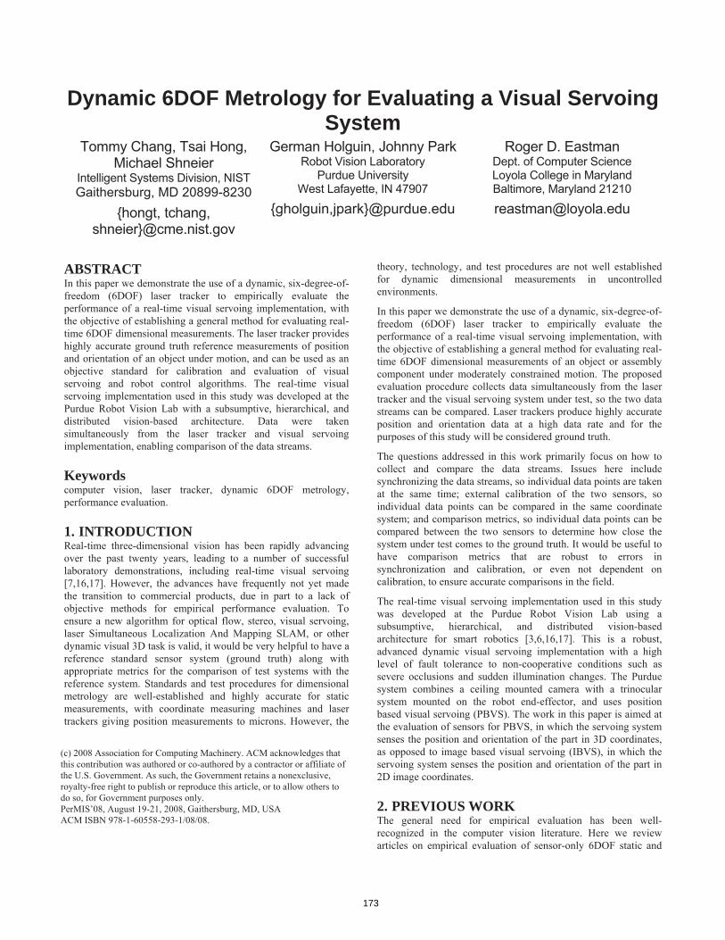
Dynamic 6DOF Metrology for Evaluating a Visual Servoing System

Tommy Chang, Tsai Hong, Michael Shneier

Intelligent Systems Division, NIST Gaithersburg, MD 20899-8230

{hongt, tchang, shneier}@cme.nist.gov

German Holguin, Johnny Park Robot Vision Laboratory

Purdue University West Lafayette, IN 47907

{gholguin,jpark}@purdue.edu

Roger D. Eastman Dept. of Computer Science Loyola College in Maryland Baltimore, Maryland 21210

reastman@loyola.edu

ABSTRACT In this paper we demonstrate the use of a dynamic, six-degree-of-freedom (6DOF) laser tracker to empirically evaluate the performance of a real-time visual servoing implementation, with the objective of establishing a general method for evaluating real-time 6DOF dimensional measurements. The laser tracker provides highly accurate ground truth reference measurements of position and orientation of an object under motion, and can be used as an objective standard for calibration and evaluation of visual servoing and robot control algorithms. The real-time visual servoing implementation used in this study was developed at the Purdue Robot Vision Lab with a subsumptive, hierarchical, and distributed vision-based architecture. Data were taken simultaneously from the laser tracker and visual servoing implementation, enabling comparison of the data streams.

Keywords computer vision, laser tracker, dynamic 6DOF metrology, performance evaluation.

1. INTRODUCTION Real-time three-dimensional vision has been rapidly advancing over the past twenty years, leading to a number of successful laboratory demonstrations, including real-time visual servoing [7,16,17]. However, the advances have frequently not yet made the transition to commercial products, due in part to a lack of objective methods for empirical performance evaluation. To ensure a new algorithm for optical flow, stereo, visual servoing, laser Simultaneous Localization And Mapping SLAM, or other dynamic visual 3D task is valid, it would be very helpful to have a reference standard sensor system (ground truth) along with appropriate metrics for the comparison of test systems with the reference system. Standards and test procedures for dimensional metrology are well-established and highly accurate for static measurements, with coordinate measuring machines and laser trackers giving position measurements to microns. However, the

theory, technology, and test procedures are not well established for dynamic dimensional measurements in uncontrolled environments.

In this paper we demonstrate the use of a dynamic, six-degree-of-freedom (6DOF) laser tracker to empirically evaluate the performance of a real-time visual servoing implementation, with the objective of establishing a general method for evaluating real-time 6DOF dimensional measurements of an object or assembly component under moderately constrained motion. The proposed evaluation procedure collects data simultaneously from the laser tracker and the visual servoing system under test, so the two data streams can be compared. Laser trackers produce highly accurate position and orientation data at a high data rate and for the purposes of this study will be considered ground truth.

The questions addressed in this work primarily focus on how to collect and compare the data streams. Issues here include synchronizing the data streams, so individual data points are taken at the same time; external calibration of the two sensors, so individual data points can be compared in the same coordinate system; and comparison metrics, so individual data points can be compared between the two sensors to determine how close the system under test comes to the ground truth. It would be useful to have comparison metrics that are robust to errors in synchronization and calibration, or even not dependent on calibration, to ensure accurate comparisons in the field.

The real-time visual servoing implementation used in this study was developed at the Purdue Robot Vision Lab using a subsumptive, hierarchical, and distributed vision-based architecture for smart robotics [3,6,16,17]. This is a robust, advanced dynamic visual servoing implementation with a high level of fault tolerance to non-cooperative conditions such as severe occlusions and sudden illumination changes. The Purdue system combines a ceiling mounted camera with a trinocular system mounted on the robot end-effector, and uses position based visual servoing (PBVS). The work in this paper is aimed at the evaluation of sensors for PBVS, in which the servoing system senses the position and orientation of the part in 3D coordinates, as opposed to image based visual servoing (IBVS), in which the servoing system senses the position and orientation of the part in 2D image coordinates.

(c) 2008 Association for Computing Machinery. ACM acknowledges that this contribution was authored or co-authored by a contractor or affiliate of the U.S. Government. As such, the Government retains a nonexclusive, royalty-free right to publish or reproduce this article, or to allow others to do so, for Government purposes only. PerMIS’08, August 19-21, 2008, Gaithersburg, MD, USA ACM ISBN 978-1-60558-293-1/08/08.

2. PREVIOUS WORK The general need for empirical evaluation has been well-recognized in the computer vision literature. Here we review articles on empirical evaluation of sensor-only 6DOF static and

173

dynamic pose estimation, as well as articles on evaluation of visual servoing algorithms that may combine sensor evaluation with robot control issues. In reviewing the literature, there are a number of questions that can be asked: what is under evaluation (pose estimation only, pose calculated for visual seroving, or other tasks), how measurements are taken from the system under test, how ground truth or other reference measurements are taken, what metrics are computed from the measurements, and how the metrics are interpreted to give summary judgments on system performance. We also have looked at the conditions of each test to consider the objects, motions, occlusions and environment.

For pose estimation, most evaluation papers consider static pose only [9,12] and not dynamic 6DOF sensor measurements of a part under motion. References [12,13] use Monte Carlo simulation for the evaluation of pose algorithm accuracy under noise and object orientations. In those articles, results are given for pose estimation for a complex industrial part and the error from unnamed ground truth is plotted as position or orientation error vs. the rotation of the object. The key result is to note the error as a function of part rotation varies considerably, spiking at ambiguous orientations of the object. Two papers that do consider dynamic pose are [10,15]. In [10] benchmarked video sequences are used for tests of a model-based algorithm with four parameter variations to analyze the relative contributions of subcomponents such as the edge detection operator or search technique. The results are given as deviations from the results of the one parameter set that successfully maintained track through the video sequences, but the nature and quality of this retrospective ground truth is not described in the article. In [15] three tracking approaches for 6DOF pose estimation and grasping of hand-held objects are evaluated using ground truth from an unnamed infrared marker tracking system good to 1.5 meters in position but with no rotation accuracy or measurements per second cited. The three approaches run at 8 Hz to 25 Hz. The article gives results in graphs that compare ground truth position and orientation data to robot end-effector position and tracked position, but no quantitative or summary statistics are given for the graphed data.

For visual servoing, many papers that present a new approach include an empirical evaluation, but since the paper emphasizes the development of the new approach, the evaluation section can be brief. An exception is [8] which uses sensitivity analysis and simulation to compute the contribution of image measurement errors to the calculated pose and control trajectory for PBVS and hybrid visual servoing.

The metrics used to evaluate pose estimation and visual servoing systems vary. Typical is the mean and standard deviation of a measure of error in world coordinates, including individual differences for each coordinate, a norm for position and orientation separately, or rarely a combined norm for all 6 degrees of freedom. The orientation can be compared in roll-pitch-yaw or as quaternions. In experiments without ground truth in world coordinates, or for IBVS in which pose in world coordinates is not computed, errors are computed in the image domain. [5] uses the reprojection error in the image domain. In some visual servoing evaluations, the metric is the number of cases successfully completed during the experiments.

In physical experiments in the evaluation of pose estimation or visual servoing, a mechanism must be used to generate motion, frequently a robot arm [2,4,15]. [15] uses an arm to move a

camera towards a car battery through a known trajectory linear in both translation and angle, and repeats the motion 80 times to judge repeatability of the tracking algorithm.

3. PURDUE LINE TRACKING SYSTEM Using robots to perform industrial assembly tasks is not new. In fact, robots have been used successfully in such applications over the past few decades. However, one common constraint still present in most of these applications is that the objects to be manipulated by the robot must be stationary in a known position, or moving along a well-known path with a very small amount of uncertainty. Consequently, industrial tasks such as painting, palletizing, welding, or decking have traditionally been set up in stationary locations in the assembly line where the involved parts have to come to a complete stop.

In order to eliminate inflexible, expensive stationary stations in the assembly line, robots must be able to perform their tasks on moving targets. The Purdue Robot Vision Lab addresses this goal using a subsumptive, hierarchical, and distributed vision-based architecture for smart robotics [3]. The system consists of multiple real-time control modules running in parallel, where each module is controlled by a different tracking method, with unique capabilities with respect to accuracy, computational efficiency, sensitivity to varying conditions, etc. By taking the most reliable input from all the modules, the system is able to achieve a high level of fault tolerance and robustness to non-cooperative conditions such as severe occlusions and sudden illumination changes.

In this architecture, each control module can be in a different hierarchy level. The more accurate the module is, the higher its hierarchy level. Modules from higher hierarchies can subsume functionality of modules in lower levels. Each module can run independently in a different computer over a network. Any number of modules is allowed in any given level of hierarchy, providing redundancy and fault tolerance.

Each module is composed of two main parallel processes. The first process is the visual-tracking loop that estimates the 6DOF 3D pose of the target object. This loop can be further broken down into three main parallel threads: data acquisition, data processing, and message exchange. The second process is the visual-servoing loop, which generates commands to the robot to move its end-effector to a desired position. This second loop is composed of two main threads: the message exchange and the control law calculation.

Even though every control module is able to run at its own sample rate and accuracy level in our architecture, only one module will be able to pass its generated command to the robot controller. The arbitrator listens to all the control modules and decides which module input to use to control the robot, based on module availability, estimation reliability, and module hierarchy.

Finally, the robot controller is implemented at the top of the robot controller interface. Therefore, the control modules in our system fall into the position-based look-and-move category [7]. This means that the robot controller is receiving commands directly in the Cartesian space, which makes the control plant much simpler compared to the image-based servoing category [3]. However, the position-based servoing requires camera calibration, robot calibration, and hand-eye calibration [6].

174

3.1 Peg and Hole Experiment In order to demonstrate the capabilities of this architecture, we set up a variation of the traditional peg-and-hole experiment (see Figure 1). In our experiment, we attached a hollow wooden cylinder to an engine cover part, and attached a peg to the end-effector of a 6DOF robot manipulator. The engine cover is loosely attached to a linear slide, so the main motion of the engine cover is provided by the motion of the linear slide. In addition, we also attached strings to the engine cover, which a human can manipulate to generate random motions of the engine cover during the experiment. The goal of this experiment is to command the robot to insert the peg into the cylinder on the engine cover while the engine cover is in motion, resembling the automation needed to perform tasks such as glass decking or wheel decking on-the-fly [16].

Our system consists of three control modules, a system arbitrator, and a robot controller interface. The three control modules are: coarse control, model-based fine control, and stereo-based fine control.

Figure 1. Peg and Hole experiment

3.2 Coarse Control The coarse control module resides at the lowest level in the system hierarchy, meaning that it will work only when the other two modules become unavailable or unreliable. Its main purpose is to provide an initialization point for the controllers with higher hierarchy. That is, the coarse control is intended to track the target and command the robot to an approximate location in front of it. This module only requires the level of accuracy that would place the end-effector in front of the target such that cameras for the other controllers can view the target.

Coarse control visual-tracking uses a camera mounted on the ceiling with a view of the entire workspace. When the target object enters the workspace, the bar holding the target is detected and the 3D translational position of the bar in the coordinates of the robot is estimated. No rotation information is needed here. This estimated pose is passed to the visual-servoing loop that in this case would simply command the robot to move its end-effector near the target.

3.3 Stereo-based Fine Control This is the control module that resides at the highest hierarchy level in the system, meaning that while tracking the target it

subsumes the other two modules. It uses a stereo pair of cameras located on the robot's end-effector.

The visual-tracking loop in this module uses a blob analysis algorithm to detect, in both cameras, three prominent coplanar features on the engine cover. Then, using the calibration information, the 3D coordinates of those features are reconstructed, and the 6DOF 3D pose of the target is estimated in the robot coordinate system [17]. Based on the estimated pose, the visual-servoing loop then performs the peg-and-hole motion using a Proportional-Integral-derivative (PID) control law.

Since the 3D pose estimation relies on the visibility of three specific features on the engine cover, this module will only work if all three features are detected in both cameras.

Using an efficient blob analysis algorithm makes this module run very fast. It takes an average of 8.2 ms to estimate the 3D pose of the target, which is more than sufficient to process stereo images at 30 frames per second. However, this approach requires some thresholds to extract the blobs, making this module sensitive to sudden illumination changes.

3.4 Model-Based Fine Control The main purpose of this module is to provide redundancy to the stereo-based fine controller. It uses a monocular vision system and a known wire-frame model of the target [16].

The visual-tracking loop of this module first projects the model into the input scene with respect to the initial pose that is given by the coarse control module or the stereo-based control module. Then, it sequentially matches the straight lines of the wire-frame model to the detected edges in the scene for an updated calculation of the pose of the target. For robust pose estimation, it uses a backtracking scheme for correspondence search [16].

Since this module uses extracted edges in the image, as opposed to applying thresholding to extract blobs in the stereo-based control module, it is less sensitive to illumination changes. Also, since the number of model features used in this module is typically much larger than 3 (the bare minimum number of features required to estimate the pose of an object), it is naturally robust to partial occlusions. However, it is slower than the Stereo-Based controller. It takes an average of 48 ms to estimate the 3D pose of the target, where 80 % of the computation time is taken by the edge detection phase.

4. EVALUATION EXPERIMENTS In the experiments, the visual tracking system was set up to perform the peg and hole task using an engine part cover as the target. The engine part was either stationary or moved by an overhead linear rail at a constant velocity. The part was suspended from the linear rail to allow the experimenters to move the part back and forth by an attached string.

During each pass of the experiment, the position of the engine part was measured simultaneously by the Purdue visual tracking system and the NIST laser tracker. Data acquisition from each system was triggered by a common hardware signal, and the data time stamped and streamed to storage for off-line comparison.

175

The key elements of the data collection system were the laser tracker, the simultaneous data collection, and the establishment of common coordinate systems through calibration.

4.1 Laser Tracker

Figure 2. SmartTRACK sensor below engine part

The laser tracker system used consisted of two major components, a base unit and an active target, both made by Automated Precision Inc1. (API). The active target is a SmartTRACK Sensor (STS) capable of determining its orientation in 3D space. Weighing 1.4 kg, the STS has an angular resolution specification of ±3 arc-sec (or ±0.000833… degrees). The complete manufacturer’s specification can be found in [18]. The base unit is the Tracker3TM Laser Tracking System (T3) which tracks the 3D position of the STS. The T3 system has ± 10 ppm absolute accuracy (e.g., ± 50 m at 5 m). In addition, the base unit can be used with a passive target (a spherically mounted reflector (SMR) retro-reflective mirror) instead of the active target for single point measurements.

Together, the T3 and STS provide an accurate but limited 6DOF pose estimation system. The STS and T3 devices can take measurements independently at their own rate or they can be connected to a common external trigger.

4.2 Synchronization Issues Both the T3/STS system and the Purdue visual-tracking system allow an external signal to trigger their data acquisition. Although the STS/T3 system is capable of handling a trigger signal up to 150 Hz, the visual-tracking system requires a 30 Hz data stream. We use a single 30 Hz trigger signal shared by both systems.

YHX

1 Certain commercial equipment, instruments, or materials are identified in this paper in order to adequately specify the experimental procedure. Such identification does not imply recommendation or endorsement by NIST, nor does it imply that the materials or equipment identified are necessarily best for the purpose.

Although a shared trigger signal provides a solution to simultaneous measurements, the trigger itself needs to be reliable, repeatable, and controllable. We use a digital function generator that can be programmed to produce a clean squarewave signal. The digital function generator also allows us to start and stop the signal with a push of a button. The resulting signal is deterministic and free of the button-bouncing effect typically associated with inexpensive analog function generators.

The data collection programs maintain their own sequence number, which is increased each time a trigger signal is received. In addition, the program time-stamps the sequence number with a microsecond timer from the computer clock. Both systems synchronize their computer clock with a NTP (Network Time Protocol) server every 10 s throughout the entire data collection.

For data to be a matched pair, we require them to have the same sequence number. In addition, we check the difference between the corresponding timestamps and verify that the difference is small (i.e., the difference should never be greater than the period of the trigger signal shared by the two systems).

4.3 External Calibration Issues To evaluate data collected during the experiments, we need to define metrics to compare the 6DOF pose data collected by the API T3/STS laser tracker and the Purdue line tracking system. There are eight coordinate systems involved, defined in Figure 2. We want to establish relationships between data collected in the coordinate system T of the laser tracker and one more coordinate systems of the Purdue system. We use the notation to denote the homogenous transformation from coordinate system Y to X, so HT W is a transformation from W coordinates to T coordinates. The 6DOF pose of the object O in the T3 coordinate system would be represented by . OHT

Figure 2. The coordinate systems of the Purdue Line Tracker

and the STS/T3 Tracker System

176

Figure 3. The world coordinate system

External calibration provides an estimate of the homogeneous transformation matrix (H) between the world W, and the robot base B, where W is defined by the calibration pattern behind the target as shown in Figure 3.

If we can successfully use the laser tracker coordinates T to establish the transformation HT r HW tween the world (W) and T3, we can relate the coordinate T to the robot base B coordinate as in Equation 1.

W o T be

X Y

Z

Figure 4. The object coordinate system (Y=OB, Z=up)

We don't have direct access to the origin of the engine cover O coordinates. Instead we use the Cartesian positions of three features (A,B,C), to reconstruct the coordinate frame for O with respect to coordinate T (see Figure 4).

We use the T3 laser tracker with an SMR to measure A, B and C in T coordinates. We then compute the origin O as the midpoint between A and B, and use the position of C to complete the object reference frames. Hence we construct T or .

Similarly, we construct T by measuring the origin of W. OH THO

WH

THS OHS

OTTSOS HHH

Given from T3/STS system, we obtain from Equation 2.

Eq. 2

Using Equation 1 and Equation 2, we establish transformations between the T3 base system T and the object system O in both the T3 and Purdue system, and compare those two transformations. The ground truth transformations provided by the T3/STS are on the left hand side, and the measurements provided by Purdue system and the hand-eye calibration are on the right hand side:

OBBWOSSTTW HHHHH Eq. 3

HO (laser )This gives the relationship W W HO (visual )

H

and the inverse between the two systems in a common coordinate system, where visual stands for the Purdue tracking system.

Now we relate the two estimations of the inverse O W in the world coordinate system. In Equation 3, the calibration error in

, and W can’t be eliminated, so the absolute measurement approach was not used in this paper.

THW OHS BH

Oi H

Since the Purdue system is a tracking system, the differential pose with respect to time is computed every cycle. It is reasonable to compare the differential pose between ground truth and the Purdue system using the world coordinates. We define W (P )

)(GHWOi

)()()( 11 PHPHPH OiOiOiWWOi

)()()( 1 GHGH OiOiWWOi

)(1 GHOiOi

)(1 PHOi

BWWTBT HHH as the pose of the engine part in the world coordinate at time i for the Purdue Tracking system as the pose of the engine part in world coordinate at time i for the ground truth system (laser tracker).

We can then obtain the following relationships for each system between time i and time i+1:

1 GHOi

As one can see from the above derivation, the differential measurement will not depend on coordinate system. This approach produces the same numerical result for

and Oi in any coordinate system.

5. EXPERIMENTAL RESULTS We present here preliminary results from a series of experiments conducted at Purdue in April, 2008. The protocol was to run three sets of experiments, one with the target stationary, one with the target moving with a simple linear velocity, and one with the target moving with a linear velocity but randomly displaced manually by the experimenters. The results are given below for the three sets.

The experiment had two complications. One is that the calibration of the laser tracker and Purdue system proved difficult and we were not able to establish a full set of coordinate transformations between laser tracker and visual system data. We did establish enough to compare relative poses, which are reported. Also, the

Eq. 1

177

Purdue system is both a visual tracker and a robot control system. The data may at times confound the effects of both subsystems, as the robot introduces a physical motion. We only wished to evaluate the performance of the visual tracker.

5.1 Stationary Tests The stationary tests allowed us to evaluate the basic performance of both systems and assure that the laser tracker was performing to specifications after shipping. The target was placed in four positions and data collected for 15 to 30 seconds for each. The results showed that both systems performed within specifications.

Table 1 lists the standard deviations of the stationary data set measured by the STS/T3 system. The results are consistent with the specifications [7]. The laser tracker stayed in a fixed position so the target distance varied.

Table 1. STS/T3 system: repeatability for stationary data

Sample Size

T3/STS mean distance (mm)

2 std (mm)

Position 1 466 3550.054 0.006

Position 2 1157 3781.466 0.006

Position 3 1050 3882.787 0.005

Position 4 1018 4002.035 0.008

Table 2 lists the standard deviations of the stationary data set measured by the Purdue system. The Purdue system moves the robot end-effector near the object, so the distance remains relatively constant. The results show a consistent value near 0.6 mm at a range of approximately 2.6 m.

Table 2. Purdue system: repeatability for stationary data

Sample Size

T3/STS mean distance (mm)

2 std (mm)

Position 1 466 2670.582 0.629

Position 2 1157 2625.820 0.582

Position 3 1050 2625.036 0.560

Position 4 1018 2636.701 0.561

For use as a reference system, a metrology technology should have an accuracy at least one order of magnitude greater than the system under test. In this case, the laser tracker is two orders of magnitude more accurate than the Purdue vision system.

5.2 Linear Motion Tests In the linear motion tests, the target was moved about 1.5 meters left to right and tracked by both the laser tracker and the Purdue system. For each trial, the motion was repeated 30 times as the target moved, and then was quickly moved back to the start position. The backward sweep was ignored in the data analysis as the Purdue system only tracked during the forward motion.

The differential motion as measured by both systems was used to determine the consistency between laser tracker and Purdue system. In effect, the comparison is being made on the measured

speed of the target in each separate coordinate (X,Y,Z, roll, pitch, yaw).

The data below are from pass 6 of the first trial, and are typical of the linear runs. The sample size is 453, with 33 ms between data points. In the graphs below the horizontal axis is frame number, and the vertical axis is the difference between the laser tracker motion change (delta) in each coordinate and the Purdue system delta. Since the laser tracker was accepted as ground truth, the difference is defined as the error in the Purdue system.

In Figure 5 the errors can be seen to be consistent and relatively independent of position along the path, although that is yet to be evaluated statistically. The error does vary by coordinate – different coordinates proved to be more sensitive to the left-to-right motion. In object coordinates the target is moving in the Y-Z plane, primarily in the Y direction, and the Z coordinate has slightly less error. Similarly, the roll angle is around the X axis, and proved an order of magnitude reduced in error over the other rotations. Table 3 quantifies the error values, while Figure 6 gives a histogram of the error values to show roughly symmetric, zero centered error distributions. For coordinate Y there appears to be a secondary peak in positive error.

Figure 5. Pass 6 – Coordinate Errors in Delta vs. Frame

Number

Figure 6. Pass 6 – Coordinate Errors in Delta (histogram)

178

Table 3. Pass 6 – Coordinate Error Statistics (n=453)

Mean Std Max Min

X in mm 0.01614 0.45376 1.49003 -1.41190

Y in mm -0.03513 0.33355 1.27399 -1.32852

Z in mm 0.05206 0.21991 0.74652 -0.69851

distance -0.04305 0.33273 1.21320 -1.50436

Roll in deg 0.00168 0.04915 0.14368 -0.16532

Pitch in deg 0.00088 0.40811 1.21672 -1.27938

Yaw in deg 0.00184 0.21589 0.56194 -0.71260

Total angle -0.04798 0.05195 0.03383 -0.28635

5.3 Shaking Motion Tests In the shaking motion tests, the basic target motion and repetitions were identical to those in the moving target test, but the experimenters could pull a string to swing the target with an impulse motion. This was done through a series of different motions – first with no extra motion to match the linear case, then with the impulse motion varying by amplitude and frequency.

The data below are from pass 3 of the first shaking motion trial. The sample size is 455, with 33 ms between data points. In the graphs below, the horizontal axis is frame number, and the vertical axis the difference between the laser tracker delta in each coordinate and the Purdue system delta.

Figure 8. Pass 3 – Coordinate Errors in Delta vs. Frame

Number The graphs show four impulse motions as the target was pulled back four times, relatively smoothly and consistently. The error first goes positive as the speed of the target slows down and the Purdue system undershoots the speed, and then negative as the Purdue system overshoots the speed. The graph scales have changed from the linear motion case, as the error range has approximately doubled. The Z axis remains the one with lowest error, while the roll angle error is greater compared to the linear

motion tests as the impulse motion rotated the target around the X-axis.

6. CONCLUSIONS In this paper we have demonstrated the use of a precision laser tracker to evaluate a state-of-the-art visual servoing perception system, with the objective of establishing general techniques for evaluating 6DOF sensors. The demonstration involved a synchronized data collection system that used a hardware trigger to collect at a 30 Hz rate, while the laser tracker has the ability to collect at up to 150 Hz. The laser tracker was verified accurate enough for the approximate 1 mm range of error that needed to be measured.

Future work will involve a more detailed analysis of the data and the establishment of better calibration techniques and metrics to insure consistent comparisons between laser tracker and sensor data streams.

Figure 9. Run 6 – Coordinate Errors in Delta (histogram)

Table 4. Run 6 – Coordinate Error Statistics (n=453)

Mean Std Max Min

X in mm 0.00219 1.13255 2.90429 -3.32659

Y in mm -0.04633 1.26350 2.21070 -3.62808

Z in mm -0.01445 0.58950 1.42051 -1.53047

distance 0.90879 0.95975 3.77670 -1.84237

Roll in deg 0.00362 0.30460 0.87745 -0.78979

Pitch in deg -0.00329 0.50645 1.48264 -2.10615

Yaw in deg 0.00103 0.23520 0.61750 -0.76112

Total angle -0.42713 0.30752 0.15745 -1.51979

7. ACKNOWEDGMENT We thank Elena Messina and Hui-Min Huang for the fruitful discussions. We thank Nick Scott, Alan Lytle, Chris Blackburn, Daniel Sawyer, Steve Phillips from NIST , Avi Kak from Purdue University, Jane Shi from General Motors , and Kam Lau, Alan Cui, Zaifeng Chen from API for their collaborations.

179

8. REFERENCES [1] Chai, X., Shan, S., Qing, L. and Gao, W. 2006 Pose

Estimation Based on Gaussian Error Models, International Conference on Biometrics, 2006: 136-143

[2] Deguchi, K., 2000 A Direct Interpretation of Dynamic Images with Camera and Object Motions for Vision Guided Robot Control. International Journal of Computer Vision 37(1): 7-20 (2000).

[3] DeSouza, G. N. and Kak, A. C., 2004, A Subsumptive, Hierarchical, and Distributed Vision-Based Architecture for Smart Robotics, IEEE Transactions on Systems, Man, and Cybernetics -- Part B: Cybernetics, 34(5): 1988-2002.

[4] Espiau, B., 1993 Effect of Camera Calibration Errors on Visual Servoing in Robotics. Experimental Robotics III, The 3rd International Symposium, Kyoto, Japan, October, 1993: 182-192.

[5] Fiore, P. D, 2001 Efficient Linear Solution of Exterior Orientation, IEEE Trans. Pattern Analysis and Machine Intelligence, vol. 23(12): 140-148, 2001

[6] Hirsh, R., DeSouza, G. N. and Kak, A. C., 2001 An Iterative Approach to the Hand-Eye and Base-World Calibration Problem, Proceedings of the IEEE International Conference on Robotics and Automation, Seoul, May 2001

[7] Hutchinson, S.A., Hager, G.D., and Corke, P.I, 1996 A tutorial on visual servo control. IEEE Transactions on Robotics and Automation, 12(5):651--670, October 1996.

[8] Kyrki, V., Kragic, D., and Christensen, H. I., 2006 Measurement errors in visual servoing. Robotics and Autonomous Systems 54(10): 815-827 (2006)

[9] Madsen, C.B, A comparative study of the robustness of two pose estimation techniques. In H.I. Christensen, W. Förstner, and C.B. Madsen, editors, Proceedings: ECVnet Workshop on Performance Characteristics of Vision Algorithms, held in conjunction with Fourth European Conference on Computer Vision, Cambridge, England, pp. 181 - 200, April 1996.

[10] Preisig, P.. and Kragic, D., 2006 Robust Statistics for 3D Object Tracking. Proceedings of the Int. Conference on Robotics and Automation, Orlando, Florida, 2006.

[11] Chai, X., Shan, S., Qing, L. and Gao, W. 2006 Pose Estimation based on Gaussian Error Models, Proceeding of International Conference on Biometrics (ICB2006), Lecture Notes on Computer Sciences (LNCS3832), D.Zhang, A.Jain (Eds.), pp136-143, Hong Kong.

[12] Reid, G. J., Tang J., and Zhi, L., 2003 A complete symbolic-numeric linear method for camera pose determination, International Symposium on Symbolic and Algebraic Computation, Philadelphia, Pennsylvania 2003: 215-223.

[13] Rivera-Ríos, A. H., Shih F. L, and Marefat, M. M. 2005 Stereo Camera Pose Determination with Error Reduction and Tolerance Satisfaction for Dimensional Measurements, Proceedings of the Int. Conference on Robotics and Automation, Barcelona, Spain, 2005: 423-428.

[14] Sepp, W., Fuchs, S. and Gerd Hirzinger. 2006 Hierarchical Featureless Tracking for Position-Based 6-DoF Visual Servoing, Proceedings of the IEEE/RSJ International Conference on Intelligent Robots and Systems (IROS) 2006, Beijing (China), 2006

[15] Tonko, M. and Nagel, H. 2000 Model-Based Stereo-Tracking of Non-Polyhedral Objects for Automatic Disassembly Experiments, International Journal of Computer Vision 37(1): 99-118 (2000).

[16] Yoon, Y., DeSouza, G. N. and Kak, A. C., 2003 Real-time Tracking and Pose Estimation for Industrial Objects using Geometric Features, in Proceedings of the Int. Conference in Robotics and Automation, Taiwan, 2003

[17] Yoon, Y., Park, J. and Kak, A.C. 2006 A Heterogeneous Distributed Visual Servoing System for Real-time Robotic Assembly Applications, in Proceedings of the Int. Conference on Robotics and Automation, Orlando, Florida, 2006.

[18] SMARTTRACK SENSOR, Automated Precision Inc., http://www.apisensor.com/PDF/SmartTrackeuDE.pdf, 2007.

180

Integrating Reification and Ontologies for MobileAutonomous Robots

J. P. GundersonGamma Two, Inc.

209 Kalamath Street, Unit 13Denver, CO, USA

jgunders@gamma-two.com

L. F. GundersonGamma Two, Inc.

209 Kalamath Street, Unit 13Denver, CO, USA

lgunders@gamma-two.com

ABSTRACTA significant problem that has plagued autonomous mobilerobots is the need to reason about a complex and dynamicworld in a timely fashion. Huge strides have been made inartificial intelligence systems that deal with symbolic repre-sentations, and the hardware for robotics has seen significantgrowth. However, autonomous robots have not seen equiv-alent improvement. In this paper we examine a techniqueto couple deliberative reasoning systems with mobile roboticplatforms to enable the robot to reason about the world.

Mobile autonomous robots operate under extremely tightconstraints in power and computational loads, and must beresponsive to the dynamic environments in which they aredeployed. Since they do not have the luxury of operatingin a static, controlled environment, they must be capableof quickly recognizing changes to the environment, assessingthe impacts of these changes, and implementing intelligentresponses to those changes. All of these requirements mustbe met in a real-time environment, using limited computa-tional resources. Since living organisms also operate underthese same constraints we present a design that is biolog-ically principled. This design integrates both reactive anddeliberative components using a biologically principled com-ponent called a Reification Engine.

The Reification Engine acts as a bi-directional bridgebetween the sensor domain and the symbolic domain. It pro-vides the ability to map the changes detected by the sensorsinto a symbolic representation, which is expanded by the on-board ontology to generate a semantic representation of thesalient aspects of problem. This, in turn, can be analyzed bya deliberative system to generate a planned response to thechanges, which can be mapped by the Reification Engine

back into the sensor/effector space of the robot’s hardware.

Keywordsrobotics, ontology, reification, artificial intelligence, auton-omy, biologically inspired computing

Permission to make digital or hard copies of all or part of this work forpersonal or classroom use is granted without fee provided that copies arenot made or distributed for profit or commercial advantage and that copiesbear this notice and the full citation on the first page. To copy otherwise, torepublish, to post on servers or to redistribute to lists, requires prior specificpermission and/or a fee.PerMIS‘08 August 19 - 21 2008, Gaithersburg, MD, USACopyright 2008 ACM 978-1-60558-293-1 ...$5.00.

������������������������

�� ���������

���������� �� ��� ������

��������

Figure 1: The four major components of an au-tonomous robotic system. The Reasoning com-ponent provides the ability to determine how toachieve goals. The Robot Chassis enables the sys-tem to execute the behaviors in the physical world.The middle components - the Ontology and theReification Engine, translate between the symbolicand the sensor-based domains.

1. INTRODUCTIONThis research has been driven by a single question: “Where

is my Robot?” The last few decades have seen an explosionin robotic systems in many domains, including factory andlaboratory automation[6, 11, 15, 22, 23], deep sea explo-ration[1, 12, 5], and exploration of deep space[20]. At thesame time we have seen the use of teleoperated systems insearch and rescue, bomb disposal, and surveillance aircraft;all of which have saved lives. However, we have not seen anequivalent explosion of autonomous systems.

An autonomous robot can be modeled as a system con-sisting of four major components. The first of these is thephysical manifestation of the robot - the sensors, effectors,and electronics that make up the hardware. Since an in-telligent, autonomous robot is being considered, the secondmajor component is the software that makes up the ‘brains’of the autonomous robot. The reasoning component oper-ates in a purely symbolic domain: it manipulates symbolsaccording to abstract rules. Between the reasoning and ex-ecution components lie two others - a mechanism to linkmeaning to those abstract symbols (the ontology), and areification mechanism[9] that bridges the gap between thesesymbols and the physical domain. The ontology and theReification Engine are the interface between the ‘brains’and the ‘brawn’ - they translate between the domain of sen-sors and effectors into the domain of symbols and semantics.These four components are shown in figure 1.

In this paper we will focus primarily on the interactionbetween the ontology and the Reification Engine. Ratherthan focusing on any specific robotic chassis, we will referto an abstract perception/action system. In the same waywe will refer to a generic deliberative system, rather than

181

any specific architecture for the generation of behaviors orplans. We will focus on specific implementations of the on-tology and the Reification Engine, since we are exploringthe integration between the mechanisms used to representknowledge in these two components.

2. REASONINGFor most of its history, artificial intelligence has been fo-

cused on reasoning. Some of the earliest AI programs weredesigned as problem solvers[13, 7], planners[18], or designedto excel at games like checkers[19]. These programs ma-nipulated symbols according to specific rules, and searchedthrough solution spaces to find plans that would achieve thesystem’s goals. These systems frequently relied on ad hocrepresentations of the symbols and their allowed manipula-tions.

Recently there has been more research into the use of on-tologies as a standardized format for representing the mean-ing of symbols. The reasoning components of the ontologyuse the relationships between the concepts as rules control-ling the manipulation. In some systems, the ontology fillsthe role of semantic memory in humans: a large diverse,persistent storage of all available knowledge. Since only asmall portion of the entire knowledge base is needed for anyspecific problem, a subset of the ontology is used to generatethe actual problem that the reasoning system processes (See[10] Chapter 9 for more information). With mobile robots,these ontologies must not only capture the abstract conceptsthat are the focus of much of the research, they must alsocapture the knowledge associated with the physical domainin which the robot functions.

2.1 Personal Rough OntologiesCurrent research into artificial intelligence has addressed

the need for an intelligent system to have a complex and de-tailed body of knowledge to function effectively in a complex,dynamic, and uncertain world. Unfortunately, these on-tologies are not well suited to deployment into autonomousrobots, since they tend to be computationally expensive.However, an autonomous robot has a critical need for theability to reason effectively about the world into which itis deployed, especially in unconstrained environments. Wedemonstrate how the integration of a Reification Engine

with an ontology tailored for a robot’s needs can enable therobot to function more effectively in a dynamic world.

We utilize a biologically principled form of an ontology,designed for effective integration into an autonomous robot.The key differences lie in the area of completeness and con-sistency. Most living systems do not have complex truthmaintenance systems analyzing every new fact or belief thatis added into their cognitive systems. In spite of this, theyfar outperform most autonomous robotic applications. Wehave extended (or crippled, depending on one’s viewpoint)ontologies so that they can contain inconsistent data with-out causing logical operations to result in invalid states. Thisis done by controlling the deductive reasoning to a limiteddistance within the ontological graph. This has two sig-nificant benefits to autonomous robots. First,the computa-tional complexity of navigating the ontological graph is dra-matically reduced, since the expansion of edges eventuallytapers off to zero. Second, this mechanism acts as a focusof attention which enables the extraction of a small, salientsubgraph to be used by the deliberative system for problem

solving - thus dramatically reducing the computational bur-den of the planning system. Because of this lack of truthmaintenance we call this a rough ontology. Since the systemwill modify its ontology based on personal experience, wecall this a personal rough ontology (PRO).

The basic structure of an ontology is a directed multi-graph:

Ontology ≡ (C,E) (1)

where: C is a collection of nodes; andE is a collection of directed edges from

one node to another.

2.2 The nodes in the multi-graphReferring back to Equation 1, we see that the multigraph

consists of a collection of nodes and a collection of directededges. Each node C corresponds to a symbolic representa-tion of an entity. The base class for these nodes is a Cept,hence the non-traditional use of C in equation 1. Each Cept

may have a collection of properties that describe it. Theseproperties are used in two ways. First, the ontological sys-tem can use these properties when applying rules, and sec-ond, the deliberative system uses these properties to developplans to achieve its goals. To facilitate these uses, the prop-erties are represented as specific relationship arcs to otherCepts.

Cept(C) ≡ (symbol, {P}, {R}) (2)

where: symbol is the symbolic representation ofthe concept (its name);

{P} are the properties; and{R} are the relationships to other Cepts.

The Cepts in our ontology represent the things aboutwhich we have knowledge. These things correspond to thesubject and object of the relationships. The common ele-ment of these things is the symbol and the list of properties.This base class is extended to represent specific types ofknowledge in the ontology.

The simplest variant of a Cept is a ConCept. This is whatis represented in a typical ontology. The ConCept extendsthe basic Cept by adding the idea that a ConCept can repre-sent either an abstract concept or something more concrete.As an example, the ConCept of a chair represents a percepti-ble thing that might exist in the world; however the ConCeptof ‘laid-back’ is not something that is directly perceptible.In the case of perceptible ConCepts, the Reification En-

gine has the responsibility of maintaining the mechanismsthat allow the recognition of objects in the real world, andlinking those perceived objects to the symbolic representa-tions. This is done by adding a link from each perceptiblething in the ontology to a data structure called a PerCept,maintained by the Reification Engine, described in Sec-tion 3.

Much as the ConCepts correspond to nouns, the world isalso full of verbs - the actions and events that cause change.Although knowledge about actions may seem to be funda-mentally different than knowledge about things, they arestill symbolic representations about the world. In the chairdiscussion above, it seemed natural that there would be arelationship between a chair and the concept of sitting, justas there seems to be a natural relationship between a bi-cycle and riding or a ladder and climbing. Note that the

182

conceptual symbol associated with sitting differs from themechanics of lowering ones body into a seated position -that is a function of the perception/action system.

To represent the conceptual model of an action, we mod-ify the base Cept class. This subclass is called an ActCept

in the ontology. The base class is extended by adding twoadditional components - the conditions under which the ac-tion can be taken (e.g., to drive the car it is necessary tohave a car), and the possible outcomes of acting (you mightget where you want to go, or you might run out of gas). Theenabling conditions and outcomes can be directly mappedonto the corresponding components of the action represen-tation used by the deliberative system, and so the semanticmemory fulfills its design goal of being the repository ofknowledge for the reasoning system.

2.3 Relationships, the Edges of the GraphEach edge in the multi-graph is a directed arc that leads

from the subject node to the object node. Directed arcs areneeded since not all relationships are symmetric, for exam-ple, if the type of the relationship is part of , it makes senseto say that a leg is part of a chair; however the reverse is nottrue. Each edge captures one specific type of relationship.The representational schema for the arcs is:

Edge(E) ≡ (C, I, N, T, S, L) (3)

where: C is the class ofthe relationship;

I is the unique identifier;N is the destination node;T is the transitivity;S is the strength; andL is the likelihood

that the relationship holds.

Each relationship E is an instance of a class of relation-ships. While the ontology is very generic, there seem to bea number of relationship types that are common across on-tologies for systems embedded in the physical world. Theseinclude relationships like is a, has a, is part of , and is at.To facilitate the encoding of capabilities we also add can dowhich is the relationship between a ConCept and an ActCept

that it is capable of executing.

2.4 Transient versus Persistent KnowledgeKnowledge changes over time. While many ontologies are

designed to capture the relationships between permanentconcepts such as what it means to be a mammal or whatthe definition of a prime number is; there is also a needto represent more transient information. There is a vastamount of relatively transient knowledge, far more than canbe maintained in working memory at any point in time.So there must be a more permanent storage place. Weinclude this transient knowledge in the form of propertiesattached to the ConCept, and use a specific relationshipinstance of to link the individual ConCept to the frame-work of knowledge of more abstract concepts. In practicewe have two specialized relationships for handling instanceConCepts: thing instance and location instance. These areused to provide the linkage from the specific instances to twocorresponding nodes in the ontological frame work. Theseare labeled as Place and Thing.

In addition, there are instance ConCepts that appear anddisappear from our knowledge base. We often encounter new

people in our day to day interactions. While some of themmay become friends or colleagues, many will be a single,short-term encounter. While we are interacting with them,we need to access the complex web of knowledge we haveof people, and this can be done by instantiating an ‘anony-mous’ person ConCept. This provides access to generic back-ground information that allows us to reason about this per-son, but we do not need (or want) to clutter our ontologywith references to every person we have ever encountered inour lives.

The final type of symbolic knowledge is knowledge aboutthe current state of the world. In order for the planningsystem to work it needs a relatively accurate model of thestate of the world. This is contained in the Current WorldState (CWS). The CWS is the symbolic representation uti-lized by the deliberative system. A more spatially detailedrepresentation, called a Mental Model is used by the Reifi-cation Engine. When the robot encounters an object inthe real world, it attempts to classify the object, so thata semantically tagged representation can be added to theCWS. The CWS includes knowledge about the permanentpersistent features of the world, and it contains informationabout the current state of previously encountered transientobjects. However, there is no pre-existing representation foran object that is encountered for the first time.

As an example, consider a robot serving drinks at a cock-tail party. It knows about the general layout of the room- the walls, the big furniture, etc. This is permanent andpersistent data. It also knows about a few smaller chairs,which are permanent, however, their current location maychange as the chairs get moved around. It does not haveinstantiated representations for all the people who mightarrive. Rather, when the robot encounters a new object, itwill attempt to classify it. Using its sensor data, and thePerCepts that correspond to the currently instantiated ob-jects, if the object can be classified, both the CWS and theMental Model are updated with the new knowledge. If itfails to classify the object, it then accesses the PerCepts

associated with more general concepts. For example, thePerCept for a generic Person has a high probability of amatch, and the Reification Engine uses this to instanti-ate a new object in its CWS. This object is not permanent- rather it is transient. It comes into existence, and, afternot being reinforced, it vanishes. In this way the size of theontology is not ever increasing with references to concepts,objects, and entities that will never be accessed again.

3. REIFICATION ENGINEThe bi-directional mapping between the symbolic repre-

sentations used by the ontology and the sensor based rep-resentation utilized by the perception/action system of anautonomous robot is called reification (See Robots, Reason-ing, and Reification[10] for more detail). This process isderived from current research in cognitive science and neu-rophysiology. There has been research into the two areas ofSymbol Grounding (mapping symbolic representations ontosensor based leaf terms) and Pattern Recognition (project-ing from sensor based data onto symbolic representations).One belief is that either of these approaches, if continuedsufficiently, will bridge the Sensor/Symbol gap. We believethat there is no overlap between these two research areas,and that a separate process - reification - is used by livingsystems when they perform these mappings.

183

����������� �������

��������

����������

�����������������

����� ����

������������

������������� � �

���

������

�������

�������

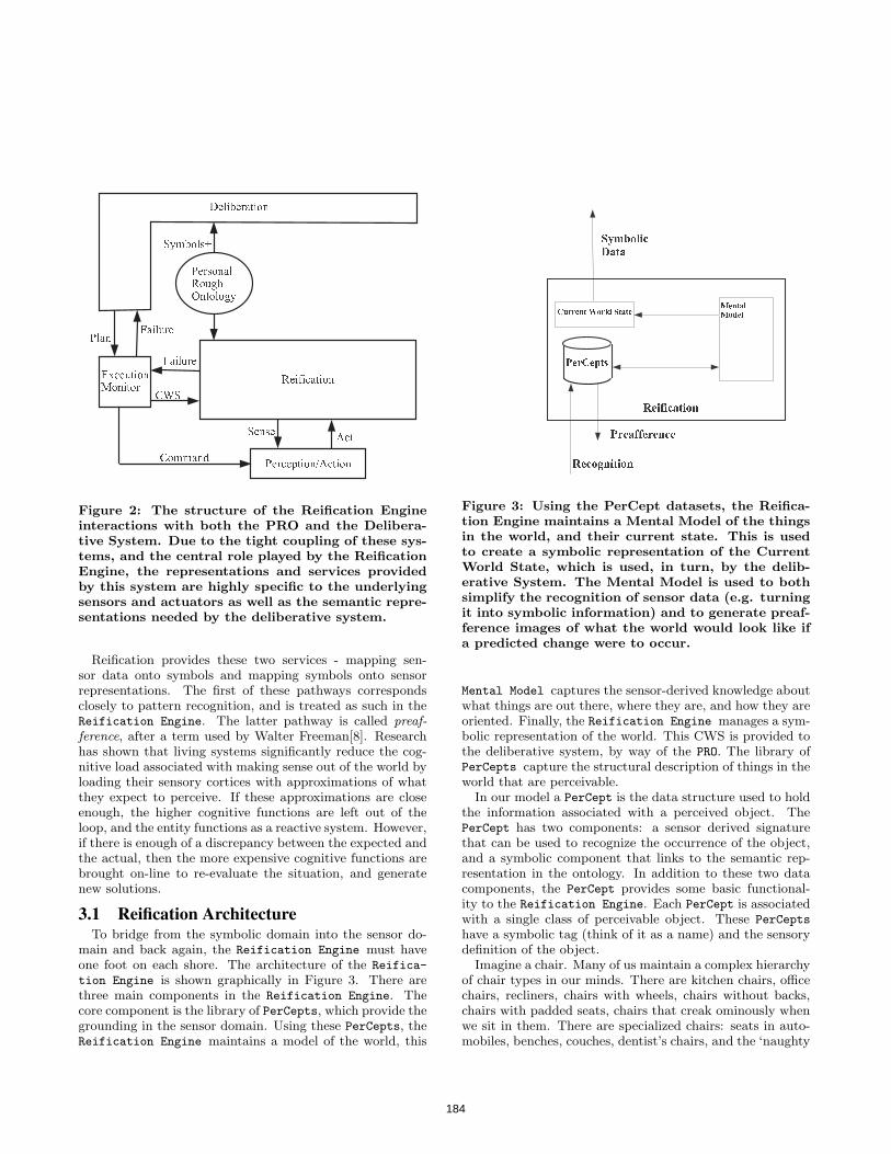
Figure 2: The structure of the Reification Engineinteractions with both the PRO and the Delibera-tive System. Due to the tight coupling of these sys-tems, and the central role played by the ReificationEngine, the representations and services providedby this system are highly specific to the underlyingsensors and actuators as well as the semantic repre-sentations needed by the deliberative system.

Reification provides these two services - mapping sen-sor data onto symbols and mapping symbols onto sensorrepresentations. The first of these pathways correspondsclosely to pattern recognition, and is treated as such in theReification Engine. The latter pathway is called preaf-ference, after a term used by Walter Freeman[8]. Researchhas shown that living systems significantly reduce the cog-nitive load associated with making sense out of the world byloading their sensory cortices with approximations of whatthey expect to perceive. If these approximations are closeenough, the higher cognitive functions are left out of theloop, and the entity functions as a reactive system. However,if there is enough of a discrepancy between the expected andthe actual, then the more expensive cognitive functions arebrought on-line to re-evaluate the situation, and generatenew solutions.

3.1 Reification ArchitectureTo bridge from the symbolic domain into the sensor do-

main and back again, the Reification Engine must haveone foot on each shore. The architecture of the Reifica-

tion Engine is shown graphically in Figure 3. There arethree main components in the Reification Engine. Thecore component is the library of PerCepts, which provide thegrounding in the sensor domain. Using these PerCepts, theReification Engine maintains a model of the world, this

��������

��� ���

�������� �

�� �����

�������� ��!"##��� $�#� %����

���&����

Figure 3: Using the PerCept datasets, the Reifica-tion Engine maintains a Mental Model of the thingsin the world, and their current state. This is usedto create a symbolic representation of the CurrentWorld State, which is used, in turn, by the delib-erative System. The Mental Model is used to bothsimplify the recognition of sensor data (e.g. turningit into symbolic information) and to generate preaf-ference images of what the world would look like ifa predicted change were to occur.

Mental Model captures the sensor-derived knowledge aboutwhat things are out there, where they are, and how they areoriented. Finally, the Reification Engine manages a sym-bolic representation of the world. This CWS is provided tothe deliberative system, by way of the PRO. The library ofPerCepts capture the structural description of things in theworld that are perceivable.

In our model a PerCept is the data structure used to holdthe information associated with a perceived object. ThePerCept has two components: a sensor derived signaturethat can be used to recognize the occurrence of the object,and a symbolic component that links to the semantic rep-resentation in the ontology. In addition to these two datacomponents, the PerCept provides some basic functional-ity to the Reification Engine. Each PerCept is associatedwith a single class of perceivable object. These PerCepts

have a symbolic tag (think of it as a name) and the sensorydefinition of the object.

Imagine a chair. Many of us maintain a complex hierarchyof chair types in our minds. There are kitchen chairs, officechairs, recliners, chairs with wheels, chairs without backs,chairs with padded seats, chairs that creak ominously whenwe sit in them. There are specialized chairs: seats in auto-mobiles, benches, couches, dentist’s chairs, and the ‘naughty

184

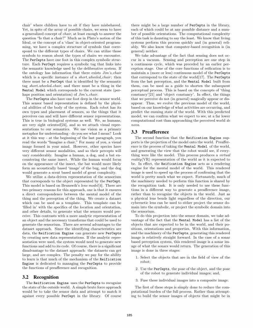
chair’ where children have to sit if they have misbehaved.Yet, in spite of the array of possible chairs, we seem to havea generalized concept of chair, at least enough to answer thequestion “Is that a chair?” Much as in Plato’s notion of theIdeal, or the concept of a ‘class’ in object-oriented program-ming, we have a complex structure of symbols that corre-spond to the different types of chairs. We can utilize thosesymbols to reason about the types of chairs we encounter.The PerCepts have one foot in this complex symbolic struc-ture. Each PerCept requires a symbolic tag that links intothe semantic knowledge used by the deliberative system. Ifthe ontology has information that there exists Jim’s chairwhich is a specific instance of a short wheeled chair ; thenthere must be a PerCept that is identified by the semantictag short wheeled chair, and there must be a thing in theMental Model which corresponds to the current state (per-haps position and orientation) of Jim’s chair.

The PerCepts also have one foot deep in the sensor world.This sensor based representation is defined by the physi-cal abilities of the body of the system. Each robot has itsown types and placement of sensors, so the things that itperceives can and will have different sensor representations.This is true in biological systems as well. We, as humans,are very sight oriented[24], and so we attach visual repre-sentations to our semantics. We use vision as a primarymetaphor for understanding - do you see what I mean? Lookat it this way - at the beginning of the last paragraph, youread the words “Imagine a chair.” For many of you, a visualimage formed in your mind. However, other species havevery different sensor modalities, and so their percepts willvary considerably. Imagine a human, a dog, and a bat en-countering the same insect. While the human would focuson the appearance of the insect, the bat would more likelyform an acoustically based ‘image’ of the bug, and the dogwould generate a scent based model of great complexity.

We utilize a data-driven representation of the sensoriumthat corresponds to the object represented by the PerCept.This model is based on Brunswik’s lens model [4]. There aretwo primary reasons for this approach, one is that it ensuresa direct correspondence between the mental model of thething and the perception of the thing. We create a datasetwhich can be used as a template. This template can be‘filled in’ with the specifics of the location and orientation,and other details, to generate what the sensors would per-ceive. This contrasts with a more analytic representation ofan object and the necessary transforms that could be used togenerate the sensorium. There are several advantages to thedataset approach. Since the identifying characteristics aredata, the Reification Engine can generate new PerCepts

by creating new data representations. If the analytic repre-sentation were used, the system would need to generate newfunctions and add to its code. Of course, there is a significantdisadvantage to the dataset approach: the datasets can getlarge, and are complex. The penalty we pay for the abilityto learn is that much of the mechanism of the Reification

Engine is dedicated to managing the PerCepts to providethe functions of preafference and recognition.

3.2 RecognitionThe Reification Engine uses the PerCepts to recognize

the state of the outside world. A simple brute force approachwould be to take the sensor data and attempt to match itagainst every possible PerCept in the library. Of course

there might be a large number of PerCepts in the library,each of which could be at any possible distance and a num-ber of possible orientations. The computational complexityof this task is daunting to say the least. We know that livingsystems perform this process quickly and (in general) reli-ably. We also know that computer-based recognition is (ingeneral) neither.

We take advantage of the fact that sensing does not oc-cur in a vacuum. Sensing and perception are one step ina continuous cycle, which was preceded by an earlier per-ception stage. One of the core functions of reification is tomaintain a (more or less) continuous model of the PerCepts

that correspond to the state of the world[17]. The PerCepts

from the last perception, and the Mental Model built fromthem, can be used as a guide to shorten the subsequentperceptual process. This is based on the concepts of ‘thingconstancy’[21] and ‘object constancy’. In effect, the thingsthat we perceive do not (in general) magically appear or dis-appear. Thus, we evolve the previous model of the world,based on our knowledge of what activities are occurring, andpredict the ensuing state of the world. With this predictedmodel, we can confirm what we expect to see, at a far lowercomputational cost than approaching the perceived world denova.

3.3 PreafferenceThe second function that the Reification Engine sup-

ports is the projection of the model onto the world. Preaffer-ence is the process of taking the Mental Model of the world,and generating the view that the robot would see, if every-thing were like the model. This process produces a virtualreality(VR) representation of the world as it is expected tobe. In effect, the Reification Engine acts as a renderingengine for the mental model of the world. This renderedimage is used to speed up the process of confirming that theworld is pretty much what we expect. Fortunately, much ofthe machinery needed to perform this function is shared bythe recognition task. It is only needed to use these func-tions in a different way to generate a preafference image,rather than to recognize the objects in the world. Just asa physical lens bends light regardless of the direction, ourcybernetic lens can be used to either project the sensor do-main into the symbolic, or project the symbolic domain intothe sensorium.

To do this projection into the sensor domain, we take ad-vantage of the fact that the Mental Model has a list of theobjects that are expected to be in the world, and their po-sitions, orientations and properties. With this information,and the machinery of the PerCepts, generating this renderedimage is relatively straight forward. In the case of a sonarbased perception system, this rendered image is a sonar im-age of what the sonars would return. The generation of thisimage is done in three stages:

1. Select the objects that are in the field of view of therobot;

2. Use the PerCepts, the pose of the object, and the poseof the robot to generate individual images; and,

3. Fuse these individual images into a composite image.

The first of these steps is simply done to reduce the com-putational burden of the full process. Rather than attempt-ing to build the sensor images of objects that might be in

185

another room, or even attempting to generate a complete360◦ panoramic view, we only generate images for objectsthat are likely to be in view. This is the same process that isused in VR rendering systems in the form of bounding sur-faces[16]. The Reification Engine uses the sensor param-eters for the specific sensors, and slightly over estimates thefield of view of the robot. This angular interval is comparedwith each of the individual objects. We take advantage of afunction of the PerCept that calculates the perceived angu-lar extent of an object, based on its position and orientation,and the position of the robot. A quick test to see if the twointervals overlap is sufficient to determine if this object is inthe field of view.

The final step is for the Reification Engine to fuse theseindividual views into a complete sensor image. If there isonly one object generating a sensor image, this task is triv-ial. The difficulties arise when there are multiple objects inthe field of view and there are occlusions (e.g., one objectgenerates a return that blocks the view of another object).This is a common occurrence as the resolution of the sensorincreases. However, the techniques for resolving occlusionshave been well tested in visual rendering software. Utiliz-ing the information encoded in the individual returns, andthe relative positions of the robot and each item, it is fairlystraight forward (if computationally intensive) to generatea final rendered sensor image. This final preafference imagecan be quickly compared against the actual sensor image tosee if there are major discrepancies.

3.4 Updating the Current World StateThe final task of the Reification Engine is to take the

changes that have been made to the Mental Model, andproject them into the semantic space of the Current WorldState. This process requires the translation from the sensordriven, numerically based information in the Mental Model.The key support structures for this translation are represen-tations that link the semantic terms utilized by the deliber-ative system, with representations that are consistent withthe PerCepts. For example, The Mental Model maintainsprecise locations of the objects that the robot knows about.However, the deliberative system does not model the loca-tion of objects at this resolution. It keeps track of the factthat the chair is over by the assembly bench, not that it is atcoordinates X=10,100, Y=500. So the Current World Statemust maintain information at the level of detail needed bythe deliberative system, using the symbolic names of thelocations in the ontology.

As an example, imagine our robot traversing a room. Atthe start of the motion, the robot has a Mental Model of theroom, its relative position to the walls, the distance to thetable, the location of the chair. When the robot moves for-ward, the Reification Engine updates the expected worldstate, changing the position of the robot in the room. Whenthe sensory data arrives from the perception/action system,the robot can ask the PerCept for the table “If I am in thisposition, and looking this way, am I seeing you?” Sincethe PerCept includes the necessary structural description,it can quickly confirm (or deny) whether the sensory datais consistent with the expectation. This can be continuedwith the chair, the walls, the picture on the wall; and if theworld model is confirmed, it can be updated. This processdoes not require querying every possible PerCept, or evenquerying every expected PerCept for every possible position

and orientation. Rather, it quickly attempts to confirm theexpected world state.

3.4.1 Dealing with the UnexpectedSure, but what if the world is not what the robot expects?

What if someone sneaked in and moved the chair, or sim-ply stepped into the robot’s field of view? In this case thepresumptive confirmation of the world fails. Now the Reifi-cation Engine begins to expand the range over which thesearch occurs. If there are people (or other moving enti-ties) in the world model, they are added to the search “Is itpossible that this person stepped to the left?” “Is it possi-ble that the chair moved?” “Am I really where I expect tobe?” If this level of relaxation of the model fails to producea consistent world model further relaxation may occur, lesslikely objects are added to the search list (although it willbe a while before the robot considers the possibility that azebra has suddenly appeared in the living room). This isconsistent with the results of studies on humans in disas-ters. People who experience dramatic destruction (such ascoming out of a storm cellar after a tornado) report that forseveral minutes they cannot place themselves in space, thepermanent features that they expected to see, the buildings,the walls, the trees, have been altered to the point wherethey cannot perceive a frame of reference. Nor is this lim-ited to humans, pets can also experience disorientation dueto the disruption of their sensorium, notably the changes tothe landscape of scents that they use to define space[14].

3.5 Wrapping Up ReificationReification appears to be a component necessary for au-

tonomous systems to function effectively in a dynamic anduncertain world. Reification is the mechanism that trans-lates between the sensor domain - the world of images, echoes,encoders, and force transducers - into the semantic domainof chairs and trees, rooms and fragile packages. In this sec-tion we sum up the various pieces, and look at how theywork together to provide reification to the robot.

Reification can be viewed as a necessary middle-ware com-ponent for autonomous robots. It provides recognition ser-vices to map the sensorium into symbolic representations,and provides the complementary service preafference to mapthe expected state of the world into the anticipates sensorrepresentations.

The Reification Engine presented here both anchors thedeliberative symbols in the sensor domain, and attaches se-mantic tags to the patterns presented by those sensors. Itdoes this, not by extensively hard-coding the patterns, butby associating the data derived patterns with the meaningsused by the ontology. The data derived patterns are en-coded as PerCepts, utilizing the lens model pioneered byBrunswik. This PerCept based approach has several bene-fits, as well as costs, in comparison to an analytic represen-tation scheme. One of these benefits is that the data drivenapproach is based on the actual properties of the objects asviewed by the actual sensors, rather than an idealized model.As a result, if a given sensor has an idiosyncrasy (perhapsit is mounted at a slight angle), or if a specific object hasa unique property (e.g., it absorbs both IR and ultrasonicpulses) that is reflected in the data derived pattern.

The second major benefit is that the patterns are simplydata. There are several basic algorithms that are groundedin the physical relationships of the world: things like dis-

186

tance calculations, and the determination of relative an-gles. However, the representation of objects, sensors, andthe structural descriptions of the world are simply data.This means that the cybernetic brain, and specifically theReification Engine, can modify these patterns as it expe-riences more of the world, and can modify the parametersin response to the changes that the world will have on therobot’s own structure. By using data structures for as muchas possible, the robot can both stay synchronous with thedynamic world, and can update its mental representationsas it experiences new things.

4. INTEGRATIONThe integration of the Reification Engine and the PRO

is driven by the need to effectively and efficiently share rep-resentations across a range of resolutions. The cycle canbe traced from almost any point, but we will start from achange detected by the sensors in the perception/action Sys-tem. Perhaps the sonars on the robot have been pinging adoorway, and the range value in the opening is 4 meters. Ifthe door closes, the range drops to only 1.5m. The questionis how does the robot interpret this change in a way thatcan be reasoned about?

The output from the sensor system is passed upwardsto the Reification Engine along the Recognition pathway.Since the Reification Engine has a model of the CWS, itcan detect the change, determine that the the change af-fects the doorway, and query additional PerCepts to con-clude that the change is likely to indicate that the door hasclosed. The enables the Reification Engine to update thesymbolic representation of the CWS to include a closed door.This symbolic information is passed to the PRO, which canextract a new problem statement. This semantics of a closeddoor (from the ontological relationships and properties) re-sults in the extraction of possible actions that might affectthe door state, as well as actions that can circumvent theclosed door. These are packaged into a problem descrip-tion which is passed to the deliberative system for solutiongeneration.

When the deliberative system produces a plan (purelysymbolic) it is passed down to the Reification Engine forthe generation of preafference maps, which are passed downto the perception/action system for execution. Since eachaction has the expected sensor-based representation of theworld required for its application, and the representation forthe expected outcome of the action, the perception/actionsystem can quickly detect any salient change to the environ-ment that would require the invocation of the deliberativesystem. In effect, we generate a purely reactive system onthe fly, and as long as things are going well, the computa-tionally expensive operations are off-line.

Traditionally, mobile autonomous robots are built withwell developed perception/action systems and fairly lightweight deliberative systems. In fact much of the robotics re-search in the 1980’s and 1990’s focused on removing the de-liberative systems entirely[2, 3]. This was based on the ideathat deliberation is computationally expensive, and repre-sentation of a world model is both expensive and hard tomaintain. Our research has shown that the correct applica-tion of representation in the PRO is far easier to maintain,since the need for strict truth maintenance is reduced. Inaddition, the use of a specialized reification mechanism canactually reduce the computational overhead, while increas-

Figure 4: This chart compares the ability of therobot to classify objects using simple recognitionversus a complete reification process. The full reifi-cation process first attempts to do a presumptiveclassification, based on the last known position andorientation of the object. If that fails, the recogni-tion process is invoked. The quality of the classifi-cation is shown as the Jaccard Index between theclassification set and the actual state.

ing the functionality of the system.In our tests the integration of the PRO and Reification

Engine into a deployed mobile robot was shown to reducethe errors in classifying objects by 60%, and to reduce lo-calization errors from 200mm to an average of 13mm (Morecomprehesive test data can be found in [10], chapter 12).

In Figure 4 we show the relative improvement provided bycomplete reification over simple pattern recognition alone.These comparison tests were done using exactly the samePerCepts, so there was no additional structural informa-tion available to the cybernetic brain. The only additionalinformation was that the brain had a Mental Model thatincluded the last position of the objects it knew about anda PRO that linked the PerCept with the symbolic knowledgeof the object. Since it knew where the objects were the lasttime it looked, it was able to generate a preafference image -the way the world was expected to look. Using this expecta-tion, the robot could quickly and accurately assess whetherthe world was generally as it was expected to be. These re-sults were generated with small perturbations of the actualposition of the objects away from their last known posi-tion. In spite of these perturbations, the preafference imageenabled the Reification Engine to increase its ability toboth model the world, and to maintain that model. Thisclearly shows the benefits provided by reification in roboticsystems.

5. REFERENCES[1] J. Ayers and J. Witting. Biomimetic approach to the

control of underwater walking machines. PhilosophicalTransactions of the Royal Society A, 365:273–295,2007.

[2] R. A. Brooks. Intelligence without reason. InJ. Myopoulos and R. Reiter, editors, Proceedings ofthe 12th International Joint Conference on ArtificialIntelligence (IJCAI-91), pages 569–595, Sydney,Australia, 1991. Morgan Kaufmann publishers Inc.:San Mateo, CA, USA.

187

[3] R. A. Brooks. Intelligence without representation(revised). In Mind Design II. The MIT Press,Cambridge, MA, 2000.

[4] E. Brunswik. Representative design and probabilistictheory in a functional psychology. PsychologicalReview, 62:192–217, 1955.

[5] U. N. N. U. W. Center. Uuv, aus, and usv technologyand assessment. Broad Area Announcement 01-01,2001. http://www.npt.nuwc.navy.mil/contract/announce/baa/2001-01/#TOPIC13.

[6] J. F. Engelberger. Robotics in Practice: Managementand Applications of Industrial Robots. Kogan Page,London, UK, 1980.

[7] G. W. Ernst and A. Newell. GPS: A Case Study inGenerality and Problem Solving. Academic Press,London, UK, 1969.

[8] W. J. Freeman. The physiology of perception.Scientific American, 242:78, February 1991.

[9] J. P. Gunderson and L. F. Gunderson. Reification:What is it and why should i care? In Proceedings ofthe 6th Workshop on Performance Metrics forIntelligent Systems, page unknown, Gaithersburg, MD,2006. National Institutes of Standards and Technology.

[10] L. F. Gunderson and J. P. Gunderson. Robots,Reasoning, and Reification. Springer, in press.

[11] J. Hollingum. Unmanned vehicles go to war. IndustrialRobot, 25(6), 1998.

[12] D. B. Marco, A. J. Healey, and R. B. McGhee.Autonomous underwater vehicles: hybrid control ofmission and motion. Autonomous Robots, 3(2–3), 1996.

[13] A. Newell and H. Simon. Gps, a program thatsimulates human thought. In E. A. Feigenbaum andJ. Feldman, editors, Computers and Thought. R.Oldenbourg KG., 1963.

[14] M. Pai. Latest tornadoes bring destruction; red crossprovides care, May 2008.

[15] L. E. Parker and J. V. Draper. Robotics applicationsin maintenance and repair. In S. Nof, editor, Handbookof Industrial Robotics, chapter 53. Wiley, New York,1999.

[16] J. Pettre, P. de Heras, J. Maim, B. Yersin, J.-P.Laumond, and D. Thalmann. Real-time navigatingcrowds: Scalable simulation and rendering. ComputerAnimation and Virtual World (CAVW) Journal -CASA 2006 special issue, 2006.

[17] C. M. Portas, B. A. Strange, K. J. Friston, D. R. J.,and C. D. Frith. How does the brain sustain a visualpercept. Proceedings of the Royal Society of London,B, 267:845–850, 2000.

[18] E. D. Sacerdoti. Planning in a hierarchy of abstractionspaces. Artificial Intelligence, 5:115–135, 1974.

[19] A. Samuel. Some studies in machine learning using the

game of checkers. IBM Journal, 3(3):210U–229, 1959.

[20] H. C. Schubert and J. P. How. Space construction: anexperimental testbed to develop enabling technologies.In Proc. of the SPIE, volume 3206, 1997.

[21] A. K. Singh. Field Theory, chapter 14, pages 390–410.Motilal Banarsidass Publishers, Delhi, India, 1991.

[22] T. Tsuda, D. Kato, A. Ishikawa, and S. Inoue.Automatic tracking sensor camera system. In M. A.Hunt, editor, Machine Vision Applications in

Industrial Inspection IX. SPIE–The InternationalSociety for Optical Engineering, 2001.

[23] I. Walker, Hoover, A., and Y. Liu. Handlingunpredicted motion in industrial robot workcells usingsensor networks. Industrial Robot: An InternationalJournal, 33:56–59(4), 2006.

[24] F. Werblin and B. Roska. The movies in our eyes.Scientific American, pages 72–79, April 2007.

188

Quantification of Line Tracking Solutions for Automotive Applications

Jane Shi, Ph.D GM R&D Center

30500 Mound RoadWarren, MI, USA

Jane.Shi@gm.com

Rick F. Rourke Dave Groll

Peter W. Tavora GM Manufacturing Engineering

30300 Mound Road Warren, MI, USA

Rick.f.Rourke@gm.comDave.Groll@gm.com

Peter.Tavora@gm.com

ABSTRACTUnlike line tracking in automotive painting applications, line tracking for automotive general assembly applications requires position tracking in order to perform assembly operations to a required assembly tolerance. Line tracking quantification experiments have been conducted for a total of 16 test cases for two line tracking scenarios with three types of line tracking solutions: encoder based tracking, encoder plus static vision based tracking, and the analog sensor-based tracking for general assembly robotic automation. This paper presents the quantification results and identifies two key performance drivers fro line tracking for automotive assembly applications.

Categories and Subject DescriptorsC.4 [Performance of Systems]: Performance attributes. C.3 [Special-Purpose and Application-Based Systems]: Process control systems; Real-time and embedded systems.

General TermsPerformance, Experimentation, Verification.

KeywordsPosition tracking performance.

1. INTRODUCTIONIn automotive general assembly (GA), vehicle bodies are being carried on a continuous moving assembly line through hundreds of workstations where a variety of parts are being assembled together as shown in Figure 1.

In order to robotically assembly parts onto a continuous moving vehicle body, the performance of current available line tracking solutions for automotive general assembly applications should be well understood. For automotive general assembly applications, the vehicle body position at the point of assembly operations on a moving conveyor needs to be tracked by encoders or other sensors for the duration of the part assembly. This means that a specific position is to be tracked for a fixed time period with a required position tolerance.

Figure 1 Automotive General Assembly Conveyors Transport Vehicle Bodies for

Assembly Operations

In the past several months, a collaborative study has been conducted to thoroughly quantify the performance of three types of robotic line tracking solutions, encoder-based, encoder plus static vision, analog laser sensor-based. This paper describes the quantification methodology, illustrates the experimental setup, summarizes the quantification results, and identifies two key performance drivers fro line tracking for automotive assembly applications.Permission to make digital or hard copies of all or part of this work for

personal or classroom use is granted without fee provided that copies are not made or distributed for profit or commercial advantage and that copies bear this notice and the full citation on the first page. To copy otherwise, or republish, to post on servers or to redistribute to lists, requires prior specific permission and/or a fee.

2. QUANTIFYING LINE TRACKING SOLUTIONS

PerMIS’08, August 19–21, 2008, Gaithersburg, MD, USA. Copyright 2008 ACM 978-1-60558-293-1…$5.00.

189

Figure 3 Quantification Experimental Setup and Data Collection Method

Zw

Upstream Boundary

Downstream Boundary

Part Detection Trigger

Xw

Yw

X

Y

Z

The operating principal of the robotic line tracking is for a robot to use a sensor’s outputs to track a moving part as shown in Figure 2.

Motion Direction

The Nominal Tracking Frame

The World Frame

Measured Position

Figure 2 Robotic Line Tracking

A world frame is specified for the robot location. A nominal tracking frame is set to be rigidly attached to the moving part. Once part detection is triggered, a sensor, such as an encoder, measures the part position and robot uses the sensor’s reading to track the moving part.

Several key technical issues need to be addressed when quantifying the performance of a line tracking solution:

How to measure the part position with respect to time? How to measure the robot position with respect to time? How to synchronize above two position measurements? Which case of part movement should be evaluated? How many of part movement cases should be evaluated?

The relative position between the robot and the moving part is critical to the success of the line tracking application when robot is in a tracking mode. It is valid to combine the issue (1) and (2) to measure the relative position between the robot and the moving part. This means that only one relative position needs to be evaluated with respect to time. In the actual evaluation experiments described in the next section, the relative position is measured with Dynalog’s CompuGauge. At the same time, both part position and the robot position in the tracking mode are recorded and then relative position is computed with synchronized trigger. It has been determined that the computed robot position data is accurate enough for the evaluation purpose.

Application environment plays a critical role in deciding which and how many evaluation test cases for the part movement. Several key relationships we would like to determine:

Does the tracked position change for the same constant moving speed reached by different acceleration? Does the tracked position change for different constant moving speeds? How does the tracked position change for an unstable moving speed?

A total of sixteen evaluation test cases are designed to cover three classes of motion profile including a variety of accelerations, an

emergency stop case, and an unstable conveyor bounce motion as detailed in a later section.

3. EXPERIMENTAL SETUP AND PERFORMANCEDATA COLLECTION METHOD

In the experimental setup for the line tracking evaluation, the moving vehicle body is emulated by a robot on one dimensional rail as illustrated by Figure 3.

Three main components of the experimental setup are as followings:

Emulator: it is emulating a moving vehicle body on the assembly plant floor. A variety of motion profiles have been implemented by the Emulator as summarized in next section.Rail Follower: it is a robot transport unit (RTU) that utilizes one linear rail to follow the Emulator’s motion. Pedestal Follower: it is a stationary six axes robot that utilizes its arm to follow the Emulator’s motion.

Two types of tracking solutions have been evaluated: the rail tracking and the arm tracking:

A. The rail tracking: the Rail Follower is tracking the Emulator with one linear rail motion.

B. The arm tracking: the Pedestal Follower is tracking the Emulator with its 6DOF arm motion.

Both Emulator and Follower’s positional data are collected using a position recording software provided by the robot controller. The collected data are then calculated to derive the relative position between the Follower and the Emulator. The computed relative position was validated with Dynalog’s CompuGauge at the start of project. It has been determined that the computed relative position data is accurate to be within 5%. For all evaluation tests and their associated data graph, the recorded position data by the Follower and the Emulator are analyzed.

190

4. QUANTIFICATION TEST CASES

Figure 4 Encoder Connects to the Robot Controller of the Rail or Pedestal Follower

Three classes of vehicle motion profiles have been emulated by the Emulator for the quantification tests:

Stable motion with a variety of accelerations E-StopActual measured conveyor bounce motion [1]

A total of 16 test cases are designed and conducted for both the rail tracking and the arm tracking scenarios. For high volume assembly plants, three line rates are used as representative cases: 40, 60, and 80 in Jobs Per Hour (JPH) which translates to conveyor speed in mm per second (mm/sec) The test cases are organized for three stable constant speeds (60mm/sec, 120mm/sec, and 160mm/sec) with four different acceleration profile (rising edge of the speed chart) plus an emergency stop cases (acceleration with very high negative number). In addition, one special test case is included that is based on the actual measured conveyor bounce motion.

Table 1 summarizes all test cases with a speed profile graph that illustrates the constant top speed and four accelerations and one emergency stop deceleration.

Table 1 Evaluation Test Cases Line Rate

(JPH)Conveyor Constant

Speed (mm/sec)

Acceleration(mm/sec^2)

Speed Profile (mm/sec vs. second)

150

320

650

745

40 JPH

60 mm/sec

-11190

150

320

650

745

60 JPH

120mm/sec

-11190

150

320

650

745

80 JPH

160mm/sec

-11190

40 JPH

60 mm/sec

Bounce with various

magnitude

5. QUANTIFICATION RESULTS OF THEENCODER BASED LINE TRACKING SOLUTION

For the encoder based line tracking, the encoder is connected to the robot controller that drives the Follower as illustrated in Figure 4.A set of gear boxes drive the encoder while the Emulator is

moving per the specification of the speed profile in each test case. With a properly selected gear ratio, the resolution for the encoder is set to be at least 500 counts per mm. This represents minimum resolution of 0.002mm per count. The encoder digital counts are applied to the Follower in both rail and arm tracking cases every 0.012 seconds.

A digital I/O handshaking signal between the Emulator and the Follower simulates the part detection trigger to start the line tracking. In the data collection process, the trigger signal is emulated by a digital handshaking between the Emulator and Follower to start recording robot position data at the same time. Thus the relative position between the Emulator and the Follower can be computed during the data analysis.

5.1 Rail Tracking Results

All test cases are conducted for the encoder-based rail tracking and repeated at least three times to validate the repeatability. The position lag errors are plotted in Figure 5 through 7 for the constant conveyor motion cases.

191

Figure 5 The Position Lag Error for the Encoder Based Rail Tracking: 60mm/sec Case

Figure 6 The Position Lag Error for the Encoder Based Rail Tracking: 120mm/sec Case

Figure 7 The Position Lag Error for the Encoder Based Rail Tracking: 160mm/sec Case

Figure 8 The Position Lag Error for the Encoder Based Rail Tracking: Emulated Conveyor Bounce Case

For the constant motion cases, several observations can be made of encoder based rail tracking results:

Lag error is proportional, although not exactly linearly, to the stable top speed. Higher acceleration does not increase the total lag error: it seems to have reduced the total lag error slightly (about 1mm) for the rail tracking. And all test cases are repeatable within 1mm.

For the emulated conveyor bounce motion case, the position lag error is plotted in Figure 8.

Table 2 below summarizes the results of the encoder based rail tracking test cases.

Table 2 Encoder (0.002mm Resolution) Based Rail Tracking Performance

Line Rate (JPH)

Conveyor Constant

Speed (mm/sec)

Acceleration(mm/sec^2)

Range of PositionTracking

Error(mm)

Repeatability (mm)

150

320

650

745

< 6.8mm < 0.5mm 40 JPH

60 mm/sec -11190(emergency

stop)

Overshoot -1.2mm < 0.5mm

150

320

650

745

< 12.5mm < 0.5mm 60 JPH

120mm/sec

-11190(emergency

stop)

Overshoot -2.1mm < 0.5mm

150

320

650

745

< 14.5mm < 0.5mm 80 JPH

160mm/sec -11190

(emergency stop)

Overshoot -2.1mm < 0.5mm

192

40 JPH 60 mm/sec

Bounce with various

magnitude

-3.8mm ~ 16.0mm < 4.0mm

Figure 10 The Position Lag Error for the Encoder Based Arm Tracking: 120mm/sec Case

Figure 11 The Position Lag Error for the Encoder Based Arm Tracking: 160mm/sec Case

Figure 9 The Position Lag Error for the Encoder Based Arm Tracking: 60mm/sec Case Figure 12 The Position Lag Error for the Encoder Based

Arm Tracking: Emulated Conveyor Bounce Case

5.2 Arm Tracking Results

All test cases are conducted for the encoder-based arm tracking and repeated at least three times to validate the repeatability. The position lag errors are plotted in Figure 9 through 11 for the constant conveyor motion cases.

For the constant motion cases, similar observations can be made of encoder based arm tracking results:

Lag error is proportional, although not exactly linearly, to the stable speed. Higher acceleration does not increase the total lag error: it seems to have reduced the lag error slightly (about 1mm) for the arm tracking. And all test cases are repeatable within 2mm.

For the emulated conveyor bounce motion case, the position lag error is plotted in Figure 12. The arm tracking error is within +16 and -3 mm with a repeatability of about 5 mm.

Table 3 below summarizes the results of the encoder based arm tracking test cases.

Table 3 Encoder (0.002mm Resolution) Based Arm Tracking Performance

Line Rate (JPH)

Conveyor Constant

Speed (mm/sec)

Acceleration(mm/sec^2)

Range of PositionTracking

Error(mm)

Repeatability (mm)

150

320

650

745

< 6.0mm < 1.0mm 40 JPH

60 mm/sec -11190

(emergency stop) Overshoot

-2.5mm < 1.0mm

150

320

650

745

< 11.5mm < 1.5mm 60 JPH

120 mm/sec

-11190(emergency stop)

Overshoot -4.0mm < 1.0mm

193

150

320

650

745

< 13.5mm < 2.0mm 80 JPH

160 mm/sec -11190

(emergency stop) Overshoot

-4.5mm < 1.0mm

40 JPH 60 mm/sec

Bounce with various

magnitude

-3.0mm ~ 16.0mm < 5.0mm

Figure 13 Setup of Vision System for Line Tracking Evaluation

Compared with the encoder based rail tracking, the arm tracking has

similar position lag error,slightly worse repeatability, and worse emergency stop performance.

6. QUANTIFICATION RESULTS OF THEENCODER PLUS STATIC VISION LINETRACKING SOLUTION

When a static vision is used for the line tracking, the Follower uses the detected object location to correct its position relative to the object. This one time correction of robot’s position based on the vision results is “static” compared with the use of vision results at a fixed time period to track an object’s position [2]. The encoder counts are the sensor inputs that drive the Follower to track the Emulator.

Table 4 lists the vision system setup used in the evaluation testing.

Table 4 Vision System Parameters

Figure 13 illustrates the setup of the vision system used in the line tracking evaluation. The vision camera is attached to the Pedestal Follower and the vision grid object is attached to the Emulator so that there is no relative motion when the Follower is tracking the Emulator at the constant speed.

The following procedures are implemented to quantify the static vision use in the encoder based line tracking:

(1) Before the Emulator starts to move, the Arm Follower is centered with the vision calibration grid so that the vision can use it to “set reference”. This means that the vision snap and find operation will return a zero offset.

(2) Enter a static 2D offset, (x1, y1, R1), to the Emulator robot so that the robot arm moves the specified offset before the Emulator starts moving.

(3) After the Emulator reaches its constant speed, the camera mounted on the Pedestal Follower captures the image of the vision calibration grid. The second vision snap and find operation determines the vision offset (x2, y2, R2).

(4) Apply the vision offset (x2,y2,R2) from step 3 to the Pedestal Follower so that the Pedestal Follower compensates the offset value.

(5) Verify the applied vision offset: the camera mounted on the Follower captures the image of the vision calibration grid again. The third vision snap and find operation determines the offset (x3, y3, R3) that, in theory, should be zero if compensated correctly and perfectly.

Table 5 summarizes the test cases and the performance for the static vision with the encoder based line tracking.

Table 5 Static Vision (0.15mm Resolution) Arm Tracking Evaluation Results

Offset Applied Offset Detected by Vision at Constant Speed

Vision Offset after

Compensating Detected Offset

Con

stan

t Spe

ed (m

m/s

ec)

X1

(mm

)

Y1

(mm

)

R1

(deg

)

X2

(mm

)

X2+

X1

(mm

)

Y2

(mm

)

R2

(deg

)

X3

(mm

)

Y3

(mm

)

R3

(deg

) 0 0 0 -8.4 -8.4 -0.9 0 -1.3 0 0

0 0 0 -8.4 -8.4 -0.8 0 -1.2 0 0

0 0 0 -8.4 -8.4 -0.8 0 -1.2 0 0

-5 0 0 -3.3 -8.3 -0.9 0 -0.5 0.1 0

5 0 0 -13.3 -8.3 0 0 -1.9 0 0

-15 0 0 6.7 -8.3 -0.8 0 0.7 -0.1 0

114

15 0 0 -23.3 -8.3 -1.1 0 -3.1 -

0.1 0

CameraLens(mm)

CameraStandoffDistance

(mm)

the Grid Object

Dimension(mm x mm)

Pixel Resolution(mm/pixel)

ObjectResolution

(mm)

8 640 320 by 320 0.599 0.15

194

10 -15 3 -18.6 -8.6 13.9 3.1 -2.2 2.2 0

10 -15 3.1

-18.6 -8.6 13.9 3.0 -2.2 2.2 0

-10 15 -2 1.9 -8.1 -15.8

-2.0 -0.2 -

2.4 0

-10 15 -2 1.8 -8.2 -15.8

-2.0 -0.1 -

2.3 0

Figure 14 Position Correction is the Combination of Static Lag plus Initial Object Offset

The first three columns (X1,Y1,R1) are the static offset of the grid object applied by the Emulator in step (2). The columns (X2,Y2,R2) are the object position detected by the vision system in step (3). The last three columns (X3,Y3,R3) are the object position detected by the vision systems in step (5) after the correction has been applied in step (4).

The shaded column in Table 5, X2-X1, is the difference between the detected X offset and the applied X offset. The values in this column are the relative position lag detected by the vision when the Emulator is traveling at the steady state speed of 114mm/sec. This is this steady state position lag that is proportional to the constant speed of the Emulator. In this case (114mm/sec), it is averaged at 8.35mm with one standard derivation of 0.15mm.

Figure 14 below plots the position lag between the Emulator and the Pedestal Follower for the first seven rows in Table 5.

Detailed analysis of the collected robot position data reveals that the corrected position is the combination of the static position lag (caused by the motion) and the initial object position offset. How accurately the robot can compensate the position is a different evaluation question that could be a separate investigation study. The rough indicator is the last three column (X3,Y3,R3) in Table 5.

It is worthwhile to note that the vision grid is a perfect object for the vision system to recognize and locate. In actual applications, all factors should be considered carefully to achieve the best result. It is critical to understand that the selection of the camera focal length, the camera standoff distance to the object, and the conveyor constant speed all impact the final performance of the vision use in the line tracking applications.

7. QUANTIFICATION RESULTS OF THEANALOG LASER BASED LINE TRACKINGSOLUTION

An analog ranging laser can be used in the place of an encoder where mounting an coder is not feasible in the line tracking applications. The analog laser ranging sensor, ILD1700-100 [3], uses the optical triangulation principal to measure the distance between the laser sensor and the smooth surface target as shown in Figure 15. The measurement range is between 70mm the Start of Measuring Range (SMR) and 170mm the End of Measuring Range (EMR). The midrange (MMR) is used for the line tracking application. This means that the analog laser signal drives the Rail or Pedestal Follower to maintain a constant distance with the Emulator. Customized software has been developed to use the analog laser sensor for the line tracking function.

Figure 16 illustrates the setup for the analog laser based line

tracking. While the Emulator is moving, the analog laser measures the distance between the Emulator and the Follower. This analog laser sensor based line tracking method is only concerned with one dimension: the conveyor main travel direction. It does not require the sensor to recognize any object geometry feature as in a traditional tracking method. Any flat reflecting surface can be used for the laser signal to return to its receiver. The goal is to keep the laser reading constant by driving the Follower to track the Emulator’s position.

0 VDC SMR

Measurem

entR

ange

5 VDC MMR

10 VDC EMR

Analog Output

Figure 15 An Analog Ranging Laser Sensor ILD1700-100

195

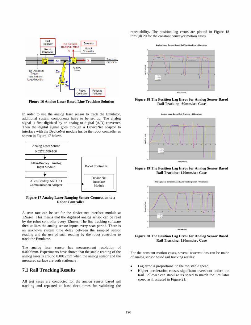
Figure 19 The Position Lag Error for Analog Sensor Based Rail Tracking: 120mm/sec Case

Figure 16 Analog Laser Based Line Tracking Solution Figure 18 The Position Lag Error for Analog Sensor Based Rail Tracking: 60mm/sec Case

Figure 20 The Position Lag Error for Analog Sensor Based Rail Tracking: 120mm/sec Case

In order to use the analog laser sensor to track the Emulator, additional system components have to be set up. The analog signal is first digitized by an analog to digital (A/D) converter. Then the digital signal goes through a DeviceNet adaptor to interface with the DeviceNet module inside the robot controller as shown in Figure 17 below.

For the constant motion cases, several observations can be made of encoder based rail tracking results:

Lag error is proportional, although not exactly linearly, to the stable top speed. Higher acceleration does not increase the total lag error: it seems to have reduced the total lag error slightly (about 1mm) for the rail tracking. And all test cases are repeatable within 1mm.

For the emulated conveyor bounce motion case, the position lag error is plotted in Figure 8.

A scan rate can be set for the device net interface module at 12msec. This means that the digitized analog sensor can be read by the robot controller every 12msec. The line tracking software then utilizes the analog sensor inputs every scan period. There is an unknown system time delay between the sampled sensor reading and the use of such reading by the robot controller to track the Emulator.

The analog laser sensor has measurement resolution of 0.0006mm. Experiments have shown that the stable reading of the analog laser is around 0.0012mm when the analog sensor and the measured surface are both stationary.

7.1 Rail Tracking Results

All test cases are conducted for the analog sensor based rail tracking and repeated at least three times for validating the

repeatability. The position lag errors are plotted in Figure 18 through 20 for the constant conveyor motion cases.

Figure 17 Analog Laser Ranging Sensor Connection to a Robot Controller

Analog Laser Sensor

NCDT1700-100

Allen-Bradley Analog Input Module

Allen-Bradley AND I/O Communication Adapter

For the constant motion cases, several observations can be made of analog sensor based rail tracking results:

Lag error is proportional to the top stable speed. Higher acceleration causes significant overshoot before the Rail Follower can stabilize its speed to match the Emulator speed as illustrated in Figure 21.

Robot Controller

Device NetInterface Module

196

Figure 21 The Rail Follower Overshoots Before Stabilizes in High Acceleration Case

For the emulated conveyor bounce motion case, the position lag error is plotted in Figure 22.

Figure 22 The Position Lag Error for the Analog Sensor Based Rail Tracking: Emulated Conveyor Bounce Case

Compared with the encoder based rail tracking result shown in Figure 8, The analog laser based rail tracking exhibits significant overshoot and oscillation.. Further examination of the Rail Follower speed identifies the root cause of the large position lag error as shown by Figure 23. With the analog sensor’s inputs, the Rail Follower can not closely follow the Emulator speed.

Figure 23 The Emulator Speed vs. The Rail Follower Speed with the Analog Laser

Table 6 below summarizes the results of the analog laser rail tracking test cases.

Table 6 Analog Laser (0.0012mm Resolution) Based Rail Tracking Performance

Line Rate (JPH)

Conveyor Constant

Speed (mm/sec)

Acceleration(mm/sec^2)

Range of PositionTracking

Error(mm)

Repeatability (mm)

150

320

650

745

< 7.0mm < 2.5mm 40 JPH

60 mm/sec -11190

(emergency stop) Overshoot

-5.5mm < 1.0mm

150

320

650

745

< 14.0mm < 2.0mm 60 JPH

120mm/sec

-11190(emergency stop)

Overshoot-8.0mm <1.0mm

150

320

650

745

< 18.5mm < 4.0mm 80 JPH

160mm/sec -11190

(emergency stop) Overshoot-12.0mm < 2. 0mm

40 JPH 60 mm/sec

Bounce with various

magnitude

-3.0mm ~ 21.0mm < 5.0mm

Compared with the encoder based rail tracking of Table 2, the rail tracking with the analog laser has

larger position lag error for constant motion speeds,worse repeatability, significantly worse emergency stop performance, and significantly larger position lag error for the dynamic motion speed.

7.2 Arm Tracking Results

All test cases are conducted for the analog laser based arm tracking and repeated at least three times to validate the repeatability. The position lag errors are plotted in Figure 24 through 26 for the constant conveyor motion cases.

197

Figure 24 The Position Lag Error for the Analog Sensor Based Arm Tracking: 60mm/sec Case

Figure 25 The Position Lag Error for the Analog Sensor Based Arm Tracking: 120mm/sec Case

Figure 26 The Position Lag Error for the Analog Sensor Based Arm Tracking: 160mm/sec Case

Figure 27 The Emulated Speed vs. The Arm Follower Speed with the Analog Laser Sensor

Figure 28 The Position Lag Error for the Analog Laser Arm Tracking: Emulated Conveyor Bounce Case

Figure 29 The Emulator Speed vs. The Arm Follower Speed with the Analog Sensor

For the constant motion cases, similar observations can be made of encoder based arm tracking results:

Lag error is proportional to the top stable speed. Higher acceleration causes significant overshoot before the Arm Follower can stabilize its speed to match the Emulator speed as illustrated in Figure 27.

For the emulated conveyor bounce motion case, the position lag error is plotted in Figure 28.

Compared with the encoder based arm tracking results shown in Figure 12, the analog laser based arm tracking exhibits significant overshoot and oscillation.. Further examination of the Arm Follower speed identifies the root cause of the large position lag error as shown by Figure 29 below. With the analog sensor’s inputs, the Arm Follower can not closely follow the Emulator speed.

198

Table 7 below summarizes the results of the analog laser sensor based arm tracking test cases.

Table 7 Analog Laser (0.0012mm Resolution) Based Arm Tracking Performance

Line Rate (JPH)

Conveyor Constant

Speed (mm/sec)

Acceleration(mm/sec^2)

Range of PositionTracking

Error(mm)

Repeatability (mm)

150

320

650

745

< 6.5mm < 1.0mm 40 JPH

60 mm/sec -11190(emergency

stop)

Overshoot-5.0mm < 1.0mm

150

320

650

745

< 12.0mm < 2.0mm 60 JPH

120mm/sec

-11190(emergency

stop)

Overshoot-7.5mm < 1.0mm

150

320

650

745

< 17.0mm < 2.0mm 80 JPH

160mm/sec -11190

(emergency stop)

Overshoot-10.0mm < 1.0mm

40 JPH

60 mm/sec

Bounce with various

magnitude

-2.0mm ~ 19.0mm < 6.0mm

Compared with the encoder based arm tracking of Table 3, the arm tracking with the analog laser has

larger position lag error for constant motion speeds,worse repeatability, significantly worse emergency stop performance, and significantly larger position lag error for the dynamic motion speed.

8. CONCLUSIONSUnlike the line tracking for automotive paint applications where the speed match between the robot and the vehicle body plays critical role for the paint quality, the line tracking for automotive general assembly applications requires position tracking of the system to perform assembly operations within a required assembly tolerance for a period of time. By comparing and contrasting experimental results, key performance drivers for the robotic line tracking can be concluded. Among three line tracking solutions, the encoder-based tracking method offers the tightest and most responsive robotic tracking performance. The encoder plus static vision based tracking method can be used for compensating the steady-state tracking position lag and the initial object offsets. The analog sensor-based tracking method is the least responsive due to its delayed signal propagation in the entire system.

Two key drivers have been identified for impacting the line position tracking performance:

Sensor resolution: it limits how tight the robot system can track the conveyor line motion.

Actual time delay of applying the sensor data: it limits how dynamically responsive the robot system can respond to the change in the conveyor line motion.

By understanding current capabilities of line tracking solutions, appropriate robotic automation systems can be developed and designed for a variety of GA applications. Key fundamental system drivers can be specified for robots to track the moving conveyor accurately enough for the specific assembly tolerance plus the environment uncertainty with adequate dynamic response at the appropriate location for the general assembly automation.

9. ACKNOWLEDGMENTS

The authors would like to acknowledge Bob Scheuerman, Marty Linn, Marjorie Winston, Thomas McGraw, Ke Zhang-Miske, Brooks A. Curtis, Ronald Reardon, Loring Dohm, Michael Poma, Neil McKay, Charles W. Wampler, and Roland Menassa. Their inputs, support, contribution, and knowledge have shaped this project from its initial concept to the final results.

10. REFERENCES

[1] J. Shi, “Preliminary Analysis of Conveyor Dynamic Motion for Automation Applications”, PreMIS’08, 2008

[2] G. DeSouza, “A Subsumptive, Hierarchical, and Distributed Vision-based Architecture for Smart Robotics”, Ph.D. Dissertation, School of Electrical and Computer Engineering, Purdue University, May 2002

[3] Analog Laser Ranging Sensor ILD1700 www.micro-epsilon.com

199

Mobile Robotic Surveying Performance for Planetary Surface Site Characterization

Edward Tunstel Space Department

Johns Hopkins University Applied Physics Laboratory

Laurel, MD 20723 USA

Edward.Tunstel@jhuapl.edu

ABSTRACT Robotic systems will perform mobile surveys for scientific and engineering purposes as part of future missions on lunar and planetary surfaces. With site characterization as a task objective various system configurations and surveying techniques are possible. This paper describes several examples of mobile surveying approaches using local and remote sensing configurations. A geometric measure of area coverage performance is applied to each and relative performance in surveying a common area is characterized by expected performance trends. Performance metrics that solely express geometric aspects of the task are limited in utility as decision aids to mission operators. As such, the importance of enriching such metrics by incorporating additional attributes germane to surveying on planetary surfaces is highlighted.

Keywords robotic surveying, planetary surface exploration, in-situ remote sensing, area coverage performance, site characterization

1. INTRODUCTION Task-oriented algorithms that support systematic mobile surveys using science instruments are needed for planetary surface characterization on science missions. They are also needed for in-situ resource mapping on robotic missions that serve as precursors to human exploration missions. Typical objectives of site surveys include sensor coverage of designated areas. Area coverage problems for mobile robotic survey systems commonly employ sensing devices requiring close proximity to or contact with the measured phenomenon. Examples of such “local sensing” devices include ground penetrating radar, metal detectors for humanitarian de-mining, fluorescence imagers for organic molecule detection, a variety of spectrometer types, etc. Mobile robotic vehicles, or rovers, that carry survey systems comprised of local sensing devices must physically cover most, if not all, of the terrain in the designated survey area.

Remote sensor-based area coverage contrasts with these more common area coverage problems for mobile robotic surveys. Remote sensing instruments (e.g., based on radar or optical devices such as lasers) can acquire measurements at significant distances away from the measured phenomenon. Measurements along a line-of-sight to detect airborne phenomena such as surface gas emissions, for example, account for coverage of terrain below that line-of-sight. This permits a two-dimensional search over terrain using discrete linear measurements from a distance (similar to scanning laser rangefinders).

Remote sensor-based methods are not applicable to all surveying tasks. For surveys in which they are not a better solution, they are often excellent complements to local sensor-based methods. That is, remote sensor-based surveys can serve as an efficient means to cover wide areas with the purpose of localizing smaller areas at which local sensor-based surveys of higher resolution are appropriate.

Mobility algorithms for surveying provide a means to systematically acquire measurements covering an area to be surveyed by transporting sensors and instruments to multiple locations and vantage points. Algorithms employing parallel-line transects or parallel swaths are commonly used to address robotic area coverage problems by single robots [1, 2] and multiple robots [3] when using local sensing devices. Full and partial coverage planners have also been proposed for rovers that survey terrain using local sensing devices [4]. Remote sensor-based survey approaches for rovers have recently been proposed for single- and two-rover systems performing measurements through the near-surface atmosphere [5, 6].

This paper examines examples of both mobile survey types and applies a geometric measure of their area coverage performance. It further suggests additional attributes germane to surveying tasks for planetary surface exploration. The additional attributes are intended to enrich the effectiveness and relevance of basic geometric measures or support formulation of new metrics for planetary surface domains.

2. LOCAL SENSOR-BASED SURVEYING Due to required proximity to measured phenomena and relatively small footprints of sensitivity, local sensing devices typically necessitate dense coverage of a designated survey region by the host mobile platform. As such, local sensor-based mobile surveys seek to acquire measurements that cumulatively cover all or most of the survey region. Associated survey sensors or instruments are typically mounted on a rover body or deployed on a rover-

Permission to make digital or hard copies of all or part of this work for personal or classroom use is granted without fee provided that copies are not made or distributed for profit or commercial advantage and that copies bear this notice and the full citation on the first page. To copy otherwise, or republish, to post on servers or to redistribute to lists, requires prior specific permission and/or a fee. PerMIS’08, August 19–21, 2008, Gaithersburg, MD, USA. Copyright 2008 ACM 978-1-60558-293-1…$5.00.

200

attached boom or manipulator arm. Rover mobility serves to transport the footprint of the survey instrument(s) over terrain along trajectories that fill the survey region. Fig. 1 depicts this scenario.

Figure 1. Local sensor-based surveying along n parallel transects of length m.

Among alternative survey trajectories for the mobile platform, parallel transects, spirals, and random walks have been proposed. Parallel transects are most commonly applied for coverage tasks although a spiral coverage approach was proposed for mobile mining of regolith on the lunar surface as part of a so-called spiral mining system [7]. Recent field tests, focused on planetary surface site characterization, used a rover operating ground penetrating radar (GPR) along parallel transects covering a 700 m x 700 m survey region [8]. This instrument was used to map the subsurface structure at the site. A total traverse distance of 20.5 km was sufficient to cover the survey region using densely spaced parallel transects (with no overlap of the GPR sensor footprint on adjacent transects) [8].

Basic geometric measures are often used to measure area coverage performance of such local sensor-based survey algorithms. Examples include measures of distance traveled and percent of total area covered [2]. Variants of the latter have been proposed based on distribution of measurement samples within the cells of a tessellated grid representation of the survey region [4]. Here, we apply a basic geometric measure comprising a combination of such attributes. It is referred to as the quality of performance, QoP, defined as a ratio of area covered to distance traveled [9]. Applying this metric to the recent field test result mentioned above would yield a QoP of 24 based on the survey region area and total traverse distance. In general, the QoP for a local sensor-based survey along parallel transects (Fig. 1) is computed as

Q p =

m(n 1) p

[mn + (n 1) p] (1)

where m is the transect length, n is the number of transects traversed, and p is the separation distance between adjacent transects and is assumed here to be comparable to the survey sensor footprint. The numerator and denominator of Eq. (1) respectively represent the area surveyed and total distance traversed during the survey.

In the next section we discuss mobile surveying using in-situ remote sensing and apply the same metric to area coverage performance of several types of remote sensor-based survey trajectories.

3. REMOTE SENSOR-BASED SURVEYING Mobile remote sensor-based surveys can be performed by measurement systems whose components are separated by a distance across terrain. Such systems are comprised of an active/passive instrument component on one end and a passive/active component on the other end. One end could be stationary while the other is mobile (fixed-mobile) or both ends could be mobile (mobile-mobile). Both are considered here beginning with a fixed-mobile configuration, which is suitable for single-site surveys (unless the fixed component is also transportable to other sites).

3.1 Single-Site Remote Sensing Surveys Consider a fixed-mobile configuration comprised of an active rover-mounted instrument, a passive receiver or retroreflector at a fixed location a distance away, a rover pan-tilt unit to point the instrument at the passive component for measurements, and the rover itself to move the instrument spatially over terrain. The passive component would remain stationary at a position central to a designated survey region. This configuration is similar to those of Total Station systems commonly used by civil engineers for land surveys and comprised of a theodolite on one end and stationary 360° retroreflector on the other. Like a civil engineer, a rover using such a survey system can acquire measurements from any radial direction when the fixed component is within line-of-sight and measurement range.

For mobile surveys, measurements are coordinated with rover mobility to survey terrain via a series of measurements across a distance d, which varies with rover position relative to the fixed component (Fig. 2). Such mobile robotic systems are under development for planetary surface surveying to achieve optical measurements at maximum distances of hundreds of meters [10]. The long-range measurement capability coupled with rover mobility enables wide-area surveys.

Figure 2. Example of a distributed fixed-mobile measurement configuration.

Concentric circular or spiral trajectories are compatible with distributed fixed-mobile configurations for remote sensor-based surveying. A designated survey region with a fixed instrument component at its center can be covered by traversing concentric circular trajectories as follows. The location of the fixed component is known and considered to be the origin of an inertial coordinate system in which the survey region and task is defined. Rover pose during surveys is estimated relative to this coordinate system. Beginning at a designated radial distance from the fixed component, the rover moves in arc-increments stopping periodically on the trajectory to acquire measurements. We refer to these measurement locations as m-nodes. Measurements along a line-of-sight between the rover-mounted active instrument and the fixed component account for 2-D coverage of terrain below the line-of-sight. Such measurement techniques are used on Earth

201

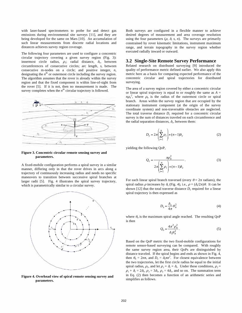
with laser-based spectrometers to probe for and detect gas emissions during environmental site surveys [11], and they are being developed for the same on Mars [10]. An accumulation of such linear measurements from discrete radial locations and distances achieves survey region coverage.

The following four parameters are used to configure a concentric circular trajectory covering a given survey region (Fig. 3): innermost circle radius, 1; radial distance, c, between circumferences of consecutive circles; arc length, s, between consecutive m-nodes on a circle; and positive integer, n, designating the nth or outermost circle including the survey region. The algorithm assumes that the rover is already within the survey region and that the fixed component is within line-of-sight from the rover [5]. If it is not, then no measurement is made. The survey completes when the nth circular trajectory is followed.

Figure 3. Concentric circular remote sensing survey and parameters.

A fixed-mobile configuration performs a spiral survey in a similar manner, differing only in that the rover drives in arcs along a trajectory of continuously increasing radius and needs no specific maneuvers to transition between successive spiral branches at larger radii [5]. Fig. 4 illustrates the spiral survey trajectory, which is parametrically similar to a circular survey.

Figure 4. Overhead view of spiral remote sensing survey and

parameters.

Both surveys are configured in a flexible manner to achieve desired degrees of measurement and area coverage resolution using the four parameters ( , , s, n). The surveys are primarily constrained by rover kinematic limitations, instrument maximum range, and terrain topography in the survey region whether executed radially inward or outward.

3.2 Single-Site Remote Survey Performance Related research on distributed surveying [9] introduced the quality of performance metric defined earlier. We also apply this metric here as a basis for comparing expected performance of the concentric circular and spiral trajectories for distributed surveying.

The area of a survey region covered by either a concentric circular or linear spiral trajectory is equal to or roughly the same as A =

n2, where n is the radius of the outermost circle or spiral

branch. Areas within the survey region that are occupied by the stationary instrument component (at the origin of the survey coordinate system) and non-traversable obstacles are neglected. The total traverse distance Dc required for a concentric circular survey is the sum of distances traveled on each circumference and the radial separation distances, c, between them:

Dc = 2 ii=1

n

+ (n 1) c (2)

yielding the following QoP,

Qc = n2

2 ii=1

n

+ (n 1) c

. (3)

For each linear spiral branch traversed (every = 2 radians), the spiral radius increases by s (Fig. 4), i.e., = ( s/2 ) . It can be shown [12] that the total traverse distance Ds required for a linear spiral trajectory is then expressed as

Ds = s

4 n2 (4)

where n is the maximum spiral angle reached. The resulting QoP is then

Qs =

4 2n2

s n2

. (5)

Based on the QoP metric the two fixed-mobile configurations for remote sensor-based surveying can be compared. With roughly the same survey region area, their QoPs are distinguished by distance traveled. If the spiral begins and ends as shown in Fig. 4, then n = 2n , and Ds = s n2. For closest equivalence between the two trajectories, let the first circle radius be equal to the initial spiral radius, 1, and let 1 = c = s. Under these conditions, 2 =

1 + c = 2 c, 3 = 3 c, 4 = 4 c, and so on. The summation term in Eq. (2) then becomes a function of an arithmetic series and simplifies as follows.

m-nodes

202

i

i=1

n= c + 2 c + 2 c + ... + n c (6)

= c(1+ 2 + 3+ ... + n)

= c12

n(n +1)[ ]

Using this result in Eq. (2), we have

Dc = 2 c

12

n(n +1)[ ] + (n 1) c (7)

= c n2 + ( +1)n 1[ ] .

Therefore, Dc > Ds independent of an equivalent separation distance. A rover executing a concentric circular survey of n circles would need to traverse over (4n–1) c meters more to cover the same area as it could with a spiral trajectory of n branches. As an example, to traverse a survey trajectory of n = 3 concentric circles separated by c = 10 m, a rover would drive a linear distance of 397 m; to survey a roughly equivalent area using a spiral trajectory of n = 3 branches separated by s = 10 m it would drive a linear distance of 283 m, or 29% less in this case.

3.3 Multiple-Site Remote Sensing Surveys An example of a mobile-mobile, or tandem, survey system configuration is illustrated in Fig. 5. Both rovers could carry the active and passive components of the distributed survey instrument (e.g., for redundancy), or each rover could carry the companion component to the other’s payload. Such survey configurations are suitable for multiple-site surveys due to the mobility of both platforms. The same dual mobility enables this tandem configuration to perform a number of approaches to remote sensor-based mobile surveying including, as special cases, the approaches described above for single-site surveys.

Figure 5. Tandem distributed remote sensing configuration.

3.4 Multi-Site Remote Survey Performance A tandem-robot system was proposed in [6, 9] in which one robot carried an active instrument and the other carried the instrument’s passive receiver. The robots would cooperatively perform remote

sensor-based surveys using either parallel-swath or circular patterns where the width of a swath is the separation distance between the robots. The QoP metric was applied to compare several variants of these survey patterns including those illustrated below in Fig. 6. These survey approaches are referred to here as tandem-parallel and tandem-circular, and the QoPs for each are:

Qtp =

mn tp

[2mn + 2(n 1) tp] (8)

Qtc =(n tc / 2)2

tc2

n2 + 2n 4( ) (9)

where m is the length of a surveyed parallel swath (see Fig. 6), tp and tc are the robot separation/measurement distances during a survey, and n (in both equations) is the total number of swaths surveyed [9]. The denominators of Eqs. (8) and (9) express the total distances, Dtp and Dtc, traversed by both robots for the respective tandem survey types.

Figure 6. Tandem parallel and circular remote sensing survey

trajectories.

4. CHARACTERISTIC PERFORMANCE OF MOBILE SURVEYS

The use of a common performance metric to comparatively rank a set of options provides a valuable basis or choosing the best option for a given task. However, direct one-to-one comparisons of the mobile surveying approaches discussed above are not straightforward given their respective differences in survey system configuration and survey trajectories. In fact, they can be prescribed for considerably different types of survey tasks in practice. Nonetheless, somewhat common grounds for comparison would provide a general sense for the relative performance of each approach. As a useful compromise a characteristic comparison is made here, still using a common metric, but based on assumptions that serve to equalize differences across the set of options. We use the QoP as the common metric here but any of a variety of metrics could be used instead.

203

Consider a mobile survey of a designated region with common area, A, and performed by each of the local and remote sensor-based methods discussed above. Recall that the metric for each survey type is the total area covered divided by the total distance traversed, D, during the survey (QoP = A/D). Since A is considered to be a common survey region size, differences in the QoP are a function of differences in D only. Further assume that each survey is designed for a comparable area coverage resolution; this would call for equal values of the parameters p,

c, s, tp, and tc. For the respective QoPs given by Eqs. (1), (3), (5), (8), and (9), the distance traveled is a function of the area coverage resolution. For simplicity, we assume a value of unity as the common value for the respective resolution parameters. With this assumption the expression of distance traversed for each QoP becomes a function of parameter n only, with the exception of Qp and Qtp, i.e., the local parallel and tandem-parallel survey metrics in Eqs. (1) and (8). If we assume a square survey region, then the length of a transect for a local parallel survey becomes m = (n-1) p = (n-1), since p is set to unity. Similarly, the length of a swath for a remote tandem-parallel survey becomes m = n tp = n, since tp is set to unity. With all traverse distances as functions of the n-parameter for each survey type the following characteristic expressions, D(n), can be created

D p(n) = n2 1 (10)

Dc(n) = n2+ ( +1)n 1 (11)

Ds(n) = n2 (12)

Dtp(n) = 2n2+ 2(n 1) (13)

Dtc(n) = 1

2n2

+ n 2 . (14)

Note that Eqs. (10)-(14) are only characteristic of the respective distances traversed due to the different meanings for n for each survey type, i.e., the number of parallel transects, concentric circles, spiral branches, and parallel swaths. For this discussion we will generally refer to n as the number of survey passes. Fig. 7 shows the characteristic trends of traverse distances required by each mobile survey configuration to cover the same area with comparable coverage resolution.

The characteristic trends are shown for up to 100 survey passes. As the number of survey passes increases the characteristic distances for the circular and spiral remote sensor-based surveys increase at the fastest and roughly the same rate. Circular remote-sensing surveys require the longest characteristic traverse distances. The inset graph in Fig. 7, which shows the same trends for up to an order of magnitude less survey passes (up to 10), reveals a more pronounced difference between expected distances required for circular and spiral surveys. The QoPs for these fixed-mobile surveys would be expected to decrease most rapidly with large numbers of survey passes, while higher QoPs would be expected for spiral surveys with low numbers of passes. For the tandem configurations, parallel circular surveys would be expected to perform better than parallel swath surveys, which would require characteristically longer traverse distances. The QoPs for tandem approaches would be expected to be higher than those of fixed-mobile approaches for the same survey region and coverage resolution. This reflects the advantage of using more than one rover for distributed remote sensing survey tasks [6]. The popular parallel transect survey approach for single rovers

with local sensing devices has the slowest trend of increasing distance as the number of survey passes increases. Thus, its QoP would be expected to be high and least impacted by n, relative to the other approaches, for surveying the same area at a comparable coverage resolution.

Figure 7. Characteristic traverse distances for mobile survey

configurations.

5. ENRICHING METRICS FOR SURVEYS ON PLANETARY SURFACES

Thus far we have considered evaluation of coverage performance for surveys based on simple geometric measures of area and distance. Other important measures should be considered to enrich performance evaluation in the domain of planetary robotic systems and otherwise resource-constrained field robot systems. In fact, the selection of a candidate survey trajectory type for a given survey region can be based on metrics that provide some measure of relative resource usage during trajectory following (e.g., time, power, survey data storage). Selection of a survey type can also be based on any known physical constraints about the survey region such as terrain topography or the size and distribution of phenomena to be measured.

Past work provides guidance in this direction. For example, maximization of incident solar energy on rover solar arrays has been considered as a determinant for selection among several survey trajectory types [13]. Another study applied an energy efficiency metric, defined as a ratio of area covered to energy consumed, to evaluate parallel line, circular spiral, and square spiral trajectories [12]. Other attributes can be adopted that are germane to surveying for planetary surface exploration but proposed in the context of mobility/navigation or task performance. These include terrain traversability measures such as obstacle abundance [14, 15] and number or effort of rovers and humans operators involved [16]. While identifying domain specific attributes that would enrich the relevance of existing geometric measures is helpful, the manner in which they would be incorporated into a metric formulation is also worth considering. Computationally complicated metric formulations can sometimes make the use of a metric as a decision aid difficult or can obscure the interpretation of the metric. In the domain of planetary site characterization a host of system, mission, and/or environmental constraints will affect the performance of mobile surveying tasks.

204

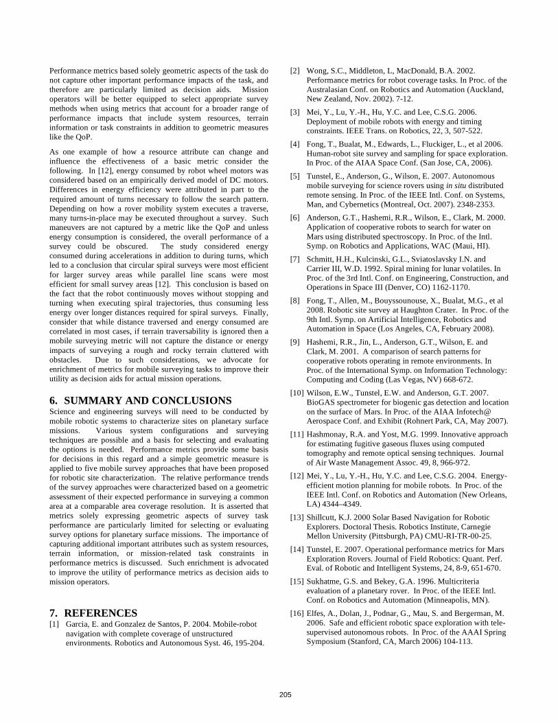
Performance metrics based solely geometric aspects of the task do not capture other important performance impacts of the task, and therefore are particularly limited as decision aids. Mission operators will be better equipped to select appropriate survey methods when using metrics that account for a broader range of performance impacts that include system resources, terrain information or task constraints in addition to geometric measures like the QoP.

As one example of how a resource attribute can change and influence the effectiveness of a basic metric consider the following. In [12], energy consumed by robot wheel motors was considered based on an empirically derived model of DC motors. Differences in energy efficiency were attributed in part to the required amount of turns necessary to follow the search pattern. Depending on how a rover mobility system executes a traverse, many turns-in-place may be executed throughout a survey. Such maneuvers are not captured by a metric like the QoP and unless energy consumption is considered, the overall performance of a survey could be obscured. The study considered energy consumed during accelerations in addition to during turns, which led to a conclusion that circular spiral surveys were most efficient for larger survey areas while parallel line scans were most efficient for small survey areas [12]. This conclusion is based on the fact that the robot continuously moves without stopping and turning when executing spiral trajectories, thus consuming less energy over longer distances required for spiral surveys. Finally, consider that while distance traversed and energy consumed are correlated in most cases, if terrain traversability is ignored then a mobile surveying metric will not capture the distance or energy impacts of surveying a rough and rocky terrain cluttered with obstacles. Due to such considerations, we advocate for enrichment of metrics for mobile surveying tasks to improve their utility as decision aids for actual mission operations.

6. SUMMARY AND CONCLUSIONS Science and engineering surveys will need to be conducted by mobile robotic systems to characterize sites on planetary surface missions. Various system configurations and surveying techniques are possible and a basis for selecting and evaluating the options is needed. Performance metrics provide some basis for decisions in this regard and a simple geometric measure is applied to five mobile survey approaches that have been proposed for robotic site characterization. The relative performance trends of the survey approaches were characterized based on a geometric assessment of their expected performance in surveying a common area at a comparable area coverage resolution. It is asserted that metrics solely expressing geometric aspects of survey task performance are particularly limited for selecting or evaluating survey options for planetary surface missions. The importance of capturing additional important attributes such as system resources, terrain information, or mission-related task constraints in performance metrics is discussed. Such enrichment is advocated to improve the utility of performance metrics as decision aids to mission operators.

7. REFERENCES [1] Garcia, E. and Gonzalez de Santos, P. 2004. Mobile-robot

navigation with complete coverage of unstructured environments. Robotics and Autonomous Syst. 46, 195-204.

[2] Wong, S.C., Middleton, L, MacDonald, B.A. 2002. Performance metrics for robot coverage tasks. In Proc. of the Australasian Conf. on Robotics and Automation (Auckland, New Zealand, Nov. 2002). 7-12.

[3] Mei, Y., Lu, Y.-H., Hu, Y.C. and Lee, C.S.G. 2006. Deployment of mobile robots with energy and timing constraints. IEEE Trans. on Robotics, 22, 3, 507-522.

[4] Fong, T., Bualat, M., Edwards, L., Fluckiger, L., et al 2006. Human-robot site survey and sampling for space exploration. In Proc. of the AIAA Space Conf. (San Jose, CA, 2006).

[5] Tunstel, E., Anderson, G., Wilson, E. 2007. Autonomous mobile surveying for science rovers using in situ distributed remote sensing. In Proc. of the IEEE Intl. Conf. on Systems, Man, and Cybernetics (Montreal, Oct. 2007). 2348-2353.

[6] Anderson, G.T., Hashemi, R.R., Wilson, E., Clark, M. 2000. Application of cooperative robots to search for water on Mars using distributed spectroscopy. In Proc. of the Intl. Symp. on Robotics and Applications, WAC (Maui, HI).

[7] Schmitt, H.H., Kulcinski, G.L., Sviatoslavsky I.N. and Carrier III, W.D. 1992. Spiral mining for lunar volatiles. In Proc. of the 3rd Intl. Conf. on Engineering, Construction, and Operations in Space III (Denver, CO) 1162-1170.

[8] Fong, T., Allen, M., Bouyssounouse, X., Bualat, M.G., et al 2008. Robotic site survey at Haughton Crater. In Proc. of the 9th Intl. Symp. on Artificial Intelligence, Robotics and Automation in Space (Los Angeles, CA, February 2008).

[9] Hashemi, R.R., Jin, L., Anderson, G.T., Wilson, E. and Clark, M. 2001. A comparison of search patterns for cooperative robots operating in remote environments. In Proc. of the International Symp. on Information Technology: Computing and Coding (Las Vegas, NV) 668-672.

[10] Wilson, E.W., Tunstel, E.W. and Anderson, G.T. 2007. BioGAS spectrometer for biogenic gas detection and location on the surface of Mars. In Proc. of the AIAA Infotech@ Aerospace Conf. and Exhibit (Rohnert Park, CA, May 2007).

[11] Hashmonay, R.A. and Yost, M.G. 1999. Innovative approach for estimating fugitive gaseous fluxes using computed tomography and remote optical sensing techniques. Journal of Air Waste Management Assoc. 49, 8, 966-972.

[12] Mei, Y., Lu, Y.-H., Hu, Y.C. and Lee, C.S.G. 2004. Energy-efficient motion planning for mobile robots. In Proc. of the IEEE Intl. Conf. on Robotics and Automation (New Orleans, LA) 4344–4349.

[13] Shillcutt, K.J. 2000 Solar Based Navigation for Robotic Explorers. Doctoral Thesis. Robotics Institute, Carnegie Mellon University (Pittsburgh, PA) CMU-RI-TR-00-25.

[14] Tunstel, E. 2007. Operational performance metrics for Mars Exploration Rovers. Journal of Field Robotics: Quant. Perf. Eval. of Robotic and Intelligent Systems, 24, 8-9, 651-670.

[15] Sukhatme, G.S. and Bekey, G.A. 1996. Multicriteria evaluation of a planetary rover. In Proc. of the IEEE Intl. Conf. on Robotics and Automation (Minneapolis, MN).

[16] Elfes, A., Dolan, J., Podnar, G., Mau, S. and Bergerman, M. 2006. Safe and efficient robotic space exploration with tele-supervised autonomous robots. In Proc. of the AAAI Spring Symposium (Stanford, CA, March 2006) 104-113.

205

Evaluating Situation Awareness of Autonomous Systems

Jan D. GehrkeCenter for Computing Technologies (TZI)

Universität BremenAm Fallturm 1, 28359 Bremen, Germany

jgehrke@tzi.de

ABSTRACTAutonomous systems proved to be very successful in spe-cialized problem domains. But their perception, reasoning,planning and behavior capabilities are generally designed tofit special purposes. For instance, a robotic agent perceivesits environment in a way that was defined in advance bya human designer. The agent does not exhibit a certainperception behavior because it actually thinks it would bereasonable to do so. But with an increasing level of au-tonomy as well as a larger temporal and spatial scope ofagent operation higher-level situation analysis and assess-ment become essential. This paper examines criteria forevaluating situation-awareness of autonomous systems andproposes methods to satisfy them. An example applicationscenario is presented that provides initial results for evalu-ating situation-aware systems.

1. INTRODUCTIONAutonomous systems are being developed for numerous

application areas. These systems proved to be very success-ful in specialized problem domains, e. g., road driving, areaexploration, or robot soccer. Nevertheless, in many cases,the perception, reasoning, planning and behavior capabil-ities of autonomous systems are designed to fit a specialpurpose. For instance, a robotic agent perceives its envi-ronment in a way that was defined in advance by a hu-man designer. Therefore, the agent does not show a certainperception behavior because it actually thinks it would bereasonable to do so. It is a reflex rather than a deliberateaction. For a lot of applications this might be sufficient.But with an increasing level of autonomy as well as a largertemporal and spatial scope of agent operation higher-levelsituation analysis and assessment become essential. We willfocus on knowledge-based autonomous systems that requireup-to-date knowledge to decide on their next course of ac-tion. Knowledge-based systems are particularly challengingif they require knowledge of distant locations and/or predic-tion of future events. These systems cannot rely on their own

Permission to make digital or hard copies of all or part of this work forpersonal or classroom use is granted without fee provided that copies arenot made or distributed for profit or commercial advantage and that copiesbear this notice and the full citation on the first page. To copy otherwise, torepublish, to post on servers or to redistribute to lists, requires prior specificpermission and/or a fee.PerMIS ’08, August 19–21, 2008, Gaithersburg, MD, USACopyright 2008 ACM 978-1-60558-293-1 ...$5.00.

sensory capabilities only. They need to infer future statesand communicate with other agents to share information.

Situation assessment depends on the current goals of theautonomous system and knowledge about the state of theworld. The relevance of a specific piece of information orsome kind of information for situation assessment is deter-mined by the current plan and other potential plans underconsideration. Information relevance leads to the pragmaticdimension of knowledge-based systems, i. e., information onhow to use information. Usually, this is implicitly specifiedby the decision system. For instance, the decision systemmay use behavior rules whose rule body implies the informa-tion needed to evaluate the rule head. Problems arise if thedecision-relevant information is not available to the agent.Depending on the applied knowledge representation and rea-soning mechanism, missing information is simply consideredundefined, default-valued, or false. The latter applies forpredicates when using negation as failure [7] as in logic pro-gramming. This seems inadequate for autonomous systemsin partially observable environments. Even the Open WorldAssumption turns out to be insufficient for situation assess-ment. While it prevents to assume wrong states of the un-known world and to base inferences on them, it does notdirectly enable to reason about what is unknown. As a con-sequence, the system would not be able to assess a situationcorrectly, e. g., to detect a harmful risk, because it has a lackof information which it is not aware of.

Hence, autonomous systems doing situation assessmenthave to be enabled to detect unknown information, therebybecoming known unknowns. This detection process mustbe governed and prioritized by information relevance. Ifthe agent’s sensory capabilities cannot provide informationneeded, other agents or information sources have to be in-quired. As an alternative, the agent has to accept its lack ofinformation and address it, e. g., by more cautious behavior.

Only autonomous systems possessing such higher levelreasoning capabilities are able to have true situation aware-ness [10]. It even becomes more complicated if agents haveto reason about future events. Such agents would needprediction abilities including knowledge on how the worldevolves in order to qualify the probability that some infor-mation does not change in a given time interval. In spa-cious environments with mobile robots, additional spatialreasoning about information dynamics is required. This pa-per outlines a classification of criteria for situation awarenessof autonomous systems and suggests knowledge representa-tion and reasoning methods to address them.

The remainder of this paper is structured as follows. Sec-

206

tion 2 discusses issues of situation awareness in establishedautonomous system architectures. Section 3 defines and ex-amines awareness criteria and possible techniques to imple-ment them. A corresponding example scenario for a prelim-inary study is presented in section 4). The paper concludeswith a discussion of this survey (Sect. 5) and a summary(Sect. 6).

2. AUTONOMOUS AGENTS ANDSITUATION AWARENESS

Intelligent agents are a fundamental concept in ArtificialIntelligence for autonomous decision-making. For most ap-plications domains of agents up-to-date and precise knowl-edge on the state of the world is crucial for system per-formance. But surprisingly a lot of usual architectures donot explicitly consider the acquisition of information needed.This limitation might lead to suboptimal, wrong, or even dis-astrous decisions. Thus situation awareness for autonomoussystems intends to evaluate and establish the basis for de-cision making depending on the agent’s current tasks andgoals.

Williams et al. [22] have a similar goal. They evaluatethe so-called groundedness of representations in autonomoussystems (mainly those applied in RoboCup competitions).The approach defines a measure for the capability of cre-ating and maintaining correct associations between repre-sentations and their (physical) real-world counterparts inthe system’s knowledge base. Proposed qualities of ground-edness include, e. g., relevance, accuracy/precision, uncer-tainty management, and self-awareness w. r. t. the state ofthe robot body, location, and sensors. The correspondingsystem evaluation is rather qualitative and performed offlineby humans. Thus, the approach provides useful criteria forsystem evaluation but does not enable the system to reasonabout itself in order to improve its groundedness.

The simple reflex agent, as the most basic kind of agent,is the worst example for groundedness or situation aware-ness. Such agents are governed by condition/action rulesand always do the same thing given the same perception. Incontrast to the model-based reflex agent it has no internalstate influencing its decisions [20]. Both reflex agents can-not be considered situation-aware. The simple reflex agentonly takes into account instantaneous knowledge; the model-based variant has no notion of information relevance becauseit has no explicit goals. Anyway, there may be simple butuseful tasks that are successfully handled by reflex agents.

The most important term in AI is the rational agent.Wooldridge defines an agent to be “rational if it chooses toperform actions that are in its own best interests, given thebeliefs it has about the world” [23, p. 1]. But this definitioncould also consider an agent rational if it chooses an actionwithout knowing the state of the world. Thus, the situation-aware agent extends and substantiates the classical rationalagent definition. The belief about the world is no longertaken for granted but actively controlled by knowledge ac-quisition as an additional reasoning process.

The belief-desire-intention (BDI) model has become a pre-valent approach in academia for deliberative software agentarchitectures (cf. [23, 15]). It is based on a theory of humanpractical reasoning developed by Bratman [6]. Human prac-tical reasoning, according to BDI, consists of deliberation,i. e., deciding what state should be achieved, and means-

ends reasoning, i. e., deciding how to achieve it. In the BDImodel, an agent is represented by its subjective knowledgeabout the world (beliefs) and persistent goals that shouldbe achieved (desires). Desires and current beliefs result inachievable goals and possible actions towards them. Finally,in a process of deliberation, the agent commits to a goaland a corresponding plan (intention). The fundamental BDImodel does not consider the assessment of beliefs in terms ofcompleteness, correctness/uncertainty, or being up-to-datewith respect to the goals to be achieved. Additionally, themodel does not take into account different levels of decisionmaking with respect to real-time requirements or temporalscope of action and decision making.

The Real-time Control System (RCS) developed at Na-tional Institute of Standards and Technology (NIST) modelsan intelligent system as a hierarchy of goal-directed sensory-interactive control processes [2] representing organizationallevels as well as temporal scopes of decision making. Theprocess hierarchy in RCS enables the decomposition of sub-tasks to different agents as well as different planning in-tervals within a single agent. Each level contains computa-tional elements for sensory processing, world modeling, valuejudgment, and behavior generation [1]. Situation awarenesscould be assigned to the higher-level RCS world modelingcomponents with a tight connection to behavior generationand sensory processing. That is, RCS could be augmentedin world modeling by goal-oriented pro-active knowledge ac-quisition that is governed by behavior generation demandsand may provide a focus of attention in sensory processing.

3. CRITERIA FOR SITUATIONAWARENESS

Situation awareness is a field of research that commonlyexamines information requirements of humans for specialjobs such as facility monitoring or flying aircraft [10]. End-sley [9, p. 97] describes situation awareness as “the percep-tion of the elements in the environment within a volume oftime and space, the comprehension of their meaning and theprojection of their status in the near future”. This leads toEndsley’s three levels of situation awareness:

• Level 1 – Perception: Basic perception of importantinformation.

• Level 2 – Comprehension: Correct interpretationand integration of perceptions as well as relevance as-sessment.

• Level 3 – Projection: The ability to predict fu-ture situations based on current perceptions and back-ground knowledge.

Although the definition and the three levels of awarenessare intended for human situation awareness they can beadopted for autonomous systems, too. Nevertheless, thereare a lot of technical requirements that are partially takenfor granted regarding humans but much more challenging fortechnical systems. Thus, this section proposes the followingcriteria for situation awareness of autonomous systems andpossible methods to fulfill them:

1. Reasoning about ignorance: The agent’s knowl-edge base can be queried for unknown or uncertaininformation.

207

2. Model of perception abilities: The agent is awareof its sensors and the kind of information they maygenerate.

3. Model of information relevance: Based on the cur-rent set of goals or a general utility function as well asapplied decision rules, the agent can identify informa-tion needed and qualify its importance for its perfor-mance measure.

4. Model of information dynamics: Knowledge oninformation dynamics that provides stability informa-tion for prediction of future states of the world.

5. Spatio-temporal reasoning: The model of infor-mation dynamics is applied for temporal reasoning onchange over time and spatial reasoning on neighbor-hood and hierarchies of regions

6. Social ability: If agents need information beyondtheir sensory capabilities they have to cooperate withother agents for external information acquisition.

3.1 Reasoning about IgnoranceTo enable an autonomous system to measure awareness in

a given situation the system needs to know what it does notknow (known unknowns). That is, it has to detect a possiblelack of knowledge in its knowledge base. This is particularlyimportant and challenging in environments that are highlydynamic and only partially observable. Unfortunately, manylogic-based systems use negation as failure in reasoning, i. e.,propositions or predicates are assumed to be false if thereis no fact or prove stating the opposite. This closed worldassumption (CWA) is opposed to the open world assumption(OWA) which does not make any assumptions about missingknowledge. Instead, logical inference only relies on givenfacts.

Open world reasoning is particularly applied in ontologiesand description logics [3] for concept subsumption in on-tology TBoxes, i. e., the schema level of a knowledge base.Situation awareness is rather focused on the instance or as-sertional level (ABox) of a knowledge base. While the openworld assumption also applies for ABox reasoning, it doesnot provide inferences that would directly provide informa-tion on unknown facts. In contrast, a query for the truth offacts that are neither known nor deducible will just returnfalse.

As a consequence, CWA and OWA reasoning systems willcreate a biased view of the state of the world that is verylikely to be wrong. If decisions rely on that wrong beliefssystem performance is jeopardized. But a strictly logicalapproach to reason about agent ignorance will raise severaldifficulties for the logical foundations of representation andreasoning as well as computational efficiency. A structuralapproach that keeps track of knowledge base changes and in-stantly replies to queries on ignorance is probably preferable.Anyway, a three-valued logic with OWA reasoning would berequired, too.

In general, a strictly logic-based knowledge representationin dynamic environments is debatable. These approaches donot sufficiently handle the uncertainty that is an inevitableconsequence in such domains. Though logics are still veryuseful and powerful for representing background knowledgeof an autonomous system, dynamic environmental proper-ties should rather be represented by probabilistic approaches

with aleatory variables. In particular, Bayesian inferenceprovides powerful means to reason about uncertainty. Acorresponding approach for value measurement of missinginformation is presented in Sect. 3.3.

3.2 Model of Perception AbilitiesWhile it is important to be aware of ignorance, agents

might deliberately or of necessity choose to decide instantlyalthough having incomplete or uncertain knowledge. Thismight be due to limited resources or perception abilities, i. e.,sensors. An autonomous system that desires a certain kindof information may not be able to acquire this informationfrom its own sensors or data sources. In such cases, it isobviously not reasonable to wait for that information beforethe decision for which it is considered helpful.

But deliberate ignorance requires background knowledgeon what information can be obtained or not. This knowledgecan be provided by a sensor model that describes sensors bythe type of information they may deliver as well as precision,accuracy, spatial range, and response time. A related ability,the projection of future events, is discussed in Sect. 3.4.

For situation-aware agents we created an OWL-DL [4] on-tology of possible sensors and their properties. This ontologydoes not describe concrete sensor, e. g., some special LIDARproduct. Instead, it represents

• types of sensor devices (simple and complex),

• the (usually physical) quantities that are measured,

• the unit of measurement (e. g. SI units),

• the method of measurement (mechanical, electrical,optical, chemical etc.), and

• the sensor quality in terms of measurement errors, pre-cision/accuracy, range, response time etc.

Examples of modeled sensors are those for electrical quan-tities (i. e. ohmmeter, galvanometer, voltmeter, etc.), elec-tromagnetic radiation sensors for a given spectrum (i. e. in-frared, visible light, etc.), acoustic sensors, thermal sensorsand range sensors etc. The basic sensors were called detec-tors. But sensors as well as measured quantities can alsobe more complex. For instance, a weather “sensor” providesmore than just one quantity and may aggregate raw mea-surements to some qualitative information.

The general advantage for agents using this ontology isthat they can logically infer whether they have a sensor(or other information source) that will provide a desiredinformation on some quantity or other environmental fea-ture. Additionally, an ontology-grounded value descriptionwill allow for better interpretation of sensor data. The on-tology also enables agents to communication about desiredinformation abstracting from the specific sensors used (cf.Sect. 3.6).

3.3 Model of Information RelevanceIn large and dynamic environments there will be a lot

of information that is inaccessible or unknown to the au-tonomous system. Other information is available but thereare no sufficient resources for processing. Obviously thisalso holds for humans but they perform very good in a lotof tasks anyway. This is because the major part of the stateof the world is simply irrelevant. Humans have the basic

208

cognitive capability to focus on the relevant stimuli and ig-nore the others. For low-level tasks this human capabilityis not based on a deliberation of relevance but basic cog-nitive functions, e. g., within superior colliculus for visual,auditory and somatosensory stimuli. Only relevant stimuliarrive at short-term memory [16].

When trying to imitate this human capability in a cogni-tive approach to autonomous systems it is practically impos-sible to design a generic approach for all purposes. Low-levelattention control will require low-level implementation be-cause of real-time constraints. But there are also other kindsof information that allow for higher-level assessment of infor-mation relevance for determining a focus of attention. Suchinformation is related to decisions with temporal scopes be-yond the servo level with 0.05 seconds plans (cf. [2]).

Based on the current set of goals or a general utility func-tion as well as applied decision rules, the agent could identifyinformation needed and qualify its importance for its perfor-mance measure. For goal-oriented systems with rule-baseddecisions, information (as logical predicate) is relevant if it iscontained in the body of some rule whose head is going to beevaluated. While this could be identified in a quite straight-forward way on syntax level, such a system would require todetermine predicates with unknown truth value. This again,has to apply some reasoning on ignorance (Sect. 3.1).

Utility-based systems with probabilistic knowledge repre-sentation need to assess information relevance differently.Here we consider a decision-theoretic agent that tries tomaximize its utility based on expected utility of each actionA with possible outcomes O1 to On of different probabilitiesgiven a set of evidences E. In simple cases there is a singledecision (not a sequence) and a corresponding action witha discrete distribution of results. Then, the expected utilityof action A is defined by:

EU(A|E) =

n∑i=1

P (Oi(A)|Do(A), E) · U(Oi(A))

Here the best action α = maxA EU(A|E) depends on thegiven evidence E. Thus α will potentially change given ad-ditional evidence Ej :

αEj = maxA

EU(A|E, Ej)

Intuitively, the relevance (or value) VEj of a new evidenceEj is then defined as the difference in expected utility ofthe chosen action after and before knowing Ej . But becausethe agent needs to evaluate the value before acquiring theinformation it will need to average over possible assignmentsejk of Ej , i. e.,

VEj =

(∑k

P (Ej = ejk|E) · EU(αejk |E, Ej = ejk)

)

− EU(α|E)

This approach is proposed in information value theory byHoward [13]. If the acquisition of information Ej is costlyit is only worthwhile if its price is less than its value (pre-supposing utility is measured in same quantity as price).Note that the information value formula presupposes per-fect information. Uncertain information can be included bymodeling a probabilistic relation from the uncertain variableto the actual variable.

In order to apply this relevance measurement to assessand potentially increase situation awareness an agent will

Figure 1: Simple decision network example for aroute selection problem (adapted from [20, p. 598])

need to proceed in a systematic way. That is, there isno sense in evaluating relevance of all possible information(i. e., aleatory variables). The agent needs some backgroundknowledge on utility-influencing factors.

This knowledge can be provided as a simple list or, moreelaborately, as a decision network (or decision diagram) [14].A decision network combines Bayesian inference with actionsand utilities as additional types of nodes besides the usualchance nodes. The factors directly influencing agent utilityare represented as parent chance nodes. Possible outcomesof actions are modeled as child chance nodes of each actionrespectively. There may be additional chance nodes thatinfluence other chance nodes as in Bayesian networks. Anexample is given in Figure 1.

This decision problem representation enables a system-atic ordering of information evaluation and acquisition bytraversing the network from the utility node(s) along thepath with highest influence on utility. For this purpose, it isnecessary to distinguish sensor nodes as special chance nodessince only evidence from sensor nodes is actually available.

Unfortunately, the design of decision networks featuresthe same difficulties as in Bayesian networks: one needs toassign prior probabilities as well as conditional probabilitiesbased on sufficient experience. Because this is not given ingeneral, the agent should be able to update the Bayesian in-fluence model based on ongoing experience. Updates shouldprimarily concern the assignment of probabilities. Creatingnew Bayesian links between chance nodes is likely to fail dueto insufficient statistical evidence in complex and dynamicenvironments causing possible post-hoc or cum-hoc fallacies.

3.4 Model of Information DynamicsWhereas decision-theoretic information-gathering agents

can be implemented based on decision networks there arespecial requirements in dynamic environments with deci-sions of long temporal and spatial scope. As an example,we will use a simple route planning task with a truck thataims at finding the fastest route between two locations ina road network. A decision network for that problem couldinclude chance nodes for influencing factors such as con-struction work, weather, traffic, time of day, and others (cf.Fig. 1).

The special challenge is that these factors describe futurestates of the world as well as properties of distant locations.

209

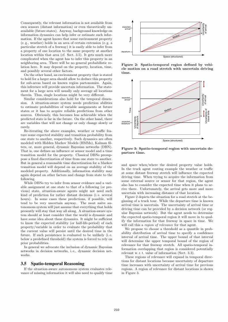
Consequently, the relevant information is not available fromown sensors (distant information) or even theoretically un-available (future states). Anyway, background knowledge oninformation dynamics can help infer or estimate such infor-mation. If the agent knows that some environment property(e. g., weather) holds in an area of certain extension (e. g. aparticular stretch of a freeway) it is easily able to infer froma property of one location to the same property at anotherlocation within that area (cf. Sect. 3.5). It gets much morecomplicated when the agent has to infer this property in anneighboring area. There will be no general probabilistic re-lation here. It may depend on the property, location, time,and possibly several other factors.

On the other hand, an environment property that is statedto hold for a larger area should allow to deduce this propertyfor sub-areas based on known region partonomies. Again,this inference will provide uncertain information. The state-ment for a large area will usually only average all locationstherein. Thus, single locations might be very different.

Similar considerations also hold for the temporal dimen-sion. A situation-aware system needs prediction abilitiesto estimate probabilities of variable assignments at futurestates or it has to acquire reliable predictions from othersources. Obviously, this becomes less achievable when thepredicted state is far in the future. On the other hand, thereare variables that will not change or only change slowly orrarely.

Re-iterating the above examples, weather or traffic fea-ture some expected stability and transition probability fromone state to another, respectively. Such dynamics are oftenmodeled with Hidden Markov Models (HMMs), Kalman fil-ters, or, more general, dynamic Bayesian networks (DBN).That is, one defines an influence or sensor model and a timetransition model for the property. Classical DBNs presup-pose a fixed discretization of time from one state to another.But in general a reasonable time discretization for a Markovtransition model will depend on an average stability of themodeled property. Additionally, information stability mayagain depend on other factors and change from state to thefollowing.

While DBNs try to infer from sensor evidence and a vari-able assignment at one state to that of a following (or pre-vious) state, situation-aware agents might not need suchkind of prediction for rather distant decisions (i. e. severalhours). In some cases these predictions, if possible, willtend to be very uncertain anyway. The most naıve au-tonomous system will just assume that everything that holdspresently will stay that way all along. A situation-aware sys-tem should at least consider that the world is dynamic andhave some idea about these dynamics. It might be sufficientto know the expected stability (or half-life-period) of eachproperty/variable in order to evaluate the probability thatthe current value will persist until the desired time in thefuture. If such persistence is evaluated to be unlikely (i. e.below a predefined threshold) the system is forced to rely onprior probabilities.

In general we advocate the inclusion of dynamic Bayesiannetworks in decision networks, i. e., dynamic decision net-works.

3.5 Spatio-temporal ReasoningIf the situation-aware autonomous system evaluates rele-

vance of missing information it will also need to qualify time

Figure 2: Spatio-temporal region defined by vehi-cle motion on a road stretch with uncertain drivingtime.

Figure 3: Spatio-temporal region with uncertain de-parture time.

and space when/where the desired property value holds.In the truck agent routing example the weather or trafficat some distant freeway stretch will influence the expecteddriving time. When trying to acquire the information fromsome external source or sensor for that region, the agentalso has to consider the expected time when it plans to ar-rive there. Unfortunately, the arrival gets more and moreuncertain with increasing distance of that location.

Figure 2 depicts the situation for a road stretch at the be-ginning of a truck tour. While the departure time is knownarrival time is uncertain. The uncertainty of arrival time ordriving time can be provided by a decision network (or reg-ular Bayesian network). But the agent needs to determinethe expected spatio-temporal region it will move in to qual-ify the information for that freeway in space in time. Wewill call this a region of relevance for that agent.

We propose to choose a threshold as a quantile in prob-ability distribution of arrival time to specify a confidenceinterval of arrival time. The upper bound of that intervalwill determine the upper temporal bound of the region ofrelevance for that freeway stretch. All spatio-temporal in-formation overlapping that region is considered potentiallyrelevant w. r. t. value of information (Sect. 3.3).

These regions of relevance will expand in temporal direc-tions for distant locations because uncertainty of departuretime increases with uncertainty of arrival time for previousregions. A region of relevance for distant locations is shownin Figure 3.

210

For qualitative topological inference on this regions theagent can apply usual spatial calculi such as Region Con-nection Calculus (RCC) [19]. This is of particular interestwhen agents want to share information and need to deter-mine whether there is potential for cooperation. The regionsof relevance are then complemented by regions of expertise,i. e., regions other agents can provide information for.

3.6 Social AbilitySocial ability is one of the minimal criteria for intelligent

agents defined by Wooldridge and Jennings [24]. In thiscontext, social ability refers to communication with otheragents. For situation-awareness communication is neededwhen there is relevant information that is neither availablefrom own sensors nor inferable by reasoning. For instance,information on distant locations needs to be acquired fromexternal sources.

In practice, the mere ability of communication will notsuffice. A situation-aware system must determine that someinformation cannot be acquired from own sensors (Sect. 3.2)but is available from other sources instead. This includes thediscovery of such sources, a common communication lan-guage with agreed content semantics, and price negotiationsif information is subject to charges.

4. APPLICATION SCENARIOOne particular application domain in our research has

been autonomous logistics [21]. That means, there are agentsas autonomous decision makers that represent one or morelogistic objects (e. g. truck, container, or pallet) and controllogistic processes locally. This usually requires cooperationwith other logistic agents as well as continuous acquisitionof information for decision-making. This information is pro-vided by local sensors (e. g., humidity sensors for monitoringof perishable goods) as well as external data sources (e. g.for weather and traffic reports).

When developing an autonomous logistics system, we eval-uate agent behavior by stochastic simulation before deploy-ment. That is, the developed agents as well as test mocksrepresenting external agents and other entities run in a sim-ulated logistics environment before they are released to areal-world environment. For this purpose we implementedthe multiagent-based simulation system PlaSMA (Platformfor Simulations with Multiple Agents). PlaSMA is basedon the FIPA-compatible multiagent development environ-ment JADE [5]. Multiagent-based simulation (MABS) ap-plies object-based modeling [18, 8] as well as discrete time,distributed simulation techniques [11]. In MABS, the agentsare parallel logical simulation processes that, in general, rep-resent objects of the simulation model at the same time.Thus, MABS is a natural way to test agent behavior andinteraction.

We applied this simulation platform for studies of agentsituation awareness in vehicle route planning (similar to theexample in section 3). Uncertainty in vehicle route plan-ning is an everyday problem in transportation over longerdistances. The shortest route is not always the fastest.Even when considering maximum allowed or average ex-pected speed on single roads the planned routes may proveto be suboptimal. While suboptimal solutions are a naturalproperty in dynamic, open environments with partial ob-servability, usual route planning does not make use of muchup-to-date or background information that would be obtain-

able and correlates with travel time.We conducted simulation studies [12] that help find the

utility or relevance of environmental information on traveltime and its application in route planning cost functions.Furthermore, the experiments should provide evidence forthe time in the future when incoming information is usefuland the robustness when working with uncertain or wronginformation.

Inductive machine learning was applied to pre-processedtraffic information in order to learn traffic models for spe-cific roads depending on weather, time of day, and day ofweek [12]. The data was based on German and Austriantraffic censuses. The learned traffic model includes predic-tion rules like

[Speed=60]

<= [Day=Mo] [Time=morning]

[Weather=moderate..good]

That is, average possible speed on the corresponding roadis expected to be 60 kmph on Monday mornings if weatherconditions are from moderate to good. Such predictionswere integrated in a truck agent’s utility function for bestroutes in a transportation process. As part of the agentsknowledge acquisition component, the planning system ini-tiates the gathering of weather information within a certaindistance towards its destination. This information from ex-ternal weather services together with time and date infor-mation is used to consult the rule base for a travel time pre-diction. The time and date in these rule base queries againdepends on prediction of travel time to reach the location ofinterest (cf. discussion in Sect. 3.5).

In several stochastic simulations these predictions turnedout to be valuable. Situation-aware vehicle agents were up to6.3% faster on average than regular, non-predictive agents.Additionally, the standard deviation of travel time was re-duced by 28%. With significance level α = 0.05 the sim-ulated results to not differ more than 0.0016% from theactual values. Thus, dedicated means to increase situation-awareness are actually shown to be of advantage in the pre-sented logistics scenario.

5. DISCUSSIONThe survey on situation awareness in this paper identi-

fies criteria for knowledge representation and reasoning ofautonomous systems in dynamic environments. In particu-lar, the paper focuses on domains with decisions that mayhave a larger spatio-temporal scope. We do not claim thatthe means proposed for implementing these criteria are im-perative. Furthermore, a reference implementation of thedescribed approach is work in progress. The presented ap-plication example still relies on some pre-designed informa-tion acquisition behaviors instead of fully goal-oriented anddeliberate acquisition. An extended conceptual architecturethat includes explicit information acquisition for situationassessment was proposed in [17].

The general question arises whether situation awarenessturns out to be necessary or even futile for particular au-tonomous systems. Furthermore, most systems will prob-ably only fulfill a subset of all criteria. Some criteria areprobably not imperative for some degree of situation aware-ness. Endsley [10] also distinguishes three levels for humansituation awareness that could match a particular subset

211

of the criteria proposed here. Relevance assessment is cer-tainly mandatory for level 2 (comprehension). Representingand reasoning with information dynamics pertains to level 3(projection). But social ability (i. e. information exchange)is beyond the scope of Endsley’s approach. This criteriacould establish a fourth level of awareness. On the otherhand, a system could be able to share information but notbe capable of projection. So it does not fit in as an extensionof level 3.

But assuming an agent that is matching all criteria: Issuch an agent capable of actually measuring (i. e. quanti-fying) its situation awareness? We think that informationvalue theory has the answer. The difference between theexpected utility with current sensory evidence and the ex-pected utility given complete sensory evidence (consideringperception abilities) could provide a corresponding measure.But future research has to be done for a complete theory ofsituation awareness and its assessment.

6. CONCLUSIONThis paper provides a survey on situation awareness for

autonomous systems by analyzing features and limitationsof existing architectures and proposing a set of criteria tobe satisfied by situation-aware agents. The proposed crite-ria build upon the definition of human situation awarenessby Endsley [9, 10] but take into account the special require-ments and needed capabilities of technical systems. Theproposed criteria are reasoning about ignorance, an agentperception model, information relevance assessment, a modelof information dynamics and associated spatio-temporal rea-soning capabilities, and social ability for acquiring informa-tion beyond own sensors.

The presented logistics routing scenario shows that seem-ingly barely relevant information on environmental proper-ties can significantly increase performance of autonomousagents. Future work will address a theoretical foundation ofsituation awareness and its measurement based on dynamicdecision networks and information value theory.

7. ACKNOWLEDGMENTSThis research is funded by the German Research Founda-

tion (DFG) within the Collaborative Research Center 637“Autonomous Cooperating Logistic Processes: A ParadigmShift and its Limitations” (SFB637) at the University ofBremen, Germany.

8. REFERENCES[1] J. Albus. A reference model architecture for intelligent

unmanned ground vehicles. In Proceedings of the SPIE16th Annual International Symposium on Aerospace /Defense Sensing, Simulation and Controls, pages303–310, Apr. 1–5 2002.

[2] J. Albus, T. Barbera, and C. Schlenoff. RCS: Anintelligent agent architecture. In R. M. Jones, editor,Intelligent Agent Architectures: Combining theStrengths of Software Engineering and CognitiveSystems, number WS-04-07 in AAAI WorkshopReports. AAAI Press, 2004.

[3] F. Baader, D. Calvanese, D. L. McGuinness, D. Nardi,and P. F. Patel-Schneider, editors. The DescriptionLogic Handbook. Theory, Implementation and

Applications. Cambridge University Press, 2nd edition,2007.

[4] S. Bechhofer, F. van Harmelen, J. Hendler,I. Horrocks, D. L. McGuinness, P. F. Patel-Schneider,L. A. Stein, and F. W. Olin. OWL web ontologylanguage reference. Available fromhttp://www.w3.org/TR/owl-ref/, Feb. 10 2004.

[5] F. Bellifemine, A. Poggi, and G. Rimassa. Developingmulti-agent systems with a FIPA-compliant agentframework. Software-Practice and Experience,31(2):103–128, Feb. 2001.

[6] M. E. Bratman. Intention, Plans, and PracticalReason. Harvard University Press, Cambridge, MA,USA, 1987.

[7] K. L. Clark. Negation as failure. In H. Gallaire andJ. Minker, editors, Logic and Data Bases, pages293–322, New York, 1978. Plenum Press.

[8] P. Davidsson. Multi agent based simulation: Beyondsocial simulation. In Multi-Agent Based Simulation,Second International Workshop (MABS 2000),number 1979 in LNCS, pages 97–107, Boston, MA,USA, July 8–9 2000. Springer-Verlag.

[9] M. R. Endsley. Design and evaluation of situationawareness enhancement. In Proceedings of the HumanFactors Society 32nd Annual Meeting, volume 1, pages97–101, Santa Mocica, CA, USA, 1988. HumanFactors Society.

[10] M. R. Endsley. Theoretical underpinnings of situationawareness. A critical review. In M. R. Endsley andD. J. Garland, editors, Situation Awareness Analysisand Measurement, pages 3–32. Lawrence ErlbaumAssociates, Mahwah, NJ, USA, 2000.

[11] R. Fujimoto. Parallel and Distributed SimulationSystems. John Wiley & Sons, New York, NY, 2000.

[12] J. D. Gehrke and J. Wojtusiak. Traffic Prediction forAgent Route Planning. In International Conference onComputational Science (ICCS 2008), number 5103 inLNCS, pages 692–701, Krakow, Poland, June 23–252008. Springer-Verlag.

[13] R. A. Howard. Information value theory. IEEETransactions on Systems Science and Cybernetics,SSC-2(1):22–26, Aug. 1966.

[14] R. A. Howard and J. E. Matheson. Influencediagrams. Decision Analysis, 2(3):127–143, Sept. 2005.

[15] S. Kirn, O. Herzog, P. Lockemann, and O. Spaniol,editors. Multiagent Engineering: Theory andApplications in Enterprises. Springer-Verlag, 2006.

[16] E. I. Knudsen. Fundamental components of attention.Annual Review of Neuroscience, 30:57–78, July 2007.

[17] M. Lorenz, J. D. Gehrke, J. Hammer, H. Langer, andI. J. Timm. Knowledge management to supportsituation-aware risk management in autonomous,self-managing agents. In Self-Organization andAutonomic Informatics (I), volume 135 of Frontiers inArtificial Intelligence and Applications, pages 114–128,Amsterdam, 2005. IOS Press.

[18] H. V. D. Parunak, R. Savit, and R. L. Riolo.Agent-Based Modeling vs. Equation-Based Modeling:A Case Study and Users’ Guide. In MABS 1998,pages 10–25, Paris, France, 1998. Springer-Verlag.

[19] D. A. Randell, Z. Cui, and A. G. Cohn. A spatial logic

212

based on regions and connection. In B. Nebel, C. Rich,and W. Swartout, editors, Proceedings of the 3rdInternational Conference on Principles of KnowledgeRepresentation and Reasoning, pages 165–176. MorganKaufmann, 1992.

[20] S. J. Russell and P. Norvig. Artificial Intelligence: AModern Approach. Prentice Hall, Upper Saddle River,NJ, USA, 2nd edition, 2003.

[21] B. Scholz-Reiter, K. Windt, and M. Freitag.Autonomous logistic processes - New demands andfirst approaches. In Proceedings of the 37thCIRP-International Seminar on ManufacturingSystems, pages 357–362, Budapest, May 19–21 2004.

[22] M.-A. Williams, P. Gardenfors, A. Karol, J. McCarthy,and C. Stantom. A framework for evaluatinggroundedness of representations in systems: Frombrains in vats to mobile robots. In IJCAI-05 Workshopon Agents in Real-Time and Dynamic Environments,pages 17–24, Edinburg, UK, July 30 2005.

[23] M. Wooldridge. Reasoning about Rational Agents. TheMIT Press, 2000.

[24] M. Wooldridge and N. R. Jennings. Intelligent agents:Theory and practice. The Knowledge EngineeringReview, 10(2):115–152, 1995.

213

NIST/IEEE Virtual Manufacturing Automation Competition: From Earliest Beginnings to Future

Directions Stephen Balakirsky

National Institute of Standards and Technology

100 Bureau Drive Gaithersburg, MD 20878

stephen@nist.gov

Raj Madhavan National Institute of Standards and

Technology Gaithersburg, MD 20878

Oak Ridge National Laboratory Oak Ridge, TN 37831

raj.madhavan@nist.gov

Chris Scrapper National Institute of Standards and

Technology 100 Bureau Drive

Gaithersburg, MD 20878

chris.scrapper@nist.gov

ABSTRACT This paper provides an overview of the National Institute of Standards and Technology (NIST)/IEEE Virtual Manufacturing and Automation Competition (VMAC). Detailed information will be provided on the competition’s objectives, history, and operation. In addition, the supporting software infrastructure will be discussed.

Categories and Subject Descriptors I.2.9 [Robotics]: Autonomous vehicles; commercial robots and applications; kinematics and dynamics,; workcell organization and planning.

General Terms Performance, Experimentation, Verification, Management.

Keywords Competition, simulation, manufacturing, USARSim.

1. INTRODUCTION Automated Guided Vehicles (AGVs) represent an integral component of today’s manufacturing processes. Major corporations use them on factory floors for jobs as diverse as intra-factory transport of goods between conveyors and assembly sections, parts and frame movements, and truck trailer loading/unloading. The National Institute of Standards and Technology (NIST) is currently running a program to develop test method standards for the next generation of AGVs. These test methods specifically target small- and medium-sized manufactures and the problems that they face in applying

automation to legacy manufacturing facilities.

In order to assess future automation needs, focus on solutions, and ease entry of new features into AGV product lines, NIST is striving to form a coalition that brings together the three communities of industrial end-users, researchers, and manufacturers of AGV equipment. This coalition will then focus on moving from real-world problems, to research activities, to system features. As the first thrust of this effort, NIST performed outreach to several small- and medium-sized manufactures. Phone interviews and site visits were conducted, and a common automation need emerged. This need is for both unit loaders and forklifts to operate in unstructured cramped environments to deliver parts and materials for use in the manufacturing process.

Automating these systems to operate in unstructured environments presents an exciting area of current research in robotics and automation. Unfortunately, the traditional entry barrier into this research area is quite high. Researchers need an extensive physical environment, robotic hardware, and knowledge in research areas ranging from mobility and mapping to behavior generation. An accepted approach to lowering this entry barrier is through the use of simulation systems and open source software. The use of simulation significantly reduces the amount of infrastructure required, the number of AGV systems needed, and the risk to both humans and robots. In addition, hardware-in-the-loop (HIL) or real/virtual testing allows for the exploration of scenarios that would be unsafe to pursue with actual robotic equipment.

NIST turned to the IEEE to build researcher involvement in this new coalition by submitting a successful proposal to the Washington section of the Robotics and Automation Society of IEEE to create a new Virtual Manufacturing and Automation Competition (VMAC).

2. VMAC PRELIMINARIES By soliciting proposals from IEEE members and local student branches and robotic clubs in the Greater Washington area (Maryland, Virginia, and the District of Columbia), the organizers were able to bring together eight teams from regional universities consisting of faculty mentors, undergraduate students, and graduate students. The original VMAC participants are shown in Figure 1. The educational institutions that participated in this effort were: two teams from Hood College (Frederick, MD), one team from George Mason University (Fairfax, VA), and two

This paper is authored by employees of the United States Government and is in the public domain. PerMIS’08, August 19–21, 2008, Gaithersburg, MD, USA ACM ISBN 978-1-60558-293-1/08/08.

214

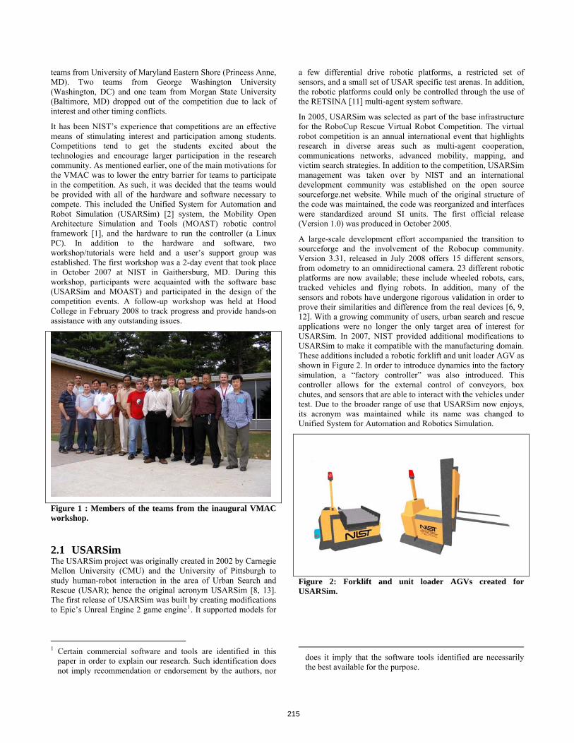
teams from University of Maryland Eastern Shore (Princess Anne, MD). Two teams from George Washington University (Washington, DC) and one team from Morgan State University (Baltimore, MD) dropped out of the competition due to lack of interest and other timing conflicts.

It has been NIST’s experience that competitions are an effective means of stimulating interest and participation among students. Competitions tend to get the students excited about the technologies and encourage larger participation in the research community. As mentioned earlier, one of the main motivations for the VMAC was to lower the entry barrier for teams to participate in the competition. As such, it was decided that the teams would be provided with all of the hardware and software necessary to compete. This included the Unified System for Automation and Robot Simulation (USARSim) [2] system, the Mobility Open Architecture Simulation and Tools (MOAST) robotic control framework [1], and the hardware to run the controller (a Linux PC). In addition to the hardware and software, two workshop/tutorials were held and a user’s support group was established. The first workshop was a 2-day event that took place in October 2007 at NIST in Gaithersburg, MD. During this workshop, participants were acquainted with the software base (USARSim and MOAST) and participated in the design of the competition events. A follow-up workshop was held at Hood College in February 2008 to track progress and provide hands-on assistance with any outstanding issues.

Figure 1 : Members of the teams from the inaugural VMAC workshop.

2.1 USARSim The USARSim project was originally created in 2002 by Carnegie Mellon University (CMU) and the University of Pittsburgh to study human-robot interaction in the area of Urban Search and Rescue (USAR); hence the original acronym USARSim [8, 13]. The first release of USARSim was built by creating modifications to Epic’s Unreal Engine 2 game engine1. It supported models for

e.

1 Certain commercial software and tools are identified in this paper in order to explain our research. Such identification does not imply recommendation or endorsement by the authors, nor

a few differential drive robotic platforms, a restricted set of sensors, and a small set of USAR specific test arenas. In addition, the robotic platforms could only be controlled through the use of the RETSINA [11] multi-agent system softwar

In 2005, USARSim was selected as part of the base infrastructure for the RoboCup Rescue Virtual Robot Competition. The virtual robot competition is an annual international event that highlights research in diverse areas such as multi-agent cooperation, communications networks, advanced mobility, mapping, and victim search strategies. In addition to the competition, USARSim management was taken over by NIST and an international development community was established on the open source sourceforge.net website. While much of the original structure of the code was maintained, the code was reorganized and interfaces were standardized around SI units. The first official release (Version 1.0) was produced in October 2005.

A large-scale development effort accompanied the transition to sourceforge and the involvement of the Robocup community. Version 3.31, released in July 2008 offers 15 different sensors, from odometry to an omnidirectional camera. 23 different robotic platforms are now available; these include wheeled robots, cars, tracked vehicles and flying robots. In addition, many of the sensors and robots have undergone rigorous validation in order to prove their similarities and difference from the real devices [6, 9, 12]. With a growing community of users, urban search and rescue applications were no longer the only target area of interest for USARSim. In 2007, NIST provided additional modifications to USARSim to make it compatible with the manufacturing domain. These additions included a robotic forklift and unit loader AGV as shown in Figure 2. In order to introduce dynamics into the factory simulation, a “factory controller” was also introduced. This controller allows for the external control of conveyors, box chutes, and sensors that are able to interact with the vehicles under test. Due to the broader range of use that USARSim now enjoys, its acronym was maintained while its name was changed to Unified System for Automation and Robotics Simulation.

Figure 2: Forklift and unit loader AGVs created for USARSim.

does it imply that the software tools identified are necessarily the best available for the purpose.

215

2.2 MOAST The MOAST framework builds upon several decades of robotic architecture and control system work that has been performed by NIST. The framework is designed to be a sample implementation of the 4D/RCS reference model architecture [4,5]. The RCS reference model architecture is a hierarchical, distributed, real-time control system architecture that decomposes a robotic system into manageable pieces while providing clear interfaces and roles for a variety of functional elements.

Figure 3 depicts the general structure of each echelon (level) of the 4D/RCS hierarchy. Each echelon in 4D/RCS contains a systematic regularity and is composed of control nodes that follow a sense-model-act paradigm. These control nodes are sensory processing (SP), world modeling (WM), value judgment (VJ), and behavior generation (BG). Sensory processing is responsible for populating the world model with relevant facts. These facts are based on both raw sensor data and the results of previous SP (in the form of partial results or predictions of future results). WM must store this information, information about the system self, and general world knowledge and rules. Furthermore, it must provide a means of interpreting and accessing this data. BG computes possible courses of action to take based on the knowledge in the WM, the system’s goals, and the results of plan simulations. VJ aids in the BG process by providing a cost/benefit ratio for possible actions and world states.

Figure 3: Generic 4D/RCS control node.

All of the echelons in 4D/RCS follow the sense-model-act paradigm with the principal difference between echelons being in the knowledge requirements and the fidelity of the planning space. This regularity in the structure enables flexibility in the system architecture that allows scaling of the system to any arbitrary size or level of complexity [7].

In 2005, MOAST was officially released on sourceforge as a public domain robotic control system. Since that time, it has attracted an international developer community and now contains control modules for robotic vehicles, manipulators, and end effectors. Figure 4 depicts the currently implemented echelons of the control system and their responsibilities. The central idea behind the VMAC competition is that research groups would be able to select their area of expertise and modify a small subset of control modules in order to improve the overall system performance. After the competition, each research group is required to contribute their modified modules back to the community. Thus, all teams benefit from each other’s strengths.

Figure 4: Control module responsibilities in the MOAST implementation of 4D/RCS.

2.3 Competition Design This competition design was based on the successful RoboCup Rescue Virtual Robots Competitions [3]. Since all code used in these competitions is open source, participants are able to learn from their competitors and concentrate their research in their particular areas of expertise. It was envisioned that researchers from multi-agent cooperation, mapping, communications networks, and sensory processing backgrounds would all be interested in participating.

The initial competition design was formulated by using the SCORE framework [10]. This framework specifies that an overall system scenario be defined, and then basic elemental skills that allow for the successful completion of the scenario be extracted. Systems are then evaluated on both their ability in the elemental tasks as well as the overall scenario.

From the outset, the competition was to be based on real-world scenarios. Based on NIST’s industry outreach effort, the scenario chosen was a factory setting that had significant clutter, maze-like passageways of various widths, and dynamic obstacles. The objective was to have several Ackerman-steered AGVs pick-up packages at a central loading station, and deliver these packages to one of several unloading stations. The package destinations were encoded in a Radio Frequency IDentification (RFID) Tag on each package.

Utilizing the SCORE framework, this scenario was decomposed into elemental tasks that included traffic management, route planning, accurate path following, and docking with loading/unloading stations. While the baseline code provided to the teams was capable of performing the objectives, it was far from optimal.

As time progressed, it became apparent that performing a complete SCORE evaluation of all of the elemental tasks and the overall scenario was an overly ambitious set of tasks for the first year of the competition. A decision was made to break the competition into several discrete best-in-class elemental tasks that would contribute to the scenario, and to leave the end-to-end objective and remaining elemental tasks for next year. The tasks of accurate route following and docking with loading/unloading stations were chosen as the VMAC tasks for the 2007-2008 competition year.

216

For the competition, the teams examined the BG modules at the prim and AM echelons in order to improve upon the existing baseline operation of the control system.

3. VMAC COMPETITION The regional competition was held on April 18th 2008 at NIST. The competition was broken down into two tasks: path following and docking. For both tasks, the teams were required to accept a standard command message as input. They were free to use as much of the provided infrastructure as they desired (e.g. groundtruth).

For path following, the input consisted of a set of constant curvature arcs that were to be followed. In order to allow observers to examine the system’s real-time performance, the target trajectory’s arcs were shown in the simulated world. These arcs were represented as a red centerline with a blue error radius as shown in Figure 5. The vehicle could then be observed while driving in the simulation. In addition to the simulated view, as shown in Figure 6, the passageway boundaries and vehicle centerline trajectory were plotted in real-time and statistics were automatically generated. As the path progressed, the arc complexity was increased and the error radius was reduced. Hood College produced the best-in-class algorithm for path following followed by George Mason University in a close second. The scoring criteria included the distance traveled before the first crossing over the error radius and the average path and speed deviation. The team’s score, as shown in Figure 7, was displayed in real-time during the competition.

Figure 5: Example of the path following task. The red line is the centerline that is to be followed. The blue line represents the allowable error radius for the center of the vehicle.

Docking ability was measured by placing the AGV in a room with a docking station. The input for the docking behavior consists of the upper right and lower left corners of both the room and docking table, as well as the desired location of the vehicle’s center point when docked. As shown in Figure 8, the AGV was required to successfully dock without a collision, where docking amounts to parallel parking a rear steered Ackerman vehicle. Upon successful docking, the AGV was placed in a smaller room and the procedure was repeated. The size of the room ranged in size from 10m x 10m to 4m x 4m. Once again, Hood College

received top honors in this competition. They were able to successfully dock in every room in which they were placed.

Figure 6: Plot of robot centerline trajectory and error boundaries. Note that allowable path deviation decreases as with distance traveled.

Path data file VMAC_CompDay1/pathPts.datTean's data file VMAC_CompDay1/team_logs/team1_v4.dat

Commanded Speed 0.4Path Length 116.795183Vehicle Path Deviation Normalizing Factor 1.167

Number of Deviation Outside Error Bound 7Total Time of Deviation Outside Error Bound 6.1981Completed Entire Path TRUE

Total Time of Run 401.0019Distance Traveled During Run 153.004972Distance Traveled Along Path During Run 116.102756Mean of Speed During Run 0.381603Standard Deviation of Speed During Run 0.123377Mean of Deviation During Run 0.266681Standard Deviation of Deviation During Run 0.284552

Total Time of Run 216.8005Distance Traveled During Run 81.185515Distance Traveled Along Path During Run 64.84049Mean of Speed During Run 0.374628Standard Deviation of Speed During Run 0.1308Mean of Deviation During Run 0.304629Standard Deviation of Deviation During Run 0.327008

0.7 Percentage Completed 55.51640773 38.861490.1 Deviation of Speed from Commanded Speed -39.043 -3.90430.1 Deviation of Vehicle from Commanded Path -54.12485004 -5.412485

1 Completion Bonus 10 10total 39.5447

Performance Evaluation of Path Following Until First Deviation

Summary of Results

File Information

Path Information

Performance Evaluation of Deviations Over Entire Run

Performance Evaluation of Path Following Over Entire Run

Figure 7: Sample of statistics gathered for each run of the path following elemental evaluation.

3.1 Follow-on with a Real Platform One of the main criticisms of simulation is that algorithms that work in virtual reality do not translate well to the real-world. The VMAC competition tried to address this concern by allowing the winning team’s code to run on the NIST surrogate AGV. This transition was made possible due to USARSim and MOAST providing validated models of real-world sensors and robotic platforms. In addition, the MOAST implementation provides for standardized interfaces that are followed by both our real platform and the simulation.

217

Figure 8: Example of the docking task. The vehicle was required to dock with a loading station without experiencing any collisions. Upon success, the vehicle was moved to a space with less maneuver room and the test was repeated.

Figure 9: The winning code from Hood College was placed without change on NIST’s surrogate AGV. The vehicle was able to successfully navigate and dock with a loading area.

Significant differences exist between the NIST surrogate vehicle and the simulated AGV. For example, the simulated AGV is a rear-steered Ackerman vehicle while the NIST surrogate is skid steered. However, the modularity of the 4D/RCS architecture makes many system specific details irrelevant to higher echelons in the architecture. A constant curvature arc sent from the AM echelon to the PRIM echelon must be accurately followed. AM is unaware of how PRIM will follow that arc. It is up to PRIM to account for the individual vehicle differences.

Figure 9 shows the NIST AGV driving through a performance test metric that allows for vehicle side clearance and free space for turns to be precisely controlled. The Hood College code was run

without alteration on the NIST vehicle and docking procedures were successfully performed.

3.2 ICRA Participation The successful National VMAC has been used as a model for a virtual manufacturing competition that is now an annual event at the robot challenge which is part of the IEEE International Conference on Robotics and Automation (ICRA). The first step to making this a reality occurred recently when with funding from IEEE, the organizers and the winning team from Hood College were able to demonstrate their code to all attendees for the first two days of the ICRA conference that was held in Pasadena, California from May 19-23, 2008.

4. FUTURE The organizers are continuing this highly successful joint RAS/NIST effort with already approved follow-on funding from RAS. The teams from this year’s competition are demonstrating and presenting their research as team-description papers during a special session at the annual Performance Metrics for Intelligent Systems (PerMIS’08) Workshop held at NIST. The seeds from last year’s funds are already bearing fruit. Several of the Universities are planning courses based on the material and expertise that they have gained as a direct result of their participation in this competition. In addition, a public forum and website (www.vmac.hood.edu) has been created where participants are able to post and answer questions and initiate discussions with other members. The continued funding will facilitate expanding the user base and building a self-sustaining community that is able to pool resources and create improvements to the simulation system. Additional corporate interest is also being generated with a major manufacturer being interested in expanding the competition to include the autonomous handling of pallets by a forklift in the factories buffer zone area (the area where shipments are first received and unloaded).

In terms of the actual competition, a national competition is being planned for the 2008-2009 year and the organizers have submitted a proposal requesting that the VMAC be included as an event in the robot challenge at ICRA’09 to be held in Kobe, Japan. As a lead-in for next year’s national competition, all of the Hood code has now been checked-in to the CVS repository of MOAST.

5. ACKNOWLEDGMENTS The authors would like to thank NIST and the Robotics and Automation Society (RAS) of IEEE for their continued support of this effort. This work was made possible through a grant received under the RAS new initiatives competition.

6. REFERENCES [1] MOAST Homepage. http://moast.sourceforge.net . 2007. [2] USARSim Homepage. http://usarsim.sourceforge.net .

2007. [3] RoboCup Rescue Virtual Robots Competition.

http://www.robocuprescue.org/wiki/index.php?title=Virtualrobots . 2008.

[4] Albus, J., "Outline for a Theory of Intelligence," IEEE Transactions on Systems Man and Cybernetics, Vol. 21, 1991, pp. 473-509.

[5] Albus, J., Bostleman, R., Madhavan, R., Scott, H., Barbera, A., Szabo, S., Hong, T., Chang, T., Shackleford, W. P., Shneier, M., Balakirsky, S., Schlenoff, C., Huang, H., and Proctor, F., "Intelligent Control of Mobility

218

Systems," Computational Intelligence in Automotive Applications, Vol. 132/2008, Studies in Computational Intelligence, Springer Berlin, Heidelberg, 2008, pp. 237-274.

[6] Balaguer, B. and Carpin, S., "Where am I? A Simulated GPS Sensor for Outdoor Robotic Applications," Proceedings of the First International Conference on Simulation, Modeling, and Programming of Mobile Robots, 2008.

[7] Balakirsky, S. and Scrapper, C., "Planning for On-Road Driving through Incrementally Created Graphs," Proceedings of the 7th International IEEE Conference on Intelligent Transportation Systems, 2004.

[8] Lewis, M., Sycara, K., and Nourbakhsh, I., "Developing a Testbed for Studying Human-Robot Interaction in Urban Search and Rescue," Proceedings of the 10th International Conference on Human Computer Interaction (HCII'03), 2003.

[9] Pepper, C., Balakirsky, S., and Scrapper, C., "Robot Simulation Physics Validation," Proceedings of the Performance Metrics for Intelligent Systems (PerMIS) Workshop, 2007.

[10] Schlenoff, C., Steves, M., Weiss, B., Shneier, M., and Virts, A., "Applying SCORE to Field-based Performance Evaluations of Soldier Worn Sensor Technologies," Journal of Field Robotics, Vol. 24, No. 8-9, 2006, pp. 671-698.

[11] Sycara, K. and Pannu, A. S., "The RETSINA multiagent system (video session): towards integrating planning, execution and information gathering," Proceedings of the Second International Conference on Autonomous Agents, ACM, New York, NY, 1998.

[12] Taylor, B., Balakirsky, S., Messina, E., and Quinn, R., "Design and Validation of a Whegs Robot in USARSim," Proceedings of the Performance Metrics for Intelligent Systems (PerMIS) Workshop, 2007.

[13] Wang, J., Lewis, M., and Gennari, J., "A Game Engine Based Simulation of the NIST Urban Search & Rescue Arenas," Proceedings of the 2003 Winter Simulation Conference, 2003.

219

Analysis of a Novel Docking Technique for AutonomousRobots

Henson, G., Maynard, M., Liu, X., Dimitoglou, G.Department of Computer Science

Hood CollegeFrederick, MD 21701, USA

{gah1, mmaynard, xliu, dimitoglou} @hood.edu

ABSTRACTAutonomous robot docking requires accurate path follow-ing and ultimately, accurate alignment with the target loca-tion, typically a docking station. In this paper we developa novel, partially heuristic, technique that allows accuratedocking for Ackerman-steered vehicles. The technique is val-idated via simulation. Multiple experiments were performedto better understand and analyze the heuristic element of thetechnique. The results underscore the impact of the vehicle’ssteering characteristics in docking precision and may provevaluable in attempting to remove the heuristic element.

Categories and Subject DescriptorsI.2.9 [Robotics]: Autonomous vehicles; I.6 [Simulationand modeling]: Applications

General TermsRobotics, Simulation

KeywordsMobile robot motion-planning, simulation

1. INTRODUCTIONAutonomous mobile robots are designed to perform cer-

tain tasks. Typically to perform these tasks, robots haveto plan their path, avoid objects and navigate in the op-erational environment. Often task completion requires ap-proaching a target location where some additional final op-eration is required, such as moving an actuator. In manu-facturing environments docking to a target location (e.g. apalette shelf or a conveyor belt) is a common final operation.The docking process itself can be complex, requiring maneu-vering and precision which can be affected by the size andshape of the workspace and the physical dimensions and ma-neuverability of the robotic platform.

Permission to make digital or hard copies of all or part of this work forpersonal or classroom use is granted without fee provided that copies arenot made or distributed for profit or commercial advantage and that copiesbear this notice and the full citation on the first page. To copy otherwise, torepublish, to post on servers or to redistribute to lists, requires prior specificpermission and/or a fee.PerMIS’08 August 19-21, 2008, Gaithersburg, MD, USA.Copyright 2008 ACM 978-1-60558-293-1 ...$5.00.

In this paper we examine docking of an autonomous roboticplatform by knowing only two locations in the workspace:the point of origin and the target location. We propose analgorithm that allows docking using only numerical calcula-tions considering, besides the robot’s physical geometry, theorigin and target location. We presume the robot has noproximity detection capability or any other relevant sensorpayload and the workspace is obstacle-free.The following section provides a description of the environ-ment and robotic platform assumptions and constraints forthe docking problem. In Section 3, the proposed techniqueis presented. Section 4 describes the simulation experimentsconducted to confirm the validity of the proposed algorithmand to collect some performance metrics with respect todocking accuracy.

2. OPERATIONAL ENVIRONMENTWe assume the operational environment to be a rectangu-

lar workspace (W). In the workspace there is a docking loca-tion (D) and an arbitrary starting location (L1) for the robot(A). The robot, an Ackerman-steered, Automatic GuidedVehicle (AGV) is fitted with a roller deck.The docking location also has a roller deck which should en-able the AGV to unload cargo if it is properly docked. Anarea in front of the dock is also the target location (LD)the robot must reach by maneuvering in the obstacle-freeworkspace (Figure 1). Since there are no obstacles in theworkspace, there are many more paths [3] in the configura-tion space (C-space) that can be expressed as a continuousmap:

τ : S ∈ [0, 1] �→ τ (s) ∈ C (1)

where τ (0) = Li is the initial configuration and τ (0) = LD

is the target configuration of the path. However, Equation1 does not take into account the additional requirement ofarriving at the dock in the correct orientation (pose).For task completion, the robot needs to arrive at the targetlocation LD and also to park in such a way that the rollerdecks of both the vehicle and the dock are aligned. Thisexcludes any docking approach that does not conclude withthe left wide side of the vehicle aligned to the dock’s rollerdeck.

In the environment, the following is known:

1. the coordinates of the four corners defining the workspaceand the room boundary

2. the coordinates of the corners defining the dock

3. the initial (L1) and target (LD) robot locations

220

DockRobot

Initial Location Target Location

L1 LD

Workspace

Figure 1: A generalized view of the workspace withthe robot in its initial position.

4. the initial orientation (pose) of the robot and its phys-ical dimensions.

The point we will use as the location of the robot in theworld during the simulation is between the front wheels.The side to side location is calculated by centering the load-ing site on the UnitLoader to the center of the docking sta-tion.

3. APPROACHThe problem of docking the robot is the same as parallel

parking a vehicle next to a fixed location.We begin by calculating the required maneuvers in reverseorder. This simplifies the problem as we obtain both thefinal position and the required orientation. We can then cal-culate the points that form a traversable path to the robot’sposition.The key point in this path is the point that the robot travelsto immediately before arriving at the docked position. Wecall this this the penultimate point (p) and it is chosen toprovide a simple traversable path to the docking position aswell as being easily reachable from the robot’s current loca-tion.

The final docking position the robot needs to obtain is

k

1.608m

1.096m VEHICLE CHARACTERSTICSWidth: 1.096mLength: 1.608mHeight: 0.8mSpeed: 5m/secMax Steer Angle: 79.9 deg

m

Figure 2: Robot physical dimensions.

calculated using the physical dimensions of the robot andthe location of the docking station. Because the naviga-tion coordinates are calculated using a point (k) in the frontmid-line of the robot, another point (m) is calculated to de-termine the point of alignment between the center of thedock and the center of the vehicle’s roller deck (Figure 2).The docking target location is half of the robot’s width fromthe docking side of the docking station. Once this dockingpoint is calculated, a penultimate point can also be calcu-lated.The penultimate point also needed to be located in such aplace as to allow the robot to easily reach the docking loca-tion.

To take advantage of the vehicle’s rear steered Ackermandesign, we chose to approach the docking position using therobot’s reverse direction. This put the steering wheels in thefront and allowed a smoother motion to pivot to the dockinglocation.To accomplish this, the penultimate point can be on eitherside (left or right) of the docking location to allow the robotto reverse into the correct position. The optimal LD pointis determined according to the physical dimensions of thedocking station and the physical geometry of the vehicle.Algorithm 1 illustrates in pseudocode the required steps inorder to calculate the x and y coordinates for both the penul-timate (p) and goal point (LD). The terms half robot length

and half robot width are measurements that are used toproperly align the vehicle and its roller deck to the dockand its roller deck.Once these calculations are made, function FollowPath

performs the steering and direction maneuvers for the vehi-cle to begin moving first towards the calculated penultimatepoint and then to the goal point.While the p is a single reachable point in the workspace, weconsider it to have a much larger footprint indicated by atolerance, which is an arbitrary radius around the center ofp.The goal point, however, does not have such tolerance as anydeviation may indicate a misalignment with dock, renderingthe unloading of any package impossible.

Algorithm 1 Calculate and Find the penultimate point p

p.x ← dock.center.x + robot length;p.y ← dock.center.y + half robot length;LD.x ← dock.center.x + rollerdeck nav point offset;LD.y ← dock.center.y + half robot width;repeat

FollowPath towards pdistance = current.location − p

until distance < pt

repeatFollowPath towards LD

distance = current.location − LD

until distance < pt

4. SIMULATION

4.1 ExperimentationThe developed docking algorithm was exercised, tested

and verified using a simulation infrastructure comprised ofUSARSim [5, 7], a Gamebots [2] variant of the Unreal En-gine [6] and the Mobility Open Architecture Simulation andTools (MOAST)[4] framework [1].

4.1.1 DesignThe simulation environment provides a number of config-

urable parameters for the vehicle that can be adjusted tomodify the navigation performance.For the experiments a Unit Loader AGV was used and allparameters were kept at their default settings. As we weremore concerned with docking accuracy rather than the pathfollowing speed or reducing task completion, none of theseparameters were altered. Velocity, in particular, remainedconstant at 5m/sec.

221

The critical element to the success of a docking attempt isthe determination of the penultimate point.The single success factor in this experiment is the accuratedocking of the vehicle to the dock. As the penultimate point(p) is arbitrarily determined with respect to the dock, weexamined the possibility of moving p to examine if differentlocations would yield more accurate results. Through exper-imentation, we determined the optimal (fully aligned) goalpoint (LD) to be at xy-location (-0.26, -2.36).Assuming a constant vertical distance from the initial loca-tion (L1) to the p, multiple points were examined on thehorizontal axes by increasing and decreasing the distance tothe dock.The intention of the experimentation was to measure theperformance of the vehicle with respect to its accuracy inarriving at the optimal location by changing the proximityof p.The expectation was that a more distant p may result inmore accurate docking. This expectation was based on howcoarse Ackerman-steered vehicles are when maneuvering, there-fore more distance from the dock should have resulted in amore ”comfortable” steering environment.

4.1.2 Execution & AnalysisIn Table 1, the coordinates of seven executions illustrate

the different p positions and their corresponding LD loca-tions. In the simulated workspace, the optimal docked LD

is (-0.57, -2.39).The results indicate a considerable spread of values in thehorizontal distance from the optimal LD x -location of -0.57with deviations as large as 0.62m (ID 2).

Table 1: x,y coordinates of various p points and theircorresponding final docking locations

ID Penultimate (p) Location Final Location (LD)1 (-1.57, -2.39) (-0.03, -2.40)2 (-1.37, -2.39) (0.05, -2.39)3 (-1.17, -2.39) (0.04, -2.39)4 (-0.97, -2.39) (-0.26, -2.36)5 (-0.77, -2.39) (-0.15, -2.17)6 (-0.67, -2.39) (-0.18, -2.04)7 (-0.57, -2.39) (-0.29, -1.96)

These effects are most prominent in Figure 3. Super-imposed on an xy-axis, seven penultimate points (P1 − P7)are examined on the horizontal axis.Penultimate point P1 enables the vehicle to reach and dockas LD4 which is the optimal target location LD. Subsequentexecutions with p closer to the dock (e.g. P5 − P7) resultin far LD’s. Similarly, executions with p further away fromthe dock (e.g. P1 − P3) also end up in points distant fromthe dock LD’s.As expected, LD4 is aligned with the center of the dock(Dcenter) but not adjacent to it. Because LD4 is calculatedto be in the middle of the vehicle, a distance is required toensure that at least half of the vehicle’s width and some ad-ditional space is allotted to ensure proper proximity but notcollision with the dock.

5. CONCLUSION AND FUTURE WORKAutonomous robot docking is an interesting problem with

many practical applications.

-1-2

-1

-2

-3

P1 P2 P3 P4 P5 P6 P7

LD4LD7

LD6

LD5

LD3

LD2

LD1

x

y

Figure 3: Graphical depiction of multiple simulationexecutions with varying penultimate points.

However, specific vehicle characteristics that may affect steer-ability may render the application of the technique morechallenging and far less accurate than expected. Using anAckerman-steered vehicle provided such a challenge.To address the problem, a simple technique was developedthat enables Ackerman-steered vehicles to accurately dock.The technique is based on the assumption that certain envi-ronment and workspace information is known. The key ele-ment of the techniques is heuristically determining a penulti-mate point (p) off the final docking destination that enablesthe vehicle to maneuver and essentially parallel park next tothe docking station. The technique was verified using a sim-ulation environment and the proposed algorithm performedas expected in the synthetic workspaces. As the determina-tion of p is based on heuristics, numerous different p pointson the horizontal axes were examined to assess their via-bility. The results were somewhat unexpected as dockingaccuracy varied for both closer and more distant p points.Further examination is required to better understand thereasons for the variation in accuracy, particularly for dis-tant points, as well as more work for the further analysis ofthe collected data.Beyond the simulated experimentation, the proposed dock-ing technique was also tested using a physical platform, anactual AGV. Albeit the vehicle was skid-steered, thereforeit had a greater degree of maneuverability, the results warecongruent with the expected behavior and the simulationspresented in this paper: the vehicle docked perfectly next tothe dock.We anticipate that a deeper examination of the observedvehicle behavior will enable the development of intelligent,adaptive and non-heuristic-based methods for the calcula-tion of one or more penultimate points.

6. ACKNOWLEDGMENTSThe authors are grateful to S. Balakirsky (NIST), R. Mad-

havan (NIST/ORNL) and C. Scrapper (NIST) for their guid-ance with the Virtual Manufacturing & Automation Com-petition (VMAC). The authors also appreciate the continu-ous and generous support provided by Dean Bands and theHood College Graduate School.

7. REFERENCES[1] S. Balakirsky and E. Messina. MOAST and USARSim -

222

a combined framework for the development and testingof autonomous systems. In Proceedings of the 2006SPIE Defense and Security Symposium, 2006.

[2] G. A. Kaminka and M. M. Veloso et al. Gamebots: aflexible test bed for multiagent team research.Commun. ACM, 45(1):43–45, 2002.

[3] J-C. Latombe. Robot Motion Planning. Springer, 1990.

[4] MOAST project. http://moast.sourceforge.net, accessedJune 1 2008.

[5] S. Carpin M. Lewis S. Balakirsky, C. Scrapper.USARSim: providing a framework for multi-robotperformance evaluation. In PerMIS 2006, 2006.

[6] Unreal Engine (UNR). http://www.epicgames.com,accessed June 1 2008.

[7] USARSim. http://sourceforge.net/projects/usarsim,accessed June 1 2008.

223

1 2 G M U

224

225

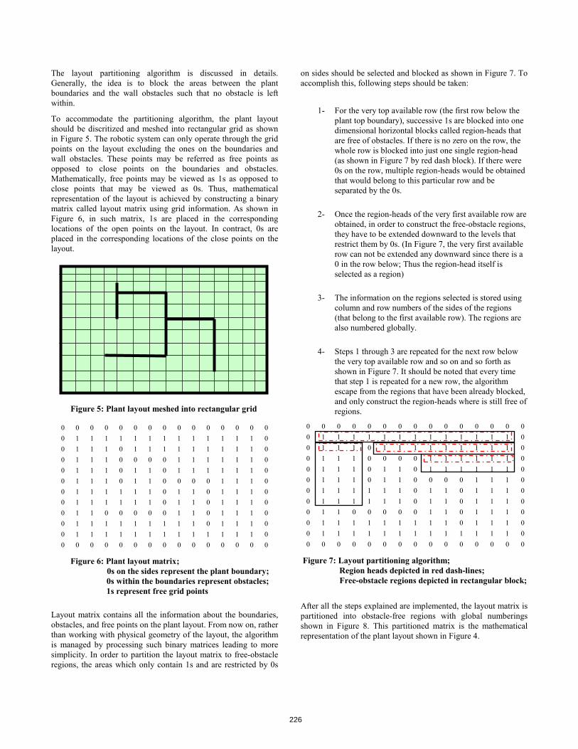
226

227

228

229

Algorithms and Performance Analysis for Path Navigation of Ackerman-Steered Autonomous Robots

G. Henson, M. Maynard, G. Dimitoglou, X. LiuDepartment of Computer Science

Hood CollegeFrederick, MD 21701

{gah1, mmaynard, dimitoglou, liu}@hood.edu

230

231

232

233

234

235

Wireless Communications in Tunnels for Urban Search and Rescue Robots

Kate A. Remley, Galen Koepke, Dennis G. Camell,Chriss Grosvenor

NIST Electromagnetics Division 325 Broadway

Boulder, CO, USA 80305 +1 303 497-3652

remley@boulder.nist.gov

Lt. George Hough New York City Fire Department

New York City, NY USA

gch9@columbia.edu

Robert T. Johnk Institute for Telecommunications

Sciences325 Broadway

Boulder, CO, USA 80305

bjohnk@its.bldrdoc.gov

ABSTRACT

We report on propagation tests carried out in a subterranean tunnel to support improved wireless communications for urban search and rescue robots. We describe single-frequency and ultrawideband channel-characterization tests that we conducted, as well as tests of telem etry and control of a robot. We utilize propagation models of both single-frequency path loss and channel capacity to predict robot performance. These models can also be used for optimizing wireless communications in tunnels of various sizes, materials, and surface roughness.

Categories and Subject Descriptors

Defining and measuring aspects of an intelligent system. Evaluating components within intelligent systems

General Terms Measurement, Perform ance, Reliability , Experimentation, Standardization, Verification.

Keywords

Multipath; radiowave propagation; RMS delay spread; robot; urban search and rescue; wireless communication; wireless system

INTRODUCTION Researchers from the Electrom agnetics Division of the National Institute of Standards and Technology (NIST) and the Fire Department of New York (FDNY) conducted tests of radiowave transmission and detection in tunnels at the Black Diamond Mines Regional Park near Antioch, California on March 19-21, 2007. Our goal was to investigate propagation channel characteristics that affect the reliability of wireless telem etry and control of Urban Search and Rescue (US&R) robots in tunnels and other weak-signal environments. We describe measurement methods that we used to study parameters relevant to robot performance. We also use the m easured data to verify models of radiowave propagation in tunnels. These models can be used to predict robot performance in tunnels having characteristics different from the ones we measured, such as subways and utility tunnels. This work supports the development of technically sound standards for US&R robots [1-3].

We used both time- and frequency -domain techniques to study issues such as channel multipath and loss that may impede

successful wireless communications in tunnels. We tested both video and control of a robot inside a mine tunnel. We also implemented propagation models of path loss and channel capacity and compared our measured results to these m odels. We summarize below the data we collected and interpret the key findings from the study, which is described in its entirety in [4].

Recently, the wireless field has seen a renewed interest in studies of signal propagation in both mine and subway tunnels, following a good deal of study on mine communications in the 1970s. A seminal work on mine tunnel propagation by Emslie et al. [5], studied radiowave propagation in small underground coal tunnels (4.3 m wide x 2.1 m high) for frequencies ranging from 200 MHz to 4 GHz. Emslie developed a model for propagation in tunnels that is used today . Recently , Rak and Pechak [6] applied Emslie’s work to sm all cave galleries for speleological applications, confirming Emslie’s findings that once a few wavelengths separate the transmitter and receiver, the tunnel acts as a waveguide that strongly attenuates signals below the waveguide’s cutoff frequency. Because the walls of the tunnel are not perfectly conducting, signals operating above the cut-off frequency also experience significant loss. In a recent paper, Dudley, Lienard, Mahmoud, and Degauque [7] performed a detailed assessment of operating frequency in a variety of tunnels. They found that as frequency increases, the lossy waveguide effect decreases.

Our measurements, covering a much wider frequency range than [7], and implementation of the model of [6] also confirm the lossy waveguide effect in the tunnels we studied. This effect can have a significant impact on choice of frequency for critical applications such as US&R operations, where typically infrastructure such as a repeater network is not available and lives may be at stake.

Another factor in tunnel com munications is m ultipath caused by reflections off the walls, floor, and ceiling of the tunnel. This was clearly seen in the work of Dudley , et al. [7] . Multipath can have a pronounced effect on successful transmission of wideband data. Multipath interference m ay affect certain frequencies in a wideband signal while sim ultaneously having little im pact on other frequencies. This frequency selectivity can make decoding signals difficult for the demodulator in a receiver.

We studied the severity of multipath in the tunnel environment by m easuring the RMS delay spread, as well as the success or failure of wideband data transfer by use of a commercially available robot. We compare our m easured results to a model of channel capacity based on Shannon’s theory of channel capacity

(c) 2008 Association for Computing Machinery. ACM acknowledges that this contribution was authored or co-authored by a contractoror affliate of the U.S. Government. As such, the Government retains a nonexclusive, royalty-free right to publish or reproduce this article,or to allow others to do so, for Government purposes only.PerMIS’08,August19-21,2008,Gaithersburg,MD,USA.ACM ISBN 978-1-60558-293-1/08/08.

236

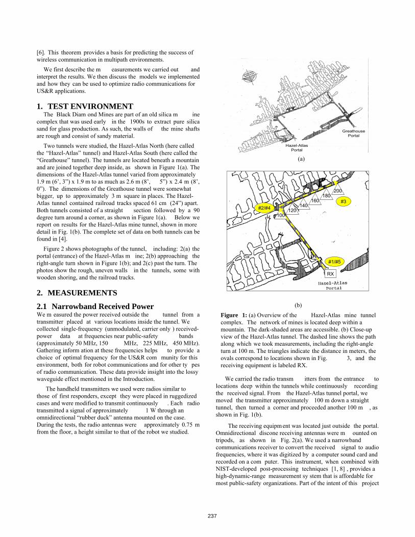
[6]. This theorem provides a basis for predicting the success of wireless communication in multipath environments.

We first describe the m easurements we carried out and interpret the results. We then discuss the models we implemented and how they can be used to optimize radio communications for US&R applications.

1. TEST ENVIRONMENT The Black Diam ond Mines are part of an old silica m ine

complex that was used early in the 1900s to extract pure silica sand for glass production. As such, the walls of the mine shafts are rough and consist of sandy material.

Two tunnels were studied, the Hazel-Atlas North (here called the “Hazel-Atlas” tunnel) and Hazel-Atlas South (here called the “Greathouse” tunnel). The tunnels are located beneath a mountain and are joined together deep inside, as shown in Figure 1(a). The dimensions of the Hazel-Atlas tunnel varied from approximately 1.9 m (6’, 3”) x 1.9 m to as much as 2.6 m (8’, 5”) x 2.4 m (8’, 0”). The dimensions of the Greathouse tunnel were somewhat bigger, up to approximately 3 m square in places. The Hazel-Atlas tunnel contained railroad tracks spaced 61 cm (24”) apart. Both tunnels consisted of a straight section followed by a 90 degree turn around a corner, as shown in Figure 1(a). Below we report on results for the Hazel-Atlas mine tunnel, shown in more detail in Fig. 1(b). The complete set of data on both tunnels can be found in [4].

Figure 2 shows photographs of the tunnel, including: 2(a) the portal (entrance) of the Hazel-Atlas m ine; 2(b) approaching the right-angle turn shown in Figure 1(b); and 2(c) past the turn. The photos show the rough, uneven walls in the tunnels, some with wooden shoring, and the railroad tracks.

2. MEASUREMENTS

2.1 Narrowband Received Power We m easured the power received outside the tunnel from a transmitter placed at various locations inside the tunnel. We collected single-frequency (unmodulated, carrier only ) received-power data at frequencies near public-safety bands (approximately 50 MHz, 150 MHz, 225 MHz, 450 MHz). Gathering inform ation at these frequencies helps to provide a choice of optimal frequency for the US&R com munity for this environment, both for robot communications and for other ty pes of radio communication. These data provide insight into the lossy waveguide effect mentioned in the Introduction.

The handheld transmitters we used were radios similar to those of first responders, except they were placed in ruggedized cases and were modified to transmit continuously . Each radio transmitted a signal of approximately 1 W through an omnidirectional “rubber duck” antenna mounted on the case. During the tests, the radio antennas were approximately 0.75 m from the floor, a height similar to that of the robot we studied.

We carried the radio transm itters from the entrance to

locations deep within the tunnels while continuously recording the received signal. From the Hazel-Atlas tunnel portal, we moved the transmitter approximately 100 m down a straight tunnel, then turned a corner and proceeded another 100 m , as shown in Fig. 1(b).

The receiving equipm ent was located just outside the portal. Omnidirectional discone receiving antennas were m ounted on tripods, as shown in Fig. 2(a). We used a narrowband communications receiver to convert the received signal to audio frequencies, where it was digitized by a computer sound card and recorded on a com puter. This instrument, when combined with NIST-developed post-processing techniques [1, 8] , provides a high-dynamic-range measurement sy stem that is affordable for most public-safety organizations. Part of the intent of this project

GreathousePortal

Hazel-AtlasPortal

(b) Figure 1: (a) Overview of the Hazel-Atlas mine tunnel complex. The network of mines is located deep within a mountain. The dark-shaded areas are accessible. (b) Close-up view of the Hazel-Atlas tunnel. The dashed line shows the path along which we took measurements, including the right-angle turn at 100 m. The triangles indicate the distance in meters, the ovals correspond to locations shown in Fig. 3, and the receiving equipment is labeled RX.

100120

200

160140

180

RX

#1/#5

#3#2/#4

(a)

237

was to dem onstrate a user-friendly sy stem that could be utilized by US&R organizations to assess their own unique propagation environments.

(a)

Figure 3 shows representative m easured received-power data at frequencies of 50 MHz, 162 MHz, and 448 MHz acquired while the transmitters were carried by foot through the tunnel. The signals were sampled at approximately 48 kHz and the power averaged over one-second intervals. The left and right halves of the graph show measurements made walking into and out of the tunnel, respectively , and thus m irror each other. The vertical dashed lines on the graph correspond to the entrance (#1, #5), turn (#2, #4), and turn-around point (#3) in the measurement path, as shown in Fig. 1(b).

The cut-off frequency for this ty pe of tunnel is difficult to define since the walls behave as lossy dielectrics rather than conductors. These conditions are discussed in [9] , where the attenuation constant is found to vary as the inverse of frequency squared [Section 2.7, pp. 80-83] . Hence, we would expect higher attenuation at the lower frequencies but no sharp cut-off. Further complications in this tunnel ar e the axial conductors (cables, water pipes, rails) that may support a TEM-like mode of propagation, the irregular cross-section, and the side chambers and tunnels.

For the Hazel-Atlas mine tunnel, we see in Fig. 3(a), strong attenuation of the 50 MHz signal and in Fig. 3(b), the received power of the 162 MHz signal also decreases rapidly as the transmitter moves into the tunnel. This rapid attenuation is due to the lossy waveguide effect described in references [4-7] . The signal for the 448 MHz carrier frequency (Fig. 3(c)) exhibits less attenuation and this is where the models of [5] may apply. Signals may travel even further at higher frequencies, as discussed in [5-7]. This frequency dependence may play a significant role in deciding which frequencies to utilize in US&R robot deploy ment applications, as will be discussed in Section 3.

2.2 Excess Path Loss and RMS Delay Spread We also conducted measuremen ts at several stationary

positions covering a very wide frequency band. These “excess-path-loss” m easurements provide the received signal power relative to a direct-path signal over a frequency band. When transformed to the time domain, the wide frequency band yields a short-time-duration pulse. This pulse can be used to study the number and duration of multipath reflections in an environment.

Our synthetic-pulse, ultrawideband sy stem is based on a vector network analy zer (VNA). Our measurements covered frequencies from 25 MHz to 18 GHz. The post-processing and calibration routines associated with it were developed at NIST [10]. In the synthetic-pulse system, the VNA acts as both transmitter and receiver. The transmitting section of the VNA sweeps over a wide range of frequencies a single frequency at a time. The transmitted signal is amplified and fed to a transm itting antenna. For this study, we used omnidirectional discone antennas for frequencies between 25 MHz and 1.6 GHz, and directional horn-type transm itting and receiving antennas for frequencies between 1 GHz and 18 GHz.

(b)

(c) Figure 2: (a) Portal into the Hazel-Atlas mine tunnel. (b) 90 m inside showing the bend depicted in Fig. 1(b) and the rough, sandy wall material. (c) Wood shoring approximately 150 m into the tunnel. The robot we tested can be seen on the cart between the railroad tracks.

238

The received signal was picked up over the air in the tunnel

by the receiving antenna and was relay ed back to the VNA via a fiber-optic cable. The fiber-optic cable phase-locks the received signal to the transmitted signal, enabling post processing reconstruction of the time-domain waveform associated with the received signal. The broad range of frequencies and time-domain representation provide insight into the reflective m ultipath nature of the tunnel that cannot be captured by use of single-frequency measurements. The receive antenna m ust rem ain fixed during each m easurement, so these tests are carried out at discrete locations, unlike the single-frequency tests.

We m easured excess path loss every 20 m starting approximately 10 m into the tunnel. The VNA was located at the Hazel-Atlas portal. The transm itting antenna was located at the portal as well. The graphs show data starting from 0 Hz, however the valid (calibrated) measurement range is stated for each graph.

50 100 150 200 250 300 350-140

-120

-100

-80

-60

-40

-20

0 #2 #3 #4 #5

time [sec]

Pav

g [dB

m]

#3 #4 #5#2#1

50 MHz

Figures 4 and 5 show measured excess path loss over a wide frequency band measured 50 m and 120 m, respectively , in the Hazel-Atlas tunnel. Note that at 120 m , we have passed the right-angle turn in the tunnel. The t op curve in each graph represents the received power level, referenced to the calculated free-space path loss at that location. The bottom curve represents the noise floor of the measurement system.

(a) Figure 4 shows that even in a line-of-sight condition approximately 50 m from the tunnel entrance, the spectrum of the received signal display s significant frequency dependence. At frequencies between 25 MHz and 1.6 GHz (Fig. 4(a)), the lossy waveguide effect is shown by the rapidly decreasing signal on the left-hand side of the graph. We see that a carrier frequency higher than approximately 700 MHz would suffer less loss compared to lower frequencies in this particular tunnel. Figure 4(b) shows frequencies from 1 GHz to 18 GHz. In this case, we see frequency dependence in received power caused by strong reflections, as shown by the deep nulls and peaks in the top curve of Fig. 4(b).

Once the receiving antenna turns the corner, see Fig. 5, the signal takes on a more random variation with frequency since transmission consists of reflected signals only . For frequencies from 25 MHz to 1.6 GHz (Fig. 5(a)), the received signal power is near the noise floor of the receiver since the two curves almost overlay. For the higher frequencies (Fig. 5(b)), we see that the average received signal level is relatively constant with frequency, but the peaks and nulls are still significant.

Finally, we present the RMS delay spread for the Hazel-Atlas mine tunnel in Table 1 for frequencies from 25 MHz to 1.6 GHz and 1 GHz to 18 GHz. We see that the shortest delay spreads are found by use of the directional antennas. The complete set of UWB excess-path-loss data is given in [4].

2.3 Tests of Robot Communications We carried out tests on a commercially available robot. Control and video were as-built for the com mercial product. We used the omnidirectional antennas that came with the system for all tests in order to assess the default capabilities of this robot.

The robot we used is controlled with a 2.4 GHz spread-spectrum, frequency-hopping protocol, which was configured to transmit in the unlicensed 2.4 GHz industrial, scientific, and medical (ISM) band. The control channel utilizes a modulation bandwidth of approximately 20 MHz. The output power of the bidirectional control link is nominally 500 mW.

The robot transmits video by use of one of ten channels between 1.7 GHz and 1.835 GHz. The robot we tested transm itted at 1.78 GHz by use of an analog modulation format that was non-bursted and non-frequency-agile. The video channel utilized approximately 6 MHz of modulation bandwidth. The output power was nominally 2 watts.

50 100 150 200 250 300-140

-120

-100

-80

-60

-40

-20

0

time [sec]

Pav

g [dB

m]

#2 #3 #4 #5

#3 #4 #5#2#1

162 MHz

(b)

(c)

0

Figure 3: Received-power data in the Hazel-Atlas Mine for three carrier frequencies: (a) 50 MHz, (b) 162 MHz, (c) 448 MHz. In each case the #2 and #4 vertical dashed lines correspond to the turn at 100 m: once on the way into the tunnel and once on the way out. The #3 dashed line represents the end point at 200 m, shown in Fig. 1(b).

50 100 150 200 250-140

-120

-100

-80

-60

-40

-20

time [sec]

Pav

g [dB

m]

#2 #3 #4 #5

#1 #2 #3 #4 #5

448 MHz

239

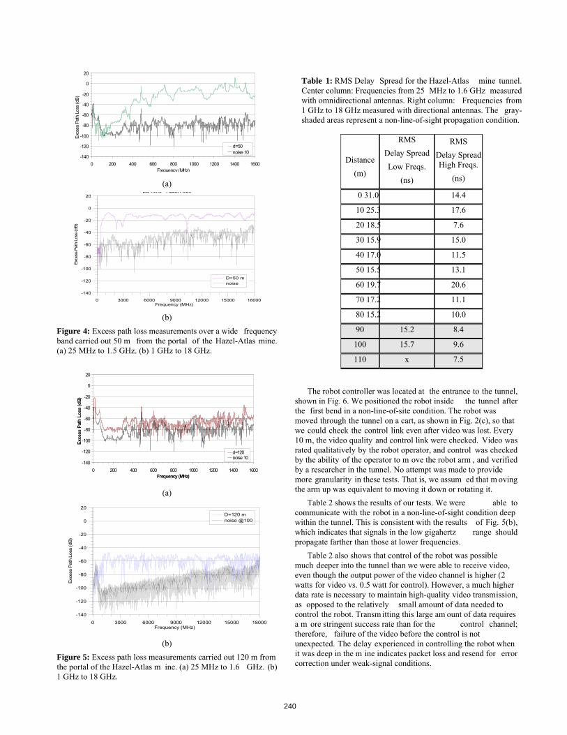
The robot controller was located at the entrance to the tunnel, shown in Fig. 6. We positioned the robot inside the tunnel after the first bend in a non-line-of-site condition. The robot was moved through the tunnel on a cart, as shown in Fig. 2(c), so that we could check the control link even after video was lost. Every 10 m, the video quality and control link were checked. Video was rated qualitatively by the robot operator, and control was checked by the ability of the operator to m ove the robot arm , and verified by a researcher in the tunnel. No attempt was made to provide more granularity in these tests. That is, we assum ed that m oving the arm up was equivalent to moving it down or rotating it.

Table 2 shows the results of our tests. We were able to communicate with the robot in a non-line-of-sight condition deep within the tunnel. This is consistent with the results of Fig. 5(b), which indicates that signals in the low gigahertz range should propagate farther than those at lower frequencies.

Table 2 also shows that control of the robot was possible much deeper into the tunnel than we were able to receive video, even though the output power of the video channel is higher (2 watts for video vs. 0.5 watt for control). However, a much higher data rate is necessary to maintain high-quality video transmission, as opposed to the relatively small amount of data needed to control the robot. Transm itting this large am ount of data requires a m ore stringent success rate than for the control channel; therefore, failure of the video before the control is not unexpected. The delay experienced in controlling the robot when it was deep in the m ine indicates packet loss and resend for error correction under weak-signal conditions.

-140

-120

-100

-80

-60

-40

-20

0

20

0 200 400 600 800 1000 1200 1400 1600Frequency (MHz)

Exce

ss P

ath

Loss

(dB)

d=50noise 10

0 3000 6000 9000 12000 15000 18000Frequency (MHz)

-140

-120

-100

-80

-60

-40

-20

0

20

Exc

ess

Pat

h Lo

ss (d

B)

D=50 mnoise

BD mine Hazel Atlas

(b)

Figure 4: Excess path loss measurements over a wide frequency band carried out 50 m from the portal of the Hazel-Atlas mine. (a) 25 MHz to 1.5 GHz. (b) 1 GHz to 18 GHz.

(a)

(a)

-140

-120

-100

-80

-60

-40

-20

0

20

0 200 400 600 800 1000 1200 1400 1600Frequency (MHz)

Exce

ss P

ath

Loss

(dB)

d=120noise 10

(b) Figure 5: Excess path loss measurements carried out 120 m from the portal of the Hazel-Atlas m ine. (a) 25 MHz to 1.6 GHz. (b) 1 GHz to 18 GHz.

(a)

0 3000 6000 9000 12000 15000 18000Frequency (MHz)

-140

-120

-100

-80

-60

-40

-20

0

20

Exce

ss P

ath

Loss

(dB)

D=120 mnoise @100

Distance

(m)

RMS Delay Spread Low Freqs.

(ns)

RMS Delay SpreadHigh Freqs.

(ns)

0 31.0 14.4

10 25.3 17.6

20 18.5 7.6

30 15.9 15.0

40 17.0 11.5

50 15.5 13.1

60 19.7 20.6

70 17.2 11.1

80 15.2 10.0

90 15.2 8.4

100 15.7 9.6

110 x 7.5

Table 1: RMS Delay Spread for the Hazel-Atlas mine tunnel. Center column: Frequencies from 25 MHz to 1.6 GHz measured with omnidirectional antennas. Right column: Frequencies from 1 GHz to 18 GHz measured with directional antennas. The gray-shaded areas represent a non-line-of-sight propagation condition.

240

3. MODELED RESULTS

3.1 Single-Frequency Path Gain Models To study the extent of waveguiding in these tunnels, we implemented an analy tical m odel that sim ulates signal propagation in tunnel environm ents having various phy sical parameters [5, 6, 11] . Briefly , the model assumes a dominant EH11 mode in a lossy rectangular waveguide with the attenuation

in dB/m expressed for vertical polarization as

TILTROUGHNESSTUNNEL ,

(1) where

111343.4

332

TUNNELR

R

R ba , (2a)

4422

ROUGHNESS11343.4

bah

, (2b)

22

TILT 343.4, (2c)

and is the wavelength, a is the width of the tunnel, b is the height of the tunnel, and h is the roughness, all in meters. Other parameters include R, the dielectric constant of the rock walls, and , the angle of the tunnel-floor tilt in degrees.

We set the parameters of the model to approximate the Hazel-Atlas tunnel, given below in Tabl e 3. This model works well only for frequencies will above the cut-off frequency , that is, for wavelengths significantly less than the dimensions of the tunnel [5, 6] . Hence, in Fig. 7 we show results for 448 MHz only. At distances around 80 m, the signal was able to propagate through an air vent as well as through the tunnel, so the overall received signal level increases. The good ag reement between the measured and modeled data led us to conclude that waveguiding play s a significant role in radio propagation in these tunnels.

The model also lets us explore which frequencies may be

optimal for robot or other wireless communications in the tunnel. Figure 8 compares a number of commonly used emergency

20 40 60 80 100-120

-100

-80

-60

-40

-20

0

Distance (m)

Pat

h G

ain

(dB

)

448 MHz model448 MHz measured

Figure 7: Comparison of measured and modeled data for the Hazel-Atlas tunnel. The carrier frequency is 448 MHz. The modeled data simulate waveguide propagation for a waveguide whose physical parameters approximate those of the tunnels.

Parameter Value

Width Height

Wall roughness

r tilt

2 m 2 m 0.3 6 1°

Table 3: Parameters used in tunnel model.

Distance in tunnel (m)

Table 2: Results of wireless communication link tests carried out inside Hazel-Atlas tunnel at Black Diamond Mines Regional Park.

Figure 6: Robot operator positioned at the entrance to the Hazel-Atlas mine tunnel. The robot was operated in a non-line-of-sight condition more than 100 m inside the tunnel.

Video quality (1.7 GHz)

Control of arm (2.4 GHz)

100 good yes

110 good yes

120 poor (intermittent) yes

130 poor (intermittent) yes

140 very poor yes

150 none yes

160 none delay experienced

170 none intermittent control

180 none delay experienced

190 none delay experienced

200 none delay experienced

205 none none

241

responder frequencies as a function of distance within the tunnel. As discussed in [5, 6] , the frequency -dependent behavior of the tunnel leads to a “sweet spot” in frequency. Below the sweet spot, signals do not propagate well, due to the effect of waveguide-below-cutoff attenuation and wall loss. Above the sweet spot, free-space path loss (which increases with frequency ) and TILT dominate and signals do not propagate well. Again, models such as these may enable a choice of appropriate frequency for US&R robot communications in tunnel environments. Note that these results are valid only for a tunnel with these dimensions, wall materials, and surface roughness. The curves would need to be recalculated for other types of tunnels.

We also used the m odel to investigate the video performance

of the robot, described in S ection 3.c. The frequency-hopping control channel would need to be modeled by use of other methods, since it consists of several narrowband channels frequency hopping within a wide modulation bandwidth. In Fig. 9, we plot the estimated path gain at a carrier frequency of 1.78 GHz for the tunnel environment with a right-angle turn 100 m from the receiver. We used the parameters in Table 3 for the model. A path gain of 40 dBW was used as an approximation for the turn in the tunnel at 100 m, based on work done by Lee and Bertoni in [12] . We plot the flat earth path gain for comparison.

Figure 9 also shows the theoretically com puted excess link margin (ELM). The ELM is the difference between the received signal strength and the minimum receiver sensitivity. The receiver sensitivity is determined by the therm al noise of the receiver and the receiver’s front-end amplifier noise (5 dB, as a rule of thumb). The thermal noise is given by N = kTB, where k is the Boltzmann constant, T is the temperature in Kelvin, and B is the bandwidth of the receiver. In order for a wireless link to be m aintained, the ELM must be greater than zero dB.

The ELM plotted in Fig. 9 agrees well with the measured results from Table 2, which show that the video completely drops out between approximately 140 m and 150 m. Given the fluctuation in signal strength due to multipath fading in this tunnel environment, once the link margin drops below 10 dB at

approximately 120 m, the video quality degrades and the picture becomes intermittent.

0 50 100 150 200-150

-100

-50

0

Distance (m)

Pat

h G

ain

(dB

)

TunnelFlat EarthELM=0dB

500 1000 1500 2000 2500 3000 3500 4000-200

-180

-160

-140

-120

-100

-80

-60

-40

-20

0

Frequency (MHz)

Pat

h G

ain

(dB

)

10m20m30m40m50m60m70m80m90m100m

Increasing distance

into tunnel

Frequencies with lowest

loss in tunnel

Figure 9: Path gain curves for tunnel with a right-angle turn at 100 m (solid) and flat earth (dashed) environments. The curve labeled “ELM = 0” indicates where the excess link margin calculation predicts loss of signal. As shown, this occurs approximately 150 m into the tunnel.

3.2 Channel Capacity Model In general, received RF power and bandwidth effectively

place an upper bound on the capacity of a com munications link. The Shannon channel capacity theorem [13] can be used to predict the approximate maximum data rate for tunnel communications, even though the Shannon theorem is based on the assumption of a Gaussian noise (low multipath) environment. For a given m odulation bandwidth, the received signal power relative to the noise power determines the theoretical upper limit on the data rate (channel capacity ). The Shannon capacity theorem is given by

Figure 8: Path gain versus frequency for various distances in a tunnel having physical characteristics similar to those of the Hazel-Atlas tunnel. Frequencies around approximately 400 MHz to 1 GHz propagate better than either lower or higher carrier frequencies.

NSBC /1log2 , (3) where C is the channel capacity in bits/second, B is the channel bandwidth in hertz, S is the received signal power in watts, and N is the measured noise power in watts. The capacity represented by this equation is the upper lim it, and in reality the capacity would be difficult to attain with real hardware.

For an analog transmission, Shannon’s limit gives us a way to estimate the channel capacity . The National Television S ystem Committee (NTSC) analog video channel that our robot used has a video bandwidth of 4.2 MHz and a transmission rate of approximately 30 frames per second, where each frame consists of 525 scanning lines, giving a line rate of 15.734 kHz [14]. We can place an upper bound on the am ount of data that could be transmitted in each line by considering a ty pical implementation of NTSC, where each line is digiti zed into 768 pixels. This gives a digital scanning rate of approximately 12 MHz. The specification of 768 pixels per line is used in studio environments. We expect the potential channel capacity to be lower in the analog transmission case.

Figure 10 shows simulations of the Shannon limit for our robot’s 4.2 MHz video bandwidth, 1.78 GHz video channel. Table 4 shows the distance into the tunnel where 12 Mb/sec transmission rate occurs assuming our maximum possible channel

242

capacity to be various fractions of the Shannon limit. Based on this information, we would expect to encounter video problems somewhere between 120 m and 130 m into the tunnel, which Table 2 shows is indeed where we started to experience signal degradation. Thus, we are able to form a rough estimate of the distance into the tunnel where we expect the video to fail based on a simple implementation of the Shannon theorem.

4. CONCLUSIONWe have presented measured data collected in a subterranean

tunnel environment. Results show ed waveguide-below-cutoff and wall attenuation effects. We saw frequency -dependent peaks and nulls in the channel due to strong m ultipath reflections and attenuation in the tunnel. In non-line-of-sight conditions, we saw classic Rayleigh-distributed noise-like signals.

We implemented models that m ay be used to predict radiowave propagation and modulated-signal performance within tunnels for robots or other wire less devices. Using the models, it was possible to ascertain the optimal carrier frequency range for a robot within this tunnel environment. The intent of this work is to improve radio communications for urban search and rescue robots when they transmit wideband, digitally modulated signals. We hope that these data will prove us eful in standards development,

as well as improved technology and sy stem design for the emergency-responder community.

5. ACKNOWLEDGEMENTThe authors thank Alex Bordetsky of the Naval Postgraduate

School for facilitating the m easurements during recent interagency m arine interdiction operation sy stem tests. We also thank Bill Dunlop, Steve MacLaren, and Dave Benzel of Lawrence Livermore National Laboratory for logistical and technical support. We are indebted to Frederick M. Remley for details on the NTSC video standard.

0 50 100 150 2000

50

100

150

200

Distance (m)

Cap

acity

(Mb/

sec)

100% of Shannon Capacity90% of Shannon Capacity80% of Shannon Capacity70% of Shannon Capacity

Figure 10: Channel capacity predicted by the Shannon theorem for a carrier frequency of 1.78 GHz and a video modulation bandwidth of 4.2 MHz. At 120 m, where we experienced intermittent video, 80 % of the Shannon limit is 15.4 Mb/sec and 70 % of the Shannon limit is 13.5 Mb/sec.

6. REFERENCES[1] Elena Messina, “ Performance Standards for Urban Search and

Rescue Robots,” ASTM Standardization News, August 2006, http://www.astm.org/cgi-bin/SoftCart.exe/SNEWS/AUGUST_2006/messina_aug06.html .

[2] National Institute of Standards and Technology, “Statement of Requirements for Urban Search and Rescue Robot Performance Standards-Preliminary Report” http://www.isd.mel.nist.gov/US&R_Robot_Standards/Requirements%20Report%20(prelim).pdf

[3] K. A. Rem ley, G. Koepke, E. Messina, A. Jacoff, G. Hough, “Standards development for wireless com munications for urban search and rescue robots,” Proc. Int. Symp. Advanced Radio Technol., pp. 66-70, Boulder, CO, Feb. 2007.

[4] K.A. Remley, G. Koepke, C.L. Holloway, C. Grosvenor, D. Camell, J. Ladbury, D. Novotny, W.F. Young, G. Hough, M.D. McKinley, Y. Becquet, J. Korsnes, “Measurements to support broadband modulated-signal radio transmissions for the public-safety sector,” Natl. Inst. Stand. Technol. Note 1546, Apr. 2008.

[5] A.G. Emslie, R.L. Lagace, and P.F. Strong, “Theory of the propagation of UHF radio waves in coal mine tunnels,” IEEE Trans. Antennas and Prop., vol. 23, no. 2, Mar. 1975, pp. 192-205.

[6] M. Rak and P. Pechac, “UHF propagation in caves and subterranean galleries,” IEEE Trans. Antennas and Prop., vol. 55, no. 4, April 2007, pp. 1134-1138.

[7] D. G. Dudley, M. Lienard, S.F. Mahmoud and P. Degauque, “Wireless propagation in tunnels,” IEEE Antennas Prop. Mag., vol. 49, no. 2, April 2007, pp. 11-26.

[8] M. Rütschlin, K. A. Remley, R. T. Johnk, D. F. Williams, G. Koepke, C. Holloway, A. MacFarlane, and M. Worrell, “Measurement of weak signals using a communications receiver system,” Proc. Intl. Symp. Advanced Radio Technol., Boulder, CO, March 2005, pp. 199-204.

Fraction of Shannon capacity (%)

Distance into tunnel (m)

100 133

90 129

80 122

70 114

Table 4: Distance into tunnel for a channel capacity of approximately 12 Mb/sec.

[9] P. Delogne, “Leaky Feeders and Subsurface Radio Communications, IEE press, 1982.

[10] B. Davis, C. Grosvenor, R.T. Johnk, D. Novotny, J. Baker-Jarvis, M. Janezic, “Complex permittivity of planar building materials measured with an ultra-wideband free-field antenna measurement system,” NIST Journal of Research, Vol. 112, No. 1, Jan.-Feb., 2007, pp. 67-73.

[11] G. Hough, “Wireless robotic communications in urban environments: issues for the fire service,” Thesis, Naval Postgraduate School, March 2008. http://theses.nps.navy.mil/08Mar_Hough.pdf

[12] J. Lee and H. Bertoni, “Coupling at cross, T, and L junctions in tunnels and urban street canyons,” IEEE Trans. Antennas Prop., vol. 51, no. 5 , May 2003, pp. 926-935.

[13] C.E. Shannon, “Communication in the presence of noise,” Proc. IRE, vo. 37, no. 1, Jan. 1949, pp. 10-21.

[14] C.A. Poynton, “A Technical Introduction to Digital Video,” Wiley, 1996, pp 26-27.

243

A Performance Assessment of Calibrated CameraNetworks for Construction Site Monitoring

Itai Katz, Nicholas Scott, Kamel SaidiNational Institute of Standards and Technology

100 Bureau Drive Stop 8611Gaithersburg, MD, 20899-8611, USA

{itai.katz, nicholas.scott, kamel.saidi}@nist.gov

ABSTRACTMonitoring the status of construction activity is a key fac-tor in maximizing e!ciency and reducing cost on capitalconstruction sites. In contrast to human inspection, an au-tomated technology would provide more frequent updates.However, real-time construction site monitoring remains anelusive goal because of many factors including the environ-ment’s large size and dynamic behavior. Calibrated cameranetworks have recently been developed to enable smart en-vironments, where the location of people and objects in thescene are updated in real-time. Despite a growing interestin this technology, a detailed performance analysis has notbeen conducted. In this paper, empirical results on the cal-ibration and static 3D localization error are presented fora calibrated camera network prototype using four cameras.Using a total station to provide ground truth, the camerasare calibrated and points in the workspace are reconstructedin 3D by combining observations from each image plane. Re-sults show that performance is well suited for localizing ob-jects typically found on a construction site (although scalingerrors have not yet been characterized).

Keywordsconstruction automation, calibrated camera network, per-formance evaluation

1. INTRODUCTION

1.1 The ProblemSituation awareness on a construction site is a key ele-

ment in maintaining a safe and productive project. In in-dustries such as manufacturing, where the work environmentis highly controlled and predictable, situation awareness isrelatively easy to achieve. However, the dynamic and clut-tered nature of a construction site makes a similar degreeof control virtually impossible. Nevertheless, in order forproject managers and others to make informed and timely

This paper is authored by employees of the United States Government andis in the public domain.PerMIS’08 August 19-21, 2008, Gaithersburg, MD, USACopyright 2008 ACM 978-1-60558-293-1/08/08.

decisions, they must have accurate information of the cur-rent status of all project activities. Decisions made basedon old or inaccurate information could have wide-reachingramifications on the schedule, budget and safety of a project,particularly on large capital projects.

Critical information needed for proper decision-making in-cludes:

• Locations of workers and equipment

• Locations of bulk materials and manufactured con-struction components

• Level of completion for construction activities

• Locations of potential safety hazards

1.2 Camera Networks as a SolutionIn this paper, we propose a solution to the situation aware-

ness problem on construction sites using calibrated cameranetworks. Rather than simply providing raw video feeds,calibrated camera networks provide a method to abstractthe data into a form that is more readily usable. Whilethese systems are well known in the academic community [3],their use in the construction industry is novel. This paperextends previous results in [4] on localization error for long-baseline methods using an alternative calibration technique.The data set is 50 % larger and better characterizes the workvolume.

1.3 OutlineBelow we introduce the calibrated camera network (CCN)

concept and describe a potential role in the constructiondomain. Section 2 provides an overview of CCNs and illus-trates how they could potentially be applied to the construc-tion domain. Section 3 demonstrates the setup and testingof a camera network and reports on experimentally-derivederrors for 3D localization. Conclusions are provided in Sec-tion 4.

2. CALIBRATED CAMERA NETWORKS INCONSTRUCTION

2.1 System DescriptionA CCN is a collection of three or more vision sensors

whose positions and orientations in 3D space have been de-termined. In contrast to a collection of isolated cameras,CCNs have two key di"erences:

244

1. Each camera in the network is a ”smart” node thatcombines an image sensor, on-board computing, andthe capability to network with other nodes (typicallywirelessly). This allows each node to independentlycarry out low-level image processing tasks (e.g., back-ground subtraction) or more sophisticated vision algo-rithms (e.g., pedestrian detection). By communicatingonly the output of these algorithms, rather than theraw video streams, bandwidth is conserved.

2. Each camera is calibrated with respect to a commoncoordinate system (i.e., the pose and internal param-eters – intrinsic and extrinsic – of the cameras areknown). This step is performed before the nominaloperating mode and allows the 2D image planes to becombined in order to recover 3D structures.

An example of a CCN is shown in Figure 1. In principle,a CCN can be used to detect and track objects in 3D, andto perform geometric reconstruction.

Figure 1: Photo of a calibrated camera network withfour cameras. The checkerboard pattern in the cen-ter is a calibration target.

2.2 Benefits Over Existing SensorsThere are various manufacturers of video cameras designed

specifically for remote monitoring of construction sites. Al-though these systems could be of benefit for large sites wherecontinuous, in-person monitoring is impractical, the e"ortrequired by the human operator increases with the numberof video feeds to be monitored. As the number of feedsincreases, visual clutter for the human operator also in-creases and the ability to discriminate interesting or anoma-lous events can actually decrease [4].

A CCN has additional advantages over other 3D trackingsensors such as laser trackers, ultra wideband locators, laser-based localization systems, and high-frame rate 3D imagingsystems. The advantages include:

• Robustness to noise: Individual localization errors canbe averaged together. Localization error can be re-duced by incorporating additional nodes into the net-work.

• Occlusion handling: CCNs are inherently redundant.By placing cameras around the perimeter of the workspace,

occluded objects can still be tracked as long as they re-main visible in two or more cameras.

• Arbitrarily-sized workspace: Adding coverage in a CCNcan be achieved by incorporating additional nodes intothe network.

• Token-less operation: Tracking an object or a per-son does not require placing a token such as a Radio-Frequency Identification (RFID) tag, optical receiver,or other cooperative target on the object being tracked.

• Passive operation: As long as multiple cameras in aCCN can ”see” an object within a workspace, no sup-plementary illumination source is necessary to trackthat object.

• Decentralized communication: Since the nodes in aCCN can form an ad-hoc mesh network in order toshare and transmit data, as long as a node can see atleast one other node within the network, the CCN canfunction in noisy environments where a central deviceacting as the bridge between multiple wireless sensorscan experience range and interference problems.

2.3 Site DeploymentPrior to installation at a construction site, a suitable cam-

era configuration must be determined that will provide thedesired tracking performance. The number and layout ofcameras will depend on many factors including the workspacevolume, camera field of view and resolution, and the de-sired spatial and temporal resolution. An exploration ofthe tradeo" between camera resolution and the number ofcameras is discussed in [2]. For a given point in space, twocameras are su!cient to recover the 3D position, however,additional cameras will tend to improve the system perfor-mance by reducing the uncertainty.

Once a configuration has been chosen and the camera net-work has been installed on-site, the system must be cali-brated. Calibration requires characterization of both intrin-sic and extrinsic parameters for each camera. Intrinsic cali-bration determines a set of internal parameters (focal length,image center, pixel size, and lens distortion) that define howpoints in 3D are projected onto the 2D image plane of thecamera. Extrinsic calibration determines the relative posi-tion and orientation of each camera. Both calibrations arecommonly performed by taking images of calibration targetsand then exploiting the known target dimensions to deter-mine the unknown parameters [5].

2.4 ApplicationsThe real-time 3D localization capabilities of CCNs can as-

sist with a number of problems relevant to the constructionindustry. The following are some examples of CCN con-struction applications:

• Personnel, equipment and material tracking

• Automated project status monitoring

• Productivity assessment

• Automated safety and security alerts

245

3. EXPERIMENTThe majority of CCN literature focuses on short-baseline

(< 5 m) configurations. Despite growing interest, a detailedperformance analysis of long-baseline (> 5 m) calibratedcamera networks has not been conducted.

3.1 ProcedureFour cameras were mounted indoors on tripods roughly 4

m high and were arranged in a rectangle with dimensions ofapproximately 12 m x 6 m. Each camera had a resolutionof 1024 pixels x 768 pixels, and the height, angle, and fieldof view were adjusted to provide an overlapping workspacevolume of roughly 4 m x 4 m x 2.4 m. To provide groundtruth points for determining camera poses, the positions of36 points distributed throughout the work volume were ob-served with a total station. Twelve coplanar points weretaken at three di"erent heights (roughly 0 m, 1 m, and 2m). A black 3.81 cm retroreflector was used both as a coop-erative target for measurement with a total station as wellas a visible target in the camera images. The retroreflec-tor was placed either directly on the ground or on a tripodset to the desired height. The model of total station usedprovides 0.2 mm spatial uncertainty, an order of magnitudebetter performance than estimated for the camera network.

For each observation, the 3D position of the retroreflectorwas found with the total station, while the corresponding 2Dpixel coordinates in each image were manually identified. Anexample of an image from one of the cameras is shown inFigure 2. Note the retroreflector mounted on the tripod inthe center of the image.

Figure 2: A typical view from one camera. Thetripod in the center holds a retroreflector.

Intrinsic and extrinsic calibration, including lens distor-tion parameters, were obtained using the well-known DirectLinear Transformation (DLT) algorithm. First described in1971 [1], the DLT method has become the gold-standard al-gorithm for camera calibration. For convenience, we brieflydescribe its derivation below. A thorough explanation is be-yond the scope of this paper, however the interested readeris directed to [3] for a complete derivation.

The projective model for a pinhole camera maps 3D worldcoordinates to 2D pixel coordinates by way of a projection

matrix. The basic equation is given by

!

2

4xy1

3

5 = P

2

664

XYZ1

3

775 (1)

where [x y 1]T is the homogenous pixel coordinate vector,[X Y Z 1]T is the homogenous world coordinate vector, P isthe 3 x 4 projective matrix which encompasses both intrin-sic and extrinsic parameters, and ! is an arbitrary scalingfactor. Given a pixel coordinate vector [xi yi]

T and worldcoordinate vector [Xi Yi Zi]

T , the objective is to solve for P .Through straightforward manipulation, (1) can be rewrittenin linear form as

2

666664

X1 Y1 Z1 1 0 0 0 00 0 0 0 X1 Y1 Z1 1...

......

......

......

...XN YN ZN 1 0 0 0 00 0 0 0 XN YN ZN 1

!x1X1 !x1Y1 !x1Z1

!y1X1 !y1Y1 !y1Z1

......

...!xNXN !xNYN !xNZN

!yNXN !yNYN !yNZN

3

777775

2

6664

P1

P2

...P11

3

7775=

2

666664

x1

y1

...xN

yN

3

777775(2)

where the elements of P can be solved for using the methodof least mean squares. When lens distortion parameters aretaken into consideration, (2) takes on a non-linear form. Inthis case, an initial estimate for P can be obtained linearly,and a non-linear, iterative solver can be used to jointly re-fine the estimate for P and the distortion parameters. Thisprocess is depicted in Figure 3.

Direct Linear Transform

Non-linear Minimization

Manual Point Selection

images

camera

total station

!

""#

Xi

Yi

Zi

1

$

%%&

!

"xi

yi

1

#

$

P

Figure 3: Process for calibrating a CCN

The approach to reconstructing 3D points from multi-ple camera images follows directly from (1), where P and[xi yi]

T are known, and [Xi Yi Zi]T are the unknown values

to be solved for. Geometrically, this is equivalent to project-ing a line from the focal point of each camera through thepixel viewing the retroreflector. The reconstructed point isthat which minimizes the perpendicular distances to theseprojected lines.

To test performance, a subset of the 36 observed pointswas reserved for calibration and the remaining points were

246

used to measure error. The number of points in the calibra-tion subset varied from 10 to 35 and were chosen at random.This process was repeated 1000 times. Each of these cali-bration subsets was used to calibrate three camera networksconsisting of 2, 3, and 4 cameras, respectively. The errormetric used is the average Euclidean distance between thereconstructed point and the ground truth point as observedby the total station. The results are discussed in Section 3.2.

3.2 ResultsSeveral trends are evident from the analysis presented in

Figure 4. Reconstruction error tends to decrease as the num-ber of calibration points increases. Reconstruction error alsodecreases with additional cameras. With four cameras and35 calibration points, the CCN can resolve points to within7 cm of ground truth, on average. This level of performanceis inadequate for precision control applications, but is well-suited for tracking movements of relatively large objects suchas personnel and heavy equipment.

10 15 20 25 30 350

0.02

0.04

0.06

0.08

0.1

0.12

# Calibration points

Reconstr

uction e

rror

(m)

CCN point reconstruction error

4 cameras

3 cameras

2 cameras

Figure 4: The localization error of the calibratedcamera network decreases as the number of calibra-tion points is increased.

4. CONCLUSIONSituation awareness is a critical factor in maintaining a

safe, e!cient construction site. As the quantity of informa-tion increases, intelligent sensors will become increasinglyimportant. Calibrated camera networks are well suited tothis role by providing 3D imaging capabilities that are com-plementary to existing technologies. In this paper, we de-scribed the characteristics and design considerations of cam-era networks, and empirically showed that errors within 7cm are achievable.

As an in-depth experimental verification of calibrated cam-era networks has largely been unexplored, the experimentdescribed in this paper can be considered a pilot study. Fu-ture experiments will characterize the e"ect of calibrationschemes, workspace volume, and lighting variations on cam-era network error.

5. ACKNOWLEDGMENTS

The authors would like to thank Nicolas Philippon forhis invaluable support of the data collection that made thiswork possible.

6. REFERENCES[1] Y. I. Abdel-Aziz and H. M. Karara. Direct linear

transformation from comparator coordinates intoobject space coordinates in close-rangephotogrammetry. In Proceedings of the Symposium onClose-Range Photogrammetry, Falls Church, Virginia,1971. American Society of Photogrammetry.

[2] P. Carr, P. J. Thomas, and R. Hornsey. Performancebenefits and limitations of a camera network. InProceedings of SPIE Digital Wireless CommunicationsVII and Space Communication Technologies, volume5819, pages 328–339, March 2005.

[3] R. I. Hartley and A. Zisserman. Multiple ViewGeometry in Computer Vision. Cambridge UniversityPress, ISBN: 0521623049, 2000.

[4] R. Rosenholtz, Y. Li, and L. Nakano. Measuring visualclutter. Journal of Vision, 7(2):1–22, 2007.

[5] Z. Zhang. A flexible new technique for cameracalibration. IEEE Transactions on Pattern Analysisand Machine Intelligence, 2000.

247

A Queuing-Theoretic Framework for Modeling andAnalysis of Mobility in WSNs

Harsh BhatiaDhirubhai Ambani Institute of

of ICTNear Indroda Circle,

GandhinagarGujarat - 382007, India

harsh_bhatia@daiict.ac.in

R.B. LeninDepartment of Computer

ScienceUniversity of Arkansas

at Little RockLittle Rock, AR 72204, U.S.A.

rblenin@ualr.edu

Aarti MunjalDepartment of Mathematical

and Computer ScienceColorado School of Mines

1500 Illinois St, Golden, CO80401, U.S.A.

amunjal@mines.edu

S. RamaswamyDepartment of Computer

ScienceUniversity of Arkansas

at Little RockLittle Rock, AR 72204, U.S.A.sxramaswamy@ualr.edu

Sanjay SrivastavaDhirubhai Ambani Institute of

of ICTNear Indroda Circle,

GandhinagarGujarat - 382007, India

sanjay_srivastava@daiict.ac.in

ABSTRACTIn this paper, we present a complete framework for modelingand analysis of Mobility in Wireless Sensor Networks usingOQNs with GI/G/1 nodes and single-class customers. Weformalize and present three variations - gated queues, inter-mittent links and intermittent servers. We suitably modifyand use the Queuing Network Analyzer (QNA) to study per-formance measures including: throughput, average waitingtime (end-to-end delay), and packet loss probability. Theresults are verified by simulation in OMNeT++.

General TermsPerformance, Theory

KeywordsUnreliable servers, squared coefficient of variation, Poissonprocess, Rayleigh and exponential distributions

1. INTRODUCTIONOpen queuing networks (OQNs) have been widely used

as efficient tools to analyze the performance measures incomputer and communication systems ([2], [6], [8], [9]). Formany classes of OQNs, elegant and efficient solution meth-ods exist. Well known closed product-form solutions areavailable for simplified networks such as Jackson and BCMPnetworks under a number of restrictions ([14],[5]). Thesenetworks, however, do not always apply in practice.

Permission to make digital or hard copies of all or part of this work forpersonal or classroom use is granted without fee provided that copies arenot made or distributed for profit or commercial advantage and that copiesbear this notice and the full citation on the first page. To copy otherwise, torepublish, to post on servers or to redistribute to lists, requires prior specificpermission and/or a fee.PerMIS’ 08, August 19-21, 2008, Gaithersburg, MD, USA.Copyright 2008 ACM 978-1-60558-293-1 ...$5.00.

In wireless sensor networks with mobile nodes – we referthem as Mobile Wireless Sensor Networks (MWSNs) – thelink between any two nodes will be either available or un-available due to node mobility. Node unavailability is causedby poor node signal strengths due to low battery, weatherconditions or both, or when the node is out of radio-range.In [11], the authors have developed a random walk basedmobility model for a MWSN and have derived the probabil-ity distributions of link availability between any two nodes.In [4], the authors had used a queuing network for delayanalysis of wireless ad hoc networks in which static nodesare distributed uniformly and independently over a torus ofunit area. In this network, the transition probabilities forforwarding packets from one node to another node are con-sidered as functions of communication area of nodes of adhoc networks.

The mobility of nodes in a MWSN can be captured interms of gated queues, intermittent links or intermittentservers of the queuing networks under investigation with im-mobile nodes. Hence, in this paper we analyze three typesof OQNs with GI/G/1 immobile nodes and single-class cus-tomers - one with gated nodes, second with intermittentlinks and third with intermittent servers. We use appropri-ate distributions for the time durations for gate open/close,link up/down, and server up/down. We also suitably mod-ify the Queuing Network Analyzer (QNA), a method pro-posed by Kuhn [10], and later expanded by Whitt [16] toapproximate performance measures of large OQNs with gen-eral inter-arrival and general service distributions; to studythe performance measures of networks under investigationwith general distributions for the time duration of gate openand close, link up and down, and server up and down. Theperformance measures include throughput, average waitingtime (end-to-end delay), customer loss probability and pathavailability.

The paper is structured as follows. Section II introduces ageneral OQN and its performance measures. In section III,the QNA method is discussed. In sections IV, V and VI, wemodify the QNA method for OQNs with gated nodes, with

248

interrupted links and with interrupted servers, respectively.In section VII, we briefly outline the validation of our resultsand present out conclusions.

2. GENERAL OQNA queuing network is a natural extension of a collection of

interactive queuing systems, referred to as nodes. Consideran OQN with M single-server and infinite buffer nodes. Letμi denote the mean service rate and λ0i denote the meanexternal arrival rate at node i. Let pij , i, j = 1, 2, . . . , M ,denote the transition probability by which customers finish-ing service at node i will join node j. The matrix P =(pij) is the sub-stochastic matrix such that with probabil-

ity 1 −PMj=1 pij customers finishing service at node i will

leave the network. The average arrival rate λj and the de-parture rate λj0 of customers at node j are given as followsfor j = 1, 2, . . . , M ,

λj = λ0j +MX

i=1

pijλi; λj0 =

1 −

MXi=1

pji

!λj . (1)

For an acyclic network (where customers are not allowedto revisit the nodes) with Poisson external arrivals and ex-ponential service times, the total arrivals at node i follow aPoisson process with rate λi given by (1). For cyclic net-works, due to dependency amongst the arrival streams, thetotal arrivals at node i do not follow Poisson process thoughthe external arrivals and service times are Poisson and expo-nential, respectively, in all nodes. The Jackson and BCMPnetworks are examples of cyclic networks [14]. For thesenetworks, the steady-state joint probability distribution ofnumber of customers in all the nodes of the network admitsproduct-form solution and hence leading to closed-form so-lutions for performance measures like average wait times forcustomers in the network.

For networks with GI/G/1 nodes, finding closed-form so-lutions for performance measures is more subtle. To over-come this difficulty, the QNA method is used to find approx-imate solutions for the performance measures of OQN withGI/G/1 nodes. We discuss this method in more detail insection 3.

For the queuing networks under investigation in sections4, 5 and 6, one can analyze the performance measures likethroughput, customer loss probability, and average waitingtime. These measures are defined as follows.

The throughput T of the network is given by

T =

MXj=1

λj0, (2)

where λj0 is given by (1).The customer loss probability PL is given by

PL =γ − T

γ, with γ =

MXj=1

λ0j . (3)

where γ is the total inflow to the network. The averagewaiting time Ws of a customer in the network (end-to-enddelay) is given by

Ws =MX

j=1

Wsj , with Wsj = Wqj +1

μj, (4)

where Wsj , Wqj and μj are the average waiting time, aver-age queuing time and average service rate at node j, j =1, 2, . . . , M . In this paper, we find analytical formulas forWs of the proposed queuing-theoretic framework.

3. QNA METHODThe QNA is an approximation technique and a software

package developed at Bell Laboratories to calculate approx-imate congestion measures of a network of queues [16]. It isa powerful tool to analyze general queuing networks. Themost important feature of the QNA is that the external ar-rival processes need not be Poisson, and the service-timedistributions need not be exponential. The QNA can pro-vide a fast approximate solution for large networks.

The QNA has been used extensively in many theoreticaland practical applications and the results have been com-pared with simulation results and/or the results of othertechniques ([15], [7], [13]). The low relative error percentagemakes QNA one of the most important tools for analyzinggeneral networks.

The input to QNA comprises of the number of nodes M ,mean arrival rate λ0i and squared coefficient of variation(SCV) c2

0i for external arrivals at node i, i = 1, 2, . . . , M ,mean service rate μi and SCV c2

si for service time at nodei, i = 1, 2, . . . , M , and the transition (routing) probabilitiespij , i, j = 1, 2, . . . , M .

The total arrival rate at node i is given by (1). The trafficintensities or utilization of node i is given by ρi = λi/μi. Thearrival rate from node i to node j is given by λij = pijλi.The proportion of arrivals to node j from node i is given byqij = λij/λj , i = 0, 1, . . . , M . The SCV of the total arrivalsat node j is calculated as follows [16]:

c2aj = aj +

MXi=1

bijc2ai, (5)

where aj and bij are derived after considering merging andsplitting of traffic streams and are given as follows:

aj = 1 + wj{(q0jc20j − 1)

+

mX

i=1

qij

ˆ(1− pij) + (pijρ2

i xi)˜} (6)

and bij = wjpijqij(1− ρ2i ), xi = max1≤i≤M (c2

si, 0.2), wj =ˆ1 + 4(1 − ρi)

2(vj − 1)˜−1

, and vj =ˆPm

i=0 qij

˜−1. The

SCV c2aj can also be calculated as follows [16, eqn. (41)]:

c2aj = 1 − wj + wj

MXi=1

pijc2ij , (7)

where c2ij is the SCV of the traffic flow from node i to node

j and is given by

c2ij = qij [1 + (1 − ρ2

i )(c2ai − 1)

+ρ2i (c

2si − 1)] + 1 − qij . (8)

The expressions in (6) and (8) are obtained by setting m =1 (number of servers in each node) and vij = 0 in equations(25) and (41) of [16], respectively. The approximate formulafor the average waiting time of a customer at node j is thengiven by [16]

Wqj =λj(c

2aj + c2

sj)gj

2(1 − ρj), (9)

249

where gj is a function of ρj , c2aj and c2

sj , such that gj = 1 for

c2aj ≥ 1. On substituting (9) in (4) we get the end-to-end

delay Ws.

4. OQN WITH GATED NODESWe consider an OQN as discussed in section 2 with the

following modifications: each node has a gate which goeson and off with rates α and β with variances von and voff ,respectively. When the gate is on, the customers are allowedto enter the queue, otherwise they are lost including theexternal arrivals as shown in Figure 1.

μ

μ

μ

1

3

2

λ

λ

λ

1

2

3

λ3

λ2

λ1λ 1λ2

λ2

λ3

λ

1λ,

,

,

,3

,,

,

,

,

p11

p12

p13

p21

p22

p23

p33

p31

p32

λ01 λ03

λ02

λ30

λ20

α

β

α

β

α

β

λ10

Figure 1: 3-node OQN with gated nodes

Let λ′j denote the mean arrival rate of the interrupted ar-

rival process, due the presence of on-off gate, at node j. Thetotal arrival rate λj at node j due to external and internal

traffic flows at node j is given by λj = λ0j +PM

i=1 pjiλ′i.

Theorem 1. The mean arrival rate λ′j = ponλj and SCV

c′2aj of the interrupted arrival process at node j, due to pres-

ence of the on-off gate, is given by

c′2aj = c2

aj + kλj , (10)

where pon is the probability that the gate of node j is on andis given by

pon =β

α + β, and (11)

k =α(vonα2 + voffβ2)

(α + β)2. (12)

Proof: In [3], the author has analyzed switched generalprocess (SGP), denoted by A, wherein the arrivals to thequeuing system switches between two general renewal pro-cesses A1 and A2 with rates λ1 and λ2 according to a generalrenewal switching (on-off) periods V1 and V2 with rate α andβ, respectively. The author has derived the effective mean

arrival rate λ′ and SCV C(A) of A as

λ′ =λ1E[V1] + λ2E[V2]

E[V1] + E[V2],

C(A) =λ1C(A1)E[V1]

λ′(E[V1] + E[V2])+

λ2C(A2)E[V2]

λ′(E[V1] + E[V2])

+(λ1 − λ2)2

ˆE[V1]2V ar[V2] + E[V2]2V ar[V1]

˜

λ′(E[V1] + E[V2])3,

where E[Vi] and V ar[Vi] are the mean and variance ofVi, i = 1, 2, respectively.

Since in our network, arrivals are not allowed to enter anode when its gate is closed, we have λ2 = 0 = C(A2).Setting λ1 = λ, E[V1] = 1/α, E[V2] = 1/β, V ar[V1] = von

and V ar[V2] = voff , we get

λ′ =β

α + βλ, (13)

C(A) = C(A1) + λα(vonα2 + voffβ2)

(α + β)2. (14)

Since λj is the total arrival rate at node j of the queuingnetwork with gated nodes, the mean arrival rate λ′

j and SCV

c′2aj of the effective arrival process at this node j are obtained

by replacing λ′ by λ′j , λ by λj , C(A) by c

′2aj and C(A1) by

c2aj in (13) and (14). Hence the theorem. Q.E.DThe utilization at node j is given by ρj = λ′

j/μj and thearrival rate from node i to node j is given by λ′

ij = λ′ipij .

The proportion of arrivals from node i to node j is givenby qij = λ′

ij/λj , i ≥ 0. Customers from node j leave thenetwork with rate

λj0 =

1 −

MXi=1

pji

!λ′

j , j = 1, 2, . . . , M. (15)

Substituting (15) in (2) and in (3), the throughput T andcustomer loss probability PL(N) can be calculated, respec-tively.

The c2aj in (10) is computed as follows: For j = 1, 2, . . . , M ,

c2aj = aj +

MXi=1

bijc2ai + k

MXi=1

bijλi, (16)

where k is given by (12). By replacing λj by λ′j and c2

aj by

c′2aj , we can use the QNA method (modified) presented in

section 3 to compute the Wqj , j = 1, 2, . . . , M of this gatedOQN.

5. OQN WITH INTERMITTENT LINKSWe consider an OQN as discussed in section 2 with the

following modifications: the link connecting between anytwo nodes goes on and off with rates α and β with variancesvon and voff , respectively. When the link is on betweennodes i and j, the customers departing node i are allowedto enter the queue of node j with probability pij as shown inFigure 2. In the model discussed in previous section, whenthe gate of a node is off, then the node is disconnected fromthe entire network since no other node can send customers tothis node. This is, however, an unrealistic assumption modelas for as its application to MWSNs are concerned because inMWSNs, a link between two nodes may be down, but thesenodes may still be connected to other nodes in the network.

250

μ

μ

μ

1

3

2

λ

λ

λ

1

2

3

λ3

λ2

λ1λ 1λ2

λ2

λ3

λ

1λ,

,

,

,3

,,

,

,

,

p11

p12

p13

p21

p22

p23

p33

p31

p32

λ01 λ03

λ02

λ30

λ20

λ10

β

α

α

β

β

α

α

β

αβ

β

α

β

α

α

β

β

α

Figure 2: 3-node OQN with intermittent links

Theorem 2. The mean arrival rate λj and SCV c′2aj of

the interrupted arrival process, due to presence of the on-offlinks, at node j of the network is given by

λj = λ0j + pon

MX

i=1

λij , (17)

c′2aj = 1− wj(1−

MX

i=1

pijc2ij − k

MX

i=1

pijλij), (18)

where pon is the probability that the link between two nodesis on and is given by (11) and wj is the same as the onegiven in (6) and k is given by (12).

Proof: Due to the presence of on-off links between nodesi and j, the mean arrival rate λ′

ij between these nodes isobtained by simply replacing λ by λij and λ′ by λ′

ij in (14).That is,

λ′ij = ponλij . (19)

Similarly, the SCV c2ij of the traffic flow between node i and

node j is obtained by replacing C(A) by c′2ij , C(A1) by c2

ij

and λ by λij in (14). That is,

c′2ij = c2

ij + kλij , (20)

where k is given by (12).The total arrival rate at node j is given by λj = λ0j +PMi=1 λ′

ij . On substituting for λ′ij from (19) in this equation,

we get (17).The SCV c2

aj of the total traffic flow to node j is obtained

by replacing c2ij by c

′2ij in (7). That is,

c2aj = 1 − wj + wj

MXi=1

pijc′2ij , (21)

On substituting (20) in (21) yields (18). Hence the theo-rem. Q.E.D.

Using (17), (2) and (3), we can compute the T and PL.Using (18) and (9) we can compute Wqj at node j for j =1, 2, . . . , M .

6. OQN WITH INTERMITTENT SERVERSWe consider an OQN as discussed in section 2 with the

following modifications: the server in each node goes on andoff with rates α and β, respectively. When the server ofnode j is on, the customers are served at the rate μj andthe server is off, the customers will wait in the queue untilthe server becomes on. A 3-node network with intermittentservers is shown in Figure 3.

βα

μ1

λ01

λ02

λ30

λ03

λ20

λ10λ1

λ2

λ3

βα

μ3

βα

μ2

λ3p31

λ1p13

λ 1p12

2λp21

λ2p22

3λp32

λ2p23

λ3p33

1λp11

0

0

0

Figure 3: 3-node OQN with intermittent servers

Theorem 3. For the network under investigation, the meanservice rate μ′

j = ponμj and the SCV of the effective servicetime distribution is given by

c′2sj = c2

sj + kμj , (22)

where pon is the probability the server at node j goes onand is given by (11) and the constant k is given by k =

αp2on

(1+c2off )

β2 with c2off being the SCV of the server off dis-

tribution.

Proof: This model falls under the category of the unreli-able server models. In [1, section 10.2.2], the authors havegiven the first two moments of the effective service time dis-tribution for an unreliable server with general service andgeneral up and down time distributions as follows1:

E[G] = E[B](1 + ηE[D]) (23)

E[G2] = E[B2](1 + ηE[D])2 + E[B]ηE[D2], (24)

where G is the random variable denoting the effective servicetime of an interrupted server whose down time is given bythe random variable D. E[B] and E[B2] are the first andsecond moments of the processing time of this unreliableserver when it is up and η is its expected up time. Thoughthe second moment result is proved with the assumption thatthe arrivals follow Poisson process, it can be proved that itholds even for general arrival process when the arrivals arerenewal processes. Dividing (24) by square of (23) yields

c′2s = c2s +

η(1 + c2off )

E[B]E[D]2(1 + ηE[D])2, (25)

1Reproduced here for ease of reading and completeness.

251

where c′2s , c2

s and c2off are the SCVs of the effective ser-

vice time, processing time and server off time distributions,respectively.

For node j of the queuing network under investigation we

have E[B] = 1/μj , E[D] = 1/β, E[G] = 1/μ′j , η = α, c

′2s =

c′2sj , c2

s = c2sj . Hence the theorem is proved on substituting

these in (23) and (25). Hence the theorem. Q.E.D.Since there are no changes in the arrival process and its

moments, the inflow of customers is equal to the outflow aswe do not lose any customers and hence PL = 0. We canget other performance measures by simply replacing μ by

μ′, c2sj by c

′2sj in the standard QNA.

7. NUMERICAL RESULTSTo verify the analytical results, we simulated these three

types of queuing network models. The stopping criterion forthe simulation guaranteed a maximum relative error of 5%.The relative error in the simulation was computed from theassociated confidence interval, which was obtained throughthe usual normal distribution approximation.

We used OMNeT++ [12], a discrete-event simulation pack-age to perform all the simulations. In the simulation, the fol-lowing inputs were given depending on the type of networks.For all the three types of networks: External arrival distribu-tions and the corresponding rates λ0j , j = 1, 2, . . . , M . Ser-vice time distributions and the corresponding rates μj , j =1, 2, . . . , M . For the gated nodes network: On-off distribu-tions of M gates and the corresponding rates α and β. Forthe intermittent links network: On-off distributions of linksand the corresponding rates α and β. For the intermittentserver network: On-off distributions of servers and the cor-responding rates α and β.

WsNode j 1/μj λ0jQNA Simulation

Error

1 0.0400 2.0 0.0711 0.0682 4.09252 0.0400 2.0 0.1422 0.1365 4.01273 0.0400 2.0 0.1196 0.1137 4.90384 0.0400 2.0 0.2915 0.2965 1.73075 0.0400 2.0 0.1030 0.0979 4.90876 0.0400 2.0 0.2248 0.2219 1.28657 0.0400 2.0 0.0756 0.0723 4.35418 0.0400 2.0 0.1025 0.0996 2.81419 0.0400 2.0 0.0722 0.0690 4.397410 0.0400 2.0 0.0648 0.0622 3.9498

Table 1: Network with 10 gated nodes

We did not use any other information like SCV and dis-tribution of internal arrivals. In each simulation we com-puted the following statistics: mean and standard deviationof inter-arrival times, Wsj for each node, the customer lossprobability and Ws of the network.

In Tables 1 - 3, we have compared both analytical andsimulation results for queuing networks with specific distri-butions for on-off durations of gates, links and servers andservice time of servers. In all the examples, the externalarrivals to the networks are assumed to follow Poisson pro-cesses.

In Table 1, we considered a network with 10 gated nodes,deterministic service, and Rayleigh on and off times withrates α = 0.7181, β = 0.0319. In Table 2, we considereda network with 10 nodes connected by intermittent links,exponential service, and exponential on and off times withrates α = 10/9, β = 25. In Table 3, we considered a net-

work with 10 intermittent server nodes, deterministic ser-vice, Rayleigh on and off times with rates α = 0.7181, β =0.0319.

WsNode j 1/μj λ0jQNA Simulation

Error

1 0.0400 2.0 0.0724 0.0719 0.70262 0.0400 2.0 0.1029 0.1026 0.32363 0.0400 2.0 0.0962 0.0950 1.24754 0.0400 2.0 0.1222 1.1207 1.25205 0.0400 2.0 0.0902 0.0885 1.87656 0.0400 2.0 0.1173 0.1159 1.20807 0.0400 2.0 0.0750 0.0746 0.47248 0.0400 2.0 0.0896 0.0881 1.62729 0.0400 2.0 0.0781 0.0762 2.385110 0.0400 2.0 0.0679 0.0675 0.5775

Table 2: 10-node Network with intermittent links

The simulation values match with the analytical valuesgiven by QNA with very less relative error. In most of thecases, the relative error (last columns in all tables) is ap-proximately 1%.

WsNode j 1/μj λ0jQNA Simulation

Error

1 0.0511 2.0 0.0504 0.0485 5.09332 0.1415 2.0 0.1423 0.1544 9.08693 0.1036 2.0 0.1043 0.1047 1.06184 0.0653 2.0 0.6283 0.0626 4.11725 0.0832 2.0 0.0833 0.0812 2.38616 0.4423 2.0 0.4494 0.4051 8.41197 0.0546 2.0 0.0544 0.0524 4.08118 0.0823 2.0 0.0825 0.0808 1.76349 0.0516 2.0 0.0514 0.0491 4.827110 0.0450 2.0 0.0449 0.0432 3.8929

Table 3: Network with intermittent server nodes

8. CONCLUSIONThe research work presented in this paper provides a queuing-

theoretic framework to model and analyze MWSNs by meansof a mechanism that leverages the power of QNA. WhileQNA is an approximation technique, the results show thatit results in very less error; and its use is highlighted by itsapplicability to model and analyze the vagaries of complexreal-world networks. The paper is an attempt to analyt-ically address this emerging need in this area; and hencewe have made some realistic assumptions. Our current re-search is directed towards relaxing some of these assump-tions, finding various other parameters - such as incorpo-rating finite buffers, varying battery levels of a node andprevailing weather conditions; and identifying appropriatestatistical distributions for such parameters.

AcknowledgmentThis work is based in part, upon research supported bythe National Science Foundation (grant nos. CNS-0619069,EPS-0701890 and OISE 0650939), National Board of HigherMathematics, India (grant no. 48/5/2004/R&D-II/2120),NASA EPSCoR Arkansas Space Grant Consortium (grant

252

no. UALR 16804), and Acxiom Corporation (contract no.281539). Any opinions, findings, and conclusions or recom-mendations expressed in this material are those of the au-thor(s) and do not necessarily reflect the views of the fundingagencies.

9. REFERENCES[1] I. Adan and J. Resing. Course note on queueing

theory. http://www.win.tue.nl/ iadan/que/, 2003.

[2] D. Bertsekas and R. Gallager. Data Networks. Pearsoneducation, 2006.

[3] V. N. Bhat. Renewal approximations of the switchedPoisson processes and their applications to queueingsystems. Journal of the Operational Research Society,45(3):345–353, 1994.

[4] N. Bisnik and A. Abouzeid. Queueing network modelsfor delay analysis of multihop wireless ad hocnetworks. In Proceeding of the 2006 internationalconference on Communications and mobile computing,pages 773–778, Vancouver, British Columbia, Canada,2006. IWCMC’06.

[5] E. Gelenbe and G. Pujolle. Introduction to QueueingNetworks. John Wiley and Sons, 1987.

[6] G. Giambene. Queueing Theory andTelecommunications – Networks and Applications.Springer, 2005.

[7] B. R. Haverkort. Approximate analysis of networks ofPH/PH/1/K queues with customer loss: Test results.Annals of Operations Research, 9:271–291, 1998.

[8] B. R. Haverkort. Performance of ComputerCommunication Systems – A Model-Based Approach.Wiley, 1999.

[9] F. J. Hayes and T. V. Ganesh Babu. Modeling andanalysis of telecommunications networks.Wiley-Interscience, Hoboken, New Jersey, 2004.

[10] P. Kuhn. Approximate analysis of general queueingnetworks by decomposition. IEEE Transactions onCommunications, 27(1):113–126, 1979.

[11] A. B. McDonald and T. Znati. A mobility-basedframework for adaptive clustering in wireless ad hocnetworks. IEEE Journal on Selected Areas inCommunications, 17(8):1466–1487, 1999.

[12] OMNeT++. http://www.omnetpp.org/index.php,2007.

[13] G. Schneider, M. Schuba, and B. R. Haverkort.QNA-MC: A performance evaluation tool forcommunication networks with multicast data streams.In R. P. et al., editor, Tools’98, 1469, pages 63–74,Spain, 1998. Universitat de les Illes Balears, LectureNotes in Computer Science, Springer-Verlag.

[14] J. Walrand. An Introduction to Stochastic Modeling.Academic Press, 3rd edition, 1998.

[15] W. Whitt. Performance of the queueing networkanalyzer. The Bell System Technical Journal,62(9):2818–2843, 1983.

[16] W. Whitt. The queueing network analyzer. The BellSystem Technical Journal, 62(9):2779–2815, November1983.

253

Towards Information Networks to Support Composable Manufacturing

Mahesh Mani Design and Process Group

Manufacturing System Integration Division National Institute of Standards and Technology

100 Bureau Drive, Gaithersburg, MD USA (301) 975 -5219

mahesh@nist.gov

Junho Shin Enterprise Systems Group

Manufacturing System Integration Division National Institute of Standards and Technology

100 Bureau Drive, Gaithersburg, MD USA (301) 975 -3654

junho.shin@nist.gov

Albert. T. Jones Enterprise Systems Group

Manufacturing System Integration Division National Institute of Standards and Technology

100 Bureau Drive, Gaithersburg, MD USA (301) 975 - 3554

albert.jones@nist.gov

Ram D. Sriram Design and Process Group

Manufacturing System Integration Division National Institute of Standards and Technology

100 Bureau Drive, Gaithersburg, MD USA (301) 975 -3507

sriram@nist.gov

ABSTRACT Rigid, supply-chain organizational structures are giving way to highly dynamic collaborative partnerships. These partnerships will develop rapidly by composing global manufacturing resources in response to open market opportunities and they will disband just as rapidly when those opportunities disappear. Cooperation, coordination, and distributed decision-making will be critical to the success of these dynamically composable systems. That success, in turn, will depend on the creation of a manufacturing information network that automates as much as possible, the identification, formalization, encoding, and sharing of appropriate manufacturing- and business-related knowledge. In this paper we present some of the issues and requirements associated with the creation of such networks.

Categories and Subject Descriptors C.2.1 [Computer-Communication Networks]: Network Architecture and Design- Distributed networks.

General Terms Algorithms, Management, Performance, Design, Standardization, Languages

Keywords Manufacturing information networks, interoperability, common vocabulary, standards, composable manufacturing

1. INTRODUCTION For most of the 20th century, competitive advantage was defined by the production and labor capabilities of individual original equipment manufacturers (OEMs). In the mid 90s, OEMs sought to reduce production and labor costs by outsourcing those capabilities globally. Thus, the rigid supply chain structures of the past are slowly giving way to virtual supply networks of collaborative partnerships. These partnerships will develop rapidly by composing global resources in response to market opportunities and they will disband just as rapidly when those opportunities disappear. These resources now include designers, engineers, planners, transporters, suppliers, fabricators, assemblers, buyers, vendors, and service providers, among others. The only way to improve competitive advantage in such a networked system is to improve the orchestration of all of these resources so that they behave as if they were a single virtual factory.

A major concern in these networked systems is the availability of the right product, process, and business information when and where it is needed. We believe that this requires a separate integration infrastructure, which we call the manufacturing

This paper is authored by employees of the United States Government and is in the public domain. PerMIS’08, August 19–21, 2008, Gaithersburg, MD, USA ACM ISBN 978-1-60558-293-1/08/08.

254

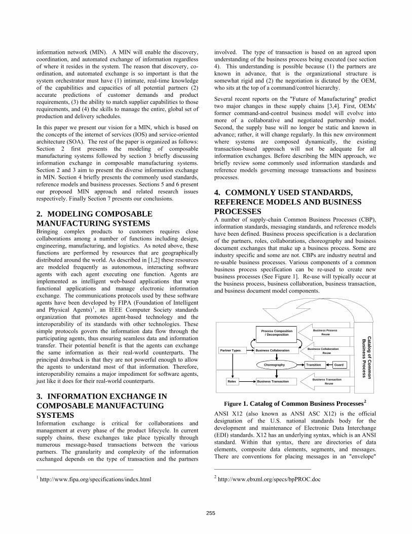
information network (MIN). A MIN will enable the discovery, coordination, and automated exchange of information regardless of where it resides in the system. The reason that discovery, co-ordination, and automated exchange is so important is that the system orchestrator must have (1) intimate, real-time knowledge of the capabilities and capacities of all potential partners (2) accurate predictions of customer demands and product requirements, (3) the ability to match supplier capabilities to those requirements, and (4) the skills to manage the entire, global set of production and delivery schedules.

In this paper we present our vision for a MIN, which is based on the concepts of the internet of services (IOS) and service-oriented architecture (SOA). The rest of the paper is organized as follows: Section 2 first presents the modeling of composable manufacturing systems followed by section 3 briefly discussing information exchange in composable manufacturing systems. Section 2 and 3 aim to present the diverse information exchange in MIN. Section 4 briefly presents the commonly used standards, reference models and business processes. Sections 5 and 6 present our proposed MIN approach and related research issues respectively. Finally Section 7 presents our conclusions.

2. MODELING COMPOSABLE MANUFACTURING SYSTEMS Bringing complex products to customers requires close collaborations among a number of functions including design, engineering, manufacturing, and logistics. As noted above, these functions are performed by resources that are geographically distributed around the world. As described in [1,2] these resources are modeled frequently as autonomous, interacting software agents with each agent executing one function. Agents are implemented as intelligent web-based applications that wrap functional applications and manage electronic information exchange. The communications protocols used by these software agents have been developed by FIPA (Foundation of Intelligent and Physical Agents)1, an IEEE Computer Society standards organization that promotes agent-based technology and the interoperability of its standards with other technologies. These simple protocols govern the information data flow through the participating agents, thus ensuring seamless data and information transfer. Their potential benefit is that the agents can exchange the same information as their real-world counterparts. The principal drawback is that they are not powerful enough to allow the agents to understand most of that information. Therefore, interoperability remains a major impediment for software agents, just like it does for their real-world counterparts.

3. INFORMATION EXCHANGE IN COMPOSABLE MANUFACTUING SYSTEMS Information exchange is critical for collaborations and management at every phase of the product lifecycle. In current supply chains, these exchanges take place typically through numerous message-based transactions between the various partners. The granularity and complexity of the information exchanged depends on the type of transaction and the partners

1 http://www.fipa.org/specifications/index.html

involved. The type of transaction is based on an agreed upon understanding of the business process being executed (see section 4). This understanding is possible because (1) the partners are known in advance, that is the organizational structure is somewhat rigid and (2) the negotiation is dictated by the OEM, who sits at the top of a command/control hierarchy.

Several recent reports on the "Future of Manufacturing" predict two major changes in these supply chains [3,4]. First, OEMs' former command-and-control business model will evolve into more of a collaborative and negotiated partnership model. Second, the supply base will no longer be static and known in advance; rather, it will change regularly. In this new environment where systems are composed dynamically, the existing transaction-based approach will not be adequate for all information exchanges. Before describing the MIN approach, we briefly review some commonly used information standards and reference models governing message transactions and business processes.

4. COMMONLY USED STANDARDS, REFERENCE MODELS AND BUSINESS PROCESSES A number of supply-chain Common Business Processes (CBP), information standards, messaging standards, and reference models have been defined. Business process specification is a declaration of the partners, roles, collaborations, choreography and business document exchanges that make up a business process. Some are industry specific and some are not. CBPs are industry neutral and re-usable business processes. Various components of a common business process specification can be re-used to create new business processes (See Figure 1]. Re-use will typically occur at the business process, business collaboration, business transaction, and business document model components.

Business Transaction

Business Collaboration

Roles

Partner Types

Choreography Transition Guard

Business CollaborationReuse

Business TransactionReuse

Process Composition/ Decomposition

Business ProcessReuse C

ata logof C

o mm

o nBu si ne ss Pr oce ss

Figure 1. Catalog of Common Business Processes2 ANSI X12 (also known as ANSI ASC X12) is the official designation of the U.S. national standards body for the development and maintenance of Electronic Data Interchange (EDI) standards. X12 has an underlying syntax, which is an ANSI standard. Within that syntax, there are directories of data elements, composite data elements, segments, and messages. There are conventions for placing messages in an "envelope"

2 http://www.ebxml.org/specs/bpPROC.doc

255

which identifies the sender and receiver and other attributes of a transmission3.

EDIFACT (Electronic Data Interchange for Administration, Commerce, and Transport) is the international Electronic Data Interchange developed under the United Nations. EDIFACT has an underlying syntax, which is an ISO standard. Within that syntax, there are directories of data elements, composite data elements, segments, and messages4. It also provides interactive exchange protocols and standard messages.

EIDX represents the Electronics Industry Data Exchange Group. As part of the Computing Technology Industry Association (CompTIA), EIDX is committed to advancing industry growth through the development of standards, best practices, accreditations, professional education and development, tools and business solutions5. EIDX provides implementation guidelines for EDI and XML-based vocabulary standards.

RosettaNet is an independent, self-funded, non-profit consortium dedicated to the development and deployment of standard electronic business interfaces. These standards form a common e-Business language, aligning processes between supply chain partners on a global basis. RosettaNet’s Partner Interface Processes (PIP) standards allows trading partners of all sizes to connect electronically to process transactions and move information within their extended supply chains6.

The Open Applications Group Integration Specification (OAGIS) is an effort to provide a canonical business language for information integration. It uses XML as the common alphabet for defining business messages, and for identifying business processes (scenarios) that allow businesses and business applications to communicate. OAGIS provides the definition of business messages in the form of Business Object Documents (BODs) standards and example business scenarios that provide example usages of the BODs7.

Table 1 presents possible mappings between several of these standards.

Table 1. Example mapping of common business processes

Common Business Processes

Normative Category

Normative Sub Category

EDIFACT including sub-sets

X12 including sub-set

RosettaNet Partner Interface Process

CII (HWSW001A)

OAG BODs

Distribute Dispatch Instructions

Procurement Management

Transportation and Distribution

INSDES 862, 858 PIP3B1 165_sync_shipschd_001

Notify Of Advance Shipment

Procurement Management

Transportation and Distribution

DESADV 856, 869 PIP3B2 0520 165_sync_shipschd_001

Besides the above, SCOR and DCOR present process reference models for any supply chain.

and amend.

3 http://www.x12.org 4 http://www.stylusstudio.com/edifact

5 http://eidx.comptia.org 6 http://www.rosettanet.org

7 http://www.openapplications.org

SCOR: Supply-Chain Operations Reference is a process reference model that has been developed and endorsed by the Supply-Chain Council (SCC). The SCC is an independent, not-for-profit, global corporation with membership open to all companies and organizations interested in applying and advancing the state-of-the-art in supply and design chain management systems and practices. SCOR has been adopted as the cross-industry de facto standard diagnostic tool for supply chain management8. It is a hierarchical model that has five major building-block processes: plan, make, source, deliver, and return.

DCOR: The Design Chain Operations Reference-model (DCOR)9. The newest model from the SCC, the DCOR-model captures the SCC’s Technical Development Steering Committee’s consensus view of design chain management. The structure is based on the same hierarchical philosophy as SCOR, but with five different building-block processes: plan, research, design, integrate,

5. OUR APPROACH: MANUFACTURING INFORMATION NETWORKS (MINS) As noted above, future manufacturing networks will be dynamically created from global resources (see Figure 2). Orchestration, cooperation, coordination, and distributed decision-making will be critical to their success. The execution of these functions, in turn, will depend on the creation of an infrastructure that automates, as much as possible, the exchange of required manufacturing- and business-related knowledge. We call such an infrastructure a manufacturing information network (MIN). A MIN (see Figure 3) is created every time an application needs to find or exchange information.

Conceptually, the MIN will constitute another “layer” of open cyberspace, sitting atop the Internet and other evolving Web technologies. As such, it will be independent of any particular enterprise software applications. Such an infrastructure will enable the complete virtualization of and ubiquitous access to global manufacturing resources allowing information to be exchanged anywhere, anytime, on any device. The primary feature of the MIN is composability.

Composability is a system design principle that deals with component inter-relationships. A high degree of composability means the system has recombinant components that can be selected and assembled in arbitrary ways to satisfy user requirements. A composable component must be self-contained (modular), self-descriptive, and be able to integrate easily with other components in the system.

The key to achieving this capability is to link these various components together in arbitrary ways to exchange the information necessary to meet business needs.

The primary components of the MIN include services, repositories, brokers, and registries (See Figure 2).

8http://www.supply-

chain.org/cs/root/scor_tools_resources/scor_model/scor_model 9http://www.supply-

chain.org/cs/root/scor_tools_resources/designchain_dcor/dcor_models

256

Services: The goal of the services is to be discovered and used as frequently as possible and by as many different actors. A service must be engineered for interoperability and designed to live in a completely open environment where they will not know who their potential partners will be in advance. This means, at a minimum, they must publish complete (register with the Service Registry), semantically rich descriptions and representations of what they do (their capabilities), the information they need to do it (their inputs), and the information they provide when they are done (their outputs). Ultimately, if the descriptions and representations are not easily understood, a service will not get used.

A number of different services are envisioned: • Services that facilitate real-time information sharing and collaboration between enterprises, such as reasoning, searching, discovery, composition, assembly, and delivery of semantics automatically. • Services that leverage emerging Web technologies for enabling a new generation of information-based applications that can self-compose, self-declare, self-document, self-integrate, self-optimize, self-adapt, and self-heal. • Services that support knowledge creation, management, and acquisition to enable knowledge sharing between virtual organizations. • Services that help connect islands of interoperability by federating, orchestrating, or providing common e-business infrastructural capabilities such as digital signature management, certification, user profiling, identity management, and libraries of templates and interface specifications. • Services that support the use of mashup technologies such as verification of credentials; reputation management; assessment of e-business capabilities; assessment of collaboration capabilities; facilities for data sourcing, integrity, security and storage; contracting; registration and labeling; and payment facilities, among others.

Figure 2. MIN Concept

Interoperability Framework

Interoperability

A2 A3A4

A5

A6 A7A8

A1

I

(New Application)

I

I

Knowledge Repositories Services Brokers Registries

Figure 3. Composable-On-Demand MINs

Knowledge Repositories: Knowledge Repositories continuously capture, store, and analyze all manufacturing-related information, for example, the knowledge of assets, manufacturing facilities/ capabilities of an organization or enterprise. Participating applications can then query or browse both structured and unstructured information in order to retrieve and update information. Besides being dynamic, knowledge repositories must cater for explicit form of knowledge to be able to retrieve context sensitive data.

Brokers: Brokers can also be referred to as the MIN infrastructure bureau services. Depending on the demand and request, the broker identifies the service component that fills the need, locates it, and plugs it into the framework. The broker’s function is to select and assemble components belonging to different applications into integrated processes; for example, for order fulfillment. This integration is analogous to the formation of virtual enterprises from separate enterprises. Component technology provides seamless communication between applications residing in the different supply-chain partners.

Registries: Registries can be thought of as advertisement services or yellow pages. They can also be useful to locate knowledge repositories and services.

6. RESEARCH ISSUES To address the development of the above discussed composable MIN and its corresponding infrastructure, we need structured research into the conditions/requirements for interoperability in these networks. The following research questions will have to be investigated:

an interoperability framework in the context of MIN specific roles of a MIN component like brokers,

services, registries, will have to be investigated as part of the framework

minimum requirements for an application to participate in MIN (for service provider and service requester)

level of information transparency required to participate in MIN

roles of an interpreter/ translator for new application services

257

common vocabulary requirements for interoperability level of intelligence that will make these application

systems adaptive and self configuring (implies an application to be either context-aware, adaptive or anticipated based on experience)

specific use cases of manufacturing and business processes (scenarios or transactions)

There are undertakings at NIST to develop and demonstrate an open, standards-based, testing and integration infrastructure that enables the automated exchange of manufacturing information among suppliers [3]. This infrastructure will provide the foundation for the new types of collaboration and management described above as a number of NIST-supported economic impact studies claim that such an infrastructure does not exist today [4].

7. CONCLUSION In this paper, we presented an approach towards information networks that supports composable manufacturing. We identified a need for a MIN infrastructure that provides a mechanism for information acquisition, sharing, delegation of tasks, and decision making between the various entities. We speculate on how the future of MINs may evolve as composable on demand MINs. Correspondingly we presented and discussed the issues and prerequisites that need to be addressed to support interoperability in such MINs. Semantic interoperability may be the key to MINs of the future. Adopting semantic interoperability for product-process automates information flow in an extended enterprise among different levels of information resources. Future research is on composable MIN and architectures to enable the way manufacturing organizations use information technology (computers, networks, information systems, data, algorithms, and decision support) to make their manufacturing processes more effective.

8. ACKNOWLEDGEMENTS The authors wish to acknowledge Steven Fenves, Eswaran Subramanian and Nenad Ivezic for participating and contributing to discussions pertaining to the Manufacturing Information Networks.

DISCLAIMER No approval or endorsement of any commercial product by the National Institute of Standards and Technology is intended or implied.

9. REFERENCES [1] Mahesh, M., Ong, S.K., Nee, A.Y.C., Fuh, J.Y.H., and

Zhang, Y.F. 2007. Towards A Generic Distributed and Collaborative Digital Manufacturing. Robotics and Computer Integrated Manufacturing, International Journal of Manufacturing and Product and Process Development. 23, 3, (June 2007), 267-27. DOI=http://dx.doi.org/10.1016/j.rcim.2006.02.008

[2] Sriram, R.D. 2002. Distributed and Integrated Collaborative Engineering Design. Sarvan Publishers, Maryland.

[3] Li, M.S., Jones, A. 2008. An information infrastructure for next generation Global enterprises, International Multi-Conference on Engineering and Technological Innovation: IMETI 2008. Orlando. Florida. USA.

[4] Comparisons and Analyses of U.S. and Global Economic Data and Trends: Globalization: Trends and Impact Factors of Globalization of Manufacturing Input Factors on Future U.S. Manufacturing Capability. National Institute of Standards and Technology. U.S. Department of Commerce 2004. http://www.sri.com/policy/csted/reports/nist/NIST_SUBD_Globalization.pdf

258

3D Reconstruction of Rough Terrain for USARSim Using a Height-map Method

G. Roberts Intelligent Systems Division, National Institute of Standards

& Technology, 100 Bureau Drive, MS 8230, Gaithersburg,

MD 20899 USA. 1-301-975-3434,

gael.roberts@nist.gov

S. Balakirsky Intelligent Systems Division,

National Institute of Standards & Technology, 100 Bureau Drive,

MS 8230, Gaithersburg, MD 20899 USA.

1-301-975-4791, stephen.balakirsky@nist.gov

S. Foufou

Laboratoire Electronique, In-formatique et Image (LE2i

Lab). UMR CNRS 5158, Uni-versity of Burgundy, 21000,

Dijon, FRANCE. 00-333-8039-3805,

sfoufou@u-bourgogne.fr

ABSTRACT In this paper, a process for a simplified reconstruction of rough terrains from point clouds acquired using laser scanners is pre-sented. The main idea of this work is to build height-maps which are level gray-scale images representing the ground elevation. These height-maps are generated from step-fields which can be represented by a set of side-by-side pillars. Although height-maps are a practical means for rough terrain reconstruction, it is not possible to represent two different elevations for a given location with one height-map. This is an important drawback as terrain point clouds can show different zones representing surfaces above other surfaces. In this paper, a methodology to create several height-maps for the same terrain is described. Experimental results are shown using the high-fidelity physics-based framework for the Unified System for Automation and Robot Simulation (USARSim). Keywords 3D Reconstruction, height-map, step-field, point cloud, USAR-Sim.

1. INTRODUCTION The usefulness of simulation systems for developing agent control systems is well established. The role of the simulation is to pro-vide convincing sensor measurements as input to the control sys-tem and to accurately model the system’s response to actuator outputs (physics, dynamics, and statics). An important enabler that allows the simulation system to meet these requirements is the existence of an accurate model of the real world.

One aspect of this world model is its representation of the ground surface, or a height-map. The required complexity of the ground surface representation is directly related to the agent’s application and target environment. For example, an agent that is required to operate in a flat-floored environment with no overhanging obsta-cles may only require occupancy information in its model. More complex environments that include uneven terrain may require a 2.5D model (a single elevation value per unit area). Even more complex environments that include overhanging obstacles or multi-level terrain may require a full 3D model (multiple eleva-tion values per unit area). This paper addresses the automatic creation of height-maps from data collected with laser scanners. The overall objective is to be able to recreate complex 3D terrains such as those that may be found at disaster sites (partially destroyed buildings, large amounts of debris, etc.) for use in simulation and in reconstructed physical representations. While the general techniques developed in this paper should be applicable to the general problem, the specific output formats have been tailored for the Unified System for Automation and Robotics Simulation (USARSim) framework [1]. USARSim was initially developed in 2002 as a low cost (under $40) robotics simulator at Carnegie Mellon University (CMU) and the University of Pittsburgh [2]. In 2005, USARSim man-agement was handed off to the National Institute of Standards & Technology (NIST) and it became an open source project hosted on the Sourceforge network (www.sourceforge.net/projects/usar-sim). USARSim is based on the UnReal Game Engine from Epic Games1 and provides a high-fidelity, physics based simulation environment for robotic development. One of the unique features of USARSim lies in its validated sensor and robot models [3]. In addition to its use as a research tool, USARSim is also used as the basis for the RoboCup Rescue Virtual Competition as well as the

(c) 2008 Association for Computing Machinery. ACM acknowledges that this contribution was authored or co-authored by a contractor or affiliate of the U.S. Government. As such, the Government retains a nonexclusive, royalty-free right to publish or reproduce this article, or to allow others to do so, for Government purposes only. PerMIS’08, August 19-21, 2008, Gaithersburg, MD, USA ACM ISBN 978-1-60558-293-1/08/08.

1 Certain commercial software and tools are identified in this pa-per in order to explain our research. Such identification does not imply recommendation or endorsement by the authors, nor does it imply that the software tools identified are necessarily the best available for the purpose.

259

IEEE Virtual Automation and Manufacturing Competition. More information on USARSim may be found in [4]. The remainder of this paper is laid out as follows: Section 2 re-calls some preliminary definitions regarding the dataset, step-fields, and height-maps. The relation between our work and other works is explained in Section 3. Section 4 gives the general ap-proach adapted in this work. Section 5 details the proposed algo-rithm for terrain reconstruction using height-maps. Some experi-mental results are shown and discussed in Section 6. Section 7 concludes and discusses about future extensions of this work.

2. PREREQUISITE This section indicates the type of data used in this project and gives some fundamental definitions. The purpose of this work is to reconstruct models of rough ter-rains for use in a simulator. Laser based scanners are used to ac-quire 3D numerical data (point clouds) representing the ground. Point clouds may be complex, containing ground, surfaces, and heaps of objects. Point clouds are muddled, contain no texture, and their points are not uniformly distributed in space. In this work, the complexity of point clouds representing real-world scenes is intentionally avoided by only considering point clouds generated artificially. These point clouds are simpler but keep approximately the same characteristics (muddled, not tex-tured, not uniform) as those acquired from real-world scenes. These artificial point clouds are generated as follows: a scene is created with different simple objects (planes, spheres, cylinders …) and points are randomly put onto the surface of each object using their equation. At the end, noise is added to make the clouds more realistic. Two important models are calculated for each point cloud: a step-field model and a height-map model. A step-field can be repre-sented by a set of side-by-side pillars (see Figure 1) and is com-puted as follows: starting from a horizontal plane, side by side pillars are placed with predefined dimension (height * width * depth). These pillars will all have identical width and depth, but their height will vary according to the configuration and proper-ties of the point cloud. More details regarding the construction of these pillars are given later.

The height-map model, also called CEM (Cartesian Elevation Map) or elevation map, is a gray scale picture (based on 256 lev-els of gray) which represents the height information of the studied terrain (see Figure 2). The lighter the color of a pixel is, the higher the elevation of the terrain is for the location represented by this pixel.

3. RELATED WORK Since the beginning of mobile robot development, researchers have been striving to find ways for the platforms to navigate through various terrains. Work has even been performed on clas-sifying the difficulty of terrain for robotic traversal. The general idea of our work is to find an adequate representation of rough terrains that will allow simulations of robots to be used to create and evaluate algorithms that will allow mobile robots to be more or less autonomous on rough terrains. Because robots come in many different shapes, sizes and abilities, simulation is a useful tool that allows one to predict which types of robots will be best-suited for particular types of terrain under consideration. Simulation is also an efficient way to test the im-pact of algorithm changes on the effectiveness of a given plat-form. There are two main types of ground mobility: walking ro-bots [5, 6] and rolling robots (with tracks or wheels). Despite a large effort in the area of walking robots, they are not completely adequate for the ground studied for this paper. The reason for this is the rocky and uneven nature of a disaster site. Consequently, rolling robots which are also the subject of studies as regards their efficiency for rough terrains are used [7, 8, 9]. The terrains are created from a cloud of points. These reconstruc-tions are an important area of computer graphics and there are many methods of 3D reconstruction from point clouds. Among these methods, which have the objective of creating a mesh, there are the Delaunay triangulation (which is joined to the Voronoi diagram) [10, 11, 12], related methods such as Ball-Pivoting (pivot of a sphere) [13] or other methods such as the one from Chang et al. [14]. All these methods give very good constructions, but the results are often very costly in memory. To resolve this problem, other research aims at simplifying the obtained meshing. These simplifications consist in reducing the number of polygons in a meshing by grouping polygons according to certain criteria such as the orientation of polygons or their con-figurations [15, 16, 17]. Although these mesh simplifications give reasonable results, the processes to do this are very costly in memory compared to the creation of height-maps as discussed in the next paragraph. Other methods for creating ground representations use height-maps. The concept of height-map is used for several studies in-cluding the crossing possibilities of grounds or the construction of obstacles on a ground [18, 19]. Height-maps are useful for path planning and collision avoidance [20], they are also used to repre-sent surfaces having a low-level of detail such as landscapes (e.g., video games).

4. THE APPROACH TO THE PROBLEM The purpose of this work is to create a 3D terrain model that will be used in a simulator, consequently the simplest possible con-struction is necessary in order to reduce the computation costs during simulation. Therefore, in order to have a good simulation, it is very important to have a very simple scene because the Frame Per Second (FPS) is taken into consideration. For a complex scene with big meshed objects, the FPS will be too low for effective rendering and the simulation will certainly be too slow.

Fig. 2: Example of height-map

Fig. 1: Example of step-field

Our simulator utilizes the Unreal 3D engine, thus the editor of this engine is used to construct the 3D models either by importing them as meshed scenes or by generating a height-map from point clouds. However, it is only considering the use of height-maps to avoid having bad FPS during the simulation.

260

5. ALGORITHM DESCRIPTION The algorithm operates in two steps: (i) compute the step-field from the point cloud, (ii) and then compute the height-map. Sev-eral height-maps may be created for the same scene in order to have various layers representing surfaces (or objects) because these surfaces can be positioned one on the top of the other.

5.1. Step-fields elaboration Having acquired the point cloud, a virtual horizontal plane P(x,y) is created:

P(x,y) = Zmin –

Where Zmin represents the coordinates of the lowest point of the cloud on the Z axis, and represents a small distance defined by the user. Therefore, the plane will be “ units” below the point cloud. This plane is bounded by the cloud on the X and Y axes. Then a grid on this plane is created. Each compartment of this grid represents the possible base of a future pillar. The side sizes of each compartment will be equal to the dimension of the pillar sides. The size of a compartment is given by the user. Thus, the dimensions of the grid (length * width compartments) are a func-tion of the plan size and the compartments size. A pillar is created in each compartment situated under a non-empty subset of points. The height of this pillar is the average of the heights (Z-components) of the points of the subset. The ob-tained set of pillars defines the step-field of the scene (terrain), and will be used to construct the height-map.

5.2. Height-map construction The height-map is built from the step-field. To this end, each pil-lar created is correlated with a pixel of a gray-scale image. If a pillar has a width of 10 cm, a pixel of the image will also repre-sent a zone of 10 cm in reality. One should notice that if there was beforehand a grid of 64*64 compartments on the initial plane, there will be a height-map of 64*64 pixels. Height-map being an image of 256 levels of gray, the maximal height (Hmax) of the pillars is put in correspondence to the highest level of the scales of gray (that is 256). Other heights (h) of pillars will be represented by a proportional gray level g, such that:

g = h * 256 / Hmax. We note that the simulator constrains the height-map to have a number of pixels equal to a power of 2 for each of its sides. For that purpose, padding is added around the height-map obtained previously. This padding will have a value equal to 0 on the scale of the gray-levels. (see Figure 2).

5.3. Construction of different layers A layer can be assimilated to one height-map or to one surface in the 3D reconstruction.

5.3.1. Why different layers? The purpose of creating different layers is to rebuild surfaces which are above other surfaces. Effectively, in a point cloud, sev-eral objects heaped upon each other can be represented. A per-spective scan of a table is a perfect simple example of this situa-tion, because in the associated point cloud, there is the surface of the ground and the top surface of the table.

A height-map is a gray scale picture and with only one gray color. It is not possible to represent different elevations. Thus, different surfaces (or elevations) cannot be represented for a given location with only one height-map.

5.3.2. The process With one step-field, one height-map is constructed, and with one height-map, one surface is constructed for the simulator. So, in order to have different surfaces in the final 3D model, it is neces-sary to construct different step-fields for the same scene. As presented in Section 5.1, a plane is placed below the point cloud and it is subdivided into a grid. Each compartment of the grid is potentially the base of several pillars. Since the height of a pillar is equal to the average of the Z-coordinates of the points above it, to construct different pillars at the same location the points above the compartment are portioned according to their elevations into different subsets. Then, the height of each pillar will be equal to the average of the Z-coordinate of the points of one particular subset. Grouping the obtained pillars into different sets gives different step-fields. The pillars of the same compart-ment cannot be placed in the same set (every step-field is com-posed of pillars from different compartments). Consequently, if there are X sets of points, there will be X pillars for the same location. The number of pillars can be different from one compartment to another. The number of layers equals the maximum number of pillars created on the grid for one compart-ment.

5.3.3. Classification of pillars When pillars are created for one compartment of the grid, the first created pillar is placed in the first layer, the second pillar in the second layer and so on. This placement of this pillar leads to lay-ers containing pillars not according to their heights, but according to their creation rank. A pillar which should be in step-field num-ber N can be in step-field number N-1. As a consequence, the built surfaces will not be regular and a pillar replacement process is needed to classify each pillar in the adequate layer. To classify the pillars, the average elevation of each layer is com-puted. Then, pillars having heights close to the average of a par-ticular layer are moved to this layer. This process is repeated sev-eral times until stability is reached.

6. EXPERIMENTAL RESULTS Some experimental results are presented and discussed in this section,. Figures 3, 4, 5, and 6 show different reconstruction cases. Figures 3.a, 4.a, 5.a, and 6.a show the point clouds and Figures 3.b, 4.b, 5.b, and 6.b show the associated computed re-construction. Textures that appear on these reconstructions repre-sent the layers found on the reconstructed surfaces. In the first example (see Figure 3.a and Figure 3.b), there are 3 horizontal overlaid planes. A point in a plane does not have the same elevation as a point in another plane. By this fact, at the creation of the step-field, it is easy to classify the pillars according to their elevations for each layer, and one may notice remark that the associated height-maps are very homogeneous (there is one height-map for each surface). Of course this is the perfect case where the reconstructed layers (Figure 3.b) correspond to the surfaces of the initial planes.

261

Fig. 3.a: Point cloud representing 3 planes

Fig. 3.b: Construction representing 3 planes The second example (Figure 4.a) represents a scene that is a little more complicated. There are the three planes from Figure 3.a above which a fourth inclined plane is positioned. This fourth plane crosses the elevation of the two highest horizontal planes. Figure 4.b displays the associated construction, where one can see that the three parallel planes are constructed correctly, but the inclined plane presents some discrepancies. This inclined plane is constructed with three different layers because the pillars are clas-sified according to their elevations. Since the inclined plane crosses the elevations of the two other planes, the pillars for the inclined plane are classified in different layers. This classification may lead the pillars of the inclined plane to be positioned in the same layer as the pillars of the other planes with approximately the same elevation. Notice that the reconstruction of the inclined surface is not con-tinuous. That is explained by the fact that the inclined plane is reconstructed with three layers, and although no data are lost, the continuity of the surface at this location is lost, which creates a discontinuity in the 3D model. The 3D model is used to manipu-late a robot in a simulator, and the created holes have the size of the pillars (a small size). Thus the robots can cross over these holes and there is no real impact for the simulation.

Fig. 4.a: Point cloud representing 4 planes

Fig. 4.b: Construction representing 4 planes The third example (see Figure 5) is more complicated than the second example where the inclined plane does not only cross the elevation of others surfaces, but also crosses one of these planes. The same problem as previously is noticed (the holes because of the discontinuity) and the construction is more complicated too. Actually, even the horizontal planes are built with several layers but the 3D reconstruction is still correct. The fourth example (see Figure 6) presents a more complex scene where a cylindrical object is positioned on an horizontal plane. The relevance of this scene is to show how one object (the cylin-der) which presents a surface above itself is reconstructed. The algorithm cuts the object surface into two parts (see Figure 6.b) in order to create two different layers for the same object. During the process of creating the ground, there are edge effects. It is during the process of creation of a 3D scene from height-maps that there is a loss of information. This is due to the fact that a pixel of the height-map represents a vertex and not a compart-ment of the surface in the simulator. This fact has the effect of cutting down the side of the surfaces. Consequently, if there is a ground (or a height-map) which is strewed with holes, these holes will be increased in the final reconstruction, and if the surface is too thin, it will totally disappear.

262

Fig. 5.a: Point cloud representing 4 planes with intersection

Fig. 5.b: Construction representing 4 planes with intersection

Fig. 6.a: Point cloud representing a cylinder onto a plane

Fig. 6.b: Construction representing a cylinder onto a plane

7. CONCLUSION We have presented a method to build a simplified 3D scene from point clouds using height-maps. The use of several height-maps allows us to reconstruct in a very simplistic way different scenes, which could have had a heavy and high cost mesh based recon-struction. Furthermore, the elaboration of overlapped height-maps representing grounds to be analyzed permits one to simplify the reconstruction of overlapped surfaces. This new reconstruction method gives satisfactory results for relatively simple scenes. However, height-maps based reconstruction methods are still limited for ground representations, which become complex by the presence of several kinds of objects. The height-maps method works very well for the generation of grounds having few discon-tinuities, but fails with complex grounds with many discontinui-ties or with important variations. A future work is to validate this method in two different ways. The first is to create a terrain as similar as possible with the reality. The second way is to compare the similarity between the behaviors of a robot on the terrain in the simulation and in the real world. Namely, the second way is more important than the first one. The objective is to reconstruct real rough terrains for a simulation, thus we can have very complex scenes. In these scenes, we can differentiate what we call the simple parts of the scene and the complex parts of the scene. To differentiate these two sorts of parts, the local density of points and the shape of the representa-tion of the points are taken in consideration. In this way, a smooth shape will be assimilated to a simple part, and a small area with much variation will be assimilated to a complex part. In order to improve our algorithm, we envisage combining the overlapped height-maps method (for the simple parts of the ground) with a simple mesh-based method (for the complex parts of the ground). Actually, we can also define the boundary between a simple and a complex part with the effectiveness of local reconstructions using the overlapping height-maps method.

8. REFERENCES [1] Carpin, S.; Lewis, M.; Wang, J.; Balarkirsky, S.; Scrapper, C.; USARSim: a robot simulator for research and education. Proceed-ings of the IEEE 2007 International Conference on Robotics and Automation, Page(s):1400-1405 [2] Balaguer, B.; Balakirsky, S.; Carpin, S.; Lewis, M.; Scrapper, C.; “USARSim: A Validated Simulator for Research in Robotics and Automation”, Workshop on “Robot Simulators: Available Software, Scientific Applications, and Future Trends” at IEEE/RSJ 2008. [3] Carpin, S.; Stoyanov, T.; Nevatia Y.; Lewis, M.; Wang, J.; Quantitative Assessments of USARSim Accuracy. Proceedings of PerMIS 2006, NIST Special Publication 1062, August 2006. [4] Usarsim homepage: http://sourceforge.net/projects/usarsim (Accessed: 2008) [5] Pongas, D.; Mistry, M.; Schaal, S.; “A Robust Quadruped Walking Gait for Traversing Rough Terrain”, Robotics and Automation 10-14 April 2007 Page(s):1474 – 1479. [6] Rebula, J.R.; Neuhaus, P.D.; Bonnlander, B.V.; Johnson, M.J.; Pratt, J.E.; “A Controller for the LittleDog Quadruped Walking on Rough Terrain”, Robotics and Automation, 2007 IEEE Interna-tional Conference on 10-14 April 2007 Page(s):1467 – 1473. [7] Fukuda, T.; Zhang, X.; Hasegawa, Y.; Matsuno, T.; Hoshino, H.; “Preview posture control and impact load control of rough terrain vehicle with interconnected suspension”, Intelligent Ro-bots and Systems, 2004. (IROS 2004). Proceedings. 2004

263

IEEE/RSJ International Conference on Volume 1, 28 Sept.-2 Oct. 2004 Page(s):761 - 766 vol.1, [8] Udengaard, M.; Iagnemma, K.; “Kinematic analysis and con-trol of an omnidirectional mobile robot in rough terrain”, Intelligent Robots and Systems, 2007. IROS 2007. IEEE/RSJ International Conference on Oct. 29 2007-Nov. 2 2007 Page(s):795 – 800. [9] Nakamura, S.; Faragalli, M.; Mizukami, N.; Nakatani, I.; Ku-nii, Y.; Kubota, T.; “Wheeled robot with movable center of mass for traversing over rough terrain”, Intelligent Robots and Systems, 2007. IROS 2007. IEEE/RSJ International Conference on Oct. 29 2007-Nov. 2 2007 Page(s):1228 – 1233. [10] Ledoux, H.; “Computing the 3D Voronoi Diagram Robustly: An Easy Explanation”, Voronoi Diagrams in Science and Engi-neering, 2007. ISVD '07. 4th International Symposium on 9-11 July 2007 Page(s):117 - 129. [11] Tse, R.; Gold, C.; Kidner, D.; “Using the Delaunay Triangu-lation/ Voronoi Diagram to extract Building Information from Raw LIDAR Data”, Voronoi Diagrams in Science and Engineer-ing, 2007. ISVD '07. 4th International Symposium on 9-11 July 2007 Page(s):222 – 229. [12] Labatut, P.; Pons, J.-P.; Keriven, R.; “Efficient Multi-View Reconstruction of Large-Scale Scenes using Interest Points, De-launay Triangulation and Graph Cuts”, Computer Vision, 2007. ICCV 2007. IEEE 11th International Conference on 14-21 Oct. 2007 Page(s):1 – 8. [13] Bernardini, F.; Mittleman, J.; Rushmeier, H.; Silva, C.; Taubin, G.; “The ball-pivoting algorithm for surface reconstruc-tion”, Visualization and Computer Graphics, IEEE Transactions on Volume 5, Issue 4, Oct.-Dec. 1999 Page(s):349 – 359.

[14] Ming-Ching, C.; Leymarie, F.F.; Kimia, B.B.; “Surface Re-construction from Point Clouds by Transforming the Medial Scaf-fold”, 3-D Digital Imaging and Modeling, 2007. 3DIM '07. Sixth International Conference on 21-23 Aug. 2007 Page(s):13 – 20. [15] Hua-Hong, C.; Xiao-nan, L.; Ruo-tian, L.; “Surface Simplifi-cation Using multi-edge mesh collapse”, Image and Graphics, 2007. ICIG 2007. Fourth International Conference on 22-24 Aug. 2007 Page(s):954 - 959. [16] Qu, L.; Meyer, G. W.; “Perceptually Guided Polygon Reduc-tion”, Visualization and Computer Graphics, IEEE Transactions on Volume 14, Issue 5, Sept.-Oct. 2008 Page(s):1015 – 1029. [17] In Kyu, P.; Sang Wook, L.; Sang Uk, L.; “Shape-adaptive 3D mesh simplification based on local optimality measurement”, Computer Graphics and Applications, 2002. Proceedings. 10th Pacific Conference on 9-11 Oct. 2002 Page(s):462 – 466. [18] Asada, M.; “Building a 3D world model for mobile robot from sensory data”, Robotics and Automation, 1988. Proceed-ings., 1988 IEEE International Conference on 24-29 April 1988 Page(s):918 – 923, vol.2. [19] Asada, M.; “Map building for a mobile robot from sensory data”, Systems, Man and Cybernetics, IEEE Transactions on Vol-ume 20, Issue 6, Nov.-Dec. 1990 Page(s):1326 – 1336. [20] Gutmann, J.S.; Fukuchi, M.; Fujita, M.; “A Floor and Obsta-cle Height Map for 3D Navigation of a Humanoid Robot”, Robotics and Automation, 2005. ICRA 2005. Proceedings of the 2005 IEEE International Conference on 18-22 April 2005 Page(s):1066 – 1071.

264

Using Virtual Scans to Improve Alignment Performance inRobot Mapping

Rolf LakaemperTemple University

Philadelphia, PA, USAlakamper@temple.edu

Nagesh AdluruTemple University

Philadelphia, PA, USAnagesh@temple.edu

ABSTRACTWe present a concept and implementation of a system to in-tegrate low level and mid level spatial cognition processes foran application in robot mapping. Feedback between the twoprocesses helps to improve performance of the recognitiontask, in our example the alignment of laser scans. The lowlevel laser range scan data (’real scans’), are analyzed withrespect to mid level geometric structures. The analysis leadsto generation of hypotheses (Virtual Scans) about existingreal world objects. These hypotheses are used to augmentthe real scan data. The core mapping process, called ForceField Simulation, iteratively aligns the augmented data setwhich then in turn is re analyzed to confirm, modify, ordiscard the hypotheses in each iteration. Experiments withscan data from a Rescue Robot Scenario show the applica-bility and advantages of the approach.

1. INTRODUCTIONThis article demonstrates how the integration of low level

spatial cognition processes (LLSC) and mid level spatial cog-nition processes (MLSC) can help to improve the perfor-mance of spatial recognition tasks in robotics. We are usingthe area of robot perception for mobile rescue robots, specif-ically alignment of 2D laser scans, as a showcase to demon-strate the advantages of the integration of LLSC and MLSCprocesses. Alignment of data, e.g. acquired from multiplerobots from different positions, is a required task for envi-ronment mapping. The basic task of mapping is to combinespatial data usually gained from laser range devices, called’scans’, to a single data set, the ’global map’. The globalmap represents the environment as scanned from differentlocations, even possibly scanned by different robots (’multirobot mapping’), usually without knowledge of their pose(= position and heading).

We apply our LLSC/MLSC system to map an environ-ment from Urban Search and Rescue Robots. Mapping is arequirement for these robots to perform their main task: toautonomously detect victims in disaster areas (e.g. tsunami,

Permission to make digital or hard copies of all or part of this work forpersonal or classroom use is granted without fee provided that copies arenot made or distributed for prof t or commercial advantage and that copiesbear this notice and the full citation on the f rst page. To copy otherwise, torepublish, to post on servers or to redistribute to lists, requires prior specif cpermission and/or a fee.PerMIS'08 August 19-21, 2008, Gaithersburg, MD, USAACM ISBN 978-1-60558-293-1/08/08...$5.00.

earthquake or terrorist attack). The goal is to assist the res-cue teams generating location and best access path. Typ-ically multiple robots are deployed in the area to coopera-tively map the disaster area. Currently their applicability islimited due to the extreme constraints to robot mapping insuch an environment: single scans have little overlap, no ad-ditional sensor information, e.g. odometry, is reliably avail-able, and none or just a few landmark features are present.

In robot cognition, MLSC processes infer the presence ofmid level features from low level data based on regional prop-erties of the data. In our case, we detect the presence ofsimple mid level objects, i.e. line segments and rectangles.The MLSC processes model world knowledge, or assump-tions about the environment. In our case, we assume thepresence of (collapsed) walls and other man made struc-tures. If possible wall-like elements or elements somewhatresembling rectangular structures are detected, our systemgenerates the most likely ideal model as a hypothesis, called’Virtual Scan’. Virtual Scans are generated from the ideal,expected model in the same data format as the raw sensordata, hence Virtual Scans are added to the original scandata indistinguishably for the low level alignment process;the alignment is therefore performed on an augmented dataset.

In robot cognition, LLSC processes usually describe fea-ture extraction based on local properties like spatial prox-imity, e.g. based on metric inferences on data points, likeedges in images or laser reflection points. In our systemlaser scans (virtual or real) are aligned to a global map us-ing mainly features of local proximity using the LLSC coreprocess of ’Force Field Simulation’ (FFS). FFS was recentlyintroduced to robotics [20]. In FFS, each data point canbe assigned a weight, or value of certainty. It also doesnot make a hard, but soft decision about the data corre-spondences as a basis for the alignment. This is achievedby computation of a correspondence probability to multipleneighboring points, based on weight, distance and directionof underlying linear structures. Mainly this feature makesFFS a natural choice over its main competitor, ICP [2, 24],for the combination with Virtual Scans (however, the generalidea of Virtual Scans is applicable to both approaches). Theweight parameter can be utilized to indicate the strength ofhypotheses, represented by the weight of virtual data.

FFS is an iterative alignment algorithm. The two levels(LLSC: data alignment by FFS, MLSC: data augmentation)are connected by a feedback structure, which is repeated ineach iteration:

• The FFS-low-level-instances pre-process the data. They

265

find correspondences based on low level features. Thelow level processing builds a current version of theglobal map, which assists the mid-level feature detec-tion

• The mid level cognition module analyzes the currentglobal map, detects possible mid level objects and mod-els ideal hypothetical sources possibly being present inthe real world. These can be seen as suggestions, fedback into the low level system by Virtual Scans. Thelow level system in turn adjusts its processing for re-evaluation by the mid level systems.

Figure 1: LLSC/MLSC feedback. The LLSC mod-ule works on the union of real scans and the VirtualScan. The MLSC module in turn re-creates a newVirtual Scan based on the result of the LLSC mod-ule.

In such a system, MLSC processes steer LLSC processes in-troducing higher knowledge to enable spatial inferences theLLSC system is not able to draw by itself. However, theMLSC system also needs assistance of the LLSC for tworeasons: MLSC systems concentrate on higher informationwhich needs LLSC pre-processed data (e.g. a set of collinearpoints is passed to the MLSC as a single line segment). Butalso LLSC processes have to support the suggestions statedby the MLSC. Since MLSC introduces higher knowledge,it is dangerous to focus on spatial mid level inferences tooearly. Feedback with the LLSC system enables more care-ful evaluation of plausibility (see also final note in section’Experiments’). The following example will illustrate the

Figure 2: Alignment using Virtual Scans (VS). Toprow: Alignment without VS. The LLSC misalignesthe scene due to lack of global information. Bot-tom row: two iterations using VS. The hypotheticalrectangle createa a the VS add global information,leading to correct alignment. The VS are newly cre-ated in each iteration.

approach: Figure 2, top left, assumes 2 scans, e.g. takenfrom robots in 2 different positions. A typical LLSC align-ment process like ICP or FFS tries to find correspondencesbetween single points in the scans, and to superimpose the

scans in an optimal way, e.g. minimizing the summed dis-tances between corresponding points. These approaches as-sume the existence of overlapping features in scans. Like inthis example, such a constraint is often not met, and theassumption leads to wrong results. The LLSC alignmentprocess works on a local basis, hence it is not able to detecta possible rectangular feature. Figure 2 illustrates the re-sult of an alignment process with (bottom row) and without(top row) Virtual Scans. In the illustration of our approachin fig.2, bottom, an MLSC process detects a rectangularstructure and adds an optimal model to the data set. TheLLSC module aligns the augmented data. The hypothesisnow directs the scans to better location. In each iteration,the relocated real scans are analyzed to adjust the MLSChypothesis, LLSC and MLSC assist each other in a feedbackloop.

2. RELATED WORK IN SPATIAL COGNI-TION AND ROBOT MAPPING

The potential of MLSC has been largely unexplored inrobotics, since recent research mainly addressed LLSC sys-tems. They show an astonishing performance: especiallyadvances in statistical inferences [5, 10, 13] in connectionwith geometric modeling of human perception [6, 9, 25] andthe usage of laser range scanners contributed to a break-through in robot applications, with the most spectacular re-sults achieved in the 2005 DARPA Grand Challenge whereseveral autonomous vehicles were able to successfully com-plete the race [26]. But although the work on sophisticatedstatistical and geometrical models like extended Kalman Fil-ters (EKF),e.g. [12], Particle Filters [10] and ICP (Itera-tive Closest Point) [2, 24] utilized in mapping approachesshow impressive results, their limits are clearly visible, e.g.in the aforementioned rescue scenarios. These systems arestill based on low level cognitive features, since they con-struct metric maps using correspondences between sensordata points. However, having these well-engineered low levelsystems at hand, it is natural to connect them to MLSC pro-cesses to mutually assist each other.

The knowledge in the area of MLSC in humans, in particu-lar in spatial intelligence and learning, is advancing rapidly[7, 14, 27]. Research in AI models such results to gener-ate generic representations of space for mobile robots usingboth symbolic, e.g. [16], and non symbolic, e.g. [8], ap-proaches. Each is trying to identify various aspects of thecognitive mapping process. Naturally, SLAM (SimultaneousLocalization and Mapping [4] is often used as an applicationexample [23]. In [28], a spatial cognition based map is gener-ated based on High Level Objects. Representation of spaceis mostly based on the notion of a hierarchical representa-tion of space. Kuipers [16] suggests a general framework fora Spatial Semantic Hierarchy (SSH), which organizes spatialknowledge representations into levels according to ontologyfrom sensory to metrical information. SSH is an attemptto understand and conceptualize the cognitive map [15], theway we believe humans understand space. More recently,Yeap and Jefferies [29] trace the theories of early cognitivemapping. They classify representations as being space-basedand object-based. Comparing to our framework, these clas-sifications could be described being related to LLSC andHigh Level Spatial Cognition (HLSC), hence the supposedLLSC/MLSC system would relate closer to space-based sys-

266

tems.In [1], the importance of ’Mental Imagery’ in (Spatial)

Cognition is emphasized and basic requirements of modelingare stated. Mental Images invent or recreate experiences re-semble actually perceived events or objects. This is closelyrelated to the ”Virtual Scans” described in this proposal.Recently, Chang et al. [3] presented a predictive mappingapproach (P-SLAM), which analyzes the environment forrepetitive structures on the LLSC level (lines and corners)to generate a ”virtual map”. This map is either used as ahypothesis in unexplored regions to speed up the mappingprocess or as an initialization help for the utilized particlefilters when a region is first explored. In the second casethe approach has principles similar to the presented VirtualScans. The impressive results of P-SLAM can also be seenas proof of concept of integrating prediction into robot per-ception.

The problem of geometric robot mapping is based on align-ing a set of scans. On the LLSC level the problem of simulta-neous aligning of scans has been treated as estimating setsof poses [22]. The underlying framework for such a tech-nique is to optimize a constraint-graph, in which nodes arefeatures, poses and edges are constraints built using variousobservations and measurements.

There are numerous image registration techniques, themost famous being Iterative Closest Point (ICP)[2], and itsnumerous variants to improve speed and converge basins.Basically all these techniques do search in transformationspace trying to find the set of pair-wise transformations ofscans by optimizing some function defined on transforma-tion space. The techniques vary in defining the optimiza-tion functions that range from being error metrics like ”sumof least square distances” to quality metrics like ”image dis-tance”. ’Force Field Simulation’ (FFS), [20], minimizes apotential derived from forces between corresponding datapoints. The Virtual Scan technique presented in this paperwill interact with FFS as underlying alignment technique.

3. SCAN ALIGNMENT USING FORCE FIELDSIMULATION

The understanding of FFS is crucial to the understand-ing of the presented extension of the FFS alignment usingVirtual Scans. We will give an overview here. FFS alignssingle scans Si obtained by robots, typically from differentpositions. We assume the scans to be roughly pre-aligned(see fig.7), e.g. by odometry or shape based pre-alignment.This is in accord with the performance comparison betweenFFS and ICP described in [19]. FFS alignment, in detaildescribed in [20] is able to iteratively refine such an align-ment based on the scan data only. In FFS, each single scanis seen as a non-deformable entity, a ’rigid body’. In eachiteration, a translation and rotation is computed for eachsingle scan simultaneously. This process minimizes a targetfunction, the ’point potential’, which is defined on the set ofall data points (real and Virtual Scans: FFS can not distin-guish). FFS solves the alignment problem as optimizationproblem utilizing a gradient descent approach motivated bysimulation of dynamics of rigid bodies (the scans) in gravi-tational fields, but ”replaces laws of physics with constraintsderived from human perception” [20]. The gravitational fieldis based on a correspondence function between all pairs ofdata points, the ’force’ function. FFS minimizes the over-

laying potential function induced by the force and convergestowards a local minimum of the potential, representing a lo-cally optimal transformation of scans. The force function isdesigned in a manner that a low potential corresponds to avisually good appearance of the global map. As scans aremoved according to the laws of motion of rigid bodies in aforce field, single scans are not deformed.

Fig. 3 shows the basic principle: forces (red arrows) arecomputed between 4 single scans (the 4 corners). FFS simul-taneously transforms all scans until a stable configuration isgained.

With S1, S2 being two different scans, the force betweentwo single data points vi ∈ S1 and uj ∈ S2 is defined as avector

V (v1, v2) = M(v1, v2)vi − uj

‖vi − uj‖

(1)

Its magnitude ‖V (vi, uj)‖ = M(vi, uj) is defined as:

M(vi, uj) =1

σt

√

2πe

(−

‖vi,uj‖2

2σ2t

)

wiwj cos(∠(vi, uj)) (2)

with parameters σt, wi, wj , ∠(vi, uj) defined as follows:∠(vi, uj) denotes the angle between the directions of points,which is defined as the angle between directions of assumedunderlying locally linear structures. See fig. 4, left, for anexample, which especially shows the influence of the cosine-term in eq.2: forces are strong between parallel structuresonly. In eq.2, the forces are strongly depending on σt, whichis a parameter steering the radius of influence. With σt de-creasing during the iterative process, FFS changes the influ-ence of each data point from global to local. In addition, theweight wi, wj (or mass) determines the influence of pointsvi, uj . The weight is a parameter which can e.g. express thecertainty about a point, or it can model the feature impor-tance. We utilize this feature of FFS to model the strengthof hypothesis in the Virtual Scans. Hence in eq.2 the in-terfacing between LLSC and MLSC can be seen directly:distance and cosine term refer to LLSC, while the weightsare derived from MLSC (in case of the Virtual Scans).

To compute the resulting movement from the forces of allpoint pairs between different scans, FFS re-assigns a con-stant mass to all data points and applies Newton’s law ofmovement of rigid bodies in force fields. Constant masscauses data points participating in stronger force relationsto influence the transformation stronger than those respond-ing to weaker forces. For a single transformation step see fig.4, right.

The step width Δt of FFS is determinded by a ’coolingprocess’. Δt It is monotonically decreasing, allowing thesystem in early iterations to jump out of local minima, yetto be attracted by local features in later steps. The inter-play between σt and Δt is an important feature of FFS. Seefigures 7 and 8 for an example of the performance of FFSon a laser range data set.

FFS is closely related to simultaneous ICP. A performanceevaluation of both algorithms [19] showed similar results.In general, FFS can be seen as more robust with respectto global convergence with non near optimal initialization,since the point relations are not built in a hard (nearestneighbor) but soft(sum of forces) way. Also the inclusionof weight parameters makes it a natural decision for ourpurposes of extension using Virtual Scans.

267

Figure 3: Basic principle of FFS. Forces are com-puted between 4 single scans. Red arrows illustratethe principle of forces. The scans are iteratively(here: two iterations) transformed by translationand rotation until a stable configuration is achieved.

Figure 4: FFS example. Left: Forces (green) be-tween two rigid structures (brown, black). Theblack and brown lines connect the actual data set fordisplay reasons only. The figure shows a magnifica-tion of the upper left corner of fig. 7, right. Right:example of force and movement. Dotted lines show2 scans (black, brown) and their forces (green) in it-eration t. Solid lines show the resulting transformedscans at iteration t + 1.

4. CREATING VIRTUAL SCANS: MID LEVELANALYSIS

The analysis module detects line segments and rectanglesin each iteration of the FFS alignment. Both detection stepswork on the entire point set of the current global map, i.e.the union

⋃iSi of all points of the real scans Si.

4.1 LinesThe usage of lines for our Virtual Scan approach is moti-

vated by the world knowledge assumption of scanning a manmade environment (e.g. a collapsed house): although theseenvironments often locally don’t show major linear elementsany longer, a global view still often reveals an underlyinggrid structure. In our line detection, we use the classic linedetection approach of Hough transform [11], since it detectsglobally present linear structures. Hough transform does notonly show location and direction of a line, but also the num-ber of participating data points. We use this value to com-pute a certainty-of-presence measure, i.e. the strength of theline hypothesis. We only use lines above a certain thresholdof certainty. We will specify below how the detected linesare utilized to create the Virtual Scan.

4.2 RectanglesFor rectangle detection, we use an approach described in

[17]. This approach needs line segments as input, whichmodel the underlying point data. Each line segment is trans-lated into the ’S,L,D space’ (Slope,Length,Distance), whichsimplifies the detection of appropriate (rectangular like) con-figurations of four near parallel and near perpendicular seg-ments. To use this approach, the laser data has to be mod-eled by underlying line segments. Since line segments rely onlocal linearity of the underlying data points, global Hough

detection is not feasible. A recently published technique [21]from robot mapping, using a statistical approach, ’ExtendedExpectation Maximization’, is specifically tailored to modellaser scan data with line segments. To speed up the rectangledetection process, we detect line segments in each single scanonce before the FFS process. Hence, for rectangle detection,we superimpose the data represented the pre-computed linesegments line segments according to the FFS transformationof the underlying scan, rather than data points. Due to yetimprecise single scan alignment during the early FFS pro-cess, single lines in the environment are frequently presentedby clusters of line segments, rather than the required singleline segments. We merge similar lines in a cluster to a sin-gle prototype using a line merge approach described in [18],see figure 5. The rectangle detection module then predictslocation, dimension and certainty-of-presence of hypotheti-cal, ideal rectangles present in the data set of line segments.The certainty, or strength of the hypothesis is derived fromproperties (segment length, perpendicularity) of participat-ing rectangle-generating line segments. This value is used tocreate the weight of the ideal rectangle in the Virtual Scan.

Figure 5: Rectangle detection. a) Global mapbuilt by line segments of all single scans. b) resultof global line merging c) red: detected rectangles(magnification of area encircled in b)

4.3 Creating a Virtual ScanA Virtual Scan is a set of virtual laser scan points, su-

perimposed over the entire area of the global map. Thedetected line segments and rectangles are ’plotted’ into theVirtual Scans, i.e. they are represented by point sets as ifthey would be detected by a laser scanner. We assume avirtual laser scanner that represents each line and rectangleby a set of points, sub sampled equidistantly according tothe point density of the underlying point data in the originaldata set.

An important feature of the Virtual Scan is, that eachpoint in the Virtual Scan is assigned a weight, being thestrength of hypothesis of a virtual structure it represents.Utilizing this feature, we benefit from the weights steeringthe FFS alignment. As defined in eq.2, the weight wi, wj

directly influences the alignment process; stronger points,i.e. points with higher value wi, have a stronger attraction.Hence, a strong hypothesis translates into a locally stronglyattractive structure. The hypothesis value reflects the beliefinto the hypothesis relative to the real data; all data pointsof the real data are assigned a ’normal’ weight of 1.

5. ALIGNMENT USING VIRTUAL SCANS:ALGORITHM

The algorithm describes the interplay between LLSC (FFS)and the MLSC analysis. Si, i = 1..n, denotes the real scan

268

Figure 6: Virtual Scans in an early stage of FFS. a)global map b) the Virtual Scan consisting of pointsrepresenting detected lines and rectangles c) super-imposition of real data and Virtual Scan. This is thedata used in the next FFS iteration.

data, consisting of n scans. V [t] is the Virtual Scan in iter-ation t. Init: t = 1, V [0] = ∅, create set of line segments Li

for each scan Si

—————————————————–1) Perform FFS on

⋃i=1..n

Si ∪V [t−1], resulting in transfor-

mations T[t]i

for each scan Si=1..n

2) Form global map G of points and GL of line segments,superimposing the transformed scans and their line segment

representation: G =⋃

i=1..nT

[t]i

(Si), GL =⋃

i=1..nT

[t]i

(Li)

3) Detect set of lines L in G, set of rectangles R in GL

4) Create Virtual Scan V [t]. V [t] contains scan points rep-resenting the elements of L and R.

5) Compute parameters σt and Δt for the FFS process

6) Loop: goto 1, or end if FFS converged (stable globalmap).

—————————————————–

6. EXPERIMENTS AND RESULTS

6.1 NIST Disaster AreaThis data set consists of 60 single laser scans, taken from

15 different positions in 4 directions (N,W,S,E) with 20◦

overlap. It can be interpreted as a scene scanned by 15robots, 4 scans each. No order of scans is given. Thescans resemble the situation of an indoors disaster scenery,scanned by multiple robots. The scans have little overlapand no distinct landmarks. The initial global map was com-puted using a shape based approach described in [19]. Seefig. 7 for example scans and the initial map. We used theinitial global map for two different runs of FFS, once withVirtual Scans, once without. The experiment was performedto demonstrate the increase in alignment performance usingVirtual Scans. The increase in performance was evaluatedby visual inspection, since for this data set no ground truthdata is available. Comparing the final global maps of bothruns, the utilization of Virtual Scans leads to distinct im-provement in overall appearance and mapping details, seefig.8. Overall, the map is more ’straight’ (compare e.g. thetop wall), since the detection of globally present linear struc-tures (top and left wall in fig.8) adjusts all participating sin-gle segments to be collinear. These corrections advance intothe entire structure. More objectively, the improvementscan be seen in certain details, the most distinct encircledin fig.8, bottom right. There especially the rectangle in thecenter of the global map is an excellent example for a sit-

Figure 7: The NIST disaster area data set. Left: 6

example scans (from a total of 60). Crosses show each

robot’s position. Right: 60 scans superimposed using a

rough pre-estimation, building the initial global map.

uation where correct alignment is not achievable with lowlevel knowledge only. Only the suggested rectangle from theVirtual Scan (see fig.8, top left) can force the low level pro-cess to transform the scan correctly. Without the assumedrectangle the low level optimization process necessarily triedto superimpose 2 parallel sides of the rectangle to falsely ap-pear as one (fig.8,bottom right).

Comparison of fig.8, top left, and fig.6 shows the effect offeedback between the core FFS alignment process and themap analysis to create Virtual Scans. Figure 6 shows itera-tion 5 of the same experiment. Objects and object locationsdiffer between the 2 Virtual Scans. Fig. 8 has discardedsome hypotheses (objects) present in fig. 6, e.g. some of therectangles. Other hypotheses are modified, e.g. the top wallis adjusted.

Note: The proposed system handles errors caused by pre-mature belief in MLSC features by implementing the feed-back principle, which evaluates a single MLSC-hypothesis.It is known that single hypothesis systems introducing higherknowledge tend to be not robust. Under certain circum-stances this behavior could also be observed in experimentswith our system. However, this single hypothesis system al-ready significantly improves the alignment performance andtherefore highlights the advantages of LLSC/MLSC connec-tion. It can easily be embedded into a multiple hypothesesframework, e.g. particle filters, which will also be part offuture work.

7. CONCLUSION AND OUTLOOKThe presented implementation of the alignment process

FFS in feedback with MLSC recognition modules could sig-nificantly improve the results for the alignment task. Theimplementation proves the applicability of the presented con-cept for the combination of LLSC and MLSC processes.In this implementation, already the detection of simple el-ements (lines, rectangles) could improve the performance.These elements modeled assumptions of indoor disaster ar-eas. Future implementations will work with different as-sumptions to adjust to outdoor disaster settings.

8. REFERENCES[1] S. Bertel. Thomas barkowsky, dominik engel, christian

freksa. computational modeling of reasoning withmental images: basic requirements. D. Fum, F. del

269

Figure 8: Alignment of NIST data set (initial alignment

see fig. 6). Top left: after 10 iterations with detected line

and rectangular objects plotted into the Virtual Scan

(red). Top right: Final result using Virtual Scans, after

100 iterations. MLSC objects are not shown for clarity

of display. Compare to Bottom Right: final result of

alignment without Virtual Scans. Encircled areas show

examples of improvement using Virtual Scans. Bottom

left: The center rectangle could only be aligned correctly

using MLSC information. Compare to motivational ex-

ample fig. 2

Missier, A. Stocco (Eds.), Proceedings of the 7thInternational Conference on Cognitive ModelingICCM06, 2006.

[2] P. Besl. N. mckay. a method for registration of 3.dshapes. IEEE PAMI, 14(2), 1992.

[3] H. J. Chang. C.s.george lee and y.h. lu and y.c.hu.p-slam: Simultaneous localization and mapping withenvironmental structure prediction. IEEETransactions on Robotics, Vol.23, No.2, April 2007.

[4] G. Dissanayake. H. durrant-whyte and t. bailey. acomputationally efficient solution to the simultaneouslocalization and map building (slam) problem.ICRA2000 Workshop on Mobile Robot Navigation andMapping, 2000.

[5] A. Doucet. N. defreitas, n. gordon. sequential montecarlo methods in practice. Springer, 2000.

[6] D. J. Field. A. hayes, r.f. hess. contour integration bythe human visual system: evidence for a localassociation field. Vision Research, 33, pages 173–193,1993.

[7] C. Freksa. M. knauff, b. krieg-brueckner, b. nebel, t.barkowsky. spatial cognition iv: Reasoning, action,interaction. Springer, 2004.

[8] T. Ghiselli-Crippa. Hirtle s.c., munro, p. connectionistmodels in spatial cognition. The Construction ofCognitive Maps, Kluwer Academic Publishers. 1-51,pages 87–104, 1996.

[9] W. Grimson. Object recognition by computer: Therole of geometric constraints. Boston, MA: MIT Press,1991.

[10] G. Grisetti. C. stachniss, burgard w. improvinggrid-based slam with rao-blackwellized particle filtersby adaptive proposals and selective resampling. ICRA,2005.

[11] P. V. C. Hough. Methods and means for recognizing

complex patterns. US patent 3,069,654, 1962.[12] S. Huang. G. dissanayake. convergence analysis for

extended kalman filter based slam. IEEE InternationalConference on Robotics and Automation, 2006.

[13] D. C. Knill. W. richards. perception as bayesianinference. New York: Cambridge, 1996.

[14] G. J. M. Kruijff. H. zender, p. jensfelt, h. i.christensen. situated dialogue and spatialorganization: What, whereE and why? Int. J. ofAdvanced Robotic Systems, 2007.

[15] B. J. Kuipers. The cognitive map: ’could it have beenany other way?’. Spatial Orientation: Theory,Research, and Application. New York: Plenum Press,pages 345–359, 1983.

[16] B. J. Kuipers. The spatial semantic hierarchy.Artificial Intelligence 119, pages 191–233, 2000.

[17] D. Lagunovsky. Ablameyko s. fast line and rectangledetection by clustering and grouping. Proc. ofCAIP’97, Kiel, Germany, 1997.

[18] R. Lakaemper. L. j. latecki, d. wolter. geometric robotmapping. Int. Conf. on Discrete Geometry forComputer Imagery (DGCI), 2005.

[19] R. Lakaemper. A.nuechter, n.adluru. performance of6d lum and ffs slam. Workshop on PerformanceMetrics and Intelligent Systems (PerMIS),Gaithersburg, MD, August 2007.

[20] R. Lakaemper. N.adluru, l.j.latecki, r.madhavan. multirobot mapping using force field simulation. Journal ofField Robotics, Special Issue on QuantitativePerformance Evaluation of Robotic and IntelligentSystems, 2007.

[21] L. J. Latecki. R. lakaemper. polygonal approximationof laser range data based on perceptual grouping andem. IEEE Int. Conf. on Robotics and Automation(ICRA), Orlando, Florida, May 2006.

[22] F. Lu. Milios, e. globally consistent range scanalignment for environment mapping. Auton. Robots,4(4), pages 333–349, 1997.

[23] A. Martinelli. A. tapus, k.o. arras, r. siegwart.multi-resolution slam for real world navigation.Proceedings of the 11th International Symposium ofRobotics Research, Siena, Italy, 2003.

[24] A. Nuechter. K. lingemann, j. hertzberg, h. surmann,k. pervoelz, m. hennig, k. r. tiruchinapalli, r. worst, t.christaller. mapping of rescue environments withkurt3d. Proceedings of the International Workshop onSafety, Security and Rescue Robotics (SSRR’05),Kobe, Japan, June 2005.

[25] A. Pentland. Perceptual organization and therepresentation of natural form. AI Journal, Vol. 28,No. 2, pages 1–38, 1986.

[26] e. a. Thrun. Stanley: The robot that won the darpagrand challenge. Journal of Field Robotics 23(9),pages 661–692, 2006.

[27] D. Uttal. Seeing the big picture: Map use and thedevelopment of spatial cognition. DevelopmentalScience, 3, pages 247–286, 2000.

[28] S. Vasudevan. V. nguyen, r. siegwart. towards acognitive probabilistic representation of space formobile robots. Proceedings of the IEEE InternationalConference on Information Acquisition (ICIA),Shandong, China, pages 20–23, August 2006.

[29] W. K. Yeap. M.e. jefferies. on early cognitivemapping. Spatial Cognition and Computation 2(2),pages 85–116, 2001.

270

The role of Bayesian bounds in comparing SLAMalgorithms performance

Andrea Censi

Control & Dynamical SystemsCalifornia Institute of Technology

ABSTRACTIt is certainly hard to establish performance metrics for in-telligent systems. Thankfully, no intelligence is needed tosolve SLAM at all. Actually, when we cast the SLAM prob-lem in the Bayesian framework, we already have a formulafor the solution — SLAM research is essentially about find-ing good approximations to this computationally monstrousformula. Still, SLAM algorithms are difficult to analyze for-mally, partly because of such out-of-model ad hoc approxi-mations. This paper explains the role of Bayesian bounds inthe analysis of such algorithms, according to the principlethat sometimes it is better to analyze the problem than thesolutions. The theme is explored with particular regard tothe problem of comparing algorithms using different repre-sentations and different prior information.

1. INTRODUCTIONIn this paper I will often compare localization and SLAM.

By “localization” I mean the problem of estimating the poseof the robot given a known, perfect map. Localization canbe seen as a problem of the kind y = f(x) where x isthe pose (or the trajectory) of the robot, y are the sen-sor measurements, and a known function f encodes boththe sensor model and the known map (which is “hidden”inside f). For most sensors, noise can be modeled as an ad-ditive stochastic term. The other piece of information wehave is some relation between successive poses, for exam-ple given by odometry, and usually described by a certaindistribution p(xk|xk−1). SLAM, instead, is a problem ofthe kind y = f(x, m), where f is still thought as a knownfunction, and m, the map, is some parameterization for f.This relation in the literature is usually written in the formp(y|x, m), but in this context it will be useful to highlightthe functional relation between y and x, m.

There are many qualitative differences between localiza-tion and SLAM. On a superficial level, it is clear that “es-timate x and m” is much more difficult than “estimate x”.But there are subtler points. For one thing, while we know

Permission to make digital or hard copies of all or part of this work forpersonal or classroom use is granted without fee provided that copies arenot made or distributed for profit or commercial advantage and that copiesbear this notice and the full citation on the first page. To copy otherwise, torepublish, to post on servers or to redistribute to lists, requires prior specificpermission and/or a fee.PerMIS’08 August 19–21, 2008, Gaithersburg, MD, USACopyright 2008 ACM 978-1-60558-293-1 ...$5.00.

the physical meaning of x, what exactly is the map m?One possible pragmatic answer is that the map is that

which, together with the pose of the robot, allows to predictthe observations, through a certain function f. But this an-swer is not entirely satisfying: in this problem, it is literallytrue that “the map is not the territory”1; the design of aSLAM algorithm must deal up-front with the map-territoryabstraction, which manifests itself as two main problems:the problem of representation, and the problem of the prior.

There is a “geometric” representation issue: unstructuredmaps are inherently infinite-dimensional, and yet the de-signer must chose a finite-dimensional approximated repre-sentation, such as occupancy grids [7], the Normal distribu-tion transform [2], or other similar variations [9]. There isalso a representation problem for probability distributions:in theory one should estimate the full distribution p(x, m|y)which implies keeping track of the correlation between thepose and every part of the map. While this is relativelystraightforward for landmark-based SLAM (a big covariancematrix), it is quite a problem keeping track of the correla-tion of the pose and, say, each cell of an occupancy grid(Rao-Blackwellized particle filters essentially work by notconsidering this correlation).

Another important problem is that of the prior: correctBayesian inference needs the knowledge of the prior p(m),and the posterior density p(m|y) can vary almost arbitrar-ily as a functional of p(m). This distribution encodes allthe information we know about the environment: Whatis the average size of the rooms? Is it structured (walls,corners, etc.), unstructured (cave-like), or is the robot out-doors? How many bathrooms are there in a typical suburbanPasadena house? These are all examples of prior knowledge,from measurement space to high-level semantic information,which should be encoded in the prior.

All modern SLAM research is well grounded in a proba-bilistic framework, but for SLAM algorithms it is not easyto prove the typical properties of estimators, like unbiased-ness, efficiency, and so on: there are no SLAM algorithmsworking with dense sensors and maps for which it is possibleto guarantee a given accuracy in a given environment. Themain reason is that, for efficiency reasons, SLAM algorithmsare a carnival of reasonable approximations, and this makestheir analysis difficult.

I argue that in this context it is fruitful to study Bayesianbounds for SLAM: sometimes it is easier to study the prob-lem than a particular solution to it. This theme has not

1Remark by Alfred Korzybski, 1879-1950, linguist andphilosopher.

271

been approached in the literature; this paper gives a firstexploratory look at it, with particular regard to the problemof comparing SLAM methods which use different represen-tations and those which use different prior information onthe map.

The remainder of this paper is organized as follows. Sec-tion II recalls some basic notions of estimation theory. Sec-tion III touches on some of the reasons it is hard to analyzeSLAM algorithms formally. Section IV illustrates the use ofBayesian bounds in SLAM. Section V discusses a practicalexample.

2. PROPERTIES OF ESTIMATORSIn the Bayesian formalization, a SLAM algorithm is noth-

ing but an estimator of x and m: “performance metrics” arejust the usual properties one looks for in an estimator.

Basic properties of an estimator are its bias, its vari-ance, and the mean squared error (MSE) which takes intoaccount both bias and variance. In some fields, an estima-tor is called robust if it tolerates out-of-model errors. Forexample, the vanilla linear-least-squares estimator is not ro-bust to outliers, as any one of them can lead the estimateastray.

There are two different meanings associated to “consis-tency” in the literature. A consistent(1) estimator is onewhose estimate converges in probability to the true value,as the number of observations grows to infinity. A consis-tent(2) filter is one that it is not overconfident; that is, itis not too optimistic about the quality of its estimate.

Intuitively, an estimator is statistically efficient2 if itmakes use of all the information contained in the data; for-mally, it is efficient if it reaches the Cramer–Rao Bound(CRB).

2.1 The Cramér-Rao boundThere are many results about theoretical bounds for the

performance of estimators [13]. The Cramer-Rao inequal-ity is a classic one, and the proof is surprisingly easy andenjoyable [3].Cramer-Rao inequality. If the density p(y, x) satisfiessome regularity conditions [3], then for any unbiased esti-mator x,

cov[x] ≥ (I [x])−1 (1)

The n × n symmetric matrix I [x], called Fisher’s informa-tion matrix (FIM), is defined as3

I [x] = E

j∂ log p(y, x)

∂x

t ∂ log p(y, x)

∂x

ff(2)

In the case of a Gaussian measurement model: y ∼ N (f(x), Σ),the FIM is

I [x] =∂f

∂x

T

Σ−1 ∂f

∂x(3)

There is an extension to the case of biased estimators, forwhich it is possible to prove a bound that can be lower or

2which has nothing to do as with computationally efficient.3A more correct but cumbersome expression for the FIMwould be I [x](x), in the sense that it is the information for[x], but it also depends on the particular point (x) being con-sidered. We will drop the functional dependence throughoutthe paper.

higher than (1):

cov[x] ≥»I+

d

dxbiasx(x)

–(I [x])−1

»I+

d

dxbiasx(x)

–t

This result is however not practically useful because oneneeds to know the function biasx(x) which in general is notknown.

The bound depends on the particular “true” value of xwhich is considered fixed but unknown. In general, thereis no guarantee that this bound is tight, except in specialcases, for example when the model is linear with Gaussiannoise (y = f(x) = Lx + ε).

There are tighter bounds that consider higher-order deriva-tives of the density; unfortunately the computations quicklybecome convolute: see [13] for details.

3. WHY IS IT HARD TO ANALYZE SLAMALGORITHMS?

In estimation theory there are a number of ready-maderesults for the “canonical” estimators: for example, we knowthat the maximum-likelihood estimator is consistent(1) whileit is not efficient. This kind of results are not usable inSLAM, because SLAM algorithms is that they are oftencrude ad-hoc approximations to one of the canonical esti-mators, and while it might be intuitive that “almost” a MLestimator would be “almost” consistent, it is difficult to as-sess the impact of the approximations on the quality of theestimate.

It is interesting to give an example of where exactly theseapproximations are introduced. In the Bayesian framework,one already knows the solution, and the problem is just ofmatter of making its computation efficient: many papersstart with the formula for the Bayesian filter, and then startto demolish it using the dreaded approximation symbol “”until there is something which is actually computable. As atypical example of this practice — to not smear the work ofothers — I will take my paper [5]: it is about global localiza-tion and its use inside SLAM for loop closing. We start withthe usual formula for the Bayesian filter, and then we makethe assumptions that for small distances the scan matchingestimate can be considered overly precise (the distributionis equivalent to a Dirac delta) with respect to, say, the finiteresolution of the grid. This completely reasonable assump-tion makes it hard to analyze the algorithm: it seems towork splendidly, but we cannot say how this approximationmakes its performance differ from the exact algorithm.

A canonical example of theoretically sound, but hard toanalyze, estimators are particle filters. Pretty much the onlyresults that one can get is that everything is fine when thenumber of particles goes to infinity, but nothing is guaran-teed for a finite computation [6]. The answer to the questionof how many particles does one actually need is usually veryfuzzy [8]. Additionally, there is a whole line of research in-volved with something that is, essentially, “cheating”: usingmore relaxed observation models to deal with the problem ofhaving just so many particles (see for example [11] and ref-erences therein); although this makes the filter more robustand computationally efficient, it is yet another out-of-modelapproximation that makes the analysis difficult.

It should be noted that not even for landmark-based SLAMit is possible to do correct inference, even though the statespace is finite-dimensional. In fact, methods like the Ex-

272

tended Kalman Filter (or the Information filter [12]) workby doing some kind of linearization, hence they are very farfrom correct inference. Linearization is a necessary evil, butit completely destroys the structure of the problem: in acertain sense, a linearized filter is not solving the originalproblem anymore. As a consequence, it can be shown thatthe EKF is not consistent(2) with respect to the originalproblem (see for example [10, 1]).

4. BAYESIAN BOUNDS FOR SLAMIn the PerMIS context, Bayesian bounds and the CRB in

particular have many uses:

• The CRB provides a lower bound for accuracy that is abaseline for comparing the actual experimental results.

• It allows to verify the realism of accuracy claims: analgorithm claiming an accuracy below the CRB wouldbe clearly wrong.

• In some cases, when it is tight, it provides the actual,or asymptotic, accuracy of canonical estimators likethe ML.

4.1 The “easy” case: CRB for localizationThe paper [4] studied the CRB for the case of 2D local-

ization with range-finders. In that case, the observation area set of ranges {ρi}, each corresponding to a direction ϕi.The equation y = f(x) becomes in this case:

ρi = r(x, y, θ + ϕi) + εi i = 1 . . . n (4)

where εi is a Gaussian noise with variance σ2i , and r is the

“ray-tracing” function: r(x, y, ψ) is the distance from point(x, y) to the first obstacle in direction ψ. The FIM dependson the geometry of the environment: in the following αi

is the surface orientation at the point intercepted by thei-th ray, and βi is the angle of incidence, defined as βi �

αi − (θ + ϕi):

I [x] =nXi

1

σ2i cos2 βi

"v(αi)v(αi)

t ri sin βiv(αi)

∗ r2i sin2 βi

#(5)

4.2 The CRB for SLAMAssume we have a Gaussian independent measurements

according to the model y = f(x, m)+ε. The FIM for SLAMcan be written as

I [x, m] =

"I [x] I [x|m]

∗ I [m]

#(6)

The upper left block I(x) is exactly the same as the FIM forlocalization, so it is (5) in the case of range finders. Here xshould properly be a parameterization of the whole trajec-tory; however, for simplicity, we let x be a single pose (thismodels a sort of “one-shot” SLAM).

The term I [x] represents the achievable accuracy for lo-calization; that is, assuming m known. Analogously, thereis an interesting interpretation of the block I [m]: it repre-sents the achievable accuracy for mapping, that is how pre-cise can the reconstruction of m be if we assume x known.The term I [x|m] represents the mutual information that xgives about m and vice versa. The upper-right block I [x|m]represents the “simultaneous” in Simultaneous Localizationand Mapping.

The CRB is the inverse of the FIM:

cov[x, m] ≥ (I [x, m])−1 (7)

and must be interpreted as a bound on the joint covarianceof x and m, given one sensor reading. The bound (7) de-pends on the particular representation used for m. This isbad, because one would want to compare the performanceof SLAM algorithms that use different representations.

However, it can be shown that the upper left block of[I(x, m)]−1 is independent of the representation of m, inthe sense that it is invariant to a change of variable m′ =g(m). The upper-left block is given by (I [x/m])−1 whereI [x/m] is a non-standard but useful notation:

I [x/m] � I [x] − I [x|m] (I [m])−1 I [x|m]t

The correct interpretation of I [x/m] is as the information inthe data about x, after considering that the nuisance param-eter m is unknown. Note that if x and m were “orthogonal”(I [x|m] = 0), then one would have I [x/m] = I [x].

Formally, we prove the following proposition:

Proposition 1: Assume a model of the kind y = f(x, w).Then the CRB for x is independent of a 1-to-1 reparametriza-tion w �→ m = p(w).

Proof: Suppose we do a reparametrization w �→ m. Thenew sensor model is a function g of m:

y = g(x, m) = f(x, p−1(m))

The FIM for x is

I [x/m] = I [x] − I [x|m] (I [m])−1 I [x|m]t (8)

Assuming a normalized covariance for the measurements(σ2 = 1), the elements in (8) are given by

I [x|m] =∂g

∂x

t ∂g

∂mI [m] =

∂g

∂m

t ∂g

∂m

Now note that the chain rule says that

∂g

∂x=

∂f

∂x

∂g

∂m=

∂f

∂w

∂

∂mp−1(m) =

∂f

∂w

»∂p(w)

∂w

–−1

Let J �∂p(w)

∂wto obtain

I [m] = J−t ∂f

∂w

t ∂f

∂wJ−1 = J−tI [w]J−1

and

I [x|m] =∂g

∂x

t ∂f

∂wJ−1 = I [x|w]J−1

By substituting these in (8), one obtains:

I [x/m] = I [x]−ˆI [x|w]J−1˜ ˆJ−tI [w]J−1˜−1 ˆI [x|w]J−1˜t= I [x] − I [x|w] (I [w])−1 I [x|w]t = I [x/w]

This result makes sense: no matter what exotic repre-sentation one uses for estimating the map, still there is awell-defined bound for the accuracy of x.

273

align along green line

docking station

(a) Docking task

(x, y, θ)

global reference frame

(b) Unobservable representa-tion

x (δ/2, 0)(−δ/2, 0)

y

(c) Rectangular assumption

α2

(−δ/2, 0)

α1

yx (δ/2, 0)

(d) Polygonal assumption

Figure 1: (a): The robot must execute a simple docking task. (b): Expressing the pose of the robotand of the walls in an absolute frame of reference makes the representation unobservable. (c) shows apossible representation, with the only unknown being the width of the docking station. (d) augments thisrepresentation by introducing the possibility of not perpendicular walls.

In the context of PerMIS, this suggests that a correct wayof evaluating a SLAM algorithm is by comparing its accu-racy in estimating the posterior of x with the well-definedCRB: implicitly, this will also assess the accuracy of themap. This has some practical consequences: one only needsthe ground truth for x, and it is possible to compare theaccuracy of algorithms using different map representations.

Unfortunately, this result is not useful to treat the case ofdifferent prior information. That would be the case in whichthe two representations w and m belong to two sets thatcannot be put in a 1-to-1 correspondence. The example inthe next section illustrate such a case and shows that theprior information on the map does influence the achievableaccuracy for the pose.

5. AN EXAMPLEThe purpose of this example is to show in detail a practical

computation of the CRB in a SLAM setting, and to illustratethe impact of different prior information for the map on theachievable accuracy for the pose.

5.1 ScenarioSuppose we are designing a mobile robot which must exe-

cute a docking task, perhaps to attach to its battery charger.The docking station geometry is not completely known: forexample, it might be known that it is rectangular, but theprecise dimensions are not known. This is a practical case inwhich the robot must do SLAM: estimate both the geometryof the docking station and its position inside it.

We are interested in how accurately such task can be ac-complished given the robot’s range-sensor sensor accuracy,the geometry of the environment, and the a-priori informa-tion.

We consider three cases:

1. (Fig. 1(a)) The robot knows the docking station is rect-angular, with a known geometry. The robot must dockat the middle of the side, properly orientated.

2. (Fig. 1(c)) The robot knows the docking station is rect-angular, but it does not know the width δ.

3. (Fig. 1(d)) The robot knows the docking station ispolygonal.

The first case corresponds to localization; the other two areSLAM with different prior hypotheses. Notice that the threecases are progressive generalizations: if we denote by Mi

the sets of possible worlds in the i-th case, we have thatM1 ⊂ M2 ⊂ M3.

5.2 Steps for the analysisThe CRB analysis follows these steps:

1. Find a parametrization of the map m and of the poseswhich is observable.

2. Write all measurements as a function y = r(x, m) andcompute the FIM.

3. Decide which variables are known, completely unknown,or unknown with some a priori information, and ob-tain the CRB for a chosen subset of the state which isof interest.

The computations are not difficult, but pretty tedious: thisis an excellent case for which one should use a computeraided algebra system; Appendix I shows the Mathematicanotebook used.

5.3 Parameterizing the worldEven if not strictly necessary, it is better to work with

a representation of the world which is fully observable. Toachieve this, it suffices to choose the reference frames cor-rectly: SLAM with relative measurements is not observable,if global coordinates are chosen. For example, Fig. 1(b)shows a unobservable way to parametrize the environment:a relative distance sensor can only observe the distance be-tween itself and the walls, but not their absolute position.

It is convenient to choose the variable of interest amongthe state variables. Because we assume the task is to alignalong the middle of the front edge, we put the referenceframe at its midpoint, and we call δ the total length (Fig. 1(c)).

In 2D it is a good choice to use the polar representation oflines: {(x, y)| cos(α)x + sin(α)y = ρ}. In this environment,the lines on the sides pass through the points (−δ/2, 0) and(δ/2, 0): this gives another constraint between α and ρ. As-suming α as the independent variable, we obtain for the firstline ρ1 = cos(α1)δ/2, and similarly for the other. (Thanks to

274

1.0 1.2 1.4 1.6 1.8 2.0�0.5

0.0

0.5

1.0

1.5

2.0

2.5

3.0

Δ �m�

Σx�Σsens

CRB for x versus Δ

(a) CRB for x as a function of δ

�15 �10 �5 0 5 10 15�0.5

0.0

0.5

1.0

1.5

2.0

2.5

3.0

Α1 � �Α2 �deg�

Σx�Σsens

CRB for x versus Α1��Α2

(b) CRB for x as a function of α1

�0.2 �0.1 0.0 0.1 0.2�0.5

0.0

0.5

1.0

1.5

2.0

2.5

3.0

x �m�

Σx�Σsens

CRB for x versus x

(c) CRB for x as a function of x

Figure 2: Changes in the CRB for x as a function of small perturbations of the other variables.

Proposition 1, the representation does not matter, hence wecould have chosen ρ1 as the independent variable). Fig. 1(d)shows the resulting parametrization m = (δ, α1, α2) for thefull SLAM case.

5.4 Writing the measurements equationSuppose the i-th ray is colliding with the j-th line, which

has coordinates (αj , ρj). We should find the expression forthe “ray-tracing function” r(x, y, φ) for a line expressed inpolar coordinates (α, ρ). A bit of geometry shows that thedistance from point (x, y) to the line (α, ρ) along directionφ is

r(α,ρ)(x, y, φ) =cos(α)x + sin(α)y − ρ

cos(α − φ)

The measurement equation is written for each ray i:

yi = r(αi,ρi)(x, y, θ + ϕi) + εi

where (αi, ρi) is the line intercepted by the ray, (x, y, θ) isthe robot pose, and ϕi is the orientation of the ray in therobot frame.

Group all the measurements in an equation

y = r(x, y, θ, δ, α1, α2)

and compute the FIM using (3).

5.5 Computing the CRBTo compute the CRB given the global FIM, one should

divide the variables into three groups:

1. The variables of interest xi for which one wants tocompute the CRB.

2. The variables considered known xk.

3. The other unknown variables xn, called nuisance vari-ables, which are not of interest but the fact of thembeing unknown affects the achievable accuracy for thevariables of interest.

In the three scenarios, the division is as follows:

Case interest (xi) known (xk) nuisance (xn)

1 x, θ δ, α1, α2 y2 x, θ α1, α2 y, δ3 x, θ y, δ, α1, α2

By doing permutations if necessary, rewrite the FIM as:

I [xi, xn, xk] =

24 I [xi] I [xi|xn] I [xi|xk]

∗ I [xn] I [xn|xk]∗ ∗ I [xk]

35

Variables that are considered known are effectively ignoredand their rows/columns can be cancelled from the matrix.We are left with

I [xi, xn] =

» I [xi] I [xi|xn]∗ I [xn]

–

To compute the CRB for the variables of interest, do notinvert the whole matrix, just compute the upper left block

of`I [xi, xn]

´−1, which in Section IV was shown to be com-

puted as`I [xi/xn]

´−1.

5.6 ResultsThe full details for the computation are provided in the

Mathematica notebook in Appendix I. In the following, σsens

is the accuracy of the sensor and serves as a scale parameter.We obtain for the first case (localization):

σ[x] ≥ 0.49 σsens σ[θ] ≥ 0.90 σsens

and for the case of unknown δ:

σ[x] ≥ 0.49 σsens σ[θ] ≥ 0.91 σsens

It appears that not knowing δ does not have much impact inthe accuracy for estimating x. It is usually not immediate tointerpret these results. In this case, one intuitive explanationmight be that the robot needs to align halfway through thefront edge by observing the distances to the left and rightwalls; even if there is an error in the estimate for δ, this erroris evenly distributed on the left and right side, and it doesnot impact the accuracy of the task (the small variation isdue to second-order couplings between the variables).

The results for the full SLAM case are:

σ[x] ≥ 1.94 σsens σ[θ] ≥ 0.98 σsens

In this case, not knowing α1, α2 has a serious repercussionon the accuracy on x.

Further insights on the process can be gained by consid-ering a variation of the parameters. Suppose we start witha rectangular docking station (α1 = α2 = 0). If we wantto improve the accuracy on the task, would it be better toincrease δ? Fig. 2(a) shows that it is: if the sides are fur-ther away, they are a better localizing reference. Fig. 2(b)

275

shows that, if possible, it is better to design a docking sta-tion which is slightly triangular (α1 = −α2 < 0). Fig. 2(b)shows that the accuracy for x is maximum at the middle ofthe environment (x = 0) so it would not pay to change thedocking position.

6. CONCLUSIONS AND OUTLOOKThe study of the FIM provides good insight into the SLAM

process. The CRB is a necessary component in every ex-perimentalist’s toolkit. In the PerMIS context, the CRBfor SLAM suggests that the right way of comparing SLAMalgorithms is by comparing the accuracy in the posteriorestimate of x. This is also the most practical way and itbypasses the problem of comparing algorithms that use adifferent representation for the map.

However, it should be understood that, in general, theCRB is not a tight bound, in the sense that it can be op-timistic. As a rule of thumb, the more the problem is non-linear, the more the CRB is optimistic. In the case of lo-calization with range-finders, in [4] it has been shown thatthe CRB is quite tight. A similar experimental investigationshould be completed for SLAM, and other sensors should beconsidered as well.

7. REFERENCES[1] T. Bailey, J. Nieto, J. Guivant, M. Stevens, and

E. Nebot. Consistency of the EKF-SLAM algorithm.In IEEE/RSJ Intern. Conf. on Intelligent Robots andSystems (IROS), 2006.

[2] P. Biber and W. Strasser. The Normal distributionstransform: a new approach to laser scan matching. InIEEE/RSJ Intern. Conf. on Intelligent Robots andSystems (IROS), 2003.

[3] G. Casella and R. L. Berger. Statistical Inference.Duxbury Press, 1990.

[4] A. Censi. On achievable accuracy for range-finderlocalization. In Proceedings of the IEEE InternationalConference on Robotics and Automation (ICRA),pages 4170–4175, Rome, Italy, Apr. 2007.

[5] A. Censi and G. D. Tipaldi. Lazy localization usingthe Frozen-Time Smoother. In Proceedings of theIEEE International Conference on Robotics andAutomation (ICRA), Pasadena, CA, May 2008.

[6] D. Crisan and A. Doucet. A survey of convergenceresults on particle filtering for practitioners. IEEETrans. Signal Processing, 50(3):736–746, 2002.

[7] A. Elfes. Using occupancy grids for mobile robotperception and navigation. IEEE Computer, 22(6),1989.

[8] D. Fox. Adapting the sample size in particle filtersthrough KLD-sampling. International Journal ofRobotics Research, 22, 2003.

[9] G. Grisetti, C. Stachniss, and W. Burgard. Improvedtechniques for grid mapping with Rao-Blackwellizedparticle filters. IEEE Transactions on Robotics,23(1):34–46, Feb. 2007.

[10] S. Huang and G. Dissanayake. Convergence andconsistency analysis for Extended Kalman Filter basedSLAM. IEEE Transactions on Robotics,23(5):1036–1049, Oct. 2007.

[11] P. Pfaff, C. Plagemann, and W. Burgard. Gaussianmixture models for probabilistic localization. In

Intern. Conf. on Robotics and Automation (ICRA),Pasadena, CA, 2008.

[12] S. Thrun, D. Koller, Z. Ghahramani,H. Durrant-Whyte, and A. Ng. Simultaneouslocalization and mapping with sparse extendedinformation filters. International Journal of RoboticsResearch,, 23(7-8), 2004.

[13] H. L. V. Trees and K. L. Bell. Bayesian Bounds forParameter Estimation and NonlinearFiltering/Tracking. Wiley-IEEE Press, 2007.

276

APPENDIXA. MATHEMATICA CODE

This is the model of a range finder: distance to the line (a,r) from point (x,y) in direction f.

In[1]:= range@a_, r_, x_, y_, f_D := HCos@aD x + Sin@aD y - rL ê Cos@a - fD;

These are the three lines (R=Right, L=Left, U=Up):

In[2]:= rangeR@x_, y_, f_D := range@a1, Cos@a1D d ê 2, x, y, fD;rangeL@x_, y_, f_D := range@a2, -Cos@a2D d ê 2, x, y, fD;rangeU@x_, y_, f_D := range@p ê 2, 0, x, y, fD;

Because we don‘t want to write here a full-fledged ray-tracer, we make the hypothesis that rays 1,2 intersect line on the right, rays 3,4 intersect the line in front, rays 5,6intersect the line on the left. The analysis is valid only in such interval.

In[5]:= Y = 8 rangeR@x, y, q + f1D, rangeR@x, y, q + f2D,rangeU@x, y, q + f3D, rangeU@x, y, q + f4D, rangeL@x, y, q + f5D, rangeL@x, y, q + f6D<;

Computing the FIM is a easy but tedious task, we are happy in letting Mathematica do the derivations for us. The vector vars chooses the order of variables in the matrix.

In[6]:= vars = 8x, y, q, d, a1, a2<;FisherInformation@Y_, vars_D := Transpose@D@Y, 8vars<DD.D@Y, 8vars<D;fim = FisherInformation@Y, varsD;

To compute the Cramér-Rao Bound correctly, we need to take into account nuisance parameters.

In[9]:= iCRB@fim_, varOfInterest_, varNuisance_D := H

VarIndexes@v_D := Flatten@Map@Flatten@Position@vars, ÒDD &, vDD;inte = VarIndexes@varOfInterestD; nuis = VarIndexes@varNuisanceD;If@ Length@varNuisanceD > 0, fim@@inte, inteDD - fim@@inte, nuisDD.Inverse@fim@@nuis, nuisDDD.fim@@nuis, inteDD,fim@@inte, inteDD D

L;CRB@fim_, vars_, nuisances_D := Inverse@iCRB@fim, vars, nuisancesDD;CRBdesc@fim_, vars_, nuisances_D := H mat = CRB@fim, vars, nuisancesD;

Map@s@vars@@ÒDDD ¥ Hmat@@Ò, ÒDDL^H1 ê 2L ssens &, 81, 2<DL;

To evaluate the FIM and CRB, we must decide a true state:

In[12]:= trueState =8a1 Ø 0.1, a2 Ø -0.1, d Ø 1.5, x Ø 0.1, y Ø 0.5, q Ø p ê 2 + 0.1, f1 Ø -p ê 2, f2 Ø -p ê 3, f3 Ø -p ê 4, f4 Ø p ê 4, f5 Ø p ê 3, f6 Ø +p ê 2<;

In the case of localization, we assume the variables a1, a2, d are known:

In[13]:= CRBdesc@fim ê. trueState, 8x, q<, 8y<D

Out[13]= 8s@xD ¥ 0.489147 ssens, s@qD ¥ 0.897132 ssens<

In the first example of SLAM, we assume d is not known; that is, it is a nuisance parameter.

In[14]:= CRBdesc@fim ê. trueState, 8x, q<, 8y, d<D

Out[14]= 8s@xD ¥ 0.489148 ssens, s@qD ¥ 0.910006 ssens<

In the last example, a1, a2, d are not known:

In[15]:= CRBdesc@fim ê. trueState, 8x, q<, 8y, d, a1, a2<D

Out[15]= 8s@xD ¥ 1.93523 ssens, s@qD ¥ 0.980067 ssens<

This is the code to create the graphs in the last figure:

In[16]:= p1 = Plot@HCRB@fim ê. 8a1 Ø b Hp ê 180L, a2 Ø -b Hp ê 180L< ê. trueState, 8x<, 8d, a1, a2, y, q<DL^H1 ê 2L, 8b, -15, 15<, Frame Ø True, PlotRange Ø 8-0.5, 3<,AxesLabel Ø 8"a1 = -a2 HdegL", "sxêssens"<, AxesOrigin Ø 80, 0<, PlotLabel Ø "CRB for x versus a1=-a2"D;

In[17]:= p2 = Plot@HCRB@fim ê. 8d Ø d< ê. trueState, 8x<, 8d, a1, a2, y, q<DL^H1 ê 2L, 8d, 1, 2<,Frame Ø True, PlotRange Ø 8-0.5, 3<,AxesLabel Ø 8"d HmL", "sxêssens"<, AxesOrigin Ø 81.5, 0<, PlotLabel Ø "CRB for x versus d"D;

In[18]:= p3 = Plot@HCRB@fim ê. 8x Ø d< ê. trueState, 8x<, 8d, a1, a2, y, q<DL^H1 ê 2L, 8d, -0.25, 0.25<,Frame Ø True, AxesLabel Ø 8"x HmL", "sxêssens"<,PlotLabel Ø "CRB for x versus x", AxesOrigin Ø 80, 0<, PlotRange Ø 8-0.5, 3<D;

In[19]:= Export@"crb1.pdf", p1D; Export@"crb2.pdf", p2D; Export@"crb3.pdf", p3D;

277

Map Quality Assessment

Asim Imdad Wagan1, Afzal Godil1, Xiaolan Li1,21National Institute of Standards and Technology

2Zhejiang Gongshang University {wagan, godil, lixlan}@nist.gov

ABSTRACTThe maps generated by robots in real environment are usually incomplete, distorted, and noisy. The map quality is a quantitative performance measure of a robot's understanding of its environment. Map quality also helps researcher study the effects of different mapping algorithms and hardware components used. In this paper we present an algorithm to assess the quality of the map generated by the robot in terms of a ground truth map. To do that, First, localized features are calculated on the pre-evaluated map. Second, nearest neighbor of each valid local feature is searched between the map and the ground truth map. The quality of the map is defined according to the number of the features having the correspondence in the ground truth map. Three feature detectors are tested in terms of their effectiveness, these are the Harris corner detector, Hough Transform and Scale Invariant Feature Transform.

Categories and Subject DescriptorsI.2.9 [Robotics]: Robot Map Quality.

General TermsAlgorithms

KeywordsHarris corner detector, Scale Invariant Feature Transform, Hough Transform

1. INTRODUCTION Assessing the map quality generated by the robots is one of the useful ways to assess the capability of a robot's understanding of its surrounding environment. Robot map quality is one of the quantitative measures which can be helpful in determining which robots will perform better in the field. When a robot moves, it generates the map which helps in its localization and planning. Normal image noise measures are not suitable to assess the map quality because the differences in maps are structural in nature. To assess these kinds of maps we had assumed that the quality is defined not in terms of overall image but on the structural detail contained inside the image. This can be observed in the ground truth image as shown in figure 1 while one test map is shown in figure 2 which was generated by the robot. So we consider a map as accurate even if there is noise and distortions present but it contains all the salient details of the ground truth.

There is not much work done in this field. Most of the work done is either in the field of image quality measure or in the range data quality measure for moving robots. The initial work was done by Chandran et al in [12] and [13]. Their method measures the quality of the map from 3D point cloud generated from the robot. This point cloud is further classified into plausible and suspicious patches using the conditional random fields. The number of suspicious patches is used to calculate the quality. Although this method seems promising but it is dependent upon the mapping where the data generated is in 3D point cloud format. The testing was done with data generated from 3D laser scanners.

In [14] the authors have used the polylines to model the shapes from the robot generated maps and utilization of these models for the solution of the SLAM problem. Although this paper is not directly related with the map quality problem but it provides an interesting insight into map generation which can be used to identify different parts of the map. As identification of different regions inside the map can be helpful in assessing the map quality.

Recently a manual map evaluation toolkit," Jacob's Map Analysis Toolkit" has been suggested by [16]. This application provides the manual map viewer which is designed in a way to help the quality assessor to judge the quality of the map by overlapping the maps over each other. This toolkit also provides a simple measure to assess the map quality based on evolutionary algorithms. However, using the evolutionary algorithms does not guarantee that the results for the map quality will be similar when used each time.

Another recent development is the usage of localized features for map quality assessment [17]. Authors have used the rooms as the localized features. They propose an algorithm to detect the rooms and then find the map quality using these localized features. But it is not necessary that a map will always contain features such as rooms and room like structures. Most of the time the robot generated maps do not contain lines but the collection of point clouds generated from the sensors. In that case, it will be difficult to identify rooms.

Our proposed algorithm is based on techniques which try to cover most of the short comings found in other algorithms. There are still many cases where our algorithm can fail. The reason to use multiple features is that if one kind of algorithm fails in some specific type of map, there are still two other options to judge the map quality correctly.

Some of the limitations are because of inherent nature of the algorithms used which will be discussed later in this paper.

(c) 2008 Association for Computing Machinery. ACM acknowledges that this contribution was authored or co-authored by a contractor or affiliate of the U.S. Government. As such, the Government retains a nonexclusive, royalty-free right to publish or reproduce this article, or to allow others to do so, for Government purposes only. PerMIS'08, August 19-21, 2008, Gaithersburg, MD, USA ACM ISBN 978-1-60558-293-1/08/08.

278

Rest of our paper discusses our algorithm which consists of three separate sub parts. Our algorithm can be described in following steps:

1. Generation of the localized features on the map.

2. Similar features are identified in Target image and ground truth image.

3. Quality is calculated from the final number of matched features.

Figure 1. Ground Truth Map.

Figure 2. Robot generated Map

2. MAP QUALITY 2.1 Introduction Measuring the map quality is a very difficult task because it is difficult to define quality in terms of the image. There can be different criteria to define the map quality. Some of them can be based on the noise generated in the maps and on the other side some can be based on the rotation and translation observed in the generated map. There can be many ways to define the map quality. But one important factor which we want to measure in the map quality for robot is the structural details in the map, so although there might be some other noise in the map it is assumed that any map is accurate if it thoroughly represents all the important structure features when compared to the ground truth. So to assess this measure we cannot use the noise to signal ratio or some other measures. We are proposing a novel method to assess the map quality based on three separate algorithms each corresponding to different type of features found in the map. These are Harris Corner Detector, Hough Transforms and Scale Invariant Feature transform. These measures will gives us three values which can be used to assess the quality of the map in three different terms.

2.2 Harris based algorithm Our first algorithm is defined on the principals of closest point matching. Let us assume we are given two images to compare named X and Y. To compare these images we need to find interest points in these images. These images are binary so we have limited choice in selecting the interest point algorithms. Most of the interest point detectors work on gray scale or color images. The interest points should be useful with enough detail so that they can be compared with points in other image.

Corner detectors are effective in case we have binary images so we have chosen Harris corner detector [8] [9]. This algorithm is very effective in capturing corners and is effectively invariant to rotation, scale, illumination variation and image noise. This is a desirable metric which will enable us to deal with minor noise, rotation and scale problems in the map, see figure 3.

Figure 3. Harris corner detector After calculating the interest point using the Harris corner detector, we use the closest point matching process to generate the vector maps which are later used for calculating the quality metric. To generate the vector map we find the corners which are closest to the point under consideration and then use that point in map and find its closest point in the ground truth and eliminate those points from both maps with increase in the value for true points matched counter for the map quality.

2.3 Hough based algorithm To account for the structural detail we have used Hough transform [5] [6] to transfer the map from Euclidean space to Hough space. This has the benefit of identifying lines in the image. These lines are compared according to the position of lines as points in the Hough space. Hough space is created by exchanging the Euclidean coordinates with the parameterized values form the parametric form of the equation of the line.

θθθ sincos)( yxr += (1) This helps in identifying lines easily as in the Hough space the points with large values will be highly likely to represent the lines. This same process can be repeated to generate the space for circle and other geometrical objects detection. A variation of the Hough transform which is known as the generalized Hough transform, can be used to detect different type of arbitrary shapes in the

279

image. This can be used to detect lines, squares (rooms etc), circle (roundabouts etc) in the map which will be a more generalized way to calculate the map quality. After detection of these features the matching features can be located in the ground truth map and compared for the map quality as described in the last section.

2.4 Scale Invariant Feature Transform Scale Invariant Feature Transform (SIFT) was introduced by the David Lowe in [15]. Since then SIFT based localized feature have gained prominence among researchers due to there invariability to rotation scale and even dynamic changes. To assess the map quality we have proposed an algorithm based the SIFT. SIFT feature are calculated from extrema detection by finding the extrema points from difference of Gaussian images as shown in equation 2, where the Gm and Gn represent the Gaussian filters at multiple scales and I is the original image. These points are further processed to find out the stable point under various conditions like edge response and low contrast point elimination.

)*()*()( IGIGIDOG nm −= (2)

SIFT points detection is the first part of the process, after detection usually a descriptor is calculated and stored for each point so that it can be used to compare point from different images. The length of the SIFT detector is equal to 128 elements, which is basically the directional histogram of the local region.

Figure 4. SIFT features on ground truth and robot generated maps. For our algorithm we have used the following procedure:

1- First the entropy [18] of the image is calculated so that important regions with high entropy are identified. As our maps are binary images it is necessary to convert them into multiple scales with more information so that useful features are calculated.

2- This image is passed on to the SIFT for feature detection and descriptor calculation, see figure 4 for an example of SIFT features.

2.5 Closest Point Matching Closest point matching is performed by finding the closest point to the corresponding interest points in one image to another. Each point in the ground truth is mapped in a one to one fashion between the ground truth image and the target image. To keep points from matching to a point which is extremely far, the matching is performed only for the points which exist below a specified threshold. So it generates a displacement map for each point from one image to another image. The obvious benefit is the localized identification of the object interest points.

The closest point match can be described by equation 3.

)))y (x,FV(P-y))(FV(P(x,Dis=Match θ (3)

Where equation 3 describes that the match is the point which is equivalent to the point in one map to the corresponding region in another map under an specified threshold, where FV is the feature vector of the P(x,y) and Dis is the distance between two corresponding feature vectors. Only in the case of the SIFT features the comparing criteria is based on the calculated descriptors.

Figure 5. Map showing displacement of interest points.

Figure 6. Displacement in test image.

2.6 Vectorial Space The displacement or vector map calculated in the last step provides much more information regarding the kind of distortion which appeared in the image. This way this vector map is a localized distortion map in the image. This can be done in both directions to identify the missing features which were not captured and extra features which don't really exist. The figure 5 shows the displacement of closest points in ground truth while the vectorial space is shown in figure 6 for the test image.

2.7 Quality Measure The map quality measure is calculated using the ratio between the set of features. The map quality can be defined mathematically as

GTFRMFq /= (4)

where RMF are the number of valid feature points found in the robot generated map while GTF are the number of feature points in the ground truth map.

The map quality obtained from the set of test images (as show in Figure 8) is shown in Table 1 and figure 7.

Image quality assessment is difficult [7] [10] because for each case there can be different criteria to define the quality. For these robot generated maps the most important quality measure is the amount of features or landmarks (points, lines, etc) which are contained in the generated map. That is why we have based our quality measure on the feature having same shapes. We have not

280

used the texture and color information because the maps are only binary images.

Table 1. Quality values obtained with different algorithms.

Map Hough SIFT Harris 1 0.61818 0.52966 0.68981

2 0.74545 0.55085 0.81481

3 0.41818 0.47175 0.35648

4 0.58182 0.50000 0.67593

5 0.47273 0.41102 0.84722

6 0.50909 0.40395 0.71759

7 0.49091 0.39407 0.40741

8 0.30909 0.45763 0.24074

0

0.1

0.2

0.3

0.4

0.5

0.6

0.7

0.8

0.9

1 2 3 4 5 6 7 8

Map Number

Qua

lity

Hough SIFT Harris

Figure 7. Comparative view of different algorithms.

A very subtle issue is with the finding of the quality of the maps when they are the subset of a larger map. The ground truth is assumed to be the superset of all the maps so it contains all the features and information. So to assess the quality of the map which is smaller than the ground truth, we have to identify the subset from ground truth for which the map was generated. This remains an issue with this algorithm although for maps which are equivalent to the ground truth the algorithm gives fairly accurate results.

Only other remaining issue is the utilization of the threshold. Utilization of threshold can be a problem because we will not be able to match features if the maps are not aligned as in the case of Harris and Hough transform but this is not the case for SIFT based detector because it can detect matches even if they are far away, independent of scale, rotation and dislocation. Although for the Harris and Hough alignment of the map remains an important point. Alignment can be achieved by a startup marker that identifies a stable point between the robot generated map and the ground truth. A map can be considered more accurate if it consistently shows good performance in all three measures.

3. LIMITATIONS This system is only suitable for offline-measurement for the quality of the maps. As per definition the measure of quality is

very difficult to define because requirements on which the map quality is based can be changed according to the need.

This algorithm measures the quality only on the basis of the information content of the image. These maps only contain bi-level images without any additional information. Map distortions and noise are not considered because the information is intact even with the added noise.

Some of the limitations which are observed are due to the type of maps used for processing. If the map has signal noise, such as, a jagged line or map with distortions, most likely the Harris corner detector will find lots of corners which could give erroneous results. Also Hough transform will fail for the case when point cloud data is separated quit far apart. Similarly for the SIFT case, if there is too much noise in the maps, this will introduce additional features which can cause problems during comparison of the features, because closely related features will give similar results.

Figure 8. Maps used for the comparison.

4. CONCLUSION We have tested our algorithm on the test map images generated by robots. The map images are also augmented with additional set of artificially created images to check the quality.

In conclusion, we have devised an automated method to calculate the quality of the maps generated by the robot. We have used the Harris corner detector to detect the interest points while we have used Hough transforms to detect lines, another important localized feature which we have used is scale invariant feature transform (SIFT). In the end we propose the three measures that can define the map quality in three separate terms. We also provide a vectorial map that basically tells us the local distortions found in the image.

281

ACKNOWLEDGMENTS We would like to acknowledge Chris Scrapper and Raj Madhavan for their help and the map data. We would also like to thank the SIMA program and the IDUS program for supporting this work.

REFERENCES [1] B. Girod, “What's wrong with mean-squared error,” Digital

Images and Human Vision, A. B. Watson, Ed. Cambridge, MA: MIT Press, 1993, pp. 207-220.

[2] P. C. Teo and D. J. Heeger, “Perceptual image distortion,” in Proc. SPIE, vol. 2179, 1994, pp. 127-141.

[3] A. M. Eskicioglu and P. S. Fisher, “Image quality measures and their performance,” IEEE Trans. Commun., vol. 43, pp. 2959-2965, D

[4] M. P. Eckert and A. P. Bradley, “Perceptual quality metrics applied to still image compression,” Signal Processing, vol. 70, pp. 177-200, Nov. 1998.

[5] J. Illingworth and J. Kittler, “A survey of the Hough transform,” Computer Vision, Graphics, and Image Processing 44, no. 1 (1988): 87-116.

[6] D. H. Ballard, “Generalizing the Hough transform to detect arbitrary shapes,” Pattern Recognition 13, no. 2 (1981): 111-122.

[7] Z. Wang and A. C. Bovik, “A universal image quality index,” IEEE Signal Processing Letters, vol. 9, pp. 81-84, Mar. 2

[8] C. Harris and M. Stephens, “A combined corner and edge detector,” Alvey Vision Conference 15 (1988): 50.

[9] M. Trajkovic and M. Hedley, “Fast corner detection,” Image and Vision Computing 16, no. 2 (1998): 75-87.

[10] Z. Wang, A. C. Bovik, and L. Lu, “Why is image quality assessment so difficult,” in Proc. IEEE Int. Conf. Acoustics, Speech, and Signal Processing Orlando, FL, vol. 4, May 2002, pp. 3313-3316.

[11] J. L. Mannos and D. J. Sakrison, “The effects of a visual fidelity criterion on the encoding of images,” IEEE Trans. Inform. Theory, vol. IT-4, pp. 525-536, 1974.

[12] M. Chandran and P. Newman, “Motion Estimation from Map Quality with Millimeter Wave Radar,” Intelligent Robots and Systems, 2006 IEEE/RSJ International Conference on (2006): 808-813.

[13] Manjari Chandran-Ramesh and Paul Newman, Assessing Map Quality using Conditional Random Fields, International Conference on Field and Service Robotics (FSR), Chamonix, July 2007.

[14] D. Wolter and L. J. Latecki, “Shape matching for robot mapping.” Proceedings of 8th Pacific Rim International Conference on Artificial Intelligence, Auckland, New Zealand, August (2004).

[15] D. G. Lowe, "Distinctive image features from scale-invariant key points", IJCV, vol. 2, no. 60, pp. 91-110, 2004.

[16] Ioana Varsadan, Andreas Birk, and Max Pfingsthorn, "Determining Map Quality through an Image Similarity Metric", RoboCup 2008: Robot WorldCup XII, L. Iocchi, H. Matsubara, A. Weitzenfeld, C. Zhou (Eds.) Lecture Notes in Artificial Intelligence (LNAI), Springer.

[17] Johannes Pellenz,Dietrich Paulus, “Mapping and Map Scoring at the RoboCupRescue Competition “ , Robotics Science and Systems Workshop, 2008.

[18] Gonzalez, R.C., R.E. Woods, S.L. Eddins, Digital Image Processing Using MATLAB, New Jersey, Prentice Hall, 2003, Chapter 11.

[19] C. J. van Rijsbergen (1979) Information Retrieval (London: Butterworths)

[20] Kondrak, G., Marcu, D. and Knight, K. (2003) "Cognates Can Improve Statistical Translation Models" in Proceedings of HLT-NAACL 2003: Human Language Technology Conference of the North American Chapter of the Association for Computational Linguistics, pp. 46--48

282

Introduction to Biological Inspiration for Intelligent Systems

Gary Berg-Cross Engineering, Management and Integration

Potomac, MD 20854 301-424-9256

Gary.berg-cross@em-i.com and gbergcross@gmail.com

Abstract

This paper serves as a short introduction for the special PerMIS session on Biological Inspiration (BI) for Intelligent Systems. The paper is organized into 4 parts. Part 1 provides a brief introduction to the idea and history of bio-inspiration for computation. Part 2 discusses the increased relevance of bio-understanding and presents a few examples of increased bio-understanding in cognitive areas. Part 3 provides examples of alternate focuses and levels of bio-reality that BI can take. Finally Part 4 notes some potential challenges in BI for intelligent systems.

Categories and Subject Descriptors

F.1 COMPUTATION BY ABSTRACT DEVICES, I.2.9 Robotics, K.2 HISTORY OF COMPUTING

General Terms Performance, Design, Experimentation

Keywords

Biological Inspiration, Developmental Robotics, Intelligent Systems, Dual Cognitive Systems

1. INTRODUCTION Biology has long “inspired” computation and cognitive models through examples and principles. A representative sampling from the origins of digital computation includes classic discussions in various disciplines involved in the study of cognitive systems, namely biology/neuroscience, developmental sciences, psychology, philosophy and artificial intelligence. Notable examples might start with Alan Turing, whose role in algorithmic computation and symbolic processing is well known. Turing is Permission to make digital or hard copies of all or part of this work for personal or classroom use is granted without fee provided that copies are not made or distributed for profit or commercial advantage and that copies bear this notice and the full citation on the first page. To copy otherwise, to republish, to post on servers or to redistribute to lists, requires prior specific permission and/or a fee.

PerMIS’08 August 19-21, 2008, Gaithersburg, MD, USA ACM ISBN 978-1-60558-293-1/08/08...$5.00.

less known for using interaction as way of naturally educating “intelligent machines” (Turing, 1950). He pointed out that one might want to develop an intelligent machine by “simulating the child’s mind” the way it develops interactively in nature. This is similar to Piaget’s approach to understanding cognitive growth as multi-cellular organisms grow in complexity from relatively simple initial states. In this model a child’s mind provides a relatively simple state that we might understand as a step to understanding the full range of natural computing. Another bio-model for computation is to relate it directly to the function of the nervous system and its hierarchy of sub-components. Thus, the way neurons assemble into computational networks has been a common source of designs starting with the famous example from research on how neural networks might support logical calculation (McCulloch & Pitts, 1943). This work develops the idea of a brain-computer analogy, something that “inspired” John von Neumann’s subsequent work on the logical design of digital computers. Such brain analogies to automata were Also part of the Dartmouth Summer Research Project on Artificial Intelligence in 1956. However the bulk of work continuing into the 60s was less bio-inspired and viewed thinking as a form of symbolic computation. This moved computer science away from natural computing to a human engineering one where computation processes are “optimized” by an architect rather than selected from natural, evolutionary processes. This is not necessarily a fatally flawed approach since it is reasonable to believe that significant progress in symbolic computing can occur without the application of principles derived from the study of biology. Computation may follow some general principles like gases and organic tissue and need not always imitate biological processes or our idea of mental operations. On the other hand, it is not obvious that human engineers have an adequate understanding of problems and computational approaches to build-in solutions before a system is operating and can be gauged against and adapt to problems. Indeed, the human brain is currently the only known entity capable of exhibiting the type of general aptitudes & capabilities we target for many intelligent systems. These include some integrated form of capabilities such as adaptive/creative problem solving, language/communications processing, integrated planning, creative, and multi-level, goal directed learning. Nevertheless the computational path has followed a more abstract approach with computational class of machines technically referred to as 'automata'. Underlying the approach is that computation is effectively equivalent to the products of thinking and can be modeled within the domain of the mechanical rather than what we think we understand from the biological. Some doubts about this simple view have crept into the discussion recently.

283

2. THE INCREASED RELEVANCE OF BIO-UNDERSTANDING While there is an early history of inspiration from biology to computational system, the nature of this inspiration lessened as traditional algorithmic computational systems became the dominant example of computation. However this trend has slowed recently and biological inspiration seems increasingly relevant for two reasons. The first is due to broad advances in biological understanding and the second is the accumulation of problems with the traditional automata approach. There is much to say on the first point where we have recently experienced notable advances across a broad range of biological sciences. Some argue that we have reason to believe that “we are on the advent of being able to model or simulate biological systems multiple levels (Coates, 2007).” The way it works is shown in Figure 1. An increased understanding of bio-reality leads to better hypotheses to guide experimentation which turn can validate models of underlying mechanisms. Robotics researchers increasingly agree that models from biology and self-organization provide valuable insights for the

engineering of autonomous robots. These models may help to understand complicated and non-obvious underlying neural dynamics, which in turn can serve as basis for simulation, robotic experimentation etc. Taken as whole all of this can then be used to design and build more robust and intelligent systems. For example, improved bio-inspiration might lead to significant progress in computing by applying adaptive principles that are derived from the enhanced study of biology. For example, more abstractly biological models (e.g. ethological, neuro-physiological, functional & anatomical organization etc.), may suggest what data is critical to gather to validate both traditional computational models and bio-inspired cognitive models. Scientists studying artificial intelligence have traditionally separated physical behavior and sensory input, but recent work stresses a more biological hybrid approach (Berg-Cross, 2004). These can provide some understanding of deep relations between cognition, environment and embodiment. For example, experiments involving real and simulated robots suggest that the relationship between physical movement and sensory input can be important to developing intelligent systems (IS). Tests involving

both real and simulated robots have shown that feedback between sensory input and body movement is crucial to successfully navigating the surrounding world. Understanding this relationship may help engineers build more adaptive and intelligent robotic systems. Among the more rigorous summaries discussing useful issues are Wooley and Lin (2005) and de Castro and Von Zuben (2004). Wooley and Lin (2005) discuss how a biological system may operate according to general principles that have applicability to our now traditional non-biological computing problems such as security and autonomy. By studying an appropriate biological system and its characteristics, research may develop an understanding of the relevant principles that can be used to handle a traditional computer problem. Among the notable characteristics biological systems exhibit and whose principles may be relevant are: Metabolism, Growth/Development, Reproduction, Adaptability, Autonomy/Self-maintenance, Self-repair, Reactivity, Evolution and Choice. Wooley and Lin (2005) note, for example, one value of considering biological models is that all biological organisms have some mechanisms for things like self-repair, a characteristic related to autonomy and of value to approaches to computer security:

“in the sense that it classifies and eliminates pathogens and repairs itself by replacing damaged cells without the benefit of any centralized control mechanism. Given the growing security burden placed on today’s computer systems and networks, it will be increasingly desirable for these system and networks to manage security problems with minimal human intervention.“ Wooley and Lin (2005)

This illustrates how biology can be relevant to computing as principles emerge directly from the study of biological phenomena. The second reason to look to the biological realm for inspiration is that traditional systems have proven fragile, difficult to maintain and subject to catastrophic failure. A bio-development hypothesis suggests why the engineering of Intelligent Systems sometimes fail. In biological systems the adaptive nature of behavior derives a very indirect relationship between the properties of the interacting elements and the emergent results of the interactions. Thus, as Nolfi et al (2008) says, “behavioral systems can hardly be designed while they can be effectively developed through self-organizing methods in which properties emerging from interactions can be discovered and retained through an adaptive process based on exploration and selection.“ In contrast to engineered systems, biological ones represent powerful cognitive architectures for managing complexity in a robust and sometimes even an elegant manner. An example of this is computer vision, where some visual tasks (e.g, segmentation and motion) aren’t well handled perhaps due to the over simplified way classical models have been developed. To handle this gap, some current research lines are going back to more biologically “plausible” models of visual perception based on an understanding, modeling and simulation of the mechanisms observed in neural processes within the brain.

284

3. DIFFERENT DIRECTIONS & LEVELS FOR BIO-INSPIRATION Intelligent robotics, like animals are behaving systems with sensors and effectors that easily be embedded in the physical world. Both have sensors and actuators and require an autonomous control system that enables them to successfully carry out various tasks in a complex, dynamic world. It is pretty natural to see the study of autonomous robots as analogous to the study of animal behavior (Dean 1998). But there are many variations on how to proceed from this broad analogy. For example in “Biorobotics” autonomous agents have been used as empirical models of simple behavioral patterns to study the influence of morphology on adaptive behavior. Alternatively the bio-characteristic of interaction with the environment can be combined with the idea of development to study how intelligence emerges. A panel at last year’s PerMIS called “Can the Development of Intelligent Robots be Benchmarked? Concepts and Issues from Developmental/Epigenetic Robotics” (Berg-Cross et al 2007) made a start on describing emerging this subfield of AI. As described there developmental robotics (DR) studies how autonomous robots can learn to acquire behavior and knowledge on their own, based in their interactions with an “environment”. A major benefit of this view of intelligent systems to that it removes engineer bias (Blank, Kumar, & Meeden 2002) and opens up the possibility of adaptive intelligence – a major topic at prior PerMIS workshops. Among other things the DR panel session discussed what primitive capabilities should be built into an intelligent system. Blank, Marshall and Meeden (Berg-Cross et al 2007) described their developmental algorithmic design using core ingredients of abstractions, anticipations, and self-motivations. This design is proposed to allow a mobile robot to incrementally progress from sensory-motor activities through levels of increasingly sophisticated behavior. This design attempts to answer the question of how to learn and represent increasingly complex behavior in a self-motivated, open-ended way.

Another direction BI takes is a more faithful biological realism of the central nervous system and in particular the brain. Recent work such DARPA’s BICA program is illustrative of recent efforts to emphasize “Bio-neural Realism” and “develop integrated psychologically-based and neurobiology-based cognitive architectures that can simulate human cognition in a variety of situations.” Among the Phase I projects perused in DARPA’s BICA program was the development of cognitive theories that could map cognitive functions to neurological functions and provide an inspiration for the emerging field of developmental robotics. Figure 2 illustrates the two parts of such neuroscience related efforts to fully understand neural processes and their relations to mental processes. On the left are models of brain/CNS system reality and on the right are corresponding level of cognitive activities, from simple to complex that might map to the operations of some levels. As shown in the Figure CNS components span sizes at the molecular (such as DNA)/ synapse level to structures 105 larger. Corresponding time for functional activity can span the order of nanoseconds to seconds or longer. A neuroscience theory to simultaneously handel all these level would be a single bio-physical/chemical theory and obviously such a “theory of everything” does not currently exist. Nor can one expected one that integrates most of these levels in the near future. At this stage of computational modeling we can understand

animal/human behavior by studying computer models of a subset of levels. For example, one current model of the brain suggests how neurons are organized into basic functional units and operate much like microcircuits in a computer. The model proposes that in the cortex, neurons are organized into these functional units are roughly cylindrical volumes 0.5 mm wide by 2 mm high, each containing about 10,000 neurons that are connected in an intricate but consistent way. Each microcircuit, known as the neocortical column is repeated millions of times across the cortex and the model can be tested by the larger computer systems currently available (IBM Blue Brain Project, 2005). It remains to be seen if this neural circuit-cortical model is correct and if our current hardware is up to simulating such large models. There are obviously many other biological issues to consider in modeling the CNS, but there are also many related issues to consider on the cognitive-behavioral side too. Some of these are summarized in the concluding section.

4. SOME CHALLENGES IN BIO-INSPIRATION OF INTELLIGENT SYSTEMS

There is considerably evidence that humans reasoning and cognition is based on two distinct processing systems with different evolutionary histories. Essentially the dual cognitive processes theory proposes that higher animal brains have two mental systems that compete in humans for control of reasoned actions. There is a range of experimental psychological evidence supporting this view, as summarized in Stanovich (2004), although this dichotomy may oversimplify the evolutionary nature of the divide (Evans 2008). For example, there is evidence for the presence of higher-level cognition in many species which Toates

285

(2006) argues may have developed into human consciousness. In the standard theory there are two cognitive systems. System 11 is the evolutionarily older one which is common to many animals and is characterized by stimulus-bound, heuristic processes that are fast, automatic, effortless and unconscious (Stanovich 1999). System 1 is thought to be made up of a set of relatively autonomous/modular subsystems that include both innate input modules and domain-specific knowledge that is constructed by one or more general learning mechanism. System 22 is evolutionarily recent with higher, more controlled processes that are slow, deliberative, and conscious – making them more characteristic of humans and other primates. System 2 permits abstract reasoning and hypothetical thinking, but is constrained by modular working memory capacity. Dual processing challenges classical ideas of monolithic control which seems important for characterizing the plasticity and robustness of human reasoning as a broad interplay between an automatic and belief-based system (Berg-Cross et al. 2007). But we have scant research on the interplay of System 1 and System 2 adaptive mechanisms "designed" by natural selection to solve the kinds of problems faced by human. Thus, we do not yet have adequate models of cross-linkage between specialized intelligences and those with wider reaching domain-generality. This is in part due to the fragmentary nature of the evolutionary data on which to base our theories. The harmonization of dual cognitive processes may have evolved through a still unknown, complex selection path. Developmental and epigenetic robotics may be one way to investigating a path that characterizes the robust interplay between an easily believed perception-based system and a more cognitively demanding logic-based reasoning system of human reasoning. This views intelligence as a developed phenomena that balances multiple reasoning mechanisms, together with scruffy modules of knowledge which learn to deal with situations that are only partial predictability, due to dynamics, and the absence of precisely defined states. Berg-Cross (2004, 2006) has suggested that a multi-level, hybrid architecture, based on a cognitively realistic foundation, could approximate human performance for this class of problems. To be practical such an architecture would build on the existing agent models, semantic web technology and standards, as well as a reasonably adequate knowledge and domain models.

In concluding it may be worth suggesting that designing intelligent systems based on slavish adherence to bio-cognitive “realism” at this level of understanding is likely to yield systems with strengths and weaknesses in an attempt to harmonize the two processes. Thus it may a dual cognitive process inspired approach to developing an IS could yield some greater ability to integrate information from many sources and effective coupling of “higher-level” cognition with perception. However, it may yield integration this with a relatively high error rate and slow responses compared to what is possible with digital processing time scales. Effectively large memory may be achieved using “experience” and a constructionist approach to memory that 1 System 1 is a neutral term. Other labels are experiential, heuristic, implicit and associative. 2 Non neutral labels include: rational, analytic, systematic, explicit and rule-based.

integrates “relevant” past experience with the present “situation”. But we lack adequate theories to handle such distributed and quite fallible memory representations. For example we don’t know how to handle interferences from broadly distributed memories. And human reasoning is often biased by stereotypical judgments (built in pre-judgments we call biased) that is influenced by a limited set of experiences. And we don’t know how to balance the fast, modular a-logical/un-analytic processes that seem to be built in for typical situation prediction and understanding. In this regard we have a interesting road ahead which is well summarized by Evans (2006):

“If the conscious, analytic system is at best only partially in control and in competition with not one but several implicit systems, how come everything works so well? Understanding how generally adaptive behavior can result from such an apparently chaotic cognitive architecture is one of the great challenges for cognitive science.”

5. REFERENCES [1]. Barto, A; Singh, S.; and Chentanez, N. (2004). “Intrinsically motivated learning of hierarchical collections of skills. “In 3rd International Conference on Development and Learning.

[2]. Berg-Cross, G. (2004). “Developing Rational-Empirical Views of Intelligent Adaptive Behavior “ Performance Metrics for Intelligent Systems. PerMIS Proceedings 2004.

[3]. Berg-Cross, G.; Fu W.; and Kwon A. (2004). "A Cognitive-based Agent Architecture for Autonomous Situation Analysis" Performance Metrics for Intelligent Systems. PerMIS Proceedings 2007.

[4]. Blank, D.; Kumar, D.; and Meeden, L. (2002). Bringing up robot: Fundamental mechanisms for creating a self motivating, self-organizing architecture. In Proc. of the Growing Up Artifacts that Live workshop at Simulation of Adaptive Behavior 2002.

[5]. Coates, Christopher; (2007); “ The Air Force ‘In Silico’ -- Computational Biology in 2025, DTEC Report No.(s): AD-A474845; Nov 2007; 49 pp.de Castro, L. N. and Von Zuben, F. J. (2004) Recent Developments in Biologically Inspired Computing, , Idea Group Publishing. Dean J. (1998) “Animats and what they can tell us. “ Trends in Cognitive Sciences 2(2):60–67.

[6]. Gunning D. (2005) “Biologically-Inspired Cognitive Architectures” (BICA),

[7]. http://www.darpa.mil/IPTO/programs/bica/bica_phase1.asp

[8]. IBM Blue Brain Project (2005), http://bluebrainproject.epfl.ch/

[9]. McCulloch, W. S. and Pitts, W. H. (1943). “A logical calculus of the ideas immanent in nervous activity. “ Bulletin of Mathematical Biophysics, 5:115-133.

[10]. Nolfi, N., Ikegami,T. and Tani, J., “Behavior as a Complex Adaptive System: On the role of Self-Organization in the Development of Individual and Collective Behavior”, Adaptive Behavior, Vol. 16, No. 2-3, 101-103 (2008)

286

[11]. Prince, C., Helder, N. A., and Hollich, G. J. (2005). “Ongoing emergence: A core concept in epigenetic robotics.” In Proceedings of the fifth international workshop Epigenetic Robotics, pages 63–70.

[12]. Schlesinger, M., Amso, D. & Johnson S. (2007) Simulating Infants’ Gaze Patterns during the Development of Perceptual Completion., Proceedings of the Seventh International Conference on Epigenetic Robotics: Modeling Cognitive Development in Robotic Systems. Lund University Cognitive Studies, 135.

[13]. Stanovich, K. E. (1999). Who is Rational? Studies of Individual Differences in Reasoning. Mahway, NJ: Lawrence Elrbaum Associates.

[14]. Stanovich, K. E. (2004). The robot's rebellion: Finding meaning the age of Darwin. Chicago: Chicago University Press.

[15]. Toates, F., (2006 ) “A model of the hierarchy of behaviour, cognition, and consciousness.”, Consciousness and Cognition, Mar;15(1):75-118.Torres-Huitzil, C., Girau B. and Castellanos-Sanchez, D., (2005) “Digital Implementation of a Bio-inspired Neural Model for Motion Estimation”, International Joint conference on Neural Networks, IJCNN05.

[16]. Turing, A. (1950), ‘Computing Machinery and Intelligence.’, Mind 59(236), pp. 433–460.

[17]. Wooley, J. C., and Lin, H. S. (2005) “Biological Inspiration for Computing.” In: Catalyzing Inquiry at the Interface of Computing and Biology, Computer Science and Telecommunications Board, The National Academies Press, John C. Wooley and Herbert S. Lin, editors.

287

Applying Developmental-Inspired Principles to the Field of Developmental Robotics

Gary Berg-Cross Engineering, Management and Integration

Potomac, MD 20854 301-424-9256

Gary.berg-cross@em-i.com and gbergcross@gmail.com

ABSTRACT Bio-inspired principles of development and evolution are a special part of the bio-models and principles that can be used to improve intelligent systems (IS). Such principles are central to cognitive developmental robotics (DR) and its effort to understand cognition by imitating development. DR approach takes inspiration from nature process so that engineered intelligent systems may create solutions to problems in way similar to what is believed to occur with biologics in their natural environment. This paper uses a three-level, bio-inspired framework to illustrate methodological issues in DR research. I stress the importance of using bio-realistic developmental principles to guide research keeping models and implementation separate to avoid the possible of falling into a Ptolemaic paradigm of endless tweaking of models. Several of Lungarella’s design principles for developmental robotics are discussed as constraints on intelligence as it emerges from a ecologically balanced, three-way interactions between an agents’ control systems, physical embodiment, and the external environment.

Categories and Subject Descriptors F.1 COMPUTATION BY ABSTRACT DEVICES, I.2.9 Robotics, K.2 HISTORY OF COMPUTING.

General Terms Performance, Design, Experimentation.

Keywords Bio-inspiration, developmental robotics, bio-realism, Ptolemaic paradigm, embodiment. Permission to make digital or hard copies of all or part of this work for personal or classroom use is granted without fee provided that copies are not made or distributed for profit or commercial advantage and that copies bear this notice and the full citation on the first page. To copy otherwise, to republish, to post on servers or to redistribute to lists, requires prior specific permission and/or a fee. PerMIS’08 August 19-21, 2008, Gaithersburg, MD, USA ACM ISBN 978-1-60558-293-1/08/08...$5.00.

1. INTRODUCTION As noted in Berg-Cross (2008) efforts to make synthetic/artificial systems more intelligent increasingly borrow from biologically-inspired models in part due to advanced understanding in the relevant domains. Indeed the bio-adaptive nature of intelligence in realistic environments has been discussed previously at PerMIS meetings and is well summarized by Freeman (2003):

“Why do brains work this way? Animals and humans survive and flourish in an infinitely complex world despite having finite brains. Their mode of coping is to construct hypotheses in the form of neural activity patterns and test them by movements into the environment. All that they can know is the hypotheses they have constructed, tested, and either accepted or rejected. The same limitation is currently encountered in the failure of machines to function in environments that are not circumscribed and drastically reduced in complexity from the real world. Truly flexible and adaptive intelligence operating in realistic environments and cannot flourish without meaning.”

Over the last few years embodied, development thinking has emerged in the form of a “new robotics” partly in response to lack of progress with the information processing paradigm which currently seems ill-suited to come to grips with natural, adaptive forms of intelligence. But part of the question on bio-inspiration for intelligent systems (IS) involves epistemological and methodological questions of the risks of such inspiration to improve our understanding and implementations. Following an introduction the development as an inspiration some of these general methodological issues are broached and some bio-developmental principles from the literature discussed as important constraints on unbridled influence.

2. DEVELOPMENTAL ROBOTICS METHODS One sub-set of this work is developmental robotics (DR), with various names depending on the emphasis1. Developmental 1 Terms besides Developmental Robotics include the more

general BioRobotics, the more specific ones of Cognitive Developmental Robotics, Epigenetic Robots and Evolutionary Robotics

288

Robotics (DR) is an emerging experimental science inspired by increased understanding of the importance of a developmental stance . That is, DR uses “synthetic” experimental studies of development as a core idea e.g. Piagetian stage-theory processes involving prolonged epigenetic development to elucidate general mechanisms of intelligence development, starting with proposed cognitive development mechanisms. While the idea may not be new, using present day robotic technology embedding neural systems as building blocks we now have the unique opportunity to test challenging hypotheses representing complex principles of cognitive development in realistic environments. Such embedded, bio-adaptive nature of intelligence, responding to environmental challenges was recently discussed at a PerMIS Special Session on Epigenetic/ Developmental Robotics (Berg-Cross, 2007). The session discussed how research leverages our increased understanding of the mechanisms underlying development using computational models of development, cognitive architecture and neural models. The session included, as an example, the work of Blank, Marshall and Meeden (2002) who describe a developmental, algorithmic design using core ingredients of abstractions, anticipations, and self-motivations. This design is designed to allow a mobile robot to incrementally progress from sensory-motor activities through levels of increasingly sophisticated behavior and it also attempts to answer the question of how to learn and represent increasingly complex behavior in a self-motivated, open-ended way. Self motivation is hypothesized as an important link between “low level” cognitive phenomena, such as pattern formation and higher complexities (such as concept formation, plans, the emergence of simple syntactic categories, e.g. action names) are research topics. DR often takes such constructivist perspective to study how higher processes emerge via self-organize for general-purposes as skill and knowledge is learned from environmental interactions. The overall DR research program is synthetic and iterative: initially, robot technology is used to instantiate and investigate models originating from developmental sciences, and results eventually feeds back to new hypotheses about the nature of development and intelligence. The resulting improved models can then be used to construct better robotic systems by exploiting insights gained from deeper understanding of developmental mechanism. A major attraction of DR is this combination of development-inspired principles combined with progressive, empirical methods for validating derived hypotheses. A simple four part version of the methodology is summarized in Figure 1 starting with a cognitive developmental model based on “developmental sources” such as prior research and/or theory. To mimic development we also start with a realistic approach to some innate substrates (e.g.

motivation, attention), a cognitive design that may afford emergence through interactions with some realistic environment. Model-based hypotheses can be empirically tested in a 2nd step by building a robot (embodiment) that is situated and can develop certain capabilities though interaction with the environment. One example is Piaget’s hypothesis on the importance of sensory-motor interaction, staged competence learning and the sequential lifting of constraints over a developmental path. Such hypotheses suggest robotic “development” studies that can checked against behavioral stages (periods of growth and consolidation) followed by transitions (phases where new behavior patterns emerge) that we observe in children. The next section discusses some of the issues that influence design, modeling and experimentation within DR in an attempt to improve the overall process.

3. A SCIENTIFIC FRAMEWORK FOR DR Generally, DR methods follow a basic hypothetical-deductive framework of a scientific method and its characteristic dual sources of inspirations from observations and prior theory and a central use of models. Webb (2001) provides a useful three-level, general frame (Figure 2) to discuss some of the bio-inspiration issues. We can approximately call the levels running from bottom to top bio-reality, model-based experimentation, and embodied implementation. Taken together they integrate hypotheses, models and robots as a scientific device to learn about & understand the “bio-reality” of developmental phenomena such as adaptive learning. It is worth noting in passing that the right side of the figure that compares target behavior, predicted behavior and the embodied behavior achieved as part of the actual experiment. This is often the topic of PerMIS papers and provides the general model-experimental context for these measurements.

289

We can understand the bio-modeling in many types of DR studies using this framework, starting at the lower level, which grounds itself in the reality of biological “target systems” that exist in the world. In DR studies are targets are typically human infants/children whose behavior is known for certain circumstances at certain developmental “stages”. For example, there is the sequence seem from inaccurate reaching reflex to accurate visual target fixation and learning reaches that correspond to visual targets. It is commonly observed that visually guided reaching is the earliest “accurate” reaching behavior to occur. Infants spend notable time observing their hands around 12 weeks and by 15 to 20 weeks are performing “visually guided” reaching. This bottom level is experimentally related to the second (middle) level which is essentially part of the first step shown in Figure 1 where “sources” are used to set a hypothesized mechanism that can be tested via the robot mechanism experiments of steps 2 and the developmental structures of step 3. An example model at this level is Scassellati’s (2001) shared attention model whose source was the more the general developmental theories of children’s cognitive abilities (Baron-Cohen, 1995). In Scassellati’s hypothesis there are modular processes such as “Eye Direction Detector” which can determine the angle of gaze of an individual, usually the parent, and extrapolate to find an object of gaze interest. Complementing this is an “Intentionality Detector” observes other’s motion patterns and attributes the simple intentional states of desire and fear to animate objects. Finally a “Shared Attention Mechanism” produces representations of attentional states and allows a child to observe highly salient objects that are under consideration by the observing child. All of this can be implementation as shown in the upper level of Figure 3 by a robotic system, whose behavior now simulates the gaze behavior of young children. Webb’s (2001) framework nicely illustrates some of the problems that may arise in such DR efforts. One of them is that they sometimes attempt to test and validate a bio-mechanistic hypotheses based on particular models (e.g. models of neural circuits for particular regions of the brain) but then use related neural networks as the implementation method to test such models. That is Source models at level 2 and Implementation at level 3 are effectively the same and we have circular validation. Or they may “simulate” virtual implement an embodied robot rather than physically implement it and tweak parameters in the simulation to make it fit observation. This is hardly a real validation as the model at level 2 and the test at level 3 are both mathematical models and connection to the real world has been skipped. That is, there are problems with some circular aspects of

how researchers may define source, mechanisms, implementations and how close performance must be and to what level of detail it is tested in some of the work. Of particular interest are questions that can be generated from Webb’s (2001) framework such as:

• whether all “biases” are eliminated simply by letting a system develop from general capabilities since one still has to pick some innate substrate, relevant biological levels, and relevant environments.

o There are many competing view of what is “real” vs. hypothesized concepts & principles e.g. sensori-motor schemas are the source of more abstract schemas.

• Related to this is the issue of relevance & realism: do models test and generate hypotheses that are bio-developmentally applicable?

• When collections of distributed, specialized neural models are the source of inspiration multiple “hierarchical units” need to be modeled - neuron to nets to circuits to brains.

• Generality: what range of bio-developmental systems & phenomena can the model represent?

o If adaptive mechanisms are included in the model, there may be long chains of environmental interactions that may be needed to carry through a realistic experiment.

Some of these issues interact with the issue of performance, for example, the issue of levels. We have trouble comparing target, expected and actual performance since the amount of detail to do this starting at the lowest “level” exceeds not only our ability to build such distributed specialized networks but even to simulate them. And the physical levels have correspondingly different time scales on which they work, so integrating these scales within a robot implementation is explicitly handled Lungarella (2004). Performance definition is a central issue as Webb (2001) notes, arguing that we need to consider more than a naive match of behavior. When a direct comparison of the development of higher processes is attempted, the possible variability going into the match between various behaviors is considerable. Researchers have to consider whether the behaviors need to be identical (indistinguishable by some interpretive criteria) or merely similar (again by some interpretive criteria). Indeed Deakin (1990) argues that a behavioral match is never sufficient evidence for drawing conclusions about the accuracy or relevance of a model. This seems to be particularly true when the target is adaptive behavior which may respond to chains of small changes in the environment where time is important. There are an enormous range and number of variables to consider. An overall problem is that researches may “finesse” these problems in various ways such simplifying performance accuracy assumptions, tweaking simulations etc. (Webb, 2001). It may make the models and implementations take on a Ptolemaic character (Gary Berg-Cross, 2003). By that I mean that the current state of work (in both IS and related, if simpler, problem fields) seems a bit like a Ptolemaic paradigm. As noted above mathematical models can be used as sources in DR. Such models are a bit Ptolemaic in that they break complex intelligent behavior into known neat, related components that are bit analogous to Ptolemy’s “perfect circular motions”. It is a system of step by step complexity build by cycles/epicycles with certain perfect cognitive

290

process/mechanisms as the functional/circular primitives. Bio-inspired to begin with we accept heuristic devices for their practical computational usefulness and ease of implementation. Such core functions are added to in an ad hoc (rather than bio-development constrained way) as required to obtain any desired degree of performance and accuracy. Using large combinations of constructions we are able to measure performance in some small problem domain for some of the agreed upon intelligent behaviors within the standards of observational accuracy. The ultimate concern is that, like a Ptolemaic system, when we encounter anomalies, parameters can all-to -easily be modified to account for them. Thus the model becomes more an after-the-event description then a deep capture of the underlying problem. Such descriptions may be very useful, making it possible to economically summarize a great amount of brute observational data, and to produce empirical predictions, but they often prove to be brittle, do not scale and might not be fruitful to further predictive IS research. The field seems to understand this potential downside of some of these issues and has begun to develop some principles to constrain and guide the work. In the next section we consider some of Lungarella’s principles (2004) that can help, behind the scenes, adding realistic constraints as part of DR experimentation.

4. DEVELOPMENTAL PRINCIPLES WITHIN AN EMBODIED, INTERACTIVE MODEL Lungarella (2004) has outlined a broad set of bio-development principles that DR can employ to guide research. He proposes that we embed these within a developmental framework the interactive coupling of three things - control, body, and environment as shown in Figure 4. This coupling reflects principles of ecological balance between the three factors. Such balancing of embodied intelligent systems includes adaptation to natural constraints from gravity, friction, energy limitations, living with damage, etc.

This reflects what Lungarella (2004) calls the principle of “cheap design” which means that the design of a developmental agent must be parsimonious, and must opportunistically exploit the physics of the system-environment interaction, as well as the

constraints of an agent’s ecological niche. Building on this is the principle of developmental “design for emergence” of higher cognition. This principle says that when engineering agents one should not design them completely for target behavior, but instead design should endowed an agent with more general ability that will let higher abilities emerge. For example, as in Blank et al (2002) they should self-direct the exploration of their own sensory-motor capabilities, and have some realistic capabilities to enhance their limited initial behavioral repertoire, and acquire a cognitive-experiential history. A related principle is that of “ecological balance”, which can be understood in terms the 3 part coupling model. For balance an agent’s complexity or behavioral diversity has to match the complexity of the environment as measured against the agent’s sensory apparatus. Thus when designing or developing an agent for a particular task environment, a balance is required between the complexity of the sensor, motor, and control system. This happens naturally in natural environment through selection, but has to be through in design - a difficult problem since the coupling of the three elements is not obvious. This happens more readily in nature as understood by Lungarella’s “value principle”, which provides a substrate repertoire of motivated learning & adaptive behavior. A motivation substrate is needed for a developmental process to take place and for an autonomous agent to behave adaptively in the real world, along with a set of mechanisms for self-supervised learning. This substrate provides values that shape the development of the agent’s control and bodily structure. Principles for the embodiment add important constraints since embodiment implies far than just some limiting physical constraints to an organism. embodiment is a challenge that actively supports and promotes intelligent information processing. It encourages agents to exploit the dynamics of the interaction between an embodied system and their environment. It thus directly supports the selection and processing of information by coupling with the agent control systems and interaction within the environment (Pfeifer and Bongard, 2006). They argue that “ artificial evolution together with morphogenesis is not only ‘nice to have’ but is in fact a necessary tool for designing embodied agents.” This coupling is different from non-biological views of computation in that it favors the developmental emergence of stable computational patterns, including adaptivity and robustness against changing environments and indeed the corporal changes of development or damage. Lungarella (2004) has formalized how embodiment affects agent processing as the principle of “information self-structuring” (active perception). As part of sensory activity an agent is not passively exposed to information from its surrounding environment. Due to its particular morphology, and through its actions on the environment; it actively structures, selects, and exploits such information. This reflects what Lungarella (2004) calls the “starting simple” principle for development. We don’t start with a high level model but an unfolding hybrid with a gradual and well-balanced increase of both the agent’s internal complexity (perceptual and motor) and its external complexity (regulated by the task environment or an instructor). This speeds up the learning of tasks and the acquisition of new skills, compared to an agent that is complex from the onset. From this perspective, behavior informs and shapes cognition as it is the outcome of the dynamic interplay of physical and information theoretic processes, and not the end result of a control process (computation) that can be understood at any single level of analysis. Instead there emerges an emphasis on a general understanding of cognitive aspects.

291

5. SUMMARY I have discussed some of the bio-developmental thinking that inspires work to understand and develop more intelligent systems. A major benefit argued for a DR view of intelligent systems (IS) to that it removes engineer bias (Blank, Kumar, & Meeden 2002) inherent in artificial design. There is a good deal to this criticism, based on problems we see with engineered systems. On the other hand bio-inspiration might be considered to have some biases of its own based on chance events along the evolutionary path. In addition DR research is still influences by interpretations of reality and selection among the complexity of bio-reality. For example researchers may select some levels of the neural system to emulate and some design selections are driven by the sheer practicality of the time scales involved in phenomena as outlined in Berg-Cross (2008). I have noted a number of research issues in such inspiration including the, challenge of integrating levels of bio-reality and cognitive levels; the mixing of models with implementation especially when mathematical simulations are used; and problems with handling the degree of behavioral similarity that constitutes validation of hypotheses. Indeed there remains a serious difference of opinion on how to proceed based on models. One group which I’ll call “neat formalists” believes in centering on models as expressed by Barto (1991) that “the complexity of animal behavior demands the application of powerful theoretical frameworks” (and “nervous systems are simply too complex to be understood without the quantitative approach that modeling provides”). Another group, that I’ll call scruffy empiricists, are represented by Croon and van de Vijver (1994) who are uncomfortable with “developing formalized models for phenomena which are not even understood on an elementary level is a risky venture: what can be gained by casting some quite gratuitous assumptions about particular phenomena in a mathematical form?” Advice for the current stage of work DR researchers might be follow such principles rather than trying to tweak particular results against target behavior. That is, they should be concerned with: “building a complete, but possibly rough or inaccurate model, than with strict accuracy per se” (Webb, 2002). This would be a complete system that connects action and sensing to achieve a task in an environment, even if this limits the individual accuracy of particular parts of the model because of necessary substitutions, interpolations etc. . The direction proposed herein is not to slavishly follow bio-inspiration. Rather we should proceed with a developmental approach using developmental principles based on our understanding of how intelligence develops. A final note is an observation that I add as Gary’s principle. It’s based on the observation of the large, interdisciplinary nature of the teams now working on bio-inspired robots which stand in some contrast to the simple application

development teams of the past. Due to the inherent complexity of cognitive systems, interdisciplinary teams are required where biological, theoretic and robotic systems are studied at different levels of granularity. This suggestion is simply that successful developments will require a considerable, explicit expertise in the development team to understand what is implicit in the agent to be developed.

6. REFERENCES [1]. Baron-Cohen, S.. Mindblindness MIT Press, 1995. [2]. Berg-Cross, G. (2003), “A Pragmatic Approach to

Discussing Intelligence in Systems”, PerMIS Proceedings 2003.

[3]. Berg-Cross, G. (2007), Panel discussion “Can the Development of Intelligent Robots be Benchmarked? Concepts and Issues from Epigenetic Robotics”, PerMIS Proceedings 2007.

[4]. Berg-Cross, G. (2008) “Introduction to biological inspirations for intelligent systems”, PerMIS Proceedings 2008.

[5]. Croon, M. A. & van de Vijver, F. J. R. (1994) Introduction. In: Viability of mathematical models in the social and behavioural science, ed. M. A. Croon & F. J. R. van de Vijver. Swets and Zeitlinger.

[6]. Deakin, M. (2000) “Modelling biological systems.” In: Dynamics of complex interconnected biological systems”, ed. T. L. Vincent, A. I. Mees & L. S. Jennings. Birkhauser.

[7]. Freeman W. (2002), “On Communicating with Semantic Machines”, PerMIS Proceedings, 2002.

[8]. Lee, M., Meng Q. and Chaom F. “Developmental Robotics from Developmental Psychology”

[9]. Lungarella., M. (2004 ) “Exploring Principles Toward a Developmental Theory of Embodied Artificial Intelligence”, Ph.D. Disertation, Zurich. http://www.ifi.uzh.ch/ailab/people/lunga/Download/PhDThesis/thesis040504_complete.pdf

[10]. Pfeifer R, and Bongard, J. C. (2006) How the body shapes the way we think—A new view of intelligence. Cambridge (Massachusetts): MIT Press.

[11]. Scassellati (2001) “Foundations for a Theory of Mind for a Humanoid Robot” Ph.D. Dissertaion, MIT, http://www.cs.yale.edu/homes/scaz/papers/scassellati-phd.pdf.

[12]. Webb, B. (2001) “Can robots make good models of biological behaviour?” BEHAVIORAL AND BRAIN SCIENCES (2001) 24, 1033–1050.

292

Overcoming Barriers to Wider Adoption of Mobile Telerobotic Surgery: Engineering, Clinical and Business Challenges Gerald R. Moses, PhD

MASTRI Center, University of Maryland Medical Center

22 S. Greene Street Baltimore, MD 21201

410-328-8431gmoses@smail.umaryland.edu

Charles R. Doarn, MBA University of Cincinnati Advanced

Center for Telemedicine and Surgical Innovation

231 Albert Sabin Way Cincinnati, Ohio 45267

513 558 6148 charles.doarn@uc.edu

Blake Hannaford, PhD & Jacob Rosen, PhD

Biorobotics Laboratory, University of Washington

Dept. of Electrical EngineeringSeattle, Washington

206 543 2197 http://brl.ee.washington.edu

ABSTRACTA portable robotic telesurgery network could remove the geographic disparity of surgical care and provide expert surgical support for first responders to traumatic injury. This is particularly relevant to battlefield medicine where surgical intervention is currently not available to the most perilous fighting circumstances. Similar utility applies to the peacetime healthcare mission. The authors identify the potential advantage to healthcare from a mobile robotic telesurgery system and specify barriers to the employability and acceptance of such a system. This presentation will describe a collaborative effort to design and develop one or more portable robotic systems for telesurgery and develop those systems through successful animal trials. Recent advances in engineering, computer science and clinical technologies have enabled prototypes of portable robotic surgical platforms. Specific challenges remain before a working platform is suitable for animal trials, such as the inclusion of image-guidance and automated tasks

Other barriers to the development of mobile robotic surgical platform will be described. These include technical challenges of refinement of robotic surgical platforms, reduction of weight, cube, complexity and cost, and expansion of applications of technology to several procedures. Clinical challenges involve the protection of patient rights and safety, selection of surgical procedures appropriate for the system, the application of surgical skill to evaluate hardware and the application of surgical lore to software programs. Finally, business challenges include resolution of intellectual property considerations, legal liability aspects of telesurgery, patient safety and HIPPA, reimbursement and insurance issues, FDA approval of the final product and development of a commercialization plan.

Keywords

Surgery, robotic telesurgery, access to surgical care.

1. INTRODUCTIONThe past decade has witnessed the growth of both interest in and capability of telesurgery systems. These developments are based in great measure upon enabling of technologies related to engineering, computer science, robotics, telecommunications, medical informatics, and surgery [1]. Barriers to the conduct of telesurgery have been identified and to some extent ameliorated [2]. The physical barriers of latency, visual discrepancy, round-trip delay, jitter and limited bandwidth have been studied and measured as quality of service indicators [3,4]. Additional challenges include strong business cases for wider adoption in clinical practice.

Various demonstrations have shown the possibility and potential of telerobotic systems; including the conduct of the first transcontinental telesurgery in the United States, the conduct of collaborative experiments with NASA within the NASA Extreme Environments Mission Operations (NEEMO) program, the refinement of prototype microsurgery equipment as a model for portable surgery systems, robotic laser tissue welding, robotic replacement for surgical scrub technicians, control of time-delayed telesurgery, and the use of high altitude platforms for transmission of telesurgery signals [5,6,7,8].

2. THE CHALLENGE OF FUNDING Various working groups have identified the lack of multi/interdisciplinary collaboration as a barrier that could be overcome by funding specifically targeted to improve interdisciplinary research, design and commercialization. Failure to resolve intellectual property issues could impair and potentially stop development of robotic surgery. The lengthy and costly IP battle waged between Computer Motion and Intuitive Surgical exemplifies how intellectual property litigation can consume resources that could be used for further system development.

Permission to make digital or hard copies of all or part of this work for personal or classroom use is granted without fee provided that copies are not made or distributed for profit or commercial advantage and that copies bear this notice and the full citation on the first page. To copy otherwise, or republish, to post on servers or to redistribute to lists, requires prior specific permission and/or a fee. PerMIS’08, August 19–21, 2008, Gaithersburg, MD, USA. Copyright 2008 ACM 978-1-60558-293-1…$5.00.

293

It was estimated by a Defense Department working group that funding in excess of $380M would be required to advance robotic surgical assistants to the point of “crossing the chasm” into early acceptance, from the perspective that we are now at the stage of “early adopters”. This places the effort in the realm of “Grand Challenges” on par with the National Nanotechnology Initiative, where many believe it rightly belongs. Early reports do demonstrate that these surgical robots can allow the performance of safer, faster surgery, but the technology is tightly bound to economies of scale as long as the current designs and poor business practices are utilized.

The primary hurdles that need to be overcome in order to even begin addressing the roadmap include funding; the resistance of funding agencies to fund, and academia to support, large-scale, distributed, multidisciplinary teams; the culture and communication barriers between the disparate groups that would need to collaborate; industry’s resistance to open architectures and large-scale collaboration. The “Grand Challenge” of developing surgical robotics should begin with a “grand” meeting where the relevant technologies, their current state, and the roadmap are described. Any future effort to plan a strategic roadmap for telesurgery research funding must engage all of the stockholders. Relevant federal agencies such as NIBIB, NIH, NSF, FDA, NIST, stakeholders from industry, academia and professional and standards organizations would need to join the community of clinicians and scientists who seek to advance telesurgery as a vital force in the provision of health care.

3. CURRENT STATUS OF TELESURGERY For nearly a decade, the Department of Defense medical research agencies have explored the development of a portable robotic telesurgery system. Both the Defense Advanced Research Projects Agency (DARPA) and the Telemedicine and Advanced Technology Research Center (TATRC) have invested considerable resources in this investigation. The DARPA Trauma Pod project demonstrated that a single surgeon located outside of the operating environment could control multiple surgical assistant robotic functions. TATRC’s support to several projects demonstrated that live animal telesurgery could be performed safely and effectively over the Internet, that telesurgical manipulation could be accomplished across great distances and into extreme environments and that alternative modes of transmitting signals could support robotic telesurgical tasks and movements.

The development of the current M7 “Army Arm” for robotic telesurgery demonstrated the possibility of a portable robotic surgery system. This system was constructed by SRI International from an earlier ophthalmic telepresence microsurgery model.

Figure 1. The M7 Surgical Robotic System

Similarly, progress was made in a robotic C-Arm system, named RAVEN, by the University of Washington HIT Lab. The development of a surgical robotic arm by MD Robotics in Toronto, Canada rounded out a significant North American effort to expand capabilities in the realm of medical robotics for telesurgery. MD had proven success as a company that develops robotic arms for space exploration, and had applied space-based robotic lore to produce a prototype single-arm system.

Figure 2. The RAVEN robotic surgery system.

In addition to the engineering and computer science related challenges, there are non-technical challenges that impede the implementation of a mobile telesurgery system. There is a need for industry and political arena representatives to establish a nation-wide communications network capable of supporting telesurgery. Also, licensure, privacy, liability and third-party payer issues must be addressed to enable wider adoption of telecollaboration and its effective use. Robust business models will offer greater adoption across a broader spectrum.

Given the current nature of support to mobile robotics and the reduction in DOD funding there has been slowdown in development of mobile robotic surgery systems. What is needed now is clarification of DIRECTION of research efforts and restoration of momentum for research and development.

294

4. POSSIBILITIES AND DIRECTION Our presentation will address the identification and description of challenges to the development of portable telerobotic surgery, then articulate specific actions to overcome those challenges. The long-term goal of this and related research is the development of a portable telerobotic surgery system, capable of permitting surgical intervention across distances and into extreme and remote environments. That goal will likely be attained by the engagement of a multidisciplinary team of engineers, surgeons, computer scientists and informaticists to build on developing technologies to create the portable telerobotic surgery system. The multidisciplinary team would then need to address the technical challenges of quality of service over a telecommunication system and other systems to reduce latency and jitter of the signal. It is anticipated that animal trials would be conducted, leading up to a human surgical event within five years. The ultimate goal of the project is to enhance patient safety and quality of care by way of distributed surgical intervention.

Because the problems related to the development of a portable telesurgical system are many and varied, the contributions of collaborators can take many forms. There is the singular challenge of developing a robotic surgery system that is considerably smaller and lighter than current, commercial hospital-based systems. The reduction in weight and cube must be accomplished without degradation of efficiency and accuracy of robotically-controlled aspects. Once a master-slave system has been developed, the two parts must be connected over a secure, efficient and unfailing transmission link, which guarantees robustness, reliability, redundancy, minimal or zero latency, and quality of service. Various transmission modes have been explored, including the use of the Internet with enhanced connectivity to ensure quality of signal and an airborne platform capable of “bouncing” signals across distances.

Before this endeavor of developing a portable robotic telesurgery system can be attempted, a roadmap for its attainment must be drawn. That roadmap should identify the currently known obstacles to success and predict some likely obstacles to be encountered. The purpose of this presentation is to identify the barriers to success and chart alternative routes to the long-term goal.

5. A ROADMAP FOR RESEARCH We propose to develop a comprehensive strategic roadmap for investment of research dollars for the development of a portable robotic telesurgery system, one that leads to animal trials within one year of completion. Our plan of work is to convene a conference of recognized experts in robotic telesurgery with the objective of crafting specific guidance for development, testing and refinement of a robotic telesurgery system. We predict that several physical barriers to telesurgery will be identified; their characteristics will need to be defined. These include control latency, visual discrepancy, round-trip delay, jitter, bandwidth and quality of service. Our plan is to understand the nature of these barriers and develop solutions to them. We anticipate also that non-physical barriers will be identified and hypothesize that they will include the need for a refined nation-wide communications network, resolution of privacy and

confidentiality issues, acceptance of a broad license-to-practice, clarification of legal and regulatory matters and creation of an electronic medical record

The methodology of the study will begin with an extensive review of related research and background literature related to robotic telesurgery. Findings from recent experiments throughout the world will be considered in framing the research and development challenge. We will conduct discussions with scientists, surgeons, and engineers who understand robotics, telecommunications, and surgery, then expand our investigation to include related factors of intellectual property, device development as approved by the FDA, medical reimbursement, security and confidentiality of data, and patient safety.

We will obtain information and guidance from experts in two ways; first by means of convening a strategic planning conference; second by direct interview. The conference will address developments in robotic form, factor and function; effector structure and function requirements; controller ergonomics and haptics; integration with imaging; quality of service in signal transmission; and preparation for testing a prototype robotic telesurgery system by way of animal trials. Individual direct interviews will expand on the topics of establishing and maintaining intellectual property, resolution of business practices and patent registration arising from collaborative product development, informing the FDA of plans for both product development and animal trials, conducting discussions with CMMS and third-party payers regarding reimbursement of eventual health care services delivered by way of telesurgery.

The deliverable from the research effort will be a comprehensive report with specific targets and timelines for research and development leading to the establishment of a functional and safe robotic telesurgery system.

6. REFERENCES [1] Cleary K and Mun SK, “OR 2020, The Operating Room of the Future”, Workshop Report, March 2004.

[2] Curley K and Moses G, “Innovation by Committee” Reigniting Surgical Robotics Research and Development”, Surgical Innovation, December, 2005, 12(4), 291-95.

[3] Curley K, Broderick T , Marchessault R, Moses G, Taylor R, Grundfest W, Hanly E, Miller B, Gallagher A, Marohn M., “An Integrated Research Team (IRT) meeting for Surgical Robotics – The Next Steps, TATRC Report, No. 04-03, 2005, January.

[4] Doarn C, Broderick T, Harnett B, Marchessault, Moses G and Anvari M, “Telesurgery and Telerobotics: Where we Need to Focus Research” Meeting Summary, 2004, May.

[5] Hanly E, Marohn M, Schenkman N, Miller B, Moses G, Marchessault R and Broderick, T, “Dynamics and

295

Organizations of Telesurgery”, European Surgery, Vol 37, No. 5, Oct, 2005.

[6] Hanly RJ, Miller BE, Herman BC, Marohn MR, Broderick TJ, Shih SP, Sterbis, JR, Doarn CR, Harnett B, Hasser CJ, Talamini MA, Moses GR, Marchessault R. Schenkman NS. Remote Robotic Surgery Using the Public Internet: Cheap Transcontinental Telesurgery. 11

thAnnual Meeting and Exposition of the American

Telemedicine Association, San Diego, CA. May 2006.Telemed and E Health 2006; 12(2):223.

[7] Hoffman L, Doarn CR, Harnett B, Moses G, Broderick TJ. “Recent Advances in Robotic Telesurgery and Applications to Battlefield Trauma”, 2

nd Annual

Meeting of the Association of Academic Surgeons. Phoenix, AZ. February 2007.

[8] Harnett BM, Doarn CR, Rosen J, Hannaford B, Broderick TJ. Evaluation of Unmanned Airborne Vehicles and Mobile Robotic Telesurgery in an Extreme Environment. Telemed J E Health 2007; 14(6):537-42.

296

Calibration of a Computer Assisted Orthopedic Hip Surgery Phantom

Daniel Sawyer NIST

100 Bureau Drive Gaithersburg, MD20899

(301) 975-5863 dssawyer@nist.gov

Nick Dagalakis NIST

100 Bureau Drive Gaithersburg, MD20899

(301) 975-5845 dagalaki@nist.gov

Yong Sik Kim NIST

100 Bureau Drive Gaithersburg, MD20899

(301) 975-8081 yong@nist.gov

Craig Shakarji NIST

100 Bureau Drive Gaithersburg, MD20899

(301) 975-3545 shakarji@nist.gov

ABSTRACT Orthopedic surgeons have identified a need for calibration artifacts (phantoms) to establish the traceability (to the SI unit of length) of measurements performed with Computer Assisted Orthopedic Surgery (CAOS) systems. These phantoms must be lightweight, easy to transport and simple to use. In collaboration with medical professionals, National Institute of Standards and Technology (NIST) researchers have developed a family of novel CAOS phantoms designed to meet the metrology needs of this critical segment of the US healthcare industry. The phantoms function as a surrogate hip joint and pelvis and can be measured with CAOS systems using the same technique employed to measure a patient’s hip joint and pelvis for replacement surgery. The phantoms contain a mechanical ball joint, which functions as a substitute for a patient’s hip joint and small holes, referred to as target holes, for receiving the measuring probe of CAOS systems. The location of the mechanical ball joint and the relative positions of the target holes are measured using the CAOS system and the results compared to the known values for these quantities. The results of this comparison are then used to verify the CAOS system performance specifications. In order to determine the known values for the critical dimensions of the phantom, the mechanical ball joint location and target hole positions are measured with a Coordinate Measuring Machine [1] (CMM), which is more accurate than CAOS Systems. This paper will report on the calibration of the NIST prototype phantom using a CMM and simulation tools at NIST.

Keywords computer assisted surgery, computer assisted orthopedic surgery, hip arthroplasty, phantom, calibration. 1. INTRODUCTION The NIST operating room artifact (known as the phantom)[2][3] is designed to evaluate the measurement performance of three-dimensional coordinate measuring instruments that are used for Computer Assisted Orthopedic Surgery (CAOS). The intent of this report is not to describe the development and use of the phantom. (See [2] and [3].) Instead, this report provides a description of the critical features of the NIST phantom with only enough details about its construction to clearly describe the calibrated dimensions and their general intent. Further, this document will not provide the values of the results of the measurements. Such information is not part of the description of the measurement procedures. Finally, a description of a novel tool for calculating the task specific measurement uncertainty for all of the measurements performed is provided [4]. The phantom is comprised of two independent parts. The base is the primary support structure and is the “L” shaped part depicted on the right-hand side of figure 1 and shown in the photograph of figure 2. The femur bar is removable and connected to the base via a magnetic ball socket; it has kinematic constraints similar as to the human femur bone relative to the pelvis, which is depicted on the left-hand side of figure 1. The base and femur bar are constructed of INVAR with a coefficient of thermal expansion of 1.30 m · m-1 · C-1 and include three types of calibrated features. First, there are small holes (approximately 1 mm in diameter and 1.4 mm in depth) on the base of the phantom, referred to as target holes. Collectively, these target holes function as a three-dimensional point coordinate artifact. The base has target holes aligned along two nominally orthogonal axes and additional target holes aligned along a semicircular path about the intersection of these axes.

This paper is authored by employees of the United States Government and is in the public domain. PerMIS’08, August 19–21, 2008, Gaithersburg, MD, USA ACM ISBN 978-1-60558-293-1/08/08.

297

(See figure 3.) The three-dimensional coordinates of these target holes are provided as part of the phantom calibration and when referenced to the appropriate coordinate frame (see the next section) these known values can be used to evaluate the performance of CAOS systems in point coordinate measurements. Second, a stainless steel magnetic kinematic ball nest is bolted to the base; it is designed to firmly hold a highly spherical 38.1 mm diameter stainless steel sphere. The coordinates of the center location of the sphere placed in the kinematic nest, along with its measured diameter, are included in the calibration report. This kinematic ball nest functions as a surrogate hip socket. When fitted with the sphere on the femur bar, CAOS systems can measure the ball center location in a manner consistent with operating room procedures. The calibrated value for the ball center can then be used to evaluate the performance of the CAOS system in determining the location of the center of rotation. This is similar in practice to determining the center of rotation of a patient’s hip joint. Finally, the angles between three sets of planes are also provided. CAOS systems are often configured with a supplemental cutting blade and spatula tools. When these tools

are present, the sides of the tools will be brought into contact with these surfaces and their angular orientation recorded by CAOS systems. The calibrated value for the angles between each set of planes can be compared to the CAOS measured angles to determine the tool angular positioning performance. In all cases, the measured coordinates provided as part of the calibration report are relative to a common coordinate frame. The details for establishing this common or part-coordinate frame and the method employed to inspect each of the calibrated features are included in the applicable section of this paper.

Calibration of the phantom features was performed using a Coordinate Measuring Machine (CMM) with active part temperature compensation and the task specific measurement uncertainty was evaluated using Pundit/CMM software1 [3] which incorporates a measurement uncertainty tool developed at NIST [4] and following NIST Technical Note 1297, Guidelines for Evaluating and Expressing the Uncertainty of NIST Measurement Results. 2. PART COORDINATE FRAME Referring to figure 2, the part-coordinate frame origin is located at the center of the bottom plane of the target hole labeled Origin. The X-axis is defined as the line that passes through the origin and the bottom center of the target hole labeled X20. The X-Y plane contains the X-axis and the bottom center of target hole Y15. And finally, the Y-axis lies nominally along the direction of the line from the origin through the bottom center of target hole Y15. It’s important to note that the coordinate frame as drawn in figure 2 is misleading as the part-coordinate frame’s X- and Y-axes lie along the bottom of the target holes and, consequently, the part coordinate frame’s X- and Y-axes are inside the part. 3. TARGET HOLE MEASUREMENTS During calibration, the phantom is positioned with the X- and Y-axes in the X-Y plane of the NIST Resource Engineering Incorporated 1 (REI) CMM. This class of CMM is a standard commercial grade CMM. (Volumetric performance number [6] is approximately 10 μm.) The center of each target hole is designated by its X and Y coordinates. These centers are determined by measuring 4 points distributed along a circular path around the interior of the cylindrical bore that forms the top two thirds of the target hole. The Z coordinates are then obtained by probing vertically, towards the bottom of the target hole, with the probe positioned in the center of the target hole. (Uncertainties associated with the non-perpendicularity of the target hole axis and the X-Y plane have been assessed and are included in the uncertainty statement that is part of the phantom calibration report.)

Figure 1. The image on the left is a depiction of a patient pelvis along with a femur bone and an artificial ball joint. Comparing this to the NIST phantom and femur bar on the right side of the figure, it is easy to recognize the motivation for the construction of the measurement artifact.

Unlike the CAOS systems, which use pinpoint probes, CMMs use spherical probes with finite diameters. Consequently, the measured coordinate obtained using a CMM represent the center of the probe. As a consequence, the Z coordinates had to be corrected for the effect of the probe tip radius to be consistent with the coordinates measured by the CAOS systems.

The target holes with names that begin with R are labeled from R15 through R75 in figure 3. These target holes are labeled using integer increments of 15. The number following R in the name corresponds to the approximate angle in degrees that a vector through the origin and the target hole makes with the X-axis, as shown in figure 3.

1 Certain commercial products and processes are identified in this paper to foster understanding. Such identification does not imply recommendation or endorsement by the National Institute of Standards and Technology, nor does it imply that the products and processes identified are necessarily the best available for the purpose.

298

4. SPHERE MEASUREMENT (CENTER OF ROTATION)

A sphere with 38.1 mm nominal diameter was measured while positioned in the kinematic ball nest. (See figure 2 below.) The sphere was measured with five points; one on the pole and 4 points distributed approximately 15° above the equator. This measured quantity represents the center of rotation when the femur bar is attached to the phantom base. There is approximately a 3 μm difference in diameter between the size of the sphere attached to the femur bar and the sphere used during calibration. The effects of the difference in size of the two

spheres are included in the uncertainty analysis, and the

expanded uncertainty provided in the calibration report reflects the effect of this difference. 5. ANGLE MEASUREMENT Three sets of planes were measured and the angle between the calculated surface normals is reported for each set of planes. The planes were measured using 5 points: 4 points in each of the

corners of the plane and one point in the approximate center. These planes are shown in figures 4 and 5.

R30

R15

R45

R60

R75

15

30

45

60 75 R30

R15

R45

R60

R75

15 15

30 30

45 45

60 60 75 75

Figure 3. The target holes with names that begin with R are labeled from R15 through R75. These target holes are labeled using integer increments of 15. The number following R in the name corresponds to the approximate angle in degrees that a vector through the origin and the target hole makes with the X-axis, as shown in figure 2b.

Origin

X1

X20

Y15

Y1

R15

R30

R75

X Axis

Y Axis

Z Axis

Y15

Origin (0,0,0)

XY

Y14

Y13

Y12

Y11

Y10

Y09

Y08

Y07

Y06

Y05

Y04

Y03

Y02

Y01

X01X02X03X04X05

X06X07X08X09X10X16X17X18X19X20

X11X12X13X14X15

Y15

Origin (0,0,0)

XY

Y14

Y13

Y12

Y11

Y10

Y09

Y08

Y07

Y06

Y05

Y04

Y03

Y02

Y01

X01X02X03X04X05

X06X07X08X09X10X16X17X18X19X20

X11X12X13X14X15

Figure 2. The coordinate of each target hole is defined as the point in its bottom center. The names for the target holes are labeled X1 through X20. They are labeled sequentially from the origin through point X20. The numbering is the same for the Y-Axis, although there are fewer target holes along this axis.

6. MEASUREMENT UNCERTAINTY Because of the versatility of CMMs, the calculation of measurement uncertainty for the broad array of measurements they can perform is a challenging task. This challenge is a result of the large number of factors that affect the accuracy of CMM measurements. Specifically, CMM hardware errors, environ-mental effects, form errors in the feature under inspection and the number and distribution of points used to inspect the feature all affect the accuracy of the measurements performed. In response to this challenge, industry has developed some tools to simulate the measurement task while varying the parameters that characterize these factors. To calculate these critical components of uncertainties for the measurements described in this paper, NIST used one such tool, PUNDIT/CMM [4]. This software tool implements a technique called Simulation by Constraints [5] to estimate the components of the measurement uncertainty mentioned above. In the software, all of these effects are modeled and varied and the measurement process simulated.

299

In particular, the determination of the uncertainty in the X and Y target hole coordinates is complicated by the fact that the cylindrical portion of the target hole is neither perfectly cylindrical nor orthogonal to the X-Y plane. In fact, the angle and shape of each target hole varies slightly due to manufacturing inaccuracy. Clearly, the number and the distribution of points along the surface of the cylindrical portion of the target hole affect the value of calculated coordinates. In order to include the variation of the axis direction and the form error, 4 of the target holes were measured using a large number of points (approximately 26 points total). The data was then

evaluated and information about the characteristic form error in the cylindrical surface and the variation of the target hole axis direction was entered into the uncertainty software. Further, the bottoms of the target holes are not perfectly flat and smooth. To obtain information for input into the simulation software, a large number of points were measured along the bottom surface of the

target hole. The software then uses this information to vary the form of the surface for each measurement simulation. The

variation in the simulation results characterizes these important components of the measurement uncertainty.

606060

45

17.5

4545

17.517.5

Figure 4. The angle between the adjacent planes labeled in the figure is provided to evaluate the angular measurement performance of CAOS systems when fitted with a supplementary cutting tool.

Figure 5. The femur bar shown with the sphere attached. The sphere shown in Figure 3 is removed and replaced with the sphere shown here allowing the femur to be rotated much like a hip joint.

The simulation tool is also used to determine which points should be measured. That is, potential users of the phantom specified the required uncertainties for the calibration before

300

hand. As typical CAOS point coordinate measurement uncertainty is on the order of 1 mm, it is desirable for the calibration uncertainty to be on the order of 0.1 mm. Consequently, the number and distribution of the points used to calibrate each of the features of the phantom were determined using the simulation software. Specifically, the uncertainty software was used to perform experiments to find more efficient procedures to calibrate parts given a required uncertainty. That is, it would not be an efficient use of measurement and programming time to measure a large number of points on each surface if the required uncertainties do not warrant such effort. By using the simulation tool, sampling points can be increased or decreased and the measurement simulation performed to determine if the required level of accuracy is obtained. In fact, to obtain the required level of accuracy, only measurements of a circular feature on the cylindrical surface of the target hole are required. This greatly simplified the measurement programming and significantly reduces the measurement time.

7. CONCLUSION We have described the methods, procedures and tool used to calibrate the critical dimensions of the NIST phantom artifact. Field-testing of the prototype phantom artifact has led to proposed refinements in the phantom artifact design. However, the methods and procedures described here may be used to develop a measurement strategy to calibrate future designs of this important artifact. 8. REFERENCES [1] John A. Bosch, Coordinate Measuring Machines and

Systems, Marcel Dekker, Inc., 1995 [2] http://www.orthosupplier.com/bonezone/online/2007/fall/e

ditorial_dagalakis.pdf [3] http://www.isd.mel.nist.gov/medical_devices/PerMIS_OR_

CAOHS_Artfct_Vs32.pdf [4] http://www.metrosage.com/pundit.htm [5] S.D. Phillips, B. Borchardt, D. Sawyer, et al., The

Calculation of CMM Measurement Uncertainty via the Simulation by Constraints, Proceedings of the ASPE, 1997, pages 443-446

[6] ANSI/ASME B89.4.1-1997 Methods for Performance Evaluation of Coordinate Measuring Machines

301

HLPR Chair – A Novel Patient Transfer Device Roger Bostelman

National Institute of Standards and Technology

100 Bureau Drive MS 8230 Gaithersburg, MD 20899

301-975-3426

roger.bostelman@nist.gov

James Albus (retired) National Institute of Standards

and Technology 100 Bureau Drive MS 8230 Gaithersburg, MD 20899

301-975-3420

james.albus@nist.gov

Joshua Johnson Florida Gulf Coast University 10501 FGCU Blvd., South

Fort Myers, FL 33965-6565� (239) 590-1000

joshua.johnson@nist.gov

ABSTRACT In this paper, we briefly describe the design of the Home Lift, Position and Rehabilitation (HLPR) Chair, invented at the National Institute of Standards and Technology (NIST), Manufacturing Engineering Laboratory (MEL) under the Healthcare Mobility Project. The HLPR Chair was designed to provide independent patient mobility for indoor tasks, such as moving to and placing a person on a toilet or bed, and lift assistance for tasks, such as accessing kitchen or other tall shelves. These functionalities are currently out of reach of most wheelchair users. One of the design motivations of the HLPR Chair is to reduce back injury, typically an important issue in the care of this group. Static and dynamic stability tests of the HLPR Chair prototype were also recently completed and are also described here. The tests followed the appropriate and current wheelchair standards and provide suggestions for improvement to these standards. While the Healthcare Mobility Project has recently ended, stability test methods of a lift wheelchair, such as the HLPR Chair, potentially overlap into forklift standard stability test methods and could be useful to the manufacturing industry.

General Terms Design, Performance, Experimentation, Standardization.

Keywords HLPR Chair, wheelchair standards, stability, forklift, static, dynamic.

1. INTRODUCTION Reference [1] says “today, approximately 10 percent of the world’s population is over 60; by 2050 this proportion will have more than doubled” and “the greatest rate of increase is amongst the oldest old, people aged 85 and older.” She follows by adding that this group is subject to both physical and cognitive impairments more than younger people. These facts have a profound impact on how the world will maintain the elderly independent as long as possible from caregivers. Both physical and cognitive diminishing abilities address the body and the mental process of knowing, including aspects such as awareness,

perception, reasoning, intuition and judgment. Assistive technology for the mobility impaired includes the wheelchair, lift aids and other devices, all of which have been around for decades. However, the patient typically or eventually requires assistance to use the device; whether it’s someone to push them in a wheelchair, to lift them from the bed to a chair or to the toilet or for guiding them through cluttered areas. With fewer caregivers and more elderly, there is a need for improving these devices to provide them independent assistance.

There has been an increasing need for wheelchairs over time. L.H.V. van der Woude [2] states that mobility is fundamental to health, social integration and individual well-being of humans. Henceforth, mobility must be viewed as being essential to the outcome of the rehabilitation process of wheelchair dependent persons and to their successful (re-)integration into society and to a productive and active life. Thrun [3] said that, if possible, rehabilitation to relieve the dependence on the wheelchair is ideal for this type of patient to live a longer, healthier life. Van der Woude continues stating that many lower limb disabled subjects depend upon a wheelchair for their mobility. Estimated numbers for Europe and USA are 2.5 million and 1.25 million, respectively. The quality of the wheelchair, the individual work capacity, the functionality of the wheelchair/user combination, and the effectiveness of the rehabilitation program do indeed determine the freedom of mobility.

Just as important as wheelchairs are the lift devices and people who lift patients into wheelchairs and other seats, beds, automobiles, etc. The need for patient lift devices will also increase as generations get older. When considering if there is a need for patient lift devices, several references state the positive, for example:

• “The question is, what does it cost not to buy this equipment? A back injury can cost as much as $50,000, and that’s not even including all the indirect costs. If a nursing home can buy these lifting devices for $1,000 to $2,000, and eliminate a back injury that costs tens of thousands of dollars, that’s a good deal,” [4]

• 1 in every 3 nurses becomes injured from the physical exertion put forth while moving non-ambulatory patients; costing their employers $35,000 per injured nurse. [5]

(c) 2008 Association for Computing Machinery. ACM acknowledges that this contribution was authored or co-authored by a contractor or affiliate of the U.S. Government. As such, the Government retains a nonexclusive, royalty-free right to publish or reproduce this article, or to allow others to do so, for Government purposes only. PerMIS'08, August 19-21, 2008, Gaithersburg, MD, USA ACM ISBN 978-1-60558-293-1/08/08.

• 1 in 2 non-ambulatory patients falls to the floor and becomes injured when being transferred from a bed to a wheelchair. [6]

• "Nursing and personal care facilities are a growing industry where hazards are known and effective controls are available," said OSHA Administrator John Henshaw. "The industry also ranks among the highest in terms of injuries and illnesses, with rates about 2 1⁄2 times that of all other general industries..." [7]

302

• “Already today there are over 400,000 unfilled nursing positions causing healthcare providers across the country to close wings or risk negative outcomes. Over the coming years, the declining ratio of working age adults to elderly will further exacerbate the shortage. In 1950 there were 8 adults available to support each elder 65+, today the ratio is 5:1 and by 2020 the ratio will drop to 3 working age adults per elder person.” [8]

Wheelchairs and patient lift devices have been built and are commercially available today. What has not been built, prior to the HLPR Chair, is a combined: intelligent, powered, lift-wheelchair, geared towards home use that can provide independent or dependent patient transfer to beds, chairs, and/or toilets while also providing a support structure for rehabilitation. Similarly, there are no standards for such devices. [9] Therefore, NIST MEL developed the HLPR Chair to investigate this type of patient transfer device while advancing standards in this area. Of particular concern for safe operation of a device like HLPR Chair is its stability. The question here is: can the device meet current wheelchair standards and are there new standards that can be suggested for these devices as they become commercialized?

This paper includes the HLPR Chair: design, specifications and recent static stability test descriptions and results. Conclusions and references close the paper. References [10, 11, 12, and 13] provide in-depth discussion of the HLPR Chair design and capabilities.

2. HLPR CHAIR DESIGN The HLPR Chair [10, 11, 12, 13] prototype, shown in Figure 1, is based on a manual, steel, inexpensive, off-the-shelf, and sturdy forklift. The forklift includes a U-frame base with casters in the front and rear and a rectangular vertical frame. The lift and chair frame measures 58 cm (23 in) wide by 109 cm (43 in) long by 193 cm (76 in) high (when not in the lift position) making it small enough to pass through even the smallest, typically 61 cm (24 in) wide x 203 cm (80 in) high, residential bathroom doors. The HLPR Chair frame could be made lighter with aluminum instead of steel.

The patient seat structure is a double, nested and inverted L-shape where the outer L is a seat base frame that provides a lift and rotation point for the inner L seat frame. The L frames are made of square aluminum tubing welded as shown in the photograph. The outer L is bolted to the lift device while the inner L rotates with respect to the seat base frame at the end of the L as shown in Figure 1. The frame’s rotation point is above the casters at the very front of the HLPR Chair frame to allow for outside wheelbase access when the seat is rotated 180º and is the main reason access to other seats is available. Drive and steering motors, batteries and control electronics along with their aluminum support frame provide counterweight for the patient to rotate beyond the wheelbase. When not rotated, the center of gravity remains near the middle of the HLPR Chair. When rotated to 180º with a 136 kg (300 lb) patient on board, the center of gravity remains within the wheelbase for safe seat access. Heavier patients would require additional counterweight.

The HLPR Chair is powered similarly to typical powered chairs on the market. Powered chairs include battery powered, drive and steer motors. However, the HLPR Chair has a tricycle design to simplify the need to provide steering and drive linkages and provide for a more vertical and compact drive system design. The drive motor is mounted perpendicular to the floor and above the

drive wheel with chain drive to it with maximum speed set to 0.7 m/s (27 in/s). The steering motor is coupled to an end cap on the drive motor and provides approximately 180º rotation of the drive wheel to steer the HLPR Chair. The front of the robot has two casters mounted to a U-shaped frame.

3D imaging camera

Color camera

Rotation point

Torso lifts

Patient controls

Retractable seat

Retractable footrest

Lift Actuator

Casters

Steel forklift frame Wheel encoders (1 of 2)

Drive/Steering motors and wheel Batteries

Load washer (future)

Outer L-Frame

Inner L-Frame

Figure 1: HLPR Chair Prototype

Steering is a novel single wheel design hard stopping the wheel at just beyond 180º for safety of the steering system. Steering is reverse Ackerman controlled as joystick left rotates the drive wheel counterclockwise and joystick right rotates the drive wheel clockwise. The steering rotation amount can be limited by the amount of drive speed so as not to roll the frame during excessive speed with large steering rotation.

Access to and from the HLPR Chair, lift, and rehabilitation configurations, as well as autonomous control efforts and designs are described in detail in [10, 11, 12, 13]. Two prototypes of the HLPR Chair have been built where the first version is used to study stability and autonomous control. The second was built to study ergonomics and manufacturability of the seat and sling designs.

3. HLPR CHAIR SPECIFICATIONS Current specifications for the HLPR Chair are listed in Table 1. Weight was measured unloaded using a spring scale. Maximum payload was designed into the seat and frame structures. The manufacturer’s specifications of the manual forklift and lift actuator lists 227 kg and 454 kg (500 lb and 1000 lb), respectively. Maximum speed can be adjusted via the drive amplifier but has been set at 0.7 m/s (28 in/s). A conservative tilt estimate is shown in the table as 0.06 rad (10º) as determined using a CAD model of the HLPR Chair as previously shown in

303

[13]. However, Stability tests, explained in Section 4, note a larger static tilt in some orientations. A future test of the battery per-charge range is expected.

Table 1: HLPR Chair Specifications.

4. STABILITY TESTS A test platform measuring 2.4 m x 1.2 m (8 ft x 4 ft) was recently designed and built, as shown in Figure 2, to perform static stability tests on the HLPR Chair. The platform, made of extruded aluminum framing and plywood base, was lifted with a hoist on one end. Safety straps attached to the facility structure were attached to the HLPR Chair during all tests. Slip prevention bars were also attached to the platform to prevent HLPR Chair from slipping down the ramp as the platform was tilted.

Figure 2: Static Stability Test Set-up.

For stability tests, we needed to verify safe operating parameters of HLPR Chair, including: maximum safe loading capabilities and angle of operation, braking/retardation capabilities, and lift height in relation to the payload. We followed existing wheelchair (patient mobility and transfer application) and forklift (manufacturing application) standards as a basis for the development of the stability tests. For wheelchair standards, we studied various ANSI/RESNA (American National Standards Institute)/(Rehabilitation Engineering and Assistive Technology Society of North America) and ISO (International Organization for Standardization) standards. Those standards were:

• ANSI/RESNA WC/Vol. 1-1998 Wheelchairs- Volume 1: Requirements and test methods for wheelchairs (including scooters)

• ISO 7176-1 Wheelchairs- Part 1: Determination of static stability

• ISO 7176-2 "Wheelchairs- Part 2: Determination of dynamic stability of electric wheelchairs.

For manufacturing, we studied the ISO 1074 Counterbalanced fork-lift trucks - Stability Tests standard. In the static stability tests the discrete tip angle was measured by placing a piece of paper under the tipping wheel as suggested by the above standards. When the paper could easily be removed from beneath the wheel, the angle was recorded. The test was not designed to measure mechanical failure or device durability using a payload of 114 kg (250 lbs). Instead, the discrete tip angle in the most and least stable configuration was tested. Factors included: load/lift height, load orientation, and HLPR orientation on the test platform. Load height was chosen to be a medium height of 1.3 m (4.2 ft) and a high height of 1.8 m (5.9 ft), the highest the HLPR Chair can lift. Figure 3 shows a series of example test configurations including the forward, lateral and rear configurations. Figure 4 shows a series of load or seat orientations including forward, side and rear orientations. Results of the static stability test are shown in Table 2.

Figure 3: Photos of example test configurations, including: (left) forward, (middle) lateral, and (right) rear configurations. Safety Devices

Hoist

HLPR with payload

Platform

Slip Prevention

Figure 4: Load/Seat Orientations of the HLPR Chair with respect to the frame including: (left) forward, (middle) side, and (right) rear orientations.

304

Table 2: Static Stability Test Results.

In future dynamic stability tests, we will be looking for loss of contact of the load-bearing wheels when the platform angle relative to horizontal is at 0, 0.05, 0.1, and 0.15 rad (0º, 3º, 6º, and 9º, respectively). Results will be based on the severity of the lost wheel (drive, caster or stabilizer) contact with the ground as follows:

• 3 – No Tip • 2- Transient Tip (lifting wheels lose contact then drop back

onto the test plane • 1- Stuck on Anti-tip device • 0- Full Tip (device is π/2 (90°) or more from original

orientation) Dynamic tests will include:

• Rearward dynamic stability on a ramp • Forward dynamic stability on a ramp • Lateral dynamic stability on a ramp • Lateral dynamic stability while turning in circles • Lateral dynamic stability while turning suddenly • Dynamic stability while traversing a step Suggestions for changes or additions to current standards, regarding static stability tests, include:

• “Loose” tie-down supports for the vehicle base to the ramp allowing wheel lift from the ramp without catastrophic tip,

• Safety straps to support structures near or at the top of the lift-wheelchair,

• Duplicate tests for aligned-seat-with-base-frame and various misaligned-seat-with-base-frame configurations.

• The standard reads that the operator can currently use a sheet of paper beneath the lifted wheel caused by the tilted platform. Instead, suggested text stating to “use a paper-retractor device (e.g., spring or rubber-band) attached to the paper under the wheel” will allow a safer, single operator for the static tests.

Once dynamic tests are completed, further suggestions to wheelchair standards can be made.

5. CONCLUSION The HLPR Chair has been prototyped in two versions. Static stability tests were completed on the first HLPR Chair prototype. The results proved higher than expected tilt angles. The second prototype has been loaned to the Florida Gulf Coast University as an example device for their Bio-Engineering Product Design

Course. Improvements to the HLPR Chair design are the subject of the course. Future plans are to perform dynamic stability tests and to transfer the HLPR Chair design to the healthcare industry and to the manufacturing industry for semi-autonomous forklift control research.

18.4º (0.32 rad)__ 17.8º (0.31 rad)__ 17.3º (0.30 rad)__ 8.0º (0.14 rad)__ 8.1º (0.14 rad)__ 8.7º (0.15 rad)__ >25º (>0.44 rad)_ >25º (>0.44 rad)_ >25º (>0.44 rad)_

12.9º (0.23 rad)__12.7º (0.22 rad)__12.2º (0.21 rad)__4.9º (0.09 rad)__ 6. REFERENCES 4.8º (0.09 rad)__

[1] Pollack, Martha, Intelligent Technology for Adaptive Aging, Presentation, AAAI-04 American Association for SArtificial Intelligence Conference Keynote Address, 2004.

5.1º (0.09 rad)__>25º (>0.44 rad)>25º (>0.44 rad)>25º (>0.44 rad)

[2] L.H.V. van der Woude, M.T.E. Hopman and C.H. van Kemenade, Biomedical Aspects of Manual Wheelchair Propulsion: The State of the Art II, Volume 5, Assistive Technology Research Series, 1999, 392 pp., hardcover.

[3] Thrun, Sebastian, Visit to Stanford University to discuss healthcare mobility devices, August 2006.

[4] Marras, William, Lifting Patients Poses High Risk for Back Injuries, Ohio State University, http://researchnews.osu.edu/archive/resthome.htm, 1999.

[5] Blevins, Healthcare Statistics: Blevins Medical, Inc., http://www.patientlift.net/282164.html, 2006.

[6] U.S. Bureau of Labor Statistics, from Blevins website: http://www.patientlift.net/282164.html, 1994.

[7] John Henshaw, http://www.osha.gov/SLTC/nursinghome/ solutions.html, Occupational Safety and Health Administration, 2005

[8] Wasatch Digital iQ, InTouch Health's Remote Presence Robot Used by Healthcare Experts, http://www.wasatch digitaliq.com/parser.php?nav=article&article_id=43, Santa Barbara, CA & Salt Lake City --(Business Wire)--June 16, 2003.

[9] Bostelman, Roger; Albus, James, Survey of Patient Mobility and Lift Technologies Toward Advancements and Standards, NISTIR #7384, 2006.

[10] Bostelman, R., Albus, J., HLPR Chair – A Service Robot for the Healthcare Industry, 3rd International Workshop on Advances in Service Robotics, Vienna, Austria, July 7, 2006.

[11] Roger Bostelman, James Albus, Tommy Chang, Tsai Hong, Sunil K. Agrawal, Ji-Chul Ryu, HLPR Chair: A Novel Indoor Mobility-Assist and Lift System, Proceedings of IDETC/CIE 2007, ASME 2007 International Design Engineering Technical Conferences & Computers and Information in Engineering Conference, Las Vegas, Nevada, September 4-7, 2007.

[12] Bostelman, R., Albus, J., Sensor Experiments to Facilitate Robot Use in Assistive Environments, Proc. of the 1st International Conference on Pervasive Technologies Related to Assistive Environments (PETRA), Athens, Greece, July 15-19, 2008.

[13] Bostelman, R., Albus, J., Chang, T., Recent Developments of the HLPR Chair, Proc. of the 10th edition of the International Conference on Rehabilitation Robotics (ICORR 2007), Noordwijk aan Zee, Netherlands, June 13-15, 2007.

305

Robotic Navigation in Crowded Environments: Key Challenges for Autonomous Navigation Systems

James Ballantyne Salman Valibeik Ara Darzi Guang-Zhong YangDepartment of Biosurgery and Surgical Technology

Institute of Biomedical Engineering Imperial College London London, United Kingdom

ABSTRACT Crowded environments provide significant challenges for autonomous navigation systems. The robot must be fully aware of its surroundings and incorporate this knowledge into its decision-making and planning processes. The purpose of this paper is to outline major challenges that an autonomous navigation system needs to overcome to enable effective navigation in crowded environments such as hospital wards. We will discuss several key components of autonomous navigation systems to include localization and mapping, human-robot interaction, and dynamic object detection.

Categories and Subject Descriptors I.2.9 [Artificial Intelligence]: Robotics – Autonomous Vehicles, Sensors

General Terms Navigation Algorithms, Performance, Reliability, Verification.

Keywords Robotic navigation in crowded environments.

1. INTRODUCTION Autonomous navigation systems aim to provide seamless integration of robots into everyday life. The robot must fully understand the environment and sense alterations and potential problems. Furthermore, interaction between humans and robots provides an important link that allows humans to help in difficult navigation situations. This paper outlines the current challenges that autonomous navigation systems must overcome before full immersion is possible. Developing accurate environment maps is one of the most difficult challenges for autonomous navigation systems. An accurate representation of the environment improves the capabilities of the robot in navigation and dealing with dynamic

objects. The pre-requisite of the task is correct map creation while maintaining an accurate estimate of the pose of the moving robot. This is commonly referred to as the Simultaneous Localization and Mapping (SLAM) problem. The inclusion of dynamic objects can cause difficulties to SLAM, and therefore may require additional information to simplify the problem. One such source of information is Human-Robot Interaction (HRI), which can play a valuable role in preventing the robot from getting lost in crowded and highly congested areas. However, there are many difficulties involved in achieving successful human guided navigation including robust identification of human and human gestures. An effective means of establishing such communication can come from the identification of facial expression and eye-gaze. To this end, localizing the person with attention is necessary. This requires the detection and tracking of objects such as the face, eyes, hands, as well as the posture of the whole body. In a crowded environment, however, this is difficult due to scene complexity, constant occlusions of objects, and changes in lighting conditions due to inter-reflection and shadows. In SLAM, dynamic objects are the primary reason for failures if the majority of features tracked belong to the dynamic objects. Without the effective use of temporal information, the system can have difficulties in distinguishing dynamic and static parts of the environment. Therefore, dynamic object detection is essential. In a crowded environment, this also entails the segmentation of different moving objects as each of them can have different motion characteristics. In the following sections, we will review some of our approaches in dealing with the problems mentioned above. In particular, we will discuss issues related to motion planning and its dependency on SLAM, HRI, and dynamic object detection.

2. SYSTEM HARDWARE SETUP To demonstrate our methods for navigation in crowded environments, a Mesa-Imaging SR-3000 [1] Time-of-Flight camera and a Point Grey DragonFly2 [2] digital camera mounted on an ActivMedia PeopleBot [3] were used. The system set-up is illustrated in Figure 1.

Permission to make digital or hard copies of all or part of this work for personal or classroom use is granted without fee provided that copies are not made or distributed for profit or commercial advantage and that copies bear this notice and the full citation on the first page. To copy otherwise, or republish, to post on servers or to redistribute to lists, requires prior specific permission and/or a fee. PerMIS’08, August 19–21, 2008, Gaithersburg, MD, USA. ACM ISBN 978-1-60558-293-1…$5.00.

The time-of-flight camera provides 4D information at frame rates up to 30fps. The sensor provides a pixel array of size 176×144, where each pixel provides x, y, z, and intensity information. The field of view of the camera is about 48 by 40 degrees of visual angle. We used a time-of-flight camera over the traditional laser range finder due to its compact size and high frame rate. The digital camera provides 648×488 RGB color images at 30 fps. For the HRI experiment, we used a lens with adjustable focal length

306

between 3.5–8mm, while for SLAM, we used a fisheye lens with a 1.78 mm focal length.

Figure 1. Experimental Setup; an Activmedia PeopleBot equipped with a Mesa-Imaging SR-3000 time-of-flight camera (right) and a Point Grey DragonFly2 camera (left) are used.

3. LOCALIZATION AND MAPPING In an ideal situation, robots need to create accurate maps of the environment without the use of prior knowledge. SLAM has received significant attention [4, 5, 6, 7, 8, 9, 10, 11] in recent years and existing techniques can efficiently map large environments with high accuracy if the environment is static. Crowded environments present many difficulties for SLAM due to its reliance on static landmarks. The following example demonstrates the limitations of the existing solutions in a crowded and congested environment. Range-based SLAM systems are capable of mapping large-scale environments, both indoors and outdoors. However, these environments typically only have limited moving objects. Figure 2 shows both the scan line (top row) and intensity image (bottom row) taken from the time-of-flight camera for a short video sequence, which gives insight into the fundamental challenge for range-based SLAM systems. The majority of the scan corresponds to dynamic objects (circled in red). This prevents scan matching algorithms from functioning correctly, thus forcing the system to fall back to odometry readings. In the initial map-building phase, scan-matching failures prevent the understanding of the environment due to a lack of knowledge of its location. Furthermore, even when the static objects exist in one frame, there is no guarantee that they will be visible in the next. Vision-based systems provide an alternative to range-based methods. They aim to identity landmarks in the environment for reliable matching to help determine the location of the robot in the environment. The key to feature-based methods is to identify high quality features that are easily recognizable from varying orientations and illumination conditions. For our investigation, we used an implementation of MonoSLAM [6], which has shown favorable results for indoor environments based only on

Figure 2. The top row provides scan lines taken from the time-of-flight camera. A red circle identifies the dynamic areas of the environment, which were manually segmented. This short sequence illustrates the problem for range-based systems, where the lack of static information prevents scan matching.

307

monocular vision. The system uses Shi and Tomasi feature detection [12] to identify salient regions. The acquired sequences were captured from a fisheye lens because features can remain visible for longer periods of time. Figure 3 illustrates some select image frames from two different sequences. The top row corresponds to the current image taken from the camera, while the bottom row illustrates the estimated movement as determined by the SLAM algorithm. The first sequence involved the robot travelling down a corridor with no dynamic objects in the field-of-view, while the second sequence shows the corresponding scene with a crowd of people. It is evident that the SLAM approach maintained an accurate estimation of the robot’s motion in the static scene. However, the system failed to track the movement of the robot accurately in the crowded environment. This occurred because the majority of features corresponded to the dynamic objects. As the objects moved, the system was not able to maintain enough features for accurate tracking. Even with a large field of view based on the fisheye lens, the static features remained scarce and many of

which corresponded to the ceiling and lights, which could cause further problems if lighting condition changed.

Figure 3. Top: a short sequence taken from a moving robot in a static scene. The SLAM algorithm correctly tracks the forward movement of the robot down the corridor. Bottom: a similar sequence but with a group of people in the corridor. In this case, the majority of tracked features belong to the moving people and for this reason the SLAM algorithm is unable to function during the initial map-building phase.

The above results illustrate the main difficulties of the existing SLAM implementations in crowded environments. The main difficulties are involved in the initial map-building phase where the amount of usable sensor information is limited. In such situations, we propose the use of HRI and dynamic object detection to help with this initial phase in SLAM. HRI would allow humans to guide the robot through congested areas of the environment where it would be able to track its estimated position based on the movement of the person. Dynamic object detection could further improve the SLAM algorithm by segmenting out the dynamic information, leaving only static data for environment mapping.

4. HUMAN-ROBOT INTERACTION Human guided navigation is used to allow the robot to learn from humans about a specific environment such that the domain specific knowledge acquired can be used for subsequent

308

Figure 4. A probabilistic framework for face and gesture association. Top: the result of face detection (labeled with yellow rectangles). Middle: potential hand gestures identified with green rectangles. Bottom: data association based on normalized likelihood. In (a) and (b), the likelihood is correctly computed, whereas in (c) and (d) the correlation fails and further visual cues are required for correct data association.

(a) (b) (c) (d)

navigation. Currently, there are a number of difficulties involved in achieving successful human guided navigation. The main difficulty is in the robust identification of humans and establishing effective communication via visual cues involving facial expression, hand gestures and posture of the body. Face detection is a common method for identifying humans based on its distinctive geometrical and color features and limited pose variability with respect to other parts of the body [13, 14, 15]. However, existing methods are sensitive to illumination, size and orientation changes. Furthermore, the presence of multiple people in the environment can significantly increase the complexity of the algorithm. For commanding the robot, hand gesture detection is desirable as it best represents human-machine interaction [16, 17, 18]. This allows the robot to identify different gestures suitable for HRI. Most dynamic and static hand gesture recognition techniques rely on finding large hand silhouettes [18, 19], which is difficult in a crowded scene. To facilitate the association of hand silhouettes with the right person and his/her face, we have used a statistical method based on a fast and accurate face detection system as described by Kienzle et al [20]. Initially, we trained the system by segmenting the correlated faces and hands based on an observation factor O defined as: O = [Fwidth, Fheight, Hwidth, Hheight, D]. Where Fwidth and Hwidth represent the face and hand width, Fheight and Hheight indicate the face and hand height,

and specifies the distance between the face and hand. The training data involves different gestures and movements. When a face was detected, we stored feature information for the hand silhouettes according to the observation factor. This then allows the creation of a Gaussian Mixture Model (GMM) to describe the statistical description of the gesture space given a detected face.

D

For real-time deployment, the mean and covariance matrices can be used to identify the likely position of the hands after face detection. Figure 4 illustrates some example results from the GMM based on a real-time footage. Figures 4 (c) and (d) illustrate potential problems arisen in a crowded and dynamic environment. The correlation between hands and face was wrongly identified due to a large number of potential hand silhouettes. In contrast, Figures 4 (a) and (b) provide the correct correlation between the face and hand due to a less complicated environment. This highlights the difficulty of HRI in a crowded environment.

5. DYNAMIC OBJECT DETECTION Another key component for autonomous navigation systems in crowded environments is dynamic object detection. This requires the system to segment the scene into static and dynamic objects. Segmentation can potentially help alleviate some of the drawbacks of SLAM. In our work, we have attempted two methods for dynamic object detection. Since our main sensor is

309

range based, we have mainly focused on range-based frame differencing techniques. The goal of frame differencing is to distinguish static and dynamic objects by comparing the current frame with the previous one. The underlying principle regards the scene as static, therefore specifying objects as dynamic requires finding current occupied space that was previously unoccupied. We chose frame differencing due to its speed and low computation complexity. The focus of our investigation of dynamic object detection is how to enhance the power of SLAM. It should be noted that our intent is to detect the dynamic aspects of the scene on a frame-to-frame basis, although long-term tracking should further enhance the robustness of the results. As an example, we implemented a two dimensional system as described by Prassler et al [21]. The method used Time-Stamping Maps (TSM) to compare cells occupied in the current map, TSMt, against the previous map, TSMt-1. Any cells with no correspondence were considered dynamic. To prevent false moving object detection, groups of cells were created by linking neighboring cells. Then, if the majority of a group was moving, the whole group was marked as moving. To identify potential problems in crowded environments, we gathered sequences of images with a group of people in front of the robot while it performed simple rotations and translations. Figure 5 provides an example of five frames where the robot performed a small rotation to the right. The top row shows the scan line from the time-of-flight camera, while the bottom row shows the intensity image of the scene. This short sequence demonstrates the challenge of the detection systems in a crowded environment, where global and local motion separation is necessary. During rotation, static objects were highlighted as moving for two reasons. First, new information entered the field of view that was not visible in the previous image. Second, previously occluded objects became visible as other objects moved.

The main problem stems from the lack of understanding of the robot motion. Since, the majority of the scene was moving, it was difficult to determine the robot’s motion. This prevented the correct projection of the previous frame into the current frame’s reference point. Thus, there are both false and missing detections.

Figure 5. Top: the local occupancy grid from the time-of-flight camera. Bottom: the full scene as seen through the camera’s viewpoint. Cells colored in red correspond to detected dynamic objects in the environment. This short sequence illustrates the key challenge of handling both local and global motion. The figure shows incorrect labeling of both static and dynamic parts of the environment.

As a second example, we implemented a 3D system where we performed a straight comparison of the current and previous images using 3D information taken from the time-of-flight camera. The algorithm worked as follows:

1) Grab the current image. 2) Project the previous image into the current field of

reference. 3) Mark pixels as moving if there is a difference in depth

between current and previous. 4) Perform a flood-filling algorithm to highlight the full

object. To project the previous image into the current frame of reference, we first converted the depth map to the world coordinate system using the estimated pose from odometry. Then, we computed a reverse projection onto the current coordinate system using the method described by Stipes et al [22]. Finally, we compared each pixel in the projected image against the current image. Any pixels that did not match within a certain threshold (0.1m for this study) were marked as dynamic. The final step highlighted the full object using a flood-filling algorithm based on depth. The top row of Figure 6 presents three consecutive frames to highlight one of the problems for 3D frame differencing. As the robot rotates to the right with several moving objects, the system incorrectly labeled objects due to inaccuracies in the estimated pose, which causes errors in the reverse projection. The bottom row of Figure 6 highlights the second difficulty for the frame differencing algorithms and dynamic object detection, which is the cancellation of global and local motion causing

310

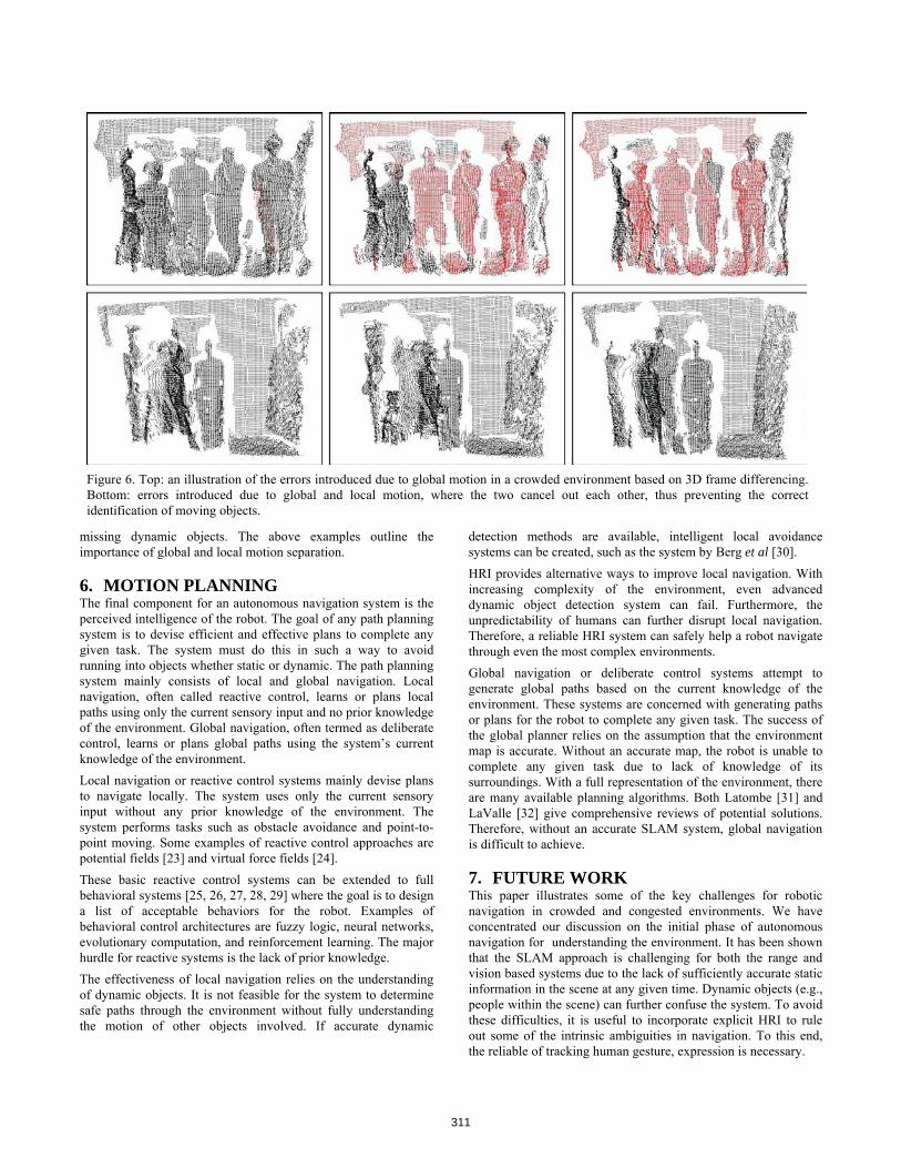
missing dynamic objects. The above examples outline the importance of global and local motion separation.

6. MOTION PLANNING The final component for an autonomous navigation system is the perceived intelligence of the robot. The goal of any path planning system is to devise efficient and effective plans to complete any given task. The system must do this in such a way to avoid running into objects whether static or dynamic. The path planning system mainly consists of local and global navigation. Local navigation, often called reactive control, learns or plans local paths using only the current sensory input and no prior knowledge of the environment. Global navigation, often termed as deliberate control, learns or plans global paths using the system’s current knowledge of the environment. Local navigation or reactive control systems mainly devise plans to navigate locally. The system uses only the current sensory input without any prior knowledge of the environment. The system performs tasks such as obstacle avoidance and point-to-point moving. Some examples of reactive control approaches are potential fields [23] and virtual force fields [24]. These basic reactive control systems can be extended to full behavioral systems [25, 26, 27, 28, 29] where the goal is to design a list of acceptable behaviors for the robot. Examples of behavioral control architectures are fuzzy logic, neural networks, evolutionary computation, and reinforcement learning. The major hurdle for reactive systems is the lack of prior knowledge. The effectiveness of local navigation relies on the understanding of dynamic objects. It is not feasible for the system to determine safe paths through the environment without fully understanding the motion of other objects involved. If accurate dynamic

detection methods are available, intelligent local avoidance systems can be created, such as the system by Berg et al [30].

Figure 6. Top: an illustration of the errors introduced due to global motion in a crowded environment based on 3D frame differencing. Bottom: errors introduced due to global and local motion, where the two cancel out each other, thus preventing the correct identification of moving objects.

HRI provides alternative ways to improve local navigation. With increasing complexity of the environment, even advanced dynamic object detection system can fail. Furthermore, the unpredictability of humans can further disrupt local navigation. Therefore, a reliable HRI system can safely help a robot navigate through even the most complex environments. Global navigation or deliberate control systems attempt to generate global paths based on the current knowledge of the environment. These systems are concerned with generating paths or plans for the robot to complete any given task. The success of the global planner relies on the assumption that the environment map is accurate. Without an accurate map, the robot is unable to complete any given task due to lack of knowledge of its surroundings. With a full representation of the environment, there are many available planning algorithms. Both Latombe [31] and LaValle [32] give comprehensive reviews of potential solutions. Therefore, without an accurate SLAM system, global navigation is difficult to achieve.

7. FUTURE WORK This paper illustrates some of the key challenges for robotic navigation in crowded and congested environments. We have concentrated our discussion on the initial phase of autonomous navigation for understanding the environment. It has been shown that the SLAM approach is challenging for both the range and vision based systems due to the lack of sufficiently accurate static information in the scene at any given time. Dynamic objects (e.g., people within the scene) can further confuse the system. To avoid these difficulties, it is useful to incorporate explicit HRI to rule out some of the intrinsic ambiguities in navigation. To this end, the reliable of tracking human gesture, expression is necessary.

311

8. REFERENCES [1] Mesa-Imaging, "http://www.mesa-imaging.ch." [2] "Point Grey Research,"

http://www.ptgrey.com/products/dragonfly/index.asp. [3] "Mobile Robots: ActivMedia Robotics,"

http://www.activrobots.com/. [4] Hähnel., D., Burgard, W., Fox, D. and Thrun, S., "An

efficient FastSLAM algorithm for generating maps of large-scale cyclic environments from raw laser range measurements," in IEEE/RSJ International Conference on Intelligent Robots and Systems (IROS), Las Vegas, NV, USA, 2003, pp. 206-211.

[5] Thrun, S., Liu, Y., Koller, D., Ng, A., Ghahramani, Z. and Durrant-Whyte, H., "Simultaneous Localization and Mapping with sparse extended information filters," International Journal of Robotics Research, vol. 23, pp. 693-716, 2004.

[6] Davison, A. J., Reid, I. D., Molton, N. D. and Stasse, O., "MonoSLAM: Real-Time Single Camera SLAM," IEEE Transactions on Pattern Analysis and Machine Intelligence, vol. 29, pp. 1-16, 2007.

[7] Montemerlo, M., Koller, S. T. D. and Wegbreit, B., "FastSLAM 2.0: An improved particle filtering algorithm for simultaneous localization and mapping that provably converges," in International Conference on Artificial Intelligence (IJCAI), Acapulco, Mexico, 2003, pp. 1151-1156.

[8] Murphy, K., "Bayesian map learning in dynamic environments," in Conference on Neural Information Processing Systems (NIPS), Denver, CO, USA, 1999, pp. 1015-1021.

[9] Montemerlo, M., Thrun, S., Koller, D. and Wegbreit, B., "FastSLAM: A Factored Solution to the Simultaneous Localization and Mapping Problem," in National Conference on Artificial Intelligence, Edmonton, Alberta, Canada, 2002, pp. 593-598.

[10] Grisetti, G., Tipaldi, G. D., Stachniss, C., Burgard, W. and Nardi, D., "Fast and Accurate SLAM with Rao-Blackwellized Particle Filters," Robotics and Autonomous Systems, vol. 55, pp. 30-38, 2007.

[11] Eliazar, A. and Parr, R., "DP-SLAM: Fast, robust simultaneous localization and mapping with predetermined landmarks," in International Conference on Artificial Intelligence (IJCAI), Acapulco, Mexico, 2003, pp. 1135-1142.

[12] Shi, J. and Tomasi, C., "Good Features to Track," in IEEE International Conference on Computer Vision and Pattern Recognition, 1994.

[13] Li, S. Z. and Zhenqiu, Z., "FloatBoost learning and statistical face detection," Pattern Analysis and Machine Intelligence, IEEE Transactions on, vol. 26, pp. 1112-1123, 2004.

[14] Chengjun, L., "A Bayesian discriminating features method for face detection," Pattern Analysis and Machine Intelligence, IEEE Transactions on, vol. 25, pp. 725-740, 2003.

[15] Ming-Hsuan, Y., Kriegman, D. J. and Ahuja, N., "Detecting faces in images: a survey," Pattern Analysis and Machine Intelligence, IEEE Transactions on, vol. 24, pp. 34-58, 2002.

[16] Xia, L. and Fujimura, K., "Hand gesture recognition using depth data," in Automatic Face and Gesture Recognition, 2004. Proceedings. Sixth IEEE International Conference on, 2004, pp. 529-534.

[17] Hasanuzzaman, M., Ampornaramveth, V., Tao, Z., Bhuiyan, M. A., Shirai, Y. and Ueno, H., "Real-time Vision-based Gesture Recognition for Human Robot Interaction," in Robotics and Biomimetics, 2004. ROBIO 2004. IEEE International Conference on, 2004, pp. 413-418.

[18] Ying, W. and Huang, T. S., "Hand modeling, analysis and recognition," Signal Processing Magazine, IEEE, vol. 18, pp. 51-60, 2001.

[19] Yuanxin, Z., Haibing, R., Guangyou, X. and Xueyin, L., "Toward real-time human-computer interaction with continuous dynamic hand gestures," in Automatic Face and Gesture Recognition, 2000. Proceedings. Fourth IEEE International Conference on, 2000, pp. 544-549.

[20] Kienzle, W., Bakir, G., Franz, M. and Schölkopf, B., "Face Detection - Efficient and Rank Deficient," 2005.

[21] Erwin Prassler, J. S., Alberto Elfes, "Tracking Multiple Moving Objects for Real-time Robot Navigation," Autonomous Robots, vol. 8, pp. 105-116, April 2000.

[22] Stipes, J. A., Cole, J. G. P. and Humphreys, J., "4D Scan Registration with the SR-3000 LIDAR," in IEEE International Conference on Robotics and Automation (ICRA), Pasadena, CA, USA, 2008.

[23] Khatib, O., "Real-time obstacle avoidance for manipulators and mobile robots," International Journal of Robotics Research, vol. 5, pp. 90-98, 1986.

[24] Borenstein, J. and Koren, Y., "Real-time Obstacle avoidance for fast mobile robot," IEEE Transactions on Systems, Man, and Cybernetics, vol. 19, pp. 1179-1187, 1989.

[25] Zhu, A. M., Yang, S. X., Wang, F. J. and Mittal, G. S., "A neuro-fuzzy controller for reactive navigation of a behavior-based mobile robot," Lecture Notes Computer Science, vol. 3498, pp. 259-264, 2005.

[26] Thrun, S., "Probabilistic algorithms for robotics," in AI Magazine. vol. 21, 2000, pp. 93-109.

[27] Kondo, T. and Ito, K., "A Reinforcement learning with evolutionary state recruitment strategy for autonomous mobile robots control," Robotic Autonomous Systems, vol. 46, pp. 111-124, 2004.

[28] Chen, C., Li, H.-X. and Dong, D., "Hybrid Control for Robot Navigation," in IEEE Robotics & Automation Magazine, 2008.

[29] Chen, C. L. and Chen, Z. H., "Reinforcement learning for mobile robot: From reaction to deliberation," Journal of System Engineering Electronics, vol. 16, pp. 611-617, 2005.

[30] Berg, J. V. D., Patil, S., Sewall, J., Manocha, D. and Lin, M., "Interactive navigation of multiple agents in crowded environments," in Proceedings of the 2008 symposium on Interactive 3D graphics and games, Redwood City, CA USA, 2008, pp. 139-147.

[31] Latombe, J.-C., Robot Motion Planning. Norwell, MA, USA: Kluwer, 1991.

[32] LaValle, S. M., "Planning Algorithms [Online]," in http://planning.cs.uiuc.edu/, 2006.

312