INTELLIGENT PROCESS QUALITY CONTROL AND TOOL

MONITORING IN MANUFACTURING SYSTEMS

by

RATNA BABU CHINNAM, B.S.M.E., M.S.I.E.

A DISSERTATION

IN

INDUSTRIAL ENGINEERING

Submitted to the Graduate Faculty of Texas Tech University in

Partial Fulfillment of the Requirements for

the Degree of

DOCTOR OF PHILOSOPHY

Approved

May, 1994

® ? ' ACKNOWLEDGMENTS ^^^ c?7 ^ " ^ ^

I would like to thank Dr. William Kolarik for giving me the motivation, and

invaluable guidance and support all along this research. I would like to thank Dr.

William Oldham, Dr. Milton Smith, Dr. Surya Liman, and Dr. Jose Macedo for their

valuable suggestions.

I would like to express my appreciation to the members of my department. Finally, I

would like to thank my fiancee Kamepalli Smuruthi and my dear friends for providing

moral support all along this research. I dedicate this work to my parents, niece, and

nephew.

11

TABLE OF CONTENTS

ACKNOWLEDGMENTS ii

ABSTRACT v

LIST OF TABLES vi

LIST OF FIGURES vii

CHAPTER

I. INTRODUCTION 1 1.1 Fundamental Objective 1 1.2 Basic Assumptions and Scope 2 1.3 Overview of Feedforward Neural Networks 4

1.3.1 Multilayer Perceptron Networks 5 1.3.2 Back-propagation in Static Systems 7 1.3.3 Radial Basis Function Neural Networks 8 1.3.4 Validity Index Neural Networks 12

1.4 Overview of Neural Network Applications to Control 13 1.5 Overview of Time Series Forecasting Methods 14

II. INTELLIGENT PROCESS QUALITY CONTROL MODEL 17 2.1 Overview of Process Quality Control Practices 17

2.1.1 On-line Quality Improvement Practices 18 2.1.2 Off-line Quality Improvement Practices 19

2.2 Quality Controller Structure 20 2.2.1 Modeling Process Response Characteristics 23

2.2.1.1 Characterization and Identiflcation of Systems 23 2.2.1.2 Input-Output Representation of Systems 24

2.2.2 Schematic Outline of the Quality Controller Operation 25 2.2.2.1 Optimal Process Parameter Determination 27

2.3 Technical Design ofthe Quality Controller 30 2.3.1 Process Identification 30 2.3.2 Process Parameter Determination 31

2.3.2.1 Iterative Inversion based Parameter Determination 31 2.3.2.2 Inversion in a Multilayer Perceptron Network 34 2.3.2.3 Inversion in a Radial Basis Function Network 35 2.3.2.4 Critic-Action Approach based Parameter Determination 36

III. TOOL PERFORMANCE RELL\BILITY MODELING 40 3.1 Overview of Tool Monitoring Practices 40

3.1.1 Failure Criteria, Failure Modes and Performance Measures 41 3.1.2 Monitoring 42 3.1.3 Interpretation and Decision-Making Procedures 43

3.2 Performance Reliability 44

ill

3.2.1 Definition 45 3.2.2 Characteristics of Performance 47 3.2.3 Performance Model and Reliability 47 3.2.4 General Standard Performance Models 51

3.3 Time-Series Modeling of Performance Measures 52 3.4 Tool Performance Reliability Modeling 54

3.4.1 Real-time Tool Performance Reliability Assessment 55 3.4.2 Extensionofthe Validity Index Network 55

IV. PERFORMANCE EVALUATION OF QUALITY CONTROL AND TOOL MONITORING MODELS 56

4.1 Design and Development of a Simulation Test-Bed 56 4.1.1 Overview of Computer Modeling 56 4.1.2 Emulation of Static Non-linear Processes using ProtoSim 57 4.1.3 ProtoSim - A Test-bed for Quality Controller Evaluation 59

4.1.3.1 Overview of ProtoSim 59 4.1.3.2 Flow of Control during Identification Mode 61 4.1.3.3 Flow of Control during Parameter Design Mode 61

4.2 Evaluationof Quality Controller Models 63 4.2.1 An Experiment for Evaluation of Quality Controllers 65

4.2.1.1 Quality Controller in Leaming Mode 65 4.2.1.2 Quality Controller in Parameter Design Mode 73

4.2.2 Performance Results 79 4.3 Evaluation of the Performance Reliability Assessment Techniques

Developed 79 4.3.1 Case Study: Monitoring Drill Bits in a Drilling Process 79

4.3.1.1 Design of Experiments 80 4.3.1.2 Network Design Issues 83 4.3.1.3 Performance Results 83

V. CONCLUSION 90 5.1 Summary 90 5.2 Contributions 92

REFERENCES 93

APPENDIX: SMUUARY OF ERROR BACK-PROPOGATION TRAINING ALGORITHM 106

IV

ABSTRACT

The work presented is best characterized as an investigation of neural networks for

effective process quality control and monitoring in automated manufacturing systems.

The research addresses two basic questions. The first question is whether neural

networks have the potential to "identify" cause-effect relationships associated with

advanced manufacturing systems to achieve real-time quality control? The second

question is whether it is possible to use neural networks to develop effective reliability

based real-time tool condition monitoring models for manufacturing systems?

Both multilayer feedforward perceptron networks and radial basis fiinction networks

are used in novel configurations to achieve real-time process parameter design. The

models developed are capable of monitoring process performance characteristics of

interest by building empirical based relationships to relate the process response

characteristics with controllable and uncontrollable parameters, simultaneously. Using

these empirical models and the levels ofthe uncontrollable parameters obtained through

sensors, the quality controller provides levels for the controllable parameters that will

lead to the desired levels ofthe quality characteristics in real-time. In general, the quality

controller models were able to provide levels for the controllable variables that resulted in

the desired process quality characteristics. Test results are discussed for several

simulated production processes.

A validity index neural network based approach was developed to automate the tool-

wear monitoring problem. In contrast to the contemporary approaches that basically deal

with a classification problem, classifying a given tool as either fresh or worn, the model

derived fi^om radial basis function networks predicts the conditional probability of tool

survival in accordance with the traditional reliability theory, given a critical performance

plane, using on-line sensory data. In general, the radial basis fimction networks

performed extremely well in time-series prediction, when tested on actual data collected

from a drilling process. The validity index neural network is extended to arrive at the

desired conditional tool reliability.

LIST OF TABLES

4.1 The MSE values corresponding to various combinations of H and P; three-level factorial experiment. 68

4.2 The MSE values corresponding to various combinations of H and P; four-level factorial experiment. 70

4.3 Combinations of starting points and desired targets. 74

4.4 Training and prediction errors for different optimal network structures in the case of One-Hole ahead thrust force predictions. 84

4.5 Training and prediction errors for different optimal network structures in the case of simultaneous One-Hole and Five-Hole ahead thrust force predictions. 84

VI

LIST OF FIGURES

1.1 A three-layer perceptron neural network. 6

1.2 A block diagram representation of a three-layer perceptron neural network. 6

1.3 Architecture for back-propagation. 9

1.4 The VI Network architecture, with confidence limits. The underlying RBF network is indicated by dashed lines. 11

2.1 Classical model of adaptive control. 22

2.2 Architecture for the quality controller at the machine level. 22

2.3 Schematic outline ofthe quality controller operation. 26

2.4 Using a neural network for identifying a process inverse. 28

2.5 Using a neural network for process identification. 32

2.6 Critic-Action networks based quality controller structure. 37

2.7 The Critic network neural structure. 37

2.8 The Action network neural structure. 38

3.1 Conceptual performance curves for a specified environment, with a performance plane superimposed. 46

3.2 Typical cases of physical performance. 48

3.3 Relationship between physical performance and reliability. 50

3.4 Using a connectionist network for adaptive prediction. 53

4.1 Simulator acting as a test-bed for quality controllers. 60

4.2 Layout ofthe simulator. 60

4.3 Flow of control in process identification mode 62

4.4 Flow of control in parameter design mode 64

4.5 Response surfaces of a simulated process. 66

4.6 Predicted and actual response surfaces of a simulated process; three-level factorial experiment, (a) Predicted surface for ResMeas\(X) superimposed on the actual surface, (b) Predicted surface for ResMeas2(X) superimposed on the actual surface, (c) Error surface. 69

4.7 MSE values for different values of P when H was controlled at 20. 71

vu

4.8 Predicted and actual response surfaces of a simulated process; four-level factorial experiment, (a) Predicted surface for ResMeasi(X) superimposed on the actual surface, (b) Predicted surface for ResMeas2(X) superimposed on the actual surface, (c) Error surface. 72

4.9 Predicted response surfaces of a simulated process; with superimposed search trajectory (Case 1). (a) Predicted surface for ResMeasi(X). (b) Predicted surface for ResMeas2(X). (c) Energy surface with desired targets at 0.93 and 0.57; and starting points at X2=0.0, ^3=0.85. 75

4.10 Predicted response surfaces of a simulated process; with superimposed search trajectory (Case 2). (a) Predicted surface for ResMeasi(X). (b) Predicted surface for ResMeas2(X). (c) Energy surface with desired targets at 0.817 and 0.549; and starting points at 2=0.0, 3=0.85. 76

4.11 Predicted response surfaces of a simulated process; with superimposed search trajectory (Case 3). (a) Predicted surface for ResMeas\(X). (b) Predicted surface for ResMeas2(X). (c) Energy surface with desired targets at 0.93 and 0.57; and starting points at X2=0.805, X =0.119. 11

4.12 Predicted response surfaces of a simulated process; with superimposed search trajectory (Case 4). (a) Predicted surface for ResMeas\(X). (b) Predicted surface for ResMeas2(X). (c) Energy surface with desired targets at 0.817 and 0.549; and starting points at X2=0.805, X^=0.119. 78

4.13 Drill performance in terms of average thrust force for eight drill bits. 82

4.14 Curves of thrust force as recorded for drill bit 4. 82

4.15 Confidence limits for one-hole ahead prediction (Drill bit 1) 86

4.16 Confidence limits for one-hole ahead prediction (Drill bit 4) 86

4.17 Tool conditional performance reliability curve (Drill bit 1: YpcL = 2601bs.) 87

4.18 Tool conditional performance reliability curve (Drill bit 4: TPCL = 2601bs.) 87

4.19 Tool performance reliability curve (Drill bit 1: YpcL = 2601bs.) 88

4.20 Tool performance reliability curve (Drill bit 4: 7PCL = 2601bs.) 88

A. 1 Basic two layer perceptron network. 107

Vlll

CHAPTER I

INTRODUCTION

The late 80's and early 90's saw an unprecedented emphasis on quality throughout the

world. Product quality, responsiveness to customers, process control and flexibility, and

development and maintenance of an organizational skill base capable of spurring constant

improvement have become the determinants of global manufacturing competitiveness.

With ever increasing global competition, manufacturers are pressed for higher

performance levels, to offer essentially "zero defect" products that are nonetheless

produced at much lower costs. In an effort to solve this problem, various advanced

manufacturing principles and technologies are being introduced. To ensure higher yields

and to attain increasingly tighter performance levels over extended periods of operation,

equipment engineers are being asked to design automatic, self-calibrating systems with

real-time closed-loop control. At this point in time, the application of advanced control

techniques to accomplish real-time closed-loop control is very limited [MSB, CETS, and

NRC, 1991]. This problem is most acute in areas where the complexity of fabrication has

increased to an extent that the process engineers are not able to respond fast enough to

provide real-time control under changing process conditions. One key to engineering

solutions to these problems lies in the application ofthe intelligent manufacturing control

technology [MSB, CETS, and NRC, 1991].

1.1 Fundamental Obj ective

This research work is carried out with two principal objectives, both involving the

replacement of classical statistical based models with neural network based models,

compatible with automated manufacturing systems. The first objective is to develop

identification and controller structures using neural networks for achieving effective real­

time process quality control in non-linear static processes where the process physics is not

well-understood. In other words, the objective is to define, develop, and test models that

will lead to more intelligent control of any manufacturing process in which the

relationships between controlled variables, uncontrolled variables (inputs) and critical

process quality characteristics (outputs) are poorly understood.

Traditional approaches to process quality control primarily deal with conventional

open-loop control. This, in an abstract sense, includes: (1) monitoring the manufacturing

process to detect shifts in its performance level, and (2) taking corrective actions to bring

the process into statistical control. It is a fact that in most manufacturing systems, process

settings are based on experiences gained by the workers associated with the process, and

on small-scale studies. Almost inevitably, in most situations, the product is manufactured

at lower production rates, lower yields, and at lower quality than the facilities are capable

of. What is important is the continuous process of "tuning" the system to operate at

optimal levels of production and quality under all circumstances. While major advances

have been made in the improvement of these traditional approaches, none thus far

developed has the potential to deal with closed-loop process quality control. The models

developed consequently represent a first step in this direction.

A second objective is to design, develop, and test neural network based tool

monitoring models that are capable of providing conditional reliability estimates.

Automated tool-wear "identification" involving neural networks has been proposed and

successfully tested in the past [Burke, 1989; Burke, 1992; Burke and Rangwala, 1991;

Chryssolouris, 1988; Hou and Lin, 1993; Masory, 1991; Rangwala, 1988]. But, rather

than develop a model that can merely classify a tool as "wom" or "fresh," the objective

here is to develop a monitoring system that can predict the conditional probabilities of

tool survival in accordance with the traditional reliability theory, using on-line sensory

data.

1.2 Basic Assumptions and Scope

In general, one can state that there are two broad classes of problems in effectively

controlling production processes. The first class of control problems is related to

understanding and monitoring process response characteristics, so as to be able to run the

process efficiently, with improved performance and yield. One task is the development

of empirical models relating process performance characteristics with controllable

variables and uncontrollable variables. Other tasks include process parameter design,

experimental design and analysis to detect shifts in process response characteristics (in

case of time-variant systems), decision making to identify assignable causes, and so on.

The second class of control problems is related to the task of achieving and

maintaining process control parameter values or set-points suggested. The solution to the

first class of control problems establishes the process parameter targets that are used as

set-points.

This study focuses on the first class of control problems. In solving the real-time

parameter design (control) problem, the following assumptions are made:

1. Process performance characteristics of interest at any single instant of time can

be expressed as static non-linear maps in the input space (vector space defined by

controllable and uncontrollable variables).

2. Levels of uncontrolled variables do not change radically, but change in a

reasonably smooth fashion.

3. It is possible to monitor all critical variables that affect process performance, in

real-time.

4. Scales for the controllable variable(s) are continuous.

In dealing with the tool condition monitoring problem, it is assumed that a conditional

reliability structure can be useful for effective tool management in the computer-aided

environment. Assumptions underlying the performance reliability models developed in

this study are described below:

1. Performance measures may drift up and down, but must eventually decrease or

increase. That is performance degradation exists, and, in the long run, is not

reversible.

2. Performance characteristics can be measured (the performance signal is

detectable, even though noise in the measurement and natural variation exists).

Both multilayer feedforward perceptron networks and radial basis function networks

are used in novel configurations to achieve real-time process parameter design. The

models developed are capable of monitoring process performance characteristics of

interest, by building empirical based relationships to relate the process response

characteristics with controllable and uncontrollable parameters, simultaneously. Using

these empirical models and the levels ofthe uncontrollable parameters obtained through

sensors, the quality controller provides levels for the controllable parameters that will

lead to the desired levels ofthe quality characteristics in real-time. In general, the quality

controller models were able to provide levels for the controllable variables that resulted in

the desired process quality characteristics. Test results are discussed for several

simulated production processes.

A validity index neural network based approach was developed to automate the tool-

wear monitoring problem. An underlying problem deals with the time-series prediction.

In contrast to the contemporary approaches that basically deal with a classification

problem, classifying a given tool as either fresh or wom, the model derived from radial

basis function networks predicts the conditional probability of tool survival in accordance

with the traditional reliability theory, given a critical performance plane, using on-line

sensory data. In general, the radial basis function networks performed extremely well in

time-series prediction, when tested on actual data collected from a drilling process. The

validity index neural network is extended to arrive at the desired conditional tool

reliability.

1.3 Overview of Feedforward Neural Networks

Multilayer neural networks have received considerable attention in recent years.

From a systems theoretic point of view, multilayer networks represent static non-linear

maps. In general, networks are composed of many non-linear computational elements,

called nodes, operating in parallel and arranged in pattems reminiscent of biological

neural nets [Lippman, 1987]. These processing elements are connected by weight values,

responsible for modifying signals propagating along connections and used for the training

process. The number of the nodes plus the connectivity define the topology of the

network. Networks can range from totally connected to a topology where each node is

just connected to its neighbors. The two extreme cases are easier to analyze than random

connectivity, which makes these topologies most popular. In general, a node or

processing element has several inputs and an output, and the node generates the output as

a function of the inputs. The functions do not have to be the same for every node in the

network, but the network is easier to analyze if they are. The most popular nodal

functions are the hard-limiter [f(x) = +l for all JC > 0 andf(x) = -1 for all jc < 0], the

threshold [f(x) = x for allXo>x> 0,f(x) = +1 for all ;c >XQ, and f(x) = 0 for all ;c < 0],

and the sigmoid [unipolar -f(x) =l/(l+e'^) and bipolar -f(x) = (\ -e'^)/(\ + e'"")].

1.3.1 Multilayer Perceptron Networks

A typical multilayer neural network with an input layer, an output layer, and two

hidden layers is shown in Figure 1.1. For convenience, the same network is denoted in

block diagram form as shown in Figure 1.2 with three weight matrices W^, W^, and Jr

and a diagonal non-linear operator F with identical sigmoidal elements ;'following each

ofthe weight matrices. Each layer ofthe network can then be represented by the operator

N,[x] = TW'xl (1.1)

and the input-output mapping ofthe multilayer network can be represented by

y = N[x] = I{W'I[W'T{W'X]^ = N,N,N,[x]. (1.2)

In practice, multilayer networks have been used successfully in pattern recognition

problems [Burr, 1988; Gorman and Sejnowski, 1988; Sejnowski and Rosenberg, 1987;

Widrow, Winter, and Baxter, 1988]. The weights ofthe network W^, W^, and W^ are

adjusted as described in Section 1.3.2 to minimize a suitable function of error e between

the output;^ ofthe network and a desired output ; rf. This results in the mapping function

A jc], mapping input vectors into corresponding output classes. From a systems theoretic

point of view, multilayer networks can be considered as versatile non-linear maps with

the elements ofthe weight matrices as fitting parameters.

From the above discussion, it follows that the mapping properties of A' , [.] and

consequently N[ ] (as defined in (1.2)) play a central role in all analytical studies of such

networks. It has been recently shown in Homik et al. [1988], using the

5

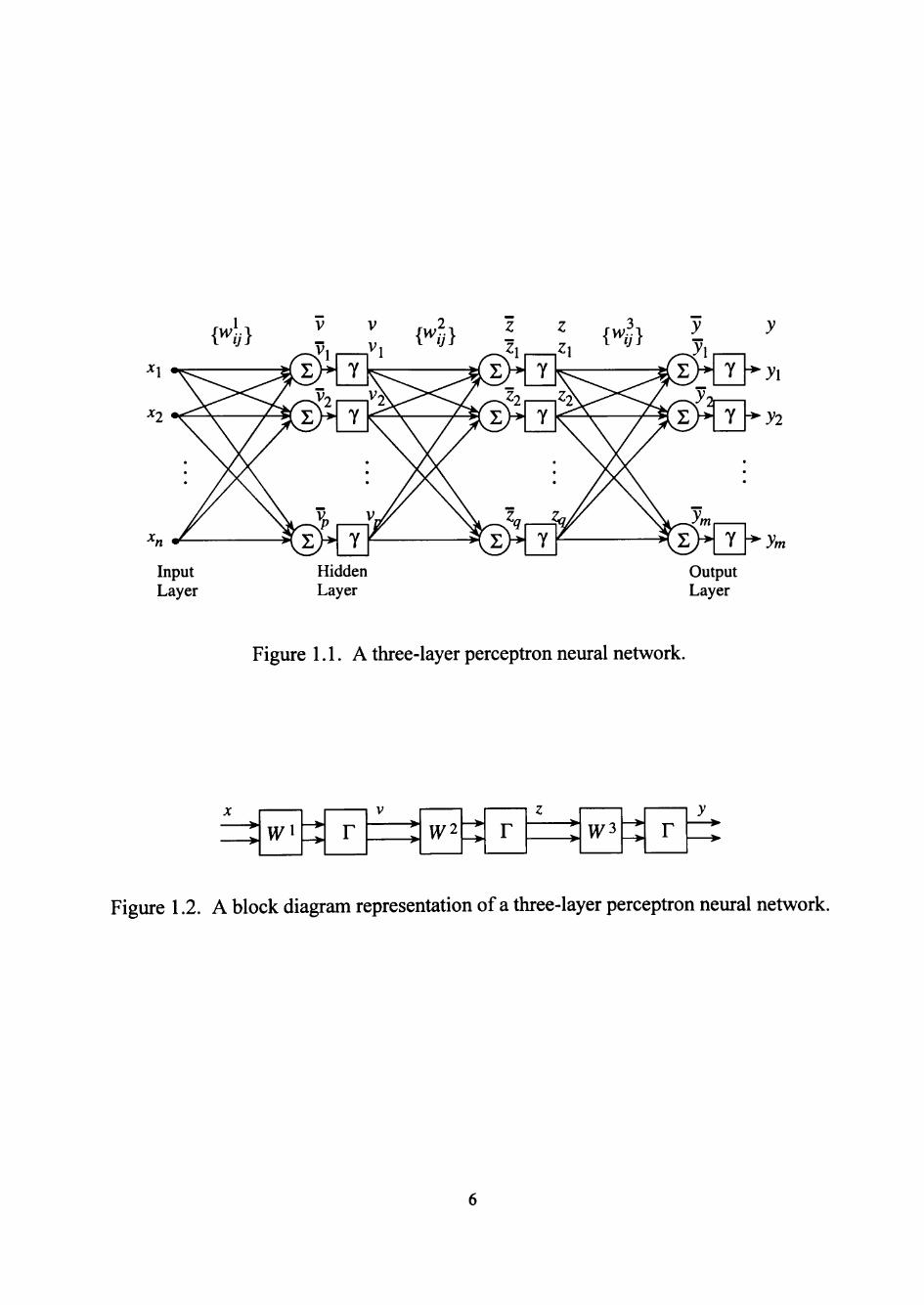
Input Layer

Hidden Layer

y

y\

yi

y m Output Layer

Figure 1.1. A three-layer perceptron neural network.

X

> >

w^ —> r V

^ jy2

—> r z W^

—> —> F

y

Figure 1.2. A block diagram representation of a three-layer perceptron neural network.

Stone-Weierstrass theorem, that a two-layer network with an arbitrarily large number of

nodes in the hidden layer can approximate any continuous function / e C(R^, R" ) over

a compact subset of R^ to arbitrary precision. This provides the motivation to use multi­

layer perceptron networks in modeling the process response characteristics.

1.3.2 Back-propagation in Static Systems

If neural networks are used to solve the static identification problems treated in this

research, the objective is to determine an adaptive algorithm or rule which adjusts the

parameters ofthe network based on a given set of input-output pairs. If the weights ofthe

networks are considered as elements of a parameter vector 0, the leaming process

involves the determination ofthe vector 0* which optimizes a performance function J

based on the output error. Back-propagation is the most commonly used method for this

purpose in static contexts. The gradient ofthe performance function with respect to 0 is

adjusted along the negative gradient as

e = e _ - T i V e J U _ (1.3)

where r\, the step size, is a suitably chosen constant and 0^^ denotes the nominal value

of 0 at which the gradient is computed.

In the three-layered neural network shown in Figure \.2,x = [Xy^x^y-.-Xj^Y denotes

the input vector while y = [yi,J'2 ,• • • yJu^ is the output vector, i; = [Uj ,^2,. • • y^pF and

2; = [Zj ,22 V • • i^Q ]^ are the outputs at the first and the second hidden layers, respectively.

\w] I , \wl^} and \w\} are the weight matrices associated with the three layers as

shown in Figure 1.2. The vectors v e R'', z e R^, > G R"^ are as shown in Figure 1.2

with Y (v,) = v , 7 ( z j = z and Y (yi) = yi where v , z^, and yi are elements of v, z and

y respectively. If y^ = [yf ,^3 »••• J^M 3 is the desired output vector, the output error

vector for a given input pattem x is defined as e = y- y^. The performance criterion J is

then defined as

J = l.hf (1.4)

where the summation is carried out over all pattems in a given set S. If the input pattems

are assumed to be presented at each instant of time, the performance criterion J may be

interpreted as the sum of squared errors over an interval of time.

While strictly speaking, the adjustment ofthe parameters should be carried out by

determining the gradient of J in parameter space, the procedure commonly followed is to

adjust it at every instant based on the error at that instant and a small step size r\. If 0y

represents a typical parameter, de I dQj has to be determined to compute the gradient as

e (del 30^). The back-propagation method is a convenient method of determining this

gradient.

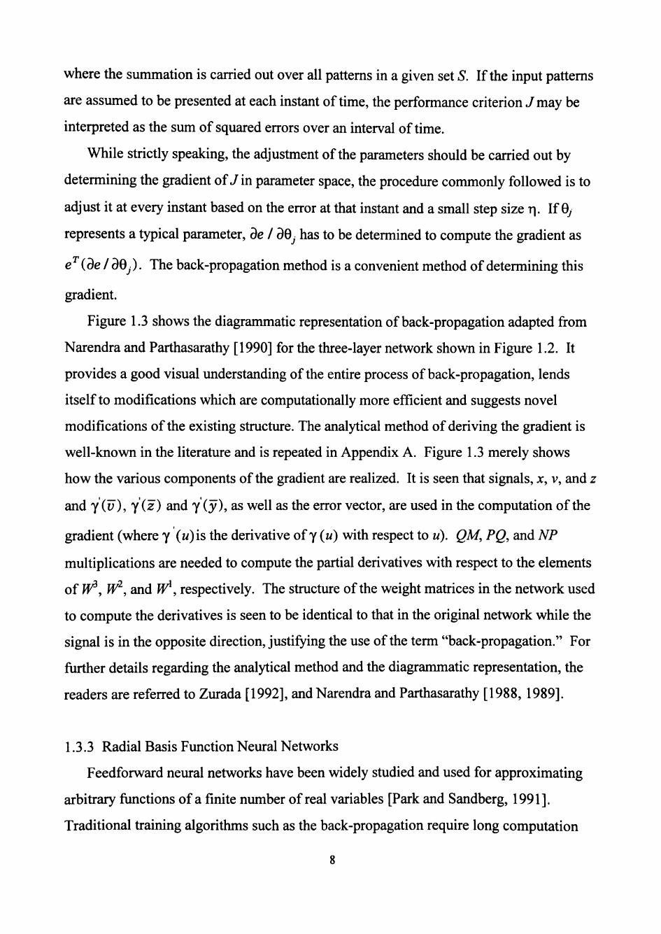
Figure 1.3 shows the diagrammatic representation of back-propagation adapted from

Narendra and Parthasarathy [1990] for the three-layer network shown in Figure 1.2. It

provides a good visual understanding ofthe entire process of back-propagation, lends

itself to modifications which are computationally more efficient and suggests novel

modifications ofthe existing structure. The analytical method of deriving the gradient is

well-known in the literature and is repeated in Appendix A. Figure 1.3 merely shows

how the various components ofthe gradient are realized. It is seen that signals, x, v, and z

and i(v), y(z) and y(y), as well as the error vector, are used in the computation ofthe t

gradient (where Y (w)is the derivative of Y («) with respect to u). QM, PQ, and NP

multiplications are needed to compute the partial derivatives with respect to the elements

of ^ , W^, and W^, respectively. The structure ofthe weight matrices in the network used

to compute the derivatives is seen to be identical to that in the original network while the

signal is in the opposite direction, justifying the use ofthe term "back-propagation." For

further details regarding the analytical method and the diagrammatic representation, the

readers are referred to Zurada [1992], and Narendra and Parthasarathy [1988, 1989].

1.3.3 Radial Basis Function Neural Networks

Feedforward neural networks have been widely studied and used for approximating

arbitrary functions of a finite number of real variables [Park and Sandberg, 1991].

Traditional training algorithms such as the back-propagation require long computation

^2

AI

multiplications multiplications

- V H , I 7 - \ 2 j

^>«--^ multiplications

-Vw3 7

Figure 1.3. Architecture for back-propagafion [Narendra and Parthasarathy, 1990].

times for training. The incremental adaptation approach of back-propagation can be

shown to be susceptible to false minima [Specht, 1990]. It has been proven that

feedforward networks that incorporate radial basis functions as nodal functions (RBF

networks) are capable of universal approximation with one hidden layer [Park and

Sandberg, 1991]. Also, in contrast to perceptron networks, RBF networks can be trained

more rapidly [Moody and Darken, 1989].

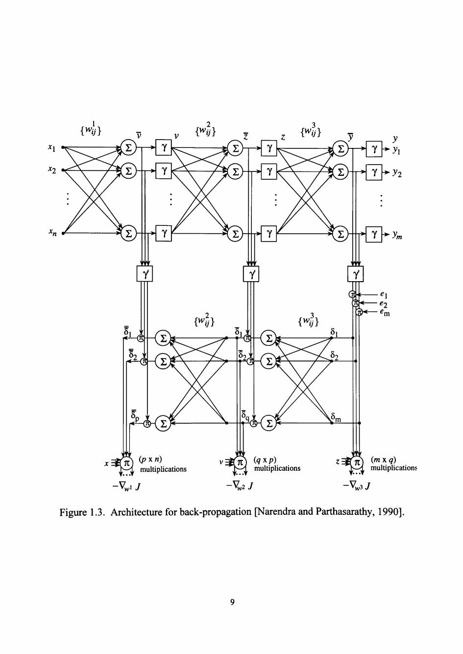
A typical RBF network consists of three layers of nodes with successive layers fiilly

connected by feedforward arcs, as shown in Figure 1.4. The connections between the

input and the hidden layers are unweighted, and the transfer functions at the hidden layer

nodes are radial basis functions. Many different architectures are discussed in the

literature. Here, the particular architecture and training scheme described in Moody and

Darken [1989] is presented along with a transfer function similar to the multivariate

Gaussian density function

^h=e' ,h=l,...,H, (1.5)

where «;, is the output of node h in the hidden layer given the input vector X Each RBF

node has A +1 intemal parameters: y.^, the position ofthe center ofthe radial unit in the

input space, and cj^, the unit width. Each RBF unit has a significant activation over a

specific region determined by p , and a ,. The value ofthe /th output node, y^, is given by

H+\

h=l

A bias node is represented by %+j = 1. A three-step polynomial time method presented

in [Moody and Darken, 1989] is generally used to determine the parameters p ,, a ,, and

w.fj. First, unit centers p^ are determined by k-means clustering [MacQueen, 1967].

Then, a P-nearest neighbor heuristic is used to determine the unit widths a ,. Finally,

second-layer weights are determined by linear least squares.

10

X

Input Layer

Bias

Hidden Layer

Output Layer

_p)-^CLi(X)

Figure 1.4. VI Network architecture, with confidence limits. The underlying RBF network is indicated by dashed lines. Adapted from Leonard, Kramer, and Ungar[1992].

11

1.3.4 Validity Index Neural Networks

Radial units have been used by Specht [Specht, 1990] to estimate probability

densities, but as with Parzen windows [Weiss and Kulikowski, 1991], identical radial

units centered at each training point are required [Leonard, Kramer, and Ungar, 1992].

The method of Traven [Hou and Lin, 1993] allocates fewer radial units, but units are

distributed specifically for density estimation [Leonard, Kramer, and Ungar, 1992]. The

validity index neural network (VI Network), Leonard, Kramer, and Ungar [1992], is

based on RBF networks where there are fewer radial units than the data points, unit

widths are not identical, and unit parameters are optimized for prediction of Y, rather than

data density estimation.

The VI Network also includes confidence intervals on network predictions. Unlike

global measures of goodness of fit, such as R in linear regression, the local goodness of

fit measure is expressed as a function of X Training data are considered "local" to a test

point if they are within a limited region around the test point. Because, RBF networks

partition training data into local clusters, the concept of a local neighborhood is naturally

well defined in RBF networks [Leonard, Kramer, and Ungar, 1992]. The VI Network

architecture includes M+\ additional outputs: one node to indicate extrapolation and M

nodes for the confidence limit on each element of Y.

A local estimate for the variance ofthe model residual in output i within the domain

of hidden unit/z is

Kn,-\), (1.7) ^hi ~ I,a,iX,)*El, LA=1

where «;, is the effective number of training points contributing to unit h. Since the

activation at a hidden unit caused by a training point can be taken as the membership

function ofthe point in that unit [Leonard, Kramer, and Ungar, 1992], the effecfive

number of training points contributing to unit h is

K

1 n,='la,{X,). (1.8)

12

Assuming that the residuals are independent and normally distributed with a mean of zero

and a constant variance over the neighborhood defined by each RBF unit but varying

from unit to unit, the (1-a) confidence limits for the expected value ofthe residual of

output / for unit h is given by

CL,,=t^,*s^*n^\ (1.9)

where t^2 i the critical value ofthe Student's / statistic with n^-\ degrees of freedom.

The confidence limits for the individual value ofthe residual rather than that for the

expected value can be calculated in much the same way using

c 4 . = < < v 2 * s « * ( i + i / » J ° ' - (110)

The confidence limit for an arbitrary test point is an average ofthe RBF unit confidence

limits weighted by the contribution of each hidden unit to the output for the current input

[Leonard, Kramer, and Ungar, 1992]. In the case ofthe expected value, this would be

CL,(X) = H

J,a,(X)*CL, 'hi Lh=\ J/ L;I=I

H

(1.11)

Note that (1.11) can also serve to weight the contributions ofthe individual values. For

further treatment on the VI Network, the reader is referred to [Leonard, Kramer, and

Ungar, 1992].

1.4 Overview of Neural Network Applications to Control

Neural networks have received considerable attention for their application to control

problems [Narendra and Parthasarathy, 1990]. One approach to this is the development

of a neural-network-based controller, which takes as inputs either commanded system

outputs or feedback variables from the plant [Hoskins, Hwang and Vagners, 1992]. One

significant difficulty with this approach is that of credit assignment. That is, how should

error in the desired plant output be used to modify the controller network, since the plant

dynamics are interposed between the network output and the "scored" output [Hoskins,

Hwang and Vagners, 1992]. One approach to this problem is the adaptive critic approach

of Barto [Barto, Sutton and Anderson, 1986].

13

A second approach, inifially proposed by Werbos [1974, 1977, 1988], is that of back-

propagation of utility. In this approach, a neural network is first trained to model the

forward dynamics ofthe plant. Then, an untrained controller network is placed in series

with the network model ofthe plant. Finally, the weights for the controller are trained

using back-propagation ofthe command input to plant output response, while holding the

plant model weights constant. The output errors are back-propagated through the plant

model to provide credit assignment for the plant inputs. This strategy is the basis for

many current neuro controllers [Kawato, Uno and Isobe, 1987; Guez and Ahmad, 1989;

Jordan, 1988, 1990; Nguyen and Widrow, 1989; Widrow, 1986].

1.5 Overview of Time Series Forecasting Methods

A time series is a sequence of time-ordered values that are measurements of some

physical process. Many forecasting methods have been developed in the last few decades

[Makridakis et al., 1982]. While the Box-Jenkins method is a fairly standard time series

forecasting method [Box and Jenkins, 1976], neural nets as forecasting models are

relatively new [Dutta and Shekhar, 1988, Sharda and Patil, 1990]. A brief account ofthe

Box-Jenkins method and the neural net approaches is provided. More complete

treatments of both the statistical and neural net approaches can be found in Box and

Jenkins [1976], Hoff [1983], and Rumelhart and McClelland [1986].

Box-Jenkins uses a systematic procedure to select an appropriate model from a rich

family of models, namely, ARIMA models. Here AR stands for autoregressive and MA

for moving average. AR and MA are themselves time series models. The former model

yields a series value Xt as a linear combination of some finite past series values,

jc,_i,..., jc,_ , where/? is an integer, plus some random error Ct. The latter gives a series

value Xt as a linear combination of some finite past random errors, e, _,,..., e,_ , where q is

an integer, p and q are referred to as orders ofthe models. Note that in the AR and MA

models some ofthe coefficients may be zero, meaning that some ofthe lower-order terms

may be dropped [Tang and Fishwick, 1993]. AR and MA models can be combined to

form an ARMA model. Most time series are "non-stationary" meaning that the level or

14

variance ofthe series change over time. Differencing is often used to remove the trend

component of such time series before a ARMA model can be used to describe the series.

The ARMA models applied to the differenced series are called integrated models,

denoted by ARIMA.

A general ARIMA model has the following form [Bowerman and O'Connell, 1987]:

0^(f i )a)p(B^)( l -B^)^( l -5) ' 'y , = a + 0^(fi)eQ(B^)£, (1.12)

where 0(5) and Q(B) are autoregressive and moving average operators, respectively; B

is the back shift operator; e is a random error with normal distribution N(0,d^); a is a

constant, and>'/ is the time series data, transformed if necessary. The Box-Jenkins

method performs forecasting through the following process:

1. Model Identiflcation. The orders ofthe model are determined.

2. Model Estimation. The linear coefficients ofthe model are estimated (based on

maximum likelihood).

3. Model Validation. Certain diagnostic methods are used to test the suitability of

the estimated model. Altemative models may be considered.

4. Forecasting. The best model chosen is used for forecasting. The quality ofthe

forecast is monitored. The parameters ofthe model may be reestimated or the

whole modeling process repeated if the quality of forecast deteriorates.

A neural network with a single hidden layer can capture the non-linearity ofthe

logistic series. As was mentioned in section 1.3.1, a feedforward neural network can be

regarded as a static non-linear map. It was also stated that a two-layer feedforward neural

network with a finite number of hidden layer units can represent any continuous function.

These theoretic results make feedforward neural nets reasonable candidates for any

complex function mapping. Neural networks have the potential to represent any

complex, non-linear underlying mapping that may govem changes in a time series [Tang

and Fishwick, 1993]. In the three-layered neiu-al network shown in Figure 1.2, if u^ the

input vector constitutes the finite past series values, [x,_i,...,x,_^], and the output vector

constitutes the time series value [xj, from (1.2) it is clear that the neural network models

can be super sets ofthe Box-Jenkins models [Tang and Fishwick, 1993].

15

Concerning the application of neural nets to time series forecasting, there have been

mixed reviews. For instance, Lapedes and Farber [1987] reported that simple neural

networks can outperform conventional methods, sometimes by orders of magnitude.

Their conclusions are based on two specific time series without noise. Weigend,

Huberman, and Rumelhart [1990] applied feedforward neural nets to forecasting with

noisy real-world data from sun spots and computational ecosystems. A neural network,

trained with past data, generated accurate future predictions and consistently

outperformed traditional statistical methods such as the TAR (threshold autoregressive)

model [Tong and Lim, 1980]. Sharda and Patil [1990] conducted a forecasting

competition between neural network models and the Box-Jenkins procedure using a

variety of 75 time series. They concluded that simple neural nets could forecast about as

well as the Box-Jenkins forecasting system.

16

CHAPTER II

INTELLIGENT PROCESS QUALITY CONTROL MODEL

As with most systems, the changes in performance characteristics of advanced

manufacturing systems can be categorized as: (1) sudden changes and (2) gradual

changes. Sudden changes in time-variant systems can be attributed to:

1. Changes incorporated by process designers,

2. Activities such as routine maintenance and or part replacement, and

3. Abrupt failures in system components.

Gradual changes are mostly due to natural degradation or ascendance ofthe system's

performance due to wear and tear, aging, wear-in and so on. Even in time-invariant

systems, response characteristics could vary with time due to changes in raw-material

parameters and noise parameters such as humidity and temperature.

In order to develop effective process quality control algorithms, it is necessary to

track these changes in the system's response characteristics. This chapter starts with an

overview of traditional process quality control practices and then introduces identification

as well as quality controller structures using neural networks for effective parameter

design of unknown non-linear static manufacturing systems. The theoretical assumptions

necessary to have well-posed problems and concepts required to achieve effective

identification and process parameter design are introduced.

2.1 Overview of Process Quality Control Practices

Box and Draper [1969] explained the many stages of development involved with a

typical industrial process in an abstract sense. The idea for a promising manufacturing

route is followed by laboratory work that is often lengthy, in order to explore its (idea's)

possibilities. The laboratory results and the pilot plant studies provide preliminary

estimates of feasibility, permit realistic objectives to be defined, and lead to tentative

outline of an industrial process. Based on the credibility ofthe results of preliminary

studies, engineering expertise may then be applied to design a full-scale plant. Assuming

that the plant is built, then, ideally, it will incorporate the best design possible, given the

17

available knowledge and resources. To run the process however, there is usually a wide

choice of available operating conditions. The small-scale work will have provided "ball

park" estimates ofthe operating conditions. Even though these estimates are useful, they

usually represent only good first guesses in a continuing process of iteration. This fact is

recognized in the special attention given at plant startup. Special technical teams are

usually assigned to determine the major adjustments that may be necessary before the

process can be made to perform reasonably well (or sometimes to perform at all).

However, almost inevitably, the product is being manufactured at lower production rates,

at lower yield, and at lower quality than the plant is capable of The process of "tuning"

still remains to be done. The fact that this tuning is capable of producing rich rewards is

clear, considering typical plant histories [Box and Draper, 1969].

The next two sections briefly review successful research efforts accomplished thus far

in the areas of on-line quality improvement and off-line quality improvement.

2.1.1 On-line Quality Improvement Practices

The work of Shewhart [1931], Dodge, and Romig [see Duncan, 1986] more or less

laid the foundation for what today comprises the theory of statistical quality control. One

critical tool is the Shewhart control chart. The power ofthe control chart technique lies

in its ability to detect shifts in process level, increases or decreases in process variability,

or non-randomness (as typified by trends, cycles, etc.). This makes possible the diagnosis

and correction of many production troubles and often brings substantial improvements in

product quality and reduction of spoilage and rework [Grant and Leavenworth, 1988].

Moreover, by identifying certain ofthe quality variations as inevitable chance variations,

the control chart tells when to leave the process alone and thus prevents unnecessary

adjustments that tend to increase the variability ofthe process rather than to decrease it.

As such, control charts act as waming devices. The control chart by itself does not

have the potential to identify the kind or amount of action necessary to bring the process

into control. Recently, the sequential aspects of quality control have been emphasized,

leading to the introduction of geometric moving average charts by Roberts [1959],

18

cumulative sum charts by Page [1957, 1961], and Barnard [1959] and cause selection

control charts. Several studies have been made to determine the optimal sample sizes,

sampling frequency and so on for different scenarios of interest.

Growing interest in stochastic processes has led to the development of a procedure

known as adaptive quality control in the industrial field. Adaptive quality control, a

technique promoted by Box and Jenkins [1976], aims to improve process control and

thereby outgoing product by anticipating where the process will wander if left unadjusted.

The approach to control taken in this research is to typify the disturbance by a suitable

time series or stochastic model and the inertial characteristics ofthe system by a suitable

transfer function model, and then calculate the optimal control equation. Optimal action

is interpreted as that which produces the smallest mean square error at the output.

2.1.2 Off-line Quality Improvement Practices

After the introduction of control charts and sampling plans, other techniques, such as

correlation, analysis of variance, and the design of experiments, found their way into the

industrial laboratories and research departments [Duncan, 1986]. In recent years, there

have been several new lines of development. One of these has been the response surface

analysis associated largely with the name of Professor George E. P. Box. This

systematized exploratory technique has found applications in the continuous process

industries together with the closely associated procedure known as evolutionary operation

[Duncan, 1986].

Evolutionary operation (EVOP) proposed by Box [1957] is an analytical approach

aimed at securing information about the process while subjecting the process to small

systematic changes (on-line as distinguished from laboratory or pilot plant experiments),

and could certainly be classified as an on-line quality improvement tool. Its basic

philosophy is that it is inefficient to run an industrial process in such a way that only a

product is produced, and that a process should be operated so as to produce not only a

product but also information on how to improve the product [Box and Draper, 1969].

19

For the last two decades, classical experimental design techniques have been widely

used for setting process parameters or targets. But, recently their potential is being

questioned for they tend to focus primarily on the process mean. Encountering an

increasing need to develop experimental strategies to achieve some target condition while

simultaneously minimizing product variation, parameter design methods along with

signal-to-noise-ratios are being advocated in designing products and processes that are

robust to uncontrollable variations [Taguchi, 1986; Taguchi and Phadke, 1984; Taguchi

and Wu, 1985; Vining and Myers, 1990]. Box [1985] points out that the Taguchi

approach represents a significant advance in application of experimental designs to

improve producVprocess quality. However, he also points out shortcommgs to the

Taguchi procedure. Among these criticisms are the following: (1) the Taguchi method

does not exploit a sequential nature of investigation; (2) the designs advocated are rather

limited and fail to deal adequately with interactions; (3) more efficient and simpler

methods of analysis are available; and (4) the arguments for the universal use ofthe

signal-to-noise ratio are unconvincing.

The response to these criticisms requires that the Taguchi philosophy be blended with

a data analysis strategy in which the mean and variance ofthe quality characteristic are

both empirically modeled to a considerably greater degree than practiced by Taguchi.

Vining and Myers [1990] established that one can achieve the primary goal ofthe

Taguchi philosophy, to obtain a target condition on the mean while minimizing the

variance, within a response surface methodology framework. Essentially, the framework

views both the mean and the variances as responses of interest. In such a perspective, the

dual response approach developed by Myers and Carter [1973] provides a more rigorous

method for achieving a target for the mean while also achieving a target for the variance.

2.2 Quality Controller Structure

The on-line and off-line quality assurance procedures previously discussed are

compatible with open-loop process control (involving human judgment and intervention)

rather than closed-loop control. Classical open-loop adaptive control basically comprises

20

feed-back control (see Figure 2.1). It uses the detected deviation from target, i.e., "error

signal" ofthe output characteristics, to calculate appropriate compensatory changes [Box

and Jenkins, 1976]. This mode of correction can be employed even when the source of

the disturbances is not accurately known or the magnitude ofthe disturbances is not

measured. Its only response is to make whatever adjustments necessary to get process

response back to target.

In contrast with the classical adaptive control, the quality controller structure

introduced here views these disruptions as having both random and systematic elements,

and treats the latter as assignable to a cause. In order to reach the desired state of

effective process quality control, a quality control loop is proposed along with a process

control loop for each ofthe basic production process steps (see Figure 2.2). The purpose

ofthe quality controller is to solve the first class of control problems (a target setting

function) discussed in section 1.2. In an abstract sense, a quality controller needs the

potential to perform the following three basic functions:

1. Identiflcation fiinction. Identification function involves determination of current

process performance characteristics using on-line and off-line experimental data.

2. Decision function. Decision function involves decision on the means to adjust the

control mechanism so as to improve process performance, and determine/correct

the assignable causes.

3. Modification fiinction. Modification function involves the means to implement

the decision, i.e., changing the system parameters or variables so as to drive the

process toward a more optimal state.

Potential decision making algorithms used by the quality controller are explained in the

following sections.

In solving the real-time parameter design (control) problem, the following

assumptions are made:

1. Process performance characteristics of interest at any single instant of time can be

expressed as static non-linear maps in the input space (vector space defined by

controllable and uncontrollable variables).

21

Some Inputs '

Environment

V i 1

AMS Process iiiC>

Target

Actual Output

•^ Difference between is

"*" processed

Adjustment Procedures

Figure 2.1. Classical model of adaptive control.

Production Schedule

Process Controller

in:

Process Parameter Design Inputs

Empirical Models

Quality Controller

^ ^Environment

Process Sensors

Control Parameters

Process Control Loop

Process

Feed Back

Experiment Planner

Response

Qualitj Loop

Control

Figure 2.2. Architecture for the quality controller at the machine level.

22

2. Levels of uncontrolled variables do not change radically, but change in a

reasonably smooth fashion.

3. It is possible to monitor all critical variables that affect process performance, in

real-time.

4. Scales for the controllable variable(s) are continuous.

The function ofthe process controller is to "maintain" the controllable process

parameters (set-points/targets) "suggested" by the quality controller using feed-back/feed­

forward control logic. It could involve any, or combinations, ofthe following actions: (1)

proportional control, (2) integral control, (3) derivative control, (4) on/off control, (5)

model reference adaptive control, and is not the focus of this research.

The function ofthe experiment planner is to track changes in process response

characteristics, and in turn choose the experimental space and appropriate experimental

designs to gain rapid understanding. However, design and development of the

experiment planner is not the focus of this research. Experiment planner is also

responsible for screening critical variables whenever significant changes occur in the

process performance characteristics.

2.2.1 Modeling Process Response Characteristics

The following section describes the importance of effective characterization and

identification on overall performance ofthe quality controller. The concepts of input-

output representation of time-variant static non-linear systems are introduced with respect

to the process quality control problem at hand.

2.2.1.1 Characterization and Identification of Systems. The problem of

characterization and identification are fundamental problems in systems theory.

Characterization is concemed with the mathematical representation of a system; a model

of a system is expressed as an operator P from an input space Jf into an output space Y

and the objective is to characterize the class P to which P belongs. Given a class P and A

the fact that P G P, the problem of identification is to determine a class P a^ and an

element P e4^ so that P approximates P in some desired sense. Since this research is

23

concemed with the control of static systems alone, the spaces X and Fare subsets of R^

and R , respectively. The choice ofthe class of identification models P, as well as the

specific method used to determine P, depends upon a variety of factors which are related

to the accuracy desired, as well as analytical tractability. These include the adequacy of

the model P to represent P, its simplicity, the ease with which it can be identified, how

readily it can be extended if it does not satisfy specifications, and finally whether the P

chosen is to be used off-line or on-line.

The problem of pattem recognition is a typical example of identification of static

systems. Compact sets jc,c R^ are mapped into elements y eR^;(i =1,2, . . . ,) in the

output space by a decision function P. The elements of x, denote the pattem vectors

corresponding to class >',. The objective is to determine P so that

y-y P(x)-P(x) <e , xeX (2.1)

for some desired E > 0 and a suitably defined norm (denoted by ||.||) on the output space.

In (2.1), P(x) = y denotes the output ofthe identification model and hence y-y = e is the

error between the output generated by P and the observed output y.

2.2.1.2 Input-Output Representation of Manufacturing Systems. Let

X = (X^,...,Xf., Xj^+^,...,Xj^) beacolumn vector of A" controllable variables, Xj

through Xf.^ and N-K uncontrolled variables, Xf.^^ through Xj^, where K <N. Let

Y = (Y^,...,Yj^y hea vector of M process response characteristics of interest.

Traditionally the process response characteristic vector Y is treated as a function of Xj

through X^, and takes the form:

Y=f(X). (2.2)

Typically, it is assumed that the function/is known and given (either explicitiy or

implicitly) [Fathi, 1991]. Usually, however, the^ialytical form of this function is either

not known or is very difficult to obtain. In such cases, one resorts to estimation

techniques such as: (1) Monte Carlo simulations [Barker, 1985], (2) Statistical designed

experiments, and or (3) Functional approximation techniques [Fathi, 1991].

24

In the case of time-variant systems, the process response characteristics change with

time. In such systems, it would be most logical and reasonable to model 7 as a function

of Jf and time t, and hence, take the form

y = f(X. t). (2.3)

Currently, no universal procedures exist that could help in arriving at the desired function

/ It could be a linear function in simple systems and highly non-linear in complex

systems. Particularly, in complex dynamic advanced manufacturing systems it would be

unlikely to arrive at a single stochastic model that could describe the system's response

characteristics at all points in time t (both present and the future).

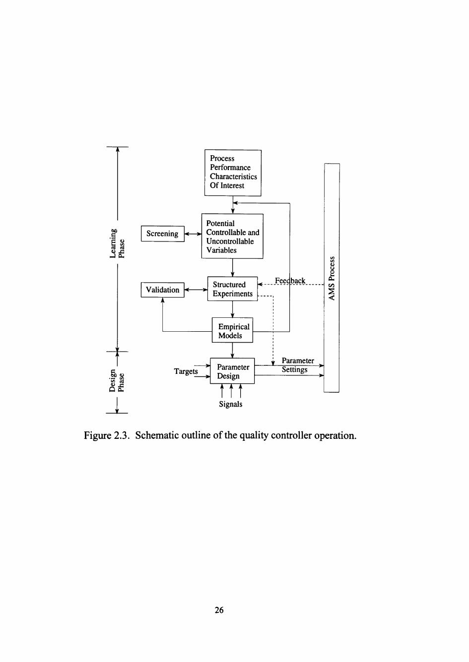
2.2.2 Schematic Outline ofthe Quality Controller Operation

Figure 2.3 illustrates a schematic outline ofthe quality controller in operation. In

addition to gaining a "thorough" understanding ofthe cause-and-effect relationships

associated with the particular process of interest, it works towards real-time optimal

process quality control. It basically operates in two modes or phases: (1) a leaming mode

and (2) a process parameter design mode.

During the leaming mode or phase, the quality controller with the aid ofthe process

designers, will repeatedly go through the following stages:

1. Identification of significant process performance characteristics. These

characteristics depend on the formal objectives ofthe process designer.

2. Identification of potential variables, and process parameters that have significant

influence on the process performance characteristics.

3. Model building. Beginning with approximate estimates (given by process

designers and/or operators), empirical models are built which relate each

performance characteristic with significant controllable and uncontrollable

variables in the desired region of interest (through structured experimentation and

on-line^ata, to the desired level of accuracy).

From the discussion in section 2.1.1, it is clear that no universal procedure exists to

arrive at a single stochastic model that could describe the system's response

25

i k

ling

L

ean

Phas

(

) 1

r I

Q

Screening < >

Validation ;

Targets

Process Performance Characteristics Of Interest

\ '

Potential Controllable and Uncontrollable Variables

^ '

Structured Experiments

1 '

Empiri Model!

^

cal 5

'

* Parameter • Design

1

S w •ign

1

lal! 5

^ Feec <•

back

y Parameter Settings

AM

S P

roce

ss

Figure 2.3. Schematic outline ofthe quality controller operation.

26

characteristics at all points in time t if from (2.3)). However, to solve the real-time

process parameter design problem, it would suffice if we can approximate/fi-om (2.3)

with the following empirical model:

f\X) = f{X,tit = t„ (2.4)

such that

\\fXX)-f(X,t)\<z (2.5)

for some specified constant £:> 0, at all points in real-time t = tQ. In other words, it is

sufficient enough to update the system's fimctional relationship / in real-time, and utilize

the information on the levels ofthe uncontrolled variables at that instant of time /o to

decide on the optimal process parameter settings for the immediate fiiture.

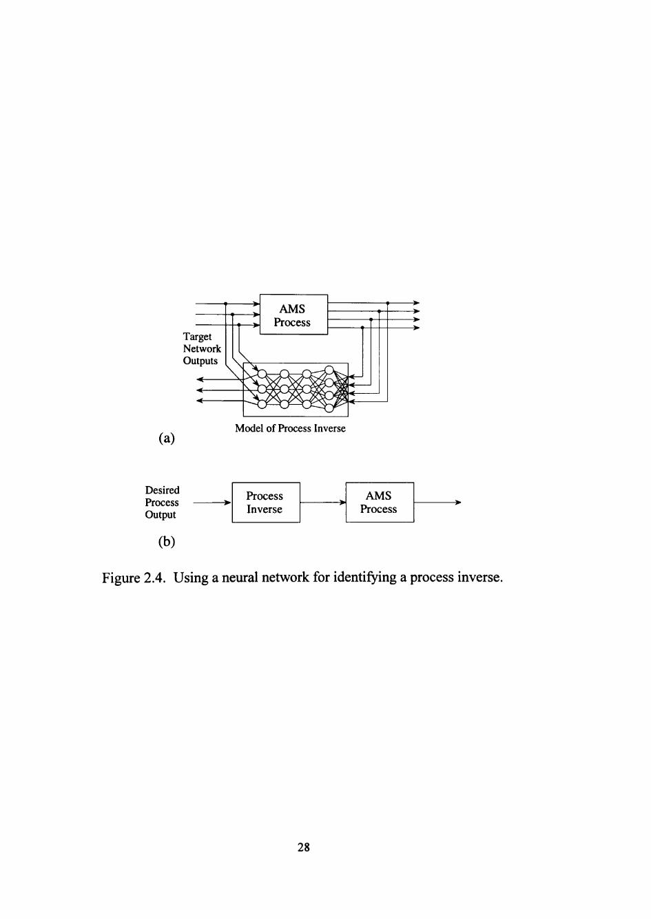
2.2.2.1 Optimal Process Parameter Determination. Figure 2.4a shows how an

adaptive neural network can be used to identify the inverse of a process. The input to the

network is the output ofthe process, and the target output ofthe network is the process

input. If the network can be trained to match these targets, it will implement a mapping

that is a process inverse. Once one has such an inverse, it can be used for optimal process

parameter determination as shown in Figure 2.4b. The desired plant output is provided as

input to the network; the resulting network output is then used as input to the process. If

the network is a process inverse, then this process input causes this desired process output

[Barto, 1991].

Widrow, McCool, and Medoff [1978] proposed this method for the adaptive control

of linear systems (also see Widrow 1986; and Widrow and Steams 1985), and it can be

applied to the control of nonlinear systems as illustrated by Psaltis, Sideris, and

Yamamura [1988] and Srinivasan, Barto, and Ydstie [1988], who use back-propagation

to identify a process inverse.

A major problem with inverse identification arises when many process inputs produce

the same response, i.e., when the process inverse is not well defined. In such situations,

most network parameter estimation methods tend to average over the various targets and

thereby produce a mapping that is not necessarily an inverse [Jordan, 1988]. This is the

27

- <

Target Network Outputs 1

<

—^ >

« >

^ \

X ^ X

AMS Process

< ' < '

^

> •

(a) Model of Process Inverse

Desired Process Output

Process Inverse

AMS Process

(b)

Figure 2.4. Using a neural network for identifying a process inverse.

28

case with most manufacturing processes, meaning that multiple combinations of

controllable and uncontrollable parameter levels result in the same process response

characteristics. An unconventional approach was necessary for two main reasons: (1)

there exists no well-defined inverse for most process parameter design problems, and (2)

there exists no means to generate the information necessary to train the inverse network;

in other words, the capability to identify optimal controllable parameter levels for various

combinations of uncontrollable parameters and desired process response characteristics is

lacking.

Let y = (Y^'',...,Y^)^denote the vector of Mdesired/target process response

characteristics of interest. The objective is to determine the optimal levels for the K set of

controllable variables, X, through Xf.^ such that

J = \\Y-Y,\\ = \\f(X,t)-Y,\\<E (2.6)

for some desired £>0 and a suitably defined norm (denoted by ||.||) on the output space, at

all points in real-time t = to. In (2.5), f(X, t) denotes the output ofthe process and hence

f(X,t)-Y^ = Cj is the difference between the output generated by the process and the

desired output Yd. If f(X, t) is known, the problem of parameter determination is simply

a non-linear constrained optimization problem. As such, one can proceed with solving

the problem using an appropriate non-linear programming algorithm. The constraints

would be those restricting the expected value ofthe response characteristic to the desired

target, and the values ofthe design parameters to an acceptable domain.

However, if f(X, t) is not known, the objective is to minimize the performance

criterion

j = \]^-Y,\\ = \\r(X)-Y,\\<e (2.7)

for some desired f > 0 and a suitably defined norm (denoted by ||.||) on the output space, at

all points in real-time / = o. This study treats J as an Euclidean norm unless stated

otherwise.

29

A first approach used in this study to minimize the criterion J (to determine the

optimal set of controllable variables) is to iteratively invert the network, i.e., to take the

gradient of J with respect to Xj and adjust it along the negative gradient as

^j = ^j^nom) ~ ' ^ ' ^ ^j = ^J(ru>m) (2.8) jinom)

where Xj^nom) denotes the nominal value ofXj at which the gradient is computed.

Throughout the rest of this report, this approach is referred to as the "Iterative Inversion"

method of process parameter determination. A second approach used was to back-

propagate the difference between the obtained output and the target through an action

network. This approach is referred to as the "Critic-Action" method. Section 2.3

provides a detailed discussion on the iterative inversion approach and the critic-action

approach to calculate these gradients when using multilayer perceptron networks and

RBF networks to identify the process response characteristics.

2.3 Technical Design ofthe Quality Controller

This section introduces the means to solve the identification and process parameter

design problems posed in section 2.1, with respect to the introduced quality controller

model. Both multilayer perceptron networks and RBF networks are utilized to

approximate the static non-linear maps ofthe process response characteristics. Two

methods are suggested to determine the optimal controllable variable target levels in real­

time.

2.3.1 Process Identification

In contrast to traditional statistical tools, neural networks are essentially non-

parametric. Thus, they prove to be more robust when dismptions are generated by

nonlinear processes and are strongly non-Gaussian [Lippman, 1987]. Also, traditional

statistical techniques are not adaptive but typically process all training data

simultaneously before being used with new data [Lippman, 1987]. From section 1.5, it

was clear that both multilayer perceptron networks (with a non-linear nodal fimction such

30

as the sigmoid) and RBF networks are capable of approximating any continuous fimction

/*€ C (R , R^) over a compact subset of R^. These results provide the motivation to

assume that the non-linear maps generated by these networks are adequate to model the

process response characteristics in general.

Training information can be obtained by observing the input-output behavior ofthe

process, as suggested in Figure 2.5. Here, the network receives the same input signals as

the process, and the process response characteristics are used as the target network output.

The network topology (number of layers, hidden nodes per layer, and connectivity)

has to be selected in such a fashion that generalization is maintained. Several guidelines

are discussed in the literature and will not be repeated here [Weigand, Rumelhart, and

Huberman, 1992; Denker et al., 1987; Solla, 1989; Baum and Haussler, 1989; Leonard,

Kramer, and Ungar, 1992]. The standard procedures for adjusting the network

parameters are discussed in sections 1.5.2 and 1.5.3 for multilayer perceptron networks

and RBF networks, respectively.

2.3.2 Process Parameter Determination

This section demonstrates the iterative inversion method and the critic-action

approach to determine the optimal controllable variable levels in real-time. These two

approaches utilize the non-linear connectionist network that resulted fi-om the previous

identification phase.

2.3.2.1 Iterative Inversion based Parameter Determination. In error back-propagation

training of neural networks, the output error is "propagated backward" through the

network. Linden and Kindermann [1989] have shown that the same mechanism of

weight leaming can be used to iteratively invert a neural network model. In this

approach, errors in the network output are ascribed to errors in the network input signal,

rather than to errors in the weights. Thus, iterative inversion of neural networks proceeds

by a gradient descent search ofthe network input space, while error back-propagation

training proceeds through a search in the weight space.

31

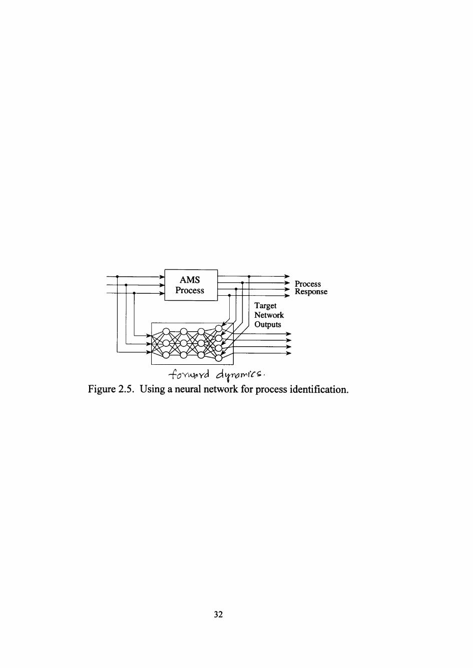
Process Response

Figure 2.5. Using a neural network for process identification.

32

One can use the iterative inversion technique of Linden and Kindermann [1989] to

find the control inputs to the process. That is, rather than training a controller network

and placing this network directiy in the feedback or feedforward paths, the forward model

ofthe process is leamed, and the iterative inversion performed on-line, to generate control

commands. This technique is similar in philosophy to that of Donat et al. [1990], in

which a non-linear optimizer uses a forward model ofthe process to determine a set of

control inputs based on minimizing the predicted error for a finite number of time steps

into the fiiture.

One reason for taking this route is that our interest is in adaptive control in the sense

used in the controls community; that is, in controllers which can respond on-line to

changes in plant performance characteristics. When the training data must be taken from

input-output pairs developed during a single on-line operation ofthe process, the problem

of identifying the forward dynamics becomes nontrivial. Attempting to use the forward

model to train a "controller" network adds many complexities to the training problem.

Another reason that the present approach was taken is that stability and performance

robustness measures are needed for many applications where neural-network-based

adaptive control would be most usefiil [Narendra, 1991]. Placing the highly non-linear

neural network directly in the feedback path introduces difficulty in such an analysis. The

current approach attempts to avoid this by removing the network from the direct feedback

path. This approach takes a step toward analysis ofthe closed-loop system, in that the

network may be characterized in terms ofthe prediction error.

Iterative inversion ofthe network generates the controllable variable input vector,

[X,,..., X^], that gives an output as close as possible to the desired process performance

characteristics of interest. By taking advantage ofthe duality between the weights and the

input activation values in minimizing the performance criterion, J, the iterative gradient

descent algorithm can again be applied to obtain the desired input vector [Linden and

Kindermann, 1989]:

^.-1) = ^ ; > - T i . - ^ + a ( : r / > - X ; . ^ - ' > ) . (2.9) ax</

33

Here the superscript refers to the iteration step, r\ and a are the rates for the leaming and

momentum in the gradient descent approach. The values for these constants are not, in

general, the same as those used in the error back-propagation training ofthe network.

The idea is similar to the back-propagation algorithm, where the error signals are

propagated back through the network to adjust the weights so as to decrease the

performance criterion. The inversion algorithm back-propagates the error signals down to

the input layer to update the activation values ofthe controllable variable levels so that

the performance criterion, J, is decreased. Most ofthe second-order optimization

algorithms proposed for back-propagation leaming [Hwang and Lewis 1990] can also be

applied to iterative network inversion.

2.3.2.2 Inversion in a Multilayer Perceptron Network. For the three-layered

perceptron network shown in Figure 1.1, the gradient ofthe performance criterion with

respect to the controllable variable Xj, dJ I dXj, can be calculated as follows:

The performance criterion was defined as

" J = \\i'-YA = mY^-Y^)- (2-10)

m=l

Hence,

^ =t{Y„-Y^)^. (2.11)

The gradient in expression (2.11) can be computed as follows:

(2.12) ax. ay ax..

J m J

Under the assumption that all nodes in the perceptron network are unipolar sigmoidal

fimctions {f(x) = 1/(1 + e% the first term of (2.12) is equal to

^ = y ( l _ y ). (2.12a)

The second term of (2.12) can be expressed as

34

^l,-^. ax. ax.. -il 9=1

W3 3 ^ , mg ax.. 7 J

The second term of (2.12b) can be again expressed as

a

(2.12b)

ax, "az "ax"^^^^"^^^ Lp=i

ax..

=^,(i-^j-r p=\ ax.. 9 P (2.12c)

In a similar fashion, the last term in (2.12c) can be expressed as follows:

av„ av av„ - ^ — ^ -^=v, ( i -y , )

AT

L>1

ax, ax, av, ax,

= V / l - y ^ ) . W ; , . (2.12e)

From (2.11), (2.12), (2.12a), (2.12b), (2.12c), (2.12d), and (2.12e), the desired gradient

can be expressed as follows:

^ = t.[Y„-Y^)Y^(\-Yjt\wl^-Z^(\-Z^)-tXKp-U^ • (2.13)

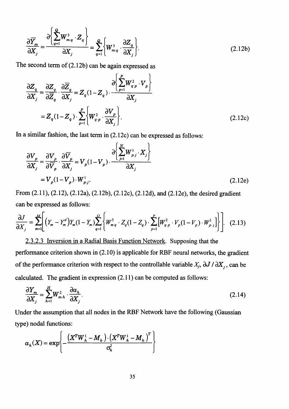
2.3.2.3 Inversion in a Radial Basis Function Network. Supposing that the

performance criterion shown in (2.10) is applicable for RBF neural networks, the gradient

ofthe performance criterion with respect to the controllable variable Xj, dJ I dXj, can be

calculated. The gradient in expression (2.11) can be computed as follows:

ax/ (2- )

Under the assumption that all nodes in the RBF Network have the following (Gaussian

type) nodal fimctions:

(X^WJ:-MJ.(X^W'-MJ af^(X) = exp

35

= exp'

N 1 |(x,-Wi.-Mj

oj (2.15)

the second term from (2.14) can be calculated to be

da. ax. «.-M^>-wi-M,.)}.wi (2.15a)

From (2.11), (2.14), and (2.15a), the desired gradient can be expressed as follows:

dJ ax.. m=\

(n. -Yd tw^a, • {2(X,.W -MJ}.W^ (2.16)

2.3.2.4 Critic-Action Approach based Parameter Determination. This approach for

determining the controllable variable levels relies more on back-propagation than on

general network methods. The approach is illustrated in Figure 2.6, and comprises a

Critic neural network and an Action neural network. The back-propagation algorithm is

used to identify the process as shown in Figure 2.5 (the training signals for this

identification stage are not shown in Figure 2.6), resulting in a forward model ofthe

process in the form of a layered network, and is referred to as a Critic network.

The topology for the critic neural network is shown in Figure 2.7. Input to the

network includes levels ofthe uncontrollable and controllable parameters, and the output

constitutes the respective process response characteristics and suggested controllable

parameters. During the training phase, suggested controllable variable levels are none

other than the controllable variable levels provided in the input.

The action neural network illustrated in Figure 2.8 is responsible for optimal process

parameter design in real-time. Given the levels ofthe A -A: uncontrollable variables

X^ = (X^^.1,...,X^ )^ obtained from the process sensors, the desired target quality

characteristics, Y"^ = (Yf,... ,Y^ f, and the trained critic network, the action network

provides the optimal or near optimal levels for the K controllable variables,

X^ = (X,,... ,X^)^. The various steps associated with the process parameter design

phase are given below:

Step 1: IhQ-eritic network is a duplicate ofthe trained action network.

'(:'"'(?vw ) 6 -

36

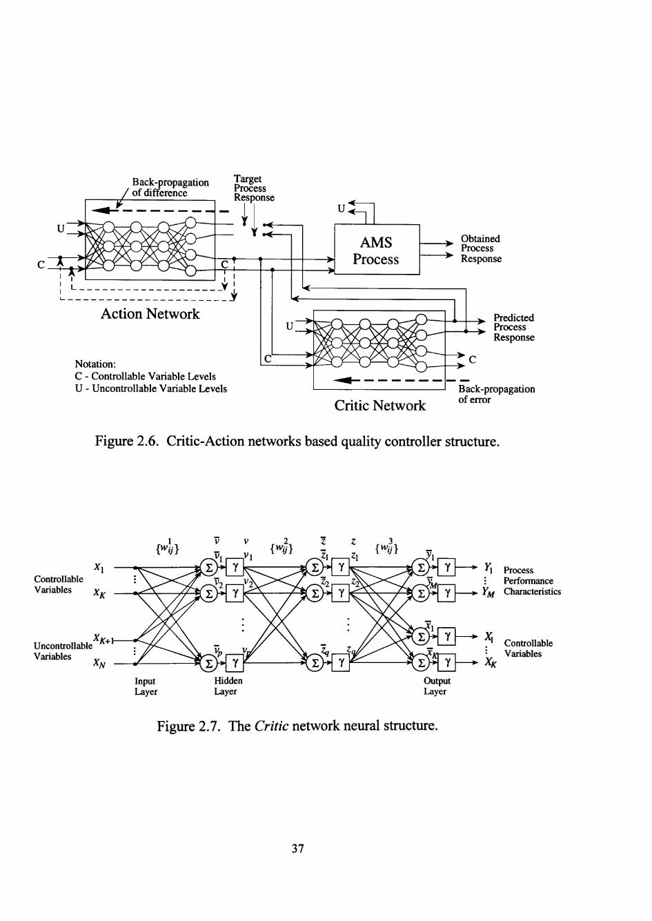
Back-propagation p^f[^ ^fAiff^^^^^^ rrocess " difference Response

Notation: C - Controllable Variable Levels U - Uncontrollable Variable Levels

Obtained Process

^ Response

Critic Network

Predicted Process Response

B ack-propagation of error

Figure 2.6. Critic-Action networks based quality controller stmcture.

Controllable Variables

Uncontrollable Variables

^K+)r

yv Input Layer

Hidden Layer

Output Layer

*• M Process : Performance

*. Yj^ Characteristics

Controllable Variables

Figure 2.7. The Critic network neural stmcture.

37

Weights are Weights will be adjusted never adjusted /"during every iteration

Starting or Xi Current Controllable Parameters Levels

UncontroUable Variables X\

"*• M Process : Performance

-». Y]^ Characteristics

, y Suggested "*~^ ^1 ControUable

: Parameters -J*- X/( Levels During

This Iteration

(Inputs For Next Iteration)

Figure 2.8. The Action network neural structure.

38

Step 2: Use current^, J^, and the critic network, to predict process response

characteristics (Y).

Step 3: Compare 7 from step-2 with Y^, and calculate gradients for weights on the

connections between the nodes on the last hidden layer and the process response

nodes to reduce the performance criterion J (Euclidean norm ofthe difference

between 7 and Y^).

Step 4: Back-propagate the difference to adjust the weights on the connections ofthe

action network.^

Step 5: Use the updated action network from step-4, X^, and current jf , to suggest better

controllable parameters levels (Xf„^) of this iteration.

Step 6: If is different fromXf^^^, adjus t^ to Xf^^, and refresh the action network with

the weights from the critic network,^ and go to step-2.

Otherwise, suggest Xf„^ as the optimal process parameter levels in light ofthe

current process response characteristics and X^, and exit the phase.

* Note that the weights on the connections between the output nodes representing X^ and the nodes on the last hidden layer, and connections between the nodes denoting

sug •'

J ^ on the input layer and the nodes on the first hidden layer are not changed. These connections are illustrated with dotted lines in Figure 2.8.

2 At this stage, the action network is again an exact duplicate ofthe critic network. 39

CHAPTER III

TOOL PERFORMANCE RELIABILITY MODELING

The objective here is to develop a fimdamental theory and model linking physical

cutting tool performance and real-time reliability prediction in manufacturing systems.

Present day historic, or actuarial, based reliability models are inadequate, if one desires to

maximize system through-put and product quality as well as tooling resources, within an

economic environment. Real-time look-ahead reliability is necessary in order to assess

the prospects of a failure-free next cycle.

This chapter, at first, provides an overview of contemporary tool monitoring

practices. Then, it introduces the concept of performance reliability. Later, the means to

arrive at real-time performance reliability assessment in manufacturing systems using a

novel extension ofthe validity index neural network were developed.

3.1 Overview of Tool Monitoring Practices

Downtime due to tool failure, a critical issue in many manufacturing systems,

contributes up to one-third ofthe total downtime [Subramanian and Cook, 1977]. The

identification of fresh and wom machine tools provides a classic model of a decision

situation in which human experts excel at synthesizing various sensory cues and making

weighty and fast adjustments, while computer-based and theoretical approaches lag far

behind [Rangwala, 1988; Rangwala and Domfeld, 1990]. However, knowledge of tool

behavior during the manufacturing process, and automation of effective tool failure

prediction, contribute to controlling machining costs [Kim and Kolarik, 1992], ensure

optimal utilization of machine tools, enhance the capability ofthe machine tool in terms

of precision and dimensional control [Burke and Rangwala, 1991], and can release human

operators to pursue higher level tasks [Burke, 1992]. hi fact, advanced sensing and

control systems are necessary for implementing optimal machining strategies (such as

adaptive control with optimization) as well as for monitoring and diagnostic purposes

[Burke and Rangwala, 1991].

40

Scatter in tool performance is more often the rule than the exception in most

machining operations, and can be attributed to different chemical and mechanical

properties ofthe tool as well as variation in the work material, environment and operating

conditions. Considerable variation may be explained by accounting for explanatory

variables, as well as usage or time. Conservative strategies such as instituting frequent

tool changes have proved to result in large machine downtimes (associated with tool

changing and setups). Statistical models such as Taylor's classical tool life equation

[Taylor, 1906] account for the effects of machining variables, but fail to account for the

usage level (age) and wear-out characteristics ofthe tool [Kim and Kolarik, 1992].

Hence, in an automated environment, it is necessary to resort to on-line sensory data in

order to make decisions on tool wear and breakage [Burke and Rangwala, 1991].

3.1.1 Failure Criteria, Failure Modes and Performance Measures

Several authors [Bougler, 1978; Kaldor and Lenz, 1980; Kanai and Kanda, 1978;

Singpurwalla and Kuebler, 1966; Soderberg, Vingsbo and Nissle, 1981] have defined

criteria that may be used for the failure ofthe cutting tools. The criteria include: (1)

complete destruction ofthe cutting tool surface, (2) the wear ofthe tool, to the extent that

the quality ofthe machine surface becomes unacceptable, (3) the wear ofthe tool surface

to some predetermined level, (4) the change of color ofthe tool, due to loss of temper, (5)

the change ofthe sound, (6) the time to removal from service, and (7) flank wear, crater

wear or an increase in torsional moment.

The third criterion is probably the most widely used criterion for tool failure [Kim,

1991]. The seventh criterion shows poor correlation to the tool failure criterion. The

fifth criterion mentioned is very subjective, because cutting tools such as drills possess

self-sharpening qualities. In general, the failure of a cutting tool occurs by one of the

following two modes [Trent, 1977]: (1) fracture or chipping and (2) excessive wear

leading to plastic deformation resuhing in collapse of region(s) subjected to high normal

stresses acting at elevated temperatures.

41

Performance measures indicate some relative degree of success a component/system

is experiencing. Three basic cases exist: (1) nominal is best: infers that there is a "best"

target point, (2) smaller is better, and (3) larger is better. In an ideal situation, the

performance measure has to take into consideration all the attributes ofthe probability

density fimction. Unfortunately, most ofthe performance measures developed thus far

concentrate on the mean ofthe response of interest alone. Taguchi's introduction of

parameter design in the late 1970s and early 1980s drew a lot of attention to concepts in

the area of dispersion effects and variance modeling [Myers and Vining, 1992].

Taguchi has defined over 60 different signal-to-noise (SN) ratios [Vining and Myers,

1990] to capture both location and dispersion effects in performance measures. However,

Taguchi's use of .STV ratios to capture variability has been a subject of controversy [Nair et

al., 1992]. There have been efforts at understanding his ideas and developing more

statistically efficient altematives [Box, 1988; Leon, Shoemaker, and Kacker, 1987; Nair

and Pregibon, 1986]. Altemative methods proposed include the use of data

transformations [Box, 1988; Nair and Pregibon, 1986] and the use of GLM's for the joint

modeling of mean and dispersion [Nelder and Lee, 1991].

3.1.2 Monitoring

Effective sensor systems for tool monitoring consist of sensing elements, signal

conditioning devices, signal processing algorithms, and signal interpretation and decision­

making procedures. The development of reliable tool wear sensors has been an active

area of metal cutting research [Burke and Rangwala, 1991]. An overview ofthe various

tool wear sensing schemes under development has been provided in a number of review

articles [Andrews and Tlusty, 1983; Micheletti et al., 1976]. Tool wear sensing methods

can be divided into direct and indirect measurements [Masory, 1991]. Indirect sensing

schemes include force [Koren et al., 1987], torque [Subramanian and Cook, 1977],

acoustic emission [Kannatey-Asibu and Domfeld, 1982; Iwata and Moriwaki, 1977], tool

temperature [Solaja and Vukelja, 1973], vibration [Subramanian and Cook, 1977; Szabo,

Du and Wu, 1989; Yee, 1984], and surface roughness to name a few. Such schemes are

^^

42

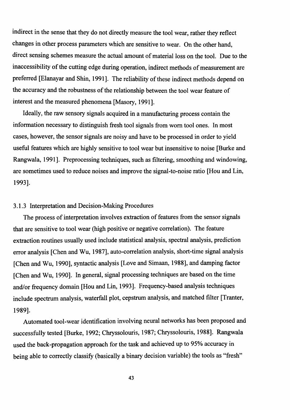
indirect in the sense that they do not directiy measure the tool wear, rather they reflect

changes in other process parameters which are sensitive to wear. On the other hand,

direct sensing schemes measure the actual amount of material loss on the tool. Due to the

inaccessibility ofthe cutting edge during operation, indirect methods of measurement are

preferred [Elanayar and Shin, 1991]. The reliability of these indirect methods depend on

the accuracy and the robustness ofthe relationship between the tool wear feature of

interest and the measured phenomena [Masory, 1991].

Ideally, the raw sensory signals acquired in a manufacturing process contain the

information necessary to distinguish fresh tool signals from wom tool ones. In most

cases, however, the sensor signals are noisy and have to be processed in order to yield

usefiil features which are highly sensitive to tool wear but insensitive to noise [Burke and

Rangwala, 1991]. Preprocessing techniques, such as filtering, smoothing and windowing,

are sometimes used to reduce noises and improve the signal-to-noise ratio [Hou and Lin,

1993].

3.1.3 Interpretation and Decision-Making Procedures

The process of interpretation involves extraction of features from the sensor signals

that are sensitive to tool wear (high positive or negative correlation). The feature

extraction routines usually used include statistical analysis, spectral analysis, prediction

error analysis [Chen and Wu, 1987], auto-correlation analysis, short-time signal analysis

[Chen and Wu, 1990], syntactic analysis [Love and Simaan, 1988], and damping factor

[Chen and Wu, 1990]. In general, signal processing techniques are based on the time

and/or frequency domain [Hou and Lin, 1993]. Frequency-based analysis techniques

include spectrum analysis, waterfall plot, cepstrum analysis, and matched filter [Tranter,

1989].

Automated tool-wear identification involving neural networks has been proposed and

successfiiUy tested [Burke, 1992; Chryssolouris, 1987; Chryssolouris, 1988]. Rangwala

used the back-propagation approach for the task and achieved up to 95% accuracy in

being able to correctly classify (basically a binary decision variable) the tools as "fresh"

43

and "wom." Burke [1992] points out that the back-propagation approach lacks

flexibility, requires fiilly defined training sets (supervision), and needs complete

retraining if the environment should change. He proposed altemative approaches via

unsupervised methods for the same classification problem; specifically, competitive

leaming and adaptive resonance.

The results of adaptive resonance-based approaches appear in [Chryssolouris, 1988;

Burke, in press], and [Burke and Rangwala, 1991]. For details on the adaptive resonance

stmcture, see Burke [in press]; Burke [1991]; and Carpenter and Grossberg [1987]. The

neural stmcture for the competitive leaming approach and its results appear in Burke

[1992]. The results of applying a Euclidean variant of competitive leaming (ECL) to

actual sensor measurements revealed the practical advantages ofthe unsupervised system,

which include the ability to leam and produce classifications with out supervision Burke

[1992]. Moreover, the unsupervised system can indicate environmental changes, and

easily shift in and out of training mode without complete training. The ECL system was

able to classify a tool wear with up to 95% accuracy. Thus, in terms of classification

accuracy, the unsupervised system and the supervised back-propagation network do not

differ [Burke 1992].

3.2 Performance Reliability

Reliability is classically thought of in a binary sense (success and failure) and

performance is thought of in a continuous sense (thmst, torque and so forth). The

classical approach to prediction of reliability is based on numerical values ofthe recorded

operating times to failure of a system or component under consideration. Hence,

traditional reliability is "posterial" and can only be determined after failure has occurred

[Kim, 1991]. Present day abilities to monitor, measure and model allow the opportunity

to link reliability more closely to the total system performance concept. Within the

framework of continuous performance monitoring, it is generally insufficient to

characterize reliability as just an excessive value of a single fimctional or maintenance

parameter. Physical failures or breakdowns usually result from joint occurrence of

44

deviations of several such parameters, sometimes even with all the parameters remaining

within specified tolerance values. To the notion of automatic classification and analysis

of these deviation vectors, one can relate concepts of reliability and classes of degraded

performance [Kolarik, 1988]. This procedure enables us to envisage reliability as a

conditional indicator that activates an alarm whenever the level of degraded performance

"drops" too far. The use of such indicators complies with the requirements of on-line

failure diagnosis and may lead to enhanced availability and capability of machine tools to

which they are connected.

3.2.1 Definition

The term "performance" used in conjunction with "performance reliability" is defined

as the physical output of a product which is fimctioning or operating according to its

designed purpose, specification, and intended fimction from the beginning of its

deployment into service until withdrawal or retirement [Kim, 1991]. Usually physical

performance can be measured to some degree with regard to effectiveness of any product.

These measurements represent some relative degree of success that a component,

subsystem, or system is experiencing. These performance measures differ from time to

time depending on usage level, operating conditions, and environmental conditions, and

product deterioration. Figure 3.1 depicts one such set of conceptual performance curves

(taken out at one level of operating conditions and environmental conditions). A critical

performance plane is also shown in Figure 3.1. The points at which these performance

curves pass through this plane are equivalent to failure times (life times) that would be

recorded in a classical reliability study. The classical practice has been to take these

failure times and fit them to parametric models, such as a WeibuU model, and then use

this model as a reliability predictor. From a conceptual standpoint, the use of

contemporary covariate models can extend this plane into operating and environmental

load dimensions. Thus, one can think ofthe current practice of reliability assessment and

analysis as a subset ofthe performance reliability concept.

45

Classical "failure times

Performance plane

0 Time

Figure 3.1. Conceptual performance curves for a specified environment, with a performance plane superimposed [Kolarik, 1988].

46

Given an appropriate definition of failure in terms of a performance characteristic,

performance reliability is defined as "the conditional probability that the performance

measure 7 is less (or greater) than a performance critical limit FPCL (which represents an

appropriate definition of failure in terms of physical performance), given operating

environmental conditions, for a specific period of time or cycles r." The same definition

can be logically extended to handle muhiple performance characteristics, provided the

conditional probability is associated with multiple performance critical limits.

3.2.2 Characteristics of Performance

Different products have different intended uses, resulting in different critical physical

performance measures (e.g., for an automobile; miles per gallon, engine power, and so

on). When dealing with reliabilities, a corresponding appropriate definition of failure in

terms of physical performance must be defined, relative to product application. Physical

performance is the integral performance measure ofthe integrity ofthe designed part,

component, product, subsystem, or system. Many devices experience deterioration over

time and finally fail when they reach a predetermined performance level or performance

plane. A feature of physical performance is that it is potentially measurable and can be

monitored continuously over time.

Provided physical performance can be measured, three basic possibilities exist: (1)

lower is better, (2) higher is better, and (3) a nominal value is best. Figure 3.2 depicts

some typical cases of physical performance along with FPCL over time or usage.

Application requirements will determine the level of 7PCL-

3.2.3 Performance Model and Reliability

Product failure involves a change in a performance measure from a satisfactory level

to an unacceptable level. Under the assumption that one can always find (perhaps from a

life test) or postulate (perhaps from theoretical analyses) a deterministic or probabilistic

relationship to explain typical or expected performance, for a performance measure Y,

such a relationship takes the following generic form:

47

(a)

PCL

Time/Usage /

o

€ ^

(b)

Upper Critical Limit / „ PCL

Time/Usage t

0)

o

0)

(c)

Upper Critical Limit

'PCL

'PCL

Lower Critical Limit

Time/Usage t

Figure 3.2. Typical cases of physical performance. (a) Higher is better. (b) Lower is better. (c) Nominal is best.

48

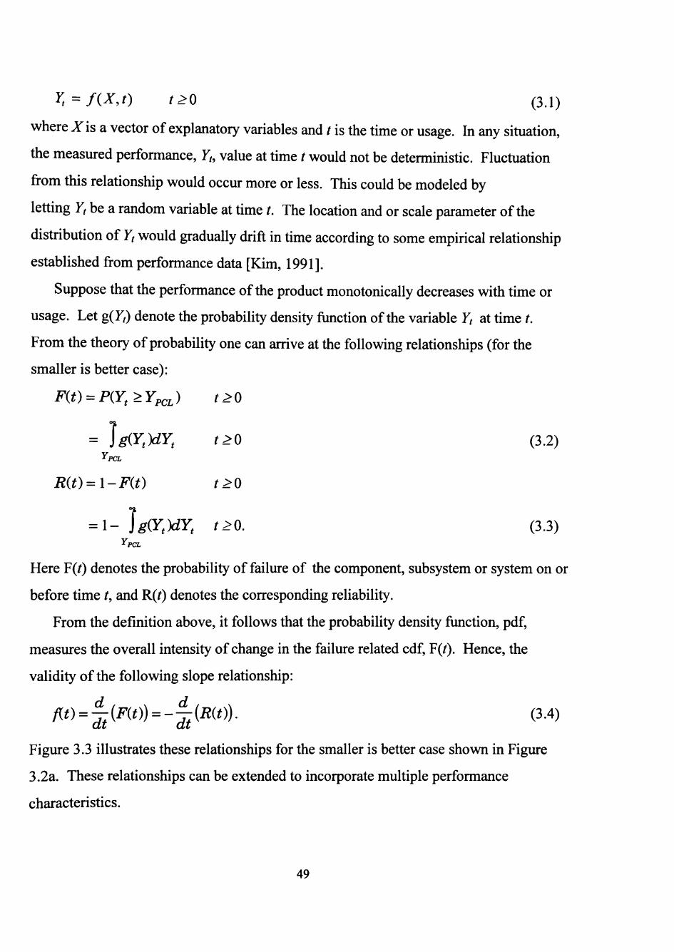
Y,=f(x,t) r>0 (3.1)

where X is a vector of explanatory variables and t is the time or usage. In any situation,

the measured performance, Yt, value at time t would not be deterministic. Fluctuation

from this relationship would occur more or less. This could be modeled by

letting Yt be a random variable at time t. The location and or scale parameter ofthe

distribution of Yt would gradually drift in time according to some empirical relationship

established from performance data [Kim, 1991].

Suppose that the performance ofthe product monotonically decreases with time or

usage. Let g(F/) denote the probability density fimction ofthe variable Yt at time t.

From the theory of probability one can arrive at the following relationships (for the

smaller is better case):

F(t) = P(Y,>YpcL) t>0

- ] g(Y,)dY, t>0 (3.2) ^PCL

R(t)=l-F(t) t>0

= 1- ]g(Y,)dY, t>0. (3.3) Y. PCL

Here ¥(t) denotes the probability of failure of the component, subsystem or system on or

before time t, and R(t) denotes the corresponding reliability.

From the definition above, it follows that the probability density fimction, pdf,

measures the overall intensity of change in the failure related cdf, ¥(t). Hence, the

validity ofthe following slope relationship:

m = f^{P(t)) = -j^{R(t)). (3.4)

Figure 3.3 illustrates these relationships for the smaller is better case shown in Figure

3.2a. These relationships can be extended to incorporate multiple performance

characteristics.

49

PCL

TimeAJsage t

Figure 3.3. Relationship between physical performance and reliability.

50

The arguments above demonstrate that physical performance data can be readily

transformed into a classical reliability model. Dealing with physical performance is more

attractive to the practitioner. It has the following advantages over classical reliability

measures in the time domain: (1) it can be measured and analyzed before failures occur,

and (2) it is a continuous measure rather than a binomial event measure, and hence more

informative [Kim 1991]. However, these advantages can be realized if and only if (1) a

suitable model exists for extrapolating performance degradation, and (2) failure is defined

in terms of performance rather than time.

3.2.4 General Standard Performance Models

Nelson [1990] described degradation models and data analysis techniques for

degradation of product performance over time at over stress and design conditions. For

some degradation processes, the degradation rate itself could be a fimction ofthe stress

variable. Thus, there could be a dependence between the degradation rates and stress

variables such as temperature, voltage, velocity, strain and so forth. In such cases, many

well established physical process models may be applicable to the degradation rate.

The Arrhenius and the Eyring models are often used when temperature is the stress

variable. The inverse power law is sometimes used to model voltage as a stress variable

for electronic and dielectric tools. The power law is used in Taylor's tool performance

model for wear of machine tools as a function of cutting velocity.

Thus far, established standard performance models are discussed. Furthermore,

performance models can be extended into the simultaneous, multiple stress dimension.

One obvious choice would be to use classical regression analysis tools to arrive at general

mathematical relationships (polynomial models and so on) to model location as well as

dispersion measures. The response space becomes more complex as more variables are

added to the model.

The performance of individual units is expected to follow the general performance

model, with variation attributable to differences in the individual devices, operating

conditions, and environmental conditions.

51

However, a major problem with the above performance models and reliability

modeling approach (see section 3.2.3) is that the performance measures may drift up and

down with time or usage, thus violating the assumption of a monotonically

decreasing/increasing performance fiinction. Besides this, dispersion associated with the

performance measure is relatively large in most cases, thus making it difficult to justify

the concept of an expected performance measure. It appears reasonable and logical to

model the change in performance measure with time as a time-series rather than as a

deterministic or probabilistic relationship. This significantly reduces the complexity of

the models, and is more compatible with real-time performance reliability modeling.

3.3 Time Series Modeling of Performance Measures

Physical performance measures of a component, sub-system or system can be viewed

as a time-series. Section 1.5 has given an overview ofthe most popular time series

forecasting methods developed in the last few decades. While the Box-Jenkins method is

a fairly standard time series forecasting method, the procedure (identification, estimation,

validation, and forecasting) is not compatible with autonomous systems. It was

established in section 1.5 that perceptron neural networks, as forecasting models, are

comparable and, in most cases, more effective than their statistical counterparts.

In the case ofthe performance reliability modeling problem at hand, in addition to

forecasting the performance characteristic into the fiiture, it is necessary to be able to

model the characteristics of g(y/). In other words, it is also necessary to be able to

provide error bounds for forecasts. Hence, a Validity Index neural network is used.

Figure 3.4 illustrates the basic idea in training a network to be a predictor. Suppose

that the lines across the top ofthe figure carry process performance characteristic signals

whose values one wishes to predict. For simplicity, also suppose that these signals

provide the information from which the predictions will be made. For training purposes,

the input vector to the network consists of finite past (delayed) process performance

characteristic values, [jc^_i,...,x^_p], and the target output vector consists of current time

series values [ ,_,+g, ,...,:x: _,+g ]. Kerep, q\,..., q„, and n are all finite positive integers.

52

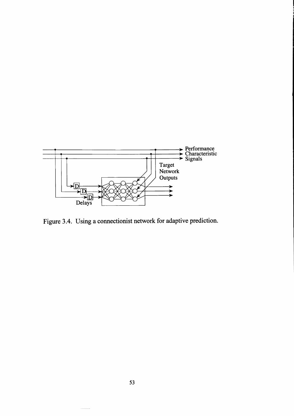
Target Network Outputs

-^ Performance ->- Characteristic -^ Signals

Delays

Figure 3.4. Using a connectionist network for adaptive prediction.

53

The network therefore tries to match the current process performance characteristic signal

values by adjusting a function of their past values. Then, when the input to the network

bypasses the delay units, the output ofthe network is a prediction ofthe values the signals

will have in the fiiture. Assuming that the network requires a negligible amount of time

to compute its output from its input, the trained VI Network provides estimates for the

values ofthe process performance characteristics in the fiiture. This approach to adaptive

prediction rests on the assumption of a parameterized class of models for the fimctional

relationship between the current and past values ofthe signals and their later values, or

equivalently between earlier values ofthe signals and their current values [Barto, 1991].

The RBF network parameter estimation method discussed in section (1.3.3) will be

applied along with training information supplied by observations ofthe process

performance characteristic signal values over time.

In addition to providing VI Network with past performance characteristics alone as

input, it is possible to provide explanatory variables as well. Chapter IV discusses in

detail the influence of appending explanatory variables into the network input for training

purposes.

The larger the size of «, the more complex is the overall network map. It isimportant

to choose the right number of hidden RBF centers so as to maintain the^neralization in

the overalljna£s___

3.4 Tool Performance Reliability Modeling

Usually, physical performance characteristics such as the thmst force acting on a tool,

acoustic emission and so on can be measured to evaluate the degree of a tool

performance, with regard to the machining process at hand. Throughout this study, thmst

cutting force acting on the drill bit was chosen as the substitute quality characteristic to

evaluate the degree of tool performance. However, the methodology presented is

applicable to other tool performance characteristics as well. The history of this

performance information along with a measurement ofthe explanatory variables such as

the environmental and operational conditions can help make inferences regarding the

performance reliability ofthe tool.

54

In dealing with the tool condition monitoring problem, it is assumed that a conditional

reliability stmcture can be usefiil for effective tool management in the computer aided

environment. Assumptions underiying the performance reliability models developed in

this study are described below:

1. Performance measures may drift up and down, but must eventually decrease or

increase. That is performance degradation exists, and, in the long run, not

reversible.

2. Performance characteristics can be measured (the performance signal is

detectable, even though noise in the measurement and natural variation exists).

The objective here is to demonstrate the concepts introduced thus far in modeling tool

performance reliability. At first, the means to arrive at valid error bounds for tool

performance predictions are introduced. Finally, a discussion is presented on the means

to achieve performance reliability assessment in real-time.

3.4.1 Real-time Tool Performance Reliability Assessment

Let ¥(t) denote the probability that failure takes place at a time or usage less than or

equal to / (i.e. P{t < /}), where the random variable t denotes the time to tool failure.

From the definition of conditional probability, the conditional reliability that a tool will

fail at some time or usage i> t + At, given that it has not yet failed at time t = t will be:

R((t + At)\ t)=P{t>t + At\i>t) = [ l - P { t < ^ + A^)}]/P{t>^} P 3 ^

3.4.2 Extension ofthe Validity Index Neural Network

Since the VI Network provides us with a predicted performance measure into the

future (at time tX using (1.10) and (1.11) one can determine the value of a at which the

confidence limit on the individual value ofthe predicted performance measure meets the

Tp L- Under the assumption that the change in the performance measure from the current

time point (t^) to the predicted time point (t^) is either monotonically decreasing or

increasing, (1-a) denotes the reliability that the tool will operate without failure until tj.

55

CHAPTER TV

PERFORMANCE EVALUATION OF QUALITY CONTROL

AND TOOL MONITORING MODELS

This chapter at first introduces a novel test-bed developed for this research project,

based on Monte Carlo simulation techniques, named ProtoSim. ProtoSim was developed

to emulate performance characteristics of advanced manufacturing systems, and was used

to evaluate tiie different quality controller models introduced in Chapter II. At the end,

the results of evaluating the real-time tool monitoring models developed in Chapter III on

an actual drilling process are discussed.

4.1 Design and Development of a Simulation Test-Bed

Each physical process is different by its very nature, but from a statistical point of

view many similarities exist. These similarities allow development of a simulation based

test-bed, useful for qualitative assessment of both the benefits and burdens associated

with experimental based strategies (e.g., quality controllers, experimental designs).

Focusing on rapid process identification and real-time process parameter design, this

section presents the design and development issues for a simulation test-bed, ProtoSim.

It incorporates Monte Carlo simulation techniques to simulate pre-defined but

hypothetical process response characteristics as closely as possible.

In the absence of first-principle cause-effect models for the particular process of

interest, empirical models developed from physical experimentation results provide the

means for emulation. A combination of cause-effect models and empirical models can be

utilized when limited cause-effect information is available. ProtoSim has the ability to

handle non-stationary processes with complex non-linearities and interactions.

4.1.1 Overview of Computer Modeling

With recent advances in the computer industry, computer modeling in certain fields of

advanced manufacturing systems is invariably quicker and cheaper than physical

56

experimentation [Welch, Yu, Kang, and Sacks, 1990]. In fact, the widespread use of

computer models and experiments for simulating real phenomena generates examples

virtually in all areas of science and engineering [Sacks, Schiller, and Welch, 1989]. As

experimental approaches to studying advanced manufacturing systems, such as the

Integrated Circuit (IC) manufacturing, are usually expensive and slow given the

competitive environment, process designers are turning towards physical and numerical

based simulators [Sharifzadeh, Koehler, Owen, and Short, 1989]. For example, statistical

process based simulators such as SUPREM III [Ho et al., 1982] and FABRICS II [Nassif

et al., 1989] have been developed to model IC fabrication.

4.1.2 Emulation of Static Non-linear Processes using ProtoSim

Let X = (X^,...,Xf., Xj^+j,...,X^)^cR^ denote a vector of A" controllable variables

and N-K uncontrollable variables (K <N), that significantly affect the M process response

characteristics of interest, Y = (Y^,...,Yj^f e R^. Under the assumption that the

mechanistic relationship relating X with 7 is available (either explicitly or implicitly), the

critical task associated with the process of emulation is that of identifying typical

signatures associated with the N-K uncontrollable variables. However, in most cases, the

analytical form of this relationship is either unknown or is very difficult to obtain. In

such cases, one resorts to estimation techniques such as: (1) Monte Carlo simulations

[Barker, 1985], (2) Statistical designed experiments, and (3) Functional approximation

techniques [Fathi, 1991]. These relationships can be linear fimctions in simple systems

and highly non-linear in complex systems.

In the absence of any knowledge of mechanistic relationships, ProtoSim simulates

both the mean and the variance attributes for each ofthe M process response

characteristics in terms of X, in line with contemporary quality engineering practices

(assuming a Gaussian pdf). The response characteristics are provided to ProtoSim in the

form of mean and variance response models. The mean and variance response models

provided along with signatures ofthe uncontrollable variables allow ProtoSim to

57

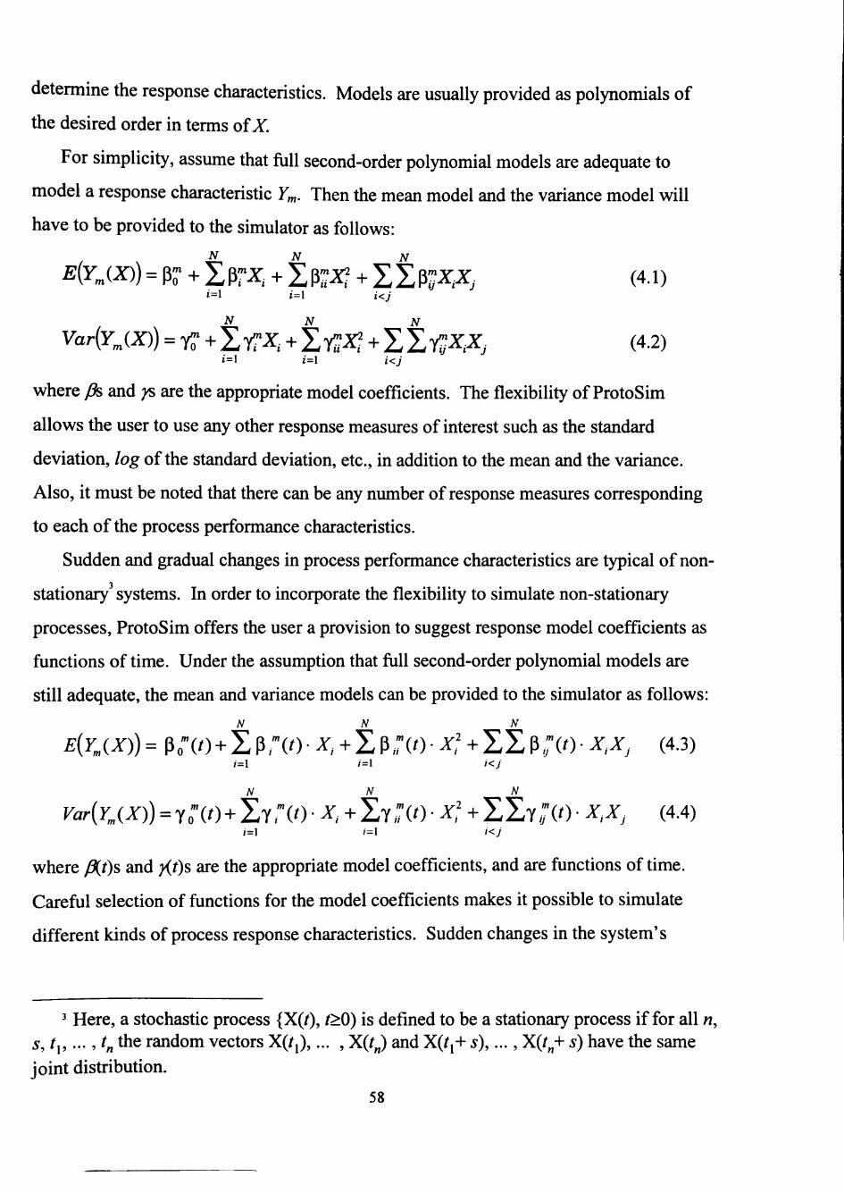
determine the response characteristics. Models are usually provided as polynomials of

the desired order in terms of X.

For simplicity, assume that full second-order polynomial models are adequate to

model a response characteristic Yrr,. Then the mean model and the variance model will

have to be provided to the simulator as follows:

E{YJX)) = p- + £ p - X , + i p - X f + l i p - X , X , (4.1) 1=1 i=l i<j

Var{YJX)) = TT + I T T ^ , + lyj^A^ + ltY^X,Xj (4.2) 1=1 i=\ i<j

where y^ and ;^ are the appropriate model coefficients. The fiexibility of ProtoSim

allows the user to use any other response measures of interest such as the standard

deviation, log ofthe standard deviation, etc., in addition to the mean and the variance.

Also, it must be noted that there can be any number of response measures corresponding

to each ofthe process performance characteristics.

Sudden and gradual changes in process performance characteristics are typical of non-

stationary systems. In order to incorporate the flexibility to simulate non-stationary

processes, ProtoSim offers the user a provision to suggest response model coefficients as

functions of time. Under the assumption that full second-order polynomial models are

still adequate, the mean and variance models can be provided to the simulator as follows: N N N

£(y„(x))= P;(O+EP;W-A',+i;p,r( ' )- j^, '+IIP,;(o-^, j^y (4.3) ;=1 /=1 i<j

N N N

Var{Y„(X)) = Yo'"(0 + I Y : ( 0 • ^, + I Y , : « • ^f + X S Y , ; ( 0 • ^:^j (4.4) i=\ i=\ i<J

where fl(t)s and y(t)s are the appropriate model coefficients, and are functions of time.

Careful selection of functions for the model coefficients makes it possible to simulate

different kinds of process response characteristics. Sudden changes in the system's

^ Here, a stochastic process {X(t), t>0) is defined to be a stationary process if for all n, s,t^,... Jn the random vectors X(/j),... , X(/J and X(t^-^ s),..., X(/„+ s) have the same joint distribution.

58

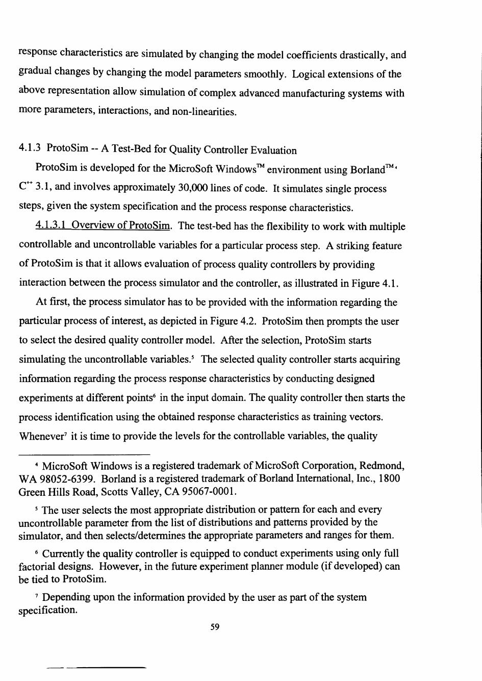
response characteristics are simulated by changing the model coefficients drastically, and

gradual changes by changing the model parameters smoothly. Logical extensions of the

above representation allow simulation of complex advanced manufacturing systems with

more parameters, interactions, and non-linearities.

4.1.3 ProtoSim - A Test-Bed for Quality Controller Evaluation

ProtoSim is developed for the MicroSoft Windows™ environment using Boriand™^

C^ 3.1, and involves approximately 30,000 lines of code. It simulates single process

steps, given the system specification and the process response characteristics.

4.1.3.1 Overview of ProtoSim. The test-bed has the flexibility to work with multiple

controllable and uncontrollable variables for a particular process step. A striking feature

of ProtoSim is that it allows evaluation of process quality controllers by providing

interaction between the process simulator and the controller, as illustrated in Figiu-e 4.1.

At first, the process simulator has to be provided with the information regarding the

particular process of interest, as depicted in Figure 4.2. ProtoSim then prompts the user

to select the desired quality controller model. After the selection, ProtoSim starts

simulating the uncontrollable variables.* The selected quality controller starts acquiring

information regarding the process response characteristics by conducting designed

experiments at different points^ in the input domain. The quality controller then starts the

process identification using the obtained response characteristics as training vectors.

Whenever' it is time to provide the levels for the controllable variables, the quality

" Microsoft Windows is a registered trademark of MicroSoft Corporation, Redmond, WA 98052-6399. Borland is a registered trademark of Borland Intemational, Inc., 1800 Green Hills Road, Scorts Valley, CA 95067-0001.

* The user selects the most appropriate distribution or pattem for each and every uncontrollable parameter from the list of distributions and pattems provided by the simulator, and then selects/determines the appropriate parameters and ranges for them.

^ Currently the quality controller is equipped to conduct experiments using only fiill factorial designs. However, in the fiiture experiment planner module (if developed) can be tied to ProtoSim.

' Depending upon the information provided by the user as part ofthe system specification.

59

e s

s

Process Simulator Quality Controller

Simulate Uncontrollable Variables Process

Response

Leam Process Response Characteristics

Simulate Response Characteristics

Simulate Operation Policies

,Control Parameters

Yes

Process Parameter Design

Figure 4.1. Simulator acting as a test-bed for quality controllers.

Obtain System Specification

Obtain Response Characteristics

Obtain Operation Pohcies

Obtain Target Characteristics

System Characteristics of the system Specification - Continuous process or piece-part

manufacturing - Production rate

Operating ranges of controllable variables and signatures of uncontrollable variables

Response Models for location and dispersion Characteristics measures of process response

characteristics in the input domain

Operation Maintenance policies Policies - Preventive

- Corrective

Desired Static targets Targets - SIB, NIB, and LIB

Dynamic targets

Figure 4.2. Layout ofthe simulator.

60

controller temporarily moves from the process identification mode into parameter design

mode, and suggests "optimal" levels for the controllable variables.

4.1.3.2 Flow of Control during Identification Mode. Structural learning is the

critical issue in the system identification process. Here, stmcttiral leaming is defined as

tiie process of determining what class of models are applicable for a particular set of

applications [Barto 1991]. hi quality controllers that incorporate multilayer perceptron

networks (Critic-Action controller and perceptron network based iterative inversion

conttoUer), stmctural leaming involves how many layers, how many hidden units, and

what kinds of constraints should be used. In quality controllers that utilize RBF

networks, this leaming involves the number of RBF centers, and parameters associated

with the activation fimction used. It is tme that a class of models with a very large

number of parameters can include within them many different kinds of stmctures [Barto,

1991]. However, estimating such a large number of parameters does not automatically

qualify as a stmctural leaming technique because there is no guarantee that a stmcture

that is best in any sense, or even good, will be selected by the parameter estimation

process, nor that generalization, i.e., extrapolation to novel instances will be effective.

Adjusting parameters to maximize a performance criterion defined only in terms of

matching the training data has no automatic implications for selecting suitable stmctures.

In order to overcome this problem to certain extent, ProtoSim initializes the

connectionist network used for process identification with the fewest number of

parameters. Then, the number of parameters are incremented till the desired level of

accuracy is attained as depicted in Figure 4.3. ProtoSim incorporates features to handle

partially connected networks, and generalization enhancement techniques such as weight

elimination proposed by Weigand et al. [1992], 5'-fold cross-validation proposed by

Weiss and Kulikowski [1991], etc.

4.1.3.3 Flow of Control during Parameter Design Mode. In searching for optimal

controllable variable levels, ProtoSim incorporates gradient descent approach w.r.t. the

energy surface in the input domain. At any given set of controllable variables levels,

ProtoSim, by default, defines the energy function as the least squares difference between

61

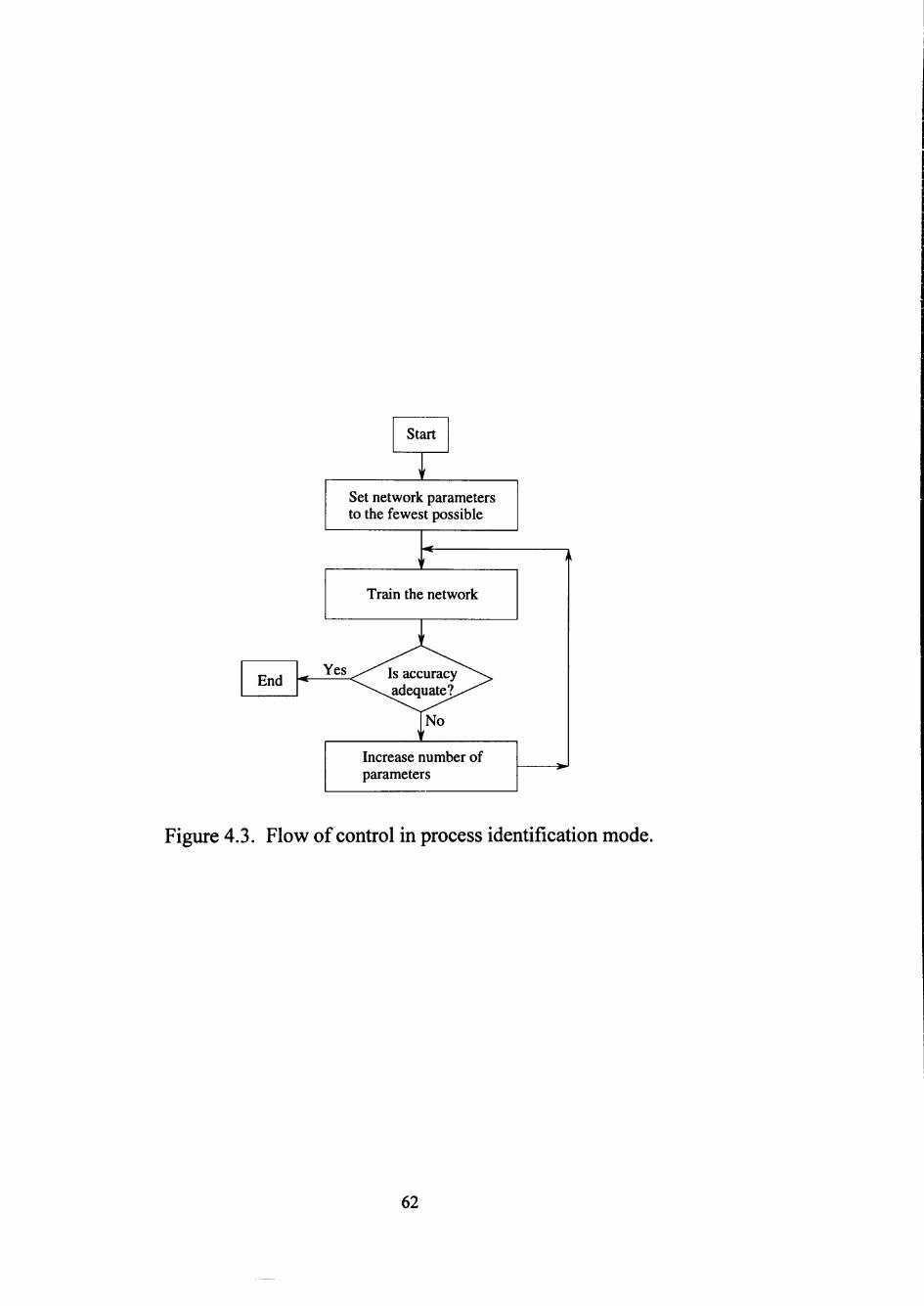
End

Start

) '

Set network parameters to the fewest possible

' '

Train the network

^ Y e s ^ ^ ^ I s accuracy ^ ~ \ adeauate?^^'^

jl5o

Increase number of parat netei rs

1

Figure 4,3. Flow of control in process identification mode.

62

the desired performance characteristics and the predicted performance characteristics

w.r.t. the uncontrollable variables levels at that instant.

If the energy function meets all the criteria for a strictly convex fimction* in the input

domain (of interest), gradient descent techniques lead to a global optimal solution.

However, if the energy fimction is not a convex fimction, gradient descent techniques

lead to a local optimal solution.' Hence, it is necessary that ProtoSim search through all

the basins to locate the global optimal levels for the controllable variables.'"

Currently, ProtoSim lacks the ability to locate global optimal solutions, and converges

to local optimal solutions." However, it is easy to incorporate a simulated annealing

module (or other enhanced optimization techniques) to improve ProtoSim's performance.

This search process is illustrated in Figure 4.4.

4.2 Evaluation ofthe Quality Controller Models

Software constraints posed by the Graphic User Interface (GUI), have restricted the

flexibility of ProtoSim to allow for the simulation of processes having a maximum of two

uncontrollable variables, two controllable variables, and two response measures. To

evaluate the effectiveness ofthe different quality controllers developed in Chapter II,

* Letf.S —> E^, where Sis a nonempty set in E„. The function/is said to be convex on S if /(AXi + (1 - X)X2) < Xf(X,) + (1 - X)f(X^) for each Xi, X2 e 5 and for each X e (0,1). The function/is called strictly convex on S if the above inequality is tme as a strict inequality for each distinct Xi andX2 in S and for each X, e (0,1) [Bazaraa, Sherali, and Shetty, 1993].

' Consider the problem of minimizing/X) over E„, and let X e E„. IffiX) <f(X)for all X G E„, then X is called a global minimum. If there exists an ^-neighborhood NJ^X) around X such t h a t / X ) <f(X) for eachX e NJ^X), then X is called a local minimum [Bazaraa et al., 1993]

'° An iterative constrain satisfaction module provided along with ProtoSim ensures that the steps taken along the negative gradient are contained in the feasible input domain.

" The solution depends on the location ofthe starting point in the input domain from which the search process was initiated. Under the assumption that the step sizes taken along the negative gradient are not large enough to move into a different basin, ProtoSim converges to the local minimum in the basin holding the starting point.

63

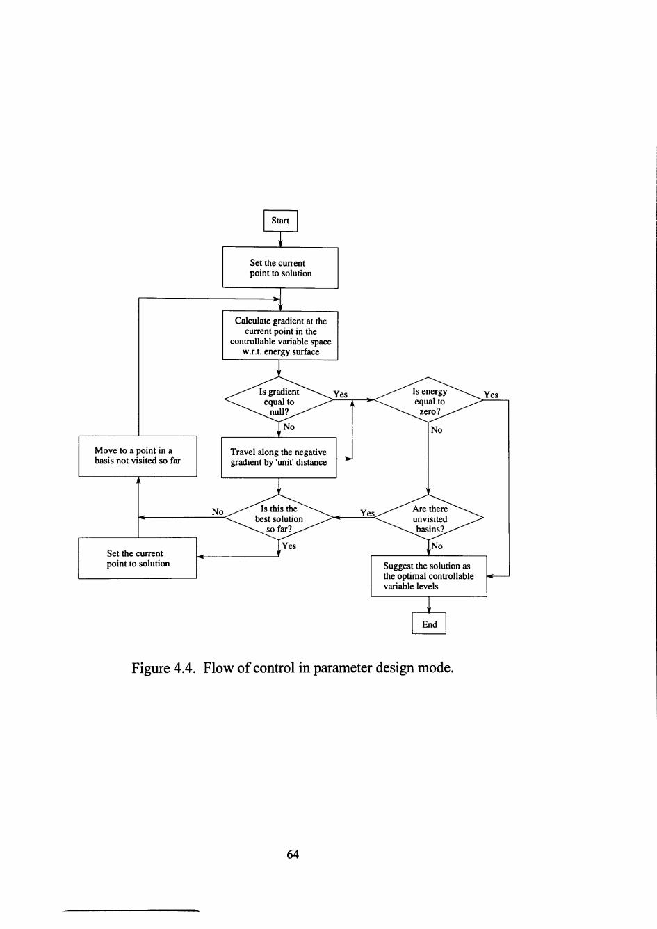
Start

Set the current point to solution

Calculate gradient at the current point in the

controllable variable space w.r.t. energy surface

Move to a point in a basis not visited so far

Yes

Travel along the negative gradient by 'unit' distance

Yes

Set the current point to solution

Yes

Suggest the solution as the optimal controllable variable levels

End

Figure 4.4. Flow of control in parameter design mode.

64

several production processes had been simulated on ProtoSim. These simulations were

designed and executed with various kinds of response characteristics.'^ The following

section provides a detailed discussion about a specific experiment that involved an

uncontrollable variable Xx, two controllable variables, Xi, X^, and two process response

measures.

4.2.1 An Experiment for Evaluation of Quality Controllers

An experiment was designed for evaluating the performance ofthe RBF network

based iterative-inversion quality controller. This experiment tested the quality controller

in the leaming mode as well as the process parameter design mode by providing the

following models to the process simulator:

ResMeasx(X) = 327.6 + 131.5Xi + 177.0X2 + 109.4^3 - 2 9 . 1 ^ + 32.0X^

- 2 2 .4^ + 75.5X1X2 + 43.6X1X3 + 66.0X2X3,

ResMeas2(X) = 34.9 + 29.2Xi + 11.5X2 + 15.3X3 + 16 .8^ + 4.2 X^

- 1.3 J^ + 5.1 X1X2 + 14.1X1X3 + 7.7X2X3,

where:-1 < X / < + l ; / = 1, 2, 3.

These models are illustrated in Figure 4.5.

4.2.1.1 Quality Controller in Leaming Mode. As discussed in section 2.2.2, the

quality controller in the leaming mode generates the identification stmcture through

stmctural leaming using training pattems that can be generated from designed

experiments and/or on-line data. In this case a three-level factorial experiment was

conducted by the quality controller, and the resulting 27 observed data sets served as

training pattems for the quality controller. The levels for each ofthe three independent

variables were chosen as -1, 0, and +1.'^

•2 This is achieved by providing ProtoSim with distinct models for the different response measures, for each ofthe simulation experiments.

' It must be noted that the level ofthe uncontrollable variable was zero for all the response surfaces that were illustrated for this particular experiment.

65

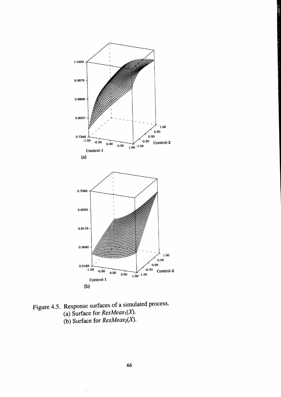
1.0489

0.9679

0.8868

Control-1 0.50 1 0 0 - 1 0 0

1.00

Control-2

(a)

0.7069

0.6593

0.6116

0.5640

0.5163 -1.00

1.00

0.00

Control-1 0.50 1 00 -1.00

0- ° Control-2

(b)

Figure 4.5. Response surfaces of a simulated process. (a) Surface for ResMeasi(X). (b) Surface for ResMeas2(X).

66

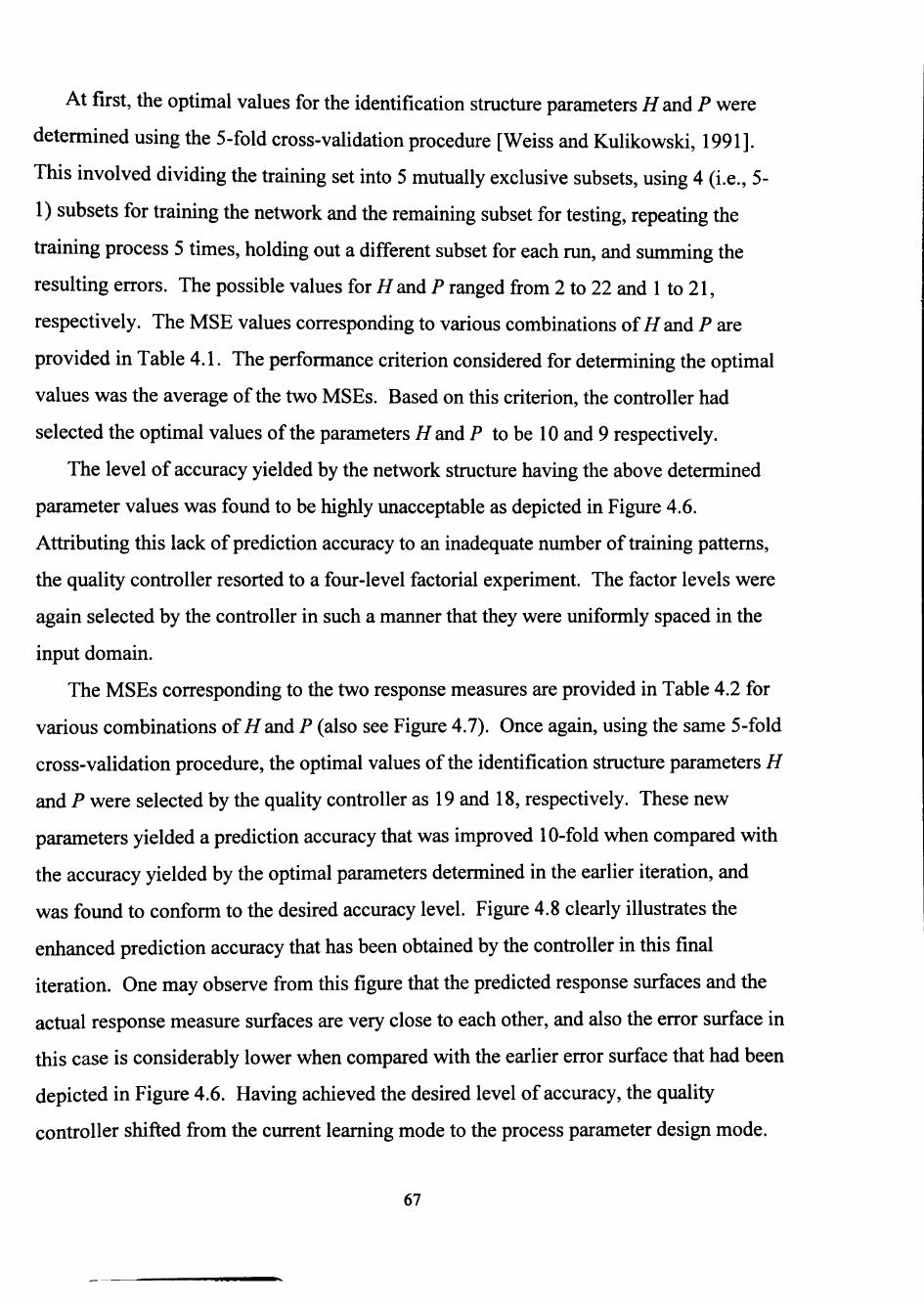
At first, the optimal values for the identification stmcture parameters //and P were

determined using the 5-fold cross-validation procedure [Weiss and Kulikowski, 1991].

This involved dividing the training set into 5 mutually exclusive subsets, using 4 (i.e., 5-

1) subsets for training the network and the remaining subset for testing, repeating the

training process 5 times, holding out a different subset for each mn, and summing the

resulting errors. The possible values for //and P ranged from 2 to 22 and 1 to 21,

respectively. The MSE values corresponding to various combinations of//and P are

provided in Table 4.1. The performance criterion considered for determining the optimal

values was the average ofthe two MSEs. Based on this criterion, the controller had

selected the optimal values ofthe parameters //and P to be 10 and 9 respectively.

The level of accuracy yielded by the network stmcture having the above determined

parameter values was found to be highly unacceptable as depicted in Figure 4.6.

Attributing this lack of prediction accuracy to an inadequate number of training pattems,

the quality controller resorted to a four-level factorial experiment. The factor levels were

again selected by the controller in such a manner that they were uniformly spaced in the

input domain.

The MSEs corresponding to the two response measures are provided in Table 4.2 for

various combinations of//and P (also see Figure 4.7). Once again, using the same 5-fold

cross-validation procedure, the optimal values ofthe identification stmcture parameters H

and P were selected by the quality controller as 19 and 18, respectively. These new

parameters yielded a prediction accuracy that was improved 10-fold when compared with

the accuracy yielded by the optimal parameters determined in the earlier iteration, and

was found to conform to the desired accuracy level. Figure 4.8 clearly illustrates the

enhanced prediction accuracy that has been obtained by the controller in this final

iteration. One may observe from this figure that the predicted response surfaces and the

actual response measure surfaces are very close to each other, and also the error surface in

this case is considerably lower when compared with the earlier error surface that had been

depicted in Figure 4.6. Having achieved the desired level of accuracy, the quality

controller shifted from the current leaming mode to the process parameter design mode.

67

Table 4.1. The MSE values corresponding to various combinations of//and P; three-level factorial experiment.

\ . p

10

9

8

7

6

5

4

3

2

1

7.16 1.39

6.49 2.10

6.14 2.44

6.18 3.22

5.74 2.58

6.19 3.43

7.28 4.17

9.73 5.74

10.27 7.10

2

7.08 1.47

6.46 2.07

6.44 2.49

6.14 3.17

5.70 2.77

6.44 3.68

7.63 4.96

10.00 5.77

3

7.09 1.58

6.25 2.28

6.82 2.89

6.38 3.27

5.77 2.87

6.58 3.76

8.08 5.09

4

7.13 1.89

6.40 2.44

7.07 2.98

6.80 3.65

6.83 2.91

7.11 3.96

5

7.09 2.08

6.50 2.55

7.52 3.23

6.73 3.80

8.11 4.18

6

6.88 2.30

6.33 2.81

8.55 3.95

7.27 3.93

7

6.89 2.68

6.19 3.07

9.45 4.29

8

6.72 3.02

7.32 1.26

9

7.60 3.74

All entries were scaled by a factor of 100. The first and second cell entries refer to the MSEs corresponding to the first and second response measures respectively.

68

1.0489

0.9679

0.8868

0.8057

0.7246 -1.00

0.00

Control-l 0.50 j_oo -1.00

0.7069

0.6593

0.6116

0.5640

0.5163 -1.00

1.00

0.50

0.00

Control-l 0.50 j^oo -1.00

°^° Control-2

(a) (b)

0.0054

0.0041

0.0027

Control-l 0.50 1 ,00-100

1.00

Control-2

(C)

Figure 4.6. Predicted and actual response surfaces of a simulated process; three level factorial experiment. (a) Predicted surface for ResMeas\(X)

superimposed on the actual surface. (b) Predicted surface for ResMeas2(X).

superimposed on the actual surface. (c) Error surface.

69

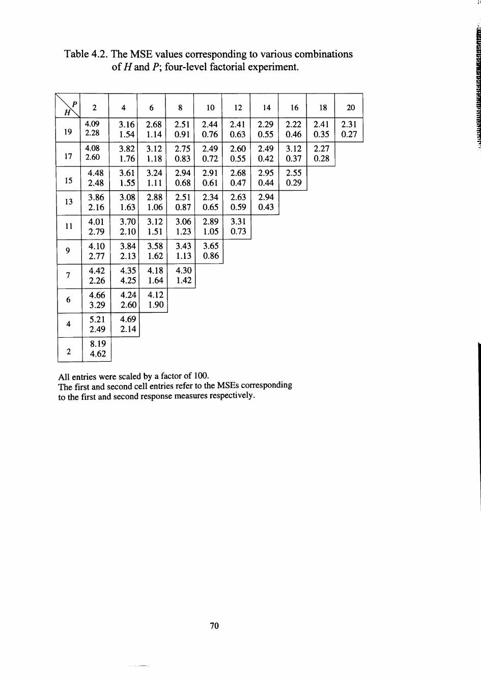
Table 4.2. The MSE values corresponding to various combinations of//and P; four-level factorial experiment.

s s

19

17

15

13

11

9

7

6

4

2

2

4.09 2.28

4.08 2.60

4.48 2.48

3.86 2.16

4.01 2.79

4.10 2.77

4.42 2.26

4.66 3.29

5.21 2.49

8.19 4.62

4

3.16 1.54

3.82 1.76

3.61 1.55

3.08 1.63

3.70 2.10

3.84 2.13

4.35 4.25

4.24 2.60

4.69 2.14

6

2.68 1.14

3.12 1.18

3.24 1.11

2.88 1.06

3.12 1.51

3.58 1.62

4.18 1.64

4.12 1.90

8

2.51 0.91

2.75 0.83

2.94 0.68

2.51 0.87

3.06 1.23

3.43 1.13

4.30 1.42

10

2.44 0.76

2.49 0.72

2.91 0.61

2.34 0.65

2.89 1.05

3.65 0.86

12

2.41 0.63

2.60 0.55

2.68 0.47

2.63 0.59

3.31 0.73

14

2.29 0.55

2.49 0.42

2.95 0.44

2.94 0.43

16

2.22 0.46

3.12 0.37

2.55 0.29

18

2.41 0.35

2.27 0.28

20

2.31 0.27

All entries were scaled by a factor of 100. The first and second cell entries refer to the MSEs corresponding to the first and second response measures respectively.

70

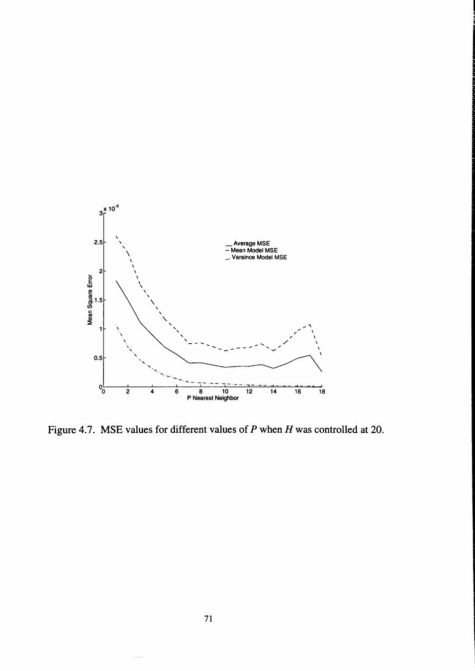
3?^°"

2.5

2 ce 3 a-

(/} c <d a>

1.5

0.5

\

\

_ Average MSE Mean Model MSE

. Varaince Model MSE

/

_i I I ] _ — • 1

6 8 10 12 14 16 18 P Nearest Neighbor

Figure 4.7. MSE values for different values of P when H was controlled at 20.

71

1.0489

0.9679

0.8868

0.8057 -

0.7246 -1.00

1.00

0.50

0.00

0.50

Control-l 0.50 ^_pQ.i.oo Control-2

0.7069

0.6593

0.6116 -

0.5640 -

0.5163 -1.00

1.00

Control-l 0.50 j ^ ^ . 1 . 0 0

0.50

Control-2

(a) (b)

0.0004

0.0003

0.0002 -

0.0001

0.0000 -1.00

1.00

0.50

-0-50 o.oo'~~7r-~^5^ -°-=° Control-2 0.50 1 0 0 - 1 . 0 0

Control-1 (C)

Figure 4.8. Predicted and actual response surfaces of a simulated process; four level factorial experiment. (a) Predicted surface for ResMeas\(X)

superimposed on the actual surface. (b) Predicted surface for ResMeas2(X).

superimposed on the actual surface. (c) Error surface.

72

4.2.1.2 Quality Controller in Parameter Design Mode. This section illustrates the

effectiveness ofthe quality controller in the parameter design mode under various

combinations of starting points''' and desired target levels with respect to the two

response measures. In case the targets happen to be infeasible, the quality controller in

the parameter design mode provides the best possible solution within the feasible region

as illustrated in Figure 4.4.

The effectiveness ofthe quality controller in the parameter design mode was tested

under a number of possible combinations of starting points and desired response measure

targets. For illustrative purposes, the results corresponding to the four combinations

shovm in Table 4.3 are discussed in detail here. For Case 1, the quality controller in the

parameter design mode was successful in converging to an optimal solution within the

basin as shown in Figure 4.9. The white bullet on the two response measure surfaces

shown in the figure indicate the corresponding values ofthe two response measures at the

instant the desired targets were provided to the quality controller. The connected black

bullets on the response surfaces depict the gradient descent trajectory followed by the

search process adopted by the quality controller in the parameter design mode. A unique

energy surface exists for any desired target as discussed in section 4.1.3.3. The energy

surface corresponding to the desired targets for the above discussed case shown in Figure

4.9 indicates that the search process adopted by the quality controller yielded optimal

values for the controllable variables in the input domain that resulted in zero energy. The

other three cases reiterated the same convergence phenomena that had been discussed for

Case 1. The response surfaces corresponding to the three Cases 2, 3, and 4 have been

shown in Figures 4.10, 4.11, and 4.12, respectively.

Based on the various tests conducted to evaluate the effectiveness ofthe quality

controller, the following three features ofthe search process in the parameter design mode

were observed:

1. The energy surface changes with changing desired target values.

'" Starting point defines the values ofthe controllable variables in the input domain at the time the desired targets were provided to the quality controller in the parameter design mode.

73

Table 4.3. Combinations of starting points and desired targets.

B sa S3

3 s

Case 1

Case 2

Case 3 Case 4

Starting Point

Uncontrollable Variable

^1

0.000

0.000

0.000 0.000

Controllable Variables

X2

0.000

0.000

0.805 0.805

X3

0.850

0.850

0.779 0.779

Target

ResMeas\{X)

0.930

0.817

0.930 0.817

Values

ResMeasjiX)

0.570

0.549

0.570 0.549

74

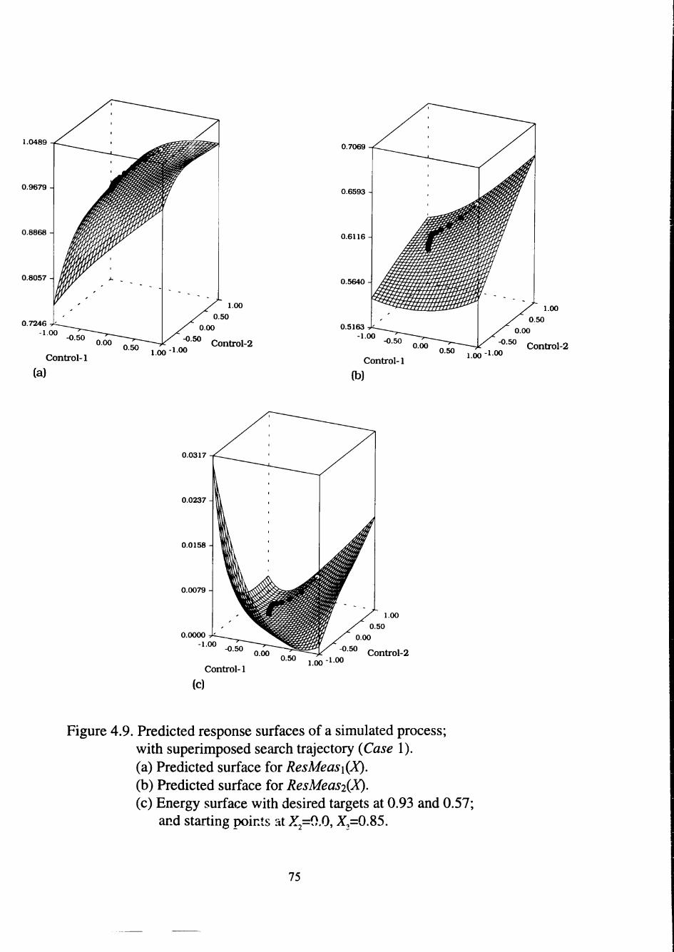
1.0489

0.9679

0.8868

1.00

0.50

-0.50

Control-1

0.00 -0.50

° ^ 1 . 0 0 - 1 0 0 Control-2

(a)

0.7069

0.6593

0 . 6 1 1 6 -

0.5640

0.5163 -1.00

1.00

-0.50 -0.50

Control-1 0.50 j ^ ^ . 1 . 0 0

0.50

Control-2

(b)

0.0317

0.0237

0.0158

0.0079 -

0.0000 -1.00

-0.50

1.00

0.50 0.00

-0.50

Control-1 0.50 j_jjQ.i.oo Control-2

(C)

Figure 4.9. Predicted response surfaces of a simulated process; with superimposed search trajectory (Case 1). (a) Predicted surface for ResMeas\(X). (b) Predicted surface for ResMeas2(X). (c) Energy surface with desired targets at 0.93 and 0.57;

and starting points at X=^,.(), ^3=0.85.

75

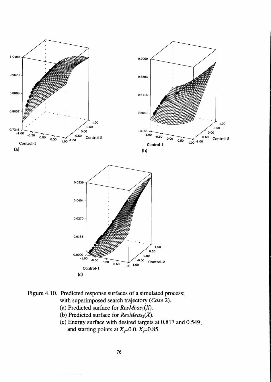
1.0489

0.9679

0.8868 -

0.8057 -

0.7246 -1.00

1.00

0.50

-0.50 0.00

0.50

Control-1 0.50 . „ „ -1 oo 1.00 * • " "

Control-2

0.7069

0.6593

0.6116

0.5640

0.5163 -1.00

1.00

0.50

-0.50 0.00

-0.50

Control-l °-^ 1 . 0 0 - 1 0 0

Control-2

(a) (b)

0.0539

0.0404 -

0.0270

0.0135

0.0000 -1.00

-0.50

1.00

0.50 0.00

0.50

Control-1 ° = ° 1 .00 -100

Control-2

(C)

Figure 4.10. Predicted response surfaces of a simulated process; with superimposed search trajectory (Case 2). (a) Predicted surface for ResMeas\(X). (b) Predicted surface for ResMeas2(X). (c) Energy surface with desired targets at 0.817 and 0.549;

and starting points at ^2=0.0, 3=0.85.

76

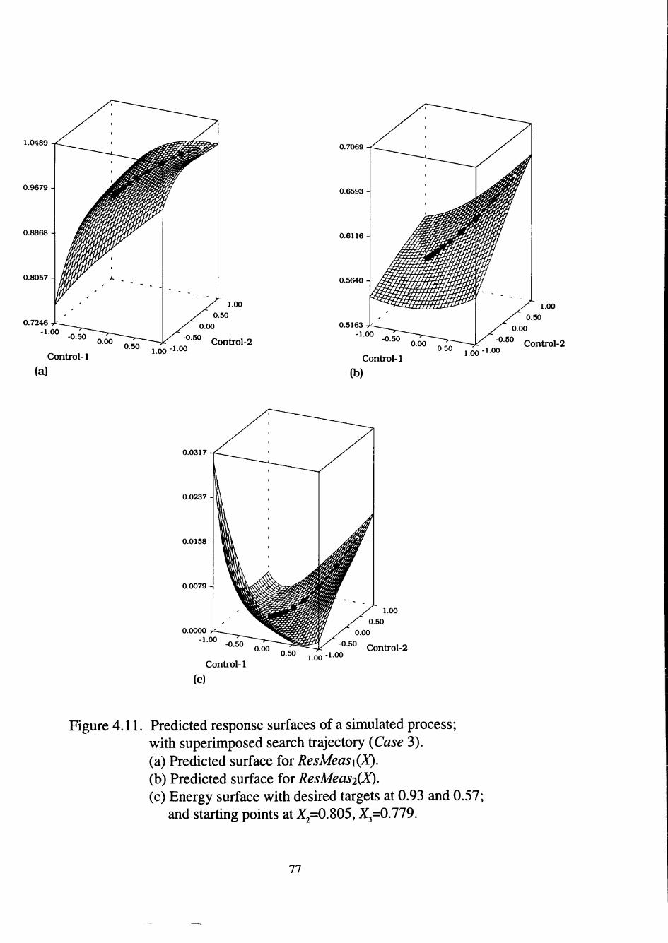
1.0489

0.9679

0.8868

0.8057

0.7246 -1.00

1.00

0.50

0.00

0.50

Control-1 °-=° 1 . 0 0 - 1 0 0

Control-2

0.7069

0.6593

0.6116

0.5640 -

0.5163 -1.00

1.00

-0.50 0.50

Control-1 1 . 0 0 - 1 0 0

0.50

Control-2

(a) (b)

0.0317

0.0237 -

Control-1 0.50 1 0 0 - 1 0 0

1.00

Control-2

(c)

Figure 4.11. Predicted response surfaces of a simulated process; with superimposed search trajectory (Case 3). (a) Predicted surface for ResMeas\(X). (b) Predicted surface for ResMeas2(X). (c) Energy surface with desired targets at 0.93 and 0.57;

and starting points at X2=0.805, X =0.119.

77

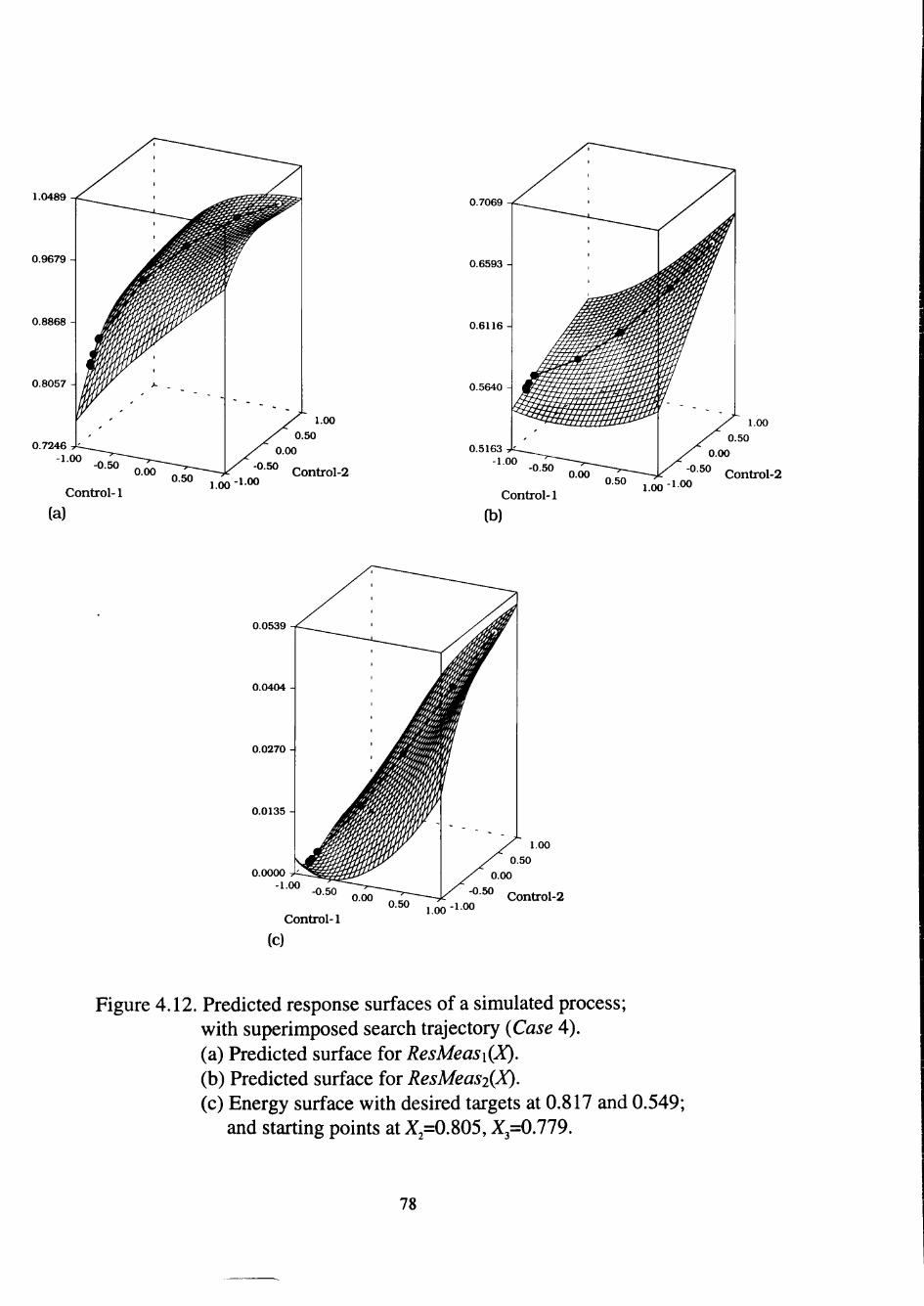
1.0489

0.9679

0.8868

0.8057

0.7246 -1.00

1.00

0.50

-0.50 0.00

0.50

Control-1 0.50 , „„ -1 00 1.00 '•""

Control-2

(a)

0.7069

0.6593 -

0.6116 -

1.00

0.50

0.00

0.50

Control-l 0.50 . „ „ .1 00 1.00 ' . " "

Control-2

(b)

0.0539

0.0404 -

0.0270

0.0135 -

0.0000 -1.00

1.00

0.50

0.00

0.50

Control-l 0.50 , 0 0 - 1 0 0

Control-2

(C)

Figure 4.12. Predicted response surfaces of a simulated process; with superimposed search trajectory (Case 4). (a) Predicted surface for ResMeasi(X). (b) Predicted surface for ResMeas2(X). (c) Energy surface with desired targets at 0.817 and 0.549;

and starting points at ^2=0.805, X =0.119.

78

2. The starting point greatly influences the search process.

3. The search process was found to converge successfully in an efficient manner.

4.2.2 Performance Results

Based on the results fi-om the process simulation test-bed, it was observed that all the

different quality controllers performed extremely well in building effective empirical

models relating the controllable and uncontrollable variables simultaneously with process

response characteristics.

The iterative-inversion method for process parameter design proved very effective in

identifying the optimal levels for the controllable variables. But the critic-action

approach was not very successful in dealing with more than one process response

measure. The performance ofthe critic-action approach was improved by using partially

connected network structures for process identification. In particular, there was

significant improvement in the performance of this approach when the output layer ofthe

network structure was not totally connected with the nodes in the previous layer.

However, even after this improvement, the performance ofthe quality controller was still

inferior when compared with that ofthe iterative-inversion approach based quality

controllers.

Both the perceptron network based iterative-inversion and the RBF network based

iterative-inversion approaches were extremely consistent in converging towards

"optimal" solutions within the basin of attraction.

4.3 Evaluation ofthe Performance Reliability Assessment Techniques Developed

4.3.1 Case Study: Monitoring Drill Bits in a Drilling Process

To demonstrate the performance reliability concepts developed in Chapter III, it was

decided to apply the concepts to monitor carbide-tipped HSS drill bits in a drilling

process. Several experiments were designed and executed in the Manufacturing

Laboratory at Texas Tech University. First, the experimental design issues and the RBF

79

network design issues are discussed. Later, the results of evaluation are presented in

detail.

4.3.1.1 Design of Experiments. A series of drilling tests were conducted and the

resulting data were used to train and test the tool performance reliability prediction

capability ofthe enhanced VI Network introduced in Chapter III. A power feed drill

press from Solverga Mekaniska Verkstads Manufacturing Co., Model Number: S-57100

(Made in Sweden) was used for the drilling experiments. It is an upright drilling machine

with 2 hp motor, and 220/440 volts. Cast Duralcan aluminum (A356 base wdth 20±2%

Sic by volume) bars with a thickness of 0.25 inches were used as specimens for the tests.

This material is a metal matrix composite (MMC) based on aluminum alloys reinforced

with 10-15 pm SiC particles. This material is very abrasive in nature, and results in

significantly short tool life when compared to other conventional aluminum alloys. At

room temperature, the tensile properties of A3 56 with 20% SiC* are as follows

[Mechanical and Physical Property Data ~ Foundry Composites, 1990]: yield strength of

48 to 46 ksi, ultimate strength of 51 to 48 ksi, 0.4% elongation, and modulus of 14 Msi.

The drill bits used were IMCO straight-fluted series 4850 carbide-tipped HSS grade

(0.25 inch diameter, 2 inch flute length, 4 inch overall length, and 118^ point angle).

These drill bits are primarily designed for drilling hardened steel in the 48 to 65 Re range.

The carbide tips are longer than normal for added resharpening life and high temperature

brazed to hardened high speed steel bodies.

Due to the strong abrasive nature ofthe work material, the high temperature generated

(while cutting) creates problems, such as local welding, stick, and seizure, which lead to

drill fracture. Cutting fluid is essential to alleviate the temperature effects. Several

cutting fluids and water were tested. Little difference existed in recorded thrusts between

the fluids and water. Since the primary objective ofthe experiment was to demonstrate

the performance reliability concept and not to optimize drill lift, water at room

'5 Cast-to-size tension bars, solutionized for 12 hours at 1005°F, and aged 24 hours at 320^F.

80

temperature (72 F) was used in the drilling process as a coolant. Water was flooded to

the drilling point with a flow rate of about 4.5 cu-in/minute.

During a drilling operation, the axial component (thrust force) provides a better

indication of cutting tool performance that the torque force value [Smith, 1989]. The

increase in the thrust force for a wom tool is more clearly revealed. The difference in the

thrust from the first hole to the last hole (end of tool life) is generally much greater than

the corresponding difference in the torque [Jalali, 1990; Smith, 1989]. For this reason, it

was decided to use the thrust force information (collected as the drill progressed through

the work material) to evaluate tool performance reliability. The independent variables

were the machining variables: speed (rpm), feed rate (ipr), and depth of hole (inches). In

this investigation, the speed, feed rate and depth of cut were set at 1548 rpm, 0.012 ipr

and 0.25 inch, respectively.

The specimen was mounted in a fixture instrumented with a Kistler force and torque

dynamometer (type 9271 A). The thrust cutting force (force component along the axis of

the drill bit) signal was passed through a Kistler charge amplifier (type 5004) and

digitized at the rate of 500 Hz using MetraByte's DAS-16F A/D Board. Eight drill bits

were used in the experiment; each drill bit was used to drill 40 holes. In this case, 40

holes yielded drill cutting edge wear well beyond typical wear in a production operation.

A definite effect of hardness on cutting forces in machining operations has been

reported [Subramanian and Cook, 1977]. Microstructure of work material differs slightly

depending on the location at which the hole has to be drilled. When a hard spot in the

work material is drilled, a sudden rise in thrust force is expected. In order to avoid any

systematic effects of different microstructures, holes were drilled at random locations.

The average thrust cutting force levels collected'* for the eight drill bits are displayed

in Figure 4.13. The data were obtained by averaging the recorded data values within the

rectangular area shown in Figure 4.14. These represent the average ofthe thrust cutting

force on the drill after the drill entered the work piece and actually started a fiiU cut till

'* These experiments were conducted by Kim, Y. S. in 1991, and the data was provided in his Ph. D. dissertation. For fiirther discussion ofthe experiments see Kim [1991].

81

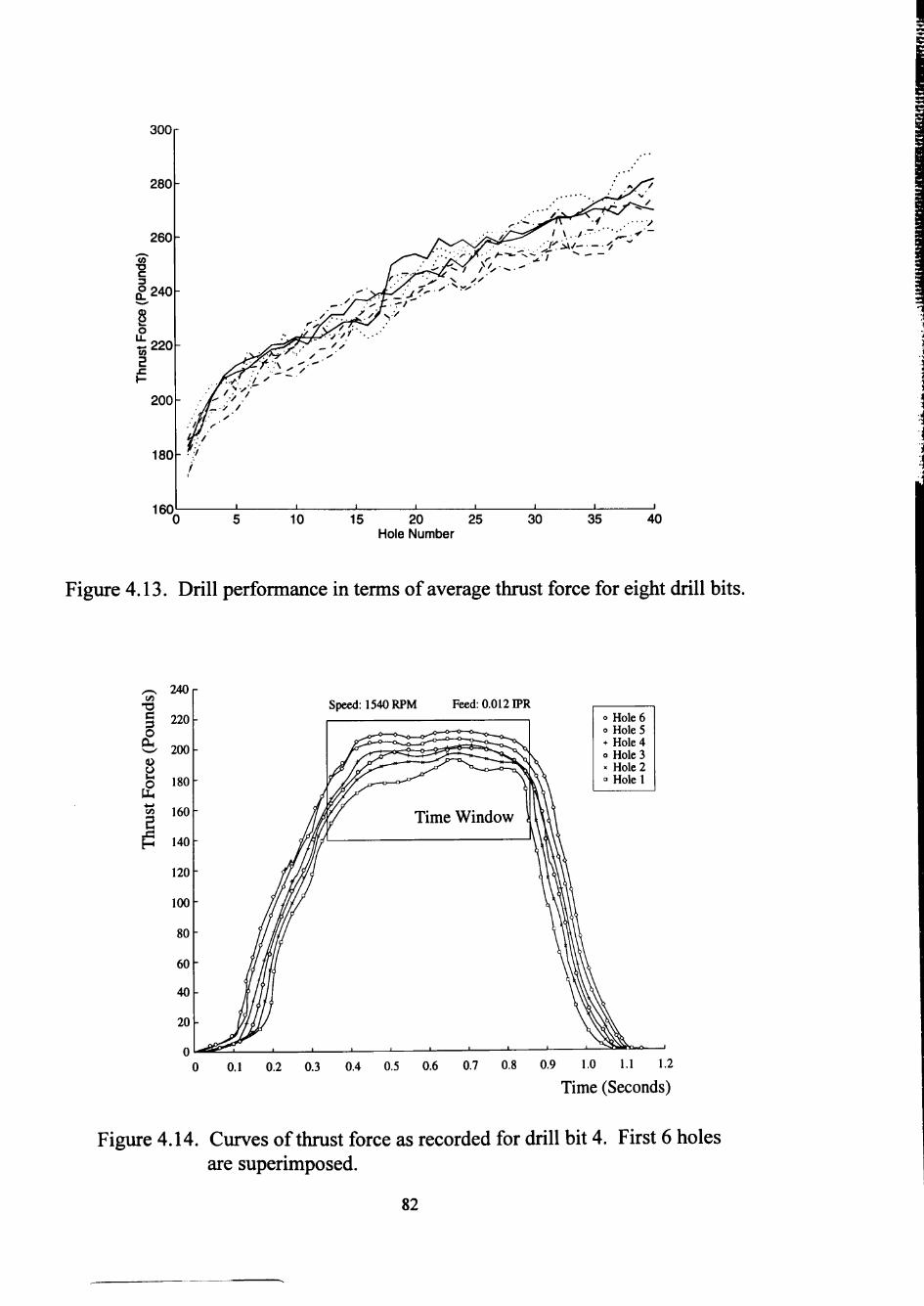
300

15 20 25 Hole Number

40

Figure 4.13. Drill performance in terms of average thrust force for eight drill bits.

(Pou

nds)

Fo

rce

Thr

ust

240r

220 -

200 -

180 -

160-

140-

120-

100-

80 -

6 0 -

40 -

20 -

oL

Speed: 1540 RPM Feed: 0.012 IPR o Hole 6 o Hole 5 + Hole 4 o Hole 3 X Hole 2 •> Hole 1

0.1 0.2 0.3 0.4 0.5 0.6 0.7 0.8 0.9 1.0 1.1 1.2

Time (Seconds)

Figure 4.14. Curves ofthrust force as recorded for drill bit 4. First 6 holes are superimposed.

82

the end ofthe cut. These collected thrust force signals along with average thrust force

levels constitute the database used for training and testing the enhanced VI network.

Although one can attempt to estimate the tool performance reliability every micro­

second, it is sufficient to provide the conditional performance reliability ofthe tool, on a

hole by hole basis. Here the conditional performance reliability is equivalent to a mission

reliability, where the mission constitutes successfully drilling one hole, given that the bit

has survived the previous hole. With this in mind, the network was trained to predict

these conditional performance reliabilities one hole at a time. The approach presented is

also applicable when working at micro-second intervals.

4.3.1.2 Network Design Issues. In training the VI Network, the network design

parameters H and P are selected using an ^-fold cross-validation procedure. Two other

parameters ofthe network need to be determined: A , the number of input nodes

representing the average thrust forces for the last A' holes drilled, and M, the number of

output nodes, representing the number of holes for which the thrust forces are to be

predicted. The effects of neural network structure with respect to the number of input

nodes and output nodes on the training and assessment of performance reliability will be

discussed later. In conducting the experiments, the number of nodes in the input layer,

were varied from 2 to 8 in steps of one, and the number of output nodes were varied from

1 to 5. In determining the conditional tool reliabilities, a binary search procedure was

incorporated on a.

4.3.1.3 Performance Results. The square root ofthe mean square errors for different

network structures resulting from the ^-fold cross-validation over the total training set for

One-Hole ahead prediction are shown in Table 4.4. Table 4.5 summarizes the training

and prediction errors for simultaneous prediction of One-Hole and Five-Hole ahead

average thrust force predictions. In determining the optimal parameters //and P, priority

was given to the one-hole ahead prediction accuracy in all experiments. The results show

that the networks made reasonably good approximations to the tool response

characteristics (small prediction errors were observed).

83

i<ww«(MHi

Table 4.4. Training and prediction errors for different optimal network structures in the case of One-Hole ahead thrust force predictions (M=l).

VI Network Structure

N

2 3 4 5 6 7 8

Optimal Parameters*

H

10 10 25 15 15 15 20

P

4 4 5 4 5 4 6

Training Error Sqrt(MSE)»*

One-Hole Ahead

3.342 3.485 3.193 3.283 3.095 3.248 3.290

Prediction Error Sqrt(MSE)*»

One-Hole Ahead

3.658 3.893 3.632 3.597 3.452 3.531 3.557

• Based on 10-fold cross-validation.

**Units are in pounds.

Table 4.5. Training and prediction errors for different optimal network structures in the case of simultaneous One-Hole and Five-Hole ahead thrust force predictions (M=2).

VI Network

Structure

A

2 3 4 5 6 7 8

Optimal Parameters*

H

15 20 30 25 30 35 30

P

4 5 6 5 7 7 7

Training Error Sqrt(MSE)**

One-Hole Ahead

1.670 1.820 1.281 1.586 1.441 1.346 2.010

Five-Hole Ahead

3.292 4.223 3.082 3.287 3.156 2.990 3.027

Prediction Error Sqrt(MSE)**

One-Hole Ahead

1.336 1.490 1.465 2.060 2.138 1.844 1.925

Five-Hole Ahead

3.754 3.339 3.912 3.700 3.618 3.798 3.745

Based on 10-fold cross-validation, priority is One-Hole ahead prediction.

'Units are in pounds.

84

The neural network structure has a strong influence on its prediction capability. In

particular, it can be seen that the network prediction capability had significantly improved

in the case of simultaneous prediction. This resuh can be attributed to the fact that more

information has been provided to the VI Network in the training mode. The reason for

seeing a relatively large number of RBF nodes (H) in the simultaneous prediction case (M

=2) can be attributed to the same fact, that the network is being provided more

information and hence needs a larger network to store the response characteristics. The

same pattem more or less appears even when the number of input nodes (N) is increased.

For illustrative purposes, the plots ofthe one-hole ahead predicted thrust force levels

and their 95% confidence limits are shown in Figures 4.15 and 4.16 for drill bits 1 and 4,

respectively. The neural network structure used for this prediction used the following

parameters: A^=7,//^=30,P = 5, andA/=l . The parameters HandP were determined

using a 10-fold cross-validation procedure. The outer limits represent the confidence

limits on the individual values ofthe predictions and the inner band represents the

confidence limits on the expected value ofthe predicted thrust force level.

The conditional performance reliability predictions for drill bits 1 and 4 are depicted

in Figures 4.17 and 4.18. Here again, the conditional performance reliability is equivalent

to a mission reliability where the mission constitutes the probability of successftilly

drilling one more hole, given that it has survived the previous hole. From Figures 4.17

and 4.18, there is significant difference in the performance ofthe two drill bits. For

example, the performance reliability for drill bit 1 in surviving the 25th hole given that it

has survived the 24th hole is 0.7, as shown in Figure 4.17. In the case of drill bit 4, this

reliability is 0.05 (Figure 4.18). Figures 4.19 and 4.20 depict the change in the

performance reliabilities for drill bits 1 and 4. These unconditional performance

reliabilities are calculated from their respective conditional reliabilities developed above.

For example, the performance reliability that a particular drill bit would survive Z holes is

simply the product ofthe conditional performance reliabilities of surviving each of these

Z holes (basically the product of Z conditional performance reliabilities). Since the

85

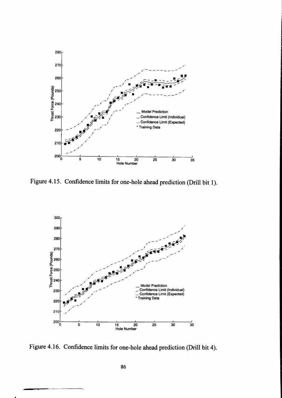
280 r

270

260

CO

1250 3

o

?240 o Ll. *^ (0

I 230

220

200

210-B-B-

Model Prediction

_. Confidence Limit (Individual) ... Confidence Limit (Expected) * Training Data

10 15 20 Hole Numtier

25 30 35

Figure 4.15. Confidence limits for one-hole ahead prediction (Drill bit 1).

300 r

Model Prediction _. Confidence Limit (Individual) ... Confidence Limit (Expected) * Training Data

10 15 20 Hole Number

25 30 35

Figure 4.16. Confidence limits for one-hole ahead prediction (Drill bit 4).

86

I r

0.9

0.8

n .2 CC0.7 o o

A

.1' T3 C o o 0.5

0.4

0.3 10 15 20

Hole Number 25 30 35

Figure 4.17. Tool conditional performance reliability curve (Drill bit 1: YO A = 2601bs.)

1

0.9

0.8

^ 0 . 7 JQ CO

1)0.6-(£ •5 j2 0.5 CD

I 0.4 C o

" 0 . 3

0.2

0.1

0 10 15 20

Hole Number

Figure 4.18. Tool conditional performance reliability curve (Drill bit 4: Y ^ = 2601bs.)

87

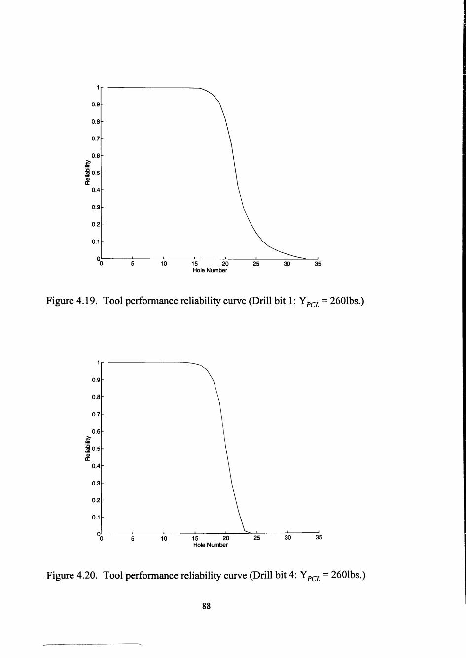
1

0.9

0.8

0.7

0.6

•§0.5 0)

0.4

0.3

0.2

0.1

0 10 15 20

Hole Number 25 30 35

Figure 4.19. Tool performance reliability curve (Drill bit 1: Yz, , = 2601bs.)

1

0.9

0.8

0.7

0.6

•§0.5

0.4

0.3

0.2

0.1

0 10 15 20

Hole Number 25 30 35

Figure 4.20. Tool performance reliability curve (Drill bit 4: Yp . = 2601bs.)

88

network parameter A was set to 7 in this particular structure, these calculations are based

on the assumption that the drill bit will survive the first 7 holes with certainty.

3

89

CHAPTER V

CONCLUSION

5.1 Summary

The work presented is best characterized as an investigation of neural networks for

effective process quality control and monitoring in automated manufacturing systems.

The first objective was to develop identification and controller structures using neural

networks for achieving effective real-time process quality control in non-linear static

processes where the process physics is not well-understood. In other words, the objective

was to define, develop, and test models that will lead to intelligent quality control of a

manufacturing process in which the mechanistic relationships between controllable

variables, uncontrollable variables (inputs) and critical process quality characteristics

(outputs) are either unknown or poorly understood. A second objective was to design,

develop, and test effective reliability based real-time tool condition monitoring systems

for manufacturing processes.

In contrast to classical on-line and off-line quality assurance procedures that are

compatible with open-loop process control, the concept of a closed-loop quality controller

was introduced. In order to reach the desired state of effective process quality control,

one needs a quality control loop along with a process control loop for each ofthe basic

production process steps (see Figure 2.2).

The quality controller, a critical component in the quality control loop, is responsible

for real-time process identification and process parameter design. The identification

fimction involves development of empirical models relating controllable and

uncontrollable variables to process response characteristics of interest. Two general

classes of identification sttoicttn-es have been developed to achieve the identification

fimction. The structures use multilayer feedforward perceptron networks and radial basis

function networks to achieve tiie identification fimction. The developed identification

structures have been tested on several simulated production processes with up to two

controllable variables, two uncontrollable variables, and two process performance

90

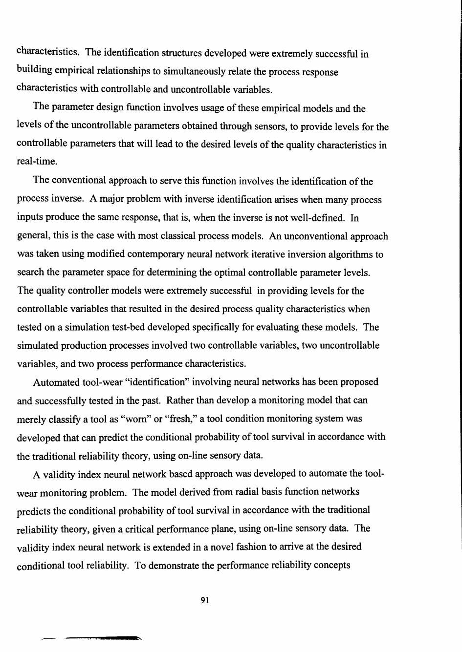
characteristics. The identification structures developed were extremely successfiil in

building empirical relationships to simultaneously relate the process response

characteristics with controllable and uncontrollable variables.

The parameter design fimction involves usage of these empirical models and the

levels ofthe uncontrollable parameters obtained through sensors, to provide levels for the

controllable parameters that will lead to the desired levels ofthe quality characteristics in

real-time.

The conventional approach to serve this fimction involves the identification ofthe

process inverse. A major problem with inverse identification arises when many process

inputs produce the same response, that is, when the inverse is not well-defined. In

general, this is the case with most classical process models. An unconventional approach

was taken using modified contemporary neural network iterative inversion algorithms to

search the parameter space for determining the optimal controllable parameter levels.

The quality controller models were extremely successfiil in providing levels for the

controllable variables that resulted in the desired process quality characteristics when

tested on a simulation test-bed developed specifically for evaluating these models. The

simulated production processes involved two controllable variables, two uncontrollable

variables, and two process performance characteristics.

Automated tool-wear "identification" involving neural networks has been proposed

and successfiiUy tested in the past. Rather than develop a monitoring model that can

merely classify a tool as "wom" or "fresh," a tool condition monitoring system was

developed that can predict the conditional probability of tool survival in accordance with

the traditional reliability theory, using on-line sensory data.

A validity index neural network based approach was developed to automate the tool-

wear monitoring problem. The model derived from radial basis fimction networks

predicts the conditional probability of tool survival in accordance with the traditional

reliability theory, given a critical performance plane, using on-line sensory data. The

validity index neural network is extended in a novel fashion to arrive at the desired

conditional tool reliability. To demonstrate the performance reliability concepts

91

developed, several experiments were designed and executed on a drilling process to

monitor carbide-tipped HSS drill bits. The tool condition monitoring system performed

extremely well in making real-time tool performance reliability predictions on a hole by

hole basis.

5.2 Contributions

This research has produced the following major contributions.

1. The concept of a closed-loop quality controller was developed for achieving real­

time process quality control in automated manufacturing systems.

2. Innovative process identification structures have been suggested using neural

networks for developing empirical models relating controllable and uncontrollable

variables to performance characteristics of non-linear static processes with either

unknown or poorly understood mechanistic relationships.

3. Methods that make use of neural network based process identification structures

have been developed to determine the optimal controllable variable levels in real­

time. These methods are compatible with automated manufacturing systems, and

represent a first step in achieving closed-loop quality control for such systems.

4. A Monte Carlo simulation technique based process simulation test-bed has been

developed to test the effectiveness and efficiency of process discovery strategies

and quality controllers.

5. A reliability based real-time tool condition monitoring system for automated

manufacturing processes has been developed using a novel extension ofthe

validity index neural network.

92

REFERENCES

Andrews, G. and Tlusty, J., "A Critical Review of Sensors for Unmanned Machining," Annals ofthe CIRP, Vol. 32, pp. 563-572, 1983.

Barker, T. B., Quality by Experimental Design, New York: Marcel Dekker, 1985.

Barnard, G. A., "Control Charts and Stochastic Processes," Journal of Royal Statistical Society, Vol. B21, pp. 239, 1959.

Barto, A. G., "Connectionist Leaming for Control: An Overview," Neural Networks for Control, Cambridge, MA: The MIT Press, 1991.

Barto, A. G., Sutton, R. S., and Anderson, C , "Neuron-like adaptive Elements that can Solve Difficult Leaming Problems," IEEE Transactions on Systems, Man, and Cybernetics, Vol. SMC-13, pp. 834-846, 1986.

Baum, E. B. and Haussler, D., "What Size Net gives Valid Generalization?," Neural Computation, Vol l,pp. 151-160, 1989.

Bazaraa, M. S., Sherali, H. D., and Shetty, C. M., Nonlinear Programming: Theory and Applications, New York, NY: John Wiley & Sons, 1993.

Bingham, R. S. Jr. andWalden, C. H., "Section 26: Process Industries,"Jwraw'^ Quality Control Handbook, 4th Edition, New York: McGraw-Hill Co., 1988.

Bohn, R. and Jaikumar, R., "The Dynamic Approach: An Altemative Paradigm for Operations Management," Harvard Business School Working Paper No. 88011, Boston, Massachusetts, 1989.

Bougler, F. W., "Machining Characteristics of Steels," Metals Handbook, 9th Edition, Vol. 1,1978.

Bowerman, B. L. and O'Connell, R. T., Time Series Forecasting: Unified Concepts and Computer Implementation, 2nd Edition, Boston, MA: Duxbury Press, 1987.

Box, G. E. P., "Evolutionary Operation: A Method for Increasing Industrial ' ?Toductiyity;' Applied Statistics,Wo\. 6, pp. 81-101,1957.

, "Discussion of'Off-line Quality Control, Parameter Design, and the Taguchi Method'by R. N. Kacker;' Journal of Quality Technology, Vol 17, pp. 189-190, 1985.

, "Signal-to-Noise Ratios, Performance Criteria, and Transformations," (with discussion), Technometrics, Vol. 30, pp. 1-40,1988.

93

Box, G. E. P. and Draper, N. R., "A Basis for the Selection of a Response Surface Design," Journal ofthe American Statistical Association, Vol. 54, pp. 622-654, 1959.

, "The Choice ofa Second Order Rotatable Design," 5zowe/r/^, Vol. 50, pp. 335-352,1963.

, Evolutionary Operation, New York: John Wiley & Sons, 1969.

, Empirical Model-Building and Response Surfaces, New York: John Wiley & Sons, 1987.

Box, G. E. P. and Hunter, J. S., "Multi-Factor Experimental Designs for Exploring Response Surfaces," The Annals of Mathematical Statistics, Vol. 28, pp. 195-241, 1957.

, "The 2k-p fractional factorial designs, I," Technometrics, Vol. 3, pp. 311-351, 1961a.

, "The 2k-p fractional factorial designs, II," Technometrics, Vol. 3, pp. 449-458, 1961b.

Box, G. E. P., Hunter, W. G., and Hunter, J. S., Statistics for Experimenters. An Introduction to Design, Data Analysis, and Model Building, New York: John Wiley, 1978.

Box, G. E. P. and Jenkins, G. M., Time Series Analysis, Forecasting and Control, Revised Edition, Oakland: Holden-Day, 1976.

Brahim, S. B., On the Application of Back propagation Neural Networks for Product Design: A Case Study in Water Closet Design, Master Thesis, Department of Industrial Engineering, University of Pittsburgh, Pittsburgh, 1992.

Brahim, S. B., Smith, A. E., and Bidanda, B., "Estimating Product Performance and Quality From Design Parameters Via Neural Networks," Proceedings ofthe 1st Industrial Engineering Research Conference, Chicago, May 20-21, pp. 319-323, 1992.

Burke, L. I., "Automated Identification of Tool Wear States in Machining Processes: An Application of Self-Organizing Neural Networks," Ph.D. Dissertation, University of California, Berkeley, 1989.

, "Clustering Characterization of Adaptive Resonance," Neural Networks, Vol. 4, No. 5, pp. 485-492,1991.

94

-"p^w

, "Competitive Leaming Based Approaches to Tool-Wear Identification," IEEE Trans, on Systems, Man, and Cybernetics, Vol. 22, No. 3, pp. 559-563,1992.

, "An Unsupervised Approach to Tool Wear Identification," HE Trans., in press.

Burke, L. I. and Rangwala, S., "Tool Condition Monitoring in Metal Cutting: A Neural Network Approach," Journal of Intelligent Manufacturing, Special Issue on Neural Networks in Manufacturing, Wol 2, pp. 269-280,1991.

Burr, D. J., "Experiments on Neural Net Recognition of Spoken and Written Text," IEEE Trans, in Acoustics, Speech, Signal Processing, Vol. 36, pp. 1162-1168, 1988.

Cariapa, V., Kunter, S. A., and Rudraraju, R., "Application of Neural Networks for Complaint Tool Polishing Operation," Computer-Aided Production Engineering, pp. 271-280, 1991.

Carpenter, G. A., and Grossberg, S., "ART2: Self-Organization of Stable Category Recognition Codes for Analog Input Pattems," Applied Optics, Vol. 26, No. 23, pp. 4919-4946, 1987.

Chen, Y. B. and Wu, S. M., "Machinery Condition Monitoring by Prediction Error Analysis," Intelligent and Integrated Manufacturing Analysis and Synthesis (Edited byC. R. Liu et al.), ASME, PED, Vol. 25, pp. 129-139,1987.

, "A Real-Time Automated Diagnostic Monitoring System for Manufacturing Process," Proceedings ofthe Manufacturing International, pp. 51-56, 1990.

Chinnam, R. B. and Kolarik, W. J., "Empirical Model Based Real-time Process Quality Control in Advanced Manufacturing Systems," TIMS/ORSA Joint National Meeting, Chicago, May 16-19, 1993.

, "Simulation Test-Bed for Testing Effectiveness of Quality Control Strategies and Experimental Designs," Proceedings ofthe 2nd Industrial Engineering Research Conference, Los Angeles, May 26-27, 1993.

Chryssolouris, G., "Statistical Approach to Sensor Synthesis," Proceedings ofthe 19th NAMRC, SME, Rolla, MO, 1987.

, "Decision-Making Approach to Machine Control," Trans. ASME, Journal of Engineering for Industry,Vo\. 110, No. 4, pp. 397-398,1988.

Chryssolouris, G., Lee, M., Pierce, J., and Domroese, M., "Use of Neural Networks for the Design of Manufacturing Systems," The Winter Annual Meeting ofthe American Society of Mechanical Engineers, San Francisco, pp. 57-63, 1989.

95

Deborah F. C. and Whittaker, A. D., "Neural Network Models for Prediction of Process Parameters in Wood Products Manufacturing," Proceedings ofthe 1st Industrial Engineering Research Conference, Chicago, May, 20-21, pp. 209-211, 1992.

Denker, J. S., Schwartz, D. B., Wittner, B. S., Solla, S. A., Howard, R. E., Jackel, L. D., and Hopfield, J. J., "Automatic Leaming, Rule Extraction, and Generalization," Complex Systems, Vol. 1, pp. 877-922, 1987.

Dilts, D. M., Boyd, N. P., and Whorms, H. H., "The Evolution of Control Architectures for Advanced Manufacturing Systems," Journal of Manufacturing Systems, Vol. 10, No. l,pp. 79-93,1991.

Donat, J. S., Bhat, N., and McAvoy, T. J., "Optimizing Neural Net Based Predictive Control," Proceedings ofthe American Controls Conference, San Diego, CA, pp. 2463-2471,1990.

Domfeld, D., "Acoustic Emission Monitoring for Untended Manufacturing " Proceedings ofthe Japan-USA Symposium on Flexible Automation, JAACE, Osaka, 1986.

Draper, N. R., "Ridge Analysis of Response Surfaces," 7ec/z«owe^zc5, Vol. 5, pp. 469-479,1963.

Duffie, N. A. and Chitturi, R., Mou, J., "Fault -Tolerant Hetararchical Control of Heterogeneous Manufacturing System Entities," Journal of Manufacturing Systems, Vol. 7, No. 4, pp. 315-27,1988.

Duncan, A. J., Quality Control and Industrial Statistics, 5th Edition, Homewood, IL: Richard D. Irwin, 1986.

Dutta, S. and Shekhar, S., "Bond Rating: A Non-conservative Application of Neural Networks," International Joint Conference on Neural Networks, II, San Mateo, CA, pp. 443-450, 1988.

Elanayar, S. and Shin, Y. C , "Toll Wear Estimation in Tuming Operations Based on Radial Basis Functions," Intelligent Engineering Systems Through Artificial Neural Networks {EdMedhy C. H. Dagli et al). New York: ASME Press, pp. 685-691,

1991.

Fathi, Y., "A nonlinear programming approach to the parameter design problem," European Journal of Operational Research, Wol 53, pp. 371-381,1991.

Geoffrey, G. V. and Raymond, H. M., "Combining Taguchi and Response Surface Philosophies: A Dual Response Approach," Journal of Quality Technology, Vol. 22, No. 1, pp. 38-45,1990.

96

Glover, D. E., "Optical Processing and Neurocomputing in an Automated Inspection System," Journal of Neural Network Computing, Vol. 1, No. 2, pp. 17, 1989.

Goodwin, G. C. and Sin, K. ^., Adaptive Filtering Prediction and Control, EngXev^ood Cliffs, NJ: Prentice-Hall, 1984.

Gorman, R. P. and Sejnowski, T. J., "Leamed Classification of Sonar Targets using a Massively Parallel Network," IEEE Trans, in Acoustics, Speech, Signal Processing Vol. 36, pp. 1135-1140,1988.

Grant, E. L. and Leavenworth, R. S., Statistical Quality Control, New York- McGraw-Hill, 1988.

Groover, M. P., Automation, Production Systems, and Computer Integrated Manufacturing, 2nd Edition, Englewood Cliffs, NJ: Prentice-Hall, 1987.

Guez, A. and Ahmad, Z., "Accelerated Convergence in the Inverse Kinematics via Multilayer Feed-forward Networks," Proceedings ofthe International Joint Conference in Neural Networks, Washington, DC, pp. II341-II349, 1989.

Ho, C. P. et al., "SUPREM III - Program for integrated circuit process modeling and simulation," Stanford Univ., Stanford, CA, Tech. Rep. TRG201,1982.

Hoerl, A. E., "Optimum Solution of Many Variables Equations, " Chemical Engineering Progress,Vol 55,pp. 69,1959.

Hoff, C. J., A Practical Guide to BOX-JENKINS Forecasting, Belmont, CA: Lifetime Leaming Publications, 1983.

Homik, K., Stinchcombe, M., and White, H., "Multilayer Feedforward Networks are Universal Approximators," Disc. Paper, Dept. of Economics, University of Califomia, San Diego, CA, 1988.

Hoskins, D. A., Hwang, J. N., and Vagners, J., "Iterative Inversion of Neural Networks and Its Application to Adaptive Control," IEEE Transactions on Neural Networks, Vol. 3, No. 2, pp. 292-301, 1992.

Hou, T. H. and Lin, L., "Manufacturing Process Monitoring Using Neural Networks," Computers in Electrical Engineering, Wol 19, No. 2, pp. 129-141,1993.

Hung, S. L. and Adeli, H., "A Model of Perceptron Leaming with a Hidden Layer for Engineering Design," Neurocomputing, Vol. 3, pp. 3-14, 1991.

Hwang, J. N. and Lewis, P. S., "From Nonlinear Optimization to Neural Network Leaming," Proceedings ofthe 24th Asilomar Conference on Signals, Systems, & Computers, Pacific Grove, CA, pp. 985-989, 1990.

97

Iman, R. L. and Conover, W. J., "Small Sample Sensitivity Analysis Techniques for Computer Models, With an Application to Risk Assessment", Communications in Statistics, Part A-Theory and Methods, Vol 9, pp. 1749-1874,1980.

Iwata, K. and Moriwaki, T., "An Application of Acoustic Emission to in Process Sensing of Tool Wear," Annals ofthe CIRP, Vol. 26, pp. 21-26, 1977.

Jaikumar, R., "An architecture for a process control costing system, in Measures for Manufacturing excellence," Edited by Kaplan, R. S., Boston, MA: HBS Press, pp. 193-222,1990.

Jalali, S. A., "Real-time Monitoring and Machinability Models for Drilling Steels," Ph.D. Dissertation, Texas Tech University, Lubbock, Texas, 1990.

Jordan, M. I., Sequential Dependencies and Systems with Excess Degrees of Freedom, COINS Technical Report 88-27, Department of Computer and Information Science, University of Massachusetts, Amherst, 1988.

, "Leaming and the Degrees of Freedom Problem, " Attention and Performance XIII, Edited by Jeannerod. M., Hillsdale: Erlbaum, 1990.

Kaldor, S. and Lenz, E., "Investigation of Tool Life of Twist Drills," Annals of CI R. P., pp. 23-27, 1980.

Kanai, M. and Kanda, M., "Statistical Characteristic of Drill Wear and Drill Life for the Standardization Performance Tests," Annals ofCIR.P., pp. 61-66, 1978.

Kannatey-Asibu, E. and Domfeld, D. A., "A Sttidy of Tool Wear Using Statistical Analysis of Metal-Cutting Acoustic Emission," Wear, Vol. 76,1982.

Kawato, M., Uno, Y., and Isobe, M., "A Hierarchical Model for Voluntary Movement and Its Application to Robotics," Proceedings ofthe IEEE International Conference on Neural Networks, San Diego, pp. IV573-IV582, 1987.

Khuri,A. L andComell,J. A., Response Surfaces: Design and Analyses, ^e^ York: Marcel Dekker, 1987.

Kim, Y. S., Performance and Tool Reliabilityfor Metallic Composites, ?h. D. Dissertation, Texas Tech University, Lubbock, Texas, 1991.

Kim, Y. S. and Kolarik, W. J., "Real-time Conditional Reliability Prediction from On-' line Tool Performance Data," International Journal of Production Research, Vol.

30, No. 8, pp. 1831-1844,1992.

Kolarik, W. J., "Performance Reliability," working paper. Industrial Engineering Department, Texas Tech University, Lubbock, TX, 1988.

98

Koren, Y. et al, "Monitoring Tool Wear Through Force Measurements, " Trans NAMRC XV, 1987.

Lapedes, A. and Farber, R., "Nonlinear Signal Processing using Neural Networks: Prediction and System Modeling," Technical Report LA-UR-87-2662, Los Alamos National Laboratory, Los Alamos, NM, 1987.

Leon, R. V., Shoemaker, A. C , and Kacker, R. N., "Performance Measures Independent of Adjustment: An Explanation and Extension of Taguchi's Signal to ^oiseKatio;'Technometrics, Vol 29, pp. 253-285,1987.

Leonard, J. A., Kramer, M. A., and Ungar, L. H., "Using Radial Basis Functions to Approximate a Function and Its Error Bounds," IEEE Trans, on Neural Networks, Vol. 3,1992. / 9 4 ' ^ ^ ' ^ - X a

Linden, A. and Kindermann, J., "Inversion of Multilayer Nets," Proceedings ofthe International Joint Conference on Neural Networks, Washington, DC, pp. 425-430, 1989. ^

Lippman, R. P., "An Introduction to Computing with Neural Nets, " lEEEASSP Magazine, April, pp. 4-22,1987.

Liu, L. and Liu, G. H., "Neural Network Computing Applied in Design for Manufacturability," IEEE/SEMI International Semiconductor Manufacturing Science Symposium, pp. 107-110, 1990.

Love, P. L. and Simaan, M., "Automatic Recognition of Primitive Changes in Manufacturing Process Signals," Pattern Recognition, Vol. 21, pp. 333-342, 1988.

MacQueen, J., "Some Methods for Classification and Analysis of Multivariate Observations," Proceedings ofthe 5th Berkeley Symposium Mathematical Statistics and Probability, Berkeley, CA, pp. 281-297, 1967.

Makridakis, S., Anderson, A., Carbone, R., Fildes, R., and Hibon, M., "The Accuracy of Extrapolation (Time Series) Methods: Results of a Forecasting Competition, Journal of Forecasting, Vol. 1, pp. 111-153, 1982.

Manufacturing Studies Board, Commission on Engineering and Technical Systems, and National Research Council, THE COMPETITIVE EDGE - Research Priorities for U.S. Manufacturing, Washington, D. C: National Academy Press, 1991.

Masory, O., " Monitoring Machining Processes Using Multi-Sensor Readings Fused by ^^ Artificial Neural Network," Journal of Materials Processing Technology, Vol. 28, pp. 231-240, 1991.

99

McKay, M. D., Conover, W. J., and Beckman, R. J., "A Comparison of the Three Methods for Selecting Values of Input Variables in the Analysis of Output From a Computer Code," Tec/zwowerr/c , Vol. 21, pp. 239-245,1979.

Mechanical and Physical Property Data - Foundry Composites, pp. 1-4, Duralcan USA, San Diego, CA, 1990.

Micheletti, G. F., Koenig, W., and Victor, H. R., "In Process Tool Wear Sensors for Cutting Operations," ««a/5 ofthe CIRP, Vol. 25, pp. 483-494, 1976.

Moody, J. and Darken, C. J., "Fast Leaning in Networks of Locally Tuned Processing Units;'Neural Computation, Vol l,pp. 281-294,1989.

Myers, R. H., Response Surface Methodology, Department of Statistics, Virginia Polytechnic Institute and State University, Blacksburg, VA, 1976.

Myers, R. H. and Carter, W. H. Jr., "Response Surface Techniques for Dual Response Surfaces;'Technometrics,Vol 15,pp. 301-317,1973.

Myers, R. H. and Vining, G. G., "Taguchi's Parameter Design: A Panel Discussion," Edited by: Nair, V. N., Technometrics, Vol. 34, pp. 127-161, 1992.

Nair, V. N. et al., "Taguchi's Parameter Design: A Panel Discussion," Edited by: Nair, V. ^., Technometrics, Vol 34, pp. 127-161,1992.

Nair, V. N. and Pregibon, D., "A Data Analysis Strategy for Quality Engineering Experiments," AT&T Technical Journal, pp. 73-84, 1986.

Narendra, K. S., "Adaptive Controls using Neural Networks," Neural Networks for Control, Edited by Miller, W. T., Sutton, R. S., and Werbos, P. W., Cambridge, MA: MIT Press, 1991.

Narendra, K. S. and Parthasarathy, K., "A Diagrammatic Representation of Back Propagation," Center for Systems Science, Dept. of Electrical Engineering, Yale University, New Haven, CT, technical report 8815, 1988.

, "Back Propagation in Dynamical Systems Containing Neural Networks," Center for Systems Science, Dept. of Electrical Engineering, Yale University, New Haven, CT, technical report 8902, 1989.

-, "Identification and Control of Dynamical Systems Using Neural Networks," IEEE Transactions on Neural Networks, Vol l,pp. 4-27,1990. i / M 7-< . X'l

Nassif, S. R. et al., "FABRICS II: A statistically based IC fabrication process simulator," IEEE Trans. Computer Aided Design, Vol CAD-3,No. l,pp. 40-46,1984.

100

Nelder, J. A. and Lee, Y., "Generalized Linear Models for the Analysis of Taguchi-type Experiments," Applied Stochastic Models and Data Analysis, Vol. 7, pp. 107-120, 1991.

Nelson, W., Accelerated Testing: Statistical Models, Test Plans, and Data Analyses, New York, NY: John Wiley & Sons, 1990.

Nguyen, D. and Widrow, B., The Tmck Backer-upper: An Example of Self-leammg in Neural Networks," Proceedings ofthe International Joint Conference in Neural Networks, Washington, DC, pp. II357-II363, 1989.

Oldham, W. J. B., Fundamentals of Neural Networks, Department of Computer Science, Texas Tech University, Lubbock, TX, 1991.

Orkin, F. I., "Section 27: Computers and Quality," Juran's Quality Control Handbook, 4th Edition, New York: McGraw-Hill Co., 1988.

Page, E. S., "On Problems in which a Change in a Parameter Occurs at an Unknown Point," Biometrika, Vol. 44, pp. 249, 1957.

, "Cumulative Sum Charts," Technometrics, Vol. 3, pp. 1, 1961.

Park, J. and Sandberg, I. W., "Universal Approximation Using Radial-Basis-Function Networks," Neural Computation, Vol. 3, pp. 246-257, 1991.

Phadke S. M., Quality Engineering Using Robust Design, Englewood Cliffs, NJ: Prentice Hall, 1989.

Psaltis, D., Sideris, A., and Yamamura, A., A., "A Multi-layered Neural Network Controller," IEEE Control Systems Magazine, Vol. 8, pp. 17-21, 1988.

Rana, S. P. and Taneja, S. K., "A Distributed Architecture for Advanced Manufacturing Systems," International Journal of Advanced Manufacturing technology. Vol. 3, No. 5, pp. 81-98,1988.

Rangwala, S., "Machining Process Characterization and Intelligent Tool Condition Monitoring using Acoustic Emission Signal Analysis," unpublished Ph.D. dissertation, Univ. Calif, Berkeley, 1988.

Rangwala, S. and Domfeld, D., "Sensor Integration using Neural Networks for Intelligent Tool Condition Monitoring," Trans. ASME, Journal of Engineering for Industry,Vol 112, No. 3, pp. 219-228,1990.

Rathmill, Ed. K., Control and Programming in Advanced Manufacturing, Berlin: IFS Publication Ltd., UK, Springer-Veriag, 1982.

101

Roberts, S. W., "Control Chart Tests Based on Geometric Moving Average Averages," Technometrics, Vol. 1, pp. 239, 1959.

Roquemore, K. G., "Hybrid Designs for Quadratic Response Surfaces," Technometrics, Vol. 18, pp. 419-423,1976.

Rumelhart, D., McClelland, J., and the PDP Research Group, Parallel Distributed Processing: Explorations in the Microstructure of Cognition, Vol. 1, Cambridge, MA: MIT Press, 1986.

Sacks, J., Schiller, S. B., and Welch W. J., "Designs for Computer Experiments," Technometrics, Vol 31, No. l,pp. 41-47,1989.

Sacks, J. and Ylvisaker, D., "Some Model Robust Designs in Regression," The Annals of Statistics, Vol 12, pp. 1324-1348,1984.

Sejnowski, T. J. and Rosenberg, C. R., "Parallel Networks that Leam to Pronounce EngYishlext;' Complex Systems,V ol l,pp. 145-168,1987.

Sharifzadeh, S., Koehler, J. R., Owen, A. B., and Shott, J. D., "Using Simulators to Model Transmitted Variability in IC Manufacturing," IEEE Trans, on Semiconductor Manufacturing, Vol. 2, pp. 82-93, 1989.

Sharda R. and Patil, T., "Neural Networks as Forecasting Experts: An Empirical Test," Proceedings ofthe International Joint Conference on Neural Networks, I, Washington, DC, pp. 491-494,1990.

Shewhart, W. A., Economic Control of Quality of Manufactured Product, New York: D. VanNostrandCo., 1931.

Singpurwalla, N. D. and Kuebler, A. A., "Drill Life: A Meaningfiil Test," The Iron Age, Vol. 43, 1966.

Smith, A. E., "Quality Control Using Back propagation; An Injection Molding Application," Intelligent Engineering Systems through Artificial Neural Networks, New York: ASME Press, pp. 729-734, 1991.

Smith, G. T., Advanced Machining The Handbook of Cutting Technology, Secaucus: IFS Publications/Springer-Veriag, 1989.

Soderberg, S., Vingsbo, O., and Nissle, M., "Performance and Failure of High Speed Drills Related to Wear," Proceedings ofthe International Conference on Wear of Materials, Sanfrancisco, pp. 456-467, 1981.

Solaza, V. and Vukelja, D., "Identification of Tool Wear Rate by Temperature Variation of a Carbide Tip," Annals of CIRP, Vol. 22, No. 1, 1973.

102

Solla, S. A., "Leaming and Generalization in Layered Neural Networks: The Contiguity Problem," Neural Networks from Models to Applications, Edited by Dreyfus, G. and Personnaz, L., pp. 168-177, Paris: I.D.S.E.T., 1989.

Soundar, R. T. K. and Karthikeyan, C , "Neural Networks in Process Monitoring," Proceedings ofthe 1st Industrial Engineering Research Conference, Chicago, May 20-21, pp. 219-222,1992.

Specht, D. F., "Probabilistic Neural Networks," A ewra/A efM orfo, Vol. 3, pp. 109-118, 1990.

Srinivasan, V., Barto, A. G., and Ydstie, B. E., "Pattem Recognition and Feed-back via Parallel Distributed Processing, Annual Meeting ofthe American Institute of Chemical Engineers, Washington, D.C., 1988.

Stein, M., "Large Sample Properties of Simulations Using Latin Hypercube Samplmg," Technometrics, Vol 29, pp. 143-151,1987.

Subramanian, K. and Cook, N. H., "Sensing of Drill Wear and Prediction of Drill Life," Trans. ASME, Journal of Engineering for Industry, Vol 99, pp. 295-301,1977.

Szabo, B., Du, R., and Wu, S. M., "Tool Wear Monitoring for Milling Processes Using DDS Methodology," Trans. NAMRC XVII, 19^9.

Taguchi, G., Introduction to Quality Engineering: Designing Quality into Products and Processes, White Plains, NY: Kraus hitemational Publications, 1986.

Taguchi, G. and Phadke, M. S., "Quality Engineering Through Design Optimization," Proceedings ofthe IEEE GlobecomConference,Vol 3, pp. 1106-1113,1984.

Taguchi, G. and Wu, Y., Introduction to Off-line Quality Control, Central Japan Quality Control Association, Nagaya, Japan, 1985.

Tang, Z. and Fishwick, P. A., "Feedforward Neural Nets as Models of Time Series Forecasting," ORSA Journal of Computing, Vol. 5, 1993.

Taylor, F., "On the Art of Cutting Metals," Trans, ofthe ASME, Vol. 28, 1906.

Tong, H. and Lim, K., "Threshold Autoregression, Limit Cycle and Cyclical Data," Journal of Royal Statistical Society, B 42, 245, 1980.

Tranter, J., "The Fundamentals of, and the Application of Computer to. Condition Monitoring and Predictive Maintenance," Proceedings ofthe 1st International Machine Monitoring and Diagnostics Conference and Exhibition, Las Vegas, NV, pp. 394-401, 1989.

103

K^

Trent, E. M., Metal Cutting, London, Butterworths, 1977.

Vining, G. G. and Myers, R. H., "Combining Taguchi and Response Surface Philosophies: A Dual Response Approach," Journal of Quality Technology, Vol. 22, pp. 38-45,1990.

Weigand, A. S., Huberman, B. A, and Rumelhart, D. E., "Predicting the Future: A Connectionist Approach," Technical Report Stanford-PDP-90-01, Stanford University, Stanford, CA, 1990.

Weigand, A. S., Rumelhart, D. E., and Huberman, B. A, Advances in Neural Information Processing Systems, Vol. 3, San Mateo, CA: Morgan Kaufinann Publishers, 1992.

Weiss S. M. and Kulikowski, C. A., Computer Systems that Learn, San Mateo, CA: Morgan Kaufmaim, 1991.

Welch, W. J., "Branch-and-Bound Search for Experimental Designs Based on D OptivnaXityari&OthQr Criteria;'Technometrics, Vol 24, pp. 41-48,1982.

, "A Mean Squared Error Criterion for the Design of Experiments," Biometrika, Vol. 70, pp. 205-213,1983.

, "Computer -Aided Design of Experiments for Response Estimation," Technometrics, Vol 26, pp. 217-224,1984.

Welch, W. J., Yu, T., Kang, S. M., and Sacks, J., "Computer Experiments for Quality Control by Parameter Design," Journal of Quality Technology, Vol. 22, No. 1, pp. 15-22, 1990.

Werbos, P. J., Beyond Regression: New Tools for Prediction and Analysis in the Behavioral Sciences, Ph.D. Dissertation, Harvard University, Cambridge, MA, 1974.

, "Advanced Forecasting Methods for Global Crisis Warnings and Models of Intelligence," General System Yearbook, Vol. 22, pp. 25-38, 1977.

^ "Generalization of Back-propagation with Applications to a Recurrent Gas Market 'Model;'Neural Networks, Vol l,pp. 339-356, 1988.

Widrow, B., "Adaptive Inverse Control," Proceedings ofthe Second IFAC Workshop on Adaptive Systems in Control and Signal Processing, pp. 1-5, Lund, Sweden: Lund Institute of Technology, 1986.

Widrow, B., McCool, J., and Medoff, B., "Adaptive Control by Inverse Modeling," Twelfth Asilomar Conference on Circuits, Systems, and Computers, 1978.

104

Widrow, B. and Steams, S. D., Adaptive Signal Processing, Englewood Cliffs, NJ: Prentice-Hall, 1985.

Widrow, B., Winter, R. G., and Baxter, R. A., "Layered Neural Networks for Pattem Recognition," IEEE Trans, in Acoustics, Speech, Signal Processing, Vol. 36, pp. 1109-1118,1988.

Yazici, H. and Smith, A. E., "A Composite System Approach for Intelligent Quality Control," Proceedings ofthe 1st Industrial Engineering Research Conference, pp. 325-328, 1992.

Yee, K. W., "On the Use of Drill-Up for On-line Determination of Drill Wear," SME Paper "No. MS84-914, 1984.

Zurada, J. M., Introduction to Artificial Neural Systems, St. Paul, MN: West Publishing, 1992.

105

APPENDIX

SUMMARY OF ERROR BACK-PROPAGATION

TRAINING ALGORITHM

This section presents a summary ofthe error back-propagation algorithm (adapted

from Zurada [1992]) for a basic two-layer network shown in Figure A.l.

Given are P training pairs

| Z j , U j ,2^2 >Ct2 V >^p >^p J 5

where z, is (/xl), d^ is (/Cxi), and / = 1, 2,..., P. Note that the Tth component of each z,

is of value -1 since the vectors have been augmented. Size J-\ ofthe hidden layer having

outputs y is selected. Note that the J'th component ofy is of value -1, since hidden layer

outputs have also been augmented; y is (Jxl) and o is (/Txl).

Step 1: r| > 0, Emw. chosen.

Weights WanA Vare initialized at small random values; Wis (KxJ), Kis (Jxl).

q <^\,p<r- \,E <r- 0

Step 2: Training step starts here (See Note at the end ofthe list.)

Input is presented and the layers' outputs computed [unipolar sigmoidal function

/JC) = 1 / ( 1 + 0 , is used]:

z<r-Zp,d<^dp

yj<r-f{vyz), forj=\,2,...,J

where Vj, a column vector, is they'th row of V, and

Ok < - / ( ^ i y) . forA:= 1,2, ...,K

where Wk, a column vector, is the ^'th row of W.

Step 3: Error value is computed:

E^iidk-Okf +E, fork=l,2,...,K

Step 4: Error signal vectors 6 and 6^ of both layers are computed. Vector 5^ is (Kx\),by

is (Jx 1). (See Note 2 at end of Hst.)

106

rwc\

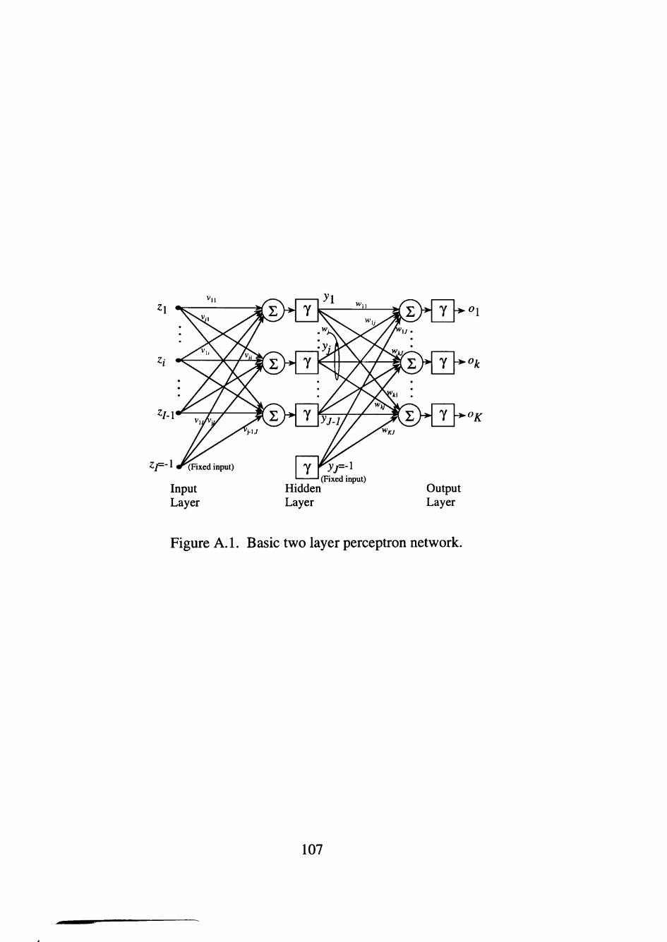
Ol

'>k

•OK

Zy=-1 ir(Fixed input)

Hidden Layer

(Fixed input) Output Layer

Figure A. 1. Basic two layer perceptron network.

107

The error signal terms ofthe output layer in this step are

^ok = - ^^^^ ) = (c ife - o J( l - Ok )ok, fork=l,2,...,K

The error signal terms ofthe hidden layer in this step are

dE ^ ^yJ = -^(^) = yM-yj)^^^ok^kp fory =1,2,. . . , J

Here net denotes the total activation at the node.

Step 5: Output layer weights are adjusted:

^kj <- u)kj+^-^ok -yp ^ork= 1, 2,..., ATand j = 1, 2,..., J

Step 6: Hidden layer weights are adjusted:

Vji <r- Vji +r\-6yj'Zi, forj=\, 2,..., Jand /= 1, 2,..., /

Step 7: If/? <P then p<- p+l,q <r- q + l, and go to Step 2; otherwise, go to Step 8.

Step 8: The training cycle is completed.

For E < Emax terminate the training session. Output weights W, V, q, and E.

\iE< Emax, then E <— 0,/? <— 1, and initiate the new training cycle by going to Step 2.

Note 1 For best results, pattems should be chosen at random from the training set.

Note 2 If a bipolar nodal fimction (f(x) = ((1 - e'y(\ + e'^) is used in Step 2, then the

error signal terms in Step 4 are computed as follows

5.* = i k -o,)(l-ol), fort= 1,2, ...,K K

^yj = i{^-y])l,^okU^kj^ fory = 1, 2,..., J k=\

108