THE INTEGRATION MODELING FRAMEWORK FOR ESTIMATING MOBILE

SOURCE EMISSIONS

By:

Hesham Rakha1 and Kyoungho Ahn2

ABSTRACT

Transportation network improvements are commonly evaluated by estimating average speeds from

a transportation/traffic model and converting them into emission estimates using an environmental

model such as MOBILE or EMFAC. Unfortunately, recent research has demonstrated that average

speed, and perhaps even simple estimates of the amount of delay and the number of vehicle stops

on a roadway, is insufficient to fully capture the environmental impacts of Intelligent

Transportation System (ITS) strategies such as adaptive traffic signal control. Specifically, for the

same average speed, one can observe widely different instantaneous speed and acceleration

profiles, each resulting in very different fuel consumption and emission levels. In an attempt to

address this limitation, the paper presents the INTEGRATION model framework for quantifying

1 Assistant Professor, Charles Via Department of Civil and Environmental Engineering. Virginia

Tech Transportation Institute, 3500 Transportation Research Plaza (0536), Blacksburg, VA 24061.

Tel: (540) 231-1505. Fax: (540) 231-1555. E-mail: hrakha@vt.edu.

2 Research Scientist, Virginia Tech Transportation Institute, 3500 Transportation Research Plaza

(0536), Blacksburg, VA 24061. E-mail: kahn@vt.edu.

Rakha and Ahn 2

the environmental impacts of ITS alternatives. The model combines car-following, vehicle

dynamics, lane changing, energy, and emission models to estimate mobile source emissions

directly from instantaneous speed and acceleration levels. The validity of the model is

demonstrated using sample test scenarios that include traveling at a constant speed, traveling at

variable speeds, stopping at a stop sign, and traveling along a signalized arterial. The study also

demonstrates that an adjustment in driver aggressiveness can provide environmental benefits that

are equivalent to the benefits of adaptive traffic signal control.

Rakha and Ahn 3

1. INTRODUCTION

With the introduction of Intelligent Transportation Systems (ITS), there is a need to evaluate and

compare alternative ITS and non-ITS investments. In comparing alternatives, a number of

Measures of Effectiveness (MOEs) are typically considered, such as vehicle delay, stops, fuel

consumption, emissions, and accident risk. The assessment of the fuel consumption and emission

impacts of alternative investments requires a highly sophisticated evaluation tool in order to

capture both the microscopic dynamics of vehicle-to-vehicle and vehicle-to-control interaction, as

well as model the intricacies of vehicle fuel consumption and emissions that result from these

vehicle dynamics.

Consequently, the assessment of the energy and emission impacts of alternative investments can be

viewed as a two-level process. The first level is the microscopic behavior of traffic, which includes

a system of car-following and lane changing models. This behavior is utilized to characterize

vehicle speed and acceleration behavior. At the second level, the energy and emissions of

hydrocarbons (HC), carbon monoxide (CO), and nitrogen oxides (NOx) are computed based on

instantaneous speed and acceleration estimates that were derived from the first level. It should be

noted that research is underway to develop models for carbon dioxide (CO2) and particulate matter

(PM).

The system of car-following models captures both steady state and non-steady state longitudinal

vehicle behavior along a roadway section. The steady state behavior is characterized by vehicles

traveling at identical cruising speeds (du/dt=0). The non-steady state behavior characterizes how

vehicles move from one steady state to another, which involves either vehicle decelerations or

accelerations. Alternatively, lane-changing behavior describes the lateral behavior of vehicles

Rakha and Ahn 4

along a roadway segment. Lane changing behavior affects the vehicle car-following behavior

especially at high intensity lane changing locations such as merge, diverge, and weaving sections.

The objective of this paper is to demonstrate how the combination of these two integrated

processes (traffic simulation model and an energy and emission model) can be utilized to evaluate

alternative ITS initiatives. It also describes the approach that is implemented within the

INTEGRATION microscopic traffic assignment and simulation software and demonstrates the

feasibility of the proposed approach using a number of traffic signal control examples. These

examples are presented in order to show the flexibility, feasibility, and validity of the

INTEGRATION framework rather than to present specific results. It should be noted that a

comparison of the INTEGRATION framework to other microscopic simulation models is beyond

the scope of this paper.

2. TRAFFIC MODELING

The combined use of traffic modeling in conjunction with energy and emission modeling can be

utilized for the evaluation of environmental impacts of ITS and non-ITS deployments. The

approach described in this paper utilizes the INTEGRATION microscopic traffic assignment and

simulation software for traffic modeling (Van Aerde and Yagar, 1988a and b; M. Van Aerde &

Assoc. Ltd., 2002a and b). The INTEGRATION model, which was developed over the past two

decades, has not only been validated against standard traffic flow theory (Rakha and Van Aerde,

1996; Rakha and Crowther, 2002), but has also been utilized for the evaluation of real-life

applications (Rakha et al., 1998; Rakha et al., 2000). Further enhancements to the INTEGRATION

model have been incorporated in order to model vehicle dynamics more accurately. These

enhancements are based on research described elsewhere (Rakha et al., 2001; Rakha and Lucic,

Rakha and Ahn 5

2002). This section provides a brief description of the INTEGRATION model and the

enhancements that have been implemented in the latest version of the model (Version 2.10) to

provide the reader with a basic understanding of the traffic-modeling component of the proposed

framework. The following section describes how energy and emission models were developed

using field data, and how these models were incorporated within the INTEGRATION software in

order to develop a fully integrated mobile emission evaluation tool. It should be noted that the

energy and emission models that are described have been enhanced to include high emitting

vehicles, effect of vehicle starts on vehicle emissions, and different types of vehicles. Subsequent

publications will describe these efforts separately.

The manner in which the INTEGRATION model represents traffic flow can be best presented by

discussing how a typical vehicle initiates its trip, selects its speed, changes lanes, and transitions

from one speed to another.

2.1 Initiation of Vehicle Trips

Prior to initiating the actual simulation logic, the individual vehicles that are to be loaded onto the

network must be generated. Vehicle types, such as passenger cars and trucks, can be pre-assigned

by modifying the model input files. As most available O-D (Origin-Destination) information is

macroscopic in nature, INTEGRATION permits the traffic demand to be specified as a time series

histogram of O-D departure rates for each possible O-D pair within the entire network. The actual

generation of individual vehicles satisfies the time-varying macroscopic departure rates that were

specified by the modeler within the model’s input data files. This model simply disaggregates an

externally specified time-varying O-D demand matrix into a series of individual vehicle departures

Rakha and Ahn 6

prior to the start of the simulation. These departure rates can be fully random (negative exponential

time headway distribution), fully uniform, or partially uniform and random.

As the externally specified demand file is disaggregated, each of the individual vehicle departures

is tagged with its desired departure time, trip origin, and trip destination, as well as a unique vehicle

number. This unique vehicle number can subsequently be utilized to trace a particular vehicle along

the entire path towards its destination. It can also be utilized to verify that subsequent turning

movements of vehicles at network diverges are assigned according to the actual vehicle

destinations, rather than arbitrary turning movement probabilities as is the case in many other

microscopic models that are not assignment-based.

The calibration of O-D demand is achieved using a maximum likelihood approach, the details of

which are beyond the scope of this paper but are provided in the literature (Van Aerde et al., 2003).

It should be noted that this approach has been successfully applied in numerous modeling studies

(Rakha et al., 1998; Rakha et al., 2000).

2.2 Steady State Car-Following Behavior

When the simulation clock reaches a particular vehicle’s scheduled departure time, an attempt is

made to enter that vehicle into the network at its origin zone. From this point, the vehicle proceeds

along its trip towards its final destination in a link-by-link fashion. Once the vehicle has selected

which lane to enter, INTEGRATION computes the vehicle’s desired initial speed on the basis of

the distance headway between the vehicle and the vehicle immediately downstream within the

same lane. This computation is based on a link-specific microscopic car-following relationship that

is calibrated macroscopically to yield the appropriate target aggregate speed-flow attributes for that

particular link. The steady state car-following model, which was proposed by Van Aerde (1995)

Rakha and Ahn 7

and Van Aerde and Rakha (1995), combines the Pipes and Greenshields models into a single-

regime model (Rakha and Crowther, 2002), as demonstrated in Equation 1. Specifically, the first

two terms constitute the Pipes steady state model (Pipes, 1953), and the third term constitutes the

Greenshields steady state model (Greenshields, 1935). This combination provides a functional form

that includes four parameters that require calibration using field data (constants c1, c2, c3 and the

roadway free-speed uf). The first two terms of the relationship provide the linear increase in vehicle

speed as a function of the distance headway, and the third term introduces curvature to the model

and ensures that the vehicle speed does not exceed the free-speed. The addition of the third term

allows the model to operate with a speed-at-capacity that does not necessarily equal the free-speed,

as is the case with the Pipes model. The Pipes model is proven to be inconsistent with a variety of

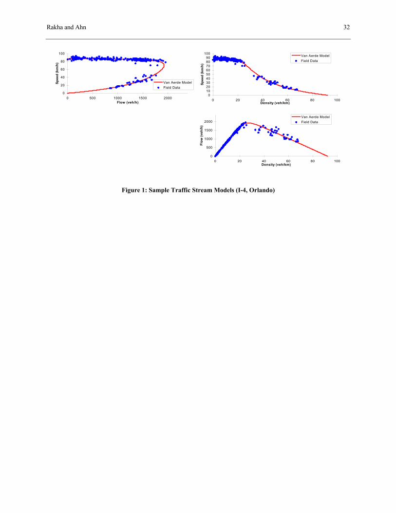
field data from different facility types, as illustrated in Figure 1. Alternatively, the Van Aerde

model overcomes the main shortcoming of the Greenshields model, which assumes that the speed-

flow relationship is parabolic, and again is inconsistent with field data from a variety of facility

types, as demonstrated in Figure 1. A detailed comparison of the Van Aerde, Pipes, and

Greenshields models is described by Rakha and Crowther (2002).

uuc

ucchf −

++= 231

[1]

Equations 2 through 5 are utilized to compute the c1, c2, and c3 constants based on four parameters;

free-speed, speed-at-capacity, capacity, and jam density (Rakha and Crowther, 2002). These

parameters can be calibrated to loop detector data (Van Aerde and Rakha, 1995) or can be input

based on typical values. It should be noted that all variables are defined in the paper Appendix.

Rakha and Ahn 8

Once the vehicle’s speed is computed, the vehicle’s position is updated every 0.1 seconds to reflect

the distance that it travels during each previous 0.1 seconds. The vehicle’s headway and speed is

then re-computed.

( )22

cf

fc

uuuum

−−

= [2]

+

=

fj u

mkc

11

2 [3]

21 mcc = [4]

c

cfc

c

uuu

cquc

c −−+−

=

21

3 [5]

2.3 Vehicle Decelerations

INTEGRATION provides separate deceleration and acceleration logic. The deceleration logic

recognizes speed differentials between the vehicle that is making desired speed decisions and the

vehicle ahead of it. It is simplest to first describe how this logic applies to a vehicle approaching a

stationary object. In this case, a vehicle will first estimate the excess headway between itself and

the vehicle ahead of it. This excess headway is defined as the residual distance that remains when

the currently available headway is reduced by the minimum headway (jam density headway).

Based on the residual headway, the vehicle computes the time it has to comfortably decelerate from

its current speed to the speed of the object/vehicle in front of it. For constant deceleration rates,

this time is equal to the residual headway divided by the average speed of the initial and final

Rakha and Ahn 9

speeds of the following vehicle. The following vehicle computes the required deceleration rate as

the speed differential divided by the deceleration time.

Alternatively, if the lead vehicle is actually moving, the following vehicle would attempt to

decelerate at a constant rate in such a manner as to attain the speed of the lead vehicle over a

distance equal to the spacing of vehicles minus the jam density headway. Of course, by the time the

following vehicle reached this location, the lead vehicle would have already moved ahead on the

highway, resulting in an asymptotic deceleration of the following vehicle to the lead vehicle’s

speed, rather than a constant deceleration. Similarly, if the lead vehicle were accelerating, the

following vehicle would only continue to decelerate until it was traveling at the same speed of the

lead vehicle. From this point onward, the following vehicle would likely begin to accelerate again,

as the increasing gap to the lead vehicle would cause the following vehicle to perceive increasing

desired speeds.

2.4 Vehicle Accelerations

The INTEGRATION model updates vehicle speeds every 0.1 seconds based on the distance

headway and speed differential between the subject vehicle and the vehicle immediately ahead of

it. Unfortunately, using this type of car-following model can result in unrealistically high vehicle

accelerations. Consequently, the model constrains vehicle accelerations using a vehicle dynamics

model that estimates the maximum vehicle acceleration (Rakha et al., 2001; Rakha and Lucic,

2002). Two important points are worth noting. First, the INTEGRATION framework currently

captures a total of 25 default vehicle types including light-duty cars, light-duty trucks, and heavy-

duty trucks. In addition, 25 user-specific vehicle parameters can be input to the model. Second,

the level of acceleration can be varied utilizing a user-defined acceleration reduction factor.

Rakha and Ahn 10

Consequently, the impact of different acceleration levels can be analyzed, as will be demonstrated

later in the paper.

The model computes the maximum acceleration based on the resultant force, as indicated in

Equation 6. Given that acceleration is the second derivative of distance with respect to time,

Equation 6 resolves to a second-order Ordinary Differential Equation (ODE) of the form

indicated in Equation 7.

MRFa −

= [6]

),( xxfx &&& = [7]

gra RRRR ++= [8]

The state-of-practice vehicle dynamics models estimate the vehicle tractive effort using Equation

9 with a maximum value based on Equation 10, demonstrated in Equation 11. Equation 10

accounts for the maximum friction force that can be maintained between the tires of the vehicle’s

tractive axle and the roadway surface. The use of Equation 11 ensures that the tractive effort

does not approach infinity at low vehicle speeds.

Equation 9 indicates that the tractive force Ft is a function of the ratio between the vehicle speed u

and the engine power P. The model assumes the vehicle power to be constant and equal to the

maximum potential power. It considers two main sources of power loss that degrade the tractive

effort produced by the truck engine: losses in the engine and losses in the transmission system with

an engine efficiency of 0.89 to 0.94, depending on the type of transmission (Society of Automotive

Engineers, 1996). Equations 10 and 11 ensure that the tractive force does not exceed the maximum

sustainable force between the vehicle tires and the pavement surface.

Rakha and Ahn 11

uPFt η3600= [9]

µtaMF 8066.9max = [10]

),(min maxFFF t= [11]

2.5 Lane Changing Logic

The above presentation of a vehicle’s selection of its desired speed, required deceleration, and

potential acceleration rate considers that vehicles stay primarily in their own lane. Unfortunately,

many of the complications within traffic flow theory arise when vehicles change lanes, either

voluntarily or when required.

INTEGRATION’s discretionary lane-changing logic is predominant when a vehicle is traveling on

a multi-lane facility and is out of the influence area of downstream diverges or lane drops. Under

these conditions, vehicles are essentially free to travel in any lane unless the user provides a bias

towards a specific lane or group of lanes. When a vehicle travels under these conditions on a multi-

lane facility without any other vehicles ahead of it, INTEGRATION’s default logic provides

incentives for vehicles to migrate towards the middle lane. This incentive leaves the left-most lane

open for any faster vehicles to get around the vehicle in question and also keeps the vehicle away

from the right shoulder lane, where vehicles entering the highway might merge in.

As soon as multiple vehicles become present on the highway, simulated vehicles tend to spread

themselves across the multiple lanes, with slower vehicles moving to the right and faster vehicles

moving to the left. This logic is especially important when slow-moving trucks are present on the

highway, as they should move to the right in order to allow faster vehicles or faster trucks to move

around them to the left. However, vehicles generally attempt to move towards lanes that provide

Rakha and Ahn 12

them with the longest headway, for longer headways will result in longer desired speeds. The

potential for a vehicle to move from its current lane into a lane with a longer headway is examined

once every 0.1 seconds, with respect to the lanes immediately adjacent to the current lane. In

addition, the potential to move to any other lanes on the facility, not necessarily adjacent to the

current lane, is examined once every second.

In deciding whether to move to an adjacent lane with a longer headway, the vehicle considers both

an absolute and a relative improvement threshold. This threshold represents the minimum

improvement that is needed for a vehicle to consider a lane change and to guard between frequent

oscillations between two lanes that provide virtually identical headways. Once a vehicle has

identified that a lane change may be desirable, it considers the availability of an acceptable gap in

that lane. Such availability depends upon the distance that is available in the desired lane both

ahead of and behind the vehicle. Both distances ensure that, at a minimum, sufficient space is

available to physically hold the vehicle and, ideally, some additional buffer. This additional buffer

is speed dependent.

In summary, INTEGRATION considers discretionary lane changes in two stages. Every 0.1

seconds it considers whether a discretionary lane change is desirable. If a change is desirable, it

determines if such a lane change is possible given the availability of a suitable gap. The

combination of these decisions results in a spreading of vehicles across all available lanes for

roadway sections outside of the influence of lane drops or diverges.

When a lane drop or diverge is being approached, vehicles will be forced to consider the model’s

mandatory and discretionary lane-changing logic. The transition from discretionary to mandatory

lane-changing logic occurs gradually as the influence area of the lane-drop or diverge area is

penetrated further. The management of this transition is best visualized by considering the presence

Rakha and Ahn 13

of both virtual softwalls and hardwalls on the roadway. Specifically, the softwall represents the first

point in space where a vehicle becomes aware of a pending mandatory lane change, and the

hardwall represents the absolute last point in space before which a mandatory lane change must

occur.

During the transition from the softwall to the hardwall, the mandatory lane change logic gradually

phases in and has four effects. First, vehicles that pass the softwall will not be able to make any

discretionary lane changes that are opposite to the direction of the required mandatory lane change.

Second, once the softwall is passed, the additional advantage that the current lane must provide (in

order to remain preferred over the lane in which the mandatory logic requires to be utilized) is

gradually increased (eventually to the point where no advantage will be sufficient to resist the

incentive to change lanes). Third, once the softwall is passed, vehicles are gradually prohibited

from passing vehicles that are on the same side as the direction of their mandatory lane change

requirement. Finally, as a vehicle transitions from the softwall to the hardwall, the vehicle will be

required to gradually come to a stop.

The first rule prohibits vehicles from moving into a lane that is temporarily preferred but that will

very shortly become heavily penalized. The second rule ensures that, when possible, vehicles move

towards the direction of the mandatory lane change before the hardwall is reached. The third rule

ensures that when vehicles are queued up in a turning base or an off-ramp, the vehicles join the

queue. The fourth rule ensures that vehicles, even when unable to initially find a gap, will not miss

their exit, off-ramp, turn lane, or turn bay.

As part of the lane-changing logic within INTEGRATION, a vehicle occupies both the lane it is

changing from and the lane it is changing to for the duration of the lane change maneuver. In doing

Rakha and Ahn 14

so, the INTEGRATION model can capture capacity losses that occur at on-ramp, off-ramp, and

weaving sections.

3. ENERGY AND EMISSION MODELING

Having estimated the vehicle speed and acceleration levels, the next step is to compute the vehicle

fuel consumption and emission rates. This section describes the VT-Micro model (Version 1.0) that

was developed to estimate light-duty hot stabilized vehicle fuel consumption and emission rates.

Initially, the data that were utilized to develop the models are described followed by a description

of the models.

It should be noted that different energy and emission models could be incorporated fairly easily,

given the modular design of the INTEGRATION framework. Currently, research is underway to

develop VT-Micro Version 2.0 by expanding energy and emission models using 101 light-duty

vehicles and light-duty trucks to capture the effects of different vehicle types, high emitting

vehicles, and the effect of cold starts on vehicle emissions. The VT-Micro Version 2.0 has been

incorporated into the INTEGRATION software and is available for public use.

The application of the model that is presented in this paper is intended to demonstrate a

comprehensive framework for quantifying traffic-related energy and emission effects rather than to

present specific results.

3.1 Raw Data Description

The data that were utilized to develop the fuel consumption and emission models were gathered on

a dynamometer at the Oak Ridge National Laboratory (ORNL) (West et al., 1997). Given that the

focus of this paper is on the development of evaluation tools that are sensitive to vehicle dynamics

Rakha and Ahn 15

and not on the ORNL data per se, these data are not described in much detail; however, they are

described elsewhere in the literature (West et al., 1997). The ORNL data were in the form of look-

up tables that included the steady state fuel consumption and emission rates as a function of the

vehicle’s instantaneous speed and acceleration levels. The emission data included hydrocarbon

(HC), carbon monoxide (CO), and nitrogen oxide (NOx) emissions. A total of eight light-duty

vehicles of various weights and engine sizes were utilized (West et al., 1997). The reference

indicates that these eight vehicles are representative of internal combustion (IC) engine technology

at the time the data were gathered.

The fuel consumption and emission rates were provided for a range of speeds from 0 to 120 km/h

(75 mph) at increments of 1.1 km/h (0.69 mph) and for a range of accelerations from –1.5 m/s2 (-5

ft/s2) to 3.6 m/s2 (12 ft/s2) at increments of 0.3 m/s2 (1 ft/s2). These data included typical driving

conditions that ranged from decelerating (acceleration less than zero), idling (acceleration and

speed equal to zero), and acceleration (acceleration greater than zero). Some of the

speed/acceleration combinations were unachievable by the vehicles (e.g. high accelerations at high

speeds). In general, the number of data points ranged from 1300 to 1600 depending on the power of

the vehicle (maximum number of potential points was 1980 points [110 speed bins × 18

acceleration bins]).

Utilizing the data for the eight vehicles, composite fuel consumption and emission surfaces were

derived by averaging across all the vehicles (West et al., 1997). The composite vehicle fuel

consumption data varied fairly linearly when the vehicle was cruising or decelerating; however, the

relationship was significantly non-linear for higher levels of acceleration (acceleration greater than

or equal to 1.2 m/s2). In terms of emissions, the HC and CO surfaces appeared to be very similar

except for the fact that CO emissions were much higher (up to 2500 mg/s in the case of CO versus

Rakha and Ahn 16

60 mg/s in the case of HC). The NOx surface appeared to be more non-linear than the HC and CO

surfaces when the vehicle was decelerating or cruising.

The authors are aware that the ORNL data utilized in developing these models are limited (only

nine vehicles), and do not account for cold-start effects or high-emitting vehicles. Furthermore,

these data were collected under hot stabilized conditions and, as a result, may not adequately

represent transient catalytic conversion behavior; however, the ORNL data were the only energy

and emission data that were available for third party usage at the time the models were developed.

The authors are currently utilizing EPA data (101 vehicles) and will be using the University of

California, Riverside data (Barth et al., 1997), which includes over 300 vehicles, to expand these

statistical energy and emission models.

3.3 Model Structure

The Virginia Tech Microscopic energy and emission model (VT-Micro) was developed from

experimentation with numerous polynomial combinations of speed and acceleration levels (Rakha

et al., 2000; Ahn et al., 2002). Linear, quadratic, cubic, and quartic terms of speed and acceleration

were tested using chassis dynamometer data collected at the ORNL. The final regression model

included a combination of linear, quadratic, and cubic speed and acceleration terms because it

provided the least number of terms with a relatively good fit to the original data (R2 in excess of

0.92 for all MOEs). Due to the simplicity of the model structure, the model can be easily

incorporated within any microscopic traffic simulation model. While a more detailed description of

the model derivation and model validation is provided in the literature (Ahn et al., 2002), it is

sufficient at this point to note that the final structure of the model, summarized in Equation 12,

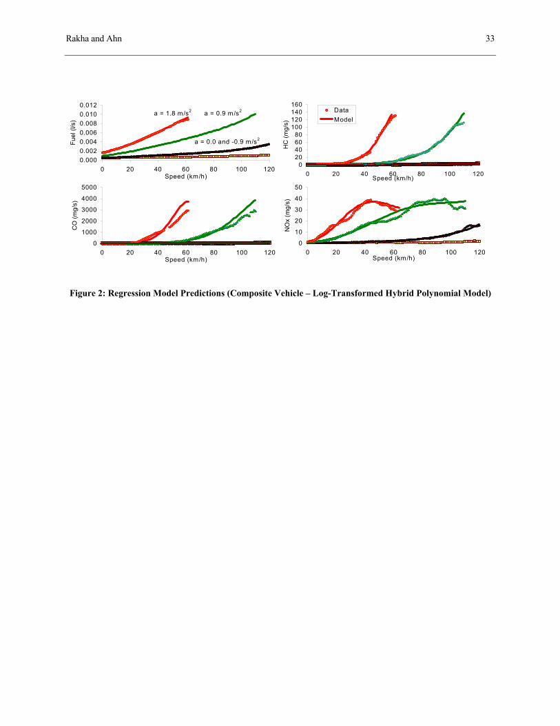
involved a logarithmic transformation of a dual-regime third order polynomial. Figure 2 further

Rakha and Ahn 17

illustrates the effectiveness of the hybrid log-transformed models in predicting vehicle fuel

consumption and emission rates as a function of a vehicle’s instantaneous speed and acceleration

levels showing good estimations against the ORNL data.

The use of polynomial speed and acceleration terms could result in multi-colinearity between the

independent variables, as a result of the dependency of these variables. A measure of multi-

colinearity, the Variance Inflation Factor (VIF) can be reduced by removing some of the regression

terms; however, this also results in a reduction in the accuracy of the model predictions. The

existence of multi-colinearity results in model estimations of the dependent variable that are

unreliable for dependent variable values outside the bounds of the original data. Consequently, the

model was maintained with the caveat that it should not be utilized for data outside the bounds of

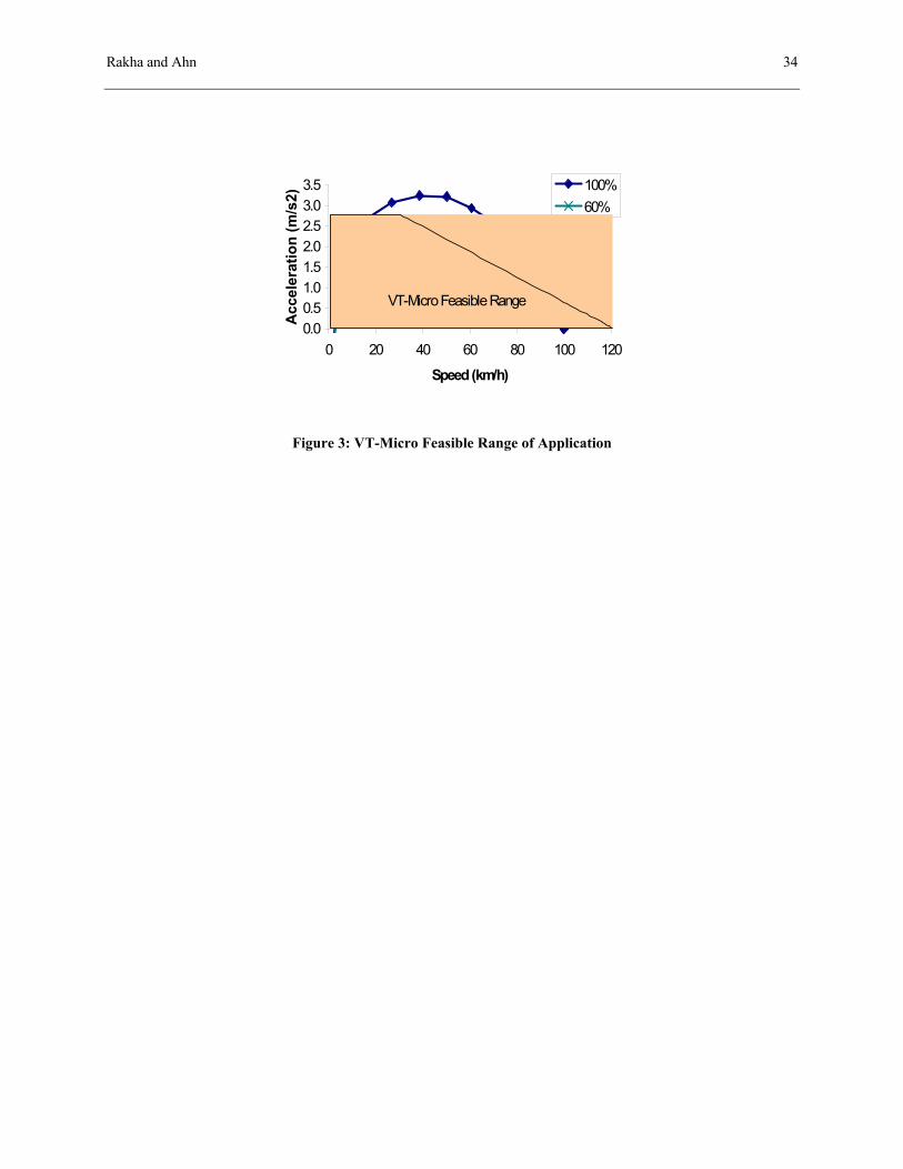
the ORNL data. Figure 3 illustrates the feasible range of the ORNL data (shaded area)

superimposed on the maximum vehicle acceleration envelope for an average composite vehicle.

The figure demonstrates that the maximum acceleration bounds exceed the VT-Micro feasible

range. Because of the existence of variable multi-colinearity, the dependent variable estimates (fuel

consumption and emissions) outside the VT-Micro feasible range were estimated using MOE

values at the boundary of the feasible regime for an identical vehicle speed. In addition, Figure 3

illustrates the vehicle speed/acceleration envelope for a vehicle that accelerates from a complete

stop to a speed of 100 km/h at an acceleration rate of 60 percent the maximum acceleration rate as

obtained from the INTEGRATION simulation model. This example is consistent with the VT-

Micro feasible range. The default maximum acceleration level embedded in the INTEGRATION

model is currently 100 percent; however, users can modify the acceleration level.

Rakha and Ahn 18

<

≥=∑ ××∑

∑ ××∑

= =

= =

0for

0for3

0,

3

0

3

0,

3

0

)(

)(

ae

aeMOEi

jieji

j

i

jieji

j

auM

auL

e [12]

4. MODEL APPLICATION

The energy and emission models that were described earlier were incorporated within the

INTEGRATION model as subroutines. Although the simulation model updates vehicle’s speed and

accelerations every 0.1 seconds, the fuel consumption and emission model estimates are made

every second, for two reasons. First, a 0.1s level resolution in computing vehicle emissions would

only increase the computational load with minimum enhancements to the emission estimate

accuracy. However, the use of a 0.1 second resolution is required for accurate modeling of gap

acceptance behavior. Consequently, the INTEGRATION model uses the average speed and

acceleration of the entire second to compute the vehicle’s fuel consumption and emission rate.

In addition to accumulating the MOEs across all the vehicles that travel between two O-D pairs, the

model accumulates MOEs across all the vehicles that traverse a specific link. Simulation runs

required only a few minutes to complete because they did not involve the simulation of a large

traffic demand., and summary statistics are provided on a vehicle, link, and O-D basis. Details of

how vehicles are generated and the specifics of the INTEGRATION model can be found elsewhere

(M. Van Aerde & Assoc. Ltd., 2002a and b).

Incorporating the previously described energy and emission models within the INTEGRATION

traffic assignment and simulation model provides a unique evaluation tool that can be utilized to

evaluate alternative ITS and non-ITS applications. This section describes a sample application of

the evaluation tool to a traffic-signalized network. A more comprehensive and realistic application

Rakha and Ahn 19

in which simulated vehicle speed profiles and energy and emission estimates were compared to

estimates that were computed using second-by-second GPS speed measurements along a signalized

arterial are provided elsewhere (Rakha et al., 2000).

The objective of the comparison presented in this paper is to demonstrate the flexibility of the

framework in analyzing the sensitivity of vehicle fuel consumption and emissions to operating

conditions. This approach represents a great enhancement to the standard correction-factor based

approaches using MOBILE or EMFAC. A detailed comparison of the proposed framework to the

current state-of-practice approach using MOBILE and EMFAC is beyond the scope of this paper

but will be presented in a future publication.

The paper demonstrates that the two main building blocks (traffic modeling and energy and

emission modeling) together produce valid fuel consumption and emission estimates, using

systematic simple scenarios. The scenarios are ordered to evaluate the tool’s various levels of

sophistication, ranging from simple constant-speed scenarios to more sophisticated types of

adaptive traffic signal control scenarios. Specifically, the initial set of scenarios involves

simulating a single vehicle driving at a constant speed in order to demonstrate the validity of the

approach under steady state conditions. The objective of this scenario is two-fold. First, it validates

the energy and emission models that are incorporated within the INTEGRATION software when

the vehicle is cruising. Second, it validates the simulated vehicle speed profile when the vehicle

does not interact with other vehicles.

In the second set of scenarios, various levels of complexity are introduced to the first scenario.

These include variable speeds along a trip and engaging in a number of complete stops. The

objective of this set of scenarios is to quantify the increase in fuel consumption and emissions as a

Rakha and Ahn 20

result of vehicle accelerations. Different levels of vehicle accelerations are analyzed in order to

identify changes in vehicle emissions as a function of vehicle acceleration levels.

The final scenario involves the interaction of vehicles with one another and with traffic control

devices considering different levels of vehicle acceleration. The objective of this scenario is to

demonstrate the validity of the combined modeling framework for the evaluation of typical traffic

operation applications.

4.1 Constant Speed Scenario

The first step in the evaluation exercise was to validate how the combined traffic and

energy/emission models operated for a number of simple constant speed scenarios. These constant

speed scenarios represent artificial scenarios given that they do not involve any vehicle

accelerations or decelerations.

The network that was utilized in the analysis was an eight-kilometer arterial section. The network

was simulated within the INTEGRATION model as four two-kilometer links in order to allow the

same network to be utilized for the remaining scenario runs.

Within the constant-speed scenario, a series of sub-scenarios were evaluated in which the

maximum speed was varied from 25 km/h to 100 km/h at 25 km/h increments (Scenarios 1a

through 1d). The objective of Scenarios 1a through 1d was two-fold. First, these scenarios validate

the use of a combined traffic/energy and emission model under constant speeds (no

deceleration/acceleration). Second, they develop relationships between the steady state speed and

the various Measures of Effectiveness (MOEs) against which the reasonableness of the model’s

responses to other scenarios can be compared.

Rakha and Ahn 21

The simulation output indicated that the instantaneous speed remained constant throughout the

entire trip. Because the vehicle traveled at a constant speed, the acceleration remained at 0 m/s2 for

the entire trip. The fuel consumption rate remained constant at approximately 0.78 liters/s for a

cruising speed of 25 km/h (0.11 liters/km). This fuel consumption rate is consistent with the ORNL

data for a constant speed of 25 km/h. The CO emission rates were approximately ten-fold higher

than the HC and NOx emission rates (8 versus 0.8 mg/s). These findings are consistent with the raw

data that were obtained from the ORNL.

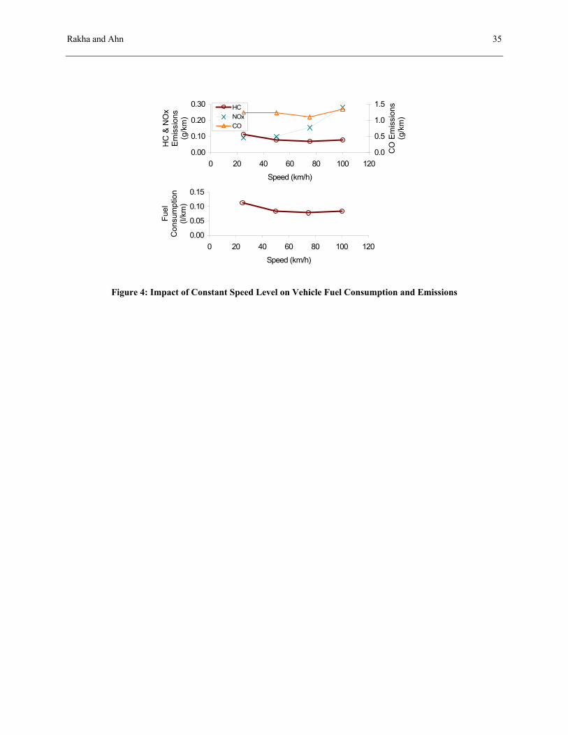
Figure 4 illustrates the impact of various constant speeds on the fuel consumption along the eight-

kilometer trip. The fuel consumption varies from a maximum of 0.113 l/km (at a constant speed of

25 km/h) to a minimum of 0.078 l/km (at a constant speed of 75 km/h). The fuel consumption

function, together with the fuel consumption rates, is consistent with the raw data that were

obtained from ORNL. Figure 4 illustrates that CO emissions are considerably higher than HC and

NOx emissions. Furthermore, the relationship indicates that fuel consumption, HC, and CO

emissions are optimum at a speed of approximately 75 km/h; however, NOx emissions are highly

sensitive to travel speeds as indicated by the four-fold increase from a speed of 25 to 100 km/h

(increase from 0.5 grams/trip to 2.0 grams/trip).

4.2 Variable Speed Scenario

The next scenario to be evaluated was a variable speed scenario (Scenario 2). In the variable speed

scenario, the free-speed was set at 25 km/h for links 1 and 3 (0-2km and 4-6km), and on links 2 and

4 was set at 75 km/h (2-4km and 6-8km). Again, a single vehicle was simulated to travel between

origin 1 and destination 2.

Rakha and Ahn 22

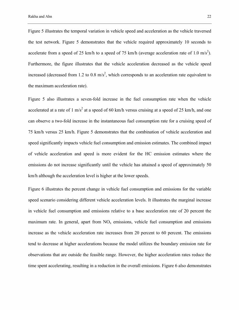
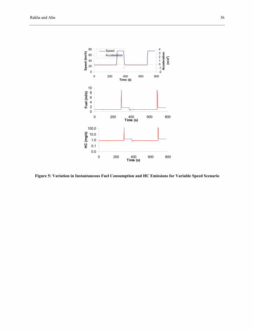
Figure 5 illustrates the temporal variation in vehicle speed and acceleration as the vehicle traversed

the test network. Figure 5 demonstrates that the vehicle required approximately 10 seconds to

accelerate from a speed of 25 km/h to a speed of 75 km/h (average acceleration rate of 1.0 m/s2).

Furthermore, the figure illustrates that the vehicle acceleration decreased as the vehicle speed

increased (decreased from 1.2 to 0.8 m/s2, which corresponds to an acceleration rate equivalent to

the maximum acceleration rate).

Figure 5 also illustrates a seven-fold increase in the fuel consumption rate when the vehicle

accelerated at a rate of 1 m/s2 at a speed of 60 km/h versus cruising at a speed of 25 km/h, and one

can observe a two-fold increase in the instantaneous fuel consumption rate for a cruising speed of

75 km/h versus 25 km/h. Figure 5 demonstrates that the combination of vehicle acceleration and

speed significantly impacts vehicle fuel consumption and emission estimates. The combined impact

of vehicle acceleration and speed is more evident for the HC emission estimates where the

emissions do not increase significantly until the vehicle has attained a speed of approximately 50

km/h although the acceleration level is higher at the lower speeds.

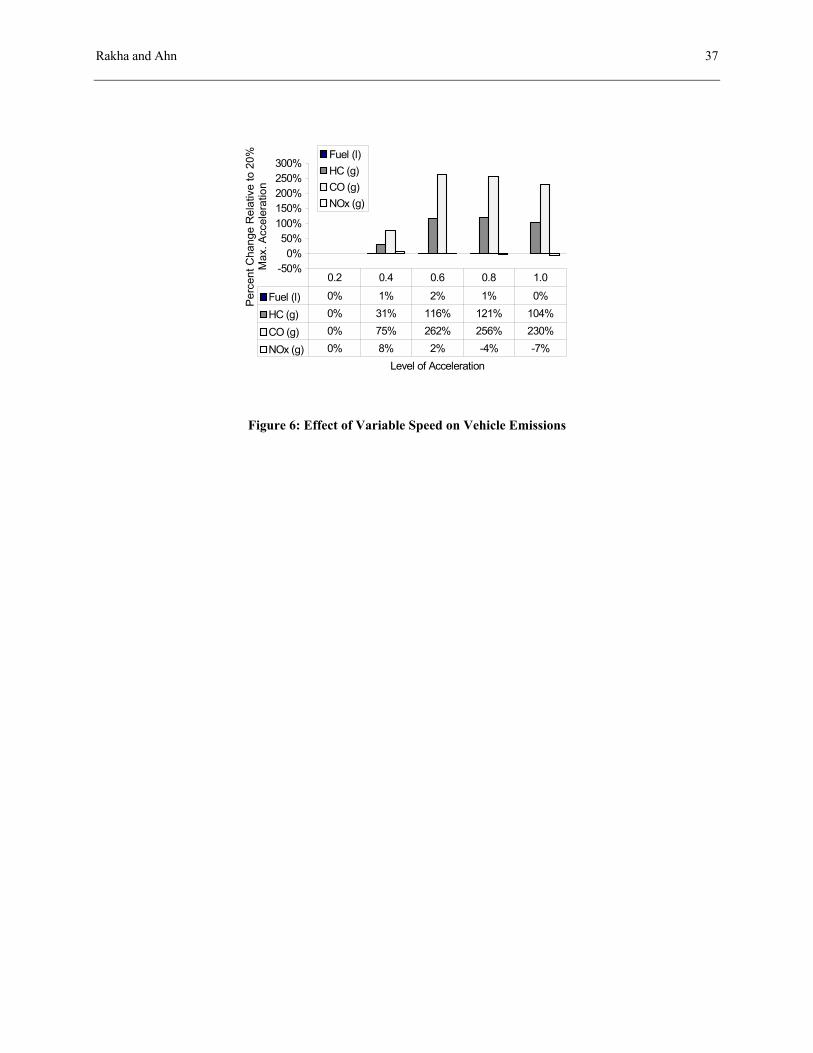
Figure 6 illustrates the percent change in vehicle fuel consumption and emissions for the variable

speed scenario considering different vehicle acceleration levels. It illustrates the marginal increase

in vehicle fuel consumption and emissions relative to a base acceleration rate of 20 percent the

maximum rate. In general, apart from NOx emissions, vehicle fuel consumption and emissions

increase as the vehicle acceleration rate increases from 20 percent to 60 percent. The emissions

tend to decrease at higher accelerations because the model utilizes the boundary emission rate for

observations that are outside the feasible range. However, the higher acceleration rates reduce the

time spent accelerating, resulting in a reduction in the overall emissions. Figure 6 also demonstrates

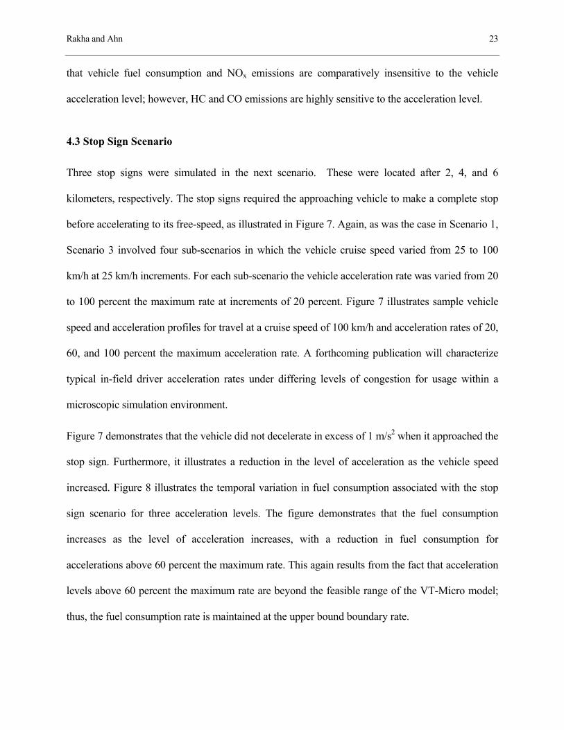
Rakha and Ahn 23

that vehicle fuel consumption and NOx emissions are comparatively insensitive to the vehicle

acceleration level; however, HC and CO emissions are highly sensitive to the acceleration level.

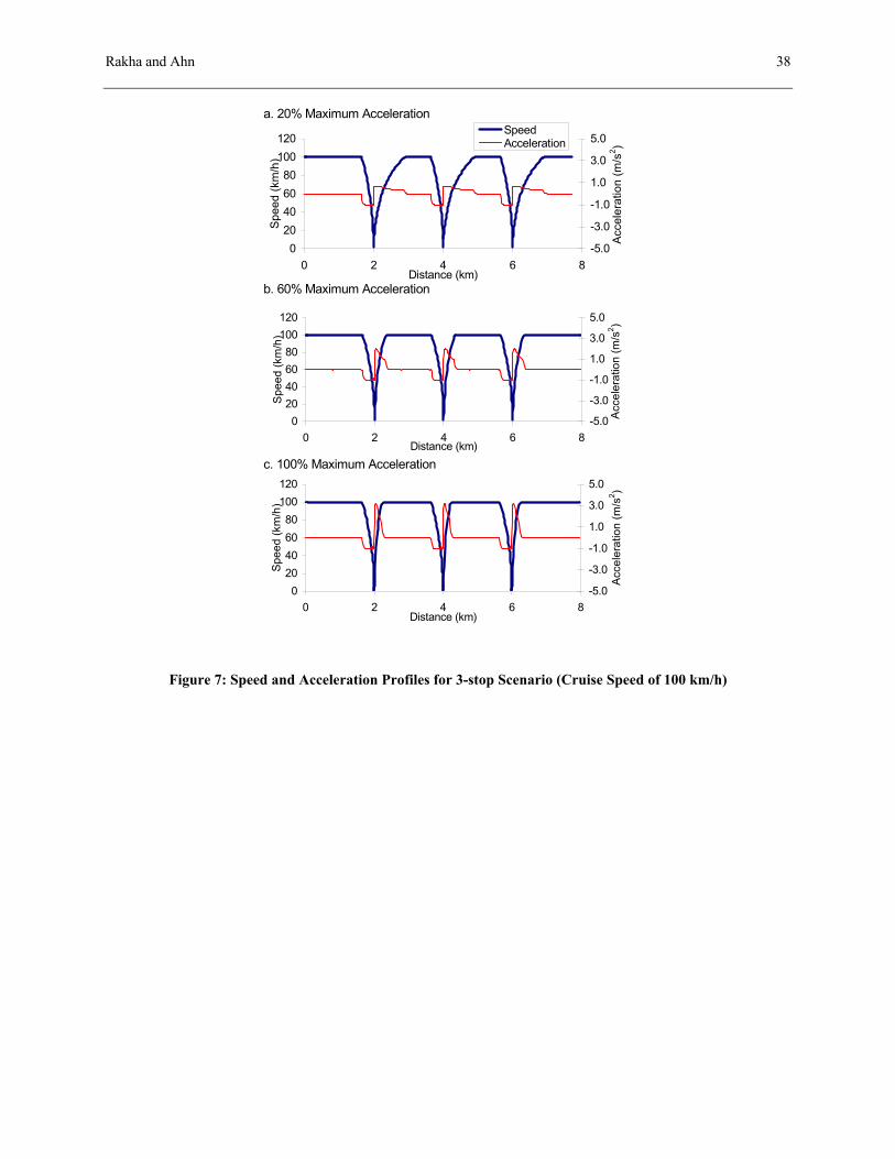
4.3 Stop Sign Scenario

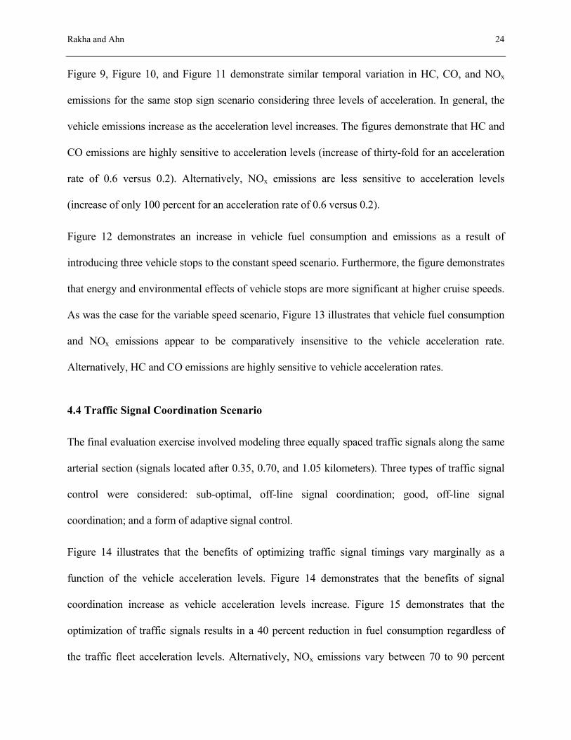
Three stop signs were simulated in the next scenario. These were located after 2, 4, and 6

kilometers, respectively. The stop signs required the approaching vehicle to make a complete stop

before accelerating to its free-speed, as illustrated in Figure 7. Again, as was the case in Scenario 1,

Scenario 3 involved four sub-scenarios in which the vehicle cruise speed varied from 25 to 100

km/h at 25 km/h increments. For each sub-scenario the vehicle acceleration rate was varied from 20

to 100 percent the maximum rate at increments of 20 percent. Figure 7 illustrates sample vehicle

speed and acceleration profiles for travel at a cruise speed of 100 km/h and acceleration rates of 20,

60, and 100 percent the maximum acceleration rate. A forthcoming publication will characterize

typical in-field driver acceleration rates under differing levels of congestion for usage within a

microscopic simulation environment.

Figure 7 demonstrates that the vehicle did not decelerate in excess of 1 m/s2 when it approached the

stop sign. Furthermore, it illustrates a reduction in the level of acceleration as the vehicle speed

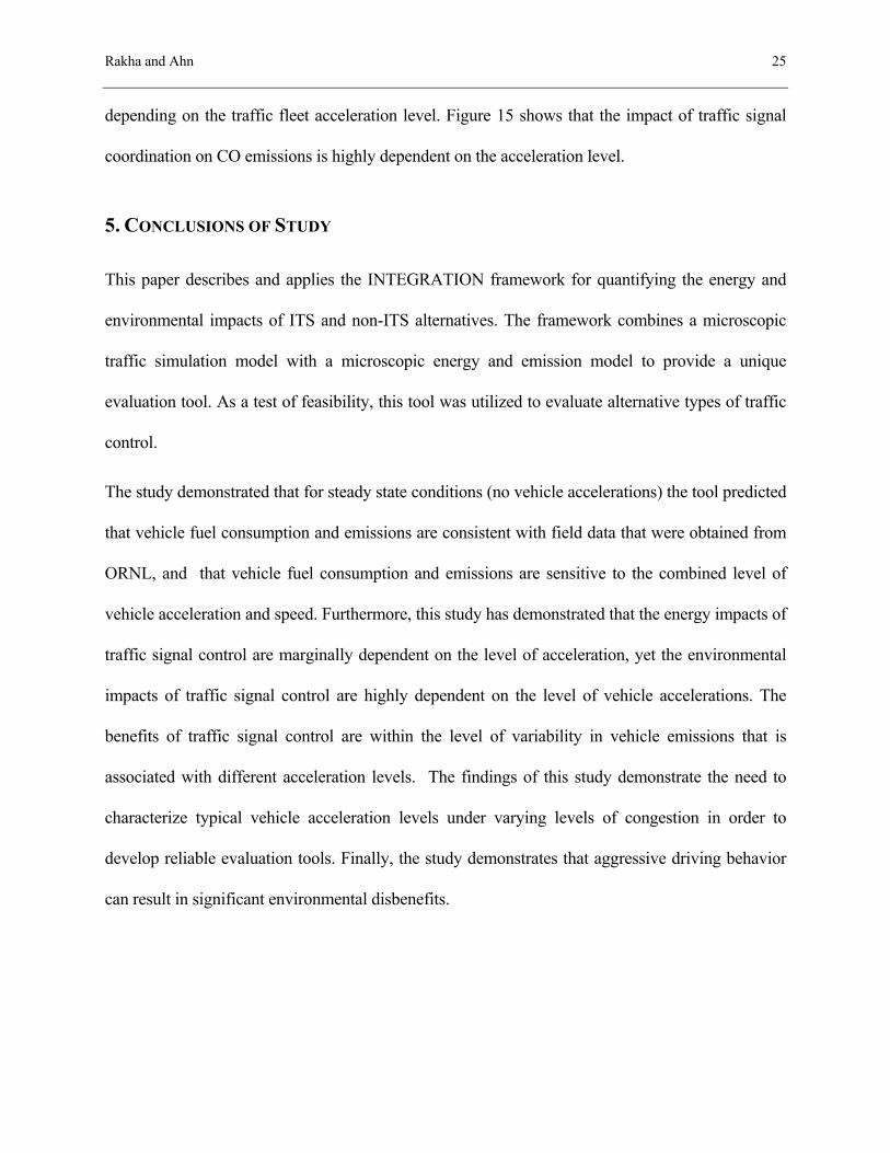
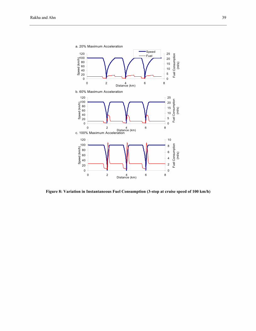
increased. Figure 8 illustrates the temporal variation in fuel consumption associated with the stop

sign scenario for three acceleration levels. The figure demonstrates that the fuel consumption

increases as the level of acceleration increases, with a reduction in fuel consumption for

accelerations above 60 percent the maximum rate. This again results from the fact that acceleration

levels above 60 percent the maximum rate are beyond the feasible range of the VT-Micro model;

thus, the fuel consumption rate is maintained at the upper bound boundary rate.

Rakha and Ahn 24

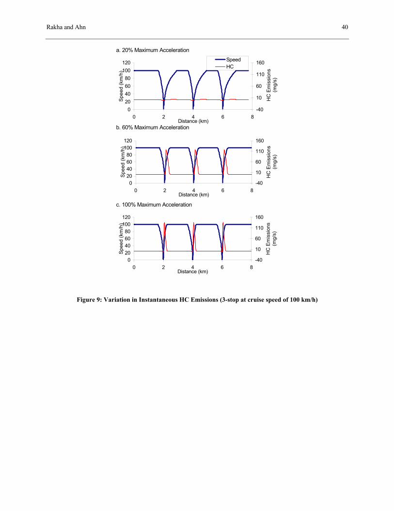
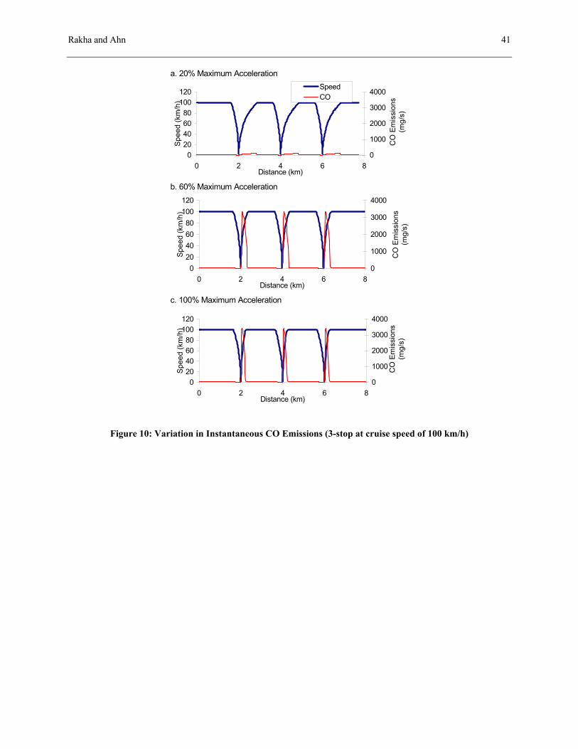
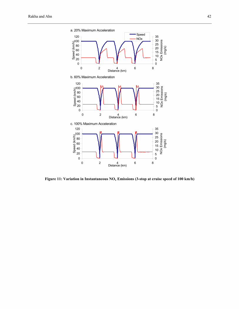
Figure 9, Figure 10, and Figure 11 demonstrate similar temporal variation in HC, CO, and NOx

emissions for the same stop sign scenario considering three levels of acceleration. In general, the

vehicle emissions increase as the acceleration level increases. The figures demonstrate that HC and

CO emissions are highly sensitive to acceleration levels (increase of thirty-fold for an acceleration

rate of 0.6 versus 0.2). Alternatively, NOx emissions are less sensitive to acceleration levels

(increase of only 100 percent for an acceleration rate of 0.6 versus 0.2).

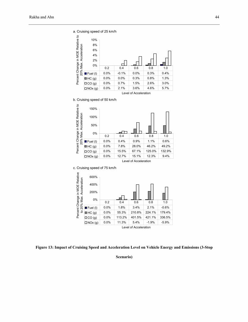
Figure 12 demonstrates an increase in vehicle fuel consumption and emissions as a result of

introducing three vehicle stops to the constant speed scenario. Furthermore, the figure demonstrates

that energy and environmental effects of vehicle stops are more significant at higher cruise speeds.

As was the case for the variable speed scenario, Figure 13 illustrates that vehicle fuel consumption

and NOx emissions appear to be comparatively insensitive to the vehicle acceleration rate.

Alternatively, HC and CO emissions are highly sensitive to vehicle acceleration rates.

4.4 Traffic Signal Coordination Scenario

The final evaluation exercise involved modeling three equally spaced traffic signals along the same

arterial section (signals located after 0.35, 0.70, and 1.05 kilometers). Three types of traffic signal

control were considered: sub-optimal, off-line signal coordination; good, off-line signal

coordination; and a form of adaptive signal control.

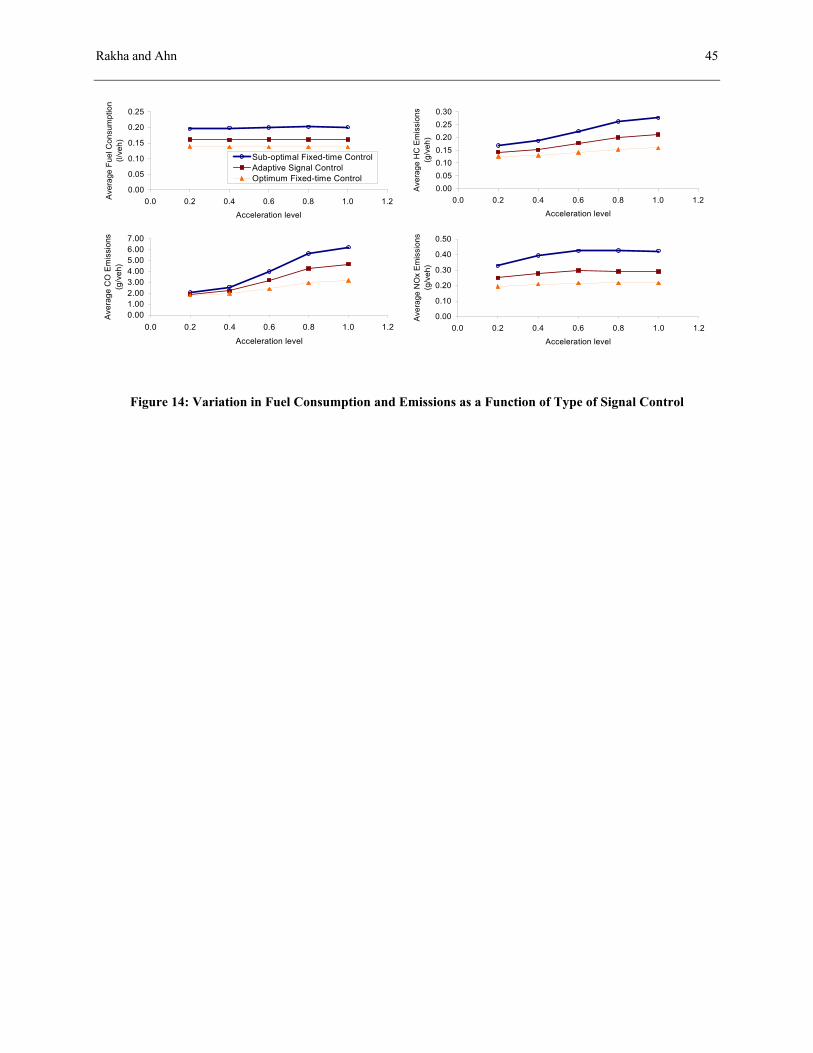
Figure 14 illustrates that the benefits of optimizing traffic signal timings vary marginally as a

function of the vehicle acceleration levels. Figure 14 demonstrates that the benefits of signal

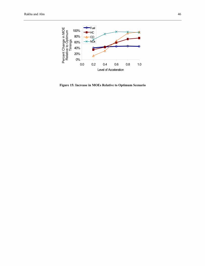
coordination increase as vehicle acceleration levels increase. Figure 15 demonstrates that the

optimization of traffic signals results in a 40 percent reduction in fuel consumption regardless of

the traffic fleet acceleration levels. Alternatively, NOx emissions vary between 70 to 90 percent

Rakha and Ahn 25

depending on the traffic fleet acceleration level. Figure 15 shows that the impact of traffic signal

coordination on CO emissions is highly dependent on the acceleration level.

5. CONCLUSIONS OF STUDY

This paper describes and applies the INTEGRATION framework for quantifying the energy and

environmental impacts of ITS and non-ITS alternatives. The framework combines a microscopic

traffic simulation model with a microscopic energy and emission model to provide a unique

evaluation tool. As a test of feasibility, this tool was utilized to evaluate alternative types of traffic

control.

The study demonstrated that for steady state conditions (no vehicle accelerations) the tool predicted

that vehicle fuel consumption and emissions are consistent with field data that were obtained from

ORNL, and that vehicle fuel consumption and emissions are sensitive to the combined level of

vehicle acceleration and speed. Furthermore, this study has demonstrated that the energy impacts of

traffic signal control are marginally dependent on the level of acceleration, yet the environmental

impacts of traffic signal control are highly dependent on the level of vehicle accelerations. The

benefits of traffic signal control are within the level of variability in vehicle emissions that is

associated with different acceleration levels. The findings of this study demonstrate the need to

characterize typical vehicle acceleration levels under varying levels of congestion in order to

develop reliable evaluation tools. Finally, the study demonstrates that aggressive driving behavior

can result in significant environmental disbenefits.

Rakha and Ahn 26

ACKNOWLEDGEMENTS

The authors would like to acknowledge the funding provided by the Intelligent Transportation

System (ITS) Implementation Center. Furthermore, the authors are indebted to the late Michel Van

Aerde, who initiated the work that is presented in this paper. Finally, the authors would like to

thank the anonymous reviewers for their thorough review and valuable comments.

Rakha and Ahn 27

APPENDIX REFERENCES

Ahn, K., Rakha, H., Trani, A., and Van Aerde, M. (2002). “Estimating vehicle fuel consumption

and emissions based on instantaneous speed and acceleration levels.” Journal of Transportation

Engineering, ASCE, 128(2), 182-190.

Barth, M., Younglove, T., Wenzel, T., Scora, G., An, F., Ross, M., and Norbeck, J. (1997).

“Analysis of model emissions from diverse in-use vehicle fleet.” Transportation Research Record,

1587, 73-84.

Greenshields, B.D. (1935). “A study in highway capacity.” Highway Research Board Proceedings,

14, 458.

M. Van Aerde and Associates, Ltd. (2002a). “INTEGRATION release 2.30 for Windows: User’s

guide – Volume I: Fundamental features.”

M. Van Aerde and Associates, Ltd. (2002b). “INTEGRATION release 2.30 for Windows: User’s

guide – Volume II: Advanced features.”

Pipes, L.A. (1953). “An operational analysis of traffic dynamics.” Journal of Applied Physics, 24:3,

274-287.

Rakha, H. and Crowther, B. (2003). “Comparison and calibration of FRESIM and INTEGRATION

steady state car-following behavior.” Transportation Research: Part A. 37 (2003) 1-27

Rakha, H. and Lucic, I. (2002). “Variable power vehicle dynamics model for estimating maximum

truck acceleration levels.” ASCE Journal of Transportation Engineering, Vol. 128(5), pp. 412-419.

Rakha and Ahn 28

Rakha, H., Lucic, I., Demarchi, S., Setti, J., and Van Aerde, M. (2001). “Vehicle dynamics model

for predicting maximum truck accelerations.” Journal of Transportation Engineering, ASCE

127(5), 418-425.

Rakha, H., Medina, A., Sin, H. Dion, F., Van Aerde, M., and Jenq, J. (2000). “Field evaluation of

efficiency, energy, environmental and safety impacts of traffic signal coordination across

jurisdictional boundaries.” Transportation Research Record, 1727, 42-51.

Rakha, H. and Van Aerde, M. (1996). “Comparison of simulation modules of TRANSYT and

INTEGRATION models.” Transportation Research Record, 1566, 1-7.

Rakha, H., Van Aerde, M., Bloomberg, L., and Huang, X. (1998). “Construction and calibration of

a large-scale micro-simulation model of the Salt Lake area.” Transportation Research Record,

1644, 93-102.

Society of Automotive Engineers. (1996). “Commercial truck and bus SAE recommended

procedure for vehicle performance prediction and charting.” SAE Procedure J2188, Warrendale,

PA.

Van Aerde M. (1995), “Single regime speed-flow-density relationship for congested and

uncongested highways.” Presented at the 74th TRB Annual Conference, Washington DC, Paper No.

950802.

Van Aerde, M. and Rakha, H. (1995). “Multivariate Calibration of Single Regime Speed-Flow-

Density Relationships.” VNIS/Pacific Rim Conference Proceedings, Seattle, WA, pp. 334-341,

ISBN 0-7803-2587-7, IEEE 95CH35776.

Rakha and Ahn 29

Van Aerde M., Rakha H., and Paramahamsan H. (2003), “Estimation of O-D Matrices: The

Relationship between Practical and Theoretical Considerations.” Accepted for presentation at the

82nd Transportation Research Board Annual Meeting, Washington DC.

Van Aerde, M. and Yagar, S. (1988a). “Dynamic integrated freeway/traffic signal networks:

Problems and proposed solutions.” Transportation Research, 22A, 6, 435-443.

Van Aerde, M. and Yagar, S. (1988b). “Dynamic integrated freeway/traffic signal networks: A

routing-based modeling approach.” Transportation Research, 22A, 6, 445-453.

West, B., McGill, R., Hodgson, J., Sluder, S., and Smith, D. (1997). "Development of Data-Based

Light-Duty Modal Emissions and Fuel Consumption Models", Society of Automotive Engineers,

Paper No. 972910., 1274-1280

APPENDIX NOTATION

The following symbols are used in this paper:

a = Instantaneous vehicle acceleration (m/s2)

c1 = fixed distance headway constant (km)

c2 = first variable distance headway constant (km2/h)

c3 = second variable distance headway constant (h)

F = residual force acting on the truck (N)

F = tractive force acting on the truck (N)

Fmax = maximum tractive force (N)

Ft = tractive force (N)

h = headway (km)

Rakha and Ahn 30

kj = jam density (veh/km)

Lei,j = Model regression coefficient for MOE “e” at speed power “i” and acceleration

power “j”

M = vehicle mass (kg)

Mta = vehicle mass on tractive axle, M × percta (kg)

Mei,j = Model regression coefficient for MOE “e” at speed power “i” and acceleration

power “j”

MOEe = instantaneous fuel consumption or emission rate (l/s or mg/s)

m = is a constant used to solve for the three headway constants (h/km)

P = engine power (kW)

qc = flow at capacity (veh/h)

R = total resistance force (N)

Ra = aerodynamic resistance (N)

Rr = rolling resistance (N)

Rg = grade resistance (N)

u = vehicle speed (km/h)

uf = free-speed (km/h)

uc = speed at capacity (km/h)

x = distance traveled (km)

η= power transmission efficiency (ranges from 0.89 to 0.94)

µ = coefficient of friction between tires and pavement

Rakha and Ahn 31

LIST OF FIGURES

Figure 1: Sample Traffic Stream Models (I-4, Orlando)

Figure 2: Regression Model Predictions (Composite Vehicle – Log-Transformed Hybrid

Polynomial Model)

Figure 3: VT-Micro Feasible Range of Application

Figure 4: Impact of Constant Speed Level on Vehicle Fuel Consumption and Emissions

Figure 5: Variation in Instantaneous Fuel Consumption and HC Emissions for Variable Speed

Scenario

Figure 6: Effect of Variable Speed on Vehicle Emissions

Figure 7: Speed and Acceleration Profiles for 3-stop Scenario (Cruise Speed of 100 km/h)

Figure 8: Variation in Instantaneous Fuel Consumption (3-stop at cruise speed of 100 km/h)

Figure 9: Variation in Instantaneous HC Emissions (3-stop at cruise speed of 100 km/h)

Figure 10: Variation in Instantaneous CO Emissions (3-stop at cruise speed of 100 km/h)

Figure 11: Variation in Instantaneous NOx Emissions (3-stop at cruise speed of 100 km/h)

Figure 12: Effect of Stops on Vehicle Fuel Consumption and Emissions

Figure 13: Impact of Cruising Speed and Acceleration Level on Vehicle Energy and Emissions (3-

Stop Scenario)

Figure 14: Variation in Fuel Consumption and Emissions as a Function of Type of Signal Control

Figure 15: Increase in MOEs Relative to Optimum Scenario

Rakha and Ahn 32

0

20

40

60

80

100

0 500 1000 1500 2000Flow (veh/h)

Spee

d (k

m/h

)

Van Aerde ModelField Data

0102030405060708090

100

0 20 40 60 80 100Density (veh/km)

Spee

d (k

m/h

)

Van Aerde ModelField Data

0

500

1000

1500

2000

0 20 40 60 80 100Density (veh/km)

Flow

(veh

/h)

Van Aerde ModelField Data

Figure 1: Sample Traffic Stream Models (I-4, Orlando)

Rakha and Ahn 33

0.0000.0020.0040.0060.0080.0100.012

0 20 40 60 80 100 120Speed (km/h)

Fuel

(l/s

)

a = 1.8 m/s2 a = 0.9 m/s2

a = 0.0 and -0.9 m/s2

020406080

100120140160

0 20 40 60 80 100 120Speed (km/h)

HC

(mg/

s)

DataModel

0

1000

2000

3000

4000

5000

0 20 40 60 80 100 120Speed (km/h)

CO

(mg/

s)

0

10

20

30

40

50

0 20 40 60 80 100 120Speed (km/h)

NO

x (m

g/s)

Figure 2: Regression Model Predictions (Composite Vehicle – Log-Transformed Hybrid Polynomial Model)

Rakha and Ahn 34

0.00.51.01.52.02.53.03.5

0 20 40 60 80 100 120

Speed (km/h)

Acc

eler

atio

n (m

/s2)

100%60%

VT-Micro Feasible Range

Figure 3: VT-Micro Feasible Range of Application

Rakha and Ahn 35

0.00

0.10

0.20

0.30

0 20 40 60 80 100 120Speed (km/h)

HC

& N

Ox

Emis

sion

s (g

/km

)

0.0

0.5

1.0

1.5

CO

Em

issi

ons

(g/k

m)

HCNOxCO

0.00

0.05

0.10

0.15

0 20 40 60 80 100 120Speed (km/h)

Fuel

C

onsu

mpt

ion

(l/km

)

Figure 4: Impact of Constant Speed Level on Vehicle Fuel Consumption and Emissions

Rakha and Ahn 36

02468

10

0 200 400 600 800Time (s)

Fuel

(ml/s

)

0

20

40

60

80

0 200 400 600 800Time (s)

Spee

d (k

m/h

)

-2-101234

Acce

lera

tion

(m/s

2 )

SpeedAcceleration

0.00.11.0

10.0100.0

0 200 400 600 800Time (s)

HC

(mg/

s)

Figure 5: Variation in Instantaneous Fuel Consumption and HC Emissions for Variable Speed Scenario

Rakha and Ahn 37

-50%0%

50%100%150%200%250%300%

Level of Acceleration

Perc

ent C

hang

e R

elat

ive

to 2

0%

Max

. Acc

eler

atio

n

Fuel (l)HC (g)CO (g)NOx (g)

Fuel (l) 0% 1% 2% 1% 0%

HC (g) 0% 31% 116% 121% 104%

CO (g) 0% 75% 262% 256% 230%

NOx (g) 0% 8% 2% -4% -7%

0.2 0.4 0.6 0.8 1.0

Figure 6: Effect of Variable Speed on Vehicle Emissions

Rakha and Ahn 38

a. 20% Maximum Acceleration

b. 60% Maximum Acceleration

c. 100% Maximum Acceleration

020406080

100120

0 2 4 6 8Distance (km)

Spee

d (k

m/h

)

-5.0

-3.0

-1.0

1.0

3.0

5.0

Acce

lera

tion

(m/s

2 )

SpeedAcceleration

020406080

100120

0 2 4 6 8Distance (km)

Spee

d (k

m/h

)

-5.0

-3.0

-1.0

1.0

3.0

5.0

Acce

lera

tion

(m/s

2 )

020406080

100120

0 2 4 6 8Distance (km)

Spee

d (k

m/h

)

-5.0

-3.0

-1.0

1.0

3.0

5.0

Acce

lera

tion

(m/s

2 )

Figure 7: Speed and Acceleration Profiles for 3-stop Scenario (Cruise Speed of 100 km/h)

Rakha and Ahn 39

a. 20% Maximum Acceleration

b. 60% Maximum Acceleration

c. 100% Maximum Acceleration

020406080

100120

0 2 4 6 8Distance (km)

Spee

d (k

m/h

)0510152025

Fuel

Con

sum

ptio

n (m

l/s)

SpeedFuel

020406080

100120

0 2 4 6 8Distance (km)

Spee

d (k

m/h

)

0

5

10

15

20

25

Fuel

Con

sum

ptio

n (m

l/s)

0

20

40

60

80

100

120

0 2 4 6 8Distance (km)

Spee

d (k

m/h

)

0

2

4

6

8

10

Fuel

Con

sum

ptio

n (m

l/s)

Figure 8: Variation in Instantaneous Fuel Consumption (3-stop at cruise speed of 100 km/h)

Rakha and Ahn 40

a. 20% Maximum Acceleration

b. 60% Maximum Acceleration

c. 100% Maximum Acceleration

020406080

100120

0 2 4 6 8Distance (km)

Spee

d (k

m/h

)

-40

10

60

110

160

HC

Em

issi

ons

(mg/

s)

SpeedHC

020406080

100120

0 2 4 6 8Distance (km)

Spee

d (k

m/h

)

-40

10

60

110

160

HC

Em

issi

ons

(mg/

s)

020406080

100120

0 2 4 6 8Distance (km)

Spee

d (k

m/h

)

-40

10

60

110

160

HC

Em

issi

ons

(mg/

s)

Figure 9: Variation in Instantaneous HC Emissions (3-stop at cruise speed of 100 km/h)

Rakha and Ahn 41

a. 20% Maximum Acceleration

b. 60% Maximum Acceleration

c. 100% Maximum Acceleration

020406080

100120

0 2 4 6 8Distance (km)

Spee

d (k

m/h

)

0

1000

2000

3000

4000

CO

Em

issi

ons

(mg/

s)

SpeedCO

020406080

100120

0 2 4 6 8Distance (km)

Spee

d (k

m/h

)

0

1000

2000

3000

4000

CO

Em

issi

ons

(mg/

s)

020406080

100120

0 2 4 6 8Distance (km)

Spee

d (k

m/h

)

0

1000

2000

3000

4000

CO

Em

issi

ons

(mg/

s)

Figure 10: Variation in Instantaneous CO Emissions (3-stop at cruise speed of 100 km/h)

Rakha and Ahn 42

a. 20% Maximum Acceleration

b. 60% Maximum Acceleration

c. 100% Maximum Acceleration

020406080

100120

0 2 4 6 8Distance (km)

Spee

d (k

m/h

)

05101520253035

NO

x Em

issi

ons

(mg/

s)

SpeedNOx

020406080

100120

0 2 4 6 8Distance (km)

Spee

d (k

m/h

)

05101520253035

NO

x Em

issi

ons

(mg/

s)

020406080

100120

0 2 4 6 8Distance (km)

Spee

d (k

m/h

)

05101520253035

NO

x Em

issi

ons

(mg/

s)

Figure 11: Variation in Instantaneous NOx Emissions (3-stop at cruise speed of 100 km/h)

Rakha and Ahn 43

0%1000%2000%3000%4000%5000%6000%7000%

Speed (km/h)

% C

hang

e R

elat

ive

to C

onst

ant

Spee

dFuel (l) 730% 793% 860% 886%

HC (g) 713% 1187% 2675% 3579%

CO (g) 719% 1844% 4369% 5764%

NOx (g) 803% 1046% 1028% 891%

25 50 75 100

Figure 12: Effect of Stops on Vehicle Fuel Consumption and Emissions

Rakha and Ahn 44

a. Cruising speed of 25 km/h

b. Cruising speed of 50 km/h

c. Cruising speed of 75 km/h

0%2%4%6%8%

10%

Level of Acceleration

Perc

ent C

hang

e in

MO

E R

elat

ive

to

20%

Max

. Acc

eler

atio

n

Fuel (l) 0.0% -0.1% 0.0% 0.3% 0.4%

HC (g) 0.0% 0.0% 0.3% 0.8% 1.3%

CO (g) 0.0% 0.7% 1.5% 2.6% 3.0%

NOx (g) 0.0% 2.1% 3.6% 4.6% 5.7%

0.2 0.4 0.6 0.8 1.0

0%

50%

100%

150%

Level of Acceleration

Perc

ent C

hang

e in

MO

E R

elat

ive

to

20%

Max

. Acc

eler

atio

n

Fuel (l) 0.0% 0.4% 0.9% 1.1% 0.6%

HC (g) 0.0% 7.8% 28.0% 46.2% 49.2%

CO (g) 0.0% 15.5% 67.1% 125.0% 132.9%

NOx (g) 0.0% 12.7% 15.1% 12.3% 9.4%

0.2 0.4 0.6 0.8 1.0

0%

200%

400%

600%

Level of Acceleration

Perc

ent C

hang

e in

MO

E R

elat

ive

to 2

0% M

ax. A

ccel

erat

ion

Fuel (l) 0.0% 1.8% 3.4% 2.1% -0.6%

HC (g) 0.0% 55.3% 210.8% 224.1% 179.4%

CO (g) 0.0% 113.2% 401.5% 421.1% 336.5%

NOx (g) 0.0% 11.3% 5.4% -1.9% -5.9%

0.2 0.4 0.6 0.8 1.0

Figure 13: Impact of Cruising Speed and Acceleration Level on Vehicle Energy and Emissions (3-Stop

Scenario)

Rakha and Ahn 45

0.00

0.05

0.10

0.15

0.20

0.25

0.0 0.2 0.4 0.6 0.8 1.0 1.2Acceleration level

Aver

age

Fuel

Con

sum

ptio

n (l/

veh)

Sub-optimal Fixed-time ControlAdaptive Signal ControlOptimum Fixed-time Control

0.000.050.100.150.200.250.30

0.0 0.2 0.4 0.6 0.8 1.0 1.2Acceleration level

Aver

age

HC

Em

issi

ons

(g/v

eh)

0.001.002.003.004.005.006.007.00

0.0 0.2 0.4 0.6 0.8 1.0 1.2Acceleration level

Aver

age

CO

Em

issi

ons

(g/v

eh)

0.00

0.10

0.20

0.30

0.40

0.50

0.0 0.2 0.4 0.6 0.8 1.0 1.2Acceleration level

Aver

age

NO

x Em

issi

ons

(g/v

eh)

Figure 14: Variation in Fuel Consumption and Emissions as a Function of Type of Signal Control

Rakha and Ahn 46

0%

20%

40%

60%

80%

100%

0.0 0.2 0.4 0.6 0.8 1.0Level of Acceleration

Perc

ent C

hang

e in

MO

E R

elat

ive

to O

ptim

um

Tim

ings

FuelHCCONOx

Figure 15: Increase in MOEs Relative to Optimum Scenario