IMPORTANT COPYRIGHT INFORMATION The following PDF article was originally published in the Journal of the Air & Waste Management Association and is fully protected under the copyright laws of the United States of America. The author of this article alone has been granted permission to copy and distribute this PDF. Additional uses of the PDF/article by the author(s) or recipients, including posting it on a Web site, are prohibited without the express consent of the Air & Waste Management Association. If you are interested in reusing, redistributing, or posting online all or parts of the enclosed article, please contact the offices of the Journal of the Air & Waste Management Association at Phone: +1-412-232-3444, ext. 6027 E-mail: journal@awma.org Web: www.awma.org You may also contact the Copyright Clearance Center for all permissions related to the Journal of the Air & Waste Management Association: www.copyright.com.

Copyright © 2006 Air & Waste Management Association

Estimating Gas Emissions from Multiple Sources Using aBackward Lagrangian Stochastic Model

Zhiling Gao, Raymond L. Desjardins, and Ronald P. van HaarlemResearch Branch, Agriculture and Agri-Food Canada, Ottawa, Ontario, Canada

Thomas K. FleschDepartment of Earth and Atmospheric Sciences, University of Alberta, Edmonton, Alberta, Canada

ABSTRACTManure storage tanks and animals in barns are importantagricultural sources of methane. To examine the possibil-ity of using an inverse dispersion technique based on abackward Lagrangian Stochastic (bLS) model to quantifymethane (CH4) emissions from multiple on-farm sources,a series of tests were carried out with four possible sourceconfigurations and three controlled area sources. The sim-ulated configurations were: (C1) three spatially separateground-level sources, (C2) three spatially separate sourceswith wind-flow disturbance, (C3) three adjacent ground-level sources to simulate a group of adjacent sources withdifferent emission rates, and (C4) a configuration with aground level and two elevated sources. For multipleground-level sources without flow obstructions (C1 andC3), we can use the condition number (�, the ratio of theuncertainty in the calculated emission rate to the uncer-tainty in the predicted ratio of concentration to emissionrate) to evaluate the applicability of this inverse disper-sion technique and a preliminary threshold of � � 10 isrecommended. For multiple sources with wind distur-bance (C2) or an even more complex configuration in-cluding ground level and elevated sources (C4), a low � isnot sufficient to provide reasonable discrete and totalemission rates. The effect of flow obstructions can beneglected as long as the distance between the source andthe measurement location is greater than approximately10 times the height of the flow obstructions. This studyshows that the bLS model has the potential to provideaccurate discrete emission rates from multiple on-farmemissions of gases provided that certain conditions aremet.

INTRODUCTIONOn-farm greenhouse gas emissions often originate from avariety of sources in close proximity to each other. Exam-ples of such sources are animals in barns, waste lagoons,and manure piles, etc. Quantifying these sources is im-portant to improve greenhouse gas (GHG) inventoriesand test the impact of management practices for reducingGHG emissions.1,2

Composite sources are difficult to quantify, eitherbecause of the difficulty of isolating each source, or thelimitations of measurement techniques in the particularenvironment. Accordingly, on farm, one might: (1) iden-tify air inlets and outlets in the barn and make a massbalance calculation of barn emissions,3,4 (2) use a floatingchamber to measure lagoon emissions,5,6 (3) surround themanure stockpile with wind and concentration sensorsand use a meteorological mass difference (MMD) tech-nique,7,8 or (4) modify MMD using concentration mea-surements at a single height.9,10 All of these techniquescan provide valuable information, but all have their lim-itations. For example, it is expensive to instrument a barnand results might be affected by leaky barns, chambermeasurements cannot be representative of the wholesource,11 and source size limitations of the MMD methodmake it impossible to measure the whole plume frommost sources.12

Inverse-dispersion calculations provide a simple tech-nique for inferring emission rates.13,14 Here, a downwindconcentration of the gas of interest is used to infer theemission rate with the help of an atmospheric dispersionmodel. This technique is commonly used to either quan-tify emissions from a single source,15–20 or in some casesto quantify total emissions from a composite source.21

The accuracy obtained in these studies is claimed to besimilar to those provided by other noninterference tech-niques. This technique can also be used to deduce thediscrete emission rates from a composite source, and ithas great potential to simplify the measurement problem.

Using an inverse-dispersion technique to infer emis-sions from composite sources is mathematically straight-forward.22 It requires multiple concentration measure-ments (at least as many downwind locations as there arediscrete sources), which provide a set of linear equationsand allow calculation of each component emission ratefor each single measurement period. Unfortunately, these

IMPLICATIONSA bLS model has been demonstrated to have the potentialto estimate discrete greenhouse gas emissions from com-posite on-farm sources. Therefore, this technique can beused to provide accurate greenhouse gas and ammoniaemission estimates simultaneously from multiple on-farmsources such as barns, lagoons, and manure piles. Thistechnique has several advantages over conventional green-house gas measurement techniques, such as the ability tomeasure emissions from large area sources.

TECHNICAL PAPER ISSN:1047-3289 J. Air & Waste Manage. Assoc. 58:1415–1421DOI:10.3155/1047-3289.58.11.1415Copyright 2008 Air & Waste Management Association

Volume 58 November 2008 Journal of the Air & Waste Management Association 1415

“multisource” problems have a tendency to be ill condi-tioned, that is, calculated emissions are susceptible to verylarge errors. Crenna et al.23 describe how the degree of illconditioning, quantified by the condition number (�), isinfluenced by the geometry of the source-sensor loca-tions.22 Therefore, although there is the practical poten-tial to use the inverse-dispersion technique to quantifycomposite sources, the method is limited by the potentialfor large errors. The objective of this study is to investigatethe potential of inverse dispersion calculations for multi-source problems in several typical agricultural situations.

METHODOLOGYThe inverse-dispersion technique requires an atmosphericdispersion model to calculate the theoretical relationshipbetween emissions and a downwind concentration. Weuse a backward Lagrangian stochastic (bLS) dispersionmodel for these calculations. The software WindTrax2.0(Thunder Beach Scientific) combines the bLS model de-scribed by Flesch et al.13,14 with an interface where sourcesand sensors are conveniently mapped.

For a multi-source problem, the bLS model computesthousands of trajectories upwind of each concentrationsensor, with the emission-concentration relationships cal-culated between all of the sources and sensors.WindTrax2.0 then solves the following system of equa-tions:

a11Q1 � a12Q2 � a13Q3 � Cb � C1 (1)

a21Q1 � a22Q2 � a23Q3 � Cb � C2 (2)

am1Q1 � am2Q2 � am3Q3 � Cb � Cm (3)

where Cb is the background concentration, and the coef-ficient aij relating emission rates Qj to measured concen-trations Ci is obtained from the particle models. When thenumber of known concentrations Ci is greater than thenumber of unknown sources, the solution will be the bestfit in the least squares. The proportional recovery is cal-culated as:

�Q1bLS � Q2bLS � Q3bLS�/�Q1 � Q2 � Q3�, (4)

where QnbLS are the calculated emission rates and Qn arethe release rates.

CONDITION NUMBERWhen estimating the discrete emission rates from multi-ple sources, an inevitable issue is that of ill condition-ing.22 The condition number, �, is defined as the ratio ofthe uncertainty in the calculated QbLS to the uncertaintyin CL/Q (CL, the line average concentration):

� � � ��CL

Q �sim

� � � ��CL

Q �sim

� 1 �� (5)

A system is called ill conditioned is when it is very sensi-

tive to small changes in coefficients, �CL

Q�sim

. The accuracy

of the bLS model for multiple source configurations canbe indicated by �. Within WindTrax2.0, � can be calcu-lated from the sensitivity parameter, � (� � 10�). Thevalue of � is 0 (i.e., � � 1) when estimating the emissionrate from single source, but it varies with the source con-figuration of multiple sources. In a companion study,Flesch et al.24 looked in more detail at the problem ofinferring multiple emission rates from composite emis-sion sites. They demonstrated that multisource problemstend to be ill conditioned, with the calculated emissionsbeing very sensitive to errors in either the dispersionmodel calculations or the concentration measurements.

EXPERIMENTAL SETUPMethane (CH4) release trials were carried out at the Cen-tral Experimental Farm in Ottawa, Ontario, during the fallof 2006. The site was relatively flat and there was nosignificant obstruction to the wind flow. The surface wascovered with grass 10 cm high during the measurementperiod.

CH4 MeasurementsCH4 concentrations were measured using a GasFinder MCopen-path laser system developed by Boreal Laser Inc.This laser system was operated in the near infrared spec-trum (1653 nm) and consisted of a central unit that con-trolled reflectors and eight laser transmitter heads. Thelaser beam was transferred from the control unit to thetransmitter head via fiber-optic cable. The beam from thetransmitter was directed to a reflector through the air, andthe returning signal was transmitted to the central unitvia coaxial cable. A portion of the laser beam was passedthrough an onboard reference cell to provide the contin-uous calibration updates. These two optical signals werethen converted into electrical waveforms and then wereprocessed by the internal computer to obtain the CH4

concentration along the laser path. The resolution of theMC laser system was given by the manufacture as 1ppmm, which in this study corresponded to an analyticaldetection limit of 0.025 ppmv.

Laser SetupFive laser paths were set up to isolate the emissions fromthree CH4 sources: S1, S2 and S3 (Figure 1). The lasers weresituated at 0.75 m above the ground surface and the pathlength between each laser transmitter and its correspond-ing reflector was 40 m. The location of the sources isshown in Figure 1. The laser orientation with respect tothe sources only permitted evaluation of the bLS modelwhen the wind was predominantly from the west.

CH4 Releases and Sources ConfigurationsCH4 with 99% purity was released from three grids (2 �2 m) through three mass flow controllers (MKS Instru-ments Inc.) at flow rates of 7 L�min�1 for S1, 14 L�min�1

for S2, and 20 L�min�1 for S3 (that is 77, 156, and 221 mgCH4�sec�1, respectively). The background concentration

Gao, Desjardins, van Haarlem, and Flesch

1416 Journal of the Air & Waste Management Association Volume 58 November 2008

for each release period was calculated using the averagebackground concentration before and after each 15-minrelease. Release periods with a significant backgroundshift before and after the release period were not used.

During the experiment, the lasers’ orientations werenot changed, but the release grids were moved to meet therequirement of different configurations. Four sources con-figurations were simulated:

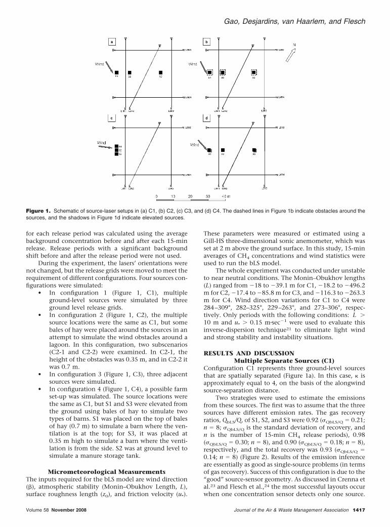
• In configuration 1 (Figure 1, C1), multipleground-level sources were simulated by threeground level release grids.

• In configuration 2 (Figure 1, C2), the multiplesource locations were the same as C1, but somebales of hay were placed around the sources in anattempt to simulate the wind obstacles around alagoon. In this configuration, two subscenarios(C2-1 and C2-2) were examined. In C2-1, theheight of the obstacles was 0.35 m, and in C2-2 itwas 0.7 m.

• In configuration 3 (Figure 1, C3), three adjacentsources were simulated.

• In configuration 4 (Figure 1, C4), a possible farmset-up was simulated. The source locations werethe same as C1, but S1 and S3 were elevated fromthe ground using bales of hay to simulate twotypes of barns. S1 was placed on the top of balesof hay (0.7 m) to simulate a barn where the ven-tilation is at the top; for S3, it was placed at0.35 m high to simulate a barn where the venti-lation is from the side. S2 was at ground level tosimulate a manure storage tank.

Micrometeorological MeasurementsThe inputs required for the bLS model are wind direction(), atmospheric stability (Monin–Obukhov Length, L),surface roughness length (z0), and friction velocity (u*).

These parameters were measured or estimated using aGill-HS three-dimensional sonic anemometer, which wasset at 2 m above the ground surface. In this study, 15-minaverages of CH4 concentrations and wind statistics wereused to run the bLS model.

The whole experiment was conducted under unstableto near neutral conditions. The Monin–Obukhov lengths(L) ranged from �18 to �39.1 m for C1, �18.2 to �496.2m for C2, �17.4 to �85.8 m for C3, and �116.3 to �263.3m for C4. Wind direction variations for C1 to C4 were284–309°, 282–325°, 229–263°, and 273–306°, respec-tively. Only periods with the following conditions: L 10 m and u* 0.15 m�sec�1 were used to evaluate thisinverse-dispersion technique21 to eliminate light windand strong stability and instability situations.

RESULTS AND DISCUSSIONMultiple Separate Sources (C1)

Configuration C1 represents three ground-level sourcesthat are spatially separated (Figure 1a). In this case, � isapproximately equal to 4, on the basis of the alongwindsource-separation distance.

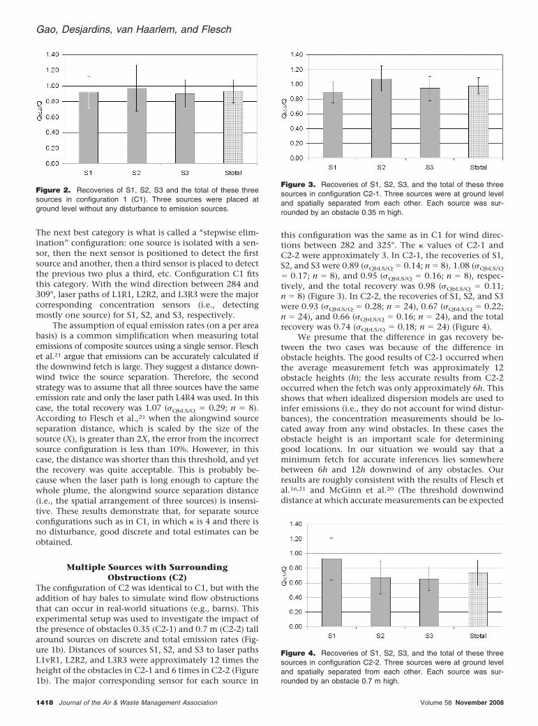
Two strategies were used to estimate the emissionsfrom these sources. The first was to assume that the threesources have different emission rates. The gas recoveryratios, QbLS/Q, of S1, S2, and S3 were 0.92 (�QbLS/Q � 0.21;n � 8; �QbLS/Q is the standard deviation of recovery, andn is the number of 15-min CH4 release periods), 0.98(�QbLS/Q � 0.30; n � 8), and 0.90 (�QbLS/Q � 0.18; n � 8),respectively, and the total recovery was 0.93 (�QbLS/Q �0.14; n � 8) (Figure 2). Results of the emission inferenceare essentially as good as single-source problems (in termsof gas recovery). Success of this configuration is due to the“good” source-sensor geometry. As discussed in Crenna etal.23 and Flesch et al.,24 the most successful layouts occurwhen one concentration sensor detects only one source.

Figure 1. Schematic of source-laser setups in (a) C1, (b) C2, (c) C3, and (d) C4. The dashed lines in Figure 1b indicate obstacles around thesources, and the shadows in Figure 1d indicate elevated sources.

Gao, Desjardins, van Haarlem, and Flesch

Volume 58 November 2008 Journal of the Air & Waste Management Association 1417

The next best category is what is called a “stepwise elim-ination” configuration: one source is isolated with a sen-sor, then the next sensor is positioned to detect the firstsource and another, then a third sensor is placed to detectthe previous two plus a third, etc. Configuration C1 fitsthis category. With the wind direction between 284 and309°, laser paths of L1R1, L2R2, and L3R3 were the majorcorresponding concentration sensors (i.e., detectingmostly one source) for S1, S2, and S3, respectively.

The assumption of equal emission rates (on a per areabasis) is a common simplification when measuring totalemissions of composite sources using a single sensor. Fleschet al.21 argue that emissions can be accurately calculated ifthe downwind fetch is large. They suggest a distance down-wind twice the source separation. Therefore, the secondstrategy was to assume that all three sources have the sameemission rate and only the laser path L4R4 was used. In thiscase, the total recovery was 1.07 (�QbLS/Q � 0.29; n � 8).According to Flesch et al.,21 when the alongwind sourceseparation distance, which is scaled by the size of thesource (X), is greater than 2X, the error from the incorrectsource configuration is less than 10%. However, in thiscase, the distance was shorter than this threshold, and yetthe recovery was quite acceptable. This is probably be-cause when the laser path is long enough to capture thewhole plume, the alongwind source separation distance(i.e., the spatial arrangement of three sources) is insensi-tive. These results demonstrate that, for separate sourceconfigurations such as in C1, in which � is 4 and there isno disturbance, good discrete and total estimates can beobtained.

Multiple Sources with SurroundingObstructions (C2)

The configuration of C2 was identical to C1, but with theaddition of hay bales to simulate wind flow obstructionsthat can occur in real-world situations (e.g., barns). Thisexperimental setup was used to investigate the impact ofthe presence of obstacles 0.35 (C2-1) and 0.7 m (C2-2) tallaround sources on discrete and total emission rates (Fig-ure 1b). Distances of sources S1, S2, and S3 to laser pathsL1vR1, L2R2, and L3R3 were approximately 12 times theheight of the obstacles in C2-1 and 6 times in C2-2 (Figure1b). The major corresponding sensor for each source in

this configuration was the same as in C1 for wind direc-tions between 282 and 325°. The � values of C2-1 andC2-2 were approximately 3. In C2-1, the recoveries of S1,S2, and S3 were 0.89 (�QbLS/Q � 0.14; n � 8), 1.08 (�QbLS/Q

� 0.17; n � 8), and 0.95 (�QbLS/Q � 0.16; n � 8), respec-tively, and the total recovery was 0.98 (�QbLS/Q � 0.11;n � 8) (Figure 3). In C2-2, the recoveries of S1, S2, and S3were 0.93 (�QbLS/Q � 0.28; n � 24), 0.67 (�QbLS/Q � 0.22;n � 24), and 0.66 (�QbLS/Q � 0.16; n � 24), and the totalrecovery was 0.74 (�QbLS/Q � 0.18; n � 24) (Figure 4).

We presume that the difference in gas recovery be-tween the two cases was because of the difference inobstacle heights. The good results of C2-1 occurred whenthe average measurement fetch was approximately 12obstacle heights (h); the less accurate results from C2-2occurred when the fetch was only approximately 6h. Thisshows that when idealized dispersion models are used toinfer emissions (i.e., they do not account for wind distur-bances), the concentration measurements should be lo-cated away from any wind obstacles. In these cases theobstacle height is an important scale for determininggood locations. In our situation we would say that aminimum fetch for accurate inferences lies somewherebetween 6h and 12h downwind of any obstacles. Ourresults are roughly consistent with the results of Flesch etal.16,21 and McGinn et al.20 (The threshold downwinddistance at which accurate measurements can be expected

Figure 2. Recoveries of S1, S2, S3 and the total of these threesources in configuration 1 (C1). Three sources were placed atground level without any disturbance to emission sources.

Figure 3. Recoveries of S1, S2, S3, and the total of these threesources in configuration C2-1. Three sources were at ground leveland spatially separated from each other. Each source was sur-rounded by an obstacle 0.35 m high.

Figure 4. Recoveries of S1, S2, S3, and the total of these threesources in configuration C2-2. Three sources were at ground leveland spatially separated from each other. Each source was sur-rounded by an obstacle 0.7 m high.

Gao, Desjardins, van Haarlem, and Flesch

1418 Journal of the Air & Waste Management Association Volume 58 November 2008

seems to vary with the details of each situation. In Fleschet al.16 this distance was somewhere between 5h and 35h,in Flesch et al.21 the recommendation was 20h, and inMcGinn et al.20 accurate measurements were made at 9h).Additionally, although � (�3) in these cases is low, it doesnot account for the influence of the wind disturbances.Thus a low � alone is not sufficient for a successfulinference and does not guarantee the success of a fieldapplication.

Multiple Adjacent Sources (C3)On farms, a very common configuration consists of sev-eral adjacent sources with different emission rates. In thisstudy, three ground-level sources were placed side by sideto simulate this situation (Figure 1c). The � value of thisconfiguration is approximately 38. The recoveries of S1,S2, and S3 were 4.31 (�QbLS/Q � 7.20; n � 10), �1.70(�QbLS/Q � 9.34; n � 10), and 1.50 (�QbLS/Q � 2.92; n �10), respectively. Despite the very inaccurate results forthe component emissions, the total recovery was a perfect1.00 (�QbLS/Q � 0.17; n � 10) (Figure 5). In contrast, whenthe three sources were assumed to have an identical emis-sion rate, the laser paths L1R1, L2R2, and L3R3 were usedto estimate total emission rates from S1, S2, and S3, andthe total recoveries were 0.47 (�QbLS/Q � 0.17; n � 10),0.69 (�QbLS/Q � 0.14; n � 10), and 0.91 (�QbLS/Q � 0.17;n � 10), respectively, which confirms that moving sensorsdownwind of the multiple sources can improve the emis-sion estimates.21 This case demonstrates that, when mul-tiple sources are not adequately separated from eachother, unrealistic discrete estimates from these sourcesmay be provided by the bLS model, but in these situationsit is still possible to deduce the total emissions.

Simulating an On-Farm Situation (C4)In this configuration, S1 and S3 were elevated to 0.70 and0.35 m to simulate CH4 emissions from more complexconditions (Figure 1d). The � value of this configurationwas approximately 3. With the wind directions between229 and 263°, the distances of S1 to laser path L1R1 andS3 to L3R3 were approximately 6 and 12 times the heightof the S1 and S3 elevations, respectively, and the majorsensors for S1 and S3 were the same as in C1. The discreterecoveries of S1, S2, and S3 were 1.35 (�QbLS/Q � 0.33; n �8), 0.65 (�QbLS/Q � 0.14; n � 8), and 0.95 (�QbLS/Q � 0.18;

n � 8), respectively, and the total recovery was 0.91(�QbLS/Q � 0.15; n � 8) (Figure 6). Results show that,under this more complex configuration with both ele-vated and ground-level sources, the bLS model cannotprovide reliable estimates for all discrete sources exceptfor S3. This is probably due to the large distance betweenL3R3 and S3 (12 times the height of S3 elevation) inconjunction with the long distance between L3R3 and S1and S2 and thus the impacts of the disturbance of S1 andS3 obstacles on their corresponding gas dispersions atL3R3 is minor. Poor discrete emission rates of S1 and S2are probably caused by the poor allocation from totalemission because of the flow disturbance from S1.

Above all, in terms of differentiating the componentemission rates, the worst case is clearly C3, which is dis-tinguished by the higher � value. The poorer results for C2and C4 occur presumably because of wind disturbances, afactor that is completely irrelevant to geometry problems.The � value is very important as a predictor of success, butit is not sufficient as the only predictor. This is most likelybecause WindTrax cannot deal with disturbance to dis-persion, for example, sources configurations of C1, C2,and C4 were the same if we ignored the wind flow distur-bance. Therefore, the � of C2 and C4 do not indicate theactual source configurations. However, for the undis-turbed source configurations such as C1 and C3, C3 doeshave a much greater � than C1, which explains the betterestimates in C1 than in C3. It indicates that � is a usefulindicator for multiple sources, if there is no wind distur-bance to gas dispersion.

PRACTICAL SUGGESTIONSFor estimating discrete emissions from multiple sources,the ideal condition is that each sensor should only cap-ture the plume from one source. Although this ideal re-quirement is hard to meet on farm, some useful sugges-tions are provided through this study.

Multiple Sources without Flow ObstructionsFor cases such as C1, the requirements of the distancebetween the source and concentration measurement maynot be met for all wind directions. Hence, one can run themodel with different wind directions to select the mostappropriate wind directions so as to determine the place-ments of laser paths. As discussed earlier, the � value can

Figure 6. Recoveries of S1, S2, S3, and the total of these threesources in configuration 4 (C4). S1 and S3 were elevated 0.7 and0.35 m from the ground, respectively, whereas S2 was at groundlevel.

Figure 5. Recoveries of S1, S2, S3, and the total of these threesources in configuration 3 (C3). Three sources were placed togetherwithout obstacles.

Gao, Desjardins, van Haarlem, and Flesch

Volume 58 November 2008 Journal of the Air & Waste Management Association 1419

also be used to evaluate the degree of ill conditioning anddetermine the best laser setup, and a stepwise eliminationconfiguration, which is directly related to a low � value,will normally be a good sensor-source configuration.

For multiple adjacent sources such as the case of C3,the estimates obtained from these sources were unsatis-factory, because the � values were too high; however,assuming these sources have similar emission rates canprovide acceptable total estimates. Flesch et al.21 esti-mated that when downwind concentrations are measuredbeyond two times the distance between two sources, theerror from this incorrect source configuration is less than10%, and when the measurements are made beyond adistance of 10 times the heights or widths, an area sourcecan be considered as a single point source.25 This studyalso indicates that longer alongwind fetches betweensources and concentration sensors can provide more sat-isfactory estimates. Thus, under this condition it is impos-sible to estimate discrete emission rates from multiplesources using this bLS model, and one needs to move themeasurement sensor farther downwind of the sources toobtain accurate total emissions.

Multiple Sources with Flow ObstructionsThe � value is inappropriate to evaluate a source config-uration with flow disturbance. Although C2 and C4 had asimilar source separation distance to C1, the presence ofobstacles around the source in C2 or the combination ofground level and elevated sources in C4 resulted in dis-crete emission rates much worse than in the case of C1,even though the � value was slightly less than that in C1.Thus, for multiple sources with wind flow disturbancesuch as for C2, the alongwind distance of 12 times theobstacle height between two sources is considered a pre-liminary threshold.

CONCLUSIONSInverse dispersion techniques provide a method of calcu-lating the emission components of composite sources.This study investigated the application of this techniqueto mock composite configurations common for agricul-tural sources. Using synthetic gas sources and open-pathlasers placed in various configurations and adding windflow obstructions in the source configuration, we foundthe following:

(1) The inverse dispersion technique applied to mul-tisource situations can result in an ill-conditionedmathematical problem. The degree of ill condi-tioning is determined by the source-sensor geom-etry and is quantified by the � value. Configura-tions having large � are prone to large errors. Inthis experiment, we had good success in deducingemissions when � � 5, but poor results when � 30.

(2) Although a low � is a prerequisite for calculatingcomponent emissions, it is not sufficient for thesuccess of a multisource emission inference. Ob-stacles that create wind disturbances invalidatethe idealized dispersion models used in this tech-nique and cause poor emission estimates evenwhen � is low.

(3) The effect of wind obstacles can be neglected by

choosing concentration measurement locationsfar downwind from the obstacles. We found goodresults if our measurements were approximately12 obstacle heights downwind (but poor results 6heights downwind).

We suggest that two conditions are required for an accu-rate application to composite sources: (1) that the mea-surement configuration (source-sensor geometry) is asso-ciated with a low � value (we suggest � � 10), and (2) thatif there are wind obstacles of height h near the sources,that measurement locations be approximately 10h fromthese obstacles. The first condition is the more difficult tojudge in a field setting. Although � can be calculated inadvance using a dispersion model, we know from experi-ence that � is minimized if each member of the set ofconcentration sensors detects only the emission plume ofa single source (each source isolated by a sensor). In thisexperiment we also had a suitably low � for a stepwiseelimination configuration, in which one source was iso-lated with a sensor, then the next sensor was positionedto see the first source plus another, then a third sensor wasplaced to see the previous two plus a third, etc. Unaccept-ably high � values occurred when all of the sensors saw ablended plume from all of the sources.

REFERENCES1. Webb, J.; Menzi, H.; Pain, B.F.; Misselbrook, T.H.; Dammgen, U.;

Hendriks, H.; Dohler, H. Managing Ammonia Emissions from Live-stock Production in Europe; Environ. Pollut. 2005, 135, 399-406.

2. Weiska, A.; Vabitsch, A.; Olesen, J.E.; Schelde, K.; Michel, J.; Friedrich,R.; Kaltschmitt, M. Mitigation of Greenhouse Gas Emissions in Euro-pean Conventional and Organic Dairy Farming; Agric. Ecosyst. Environ.2006, 112, 221-232.

3. Jungbluth, T.; Hartung, E.; Brose, G. Greenhouse Gas Emissions fromAnimal Houses and Manure Stores; Nutr. Cycl. Agroecosyst. 2001, 60,133-145.

4. Hoff, S.J.; Bundy, D.S.; Nelson, M.A.; Zelle, B.C.; Jacobson, L.D.; Heber,A.J.; Ni, J.; Zhang, Y.; Koziel, J.A.; Beasly, D.B. Emissions of Ammonia,Hydrogen Sulphide, and Odor before, during, and after Slurry Removalfrom a Deep-Pit Swine Finisher; J. Air & Waste Manage. Assoc. 2006, 56,581-590.

5. Hobbs, P.J.; Misselbrook, T.H.; Cumby, T.R. Production and Emissionof Odours and Gases from Ageing Pig Waste; J. Agric. Engineer. Res.1999, 72, 291-298.

6. Peu, P.; Beline, F.; Martinez, J. A Floating Chamber for EstimatingNitrous Oxide Emissions from Farm Scale Treatment Units for Live-stock Wastes; J. Agric. Engineer. Res. 1999, 73, 101-104.

7. Harper, L.A.; Denmead, O.T.; Freney, J.R.; Byers, F.M. Direct Measure-ments of Methane Emissions from Grazing and Feedlot Cattle; J. Anim.Sci. 1999, 77, 3903-3912.

8. Khan, R.Z.; Muller, C.; Sommer, S.G. Micrometeorological Mass Bal-ance Technique for Measuring CH4 Emission from Stored Cattle Slur-ry; Bio. Fertil. Soils 1997, 24, 442-444.

9. Cassel, T.; Ashbaugh, L.; Flocchini, R.; Meyer, D. Ammonia EmissionFactors for Open-Lot Dairies: Direct Measurements and Estimation byNitrogen Intake; J. Air & Waste Manage. Assoc. 2005, 55, 826-833.

10. Cassel, T.; Ashbaugh, L.; Flocchini, R.; Meyer, D. Ammonia Flux fromOpen-Lot Dairies: Development of Measurement Methodology andEmission Factors; J. Air & Waste Manage. Assoc. 2005, 55, 816-825.

11. Johnson, K.; Huyler, M.; Westberg, H.; Lamb, B.; Zimmerman. P.Measurement of Methane Emissions from Ruminant Livestock Using aSF6 Tracer Technique; Environ. Sci. Technol. 1994, 28, 359-362.

12. Harper, L.A. Comparisons of Methods to Measure Ammonia Volatil-ization in the Field. In Ammonia Volatilization from Urea Fertilizers;Bock, B.R., Kissel, D.E., Eds.; Tennessee Valley Authority: MuscleShoals, AL, 1988; pp 93-109.

13. Flesch, T.K.; Wilson, J.D.; Yee, E. Backward-Time Lagrangian Stochas-tic Dispersion Models and Their Applications to Estimate GaseousEmissions; J. Appl. Meteorol. 1995, 34, 1320-1332.

14. Flesch, T.K.; Wilson, J.D.; Harper, L.A.; Crenna, B.P.; Sharpe, R.R.Deducing Ground-Air Emissions from Observed Trace-Gas Concentra-tions: a Field Trial; J. Appl. Meteorol. 2004, 43, 487-502.

15. Denmead, O.T.; Chen, D.; Turner, D.; Li, U.; Edis, R. Micrometeoro-logical Measurements of Ammonia Emissions during Phases of theGrazing Rotation of Irrigated Dairy Pastures. Presented at SuperSoil

Gao, Desjardins, van Haarlem, and Flesch

1420 Journal of the Air & Waste Management Association Volume 58 November 2008

2004, 3rd Australian New Zealand Soils Conference, University ofSydney, Sydney, Australia, December 2004.

16. Flesch, T.K.; Wilson, J.D.; Harper, L.A. Deducing Ground-Air Emis-sions from Observed Trace Gas Concentrations: a Field Trial withWind Disturbance; J. Appl. Meteorol. 2005, 44, 475-484.

17. Flesch, T.K.; Wilson, J.D.; Harper, L.A.; Todd, R.W.; Cole, N.A. Deter-mining Ammonia Emissions from a Cattle Feedlot with an InverseDispersion Technique; Agric. For. Meteorol. 2007, 144, 139-155.

18. Laubach, J.; Kelliher, F.M. Methane Emissions from Dairy Cows: Com-paring Open-Path Laser Measurements to Profile-Based Techniques;Agric. For. Meteorol. 2005, 135, 340-345.

19. McBain, M.C.; Desjardins, R.L. The Evaluation of a Backward Lagrang-ian Stochastic (bLS) Model to Estimate Greenhouse Gas Emissionsfrom Agricultural Sources Using a Synthetic Tracer Gas; Agric. For.Meteorol. 2005, 135, 61-72.

20. McGinn, S.M.; Flesch, T.K.; Harper, L.A.; Beauchemin, K.A. An Ap-proach for Measuring Methane Emissions from Whole Farms; J. Envi-ron. Qual. 2006, 35, 14-20.

21. Flesch, T.K.; Wilson, J.D.; Harper, L.A.; Crenna, B.P. Estimating GasEmissions from a Farm with an Inverse-Dispersion Technique; Atmos.Environ. 2005, 38, 4863-4874.

22. Gerald, C.F.; Wheatley, P.O. Applied Numerical Analysis; Addison-Wes-ley: Reading, MA, 1984; p 579.

23. Crenna, B.P.; Wilson, J.D.; Flesch, T.K. Influence of Source-SensorGeometry in Multi-Source Emission Rate Estimates; Atmos. Environ.,submitted for publication.

24. Flesch, T.K.; Harper, L.A.; Desjardins, R.L.; Gao, Z.; Crenna, B.P. Multi-Source Emissions Determination Using an Inverse-Dispersion Tech-nique; J. Appl. Meteorol. Climatol., submitted for publication.

25. Phillip, V.R.; Scholtens, R.; Lee, D.S.; Garland, F.A.; Sneath, R.W. AReview of Methods for Measuring Emission Rates of Ammonia fromLivestock Buildings and Slurry or Manure Stores. Part 1: Assessment ofBasic Approaches; J. Agric. Eng. Res. 2000, 77, 355-364.

About the AuthorsZhiling Gao is a postdoctoral fellow, Dr. Raymond L. Des-jardins is a research scientist, and Ronald P. van Haarlem isa research assistant in the Research Branch of Agricultureand Agri-Food Canada, Ottawa, ON, Canada. Thomas K.Flesch is a research scientist in the Department of Earthand Atmospheric Sciences at the University of Alberta inEdmonton, Alberta, Canada. Please address correspon-dence to: Dr. Raymond L. Desjardins, Research Branch,Agriculture and Agri-Food Canada, 960 Carling Avenue,Ottawa, Ontario, Canada K1A 0C6; phone: 1-613-759-1522; e-mail: Desjardins@agr.gc.ca.

Gao, Desjardins, van Haarlem, and Flesch

Volume 58 November 2008 Journal of the Air & Waste Management Association 1421