A Three-Dimensional Backward Lagrangian Footprint Model For A Wide Range Of Boundary-Layer...

A THREE-DIMENSIONAL BACKWARD LAGRANGIAN FOOTPRINTMODEL FOR A WIDE RANGE OF BOUNDARY-LAYER

STRATIFICATIONS

N. KLJUN1,!, M. W. ROTACH1 and H. P. SCHMID2

1Institute for Atmospheric and Climate Science ETH, Zurich, Switzerland; 2Department ofGeography, Indiana University, Bloomington, Indiana, U.S.A.

(Received in final form 10 September 2001)

Abstract. We present a three-dimensional Lagrangian footprint model with the ability to predict thearea of influence (footprint) of a measurement within a wide range of boundary-layer stratificationsand receptor heights. The model approach uses stochastic backward trajectories of particles and sat-isfies the well-mixed condition in inhomogeneous turbulence for continuous transitions from stableto convective stratification. We introduce a spin-up procedure of the model and a statistical treatmentof particle touchdowns which leads to a significant reduction of CPU time compared to conventionalfootprint modelling approaches. A comparison with other footprint models (of the analytical andLagrangian type) suggests that the present backward Lagrangian model provides valid footprint pre-dictions under any stratification and, moreover, for applications that reach across different similarityscaling domains (e.g., surface layer to mixed layer, for use in connection with aircraft measurementsor with observations on high towers).

Keywords: Backward trajectories, Boundary-layer stability, Density kernel estimation, Lagrangianparticle model, Source area, Spin-up.

1. Introduction

Common micrometeorological techniques for determining the trace gas concentra-tion or flux at a fixed receptor downwind of a source give little information aboutthe source location and size. Moreover, these concentrations and fluxes vary as aresult of the turbulence state of the planetary boundary layer. Thus, a quantitativedescription of the surface flux budgets of atmospheric trace gases on a regionalscale is far from trivial, as any source near the ground could potentially contributeto the measured concentration or flux.

In order to describe the area of influence to a measurement, Schmid and Oke(1990) define a ‘source area’ as that part of the upwind area which contains theeffective sources and sinks contributing to a given measurement point. The term‘footprint’ is specified as the relative contribution from each element of the up-wind surface area source to the measured concentration or vertical flux (Schueppet al., 1990). It can be interpreted as the probability that trace gas emitted from a

! E-mail: [email protected]

Boundary-Layer Meteorology 103: 205–226, 2002.© 2002 Kluwer Academic Publishers. Printed in the Netherlands.

206 N. KLJUN ET AL.

given elemental source reaches the measurement point. Functions describing therelationship between the spatial distribution of surface sources (or sinks) and ameasured signal have been termed the ‘footprint function’ or the ‘source weightfunction’ (Schmid, 1994).

In recent years, several models have been proposed to estimate the size of thefootprint and its dependence on the height of the measurement, wind velocity,surface roughness, heterogeneous underlying surfaces, and atmospheric stability.Basically, a footprint can be derived using three different methods: Lagrangianstochastic dispersion models, in most cases assuming Gaussian turbulence (e.g.,Leclerc and Thurtell, 1990; Horst and Weil, 1992; Flesch et al., 1995; Rannik etal., 2000), analytical solutions of the diffusion equation by applying a K-theorymodel (e.g., Schuepp et al., 1990; Schmid and Oke, 1990; Wilson and Swaters,1991; Horst and Weil, 1992) or large eddy simulation (e.g., Leclerc et al., 1997).See Schmid (2001) for a review.

Ideally, a footprint model is expected to yield information for the design ofexperiments under various environmental and experimental conditions (i.e., dif-ferent measurement heights, atmospheric stability, and surface properties), andfor the correct interpretation of measurement results. However, none of the ana-lytical footprint models is valid outside the surface layer, whereas most of theLagrangian particle models used for footprint modelling fulfill the well-mixedcondition (Thomson, 1987) for only one given stability regime. On the other hand,large eddy simulation (LES) is highly CPU time intensive, and is notoriously weakin predicting the eddy structure close to the surface.

The present footprint model is based on the Lagrangian stochastic particle dis-persion model developed by Rotach et al. (1996) in its two-dimensional version,and later extended to three dimensions by de Haan and Rotach (1998). This modelsatisfies the well-mixed condition continuously for stable to convective conditions,as well as for receptors above the surface layer (e.g., for use in connection withaircraft measurements as done in Schuepp et al., 1990, and others). The modelemploys a recently established approach using stochastic backward trajectories ofparticles (Flesch et al., 1995). This approach allows one to calculate the footprintfor a measurement point instead of an average over a sensor volume without acoordinate transformation that requires horizontal homogeneity of the flow. Inspatially inhomogeneous flow, ‘forward’ (dispersion) models need to simulate apotentially large number of sources, to resolve the inhomogeneity. Their compu-tational expense is proportional to the number of sources needed (Luhar and Rao,1994).

The following section describes a backward-trajectory model, and its applic-ation in the determination of a flux or concentration footprint. The sensitivity ofthe footprint to the initial velocities and the atmospheric stability is discussed inSection 3. Finally, in Section 4, the approach is evaluated indirectly by comparingthe model results with corresponding estimates of the analytical footprint models

A THREE-DIMENSIONAL BACKWARD LAGRANGIAN FOOTPRINT MODEL 207

FSAM and SAM of Schmid (1997), based on Horst and Weil (1992), as well aswith another footprint model of the Lagrangian type after Rannik et al. (2000).

2. Model Description

2.1. THE LAGRANGIAN STOCHASTIC PARTICLE MODEL

The Lagrangian formulation assumes that the diffusion of a passive scalar releasedfrom a surface source is statistically equivalent to the dispersion of an ensemble ofparticles that impact the ground within the surface source and thereafter ‘carry’ thescalar. Each of those ‘marked’ particles moves independently of all the others andis advected downwind by the mean flow and dispersed by turbulence. The diffusionof the scalar is described by a stochastic differential equation (the generalisedLangevin equation), which determines the evolution of a Lagrangian particle atposition x = (x, y, z) with the particle velocity u = (u + u!, v!, w!) in space andtime (Thomson, 1987)

du!i = ai(x, u, t) dt + bij (x, u, t) d"j

dx = u dt . (1)

The functions ai determine the correlated part depending on turbulent velocitycomponents, functions bij the uncorrelated random contribution of the accelera-tion of the velocity components u!

i (i = 1, 2, 3) with the increments d"j from aGaussian distribution with zero mean and variance dt .

The well-mixed condition (Thomson, 1987) implies that the Fokker–Planckequation is an Eulerian form of (1) and can be used to determine the func-tions ai and bij of Equation (1). For stationary turbulence, the correspondingFokker–Planck equation can be written

aiPtot = #

#u!j

(BijPtot) + $i , (2)

where Ptot denotes the probability density function (PDF) of the particle velocities,and (applying Einstein’s summation convention)

2Bij = bikbjk (3)#$i

#u!i

= " #

#xi

(u!iPtot) . (4)

We follow Thomson (1987) in using the behaviour of the structure function inthe inertial subrange to specify Bij . Thomson (1987) shows that Bij is non-zeroonly for i = j . Thus, we use Bii = B# = 1

2 C0 % (here, the summation convention

208 N. KLJUN ET AL.

does not apply). C0 is a universal constant for the structure function, taken to be3 in the present simulations (Rotach et al., 1996; Du, 1995, 1997) and % is thedissipation rate of turbulence kinetic energy. Since B# is not an explicit function ofu, Equation (2) can be rewritten as

ai = 1Ptot

("B# Qi + $i ) (5)

with

Qi = "#Ptot

#u!i

. (6)

The conventional approach of using a Lagrangian model for footprint estimatesis to release particles at the surface source and track their trajectories until they havepassed the receptor location. The footprint can then be computed after a coordinatetransformation that requires horizontal homogeneity of the flow. Alternatively, itis possible to calculate the trajectories of a Lagrangian model in a backward timeframe. In this case, the trajectories are initiated at the measurement point itself andare tracked backward in time, with a negative time step, from the sensor to anypotential surface source (cf. Flesch et al., 1995). The advantage of this approach(in the following denoted as LPDM-B) is that only the trajectories that pass exactlythrough the measurement point need to be followed and therefore all of the cal-culated trajectories can be used directly and without coordinate transformation. Inprinciple, the backward approach can consider sources at arbitrary levels or geo-metries with one single simulation, but is specific to a given measurement height,in contrast to the forward approach.

Thomson (1987) stated that the only change required to adapt the Langevinequation for reverse diffusion is a sign change of the first term of the coefficient ai

in Equation (5). Therefore, for the LPDM-B, the derivative Qi in Equation (6) ismodified to

Qi = +#Ptot

#u!i

. (7)

Turbulence is not generally a Gaussian process, but for many applications, theassumption of Gaussian turbulent diffusion is an acceptable approximation. A ma-jor exception is the convective boundary layer (CBL) where vertical dispersion isdramatically different from that in neutral or stable boundary layers since largecoherent updrafts and downdrafts dominate the vertical flow statistics. Therefore,the PDF of the vertical velocity in the CBL is non-Gaussian. Lagrangian stochasticmodelling is able to account for the effects of skewed velocity distributions. In theCBL, updrafts have higher vertical velocities but occupy less area than downdrafts,and thus the skewness is positive in a forward time frame. Due to the reverse


time development in the LPDM-B approach, the corresponding vertical velocityskewness is also reversed.

Baerentsen and Berkowicz (1984) proposed to approximate the skewed verticalvelocity PDF of the CBL by the sum of two Gaussian distributions, one for theupdrafts and the other for the downdrafts. This technique was adopted by Rotachet al. (1996). The skewed PDF of the vertical velocity PS for the ‘backward’ modelmay then be written as

PS = Cup Pup + Cdown Pdown . (8)

The parameters Cup and Cdown determine the relative strengths of updrafts anddowndrafts with Cup = 1 " Cdown. The two Gaussian distributions are

Pup = 1$2&'up

exp

!

"12

"

w + wup

'up

#2$

Pdown = 1$2&'down

exp

!

"12

"

w " wdown

'down

#2$

. (9)

To account for the whole range of boundary-layer stabilities, Ptot is modelledusing a transition function F , a continuous function of the boundary-layer heightzi , the stability within the boundary layer, L, and the height z of each particle,following Rotach et al. (1996). F is specified to approach 1 under fully convectiveconditions (sufficiently far above the surface) and F % 0 under near-neutral orstable stratification and when approaching the surface. For details see Rotach et al.(1996). In this fashion, a continuous PDF from skewed to Gaussian, Ptot, is givenby

Ptot = (1 " F ) PG + F PuPvPS, (10)

where PS is given by (8) and

PG = PuPvPwPuw (11)

Pui= 1$

2&'ui

exp

!

" u!2i

2(1 " (2)' 2ui

$

(12)

Puw = 1%

1 " (2exp

&

" (

(1 " (2)'u'w

u!w!'

, (13)

and ( = u!w!/('u'w) is the correlation coefficient of streamwise and verticalvelocities. Thus, in the convective limit, the PDF (Equation (10)) is skewed in thevertical velocity and the components are independent of each other. On the otherhand, in neutral or stable conditions, u! and w! are correlated and Gaussian.

210 N. KLJUN ET AL.

For an appropriate evolution of the particle trajectories, several turbulence para-meterisations need to be considered, namely the profiles of mean wind speed,Reynolds stress, the dissipation rate of turbulence kinetic energy, the particle ve-locity variances, the vertical velocity skewness, and the constants Cup and Cdown.These parameterisations have been validated within the forward Lagrangian dis-persion model (LPDM) for fully convective, forced convective and ideally neutralconditions. For a complete description of the model development, its turbulenceparameterisations, and the validation of the dispersion model, the reader is referredto Rotach et al. (1996).

2.2. THE FOOTPRINT FOR CONCENTRATION AND FLUX ESTIMATES

For the determination of footprint distributions in the backward mode, an ensembleof n particle trajectories is initiated at the receptor location P(x, y, zm) with ran-dom initial velocities uini . Most of the particles touch the ground (represented byreflection at a small height, zr), once or several times with a vertical velocity wt

(touchdown velocity) at various points (xt , yt ), most of them upwind. Throughoutthe simulation, all touchdown locations and velocities are stored to be used in thefootprint estimation following Flesch (1996).

A surface area source with uniform emission rate of strength Q (kg m"2 s"1)can be viewed as a thin volume extending an infinitesimal height dz above theground (Vsrc = Asrc dz), with an equivalent volumetric emission rate S = Q/dz(Flesch et al., 1995). Each particle i that touches the ground within the source witha vertical velocity wi

t has a residence time ‘within’ the source of

Ti = 2dz

wit

(14)

as it passes the source volume on its impact as well as after the reflection onthe ground. The contribution of this particle to the concentration increment at thereceptor is then

)Ci(x) = S · Ti = 2Q

wit

. (15)

For n released particles, the concentration at the receptor can be written as (cf.Flesch et al., 1995)

C(x) = S1n

nt(

i=1

2dz

wit

= Q

n

nt(

i=1

2wi

t

, (16)

where the summation refers to all touchdowns (nt ) assuming an extended surfacesource. For the case where the spatial extent of a surface source is known, thesummation may run over touchdowns within this source only.


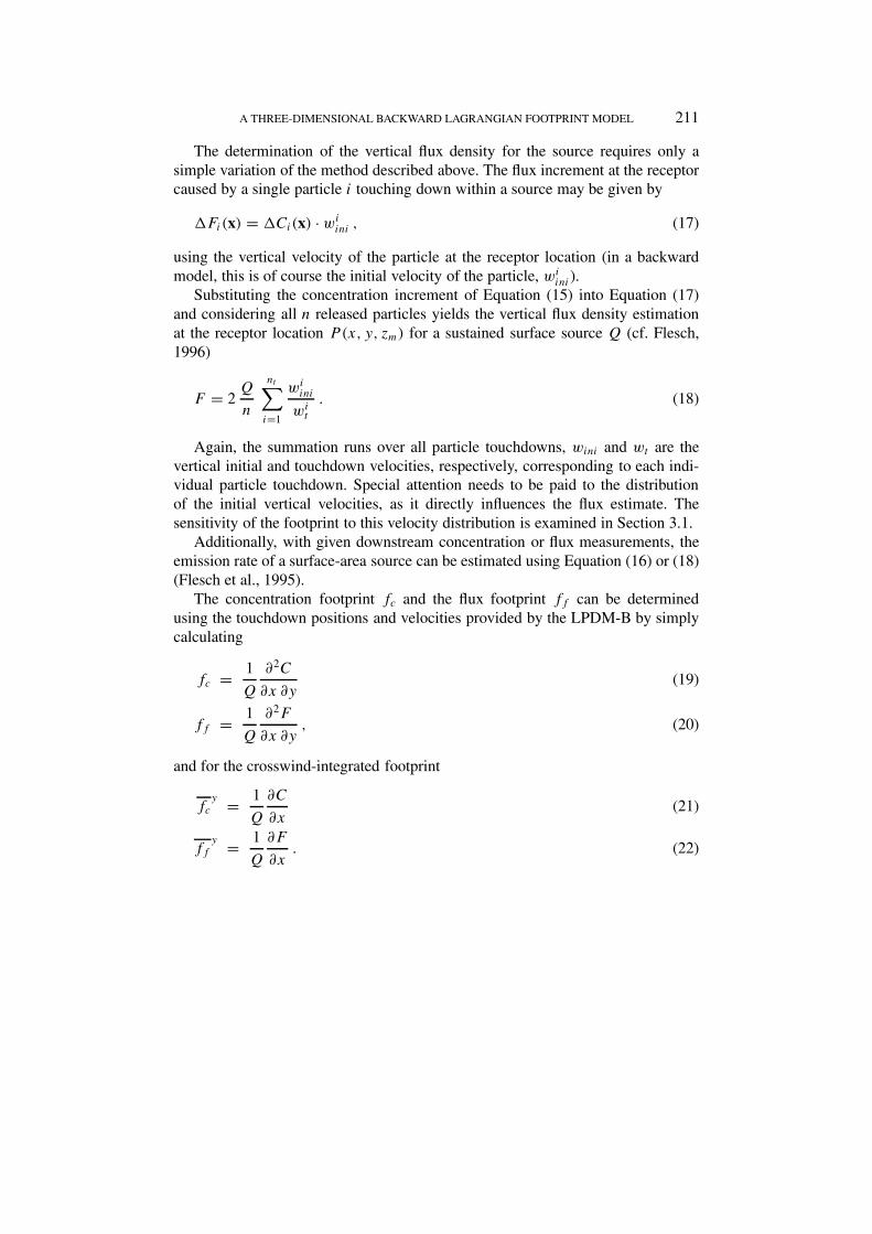
The determination of the vertical flux density for the source requires only asimple variation of the method described above. The flux increment at the receptorcaused by a single particle i touching down within a source may be given by

)Fi(x) = )Ci(x) · wiini , (17)

using the vertical velocity of the particle at the receptor location (in a backwardmodel, this is of course the initial velocity of the particle, wi

ini).Substituting the concentration increment of Equation (15) into Equation (17)

and considering all n released particles yields the vertical flux density estimationat the receptor location P(x, y, zm) for a sustained surface source Q (cf. Flesch,1996)

F = 2Q

n

nt(

i=1

wiini

wit

. (18)

Again, the summation runs over all particle touchdowns, wini and wt are thevertical initial and touchdown velocities, respectively, corresponding to each indi-vidual particle touchdown. Special attention needs to be paid to the distributionof the initial vertical velocities, as it directly influences the flux estimate. Thesensitivity of the footprint to this velocity distribution is examined in Section 3.1.

Additionally, with given downstream concentration or flux measurements, theemission rate of a surface-area source can be estimated using Equation (16) or (18)(Flesch et al., 1995).

The concentration footprint fc and the flux footprint ff can be determinedusing the touchdown positions and velocities provided by the LPDM-B by simplycalculating

fc = 1Q

#2C

#x #y(19)

ff = 1Q

#2F

#x #y, (20)

and for the crosswind-integrated footprint

fcy = 1

Q

#C

#x(21)

ffy = 1

Q

#F

#x. (22)

212 N. KLJUN ET AL.

2.3. DENSITY KERNEL ESTIMATION

The traditional way of evaluating the footprint is to overlay the upwind area with agrid and sum the footprint value of the particle touchdowns within each grid cell.Using this method, the footprint strongly depends on the selected grid spacing andon the number of particles released in the simulation. Here, we propose a statisticaltreatment of the particle touchdowns (Kljun et al., 2000a), using the density kernelmethod after de Haan (1999) who investigates this approach in detail for dispersionmodelling.

The footprint values of the touchdowns are treated as data points and a distribu-tion (kernel function K) is attached to each data point, to express the touchdowndensity in a point, rather than over a discrete grid-cell. These distributions may beGaussian or Epanechnikov, bi-, tri-, quad- and quint-weight kernels. In the presentstudy, we use biweight kernels according to

K(r) =&

C2(1 " r · rT )2 (r · rT < 1)0 otherwise (23)

with)

K(r) dr = 1 , (24)

where r is a d-dimensional vector and C2 a normalising factor (cf. de Haan, 1999).We then evaluate and sum the values of those distributions weighted by fi at anyselected point x in space to get

f (x) =nt

(

i=1

fi

h2i

K

"

x " xi

hi

#

, (25)

where nt is the total number of touchdowns and h is the size (bandwidth) of thekernels. For the optimal specification of h, see de Haan (1999).

A so-called locally optimised density kernel estimation is performed. A first-guess density estimate is computed using the same global kernel size, h, forall touchdown locations. Then, an optimised density estimation using individualkernel sizes, hi , for each data point (i.e., touchdown location) is performed. Wedecrease the bandwidth of the kernels if the data points are close to each other(i.e., the first-guess kernel is high), and increase the bandwidth in areas with alow first-guess density. This way, a continuous distribution adjusted to the touch-down density is derived. A grid-box average, on the other hand, would lead toa resolution of the footprint that is not adjusted to the touchdown density. Thediscrete distribution of the grid-box average requires smoothing, further decreasingthe resolution.

The main advantages of the density kernel estimation method are the lack ofthe need to choose (more or less arbitrary) values for the size and location of the


averaging grid boxes, the higher efficiency due to the locally optimised kernel sizes,and the higher resolution as compared to grid-box averaging for identical num-bers of data points. Therefore, it is possible to decrease the number of simulatedparticles to something between 1–5 & 103 particles (compared to 5 & 104 particlesnecessary when using a grid-box average to obtain a similar footprint resolution).This decrease of course results in a significant reduction of CPU-time by more thanan order of magnitude. Typically, a simulation of LPDM-B applying the densitykernel method needs 5 to 15 minutes on a Sun Ultra60 workstation.

3. Sensitivity Analysis

3.1. INITIAL VELOCITIES

The simulated flux footprint depends strongly on the initial velocities since theinitial velocities are explicitly included in the footprint calculation (Equation(18)). However, using Lagrangian particle models, it is not straightforward to cre-ate appropriate initial velocity distributions for any atmospheric stability. Often,the correlation of the streamwise and vertical velocity components is neglectedwhen creating them. As a result, unrealistic individual particle velocities may beproduced, with detrimental consequences for the evaluation of Equation (18).

A very simple solution to this problem is the introduction of a spin-up routine(after T. Flesch, personal communication, 2001): At first, velocities are assignedto each of the particles from a sample that approximates the atmospheric velo-city PDF at the sensor location. During the spin-up, the evolution of the particlevelocities is calculated as usual, according to the first part of Equation (1), butthe incremental displacement in the second part is ignored (dx = 0), so that theparticles are kept at their original position. Note that this procedure implies that allthe involved spatial derivatives must be forced to zero because the particles are not‘allowed’ to move. Thus, when the particles finally leave the receptor after the spin-up, unrealistic velocity distributions of the initial approximate PDF are smoothedout and almost perfect density distributions of initial velocities are reached. Whilethe distributions without spin-up were almost symmetric (neglected correlation ofu! and w!), the spin-up procedure leads to a more realistic distribution between theflow quadrants (Figure 1). It was found that a spin-up of about 1000 updates ofthe particle velocities is sufficient over the range of boundary-layer stabilities andreceptor heights simulated here.

Moreover, the modelled velocity distributions were compared to distributions asobtained from observations. For this purpose, ten half-hourly periods with stable(z/L ' 1) and near-neutral (z/L ' 0.03) conditions were selected from the data ofForrer and Rotach (1997), and ten periods of convective stability (z/L ' "1) wereconsidered from observations over a flat agricultural site in Switzerland. Table Ishows a quadrant analysis of the fluctuating components as introduced by Shaw

214 N. KLJUN ET AL.

Figure 1. Distribution of the fluctuating components w! against u! with (!) and without (#) spin-upunder near-neutral stratification with z/L = 0.03. I: outward interaction, II: ejection, III: inwardinteraction, IV: sweep, referring to the ‘forward’ terminology.

et al. (1983). The stress fractions contributed by each quadrant (referring to the‘forward’ terminology; I: outward interaction, II: ejection, III: inward interaction,IV: sweep, cf. Figure 1) predicted by the model with spin-up were compared to thecorresponding measured distributions. Very good correspondence to the measuredvelocity distributions was obtained by the spin-up method. Without spin-up, thecorrelation between horizontal and vertical velocity components vanishes (Fig-ure 1) and thus a quadrant analysis becomes problematic. However, it is clear fromFigure 1 that neither the quadrant contribution nor the total flux can be correct forthe velocity distributions without spin-up.

How does the spin-up affect the footprint estimate? Figure 2 compares a foot-print simulation using the velocity distribution after a spin-up and a simulation withthe raw initial velocities without spin-up. The position of the maximum influence(peak of the footprint), as well as its magnitude, was significantly altered by startingwith an imperfect velocity distribution. Comparing footprint simulations with andwithout spin-up under different stability-regimes (convective, neutral, stable), thepeak distance of the footprint was typically 30% smaller with spin-up. This dif-ference clearly demonstrates the importance of the correct correlation of the initialvelocity components.

All simulations presented in the following were run with spin-up.


TABLE I

Quadrant analysis for the fluctuating components w! and u! (u!w!(Quadrant)/u!w!) derivedfrom observations and from the LPDM-B with spin-up (cf. Figure 1). Units of m2 s"2.

Stable: z/L ' 1 Near-neutral: z/L ' 0.03 Convective: z/L ' "1Observation LPDM-B Observation LPDM-B Observation LPDM-B

I "0.48 ± 0.10 "0.39 "0.60 ± 0.13 "0.56 "0.66 ± 0.03 "0.67II 1.07 ± 0.13 0.86 1.12 ± 0.07 1.06 1.25 ± 0.13 1.16III "0.49 ± 0.08 "0.38 "0.53 ± 0.09 "0.54 "0.68 ± 0.14 "0.65IV 0.90 ± 0.09 0.91 1.02 ± 0.22 1.04 1.09 ± 0.05 1.16

u!w! "0.13 ± 0.01 "0.12 "0.26 ± 0.04 "0.23 "0.11 ± 0.08 "0.04

Figure 2. Crosswind-integrated flux footprint as predicted with and without using a spin-up understable stratification (cf. Table II). The arrow indicates the wind direction.

3.2. BOUNDARY-LAYER STABILITY

As is well-known, the footprint is sensitive to the stability. With its ability to pre-dict footprint estimates for a broad range of boundary-layer stabilities, the presentmodel is well-suited to reveal this sensitivity. For this reason, four typical casesof stability were selected as described in Table II and the corresponding flux andconcentration footprints were calculated for a receptor height of 50 m.

Figure 3 shows the crosswind-integrated footprints predicted by the Lagrangianmodel. It can be seen that, for both footprint types, the peak location varies with

216 N. KLJUN ET AL.

TABLE II

Velocity scales, Obukhov length, and boundary-layer height describingthe stabilities for four different simulations.

u# (m s"1) w# (m s"1) L (m) zi (m)

Strongly convective 0.2 2.0 "5 2000Forced convective 0.2 1.0 "36 1800Neutral 0.8 – ( 1500Stable 0.5 – 100 190

Receptor at (0, 0, 50) m, roughness length z0 = 0.05 m.

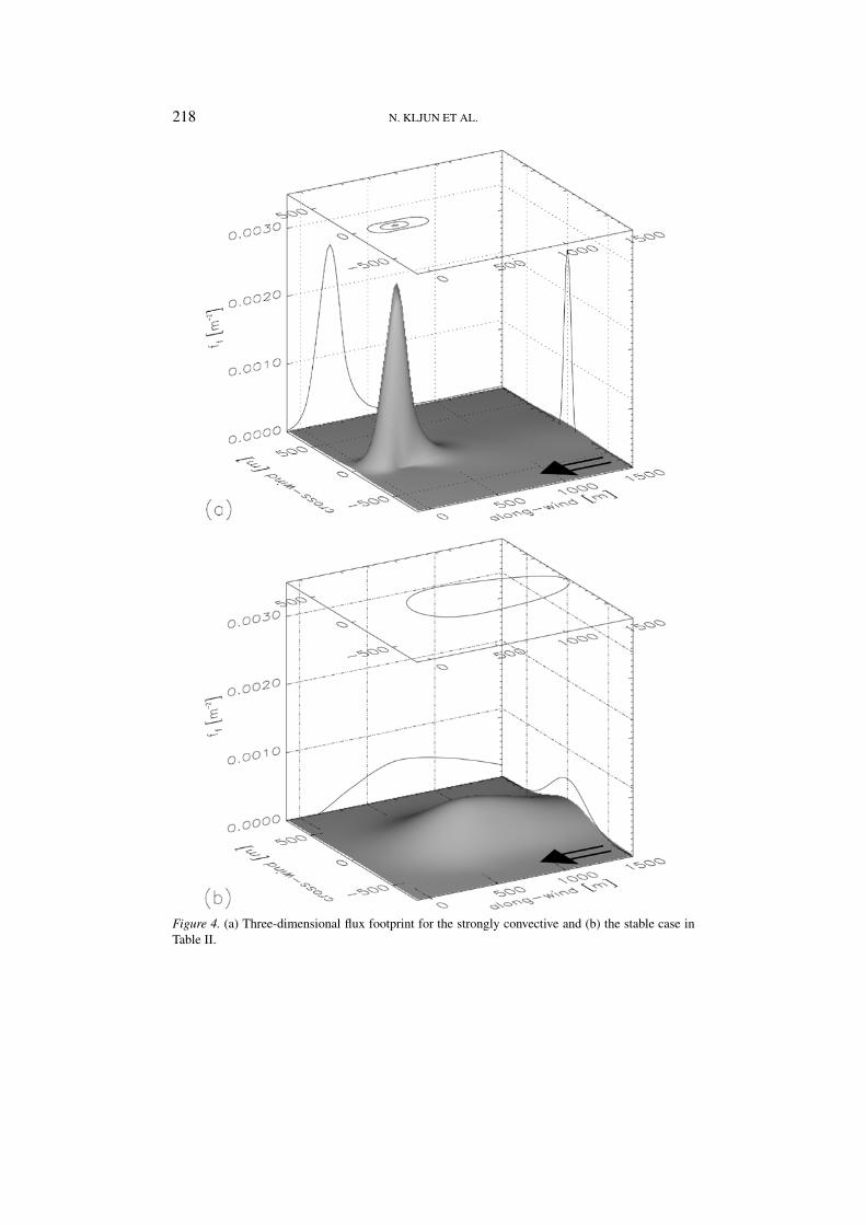
stability; it is closer to the receptor with increasingly convective stratification.Moreover, under convective stratification, the footprint is less skewed in upstreamdirection. The overall surface area of influence is in convective than in stableconditions since the boundary-layer stability also influences the lateral footprintdimension (Figure 4).

As a measure for the surface area of influence, the 50%-level source area wascalculated following Schmid (1994), i.e., the smallest possible area that includes50% of the total flux or concentration footprint (Figure 5). Again, this figure clearlydepicts the dependence of the area of influence on the stability regime: It is largestunder stable stratification and decreases under convective conditions. The footprintfor concentration measurements extends much further upwind than the flux foot-print, especially in neutral and stable stratification. This is consistent with earlierfindings by Schmid (1994) and by Rannik et al. (2000).

4. Model Evaluation

Due to the unavailability of appropriate experimental data sets, validation strategiesfor footprint models are still an open question. Therefore, we evaluate the presentLagrangian footprint model indirectly by first assuring that the dispersion model,on which the backward trajectory model LPDM-B is based, is able to reproducethe dispersion process adequately. Secondly, in order to evaluate the footprint es-timation from the Lagrangian trajectories (Equations (16) and (18)), a comparisonto results of other footprint models is presented (Section 4.2).

4.1. THE DISPERSION MODEL

The present Lagrangian footprint model is based on the dispersion model (LPDM)of Rotach et al. (1996). Its central assumption, i.e., the simulation of the velocityPDF (Equation (10)), has been shown to compare favourably with observationsunder various stability regimes (Rotach et al., 1996).


Figure 3. (a) Crosswind-integrated footprint for flux and (b) concentration measurements for four dif-ferent cases of stabilities as described in Table II. The locations of the respective peaks are indicatedby vertical lines.

218 N. KLJUN ET AL.

Figure 4. (a) Three-dimensional flux footprint for the strongly convective and (b) the stable case inTable II.


Figure 5. (a) 50%-level source area for flux and (b) concentration measurements for four differentcases of stability as described in Table II. The square indicates the receptor location.

220 N. KLJUN ET AL.

In free convection conditions, the model is able to reproduce all the featuresof the dispersion process qualitatively and quantitatively for sources at differentheights within the convective boundary layer (see the comparison to the water-tankexperiments of Willis and Deardorff (1976, 1978, 1981) in Rotach et al. (1996)).For stability conditions between neutral and strongly convective, the LPDM hasbeen shown to successfully reproduce both field data from a full-scale tracer experi-ment in Copenhagen and results for LES by Mason (1992). See Rotach et al. (1996)for details. Moreover, PPM, another dispersion model (de Haan and Rotach, 1998),has the LPDM at its core and reproduces the tracer experiments of Copenhagen andKincaid very well. As far as stable conditions are concerned, no true validation ofthe LPDM has been published so far. When trying to reproduce the observationsfrom the tracer experiment in Lillestrøm under highly stable conditions, both theLPDM and the PPM are similar to or better than other dispersion models (de Haanand Rotach, 1998), but still hardly satisfactory in their performance. However, thispartial ‘failure’ can be attributed to the turbulence description (similarity approach)rather than to the model formulation itself (Gryning, 1999). Only recently, theLPDM has been used to successfully simulate the stable runs of the Prairie grassexperiment, for which Gryning (1999) states that it corresponds to moderatelystable conditions and thus similarity-based dispersion models are adequate.

Overall, the dispersion model is validated for a wide range of boundary-layerstabilities and source heights. We can therefore be confident that the dispersionprocess in the backward model LPDM-B is also adequately described. Moreover,Kljun et al. (1999) have shown that, under convective stratification, the footprintspredicted by LPDM-B represent flux observations much better than the simplerLagrangian model of Thomson (1987), which neglects the skewness in the verticalvelocity PDF.

4.2. COMPARISON OF LPDM-B WITH OTHER FOOTPRINT MODELS

The estimated footprint functions from the present model are compared with thoseobtained by an analytical footprint model. The analytical model used in this studyis that contained in SAM/FSAM (concentration/flux footprint) after Schmid (1994,1997) based on an analytical solution of the Eulerian advection-diffusion equationfor vertical diffusion using standard surface-layer scaling parameters (Van Ulden,1978). It is based on K-theory and has a short-range plume model for surface-layer scaling conditions and ground-level sources (Gryning et al., 1987) at its core,to describe the diffusion characteristics. The latest version of the model uses anapproximate equation for the flux footprint function proposed by Horst and Weil(1994). This latter model has been tested against experimental data of trace gasfluxes by Finn (1996), showing that the model predictions usually fell within theuncertainties of the measurements, which, however, were found to be particularlylarge around neutral stability. For a complete description of SAM/FSAM, thereader is referred to Schmid (1994, 1997).


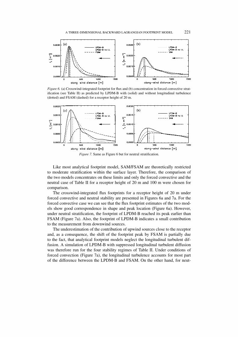
Figure 6. (a) Crosswind-integrated footprint for flux and (b) concentration in forced convective strat-ification (see Table II) as predicted by LPDM-B with (solid) and without longitudinal turbulence(dotted) and FSAM (dashed) for a receptor height of 20 m.

Figure 7. Same as Figure 6 but for neutral stratification.

Like most analytical footprint model, SAM/FSAM are theoretically restrictedto moderate stratification within the surface layer. Therefore, the comparison ofthe two models concentrates on these limits and only the forced convective and theneutral case of Table II for a receptor height of 20 m and 100 m were chosen forcomparison.

The crosswind-integrated flux footprints for a receptor height of 20 m underforced convective and neutral stability are presented in Figures 6a and 7a. For theforced convective case we can see that the flux footprint estimates of the two mod-els show good correspondence in shape and peak location (Figure 6a). However,under neutral stratification, the footprint of LPDM-B reached its peak earlier thanFSAM (Figure 7a). Also, the footprint of LPDM-B indicates a small contributionto the measurement from downwind sources.

The underestimation of the contribution of upwind sources close to the receptorand, as a consequence, the shift of the footprint peak by FSAM is partially dueto the fact, that analytical footprint models neglect the longitudinal turbulent dif-fusion. A simulation of LPDM-B with suppressed longitudinal turbulent diffusionwas therefore run for the four stability regimes of Table II. Under conditions offorced convection (Figure 7a), the longitudinal turbulence accounts for most partof the difference between the LPDM-B and FSAM. On the other hand, for neut-

222 N. KLJUN ET AL.

ral stratification (Figure 7a), the relative importance of longitudinal diffusion wassomewhat larger but cannot explain the whole discrepancy between the two mod-els. Other factors that may be responsible for the observed difference include thechoice of some parameters in FSAM, which are selected for optimal performanceunder conditions of forced convection (i.e., the most ‘common’ case) and heldconstant for all stabilities. This is in contrast to the model by Horst and Weil (1994)and Horst (1999), which dynamically adjusts these parameters for stability (e.g., todescribe the mean plume velocity). The peak footprint location predicted by theHorst (1994) model closely matches the current results of LPDM-B (not-shown).

Generally, the behaviour of the concentration footprints was similar to thatof the flux footprints. The magnitude and the shape of the footprints of the twomodels were in good correspondence under neutral and convective stratificationfor the receptor height of 20 m (Figures 6b and 7b). The footprints predicted byLPDM-B increased earlier than those predicted by SAM which again can partlybe explained by the neglected longitudinal turbulence in SAM (Figures 6b, 7b).In general, the correspondence between the two models is somewhat better if con-centration footprints are concerned rather than flux footprints. This would suggestthe method of calculating the flux estimates from the present LPDM-B simulationscould have a major contribution to the observed difference in the flux footprintunder neutral conditions. We will come back to this issue when comparing thepresent simulations with another Lagrangian footprint model below.

Figure 8 shows the flux footprints under neutral and free convection conditionsfor a receptor height of 100 m. For neutral stratification, there is no formal reasonthat would inhibit the application of FSAM. Still, with zm/z0 = 2000, and a re-ceptor height in the upper part of the surface layer, this simulation means to pushFSAM to its limits. These limits are formally broken under convective conditionssince "zm/L > 1 (Schmid, 1994). As expected, the flux footprints differ consider-ably for these high receptor locations (Figure 8). The distance of the peak footprintlocation is different by almost a factor of two or more, and even the simulation ofLPDM-B without longitudinal turbulence cannot explain this difference.

Over all, the comparison between the present model and SAM/FSAM is sat-isfactory in conditions where the latter is valid (Kljun et al., 2000b). However,under neutral conditions non-negligible differences in the location of the peak fluxfootprint are found and, at the same time, an important contribution of longitud-inal dispersion (which is not accounted for in the analytical model). The presentLagrangian model has a much wider range of applicability in terms of stabilityand receptor height and its algorithm is not subject to strong assumptions concern-ing the turbulence regime as is the case for the analytical models. Therefore, wemay conclude that its footprint estimates are more trustworthy than those from theanalytical model. It should be noted that, very often, the limitations of analyticalfootprint models are too restrictive for real situations. Thus, it is advisable to usea model such as LPDM-B that is valid for a wide range of practical applications.However, we cannot fully validate the footprint estimates without suitable experi-


Figure 8. (a) Crosswind-integrated flux footprint for forced convective and (b) neutral stratification(see Table II) as predicted by LPDM-B with (solid) and without longitudinal turbulence (dotted) andFSAM (dashed) for a receptor height of 100 m.

Figure 9. (a) Crosswind-integrated footprint for flux and (b) concentration in neutral stratification aspredicted by LPDM-B (solid) and Rannik et al. (2000) (RKS; dashed) for a receptor height of 15 m.

mental data or, at least, another footprint model that allows for high receptor pointsand stratification outside ‘moderate stability’.

As a next step, LPDM-B was compared to the Lagrangian (forward) footprintmodel of Rannik et al. (2000). This model differs from the present LPDM-B in thatit uses a forward approach, and consequently in the method it uses to calculate thefluxes from the particle trajectories. Thus, this comparison provides an independenttest of the flux footprint estimation used in our model. Unfortunately, Rannik etal. (2000) present only footprints for neutral stratification. Figure 9 shows fluxand concentration footprints for their neutral case (Receptor height = 15 m, z0 =1.5 m). There is excellent agreement between the two models in terms of boththe peak location and the shape of the footprint functions. Thus, we conclude thatthe present flux footprint estimation is robust and the differences as observed inFigure 7a (for another neutral case) are due to differences in the simulation of thediffusion process or some assumptions in the analytical model, rather than due tothe flux footprint estimation in the present approach. Yet we stress the point thatsuitable experimental data are necessary to decide which of the footprint modelsyields the ‘correct’ footprint estimates.

224 N. KLJUN ET AL.

5. Summary and Conclusions

A Lagrangian footprint model with a validity range from stable to convective strat-ification, and for receptor locations ranging over the entire boundary-layer depth ispresented. We introduce a statistical treatment of particle touchdowns, the so-calleddensity kernel method. Using this method, a significant reduction of CPU-timewas achieved: To obtain the same footprint resolution, the model runs ten timesfaster than without the kernel method. Thus, the backward Lagrangian model isan efficient tool for footprint predictions. Thanks to a spin-up procedure duringinitialisation, very good agreement was found between the modelled initial particlevelocity distributions and observations. This agreement is important because of thestrong influence of the initial velocities on the shape and the peak location of thefootprint. The location of the peak footprint contribution is found to differ by up to30% under different stability regimes when neglecting the spin-up procedure.

Excellent agreement was found when comparing the present footprint modelwith a Lagrangian model applying the forward approach. When the footprints pre-dicted by the present Lagrangian model are compared with an analytical model,satisfying correspondence was generally found, as long as the models were appliedwithin the restrictive limits of the analytical model (moderate stability within thesurface layer: "zm/L < 1 and zm < 0.1zi). However, the flux footprints of the ana-lytical model were clearly further upstream from the receptor location than thosepredicted by the Lagrangian model. Also, the analytical model was not capable ofpredicting the small contribution to the footprint downwind of the receptor. Thesedifferences are at least partly due to the neglected longitudinal turbulent diffusionof the analytical model.

Analytical models are often used outside their limits of application, as no othersimple models for convective conditions exist so far. When the footprints of theLagrangian model are compared to those of the analytical model applied outside itsrange (receptor outside the surface layer, or stability too extreme), large differenceswere found in the peak location and the shape of the footprints. Note, that footprintpredictions are often needed for application outside the surface layer (e.g., for usein connection with aircraft measurements or with observations on high towers) andunder arbitrary stratification.

Finally, as a backward Lagrangian footprint model, LPDM-B holds the poten-tial to be applied efficiently over inhomogeneous terrain. Even though the presentfootprint model is constructed from a horizontally homogeneous PDF, it may beused in conjunction with inhomogeneous flow and turbulence fields obtained fromnumerical models as done in many practical applications of dispersion modelling(e.g., Physick et al., 1994; Luhar and Rao 1994). Furthermore, horizontally in-homogeneous LPDMs are available in the literature for purely Gaussian turbulence(e.g., Thomson, 1987). Even though it may prove to be a major task to extend thepresent LPDM-B to inhomogeneous conditions, the potential for this is likely one


of the most important qualities of the present model, considering that footprintestimates are important particularly under inhomogeneous surface conditions.

The present Lagrangian backward footprint model appears to be the first that isable to treat receptor heights throughout the entire boundary layer (as most Lag-rangian footprint models do) at the same time as being able to handle a broad rangeof boundary-layer stratifications. Moreover, with its kernel density estimation, it ismuch faster than conventional Lagrangian footprint models.

Acknowledgements

This research was supported by the Swiss Commission for Technology and Innov-ation (KTI) in the framework of EUROTRAC II (#3532.1 and #4092.1), and by agrant from the Terrestrial Carbon Processes program of US-DOE (through a sub-contract from Harvard University to HPS). We are grateful to Dr. P. de Haan forhelping us with the density kernel estimation.

References

Baerentsen, J. H. and Berkowicz, R.: 1984, ‘Monte Carlo Simulation of Plume Dispersion in theConvective Boundary Layer’, Atmos. Environ. 18, 701–712.

de Haan, P.: 1999, ‘On the Use of Density Kernels for Concentration Estimations within Particle andPuff Dispersion Models’, Atmos. Environ. 33, 2007–2021.

de Haan, P. and Rotach, M. W. : 1998, ‘A Novel Approach to Atmospheric Dispersion Modelling:The Puff-Particle Model (PPM)’, Quart. J. Roy. Meteorol. Soc. 124, 2771–2792.

Du, S.: 1995, ‘Estimation of the Kolmogorov Constant C0) for the Lagrangian Structure Function,Using a Second-Order Lagrangian Model of Grid Turbulence’, Phys. Fluids 7, 3083–3090.

Du, S.: 1997, ‘Universality of the Lagrangian Velocity Structure Function Constant (C0) acrossDifferent Kinds of Turbulence’, Boundary-Layer Meteorol. 83, 207–219.

Finn, D., Lamb, B., Leclerc, M. Y., and Horst, T. W.: 1996, ‘Experimental Evaluation of Analyticaland Lagrangian Surface-Layer Flux Footprint Models’, Boundary-Layer Meteorol. 80, 283–308.

Flesch, T. K.: 1996, ‘The Footprint for Flux Measurements, from Backward Lagrangian StochasticModels’, Boundary-Layer Meteorol. 78, 399–404.

Flesch, T. K., Wilson, J. E., and Yee, E.: 1995, ‘Backward-Time Langrangian Stochastic DispersionModels and their Application to Estimate Gaseous Emissions’, J. Appl. Meteorol. 34, 1320–1332.

Forrer, J. and Rotach, M. W.: 1997, ‘On the Turbulence Structure in the Stable Boundary Layer overthe Greenland Ice Sheet’, Boundary-Layer Meteorol. 85, 111–136.

Gryning, S.-E. 1999, ‘Some Aspects of Atmospheric Dispersion in the Stratified AtmosphericBoundary Layer over Homogeneous Terrain’, Boundary-Layer Meteorol. 90, 479–494.

Gryning, S.-E., Holtslag, A. A. M., Irwin, J. S., and Sivertsen, B.: 1987, ‘Applied DispersionModelling Based on Meteorological Scaling Parameters’, Atmos. Environ. 21, 79–89.

Horst, T. W.: 1999, ‘The Footprint for Estimation of Atmosphere-Surface Exchange Fluxes by ProfileTechniques’, Boundary-Layer Meteorol. 90, 171–188.

Horst, T. W. and Weil, J. C.: 1992, ‘Footprint Estimation for Scalar Flux Measurements in theAtmospheric Surface Layer’, Boundary-Layer Meteorol. 90, 171–188.

Horst, T. W. and Weil, J. C.: 1994, ‘How Far Is Far Enough?: The Fetch Requirements for Microme-teorological Measurement of Surface Fluxes’, J. Atmos. Ocean. Tech. 11, 1018–1025.

Kljun, N., Rotach, M. W., and Schmid, H. P.: 1999, ‘Allocation of Surface Sources Using “BackwardTrajectory”-Simulations’, in preprint, 13th Symposium on Boundary Layers and Turbulence,Dallas, TX, American Meteorological Society, Boston, MA, pp. 187–188.

226 N. KLJUN ET AL.

Kljun, N., de Haan, P., Rotach, M. W., and Schmid, H. P.: 2000a, ‘Footprint Determination inStable to Convective Stratification Using an Inverse 3D Lagrangian Particle Model’, in preprint,24th Conference on Agricultural and Forest Meteorology, Davis, CA, American MeteorologicalSociety, Boston, MA, pp. 156–157.

Kljun, N., Rotach, M. W., and Schmid, H. P.: 2000b, ‘A Lagrangian Footprint Model for Stratifica-tions Ranging from Stable to Convective’, in preprint, 14th Symposium on Boundary Layers andTurbulence, Aspen, CO, American Meteorological Society, Boston, MA, pp. 130–132.

Leclerc, M. Y. and Thurtell, G. W.: 1990, ‘Footprint Prediction of Scalar Fluxes Using a MarkovianAnalysis’, Boundary-Layer Meteorol. 52, 247–258.

Leclerc, M. Y., Shen, S., and Lamb, B.: 1997, ‘Observations and Large-Eddy Simulation Modelingof Footprints in the Lower Convective Boundary Layer’, J. Geophys. Res. 102, 9323–9334.

Luhar, A. K. and Rao, K. S.: 1994, ‘Source Footprint Analysis for Scalar Fluxes Measured in Flowsover an Inhomogeneous Surface’, Air Pollut. Model. Appl. X, 315–322.

Mason, P. J.: 1992, ‘Large-Eddy Simulation of Dispersion in Convective Boundary Layers with WindShear’, Atmos. Environ. 26A, 1561–1571.

Physick, W. L., Noonan, J. A., McGregor, J. L., Abbs, D. J., and Manins, P. C.: 1994, LADM: A Lag-rangian Atmospheric Dispersion Model, Technical Report 24, CSIRO Division of AtmosphericResearch, Australia, 137 pp.

Rannik, U., Aubinet, M., Kurbanmuradov, O., Sabelfeld, K. K., Markkanen, T., and Vesala, T.: 2000,‘Footprint Analysis for Measurements over a Heterogeneous Forest’, Boundary-Layer Meteorol.97, 137–166.

Rotach, M. W., Gryning, S.-E., and Tassone, C.: 1996, ‘A Two-Dimensional Lagrangian StochasticDispersion Model for Daytime Conditions’, Quart. J. Roy. Meteorol. Soc. 122, 367–389.

Schmid, H. P.: 1994, ‘Source Areas for Scalars and Scalar Fluxes’, Boundary-Layer Meteorol. 67,293–318.

Schmid, H. P.: 1997, ‘Experimental Design for Flux Measurements: Matching Scales of Observationsand Fluxes’, Agric. For. Meteorol. 87, 179–200.

Schmid, H. P.: 2002, ‘Footprint Modeling for Vegetation Atmosphere Exchange Studies: A Reviewand Perspective’, Agric. For. Meteorol. (Special Issue on FLUXNET), in press.

Schmid, H. P. and Oke, T. R.: 1990, ‘A Model to Estimate the Source Area Contributing to TurbulentExchange in the Surface Layer over Patchy Terrain’, Quart. J. Roy. Meteorol. Soc. 16, 965–988.

Schuepp, P. H., Leclerc, M. Y., Macpherson, J. I., and Desjardins, R. L.: 1990, ‘Footprint Predic-tion of Scalar Fluxes from Analytical Solutions of the Diffusion Equation’, Boundary-LayerMeteorol. 50, 355–373.

Shaw, R. H., Tavangar, J., and David, P. W.: 1983, ‘Structure of the Reynolds Stress in a CanopyLayer’, J. Clim. Appl. Meteorol. 22, 1922–1931.

Thomson, D. J.: 1987, ‘Criteria for the Selection of Stochastic Models of Particle Trajectories inTurbulent Flows’, J. Fluid Mech. 180, 529–556.

Van Ulden, A. P.: 1978, ‘Simple Estimates for Vertical Diffusion from Sources near the Ground’,Atmos. Environ. 12, 2125–2129.

Willis, G. E. and Deardorff, J. W.: 1976, ‘A Laboratory Model of Diffusion into the ConvectivePlanetary Boundary Layer’, Quart. J. Roy. Meteorol. Soc. 102, 427–445.

Willis, G. E. and Deardorff, J. W.: 1978, ‘A Laboratory Study of Dispersion from an Elevated Sourcewithin a Modelled Convective Planetary Boundary Layer’, Atmos. Environ. 12, 1305–1311.

Willis, G. E. and Deardorff, J. W.: 1981, ‘A Laboratory Study of Dispersion from a Source in theMiddle of the Convective Layer’, Atmos. Environ. 15, 109–117.

Wilson, J. D. and Swaters, G. E.: 1991, ‘The Source Area Influencing a Measurement in the PlanetaryBoundary Layer: The “Footprint” and the “Distribution of Contact Distance” ’, Boundary-LayerMeteorol. 55, 25–46.

A Three-Dimensional Backward Lagrangian Footprint Model For A Wide Range Of Boundary-Layer...

Documents

Transcript of A Three-Dimensional Backward Lagrangian Footprint Model For A Wide Range Of Boundary-Layer...