MS ill: BO 1.005.5

Integrating Visua liza t ion into tbe ModelingOf Business Simulations

3647 words10 Figures4 Tables

by

Victor Perotti, Ph.D.Home:8 BUIT Oak DrivePittsford, "TV 14534 USAPhone: 585-249-995 1

Work:Rochester Inst itute ofTechnologyCollege of Business107 Lomb Memorial DriveRochester, NY 14623 USAPhone: 585-475·7753Fax: 585-475-6571Email: vjpbbU@rit.edu

Tom F. Pray, Ph.D.Home:23 Locke DrivePitt sford, NY 14534 USAPhone: 585-3 83- 1653

Work:Rochester Institute of TechnologyCollege of Business107 Lomb Memorial DriveRochester, NY 14623 USAPhone: 585-475-2344Fax: 585-475·6571Email: tfpbbu@rit.edu

•

Integraung visualization imo the modeling of bus lrlC$S simulatioll$

Victor PerottiThomas PTa)

Rochester Institute ofT~hnolog)

This article demonstrates the advllI1tages of using visualization as part of the modelingprocess. Several exampks are gil'en to show how visualization can help developers tomore completely underst.and the range of behaviors for lheir algorithm s. Specifically. theCobb Doullla.s function and Gold Prny demaad sys tem arc exam ined using a tool thatcombines mathematical modeling with visualization capabilities.

KEYWORDS: algorithm development: algorithm behavior; bus'I"ICSS simulation;Mathematica.. modeling: .'isualiutioo

Over the past 20 years, model builders have worked diligently to improve the algorithms

that drive business simulations. Researchers have published numerous papers on

different aspects o f improving the realism and the reliability o f business games. Sti ll,

many designers. even after developing equations. st ruggle with: (,) how to select starting

,·al~. (i1) how to gage sensitivity ofthc parameters used in the model and (iii) how to

ensure the system is robust. This paper illustmtes the use of visualization t~hniquesand

tools for designers to gain a better understanding ofexisting or developing models.

The paper begins with a brie f summary of the literature on algorithm ~Iopment and

then gives a gene ral description o f a mode ling and visualization tool ea lled

Malhematica<!!) (Wo lfram. 1993). Fina]]y, it demonstrates the use of visualiza tion through

an analysis of thrcc commonly used demand models:(i) the Cobb Douglas Power

Function, (ii) the Gold and Pray Demand Syste m ( 19&4), and ( iii) the Product Auri bute

Model ofGold and Pray ( 1997) mod ified to ineludc an interaction or cross-elasticity

effect between independent variables. Mathematica~ is utilized to identi fy both the

~bil ily and lllC"k of stability ofa system of equations. 1hc paper concludes with some

suggestions on the use of the softv.-are package and offes caveats lISSOCialed ",i th the

methodological approach suggested by the autho rs.

2

•

•

•

•

•

Bll5iness simulation algorithms

A review orm.: modeling lilttall1Jl' illustrates that then: has been considerable work in

algonlhm enhancement or bcscess games. In the operations arena. Thevikulwat (1993)

propo5<'d a linear SCI of equations 10 model production pTQCCS5e5. Gold and Pray (1989).

Gold (1990). and Gol d ( 1992) develope d models for COSI and product ion funct ions

embodied in business games. Pray and Methc ( 199 1) put forth a model for new produc t

development with genera lized demand and production functions.

Q uality modeling became popular in the 1990s with the work o f Thavikulwat (1992).

Mergen and Pray (1992). Teach ( 1992). and Teach and Sc h..'al1Z (2000). All ofthcsc

authon dCmoDStnllro melhods and algoritluns fOl" modding qual it)' that could be added to

c."'sting or 10 new ! imulluiorlS_

In the Mea ofmarketing. many aniclI:$ M\'C been wrinen about dmwwl modeling

including how 10 model price and eon-price issues. Pray and Gol d ( 1982) investigated the

demand robustness of a number ofcommonly used business games. Anick s soon

follo....'ed by Teach (1984). Gold and Pray (1984). Goosen (1986) and Decker. LabBam

and Adler (1987 ) that moved the modeling of demand to a higher level. Further

extensions by Golden ( 1987). Lambert and Lam bert (1988) and Thnvikulwat ( 1988.

1989) tested the reliability of various models and raised new issues about how demand

$hould be modeled. Market segmen tation was addressed forma lly by Teach (1990).

Carvalho (199 1. 1995) and Gold and. PI3Y (1997. 1998).

This brie f review shows thaI the leading business game des.igneD have shared their

design contributions ....ith the field. It is also tbe case. bowever.jhat all of the algorithms

described in the literature are just mathematical models and. thus have certa in limitations..

Some algorithms are highly sensitive 10 the starti ng parameters selected, Others require

the decision variables to be constrained in a narrow range for the simulat ion to behave in

•

a manner that is consistent with lbcory. Somc moods have discontinuities. which can

also }ield Wlfeasonable resuhs.

T1lc methodology 10 be presented addresses lhc:sc limita tions by offering a relativel y

easy ··,isual method" of testing and verif}ing the overal l etfecuveness ofan algorithm

and providing insights into where difficulties may arise with actual usage. The drudgery

o f hours of mathematical sensi tivity anal ysis can be: avoided by including visualization in

the model ing process.

Integrating Visualization Imo the Modeling Process

Vi$Ualization is the rendering of complex clala in a visual image that is understandable for

human observers. Tbe ad''mt of computer technology has allo....'ed visualization 10 impac1

a wide ,'ariely of areas from airuaft design to advanced physics. BusillCSSCS are also

turning to dedicated software visual ization packages (e.g. OpenViz8. Visiorw)~} to

hel p them understand and assess thei r processes or performance.

Integrating visualization into the model ing proc ess is relatively straighrforward . While it

is certa inly possib le 10 deve lop the mathemati cal model and visuali zation in separate

software packages. it is probably easiest to use an appl icat ion package that permits both.

Spreadsheet programs like Microsoft Excel will do both, but there are se veral

mathe matical packages (e.g. Mapl~. Mathematica~ or MatLa~) thatare expressly

designed to Iecilitate simultaneous mathematical modeling and Visual ization. Although

each one has its me rits , .....e ....ill demonstrate the advantages o f eombining visualizancns

and modelina ....ith Mathemat;"""t!Il

MathcmaticaS, by Wolfntm Research is a soft.....are toolthat a1 lo.....s the creation, solution.

visual izat ion and di stribution of compleJ( mathematical models. The interface is an

elcctronic notebook whe re one can include ideas. partial results. and graphics. Users

4

•

•

•

develop mathematical moods by e-"Iuating individualline$ c r cooe. thus c~aling panial

results thai can be combi"",d over and OVCT again 10d~~1op IT10n rompl"':< models ,

Visualization functions are available at "" ''''1'}' step of the developmen t process 10 help a

model huild"'r verify the behavior of thc mod el. Because of Ihe variety oftools and

funct ions available, developers will frcquemly discover unanticipated behaviors thai can

enhance their understllTlding or help them avoid fUlurc problems with a model.

Once mosl ofthe oo'dopn1enl has been compleled, \he notebook mterf~ can be used to

explore the model both numerically and visually. This exploratory modeof interaction

can take the fonn of. SCI of" whal-if' scenarios that allow the user 10 """ICT comprehend

the full complexity of the ....o rk. Charts, grap hics and animations can be creale<!

automatically to contribute to the USCT' Sunderstanding. Sharing such a model onl ine is

simple since the freely available MathReader{l!l SQftwarc allows anyone to explore and

interact with a notebook.

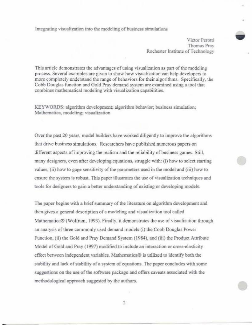
Figure I sho"''li portions of Mathematica~ in aclion . A Cobb Douglas demand function is

fim defined. with parame~: a (scale param~er), st (elasticity for price). s2 (elasticity

for market ing). price an d mkl (marketing). N<:'XI, the function is evaluated "..ilh specific

values so that the demand is 6000 units at the sta rting valu es. Vary ing on ly the price

generales the two-dimensional demand plot in the figure.

Figure I about hen:

As with any piec e of soft ware, a new user to t he so ftware will hove 10 spend some lime

learning both the notebook inlerface and the lanll uage u...d In writt: 1:'1""';on5 and

functions. While the notebook imerfece is quite easy. \he language of avai lable

commands is vast and can be intimidating . Fortwtately. one can accomplish most

anal~by cxploring just the small subset of the language tha t is applicable to I specific

problem . The documentation for Mathematic. is well wrinen and illustrated. and

5

additiol13l reference guides make developing signi ficant lDO<kls possible even for

beginners.

Visua.l Modeling Example.t

What follows is 8 de monstration of'rbe visual modeling and exploratory techniques using

three dilTerenl deman d model s. In the first tWO cases. visualization is used to bener

understand the behavior of the Cobb Douglas and Gold and Pray demand models. In the

last case. visual izat ion is used to develop a new C1<lension to the Gold and Pray demand

model that handles cross elastic ities.

Cobb Douglas market demand function : a stable function ....-ith constant elasticity

The first model analyzed is theCobb Douglas function. This fwlction was flnl deployed as

a way to describe production functiorts in microcoonomics but it can be modified easily to

fit thedemand side. To dcmonstT1l\e the ,iSI,W modeling 3SpC'Cts,"''C ....i ll simulate a simple

demand funct ion where price (P) and marketing (M) lU'C the independent variables. and

demand (Ql is thc response or dependent variable.

The functio nal fonn is as follows :

--

•

OJ

....iltte:!he elasticities for price and marketing lU'C ep

and em respectively; -e" is the scal ing coc:fficicnt

6

•

•

To verify \he coding of \he model "'~ set the price elasticity (ep) at - 1.2. \hemarke'!ing

elasticil) (em) III ,3. and the$CaIing coelT"lCief!t M a~ lit 44257_ Sensithil)'lIIIlIIysison the

Cobb Dou&Jas fimction isd~ed below.

The Cobb Douglas Demand Curve

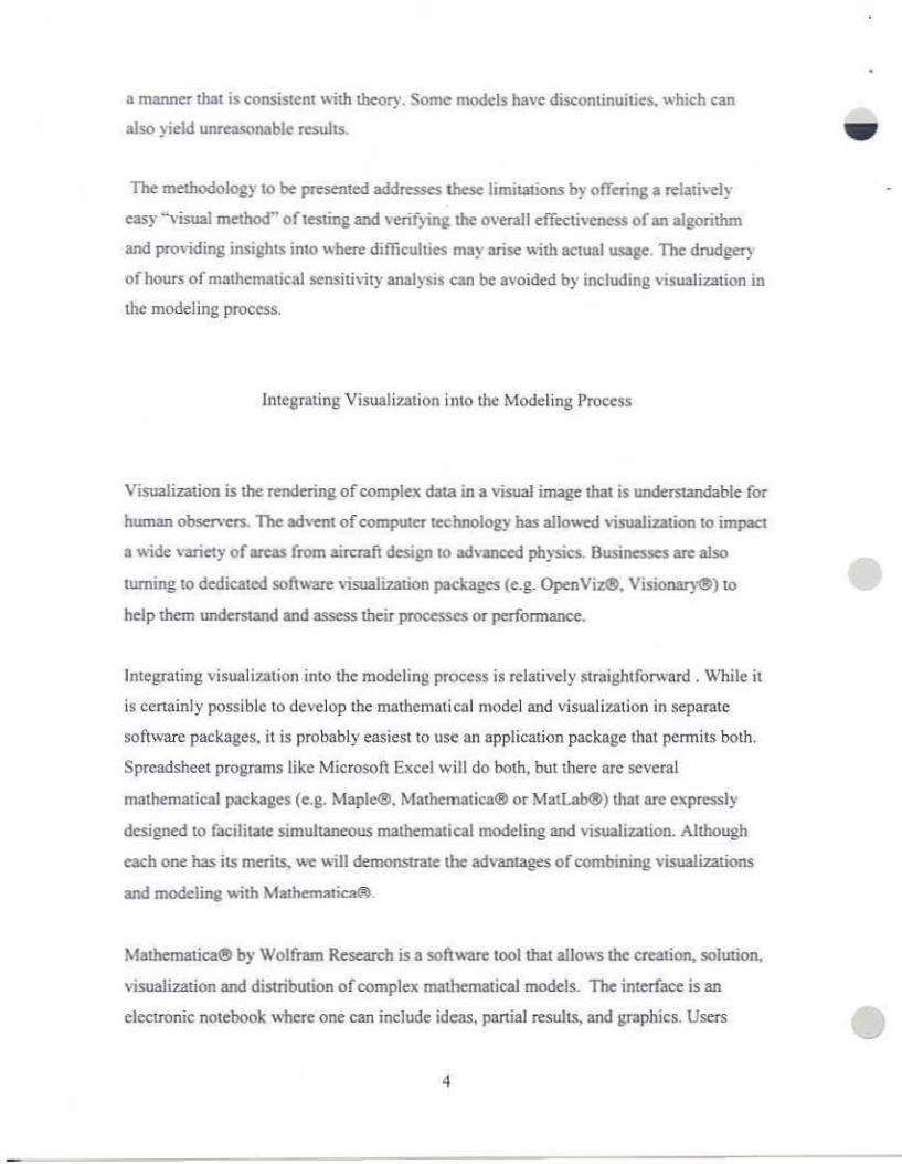
Figure 2 shows a two-dimensional plOI depicting a classic Marshalllan demand curve. In this

example. price WlIS varied from $10 to 545 whi le marketing was held constant at S5OO.

Note: the authors arbitrarily scaled Marketing to $1000 units. Designers or users can scale

coefficiems either befo~ IlSe oflht: demand ~uation or through \he scaling coefficient

-3" to get the desired le\"el of demand. The plO! sJxM., thai tkmand is maximized at 17.500

and that !he quantity demandcd appean; to beasymptotic to !he x-axis.

Figure 2 about here

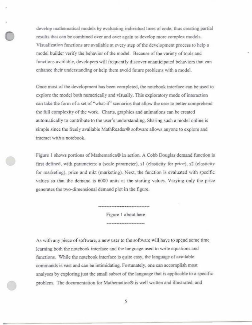
In \he ne.'(t illUSU1llion. Figure 3. the diminishing re'lUfm to marketing are dearl~' scm ali we

\~. marketing from $200 to $3000 ","hile holding price (Xlll$Wl1 at S2S. 1t is inleRSting to

note thaI demand reaches zero and that. for this model. it is possible to gmemte "negative

demand ~ for very smallle\"c1s ofmarketing, Such an observation is easy Voith 3 visual

representation, but might be much more difficult otherwise.

Figure 3 about he re

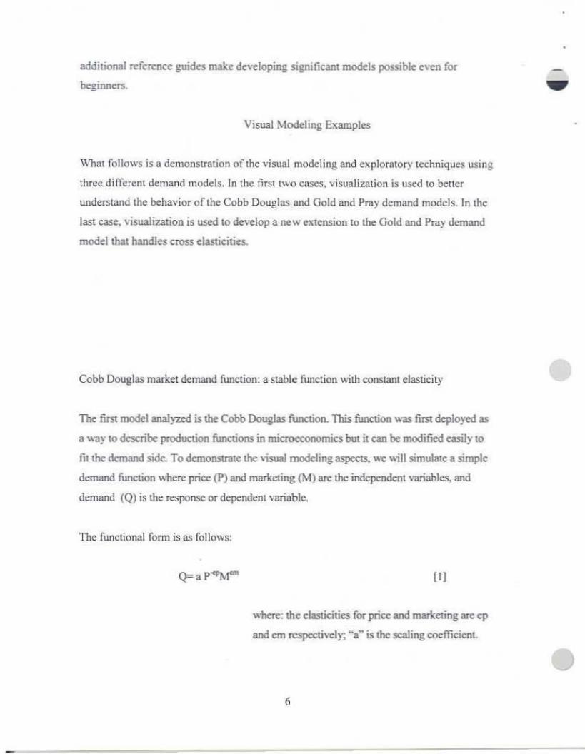
One wlI'Ilo look lit sysiens ofmore than tVol) ,-ariables is through three-dimensional plots.

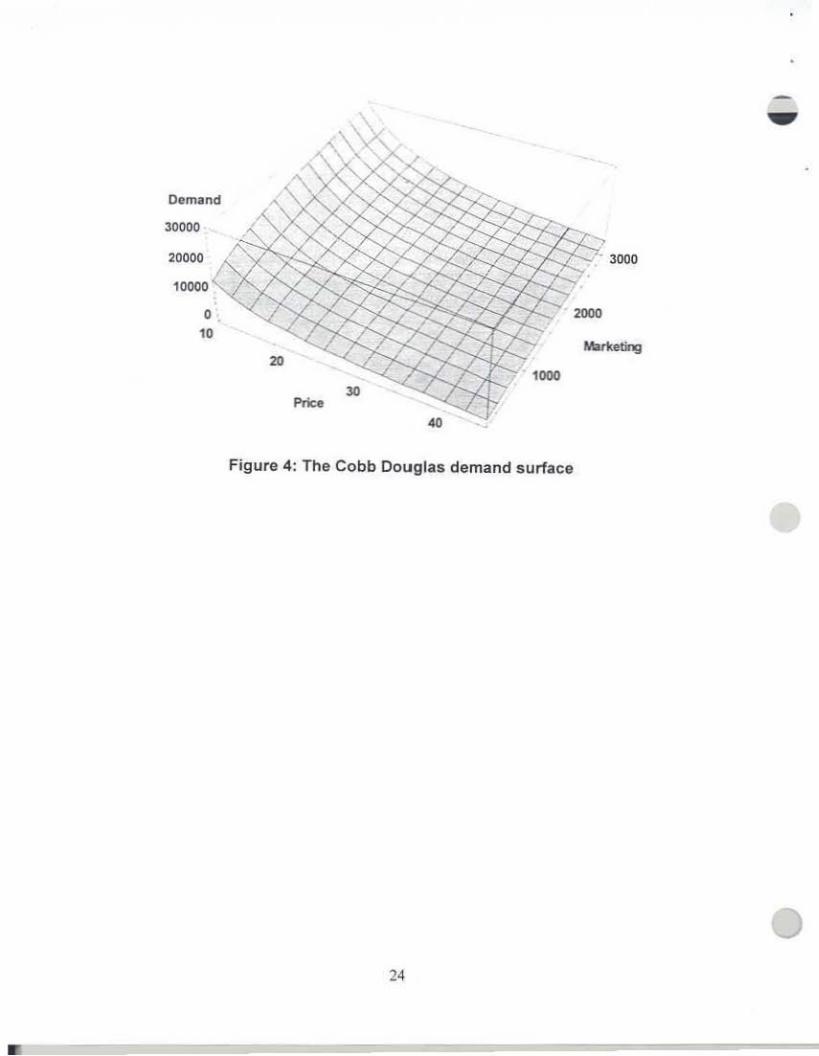
In the Figure 4. we '"31)' both price and marketing. Figure 4 illUSUlltCS the non--linearity of

the: demand ftmClion and the relanve stability of behavior O\"eJ the range. WhaI is interesting

7

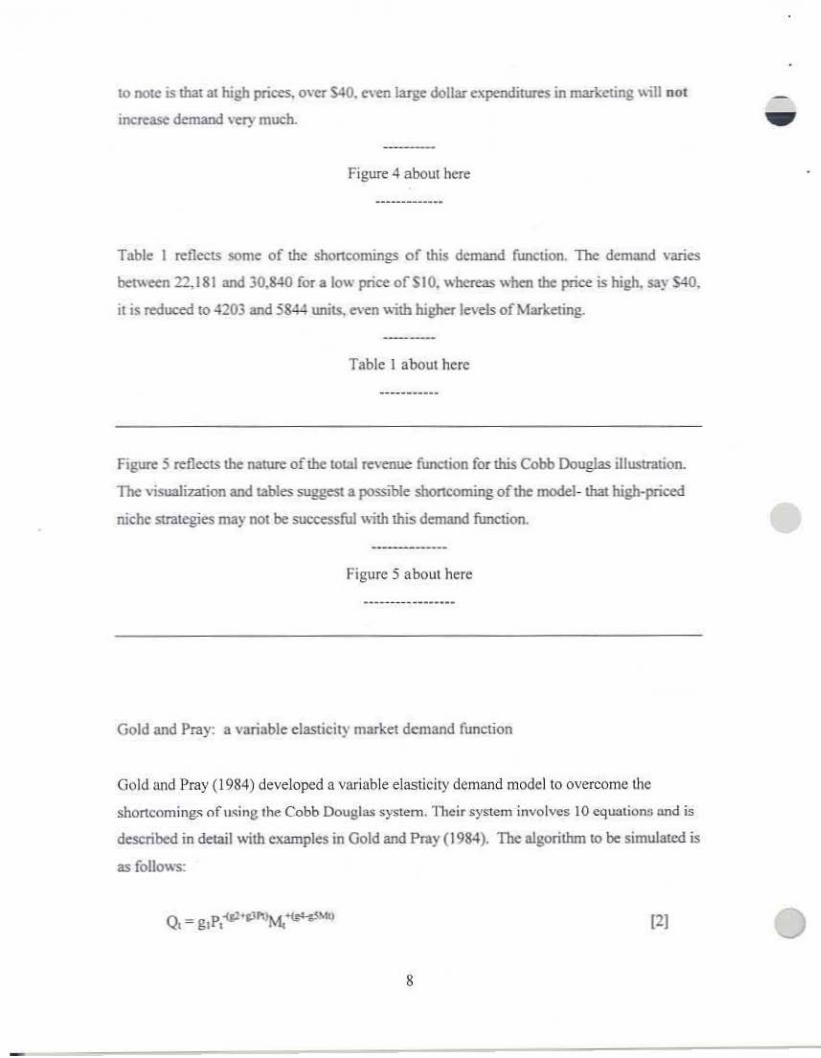
to ncMc is that at high prices, over S40. e-.·en !aJl;edollacexpendiltRS in marl.:eting "ill DOl

increase demand \'erY much.

Figure 4 about here

Table I reflects some of the shoncomings o f this dC1l13lld fwx:tion. lbc demand varies

b:t\o."tCD 22.1 81 and 30.840 for a low price of SIO. whcreas when tile price is high, say S40.

illS reduced to 420) and 5844 units, even " ilh higher levels of Marketing.

Table I abo ut here

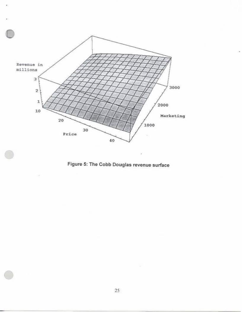
Figure 5 reflects the nature of the IOlaI revenue function for thU Cobb Douglas iIlllStnltion.

The 'isuaJi:l.a1ion and tables suggest a possible~ing of the model. thar. 1Ugh· prioed

niche sttalegies may001 be surxessful with this demard function.

Figure 5 a bout here

Gold and Pray: a variab le elasticity market demand function

Gold and Pray ( 1984) developed a variable elast icity demand model to overcome the

shortcomings of"s;ne lhe Cobb Douglas system. Their system involves 10 equal iOn!! and is

described in detail with examples in Gold and Pray ( 1984). The algorithm to be simulated is

as follows:

(2)

8

-

•

•

"1lere: 0. • market demand aI Iirne l

P, • average price al!iJn., l

M, - average marketing cxpmditUTe aI time I.

gt; = marke t demand parameters k where k ~ I through 5

To solve for the paramelers of the market demand equation the administrator mus t specify

the desired exogenous elasucities of each independent demand ,·ariahle ettwo difTerml

levels (i.e. P, M). The elasticity fonnulas are as follows:

•

EPI - g2-.vp, ( I ... In PJ

Em. " g4-g5M.{1---In MJ

where : Ep. - price elasticit y at lime l.

Em," marketing expenditure elasticity allimc L

III1'1

•

Selecting IWO levels for each elasticity (Ep. and E.) and!he eo"espooding demand ' -ariablc

(P and M) over a reasonable range gives two eq uations with two lUIkno"ns and allow

simultaneous solution of the systen parameters Sl (for k=2.5). The selection of gl

determines the initial market size. A model ing 1001 makes solving and simplifying this

system ofequalions relatively easy. Thus. beyo nd its visualization uses. Malhematiea~

offers many mathematicaltools 10 aid in the development of the functional structure of a

model . To demonslIa le the demand sySlem. Tab le 2 includes the values used to produce the

subsequenl visual izmions.

Table 2 about here

9

With these parameters. the: price elasticil>' or demand lit themarket level ino:reascs from an

ieelastic .95 10 . highly etasoc 3.00 ""bm the price increases from S25 10 S35, Likewise. the

marl.:t"l:ing dasticil~ dechnes as more 1TIllllt">' is allocated to marl;eting.

With these values and II scaling coefficient, market demand is aboul 6000 units when price

is 520 and marketing S500. A visualization Where price varies over the relevant range from

S25 10 $35 and marketing ranges from S500 to $1 500 reveals some very interesting results.

The 3-D plot of Figure 6 demonstrates that the gross behavior of the Gold and Pray

model is consistent with the theory renttted in the Cobb Douglas function. It is

intereSting to note that this variable elasti cily behaves similarly 10 Ihat in the Cobb Douglas

model in Ihat at the Iughcrprices. demand is nOI very responsi,-c 10 il'll:'l"USes in marl:eting.

Such a global view orthc: beha'ior of. function mar be difficult 10apJRhend quickly

" i thout utilizing visualization.

Figure 6 about hen:

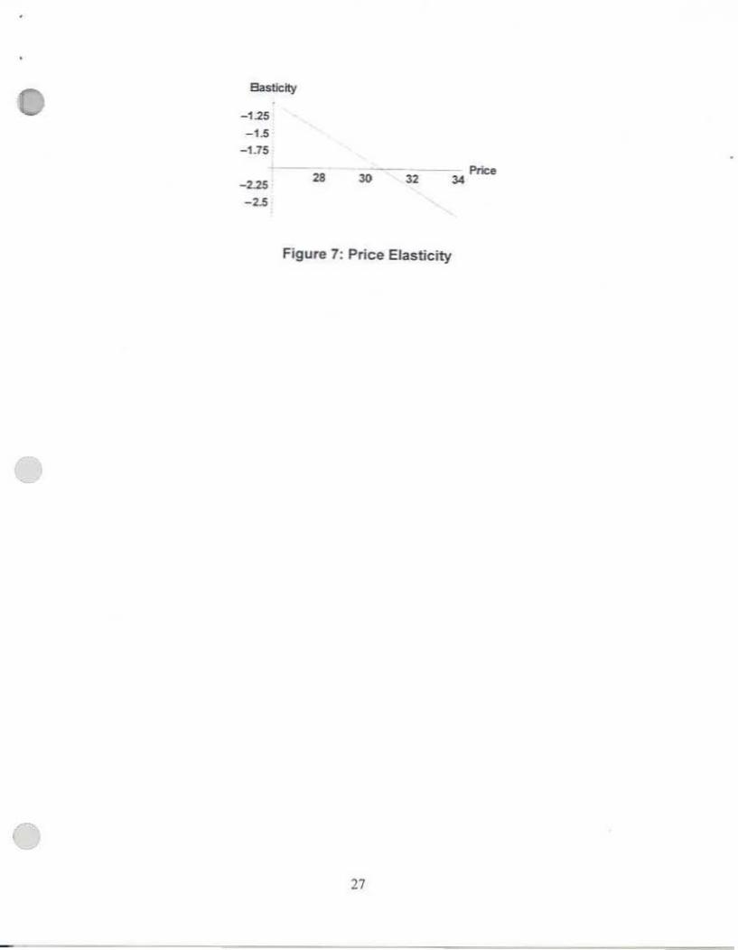
The Gold and Pray model can be furth er veri fied by using the modeli ng program to

calculate the arc elastici ties for price and mar keting. Indeed. the line graph roo"," in

Figure 1 demonstrates Ihatlhe price elasticities arc consistent with preestablished ranges

and expectations. Hi&Jler price elasticities are associated with higher prices. ctll'ri~

parabus. Howe ver. the model and theory arc in agTttrT\CJIt onlr if the price and marl.:etin2

values are constnined to be within the relevant ranges sbo"n in Table I .

Figure 1 about here

10

•

•

•

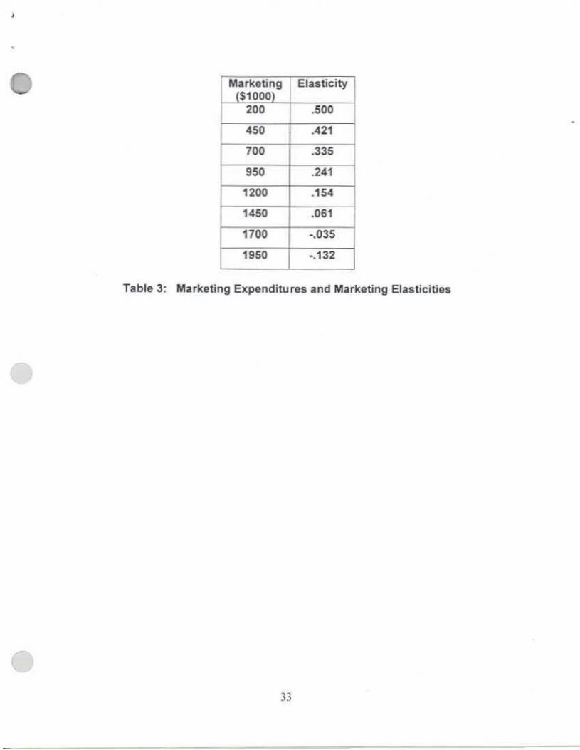
Table 3 shows t!'IaI \he elastic ities for marl.:ning over the~ $250 10 $ I SOO an: consistcnt

" ith thepm:stabished , ..lues 'Ihov.n in Table I and with ma:ri:ning ihcol)'. Howl'v~. above

the$I SOO 1e\~I . negative returns occ ur 10marketing. Tbese nq>,ali\~ returns an: one

ex ample of inst.:tbHil), in !he demand function ,

Table 3 about here

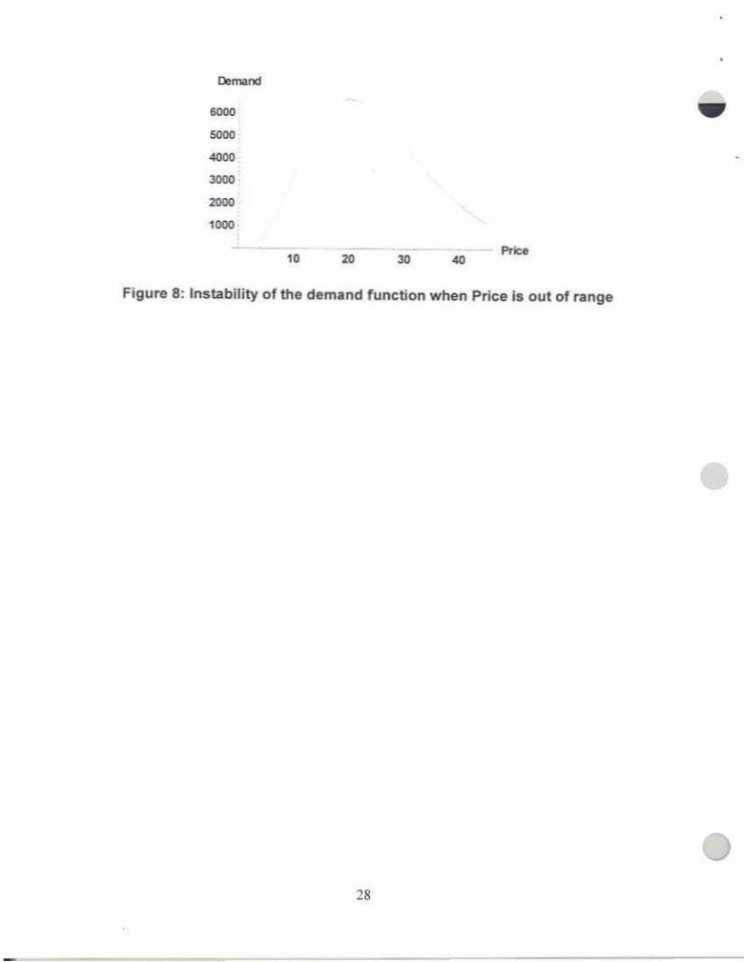
Instability in the fwxtion

Mathemalical!! makes it readi l)' apparcnt thai me dertwld syssem is robust ever the

consuaincd rangeo f decision inputs. Increasing the price and marketing out of the range

rcveals some extreme behaviors"'ithin!he model,

Notice in Figure 8 thai at prices from S4 10 $20 the function behaves in a mann~!hat is

inconsislent with demand tbecry. The mod el behaves consistcntly " i tb theo ry for all prices

above $20. Wh at is interesting, bowevcr. is thaI at lo.....er prices, say from $5 10 $18 dollars,

price increases cause demand 10 increase! Price s outside the des igned range can make the

model behave as an economic Giffen good ,

Figure 8 about here

Figure 9 depicts quant ity demanded v,i lh marketing V8l)ing from S200 10 $3000 and

price fixed at 525. The marketing response. appears 10 be COnsiSlcrtt with expectations

over the: relevant range . But negative renrrns to marke ting occur outsi de the: upper limit of

11

S ISIlO. The negative ret urns ma y be hel pful in SOITlC' simulatio n situatlens. BUI the

theoretical realism o f negali...e retumlI can be challenged.

FigIR 9 aboul here

Discovering Wlexpeelcd beha\~O\"!i in a model is One of the key benefits of usmg

vis ualization techniques. A classic example is that of Ansccmbc (1973) ...ho developed a

data set ...here. a nerve student of statistic s rnight l:cnerate four identical two variable

regre ssion models. However. ploUing the dati and res iduals reveals that three of the model s

have serious shortcomings including: CU!\'alUI'C, outliers and extremely influential dati

points! There are many situations like Anscembe's ...here visualizing a mathematical

function will pro"ide!he quickest and most clear indiClu ion of!he funclion 's behavior.

In our example. visualintion has made clear that the: Gold and Pray demand function

bebaves in a thc:ofetica1ly appropriate way. bul only as long as the: assumed ntnge of price

and marketing values areobe)-ed.

Using visualization 10 develop new model s

Teach and Schwartz (2000) have developed a mod ification of the Teach (19 84) model 10

allow for interactive effects between independent variables. As Teach points out. the

original Gold and Pray (1 997) anribute demand model does nOI a llow for cross

elasticities or for an imcractive e ffect between say price and advertising. In Ihis final

example. vis ual modeling is used 10 dernon5uate bow !he varia ble elasticity model of

Gold and Pray can be easi ly eXleDded to allow for imersetive effects bet ween

combi nations of indcpcndml variables. In this case. visualization is used as part of the

development of this extension 10 the: model,

12

•

•

•

•

T1lc fInal system is described ';3 a sct of simple examples. To determine the market- and

firm-level demand for ~eh segment. Equatio n .5 is used. Price is setto vary between 525

and 535 and advenlsinafmarketing expenditures bet ween 5500 and $1200. A 1le\Io"

\'3Jiable is set up 10 account for the interactive: effect. wh ich is the ratio ofrmuketing to

price. This new "aria ble includes the joint effectS of price and m.arl.etmg o n demand.

The elasticities on the ratio (R.J are controlled over a range from 0 to - J.D.

ts[

where: 01 .. market demand at time I.

P, ., harmonic average pnce o rall pmduetsat time L

Me .. average marketing apendirure for all producu at lime L

R. " average mtio of mark~ng divided by price (M/PJ o r all products for

lII. time l.

8l: .. market demand parameters k.

The range of parameters is displayed in Table 4.

Table: 4 aboul hell'

In Figures 10 we replicate !he simulation prese nted in Figure 6 bot add a new ele ment: a

ratio variable of marketing 10price which allows for an imeractive effect bC'rween price and

marketing.

Figure 10 abouthere

13

A vtsual comparison of Figure 10 with Figure 6 iIIU5l1l1tes how the interactive effect of price

and markaing change the enti re shape of the response function - from oonca''t: 10 C:On''CX

from the oriJl.ln. 1bc interxth" impact ha$ some interesting p<ope'''o:s. Now if a finn has a

low pnce (S2S) and markets extensively (SI(00). iu quantity demanded toceees from

1500to over IS.ooo units! Furthermore il appears that"'branding-rna)' be modeled with the

imcrncrive \"luillblcs. Notice that firms with high prices ($32) and 1arge amounts of

mart.:eting ($ 1200) can still have a high level of demand. O"CT 11.000 units compared to

S.200 from Figure 6.

Summary and concl usions

The purpose of this paper was to demon stra te a visualization technique that is useful to

designers of business simulations. Certainly, the idea of using visualization to supplement

modeling is a simple one. Howe ,·er. the benefits of em ploying visuali zation can be

considerable. Three examples were presented 10 demonstrate some ofthc capabilities and

benefits o f a ,· isual approach to modeling. In one example. viSUlllizal ion helped id~lify

the shortcomingsof lhc Cobb Douglas function as a demand model . Then, the Gold and

Pra> demand S)'SlCTII was sho\\n 10 resolve some o f these sbortccmin gs [i.e. allowing the

e lasl ieities to "ary) but was demonstrated to be highly unstable outside the preset

paramele~ . In the final illustration, visualization was used to create a new extension of an

existing model. Speci fically. the Gold and Pray demand system was enhanced 10 include

a new variable (the rat io of market ing to price ) to account for cross-elast icity effects . The

vis ualizat ions sllggest that the interactive effec ts may be readily handled by this simple

modification to the Gold and Pray demand system.

orcourse. a visuaJicalion by itself is not enough to communicate all the nuaoces o f a

complex business demand function_As in the examples presented here. combininlil

visualintion with tables ofnwnbcr:s mar provide the modeler wi th enough information 10

address many questions.

14

•

•

•

Because of lhe \li despread evaiiabllhy of powerful software 1OO1s. visualization is now

being applied to a large number of problem$. For bu5iness simulation dcslgnen. tools lhat

com bine lJlalhI,~ modding \li th visualization mak~ possibk a WIer:tnd mon'

interactin design p oeess. In tum. such a pooccss can enabl~ new insiSlu5 imo elliSling

models. or allow rapid inclusion of new «Ol'lOnlic issues into modem business simulations.

"

Refereeces

Anscombe. F. J. (1973). Graphs in StaIistieal AnaI~'S;s. T1te Amu,can Statist/rilln. 27. 17­

21.

Carvalho. O. F. (1993). A Dynamic Markel Share Allocation Model for Computerized

Business Simulations. lHn/opmCnls in B"s;rn'$SSimulol;on and Experiential Enrcises .

20. 31-33 .

Can"a1bo. G. F. (1995). Modeling the Law o r Dernand in Business Simuhllon..

Sima/ulion & Gaming~ An InltrllOfional Journal. 26(1). 60-79.

Decker . R., laBarre, J. & Adler. T. (19 87). The Exponential Logarithm Function as an

Algori thm for Business Simul at ion. Dudopnll!/lIS in Business Simulalion and Experientia l

Exercises, 14. 47-49.

Golden. P. A. (19 87). Demand Gene ration in a Service Industry Simulation: An

Algorithmic Paradox. [h"fdopmCniS in BusiMSS Simulotion and ExpericmiaJ Exercises.

14.67·70.

Gold. S. C. (1990). Modeling Cost Functions in Computerized Business Simulations.

Ihwdoprncnls in BusilU5s Simulation and U p"ricmial Exercist$. 17. 70-72.

Gold. S.. & Pray , T. (1984) . Modeling Markel and Finn Level Demand Functions in

Compu terized Business Simulatio ns, SimI/la/ion and Gaming: An IlIIl.'TYlational Jourl1l.lf.

15(3).J46-J63.

Gold. S. C .• &:. Pray. T. F. (19 84). Modeling Non-Price Factors in the Demand FlUlCtions

ofComputerittd Business Simulalions.. rx.Tlap~nl S in Business Simulation and

u~ri~ntial Exercises. I I. 240..243.

16

•

••

•

•

•

Gold, S_ C, & Pray, T. F. ( 1989). The Production Frontier in Computerized BU$iness

Simulations. !NIylopmcnts in Buslnrn SImulation and ExfRrientiol Exercises. 16, 24-30.

Gold. S. C ( 1993). Mod eling lmeractive Effects in /I'!athemaI ical Functions for BU$ill<:SS

Simulations: A Crmque of Goosen lind Kusel's Interpolation Approach. Simulation &

Gaming - A" InlUtllltional Journal, 24(1). 90-94.

Gold, S. C . & Pray. T. F. ( 1995). TIle: use crue Gamm a Probability Distribution: A

Critiq ue of Carvalho's Demand Simulator Stmula tion & Gaming - An Internalional

Journal. 26(1). 80-87.

Gold. S. C. (1992). Modeling Short -Run Cost and Production Functions in Computerized

Business Simulalions. Siml/Jalion& Gaming _ An International Journal, 23(4). 417--430.

Gold, S. C . &. Pray . T. F. ( 1998). Technological Change and lntertemperal Mo\·~nts in

Consumer Preferences In the Design ofCompu tm ttd Business Sirnulatlces ...ith Markel.

Segmentation. ~I"tlopmerus in Business SI,"I/Iotion and bperien/lof Exercises. 25. 156­

167_

Gold. S.c.. & Pray, T. F. (1997). Modeling Attribu tes in Demand Functions of

Computerized Business Simu lations: An Extension ofTeach's Gravity Flow Algorithm.

Develop ments in fluslnns Sim,da/ion (md Experiential Exercises. 24. 132-141 .

Gold, S. C. & Pray. T. F. (1999). Changing C ustomer Prefen:nces and Product

Ch:lnlCleristics in the Design of Demand Functions . Simulation & Gaming _ An

Internat/ona f JOl/rna f. 30(3). 264-2g:z.

Ooosen, K. R. 8:. Kuse l. J. ( 1993). Achieving IlIIeractive Variabk Modeling Through

Interpo lation: A R<:$ponse to Gold's Commen ts, Simulation & Gammg - An

Inlunalional Jaurnal. 24(1), 95-105 .

17

Goosen. K. R. & KII5C'I. J. (1993). An Inlcrpolation Approach to Developing

Mathematical Functions for BIISine3.s Simulations. Simulation <£ Gaming _ An

InlunationalJolU7tQl. 24( 1). 76-89.

Mergen. A. E.. & Pray. T. F. ( 1992). Model ing Total Quality Elements Into a Slflltegr­

Oriented Simulation. SImulation <£ Gaming - An Imernationol JOllrtWl. 23(3). 277-297.

"ray. T. & Mctbe. D. ( 199 1) . Model ing Radic al Changes in Tech nology wi thin Slflllegy­

Oriented Business Simula tions. Stmutationand Gaming - An Inlernolional Jal/rnal. 22.

19-35.

Teach, R. (1993). Forecasting and Manageme nt Ability: A Response to Wolfe.

Simulation <£ Gaming - An Inlerna/ional Journal. 24(1). 63-72.

--

Teach. R. (198-1>' Using Spatial Rela tionships to Estimate Demand in Busiocss

Simulations. DtwfopmenU in Business SimllllJfion and~rienlial b t rdu s. lIb. 244-

246. ~

Teach. R. & Schwanz. R. (2000). Introd ucing cross-elasticities in demand equations.

Simulation and Gaming - An InterdiscipUnaryJournal, 27( 1), 125·13 I .

Thavikulwat. P. ( 1993). Multiple Industries in co mputerized business gaming simulat ions.

Developments in Business Simulation and Experil.'ll/ial Exercises. 20, 108- 109.

Thavikul .....u. P. ( 1992) Product Quality in Computerized Business Simulations. Simulation

<£ Gaming - An lnlu lIO/lonol Journal. 23(4). 4314 41 .

T'h.a"ikulwll.t. P. ( 1988). Simuilltin~ Demand in an Independent-Aeross-Fillns

Manilgement Game. lNlvlopmems in Businus Simulation and Ex~riemial Exercises. 15.

183·187.

•"

ThavikulwlIl. P. ( 1992). ProdUCl Quality in Business Simulalions Dr"t/apments in

BUl;'/US Simulalian and bperiemial Sxerciset, 19. 165·168.

Wolfram. S. ( 1993). Mal~ftIG/lCQ I!t: A S)Ilttm fr doing MutMftIG/'CS b), Computer,

Readin£. " 'lass; Addi5Qfl-.-Wc:sle) .

19

B~'JaPhicallnformalion:

Victor Peretti is an assislanl professor of manageman information systems at Rcchesrer ...

lnsutute of T~hnology. His research "'-as ad;no...kdgw. at ABSEL 2000 ...i th .. best

paper .....-ard, He has condOClW. and presenJed research izno the "isualiution of business

data. His ...ork in the classroom was ""';lIded the Richard and Virginb Eiscnhan Provost's

A...'ard for ExccllCTlCC in Teaching at RIT.

Thomas F. Pray is Dprofessor of the Collelle of' Business, Rochester lnstitute ofTechnology.

I-Ie is a past presiden t and fellow of the national Associat ion for Business Simulation and

Experiential Learning (ABSEL). Much of his published research is in the modchng of

dem and algorithms. quali ty' model ing. and new product dcvelopment issues in computerized

business simul31ions. He is an active business consultant. who conducts business decision

simulation seminars nationally and intenlalionaJly.

COl\'TACT OETAILS: Victor J. Peroni. ColI~ of Business. Ma.x Lowenlhal Building.

106 Lomb Memorial Drive. Rochester. NY 14613-S60S, USA; relcphonto + 1 585-475-n53;

fax +1 585-475-0571 ; email ,jpbbu@riLcdu. Thomas F. Pray. College of Business. MIDI

Lo....'eJl1haI Building. 106 Lomb Manorial Drive , Rocbesaer. NY 14623·5608, USA;

telephone +1 585..H 5·2344: fax +1 585-475 -6571 ; email lfubbu@riJ.edu.

20

•

II ' '_I. ..,. . ... . _• . 1, • • • , n , .01 1

..•........"-1----,,---"0---"0--- "0---,,---,:;----:::- .....

lOCI' • •

.-

....-

" "I ..1_ 1... n . ... . - 1. 1, • .•. " . ' ''1 . , ... . u . cu .·__._ 1·,...0.·. ·_ 11

• Her. Is the plot for Marketing of5OO, with pri,. ~arylng from 10 to AS.

Figure 1: Working w ith Mathematiea

•21

10000

"..SOOO

""" as " as os -

..

Figure 2: The Cobb Douglas demand curve decreasing with price

22

•

•

.......,"""

....'000

50"

'000 "" ' 000 '000Marketing

"'"Figure 3: The Cobb Douglas demllrld curve increasing with mal1l.eting

•23

~ ------

--O.lTUInd

30000

20000

""

..Figure 4: The Cobb Douglas demand s urface

. 3000

•

•...~~~-----------------

R.v.n.... in"'ill ion.

a

2

,ac

"

)000

H.. rketing

•

Figure 5: The Cobb Douglas revenue surface

25

......,

"

""'. 32

"dO

" dO

•

•Figure 6: The Gold Pr_y dema nd surface

"•

- 1.25

~U

- 1.75

" -~. ­" "•

•

Figure 7: Price Elasticity

27

"'~""

"""""'""'"""'""'""'"

" " se -

..

Figure 8: Instability of the demand functi on when Price is out of range

as

•

•

•

n~

"'",,~

moo6750

" oo

Figure 9: Instabil ity in t he demand function when Marketing is out of range

29

" "Pril;:. 32

"..800 Mi rtleting

..

Figure 10: Gold Pray Dema nd fu nction with cross-e las ticlty

]0

•

•

•

Marketing •

SO $1000 ' $2000 $3000,

Price $10

I0 22,181 27,308 30 ,841

• $200 9,655 11 ,867 13,424

$ 300 5,935 7,307 8,252

$40 04,203 5,174 5,843

Table 1; Demand as a function of Price ..nd Marketing with the CobbDouglas Function

31

Pr ice (P)e,

Stilrting value

'2'.OS

Final valueS3S3.00

•

•

Marketing (M)E,.

ssoo0.4

$15000.15

Tab le 2; Parameters used in Gold Pray model vis ualizations

J2

•

•

•

M,~rke~~g Elasticity$1000

200 .500

450 .421

700 .335

950 .241

1200 .154

1450 .061

1700 -.035

1950 _.132

Table 3: Marketing Expenditures and Marketing Elasticities

33

Price (P)E,

Starting value$2S0.9 5

Final valuesas3.00

•Marketin g (M)E.

Rati o ( MlP)E,

$5000.4

(500/25)=200.0

$1 5000.15

(1200/35)=34.281.0

Table 4: Parameters used In th e Gold Pray cro ss elasticity vleualiza tlon

J4

•

•