INTEGRATED WATER MANAGEMENT PRACTICES IN MEXICO AND THEIR

IMPACT ON LOCAL DRINKING WATER QUALITY: EFFICIENT ASSESSMENT

METHODS

A Thesis

By

JANET TORRES

Submitted to the Office of Graduate and Professional Studies of Texas A&M University

In partial fulfillment of the requirements for the degree of

MASTER OF SCIENCE

Chair of Committee, Jacqueline A. Aitkenhead-Peterson Co-Chair of Committee, Scott Senseman Committee Member, Ronald A. Kaiser Head of Department, Ronald A. Kaiser

May 2016

Major Subject: Water Management and Hydrological Science

Copyright 2016 Janet Torres

ii

ABSTRACT

While supplying safe drinking water is a critical issue in the development of nations

worldwide it has not been formalized as a requirement by the United Nations (UN). As a

result, efforts to bring modern water distribution to the citizens of developing countries have

resulted in greater access to unsanitized water. As has been observed in Mexico,

governmental centralization can leave municipal governments weak; lacking the essential

resources and skills to manage water distribution systems. This study sought to examine the

water distribution system San José de Gracia, Michoacán in Central Mexico using readily

available water quality testing kits. A further objective of the study was to use EPANET

models of the water distribution system to examine how chlorination and pumping regimes

affect water quality in this town. Sampling sites and indicators were chosen using Rapid

Drinking Water Quality methods promoted by the World Health Organization (WHO).

Despite being classified as having “improved” potable water by the WHO, the water

distributed in the town was not found to be safe for human consumption. Costly

inefficiencies in the distribution system were found to be built in that make the chlorination

system in use obsolete.

iii

DEDICATION

To my sources of energy Maria de los Angeles Gonzalez Partida, Bruno, Marley,

Edgar, Ethan, and Jimena. To my wife and our future together. Towards responsible resource

development in the Anthropocene.

iv

ACKNOWLEDGEMENTS

I would like to thank my committee chair, Dr. Jacqueline Aitkenhead-Peterson, and

my committee members, Dr. Senseman and Dr. Kaiser, for their patience and guidance

throughout the course of this research. The Municipality of Marcos Castellanos for their help

collecting data and information on local water resources. The L.T. Jordan Institute, which

provided me with enthusiasm and funding to complete my research trip abroad. Thanks also

go to my friends and colleagues and the College of Geosciences for making my time at Texas

A&M University a memorable and valuable experience. Also, thanks to Geneva Redmond

for lending me her skills as an editor and reminding me that I can do anything I set my mind

to. Finally, thanks to Spencer “Spok” Pokorski and Alan Lewis for their encouragement and

support throughout.

v

NOMENCLATURE

IMF International Monetary fund

IBRD International Bank of Reconstruction and Development

UN United Nations

MDG Millennium Development Goal

GDP Gross Domestic Product

GIS Geographic Information Systems

IWRM Integrated Water Resource Management

WHO World Health Organization

DWQG Drinking Water Quality Guidelines

pcpy per capita per year

TAMU Texas A&M University

RADWQ Rapid Assessment of Drinking-water Quality

CONAGUA Comisión Nacional del Agua

RBC River Basin Councils

EC electric conductivity

INEGI Instituto Nacional de Estadística y Geografía

TMVB Trans-Mexican Volcanic Belt

LDC Least Developed Country

vi

TABLE OF CONTENTS

Page

ABSTRACT .............................................................................................................................. ii

DEDICATION ......................................................................................................................... iii

ACKNOWLEDGEMENTS ..................................................................................................... iv

NOMENCLATURE ..................................................................................................................v

TABLE OF CONTENTS ......................................................................................................... vi

LIST OF FIGURES ............................................................................................................... viii

LIST OF TABLES ................................................................................................................... xi

1. INTRODUCTION .............................................................................................................1

1.1 History of International Development Strategies ..................................................... 1 1.2 Modern Mechanisms for Water Development .......................................................... 5 1.3 Integrated Water Resource Management .................................................................. 7

2. CAPACITY DEVELOPMENT IN WATER MANAGEMENT .....................................10

2.1 International Guidelines for Drinking-Water Quality ............................................ 11 Chlorine in water distribution systems................................................................ 12

2.2 National Development Strategies ........................................................................... 16 Development background of Mexico .................................................................. 16 Water management in Mexico ............................................................................ 21

2.3 Research Objectives ................................................................................................ 23 2.4 Hypotheses .............................................................................................................. 25

3. MATERIALS AND METHODS .....................................................................................27

3.1 Site Description ....................................................................................................... 27 Characteristics of the Lerma-Chapala basin ....................................................... 27 Local characteristics ............................................................................................ 33

3.2 Modified RADWQ Procedure ................................................................................ 42 3.3 Sample Collection and Chemical and Biological Analyses.................................... 45 3.4 Analytical Chemistry .............................................................................................. 49

vii

3.5 EPANET Model ...................................................................................................... 49 Calculating demand for EPANET model............................................................ 53 Chlorine decay .................................................................................................... 57

3.6 Statistical Analyses ................................................................................................. 59

4. RESULTS ........................................................................................................................61

4.1 RADWQ Evaluation ............................................................................................... 61 4.2 Water Quality Results from Test Kits ..................................................................... 65

pH and electrical conductivity ............................................................................ 65 Total dissolved solids .......................................................................................... 71 Pesticides ............................................................................................................. 71 Metals .................................................................................................................. 71 Total coliform, E. coli and other coliform .......................................................... 71 Chlorine ............................................................................................................... 81

4.3 Analytical Chemistry .............................................................................................. 85 Dissolved organic carbon .................................................................................... 85 Nitrate-N ............................................................................................................. 85 Ammonium-N ..................................................................................................... 85 Phosphate-P ......................................................................................................... 91

4.3.5 Cations: Sodium, Potassium. Magnesium and Calcium ..................................... 91 4.4 EPANET Model ...................................................................................................... 93

5. DISCUSSION ..................................................................................................................98

5.1 Lerma-Chapala Basin ............................................................................................. 98 5.2 Marcos Castellanos Municipality and Town of San José de Gracia ....................... 99 5.3 Indicators and Testing ........................................................................................... 100 5.4 Disinfection of Drinking Water Systems .............................................................. 103 5.5 Water Costs ........................................................................................................... 106 5.6 Limitations of Study ............................................................................................. 110

6. CONCLUSION AND RECOMMENDATIONS ..........................................................111

REFERENCES ......................................................................................................................114

APPENDIX ............................................................................................................................130

viii

LIST OF FIGURES

Page

Figure 1 Climate regions and boundaries of federally protected areas. Data Source: INEGI. 18

Figure 2 Land cover in Mexico. Data source: INEGI ............................................................. 20

Figure 3 Populations by municipalities. Data source: INEGI................................................. 20

Figure 4 Location of Marcos Castellanos municipality. Source of data: INEGI .................... 29

Figure 5 hydro-political sub-divisions of the study area. Source of Data: INEGI ................. 30

Figure 6 Rock types and the potential permeability of rocks in the Lerma-Chapala Basin ... 32

Figure 7 Marcos Castellanos and surrounding communities including San José de Gracia .. 35

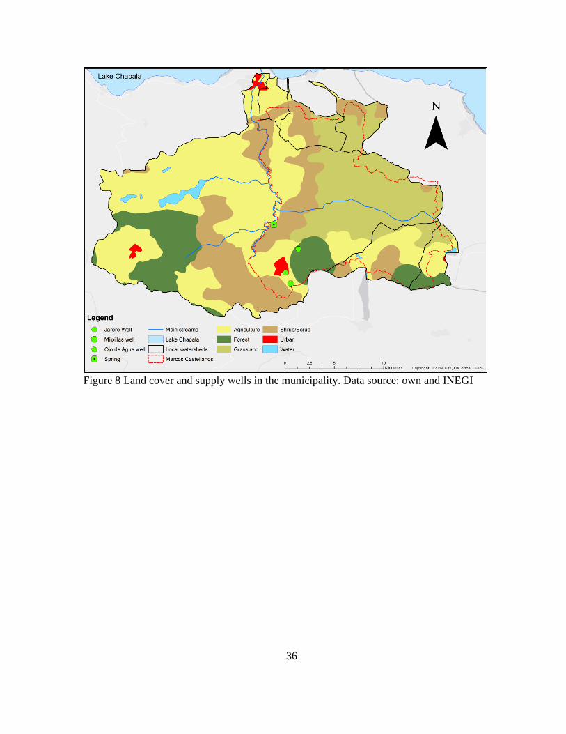
Figure 8 Land cover and supply wells in the municipality. Data source: own and INEGI .... 36

Figure 9 Water sources for the town of San José de Gracia ................................................... 37

Figure 10 Chlorination sites for water supplies in San Jose de Garcia ................................... 39

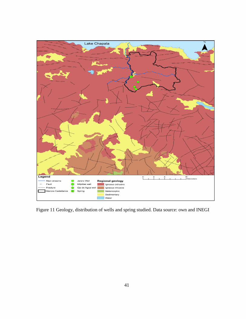
Figure 11 Geology, distribution of wells and spring studied. Data source: own and INEGI . 41

Figure 12 RADWQ procedure followed by this study. Figure adapted from Handbook of Catchment Management (Ferrier et al., 2009) ............................................................ 44

Figure 13 Spatial distribution of water samples collected in 2012 ......................................... 47

Figure 14 Sample sites in 2013 ............................................................................................... 48

Figure 15 the assumed water demand pattern used in EPANET model ................................. 52

Figure 16 Estimated block demand used in EPANET model for San José de Gracia ............ 56

Figure 17 Box and whisker plot of DOC N=25 ...................................................................... 58

Figure 18 Sample of collected scoria ...................................................................................... 63

Figure 19 Exposed lava flows in the municipality .................................................................. 63

Figure 20 Land use and geological features around the Rio de la Passion watershed ............ 64

ix

Figure 21 Box and whisker plots of pH in water samples. N=38 ........................................... 68

Figure 22 Box and whisker plots of electrical conductivity (EC) in water samples. N=26 ... 70

Figure 23. Spatial Distribution of pesticides tested ................................................................ 73

Figure 24 Sample of coliform tests on samples and control. .................................................. 73

Figure 25 Spatial distribution of coliform in drinking water samples .................................... 74

Figure 26 Histogram of coliform counts by sample type. N=37 ............................................ 75

Figure 27 Box and whisker plots of coliforms in water samples. N=37 ................................ 75

Figure 28 Spatial distribution of E.coli detected in samples .................................................. 76

Figure 29 Frequency of E.coli by sample source N=37 ......................................................... 77

Figure 30 Box and whisker plots of E. coli in water samples. N=38 ..................................... 79

Figure 31 Scatter plot relating chlorine and total coliforms in water samples ....................... 80

Figure 32 Total coliforms throughout the drinking water delivery system ............................ 80

Figure 33 Frequency of Cl concentrations in drinking water by year N=37 .......................... 82

Figure 34 Spatial distribution of total chlorine ....................................................................... 83

Figure 35 Spatial distribution of free chlorine ........................................................................ 84

Figure 36 Spatial distribution of DOC N = 25 ........................................................................ 86

Figure 37 Box and whisker plots of nitrate-N in water sources and storage (deposit). N=12 87

Figure 38 Spatial distribution of NO3 measured in samples N = 12 ....................................... 88

Figure 39 Box and whisker plots of NH4-N in water samples. N = 25 .................................. 89

Figure 40 Spatial distribution of NH4-N measured in samples N = 25 ................................... 90

Figure 41 Spatial distribution of cations (meq/L) .................................................................. 92

Figure 42 Concentration of Chlorine at nodes in all scenarios at 6:00 am ............................. 96

Figure 43 Concentration of Chlorine at nodes in all scenarios at 12:00 pm ........................... 96

x

Figure 44 Concentration of Chlorine at nodes in all scenarios at 5:00 pm ............................. 97

Figure 45 Comparison of water cost in San José de Gracia to U.S. cities ............................ 107

Figure 46 EPANET water distribution system model of San Jose de Gracia. Map by Janet Torres using own data and town CAD data. ............................................................. 130

Figure 47 Histogram of water users’ consumption in 2012 .................................................. 131

Figure 48 Distribution of water consumption by domestic users ......................................... 131

Figure 49 Frequency of water consumption by non-domestic users .................................... 132

Figure 50 Distribution of water consumption by non-domestic users .................................. 132

Figure 51 Consumption of all metered users ........................................................................ 133

Figure 52 Distribution of water consumption by all metered users ...................................... 133

Figure 53 Contour of free chlorine predicted by models P0-P3 ........................................... 134

Figure 54 Contour of free chlorine predicted by models P4-P7 ........................................... 135

Figure 55 Contour of free chlorine predicted by models P8-C2 ........................................... 136

Figure 56 Contour of free chlorine predicted by models C3-C6 .......................................... 137

Figure 57 Contour of free chlorine predicted by models C7-N1 .......................................... 138

Figure 58 Contour of free chlorine predicted by models N2-N5 .......................................... 139

Figure 59 Contour of free chlorine predicted by models N6-N8 .......................................... 140

xi

LIST OF TABLES

Page

Table 1 Comparison of water indicators across multiple countries. N/A – data not available. Source: IBNET.............................................................................................................. 6

Table 2 Codes for model runs in EPANET. AC=Agua Caliente spring, JR=Jarero well, MP=Milpillas well and ODA=Ojo de Agua well ....................................................... 52

Table 3 Classes of water users in San José de Gracia. Data source: town records ................. 54

Table 4 Median water use in m3 per year from contracts with 12 months of data in 2012 ..... 54

Table 5 Bulk decay rates used in EPANET model for each of the sources ............................ 58

Table 6 Summary of water quality indicators. †Test kits used ............................................... 66

Table 7 Analysis of water chemistry as it relates to sources of groundwater ......................... 67

Table 8 One tailed T-tests on number of nodes below 2.0 mg/L of free chlorine. P = Partial supply (current regime in town), C = Continuous supply and N = Continuous supply with no demand pattern. Numbers following letters indicate the number of scenario run ............................................................................................................................... 94

Table 9 One tailed T-tests on chlorine concentrations between pumping scenarios .............. 94

Table 10 Comparison of WB indicators of water costs using IBNET and collected data .... 109

Table 11 Overview of sample sizes for each test .................................................................. 141

1

1. INTRODUCTION

Water is an essential part of a country’s wellbeing and stability as it touches all three

essential components of sustainability: the economy, government, and environment.

Historically, international development has been mostly synonymous with economic

development. However, over the past several decades the term has regarded in a more

holistic and multidisciplinary sense, encompassing human development and sustainability in

addition to economic productivity (Todaro, 2011). Water quality can be used to assess

whether national policies are being followed and how effectively management structures are

adapting to regional and local conditions. The growth and development of a community,

thus, can be measured in terms of water quality.

Mexico has identified water infrastructure to be a crucial component of its national

development goals. Unfortunately, water management in Mexico has suffered from a long

history of centralization and shortsighted planning (Sánchez et al., 2012; Scott et al., 2008;

Tortajada et al., 2005). The absence of comprehensive planning for both water and land

resources has created an inefficient water management system that widely lacks clear goals

and objectives. Deficiencies in the Mexican federal government have adversely impacted the

welfare of the Mexican people and complicate its relationship with other nations (McDonald

et al., 2003; Wilder et al. 2006).

1.1 History of International Development Strategies

Water has been the subject of international development efforts since the first years of

the United Nations because of its integral role in life and the economy. The United Nations

2

(UN) was chartered at the end of World War II with the principal aims of maintaining peace

by establishing friendly relations between nations, promoting universal human rights, and

improving the lives of the poor (Amrith et al., 2008). Values such as social equity and

environmental justice have been slowly integrated into the UN’s mission, including those

that target long-term planning and management of water resources (Gleick, 1998). Assessing

how well agreements are implemented in developing countries has recently become a focus

in academic research and international development. To tackle poverty issues, including

those related to water, the UN has asked for cooperation from its member nations in

accomplishing development goals. The UN comprises six organizations that tackle these

challenges by building human capital, enhancing the transfer of technology, and financing

development. The UN first gave Technical Assistance to the Republic of Haiti in 1948 to

assess the reasons for the nation’s lack of economic growth (Amrith et al., 2008). This was

the first attempt to define and identify development and the problems which needed to be

addressed in future attempts to assist a nation.

In order to finance development and the reconstruction of countries after World War II,

an agreement between 44 nations in 1944 formed the Economic and Social Council, one of

the six organizations of the UN, to enhance development efforts through economic assistance

by mobilizing capital. The International Monetary Fund (IMF) and the International Bank of

Reconstruction and Development (IBRD, or World Bank) were created to finance, assist and

regulate member nations of the larger UN assembly (Zanetta, 2004). The ideals of the neo-

classical model that was being applied at the time were centered on supply-side economics.

The neo-classical model was predicated on the theory that development could be generated

3

by simply supplying infrastructure related to economic growth. The growth would in turn

trickle down throughout society and stabilize national governments (Williamson, 2009).

In the late 1940s, the World Bank (WB) focused on increasing necessary infrastructure to

promote economic growth through what were then thought to be the drivers of growth:

energy, transportation and agriculture. Projects aimed at the modernization of agriculture,

which first began making development loans in Latin America between 1948-1959, were the

third largest funding target by the World Bank (Zanetta, 2004). From these loans, dams,

power plants and transportation networks were built to drive output from markets and satisfy

the economic ideals of Import Substitution Industrialization (ISI) (Weintraub, 2009). ISI

increased GDP as governments borrowed money to develop infrastructure. However, this did

not impact the inequality of income distribution because no investments were made into

human capital (Weintraub, 2009).

Water management in the twentieth century was centered on resource exploitation to

further economic and population growth. This led to large water development projects to

increase the supply for uses deemed beneficial around the world (Hughes et al., 2013).

However, little concern was given for environmental impacts, sustainability, equity or the

role of community (Gleick, 1998). Although, the modernization of countries to meet

development standards has long been incorporated into the process of globalization, social

and ecological impacts were not seriously considered at the international level until the 1970s

(Rahaman et al., 2005). Member nations of international institutions are subjected to non-

binding agreements that define problems, outline solutions and promote international

cooperation. The first major declaration of a need to act on the environment came from the

1972 Stockholm Conference on the Human Environment. International consensuses such as

4

these provided catalysts for governments of developing nations to pursue Integrated Water

Resource Management (IWRM).

Throughout the 1960s and 1970s, nations in Latin America took on greater debt in order

to fund social programs targeting urban and, to a lesser extent, rural areas (Todaro, 2011).

Since urban population growth was at the center of international development at the time,

these social programs created further gaps in quality of life between urban and rural

populations, especially in terms of access to water infrastructure and human capital in the

form of education (Levy, 2010). The inefficiency of economic development programs led

Latin America into a debt crisis during the 1980s, which worsened because of a national

currency crash fueled by loans that were largely in foreign currency (Williamson, 2009).

The debt crisis of the 1980s changed the directive of the WB and IMF to promote

structural financial reforms (Todaro, 2011). These took form in structural adjustment loans,

which given with directives on structural economic and political changes to which borrowing

nations must comply. These changes were centered on the ideas of market liberalization and

fiscal discipline, often regarded as the “Washington consensus” (Williamson, 2009). This

began to challenge national autonomy by giving international powers a means by which to

dictate national policy. Liberalization strategies were encouraged, partly because much of

the investment in international development prior to the 1980s was ultimately borrowed and

used in the country to build self-sufficiency, instead of encouraging participation in the

global economy. This type of capital flow minimized Foreign Direct Investment (FDI),

which could have otherwise fueled development at no cost to nations (Cooper, 2009).

5

1.2 Modern Mechanisms for Water Development

During the 1990s and 2000s, the UN and its financing organization shifted focus to

social protection and improving governance. Efforts by the UN have since delivered several

publications meant to transfer technology in the form of development-oriented knowledge

and procedures. Among these, the eight Millennium Development Goals (MDGs)

established in 2000, and Drinking-water Quality Guidelines (DQG), first published in 1984,

set measurable standards and specified indicators for nations to target. Other publications on

IWRM and the Rapid Assessment of Drinking-water Quality (RADWQ) provided

instructions on how to manage and evaluate water resources.

The modern framework for implementing integrated resource management places water

at the center of development goals. The eight MDGs, established in 2000 had attainment

targets set for 2015, encompassed: education, health, eradication of hunger, empowerment of

women, and sustainability. Eight MDGs contained eighteen targets that outlined the

parameters needed to be addressed for the goals to be achieved. The MDGs also identified

forty-eight indicators to be used when evaluating the success or failure of development in a

country (UN, 2010).

Although the MDGs promoted long-established universal human rights, they have been

criticized because of their continuing approach to development schemes that apply a single

set of methods across diverse development scenarios (Vandemoortele, 2009). The MDGs

have also been criticized as idealistic because they outlined a desired state of development

without describing precisely how the changes should be achieved. This ambiguity makes it

possible for interest groups to use MDGs to push private agendas (i.e. foreign loans and

6

policy recommendations) that are not necessarily in the best interest of the country or people

(Vandemoortele, 2009). Furthermore, Vandermoortele (2009) explained that, because the

MDGs used benchmarks based on data from development indicators from 1990, present

efforts to apply them have failed to account for over ten years of changes in development

conditions. While setting the benchmarks to 1990 levels allowed the UN to establish what

originally seemed to be more obtainable targets, the magnitude of improvements will reflect

progress in development conditions from 1990 and not 2000. The current parameters of

several indicators collected and used by the UN through the World Bank and UN

Development Program are illustrated (Table 1). The data is made available through the

International Benchmarking Network for Water and Sanitation Utilities, a worldwide

database for performance of water and sanitation utilities.

Table 1 Comparison of water indicators across multiple countries. N/A – data not available. Source: IBNET

Indicator Ghana 2009

USA 2011

Mexico 2012

Brazil 2011

Water Coverage (%) 55 100 98 81 Sewerage Coverage (%) N/A 46 89 47 Total Water Consumption (l/person/day) 46 610 228 174 Residential Consumption (l/person/day) N/A 218 F 116 Non-Revenue Water (%) 52 13 24 39 Non-Revenue Water (m3/km/day) 42.1 10 21.5 32.6 % Sold that is Metered (%) N/A 100 75 N/A Operational Cost W&WW (US$/m3 water sold) 0.54 0.92 0.67 1.41 Staff W/1000 W pop served (W/1000 W pop served) N/A 0.7 0.5 N/A Average Revenue W&WW (US$/m3 water sold) 0.63 1.36 1.05 2.03 Collection Period (Days) 372 415 397 138 Collection Ratio (%) 79 168 79 99 Operating Cost Coverage (ratio) 1.16 1.48 1.56 1.44

7

Additional criticisms came in 2012, when the United Nations (UN) and World Health

Organization (WHO) reported achieving a 50% reduction in the population without access to

improved drinking water sources (Clasen, 2012). The announcement meant that a MDG

target had been reached three years ahead of schedule. Several authors have written on the

systematic overestimation of the methods used to monitor the progress. One author

estimated that a 25% of the world’s population lacked access to improved water sources,

rather than the 11% that was reported by UN and WHO (Onda et al., 2012; Zawahri et al.,

2011). Other authors have remarked on the failure of the definitions to distinguish between

“improved” and “unimproved” access to water. Suggesting that “improved” did not

realistically reflect the safety of the water being provided or the level of sanitary risk (Bain et

al. 2012; Gine-Garriga et al. 2011). The literature has also suggested that the MDGs did not

require monitoring of location-specific indicators and they merely use monetary metrics that

continue a tradition of donor-centric development ( Bain et al., 2012; Saith, 2006;

Vandemoortele, 2009).

1.3 Integrated Water Resource Management

Since the MDGs inherently required water resource management, IWRM has often been

referred to as the most holistic and efficient approach for countries to protect their water

resources (Giordano et al., 2014). IWRM is the accepted mechanism for improving the water

sector worldwide (Richter et al., 2013). The ideals of IWRM were first embodied in the

formation of the Tennessee Valley Authority in 1933, the first effort to regionalize water

management (Ludwig et al., 2013). The first international agreement on IWRM followed

many years later during the 1977 UN Conference on Water in Mar del Plata, Argentina,

8

which emphasized regional, national, and international coordination between water sectors

(Rahaman et al., 2005). Throughout water conferences that followed, the UN and

participating nations agreed to incorporate equity, the environment, and most importantly, the

economy, declaring water an economic good (Rahaman et al., 2005). The 2002 World

Summit on Sustainable Development in Johannesburg, South Africa, defined IWRM as an

economic and welfare-maximizing process that coordinated management and development of

water, land, and related resources without compromising the environment (Rahaman et al.,

2005).

Similar to the MDGs, IWRM has been criticized as simply presenting more goals and

ideals than actual mechanisms for achieving an integrated regional water management.

However, IWRM does promote efficiency through coordination to tackle multi-dimensional

problems (Biswas et al., 2005; Stålnacke et al., 2010). In order to bring efficiency into the

regulatory system, international organizations often recommend IWRM for its ability to

promote coordinated management of land, water and other natural resources (Durán Juárez et

al., 2006; Kalbus et al., 2012; Sánchez et al., 2012; Scott et al., 2008). This process of

enabling individuals, organizations, and societies to obtain, strengthen, and maintain the

capabilities to set and achieve their own development objectives over time is known as

“capacity development” (UNDP, 2008). Capacity development has evolved from technical

training and foreign expertise into a dynamic process for assisting national governments,

civil society organizations, independent national and regional institutions and other

stakeholders as they pursue their own development goals. International organizations

working with IWRM are increasingly engaged in supporting capacity development of water

managers through adequate venues for knowledge transfer that is tailored to regional

9

conditions (Kalbus et al., 2012). Similarly, the UN plays an important role in capacity

development around the world (Fukuda-Parr et al., 2013).

Promising advances have been made in the use of computer models to support IWRM

decision-making. The goal of such models is to address spatial and temporal variability in

water quality and quantity by incorporating the physical characteristics of a basin,

anthropogenic water systems, and local stakeholders (Jamieson et al., 1996; Nikolic et al.,

2013;). Such models however require a variety of physical data, which may not always

available in developing nations. With climate change threats, implementation of IWRM will

be crucial for all nations (Stålnacke et al., 2010). In theory, IWRM could provide developing

regions with the necessary framework to make effective decisions and possibly mitigate

climate change effects. This benefit can only be achieved if water management institutions

are able to cope with the uncertainty that comes with climate change planning (Ludwig et al.,

2013). IWRM presently focuses on current and historic issues in management, often using

system models that require historical data on the hydrologic cycle. Managers must be able to

incorporate long-term adaptation strategies that can address the unpredictability of climate

change. The literature overwhelmingly suggests that IWRM has not been successful, mainly

because authorities have not sufficiently incentivized the formation of strong regional

authorities provided room for alternative pragmatic solutions in the global discourse (Biswas

et al., 2005; Giordano et al., 2014;). Various methods for implementing IWRM have been

applied around the world. Such efforts have been hampered though because two key

components have been difficult to achieve in developing nations: good governance and

reliable data mining (Stålnacke et al., 2010).

10

2. CAPACITY DEVELOPMENT IN WATER MANAGEMENT

Implementing IWRM internationally requires cooperation and coordination between

many levels of governance. Having recognized this, international organizations have

developed programs and procedures to work with countries towards this goal. Target 3 of

Millennium Development Goal 7 (ensuring environmental sustainability), which seeks to

halve the proportion of the world’s population without sustainable access to safe drinking

water and sanitation, is assessed by the Joint Monitoring Programme (JMP), run by the

United Nation Children’s Fund (UNICEF) and the WHO (Zawahri et al., 2011). The JMP

uses household level surveys and assessment questionnaires to collect data on drinking water

and sanitation services (Shordt et al., 2004). In 2004, the WHO and UNICEF began to use

the RADWQ methods to assess the ability for JMP to monitor water safety in conjunction

with water access by using physical indicators (Egbuna et al., 2013). The goal of the

RADWQ handbook, which outlines methods and procedures to assess water quality

management in a holistic fashion, is to define critical areas and identify entities that may

require capacity development and a new regulatory framework (Howard et al., 2012).

The Millennium Development Goals (MDGs) set an arguably narrow definition of

‘improved’ water access, failing to account for the quality of water being delivered. The

quality of drinking water will depend on the types of contaminants to which the source

waters are exposed and the level of treatment the water receives before distribution.

Increased water access increases the responsibility to provide safe potable water, thereby

challenging the government’s ability to protect and manage natural resources. Governments

11

must take steps toward IWRM in order to efficiently protect water resources from

contamination in the interest of protecting human health.

2.1 International Guidelines for Drinking-Water Quality

Not all efforts made by the UN and its associated bodies have lacked specificity. Many

have formulated guidelines for developing nations to help them design effective water

management and water-monitoring. The WHO produced the Drinking Water Quality

Guidelines (DWQG), a Water Safety Plan Manual, and the Rapid Assessment of Drinking

Water Quality (RADWQ) handbook, which dealt specifically with improving water

management and quality (Howard et al., 2012). These tools account for the constraints on

available resources for testing water quality, while providing instructions for assembling

region-specific programs. Additional publications by the WHO have provided background

into methods of treating and testing drinking water (Au, 2004; Howard et al., 2003). This has

served as a form of technology transfer allowing developing countries access to scientific

knowledge and management strategies.

The WHO guidelines for drinking water quality (DWQG) established environmental

indicators and standards of quality, which developing countries often lack (Onda et al., 2012;

Sánchez et al., 2012; Tortajada et al., 2005). Despite their non-binding nature, the DWQG

transfers knowledge to underdeveloped regions that are considered essential toward

removing barriers to progress (Wade-Miller, 2006). In DWQG publications since 2003, the

WHO has emphasized a risk-based integrated approach to drinking water quality that

considers protecting water from contaminants at all stages of domestic supply and delivery

(Sobsey et al., 2002). The guidelines include chapters on topics ranging from disinfection to

12

plumbing, surveillance, system assessment, indicator parameters, safety plans, and even

guidelines for things like climate change, airports, and intense rainfall events (WHO, 2011).

The water quality indicators selected for publication in the DWQG include essential

physiochemical properties of water, such as pH and electrical conductivity (EC), that give

insight into the source of water and its aesthetics (WHO, 2011). Through DWQG, the WHO

recommends that developing nations test their drinking water for indicator bacteria once per

month (WHO, 2011). Their low- resolution recommendation considers the reality that many

communities in developing nations may lack access to elementary monitoring equipment and

management methods (Yang et al., 2013). Data with low temporal resolution can be used to

test for localized hazards and more quickly identify the most pressing challenges, such as

natural or human contaminants (Bain et al., 2012). Rapid assessment of water quality

provides two key services: a quantitative measure of water quality and insight into local

water management challenges and opportunities for improvement. In essence, rapid water

quality analyses can provide a measure of the effectiveness of local water management

strategies towards providing safe drinking-water.

Chlorine in water distribution systems

Water distribution systems (WDS) represent considerable investments for utilities and

governments in developing countries. The main priority of a water utility is to reliably

provide safe water. Maintaining the proper disinfection inputs for a WDS to provide safe

water to citizens represents an ongoing investment. Chlorine is the most commonly used

disinfectant used as a safeguard against pathogens because of its high reactivity with organic

matter and relative safety (Hallam et al., 2003; LeChevallier et al., 1990; Ozdemir et al.,

13

2002). Unfortunately, because of this high reactivity, chlorine concentrations are not

constant throughout the distribution network, and furthermore cannot be guaranteed to

eliminate all dangerous pathogens. LeChevallier (1990) recommended using a strong, highly

reactive disinfectant such as free chlorine as a primary disinfectant and monochloramine as a

secondary disinfectant in the distribution system because it showed promise in more

effectively penetrating biofilm. There have been some health concerns regarding the use of

monochloramines, although the EPA still permits their use in drinking water disinfection

(WHO, 2011). Mexico has set permissible limits on free chlorine between 0.2-1.5 mg/L and

may not exceed 3 mg/L (NOM-127-SSA1-1994) (Alcocer-Yamanaka et al., 2004). As a

result of the various variables which affect chlorine concentrations throughout distribution

systems as well as the creation of THM, multiple regression analysis is the most common

approach to model water networks. Through a multiple regression method, the water quality

parameters that impact the evolution of water in a system; such as, pH, temperature, organic

matter content, initial chlorine dosage, and distance traveled can be taken into consideration

(Ahn et al., 2012; Grayman et al., 1993).

Chlorine decay is often modeled as a time-varying, first-order decay factor because

organic matter content is usually an unknown variable. Chlorine decay is divided into two

parts, chlorine bulk decay from general consumption by organic matter in the water column,

and wall decay from reaction with biofilm and pipe materials (Ahn et al., 2012). Modeling

parameters of chlorine decay are also affected by conditions within the storage tanks, water

itself and ambient temperature (Grayman et al., 1993; Rossman et al., 1995;). Additionally,

models provide less accurate results in areas off the main water line and after storage. This is

because water quality, chlorine concentrations, in areas off the main water line depends

14

heavily on water consumption, and such data is difficult to obtain. Chlorine concentrations

in water prior to entering a distribution network is a key factor in determining what

concentrations will be throughout the system. Considering seasonal changes in water

demand, water treatment plants need to be flexible in the volume of chlorine initially mixed

into the water to maintain a minimum of 0.1 mg/L throughout the system (Ahn et al., 2012).

The most commonly used and accepted model for first order decay is Equation 1, in

which the chlorine residual (Ct) is a function of the initial chlorine concentration (C0) as

affect by a decay coefficient (-k) (Ahn et al., 2012; Alcocer-Yamanaka et al., 2004; Clark et

al., 1994; Georgescu et al., 2012; Grayman et al., 1993; Rossman et al., 1995; Vasconcelos,

1996). The decay coefficient (k) can be calibrated by incorporating parameters specific to

the distribution system (Equation 2), which attributes decay to the sum of bulk water decay

(Kb) and wall decay (Kw) (Powell et al., 2000). Bulk decay coefficients can vary greatly

depending on the quality of water before chlorination, ranges have been reported anywhere

from 0.02 - 0.74 h-1 (Hallam et al., 2003). The bulk decay coefficient has been further

expanded (Equation 3), such as wall decay of chlorine (kw), mass transfer coefficient between

bulk flow and pipe wall (kf), and the hydraulic radius of the pipeline (RH) (Ahn et al., 2012).

The decay coefficient can be further calibrated to the specific water system being modeled, in

its simplest form, by calculating kb and incorporating temperature (T) and Total Organic

Carbon (TOC) (Equation 4). Serious limitations in accuracy can arise when there is a lack of

design knowledge of the water distribution network (Ahn et al., 2012; Vasconcelos, 1996).

This is especially important for obtaining accurate results when modeling storage tank

chlorine dynamics, because flow rates in and out of the tanks as well as the ratio of active to

emergency storage volume need to be known (Rossman et al., 1995).

15

𝐶𝐶 = 𝐶𝐶0−𝑘𝑘𝑘𝑘 (Eq.1)

𝑘𝑘 = 𝑘𝑘𝑏𝑏 + 𝑘𝑘𝑤𝑤 (Eq.2)

𝑘𝑘 = 𝑘𝑘𝑏𝑏 + 𝑘𝑘𝑤𝑤𝑘𝑘𝑅𝑅𝐻𝐻(𝑘𝑘𝑤𝑤+𝑘𝑘𝑓𝑓)

(Eq.3)

𝑘𝑘𝑏𝑏 = 1.8 × 106𝑇𝑇𝑇𝑇𝐶𝐶𝑇𝑇�−6050𝑇𝑇+273� (Eq.4)

Dangerous by-products can be produced when chlorine reacts with organic matter as it

decays, such as total trihalomethanes (TTHM) which are potentially carcinogenic (Ahn et al.,

2012). Measuring organic content in the drinking water source is important for adding

appropriate chlorination volumes and also to protect consumers and utility workers from

these dangerous disinfectant by-products. EPANET is capable of modeling TTHM

formation in a distribution system through a first order regression model. It does this by

using a kinetic model developed using nonlinear least squares regression. Mexico does

regulate THM, setting the maximum exposure limit at 0.2 mg/L.

2.1.1.1 Biofilms

Biofilm growth is influenced by many factors including; pipe material, disinfectant

type used for water treatment, quality of source water, and physic-chemical parameters of

water such as nutrient amounts and temperature (Srinivasan et al., 2008). Suppression of

biofilm growth requires chlorine concentrations estimated at 1.8 mg/L but may differ

depending on the pipe material and roughness (Block, 1992). In PVC and copper pipes, 1

mg/L of chlorine was able to remove viable biofilm up to 100-fold (LeChevallier et al.,

1990). However, in iron pipes, whose rough surface harbors biofilm, concentration of free

chlorine up 4 mg/L were ineffective at controlling biofilm (LeChevallier et al., 1990). In

areas where coliform regrowth is a problem, utilities keep free chlorine residual

16

concentration between 3-6 mg/L. Past research from as early as 1986 demonstrated that

biofilm could be a source of coliform bacteria in drinking water (LeChevallier et al., 1990).

It is important to maintain residual chlorine concentrations in distribution systems to

maintain a low biofilm growth. However, high concentrations of chlorine residuals are

usually not accepted by water utilities, as they can cause corrosion, excessive concentrations

of trihalomethanes, and consumer complaints of aesthetics such as chorine taste and odor

(Ahn et al., 2012; Ozdemir et al., 2002).

2.2 National Development Strategies

The Latin American average withdrawal per capita per year (pcpy) for domestic use is 98

m3 (Castro et al., 2009). As is true in most of Latin America, Mexico’s greatest obstacle in

implementing IWRM come from rapid, unregulated urban expansion and destruction of

natural land cover to expand the agricultural exploitation of land (Lorz et al., 2012). IWRM

in Latin America has mainly focused on building the knowledge base for understanding the

natural framework, sediment characteristics, drinking water supply systems, and wastewater

treatment (Kalbus et al., 2012). However, coordination failure resulting from a lack of

coordinated decision-making, at all levels of government has made it difficult to implement

such management strategies (Tortajada et al., 2005).

Development background of Mexico

The World Bank classifies Mexico as an upper-middle income nation. Despite having a

GPD of more than 1.5 trillion dollars a year and 287 billion dollars of external debt stock in

2011, Mexico’s development is considerably limited for a country with such wealth (Bank,

17

2014; Castro et al., 2009), which may be in part due to its widespread range in climate and

biomes. Mexico has favorable trade access through coastlines in both the Pacific Ocean and

the Gulf of Mexico which it has tried to utilize through various free trade agreements.

Mexico has a wide range of climates and biomes; ranging from arid desert along the

U.S.-Mexico border to alpine temperate in Central Mexico and tropical rainforests in the

south (Figure 1). Such extensive natural diversity is in part due do to its active geologic

history. Much of the country is mountainous and enriched with metals and minerals. It is

currently a leading producer of petroleum, silver, copper, gold, lead, fluorspar, zinc, and

natural gas (Perez, 2011). Taking into account the existence of extensive natural diversity in

the country, the federal government has protected relatively small areas that fall into limited

types of biomes. Figure 1 shows that large protected areas are limited to Warm sub humid

and Very dry warm locations.

Today, approximately 59% percent of the land area in Mexico is owned by community-

based land holdings called Ejidos, (communally owned land distributed after the revolution

of 1917), which represent 66% of agricultural production units (Berkes et al., 2000). Almost

41% of land is owned by private individuals, but only represent 31% of agricultural

production. While only 13% of land in Mexico is arable, just 3% of this arable land is used

for irrigated agriculture (Figure 2). In spite of the low agricultural production in Mexico,

77% percent of withdrawn freshwater is used for agricultural purposes and only 23% of

withdrawals are used for domestic or industrial purposes (CIA, 2013).

18

Figure 1 Climate regions and boundaries of federally protected areas. Data Source: INEGI.

19

The lack of access to safe drinking-water and sanitation facilities reflects much of the

nation’s high level of poverty and inequality (Armentia et al., 2009; Bank, 2003). In Mexico,

only 13% of urban wastewater receives treatment before being discharged into streams

(Bank, 2012). Raw sewage in combination with non-point sources of pollution has rendered

most surface waters unsuitable for most uses. While the per capita water availability for

Mexico is around 4,400 m3 pcpy, northern states have only 2,044 m3 pcpy. In spite of having

less water resources, the northern states house a staggering 77% of the population and

generate 86% of the national GDP (Castro et al., 2009).

Mexico is a youthful country, with almost half of its population below the age of 25 and a

median age of 27. Dependency is primarily associated with minors and the elderly are less

than 10% of the population (CIA, 2013). Widespread income and social inequality in

Mexico have hindered national and local development. Nearly half of the country’s

population lives on an income of less than 2.5 USD per day, the majority of which are

indigenous groups (Crandall et al., 2005). High levels of income inequality can be attributed

to residual effects of colonization. In 1910, only 2.5% of the population owned land in

Mexico, compared to 75% of the population in the United States (Haber et al., 2003). A lack

of substantial growth in cities throughout the country, has created unsustainable populations

in the country’s major cities, and prevented growth in labor from rural migrants outside of

the central region (Figure 3). Populations are greatest in the central region with pockets of

development along border cities, tourist areas in the south and oil producing communities in

the Gulf coast.

20

Figure 2 Land cover in Mexico. Data source: INEGI

Figure 3 Populations by municipalities. Data source: INEGI

21

Water management in Mexico

The goal of providing safe drinking water challenges developing countries to update their

water policy and execute infrastructure development projects that are within their means. In

Mexico, expansion of hydraulic systems accounted for up to 14% of the federal budget

between 1941 and 1955 (Aguilar, 2004). By the 1970s, it became apparent that urban

population growth demanded more attention than rural agricultural needs and so financial

investment began to shift to development of urban water systems (Ley et al., 2011; Soarez,

2007). Since then, efforts for economic development tied to water resources have continued

but have focused on domestic uses of water. Unfortunately, Mexico’s water resources

planning and management has often failed to guarantee that clean, safe water is delivered to

users.

Mexico’s failures in improving water quality have long been attributed to a historically

centralized government and a lack of comprehensive planning (Aguilar et al., 2011; Azuela,

1995; Tortajada et al., 2005; Viesca, 2003). Mexico is centralized not only in terms of

population, but also in terms of government control. The federal government controls all

natural resources including water and oil, the majority of social programs and access to

funding from international lenders (Berkes et al., 2000). Federal taxes are at a high level and

prohibit meaningful taxation at the state level. As a result states are unable to generate

revenues from fees, taxes or resources extracted from within their own boundaries. In this

manner, the federal government of Mexico has created a dependency for infrastructure

investment and enforcement of legislation, constricting the role of state and local

governments (Rich, 2003).

22

Lack of access to safe water continues to threaten the health of citizens, despite federal

law, NOM-127-SSA1-1994, mandating potable water service (CONAGUA, 1994; Scott et

al., 2008; Viesca, 2003). Research has long highlighted the importance of developing

management practices that are specific to the characteristics of the watershed and/or aquifer

that serves a population (Lloyd, 1999; Tortajada et al., 2005;). Key among these

management practices is regular water quality monitoring, as it helps to establish a working

relationship between human activity and water quality (Bartram, 2009; Ferrier et al., 2009;

Howard et al., 2012; Lloyd, 1999; Sara, 2010). Once a relationship is established, authorities

can take measures to ensure that land use and water delivery systems are regulated

appropriately to protect water resources.

Unfortunately, for developing countries such as Mexico, the most accepted methods for

testing water used in developed nations require expensive equipment and facilities that are

generally unavailable to rural areas and even most urban areas (Giné-Garriga et al., 2011;

Sutton, 2008). Frequent water testing provides data with higher temporal resolution, which

can help to better explain the spatial-temporal variability of water quality in a community.

However, this requires a detailed understanding of water quality that raises the cost of

monitoring, making it impractical for most Mexican municipalities with the current structure

of financing. Complicated systems of jurisdiction for different levels of government, has

made reform in the water sector extremely difficult.

In 1992, Mexico adopted new water laws outlining the role of Federal, State and Local

Governments in managing water resources. Although the federal government promised

further decentralization of its water management, the National Water Commission

(CONAGUA) is still the primary operator and regulator of the nation’s waters (Barkin et al.,

23

2006; Hazin, 1997; Sánchez et al., 2012; Tortajada et al., 2007). Water quality regulations

have been in place for several decades in Mexico although state and municipal governments

have been largely unsuccessful in enforcing them (Durán Juárez et al., 2006). The formal

River Basin Councils (RBC), established in 1989, have not been successful in applying an

integrative approach and lack the power to develop and enforce policy (Barkin et al., 2006;

Sánchez et al., 2012; Scott et al., 2008). Since the federal government controls the financing

of infrastructure projects and allocation of water rights, RBCs have no way to incentivize

sustainable practices (Tortajada et al., 2007).

Additional policy inconsistencies in land use management have further complicated

attempts to implement integrated water management. Regulation and enforcement of land

use falls under municipal control, however Ejidial land, falls under federal jurisdiction and

not under the jurisdiction of RBCs or municipal governments, making it harder to develop

and implement sustainable land use projects (Aguilar et al., 2011; Azuela, 1995; Tortajada et

al., 2007;). Mexico’s mountainous terrain further complicates attempts to regionalize water

management. Mexico has 1,471 sub-basins, creating 722 hydrologic basins that the nation’s

water authority has grouped into 37 hydrologic regions (CONAGUA, 2012). Politically,

Mexico’s basins are subdivided into 13 Regiones Hidrológico-Administrativas (RHAs) or,

Hydrologic-Administrative Regions. Within these, 26 River Basin Commissions, RBCs

operate to manage surface water and often groundwater as well (Scott et al., 2008).

2.3 Research Objectives

The aim of this study was to use water quality as a measure of water management

performance in Mexico at the local, regional, and federal levels. Low-cost, field water

24

quality sampling methods were used to assess possible threats to safe drinking water in the

town of San José de Gracia and the municipality of Marcos Castellanos. The town’s water

distribution system was modeled using EPANET to examine how local management regimes

can affect the safety of drinking water. Federal government management regimes were

assessed by comparing local and regional water quality to national and international

standards.

This study is an exploratory overview of the successes and failures of water

disinfection in the urban center of the town of San José de Gracia. The study will attempt to

answer the following questions:

• What is the current state of municipal level IWRM in Mexico?

• Is the disinfection system of the local water utility adequate to handling the volumes

of water demanded?

• Is the design of the water treatment and distribution system adequate for the

population demands and financial constraints of local water utility?

• What is the adequate quantity of chlorine that should be applied once calibrated to

meet the distribution system’s needs?

These questions will be answered in part by conducting low-cost water quality tests that

measure pH, electrical conductivity (EC), coliform bacteria and E. coli and total and free

chlorine. Field test results, as well as results obtained from traditional analytical chemistry

will be used to construct a model (EPANET) of the town’s water distribution system (WDS).

The model will be used to determine how areas of the town could be affected by insufficient

free chlorine present in the system at the neighborhood block resolution.

25

2.4 Hypotheses

Objective 1: Assess whether federal potable water quality standards and international

standards are being met in the town of San José de Gracia, Mexico.

Sub-objective 1: Determine whether chlorine concentration at water customer

connections satisfy minimum safe concentration specified by the Mexican federal

government, the WHO DWQG, and the U.S. EPA.

H0: The mean of sampled chlorine concentration meets minimum safety

standard of 0.2 mg/L.

H1: The mean of sampled chlorine concentration is below the minimum safety

standard of 0.2 mg/L.

Sub-objective 2: Determine whether coliform bacteria are present at water customer

connections.

H0: Coliform bacteria are not present in water delivered to customers.

H1: Coliform bacteria are present in water delivered to customers.

Objective 2: Develop an EPANET model representing the town’s water distribution system

to analyze the effectiveness of water management at the municipal level. This objective will

be accomplished by determining if chlorination at the system’s water sources contributes to

observed variability in the quality of drinking water from field studies.

Objective 3: Since the local aquifer is unconfined, land uses could affect water quality of the

town’s groundwater supplies. By detecting herbicides in the town’s drinking water, there

may be a possible threat from contamination.

26

H0: If herbicides are not detected in any of the drinking water samples, then the

town’s water supply may not be vulnerable to human activity.

H1: If herbicides are detected in any of the drinking water samples, then the town’s

water supply may be vulnerable to human activity.

27

3. MATERIALS AND METHODS

3.1 Site Description

This research takes place in RHA 8, the Lerma-Santiago-Pacífico Basin (Figures 4 and

5). Marcos Castellanos, the municipality, and the town of San José de Gracia, the areas

studied are primarily in the Lerma basin. Hydrologic region 8 has a current population of

more than twenty two million people, and falls within nine state boundaries (CONAGUA,

2012). The Lerma-Chapala Basin produces 11.5% of Mexico’s GDP, more than 50% of

Mexico’s exported manufactured goods and 20% of the nation’s service activity (UNESCO,

2012). Irrigated agriculture, which represents 78% of surface water abstractions, produces

only five percent of GDP but employs 21% of the basin’s population (Mestre, 2001;

UNESCO, 2012).

Characteristics of the Lerma-Chapala basin

The Lerma-Chapala Basin, with an area of 54,421 km2, is home to just over 11 million

people. The basin supplies an additional 4 million people in the two most important cities in

Mexico: Mexico City and Guadalajara (Juarez-Aguilar, 2010; Mestre, 2001;Wester et al.,

2003). The headwaters of the 750-km long Lerma River, the basin’s primary tributary,

originate from the high mountains near the city of Toluca in the State of Mexico at more than

3,000 m MSL (Millington et al., 2006). The River empties an average of 1.5 billion m3 per

year into Lake Chapala, the largest natural lake in Mexico, located at an elevation of 1,510 m

ASL. The basin receives an average of 755 mm of rain annually, primarily during the month

of July (De Anda et al., 1998). Although studies have been performed on the hydrological

28

balance of Lake Chapala, the Lerma River has been ignored in the research, its impact left

out of the Lake Chapala basin models of hydrology and phosphorus loading (de Anda et al.,

1998, 2000). Since the City of Mexico relies on inter-basin transfer of water from the Lerma

River it is critical that models of the lake be updated to include flows from the Lerma River

and possible impacts of flow based on what Mexico City extracts. Since basin management

organizations do not include inter-basin users, the current management scenario is seriously

lacking full stakeholder participation.

29

Figure 4 Location of Marcos Castellanos municipality. Source of data: INEGI

30

Figure 5 hydro-political sub-divisions of the study area. Source of Data: INEGI

31

3.1.1.1 Geology

The geology of the Lerma-Chapala Basin’s is the primary factor determining how land

use affects the quality of water available for human consumption. Managing threats to

groundwater quality that can arise from geologic features, such as heavy metals, have been

difficult because detailed geological maps exist for only about 20% of Mexico’s land area

(Perez, 2011). The Lerma-Chapala Basin contains 90% basaltic rock because of its location

in the Trans-Mexican Volcanic Belt (TMVB) which was undergoing tectonic deformation

and volcanism for the better part of the late Tertiary to Quaternary periods (Israde-Alcantara

et al., 1999; UNESCO, 2012). As a result, a large portion of the aquifers are recharged

through fractures and fissures, making water quality management a very difficult task (Lloyd,

1999). Lake Chapala lays on a graben (depressed landform or rift valley) controlled by three

tectonic features, the Zacoalco, Colima and Citala Rift (Michaud et al., 2006). The graben is

thought to have started its lacustrine phase in the Early Pliocene, originally draining in

directly into the Pacific Ocean. Tectonic uplifting created a small mountain range to the west

damming the river and producing the outflow through the Santiago River (Israde-Alcantara et

al., 1999; Lind et al., 2002).

The basin is interlaced with basaltic fracture aquifers that are poorly understood because

of lack of geological research in this area. There have been no studies to define the recharge

area or size of the aquifer from which the Municipality of Marcos Castellanos draws its water

(Figure 6).

32

Figure 6 Rock types and the potential permeability of rocks in the Lerma-Chapala Basin

P* is permeability

33

Heavy industrialization near the headwaters of the Lerma River, agricultural landscapes

and a lack of a general understanding of the basin’s recharge zones throughout the basin have

left its population vulnerable to contaminated groundwater and unable to utilize surface water

for municipal supplies. Where dynamic groundwater models cannot be used because of the

lack of data, vulnerability can be classified using a geographical surface analysis (Al-Adamat

et al., 2003). This is where the logic behind IWRM begins to play out in the development of

datasets and strategies for developing nations.

3.1.1.2 Land use

The Lerma-Chapala basin is primarily agricultural, over 50%, with induced grasslands as

the second largest use at 11% (Cotler et al., 2006). The Lerma-Chapala basin experiences

degradation in about 36% of its soils, in part because of the reduction in conifer and

hardwood forests cover that used to prevail in the basin (Cotler et al., 2006). Loss in

agricultural production averages 22% and up to 60% in the Cienega de Chapala region,

directly east of Lake Chapala ( Silva-García et al., 2006; UNESCO, 2012).

Local characteristics

The municipality selected for this research, Marcos Castellanos, is located in an

economically key area of Mexico; it has an area of 233 km2 and a maximum elevation of

2,000 m ASL (Figure 7). Marcos Castellanos was described by the famous historian, Luis

González as a place representative of the typical central Mexican town, found in a primarily

agrarian municipality with no other urban centers (González and González, 1974). The

municipality has a temperate climate with temperatures ranging from 10 to 21° C with an

average annual rainfall of 1016 mm that falls primarily in the summer months of June-

34

August (SNIM, 2010). Its location, 21°13'56'' N 86°43'54'' W, in the Lerma-Chapala Basin

near Lake Chapala has made it an ideal place for commerce since colonization. Marcos

Castellanos lacks a manufacturing sector; the main industry is the production of dairy

products and is therefore an agriculture based economy (McDonald, 2003, 2001). The

municipality is located in the Rio de la Passion, (River of Passion) watershed (Figure 8).

Agriculture and grassland are the primary land covers of the Rio de la Passion watershed.

This land cover is used to sustain small herds of dairy cattle by growing corn and grazing

grasses. There are small patches of forests with low densities of trees and larger areas with

scrub and scrub cover.

One of the town’s water supplies, the Ojo de Agua well, is located in the urban area and

three (Milpillas and Jarero wells and Agua Caliente spring) are located in agricultural areas.

When the Jarero well was visited it appeared to be surrounded by land in transition from

agricultural to urban with some shrub/scrub. The spring and wells are considered

“improved” sources of water because they are protected by a fence and receive dosages of

chlorine. However, despite the fences used to protect the Agua Caliente Spring and Milpillas

well they are exposed to runoff and the immediately surrounding land uses can also pose a

threat to water quality (Figure 9).

35

Figure 7 Marcos Castellanos and surrounding communities including San José de Gracia

36

Figure 8 Land cover and supply wells in the municipality. Data source: own and INEGI

37

Figure 9 Water sources for the town of San José de Gracia

38

The chlorination systems used in the municipality are rudimentary and receive little

maintenance. Only 3 of the 4 storage water deposits were accessible (Figure 10). The fourth

storage water deposit for Ojo de Agua well is not pictured because the chlorination system

was not accessible as it was locked in a room that is also used to store herbicides, pesticides

and fungicides used by the municipality for gardens throughout the town of San José de

Gracia. During the visit to the storage water deposit for Milpillas well, the bucket used to

feed the chlorine pump was empty suggesting that the water coming out of the well was not

being chlorinated at the time. During one of the visits the chlorination system of the main

supply line was off because of a lack of chlorine. The workers confirmed that even if they are

out of the disinfectant they will run the pumps to supply the town. This brings up the issue of

biofilm in the pipe network building up, creating issues with disinfection even when the

managers have the appropriate supplies. It should be noted that workers are also being

directly exposed to the disinfectant with no safety gear, no policy limiting exposure, and little

training.

39

Figure 10 Chlorination sites for water supplies in San Jose de Garcia

40

Although the municipality is primarily rural, INEGI categorizes Marcos Castellanos as

semi-urban because of its 13,031 citizens, more than fifty percent of which are concentrated

in one urban area (INEGI, 2010). The largest city in a municipality, San José de Gracia, with

a population of 9,537, heads the municipality. The municipality is in the central western

region of Mexico, which was a traditional source of Mexicans emigrating to the U.S.

between the 1970s and 1990s (Riosmena et al., 2012). The most recent census, conducted by

the Mexican authorities in 2010, showed the first increase, in the municipal population since

1995 (10%), presumably caused by the changes in immigration patterns. Although the

indigenous speaking population is only 0.2%, the municipality has 8 Ejidial communities

(INEGI, 2010). In 2012 INEGI reported that 94% and 98% of households in the

municipality have improved sewage and water connections, respectively. In the town of San

José de Gracia, water delivery service is limited to a 12-hr period daily, from 6:00 am to 6:00

pm, for most people in the center of the town. For residents in the Northern and Southern

developments of the town water delivery is for twelve hour periods every other day.

Over the last decade, the municipality of Marcos Castellanos has experienced urban

population growth (INEGI, 2010). While problems related to urban development and poor

land management have increased the population potentially affected by water-borne diseases,

the town’s water quality monitoring has not improved. There is currently no monitoring of

water quality by the municipality. Current disinfection methods of the town’s three wells

and a spring are in need of an assessment to determine drinking water quality and the nature

of potential threats. Although the WDS is complex, a simplified model could be developed

and used to aid municipal managers toward recognizing threats to the delivery of clean, safe

potable water.

41

Figure 11 Geology, distribution of wells and spring studied. Data source: own and INEGI

42

The only geological data available for the municipality and town was very low resolution

without much detail (Figure 11). The majority of the municipality comprises of extrusive

igneous rocks with two patches of sedimentary rock (Figure 11). There is also a fracture line

reported running along the base of an old volcano and some faults at the Northern extent of

the municipality. More frequent fracturing can be observed at the south of the region (Figure

11) which is a possible location of a recharge zone for the local aquifers. Faulting can be

seen along the edge of the Lake Chapala and some metamorphic rock can be seen on the far

South edge, a possible source of natural contaminants to groundwater.

3.2 Modified RADWQ Procedure

In this study both RADWQ and EPANET were used to determine the chlorine

concentrations required for the town’s water system to provide safe drinking water at

household nodes throughout the system. Coliform and chlorine tests were used to verify

disinfection at various nodes in the actual system. The secondary objective of this study was

to use RADWQ methods to select additional indicators of water quality that the municipality

could be testing. Water testing kits were used to test for the indicators determined for

recommendation by RADWQ methods.

Possible threats to drinking water quality were identified by using Geographical

Information Systems (GIS) by conducting a surface analysis of land use, geology and

hydrology. A RADWQ survey was conducted in the Municipality to assess the level of

IWRM being implemented and the accuracy of development indicators for the region (Figure

12). The survey included the use of land cover, geological, hydrological, and infrastructure

43

data while provided by the local government was mostly collected by the federal

government.

Marcos Castellanos was visited on two occasions, once in 2012 and once in 2013. The

first visit in 2012 was an opportunity to get an overview of the water management situation

in the town of San José de Gracia and evaluate the general quality of water in the

municipality. The second visit focused on taking samples of drinking water in the main town

of San José de Gracia. Basic chemical parameters pH and EC were taken, as well as chlorine

concentrations. Samples were also tested for total coliform bacteria and E.coli using a color

changing medium that reacts to glucoronidase and galactosidase. These tests were completed

as a way to check on the effectiveness of the water utility providers at maintaining a system

compliant with federal law.

44

Figure 12 RADWQ procedure followed by this study. Figure adapted from Handbook of Catchment Management (Ferrier et al., 2009)

45

3.3 Sample Collection and Chemical and Biological Analyses

In 2012, the town’s water sources were evaluated using the Watersafe® Well Water

Testing Kit (Silver Lake Research Corporation, Monrovia, CA, USA). Using test strips the

kits measured concentrations of nitrates/nitrites, hardness, chlorine, copper, iron and the pH

of water. The kit also included present/absent tests for lead above 15 ugL-1, trazine/simazine

above 3 ugL-1 and fecal coliform. Although test strips are not as accurate as laboratory

results, they provided an insight into the quality of water being served. As a backup,

Sensafe™ heavy metals water testing kit (Sensafe, Rock Hill, SC, USA) was also used to

compare with the Watersafe® results for metals. A stop watch was used to standardize strip

exposure time.

A Coliscan® Easygel® kit (Micrology Laboratories, Goshen, IN, USA) was used to

detect and measure E.coli, coliforms and total coliforms present in source water, storage and

homeowner faucets. Coliscan kits have been utilized by other researchers and are proven to

give reliable results when used properly (Bain et al., 2012; Stepenuck et al., 2011). Here 5

mL of spring water or well water samples or 1 to 5 mL of surface water was added to a

Coliscan Easygel bottle and shaken prior to transfer to a petri dish for incubation. Volume of

sample added was recorded. A chicken egg incubator (G.Q.F. Manufacturing Co., Savannah,

GA, USA; Model: 1602N Thermal Air Hova-Bator) was used to incubate the petri dishes.

The incubator was set at 35˚ C and plates were counted for colony forming units (CFU) after

a 24 to 48-hr incubation period. The number of purple colonies was recorded as E. coli, pink

colonies as coliforms and the number of pink plus purple colonies was recorded as total

coliforms. To calculate the number of colony forming units per 100 mL, 100 mL was

46

divided by the volume of water used and the resultant number was multiplied by the number

of CFUs recorded for each petri dish. One sample was used for each petri dish and no

sample replicates were used due to costs.

Twenty-five water samples were collected in 2012 (Figure 13). Overall four samples

were taken from surface waters, nine from drinking water sources and storage water deposits

and twelve from household faucets.

In 2013, only the drinking water for the town of San José de Gracia, was collected where

26 water samples were collected (Figure 14). Water testing in 2013 was limited to a meter to

measure pH/Conductivity/TDS (Hanna Instruments, Woonsocket, RI, USA; Model HI

98129). Total/free chlorine was quantified using a test kit for Cl2 (range between 0 and 3.4

mg/L) (Hach Company, Loveland, CO, USA; Model CN-70) Coliforms were quantified

using Coliscan® Membrane Filter (MF) (Micrology Laboratories, Goshen, IN, USA). Here

100 mL of each water sample collected was vacuum filtered through a 47-mm diameter

membrane filter. Two mL of Coliscan Plus solution was added to a sterile pad within a petri

dish and the membrane filter was transferred from the filter tower using ascetic techniques

(sterile forceps) and placed on the Coliscan Plus impregnated pad. No incubator was

necessary for this method. The petri dishes were placed in a warm place and once CFU

growth was noted on the membrane filters, a 24-hr period was needed before counting the

colonies. Blue CFUs were counted as E. coli and red CFU’s were counted as coliforms; the

sum of the blue and red colonies was recorded as total coliforms. Because 100 mL of sample

was used CFUs counted are per 100 mL no data transformation was necessary and

concentrations were recorded as CFU/100 mL.

47

Figure 13 Spatial distribution of water samples collected in 2012

48

Figure 14 Sample sites in 2013

49

3.4 Analytical Chemistry

Water samples of 60 mL were collected, to be analyzed for cation (Na+, K+, Mg2+,

Ca2+), dissolved organic carbon, NO3-N, NH4-N and PO4-P concentrations. Sodium,

potassium, magnesium and calcium were quantified by ion chromatography using an Ionpac

CS16 analytical and Ionpac CG16 guard column for separation and 20 mM methanesulfonic

acid as eluent at a flow rate of 1 mL min-1 and injection volume of 10 μL using a Dionex ICS

1000 (Dionex Corp. Sunnyvale, CA, USA). Dissolved organic carbon (DOC) was quantified

using high-temperature Pt-catalyzed combustion with a Shimadzu TOC-VCSH (Shimadzu

Corp Houston, TX, USA). Dissolved organic carbon was measured as non-purgeable carbon

using USEPA method 415.1 which entails acidifying the sample and sparging for 4 min with

C-free air. Ammonium-N was analyzed using the phenate hypochlorite method with sodium

nitroprusside enhancement (USEPA method 350.1) and nitrate-N was analyzed using Cd–Cu

reduction (USEPA method 353.3). Orthophosphate-P was quantified using the ammonium

molybdate method. Colorimetric methods were performed with a Smartchem Discrete

Analyzer (Model 200 Westco Scientific Instruments Inc., Brookfield, CT, USA). Sample

replicates, blanks, NIST traceable and check standards were analyzed every 12th sample to

monitor instrument precision.

3.5 EPANET Model

EPANET is a public-domain, water distribution system modeling software application

developed by the Water Supply and Water Resources Division at the U.S. Environmental

Protection Agency (EPA). EPANET can be used to simulate both water movement and

quality behavior within pressurized pipe networks and is equipped to simultaneously model

50

the decay of chlorine residual over time. The version used in this study, EPANET 2, is

widely considered the industry standard because of its versatility as a standalone program

and as an open-source toolkit. The software performs hydraulic simulation, given inputs of

pipe diameter, pipe length, node elevation, constant or temporally varying water demand,

constant or variable pump speeds, and head losses. Head losses are computed using the

Hazen-Williams formula to account for changes in pressure throughout the system and

coefficient values were entered based on parameters given for pipe diameter and material in

the town public works department AutoCAD drawing.

The EPANET 2 program’s water quality modeling functionality makes it the primary

choice for analyzing the movement, spread, and decay of chlorine through the network over

time. A global reaction rate coefficient was applied to the system since the precise

conditions of each pipe are unknown. Storage tanks were modeled as complete mix reactors.

Water-borne constituents were assumed to have no interactions. DOC is important for this

model as it can help to calibrate the rate of disinfectant decay.

This study modeled chlorine concentrations in the water distribution system under

current and alternative scenarios. In the current scenario, pumps were run on an operational

schedule as indicated by the town engineer from 6:00 am to 6:00 pm using an assumed

demand pattern (Figure 15). Chlorine concentrations in the model were based on sampled

concentrations at sources or storage tank deposits immediately after chlorination. The

chlorine concentrations used were; Agua Caliente Spring: 3 mg/L, Jarero well: 3 mg/L,

Milpillas well: 2 mg/L and Ojo de Agua well: 2 mg/L. Additional scenarios were run with

all initial chlorine concentrations at 3.5 mg/L which is the national maximum concentration

of chlorine allowed in Mexico. Three scenarios were chosen, 1) partial supply as is currently

51

pumped, 2) continuous supply, which would be the ideal development concentration and 3)

continuous supply with no demand pattern which functions as the control. For each of these

pumping scenarios chlorine concentrations in the model were recorded at 6:00 am, 12:00

noon and 5:00 pm using a contour map function in EPANET (see Appendices). Each

scenario was then tested under different possible chlorination schedules. Each pumping

scenario was run once with measured chlorine concentrations at the point of chlorination

with concentrations of 3.5 mg/L and then with a failure to chlorinate at each source and at

multiple sources (Table 2). The scenario’s run can indicate the vulnerability of the water

quality under partial and continuous supply and the impact of having multiple sources of

chlorination.

52

Table 2 Codes for model runs in EPANET. AC=Agua Caliente spring, JR=Jarero well, MP=Milpillas well and ODA=Ojo de Agua well

Symbol Definition P Partial Supply C Continuous Supply N Continuous Supply, No Demand Pattern (control) 0 Model based on sampled source chlorination: AC-3 mg/L, JR-3 mg/L,

MP-2 mg/L, ODA-2 mg/L 1 All sources chlorinated at 3.5 mg/L 2 AC not chlorinated 3 JR not chlorinated 4 ODA not chlorinated 5 MP not chlorinated 6 Only AC, JR chlorinated at 3.5 mg/L; ODA, MP not chlorinated 7 Only JR chlorinated at 3.5 mg/L; AC, ODA, MP not chlorinated 8 Only AC chlorinated at 3.5 mg/L; JR, ODA, MP not chlorinated

Figure 15 the assumed water demand pattern used in EPANET model

0.00.20.40.60.81.01.21.41.61.82.0

12:0

0 A

M1:

00 A

M2:

00 A

M3:

00 A

M4:

00 A

M5:

00 A

M6:

00 A

M7:

00 A

M8:

00 A

M9:

00 A

M10

:00

AM

11:0

0 A

M12

:00

PM1:

00 P

M2:

00 P

M3:

00 P

M4:

00 P

M5:

00 P

M6:

00 P

M7:

00 P

M8:

00 P

M9:

00 P

M10

:00

PM11

:00

PM

Dem

and

mul

tiplie

r

Diurnal demand pattern for San Jose de Gracia

53

Calculating demand for EPANET model

The architecture of EPANET allows for a pipe network to be modeled at any level

network detail, known as skeletonization. The water use data provided by the municipal

government was not at the individual user level, because not all users are metered, so demand

was calculated by town block (Table 2 and Figure 16). Most of the users were domestic

(93%), but not metered (69%). Therefore, the model could not be designed at the individual

user level. As a result, the distribution system model did not include pipes sizes smaller than

6.4 cm (Figure 17). In the model, nodes represent junctions in the system that can represent

any number of users, their demand, and the elevation of the point. The elevation of the nodes

was calculated using a function in ArcMap to extract the elevation value from a digital

elevation model (DEM) and add it to a point file. Daily water demand was calculated using

the average yearly demand for metered users with twelve months of consumption data. In

2012 there were 1,247 metered users, of those only 882 had all twelve months of water use

data recorded (Table 3). The median volume of water consumed by these users was 195 m3

/yr. Assuming that all water users (4,665; Table 3) had an annual median water use of 195

m3 the total water use for 2012 was calculated as 909,675 m3.

54

Table 3 Classes of water users in San José de Gracia. Data source: town records

Type Number of contracts Percent of all users (%)

Metered non-domestic 129 2.8 Metered domestic 1,118 24 Non-metered domestic 3,220 69 Non-metered non-domestic 103 2 Public 95 2 Total 2012 users 4,665

Table 4 Median water use in m3 per year from contracts with 12 months of data in 2012

Type of use Metered with 12 months data in 2012

Number of contracts 2012 median Daily median

Domestic 816 184 0.5

Non-domestic 66 611.5 1.7

Total 882 195 0.5

55

Town blocks with one lot were assumed to be non-domestic and assigned the median

daily commercial consumption of 1.68 m3 /day (Table 4). This resulted in 62 non-domestic

town blocks, leaving 326 city blocks; the remaining town blocks were assigned the median

daily water consumption of 0.53 m3 per lot, the combined median (Table 4). It was decided

to use 0.53 m3, the median for all metered users with 12 months of data, because doing a

weighted distribution (Equation 10) proved to be unnecessary, as the total number of non-

domestic users was very low and would have produced an average median consumption per

block close to 0.53 m3 anyway if all non-domestic users were evenly distributed among all

town blocks. If town blocks with more than one lot were assigned a weighted consumption

value it would be calculated as shown in Equation 9 and 10.

𝑁𝑁𝑁𝑁���� = 𝑁𝑁𝑁𝑁𝑁𝑁𝑁𝑁 Eq.9

𝑥𝑥𝑙𝑙𝑙𝑙𝑘𝑘� = (𝑁𝑁𝑙𝑙𝑙𝑙𝑙𝑙𝑙𝑙−𝑁𝑁𝑁𝑁�����)∗𝑥𝑥𝑑𝑑�+𝑁𝑁𝑁𝑁�����∗𝑥𝑥𝑛𝑛𝑑𝑑� 𝑁𝑁𝑙𝑙𝑙𝑙𝑙𝑙𝑙𝑙

Eq.10

Where 𝑁𝑁𝑁𝑁���� is the average number of non-domestic user per block, ND is number of non-

domestic users, NB is number of blocks, Nlots represents the number of lots, 𝑥𝑥𝑑𝑑� is the median

domestic consumption, and 𝑥𝑥𝑛𝑛𝑑𝑑� is median non-domestic consumption. The water

consumption by town block was generated from using the number of lots in the block as a

multiplier for the daily demand median of all users (Figure 16).

56

Figure 16 Estimated block demand used in EPANET model for San José de Gracia

57

Chlorine decay

The median concentration of DOC in the water samples taken in 2013 was 17.9 mg/L

with a range of 14.6 to 20.0 mg/L (Figure 17). DOC was used to calculate decay instead of

the TOC value required by EPANET because it was highly unlikely that particulate organic

carbon (POC) was present in the source water samples taken from groundwater sources. The

chlorine decay in the system was calculated for each source of water (Equation 4; Ahn 2012).

In this equation C0 is the initial chlorine concentration, and Kb (day-1) is the decay rate. A

decay rate for each of the water sources was calculated (Table 5). The Milpillas well and

Agua Caliente spring had the highest decay rates. This was expected because the spring is

effectively a surface water source complete with various aquatic fauna living in it and the

area around the well is used for dairy farming. It should be noted that the water managers do

not currently consider this when attempting to disinfect the water.

58

Table 5 Bulk decay rates used in EPANET model for each of the sources Source C0 mg/L TOC T (°C) Kb (day-1)

Spring 3.5 18.5 21.7 1.0

Jarerro 3 14.6 24.7 0.9

Milpillas 2 18.7 24.8 1.2

Ojo de Agua 2 15.1 24.5 1.0

Median 2.5 17.9 24.6 1.1

Figure 17 Box and whisker plot of DOC N=25

59

3.6 Statistical Analyses

This study was designed to provide a preliminary description of the water system in a

small Mexican town. The level of IWRM implemented in the municipality was observed and

qualitatively measured through RADWQ methods. Quantitative measurements of IWRM are

in the form of water quality analysis. The funding was not available for enough testing to

delve deeply into an inferential analysis. The majority of the data was used to describe water

quality parameters that can give the municipality a basic idea of the main threats to water

quality. Inferences were made about the potential source of groundwater based on geologic

maps and water chemistry. Regression analysis was completed to determine the ability of

free chlorine to predict the presence of coliform bacteria in the town of San José de Gracia.

For this study the population was defined as the number of contracts the water utility has

(4,665 registered users). The target population for sampling was broken down into service

areas. These areas were defined by the water distribution system. The town has four distinct

drinking water sources, which are distributed to three individual delivery areas and one

mixed zone. Non-probability samples were taken from each of the four water supply service

areas. The samples were purposefully selected based on accessibility, and location within

each of the four water supply service areas. Although this is not the ideal method of

sampling, as sampling biases may occur, this was a preliminary study to determine the

implications of water quality data for development in Mexico. In addition to descriptive

statistics to get an idea of the variance generated by the methods and the quality of water,

some inferential statistics, regression models, ANOVA, and one-tailed T-tests were

conducted. Regression analyses were conducted for chlorine and coliform, as well as

60

coliform and location of the sample within the distribution system. The location of the

sample within the distribution systems is a choice of 1) source (well or spring), 2) deposit

(water storage) or 3) household faucet. Two-sample 2-tailed t-tests were conducted on the

results from EPANET to test if the operational and chlorination scenarios resulted in a

significantly different number of nodes having safe levels of chlorine.

61

4. RESULTS

4.1 RADWQ Evaluation

The town of San José de Gracia utilizes surface water derived from a nearby spring in

combination with three wells. Groundwater is the major source for drinking water at this

location. While there has been no formal evaluation of the town’s groundwater source, I

concluded that based on water chemistry and its location in the middle of the Trans-Mexican

Volcanic Belt (TMVB) and known basaltic deposits in the region, that the groundwater

sources are likely a basaltic aquifer. Further support of a basaltic aquifer can be inferred

from the shallow nature of the town’s wells, averaging 130 m, since the average thickness of

basalt deposits in the region are far greater, although the possibility of a shallow deposit of

alluvial material below a thin section of basalt sourcing the water is still plausible. A sample

of what appeared to be scoria was collected from a location near the Agua Caliente spring

(Figure 18). The spring was at a low elevation and is near a stream that could have eroded

the land near the scoria deposit, exposing the porous rock which can be a groundwater

reservoir. The designation by INEGI of the region as having high to medium porosity is

plausible considering the scoria deposits and lava flows which can have high degrees of

fracturing that allow for infiltration. Although fractures were not specifically identified for

this research, lava flows were observed (Figure 19) and INEGI geological data shows a

fracture cutting through the municipality (Figure 11). Since the geological data from INEGI

is very low resolution, more fractures could be present but not identified.

Only one well was found in relatively natural land cover. None of the water sources had a

perimeter that is protected, as is recommended by the US EPA. None of the obvious, known,

62

recharge areas, fractures or faults are protected with land use policies that could mitigate

contamination of the aquifer. Most of the watershed studied was in use for agricultural

purposes (Figure 20) such as growing crops for human or animal consumption, grazing of

cattle, or urban development. Furthermore, the watershed had a long history of deforestation.

Exposed soil profiles were also observed, leading to assumed problems of erosion and poor

crop yields. Additionally, none of the towns or communities in the area treated their waste

water to any degree. When asked, none of the workers in the water company knew the name

of the aquifer, or had knowledge about where the water was coming from.

63

Figure 18 Sample of collected scoria

Figure 19 Exposed lava flows in the municipality

64

Figure 20 Land use and geological features around the Rio de la Passion watershed

65

4.2 Water Quality Results from Test Kits

Test kit results were recorded at source water, storage deposits and household faucets

(Tables 6 and 7).

pH and electrical conductivity

The pH and conductivity of the samples were found to be within normal parameters

(Table 6), and consistent with a basaltic aquifer (Table 7). The median pH was 8.2 with a

standard deviation of 0.3 (Table 6). pH tended to increase from the water source to the

storage deposits and household faucets and the pH of water in household faucets had a larger

range (Figure 21). There appeared to be no distinct pattern of high or low pH in the town

(Figure 22). Electrical conductivity had a median of 221 µS/cm and a standard deviation of

11.1 µS/cm (Table 6). EC concentrations were less variable in the water sources compared

to the storage deposits or household faucets (Figure 23).

66

Table 6 Summary of water quality indicators. †Test kits used Variable n Mean Std.

Dev. Minimum 1st

Quartile Median 3rd

Quartile Maximum

†pH 38 8.14 0.29 7.25 8.01 8.2 8.33 8.63

†Temperature (F°) 38 71.57 4.37 67.50 69.00 69.35 71.90 83.40

†EC (µS/cm) 26 220.65

11.08 207.00 213.00 219.00 224.00 251.00

†TDS (mg/L) 26 110.12 5.61 102.88 105.88 108.88 112.87 124.86

Na+ (mg/L) 6 18.66 2.81 16.02 17.63 17.90 18.34 24.15

K+ (mg/L) 6 5.54 1.43 3.76 4.42 5.58 6.71 7.21

Mg2+ (mg/L) 6 8.18 1.72 6.31 6.67 7.97 9.21 10.94

Ca2+ (mg/L) 6 5.07 1.22 3.54 4.34 4.85 5.82 7.03

Cations (meq/L) 6 0.39 0.15 0.28 0.29 0.32 0.55 0.61

NO3-N (mg/L) 6 0.39 0.15 0.28 0.29 0.32 0.55 0.61

DOC (mg/L) 25 17.58 1.49 14.56 16.73 17.93 18.57 20.04

NH4-N (mg/L) 25 0.43 0.43 0.17 0.21 0.24 0.58 2.26

†Total coliform (CFU/100 mL)

37 46.57 101.64 0 0 1 33.33 466.62

†E. coli (CFU/100 mL)

37 8.89 24.58 0 0 0 1.00 112.00

†Other coliform (CFU/100 mL)

37 37.67 87.99 0 0 1 8.00 433.29

†Total Cl2 37 0.65 0.97 0 0 0 1.000 3.40

†Free Cl2 25 0.37 0.72 0 0 0 0.4 3.20

67

Table 7 Analysis of water chemistry as it relates to sources of groundwater

Reliability check Formula Agua Caliente Jarero Milpillas Ojo de

Agua Confirm

TDS mg/L (actual) <500 Silicate weathering 108 103 117 106 Yes

Conductivity (µS/cm) (actual) 216 207 233 212

TDS is Approximate Conductivity * 0.66 143 137 154 140 No

EC is Approximate ∑ cations (meq/L) * 100 161 196 219 194 Yes

TDS & conductivity TDS/conductivity = Approx. 0.55-0.76 0.5 0.5 0.5 0.5 Yes

Cations and conductivity conductivity/∑ meq cations = Approx. 100 134 105 106 109 Yes

Source water: Silicate weathering: >0.5 = Ferromagnesian minerals <5 = Granitic weathering

Mg2+Ca2+Mg2+ 0.76 0.70 0.64 0.78 Yes

68

Figure 21 Box and whisker plots of pH in water samples. N=38

69

Figure 22. Spatial distribution of pH in water samples

70

Figure 22 Box and whisker plots of electrical conductivity (EC) in water samples. N=26

71

Total dissolved solids

Total dissolved solids (TDS) were measured using the Hanna meter. The median TDS

measured was 108.88 mg/L with a standard deviation of 5.61 mg/L. The results were

consistent with a hard rock aquifer (Table 7).

Pesticides

There were 18 samples tested for pesticides using the Watersafe® Well Water Testing

Kit in 2012. Of those all but two tested positive for atrazine/triazines above EPA determined

MCL of 3 ppb (Figure 23). Problems with bringing samples of a large prevented inclusion of

laboratory results on exact concentrations of atrazine. Local authorities are aware however,

that such pesticides are in use in the municipality. Since the recharge zone for the local

aquifer may be at a distance there was no way of knowing if pesticides are being directly

applied on recharge zones.

Metals

None of the samples collected tested positive for heavy metals, including lead, copper or

iron.

Total coliform, E. coli and other coliform

Average total coliforms were 46.57±101.64 cfu/100 mL. Average E. coli was 8.9±24.6

cfu/100 mL (Table 6). A sample of results collected can be seen in Figure 24. Coliform and

chlorine varied greatly between sample sites, indicative of a chlorination system that is not

stable (Figure 25). Of the 37 samples tested over the two visits 60% of them failed to meet

72

drinking water standards of 0 CFU/100 mL for total coliform. Almost 30% of the samples

collected were found to contain E.coli. Only one sample, taken from the Milpillas well,

tested positive for Pseudonomas spp. Some of colony forming units were so high that

enumeration in the field was difficult when recommended sample volumes were used (Figure

26). These samples had to be diluted and reincubated so that a count could be made with

confidence.

The highest coliform count in the town came from a house serviced by the Agua caliente

spring, but overall results were very mixed (Figures 27, 28, and 29). Areas closest to the

chlorination sites tended to have lower counts of coliforms and areas that are known to have

mixed sources of water had both low and high counts at close proximities indicative of a very

heterogeneous system. Overall areas sourced by water from the Jarero well, the best

protected source, had the lowest coliform counts. Water sources had the highest median

number of coliform colonies followed by storage deposits while samples from household

faucets had the lowest median number of coliform colonies; but also had several outliers of

very high counts (Figures 28 and 29). The results of coliform counts supported the notion

that drinking water is being treated, as colonies decreased as they approached consumers,

although it is not being treated to the extent that the water is safe. All of the storage tanks

tested negative for coliform (Figure 28), with the exception of a pre-chlorination sample from

a storage tank holding water from the Agua Caliente spring.

73

Figure 24 Sample of coliform tests on samples and control.

Figure 23 Spatial Distribution of pesticides tested

74

Figure 25 Spatial distribution of coliform in drinking water samples

75

Figure 27 Box and whisker plots of coliforms in water samples. N=37

Figure 26 Histogram of coliform counts by sample type. N=37

76

Figure 28 Spatial distribution of E.coli detected in samples

77

Figure 29 Frequency of E.coli by sample source N=37

78

A similar pattern to that of coliforms was observed with E.coli. None of the samples

coming from the area supplied by the Jarero well had evidence of E.coli, but the Agua

Caliente spring, Milpillas well and the mixed zone all high E.coli counts of between 76 and

112 CFU/100 mL (Figure 30). It should be noted that samples from storage deposits were

primarily taken from the deposits holding water from Agua Caliente spring. Out of the four

storage deposits visited three samples were from the spring and one from the Jarero well.

Overall the presence of chlorine was a good predictor against the presence of coliform

bacteria (Figure 31). All of the storage deposits tested negative for E.coli, with the exception

of one pre-chlorination sample from a deposit holding water from the Agua Caliente spring.

In the household faucet samples 22% had E.coli, compared to 50% of samples from source

waters indicative that water may be re-contaminated in the distribution system (Figure 33).

When there is free chlorine in the system the presence of coliform bacteria is zero and

although the relationship shows an exponential decay function the relationship was not

significant.

79

Figure 30 Box and whisker plots of E. coli in water samples. N=38

80

Figure 31 Scatter plot relating chlorine and total coliforms in water samples

Figure 32 Total coliforms throughout the drinking water delivery system

0.050.0

100.0150.0200.0250.0300.0350.0400.0450.0500.0

0.0 0.5 1.0 1.5 2.0 2.5 3.0 3.5

Tota

l col

iform

cfu

per

100

ml

Free Chlorine mg/L

Free Cl & Total Coliforms

0

50

100

150

200

250

300

350

400

450

500

Tot

al c

olifo

rm (C

FU/1

00 m

L)

Step in water distribution system

Source Deposit Household Faucet

81

Chlorine

Mean total chlorine was 0.7±1.0 mg/L and free chlorine was 0.4±0.7 mg/L (Table 6).

During the second visit in 2013 there was a higher percentage of recorded zero

concentrations of chlorine in the samples taken (Figure 33). Sixty percent of all samples

taken from both years had no detectable concentrations of free chlorine, and 57% had no

detectable concentrations of total chlorine. The spatial distribution of total and free chlorine

was very irregular (Figures 34 and 35). Samples were collected in the afternoons, as it is at

this time of day that chlorination should be highest because sources would have been

receiving chlorine for a longer period of time. The highest concentrations of chlorine were

closest to the chlorination sites. The lack of chlorine in water samples was also reflected in

the number of samples that had coliform bacteria, nearly 62% in 2013 but only 45% in 2012.

82

Figure 33 Frequency of Cl concentrations in drinking water by year N=37

83

Figure 34 Spatial distribution of total chlorine

84

Figure 35 Spatial distribution of free chlorine

85

4.3 Analytical Chemistry

Below are the results of chemical analyses performed on water samples.

Dissolved organic carbon

Dissolved organic carbon concentrations ranged from 14.6 to 20.0 mg/L (Tables 6 and 8).

Sample supply was short and so the surface waters Rio de la Passion and Southern creek did

not have DOC analysis (Table 8). The spatial distribution of measured DOC can be found on

Figure 36.

Nitrate-N

Nitrate-N concentrations ranged from 0.3 to 0.6 mg/L with a mean concentration of

0.4±0.2 (Table 6). Highest concentrations were observed in the water sources and by the

time water reached storage concentrations tended to be around 0.3 mg/L with little variability

(Figure 37 and 38). Nitrate-N concentrations were highest in the surface water collections

1.7 and 4.6 mg/L for the Rio de Passion and Southern Creek, respectively (Table 8).

Ammonium-N

Ammonium-N concentrations ranged from 0.17 to 2.26 mg/L with a mean sand standard

deviation of 0.43±0.43 mg/L (Table 6). One sample taken from a household faucet had a

concentration of 2.3 mg/L (Figure 39). Ammonium-N concentrations were highest in a

surface water sample collected from the Southern Creek which was 7.2 mg/L (Table 8)

indicative of raw sewage. Figure 40 shows the spatial distribution of Ammonium-N

concentrations.

86

Figure 36 Spatial distribution of DOC N = 25

87

Figure 37 Box and whisker plots of nitrate-N in water sources and storage (deposit). N=12

88

Figure 38 Spatial distribution of NO3 measured in samples N = 12

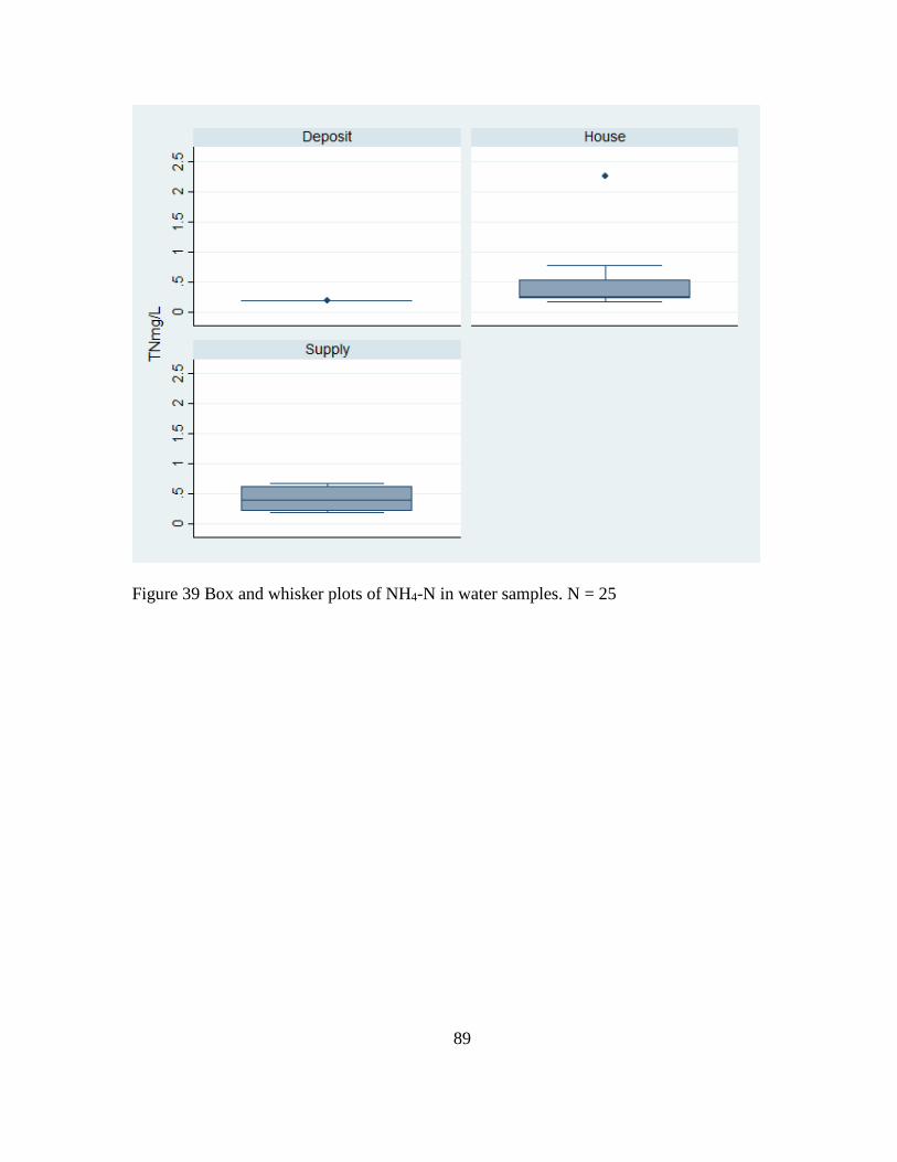
89

Figure 39 Box and whisker plots of NH4-N in water samples. N = 25

90

Figure 40 Spatial distribution of NH4-N measured in samples N = 25

91

Phosphate-P

PO43− concentrations in samples taken from sources and deposits of water are all

fairly low, and ranged from 0.01 mg/L to 0.03 mg/L (Table 8). Drinking water samples

derived from the Agua Caliente spring had the highest concentration of PO4-P. Surface

water samples taken from the southern creek had the highest concentration of phosphate-P at

2.8 mg/L (Table 8).

4.3.5 Cations: Sodium, Potassium. Magnesium and Calcium

Sodium concentrations ranged from 0.7 meq/L in the Ojo de Agua well water supply to

5.1 meq/L in the Southern creek (Table 8). Potassium concentrations ranged from 0.10

meq/L in the Ojo de Agua well water supply to 0.5 meq/L in the Southern creek (Table 8).

Magnesium concentrations ranged from 0.5 meq/L in the Agua Caliente storage deposit to

2.2 meq/L in the Southern creek water (Table 8). Calcium concentrations ranged from 0.2

meq/L in the Agua Caliente spring water supply to 1.8 meq/L in the Southern creek (Table

8). Source water cations were > 0.5 indicative of the weathering of ferromagnesian minerals

(Table 7). Figure 41 shows the spatial distribution of these results.

Surface waters were only tested on two occasions for safety because they were known to

be contaminated with raw sewage. Both the Rio de la Passion, and a small creek that drains

the southern portion of the municipality had elevated cations (Table 8). Surface water

samples had much higher cation content than groundwater samples from water sources and

their storage deposits.

92

Table 8 Laboratory tested water chemistry of drinking water sources, storage and surface waters. ND = no data because of short sample volume N = 6

Type Description Na+

meq/L

K+

meq/L

Mg2+ meq/

L

Ca2+ meq/

L

NO3-N mg/L

NH4-N mg/L

PO4-P

mg/L

DOC mg/L

TDN mg/L

Supply Jarero well 0.8 0.2 0.7 0.3 0.3 0.2 0.01 14.6 0.2

Supply Milpillas Well 1.1 0.2 0.6 0.3 0.3 0.2 0.01 18.7 0.6

Supply Agua Caliente Spring 0.8 0.1 0.6 0.2 0.6 0.3 0.03 18.5 0.2

Supply Ojo de Agua Well 0.7 0.1 0.9 0.3 0.3 0.2 0.01 15.1 0.7

Storage Jarero deposit 0.8 0.2 0.8 0.2 0.3 0.2 0.01 ND ND

Storage Agua Caliente deposit 0.8 0.1 0.5 0.2 0.6 0.3 0.01 18.0 0.2

Surface Rio de la Passion 0.7 0.5 0.6 0.7 1.7 0.5 0.8 ND ND

Surface Southern creek 5.1 0.5 2.2 1.8 4.6 7.2 2.8 ND ND

Figure 41 Spatial distribution of cations (meq/L)

93

4.4 EPANET Model

The scenarios chosen for modeling in EPANET reflect possible pumping and

chlorination schedules. The two pumping schedules, partial and continuous, reflected certain

levels of development. The ideal would be a continuous pumping schedule that would allow

water to be delivered to household 24 hours a day. The partial pumping schedule, which is

the current regime in the town, reflects the low availability of funds to pay for pumping costs

and perhaps water availability. Most of the scenarios produced significantly different results

in chlorine concentrations throughout the distribution system (Tables 9 and 10). Difficulties

were encountered when designing the EPANET system using my sample concentrations and

in maintaining homogeneous concentrations of chlorine. This may have been because the

system has 4 different source points of water, in terms of both DOC content and in their

location. Surprisingly, the highest decay rate was from the Milpillas well, where one would

assume that the Agua Caliente Spring would have the highest decay rate since it is

technically surface water. More samples and DOC analysis should be done in the future to

address this anomaly. There were both spatial and temporal variations to chlorine

concentrations in the system. For the most part chlorine concentrations were very low in the

morning, reached their peak in the early afternoon, and begin to decline again before 5:00 pm

when some well pumps and chlorination systems go offline (Figure 44 through 46). An ideal

system would have low percentages of nodes below 2.0 mg/L of free chlorine, producing a

somewhat concave line that increases slowly from left to right. Under current management

conditions the model suggests that it is impossible to reach the minimum safety value of 2.0

mg/L in all of the nodes.

94

Table 8 One tailed T-tests on number of nodes below 2.0 mg/L of free chlorine. P = Partial supply (current regime in town), C = Continuous supply and N = Continuous supply with no demand pattern. Numbers following letters indicate the number of scenario run

Scenario P1 P2 P3 P4 P5 P6 P7 P8 P0 0.298 0.001 <0.001 0.326 0.070 0.140 <0.001 <0.001 C1 C2 C3 C4 C5 C6 C7 C8 C0 0.078 <0.001 <0.001 <0.001 <0.001 <0.001 <0.001 <0.001 N1 N2 N3 N4 N5 N6 N7 N8 N0 <0.001 <0.001 <0.001 <0.001 <0.001 <0.001 <0.001 <0.001

Table 9 One tailed T-tests on chlorine concentrations between pumping scenarios Scenario pairing

P0-C0 P1-C1 P2-C2 P3-C3 P4-C4 P5-C5 P6-C6 P7-C7 P8-C8 <0.001 <0.001 <0.001 <0.001 <0.001 <0.001 <0.001 <0.001 <0.001 P0-N0 P1-N1 P2-N2 P3-N3 P4-N4 P5-N5 P6-N6 P7-N7 P8-N8 <0.001 <0.001 <0.001 <0.001 <0.001 <0.001 <0.001 <0.001 <0.001 C0-N0 C1-N1 C2-N2 C3-N3 C4-N4 C5-N5 C6-N6 C7-N7 C8-N8 <0.001 <0.001 <0.001 <0.001 <0.001 0.001 <0.001 <0.001 0.076

95

The continuous model with a demand pattern performed the best, where only 3% of

nodes had less than 2.0 mg/L of free chlorine when all sources are being chlorinated at the

3.5 mg/L maximum. The worst scenarios under this pumping schedule were scenarios

number 7 and 8 at 6:00 am, 8 and 3 at 12:00 noon, and 3 and 8 at 5:00 pm (Figures 42, 43,

and 44). Since EPANET incorporates demand when calculating the concentration of chlorine

in the system, the importance of Jarero Well water receiving disinfection could be caused by

the high demand from the North of the town that receives water from the Jarero Well. The

system also performed poorly when only the Agua Caliente Well received chlorination. This

could be because the water has to travel far from the chlorination site before reaching most of

the users, allowing the chlorine to be mostly inactivated in the process of being distributed.

The partial supply pumping scenario was able to reach a level of 95% of nodes with greater

than 2.0 mg/L of free chlorine at 12:00 noon if all sources were chlorinated at 3.5 mg/L. The

worst scenarios under this pumping schedule were scenarios number 8 and 7 at 6:00 am,

which never reached levels lower than 60% of nodes with less than 2.0 mg/L. Chlorine

concentrations at 12:00 noon were the worst under scenarios 8 and 3, the same scenarios

were also the worst at 5:00 pm. Under the control scenario (N), which used continues supply

but with no demand schedule, chlorination scenarios 2 and 7 had the most impact where

nodes with lower than 2.0 mg/L never got below 10%. This supports the idea that Agua

Caliente water has to travel further than the chlorine can stay active.

96

Figure 42 Concentration of Chlorine at nodes in all scenarios at 6:00 am

Figure 43 Concentration of Chlorine at nodes in all scenarios at 12:00 pm

0%10%20%30%40%50%60%70%80%90%

100%

0 1 2 3 4 5 6 7 8

Nod

es w

ith le

ss th

an 0

.2 m

g/L

(%)

Chlorination Scenario

Nodes at 6:00 A.M.

partial continuous Control

0%

10%

20%

30%

40%

50%

60%

70%

80%

0 1 2 3 4 5 6 7 8

Nod

es w

ith le

ss th

an 0

.2 m

g/L

(%)

Chlorination Scenario

Nodes at 12:00 P.M.

partial continuous Control

97

Figure 44 Concentration of Chlorine at nodes in all scenarios at 5:00 pm

The spatial variability of chlorine in the system mirrors the results from samples taken in

the town. Areas closest to chlorination sites have the highest concentrations of chlorine, and

the system itself is highly heterogeneous depending on the chlorination schedule. Overall the

southern portion of the city is the most at risk of having low concentrations of chlorine and

coliform bacteria present. The center of the town had the highest variability from block to

block, while the northern part of the town had the most consistently acceptable levels. The

continuous supply regime produced the greatest amount of spatial homogeneity of chlorine,

although there were still areas receiving unacceptable concentrations. This was probably

influenced by the differences in water quality between supply sources.

0%

20%

40%

60%

80%

100%

0 1 2 3 4 5 6 7 8Nod

es w

ith le

ss th

an 0

.2 m

g/L

(%)

Chlorination Scenario

Nodes at 5:00 P.M.

partial continuous Control

98

5. DISCUSSION

5.1 Lerma-Chapala Basin

Water abstractions in the Lerma-Chapala Basin are occurring at unsustainable volumes;

in fact 70% of the groundwater wells in the basin are over utilized (Rodriguez 1997).

Agriculture accounts for 68% of total water use in the basin. Combined with industrial and

human needs, the basin is experiencing an annual deficit, of both ground and surface water,

of more than 900 million m3 (Wester et al., 2003). The basin’s water crisis is exacerbated by

pollution, as more than 90% of surface waters are deemed to be highly contaminated with

industrial discharges and raw sewage (Millington et al., 2006). Indication of raw sewage in

terms of high ammonium-N concentrations in surface waters was also observed in my study.

Groundwater mining has also become an issue as municipalities have to turn to groundwater

as a source of drinking water; aquifers in the basin are experiencing declines of 1.0 to 2.6

m/yr as abstractions from both agricultural and municipal exceed sustainable levels.

The UN and related international groups have used the Lerma Basin as an example of

successful IWRM in a developing country (Casillas and González, 2007; Mestre, 2001;

Millington et al., 2006). Much like UN’s claim to reaching MDGs, this seems to be

premature and loosely based. The decentralization efforts in the 1990’s placed the building

of waste water treatment facilities on the shoulders of municipal governments. Many of the

local governments at the municipal and state level have very little ingress to work with. This

is partially a result of Mexico’s federally driven taxation system and high levels of poverty.

As a result wastewater treatment systems are not common in Mexico. Incorporation of

International drinking water standards are also weak in this regard. Waste water treatment is

99

not required by these standards. As long as households have hygienically separated human

waste from human contact and facilities and are not publically shared they are considered to

be ‘improved’. While this standard may help Least Developed Countries (LDCs) take the

small steps into modernization that they can afford, middle income countries such as Mexico

are able to artificially shine with accomplishment.

5.2 Marcos Castellanos Municipality and Town of San José de Gracia

The level of integrated water management in Marcos Castellanos is low. Although the

town of San José de Gracia does keep a simple record of payments and meter readings they

do not use the data for any analysis. This record was useful for my research for estimating

water use by homeowners and commercial entities. The water managers of the town are

unaware of the total volume of water being extracted, lost in the system or ultimately used by

consumers. While CONAGUA requires that groundwater users have a permit stating the

volume of water being abstracted, the municipality has only one registered well.

Additionally, no one in the municipal government of utilities is aware which aquifer their

water is pumped from, the size of their pumps, or the areas of recharge. There are currently

no land use regulations being implemented in the municipality or participation in regional

basin management groups.

The town of San José de Gracia does not treat sewage or regulate effluent discharge

by major dairy product manufacturers located in the town. Surface water samples from the

Southern Creek were a magnitude higher in sodium, magnesium and calcium concentrations

than water from other parts of the municipality, such as well and spring water sources, water

storage deposits and household faucets. This may indicate significant illegal dumping of

100

saline waters that are produced as waste by the industry. The Southern Creek when sampled

had a white, grey appearance with no noticeable aquatic life forms. There are currently no

programs run by the municipality to incentivize or educate farmers about buffer zones or

riparian zone restoration near streams. Besides human fecal matter, some smaller creeks had

noticeable accumulation of what appears to be bovine waste. It should also be noted that the

local slaughterhouse also disposes of their waste, including blood and other biological

materials, straight into the Northern Creek. Decomposition products from dead mammals in

the form of DOC, nitrate-N, ammonium-N and phosphate-P and cations are reportedly

extremely high (Aitkenhead-Peterson et al. 2012; Carter et al. 2007) and can be expected to

have a negative effect on surface waters.

5.3 Indicators and Testing

Poor drinking water quality impacts the economy by increasing the cost of health care

and reducing worker productivity by spreading illness (Hutton et al., 2004). Ironically,

economic growth can prevent governments from making key investments that help to secure

the quality of water being served. It is now generally accepted that improved access to water

does not necessarily mean that water is free from chemical or microbial constituents or that

the quality satisfies World Health Organization (WHO) and national safety standards (Yang

et al., 2013). While efforts to improve access to water have increased welfare, they have

lacked both treatment and monitoring. For example, drinking water sources for the town of

San José de Gracia had above E. coli counts which ranged from 0 to 112 cfu/100 mL

illustrating this problem. While high concentrations of E. coli were observed in water

sources, their concentrations dropped in storage deposits and increased again in household

101

faucets indicating potential regrowth within the system. Failing to monitor water quality has

diminished the potential benefits from international and national investments. Water quality

testing plays an important role in solving public health problems that can pose a significant

financial burden to developing countries. Achieving the targets of MDG 7 to decrease the

population without access to safe water will require regular monitoring of water quality.

When selecting indicators to test drinking water quality, it is important to consider the

spatial and political context of the basin and efficiently select the most relevant variables for

each distribution system (Abdul et al., 2012; Ferrier et al., 2009; Stedmon et al., 2011;

Stepenuck et al., 2011). Utilizing systemic planning and understanding of local geography,

RADWQ helps to maximize the utility of data that can be acquired with a low budget. With

a basic understanding of the regional geography, low-cost tests can be used as affordable

assessment tools to establish baseline information (Bain et al., 2012; Howard et al., 2012).

Since a watershed’s physical and anthropogenic characteristics, such as its, climate, geology,

land use, and land management strategies are the overarching factors that determine local

water quality, the RADWQ is a strategic move toward implementing IWRM into the

development scheme more efficiently.

Physio-chemical properties of water, such as pH and conductivity, and water quality

indicators, such coliform bacteria, are among the most common parameters chosen for initial

evaluations in developing countries (Abdul et al., 2012; Bain et al., 2012; Giné-Garriga et al.,

2013; Nnane et al., 2011; Stepenuck et al., 2011). Where local conditions create

vulnerability for contamination from other contaminants, often heavy metals or pesticides,

further testing can be done. Costs for testing for E. coli and coliforms were less than $2.50

for each for the Coliscan Easygel test and less than $5.00 each for membrane filtration. This

102

is quite a reasonable cost per test but often E. coli growth can be too high to confidently

count the number of colony forming units; meaning that 2 to 3 tests are needed for each site

which will increase the per site sample cost. To ensure the safety and sustainability of water,

governments must develop monitoring schemes that collect critical information needed to

manage food and water safety (Farahi et al., 2012). Establishing comprehensive datasets in

developing nations requires two essential elements; training personnel and inexpensive

testing equipment (Mabey et al., 2004). The WHO has established seven criteria for

scientists to develop Point of Care (POC) diagnostics; affordability, sensitivity, specificity,

ease of use, rapid and robust, equipment free, and easily delivered to those in need. Research

has already begun to quantify the reliability of commercial water testing kits for

contaminants such as arsenic (Van Geen et al., 2005). Products using immunoassay-based

kits for pesticide detection that allow for simple methods to be implemented have already

been developed (Gabaldón et al., 1999). Although much research is needed to further

develop simple but reliable testing kits for many other contaminants, research on efficacy of

volunteers also provides resources for creating training manuals that can help build human

capacity.

Low cost testing methods include the use of kits of varying costs, which give varying

levels of accuracy from which to assess water management strategies being implemented.

Low income test settings most commonly use fecal coliform tests, surveys, and the basic

water quality parameters that can be measured with relatively inexpensive and re-usable

meters (Abdul et al., 2012; Bain et al., 2012; Giné-Garriga et al., 2013; Nnane et al., 2011;

Stepenuck et al., 2011). To assess the level of integrated management being used by water

103

managers, RADWQ recommends obtaining information about the political and social

atmosphere of the study region.

5.4 Disinfection of Drinking Water Systems

Water quality can be seriously degraded in storage tanks if it has a long residence time

and poor mixing (Grayman et al., 1993). Additionally, water in the periphery of system will

have less residual disinfectant than water for users closer to the disinfection site. Factors that

decay chlorine range for system design, operational variables, and the physio-chemical

properties of the water being used (Ahn et al., 2012; Clark et al., 1994, 2005; Hallam et al.,

2003). Managing the concentration of chlorine in a distribution system is usually limited to

controlling the amount of chlorine added at the water treatment plant. Water utility operators

need to be knowledgeable of the water system they operate in order to adjust chlorination

rates to their particular system.

Since chlorine reacts with organic matter throughout time; the age of water is an

important factor in determining the quality of drinking water. The longer the residence time

of the water in a distribution system the more time the chlorine has had to react with organic

matter, decreasing chlorine residuals and increasing the concentration of disinfection by-

products (Georgescu et al., 2012; Grayman et al., 1993; Powell et al., 2000). When water

initially enters a distribution system after being taken from the source and treated, water age

is modeled as being zero. Storage tanks (deposits) built into the distribution system can have

a significant effect on water age. If the level of water in the tank is allowed to vary greatly,

newer water can come in and replace old water decreasing the average age. If the tank is not

allowed to vary greatly, that is when the tank is refilled after only a short decrease in the

104

water level, the average age of water in the tank increases. One study found that a 9 foot

variation in water level produced an average water age of 7 days; however a 1 foot variation

increased average age to almost 20 days (Grayman et al., 1993).

Direct pumping from water sources to consumers is rare today even though it would

shorten water age because storage tanks provide a controlled demand on sources and

disinfection facilities. As a result the distribution system is more stable in terms of flows and

pressure as well as in terms of equalizing service for all users. Storage tanks also add a

factor of safety because they can reserve supplies for fire emergencies or power outages. In

the United States it is estimated that less than 25% of water in a storage tank is actively used

throughout the day, the rest remaining in reserve for fire storage (Grayman et al., 1993;

Rossman et al., 1995). Storage tank location, distance from initial disinfection, and operating

policies are very important in determining water age and quality. Modeling tank storage is a

difficult and recent undertaking because of the considerable variability in the behavior of

water within a tank. One of the phenomena that can take place is short circuiting, where the

inflow of water into a tank has a direct flow path to the outflow of the tank. The result is

dead zones, where mixing of water is limited, and water that most recently entered the tank is

also the first to exit the tank (Grayman et al., 1993).

Chlorination systems at all of the sources in my study were somewhat passive, as there

were no obvious design features of the systems that ensured a full mixing of the disinfectant.

The distribution system for the Agua Caliente Spring lacked a filtration system to rid the

water of suspended solids that are present in the water. This is a serious design flaw that

contributes to elevated bulk decay rates and raises the concentration needed for chlorine to be

an effective disinfectant. Overall it seemed chlorination was irregular and ineffective overall

105

in the town of San José de Gracia. Irregularity of chlorination can contribute significantly to

biofilm growth within the system and raises concerns over the health risks citizens are

exposed to.

The results from EPANET indicated that under current operational schedules the

maximum allowed concentration of 3.5 mg/L at the point of chlorination would provide

enough disinfection for the whole system. The EPANET model also illustrated that having

partial service as oppose to continuous service throughout the day can contribute to higher

chlorine decay rates. The EPANET model results also suggested that chlorine is least present

in the Southern and Western developments in the town which are furthest from the

chlorination sites. Although water quality tests for chlorine and coliform bacteria showed

some spatial patterns, there were not clear enough to make confident inferences. At the time

the samples were collected chlorination was not regular, therefore results had added variance

related to the lack of steady disinfection.

The water distribution model of the town did not include cisterns which are used in most

homes. These water storage tanks are used to alleviate water scarcity caused by the fact that

water is only delivered for 6 hours of the day, and for some locations only every other day.

The presence of these storage tanks would contribute to chlorine decay prior to use by the

household. The added variability to the distribution system of on and off chlorination,

multiple sources, partial supply, and cisterns all contribute to variability in the number of

coliforms and E. coli observed in samples from household faucets.

An assessment of 319 studies containing more than 96,000 samples found that more than

a third of samples from improved sources still contained fecal contamination (Bain et al.,

2014). The author of the study pointed out that this might even be an overestimation of

106

safety because the studies routinely lacked a robust random sample. Studies often lacked

samples that reflected the quality of water after storage. Bain (2014) also suggested that the

priority should be to improve the international monitoring strategy and include the measuring

of water quality with physical indicators.

There are several different steps the municipality could take to solve their ineffective

chlorination system. The utility group could install additional chlorination stations within the

city. Determining the location of these would require a diurnal study of coliforms and

chlorine concentrations throughout the system. This measure however, would not be able to

take into account the cisterns which are currently in use. The cisterns are currently essential

to water users, and it would require a change to continuous supply to change the trend.

Under the current system design with four separate water sources, the largest of which

requires water to be pumped up more than 300 m, the municipality cannot afford to provide

continuous water supply. They would have to perform a geological analysis of the area in

hopes of finding a location at a higher elevation than the town that could provide enough

water to supply the population to decrease pumping costs and perhaps be able to provide

water throughout the day.

5.5 Water Costs

The cost of water to the citizens of the town of San Jose de Garcia was comparable to the

cost of water in Glasgow, UK and close to being as high as water costs in Santa Fe, NM

(Figure 45 and Table 11). Surface water from Loch Katrine is the primary source water for

Glasgow’s potable water. The United Kingdom protects its surface waters allocated for

drinking water by reducing development in the watershed and having strong regulations of

107

types of recreation allowed (i.e. no motor boats only row boats). This is done to reduce

treatment costs and ensuring water supplies are as uncontaminated as possible. Potable water

for Santa Fe is derived from both surface and groundwater sources 1) Santa Fe River (stored

in the McClure and Nichols Reservoirs), 2) well fields within the city and near the Rio

Grande River. In the town of San José de Gracia, despite having a highly subsidized utility,

irregular service, inadequate quality and no security, the citizens of the town are paying a

highly inflated price for their water. Users are not only paying more for lower quality water

and no waste water treatment, they are also charged at a declining block rate. Industrial users

pay the lowest fee for a flat volumetric rate, while the rest of tariffs are on a declining block

rate.

Figure 45 Comparison of water cost in San José de Gracia to U.S. cities

$4.75

$1.80 $2.26

$6.06

$9.41

$3.57 $4.48

$12.01

$-

$2.00

$4.00

$6.00

$8.00

$10.00

$12.00

San Jose de Gracia,Mexico

Dallas, TX College Station, TX Santa Fe, NM

Relative cost for 7.5 m3 (~2,000 gal) of water in Mexico and the U.S.

Rate per 1,000 gallons Cost

108

System requirements for providing safe water under the current design would be very

expensive and complicated. Water disinfection could be improved through additional

chlorination points and treatment before being distributed. Currently the spring water used is

not being filtered to have suspended solids removed. This can significantly contribute to

bulk decay rates of chlorine and poses a serious threat to the health of water consumers.

Additionally well sites are not given a protective radius to limit the possibility of surface

contaminants infiltrating the aquifer and causing negative health impacts. The town is also

not protected against fire, not only are there no fire hydrants, but storage tanks operated by

the town do not maintain a minimum level of water for use in cases of emergencies. Water

security is a huge problem in the municipality, if there is a power outage the distribution

system will not be functional as it has no backup generators and surface water is too far

contaminated to be used in case of emergencies. The town’s water utility is not able to

provide an efficient system and despite serving expensive water, they are not able to utilize

the money in ways that improve the situation.

109

Table 10 Comparison of WB indicators of water costs using IBNET and collected data

Tariff report

for domestic

users

UK U.S. U.S. Brazil Mexico Mexico Mexico

City Glasgow El Paso Houston Sao Paulo Mexico city

Monterrey San José de

Gracia Utility Scottish

Water El Paso Water

Utilities

Dept. of public

works and engineering

SABESP SACM SADM Sistema de Agua Potable

Service Water and

waste water

Water and waste water

Water and waste water

Water and waste water

Water and

waste water

Water only Water only

Tariff type

Incline Block Tariffs

Incline Block Tariffs

Incline Block Tariffs

Incline Block Tariffs

Incline Block Tariffs

Volumetric flat

Decline Block Tariffs

Water (local

currency/m3)

2.9 1.0 2.9 1.7 34.5 6.6 57.0

Water (US$/m3)

4.7 1.0 2.9 1.0 3.0 0.6 4.8

Wastewater (local

currency)

3.5 1.3 3.5 N/A 3 N/A N/A

US$/m3 5.7 1.3 3.5 N/A 0.3 N/A N/A Total tariff

(Local currency/

m3)

6.5 2.3 6.4 1.7 37.5 6.6 170.5

Total tariff

(US$/m3)

10.4 2.3 6.4 1.0 3.2 0.6 14.2

Tariff per m3 = [connection fee +volumetric charge per 15 m3 per month +taxes and other fees]/15. The exchange rate to the $US is as of April 30, 2011.

110

5.6 Limitations of Study

There were several limitations of this study which can be comparable to limitations faced

by non-profit and international organizations working in developing countries. Limitations

included 1) accuracy of testing kits is variable, 2) very low materials and transportation

budget, and 3) lack of base knowledge and data from the local government to act as

background to this study. These all posed serious barriers to understanding the water system

in a small town of a developing nation. However, since water quality directly affects the

quality of life and health of citizens it is important to evaluate the effectiveness of high level

decisions taken to build water infrastructure with borrowed money.

111

6. CONCLUSION AND RECOMMENDATIONS

Water quality regulations serve not only to improve public health but also to raise living

standards. The rate of a country’s development is highly dependent on the efficacy of local

governments to implement national standards. Federal and state laws regarding water

resources should provide the framework for watershed management at the local level. Those

laws are expected to provide sufficient guidance for municipal governments to achieve

uniform national standards, while providing enough freedom for implementation strategies to

be tailored to local needs. The highly centralized structure of the federal government has left

local institutions financially and technically unable to meet water quality criteria.

Centralization also weakened attempts at regional management through lack of continuity in

funding and projects. Furthermore, testing frequencies recommended by international

organizations do not reflect the amount of testing that needs to be done to confidently assure

the public that safe water is being distributed for human consumption.

Inadequate local planning has contributed to a lack of uniform water quality that fails to

meet national standards. Arguably, water related infrastructure and planning shows the

government’s ability to translate values and desired outcomes into policy that is effective at

the micro and macro scale. The ground truth at the local level displays heterogeneous,

geographically variable responses to homogeneous national policy. In general, the MDGs

highlight the bearing that improved access to drinking water and sanitation services has for a

nation’s welfare (Kalbus et al., 2012). These goals called for active intervention by

governments through the construction of water supply, distribution, and sanitation systems to

improve health and environmental sustainability as an integral part of meeting poverty

112

reduction goals (Zawahri et al., 2011). This ultimately promotes developing countries to take

additional loans to build more infrastructure in order to meet development indexes set by

non-binding agreements. These loans come with binding agreements to make changes to the

nation’s market systems, which are supposed to act in coordination with poverty reducing

programs and new infrastructure to eliminate poverty. This much more inclusive and holistic

development scheme is the result of failed attempts which did not incorporate all of these

elements. However, much work to make global initiatives translatable to local terms is still

needed. The definitions of improved water and sanitary services used by the UN have in a

way helped stall progress in Mexico and perhaps other middle income countries as well.

While critics point to the unfairness of MDGs to LDCs in Africa, for they have much more

work to do, less stability and fewer funding opportunities, they are too relaxed to really put

pressure on middle income countries like Mexico to improve conditions.

A common theme across the literature is the lack of data. Although the UN, and its

associated organizations, requires some indicators be recorded, they are primarily

development indicators. While publications from the UN highlight the importance of

capacity development, they have overlooked baseline physical data collection, a crucial

factor of resource management. Procedures in RADWQ and initiatives promoted by IWRM

require high resolution physical data, such as geologic and soil maps. However, besides the

recent interest by the World Bank to map Africa’s geology there has been little effort in

mobilizing global partnerships to help developing countries enrich their databases.

Establishing a database with baseline indicators provides information that can be used to

define hazards in need of safeguarding and identify where investments are needed for

capacity building of water managers. Water quality assessment programs are an important

113

step towards reducing the costs of water governance and increase the efficacy of policy.

Ultimately, I have found through this research that international efforts to reduce poverty and

enrich resource management have missed out of efforts to aid developing nations in creating

databases with the preliminary data needed to implement IWRM. Creating these would

require coordination between institutions of higher education, all government levels, and

international developers. There is also a lack of equipment that can be used in the field for

quick and accurate results. It is imperative that these instruments be made so that they can be

used in developing countries that do not have the resources to maintain the various large and

expensive instruments currently used to analyze water quality. Partnerships could also be

built between educational institutions to allow for students to collect data and preform studies

to better understand geology, pedology, and ecological studies that are essential to

understanding and managing space.

114

REFERENCES

Abdul, R. M., Mutnuri, L., Dattatreya, P. J., & Mohan, D. A. (2012). Assessment Of

Drinking Water Quality Using ICP-MS And Microbiological Methods In The

Bholakpur Area, Hyderabad, India. Environmental Monitoring And Assessment,

184(3), 1581-1592.

Aguilar, A. G., & Santos, C. (2011). Informal Settlements’ Needs And Environmental

Conservation In Mexico City: An Unsolved Challenge For Land-Use Policy. Land

Use Policy, 28(4), 649-662.

Aguilar, L. A. (2004). De Bastión A Amenaza: Agua, Políticas Públicas Y Cambio

Institucional En México, 1947-2001. Paper Presented At The El Futuro Del Agua En

México.

Ahn, J. C., Lee, S. W., Choi, K. Y., & Koo, J. Y. (2012). Application Of EPANET For The

Determination Of Chlorine Dose And Prediction Of Thms In A Water Distribution

System. Sustainable Environment Research, 22(1), 31-38.

Al-Adamat, R. A., Foster, I. D., & Baban, S. M. (2003). Groundwater Vulnerability And

Risk Mapping For The Basaltic Aquifer Of The Azraq Basin Of Jordan Using GIS,

Remote Sensing And DRASTIC. Applied Geography, 23(4), 303-324.

Alcocer-Yamanaka, V. H., Tzatchkov, V. G., & Arreguín-Cortés, F. I. (2004). Modelo De

Calidad Del Agua En Redes De Distribución. Ingeniería Hidráulica En México,

19(2), 77-88.

Amrith, S., & Sluga, G. (2008). New Histories Of The United Nations. Journal Of World

History, 19(3), 251-274.

115

Armentia, M. L. T., & Cisneros, B. J. (2009). Challenges Facing The Universal Access Of

Water And Sanitation In Mexico. Water And Sanitation Services: Public Policy And

Management, 338.

Au, K.-K. (2004). Water Treatment And Pathogen Control: Process Efficiency In Achieving

Safe Drinking-Water: IWA Publishing.

Azuela, A. (1995). La Distribución De Competencias En La Regulación De Los Usos Del

Suelo. PEMEX: Ambiente Y Energía. Los Retos Del Futuro, México, UNAM-PEMEX.

Bain, R., Bartram, J., Elliott, M., Matthews, R., Mcmahan, L., Tung, R., . . . Gundry, S.

(2012). A Summary Catalogue Of Microbial Drinking Water Tests For Low And

Medium Resource Settings. International Journal Of Environmental Research And

Public Health, 9(5), 1609-1625.

Bain, R., Cronk, R., Wright, J., Yang, H., Slaymaker, T., & Bartram, J. (2014). Fecal

Contamination Of Drinking-Water In Low- And Middle-Income Countries: A

Systematic Review And Meta-Analysis. Plos Med, 11(5), E1001644. Doi:

10.1371/Journal.Pmed.1001644

Bain, R. E., Gundry, S. W., Wright, J. A., Yang, H., Pedley, S., & Bartram, J. K. (2012).

Accounting For Water Quality In Monitoring Access To Safe Drinking-Water As Part

Of The Millennium Development Goals: Lessons From Five Countries. Bulletin Of

The World Health Organization, 90(3), 228-235.

Bank, W. (2003). Private Solutions For Infrastructure In Mexico. Country Framework Report

For Private Participation In Infrastructure, Washington, Banco Mundial.

Bank, W. (2012). The Little Green Data: World Bank Publications.

116

Bank, W. (2014). World Development Indicators, The World Bank.

Http://Www.Worldbank.Org/En/Country/Mexico.

Barkin, D., & Klooster, D. (2006). Estrategias De La Gestión Del Agua Urbana En México:

Un Análisis De Su Evolución Y Las Limitaciones Del Debate De La Privatización.

Barkin, D., La Gestión Del Agua Urbana En México, Guadalajara, Universidad De

Guadalajara, México, 1-45.

Bartram, J. (2009). Water Safety Plan Manual: Step-By-Step Risk Management For

Drinking-Water Suppliers: World Health Organization.

http://apps.who.int/iris/bitstream/10665/75141/1/9789241562638_eng.pdf

Berkes, F., Folke, C., & Colding, J. (2000). Linking Social And Ecological Systems:

Management Practices And Social Mechanisms For Building Resilience: Cambridge

University Press.

Biswas, A. K., & Tortajada, C. (2005). Appraising Sustainable Development : Water

Management And Environmental Challenges. New Delhi ; New York: Oxford

University Press.

Block, J. (1992). Biofilms In Drinking Water Distribution Systems Biofilms—Science And

Technology (Pp. 469-485): Springer.

Burt, J. E., Barber, G. M., & Rigby, D. L. (2009). Elementary Statistics For Geographers:

Guilford Press.

Carter, D. O. Yellowlees,D. And Tibbett,M (2007) Cadaver Decomposition In Terrestrial

Ecosystems. Naturwissenschaften, 94 12-24.

117

Casillas González, J. A. (2007). El Programa Nacional De Microcuencas: Una Estrategia De

Desarrollo Integral. El Manejo Integrado De Cuencas En México. Estudios Y

Reflexiones Para Reorientar La Política Ambiental.

Castro, J. E., & Heller, L. (2009). Water And Sanitation Services: Public Policy And

Management: Earthscan.

CIA. (2013). The World Factbook 2013-14. Central Intelligence Agency, 2013.

Clark, R. M., Grayman, W. M., Goodrich, J. A., Deininger, R. A., & Skov, K. (1994).

Measuring And Modeling Chlorine Propagation In Water Distribution Systems.

Journal Of Water Resources Planning And Management, 120(6), 871-887.

Clark, R. M., & Haught, R. C. (2005). Characterizing Pipe Wall Demand: Implications For

Water Quality Modeling. Journal Of Water Resources Planning And Management,

131(3), 208-217.

Clasen, T. F. (2012). Millennium Development Goals Water Target Claim Exaggerates

Achievement. Tropical Medicine & International Health, 17(10), 1178-1180.

CONAGUA. (1994). NOM-127-SSA1-1994. Salud Ambiental, Agua Para Uso Y Consumo

Humano. Límites Permisibles De Calidad Y Tratamiento A Que Debe Someterse Para

Su Potabilización. Diario Oficial De La Federación, Norma Oficial Mexicana.

CONAGUA. (2012). Atlas Del Agua En México 2012. Secretaría De Medio Ambiente Y

Recursos Naturales.

Cooper, K. B. (2009). Economic Policy In The Hemisphere: Successes And Failures. Law &

Bus. Rev. Am., 15, 27.

118

Cotler, H., Fregoso, A., & Damián, J. L. (2006). Caracterización De Los Sistemas De

Producción En La Cuenca Lerma-Chapala A Escala Regional. Instituto Nacional De

Ecología.

Cotler, H., Mazari, M., & De Anda, J. (2006). Atlas De La Cuenca Lerma-Chapala:

Construyendo Una Visión Conjunta. Instituto Nacional De Ecología, Secretaría De

Medio Ambiente Y Recursos Naturales/Instituto De Ecología, Universidad Nacional

Autónoma De México. México, DF.

Crandall, R., Paz, G., & Roett, R. (2005). Mexico's Democracy At Work: Political And

Economic Dynamics: Lynne Rienner Publishers.

De Anda, J., Quiñones-Cisneros, S. E., French, R. H., & Guzman, M. (1998). Hydrologic

Balance Of Lake Chapala (Mexico). Water Resources Bulletin, 34(6), 1319-1331.

De Anda, J., Shear, H., Maniak, U., & Riedel, G. (2000). Phosphorus Balance In Lake

Chapala (Mexico). Journal Of Great Lakes Research, 26(2), 129-140.

Durán Juárez, J. M., & Torres Rodríguez, A. (2006). Los Problemas Del Abastecimiento De

Agua Potable En Una Ciudad Media. Espiral: Estudios Sobre Estado Y Sociedad,

12(36), 129-163.

Egbuna, C. K., Howden, N. J., & Gundry, S. W. (2013). Comparative Analysis Of The

RADWQ Report And Academic Literature On The Quality Of Water In Nigeria.

Civil And Environmental Research, 3(3), 38-52.

Farahi, R., Passian, A., Tetard, L., & Thundat, T. (2012). Critical Issues In Sensor Science

To Aid Food And Water Safety. ACS Nano, 6(6), 4548-4556.

Ferrier, R., & Jenkins, A. (2009). Handbook Of Catchment Management: John Wiley &

Sons.

119

Fetter, C. W., & Fetter, C. (2001). Applied Hydrogeology (Vol. 3): Prentice Hall Upper

Saddle River, NJ.

Fukuda-Parr, S., & Lopes, C. (2013). Capacity For Development: New Solutions To Old

Problems: Routledge.

Gabaldón, J. A., Maquieira, A., & Puchades, R. (1999). Current Trends In Immunoassay-

Based Kits For Pesticide Analysis. Critical Reviews In Food Science And Nutrition,

39(6), 519-538.

Georgescu, A.-M., & Georgescu, S.-C. (2012). Chlorine Concentration Decay In The Water

Distribution System Of A Town With 50000 Inhabitants. University" Politehnica" Of

Bucharest Scientific Bulletin, Series D: Mechanical Engineering, 74(1), 103-114.

Giné-Garriga, R., De Palencia, A. J.-F., & Pérez-Foguet, A. (2013). Water–Sanitation–

Hygiene Mapping: An Improved Approach For Data Collection At Local Level.

Science Of The Total Environment, 463, 700-711.

Giné-Garriga, R., Jiménez Fernández De Palencia, A., & Pérez Foguet, A. (2011). A Closer

Look At The Sanitation Ladder: Issues Of Monitoring The Sector.

Giordano, M., & Shah, T. (2014). From IWRM Back To Integrated Water Resources

Management. International Journal Of Water Resources Development(Ahead-Of-

Print), 1-13.

Gleick, P. H. (1998). Water In Crisis: Paths To Sustainable Water Use. Ecological

Applications, 8(3), 571-579.

González Y González, L. (1974). San José De Gracia: Mexican Village In Transition. Trans.

John Upton. Austin: University Of Texas Press.

120

Grayman, W. M., & Clark, R. M. (1993). Using Computer Models To Determine The Effect

Of Storage On Water Quality. Journal-American Water Works Association, 85(7),

67-77.

Haber, S., Maurer, N., & Razo, A. (2003). The Politics Of Property Rights: Political

Instability, Credible Commitments, And Economic Growth In Mexico, 1876-1929:

Cambridge University Press.

Hallam, N. B., Hua, F., West, J. R., Forster, C. F., & Simms, J. (2003). Bulk Decay Of

Chlorine In Water Distribution Systems. Journal Of Water Resources Planning And

Management, 129(1), 78-81.

Hardoy, J., Hernández, I., Pacheco, J. A., & Sierra, G. (2014). Institutionalizing Climate

Change Adaptation At Municipal And State Level In Chetumal And Quintana Roo,

Mexico. Environment And Urbanization, 26(1), 69-85.

Hazin, L. S. (1997). Toward Moreefficient Urban Water Management In Mexico. Water

International, 22(3), 153-158.

Hounslow, A. (1995). Water Quality Data: Analysis And Interpretation: CRC Press.

Howard, G., & Bartram, J. (2003). Domestic Water Quantity, Service Level, And Health:

World Health Organization Geneva.

Howard, G., Ince, M., & Smith, M. D. (2012). Rapid Assessment Of Drinking Water Quality:

A Handbook For Implementation (W. H. O. UNICEF Ed.): © WEDC, Loughborough

University.

Hughes, S., & Wilkinson, R. (2013). The Role Of Governance In Shaping Freshwater

Management In America: Toward Integrated Resources Planning.

http://www.bren.ucsb.edu/people/faculty/documents/wilkinson_USFreshwater.pdf

121

Hutton, G., & Haller, L. (2004). Evaluation Of The Costs And Benefits Of Water And

Sanitation Improvements At The Global Level: Water, Sanitation, And Health,

Protection Of The Human Environment, World Health Organization.

INEGI. (2010). Censuses In Mexico, Censo General De Población Y Vivienda, Instituto

Nacional De Estadística Y Geografía, Conteo De Población Y Vivienda.

(9781157854005). Http://Www.Snim.Rami.Gob.Mx/: General Books LLC Retrieved

From Http://Books.Google.Com/Books?Id=Losisgaacaaj.

Israde-Alcantara, I., & Garduño-Monroy, V. H. (1999). Lacustrine Record In A Volcanic

Intra-Arc Setting: The Evolution Of The Late Neogene Cuitzeo Basin System

(Central-Western Mexico, Michoacán). Palaeogeography, Palaeoclimatology,

Palaeoecology, 151(1), 209-227.

Jamieson, D., & Fedra, K. (1996). The ‘Waterware’decision-Support System For River-Basin

Planning. 1. Conceptual Design. Journal Of Hydrology, 177(3), 163-175.

Juarez-Aguilar, A. (2010). Lake Chapala Basin, Mexico: Linking Sub-Basins As An

Integrated Lake Basin Management (ILBM) Strategy. Corazon De La Tierra,

Chapala, Mexico. http://rcse.edu.shiga-u.ac.jp/gov-pro/plan/2009list/12mexico-

lerma/workshop/02alejandropaper-on_linking_sub-basins_as_ilbm_strategy..pdf

Kalbus, E., Kalbacher, T., Kolditz, O., Krüger, E., Seegert, J., Röstel, G., . . . Krebs, P.

(2012). Integrated Water Resources Management Under Different Hydrological,

Climatic And Socio-Economic Conditions. Environmental Earth Sciences, 65(5),

1363-1366.

122

Lechevallier, M. W., Lowry, C. D., & Lee, R. G. (1990). Disinfecting Biofilms In A Model

Distribution System. Journal Of The American Water Works Association, 82(7), 87-

99.

Levy, S. (2010). Good Intentions, Bad Outcomes: Social Policy, Informality, And Economic

Growth In Mexico: Washington D.C. Brookings Institution Press.

Ley, A. N. L., & Adams, A. S. (2011). Evolución Y Perfiles De Eficiencia De Los

Organismos Operadores De Agua Potable En México. Estudios Demográficos Y

Urbanos, 563-599. http://www.jstor.org/stable/41408284

Lind, O. T., & Dávalos-Lind, L. (2002). Interaction Of Water Quantity With Water Quality:

The Lake Chapala Example. Hydrobiologia, 467(1-3), 159-167.

Lloyd, J. W. (1999). Water Resources Of Hard Rock Aquifers In Arid And Semi-Arid Zones.

Lorz, C., Abbt-Braun, G., Bakker, F., Borges, P., Börnick, H., Fortes, L., . . . Höfer, R.

(2012). Challenges Of An Integrated Water Resource Management For The Distrito

Federal, Western Central Brazil: Climate, Land-Use And Water Resources.

Environmental Earth Sciences, 65(5), 1575-1586.

Ludwig, F., Van Slobbe, E., & Cofino, W. (2013). Climate Change Adaptation And

Integrated Water Resource Management In The Water Sector. Journal Of Hydrology,

518, 235-242.

Mabey, D., Peeling, R. W., Ustianowski, A., & Perkins, M. D. (2004). Tropical Infectious

Diseases: Diagnostics For The Developing World. Nature Reviews Microbiology,

2(3), 231-240.

123

Mcdonald, J. H. (2001). Milk Quality And Globalization: Metaphors Of Modernity In

Northwestern Michoacán, Mexico. Research In Rural Sociology And Development, 8,

181-209.

Mcdonald, J. H. (2003). An Exploration In The Veiling Of Power: The Politics Of

Development In Rural West Mexico. Mexican Studies, 19(1), 161-185.

Mestre, E. (2001). The Design Of River Basin Organizations In Mexico–The Example Of

Lerma–Chapala. Paper Presented At The Documento Presentado En El Taller 5th

River Basin Management Institutions Workshop Por El Water Resources

Management Thematic Group In RDV And World Bank Institute En Agosto De.

Michaud, F., Ramírez-Sánchez, H. U., Parron, C., Zarate-Del Valle, P. F., Fernex, F., &

Barci-Funel, G. (2006). Strong Magnetic Levels In Lake Chapala Sediments (Western

Mexico): Their Mineralogy And Stratigraphic Significance. Journal Of

Paleolimnology, 35(4), 819-836.

Millington, P., Olson, D., & Mcmillan, S. (2006). Mexico - The Lerma-Chapala River Basin.

Integrated River Basin Management. Concepts To Good Practice ; Case Study 5.,

Washington, DC: World Bank.

(Http://Documents.Worldbank.Org/Curated/En/2006/02/8531700/Mexico-Lerma-

Chapala-River-Basin).

Nikolic, V. V., Simonovic, S. P., & Milicevic, D. B. (2013). Analytical Support For

Integrated Water Resources Management: A New Method For Addressing Spatial

And Temporal Variability. Water Resources Management, 27(2), 401-417.

124

Nnane, D. E., Ebdon, J. E., & Taylor, H. D. (2011). Integrated Analysis Of Water Quality

Parameters For Cost-Effective Faecal Pollution Management In River Catchments.

Water Research, 45(6), 2235-2246.

Onda, K., Lobuglio, J., & Bartram, J. (2012). Global Access To Safe Water: Accounting For

Water Quality And The Resulting Impact On MDG Progress. International Journal

Of Environmental Research And Public Health, 9(3), 880-894.

Ozdemir, O. N., & Ucak, A. (2002). Simulation Of Chlorine Decay In Drinking-Water

Distribution Systems. Journal Of Environmental Engineering, 128(1), 31-39.

Perez, A. A. (2011). The Mineral Industry Of Mexico. Minerals Yearbook: Area Reports:

International 2009 Latin America And Canada, 3, 221-530.

Powell, J. C., Hallam, N. B., West, J. R., Forster, C. F., & Simms, J. (2000). Factors Which

Control Bulk Chlorine Decay Rates. Water Research, 34(1), 117-126.

Rahaman, M. M., & Varis, O. (2005). Integrated Water Resources Management: Evolution,

Prospects And Future Challenges. Sustainability: Science, Practice & Policy, 1(1),

15-21.

Rich, J. G. (2003). Environment And Development In Mexico: Recommendations For

Reconciliation (Vol. 22): CSIS.

Richter, S., Völker, J., Borchardt, D., & Mohaupt, V. (2013). The Water Framework

Directive As An Approach For Integrated Water Resources Management: Results

From The Experiences In Germany On Implementation, And Future Perspectives.

Environmental Earth Sciences, 69(2), 719-728.

125

Riosmena, F., & Massey, D. S. (2012). Pathways To El Norte: Origins, Destinations, And

Characteristics Of Mexican Migrants To The United States1. International Migration

Review, 46(1), 3-36. Doi: 10.1111/J.1747-7379.2012.00879.X

Rodriguez J. E. M (1997). Case Study VIII* - Lerma-Chapala Basin, Mexico In: (Editors:

Richard Helmer And Ivanildo Hespanhol). Water Pollution Control - A Guide To The

Use Of Water Quality Management. Published On Behalf Of The United Nations

Environment Programme, The Water Supply And Collaboratibe Council And The

World Health Organization By E And F Spon Publishers

Rosenthal, E. (1987). Chemical Composition Of Rainfall And Groundwater In Recharge

Areas Of The Bet Shean-Harod Multiple Aquifer System, Israel. Journal Of

Hydrology, 89(3), 329-352.

Rossman, L. A., Uber, J. G., & Grayman, W. M. (1995). Modeling Disinfectant Residuals In

Drinking-Water Storage Tanks. Journal Of Environmental Engineering, 121(10),

752-755.

Saith, A. (2006). From Universal Values To Millennium Development Goals: Lost In

Translation. Development And Change, 37(6), 1167-1199.

Sánchez, A. T., & Perevochtchikova, M. (2012). La Gestión Del Agua Y El Desarrollo De

Indicadores Ambientales En México Y Canadá: Un Análisis Comparativo. Journal Of

Latin American Geography, 11(2), 145-165.

Sara, M. N. (2010). Site Assessment And Remediation Handbook: CRC Press.

Scott, C. A., & Banister, J. M. (2008). The Dilemma Of Water Management

‘Regionalization’in Mexico Under Centralized Resource Allocation. Water Resources

Development, 24(1), 61-74.

126

Shordt, K., Wijk, C. V., Brikke, F., & Hesselbarth, S. (2004). Monitoring Millennium

Development Goals For Water And Sanitation: A Review Of Experiences And

Challenges Monitoring Millennium Development Goals For Water And Sanitation: A

Review Of Experiences And Challenges: IRC.

Silva-García, J., Ochoa-Estrada, S., Cristóbal-Acevedo, D., & Estrada-Godoy, F. (2006).

Calidad Química Del Agua Subterránea De La Ciénega De Chapala Como Factor De

Degradación Del Suelo. Terra Latinoamericana, 24(4), 503-513.

SNIM. (2010). Sistema Nacional De Información Municipal. Instituto Nacional Para El

Federalismo Y El Desarrollo Municipal, Http://Www.Snim.Rami.Gob.Mx/.

Soarez, D. (2007). Crónica De Un Fracaso Anunciado: La Descentralización En La Gestión

Del Agua Potable En México. Revista Agricultura, Sociedad Y Desarrollo, 1(4), 19-

37.

Sobsey, M., & Bartram, S. (2002). Water Quality And Health In The New Millennium: The

Role Of The World Health Organization Guidelines For Drinking-Water Quality.

Paper Presented At The Forum Of Nutrition.

Srinivasan, S., Harrington, G. W., Xagoraraki, I., & Goel, R. (2008). Factors Affecting Bulk

To Total Bacteria Ratio In Drinking Water Distribution Systems. Water Research,

42(13), 3393-3404.

Stålnacke, P., & Gooch, G. D. (2010). Integrated Water Resources Management. Irrigation

And Drainage Systems, 24(3), 155-159.

Stedmon, C. A., Seredyńska-Sobecka, B., Boe-Hansen, R., Le Tallec, N., Waul, C. K., &

Arvin, E. (2011). A Potential Approach For Monitoring Drinking Water Quality From

127

Groundwater Systems Using Organic Matter Fluorescence As An Early Warning For

Contamination Events. Water Research, 45(18), 6030-6038.

Stepenuck, K. F., Wolfson, L. G., Liukkonen, B. W., Iles, J. M., & Grant, T. S. (2011).

Volunteer Monitoring Of E. Coli In Streams Of The Upper Midwestern United

States: A Comparison Of Methods. Environmental Monitoring And Assessment,

174(1-4), 625-633.

Stevens, T. O., & Mckinley, J. P. (1995). Lithoautotrophic Microbial Ecosystems In Deep

Basalt Aquifers. Science, 270(5235), 450-455.

Sutton, S. (2008). The Risks Of A Technology-Based MDG Indicator For Rural Water

Supply. Paper Presented At The Access To Sanitation And Safe Water: Global

Partnerships And Local Actions, Proceedings Of The 33rd WEDC International

Conference Held In Accra, Ghana.

Todaro, M. P. (2011). Economic Development (The Pearson Series In Economics) Author:

Michael P. Todaro, Stephen C. Smith, Publish.

Torres, R., & Skillicorn, P. (2004). Montezuma’s Revenge How Sanitation Concerns May

Injure Mexico’s Tourist Industry. Cornell Hotel And Restaurant Administration

Quarterly, 45(2), 132-144.

Tortajada, C., & Contreras-Moreno, N. (2005). Institutions For Water Management In

Mexico Water Institutions: Policies, Performance And Prospects (Pp. 99-130):

Springer.

Tortajada, C., & Contreras-Moreno, N. (2007). Institutions For River Basin Development In

Mexico.

128

UN. (2010). The Millennium Development Goals Report 2010. Pre-Publication History The

Pre-Publication History For This Paper Can Be Accessed Here: Http://Www.

Biomedcentral. Com/1472-698X/10/30/Prepub Http://Www. Biomedcentral.

Com/1472-698X/10/30, United Nations.

UNDP. (2008). Support Capacity Development: The UNDP Approach. This Paper Can Be

Accessed Here:

Http://Www.Undp.Org/Content/Dam/Aplaws/Publication/En/Publications/Capacity-

Development/Support-Capacity-Development-The-Undp-

Approach/CDG_Brochure_2009.Pdf.

UNESCO. (2012). Managing Water Under Uncertainty And Risk: The United Nations World

Water Development Report 4: París: UNESCO.

Van Geen, A., Cheng, Z., Seddique, A., Hoque, M., Gelman, A., Graziano, J., . . . Ahmed, K.

(2005). Reliability Of A Commercial Kit To Test Groundwater For Arsenic In

Bangladesh. Environmental Science & Technology, 39(1), 299-303.

Vandemoortele, J. (2009). The MDG Conundrum: Meeting The Targets Without Missing

The Point. Development Policy Review, 27(4), 355-371.

Vasconcelos, J. (1996). Characterization And Modeling Of Chlorine Decay In Distribution

Systems (90705). AWWARF, Denver.

Viesca, E. (2003). Emerging Water Issues In Mexico. US-Mex. LJ, 11, 29.

Wade-Miller, G. (2006). Integrated Concepts In Water Reuse: Managing Global Water

Needs. Desalination, 187(1), 65-75.

Weintraub, S. (2009). Trade Integration In The Americas: Revisiting The Washington

Consensus. Law & Bus. Rev. Am., 15, 29.

129

Wester, P., Merrey, D. J., & De Lange, M. (2003). Boundaries Of Consent: Stakeholder

Representation In River Basin Management In Mexico And South Africa. World

Development, 31(5), 797-812.

WHO. (2011). Guidelines For Drinking-Water Quality: World Health Organization.

Wilder, M., & Romero Lankao, P. (2006). Paradoxes Of Decentralization: Water Reform

And Social Implications In Mexico. World Development, 34(11), 1977-1995.

Williamson, J. (2009). Short History Of The Washington Consensus, A. Law & Bus. Rev.

Am., 15, 7.

Yang, H., Bain, R., Bartram, J., Gundry, S., Pedley, S., & Wright, J. (2013). Water Safety

And Inequality In Access To Drinking-Water Between Rich And Poor Households.

Environmental Science & Technology, 47(3), 1222-1230.

Zanetta, C. (2004). The Influence Of The World Bank On National Housing And Urban

Policies: The Case Of Mexico And Argentina During The 1990s: Ashgate Publishing,

Ltd.

Zawahri, N., Sowers, J., & Weinthal, E. (2011). The Politics Of Assessment: Water And

Sanitation Mdgs In The Middle East. Development And Change, 42(5), 1153-1178.

130

APPENDIX

Figure 46 EPANET water distribution system model of San Jose de Gracia. Map by Janet Torres using own data and town CAD data.

131

Figure 47 Histogram of water users’ consumption in 2012

Figure 48 Distribution of water consumption by domestic users

132

Figure 49 Frequency of water consumption by non-domestic users

Figure 50 Distribution of water consumption by non-domestic users

133

Figure 51 Consumption of all metered users

Figure 52 Distribution of water consumption by all metered users

134

Figure 53 Contour of free chlorine predicted by models P0-P3

135

Figure 54 Contour of free chlorine predicted by models P4-P7

136

Figure 55 Contour of free chlorine predicted by models P8-C2

137

Figure 56 Contour of free chlorine predicted by models C3-C6

138

Figure 57 Contour of free chlorine predicted by models C7-N1

139

Figure 58 Contour of free chlorine predicted by models N2-N5

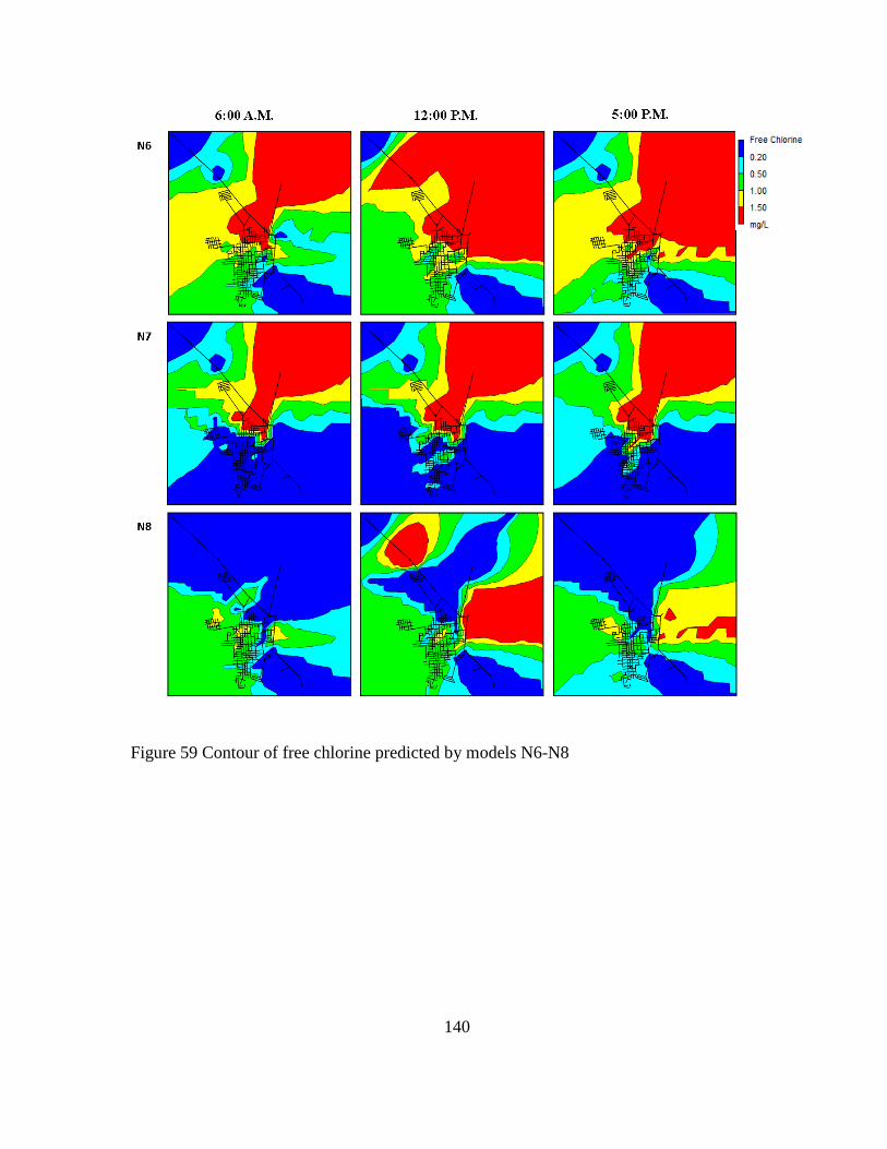
140

Figure 59 Contour of free chlorine predicted by models N6-N8

141

Table 11 Overview of sample sizes for each test Sample type Number of samples Year taken Storage tanks 3 2012 Storage tanks 3 2013 Households 12 2012 Households 18 2013

Supply 6 2012 Supply 4 2013 Surface 4 2012

Coliscan® Easygel® kit 16 2012 Coliscan® Membrane Filter 21 2013

Watersafe® Well Water Testing Kit 18 2012 Hanna Instruments Model HI 98129 26 2013

Hach Company Model CN-70 25 2013 Dionex ICS 1000 14 2012

Shimadzu TOC-VCSH 25 2013 Total visit 1 25 2012 Total visit 2 26 2013

Total 51