
INTEGRATED MANAGEMENT OF CHEMICAL PROCESSES ...
254
INTEGRATED MANAGEMENT OF CHEMICAL PROCESSES IN A COMPETITIVE ENVIRONMENT
-
Upload
khangminh22 -
Category
Documents
-
view
2 -
download
0
Transcript of INTEGRATED MANAGEMENT OF CHEMICAL PROCESSES ...
INTEGRATED MANAGEMENT OF CHEMICAL PROCESSES IN A COMPETITIVE ENVIRONMENT

INTEGRATED MANAGEMENT OF CHEMICAL PROCESSES IN A COMPETITIVE
ENVIRONMENT
Miguel Ángel Zamarripa Pérez
A Thesis presented for the degree of
Doctor of Philosophy
Thesis advisor: Dr. Antonio Espuña
Escola Tècnica Superior d’Enginyeria Industrial de
Barcelona
Universitat Politècnica de Catalunya
June 2013

Copyright © 2013 by Miguel Ángel Zamarripa Pérez.

Todo el esfuerzo es dedicado a las personas que han compartido, disfrutado, y en ocasiones han sufrido para verme llegar hasta aquí: Filiberto, María de Lourdes, Juan Francisco,
Jorge, y a mis grandes amores Martha y mi hija Danna Lourdes Zamarripa.


Most people say that it is the intellect which makes a great scientist. They wrong: it is the character.
Albert Einstein (1879‐195)

i
Summary
This Thesis aims to enhance the decision making process in the SCM, remarking the difference between optimizing the SC to be competitive by its own, and to be competitive in a global market in cooperative and competitive environments. The structure of this work has been divided in four main parts:
Part I: consists in a general introduction of the main topics covered in this manuscript (Chapter I); a review of the State of the Art that allows us to identify new open issues in the PSE (Chapter 2). Finally, Chapter 3 introduces the main optimization techniques and methods used in this contribution.
Part II focuses on the integration of decision making levels in order to improve the decision making of a single SC: Chapter 4 presents a novel formulation to integrate synthesis and scheduling decision making models, additionally, this chapter also shows an integrated operational and control decision making model for distributed generations systems (EGS). Chapter 5 shows the integration of tactical and operational decision making levels. In this chapter a knowledge based approach has been developed capturing the information related to the operational decision making level. Then, this information has been included in the tactical decision making model. In Chapter 6 a simplified approach for integrated SCs is developed, the detailed information of the typical production‐distribution SC echelons has been introduced in a coordinated SC model.
Part III proposes the explicit integration of several SC’s decision making in order to face several real market situations. As well, a novel formulation is developed using an MILP model and Game Theory (GT) as a decision making tool. Chapter 7 includes the tactical and operational analysis of several SC’s cooperating or competing for the global market demand. Moreover, Chapter 8 includes a comparison, based on the previous results (MILP‐GT optimization tool) and a two stage stochastic optimization model. Results from both Chapters show how cooperating for the global demand represent an improvement of the overall total cost. Consequently, Chapter 9 presents a bargaining tool obtained by the Multi‐objective (MO) resolution of the model presented in Chapter 7.
Finally, final conclusions and further work have been provided in Part IV.

ii
iii
Resumen
El objetivo general de esta Tesis es mejorar el proceso de la toma de decisiones en la gestión de cadenas de suministro, tomando en cuenta principalmente dos diferencias: ser competitivo considerando las decisiones propias de la cadena de suministro, y ser competitivo dentro de un entorno global. La estructura de ésta tesis se divide en 4 partes principales:
La Parte I consiste en una introducción general de los temas cubiertos en esta Tesis (Capítulo 1). Una revisión de la literatura, que nos permite identificar las problemáticas asociadas al proceso de toma de decisiones (Capítulo 2). El Capítulo 3 presenta una introducción de las técnicas y métodos de optimización utilizados para resolver los problemas propuestos en esta Tesis.
La Parte II se enfoca en la integración de los niveles de decisión, buscando mejorar la toma de decisiones de la propia cadena de suministro. El Capítulo 4 presenta una formulación matemática que integra las decisiones de síntesis de procesos y las decisiones operacionales. Además, este capítulo presenta un modelo integrado para la toma de decisiones operacionales incluyendo las características del control de procesos. El Capítulo 5 muestra la integración de las decisiones del nivel táctico y el operacional, dicha propuesta está basada en el conocimiento adquirido capturando la información relacionada al nivel operacional. Una vez obtenida esta información se incluye en la toma de decisiones a nivel táctico. Finalmente en el capítulo 6 se desarrolla un modelo simplificado para integrar múltiples cadenas de suministro. El modelo propuesto incluye la información detallada de las entidades presentes en una cadena de suministro (suministradores, plantas de producción, distribuidores y mercados) introduciéndola en un modelo matemático para su coordinación.
La Parte III propone la integración explicita de múltiples cadenas de suministro que tienen que enfrentar numerosas situaciones propias de un mercado global. Asimismo, esta parte presenta una nueva herramienta de optimización basada en el uso integrado de métodos de programación matemática y conceptos relacionados a la Teoría de Juegos. En el Capítulo 7 analiza múltiples cadenas de suministro que cooperan o compiten por la demanda global del mercado. El Capítulo 8 incluye una comparación entre el problema resuelto en el Capítulo anterior y un

iv
modelo estocástico, los resultados obtenidos nos permiten situar el comportamiento de los competidores como fuente exógena de la incertidumbre típicamente asociada la demanda del mercado. Además, los resultados de ambos Capítulos muestran una mejora sustancial en el coste total de las cadenas de suministro asociada al hecho de cooperar para atender de forma conjunta la demanda disponible. Es por esto, que el Capítulo 9 presenta una nueva herramienta de negociación, basada en la resolución del mismo problema (Capítulo 7) bajo un análisis multiobjetivo.
Finalmente, la parte IV presenta las conclusiones finales y una descripción general del trabajo futuro.

v
Acknowledgments
I would like to thank my thesis advisor, Prof. Antonio Espuña, his ability and persistence for finding the pros in my ideas pushed me forward all the time through this year’s. I was lucky to have him as thesis supervisor because he introduced me the PSE scope and directed me to the cooperative and non‐cooperative research line. I also would like to thank to Prof. Carlos Méndez, who helped me to find the right path to introduce new concepts during this Thesis research.
I would like to express gratitude to those who helped in different discussions related to methods and tools. They are without order of importance: José Miguel Laínez, Carlos Méndez, Prof. Luis Puigjaner, Moises Graells, Javier Silvente, Aarón Bojarski, Adrian Aguirre, Mariana Cóccola, Kefah Hjaila, Esteban Bernechea and Edxon Licón.
I am also grateful to all my professors during my undergraduate studies at Instituto Tecnológico de la Laguna (ITL), and also during my Master degree at the Universidad Autónoma de Nuevo Léon (UANL), for providing me with many of the skills that I required during my graduate studies, specially to professors Flores, Javier Rivera, Oscar Huerta and Ricardo Gómez.
I am thankful to all my colleagues at the CEPIMA and CAPSE research groups for the fruitful arguments that we had over coffee breaks and lunches during the last four years. This friendly environment allowed me to learn and grow. I am especially grateful to: José Miguel, Edrisi, Aáron, Javier Silvente, Javier Etxabarri, Marcos Maroñas, Guillem Crexells, Ariel Diaz, Kefah Hjaila, Victor, Martin, Mar, Marta, Elisabeth, Adrian, Mariana, Vannina & Diego Cafaro, Mrs. Nelida, Rodolfo Dondo, Issac, Evelyn, Martin, Esteban, and Edxon for their friendly support.
I thank all my family for their continuous support, Jorge, Paco, Fili and Lourdes which on the distance they know how to help and become part of this work. Special mention to my wife Martha, without her encouragement and understanding it would have been impossible for me to finish this work. Finally, to my daughter who with her birth gave me the strength and courage to be a better person.

vi
I would like to acknowledge the financial support received from:
First two years scholarship financed by the Erasmus Mundus External window cooperation for Mexico (lot 18).
Last two years scholarship financed by The Mexican Council of Science and Technology (Consejo Nacional de Ciencia y Tecnología CONACYT).
Attendance of all the conferences and congresses financed by the Spanish “Ministerio de Economia y Competitividad” and the European Regional Development Fund, both funding the research projects EHMAN DPI2009‐09386 and SIGERA DPI2012‐37154‐C02‐01.
The mobility/internship financed by the “Agencia Española de Cooperación Internacional para el Desarrollo” (Acción AECID PCI A1/044876/11).
vii
Agradecimientos
En primer lugar me gustaría agradecer al profesor Antonio Espuña, director de esta Tesis, por su dedicación para supervisar las ideas desarrolladas durante este trabajo. Además, gracias a su esfuerzo continuo me ayudó a la comprensión del concepto “Ingeniería de Procesos y Sistemas” y su aplicación a la gestión de cadenas de suministro en un entorno cooperativo y competitivo.
Me gustaría expresar mi gratitud a aquellos que han colaborado y ayudado con discusiones, comentarios relacionados con la investigación desarrollada en esta Tesis. Entre ellos se encuentran: José Miguel Laínez, Carlos Méndez, el profesor Luis Puigjaner, Javier Silvente, Moises Graells, Aarón Bojarski, Adrian Aguirre, Mariana Cóccola, Kefah Hjaila, Esteban Bernechea y Edxon Licón. De la misma manera, me gustaría agradecer a los profesores que han sido importantes durante mi formación profesional. Entre ellos una mención especial para el profesor Flores, Javier Rivera, Oscar Huerta y Ricardo Gómez.
De una forma especial, considero que estoy en deuda con mis compañeros de trabajo tanto del grupo CEPIMA como del grupo CAPSE, que han servido de ayuda mediante discusiones y argumentos durante estos cuatro años de investigación. Especialmente José Miguel, Edrisi, Aarón, Javier Silvente, Javier Etxabarri, Marcos Maroñas, Guillem Crexells, Ariel Diaz, Kefah Hjaila, Victor, Martin, Mar, Marta, Elisabeth, Adrian, Mariana, Vannina & Diego Cafaro, Mrs. Nelida, Rodolfo Dondo, Issac, Evelyn, Martin, Esteban, y Edxon.
También quisiera agradecer a mi familia por su apoyo incondicional. Jorge, Paco, Fili, y Loru, que incluso en la distancia han sabido ayudarme y ser parte importante de este trabajo. Una mención especial para mi querida esposa Martha que me ha acompañado durante esta aventura, convirtiéndose en un pilar de este trabajo, ya que sin ella todo esto no habría sido posible. Finalmente agradezco a mi hija que con su nacimiento me ha dado el valor y el coraje para intentar ser mejor cada día.

ix
Table of Contents
Summary ........................................................................................................................................................ i
Resumen ...................................................................................................................................................... iii
Acknowledgments ..................................................................................................................................... v
Agradecimientos ..................................................................................................................................... vii
Table of Contents ...................................................................................................................................... ix
List of Figures ........................................................................................................................................... xv
List of Tables ............................................................................................................................................ xix
Part I Overview ................................................................................................................................... 1
Chapter 1. Introduction .............................................................................................................. 3
1.1. Motivation ........................................................................................................................... 3
1.2. Process Management ...................................................................................................... 4
1.3. Supply Chain Management ........................................................................................... 5
1.4. SCM in Chemical Engineering ..................................................................................... 6
1.5. Main Objectives ................................................................................................................. 7
1.6. Thesis Outline .................................................................................................................... 8
Chapter 2. State of the art ...................................................................................................... 11
2.1. Strategic decision‐making ......................................................................................... 12
2.2. Tactical decision making (planning problem) .................................................. 13
2.3. Operational decision‐making (Scheduling) ....................................................... 15
2.4. Enterprise wide optimization (EWO) ................................................................... 16
2.5. Open issues ...................................................................................................................... 17

x
2.5.1. Vertical Integration ............................................................................................ 18
2.5.2. Uncertainty Management ................................................................................ 19
2.5.3. Cooperative and non cooperative SC’s ....................................................... 25
2.5.4. Multi‐objective analysis .................................................................................... 27
Chapter 3. Methods and Tools ............................................................................................. 29
3.1. System definition ........................................................................................................... 29
3.2. Mathematical Programming ..................................................................................... 30
3.2.1. Convexity ................................................................................................................ 31
3.2.2. Karush‐Kuhn‐Tucker first order conditions ............................................ 31
3.2.3. Duality ...................................................................................................................... 32
3.3. Linear Programming .................................................................................................... 33
3.3.1. The Simplex Method .......................................................................................... 33
3.3.2. Interior point methods ..................................................................................... 33
3.4. Nonlinear Programming ............................................................................................. 34
3.4.1. Unconstrained optimization ........................................................................... 34
3.4.2. Constrained optimization ................................................................................ 34
3.5. Mixed Integer programming .................................................................................... 34
3.5.1. Branch and Bound methods ........................................................................... 35
3.5.2. Cutting plane methods ...................................................................................... 35
3.6. Multi‐Objective Optimization (MOO) .................................................................... 36
3.6.1. The ‐constraint method ................................................................................. 37
3.7. Stochastic programming with recourse .............................................................. 38
3.8. Game Theory ................................................................................................................... 39
3.9. Software ............................................................................................................................ 40
3.9.1. General Algebraic Modeling System (GAMS) .......................................... 41
3.10. Summary ........................................................................................................................... 41
Part II Enhancing Plant and SC Competitiveness ................................................................ 43
Summary ............................................................................................................................................... 45
Chapter 4. Plant decision‐making ....................................................................................... 47
4.1. Integrated Synthesis and Scheduling decision‐making ................................ 47
xi
4.1.1. Synthesis State Task Network (SSTN) ....................................................... 49
4.1.2. Problem statement ............................................................................................. 51
4.1.3. Case study ............................................................................................................... 54
4.1.4. Conclusions ............................................................................................................ 61
4.2. Integrated Scheduling and Control decision‐making .................................... 65
4.2.1. Energy Management .......................................................................................... 66
4.2.2. Detailed Case Study ............................................................................................ 68
4.2.3. Conclusions ............................................................................................................ 70
Chapter 5. Tactical and Operational Integration .......................................................... 73
5.1. Introduction ..................................................................................................................... 73
5.2. Problem Statement ....................................................................................................... 74
5.2.1. Scheduling .............................................................................................................. 74
5.2.2. Planning ................................................................................................................... 75
5.2.3. Integrated Planning‐Scheduling ................................................................... 75
5.3. Case Study......................................................................................................................... 75
5.4. Results ................................................................................................................................ 76
5.5. Conclusions ...................................................................................................................... 78
Chapter 6. Coordinated Supply Chains ............................................................................. 81
6.1. Introduction ..................................................................................................................... 81
6.2. Problem Statement ....................................................................................................... 82
6.2.1. Planning ................................................................................................................... 82
6.3. Case Study......................................................................................................................... 86
6.3.1. Entire Supply Chain ............................................................................................ 86
6.3.2. Energy Generation SC ........................................................................................ 88
6.4. Results ................................................................................................................................ 91
6.4.1. Non‐coordinated scenario ............................................................................... 92
6.4.2. Coordinated scenario ........................................................................................ 95
6.4.3. Economical Analysis .......................................................................................... 97
6.5. Conclusions ...................................................................................................................... 99
Part III Cooperative and Competitive SC’s ........................................................................... 103
xii
Chapter 7. SC’s in a Competitive Environment .......................................................... 105
7.1. Cooperative and Competitive SC planning ...................................................... 105
7.1.1. Introduction ........................................................................................................ 105
7.1.2. Supply Chain Planning ................................................................................... 106
7.1.3. Case Study ........................................................................................................... 111
7.1.4. Results and Discussion .................................................................................. 113
7.1.5. Bargaining Tool ................................................................................................. 120
7.2. Supply Chain Scheduling in a Competitive Environment .......................... 125
7.2.1. Introduction ........................................................................................................ 125
7.2.2. Problem Statement .......................................................................................... 126
7.2.3. Case Study ........................................................................................................... 130
7.2.4. Results and Discussion .................................................................................. 131
7.3. Conclusions ................................................................................................................... 137
Chapter 8. Uncertainty Management ............................................................................. 139
8.1. Introduction .................................................................................................................. 139
8.2. Problem Statement .................................................................................................... 140
8.2.1. Supply Chain Planning ................................................................................... 140
8.2.2. Representation of the Uncertainty ........................................................... 140
8.2.3. Two Stage Stochastic Optimization .......................................................... 140
8.2.4. Parameters under uncertainty ................................................................... 141
8.2.5. Demand uncertainty (cooperative problem) ....................................... 141
8.2.6. Competitive behavior ..................................................................................... 143
8.3. Case Study...................................................................................................................... 145
8.4. Results ............................................................................................................................. 145
8.4.1. Demand uncertainty(cooperative problem) ........................................ 146
8.4.2. Market Competition Uncertainty ............................................................... 153
8.4.3. Exogenous source of uncertainty .............................................................. 159
8.5. Conclusions ................................................................................................................... 161
Chapter 9. MOO as a Bargaining Tool ............................................................................ 165
9.1. Introduction .................................................................................................................. 165
9.2. Problem Statement .................................................................................................... 166
xiii
9.2.1. Supply Chain Planning ................................................................................... 166
9.2.1. Cooperative problem ...................................................................................... 166
9.2.2. Competitive problem ...................................................................................... 166
9.2.3. Multi‐Objective Optimization (MOO)....................................................... 167
9.2.4. Game Theory and Equilibrium Point ....................................................... 167
9.2.5. Proposed Framework ..................................................................................... 168
9.3. Case Study...................................................................................................................... 170
9.4. Results ............................................................................................................................. 170
9.4.1. Cooperative Case .............................................................................................. 170
9.4.2. Competitive Case .............................................................................................. 172
9.5. Conclusions ................................................................................................................... 174
Part IV Final Remarks ................................................................................................................... 175
Chapter 10. Conclusions and Further work ................................................................... 177
10.1. Conclusions ................................................................................................................... 177
10.2. Further Work ............................................................................................................... 179
Appendixes ............................................................................................................................................. 181
Appendix A. Publications ........................................................................................................ 183
A.1. Journals ........................................................................................................................... 183
A.2. Submitted ....................................................................................................................... 183
A.3. Conference proceeding articles ............................................................................ 183
A.4. Participation in research projects ....................................................................... 185
Appendix B. Case Study Data ................................................................................................. 187
Appendix C. Case Study Data ................................................................................................. 191
Appendix D. Case Study Data ................................................................................................. 195
Appendix E. Case Study Data ................................................................................................. 197
Appendix F. Glossary ................................................................................................................ 203
Appendix G. Author Index ...................................................................................................... 205
Bibliography ........................................................................................................................................... 209


xv
List of Figures
Figure 1.1. Geographical distribution of the chemical products in Spain. ................. 3
Figure 1.2. Typical SC network configuration ........................................................................ 5
Figure 1.3. Decision making levels. ............................................................................................. 6
Figure 1.4. Thesis schema ............................................................................................................ 10
Figure 2.1. Open issues to improve the decision making………………………………………18
Figure 2.2. Game Theory Optimization .................................................................................. 26
Figure 3.1. Convexity………………………………………………………………………………………. 31
Figure 4.1. Evolution of network representations (a, b, and c)…………………………….51
Figure 4.2. Description of the Synthesis State Task Network (SSTN). ..................... 56
Figure 4.3. Case 1 Scheduling ..................................................................................................... 57
Figure 4.4. Case 2 results (schedule) ...................................................................................... 58
Figure 4.5. Case 3 results (schedule) ...................................................................................... 58
Figure 4.6. Production level and forecasted demand of each case ............................ 59
Figure 4.7. Power demand (Dh) and production capacity for the two sources (Pihmax = Pihmin). .......................................................................................................... 69
Figure 4.8. Results for generation (Pih), storage (SEih) and power supply obtained. ...................................................................................................................... 69
Figure 4.9. Detailed Simulation (Simulink‐capture) ........................................................ 70
xvi
Figure 5.1. STN case study. 76
Figure 5.2. Production cost vs. product demand (Scheduling model) 77
Figure 5.3. Production and inventory levels. 77
Figure 5.4. Economic analysis 78
Figure 6.1. The entire SC Scheme 87
Figure 6.2. Energy flows among the Entire SC 88
Figure 6.3. Energy generation SC 89
Figure 6.4. Energy production‐distribution echelon 89
Figure 6.5. Polystyrene production echelon SC network 91
Figure 6.6. Production levels of (a) polystyrene 97 and (b) polystyrene 99 92
Figure 6.7. Inventory levels (a) polystyrene 97 and (b) polystyrene 99 93
Figure 6.8. Energy required for PDSC 93
Figure 6.9. Energy production levels 94
Figure 6.10. Energy distribution 94
Figure 6.11. Acquisition of raw material EGSC 94
Figure 6.12. Polystyrene production levels a) polystyrene 99 and b) polystyrene 97 96
Figure 6.13. Storage levels of PDSC 96
Figure 6.14. Polystyrene production comparison (%, non‐coordinated/coordinated scenarios) 97
Figure 6.15. Detailed costs distribution 98
xvii
Figure 7.1. Description of the SC Network. Plant1‐4 serves Distr1‐4. 112
Figure 7.2. Optimal Production level (Qinh) SC‐Source‐Product in time period (exp^3). 115
Figure 7.3. Optimal Inventory level (Winh) SC‐Source‐Product in time period (exp^3). 116
Figure 7.4. Cost Analysis for the studied examples 120
Figure 7.5. SC Configuration 128
Figure 7.6. Cooperative results (High‐High quality schedule). 132
Figure 7.7. Nash Equilibrium of SC1 135
Figure 7.8. Nash Equilibrium of SC2 136
Figure 8.1. Production levels (deterministic Solutions) .............................................. 147
Figure 8.2. Inventory levels (deterministic solutions) ................................................. 148
Figure 8.3. Distribution levels (deterministic solutions) ............................................ 149
Figure 8.4. Production and subcontracted products (two stage model) .............. 150
Figure 8.5. Inventory levels (two stage model) ............................................................... 151
Figure 8.6. Distribution levels (two stage model) .......................................................... 152
Figure 8.7. Production levels ................................................................................................... 154
Figure 8.8. Inventory levels (competitive problem) ..................................................... 155
Figure 8.9. Distribution levels (two stage model) .......................................................... 156
Figure 8.10. Attendance of the market demand (SC1: Plant1 and Plant2; SC2: Plant3 and Plant4) ............................................................................................... 160
Figure 8.11. Market demand scenarios of SC1 (1x10²) .................................................. 160
Figure 9.1. Proposed Framework .......................................................................................... 169
Figure 9.2. Pareto solutions for the cooperative case................................................... 172

xviii
Appendixes
Figure E.1. Pareto frontier scenario (% of discount, SC1 0.0, SC2 0.0) ................. 197
Figure E.2. Pareto frontier scenario (% of discount, SC1 0.0, SC2 0.1) ................. 197
Figure E.3. Pareto frontier scenario (% of discount, SC1 0.0, SC2 0.2) ................. 198
Figure E.4. Pareto frontier scenario (% of discount, SC1 0.1, SC2 0.0) ................. 198
Figure E.5. Pareto frontier scenario (% of discount, SC1 0.1, SC2 0.1) ................. 199
Figure E.6. Pareto frontier scenario (% of discount, SC1 0.1, SC2 0.2) ................. 199
Figure E.7. Pareto frontier scenario (% of discount, SC1 0.2, SC2 0.0) ................. 200
Figure E.8. Pareto frontier scenario (% of discount, SC1 0.2, SC2 0.1) ................. 200
Figure E.9. Pareto frontier scenario (% of discount, SC1 0.2, SC2 0.2) ................. 201
xix
List of Tables
Table 2.1. Decision making levels ................................................................................................ 12
Table 2.2. Uncertainty management: Reactive approaches ............................................. 22
Table 2.3. Uncertainty management: Preventive approaches ........................................ 23
Table 3.1. Payoff matrix (illustrative example, $) ................................................................. 40
Table 4.1. Case Study Equipment units, conversion and costs. ...................................... 55
Table 4.2. Execution report ............................................................................................................ 57
Table 4.3. Economical analysis of case 1 .................................................................................. 59
Table 4.4. Economical Results case 2 ......................................................................................... 60
Table 4.5. Economical Results case 3 ......................................................................................... 60
Table 4.6. Storage parameters for the storage facility (k=1). .......................................... 68
Table 5.1. Data analysis .................................................................................................................... 76
Table 5.2. Economics ......................................................................................................................... 78
Table 6.1. Markets demands of polystyrene (kg) ................................................................. 87
Table 6.2. Fixed markets energy demands .............................................................................. 87
Table 6.3. RM echelon SC Parameters ....................................................................................... 89
Table 6.4. The distance between RM supplier and the energy plants (km) .............. 89
Table 6.5. Energy production SC parameters ......................................................................... 91
Table 6.6. Economic analysis ......................................................................................................... 98
xx
Table 7.1. Solution Report ........................................................................................................... 113
Table 7.2. Comparative results between SCs (standalone cases) ............................... 113
Table 7.3. Optimal Distribution planning for SC1 and SC2. ........................................... 114
Table 7.4. Comparative results between SCs (cooperative/competitive scenarios) 117
Table 7.5. Payoff matrix for the Competitive case (original demand). ..................... 119
Table 7.6. Parameters associated to the quality scenarios ............................................ 131
Table 7.7. Solution Report ........................................................................................................... 131
Table 7.8. Payoff Matrix. ............................................................................................................... 134
Table 8.1. Execution Report of the Demand uncertainty problem (cooperative) 146
Table 8.2. Execution Report of the competitive problem ............................................... 146
Table 8.3. Economical results of the deterministic solutions ....................................... 150
Table 8.4. Economic report ......................................................................................................... 153
Table 8.5. Deterministic solutions for the different scenarios of the discount rate. 153
Table 8.6. Costs summary. ........................................................................................................... 158
Table 8.7. Economic summary of the “apparent demand” problem .......................... 161
Table 9.1. Execution Report ........................................................................................................ 170
Table 9.2. Comparative results between SC (original data and standalone cases) 171
Table 9.3. Payoff Matrix of the competitive case (discount rate, %) ......................... 173
Table 9.4. Nash Equilibrium of the payoff matrix .............................................................. 173
Appendixes
Table B.1. RM purchase price (€/ kg) ..................................................................................... 187
Table B.2. Distance between production plants and distribution centers (km) ... 187
Table B.3. Distance between distribution centers and markets (km) ....................... 187
Table B.4. Maximum storage capacity (kg) ........................................................................... 188
Table B.5. Maximum production capacity (kg per day) .................................................. 188
Table B.6. Maximum supplier capacity (kg/day) ............................................................... 188
Table B.7. Polystyrene production cost (€/kg) .................................................................. 188
xxi
Table B.8. Polystyrene retailed price (€/kg) ....................................................................... 189
Table C.1. Payoff Matrix Percent of discount. ...................................................................... 191
Table C.2. Data of the problem. .................................................................................................. 191
Table C.3. Demand to be forecasted. ....................................................................................... 192
Table C.4. Distribution cost/delivery time of the network. ........................................... 192
Table C.5. Available labor levels (Fi,h). .................................................................................... 192
Table C.6. Production Capacities (Mi,h). .................................................................................. 192
Table C.7. Payoff matrix for the Competitive case (double demand). ....................... 193
Table D.1. Forecasted demand of the markets .................................................................... 195
Table D.2. Distribution cost ......................................................................................................... 195
Table F.1. List of acronyms used in this Thesis. ................................................................. 203


Part I Overview

3
Chapter 1. Introduction
1.1. Motivation
In 2007, the turnover of the global chemical industry accounted more than 2.1 billion of Euros. In the European Union (EU), the chemical industry accumulated over than 55% of world exports and 46% of imports putting the EU as the only area with a net positive coverage ratio. Regarding the distribution of the chemical consumption, over 40% of demand in Europe came from various sectors such as textiles, automotive, consumer products, agriculture, and construction.
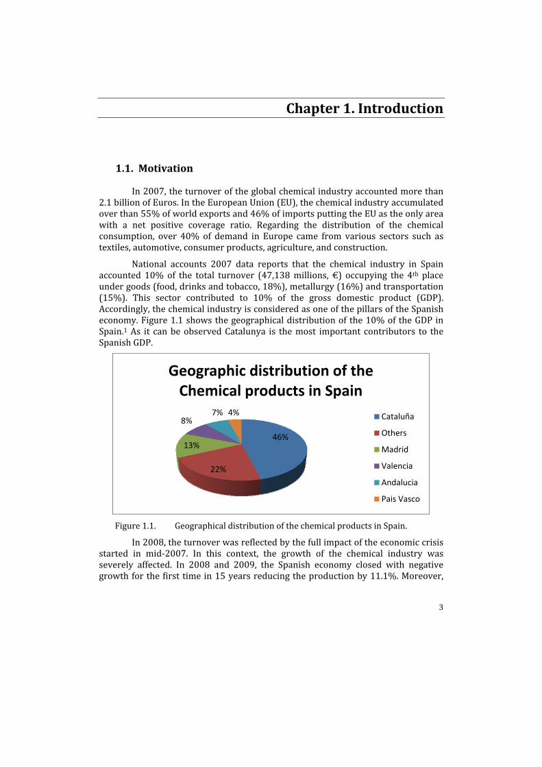
National accounts 2007 data reports that the chemical industry in Spain accounted 10% of the total turnover (47,138 millions, €) occupying the 4th place under goods (food, drinks and tobacco, 18%), metallurgy (16%) and transportation (15%). This sector contributed to 10% of the gross domestic product (GDP). Accordingly, the chemical industry is considered as one of the pillars of the Spanish economy. Figure 1.1 shows the geographical distribution of the 10% of the GDP in Spain.1 As it can be observed Catalunya is the most important contributors to the Spanish GDP.
Figure 1.1. Geographical distribution of the chemical products in Spain.
In 2008, the turnover was reflected by the full impact of the economic crisis started in mid‐2007. In this context, the growth of the chemical industry was severely affected. In 2008 and 2009, the Spanish economy closed with negative growth for the first time in 15 years reducing the production by 11.1%. Moreover,
46%
22%
13%
8%7% 4%
Geographic distribution of the Chemical products in Spain
Cataluña
Others
Madrid
Valencia
Andalucia
Pais Vasco

Chapter 1 ‐ Introduction
4
during the 2009 and 2010, the Spanish chemical sector closed with a positive balance of 6.2% growth in production volume raising its turnover by 11.4% compared to 2009.1 This confirmed a positive evolution in the chemical industry throughout the past year (2011) with a recovery in most industrial sectors.
Analysts agree that the chemical industry demands a solid economic model based on internationalized industry and a plan of measures to attract productive investments. In addition, the study done by the Business Federation of the Spanish Chemical Industry (FEIQE) concludes that “the solid and sustainable recovery of the Spanish economy over the time is only possible if its prioritization of the policies oriented to improve the competitiveness of the industry in Spain”. Furthermore, this study repositioned the chemical industry as an important sector representing 11% of Spain GDP. Thus, the chemical industry represents 500,000 direct; indirect; and induced jobs in 2011. In addition, the chemical sector is the second in Europe for imports and the first for private investment in environmental protection and R&D+I.2
A wide range of applied research has been developed to manage business decision making (such as Supply Chain Management, SCM). It is important to develop new business decision making models adapting the changes of the market trends to improve the use of resources; minimize production, inventory, distribution, and investment costs; and in many cases to re‐design the supply chain (SC). Additionally, the competition in the global market is necessary to include the role of the competitors and to maintain a high level of quality in the processes, products, services, etc.
1.2. Process Management
Currently, the added value to the enterprises is as important as their SCM and processes efficiency. Most of the enterprises have considered these rules to drive their performance during the last 50 years. Several methodologies have been developed to improve the decision making process and to avoid some common ailments such as low productive processes, poor service level, departmental barriers, useless threads, etc.
The general objectives of the process management aim to:
enhance the economic benefits by increasing process performance, increase customer satisfaction by improving the service level and quality of the
products, increase staff satisfaction, increase knowledge and process control, get a better flow of information and materials, decrease processing times, and to satisfy greater flexibility for customer needs.
In the late nineties, the SCM has been defined and designed in order to address the abovementioned objectives. Taking into account the resources to design
Chapter 1 ‐ Introduction
5
a plan whereby decisions are taken trying to improve the use of goods and services of the company. The main objectives were to increase the profit, minimize the transportation, production, inventory, installation, environmental, quality and so other costs.
1.3. Supply Chain Management
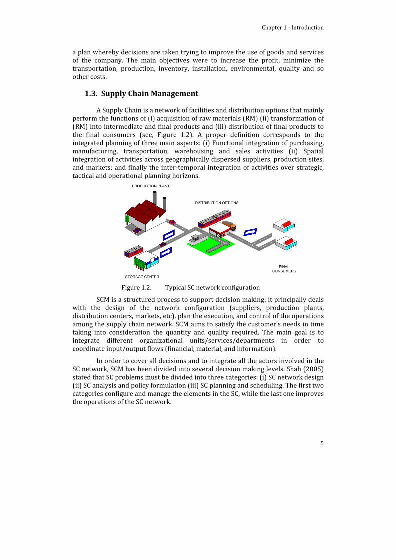
A Supply Chain is a network of facilities and distribution options that mainly perform the functions of (i) acquisition of raw materials (RM) (ii) transformation of (RM) into intermediate and final products and (iii) distribution of final products to the final consumers (see, Figure 1.2). A proper definition corresponds to the integrated planning of three main aspects: (i) Functional integration of purchasing, manufacturing, transportation, warehousing and sales activities (ii) Spatial integration of activities across geographically dispersed suppliers, production sites, and markets; and finally the inter‐temporal integration of activities over strategic, tactical and operational planning horizons.
Figure 1.2. Typical SC network configuration
SCM is a structured process to support decision making: it principally deals with the design of the network configuration (suppliers, production plants, distribution centers, markets, etc), plan the execution, and control of the operations among the supply chain network. SCM aims to satisfy the customer’s needs in time taking into consideration the quantity and quality required. The main goal is to integrate different organizational units/services/departments in order to coordinate input/output flows (financial, material, and information).
In order to cover all decisions and to integrate all the actors involved in the SC network, SCM has been divided into several decision making levels. Shah (2005) stated that SC problems must be divided into three categories: (i) SC network design (ii) SC analysis and policy formulation (iii) SC planning and scheduling. The first two categories configure and manage the elements in the SC, while the last one improves the operations of the SC network.

Chapter 1 ‐ Introduction
6
This work focuses in 3 main decision levels: strategic, tactical and operational. And they have been hierarchically distributed in terms of the importance and time to be re‐scheduled. (See, Figure 1.3).
Figure 1.3. Decision making levels.
A detailed description of the decision making levels can be encountered in the next subsections. The decision making in these levels are mainly:
Strategic decisions: the main objective is to design the system by determining the optimal location of production plants, warehouses; supplier and raw material selection, the production technologies and equipment capacities to be installed in order to fulfill the market demands.
Tactical decisions: at this decision making level the optimal production, distribution, inventory and subcontracting levels must be determined considering a fixed SC network configuration (previously determined in the strategic decision making level).
Operational decisions: this decision making level typically receives the results of the tactical decisions and allocates the availability of equipments, sequencing the production tasks in order to enhance the production plans/objectives.
Traditionally, each level objective and capacity are fixed by the decisions made in previous levels, although more comprehensive view of the system may be obtained by a global objectives definition and decision making.
1.4. SCM in Chemical Engineering
Process systems engineering (PSE) traditionally has been concerned of the development of systematic procedures for the design, control, and operation of chemical processes (Sargent, 1991). However, Grossmann and Westerberg (2000) extended the concept of “Chemical Supply Chain, ChSC” observing that SC starts at the molecular level involving the synthesis of the studied chemical molecules into particles and finally into products. This process becomes part of the production plant that connects suppliers, warehouses, and distribution centers. In other words,
Strategic (Design)
Tactical (Planning)
Operational (Scheduling)
Control, transport, etc.
Chapter 1 ‐ Introduction
7
PSE can be defined as the field concerned with the improvement of decision making processes.
Chemical industry is one of the most important sectors all over the world especially Spain and USA as they are the highest private investors in R+D. Financial incentives to apply the SCM theory are considerable; Exxon Chemicals estimates a significant reduction in annual operating costs (2%) and an important reduction in the inventory (20%) while DuPont was able to reduce the working capital from $165 to 90 millions. (Sung and Maravelias 2007).
Several works presented in the literature stated that the SCM aims to improve the decision making process reducing costs and/or improving benefits. Grossmann (2005) encountered that SCM has become the “holy grail” in process industries in order to remain competitive in the global marketplace due to the increasing pressure to reduce operation costs and inventories. Ferrio and Wassick (2007) stated that the chemical supply chains (ChSC) are a fruitful area of cost reductions. They remarked 3 principal aspects: (i) ChSC represent the most important portion of the total cost to attend the customers (ii) ChSC change constantly (iii) ChSC always reflect a lower cost option.
1.5. Main Objectives
Nowadays, the enterprises goal is to be competitive in a global market. However, this goal is very difficult to achieve due to the nature of the enterprises:
several SC echelons with different roles, numerous SCs interacting or competing for the same market, a number of decisions that must be taken in changing environments and
considering different objectives.
This Thesis aims to enhance the decision making process of ChSC facing nowadays open issues, such as: new market trends, market globalization, and high market competitiveness. In order to achieve the main goal and to satisfy the introduction of competitiveness into the ChSC, three specific objectives have been encountered:
implement and develop integrated decision making approaches looking to optimize more than one decision level of the SCM theory,
characterize and integrate several and different Supply Chains in the typical SCM scope,
develop models capable to manage the uncertain competition behavior include decision making of other SC’s as an exogenous source of
uncertainty identify control parameters to manage the new uncertain term (market
prices and product quality) develop robust tools in order to improve SCM in cooperative and
competitive environments.

8
1.6. Thesis Outline
Currently, financial issues change the way to do business around the world. Decision makers are seeking to reduce the costs to be competitive in a global market. This need starts to increase towards environmentally friendly products, higher quality products, less expenses of distribution/production, reduce losses driven by uncertainties, etc. The complexity to manage decision‐making process (strategic, tactical and operational plans) has increased and the old policies to satisfy consumer demands have changed leading to several structural changes in the management of Supply Chains (SC). Nowadays, it is necessary to take into account several factors that have not previously considered such as integration of specific objectives at different decision levels of the enterprise, eventualities that cannot be prevented, etc. so policies such as “no stock”, “just in time”, etc create different conflicts within the company itself. In order to attract more markets and higher benefits, the decision‐making process must be improved.
Process system engineering (PSE) researchers have been working hard in recent years solving chemical engineering related problems looking to improve productivity, reduce wastes, and maximize benefits of all the parties in a Supply Chain (suppliers, producers, distributors and costumers). Supply chain management (SCM) aims to obtain optimal decision making through finding the best performance of the enterprise (maximize benefit and/or minimize losses). Several SCM industrial applications are exposed in this work highlighting the fact that the study of multiple SCs under cooperation/competition environments has not been exploited yet.
The main objective of this Thesis is to improve decision‐making in cooperative and competitive environments. At this point it is important to define that the concept of “competitive” will be implemented in two ways:
“Due to continuous processes improvements, decisionmaking, marketing, etc., In brief increase the competitiveness of a company to improve decisionmaking in the
chemical industry”
&
"Due to the inclusion of one or more competitors into the scope covered by typical decisionmaking analysis, including the behavior of the competitors in the
decisionmaking process simulating a global market"
This Thesis is divided in four main parts (general scope can be observed in the outline scheme, see Figure 1.4).
Part I presents an overview of the Process System Engineering (PSE) techniques applied to chemical processes (such as Supply Chain Management SCM, mathematical programming tools, etc.) and an extensive review of the topics covered. The extensive literature review provides a broad overview of the applications and the techniques used to address specific problems in Supply Chain (SC) decision‐making process. Also, it provides an overview of the open issues in the SCM. Three main issues will be addressed in the following Chapters and sections of

Chapter 1 ‐ Introduction
9
the Thesis: integration of decision‐making levels, integration of uncertainty, and development of optimization tools/techniques to optimize complex optimization models.
Part II studies the integration of decision‐making levels in SCM. This part aims to improve process productivity by integrating different decision‐making levels and developing mathematical models able to integrate the features of more than one decision level in the SCM (decisions levels: strategic, tactical, operational, delivery (transportation), process control, process synthesis, etc.).
Part III considers the integration multiple SCs under cooperation and competition scenarios. Several applications capable to consider uncertain events (process control and operation parameters, forecasted demands, market conditions, etc.) have been developed by PSE researchers at different decision‐making levels. Specifically, this Thesis develops mathematical models to optimize the production planning problem including uncertainties, improving the decision‐making under demand uncertainty (typical problem), and studying a new source of uncertainty (the competition behavior).
Finally, Part IV includes some concluding remarks and further work.
Chapter 1 ‐ Introduction
10
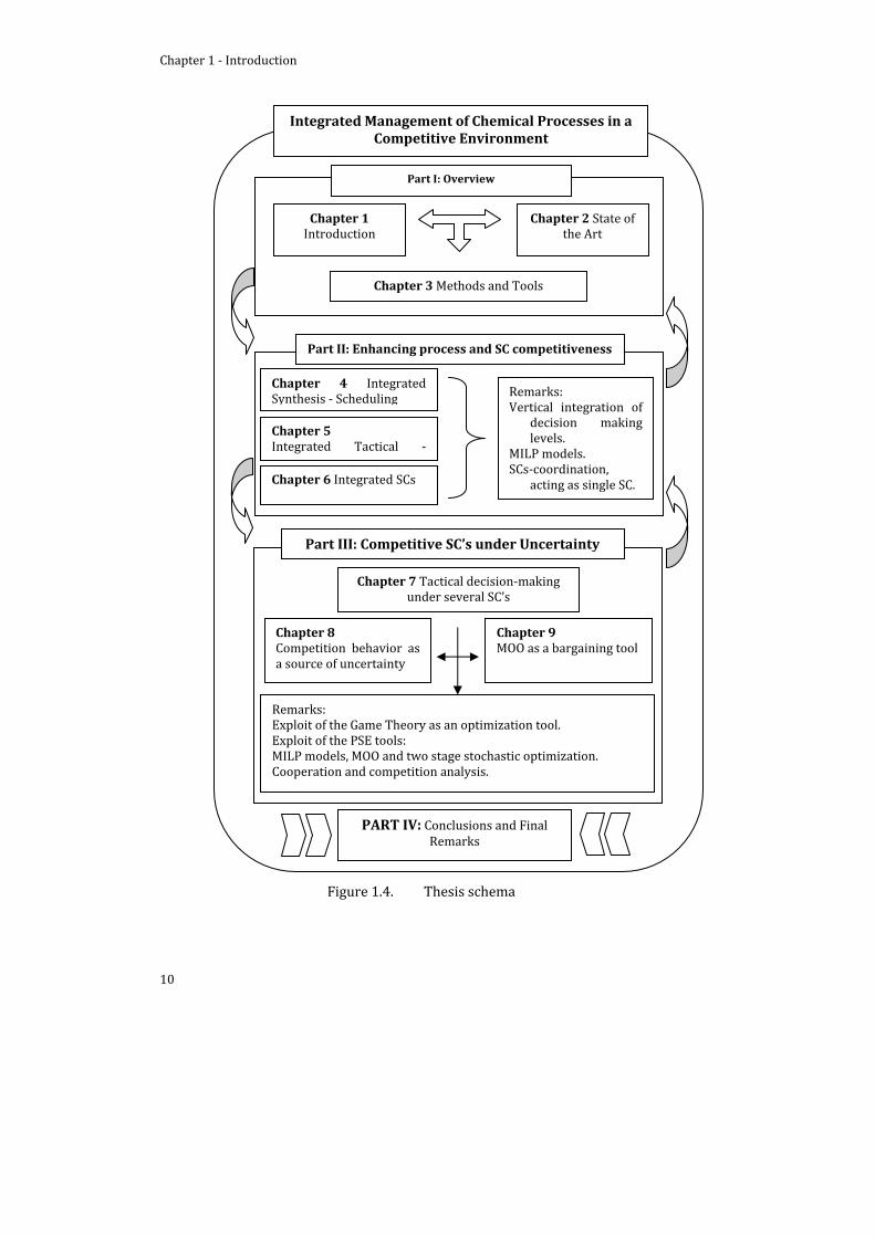
Figure 1.4. Thesis schema
PART IV: Conclusions and Final Remarks
Part I: Overview
Chapter 1Introduction
Chapter 2 State of the Art
Chapter 3 Methods and Tools
Part III: Competitive SC’s under Uncertainty
Chapter 7 Tactical decision‐making under several SC’s
Remarks: Exploit of the Game Theory as an optimization tool. Exploit of the PSE tools: MILP models, MOO and two stage stochastic optimization. Cooperation and competition analysis.
Chapter 9 MOO as a bargaining tool
Chapter 8 Competition behavior as a source of uncertainty
Part II: Enhancing process and SC competitiveness
Chapter 4 Integrated Synthesis ‐ Scheduling Remarks:
Vertical integration of decision making levels.
MILP models. SCs‐coordination,
acting as single SC.
Chapter 5 Integrated Tactical ‐
Chapter 6 Integrated SCs
Integrated Management of Chemical Processes in a Competitive Environment

11
Chapter 2. State of the art
This Chapter includes a summary of the major contributions made so far of the topics covered during the document. The problems that are pending or have special interest will be illustrated for the development of this Thesis.
The concept of Supply Chain (SC) is relatively new. During the last century, the SC concept does not exist and the most used keywords were business planning, location problems, and routing problems. In the 90’s, the first contributions appear with the term Supply Chain Management (SCM). SC models and concepts have been successfully applied in the last decades for different industries (pharmaceutical, automotive, paper industry, chemical, petrochemical, etc.).
Conceptually, the scope covered by the SCM is very wide and diverse so that numerous reviews can be found in this regard. Lummus et al. (1999) focused his review in the definition of the SCM. Ho et al. (1989); Giannakis and Croom (2004); and Chen and Paulraj (2004) focused on strategic management perspective. Likewise, Mentzer et al. (2001) recommended that a systematic review of relevant literature is needed and defined the SCM from a general standpoint based on the decisions covered by the proper term. “Supply chain management is defined as the systemic, strategic coordination of the traditional business functions and the tactics across these business functions within a particular company and across businesses within the supply chain for the purposes of improving the long term performance of the individual companies and the supply chain as a whole (Mentzer et al., p. 18)”
The general definition of the SCM covers many discipline areas, and some definitions have been encountered: Ellram and Cooper (1993) described the SCM as the “integrated philosophy to manage the total flow of a distribution channel, from the supplier to the customer.” Christopher (1995) defined it as the “management of flows between suppliers and customers to add value to the delivery at the lowest total cost”. Along the same line, ”SupplyChain.com” defines the SCM as the strategy where business partners jointly commit to work closely together, to bring greater value to the consumer and/or their customers for the least possible overall supply cost. This coordination includes that of order generation, order taking and order fulfillment/distribution of products, services or information. Effective SCM enables business to make effective decisions among the elements of the SC: from acquiring raw materials, to manufacturing products, to distributing finished goods to the consumers. At each link/echelon, decision makers need to make the best choices about what their customers need, and how they can meet those requirements at the lowest possible cost.
Chapter 2 – State of the art
12
Analyzing the aforementioned three definitions, the integration of the decisions levels must consider all the active organizations within the product SC (suppliers, manufacture plants, distribution centers, markets, competitors, etc). Integrating and coordinating all the information among the principal actors through of the SC as a one system. This coordination must break the centralized decision‐making paradigm (decision makers disregard the decisions that cannot be controlled, i.e. during several years SC approaches consider a narrow picture of the problem of interest: Single SC improving its own benefits, etc.).
Schary and Skjott‐Larsen (1995) described the SCM strategy based on three main features to be considered: structure, organization, and process operation. The three main features can be compared within the planning matrix described by Meyr et al. (2002) and used for this Thesis (Strategic, tactical, and operational decision‐making; see, Figure 1.3 in Chapter 1).
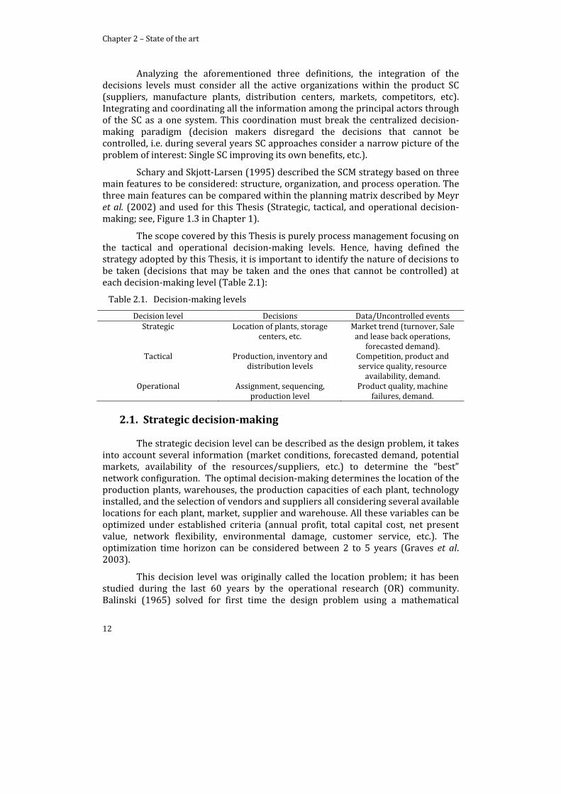
The scope covered by this Thesis is purely process management focusing on the tactical and operational decision‐making levels. Hence, having defined the strategy adopted by this Thesis, it is important to identify the nature of decisions to be taken (decisions that may be taken and the ones that cannot be controlled) at each decision‐making level (Table 2.1):
Table 2.1. Decision‐making levels
Decision level Decisions Data/Uncontrolled events Strategic Location of plants, storage
centers, etc. Market trend (turnover, Sale and lease back operations,
forecasted demand). Tactical Production, inventory and
distribution levels Competition, product and service quality, resource availability, demand.
Operational Assignment, sequencing, production level
Product quality, machine failures, demand.
2.1. Strategic decisionmaking
The strategic decision level can be described as the design problem, it takes into account several information (market conditions, forecasted demand, potential markets, availability of the resources/suppliers, etc.) to determine the “best” network configuration. The optimal decision‐making determines the location of the production plants, warehouses, the production capacities of each plant, technology installed, and the selection of vendors and suppliers all considering several available locations for each plant, market, supplier and warehouse. All these variables can be optimized under established criteria (annual profit, total capital cost, net present value, network flexibility, environmental damage, customer service, etc.). The optimization time horizon can be considered between 2 to 5 years (Graves et al. 2003).
This decision level was originally called the location problem; it has been studied during the last 60 years by the operational research (OR) community. Balinski (1965) solved for first time the design problem using a mathematical
Chapter 2 – State of the art
13
optimization procedure. Brown, Graves and Honczarenko (1987) proposed an optimization of a production‐distribution network in the process industry (NABISCO). This work was the first application to real scale industrial problems.
Due to the nature of the decisions covered by this topic (most of them linear and others discrete like install or not) the decision‐making model is typically formulated as a mixed integer linear programming model (MILP) and needs high computational effort (Laínez et al. 2007; Cakravastia, Toha and Nakamura 2002; Bansal, Karimi and Srinvasan 2008). Due to the lack of applicability of the proposed approaches of this Thesis, the analysis under cooperation and competition at the strategic decision‐making level has been disregarded. Nevertheless, seeking for uncertainty management, vertical integration, and interesting applications at this decision making level this Thesis recommends Laínez (2010).
2.2. Tactical decision making (planning problem)
Tactical decision level can be encountered as the planning problem or mid‐term SC planning. SC planning typically determines the production, distribution, subcontracting, backorder and storage levels, purchase, and distribution of raw materials and intermediate products among the network configuration (distribution centers, production plants, suppliers and markets).
The constraints associated with the tactical decision‐making level mainly consider the availability of raw materials, and maximum and minimum capacities (production, distribution and storage). The problem can be formulated as a linear programming model (since the production, storage and distribution can be continuous variables), but, in order to be more realistic in most of the cases the formulation corresponds to a MILP model, due to the constraints associated to discrete decision‐making (produce or not, distribute or not) and also due to the characterization of the SC (in the case where # of products are distributed, integer variables must be considered). The model seeks to maximize production and benefits or minimize total cost, total delivery time, tardiness, etc. during the corresponding time horizon 6 to 24 months (Silver et al., 1998). Additionally, some fixed data is considered such as fixed SC network configuration, fixed demands, costs (production, storage, distribution, subcontracting and backlog demand), distance between production plants – distribution centers – markets, maximum and minimum capacities (production, distribution, subcontracting, backlog and storage, etc.)
During the last two decades, an increasing number of researchers have been published in the academic literature addressing tactical decision‐making problem. Although few works address the inventory, production, and distribution tasks involved to optimize SC planning problems specially for general operation networks with multipurpose pathways, combination of different intermediate storage policies, task changeovers management, etc. (McDonald and Karimi, 1997).
A significant number of works address the problem of SC production planning for multi‐product, multi‐site production networks including production‐
Chapter 2 – State of the art
14
distribution options. For example, Wilkinson, Cortier, Shah and Pantelides (1996) presented an optimal production and distribution planning of a wide case study (over 100 products, 3 factories, and 14 market warehouses). Tsiakis and Papageorgiou (2008) also considered production and distribution networks with special emphasis on product site allocation among sites and outsourcing possibility. A MILP approach is proposed by Timpe and Kallrath (2000) where the optimal planning of multisite production networks is intended. Another production‐distribution ‐optimization approach is applied to a large case study in Kallrath (2000) containing 7 production sites with 27 production units operating in fixed batch mode. In order to be more realistic, Jackson and Grossmann (2003) described a multi‐period nonlinear programming model for the production planning and distribution of multi‐site continuous multiproduct plants where each production plant is represented by nonlinear process models.
SC planning in pharmaceutical applications was considered by Papageorgiou, Rotstein and Shah (2001). They presented an optimal product portfolio and long term capacity planning at multiple sites. Sousa, Shah, and Papageorgiou (2005) proposed an MILP model for the optimal production‐distribution problem applied for this type of SCs. Two decomposition schemes where developed for the solution of the large‐scale optimization problem. Other industries take benefit from the implementation of the SCM theory. An agrochemical SC network production and distribution was optimized and redesigned by solving a two level planning approach (Sousa, Shah, and Papageorgiou, 2008). Clinical SC applications have been also studied. Chen et al. (2012) presented a demand simulation and demand scenario forecast, using mathematical programming and discrete event simulation of the entire SC.
In other real applications, Neiro and Pinto (2004) presented an integrated mathematical framework for petroleum SC planning by considering refineries, terminals, and pipeline networks. In order to include more realistic operation including nonlinearities (pipeline distribution model) a Multiperiod MILP and MINLP for petrochemical plants converting natural gas to final industrial products are reported by Schulz, Diaz and Bandoni (2005). A novel MILP approach optimizing hydrogen SCs has been presented by Almansoori and Shah (2006). Same line, Susarla and Karimi (2012) presented a MILP model for multi‐site, multi‐product SC network of a multinational pharmaceutical providing the optimal procurement, production, and distribution levels for an industrial case study (34 entities producing 9 different products). The integration of financial issues has been successfully covered by Badell and Puigjaner (2001); Badell et al. (2004); Romero, Badell, Bagajewicz, & Puigjaner (2003); and Laínez et al. (2007 and 2009).
According to Shah (2005), industries are facing new challenges including changes in the orientation of their business policy moving from a product‐oriented to service‐oriented processes due to the increasing dynamism and competition of the markets in order to deliver products at commodity costs and service. As a result, the most typical SC planning problems/models should consider backorder and subcontracting actions for intermediate and final products, as suggested by Kuo and

Chapter 2 – State of the art
15
Chang (2008), although the current economic situation is leading drastic reduction demands while the production capacity is maintained.
But in any case, one basic characteristic of the SC planning problem, as already indicated, is the presence of uncertainty affecting the “here and now” decision‐making. Uncertainty affects demand, availability of resources, raw materials supply, operating parameters (lead times, transport times, etc.), and/or market prices. The incorporation of uncertainty remains as a great challenge due to computational requirements needed (Sahinidis, 2004). In this sense, Papageorgiou (2009) presented a critical review of methodologies for enhancing decision‐making for process industry SCs where states the presence of uncertainty within supply chains as an important issue to be considered. Accordingly to the literature, new sources of uncertainty must be studied taking into account that multiple SCs cooperation and competition for the market demand has not been yet analyzed. Research to develop bargaining tools among those competitive SCs should be also considered
2.3. Operational decisionmaking (Scheduling)
The operational decision‐making intends to responds to the what, where, how and when questions with a unit based level of detail. What to produce in terms of batch or campaign to be processed; where to produce, solving the proper allocation of resources (units‐tasks); how to produce, allocating the resources such as: steam, electricity, raw materials, manpower, etc.; and, finally, when to produce in order to allocate the tasks in timing of manufacturing operations.
In summary, the decision‐making problem aims to obtain the best possible scheduling: lot‐sizing (assignment of equipment and resources to tasks), production allocation (resources utilization profiles), sequencing and timing (start and end times).
Typical scheduling problems are formulated considering some fixed data, such as:
Plant configuration Physical plant (processing units, storage tanks, transfer units, connecting
networks). Resources (electricity, manpower, heating/cooling utilities, raw materials) Product recipes Product precedence relations Demands
The optimization criterion depends on the data and/or the problem considered. The most common objectives to solve the operational decision‐making level are to minimize makespam and to maximize production over the time horizon (commonly under hours, days or weeks). The mathematical model associated to this problem usually ended in a MILP formulation. Méndez et al., (2006) presented an extended review of short term scheduling.
Chapter 2 – State of the art
16
Several works have been published in order to improve the operational decision‐making at the plant level, solving the most important challenges such as: assignments and sequencing models (Pinto and Grossmann, 1998), short term models (Kondili et al., 1993), multi‐task and multiproduct plants (Sanmartí, Puigjaner, Holczinger, and Friedler; 2002; Méndez et al., 2007). Moreover, operational applications including single stage facilities for multiproduct, multi‐task and batch processes have been covered by (Castro et al. 2008; Castro and Grossmann, 2012). In addition, multi stage facilities have been considered (Prasad and Maravelias, 2008).
Regarding the integration of uncertainty, a few works deal with this issue. Guillén‐Gonsálbez, Espuña, and Puigjaner (2006) proposed a MILP model to solve SC scheduling under uncertainty; the proposed model was solved using an approximation strategy based on the rolling horizon approach and the deterministic solution of the model. Also, Bose and Penky (2000) presented a model predictive approach to solve planning and scheduling problems under uncertainty.
Integration of decision levels and developing strategies to reduce the computational effort required to find optimal solutions still remain as open issues to be studied. Some solutions to single site scheduling‐distribution problems can be found in the literature, however, the implications of considering multi‐sites cases and multi‐site SC under cooperation and competition have not been yet analyzed. Research devoted to this issue should be fostered.
2.4. Enterprise wide optimization (EWO)
Enterprise‐wide optimization (EWO) has been defined as the area that takes decisions at the interface of Chemical Engineering (Process system engineering) and operations research. The EWO aims to optimize process operations, supply, manufacturing, and distributions of enterprises. Accordingly, Shapiro (2001) stated that EWO should be considered as a complement of Supply Chain Management (SCM). The main differences between SCM and EWO are that SCM focuses on detailed logistics and distribution, while, EWO includes the production, scheduling and control optimization. Grossmann (2005) stated that a key feature of the EWO is the integration of the information among the various SC echelons. In order to improve decision‐making at SCM and EWO, several open issues should be faced (i.e., modeling including nonlinearities, multi‐scale optimization, uncertainty, multiple SCs consideration, algorithmic, and computational challenges). Laínez et al. (2012) presented an interesting review of the EWO applications in real pharmaceutical industrial problems.

Chapter 2 – State of the art
17
2.5. Open issues
The 21st century was accompanied with changes in the business environment. Business leaders today have found much difficulty adjusting to changes (mergers roles, inventory reduction, lower demands and high production capacities, market globalization, extreme market competition, etc.)
Specifically, new market trends, global crisis, and market diversification arise as new challenges for the Process Systems Engineering (PSE) society leading to redesign many problems previously solved, such as:
Although integrated decision‐making and development of strategies to reduce the computational effort required to find optimal solutions have been studied in last year’s, these topics still remain as open issues to be concerned.
Single site scheduling‐distribution solutions can be found in the literature; however, the implications considering multi‐site and multiple SCs have not been yet exploited.
Most of the SC case studies presented in the literature consider fixed production, distribution and suppliers capacities, but in a complex scenario the integration of the detailed information of each echelon must be analyzed.
During the last years several applications integrating decision‐making models, managing uncertainty, and integrating financial issues are shown in the literature review. Disregarding the consideration of cooperation among SC, by including the information of several SC’s acting as a single entity to enhance global benefits and reduce costs. Due to the market trends and the current economic crisis a coordinated management must be studied.
A large portion of SC models in tactical decision‐making literature consider subcontracting and backorder actions. Current changes of the market globalization (local, regional and global competitors) correspond to analyzing SCs facing demand reductions under the same production capacities.
Several works have been exposed integrating demand uncertainty while the analysis of different sources of uncertainty (market trends, product quality, competitors´ behavior, etc.) still remains open. Regarding inclusion of third actors involving the SC decision‐making should be subjected to important improvements focusing on the systematic consideration. It is a fact that the SC of interest should face a global market.
Cooperative and non‐cooperative analysis should be deepness studied. In order to enforce cooperation among SC’s, methods and tools able to study several policies to enhance the fairly competitiveness must be developed. PSE decision‐making tools can be used for this propose including Multi Objective optimization, multi‐parametric optimization, two stage stochastic optimization, etc.

Chapter 2 – State of the art
18
In this framework, most of the recent work devoted to improve the decision‐making strategies associated to SC Management (SCM) is focused to analyze and solve the problems associated to the following open issues (see, Figure 2.1). Regarding the previous literature review, In order to improve the decision‐making process among SCM, this Thesis focuses on some of open issues previously mentioned (Uncertainty management, vertical integration and multiple objective analysis). In this scope, it is not enough to apply fast and reliable optimization techniques to find isolated robust solutions. SCs are embedded in a competitive market, and managers have to consider the decisions of other SCs (known or uncertain) since these decisions will impact the profit of their own SC.
Figure 2.1. Open issues to improve the decision‐making.
2.5.1. Vertical Integration
Vertical integration: The need to ensure coherence among different decisions, usually associated to different time and economic scales, is one of the main complicating elements to model and solve the SC planning problem. In this sense, some current approaches are based on the development of design‐planning models (Laínez et al., 2009).
Regarding the integration of low decision levels as planning‐scheduling models (Sung and Maravelias, 2007; Guillén et al., 2005), or Huang and Karimi (2006) focused on transshipment operations of liquid chemical cargos and proposed MILP models based on continuous‐time representations. Same while, Al‐Ameri, Shah, and Papageorgiou (2008) proposed a rolling horizon approach for the ship‐scheduling problem by combining aggregate and detailed MILP models. A single‐level MILP is solved by Amaro and Barbosa‐Povoa (2008) by integrating operational decision and transportation policies. Dondo, Méndez, and Cerdá (2008) considered a MILP‐based approach focusing on the operational level of multiple vehicle pickup and delivery problems with time windows commonly arising in multi‐site systems.
Berning, Brandenburg, Gursoy, Mehta and Tölle (2002) described a multi‐site planning‐scheduling application coordinating plans across production sites and solving the detailed scheduling at each site. van den Heever and Grossmann (2003) proposed an integrated production planning and scheduling model for hydrogen SCs. Also, Dunnett, Adjiman, and Shah (2007) presented an STN‐based MILP
Oppen Issues
Vertical Integration
Uncertainty Management
Market globalization
(third partners)
Multi-objective analysis

Chapter 2 – State of the art
19
approach to solve short‐term planning of Bioenergy SCs. The major pending research problem, that still remains, is the integration of planning, scheduling and control whether at the plant level, or at the supply chain level. Major difficulty is ensuring consistency, feasibility and optimality across models that are applied over large changes in time scales (years, months, down to days and seconds) Grossmann (2005).
2.5.2. Uncertainty Management
In the last few decades, there was an important advance in optimizing SCs considering uncertainty behavior in SCM applications (chemical, production planning, and scheduling problems). The first works were applied at the operational decision‐making level, studying the uncertain behavior of the product quality, inventory management, and handling uncertain processing time. (Reklaitis, 1982; Zipkin, 2000; Montgomery, 2000; Balasubramanian and Grossmann, 2002).
Grossmann (2005) stated that the uncertainty is a critical issue in the SC operations and is complicated by the fact of the nature of uncertainties. Al‐Othman et al. (2008) stated that SCs systems have a high degree of uncertainty as the stochastic nature of the problem arises from the fact that “there are many parameters and their values cannot be controlled by the decision maker hence are uncertain”. In the other hand, it is important to remark that the uncertainty behavior becomes from the nature of the SC problem. It is necessary to allocate resources for the future, based on current information using future projections. Accordingly, the SC design problem is solved for 2‐5 years; the planning problem for 1‐24 months and the scheduling problem from hours to weeks (Laínez et al. 2007).
Davis (1993) summarized the uncertainty sources in: (i) supply uncertainty (suppliers variability, deliveries, etc.), (ii) process uncertainty (machine breakdowns) and (iii) demand uncertainty (volatile demand or inaccurate forecasts). In addition, Dolgui et al. (2002) identified different sources of uncertainties among the SCM (supplying reliability, assembly and manufacturing random lead times; random level, and customers demand). Ho (1989) classified the uncertainty into two groups (i) environmental uncertainty (demand and supply uncertainty) and (ii) system uncertainty (due to process operation, yield, production lead time, quality, failure of machines, and changes of the product structure).
The safety stocks have been used as a solution to the problems associated with certain sources of uncertainty (demand forecast, suppliers’ variability, process failure, etc...). Safety stocks provide flexibility to the SC but can be costly (You and Grossmann, 2008; Jung et al. 2004). According to the literature review, there are some open issues regarding this topic: (i) the research of new sources of uncertainty and (ii) the application of robust models to improve the decision‐making in uncertain environments.
A literature review on this topic reveals that most of the systematic tools currently existing, to manage decision‐making under uncertainty have been proposed to be solved under two assumptions Reactive & Preventive approaches. (Sahinidis, 2004; Cheng, Subrahmanian, and Westerber 2005; and Li and
Chapter 2 – State of the art
20
Ierapetritou 2008). Reactive approaches use the knowledge of the process to define potential uncertainties and obtain a deterministic solution for each possible scenario. The results consist in a range of solutions that allow the decision makers to improve the decision‐making process. This approach is as robust as the parameter characterization. Preventive approaches explicitly include the potential uncertainties into the model formulation, obtaining an expected solution of the uncertain parameters at each eventuality. The latest advances and applications related to the integration of uncertainty in SC problems are shown in Table 2.2 and Table 2.3. Such works are separated by type of approaches (reactive and preventive, respectively) and due to the decision level (Strategic, tactical and operational).
As it can be observed in Tables 2.2 and 2.3, most of the works presented consider the market price and forecasted demand as the parameter under uncertainty. Most commonly approaches treat the uncertainty using tools like Model Predictive Control (Bose and Penky, 2000), Multi‐Parametric Programming (Wellons and Reklaitis, 1989; Dua et al., 2009), Fuzzy programming models (Schultmann et al., 2006; Peidro et al., 2010; Deshpande et al., 2011), and Stochastic Programming (Weng and McClurg, 2003; Gupta and Maranas, 2003; Haitham et al., 2004; Dalal and Alghalith, 2009; You and Grossmann, 2010; Das, 2011; ; Baghalian, 2013; Klibi and Martel, 2012).
A multi‐scenario multi‐period optimization models for long‐range planning of process networks have been presented in Liu and Sahinidis (1996) and Iyer and Grossmann (1998), where uncertain demand and market prices are modeled. Moreover, Demand uncertainty was introduced in the mathematical model of Tsiakis et al. (2001) by using a scenario based approach with a given probability of occurrence. While, Gupta and Maranas (2000) considered the SC planning under demand uncertainty, presenting a two stage stochastic programming model; this model considers the production decisions as the first stage variables (here‐and‐now) and the inventory and distribution tasks as the second stage variables (wait‐and‐see). Moreover, Gupta, Maranas and McDonald (2000) presented an extension of the previous work integrating the two stage approach with a chance programming approach. In order to improve the results previously obtained, Gupta and Maranas (2003) proposed a bi‐level optimization framework for SC planning under demand uncertainty.
Moreover, Wu et al. 2009 studied the equilibrium behavior of two competing supply chains in the presence of demand uncertainty. In the same line, Rodriguez and Vecchietti (2012) developed a midterm planning model under seasonal demand uncertainty, the proposed model deals with the inventory, purchase and delivery optimization problem. Otherwise, stochastic demand and supply uncertainties have been applied to optimize inventory systems (Schmitt et al. 2010). Ribas et al. 2010 proposed a two stage stochastic optimization model of an oil supply chain. The study manages the uncertainty of the products demand, crude oil production and market prices.
PSE tools have been applied on several industries such as petrochemical, pharmaceutical, chemical, automotive, etc. Dempster et al. (2000) proposed a multi‐
Chapter 2 – State of the art
21
period stochastic programming approach to solve a planning problem for a consortium of oil operators considering uncertainty in product demands and spot supply cost. Yin et al. (2004) managed the inventory levels using Markov Decision Processes taking into account random demand during the time horizon. Peidro et al. (2009) developed a fuzzy mathematical model for supply chain planning considering the supply, demand and process uncertainties testing the model in a real automotive industry case study. Balasubramanian and Grossmann (2004) studied the uncertainty at the tactical decision level treating uncertain demands in multi‐period batch plants (typically used in chemical plants). While, Zhang et al. (2011) proposed a combination of scatter evolutionary algorithm, fuzzy programming and stochastic programming to optimize an automobile manufacturing supply chain network under price and market uncertainty. Amaro and Barbosa‐Póvoa (2009) improved the tactical decisions of a real case study in the pharmaceutical sector considering market price and demand uncertainty. Adding to the aforementioned studies, there are wide applications of industry problems under uncertainty. However, the analysis where third parties are included remains open. Based on the fact that the market enterprises need to innovate and improve, and eventual cooperation and competition among SC’s have to be considered.
Grossmann (2004) remarked that the solution of planning and scheduling problems through stochastic optimization still remains a challenge due to much computational requirements. Sahinidis (2004) made an exhaustive revision of the state of the art of optimization under uncertainty; he set the two stage stochastic programming as a principal recourse: the first stage variables are those must be identified before the uncertain parameters; subsequently, the random scenarios represent the policy of selecting the values of the second stage variables among the same model.
This Thesis identifies the competition behavior as an exogenous source of the uncertain demand. To prove it, Part III includes reactive and preventive approaches to deal with this new uncertain source.
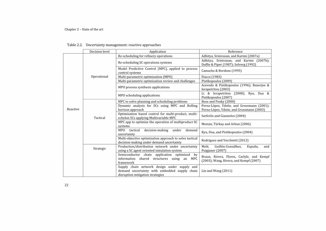
Chapter 2 – State of the art
22
Table 2.2. Uncertainty management: reactive approaches
Decision level Application Reference
Reactive
Operational
Re‐scheduling for refinery operations Adhitya, Srinivasan, and Karimi (2007a)
Re‐scheduling SC operations systems Adhitya, Srinivasan, and Karimi (2007b); Duffie & Piper (1987); Solverg (1992)
Model Predictive Control (MPC), applied to process control systems
Camacho & Bordons (1995)
Multi‐parametric optimization (MPO) Fiacco (1983)Multi‐parametric optimization review and challenges Pistikopoulos (2009)
MPO process synthesis applications Acevedo & Pistikopoulos (1996); Banerjee & Ierapetritou (2003)
MPO scheduling applications Li & Ierapetritou (2008); Ryu, Dua & Pistikopoulos (2007)
Tactical
MPC to solve planning and scheduling problems Bose and Penky (2000) Dynamic analysis for SCs using MPC and Rolling horizon approach
Perea‐López, Ydstie, and Grossmann (2001); Perea‐López, Ydstie, and Grossmann (2003)
Optimization based control for multi‐product, multi‐echelon SCs applying Multivariable MPC
Sarferlis and Giannelos (2004)
MPC app to optimize the operation of multiproduct SC systems
Mestan, Türkay and Arkun (2006)
MPO tactical decision‐making under demand uncertainty
Ryu, Dua, and Pistikopoulos (2004)
Multi‐objective optimization approach to solve tactical decision‐making under demand uncertainty
Rodriguez and Vecchietti (2012)
Strategic Production/distribution network under uncertainty using a SC agent oriented simulation system
Melé, Guillén‐Gonsálbez, Espuña, and Puigjaner (2007)
Semiconductor chain application optimized by information shared structures using an MPC framework
Braun, Rivera, Flores, Carlyle, and Kempf (2003); Wang, Rivera, and Kempf (2007)
Supply chain network design under supply and demand uncertainty with embedded supply chain disruption mitigation strategies
Lin and Wang (2011)
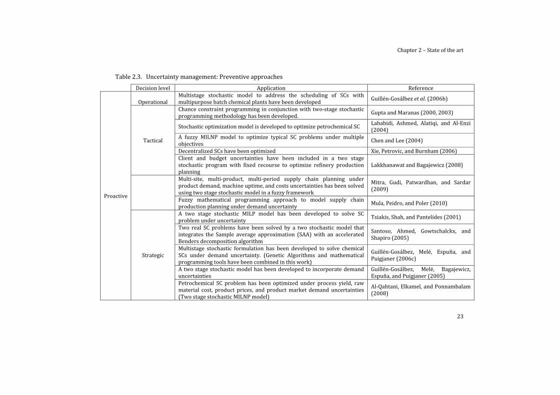
Chapter 2 – State of the art
23
Table 2.3. Uncertainty management: Preventive approaches
Decision level Application Reference
Proactive
Operational Multistage stochastic model to address the scheduling of SCs with multipurpose batch chemical plants have been developed Guillén‐Gosálbez et al. (2006b)
Tactical
Chance constraint programming in conjunction with two‐stage stochastic programming methodology has been developed. Gupta and Maranas (2000, 2003)
Stochastic optimization model is developed to optimize petrochemical SC Lababidi, Ashmed, Alatiqi, and Al‐Enzi (2004)
A fuzzy MILNP model to optimize typical SC problems under multiple objectives
Chen and Lee (2004)
Decentralized SCs have been optimized Xie, Petrovic, and Burnham (2006) Client and budget uncertainties have been included in a two stage stochastic program with fixed recourse to optimize refinery production planning
Lakkhanawat and Bagajewicz (2008)
Multi‐site, multi‐product, multi‐period supply chain planning under product demand, machine uptime, and costs uncertainties has been solved using two stage stochastic model in a fuzzy framework
Mitra, Gudi, Patwardhan, and Sardar (2009)
Fuzzy mathematical programming approach to model supply chain production planning under demand uncertainty Mula, Peidro, and Poler (2010)
Strategic
A two stage stochastic MILP model has been developed to solve SC problem under uncertainty Tsiakis, Shah, and Pantelides (2001)
Two real SC problems have been solved by a two stochastic model that integrates the Sample average approximation (SAA) with an accelerated Benders decomposition algorithm
Santoso, Ahmed, Gowtschalckx, and Shapiro (2005)
Multistage stochastic formulation has been developed to solve chemical SCs under demand uncertainty. (Genetic Algorithms and mathematical programming tools have been combined in this work)
Guillén‐Gosálbez, Melé, Espuña, and Puigjaner (2006c)
A two stage stochastic model has been developed to incorporate demand uncertainties
Guillén‐Gosálbez, Melé, Bagajewicz, Espuña, and Puigjaner (2005)
Petrochemical SC problem has been optimized under process yield, raw material cost, product prices, and product market demand uncertainties (Two stage stochastic MILNP model)
Al‐Qahtani, Elkamel, and Ponnambalam (2008)

Chapter 2 – State of the art
24
Two stage stochastic approach to design SC with financial decisions and risk management
Nickel, Saldanha‐da‐Gama, Ziegler (2012)
Maximize the NPV under demand uncertainty, considering chance constraint approach with safety stocks. You and Grossmann (2008)
Discrete event‐driven model approach is proposed to solve sequential decision‐making problems under uncertainty
Melé et al., (2005, 2006a,b); Puigjaner & Espuña (2006)
Two stage model solved through a heuristic approach for SC design of new market selection under uncertain demand Pan and Nagi (2010)
Chapter 2 – State of the art
25
2.5.3. Cooperative and non cooperative SC’s
Cooperation and competition among SC’s correspond to a complex scenario of a fairy separation of the market. Decision makers need to develop new tools to manage the competition and cooperation.
In this Thesis this complex scenario is specifically addressed by the Game Theory (GT). GT can be used as a new decision‐making tool to analyze the eventual cooperation/competition analyzing the success of some decision among other alternatives. It has been widely proposed by researchers and practitioners the use of this approach to develop systematic procedures to assist decision makers (Mahesh and Greys, 2006).
The different concepts describing the GT and its application to solve industrial decision‐making problems can be easily found in the literature. It is worth to mention here that one of the first steps is to characterize the scenario where the GT is applied starting with the identification of two opposite types of game: the cooperative game and the non‐cooperative game. In fact, the industrial practice is not as simple as the elements of both types of game can be specifically found in situations like the ones described in the previous paragraphs. This and many other practical problems cause nowadays, only some aspects of this theory have been successfully applied to SC Management (SCM). It is easy to find applications related to non‐cooperative games and non‐zero sum while the use of cooperative games, dynamic or asymmetric games for decision‐making has not been exploited yet (Cachon and Netessine, 2004).
In this sense, GT has not been extensively used to analyze the behavior between different SCs yet, and only some works can be found which address very specific situations: Leng and Parlar (2010) use Nash and Stackelberg Equilibriums to determine production levels playing different scenarios to fix the price between seller and buyer; this kind of game has been also successfully used by other authors (Cachon and Zipkin, 1999; Granot and Yin, 2008; Leng and Zhu, 2009; Wang, 2006), each one using different techniques from the GT.
There are many useful concepts/policies related to decision‐making optimization in cooperative/competitive games which can be applied to SCM, but obviously this work does not intend to review all of them. Specifically, the objective of this Thesis is to set the basis of a SC planning support system capable to explicitly consider the presence of other SCs, reducing the uncertainty usually incorporated to the demand forecasting model used for decision‐making. Then, the focus of the analysis of cooperative games in this work is related to the targeting of the overall profit which can be reached through the cooperation among several SCs, while each SC makes decisions to maintain its production, storage and distribution capacity. On the contrary, in the case of non‐cooperative games, the main objective is the identification of the way to adapt the market share to get the maximum benefits from the specific working scenario.
Other topics to be analyzed through the use of the GT may include negotiation, profit sharing and alliance formations. For example, Greene (2002)
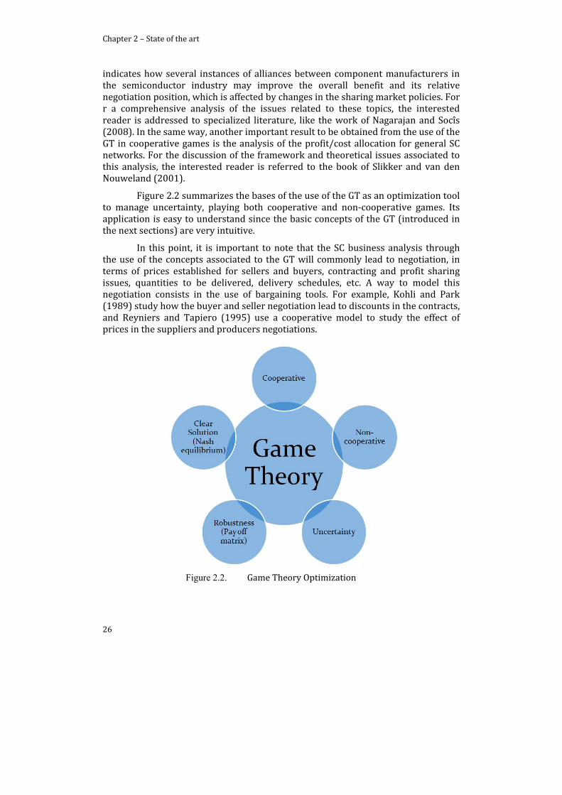
Chapter 2 – State of the art
26
indicates how several instances of alliances between component manufacturers in the semiconductor industry may improve the overall benefit and its relative negotiation position, which is affected by changes in the sharing market policies. For r a comprehensive analysis of the issues related to these topics, the interested reader is addressed to specialized literature, like the work of Nagarajan and Socîs (2008). In the same way, another important result to be obtained from the use of the GT in cooperative games is the analysis of the profit/cost allocation for general SC networks. For the discussion of the framework and theoretical issues associated to this analysis, the interested reader is referred to the book of Slikker and van den Nouweland (2001).
Figure 2.2 summarizes the bases of the use of the GT as an optimization tool to manage uncertainty, playing both cooperative and non‐cooperative games. Its application is easy to understand since the basic concepts of the GT (introduced in the next sections) are very intuitive.
In this point, it is important to note that the SC business analysis through the use of the concepts associated to the GT will commonly lead to negotiation, in terms of prices established for sellers and buyers, contracting and profit sharing issues, quantities to be delivered, delivery schedules, etc. A way to model this negotiation consists in the use of bargaining tools. For example, Kohli and Park (1989) study how the buyer and seller negotiation lead to discounts in the contracts, and Reyniers and Tapiero (1995) use a cooperative model to study the effect of prices in the suppliers and producers negotiations.
Figure 2.2. Game Theory Optimization
Chapter 2 – State of the art
27
As previously mentioned, Part III involves the use of robust tools to improve decision‐making (MILP‐GT optimization). Chapter 9 presents a Bargaining tool to enforce cooperation and competition using a MOO approach.
2.5.4. Multiobjective analysis
Given the corporate structure and the market globalization in recent years, industries need become more competitive trying to obtain more benefits, reduce looses, improve services and products quality, etc. However, it is also necessary to be environmentally friendly and reduce the harmful aspects to the environment, such as: reduce emissions and discharges of waste, increase the reuse of natural resources, recycle, etc. So it is necessary to consider the tradeoff of the multiple objectives to improve the decision‐making (Bojarski et al., 2009; Guillén‐Gonsálbez and Grossmann, 2010).
Approaches used to solve SCM decision‐making problems, generally have two limitations. (i) Most of the approaches developed in SCM are MILP and are solved under one single optimization criterion. Consequently, the tactical management problem is formulated to minimize a single objective problem (SOO). The main criterion usually consists in minimizing the total cost of the SC. However, the problem formulation could include multiple targets. Accordingly, the tradeoff among multiple objectives must be considered by the decision makers/planer designers. (ii) The complexity associated to the system under study, in most of the approaches such complexity is reduced by techniques or simplifications (such as: linearization, general assumptions, fixed parameters for changing processes, etc.). As it is shown in previous Chapters, the competitive behavior affects the decision‐making of the SC of interest, but, the presence of these competitors has been weakly considered.
Manage multiple objectives represent one of the most critical problem in SCM, typically enterprises have different departments taking their own decisions, and in most of the cases they are contradictories (i.e., marketing and manufacturing departments have different goals and policies). This issue is exacerbated when uncertainty is considered. The use of Multi‐Objective Optimization (MOO) techniques become essential in order to improve the decision‐making looking for the tradeoff among different objectives. The solution obtained provides greater degree of accuracy to the decision maker, but, these methods cannot offer a single final decision. Innovative approaches can help to decision makers to choose the best solution in these kinds of complex problems.
The MOO optimization has been successfully applied in several SC industrial problems, such as chemical (Rodera et al., 2002), pharmaceutical (Nicolotti et al., 2011), petrochemical (Zhong and You, 2011), or automotive industries (Cook et al., 2007). Also, there are several methods/strategies, like Meta‐heuristic procedures, mathematical frameworks, and constrained methods, to manage the MOO problems. MOO approaches solving typical SCM issues can be devised. Integrated Management: Li et al. (2012) solved a multi‐objective integrated planning and

Chapter 2 – State of the art
28
scheduling approach. A hybrid algorithm has been developed and applied to manufacturing systems. Fahiminia et al. (2009) optimized the aggregated production planning and the distribution planning of a two echelon supply chain network using MOO. Farahani and Elahipanah (2008) proposed a genetic algorithm to optimize total cost and service level for a supply chain network, modeling a just in time (JIT) decision‐making model. Messac et al. (2003) enlisted the most effective methods to generate the Pareto solutions (see, section 3.7). According to the current literature, none of the previous models have considered a detailed production and inventory planning, integrated with the detailed distribution network of multiple SCs under cooperation/competition. These characteristics contribute to the model to be adapted to a competitive market scenario.

29
Chapter 3. Methods and Tools
A. Ravindran et al. (2006) define the optimization procedure as the “body of mathematical results and numerical methods for finding and identifying the best candidate from a collection of alternatives without having to explicitly enumerate and evaluate all possible alternatives. The power of optimization methods to determine the best case without actually testing all possible cases comes through the use of a modest level of mathematics and at the cost of performing iterative numerical calculations using logical procedures or algorithms implemented on computing machines”
The basic steps to construct an optimization problem, the main mathematical methods and tools used to solve the proposed models in this Thesis have been described in this Chapter. Basic introduction to stochastic optimization, Game Theory, and multi‐objective (MOO) optimization tools have been also included.
3.1. System definition
A few steps to apply the mathematical results and numerical techniques of optimization theory to concrete engineering problems have been defined:
to define the quantitative criterion on the basis of which candidates will be ranked to determine the ‘‘best’’
it is necessary to clearly delineate the boundaries of the engineering system to be optimized,
to select the system variables that will be used to characterize or identify candidates,
and to define a model that will express the manner in which the variables are related.
This composite activity constitutes the process of formulating the engineering optimization problem. Good problem formulation is the key to the success of an optimization study and is to a large degree an art. It is learned through practice and the study of successful applications and is based on the knowledge of the strengths, weaknesses, and peculiarities of the techniques provided by optimization theory.

Chapter 3 – Methods and Tools
30
3.2. Mathematical Programming
Mathematical programming corresponds to the branch of mathematics dealing with techniques and methods for optimizing the performance of a given system.
A general representation of a mathematical programming model can be written as:
0
0
, ,
, :
(3.1)
Its main components are:
Objective Function. It is a quantitative measure of the performance the given system (i.e., f).
Decision Variables. These are the unknowns’ variables, which values are to be determined such that the objective function is optimized (i.e., x).
Constraints. These are any restriction which the decision variables must satisfy (i.e., h g).
Modeling is related on the correct identification of these components. Depending on the properties related to the functions f, h, g, and sets of X, the model is called:
Linear If the set X is continuous and the functions f, h, g are linear. Nonlinear if the set X is continuous and at least one of the functions represent nonlinear behavior/performance. Mixed integer linear If the set of X must correspond to integer values; and if the functions f, h, and g are linear. Mixed integer nonlinear If the set of X requires at least one of the variables x to take integer values only; and at least some of the functions f, h, and g is nonlinear.
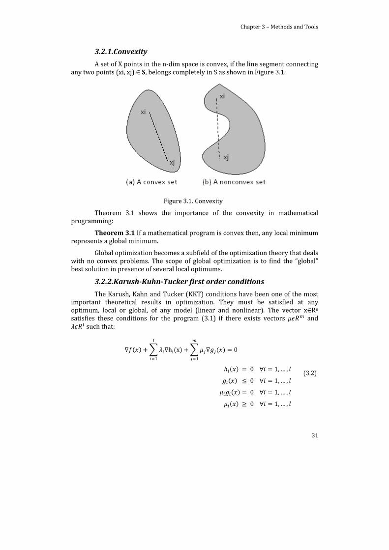
Chapter 3 – Methods and Tools
31
3.2.1. Convexity
A set of X points in the n‐dim space is convex, if the line segment connecting any two points (xi, xj) S, belongs completely in S as shown in Figure 3.1.
Figure 3.1. Convexity
Theorem 3.1 shows the importance of the convexity in mathematical programming:
Theorem 3.1 If a mathematical program is convex then, any local minimum represents a global minimum.
Global optimization becomes a subfield of the optimization theory that deals with no convex problems. The scope of global optimization is to find the “global” best solution in presence of several local optimums.
3.2.2. KarushKuhnTucker first order conditions
The Karush, Kahn and Tucker (KKT) conditions have been one of the most important theoretical results in optimization. They must be satisfied at any optimum, local or global, of any model (linear and nonlinear). The vector x Rn satisfies these conditions for the program (3.1) if there exists vectors and
such that:
h x 0
0 1, … ,
0 1, … ,
0 1, … ,
0 1, … ,
(3.2)
Chapter 3 – Methods and Tools
32
The vectors and are called Lagrangian multipliers. If the Lagrangian function is defined by:
, , (3.3)
The KKT conditions can be rewritten as:
, , 0
, , 0
, , 0
µT µ , , 0
0 (3.4)
3.2.3. Duality
The term duality is often used to invoke a contrast between two related concepts. Duality is one of the most fundamental concepts in mathematical programming and establishes a connection between two symmetric programs, namely the primal and dual problem.
First of all, the dual function is introduced as:
, (3.5)
Hence, the dual problem of the primal problem (3.1) is defined as follows:
0 (3.6)
Then using the Lagrangian function, the dual problem can be rewritten as:
maximize ,µ;µ L x, λ, µ (3.7)
The Theorem 3.2 establishes an important relationship between the dual and primal problems.
Theorem 3.2 Weak duality For any feasible solution x of the primal problem (3.1) and for any feasible solution , , of the dual problem (3.8), the following holds
, (3.8)
Additionally, the Theorem 3.3 is of relevant importance in mathematical programming. It shows that for convex programs the primal problem solution can be obtained by solving the dual problem.
Chapter 3 – Methods and Tools
33
Theorem 3.3 If the primal problem is convex, then . Otherwise, one or both of the two sets of feasible solutions is empty.
Here, x* represents the optimal solution of the primal problem; and are the optimal solutions of the dual problem.
For nonconvex programs, the difference between the optimal objective function values of the dual and primal problems is called duality gap.
3.3. Linear Programming
In this type of problems the most important part, is that all the functions involved (objective function, all the constraints) must be linear. The feasible region of the problem corresponds to the intersection of the hyperplanes and halfspaces of the constraints. This is a basic characteristic of a convex polytope.
Theorem 3.4 If an LP has an optimal solution; there is a vertex of the feasible polytope that is optimal.
This Theorem is fundamental in linear programming and is the basis of algorithms proposed for solving linear programming programs: the Simplex and interior point methods.
3.3.1. The Simplex Method
This is the most used algorithm for solving LP problems. It starts with an initial vertex of the feasible region, tests the optimality. If some optimality condition is verified, then the algorithm terminates. Otherwise, the algorithm identifies an adjacent vertex with a better objective value, and checks the optimality of the new point, and the entire scheme is repeated until the optimal solution is encountered.
George B. Dantzig was a mathematical advisor of the US Air Force, who was the Simplex method inventor at 1947, and the first using the linear programming term (Gill et al., 2008).
3.3.2. Interior point methods
An interior‐point algorithm is one that improves a feasible interior solution point of the linear program by steps through the interior feasible region. A theoretical breakthrough for interior point methods came in 1979; the Russian mathematician L.G. Khachian discovered an ellipsoid algorithm whose running time in its worst case was significantly lower than that of the Simplex Algorithm. Other theoretical results quickly followed, notably that of N. Karmarkar who discovered an interior‐point algorithm whose running time performance in its worst case was significantly lower than that of Kachiyan’s (Dantzig & Thapa, 1997). While the Simplex method looks at the vertex of the problem, the interior point methods assume an initial feasible interior point and moves through the feasible region moving in one direction. The stopping rule typically followed is to finish with an approximate optimal solution when the difference between iterates is sufficiently small in the original space.
Chapter 3 – Methods and Tools
34
3.4. Nonlinear Programming
As previously defined, the nonlinear model corresponds to the model which, all the variables are continuous and contains any nonlinearity in the objective function and/or the constraints. The unconstrained and constrained optimization algorithms have been developed to solve this kind of programs.
3.4.1. Unconstrained optimization
Unconstrained optimization algorithms can be divided into two groups: line search methods and trust region methods. They basically determine a direction (pk), and the distance or step length (αk) to move towards an improved solution. In both type of methods an initial feasible solution (x0) of the problem is needed.
Line search methods. This algorithms firstly chooses the direction and then search along this direction for an adequate step length, so that one moves from the current iterate (xk) for a new iterate (xk+1) with a better value in the objective function. The steepestdecent direction, Newton direction, and QuasiNewton search direction are the most important methods to obtain the search direction.
The step length should be chosen such that a sufficient improvement is assured and the length is not too short. For this purpose, a good step length must satisfy the so called Wolfe conditions. There are several methods to determine the step length; among them the interpolation method, the golden section method and the Fibonacci method.
Another very important algorithm in this optimization type of problems is the conjugate gradient method. Its principal idea is to improve convergence through the construction of search directions by using the conjugate (A‐orthogonal) of the steepest decent direction.
3.4.2. Constrained optimization
Methods to solve constrained programs are addressed. This kind of methods seeks an approximate solution by replacing the original constrained problem by a sequence of unconstrained sub‐problems. Hence, the underlying idea is to construct a closely related, unconstrained problem and apply the algorithms proposed for the unconstrained optimization problems. Two types of methods can be encountered: those ones which do not attain Lagrange multipliers information and those methods based on the KKT conditions.
3.5. Mixed Integer programming
The use of binary variables turns out from a variety of purposes as modeling on/off decisions, enforcing logical conditions, modeling fixed costs of pricewise linear functions. Additionally, integer variables appear when modeling some industrial cases (products, entities, etc.). Most of the models associated to SCM decision‐making process could include Discrete variables (integer and binary), due to the decisions involved in such problems. As previously stated, mathematical

Chapter 3 – Methods and Tools
35
programs which some of this type of variables are called mixed integer programs. Basically, there are two algorithms for solving this type of programs, the Branch and Bound (BB) and the cutting planes methods.
3.5.1. Branch and Bound methods
This algorithm consists in generating a sequence of continuous sub‐problems, solving them, and analyzing and comparing the different solutions until the optimal solution is reached. The algorithm searches the complete space of solutions. The use of bounds for the function to be optimized combined with the value of the current best solution enables the algorithm to implicitly search parts of the solution space.
The solution of a problem with a BB algorithm is traditionally described as a search through a tree, in which the root node corresponds to the relaxed original problem (solving the original problem as a LP program). Then, given a node Q of the tree, assume that is a variable whose solution is that is not satisfying the integrality constraint in the node Q solution. Then, the two children nodes of Q are disjoint subproblems derived from adding to the Q problem the further constraint in one case, and 1. Here, p is an integer value (p Z) and must
satisfy the next condition:
1 1 1 (3.9)
On the other hand, the bounding procedure consists in disregarding a node when is infeasible or when the objective value is not better than the other children node.
Two questions need to be answered during the branching procedure so as to select the next sub‐problem, namely, What node Q should be selected for branching?, and What variable not satisfying integrality in Q should be chosen for branching? Several strategies have been proposed for these purposes, but they are out of the scope of this Chapter.
3.5.2. Cutting plane methods
There is an alternative to BB method called cutting planes which can be used to solve mixed integer programs. The main idea behind cutting planes is to add constraints to a program until the optimal solution satisfies integrality constraints. Of course, a cut or constraint to be added to a current fractional solution must assure that, every feasible integer solution of the actual program is feasible for the cut; and that the current fractional solution is not feasible for the cut.
Some techniques to generate these cuts are the Gomorys cut methods, the Kelleys method, and the Kelley, Cheney, Goldstein method.
Both (BB and cutting plane techniques) can be applied to linear and nonlinear programs. A special methodology for mixed integer nonlinear programs is the outer approximation algorithm developed by Duran and Grossmann (1986). Also, is noteworthy to mention a special set of integer programs called disjunctive
Chapter 3 – Methods and Tools
36
programs. The theory of disjunctive programming can be found in the work of Raman and Grossmann (1994) and Lee and Grossmann (2000). In a nutshell, disjunctive programs comprised a logical system of conjunctive and disjunctive statements, where each statement is defined by a constraint.
3.6. MultiObjective Optimization (MOO)
Multi‐objective optimization (MOO) plays an important role in engineering design, management, and decision‐making in general. Usually, a decision maker needs to make tradeoffs between disparate and conflicting objectives. The field of MOO defines the art and science of making such decisions.
The general mathematical representation of an MOO problem is as follows:
, , … , 2
0
0
, ,
, :
(3.10)
The solution of an MOO problem is said to be a set of Pareto solutions, or Pareto frontier. A Pareto solution is one for which any improvement on the objective can only takes place if at least one other objective worsens (Messac, Ismail‐Yahaya, and Mattson, 2003).
Dominance, this concept formally defines the Pareto solution. A solution xa, associated to the objective function values { , , … , } dominates other solution xb, with its corresponding point { , , … , }, if and only if
1… 1… / (3.11)
Where: 1… and 1… .
From here forth, Zp is a scalar that shall be associated to the objective function value fp(x).
Thereby, if a solution x* is Pareto solution then it does not exist a different solution x X that dominates it.
There are several approaches to obtain Pareto solutions (physical programming method (PP), normal boundary intersection method (NBI), ‐constraint method ( ‐C) normal constraint method (NC), weighted sum method (WS) and the compromise programming method (CP)). They are based on the conversion of the MOO problem into one single objective problem; solving it several
Chapter 3 – Methods and Tools
37
times at the same time that each solution represents one feasible point; all the solutions represent the Pareto frontier. The next section is focused on the ‐constraint method which is the one used in this Thesis.
3.6.1. The constraint method
This method approximates the Pareto frontier by finding a set of Pareto solutions that belong to it. Each single Pareto solution is found by solving one single objective problem; the single objective problem includes the bounds of the remaining objective function which are computed but not being directly optimized. The detailed description follows a similar procedure by the one presented by Messac et al. (2003). In this case the normalization steps are not considered. In order to explain the method the p‐anchor points and utopia point must be described.
The utopia point is defined as comprised by every single optimized objective function Zp value. Clearly, this ideal point is an imaginary solution for conflicting objectives; such solution corresponds to a non feasible solution. The utopia point can be found by solving P times the program (3.14).
0
0
, ,
, :
1… (3.12)
The p‐anchor points , , … , are non‐dominated points, an extreme Pareto solution, resulting for the optimal resolution of the single objective problem (3.14) P times.
Then, the procedure is to find the non‐extreme Pareto solutions so as to approximate the Pareto frontier. Step 1: define the numbers of N Pareto solutions, and solve the problem 3.16 for all the np (n1, n2, …, N) points.
0
0
1…
, , … ,
(3.13)
Chapter 3 – Methods and Tools
38
, ,
, :
This method is applied in Chapter 9 in order to track the tradeoff among two different objectives. Fig. 3.2 shows the representation of the model above described.
3.7. Stochastic programming with recourse
All previously discussed optimization problems are considered deterministic, due all of the information used in such problems have been assumed to be perfectly known. In stochastic programming programs, models in which some data may be considered uncertain are addressed. In this type of problems, it is relevant to distinguish among two set of decisions variables (main and secondary variables):
First stage decisions. These sets of decisions must be taken before any uncertain parameter is unveiled. They are also known as “here and now” decisions. The interval of time associated with them is known as the first stage of the stochastic program.
Second stage decisions. Are determined after some or all the uncertain data is reveled. These kinds of decisions are also known as the Recourse and so forth stage or “wait and see” decisions.
Two stage programs represents the most widely used and simplest stochastic program. At this point, the first stage decisions are represented by the vector x, while second stage decisions by the vector y. The uncertain parameter is represented by the vector ξ. It is important to mention that, the second stage decisions y are a function the first stage decisions x, and the uncertain events. In order to simplify the problem representation, the recourse function Q is introduced next.
, , ξ
, , ξ 0
, , ξ 0
, ,
, :
(3.14)
All the equations involving recourse decisions y are considered in Q. As it can be seen, Q is a mathematical program that minimizes the second‐stage “cost” for a given value of the uncertain parameter . Then, the expected recourse function Q, is defined by the expression (Eq. 3.15).
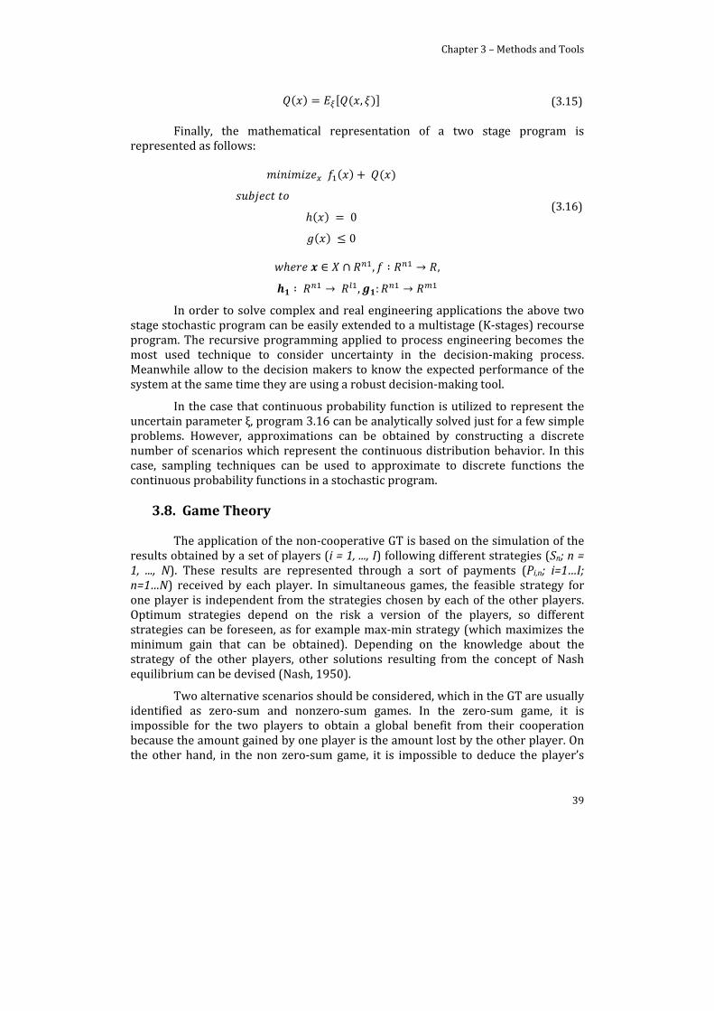
Chapter 3 – Methods and Tools
39
, (3.15)
Finally, the mathematical representation of a two stage program is represented as follows:
0
0
(3.16)
, ,
, :
In order to solve complex and real engineering applications the above two stage stochastic program can be easily extended to a multistage (K‐stages) recourse program. The recursive programming applied to process engineering becomes the most used technique to consider uncertainty in the decision‐making process. Meanwhile allow to the decision makers to know the expected performance of the system at the same time they are using a robust decision‐making tool.
In the case that continuous probability function is utilized to represent the uncertain parameter ξ, program 3.16 can be analytically solved just for a few simple problems. However, approximations can be obtained by constructing a discrete number of scenarios which represent the continuous distribution behavior. In this case, sampling techniques can be used to approximate to discrete functions the continuous probability functions in a stochastic program.
3.8. Game Theory
The application of the non‐cooperative GT is based on the simulation of the results obtained by a set of players (i = 1, ..., I) following different strategies (Sn; n = 1, ..., N). These results are represented through a sort of payments (Pi,n; i=1…I; n=1…N) received by each player. In simultaneous games, the feasible strategy for one player is independent from the strategies chosen by each of the other players. Optimum strategies depend on the risk a version of the players, so different strategies can be foreseen, as for example max‐min strategy (which maximizes the minimum gain that can be obtained). Depending on the knowledge about the strategy of the other players, other solutions resulting from the concept of Nash equilibrium can be devised (Nash, 1950).
Two alternative scenarios should be considered, which in the GT are usually identified as zero‐sum and nonzero‐sum games. In the zero‐sum game, it is impossible for the two players to obtain a global benefit from their cooperation because the amount gained by one player is the amount lost by the other player. On the other hand, in the non zero‐sum game, it is impossible to deduce the player’s
Chapter 3 – Methods and Tools
40
payoff from the payoff of the others; the nonlinearities of the problem also arise in this second kind of games.
The problems proposed in Part III can be classified as a non zero‐sum game. This characteristic and the fact that the SC of interest tries to maximize its own benefit disregarding the overall benefit of the system, lead to an optimization procedure based on the computation of a payoff matrix. Such matrix is made up by the assessment of different potential strategies of multiple players (supply chains), and it shows the behavior for each action of the SC against the actions of its competitors. If the computation of this payoff matrix ensures that it is composed by the different Nash Equilibrium points, as previously defined, the problem solution will be reduced to find the optimum performance resulting from this payoff matrix.
Illustrative example: the payoff matrix (Table 3.1) summarizes the benefits for two players (SC1 and SC2) considering 2 strategies (s1 and s2):
Table 3.1. Payoff matrix (illustrative example, $)
SC2
SC1
s1 s2Benefit SC1
Benefit SC2
Benefit SC1
Benefit SC2
s1 110 90 120 80s2 120 100 140 60
The Nash equilibrium of SC1 corresponds to: the scenario 2 of SC1 and scenario 2 of SC2, since the benefit of SC1 is 140$, and the Nash equilibrium of SC2 corresponds to: the scenario 2 of SC1 and scenario 1 of SC2, since the benefit of SC2 is 100$.
In this way, the framework developed in Thesis integrates multiple SC’s interacting (cooperating and/or competing) for the global market demand. Detailed information of it application can be encountered in Chapter 7.
3.9. Software
There are some commercial tools for general optimization purposes such as General Algebraic Modeling System (GAMS), A Modeling Language for Mathematical Programming (AMPL, Fourer et al. 2002). All of them render very similar characteristics (general mathematical language, use different solvers to solve the modeled problems, etc). Optimization problems in this Thesis have been solved using GAMS, given that the research group CEPIMA is familiar with this tool. Additionally, GAMS is the most used optimization software in PSE field.

Chapter 3 – Methods and Tools
41
3.9.1. General Algebraic Modeling System (GAMS)
GAMS is a programming language that allows modeling and solving optimization problems (Rosenthal, 2012). Castillo et al. (2001) point out some important characteristics, such as: (i) Modeling and solving procedure are completely separated. Once the model is developed; several solvers are available to optimize the problem. (ii) The model representation in GAMS is analogous to the mathematical description of the problem. (iii) MATLAB and GAMS could be easily connected through Matgams (Ferris, 2005). It is worth mention, optimization algorithms mentioned above are embedded in some of the different GAMS solvers. Each solver is usually developed to tackle a specific type of program (i.e., LP, NLP, MILP, MINLP, etc.).
3.10. Summary
Finally, general description of the main optimization techniques has been presented in this Chapter. The purpose to present these techniques is that all of them have been used through the Thesis. Chapters 3 – 6 face LP and MILP programs. Chapter 7 presents a cooperative and competitive approach using Game Theory optimization, where a MILP model has been solved several times. Solutions reported in Chapter 7 have been compared with the solutions obtained in by the two stage stochastic programming model presented in Chapter 9. Chapter 10 develops a bargaining tool by integrating Game Theory and Multi‐objective optimization.

Part II Enhancing Plant and SC Competitiveness

45
Summary
Part II has been developed to enhance the competitiveness of the single supply chain (enterprise) disregarding the consideration of other SCs. This part is mainly focused on the integration of decision‐making levels.
This part is composed by three Chapters; Chapter 4 improves the decision‐making process exploiting Plant and process flexibility. Otherwise, Chapter 5 and 6 are focused on the integrated decision‐making of the typical SC.
Chapter 4 presents two novel approaches for integrated management. Section 4.1 shows the integration among synthesis and scheduling decision‐making process. This work solves the typical scheduling problem considering multiple equipments to be installed (synthesis problem), the analysis of multiple scenarios allows selecting the “best” plant superstructure for the goals considered. Section 4.2 shows the integration of scheduling problem and the control layer in simplified cases though an example applied to an energy generation network case study.
Chapter 5 presents a novel MINLP formulation for the integration of the planning task and the scheduling decision‐making problem.
Part II ends with the consideration of others SC’s into the model formulation, Chapter 6 includes the information of several SC’s acting as one entire SC. In this case all the SC considered corresponds to the echelons of the main SC. At this point the inclusion of others SCs is presented in order to coordinate their decision‐making process, and the cooperation and competition of those SCs must be studied in the Part III of this Thesis.

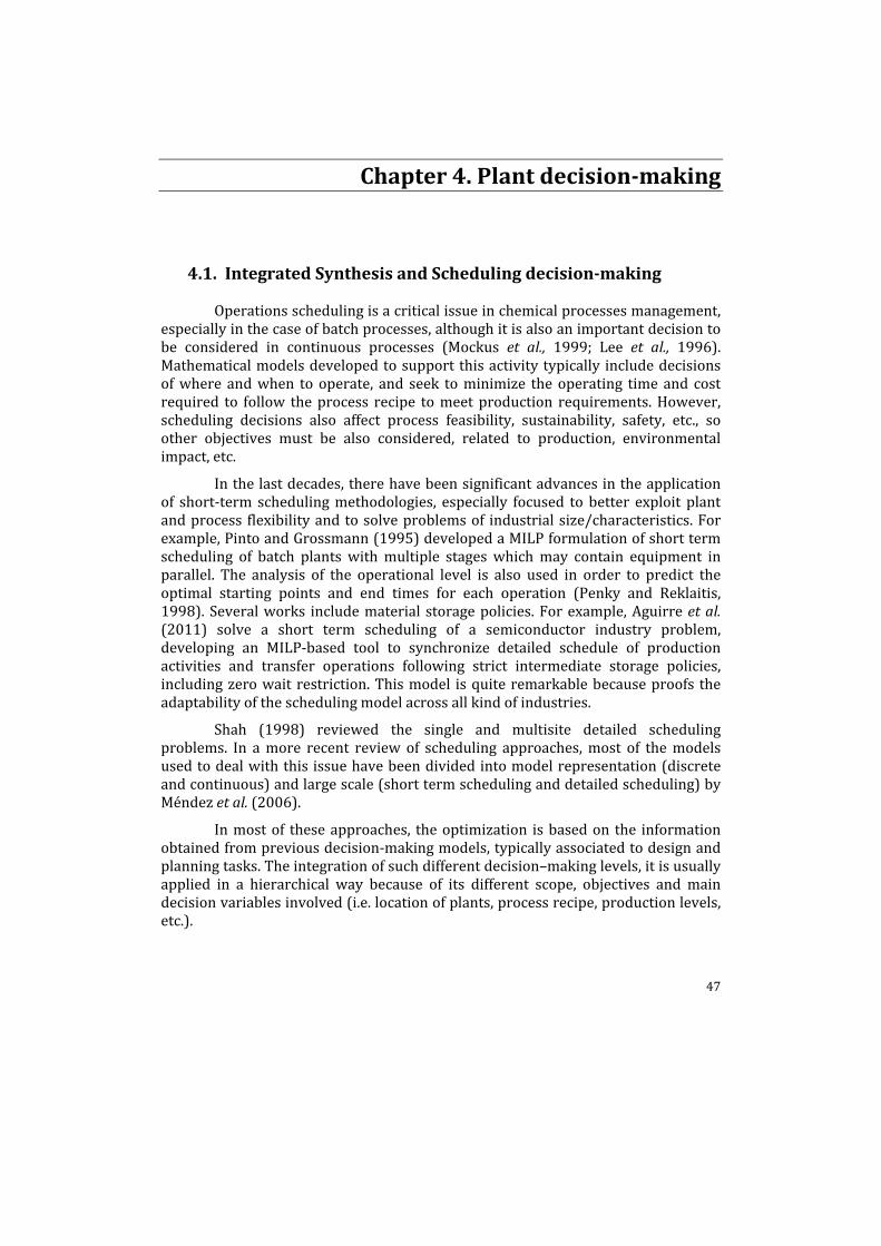
47
Chapter 4. Plant decisionmaking
4.1. Integrated Synthesis and Scheduling decisionmaking
Operations scheduling is a critical issue in chemical processes management, especially in the case of batch processes, although it is also an important decision to be considered in continuous processes (Mockus et al., 1999; Lee et al., 1996). Mathematical models developed to support this activity typically include decisions of where and when to operate, and seek to minimize the operating time and cost required to follow the process recipe to meet production requirements. However, scheduling decisions also affect process feasibility, sustainability, safety, etc., so other objectives must be also considered, related to production, environmental impact, etc.
In the last decades, there have been significant advances in the application of short‐term scheduling methodologies, especially focused to better exploit plant and process flexibility and to solve problems of industrial size/characteristics. For example, Pinto and Grossmann (1995) developed a MILP formulation of short term scheduling of batch plants with multiple stages which may contain equipment in parallel. The analysis of the operational level is also used in order to predict the optimal starting points and end times for each operation (Penky and Reklaitis, 1998). Several works include material storage policies. For example, Aguirre et al. (2011) solve a short term scheduling of a semiconductor industry problem, developing an MILP‐based tool to synchronize detailed schedule of production activities and transfer operations following strict intermediate storage policies, including zero wait restriction. This model is quite remarkable because proofs the adaptability of the scheduling model across all kind of industries.
Shah (1998) reviewed the single and multisite detailed scheduling problems. In a more recent review of scheduling approaches, most of the models used to deal with this issue have been divided into model representation (discrete and continuous) and large scale (short term scheduling and detailed scheduling) by Méndez et al. (2006).
In most of these approaches, the optimization is based on the information obtained from previous decision‐making models, typically associated to design and planning tasks. The integration of such different decision–making levels, it is usually applied in a hierarchical way because of its different scope, objectives and main decision variables involved (i.e. location of plants, process recipe, production levels, etc.).
Chapter 4 – Plant decision making
48
Integrated decision‐making still represents an open issue to be studied: Laínez et al. (2007) presented an important improvement in the integrated decision‐making process, developing an integrated design and planning model. Meanwhile, Kallrath (2002) presented an overview of planning and scheduling models focused on industrial processes, where the opportunity to solve tactical and operational planning problems in one model was described. In the same line, Sung and Maravelias (2007) developed a hybrid planning‐scheduling optimization technique, where the optimal schedule is obtained through an off‐line optimization procedure and then integrated to the planning model as a convex approximation of the production levels. Moreover, Guillén et al. (2005) also developed an integrated planning and scheduling model. Floudas and Lin (2004) present an overview of techniques for scheduling of multiproduct/multipurpose batch and continuous processes, including computational studies focused on the integration of design and synthesis tasks under uncertain scenarios, requiring the application of reactive and stochastic scheduling techniques.
On the other hand, Process synthesis is one of the most challenging problems in Chemical Engineering; its aim is the identification of the best solution within a flowsheet super‐structure. The objective of process synthesis is to obtain the best superstructure or the best flowsheet of the proposed plant, given several alternatives. This kind of problems takes into account different aspects, such as conversion reaction, raw materials, equipment units and generation of sub‐products or contaminants. The decision‐making process involves the consideration of different alternatives in the flow sheet for carrying out the process of transforming raw materials into finished products. Accordingly, the use of process synthesis systematic approaches is essential to identify the most efficient or economic process flowsheets, integrating the solutions of the different sub problems and their corresponding targets (pollution prevention, freshwater consumption, minimization of energy consumption, etc.) and leading to flexible systems capable to be adapted to different working scenarios. Several applications of the process synthesis can be encountered, such as: the synthesis of heat exchanger networks and also to the synthesis of integrated process water networks, developed to determine the interconnection of process and treatment units, the flow rates and contaminants concentration of each stream and to determine the minimum total annual cost of water network, using global NLP or MINLP superstructure optimization models (Foo, 2009). The typical constraints associated are mass balances (splitter, mixer, process units, treatment units, etc) and design constraints. Moreover, synthesis problems are also applied to reaction synthesis, separation synthesis (distillation process), and services synthesis (steams and electricity). This study also concluded that the computation capacity is an important parameter to consider the effectiveness of this issue solved.
Approaches aiming the simultaneous consideration of synthesis and scheduling objectives can be found in the literature but the integration has not been yet exploited as a part of a common decision‐making model. For example, Lin and Floudas (2001) proposed a continuous‐time formulation, where a design, synthesis

Chapter 4 – Plant decision making
49
and scheduling approach of multipurpose batch plants was presented in the context of the decision‐making process within the Supply Chain.
Either for solving the process synthesis problem or the scheduling problem, it is essential to manage sufficient knowledge of the process. In the sense, the available alternatives should be clearly identified in order to solve the problem fulfilling certain objectives. In particular, reaction synthesis problem is important not only to determine raw material necessities, but also because the constraints imposed by this element to the final process configuration to be installed.
Therefore, this Chapter proposes a mixed integer linear programming (MILP) model that integrates the typical synthesis problem with the operational decision‐making problem (Scheduling). This application aims to improve decision‐making support, optimizing the allocation, production and installation/use of several technologies in chemical processes. In this line, section 4.1.2 introduces the Synthesis State Task Network (SSTN) as a way to represent the links among the different elements to be taken into account in this kind of problems. Section 4.3 formally introduces the synthesis and scheduling problems on the basis of such representation. Then, Section 4.4 introduces 3 case studies based on literature examples, and shows the results of the proposed approach. Finally, Section 4.5 summarizes the main conclusions of the Chapter.
4.1.1. Synthesis State Task Network (SSTN)
Process recipe is one of the basic sets of information required to be managed to run a batch (or continuous) process. The representation of such information is usually based on the flowsheet view of the plant, as a basic schema to describe the process itself (units, tasks, etc.). Kondili et al. (1993) defined the state task network (STN) representation in order to organize the information of the process, based on the identification of the process recipe as a set of tasks leading to different states, defining the links among them on the bases of the precedence rules and other recipe information.
Different details can be incorporated to such networks, in order to adapt the resulting information structure to the specific objectives of the analysis to be performed. As a result, this kind of network representation was originally proposed to address the short‐term scheduling problem of multipurpose batch plants. During almost 30 years their capacity to adequately represent the information associated to processes of different degree of complexity in different circumstances has been demonstrated. Additionally, it could be used under different modeling paradigms, as for example discrete time models (Maravelias and Grossmann, 2003a; Sung and Maravelias, 2007) and continuous time models (Schiling and Pantelides, 1996; Zhang and Sargent, 1998; etc.).
Moreover, during the last 20 years, several authors use the state‐task network (STN) representation. Kondili et al. (1993) formulated a mixed integer linear program (MILP) based on a discrete time representation in order to solve short‐term scheduling, taking into account equipment allocation, storage levels, the availability of raw materials, the batch size and production deliveries in order to

Chapter 4 – Plant decision making
50
maximize the profit of the process. In addition, this work proposes a detailed scheduling model in order to optimize multiple products and multiple tasks plants.
Furthermore, several authors use the STN representation for discrete time formulations, such as Maravelias and Grossmann (2006) who developed an algorithm to minimize the makespan of multipurpose batch plants, studying the relationship between discrete and continuous‐time MILP formulation. The STN representation is also used for continuous time formulations in several works. For example, Maravelias and Grossmann (2003b) proposed a continuous‐time MILP model for short‐term scheduling of multipurpose batch plants, including resource constraints, variable batch sizes and processing times, storage policies, batch mixing/splitting and sequence‐dependent changeover times. Moreover, Bose and Bhattacharya (2009) developed a MILP formulation in order to generate an optimal schedule for a sequence of several continuous units for processing products using the STN representation.
In this line, an extended version of the STN is proposed in this Chapter, in order to introduce information about the underlying synthesis problem. In the resulting representation (Synthesis State Task Network ‐ SSTN), the states and task nodes keep performing the same role (representing feed, intermediate and final products, and processing stages as defined by the production recipe, respectively), but states are now connected to Synthesis blocks incorporating the information associated to the synthesis problem: inside these blocks, complementary and/or alternative task nodes are defined. New information has been considered in order to perform the required tasks according to their respective: costs (fixed, operational, installation cost, etc.), process operation (conversion rates, processing time, etc.), etc. Figure 4.1 (a, b, c) summarizes the evolution of such network representations: Compared with Fig. 4.1a (flowsheet‐based network representation, including tasks and flow indications), the STN representation (Figure 4.1b) introduced state nodes representing the feeds, intermediate and final products and task nodes, which represent the processing operations which transform the material (inputs) to one or more output states (state and task nodes are denoted by circles and rectangles, respectively).
The proposed SSTN view (Figure 4.1c) incorporates information about equipment units’ and flexibility to be installed in different configurations in order to take profit of eventual plant/process operation. This Chapter uses the typical consideration of a superstructure of the process. This superstructure is introduced into the scheduling process recipe, then the solution obtained by the model approach consider different equipment options to solve the same operation, the consideration of different equipment units is related with the consideration of different costs (fixed and variable) and conversions.
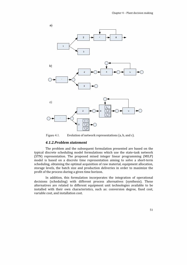
Chapter 4 – Plant decision making
51
Figure 4.1. Evolution of network representations (a, b, and c).
4.1.2. Problem statement
The problem and the subsequent formulation presented are based on the typical discrete scheduling model formulations which use the state‐task network (STN) representation. The proposed mixed integer linear programming (MILP) model is based on a discrete time representation aiming to solve a short‐term scheduling, obtaining the optimal acquisition of raw material, equipment allocation, storage levels, the batch size and production deliveries in order to maximize the profit of the process during a given time horizon.
In addition, this formulation incorporates the integration of operational decisions (scheduling) with different process alternatives (synthesis). These alternatives are related to different equipment unit technologies available to be installed with their own characteristics, such as: conversion degree, fixed cost, variable cost, and installation cost.

Chapter 4 – Plant decision making
52
The main decision variables considered are:
Wijt binary variable, equal to 1 if unit j is being used, and processing task i at time t; 0 otherwise.
Bijt is the amount of material processed according to task i at unit j at time t. Sst represents the amount of material stored at state s in time t. Rmst is the amount of raw material s acquired at time t. yj binary variable, equal to 1 if the equipment technology is installed.
The synthesis decisions are constrained to the use of specific units by their specific task, and then the presence of stock is penalized, obtaining the optimal unit allocation admitting the most efficient schedules in terms of production performance.
4.1.2.1. Mathematical Model
The MILP‐based mathematical model that integrates the scheduling problem and synthesis decisions consists in allocation, equipment capacity and material balance constrains:
Allocation:
The allocation of units across the time horizon is taken into account, considering the different residence time of the tasks in the units (Eq. 4.1), where M is a sufficiently large positive number. In addition, at each period of time t, each equipment unit can only start at most one task (Eq. 4.2).
1 · 1 , , , , (4.1)
1 , , (4.2)
Capacity:
The amount of material processed at unit j at time t is limited by the consideration of maximum and minimum capacity of the equipment units (Eq. 4.3). These capacity limitations include the maximum and minimum storage limits of the states (Eq. 4.4).
· · , , , , (4.3)
0 C , , (4.4)
The model also considers the demand of the products: in the case where the plans are known this demand must be satisfied. In the case where the production capacity is lower than the demand, the demand could not be enhanced (Eq. 4.5). The quantity of material s that corresponds to the final products (FP) at final time period (TF) must be equal or greater (or lower) than the quantity demanded of product s.
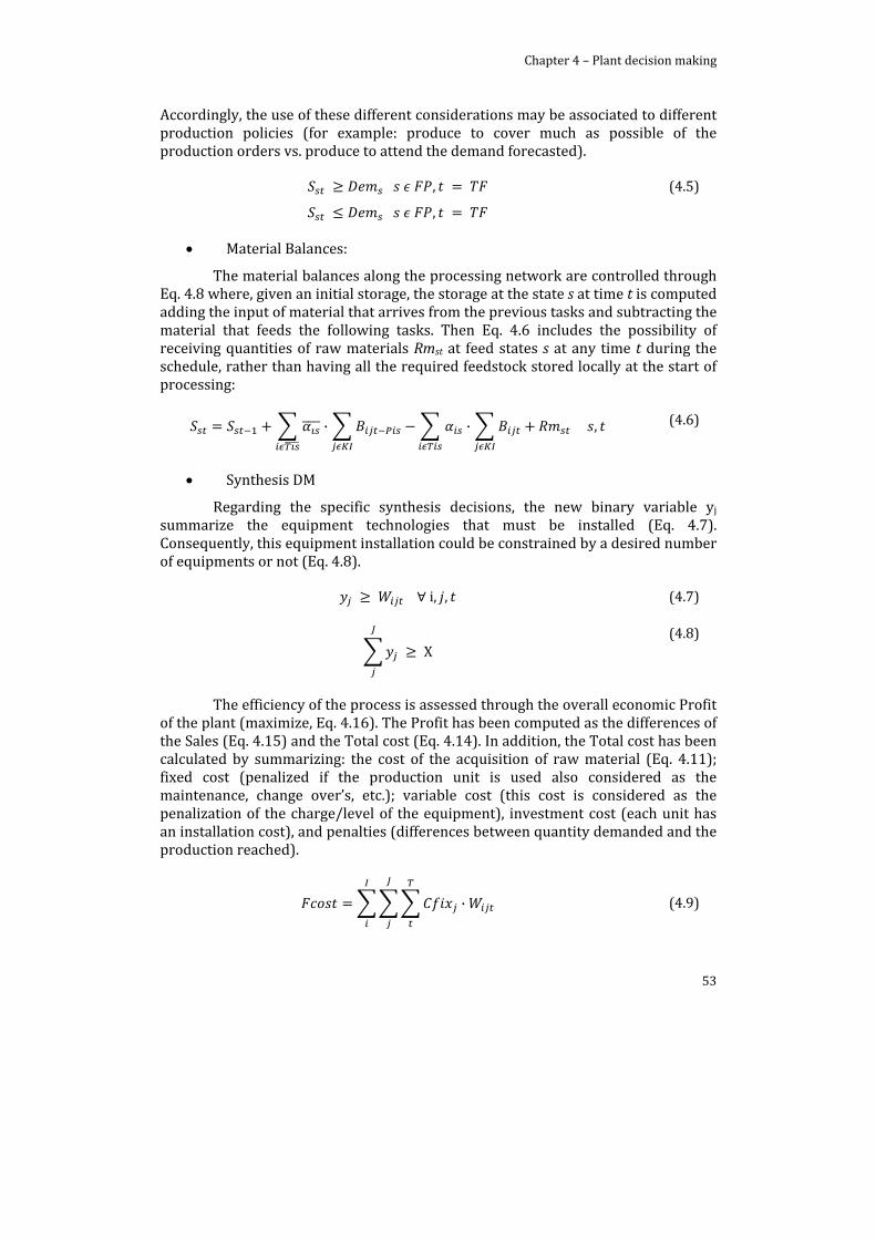
Chapter 4 – Plant decision making
53
Accordingly, the use of these different considerations may be associated to different production policies (for example: produce to cover much as possible of the production orders vs. produce to attend the demand forecasted).
,
,
(4.5)
Material Balances:
The material balances along the processing network are controlled through Eq. 4.8 where, given an initial storage, the storage at the state s at time t is computed adding the input of material that arrives from the previous tasks and subtracting the material that feeds the following tasks. Then Eq. 4.6 includes the possibility of receiving quantities of raw materials Rmst at feed states s at any time t during the schedule, rather than having all the required feedstock stored locally at the start of processing:
· · , (4.6)
Synthesis DM
Regarding the specific synthesis decisions, the new binary variable yj summarize the equipment technologies that must be installed (Eq. 4.7). Consequently, this equipment installation could be constrained by a desired number of equipments or not (Eq. 4.8).
i, , (4.7)
X (4.8)
The efficiency of the process is assessed through the overall economic Profit of the plant (maximize, Eq. 4.16). The Profit has been computed as the differences of the Sales (Eq. 4.15) and the Total cost (Eq. 4.14). In addition, the Total cost has been calculated by summarizing: the cost of the acquisition of raw material (Eq. 4.11); fixed cost (penalized if the production unit is used also considered as the maintenance, change over’s, etc.); variable cost (this cost is considered as the penalization of the charge/level of the equipment), investment cost (each unit has an installation cost), and penalties (differences between quantity demanded and the production reached).
· (4.9)
Chapter 4 – Plant decision making
54
· (4.10)
· (4.11)
· (4.12)
, (4.13)
(4.14)
(4.15)
(4.16)
Regarding the operational decision‐making Equations (4.1‐4.6) represent the typical scheduling model including (batch sequencing and sizing). Otherwise, Equations (4.7‐4.16) have been included to model the synthesis decision‐making, considering the installation or not, raw material, investment, fixed and variable cost, and economical analysis of the optimal superstructure to be used.
The proposed model takes the advantage of the flexibility of the process definition, by considering several alternatives to be installed determining the plant superstructure. Also states that the design decision‐making is very important at the operational level. In addition, the model allows to the decision makers to reformulate the plant and process superstructure, by re‐optimizing the existing plant and/or design the plant. Thus concepts are clarified and highlighted in the case study results.
4.1.3. Case study
Multiple plants scenarios have been analyzed under different operation conditions, in order to prove the flexibility of the proposed approach. The results show how different plans (demands) represent different optimal superstructure/scheduling solution.
The case study (see, Fig. 4.2c) is based on the scheduling example proposed by Kondili et al. (1993), and the synthesis problem presented by Grossmann et al. (1996). The problem to be solved involves 5 tasks (heat, reaction 1, reaction 2, reaction 3 and distillation), 9 states (feed A, feed B, feed C, hot A, intermediate AB,
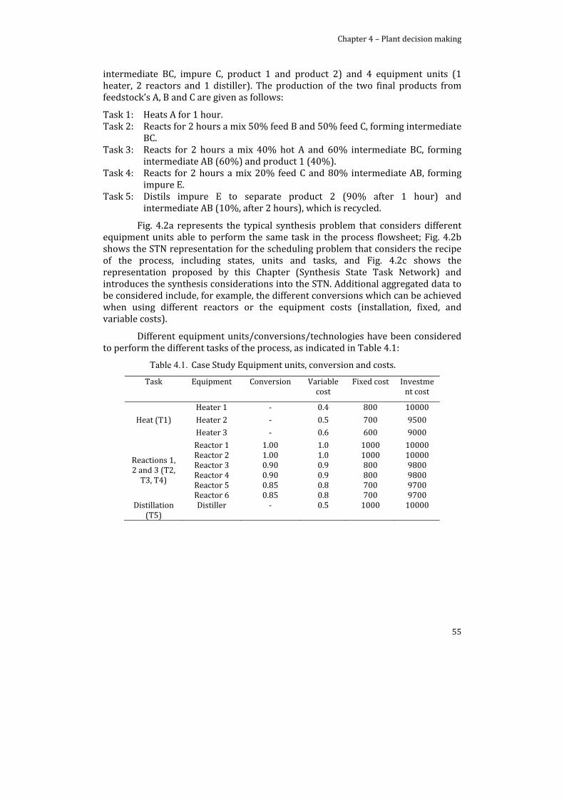
Chapter 4 – Plant decision making
55
intermediate BC, impure C, product 1 and product 2) and 4 equipment units (1 heater, 2 reactors and 1 distiller). The production of the two final products from feedstock’s A, B and C are given as follows:
Task 1: Heats A for 1 hour. Task 2: Reacts for 2 hours a mix 50% feed B and 50% feed C, forming intermediate
BC. Task 3: Reacts for 2 hours a mix 40% hot A and 60% intermediate BC, forming
intermediate AB (60%) and product 1 (40%). Task 4: Reacts for 2 hours a mix 20% feed C and 80% intermediate AB, forming
impure E. Task 5: Distils impure E to separate product 2 (90% after 1 hour) and
intermediate AB (10%, after 2 hours), which is recycled.
Fig. 4.2a represents the typical synthesis problem that considers different equipment units able to perform the same task in the process flowsheet; Fig. 4.2b shows the STN representation for the scheduling problem that considers the recipe of the process, including states, units and tasks, and Fig. 4.2c shows the representation proposed by this Chapter (Synthesis State Task Network) and introduces the synthesis considerations into the STN. Additional aggregated data to be considered include, for example, the different conversions which can be achieved when using different reactors or the equipment costs (installation, fixed, and variable costs).
Different equipment units/conversions/technologies have been considered to perform the different tasks of the process, as indicated in Table 4.1:
Table 4.1. Case Study Equipment units, conversion and costs.
Task Equipment Conversion Variable cost
Fixed cost Investment cost
Heater 1 ‐ 0.4 800 10000
Heat (T1) Heater 2 ‐ 0.5 700 9500
Heater 3 ‐ 0.6 600 9000
Reactions 1, 2 and 3 (T2, T3, T4)
Reactor 1 1.00 1.0 1000 10000 Reactor 2 1.00 1.0 1000 10000 Reactor 3 0.90 0.9 800 9800 Reactor 4 0.90 0.9 800 9800 Reactor 5 0.85 0.8 700 9700 Reactor 6 0.85 0.8 700 9700
Distillation (T5)
Distiller ‐ 0.5 1000 10000
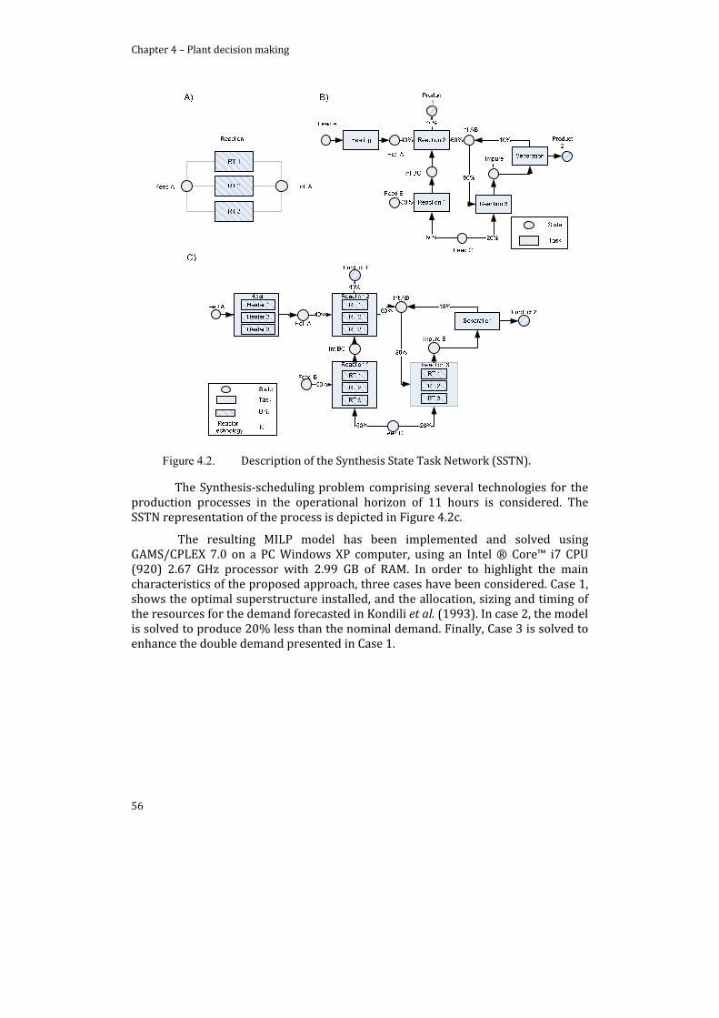
Chapter 4 – Plant decision making
56
Figure 4.2. Description of the Synthesis State Task Network (SSTN).
The Synthesis‐scheduling problem comprising several technologies for the production processes in the operational horizon of 11 hours is considered. The SSTN representation of the process is depicted in Figure 4.2c.
The resulting MILP model has been implemented and solved using GAMS/CPLEX 7.0 on a PC Windows XP computer, using an Intel ® Core™ i7 CPU (920) 2.67 GHz processor with 2.99 GB of RAM. In order to highlight the main characteristics of the proposed approach, three cases have been considered. Case 1, shows the optimal superstructure installed, and the allocation, sizing and timing of the resources for the demand forecasted in Kondili et al. (1993). In case 2, the model is solved to produce 20% less than the nominal demand. Finally, Case 3 is solved to enhance the double demand presented in Case 1.
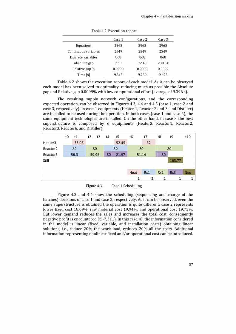
Chapter 4 – Plant decision making
57
Table 4.2. Execution report
Case 1 Case 2 Case 3
Equations 2965 2965 2965
Continuous variables 2549 2549 2549
Discrete variables 868 868 868
Absolute gap 7.59 72.45 230.04
Relative gap % 0.0090 0.0099 0.0099
Time [s] 9.313 9.250 9.625
Table 4.2 shows the execution report of each model. As it can be observed each model has been solved to optimality, reducing much as possible the Absolute gap and Relative gap 0.0099% with low computational effort (average of 9.396 s).
The resulting supply network configurations, and the corresponding expected operation, can be observed in Figures 4.3, 4.4 and 4.5 (case 1, case 2 and case 3, respectively). In case 1 equipments (Heater 1, Reactor 2 and 3, and Distiller) are installed to be used during the operation. In both cases (case 1 and case 2), the same equipment technologies are installed. On the other hand, in case 3 the best superstructure is composed by 6 equipments (Heater3, Reactor1, Reactor2, Reactor3, Reactor6, and Distiller).
t0 t1 t2 t3 t4 t5 t6 t7 t8 t9 t10
Heater3 55.98 52.45 32
Reactor2 80 80 80 80 80
Reactor3 56.3 59.96 80 21.97 51.14 80
Still 163.77
Heat Rx1 Rx2 Rx3 Sep
1 2 2 1 1
Figure 4.3. Case 1 Scheduling
Figure 4.3 and 4.4 show the scheduling (sequencing and charge of the batches) decisions of case 1 and case 2, respectively. As it can be observed, even the same superstructure is obtained the operation is quite different: case 2 represents lower fixed cost 18.69%, raw material cost 19.94%, and operational cost 19.75%. But lower demand reduces the sales and increases the total cost, consequently negative profit is encountered (€ ‐7,311). In this case, all the information considered in the model is linear (fixed, variable, and installation costs) obtaining linear solutions, i.e., reduce 20% the work load, reduces 20% all the costs. Additional information representing nonlinear fixed and/or operational cost can be introduced.
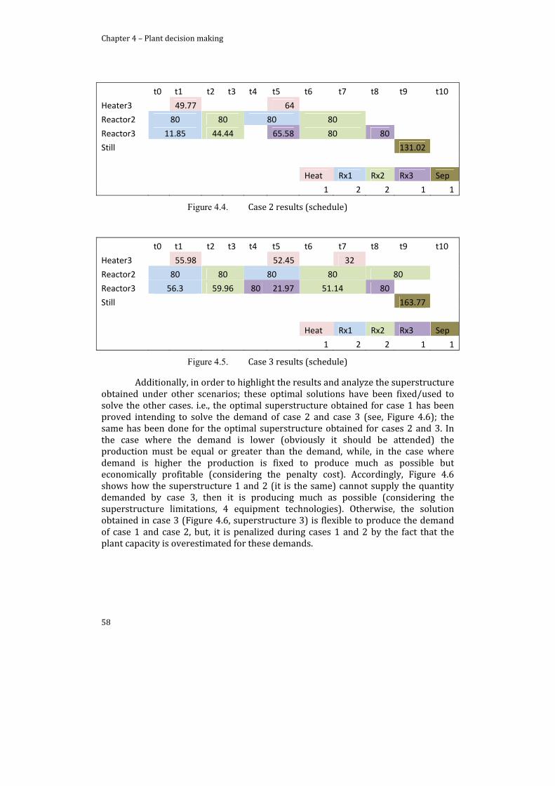
Chapter 4 – Plant decision making
58
Figure 4.4. Case 2 results (schedule)
Figure 4.5. Case 3 results (schedule)
Additionally, in order to highlight the results and analyze the superstructure obtained under other scenarios; these optimal solutions have been fixed/used to solve the other cases. i.e., the optimal superstructure obtained for case 1 has been proved intending to solve the demand of case 2 and case 3 (see, Figure 4.6); the same has been done for the optimal superstructure obtained for cases 2 and 3. In the case where the demand is lower (obviously it should be attended) the production must be equal or greater than the demand, while, in the case where demand is higher the production is fixed to produce much as possible but economically profitable (considering the penalty cost). Accordingly, Figure 4.6 shows how the superstructure 1 and 2 (it is the same) cannot supply the quantity demanded by case 3, then it is producing much as possible (considering the superstructure limitations, 4 equipment technologies). Otherwise, the solution obtained in case 3 (Figure 4.6, superstructure 3) is flexible to produce the demand of case 1 and case 2, but, it is penalized during cases 1 and 2 by the fact that the plant capacity is overestimated for these demands.
t0 t1 t2 t3 t4 t5 t6 t7 t8 t9 t10
Heater3 49.77 64
Reactor2 80 80 80 80
Reactor3 11.85 44.44 65.58 80 80
Still 131.02
Heat Rx1 Rx2 Rx3 Sep
1 2 2 1 1
t0 t1 t2 t3 t4 t5 t6 t7 t8 t9 t10
Heater3 55.98 52.45 32
Reactor2 80 80 80 80 80
Reactor3 56.3 59.96 80 21.97 51.14 80
Still 163.77
Heat Rx1 Rx2 Rx3 Sep
1 2 2 1 1
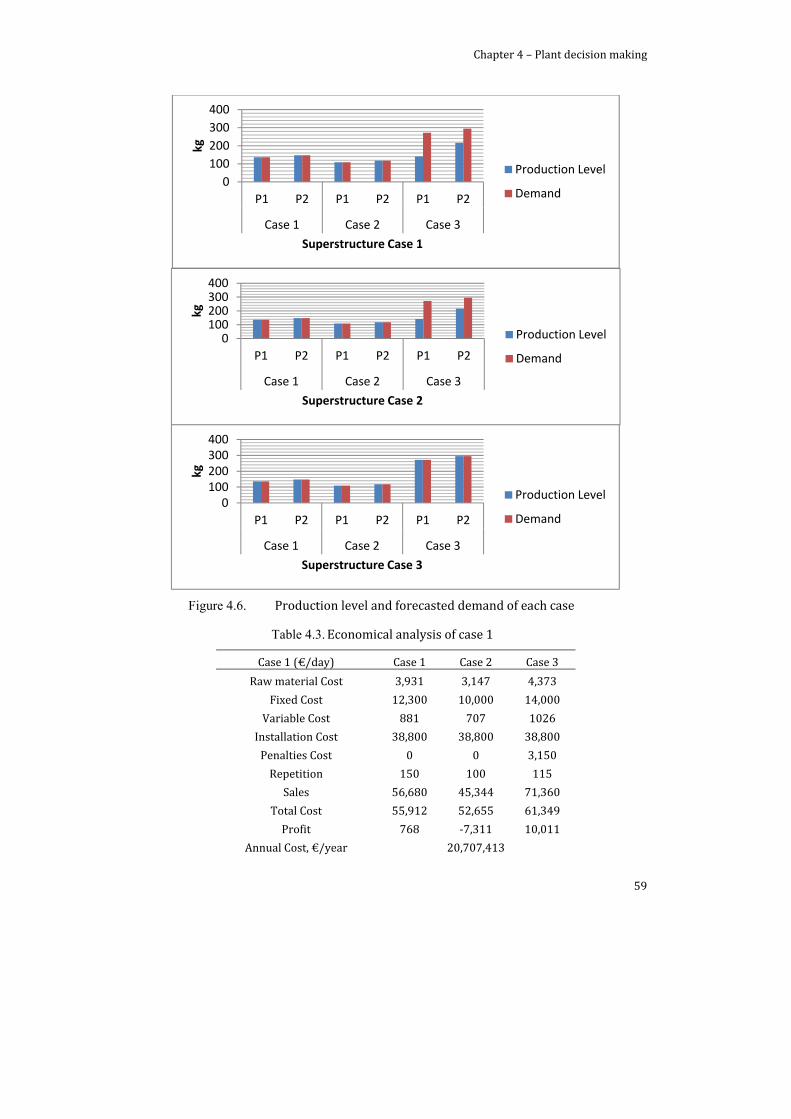
Chapter 4 – Plant decision making
59
Figure 4.6. Production level and forecasted demand of each case
Table 4.3. Economical analysis of case 1
Case 1 (€/day) Case 1 Case 2 Case 3
Raw material Cost 3,931 3,147 4,373
Fixed Cost 12,300 10,000 14,000
Variable Cost 881 707 1026
Installation Cost 38,800 38,800 38,800
Penalties Cost 0 0 3,150
Repetition 150 100 115
Sales 56,680 45,344 71,360
Total Cost 55,912 52,655 61,349
Profit 768 ‐7,311 10,011
Annual Cost, €/year 20,707,413
0
100
200
300
400
P1 P2 P1 P2 P1 P2
Case 1 Case 2 Case 3
kg
Superstructure Case 1
Production Level
Demand
0100200300400
P1 P2 P1 P2 P1 P2
Case 1 Case 2 Case 3
kg
Superstructure Case 2
Production Level
Demand
0100200300400
P1 P2 P1 P2 P1 P2
Case 1 Case 2 Case 3
kg
Superstructure Case 3
Production Level
Demand
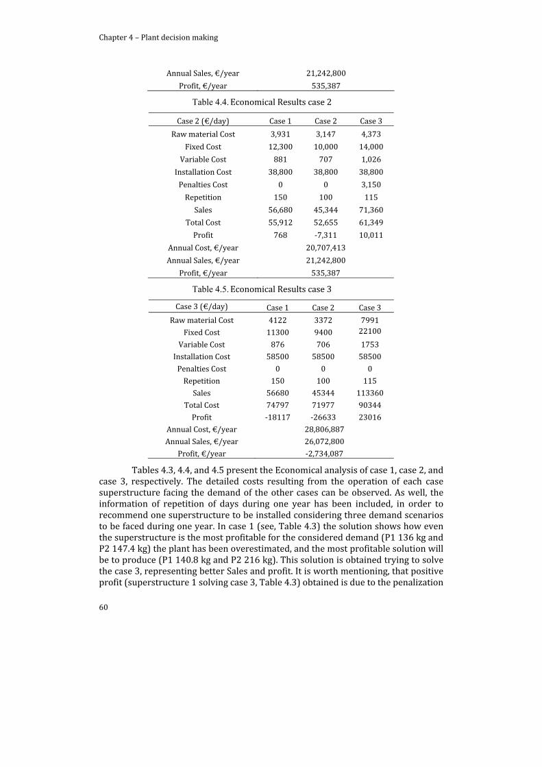
Chapter 4 – Plant decision making
60
Annual Sales, €/year 21,242,800
Profit, €/year 535,387
Table 4.4. Economical Results case 2
Case 2 (€/day) Case 1 Case 2 Case 3
Raw material Cost 3,931 3,147 4,373
Fixed Cost 12,300 10,000 14,000
Variable Cost 881 707 1,026
Installation Cost 38,800 38,800 38,800
Penalties Cost 0 0 3,150
Repetition 150 100 115
Sales 56,680 45,344 71,360
Total Cost 55,912 52,655 61,349
Profit 768 ‐7,311 10,011
Annual Cost, €/year 20,707,413
Annual Sales, €/year 21,242,800
Profit, €/year 535,387
Table 4.5. Economical Results case 3
Case 3 (€/day) Case 1 Case 2 Case 3
Raw material Cost 4122 3372 7991
Fixed Cost 11300 9400 22100
Variable Cost 876 706 1753
Installation Cost 58500 58500 58500
Penalties Cost 0 0 0
Repetition 150 100 115
Sales 56680 45344 113360
Total Cost 74797 71977 90344
Profit ‐18117 ‐26633 23016
Annual Cost, €/year 28,806,887
Annual Sales, €/year 26,072,800
Profit, €/year ‐2,734,087
Tables 4.3, 4.4, and 4.5 present the Economical analysis of case 1, case 2, and case 3, respectively. The detailed costs resulting from the operation of each case superstructure facing the demand of the other cases can be observed. As well, the information of repetition of days during one year has been included, in order to recommend one superstructure to be installed considering three demand scenarios to be faced during one year. In case 1 (see, Table 4.3) the solution shows how even the superstructure is the most profitable for the considered demand (P1 136 kg and P2 147.4 kg) the plant has been overestimated, and the most profitable solution will be to produce (P1 140.8 kg and P2 216 kg). This solution is obtained trying to solve the case 3, representing better Sales and profit. It is worth mentioning, that positive profit (superstructure 1 solving case 3, Table 4.3) obtained is due to the penalization
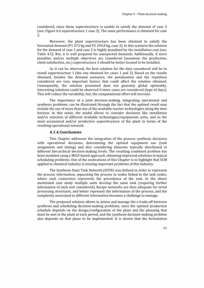
Chapter 4 – Plant decision making
61
considered, since these superstructure is unable to satisfy the demand of case 3 (see, Figure 4.6 superstructure 1 case 3). The same performance is obtained for case 2.
Moreover, the plant superstructure has been obtained to satisfy the forecasted demand (P1 272 kg and P2 294.8 kg, case 3). In this scenario the solution for the demand of case 1 and case 2 is highly penalized by the installation cost (see, Table 4.5). But, it is well prepared for unexpected demands. Additionally, if more penalties and/or multiple objectives are considered (maximize the production, client satisfaction, etc.) superstructure 3 should be better located to be installed.
As it can be observed, the best solution for the data considered will be to install superstructure 1 (the one obtained for cases 1 and 2). Based on the results obtained, besides the demand scenarios, the penalization and the repetition considered are very important factors that could affect the solution obtained. Consequently, the solution presented does not guaranty global optimality. Interesting solutions could be observed if more cases are considered (type of days), This will reduce the variability, but, the computational effort will increase.
The importance of a joint decision‐making, integrating operational and synthesis problems, can be illustrated through the fact that the optimal result may include the use of more than one of the available reactor technologies along the time horizon. In this sense, the model allows to consider decisions like installation and/or selection of different available technologies/equipments units, and so the most economical and/or productive superstructure of the plant in terms of the resulting operational network.
4.1.4. Conclusions
This Chapter addresses the integration of the process synthesis decisions with operational decisions, determining the optimal equipment use (task assignment and timing) and also considering elements typically distributed in different hierarchical decision‐making levels. The resulting combined problem has been modeled using a MILP‐based approach, obtaining improved solutions in typical scheduling problems. One of the motivations of this Chapter is to highlight that SCM applied to chemical industry is missing important problems of this industry.
The Synthesis State Task Network (SSTN) was defined in order to represent the process information, separating the process in nodes linked to the task nodes, where each connection represents the precedence of the task. In the above mentioned case study multiple units develop the same task (requiring further information of each unit considered). Recipe networks are then adequate for serial processing structures, and better represent the information of the process, and the complexity associated to different information becomes a challenge to manage.
The proposed solution allows to assess and manage the a trade‐off between synthesis and scheduling decision‐making problems, since the optimal production schedule depends on the design/configuration of the plant and the planning that must be met in the plant at each period, and the synthesis decision‐making problem also depends on that plans to be implemented. It is shown that the formulation

Chapter 4 – Plant decision making
62
presented in this Chapter introduces the consideration of several technologies, this consideration shows how the operations will change and thus may represent more efficient solutions. This is an important improvement in the process optimization in terms of flexibility and integration in the decision‐making process.
Chapter 4 – Plant decision making
63
Notation:
Indexes and Sets: i tasks (i= 1, 2,…, I) j units (j=1,2,..., J) s state (s=1,2,…, S) t time periods (t=1,2,…, T) FP(s) State’s that correspond to final products TF(t) Final time period R(s) state’s that correspond to Raw materials. KI task i that can be developed by unit j Js units that produce intermediate products Parameters: V minimum equipment capacity for the task i processed in unit j. V maximum equipment capacity for the task i processed in unit j. Cs maximum storage capacity of the state s. X’ positive number. X positive number. Dems Demand of the state s. α determines if state s feed task i. α determines if state s is an output of task i. Cfix fixed cost of unit j. Cvar variable cost of task i produced in unit j. Crm raw material cost of state s at time t (s R s ) Ps price of the products s FP s M big M

Chapter 4 – Plant decision making
65
4.2. Integrated Scheduling and Control decisionmaking
As previously stated, the integrated management becomes one of the most applied techniques to enhance process reliability and also to prove that plans are feasible in the subsequent decision level. Although the proper decision‐making of scheduling and control theory is quite different, it jointly resolution allows decision makers to enhance feasible plans at plant and process level.
When computer control systems are implemented, the computer platform used can provide the deterministic performance. However, the commonly used platforms to implement control systems are not able to determine effective/optimal operation. Is in this sense that, control loop cannot be included into the scheduling decision‐making, while information regarding the scheduling actions could be delivered to the control systems.
A detailed operational and control integration can be observed in Moreno‐Benito et al. (2012), where the optimal interconnection of process stages and the specification of their operating strategy are intended. In this regard, integrated (operational‐control) approaches are represented by: (i) operational information: processing and recipe; (ii) operation information: detailed information of the process connections as the superstructure of the process operation is used. (iii) logic variables and disjunctive equations are defined in order to represent these information. Such models are typically represented as a mixed integer logic optimization (MLDO) programs. (Moreno‐Benito and Espuña, 2012)
In this line, Moreno‐Benito and Espuña (2011) describe how the MLDO problem could be reformulated as a mixed integer dynamic optimization program (MIDO) by: replacing the Boolean variables by binaries logical propositions by algebraic equations and disjunctions by big‐M relaxations. Then, the obtained MIDO problem is solved using direct‐simultaneous approach by full discretization of state and control variable profiles, resulting in a MINLP problem.
Complexity of the model representation depends on the dynamic of the process in consideration; processes with low dynamics in the transient state could be represented by a MILP formulation.
In a general point of view this work is focused on the integration of scheduling decision‐making problem and process control verification. All these concepts have been applied to a simplified case study, were scheduling decision‐making model has been developed including the control characteristics of the problem considered. Hence, the solutions are proposed as decisions that must take place in the control loop (as the target of the plant). It is worth to mention that this section has been developed in collaboration with the Electrical Engineering Department of the Universitat Politècnica de Catalunya (UPC Barcelona tech), and the simulation and control actions are not included in this Thesis. In this line, the proposed framework can be used in general operational decision‐making model and can be also applied in any industrial case study with low dynamics.
Chapter 4 – Plant decision making
66
4.2.1. Energy Management
In the last years, the distributed paradigm is gaining popularity at the expense of the centralized production models inspired by the economy of scale. The Microgrids (MG) include energy transformation, storage and use, for which microgrids emerge as the most practical solution to interconnect and interoperate a network of energy dealers (typically known as producers and consumers, despite the conservation principle). Accordingly, the need for efficient management arises as a key issue not only in a specific planning or control level, but for all the hierarchy of decision levels.
At the beginning the MG reach needs far away from the main grids, such as: farms, communities in the woods and/or mountains, etc. Nevertheless, Distributed generation (DG) systems close to consumers allow better meeting local energy needs. DG reduces network distribution losses and better match consumption and generation profiles. Besides, reliability increases as the power supply does not rely on the main grid and the size of Electricity storage systems (ESS) largely decreases. Furthermore, DG integrating renewable energy systems (RES) are gaining acceptation due to: financial risks, the reduction of fuel‐based power production and the autonomy and flexibility opportunities given by the interoperability of heterogeneous technologies. Such systems may consist of photovoltaic (PV) panels and small wind turbines, and incorporate ESS in order to cope with the fluctuating availability of the related primary resources.
A key issue to efficiently integrate DGS, ESS, and power loads (consumption points) is the use of Power Electronics (PE) to interface these elements and the reduced local grid, also called Microgrid (MG), which may be operated both, grid connected and in island (stand‐alone) modes. The MG is required to coordinate generation, storage and use to minimize loses, maximize efficiency, green energy generation, adjust production, and demand profiles. For design purposes, long‐term energy balances are normally solved (Bernal‐Agustín and Dufo‐López, 2009) with standard available software (i.e. HOMER energy modeling software). Very recently, design strategies (Giannakoudis et al., 2010) and energy planning in process industries using aggregated algebraic models (Zondervan et al., 2010) have been presented. However, detailed operation optimization contemplating scheduling and control issues have been hardly addressed.
An ODE MG model can be developed (Guerrero et al., 2009). The DG parts are voltage sources connected through PE interfaces regulating the active and reactive power flows thorough virtual inertias. The so called droop method consists of measuring active and reactive power drawn by the DG to the MG, and adjusting the output voltage frequency and amplitude accordingly. This control technique stems from the large power systems theory in which a synchronous generator reduces frequency when the power drawn is increased due to its inertia, resulting in a global synchronization and power sharing. Since PE has no inertia, the same idea can be implemented via control loops, thus obtaining a virtual inertia. However, when power demand increases, MG frequency can decrease below its limits. In addition, the MG itself cannot control the energy flow between the MG and the grid.
Chapter 4 – Plant decision making
67
Thus, MGs need a hierarchical control similar to those used in large power plants, but with the next control levels (Guerrero et al., 2009):
Primary. Virtual inertias to balance the active and the reactive power autonomously.
Secondary. Adjust the MG frequency and amplitude by means of an external controller that sends the references to the primary control of each DG.
Tertiary. Regulate the active and reactive power exchanged with the mains grid.
Thus, an additional control level, an upper operational layer including planning, is needed to manage energy flows within the MG, i.e. an Energy Management System (EMS). This Chapter is a preliminary step to the development of a communication and interoperability framework aimed at determining the assignment and timing of the MG tasks that will be later simulated in detail.
4.2.1.1. Problem Formulation
The problem and the subsequent formulation presented is to determine the production and storage levels to be managed by the MG along a given time period. The mathematical model presented contemplates two main aspects: the energy balances describing the energy flows, generation, storage and consumption, and the capacity constraints associated to the equipment and technologies involved in the MG.
The main aspects considered in the model are next introduced. The decisions to be made are whether or not a production unit i is switch on at a given time period k (Eq. 4.17). Once switched, the power production may be adjusted (Eq. 4.18) and consumed or stored, according to capacity (Eq. 4.19, for energy), and flow constraints (Eq. 4.20 and 4.21, for power). The constraint to be observed for all the energy flows is the balance (Eq. 4.22), which includes the power that is dissipated when units need to be switched to satisfy power demands below their minimum yield capacity (and storage isn’t available). The balance is given in this way since transport issues and costs regarding transportation between power supply systems i and Electricity storage systems k is not considered.
0,1 , (4.17)
, (4.18)
, (4.19)
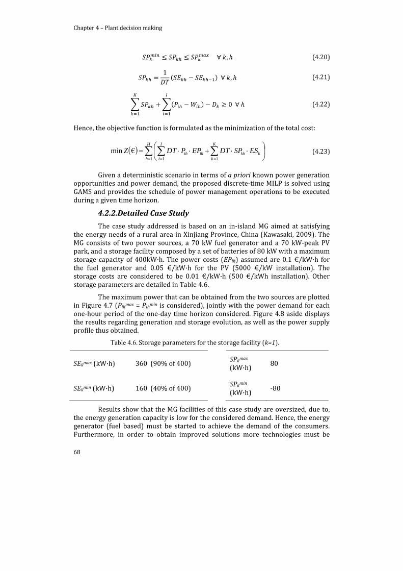
Chapter 4 – Plant decision making
68
, (4.20)
1, (4.21)
0 (4.22)
Hence, the objective function is formulated as the minimization of the total cost:
H
h
K
kkkh
I
iihih ESSPDTEPPDTZ
1 11
€min (4.23)
Given a deterministic scenario in terms of a priori known power generation opportunities and power demand, the proposed discrete‐time MILP is solved using GAMS and provides the schedule of power management operations to be executed during a given time horizon.
4.2.2. Detailed Case Study
The case study addressed is based on an in‐island MG aimed at satisfying the energy needs of a rural area in Xinjiang Province, China (Kawasaki, 2009). The MG consists of two power sources, a 70 kW fuel generator and a 70 kW‐peak PV park, and a storage facility composed by a set of batteries of 80 kW with a maximum storage capacity of 400kW·h. The power costs (EPih) assumed are 0.1 €/kW·h for the fuel generator and 0.05 €/kW·h for the PV (5000 €/kW installation). The storage costs are considered to be 0.01 €/kW·h (500 €/kWh installation). Other storage parameters are detailed in Table 4.6.
The maximum power that can be obtained from the two sources are plotted in Figure 4.7 (Pihmax = Pihmin is considered), jointly with the power demand for each one‐hour period of the one‐day time horizon considered. Figure 4.8 aside displays the results regarding generation and storage evolution, as well as the power supply profile thus obtained.
Table 4.6. Storage parameters for the storage facility (k=1).
SEkmax (kW·h) 360 (90% of 400) SPkmax (kW·h) 80
SEkmin (kW·h) 160 (40% of 400) SPkmin (kW·h)
‐80
Results show that the MG facilities of this case study are oversized, due to, the energy generation capacity is low for the considered demand. Hence, the energy generator (fuel based) must be started to achieve the demand of the consumers. Furthermore, in order to obtain improved solutions more technologies must be
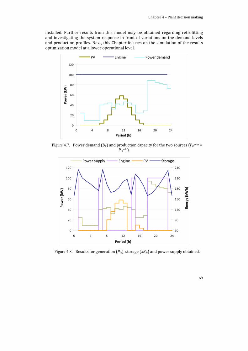
Chapter 4 – Plant decision making
69
installed. Further results from this model may be obtained regarding retrofitting and investigating the system response in front of variations on the demand levels and production profiles. Next, this Chapter focuses on the simulation of the results optimization model at a lower operational level.
Figure 4.7. Power demand (Dh) and production capacity for the two sources (Pihmax = Pihmin).
Figure 4.8. Results for generation (Pih), storage (SEih) and power supply obtained.
0
20
40
60
80
100
120
0 4 8 12 16 20 24
Period (h)
Power (kW)
PV Engine Power demand
0
20
40
60
80
100
120
0 4 8 12 16 20 24
Power (kW)
60
90
120
150
180
210
240
Period (h)
Energy (kWh)
Power supply Engine PV Storage

Chapter 4 – Plant decision making
70
Detailed simulation
Results from the upper planning level allow determining the series of power management actions that optimally satisfy a given demand. These decisions should be communicated and executed at a lower operational level, real or virtual. In this case study, they are communicated to a detailed simulation model developed in Matlab /Simulink. The model contemplates the differential equations discretized and solved by means of the ODE45 (Dormand‐Prince) numerical method. The communication framework between the optimization model in GAMS and the detailed ODE model in Matlab has been developed using Matgams (Ferris, 2010).
Results from the dynamic Matlab/Simulink simulation allow validating the assignment and timing decisions determined at the planning level. The extensive ODE model reveals the effects of discrete switching on and off actions and describes the transitions in a detailed way that allows providing guarantee of reliable model matching (see, Figure 4.9).
Figure 4.9. Detailed Simulation (Simulink‐capture)
4.2.3. Conclusions
This Chapter introduces the basis for developing a communication scheme for the planning and control layers of a microgrid. A case study has been addressed and the assignment and timing of energy production and storage actions has been formulated. Given a network of power generators, the resulting MILP has been solved using GAMS for a deterministic case study with fixed resource and demand availability. A detailed ODE model developed in Matlab has been connected to the upper layer in order to validate the proposed schedule.
Further work is under way towards solving the communication within an Energy Management System (EMS) including both, simulated and real pilot systems, and allowing the management of power loads and rescheduling actions. Nevertheless, the proposed mathematical model is considered a starting point.
simout1
To Workspace1
Scope1
In S/H
Sampleand Hold
PulseGenerator
datasFrom
Workspace
12:34Digital Clock

Chapter 4 – Plant decision making
71
Hence, it must be improved and applied to a real case study composed by 3 photovoltaic panels, wind turbine and an engine generator.

Chapter 4 – Plant decision making
72
Notation
Indexes: i=1,… ,I Power Source (production/purchase) k=1,… , K Electricity storage system h=1,…, H Time interval Parameters: DT Span of the time interval (h) Pihmax Maximum power supply of source i at interval h (kW) Pihmin Minimum power supply of source i at interval h (kW) EPih Cost of obtaining energy from source i interval h (€/kW·h) SEkmax Maximum Electricity storage of system k (kW·h) SEkmin Minimum Electricity storage of system k (kW·h) SPkmax Maximum power supply from/to system k (kW) SPkmin Minimum power supply from/to system k (kW) ESk Cost of storing (obtaining) energy in (from) system k (€/kW·h) Dh Power demand during interval h (kW·h) Variables: Pih Energy supply of source i at interval h (kW) SEih Electricity storage level of system k at the end of interval h (kW·h) SPih Power supplied by / given to system k during interval h (kW·h) Wih Wasted / dissipated power from source i at interval h (kW) Xih Binary variable indicating whether or not supply i is used at interval h

73
Chapter 5. Tactical and Operational Integration
This Chapter presents an integrated planning and scheduling approach for SCM. Two optimization stages have been solved. First one solves the scheduling problem for several demand scenarios and the performance obtained from these solutions has been characterized as constraints, these constraints have been included in a general planning formulation. The second optimization stage consists in the solution of the planning problem considering the scheduling information.
5.1. Introduction
The problem of decision‐making associated to Supply Chain (SC) tactical management (procurement of raw materials in different markets, allocation of products to different plants and distributing them to different customers) has been studied during the last decades. But nowadays, chemical industry faces new challenges which increase the pressure for an improved decision‐making, able to better exploit plant and process flexibility. The case of batch processes, because of its inherent flexibility, offers a significant improvement potential in this line.
It is worth mentioning that in most of the SCM decision‐making models; the optimization is based on information derived from previous and/or sub‐sequent decision‐making models. i.e., tactical decision‐making typically uses fixed SC network configuration (decision related to the design problem) and also fixed production levels (which is a solution of the scheduling problem).
Production planning estimates the capacities of the SC network (production, transportation, acquisition of raw materials, storage, etc.) and intends to maximize the efficiency of the material flows to satisfy the market considering weekly, monthly, or annual resolution of the proposed model. Disregarding the issues associated with the process operation, goods and product transportation, and unexpected situations during the plan resolution. Also, constant process duration, production and product costs are considered through linear functions to represent the process behavior.
The nature of both planning and scheduling deterministic problems hinders their joint resolution, principally, due to the computational effort needed to solve the detailed planning‐scheduling model resulted from the time horizon considered by each decision‐making level. But, the development of techniques to include information of one model into the others must be a promising issue.
In this Chapter, the integration of the tactical and operational decision‐making at the SC level is intended. The recursive resolution of the operational
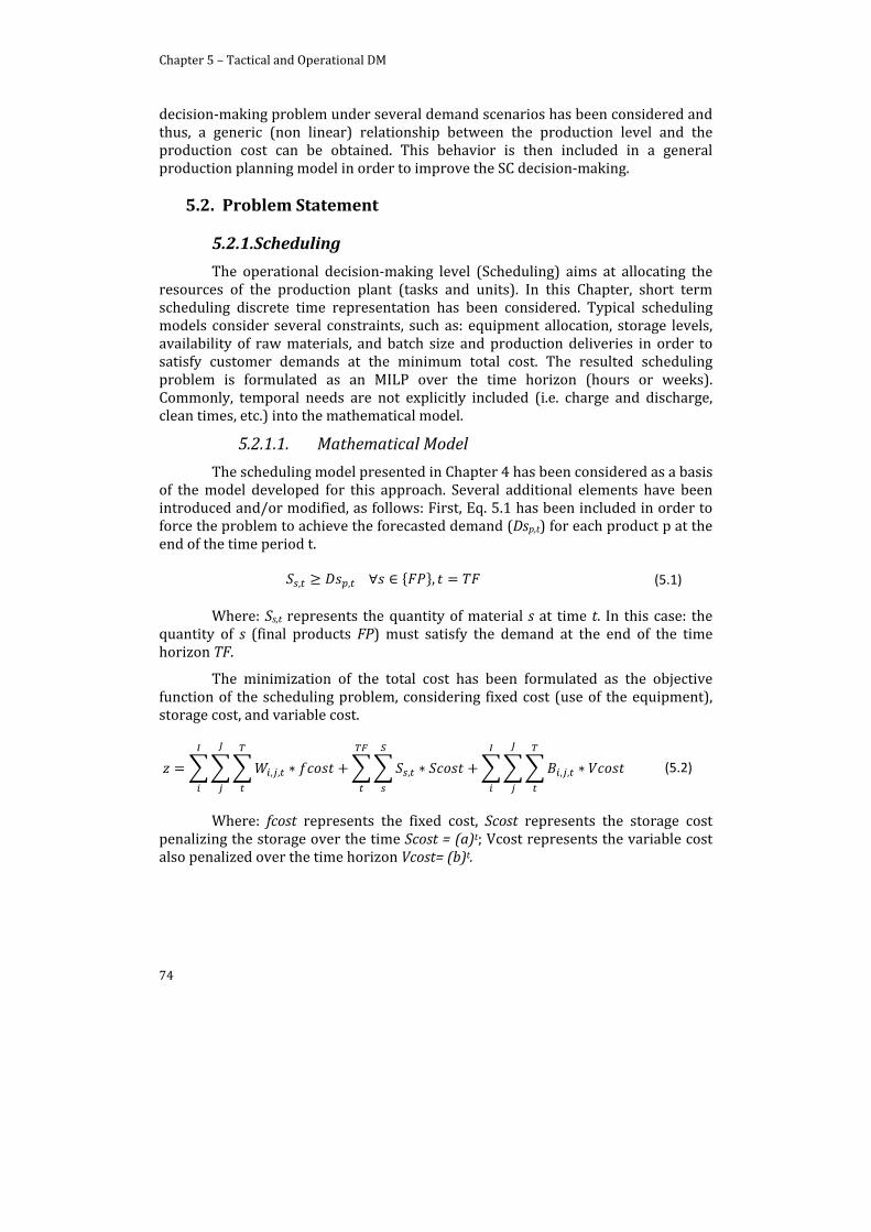
Chapter 5 – Tactical and Operational DM
74
decision‐making problem under several demand scenarios has been considered and thus, a generic (non linear) relationship between the production level and the production cost can be obtained. This behavior is then included in a general production planning model in order to improve the SC decision‐making.
5.2. Problem Statement
5.2.1. Scheduling
The operational decision‐making level (Scheduling) aims at allocating the resources of the production plant (tasks and units). In this Chapter, short term scheduling discrete time representation has been considered. Typical scheduling models consider several constraints, such as: equipment allocation, storage levels, availability of raw materials, and batch size and production deliveries in order to satisfy customer demands at the minimum total cost. The resulted scheduling problem is formulated as an MILP over the time horizon (hours or weeks). Commonly, temporal needs are not explicitly included (i.e. charge and discharge, clean times, etc.) into the mathematical model.
5.2.1.1. Mathematical Model
The scheduling model presented in Chapter 4 has been considered as a basis of the model developed for this approach. Several additional elements have been introduced and/or modified, as follows: First, Eq. 5.1 has been included in order to force the problem to achieve the forecasted demand (Dsp,t) for each product p at the end of the time period t.
, , , (5.1)
Where: Ss,t represents the quantity of material s at time t. In this case: the quantity of s (final products FP) must satisfy the demand at the end of the time horizon TF.
The minimization of the total cost has been formulated as the objective function of the scheduling problem, considering fixed cost (use of the equipment), storage cost, and variable cost.
, , , , , (5.2)
Where: fcost represents the fixed cost, Scost represents the storage cost penalizing the storage over the time Scost = (a)t; Vcost represents the variable cost also penalized over the time horizon Vcost= (b)t.
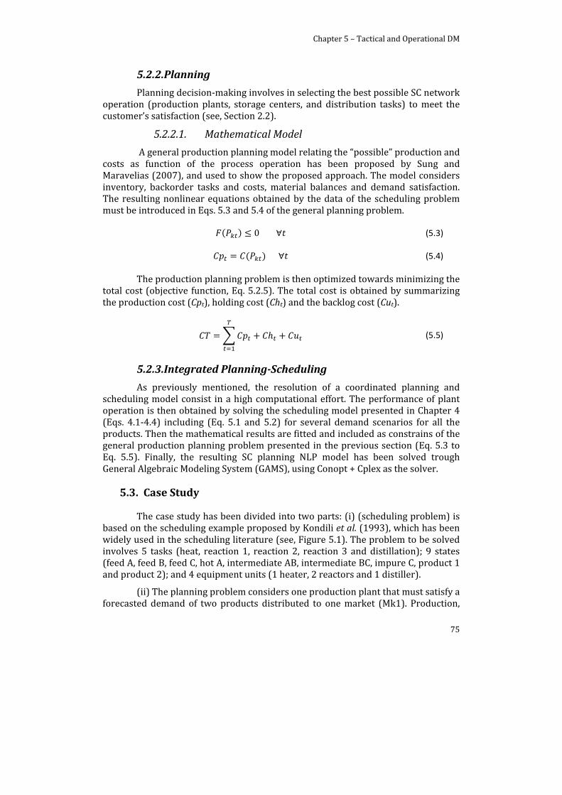
Chapter 5 – Tactical and Operational DM
75
5.2.2. Planning
Planning decision‐making involves in selecting the best possible SC network operation (production plants, storage centers, and distribution tasks) to meet the customer’s satisfaction (see, Section 2.2).
5.2.2.1. Mathematical Model
A general production planning model relating the “possible” production and costs as function of the process operation has been proposed by Sung and Maravelias (2007), and used to show the proposed approach. The model considers inventory, backorder tasks and costs, material balances and demand satisfaction. The resulting nonlinear equations obtained by the data of the scheduling problem must be introduced in Eqs. 5.3 and 5.4 of the general planning problem.
0 (5.3)
(5.4)
The production planning problem is then optimized towards minimizing the total cost (objective function, Eq. 5.2.5). The total cost is obtained by summarizing the production cost (Cpt), holding cost (Cht) and the backlog cost (Cut).
(5.5)
5.2.3. Integrated PlanningScheduling
As previously mentioned, the resolution of a coordinated planning and scheduling model consist in a high computational effort. The performance of plant operation is then obtained by solving the scheduling model presented in Chapter 4 (Eqs. 4.1‐4.4) including (Eq. 5.1 and 5.2) for several demand scenarios for all the products. Then the mathematical results are fitted and included as constrains of the general production planning problem presented in the previous section (Eq. 5.3 to Eq. 5.5). Finally, the resulting SC planning NLP model has been solved trough General Algebraic Modeling System (GAMS), using Conopt + Cplex as the solver.
5.3. Case Study
The case study has been divided into two parts: (i) (scheduling problem) is based on the scheduling example proposed by Kondili et al. (1993), which has been widely used in the scheduling literature (see, Figure 5.1). The problem to be solved involves 5 tasks (heat, reaction 1, reaction 2, reaction 3 and distillation); 9 states (feed A, feed B, feed C, hot A, intermediate AB, intermediate BC, impure C, product 1 and product 2); and 4 equipment units (1 heater, 2 reactors and 1 distiller).
(ii) The planning problem considers one production plant that must satisfy a forecasted demand of two products distributed to one market (Mk1). Production,

Chapter 5 – Tactical and Operational DM
76
backlog, and inventory management must be optimized over the considered time horizon (six months). Fixed holding (P1: 10; P2: 20) and backlog (P1: 2; P2: 3) costs have been considered for each product.
Figure 5.1. Case study.
5.4. Results
The optimal assignment of equipment units to tasks and the resulting schedules were determined in order to satisfy the proposed goals in several demand scenarios (Figure 5.2). For each demand scenario, the optimal scheduling has been obtained. The results show the best equation to be used in order to represent the performance of each product (Table 5.1).
Table 5.1. Data analysis
Product Equation R2 ParametersProduct 1 Y=A*X^B 0.9984 A: 0.4736E+03 B: 0.1571E+01 Product 2 Y=A*X^2+B 0.9841 A: 0.2091E+02 B: 0.2387E+06
The aforementioned equations have been introduced in the planning problem. The optimal production, storage and distribution decisions have been obtained. Figure 5.3 shows the production for all the time periods. In this case study, the holding cost represents minimum part of the total cost: the production‐distribution policy dominates the decision‐making during the time horizon. Nevertheless, the storage capacity (see, Figure 5.3) is used to save production penalties while distribution costs have been disregarded due to the number of markets.
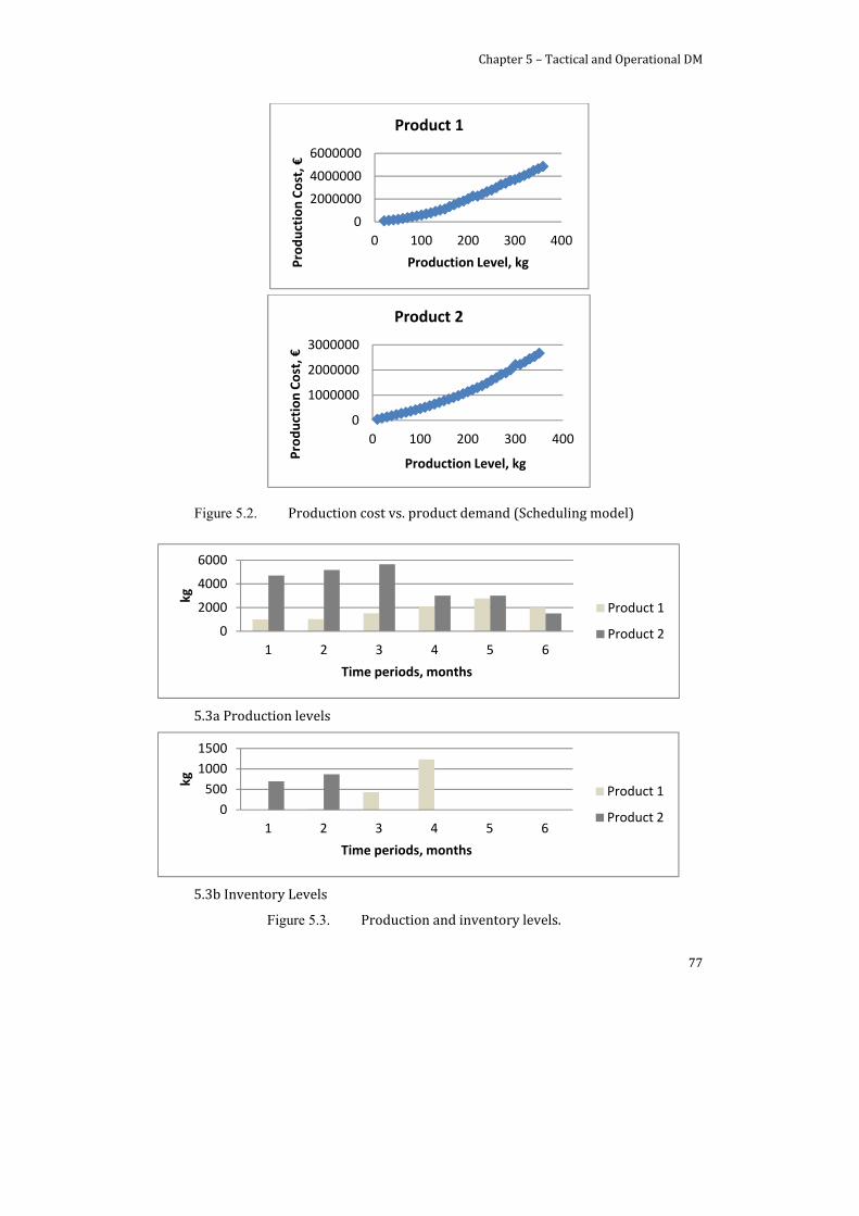
Chapter 5 – Tactical and Operational DM
77
Figure 5.2. Production cost vs. product demand (Scheduling model)
5.3a Production levels
5.3b Inventory Levels
Figure 5.3. Production and inventory levels.
0
2000000
4000000
6000000
0 100 200 300 400
Production Cost, €
Production Level, kg
Product 1
0
1000000
2000000
3000000
0 100 200 300 400
Production Cost, €
Production Level, kg
Product 2
0
2000
4000
6000
1 2 3 4 5 6
kg
Time periods, months
Product 1
Product 2
0
500
1000
1500
1 2 3 4 5 6
kg
Time periods, months
Product 1
Product 2
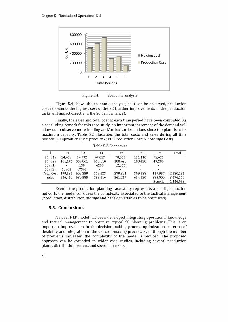
Chapter 5 – Tactical and Operational DM
78
Figure 5.4. Economic analysis
Figure 5.4 shows the economic analysis; as it can be observed, production cost represents the highest cost of the SC (further improvements in the production tasks will impact directly in the SC performance).
Finally, the sales and total cost at each time period have been computed. As a concluding remark for this case study, an important increment of the demand will allow us to observe more holding and/or backorder actions since the plant is at its maximum capacity. Table 5.2 illustrates the total costs and sales during all time periods (P1=product 1; P2: product 2; PC: Production Cost; SC: Storage Cost).
Table 5.2. Economics
$ t1 T2 t3 t4 t5 t6 Total PC (P1) 24,459 24,992 47,017 78,577 121,110 72,671 PC (P2) 461,176 559,861 668,110 188,428 188,428 47,286 SC (P1) ‐ 138 4296 12,316 ‐ ‐ SC (P2) 13901 17368 ‐ ‐ ‐ ‐ Total Cost 499,536 602,359 719,423 279,321 309,538 119,957 2,530,136 Sales 626,460 680,585 788,416 561,217 634,520 385,000 3,676,200 Benefit 1,146,063
Even if the production planning case study represents a small production network, the model considers the complexity associated to the tactical management (production, distribution, storage and backlog variables to be optimized).
5.5. Conclusions
A novel NLP model has been developed integrating operational knowledge and tactical management to optimize typical SC planning problems. This is an important improvement in the decision‐making process optimization in terms of flexibility and integration in the decision‐making process. Even though the number of problems increases, the complexity of the model is reduced. The proposed approach can be extended to wider case studies, including several production plants, distribution centers, and several markets.
0
200000
400000
600000
800000
1 2 3 4 5 6
Cost, €
Time Periods
Holding cost
Production Cost

Chapter 5 – Tactical and Operational DM
79
Some opportunities remain open in this kind of works. In the case study presented (production cost vs. production level), the products have been considered as independent variables. In order to improve the results, the products analysis could be considered as dependent variables. The complexity of the scheduling problem might require the use of more complex models to ensure that all the basic information is retained by the surrogate model. The introduction of other nonlinearities in the model (i.e., in the cost functions) and the existence of process alternatives, leading to integer constraints, will affect the mathematical behavior of the resulting model, which may require alternative formulations and/or the use of other mathematical programming tools. And the case of integrating a large number of echelons in the SC will exponentially increase the size of the problem. Finally, uncertainty should be also considered to reach more robust solutions to the decision‐making problem

81
Chapter 6. Coordinated Supply Chains
6.1. Introduction
The scope of the Supply Chain Management usually takes into account the few single echelons directly linked to the process of interest (raw materials acquisition, production, and market distribution; see Figure 1.2), which are assumed to present a previously known behavior (even this behavior may include some uncertainty). Decisions based on this limited picture disregard the important information associated to the interaction among different cooperative SCs.
The incorporation of information from the different interacting enterprises in a single process model is essential to rationalize the tactical management of any of these interacting systems, requiring the procurement of RM from different suppliers, the allocation of materials to different plants, or deciding the distribution of products to the final consumers. So the features of each one of the single echelons of the entire SC have to be integrated in a specific model with its own objectives and management practices.
In this line, Coordinated Management has been commonly used in PSE approaches. But, the scope covered by this issue has not been clearly distinguished in the literature although it is mentioned. For example, in the marketing literature, some interesting applications show coordination schemes related to pricing decisions taking into consideration deterministic and uncertain demands. Xiangtong et al. (2004) solved the tactical management of one‐supplier one retailer SC with uncertain demands in the model formulation.
The need to ensure coherence among different decisions, usually associated to different time and economic scales, is one of the main complicating points in modeling and solving integrated SCM. In this regard, many current approaches are based on the development of coordinated models (Cardoso et al., 2013), while others focused on the integration of midterm decision‐making levels such as: planning‐scheduling models (Guillén et al., 2005a) and production/ distribution planning models (Cóccola et al., 2012; Fröhling et al., 2010; Erengüç et al., 1999). In addition, another type of coordination management can be seen in the Closed Loop SC Management. Most of these approaches present coordination models including remanufacturing, reprocessing, and reused products. In closed loop SC the interaction among SC echelons is introduced into the model formulation by considering recovery processes to reuse of final products (Atasu et al., 2008). Reverse channel collects the used products to be included into the reprocessing stage. The demand is therefore satisfied by a mix of new and remanufactured
Chapter 6 – Coordinated Supply Chains
82
products (Georgiadis and Athanasiou, 2013). Several benefits have been achieved by re‐used products, reducing the environmental damage (Chi et al., 2011), and government incentives (Wei‐min et al., 2013), etc. Integration of uncertainty has been also included in multi‐period, multiproduct networks with reverse flows for strategic and tactical decision‐making (Salema et al., 2007 and 2010, respectively).
As it is previously mentioned, most of the SCM literature disregards or weakly includes the effects of interaction, coordination and/or cooperation (Zamarripa et al., 2012) among different SC’s. In other words, SCM literature focuses on typical single SC echelons directly linked to the process of interest (suppliers, production sites, distribution centers, markets) disregarding the characteristics of each enterprise (echelon) SC. By doing so, much information is lost and, accordingly, the generated model does not represent the real behavior of the system leading to inappropriate decisions.
This Chapter aims to optimize the tactical management of several SC’s by coordinating them as one “entire coordinated SC”. The behavior of each echelon will be characterized as a SC (with their objectives and management practices) and then integrated together to form a single model representing the entire SC. A MILP based model has been developed to coordinate suppliers with producers and minimize the Total Cost of the “entire SC”. The main characteristics of the “entire” SC (raw materials SC, production‐distribution SC, products, and wastes) are considered among the proposed tactical decision‐making model. Consequently, the optimal solution identifies the optimal production, distribution and storage levels of the entire SC.
6.2. Problem Statement
6.2.1. Planning
Typical supply chain planning usually takes into account four single echelons (suppliers, production plants, distribution centers, and markets) with fixed data related to the interaction among such echelons. Based on the typical planning scope, this work includes detailed information of each echelon converting it into a complete SC with multiple echelons. The proposed framework is based on developing a coordinated planning model integrating the information of several SCs among one entire multi echelon SC. The main characteristics of the entire SC have been modeled (including suppliers, production plants, storage centers, wastes, and markets). The model is developed taking into account several constrains such as mass balances, production/storage/distribution capacities, and suppliers’ capacities. The resulted MILP planning model is able to deal with the complexity arising when integrating different SCs with their independent characteristics and objectives. It is flexible enough to optimize the overall total cost of the entire coordinated SC. The entire SC structure considers mainly continuous and integer variables through linear functions represented by mixed integer linear programming model (MILP).

Chapter 6 – Coordinated Supply Chains
83
6.2.1.1. Mathematical model
The proposed model includes the typical sets of products, distribution centers, production plants, and markets. In order to represent the new concepts described above (multiple SCs interacting among them), a set of SCs and subsets have been included into the model formulation. The main function of the subsets is to assign the sets of elements (plant/product/distribution center/ market) to its corresponding SC.
Consequently, a set of SCs (i=1,2,..,I), a set of production plants pl (pl=pl1,pl2,……,PL), a set of products p (p=p1,p2,…, P), a set of distribution centers dc (dc=dc1,2,…,DC), and a set of markets (m=m1,m2,…,M). Subsets have been identified in order to link each facility/producer/supplier of the entire SC with its corresponding SC (RMi raw material corresponds to SC i; Pri products correspond to SC i; Pli production plants correspond to SC i; DCi for the distribution centers; and Mi for the markets). Discrete time formulation has been considered with a time horizon T. The minimum and maximum acquisition of RM (supplier’s capacity), production, and storage limits are considered as constraints among the generated model. (Eq. 6.1, 6.2, and 6.3, respectively).
, , , , , , ,
, ;
(6.1)
, , , , , ,
, , (6.2)
, , , , , ,
, , (6.3)
Eq. 6.4 illustrates the material balance at each storage center. The incoming products to the distribution center plus the previously stored products minus the products distributed to the final markets must be equal to the storage level at each time period.
, , , , 0 , , , , , , , ,
; ;
(6.4)
The total market demand (Eq. 6.5) is equal to a fixed demand plus a dynamic demand (production plants that are markets to other SCs inside the model). The total demand must be satisfied from the distribution centers ( , , , ) plus external product provider ( , , ) as well as from the products delivered directly from the production plants. Some kind of products has the possibility to be
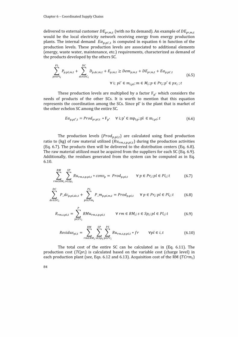
Chapter 6 – Coordinated Supply Chains
84
delivered to external customer , , (with no fix demand). An example of , , would be the local electricity network receiving energy from energy production plants. The internal demand , ´, is computed in equation 6 in function of the production levels. These production levels are associated to additional elements (energy, waste water, maintenance, etc.) requirements, characterized as demand of the products developed by the others SC.
, , , , , , , , , , , , , ´,
i; ´ , ; ; ; ;
(6.5)
These production levels are multiplied by a factor F which considers the needs of products of the other SCs. It is worth to mention that this equation represents the coordination among the SCs. Since pl’ is the plant that is market of the other echelon SC among the entire SC.
, , , , F i; p mp , ; pl m , ; (6.6)
The production levels ( , , ) are calculated using fixed production ratio to (kg) of raw material utilized ( , , , , ) during the production activities (Eq. 6.7). The products then will be delivered to the distribution centers (Eq. 6.8). The raw material utilized must be acquired from the suppliers for each SC (Eq. 6.9). Additionally, the residues generated from the system can be computed as in Eq. 6.10.
, , , , , , ; ; (6.7)
_ , , , _ , , , , , ; ; (6.8)
, , , , , , , ; ; ; (6.9)
, , , , , , (6.10)
The total cost of the entire SC can be calculated as in (Eq. 6.11). The production cost (TCpri) is calculated based on the variable cost (charge level) in each production plant (see, Eqs. 6.12 and 6.13). Acquisition cost of the RM ( )
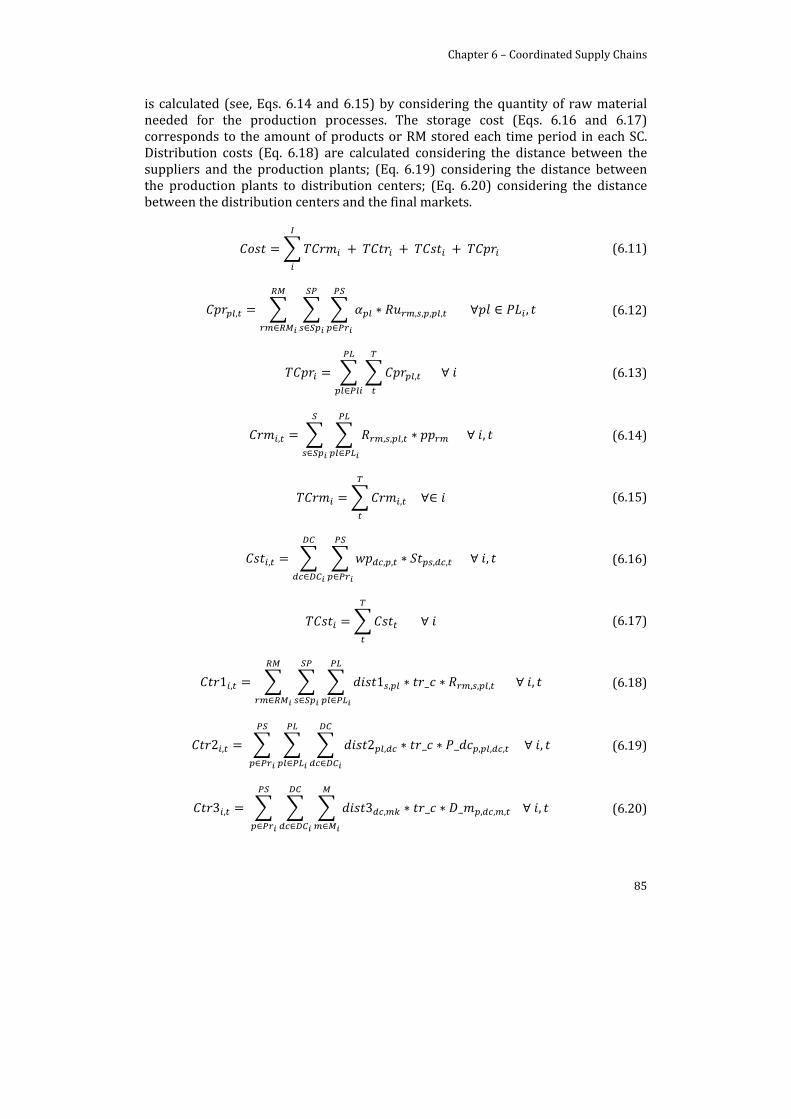
Chapter 6 – Coordinated Supply Chains
85
is calculated (see, Eqs. 6.14 and 6.15) by considering the quantity of raw material needed for the production processes. The storage cost (Eqs. 6.16 and 6.17) corresponds to the amount of products or RM stored each time period in each SC. Distribution costs (Eq. 6.18) are calculated considering the distance between the suppliers and the production plants; (Eq. 6.19) considering the distance between the production plants to distribution centers; (Eq. 6.20) considering the distance between the distribution centers and the final markets.
(6.11)
, , , , , , (6.12)
, (6.13)
, , , , , (6.14)
, (6.15)
, , , , , , (6.16)
(6.17)
1 , 1 , _ , , , , (6.18)
2 , 2 , _ _ , , , , (6.19)
3 , 3 , _ _ , , , , (6.20)
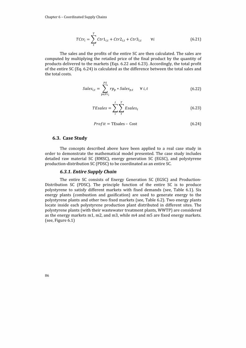
Chapter 6 – Coordinated Supply Chains
86
1 , 2 , 3 , (6.21)
The sales and the profits of the entire SC are then calculated. The sales are computed by multiplying the retailed price of the final product by the quantity of products delivered to the markets (Eqs. 6.22 and 6.23). Accordingly, the total profit of the entire SC (Eq. 6.24) is calculated as the difference between the total sales and the total costs.
, , , (6.22)
(6.23)
TEsales – Cost (6.24)
6.3. Case Study
The concepts described above have been applied to a real case study in order to demonstrate the mathematical model presented. The case study includes detailed raw material SC (RMSC), energy generation SC (EGSC), and polystyrene production‐distribution SC (PDSC) to be coordinated as an entire SC.
6.3.1. Entire Supply Chain
The entire SC consists of Energy Generation SC (EGSC) and Production‐Distribution SC (PDSC). The principle function of the entire SC is to produce polystyrene to satisfy different markets with fixed demands (see, Table 6.1). Six energy plants (combustion and gasification) are used to generate energy to the polystyrene plants and other two fixed markets (see, Table 6.2). Two energy plants locate inside each polystyrene production plant distributed in different sites. The polystyrene plants (with their wastewater treatment plants, WWTP) are considered as the energy markets m1, m2, and m3, while m4 and m5 are fixed energy markets. (see, Figure 6.1)
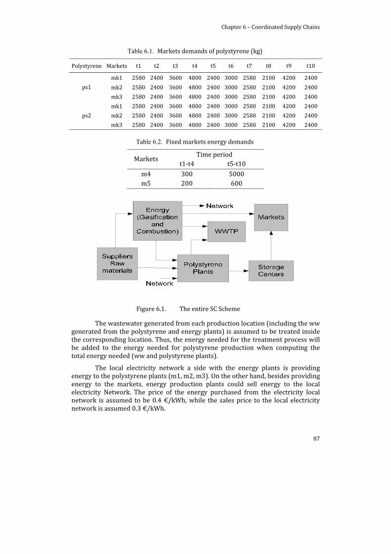
Chapter 6 – Coordinated Supply Chains
87
Table 6.1. Markets demands of polystyrene (kg)
Polystyrene Markets t1 t2 t3 t4 t5 t6 t7 t8 t9 t10
ps1
mk1 2580 2400 3600 4800 2400 3000 2580 2100 4200 2400
mk2 2580 2400 3600 4800 2400 3000 2580 2100 4200 2400
mk3 2580 2400 3600 4800 2400 3000 2580 2100 4200 2400
ps2
mk1 2580 2400 3600 4800 2400 3000 2580 2100 4200 2400
mk2 2580 2400 3600 4800 2400 3000 2580 2100 4200 2400
mk3 2580 2400 3600 4800 2400 3000 2580 2100 4200 2400
Table 6.2. Fixed markets energy demands
Markets Time period
t1‐t4 t5‐t10
m4 300 5000 m5 200 600
Figure 6.1. The entire SC Scheme
The wastewater generated from each production location (including the ww generated from the polystyrene and energy plants) is assumed to be treated inside the corresponding location. Thus, the energy needed for the treatment process will be added to the energy needed for polystyrene production when computing the total energy needed (ww and polystyrene plants).
The local electricity network a side with the energy plants is providing energy to the polystyrene plants (m1, m2, m3). On the other hand, besides providing energy to the markets, energy production plants could sell energy to the local electricity Network. The price of the energy purchased from the electricity local network is assumed to be 0.4 €/kWh, while the sales price to the local electricity network is assumed 0.3 €/kWh.
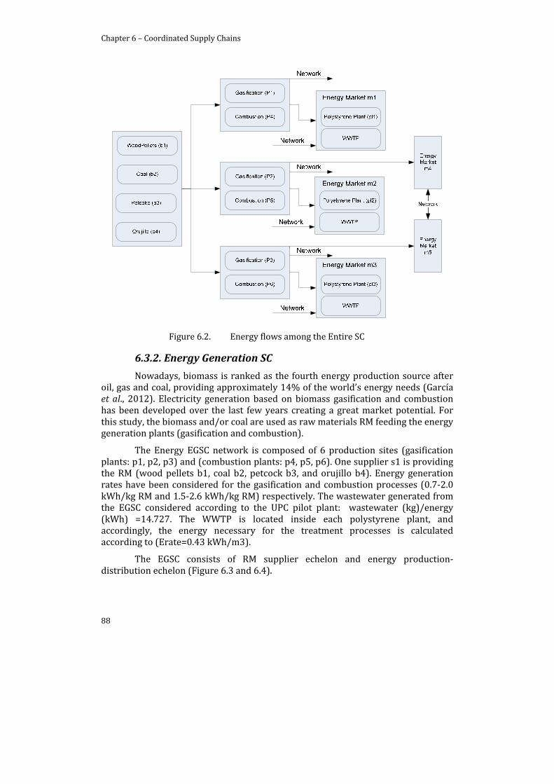
Chapter 6 – Coordinated Supply Chains
88
Figure 6.2. Energy flows among the Entire SC
6.3.2. Energy Generation SC
Nowadays, biomass is ranked as the fourth energy production source after oil, gas and coal, providing approximately 14% of the world’s energy needs (García et al., 2012). Electricity generation based on biomass gasification and combustion has been developed over the last few years creating a great market potential. For this study, the biomass and/or coal are used as raw materials RM feeding the energy generation plants (gasification and combustion).
The Energy EGSC network is composed of 6 production sites (gasification plants: p1, p2, p3) and (combustion plants: p4, p5, p6). One supplier s1 is providing the RM (wood pellets b1, coal b2, petcock b3, and orujillo b4). Energy generation rates have been considered for the gasification and combustion processes (0.7‐2.0 kWh/kg RM and 1.5‐2.6 kWh/kg RM) respectively. The wastewater generated from the EGSC considered according to the UPC pilot plant: wastewater (kg)/energy (kWh) =14.727. The WWTP is located inside each polystyrene plant, and accordingly, the energy necessary for the treatment processes is calculated according to (Erate=0.43 kWh/m3).
The EGSC consists of RM supplier echelon and energy production‐distribution echelon (Figure 6.3 and 6.4).
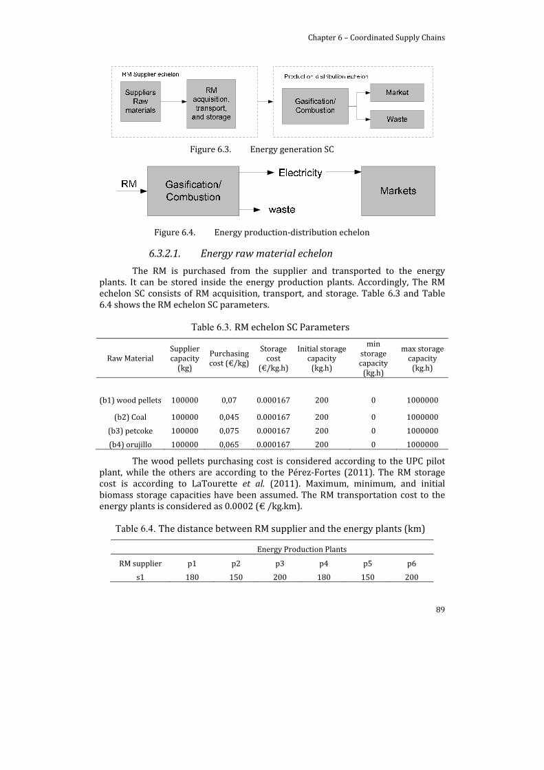
Chapter 6 – Coordinated Supply Chains
89
Figure 6.3. Energy generation SC
Figure 6.4. Energy production‐distribution echelon
6.3.2.1. Energy raw material echelon
The RM is purchased from the supplier and transported to the energy plants. It can be stored inside the energy production plants. Accordingly, The RM echelon SC consists of RM acquisition, transport, and storage. Table 6.3 and Table 6.4 shows the RM echelon SC parameters.
Table 6.3. RM echelon SC Parameters
Raw Material Supplier capacity (kg)
Purchasing cost (€/kg)
Storage cost
(€/kg.h)
Initial storage capacity (kg.h)
min storage capacity (kg.h)
max storage capacity (kg.h)
(b1) wood pellets 100000 0,07 0.000167 200 0 1000000
(b2) Coal 100000 0,045 0.000167 200 0 1000000
(b3) petcoke 100000 0,075 0.000167 200 0 1000000
(b4) orujillo 100000 0,065 0.000167 200 0 1000000
The wood pellets purchasing cost is considered according to the UPC pilot plant, while the others are according to the Pérez‐Fortes (2011). The RM storage cost is according to LaTourette et al. (2011). Maximum, minimum, and initial biomass storage capacities have been assumed. The RM transportation cost to the energy plants is considered as 0.0002 (€ /kg.km).
Table 6.4. The distance between RM supplier and the energy plants (km)
Energy Production Plants
RM supplier p1 p2 p3 p4 p5 p6
s1 180 150 200 180 150 200
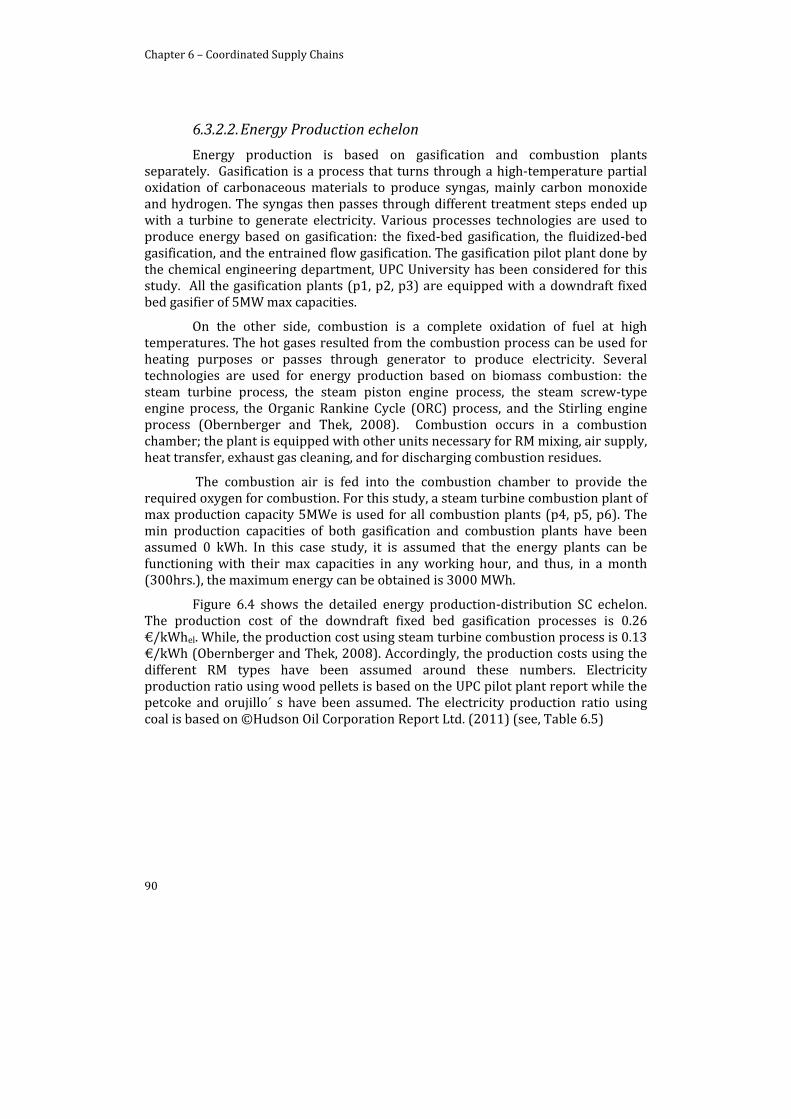
Chapter 6 – Coordinated Supply Chains
90
6.3.2.2. Energy Production echelon
Energy production is based on gasification and combustion plants separately. Gasification is a process that turns through a high‐temperature partial oxidation of carbonaceous materials to produce syngas, mainly carbon monoxide and hydrogen. The syngas then passes through different treatment steps ended up with a turbine to generate electricity. Various processes technologies are used to produce energy based on gasification: the fixed‐bed gasification, the fluidized‐bed gasification, and the entrained flow gasification. The gasification pilot plant done by the chemical engineering department, UPC University has been considered for this study. All the gasification plants (p1, p2, p3) are equipped with a downdraft fixed bed gasifier of 5MW max capacities.
On the other side, combustion is a complete oxidation of fuel at high temperatures. The hot gases resulted from the combustion process can be used for heating purposes or passes through generator to produce electricity. Several technologies are used for energy production based on biomass combustion: the steam turbine process, the steam piston engine process, the steam screw‐type engine process, the Organic Rankine Cycle (ORC) process, and the Stirling engine process (Obernberger and Thek, 2008). Combustion occurs in a combustion chamber; the plant is equipped with other units necessary for RM mixing, air supply, heat transfer, exhaust gas cleaning, and for discharging combustion residues.
The combustion air is fed into the combustion chamber to provide the required oxygen for combustion. For this study, a steam turbine combustion plant of max production capacity 5MWe is used for all combustion plants (p4, p5, p6). The min production capacities of both gasification and combustion plants have been assumed 0 kWh. In this case study, it is assumed that the energy plants can be functioning with their max capacities in any working hour, and thus, in a month (300hrs.), the maximum energy can be obtained is 3000 MWh.
Figure 6.4 shows the detailed energy production‐distribution SC echelon. The production cost of the downdraft fixed bed gasification processes is 0.26 €/kWhel. While, the production cost using steam turbine combustion process is 0.13 €/kWh (Obernberger and Thek, 2008). Accordingly, the production costs using the different RM types have been assumed around these numbers. Electricity production ratio using wood pellets is based on the UPC pilot plant report while the petcoke and orujillo´ s have been assumed. The electricity production ratio using coal is based on ©Hudson Oil Corporation Report Ltd. (2011) (see, Table 6.5)
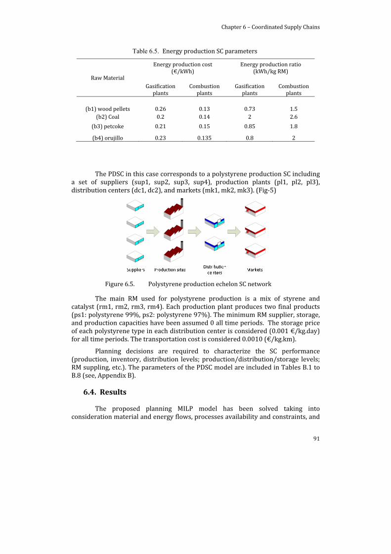
Chapter 6 – Coordinated Supply Chains
91
Table 6.5. Energy production SC parameters
Raw Material
Energy production cost (€/kWh)
Energy production ratio (kWh/kg RM)
Gasification plants
Combustion plants
Gasification plants
Combustion plants
(b1) wood pellets 0.26 0.13 0.73 1.5 (b2) Coal 0.2 0.14 2 2.6
(b3) petcoke 0.21 0.15 0.85 1.8
(b4) orujillo 0.23 0.135 0.8 2
The PDSC in this case corresponds to a polystyrene production SC including a set of suppliers (sup1, sup2, sup3, sup4), production plants (pl1, pl2, pl3), distribution centers (dc1, dc2), and markets (mk1, mk2, mk3). (Fig‐5)
Figure 6.5. Polystyrene production echelon SC network
The main RM used for polystyrene production is a mix of styrene and catalyst (rm1, rm2, rm3, rm4). Each production plant produces two final products (ps1: polystyrene 99%, ps2: polystyrene 97%). The minimum RM supplier, storage, and production capacities have been assumed 0 all time periods. The storage price of each polystyrene type in each distribution center is considered (0.001 €/kg.day) for all time periods. The transportation cost is considered 0.0010 (€/kg.km).
Planning decisions are required to characterize the SC performance (production, inventory, distribution levels; production/distribution/storage levels; RM suppling, etc.). The parameters of the PDSC model are included in Tables B.1 to B.8 (see, Appendix B).
6.4. Results
The proposed planning MILP model has been solved taking into consideration material and energy flows, processes availability and constraints, and

Chapter 6 – Coordinated Supply Chains
92
distribution tasks over a time horizon of 10 months. The resulted model reflects the optimal performance of each echelon SC among the entire SC. In order to highlight the proposed approach, the optimal planning decisions (RM acquisition, storage, production, and distribution) have been obtained for two scenarios: a) Non‐coordinated SCs: each echelon SC (Biomass SC, EGSC, PDSC) has been solved separately and the total cost of each one is obtained. b) Coordinated SCs: each echelon SC is coordinated with each other forming the entire SC model, and thus the total cost of the coordinated entire SC is obtained. Both scenarios will be discussed in details in sections 6.4.1 and 6.4.2 respectively. The main objective function in both scenarios is to minimize the total cost. In the first scenario, the total cost of the separate echelons SCs are minimized, while the second scenario aims to minimize the total cost of the coordinated “entire SC”. A comparison between the planning decisions for both scenarios will take place in the following sections to point out the potential of the SCs coordination.
6.4.1. Noncoordinated scenario
It is worth mentioning that the PDSC is the main SC of the problem and can be solved without considering the EGSC (by computing the theoretical energy needed for the production). The Polystyrene SC has been solved separately to attend the polystyrene market demands with minimum cost. Accordingly, the typical decisions behavior is expected to be in favor of the cheapest RM and the least distribution cost (distance between supplier‐production plants‐distribution centers‐markets).
Figure 6.6. Production levels of (a) polystyrene 97 and (b) polystyrene 99
0
100
200
300
t1 t2 t3 t4 t5 t6 t7 t8 t9 t10
Production of
Polystyrene 97
(tons)
Time period (months)
pl1
pl2
pl3
0
100
200
300
t1 t2 t3 t4 t5 t6 t7 t8 t9 t10
Production of
polystyrene 99
(tons)
Time period (months)
pl1
pl2
pl3
(a
(b
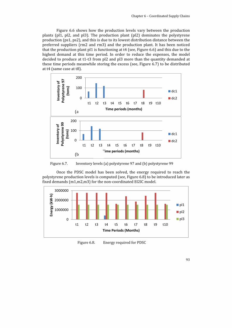
Chapter 6 – Coordinated Supply Chains
93
Figure 6.6 shows how the production levels vary between the production plants (pl1, pl2, and pl3). The production plant (pl2) dominates the polystyrene production (ps1, ps2), and this is due to its lowest distribution distance between the preferred suppliers (rm2 and rm3) and the production plant. It has been noticed that the production plant pl1 is functioning at t4 (see, Figure 6.6) and this due to the highest demand at this time period. In order to reduce the expenses, the model decided to produce at t1‐t3 from pl2 and pl3 more than the quantity demanded at these time periods meanwhile storing the excess (see, Figure 6.7) to be distributed at t4 (same case at t8).
Figure 6.7. Inventory levels (a) polystyrene 97 and (b) polystyrene 99
Once the PDSC model has been solved, the energy required to reach the polystyrene production levels is computed (see, Figure 6.8) to be introduced later as fixed demands (m1,m2,m3) for the non‐coordinated EGSC model.
Figure 6.8. Energy required for PDSC
0
100
200
t1 t2 t3 t4 t5 t6 t7 t8 t9 t10
Inventory of
Polystyrene 97
(tons)
Time periods (months)
dc1
dc2
0
100
200
t1 t2 t3 t4 t5 t6 t7 t8 t9 t10
Inventory of
Polystyrene 99
(tons)
Time periods (months)
dc1
dc2
0
1000000
2000000
3000000
t1 t2 t3 t4 t5 t6 t7 t8 t9 t10
Energy (kW∙h)
Time Periods (Months)
pl1
pl2
pl3
(a
(b
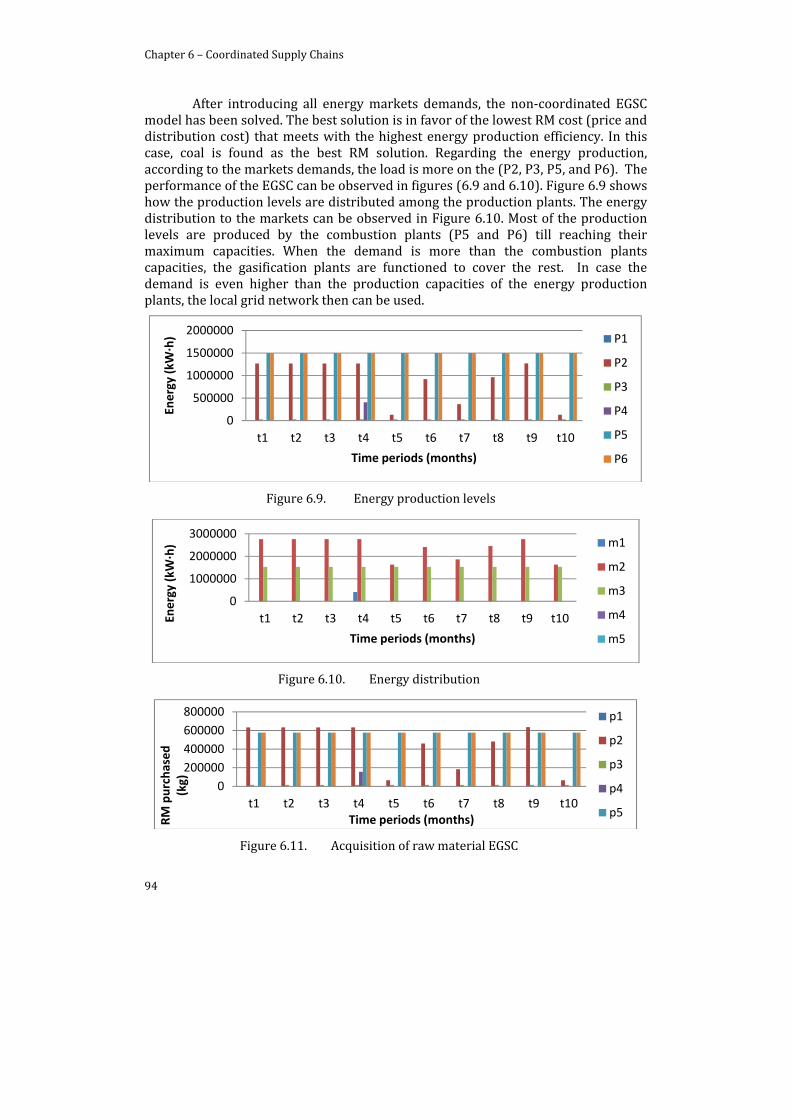
Chapter 6 – Coordinated Supply Chains
94
After introducing all energy markets demands, the non‐coordinated EGSC model has been solved. The best solution is in favor of the lowest RM cost (price and distribution cost) that meets with the highest energy production efficiency. In this case, coal is found as the best RM solution. Regarding the energy production, according to the markets demands, the load is more on the (P2, P3, P5, and P6). The performance of the EGSC can be observed in figures (6.9 and 6.10). Figure 6.9 shows how the production levels are distributed among the production plants. The energy distribution to the markets can be observed in Figure 6.10. Most of the production levels are produced by the combustion plants (P5 and P6) till reaching their maximum capacities. When the demand is more than the combustion plants capacities, the gasification plants are functioned to cover the rest. In case the demand is even higher than the production capacities of the energy production plants, the local grid network then can be used.
Figure 6.9. Energy production levels
Figure 6.10. Energy distribution
Figure 6.11. Acquisition of raw material EGSC
0
500000
1000000
1500000
2000000
t1 t2 t3 t4 t5 t6 t7 t8 t9 t10
Energy (kW∙h)
Time periods (months)
P1
P2
P3
P4
P5
P6
0
1000000
2000000
3000000
t1 t2 t3 t4 t5 t6 t7 t8 t9 t10Energy (kW∙h)
Time periods (months)
m1
m2
m3
m4
m5
0
200000
400000
600000
800000
t1 t2 t3 t4 t5 t6 t7 t8 t9 t10
RM purchased
(kg)
Time periods (months)
p1
p2
p3
p4
p5
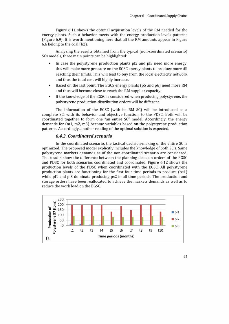
Chapter 6 – Coordinated Supply Chains
95
Figure 6.11 shows the optimal acquisition levels of the RM needed for the energy plants. Such a behavior meets with the energy production levels patterns (Figure 6.9). It is worth mentioning here that all the RM amounts appear in Figure 6.6 belong to the coal (b2).
Analyzing the results obtained from the typical (non‐coordinated scenario) SCs models, three main points can be highlighted:
In case the polystyrene production plants pl2 and pl3 need more energy, this will make more pressure on the EGSC energy plants to produce more till reaching their limits. This will lead to buy from the local electricity network and thus the total cost will highly increase.
Based on the last point, The EGCS energy plants (p5 and p6) need more RM and thus will become close to reach the RM supplier capacity.
If the knowledge of the EGSC is considered when producing polystyrene, the polystyrene production‐distribution orders will be different.
The information of the EGSC (with its RM SC) will be introduced as a complete SC, with its behavior and objective function, to the PDSC. Both will be coordinated together to form one “an entire SC” model. Accordingly, the energy demands for (m1, m2, m3) become variables based on the polystyrene production patterns. Accordingly, another reading of the optimal solution is expected.
6.4.2. Coordinated scenario
In the coordinated scenario, the tactical decision‐making of the entire SC is optimized. The proposed model explicitly includes the knowledge of both SC’s. Same polystyrene markets demands as of the non‐coordinated scenario are considered. The results show the difference between the planning decision orders of the EGSC and PDSC for both scenarios coordinated and coordinated. Figure 6.12 shows the production levels of the PDSC when coordinated with the EGSC. All polystyrene production plants are functioning for the first four time periods to produce (ps1) while pl1 and pl3 dominate producing ps2 in all time periods. The production and storage orders have been reallocated to achieve the markets demands as well as to reduce the work load on the EGSC.
0
50
100
150
200
250
t1 t2 t3 t4 t5 t6 t7 t8 t9 t10
Production of
Polystyrene 97 (tons)
Time periods (months)
pl1
pl2
pl3
(a
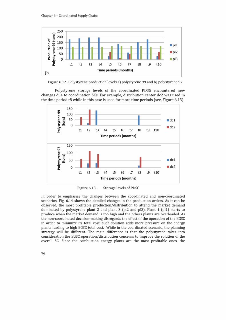
Chapter 6 – Coordinated Supply Chains
96
Figure 6.12. Polystyrene production levels a) polystyrene 99 and b) polystyrene 97
Polystyrene storage levels of the coordinated PDSG encountered new changes due to coordination SCs. For example, distribution center dc2 was used in the time period t8 while in this case is used for more time periods (see, Figure 6.13).
Figure 6.13. Storage levels of PDSC
In order to emphasize the changes between the coordinated and non‐coordinated scenarios, Fig. 6.14 shows the detailed changes in the production orders. As it can be observed, the most profitable production/distribution to attend the market demand dominated by polystyrene plant 2 and plant 3 (pl2 and pl3). Plant 1 (pl1) starts to produce when the market demand is too high and the others plants are overloaded. As the non‐coordinated decision‐making disregards the effect of the operation of the EGSC in order to minimize its total cost, such solution adds more pressure on the energy plants leading to high EGSC total cost. While in the coordinated scenario, the planning strategy will be different. The main difference is that the polystyrene takes into consideration the EGSC operation/distribution concerns to improve the solution of the overall SC. Since the combustion energy plants are the most profitable ones, the
0
50
100
150
200
250
t1 t2 t3 t4 t5 t6 t7 t8 t9 t10
Production of
Polystyrene 99 (tons)
Time periods (months)
pl1
pl2
pl3
0
50
100
150
t1 t2 t3 t4 t5 t6 t7 t8 t9 t10
Polystyrene 99
(tons)
Time periods (months)
dc1
dc2
0
50
100
150
t1 t2 t3 t4 t5 t6 t7 t8 t9 t10
Polystyrene 97
(tons)
Time periods (months)
dc1
dc2
(b

Chapter 6 – Coordinated Supply Chains
97
polystyrene production (market demand for the EGSC) is being distributed among all polystyrene plants to exploit all the combustion plants (in the non‐coordinated the combustion technology has been unexploited). Gasification plants are functioning to avoid the use of the local network.
Figure 6.14. Polystyrene production comparison (%, non‐coordinated/coordinated scenarios)
6.4.3. Economical Analysis
In the “coordinated” scenario, all the information of both SCs (costs and constraints) has been included into the problem model. The optimal solution corresponds to producing polystyrene using most of the energy available from the green energy generation plants (within energy plants capacities). The economic results reveal that the coordination between the PDSC and the EGSC improves the “entire SC” total cost with 2.46% during 10 months with a total savings of 434,169 € (see, Table 6.6).
As it can be observed from Figure 6.15, the coordinated SCs behave inside the model in favor of the most profitable performance of the entire SC. They both
0%
20%
40%
60%
80%
100%
t1 t2 t3 t4 t5 t6 t7 t8 t9 t10% Polystyrene production
Non‐coordinated scenario
ps‐97 pl3
ps‐97 pl2
ps‐97 pl1
ps‐99 pl3
ps‐99 pl2
ps‐99 pl1
0%
20%
40%
60%
80%
100%
t1 t2 t3 t4 t5 t6 t7 t8 t9 t10
% Polystyrene production
Coordinated scenario
ps‐97 pl3
ps‐97 pl2
ps‐97 pl1
ps‐99 pl3
ps‐99 pl2
ps‐99 pl1
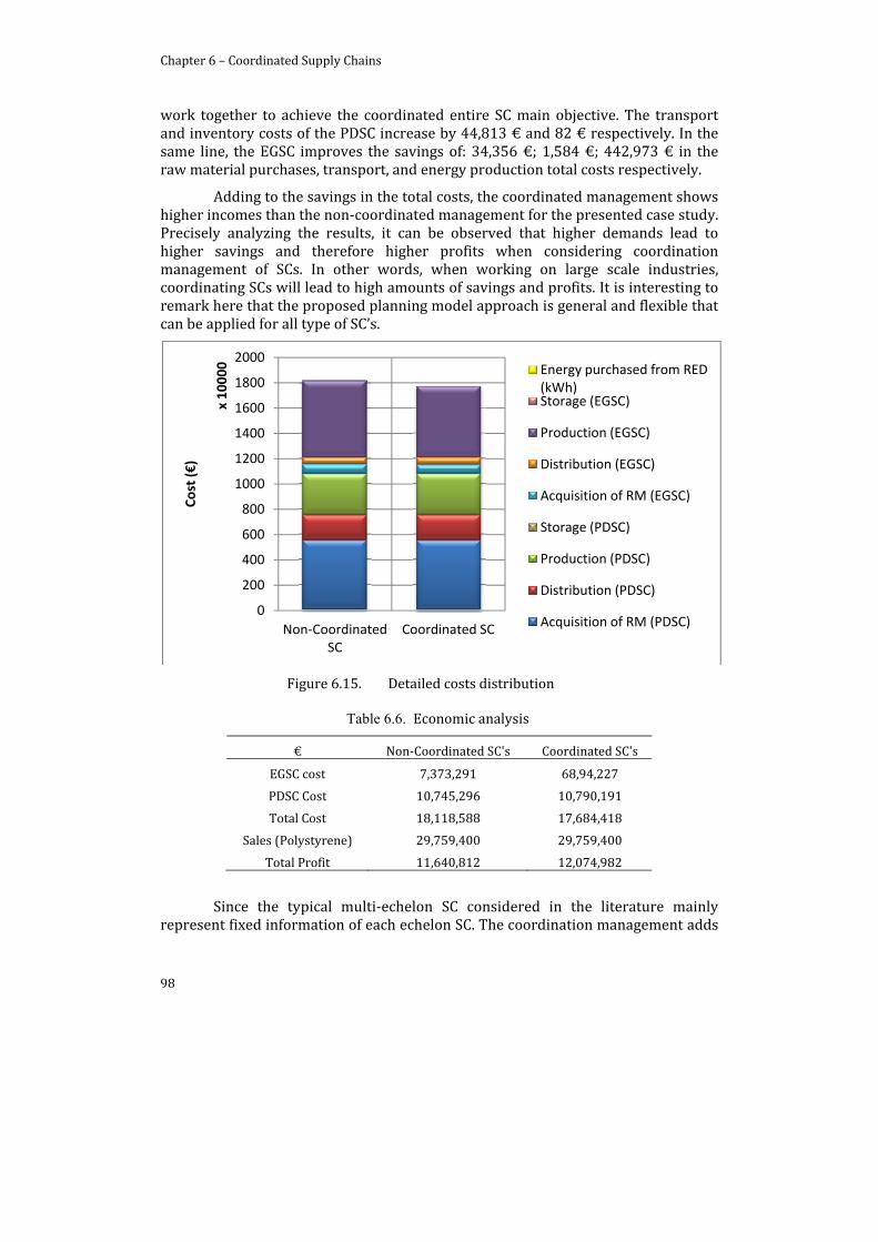
Chapter 6 – Coordinated Supply Chains
98
work together to achieve the coordinated entire SC main objective. The transport and inventory costs of the PDSC increase by 44,813 € and 82 € respectively. In the same line, the EGSC improves the savings of: 34,356 €; 1,584 €; 442,973 € in the raw material purchases, transport, and energy production total costs respectively.
Adding to the savings in the total costs, the coordinated management shows higher incomes than the non‐coordinated management for the presented case study. Precisely analyzing the results, it can be observed that higher demands lead to higher savings and therefore higher profits when considering coordination management of SCs. In other words, when working on large scale industries, coordinating SCs will lead to high amounts of savings and profits. It is interesting to remark here that the proposed planning model approach is general and flexible that can be applied for all type of SC’s.
Figure 6.15. Detailed costs distribution
Table 6.6. Economic analysis
€ Non‐Coordinated SC's Coordinated SC's
EGSC cost 7,373,291 68,94,227
PDSC Cost 10,745,296 10,790,191
Total Cost 18,118,588 17,684,418
Sales (Polystyrene) 29,759,400 29,759,400
Total Profit 11,640,812 12,074,982
Since the typical multi‐echelon SC considered in the literature mainly represent fixed information of each echelon SC. The coordination management adds
0
200
400
600
800
1000
1200
1400
1600
1800
2000
Non‐Coordinated SC
Coordinated SC
Cost (€)
x 10000 Energy purchased from RED
(kWh)Storage (EGSC)
Production (EGSC)
Distribution (EGSC)
Acquisition of RM (EGSC)
Storage (PDSC)
Production (PDSC)
Distribution (PDSC)
Acquisition of RM (PDSC)
Chapter 6 – Coordinated Supply Chains
99
to the PSC science a new profitable approach able to consider the characteristics of all enterprises sharing in the system.
6.5. Conclusions
A new perspective has been studied in this Chapter towards “Coordinated Supply Chain Management, (CSCM)”. Many echelons SCs have been coordinated together forming one “coordinated entire multi‐echelon SC” model. The main characteristics of each echelon “enterprise” SC is considered and coordinated while optimizing the total cost of the entire SC. The proposed planning model is able to integrate the objectives of all echelons SCs among one final objective function. The behavior of all echelons SCs when studied separately is found different than when integrated among one single SC, and such behavior affects the decisions orders. Furthermore, it has been found that the coordinated planning model improves cheaper decision orders.
This work provides a novel MILP model that can be applied to solve and optimize all kinds of multi‐echelon SC planning problems. The resulted model is flexible enough to allow a coordinated management of the production, storage and distribution tasks and thus helps in improving the global benefit of the new “coordinated” SC. All enterprises affect the final decisions and thus the new approach gives them the opportunity to share responsibilities. The proposed approach has been proved by applying to a real case study industrial SC (biomass acquisition, energy generation, production–distribution industry, and waste treatment).
Finally, the “CSCM” approach adds to the PSE community an important tool can be extended towards optimal use of natural resources, optimal energy production, and best industrial production‐distribution management. Further work must increase the complexity associated to the acquisition raw material‐product among each SC, discount prices can be used in order to model several scenarios of cooperation. The proposed model can be applied to extended case studies including more SC echelons. In order to obtain a robust tool to exploit this novel approach Also Multi‐objective Optimization must be applied.
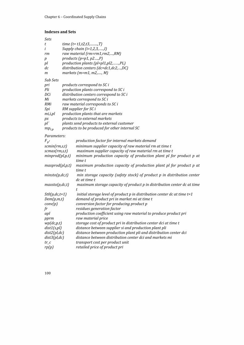
Chapter 6 – Coordinated Supply Chains
100
Indexes and Sets
Sets t time (t= t1,t2,t3,……..,T) i Supply chain (i=1,2,3,…..,I) rm raw material (rm=rm1,rm2,…,RM) p products (p=p1, p2….,P) pl production plants (pl=pl1,pl2,……,PL) dc distribution centers (dc=dc1,dc2,…,DC) m markets (m=m1, m2,....., M)
Sub Sets pri products correspond to SC i Pli production plants correspond to SC i DCi distribution centers correspond to SC i Mi markets correspond to SC i RMi raw material corresponds to SC i Spi RM supplier for SC i mi,i,pl production plants that are markets px products to external markets pl´ plants send products to external customer
, products to be produced for other internal SC
Parameters: production factor for internal markets demand
scmin(rm,s,t) minimum supplier capacity of raw material rm at time t scmax(rm,s,t) maximum supplier capacity of raw material rm at time t minprod(pl,p,t) minimum production capacity of production plant pl for product p at
time t maxprod(pl,p,t) maximum production capacity of production plant pl for product p at
time t minsto(p,dc,t) min storage capacity (safety stock) of product p in distribution center
dc at time t maxsto(p,dc,t) maximum storage capacity of product p in distribution center dc at time
t St0(p,dc,t=1) initial storage level of product p in distribution center dc at time t=1 Dem(p,m,t) demand of product pri in market mi at time t conv(p) conversion factor for producing product p fr residues generation factor αpl production coefficient using raw material to produce product pri pprm raw material price wp(dc,p,t) storage cost of product pri in distribution center dci at time t dist1(s,pl) distance between supplier si and production plant pli dist2(pl,dc) distance between production plant pli and distribution center dci dist3(pl,dc) distance between distribution center dci and markets mi tr_c transport cost per product unit rp(p) retailed price of product pri
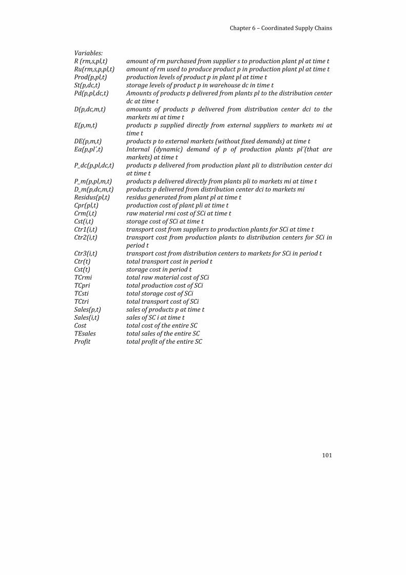
Chapter 6 – Coordinated Supply Chains
101
Variables: R (rm,s,pl,t) amount of rm purchased from supplier s to production plant pl at time t Ru(rm,s,p,pl,t) amount of rm used to produce product p in production plant pl at time t Prod(p,pl,t) production levels of product p in plant pl at time t St(p,dc,t) storage levels of product p in warehouse dc in time t Pd(p,pl,dc,t) Amounts of products p delivered from plants pl to the distribution center
dc at time t D(p,dc,m,t) amounts of products p delivered from distribution center dci to the
markets mi at time t E(p,m,t) products p supplied directly from external suppliers to markets mi at
time t DE(p,m,t) products p to external markets (without fixed demands) at time t Eα(p,pl´,t) Internal (dynamic) demand of p of production plants pl´(that are
markets) at time t P_dc(p,pl,dc,t) products p delivered from production plant pli to distribution center dci
at time t P_m(p,pl,m,t) products p delivered directly from plants pli to markets mi at time t D_m(p,dc,m,t) products p delivered from distribution center dci to markets mi Residus(pl,t) residus generated from plant pl at time t Cpr(pl,t) production cost of plant pli at time t Crm(i,t) raw material rmi cost of SCi at time t Cst(i,t) storage cost of SCi at time t Ctr1(i,t) transport cost from suppliers to production plants for SCi at time t Ctr2(i,t) transport cost from production plants to distribution centers for SCi in
period t Ctr3(i,t) transport cost from distribution centers to markets for SCi in period t Ctr(t) total transport cost in period t Cst(t) storage cost in period t TCrmi total raw material cost of SCi TCpri total production cost of SCi TCsti total storage cost of SCi TCtri total transport cost of SCi Sales(p,t) sales of products p at time t Sales(i,t) sales of SC i at time t Cost total cost of the entire SC TEsales total sales of the entire SC Profit total profit of the entire SC

Part III Cooperative and Competitive SC’s

105
Chapter 7. SC’s in a Competitive Environment
The novel optimization framework developed in this Chapter intends to exploit the cooperation and competition among several Supply Chains. In order to state the cooperation and competition applied to SC problems and prove the applicability of the proposed framework, two approaches are presented in this Chapter:
Section 7.1 considers the tactical SCM under cooperation and competition scenarios, where the production, storage and distribution levels of several SCs have been optimized under the presence of uncertainty.
Section 7.2 shows the cooperation and competition at the operational decision‐making level. The proposed model includes operation and distribution management of several SC’s under uncertain behavior.
The uncertainty associated to the competitors’ behavior (decisions of the others SCs) has been considered: Section 1 uses the market price as the parameter to capture the uncertain behavior, while, Section 2 uses the product quality. The use of Mathematical programming and Game Theory as optimization tools also have been exploited in both approaches.
In the real word is difficult to consider that all operation and market information could be shared by the enterprises. But, Holland (1995) has described that electronic market is characterized by privileged access to market data by small groups of vertically arranged companies that develop closer relationships, and this shared information will reduce the coordination costs of search and evaluate competing product offerings. Additionally, these information sharing practices will allow the enterprises to work with several suppliers. Then companies will gain the advantages of increase the market incentive and lead to lower costs.
7.1. Cooperative and Competitive SC planning
7.1.1. Introduction
The decision‐making problem in the process industry is becoming more complex as the scope covered by these decisions is extended. This increasing complexity is additionally complicated by the need to consider a greater degree of uncertainty in the models used to forecast the events that should be considered in this decision‐making (see, Figure 2.1). In the case of the Chemical Processes Industry, the complexity associated to chemical operations and the market globalization should be added to the usual difficulties related to the integration of
Chapter 7 – SC’s in a Competitive Environment
106
various objectives to be considered. So, in this sense, the problem of decision‐making tactical management associated to SC (procurement of raw materials in different markets, allocation of products to different plants and distributing them to different customers), which have attracted the attention of the scientific community in the last years, is on the top level of complexity.
Market globalization imposes the need to consider some of the above mentioned elements from a new perspective: new objectives should be considered, different from the ones typically applicable to the individual SC echelons, like financial aspects (Laínez et al., 2007). Also the market uncertainty should be managed taking into account the roles of many different players, and the vertical integration should include a much larger scope (at plant and SC level, Chapter 4 and Chapter 5, respectively). On the other hand, as described in section 2 studying the problems that industry deals with and applying fast and reliable optimization techniques to find isolated robust solutions is not enough: SCs are embedded in a competitive market, and managers have to take care of the decisions made by third parties (known or uncertain), since these decisions will impact on the profit of their own SC. This complex scenario is specifically addressed by the Game Theory (GT) strategy, to analyze the eventual success of some decisions among other alternatives. This approach has been widely proposed by researchers and practitioners to develop systematic procedures to assist decision‐makers (Nagarajan and Socîs, 2008; Cachon, 2004).
This section is focused on the systematic consideration of some of the above mentioned elements (uncertainty management and inclusion of third parties into the problem formulation) in the SC planning problem, where decisions are inventory, production and distribution management. A global market scenario should be considered, targeting the benefits and drawbacks of the eventual cooperative work with other SCs, and also their eventual competition. The next section includes a formal introduction to the SC planning problem and to the GT as optimization tool, as well as the main elements of the considered model. Then, Section 7.1.3 illustrates the combined application of these elements and tools to a specific case study, based on an example proposed in literature, and Section 7.1.4 summarizes the main conclusions of this study.
7.1.2. Supply Chain Planning
The typical scope of the SC planning problem is to determine the optimal production levels, inventories and product distribution in an organized network of production sites, distribution centers, consumers, etc. (Figure 1.2), taking care of the constraints associated to products and raw materials availability, storage limits, etc. in such network nodes. (Liang, 2008). The mathematical model associated to this problem usually leads to a mixed‐integer linear program (MILP) whose solution determines the optimal values for the mentioned variables. (see, Section 2.2)
In this Chapter it will be assumed the existence of a set of different Supply Chains that may work in a cooperative or a competitive environment. The model originally proposed by Liang (2008) has been adopted as a basic model for the presented mathematical formulation complemented with additional constraints and
Chapter 7 – SC’s in a Competitive Environment
107
different Objective Functions, according to the considered scenario. In this case, the mathematical constraints associated to the material balances and production/distribution capacities will be the same, as well as the cost structures. A discrete time formulation, which also integrates SCM decision levels, by considering a higher level planning model, with a cyclic time horizon, usually employed to solve this kind of models (Sousa et al., 2008), has been adopted in this work.
So, in summary, the logistic network considered in this model consists of several SCs, each one composed by multiple production sites and distribution centers (fixed locations and capacities). Production sites are able to produce several products to cover a common market demand over a planning horizon H. The capacity of each process is given by available labor levels and equipment capacity for each production site, and the transport between nodes is modeled as a set of trucks with fixed capacity, in which costs and required transporting times are related to the distance between nodes. The planning horizon H is discretized in medium term planning periods, as months.
7.1.2.1. Cooperative and noncooperative Games
In a non‐cooperative scenario, the different organizations are not allowed to make commitments regarding their respective strategies; instead they are competing to get their maximum individual benefit. In the opposite way, cooperative scenarios are associated to the possibility to arrange such commitments, which are dealing with side‐payments and/or other compensation agreements among organizations. In this work, it has been assumed that this second scenario will lead to a perfect integration between SCs when the cooperative game is played. Then, the complete set of SCs will try to minimize the total aggregated cost to achieve the demand of the consumers. The competition behavior will be found when each individual SC tries to maximize its individual benefit and the consumers buy from the cheaper SC.
7.1.2.2. Supply Chain Planning in a cooperative environment
On the basis of above definitions, the application of a multipurpose MILP‐based model for the cooperative case of SCs is proposed, equivalent to the one which should be formulated to solve the individual SC. So, in order to determine the optimal production, storage and distribution levels, a slightly modified version of the formulation proposed by Liang (2008) has been used.
Then, the SC management performance is characterized by the quantities produced at each source Qinh, the inventory levels Winh, the undelivered orders Einh and the quantities arriving to each distribution center Tinhj,. The detailed definition of the different variables and parameters is included in the notation section.
The same final condition assumed in the work of Liang (2008) is considered, imposing that there is not storage at the end of the time horizon. However, in order to better compare the different scenarios studied in this work, the subcontracting service introduced in the original work has not been implemented.
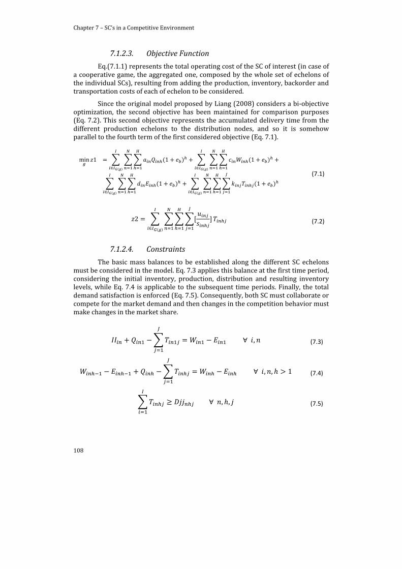
Chapter 7 – SC’s in a Competitive Environment
108
7.1.2.3. Objective Function
Eq.(7.1.1) represents the total operating cost of the SC of interest (in case of a cooperative game, the aggregated one, composed by the whole set of echelons of the individual SCs), resulting from adding the production, inventory, backorder and transportation costs of each of echelon to be considered.
Since the original model proposed by Liang (2008) considers a bi‐objective optimization, the second objective has been maintained for comparison purposes (Eq. 7.2). This second objective represents the accumulated delivery time from the different production echelons to the distribution nodes, and so it is somehow parallel to the fourth term of the first considered objective (Eq. 7.1).
min 1 1 1
1 1
(7.1)
2 (7.2)
7.1.2.4. Constraints
The basic mass balances to be established along the different SC echelons must be considered in the model. Eq. 7.3 applies this balance at the first time period, considering the initial inventory, production, distribution and resulting inventory levels, while Eq. 7.4 is applicable to the subsequent time periods. Finally, the total demand satisfaction is enforced (Eq. 7.5). Consequently, both SC must collaborate or compete for the market demand and then changes in the competition behavior must make changes in the market share.
, (7.3)
, , 1 (7.4)
, , (7.5)
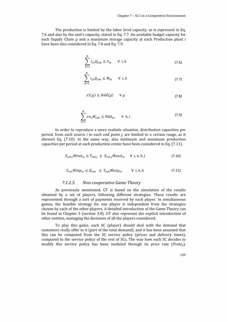
Chapter 7 – SC’s in a Competitive Environment
109
The production is limited by the labor level capacity, as it expressed in Eq. 7.6 and also by the unit’s capacity, stated in Eq. 7.7. An available budget capacity for each Supply Chain g and a maximum storage capacity at each Production plant i have been also considered in Eq. 7.8 and Eq. 7.9.
In order to reproduce a more realistic situation, distribution capacities per period, from each source i to each end point j, are limited to a certain range, as it showed Eq. (7.10). In the same way, also minimum and maximum production capacities per period at each production center have been considered in Eq. (7.11).
7.1.2.5. Noncooperative Game Theory
As previously mentioned, GT is based on the simulation of the results obtained by a set of players, following different strategies. These results are represented through a sort of payments received by each player. In simultaneous games, the feasible strategy for one player is independent from the strategies chosen by each of the other players. A detailed introduction of the Game Theory can be found in Chapter 3 (section 3.8). GT also represent the explicit introduction of other entities, managing the decisions of all the players considered.
To play this game, each SC (player) should deal with the demand that customers really offer to it (part of the total demand), and it has been assumed that this can be computed from the SC service policy (prices and delivery times), compared to the service policy of the rest of SCs. The way how each SC decides to modify this service policy has been modeled through its price rate (Prateg),
, (7.6)
, (7.7)
1 (7.8)
, , (7.9)
, , , (7.10)
, , (7.11)
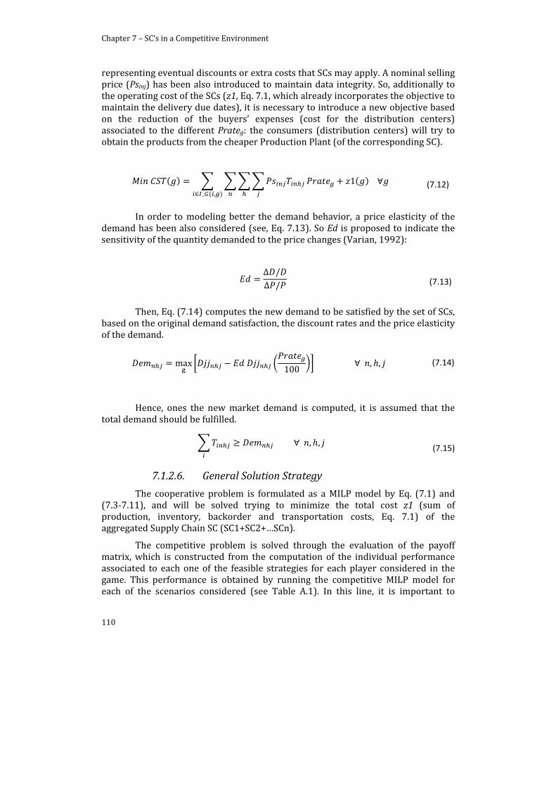
Chapter 7 – SC’s in a Competitive Environment
110
representing eventual discounts or extra costs that SCs may apply. A nominal selling price (Psinj) has been also introduced to maintain data integrity. So, additionally to the operating cost of the SCs (z1, Eq. 7.1, which already incorporates the objective to maintain the delivery due dates), it is necessary to introduce a new objective based on the reduction of the buyers’ expenses (cost for the distribution centers) associated to the different Prateg: the consumers (distribution centers) will try to obtain the products from the cheaper Production Plant (of the corresponding SC).
In order to modeling better the demand behavior, a price elasticity of the demand has been also considered (see, Eq. 7.13). So Ed is proposed to indicate the sensitivity of the quantity demanded to the price changes (Varian, 1992):
Then, Eq. (7.14) computes the new demand to be satisfied by the set of SCs, based on the original demand satisfaction, the discount rates and the price elasticity of the demand.
max100
, , (7.14)
Hence, ones the new market demand is computed, it is assumed that the total demand should be fulfilled.
7.1.2.6. General Solution Strategy
The cooperative problem is formulated as a MILP model by Eq. (7.1) and (7.3‐7.11), and will be solved trying to minimize the total cost z1 (sum of production, inventory, backorder and transportation costs, Eq. 7.1) of the aggregated Supply Chain SC (SC1+SC2+…SCn).
The competitive problem is solved through the evaluation of the payoff matrix, which is constructed from the computation of the individual performance associated to each one of the feasible strategies for each player considered in the game. This performance is obtained by running the competitive MILP model for each of the scenarios considered (see Table A.1). In this line, it is important to
_ ,
1 (7.12)
∆ /∆ /
(7.13)
, , (7.15)
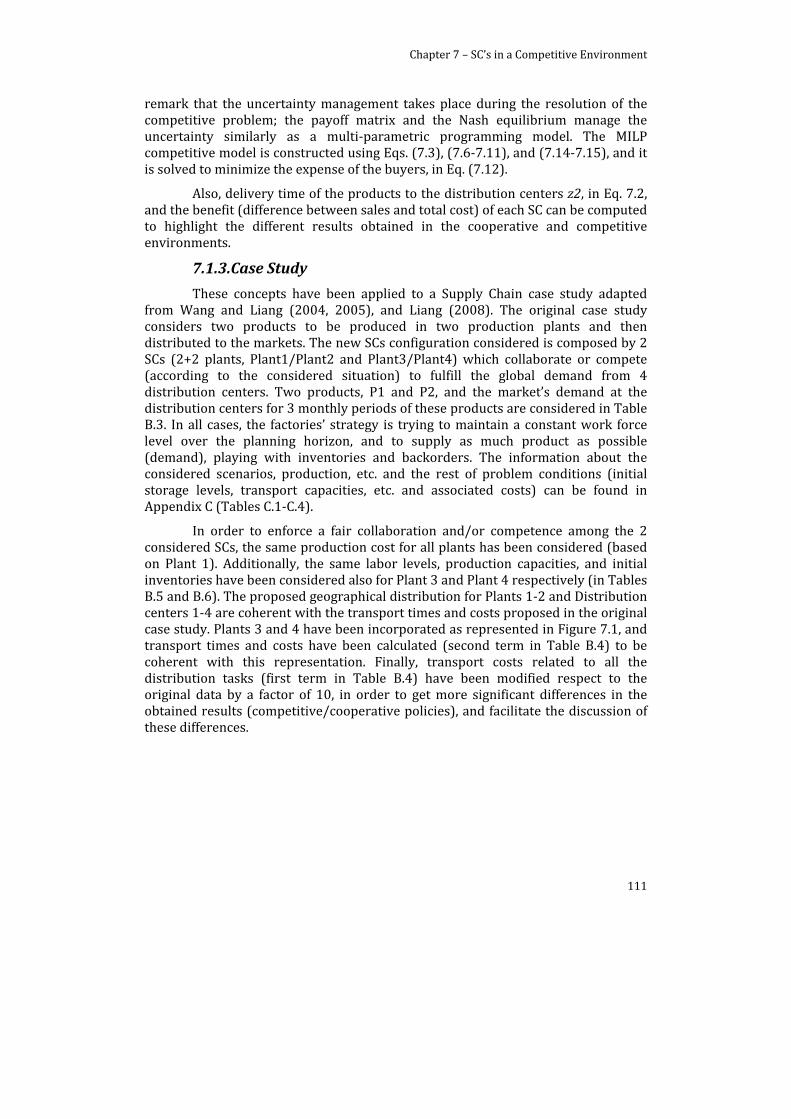
Chapter 7 – SC’s in a Competitive Environment
111
remark that the uncertainty management takes place during the resolution of the competitive problem; the payoff matrix and the Nash equilibrium manage the uncertainty similarly as a multi‐parametric programming model. The MILP competitive model is constructed using Eqs. (7.3), (7.6‐7.11), and (7.14‐7.15), and it is solved to minimize the expense of the buyers, in Eq. (7.12).
Also, delivery time of the products to the distribution centers z2, in Eq. 7.2, and the benefit (difference between sales and total cost) of each SC can be computed to highlight the different results obtained in the cooperative and competitive environments.
7.1.3. Case Study
These concepts have been applied to a Supply Chain case study adapted from Wang and Liang (2004, 2005), and Liang (2008). The original case study considers two products to be produced in two production plants and then distributed to the markets. The new SCs configuration considered is composed by 2 SCs (2+2 plants, Plant1/Plant2 and Plant3/Plant4) which collaborate or compete (according to the considered situation) to fulfill the global demand from 4 distribution centers. Two products, P1 and P2, and the market’s demand at the distribution centers for 3 monthly periods of these products are considered in Table B.3. In all cases, the factories’ strategy is trying to maintain a constant work force level over the planning horizon, and to supply as much product as possible (demand), playing with inventories and backorders. The information about the considered scenarios, production, etc. and the rest of problem conditions (initial storage levels, transport capacities, etc. and associated costs) can be found in Appendix C (Tables C.1‐C.4).
In order to enforce a fair collaboration and/or competence among the 2 considered SCs, the same production cost for all plants has been considered (based on Plant 1). Additionally, the same labor levels, production capacities, and initial inventories have been considered also for Plant 3 and Plant 4 respectively (in Tables B.5 and B.6). The proposed geographical distribution for Plants 1‐2 and Distribution centers 1‐4 are coherent with the transport times and costs proposed in the original case study. Plants 3 and 4 have been incorporated as represented in Figure 7.1, and transport times and costs have been calculated (second term in Table B.4) to be coherent with this representation. Finally, transport costs related to all the distribution tasks (first term in Table B.4) have been modified respect to the original data by a factor of 10, in order to get more significant differences in the obtained results (competitive/cooperative policies), and facilitate the discussion of these differences.
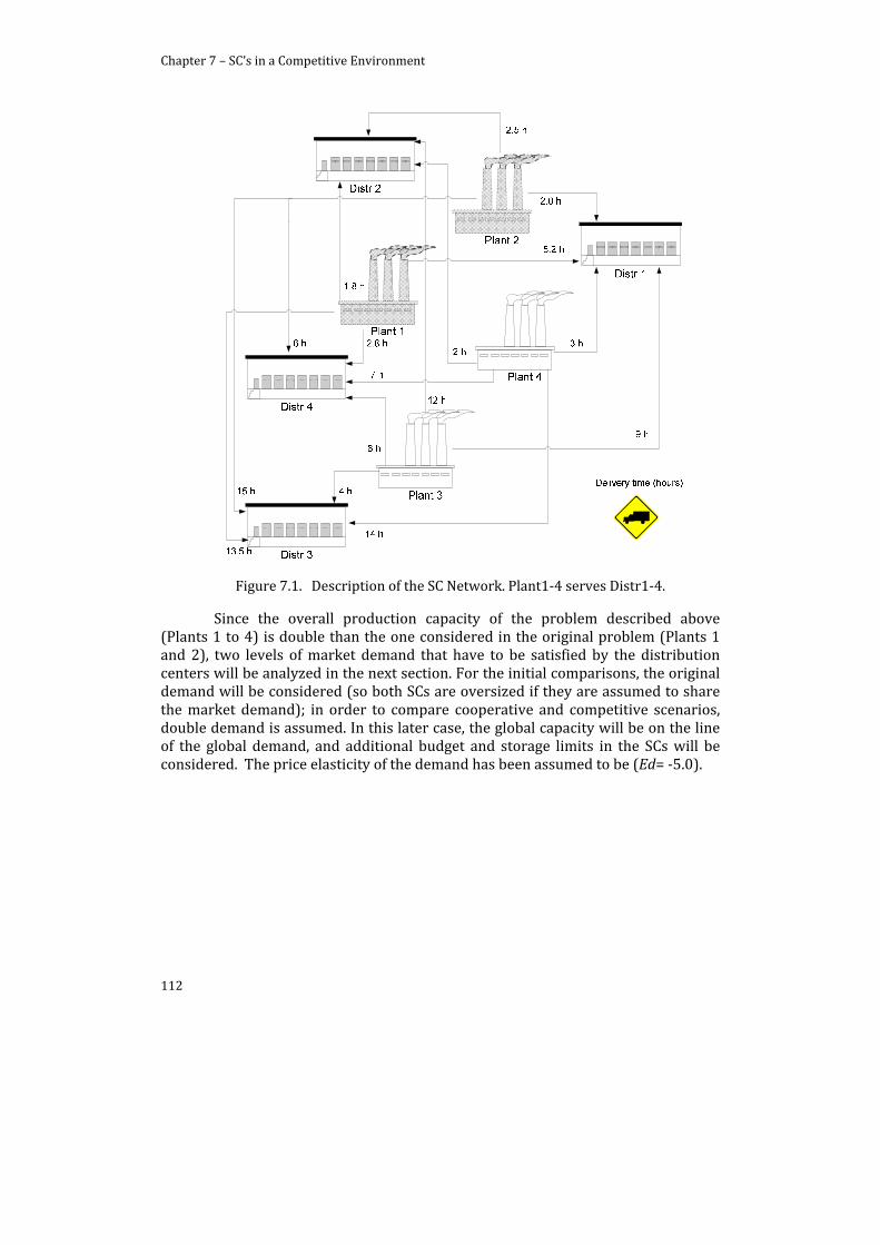
Chapter 7 – SC’s in a Competitive Environment
112
Figure 7.1. Description of the SC Network. Plant1‐4 serves Distr1‐4.
Since the overall production capacity of the problem described above (Plants 1 to 4) is double than the one considered in the original problem (Plants 1 and 2), two levels of market demand that have to be satisfied by the distribution centers will be analyzed in the next section. For the initial comparisons, the original demand will be considered (so both SCs are oversized if they are assumed to share the market demand); in order to compare cooperative and competitive scenarios, double demand is assumed. In this later case, the global capacity will be on the line of the global demand, and additional budget and storage limits in the SCs will be considered. The price elasticity of the demand has been assumed to be (Ed= ‐5.0).
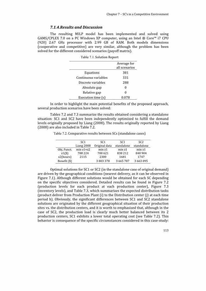
Chapter 7 – SC’s in a Competitive Environment
113
7.1.4. Results and Discussion
The resulting MILP model has been implemented and solved using GAMS/CPLEX 7.0 on a PC Windows XP computer, using an Intel ® Core™ i7 CPU (920) 2.67 GHz processor with 2.99 GB of RAM. Both models dimensions (cooperative and competitive) are very similar, although the problem has been solved for the different considered scenarios (payoff matrix).
Table 7.1. Solution Report
Average for all scenarios
Equations 381 Continuous variables 331 Discrete variables 288 Absolute gap 0 Relative gap 0
Execution time (s) 0.078
In order to highlight the main potential benefits of the proposed approach, several production scenarios have been solved:
Tables 7.2 and 7.3 summarize the results obtained considering a standalone situation: SC1 and SC2 have been independently optimized to fulfill the demand levels originally proposed by Liang (2008). The results originally reported by Liang (2008) are also included in Table 7.2.
Table 7.2. Comparative results between SCs (standalone cases)
Optimal solutions for SC1 or SC2 (in the standalone case of original demand) are driven by the geographical conditions (nearest delivery, as it can be observed in Figure 7.1). Although different solutions would be obtained for each SC depending on the specific objectives considered. Detailed results can be found in Figure 7.2 (production levels for each product at each production center), Figure 7.3 (inventory levels), and Table 7.3, which summarizes the expected distribution tasks (product deliver from Production Plant (i) to the Distribution center (j) at each time period h). Obviously, the significant differences between SC1 and SC2 standalone solutions are originated by the different geographical situation of their production sites vs. the distribution centers, and it is worth to emphasized that, although in the case of SC2, the production load is clearly much better balanced between its 2 production centers, SC1 exhibits a lower total operating cost (see Table 7.2). This behavior is consequence of the specific circumstances considered in this case‐study:
SC1 SC1 SC1 SC2Liang 2008 Original data standalone standalone
Obj. Funct. min z1+z2 min z1 min z1 min z1z1($) 788 224 700 621 838 212 840 904
z2(hours) 2115 2300 1681 1747Benefit ($) 3 803 378 3 665 787 3 663 095

Chapter 7 – SC’s in a Competitive Environment
114
Plant 1 is located in a privileged geographical situation, and work load unbalance is not penalized unless it implies storages and/or delays. So, the main policy for SC1 is trying to assign as much demand as possible to Plant1; at the specific demand levels considered in this case study. This can be done without incurring in storage/delay penalties, and the risk to suffer higher costs to accommodate additional demands from distribution centers (Distr2, Distr3 or Distr4) are not penalized either. Obviously, other production and/or storage costs would lead to other production/distribution policies, resulting in global performances which probably will be also significantly different.
Table 7.3. Optimal Distribution planning for SC1 and SC2.
Table 7.4 shows different results obtained when both considered SCs are working together in a common scenario. As it was expected, the optimal solution for SC1 when coexisting with SC2 depends on the kind of relation (cooperative/competitive) with its counterpart and its capacity to adopt different commercialization policies, in this case represented just by the selling prices it can offer to each distribution center.
In the cooperative case (Table 7.4a) the overall SCs costs (z1 associated to the aggregated SC, Eq. 7.1) are obviously reduced with respect to both standalone situations (Table 7.2), although the general rules leading to the optimum production/distribution policies are the same: to reduce the distribution costs, since the other costs are considered identical.
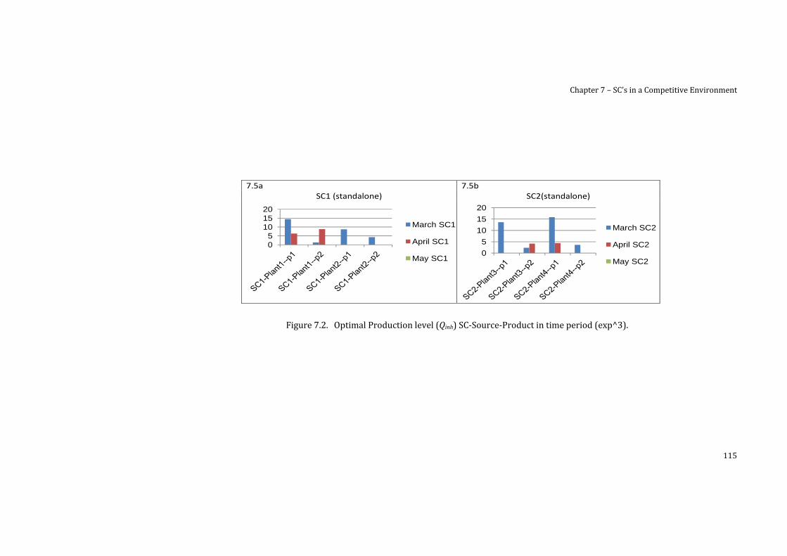
Chapter 7 – SC’s in a Competitive Environment
115
Figure 7.2. Optimal Production level (Qinh) SC‐Source‐Product in time period (exp^3).
7.5a 7.5bSC1 (standalone) SC2(standalone)
05
101520
March SC1
April SC1
May SC10
5
10
15
20
March SC2
April SC2
May SC2
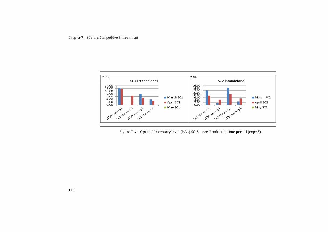
Chapter 7 – SC’s in a Competitive Environment
116
Figure 7.3. Optimal Inventory level (Winh) SC‐Source‐Product in time period (exp^3).
7.6a 7.6bSC1 (standalone) SC2 (standalone)
0.002.004.006.008.0010.0012.0014.00
March SC1
April SC1
May SC10.002.004.006.008.0010.0012.0014.0016.00
March SC2
April SC2
May SC2
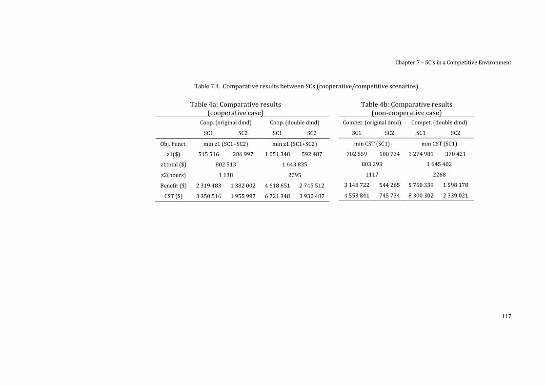
Chapter 7 – SC’s in a Competitive Environment
117
Table 7.4. Comparative results between SCs (cooperative/competitive scenarios)
Table 4a: Comparative results (cooperative case)
Table 4b: Comparative results (non‐cooperative case)
Coop. (original dmd) Coop. (double dmd)
SC1 SC2 SC1 SC2
Obj. Funct. min z1 (SC1+SC2) min z1 (SC1+SC2)
z1($) 515 516 286 997 1 051 348 592 487
z1total ($) 802 513 1 643 835
z2(hours) 1 138 2295
Benefit ($) 2 319 483 1 382 002 4 618 651 2 745 512
CST ($) 3 350 516 1 955 997 6 721 348 3 930 487
Compet. (original dmd) Compet. (double dmd)
SC1 SC2 SC1 SC2
min CST (SC1) min CST (SC1)
702 559 100 734 1 274 981 370 421
803 293 1 645 402
1117 2268
3 148 722 544 265 5 750 339 1 598 178
4 553 841 745 734 8 300 302 2 339 021
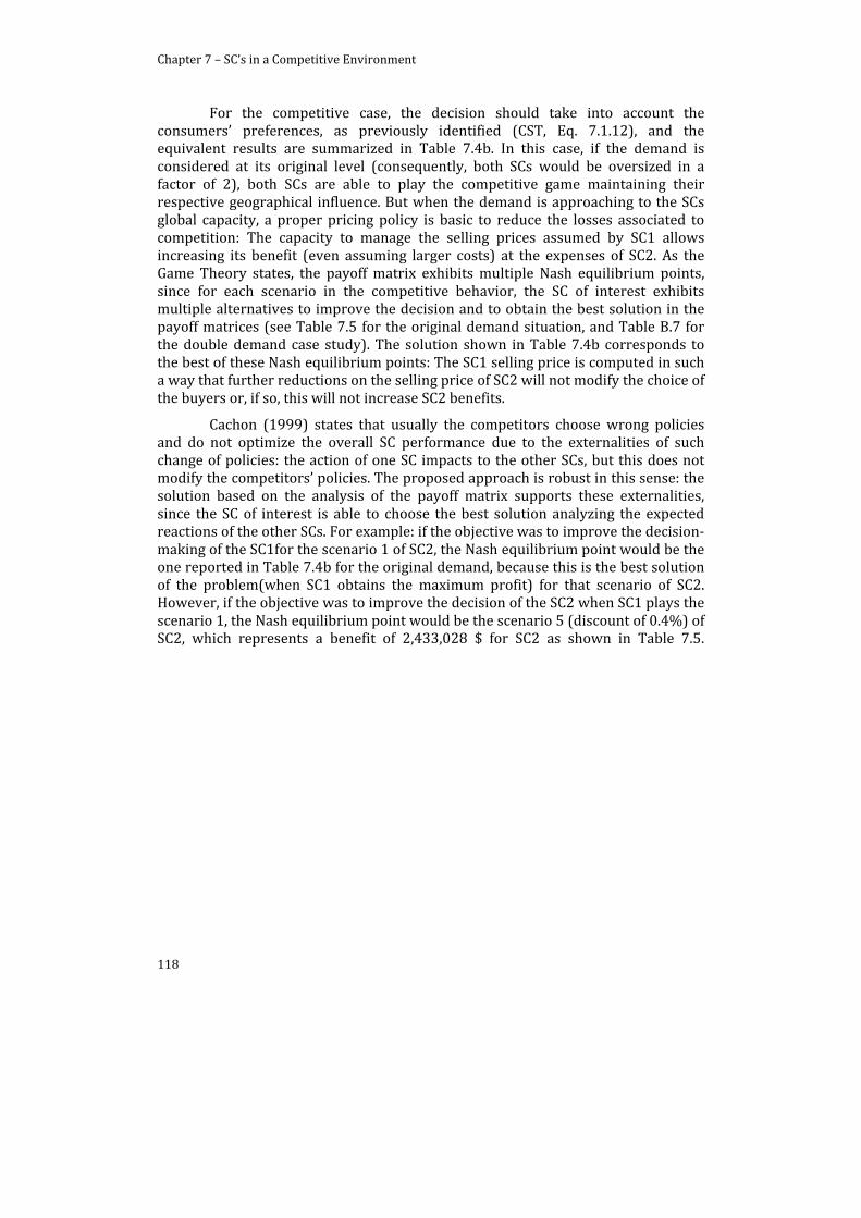
Chapter 7 – SC’s in a Competitive Environment
118
For the competitive case, the decision should take into account the consumers’ preferences, as previously identified (CST, Eq. 7.1.12), and the equivalent results are summarized in Table 7.4b. In this case, if the demand is considered at its original level (consequently, both SCs would be oversized in a factor of 2), both SCs are able to play the competitive game maintaining their respective geographical influence. But when the demand is approaching to the SCs global capacity, a proper pricing policy is basic to reduce the losses associated to competition: The capacity to manage the selling prices assumed by SC1 allows increasing its benefit (even assuming larger costs) at the expenses of SC2. As the Game Theory states, the payoff matrix exhibits multiple Nash equilibrium points, since for each scenario in the competitive behavior, the SC of interest exhibits multiple alternatives to improve the decision and to obtain the best solution in the payoff matrices (see Table 7.5 for the original demand situation, and Table B.7 for the double demand case study). The solution shown in Table 7.4b corresponds to the best of these Nash equilibrium points: The SC1 selling price is computed in such a way that further reductions on the selling price of SC2 will not modify the choice of the buyers or, if so, this will not increase SC2 benefits.
Cachon (1999) states that usually the competitors choose wrong policies and do not optimize the overall SC performance due to the externalities of such change of policies: the action of one SC impacts to the other SCs, but this does not modify the competitors’ policies. The proposed approach is robust in this sense: the solution based on the analysis of the payoff matrix supports these externalities, since the SC of interest is able to choose the best solution analyzing the expected reactions of the other SCs. For example: if the objective was to improve the decision‐making of the SC1for the scenario 1 of SC2, the Nash equilibrium point would be the one reported in Table 7.4b for the original demand, because this is the best solution of the problem(when SC1 obtains the maximum profit) for that scenario of SC2. However, if the objective was to improve the decision of the SC2 when SC1 plays the scenario 1, the Nash equilibrium point would be the scenario 5 (discount of 0.4%) of SC2, which represents a benefit of 2,433,028 $ for SC2 as shown in Table 7.5.
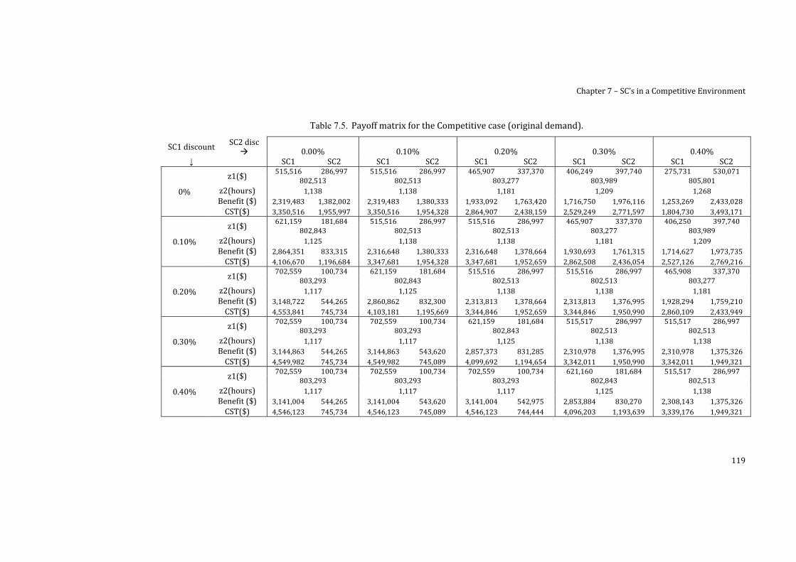
Chapter 7 – SC’s in a Competitive Environment
119
Table 7.5. Payoff matrix for the Competitive case (original demand).
SC1 discount SC2 disc 0.00% 0.10% 0.20% 0.30% 0.40%
↓ SC1 SC2 SC1 SC2 SC1 SC2 SC1 SC2 SC1 SC2
0%
z1($) 515,516 286,997 515,516 286,997 465,907 337,370 406,249 397,740 275,731 530,071
802,513 802,513 803,277 803,989 805,801 z2(hours) 1,138 1,138 1,181 1,209 1,268 Benefit ($) 2,319,483 1,382,002 2,319,483 1,380,333 1,933,092 1,763,420 1,716,750 1,976,116 1,253,269 2,433,028 CST($) 3,350,516 1,955,997 3,350,516 1,954,328 2,864,907 2,438,159 2,529,249 2,771,597 1,804,730 3,493,171
0.10%
z1($) 621,159 181,684 515,516 286,997 515,516 286,997 465,907 337,370 406,250 397,740
802,843 802,513 802,513 803,277 803,989 z2(hours) 1,125 1,138 1,138 1,181 1,209 Benefit ($) 2,864,351 833,315 2,316,648 1,380,333 2,316,648 1,378,664 1,930,693 1,761,315 1,714,627 1,973,735 CST($) 4,106,670 1,196,684 3,347,681 1,954,328 3,347,681 1,952,659 2,862,508 2,436,054 2,527,126 2,769,216
0.20%
z1($) 702,559 100,734 621,159 181,684 515,516 286,997 515,516 286,997 465,908 337,370
803,293 802,843 802,513 802,513 803,277 z2(hours) 1,117 1,125 1,138 1,138 1,181 Benefit ($) 3,148,722 544,265 2,860,862 832,300 2,313,813 1,378,664 2,313,813 1,376,995 1,928,294 1,759,210 CST($) 4,553,841 745,734 4,103,181 1,195,669 3,344,846 1,952,659 3,344,846 1,950,990 2,860,109 2,433,949
0.30%
z1($) 702,559 100,734 702,559 100,734 621,159 181,684 515,517 286,997 515,517 286,997
803,293 803,293 802,843 802,513 802,513 z2(hours) 1,117 1,117 1,125 1,138 1,138 Benefit ($) 3,144,863 544,265 3,144,863 543,620 2,857,373 831,285 2,310,978 1,376,995 2,310,978 1,375,326 CST($) 4,549,982 745,734 4,549,982 745,089 4,099,692 1,194,654 3,342,011 1,950,990 3,342,011 1,949,321
0.40%
z1($) 702,559 100,734 702,559 100,734 702,559 100,734 621,160 181,684 515,517 286,997
803,293 803,293 803,293 802,843 802,513 z2(hours) 1,117 1,117 1,117 1,125 1,138 Benefit ($) 3,141,004 544,265 3,141,004 543,620 3,141,004 542,975 2,853,884 830,270 2,308,143 1,375,326 CST($) 4,546,123 745,734 4,546,123 745,089 4,546,123 744,444 4,096,203 1,193,639 3,339,176 1,949,321

Chapter 7 – SC’s in a Competitive Environment
120
7.1.5. Bargaining Tool
Several works presented in the field of SC planning discuss the importance of considering the eventual reactions of the different SCs, especially for the cooperative case. Alliances setup, based on a given level of demand along the SC, trying to select partners that give an added value to the resulting SC (Gunasekaran et al., 2008) is a main strategic objective. Mentzer et al. (2001) establishes that the success of the cooperation is guaranteed if the SCs have the same goal and the same focus on serving customers.
Total Cost SC1
Total Cost SC2
SC1-SC2 Coop.
SC1 Comp.
SC2 Comp.0
200000
400000
600000
800000
1000000
Distribution SC2 Storage SC2 Production SC2 Distribution SC1 Storage SC1 Production SC1
Figure 7.4. Cost Analysis for the studied examples
Given the present economic situation, the approach presented in this work can be used as a Bargaining Tool in both cooperative and competitive SC market scenarios. In this sense, Fig. 7.4 (Cost analysis) shows the total production, inventory and distribution costs for the different studied scenarios. As it can be observed there, SC1 costs slightly less to operate (<1%) than SC2; also analyzing SC1 vs. SC2 in the cooperative case (SC1 ‐ SC2 coop.) it can be observed that an overall cost improvement of about 4% can be achieved when both SCs work together. Also, the scenarios identified during the discussion of the competitive cases, corresponding to the Nash equilibrium of the payoff matrix, have been represented in Fig. 7.4 (best result when playing as SC1 and best result when playing as SC2). As it can be seen there, SC1 keeps being cheaper for the competitive cases. Disregarding the effects of the geographical situation of the corresponding production facilities, these results can be also used to identify improvement

Chapter 7 – SC’s in a Competitive Environment
121
opportunities: in this specific case, a minimum change in the production costs will lead to a dramatic change in the competition scenario, since these costs represent the highest expenses of any SC. Also, the introduction of commitments between SCs and customers would significantly modify the problem conditions, reducing the pressure to get the highest market share, which might also lead to completely different production/distribution SC policies.
But probably the most important benefit of this kind of studies would be the possibility to use the overall information computed during the optimization procedure to negotiate agreements with the distribution centers and/or clients/costumers. For example: in the proposed case‐study SC2 generates the 36% of the total benefits in the optimal cooperative situation, but it would only generate the 15% of the benefits in the best solution proposed by SC1, even it might get the 66% of the benefits in the best competitive solution to be proposed by the same SC2. This information can be used both directly, or associated to other elements identifying additional trade‐offs (i.e., related to product quality, service reliability, etc.), in order to arrange new agreements aiming to modify an economically unbalanced situation.
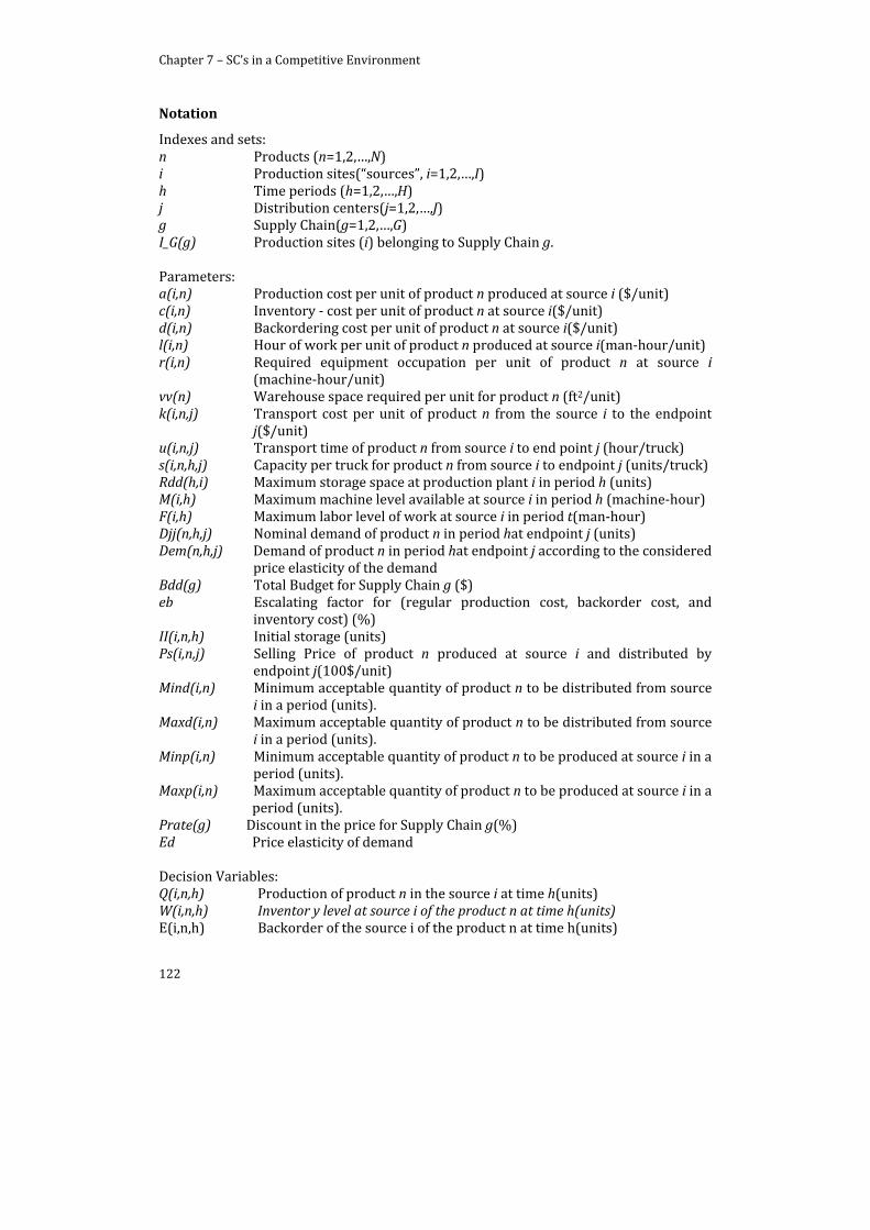
Chapter 7 – SC’s in a Competitive Environment
122
Notation
Indexes and sets: n Products (n=1,2,…,N) i Production sites(“sources”, i=1,2,…,I) h Time periods (h=1,2,…,H) j Distribution centers(j=1,2,…,J) g Supply Chain(g=1,2,…,G) I_G(g) Production sites (i) belonging to Supply Chain g. Parameters: a(i,n) Production cost per unit of product n produced at source i ($/unit) c(i,n) Inventory ‐ cost per unit of product n at source i($/unit) d(i,n) Backordering cost per unit of product n at source i($/unit) l(i,n) Hour of work per unit of product n produced at source i(man‐hour/unit) r(i,n) Required equipment occupation per unit of product n at source i
(machine‐hour/unit) vv(n) Warehouse space required per unit for product n (ft2/unit) k(i,n,j) Transport cost per unit of product n from the source i to the endpoint
j($/unit) u(i,n,j) Transport time of product n from source i to end point j (hour/truck) s(i,n,h,j) Capacity per truck for product n from source i to endpoint j (units/truck) Rdd(h,i) Maximum storage space at production plant i in period h (units) M(i,h) Maximum machine level available at source i in period h (machine‐hour) F(i,h) Maximum labor level of work at source i in period t(man‐hour) Djj(n,h,j) Nominal demand of product n in period hat endpoint j (units) Dem(n,h,j) Demand of product n in period hat endpoint j according to the considered
price elasticity of the demand Bdd(g) Total Budget for Supply Chain g ($) eb Escalating factor for (regular production cost, backorder cost, and
inventory cost) (%) II(i,n,h) Initial storage (units) Ps(i,n,j) Selling Price of product n produced at source i and distributed by
endpoint j(100$/unit) Mind(i,n) Minimum acceptable quantity of product n to be distributed from source
i in a period (units). Maxd(i,n) Maximum acceptable quantity of product n to be distributed from source
i in a period (units). Minp(i,n) Minimum acceptable quantity of product n to be produced at source i in a
period (units). Maxp(i,n) Maximum acceptable quantity of product n to be produced at source i in a
period (units). Prate(g) Discount in the price for Supply Chain g(%) Ed Price elasticity of demand Decision Variables: Q(i,n,h) Production of product n in the source i at time h(units) W(i,n,h) Inventor y level at source i of the product n at time h(units) E(i,n,h) Backorder of the source i of the product n at time h(units)

Chapter 7 – SC’s in a Competitive Environment
123
T(i,n,h,j) Quantity delivered from the source i to endpoint j of product n at time h(units)
Binary variables: X(i,n,h,j) Binary variable identifying if product n is sent from source i to the
endpoint j at time h. Y(i,n,h) Binary variable identifying if the source i produces product n at time h Objective functions: z1(g) total cost of SCg. ($) CST(g) Spend of the buyers at each SCg($).

Chapter 7 – SC’s in a Competitive Environment
125
7.2. Supply Chain Scheduling in a Competitive Environment
7.2.1. Introduction
The continued growth in complex operations, the competition and uncertainty of market for high value‐added chemicals, and products with short life cycles have renewed interest in batch operations, the development of new models and tools to improve the decision‐making of such processes. Batch production is a manufacture technique to create stage by stage a series of workstations, used to meet group orders. It is one of the main production methods used in the world (batch; job; and flow production)3. Batch process represents the most flexible design to produce several and quite different products in the same units. Multiple products, multiple task plants use this kind of batch processes and are typically successfully applied in the chemical, pharmaceutical, petrochemical, food industries.
The problem of decision‐making associated to operational SC management (“Supply Chain Scheduling”, procurement of raw materials, allocation of tasks, operation units, transport actions, allocation of products to different plants and distributing them to different customers) is attracting the attention of the scientific community in the last years (Agnetis et al., 2010). The complexity associated to the allocation/production and distribution management of raw materials, intermediate and final products is increased by the necessity to manage the uncertainties associated to the market competition. In the last decades, several sources of uncertainty have been studied: demand and supply uncertainty (Ho, 1989, process operation, production lead time, failure of machines (Dolgui et al., 2002), supplier reliability and deliveries (Davis, 1993), etc.
On the other hand, all the studies reviewed so far, suffer by the fact that the inclusion of third parties facing a global market cooperating and/or competing for the market demand has been disregarded. As previously presented in section 7.1, market price has been introduced as the parameter to optimize tactical decision‐making under cooperation and competition. However, approaches of this kind carry with them various disadvantages: (i) there are limits to determine how far the introduction of multiple SC cooperating/competing for the market demand can be done, (ii) most of the studies in cooperation/competition have only been carried out in a small number of areas (marketing and pricing mainly). Hence, in order to understand how the market behavior directly impacts the market demand and how it affects the SCM decision‐making process, different policies to face market cooperation/competition must be studied.
Furthermore, under uncertain environments it is important to develop robust decision‐making tools, creating structures that allow rapid and appropriate responses to these uncertain situations. Moreover, it is important to increase the competitiveness of the enterprises (production, processes, products, etc.) by increasing the product and process quality. It has been proved that the definition of a Quality program generates costs and expenses in all areas of the company, but
Chapter 7 – SC’s in a Competitive Environment
126
when such program is carried out properly, these costs become an investment to reduce expenses and improve the benefits of the enterprises.
Over the past century there has been a dramatic increase in Quality Cost applications. The scope covered by this issue has been defined and assumed by several authors, without merge among their definitions. Several applications of product and service quality have been considered in last decades, but, it is clear that the explicit consideration into the SC management remains open. The ISO (9000:2005) considers the Total Quality Control (TQC) as the activities coordinated to manage and control the organization in quality terms. Accordingly, Garrigos et al. (2002) enlisted tree main parameters to integrate the concept of TQC: total customer satisfaction, total motivation of the enterprise and minimum operating and production costs. There are several costs involved in the quality assessment, these cost have been evolved rapidly in recent years (such as: cost of implementation, evaluation, prevention, detection of disposals, defective products, etc.)
The TQC aims to provide a competitive advantage in businesses, ensuring full satisfaction of the needs and expectations of the customer’s. The SCM applies the theory of total quality control in order to improve decision‐making (considering some TQC policies, such as: just in time, no stock, totals satisfaction, etc.). In this sense, SCM could correspond to the quality service, since it looks to distribute the products to the final consumers in time and under the specifications. Savolainen (2000) defined that the quality management could be used to enhance the competitiveness of the organization. In order to quantify the quality cost comprehensive lists of costs have been considered (operating costs, Feigenbaum, 1971; control and fail costs, Schroeder, 1992; prevention costs, Alexander, 1994). This Chapter includes the prevention and evaluation costs in the SC Scheduling formulation, due to the characteristics of the problem considered.
In order to deal with a new uncertain parameter (competition behavior) at different decision levels, and also to introduce the use of the product quality as a control parameter to compete/or cooperate. This section introduces into the model information the expected performance of the competing supply chains (including the SC of interest) to improve the operational decision‐making in a competitive/cooperative environment using Game Theory optimization (GTO). Based on the solution for several quality scenarios, it is possible to construct a payoff matrix and also obtain the best solution “Nash Equilibrium” of the problem considered.
7.2.2. Problem Statement
7.2.2.1. SC Scheduling
The term “SC scheduling” has been introduced in the last years due to the necessity to improve the decision‐making, integrating different SCM decision levels. SC scheduling aims to optimize production allocation, sequencing, timing and distribution of the products in the SC network (raw materials, production units, production plants and distribution to the final consumers, see Figure 7.5). This issue
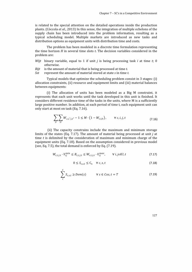
Chapter 7 – SC’s in a Competitive Environment
127
is related to the special attention on the detailed operations inside the production plants. (Cóccola et al., 2013) In this sense, the integration of multiple echelons of the supply chain has been introduced into the problem information, resulting as a typical scheduling model. Multiple markets are introduced as new tasks and distribution options as equipment units with distribution time and costs.
The problem has been modeled in a discrete time formulation representing the time horizon H in several time slots t. The decision variables considered in the problem are:
Wijt binary variable, equal to 1 if unit j is being processing task i at time t; 0 otherwise.
Bijt is the amount of material that is being processed at time t. Sst represent the amount of material stored at state s in time t.
Typical models that optimize the scheduling problem consist in 3 stages: (i) allocation constraints, (ii) resource and equipment limits and (iii) material balances between equipments:
(i) The allocation of units has been modeled as a Big M constraint, it represents that each unit works until the task developed in this unit is finished. It considers different residence time of the tasks in the units, where M is a sufficiently large positive number. In addition, at each period of time t, each equipment unit can only start at most on task (Eq. 7.16).
, , , 1 · 1 , , , , , (7.16)
(ii) The capacity constrains include the maximum and minimum storage limits of the states (Eq. 7.17). The amount of material being processed at unit j at time t is delimited by the consideration of maximum and minimum charge of the equipment units (Eq. 7.18). Based on the assumption considered in previous model (see, Eq. 7.5), the total demand is enforced by Eq. (7.19).
, , , · , , , , , , · , , , (7.17)
0 , , C , , (7.18)
, , , (7.19)
Chapter 7 – SC’s in a Competitive Environment
128
REACTOR 1
HEATER SEPARATOR
REACTOR 2
REACTOR 3
FEED A HOT A
FEED B
PRODUCT 2
INT BC
INT AB
IMPURE E
FEED C
PRODUCT 2
CONSUMERSTRANSPORTPRODUCTION
PLANTS
PLANT DETAILSA)
B) SUPPLY CHAIN
TRUCK
Figure 7.5. SC Configuration
(iii) The material balances of the network is presented in Eq. 7.20, where given an initial storage, the storage at the states is computed adding the input of material that becomes from the previous task and subtracting the material that feeds the next task in all the periods of the time horizon. This equation includes the possibility of receiving quantities of raw materials Rmst in feed state s at times t during the schedule rather than having all the required feedstock stored locally at the start of processing:
, , , , · , , , · , , , , , , (7.20)
Once the scheduling formulation was defined, the Total Quality assessment has been included into the model formulation. Evaluation quality costs have been introduced in Eq. 7.21. Quality evaluation cost (QVcs) includes the quantity evaluation cost of supervising the raw material purchased and stored during the time horizon.
, , , 1 , , 2 , , (7.21)
Chapter 7 – SC’s in a Competitive Environment
129
Where: QVT is the Total quality validation cost for each SC c. Qq (Q1q and Q2q) is the parameter associated to the quality level (q=L, M, H).
Eq. 7.23 represents the cost to verify the production quality (QPVc). This consists in the production for all the scenarios by the price to verify each production unit by the workers. (Trs price to verify by the workers).
The transport cost (CTrc) has been computed by Eq. 7.24, considering a fixed transport cost from each production plant to each market.
, , (7.24)
Since there are different product quality levels the introduction of the defective product costs have been considered by Eq. 7.25, considering that the dq represent the probability of defective’s products.
, , (7.25)
Total cost has been computed in Eq. 7.26, consists in the summary of transport cost, total quality validation cost and the cost to verify the production quality.
(7.26)
Finally, quality impacts directly in the product prices. Accordingly, the price of the products has been fixed by the approximation presented by McElreath and Mayorga (2012), which considers a fixed value ‘v’ to the product price plus an added value to the quality level of the product (Eq. 7.27), several product quality scenarios have been considered (Yq). In order to highlight the results the benefit of each SC has been computed (Eq. 7.28). Finally the objective function corresponds to maximize the Profit (Sales‐Costs) of the SC’s, considering that the SC with highest value (price and quality) should obtain better incomings (Eq. 7.29).
, (7.22)
, , , 1 (7.23)

Chapter 7 – SC’s in a Competitive Environment
130
, , (7.27)
, , , (7.28)
(7.29)
7.2.2.2. Cooperative and noncooperative problems
In previous section (7.1) the competition behavior has been introduced as the source of uncertainty to be managed. The competition behavior is typically related with product prices discounts, it was used in previous section as the parameter to control the uncertainty. In this section, the product quality has been considered as the control parameter to be included as the cooperation/competition strategy. The product quality is directly related to the product price and the defective cost (parameters Yq and dq; see, Eqs. 7.27 and 7.25), then, several product quality scenarios must be solved.
The cooperative formulation has been solved considering several SC’s operating as one (SC1+SC2+…+SCn). The model considers the quality of the products as a new control parameter: different product quality scenarios have been considered for each SC. The product quality scenarios include (L=Low, M=Medium and H=High, Quality). In the cooperative problem the product quality level will be the same for all SC’s, where equal market prices (due to the quality level) reproduce a fair cooperative game. Otherwise, in the competition behavior analysis several scenarios of quality levels have been computed. Consequently, in the competitive problem each SC chooses his quality level and competes for the demand of the markets.
7.2.3. Case Study
The concepts previously mentioned have been applied to a SC scheduling case study (see, Figure 7.5a). The network configuration is composed by 2 Supply Chains (SC1‐Plant1 and SC2‐Plant2). Each SC collaborates or competes to fulfill the forecasted demand of 2 markets (market 1 and market 2). A multi‐product and multitask plant for each SC has been considered. Where the production of 2 products has been enforced, the detailed operation data inside each plant are adapted from the case study presented in Chapter 4 (case study 1, section 4.1.4.1) and Chapter 5 (section 5.3).
A global demand of the customers (Table D.1) for a time horizon of 15 hours has been considered. The information about production capacities can be found in the Appendix D (Tables D2). In order to cooperate or compete two of the product quality scenarios (Medium and High) for each SC have been considered (see, Table 7.6).
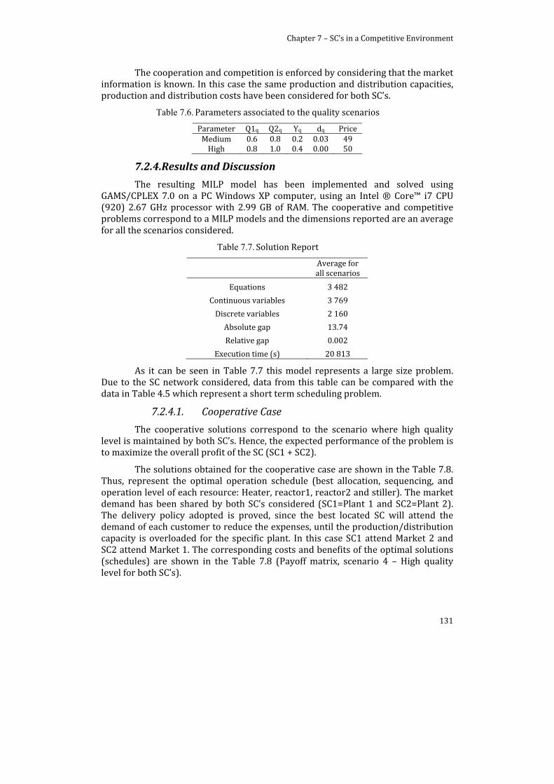
Chapter 7 – SC’s in a Competitive Environment
131
The cooperation and competition is enforced by considering that the market information is known. In this case the same production and distribution capacities, production and distribution costs have been considered for both SC’s.
Table 7.6. Parameters associated to the quality scenarios
Parameter Q1q Q2q Yq dq PriceMedium 0.6 0.8 0.2 0.03 49High 0.8 1.0 0.4 0.00 50
7.2.4. Results and Discussion
The resulting MILP model has been implemented and solved using GAMS/CPLEX 7.0 on a PC Windows XP computer, using an Intel ® Core™ i7 CPU (920) 2.67 GHz processor with 2.99 GB of RAM. The cooperative and competitive problems correspond to a MILP models and the dimensions reported are an average for all the scenarios considered.
Table 7.7. Solution Report
Average for all scenarios
Equations 3 482
Continuous variables 3 769
Discrete variables 2 160
Absolute gap 13.74
Relative gap 0.002
Execution time (s) 20 813
As it can be seen in Table 7.7 this model represents a large size problem. Due to the SC network considered, data from this table can be compared with the data in Table 4.5 which represent a short term scheduling problem.
7.2.4.1. Cooperative Case
The cooperative solutions correspond to the scenario where high quality level is maintained by both SC’s. Hence, the expected performance of the problem is to maximize the overall profit of the SC (SC1 + SC2).
The solutions obtained for the cooperative case are shown in the Table 7.8. Thus, represent the optimal operation schedule (best allocation, sequencing, and operation level of each resource: Heater, reactor1, reactor2 and stiller). The market demand has been shared by both SC’s considered (SC1=Plant 1 and SC2=Plant 2). The delivery policy adopted is proved, since the best located SC will attend the demand of each customer to reduce the expenses, until the production/distribution capacity is overloaded for the specific plant. In this case SC1 attend Market 2 and SC2 attend Market 1. The corresponding costs and benefits of the optimal solutions (schedules) are shown in the Table 7.8 (Payoff matrix, scenario 4 – High quality level for both SC’s).
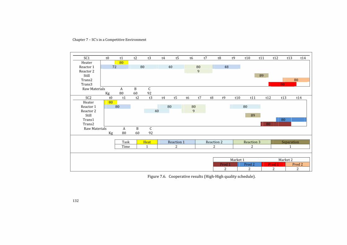
Chapter 7 – SC’s in a Competitive Environment
132
SC1 t0 t1 t2 t3 t4 t5 t6 t7 t8 t9 t10 t11 t12 t13 t14 Heater 80Reactor 1 72 80 40 80 48Reactor 2 9 Still 89
Trans2 80Trans3 80Raw Materials A B C
Kg 80 60 92SC2 t0 t1 t2 t3 t4 t5 t6 t7 t8 t9 t10 t11 t12 t13 t14
Heater 80Reactor 1 80 80 80 80Reactor 2 40 9 Still 89
Trans1 80Trans2 80Raw Materials A B C
Kg 80 60 92
Task Heat Reaction 1 Reaction 2 Reaction 3 SeparationTime 1 2 2 2 1
Market 1 Market 2
Prod 1 Prod 2 Prod 1 Prod 22 2 2 2
Figure 7.6. Cooperative results (High‐High quality schedule).
Chapter 7 – SC’s in a Competitive Environment
133
The resulting schedule (Figure 7.6) corresponds to the best global network solution, since plant 1 (SC1) is closer to market 2 representing the best distribution solution (when prices are equal); otherwise plant 2 (SC2) distributes products to his closer market (market 1).
7.2.4.2. Noncooperative Case
The payoff matrix (Table 7.8) summarizes the results of the competition scenarios (verification, production cost, transport cost, defective cost, Total Cost and benefit). In addition, the detailed operation schedules of both SC’s for all the scenarios of the payoff matrix have been computed. Detailed plant operation and distribution service of the scenario (medium‐medium quality levels) can be found in the Appendix D (Fig. D.3).
The Nash equilibriums of the problem can be obtained from the payoff matrix:
(i) The Nash equilibrium for SC1 corresponds to the strategy when player 1 (SC1) produces with the highest quality and player 2 (SC2) produces at the medium quality level. In this situation the markets look for the products from SC1 until the production capacity of SC1 is overloaded.
(ii) The Nash equilibrium for player 2 (SC2) is encountered when SC1 produce at the medium quality level and SC2 produce at the maximum quality level; obtaining the best solution possible for SC2 in the considered scenarios.
In the case when SC1 and SC2 produce at its medium quality the performance of the network will look for the products from both SC. According to the data presented in this situation the profit of both SC’s is worse. Otherwise, produce at the maximum quality levels represents the scenario with higher profits. These results are explained by the fact that working at high quality scenario avoids defective products and increase the price of the products.
Accordingly, high quality products scenario consists in high supervision of: raw materials acquisition, production and distribution of the final products. This scenario reduces the defective products and is the best option to meet the customers’ demands. As it can be expected the behavior of the “competences” directly impact the decision‐making of the SC analyzed.
The performance expected could be that a reduction of the quality must represent higher demands, due to the policy adopted, since the markets buy from the cheaper SC product. But, considering the defective product costs, the performance of the network should be to get the products with high quality and closer to the Markets.
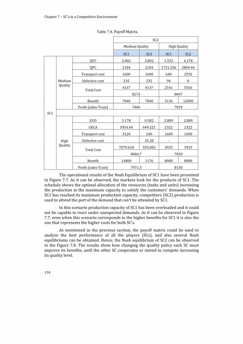
Chapter 7 – SC’s in a Competitive Environment
134
Table 7.8. Payoff Matrix.
SC2
Medium Quality High Quality
SC1 SC2 SC1 SC2
SC1
Medium Quality
QVC 2.802 2.802 1.552 4.178
QPC 2184 2184 1731.256 2804.44
Transport cost 1600 1600 640 2592
Defective cost 235 235 94 0
Total Cost 4137 4137 2541 5556
8274 8097
Benefit 7840 7840 3136 12800
Profit (sales‐Tcost) 7406 7839
High Quality
GVO 5.178 0.582 2.889 2.889
GECA 3954.44 649.221 2322 2322
Transport cost 3120 240 1600 1600
Defective cost ‐ 35.28 ‐ ‐
Total Cost 7079.618 925.083 3925 3925
8004.7 7850
Benefit 14800 1176 8000 8000
Profit (sales‐Tcost) 7971.3 8150
The operational results of the Nash Equilibrium of SC1 have been presented in Figure 7.7. As it can be observed, the markets look for the products of SC1. The schedule shows the optimal allocation of the resources (tasks and units) increasing the production at the maximum capacity to satisfy the customers’ demands. When SC1 has reached its maximum production capacity, competitors (SC2) production is used to attend the part of the demand that can’t be attended by SC1.
In this scenario production capacity of SC1 has been overloaded and it could not be capable to react under unexpected demands. As it can be observed in Figure 7.7, even when this scenario corresponds to the higher benefits for SC1 it is also the one that represents the higher costs for both SC’s.
As mentioned in the previous section, the payoff matrix could be used to analyze the best performance of all the players (SCs), and also several Nash equilibriums can be obtained. Hence, the Nash equilibrium of SC2 can be observed in the Figure 7.8. The results show how changing the quality policy each SC must improve its benefits, until the other SC cooperates or intend to compete increasing its quality level.
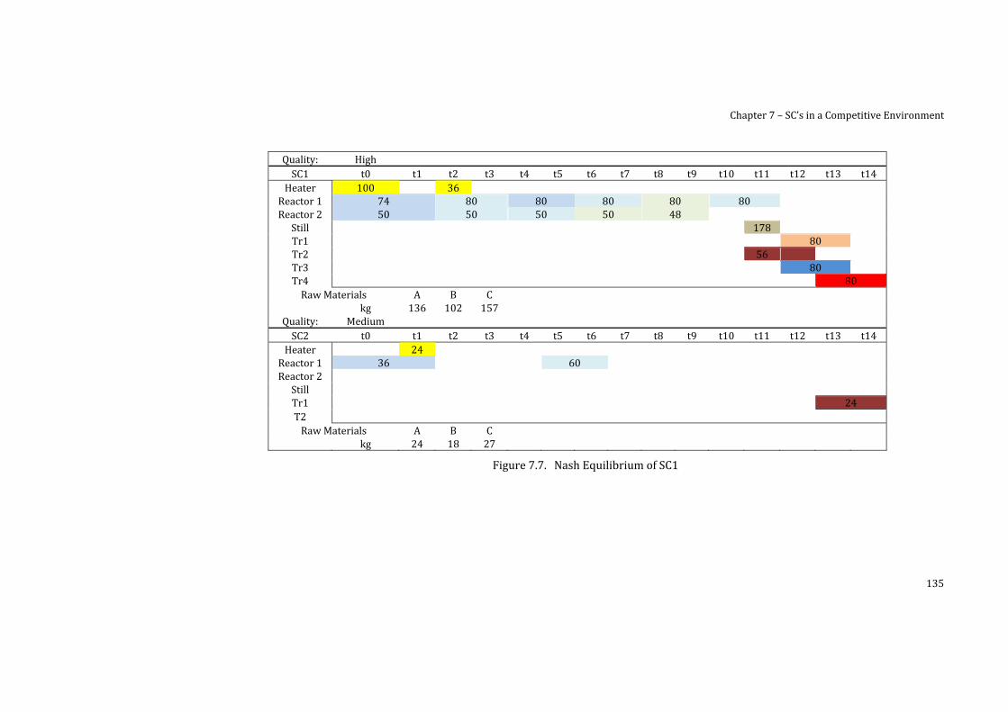
Chapter 7 – SC’s in a Competitive Environment
135
Quality: HighSC1 t0 t1 t2 t3 t4 t5 t6 t7 t8 t9 t10 t11 t12 t13 t14
Heater 100 36Reactor 1 74 80 80 80 80 80Reactor 2 50 50 50 50 48Still 178Tr1 80Tr2 56Tr3 80Tr4 80Raw Materials A B C
kg 136 102 157Quality: Medium SC2 t0 t1 t2 t3 t4 t5 t6 t7 t8 t9 t10 t11 t12 t13 t14
Heater 24Reactor 1 36 60 Reactor 2StillTr1 24T2 Raw Materials A B C
kg 24 18 27
Figure 7.7. Nash Equilibrium of SC1
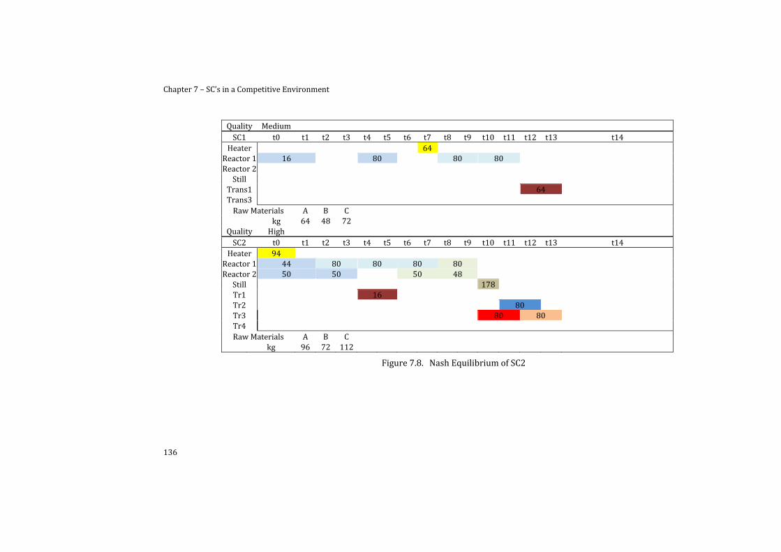
Chapter 7 – SC’s in a Competitive Environment
136
Figure 7.8. Nash Equilibrium of SC2
Quality MediumSC1 t0 t1 t2 t3 t4 t5 t6 t7 t8 t9 t10 t11 t12 t13 t14
Heater 64 Reactor 1 16 80 80 80Reactor 2Still
Trans1 64Trans3 Raw Materials A B C
kg 64 48 72Quality High SC2 t0 t1 t2 t3 t4 t5 t6 t7 t8 t9 t10 t11 t12 t13 t14
Heater 94Reactor 1 44 80 80 80 80Reactor 2 50 50 50 48Still 178Tr1 16Tr2 80Tr3 80 80Tr4 Raw Materials A B C
kg 96 72 112
Chapter 7 – SC’s in a Competitive Environment
137
7.3. Conclusions
This section exploits the optimization of SCM under cooperation and competition environments. A novel cooperative and competitive MILP‐based framework has been proposed. The proposed approach also represents an integrated decision‐making model, considering the detailed operations (production, allocation of resources and distribution tasks). Furthermore, this section shows the applicability of the open issues considered in the state of the art section, proving that the inclusion of the competitor’s behavior explicitly in the model can be done.
This Chapter presents two MILP‐based models integrating GT to optimize SCM issues. New sources of uncertainties have been detected and two parameters to control these uncertainties have been proposed. The use of Game Theory to manage the uncertain behavior of third potential actors involved in a global market has been also introduced into the PSE literature. The cooperation and competition among SC’s must be deeper studied. In order to improve the decision‐making under competitive uncertainty, complex tools must be developed.
The planning is performed under competition uncertainty, so changes in the competition behavior are explicitly contemplated; the resulting solutions can be considered as a bargaining tool between SCs. This is achieved through the use of the pay‐off matrix as decision tool to determine the best playing strategy among previously optimized SC decision‐making (production, inventory and distribution levels in a deterministic scenario).
This inner problem (optimum SC management) is modeled using a MILP‐based approach. In order to specifically take into account the considered situation (several SCs working simultaneously) some changes have been introduced in the usual problem formulation with respect to the regular way of representing the objectives, the variables and the constraints usually associated to the SC management problem (which might also consider some other endogenous or exogenous sources of uncertainty).
Then, the proposed mathematical programming formulation of the model (including the incorporation of specific terms in the objective function) and the use of the GT have allowed considering the competition behavior between SCs showing uncertain behavior. In this sense, this way of managing demand uncertainty offers the advantage that the solution for each scenario represents the optimal solution for the problem (considering each scenario as a problem), and so the optimality of the proposed solution can be guaranteed based on the knowledge of the position of the competitors (reactive approach to manage the uncertainty: the solution is adjusted to the changes in the competition scenario).
Additionally, SC managers should also consider negotiation with competitors, providers and clients. In this negotiation, issues like contracting, profit sharing, or delivery schedules should be considered. This section presents a logical approach to systematically analyze these issues, characterizing the presence of these competing SCs as a source of uncertainty linked to the demand uncertainty to
Chapter 7 – SC’s in a competitive environment
138
be considered when looking for a robust SC Management. The results allow to quantify the importance of considering different Supply Chains as competitors and/or collaborators in terms of total cost, customer satisfaction, environmental impact(including distribution actions), and cost for the consumers.
Currently the PSE and OR state of the art focus SCM considering a single SC model facing a distributed demand, which follows an uncertain behavior. But actually, this behavior results from the combination of two factors: the uncertainty on the demand itself and, in the common case in which other suppliers are available, the consumers’ preferences. It is well know that decoupling these two elements may allow a more comprehensive tactical decision‐making, but this fact has been rarely exploited to develop systematic optimization approaches in this field.
Reactive approach to manage uncertainty has been presented in this Chapter, in order to state the competition behavior as an exogenous source of uncertainty a preventive approach has been presented in Chapter 8 (robust decision‐making without previous knowledge about the competitor’s behavior).
139
Chapter 8. Uncertainty Management
8.1. Introduction
The decision‐making problem in the chemical process industry becomes more complex as the scope covered by those decisions is extended. This complexity arises by the need to consider a certain degree of uncertainty in the models used to forecast the events that should be considered in decision‐making. Many published works in this area explicitly addressed the problem associated with uncertainty in the available data.
Regarding the state of the art (section 2.4.2), it is important to consider a higher complexity degree in the developed models, i.e., considering different uncertainty sources, non linear models, etc., and new sources of uncertainties. In order to deal with the new challenges facing the PSE this work introduces the market competition behavior of several SC’s into the model information as an uncertain source. Considering the expected performance of the competing SC´s the information of the SC of the interest is dealt as a form of competing scenarios in order to improve the decision‐making under uncertainty. Accordingly, and with the competitive information, a mathematical model can be constructed to solve the problem using stochastic programming.
This Chapter addresses the SC planning problem (inventory, production, and distribution tasks) of several SC´s working in cooperative and competitive environment. As mentioned before, it is necessary to consider a greater degree of uncertainty and to develop more complex models in order to solve complex SC problems. Accordingly, a two stage stochastic linear programming model has been developed to solve SC planning problems under demand uncertainty taking into account the cooperation between SC’s, and a two stage nonlinear programming model has been developed to optimize several SCs under competition behavior.
In the next section, the problem statement of the typical SC planning; the use of the stochastic programming; the representation of the uncertainty; and the detailed description of the demand and competition uncertainties are presented. In section 8.3, the case study used to apply the model is introduced. Section 8.4 presents the solutions and discussion for both models, and also the comparison between the uncertainty sources that will allow to this Chapter to set the competition behavior as an exogenous demand uncertainty source. Finally, section 8.5 summarizes the main conclusions of this Chapter.
Chapter 8 – Uncertainty Management
140
8.2. Problem Statement
8.2.1. Supply Chain Planning
Typically, the SC network consists of suppliers (goods and raw materials), production plants, inventory warehouses, distribution/transportation services, and market places (Figure 1.2). Proper tactical management can be done through manipulating a series of decision variables such as production levels at each production plant; the inventory policy; backorders and subcontracting services; and distribution tasks (considering different distribution options). The mathematical models may lie under many constraints that represent the different behaviors of the problem under study.
Several SC’s working in cooperative and/or competitive scenarios have been assumed; the detailed description of such scenarios is illustrated in section 2.3. The main constrains of the SC models lies in the availability of the required resources for every SC echelon such as equipments, energy and/or man power for the production sites, a given storage capacity, and the fixed capacity to distribute the products to the nodes of the network. Furthermore, there are some fixed costs associated to the production, the distribution, and the storage of the products. Detailed definitions of the different variables and parameters of the model are included in the notation section.
8.2.2. Representation of the Uncertainty
Once the uncertainty source has been identified and the tool to manage it has been selected, and the information (data) needed to solve the problem has been determined. (Zimmermannm, 2000).
Two main methodologies have been proposed to represent the uncertainty: (i) following the scenario based approach, the uncertainty is described by a set of discrete scenarios capturing how the uncertainty might play out in the future.; each scenario is associated with a probability level reflecting the decision makers expectations towards the occurrence of a particular scenario, and (ii) the distribution based approach is used in the case where natural sets of discrete scenarios cannot be indentified and only continuous range of potential futures can be predicted; in this case, a probability distribution is assigned to the continuous range of potential outcomes. (Birge and Louveaux, 1997). The proposed approach assumes existence of a set of discrete scenarios and therefore, the scenario based approach has been used.
8.2.3. Two Stage Stochastic Optimization
Stochastic programming solves the problem considering several scenarios and computing the expected value as the solution. The optimization procedure is the one that satisfy the desired problem maximizing/minimizing the objective function of two types of variables. The first stage variable represents the decisions that must be made before the uncertainty is revealed. Ones the uncertainty is revealed the second stage variables are fixed. The problem size increases in parallel to the

Chapter 8 – Uncertainty Management
141
number of considered scenarios. In typical SCs problem the expected two stage variables are inventory, backorders, subcontracting actions, and distribution of the products to the final consumers. In order to introduce the competition behavior, the subcontracting action is not considered in both of the models.
8.2.4. Parameters under uncertainty
As previously mentioned, the demand is the most studied source of uncertainty. The competitive behavior as an uncertainty source in decision‐making has not been exploited yet. Chapter 7, introduces the use of game theory to determine the optimal SC production, inventory and distribution levels in a competitive planning scenario. As previously mentioned, this Chapter proposes the cooperation and competition between several SC’s. Accordingly, two models have been developed; the first one include multiple SC cooperating under demand uncertainty; in the second one the same SCs are faced for the demand and several scenarios of the competition behavior have been considered. The main features of each model are explained below.
8.2.5. Demand uncertainty (cooperative problem)
In the cooperative problem, the policy adopted is that all SC’s behave as one SC in order to cooperate and minimize the overall cost of the network, optimizing the main variables of the planning problem, and enhancing the forecasted demand for all the scenarios considered. A common approach to handle uncertainty is to define discrete number of scenarios to represent the future. Such policy constrains the SC in order to increase its benefits by meeting the demands of the customers closer to its production plants, and/or to represent the lowest cost to the global network. Each plant is limited by its production/inventory and distribution capacities. Accordingly, the performance of the SC represents the cheapest solution to satisfy the demand considered in each scenario.
Several SC scenarios are usually performed considering the overall effect of all exogenous sources of uncertainty in order to satisfy consumer needs. This can be done by modeling the problem with normal probability distribution curve of the products demands. The proposed model set the production (Qinh) as the first stage variable; and then, once the uncertainty is revealed the second stage variables are fixed/optimized (in this case the storage Wsinh; distribution levels Tsinhj; Subcontracting actions Vsinh, and Backorder Esinh. In order to obtain the best performance under demand uncertainty the proposed model minimizes the expected total cost including the probability of occurrence as Ns for all the scenarios considered (s1+s2+…+ss= 1).
8.2.5.1. Mathematical Model
The two stage stochastic model under demand uncertainty is solved to minimize the total cost (Eq. 8.1) of the SC considering the production, inventory, backorder, subcontracting, and the distribution costs of each echelon of the SC:
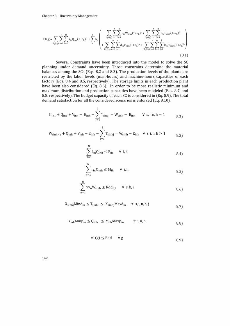
Chapter 8 – Uncertainty Management
142
z1 g = ainQinh 1+ebh
H
h=1
N
n=1i IG i,g
+ N
S
s
cinWsinh 1+eb h
H
h=1
N
n=1i IG i,g
+ binEsinh 1+eb h
H
h=1
N
n=1i IG i,g
dinVsinh 1+eb h
H
h=1
N
n=1i IG i,g
kinjTsinhj 1+eb h
J
j=1
H
h=1
N
n=1i IG i,g
(8.1)
Several Constraints have been introduced into the model to solve the SC planning under demand uncertainty. Those constrains determine the material balances among the SCs (Eqs. 8.2 and 8.3). The production levels of the plants are restricted by the labor levels (man‐hours) and machine‐hours capacities of each factory (Eqs. 8.4 and 8.5, respectively). The storage limits in each production plant have been also considered (Eq. 8.6). In order to be more realistic minimum and maximum distribution and production capacities have been modeled (Eqs. 8.7, and 8.8, respectively). The budget capacity of each SC is considered in (Eq. 8.9). The total demand satisfaction for all the considered scenarios is enforced (Eq. 8.10).
II Q V E T
J
W E s, i, n, h 1 8.2)
W Q V E T
J
W E s, i, n, h 1 8.3)
l Q
N
F i, h 8.4)
r Q
N
M i, h 8.5)
vv W
N
Rdd , s, h, i 8.6)
X Mind T X Maxd s, i, n, h, j 8.7)
Y Minp Q Y Maxp i, n, h 8.8)
z1 g Bdd g 8.9)
Chapter 8 – Uncertainty Management
143
T
I
Djj s, n, h, j 8.10)
The cooperative problem (demand uncertainty) has been formulated as a two stage stochastic MILP model by Eqs. (8.2 to 8.10) and solved to minimize the expected total cost (Eq. 8.1).
8.2.6. Competitive behavior
The proper customer satisfaction policy of a competitive market has been introduced considering several SC’s competing for the global demand and adapting their prices to gain more benefits. Additionally, several discounts in the prices of the products have been included into the problem formulation in order to enforce competition. Product quality or environmental parameters may be considered as competition policies in the SC’s problems. The demand to be covered is the result of the uncertain market demand plus the demand covered by third entities (SCs) which depend on the uncertain competitors’ behavior. The main goal/criteria is to reproduce a real markets situations, where markets get the products from the cheapest SC. In other words “minimize the expenses of the buyers Eq. (8.11).
In order to manage this source of uncertainty, the eventual discount in the price (Prate) of the products (of the SC of interest) has been introduced as new “first stage” variable to be optimized; this new variable “Prate” represents the non‐lineal term of the problem. Otherwise, the production (Qsinh), the inventory (Wsinh), Backorder (Esinh), Subcontracting (Vsinh) and distribution levels (Tsinhj) correspond to the “second stage” variables. Several scenarios of the prices discount “competence behavior” of the competitors (Discs) have been characterized as the uncertain parameters. Obviously, a new challenge appears related to the evaluation of uncertain behavior of the competitor SCs.
8.2.6.1. Mathematical model
The objective function that minimizes the expenses of the buyers is formulated as Eq. (8.11) summarizing the expenses of SC1 and SC2 and penalizing the operation cost of both SCs (zns, see, Eq. 8.12).
min CST g N Ps TIG ,
Prate
1s
Ps TIG ,
Disc zn s
(8.11)
The material balances, production capacities, maximum and minimum distribution/production limits, budget capacities, and storage limits of each SC have been considered in (Eq. 8.13 to 8.21)
Chapter 8 – Uncertainty Management
144
= ainQsinh 1+ebh
H
h=1
N
n=1i IG i,g
cinWsinh 1+eb h
H
h=1
N
n=1i IG i,g
+ binEsinh 1+eb h
H
h=1
N
n=1i IG i,g
dinVsinh 1+eb h
H
h=1
N
n=1i IG i,g
kinjTsinhj 1+eb h
J
j=1
H
h=1
N
n=1i IG i,g
(8.12)
II Q V E T
J
W E s, i, n, h 1 (8.13)
W Q V E T
J
W E s, i, n, h 1 (8.14)
l Q
N
F i, h (8.15)
r Q
N
M i, h (8.16)
Y Minp Q Y Maxp i, n, h (8.17)
In order better model the quantity demanded by the customers, a price elasticity of demand has been introduced (see Eq. 8.18). Ed is proposed to indicate the sensitivity of the quantity demanded to the price changes (Varian, 1992). Then, Eq. (8.19) computes the new demand to be satisfied by the set of SCs and the discount rates and prices elasticity of demands based on the original demand satisfaction. Accordingly, the new demand is enforced by Eq. (8.20).
Ed∆D/D∆P/P
(8.18)
Dem max Djj Ed DjjPrate
100n, h, j (8.19)
T
I
Dem s, n, h, j (8.20)
The competitive problem (competitive behavior uncertainty) is solved as a two stage stochastic programming MINLP model described in the Eqs. (8.6, 8.7, 8.9
Chapter 8 – Uncertainty Management
145
and 8.12‐8.20). The model minimizes the expenses of the buyers CST (Eq. 8.11). Additionally, the competitive behavior is introduced looking for the best discount rate of SC1 considering several discount scenarios in the prices of the competence (SC2; SC3; …; SCn).
8.3. Case Study
The aforementioned concepts have been applied to a SC case study adapted from Wang and Liang (2004; 2005), Liang (2008) and also presented in Chapter 7.
In the cooperative problem (demand uncertainty), the demand forecast considers 3 scenarios; those scenarios are emerged from the assumption that market demands are “above average”, “average (original demand; see Appendix C Table C.3)” and “below average”. Numerically, demand changes are assumed as +25% and ‐25% of the original values and the probability of occurrence is assumed as 33% for each scenario.
In the competitive problem, the discount rate of the competitors (in this case SC2) considers 4 scenarios (Discs 0.1, 0.2, 0.3 and 0.4 %) with probability of occurrence 25% for each scenario. A nominal selling price has been introduced to maintain data integrity and is the same (100$) for all products; plants; and distribution centers. Thus, changes in the prices are considered and the price elasticity of demand has been assumed to be (Ed= ‐5).
8.4. Results
This section is divided into tree subsections; the first one discusses the solutions of the demand uncertainty problem, while the second one contends the summary of the solutions of the competitive problem (competition behavior) as the uncertain source, and the third states the competition behavior as an exogenous source of the uncertain demand.
The resulting MILP (cooperative) and MINLP (competitive) models have been implemented and solved using GAMS/ DICOPT (Conópt/Ceplex) (Nonlinear model) 7.0 on a PC Windows XP computer using an IntelR Coretm i7 CPU(920) 2.67 GHz processor with 2.99 GB of RAM. The solution reported in the competitive model is the best solution obtained but global optimality is not guaranteed (see, Tables 8.1 and 8.2).

Chapter 8 – Uncertainty Management
146
Table 8.1. Execution Report of the Demand uncertainty problem (cooperative)
Deterministic problems Two stage model
s1 s2 s3
Equations 383 383 383 402
Continuous variables 337 337 337 580
Discrete variables 312 312 312 456
Absolute gap 0 0 0 0.000
Relative gap % 0.0000 0.0000 0.0000 0.0000
Time [s] 0.047 0.047 0.046 11.953
Table 8.2. Execution Report of the competitive problem
Deterministic problems Two stage model
s1 s2 s3 s4
Equations 383 383 383 383 973
Continuous variables 337 337 337 337 689
Discrete variables 312 312 312 312 648
Absolute gap 0 0 0 0 0.0000
Relative gap % 0.00 0.00 0.00 0.00 0.0000
Time [s] 0.093 0.094 0.094 0.094 0.157
8.4.1. Demand uncertainty(cooperative problem)
As it is shown in Table 8.3 three different demand scenarios have been considered. In order to highlight the solutions of the two stage model the deterministic solutions of each scenario have been computed. (see, Figures 8.1 to 8.6).
Figure 8.1 shows the production levels plus the subcontracted products of the deterministic solutions for all the demand scenarios considered s1 (a), s2 (b) and s3 (c). As it can be observed, as the objective function penalizes the production over the time, then, the results are directed to produce at the first time periods and then storage (see, Figure 8.2) the products to be distributed during the next time periods. Consequently, the main decision is form where distribute the products, and the performance of the model is conducted by these costs (distribution cost, since production and inventory cost are the same in both SCs). Consequently, products are delivered from the closer production plant until the budget capacity of each SC is reached.
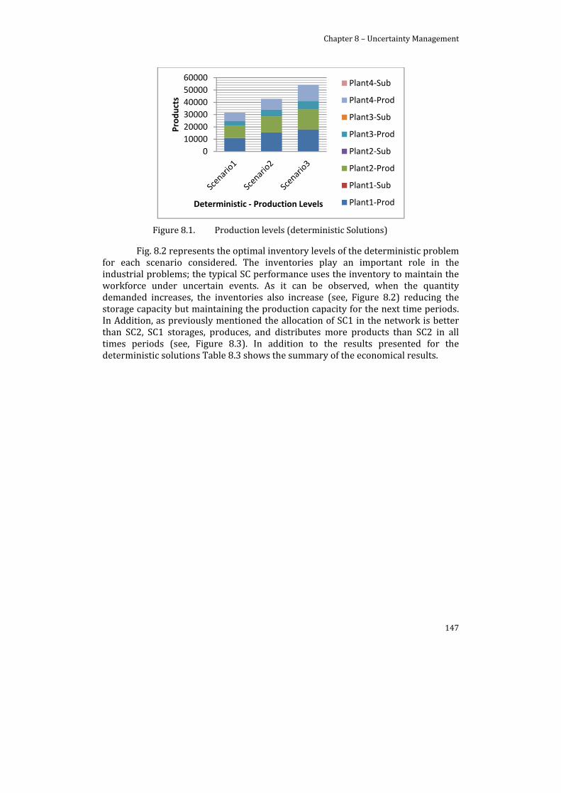
Chapter 8 – Uncertainty Management
147
Figure 8.1. Production levels (deterministic Solutions)
Fig. 8.2 represents the optimal inventory levels of the deterministic problem for each scenario considered. The inventories play an important role in the industrial problems; the typical SC performance uses the inventory to maintain the workforce under uncertain events. As it can be observed, when the quantity demanded increases, the inventories also increase (see, Figure 8.2) reducing the storage capacity but maintaining the production capacity for the next time periods. In Addition, as previously mentioned the allocation of SC1 in the network is better than SC2, SC1 storages, produces, and distributes more products than SC2 in all times periods (see, Figure 8.3). In addition to the results presented for the deterministic solutions Table 8.3 shows the summary of the economical results.
0
10000
20000
30000
40000
50000
60000
Products
Deterministic ‐ Production Levels
Plant4‐Sub
Plant4‐Prod
Plant3‐Sub
Plant3‐Prod
Plant2‐Sub
Plant2‐Prod
Plant1‐Sub
Plant1‐Prod
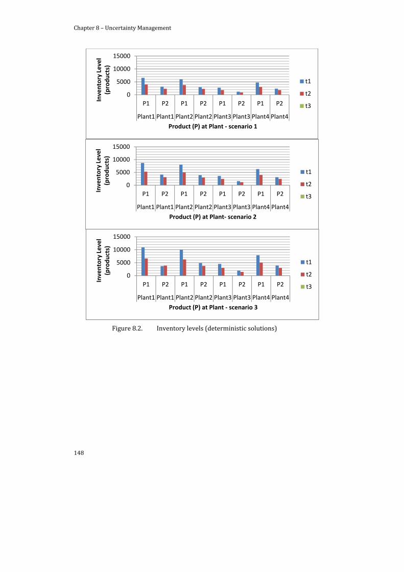
Chapter 8 – Uncertainty Management
148
Figure 8.2. Inventory levels (deterministic solutions)
0
5000
10000
15000
P1 P2 P1 P2 P1 P2 P1 P2
Plant1 Plant1 Plant2 Plant2 Plant3 Plant3 Plant4 Plant4
Inventory Level
(products)
Product (P) at Plant ‐ scenario 1
t1
t2
t3
0
5000
10000
15000
P1 P2 P1 P2 P1 P2 P1 P2
Plant1 Plant1 Plant2 Plant2 Plant3 Plant3 Plant4 Plant4
Inventory Level
(products)
Product (P) at Plant‐ scenario 2
t1
t2
t3
0
5000
10000
15000
P1 P2 P1 P2 P1 P2 P1 P2
Plant1 Plant1 Plant2 Plant2 Plant3 Plant3 Plant4 Plant4
Inventory Level
(products)
Product (P) at Plant ‐ scenario 3
t1
t2
t3
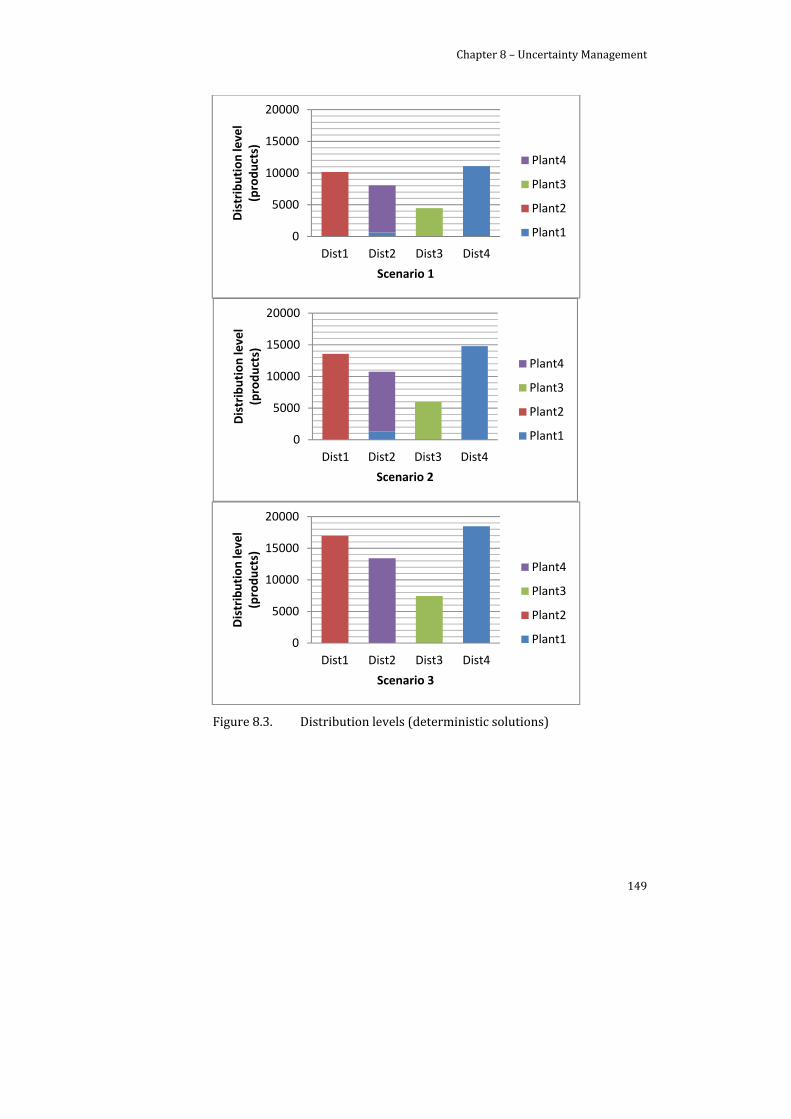
Chapter 8 – Uncertainty Management
149
Figure 8.3. Distribution levels (deterministic solutions)
0
5000
10000
15000
20000
Dist1 Dist2 Dist3 Dist4
Distribution level
(products)
Scenario 1
Plant4
Plant3
Plant2
Plant1
0
5000
10000
15000
20000
Dist1 Dist2 Dist3 Dist4
Distribution level
(products)
Scenario 2
Plant4
Plant3
Plant2
Plant1
0
5000
10000
15000
20000
Dist1 Dist2 Dist3 Dist4
Distribution level
(products)
Scenario 3
Plant4
Plant3
Plant2
Plant1
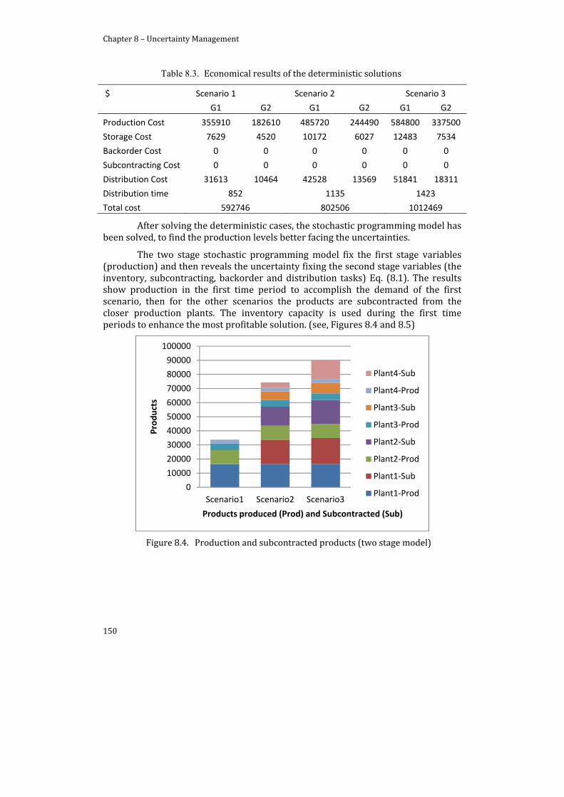
Chapter 8 – Uncertainty Management
150
Table 8.3. Economical results of the deterministic solutions
$ Scenario 1 Scenario 2 Scenario 3
G1 G2 G1 G2 G1 G2
Production Cost 355910 182610 485720 244490 584800 337500
Storage Cost 7629 4520 10172 6027 12483 7534
Backorder Cost 0 0 0 0 0 0
Subcontracting Cost 0 0 0 0 0 0
Distribution Cost 31613 10464 42528 13569 51841 18311
Distribution time 852 1135 1423
Total cost 592746 802506 1012469
After solving the deterministic cases, the stochastic programming model has been solved, to find the production levels better facing the uncertainties.
The two stage stochastic programming model fix the first stage variables (production) and then reveals the uncertainty fixing the second stage variables (the inventory, subcontracting, backorder and distribution tasks) Eq. (8.1). The results show production in the first time period to accomplish the demand of the first scenario, then for the other scenarios the products are subcontracted from the closer production plants. The inventory capacity is used during the first time periods to enhance the most profitable solution. (see, Figures 8.4 and 8.5)
Figure 8.4. Production and subcontracted products (two stage model)
0
10000
20000
30000
40000
50000
60000
70000
80000
90000
100000
Scenario1 Scenario2 Scenario3
Products
Products produced (Prod) and Subcontracted (Sub)
Plant4‐Sub
Plant4‐Prod
Plant3‐Sub
Plant3‐Prod
Plant2‐Sub
Plant2‐Prod
Plant1‐Sub
Plant1‐Prod

Chapter 8 – Uncertainty Management
151
Figure 8.5. Inventory levels (two stage model)
Distribution tasks for the different demand scenarios can be found in Figure 8.6. As it is shown, the performance is driven by the need to prioritize the distribution of production surplus to the distribution centers (customer’s) looking for the cheapest distribution option and considering the maximum distribution capacity and demands for the futures time periods.
020004000600080001000012000
P1 P2 P1 P2 P1 P2 P1 P2
Plant1 Plant1 Plant2 Plant2 Plant3 Plant3 Plant4 Plant4Inventory Level (products)
Product (P) at Plant‐ scenario 1
t1
t2
t3
0
2000
4000
6000
8000
10000
12000
P1 P2 P1 P2 P1 P2 P1 P2
Plant1 Plant1 Plant2 Plant2 Plant3 Plant3 Plant4 Plant4Inventory Level (products)
Product (P) at Plant ‐ scenario 2
t1
t2
t3
0
2000
4000
6000
8000
10000
12000
P1 P2 P1 P2 P1 P2 P1 P2
Plant1 Plant1 Plant2 Plant2 Plant3 Plant3 Plant4 Plant4Inventory Level (products)
Product (P) at Plant ‐ scenario 3
t1
t2
t3
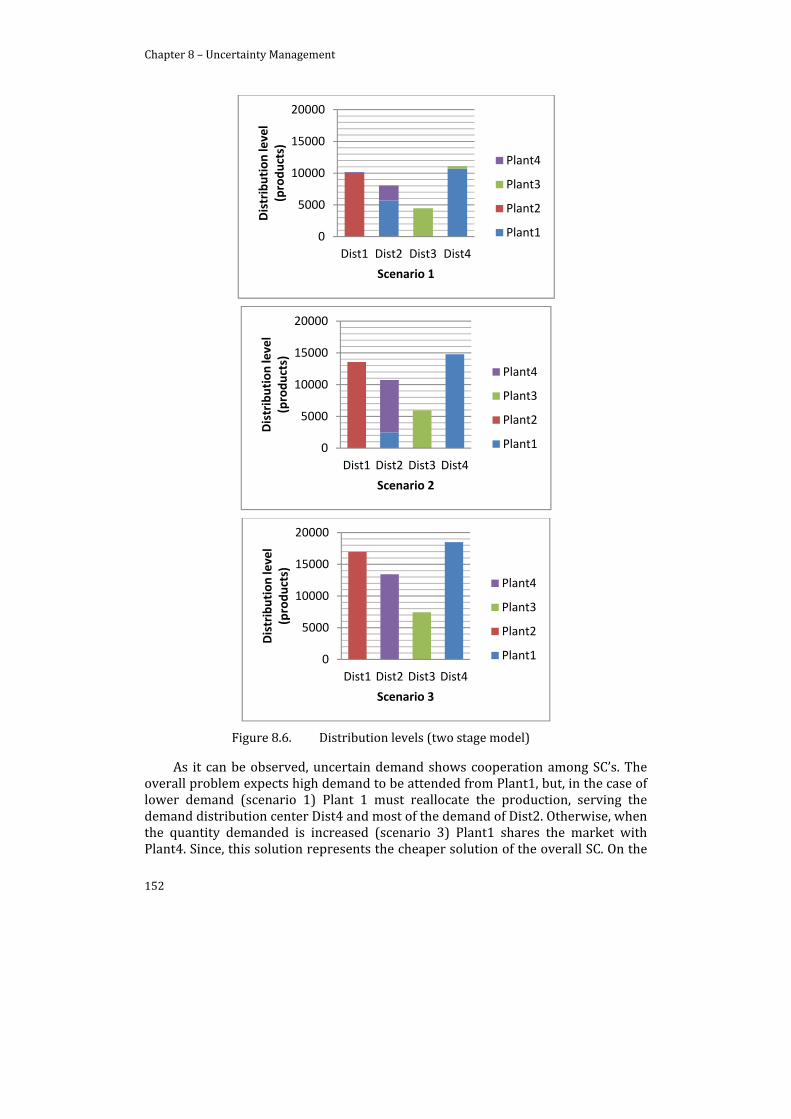
Chapter 8 – Uncertainty Management
152
Figure 8.6. Distribution levels (two stage model)
As it can be observed, uncertain demand shows cooperation among SC’s. The overall problem expects high demand to be attended from Plant1, but, in the case of lower demand (scenario 1) Plant 1 must reallocate the production, serving the demand distribution center Dist4 and most of the demand of Dist2. Otherwise, when the quantity demanded is increased (scenario 3) Plant1 shares the market with Plant4. Since, this solution represents the cheaper solution of the overall SC. On the
0
5000
10000
15000
20000
Dist1 Dist2 Dist3 Dist4Distribution level
(products)
Scenario 1
Plant4
Plant3
Plant2
Plant1
0
5000
10000
15000
20000
Dist1 Dist2 Dist3 Dist4
Distribution level
(products)
Scenario 2
Plant4
Plant3
Plant2
Plant1
0
5000
10000
15000
20000
Dist1 Dist2 Dist3 Dist4
Distribution level
(products)
Scenario 3
Plant4
Plant3
Plant2
Plant1
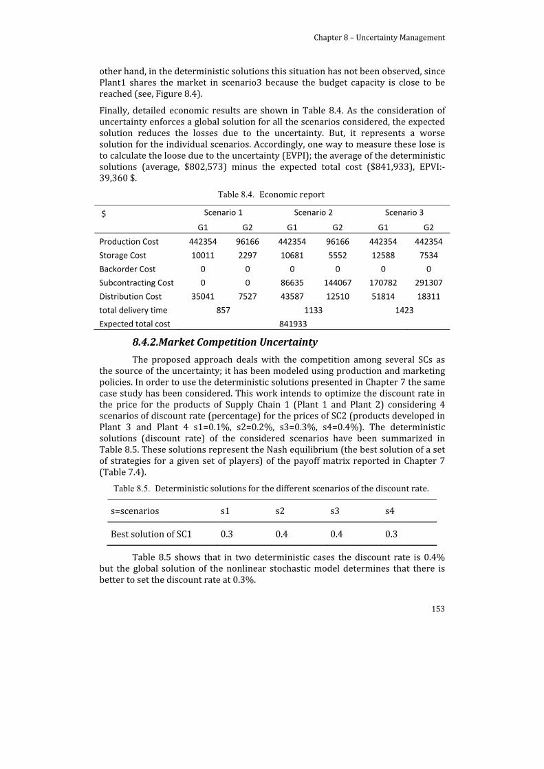
Chapter 8 – Uncertainty Management
153
other hand, in the deterministic solutions this situation has not been observed, since Plant1 shares the market in scenario3 because the budget capacity is close to be reached (see, Figure 8.4).
Finally, detailed economic results are shown in Table 8.4. As the consideration of uncertainty enforces a global solution for all the scenarios considered, the expected solution reduces the losses due to the uncertainty. But, it represents a worse solution for the individual scenarios. Accordingly, one way to measure these lose is to calculate the loose due to the uncertainty (EVPI); the average of the deterministic solutions (average, $802,573) minus the expected total cost ($841,933), EPVI:‐39,360 $.
Table 8.4. Economic report
$ Scenario 1 Scenario 2 Scenario 3
G1 G2 G1 G2 G1 G2
Production Cost 442354 96166 442354 96166 442354 442354
Storage Cost 10011 2297 10681 5552 12588 7534
Backorder Cost 0 0 0 0 0 0
Subcontracting Cost 0 0 86635 144067 170782 291307
Distribution Cost 35041 7527 43587 12510 51814 18311
total delivery time 857 1133 1423
Expected total cost 841933
8.4.2. Market Competition Uncertainty
The proposed approach deals with the competition among several SCs as the source of the uncertainty; it has been modeled using production and marketing policies. In order to use the deterministic solutions presented in Chapter 7 the same case study has been considered. This work intends to optimize the discount rate in the price for the products of Supply Chain 1 (Plant 1 and Plant 2) considering 4 scenarios of discount rate (percentage) for the prices of SC2 (products developed in Plant 3 and Plant 4 s1=0.1%, s2=0.2%, s3=0.3%, s4=0.4%). The deterministic solutions (discount rate) of the considered scenarios have been summarized in Table 8.5. These solutions represent the Nash equilibrium (the best solution of a set of strategies for a given set of players) of the payoff matrix reported in Chapter 7 (Table 7.4).
Table 8.5. Deterministic solutions for the different scenarios of the discount rate.
s=scenarios s1 s2 s3 s4
Best solution of SC1 0.3 0.4 0.4 0.3
Table 8.5 shows that in two deterministic cases the discount rate is 0.4% but the global solution of the nonlinear stochastic model determines that there is better to set the discount rate at 0.3%.
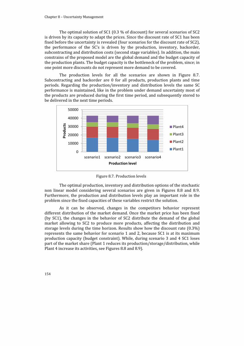
Chapter 8 – Uncertainty Management
154
The optimal solution of SC1 (0.3 % of discount) for several scenarios of SC2 is driven by its capacity to adapt the prices. Since the discount rate of SC1 has been fixed before the uncertainty is revealed (four scenarios for the discount rate of SC2), the performance of the SC’s is driven by the production, inventory, backorder, subcontracting and distribution costs (second stage variables). In addition, the main constrains of the proposed model are the global demand and the budget capacity of the production plants. The budget capacity is the bottleneck of the problem, since; in one point more discounts do not represent more demand to be covered.
The production levels for all the scenarios are shown in Figure 8.7. Subcontracting and backorder are 0 for all products, production plants and time periods. Regarding the production/inventory and distribution levels the same SC performance is maintained, like in the problem under demand uncertainty most of the products are produced during the first time period, and subsequently stored to be delivered in the next time periods.
Figure 8.7. Production levels
The optimal production, inventory and distribution options of the stochastic non linear model considering several scenarios are given in Figures 8.8 and 8.9. Furthermore, the production and distribution levels play an important role in the problem since the fixed capacities of these variables restrict the solution.
As it can be observed, changes in the competitors behavior represent different distribution of the market demand. Once the market price has been fixed (by SC1), the changes in the behavior of SC2 distribute the demand of the global market allowing to SC2 to produce more products, affecting the distribution and storage levels during the time horizon. Results show how the discount rate (0.3%) represents the same behavior for scenario 1 and 2, because SC1 is at its maximum production capacity (budget constraint). While, during scenario 3 and 4 SC1 loses part of the market share (Plant 1 reduces its production/storage/distribution, while Plant 4 increase its activities, see Figures 8.8 and 8.9).
0
10000
20000
30000
40000
50000
scenario1 scenario2 scenario3 scenario4
Products
Production level
Plant4
Plant3
Plant2
Plant1
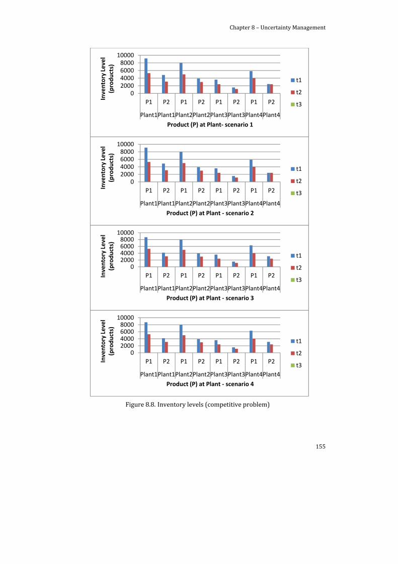
Chapter 8 – Uncertainty Management
155
Figure 8.8. Inventory levels (competitive problem)
02000400060008000
10000
P1 P2 P1 P2 P1 P2 P1 P2
Plant1Plant1Plant2Plant2Plant3Plant3Plant4Plant4
Inventory Level
(products)
Product (P) at Plant‐ scenario 1
t1
t2
t3
02000400060008000
10000
P1 P2 P1 P2 P1 P2 P1 P2
Plant1Plant1Plant2Plant2Plant3Plant3Plant4Plant4
Inventory Level
(products)
Product (P) at Plant ‐ scenario 2
t1
t2
t3
02000400060008000
10000
P1 P2 P1 P2 P1 P2 P1 P2
Plant1Plant1Plant2Plant2Plant3Plant3Plant4Plant4
Inventory Level
(products)
Product (P) at Plant ‐ scenario 3
t1
t2
t3
02000400060008000
10000
P1 P2 P1 P2 P1 P2 P1 P2
Plant1Plant1Plant2Plant2Plant3Plant3Plant4Plant4
Inventory Level
(products)
Product (P) at Plant ‐ scenario 4
t1
t2
t3
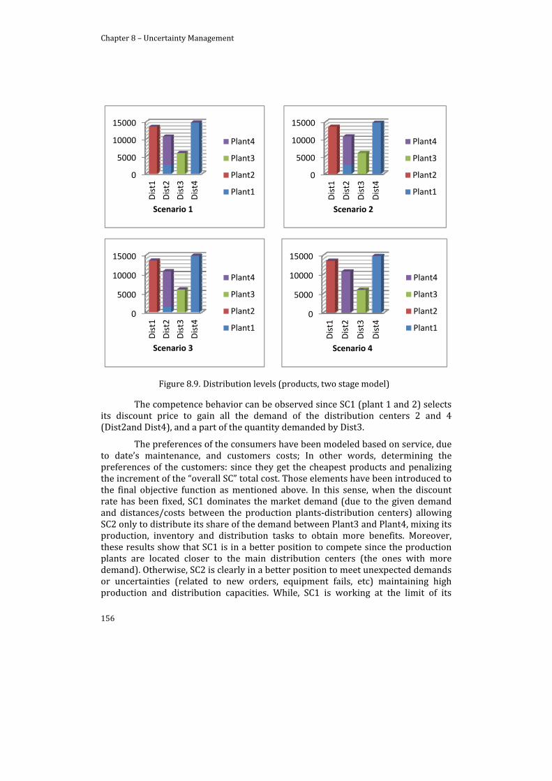
Chapter 8 – Uncertainty Management
156
Figure 8.9. Distribution levels (products, two stage model)
The competence behavior can be observed since SC1 (plant 1 and 2) selects its discount price to gain all the demand of the distribution centers 2 and 4 (Dist2and Dist4), and a part of the quantity demanded by Dist3.
The preferences of the consumers have been modeled based on service, due to date’s maintenance, and customers costs; In other words, determining the preferences of the customers: since they get the cheapest products and penalizing the increment of the “overall SC” total cost. Those elements have been introduced to the final objective function as mentioned above. In this sense, when the discount rate has been fixed, SC1 dominates the market demand (due to the given demand and distances/costs between the production plants‐distribution centers) allowing SC2 only to distribute its share of the demand between Plant3 and Plant4, mixing its production, inventory and distribution tasks to obtain more benefits. Moreover, these results show that SC1 is in a better position to compete since the production plants are located closer to the main distribution centers (the ones with more demand). Otherwise, SC2 is clearly in a better position to meet unexpected demands or uncertainties (related to new orders, equipment fails, etc) maintaining high production and distribution capacities. While, SC1 is working at the limit of its
0
5000
10000
15000
Dist1
Dist2
Dist3
Dist4
Scenario 1
Plant4
Plant3
Plant2
Plant1
0
5000
10000
15000
Dist1
Dist2
Dist3
Dist4
Scenario 2
Plant4
Plant3
Plant2
Plant1
0
5000
10000
15000
Dist1
Dist2
Dist3
Dist4
Scenario 3
Plant4
Plant3
Plant2
Plant1
0
5000
10000
15000
Dist1
Dist2
Dist3
Dist4
Scenario 4
Plant4
Plant3
Plant2
Plant1
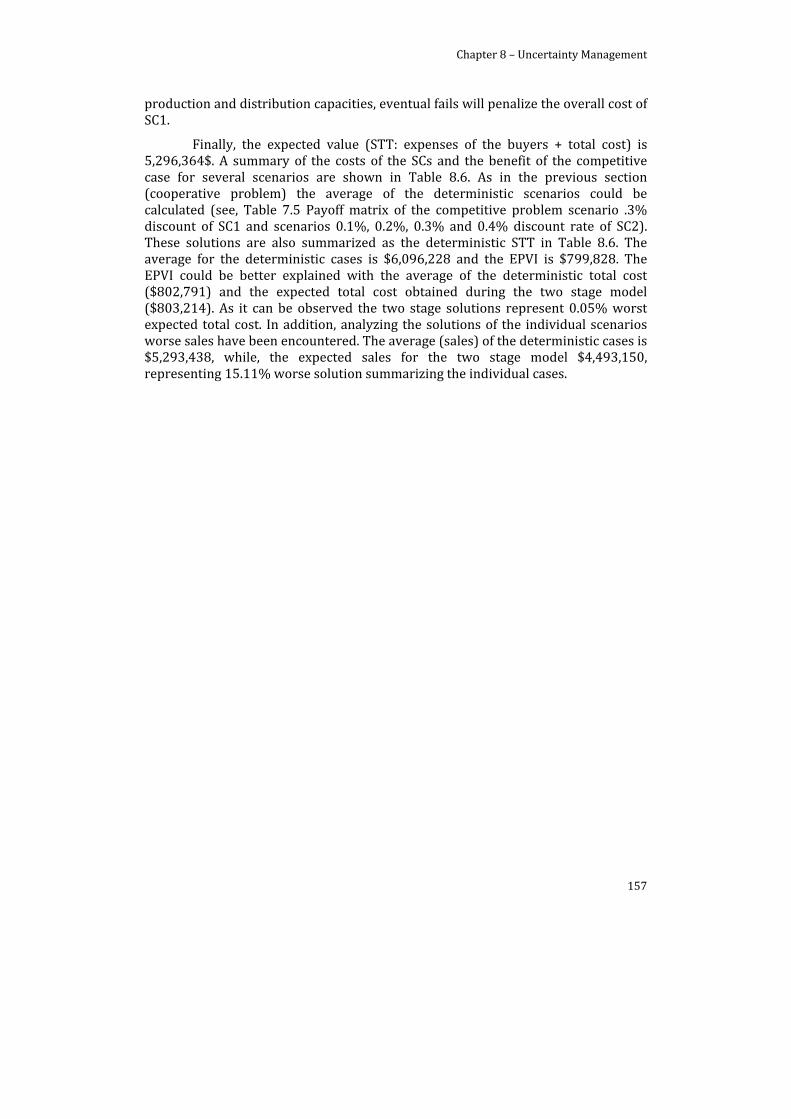
Chapter 8 – Uncertainty Management
157
production and distribution capacities, eventual fails will penalize the overall cost of SC1.
Finally, the expected value (STT: expenses of the buyers + total cost) is 5,296,364$. A summary of the costs of the SCs and the benefit of the competitive case for several scenarios are shown in Table 8.6. As in the previous section (cooperative problem) the average of the deterministic scenarios could be calculated (see, Table 7.5 Payoff matrix of the competitive problem scenario .3% discount of SC1 and scenarios 0.1%, 0.2%, 0.3% and 0.4% discount rate of SC2). These solutions are also summarized as the deterministic STT in Table 8.6. The average for the deterministic cases is $6,096,228 and the EPVI is $799,828. The EPVI could be better explained with the average of the deterministic total cost ($802,791) and the expected total cost obtained during the two stage model ($803,214). As it can be observed the two stage solutions represent 0.05% worst expected total cost. In addition, analyzing the solutions of the individual scenarios worse sales have been encountered. The average (sales) of the deterministic cases is $5,293,438, while, the expected sales for the two stage model $4,493,150, representing 15.11% worse solution summarizing the individual cases.

Chapter 8 – Uncertainty Management
158
Table 8.6. Costs summary.
$ Scenario 1 Scenario 2 Scenario 3 Scenario 4
SC1 SC2 SC1 SC2 SC1 SC2 SC1 SC2
Production cost 640,303 92,402 563,628 167,902 485,959 244,647 464,100 266,506
Storage cost 12,445 2,442 10,977 4,635 10,175 6,030 10,175 6,030
Distribution cost 50,137 5,989 46,858 9,268 42,548 13,578 41,467 14,659
Total Cost 803,717 803,267 802,936 802,936
Sales 4,494,300 4,494,000 4,493,000 4,491,300
STT 5,298,017 5,297,267 5,295,936 5,294,236
Deterministic STT 6,098,364 6,097,189 6,095,514 6,093,845
Expected STT 5,296,364

Chapter 8 – Uncertainty Management
159
8.4.3. Exogenous source of uncertainty
As previously mentioned, industrial applications considering SCM problems under uncertainties have been increased in the last 20 years. This work includes an extended revision of the sources of uncertainty and its applications in PSE scope. There are several works focused on numerous parameters that may affect the performance of single SC, i.e. processing times, changeovers, market demand, etc. In addition, clearly the market demand has been the most studied source of uncertainty. But, issues inside this market demand uncertainty should be studied.
Summarizing the results presented above (demand and competition behavior models) this work states the existence of the competition behavior as an exogenous source of the uncertain demand. Figure 8.10 shows the percentage of products to be produced and distributed by each SC for the market demand considered. As it is previously mentioned, both models (demand uncertainty and market uncertainty) show how the uncertainties are affecting the market demand perception and the treatment of such uncertainties changes the production/distribution/storage decision‐making. Figure 8.10a shows the resulting market share of both SCs considering several scenarios of the competitors’ behavior. Figure 8.10b shows the comparison among the results according to the different models developed to manage the uncertainty, considering the extreme scenarios (scenario 1 and 4 of the competitors behavior problem of Figure 8.10a) and computing the medium scenario to be solved as the typical demand uncertainty problem (for the SC of interest “SC1”). The solutions show the difference among both ways to manage the uncertainty. As it can be observed, in the demand uncertainty model the solution include subcontracting actions. In this line, changes in the market demand could be characterized to different circumstances that are usually disregarded.
These results show how part of the demand uncertainty is associated to the competition behavior. In other words the resulting solutions of the competition behavior problem allow computing the “apparent demand”. The apparent demand corresponds to the hidden part of the demand uncertainty, reveled after the solution of the treatment of the competitors’ behavior uncertainty.
In this sense, the “apparent demand” of the SC under consideration (in this case SC1) can be computed with the solutions obtained from the two stage stochastic programming problem (see, Figure 8.11). Consequently, four uncertain demand scenarios have been obtained and introduced as the typical tactical decision‐making under demand uncertainty problem (two stage model presented above).
Regarding the case study under analysis, even when the original demand considered is low (it was originally proposed for 2 plants and now four plants compete to attend this demand), the competition behavior analysis reveals the share of the market that corresponds to SC1 (in this case 68.41% of the original demand).
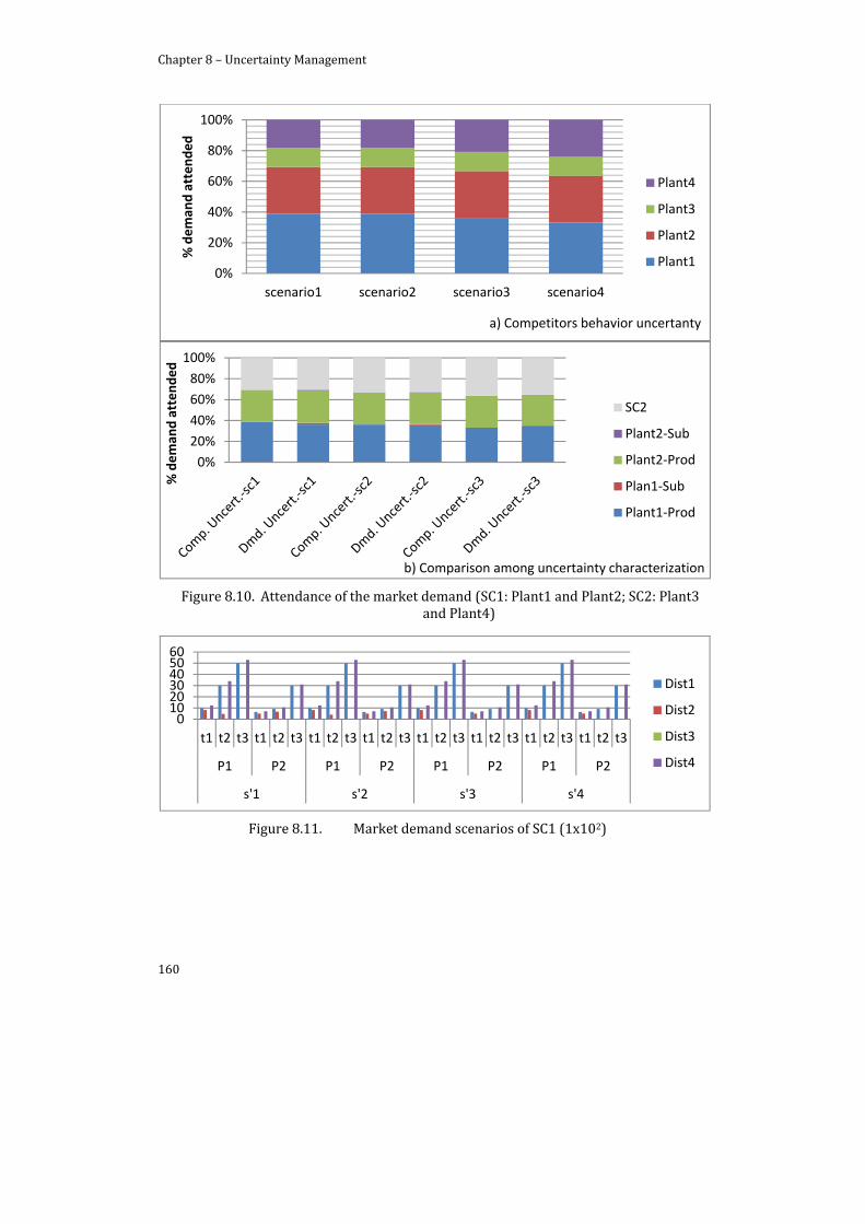
Chapter 8 – Uncertainty Management
160
Figure 8.10. Attendance of the market demand (SC1: Plant1 and Plant2; SC2: Plant3 and Plant4)
Figure 8.11. Market demand scenarios of SC1 (1x10²)
0%
20%
40%
60%
80%
100%
scenario1 scenario2 scenario3 scenario4
% deman
d attended
a) Competitors behavior uncertanty
Plant4
Plant3
Plant2
Plant1
0%
20%
40%
60%
80%
100%
% deman
d attended
b) Comparison among uncertainty characterization
SC2
Plant2‐Sub
Plant2‐Prod
Plan1‐Sub
Plant1‐Prod
0102030405060
t1 t2 t3 t1 t2 t3 t1 t2 t3 t1 t2 t3 t1 t2 t3 t1 t2 t3 t1 t2 t3 t1 t2 t3
P1 P2 P1 P2 P1 P2 P1 P2
s'1 s'2 s'3 s'4
Dist1
Dist2
Dist3
Dist4
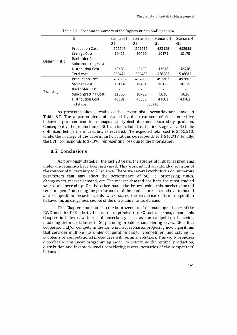
Chapter 8 – Uncertainty Management
161
Table 8.7. Economic summary of the “apparent demand” problem
$ Scenario 1 Scenario 2 Scenario 3 Scenario 4
G1 G1 G1 G1
Deterministic
Production Cost 502513 501595 485959 485959
Storage Cost 10423 10410 10175 10175
Backorder Cost ‐ ‐ ‐ ‐
Subcontracting Cost ‐ ‐ ‐ ‐
Distribution Cost 43485 43463 42548 42548
Total cost 556421 555468 538682 538682
Two stage
Production Cost 492803 492803 492803 492803
Storage Cost 10414 10401 10175 10175
Backorder Cost ‐ ‐ ‐ ‐
Subcontracting Cost 11655 10796 5826 5826
Distribution Cost 43691 43665 43501 43501
Total cost 555210
As presented above, results of the deterministic scenarios are shown in Table 8.7. The apparent demand reveled by the treatment of the competitive behavior problem can be managed as typical demand uncertainty problem. Consequently, the production of SC1 can be included as the first stage variable to be optimized before the uncertainty is revealed. The expected total cost is $555,210, while, the average of the deterministic solutions corresponds to $ 547,313. Finally, the EVPI corresponds to $7,896, representing loss due to the information.
8.5. Conclusions
As previously stated, in the last 20 years, the studies of industrial problems under uncertainties have been increased. This work added an extended revision of the sources of uncertainty to SC science. There are several works focus on numerous parameters that may affect the performance of SC, i.e. processing times, changeovers, market demand, etc. The market demand has been the most studied source of uncertainty. On the other hand, the issues inside this market demand remain open. Comparing the performance of the models presented above (demand and competition behavior), this work states the existence of the competition behavior as an exogenous source of the uncertain market demand.
This Chapter contributes to the improvement of the main open issues of the EWO and the PSE efforts. In order to optimize the SC tactical management, this Chapter includes new terms of uncertainty such as the competition behavior, modeling the uncertainties in SC planning problems considering several SC’s that cooperate and/or compete in the same market scenario; proposing new algorithms that consider multiple SCs under cooperation and/or competition; and solving SC problems by computational procedures with optimal solutions. This work proposes a stochastic non‐linear programming model to determine the optimal production, distribution and inventory levels considering several scenarios of the competitors’ behavior.

Chapter 8 – Uncertainty Management
162
The obtained solution can be compared with the resulted one from other approaches considering that the effect of the competition can be model as part of the “SC demand uncertainty”.
The proposed approach in this contribution allows the SC managers to deal with a new “control parameter” (prices or discount rates) to directly manage the competition behavior and be able to obtain improved solutions at the tactical decision level for real Supply Chain industrial problems.

Chapter 8 – Uncertainty Management
163
Notation
Indexes and sets: n Products (n=1,2,…,N) i Production sites(“sources”, i=1,2,…,I) h Time periods (h=1,2,…,H) j Distribution centers(j=1,2,…,J) g Supply Chain(g=1,2,…,G) s scenarios (s=1, 2, …, S) IG(g) Production sites that belong to Supply Chain g. Parameters: a(i,n) Production cost per unit of product n produced at source i ($/unit) c(i,n) Inventory ‐ cost per unit of product n at source i($/unit) d(i,n) Backordering cost per unit of product n at source i($/unit) l(i,n) Hour of work per unit of product n produced at source i(man‐hour/unit) r(i,n) Required equipment occupation per unit of product n at source i
(machine‐hour/unit) vv(n) Warehouse space required per unit for product n (ft2/unit) k(i,n,j) Transport cost per unit of product n from the source i to the endpoint
j($/unit) u(i,n,j) Transport time of product n from source i to end point j (hour/truck) s(i,n,h,j) Capacity per truck for product n from source i to endpoint j (units/truck) Rdd(h,i) Maximum storage space at production plant i in period h (units) M(i,h) Maximum machine level available at source i in period h (machine‐hour) F(i,h) Maximum labor level of work at source i in period t(man‐hour) Djj(s,n,h,j) Demand for scenario s of product n in period h at endpoint j (units) Dem(n,h,j) Demand of product n in period h at endpoint j according to the
considered price elasticity of the demand (units) Disc(s) Discount in the price of the competitors (%) Bdd(g) Total Budget for Supply Chain g ($) eb Escalating factor for (regular production cost, backorder cost, and
inventory cost) (%) II(i,n,h) Initial storage (units) time 1 Ps(i,n,j) Selling Price of product n produced at source i and distributed by
endpoint j(100$/unit) Mind(i,n) Minimum acceptable quantity of product n to be distributed from source i
in a period (units). Maxd(i,n) Maximum acceptable quantity of product n to be distributed from source
i in a period (units). Minp(i,n) Minimum acceptable quantity of product n to be produced at source i in a
period (units). Maxp(i,n) Maximum acceptable quantity of product n to be produced at source i in a
period (units). Prate Discount in the price for Supply Chain of interest (%) Ed Price elasticity of demand Decision Variables:

Chapter 8 – Uncertainty Management
164
Q(i,n,h) Production of product n in the source i at time h(units) (cooperative problem)
W(s,i,n,h) Inventor y level at source i of the product n at time h(units) E(s,i,n,h) Backorder of the source i of the product n at time h(units) T(s,i,n,h,j) Quantity delivered from the source i to endpoint j of product n at time
h(units) Binary variables: X(i,n,h,j) Binary variable identifying if product n is sent from source i to the
endpoint j at time h. Y(i,n,h) Binary variable identifying if the source i produces product n at time h Objective functions: z1(g) total cost of SCg ($) CST(g) Spend of the buyers at each SCg ($).

165
Chapter 9. MOO as a Bargaining Tool
9.1. Introduction
As previously mentioned, the complexity associated to solve multiple objective optimization problems is additionally complicated by the need to consider uncertainty in the model. Since, the nature of the planning problem is uncertain by the need of allocate production and storage actions considering previsions of the quantity demanded, the work levels, etc.
The literature in the area of SC under uncertainty has been very active over the last decade, arising in several sources of uncertainties such as: market demand (Peidro et al., 2009), product prices (Amaro and Barbosa‐Póvoa, 2009), operating and economic conditions (Haitham et al., 2004), etc. One of these sources of uncertainty scarcely considered in the literature is the competitors behavior, considering the presence of others SCs able to compete or to cooperate for the market demand.
As previously stated in Chapter 7 the use of the Game Theory has been considered as a decision‐making tool, in order to determine the best SC operating strategy (optimal production, inventory and distribution levels) in a competitive planning scenario under uncertainty. Also, both sections (7.1 and 7.2) describe the competition behavior of the several coexisting SCs as an uncertainty source. The resulting problem takes into account the eventual decisions of the other SCs. Since these decisions impact to the profit of the SC of interest (“own SC”), setting that the markets are embedded in this competitive scenario, all these issues improve the decision‐making (see Figure 2.1).
In order to deal with the complexity associated to the competition among markets, and also to keep looking at the different objectives simultaneously, this work proposes the development of a Multi‐Objective Mixed Integer Linear Programming (MO‐MILP) model to optimize the planning of SC in competitive/cooperative environments. When different objectives need to be considered, a final decision method is required – in this work, decisions are selected based on the epsilon‐constraint method (described in Messac et al., 2003). This will allows to compute the payoff matrix and finally to obtain the Nash equilibrium (Nash, 1950), which represents the best solution for several scenarios considered.

Chapter 9 – MOO & GT Optimization Framework
166
9.2. Problem Statement
9.2.1. Supply Chain Planning
The model originally proposed in Chapter 7 has been adopted as a basis for the formulation presented in this Chapter. This formulation assumes the existence of several Supply Chains working in cooperative or competitive scenarios. In both cases, the mathematical constrains associated to the model will considers the material balances, budget capacity, production and storage capacities, maximum and demand satisfaction. The model will be used to minimize different Objective Functions (minimize total cost and total delivery time for the cooperative case; minimize the expenses of the buyers and total delivery time for the competitive case) according to the considered scenario.
9.2.1. Cooperative problem
In the cooperative scenario, the problem has been formulated considering one set of different SCs acting as a single coordinated SC (SC1+SC2+…+SCs). The best result will be to minimize the tradeoff between the total cost (z1) and the total delivery time (z2). The total cost is based on the economic terms (Eq. 9.1: production (ain), inventory (cin) and distribution (kinj) costs of each supply chain g) and the total delivery time is defined as the time to distribute the products (n) to the distribution centers (j) (Eq. 9.2).
Minimize the total cost:
z1 g a Q 1 eI_G ,
c W 1 eI_G ,
k T 1 eI_G ,
(9.1)
Minimize total delivery time:
z2u
sI_G ,
T (9.2)
Then the cooperative model consists in the Eqs. (7.3) to (7.11), that aims to optimize the production, inventory, distribution and backorder actions under multiple criteria (objective functions Eqs., 9.1 and 9.2).
9.2.2. Competitive problem
As in Chapter 7 the competitive problem is formulated considering several SCs competing for the demand of the markets. To play this game (competition behavior), players should deal with the demand share (from the total demand) that customers really offer to each one, and this can be managed basically through their customer satisfaction policy: prices and delivery times. So, besides to the already considered objectives, it is necessary to introduce a new objective representing the

Chapter 9 – MOO & GT Optimization Framework
167
best deal for the customers (cost for the distribution centers). This has been done through the price rates (Prateg), given the price of the products (Psinj), then the discount of the prices is associated at the source and the destiny of the products, Eq. (9.13) should be now considered as the new objective function.
Min CST g Ps TI_G ,
Prate z1 g (9.3)
As in the Chapter 7 the elasticity demand price has been also included. Then the competitive model aims to optimize the tradeoff between the expense of the buyers (Eq. 9.3) and the total delivery time (Eq. 9.2) for several Supply Chains, and the cooperative model corresponds to the Eqs. (7.3) to (7.9), (7.11) and (7.14).
9.2.3. MultiObjective Optimization (MOO)
This work uses the Pareto space of dominant solutions obtained by the epsilon constraint method. The solution closer to the utopia point takes place into the payoff matrix, and this matrix shows the solutions for each scenario of the competitors behavior and let us to choose the best solution for the problem. In this work it is proposed to use the MOO paradigm to model the tradeoff associated to the competition/negotiation among the different interacting elements: Several SCs and their markets. The introduction of these external objectives enables to model this negotiation which is crucial for the decision‐making. (Eq. 9.1, 9.2 and 9,3)
The following algorithm has been developed to obtain the Pareto front and select the solution to be used in the Payoff matrix, see Fig. 9.3a.
Obtain the anchor points Optimize the single objective problem (SOO) for each objective considered
(+). Divide the Pareto frontier into mk points (········). Fix the Pareto point “mk” to be included as a constraint in one of the SOO
problems. Optimize the problem SOO for all the mk points in the Pareto frontier. Draw the Utopia Point (o). Set the solution to the point closer to the utopia point. End.
9.2.4. Game Theory and Equilibrium Point
The use of GT as a decision‐making tool has been introduced in Chapter 7, considering the competition behavior as a source of uncertainty at the tactical decision level in SCM. The proposed approach use the information of several SC’s (players) that compete for the demand of a given market, then the payoff matrix has been used to summarize the solutions for several scenarios considered by each player (SC1, SC2,…,SCn).
Chapter 9 – MOO & GT Optimization Framework
168
9.2.5. Proposed Framework
As mentioned above, the solutions from the MOO problem are very complex and difficult to observe, and this complexity is exacerbated within the consideration of uncertainty. Then, the proposed approach gives the best solution of the MO‐GT optimization for the competitive problem (the cooperative case has been solved as a typical MOO problem). As we can observe Fig. 9.3 shows the procedure to obtain the best solution (in this case the best solution is referring to the Nash equilibrium point of the payoff matrix) of the competitive problem: Fig. 9.3a shows the Pareto frontier obtained by MOO that has been explained above in section 9.2.3; Fig. 9.3b and 9.3c represent the Game Theory optimization, including several scenarios of the discount rates for all the players (SC1, SC2, …, SCn). These scenarios are included as parameters of the MOO problem, and solved as deterministic MOO problems (for all the scenarios of the payoff matrix). Fig. 9.3c reports the “best” solution obtained from the payoff matrix (Nash Equilibrium) sending it to the decision maker as the solution of the problem. Then, assuming that the MOO problem is understood it is introduced in the algorithm as a step (all the sub steps of the MOO are explained in section 9.2.4), the entire algorithm is explained as follows:
Read the data of the given scenarios of the payoff matrix (several scenarios of the competition behavior).
Solve MOO (Fig. 9.3a) Send the solution reported by the MOO problem to the payoff matrix. Repeat 1‐3 for all the competitive scenarios of the payoff matrix. Report the minimum or maximum value of the payoff matrix. (min or max
for the case of minimize total cost, maximize benefit, minimize total delivery time or tardiness, etc.).
End.
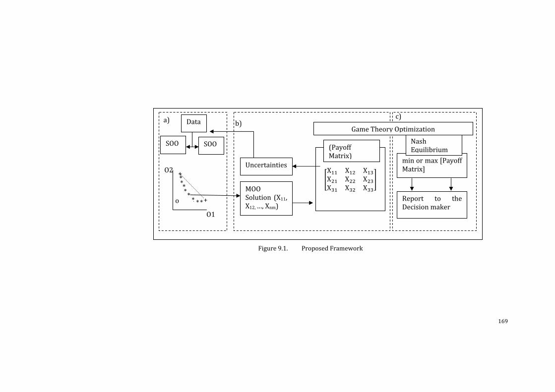
169
Figure 9.1. Proposed Framework
c)
O1
O2 +
o
* * *
*
SOO SOO
Dataa)
X X XX X XX X X
b)
Uncertainties
(Payoff Matrix)
min or max [Payoff Matrix]
Nash Equilibrium
Report to the Decision maker
MOOSolution (X11, X12, …, Xnm)
Game Theory Optimization
+* *
**
*
Chapter 9 – MOO & GT Optimization Framework
170
9.3. Case Study
All the concepts presented have been applied to a Supply Chains case study adapted from Wang and Liang (2004; 2005), Liang (2008) presented in Chapter 7. The network configuration is composed by 2 SCs, SC1: Plant1/Plant2 and SC2:Plant3/Plant4 (see, Fig. 7.3), which collaborate or compete (according to the considered situation) to fulfill the global demand from 4 distribution centers. Discrete time demands have been considered for 3 monthly periods. The information about production capacities and the rest of problem conditions (initial storage levels, transport capacities, and associated costs) can be found in Chapter 7 and Appendix C (Tables C.1‐C.4).
9.4. Results
The cooperative/competitive problems have been solved in GAMS by using Cplex v12 as the solver for the MILP models on a Windows XP computer using an IntelR Coretm i7 CPU(920) 2.67 GHz processor with 2.99 GB of RAM.
Table 9.1. Execution Report
SOO (average)
Equations 384
Continuous variables 312
Discrete variables 288
Absolute gap 0
Relative gap % 0.00
Time [s] 0.093
In this section tree subsections are introduced; one for discussing the solutions of the cooperative problem; the second one contends the summary of the solutions of the competitive problem (competition behavior as the uncertain source), and finally, the third one that summarizes the comparison between the cooperative and the competitive problems solved.
9.4.1. Cooperative Case
To better compare the different alternatives considered, the best standalone results for each SC are displayed in Table 9.2, as well as the results obtained by Liang (2008) and the ones using the original information into our model. This comparison shows how the SC1 is better located geographically than SC2. It is worth mentioning that SC1 advantage against SC2 is just for the demand considered and if other demand is considered, the results should be quite different. The main differences between SC1 Liang’s data and SC1 standalone are because an additional distribution cost has been considered (as stated in the case study description in Chapter 7).
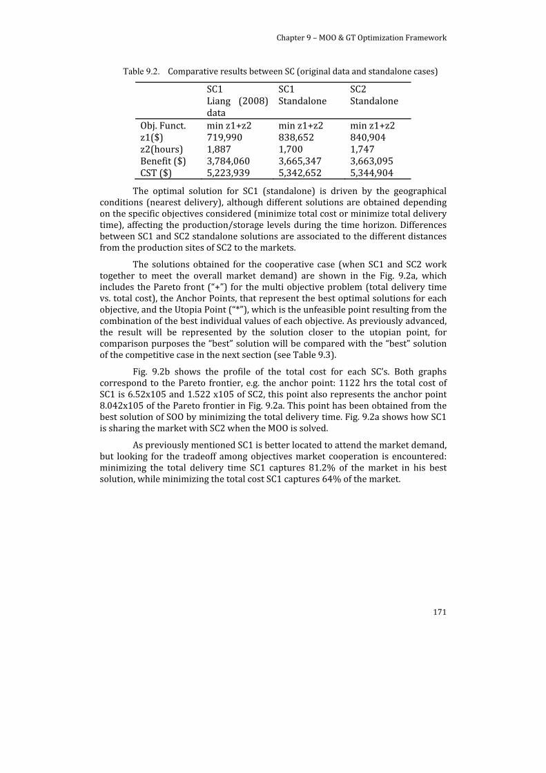
Chapter 9 – MOO & GT Optimization Framework
171
Table 9.2. Comparative results between SC (original data and standalone cases)
SC1 SC1 SC2Liang (2008) data
Standalone Standalone
Obj. Funct. min z1+z2 min z1+z2 min z1+z2 z1($) 719,990 838,652 840,904z2(hours) 1,887 1,700 1,747Benefit ($) 3,784,060 3,665,347 3,663,095 CST ($) 5,223,939 5,342,652 5,344,904
The optimal solution for SC1 (standalone) is driven by the geographical conditions (nearest delivery), although different solutions are obtained depending on the specific objectives considered (minimize total cost or minimize total delivery time), affecting the production/storage levels during the time horizon. Differences between SC1 and SC2 standalone solutions are associated to the different distances from the production sites of SC2 to the markets.
The solutions obtained for the cooperative case (when SC1 and SC2 work together to meet the overall market demand) are shown in the Fig. 9.2a, which includes the Pareto front (“+”) for the multi objective problem (total delivery time vs. total cost), the Anchor Points, that represent the best optimal solutions for each objective, and the Utopia Point (“*”), which is the unfeasible point resulting from the combination of the best individual values of each objective. As previously advanced, the result will be represented by the solution closer to the utopian point, for comparison purposes the “best” solution will be compared with the “best” solution of the competitive case in the next section (see Table 9.3).
Fig. 9.2b shows the profile of the total cost for each SC’s. Both graphs correspond to the Pareto frontier, e.g. the anchor point: 1122 hrs the total cost of SC1 is 6.52x10⁵ and 1.522 x10⁵ of SC2, this point also represents the anchor point 8.042x10⁵ of the Pareto frontier in Fig. 9.2a. This point has been obtained from the best solution of SOO by minimizing the total delivery time. Fig. 9.2a shows how SC1 is sharing the market with SC2 when the MOO is solved.
As previously mentioned SC1 is better located to attend the market demand, but looking for the tradeoff among objectives market cooperation is encountered: minimizing the total delivery time SC1 captures 81.2% of the market in his best solution, while minimizing the total cost SC1 captures 64% of the market.
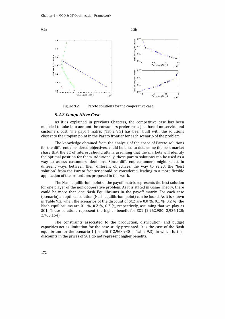
Chapter 9 – MOO & GT Optimization Framework
172
9.2a 9.2b
Figure 9.2. Pareto solutions for the cooperative case.
9.4.2. Competitive Case
As it is explained in previous Chapters, the competitive case has been modeled to take into account the consumers preferences just based on service and customers cost. The payoff matrix (Table 9.3) has been built with the solutions closest to the utopian point in the Pareto frontier for each scenario of the problem.
The knowledge obtained from the analysis of the space of Pareto solutions for the different considered objectives, could be used to determine the best market share that the SC of interest should attain, assuming that the markets will identify the optimal position for them. Additionally, these pareto solutions can be used as a way to assess customers’ decisions. Since different customers might select in different ways between their different objectives, the way to select the “best solution” from the Pareto frontier should be considered, leading to a more flexible application of the procedures proposed in this work.
The Nash equilibrium point of the payoff matrix represents the best solution for one player of the non‐cooperative problem. As it is stated in Game Theory, there could be more than one Nash Equilibriums in the payoff matrix. For each case (scenario) an optimal solution (Nash equilibrium point) can be found. As it is shown in Table 9.3, when the scenarios of the discount of SC2 are 0.0 %, 0.1 %, 0.2 %; the Nash equilibriums are 0.1 %, 0.2 %, 0.2 %, respectively, assuming that we play as SC1. These solutions represent the higher benefit for SC1 (2,962,980; 2,936,128; 2,703,154).
The constraints associated to the production, distribution, and budget capacities act as limitation for the case study presented. It is the case of the Nash equilibrium for the scenario 1 (benefit $ 2,963,980 in Table 9.3), in which further discounts in the prices of SC1 do not represent higher benefits.
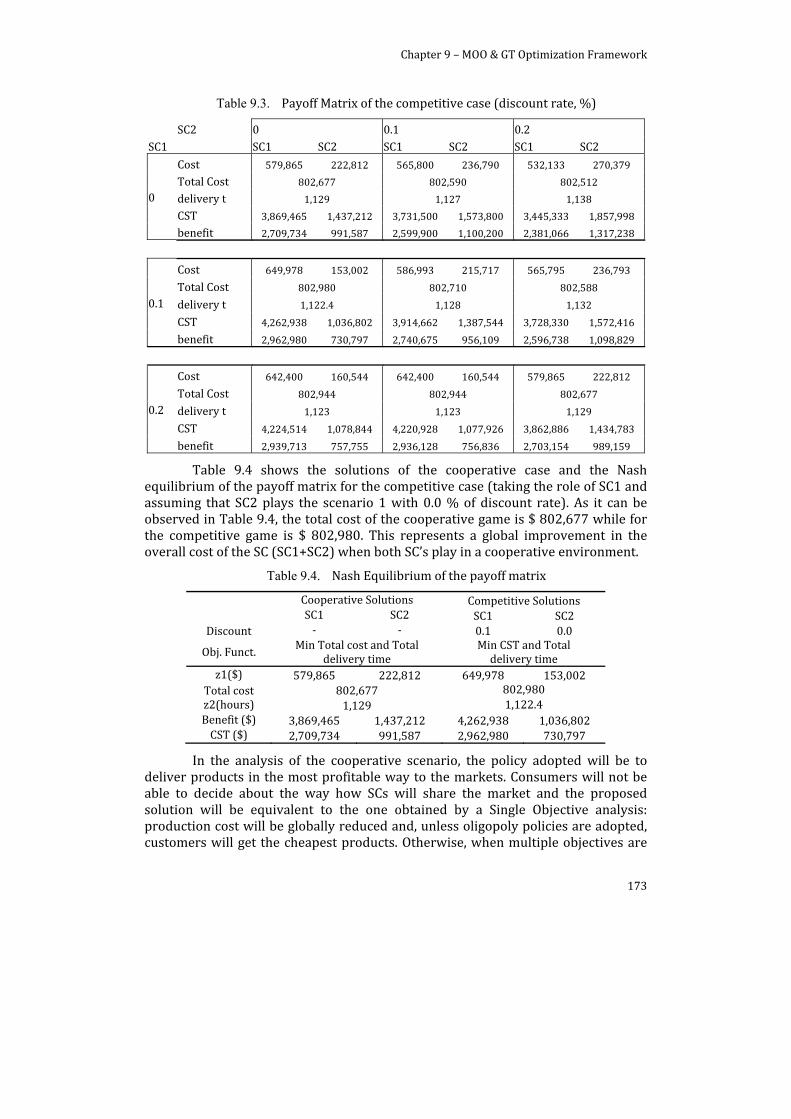
Chapter 9 – MOO & GT Optimization Framework
173
Table 9.3. Payoff Matrix of the competitive case (discount rate, %)
SC2 0 0.1 0.2 SC1 SC1 SC2 SC1 SC2 SC1 SC2
0
Cost 579,865 222,812 565,800 236,790 532,133 270,379
Total Cost 802,677 802,590 802,512
delivery t 1,129 1,127 1,138
CST 3,869,465 1,437,212 3,731,500 1,573,800 3,445,333 1,857,998
benefit 2,709,734 991,587 2,599,900 1,100,200 2,381,066 1,317,238
0.1
Cost 649,978 153,002 586,993 215,717 565,795 236,793
Total Cost 802,980 802,710 802,588
delivery t 1,122.4 1,128 1,132
CST 4,262,938 1,036,802 3,914,662 1,387,544 3,728,330 1,572,416
benefit 2,962,980 730,797 2,740,675 956,109 2,596,738 1,098,829
0.2
Cost 642,400 160,544 642,400 160,544 579,865 222,812
Total Cost 802,944 802,944 802,677
delivery t 1,123 1,123 1,129
CST 4,224,514 1,078,844 4,220,928 1,077,926 3,862,886 1,434,783
benefit 2,939,713 757,755 2,936,128 756,836 2,703,154 989,159
Table 9.4 shows the solutions of the cooperative case and the Nash equilibrium of the payoff matrix for the competitive case (taking the role of SC1 and assuming that SC2 plays the scenario 1 with 0.0 % of discount rate). As it can be observed in Table 9.4, the total cost of the cooperative game is $ 802,677 while for the competitive game is $ 802,980. This represents a global improvement in the overall cost of the SC (SC1+SC2) when both SC’s play in a cooperative environment.
Table 9.4. Nash Equilibrium of the payoff matrix
Cooperative Solutions Competitive Solutions SC1 SC2 SC1 SC2
Discount ‐ ‐ 0.1 0.0
Obj. Funct. Min Total cost and Total
delivery time Min CST and Total delivery time
z1($) 579,865 222,812 649,978 153,002 Total cost 802,677 802,980z2(hours) 1,129 1,122.4Benefit ($) 3,869,465 1,437,212 4,262,938 1,036,802 CST ($) 2,709,734 991,587 2,962,980 730,797
In the analysis of the cooperative scenario, the policy adopted will be to deliver products in the most profitable way to the markets. Consumers will not be able to decide about the way how SCs will share the market and the proposed solution will be equivalent to the one obtained by a Single Objective analysis: production cost will be globally reduced and, unless oligopoly policies are adopted, customers will get the cheapest products. Otherwise, when multiple objectives are
Chapter 9 – MOO & GT Optimization Framework
174
considered, the entire problem changes and multiple policies to satisfy the market demand should be considered. Specifically, in this case: the policy “deliver the cheapest products” has to change in order to provide cheaper products that require shorter delivery time.
The results presented in this section and the analysis from the Chapter 7 (subsection 7.1.5 Bargaining tools) show how the multiple objective optimization acts as a bargaining tool: even there is still a competition and each SC modifies their behavior looking to obtain more benefit, the proposed framework will allow to identify the situation where the tradeoff between objectives will result in a more efficient proposal (less delivery time, cheaper products, etc.). For example: if SC1 reduce its costs, the MO optimization framework will identify not only the expected increased demand from the market, but also the expected increment on the total delivery time associated to this additional demand, which should be also taken into account by SC1 to find a compromise decision. The analysis proposed in the previous Chapter 7 did not contemplate the expected market response to the competition, so each one of the elements of the payoff matrix to be analyzed only considered the optimum SC performance disregarding further market decisions.
9.5. Conclusions
This Chapter proposes and describes the integrated use of the Game Theory optimization in an MOO MILP‐based approach to determine the production, inventory and distribution profiles, optimizing the SC planning problem under cooperative and non‐cooperative environments. The cooperative and non cooperative multi objective problems have been modeled and solved using mathematical programming techniques (MILP models) and GT optimization strategies as the payoff matrix and the Nash equilibrium point.
The proposed approach introduces the use of a robustness tool, emphasizing the role of competitors as a source of uncertainty in typical SC planning problems. This work also presents, the integrated use of the different methodologies to improve the decision‐making associated to the new challenges of the present and future market scenarios (reduction of inventories, reactive policies of markets/competitors, more market competition, production capacity changes/flexibility, etc).

Part IV Final Remarks

177
Chapter 10. Conclusions and Further work
10.1. Conclusions
The contributions developed by this Thesis enhance the competitiveness of different SCs in a competitive environment. The perspective objectives have been highlighted along the chapters presented in the document. In addition, market globalization; uncertain environments; and current economic crisis were remarked in the thesis and presented as new challenges to the PSE society.
The thesis document is divided into many parts as follows:
Part I presents a state of the art extensive review discussing these new challenges and their real industrial applications. In Chapter 3, the most used techniques/methods to solve SC decision‐making models as well as the methods used throughout this Thesis have been described.
Part II proposes some mathematical models to improve the SC competitiveness by integrating enterprise functionalities (i.e. vertical integration of decision‐making levels).
Following the same competitiveness line, section 4.1 (in Chapter 4) exploits the process and the plant flexibility by integrating synthesis and scheduling models. The proposed approach shows flexibility behavior in the integrated decision‐making models. Moreover, and in order to better visualize the information used by the proposed model, a new process technique “Synthesis State Task network representation” has been proposed. Another plant decision‐making improvement has been proposed in Section 4.2, where the integration of low‐term planning and control actions has been included. MILP and ODE simulation frameworks were developed to optimize the operations of a “Distributed Energy Generation system” as a case study. The proposed model considers several energy generation technologies in obtaining optimal energy production, storage, and distribution. Furthermore, these plans have been considered as set points during the simulation of such energy generation technologies.
In Chapter 5, tactical and operational decision‐making levels have been integrated through a based knowledge planning‐scheduling model. Detailed process operation model has been optimized for several scenarios. All the solutions obtained represent nonlinear functions. These nonlinear functions have been included as constraints into the planning model. The resulted model forms a MINLP based model.
Chapter 10 – Conclusions & Further work
178
On the other hand, the proposed approach discussed in Chapter 6 coordinates the tactical management of several SCs. Normally, the typical formulation of the SC planning considers some limited/fixed information about several echelons in optimizing their interaction (raw material, production plants, distribution tasks, distribution centers, and markets). In this thesis, such information has been extended and used to characterize multiple SC behaving as one entire SC.
The echelons of the typical SC have been studied in details. For example, the raw material echelon includes several suppliers with different costs. Several production plants each can produce two types of products. The final products pass to storage centers to be delivered later to the markets. The coordination is enhanced by considering fixed and dynamic demands; the raw materials of each SC correspond to the products to be delivered by other SCs. Thus, the production plants have been characterized as markets to be satisfied by other SCs. A polystyrene SC has been considered as a case study including its energy consumption and wastewater generation. The raw material echelon has been considered as complete SC (RMSC) that deal with the raw material acquisition (four types of biomass provided by one supplier), and distribution to the energy generation SC (EGSC). The EGSC consists of four markets: two with fixed demand (local market and secondary market), and two with dynamic demand (polystyrene production plants and wastewater treatment plant). Furthermore, three energy sources were considered (biomass gasification, combustion, and local main grid). The proposed approach optimizes a MILP planning model coordinating the entire SC previously mentioned.
Part III proposes the analysis under cooperation and competition scenarios among several supply chains. Accordingly, the novel approaches developed in this part explicitly include several SCs into the SCM formulation. Specifically, Chapter 7 proposes the use of “Game Theory” optimization as a tool to observe the different situations and to select the best option “Nash Equilibrium”. In section 7.1, a MILP based model and GTO model have been integrated. A new MILP‐GT approach is implemented to solve the tactical management of the typical SC problem. Information of several competitors has been considered in order to cooperate or compete for the market demand. Several market conditions have been covered; the prices of the products have been used to control this uncertain behavior, and the payoff matrix is used to manage these uncertainties.
In section 7.2, the same scope of cooperation and competition has been considered. The proposed approach is applied to a SC scheduling problem. Together with the decisions involved in this operational issue, in this section, the quality of the products has been included as the control parameter representing the uncertain competitor’s behavior.
Moreover, Chapter 7 introduces the competition behavior using the reactive approach to manage the tactical decision‐making under uncertainty competitive behavior. The competitive behavior has been considered as an uncertain source to be included as an exogenous source of the demand uncertainty. This assumption has been extended and studied in Chapter 8. A two stage stochastic model has been

Chapter 10 – Conclusions & Further work
179
developed including the competence behavior. In this line, reactive and preventive approaches have been analyzed to manage this new source of uncertainty.
Part III presents the development of a Bargaining tool to manage the cooperation and competition behaviors among several SCs. The bargaining tool is discussed in details in Chapter 9 developing a Multi‐objective optimization approach. The proposed model clearly includes the cooperation during the multi‐objective management. Also, with the MOO solution, different customer satisfaction policies can be managed, and the best solution of the Pareto frontier can be included in the payoff matrix and accordingly, the Nash Equilibrium will be obtained. Since, this best solution represents the policy to attend market demands; it could be used to improve decision‐making of the markets or the producers.
The proposed goals of this Thesis have been achieved. Consequently, this Thesis increases the SC competitiveness by integrating several decision‐making levels. Additionally, this work modifies the typical model considered in the SCM and explicitly includes third parties facing a global market scenario. As final remark, this Thesis intends to highlight the cooperation as the most improved solution over the competition scenarios, and develops a Bargaining tool to achieve this cooperation.
10.2. Further Work
Integrated SCM is an open issue to future research. In this Thesis a number of research challenges have been proposed. Regarding the work presented in Part I, some steps to follow this work:
In order to reach the vertical integration, some improved techniques must be studied. All the approaches covering this issue seek to reduce the computational effort.
The synthesis‐scheduling framework presented in Chapter 3 is an interesting approach. It allows solving design issues and operational decision‐making levels. It also shows how design decisions directly impact the operational decisions, and how the operational solutions must be considered during the design decision‐making. Accordingly, the model presented can be extended to be applied to continuous time formulation problems. Additionally, the Synthesis State Task network presented in this Chapter can be compared with the Resource task network.
Improvements on the management of Distributed Generation Systems would be a promising area that deserves further investigation.
Knowledge based approaches must be deeply studied. Large scale problems can be solved using this technique since the computational time increases in function of the number of solutions, but the complexity of the mathematical models is reduced.
The coordinated SCs model represents the most challenging issue of the single SC approach of this Thesis. Nevertheless, future work is needed to represent more realistic operational behavior. Accordingly, new approaches to be considered:
Chapter 10 – Conclusions & Further work
180
(i) multiple sources of uncertainty such as demand and market prices; (ii) changes in the market behavior by introducing law elasticity demand terms impacting the acquisition of raw materials; (iii) multiple objectives in order to analyze different policies to reach the cooperation among all the SCs involved.
Part III. In order to extend the analysis under cooperation and competition theory, new improvements are to be explored including the competitive behavior. One interesting parameter to be considered may be the contracts among suppliers and markets including the possibility to change these commitments. In addition, all the parameters considered to extend the cooperation and competition analysis should be integrated with the frameworks proposed in Chapters 7, 8, and 9.
The MILP‐GT based model presented in Section 7.2 can be adapted as a two stage stochastic model, and also to be analyzed under MOO framework as developed in Chapter 9.
A global optimization framework should be developed to solve the two stage stochastic MINLP‐based model presented in Chapter 8. Further work is needed whereby metaheuristic approaches can be considered to solve the model.
The MOO‐GT framework presented in Chapter 9 must be deeply studied as a Bargaining tool since the changes in the decision‐making could improve the solutions. Moreover, further work should be addressed towards converting the unique solution of the MOO problem (the one “closer to the utopia point”) into a possible solution and look for different decision policies to manage these solutions. In addition, the MOO analysis proposed in this Chapter needs to be extended for more different objectives.

Appendixes

183
Appendix A. Publications
A.1. Journals
Miguel A. Zamarripa, Adrián M. Aguirre, Carlos A. Méndez, Antonio Espuña (2012). Improving Supply Chain Planning in a Competitive Environment. Computers and Chemical Engineering. 42, 178‐188.
http://dx.doi.org/10.1016/j.compchemeng.2012.03.009
M. E. Cóccola, M. Zamarripa, C. A. Méndez, A. Espuña (2012), Towards Integrated Production and Distribution Management in Multi‐echelon Supply Chains. Computers and Chemical Engineering. In Press, available on line 31 January 2013. http://dx.doi.org/10.1016/j.compchemeng.2013.01.004
A.2. Submitted
Miguel A. Zamarripa, Adrián M. Aguirre, Carlos A. Méndez, Antonio Espuña (2012). Mathematical programming and Game Theory optimization‐based tool for Supply Chain Planning in cooperative/competitive scenarios. Chemical Engineering Research and Design. September 28, 2012.
Zamarripa, M. A., Silvente, J., & Espuña, A. (2012). Exploiting plant and process flexibility at the operational level. Computers and Chemical Engineering. September 28, 2012.
Miguel A. Zamarripa, Kefah Hjaila, Javier Silvente, Antonio Espuña. Tactical decision making for coordinated SCs. European Journal of Operational Research. May 21, 2013.
A.3. Conference proceeding articles
Zamarripa, Miguel Ángel; Espuña, Antonio. Supply Chain Scheduling in a competitive environment. Proceedings of the 25th European Conference on Operational Research, 2012.
Zamarripa, Miguel Ángel; Aguirre, Adrian Marcelo; Méndez, Carlos Alberto; Espuña, Antonio. Integration of Mathematical Programming and Game Theory Optimization in Multi‐objective competitive scenarios. Proceedings of the 22th European

Appendix A Publications
184
symposium on computer aided process engineering, 2012. ISBN: 978‐0‐444‐59431‐0
Zamarripa, Miguel Ángel; Silvente, Javier; Espuña, Antonio. Exploiting process flexibility at the operational level. Proceedings of the 22th European symposium on computer aided process engineering, 2012. ISBN: 978‐0‐444‐59431‐0
Zamarripa, Miguel Ángel; Silvente, Javier; Espuña, Antonio. Supply Chain uncertainty management using Genetic Algorithms. Proceedings of the 22th European symposium on computer aided process engineering, 2012. ISBN: 978‐0‐444‐59431‐0
Silvente, Javier; Zamarripa, Miguel Ángel; Espuña, Antonio. Use of distributed simulation environment for Supply Chain decision making training. Proceedings of the 22th European symposium on computer aided process engineering, 2012. ISBN: 978‐0‐444‐59431‐0
Cóccola, Mariana; Zamarripa, Miguel Ángel; Méndez, Carlos Alberto; Espuña, Antonio. Towards Integrated Production and Distribution Management. Proceedings of the 22th European symposium on computer aided process engineering, 2012. ISBN: 978‐0‐444‐59431‐0
Bernechea, Esteban; Zamarripa, Miguel; Arnaldos, Josep. Multi‐Objective Optimization of Hazardous Substance Storage Facilities. The Decision Between Risks and Costs Associated to the Project. Proceedings of the AIChE spring annual meeting 2012. ISBN 978‐0‐8169‐1071‐7
Zamarripa, Miguel; Bojarski, Aaron; Espuña, Antonio. Scheduling of batch operations and control for Waste Water Treatment Plants. Proceedings of the 12th Mediterranean congress, 2011. ISBN: 978‐84‐615‐4777‐7.
Aguirre, Adrian Marcelo; Zamarripa, Miguel; Espuña, Antonio; Méndez, Carlos. An Optimization‐Simulation Based Scheduling Framework for Semiconductor Manufacturing Systems. Proceedings of the 12th Mediterranean congress, 2011. ISBN: 978‐84‐615‐4777‐7.
Zamarripa, Miguel; Garcia, Martha; Espuña, Antonio. Gestión de la cadena de suministro: integrando las decisiones tácticas y operacionales en procesos batch multi‐producto. Libro de resúmenes del Congreso Internacional Ingeniería Química “Innovación y Desarrollo en Ingeniería Química”. 2011, ISBN: 978‐607‐433‐754‐9
Zamarripa, Miguel Ángel; Espuña, Antonio. Improving Supply Chain Management in a competitive environment under Uncertainty. Proceedings AIChE annual meeting 2011, ISBN: 978‐0‐8169‐1070‐0
Zamarripa, Miguel Ángel; Aguirre, Adrian Marcelo; Méndez, Carlos Alberto; Espuña, Antonio. Improving supply chain management in a competitive environment. Proceedings of the European symposium on computer aided process engineering ESCAPE21, 2011, ISBN: 978‐0‐444‐53895‐6
Zamarripa, Miguel Ángel; Vasquez, Juan C.; Guerrero, Josep; Graells, Moises. Detailed Operation Scheduling and Control for Renewable Energy Powered Micro‐grids.
Appendix A Publications
185
Proceedings of the European symposium on computer aided process engineering ESCAPE21, 2011, ISBN: 978‐0‐444‐53895‐6
Aguirre, Adrian Marcelo; Zamarripa, Miguel; Espuña, Antonio; Méndez, Carlos. A novel two‐stage MILP‐based approach to vehicle routing problems with uncertain demands. Proceedings European symposium on computer aided process engineering ESCAPE21, 2011, ISBN: 978‐0‐444‐53895‐6
A.4. Participation in research projects
EHMAN, “Expanding the Horizons of Manufacturing: Solving the Integration Paradox”, supported by the Spanish “Ministerio de Economía y Competitividad” and the European Regional Development Fund (DPI2009‐09386).
SIGERA, supported by the Spanish “Ministerio de Economía y Competitividad” and the European Regional Development Fund (DPI2012‐37154‐C02‐01).

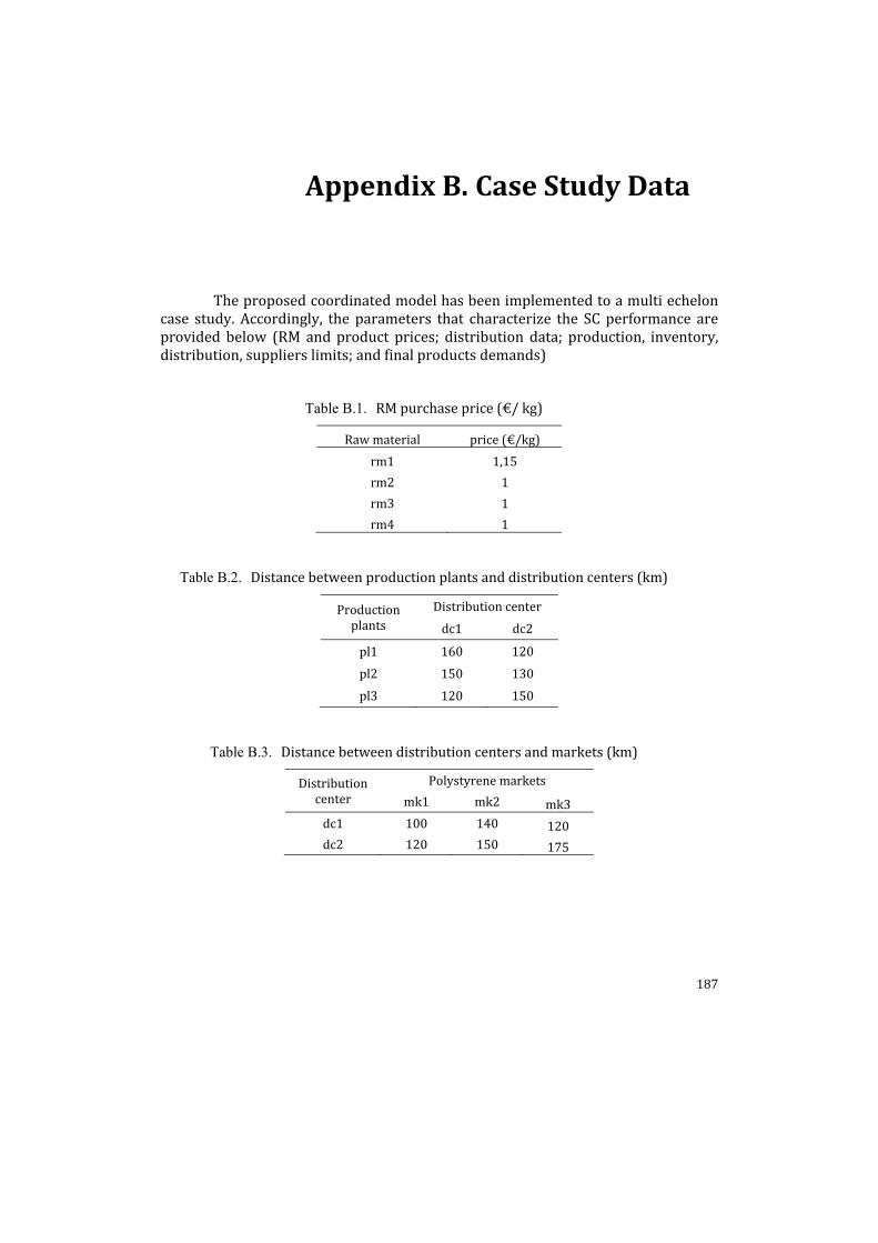
187
Appendix B. Case Study Data
The proposed coordinated model has been implemented to a multi echelon case study. Accordingly, the parameters that characterize the SC performance are provided below (RM and product prices; distribution data; production, inventory, distribution, suppliers limits; and final products demands)
Table B.1. RM purchase price (€/ kg)
Raw material price (€/kg)
rm1 1,15
rm2 1
rm3 1
rm4 1
Table B.2. Distance between production plants and distribution centers (km)
Production plants
Distribution center
dc1 dc2
pl1 160 120
pl2 150 130
pl3 120 150
Table B.3. Distance between distribution centers and markets (km)
Distribution center
Polystyrene markets
mk1 mk2 mk3 dc1 100 140 120 dc2 120 150 175

Appendix B Case Study Data
188
Table B.4. Maximum storage capacity (kg)
Distribution centers
polystyrene Time periods
t1‐t9 t10
dc1 ps1 500000 800
ps2 500000 120
dc2 ps1 400000 800
ps2 400000 120
Table B.5. Maximum production capacity (kg per day)
Production plant Polystyrene Time periods (t1‐
t10)
pl1 ps1 6500
ps2 7500
pl2 ps1 8000
ps2 9000
pl3 ps1 3000
ps2 4000
Table B.6. Maximum supplier capacity (kg/day)
RM supplier time periods (t1‐t10)
sup1 15000
sup2 10000
sup3 10000
sup4 8000
Table B.7. Polystyrene production cost (€/kg)
Polystyrene RM pl1‐pl3 and t1‐t10
ps1 rm1 0.6368
rm2 0.6182
ps2 rm3 0.5754
rm4 0.5268
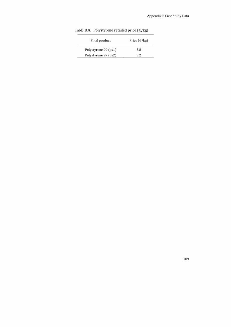
Appendix B Case Study Data
189
Table B.8. Polystyrene retailed price (€/kg)
Final product Price (€/kg)
Polystyrene 99 (ps1) 5.8
Polystyrene 97 (ps2) 5.2

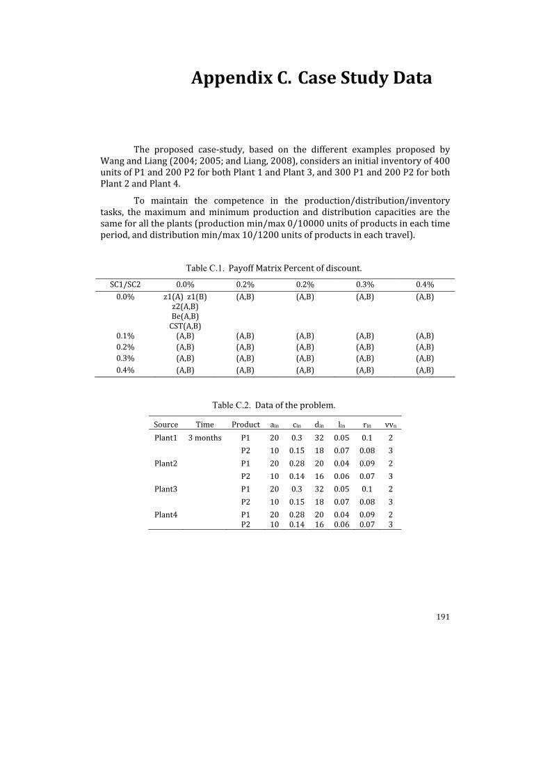
191
Appendix C. Case Study Data
The proposed case‐study, based on the different examples proposed by Wang and Liang (2004; 2005; and Liang, 2008), considers an initial inventory of 400 units of P1 and 200 P2 for both Plant 1 and Plant 3, and 300 P1 and 200 P2 for both Plant 2 and Plant 4.
To maintain the competence in the production/distribution/inventory tasks, the maximum and minimum production and distribution capacities are the same for all the plants (production min/max 0/10000 units of products in each time period, and distribution min/max 10/1200 units of products in each travel).
Table C.1. Payoff Matrix Percent of discount.
SC1/SC2 0.0% 0.2% 0.2% 0.3% 0.4%
0.0% z1(A) z1(B) z2(A,B) Be(A,B) CST(A,B)
(A,B) (A,B) (A,B) (A,B)
0.1% (A,B) (A,B) (A,B) (A,B) (A,B) 0.2% (A,B) (A,B) (A,B) (A,B) (A,B) 0.3% (A,B) (A,B) (A,B) (A,B) (A,B) 0.4% (A,B) (A,B) (A,B) (A,B) (A,B)
Table C.2. Data of the problem.
Source Time Product ain cin din lin rin vvn
Plant1 3 months P1 20 0.3 32 0.05 0.1 2
P2 10 0.15 18 0.07 0.08 3
Plant2 P1 20 0.28 20 0.04 0.09 2
P2 10 0.14 16 0.06 0.07 3
Plant3 P1 20 0.3 32 0.05 0.1 2
P2 10 0.15 18 0.07 0.08 3
Plant4 P1 20 0.28 20 0.04 0.09 2 P2 10 0.14 16 0.06 0.07 3

Appendix C Case Study Data
192
Table C.3. Demand to be forecasted.
Demand Distr1 Distr2 Distr3 Distr4
Product t1 t2 t3 t1 t2 t3 t1 t2 t3 t1 t2 t3
P1 1000 3000 5000 820 2300 4000 500 1200 2400 1230 3400 5300
P2 650 910 3000 500 720 2400 300 400 1150 710 1050 3100
Table C.4. Distribution cost/delivery time of the network.
Source Product Distribution Centers
Distr1 Distr2 Distr3 Distr4
Plant1 P1 a28/5.2b 10/1.8 42/13.5 22/2.8
P2 25/5.2 9/1.8 40/13.5 20/2.8
Plant2 P1 12/2 15/2.5 50/15 35/6
P2 11/2 14/2.5 45/15 32/6
Plant3 P1 44/9 59/12 11/4 35/6
P2 39/9 54/12 10/4 32/6
Plant4 P1 15/3 10/2.0 38/14 41/7
P2 13/3 9/2 35/14 37/7
Available space Rdd 19500 16000 10000 20000 *a delivery cost per truc to carry 100 dozen units. b delivery time.
Table C.5. Available labor levels (Fi,h).
Time period
t1 t2 t3
Plant 1 965 1040 1130
Plant 2 850 920 990
Plant 3 965 1040 1130
Plant 4 850 920 990
Table C.6. Production Capacities (Mi,h).
Time period
t1 t2 t3
Plant 1 1550 1710 1870
Plant 2 1850 2050 2250
Plant 3 1550 1710 1870
Plant 4 1850 2050 2250

Appendix C Case Study Data
193
Table C.7. Payoff matrix for the Competitive case (double demand).
SC1 discount SC2 disc 0.00% 0.10% 0.20% 0.30% 0.40%
↓ SC1 SC2 SC1 SC2 SC1 SC2 SC1 SC2 SC1 SC2
0%
z1($) 1,067,454 576,381 1,036,881 606,955 962,086 682,893 892,129 754,005 797,121 850,485
1,643,835 1,643,836 1,644,979 1,646,134 1,647,606 z2(hours) 2,292 2,295 2,360 2,404 2,448 Benefit ($) 4,746,545 2,617,618 4,573,118 2,787,646 3,992,513 3,362,399 3,625,870 3,722,524 3,283,878 4,056,806 CST($) 6,881,454 3,770,381 6,646,881 4,001,557 5,916,686 3,362,399 5,410,129 5,230,535 4,878,121 5,757,777
0.10%
z1($) 1,094,944 549,032 1,067,454 576,381 1,036,881 606,955 962,086 682,893 892,129 754,005
1,643,976 1,643,835 1,643,836 1,644,979 1,646,134 z2(hours) 2,287 2,292 2,295 2,360 2,404 Benefit ($) 4,957,796 2,400,167 4,740,731 2,614,424 4,567,508 2,784,248 3,987,558 3,358,346 3,621,352 3,718,034 CST($) 7,147,685 3,498,232 6,875,640 3,767,187 6,641,271 3,998,159 5,911,732 4,724,133 5,405,611 5,226,045
0.20%
z1($) 1,274,981 370,421 1,094,944 549,032 1,067,454 576,381 1,036,881 606,955 962,086 682,893
1,645,402 1,643,976 1,643,835 1,643,836 1,644,979 z2(hours) 2,268 2,287 2,292 2,295 2,360 Benefit ($) 5,750,339 1,598,178 4,951,738 2,397,218 4,734,917 2,611,230 4,561,898 2,780,850 3,982,603 3,354,293 CST($) 8,300,302 2,339,021 7,141,626 3,495,283 6,869,826 3,763,993 6,635,661 3,994,761 5,906,777 4,720,079
0.30%
z1($) 1,274,981 370,421 1,274,981 370,421 1,094,944 549,032 1,067,454 576,381 1,036,881 606,955
1,645,402 1,645,402 1,643,976 1,643,835 1,643,836 z2(hours) 2,268 2,268 2,287 2,292 2,295 Benefit ($) 5,743,300 1,598,178 5,743,300 1,596,209 4,945,679 2,394,269 4,729,103 2,608,036 4,556,288 2,777,452 CST($) 8,293,263 2,339,021 8,293,263 2,337,053 7,135,567 3,492,334 6,864,012 3,760,799 6,630,051 3,991,363
0.40%
z1($) 1,274,981 370,421 1,274,981 370,421 1,274,981 370,421 1,094,944 549,032 1,067,454 576,381
1,645,402 1,645,402 1,645,402 1,643,976 1,643,835 z2(hours) 2,268 2,268 2,268 2,287 2,292 Benefit ($) 5,736,260 1,598,178 5,736,260 1,596,209 5,736,223 1,594,241 4,939,620 2,391,319 4,723,289 2,604,842 CST($) 8,286,223 2,339,021 8,286,223 2,337,053 8,286,223 2,335,084 7,129,509 3,489,384 6,858,198 3,757,605

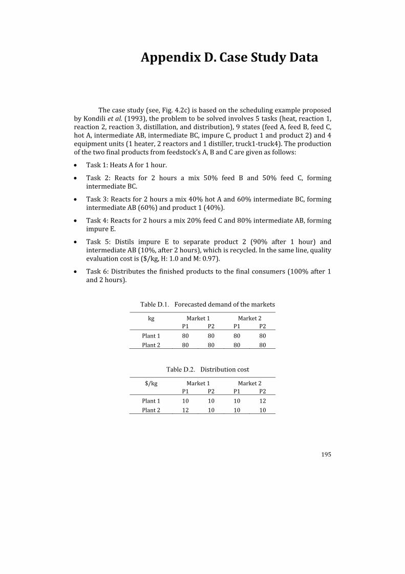
195
Appendix D. Case Study Data
The case study (see, Fig. 4.2c) is based on the scheduling example proposed by Kondili et al. (1993), the problem to be solved involves 5 tasks (heat, reaction 1, reaction 2, reaction 3, distillation, and distribution), 9 states (feed A, feed B, feed C, hot A, intermediate AB, intermediate BC, impure C, product 1 and product 2) and 4 equipment units (1 heater, 2 reactors and 1 distiller, truck1‐truck4). The production of the two final products from feedstock’s A, B and C are given as follows:
Task 1: Heats A for 1 hour.
Task 2: Reacts for 2 hours a mix 50% feed B and 50% feed C, forming intermediate BC.
Task 3: Reacts for 2 hours a mix 40% hot A and 60% intermediate BC, forming intermediate AB (60%) and product 1 (40%).
Task 4: Reacts for 2 hours a mix 20% feed C and 80% intermediate AB, forming impure E.
Task 5: Distils impure E to separate product 2 (90% after 1 hour) and intermediate AB (10%, after 2 hours), which is recycled. In the same line, quality evaluation cost is ($/kg, H: 1.0 and M: 0.97).
Task 6: Distributes the finished products to the final consumers (100% after 1 and 2 hours).
Table D.1. Forecasted demand of the markets
kg Market 1 Market 2 P1 P2 P1 P2
Plant 1 80 80 80 80
Plant 2 80 80 80 80
Table D.2. Distribution cost
$/kg Market 1 Market 2 P1 P2 P1 P2
Plant 1 10 10 10 12
Plant 2 12 10 10 10
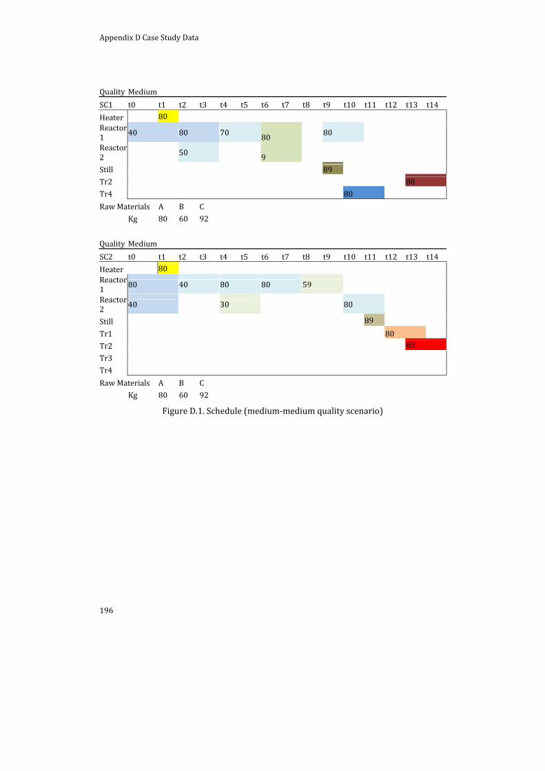
Appendix D Case Study Data
196
Quality Medium
SC1 t0 t1 t2 t3 t4 t5 t6 t7 t8 t9 t10 t11 t12 t13 t14
Heater 80 Reactor 1 40 80 70 80 80
Reactor 2
50 9
Still 89
Tr2 80
Tr4 80
Raw Materials A B C
Kg 80 60 92
Quality Medium
SC2 t0 t1 t2 t3 t4 t5 t6 t7 t8 t9 t10 t11 t12 t13 t14
Heater 80 Reactor 1
80 40 80 80 59
Reactor 2
40 30 80
Still 89
Tr1 80
Tr2 80
Tr3
Tr4
Raw Materials A B C
Kg 80 60 92
Figure D.1. Schedule (medium‐medium quality scenario)

197
Appendix E. Case Study Data
Figure E.1. Pareto frontier scenario (% of discount, SC1 0.0, SC2 0.0)
Figure E.2. Pareto frontier scenario (% of discount, SC1 0.0, SC2 0.1)
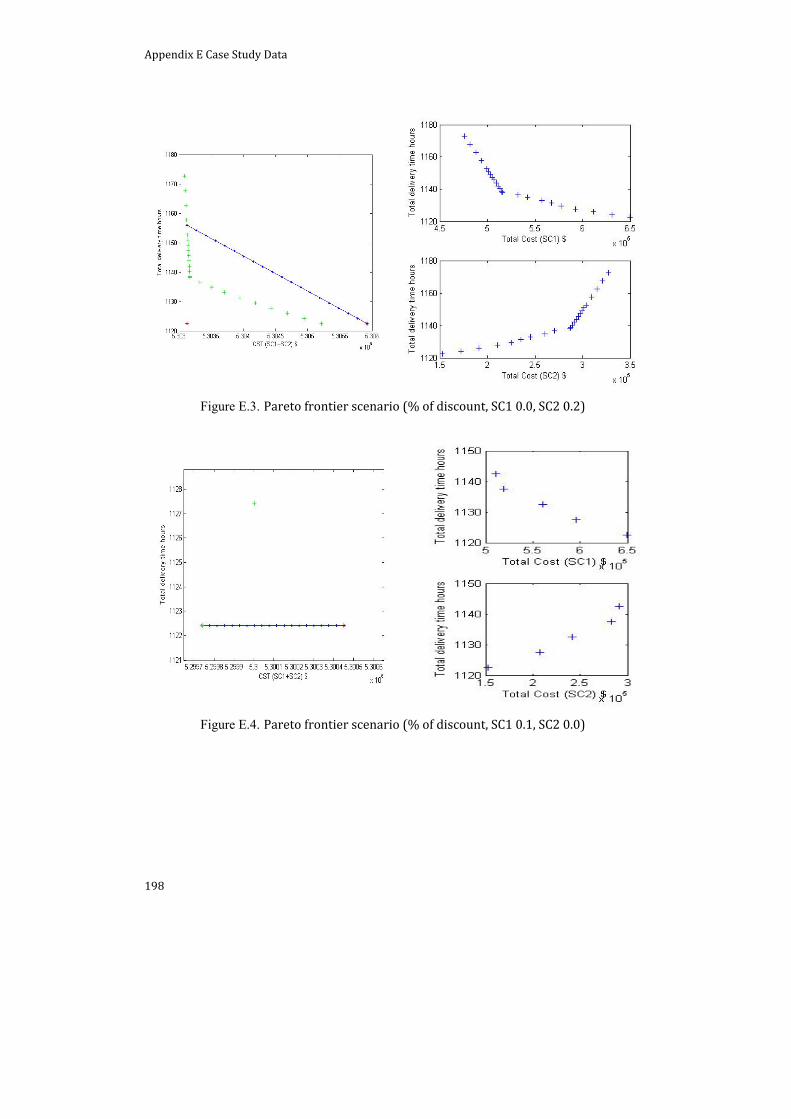
Appendix E Case Study Data
198
Figure E.3. Pareto frontier scenario (% of discount, SC1 0.0, SC2 0.2)
Figure E.4. Pareto frontier scenario (% of discount, SC1 0.1, SC2 0.0)

Appendix E Case Study Data
199
Figure E.5. Pareto frontier scenario (% of discount, SC1 0.1, SC2 0.1)
Figure E.6. Pareto frontier scenario (% of discount, SC1 0.1, SC2 0.2)
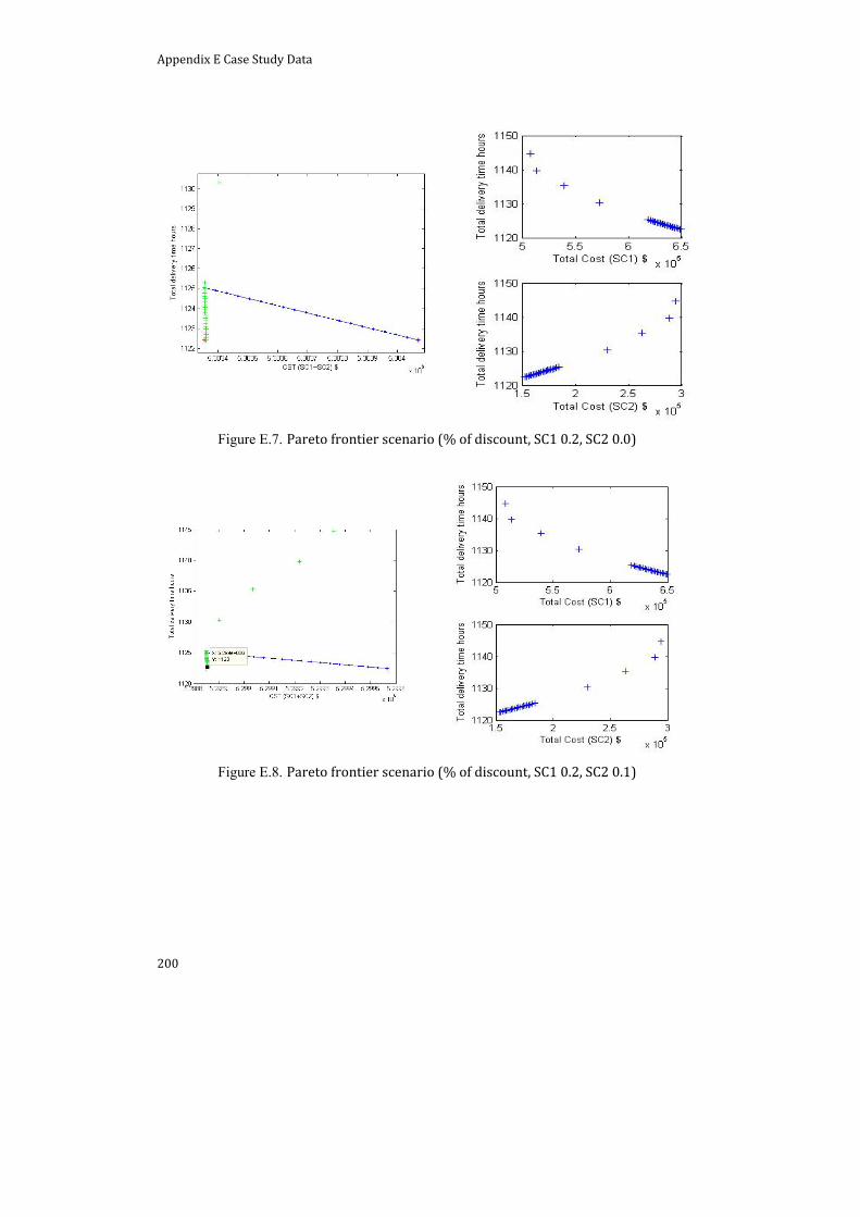
Appendix E Case Study Data
200
Figure E.7. Pareto frontier scenario (% of discount, SC1 0.2, SC2 0.0)
Figure E.8. Pareto frontier scenario (% of discount, SC1 0.2, SC2 0.1)
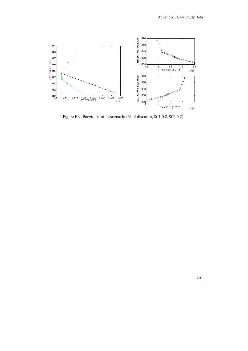
Appendix E Case Study Data
201
Figure E.9. Pareto frontier scenario (% of discount, SC1 0.2, SC2 0.2)

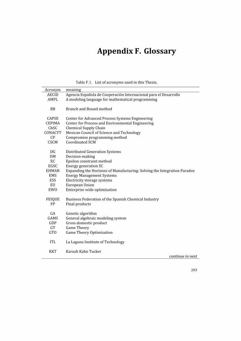
203
Appendix F. Glossary
Table F.1. List of acronyms used in this Thesis.
Acronym meaning AECID Agencia Española de Cooperación Internacional para el Desarrollo AMPL A modeling language for mathematical programming BB Branch and Bound method
CAPSE Center for Advanced Process Systems EngineeringCEPIMA Center for Process and Environmental EngineeringChSC Chemical Supply Chain
CONACYT Mexican Council of Science and TechnologyCP Compromise programming method
CSCM Coordinated SCM DG Distributed Generation SystemsDM Decision‐making EC Epsilon constraint methodEGSC Energy generation SCEHMAN Expanding the Horizons of Manufacturing: Solving the Integration Paradox EMS Energy Management SystemsESS Electricity storage systemsEU European Union EWO Enterprise wide optimization
FEIQUE Business Federation of the Spanish Chemical IndustryFP Final products GA Genetic algorithm
GAMS General algebraic modeling systemGDP Gross domestic productGT Game Theory GTO Game Theory Optimization ITL La Laguna Institute of Technology
KKT Karush Kahn Tucker continue in next
Appendix F Glossary
204
continue from previous LP Linear programming MG Microgrids MILP Mixed integer linear programmingMINLP Mixed integer nonlinear programmingMOO Multi‐objective Optimization
MO‐MILP Multi‐objective mixed integer linear programmingMPC Model predictive controlMPO Multi‐parametric optimization
NBI Normal boundary intersection methodNC Normal constraint methodNLP Nonlinear programming
ODE Ordinary Differential Equations
PDSC Production distribution SCPE Power Electronics PP Physical programming methodPSE Process Systems EngineeringPV Photovoltaic panels
R&D Research and developmentRES Renewable energy systemsRM Raw materials RMSC Raw material SC SC Supply Chain SCM Supply Chain ManagementSCs Supply Chains SSA Sample average approximationSSTN Synthesis State Task NetworkSTN State Task Network
TQC Total Quality Control
UANL Universidad Autónoma de Nuevo LeónUPC Universitat Politècnica de CatalunyaUSA United States of America WS Weighted sum method
WWTP Waste water treatment plant
205
Appendix G. Author Index
Acevedo 22
Adhitya 22
Adjiman 18
Agentis 125
Aguirre 47
Ahmed 23
Al‐Ameri 18
Al‐Enzi 23
Alexander 126
Alghalith 20
Almansoori 14
Al‐Othman 19
Al‐Qahtani 23
Altiqui 23
Amaro 18, 21, 165
Arkun 22
Ashmed 23
Atasu 81
Athanasiou 83
Badell 14
Bagajewicz 14, 23
Baghalian 20
Balasubramanian 19, 21
Baldoni 14
Balinski 12
Banerjee 22
Bansal 13
Barbosa‐Povoa 18, 21, 165
Bernal‐Agustín 66
Berning 18
Bhattacharya 50
Birge 141
Bojarski 27
Bordons 22
Bose 16, 20, 22, 50
Brandenburg 18
Braun 28
Brown 13
Burnham 23
Cachon 25, 106, 118
Cakravastia 13
Camacho 22
Cardoso 81
Carlyle 22
Castillo 41
Castro 16
Cerdá 18
Chang 15
Chen 11, 13, 23
Cheng 19
Chi 82
Christopher 11
Cóccola 81, 127
Cook 27
Cooper 11
Cortier 14
Croom 11
Dalal 20
Dantzig 33
Das 20
Appendix F Glossary
206
Davis 19, 125
Dempster 20
Deshpande 20
Díaz 14
Dolgui 19, 125
Dondo 18
Dua 20, 22
Duffie 22
Duffo‐López 66
Dunnett 18
Duran 35
Elahipanah 28
Elkamel 23
Ellram 11
Erengüc 81
Espuña 16, 22, 23, 24, 65
Fahiminia 28
Farahani 28
Feigenbaum 126
Ferris 41, 69
Fiacco 22
Fierro 7
Flores 22
Floudas 48, 49
Foo 48
Fourer 40
Friedler 16
Fröhling 81
García 87
Garrigos 126
Georgiadis 82
Giannakis 11
Giannakoudis 66
Giannelos 22
Gill 33
Gowtschalcky 23
Granot 25
Graves 12, 13
Greene 25
Greys 25
Grossmann 6, 7, 14, 16, 18, 1 9, 20, 21, 22, 24, 27, 35, 36, 47, 49, 50
Gudi 23
Guerrero 66
Guillén‐Gonsálbez 16, 22, 23, 27, 48, 81
Gunasekaran 121
Gupta 20, 23
Haitham 20, 165
Ho 11, 19, 125
Holczinger 16
Holland 105
Honczarenko 13
Huang 18
Ierapetritou 19, 22
Ismail‐Yahaya 36
Iyer 20
Jackson 14
Jung 19
Kallrath 14, 48
Karimi 13, 14, 18, 22
Kawasaki 67
Kempf 22
Klibi 20
Kohli 26
Kondili 16, 49, 54
Kuo 14
Lababidi 23
Laínez 13, 14, 16, 18, 19, 48, 106
Lakkhanawat 23
LaTourette 89
Lee 23, 36, 47
Leng 25
Li, X., 27
Li, Z., 19, 22
Liang 106, 170
Appendix E Case Study Data
207
Lin 22, 48, 49
Liu 20
Louveaux 141
Lummus 11
Mahesh 25
Maranas 20, 23
Maravelias 7, 16, 18, 48, 49, 50, 75
Martel 20
Mattson 36
Mayorga 129
McClurg 20
McDonald 13
McElreath 129
Mehta 18
Melé 22, 23, 24
Méndez 15, 16, 18, 47
Mentzer 11, 121
Messac 28, 36, 165
Mestan 22
Meyr 12
Mitra 23
Mockus 47
Montgomery 19
Mula 23
Moreno‐Benito 65
Nagarajan 26, 106
Nagi 24
Nakamura 13
Nash 39, 165
Neiro 14
Netessine 25
Nickel 24
Nicolotti 27
Obernberger 90
Pan 24
Pantelides 14, 23, 49
Papageorgiou 14, 15, 18
Park 26
Parlar 25
Patwardhan 23
Paulraj 11
Peidro 20, 23, 165
Penky 16, 20, 22, 47
Perea‐López 22, 89
Pérez‐Fortes 89
Petrovic 23
Pinto 23, 16, 47
Piper 22
Pistikopoulos 22
Poler 23
Ponnambalam 23
Prasad 16
Puigjaner 14, 16, 22, 23, 24
Raman 36
Ravindran 29
Reklaitis 19, 20, 47
Reyners 26
Ribas 20
Rivera 22
Rodera 27
Rodriguez 20, 22
Romero 14
Rosenthal 41
Rotstein 14
Ryu 22
Sahinidis 15, 19, 20, 21
Saldanha‐da‐Gama 24
Salema 82
Sanmartí 16
Santoso 23
Sardar 23
Sarferlis 22
Sargent 6, 126
Savolainen 126
Schary 12
Schilling
Appendix F Glossary
208
Schmitt 20
Schroeder 126
Schultmann 20
Schulz 14
Shah 5, 14, 18, 23, 47
Shapiro 16
Shapiro 23
Silver 13
Skjott‐Larsen 12
Slikker 26
Socîs 26, 106
Solverg 22
Sousa 14, 107
Srinvasan 13, 22
Subrahmanian 19
Sung 7, 18, 48, 49, 75
SupplyChain.com 11
Susarla 14
Tapiero 26
Thapa 33
Thek 90
Timpe 14
Toha 13
Tölle 18
Tsiakis 14, 20, 23
Türkay 22
van den Heever 18
van den Nouweland 26
Varian 110
Vecchietti 20, 22
Wang 22, 25
Wassick 7
Wei‐min 82
Wellons 20
Weng 20
Westerberg 6, 19
Wilkinson 14
Wu 20
Xiangtong 81
Xie 23
Ydstie 22
Yin 20, 25
Yin 25
You 19, 20, 24, 27
Zamarripa 82
Zhang 21, 49, 27
Zhu 25
Ziegler 24
Zimmermannm 141
Zipkin 19, 25
Zondervan 66
Bibliography
209
Bibliography
Acevedo, J., & Pistikopoulos, E. N., (1996). A parametric MINLP algorithm for process synthesis under uncertainty. Industrial & Engineering Chemistry Research 35, 147‐158.
Adhitya, A., Srinivasan, R., & Karimi, I. A., (2007a). Heuristic Rescheduling of Crude Oil Operations to Manage abnormal Supply Chain Events. AIChE Journal 53, 397‐422
Adhitya, A., Srinivasan, R., & Karimi, I. A., (2007b). A model‐based rescheduling framework for managing abnormal Supply Chain events. AIChE Journal 21, 496‐518.
Aguirre, A. M., Méndez, C. A., & Castro, P. M., (2011). A novel optimization method to automated wet‐etch station scheduling in semiconductor manufacturing systems. Computers and Chemical Engineering 35, 2960‐2972.
Agnetis, A., Flamini, M., Nicosia, G., Pacifici, A., (2010). Scheduling three chains on two parallel machines. European Journal on Operational Research 202(3), 669‐674.
Al‐Ameri, T. A., Shah, N., & Papageorgiou, L. G., (2008). “Optimization of vendor‐managed inventory systems in a rolling horizon framework.” Computers & Industrial Engineering 54, 1019–1047.
Alexander, A.G. La Mala Calidad y su Costo, Delaware, USA, Editorial Addison‐Wesley Iberoamericana, S.A. 1994.
Almansoori, A., & Shah, N., (2006). Design and operation of a future hydrogen supply chain‐Snapshot model. Chemical Engineering Research and Design, 84, 423‐438.
Al‐Othman, W. B. E., Lababidi, H. M. S., Alatiqi, I. M., Al‐Shayji, K., 2008. Supply chain optimization of petroleum organization under uncertainty in market demand and prices. European Journal of Operational Research 189, 822‐840.
Al‐Qahtani, K., Elkamel, A., & Ponnambalam, K., (2008). Robust optimization for petrochemical Network Design under Uncertainty. Industrial & Engineering Chemistry Research 47, 3912‐3919.
Amaro, A. C. S., & Barbosa‐Póvoa, A. P. F. D., (2008). Supply chain management with optimal scheduling. Industrial and Engineering Chemistry Research 47, 116‐132.
Amaro, A. C. S., & Barbosa‐Póvoa, A. P. F. D., (2009). The effect of uncertainty on the optimal closed‐loop Supply Chain planning under different partnerships structure. Computer and Chemical Engineering 33, 2144‐2158.
Bibliography
210
Atasu, A., Guide, V. D. R., Van Wassenhove, L. N., (2008). Product reuse economics in closed loop supply chain research. Production and Operations Management 17(5), 483‐496.
Badell, M., & Puigjaner, L. (2001). Advanced enterprise resource management systems. Computers and Chemical Engineering 80(3), 160.
Badell, M., Romero, J., Huertas, R., & Puigjaner, L., (2004). Planning, Scheduling and budgeting value‐added chains. Computers and Chemical Engineering 28, 45‐61.
Baghalian, A., Rezapour, S., Farahani, R. Z., (2013). Robust supply chain network design with service level against disruptions and demand uncertainties: A real‐life case. European Journal of Operational Research 227, 199‐215.
Balasubramanian, J., Grossmann, I. E., (2002). A Novel Branch and Bound Algorithm for Scheduling Flowshop Plants with Uncertain Processing Times. Computers and Chemical Engineering 26, 41.
Balasubramanian, J., Grossmann, I. E., (2004). Approximation to Multistage Stochastic Optimization in Multiperiod Batch Plant Scheduling under Demand Uncertainty. I&EC research 43, 3695.
Balinski, M., (1965). Integer programming: methods, uses computation. Management Science 12, 254–313.
Banerjee, I., & Ierapetritou, M. G., (2003). Parametric process synthesis for general nonlinear models. Computers & Chemical Engineering 27, 1499‐1522.
Bansal, M., Karimim, I. A., & Srinvasan, R., (2008). Selection of third‐party service contracts for Chemical Logistics. Industrial & Engineering Chemistry Research 47, 8301‐8316.
Bernal‐Agustín, J.L., & Dufo‐López, R. (2009). Simulation and optimization of stand‐alone hybrid renewable energy systems. Renew. Sust. Energy. Rev. 13(8), 2111‐2118.
Berning, G., Brandenburg, M., Gürsoy, K., Kussi, J. S., Mehta, V., & Tölle, F. J., (2002). Integrating collaborative planning and supply chain optimization for the chemical process industry. OR Spectrum 24, 371‐401.
Birge, J. R., Louveaux, F. Introduction to Stochastic Programming. Springer: New York, 1997.
Bojarski, A. D., Laínez, J. M., Espuña, A., & Puigjaner, L. (2009). Incorporating environmental impacts and regulations in a holistic Supply Chains modeling: An LCA approach. Computers and Chemical Engineering, 33, 1747‐1759.
Bose, S. K., & Bhattacharya, S. K., (2009). A State Task Network model for scheduling operations in cascaded continuous processing units. Computers and Chemical Engineering, 33, 287‐295.
Bose, S., & Penky, J. F., (2000). A model predictive framework for planning and scheduling problems: A case study of consumer goods Supply Chain. Computers and Chemical Engineering 24, 329‐335.
Braun, M. W., Rivera, D. E., Flores, M. E., Carlyle, W. M., & Kempf, K. G., GAMS a users guide. GAMS Development Corporation, Washington, 2003.
Bibliography
211
Brown, G. G., Graves, G. W., & Honczarenko, M. D., (1987). Design and Operation of a Multicommodity Production/Distribution System using primal goal decomposition. Management Science 33, 1469‐1480.
Cachon, G., Competitive Supply Chain Inventory Management (Sridhar Tayur, Ram Ganesham and Michael Magazine), Kluwer Academic Publishers, 1999. ISBN 0‐7923‐8344‐3.
Cachon, G. (2004). The allocation of inventory risk in a Supply Chain: push pull and advance purchase discount contracts. Management Science, 50, 222‐238.
Cachon, G., & Netessine, S., Game Theory in Supply Chain Analysis. Supply Chain Analysis in the eBusiness Era (David Simchi‐Levi, S. David Wu, and Z. Max Shen (Eds.)). Kluwer Academic Publishers, 2004, ISBN 0‐902610‐73‐2.
Cachon, G., & Zipkin, P. (1999). Cooperative and Competitive Inventory Policies in a Two‐Stages Supply Chain. Management Science, 45, 936‐953
Cakravastia, A., Toha, I.S., & Nakamura, N., (2002). A two stage model for the design of supply chain networks. International Journal of Production Economics 80, 231‐248
Camacho, E., & Bordons, C. Model Predictive Control in the Process Industry. Springer, 1995.
Cardoso, S. R., Barbosa‐Póvoa, A. P. F. D., Relvas, S., (2013). Design and planning of supply chains with integration of reverse logistics activities under demand uncertainty. European Journal of Operational Research 226, 436‐451.
Castillo, P., Conejo, A. J., Pedregal, P., Garcia, R., & Alguaci, N. Building and Solving Mathematical Programming models in Engineering and Science. New York: John Wiley & Sons, 2001.
Castro, P. M., Erdirik‐Dogan, M., Grossmann, I. E., (2008). Simulataneous batching and scheduling of single stage batch plants with parallel units. AIChE Journal 54, 183‐193.
Castro, P. M., Grossmann, I. E., (2012) Generalized disjunctive programming as a systematic modeling framework to derive scheduling formulations. Industrial and Engineering Chemistry Research 51, 5781‐5792.
Chen, C. L., & Lee, W. C., (2004). Multi‐objective optimization of multi‐echelon supply chain networks with uncertain demands and prices. Computers and Chemical Engineering 28, 1131‐1144.
Chen, Y., Mockus, L., Orcun, S., Reklaitis, G. V. (2012). Simulation‐optimization approach to clinical trial supply chain management with demand scenario forecast. Computers and Chemical Engineering 40, 82‐96.
Cheng, L., Subrahmanian, E., & Westerber, A. W., (2005). Design and planning under uncertainty: issues on problem formulation and solutions. Computers and Chemical Engineering 27, 781‐801.
Chen, I., & Paulraj, A., (2004). Towards a theory of supply chain management: the constructs and measurements. Journal of Operations Management 22, 119‐150.
Bibliography
212
Chi, X. W., Streicher‐Porte, M., Wang M. Y. L., & Reuter, M. A., (2011). Informal electronic waste recycling: a sector review with special focus on china. Waste Management 31(4), 731‐742.
Christopher, M. Logistics and Supply Chain Management. Creating Value adding Networks. Prentice Hall, 1995.
Cóccola, M., Zamarripa, M., Méndez, C.A., & Espuña A., (2013). Toward integrated production and distribution management in multi‐echelon supply chains. Computers and Chemical Engineering, in Press, DOI: http://dx.doi.org/10.1016/j.compchemeng.2013.01.004
Cook, R., Molina‐Cristobal, A., Parks, G., Osorio, C., & Clarkson, P. J.,(2007). Multi‐objective optimisation of a hybrid electric vehicle: drive train and driving strategy. Proceedings of the 4th international conference on evolutionary multi‐criterion optimization, 330‐345. ISBN: 978‐3‐540‐70927‐5.
Dalal, A. J., & Alghalith, M., (2009). Production decisions under joint price and production uncertainty. European Journal of Operational Research 197, 84‐92.
Dantzig, G. B., & Thapa, M. N. Linear Programming 1: Introduction. Springer Series in Operations Research. New York: Springer‐Verlag, 1997.
Das, K., (2011). Integrating effective flexibility measures into a strategic supply chain planning model. European Journal of Operational Research 211, 170‐183.
Davis, T., (1993). Effective supply chain management. Sloan Management Review 34, 35‐46.
Dempster, M. A. H., Pedrón, N. H., Medova, E. A., Scott, J. E., & Sembos, A., 2000. Planning logistics operations in the oil Industry. Journal of the Operational Research Society 51, 1271‐1288.
Deshpande, P., Shukla, D., & Tiwari, M. K., (2011). Fuzzy goal programming for inventory management: A bacterial foraging approach. European Journal of Operational Research 212, 325‐336.
Dolgui, A., & Louly, M. A. O., (2002). Optimization of supply chain planning under uncertainty. International Journal of Production Economics 78, 145‐152.
Dondo, R., Méndez, C. A., & Cerdá, J., (2008). Optimal management of logistic activities in multi‐site environments. Computers and Chemical Engineering 32, 2547‐2569.
Dua, P., Dua, V., Pistikopoulos, E. N., Multiparametric Mixed Integer Linear Programming. Encyclopedia of Optimization Springer US, 2009, ISBN: 978‐0‐387‐74759‐0. 2484‐2490.
Duffie, N. A., & Piper, R. S., (1987). Non‐hierarchical control of a flexible manufacturing cell. Robotics and Computer Integrated Manufacturing 3, 175‐179.
Dunnett, A., Adjiman, C., Shah, N., (2007). Biomass to heat supply chains: applications of process optimisation. Trans IChemE 85, 419‐429.
Duran, M., & Grossmann, I. E., (1986). An outer‐approximation algorithm for a class of mixed‐integer nonlinear programs. Mathematical Programming 36, 307‐339.
Bibliography
213
Ellram, L., Cooper, M., (1993). "Characteristics of supply chain management and the implications for purchasing and logistics strategy", International Journal of Logistics Management 4, 2, 1‐10.
Erengüç, S., Simpson, N.C., Vakharia, A.J., (1999). Integrated production/distribution planning in supply chains: an invited review 115, 219‐236.
Fahiminia B., Luong, L., & Marian, R., (2009), Optimization of a two‐echelon supply network using multi‐objective genetic algorithms. Proceedings of 2009 World Congress on Computer Science and Information Engineering. 406‐413.
Feigenbaum, A.V. Control Total de la Calidad. La Habana, Edición Revolucionaria, 1971.
Farahani, R. Z., & Elahipanah, M., (2008), A genetic algorithm to optimize the total cost and service level for just in‐ time distribution in a supply chain. International Journal of Production Economics 111, 229‐243
Ferrio, J., & Wassick, J., (2008). Chemical supply Chain network optimization. Computers and Chemical Engineering 32, 2481‐2504.
Ferris, M.C. MATLAB and GAMS: Interfacing Optimization and Visualization Software. Technical Report. Computer Sciences Department, University of Wisconsin, May 26, 2005 (http://www.cs.wisc.edu/math‐prog/matlab.html accessed 07/20/2010).
Fiacco, A. V., Introduction to Sensitivity and Stability Analysis in Nonlinear Programming. New York: Academic Press, 1983.
Floudas, C. A., & Lin, X., (2004). Continuous‐time versus discrete‐time approaches for scheduling of chemical processes: a review. Computers and Chemical Engineering, 28, 2109‐2129.
Foo, D.C.Y., (2009). State of the Art Review of Pinch Analysis Techniques for Water Network Synthesis. Industrial and Engineering Chemistry Research, 48, 5125‐5159.
Fourer, R., Gay, D. M., & Kernighan, B. W. AMPL: A Modeling Language for Mathematical Programming. Duxbury Press/Brooks/Cole Publishing Company, 2002 517p. ISBN: 0‐534‐38809‐4.
Fröhling, M., Schwaderer, F., Bartusch, H., & Rentz, O., (2010). Integrated planning of transportation and recycling for multiple plants based on process simulation. European Journal of Operational Research 207, 958‐970.
Fumero, Y., Corsano, G., & Montagna, J. M., (2011). Detailed design of multiproduct batch plants considering production scheduling, Industrial and Engineering Chemistry Research, 50, 6146‐8160.
García, R., Pizarro, C., Lavín, A. G., & Bueno, J. L., (2012). Characterization of Spanish biomass wastes for energy use. Bioresource Technology 103, 249–258.
Georgiadis, P., & Athanasiou, E., (2013). Flexible long‐term capacity planning in closed‐loop supply chains with remanufacturing. European Journal of Operational Research 225, 44‐58.
Giannakis, M., & Croom, S. R., (2004). Toward the development of a Supply Chain Management Paradigm: A Conceptual Framework. Journal of Supply Chain Management 40(2), 27‐37.
Bibliography
214
Giannakoudis, G., Papadopoulos, A. I., Seferlis, P., & Voutetakis, S. On the Systematic Design and Optimization under Uncertainty of a Hybrid Power Generation System Using Renewable Energy Sources and Hydrogen Storage. Proc. 20th European Symposium on Computer Aided Process Engineering – ESCAPE20, S. Pierucci and G. Buzzi Ferraris (Editors), Elsevier, 2010.
Gill, P. E., W. Murray, Saunders, M. A., Tomlin, J.A., & Wright, M.H., (2008). George B. Dantzig and systems optimization. Discrete Optimization 5, 151‐158.
Graves, S. C., & Tomlin, B. T., (2003). Process Flexibility in Supply Chains. Management Science 49, 907‐919.
Granot, D., & Yin, S. (2008). Competition and cooperation in decentralized push and pull assembly systems. Management Science, 54, 733‐747.
Greene, D. (2002). JVS, Alliances Consortia on path to survival for many. Semiconductor magazine, 3, 12‐16.
Grossmann, I. E., (2004). Challenges in the new millennium: Product discovery and design, enterprise and supply chain optimization, global life cycle assessment. Computers and Chemical Engineering 29, 29‐39.
Grossmann, I. E., (2005). Enterprise‐wide Optimization: A New Frontier in Process Systems Engineering. AICHE Journal 51, 1846‐1857.
Grossmann, I. E., & Daichendt, M.M., (1996). Optimization‐based approaches to process synthesis. Computers and Chemical Engineering, 20, 665‐674
Grossmann, I. E., & Westerberg, A. W., (2000). Research Challenges in Process Systems Engineering. AICHE Journal 326, 150‐168.
Guerrero, J.M., Vasquez, J. C., Matas, J., Castilla, M., & Garcia de Vicuna, L., (2009). Control strategy for flexible microgrid based on parallel line interactive ups systems. IEEE Trans. Ind. Electron 56, 726–736.
Guillén, G., & Grossmann, I. E., (2010). A global optimization strategy for the environmentally conscious design of chemical Supply Chains under uncertainty in the damage assessment model. Computers and Chemical Engineering, 34, 42‐58.
Guillén G., Badell, M., Espuña, A., & Piugjaner, L., (2006). Simultaneous optimization of process operations and financial decisions to enhance the integrated planning/scheduling of Chemical supply chains. Computers and Chemical Engineering, 30, 421‐436.
Guillén‐Gonsálbez, G., Melé, E., Bagajewicz, M. J., Espuña, A., & Puigjaner, L., (2005a). Multiobjective supply chain design under uncertainty, Chemical Engineering Science, 60, 1535‐1553.
Guillén‐Gonsálbez, G., Bagajewicz, Sequeira, S. E., M. J., Espuña, A., & Puigjaner, L., (2005b). Management of Pricing policies and Financial Risk as a Key Element for Short Term Scheduling optimization. Industrial and Engineering Chemistry Research 44, 557‐575.
Guillén‐Gonsálbez, G., Espuña, A., & Puigjaner, L., (2006a). Addressing the scheduling of Chemical supply chains under demand uncertainty. AIChE Journal 52(11), 3864‐3881.
Bibliography
215
Guillén‐Gosálbez, G., Melé, F. D., Espuña, A., & Puigjaner, L., (2006b). Addressing the design of Chemical supply chains under demand uncertainty. Industrial and Engineering Chemistry Research 45, 7566‐7581.
Gunasekaran, A., Lai, K. H., & Cheng, T. C. (2008). Responsive Supply Chain: A competitive strategy in a networked economy. Omega 36, 549‐564
Gupta, A., & Maranas, C. D. (2000). A two‐stage modelling and solution framework for multisite midterm planning under demand uncertainty. Ind. & Eng. Chem. Res., 39, 3799‐3813.
Gupta A., & Maranas, C. D. (2003). Managing demand uncertainty in Supply Chain planning. Computers and Chemical Engineering 27, 1219‐1227.
Haitham , L. M. S., Mohamed, A. A., Imad, A. M., Adel, A. F., (2004). Optimizing the Supply Chain of a Petrochemical Company under Uncertain Operating and Economic Conditions. Industrial and Engineering Chemical Research 43, 63‐73.
Ho, C., (1989). Evaluating the impact of operating environments on MRP system nervousness. International Journal of Production Economics 91, 215‐221.
Holland, C. P., (1995). Cooperative supply chain management: the impact of inter‐organizational information systems. Journal of Strategic Information Systems 4(2), 117‐133.
HOMER (The Hybrid Optimization Model for Electric Renewables). Available from: http://www.nrel/gov/HOMER (accessed 07/20/2010).
Huang, C., & Karimi, I. A., (2006). Scheduling trans‐shipment operations in maritime chemical transportation. Industrial and Engineering Chemistry Research 45, 1955‐1973.
Hudson Oil Corporation Report Ltd. © (2011, http://www.hudsonoil.ca/Gasification.htm).
Hugo, A., & Pistikopoulos, E. N. (2004). Environmentally conscious long‐range planning and design of Supply Chain networks. Journal of Cleaner Production 12, 1471‐1491.
Iyer, R. R., & Grossmann, I. E., (1998). A bilevel decomposition algorithm for long‐range planning of process networks. Industrial and Engineering Chemistry Research 37, 474‐481.
Jackson, J. R., & Grossmann, I. E., (2003). Temporal Decomposition Scheme for Nonlinear Multisite Production Planning & Distribution Models. Ind. & Eng. Chem. Res., 42, 3045.
Jung, J. Y., Blau, G., Pekny, J. F., Reklaitis, G. V., & Eversdyk, D., (2004). A simulation based optimization approach to supply chain management under demand uncertainty. Computers and Chemical Engineering 28, 2087–2106.
Kallrath, J., (2002). Planning and scheduling in the process industry, OR Spectrum, 24, 219‐250.
Kawasaki, K., Matsumura S., Iwabu K., Fujimura N., Iima T., (2009). Autonomous dispersed control system for independent micro grid. Electr. Eng. Jpn 166(1), 1121–7.
Bibliography
216
Kohli, R., & Park, H. (1989). A Cooperative Game Theory Model of Quantity Discounts. Management Science 35, 693‐707.
Kondili E., Pantelides C. C., & Sargent R. W., (1993). A general algorithm for short term scheduling of batch operations, Computers and Chemical Engineering 17, 211‐217.
Klibi, W., Martel, A., (2012). Scenario‐based Supply Chain Network risk modeling. European Journal of Operational Research 223, 644‐658.
Kuo, T. H., & Chang, C. T., (2008). Application of a Mathematic programming Model for Integrated Planning and Scheduling of Petroleum Supply Networks. Industrial and Engineering Chemistry Research 47, 1935‐1954.
Lababidi, H. M., Ashmed, M. A., Alatiqi, I. M., and Al‐Enzi, A. F., (2004). Optimizing the supply chain of a petrochemical company under uncertain operating and economic conditions. Industrial and Engineering Chemistry Research 43, 63‐73.
Laínez, J. M., Guillén, G., Badell, M., Espuña, A., & Puigjaner, L., (2007). Enhancing Corporate Value in the Optimal Design of Chemical Supply Chains. Industrial and Chemical Research 46 7739‐7757.
Laínez, J. M., Kopanos, G., Espuña, A., & Puigjaner, L., (2009). Flexible Design‐Planning of Supply Chain Networks, AIChE Journal, 1736‐1753.
Laínez J. M. Towards Integrated Management of the Supply Chain for Enterprise Sustainability. Barcelona, Spain, 2010. Thesis presented for the degree of Doctor of Philosophy.
Laínez, J. M., Schaefer, E., & Reklaitis, G. V., (2012). Challenges and opportunities in enterprise‐wide optimization in the pharmaceutical industry. Computers and Chemical Engineering 47, 19‐28.
Lakkhanawat, H., & Bagajewicz, M. J., (2008). Financial Risk Management with Product Pricing in the Planning of Refinery Operations. Industrial and Engineering Chemistry Research 47, 6622‐6639
LaTourrette, T., Ortiz, D., Hlavka, E., Burger, N., & Cecchine, G., Supplying Biomass to Power Plants. Rand Technical report, 2011. ISBN: 978‐0‐8330‐5218‐6
Lee, S., & Grossmann, I. E., (2000). New algorithms for nonlinear disjunctive programming. Computers and Chemical Engineering 24, 2125‐2141.
Lee, H,; Pinto, J.M.; Grossmann, I.E.; Park, S.; (1996). Mixed‐Integer Linear Programming Model for Refinery Short‐Term Scheduling of Crude Oil Unloading with Inventory Management. Industrial & Engineering Chemical Research 35, 1630‐1641.
Leng, M., & Zhu, A. (2009). Side payment contracts in two person nonzero sum Supply Chain games: review, discussion and applications. European Journal of Operational Research 196, 600‐618.
Leng, M., & Parlar, M. (2010). Game‐theoretic analyses of decentralized assembly Supply Chains: Non‐cooperative equilibria vs coordination with cost‐sharing contracts. European journal of Operational Research 204, 96‐104.
Bibliography
217
Li, X., Gao, L., & Li, W., (2012). Application of game theory based hybrid algorithm for multi‐objective integrated process planning and scheduling. Expert Systems with Applications 39, 288‐297.
Li, Z., & Ierapetritou, M. G., (2008). Process scheduling under uncertainty using Multi‐parametric programming. AIChE Journal 53, 3183‐3203
Liang, T., 2008. Fuzzy multi‐objective production/distribution planning decisions with multi product and multitime period in a Supply Chain. Computers and Industrial Engineering 55, 678‐694.
Lima, R. M., Grossmann, I. E., & Yu Jiao, (2011). Long‐term scheduling of a single unit multi‐product continuous process to manufacture high performance glass, Computers and Chemical Engineering 35, 554‐574.
Lin, X., & Floudas, C. A., (2001). Design, synthesis and scheduling of multipurpose batch plants via an effective continuous‐time formulation, Computers and Chemical Engineering 25, 665‐674.
Lin, C. C., Wang, T. H., (2011). Build to order supply chain network design under supply and demand uncertainties. Transportation Research Part B 45, 1162‐1176.
Liu, M. L., & Sahinidis, N. V., (1996). Optimization in Process Planning under Uncertainty. Industrial and Engineering Chemistry Research 35, 4154‐4165.
Lummus, R. R., & Vokurka, R.J., (1999) Defining supply chain management: A historical perspective and practical guidelines. Industrial and Data Systems 99, 11‐17.
Mahesh, N., & Greys, S., (2006). Game‐Theoretic Analysis of cooperation Among Supply Chain Agents: review and extensions, European Journal of Operational Research 37, 719‐745.
Maravelias, C. T., (2005). Mixed‐time representation for state‐task network models, Industrial and Engineering Chemistry Research, 44, 9129–9145.
Maravelias, C. T., & Grossmann, I. E., (2003a). Minimization of makespan with a discrete‐time state‐task network formulation, Industrial and Engineering Chemistry Research, 42, 6252‐6257.
Maravelias, C.T., & Grossmann, I. E., (2003b). New general continuous‐time state‐task network formulation for short‐term scheduling of multipurpose batch plants. Industrial and Engineering Chemistry Research, 42, 3056‐3074.
Maravelias, C.T., & Grossmann, I. E., (2006). On the relation of continuous and discrete‐time state‐task network formulations. AIChE Journal, 52, 843‐849.
McDonald, C.M., & Karimi, I. A. (1997). Planning and scheduling of parallel semi continuous processes. I. Production planning. Ind & Eng. Chem. Res., 36, 2691–2700.
McElreath, M. H., Mayorga, M. E., (2012). A dynamic programming approach to solving the assortment planning problem with multiple quality levels. Computers and Operations Research 39, 1521‐1529.
Melé, F. D., Guillén‐Gonsálbez, G., Espuña, A., & Puigjaner, L., (2007). An agent‐based approach for supply chain retrofitting under uncertainty. Computers and Chemical Engineering 31, 722‐735.

Bibliography
218
Melé, F. D., Espuña, A., & Puigjaner, L. Environmental impact considerations into supply chain management based on life cycle assessment. In Proceedings of Innovation by Life Cycle Management (LCM) International Conference, edited by F. Castells, & J. Rieradeball. 2005, 428‐433.
Melé, F. D., Espuña, A., & Puigjaner, L., (2006a). A simulation‐based Optimization Framework for Parameter optimization of Supply Chain Networks. Industrial and Engineering Chemistry Research 45, 3133‐3148.
Melé, F. D., Espuña, A., & Puigjaner, L. (2006b). Supply Chain Management through Dynamic model Parameters Optimization. Industrial and Engineering Chemistry Research 45, 1708‐1721.
Méndez, C. A., Cerda, J., Grossmann, I. E., Harjunkoski, I., & Fahl, M., (2006). State of the art review of optimization methods for short term scheduling of batch processes. Computers and Chemical Engineering 30, 913‐946.
Méndez, C.A., & Cerda, J., (2007). A precedence‐based Monolithic Approach to Lot‐sizing and Scheduling of Multiproduct Batch Plants. Computers and Chemical Engineering 24, 679‐684.
Mentzer, J. T., DeWitt, W., Keebler, J. S., Min, S., Nix, N. W., & Smith, C. D. (2001). Defining Supply Chain Management. Journal of Business Logistics, 22, 1‐25.
Messac, A., Ismail‐Yahara, & Mattson, C. A., (2003). The Normalized Normal Constraint Method for Generating the Pareto Frontier. Structural and Multidisciplinary Optimization 25, 86‐98.
Mestan, E., Türkay, M., & Arkun, Y., (2006). Optimization of Operations in Supply Chain Systems Using Hybrid Systems Approach and Model Predictive Control. Industrial and Engineering Chemistry Research 46, 6493‐6503.
Meyr, H., Wagner, M., Rohde, J. Structure of advanced planning systems. In: Stadtler, H., Kilger, C., (eds.). Supply Chain Management and Advanced Planning – Concepts, Models, Software, and Case Studies. Berlin 2002, 99‐104.
Mitra, K., Gudi, R. D., Patwardhan, S. C., & Sardar, G., (2009). Towards resilient supply chains: Uncertainty analysis using fuzzy mathematical programming. Chemical Engineering Research and Design 87, 967‐981.
Mockus, L., & Reklaitis, G., (1999) Continuous Time Representation Approach to Batch and Continuous Process Scheduling. 1. MINLP Formulation. Industrial & Engineering Chemical Research 38, 197‐203.
Montgomery, D. C. Introduction to Statistical Quality Control. Wiley (2000).
Moreno‐Benito, M., & Espuña, A. Stochastic and hybrid approaches to solve integrated synthesis and operation of batch processes. Proceedings of the 22nd European Symposium on Computer Aided Process Engineering 2012.
Moreno‐Benito, M., & Espuña, A. Facing New Products Demand through Simultaneous Structural and Operational Decisions in the Design of Control Recipe. Proceedings of the PRESS 2011.

Bibliography
219
Moreno‐Benito, M., Frankl, K., Marquardt, W., & Espuña A. Simultaneous Process and Recipe Design of an Acrylic Fiber Production System. Proceedings of the AIChE annual meting 2012.
Mula, J., Peidro, D., & Poler, R., (2010). The effectiveness of a fuzzy mathematical programming approach for supply chain production planning with fuzzy demand. Int. J. Production Economics 128, 136‐143.
Nagarajan, M., & Socîs, G. (2008). Game‐Theoretic Analysis of cooperation Among Supply Chain Agents: review and extensions, European Journal of Operational Research 187, 719 – 745.
Nash, J. F. (1950), "Equilibrium Points in N‐person Games", Proceedings of the National Academy of Sciences 36, 48–49.
Neiro, M.S., & Pinto, J.M., (2004). A general modeling framework for the operational planning of petroleum Supply Chains. Computers & Chemical Engineering 28, 871‐896.
Nickel, S., Saldanha‐da‐Gama, F., & Ziegler, H. P., (2012). A multi‐stage stochastic supply network design problema with financial decisions and risk management. Omega 40, 511‐524.
Nicolotti, O., Giangreco, I., & Introcaso, A., (2011) Strategies of multi‐objective optimization in drug discovery and development. Expert Opin. Drug Discov. 1‐14.
Obernberger and G.Thek (2008). Combustion and gasification of solid biomass for heat and power production in Europe‐state ‐of –the‐ art and relevant future developments. The 8th European Conference on Industrial Furnaces and Boilers, Vilamoura, Portugal, ISBN 978‐972‐99309‐3‐5.
Pan, F., Nagi, R., (2010). Robust supply chain design under uncertain demand in agile manufacturing. Computers and Operations Research 37, 668‐683.
Panagiotis, G., & Kakaras, E., (2005). Biomass Combustion Modeling in Fluidized Beds. Energy & Fuels 19, p 292‐297
Papageorgiou, L. G., (2009). Supply Chain optimization for the process industries: advances and opportunities. Computers and Chemical Engineering 33, 1931‐1938.
Papageorgiou, L. G., & Pantelides, C. C., (1996). Optimal campaign planning/scheduling of multipurpose batch/semicontinuous plants. II. A mathematical decomposition approach. Industrial Chemical Engineering. 35, 510–529.
Papageorgiou, L. G., Rotstein, G. E., & Shah, N., (2001). Strategic supply chain optimization for the pharmaceutical industries. Industrial and Engineering Chemistry Research 40, 275‐286.
Peidro, D., Mula, J., Poler, R., Verdegay, J. L., (2009). Fuzzy optimization for supply chain planning under supply, demand and process uncertainties. Fuzzy Sets and Systems 160, 2640‐2657.
Peidro, D., Mula, J., Jiménez, M., Botella, M. M., 2010. A fuzzy linear programming based approach for tactical supply chain planning in an uncertainty environment. European Journal of Operational Research 205, 65‐80.
Bibliography
220
Penky, J. F., & Reklaitis, G. V., (1998). Towards the convergence of theory and practice: A technology guide for scheduling/planning methodology. AIChE Symposium Series, 94, 91‐111.
Perea‐López, E., Grossmann, I. E., Ydstie, B. E., & Tahmassebi, T., (2001). Dynamic modeling and decentralized control of supply chains. Industrial and Engineering Chemistry Research 40, 3369‐3383.
Perea‐López, E., Ydstie, B. E., & Grossmann, I. E., (2003). A model predictive control strategy for supply chain optimization. Computers and Chemical Engineering 27, 1201‐1218
Pèrez Fortes, M. Conceptual Design of Alternative Energy Systems from Biomass. PhD thesis 2011. Industrial Engineering Department, Universitat Politècnica de Caltalunya UPC, Barcelona, Spain.
Pinto, J. M., & Grossmann, I. E., (1995). A continuous‐time mixed‐integer linear‐programming model for short‐term scheduling of multistage batch plants. Industrial and Engineering Chemistry Research 34, 3037‐3051.
Pistikopoulos, E. N., (2009). Perspectives in Multiparametric Programming and Explicit Model Predictive Control. AICHE Journal 55(8), 1918‐1925.
Prasad, P., & Maravelias, C. T., (2008). Batch selection, assignment and sequencing in multi‐stage, multi‐product processes. Computers and Chemical Engineering 32, 1114‐1127.
Puigjaner, L., & Espuña, A., Integration in Supply Chain Management. In computer Aided Product and Process Engineering, WILEY‐VCH, 2006, 695‐730
Raman, R., & Grossmann, I. E., (1994). Modeling and computational techniques for logic based integer programming. Computers and Chemical Engineering, 18, 563‐578.
Ravindran, A., Ragsdell, K. M., & Reklaitis, G. V., Engineering Optimization: Methods and Applications. John Wiley & Sons, 2006.
Reklaitis, G. V., (1982). Review of scheduling of process operations. AIChE Symposium Series 78 (214), 119–133.
Reyniers, D.J., & Tapiero, C.S. (1995). The Delivery and Control of Quality in Suplier‐Producer Contracts. Management Science, 41, 1581‐1589.
Ribas, G. P., Hamacher, S., & Street, A., (2010). Optimization under uncertainty of the integrated oil supply chain using stochastic and robust programming. International Transactions in Operational Research 17(6), 777‐796.
Rodera, H., Bagajewicz, M. J., & Trafalis, T. B., (2002). Mixed‐Integer Multiobjective Process Planning under Uncertainty. Industrial Engineering Chemical Research 41, 4075‐4084.
Rodriguez, M. A., & Vecchetti, A., (2012). Mid‐term planning optimization model with sales contracts under demand uncertainty. Computers and Chemical Engineering 47, 227‐236.
Bibliography
221
Romero, J., Badell, M., Bagajewicz, M. J., & Puigjaner, L., (2003). Integrating Budgeting Models into Scheduling and Planning Models for Chemical Batch Industry. Industrial and Engineering Chemistry Research 42, 6125‐6134.
Rosenthal, R.E., “GAMS – A User’s Guide”. GAMS Development Corporation, Washington DC, 2012.
Ryu, J., Dua, V., & Pistikopoulos, E. N., (2004). A bilevel programming framework for Enterprise wide process networks under uncertainty. Computers and Chemical Engineering 28, 1121‐1129.
Ryu, J., Dua, V., & Pistikopoulos, E. N., (2007). Proactive scheduling under uncertainty: A Parametric Optimization Approach. Industrial and Engineering Chemistry Research 46, 8044‐8049.
Ryu, J., & Pistikopoulos, E. N., (2007). A novel approach to scheduling zero‐wait batch processes under processing time variations. Computers and Chemical Engineering 31, 101‐106.
Shah, N. (2005). Process industry Supply Chains: Advances and challenges. Computers & Chemical Engineering 29, 1225‐1235.
Shah, N., (1998). Single and multisite planning and scheduling: Current status and future challenges. AIChE Symposium Series, 94, 75‐90
Sahinidis, N. V., (2004). Optimization under uncertainty: state of the art and opportunities. Computers and Chemical Engineering 28, 971‐983.
Salema, M. I. G., Barbosa‐Póvoa, A. P. D. F., Novais, A. Q., (2007). An optimization model for the design of a capacitated multi‐product reverse logistics network with uncertainty. European Journal of Operational Research 179, 1063‐1077.
Salema, M., Barbosa‐Póvoa, A., Novais A., (2010). Simultaneous design and planning of supply chains with reverse flows: A generic modelling framework. European Journal of Operational Research 203, 336–349
Sanmartí, E., Puigjaner, L., Holczinger, T., & Friedler, F., (2002). Combinatorial Framework for Effective Scheduling of multipurpose Batch Plants. AIChE Journal 48, 2557‐2570.
Santoso, T., Ahmed, S., Gowtschalckx, M., & Shapiro, A., (2005). A stochastic programming approach for supply chain network design under uncertainty. European Journal of Operational Research 167, 96‐115.
Sarferlis, P., & Giannelos, N., (2004). A two‐layered optimization‐based control strategy for multi‐echelon supply chains networks. Computers and Chemical Engineering 28, 799‐809.
Sargent, R. W. H. (1991). What is chemical engineering? CAST Newsletter, 14(1), 9–11.
Savolainen, T. I., (1999). Cycles of continuous improvement realizing competitive advantages through quality. International Journal of Operations and Production Management 19, 120‐122.
Schary, P. B., & Skjott‐Larsen, T. Managing the Global Supply Chain. New Delhi Viva Books. 2000, 350p.
Bibliography
222
Schiling, G., & Pantelides, C. C., (1996). A simple continuous‐time process scheduling formulation and a novel solution algorithm. Computers and Chemical Engineering, 20, 1221‐1226.
Schmitt, A. J., Snyder, L. V., & Shen, Z. J., (2010). Inventory Systems with Stochastic Demand and Supply: Properties and Approximations. European Journal of Operational Research 206(2), 313‐328.
Schultmann, F., Frohling, M., & Rentz, O., (2006). Fuzzy approach for production planning and detailed scheduling in paints manufacturing. International Journal of Production Research 44(8), 1589‐1612.
Schulz, E. O., Diaz, M. S., & Bandoni, J. A., (2005). Supply Chain optimization of large scale continuous processes. Computers and Chemical Engineering 29, 1305‐1316.
Schroeder, R.G. Administración de operaciones. Toma de decisiones en la función de operaciones. 3era edición. McGraw‐Hill Book Co. Interamericana de México, S.A. de C. V, 1992.
Shapiro, J. F. Modeling the Supply Chain. Duxbury, Pacific Grove, 2001.
Slikker, M. A., & Van den Nouweland. Social and Economic Networks in Cooperative Game Theory, Kluwer Academic Publishers Boston, 2001.
Silver, E. A., Pyke, D. F., & Peterson, R. Inventory Management and Production Planning and Scheduling. 3rd ed. Wiley, 1998.
Solverg, J. J., & Lin, G. Y. J., (1992). Integrated shop‐floor control using autonomous agents, IIE transactions 24, 3.
Sousa, R. T., Shah, N., & Papageorgiou, L. G., Global supply chain network optimization for pharmaceuticals. In 15th European symposium on computer aided process engineering (ESCAPE‐15) Barcelona, Spain, 2005, (pp. 1189‐1194)
Sousa, R., Shah, N., & Papageorgiou, L. G., (2008). Supply Chain design and multilevel planning ‐ an industrial case. Computers and Chemical Engineering 32, 2643‐2663.
Sung, C., & Maravelias, C. T. (2007). An Attainable Region Approach for Production Planning of Multiproduct Processes. AIChE Journal, 53, 1298‐1315.
Susarla, N., Karimi, I.A., (2012). Integrated supply chain planning for multinational pharmaceutical enterprises. Computers and Chemical Engineering 42, 168‐177.
ThyssenKrupp Uhde. “Gasification Technologies 2012” Technical report ThyssenKrupp Uhde®, GT 620e/2000 09/2012 GZD/TK printmedia, Germany.
Timpe, A.H., & Kallrath, J. (2000). Optimal planning in large multi‐site production networks. European Journal of Operational Research 40, 3585‐3604.
Tsiakis, P., Shah, N., Pantelides, C. C., (2001). Design of multi‐echelon supply chain networks under demand uncertainty. Industrial and Engineering Chemistry Research 40, 3585‐3604.
Tsiakis, P., & Papageorgiou, L. G., (2008). Optimal production allocation and distribution supply chain networks. International Journal of Production Economics, 111, 468‐483.
Bibliography
223
van den Heever, S. A., & Grossmann, I. E., (2003). A strategy for the integration of production planning and reactive scheduling in the optimization of a hydrogen supply network. Computers and Chemical Engineering, 27, 1813‐1839.
Varian, H.R. 1992. Microeconomía Intermedia. Ed. Antoni Bosch, España.
Wang, Y. (2006). Pricing production decisions in Supply Chains of complementary products with uncertain demand. Operations Research, 54, 1110‐1127.
Wang, R. C., & Liang, T., (2004). Application of fuzzy multi objective linear programming to aggregate production planning. Computers & Industrial Engineering 46, 17‐41.
Wang, R. C., Liang, T., (2005). Applying possibilistic linear programming to aggregate production planning. International Journal of Production Economics 98, 328‐341.
Wang, W., Rivera, D. E., & Kempf, K. G., (2007). Model predictive control strategies for supply chain management in semiconductor manufacturing. International Journal of Production Economics 107, 56‐77.
Wei‐Min, M., Zhao, Z., & Ke, H., (2013). Dual‐channel closed‐loop supply chain with government consumption‐subsidy. European Journal of Operational Research 226, 221‐227.
Wellons, H. S., & Reklaitis, G. V., (1989). The design of multiproduct batch plants under uncertainty with staged expansion. Computers & Chemical Engineering 13, 115
Weng, Z. K., & McClurg, T., (2003). Coordinated ordering decisions for short life cycle products with uncertainty in delivery time and demand. European Journal of Operational Research 151 (1), 12‐24.
Wilkinson, S.J., Cortier, A., Shah, N., & Pantelides, C.C. (1996). Integrated production and distribution scheduling on a Europe‐wide basis. Computers & Chemical Engineering S20, S1275–S1280.
Wu, D., Wu, D., Baron, O., Berman, O., (2009). Bargaining in competing supply chains with uncertainty. European Journal of Operational Research 197(2), 548‐556.
Xiangtong, Q., Bard, J.F., & Yu, G., (2004). Supply chain coordination with demand disruptions. Omega 32, 301‐312.
Xie, Y., Petrovic, D., & Burnham, K., (2006). A heuristic procedure for the two level control of serial supply chains under fuzzy customer demand. International Journal of Production Economics, 37‐50.
Yin, K. K., Yin, G., & Liu, H., 2004. Stochastic Modeling for Inventory and production planning in the paper industry. AIChE Journal 50, 2877‐2890.
You F., & Grossmann I.E., 2008. Design of responsive supply chains under demand uncertainty. Computers and Chemical Engineering 32, 2839–3274.
You, F., & Grossmann, I. E., 2010. Stochastic inventory management for tactical process planning under uncertainties: MINLP Models and Algorithms. AIChE Journal 57, 1250‐1277.
Bibliography
224
You, F., Wassick, J. M., & Grossmann, I. E., (2009). Risk management for global supply chain planning under uncertainty: models and algorithms, AIChE Journal 55(4), 931‐946.
Zhang, X. Y., & Sargent, R. W. H. (1998). The optimal operation of mixed production facilities‐ Extensions and improvements. Computers and Chemical Engineering 22(9), 1287‐1295.
Zhang, G., Shang, J., & Li, W., 2011. Collaborative production planning of supply chain under price and demand uncertainty. European Journal of Operational Research 215, 590‐603.
Zhong, Z., & You, F., (2011). Oil spill response planning with consideration of physicochemical evolution of the oil slick: A multiobjective optimization approach. Computers and Chemical Engineering 35, 1614‐1630.
Zamarripa, M. A., Aguirre, A. M., Méndez, C. A., & Espuña, A., (2012). Improving supply chain planning in a competitive environment. Computers and Chemical Engineering 40, 178‐188.
Zimmermann, H. J., (2000). An application‐oriented view of modeling uncertainty. European Journal of Operational Research 122, 190‐198.
Zipkin, P. H. Foundations of inventory management. Boston, MA: McGraw‐Hill, 2000.
Zondervan, E.; Grossmann I.E.; de Haan, A.B. Energy optimization in the process industries: Unit Commitment at systems level. Proc. 20th European Symposium on Computer Aided Process Engineering – ESCAPE20, S. Pierucci and G. Buzzi Ferraris (Editors), Elsevier, 2010.
1 Federación Empresarial de la Industria Química Española (FEIQUE): Radiografía de la Industria Química, Febrero de 2013. http://www.feique.org/
2 FEIQUE: Radiografía Económica del Sector Químico Español. Madrid, 14 de abril de 2011. URL: http://www.feique.org/?t=1&f=showcont&num=11&menusel=216
3 Production methods. BCSE Bitesize retrieved 2012‐10‐26. http://www.bbc.co.uk/schools/gcsebitesize/business/production/methodsofproductionrev1.shtml