Geintje

An integrated sensor system for monitoring washing processes

G.R. Langereis

ISBN 90 - 365 - 1272 - 7April 8, 1999

1.

AN INTEGRATED SENSOR SYSTEMFOR MONITORING WASHING PROCESSES

The research described in this thesis was financially supported byUnilever Nederland B.V.

Cover illustration:Artist impression of the operation of an integrated sensor array

Title: An integrated sensor systemfor monitoring washing processes

Author: Langereis, Gerardus RudolphISBN: 90-365-1272-7

Copyright © 1999, G.R. Langereis

AN INTEGRATED SENSOR SYSTEMFOR MONITORING WASHING PROCESSES

PROEFSCHRIFT

ter verkrijging vande graad van doctor aan de Universiteit Twente,

op gezag van de rector magnificus,prof.dr. F.A. van Vught

volgens besluit van het College voor Promotiesin het openbaar te verdedigen

op donderdag 8 april 1999 te 15.00 uur.

door

Gerardus Rudolph Langereis

geboren op 11 april 1970te Apeldoorn

Dit proefschrift is goedgekeurd door

de promotor: Prof.dr.ir. P. Bergveldde assistent promotor: Dr.ir. W. Olthuis

Voor Tara en Erin

1. Contents

Contents

1. Introduction ........................................................................................................................ 11.1 Motivation ..................................................................................................................... 11.2 Trends in sensor design............................................................................................... 21.3 General sensor concepts .............................................................................................. 41.4 Levels of integration .................................................................................................... 81.5 Outline of this thesis .................................................................................................. 111.6 References.................................................................................................................... 12

2. Specification of the washing environment................................................................. 152.1 Washing ....................................................................................................................... 152.2 Detergents.................................................................................................................... 192.3 Sequential dosing and interfacing ........................................................................... 232.4 Conclusion and selection of washing parameters................................................. 252.5 References.................................................................................................................... 28

3. Selection of sensor materials based on a literature overview................................. 293.1 Introduction ................................................................................................................ 293.2 Sensor classification by measured washing parameter ........................................ 313.3 Sensor classification as electronic devices .............................................................. 433.4 Sensor classification by materials and technology................................................ 503.5 Conclusions ................................................................................................................. 673.6 References.................................................................................................................... 71

4. A multi-purpose sensor-actuator structure ................................................................. 754.1 Device modelling and design................................................................................... 754.2 Experimental ............................................................................................................... 884.3 Conclusions ............................................................................................................... 1004.4 References.................................................................................................................. 1024.A Hoya® glass wafer SD-1 and SD-2 datasheet ...................................................... 1034.B The fabrication process ........................................................................................... 104

5. Amperometric bleach detection .................................................................................. 1055.1 General concepts ...................................................................................................... 1055.2 The chemistry of hydrogen peroxide .................................................................... 1065.3 Controlled potential measurement techniques.................................................... 1125.4 Experimental ............................................................................................................. 1175.5 Summary ................................................................................................................... 1245.6 References.................................................................................................................. 125

6. Thermoresistive heating............................................................................................... 1276.1 Heating a finite volume........................................................................................... 1276.2 Heating an infinite volume..................................................................................... 1296.3 The substrate material ............................................................................................. 1366.4 Mass flow measurement ......................................................................................... 1446.5 Summary ................................................................................................................... 1466.6 References.................................................................................................................. 147

7. Stimulus-response measurements.............................................................................. 1497.1 Mathematical generalisation of differential measurement systems ................. 1497.2 Some examples based on available actuators....................................................... 1557.3 Conclusions ............................................................................................................... 1677.4 References.................................................................................................................. 169

8. Ion concentration estimation using conductivity and temperature..................... 1718.1 The effect of temperature on conductivity ........................................................... 1718.2 A linear minimum mean square estimation......................................................... 1768.3 Experimental ............................................................................................................. 1878.4 Conclusions ............................................................................................................... 1938.5 References.................................................................................................................. 195

9. Supplementary results .................................................................................................. 1979.1 Hardness and conductivity of tap water .............................................................. 1979.2 A conductivity cell on a PCB .................................................................................. 1999.3 Integrated conductivity sensor - temperature actuator ...................................... 2019.4 References.................................................................................................................. 206

10. Concluding remarks and suggestions for further research ................................. 20710.1 Concluding remarks .............................................................................................. 20710.2 Suggestions for further research .......................................................................... 21110.3 References................................................................................................................ 216

List of publications............................................................................................................ 217

Summary.............................................................................................................................. 219

Samenvatting ...................................................................................................................... 221

The author ........................................................................................................................... 223

Dankwoord ......................................................................................................................... 225

CHAPTER 11. Introduction

Introduction

In general, with single sensor applications, problems with calibration andstability are experienced. By combining sensors and using smart measuringmethods, these problems might be solved since the coupled set of measuredvariables gives more information on the system than the separate sensors do.This additional information can be used to reduce the needs for stability, and toobtain calibration data.Before integration is applied to sensors for monitoring washing processes asdescribed in the rest of this thesis, this chapter gives a motivation for designingsuch an integrated sensor array. Different methods of integration are defined,justifying the structure of this thesis.

1.1 Motivation

In conventional washing processes, the operator adds a certain amountof detergent to the laundry and chooses a machine program togetherwith a washing temperature. After the washing program is completed,the wash is inspected with human sensors (eyes, nose and hands).According to the obtained information, a decision is made whether theresult is satisfying or not. Important criteria are the brightness and thesmell of the laundry. When the result is not sufficient, the next washingcycle will be performed with adapted inputs (more or less detergent,other program). However, in the case that the result is judged assufficient, a human operator will never know if the laundry was alreadyclean ten minutes before the end of the washing process.It can be questioned whether or not it is possible to replace the humansensors by electronic sensors which will give an independent decisionon the final cleanness of the laundry. While the human operator is notable to examine the laundry during the washing process, such sensorsplaced in the tub would give an on-line monitoring of the processduring washing. The advantage is that an objective decision can bemade at what time the wash is clean. When also the washing processcan be adapted, both the program and the detergent, this will result intoa more efficient (environmental friendly) use of detergent and energy.Although the intelligent human sensors, in the case of determiningwash cleanness, can never be replaced by artificial ones, neverthelessthe sensors to be developed should give signals from which decisionscan be made which are comparable to the human analysis.

1.2 Trends in sensor design

The described motivation for using sensor arrays in washing machinesis in line with the global trend in industry to introduce sensors inconsumer products. Up to now, the sensor implementation is alreadyvery successful in the car industry, but it is also observed to a certainextent in other branches of sophisticated products. For example, sensorscan already be found in computers and kitchen equipment.More and more, the research on sensors is not restricted to simplymeasuring the parameter that is asked for. The use of integrated sensorarrays with an increased functionality by a smart data interpretation istypical for today’s sensor research projects. The trend from developingsingle sensors towards such sensing systems can be illustrated by asmall overview of the projects conducted in the Biosensor Group of thefaculty of Electrical Engineering at the University of Twente. Figure 1.1shows the sequence of all the Ph. D. projects of this group from 1970 to2001.

The most important thread is the series of projects based on ISFET-likedevices. The group was initiated in 1970 by the invention of the ISFET[1], a field effect transistor with a pH modulated threshold voltage.However, a number of assignments appeared to be necessary forunderstanding its operation and optimising the fabrication process [2,3]. It was not until 1986 when the first application of an ISFET-basedmeasurement system was developed which explicitely used actuators incombination with sensors [4]. This measurement system is able tomeasure a new parameter, being the weak acid concentration, byinterpreting the pH response on a controlled proton release. Althoughthe research on single devices capable of sensing new parameters wenton [5, 6, 7], the research on the combination of sensors and actuatorswas carried out in later projects [8, 9]. For measurements usingenzymes, introducing a selective recognition system with a lowdetection limit, the use of a stimulus-response measurement appearedto be essential [10, 11]. Therefore, the integration of sensors andactuators became for the second time a hot item. Although the researchon particular problems like the packaging of sensors [12] and newsensors will not disappear [13, 14], the research on the integration ofsensors and actuators has reached maximum attention. The projects onminiaturised analysis systems, being the development of a chipcardbased system [15] and a microdialysis system [16], are just examples.

1970: ISFET (P. Bergveld [1])

1986: µTitrator (B.H. v/d Schoot [4])

1982: ISFET Theory (L.J. Bousse [3])

1978: ISFET Theory (N.F. de Rooij [2])

1990: µTitrator with IrOx actuator (W. Olthuis [8])

1994: Ion step, heparin (J.C. v. Kerkhof [10])1994: ISFET Packaging (R.E.G. v. Hal [12])

1998: Chipcard system (G.A.J. Besselink, G.F. Dirks [15])

2000: µDialysis (S. Böhm [16])

1993: µTitrator with porous Au actuator (J. Luo [9])

1988: ChemFET (A. v/d Berg [5])

1989: ImmunoFETs (R.B.M. Schasfoort [6])

1995: Ion step, proteins (J.C.T. Eijkel [11])

Chemical Physical

1996: DST (A. Volanschi [13])

1993: Glucose (J. Kruise [7])

1970

1980

1990

2000

1988: Silicon microphone (A.J. Sprenkels [19])

1989: Temperature sensor array (A.J. Kölling [23])

1986: PressFET (J.A.Voorthuyzen [17])

1992: Silicon microphone model (A.G.H. v/d Donk [20])

1993: Silicon microphone technology (P.R. Scheeper [21])1993: Intraocular pressure (C. den Besten [18])

1997: Silicon microphone integration (M. Pedersen [22])1997: Triaxial accelerometer (J.C. Lötters [24])

2001: Accelerometer with integrated gyroscope (B.J. Kooi)2000: Piezo electric transducer (E.A. Dijkstra [25])

1999: Integrated sensor array (G.R. Langereis)

FundamentalsStatic devices

Integrated systemsDynamic measurements

Figure 1.1: Ph. D. projects conducted in the biosensor group from 1970 to 2001

1998: MOSFET (J. Hendrikse [14])E

Figure 1.1: AIO

s

This global trend in the development of chemical sensors, going fromdevice fundamentals and static devices to integrated sensor-actuatorsystems capable of performing dynamic (stimulus-response) measure-ments, is also observed in the projects on physical sensors. When tryingto deploy the potentiometric FET sensor concept for the sensing ofpressure [17, 18] and sound [19], the branch of physical sensors hadstarted. The measurement of sound using a miniaturised microphone,which had nothing to do with ISFETs anymore, needed a morefundamental research on the modelling [20] and processing [21] beforeintegration became possible [22]. Whereas with chemical sensors, theneed for integration appeared to focus on the area of sensor-actuatorsystems, with physical sensors integration is more the integration ofsensors with the accompanying electronics. However, also theintegration of more than one of the same type appears to be interesting.For example, the development of an array of temperature sensors wasinitiated for measuring a temperature profile [23]. Another example isthe development of a single device capable of measuring accelerationalong three axes [24]. The integration of physical sensors is stillcontinued. For determining the position of a spinal cord stimulator, thisstimulator will be integrated with an ultrasonic stimulus-responsedistance detector [25], and the already mentioned three-axialaccelerometer is currently expanded with the function to measurerotational speeds as well.

So, the trend from single devices to completely integrated systemscapable of performing stimulus-response measurements is bothobserved in the field of chemical and physical sensors. The next sectiondescribes some general sensor concepts and the advantages of stimulus-response measurements.

1.3 General sensor concepts

Generally, a sensor should give an output signal as a function of aninput signal, related by a certain sensitivity parameter. If a linearrelation is assumed as represented in figure 1.2, two things areimportant: the slope of this relation and the intercept at zero input.The operational model of a device gives the operator information aboutthe input when the output is being measured. This requires acharacterisation of the slope and the y-axis intercept, either bycalibration or complete determination of the model. When according tothe model a guaranteed zero output is observed at zero input, as usuallyobserved with self-generating sensors, a one point calibration will besufficient, else at least a two point calibration must be performed.

Variable to be measured

Sens

or o

utpu

t

0

Slope

Intercept

Figure 1.2: Simplistic representation of the transducing function of a sensor

The origin of a non zero y-axis intercept comes from the fact that thesensor is then of the modulating type where a reference is often not welldefined. The dependency on stable references and calibration are thekey problems in sensor applications. In the following subsections somesensor principles are being considered from the calibration and stabilitypoint of view.

1.3.1 Self-generating versus modulating sensors

If a sensor is seen as a transducer of information from one domain toanother, two types can be distinguished. The first are sensors whichconvert energy from one domain to another. As a result, the outputsignal will be zero when no input is present because the only energyapplied is the energy of the signal itself. This is called a self-generatingtransducer [26]. Examples are the thermocouple and the dynamo.The second group of transducers consists of devices to which energy isapplied by a source, which is subsequently modulated by a physical orchemical parameter. These are modulating transducers [26], examplesare the pH sensing ISFET and the Pt-100 thermoresistive temperaturesensor.Because self-generating transducers have no output signal at zero input,there will be no offset (intercept in figure 1.2) and only the slope has tobe known, for example by a one point calibration.

1.3.2 Differential measurements

With modulating transducers, the offset can sometimes be eliminated bymeasuring the output with respect to another element which is notsensitive to the measured parameter. In that case, a zero output meansthat the conditions at the measuring device are equal to that at the otherdevice. This is a relative measurement with which common undesiredsignals, like unstable references, can be eliminated.An often used differential set-up is the Wheatstone bridge as drawn infigure 1.3 [27].

VVsupply

Sensor

Trimming element

Figure 1.3: The Wheatstone bridge

The advantage of bridge set-ups is that the output voltage V can be setto zero at a desired sensor output by adjusting the trimming element. Inaddition, interfering signals that are common to the branches are beingeliminated.

1.3.3 Dynamic measurements

Normally, when using voltammetric methods, a potential referenceelectrode is needed. Since reference electrodes are fragile and bulkyelements, in practical sensor systems it is desired to find an alternative.A nice example is the coulometric sensor-actuator device [4, 8, 9, 28]which uses a special principle. Two ISFETs, placed in a sample solutionof a weak acid, are differentially measured where one is modulated withlocally generated hydroxyl ions. The sensed parameter is the timeneeded to reach the end point of a titration curve, where the pHdifference has an abrupt change. The differential measurement of thelocally occuring end point results in an elimination of the demands on apotential reference, and a pseudo reference can be used instead.This technique is an example of a dynamic measurement. In a dynamicmeasurement, generally a known stimulus is created on which thesystem under test reacts with a certain response. Some parameters ofthe system will determine this response. So by observing the response,these parameters can be calculated. In some cases, the advantage is thatparameters can be measured which could not be measured using adirect, static, method. Another example of a dynamic measurementapplication using an ISFET is the ion-step technique [6, 10, 11, 29] wherea non-equilibrium situation is accomplished by changing the ionconcentration in a flow system.Other advantages can be in the smart utilising of the sensors.Sometimes, drifting offsets are passed by, when only the reaction on astimulus is observed. This increases the accuracy of the sensor. Theproblem, however, is that the accuracy is now dependent on theaccuracy of the actuator. Although the used sensors can be either of themodulating or self generating type, the whole system can be seen as a

stimulus-response measurement which is modulated by the parameterof interest.

Chrono amperometric measurements are electrochemical deter-minations of a concentration where the potential of a metal workingelectrode in an electrolyte is stepped to another potential while thecurrent is observed [30]. The observed current response has a linearrelation to the inverse of the square root of the time. This linear relationcan be utilised by only evaluating the slope (instead of absolute values)from which information about concentrations can be determined.Therefore, this is also an example of a dynamic measurement, where aproperty of the response on a stimulus is used for determininginformation without being dependent on a stable reference.

1.3.4 Sensor integration

For stimulus-response purposes and differential set-ups, as mentionedin the previous subsections, the integration of multiple devices in asingle system is required. With modern silicon technology therealisation of more than one device on a single substrate does notnecessarily result into a more complicated process or a more expensiveproduction process. The addition of a new structure of the samematerial is only a matter of adapting the masks for photolithography.

In addition to the advantages of integration concerning calibration andstable reference definition as mentioned before, there are some otheradvantages which can be obtained when combining the information of anumber of sensor outputs. When more sensor principles for deter-mining a single parameter are present in a sensor array, the combinationof the obtained data can be used for the detection of errors or todecrease the error in the measured parameter. On the other hand,measuring two different parameters of a single chemical or physicalprocess gives the possibility of eliminating certain interferences orcalculating a new parameter. An example is the elimination of atemperature dependency by implementing a temperature sensor.When a single structure is used to sense two parameters, which is in factan array as well, the amount of connecting wires will be reduced.Furthermore, the data obtained from this single structure certainly camefrom the same location in the sample. This kind of integration isinteresting because it simplifies the measuring system.

The realisation of devices on a single substrate results in sensors whichhave an extremely good similarity. The devices in the sensor array willcome from the same batch and have the same processing history.

1.3.5 Sensor miniaturisation

After the required sensors and actuators are designed to be integratedinto a single fabrication process, they can easily be miniaturised.Miniaturisation itself is benificial, because with silicon processing, alarger number of devices per wafer reduces the cost per device, at afixed set of processing steps.Besides the positive effect on the costs, there might also be somefunctional advantages. Geometric miniaturisation results in differentweight factors of effects. While some effects may be neglected whenusing macro electrodes, with micro electrodes they might be of interest.So, phenomena can be reduced or magnified when scaling down. Anexample is the effect of the diffusion of ions which can be exploited insystems smaller than the average diffusion length.Fast responses can be expected because the "micro experiments" areperformed in a local environment. For example a measurement can berepeated at elevated temperature since heating of the local environmentis possible with a relatively low consumption of energy. The heatingwill be fast because of the volume involved is small.

1.3.6 Conclusion

The most commonly observed difficulties when designing sensorsystems concern the definition of a stable reference and the calibrationof the system. Promising results for solving these problems are obtainedby using either differential set-ups or stimulus-response measurements.For both methods, the integration of sensors is essential. For the secondone also the integration with at least one actuator is needed.Integration is not limited to just bringing sensors together, they can beintegrated to a higher level by also matching their fabrication processes.An array of integrated sensors, fabricated using for example silicontechnology, can be miniaturised easily. Miniaturisation does not onlymake the array cheaper, but might also lead to new parameters whichcould not be measured using larger structures. In addition, whensensors and actuators have some geometric resemblance and they aremade of the same materials, sometimes the number of contacting leadscan be decreased by designing a single multi functional structure.

1.4 Levels of integration

In the previous section, some different kinds of integration were alreadymentioned. A sensor-actuator system is an example of an integratedsystem, while also the smart use of multiple data obtained with severalsensors is a method of integration. In the first case, the integration is the

joining of structures, while in the second case integration is in the datainterpretation.To separate the problem of designing an integrated sensor system intosmaller parts, it is necessary to have a more fundamental view on theintegration process. Therefore, the sequences passed through whenretrieving a set of data defining the state of a certain environment areschematically drawn in figure 1.4.

Structure A

Structure B

Structure C

Controllogic

Interpretation

Variablesof interest

Sensor and actuator structures

Setting ofoperational point,sensor-actuatoroperation

Mathematicaltreatment and datainterpretation

Environment

Figure 1.4: Schematic representation of the sequences in a multi sensor system

Four levels can be distinguished. The first level is the choice of a set ofenvironmental variables to be measured. In case of the sensing of awashing process, these will be the washing parameters. The firstencountered problem is already in this level. Some washing parameterscan never be measured directly. For example, there is no sensor for anindeterminate parameter like “rinsing effectiveness”. Concessions likethe conductivity or the turbidity of the washing water are in that casesecond to best. Another example is the water hardness. Water hardnessis defined as the total concentration of multivalent ions, expressed as ifthey were all calcium ions. Since calcium ions will determine thehardness for the major part, one can suffice with a calcium ion sensor,although this does not measure the real hardness parameter.So, for the representation of a certain set of washing parameters, a set ofmeasurable variables must be chosen. Fortunately, there are also somevariables which can be measured directly. Examples are temperatureand pH. For these variables, the desired washing parameter is equal to ameasurable variable.

In order to actually sense variables, certain structures have to be placedin the environment of interest. This is represented in figure 1.4 by threestructures A, B and C. These structures will in the next level, the controllevel, be utilised for retrieving data from the environment. Examples ofstructures for sensing are a platinum resistor, of which the value can bemeasured in order to obtain the temperature using the thermoresistive

effect, and a parallel plate set-up, which can be used to measureelectrolyte conductivity when this cell is immersed in water.This sensing structure level is the first level on which integration ispossible. When the structures are cleverly chosen, and structures foractuating operations are included as well, the structures might becombined into a multi purpose sensor-actuator structure. In order to dothis, the structures to combine must be realisable using the sametechnology and fabrication process, and they must have some geometricresemblance. The result will be a geometrically integrated multi purposestructure, the design of which is the main subject of this thesis.

The next level is the control level which uses the structures forconverting chemical or physical data of the washing system into usableelectrical signals. This is done by scheduling these structures usingcertain operational modes. For example, the platinum resistor structurewhich was mentioned before is scheduled into a temperature sensor byapplying a voltage over this resistor and measuring the resultingcurrent. Another example is the ISFET which must be supplied with adrain current and a gate-source voltage in order to be able to read outthe pH dependent threshold voltage. Besides setting an operationalpoint, the control logic can also take care of linearising and modifyingthe signal. This is referred to as a “signal modifier”.Being able to access both sensor and actuator functions, yields thepossibility of performing stimulus-response measurements. This kind ofintegration, which is located in the control level, can be referred to asfunctional integration since sensor and actuator functions are combinedin order to create new functions.

Finally, the information obtained from all the sensors and stimulus-response measurements has to be evaluated in order to utilise this dataoptimally. An important action is to calculate the variable of interestfrom the measured electrical signals using the calibration data. Anotheraction is to find new information by combining the information from theseveral measurements at the control level.In this interpretation level, the data coming from the included elementsare combined, and therefore one can speak of the integration ofinformation.

In the interpretation level, a set of parameters is calculated with whichthe washing process can be understood in order to control it later. So,actually, the outcome of the interpretation level is the set of chosenwashing parameters. While the structures level consists of devices, thecontrol level must be implemented as electronics. For implementing the

interpretation level, a sophisticated piece of electronics can be used, oreither a more flexible set-up consisting of a microprocessor where thecalculations are performed in software.

1.5 Outline of this thesis

In chapter 2, the first level of figure 1.4 will be evaluated for washingsystems. A set of washing parameters will be chosen, together with theirpractical ranges observed during washing. Their measurableequivalents will be described as well.To implement the structures level, in chapter 3 a set of sensors is chosenwhich are based on matched structures with respect to their materialsand fabrication technology. This matching of structures is required sincegeometric integration is desired. The design of a geometricallyintegrated multi purpose sensor-actuator structure, based on the chosenfabrication technique and set of materials, is presented in chapter 4.Then, for the continuity, chapter 5 concerning bleach detection is addedsince it refers to a sensor which is included in the array of chapter 4.Actually, this chapter describes a technique which covers all four levelsof sensor integration including stimulus-response measurements andsmart data interpretation.In addition to the shape and material of the structure itself, packaging isalso part of the structure level. In chapter 6, one aspect of the packagingis focused on. The thermal properties of the substrate material appearedto determine the heating actuator operation. Some aspects concerningheat conduction and storage are explained which surprisingly resultsinto a new sensing operation for determining the movement of thewashing water.The straight forward scheduling of sensor and actuator functionsimplemented in the multi purpose structure of chapter 4 is described inthe same chapter. Straight forward means, that only one function isused for the detection or control of one parameter at the same time.More interesting for showing the universal applicability of the multipurpose structure is chapter 7 concerning sensor-actuator operations.This chapter accounts for all the possible sensor-actuator combinationsand the potential achievements of these combinations.Chapter 8 gives an example of the interpretation of the results obtainedfrom a sensor-actuator operation: the electrolyte conductivity ismonitored as a function of the imposed temperature.In the supplementary results presented in chapter 9, the estimation oftap water hardness based on an electrolyte conductivity measurement isdescribed. In addition, a design for a conductivity cell using a cheaperalternative fabrication technology as chosen before is tested. Finally, the

experiment of chapter 8, which is performed there using laboratoryequipment, is repeated using the relatively cheap structure of chapter 4.In conclusion, the achievements will be summarised and evaluated inchapter 10. The set of variables which can be measured using thedesigned and tested implementation of the integrated multi purposesensor-actuator structure is compared to the desired set of washingparameters. Based on this comparison, the structure can be qualified asbeing suitable for monitoring washing processes, and some suggestionsfor further research can be formulated.

1.6 References

[1] P. Bergveld, De OSFET en de ISFET: veld-effekt transistor elektroden voorelektrofysiologische toepassingen, thesis, University of Twente, 1973

[2] N.F. de Rooij, The ISFET in electrochemistry, The influence of ioniccompositions of solutions on the response of the ion-sensitive field effecttransistor, thesis, University of Twente, 1978

[3] L.J. Bousse, The chemical sensitivity of electrolyte/insulator/silicon structures,fundamentals of ISFET operation, thesis, University of Twente, 1982

[4] B.H. van der Schoot, Coulometric sensors, integration of a chemical sensor-actuator system, thesis, University of Twente, 1986

[5] A. van den Berg, Ion sensors based on ISFETs with synthetic ionophores,thesis, University of Twente, 1988

[6] R.B.M. Schasfoort, A new approach to immunoFET operation, thesis,University of Twente, 1989

[7] J. Kruise, Perspectives of glucose sensing based on a charge-modulatingcompetition reaction, thesis, University of Twente, 1993

[8] W. Olthuis, Iridium oxide based coulometric sensor-actuator systems, thesis,University of Twente, 1990

[9] J. Luo, Employment of a porous gold acuator in ISFET-based coulometricsensor-actuator systems, thesis, University of Twente, 1993

[10] J.C. van Kerkhof, The development of an ISFET-based heparin sensor, thesis,University of Twente, 1994

[11] J.C.T. Eijkel, Potentiometric detection and characterization of adsorbed proteinusing stimulus-response measurement techniques, thesis, University ofTwente, 1995

[12] R.E.G. van Hal, Advanced packaging of ISFETs, thesis, University of Twente,1994

[13] A. Volanschi, Dynamic surface tension measured with single nucleation siteelectrodes, thesis, University of Twente, 1996

[14] J. Hendrikse, The EMOSFET: a potentiometric transducer based on chemicallyinduced work function changes of electrochemically active films, thesis,University of Twente, 1998

[15] G.F. Dirks, G.A.J. Besselink, W. Olthuis and P. Bergveld, Development of adisposable biosensor chipcard system, In: A. van den Berg and P. Bergveld,Sensor technology in the Netherlands: State of the art, Proceedings of theDutch sensor conference held at the University of Twente, The Netherlands, 2 -3 March 1998, Kluwer Academic Publishers, Dordrecht, The Netherlands, 1998

[16] S. Böhm, W. Olthuis and P. Bergveld, A µTAS based on microdialysis for on-line monitoring of clinically relevant substances, In: D.J. Harrison and A. van

den Berg, Micro Total Analysis Systems ’98, Proceedings of the µTAS ’98workshop, held in Banff, Canada, 13-16 October 1998, Kluwer AcademicPublishers, Dordrecht, The Netherlands, 1998

[17] J.A. Voorthuyzen, The PRESSFET: an integrated electret-MOSFET structure forapplication as a catheter tip blood-pressure sensor, thesis, University ofTwente, 1986

[18] C. den Besten, Sensor systems for the measurement of intraocular pressure,thesis, 1993

[19] A.J. Sprenkels, A silicon subminiature electret microphone, thesis, Universityof Twente, 1988

[20] A.G.H. van der Donk, A silicon condenser microphone: modelling andelectronic circuitry, thesis, University of Twente, 1992

[21] P.R. Scheeper, A silicon condenser microphone: materials and technology,thesis, University of Twente, 1993

[22] M. Pedersen, A polymer condenser microphone realised on silicon containingpreprocessed integrated circuits, thesis, University of Twente, 1997

[23] A.J. Kölling, A two-lead CMOS temperature sensor array for use inhyperthermia, thesis, University of Twente, 1989

[24] J.C. Lötters, A highly symmetrical capacitive triaxial accelerometer, thesis,University of Twente, 1997

[25] E.A. Dijkstra, J. Holsheimer, W. Olthuis, and P. Bergveld, Ultrasonic distancedetection for a closed-loop spinal cord stimulation system, Proceedings 19thinternational conference - IEEE/EMBS, page 1954-1957, 1997

[26] S. Middelhoek and S. Audet, Silicon sensors, microelectronics and signalprocessing, Academic Press Limited, London, 1989

[27] R.S.C. Cobbold, Transducers for biomedical measurements: principles andapplications, John Wiley & sons, New York, 1974

[28] B.H. van der Schoot and P. Bergveld, An ISFET-based microlitre titrator:integration of a chemical sensor-actuator system, Sensors and Actuators, 8(1985), page 11 - 22

[29] J.C. van Kerkhof, P.Bergveld, R.B.M. Schasfoort, Determination of heparinconcentrations with the ion-step measuring method, Technical digest of thefourth international meeting on chemical sensors, september 1992, Tokyo,Japan, page 370 - 373

[30] A.J. Bard and L.R. Faulkner, Electrochemical methods: fundamentals andapplications, John Wiley & sons, New York, 1980

CHAPTER 22. Specification of the washing environment

Specification of the washingenvironment

This chapter describes the washing process, with the application of relevantsensors in mind. While the importance of integrating sensors was explained inthe previous chapter, the need for placing sensors in washing systems isillustrated here. Another aim of this chapter is to show the field of application ofthe sensors to be designed. The washing process will define the variables to bemeasured and the ranges of these variables which can be expected.

2.1 Washing

Washing, in this context, is the removal of soil from textiles [1]. Themachine washing system can be separated into several elements whichtogether determine the efficiency of washing. The most importantelement is the detergent which primary task is the actual removal of soilfrom clothes. However, the detergent effect is manipulated by thewashing machine and is dependent on the washing medium beingwater. Therefore, before the detergent effect can be explained in the nextsection, first the washing machine, the water and the types of soil mustbe considered.

2.1.1 The washing machine

Although in Europe front loading washing machines are the mostcommon, the major machine market consists of twin and simple tubwashing machines (China, USA and India). The European washingmachines using a horizontal axis of rotation consume less water than thevertical axis (tub) types. It appears that with the European washinghabits the best result is obtained.

On demand of the user, the washing machine executes a certainprogram. Normal washing machines can control only a few parameters.There is the possibility to control the volume of water in the tub, eitherby opening an inlet with tap water or by opening the drain. Next, thewater in the tub can be heated using a feedback via a thermostat. Thetub can be rotated on demand, sometimes with a variable speed. At arelatively high speed of 60 cycles per minute, using a 60 cm tub, thespeed at the outside of the tub is equal to 1.9 m/s. So the mixing of

laundry and water can never be faster than this. Finally, the inlet ofdetergent and softener can be timed by flushing, using a water inlet.

The steps gone through in a typical washing program can be visualisedby observing the water conductivity in a washing machine duringwashing as shown in figure 2.1.

0

0.5

1

1.5

2

2.5

0 20 40 60 80 100Time [minutes]

Cond

ucti

vity

[mS

/cm

]

Water inlet

Main wash

Rinsing cyclesAdding detergent

Figure 2.1: Water conductivity during washing

At first instance the conductivity sensor is dry and shows a zeroelectrolyte conductivity. When the tap water is inserted, theconductivity increases to at least the conductivity of tap water (in thiscase 500 mS/cm, but lower values can be expected in regions with alower water hardness), while also the dirt of the laundry might increasethe observed value. During the main wash, which starts after applyingthe detergent, the conductivity increases to about 2 mS/cm. So aconductivity sensor needs to cover about one decade. The buildingeffect (capturing of ions) can be seen during the main wash as a slowdecrease in the observed conductivity. During the rinsing cycles, theconductivity lowers to the conductivity of tap water, alternated by dryperiods. According to the decreasing heights of the rinsing pulses, adecision can be made on whether the rinsing is effective.

Trends in washing machine developments are aiming at saving energyand detergent. Energy saving can be done by reducing the used amountof water, since then a smaller amount of water has to be heated. To dothis, the effectiveness and the volume of the tub must be adapted to theprocess. Some USA washing machines are using 150 litres of water,while new types do the same with 50 litres. Detergent saving aims at adecrease of loss and better programming of the machine, but alsoreduction of water will decrease the necessary amount.

2.1.2 The water

The medium in which the whole washing process takes place is water.Water functions as a transport medium for the detergents and mustremove the released soil. To guarantee proper transport to and from thelaundry, the water must wet the substrate completely. Since water has avery high surface tension (72 mN/m), wetting can only take placerapidly and effectively if the surface tension is reduced by surfactants,which thus become key components of any detergent.

The temperature of tap water is about 10°C but can be lower (down to5°C) in winter. During the main wash the water will be heated to either40, 60 or 90°C.

The hardness of water is defined as the amount of multivalent ions, withcalcium and magnesium ions the most dominating. The problem withthese ions is that they have bad effects on washing machines since theycan precipitate as carbonates on heating coils. In addition, they formresidues in the laundry, which requires the addition of softener foravoiding stiff fabrics. Another problem is that a high concentration ofcalcium reduces the efficiency of detergents.Figure 2.2 shows the distribution of the hardness ions in the tap water of44 Dutch cities in 1986 [2]. The calcium concentration, which issignificantly larger than the magnesium concentration, appears to benormally distributed around 1.4 mM.

0

5

10

15

20

25

Concentration [mM]

Num

ber o

f cit

ies

0.0 0.4 0.8 1.2 1.6 2.0 2.4

Ca

Mg2+

2+

Figure 2.2: Concentration distribution of hardness-ions in tap waterof 44 Dutch cities in 1986 [2]

Other elements present in water which decrease the washing efficiency,are iron, copper and manganese ions. These ions catalyse thedecomposition of bleaching agents. To avoid this effect complexingagents and ion exchangers are added to the detergent. One of their

functions is to bind multivalent alkaline-earth and heavy-metal ionsthrough chelation or ion exchange.

An impression of the most important ions present in tap water isobtained by observing the conductivity. The conductivity distribution oftap water coming from the same Dutch cities as used for figure 2.2, isplotted in figure 2.3a [2]. The normal distribution curve for the averageof 0.49 mS/cm and with a standard deviation of 0.16 mS/cm is drawnas well.

Conductivity [µS/cm]

(a)

HCO27%

Cl16%

SO6%

Na10%

K1%

Ca35%

Mg5%

2+

2+

++

-

2-4

3-

(b)

012345678

150

250

350

450

550

650 75

0

850

Num

ber o

f cit

ies

Figure 2.3: (a) Distribution of conductivity in Dutch tap water in 44 cities and(b) the average contribution of the separate ions to this conductivity

The ions that contribute to the conductivity can be found in figure 2.3b.It appears that Ca2+, Na+, Cl- and HCO3- determine the conductivity oftap water for almost 90% on the average.

2.1.3 Types of soil

Initially, the soils to be removed by washing are present on the fabricsplaced in the drum. The aim of washing is to move them from the textileinto the water. Finally, they are removed by rinsing.The types of soil can be distinguished by their chemical and physicalbehaviour. First, there are water-soluble materials like inorganic salts,sugar, urea and perspiration. Another category of soils are the pigmentslike metal oxides, carbonates, silicates, humus and soot (carbon black)which can have very intense colours. Fatty contaminations, for examplecoming from oil or food, can be removed using surfactants. At washingtemperatures most oily and greasy fats are liquid. Proteins can also bepresent, originating from foods, like eggs and milk, or from humans, forexample by blood or skin residues. Carbohydrates, especially starches,

form a category themselves. Finally, there are the bleachable dyes fromfruit, vegetables, wine, coffee and tea.Every component in the detergent will account for a certain type of soil.The removal of soils can be either chemical, like bleaching, or physical.Examples of physical soil removal are the washing of fat by the non-specific adsorption of surfactants, the specific adsorption of chelatingagents on certain polar soil components and calcium capturing by ionexchangers. The detergent components will be discussed in more detailin the next section.

2.2 Detergents

Removal of soil from a surface can either be achieved with a chemicalreaction (for example a redox process like bleaching) or without. Inmany cases the soil consists of substances that can not simply beremoved by chemical treatment, in that case only displacement byinterfacial processes will clean the substrate. Modern detergents includethis requirement and contain besides bleaches also surfactants, watersoluble complexing agents and water insoluble ion exchangers. Anenhancement of soil removal is made by the increase of the wash time,temperature or the movement of the washing water.

A division is made into surfactants, builders, bleaching agents andauxiliary agents. These will be described in the next subsections.

2.2.1 Surfactants

In the first phase of washing the textile fibres and soil must be wetted asgood as possible by the washing liquor. As a measure for the wettingthe contact angle can be taken. If the contact angle is zero it is referred toas complete wetting and the liquid will spread spontaneously over thesurface. Only liquids with a surface tension equal or less than the criticalsurface tension of a surface will cause thorough wetting.Besides the wetting operation, surfactants take also care of a washingmechanism themselves. Since surfactants are an interface between polar(hydrophilic) and apolar particles, they are capable of making apolarsoils, like oil and fat, soluble in water.

The surfactants are water soluble surface active agents. They consist of along (alkyl) chain which is hydrophobic, and a hydrophilic functionalgroup. In general both adsorption and wash effectiveness increase withincreasing chain length. Surfactants with little branching in their alkylchains generally show good wash effectiveness but relatively poorwetting characteristics, whereas more highly branched surfactants are

good wetting agents but have unsatisfactory detergency. Surfactants canbe categorised in anionic, non-ionic, cationic and amphotericsurfactants. Some examples are drawn in figure 2.4.

R C

H

H

CO

O Na R 1

R 4R 3

R 2

N+

Cl-

R H 4 SO3C 6 Na R NO

OCH 3

CH 3

+CH 2 C

-

(a) Soap (anionic) (b) QAC (cationic)

(c) Linear Alkyl Benzene Sulfonates (anionic) (d) Alkylbetaines (amphoteric)

Figure 2.4: Examples of surfactants

2.2.2 Builders

One purpose of the detergent is to keep the concentration of hardnessions (especially calcium) in the water low, so that a maximalconcentration gradient is present between soil and water. Then, thesolubility equilibrium is shifted in the desired direction. This is done bythe capture of multivalent ions by water soluble complexing agents.Next the ions are transported to insoluble ion exchangers whichexchange for example one Ca2+ ion in two Na+ ions. Examples ofcomponents which are added to perform this operation, referred to as“builders”, are ethylenediaminetetraacetic acid (EDTA), sodiumphosphates and sodium aluminium silicate (zeolite 4A).When the laundry is being soaked by the water, the calciumconcentration rises to the magnitude of about 10 mM (pCa » 2). Afterapplying detergent, the concentration of free Ca2+ is being reduced,because of the builder effect, to 0.1-0.01 mM. Using phosphate basedbuilders the pCa becomes 5.6 in general, with zeolite based builders thisvalue is about 4.2. So for measuring hardness before and duringwashing, a calcium sensor is needed which measures for over fourdecades. The empirical relation Mg2+ : Ca2+ = 1 : 4 can be used during allphases of the washing process to have an idea of the magnesiumconcentration.

The function of builders is the support of detergent action. Besides thecapturing of hardness ions, an additional operation of builders is theincrease of pH to about 12. Therefore, specific alkaline substances likesodium carbonate and sodium silicate are added. Their activity is based

on the fact that soil and fibres become more negatively charged as thepH increases, resulting in increased mutual repulsion. An additionaladvantage of an alkaline medium is that ions that contribute to thehardness will precipitate.

2.2.3 Bleaches

Bleaches are added to detergents to get a lighter shade in the colour ofan object, which physically implies an increase of the reflectance ofvisible light. Chemical bleaching is the removal of non-washable soils byreductive or oxidative decomposition of chromophoric elements. Theoxidative bleaches are more common in washing processes, since inlaundry, components are present that become colourless if they arebleached reductively and return to their coloured forms when oxidisedby air.

In many countries outside Europe the most common bleachingcomponent is sodium-hypochlorid. In Europe the dominant bleachesare active oxygen based. The active bleaching component is theintermediate hydrogen peroxide anion which is obtained fromhydrogen peroxide in alkaline medium:

H O OH H O OH2 2 2 2+ ↔ +− − . (2.1)

The most important source for hydrogen peroxide is sodium perborate(NaBO3×4H2O) which is present in the crystalline form as theperoxodiborate ion. This ion has excellent dry life time and hydrolysesin water to hydrogen peroxide.

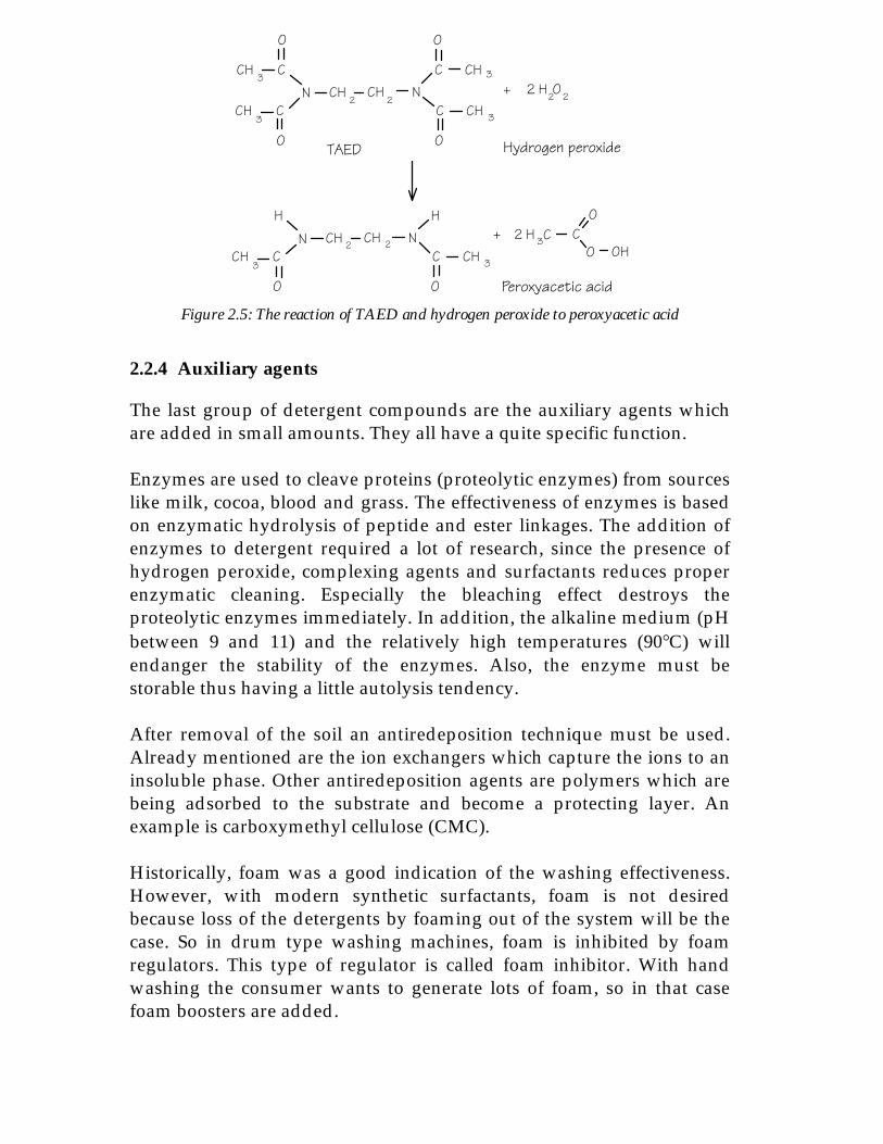
Peroxide is most active at 90°C. To wash at lower temperatures (< 60°C)a bleach activator must be added. When present in wash liquor of pH 9-12, these activators react preferentially with hydrogen peroxide to formorganic peroxy acids which have a higher oxidation potential thanhydrogen peroxide. An example is TetraAcetylEthyleneDiamine(TAED) which can activate bleaching by replacing hydrogen peroxideby peroxyacetic acid as shown in figure 2.5.Another approach for lowering the bleaching temperature is by usingbleaching catalysis, where the bleaching power of sodium perborate isincreased by some heavy metal complexes.

The concentration of bleaching compounds is generally 6 - 8 mM forperborate based systems (hydrogen peroxide) and 1 - 2 mM for peracidbased systems.

CH2

NC CH 3

O

C CH 3

O

CH2N

CCH3

O

CCH3

O

+ 2 H O2 2

CH 2 NH

C CH 3

O

CH 2N

H

CCH3

O

+ C2 H 3

OC

O OH

TAED Hydrogen peroxide

Peroxyacetic acid

Figure 2.5: The reaction of TAED and hydrogen peroxide to peroxyacetic acid

2.2.4 Auxiliary agents

The last group of detergent compounds are the auxiliary agents whichare added in small amounts. They all have a quite specific function.

Enzymes are used to cleave proteins (proteolytic enzymes) from sourceslike milk, cocoa, blood and grass. The effectiveness of enzymes is basedon enzymatic hydrolysis of peptide and ester linkages. The addition ofenzymes to detergent required a lot of research, since the presence ofhydrogen peroxide, complexing agents and surfactants reduces properenzymatic cleaning. Especially the bleaching effect destroys theproteolytic enzymes immediately. In addition, the alkaline medium (pHbetween 9 and 11) and the relatively high temperatures (90°C) willendanger the stability of the enzymes. Also, the enzyme must bestorable thus having a little autolysis tendency.

After removal of the soil an antiredeposition technique must be used.Already mentioned are the ion exchangers which capture the ions to aninsoluble phase. Other antiredeposition agents are polymers which arebeing adsorbed to the substrate and become a protecting layer. Anexample is carboxymethyl cellulose (CMC).

Historically, foam was a good indication of the washing effectiveness.However, with modern synthetic surfactants, foam is not desiredbecause loss of the detergents by foaming out of the system will be thecase. So in drum type washing machines, foam is inhibited by foamregulators. This type of regulator is called foam inhibitor. With handwashing the consumer wants to generate lots of foam, so in that casefoam boosters are added.

Various machine components are made of metals. To prevent corrosionof these parts, modern detergents are supplemented with corrosioninhibitors. These materials deposit an inert layer on metallic surfaces toprevent attack by hydroxide ions.

After bleaching a yellowish tinge remains. In detergents oftenfluorescent whitening agents (FWA) are added. They can be categorisedas cotton-, chlorine resistant-, polyamide- and polyester whiteners.

Fragrances are added to the detergent to give both the powder and theclean laundry a nice smell. In addition it masks the unpleasant odoursproduced during the washing.

To sell a product that can be distinguished from other products, thepowder is coloured by dyes. The preferred colours for both powdersand liquids are blue, green and pink. Green coloured detergent particlesare also added to give the consumer the illusion that this product isenvironmental friendly.

In powdered detergents fillers are present. These inorganic salts(sodium sulphate) give the detergent a good flowability and flushingproperties, high solubility, little caking of the powder under humidcircumstances and prevent dusting. In liquid detergents phaseseparation and precipitation due to temperature changes are preventedby formulation aids.

2.3 Sequential dosing and interfacing

In nowadays washing processes a total washing powder is appliedcontaining all detergent elements. The amount of detergent is dosed bythe user according to the water hardness and the amount of laundry. Inthis way, when the builder dosage for lowering the hardness has to beincreased, also the amount of surfactant is increased. This does not havemuch effect because the surfactant effectiveness is a matter of timerather than of concentration. This ineffective way of dosing does not fitwith the aim of reducing detergent.

The solution for this problem is sequential dosing, where all thedetergent ingredients can be supplied separately on demand. Foreffective sequential dosing some restrictions must be made. For exampleif bleaching elements are already supplied, the proteolytic enzymes aredestroyed at the moment they are added. So the bleaching must beinitiated after the enzymatic cleaning.

A logical sequence for inserting the components starts with the builder.The dosing is according to the water supply and must be applied duringthe washing to capture Ca2+ ions. The enzymes are added in an earlystage to avoid the "burn in" effect, which is the unremovable adherenceof oxidised (by bleach) peptides like blood contaminants. If thesurfactants are added thereafter, this leaves the possibility to raise thetemperature in the last phase of the washing for optimal bleaching.

An interesting new design is made by AEG which company hasintroduced a two-component washing system, on the market availableas the ÖKO-LAVAMAT 6953 [3]. The advantage is that the hightemperature step, required for accurate bleaching, is only performed ashort time. To do this, besides the softener (builder) which is alreadydosed separately in many washing machines, the detergent is split intotwo components: one for bleaching and one for the other detergentoperations. In figure 2.6 the wash cycle is schematically drawn.

Time

Tem

pera

ture

t0 t 1

Adding of detergent

Adding of bleach End

t end

Figure 2.6: Temperature during the two component system

In the first period from t0 to t1 the temperature is relatively low (< 40°C)and only detergent is added. An optimal environment for enzymaticcleaning is obtained. At time t1 the temperature is risen to thetemperature necessary for accurate bleaching. So only from t1 to tend thetemperature is high which reduces energy consumption.

Besides the possibility of controlling the dosing, a more efficient use ofsequential dosing is accomplished by interfacing between the washingprogram and the state of the washing water. A washing machine whichis capable of sensing the state of the washing water, is able to adjust theprogram to the laundry load. Interfacing will yield a further reductionof consumed detergent components, energy and used water.An example of an interfacing washing machine is the Siwamat plus 4000designed by Bosch-Siemens in co-operation with Unilever. This machineincludes the Automatic Dosing System (ADS) [4] which is based on the

separate supply of four detergent components. The interfacing betweenprocess and laundry is not achieved by sensors, but by a dialoguekeyboard on which the user specifies the contents of the tub and thequality of the tap water. After the completion of the dialogue keyboard,the machine starts to execute a washing program which is optimallyadjusted to the load. A decrease of detergent consumption of 50% isclaimed by the manufacturers.

However, for optimal interfacing between the program and the washingof the laundry, a real time monitoring by the use of sensors of thewashing water is necessary. Only in that case, the program can beadjusted during washing.

2.4 Conclusion and selection of washing parameters

In conventional washing machines, the cleaning is achieved bymechanical input, carried out by the machine, and chemical input,carried out by the detergent. Control of the washing process is done bythe user, by choosing the accurate detergent and adjusting the dosing,as well as by choosing the right program and temperature. There is nointeraction between detergent and the program executed by themachine.In order to achieve an optimal reduction of the consumption of water,detergent and energy, an interfacing washing machine is needed. Such awashing machine will monitor the state of the tub contents, resultinginto information concerning the load, tap water and washingeffectiveness. The process can be adjusted according to this information.For monitoring, sensors must be placed in the washing water.

To make a decision about the sensors that will be needed for monitoringwashing processes, table 2.1 gives an impression of desired washingparameters, mentioned implicitly in this chapter.Before the washing is initiated, the contents of the tub consists of soakedlaundry. Parameters of interest are the amount, colour and type offabrics. Also the quality of the tap water and the type of soil, partiallyalready present in the water, are important parameters based on whichthe washing has to be adapted. After the detergent is added, themeasured parameters will give information on the effectiveness ofwashing. A fast lowering of bleach activity indicates that manybleachable components are present. Finally, when the washing is done,the dirty water has to be removed by rinsing. This rinsing has to bemonitored in order to detect an end point.

Table 2.1: Washing parameters before and during a washing process

Beforewashing

Type of fabric The type of fabric (wool, cotton, etc.) present in the tub ishard to determine. Probably this can be left to theoperator.

Colour of fabric In general, two types of wash are being performed: whitewash and coloured wash. Because the difference is veryhard to measure, this will be left to the operator.

Load weight The torque on the motor that rotates the tub givesinformation about the load weight.

Amount of soil An impression can be obtained by evaluating pH,turbidity and conductivity. For a more accuratemeasurement, specific sensors for soil contaminants willbe needed.

Type of soil Specific sensors for detecting bleachable, fatty and stain-like soils are necessary.

Water quality Hardness, conductivity and turbidity have to bemeasured.

Duringwashing

Water level An explicit water-level indicator will not be necessarywhen a torque sensor is present (for the load weight). Themass of the tub will be dependent on the amount of waterin the tub.

Temperature For control of the temperature a sensor will be needed.

Detergenteffectiveness

The measurement of surfactant level, enzyme activity,bleach activity, pH and hardness (builder dosage) givesan idea of the effectiveness of washing.

Turbidity Turbidity can only be sensed optically.

Mixingeffectiveness

A flow sensor is needed for measuring mixingeffectiveness.

Duringrinsing

Rinsingeffectiveness

For rinsing effectiveness, a secondary parameter must befound which is an indication for how many dirty water isexchanged by tap water. Conductivity and pH might begood indicators.

Terms like water quality, machine load, etc. can not be determined fromsensors directly, which was mentioned in chapter 1 as the differencebetween washing parameters and measurable variables. So from this setof washing parameters, a set of equivalent measurable variables must befound. Table 2.2 gives a list of variables with which the washingparameters from table 2.1 can be approximated.

Torque sensor principles will be omitted in the rest of this thesis, sincesuch sensors will probably not be placed in the sensor array, but will berealised in combination with the tub motor. Sensors for measuring thetype of laundry (colour, fabric) are omitted as well. The reason is, thatsome techniques for fabric type determination are based on the waterresorption characteristics (from a water level versus applied watercurve), so they will also not be placed in the sensor array. In addition, it

is no big task for the user to tell the machine what type of fabric is in thetub, since a basic selection of fabrics must be made anyway.

Table 2.2: List of measurable variables which give an impression of the washing process

Measurable variables Washing parametersPhysical Temperature Temperature

Flow Mixing, turbulence or flowConductivity Water quality, rinsing effectiveness,

soil loadDynamic surface tension Detergent concentrationTorque on tub-motor Amount of laundry, water level

Concentrations pH pHH2O2 Bleach activityCa2+, Mg2+ Hardness, builder functioningEnzymes Enzymatic cleaning effectiveness,

specific soil detection

Some ranges for the measurable parameters of table 2.2 were mentionedin this chapter:Temperature: Tap water can be cold, 5°C, in winter and can be heated

up to 90°C during some washing processes;Flow: Using a 60 cm tub, with a rotation speed of 60 per

minute, the speed at the edge of the tub is equal to 1.9m/s;

Conductivity: a range from 100 mS/cm in very soft tap water to 2mS/cm during the main wash can be expected;

pH: Between the pH of tap water and the pH after theaddition of the detergent: pH = 6 - 12;

Bleach activity: For perborate based systems, the hydrogen peroxideconcentration is about 6 - 8 mM, for peracid basedsystems concentrations of 1 - 2 mM are observed;

Hardness: The hardness of tap water is the result of 0.4 to 2.4 mMcalcium and 0.1 to 0.6 mM magnesium. During washingthe concentration of hardness ions is reduced to aminimum;

The measurable parameters listed as in table 2.2 are the starting pointfor the next chapter, where the required sensor structures needed formeasuring these parameters are investigated.

2.5 References

[1] G. Jakobi and A. Löhr, Detergents and textile washing, principles and practice,VCH Verlagsgesellschaft mbH, Weinheim, Germany 1987

[2] Statistiek wateronderzoek 1986, Vereniging van Exploitanten van Water-leidingbedrijven VEWIN, Rijswijk, 1986

[3] User manual for the ÖKO-LAVAMAT 6953, AEG Hausgeräte AG, Nürnberg[4] H. Zott, S. Willemse, Automatisches dosiersystem (A.D.S.) für Haushalt-

waschmaschinen, in: Tenside surfactants detergents, vol. 27, 1990/1. CarlHanser Verlag, München

CHAPTER 33. Selection of sensor materials based on a literature overview

Selection of sensor materials based ona literature overview

The aim of this chapter is to choose the most appropriate set of materials forfabricating an integrated sensor array. Based on these materials, a set ofsensors, or even better an integrated structure has to be designed which can beused to measure as much washing parameters as possible. However, the designitself and the interpretation of the sensor outputs, is set aside for a subsequentchapter.

3.1 Introduction

A sensor is a device which converts information from a domain ofinterest into a useful signal. In general, this conversion takes place intwo parts, a selector and a transducer as indicated in figure 3.1. In theselector the information of interest is converted into a form which ismeasurable by the transducer. As the transducer is non-selective, theselector must introduce the desired selectivity [1].

Physical orElectrical domain

Variable ReceptorModulated

Sensor

Electrical signal

chemical domain

electronic device

Figure 3.1: Basic structure of a sensor

For many chemical sensors, this two-level interpretation is quite clear.Commonly observed chemical selectors are selective membranes andmodified surfaces, examples of transducers are FETs and amperometricworking electrodes. Physical sensors have a less defined separationbetween those two parts. For example, a thermistor acts as a resistor inthe transducer part, but a typical selector part is hard to point out. Inthis case, speaking of selectivity at all is difficult.Although there are a lot of possible sensors, the ones having anelectrical output are the most comfortable. Sensors giving an electricalsignal as a measure for the desired chemical or physical parameter caneasily be connected to a computer for data evaluation and storage.

When restricting to sensors having an electrical output, one can refer tothe transducer part as a modulated electronic device.

For designing an integrated sensor array, the included sensor structuresmust have some technological compatibility in order to find a singlefabrication process. The next three questions may arise considering thesensors to be integrated:• What variable (washing parameter) is being measured?• What is the modulated electronic device?• What material/technology is chosen for the implementation?The first question is necessary to reduce the enormous amount ofknown sensors to an orderly set for monitoring washing processes. Thesecond question is added for getting insight in how to read out thesensor using an electronic circuitry. Finally, the third question links thesensor material to the sensor operation since in general the selectionprocess is carried out by the properties of the chosen material.

As an example, table 3.1 gives the answers to the previous questions forthree selected sensors. First, the ISFET has a tantalum-oxide layer whichtransforms the pH of an electrolyte into a surface potential. This surfacepotential modulates the threshold voltage of the underlying FETstructure. Another example is the thermoresistive transducer whichuses a conductive material to transform temperature changes intoresistance variations. This resistance can be measured by constructingthis material in the form of a resistor. With an amperometric workingelectrode the separation into a selector and an electronic device is moreabstract. The receptor can be seen as an evoked specific chemicalreaction, in which case the modulated electronic device is a currentsource with concentration dependent output.

Table 3.1: Some sensors described in the terminology of figure 3.1

Sensor Measuredvariable

Modulatedelectronic device

Material of sensor

ISFET pH MOSFET Ta2O5 - layerhas a pH-dependent surface potentialwhich modulates the thresholdvoltage

Pt-100 Temperature Resistor Thermoresistive metalof which the resistivity is temperaturedependent

Amperometricsensor

Concentration Current source Inert metalevokes an electrochemical reactionafter applying a potential

The three questions are taken as a guideline for the classification ofknown sensing methods. The washing parameters as chosen in chapter2 are used for a first classification. Next, the most common electronicparts are listed, together with their capabilities for chemical andphysical sensing. Finally, the most important sensing methods aredescribed, classified by the used materials. Notice that for completeness,now the term “sensing methods” is used, because some mentioned“sensors” are not completely developed devices.The result will be the choice of a set of materials together with theirfabrication technology with which an array of sensors can be fabricatedcapable of sensing the desired washing parameters.

3.2 Sensor classification by measured washing parameter

In this section, a systematical categorisation of known sensors isperformed. This categorising is done with respect to the washingparameters to be measured, as chosen in chapter 2:• Temperature;• Flow;• Conductivity;• Dynamic surface tension;• Hydrogen peroxide concentration;• pH and acid concentrations;• Water hardness and calcium concentration;• Enzymes;

3.2.1 Temperature

Most chemical and physical phenomena are temperature dependent.The direct consequence of this is that with almost all sensor outputsignals, the operational temperature must be given. On the other hand,the large number of temperature dependent phenomena is the reasonfor the large amount of temperature sensing principles that can befound in literature.Besides the interest of sensing temperature itself, there are someprinciples which make use of temperature sensing. Examples can befound in flow measurements [2] and specific heat capacitydetermination. The specific heat capacity CV at a constant volume of asubstance is defined by [3]:

CUT MV

V=

δδ

1(3.1)

where U is the internal energy, T the temperature and M the mass of thesubstance. Because a change in internal energy can be identified withthe heat supplied at constant volume (qsupplied = DU), the previousequation can be used to determine the specific heat capacitance. When aknown quantity of heat is supplied to a sample and the resultingincrease in temperature is observed, the heat capacity can be calculated.An evaluation of the heat capacity of the contents of a washing tub willgive information on the laundry type, since the heat capacity of the totaltub load is partially determined by this laundry.The practical realisation of such a determination is quite simple: thewashing liquor is heated anyway at the beginning of a washing processby a known amount of heat, only the water temperature should bemonitored. The mass of the contents of the tub (both water and soakedlaundry) can be determined from the torque on the tub motor which isproportional to the current supplied to this motor.

3.2.1.1 Thermal expansion, glass thermometer

The glass thermometer is based on the thermal expansion of a liquid. Atconstant pressure, the volume of a certain amount of liquid (originallymercury, but nowadays usually coloured alcohol) changes linearly withtemperature. To make the volume change visible for the human eye, theliquid is stored in a small capillary.

3.2.1.2 Thermoresistive effect

The bulk conductivity of many semiconducting materials depends ontemperature. This has led to the development of small temperaturesensing devices called thermistors.There are in fact three categories of thermistors: the ceramic negativetemperature coefficient (NTC) type, fabricated by high-temperaturesintering of certain metallic oxide mixtures, the positive temperaturecoefficient (PTC) type, made by sintering barium and strontium titanatemixtures, and the single crystal doped semiconductor (silicon) type,which has also a positive temperature coefficient [4]. When accuracy isrequired and an offset is undesired, the thermistor is placed in aWheatstone bridge circuitry.

While the temperature dependency of thermistors is exponential,semiconductor temperature sensors based on the spreading resistancetechnology have a virtually linear temperature characteristic. Discretedevices based on this technology are commercially available [5]. Theyhave a positive temperature coefficient and their nominal resistance isabout 1 kWat 25ºC.

These sensors use n-type silicon with a doping level between 1014 and1015/cm3. Typical chip sizes are about ½ × ½ × ¼ mm. The upper planeof the chip is covered by an insulating silicon dioxide layer in which ahole of about 20 µm has been etched for a metal contact to the silicon.The bottom plane is entirely metallised. When a potential is appliedover the device, this structure results into a conical current distributionthrough the crystal, hence the name "spreading resistance".Because of the accuracy and reliability, the spreading resistancetechnology temperature devices are an attractive alternative to the moreconventional sensors using NTC or PTC thermistors.

Metal strips do have an almost linear variation in a certain temperaturerange [4]. A commonly observed implementation is the Pt-100 element,which consists of a platinum resistor with a resistance of 100 W at 0 ºC.Practical applications of Pt-100 elements are in a Wheatstone bridge set-up. To remove the effect of lead resistances, the element is suppliedwith three wires. Two of them are connected to the same side of the Ptresistor, one for the current injection and one for sensing.Problems with Pt-100 elements come from the self heating when acurrent flows trough the device. This can be avoided by measuring in apulsed way.

3.2.1.3 Thermoelectric effect, thermocouple

If two different metals are connected in a closed circuit with their twojunctions at different temperatures, a current will be observed [4]. TheSeebeck thermal emf, responsible for this current flow, depends on thetypes of metal involved and is approximately proportional to thetemperature difference between the two junctions when thetemperature difference is not too large. Since the temperature differenceresults into a voltage, this type of sensor is self generating.

3.2.1.4 Thermochemical effect

Thermochemical indicators make use of the temperature sensitivechemical changes in some substances. The rapid colour changes thatsome liquid crystals show occur within relatively small temperaturechanges. This enables one to measure surface temperatures either bypainting or spraying a liquid crystal substance on a surface. In someapplications plastic-film encapsulated liquid crystals are used.Registration of the effect is always optical.

3.2.1.5 Pyroelectric effect

Many of the temperature sensors mentioned before are used fortemperature measurements by making contact to the medium undertest. Applications of thermal sensors using the pyroelectric effect are inthe field of IR radiation sensing.The pyroelectric effect is observed with certain types of materials havinga noncentrosymmetric structure where polarisation strongly changeswith temperature [4]. Many piezoelectric materials, like ZnO, are alsopyroelectric [6]. Other examples are lead zirconate-titanate materials.Under steady state conditions, the surface charge created by thepolarisation is neutralised by external charges (due to leakage currents)and no emf is observed across the material. However, if the temperatureis changed, the state of polarisation changes and a change in theexternal emf will be observed.

3.2.1.6 pn-junction

An understanding of the temperature characteristics of pn-junctiondiodes can be achieved by considering the current I at constant voltageV of a silicon diode in a forward biased operation [7]. The characteristicof a diode depends on the structure of the junction which can varyconsiderably from type to type. So, an accurate calibration of thetemperature dependency is required. Besides that, there is no linearrelation with temperature.

3.2.1.7 PTAT set-up

Better results than using a single diode can be obtained with transistorsor transistor pairs. For a bipolar junction transistor, the temperaturedependency of the V-I characteristics resembles that of the diode.However, by placing two identical transistors in an asymmetricalcurrent mirror, resulting in dissimilar collector currents, the outputvoltage is proportional to the absolute temperature (PTAT sensor) overa wide range [8, 9]. Besides bipolar PTAT circuits, MOSFET basedPTATs are possible as well.

3.2.2 Flow

To get an impression of the stirring effectiveness in a washing machinethe flow can be measured. Whether this is mass flow or flow velocity isless important for this purpose. In this subsection an (incomplete) list offlow measurement techniques is given. Some of them are impossible toperform in a washing process, others are more easy. A major source of

flow measurement techniques comes from the field of blood flowdetermination [10].In practical applications, normally the flow velocity is determined [11],by additionally using the density of the medium and the cross section ofthe tube the medium is flowing through, this number can be convertedinto mass flow.

3.2.2.1 Time of flight

When a liquid (or gas) is locally heated by a heat pulse, the time todetect this pulse at a distance x is a measure for the flow velocity [2].Other markers like H+ clouds [12] and small bubbles are reported aswell.

3.2.2.2 Pressure gradient

The pressure gradient technique is based on a mathematical relationshipbetween the flow velocity and the pressure gradient along a vessel. Thismethod can only be used in tubes. To increase a pressure gradient, anobstruction is sometimes introduced in the tube.

3.2.2.3 Anemometric measurement

With anemometry, the cooling down of a heated element is used tocalculate the flow velocity of a heat conducting medium.

3.2.2.4 Electromagnetic

When a conductor is moved through a magnetic field, an emf isgenerated within the conductor with a value proportional to thevelocity. In case of a conducting fluid moving with a certain velocity, anemf is generated across the diameter of the fluid column, to bemeasured using appropriate electrodes. The measured emf isproportional to the flow velocity.

3.2.2.5 Ultrasonic

When an ultrasonic sound is applied to a tube with a flowing mediumcontaining particles with a certain mass and size, the sound reflected bythese particles has a frequency shift due to the Doppler effect. TheDoppler shift in the frequency is proportional to the fluid velocity with asign dependent on the flow direction [4]. This method is very popular inthe medical practice for the measurement of blood flow in humanvessels.

3.2.2.6 Indicator dilution methods

The operation of this wide scale of methods is based on themeasurement of the dilution of an injected indicator. For properoperation an accurate model of the diffusion and flow behaviour of theindicator is necessary. Examples with different indicators are dyedilution, thermal dilution and conductivity dilution methods (as in usefor the measurement of cardiac output [10]).

3.2.3 Conductivity

By measuring the electrical conductivity of the washing liquor, animpression can be obtained of the state of rinsing cycles or about the soillevel in the washing tub. Besides that, some conductivity sensors can beused as concentration sensors when they are used in combination with aselective membrane [13].

3.2.3.1 Two-points set-up

A standard conductivity measurement is based on the measurement ofthe AC potential/current relation (impedance) of an electrolyte. In a twopoints set-up the electrodes that generate the current are used formeasuring the potential as well [14].The problem with this method is that the two relative unstable electrodeinterface impedances are in series with the potential difference inducedin the electrolyte which gives an unknown error in the measuredconductivity.The insulator Ta2O5 has a relatively low oxide/solution impedance, so atwo points conductivity measurement based on a Ta2O5 on platinumprobe is an attractive alternative [15]. Sometimes the probe is realised asa planar interdigitated electrode.

3.2.3.2 Four points set-up

The problem with a two point conductivity set-up is that theimpedances of the working electrodes are influencing the measuredpotential, and so the measured conductivity. In a four points set-up, thecurrent loop and the potential sensing are realised as separate circuits.The impedances of the electrodes in the measurement loop do not affectthe measurement when this loop is sufficiently high-ohmic. Unstableelectrode potentials will not affect the measurement if the frequency ofthe AC current source is chosen high enough.The potential sensing is realised using either capacitive probes (Ta2O5

cell or ISFETs [16]) or metal strips.

3.2.3.3 Using an ISFET

In the small signal model of the ISFET, the electrolyte conductivitybetween ISFET and reference electrode becomes important [17]. The cut-off frequency of the trans-admittance (the transfer function from thegate-source voltage to the drain current) is equal to

fRCdB

G− =3

12π

(3.2)

with R the resistivity of the electrolyte and CG the small signal gatecapacitance. This small signal gate capacitance consists of the smallsignal gate to drain and gate to source capacitances in parallel, largelydetermined by the macroscopic oxide capacitance. A common range forthis frequency is 0.1 MHz to 5 MHz which can be adjusted by changingthe geometry of the structure.

3.2.4 Dynamic surface tension

The dynamic surface tension (DST) of a liquid is related to the surfactantconcentration. This phenomenon was used for the development of adynamic surface tension sensor [18, 19]. The operation of this sensor isbased on monitoring the release frequency of electrolytically generatedgas bubbles, which is dependent on the dynamic surface tension.The DST electrodes are not simple metal films. Two configurations arereported. The first one is the cavity electrode. Bubble nucleation iscontrolled here by the geometric structure of the electrode. This specificstructure is a pyramid shaped hole which is made by an anisotropic etchof silicon (KOH etch) before metal deposition. The second one is the"gas phase nucleation core" electrode where the nucleation is controlledby an initial amount of gas. This device requires an isotropic etch ofsilicon to make the gas core in the substrate.

3.2.5 Hydrogen peroxide concentration

Some hydrogen peroxide determination methods are well developed inglucose sensors where a GOD-membrane catalyses the glucoseconcentration to an equivalent hydrogen peroxide concentration. Inthese systems, the GOD membrane guarantees the selectivity. Theresulting hydrogen peroxide concentration is generally measuredamperometrically or potentiometrically.However, in washing systems, the hydrogen peroxide concentration isthe parameter of interest itself. So, this measurement technique must beselective for hydrogen peroxide.

3.2.5.1 Amperometric method

A platinum electrode for the electrochemical monitoring of hydrogenperoxide concentration is most widely used for biosensors nowadays.The Pt electrode is biased at 0.7 V versus an Ag/AgCl electrode. Thismethod, however, suffers from interferences of other electro-oxidisablecompounds in the solution (such as Fe2+), so a high performance sensoris not possible [20].

3.2.5.2 Chrono amperometric detection

After applying a potential step across an electrolyte-electrode interface,the Cottrell equation [21] can be used to determine the concentration ofH2O2 from the measured current response. This step must be highenough to deplete the H2O2 concentration at the surface completely bymeans of oxidation or reduction. Under this condition, the currentresponse becomes independent of the applied potential step size.Because the demands on the potential step size are not very critical, thereference electrode might be omitted and a two-strip set-up can be used[22].

3.2.5.3 Potentiometric method

Instead of measuring current, the concentration information can beobtained by measuring potentials as well. Good results are reported [23]using a carbon electrode loaded with Perovskite-type oxides likeLaCoxNiyMnzO3. A logarithmic variation with the hydrogen peroxideconcentration is observed. Dependent on the used oxide contaminants,the reaction

H O O2 2 + + ↔+ −2 2 2 2H e H l( ) (3.3)

can be selected. The carbon with a perovskite-type oxide is placed on aconducting material. A current is applied and the emf is being measuredin a half cell set-up, using a potentiostat. From the given reactionequation it can be concluded that the pH must be well defined during ameasurement.

3.2.5.4 Volumetric titration

The following reaction occurs when a potassium permagnate solution isadded to a hydrogen peroxide solution acidified with dilute sulphuricacid [24]:

2MnO O4- + + ↔ + ++ +5 6 2 5 82 2

22 2H O H Mn O H l( ) (3.4)

where MnO4- has an intense purple colour which is not observed withMn2+. This is a classical example of a volumetric redox titration. In alaboratory set-up the end point is detected optically when the purplecolour of the droplets coming from the burette does not disappearanymore.

3.2.5.5 Chemiluminescence

Certain compounds (molecules) can be detected by mixing them with areagent with which the molecules react to form excited molecules whichdecay spontaneously with photo emission [11]. For hydrogen peroxidesome of those reagents are available. This method requires acomplicated and sensitive optical system.

3.2.6 Acid concentrations and pH

The terminology "acid concentration" and "pH" are both related to acidsbut are quite different. The pH is defined as the logarithm of the activityof free protons in a solution while the acid concentration concerns thetotal amount of a certain (weak) acid. For example, an ISFET measuresthe activity of protons. In a solution of a strong acid this is a directindication for the acid concentration. However, with a weak acid theamount of free protons is only a fraction of the total acid concentration.By applying OH--ions to the chemical system, which can be done byeither a volumetric or a coulometric titration, the pH varies with acharacteristic shape: the titration curve. From the end point in thiscurve, which is the moment where the pH has a very steep change, theacid concentration can be determined.A solid-state version of a titrator is the coulometric sensor-actuatordevice [12, 25] where hydroxyl ions are electrochemically generated at anoble metal electrode and the resulting change in pH is monitored by anISFET.The major part of pH sensors detect proton concentrations by makinguse of potentiometric techniques.

3.2.6.1 Potentiometric metal oxide sensors

The potentiometric pH sensing capability of metal oxides (PtO2, IrO2,RuO2, OsO2, Ta2O5 and TiO2) is mentioned many times in literature [26,27]. The use of antimony-antimony(III) oxide for in vivo pH sensing hasbecome a standard technique in clinical applications [28]. However, theobserved near-nernstian behaviour in the pH range 2 - 12 suffers frominterferences from oxidising and reducing species and complexinganions. Although a metal oxide structure can be miniaturised easily, the

necessary reference electrode is a voluminous and fragile element.When sensing in a washing environment, the exposure to bleaching(oxidising) agents will be inevitable thus making the successful use ofthis type of pH sensor improbable.

3.2.6.2 The pH glass electrode

A very well known pH sensor is the pH glass electrode [29], alreadyinvented in 1901. This is an ISE (ion selective electrode) with a H+

selective glass. Inside the electrode there is a pH buffered KCl solutionwith an Ag-AgCl or calomel electrode as a reference. At the inner side ofthe glass there is a constant potential because of the constant ionactivities of the inner solution. At the outer side of the glass a pHdependent diffusion potential occurs which can be measured withrespect to the external reference electrode. The diffusion potentialsatisfies the Nernst equation and gives a dependency of minus 59 mVper pH at 25°C.

3.2.6.3 The ISFET

The ISFET, which is a transistor based ion sensitive device, has theadvantage that it is not made of fragile glass and that it is smaller thanthe glass electrode [30]. Because the operation is based on surfacepotentials, rather than diffusion potentials, the operation is fastercompared to the glass electrode. The need of a reference electrode, justas with the glass electrode, is unfortunately less elegant. A more rigidsystem is possible when a solid state reference (a REFET) would beavailable.

3.2.7 Water hardness and calcium concentration

Historically "hardness" originated from the capacity of multi chargedcations in water to replace sodium or potassium in soap [29, 31]. Thisundesired replacement decreases the efficiency of soap since badlysoluble products are the result. Because calcium and magnesium ionsgenerally exceed the concentration of other divalent cations in tapwater, in many cases only the contribution of these ions is evaluated indiscussions concerning hardness in general. For representing the waterhardness as a single number, the hardness is defined as the calciumcarbonate concentration equivalent (usually in mg/l) of the totalconcentration multivalent ions.Most of the measurement methods listed here are selective for calciumwith respect to magnesium but they are widely used for hardnessdeterminations.

3.2.7.1 Volumetric titration with EDTA

A particular property of EDTA (EthyleneDiamineTetraAcetate) as atitrant is that it complexates with metal ions in a 1:1 ratio regardless ofthe charge of the cation. According to these complexes with a largenumber of metal ions, the volumetric titration with EDTA is notselective for calcium and magnesium. The general equilibrium is

M HY MY Hn n+ − − + ++ ↔ +3 4( ) (3.5)

with Mn+ the metal ion to be titrated and Y4- the EDTA ion. Because ofits pH dependency, EDTA titrations are generally performed inbuffered solutions (for water hardness a buffered pH of 10).The key to the measurement of water hardness using an EDTA titration,is the low stability of the complex with magnesium. The last multivalention to be titrated is magnesium, and therefore, a magnesium indicatorcan be used to determine the end point where all the multivalent ionshave formed complexes. Such an indicator can either be calmagite oreriochrome black T. Often a small concentration of the EDTA complexwith magnesium is included in the buffer to assure the presence ofsufficient magnesium ions for improving indicator action [24]. Some testkits for determining the hardness of tap water work in this way.A back titration, where free calcium is first completely removed by acomplex-formation step with EDTA and afterwards quantitativelydetermined with erio-T is used as well [32].

3.2.7.2 Coulometric titration

This method makes use of the amine mercury(II) complex of EDTA-acid(H4Y). The complexing agent EDTA is released to the solution as a resultof the following reaction of the mercury electrode [24]:

HgNH Y NH e Hg NH HY32

4 332 2− + − −+ + ↔ + + (3.6)

which is followed by complexation reaction (3.5). Because the mercurychelate is more stable than the corresponding complex with calcium(also zinc, lead or copper), complexation with this ion will not occuruntil the electrode process frees the ligand.

3.2.7.3 Potentiometric detection

In analogy with the measurement of protons, the detection of calciumions can be done using potentiometry. Commercially availableionophores [33] can be used to make a calcium ion selective membrane.The interface potential between this membrane and a contactingelectrolyte is nernstian dependent on the electrolyte calcium activity.

Two methods for sensing this interface potential are used. The first oneis the calcium selective implementation of the classical liquid membraneelectrode with an aliphatic di-ester of phosphoric acid as the ionexchanger [29]. In such a set-up, the potential is measured over tworeference electrodes in the electrolyte where one of them is placed in aliquid membrane tub. In the liquid membrane tub, calcium ions arebuffered resulting in a nernstian interface potential.When the ion exchanger membrane is placed on an ISFET, this gives acalcium ChemFET [34, 35]. Although nernstian responses can beobserved, ChemFETs in general do not give promising results for theuse in the washing sensor array because the currently used lipophilicmembranes will be washed off easily in an environment with soap.

3.2.8 Enzyme detection

Detection of enzymes (or peptides in general) generally requires a twophase method: first the peptide is specifically bound to a membrane andsecondly this binding is being detected by an electronic device. In caseof a reaction which releases protons or hydroxyl ions, an ISFET can beused for detection (the ENFET). When the ionic strength in themembrane is drastically influenced by the peptide reaction, aconductivity sensor is more adequate.

3.2.9 Summary

The methods evaluated in this chapter are summarised in two separatetables for physical and chemical washing parameters respectively.

Table 3.2: Summary of methods for determining physical washing parameters

Temperature Flow Conductivity Dynamic surfacetension

Thermal expansion Time of flight Two-points set-up Bubble electrodeThermoresistive effect Anemometry Four points set-upThermoelectric effect Pressure gradient Using an ISFETThermochemical effect MechanicalPyroelectric effect Electromagneticpn-junction Ultrasonic

Indicator dilution

Table 3.3: Summary of methods for determining chemical washing parameters

H2O2 pH and acid conc. Ca2+ and hardness Enzyme detection

Amperometry Potentiometry Volumetric titration ENFETChrono amperometry ISFET Coulometric titrationPotentiometry Acid-base titration PotentiometryVolumetric titrationChemiluminescenceUV absorption

3.3 Sensor classification as electronic devices

For the electronic circuitry connected to the sensor, a sensor behaveslike a standard electronic component [36]. In chapter 1, sensors werecategorised into self generating and modulating devices. Whilemodulating sensing devices are represented by passive electroniccomponents, self generating sensing devices should be represented ascurrent and voltage sources. An exception is the category of transistorbased sensors: although these are modulating sensors in general, theyare referred to as active components from the electronic point of view.

3.3.1 Resistors

The thermoresistive effect of metal strips was already mentioned with thePt-100 as an application of this effect for sensing temperature. Othermaterials like metal oxides can be used for thermoresistive set-ups aswell.

Chemo resistors are chemically modulated resistors [1]. Standard metaloxide gas sensors consist of a sintered block of the oxide which is heatedto a few hundred degrees centigrade. Surrounding gases react with theoxygen on the hot surface causing changes in the resistivity of thematerial. Gas sensors based on this principle and employing oxides oftin, zinc, zirconium or titanium and with proper doping are known tobe sensitive to many types of gases. Metal-oxide gas sensors can befabricated using thin (silicon) and thick film technology.

3.3.2 Capacitors

The mentioned resistor based sensors are easy to use because they givean immediate (current) response on an applied DC voltage. Capacitorbased sensors, however, need an AC operational mode to getinformation from the device because no DC path is present.

For sensing purposes, two mechanisms are possible: either a change inthe geometry or in the dielectric material will result into a change in theobserved capacitance.An example of a sensor based on the change in the geometry of acapacitive structure is the condenser microphone [37]. With this type ofmicrophone, a sound wave brings one plate of a parallel plate capacitorinto vibration, while the other plate (the backplate) is made of aninflexible material. The occurring change in the distance between theplates results into a change in the capacitance which can be detected byan electronic circuitry.The dielectric constant of a material is not always a constant, butsometimes a function of some physical and chemical parameters. Somematerials show a temperature dependent dielectric constant which canbe measured by using a capacitive sensor structure [1]. Besidescapacitive temperature sensors, also capacitive humidity sensors arereported [38, 39]. By placing a water adsorbing material between twometal plates, the capacitance of the created capacitor depends on theamount of the moisture adsorbed on the dielectric material.

3.3.3 Inductors

Inductors are hard to realise in micro technology, maybe that is why nosignificant chemical and physical sensitive coils were reported inliterature. Even in macrotechnology the number of coil based sensors islow, and then only for physical movement detectors like displacementsensors and pick-up elements for both turntables and electrodynamicmicrophones. In theory it must be possible to determine variations inthe magnetic permittivity of materials due to chemical influences.Temperature, moisture and deposition measurements must be possible,but the size of the fluctuations in the magnetic permeability µr is small.

3.3.4 Impedances

A sensor like an electrolyte conductivity cell can not be placed in thesubsection with resistors or capacitors, because it is modelled as acomplex impedance of which the value can only be determinedproperly by using AC signals. However, sometimes an impedance canbe modelled as a network consisting of resistors, capacitors andinductances.Besides the interest of electrical impedance measurements fordetermining electrolyte conductivity [14], the measurement ofimpedances of selective polymer membranes can give specificinformation on gases and ions [1, 13]. Subsection 3.4.1.4 concerningconducting polymers will discuss such membranes in more detail.

3.3.5 Diodes

The applications of diodes in sensors can be separated into two types.One widely applied physical sensitive diode is the temperature sensor,another chemical sensitive diode-based device is the ion controlleddiode.The diode equation, describing the relation between the voltage across adiode and the resulting diode current is given by [40]

I I eD

qVkT

d

= −

0 1 (3.7)

with I0 the saturation current, Vd the diode voltage, q the unity ofcharge, k the Boltzmann constant and T the temperature. Theappearance of the temperature in the diode equation enablestemperature sensing using a diode [1].An ion controlled diode (ICD) uses a lateral bipolar transistor covered byan insulating material with a selective membrane on top of it [41, 42].The size of the depletion regions of the two lateral diodes depends onthe interface potential at the ion selective membrane/electrolyte contact.By measuring the differential capacitance of the two space chargeregions an impression of the ion concentration is obtained.

3.3.6 Bipolar transistors

In subsection 3.2.1.7 the use of a bipolar junction transistor in aproportional-to-absolute-temperature (PTAT) set-up was mentioned as alinear temperature sensor set-up [43].

Not many applications of bipolar transistors for chemical sensing arereported. The ICD described above looks like a bipolar transistor, but isnot used in a transistor mode.A technique called transistor technique is sometimes used for a pnjunction in contact with an electrolyte to evaluate electrode reactions,because valence band electrons and conduction band electrons can bedetected separately [44]. In this set-up only the n-type region is incontact with the liquid, the p-type layer is covered by the n-region. Abipolar junction transistor is formed with the electrolyte as a collector.

3.3.7 MOS transistors

The threshold voltage of MOSFETs is proportional to the differencebetween the gate metal and silicon work functions, FM and FSi [45, 46].This dependency is essential for the applications of most of the MOSFET

structures in chemical sensors. Variations in these parameters candirectly (as a 1:1 relation) be measured in the threshold voltage.For instance, the EMOSFET [47] has an iridium oxide gate materialwhich can still operate as a classical MOSFET. In addition, the iridiumoxide in contact with an electrolyte results into an oxidation-statedependent work function which can be measured in the thresholdvoltage of the MOSFET operation.

Gas sensorsMetal work functions change with the contamination of the metal. Anapplication is the use of a palladium gate in a MOSFET structure, thepalladium gate IGFET [48]. Since the work function of palladium isdependent on the absorbed hydrogen gas molecules, this device can beused for hydrogen gas measurements by monitoring the thresholdvoltage.In a suspended gate GASFET [48], a gap is created between theinsulating gate oxide and a platinum gate. When gaseous moleculeswith a dipole moment diffuse into the gap, they increase the surfacepotential when adsorbed to either the gate material or the insulatormaterial. While the IGFET is selectively sensitive to hydrogen gas, thesuspended gate GASFET is sensitive to all polar molecules.When the gate metal is omitted and the device exposed to a gas, anOpen Gate Field Effect Transistor is created (OGFET) [45]. This devicegives responses to polar molecules like water vapour and methanol.An improvement is obtained when the oxide layer is very thin (5 nm).For thicknesses below this value the device responds to all kind of gaseswhich have a permanent net dipole moment, such as H2, NH3, HCl, CO,NO, NO2 and SO2. This device is called the ADFET [45].The problem with these devices is that the gate potential is badlydefined. A solution to this problem is the use of the SAFET [45], whichhas an oxide layer which is partially covered by a metal gate. At theuncovered side, a dependency on polar gases (water, acetone, alcohols)is observed.

Humidity sensor, CFTThe Charge Flow Transistor (CFT) is a MOS-based field effect transistorwith the metal gate placed as a ring around a resistive layer [49]. Thislayer is humidity dependent, so an applied gate voltage appearsintegrated at the oxide surface, and the resulting time constant can bemeasured by the field effect transistor as a function of the humidity.

Pressure sensor, PRESSFETThis device contains a floating (mechanical movable) plate hangingabove the oxide of an ISFET structure. The influenced parameter is theair gap capacitance in series with the oxide capacitance [50]. This air gapcapacitance is dependent on the applied pressure.

pH Sensor, ISFETThe set-up for an ISFET looks like that of the described gas-sensitiveFETs but now the oxide is in contact with a liquid [30]. A gate contact iscreated by placing a reference electrode in the electrolyte. Although thetransistor equations of the MOSFET are still valid, an additional term isadded to the threshold voltage consisting of the surface dipole momentof the solution and the actual pH dependent electrostatic potential y0.This parameter depends on the pH as follows:

δψδ

α0 2 303pH

kTq

= − . (3.8)

with the factor a as a selectivity factor without a dimension being

αβ

= +

−2 3

12

1.

int

kTCq

dif (3.9)

where bint represents the intrinsic buffer capacity of the oxide surfaceand Cdif the differential double-layer capacitance [51]. The factor a isbetween 0 and 1. When this factor equals one, equation (3.8) reduces tominus 59 mV/pH. The pH dependency is the result of the amphotericsites at the oxide surface.

Reference probe, REFETFor a more elegant use of a pH dependent ISFET, a second modifiedISFET is necessary to form a differential set-up which gives a pure pHoutput. This device, a REFET, should be identical to the ISFET, but witha = 0. Although some devices are reported with lowered pH sensitivity(a < 1), a good REFET is still not available.

Ion sensor, ChemFETThis device was already mentioned in previous sections. In this contextit must be seen as an ISFET with an ion sensitive threshold voltage.

Enzyme based FETs, ENFET, IMFET, BIOFETWhen an ISFET is covered by a membrane with immobilised enzymes,the chemical reactions that are specifically catalysed can in some casesbe monitored as a pH variation. This is the ENFET [52].

Other ISFET based devices have specific immobilised receptors whichgive an antigen-antibody response, in early papers they were referred toas IMFET [53, 54], nowadays the word immunoFET is more common.Practical realisations of immuno FETs use a stimulus response technique[55, 56]. The response can also be generated in a bio-active reactor (forinstance containing bacteria): the BIOFET.

Conductivity sensorIn the small signal model of the ISFET, the conductivity of theelectrolyte is one of the parameters. This can be used to obtain theconductivity from the -3 dB cut-off frequency [17]. The measurableconductivity window can be shifted by modifying the geometry of theelectrochemical cell.

3.3.8 Crystal

Quartz crystals have the possibility to vibrate when they are activatedby a feed forward electronic circuit. Placed in an oscillator the ratherhigh frequency (about 10 MHz) is very stable, and is often used as clockfrequency in many electronic applications.

Crystal oscillator sensorsThe resonance frequency of crystals is not only dependent on theproperties of the material, but also on the mass of the connectingelectrodes. This is why vibrating crystals are sometimes used todetermine the mass of deposited material. An example is the monitor-crystal in a vacuum clock for determination of the thickness of a metalfilm during deposition.Crystal gas sensors are also reported. They consist of a crystal, coatedwith materials used in gas-chromatography. This coating will adsorbgases and the mass will thus be increased. The result is an increase inthe oscillation frequency. The same is possible in liquids.

SAW devicesAnother field of crystal applications are the SAW (surface acousticwave) devices which are the combination of a crystal actuator and asensor. SAW devices give information about the propagation of acousticwaves along a surface [57].

3.3.9 Summary

The mentioned devices in the previous section are summarised in table3.4. With all devices there is a certain current-voltage relation in which aparameter is dependent on an external input. Which parameter this is, isdependent on the device configuration and the chosen materials.

Table 3.4: Overview of electronic devices with their chemical and physical sensitivities

Device I-V relation Sensitiveparameter

Dependent on Name

Resistor V I RR R= ⋅ R TemperatureIonsGases

Pt-100Chemo-res.Chemo-res.

Capacitor I CdVdtC

C= ⋅ C(er) TemperatureMoisture

Inductor V LdIdtL

L= ⋅ L(µr) ?

Impedance V I ZZ Z= ⋅ Z Conductivity Finger elect.

DiodeI I eD

qVkT

d

= −FHG

IKJ0 1

TI0

TemperatureIons ICD

BJTI I e

I e

C F ES

qVkT

CS

qVkT

BE

CB

= −

− −

α 1

1

T Temperature PTAT

MOSFET IWL

C V V VV

D ox GS T DSDS= − −F

HIKµ ( )

2

2VT (FM) H2, Polar gases gas sensitive

FETsVT (FM) Oxidation state EMOSFETVT (y0) pH ISFET

VT (y0) Ions ChemFET

VGS-eff Humidity CFTCGap Pressure PRESSFET

Crystal fres Mass Depositedlayerthicknesssensor

acousticimpedance

Mass SAW

In the second column of this table, the characteristic current-voltagerelations for the electronic components are given [58]. For the resistor,this is just Ohm’s law defining a voltage proportional to the appliedcurrent. An impedance has a similar characteristic relation, however,written in terms of complex values. A first derivative to the time of thecurrent or the voltage is typical for the inductor or capacitorrespectively.

The relation between the current through a diode and the appliedvoltage over the diode was already shown as equation (3.7). Thisexponential behaviour is also observed with the bipolar junctiontransistor (BJT). The equation given for the BJT is known as the Ebers-Moll equation [40, 58] and includes the reverse saturation currents ICS

and IES together with the current gain factor aF. A MOSFET has a typicalbehaviour in which the threshold voltage VT is used as a sensitiveparameter in many sensor applications. The given equation describesthe drain current as a function of the applied gate-source and drain-source potentials for the transistor in the unsaturated mode [40, 58].

3.4 Sensor classification by materials and technology

In this section, sensing methods are categorised with respect to thematerial, or material combination, the sensing structure is made of, aswell as the technology to make the structure. This enumeration is notcompletely unbiased. As silicon processing is the most commonfabrication technique in the MESA Institute and optical detectionmethods have not been used very much in the biosensor group,electrochemical methods based on silicon technology are stronglyrepresented in the given sensor overview.The presented sensor materials and material combinations arecategorised by noticing the complexity of the sensor structures. Thisresulted into the major division of material combinations based ondeposited films only, and material combinations having diffusion areasin addition. Under this major division, the classification is doneincrementally from single layers to multi layer configurations.Given a certain combination of materials, sometimes more than onesensor realisation is possible. The measured parameter is not onlydependent on the used materials and its configuration, but is alsodetermined by the operational mode, being the electrical bias signalapplied to a specific configuration. An attempt is made to mention theknown operational modes as complete as possible.

3.4.1 Sensor materials applied by deposition and patterning

First, assume that only deposition and patterning of materials isallowed. The technology can be either thin film (silicon technology),thick film (screen printing) or a macro technology (for example metalelectrodes). However, a thin film implementation is preferred becauseof the availability of required processing equipment. Thin filmprocessing sequences are based on well defined skills which increasesreproducibility. In addition, thin film technology is optimised for massproduction of small (sensor) structures.

The most important available thin film technology materials aresummarised in table 3.5. The following subsections are according to therows of this table.

Table 3.5: Some sensor materials that can be applied using deposition and patterning in thinfilm technology

Material Examples Deposition PatterningMetal films3.4.1.1

Al, Au, Pt, Cu, ... Evaporation, sputtering Lift off, wet or dryetching

Semiconductors3.4.1.2

Si, group III-V andII-VI compounds

CVD Polysilicon Wet etching or RIE

Oxides3.4.1.3

Ta2O5, IrOx, SiO2, ... Direct sputtering orevaporation with asubsequent oxidation step

Patterning of metalbefore oxidation,several etchingtechniques, lift-off

Polymers3.4.1.4

PVC, Polysiloxane Spinning, dipping orelectrochemical deposition

Photolithographyafter adding photoinitiator, photopoly-merisation

Inorganicmembranes3.4.1.5

chalcogenideglasses, AgXcrystals

Depends on material

3.4.1.1 Metal films in sensor applications

a. Sensing methods using metal films without chemical reactions

First, the sensing methods are listed that can be performed using metalfilms in such a way that electrochemical modifications of both the metaland the electrolyte are not taking place.

Current through a metal stripThe resistivity of a conducting strip is dependent on temperature. Anexample is the Pt-100 element [4]. The Pt-100 uses the thermoresistiveeffect of a platinum strip of 100 W. Such a strip has a nearly proportionalresistive behaviour over a moderate range of temperature. Thetemperature coefficient a for platinum is equal to 0.392 %/ºC. Platinumresistance thermometers have a linearity of ±0.2% and are capable ofrealising an accuracy of 0.001ºC over the range of 0-100ºC. For largertemperature ranges polynomial fits can be used. The application of aplatinum strip as a temperature sensor is generally done in aWheatstone bridge configuration.Besides the use of the thermoresistive effect for temperature sensing,local heating is also possible. When a current flows through a resistance,

energy is lost in the form of heat. So the resistivity of a metal strip can beused either to sense or to change the local temperature.Applications of the heat actuator can be found in combination with thetemperature sensor. Generally heat is produced and the temperature ismeasured elsewhere. Examples are specific heat capacitance (withgases), time-of-flight flow measurements and anemometry [2].

In very smooth metal films with thicknesses in the range of the meanfree pathway of conduction electrons (» 50 nm), electrons will scatter atthe surface. This scattering is dependent on adsorbed substances on thefilm surface, and so is the lateral film resistance. Sensors based on thisprinciple are reported for the sensing of several heavy metal ions [59,60].

Current between metal electrodes through a liquidIn this context of methods which do not cause chemical reactions, onlyAC currents are suitable because a DC current would definitely causean oxidation or reduction.If an AC current is injected from a metal strip, through a test solution, toa second metal strip, this experiment gives information about theelectrical conductivity of the test solution in the potential drop [14]. Theproblem with this set-up is that the unknown and varying electrodeinterface impedance is part of the current loop, so this might give anerror in the measured conductance. A solution to this problem is theapplication of a four points set-up or the use of capacitive probes as willbe described in a following subsection.A possible modification is that the current is not forced through anelectrolyte, but through a selective membrane which is placed on top ofthe sensor. Changes in the membrane conductance as a function of somespecific reactions from species of the bulk solution with the membraneare being sensed then [13].

Charge step method (coulostatic impulse)With the charge step method a short current pulse is applied to a cell oftwo electrodes and the open circuit potential is recorded as a function oftime. The current-pulse length is chosen to be sufficiently short that itonly causes charging of the electrical double layer. This method hassome advantages in the study of electrodes because only non-faradaicprocesses are selected [21] and the electrical double layer capacitancecan be determined.

Schottky diode operationAlthough in theory an undoped silicon substrate with a metal layer is aSchottky diode, in practice only doped silicon will be used in this typeof diodes. The chemical sensitive Schottky diode will be discussed insection 3.4.2.2 treating the incorporation of doped regions.

b. Sensing methods using metal films that result in chemical modifications

A wide set of sensors can be summarised as devices using controlledpotential and controlled current techniques. In principle, electro-chemical experiments can be performed using two electrodes in a liquid.Reactions can take place at both electrode-liquid interfaces and so bothwill be visible in the measured signal. To monitor the behaviour of asingle electrode, a three electrode system using a potentiostat/-galvanostat is necessary.Two principles for three electrode cell control are drawn in figure 3.2[21]. When a potential is applied as in figure 3.2a, and the current ismonitored in the lead to the counter electrode, the technique is referredto as amperometry and the apparatus to control this is a potentiostat. Bychoosing the working potential, a certain selectivity is obtained: onlychemical reactions with a specific formal potential might occur. Theresulting current with amperometric experiments is controlled by masstransport.

E-

+

Counterelectrode

Counterelectrode

Workingelectrode

Workingelectrode

Referenceelectrode

Referenceelectrode

E-

+

EI

Cell

Cell R(a) (b)

Applied Applied

Figure 3.2: Simplified schematics for a potentiostat (a) and a galvanostat (b)

Two major types of amperometry are reported. When the currentresponse to a certain input potential signal (which can be either a step, asweep or a more sophisticated function) is recorded in time, thetechnique is referred to as chrono-amperometry. When the observedcurrent is plotted as a function of the applied potential, the technique isreferred to as voltammetry or sometimes polarography when a droppingmercury electrode is used.With the mentioned techniques, macroelectrodes are used with sizes ofat least some square millimeters. However, when the size of theworking electrode is smaller than the diffusion layer thickness,completely different responses are observed. In general, when a

microelectrode is used, the response is independent on convection in thesample solution [61]. In practical applications, a matrix of electrodeswith low packing density is used to increase the signals to be measured.By taking the integral of the current in one of the controlled potentialexperiments, the charge involved is obtained, and the technique iscalled coulometry. The achieved information from a coulometricexperiment is the amount of reduced or oxidised species.

Figure 3.2b represents the simplest method for applying a current andmonitoring the working electrode potential. Techniques based on thisset-up are called potentiometric measurements, and the apparatus isreferred to as galvanostat.After applying a constant current to a metal electrode, the electroactivespecies in the electrolyte will be reduced or oxidised, depending on thedirection of the current. The potential of the electrode moves topotentials characteristic for the electroactive couple. After depletion ofone species the potential changes until another electrochemical reactionis found. The time to reach depletion is called the transition time and isproportional to the diffusion constant and the square of theconcentration. This transition time is described by the Sand equation[21] and the technique is called chrono-potentiometry. In general, theword potentiometry is reserved for experiments where the appliedcurrent is zero. Programmed current techniques using a non-constantcurrent are reported rarely.

Faradaic impedance methods use a small (some millivolts) moderatefrequency signal added to a slow ramp signal. A commonly usedimpedance method is AC-voltammetry, which is called AC-polarography if a dropping mercury electrode is used. The measuredvalues are the magnitude and phase of the AC-current as a function ofthe frequency. An effective discrimination between faradaic and non-faradaic properties is possible.

The previously described methods monitor the reactions occurring justat the surface of the working electrode. With stripping analysis,electrolysis is used to preconcentrate a material on the surface of anelectrode, before a voltammetric analysis. In this way very lowconcentrations can be detected because of the concentrator effect.

Besides sensor applications by electrochemical methods using a metalworking electrode, actuator operations can be performed as well. Byapplying a current, the local electrochemical generation of H+ or OH-

from water can be controlled:

2H O + 2e2- → + −H g OH2 2( ) (3.10)

2H O O2 2→ + ++ −( )g H e4 4 (3.11)

depending on the direction of the current. An application is thecoulometric sensor-actuator device were the pH control is used toperform a coulometric acid-base titration, being sensed by ISFETs [12].The generation of hydrogen gas can be used for a second actuatorfunction. The development of a dynamic surface tension (DST) sensorwas conducted in the biosensor group [18, 19]. This device consists of acurrent controlled working electrode which generates hydrogen gasbubbles. From the fluctuations in either the electrode impedance or theover potential the bubble frequency can be determined. It appears thatthis frequency is proportional to the surfactant concentration. Actuallythis device is not a simple metal film. To control gas nucleation ananisotropically etched area is being used.

3.4.1.2 Semiconductors in sensor applications

In this subsection, the combination of semiconducting materials andmetal layers is being evaluated. Although in this context actuallydeposited semiconductor layers should be considered, the mostcommon applications use polycrystalline bulk materials.Semiconductor materials that are reported mostly are:• Ge and Si (group IV elements);• GaAs (III-V compound);• CdS and Zn, Ti, Sn, Ni, Mn and Co oxides (x -VI compounds);Since this section is not about doped materials, the semiconductorsmentioned here are intrinsic ones (doped semiconductors will beevaluated in the part of this section where diffusion areas are allowed).

a. Sensing methods using a current through a semiconductor

The conductivity of semiconductors changes with temperature [7]. Forsilicon this dependency is approximately eight percent per degree. Thistemperature dependency places a limitation on the use ofsemiconductor devices in some circuits. On the other hand, for someapplications this property of semiconductors is used as an advantage.Semiconductors used in this manner are the thermistor and the spreadingresistance temperature sensor.Silicon and germanium are not used as commercial thermistors becausetheir properties are too sensitive to impurities. Sintered mixtures ofNiO, Mn2O3 and Co2O3 are used instead. Their resistivity changesexponentially with temperature [1].

The resistivity of some semiconductors is dependent on the strain in thematerial: this is the piezo-resistive effect. Strain gauges are generally basedon slices of semiconducting material, most often silicon [1].

A well known chemical sensor for gas sensing using a semiconductingmaterial is the tin-oxide CO-gas sensor [1]. This sensor uses a sinteredblock of the oxide which is heated to a few hundred degrees centigrade.Surrounding gases react with the oxygen on the hot surface causingchanges in the resistivity of the material.Using different dopants, this type of sensor is made sensitive to a widevariety of other gases.

b. Sensing methods using piezo electric operation

Some semiconductor compounds show piezo electric behaviour. Thisphenomenon can be used in piezo crystals and pressure sensors. Piezocrystals are being used in mass sensors as SAW (surface acoustic wave)devices to measure the mass of deposited materials [1], for instanceadsorbed gases.

c. Sensing methods using electrical interaction with an electrolyte

The electron transfer across a semiconductor/liquid interface can easilybe understood by looking at the energy levels [44]. The behaviour isdependent on the overlap between energy levels in the liquid and thesolid. A semiconductor has a forbidden band gap region, and so onlyelectrons from the valence and the conduction band can interact withthe liquid. This results in small currents because the overlap is small.These conditions lead to a rectifying behaviour.When a semiconductor is completely depleted from free charge at thesurface, an insulating layer is created in the semiconductor. In contactwith an electrolyte, such an insulating layer behaves similar to thesituation that will be described in the next subsection concerninginsulating oxides [62]. Actually, many semiconductors will form aninsulating oxide layer at their surfaces in contact with an electrolyte oreven air.In literature only a small number of sensor applications ofsemiconductor/liquid interfaces are reported. A solid state sensor basedon a bare semiconductor/liquid interface is the SnO2 gas sensor [1]which has a dissolved CO-gas dependent resistivity.

3.4.1.3 Oxides in sensor applications

Oxides cover a wide variety of materials with also a wide range ofproperties. In this overview, the oxides are grouped as insulating andconducting types. Some oxides that show semiconducting propertieswere mentioned in the previous subsection. Most sensor applicationsbased on oxides make use of metal layers for contacting the oxide, so theoxide-technology must be seen as an addition to the metal layertechnology.

a. Sensing methods using insulating oxides

Whereas with conductor/liquid interfaces the potential drop is mainlyacross the Helmholtz layer, in insulator/liquid interfaces a significantpotential difference exists across the insulator. Because of the insulatinglayer only capacitive measurements can be performed.Semiconductor oxides are good insulators in general, unless thethickness is smaller than the tunnelling distance of electrons. Siliconoxide (SiO2) is an insulator which is easy to obtain in silicon processes.Tantalum oxide (Ta2O5) is also an insulator but has a lot more surfacesites than silicon oxide. The Ta2O5/solution interface has a stable andrelatively low impedance which is almost completely determined by theactivity of protons in the solution. So, noise caused by specific redoxprocesses is reduced. An application is the conductivity sensor usingthis special oxide in a two points electrolyte conductance measurement[15]. In this case a two point set-up is possible because of the lowimpedance of the oxide/solution interface. Later, a second applicationof this oxide will be discussed as a selector material for the ISFET.

b. Sensing methods using conducting oxides

The resistivity of some metal oxides (like SnO2 and TiO2) depends ontemperature and dissolved gases [1]. The tin-oxide CO gas sensor hasbecome a standard and was mentioned earlier as an application of asemiconductor/electrolyte interface.Ruthenium oxide (RuO2) electrodes have an extremely lowoverpotential for hydrogen evolution and are used for the production ofCl2 gas and in fuel cells [20].Generally, conducting oxides can transport ions besides electrons.Therefore, they are sometimes referred to as mixed conductors. Theelectrochemical properties of conducting oxide-films are completelydifferent from metal films and insulating oxides. A well knownconducting oxide in this context is iridium oxide. In theory, allelectrochemical methods listed in the metal/liquid section can be

performed. In the iridium oxide film both Ir3+ and Ir4+ are present. Theratio can be controlled electrochemically, but the total amount isconstant. An application is the controlled injection of protons from theIrOx film into the electrolyte (proton actuator). The use of iridium oxidein various oxidation states appeared to give a pH sensitivity dependenton this state [63]. In addition iridium oxide is the basis for workfunctionmodulated sensors [47].Many thin film metal oxides have been investigated for use aspotentiometric pH electrodes [26, 27] while antimony oxide is already awell known material for pH sensors in biomedical applications [28].

3.4.1.4 Polymers in sensor applications

The application of polymer membranes offers a lot of advantages forsensor technology. These are relatively low cost materials and theirfabrication techniques are quite simple (non-cleanroom processes).Polymer membranes can be placed on either metal electrodes,monolithic semiconductors, ceramics and glasses in thick and thin filmdevices. Most conventional ion selective electrodes (ISEs) contain apolymer membrane.

a. Sensing methods using dielectric properties

After applying a bias potential to some polymers, polarisation occurs.This polarisation can be changed by either mechanical stress or heatradiation (piezo-electric respectively pyro-electric effects). Thesematerials have a wide application in the field of pressure, acceleration,and acoustic sensors [64].Dielectrics which can hold an applied polarisation for a long time(dipole electrets) can be used in capacitive acoustic sensors [37]. Thechange in permittivity can be used for humidity sensing [38, 39].

b. Sensing methods using polymers as an ion exchange medium

Polymers like PolyVinylChloride (PVC) and polysiloxane are permeableto ions and gases, so those polymers can be considered as being solidelectrolytes. Thus, the liquid to polymer interface will be between twoionic conductors. Some other non-polymeric materials like ZrO2 andLaF3 show a similar behaviour [62]. The advantage of these materialslies in the possibility to make ion selective electrodes (ISE's) by creatinga selective buffering after inserting ionophoric sites in the membraneresulting in nernstian interface potentials.

Detection of the primary-ion dependent surface potential of suchmembranes can be done by placing the membrane on an ISFET (referredto as ChemFET [34, 35]).

c. Sensing methods using electrical conductance measurements of polymers

The functioning of membranes used for nernstian potential basedsensors (mentioned above) is based on a system which buffers theprimary ion concentration in the membrane. Only then, the boundarypotential changes according to Nernst law with the concentration of theprimary ion in the electrolyte. The same type of membrane, but withoutthe buffering component, can be used with a conductometric detector[13]. Detection is accomplished then by the measurement of the bulkconductance in the membrane which is proportional to the primary ionconcentration of the solution due to specific salt extraction.

d. Sensing methods using redox activities of polymers

By impregnating conducting polymers with a metal, the membranebecomes responsive to oxidising and reducing species in an aqueousenvironment. An example is poly(3-methylthiophene) with metallicplatinum [65], or other noble metals. The advantage of poly(3-methylthiophene) is that it is conducting when oxidised (after O2

exposure) and insulating when reduced (after H2 exposure). Underaerobic conditions, 1 atmosphere oxygen for example, the device isconducting at low pH and insulating at high pH. Materials likepolyaniline and polyacetylene show a metallic regime as well, where theconductivity is about 5 W-1cm-1 [66].Polypyrrole [67] shows another behaviour. It can be used to formmembranes with electrically switchable ionic permeability. The ionicpermeability is switched by control of the polypyrrole oxidation statewith a potential applied to a membrane embedded gold electrode [68].

3.4.1.5 Inorganic selective membranes in sensor applications

Glass (as used for the pH glass membrane electrode) is not the onlyelectrode material capable of a selective nernstian response to specificions. Table 3.6 gives a summary of some important electrode materials[4]. The ion selective electrodes (ISEs) constructed with these materialsare often used as potentiometric sensors.An important class of inorganic selective materials are the chalcogenideglasses [69]. These are membrane materials (mainly Ag, S, and Asalloys) that are highly ionic conductive. They are used for the

determination of heavy metal cations (Ag+, Cu2+, Pb2+, Cd2+ and Fe3+),iodide and bromide.

Table 3.6: Solid-state inorganic membrane electrodes

Ion Ion-exchange medium Operating ranges [M]Ag+ AgS crystal 1 - 10-7

Br- AgBr crystal 1 - 5×10-6

Cl- Silverchloride(polycrystalline)

1 - 5×10-5

Cu2+ CuS-Ag2S mixture 1 - 10-5

F- LaF3single crystal

1 - 10-6

I- AgI crystal 1 - 5×10-8

S2- AgS crystal 1 - 10-7

Heavymetal ions

Chalcogenide glasses

3.4.2 Adding diffusion areas

After the previous section, which gave a summary of possible sensingtechniques which can be performed using deposited and patternedstructures on for instance an oxidised silicon or glass substrate, thissection gives a summary of sensing methods that can be executed withstructures on top of diffused areas in the substrate. While in theprevious section the realisation could be in either thin-film, thick-film ormacro electrodes on any substrate, now we are restricted to using silicontechnology. Although as an exception, thin film transistors can be madeon a lot more substrates.Using diffusion areas, pn-junctions (and thus transistors) can be made.This allows a much wider range of sensors, for example a wide varietyof ISFET based devices.

3.4.2.1 Single doped regions in sensor applications

This is an expansion of the semiconductor/liquid interface mentioned insubsection 3.4.1.2. If the semiconductor is doped the application is moreconvenient because some essential material properties are controlledduring fabrication. The semiconductor/electrolyte interface nowbehaves like a pn-junction. By adding more donor or acceptor states, thesemiconductor begins to behave more like a metal. The relation betweencurrent and voltage resembles the Schottky behaviour of ametal/semiconductor interface [70] and was studied many times butdid not lead to important sensor applications.

3.4.2.2 Metal-semiconductor contacts in sensor applications

A metal layer on a semiconductor (or a heavily doped semiconductor ona semiconductor) is known as the Schottky barrier diode [7]. Twosensing principles were developed using this Schottky diode.In Schottky diode operation mode, no interaction with an electrolyte isassumed, and only the temperature dependency can be mentioned assensing possibility.When the metal layer is catalytically active, a gas dependent behaviouris observed. In practice, the metal is almost exclusively Pd and thesemiconductor ZnO, TiO2 or CdS. The dependency observed is towardsdissolved hydrogen gas. Hydrogen molecules in air are dissociated onthe Pd surface and some of the atoms diffuse through the thin metallayer. They are adsorbed on the metal-semiconductor interface whichresults in a change in the Schottky diode properties [71].

3.4.2.3 Single pn-junctions in sensor applications

Two operational modes were developed using a single pn-junction, onewith only currents in the bulk, and one with electrochemical interactionwith an electrolyte.For normal pn-junction diode operation, currents flowing in the devicemust be forced to stay in the substrate. When this is the case, onlythermal interaction with the surroundings is observed and so atemperature measurement can be performed. High doping of one of theregions gives a more Schottky-like behaviour [7].With the transistor technique, there is a direct chemical interaction withthe liquid. The set-up for this technique consists of an n-type region incontact with the liquid which covers a buried p-type layer. A bipolarjunction transistor is formed with the electrolyte as a collector. Usingthis technique, valence band electrons and conduction band electronscan be detected separately [44].

3.4.2.4 Dual pn-junctions in sensor applications

Two pn-junctions together may form a bipolar junction transistor. Thestructure can be either lateral or in the bulk. In literature, no completebipolar transistors in contact with liquids were reported (structures thatlook like a bipolar junction transistor were mentioned before as thetransistor technique, but they use a single pn-junction).Without contact to an electrolyte, a bipolar junction transistor issometimes used in a circuitry which is proportional to the absolutetemperature (PTAT-configuration). This gives a more linear

temperature signal than a single pn-junction, however, four transistorsare required [8].

3.4.2.5 Insulator on doped-silicon structures in sensor applications

Many insulators are not chemically inert, but show an equilibrium withprotons and hydroxide ions (in case of SiO2 and Ta2O5) when in contactwith an electrolyte. A wide variety of sensors is based on insulator onsilicon structures. The physical and chemical properties of insulators incontact with an electrolyte were mentioned in section 3.4.1.3aconcerning insulating oxides. To convert a chemical or physicalparameter into an electronic signal, some diffusion areas are introducedto get a modulated electronic device.

a. The ion controlled diode

The ion controlled diode (ICD) uses the phenomenon that the spacecharge is modulated by the ion-concentration of an electrolyte. Theadvantage is that the wires for electronic connection are at the back-sideof the device, so insulation from the electrolyte is more easy than withfront-side contacts.ICD's are reported with a PVC membrane with incorporatedvalinomycin for potassium sensitivity and silicon nitride for pHsensitivity [42].

b. The ISFET and its applications

While the ICD structure resembles a bipolar junction transistor, theISFET is based on the MOSFET structure and operation. The ISFET isbest understood by describing it as a MOSFET with the metal gatesubstituted by an electrolyte, contacted by a reference electrode whichnow acts as the gate. With an ISFET, the threshold voltage appears tohave a nernstian relation to the pH, due to buffered H+ and OH- ions atthe oxide-electrolyte interface [30, 25].If the insulator is thinner than about 30 nm then tunnelling is possible.This would be an ISFET with a an electron leakage through the oxidelayer. In literature experiments are reported with ISFETs having a gateof 3 nm. They still acted as ISFETs because the tunnelling current wastoo low [70].

The use of ISFETs is not limited to pH measurements only. To make anISFET selective for other species than H+ and OH-, a selective membranemust be added. The first option is to add an organic membrane asmentioned in subsection 3.4.1.4b. This device is called a ChemFET with

which a selective ion detection can be performed [34, 35]. A polyHEMAlayer is added at the interface between the polymer membrane and theoxide to eliminate pH responses due to changing CO2 equilibria and toguarantee a stable membrane/insulator interface potential. Ionophoresfor for example K+, Na+, Li+ Ca2+, Pb2+, Mg2+ and NH4+ are commerciallyavailable. Inorganic membrane based ISFETs are reported as well,making use of materials mentioned in subsection 3.4.1.5.When an ISFET is stacked with an immobilised enzyme membrane, thechemical reactions that are specifically catalysed can be monitored as apH variation. This is the ENFET. Other devices (IMFET) have specificimmobilised receptors which give an antigen-antibody response. Thisimmuno-reaction can be monitored by the ISFET in case of theapplication of a (dynamic) concentration stimulator [56]. Besides thatthe response can be generated in a bio-active reactor (for instancecontaining bacteria): the BIOFET [45].

The cut off frequency in the small signal model of an ISFET is beingdetermined by three physical parts. These are the small signal inputcapacitance, the cell constant and the electrolyte conductance (between areference electrode and the ISFET). This last dependency has led to therealisation of an ISFET-based conductivity sensor [17]. The measurableconductivity window can be shifted by adapting the geometry of thecell. To get a measurable signal, the nominal electrolyte bulk resistancemust be reduced using a configuration with a small window.

With ISFETs in the input stage of a differential amplifier, a potentialdifference in the liquid can be determined. This set-up can be used incombination with two additional metal electrodes which apply a currentthrough the electrolyte. An example is the four points conductivitymeasurement using two ISFETs [16].

c. Thin film transistors

Thin film transistors (TFTs) are structures that look like MOSFETs butare completely assembled on top of a substrate which does notnecessarily has to be silicon [72]. The staggered type can be made in anLPCVD/PECVD reactor without breaking the vacuum. The mostcommon semiconducting material is amorphous silicon. Promisingresults are obtained using silicon-germanium mixtures.Applications are in the field of active matrix liquid crystal displays andstatic memories. The use of TFTs for ion sensing (ISTFTs) and catalyticPd-gate TFTs has been demonstrated [72]. A similar technology,however not used for transistor structures, is used for light addressablepotentiometric sensors (LAPS) [73].

3.4.2.6 Metal-insulator-silicon structures in sensor applications

After having considered insulators and metals on semiconductors, thecombination of metals and insulators on semiconductors is given here.The most common application is the classical MOSFET. Historically, thisdevice must be placed before the ISFET.

Without chemical interference with an electrolyte, the device is theactual MOS field effect transistor. Applications in sensing are only in thePTAT set-up [43].

Chemical dependent versions of the MOSFET, sometimes referred to asMISFETs or MIS-capacitors, have a chemical dependent flatbandvoltage, measurable in their threshold voltage. A sensor is obtained bychoosing an appropriate chemically active gate material [1].Chemical reactivity is known from group VIII elements Ni, Pd and Pt. Inthis way devices sensitive to hydrogen, carbon monoxide, hydrogendisulphide and ammonia were realised. The behaviour comes from thedipole layer formation at the metal-insulator interface [71]. The devicemay be realised with single or multilayered dielectrics.Other MISFET devices only have a very thin layer of insulating material(some nanometers), which is used to prevent undesired formation ofintermediate species, while the electrons easily tunnel across this layer.The MISFET was historically the successor of the chemical sensitiveSchottky diode [36] as shown in subsection 3.4.2.2. Because thesemiconductor materials ZnO and CdS are not very common in theintegrated circuit technology, the combination of silicon and palladiumwas tried for gas sensing. The problem with this device was a formationof an intermediate silicide layer of Pd2Si. The solution to this problemwas the application of a tunnable SiO2 layer between palladium andsilicon.A special chemically dependent MOSFET is the EMOSFET [47]. Thisdevice has an iridium oxide gate material enabling classical MOSFEToperation. In addition, the iridium oxide is in contact with an electrolyteresulting into an oxidation-state dependent work function which can bemeasured as a modulation of the threshold voltage of the MOSFET.

3.4.2.7 Summary on sensors with diffusion areas

A summary of the mentioned doped-region structures is given in table3.7. The most solid state applications are based on the electrolyte-insulator-silicon (ISFET) and metal-insulator-silicon (MOSFET) con-figuration.

Table 3.7: Sensor structures fabricated using thin films and diffusion areas

Structure Examples ModesDoped region Impedance measurement current from silicon to liquidMetal-siliconcontact

Schottky diode,H2-electrode

currents in the substrate only,gas sensitive metal layer

Single pn-junction Temperature,transistor technique

current in diode only,current to liquid

Dual pn-junctions Bipolar junction transistor,PTAT, on chip electronics

no chem. interaction with liquid

Insulator-siliconstructure

Ion controlled diode,tunnelling diode,ion sensing ISFETcapacitive probe ISFET

thick insulator,thin insulator,"normal" ISFET mode,AC mode

Membrane-insulator-siliconstructure

ChemFET Interaction with liquid

Metal-insulator-silicon structure

MOSFET, PTAT,H2 sensor (Pd gate)

No chem. interaction with liquid,Interaction with gas

Oxide-insulator-silicon structure

EMOSFET Redox reaction with liquid

3.4.3 Summary

This section can be divided into two major parts. First subsection 3.4.1described sensor structures which can be made using just depositionand patterning of (thin) films. The second major group of sensors asdescribed in subsection 3.4.2 consists of semiconductor sensors withdoped regions. A nice overview based on this second group was givenby Saaman and Bergveld [70] who constructed a two dimensional graphpartially covering the information of table 3.7. However, the deviceswere placed along an "insulator thickness" axis and an "in contact with"axis. For completeness the information of this graph is repeated here intable 3.8.

Table 3.8: Structural overview of insulator on silicon sensors with diffusion areas [70]

In contact with:Insulator thickness: metal

(Physical sensors)electrolyte(Chemical sensors)

none metal-semiconductorSchottky diodehydrogen gas-sensor

electrolyte-semiconductorTiO2- cellpH sensitive

thin (<30 nm) metal-insulator-semiconductortunnel diodehydrogen gas

electrolyte-insulator-semiconductor.pH sensitive

thick metal-insulator-semiconductorMISFEThydrogen gas

electrolyte-insulator-semiconductor.ISFETpH sensitive

This type of representation for the contents of subsection 3.4.2, can beexpanded to subsection 3.4.1 concerning sensors which are fabricatedusing deposition and patterning of films on a substrate. In table 3.9 the“insulator thickness” axis is substituted by a material axis, and the “incontact with” axis by the criterion whether there is an observedchemical interaction with the electrolyte.

Table 3.9: Structural overview of film-type sensors without diffused areas

Chemical interaction with electrolyteMaterial No (Physical sensors) Yes (Chemical sensors)Metal through metal

Thermoresistive sensorThermoresistive heaterLateral film resistancethrough electrolyteElectrolyte conductivityCoulostatic impulseusing the Si substrateSchottky diode operation

through electrolyteControlled potential techniqueControlled current techniqueStripping techniquesMicro electrodesproton actuator

Metal +semiconductor

current through semiconduct.ThermistorSpreading resistancepiezo effectsStrain gaugeSAW device

Tin-oxide CO-gas sensor

Metal + oxide insulating oxidesConductivity cell

conducting oxidesMixed conductor pH electrodeproton actuator

Metal + polymer dielectric propertiesElectretsAcoustics transducersAcceleration transducersPressure transducers

ion exchange mediumSelective ion sensingconductance of polymerSelective ion sensingPolypyrrole systems

Metal + inorganicselective membr.

Selective ion sensors

3.5 Conclusions

The overview given in this chapter was focused on washing sensorarray applications. This is why gas sensors are considered as being lessinteresting here. In addition, optical techniques are considered as lesspractical. The application of silicon technology is preferred because it isthe most common fabrication technique in the field of microtechnology.

In the introduction the three-axes approach for categorising sensors wasproposed to be a logical result of a certain generalisation of sensoroperation. The used fabrication materials, the measured washingparameter and the measuring electronic device were chosen to beplaced on the three axes. Notice that since these axes do not containlinear information, the order along the axes is arbitrary. Only along thefabrication materials axis, a certain ordering is possible: from simple tomulti-layer structures. Figure 3.3 shows a two-dimensional projection ofthe three-axes graph. The third (measuring electronic device) axis isrepresented by comments in the graph.Not all sensors mentioned in this chapter are placed in this final figure.For example the Pd-gate H2 sensor, the TiO2 CO-gas sensor, moisturesensors and SAW-based structures are omitted in figure 3.3 becausethey can not be used for measuring one of the eight chosen washingparameters. Another difference between the text and the figure is theassumption that metal layers are always necessary. Referring to itsoperation, the ISFET was discussed in the subsection concerningsemiconductor materials with insulating oxides. For practical operation,however, the ISFET needs a metal layer for contacting the source anddrain.

Remarkable is that the upper row, containing sensors and sensortechniques based on metal films only, cover already a wide range ofphysical and chemical parameters. As a starting point, consider thepossibilities of sensor arrays consisting of metal films. The metals meanthere are chemically inert, like platinum and gold. From the first row offigure 3.3 and recalling the washing parameters of chapter 2, it can beseen that the set of washing parameters given in table 3.10 can bemeasured using this category of sensors.The required sensors referred to in table 3.10 are actually four types:• A (planar) interdigitated electrolyte conductivity cell;• An amperometric working electrode;• A thermoresistive transducer for both heating and measuring;• A bubble electrode;

Met

al f

ilm

s

Temperature Flow Conductivity DST H O pH, [H ]Hardness Enzymes

R: Pt-100R: Heat actuator

Z: Interdigitated structureZ: Four points set-up

V/Z: Bubble electrode I: Amperometry H , OH ActuatorR: Time of flightR: Anemometry

Sem

icon

du

ctor

s

Z: Ta O cell

R: Thermistor

Insu

lati

ng

met

al o

xid

esC

ond

uct

ing

met

al o

xid

es

H ActuatorV: Potentiometry

Pol

ymer

s

V: ISE V: ISE

Inor

gan

ic s

elec

tive

laye

r

V: Perovskite oxides

Dif

fusi

on a

reas

D: DiodeBJT: PTAT

BJT: Si N ICD

FET: PTAT FET: ISFET

FET: ChemFET FET: ENFET

FET: ISFET (AC mode)

ResistorCapacitorImpedanceDiode

Current sourceVoltage sourceBipolar transistorField effect transistor

R:C:Z:D:

I:V:BJT:FET:

2 2+

+

2 5

3 4

Figure 3.3: Sensors categorised on their materials and measured washing parameters

Figure 3.3: Sensors categorised on their materials and m

easured parameters

Table 3.10: Washing parameters that can be measured using metal films only

Washingparameter

Description Used sensors

Water quality The conductivity measured in the tapwater gives information about thewater quality

Interdigitated conductivitycell or four pointsconductivity set-up

Amount of soil An impression can be obtained bycomparing the conductivity before andafter the addition of laundry to the tapwater

Same as above

Rinsingeffectiveness

For rinsing effectiveness, the change inconductivity might be a good indicator

Same as above

Temperature The thermoresistive effect of platinumcan be used for a reliable temperaturemeasurement

Pt-100 sensor

Bleach activity Electrochemical detection of hydrogenperoxide seems possible

Amperometric sensor

Surfactantmonitoring

Making use of the relation betweendynamic surface tension andsurfactant concentration

Bubble electrode

Turbulence,movement ofmedium

Anemometry or time of flight using aheat pulse indicates movement of themedium

Heater and temperaturesensor

Notice that only the bubble electrode cannot be implemented as asimple planar structure, since it requires an anisotropic etching of thesubstrate. Nevertheless, integration is still attractive because allstructures use the same materials.

In addition to this integration on material level, geometric integration isconceivable. To retrieve information from the sensors, these four sensorsneed different electrical operational signals. So it is plausible that acertain shape can be constructed with which all four sensing techniquescan be carried out, scheduled by applying and reading out specificelectrical signals. Therefore, the next step will be the design of such asingle structure, having less connecting wires than the separate sensorswould have, with which the mentioned sensing techniques can beperformed by imposing certain operational modes.

Although the proposed set of measurable variables gives a rathercomplete impression of a washing process, two important washingparameters, hardness and pH, are missing. The concessions needed forimplementing these washing parameters are unacceptable. For pHsensing, the method found in literature which comes the closest to themetal film only implementation is the potentiometric pH sensing usinga conducting metal oxide. However, although an oxidised part of themetal structure can easily be generated in situ, for proper pH sensing a

reference electrode is needed. The application of a reference electrodewill partially cancel out the advantages of the simplicity of the chosenmetal film implementation.For hardness determination, the use of a hardness ion selectivemembrane is not an option. These generally lipophilic membranes willbe too fragile for the use in a washing machine where detergents arepresent for the removal of fatty species. In chapter 7, it is consideredwhether it is in principle possible to get an impression of the calciumconcentration or hardness using a new technique with the availablesensors and actuators.

To step back to figure 3.3, the next alternative is the use of a systembased on metal deposition on silicon with ion diffusion steps andpolymer membranes in addition. Although the use of a matrix ofChemFETs and ISFETs for sensing purposes seems interesting at firstglance, the possibilities of functional integration are less interesting thanis the case with the metal structures. Actually the creation of such amatrix consequently is just a matter of placing several sensors on asingle substrate and there are less possibilities for wire and sizereduction. So the choice will be to design a sensor array based on theapplication of deposited and patterned metal films only.

3.6 References

[1] S. Middelhoek and S. Audet, Silicon sensors, microelectronics and signalprocessing, Academic Press Limited, London, 1989

[2] J.H. Fluitman, A. van den Berg and T.S. Lammerink, Micromechanicalcomponents for µTAS, Proc. Micro total analysis sytems, page 73-83, Kluweracademic publishers, 1995

[3] P.W. Atkins, Physical Chemistry, fifth edition, Oxford university press, 1994[4] R.S.C. Cobbold, Transducers for biomedical measurements: principles and

applications, John Wiley & sons, New York, 1974[5] Datahandbook Philips Semiconductors, Semiconductor sensors, book SC17,

1995[6] R.S. Muller, Heat and strain sensitive thin film transducers, Sensors and

actuators, 4 (1983), page 173 - 182[7] S.M. Sze, Semiconductor devices, Physics and technology, John Wiley & Sons,

New York, 1985[8] G.C.M. Meijer, Thermal sensors based on transistors, Sensors and Actuators, 10

(1986), page 103 - 125[9] A. Kölling, F. Bak, P. Bergveld and E. Seevinck, Design of a CMOS temperature

sensor with current output, Sensors and Actuators, A21 - A23 (1990), page 645 -649

[10] J.G. Webster, Medical instrumentation systems, application and design,Houghton Mifflin Company, Boston, 1992

[11] H.N. Norton, Electronic analysis instruments, Prentice Hall Inc., New Jersey1992

[12] B.H. van der Schoot and P. Bergveld, An ISFET-based microlitre titrator:integration of a chemical sensor-actuator system, Sensors and Actuators, 8(1985), page 11 - 22

[13] A.A. Shul’ga, B. Ahlers, K. Cammann, Ion-selective conductometricmicrosensors based on the phenomenon of specific salt extraction, Journal ofElectroanalytical Chemistry, 395 (1995), page 305 - 308

[14] P. Jakobs, A. Varlan and W. Sansen, Transducers and electrodes, designoptimisation of planar electrolytic conductivity sensors, Medical & BiologicalEngineering & Computing 33, nov 1995, page 802 - 810

[15] W. Olthuis, A. Volanschi, J.G. Bomer and P. Bergveld, A new probe formeasuring electrolytic conductance, Sensors and Actuators B, 13-14 (1993),page 230 - 233

[16] A. Volanschi, W. Olthuis and P. Bergveld, Design of a miniature electrolyteconductivity probe using ISFETs in a four point configuration, Sensors andActuators B, 18-19 (1994) page 404-407

[17] A. Volanschi, W. Olthuis and P. Bergveld, Electrolyte conductivity measuredwith an ISFET, Proceedings conf. Trends in electrochemical biosensors, Trieste,Italy, June 1992

[18] A. Volanschi, W. Olthuis, P. Bergveld, Gas bubbles electrolytically generated atmicrocavity electrodes (MCE) used for the measurement of dynamic surfacetension in liquids, Proc. Transducers '95, Eurosensors IX, June 25-29 1995,Sweden

[19] A. Volanschi, W. Olthuis, R.T.J.M. van der Heijden, P. Bergveld, EuropeanPatent Application nr. 94203609.6 deposited at the European Patent Office inRijswijk, December 13, 1994

[20] M. Lambrechts and W. Sansen, Biosensors: bioelectrochemical sensors, IOPPublishing, Bristol, 1992

[21] A.J. Bard and L.R. Faulkner, Electrochemical methods: fundamentals andapplications, John Wiley & sons, New York, 1980

[22] K.D. Klein, Voltage relaxations of bi-electrodes for the long term monitoring ofconcentrations of hydrogen peroxide, glucose, etc., Sensors and Actuators B 22(1994) page 127-132

[23] Y. Shimizu, H. Komatsu, S. Michishita, N. Miura and N. Yamazoe, Hydrogenperoxide sensor based on carbon electrode loaded with perovskite-type oxide,Proceedings of Transducers '95, Eurosensors IX, page 981-984, Stockholm,Sweden, June 1995

[24] A.I. Vogel, Vogel's textbook of qualitative inorganic materials, 4th edition,Longman Group Ltd., London 1978

[25] W. Olthuis, B.H. van der Schoot, F. Chavez, P. Bergveld, A dipstick sensor forcoulometric acid-base titrations, Sensors and Actuators, 17 (1989), page 279 -283

[26] K.G. Kreider, M.J. Tarlov, J.P. Cline, Sputtered thin film pH electrodes ofplatinum, palladium, ruthenium, and iridium oxides, Sensors and Actuators B28 (1995), page 167-172

[27] A. Fog and R.P. Buck, Electronic semiconducting oxides as pH sensors, Sensorsand Actuators, 5 (1984), page 137 - 146

[28] G. Edwall, Improved antimony-antimony (III) oxide pH electrodes, Medical &Biological Engineering & Computing, vol. 16, november 1978, page 661 - 669

[29] D.A. Skoog, D.M.West and F.J. Holler, Analytical Chemistry, Saunders CollegePublishing, Philadelphia, 1992

[30] P. Bergveld and A. Sibbald, Comprehensive Analytical Chemistry, edited by G.Svehla, Volume XXIII, Analytical and biomedical applications of ion-selectivefield-effect transistors, Elsevier, Amsterdam, 1988

[31] G. Jakobi and A. Löhr, Detergents and textile washing, principles and practice,VCH Verlagsgesellschaft mbH, Weinheim, Germany, 1987

[32] W. J. Blaedel and V. W. Meloche, Elementary quantitative analysis, Theory andpractice, second edition, Harper & Row, New York, 1963

[33] Fluka Chemika, Selectophore, Ionophores for ion-selective electrodes andoptodes, catalog edition 1991, Fluka Chemie AG, Buchs, Switzerland, 1991

[34] A. van den Berg, Ion sensors based on ISFETs with synthetic ionophores,thesis, University of Twente, The Netherlands, 1988

[35] C.C. Johnson, S.D. Moss, J.A. Janata, Selective chemical sensitive FETtransducers, United States Patent no. 557,545, March 12, 1975

[36] P. Bergveld, Chemically sensitive electronic devices, microanalysis andmicroelectronics, Proc. of the 2nd int. meeting on chemical sensors, Bordeaux,1986

[37] A.J. Sprenkels, R.A. Groothengel, A.J. Verloop and P.Bergveld, Development ofan electret microphone in silicon, Sensors and Actuators, 17 (1989), page 509 -512

[38] M. Menken, Aluminium oxide sensor, Electron. Appl. (Germany), vol. 13, no.6, june 1981, page 48-49

[39] V.K. Khanna and R.K. Nahar, Effect of moisture on the dielectric properties ofporous alumina films, Sensors and Actuators, 5 (1984), page 187 - 198

[40] R.S. Muller and T.I. Kamins, Device Electronics for Integrated Circuits, JohnWiley & Sons, 1986

[41] I.R. Lauks, in P. Bergveld and J. Zemel (eds.), Proc. NATO-Advanced StudyInst. Chemically Sensitive Electronic Devices, Hightstown, N.J., 1980,Lausanne, Switzerland; Sensors and Actuators, 1 (1980), page 403

[42] I. Lauks, Polarizable electrodes, Part II, Sensors and Actuators, 1 (1981) page393 - 402

[43] R.W. Murray, Chronoamperometry, chronocoulometry and chrono-potentiometry, From: B.W. Rossiter, J.F. Hamilton, Physical methods ofchemistry, 2nd edition, volume II, 1986, page 525 - 589

[44] S. Roy Morrison, Electrochemistry at semiconductor and oxidized metalelectrodes, Plenum press, New York, 1980

[45] P. Bergveld, The impact of MOSFET-based sensors, Sensors and Actuators, 8(1985), page 109 - 127

[46] P. Bergveld, J. Hendrikse and W. Olthuis, Theory and application of thematerial work function for chemical sensors based on the field effect principle,Meas. Sci. Technol., 9 issue 11 (1998), page 1801 - 1808

[47] J. Hendrikse, W. Olthuis and P. Bergveld, A drift free nernstian iridium oxidepH sensor, proc. Transducers ‘97, Chicago, Illinois, 1997

[48] A.P.F. Turner, I. Karube and G.S. Wilson, Biosensors, Fundamentals andapplications, Oxford University Press, 1987

[49] S.D. Senturia, C.M. Secken and J.A. Wishnenski, The charge flow transistor: anew MOS device, Appl. Phys. Lett., 30 (1977), page 106

[50] A.J. Sprenkels, J.A. Voorthuyzen and P. Bergveld, Theoretical analysis of theelectret air-gap field effect structure for sensor applications, Sensors andActuators, 9 (1986), page 59 - 72

[51] R.E.G. van Hal, J.C.T. Eijkel and P. Bergveld, The pH sensitivity of ISFETsdescribed in terms of buffer capacity and double layer capacitance, Technicaldigest of the fifth international meeting on chemical sensors, July 1994, Rome(Italy), 249 - 252

[52] Y. Miyahara, F. Matsu and T. Miriizumi, Micro enzyme sensors usingsemiconductor and enzyme-immobilization techniques, in: T. Seiyama, S.Suzuki, F. Fueki and J. Shiokawa (eds.), Chemical Sensors, AnalyticalChemistry Symposia Series, Vol. 17, Elsevier, Amsterdam, 1983, page 501 - 506

[53] E. Engvall and P. Perlman, Enzyme-linked immunosorbant assay (ELISA),Quantitative assay of immunoglobulin G, Immunochemistry, 8 (1971), page871

[54] J.F. Schenck, Technical difficulties remaining to the application of ISFETdevices, in: Theory, design and biomedical applications of solid state chemicalsensors, C.R.C. Press, Boca Raton, FL, 1978, page 165

[55] J.C. van Kerkhof, P. Bergveld, R.B.M. Schasfoort, Determination of heparinconcentrations with the ion-step measuring method, Technical digest of thefourth international meeting on chemical sensors, September 1992, Tokyo,Japan, page 370 - 373

[56] J.C. van Kerkhof, J.C.T. Eijkel and P. Bergveld, ISFET responses on a stepwisechange in electrolyte concentration at constant pH, Sensors and Actuators B, 18(1994), page 56 - 59

[57] E.A. Hall, Biosensors, Open University Press, Buckingham, 1990[58] J. Millman and A. Grabel, Microelectronics, McGraw-Hill, Inc., Singapore, 1988[59] W.J. Anderson and W.N. Hansen, Observing the electrochemical interphase

via electrode surface conductance, Electroanalytical Chemistry and InterfacialElectrochemistry, 43 (1973), page 329 - 338

[60] O. Glück, M.J. Schöning, H. Lüth, H. Emons, C. Hanewinkel, D. Schumacher,A. Otto, Trace metal determination with gold microelectrodes fabricated bysilicon technology, Eurosensors XI, The 11th European Conference on SolidState Transducers, Warshaw, Poland, September 21-24, 1997, page 615 - 618

[61] W.E. Morf and N.F. de Rooij, Performance of amperometric sensors based onmultiple microelectrode arrays, Proc. Eurosensors X, Leuven, Belgium, 8-11September 1996

[62] M.J. Madou and S.R. Morrison, Chemical Sensing with solid state devices,Academic Press, Inc., 1989

[63] W. Olthuis, M.A.M. Robben, P. Bergveld, M. Bos and W.E. van der Linden, pHsensor properties of electrochemically grown iridium oxide, Sensors andActuators, B4 (1990), page 247 - 256

[64] Gábor Harsányi, Polymeric sensing films: new horizons in sensorics?, Sensorsand Actuators A, 46-47 (1995), page 85-88

[65] J.W. Thackeray and M.S. Wrighton, Chemically responsive microelectro-chemical devices based on platinized poly(3-methylthiophene): variation inconductivity with variation in hydrogen, oxygen, or pH in aqueous solution, J.Phys. Chem. 1986, 90, page 6674-6679

[66] W. Huang, B.D. Humphrey and A.G. MacDiarmid, Polyaniline, a novelconducting polymer, Journal of the Chemical Society, Faraday Trans. 1, 1986,82, page 2385 - 2400

[67] T. Shimidzu, Derivation of conducting polymers with functional moleculesdirected via molecular structural control towards a molecular device, Reactivepolymers, 11 (1989), page 177-189

[68] P. Burgmayer and R.W. Murray, Ion gate electrodes, polypyrrole as aswitchable ion conductor membrane, J. Phys. Chem. 1984, 88, page 2515-2521

[69] Y.G. Vlasov, E.A. Bychkov and A.V. Legin, Mechanism studies on lead ionselective chalcogenide glass sensors, Sensors and Actuators B, 10 (1992), page55 - 60

[70] A.A. Saaman and P. Bergveld, A classification of chemically sensitivesemiconductor devices, Sensors and Actuators, 7 (1985), page 75 - 87

[71] I. Lundström, Hydrogen sensitive MOS-structures, Part 1: principles andapplications, Sensors and Actuators, 1 (1981), page 403 - 426

[72] J. Holleman and J.B. Rem, Thin film transistors for matrix sensors andactuators, Proceedings of the 2nd international workshop on materials science(IWOMS'95), Hanoi, Oct. 1995

[73] A. Pecora, G. Fortunato, R. Carluccio and S. Sacco, Hydrogenated amorphoussilicon based light-addressable potentiometric sensor (LAPS) for hydrogendetection, Journal of non-crystalline solids, vol. 164 - 166, 1994, page 793 - 796

CHAPTER 44. A multi-purpose sensor-actuator structure

A multi-purpose sensor-actuatorstructure1,2

Using a single multi purpose sensor-actuator structure, consisting of patternedmetal films on a substrate only, three electrolyte parameters are measured.These parameters are temperature, electrolyte conductivity and hydrogenperoxide concentration, where the latter represents one example of many speciesthat can be determined amperometrically. In addition, two actuator functionsusing the same single structure are possible as well. First, the localenvironment is thermoresistively heated and secondly a local pH gradient iscreated by the electrolysis of water. Since the active area of the fabricateddevices is only about one square millimetre, the device is small and can be astarting point for a wide range of local measurements and experiments.

4.1 Device modelling and design

From the sensor overview of chapter 3, three sensor principles that canbe integrated easily concerning their fabrication technology andmethods of sensing are:

• Thermoresistive temperature measurement;• Electrolyte conductivity determination;• Amperometric bleach detection.

The following two additional actuator functions can easily beimplemented as well:

• Thermoresistive heating of the local environment;• Generation of a local pH gradient by the electrolysis of water.

These are the individual sensor and actuator operational behaviourswhich will be the guidelines for designing and testing an integratedsensor-actuator structure. The possibilities of combining these singleoperations for deducing new parameters is not evaluated in thischapter. Chapter 7 will deal with these possibilities.

As will be explained in a later subsection, the geometry of aconductivity cell determines the operational range for conductivitysensing. With the other two sensing principles, namely thermoresistivesensing and amperometry, the sensor geometry is less critical for proper

Parts of this chapter have been published before:1 Proc. Transducers ’97, Chicago, June 16-19, 1997, page 543 - 5462 Sensors and Actuators B, 53/3, page 197 - 203, April 1999

operation. This is the reason that the conductivity cell is chosen as thestarting point for the integrated sensor design.

Three configurations for conductivity cells are observed mostly: astructure of two rings with a common axis [1], a parallel plate set-up [1]and a planar interdigitated structure [2]. All three configurations can beadapted in order to create resistive pathways for thermo-resistiveexperiments as well as a working electrode for amperometry. Figure 4.1shows the three basic designs.

A

C

B

D

C

A

A

B

CD

D

B

(1) (2) (3)

Figure 4.1: Three implementations for conductivity cells, adapted for thermoresistiveexperiments. Structure 1 is based on the dual ring configuration, structure 2 is a parallel

plate set-up and structure 3 is created from an interdigitated configuration.

With all three structures of figure 4.1, the five operational modes can beaccessed by connecting two or four of the connecting pads:• Between pads A and B (or C and D) a resistive path is present for

thermoresistive temperature sensing or local heating;• When pads A and B are short circuited, and C and D as well, the

two resulting metal structures will reduce to the originalconductivity cell set-up;

• By short-circuiting all four pads, a metal surface is created whichcan function as a working electrode for electrochemical experimentswith respect to an external counter electrode. In certain experiments,also only half of the structure can be used as a working electrodewith the other half as the counter electrode.

Although these structures are functionally equal, the thirdconfiguration is preferred. The cylindrical set-up is less interestingbecause this configuration can not be switched into a square planarelectrode. A planar working electrode, like one plate of the second set-up or the whole surface of the third set-up, is more convenient becauseit has the lowest boundary effects. The third configuration is easier toimplement than the other two because of its planar shape, whichenables processing using deposition and etching techniques resulting ineasier miniaturisation. In fact, configurations 1 and 2 are actually macroelectrodes.

Now the shape for the multi purpose single sensor structure has beenchosen, its dimensions must be optimised. The following design criteriacan be formulated:• The overall size must be small to reduce the device price. Using

silicon technology the costs per wafer are fixed irrespective of thenumber of devices per wafer. So, a high yield per wafer is desired;

• A good electrolyte conductivity cell has a constant impedance over awide range of frequencies. As will be shown later, a wideoperational frequency range means that the cell can be used formeasuring a wide range of electrolyte conductivities;

• For heating purposes and sensing temperature, a resistance in theorder of a hundred ohms is preferred for the paths A-B and C-D.With a resistance in this order the measurement of the resistance canbe done using normal equipment while a considerable heatingoperation is still possible;

• The working electrode obtained when all the pads are connected,must have an optimal coverage of the device surface. Large gapsbetween the meander path loops and the conductivity fingers willreduce the effective surface area, and therefore result in lowerobserved currents;

A certain design freedom is available when implementing the resistivepaths because the number of meander loops per conductivity finger isfree to choose. So, the implementation can be started with theoptimisation of the conductivity cell.

4.1.1 Electrolyte conductivity

The functional configuration of the planar multi purpose structure whenswitched as an interdigitated conductivity cell is drawn in figure 4.2a.When such a cell is immersed in an electrolyte, the simplified equivalentelectrical circuit is as represented by figure 4.2b.

Z

R Lead 2R Lead 1

C Cell

C dl 2C dl 1

(a) (b)

Figure 4.2: (a) Configuration of interdigitated conductivity cell and (b) its equivalent circuit

The electrical components in the equivalent circuit of figure 4.2brepresent physical phenomena which determine the total electrical

impedance as will be observed with the conductivity cell shown infigure 4.2a. First, the equivalent model components are expressed interms of physical quantities.

The solution resistance RSol is the component of interest for conductivitysensing and is related to the electrolyte conductivity κSol by the cellconstant KCell:

RK

SolCell

Sol=

κ. (4.1)

This cell constant for an interdigitated structure with N fingers, fingerspacing S, finger width W and finger length L is equal to [2]

( )

( )KN L

K kK k

Cell =−

⋅−

21 1 2( )

(4.2)

with

( )( )K k

t k tdt( ) =

− −∫

1

1 12 2 20

1

and kW

S W= ⋅

+

cos

π2

where the function K(k) is the incomplete elliptic integral of the firstkind [3]. So, the cell constant entirely depends on the geometry of thesensor.

The lead resistance RLead is the result of the series resistances of theconnecting wires (± 50 cm), the copper tracks on the printed circuitboard where the device will be mounted on, and the bonding wires. Apractical value of 1 Ω is observed for both Rlead 1 and Rlead 2.

Direct capacitive coupling between the two electrodes is represented bythe cell capacitance CCell being equal to

CKCell

r Sol

Cell=

ε ε0 , (4.3)

with er,Sol » er,Water = 80. One model component which is not drawn infigure 4.2b is a capacitor representing the direct capacitive couplingbetween the connecting wires. This capacitor comes in parallel with CCell

and will therefore virtually increase the observed cell capacitance.

The impedances describing the interface phenomena occurring at theelectrode-electrolyte interfaces, are simplified to the double layercapacitances Cdl. These depend on the electrode material and theelectrolyte but can for smooth electrode surfaces be approximated by

C A C W L N Cdl dl square dl square= ⋅ ⋅ = ⋅ ⋅ ⋅ ⋅0 5 0 5. ., , (4.4)

where A is the electrode surface and Cdl,square the characteristic doublelayer capacitance of the electrode-electrolyte system. Notice that thefactor 0.5 is the result of Cdl being determined by only half of theelectrode surface A. The characteristic double layer capacitance Cdl,square

can assumed to be equal to the characteristic capacitance of the Sternlayer for electrolytes having a quite high ionic strength. Thischaracteristic capacitance of the Stern layer is approximated byCstern,square = 10-20 µF/cm2 [4, 5].

Based on the equivalent circuit of figure 4.2b, the total observedimpedance can be expressed as

Z j Rx

j C x

x Rj C

LeadCell

Soldl

( )ωω

ω

= ++

= +

21

2(4.5)

which has a characteristic frequency response as theoretically drawn infigure 4.3.

Log(Frequency)

Log(

Impe

danc

e )ê

ê

flo fhi

R is high, conductivity is low

R is low, conductivity is high

Sol

Sol

Figure 4.3: Characteristic frequency response of a two electrode conductivity cell

Above the frequency flo, the term referred to as x in equation (4.5)reduces to RSol while below fhi the influence of CCell is not yet significant.This results into a frequency band, restricted by flo and fhi, in which theconductivity can be found from the observed impedance using

Z j R RLead Sol( )ω = +2 (4.6)

with RSol proportional to the inverse of the electrolyte conductivity.When the conductivity increases, the RSol decreases and the plateaushifts to a lower impedance. In addition, a change in the height of theplateau implies a change in the boundary frequencies flo and fhi. Inpractice this results in the restriction of the conductivity measurement

range at a single operational frequency. Optimisation of a conductivitycell is the maximisation of the plateau width.

The boundary frequencies can be calculated from equation (4.5):

( )fR C R C R C R Clo

Lead dl Lead Cell Sol dl Sol dl

≈+ +

≈1

2 2

112π π

(4.7)

fR

C CC C

R Chi

Soldl Cell

dl Cell

Sol Cell

=

+

≈1

22

12π π

(4.8)

or in terms of conductivity parameters:

fW L N C Klo

sol

dl square Cell

≈⋅ ⋅ ⋅

κπ1

2 ,

(4.9)

fhisol

r Sol

≈κ

πε ε2 0 ,

(4.10)

In the derivation of the lower boundary frequency (4.7), the assumptionis made that Cdl×RSol×CCell×RLead << 1, which is practically always true withrealistic R and C values.Note that the higher boundary frequency, fhi, is not dependent on thegeometry in principle, when the wiring capacitance is not present.Obviously, maximising the width of the plateau can only be done bylowering the lower boundary frequency. In order to make the lowerboundary frequency (4.9) as low as possible, the geometrical term

( )W L N K N L S WCell⋅ ⋅ ⋅ , , , (4.11)

should be maximised. When using a square structure of L×L, onevariable can be eliminated because

( )L N W S= ⋅ + . (4.12)

Expression (4.11) is written in terms of the finger width W, the fingerspacing S, the length of the fingers L and the number of fingers N.

However, it is more illustrative to introduce a factor α = S/W. Using thesubstitutions

SLN

=+α

α 1 and W

LN

=+1

1α,

which are based on equation (4.12) together with the ratio α, expression(4.11) becomes

( )

21

21

1

12 1

⋅−

⋅+

+ ⋅+

LN

K

K

cos

cos

πα

απ α

α

(4.13)

where the function K has the same meaning as it had in equation (4.2).This optimisation expression, which has to be maximised in order tominimise flo, can be split into two parts. The first is the factor

( )2 1L N/ − , showing that the cell size L×L must be as large as possiblewhile the number of fingers must be reduced. Since there is nomaximum in the desired cell size, with respect to the optimisation of flo,the value L can be chosen arbitrarily. A cell size of about 1×1 mm2 willbe taken. The optimal number of fingers N has a maximum for N = 2since this is the lowest possible number of fingers. However, whenusing one meander of the final structure as shown in figure 4.1c as aheater, a larger number of fingers will result in a more homogenousheating of the local environment. As a compromise, N = 5 and N = 9fingers where chosen, resulting in an increase of the flo by a factor fourrespectively eight from the optimal flo.

The factor ( )2 1L N/ − is related to the sum W S+ according to equation(4.12), the second factor in expression (4.13) has only the ratio W S/ = αas a parameter. In figure 4.4 this factor is plotted as a function of α, withα ranging from 0 to 5.

0 1 2 3 4 50.2

0.3

0.4

0.5

0.6

a

f()a

a = 0.5385

( )f

K

K( )

cos

cosα

πα

απ α

α

=+

+ ⋅+

21

1

12 1

Figure 4.4: Optimisation of the S/W ratio a

For α = 1, the finger width is equal to the gap between them. It can beseen that this is not the optimal ratio, for α = 0.5385 the optimisationfunction has a maximum which means that the finger width should beapproximately twice the gap width W S= 2 . This maximum for thefunction denoted in the figure as f(α) is equal to 0.521.

Therefore, when designing a square structure, the design rule, based onthe maximum frequency range criterion becomes according to equation(4.12): L = 1.5NW. When also the minimum number of fingers , N = 2, istaken into account, the design rule becomes: L = 3W. The resultinglowest possible frequency flo becomes

fC Llosol

dl square

=⋅κ

π0 521. ,

(4.14)

which is equal to 770 Hz for L = 1 mm, Cdl,square = 10 mF/cm2 and kSol =1.26 mS/cm (the conductivity of a 10 mM KNO3 solution).

However, since the coverage of metal parts must be as large as possiblefor optimal working electrode operation, large gaps are not desired.Fortunately, a deviation from the optimal S/W ratio has not a dramaticeffect on the lower boundary frequency, as can be seen in figure 4.4. Ata ratio S/W of 0.15 the lower boundary frequency will differ a factor1.13 from the optimal frequency, while at a ratio 0.025 this factor is stillnot larger than 1.6. Therefore, these two ratios were taken as acceptable,but the ratio with the largest loss was applied on the device with thelowest number of fingers N and vice versa. This resulted into twodevices where the first one (type A) has the largest deviation from thelowest possible lower boundary frequency (4.14) due to a mediocreS/W ratio, and the second one (type B) has the largest deviation due toa number of fingers which is not optimal. Notice that the overallincrease of the lower boundary frequency is the lowest for device typeA (a factor 4 × 1.6 resulting in flo = 4.8 kHz).

The finally chosen sets of geometrical parameters are given in table 4.1.For calculating some of the resulting equivalent circuit parameters, anelectrolyte conductivity of 10 mM KNO3 is taken as an example. Acharacteristic double layer capacitance of 10 µF/cm2 is assumed.

So between the frequencies flo and fhi the measured impedance of thesystem has a resistive nature according to (4.6), which is proportional tothe electrolyte resistance RSol. This electrolyte resistance depends on theconductivity as given by equation (4.1). Far below the frequency flo, theimpedance is equal to

Z jfCdl

( )ωπ

=1

(4.15)

with a phase angle of 90 degrees. Far above fhi, the impedance is givenby

Z jfC Cell

( )ωπ

=1

2(4.16)

where the phase angle has returned to 90 degrees again after being zeroat the frequency independent plateau. This plateau and the asymptoticapproximations of the impedances, as given by equations (4.15) and(4.16), were already shown in figure 4.3.It is needless to say that the latter two measured values, Cdl and CCell

respectively, are of no interest for the intended goal, although ameasurement of Cdl might be of interest to observe possible adsorptionof certain species to the electrode. In addition, determination of CCell isactually the calibration of the cell, since equation (4.3) shows that the cellcapacitance is related to the cell constant. These additionaldeterminations are however beyond the scope of the presented research.

Table 4.1: Chosen parameters for the planar conductivity cell. For the numbers markedwith *), a conductivity of κSol = 1.26 mS·cm-1 (» 10 mM KNO3 ) is chosen

Type A Type BFinger spacing S [µm] 5 15Finger width W [µm] 200 100S/W ratio α 0.025 0.15Length of fingers L [µm] 1025 1035Number of fingers N 5 9

Resulting cell constant KCell [cm-1] 1.65 1.28

Theoretical cell capacitance CCell [pF] 4.30 5.54Theoretical solution resistance*) RSol [kΩ] 1.31 1.02Theoretical double layer capacitance Cdl [nF] 51.3 46.6Assumed lead resistance RLead [Ω] 1 1

Resulting lower cut-off frequency *) flo [kHz] 4.76 6.76Resulting upper cut-off frequency fhi [MHz] 28.3 28.3

4.1.2 Temperature sensing

When the fingers are cut along as shown in figure 4.5 for creating tworesistive paths, two conditions must be met in order not to lose theoptimised conductivity operation:• The cuttings must be narrow for maintaining the double layer

capacitance and the cell constant KCell as calculated for the non-cutdevice;

• The resistance of the cutted fingers must remain much lower thanthe resistance of the liquid because else a voltage drop along the

fingers might become a dominant factor in the conductivity cellimpedance;

A

B C

D

Figure 4.5: Basic multi purpose sensor shape

In general, the resistance of a metal strip is equal to

Rl

wh0 =ρ

(4.17)

with w the width, h the thickness and l the length of the strip and ρ thespecific resistivity of the metal. For platinum, the specific resistivity atroom temperature is 1.06⋅10-5 Ω⋅cm [6].Temperature sensing is done by observing the change in resistance dueto temperature variations. The resistance can be written as

( )( )R R T T= + −0 01 α (4.18)

with α the temperature coefficient. This coefficient is 0.00392 °C-1 forplatinum with a non-linearity of 0.2% between 0-100 °C [7].

Since implementation B has a finger width of 100 µm, when cut alongwith a cutting gap of 10 µm the width w of the resistive path will be 45µm. The length l is 8.28 mm for each meander. With an intendedplatinum thickness of 250 nm, the nominal resistance between pads Aand B (and C and D) will be approximately 78 W at room temperature.Structure A has a much larger finger width and less fingers. To avoid avery low meander resistance, each finger is double cut in order to createtwo resistive loops per finger. The lengths of these pathways are 10.25mm, the cutting gap is 5 µm, the width of the path 47 µm. At roomtemperature the resulting meander resistance will be about 92 W. Bothvalues are in the intended range of 100 W, while these are also muchlower than typically observed solution resistances. The decrease inelectrode surface due to the cutting is 7%. So the conditions which wereto be met for not losing the efficiency of the conductivity sensing andhaving an easy to measure resistance for temperature measurements arefulfilled.

Figure 4.6 shows the enlarged mask layouts for the sensors of type Aand B, with the conductivity sensing geometrics as given in table 4.1 andthe modified fingers for enabling thermoresistive measurements. Thegeometrical factors and resulting calculated meander resistances aresummarised underneath this figure.

A B C D A B C DType A

Thickness of Pt layerSize of meander areaWidth of wireWidth of cutting gapWidth of finger gapFingers for conductivity cellResistance A to BResistance C to DCell constant

250 nm1×1 mm2

47 µm5 µm5 µm592 W92 W1.65 cm-1

Type B

Thickness of Pt layerSize of meander areaWidth of wireWidth of cutting gapWidth of finger gapFingers for conductivity cellResistance A to BResistance C to DCell constant

250 nm1×1 mm2

45 µm10 µm15 µm978 W78 W1.28 cm-1

Figure 4.6: Enlarged mask layout for structure type A and B

For a practical resistance measurement, as well as for heating, apotential must be applied while monitoring the current, or vice versa.Since the metal layer is in contact with the electrolyte, this appliedpotential drop along the meander might evoke an electrochemicalreaction at the metal-electrolyte interface. A solution might be to useonly very small potentials, but when using the meander for heatingpurposes, this applied voltage becomes in the order of volts. However,with an AC operational mode of sufficiently high frequency,electrochemical reactions are not likely because the alternation of thepotential will be too fast. Therefore, faradaic processes are not occuringwhen the operational frequency is chosen sufficiently high.

4.1.3 Amperometric working electrode

By applying an insulating material on top of the metal structure, awindow can be defined where the metal is in contact with theelectrolyte. Since the meander structures cover an area of about 1´1mm2 (0.96 and 0.84 mm2 exactly for type A and B respectively), a squareplanar working electrode can be defined.The primary aim of the working electrode is to detect hydrogenperoxide as a measure for bleaching activity. For showing the use of theintegrated sensor device as a working electrode, the relatively simplemethod of chrono-amperometry using a three electrode set-up is usedhere. The application of a more sophisticated method for amperometricdetection is postponed to the next chapter.

The involved reaction for the reduction of hydrogen peroxide is:

H O H e H O2 2 22 2 2+ + ↔+ − (4.19)

which is evoked after applying a negative potential step to the workingelectrode. In case of a potential step which is high enough to deplete thereacting species (hydrogen peroxide) at the electrode surface completelyduring this step, the resulting current response for a planar electrode isgiven by the Cottrell equation [5]:

i t nFACD

tOxOx( ) =

π(4.20)

with F the Faraday constant, n the number of electrons transferred, Athe working electrode size, COx the bulk H2O2 concentration and DOx thediffusion coefficient of H2O2 (approximately 1.6⋅10-5 cm2/s at pH<10[8]). So, after applying a voltage step, the monitored current response isproportional to the hydrogen peroxide concentration.

4.1.4 Generation of a local pH gradient

By applying a current to all four short circuited pads of the structurewith respect to an external counter electrode, the anodic or cathodicelectrolysis of water can be selected:

2 4 42 2H O O H e→ + ++ − (4.21)

2 2 22 2H O e OH H+ → +− − (4.22)

where the first reaction decreases and the second increases the local pH.Notice that the reaction of equation (4.22) will not happen as long ashydrogen peroxide is present since equation (4.19) will occur first. This

is not a practical problem because the resulting pH change as a result ofa certain applied current is equal for both reactions.A method for showing a pH actuator operation using the secondreaction, is a coulometric acid to base titration of a weak acid with theelectrochemically produced OH- as base. The measured electrodepotential can be used as an end-point indicator because thecorresponding Nernst equation has a pH dependent term:

E E pH= − ⋅0 0 059. . (4.23)

For such a chrono potentiometric titration, the end point is determinedby the Sand equation [5]:

tC F D

jend

HA bulk HA

c

=

, π2

2

(4.24)

with CHA,bulk the acid bulk concentration, F Faraday’s constant, DHA thediffusion coefficient of the acid and jc the actuator current density.

4.1.5 Local heating

The dissipated energy in a resistor, when supplied with an AC currentor voltage, is equal to

P V I I Reff eff eff= ⋅ = 2 (4.25)

with Veff the effective value of the applied voltage over the resistor, Ieff

the resulting effective value of the current and R the resistance. Theassumption is made that the voltage and current are in phase which isplausible for a resistor. This energy is released as heat and will result ina rise of temperature. So the increase in temperature will beproportional to the square of the applied current.

For heating purposes, matching of relevant thermal properties betweenthe electrolyte and the substrate is important. For example, when thesubstrate consists of a relatively large piece of material with a muchhigher heat conductivity than the electrolyte, the produced heat of theresistor will immediately be lost into this undesired heat sink. A morecomplete thermal evaluation is postponed to chapter 6, where it isdeduced that a glass substrate, having the same heat resistance and heatcapacitance as the electrolyte, will result in an optimal thermalbehaviour. Under this condition, the heating of substrate and electrolytewill be equal and since there is no difference in heat storage, there willbe no undesirable heating delay. Therefore, glass is a quite optimalsubstrate material because of its thermal properties.

4.2 Experimental

The devices as shown in figure 4.6 were realised and tested. To comparethe modified conductivity cells (with cuttings) to the original cells, somecells without resistive pathways and having the dimensions as given intable 4.1 were produced as a reference.Only the testing of direct sensor and actuator functions is reported here.Possible combinations of actuating and sensing will be introduced inchapter 7 and worked out in chapter 8 and 9 respectively.

4.2.1 The fabrication process

The devices are realised on a Hoya® SD-2 glass substrate with athickness of 500 mm. A datasheet of the properties of this material isincluded in appendix 4.A. Before the platinum film can be evaporated, a20 nm tantalum layer is applied for adhesion purposes. After depositionof a 250 nm thick platinum film, a second 20 nm tantalum layer isapplied. This second tantalum layer is the base for a tantalum oxidelayer which is necessary for a good adhesion of a polyimide insulationlayer. The sandwich tantalum/platinum/tantalum is patterned photo-lithographically using reactive ion etching for tantalum and wetchemical etching for platinum. The upper tantalum layer is oxidised bydry thermal oxidation at 500 °C during one hour. A polyimide layer isspun on and patterned by photolithography to open the active area andthe contact pads. The tantalum oxide on the platinum in the openedareas can now be removed by reactive ion etching. Notice that thewhole process takes only two masks: one for the conductor definitionand one for the opening of the actual sensor surface and the contactingholes. Figure 4.7 shows a schematic cross-sectional view of the device. Inappendix 4.B there is a step by step description of the whole cleanroomprocess.

Glass substrate

HysolWire

PtTa O

TaPolyimide

Active area

2 5

Figure 4.7: Cross-section of the multi purpose sensor-actuator device realised on a glasssubstrate using thin film technology

After sawing, the devices are mounted on a printed circuit board,bonded and encapsulated with Hysol® resin. Figure 4.8a shows thedevices just after sawing. In the middle row there are four structures:

from left to right type A, type B, type A and a reference structurecontaining an unmodified conductivity cell. Figure 4.8b was taken afterpackaging. The bonding wires and copper traces are visible under thetransparent resin.

Figure 4.8a: Photograph of realised sensor structures just after sawing

Figure 4.8b: Photograph of a sensor structure after packaging on a printed circuit board

Knowledge of the thickness of the metal layer is quite important for aquantitative assessment of the device properties. This thickness wasmeasured using a Dektak surface profiler and appeared to be 255 nm, sowithin the intended value of 270 nm (consisting of a 250 nm platinumlayer and a 20 nm thick tantalum adhesion layer). From the sameanalysis the thickness of the polyimide layer was determined to be 850nm.

4.2.2 Conductivity measurement

Measurement set-upThe measurements were carried out using a Hewlett Packardimpedance/gain-phase analyser type HP4194A, controlled by acomputer using the graphical programming environment LabView. Asa reference, the electrolyte conductivities where measured using aConsort K820 commercial conductivity meter.

Measurement of model parametersImpedance versus frequency sweeps were made for sensors A and B inpotassium nitrate solutions of 0.5, 1.0, 5.0 and 10 mM. The equivalentelectrical conductivities of the sample solutions were measured usingthe Consort conductivity meter, being 72, 143, 681 and 1264 µS/cmrespectively, slightly differing from the theoretical conductivities (72,145, 725 and 1450 µS/cm respectively for the intended concentrations).

Figure 4.9 shows the measured impedance plots as a function of theapplied frequency. The amplitude of the oscillator voltage was 100 mV,the sample temperature 20°C. The theoretical curves, based on theintended geometrics as summarised in table 4.1 and impedanceequation (4.5), are added as dotted lines. The characteristic shape aspredicted in figure 4.3 is observed: a capacitive nature for lowfrequencies determined by the double layer capacitances, a resistivebehaviour for moderate frequencies and finally again a capacitivebehaviour for high frequencies. However, some deviations from theoryare observed:• The curves in the measured plots are not as sharp as can be expected

from theory using ideal electrical components. This results in plateauswhich are not completely frequency independent;

• The observed higher boundary frequency is significantly lower thanwas found in theory;

• From the heights of the plateaus observed with sensor type A, it mustbe concluded that the theoretical cell constant does not match theobservations. This error is much smaller for sensor type B;

Especially for the double layer impedances, it is known that an idealcapacitor is not the correct model. This might explain the firstdifference. Later on, the other two errors will be discussedquantitatively when the equivalent circuit components are fitted.

Frequency [Hz]1010 1010 2

10 2

10 3

4

10 4

10 5

6 8

Impe

danc

e [

]W

Sensor type A

Frequency [Hz]10 101010 2

10 2

10 3

4

10 4

10 5

6 8

Impe

danc

e [

]W

Sensor type B

Figure 4.9: Impedance versus frequency sweeps for the multi purpose sensor structures.From top to bottom: 0.5, 1.0, 5.0 and 10 mM KNO3

Both boundary frequencies flo and fhi can be fitted from the impedanceplots. This was done by drawing three slope lines in each curve for thethree regions as was already done in the theoretical plot of figure 4.3. Byobserving the intercepts of these slope lines the boundary frequenciesare found. The solution resistance is determined from the same graphby taking the impedance at the most horizontal part of the curve, wherethe first derivative shows a maximum. From the boundary frequenciesand the measured solution resistance, the cell constant, the double layercapacitance per square unit Cdl,square and equivalent electricalcomponents can now be calculated using equations (4.7) through (4.10).The results are summarised in table 4.2.

Table 4.2: Measured conductivity parameters with theoreticalvalues in parentheses at a conductivity of 1.26 mS/cm

Type A Type BMeasuredflo [kHz] 5.53 (4.76) 7.69 (6.76)fhi [MHz] 7.81 (28.4) 8.13 (28.4)RSol [kΩ] 1.07 (1.30) 0.98 (1.01)

Calculated from measurementCdl,square [µF/cm2] 10.5 (10) 9.07 (10)KCell [cm-1] 1.35 (1.65) 1.24 (1.28)CCell//Cwires[pF] 19.0 (4.30) 20.0 (5.54)Cdl [nF] 53.8 (51.3) 42.2 (46.6)

The agreement with the theoretical values of table 4.1 is large. Noticethat the observed high cut-off frequency does not correspond to thetheoretical one, since the theory assumed no influence of the wiringcapacitance. The “cell capacitance”, which can be calculated from thishigh cut-off frequency, consists of the actual cell capacitance with the

wiring capacitance in parallel, as was already mentioned in subsection4.1.1. From the difference between the observed capacitanceCCell//Cwires and the calculated CCell, the parasitic capacitance of theconnecting wires, including the parallel copper tracks on the PCB,appears to be about 15 pF.An unmodelled source of possible errors is the relatively high relativedielectric constant of the used substrate material. The metal structureitself on the substrate introduces a parallel parasitic capacitance with thesubstrate material as a dielectric material. The capacitive couplingthrough the substrate material has a capacitance which can be calculatedusing equation (4.3). With εr of the glass equal to 6, this results intocapacitances in the order of 0.1 pF. So, this effect is completelyoverruled by the presence of the wiring capacitance of 15 pF.

As was concluded from figure 4.9, the mismatch in the cell constant fortype A is larger than for type B. The observed slope in the plateau canbe explained as a result of the double layer impedance, modelled asbeing a perfect capacitor Cdl. This assumed model, resulting in theasymptote (4.15), is apparently a simplification of the actual electricaldouble layer behaviour.

Despite the obviously over simplified model, the existence of a wiringcapacitance and the mismatch in the cell constant, the devices can stillbe used for conductivity measurements. The widths of the observedplateaus show that it is in principle possible to determine the electrolyteresistance (and so the conductivity) at a single operational frequency of500 kHz for almost one and a half decade of concentrations. For anotherrange of concentrations, another operational frequency has to be chosen.However, it is also possible to adapt the operational frequency for eachindividual concentration. This can be done by determining theimpedance at the frequency where the first derivative of the impedancecurve shows a maximum.

Comparison to an unmodified conductivity cellFor determining the effect of introducing the resistive pathways into aplanar conductivity cell, an unmodified cell was processed. Figure 4.10shows the two measured curves in 10 mM potassium nitrate, wheresensor type BRef stands for type B without cut fingers. Although thedimensions of the cells B and BRef are similar, the connecting wires onthe substrate connecting the cell to the bond pads are not identical,resulting in dissimilar wiring capacitances.

33

2

4

1010

10

10

410 510 610 710

Type B

Type BFrequency [Hz]Im

peda

nce

[]

WRef

Figure 4.10: Comparison of a type B cell with an unmodified conductivity cell (type BRef)

It appears that the introduction of the resistive path does not influencethe low frequency behaviour. Whether or not the cell capacitance isaffected by introducing the cuttings in the fingers can not be seen bynoticing the shift in the higher boundary frequency. The wiringcapacitances are not exactly equal for sensor type B and BRef whichoverrules small changes in the cell capacitance. However, because theheight of the plateau is not changed, it may be concluded that the cellconstant is not affected. Since the cell capacitance is related to the cellconstant as given in equation (4.3), this capacitance is obviously notchanged either.

Measurement of the operational rangePractical observed conductivities in washing systems range from 100 -900 µS/cm in tap water to 2 mS/cm during the main wash (chapter 2).The tap water range is already verified by the measurements of figure4.9 ranging from 72 to 1264 mS/cm, the complete range is shown infigure 4.11 including measurements up to 20 mM KNO3 (equivalent to2.9 mS/cm). The plotted admittances were taken from impedanceversus frequency plots by taking the admittance at the horizontal part ofthe frequency curves where the first derivative shows a maximum. Atthis frequency, the measured admittance is related to the electrolyteconductivity with respect to the cell constant as given by equation (4.1).

0

0.5

1.0

1.5

2

0 5 1510 20Concentration KNO

Adm

ittan

ce o

f R

[m

S]

3 [mM]

Type A

Type B

Sol-1

Figure 4.11: Admittance versus potassium-nitrate concentration, measured at the frequencywhere the first derivative of the impedance plot shows a maximum. The range from 0.5 to 20

mM KNO3 is equivalent to 0.072 to 2.9 mS/cm

4.2.3 Chrono amperometry

Measurement set-upThe chrono amperometric experiments were carried out using theplanar structure as a working electrode in a three electrode set-up witha conventional glass Ag/AgCl reference electrode and a platinumcounter electrode of 1.0×0.5 cm2. Although the use of this liquid filledreference electrode is not desirable in a final sensor system, the threeelectrode set-up is used here for evaluating the amperometric operationof the designed working electrode operation. In the next chapter anamperometric sensing technique will be discussed which does not needthis reference electrode.The measurement set-up consists of an EG&G potentiostat/galvanostatmodel 173 under computer control. Measurements are carried outdirectly after dilution from a 30 wt% hydrogen peroxide stock solution.Before each experiment, the solution was saturated with nitrogen gas inorder to minimise the initial oxygen concentration. For the chronoamperometric experiments a 100 mM potassium nitrate supportingelectrolyte is used to reduce the ohmic drop, and to prevent migration.During the measurement, the solution is not stirred.

ExperimentalFor finding the optimal step size for the chrono-amperometric detection,an orientating cyclic voltammogram is made in a 10 mM hydrogenperoxide solution with 10 mM potassium nitrate as an ionic strengthadjuster (figure 4.12).

Starting at 0 Volt and following the direction of the arrows, the firstobserved peak (1) is the result of the reduction of hydrogen peroxide asgiven by equation (4.19) which is partially reversed at peak number (3).Peak (1) is the measure of interest since it is proportional to thebleaching capability of the solution. Peaks (2) and (4) are the result ofthe reduction and oxidation of water respectively. Since it isunavoidable that there is some dissolved oxygen present, the reductionof oxygen results in peak (5).

Applied electrode potential vs. Ag/AgCl [Volt]

Mea

sure

d cu

rren

t [

A]m

1.0 1.50.50.0-0.5-1.0

20

40

0

-20

Scan rate = 100 mV/sec

5

1

2

34

Figure 4.12: Measured cyclic voltammogram of 10 mM hydrogen peroxide

From the cyclic voltammogram it will be clear that stepping from zeroto minus 0.5 volts will result into a current response due to hydrogenperoxide reduction at the working electrode according to equation(4.19). This experiment gives the desired hydrogen peroxideconcentration information as described by the Cottrell equation (4.20).

0 1 2 3 40 0

20 20

40 40

60 60

Time [sec]0 1 2 3

Curr

ent

[A]m

ÖTime [ sec ]Ö

Curr

ent

[A

]m

2 mM

2 mM

4 mM

4 mM

6 mM

6 mM

8 mM

8 mM

10 mM

10 mM

(a) (b)

-1 -1

Figure 4.13: Chrono amperometric H2O2 measurement results:(a) the current relaxationcurves for sensor type B as a function of the H2O2 concentration, (b) the same data but

plotted on a non-linear time axis

Figure 4.13a shows the recorded current responses for hydrogenperoxide concentrations of 2, 4, 6, 8 and 10 mM for a sensor of type B.The characteristic 1/Öt shape is observed and confirmed by figure 4.13bwhere the recorded current is plotted as a function of the inverse of thesquare root of time. The slopes of these curves are plotted in figure 4.14as a function of the applied hydrogen peroxide concentration. Inaddition the similar data is recorded using a sensor of type A andplotted in the same graph.

0 5 100

5

10

15

20

25

30Sensor type ASensor type B

[H O ] (mM)

It

(A

×Öm

×Ö)

sec

2 2

Figure 4.14: Measured calibration curve for chronoamperometric responses

Data evaluationFigure 4.14 is constructed from figure 4.13a by plotting the recordedcurrent versus 1/Öt and determining the slope. These slopes plotted as afunction of the H2O2 concentration give the calibration curve for thesensor. This curve shows an offset (extrapolating to a zero concentrationdoes not give a zero slope) probably due to a double layer capacitanceloading current. Table 4.3 summarises the observed sensitivities.

Table 4.3: Measured sensitivity and electrode surface

Sensor Slope [µA×sec½×mM-1] Area [mm2]Type A 1.754 0.96Type B 1.842 0.84

From the Cottrell equation (4.20) the diffusion coefficient of hydrogenperoxide can be determined as a verification. Using the slope of sensorB, being equal to 1.842 µA×sec½×mM-1, this results in

DslopenFA

cmH O2 2

25 2 11 62 10=

= ⋅ ⋅ ⋅− −π . sec

which is equal to the theoretical value of 1.6⋅10-5 cm2/sec [8].

ConclusionsChrono amperometry appears to be a reliable method for the detectionof the hydrogen peroxide concentration as indicated by the straightcalibration curve of figure 4.14. The tested concentration range of 2 to 10mM hydrogen peroxide covers the actual values during washing being6 to 8 mM. Because the bleaching process is the oxidation of stains, andthis method measures reduction of hydrogen peroxide (the oxidisingoperation), this method measures the bleach activity directly. Althoughthe model, represented by the Cottrell equation (4.20), was actuallyderived for an infinite electrode surface, the used structure still satisfiesthe theory. In chapter 5 a technique will be derived which does not needa liquid filled reference electrode.

4.2.4 Measurement of temperature

Measurement set-upUsing an automated set-up the resistance of the structure while heatingthe solution is recorded. The set-up consists of a Radiometer CDM210conductivity meter configured for measuring resistance. This meter hasalso the possibility to measure temperature using a separate probe. Theset-up is controlled using the graphical programming environmentLabView 3.1 for high reproducibility. The sensor, together with thetemperature probe for reference, is placed in a glass on a heater withstirring option. The measurements are carried out in water, startingwith melting ice.

0 10 20 30 40 50 60 70 80 90 1000.95

1

1.05

1.1

1.15

1.2

Temperature [°C]

Norm

alis

ed re

sist

ance

Type A, meander 1Type A, meander 2

Type B, meander 1Type B, meander 2

Figure 4.15: Measured normalised resistance versus temperature for both meanders of sensortype A and B

Measurement resultsThe measurements as shown in figure 4.15 are constructed by recordingboth the sensor resistance and the reference temperature while heatingthe water under stirred conditions starting with melting ice. This resultsin a tested range of 5 to 95°C.

Data evaluationAt 20ºC the resistance of sensor A is equal to 69.8 W, for type B this is63.8 W. This is slightly less than the theoretical values based on the bulkresistivity of platinum. Since the platinum layer was somewhat thickerthan the intended thickness and there is a tantalum adhesion layerbetween the platinum and the substrate, this difference is not verysurprising. In addition, since the temperature information is in thechange in resistance, the nominal value is not of interest.After choosing a reference temperature, the experimentally determinedtemperature coefficient α can be found using equation (4.18). For areference temperature of T0 = 20ºC, the observed value is equal to a =0.00231°C-1 where the worst point has only a deviation from the fittedstraight line of less than 0.5%.

ConclusionThe curves for both meanders of sensors of type A and type B show animpressive similarity. Apparently, the temperature coefficient of a =0.00231°C-1 can be used for all sensor structures. However, thetheoretical value of a = 0.00392°C-1 is not observed. An explanation canbe that this value is given for bulk platinum and we are dealing herewith a thin film. In addition, an adhesion layer of tantalum is presentwhich has a different temperature dependency and might even form analloy with platinum which changes also the temperature dependency.

4.2.5 Generation of a local pH gradient

Measurement set-upThe pH actuator operation is tested by performing a coulometric acid tobase titration. Therefore, the multi purpose sensor structure is used as apotentiometric working electrode by connecting inputs A, B, C and D tothe working electrode lead of an EG&G PAR 173 potentiostat. A threeelectrode set-up is used with a platinum 1.0´0.5 cm2 counter electrodeand a conventional Ag/AgCl reference electrode. In practice, a twoelectrode set-up can be used as well, if the counter electrode is placed ata certain distance from the working electrode. The used workingelectrode is of type A with an area as given in table 4.3.

The titration is carried out in a 0.10 M acetic acid (HAc) solution with0.10 M potassium nitrate as a supporting electrolyte. An applied currentof 100 µA is used.

MeasurementThe recorded working electrode potential VPt during the currentinjection is plotted in figure 4.16. After 9.71 seconds the end point tend isobserved.

t

V

[Vol

t]

Time [seconds]0 2 4 6 8 10 12 14

0

-0.5

-1

-1.5

end

Pt

Figure 4.16: Measured potentiometric titration curve in 100 mM acetic acid

From the Sand equation (4.24) the bulk concentration acetic acid can becalculated using its diffusion constant being 1.21×10-9 m2 sec-1 [9]. Thecalculated value is 0.109 M which is almost equal to the usedconcentration.

4.2.6 Local heating

Measurement set-upAfter the thermo resistive pathways were calibrated for temperaturemeasurement as described in subsection 4.2.4, the dissipated heat can bemeasured. This is done by applying an AC current to one branch (padsA and B), while measuring the resistance of another (pads C and D). AnAC actuator current is chosen in order to avoid electrochemicalreactions in the contacting electrolyte. The electrolyte, which is notstirred during a measurement, is tap water.

ExperimentalFigure 4.17a shows the transient response when heating with a sinewave of 1 kHz and an effective current of 35 mA. The measuredresistance was converted to an equivalent temperature using the

calibration curve of figure 4.15. The 95% response time appears to be 8.9seconds. Figure 4.17b shows the linear relation between the square ofthe applied current and the measured temperature. The increase intemperature is limited here by the sine wave generator which can notapply more than 35 mA. To determine the effect of the heater currentfrequency, the experiment was performed using heater currents of 10,100 and 1000 Hz.

Tem

pera

ture

[ºC]

I [mA ]

Sine 1 kHzSine 100 HzSine 10 Hz

0 200 400 600 800 1000 120025

30

35

40

f = 1 kHzI = 35 mADevice type A

Mea

sure

d te

mpe

ratu

re [º

C]

40

35

30

250 10 20 30 40 50Time [seconds]

eff

22

(a) (b)eff

Figure 4.17: Thermoresistive heating of water::(a) transient response, (b)power response

ConclusionAs indicated by equation (4.25), the injected heat is proportional to thesquare of the effective value of the heater current. There is no observeddependency on the frequency within the tested range of 10 to 1000 Hz.The conclusions here are rather short, since chapter 6 is devoted tothermoresistive heating. The verification that it is in principle possible toheat the local environment is sufficient in this context.

4.3 Conclusions

In the previous chapter a material for the fabrication of an integratedsensor device was chosen. Structures consisting of a planar metal film,fabricated by deposition and patterning of a noble metal, appeared to bea promising starting point for integration. This chapter described thechoice of an integrated sensor structure lay-out and the optimisation ofthe geometry for proper sensing operation in the desired practicalranges.

The choice is a planar structure, since this gives the possibility to realisethe devices using standard silicon processing equipment. Planarstructures can be made on a (glass) wafer with a high reproducibility.

Two implementations are proposed, originating from an optimisationprocess for the electrolyte conductivity sensing operation where twoconcessions were made. These concessions were made in favour ofoptimal heating operation and the potential use of the device as aworking electrode. The observed resulting differences between thesetwo implementations for measuring and actuating are minimal.Although, when used as a conductivity cell, sensor type A has a slightlywider operational frequency range than type B, the observed sensor andactuator behaviour does not result in the rejection of one of the twoimplementations. Note that the higher efficiency concerning the bandwidth observed with sensor type A was predicted in subsection 4.1.1where the consessions were introduced.

In table 4.4 the practical ranges of the sensed parameters as given inchapter 2 are repeated together with the tested ranges.

Table 4.4: Observed ranges during washing and tested values

During washing process Tested rangeConductivity 100 - 2000 mS/cm 70 - 2900 mS/cmBleach activity 6 - 8 mM 2 - 10 mMTemperature 5 - 90°C 5 - 95°C

Using the proposed multi purpose sensor-actuator structure, threeparameters were successfully measured in the range of interest. Theintegrated structure yields the possibility of very local measurementsbecause the active sensing area is only 1´1 mm2. Besides the three basicsensing operational modes, two actuator modes were performed aswell. A quantitative analysis of the actuator behaviour is meaningless atthis moment, because a direct use of the actuator functions duringwashing processes is beyond the scope of this chapter. A coulometricdetermination (using potentiometry as an end point indicator method)of a 100 mM acetic acid solution verified the pH gradient actuatoroperation in an arbitrary way. An also arbitrary heating experiment wasdone as well. An application of the heating operation is described inchapter 6.

The three sensor operations and two actuator modes are obtained byconnecting the structure to advanced laboratory equipment. Adisadvantage is that for the chrono amperometric experiment aconventional reference electrode had to be used. In the next chapter, atechnique is derived which does not need a conventional reference anymore.

The actuator modes are not meaningful at this moment, but they can beused for local sensor-actuator experiments as described in chapter 7 andin the supplementary results of chapter 9. Some practical results usingthe device as a sensor-actuator system can also be found in chapter 9.Together with the sensor modes this gives a real multi purposeintegrated sensor-actuator device with which many local experimentscan be performed in order to analyse a solution more completely thanwas possible using some particular single sensors.

4.4 References

[1] Yokogawa Electrofact b.v., Cursusboek Geleidendheid in theorie en praktijk,November 1987

[2] P. Jacobs, A. Varlan, W. Sansen, Design optimisation of planar electrolyticconductivity sensors, Medical & Biological Engineering & Computing,November 1995, page 802 - 810

[3] M. Abramowitz and I. Stegun, Chapter 17: “Elliptic integrals”, Handbook ofmathematical functions, Dover Publications Inc., New York, 1965

[4] E.A.M.F. Dahmen, Electroanalysis, Theory and applications in aqueous andnon-aqueous media and in automated chemical control, Elsevier, Amsterdam,1986

[5] A.J. Bard and L.R. Faulkner, Electrochemical methods, fundamentals andapplications, John Wiley and Sons, New York, 1980

[6] D.R. Lide, Handbook of chemistry and physics, 74th edition 1993 - 1994, CRCPress, Boca-Raton, Florida

[7] R.S.C. Cobbold, Transducers for biomedical measurements: principles andapplications, John Wiley & sons, New York, 1974.

[8] V.G. Prabhu, L.R. Zarapkar and R.G. Dhaneshwar, Electrochemical studies ofhydrogen peroxide at a platinum disc electrode, Electrochimica Acta, Vol. 26,No. 6, page 725 - 729, 1981

[9] V. Vitagliano and P.A. Lyons, Diffusion in aqueous acetic acid solutions, J. Am.Chem. Soc., 78 (1956) 4538

4.A Hoya® glass wafer SD-1 and SD-2 datasheet

4.5 AppendixSD-1 SD-2

Thermal propertiesCoefficient of linear thermal

expansionα30-300

α30-450

× 10-7/°C× 10-7/°C

30.532.5

32.034.1

Transformation point °C 725 721Sag point °C 788 787Strain point (1014.5 poise) °C 673 669Thermal conductivity 20 °C cal/sec·cm·°C 0.0029 0.0026Specific heat 20 °C cal/g·°C 0.175 0.176Mechanical propertiesSpecific gravity 2.59 2.60Knoop hardness Hk kgf/mm2 640 638Young’s modulus E kgf/mm2 9010 8860Modulus of rigidity G kgf/mm2 3620 3560Poisson’s ratio 0.244 0.244Abrasion factor FA 42 44Optical propertiesRefractive index (at 587.56 nm) ηd 1.532 1.531Abbe number (at 587.56 nm) νd 59 59Physical propertiesVolumetric resistivity 20 °C Ω·cm 6.0·1014 4.1·1014

(DC 500V) 100 °C Ω·cm 1.4·1012 4.2·1012

200 °C Ω·cm 3.5·109 3.8·109

Dielectric constant 20 °C 6 6(1 MHz) 100 °C 6 7

200 °C 7 7Dielectric loss 20 °C 0.8·10-2 1.0·10-2

(1MHz) 100 °C 1.6·10-2 1.9·10-2

200 °C 3.9·10-2 4.9·10-2

Chemical propertiesAlkali durability1

(Surface method) NaOH mg/15 cm2 0.02 0.01Acid durability2

(Surface method) HNO3 mg/15 cm2 1.95 1.20

1: The test pieces of glass are 43.7 mm diameter with both surfaces polished, andare soaked for 15 hours in a well-mixed 50°C 0.01 N NaOH solution. The weightloss is measured.

2: The same method as the alkali durability test except that the test piece is soakedfor 50 hours in a 50°C 30% HNO3 solution.

4.B The fabrication process

1. Wafer cleaning

Substrate

Hoya® glass Wafer:Size: 3 inchThickness: 500 µm

Wafer Cleaning:1 min 1% HF5 min O2 plasma

2. Sputtering of Ta/Pt/Ta

Ta/Pt/Ta

Substrate

Adhesion layer: 20 nm TaPt Thickness: 250 nmAdhesion layer: 20 nm Ta

3. Lithography using mask 1"Conductors"

Mask

Pt/TaTa

Substrate

Resist:spinning HMDS, 4000 rpm 20 secpos. resist (1813), 4000 rpm 20 secpre bake at 90 ºC during 20 minexposure 8 sec mask 160 sec in 351 developerpost bake at 120 ºC during 30 min

Etching:Ta: RIEPt: HCl/HNO3 mixtureTa: RIE

Stripping of resist:15 min O2 plasma

4. Oxidation of Ta

5Pt/TaTa O

2

Substrate

Thermal, dry oxidation:1 hour 500 ºC in O2

Dry surface in vacuum oven 150 ºC

5. Polyimide

Polyimide5

Pt/TaTa O2

Substrate

Primer:19 ml methanol1 ml water1 droplet APS

(3-triethoxysilylpropylamin)Polyimide:

PI : NMP (n-methylpyrolidon) = 4 : 1Spinning of primer 4000 rpm 20 secSpinning of PI 4000 rpm 60 secPre bake 90 ºC 25 min

6. Lithography using mask 2"Contact holes and liquid-exposure areas"

Mask

5Pt/Ta

PI/Ta O2

Substrate

15 sec exposure using mask 2Dry at 90 ºC during 10 minDevel. polyimide in PI-developer

during 2 minDry 30 min in vacuum oven 300 ºCRemove Ta2O5 by RIE

7. Sawing, packaging and bonding

HysolWire

Substrate

Material: Two component resin Hysol®

CHAPTER 55. Amperometric bleach detection

Amperometric bleach detection

In this chapter the progresses that were made for sensing bleach activity usingamperometry are summarised. Hydrogen peroxide is used as a representativebleaching agent for evaluating the measurement techniques. The final result is atwo electrode set-up with which bleach activity can be monitored afterinterpreting a measured current response on a voltage sweep.

5.1 General concepts

Amperometry is an attractive tool for monitoring bleach activity since itcan be used to measure the bleaching components in the way they areintended to do their work during washing: reductively or oxidativelydecomposing a target species. It does not really matter what componentis included in the detergent for the bleaching operation, the operatorjust wants to know the effectiveness of stain removal by redoxmechanisms. In addition, the implementation of an amperometricdetector fits with the integrated sensor structure consisting of metalfilms only, as described in chapter 4.A sensing method is derived for measuring bleach activity in general,where hydrogen peroxide is used as a model for bleaching agents. Thereason is that in Western European detergents the oxidative bleachingby hydrogen peroxide based systems is the most common.

The measurement of hydrogen peroxide is frequently applied in glucosesensors. In general, glucose sensors consist of a membrane whichselectively catalyses glucose to gluconic acid and hydrogen peroxide bythe use of glucose oxidase (GOD), where the hydrogen peroxide isdetected by a subsequent amperometric method [1-3]. Thisamperometric method is normally not selective for hydrogen peroxide,which is not necessary since the GOD membrane takes care of theselection process. Nevertheless, for measuring hydrogen peroxide in asolution, simply omitting the membrane will not result into a selectivehydrogen peroxide sensor in principle. In this chapter, a certain level ofselectivity is obtained by interpreting the current response whileapplying a smart potential signal to a bare noble metal workingelectrode.In addition to the selectivity problem with the amperometricmeasurement of bleach, there is the commonly observed referencedefinition problem. In general, with amperometric techniques, a liquid

filled reference electrode is needed together with a metal counterelectrode in order to impose a desired electrode potential. Under certainconditions in practical cases, sometimes the counter electrode potentialcan be used as a reference point. For example, with glucose detection,interfering species are filtered out by the GOD membrane whichsimplifies the demands on the reference electrode enabling the use of atwo (metal) electrode system [4]. However, when measuring hydrogenperoxide in the bulk of a solution, the stability of the counter electrodepotential is no longer guaranteed.

The use of a carefully chosen working potential together with a smartinterpretation of the measured current appeared not only to be amethod for getting sufficient selectivity, but also for defining a referencepoint in the applied potential. Before focusing on measurementtechniques, first an overview of the electrochemical behaviour of theused bleaching model (being hydrogen peroxide) is given.

5.2 The chemistry of hydrogen peroxide

The reaction mechanisms and the chemical properties of hydrogenperoxide are quite difficult to understand since it can both act as anoxidator and a reductor, where the reaction products areelectrochemically active as well. To separate the influence of the reactionproducts and the single electrochemical modes, this section is dividedinto two subsections. The first one considers the thermodynamicequilibrium description of the electrochemical and acid-base propertiesof hydrogen peroxide, represented by a Pourbaix diagram. The othersubsection shows an example of the encountered interpretationproblems during the actual measurement of a cyclic voltammogramwhere the reaction kinetics and the produced oxygen influences themeasurement.

5.2.1 The Pourbaix diagram

An elegant representation for the reaction and equilibrium formulas ofhydrogen peroxide is a Pourbaix diagram [5]. This diagram containsinformation on both the acid-base behaviour and electrochemicalreactions, together plotted in a potential versus pH graph. All numericalvalues for the electrode potentials and acid or base constants are takenfrom [5, 6].

The acid-base behaviour is determined by the decomposition ofhydrogen peroxide into the intermediate hydrogen peroxide anion,which satisfies

H O HO H2 2 2↔ +− + , (5.1)

with the acid constant defined as

[ ] [ ][ ]k

HO HH Oa =

⋅= ⋅

− +−2

2 2

122 4 10. . (5.2)

It can be calculated that at pH = 10 the hydrogen peroxide is dissociatedfor only 2.3%. The logarithm of equation (5.2) yields the first equationfor the construction of the Pourbaix diagram:

[ ][ ]log .

HO

H OpH

2

2 2

1163−

= − + . (5.3)

It appears that for pH = 11.63 the ratio [HO2-]/[H2O2] = 1.

In addition to the acid-base behaviour, electrochemical half cellreactions are involved which can occur at a biased electrode or takeplace in conjunction with other half cell reactions [7]. They can bedivided in reactions using H+ and reactions using oxygen. For both HO2-

and H2O2 an electrochemical interaction with water and H+ can beobserved:

H O H e H O2 2 22 2 2+ + ↔+ − E0 = 1.776 (5.4a)

HO H e H O2 23 2 2− + −+ + ↔ E0 = 2.119 (5.5a)

with E0 the standard electrode potential. For electrolyte concentrationsnot equal to 1 molar and gas pressures not equal to 1 atmosphere, thestandard electrode potentials must be transformed to the half-cellpotentials E. This results in the following potential-concentrationdependencies:

[ ]ERT

F eH O

RTF e

pH= + −1 7762 2 2.

log( )log

log( )(5.4b)

[ ]ERT

F eHO

RTF e

pH= + −−2 1192

322.

log( )log

log( ), (5.5b)

with R, T and F having their usual meaning. Since pH is defined using alogarithm of base ten, and Nernst’s law is defined using the naturallogarithm, the factor log(e) appears in the denominators of the terms.This factor is sometimes approximated as a factor 2.3 in the numerator.Furthermore, HO2- and H2O2 can react with dissolved oxygen accordingto

O H e H O2 2 22 2+ + ↔+ − E0 = 0.695 (5.6a)

O H e HO2 22+ + ↔+ − − E0 = 0.338 (5.7a)

with the corresponding potential-concentration equations

[ ]ERT

F epO

H O

RTF e

pH= + −0 6952

2

2 2

.log( )

loglog( )

(5.6b)

[ ]ERT

F epO

HO

RTF e

pH= + −−

0 3382 2

2

2

.log( )

loglog( )

(5.7b)

where pO2 is the oxygen pressure in Atmospheres.

When equations (5.3), (5.4b), (5.5b), (5.6b) and (5.7b) are plotted into asingle potential versus pH plot, this plot is referred to as a Pourbaixdiagram [5]. Some values for the partial oxygen pressure pO2 and forthe concentrations of H2O2 and HO2- are assumed. Figure 5.1 shows thecomplete Pourbaix diagram for the system of hydrogen peroxide inwater.

2 0 2 4 6 8 10 12 14 160.5

0

0.5

1

1.5

2

pH

E [V

]

H O HO

(5.6)

(5.4)

(5.5)

(5.7)

log[H O ] = -6

0-2-4

-6

-2-4

log[H O ]/pO = 0

-6

-6

-2

-2

-4

-4

log[HO ] = 0

log[HO ]/pO = 0

Acid to base transition

H O + 2H + 2e 2H O®

H O O + 2H + 2e®

(Reduction)

(Oxidation)

2 2

2 2 2-

2 2 2+ -

2 2 2

2 2 2+ -

2-

2-

2

Figure 5.1: The Pourbaix diagram for the system H2O2 / water at 25ºC

From this graph it can be concluded that below the lines of equation(5.4), hydrogen peroxide can act as an oxidising agent with theformation of water. In general, this is the bleaching effect of hydrogenperoxide where coloured stains are oxidised into soluble non-colouredelements. Therefore, when the bleaching effectiveness has to bemeasured, it is this reaction that has to be observed.

However, the oxidation of hydrogen peroxide itself is an interferingphenomenon. Since above the lines of the equation (5.6), hydrogenperoxide is a reducing agent with the formation of dissolved oxygen,there is a common area with the oxidising behaviour. In this commonarea, hydrogen peroxide is said to be double unstable and candecompose into water and oxygen according to

H O H eH O

2 2

2 2

2 2+ ++ − ↔

↔ + ++ −

2

2 22

2

H O

O H e2 2 2H O ↔ +2 2 2H O O

Therefore, at a metallic surface with an electrode potential in the rangeof double instability, the decomposition of hydrogen peroxide is beingcatalysed without a resulting electrode current. Because the decom-position process is much slower than electrochemical reactions involvedwith amperometric experiments, this phenomenon is not likely to be ofinterest during a measurement. The spontaneous decomposition rate ofhydrogen peroxide without a catalytic electrode is even lower.

Since the electrochemical operation (5.4) representing the bleachingcapability has to be measured, without the interference of reaction (5.6),the measurement technique has to be chosen carefully. One option forselecting half cell reactions is to use a dynamic measurement byapplying a potential step or sweep. With a controlled potential, a singleline in the Pourbaix diagram can be crossed, and the measured responseis the result of the corresponding half cell reaction only. In practice, thisis not as simple as suggested, because reaction products will interfereduring the dynamic measurement. The interpretation of the cyclicvoltammogram at different pH’s will explain this complexity.

5.2.2 The cyclic voltammogram

The influence of oxygen on measurements of hydrogen peroxide at aplatinum (rotating) disk electrode is well described in literature [8-11].Oxygen is present as a product of the catalysed or spontaneousdecomposition of hydrogen peroxide or as dissolved atmosphericoxygen.

Figure 5.2a/b shows the recorded cyclic voltammograms in four 100mM hydrogen peroxide solutions at different pH’s. The experiments arecarried out at a 0.5 mm2 Pt working electrode in a 100 mM KNO3

supporting electrolyte with a scan rate of 100 mV/sec and there was nostirring during the recording of the curve. The solution is saturated withnitrogen gas just before the measurement in order to minimise the initial

oxygen concentration, so the oxygen observed during the measurementcan only be generated during this measurement.

-1.0-1.0 -0.5-0.5 0.00.0 0.50.5 1.01.0E [Volt] E [Volt]

I [m

A]

I [m

A]

-0.2

0.0

0.2

0.40.5

-0.5

0.0

(a) (b)

pH = 1.7pH = 2.5

pH = 8.0pH = 9.0

Figure 5.2: Cyclic voltammograms in H2O2 at four different pH's

In figure 5.2a, the pH is lowered to 1.7 and 2.5 by adding nitric acid.This results into a certain pH buffering operation because of the largebackground H+ concentration. In figure 5.2b, the pH is increased byadding sodium hydroxide up to pH = 8.0 and pH = 9.0, which resultsalso into a pH buffering effect. For each voltammogram, an identicalpotential sweep is chosen. The starting potential is 0 Volt versus anAg/AgCl reference electrode. After an equilibrium time of 5 sec, thepotential is lowered to minus 1 Volt resulting into a cathodic wave.Next, the potential sweeps from -1 Volt to +1 Volt, showing an anodicwave in the right half of the voltammogram. Finally, the potential isswept back to 0 Volt.

The cathodic waveIn terms of the Pourbaix diagram, the initial potential is below the linesof equation (5.4), and even below the lines of equation (5.6). This meansthat reduction of hydrogen peroxide is possible. In addition, thereduction of oxygen, present due to the spontaneous decomposition ofhydrogen peroxide during the 5 seconds equilibrium time, is notimplausible.

Direct reduction of hydrogen peroxide as given by equation (5.4a) isonly observed at pH < 6 which was shown by others using rotating discexperiments [8]. Only in that case, the nernstian dependency on the pHas expected from equation (5.4b) is observed. This is confirmed by thecyclic voltammograms in figure 5.2a since the electrode potential atwhich the cathodic peak is observed shifts about 47 mV which isequivalent to the change from pH = 2.5 to 1.7 with -59 mV/pH.

For pH > 6, the presence of oxygen becomes of interest resulting into anindirect mechanism for the reduction of hydrogen peroxide [8]. Thisoxygen can be reduced to hydrogen peroxide according to

O H e H O2 2 22 2+ + →+ − (5.8)

or to water according to

O H e H O2 24 4 2+ + →+ − . (5.9)

The overall observed reaction becomes

2 2 2H OO H e2 2 2+ ++ −

→ +2 2 2H O O→ H O2 2

H O H e2 2 2 2+ ++ − → 2 2H O

for the reduction of oxygen to hydrogen peroxide, or

2 2 2H OO H e2 4 4+ ++ −

→ +2 2 2H O O→ 2 2H O

H O H e2 2 2 2+ ++ − → 2 2H O

for the reduction of oxygen to water. Both results are equal to the directreduction of hydrogen peroxide, but due to the indirect mechanism thecathodic peak in the cyclic voltammogram will not necessarily beobserved at the equilibrium half-cell potential E. Figure 5.2b showsindeed a shift in the potential at which the cathodic peak is observedwhich can not be explained with a nernstian dependency. This indicatesa more complex, indirect mechanism.

However, independent of the responsible reaction mechanism, the peakcurrent observed when lowering the electrode potential is the result ofthe reduction of the species of interest. Whether the location and shapeof this peak is caused by dissolved oxygen or by the hydrogen peroxideconcentration does not matter: the process responsible for this peakrepresents the oxidative capability of the electrolyte under test.Therefore, the height of this peak, which was not considered up to now,is a measure for the bleach activity. So, a method for determining thebleach activity in washing water, which is generally alkaline, is torecord the current through a working electrode which is biased at apotential lower than the location of the cathodic peaks in figure 5.2.

The anodic waveConcerning the anodic currents, the interpretations in literature are lesscoherent. Both the oxidation of hydroxyl ions in alkaline media andhydrogen peroxide is possible in principle. In the case of the cyclicvoltammograms of figure 5.2, the chemical histories before arriving at

the anodic sweep potentials are completely different, resulting inirreproducible conditions (local oxygen and hydrogen peroxideconcentrations). Because in addition the interpretation of the anodicwave is of no interest in this context, no attempt is made to explain thebehaviour.

5.2.3 Conclusion

So, the most appropriate method for determining bleach activity is theapplication of a negative potential to a working electrode whilemonitoring the current. This way of measuring is the closest to theactual bleaching operation which is the oxidation of stains. What type ofbleaching system is present in a certain detergent is not of interest, anelectrode biased at a sufficiently negative potential will record anelectrical current which is proportional to the bleach effectiveness.As can be seen from some measured cyclic voltammograms, an appliedpotential of -0.5 Volt versus an Ag/AgCl reference electrode is acorrectly chosen electrode potential when hydrogen peroxide is thebleaching agent. However, a reliable reference electrode is necessary forassuring that the applied potential is indeed at this chosen potential, inorder to “select” the desired bleaching mechanism. Since such areference electrode is not desired, an indication whether the appliedpotential is in the desired region must be obtained from another source.The search for such an indication is described in the next section.

5.3 Controlled potential measurement techniques

With controlled potential techniques, the working electrode potential isswept from one potential to another while the current is beingmonitored under non-stirred conditions. A three electrode set-up usinga potentiostat is used for applying the desired potential across theworking electrode-electrolyte interface as shown in figure 5.3. Nocurrent flows through the reference electrode and in general, theworking electrode is grounded.

+

-

Working

Reference

CounterE

I

Applied

Measured

Figure 5.3: Three electrode set-up with a potentiostat

The differences in the controlled potential techniques are in the appliedpotential signals and the way the measured currents are represented. Inthe following subsections, the most appropriate amperometrictechnique for determining the hydrogen peroxide concentration will beselected. The selection criterion will be whether the technique can beused in a small sensor system. In a sensor system, the measurement maynot be too time consuming and the use of a glass reference electrode isnot desired.

5.3.1 Chrono amperometry and sampled current voltammetry

When the current is monitored while a potential step is applied to aworking electrode, this stimulus-response technique is referred to aschrono amperometry [7]. With hydrogen peroxide in the electrolyte, apotential step can be applied which immediately depletes hydrogenperoxide at the electrode surface according to (5.4a). The observedchrono amperometric current response has a 1/Öt shape and is linearlydependent on the hydrogen peroxide concentration. In general, for thechemical reaction evoking a species in the oxidised state to the reducedstate according to

Ox ne d+ →− Re , (5.10)

the observed current is given by the Cottrell equation [7]

i t nFACD

tOxOx( ) =

π(5.11)

with n the number of electrons transferred, F Faraday’s constant, A theelectrode area, COx the bulk concentration and DOx the diffusioncoefficient of the species in the oxidised state. This equation is derivedfor an infinitely large, planar electrode and an applied potential steplarge enough to deplete the particles in the oxidised state immediatelyat the electrode surface.

In chapter 4, chrono amperometric detection of hydrogen peroxide wasdemonstrated by applying potential steps of -0.5 V in a three electrodeconfiguration with an Ag/AgCl reference electrode. The step size waschosen empirically by first taking a cyclic voltammogram using thesame set-up. Because a reference electrode was used, it was sufficient tochoose the potential step size once and use it in all the subsequentexperiments. However, the final aim is to find a detection techniquewhich does not need a conventional reference electrode. So, it ispreferred to have a technique which gives information on both thehydrogen peroxide concentration itself and on whether the applied

potential is the correct one, since then information on the validity of theexperiment is available.

This idea is shown by a series of chrono amperometric experiments,each with a different step size. Consider the measured chronoamperometric curves as shown in figure 5.4a, recorded at variouspotential step sizes ranging from 0.0 to -1.0 volt. The electrolyte consistsof 10 mM hydrogen peroxide with 10 mM potassium nitrate as asupporting electrolyte. A platinum sensor of type B (as described inchapter 4) was used as the working electrode.A snap shot of the sampled currents after two seconds is given in figure5.4b, which is commonly referred to as the sampled currentvoltammogram [7]. For step sizes between 0.0 and -0.3 Volts theobserved sampled current is dependent on the applied potential.Between -0.3 and -0.8 Volts there is a step size independent plateauwhich indicates that the Cottrell equation is valid. This is the mostcommon area for chrono amperometry. Finally, the applied electrodepotential becomes negative enough to evoke the reduction of water.

Time [sec] Potential step vs. Ag/AgCl [Volt]

Curr

ent

[A]m

Curr

ent

[A

]m

0 1 2 3 4 50 0

50 50

100 100

150 150

200 200

-1.0 -0.5 0.0

(a) (b)

Figure 5.4: Chrono amperometric curves (a) in 10 mM H2O2 at various potential steps andthe sampled currents (b) after t = 2 sec

From this curve it becomes clear that under certain conditions the actualvalue of the applied potential is not of interest for a concentrationmeasurement. When the plateau in figure 5.4b is detected, the chronoamperometric experiment is meaningful and the concentration can becalculated without knowing the absolute potential. So, if the stableAg/AgCl reference electrode is being replaced by a simple platinumelectrode, and consequently the voltammogram will shift with anunpredictable value along the potential axis, the measured current willstill give the same information. Notice that this potential shift mustremain constant during all the chrono amperometric experiments. As acompromise, this condition is met in the three electrode set-up where no

current flows through this platinum reference electrode, so no time orcurrent dependent electrode potential is expected. The platinumelectrode can probably act as a pseudo reference in a three electrode set-up.

A better idea than using a series of chrono amperometric experiments,however, is to use a single potential sweep instead of a series ofpotential steps, since then the drift in the pseudo reference electrode isless likely. In addition, the application of a potential sweep and therecording of the current response is less laborious than the constructionof a sampled current voltammogram.

5.3.2 Potential sweep voltammetry

A method that has some resemblance with sampled currentvoltammetry, is potential sweep voltammetry [7]. While with thesampled current technique a set of chrono amperometric experimentshas to be done for constructing the voltammogram, sweeping theelectrode potential linearly will give a potential-current curve directly.Although the mechanisms determining the shapes of sampled currentand potential sweep methods are completely different, the possibility ofsubstituting the conventional reference electrode for a pseudo referenceelectrode remains unchanged.

Because of its different kinetics, the linear potential sweep techniqueshows no plateaus, but peaks. Figure 5.5 shows the typical shape of acathodic linear sweep voltammogram. The peak current Ipeak isdetermined by [7]:

I kn AD v Cpeak Ox Ox= 3 2 1 2 1 2/ / / (5.12)

under unstirred conditions, withk the Randles-Sevcik constant (k = 2.69·105 ampere·volt -½·sec·mol-1);n the number of electrons involved in the reduction;A the electrode surface area;DOx the diffusion constant of the particle to be reduced;v the potential sweep speed;COx the bulk concentration of the particles to be reduced.

The appearance of a peak in the current, while this was not the casewith the sampled current voltammogram, is due to the depletion of thetarget particles near to the electrode surface. Because the diffusion layerthickness of the particles to be reduced increases with the appliedpotential, the mass flux rate decreases.

Potential

Curr

ent

I Peak

Figure 5.5: Drawing of a typical linear cathodic sweep voltammogram for a reversible system

Notice that for the theoretical evaluation of the peak current, equation(5.12) can not simply be used for hydrogen peroxide when the pH islarger than 6. In that case, the observed cathodic wave is not determinedby a single reduction process, but by a complex indirect mechanism aswas described in subsection 5.2.2. If the current would have been theresult of the direct reduction of hydrogen peroxide, the height of thecurrent peak would be equal to 2.1 mA for an electrode of size 1×1 mm2,a scan rate of 500 mV/sec, a hydrogen peroxide concentration of 100mM and an assumed diffusion constant of 1.6·10-5 cm2·sec-1. With anindirect reduction mechanism, via the reduction of oxygen, this peakcan only get lower since another time consuming step is introduced inthe electrochemical process.

5.3.3 Conclusion

Amperometry is a suitable technique for measuring bleach activity sincethe bleaching is measured in the way it is supposed to work. Therecorded current through a working electrode is a measure for animposed bleaching action.When using controlled potential techniques, an orientation point in thecurrent response is sometimes present, that is independent of areference electrode potential. With sampled current voltammetry, this isa potential step independent region, with linear sweep voltammetry thisis a peak in the observed current. For constructing a sampled currentvoltammogram, a series of chrono amperometric experiments is needed.Therefore, the use of the sweep technique is preferred, since it can berecorded in a single experiment. By determining the peak andmeasuring the peak value, the concentration indication becomesindependent of the used reference electrode.Two options are possible for carrying out the experiments with aplatinum reference. First, a three electrode set-up can be used as givenin figure 5.3 where the Ag/AgCl reference is replaced by a platinumplate. In that case, no current flows through the platinum referenceelectrode, and therefore it is not likely that the potential of this electrode

will change during a measurement. However, when the counterelectrode is much larger than the working electrode, at equal current,the current density through the counter electrode surface area will bemuch lower. Since electrochemical phenomena are dependent on thecurrent density, the reactions occurring at this counter electrode will notintroduce significant changes in electrode potentials. So, a second optioncan be to use a large counter electrode as the reference which resultsinto a very simple two electrode set-up. The choice between these twoset-ups is made by comparing some practical experiments as presentedin the next section.

5.4 Experimental

The conclusion of the previous section is that it should be possible tomeasure the hydrogen peroxide concentration amperometricallywithout knowing the exact electrode potential. In this section somemeasurements are reported which verify this idea. The measurementswere done in both a three and a two electrode set-up.

5.4.1 Three electrode set-up

In a set-up with three electrodes, as represented in figure 5.3 somepotential sweep experiments are performed. The working electrode is asensor of type B (as described in chapter 4) switched as a one squaremillimetre large platinum surface. A platinum plate of 0.5 cm2 is used asa counter electrode. For the reference electrode a commercialRadiometer Ag/AgCl electrode or a second platinum 0.5 cm2 electrodehas been chosen. The measurements are performed by an EG&Gpotentiostat/galvanostat model 173 under computer control. Beforeeach measurement, the solution is saturated with nitrogen gas in orderto minimise the initial oxygen concentration. A 100 mM potassiumnitrate supporting electrolyte is used to reduce the ohmic drop in theelectrolyte and to prevent migration. During the recording of a sweep,the solution is not stirred. With all following measurements, the scanrate is 500 mV/sec. The bulk pH in the non-buffered 100 mM hydrogenperoxide solution is 6.3.

The solid loop in figure 5.6, being the cyclic voltammogram (CV) usingthe Ag/AgCl reference electrode, shows the dominant current peak atminus 0.5 Volt. As explained in subsection 5.2.2, the correspondingoverall reaction is the one given by equation (5.4a). When using the CVas a fingerprinting technique for locating a reaction peak, the absolutepotential is not of interest and therefore no attempt is made forcompletely understanding the location of this peak.

Ag/AgCl referencePt reference

Potential [Volt]

Curr

ent

[A]m

H O O+2H +2e 2H ®

2H O H O ® +2H +2e

1.00.0-1.0-2.0-50

0

50

1002

2

2

2

2

2

+

+

-

-

Figure 5.6: Cyclic voltammogram in 0.1 M H2O2 with 0.1 M KNO3 as a supportingelectrolyte

Now the primary reaction is located in the CV using this fingerprintingmethod, the experiment is repeated with the reference electrodereplaced by a simple platinum plate (dashed line in figure 5.6). The startand end potentials are changed after some initial experiments in orderto limit the currents of water electrolysis. As predicted from theory, theshape of the CV is not significantly changed, only the potential of thereference is shifted. So, although the platinum reference has anunknown electrode potential, this potential is at least sufficientlyconstant during the potential sweep which takes two seconds. However,one indication that the platinum reference does not stay completelystable during the recording of the CV, is the crossing of lines at apotential of about 0.4 Volt.

Next, this experiment is repeated for other concentrations of hydrogenperoxide. Only parts of the sweeps in the negative direction are plottedin figure 5.7, the reversal sweeps are also performed but not included inthe graphs.

100 mM100 mM

75 mM 75 mM

50 mM50 mM

25 mM25 mM

Potential [Volt] Potential [Volt]

Curr

ent

[A]m

Curr

ent

[A]m

0.0-0.5-1.0 -1.5 -1.0 -0.5 0.0-20 -20

0 0

20 20

40 40

60 60

80 80

(a) (b)Figure 5.7: Potential sweep voltammograms in various concentrations H2O2 with

(a) Ag/AgCl reference and (b) Pt reference electrode

The peak currents can easily be read from these curves and plotted intoa peak current versus hydrogen peroxide concentration graph (figure5.8). However, the theoretical peak heights can not be plotted in thisgraph, because equation (5.12) can not completely be evaluated. For acomplete evaluation of this equation, the peak height determiningspecies must be known. In the case of a pH larger than 6, the mechanismdetermining the peak is indirect, so equation (5.12) is too simplistic forcalculating the height of the peak.

3 Electrode set-up, Pt reference3 Electrode set-up, Ag/AgCl reference

[H O ] (mM)100806040200

Peak

cur

rent

(A)m

80

60

40

20

0

2 2

Figure 5.8: Measured values for the peak currents as a function of the H2O2 concentration

Figure 5.8 shows that the height of the current peak is an indication forthe hydrogen peroxide concentration in these three electrode systems.However, when using a platinum electrode as a reference, the measuredpoints are not on a straight line as can be observed when using aAg/AgCl reference electrode. The peak current not being proportionalto the concentration can not be explained by differences in double layercharging. There is no current flowing through the platinum referenceelectrode in a three electrode set-up which could charge the electricaldouble layer. So, the deviation from a straight line indicates that theplatinum reference electrode potential does change during therecording of a sweep. However, this change is still of such a level thatan almost linear relationship between the observed peak current and theapplied hydrogen peroxide concentration is observed.

5.4.2 Two electrode set-up

The advantage of a three electrode set-up is that the potential across theworking electrode-electrolyte interface can be measured or applieddirectly. In a two electrode set-up, the measured or applied potentialwill be distributed over two current carrying electrode-electrolyteinterfaces.However, in the case of the current peak detection method, theknowledge of the separate interface potentials is not needed. In

addition, the size of the counter electrode can be chosen much largerthan the size of the working electrode which results in a much lowercurrent density at this counter electrode. Therefore, it is not likely thatthe reactions at the counter electrode will be present significantly in thevoltammogram.This assumption is verified by a potential sweep experiment with a twoelectrode set-up where the separate electrode potentials weredetermined by monitoring the electrolyte potential using an Ag/AgClreference electrode. A two electrode set-up is created by connectingboth the counter lead and the reference lead of the potentiostat to asingle (0.5 cm2) platinum plate while the working electrode is a type Bsensor structure (1.0 mm2). The Ag/AgCl reference electrode isconnected to the auxiliary input of an EG&G PAR potentiostat type 273.Using this set-up, the recorded auxiliary voltage is the potential of theworking electrode with respect to the Ag/AgCl electrode, referred to asVWE-Ref. The counter/reference electrode potential with respect to thisAg/AgCl electrode (VCE-Ref) is obtained from the applied potential (VWE-

CE) and the measured auxiliary voltage by noticing that

V V VWE f CE f WE CE− − −− =Re Re .

Figure 5.9 shows the current flowing through the two electrode cell,together with the determined separate electrode potentials during apotential sweep experiment.

Cell potential [Volt]

Curr

ent

[A

]m

Elec

trod

e po

tent

ials

[Vol

t]

Working electrode vs. Ag/AgCl

Counter/reference electrode vs. Ag/AgCl

-1.5

0.5

1.0

-1.0-1.0

-0.5

-0.5

0.0

0.0

0

50

100

Figure 5.9: Potential sweep voltammogram in a two electrode set-up with an Ag/AgClreference electrode for measuring the separate electrode potentials

The same conditions as in the previous experiments were chosen: a 500mV/sec scan rate, a 0.1 M hydrogen peroxide solution with a 0.1 M

potassium nitrate supporting electrolyte. Before the measurement thesolution was bubbled with nitrogen gas. Of course, the bulk pH in thenon-buffered 100 mM hydrogen peroxide solution is 6.3 again.

The upper curve in figure 5.9 represents the cathodic current flowingthrough the working electrode, and therefore also through thecounter/reference electrode. As could be expected, this current sweephas the same shape as the sweeps given in figure 5.7 for systems usingthree electrodes, since the conditions are the same. Even the height ofthe current peak is similar: the peak current of about 75 mA is alsoobserved for the other set-ups when used in a 100 mM hydrogenperoxide solution.However, the interesting information is in the lower part of the plot. Thedotted curve represents the potential of the 0.5 cm2 counter/referenceanode with respect to a Ag/AgCl reference electrode, the solid lineshows the potential of the working electrode (cathode) with respect tothe same reference. A single x-axis is used for all three curves, on whichthe applied cell potential is written. Consequently, the differencebetween the working electrode potential and the counter/referenceelectrode potential is equal to the applied cell potential at all time.In the ideal case, the dotted curve, representing the counter/referenceelectrode potential, is a horizontal line. However, at this anode, the pHwill decrease during the sweep. Therefore, the electrode potential willincrease, which can be seen in figure 5.9 as the dotted curve going upwhen decreasing the cell potential from 0 to -1.5 Volt (note, that the timeelapses from right to left in figure 5.9). As a consequence, this shift inthe counter/reference potential can be seen in the potential of theworking electrode with respect to the Ag/AgCl reference as well.

Fortunately, this effect, which introduces a drift in thecounter/reference electrode, is much lower than the intended referenceoperation. With respect to the potential of the working electrode, thecounter/reference electrode remains almost constant. The applied cellpotential drops almost completely over the working electrode-electrolyte interface with the subtraction of an offset.The conclusion is that by introducing a difference in current densitythrough the two electrodes (due to the different sizes), the potential ofthe counter electrode is forced to be indifferent with respect to theworking electrode potential. So, during this experiment the relativelylarge counter electrode behaves more or less like a reference electrode.

Theoretically, an interfering phenomenon will be the charging currentof the electrical double layers both for the working electrode and the

counter/reference electrode. Since a potential change is applied overthese interfaces with a capacitive nature, a charging current will beobserved. Assuming the interface capacitance of a metal-liquid interfaceequal to the capacitance of the Stern layer, which is a reasonableassumption for electrolytes with a rather high ionic strength (see alsochapter 4), the capacitance of the working electrode can beapproximated by about 100 nF. Then the counter/reference electrode,which is a factor 50 larger, will have a capacitance of approximately 5.0mF. The potential change across the working electrode is equal to thescan rate being 500 mV/sec, resulting into a charging current of about50 nA. For the counter/reference electrode the potential change is lower(about 400 mV/sec in the steepest part in figure 5.9) resulting in acharging current of approximately 2.0 mA. So, probably none of thesecurrents will interfere significantly with the observed peak currentwhich is about 75 mA.

Potential sweeps are made at hydrogen peroxide concentrations of 25,50, 75 and 100 mM using the model 173 potentiostat again. The sameconditions as for the experiments of figure 5.7 are used. As a reference, asweep in a 100 mM hydrogen peroxide solution using a three electrodeset-up and an Ag/AgCl reference electrode is plotted together with thetwo electrode measurements in figure 5.10.

Potential [Volt]

Curr

ent

[A

]m

100 mM75 mM50 mM25 mM

100 mM, Ag/AgCl ref.

0.0-0.5-1.0-1.5

0

50

100

Figure 5.10: Potential sweep voltammograms in a two electrode system

At 100 mM hydrogen peroxide, the same peak current can be measuredusing either a three electrode set-up or a two electrode set-up. Thepotential at which this peak is observed, however, has moved. The peakcurrents observed with the two electrode set-up are plotted togetherwith the results of the other experiments in figure 5.11.

3 Electrodes, Pt reference3 Electrodes, Ag/AgCl reference2 Electrodes

Peak

cur

rent

(A)m

402000

60 80 100

20

40

60

80

[H O ] (mM)2 2

Figure 5.11: Summary of all measured peak currents

Since the results of the two electrode set-up are between the curves forthe three electrode set-ups, it must be concluded that the two electrodemethod is better than the three electrode set-up with the platinumreference electrode. However, the two electrode method is not as goodas the three electrode set-up with a glass reference electrode, whichcould be expected since figure 5.1 already showed a non-constantcounter/reference electrode potential. A non-constant referencepotential is not a problem itself, because this would only give ahorizontal movement of the peak, but it indicates a chemicalinterference which will determine partially the observed current.

5.4.3 Measurement in a commercially available detergent

In the previous sections, the measurements were all performed in aperfectly conditioned electrolyte. The used electrolytes are based ondemi water, the initial oxygen concentration is minimised, a supportingelectrolyte is added and the bleaching component is simplified by usinghydrogen peroxide. However, it was also stated that it does not matterwhat is the bleaching mechanism: an amperometric detection techniqueusing a sufficiently negative biased working electrode, will measure theoxidative capability of the electrolyte. Therefore, it must be quite easy toreproduce the previous experiments in a more practical environment,being a sample of washing water.A series of solutions is made by dissolving 1, 2, 3, 4 or 5 gram detergentper litre tap water. The chosen detergent is DobbelmanÒ Compact, asynthetic powder with bleach, on which package the use of 5 gram perlitre is advised for the application in hand washes. Before eachmeasurement, the solution is heated up to 40 °C since this is also thecase during washing. While a potential sweep is made, the solution isnot stirred. A sensor of type A, as described in chapter 4, is used in atwo electrode set-up with a 1×0.5 cm2 platinum counter electrode. Therecorded sweeps at 100 mV/sec are presented in figure 5.12a.

0

5

10

15

20

25

30

35

40

45

-1.0 -0.8 -0.6 -0.4 -0.2 0.0

V [V]Cell

Cell

I

[A]m

(a)

5 g/l

4 g/l3 g/l

2 g/l1 g/l

0

5

10

15

20

25

0 2 4 6

Detergent concentration [g/l]

Peak

I

[A]m

(b)

Figure 5.12: Measurements in 1 to 5 g/l detergent (DobbelmanÒ Compact) heated to 40 °C.(a) Recorded currents during applied potential sweeps, (b) sampled peak currents

The cell potential at which a peak is visible changes unpredictably.Between 3 g/l and 4 g/l an adventitious step in this potential isobserved which can not be explained better than to ascribe it to acoincidental change in the counter/reference electrode potential.However, the heights of the peaks are almost perfectly proportional tothe applied detergent concentration. Figure 5.12b shows a very smalldeviation of the peak currents from a straight line without offset.

5.4.4 Conclusion

A two electrode set-up, consisting of a small 1×1 mm2 platinum workingelectrode and a relatively large 1×0.5 cm2 platinum counter/referenceelectrode, can be used for determining the bleach activity. Owing to thedifference in electrode size, it is not necessary to include a separatereference electrode: the large counter electrode remains relatively stableduring a potential sweep. The height of the observed current peak,when lowering the cell voltage from 0 to -1 Volt, is an indication for thebleach activity. This was verified in a non-conditioned detergentsolution.

5.5 Summary

Potential sweep voltammetry appears to be a technique which does notneed a conventional reference electrode when only the concentration ofa redox active component has to be measured. In the describedtechnique, the reference potential does not have to be well defined, butmust at least remain constant during the potential sweep. Then, theinformation can be deduced from the current response by determiningthe amplitude of a peak at an arbitrary voltage.

This technique can be used with either a three or two electrode system,where the second one is more interesting because this can reduce themeasurement probe to a simple stick with a small electrode on theupper side (for example the multi purpose integrated sensor structure)and a much larger platinum (or gold-plated copper) counter electrodeon the back side.

5.6 References

[1] D.A. Skoog, D.M. West and F.J. Holler, Analytical Chemistry, Saunders CollegePublishing, Philadelphia, 1992

[2] M.J. Madou and S.R. Morrison, Chemical Sensing with solid state devices,Academic Press, Inc., 1989

[3] E.A.H. Hall, Biosensors, Open University Press, Buckingham, 1990[4] K.D. Klein, Voltage relaxations of bi-electrodes for the long term monitoring of

concentrations of hydrogen peroxide, glucose, etc., Sensors and Actuators B, 22(1994) page 127-132

[5] M. Pourbaix, Atlas of electrochemical equilibria in aqueous solutions, PergamonPress, New York, 1966

[6] D.R. Lide, H.P.R. Frederikse, Handbook of chemistry and physics, 74th edition,1993-1994, CRC Press, Inc., Boca Raton, Florida, 1993

[7] A.J. Bard and L.R. Faulkner, Electrochemical methods, fundamentals andapplications, John Wiley and Sons, New York, 1980

[8] V.G. Prabhu, L.R. Zarapkar and R.G. Dhaneshwar, Electrochemical studies ofhydrogen peroxide at a platinum disc electrode, Electrochimica Acta, Vol. 26,No. 6, page 725 - 729, 1981

[9] G. Raspi and L. Nucci, Polarographic behaviour of H2O2 on a platinummicroelectrode with periodic renewal of the diffusion layer, La RicercaScientifica, Vol. 37, No. 6, June 1967

[10] J. Koryta, M. Brezina and N. Kirz, Electrode processes of hydrogen peroxide onplatinum disk electrode in alkaline and acid medium, Revue Roumaine deChimie, 17, page 171 - 178, 1972

[11] M. Forbes, S. Lynn, Oxygen reduction at an anodically activated platinumrotating disk electrode, AIChE Journal, vol. 21, No. 4, page 763 - 769, July 1975

CHAPTER 66. Thermoresistive heating

Thermoresistive heating

A theoretical view on heating is given in order to understand the heatingoperation of the integrated sensor structure. First, the thermoresistive heatingof a medium by a planar dissipator is observed. As an introduction a finitevolume is evaluated. Subsequently, this model is expanded to the more practicalsystem by introducing heat conduction and storage within an infinite volume.It appears that the differential equation describing this system is also applicableto other phenomena like the diffusion of ions in a solution and the propagationalong an electrical transmission line. Although this equivalence is not explicitlyneeded in this context, it fits nicely within the multidisciplinary interfacesencountered when designing a sensor array. The kinetics of heating areillustrated by some temperature profiles which are the result of using a squareplanar heater in water. Next, the model for heating is expanded with a thermalanalysis in the frequency domain which appears to be a suitable tool formodelling the effect of the substrate material on the heating of water. Thisfrequency domain analysis is used for optimising the integrated sensorstructure by choosing the most appropriate substrate material. Finally, thesensor-actuator operation consisting of measuring temperature while heating isused for determining a new parameter being the movement (turbulent flow) ofthe medium.

6.1 Heating a finite volume

The quantity of heat DQ produced by a thermoresistive heater is equalto the dissipated energy in the heater, being the power P of the heatermultiplied by the time:

∆Q P t I Rt= ⋅ = 2 (6.1)

with R the resistance of the heater, I the current through the heater and tthe time in which the current is switched on. Consider the planarresistor structure of figure 6.1 which is functionally equal to theintegrated sensor device of chapter 4 switched with the two resistivepaths in series.In correspondence with the symbols used in chapter 4, the planar heatercovers a square area of L ´ L. Therefore, when the number of branchesis equal to n, the total length of the conducting strip is approximatelyequal to n×L, and also

( )n s w L⋅ + = (6.2)

with w the width of the strip and s the spacing between the branches.Notice that the capitals S and W are reserved for the spacing and widthof the fingers of the same structure used as a conductivity cell asdescribed in chapter 4.

s

w

L

L

n = 8

Figure 6.1: Structure of a heating element

Now the resistance R of the heater can be expressed in geometricalterms [1] as

Rn Lhw

n L

hLn

s

nh

=⋅

=⋅

−

≈σ σ σ

2

(6.3)

with s the electrical conductivity of the metal and h the thickness of thestrip. In the last step of this expression, the assumption w >> s is made.

The calculation of the required heat for changing the temperature of afinite medium placed on top of the heater can be done by observing theheat capacity of this medium [2] defined as

cm

QTm =

1 ∆∆

(6.4)

which represents the absorbed heat DQ due to a temperature change DTnormalised to the mass m. The temperature change DT as a result ofheat injection DQ in a cubic volume with cross section L2 and height zbecomes

∆∆ ∆

TQ

mcQ

L z cm m

= = 2 ρ(6.5)

where the density r of the medium is being introduced. If the heat isinjected by the resistive heater of figure 6.1 according to (6.1), andinserting the theoretical resistance as expressed by (6.3), the change intemperature becomes

∆TI Rt

L z cI n t

L z c hI w t

z c hm m m

= = ≈2

2

2 2

2

2 2

ρ ρ σ ρ σ(6.6)

again with the assumption that w >> s. However, this expression is onlyvalid for a homogeneously heated volume since conduction and storageof heat is not implemented. So, although the time t and distance to theheater z are in this equation, it can not be used for determining thetemperature profile in an infinitely large volume along the z-axis(perpendicular to the heater surface).

6.2 Heating an infinite volume

When there is no homogeneous heating of the medium, conduction andstorage of heat must be included in the model. Therefore, the heatdiffusion dynamics are now described by a differential equation.

6.2.1 The diffusion equation

The derivation of the differential equation describing implicitly thetemperature distribution, consists of joining the equations for thethermal conductivity and the heat capacitance [3]. If Q is the amount ofheat and T the temperature, then the one dimensional heat flow througha cross section A can be expressed using the thermal conductivity l:

dQdt

AdTdx

= λ (6.7)

with dT/dx the gradient of temperature. Consider a volume with across section A and a thickness dl as indicated in figure 6.2. This volumeis filled with a medium with a heat capacity cm. When a heat flow isapplied in the x direction, a temperature gradient occurs.

dx dxdl

# = A

dQ= AldTdx1dt

dQ= AldTdx2dt

1 2

c =m1 QDm TD

Figure 6.2: Representation of one dimensional heat conduction and storage

The difference between the influx and the outflux is according to (6.7)

dQdt

dQdt

AdTdx

dTdx1 2 1 2

− = −

λ (6.8)

which reduces to

dQdt

Ad Tdx

dldl

= λ2

2 (6.9)

for an infinitesimally small slice with thickness dl and cross section A.This difference is equal to the change in the amount of stored heat in theslice A×dl which can be found from (6.4):

dQdt

c mdTdt

c A dldTdtdl

m m= ⋅ ⋅ = ⋅ ⋅ ⋅ ⋅ρ (6.10)

where the mass is written in terms of the density r. From equations (6.9)and (6.10) it can be found that

dTdt c

d Tdxm

=⋅

λρ

2

2 (6.11)

withr the density of the medium [kg/m3],cm the heat capacity [J/kgK] andl the thermal conductivity of the medium [W/Km].

For the three dimensional case the differential equation becomes

dTdt

T= κ∇2 (6.12)

where l/r×cm is now substituted by the constant k. Since equation (6.12)is the equation for the diffusion of heat, the constant k is the diffusionconstant of heat in a certain medium with the unit [m2/sec]. Thisequation can be used for conduction of heat in solids. When applied tothe conduction of heat in liquids, it must be realised that it onlyimplements heat transfer by diffusion. If also convection is present,equation (6.12) is no longer valid.

6.2.2 Diffusion of ions and electrical transmission lines

The described behaviour of a quantity being conducted by a medium inwhich it can also be stored, is observed in other branches of science aswell. For example Fick’s second law of diffusion [4] which describes thediffusion of ions in water, is a similar differential equation where thediffusion constant D is determined by the mobility of ions. Withelectrical transmission lines [5], being networks consisting of an infinitenumber of capacitors and resistors, the potential distribution along thenetwork shows a diffusion like differential equation. In table 6.1 theequivalents are summarised.Note that the first two rows deal with the one dimensional case,whereas in the last row, the three dimensional differential equation isgiven.

Table 6.1: EquivalentsConduction of heat Diffusion of ions Electrical transmission lineFlow through across section A

dQdt

AdTdx

= l Idqdt

D A FdCdx

= = × × ×Idqdt

E1

AR

dUdx

= = =s

Through slice withthickness dl

dQdt

Ad Tdx

dldl

= l2

2 Idqdt

D A Fd Cdx

dldl

= = × ×2

2 Idqdt

1R

d Udx

dldl

dl

= =2

2

Storage in slice dQdt

c AdTdt

dldl

m= r Idqdt

A FdCdt

dldl

= = × Idqdt

CdUdt

= =

Differentialequation

dTdt c

Tm

= Ñlr

2 dCdt

D C= Ñ2 dUdt R C

U= Ñ1 2

Q : heatdQ/dt : heat flowT : temperatureA dl : slice×l : thermal conductivityr : densitycm : specific heat capacity

q : chargeI : currentC : ion concentrationA dl : slice×D : diffusion coefficientF : Faraday's constant

q : chargej : current densityU : potentialA dl : slice×R : resistance per unit lengthC : capacitance per unit lengths : electrical conductivity

Table 6.1: Equivalent phenomena in the field of heat conduction, ion diffusion and the propagation along an electrical transmission line

l

l

l

l l

ll

The diffusion coefficient describing the conduction of heat in a solid, ora liquid where convection can be neglected, is equal to k = l/r×cm, forthe diffusion of an ion in water this coefficient is referred to as D. Inpractice, the value for k is much larger than the value for D, whichmeans that diffusion of heat is faster than diffusion of ions in a solution.In the theory concerning electrical transmission lines, the term diffusioncoefficient is not used in general, although the factor (RlCl)-1 isequivalent to the diffusion coefficients in the other systems. Evaluationof transmission lines is more common in terms of (characteristic)impedances and phase differences.

6.2.3 Example solutions for the diffusion equation

For solving equation (6.12) the standard solution, being a Green’sfunction, for diffusion from an instantaneous heat point source [3] canbe used:

( )( )

T Re

tPo

R R

t

int

'

=−

−2

4

324

κ

πκ(6.13)

with | R R− ' |the distance between the source point R' and the point ofmeasurement R . For a finite instantaneous plane source with size L ´ Lthe resulting temperature at a certain location can be found fromequation (6.13) by integration, using carthesian co-ordinates:

T T dxdySquare PoL

L

L

L

= ⋅−−

∫∫ int

2

2

2

2

. (6.14)

For a non-instantaneous source, the temperature can be calculated usingconvolution with the injected heat function Q(t):

T t Q T tSquare

t

( ) ( ) ( )d= ⋅ −∫ τ τ τ0

. (6.15)

This injected heat function for a point source in a plane of size L ´ L, canbe found from the dissipated power P(t) in the heater at time t using thedensity and heat capacity of the heated medium [3]. If the heater is aresistive heater with resistance R, heated by a current I, the power isequal at any time, and the injected heat function can be written as

Q tP tc L

I Rc Lm m

( )( )

= =ρ ρ2

2

2 (6.16)

with r and cm the density and heat capacity of water. Again, the widthbetween the fingers of the heater is chosen much smaller than the width

of the resistive path s << w. When the centre of this actuator is chosen asthe origin of space, the temperature at location (x, y, z) at time t can befound from substituting equation (6.14) and (6.16) into (6.15) resulting in

( )

( ) ( )

( )T x y z tI R

c L

et

dx dy dm

x x y y z

t

L

L

L

Lt

( , , , )( )

/=−

−− + − +

−

−−

∫∫∫2

232

4

3 2 0 0

2

2

2

2

04

02

02 2

ρ πκ ττ

κ τ

. (6.17)

The integrations in space can be re-arranged according to

( ) ( )

( ) ( )T x y z t

I R

c L

et

e dx dy dm

zt x x y y

t

L

L

L

Lt

( , , , )( )

/( )=

−

−− −

− + −−

−−

∫∫∫2

232

4

3 24

0 0

2

2

2

2

04

2

02

02

ρ πκ ττ

κ τκ τ

and subsequently be solved giving

( ) ( )( ) ( ) ( )( )T x y z t

I Rc L

et

d

erf erf erf erf

m

ztt

L y

t

L y

tL x

tL x

t

( , , , )( )

/

( )

/

( )/

( )/

( )

=−

= + +

−−

−−

+−

−−

+−

∫2

2

4

0

2

4

2

42

42

4

8

2

ρ πκ τχ τ

χ

κ τ

κ τ κ τ κ τ κ τ

(6.18)

where the c-term represents the effect of a finite actuator and theexponential term the time delay due to the diffusion into the medium.

Solution on the z-axis

On the z-axis (perpendicular to the surface of the heater) the c-termsimplifies because x = y = 0. The result is

( )χ κ τz axisL

terf− −= ⋅4 2 24

/( ) (6.19)

so

( )T z tI R

c Le

terf d

m

zt

Lt

t

( , )( )

/( )=

−

−−

−∫2

2

42 2

402

2

ρ πκ ττ

κ τ

κ τ . (6.20)

Using the approximation

( )erf e24

12

ξ πξ

≈ −−

(6.21)

(where the introduced error is not larger than 1.4% for any x) it is foundthat

T z tI R

c Le

te d

m

zt L

tt

( , )( )

( )=−

−

−− −

−∫2

2

44

021

2

2

ρ πκ ττ

κ τπκ τ (6.22)

which can be written as

T z tI R

c Le

td

et

dm

ztt

z Ltt

( , )( )

/( )

=−

−−

−−

−+

−

∫ ∫2

2

4

0

4

02

2 2 2

ρ πκ ττ

ττ

κ τπ

κ τ

. (6.23)

Although the shown integrals do have the analytical solution [6]

et

d t e erft

ttt

−− −

−= ⋅ − −

∫

ητ η

ττ πη

η

0

2 2 1 (6.24)

substitution does not lead to a useful expression. However, the practicalvalue for k in water is 1.455×10-7 m2×sec-1 [6], which means that for L = 1mm and a time t smaller than 0.5 seconds, equation (6.23) can besimplified since t < L2/4pk. The temperature distribution then reducesto

T z tI R

c Le

td

m

ztt

( , )( )

=−

−−

∫2

2

4

02

2

ρ πκ ττ

κ τ

(6.25)

since the exponential term containing the heater size L is not significantanymore.For a square 1 mm2 heater of 0.1 Watt, and using the non-simplifiedexpression (6.23), the temperature distribution becomes as shown infigure 6.3. Since equation (6.13) gives the temperature due to a pointsource, the result T(z,t) thus represents the temperature due to theheater only. So T(z,t) = 0 means that the absolute temperature is equal toroom temperature.

0.1 sec

1 sec

10 sec

0.0 0.2 0.4 0.60.8 1.00

10

20

30

40

50

Distance to heater [mm]

Tem

pera

ture

cha

nge

[C]°

Figure 6.3: Temperature distribution along the z-axis using a 0.1 Watt heater in water

Solution on the x or y axis

On the x-axis where z = 0 (similar to the y-axis) the general solution(6.18) becomes

( ) ( ) ( )( )T x tI R

c L

erf

terf erf d

m

Lt L x

tL x

t

t

( , )

/( ) /

( )/

( )=−

+− −

−+−∫

2

2

24 2

42

404ρ πκ τ

τκ τ

κ τ κ τ (6.26)

which is plotted in figure 6.4 for a 1 mm2 heater of 0.1 Watt.Te

mpe

ratu

re c

hang

e [

C]°

Location along x-axis [mm]-2 -1 0 1 2

0

10

20

30

40

50

0.1 sec

1 sec

10 sec-w/2 w/2

Figure 6.4: Temperature distribution along the x-axis (z = 0) using a 0.1 Watt heater

6.2.4 Conclusions

A constant power dissipated in a planar heater results into aninhomogeneous temperature distribution in the solution. Although thiswill certainly result into convection, this effect is assumed to be small.Another effect which is neglected, is absorption of heat by the substratematerial. It is not easy to expand the derived temperature distribution toa situation where the substrate material can absorb heat as well.Therefore, later in this chapter, the analytically found solution of thetemperature distribution is not used for experimentally verifying theproperties of the heater. Instead, the thermal diffusion coefficient andthe thermal impedance are used, because the equivalence shown in theprevious subsection showed that it is correct to use the well-developedimpedance mathematics.

6.3 The substrate material

According to equation (6.11) the diffusion constant of a medium for heatis equal to

κλ

ρ=

⋅cm

. (6.27)

Some numerical values of different substrates for the heat capacity cm,the density r, the thermal conductivity l and the thermal diffusioncoefficient k can be found in table 6.2.

Table 6.2: Some thermal diffusion properties [6]

Material cm

Heat capacity[103 J·kg-1·K-1]

rDensity

[103 kg·m-3]

lThermal

conductivity[Watt·K-1·m-1]

kThermaldiffusion

coefficient[m2·sec-1]

dDiffusion

depth (in 1 ms)[µm]

Water 4.18 0.998 0.6071 1.455·10-7 17.1Silicon 0.702 2.328 148 9.055·10-5 425.6SiO2 *) 0.745 2.660 12 6.055·10-6 110.0Hoya® SD-1 0.733 2.59 1.214 6.396·10-7 35.8Hoya® SD-2 0.737 2.60 1.089 5.683·10-7 33.7Quartz 0.740 2.2 0.22 1.351·10-7 16.4PCB 1 1.85 0.4 2.162·10-7 20.8

*) Thermally grown

In this table, water is included because it is the medium to be heated,while silicon, quartz and the Hoya® glasses are the most common bulkmaterials. A typical set of parameters for printed circuit boards (PCB) isincluded as well since, in general, devices are mounted on a small pieceof PCB. Finally, the parameters for silicon dioxide are given because thismust always be used in combination with silicon for creating anelectrically insulating layer.

For the evaluation of the diffusion of ions in a solution, sometimes thediffusion depth is used [7] representing how far the ions have moved,on the average, in a certain time from their origin. This diffusion depthcan also be used for the diffusion of heat. It is given by

δ κ= 2 t (6.28)

and is an important measure for how fast a medium will absorb theheat. Therefore, this value is included in table 6.2 as well for thearbitrary time of one millisecond.Equation (6.28) can also be used to get an expression of the time neededfor complete heating of the substrate. For example, a 380 mm thick

silicon wafer is completely passed through by the heat produced at thesurface in 0.8 ms. For a quartz and a Hoya® SD-2 wafer, which are 500mm thick in general, this heating time is 0.53 and 0.22 secondsrespectively.

From the diffusion depths it can be concluded that only a quartzsubstrate has the same very low heat penetration as water. Silicon, onthe other hand, takes up the heat very well. One can imagine that a lowheat absorption is desired in order to heat the water instead of thesubstrate material. The first alternative for expensive quartz wafers arethe Hoya® glasses which are much cheaper. Surprisingly, a printedcircuit board as a substrate material seems interesting with respect to itsthermal behaviour. However, the fabrication of a metal structure on aPCB is a process different from the intended silicon technology, and thisoption is therefore not evaluated here. Therefore, Hoya® glass will bethe best option.

6.3.1 Frequency domain analysis

In order to verify the prediction as given in the previous section, twosystems are compared as shown in figure 6.5. The first one has a metalheater on a quartz substrate, but also the Hoya® materials are used in asimilar set-up. For a silicon wafer, an electrically insulating layer is usedfor avoiding a shortcut between metal traces on top of the wafer. In bothcases, the printed circuit board where the device is mounted upon isomitted, because considering their thermal properties printed circuitboards resemble the properties of water as was shown in table 6.2.

(a) (b)

Water Water Water Water

SiliconQuartzHeater HeaterSilicon dioxide

Figure 6.5: Two structures to be modelled: (a) a heater on a quartz wafer, (b) a heater on asilicon wafer electrically insulated by a silicon dioxide layer

In both figure 6.5a and figure 6.5b the thermal behaviour of presentwater can be modelled as a semi infinite transmission line of heat

resistors and heat capacitances. The input impedance of such a semiinfinite transmission line is equal to [5]

( ) ( )Z j

Rj C

Aj c AWater

W

W

W

m W Wω

ωλ

ω ρ= =

⋅−1

.(6.29)

with RW the thermal resistance per meter and CW the heat capacitanceper meter. The resistance is equal to the inverse of the thermal heatconductivity for water, lW, multiplied by the heater size A, thecapacitance is equal to the heat capacity of water cm.W multiplied by thedensity rW and the heater size A. The heater size A is equal to L × L aswas indicated in figure 6.1.Using the thermal input impedance is a practical tool, since it gives therelation between the inserted heating power P and the resultingtemperature. The temperature in the frequency domain can be foundfrom

( )T j Z j P jWaterω ω ω= ⋅( ) ( ) (6.30)

in equivalence with an electrical impedance which gives the relationbetween potential and current.

The thermal impedances of substrate materials can also be calculated. Athermal resistor equivalent to a finite heat conducting element is givenby

RdASubstrate =

λ(6.31)

with d the thickness of the material, A the cross sectional size and l thethermal conductivity. A thermal capacitor describing the heat storage ina finite bulk of material is given by

C c AdSubstrate m= ρ (6.32)

with cm the heat capacity and r the density of the material. The next stepis how to implement the network of thermal resistors and capacitors.With a quartz substrate, as shown in figure 6.5a, this substrate acts bothas a thermal resistor and a heat capacitor for heat storage. On the otherhand, when having silicon dioxide on silicon, as in figure 6.5b, thematerials accounting for heat storage and conduction are separated. Inthe relatively thick silicon bulk, conduction of heat is relatively fastconsidering the thermal conductivity of silicon as given in table 6.2.Since the mass of the silicon bulk is much larger than the mass of thesilicon dioxide layer, this bulk will have a capacitive behaviour. In thethin silicon dioxide layer, storage of heat is relatively low while it has a

much lower heat conductivity than silicon. So a thermal resistor is themost appropriate model component for the silicon dioxide layer.

The equivalent model, described in electrical components, for a planarheater on a finite substrate in water is given in figure 6.6. Theimpedance for the semi infinite transmission lines representing waterwas given by equation (6.29), the current source represents the injectionof heat, equal to dQ/dt with Q the quantity of heat. In case of a quartzsubstrate, RSubstrate and CSubstrate are the thermal resistor and capacitorrepresenting quartz. In case of a silicon dioxide layer on a siliconsubstrate, the thermal resistor is determined by the silicon dioxide layer,while the heat capacitor is determined by the silicon bulk.

( A)l-1

( A)l-1

( A)l-1

( A)l-1

( A)l-1

( A)l-1

RSubstrate

c rAmc rAm c rAmc rAm c rAmc rAm CSubstrate

dQdt

Substrate WaterWater

Figure 6.6: Equivalent model for a planar heater on a finite substrate heating an infinitevolume of water

In figure 6.7 the thermal impedances as seen by the heater are plottedfor both the system of figure 6.5a and figure 6.5b. As an alternative forthe quartz substrate, a Hoya® SD-2 substrate is included as well. Theimpedance of a semi infinite transmission line is drawn as a dotted linelabelled as ZWater. This is the impedance as seen by the source whenRSubstrate = ¥. When RSubstrate = CSubstrate = 0, the source is loaded by twoZwater transmission lines in parallel. This is represented by the dottedline labelled as ½ Zwater.

The used numerical values are:• A square planar heater of A = 1×1 mm2, resulting in a water heat

resistance per metre of 1.65·106 K·watt-1·m-1 and a water heatcapacitance per metre of 4.17 watt·sec·K-1·m-1 for a one dimensionaltransmission line;

• A thermal resistance for the bulk material as given by equation (6.31)using the surface area A of the heater. The thickness d of the silicondioxide layer is chosen equal to 1 mm, for the quartz and the Hoya®

SD-2 substrate this thickness is the thickness of the wafer which isequal to 500 mm. Using silicon dioxide this results into a thermal

resistance of 83.3·10-3 K·watt-1, for a quartz substrate 2.27·103 K·watt-1

and for SD-2 this is 0.459·103 K·watt-1;• The thermal capacitance of the bulk material is found by using

equation (6.32) and substituting the volume of the bulk material beingA×d. Normally, wafers are cut to pieces of 3×4 mm2, although themetal structures are much smaller. Using a thickness of 380 mm forthe silicon wafer and 500 mm for quartz and Hoya®, the heatcapacitances become 7.45·10-3, 9.77·10-3 and 11.50·10-3 watt·sec·K-1

respectively;

-210 010 210-410

510

410

310

110

210

Frequency [Hz]

Ther

mal

impe

danc

e [K

/wat

t]

500 m quarts

m

500 m Hoya SD-2

m1 m SiO on 380 m Si

m

m

2

CSilicon

Z

½ ZWater

Water

Figure 6.7: Theoretical thermal impedance plots for both a quartz and a silicon substrate

As can be seen from figure 6.7, for low frequencies (smaller than 0.01Hz, equivalent to more than 100 seconds after switching on the heater)the impedances to be expected are equal. Only then, they are completelydetermined by the two semi infinite water transmission lines. In thisregion the heat will be absorbed by the water, the thermal properties ofthe substrate do not contribute to the local heating at the surface.For higher frequencies (so during the seconds directly after switchingon the heater), there is a fundamental difference between a silicon bulkand a quartz bulk. Using a silicon bulk at higher frequencies, thethermal impedance to be expected is dominated by the heat capacitanceof this bulk material. A silicon substrate appears to become a heat sinkfor fast temperature changes. The impedance of the heat capacitorconsisting of the silicon bulk material is represented in the figure by thedotted line marked by CSilicon.Using a quartz substrate at higher frequencies, however, the influence ofthe bulk material is much lower. The expected impedance is determinedthen by just one transmission line, representing the thermal impedanceof the water in contact with the heater.

A Hoya® SD-2 wafer can be seen as a (cheaper) alternative of the quartzmaterial. At about 0.01 Hz there is a certain tendency to the undesiredheat sink behaviour, but this is not observed for higher frequencies aswith the silicon bulk material.So, especially in the first seconds after switching on the heater, a siliconbulk (covered by an insulating silicon dioxide layer) will absorb theproduced heat because of its low thermal impedance. A more efficientheating of the water in contact with the heater is obtained when a quartzsubstrate is used, where a Hoya® SD-2 wafer is a cheaper alternative.According to equation (6.23), a higher observed thermal impedance forquartz and Hoya® SD-2 results into a higher temperature increase afterswitching on the heater.

6.3.2 Temperature distribution in water

The evaluation in the previous subsection is used to determine whichmedium will absorb the produced heat. Based on the absorptioncharacteristics, the best substrate material could be chosen. However,besides having a model for optimising the design, a model for thetemperature distribution in the electrolyte during practical use is alsouseful. The time domain analysis of section 6.2 does not account for heatabsorption in the substrate material. On the other hand, the frequencydomain analysis of the previous subsection does only give thetemperature at the heater surface by equation (6.30). In case of theexperiments described in the next subsection this is not a problem, sincethe temperature is measured at this surface. However, when thetemperature at another point in the solution is desired in a systemwhere the substrate material is absorbing heat, the two theories must becombined.

An estimation of the temperature distribution in the electrolyte can bededuced by observing the instantaneous impedance in time. Using aquartz substrate, immediately after switching on the heater (up to 1second, equivalent to frequencies above 1 Hz) the instantaneousimpedance is equal to the thermal impedance of ZWater as can be seen infigure 6.7. This is the situation as calculated in section 6.2, so thetemperature distribution will be as plotted in figure 6.3. Afterapproximately 100 seconds (equivalent to frequencies below 0.01 Hz),the instantaneous impedance has become more like the thermalimpedance of two semi infinite volumes of water ½ ZWater. Therefore,the resulting temperature distribution will be half as high as thedistribution observed with ZWater.Using the model of an instantaneous thermal impedance, thetemperature profile can be calculated. First, the impedance which loads

the source in figure 6.6 is divided by the impedance of a semi infinitevolume of water. This ratio gives the efficiency of the dissipated heat forheating the solution. In fact, the solution is heated by a constant powermultiplied by this ratio. The instantaneous power, produced by theloaded heater, which heats the solution at a certain time can now becalculated by transforming to the time domain. Using this loadedheater, the convolution of equation (6.15) can be used to give thetemperature at every point in the solution.In figure 6.8 the calculated temperature profiles on the axisperpendicular to the heater, 10 seconds after switching on this heater,are plotted for several substrates using the dimensions given in theprevious subsection. The upper curve represents a perfectly insulatingsubstrate which is equal to the one drawn in figure 6.3 for the situationafter 10 seconds.

Silicon substrate

Hoya SD-2 substrate

Quartz substrate

Thermally insulating substrate

0.0 0.2 0.4 0.60.8 1.00

10

20

30

40

50

Distance to heater [mm]

Tem

pera

ture

cha

nge

[C]°

Figure 6.8: Temperature profile perpendicular to the 0.1 W heater after 10 seconds

The expected succession in the substrate materials can be seen. First,quartz does not differ very much from a perfectly insulating substrate,with HoyaÒ SD-2 the next in quality. A silicon substrate covered by asilicon oxide layer, however, results into a bad transport of heat to thewater.

6.3.3 Experimental

Two devices of type B, as described in chapter 4, will be compared withrespect to their heating capabilities. One device is realised on a 500 mmthick Hoya® SD-2 substrate, while the other one has the same shape, butis realised on an oxidised silicon substrate. The thickness of the siliconmaterial is 380 mm which is oxidised by a wet thermal oxidation stepresulting in a 1 mm thick SiO2 insulation layer. The substrates are cutinto pieces of 3 ´ 4 mm2.

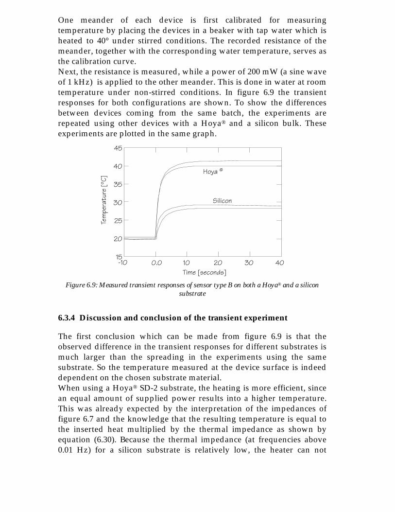
One meander of each device is first calibrated for measuringtemperature by placing the devices in a beaker with tap water which isheated to 40° under stirred conditions. The recorded resistance of themeander, together with the corresponding water temperature, serves asthe calibration curve.Next, the resistance is measured, while a power of 200 mW (a sine waveof 1 kHz) is applied to the other meander. This is done in water at roomtemperature under non-stirred conditions. In figure 6.9 the transientresponses for both configurations are shown. To show the differencesbetween devices coming from the same batch, the experiments arerepeated using other devices with a Hoya® and a silicon bulk. Theseexperiments are plotted in the same graph.

-10 0.0 10 20 30 4015

20

25

30

35

40

45

Time [seconds]

Tem

pera

ture

[ºC]

Silicon

Hoya ®

Figure 6.9: Measured transient responses of sensor type B on both a Hoya® and a siliconsubstrate

6.3.4 Discussion and conclusion of the transient experiment

The first conclusion which can be made from figure 6.9 is that theobserved difference in the transient responses for different substrates ismuch larger than the spreading in the experiments using the samesubstrate. So the temperature measured at the device surface is indeeddependent on the chosen substrate material.When using a Hoya® SD-2 substrate, the heating is more efficient, sincean equal amount of supplied power results into a higher temperature.This was already expected by the interpretation of the impedances offigure 6.7 and the knowledge that the resulting temperature is equal tothe inserted heat multiplied by the thermal impedance as shown byequation (6.30). Because the thermal impedance (at frequencies above0.01 Hz) for a silicon substrate is relatively low, the heater can not

increase the temperature as much as with a substrate having a highthermal impedance.Theoretically, the observed thermal impedance should becomeindependent on the substrate material for very low frequencies (< 0.01Hz), equivalent to hundreds of seconds after switching on the heater.This effect, however, was not observed. The reason is probably due toconvection of water. Since an inhomogeneous temperature distributionresults into an inhomogeneous density of water, the water will begin tomove. The result is that the derived differential equation which includesdiffusion only, is not valid anymore.

6.4 Mass flow measurement

Besides convection due to the inhomogeneous temperature distribution,there can be an additional flow or movement of the medium whichcomes from another, external, source. The result on the measurementdescribed in the previous section will be that the produced heat isdistributed over a larger volume resulting into a lower observedtemperature increase. This effect can be used for measuring flowbecause the measured temperature change at a constant heating powerwill be a measure for the mass flow of the liquid.Since the integrated sensor-actuator device as described in chapter 4 isin principle not used in a channel, one can not speak of a flow in onedirection. An observed decrease in temperature will only indicatemotion (turbulence) of the fluid rather than a certain flow rate.Without completely describing the theoretical background of thismeasurement, the experiment will simply be done.

6.4.1 Experimental

A fluid flow along the sensor-actuator devices is generated by placingthe devices on the inner wall of a beaker in which water is stirred. Sincethe distance of the devices from the centre of the beaker is about 2.5 cm,a stirring speed of 100 min-1 equals a flow rate at the device surface of0.26 m/s.The theory describing the operational mechanism of this experiment isnot worked out. Therefore, it is not obvious whether the direction of theflow is of influence. To investigate the influence of the flow direction,the devices are placed in the beaker using two different orientations.With the first device, the water flows from left to the right in figure 6.1.The second device is rotated 90°, resulting into a flow in the directionfrom the top to the bottom in figure 6.1.The measurements are carried out using devices of type A in a beakerwith a 6 cm diameter. The used medium is tap water. A magnetic stirrer

is used with a 4 cm magnet in the beaker. The heater element of thesensor-actuator device is supplied with a 5 V top to top, 1 kHz signal,equal to about 184 mW for this 68 W heater. Under non-stirredconditions, this resulted into a temperature increase of 14 °C. The valueof the measuring resistor is read out 15 seconds after every change inthe rotational speed since figure 6.9 showed that this time is needed forsetting up an equilibrium in an unstirred environment. The results arein figure 6.10.

Rotational speed [min ]-1

Norm

alis

ed re

sist

ance

[%]

0 200 400 600 800

100

99

98

97

96

0º Rotation90º Rotation

Figure 6.10: Measurement of the speed of rotation (mass flow) with a heating-sensing set-up

6.4.2 Discussion and conclusion of the flow measurement

There is no significant flow direction dependency. Obviously the systemdoes not measure the time of flight of a heat cloud from one to anotherfinger, because then no flow effect would be measured in the directionalong the fingers (0° rotation). What is probably being measured is thetransportation of a generated heat cloud, larger than all the separatefingers, covering whole the device. Only that mechanism confirms theobserved independence on the flow direction.

The relation between rotational speed and sensor output is not linear.At rotational speeds above 500 min-1 (equivalent to about 1.3 m/s), thechanges in the output signal become very small. Probably the heat cloudhas moved away then and the environmental temperature of water ismeasured. In chapter 4, the sensitivity of the temperature sensors wasdetermined to be 0.23 %/°C. This means that the decrease in figure 6.10of about 3.2 % corresponds to about 14 °C, which confirms that theenvironmental water temperature is measured since the non stirredtemperature is 14 °C above the environmental temperature. The rangeof speeds that can be measured can probably be increased up to acertain limit by increasing the heater current. Notice that the found

upper limit of the measurable speed is already in the range of themaximum speeds observed in washing machines. For example awashing tub with a diameter of 60 cm, rotating at a speed of 30 min-1,has a speed at the edges of 0.94 m/s. The water can never move fasterthan this speed.So, in the range of turbulent movement speeds in a washing tub, asignal can be measured which is an indication for this movement. Thiscan be interesting because the movement of the washing medium(water) is important for the washing effectiveness. First, the movementitself causes a mechanical washing which removes larger particles.Secondly, the transportation of detergent components to the laundryand the removal of dirt from the laundry is completely dependent onthe movement of the water. The mechanical washing was alreadymentioned as an important washing parameter in chapter 2.

6.5 Summary

This chapter started with a description of the diffusion of heat in amedium. Some theoretical plots were made showing the temperaturedistribution in a liquid when using a square planar heater, assumingthat the substrate does not absorb heat. For modelling the absorption ofheat into the substrate, which is necessary for choosing the bestmaterial, this transient analysis in the time domain could not be usedeasily at first instance.The differential equation describing the thermal behaviour in a mediumappeared to be equal to the differential equation describing thediffusion of ions in water and the equation for the potential distributionalong an electrical transmission line. This equivalence could later on beused for modelling the thermal behaviour of a multi-layer structureconsisting of a planar heater on a substrate in water. While an analysisin the time domain did only give some examples of temperatureprofiles, in the thermal impedance domain the available substratematerials could be compared with respect to their thermal properties.The conclusion was that a substrate consisting of quartz (with Hoya®

SD-2 as a cheaper alternative) results into a more efficient heating of thecontacting water than a substrate consisting of silicon with an oxidelayer as an electrical insulation. This was proven experimentally.Besides giving a clarification concerning whether the produced heatflows into the substrate or into the water, the impedance method couldbe used for a transient analysis in the time domain. Based on impedanceconsiderations, the loss of heat into the substrate material wasdetermined. The resulting amount of heat is injected into the water andwas used to calculate the temperature profile.

Convection of water, which is the result of the inhomogeneoustemperature distribution, is not implemented in the model. This type ofconvection was assumed to be negligible. However, an externallyimposed movement of water could be measured. When the fluid to beheated is moving, the heating becomes less efficient since virtually amuch larger volume absorbs the heat. This effect can be exploited bymeasuring one of the resistors while applying a constant amount ofenergy to the other resistor. The decrease in the observed resistance is ameasure for the movement of the medium. This value can be either flowor turbulence, depending on the configuration. In a washing machine itcan be an indication for the mechanical washing effectiveness.

6.6 References

[1] S.M. Sze, Semiconductor devices, Physics and technology, John Wiley & Sons,New York, 1985

[2] D.A. Skoog, D.M. West and F.J. Holler, Analytical Chemistry, Saunders CollegePublishing, Philadelphia, 1992

[3] H.S. Carslaw and J.C. Jaeger, Operational methods in applied mathematics,Dover publications, Inc. New York, 1947

[4] P.W. Atkins, Physical Chemistry, fifth edition, Oxford university press, 1994[5] D.K. Cheng, Field and wave electromagnetics, second edition, Addison-Wesley

Publishing Company, Reading, Massachusetts, 1989[6] D.R. Lide, Handbook of chemistry and physics, 74th edition 1993 - 1994, CRC

Press, Boca-Raton, Florida[7] A.J. Bard and L.J. Faulkner, Electrochemical methods, fundamentals and

applications, John Wiley & Sons, New York, 1980

CHAPTER 77. Stimulus-response measurements

Stimulus-response measurements

Until now, the reported measurements using the integrated sensor-actuatordevice as described in chapter 4 used only one single operational mode at thesame time. However, in chapter 1, the advantage of the functional integrationof sensors and actuators was mentioned. By combining actuator functions withsensor functions, on-line calibration can be done. In addition, the interpretationof the response on an imposed temporary disturbance of a solution under testmight give completely new information.First the effect of an actuator step is evaluated mathematically. After this, theactuator functions as available in the integrated sensor-actuator device aretaken as starting points for possible stimulus-response implementations.

7.1 Mathematical generalisation of differential measurement systems

A generalised set-up for differential measurements is given in figure 7.1.The picture shows a tube which has the possibility to shift a samplesolution in steps or continuously along sensors and actuators. In thesimplest case, two sensors and only one actuator are implemented,resulting in the set-up where a sample is measured before and after theactuator step.

Sensor A

Sensor B

ActuatorFlow

Figure 7.1: Generalised set-up for spatial differential measurements using one actuator

Because of the assumed small diameter of the tube the modification bythe actuator will be accomplished over the whole cross-section of thistube. When the input solution does not change (with respect to themeasured variable) during a measurement, the sample measured atsensor B differs from that at sensor A only due to the modificationinduced by the actuator. If the modification is complete at the time thesample is at sensor B, there is no effect of time observed in the differencein sensor outputs. Therefore, one can speak of a spatial differentialmeasurement, sampled at a single moment.

Apart from spatial differential systems, there exist time differentialsystems. When the flow direction of the liquid can be reversed, only onesensor is needed because then the sample can be measured before andafter the actuation step using the same sensor. This requires also acomposition of the input sample which is not changing due to otherfactors than the stimulus. When this single sensor is integrated with theactuator, as is the case with the integrated sensor-actuator devicedescribed in chapter 4, even the tube can be omitted since no controlledflow is needed. In such single sensor set-ups, one should speak of a timedifferential system sampled at the same location instead of a spatialdifferential system. Notice that this does not change the mathematicaloperation describing the system since in both cases a difference betweenthe sample before and after a modification stimulus is measured.

For the generalisation of spatial or time differential systems, figure 7.2will be used. Variable x1 is the input of interest and is modified by theactuator to x2 which has the same dimension as x1. The functiondescribing the stimulus operation of the actuator is referred to as fa(x),so x2 = fa(x1). This stimulus operation will be dependent on both theactuator and the properties of the solution. If a controllable actuator isused, the controlled parameter is represented by the subscript a.

x x = f (x )

Actuator

g(x ) g(x ) = g(f (x ))

Sensor A Sensor B

Channel

Sensor array

121

21 1

aa

a

Figure 7.2: Mathematical representation of a differential measurement system

Assume that both the original sample variable x1 and the modifiedvariable x2, are being sensed using two similar sensors. This means thatthe sensor outputs are both given by the same operation g(x) on thesensed variable. These sensors do not influence the sample.So two operations are involved: the sensor operation function g(x) andthe stimulus function fa(x). These operations will be discussed hereseparately.

7.1.1 Evaluation of the sensor operation g(x)

The sensor operation g(x) can be any function in principle, neverthelessthe number of functions observed with practical sensors is limited.Some special cases of g(x) functions will be evaluated here.Although it was assumed that both sensors have the same measurementprinciple, they might have a different sensitivity or offset. This results in

the same g(x) function, but with different parameters. The difference inthe sensor operation function for sensor A and B is indicated by asuperscript A or B.For a spatial differential system, the sensors A and B are differentdevices and might therefore have dissimilar parameters, for exampledue to a not perfectly reproducible fabrication process or an unequaltemperature while measuring. With a time differential system, sensor Ais the same device as B, but read out at another moment. So variations infabrication processes are cancelled out, only drift in the sensorparameters will change the function g(x).

(a) g(x) is knownWhen the sensor operation g(x) is completely known, the inversefunction g-1 can be determined and variable x can exactly be calculatedfrom the sensor output. In this case, the use of an actuator and a secondsensor is not needed for measuring x1. However, with practical sensors,the g(x) function is only known directly after calibration since drift inboth the sensitivity and the offset will change this function.

(b) g(x) is a linear function with an offsetThe operation of many sensors can be approximated by

g x a x bg g( ) = ⋅ + (7.1)

for at least a certain range of x. In many sensors the drift and interdevice deviation in the sensitivity ag is much lower than the uncertaintyin the offset bg both due to drift and differences in processing. Forexample, when x is the pH which is measured using a pH sensor, thesensitivity is equal to about ag = -59 mV/pH. This sensitivity is muchmore constant than the offset, which is among other things alsodetermined by the stability of the reference electrode.The offset bg of the sensor is determined by two parts. The first one isthe part that is common for both sensor A and B. For example, the effectof an interfering parameter, like temperature, results in such a commonoffset. The second one is a constant term which is different for sensor Aand B. Using a differential measurement it can be found that the outputis equal to

( )g x g x a x x b bB Ag g

Bg

A( ) ( )2 1 2 1− = ⋅ − + − (7.2)

assuming identical sensitivities ag for both sensors. The observed offsetsof the individual sensors, bgA and bgB, consist of the summation ofoffsets which are common for both sensors and offsets which differfrom sensor to sensor. By a differential measurement, common parts inthe offsets bg are filtered out and only the non-common offsets remain.

In practice, common offsets are the result of undesired externalinfluences, while non-common offsets are constant for the individualdevices.Equation (7.2) shows that actually only the difference between the inputx1 and output x2 can be measured, but when the actuator function fa(x)is chosen well (for example fa(x) = af×x), an absolute value for x1 can befound as will be shown later.

(c) g(x) is a logarithmic functionIn case of a pH measurement using a potentiometric technique, theoutput of the sensor (glass electrode or ISFET) is linearly dependent onthe pH. This is a linear sensing principle which has its origin in theNernst equation [1] which expresses the linear relation between aninterface potential and the pH. Actually, with all potentiometric ionselective electrodes (ISEs), the output is dependent on the logarithm of aconcentration. When a concentration is the variable of interest, and notthe logarithm of a concentration, the sensor output must be written as

( )g x a x bg g( ) log= ⋅ + (7.3)

and the differential output becomes

g x g x axx

b bB Ag g

Bg

A( ) ( ) log2 12

1

− = ⋅

+ − (7.4)

assuming the same sensitivity ag for both sensor A and B. So whenusing logarithmic sensors, the differential output shows the sameadvantage with respect to the sensor offsets. However, with respect tothe variable to be measured, x1, the difference between two logarithmicsensor outputs gives only information on the ratio between the inputand output variable x2/x1. So, to measure the absolute value of the inputvariable x1, it is not likely that a differential system based on logarithmicsensors will give the desired result1. Stimulus functions which can makethe output useful must raise the input variable to a certain power. Forexample fa(x) = x2 will reduce (7.4) to

( )g x g x a x b bB Ag g

Bg

A( ) ( ) log2 1 1− = ⋅ + − . (7.5)

However, such stimulus functions are not easy to realise using practicalactuators.

1 One can easily confuse this set-up with the successful acid to base titration set-up where theend point is determined by ISFETs and the titrant is generated coulometrically [2]. Althoughthis method measures a concentration using logarithmic sensors, it is not of the generalisedconfiguration as described here.This method uses the pH difference only as an indicator fordetecting the end point of the titration. The concentration of interest is calculated from thecharge supplied to the actuator when the end point is reached.

7.1.2 Evaluation of the stimulus function faa(x)

A linear stimulus operation will be assumed here because this describesmost of the practical observed actuator operations. Consider thestimulus function

( ) ( )f x a x bf fα α α( ) = ⋅ + (7.6)

where the parameters af(a) and bf(a) are constant at a certain chosenactuator intensity a. The constant af(a) represents an intendedamplification or attenuation of the species x placed in front of theactuator, and will therefore be without a dimension. The constant bf(a)is the result of an intended addition, or subtraction of the species x,which is not proportional to the amount placed in front of the actuator.This second constant will have the same dimension as x. The mostcommon actuator operations can be identified and categorised by theseconstants.Because the actuator intensity a is assumed to be constant in thefollowing examples, the parameters af(a) and bf(a) will be written fromnow on as af and bf.

(a) Complete depletion of x: bf = 0, af = 0When both af and bf are zero then (7.6) simplifies to fa(x) = 0, or in otherwords: the species x1 is completely depleted by the actuator to x2 = 0. Anexample is the effect of an ion exchanger which captures all ions ofinterest, when sensors are used which measure these ions selectively.Another example is an electrochemical actuator which evokes thedegeneration of hydrogen peroxide into hydrogen gas and oxygen gas,and using sensors which are selective for hydrogen peroxide.In the case of linear sensors with an equal sensitivity ag equation (7.2)now gives the absolute value of input variable x1 because x2 equals zero.In this case sensor B is solely used as an indifferent reference sensor tofilter out offsets which are common to both sensors. Notice that even ifthe sensors do not have the same sensitivity, the same result is obtained.

(b) Partial depletion or accumulation of x: bf = 0, af ¹ 0In the case of a fractional depletion or accumulation of species x, thesituation resembles the previous one. This situation represents anincomplete ion exchange where always a fraction af is not beingexchanged. Equation (7.2) becomes equal to

( )g x g x a a x b bB Ag f g

Bg

A( ) ( )2 1 11− = − ⋅ + − (7.7)

with af the fraction of depletion (<1) or accumulation (>1) and ag thesensitivity of the sensors, assumed to be equal. Even when the sensors

do not have an equal sensitivity, the differential output is still linearlyproportional to the input variable x1 according to

( )g x g x a a a x b bB Ag

Bf g

Ag

Bg

A( ) ( )2 1 1− = ⋅ − ⋅ + − . (7.8)

When the fraction af is always the same, and there is no drift in thedifferences between the sensitivities, there is no theoretical differencewith the previous situation where af = 0. Again, the advantage is in theelimination of offsets which are common for both sensors.

(c) Known addition: bf ¹ 0, af = 1A special situation occurs when the variable x1 is increased by aconstant value. This can be done by injecting a known amount of H+

ions in a sample which is not buffered, while the H+ concentration is themeasured variable. The differential output (7.2) becomes

g x g x a b b bB Ag f g

Bg

A( ) ( )2 1− = ⋅ + − (7.9)

which is not dependent on the input variable x1. This method which canbe referred to as “known addition” can be used to determine thesensitivity ag of the sensors involved. The condition that the sensitivitiesof sensor A and B are equal is now necessary, else the difference willstill be dependent on the input concentration x1.

(d) No actuator operation: bf = 0, af = 1When the actuator does nothing, the input variable x1 is exposed to bothsensor A and B. Examples are an inactive electrochemical actuator, aninactive heater and a saturated ion exchanger. For non-equal sensoroffsets bg, but with equal sensitivities ag, equation (7.2) can be written as

( ) ( )g x g x a x b a x b b bB Ag g

Bg g

Ag

Bg

A( ) ( )2 1 2 1− = ⋅ + − ⋅ + = − . (7.10)

This means that the differential offset due to unequal sensors can befound (and eliminated afterwards) by inactivating the actuator.

7.1.3 Summary

A generalised stimulus-response set-up is that of a flow system withtwo sensors and a single actuator. The sample solution is pumped alongsensor A, the actuator and then sensor B. The assumption is made thatthe variable of interest in the supplied electrolyte is homogeneouslypresent at both sensor A and B in the absence of a stimulus. Only then,the difference between the outputs of sensor A and B, after the stimulusis applied, can be completely ascribed to the influence of the actuator.

An alternative to this spatial differential system is a time differentialsystem, where using a single sensor, an electrolyte is measured beforeand after an actuator step. Here, stability of the composition of thesample is necessary. While a difference in space can be measured at thesame moment, a difference in time can be measured at the same spot inthe solution.Using a differential measurement system in combination with anactuator, data can be obtained concerning the sample as well as on thesensors itself. To get information on the sensors, the actuator must becontrollable in order to select operational modes for collectingcalibration data. Important is that both sensors have a similar, but notnecessarily identical, operation.

7.2 Some examples based on available actuators

After the theoretical evaluation in the previous section, now threeactuators are being categorised in these theoretical terms. The first twoare the available actuator operations in the integrated sensor-actuatordevice as described in chapter 4. These are the electrochemical actuator(for O2, H2, H+ or OH-) and the thermoresistive heater. In addition, anion exchanger is taken as a third actuator. Although ion exchangermaterials are not controllable actuators, an interesting intendedmodification of an electrolyte is made by such materials. The operationof ion exchangers can be monitored using the implemented electrolyteconductivity operation of the integrated device.For the sensors, the three available sensor operations in the integratedsensor-actuator device are taken. The detection of pH is evaluated aswell in each subsection, although this can not simply be realised usingmetal films. Nevertheless, this is done because the measurement of pHshows a logarithmic sensor function which is interesting to comparewith the linear operation of a conductivity sensor.The following list of possible stimulus-response measurements does notcontain all the possible options, but is more or less a brainstorm ofadvantages which can be expected when integrating sensors and anactuator.

7.2.1 Electrochemical actuator

Consider an inert metal working electrode at which the oxidation ofwater to protons and oxygen gas is controlled by an applied anodiccurrent:

2 4 42 2H O O H e→ + ++ − (7.11)

or water is reduced to hydroxyl ions and hydrogen gas by a cathodiccurrent:

2 2 22 2H O e H OH+ → +− − . (7.12)

The reaction products H+ and OH- can be used for pH control. In thecase of equation (7.11), the amount of generated protons follows fromintegrating the anodic current in time. However, in general, thisactuator is not of the "known addition" type (c) of subsection 7.1.2because the protons released will cause chemical equilibria in thesolution to change. So, the measured proton concentration increase atsensor B in figure 7.1 is not only dependent on the released amount ingeneral, for example because of the influence of pH buffers and weakacids.

Weak acid concentration determinationThe response on an imposed injection of protons of size DH+ in asolution of a weak acid is being considered. As an example, the aceticacid equilibrium is used for the complete description of the system.This equilibrium is given by

HAc H Ac↔ ++ − ka = 1.7·10-5 (7.13)

so, before and after the addition of a DH+ the acid-base equilibriumsatisfies

[ ][ ][ ]

H AcHAc

k a

+ −

= . (7.14)

Two equations can be written which describe the balance of the totalamount of Ac- and H+ respectively:

[ ] [ ] [ ] [ ]Ac HAc Ac HAc Cbefore before after after Ac− −+ = + = (7.15)

[ ] [ ] [ ] [ ]H HAc H HAc H Cbefore before after after H+ + ++ = + − =∆ . (7.16)

From equations (7.14), (7.15) and (7.16) the proton concentration beforeand after the release of H+ can be found:

[ ]Hk

k k Cbeforea

a a Ac+ = − + +

212

42 (7.17)

( )[ ]Hk H

k H k Caftera

a a Ac+

++= −

++ + +

∆∆

212

42

. (7.18)

Both a conductivity sensor or a potentiometric pH sensor can be usedfor determining a shift in the equilibrium. Two pH sensors will measure

∆pH H Hafter before= − ++ +log[ ] log[ ] (7.19)

which can be expressed in terms of the constants CAc, ka and DH+ using(7.17) and (7.18). However, this results in a complicated expression. Inthis chapter no numerical evaluation will be given on whether this leadsto interesting information on CAc or ka. Instead, a graphical method isused.

-3 -2 -1 0

0

1

2

3

log(HAc)

DpH

DH = 0.1 mol/l

DH = 0.01 mol/l

DH = 0.001 mol/lDiff

eren

tial

out

put

+

+

+

Figure 7.3: Dependency of the differential pH on a "proton step" as a function of the weakacid concentration using the acid constant of acetic acid

Figure 7.3 shows a plot of equation (7.19) for an acetic acidconcentration range of three decades and using three different H+ steps.It appears that the dependency on the logarithm of the weak acidconcentration is linear unless the DH+ is much smaller than the weakacid concentration. The lowest curve shows a deviation from a linearbehaviour because of a too low DH+. The dependency on the chosen H+

addition shows that the output signal is only useful in a certain range.

In the parts of the curves in figure 7.3 where the curves are linear, theadded amount of H+ ions is apparently an excess, resulting into a pHwhich is only dependent on this added excess. Therefore, the pHdifference is determined by the pH of the original acetic acidconcentration and the pH caused by the excess of H+ ions. So, theprinciple of operation is that the pH after the addition of a sufficientamount of H+ ions (which results into an acetic acid independent“reference” pH) is compared to the pH of the original acetic acid. Thismethod comes the closest to the type complete depletion (a) with bf notequal to zero.

In fact this method is a part of a coulometric titration which is onlysampled at two points, and where the measured information is in thepH change (and not in the supplied amount of titrant). This successfulapplication of a differential measurement system based on logarithmicsensors seems an exception to the conclusion which was drawn from

equation (7.4). However, since the logarithm of the acetic acidconcentration is measured, the used sensors are actually linear sensors.

Using a differential conductivity determination the output will be:

∆κ = −κ κafter before (7.20)

with

κ λ λ= ++ −+ −[ ] [ ]H Ac

H Ac(7.21)

where li is the limiting molar conductivity for ion i. The difference inthe conductivity Dk before and after the injection of the DH+ can becalculated by evaluating equation (7.21) in both situations. To expressthe observed Dk in terms of the acetic acid concentration CAc, the acidconstant ka and the injected amount of protons DH+, equations (7.14),(7.17) and (7.18) must be substituted into (7.21) for the situation beforeand after the H+ injection. Just like the pH measurement thisconductivity measurement gives a complicated expression.

0.0 0.2 0.4 0.6 0.8 1.0-1.0

1.5

Chan

ge in

con

duct

ivity

(mS

/cm

)

[HAc] (M)

-0.5

0.0

0.5

1.0

DH = 10 mM+

DH = 20 mM+

DH = 30 mM+

Figure 7.4: Theoretical dependency of the differential conductivity on a "proton step" as afunction of the acetic acid concentration

Figure 7.4 shows the simulated relation between the conductivitychange and the weak acid concentration. At a zero acetic acidconcentration, the injected protons are not captured by acetate ions Ac-,and the measured change in conductivity is caused by the conductivityof the DH+ only. Since the curves are not linear, the acetic acidconcentration corresponding to a measured Dk is harder to determinefor a higher acetic acid concentration. Therefore, it is more practical tofind the necessary amount of DH+ resulting into a Dk equal to zero.Empirically, using theoretically obtained data, it was determined thatthen the corresponding acetic acid concentration can be approximated

by CHAc = 0.84×103 litre/mole × (DH+)2 over quite a large range of aceticacid concentrations.

Differential temperature measurementNow the measurement of pH and conductivity is used as an example ofdifferentially monitoring the effect of an electrochemical actuator, alsothe other two sensors are described in combination with this actuator.The measurement of temperature is only of interest when an endo- orexothermic reaction is evoked by injecting oxygen gas, hydrogen gas,protons or hydroxyl ions. At first sight, such reactions are not likely in awashing system.

Differential amperometric H2O2 detectionIn the presence of hydrogen peroxide, the oxidation of water at theactuator will not occur before all hydrogen peroxide is oxidised:

2 2 22 2 2H O O H e→ + ++ − . (7.22)

This gives the possibility of the electrochemical capturing of all availablehydrogen peroxide at the actuator. The difference measured by twoH2O2 sensors is equal to the absolute amount of H2O2. Under thiscondition the actuator function is of the type (a) "complete depletion"which has the advantage that common offsets in the sensors are filteredout.

7.2.2 Thermoresistive heating

The thermoresistive heater is a metal strip with a certain resistance. Theheat being produced when a current flows through it will be used to putthermal energy in the system.Equilibria, observed in acid-base systems like equation (7.13) andprecipitation systems, are dependent on temperature because theequilibrium constants ka and ks are temperature dependent in general.However, a concentration determination based on an imposeddisturbance of such an equilibrium will be difficult. An interference isthe dependency of the ion mobility on temperature which willcomplicate the interpretation of a conductivity measurement. Althoughthis is not observed with a differential pH measurement, the logarithmicnature of pH sensing completely suppresses the very small changes inthe H+ concentration.

Differential conductivity measurementThe limiting molar ionic conductivity li is indirectly temperaturedependent, according to [3]

λπ ηi

iz Fea T

=2

61( )

(7.23)

withzi : the charge number of ion i,F : Faraday's constant,e : the charge of an electron,a : the radius of the ion andh(T) : the viscosity of the medium,

where the last one depends exponentially on temperature. This resultsinto an increase of li with temperature of 2 to 3% per degree for typicalions around room temperature. The corresponding stimulus functiondescribing the effect of heating on a conductivity measurement, is of thetype (b) “accumulation of x” with af(a) > 1, and bf(a) = 0 in equation(7.6). The parameter a represents the imposed temperature change.In general, a fitted polynomial temperature dependency for the limitingmolar ionic conductivity is more practical than the use of equation(7.23). In the next chapter, it will be shown that using such polynomials,the separate ion concentrations can be calculated of an assumed set ofpresent ions. Therefore, this stimulus-response measurement will not beevaluated here.

Differential pH measurementsIn terms of section 7.1, the effect of heating will change the sensitivity ag

of the sensors, since in general a pH measurement has a sensitivityproportional to temperature. The process of interest, the influence of thestimulus function fa(x), can not be studied separately because pHsensors are temperature dependent.

Differential amperometric H2O2 detectionHydrogen peroxide is in equilibrium with the HO2- ion under thedissociation of a proton:

H O H HO2 2 2↔ ++ − . (7.24)

When measuring, using two amperometric sensors, this equilibrium isnot relevant because whether H2O2 or HO2- is measured, in both casesthe number of electrons released per measured molecule is equalaccording to equations (5.4a) through (5.7a). What is observed as aresponse on a heating stimulus when doing chrono amperometry, isprobably the effect of a small change in the diffusion coefficient.

Differential temperature measurementBy measuring temperature differentially while heating, the system is ofthe type “known addition” (c) which does not give any information onthe input, but only on the system. An example is the use of the timedelay between stimulation and sensing for determining the speed offlow. This is described in section 7.2.4, where a flow measurement isdescribed based on the transport time of a heat marker from theactuator to a temperature sensor.

7.2.3 Ion exchangers or enzymes

The actuator function f(x) for an ion exchanger is of the type "partialdepletion or accumulation" (b) because a constant percentage of speciesx1 is being captured [4]. It makes a difference whether sensors are usedwhich can measure selectively the captured/released species or theused sensors are not selective (like electrolyte conductivity sensors).For example, the commercially available ion exchanger Dowex® CCR-2is originally saturated with H+ ions, but will release two of them whenone Ca2+ ion is captured. The operations on the proton and calciumconcentrations are

[ ] [ ]Ca a Caout f in2 2+ += (7.25)

( )[ ] [ ] [ ]H a Ca Hout f in in+ + += ⋅ − ⋅ +2 1 2 (7.26)

where 0 < af < 1. A complete exchange is characterised by af = 0 and nooperation by af = 1. The last one can be the result of a saturated ionexchanger.

From the field of applications and the available sensors this couple ofions (2H+ « Ca2+) is very interesting. The ion to be captured should becalcium while this might give information on the water hardness inwashing processes. For miniaturised sensors and actuators the exchangeof these calcium ions to protons is desired because protons are relativelyeasy measurable ions and it leaves the possibility of reversing theexchange action by electrochemically generating H+.

The operation of an enzymatic actuator can be compared to theoperation of an ion exchanger because a certain percentage of species isbeing catalysed while a product is released. This results into a partialdepletion operation. All examples in this paragraph use the ionexchange principle.

Differential pH measurementMeasurement of the pH before and after an ion exchange results in

( )

∆pH H H

H

a Ca H

out in

in

f in in

= − +

=⋅ − ⋅ +

+ +

+

+ +

log[ ] log[ ]

log[ ]

[ ] [ ]2 1 2

(7.27)

So, for a significant measured pH change, the proton concentrationmust not be very large in relation to the calcium concentration.Secondly, for determining the calcium concentration, the absoluteproton concentration must be known.

Differential conductivity measurementThe difference in conductivity induced by the ion exchanger is equal to

( ) ( )( )( )

∆κ ∆ ∆= ⋅ + ⋅ ⋅

= ⋅ − ⋅ + ⋅ −

= − −

+ +

+ +

+

+ +

+ +

+ +

[ ] [ ]

[ ] [ ]

[ ]

H Ca

a Ca a Ca

a Ca

H Ca

f in H f in Ca

f H Ca in

λ λ

λ λ

λ λ

2

2 1 2 1

2 1

2

2 2

2

2

2

2

(7.28)

which means that the output is linearly dependent on the calciumconcentration.

Differential temperature measurementThe ion exchange process most probably does not influence thetemperature of the sample. Therefore it can not be expected thatdifferentially measured temperature changes will occur.

Differential amperometric H2O2 detectionFor an ideal ion exchange the presence of H2O2 will have no effect.However, the pH change due to the exchange of calcium with protonsmight disturb the amperometric H2O2 measurement at sensor B withrespect to sensor A.

7.2.4 Additional results

Some additional techniques can be performed, using the same set-up asshown in figure 7.1, or the time differential equivalent, but which do notsatisfy the generalised measurement technique. An example is thecoulometric sensor-actuator device for performing acid-base titrations[2]. Although this set-up consists of two sensors and one actuator, thedetermination is done by recording a titration curve instead of using asingle differential measurement. In this subsection, two methods arepresented where the output is also not determined by simply taking thedifference between two sensor outputs.

Coulometric precipitation titration of calciumBesides the already mentioned acid-base equilibria like described inequation (7.13), also precipitation reactions can be evoked using a H+ orOH- stimulus. In that case, the stimulus function fa(x) is not one of thelinear examples of subsection 7.1.2, since in this case fa(x) describes thenon-linear disturbance of a solubility equilibrium. Therefore, theinterpretation of a single differential measurement will not be easy. Analternative to get useful information from this stimulus-responsemeasurement, is to control the actuator until the differentialmeasurement indicates an end point. This will be explained with theprecipitation of calcium hydroxide as an example.

The bad solubility of calcium ions in an alkaline medium is given by

( )Ca OH Ca OH22 2↔ ++ − ks = 1.3·10-6 mol3l-3 (7.29)

with ks the solubility constant of calcium hydroxide. Precipitation ofcalcium hydroxide can be monitored using a conductivity sensor sincean imposed addition of for example sodium hydroxide does not resultin the expected conductivity increase when some of the added hydroxylions have precipitated with calcium ions.The measurement of calcium ions is very interesting for qualifying thebuilder action when monitoring washing processes. As has beenexplained in chapter 2, the builder effect consists of both exchange andprecipitation of calcium ions. While ion precipitation during washingcan be monitored by measuring the electrical conductivity of the water,the exchange of ions will not result into a significant electrolyteconductivity change. Therefore, a calcium detection method is desiredfor monitoring building by means of ion exchange.

The typical shape of a volumetric conductimetric precipitation titrationcan easily be constructed [5]. Consider a solution containing calciumions and where all other charged particles are not likely to precipitate.By adding volumes of a sodium hydroxide solution, sodium willintroduce a conductivity increase proportional to the added volume andthe other ion concentrations will be constant. So, only Ca2+ and OH- willaccount for a non-linear change in the observed conductivity since theyhave a certain interaction. Normally, with precipitation titrations, thefirst addition of titrant is already enough to reach the saturation pointand will therefore result into a minimal precipitant.When adding a small amount of sodium hydroxide, all added hydroxylions will precipitate and the remaining effect is the replacement ofcalcium ions by two sodium ions. The conductivity will slightlydecrease since the molar conductivity of sodium ions is higher than that

of calcium ions. After all calcium ions are captured completely, theconductivity will increase because of the added free hydroxyl andsodium ions. So, the end point of the titration, which is a measure forthe calcium concentration, can easily be determined from the turn overpoint where the calcium ions are just exhausted. A theoretical plot of avolumetric precipitation titration with a conductivity measurement asan end point detection is drawn in figure 7.5.

100 mM Ca(NO )

50 mM Ca(NO )

3

23

2

Applied amount of NaOH [mol/litre]

Cond

ucti

vity

[mS

/cm

]

0 100 200 300 4000

20

40

60

80

100

Figure 7.5: Volumetric conductimetric precipitation titration of calcium nitrate with sodiumhydroxide

From this figure it can be seen that a fixed addition of sodiumhydroxide will not result into an unambiguous change in conductivity,since one does not know whether the end point in the titration curve ispassed. A method using a controlled titrant addition (a titration), whilemonitoring the conductivity as an end point detection, does give moreinformation on the success of the determination. Therefore, it ispreferred to measure a precipitation reaction not using the generalisedmeasurement technique of section 7.1.

While a volumetric titration requires a burette for adding the titrant, analternative is to add the titrant by coulometric generation. Hydroxylions for the titration can be generated by the reduction of wateraccording to equation (7.12). A coulometric precipitation titration ofcalcium with conductivity sensing as the end point detection, seems anideal method since it can be implemented very simply using solid statecomponents. The precipitation can easily be reversed by subsequentlylowering the local pH using an anodic current. The shape of the curvewill be different from figure 7.5 since only OH- is added without apositive counter ion. Charge neutrality is accomplished by migration ofpositive ions to the working electrode. However, in practice, theprecipitation appears to be less controllable than might be expected

from equation (7.29). When the solution is supersaturated, the solubilityconstant ks can be exceeded and the theoretical behaviour in theconductivity is not observed. Therefore, in analytical chemistry, anucleation core is used to prevent supersaturation. How this techniquecan be applied to a coulometric actuator is not yet clear.

Flow measurementFor the application of the generalised set-up, the assumption was madethat there is a flow along the sensors of an input electrolyte which is notchanging in composition, and an immediate and complete modificationof the electrolyte is generated at the actuator. Only in that case, themeasurement is continuous and the distance between sensors andactuator is not of interest. However, when the actuator is switched onand off, the time delay between the actuator and one of the sensors canbe observed. This delay is directly proportional to the flow speed of thesample.In the alternative set-up consisting of an integrated sensor actuatorstructure, a flow measurement can also be performed. The actuatedspecies will be removed proportionally to the flow speed. This isalready used in section 6.4 where a continuous supply of heat is injectedinto an electrolyte while the temperature is monitored. A lowering ofthe observed temperature indicates movement of the medium.Considering the actuators of section 7.2, two markers for determiningflow speed are available. Either a heat pulse or an electrochemicallygenerated H+ or OH- cloud can be used, since also the sensors fordetecting these pulses are available. When using a generated H+ cloudas a marker, appropriate sensors are the conductivity cell and a pHsensor. The other option is to use a heat pulse and measure this with atemperature sensor.

The difference between time of flight using ions and time of flight usinga heat pulse is in the diffusion effect. The diffusion constant of heat inwater was given in table 6.2 and is equal to 1.455·10-7 m2·sec-1, thediffusion constant of protons in water is equal to 9.311·10-9 m2·sec-1 [6].So, when using ions as a marker, the spreading of this marker is muchsmaller than when using a heat pulse. In addition, while heat can leakout of the channel by thermal conduction through the walls, particleslike H+ can not. Therefore, the use of a H+ marker is preferred,especially for determining very low flow rates.With time differential systems, using an integrated sensor-actuatorstructure, the same advantage of an ionic marker will be observed. Incorrespondence with the flow measurement described in section 6.4, themovement of a generated H+ cloud due to flow of the medium can be

measured as a decrease in the observed conductivity. In this case thesame advantage to the thermal equivalent is observed since noabsorption by the substrate material of the generated stimulus ispossible.

7.2.5 Summary

Using three actuators and four sensors, twelve combinations forbuilding a differential measurement system are possible. Table 7.1 givesa summary on the possible combinations for implementing the set-up offigure 7.1.

Table 7.1: Summary of sensor-actuator combinations

Actuator

Sensor Pt-100

Temperature

Finger structure

Conductivity

Amperometry

H2O2

Potentiometry

pHElectrochemicallygenerated H+,OH-, O2 or H2

0 Weak acid conc.Mass flowCa2+ concentration

H2O2 Weak acid conc.Mass flow

Thermoresistiveheating

Mass flow Ion concentrations(with assumed setof ions)

Diffusionconstant

Dissociation oracid constant

Ion exchanger 0 Ca2+ 0 Ca2+

(if pH is known)

The use of a time differential or spatial differential system does notmake any difference for the mathematical background of the stimulus-response measurements, with the exception of the flow measurements.However, the spatial differential system measures at one single momentat two different sensors, while a time differential system measures attwo different moments at the same spot in the electrolyte.

For the application of temperature sensors in a differential set-up, onlymass flow can be detected. The reason is that no heating due to theelectrochemical actuator and the ion exchanger is assumed.The differential conductivity measurement appears to be the mostuniversal technique for measuring. This advantage comes from the non-selectivity, resulting in a difference in conductivity after all threeactuator steps. Unless a logarithmic value, like pH of pCa, is desired, thelinear nature of sensing of a conductivity cell shows the advantages oflinear sensing described in section 7.1.A hydrogen peroxide measurement using an amperometric technique,shows little new information. Although a cancellation of offsets can beobserved when using an electrochemical actuator, either thermoresistive

heating or an imposed ion exchange does not show any promising newresults.Using potentiometric pH sensors, the results do not compete with thecoulometric acid-base titrator as was published before [2]. Probably, dueto its selectivity and logarithmic dependency on concentrations, thepractical application of pH measurements in differential set-ups willgive results which do need smart additional manipulation in order toretrieve useful electrolyte information.

For mass flow measurements, the choice of a spatial or a timedifferential set-up does make a difference. With the sensors and actuatorplaced in a row, the time of flight of a marker is measured. This resultsin the restriction that only linear flow can be measured and no turbulentflow. When, however, an integrated sensor-actuator structure is used,there is no time delay due to the geometry, and the flow information isobtained from the dilution of a marker. An example of the secondtechnique was shown in the previous chapter with heat as the marker.

7.3 Conclusions

The mathematical impact of subtracting sensor signals was demon-strated in the first section of this chapter. Promising results could beexpected from linear actuators, before and after a stimulus measured bylinear sensors. In that case, sensor offsets will cancel out and absoluteinformation on a certain input variable will be present in the differentialsignal.This rather theoretical evaluation was illustrated by brainstorming onthe combinations possible with three actuators and four simple sensors,resulting into twelve set-ups for implementing differential measurementsystems. Some of them resulted into useful ideas.

Weak acid concentration determination was mentioned more than once.Although the used weak acid model solution acetic acid is of course notpresent in a washing machine, hydrogen peroxide shows also an acid-base behaviour with the anion HO2-.Determination after the addition of H+, created by an electrochemicalactuator, can be done by both a differential pH or conductivitymeasurement. Although these methods resemble acid-base titrations,the information is in the measured sensor difference and not in theadded amount of titrant (indicated by the end-point). The differentialpH method gives information on the logarithm of the weak acidconcentration, while a differential conductivity sensing gives the weakacid concentration immediately. For efficient use of the second one, theinjected current through the actuator before the end-point (defined as

the moment where the difference in conductivity equals zero) can beused. However, the conventional coulometric titration with pH as theend point detection is still much more established and requires a similarset-up.Weak acid concentration determination by measuring either pH orconductivity while applying a temperature step in order to change theacid equilibrium was suggested. But the practical use of this method isnot easy since a temperature step will change much more parameterslike the ion mobility and sensor slopes. Moreover, the use of alogarithmic sensor for measuring a concentration is not optimal since anon-linear operation is applied to the signal of interest.

Measuring calcium could not be done using single sensors up to now.Three options where found using stimulus-response measurements.Although it is not a one-spot differential measurement, the most elegantmethod would be a precipitation titration with conductivity sensing asan end point detection. The measurement of calcium by a precipitationtechnique is preferred because the possibility to precipitate is the reasonthat this hardness ion must be measured. Practical use of this titrationmethod might fail, however, since precipitation is slow andfurthermore hard to control.Another method is to compare the conductivity at two temperatures.For this method, the pH must be increased first in order to assure thatcalcium is partially precipitated, since only then a change in thesolubility constant due to the temperature difference can be measured.But now, the same problems will be encountered as with the othercalcium precipitation method while in addition the problems with allthe other parameters varying with temperature will show up.What is probably possible for calcium sensing, is the application of anion exchanger in combination with conductivity sensors. It was shownthat an ion exchanger which exchanges one calcium ion by two H+ ions,gives a conductivity change which is proportional to the absolutecalcium concentration which is supplied to this system. Notice that thisis an example of a method using linear sensors in combination with alinear actuator. The selectivity of the ion exchanger is used to sensecalcium using non-selective conductivity sensors. The advantage of ionexchangers is that they can be reversed. An example is the use of anexchanger for the couple Ca2+ « 2H+, which can simply be reversedusing electrochemically generated H+ ions. A completely saturated ionexchanger gives calibration data on the sensors because the samesample solution is supplied to both sensors.Since the ion exchanger material needs a certain path-length in order toexchange ions, the sample solution must be pumped through a column.

The result is that this method can not directly be realised in combinationwith the integrated sensor-actuator device of chapter 4, since it requiresa spatial differential system. This pumping and the use of a column willlimit the advantages of the “all in one” sensor-actuator device. Inaddition, the use of a tube introduces a source of possible system breakdowns since obstructions might occur easily in dirty washing water.

What is interesting is the comparison of flow detection methods basedon indicators. When using a cloud of ions as a marker (preferably H+

since this can be generated electrochemically), this marker can notdiffuse out of the tube. A heat pulse instead, can be conducted by thetube material or the substrate of the sensor-actuator, and will be lost fortime of flight detection purposes. In addition, because the diffusion ofheat is faster than the diffusion of ions, very low flow rates can bedetermined with a low spreading of the marker. With an integratedsensor-actuator device, the same advantages of an ionic marker will beobserved, since there is also no sink via the bulk material.

One method was not worked out, but only mentioned superficially. Thisis the ion concentration measurement by interpreting the change inconductivity after changing the temperature. In the next chapter thismethod will be described completely, and verified with someexperiments.

7.4 References

[1] A.J. Bard and L.R. Faulkner, Electrochemical methods, fundamentals andapplications, John Wiley & Sons, Inc., New York, 1980

[2] B.H. van der Schoot and P. Bergveld, An ISFET-based microlitre titrator:integration of a chemical sensor-actuator system, Sensors and Actuators, 8(1985), page 11 - 22

[3] P.W. Atkins, Physical Chemistry, fifth edition, Oxford university press, 1994[4] C.D. Amphlett, Topics in inorganic and general chemistry: Inorganic ion

exchangers, Elsevier Publishing Company, Amsterdam, 1964[5] D.A. Skoog, D.M. West and F.J. Holler, Analytical Chemistry, Saunders College

Publishing, Philadelphia, 1992[6] D.R. Lide, Handbook of chemistry and physics, 74th edition 1993 - 1994, CRC

Press, Boca-Raton, Florida

CHAPTER 88. Ion concentration estimation using conductivity and temperature

Ion concentration estimation usingconductivity and temperature

The combination of a heater function and the measurement of electrolyteconductivity, as available on the integrated sensor structure, can be used todetermine specific ion information. In this chapter this combination is used,however, not using the integrated device, but using a commercial conductivitymeter and a heater/stirrer plate.A method is introduced with which a non-selective electrolyte conductivitymeasurement is used for determining specific information on separate ionconcentrations. This method starts with an assumed set of ions. Subsequently,the specific responses on temperature of the conductivities of these ions arerelated to the measured temperature dependency of the overall electrolyteconductivity.For the calculation of the ion concentrations from a conductivity versustemperature sweep, an estimation algorithm is introduced based on the linearminimum mean square of the error. Errors in the measured conductivity willpropagate through the algorithm into errors in the fitted ion concentrations.For the validation of the estimation method, this propagation of errors is alsoevaluated.Finally the method is applied to solutions having two and three different typesof ions, and is used to show the possibility of determining pH using aconductivity cell without a reference electrode.

8.1 The effect of temperature on conductivity

A single electrolyte conductivity measurement is not interesting unlessthe measured value is normalised for temperature. The reason for this isthat at a higher temperature, ions become more mobile and will causean increase in conductivity. So, with the same concentration, an increasein temperature results in an increase in conductivity. Therefore, inpractical conductivity measurements, the measured conductivity iscompensated to 25°C by using a simultaneous temperaturemeasurement.

The total conductivity of an electrolyte expressed in terms of thelimiting molar conductivities of the separate ions can be expressed by

Λ ==∑ z c Ti i ii

I

λ ( )1

(8.1)

with zi the charge of ion i, ci the concentration, I the number of different

types of ions and li(T) the limiting molar conductivity of ion i. This lastone is dependent on temperature and specific for every single ion. Sincea conductivity measurement can not differentiate between ions, it is notpossible to eliminate the temperature effect completely.

Industrial temperature compensation methods use the averagetemperature dependency of L which is about 2%/°C. This linear fit isthe most simple approximation of the temperature dependency and issuitable for most pure water applications for over a moderatetemperature range [1]. More sophisticated fits compensate by using athird order polynomial, but this method is electrolyte and concentrationdependent [2].

A more complicated temperature compensation uses a polynomial fitfor the limiting molar conductivities of the separate ions [3]. A thirdorder approximation was proposed by Harned and Owen [4] andtabulated for several ions. The equation is

( ) ( ) ( )[ ]λ λi i i i iT k T k T k T( ) , , ,= + − + − + −01 2

23

31 25 25 25 (8.2)

with li0 the limiting molar conductivity of ion i at 25°C. This polynomialapproach will be used for ion identification.

8.1.1 General description

The generalised polynomial fit of order J with respect to temperature T0

can be written as

( )λ λi i i j

j

j

J

T k T T( ) ,= −=∑0

00

. (8.3)

Together with equation (8.1) the total conductivity of an electrolytehaving I types of ions can now be calculated:

( ) ( )Λ T z c k T Ti i i i j

j

j

J

i

I

= −

==

∑∑ λ00

01, . (8.4)

Manipulation yields:

( ) ( )[ ]( ) ( )[ ]

Λ

Λ

T z c k T T

T z c k T T

i i i i j

j

j

J

i

I

i i i i j

j

i

I

j

J

= −

= −

==

==

∑∑

∑∑

λ

λ

00

01

00

00

,

,

and

( ) ( ) ( )Λ T T T z c kj

i i i i ji

I

j

J

= −

==∑∑ 0

0

00

λ , . (8.5)

For conductivity measurements at N different temperatures, I types ofions and a polynomial fit of order J, a matrix equation can be formedusing equation (8.5):

( ) ( ) ( )( ) ( )

( ) ( ) ( )

ΛΛ

Λ

1

2

1 0 1 02

1 0

2 0 2 02

0 02

0

1 0 2 0 0

1 1 2 1

1 2

1

1

1

.

.

.

. .. . . . .. . . . .

.

.

. .. . . .. . . .

.

, , ,

, ,

, , ,N

J

N N NJ

I

J J I J

T T T T T T

T T T T

T T T T T T

k k kk k

k k k

=

− − −− −

− − −

⋅

⋅

z cz c

z cI I I

1 1 10

2 2 20

0

λλ

λ.

(8.6)

or

Λ = ⋅ ⋅T K c .

The meaning of the terms is:Λ Vector containing measured conductivities at N different

temperatures;T Matrix with the temperature information;K Matrix with the polynomial coefficients ki,j;c Vector with the ion concentrations multiplied by the

parameters |z|·l0;

The question rises whether it is possible to calculate the vector c(containing the concentration information) from a known T matrix anda measured Λ vector. It would be interesting to know if the K matrixcan be calculated as well. This would mean that the present ions can beidentified by their found ki,j coefficients. The next section, however,shows that this is not possible, unfortunately.

8.1.2 Identification of ions by solving the coefficient matrix K

If equation (8.6) can be solved completely (both K and c separately), thepresent ions can be identified by comparing the columns of matrix K toknown coefficients. Afterwards, the corresponding concentrations canbe found from the vector c .

The solution for the K c⋅ product is given by

K c T⋅ = ⋅−1 Λ (8.7)

with

K c

k k kk k

k k k

z c

z c

z c

I

J J I JI I I

⋅ =

⋅

1 0 2 0 0

1 1 2 1

1 2

1 1 10

2 2 20

0

, , ,

, ,

, , ,

.

. .. . . .. . . .

.

.

λλ

λ

. (8.8)

From this equation it will be clear that the coefficients ki,j can never becalculated without knowing the terms |zi|ci li0. In other words: forevery set of coefficients ki,j another set of concentrations will be found.So, the coefficients must be known for solving the concentrations.Notice that the number of measurements, N, is not visible in equation(8.8) so increasing the number of measurements will not solve theproblem of the unsolvable coefficients either.

8.1.3 Calculation of ion concentrations using tabulated coefficients

When the K matrix is assumed to be known, which implies a chosen setof ions, equation (8.6) can be written as

( ) ( ) ( )

( ) ( )

( ) ( )

ΛΛ

Λ

1

2

1 1 0

0

2 1 0

0

1 0

0

1 2 0

0

2 2 0

0

1 00

00

.

.

.

. .

. . . .

. .

, , ,

, ,

, ,N

j

j

j

J

j

j

j

J

I j

j

j

J

j

j

j

J

j

j

j

J

j N

j

j

J

I j N

j

j

J

k T T k T T k T T

k T T k T T

k T T k T T

=

− − −

− −

− −

= = =

= =

= =

∑ ∑ ∑∑ ∑

∑ ∑

⋅

z cz c

z cI I I

1 1 10

2 2 20

0

λλ

λ.

(8.9)

where the T K⋅ matrix is written as a single one. The elements in thismatrix are polynomials for the n-th temperature (rows) and the i-th ion(columns). If the T K⋅ matrix has an inverse, the concentrations willfollow from

( )c T K= ⋅ ⋅−1

Λ . (8.10)

The first condition for having an inverse is that the matrix is square, sothe minimal number of necessary experiments is equal to the number ofions to fit (N = I). For N > I an estimator must be used. The secondcondition is that the determinant is not equal to zero. This is true whenthe coefficients are different for every ion and the order of thepolynomial is equal or larger than I - 1.

So, it is possible to find the concentrations of individual ions in asolution under the following conditions:• The measured conductivity scan must be a linear combination of the

temperature responses for the individual ions. This means that

→ Every ion which is significantly present in the electrolyteconductivity must be represented in the calculations;

→ No two ions may have the same temperature dependency (whichwill probably never be the case);

→ When I types of ions have to be calculated, the conductivity of theelectrolyte must be measured at at least N = I temperatures;

→ The order of the used polynomials is equal to or larger than thenumber of different ions to fit minus one (J = I - 1);

• The coefficients ki,j of the individual ions must be known. Thecoefficients for the third order fit are given by Harned and Owen [4]for nine types of ions;

8.1.4 Error propagation

Errors due to systematic errors in conductivity measurements, forexample due to an inaccurately assumed sensor slope, representing thesensitivity, can be proportional to the measurand itself. Proportionalerrors can be written as an undesired multiplication of L by x. For suchproportional errors, equation (8.10) must be expanded to

( )c T Kξ = ⋅ ⋅−1

Λξ (8.11)

where Λ is multiplied per element by the proportional error vector ξ .When x is equal for every single measurement, this results in

( )c T K cξ ξ ξ= ⋅ ⋅ ⋅ = ⋅−1

Λ . (8.12)

From this equation it can be concluded that an x per cent error in themeasured conductivity will result in an x per cent error in the calculatedion concentrations.

Other types of errors might introduce a constant offset in theconductivity measurement. The most likely origin of such an error is theunexpected presence of an ion which is not included in the fittingalgorithm. In that case, the observed conductivity versus temperaturecurve can never be a linear combination of the contributions of theassumed set of ions. Therefore, this kind of error will be much moresevere than a proportional error. Such a systematic error whichmanifests as an unknown offset in the measurement can be written as aconstant addition e of L. In this case equation (8.10) becomes

( ) ( )c T Kε ε= ⋅ ⋅ +−1

Λ (8.13)

and manipulation yields

( ) ( ) ( )c T K T K c T Kε ε ε= ⋅ + ⋅ = + ⋅− − −1 1 1

Λ (8.14)

which shows that the faulty fitted vector c ε is equal to the actual vectorc increased by a constant vector. So, the error vector ε will result inunknown additions to all the elements of c , which are different forevery element.

Random noise in the measurement shows up as unknown offsets aswell, like described in equation (8.14). However, the error vector c cε −has another property now: its elements represent random numbers withan average of zero. In other words, when the number of experiments ischosen larger, the average of the elements in c cε − will go to zero. Inthe next subsection, an estimation algorithm is introduced with whichthe number of experiments can be increased in order to reduce the errordue to random noise in the conductivity measurement.

8.2 A linear minimum mean square estimation

The calculation of ion concentrations using the basic algorithm (8.10)requires conductivity measurements at as much as temperatures as thenumber of ions to be fitted. It is more accurate to do moremeasurements (N > I) and use an estimation method. In order to findthe best fit from the measurements, some theory concerning parameterestimation is necessary. This is done in the first upcoming subsection. Inthe next subsection, the estimation algorithm is reduced to a moreconvenient form. The implementation of the condition that the sum ofcharge in a solution will be equal to zero is implemented in the thirdsubsection.

8.2.1 Parameter estimation theory

The method introduced here is a matrix based algorithm for minimisingthe mean square error of the estimation [5]. Consider the generalisedsystem

Λ = ⋅ +B c v (8.15)

withΛ the vector containing the observations,B a matrix representing the system (in our case equal to T K⋅ ),c the input vector to be estimated andv the noise or error in the measurement.

The aim is to find an estimate $c for the vector c satisfying the observedvector Λ . Introducing the operator E for the moment of the operand,

which is equal to the average, the average of x can be written as E(x). Ifthe average of the estimate is the true value

( )E c c$ = (8.16)

then the estimate is called unbiased. In the ideal case, the estimate isequal to the true value. In practice, however, an error will be presentrepresented by the error vector, defined as

( )e c c c E c= − = −$ $ $ . (8.17)

The aim of the estimation algorithm is to minimise this error vector. Ingeneral, a function of e is chosen for optimisation, which can be theaverage mean square error of the components of e . Consider themoment matrix

( ) ( )( ) ( )( )[ ]C E ee E c E c c E ceT

T≡ = − −$ $ $ $ (8.18)

known as the covariance matrix of the estimate. Notice that thetranspose operator T means that the vector is changed from a columninto a row. The diagonal elements of the covariance matrix are thevariances of the estimate’s components. The best estimate can now bedefined as the one having the smallest variances: the minimum varianceunbiased estimator.

If c and Λ are random variables with moment matrices

( )( )

( )

C E cc

C E c

C E

cT

cT

T

≡

≡

≡Λ

Λ

Λ

ΛΛ

(8.19)

and CΛ

is non-singular, implying that there is an inverse CΛ

−1 , then the

minimum variance unbiased estimate $c of c using the given data Λ isaccording to the Gauss-Markoff theorem [5] equal to

$c C Cc

= ⋅−Λ Λ

Λ1 . (8.20a)

The associated error matrix of the estimate is

C C C C Ce c c cT= − −

Λ Λ Λ1 . (8.20b)

Now the theorem will be written in terms of the covariance matrices Cc

and Ccv because these are the closest to physical interpretation. The firstone is the auto covariance of the concentration vector and the secondone represents the correlation between concentration and noise.Substituting (8.15) in (8.19) yields

C C B Cc c

TcvΛ

= + (8.21)

and for CΛ

C BC B C B BC CcT

cvT T

cv vΛ= + + + . (8.22)

The Gauss-Markoff theorem (8.20) can now be written as

( )( )$c C B C BC B C B BC CcT

cv cT

cvT T

cv v= + + + + ⋅−1

Λ (8.23a)

and

C C C B C BC B C B BC C C B Ce c cT

cv cT

cvT T

cv v cT

cv

T

= − +

+ + +

+

−1

. (8.23b)

8.2.2 Simplified estimation algorithm

Except for the covariance matrices Cc and Ccv , equation (8.23a) can

completely be determined for estimating the concentration vector $cfrom a measured set of conductivities Λ . In order to eliminate thesematrices some assumptions can be made [5]:→ c and v are uncorrelated (the moment matrix ( )C E cvcv

T≡ is equalto zero);

→ the elements of v are uncorrelated and have equal standarddeviations sv. This also implies that Cv is finite;

→ the true state of c is unknown so its moment matrix satisfies( )C E ccc

T≡ → ∞ (all variances are very large).The linear minimum variance unbiased estimate $c of c given data Λunder these conditions is according to Gauss-Markoff theorem equal to

( )$c B B BT T= ⋅−1

Λ (8.24a)

which reduces to (8.10) for a square matrix B . Because the variances sv2

of the vector v are assumed to be equal, the moment matrix Cv can alsobe eliminated, and the error matrix can be expressed as

( )C B BeT

v= ⋅−1

2σ (8.24b)

which contains all covariances of the fitted vector $c in its entries. So, thenumbers on the diagonal of this error matrix are the variances of thefitted parameters. Using this knowledge, the standard deviation of thewhole fit can be defined as

( )σ σcT

vtrace B B= ⋅−1

(8.25)

where the trace function is the summing of the elements on the diagonalof a matrix.

Experimental verification of the assumptionsThe assumptions which justify the simplification to the estimationalgorithm (8.24a/b), all refer to the measurement set-up. Some simplemeasurements for getting insight in the introduced system errors canverify these assumptions. The used set-up is the same as will be usedlater for doing the actual concentration determinations.

During some hours, a commercial conductivity meter (Radiometer CDM210) is used for monitoring temperature and conductivity in stirredpotassium chloride solutions. The solution is heated and cooled downseveral times between room temperature (18 °C) and about 55 °C. In aspreadsheet program, the data is collected and compared to thetheoretical conductivities for these temperatures.

Table 8.1: Statistical information on KCl conductivity measurements at temperaturesbetween 18 °C and 55 °C

ConcentrationKCl

[mM]

Measuredconductivity (20 °C)

[mS/cm]

CDM210range

[mS/cm]

Meanerror

[mS/cm]

Standarddeviation of error

[mS/cm]90 12.6 40 0.0009 0.05

309 38.5 400 0.0053 0.49413 55.3 400 0.0183 0.50615 86.2 400 0.0059 0.53

Notice that the conductivity meter is switched to the 40 mS range for thefirst sample which corresponds to a fixed operational frequency of 23.4kHz, and to the 400 mS range for the other three samples (46.9 kHz).Obviously, the standard deviation is dependent on the chosenoperational frequency and not on the electrolyte concentration.However, because the operational frequency is chosen according to theelectrolyte concentration, the standard deviation is indirectly dependenton this concentration in practical applications.All the measured errors of the three samples measured with the 400 mSrange are collected into a single error distribution plot as shown infigure 8.1 which approaches the normal distribution shape.

Freq

uenc

y of

occ

urre

nce

[%]

0

5

10

15

Error in measured conductivity [mS/cm]-6 -4 -2 0 2 4 6

Figure 8.1: Error distribution in conductivity measurements

DiscussionComparing column 4 to column 2 in table 8.1 it appears that the mean ofthe error is much lower than the observed conductivities. In otherwords

( )E v = 0

which implies directly that the covariance with c is equal to zero aswell:

( )C E cvcvT≡ = 0 .

This proves the first assumption of c and v being uncorrelated.

The other two conditions, being Cc → ∞ and Cv is finite, are necessaryto ensure that the moment matrix for c is much larger than the momentmatrix for v : C Cc v>> . Since the standard deviations of v are finite andknown (fifth column of table 8.1), its moment matrix will be small. Morecorrectly, the moment matrix for v will go to zero in relation to thecorresponding moment matrix for c , which will go to infinite becauseits covariance goes to infinite [5].

The value for the standard deviation appears to be constant at a chosenoperational frequency. This means that about 95% of the conductivitymeasurements is between the real conductivity plus/minus two timesthis standard deviation for the chosen operational range.Besides being dependent on the operational frequency of theconductivity meter, the standard deviation might be dependent ontemperature. Therefore, the data of the three measurements in the 400mS range, is split into four sets: lower than 30 °C, between 30 °C and 40°C, between 40 °C and 50 °C and higher than 50 °C. The calculatedstandard deviations are in table 8.2.

Table 8.2: Standard deviations calculated in several temperature ranges

Temperature range [°C] Standard deviation [mS/cm]< 30 °C 0.31

30 °C . . 40 °C 0.3640 °C . . 50 °C 0.40

> 50 °C 0.42

Although there is a small temperature dependency, it might beconcluded that no big error is introduced when assuming a temperatureindependent standard deviation.

Increasing the accuracy of estimationNow the variance in the measurement error is practically determined,the propagation of this error through the estimation algorithm can beevaluated. This was done in subsection 8.1.4 for the situation where thenumber of applied temperatures is equal to the number of ions to befitted (N = I). However, by using more than N measurements, adecrease in the final error can be expected because of suppression ofmeasurement noise.In figure 8.2 the normalised calculated standard deviation in theestimated concentration is represented for three different temperatureranges and estimations for N = 2 to 11. For this numerical example, thecoefficients ki,j for a 100 mM sodium chloride solution are used.

0.5

0.0

Number of measured data points

T1 = 20°C, TN = 30°C

0 2 4 6 8 10 12

1.0

T1 = 20°C, TN = 40°C

T1 = 20°C, TN = 50°C

Norm

alis

ed s

tand

ard

devia

tion

of e

stim

atio

n

Figure 8.2: Effect of the temperature range and the number of measurements on theestimation accuracy

It can be seen that the accuracy of the estimation can be increased, eitherby increasing the number of measurements or the temperature range.The improvement in accuracy by increasing the temperature range islarger than the improvement obtained by using more measurements.

SummaryReconsidering the original equation (8.9), describing the set ofconductivity measurements at N temperatures, the ultimate method ofdetermination should be• Perform the measurements, by heating a solution while measuring

the conductivity. Take more measurements (conductivities at knowntemperatures) than the number of ions to be fitted (N > I) since thiswill increase the accuracy of the estimation. Notice that theapplication of a large temperature sweep will increase the accuracymuch more. Some conductivity meters have an automatictemperature compensation which must thus be switched off. Alsothe use of an auto range function will disturb the measurement sincethe variance in the measurement appeared to be constant peroperational range;

• Assume a set of ions and calculate the matrix B with the elements

( )B k T Tn i i j n

j

j

J

, ,= −=∑ 0

0

with T0 the reference temperature, Tn the temperature ofmeasurement n, J the order of the polynomial fit and ki,j thepolynomial fit coefficients for the temperature dependency of themobilities (which can be found in literature [4]);

• Create the conductivity vector Λ , which is a column of Nconductivity measurements at N different temperatures;

• Use equation (8.24a) for finding the estimation vector $c , which is acolumn of the |zi|ci·li0 products for the I ions. Because the charge ofthe ions zi and the limiting molar conductivity li0 are known, theconcentrations of the individual ions can be calculated.

The size of the error in the estimated concentrations is represented byequation (8.25) in terms of the covariance of the measurement error.This covariance is determined for the Radiometer CDM210 conductivitymeter to be about 0.5 mS/cm in the 400 mS operational range, and 0.05mS/cm in the 40 mS range.

8.2.3 Error propagation

The absolute errors in the fitted concentrations due to random noise canbe calculated using equation (8.24b). This equation gives the standarddeviations in the fitted vector $c which contains the values |z|c l0 forall the fitted ions. So, when the error of a certain value is defined by twotimes its standard deviation (95% probability region), the resultingabsolute error in the fitted ion concentration will be

( )ez

B Bc iv

i i

T

i i,

,=

−20

1σ

λ(8.26)

withec,i the absolute error in the fitted ion concentration for ion i

[10-3 mole/litre];zi the ionic charge for ion i [no dimension];li0 the limiting molar ionic conductivity [m2 S mole-1];B the matrix with the temperatures and coefficients ki,j;sv the standard deviation in the measured conductivity [S/m];

Evaluation of equation (8.26) is easier with some numerical examples.When the conductivity meter is used in the 40 mS/cm range, which isequivalent to a maximum of about 300 mM KCl, the standard deviationof the measurement is approximately equal to 0.05 mS/cm as given intable 8.1. For N = 25 measurements, equidistantly distributed over atemperature range from 20 °C to 55 °C and using a polynomialapproximation of J = 3 for the ion conductivities, the absolute errors inthe fitted concentrations are calculated. In table 8.3, the results aresummarised for combinations of two, three and four selected ions.

Table 8.3: Absolute errors in fitted concentrations due to random noise,for N = 25, T = 20 - 55 °C, J = 3, sv = 0.05 mS/cm

Fitted ion:Solution:

D[Na+](mM)

D[H+](mM)

D[K+](mM)

D[Cl-](mM)

K+ and Cl- 32 30H+ and Cl- 0.80 3.4H+, Na+, and Cl- 38 1.3 20H+, K+ and Cl- 12 253 215H+, K+, Na+ and Cl- 90 28 1.2 M 0.9 M

On the average, the fitting of a larger number of ions increases therandom noise propagation error. What can also be seen, is that the typeof ion does matter. When the combination Cl- and K+ is present, theerrors are bigger. In addition, the result for H+ is more accurate, notonly in the result for H+ itself, but also for the other ions in the system.This could be expected since H+ has a much more characteristic ionicconductivity and therefore ion discrimination is more easy.Since table 8.3 is only valid when the meter is switched in the 40 mS/cmrange, errors in the concentrations around the one molar limit willcertainly exceed the actual concentrations. So, the fitting of four ionswill probably be much too sensitive to errors.Remarkable is that the absolute error is not dependent on theconcentration, which is the result from the constant standard deviationof the conductivity measurement. It is important to choose the lowest

possible conductivity sensing range on the meter since then thestandard deviation is the lowest as can be seen from table 8.1.

For errors in the measured conductivity which have not a randomnature, the noise will not be filtered out by the estimation algorithm. Anexample which was already mentioned in subsection 8.1.4 is thepresence of a background electrolyte, consisting of one or more ionswhich are not in the assumed set of ions.When the error e is assumed to be constant at every temperature, therelative error in the fitted concentration of ion i becomes

( )( )

( )( )

c cc

T K

T K

T K

T K

i i

i

Row i

Row i

Row i

Row i

ε εε

−=

⋅

⋅

⋅

⋅

=⋅

⋅

⋅

⋅

−

−

−

−

∑1

1

1

1_

_

_

_Λ Λ

(8.27)

where equation (8.14) is used and for simplicity N = I is taken. Whenlater N > I is needed, the inverse of the T K⋅ matrix can simply besubstituted by the estimation matrix of equation (8.24a). The elements inthe measured conductivity vector Λ can be normalised to theconductivity at for example 20 °C. The relative error in the fittedconcentration becomes equal to

( )( )

c cc

T K

T K

i i

i

Row i

Row iC

C

ε ε−=

⋅

⋅

⋅

⋅

−

−

°°

∑1

1

2020

_

_Λ Λ

(8.28)

which means that the relative error in the fitted ion concentrations isproportional to the relative error due to an offset in the measuredconductivity. In table 8.4 the factors which amplify the relative error inthe measurement to relative errors in the fit are given for the samesolutions as used in table 8.3. However, while the concentrations did notmatter for the errors due to random noise, now concentrations must beassumed in order to find numerical values.

Table 8.4: Amplification factor for a relative error due to an offset in the measuredconductivity to the relative error in the fitted ion concentrations,for N = 25, T = 20 - 55 °C, J = 3 and L0 = 20 °C

Solution: Fitted ion: Na+ H+ K+ Cl-

10 mM KCl 38 3510 mM HCl 2.7 7.510 mM HCl + 10 mM NaCl 16 4.0 0.610 mM HCl + 10 mM KCl 8.7 206 8210 mM NaCl + 10 mM KCl + 10 mM HCl 21 5.0 3.9 1.5

An entry in this table means that when estimating for example K+ in a10 mM KCl solution, a one percent offset in the measured conductivitieswill result into an 38% error in the fitted concentration.Some remarks can be made. The error in the fitted H+ concentrationdoes not escalate excessively, but the error amplification seems toremain lower than ten. A factor ten means that for a 5% error in the fit, a0.5% error in the measured conductivity is allowed. Roughly speaking,the allowed ”background” normality may therefore not exceed 0.5% ofthe concentration of interest.The real problem with this type of error is that it is unpredictable. Forexample the amplification of errors can range from 0.6 to 206. Withoutknowing, a small error due to a contamination in the system will beenormously amplified. The maximum amplification which empiricallyfound here is 206. Although it is not guaranteed that no largeramplifications will be observed in other systems, a rough estimation ofthe possible detection limit of ions in demi water is possible. Using demiwater with a purity of 0.5 mS/cm, for a 5% error in the fitted ionconcentrations a conductivity of 2.0 mS/cm is the lower limit. This isequivalent to for example a 15 mM KCl solution. So, when trying to fitthe ion concentration in solutions with a lower concentration, theimpurity of the demi water might already disturb the estimation.

8.2.4 Implementing the zero charge condition

Because in practical solutions the total charge is equal to zero, thecondition

z c z ci iCations

i iAnions

∑ ∑= (8.29)

can be implemented in the algorithm in order to increase accuracy andto avoid useless answers like negative concentrations. This equation canbe implemented in the model (8.9) as

( ) ( ) ( )

( ) ( )

( ) ( )

ΛΛ

Λ

1

2

1 1 00

2 1 00

1 00

1 2 00

2 2 00

1 00

00

1

1 10

20

.

.

.

. .

. . . .

. .

, , ,

, ,

, ,N

jj

j

J

jj

j

J

I jj

j

J

jj

j

J

jj

j

J

j Nj

j

J

I j Nj

j

J

k T T k T T k T T

k T T k T T

k T T k T T

z

z

z

=

− − −

− −

− −

= = =

= =

= =

∑ ∑ ∑

∑ ∑

∑ ∑

λ z

z

z

z cz c

z c

I

I I

I I I

2 20 0

1 1 10

2 2 20

0

λ λ

λλ

λ

.

.

⋅

(8.30)

were the T K⋅ matrix has now become the augmented T K⋅ matrix. Theelements in the augmented vector Λ and the augmented matrix T K⋅ do

not have an equal unity anymore. This does not make any difference fornumerical evaluations, however.

This augmented model can be evaluated like the original model usingthe same estimation algorithm. However, the condition (8.29) will havethe same priority as every single measurement and so its importancewill be suppressed with an increasing number of applied temperaturesN. Two options are available for increasing its priority:• The first option is to give the last row of the augmented T K⋅ matrix

a weight factor equal to the number of measurements. The weightedleast square form of (8.24) is [5]

( )$c B W B B WT T= ⋅−−

−11

1 Λ (8.31)

with W the weight matrix. This weight matrix is of size (N+1) ×(N+1) with on the diagonal the only non-zero entries being theweight factors. Since the matrix B will be the augmented T K⋅matrix, the element on entry (N+1, N+1) will be the weight factor forthe zero charge condition;

• Another possibility is obtained by first reducing the measuredinformation and then implementing the zero charge condition.Concerning equation (8.8) it was concluded that the number ofmeasurements is not in the K c⋅ matrix. The measured information(conductivities at N temperatures) can be reduced to J+1 points byfirst calculating an estimation for the vector K c⋅ by applying thesimple algorithm (8.24a/b) to equation (8.7). The result, being equalto

( )K c T T TEstimate

T T⋅ = ⋅−1

Λ (8.32)

is a vector with length J+1, independent on the number ofmeasurements. This estimated vector is equal to the product of thecoefficient matrix K and the concentration vector c to be estimatedas given by equation (8.8). The zero charge condition can now againbe implemented by augmenting a matrix:

K c

k k kk k

k k k

z cz c

z c

Estimate

I

J J I Jz

z

z

z

z

zI I II

I I

⋅

=

⋅

0

1 0 2 0 0

1 1 2 1

1 2

1 1 10

2 2 20

01

1 10

2

2 20 0

, , ,

, ,

, , ,

.

. .. . . .

.

.

.

λ λ λ

λλ

λ

(8.33)

To solve the concentrations from this equation, a second estimationstep is necessary since the augmented K matrix is not square.

The error coefficient matrix (8.24b) has now become meaningless, andso the standard deviation of the fit (8.25), since these are only validwhen having equal variances v for all the measurements. The variancesare not equal anymore, since the zero charge condition will haveanother variance than the actual conductivity measurements.

8.3 Experimental

The presented theory is verified using a Radiometer CDM210commercial conductivity meter in a computer controlled set-up asshown in figure 8.3. This conductivity meter is capable of measuringconductivity, using a four points electrode (type Radiometer CDC565),and the solution temperature (using a Radiometer temperature probetype T201).

C:\>

Computer

Temperaturecontrollerand stirrer

Conductivityand temperature

meterRS232

Figure 8.3: Measurement set-up

For this measurement, the automatic temperature compensation of theCDM210 must be switched off, and the automatic measurement rangeadaptation as well. Each measurement starts at room temperature. Aftera heating and stirring step, an equilibrium time of 5 seconds is usedbefore measuring. This sequence is repeated until the temperatureexceeds 55ºC.

The protocol is controlled by LabView 3.1 software, providing the userwith an interactive interface. First the user is asked to prepare a solutionand place it on the heater. The program switches on the heater andmeasures the conductivity equidistantly over the given range. After themeasurement has finished, the menu shown in figure 8.4a asks to selectthe ions which are present in the solution. Figure 8.4b shows the resultwindow with the measured curve, the fitted curve and fitted ionconcentrations.

Figure 8.4a: Screen shot of the ion selection menu in the LabView 3.1 program

Figure 8.4b: Screen shot of the result window in the LabView 3.1 program

The implementation of the estimation algorithm, both for the normaland the zero charge case, is also done in LabView. The parameters forequation (8.2) are given by Harned and Owen [4] and are repeated intable 8.5.

Table 8.5: Coefficients for equation (8.2) [4], TRef = 25.0 °C

IonMolar conductivity l0

[10-4 m2 S mol-1] k1 k2 k3

H+ 349.85 1.376576×10-2 -2.947692×10-5 -2.192368×10-7

Li+ 38.64 2.302950×10-2 1.140657×10-4 -5.284679×10-7

Na+ 50.15 2.176670×10-2 9.401795×10-5 -2.293121×10-7

K+ 73.50 1.949143×10-2 5.518776×10-5 -4.330612×10-7

Rb+ 77.81 1.901465×10-2 4.935098×10-5 -5.825729×10-7

Cs+ 77.26 1.874062×10-2 4.950815×10-5 -2.653378×10-7

Cl- 76.35 2.017511×10-2 6.090373×10-5 -1.683039×10-7

Br- 78.17 1.974799×10-2 5.718306×10-5 -2.942305×10-7

I- 76.90 1.963498×10-2 5.689207×10-5 -2.821847×10-7

8.3.1 An electrolyte with two ion types

First, the theory is tested for electrolytes having only one type of anionand one type of cation, both with and without using the zero chargecondition as implemented in equation (8.33).The number of applied temperatures per electrolyte is N = 25 and thepolynomial fit is of order J = 3. Solutions are used of 20, 40, 60, 80 and100 mM KCl and NaCl. Figure 8.5 shows the fitted concentrations.

-50

0

50

100

150

200

250

300

0 50 100

[K+] (mM)

Fitt

ed [K

+] (m

M)

No zero charge

Zero charge

-150

-100

-50

0

50

100

0 50 100

[Cl-] (mM)

Fitt

ed [C

l-] (m

M)

No zero charge

Zero charge

(a) (b)

0

20

40

60

80

100

0 50 100[H+] (mM)

Fitt

ed [H

+] (m

M)

No zero charge

Zero charge

0

10

20

30

40

50

60

0 50 100[Cl-] (mM)

Fitt

ed [C

l-] (m

M)

No zero charge

Zero charge

(c) (d)

Figure 8.5: Fitted ion concentrations for (a, b) KCl and (c, d) HCl, both with and without theincorporation of the zero charge condition

It is not very surprising that the fitting of hydrogen chloride is muchmore accurate than that of potassium chloride because the mobilities,and also the temperature dependency of these mobilities, of potassiumand chloride ions are almost equal. This property, which is exploited inconventional reference electrodes, is not observed with hydrogenchloride. The result is that for fitting KCl the usage of the zero chargecondition is essential, while for HCl this is not strictly required. In figure8.6 the fitted values using the zero charge condition are collected.

A proportional relationship between the fitted ion concentration and theactual concentration is certainly observed. However, the ratio betweenthe imposed ion concentration and the calculated concentration is notequal to one. In figure 8.6 the fitted concentrations are only 80% of thereal concentrations, while this is even lower for chloride in HCl. Suchproportional errors where already mentioned in the subsections 8.1.4and 8.2.3 as the result of a badly calibrated conductivity meter.Other types of errors discussed in these subsections, are errors due torandom noise and errors due to offsets in the measurements.While theeffect of the error due to random noise in the observed conductivity isminimised by taking a large number of measurements, the size of theerror due to offsets in the measured conductivity is unknown up tonow. In subsection 8.3.3 the propagation of errors of this type will bediscussed.

0

25

50

75

100

0 25 50 75 100Concentration (mM)

Fitt

ed c

once

ntra

tion

(mM

)

[H+] from HCl[Cl-] from HCl[K+] from KCl[Cl-] from KCl

Figure 8.6: Summary of fits using the zero charge condition

Notice that the use of the zero charge condition together with theknowledge that only two ion types are present is already enough toknow the actual separate ion concentrations. Nevertheless, a conclusionconcerning the correctness of the introduced new method is allowedsince the fitting is primarily based on the change in mobilities. Anyway,the real advantage of this method will be demonstrated when theseparate concentrations of more than two different ions are fitted.

8.3.2 An electrolyte with three ion types

The advantage of the method presented here will be in solutions havingmore than two types of ions. As a test, a series of solutions is madehaving 25 mM sodium chloride and 10 to 70 mM hydrogen chloride orpotassium chloride. The fitted results using the zero charge conditionare presented in figure 8.7.

0

20

40

60

80

0 20 40 60 80[HCl] (mM)

Fitt

ed io

n co

ncen

trat

ion

(mM

) H+

Na+

Cl-

0

20

40

60

80

0 20 40 60 80[KCl] (mM)

Fitt

ed io

n co

ncen

trat

ion

(mM

) K+

Na+

Cl-

(a) (b)

Figure 8.7: Result of fitting ions in 25 mM NaCl with various (a) HCl or (b) KClconcentrations, using the zero charge condition

As could be expected, the fitted sodium concentration remains constantwhile the other ion concentrations do change.

8.3.3 Error propagation

With the knowledge of the absolute errors introduced in subsection8.2.3, error bars can be drawn in previously measured concentrationplots. For example, figure 8.8 is repeated from figure 8.7a, but now witherror bars and plotted in three separate graphs. Since there is noformula derived for the absolute errors when using the zero chargecondition, the error bars for the non-zero charge method are placed inthe graph with concentrations fitted using the zero charge condition.This will result into a worst case guess of the error. The dotted lines inthe graphs are the imposed ion concentrations.

The error bars are obviously a bit too pessimistic for Na+ and Cl- sincethe correlation between fitted concentration and the real concentrationis much larger than may be assumed according to these error bars.

0

20

40

60

80

0 20 40 60 80[HCl] (mM)

0

20

40

60

80

0 20 40 60 80[HCl] (mM)

0

20

40

60

80

0 20 40 60 80[HCl] (mM)

[H ]

(mM

)+

[Na

] (m

M)

+

[Cl

] (m

M)

-

(a) (b) (c)Figure 8.8: Fitted ion concentrations with error bars in solutions with 25 mM NaCl and

several HCl concentrations. (a) H+, (b) Na+ and (c) Cl-

When implementing the zero charge condition, the matching betweenanions and cations will be improved. Although no algorithm is givenhere for calculating the absolute errors in the fitted results when thiscondition is included, it may be assumed that the errors will decrease.Although this decrease is not known, it is probably meaningless to fitfour ions, since table 8.3 shows that then the worst case error will exceedthe one molar limit. Because the given values are only valid in the 40mS/cm range, the errors are far more than the present ionconcentrations.

8.3.4 A pH measurement

In some processes a pH measurement using an ISFET or a glasselectrode is not possible. These problems often come from the referenceelectrode, for example because• The sample is sensitive to chloride or potassium ions;• The electrode dries out because it is not constantly immersed with

water;• The liquid junction is contaminated with proteins, oil or sulphide;• Extremely high temperatures or low pH values are present.In these situations the fitting method can still be applied because theheater and conductivity cell can be made of a solid state conductor on achemically inert substrate.

Starting in 0.9 M HCl and diluting down to 2 mM, a series of pH’s iscreated. The fitted hydrogen concentrations are presented in figure 8.9.Coming close to pH 5.5 the determination becomes worse. Theexplanation is that the measured conductivity is of the order of mS/cmwhile the used demineralised water was of the quality 0.59 mS/cm. So,clearly, the contamination with other ions disturbs the fit in this case.

0

1

2

3

4

5

6

0 1 2 3 4 5 6

Measured pH

Fitt

ed p

H

Fit

Theory

Figure 8.9: A measurement in HCl plotted as a pH determination

Although the fitting of two types of ions is quite trivial (a singleconductivity measurement with the zero charge condition in mindwould give the same result), this experiment did verify the possibility ofapplying the method in solutions with a very low pH.

8.4 Conclusions

From a non-selective conductivity measurement, it is possible to findspecific ion concentrations by recording the conductivity at differenttemperatures. The key to this is that every ion has its own specificlimiting molar conductivity which depends uniquely on temperature.This method needs an assumed set of ions: the electrolyte conductivityis a linear combination of the specific ionic conductivities of these ions.

The first condition needed for making the system solvable is that inorder to fit I ions, at least N = I measurements at different temperaturesare needed. However, to increase the accuracy, more measurements arepreferred and subsequently an estimation algorithm is used to find thebest fit. The second condition is that the characteristic polynomial usedfor the temperature dependencies of the limiting molar ionicconductivities is at least of order J = I - 1. Next, the coefficients ki,j in thispolynomial must be unique for every single ion because the wholerecognition is based on the difference in these coefficients. This is truesince every single ion has a different size and mass and will thereforehave another temperature dependency in its ionic conductivity. Finally,every ion which is significantly present in the solution must be includedin the calculation, since the method is based on the conductivity being alinear combination of all the separate ionic conductivities.

In order to increase the accuracy of the calculated ion concentrations,either the temperature sweep or the number of points N can beincreased. Increasing the temperature sweep, however, has a muchmore positive effective result on the accuracy.For N = I, one unique solution for the ion concentrations is possible. ForN > I, an estimation algorithm must be chosen. A linear estimationalgorithm based on the minimum mean square error is introduced.Actually, there is a third method for increasing the accuracy. Theknowledge that the sum of all charges is zero in equilibrium can beincluded in the estimation algorithm as a boundary condition.Especially for “difficult” ion pairs (like chloride and potassium forexample) the use of this condition appeared to be essential.However, the use of an estimation algorithm can only decrease theerrors due to random noise. An error in the observed conductivities dueto the presence of an ion which is not in the assumed set, will propagateto an error in the fitted ion concentrations which can not be decreasedby taking more measurements.

For only two ions in the solution, the introduced method is notnecessary because then a single conductivity measurement alreadydetermines both ion concentrations. When there are four ions, themethod is probably too sensitive to errors because a small error in themeasured conductivity might result into an enormous error in the fittedion concentration. A worst case analysis shows that the absolute error inthe fitted concentration becomes sometimes more than one molar whenthe conductivity meter is switched in the 40 mS/cm range. So, inconclusion, the method will show the best results in systems havingthree different types of ions.

Although the experiments were carried out using bulk heating of thewhole volume of electrolyte, it can also be done using the integratedsensor-actuator structure of chapter 4. In that case, however, only thelocal environment is heated which might shorten the time needed formeasuring the conductivities at several temperatures. This experimentwill be described in chapter 9.

Summarising, it can be said that the advantage of this method is that itintroduces selectivity by smart data interpretation, and not by thesensor itself. In general, when a sensor is made selective, fragile andcomplex selective membranes are introduced. This results intotransducers with a whole sandwich of membranes on top of it.Electrolyte conductivity sensing, on the other hand, is easy, chemically

inert and mechanically stable since it uses a solid metal structure. It is areproducible technique since the cell constant which determines thesensitivity shows no drift in principle.

8.5 References

[1] D.M. Gray and A.C. Bevilacqua, Unique temperature compensation forconductivity and resistivity measurements, Ultrapure water, volume 13, 1996

[2] Toshiaki Isono, Density, viscosity, and electrolytic conductivity of concentratedaqueous electrolyte solutions at several temperatures. Alkaline-earth chlorides,LaCl3, Na2SO4, NaNO3, NaBr, KNO3, KBr and Cd(NO3)2. Journal of chemicaland engineering data, Vol. 29, No.1, 1984

[3] A.L. Horvath, Handbook of aqueous electrolyte solutions, physical properties,estimation and correlation methods, Ellis Horwood Limited, Chichester, 1985

[4] H.S. Harned and B.B. Owen, The physical chemistry of electrolytic solutions,Reinhold Publishing Corporation, New York, 1958

[5] P.B. Liebelt, An introduction to optimal estimation, Addison-WesleyPublishing Company, Reading, Massachusetts, 1967

CHAPTER 99. Supplementary results

Supplementary results

This chapter comprises some results which were found during the developmentof the sensor array, but which did not fit in the previous chapters. The firstsection describes a technique which gives a new parameter, being the hardnessof tap water, based on a statistical analysis. Next, an implementation of aconductivity cell is proposed which does not need the chosen silicon technologyapproach, but which can be fabricated using standard printed circuit boardfabrication technology. Finally, the measurement technique which is describedin chapter 8, is carried out using the integrated sensor-actuator device asintroduced in chapter 4.

9.1 Hardness and conductivity of tap water

In chapter 2, the ions that determine the conductivity of tap water weregiven, based on a statistical analysis of the tap water in 44 Dutch cities in1986 [1]. What could be seen from figure 2.3b is that the hardness ions,calcium and magnesium, determine the conductivity for 40%. Thequestion rises whether it will be possible to approximate the tap waterhardness by measuring the water conductivity. This could beinteresting, since a conductivity sensor is already present in theintegrated sensor-actuator device of chapter 4 and a hardness sensor isnot.

Figure 9.1a shows a plot with the measured water conductivities on thehorizontal axis, and the measured hardnesses on the vertical axis. Thedata is obtained from the same data source of the composition of Dutchtap water [1]. The hardness is expressed here as the total concentrationof multivalent ions. To convert this to the more common calciumcarbonate equivalent, the factor 100.1 g/mole must be used.Using a least square algorithm, a line could be plotted in this figure. Theobserved correlation between hardness and conductivity appears to be0.85. So, based on the measured conductivity, the hardness can beguessed using this line. The average error in the guessed hardness is13% while the observed maximum error is 50%. Although this seemsquite large, the estimated hardness can be used to reduce the excessamount of dosing, which is nowadays common. Without a conductivitymeasurement, the dosing should be adjusted to the largest possiblewater hardness which is about 3.0 mM. By a single conductivitymeasurement the dosing can be reduced. For example, when a

conductivity of 20 mS/m is observed, the hardness will not be largerthan 1.2 mM using the correlation line with 50% overdosingcompensating for the maximum error.

0.0

0.5

1.0

1.5

2.0

2.5

3.0

0 10 20 30 40 50 60

Hard

ness

[mM

]

Electrolyte conductivity [mS/m](a)

0.0

0.5

1.0

1.5

2.0

2.5

3.0

0 10 20 30 40 50 60

Har

dnes

s [m

M]

Electrolyte conductivity [mS/m](b)

Figure 9.1: Correlation between water hardness and conductivity in 44 Dutch cities in 1986.(a) Measured hardness and conductivity,

(b) the same, but after elimination of sodium from the conductivity

Any knowledge on other ions will increase the accuracy of the guessedhardness. For example, sodium sensors are easier to obtain than calciumsensors. By placing a sodium sensor in the same water as in which theconductivity is measured, the conductivity due to sodium can besubtracted from the total observed electrolyte conductivity. The result isa corrected conductivity which will have a larger correlation to thewater hardness.In figure 9.1b, the corrected conductivity is plotted on the horizontalaxis for the same set of data which is used in figure 9.1a. The newcorrelation has become 0.94, which is obviously much larger. Also theaverage error in the approximated hardness has reduced to 7.8% andthe maximum error is 38.4% now.This example uses sodium, but knowledge concerning other ions willalso increase the correlation. What can be seen from figure 2.3b, is thatHCO3- has an even larger contribution to the conductivity of tap waterthan sodium. Therefore, knowing the concentration of this ion willincrease the accuracy much stronger.

After applying the builder it is not possible any more to determine thehardness by measuring the conductivity while using a pre-definedslope. An exchange of one mole of calcium to two moles of sodiumgives hardly a change in the conductivity of the liquid (in one litre anincrease of 2×50.1 mS·cm-1 for sodium and a decrease of 119 mS·cm-1 forcalcium) but the hardness decreases with one mole. Therefore, it is not

likely that the hardness can be guessed during washing based on themeasured conductivity.

9.2 A conductivity cell on a PCB

The analysis of thermal properties, as carried out in chapter 6, gave theadditional conclusion that printed circuit boards can be used assubstrates for realising a planar heater. The very low thermal diffusioncoefficient of printed circuit board materials might give a very efficientheating of water. However, in the context of this thesis, the realisation ofthe integrated sensor-actuator structure is preferably done using thinfilm technology. The reproducibility of fabricating small structures isextremely good using this technology. For thermoresistivemeasurements and heating, resistances can be defined with practicalvalues, since the sheet resistance is in a convenient range.As an alternative, printed circuit board technology can also be used todefine planar metal structures, and is even more easy to apply.However, a PCB is provided with a copper layer which would beoxidised when used in wet applications. Therefore, it must be coveredwith a noble metal layer which can easily be applied by electro plating.Since the sheet resistance of the copper layer is relatively low, makingrelatively high resistance values would require very narrow and longwires. This may become difficult because the wire width is limited bythe photolithographic method used for defining the structures.Therefore, at first instance, no resistive structures have been made, butonly a conductivity cell is produced.

9.2.1 Design and fabrication of the devices

The cell design as drawn in figure 9.2 is realised on a printed circuitboard. The number of finger units is N = 5, the fingers have a width W =0.2 mm and a spacing S = 0.16 mm. The total cell size is 2 × 2 mm2,which is defined by casting with a Hysol® two component resin.

2 mm

2 mm

0.2 mm

0.16 mm

Figure 9.2: Layout of the conductivity cell on a PCB

Before the application of this resin, the tip of the sensor is electro platedwith gold. These dimensions result into a theoretical cell constant of2.308 cm-1 as can be calculated using equation 4.2.

9.2.2 Experimental

In figure 9.3a, the measured impedance sweeps recorded in potassiumnitrate solutions of 0.5 to 100 mM are plotted. The curves are recordedusing a HP4194A gain-phase analyser under unstirred conditions.

2

3

4

5

2 3 4 5 6 7 8

log

Impe

danc

e (

ç çW

)

log[frequency] (Hz)(a)

0.5 mM1 mM

5 mM10 mM

50 mM100 mM

0123456789

0 50 100

[KNO ] (mM)

Cond

ucta

nce

(mS

)

3(b)

Figure 9.3: (a) Impedance versus frequency in various KNO3 solutions and the(b) conductance at the plateau as a function of the KNO3 concentration

Figure 9.3b is constructed by taking the reciproke of the impedance atthe frequency independent regions in figure 9.3a. As described inchapter 4, this reciproke, which is equal to the conductance, isproportional to the electrolyte conductivity via the cell constant.

9.2.3 Discussion

The first remarkable point is the difference between the impedancesweeps, shown in figure 9.3a, and the sweeps recorded using theintegrated sensor-actuator devices, as shown in figure 4.9. The observedwidths of the frequency independent areas are much larger for the PCBsensors than when using the integrated sensors. This is probably theresult of the larger size of the devices, shifting the low corner frequencyto the left, according to equation 4.9. A frequency independentimpedance is observed for almost two decades, which means that morethan two decades of conductances (and also electrolyte conductivities)can be measured using a single operational frequency.The measured conductances are perfectly proportional to the imposedpotassium nitrate concentrations as can be seen in figure 9.3b. Since theconductivity of 100 mM KNO3 is equal to 1.45 S/m [2], the measured

conductance of 8.66 mS results into a cell constant of 1.67 cm-1. This islower than the theoretical cell constant, probably because the modeldoes not account for boundary effects.So, the PCB conductivity cell can be used for determining conductivity.Although the cell constant could not be predicted very accurately, theperformance is satisfying.

9.3 Integrated conductivity sensor - temperature actuator

Chapter 8 showed the interesting result, that it is in principle possible touse the integrated multi-purpose sensor-actuator structure of chapter 4for determining specific ion concentrations. However, in that chapterthe required technique of heating an electrolyte while monitoring theelectrolyte conductivity was not applied using the integrated structure.The heating of a whole beaker filled with an electrolyte whilemonitoring the conductivity using a commercial conductivity meter wasused instead.An advantage of the integrated sensor-actuator device is that it can heatthe environment locally, while the electrolyte conductivity can bemonitored in the same local environment. This heating will be fast sincethis local volume is small. In addition, the temperature can bemonitored simultaneously.Up to now, the sensor and actuator functions present in the sensorstructure were not used at the same time. The reason is that this was notyet necessary, since the processes monitored could be sampledsequentially which simplified the scheduling. However, for theconductivity versus temperature technique, the temperature must beknown at exactly the same moment as the electrolyte conductivity. Thisrequires a measurement technique capable of reading out two variablesat the same time.

9.3.1 Measurement set-up

During some preliminary measurements, the integrated structureappeared to show (minor) permanent changes of its characteristicswhen it was used for heating. Although these changes are small, for theerror sensitive conductivity versus temperature technique it would notbe a good starting point to have a sensor which changes during ameasurement. Therefore, heating during recording of the conductivity isnot desired. A better idea is to heat first, and monitor temperature andconductivity during cooling down. Only then, possible permanentchanges due to the heating are constant to every single conductivity andtemperature sample.

Figure 9.4 shows the used measurement sequence. Starting with adevice of type A as described in chapter 4, the local environment isheated. This is done by applying a 20 V top to top voltage of 10 kHz toone of the branches of the structure as shown in figure 9.4a. This heatingpower is maintained for a few seconds. Directly after switching off thispower, the resistance of the other meander and the impedance at 1 MHzbetween the two meanders are measured simultaneously for aboutseven seconds. The resistance is a measure for the local temperature,and is calibrated before and after the experiment. The impedance at 1MHz gives the electrolyte conductivity when the cell constant asdetermined in chapter 4 is used.

10 kHz R

ZImpedance at 1 MHz

Temperature:

(a) Heating (b) Measuring

Pt-film structure

Electrolyte conductivity:

Resistance

Figure 9.4: Measurement technique for determining the electrolyte conductivity at severaltemperatures. This technique uses (a) a heating step and (b) a measurement step

The control of this two step experiment is carried out by a LabView 3.1program. Switching between the sine wave generator and themeasurement equipment is done using four relays, switched using acontrol line of the serial computer port. The impedance is measuredusing a HP4194A gain-phase analyser, controlled and read out with theGPIB bus. Measuring the resistor is done using a HP34401Amultimeter, also read out using the GPIB bus. No cross interferencebetween the measurement of electrolyte conductivity and temperatureis observed since these are recorded using different loops.The solution, which consists of 100 mM KCl in demi water with aquality of 0.5 mS/cm, is not stirred during the measurement.

9.3.2 Experimental

Figure 9.5 shows the recorded transient responses of both the electrolyteconductivity and temperature just after switching off the heating power.For converting the recorded resistance into an equivalent temperature,the calibration data obtained by heating a beaker with water whilemonitoring the resistance is used as described in chapter 4. Thisappeared to give almost equal results before and after the actualexperiment. The conductivity cell operation is not calibrated here, but

the cell constant, as determined with the experiments described inchapter 4, is used.

0 02 24 46 68 825

30

35

40

1.4

1.6

1.8

2.0

Tem

pera

ture

[C]°

Time [sec] Time [sec]

Cond

uctiv

ity

[mS/

cm]

(a) (b)

Figure 9.5: Measured (a) temperature and (b) conductivity while cooling down

The data plotted in figure 9.5 can be combined to form one single graphwith the electrolyte conductivity as a function of temperature. This isshown in figure 9.6.

Cond

ucti

vity

[mS

/cm

]

26 30 34 381.4

1.6

1.8

2.0

Temperature [ C]°

Figure 9.6: Electrolyte conductivity as a function of temperature as measured with theintegrated sensor-actuator structure

The result is a curve which does not have an equidistant distribution ofmeasurements points. In the range from 32 °C to 36 °C the number ofpoints determining the curve is much lower than below 28 °C. Thereason is that the points are measured at constant time intervals whichresults into unequal temperature intervals as can be seen in figure 9.5a.

9.3.3 Discussion

A curve necessary for applying the ion fitting theory of chapter 8 can bemade using the integrated sensor-actuator structure as presented inchapter 4. However, the theory can not directly be applied since thepolynomial coefficients, describing the temperature dependency of theionic conductivities, as valid for bulk heating are no longer valid forlocal heating.This is the result of the temperature which is not equal at every singleplace in the solution. The temperature as plotted on the horizontal axisin figure 9.6 is not the water temperature, but the temperature at theheater surface. In the vicinity of the heater, the temperature profile inthe solution as given by figure 6.8 is observed. So, the conductivity cellwill measure in an inhomogeneously heated volume of water. Animpression of the measurement depth of a conductivity cell can beobtained by realising that 90% of the current flows in a layer thicknessof 2/3 times the finger width plus spacing (which can be calculatedbased on the theory presented in [3]). So, a conductivity cell with afinger width of 200 mm and a finger spacing of 5 mm measures theconductivity approximately up to a depth of 2/3 ´ 205 mm into thesolution. According to figure 6.8 the temperature drops significantlyacross this depth.It can be questioned whether the ion fitting method is valid at all whenthe temperature is not homogeneous. The validity can be proven by thefollowing argument. Consider an infinitely large planar heater coveredby water. During heating, a temperature profile will occur in the water.Nevertheless, at equidistant planes parallel to the heater, thetemperature will be constant. The observed conductivity is thesummation of the conductivities of these parallel planes with each theirown instantaneous temperatures. To describe this by means of aformula, using a heater power P and defining each slice at a distance zto the heater, the total conductivity becomes

( ) ( )Λ ΛP Tz zz

==

∞

∑0

(9.1)

where the power P is the cause of the temperature profile Tz. In chapter8, the conductivity of an electrolyte with a uniform temperature wasgiven by (8.4):

( ) ( )Λ T z c k T Ti i i i j

j

j

J

i

I

= −

==

∑∑ λ00

01, .

Substitution of (8.4) into (9.1) and changing the order of summationyields

( ) ( )

( )

Λ P z c k T T

z c k T T

i i i i j z

j

j

J

i

I

z

i i i i j z

j

zj

J

i

I

= −

= −

===

∞

=

∞

==

∑∑∑

∑∑∑

λ

λ

00

010

00

001

,

,

where the part of the expression which is dependent on the distance zcan be changed to

( ) ( )k T T k T Ti j z

j

zi j

j

,*

,*− = −

=

∞

∑ 00

0

using a generalised temperature T* and a new set of coefficients k*i,j. Thegeneralised temperature is free to choose, but could be the temperatureat the heater surface, for example. The new coefficients k*i,j are notdependent on temperature. So, what is achieved by this manipulation isthat it proves that a set of coefficients can be defined with which theconductivity at a generalised temperature can be calculated. This overallobserved conductivity can be expressed by

( ) ( )Λ T z c k T Ti i i i jj

j

J

i

I* *

,*= −

==

∑∑ λ00

01

(9.2)

which is functionally equal to equation (8.4), but now in a non-homogeneously heated solution.The presented evaluation does not account for the electrical field linedistribution, which is not homogeneous either. A slice of water which isclose to the conductivity cell, will affect the measured conductivity morethan a slice which is located at a larger distance from the cell. Onlywhen the temperature is not homogeneously distributed, this effect willbe of interest. This confirms once more that the simple coefficients cannot be used any more.In conclusion, the ion fitting theory of chapter 8 can be applied to thesituation where an electrolyte is heated locally by a dissipator, while theconductivity is monitored. However, the polynomial coefficientsdescribing the temperature dependencies of the ionic conductivities areno longer valid. New coefficients have to be determined for this specificsystem.

9.4 References

[1] Statistiek wateronderzoek 1986, Vereniging van Exploitanten van Water-leidingbedrijven VEWIN, Rijswijk, 1986

[2] D.R. Lide, Handbook of chemistry and physics, 74th edition 1993 - 1994, CRCPress, Boca-Raton, Florida

[3] P. Jacobs, A. Varlan, W. Sansen, Design optimisation of planar electrolyticconductivity sensors, Medical & Biological Engineering & Computing,November 1995, page 802 - 810

CHAPTER 1010. Concluding remarks and suggestions for further research

Concluding remarks and suggestionsfor further research

In this thesis, general concepts for integrating sensors into a single multi-purpose structure have been described, with the monitoring of washingprocesses as a practical application. This resulted into the integrated sensor-actuator structure of chapter 4 as an optimal design.In the first section of this chapter, the conclusions are drawn of the mostinteresting achievements. The results are grouped based on the choice ofimplementation, used measurement techniques and the final set of variableswhich can be measured in washing processes. In the second section, somesuggestions for further research are given.

10.1 Concluding remarks

An optimal reduction of the energy and water consumed with washingin a machine can be achieved when the process is adapted duringwashing. In addition, when the detergent can be applied in separatecomponents, a reduction of consumed detergent is possible as well sinceonly the components that are needed can be added. To optimise theprocess during washing by controlling detergent, water inlet,mechanical action and temperature, information concerning thewashing is needed. So, for increasing the efficiency of washing in amachine, the use of sensors in the washing water is essential.These sensors must give an impression of the state of the washingprocess. In other words: an array of sensors is desired from whichoutputs both information on the soil and the detergent effect can bededuced.The scientific challenge of designing such an array of sensors, is to get amaximum amount of information from a sensor array which is assimple as possible. Therefore, the integration of sensors into a singlemulti-purpose structure is desired. The incorporation of actuatorstogether with these sensors is interesting as well, since then dynamicmeasurements are possible which might give new informationconcerning the system.

10.1.1 The chosen fabrication technology and materials

The major part of the variables of interest appeared to be measurablewith sensors consisting of planar, inert metal structures. Advantages of

planar, inert metal structures are that they will have a relatively longlifetime and that they can be cleaned easily without being destroyed.The first choice was to realise such structures using photolithographictechniques as known from silicon technology, since this technology issuitable for mass production and can be used to reproduce accuratelythe desired structures. Using this technology, a geometrically integratedsensor-actuator structure is developed and tested using platinumstructures.

A thermal evaluation of heat absorption by both the substrate materialand the water to be heated, yields that a quartz substrate will result intomore efficient heating of water than in case a silicon substrate is used.For the practical realisation of the device, however, a cheaper alternativeof quartz, being Hoya® SD-2 glass, is chosen.

Packaging of the device is preferably done on a strip of printed circuitboard material. Such a strip turns the small device into a convenientdipstick, while also the electrical connection can be established usingcopper traces on the PCB. In addition, the counter/reference electrodenecessary for amperometric experiments can easily be implemented onthe back side of this strip by electro plating a copper area with gold.

10.1.2 Obtaining selectivity

When carrying out multiple experiments using a single structure, thisstructure must be as universal as possible. Therefore, selectivity insensing is preferably not achieved by the definition of the structure andused material, but by smart control and mathematical evaluations.

Two major examples of selectivity which is not achieved by the sensor,but by the method of control, are reported in this thesis. The firstexample is the amperometric measurement of bleach activity. A methodis introduced which uses the potential at which a current peak occurs asa marker. By measuring a current at this peak, a certain level ofselectivity is obtained. The amperometric measurement of bleachactivity also has another conceptually interesting aspect. Since thewashing parameter, bleach activity, is measured in the way bleach issupposed to work, it has become a universal method, not dependent onthe typical substance accounting for the bleach operation. Measuringbleach activity by observing the oxidising strength is therefore superiorto the application of a selective sensor for, for example, hydrogenperoxide.

The second example is the fitting of specific ion concentrations bymathematical treatment of the electrolyte conductivity at severaltemperatures. While a conductivity measurement is not selective forspecific ions, the response of the conductivity on heating does give ionspecific information. This information can be extracted by assuming aset of ions (with known temperature dependencies of their specificconductivities) and estimating the best ion concentrations that fit withthe measured conductivity-temperature relation.

10.1.3 Stimulus-response measurements

Both methods for creating selectivity, as mentioned in the previoussubsection, are based on the application of a stimulus while measuring.Functional integration of sensors and actuators has proven its interestmore than once.The mentioned selectivity creating methods resulted into knowledgeconcerning new variables. Another example of a successful stimulus-response measurement which yields a new variable is the measurementof water movement (flow) by heating the local environment whilemonitoring temperature. A faster movement of the water results into alowering of the observed local temperature. Theoretically, theapplication of a cloud of electrochemically generated H+ ions whilemeasuring the local electrolyte conductivity will also give a measure forthe fluid motion.Besides finding new variables, in some cases stimulus-responsemeasurements give a reduction of noise. Using the integrated sensor-actuator device, the measurement before and after the stimulus iscarried out using the same sensor. Therefore, the same offset (noise) willbe observed which can be eliminated by subtracting the sensor outputs.This is referred to as a time differential measurement.

10.1.4 Measurable variables and washing parameters

The designed integrated sensor-actuator structure of chapter 4 has asmall sensor area of 1 × 1 mm2. Since all the variables are measuredusing the same sensor area, the measured information will be of thesame local volume. The measurements which can be carried out usingthis structure do not need sample transport through a channel or otheradditional fluid handling, but can be carried out in the bulk of thesample solution.

The device has the possibility of directly measuring three variables,being temperature, bleach activity and electrolyte conductivity. Inaddition, the structure can heat its local environment and the local pH

can be changed by the electrolytical generation of H+ or OH- ions. Whenthe information from the sensors is combined, together with themeasured responses of the sample solution on the actuators, much morevariables can be retrieved by smart data interpretation. Since the devicewill be used for monitoring washing processes, the measured variablesmust be interpreted as washing parameters.

In the tap water used for washing, the electrolyte conductivity can bemeasured. It appeared that the conductivity of tap water shows a largecorrelation to the water hardness. An estimation of the hardness basedon the observed conductivity can be used for reducing the amount ofadded builder. Another option for determining the tap water hardness,is to apply the technique using the conductivity at several temperatures.Although this technique theoretically creates a much larger selectivityfor calcium, it is probably too sensitive to errors since the number ofions observed in tap water is quite large.

After the laundry is soaked by the tap water, the conductivity can bemeasured again. Soluble parts of the soil present on the fabrics willdissolve in the water. Therefore, the new conductivity will be the resultof both the conductivity of the tap water and charged soil particles.

Then, the detergent is added and the soil on the fabrics and in the wateris affected. Directly after adding the detergent, there is not yet anywashing effect, but slowly the added detergent is consumed by the soil.For example, when the bleach is monitored using the integrated sensor-actuator device switched as an amperometric working electrode, thedecay of the bleaching component can be visualised. Based on the speedof this decay, the operator can decide to add more bleach or to stop thebleaching cycle. A similar monitoring of washing operation can be donebased on the electrolyte conductivity. The builder component willcapture charged particles from the washing water, which results into alowering of the conductivity during washing. Either the addition ofmore builder, or stopping the main wash can be the appropriate action.

Monitoring temperature and flow speed is not needed in a normalwashing machine. A machine can impose a desired temperature usingits own thermostat and can apply a rotational speed of the tub resultingin a known mechanical washing action. Nevertheless, in some cases thesensor system is not capable of accessing the temperature and rotationalspeed control system of the washing machine for technical reasons. Inthat case, the subsystem containing the sensors must retrieve thesevariables itself. Then, based on the flow sensor, this subsystem can

determine itself whether the tub is rotating, and can use the temperaturesensor for measuring the water temperature. In addition, for researchpurposes, the small flow sensor is a helpful tool for monitoring the localturbulence (mechanical washing operation) at any location in the tub.Notice that although the knowledge of temperature itself might notalways be of interest, the temperature sensing operation is needed forsome sensor-actuator operations.When, at the end of the main wash, the water and laundry in the tub donot consume added builder and bleach anymore, the washing processcan probably be stopped. The next step is a series of rinsing cycles, inwhich the possible excesses of detergent and residues of washing areremoved. The integrated sensor structure can then be switched into theconductivity sensing mode for determining when the residues areremoved, and the rinsing can be stopped.

The tested ranges for measuring electrolyte conductivity, temperatureand bleach activity using the proposed implementation of the integratedsensor-actuator structure cover the ranges observed in washingprocesses. These ranges are summarised in table 4.4. Therefore, thedevice can directly be applied for monitoring the washing processconcerning these variables. The device, switched as a sensor for the localmovement of washing water, is tested in a practical range as well, whenassuming that the water will locally not move faster than imposed byrotation of the tub.

Only bleach activity has been measured in real detergent while the othersensor functions are tested in model solutions. Nevertheless, nofundamental problems are expected when measuring conductivity,temperature and flow in a washing machine, since the sensor design isbased on a rigid structure and these three variables are in principle notaffected by chemical interferences.

10.2 Suggestions for further research

The set of variables which can be measured with the described designfor an integrated device does not completely cover the parametersdetermining a washing process. Future research on the integrateddevice should aim at the missing variables in order to employ it evenmore favourably in washing processes. Besides implementing missingvariables, future research can focus at some inspirations which arose forextending the achievements.

10.2.1 Washing parameters not measurable with the existing device

The most important washing parameters which are not measurabledirectly using the integrated device are surfactant concentration, pHand hardness. The measurement of surfactant concentration has beencarried out in an earlier Ph.D. project which has been conducted by AlexVolanschi [1, 2]. The developed sensor is capable of measuring dynamicsurface tension which can be related to surfactant concentration. Thetechnology for fabricating this sensor allows it to integrate it with theintegrated sensor device without too much additional processing steps.Nevertheless, this was not done because no possibilities for functionalintegration are likely. The dynamic surface tension sensor will remain asensor on itself because the integration with actuators and other sensorinformation will probably not increase its functionality.

The implementation of a pH sensing function in the integrated devicewill probably require some concessions which will affect the simplicityof the design. In general, determining pH requires an absolute referencepotential which should be created using a reference electrode. Althougha potentiometric pH electrode itself can be fabricated by oxidising ametal, the fabrication of a reference electrode does not fit within thechosen technology. So, for implementing a pH sensor, more researchwill be necessary on how to realise this efficiently.

An estimation of the water hardness can be done in tap water asreported in chapter 9. However, after the detergent is added thismethod can not be used anymore. Therefore, a method for determininghardness in washing water is still needed. The next subsection gives apreliminary measurement of a method which would be an optimalhardness determination.

10.2.2 Measuring hardness: a preliminary measurement

The integrated sensor-actuator structure can be used to increase thelocal pH by the reduction of water. At a certain pH, hardness ions willprecipitate, which can be monitored with the same structure switched asa conductivity cell. This technique is a coulometric precipitation titrationwith conductivity sensing as the end point detecting method. Becausethe capability to precipitate is measured, this method gives the desiredparameter, independent of what substance is actually responsible forthe precipitation. In subsection 7.2.4 this idea has already beenproposed, and a theoretical graph of a volumetric precipitation titrationwith a conductivity measurement is given there.

As a preliminary measurement, the precipitation titration of calciumnitrate with sodium hydroxide ions is performed. A volumetric titrationis chosen because then the dosed amount of hydroxide ions can becontrolled accurately, a coulometric titration would give aninhomogeneous OH- profile.The used conductivity meter is a Radiometer CDM210 which is used incombination with a Radiometer PP1311 two points conductivity probe.This is a special probe for precipitation titrations with the electrodes onthe outside, ensuring that there are no dead volumes. The cell constantof this probe is equal to 2.27 cm-1.The titration is carried out using a burette filled with 1 M sodiumhydroxide, from which volumes of 0.1 ml are dosed. The sample is 10ml of either a 70, 80, 90 or 100 mM calcium nitrate solution, resulting intheoretical end points at 0.14, 0.16, 0.18 and 0.20 mole sodium hydroxidesupplied per litre (when the volume change is not taken into account).The solution is stirred during the complete experiment, and theconductivity is measured 10 seconds after the addition of titrant.

100 mM KNO3

100 mM Ca(NO )90 mM Ca(NO )80 mM Ca(NO )70 mM Ca(NO )

3 2

3 2

3 2

3 2

Added amount of OH [Mole/litre]-

Elec

trol

yte

cond

ucti

vity

[mS/

cm]

10

20

30

40

50

60

0 0.05 0.10 0.15 0.20

Figure 10.1: Volumetric titration of calcium by sodium hydroxide

The recorded curves are shown in figure 10.1. As a reference, a solutionof 100 mM potassium nitrate is titrated as well, which should show auniform increase in conductivity. On the horizontal axis, the addedamount of OH- ions is plotted, divided by the volume of the sample plusadded titrant.

The curve for potassium nitrate shows the expected uniform increase inconductivity due to the added sodium hydroxide. On the other hand,the curves for the sample solutions, where calcium ions are present,show a discontinuity due to precipitation. However, the shape of thesecurves does not correspond to the theoretical curves as plotted in figure7.5. Initially, the conductivity is of course equal to the conductivity of

calcium nitrate. But when adding sodium hydroxide, the conductivityincreases proportionally to the conductivity corresponding to thisamount of sodium hydroxide, even before reaching the theoretical endpoint. This indicates that precipitation does not take place which meansthat the solution is super-saturated. At a certain moment a discontinuityis observed. Although probably the precipitation of calcium hydroxideis initiated then, the measured curves are still not conform theory.

So, an effect due to the precipitation of calcium ions with hydroxide ionsis observed, but the actual shape of the titration curve can not beexplained by the theory based on complete precipitation. Instead of this,the conductivity measured 10 seconds after adding sodium hydroxideindicates a super saturation of the solution. This problem can probablybe solved by the use of a nucleation core, since then the precipitationwill be fastened. Only when this problem is solved for the volumetrictitration, the same can be done with a coulometric titration using theintegrated sensor-actuator device.

10.2.3 Conductivity and temperature

A method for fitting ion concentrations using the temperaturedependency of the electrolyte conductivity is described in chapter 8.Although this method is successfully applied in simple solutions, directsuccess when applied in a washing process is not expected. The firstreason is that the number of ions that can be fitted accurately is limited.A probably even more problematic shortcoming is that the method cannot be applied in systems where the conductivity is changing due toother phenomena than the temperature dependency of the ionmobilities. An example of such an interfering phenomenon is thetemperature dependency of equilibria like acid-base and solubilities.The response on the heating of water in a washing machine duringwashing is probably too complicated.

However, when a random set of ions is assumed, which are notnecessarily the conductivity determining species, still “concentrations”of these ions can be fitted when the algorithm is applied. In that case,the resulting set of ions will not represent real concentrations but rathera characteristic fingerprint of the solution. The conclusions which can bemade based on such a fingerprint should be evaluated.

Another approach is to try to define a local volume in which thecomposition is a simplification of the washing water. For examplemicrodialysis or ultra filtration membranes will allow only a subset ofthe elements in the washing water to pass. An even higher level of

filtration is achieved using nanofiltration [3, 4]. Nanofiltration mem-branes are reported with molecular cut-offs of 200 to 1000 Da. So, achamber covered with such a membrane will have a reduced set ofparticles when placed in a washing machine. It would be interesting toknow if this subset is simple enough for the ion fitting method.

Sometimes, by using some pre-knowledge, the system is actually easierthan it seems. When the ratio of two ion concentrations is constant, theycan be taken together into one new polynomial. Or, sometimes, a wholecategory of ions can be represented by one generalised polynomial. Forexample, the ratio between calcium and magnesium in tap water is inpractice equal to 4:1. Therefore, an imaginary ion can be used which isrepresented by four times the conductivity of calcium and one time theconductivity due to magnesium. This imaginary ion can be fitted as asingle ion.

10.2.4 PCB sensors

From the thermal analysis carried out in chapter 6, printed circuit boardmaterials appeared to be suitable substrate materials for realising aplanar heater. However, although a PCB-based conductivity cell wassuccessfully tested, the complete integrated sensor-actuator device is notyet produced using this very cheap material. The reason is that thethickness of the copper layer on PCBs is fixed resulting into a badtrimming possibility for defining planar resistors.A solution to this problem can be the partial etching of the copper layerin an Fe(Cl)3 solution. First, the planar structure is defined usingphotolithography on a strip of PCB material, with the sensor structure atthe tip and copper connecting wires to the other side of this strip. Then,the strip is covered with resin, except for the sensor area and the pads tosolder wires on. When subsequently the tip of this strip is placed incopper etchant, the copper defining the sensor area will become thinner.By monitoring the resistance while etching, the resistance can betrimmed. Afterwards, the tip is plated with gold.Using this processing sequence, planar resistances can be definedwithout being limited by the default copper layer thickness.

10.2.5 Flow measurement using ions as a marker

A remarkable result of chapter 7 concerning sensor-actuator operations,refers to the determination of flow using either time of flight orindicator dilution methods. Based on the difference in diffusion speed ofheat and ions in water, the use of an ionic marker for the detection offlow speed will be more efficient than when using heat as a marker. An

ionic marker will remain longer in a defined volume since the diffusionis relatively low. In addition, while leaking of heat out of the system ispossible through the walls and via the sensor substrate, ions can notleave the water in principle. This will result into a larger signal tomeasure, and therefore lower flow rates can be detected.The possibility to use an ionic marker was already mentioned inliterature [5], but the advantage of the lower diffusion rate was not yetnoticed.

10.3 References

[1] A. Volanschi, Dynamic surface tension measured with single nucleation siteelectrodes, thesis, University of Twente, 1996

[2] A. Volanschi, W. Olthuis, R.T.J.M. van der Heijden, P. Bergveld, EuropeanPatent Application nr. 94203609.6. deposited at the European Patent Office inRijswijk, December 13, 1994

[3] Toshinori Tsuru, Shin-ichi Wada, Shuhei Izumi and Masashi Asaeda, Silica-zirconia membranes for nanofiltration, Journal of Membrane Science, vol. 149(1998), page 127-135

[4] J.M.M. Peeters, J.P. Boom, M.H.V. Mulder and H. Strathmann, Retentionmeasurements of nanofiltration membranes with electrolyte solutions, Journalof Membrane Science, vol. 145 (1998), page 199- 209

[5] B.H. van der Schoot and P. Bergveld, An ISFET-based microlitre titrator:integration of a chemical sensor-actuator system, Sensors and Actuators, 8(1985), page 11 - 22

1. List of publications

List of publications

G.R. Langereis, W. Olthuis and P. Bergveld, Measuring conductivity,temperature and hydrogen peroxide concentration using a single sensorstructure, Proc. Transducers ’97, Chicago, June 16-19, 1997, page 543 -546

G.R. Langereis, W. Olthuis and P. Bergveld, Using a single structure forthree sensor operations and two actuator operations, Sensors andActuators B, 53/3, page 197 - 203, April 1999

W. Olthuis, S. Böhm, G.R. Langereis and P. Bergveld, Selection in sensorand system, Proc. 217th American Chemical Society National Meeting,Devision of Environmental Chemistry, Anaheim, March 21-25, 1999

Multi-sensing method and device, G.R. Langereis, W. Olthuis and P.Bergveld, European patent application 98202690.8, Unilever N.V., filingdate: August 11, 1998

2. Summary

Summary

Two actions are of interest when washing clothes in a washing machine.First, the electronics in the machine control two physical washingparameters, being movement and heating. By the rotation of the tub,both water and laundry is moved, which results into a mechanicalwashing. In addition, a heating coil can be switched on in order tocontrol the water temperature. Second, the most important part ofwashing is determined by the detergent. In the detergent, severalcomponents are present which affect specific types of soil.Because washing consumes much energy and water, and the detergentcomes in the environment with the waste water, reducing theconsumption of these is important. Although both the washing programand the dosing of detergent is controllable up to a certain limit, there isno mutual communication. To bring about an efficient reduction ofconsumed energy, water and detergent, intelligent co-operationbetween detergent dosing and the washing program is necessary. Thiscan only be achieved by employing sensors for linking the chemicalinformation to the electronic control in the machine.This thesis deals with the development, realisation and testing of anarray of sensors for determining the state of a washing process. Tocombine the sensors in a single array, some techniques are used.First, the sensors which are integrated are chosen with respect to theirfabrication materials and technique. By matching these, the sensorscould be combined into a single multi-purpose structure. A reduction ofthe number of connecting wires is the result, and the single structurewill measure all parameters at the same spot in the solution.In addition, together with sensors, also actuators are integrated. Thisenables the possibility of performing stimulus-response measurements.Such experiments are based on recording the response of solutioncomponents on an imposed local disturbance. Sometimes, such dynamicmeasurements give new information on the solution.Finally, the combination of sensor readings, together with the results ofthe stimulus-response measurements, yields a set of data which can beused for smart interpretation and decisions.The final result is a system consisting of a small noble metal structure,applied on a carrier, with a size of only one square millimetre. Byscheduling this structure in several operational modes, the followingwashing parameters can be measured: temperature, bleach activity,electrolyte conductivity, movement of the washing water and the

temperature dependency of the electrolyte conductivity. The latter onecan give information on the individual types of charged particles in thesolution.Finally, some suggestions are given in order to implement washingparameters that are missing in the measurable set of variables.

3. Samenvatting

Samenvatting

Bij het wassen van kleding in een wasmachine spelen twee processeneen rol. Ten eerste voert de elektronica in de machine een programmauit dat zorg draagt voor een fysische waswerking. Door de trommel tebewegen komt een beweging van het wasgoed en waswater tot standresulterend in mechanisch wassen. Ook zorgt de machine voor hetdoorlopen van een temperatuur programma van het waswater. Tentweede resulteert het toegevoegde waspoeder in een chemischewaswerking. In het waspoeder bevinden zich wascomponenten dieieder aangrijpen op een specifiek soort vuil.Omdat wassen een aanzienlijke hoeveelheid energie en water verbruikt,en tevens het milieu belast met de afvoer van het waswater, is reductiehiervan van groot belang. Hoewel zowel het wasprogramma als dehoeveelheid gedoseerd waspoeder enigszins stuurbaar is, is er tussenbeide stuurmechanismen geen wisselwerking. Voor een efficiënteafname van verbruikte energie, water en waspoeder is het noodzakelijkdat er een intelligente samenwerking is tussen de dosering vanwaspoeder en het mechanisch wassen. Dit kan slechts tot stand komendoor sensoren in een wasmachine te plaatsen die informatie over dechemie aan het elektronisch brein van de wasmachine kunnen geven.In dit proefschrift wordt beschreven hoe een sensorsysteem isontworpen, vervaardigd en getest waarmee een indruk van de toestandvan het wasproces verkregen kan worden. Hierbij is een aantaltechnieken gebruikt om de sensoren in het systeem te combineren.Ten eerste zijn de sensoren die in het systeem geïntegreerd zijn zogekozen dat ze gemakkelijk tot één multifunctionele structuur kondenleiden op basis van materiaalkeuze en vervaardigingswijze. Dit leidt toteen afname van het aantal aansluitdraden tot vier, en tevens tot eenstructuur die steeds op hetzelfde punt in het waswater meet.Daarbij komt, dat samen met de sensoren, ook actuatoren geïntegreerdzijn. Hiermee kunnen chemische experimenten uitgevoerd wordenwaarbij opzettelijk de chemische samenstelling van het waswater lokaalverstoord wordt, terwijl de respons op deze verstoring gemeten wordt.Een dergelijke meting wordt een stimulus-respons meting genoemd enheeft als voordeel dat soms nieuwe parameters gemeten kunnenworden.Tenslotte levert het combineren van alle verkregen sensor uitlezingenmet de resultaten van de stimulus-respons metingen nieuwe gegevensop na intelligente bewerking.

Het uiteindelijke resultaat is een sensor systeem dat bestaat uit eenkleine metalen structuur op een drager met een totaal oppervlak vanslechts één bij één millimeter. Hiermee kunnen, na uitlezing met dejuiste elektronica, onder andere de volgende wasparameters bepaaldworden: temperatuur, bleekactiviteit, elektrische geleidbaarheid enbeweging van het waswater en tevens de temperatuur afhankelijkheidvan de elektrische geleidbaarheid. Deze laatste kan informatieopleveren over de afzonderlijke soorten geladen deeltjes in hetwaswater.Voor de wasparameters die nog niet direkt te meten zijn met deontwikkelde structuur, worden tenslotte aanbevelingen gegeven om hetgeïntegreerde sensor systeem uit te breiden.

4. The author

The author

Geert Langereis was born in Apeldoorn, the Netherlands, on April 11,1970. He received the M.Sc. degree in Electrical Engineering from theUniversity of Twente, Enschede, the Netherlands in 1994. During hisstudy he achieved both a biomedical and an ergonomical endorsement.He conducted the Ph.D. project on integrated sensor arrays as describedin this thesis in the Biosensor Group, part of the MESA ResearchInstitute, of the University of Twente. In June 1999 he will start as aresearch scientist at Philips Research Laboratories, Eindhoven.

5. Dankwoord

Dankwoord

“Hoe gaat het met je wasbol?” is de meest getoonde uiting vaninteresse in mijn werk zoals beschreven in dit proefschrift. Dezeenigszins cynische uitlating is natuurlijk het gevolg van hetlachwekkende imago van wasmiddelen zoals opgelegd door dereclamewereld. Toch hoop ik met dit proefschrift duidelijk te maken dater achter het onderzoek naar wassystemen wel degelijk wetenschap-pelijke kennis schuilt. Misschien zullen jullie ooit eens durven tebevestigen dat jullie je schone onderbroeken voor een deel ook aan mijte danken hebben.

De wassensor was niet wat geworden zonder het juiste wasprogrammazoals afgedraaid binnen de leerstoel Biosensoren. Wie zich de taak vanbleekmiddel en wasverzachter heeft toegeëigend weet ik zelf niet, maarhet staat vast dat Piet Bergveld en Wouter Olthuis samen voor hetgrootste deel bepaald hebben wat er uiteindelijk van mijn tere weefselsgeworden is. Voor zowel het verschaffen van inhoudelijke kennis als hetbegeleiden van mijn leerproces zijn zij van onschatbare waarde geweest.

Daarnaast is er de nodige kennis en interesse beschikbaar gesteld doorenkele personen van Unilever te Vlaardingen. AchtereenvolgensAntoine Rocourt, René van der Heijden, Robert-Jan Uhlhorn, Jan-PaulJanssens, Jan-Peter Heida en tenslotte, onze ex-collega, Alex Volanschizijn in de afgelopen vier jaar één voor één aangewezen geweest om toete zien op de praktische bruikbaarheid van het was-meetsysteem.

Een andere bron van inhoudelijke kennis is 3T-BV, waarvan dewerknemers bij onze leerstoel koffie dronken en taart aten. Albert Prak,Jeroen Wissink, Mirthe Wehrmeijer en Ke-Chun Ma om er maar enkelete noemen.

Een vierde groep personen die het project ondersteund heeft, bestaat uiteen aantal personen van de gehele vloer 6. De meest opmerkelijke istoch wel Johan Bomer. Hij kan in de cleanroom meerdere processentegelijk uitvoeren, terwijl hij de koffie zet en vervolgens niet klaagtwanneer deze opgedronken is als hij er zelf aan toe komt. Daarnaastwas het prettig om de kantoor-tuinman Sjouke Hornstra en mini-fietsenmaker Ton Verloop altijd in te kunnen schakelen voor allerleivragen en taken. Voor vragen over elektronica waren er altijd AdSprenkels en Ed Droog, ook al had ik daar niet altijd een antwoord op.

Truus Steijlen was zeker onmisbaar voor administratieve taken, en hetoplossen van problemen die het gevolg waren van de keren dat ik zelfde administratieve taken probeerde uit te voeren.

Ties Bos van de vakgroep Chemische Analyse van de ChemischeTechnologie faculteit heeft zich meerdere malen bewezen als eenhandige vraagbaak op het gebied van chemische vraagstukken.

De grootste stappen in de voortgang vonden telkens plaats wanneer ereen student begeleid moest worden bij een project of afstudeeropdracht.Sergio Botti, Radko Bankras, Christiaan Lievers, Erik Roos, Jasper vander Neut en Gideon Steijns, bedankt.

Tja, dan de kamergenoten. Door een vreselijke speling van het lot trof ikbij aankomst Joost Lötters en Jans Kruise samen in één kamer. Ik wasgetuige van het scrupuleuze beoordelingsvermogen van Jans hetgeenop mens-onterende wijze werd verbrijzeld door de onbenulligeovermaat van kwetsende taal uitgestoten door Joost. Het dieptepuntvond plaats toen het proefschrift van Jans tot muismat werd vernederd.Ik deed niets toen Joost om zijn eigen actie lachte terwijl hij eenboterham met sterk riekende salami met open mond vermaalde.Misschien was zijn meest vreselijke grap wel het vinden van een goedebaan, een ware klap in het gezicht voor iedereen die wél zijn best doet.Na het Jans en Joost tijdperk kwam de Hans Albers en Helma Kapteinperiode. Pas toen bleek dat je met kamergenoten ook inhoudelijk overwerk kon praten en dat je elkaar daarbij niet hoeft te kwetsen.

De paranimfen Bart Kooi en Joost Lötters (zie boven) dank ik voor hetnalezen van het concept proefschrift en voor het uitvoeren van debelangrijke taak van decor-vulling op de dag van de promotie.

Tenslotte het thuisfront. Zonder Kitty zou ik zonder meer geëindigd zijnals een ziekelijke Willie Wortel en een genuanceerd beeld over dewerkelijke zin van het leven gemakkelijk hebben kunnen verliezen. Ookde kinderen, Tara en Erin, lieten mij zien dat het moeilijkste vak niet heteerstejaars Elektromagnetisch Veld Practicum is, maar het levens-practicum peuter-opvoeding. Zij zijn de beste sensor-actuator systemendie ik tot nu toe gemaakt heb, ook al is het actueren voorlopig nogbeperkt gebleven tot het vullen van luiers.

Geert Langereis, 8 april 1999

StellingenBehorende bij het proefschrift

1 - De modulaire opbouw van een chemisch analyse systeem volgens hetµTAS concept vormt een beperking voor het integreren van sensor arrays.D.J. Harrison and A. van den Berg, Micro Total Analysis Systems ’98, Proceedings of theµTAS ’98 workshop held in Banff, Canada, 13-16 October 1998; Dit proefschrift, hoofdstuk 4

2 - De variabele die men overweegt te meten om een proces te volgen, dientzo nauw mogelijk aan te sluiten bij het doel van dat proces.Dit proefschrift, hoofdstuk 10

3 - Het is in principe mogelijk hardheid van water te meten met devoorgestelde geïntegreerde sensor structuur door middel van eencoulometrische precipitatie titratie met een geleidbaarheidsmeting alseindpunt detectie.Dit proefschrift, hoofdstuk 10

4 - H.S. Harned en B.B. Owen hebben een methode ontwikkeld voortemperatuurscompensatie van elektrische geleidbaarheidsmetingen invloeistoffen op basis van polynomen. Het is opzienbarend dat het hun nietis opgevallen dat zij impliciet een analytische methode voor selectieveconcentratiebepaling van ionen hebben beschreven.H.S. Harned en B.B. Owen, The physical chemistry of electrolytic solutions, AmericanChemical Society monograph series, New York, 1958; Dit proefschrift, hoofdstuk 8

5 - Dat chemische selectiviteit niet slechts door een selectieve sensor, maarook door een vernuftig meetprincipe kan worden verkregen, werd al in1952 door Hodgkin en Huxley met de voltage-clamp techniek aangetoond.A.L. Hodgkin and A.F. Huxley, A quantitative description of membrane current and itsapplication to conduction and excitation in nerve, J. Physiol. (1952) 117, 500 - 544; Ditproefschrift, hoofdstuk 8

6 - Omdat het opvoeden en verzorgen van kinderen een vergelijkbarevaardigheid vereist op het gebied van planning en creatief denken alspromoveren, dient het overwogen te worden het ouderschap als verplichtonderdeel in het promotie onderzoek op te nemen.

7 - De mate van emotie die een uitvoerend musicus in zijn spel kan leggen, isevenredig met de mate waarin zijn anatomie bij de generatie van klank isbetrokken.

8 - Een stelling hoeft pas geformuleerd te worden als aan de inhoud ervangetwijfeld kan worden.

9 - In de discussie omtrent het samenvoegen van Hengelo, Enschede en Bornetot Twentestad gebruiken de tegenstanders doorgaans argumenten opbasis van het directe belang van de burger, terwijl de voorstanders hetalgemeen economisch belang noemen. Het handhaven van verscheideneleefkernen binnen Twentestad kan beide partijen tevreden stellen.

Geert Langereis, 8 april 1999