
integrated design and simulation of chemical processes
715
-
Upload
khangminh22 -
Category
Documents
-
view
1 -
download
0
Transcript of integrated design and simulation of chemical processes


INTEGRATED DESIGN AND SIMULATION OF CHEMICAL PROCESSES

COMPUTER-AIDED CHEMICAL ENGINEERING
Advisory Editor: R. Gani
Volume 1: Volume 2: Volume3: Volume 4:
Volume 5:
Volume6: Volume 7:
Volume 8:
Volume 9:
Volume 10:
Volume 11:
Volume 12:
Volume 13:
Distillation Design in Practice (L.M. Rose) The Art of Chemical Process Design (G.L. Wells and L.M. Rose) Computer Programming Examples for Chemical Engineers (G. Ross) Analysis and Synthesis of Chemical Process Systems (K. Hartmann and K. Kaplick) Studies in Computer-Aided Modelling. Design and Operation Part A: Unite Operations (1. Pallai and Z. Fony6, Editors) Part B: Systems (1. Pallai and G.E. Veress, Editors) Neural Networks for Chemical Engineers (A.B. Bulsari, Editor) Material and Energy Balancing in the Process Industries - From Microscopic Balances to Large Plants (V.V. Veverka and F. Madron) European Symposium on Computer Aided Process Engineering-10 (S. Pierucci, Editor) European Symposium on Computer Aided Process Engineering- 11 (R. Gani and S.B. Jorgensen, Editors) European Symposium on Computer Aided Process Engineering-12 (J. Grievink and J. van Schijndel, Editors) Software Architectures and Tools for Computer Aided Process Engineering (B. Braunschweig and R. Gani, Editors) Computer Aided Molecular Design: Theory and Practice (L.E.K. Achenie, R. Gani and V. Venkatasubramanian, Editors) Integrated Design and Simulation of Chemical Processes (A.C. Dimian)

C O M P U T E R - A I D E D C H E M I C A L ENGINEERING, 13
INTEGRATED DESIGN AND SIMULATION OF CHEMICAL PROCESSES
Mexandre C. Dimian Department of Chemical Engineering Faculty of Chemistry University of Amsterdam Nieuwe Achtergracht 166 1018 WVAmsterdam
2 0 0 3 E L S E V I E R A m s t e r d a m - B o s t o n - L o n d o n - N e w York - O x f o r d - Paris S a n D i e g o - S a n F ranc isco - S i n g a p o r e - S y d n e y - T o k y o

ELSEVIER SCIENCE B.V. Sara Burgerhartstraat 25 P.O. Box 211, 1000 AE Amsterdam, The Netherlands
�9 2003 Elsevier Science B.V. All rights reserved.
This work is protected under copyright by Elsevier Science, and the following terms and conditions apply to its use:
Photocopying Single photocopies of single chapters may be made for personal use as allowed by national copyright laws. Permission of the Publisher and payment of a fee is required for all other photocopying, including multiple or systematic copying, copying for advertising or pro- motional purposes, resale, and all forms of document delivery. Special rates are available for educational institutions that wish to make photocopies for non-profit educational classroom use.
Permissions may be sought directly from Elsevier Science & Technology Rights Department in Oxford, UK: phone: (+44) 1865 843830, fax: (+44) 1865 853333, e-mail: [email protected]. You may also complete your request on-line via the Elsevier Science homepage (http://www.elsevier.com), by selecting 'Customer support' and then 'Obtaining Permissions'.
In the USA, users may clear permissions andmake payments through the Copyright Clearance Center, Inc., 222 Rosewood Drive, Danvers, MA 01923, USA; phone: (+1) (978) 7508400, fax: (+l) (978) 7504744, and in the UK through the Copyright Licensing Agency Rapid Clearance Service (CLARCS), 90 Tottenham Court Road, London WIP 0LP, UK; phone: (+44) 207 631 5555; fax: (+44) 207 6315500. Other countries may have a local reprographic rights agency for payments.
Derivative Works Tables of contents may be reproduced for internal circulation, but permission of Elsevier Science is required for external resale or distribution of such material. Permission of the Publisher is required for all other derivative works, including compilations and translations.
Electronic Storage or Usage Permission of the Publisher is required to store or use electronically any material contained in this work, including any chapter or part of a chapter.
Except as outlined above, no part of this work may be reproduced, stored in a retrieval system or transmitted in any form or by any means, electronic, mechanical, photocopying, recording or otherwise, without prior written permission of the Publisher. Address permissions requests to: Elsevier Science Global Rights Department, at the fax and e-mail addresses noted above.
Notice No responsibility is assumed by the Publisher for any injury and/or damage to persons or property as a matter of products liability, neg- ligence or otherwise, or from any use or operation of any methods, products, instructions or ideas contained in the material herein. Because of rapid advances in the medical sciences, in particular, independent verification of diagnoses and drug dosages should be made.
First edition 2003
Library of Congress Cataloging in Publication Data A catalog record from the Library of Congress has been applied for.
British Library Cataloguing in Publication Data A catalogue record from the British Library has been applied for.
ISBN: 0-444-82996-2 ISSN: 1570-7946 (Series)
The paper used in this publication meets the requirements of ANSI/NISO Z39.48-1992 (Permanence of Paper). Printed in The Netherlands.

PREFACE
In addition to high economic efficiency, Chemical Process Industries are confronted today with the challenge of sustainable development: the exploitation of the natural resources by the present society must not compromise the ability of future generations to meet their own needs. Sustainable development implies a profound change in developing and designing chemical processes, and implicitly in the education of designers. As an attempt to answer this challenge, the book deals with the design of innovative chemical processes by means of systematic methods and computer simulation techniques.
The current revolution in information technology, as well as the impressive progress in modelling and simulation has a significant impact on Process Design. Computer simulation is involved in all stages of a project, from feasibility studies, through conceptual design, to detailed engineering, and f'mally in plant operation.
In developing sustainable processes, the essential factor is the innovation capacity of chemical engineers to discover new processes and improve significantly the existing ones. The key to innovation is the integration of knowledge from different disciplines. It is also the distinctive feature of this work, in which the emphasis is set on the power of the conceptual methods incorporated in the new paradigm of Process Integration. Modem process design consists of developing not a unique flowsheet but alternatives, from which the best one is refined, integrated and optimised with respect to high efficiency of materials and energy, ecologic performance and operability properties.
This book aims is to treat the most important conceptual aspects of Process Design and Simulation in a unified frame of principles, techniques and tools. Accordingly, the material is organised in five sections, Process Simulation, Thermodynamic Methods, Process Synthesis, Process Integration, Design Project, and covered in 17 Chapters. Numerous examples illustrate both theoretical concepts and design issues. The work refers also to the newest scientific developments in the field of Computer Aided Process Engineering.
The book is primarily intended for undergraduate and postgraduate students in chemical engineering, as support material for various courses and projects dealing with Chemical Process Design and Simulation. The material can be customised to fulfil the needs of both general and technical universities. The work is intended also as a guide in advanced design techniques for practicing engineers involved in research, development and design of various chemical or related processes. The users of process simulators will find helpful guidelines and examples for an effective use of commercial systems.

This Page Intentionally Left Blank

vii
A C K N O W L E D G M E N T S
Writing this book has been a considerable challenge by the variety of topics and the amount of material. A large part of this book takes profit from the industrial experience acquired between 1982 and 1993 as consultant in process design and simulation for major French companies. In the last twenty years I had the privilege to work intensively with most of the simulation systems mentioned in this book, but also with other packages that unfortunately have not survived. Both the use of scientific principles in design and the systems approach in solving complex problems have deep roots in that industrial experience.
My first expression of gratitude is for my former teachers, as well as for my numerous colleagues from France, The Netherlands, Romania, Germany, England and USA, who helped me to progress along the years in this fascinating profession called Chemical Engineering.
I am grateful to the Department of Chemical Engineering at the University of Amsterdam, The Netherlands, for the excellent working conditions. I would like to express my gratitude to all my colleagues, particularly to Professors Alfred Bliek and Rajamani Krishna for their support and valuable advises.
The material of this book has been taught for about a decade at the University of Amsterdam. From a long list of former and actual PhD students who helped me with assistance during the course and design project I would mention only few names: Sander Groenendijk, Adrian Kodde, Sasha Kersten, Florin Omota. Susana Cruz was very obliging with the proofread of several chapters. In addition, Tony Kiss gave me a precious help to prepare simulation examples and to finish the document.
In particular I am pleased to acknowledge the important contribution of Dr. Sorin Bildea, now at the Technical University Delft, who is co-author of the chapters about Controllability Analysis and Integration of Design & Control.
Finally, I am indebted to my lovely family for the moral support and many-sided assistance during the hard work years needed to accomplish this book, most of all to my beloved wife and "editor-en-chief" Aglaia Dimian, as well as to my daughters Alexandra and Julia.
Alexandre C. Dimian
Department of Chemical Engineering University of Amsterdam The Netherlands

This Page Intentionally Left Blank

ix
CONTENTS
Preface
Acknowledgments
Nomenclature
~ 1 7 6
Vi i
XV
1 INTEGRATED PROCESS DESIGN 1.1 Introduction 1.2 Sustainable Development 1.3 Process Design 1.4 Systems Engineering 1.5 Integrated Process Design 1.6 Production-Integrated Environmental Protection 1.7 Summary 1.8 References
1
1 6 7
11 15 22 29 30
P A R T I - P R O C E S S S I M U L A T I O N
2 INTRODUCTION IN PROCESS SIMULATION 2.1 Computer simulation in Process Engineering 2.2 Steps in a simulation approach 2.3 Architecture of flowsheeting software 2.4 Integration of simulation tools 2.5 Selection of simulation software 2.6 Summary 2.7 References
3 STEADY STATE FLOWSHEETING 3.1 Fundamentals of steady state flowsheeting 3.2 Degrees of freedom analysis 3.3 Methodology in sequential-modular flowsheeting 3.4 Results 3.5 Analysis tools 3.60ptimisation 3.7 Summary 3.8 References
33
33 41 46 50 55 57 58
59 60 81 96
105 106 107 111 112

4 DYNAMIC SIMULATION
4.1 Transition from steady state to dynamic simulation 4.2 Dynamic flowsheeting 4.3 Numerical problems in dynamic simulation 4.4 Dynamic flash 4.5 Dynamic distillation column 4.6 Dynamic simulation of chemical reactors 4.7 Process Control tools 4.8 Further reading 4.9 References
113 114 117 119 121 125 129 131 133 134
P A R T II: T H E R M O D Y N A M I C M E T H O D S
5 COMPUTATIONAL METHODS IN THERMODYNAMICS
5.1 PVT behaviour of fluids 5.2 Fundamentals of thermodynamics 5.3 Fugacity 5.4 Equations of state 5.5 Generalised computational methods using PVT relationship 5.6 Summary 5.7 References
6 PHASE EQUILIBRIA
6.1 Computation of vapour-liquid equilibrium 6.2 Models for liquid activity 6.3 The regression of parameters in thermodynamic models 6.4 Special topics in phase equilibrium 6.5 Further reading 6.6 References
137 138 142 155 163 171 179 180
181 182 192 202 212 224 225
P A R T III: P R O C E S S S Y N T H E S I S
7 PROCESS SYNTHESIS BY HIERARCHICAL APPROACH
7.1 Introduction 7.2 Outline of the Hierarchical Approach 7.3 Data and requirements 7.4 Input/Output analysis 7.5 Reactor design and recycle structure 7.6 General structure of the separation system 7.7 Vapour recovery and Gas separation systems 7.8 Liquid separation system 7.9 Separation of zeotropic mixtures by distillation 7.10 Enhanced distillation 7.11 Alternatives to distillation 7.12 Reactive distillation 7.13 Economic Potential after separations
229 230 233 235 238 247 255 264 271 280 288 291 292 294

xi
7.14 Summary 7.15 References
8 SYNTHESIS OF REACTION SYSTEMS
8.1 Chemical reaction network 8.2 Chemical equilibrium 8.3 Reactors for homogeneous systems 8.4 Reactors for heterogeneous systems 8.5 Thermal design issues 8.6 Selection of chemical reactors 8.7 Synthesis of chemical reactor networks 8.8 Further reading 8.9 References
9 SYNTHESIS OF AZEOTROPIC SEPARATION SYSTEMS 9.1 Graphical representations for ternary mixtures 9.2 Homogeneous azeotropic distillation 9.3 Heterogeneous azeotropic distillation 9.4 Combined processes 9.5 Design issues 9.6 Further reading 9.7 Summary 9.8 References
296 297
299
300 307 310 318 322 331 340 349 349
351 352 362 376 382 384 388 389 390
P A R T IV: P R O C E S S I N T E G R A T I O N
10 PINCH POINT ANALYSIS 10.1 Introduction 10.2 Targets for energy recovery 10.3 Placement of utilities 10.4 Design of the Heat Exchanger Network 10.5 Mathematical programming 10.6 Design evolution 10.7 Extensions of the pinch principle 10.8 Summary of Pinch Point Analysis 10.9 References
11 PRACTICAL ENERGY INTEGRATION 11.1 Heat and Power Integration 11.2 Distillation systems 11.3 The integration of chemical reactors 11.4 Total Site integration 11.5 Summary 11.6 References
393
394 399 411 415 428 429 430 432 433
435
436 443 459 460 462 462

xii
12 CONTROLLABILITY ANALYSIS 12.1 Introduction 12.2 Modelling of dynamic systems 12.3 Controllability analysis of SISO systems 12.4 Controllability analysis of MIMO systems 12.5 Decentralized control 12.6 References
13 INTEGRATION OF DESIGN AND CONTROL
463
464 465 472 483 489 500
501
13.1 Introduction 501 13.2 Steady state design and controllability 503 13.3 Dynamic effects in recycle systems 505 13.4 Control of component inventory 513 13.5 Steady state nonlinear effects of material recycle 522 13.6 Dynamic effects of energy recycle 533 13.7 Plantwide control procedure 537 13.8 Integrating plantwide control in Hierarchical Conceptual Design 543 13.9 Summary 552 13.10 References 554
P A R T V: D E S I G N P R O J E C T
14 PROCESS DESIGN PROJECT 14.1 Scope 14.20rganisation 14.3 Process Integration courses 14.4 Process Integration project 14.5 Plant Design Project 14.6 References
15 ECONOMIC EVALUATION OF PROJECTS 15.1 Introduction 15.2 Basic concepts 15.3 Time-value of money 15.4 Capital costs 15.5 Operating costs 15.6 Profitability Analysis 15.7 Further reading 15.8 References
16 EQUIPMENT SELECTION AND DESIGN 16.1 Reactors 16.2 Separators 16.3 Heat exchangers design 16.4 Transport of fluids 16.5 References
557
558 560 561 563 564 570
571 572 572 578 583 591 595 604 604
605
606 612 625 636 638

xiii
17 CASE STUDIES
17.1 Design and simulation of HDA plant 17.2 Dynamic Simulation of the HDA plant 17.3 Control of impurities in a complex plant 17.4 References
APPENDICES A. Estimation of basic equipment cost B. Cost of utilities C. Materials of construction D. Saturated steam properties E. Vapour pressures of some hydrocarbon F. Vapour pressures of some organic components G. Conversion factors
639
639 651 658 673
675
677 683 685 688 689 690 691
INDEX 693

This Page Intentionally Left Blank

XV
Nomenclature
The symbols given bellow are general. Supplementary notations are explained in context.
a A A~ B Ci c, cl, Cv d ap D
Da
E
f F Fi FT g G G h H Hi AHR,~ k ko K., I<., KI, I,:x
K, L m Mi n Nr Nv Nmin P Pv, i Pc t T
ATaa ATtain ATLM
activity (kmol/m 3) heat exchange area (m 2) cross-sectional area bottom product flow rate molar concentration (kmol/m 3) of component I dimensionless concentration molar heat capacity at constant pressure (kJ/kmol/K) molar heat capacity at constant pressure (kJ/kmol~) diameter (m -1) particle diameter distillate flow rate (kmol/s) DamkOhler number Da = kc] -1 r
activation energy (kJ/kmol) fugacity of component i (bar) total molar feed flow rate (kmol/s) partial molar flow rate of component i temperature correction factor for shell & tubes heat exchangers acceleration due to gravity (9.81 m/s) mass feed flow rate (kg/s) molar Gibbs free energy (kJ/kmol) specific enthalpy (kJ/kg, kJ/kmol), heat transfer coefficient (W/m2K) molar or mass enthalpy (kJ/mol, kJ/kg) Henry coefficient of component i enthalpy of reaction with reference to component i reaction constant [(kmol/m3)l-ns "1] pre-exponential Arrhenius factor [(kmol/m 3)~ns-~] reaction equilibrium constant (activity, concentration, fugacity, molar fractions) K-factors or K-values liquid flow rate (kmol/s or kg/s) mass amount (kg) molar weight of component i molar amount (kmol) number of components, equations and variables number minim of theoretical stages pressure (bar) vapour pressure of component i critical pressure (bar) time (s) temperature (K or ~ critical temperature (K or ~ adiabatic temperature change (K or ~ minimum temperature approach (K or ~ logarithmic mean temperature difference (K or ~

xvi
Q Q, Q~ F
rj R gmi. S U
U V
V v~ vR W w~ X
XA Y Z
Z
Greek symbols
a
3 D A
/zi
CO
P c r
v
r l"
0
heat duty (kW) heat transferred (kW) volumetric flow rate (mS/s) radius rate of reaction (kmol/mS/s) of componentj universal gas constant, (R=8.31451 J/mol/K) minimum reflux ratio entropy (kJ/mol/K) superficial fluid velocity (mS/m2s) internal energy (kJ/kmol), overall heat transfer coefficient velocity (m/s) volume (mS), vapour flow rate (kmol/s or kg/s) critical volume (K) reaction volume (m s ) work (kJ), power (kW) shaft work in compression, expansion molar fractions of liquid phase fractional conversion of the component A molar fractions of vapour phase molar fractions of feed stream, length co-ordinate (m) compressibility factor
relative volatility reaction orders width differential operator f'mite difference operator error liquid activity coefficient thermal conductivity (W/mK) chemical potential of component i molar extent of reactionj fluid viscosity, efficiency in general accentric factor density (kg/m 3) surface tension (N/m) stoichiometric coefficient fugacity coefficient of component i reaction time (sl), constant time (s l) dimensionless time

Chapter I
INTEGRATED PROCESS DESIGN
1.1 Introduction 1.1.1 Motivation 1.1.2 The road map of the book
1.2 Sustainable Development
1.3 Process Design 1.3.1 Creative aspects in Process Design 1.3.2 Trends in Process Design
1.4 Systems Engineering 1.4.1 Systems approach 1.4.2 Life cycle modelling
1.5 Integrated Process Design 1.5.1 Process Synthesis and Process Integration 1.5.2 Systematic methods 1.5.3 Trends in Integrated Process Design
1.6 Production-Integrated Environmental Protection 1.6.1 Concepts of environmental protection 1.6.2 Measures for environmental efficiency 1.6.3 Metrics for sustainability
1.7 Summary
1.8 References

2 Chapter 1: Integrated Process Design
1.1 I N T R O D U C T I O N
1.1.1 Motivation
The products manufactured by the Chemical Process Industries (CPIs) are of greatest importance for the modern society. Chemical processes are born from the imagination of researchers and engineers. The person in charge with transforming a valuable idea in laboratory or on paper into an industrial competitive process is the designer. Its first motivation is the creation of new processes, or improving significantly the existing ones. The creative effort must be rewarded by substantial economic advantages. Thus, innovation and efficiency are key motivations for designers.
However, in the today's business and social environment we may add another dimension to creativity. Much more than in the past, the designer should be concerned about the rational use of resources and the preservation of the natural environment. The process has to be novel, efficient, and competitive in a global business environment, but also sustainable. The immediate conclusion is that the job of a designer is becoming increasingly complex and challenging. The designer has to integrate in his project a large number of constraints, and to deal often with contradictory aspects. For example, the selection of the suitable chemistry should avoid hazards and unsafe reactions. The process should be compact and economical in energetic consumption, but offer flexibility and ready to accept other raw materials or other specifications of products. The optimal combination of so many aspects gives highly integrated processes. The design of complex processes implies the availability of adequate conceptual methods and of powerful computer-based tools, which form nowadays the core of Process Systems Engineering.
Hence, in the today's world the key issue for CPIs is the innovation. We believe that the creativity cannot be left as a skill of some gifted persons or some powerful organisations. Creativity should be accessible to anyone having the basic professional knowledge and motivation for discovery. Creativity can be enhanced by systematic learning and training, thus is a teachable matter. It not excludes but reinforces the skills and motivation of individuals. The intellectual support for enhancing creativity is the use of systematic design methods. A systematic approach has at least two merits: 1) Provide guidance in identifying what is and what is not feasible; 2) Not a single solution but several alternatives are generated, corresponding to the decisions that the designer has to take. After ranking, following some performance criteria, as for example the Total Annual Cost, the most convenient alternative is refined and optimised. A remarkabl6 feature of the systematic methods available nowadays is that these can set quasi-optimal targets well ahead the detailed sizing of the equipment.
The assembly of the systematic methods applied to chemical processes forms the new design paradigm designated today by Process Integration. Its application relies on the intensive use of Process Simulation. Combining design and simulation allows the designer to understand the behaviour of complex systems, to explore several alternatives, and on this basis to propose effective innovative solutions.

Chapter 1: Integrated Process Design
1.1.2 The road map of the book
The book contains five sections, each of several chapters, in total seventeen. The road map depicted in Fig. 1.1 allows the reader an easy orientation in different topics. Because the emphasis is on the design process, a large avenue links the introductory chapter on Integrated Process Design with the section devoted to Design Project, the final goal. The activities on the right side deal with the logistic issues regarding computing tools and methods, grouped in two blocks devoted to Process Simulation and Thermodynamic Methods, respectively. The other two blocks on the left side handle conceptual activities, namely Process Synthesis dealing with the architectural design, as well as Process Integration handling the development of subsystems and the allocation of resources, and their optimisation in the frame of the whole process. A rapid tour along this roadmap will allow the user to be informed about the key issues in each chapter before she or he will take more time for a longer stay.
The tour begins with the chapter on Integrated Process Design. The key topic is the Sustainable Development and its implications on the design of chemical processes, as Production-Integrated Environmental Protection. Integrated Process Design is described as the marriage of two types of activities: Process Synthesis - architectural design, and Process Integration - development and optimisation of subsystems in a flowsheet. This distinction, although somewhat artificial, serves in fact to better structuring of the chapters devoted to learn the logical development of a design. This chapter describes also concepts from systems engineering useful in the managing engineering projects.
The first part of the book presents generic principles and techniques in Process Simulation that enable an innovative and efficient use of any commercial software. Chapter 2 serves as Introduction in Process Simulation. Particular attention is paid to the systems analysis of a design problem by means of simulation, commonly called flowsheeting. This chapter presents elements of the software architecture, as well as the main integrated commercial systems. Chapter 3 develops in larger extent the Steady state Flowsheeting. Major topics include the description of generic flowsheeting capabilities, as degrees of freedom analysis, treatment of recycles, and use of control structures. Mastering the flowsheeting techniques allows the user to get valuable insights into more subtle aspects, as plantwide control problems. Chapter 4 is devoted to Dynamic Flowsheeting, nowadays a major investigation tool in process operation and process control.
It is largely recognised that inappropriate thermodynamic modelling is the most important cause of failure in computer-aided design. That is why a section of the book - Thermodynamic Methods - reviews theoretical principles and practical aspects regarding the computer-based methods for physical properties and phase equilibria. Chapter 5 describes the Generalised Computational Methods for P VTx systems, largely based nowadays on the use of equations of state. Chapter 6 develops the computation of Phase Equilibria by various thermodynamic models, classified in equation of state and liquid activity models. Particular attention is paid to the regression of model parameters from experimental data.

4 Chapter 1: Integrated Process Design
After having solved the logistic elements, the third part of the book- Process Synthesis - enters in the core of the design. This part teaches how to invent process flowsheets by a generic approach based on systems analysis and systematic methods. Chapter 7 develops in detail the systematic development of flowsheets by applying the Hierarchical Approach. The emphasis is set on the material balance envelope formed by the sub-systems of reactions and separations connected by recycles. Reactor- Separator -Recycle structure is the basis for further integration of units with respect to low energetic consumption and good controllability properties. Additional chapters are devoted to deeper analysis of the sub-systems for reaction and separations. Chapter 8 dealing with the Synthesis of Reaction Systems is particularly important. The key issue is the reactor selection and its integration with the other units. Stoichiometry and thermodynamic calculations can supply valuable insights to designer, even when kinetic data are not available. Chapter 9 presents the Synthesis of Distillation Systems, particularly the treatment of the azeotropic mixtures. Particular attention is given to the new systematic technology based on Residue Curve Maps.
Process Integration part addresses the combination of units in an optimal system from the point of view of energetic consumption, controllability properties and environmental performance. The principles of achieving optimal energy consumption are addressed in the Chapter 10 devoted to Pinch Point Analysis. Chapter 11 deals with Practical Energy Integration by presenting specific techniques for saving energy. The next two chapters develop new challenging issues concerning the integration between design and control. This topic corresponds to the requirements set to modem plants with respect to high flexibility in manufacturing, but safe and robust controllability characteristics. Chapter 12 review basic concepts in process dynamics and control with emphasis on Controllability Analysis. Chapter 13 is devoted to Plantwide Control, a recent concept dealing with the strategy of controlling the whole plant and its relation with the design of units.
The last part, Design Project, addresses specific subjects for carrying out conceptual design projects. Chapter 14 discusses teaching aspects in Process Integration, as the organisation of courses and design projects, at both undergraduate and postgraduate levels. The Economic Evaluation of design projects is treated in Chapter 15 from the perspective of profitability analysis. Chapter 16 develops some guidelines for the Selection and Sizing of Process Equipment, namely reaction vessels, separation columns, heat exchangers, and devices for the transport of fluids. The last Chapter 17 presents two comprehensive Case Studies illustrating the design and simulation of complex plants, including full dynamic simulation with control implementation. Helpful information for design projects is given in Appendices.
This book can be used as support in teaching Process Design and Simulation. The chapters 1-3, 7, 10-11 and 14-17 are suitable for setting up an undergraduate course in Process Integration. Complementary courses or self-study could be necessary for upgrading the knowledge in thermodynamics (Chapter 5-6) and chemical reaction engineering (Chapter 8). Advanced material is more suited in postgraduate or continuous education courses, particularly the chapters 4, 9, 12-13, and 17. The best manner to consolidate the knowledge and skills in process engineering is working out a Design Project for a complete plant.

Chapter 1" Integrated Process Design 5
Figure 1.1 The road map of the book

6 Chapter 1" Integrated Process Design
1.2 S U S T A I N A B L E D E V E L O P M E N T
Nowadays, most of the manufacturing processes are based on the exploitation of fossil resources. The natural environment is under a triple threat: �9 Exhaust ofresources; �9 Increased pollution, namely of air, water and soil; �9 Reduction in the absorption capacity of the environment.
A rational response to the danger of severe dysfunctions between humans and nature is to adopt the position of Sustainable Development. This concept designates a production model in which fulfilling the needs of the present society should not compromise the ability of future generations to meet their own needs (Christ, 1999). As Fig. 1.1 illustrates, sustainable development is the result of an equilibrium state between three factors: economic success, social acceptance and environmental protection. Outside this equilibrium state severe conflicts may appear. Thus, social progress is possible only by employing sustainable manufacturing processes, since damaged environment and the perspective of exhausted resources lead at longer term to social unrest and economic decline. Therefore, it is imperative to develop the awareness about the shortage of resources and the willingness for preserving the environment.
Ecological sustainability demands to defend the bases of the natural life and not to exceed the stress limits of the environment. Economic sustainability means efficient utilisation of natural resources, use of renewable materials and alternative energies, and recycling of waste. Social sustainability recognises the prerogatives of the free market economy based on the social justice and the rights of individuals.
Figure 1.2 The concept of Sustainable Development (after Christ, 1999)

Chapter 1: Integrated Process Design 7
Chemical Process Industries are vital for the modem society. However, often these are perceived as major sources of risk and pollution. Modem technologies must face the challenge of changing this negative image into a safe and environmental friendly look. In addition, chemical processes must be more intensive. Modem plants should occupy a much modest place in the landscape compared with the old industrial giants, and offer absolute safety in operation.
An efficient use of scarce resources by non-polluting technologies is possible only by a large innovation effort in the research, development and design of processes. Sustainability must be integrated in the design practice, primarily by minimising and recycling the waste produced in the process, and not only by end-of-pipe corrections. In this respect, a systemic approach of the whole supply chain allows the designer to identify the stages of inefficient use of raw materials and energy, as well as the sources of toxic materials and pollution. Developing sustainable processes implies the availability of consistent sustainability measures.
1.3 P R O C E S S D E S I G N
1.3.1 Creative aspects in Process Design
The following definition due to J. Douglas (1988) highlights the process design as an eminently creative activity:
Process Design & the creative activity whereby we generate ideas and then translate them into equipment and process for producing new materials or for significantly upgrading the value of existing materials.
Conceptual Design designates the part from the design project that deals with the basic elements defining a process: flowsheet, material and energy balances, specifications and equipment performance, utility consumption, safety and environmental issues, as well as economic efficiency. Therefore, in conceptual design the emphasis is on the behaviour of the process as a system rather than on the sizing of the equipment items.
It is important to note that conceptual design is responsible for the most part of the investment costs in a process plant, even if its fraction in the project's fees is very limited. An erroneous decision at the conceptual level will propagate throughout the whole chain of the detailed design and equipment procurement. Even much higher costs are necessary later in operation to correct misconceptions in the basic design.
Figure 1.2 illustrates the economic incentives of a plant project, from the conceptual phase down to construction and commissioning (Pingen, 2001). Conceptual phase takes only 2% of the total project cost, but it may contribute with more than 30% in cost- reduction opportunities. In the (detailed) design phase the cost of engineering rises sharply to 12%, but saving opportunities goes down to only 15 %. In contrast, the cost of procurement and construction are more than 80%, but the savings are below 10%. At the commissioning stage the total project cost is frozen.

8 Chapter 1" Integrated Process Design
30%
25%
20%
15%
10%
5%
|
Cost Reduction ~ 1 Opport Jnity ~
12%
2%
40%
2% Concept Design
Total Projecl Cost
),
Procure Construct Commission
Figure 1.3 Economic incentives in a project
The long way from an idea to a real process can be managed nowadays by means of a systemic approach. This involves systematic methodologies for designing the whole process and its sub-systems, as reaction, separations, heat exchangers network and utilities.
A methodology consists of a combination of analysis and synthesis steps. In this context, we mean by Analysis activities devoted to the knowledge of the system's elements, as the investigation of physical properties of components and mixtures, performance characteristics of reactors and unit operations, or the evaluation of profitability. Synthesis deals with activities aiming to determine the architecture of the system, as well as the selection of the suitable components.
In the past, the development of a new process has been described often as a kind of 'art'. The strategy, called sometimes the engineering method, consisted of sketching a simple but inspired flowsheet, and improving it by successive layers of refinements, up to final optimisation. The experience of the designer, the expertise of the company, and the availability of pilot data were crucial.
Nowadays, the conceptual design of processes is becoming increasingly an applied chemical engineering science. Engineers having a solid scientific background and mastering computer design tools are capable of finding much quicker innovative ideas. Inspiration and expertise still play an important role, as well as the availability of practical data. Actually, the combination of science and engineering art makes the conceptual process design a fascinating challenge!
A design problem is always under-defined, either by the lack of data, or insufficient time and resources. Moreover, a design problem is always open-ended. There is never a single solution. The solution depends largely on design decisions that a designer has to take at different stages of project development to fulfil technical or economical constraints, or simply to avoid licence problems.

Chapter 1: Integrated Process Design 9
The systematic generation of alternatives is the most important feature of the modern conceptual design. The best solution is identified as the optimal one in the context of constraints by using consistent evaluation and ranking of alternatives.
1.3.2 Trends in Process Design
Process Intensification
Process Intensification designates the development of techniques and new equipment that can achieve significant improvement in productivity, as well as in the energetic efficiency and environmental friendliness of processes. The development in this field can be classified in two areas (Stankiewicz and Moulijn, 2000):
�9 Process-intensifying equipment, such as novel reactors, intensive mixing, heat- transfer and mass-transfer devices; �9 Process intensifying methods, such as the integration of reaction and separation steps in multifunctional reactors (examples: reactive distillation, membrane reactors, fuel cells), hybrid separations (example membrane distillation), alternative energy sources, and new operation modes (example periodic operations). Firstly, process intensification leads to a significant reduction in the equipment size
and cost. Another benefit is the reduction of safety and ecological risks due to smaller inventories, particularly important in the case of hazardous materials. Mobile plants could bring the manufacture of dangerous chemicals closer to the end-user, eliminating costly storage and transport. Process intensification is also needed for developing equipment for emerging technologies, particularly in biochemical engineering.
In this perspective, the survival of the classical unit operations might be seen critical. It is reasonable to expect that unit operations, as distillation, absorption and extraction, will continue to be used, particularly in the field of large-scale commodities. Nevertheless, new designs will offer much higher productivity as today.
Process Engineering
Increasing globalisation, as well as tighter safety and environmental constraints will bring major changes in the methods and tools of process engineering. Because of the capital- intensive nature of process industries, the main equipment items having long lifetimes, there is an important resistance in implementing new technologies. However, on long-term the change is unavoidable. Figure 1.3 depicts some major directions of progress in Process Engineering (Keller and Bryan, 2000): 1. Raw material-cost reduction. High valorisation of raw materials is the factor with
the strongest impact on process efficiency. In this respect, the breakthrough element is the chemistry. Here we mean also the development of more active and selective catalysts. Enhancing the selectivity of reactions can eliminate material and energy recycles and contributes significantly to massive cost reduction. The combination of reaction and separation steps in more compact devices eliminates intermediate costly separations, as in the case of novel processes based on reactive distillation or multifunctional reactors.

10 Chapter 1: Integrated Process Design
2. Capital-investment reduction. As mentioned, process intensification lead to significant reduction in the equipment size and capital costs. However, reducing the number of units by better flowsheet design can have a larger impact.
3. Energy-use reduction. Wide-range implementation of Pinch Point Analysis and Total Site integration are the most important factors in energy saving.
4. Increased process flexibility and inventory reduction. Computer Integrated Manufacturing systems designates the integration of plant operation with business activities. The integration has to consider not only planning and accounting tools, but also rigorous modelling technology. Process flexibility should be seen not only in term of variable production rate, but also in term of composition of the feedstock. Reduced inventory asks for the suppression of intermediate costly storage facilities.
5. Emphasis on process safety. Inherently safety can be achieved by incorporating more non-linear analysis in process dynamics and control.
6. Increased attention to quality. Reduction of impurities and by-products, and implementing advanced control systems can ensure constant product quality.
7. Better environmental performance. Modem process design should aim to zero- effluent plants by minimisation of gaseous emissions and of process waste, including wastewater.
capit ii ;st
/ i Eni ir0 ni I
t
Figure 1.4 Main directions in Process Engineering
[ I
....................... t s f:ety 1
The challenges raised by the above themes prefigure the advent of a new paradigm in process engineering, the integration of Process Design with Research & Development. For example, the simulation of virtual alternative flowsheets should start at the discovery stage in laboratory. The simulation will highlight the key variables in design, and as a result, the experimental research will be performed on the interval of temperatures, pressures and concentrations really needed later in design. Some data needs only laboratory-bench experiments; some data make necessary the development of cold or hot pilots. Note that the running plants are valuable sources of experimental data. For example, VLE measurements on industrial distillation columns offer good opportunities for the calibration of thermodynamic models.

Chapter 1: Integrated Process Design
1.4 SYSTEMS ENGINEERING
11
1.4.1 Systems approach
McGraw-Hill Dictionary of Engineering (1997) gives the following definitions: 1. System is a combination of a several pieces of equipment integrated to perform a special function. 2. Systems Analysis is the investigation of an activity, procedure, method, technique, or business to determine what must be done and how the operation may be best accomplished. It consists of applying mathematical techniques to the study of systems. 3. Systems Engineering is the design of a complex interconnection system of many elements to maximise an agreed-upon measure of the system performance, taking into consideration all the elements related in any way to the system.
Systems Engineering applied to scientific and engineering activities regarding chemical-like processes is designated by Process Systems Engineering.
Properties belonging to the system, but not obvious from the properties of components, are called emergent. For instance, the taste of water or the flavour of a fragrance can be easily identified, and not only by experts, although these cannot be attributed to any single chemical component. Similarly, the 'operability' of a process is an emergent property of design, control and operation that the operators can acknowledge.
Systems approach consists of two steps: �9 Modelling, in which each element of the systems is described and criteria for measuring
performance are assigned; �9 Optimisation, in which adjustable parameters are set in a manner that gives the best
performance of the whole system. Mathematical modelling makes use of computer simulation as the main tool of
investigation. A systemic design deals mainly with the identification of parts (sub- systems, components) and their connection, as well as with optimal targets for parts.
1.4.2 Life cycle modelling
Life cycle is a concept of systems engineering based on the assumption that every product has a finite existence, sealed by three major events: initiation (conception), installation (birth) and termination. In between there are two main periods, called here 'initial development' and 'operation'. The last may be divided roughly in 'immaturity', 'maturity' and 'decay'. The life cycle of a product describes the evolution of its potential from conception to termination (Fig. 1.5). The potential grows continuously to a maximum, after which the decline is inevitable.
Life cycle forms are generic frameworks used in systems engineering to manage the development and maintenance of complex systems. These forms have been developed for the needs of software engineering, but can be applied to other complex activities, as for example car production or architectural works. The life cycle forms are also suitable to capture the formalism of organising a team work devoted to achieve an objective in short time with high degree of reliability.

12 Chapter 1" Integrated Process Design
~
o 0
o Operation
~" i Initial i ~ i =o :: developmen't //~ ....... i rO ~< ,,, >~ ' ' i i , / lvlaturlty i ~ i !
i _ iDeca
Birth ! I~matu!ity ,, ,, ,,
i I
Time
Figure 1.5 Life cycle evolution
We will describe here three basic life cycle forms: waterfall, V-model and spiral model. These forms are suited for the design of computer-based systems, but they may have larger applicability, particularly in the field of process engineering. The general theory is presented elsewhere (Thom6, 1993). Life cycle models can be used to manage the elaboration of a design project, or the development of a sophisticated simulation system for design, operation or computer integrated manufacturing.
Waterfall model
Waterfall model decomposes the development/production cycle of a complex project in four phases (Figure 1.6): 1. Requirements and system definition. 2. System design. 3. Implementation and test of units. 4. Systems test.
Figure 1.6 Life Cycle Waterfall Model
The above description of a waterfall model seems simplistic, but in fact expresses deliberately the key features of a systemic approach of a complex problem. The phases must be clearly defined such as the output of one falls cleanly into the input of the next.

Chapter 1: Integrated Process Design 13
Clear definition of Requirements comes first. The next phase is the System (architectural) Design. Systemic design precedes always the detailed design. The modelling of units should be at the level of detail capable to capture the behaviour of the system. After solving appropriately the conceptual phase, the project may proceed with the Implementation and Units' Test, and f'mally with the System Test.
Waterfall model indicates that the project sequencing should be organised such to avoid feedback between phases, particularly to review the architectural design. This important drawback regarding the flexibility and uncertainty the can be better treated by V-cycle or spiral models explained later.
The waterfall form can be related to the framework of an integrated design project following the Hierarchical Approach, as it will be explained in Chapter 7. As depicted in Fig. 1.7, the development of an (idealised) design project can be decomposed in four major phases: Requirements, Conceptual Design, Basic Design, and Detailed Engineering. Typical integration and simulation activities concerning each phase are displayed also. For example, the flowsheet developed during the Conceptual Design phase consists of the reactor and separation systems. Other systemic issues solved at this level are safety, hazards, environmental targets, plantwide control objectives and economic feasibility. By using Process Integration techniques targets for utilities, water and solvents may be assessed well ahead the design of units. Process Simulation consists mainly of material and energy balances. As mentioned, during the conceptual design several alternatives are developed, from which a base-case will be selected for further refinement and optimisation.
Figure 1.7 Life cycle of an integrated design project

14 Chapter 1: Integrated Process Design
The evolution of the selected alternative is continued in the Basic Design phase, by the integration of subsystems, which lead to final Process Flow Diagram (PFD). Specific integration activities regard the design of the heat exchanger network, the energetic integration of distillations, or combined Heat & Power generation. Completing the flowsheet, leads to the generation of a steady state plant model. This can be used later in plant operation. In parallel, a dynamic model can be developed for supporting the design of the process control system. Detailed Engineering is the downstream activity before commissioning, where the components of the project are assembled. In reality, some backflow exists between different phases, but this should be kept limited, and only between adjacent phases. For example, the modification of the conceptual design at the detailed engineering level is highly undesirable. Note that parallel engineering may be used to improve the overall efficiency of a design project.
V-cycle model
The V-cycle model (Fig. 1.8) is appropriate for managing complex systems when systematic validation is necessary. The two basic ideas are: 1) decompose the work in a number of tasks, and 2) separate 'specification & design' tasks from 'production' tasks.
Figure 1.8 A generic V-cycle model
The left side of the cycle represents the refinement of design, while the right side describes the assembly tasks. The bottom of the V handles detailed design and test of units. Note that in a V-cycle the project management and quality assurance are carried out together. Each design step is verified before proceeding to the next one, and each production task is validated against the corresponding specification task. Here,

Chapter 1: Integrated Process Design 15
verification means that the product fulfils the quality characteristics, such as consistency, completeness and correctness, while validation means that the product satisfies the specifications. Unforeseen problems can be managed by cycling through specification-implementation-testing procedures.
The V-cycle model can be used as a generic framework for managing engineering projects. It is also a powerful concept in supervising the development of any complex system, as the development of a Plant Simulation Model (see Chapter 2). This is a software tool based on rigorous modelling that can be used firstly in diagnosis of operation problems and later, in revamping, debottlenecking and retrofitting projects.
Spiral model
The spiral life cycle model is a repeating waterfall form at successive levels of detail. In addition, it may accommodate unforeseen events by a risk-driven approach. Similar tasks but with different objectives are performed during each cycle iteration. The inner cycles carry out more evaluation and prototyping tasks, while the outer cycles deal with final design. The cumulative cost versus time is measured at each level. These characteristics make this life cycle a generic design flame, both in feasibility studies and technical proposals, as well as in contractor engineering projects.
In conclusion, the above life cycle forms are conceptual frameworks for organising a project, but not substitutes for planning tools. It is important to keep in mind that the architecture of the system is the goal, and must precede always the detailed design of components.
1.5 I N T E G R A T E D P R O C E S S D E S I G N
1.5.1 Process Synthesis and Process Integration
Process Integration (PI) emerged in the decade of 1980-90 as a new discipline in chemical engineering with emphasis on the efficient use of energy. PI revealed that significant energy saving can be achieved by analysing the problem only in the context of the whole process (system), and not from the viewpoint of the stand-alone units.
The traditional process design consists of a hierarchy of phases that can be depicted by an Onion Diagram, as illustrated in Fig. 1.9 (Linnhoff, 1994). Process design starts with the Reactor (R). Based on the mixture composition at the reactor outlet, the development continues with the Separation system (S). Then, the design addresses the Heat Recovery (H) and Utility (U) systems. It is clear that the complete separation of the above activities is not possible. For example, the plant energy management is intimately linked with the reactor design. Similarly, separation system, heat exchanger network and utility systems are interrelated. After a first trial, the designer should 'go back to the onion' and review the basic design.
It is clear that between different units and sub-systems there are large interactions. Actually, the complex plants are characterised by the existence of recycles of materials and energy, which make necessary their integration in a rational and systematic manner.

16 Chapter 1: Integrated Process Design
R - Reactor system S - Separation system H - Heat Recovery system U - Utility system
Figure 1.9 Hierachical description of process design by the Onion diagram
It may be observed that the two inner layers, Reactor and Separations, define the material balance envelope. Moreover, these define the basic structure of the flowsheet also, which is the object of a design activity named Process Synthesis. The outer layers of Heat Recovery and Utility systems deal with the heat balance envelope. Both are objects of a design activity that was called Process Integration.
Up to 1990, Process Synthesis and Process Integration were considered largely as separate although complementary activities. A definition originated in 1995 from International Energy Agency (IEA) states Process Integration as "Systematic and general methods for designing integrated production systems, ranging from individual processes to total sites, with special emphasis on the efficient use of energy and reducing environmental effects" (Gundersen, 2002).
However, in the recent years the frontier between Process Synthesis and Process Integration has become vague and practically disappeared. A large number of activities, considered of synthesis-type, deals with integration problems too. For example, one cannot handle the optimal synthesis of distillation sequences without consider the minimisation of energy. Conversely, the best energy saving is achieved when the basic flowsheet structure is redesigned. Since the label of Process Integration appears more attractive, highlighting the scope of the modem process design - optimal integration of different units in a process system - many research groups around the world have adopted it.
In this book, we take the position that Process Synthesis and Process Integration are high complementary activities that form together the paradigm of the Integrated Process Design (IPD) 1. Figure 1.10 depicts the concept by means of a representation similar with the Onion Diagram. Some differences are visible. Process Synthesis focus on the Reaction-Separation-Recycle structure that defines the material balance envelope and the flowsheet architecture. Process Integration deals mainly with energy recovery, but includes two supplementary layers" E - Environmental protection, and C - Controllability, safety and operability. In addition, the Utility layer (U) considers Site Integration. Synthesis and integration activities are interrelated. Some can be solved sequentially, some need simultaneous solution.
1 In some engineering companies, IPD is understood as the integration of design and software tools in a coherent engineering framework. We prefer for it the label Integrated Process Engineering (IPE).

Chapter 1: Integrated Process Design 17
Integrated Process Design
Process Synthesis Process Integration , , , , , i
Figure 1.10 Integrated Process Design approach
Independent of the classification problem, it is clear that both Process Synthesis and Process Integration are systems-oriented activities and belong to the same conceptual purpose. Key features of an Integrated Process Design are listed below: 1. The main objective is the architecture of the process (flowsheet structure). Systemic
design techniques are today available that are capable to determine optimal targets for sub-systems and components without detailed modelling of equipment. In this way, the detailed equipment sizing becomes a downstream activity.
2. IPD consists of developing altematives rather than a unique flowsheet. The selected solution fulfils at best the optimisation criteria and the environment of constraints.
3. Computer simulation is the main tool for analysis and synthesis. However, the quality and efficiency of the final design depends on the capacity of the designer to integrate generic software capabilities with specialised engineering skills.
4. IPD addresses both new design, as well as debottlenecking and retrofit projects. The methods and tools of IPD can be applied to any type of process industries. We stress again the importance of developing alternatives and of setting targets well
ahead the sizing of equipment. The last feature indicates a qualitative change that take distance from the concept of unit operations in favour of a more generic approach based on generic tasks. Using tasks instead standard unit operations facilitates the invention of non-conventional equipment that can combine several functionalities, as reaction and separations. This approach is designated today by Process Intensification. Moreover, this is more suited for applying modem process synthesis techniques based on the optimisation of superstructures.
1.5.2 Systematic methods
In the last two decades, a number of powerful systematic techniques have emerged to support the Integrated Process Design activities. These can be classified roughly as:
�9 Heuristics-based methods �9 Thermodynamic analysis methods �9 Optimisation methods.

18 Chapter 1: Integrated Process Design
The principles of the systematic design of process plants have been organised for the first time by Jim Douglas (1988) in the frame of a methodology for conceptual process design. Other excellent books have been published since, as by Smith (1995), Biegler, Grossmann & Westerberg (1998), and Seider, Seader & Lewin (1999). Today the field of Integrated Process Design is an active area of scientific research with immediate impact on the engineering practice. Methods accepted by the process engineering community are described briefly below, but these will be developed in more detail in different chapters of the book.
Hierarchical Approach
Hierarchical Approach can be applied for the synthesis of the whole flowsheet. The methodology consists of decomposing a complex problem in simpler sub-problems. The approach is organised as 'levels' of design decisions and flowsheet refinement. Each level makes use of heuristics to generate alternatives. Consistent evaluation eliminates unfeasible alternatives, keeping only a limited number of schemes for further development. Finally, the methodology allows the designer to develop a good 'base- case', which further can be refined and optimised by applying integration techniques. Chapter 7 presents in detail this approach.
Pinch Point Analysis
Pinch Point Analysis deals in the first place with the optimal management of energy and the synthesis, as well as with the design of the corresponding heat exchanger network. The approach is based on the identification of the Pinch Point as the region where the heat exchange between the process streams is the most constraint. Chapter 10 will explain the theoretical principles, while Chapter 11 will develop in more detail the applications. The Pinch concept has been extended to other systemic issues, as process water saving and hydrogen management in refineries.
Residue Curves Map
The feasibility of separations of non-ideal mixtures, as well as the screening of mass separation agents for breaking azeotropes can be rationalised by means of thermodynamic methods based on Residue Curve Maps (Chapter 9).
Attainable Region
The synthesis of the chemical reaction systems can be placed in a generic conceptual approach based on the mathematical properties of the reaction rate vectors (Chapter 8).
Mathematical Programming
A process synthesis problem can be formulated as a combination of tasks whose goal is the optimisation of an economic objective function subject to constraints. Two types of mathematical techniques are the most used: Mixed Integer Linear Programming (MILP), and Mixed Integer Non-linear Programming (MINLP). Mathematical Programming is embedded today in some software for the optimal design of heat exchanger networks.

Chapter 1: Integrated Process Design 19
Superstructure optimisation
Process synthesis by superstructure optimisation consists of the identification of the best flowsheet from a superstructure that considers many possible alternatives, including the optimal one. Set in this term, the approach seems extremely complicated. An obvious theoretical advantage would be that allows the designer to consider simultaneously the synthesis and integration problems. Another practical advantage is the automation of the design process. However, there are two major difficulties:
�9 How to generate a comprehensive superstructure and what is the guarantee that the optimal one is embedded in the superstructure?
�9 How to manage the large size of the problem and its strong non-linear character? The first issue could be addressed by considering a large redundancy of units and
connections, but it is clear that this manner has little conceptual value. Incorporating alternatives discovered by applying other systematic techniques, for example thermodynamic or heuristic methods, seems more rational. Therefore, superstructure optimisation and synthesis techniques based on physical principles can be seen as complementary.
The second issue regards more the algorithmic approach. Because the efficiency of mathematical techniques in optimisation depends greatly on the nature of the problem, both conceptual and algorithmic aspects should be analysed simultaneously. For more details regarding mathematical programming and optimisation with application in integrated process design, see the book of Biegler, Grossmann and Westerberg (1998), the authors being recognised as scientific authorities in this field.
1.5.3 Trends in Integrated Process Design
Process Integration is a wide scope discipline of process engineering embracing all the activities dealing with optimal conceptual design and technology improvement. Process Integration goes far beyond energy saving. The major directions in research with applications in process design are presented below with indications to the chapters in this book where the topic is discussed in more detail. More references regarding the scientific publications can be found in the literature study due to Gundersen (2002) available on Internet.
Efficient use of raw materials
a. Novel reactor systems.
New design methodologies for chemical reaction systems try to go beyond the classical CSTR and PFR models. The systematic methods developed so far are based on the concept of Attainable Region and on Mathematical Programming (see Chapter 8).
b. Analysis of recycle systems.
Because of tight material and energetic integration, strong interactions between units can occur. Mastering the conceptual problems raised by the recycle systems enables a better design of complex plants. The research in this area is also at an incipient stage (see Chapter 13).

20 Chapter 1" Integrated Process Design
c. Reactive separations.
Housing the reaction and separation in the same unit could lead to significant savings in both capital and operation costs. Reactive (catalytic) distillation has received an increased interest in the recent years. Several industrial applications demonstrate its benefits, as shown in Chapter 7.
d. Separation of non-ideal mixtures.
The synthesis of separation sequences for non-ideal mixtures is handled nowadays by means of Residue Curve Maps. Major issues are feasibility and entrainer selection. However, there are still important unsolved problems (Chapter 9).
e. Design of mass exchange networks.
Similarly to energy integration, techniques have been developed for targeting and optimisation of operations based on the exchange of mass. Simple graphical representations are not available yet, but appropriate computer methods could facilitate the application of this concept in the design practice in the future.
f Hydrogen management.
Hydrogen is today a major product because its large-scale application in refining and from the perspective of fuel cells for the automotive industry. 'Hydrogen Pinch' method has been developed to optimise the use and production of hydrogen in the context of integrated sites (Chapter 11).
Energy efficiency
a. Complex columns.
The complex columns can drastically reduce the costs of separations by performing several tasks in the same shell. Design methods based on mixed-integer linear programming (MILP) can avoid the combinatorial explosion, and can take into account other separations techniques besides distillation.
b. Thermally coupled distillation systems.
The coupling of distillation columns can offer substantial savings in energy. Chapter 11 shows some solutions, but industrial acceptance makes necessary more studies on design and control.
c. Cogeneration and site utility systems.
Cogeneration consists of simultaneous production of heat and electricity. This method is particularly attractive in the case of processes involving high exothermal reactions. Efficient solutions of cogeneration can be found by Total Site analysis (Chapter 11).
d. Design of low-temperature systems.
Refrigeration is a particularly expensive operation. Significant saving can be achieved by considering multilevel and cascaded systems, as well as by using mixed-refrigerants fluids. The design of refrigeration systems should follow the Pinch Point Analysis (Chapter 10), as well as Total Site analysis (Chapter 11).

Chapter 1: Integrated Process Design 21
e. Automatic design of heat-exchanger network.
Automatic design techniques of the heat exchanger network can increase dramatically the designer's productivity, making free more time to conceptual tasks. New techniques are available for retrofitting existing networks, as well as for guiding the implementation of heat intensification devices.
Emissions reduction
a. Water system design.
Similarly to heat saving, a 'water-pinch' method has been developed to rationalise the recycling of process water and optimise the load of wastewater treatment.
b. Minimisation of flue-gas emissions.
The minimisation of gas emissions as C02, S02, NOx and other acid gases is a key topic in sustainable process design. This problem can be handled only by a systematic approach of all the pollution sources generated by energy integration, namely the utility system, heat recovery and cogeneration, as well as by process modifications.
c. Ecologic characterisation of processes
A systematic approach based on flowsheeting, steady state and dynamic, can be applied in view of eco-balances of impurities and hazards substances, both at the level of plants and industrial sites. Methods for assessing environmental performances of processes are desirable. Some new sustainability measures are discussed at the end of this chapter.
Controllability and Operability
a. Integrated Design and Control
The relation between design and controllability is a modem topic in Process Integration, and it is also a distinctive feature of this work. Chapter 12 describes the principles of controllability analysis oriented to design.
b. Plantwide Control of integrated systems.
Tight integration of units has as result stronger interactions through recycles of material and energy. The implementation of control structures for units should take into account not only their stand-alone performance, but also the interrelation with the other units. The interactions can have in some cases a negative effect on performances, but there are situations when the interactions are beneficial. Moreover, there are issues as production rate, quality of products, emissions control, etc., which regard the whole plant, not only some particular units.
Plantwide control has emerged in the last years as a design activity dealing with the best strategy of controlling the whole plant, and its relation with the design and control of units. The research in plantwide control area is supported today by the progress in software technology for dynamic simulation. Chapter 13 presents some recent developments in this area.

22 Chapter 1" Integrated Process Design
1.6 P R O D U C T I O N - I N T E G R A T E D E N V I R O N M E N T A L P R O T E C T I O N
1.6.1 Concepts of environmental protection
The manufacture of a desired product implies the use of raw materials and energy, as well as of auxiliary chemicals (solvent, catalyst, neutralisation agents, inert gas, etc.). The chemical route consists of main reactions and side-reactions. Thus, from ecological point of view the following generic relation can describe a manufacturing process:
( A + B + I ) + ( M + C + H ) E ) p + S + R+ W+ F
As inputs we have: main reactant A, co-reactant B, and impurities in the initial materials /, all forming the raw materials. Other auxiliary materials are: reaction medium M, catalyst C, and helping chemicals H. The process requires an amount of energy E, in most cases supplied from hydrocarbon sources. As outputs we have: main product P, secondary product S, residue R and waste W. The term residue signifies all by-products and impurities produced by reaction, including those generated from the impurities in raw materials, which have no selling value and are harmful for the environment. On the contrary, the secondary products may be sold. The term waste means materials that the cannot be recycled in the process. Waste can originate from undesired reactions involving the raw materials, as well as from the degradation of the reaction medium, of the catalyst, or of other helping chemicals. A separate term F accounts for emissions, as CO2, SO2 or NOx, produced in the process or by the generation of steam and electricity.
Sustainable chemical production requires maximising the amount of the desired product P, while diminishing down to zero the amount of residues, waste and emissions. Minimum waste can be achieved in industry by the following approaches (Christ, 1999):
1. Production-integrated environmental protection. 2. End-of-pipe antipollution measures. Production-integrated environmental protection implies that ecological issues take
part from the conceptual design activities, starting with the earliest stages. Two directions can be envisaged:
�9 Development of intrinsically environmental friendly processes by avoiding the production of impurities in reactors,
�9 Recycling of waste in the manufacturing process. End-of-pipe measures could be applied when the amount of waste is rather limited,
or if there is no other possibility. As examples we may mention: �9 Transformation of residues in environmental benign waste, as for example
incineration of organic waste, or solidification followed by landfill, �9 Gas cleaning of sour components by chemical adsorption, �9 Removal of volatile organic components (VOC) from purges, �9 Waste water treatment.

Chapter 1: Integrated Process Design 23
End-of-pipe measures can fix the pollution problem, but do not remove its cause. Sometimes the problem is solved only apparently. From a systemic viewpoint, the solution might be even a disadvantage. For instance, acid-gas scrubbing may cut air pollution, but creates liquid or solid chemical pollution, without regarding the pollution associated with the manufacture of supplementary chemicals.
End-of-pipe measures can be implement at short-term, need modest investment and do not imply process modifications. In contrast, production-integrated environmental protection necessitates longer-term policy and commitment towards sustainable development.
Figure 1.10 illustrates the difference between the two approaches. In the integrated approach, all residues and material waste are recycled, so that finally only saleable products leave the plants. The use of energy is optimal. On the contrary, the end-of-pipe measures handle the pollution problems at the end of the manufacturing process when residues and waste cannot be recycled.
Summing up, the following measures can be recommended for improving the environmental performances of a process"
�9 Change the chemical route. However, this measure is heavily constraint in practice by the available raw materials. �9 Replace homogeneous catalyst by heterogeneous solid catalyst. �9 Improve the selectivity of the reaction steps leading to the desired product by using more selective catalyst. �9 Optimise the conversion that gives the best product distribution. Low conversion gives typically better selectivity, but implies higher recycling costs. Recycle costs can be reduced by energy integration and process intensification. �9 Change the reaction medium that generates pollution problem. For example, replace water by organic solvents that can be recovered and recycled. �9 Purify the feeds before the chemical reactors to prevent the formation of secondary impurities, more difficult to remove. �9 Replace toxic or harmful solvents with inoffensive materials.
Figure 1.11 Approaches in environmental protection (after Christ, 1999)

24 Chapter 1: Integrated Process Design
1.6.2 Measures for environmental efficiency
The following measures can be used to evaluate the environmental efficiency of a process in term of material flow analysis (Christ, 1999).
Stoichiometric yield can be calculated as the ratio between the actual product to the theoretical amount to be obtained from the reference reactant:
R Y - vA MA mp - ( 1 . 1 )
Vp M e m A
This measure is useful, but gives only a partial image on productivity, since it ignores the contribution of other reactants and auxiliary materials, as well as the formation of secondary products. From this point of view, the next indices are more suitable.
Theoretical balance yield BAt is a measure of an ideal process. In contrast with the stoichiometric yield, the theoretical balance yield is calculated as the ratio between the moles of the target product and the total moles of the primary raw materials (PRM), including all reactants involved in the stoichiometry of the synthesis route:
BA t = amount of target product = m---------Z~e (1.2) amount of primary raw materials Z m p ~
Real balance yield BA is defined as the ratio between the amount of target product and the total amount of materials, including the secondary materials (SRM) as solvents and catalysts, and is given by:
BA = amount of target product = mt' (1.3) amount of primary and secondary raw materials "~-~ mpRM + "~'~ mSR M
Z _ a Z _ a
Specific balance yield represents the ratio of the above indices, and is a measure of the raw material efficiency:
BA (1.4) spB A = BA t
The same index can be calculated by the following relation:
sp~ A = F • RY • EAp (1.5)
The factor EAp characterises the efficiency of primary raw materials"
EAp = amount o f primary raw materials = mpRA4 (1.6) amount o f primary and secondary raw materials Z mm~ +~-~ m sRM
The factor F expresses the excess of primary raw materials defined as:

Chapter 1" Integrated Process Design 25
s to ichiometr ic raw materials F : <1 (1.7) excess o f p r i m a r y raw materials
From (1.4) and (1.5) one gets:
BA = BA t x ( F x R Y) x EA, (1.8)
Therefore, BA can be seen as a productivity function that should be maximised by design. For example, the excess of reactant can give higher stoichiometric yield RY, but lower real balance yield BA. Increasing EAp to the theoretical limit of one is an objective of process design. This can be achieved by replacing steps involving unrecoverable auxiliary chemicals with operations where the recycle of materials is possible.
EXAMPLE 1.1 Production of phenone by acetylation reaction
Phenone is produced by the acetylation of benzyl chloride with o-xylene via a Friedel- Crafts reaction. Calculate the environmental performance indices, knowing the material balance elements given in Table 1.1 (Christ, 1999).
Solution.
The stoichiometric equation is:
C6Hs-COC1 +(C6H4)-(CH3) 2+A1C13 +3H20 = 140.6 106.2 133.4 48
(C6H,)-CO-(C6H4)-(CH3)2 +AI(OH)3 +4 HC1 210.2 78 146
From the relations (1.1) to (1.8) we get:
R Y = n---Le = 4.76 4.98
- 0.956
mp
BAt = ~ mreactants _ 210.2
theoretical (140.6+106.2+133.4+48) -- 0.484
mp ) _ 1000 BA m
L mreactants real 3300 = 0.303 spB A =
0.303 0.484
= 0.626
EAt, = PRM
Z mreactants real = (700+550+700+258) = 0.669
3300

26 Chapter 1" Integrated Process Design
F/d " Z Mw reactants 4.98 (140.6+106.2+133.4+48) F = ' = = 0.979 PRM (700 + 550 + 700 + 258)
Although the stoichiometric yield RY is acceptable, the theoretical balance yield BA~ is poor, because of the catalyst complex lost after reaction. A significant improvement would be the use of solid catalyst that will be preserved in reaction. In addition, regeneration of A1C13 complex is possible by recycling. The two solutions would lead to the same figures for the theoretical yield, but they will imply different costs. Therefore, a complete environmental investigation should consider also a cost flow analysis. More details can be found in Christ (1999).
T a b l e 1.1 Material balance for the Example 1.1
Input Output Mw Mass Moles Mw Mass Moles
PRM R-COC1 140.6 700 4.98 o-Xylene 106.2 550 5.18 A1C13 133.4 700 5.25 H20 18 258 14.33
SRM Toluene 900 H2804 192 Total 3300
Target product Phenone 210.2 1000 4.76
Waste water AI(OH)3 78 410 5.26 HC1 36.5 600 16.44 Other 123 Waste Toluene 900 Other 267
3300
PRM- primary raw materials; SRM- secondary raw materials
Industrial examples of integrated-environmental protection are described in the monograph of Christ (1999), with emphasis on German industries. One of this regards the VCM production, one of the largest chemical commodities. Here the environmental risk is apparently high, because of numerous hazardous materials, starting with raw materials (ethylene, chlorine, oxygen) and ending with the saleable product (vinyl chloride). A variety of chlorinated hydrocarbon impurities is formed in different reaction steps. However, modem VCM processes are environmental friendly, with emissions approaching zero, as well as with low consumption of energy. These performances have been obtained by means of extensive research and engineering work. Among the measures with the most impact we may cite:
- M i n i m i s a t i o n of impurities by the improvement of selectivity in the all three reactors: chlorination, thermal cracking and oxy-chlorination.
- Recycle of chlorinated hydrocarbons in totally closed material balance loops. - Advanced HC1 recovery bringing the plant close to the stoichiometric balance. - Reduction of waste-water and minimisation of emissions. - Saving energy in distillations, as well as in vent-gas incineration units.

Chapter 1" Integrated Process Design 27
The handling of impurities in a VCM plant has been investigated by Dimian et al. (2001) by means of computer simulation. It has been demonstrated that selective chemical conversion of intermediate impurities can be used to prevent their accumulation and the occurrence of snowball effects in the separation units. The separation of impurities can be properly handled by exploiting the interaction effects through recycles. More details are given in the Chapter 17 (Case Study 3).
1.6.3 Metrics for sustainability
Promoting the sustainable development implies the availability of reliable measures. These measures should regard the complete manufacturing-supply chain over the predictable product life cycle. The metrics should be simple and understandable by the large public, useful for decision-making agents, consistent and reproducible. The sustainability measures proposed recently by Schwartz, Beloff & Beaver (2002) have these properties. They refer to the same unit of outputs, for example the to the value- added dollar $ VA, defined as ' Revenues minus Costs of raw materials and utilities '. The metrics that will be presented are consistent in the sense that 1) the lower the metric the more effective the process, and 2) all indicate the same direction.
The calculation of the proposed sustainability metrics is explained below" 1. Material intensity is expressed as the mass of waste (not converted material) per unit
of output. Waste is calculated by subtracting the mass of products and saleable sub- products from the mass of raw materials. Water and air are not included unless these are incorporated in the product.
2. Energy intensity is the energy consumed per unit of output. It includes natural gas, fuel, steam and electricity, all converted in net-fuel or the same unit for energy. For consistent calculations 80% average efficiency is considered for steam generation and 31% for electricity generation, corresponding to 1350 BTU/lb steam and 11000 Btu/kWh electricity. This metric captures in a synthetic manner the energy saving not only by heat integration, reflected by diminished steam and fuel consumption, but also by more advanced techniques, as cogeneration of heat and power. Negative values would mean export of energy to other processes. This situation is likely for processes involving high exothermic reactions, where the heat developed by reaction should be added as negative term in the energy balance.
3. Water consumption gives the amount of flesh water (excluding rainwater) per unit of output, including losses by evaporation (7% from the recycled water) and by waste treatment.
4. Toxic emissions consider the mass of toxic materials released per unit of output. The list of toxic chemicals can be retrieved from the website of the Environmental Protection Agency (USA).
5. Pollutant emissions represent the mass of pollutants per unit of output. The nominator is calculated as equivalent pollutant rather than effective mass. This topic is more difficult to quantify, but the idea is to use a unified measure.
6. Greenhouse gas emissions are expressed in equivalent carbon dioxide emitted per unit of output. Besides the CO2 from direct combustion, this metric includes other sources, as the generation of steam and electricity.

28 Chapter 1: Integrated Process Design
There are significant advantages of using these measures in design. The comparison of different alternatives allows the designer to identify the best chemistry and flowsheet design that leads to the lowest resources and environmental impact. Usually the objective function is profit maximisation. Including the above measures, at least as constraints, could contribute to conciliate the economic efficiency with the environmental care, a concept designated today by the label 'eco-efficiency'.
A distinctive feature of these metrics is that they can be stacked along the whole product supply chain. In this way, ecological bottlenecks can be identified readily. For example, a chemical product that might appear as benign for the environment, could involve in reality high toxic materials in some intermediate steps of manufacturing.
As illustration, Table 1.2 shows values for some representative chemical processes. The output units refer to the added-value dollar $VA explained before. It can be seen that phosphoric acid has very unfavourable indices on the whole line, being very intensive as material, energy and water consumption. Acrylonitrile produced by ammonoxidation has also poor environmental performance with respect to toxics and pollutants. Note also the large amount of CO2 produced by methanol process. The best process in the list is the acetic acid made by the carbonylation of methanol.
Table 1.2 Sustainability metrics for some processes (after Schwartz et al., 2002)
Process Material Energy Water Toxics Pollutants CO 2 kg/$ MJ/$ m3/$ g/$ g/$ kg/$
Methanol 0.2721 165.12 0.161 5.90 0 8.80 (natural gas reforming) Acetic acid 0.1769 16.76 0.029 0.313 0 1.10 (MeOH carbonylation) Terephtalic acid 0.4264 47.34 0.085 35.38 2.721 3.05 (p-xylene oxidation) Acrylonitrile 2.1228 62.74 0.121 63.50 99.789 6.22 (Propylene ammonoxidation) Phosphoric acid 144.3 267.4 0.788 1909.62 0 17.10 (Wet process)
Sustainability metrics can be used as decision-support instruments. Among the most important tools in Life Cycle Analysis of processes we mention:
�9 Practical minimum-energy requirements (PME) set reference values for the intensive-energy steps and suggests energy reduction strategies. �9 Life cycle inventory (LCI) deals with the material inventories of each phase of a product life, namely by tracking the variation between input and output flows. �9 Life cycle assessment (LCA) consists of determining the impact on the environment of each phase of a life cycle, as material and energy intensity, emissions and toxic releases, greenhouse gases, etc. �9 Total cost assessment (TCA) provides a comparison of costs of sustainability, and by consequence, a consistent evaluation of alternative processes.

Chapter 1: Integrated Process Design 29
1.7 S U M M A R Y
In the today's economic and social environment, Chemical Process Industries are asked to discover innovative solutions that are not only economically efficient, but also sustainable. Production-integrated environmental protection implies that ecological issues are included in the conceptual design methodology. Besides economic efficiency, metrics for ecological and sustainability performance must be included in assessing the quality of a design solution.
The objective of this book is to develop a creative and integrated approach of a process design problem by means of a systemic viewpoint and of systematic techniques. In this context, systems approach means the design of a complex interconnected system of units to satisfy agreed-upon measures of performance, as high economic efficiency of raw materials and energy, down to zero waste and emissions, flexibility and controllability faced with variable production rate, etc.
Process Design should take into account the evolution of a process plant along its life cycle, from birth to death. Life cycle forms are generic concepts from systems engineering that can be used to manage the organisation of a process design project. Waterfall model consists of a sequential decomposition of the project assignment in tasks, ideally without backflow. V-cycle makes the distinction between conceptual and execution tasks, organising a systematic validation of performances against specifications.
In theory, the synthesis of the flowsheet structure should precede the integration of units. In practice solving the integration problem makes often necessary the revision of some structural elements, as for example the sequencing of separators. Therefore, a combined treatment of synthesis and integration is more appropriate. Nowadays the frontier between Process Synthesis and Process Integration is vague. In fact both are complementary and form the body of the Integrated Process Design. Extrapolating the label of Process Integration to the optimal design of the whole process is equally convenient. Because wide scope and multidisciplinary approach, Integrated Process Design is the today's paradigm for designing efficient and sustainable processes. Key features are:
�9 The main objective is the flowsheet architecture. Appropriate systemic techniques are capable to determine close-to-optimum targets for components without the need of their detailed design and sizing.
�9 Modem process design consists of developing several alternatives rather than a unique flowsheet. The reason is that every development step is controlled by design decisions. The selected solution among alternatives fulfils at best the optimisation criteria and the environment of constraints.
�9 Process Simulation is the main tool for analysis and synthesis. The power of modem simulation techniques makes possible the investigation of complex processes close to the real situation.
�9 The systematic methods and the analysis tools of Integrated Process Design can be applied to any type of chemical process industries, and addresses both new and retrofit projects.

30 Chapter 1: Integrated Process Design
1.8 REFERENCES
Biegler, L., I. Grossmann, A. Westerberg, 1998, Systematic Methods of Chemical Process Design, Prentice Hall
Christ, C. (editor), 1999, Production-Integrated Environmental Protection and Waste Management in the Chemical Industry, Wiley-VCH
Dimian, A. C., A. J. Groenendijk, P. D. Iedema, 2001, Handling of impurities in a complex plant, Ind. Eng. Chem. Res., 40, 5784-5794
Douglas, J. M., 1988, Conceptual Design of Chemical Processes, McGraw-Hill Gundersen, T., 2002, A Process integration primer, SINTEF Energy Research, available
on the website of the International Energy Agency Linnhoff, B., 1993, Pinch Analysis. A-state-of-the-art overview, Trans. Inst. Chem.
Eng., September, p. 501-522 Linnhoff, B., D. W. Townsend, D. Boland, G. F. Hewitt, B. Thomas, A. R. Guy, R. H.
Marsland, 1994, User Guide on Process Integration for the Efficient Use of Energy, The Institution of Chemical Engineers
Keller, G. E., P. F. Bryan, 2000, Process Engineering: Moving in new direction, Chem. Eng. Progress, January, p. 41-49
McGraw-Hill Dictionary of Engineering, 1997 Pingen, J., 2001, A vision of future needs and capabilities in Process Modelling,
Simulation & Control, ESAPE-11 Proceedings, Elsevier Seider, W., D. J. D., Seader, D. R. Lewin, 1999, Design Process Principles, Wiley Stankiewicz, A., J., A. Moulijn, 2000, Process intensification: transforming chemical
engineering, Chem. Eng. Progress, January, p. 22-40 Smith, R., 1995, Chemical Process Design, McGraw-Hill Thom6, B. (editor), 1993, Principles and Practice of Computer-based Systems
Engineering, Wiley series in software based systems

PART 1
PROCESS SIMULATION

This Page Intentionally Left Blank

Chapter 2
INTRODUCTION IN PROCESS
SIMULATION
2.1 Computer simulation in Process Engineering 2.1.1 Flowsheeting 2.1.2 Applications of computer simulation 2.1.3 Simulation of complex plants 2.1.4 An historical view
2.2 Steps in a simulation approach
2.3 Architecture of flowsheeting software 2.3.1 Computation strategy 2.3.2 Sequential-Modular approach 2.3.3 Equation-Oriented approach
2.4 Integration of simulation tools 2.4.1 Integrated systems 2.4.2 Open software architecture 2.4.3 Internet simulation
2.5 Selection of a simulation software
2.6 Summary
2.7 References

34 Chapter 2: Introduction in Process Simulation
2.1 C O M P U T E R S I M U L A T I O N I N P R O C E S S E N G I N E E R I N G
2.1.1 Flowsheeting
Simulation is a fundamental activity in Process Engineering. The following definition captures its essential features (Thom6, 1993)"
Simulation is a process of designing an operational model of a system and conducting experiments with this model for the purpose either of understanding the behaviour of the system or of evaluating alternative strategies for the development or operation of the system. It has to be able to reproduce selected aspects of the behaviour of the system modelled to an accepted degree of accuracy.
Simulation implies modelling, as well as tuning of models on experimental data. A simulation model serves to conduct 'virtual experiments'. Almost invisible in most cases, being incorporated in the software technology, modelling is the key feature in every simulation. It is important to keep in mind that the simulation is only an approximate representation of the reality, at a certain level of accuracy, and not the reality itself. That is why the user must always be able to evaluate the reliability of the results delivered by a simulator.
Simulation in Process Engineering requires specific scientific knowledge among we may cite accurate description of physical properties of pure components and complex mixtures, models for a large variety of reactors and unit operations, as well as numerical techniques for solving large systems of algebraic and differential equations.
The scientific and engineering activity that makes use of professional modelling and simulation for Chemical Process Industries (GPI) is designated by Computed Aided Process Engineering (CAPE). Since 1991 the European Federation of Chemical Engineering organises each year a scientific congress of the worldwide CAPE community under the label ESCAPE.
The main simulation activity in process engineering is flowsheeting. Following a previous definition (Westerberg et al., 1979) flowsheeting is the use of computer aids to perform steady state heat and mass balancing, sizing and costing calculation for a chemical process.
This interpretation reflects the fact that flowsheeting has deep roots in process design. The impressive progress in the last thirty years, both in modelling and in simulation technology, has enriched this definition. Nowadays flowsheeting is involved not only in the design of new processes, but also in the continuous improvement of existing technologies, by revamp and debottlenecking, in managing process operation and control, as well as in research and development (Dimian, 1994).
In a complex plant the units form a system that can be understood at best by simulation. Taking into account the evolution in the last decades, we may formulate a more extended definition as"
Flowsheeting is a systemic description of material and energy streams in a process plant by means of computer simulation with the scope of designing a new plant or improving the performance of an existing plant. Flowsheeting can be used as aid to implement a plantwide control strategy, as well as to manage the plant operation.

Chapter 2: Introduction in Process Simulation 3 5
According to the above definition, in flowsheeting the behaviour of the system has the highest priority. The modelling of the individual units must be subordinated to the system's goals. Flowsheeting has different purposes in Design and Operation, but these converge when the knowledge acquired in the operation of an existing plant serves as basis for improving its design or for developing a new process.
In Design the first objective of flowsheeting is a systematic investigation of different alternatives that can be developed for a given design problem. Modem design relies upon systematic methods whose main merit is to be able to set optimal targets well ahead the detailed design of units. From several sub-optimal alternatives a base-case is selected, and further submitted to integration, sizing and optimisation. In addition, combined steady state and dynamic flowsheeting can help to understand the process dynamics, and on this basis support the implementation of a plantwide control strategy. Mastering the constraints of modelling in flowsheeting can help greatly the designer to deliver a reliable project despite the lack of data or of tight schedule.
In Operation the flowsheeting is more demanding, because it has to mirror the behaviour of an existing plant submitted to various disturbances. Plant data has to be reconciled against mathematical models embedded in simulator. Again, the modelling and accuracy must be subordinated to goals, as the monitoring of unit performance, maintenance, revamping, or support in process control activities.
It may be concluded that nowadays flowsheeting is heavily involved in both Design and Operation. Steady state flowsheeting is a daily activity in engineering companies and technical services of process plants. Dynamic flowsheeting is involved increasingly in advanced engineering activities, as for example in the design of process control systems, or in Real Time Optimisation and Computer Integrated Manufacturing.
Material and energy balances remain the most important results in flowsheeting. The stream report displays the way in which the raw materials are transformed in products for given performances of units. In addition, dynamic flowsheeting can mirror the time- variation of the component inventory in different locations, as well as the dynamics of energy streams.
The economic analysis, namely the profitability, is the moment of truth of every design. Flowsheeting is the only way to solve accurately this problem, because it can account accurately for the spread of all material and energetic costs in a flowsheet.
2.1.2 Applications of computer simulation
The current revolution in information technology, as well as the impressive progress in modelling and simulation technology has a significant impact on Process Engineering. A new paradigm is emerging, in which simulation is involved through all the stages of a process life cycle, from 'idea', through experiments in laboratory, during scale-up at different levels, to process design and plant operation (Edgar, 2000).
Figure 2.1 illustrates this new approach. Simulation is placed in the core of the three main engineering activities: Research & Development, Design and Operation. The unifying matter is the scientific knowledge embedded in universal models, as well as the generic character of computational methods. These activities, apparently disconnected, can share a large number of 'first-principle' models, as thermodynamics,

36 Chapter 2: Introduction in Process Simulation
chemical kinetics, transport phenomena, etc. Note that in a larger extent process simulation should include other computer-based
activities, as Molecular Simulation and Computer Fluid Dynamics (CFD). However, in this book we will limit the presentation to the capabilities offered only by the flowsheeting software, commonly called process simulators.
Figure 2.1 The new paradigm of Process Engineering: Simulation as core activity in Research & Development, Design and Operation
Research and Development Process simulation can guide and minimise the experimental research, but not eliminate it. Actually, the calibration of models requires accurate experimental data. It is the experiment that proves the model, and not the opposite! Statistical planning of experiments is nowadays in a large extent obsolete. Instead, the experimental research should take profit from the power of rigorous models incorporated in simulation packages, particularly in the field of thermodynamics. For instance, simple vapour- liquid equilibrium (VLE) experiments in laboratory can be used to increase the reliability of a feasibility study in innovative processes. Conversely, industrial VLE measurements can be used to calibrate the thermodynamic models incorporated in a simulator when experimental information is not available.
The innovation of sustainable processes begins at the laboratory scale. The investigation of the feasible design space by simulation can reduce tremendously the experimental effort. We may speak about computer-aided experimental research.
Modelling and simulation can serve also as basis for computer-aided scale-up. Some models could pass unchanged from laboratory to the plant scale, while others should be modified to incorporate specific elements to each level.
Simulation can explore innovative solutions difficult to investigate experimentally. For example, the integration of process simulation with Computer Fluid Dynamics can replace costly prototypes. The flowsheeting of virtual plants involving rigorous hydraulic modelling of units is very likely in the next years.

Chapter 2: Introduction in Process Simulation 37
Process Design
Globalisation and sustainable development set challenges for Process Design, as high efficiency of raw materials and energy, flexibility and responsiveness to market dynamics, safe and clean manufacturing. Clearly, these characteristics must be intrinsic in the conceptual design itself, and not added later by costly modifications. In this respect process simulation can bring significantly contributions, as: �9 Development of novel sustainable technologies aiming to minimum energy and
material requirements, as well as to zero waste and pollutants. �9 Ensuring absolute safe operation and resiliency by integrating controllability in the
conceptual design at early levels. �9 Permanent improvement of existing technologies, by revamping, retrofitting, and
debottlenecking.
Process Operation
The advent of Real Time Optimisation and of Computed Integrated Manufacturing in the decade 1990 opened large opportunities for applying simulation directly in the manufacturing process. In addition to model-based process control, we may mention preventive maintenance by systematic computer monitoring of equipment performance. The integration of manufacturing with the supplying chain can be realised only by setting up a complex computer-based system, in which simulation plays a central role.
Summing up, process simulation is a key factor in ensuring excellence in research, development, design and manufacturing. Table 2.1 illustrates the wide range of applications of modelling technology in Chemical Process Industries.
Table 2.1 Process Simulation applications in Chemical Process Industries
Chemical Process Industries Applications Oil & Gas
Refining Petrochemicals Basic Organic Chemicals Inorganic Chemicals Fine Chemicals Biotechnology Metallurgy Polymers Paper & Wood Energy Nuclear industry Environment
Offshore exploration, Surface treatment, Pipeline transport, Underground storage, Gas processing Gasoline and fuels Hydrocarbon based chemicals, Methanol, Monomers Intermediates, Solvents, Detergents, Dyes Ammonia, Sulphuric Acid, Fertilisers Pharmaceuticals, Cosmetics Food and bio products Steel, Aluminium, Copper, etc. Polyethylene, PVC, Polystyrene, fibres, etc. Paper pulp Power plants, Coal gasification Waste treatment, Safety Water cleaning, Biomass valorisation

38 Chapter 2: Introduction in Process Simulation
2.1.3 Simulation of complex plants
Nowadays, by means of commercial flowsheeting software, it is possible to produce a computerised tool for simulating complex process plants, called here Plant Simulation Model (PSM). Figure 2.2 illustrates the simplified generic structure of a complex plant, as often encountered in basic chemicals or petrochemical industry. Several large interconnected recycle loops exist, each of them containing quite a number of material, energy, or process control loops. To facilitate the investigation, the plant is split in sub- flowsheets, named here A, B and C, which could be analysed independently. Simulation models for sub-flowsheets are tuned and converged separately, and later, merged in a global model.
F i g u r e 2.2 Abstraction of a complex plant
Steady state PSM serves to support both operation and design, including revamping and debottlenecking (Fig. 2.3). At higher level of complexity, a dynamic PSM can be developed to support the design of the process control system, but also for advanced applications, as operator training and real time optimisation.
The PSM should mirror the behaviour of the plant, such as the network of material and energy streams subject to variations in raw materials, energetic utilities and product specifications. Among its objectives we mention:
- Deliver a comprehensive report of material and energy streams. - Determine the correlation between the reaction and separation systems. - Investigate the formation and separation of by-products and impurities. - Support preventive maintenance. - Study how to eliminate wastes and prevent environment pollution. - Evaluate the plant flexibility to changes in feedstock or products' policy. - Validate the process instrumentation, and enhance process safety and control. - Update the process documentation and prepare future investments. - Optimise the economic performance of the plant.

Chapter 2: Introduction in Process Simulation 39
I PLANT SIMULATION MODEL(steady-state)
OPERATION REVAMPING DEBOTn.ENECKING �9 system analysis
�9 operating window . heat integration . interactions �9 sensitivity . equipment upgrade . alternative f lowsheets �9 diagnosis (distillation) . optimisation �9 maintenance . waste minimisation . design
PLANT SIMULATION MODEL(dynamic)J
I OPERATION �9 start-up �9 shut down �9 safety
~ ,,
I OPERATOR TRAINING
I DYNAMICS PLANT~DE CONTROL
REAL TIME
OPTIMISATION
Figure 2.3 Applications of steady state and dynamic Plant Simulation Models
To achieve its goals, a PSM must be calibrated on plant data collected during special organised 'test-runs'. Additional data reconciliation programs may be used to increase the reliability of the plant data, by minimising the errors in measurements and supplying estimations for non-measured variables.
The basic document of a simulation is the stream report. This helps to understand the main problems in operation, but also offers a quantitative basis for communication between different members of the plant team, particularly between technical services and plant management. A remarkable feature of a PSM consists of its diagnosis value. For example, inconsistency in the material balance of some components can be explained by a malfunction of an equipment item, so that this can be traced by fault detection (Fig. 2.2 with shaded equipment); bad designed reboiler of the column 24 produces an impurity, which by propagation affects the selectivity of the reactor 20.
Hence, the development of a Plant Simulation Model is the proper approach to deal with industrial simulation problems. The progress in software technology makes possible today the development of integrated steady state and dynamic models. However, these require significant investment in qualified staff. Recently, generic simulation products have been proposed for applications in refining and petrochemical industries, which can be customised for specific processes.

40 Chapter 2: Introduction in Process Simulation
2.1.4 An historical view
The story of process simulation began in 1966, when Simulation Science, a small company located in Los Angeles/USA, had the idea to commercialise a generic computer program for simulating distillation columns. This was the heart of a flowsheeting package, PROCESS ~, which might be considered the ancestor of process simulators. Three years later ChemShare (Houston/USA) released DESIGN 2, a capable flowsheeting program for gas & oil applications. At that time, the expansion of the refining and petrochemical industries motivated the advent of computer packages.
During the period 1970-80 the scientific computation has known its gold age. The algorithms used today have deep roots in the methods developed at that time. FORTRAN programming language became very popular among scientists and engineers. The simulations were executed on fast but expensive mainframe systems, to which the user was connected via a remote terminal. The input file was a bunch of cards, with instructions perforated on 80 columns format. Later the input of data became possible by editing a file on an electronic screen, the instructions for job execution being coded via a specific language based on 'key-words'.
In the period 1970-80's the major engineering bureaus, as well as some large manufacturing companies in refining and petrochemical industries developed in-house flowsheeting programs. Mostly adopted the modular sequential architecture. However, some were based on the equations oriented approach, as SPEEDUP at Imperial College in London (UK) and TISFLO at DSM in The Netherlands.
The first world oil crisis in 1973 has greatly stimulated the interest in simulating processes with alternative raw materials, as coal and biomass. In 1976, US Dept. of Energy and MIT launched jointly the ASPEN project 3. The advent of high-speed computation systems boosted the business of small companies specialised in modelling and simulation. More generally, the scientific computation evolved from individual programs to large packages designed as industrial products. Beginning with 1980 several all-purpose steady state flowsheeting software were available on mainframes, and distributed in time-sharing on international networks. The worldwide time-sharing computer networks from 1980-90's were the precursors of the today's Internet.
Personal Computer arrived in 1982. Although the power of PC's was weak for flowsheeting, the idea of a 'personal' tool was strong enough to incite enthusiasts 4. The challenge of leaving the elitist environment of mainframes was launched.
The arrival of workstations (1985) and of a new multi-tasking operating system, UNIX, is at the origin of a revolution in the scientific computation that continues today. Few scientific software companies survived these dramatic changes. The reusability of the old proven FORTRAN routines in a new 'object oriented programming' environment was critical.
At the beginning of 1990's the domination of PC products was a fact. The relative stabilisation in operating systems, dominated nowadays by UNIX and Windows,
1 precursor of PRO II (Simulation Science) 2 continued with DESIGN II and WINSIM 3 continued by ASPEN PLUS (ASPEN Tech) 4 development of ChemCAD (ChemStations) and Hysys (Hyprotech)

Chapter 2: Introduction in Process Simulation 41
enabled the development of new generation of simulation software. The Graphical User Interface became a central part in the software development. The power of the former super-computers was available on desktops.
Nowadays process simulation is concentrated in a surprisingly low number of systems. On the other hand, the needs in modelling of industrial users are much larger than those supplied by generic software capabilities. The solution to this contradiction involves a large cooperation between specialised software firms and the community of CAPE users. This should exploit the Internet technology.
2.2 STEPS IN A SIMULATION APPROACH
The main steps of a simulation work will be introduced by means of an industrial example. The flowsheet is rather simple, but sufficient challenging for a new user. We adopt here the strategy of a sequential computation of units, which is the most used in steady state flowsheeting.
EXAMPLE 2.1 Approach of a simulation problem
Figure 2.4 displays the simplified flowsheet of a low-pressure methanol process 5 (Ullmann, 2001). The graphical user interface of a modem simulation packages could tempt a novice user to enter a simulation problem directly, without analysis. Examine the modelling issues that simulation of this process could arise.
4 Lig tends ,clegas d d
d
c
,, V i
r ~ Wastewater
Purge gas
�9 "~ Pure methanol
Synthesis gas
Figure 2.4 Flowsheet for the low pressure process for methanol (Ullmann, 2001)
5 Low-pressure means here 1 O-1 O0 bars relative to high-pressure of 100-500 bars.

42
Solution:
Chapter 2" Introduction in Process Simulation
The process operates at pressures between 5-10 MPa and temperatures between 200-300 ~ A typical synthesis gas obtained by methane steam reforming has the composition 15 vol. % CO, 8 vol. % CO2, 74 vol. % H 2, and 3 vol. % C H 4.
The formation of methanol is described by the equilibrium reaction:
CO + 2 H 2--- ~CH3OH ; AH30 oK = - 90.77 kJ/kmol
Because of C O 2 presence, there is a second independent equilibrium reaction:
C O 2 + H 2 - = ' - - - ' ~ - C O + H 2 0 ; AH300 K = 41.21 kJ /kmol (II)
Typically the selectivity is above 99%. The following impurities may be found: higher alcohols, hydrocarbons and waxes, esters, di-methyl-ether, ketones. With these elements we may proceed with the flowsheet description.
The hot synthesis gas enters the process by two heat exchangers, in fact the reboilers of distillation columns for methanol recovery and purification. After cooling, the fresh gas is compressed, mixed with recycled gas, and preheated to the required inlet reactor temperature. To ensure an optimal temperature profile the cold gas is injected in several points. The reactor outlet is sent through a train of heat exchangers for heat recovery by feed preheating and steam generation. After cooling, the reaction mixture is submitted to phase split in a flash. Non-converted gas is recycled to the reactor, a small amount being purged to prevent inert build-up. Crude methanol containing light and heavy impurities is treated in a sequence of two distillation columns. The first removes light impurities, while pure methanol is obtained as overhead from the second column.
Now, let's see how to tackle the above process by simulation. Here we will illustrate the working procedure with ASPEN Plus release 10.2, but the approach is similar for other simulators. Figure 2.5 presents a first simulation diagram. Every simulation begins by entering the input streams, in this case designated by GAS. It is wise to enter all the components involved in simulation as earliest as possible.
Next, we may start to draw the flowsheet. A library of units is available, each characterised by input/output connections. We begin with the first two heat exchangers noted HX1 and HX2, which are coolers for the synthesis gas, but also reboilers for the distillation columns. These units can be coded as heat exchangers with duty available to exchange with other units. The next cooler HX3 is a simple utility heat exchanger. It follows the main compressor with the label COMP 1. Here there are two choices, single- stage or multistage simulation model. We let the user decide and see later the consequences.
Now, some difficulties may appear around the reactor. The inspection of the heat recovery system reveals a rather complicated structure. To simplify this first analysis, the whole heat recovery system is lumped in a single unit, called FEHE, which is the abbreviation for Feed-Effluent-Heat-Exchanger. However, coding the reactor remains difficult. Selecting a Plug Flow Reactor (PFR) model, close to physical reality, requires kinetics. Again, we can simplify the analysis by assuming the main reactions close to equilibrium in a first unit R1 (REQUIL) followed by a second unit R2 (RSTOIC) that

Chapter 2: Introduction in Process Simulation 43
describes the secondary reactions by a stoichiometric approach. In this way the reactor system supplies an outlet mixture with correct composition for separation.
Figure 2.5 Process Simulation Diagram of the low-pressure methanol synthesis
After cooling, the separation of gas and liquid streams takes place in a simple flash unit SEP. The gas stream is sent back to reactor through the compressor COMP2. Purge is necessary to prevent the accumulation of inert, simulated by a splitter SPLIT.
We proceed with the liquid separation system. The insertion of a valve for pressure reduction is recommended. Then the problem is to simulate the two distillation columns. By browsing the user may find easily that the models for the separation units are in generally of two types: design or rating mode. In design mode the unit is defined by its performance, sizing characteristics being computed by shortcut methods. In rating mode the performance of the unit is computed for a given design. In a first attempt the design mode is more suitable: specify the desired separation and ask for the number of theoretical stages and the reflux ratio. In this way the desired outputs are always achieved. However, a rating model would be more convenient for coupling the reboilers with the blocks HX 1 and HX2 by transmitting heat duty.
In this way, the layout of a complete flowsheet can be done. It may be observed that the flowsheet for simulation is somewhat different from Fig. 2.4! A first conclusion might be drawn: the technological flowsheet, commonly called Process Flow Diagram, must be translated in a diagram compatible with the capabilities of the simulator. This new flowsheet will be called here Process Simulation Diagram.
However, the work is not finished. It follows the 'specification phase'. Here the input procedure is guided usually by an intelligent navigation system. The specification of some units, as simple heat exchangers, compressors, flashes, mixers, valves, should not arise formal problems. However, they could arise infeasibility at the flowsheet level. For example, inlet reactor and flash temperatures are here key specifications for the

44 Chapter 2: Introduction in Process Simulation
overall convergence. On the contrary, the specification of the distillation columns is formally more subtle, but with little effect on the whole flowsheet.
The next stage of the input consists of selecting thermodynamic models. Here the process has two distinct parts: (1) high-pressure reaction section (2) low-pressure distillation section. Consequently, two thermodynamic models should be considered: equation of state and liquid activity model, respectively.
Suppose that the specification phase is formally successful. Before to press the button 'run', the user might ask a simple last question. Where the simulation should start and what would be the order of computations units involved in the recycle loop around the reactor? Visibly, there is a need for a topological analysis. This will determine the calculation sequence by identifying the tear streams that must be initialised to allow a sequential computation of units. Normally, the simulator performs automatically a topological analysis, but this might be not always the best. In this case, there are three tear streams, 3, 13 and 16, which gives the following sequence:
SPLIT-HX3-COMP 1 -COMP2-FEHE-COOL- SEP-D IST 1 -DI ST2-HX 1 -HX2-R 1 -R2
The initialisation of stream 3 is easy. Stream 13 should take into account a reasonable composition after reaction, which will help to initialise also the stream 16. Now the simulation is ready for 'run'. We may stop here the discussion and let the user finish the exercise. If the first attempt fails (very likely), there will be a good reason to read carefully the Chapter 3.
At this point we may remark that some differences do exist between different simulation systems, but these should not modify fundamentally the approach.
A p p r o a c h o f a s i m u l a t i o n p r o b l e m
Example 2.1 points out the methodological levels for setting-up a simulation problem (Fig. 2.6). These are briefly described.
1. D e f i n i t i o n
A real Process Flow Diagram (PFD) must be translated in a scheme compatible with the software capabilities and with the simulation goals. The flowsheet scheme built up for simulation purposes will be called in this book Process Simulation Diagram (PSD). PSD is in general different from PFD. For example, some simple units, as for pressure or temperature change, may be lumped in more complex units (from simulation viewpoint). Contrary, complex units, as distillation columns or chemical reactors, may need to be simulated as small flowsheets. Hence, a preliminary problem analysis is necessary. The steps in defining a simulation problem are:
- Convert PFD in PSD. Split the flowsheet in several sub-flowsheets, if necessary. - Analyse the simulation model for each flowsheeting unit. - Define chemical components, including user-defined or petroleum fractions. - Analyse the thermodynamic modelling issues regarding the global flowsheet, sub-
flowsheets and key units. - Analyse the specification mode (degrees or freedom) of complex units.

Chapter 2: Introduction in Process Simulation 45
F i g u r e 2.6 Methodological levels in steady-state simulation
2. I n p u t
The input of a flowsheeting problem depends on the software technology. This activity is normally supported by a Graphical User Interface (GUI). The steps are:
- Draw the flowsheet. - Select the components, from standard database or user defined. - Specify the input streams. - Specify the units (degrees of freedom analysis). - Select the thermodynamic models. Check model parameters. - Determine the computational sequence. - Initialise tear streams and difficult units. Note that correct specifications do not
always mean feasible specifications.
3. E x e c u t i o n
The simulation is successful when the convergence criteria are fulfilled both at the flowsheet and units' level. The user should pay particular attention to convergence history for troubles shootings. Here the steps involved are:
- Check the convergence algorithms and parameters, and change them if necessary. - Check the convergence errors and the bounds of variables. - Follow-up convergence history.
4. R e s u l t s
A simulation delivers a large amount of results. The most important are: - Stream report (material and heat balance), including flowsheet convergence report. - Unit report, including material and heat balance, as well as unit convergence report. - Rating performances of units. - Tables and graphs of physical properties.

46 Chapter 2: Introduction in Process Simulation
The graphical presentation of results may take various forms. Generally, advanced software provides their own analysis tools, but the exchange of data with all-purpose spreadsheets is usually available. Detailed results, as internal flows or tables of properties, may be exported to specialised design packages.
5. Analysis Flowsheeting analysis tools enable to get more value from the simulation results. The most used is the sensitivity analysis. This consists usually of recording the variation of some 'sampled variables' as function of 'manipulated variables'. The interpretation of results can be exploited directly, as trends, correlation or pre-optimisation. Case studies can be employed to investigate combinations (scenarios) of several flowsheet variables. Finally, the simulation work may be refined by multi-variable optimisation.
A more advanced use of flowsheeting capabilities is the controllability analysis of standalone units, or the study of a plantwide control strategy. This issue will be developed in the Chapters 12 and 13.
2.3 A R C H I T E C T U R E O F F L O W S H E E T I N G S O F T W A R E
2 . 3 . 1 C o m p u t a t i o n s t r a t e g y
The architecture of a flowsheeting software is determined by the strategy of computation. Three basic approaches have been developed over the years:
�9 Sequential-Modular. �9 Equation-Oriented. �9 Simultaneous-Modular.
In Sequential-Modular (SM) architecture, the computation takes place unit-by-unit following a calculation sequence. A process with recycles must be decomposed in one or several calculation sequences. Each of these begins at a certain place, where the incoming streams have to be known either as inputs, or initialised as tear streams. The computation sequence of units involved in a recycle defines a convergence loop. When tear streams are present, the final steady state solution is obtained by iterative calculations. Tear streams are modified (accelerated) after successive iterations by applying an appropriate convergence algorithm. The computation stops when both the units and the tear streams satisfy some convergence criteria, usually the closure of the material and heat balance. The SM architecture was the first used in flowsheeting, but still dominates the technology of steady state simulation.
Among the advantages of the SM architecture we may cite: - Modular development of capabilities. - Easy programming and maintenance. - Easy control of convergence, both at the units and flowsheet level. There are also disadvantages, as for example: - Need for topological analysis and systematic initialisation of tear streams. -Difficulty to treat more complex computation sequences, as nested loops or simultaneous flowsheet and design specification loops. - Difficulty to treat specifications regarding internal unit (block) variables.

Chapter 2: Introduction in Process Simulation 47
- Rigid direction of computation, normally 'outputs from inputs'. - Not well suited for dynamic simulation of systems with recycles. Some modifications have been proposed to improve the flow of information and
avoid redundant computations. Among these we may mention the bi-directional transmission of information implemented in Hysys TM.
In Equation-Oriented (EO) approach all the modelling equations are assembled in a large sparse system producing Non-linear Algebraic Equations (NAE) in steady state simulation, and stiff Differential Algebraic Equations (DAE) in dynamic simulation. Thus, the solution is obtained by solving simultaneously all the modelling equations.
Among the advantages of the equation-solving architecture we may mention: - Flexible environment for specifications, which may be inputs, outputs, or internal unit (block) variables. - Better treatment of recycles, and no need for tear streams. -Note that an object oriented modelling approach is well suited for the EO architecture. - However, there are also substantial drawbacks, as: - More programming effort. - Need of substantial computing resources, but this is less and less a problem. - Difficulties in handling large DAE systems. - Difficult convergence follow-up and debugging.
In Simultaneous-Modular approach the solution strategy is a combination of Sequential-Modular and Equation-Oriented approaches. Rigorous models are used at units' level, which are solved sequentially, while linear models are used at flowsheet level, solved globally. The linear models are updated based on results obtained with rigorous models. This architecture has been experimented in some academic products.
It may be concluded that Sequential-Modular approach keeps a dominant position in steady state simulation. The Equation-Oriented approach has proved its potential in dynamic simulation, and real time optimisation. The solution for the future generations of flowsheeting software seems to be a fusion of these strategies. The release 11.1 of Aspen Plus (2002) incorporates for the first time EO features in the environment of a SM simulator.
2 . 3 . 2 S e q u e n t i a l - M o d u l a r a p p r o a c h
Sequential-Modular approach is mostly used in steady state flowsheeting, among we may cite as major products Aspen Plus, ChemCad, Hysys, ProII, Prosim, and Winsim (see Table 2.2 for information). However, there are some dynamic simulators built on this architecture, the most popular being Hysys.
The basic element in a modular simulator is the unit operation model. A simulation model is obtained by means of conservation equations for mass, energy and momentum. These lead finally to a system of non-linear algebraic equations as:
f (u , x ,d ,p )=O (2.1)
Here the notations signify:

48 Chapter 2: Introduction in Process Simulation
- u, connectivity variables formally classified in input and output variables; - x, internal (state) variables, as temperatures, pressures, concentrations; - d, variables defining the geometry, as volume, heat exchange area, etc; - p, variables defining physical properties, as specific enthalpies, K-factors, etc.
Figure 2.7 General layout of unit operation model
Note that the system (2.1) has a strong non-linear character, particularly due to the interdependence between physical properties and state variables. It is important to keep in mind that physical properties may consume up to 90% from the computation time. The above system should be seen as completed with equations for constraints.
The difference between the total number of non-redundant variables in the system (2.1) and the number of independent algebraic equations gives the degrees offreedom. These are usually specifications that a user must supply to run a simulation.
In SM approach each simulation unit (block) is treated by the rule:
output variables = function {input variables, unit variables, unit parameters} (2.2)
The functional relation is specific for each unit, as flash, pump, reactor, distillation column, etc. Because of a large variety of physical situations, it is rational to incorporate a part of the algorithm in the routine that solves the unit. From programming point of view it is said that the approach is procedural.
Note that the specification mode of a unit operation is important for convergence. This aspect, related to degree of freedom analysis, will be discussed in Chapter 3.
The architecture of software is a matter of computer science. However, as with every complex system, the user should be aware about the main elements. Figure 2.8 presents a generic architecture of a Sequential-Modular simulator. The heart of the system is the Executive Program. Its function is to manage both computation and data exchange tasks, as for example calculation sequence, retrieval of parameters for physical properties, routines for unit operations, convergence follow-up, and management of the data file system. Other essential components are:
- Databases with physical parameters for pure components and mixtures. - Librarian for computing physical properties of components and mixtures. - Librarian for physical and chemical equilibrium calculations.

Chapter 2: Introduction in Process Simulation
- Librarian for unit operations and reactors. - Librarian with mathematical Solvers. - Graphical User Interface (GUI).
49
Figure 2.8 Software architecture of a Sequential-Modular simulator
From the above description, we may conclude that flowsheeting software is a very sophisticated computer-based system, and not a collection of algorithms for solving different unit operations. A process simulator must be designed with computer science development and management tools. It is interesting to note that in the total cost the software maintenance (typically more than 70 %) is by far more important than the cost of programming (typically under 10 %).
2 . 3 . 3 E q u a t i o n - O r i e n t e d a p p r o a c h
In Equation-Oriented (EO) approach the software architecture is close to a solver of equations. EO is more suited for dynamic simulation since this can be modelled by a system of differential-algebraic equations (DAE) of the form:
dx ~ = f (u , x ,d ,p ) (2.3) dt
The steady state solution is obtained by setting the derivatives to zero. The overall DAE system (2.3) is sparse and stiff, its size varying between 103 and 105 equations.
Dynamic simulation is more demanding as its steady state counterpart. Firstly, it needs much more sizing elements. Then, the pressure variation cannot be neglected or lumped in the specification of simulation unit. However, in general the specification of variables is more flexible. Any flowsheet variable could be set as, irrespective if this regards input or output streams, or internal unit variables (see later in Chapter 3). The software architecture built with an EO approach is presented in Fig. 2.9. The input of the simulation problem can be formulated by means of a meta-language, or be supported by an intelligent GUI. In Aspen Dynamics, the problem definition starts at

50 Chapter 2: Introduction in Process Simulation
steady state in Aspen Plus in an SM environment. Adding accumulation terms to the equations of units generates the DAE system.
In an EO simulator the algorithmic treatment includes not only the mathematical solution, but also problem debugging, compilation/linking, as well as correction and addition of equations. An important feature is the post-processing of results, as time- recordings and plots of different variables.
Figure 2.9 Software architecture of an Equation-Oriented simulator
2.4 I N T E G R A T I O N O F S I M U L A T I O N T O O L S
Computer simulation covers today practically all the activities devoted to process engineering. Flowsheeting is the key activity, but not the only one. Other computerised tools are necessary to take a true advantage from it. Some of more conceptual nature may be situated upstream, as thermodynamic analysis and process synthesis, other may be downstream, as detailed design of units and economic analysis, and some should be executed at the same level of design, as heat integration. Moreover, the simulation is involved more and more in sophisticated computer-based systems for Real Time Operation and operator training. Software for management and business planning can be also integrated with flowsheeting packages, taking into account that these tools need essential information about heat and material balance, best available via rigorous simulation. These components form the core of today's Computer Integrated Manufacturing systems.

Chapter 2: Introduction in Process Simulation 51
Hence, the applications of process simulation are shared in two categories, design and operation. These are largely interdependent, but distinctive activities may be identified inside each one.
In Computer Aided Design the key activity is Conceptual Design that includes Process Synthesis (development of the process flowsheet diagram) and Process Integration (optimal valorisation of material and energetic resources). Other computer- supported activities deal with the detailed design of equipment, and the production of documents, as drawings and plans, including piping and instrumentation diagram, up to 2D and 3D plant layout. For batch processes the key activity is the planning in time of different manufacturing tasks called Scheduling.
In Computer Aided Operation we can mention the real time monitoring of material and energy balance, managed nowadays by means of data reconciliation programs. The plant operation can be adapted and optimised in real time by means of computerised tools based on dynamic flowsheeting. Other advanced applications are simulators for safety studies and operator training.
This variety of applications mentioned above is reflected by a large number of tools, of smaller or larger extent. However, the only way to ensure an efficient use is their integration in a coherent system. Three approaches may be imagined: 1. Integration of complementary products around a central flowsheeting system. 2. Interfacing of products supplied by different vendors by means of a dedicated file
system (application program interface). 3. Clustering of several packages around a graphical environment and database
environment, driven by general accepted standards. The first approach dominates today, but only few integrated systems have survived
in the rude competition of the 1990's. The second approach was considered occasionally as a partnership between generalist simulator suppliers and smaller developers specialised in niche applications. In practice, interfacing different systems, sometimes in direct competition, has proved to be unworkable. A reason might be the high cost of developing specialised interfaces that became rapidly obsolete because of fast changes in information technology. The third approach seems the most rational. Figure 2.10 describes the concept.
The core of an integrated system is the database system and the Graphical Use Interface (GUI). The assembly can be interfaced with simulation packages, primarily for physical property and thermodynamic computations, as well as for steady state flowsheeting. Packages devoted to conceptual activities, as process synthesis or heat integration, or to engineering tasks, as design of heat exchangers or piping, can be incorporated at a second level of complexity. Even more complex is the connection of a dynamic simulator. The integrated system should also be ready to accept user models.
Several projects for developing commercial process-engineering databases have been launched in the years 1980-1990, but none has survived. Rapid changes in technology made the development of such products very risky. Instead, each major supplier developed a proprietary database. However, the absence of standards affects both software producers and users. A collaborative approach based on open software architecture becomes necessary. An example is the CAPE-OPEN initiative that will be described later in this chapter.

52 Chapter 2: Introduction in Process Simulation
Figure 2.10 Integrated software system around a database environment
2.4.1 Integrated systems
Three major integrated simulation systems will be shortly presented. Update information may be found by consulting the respective web sites.
Aspen Technology
The integrated system includes both all-purpose flowsheeting system, and specialised packages. Different packages communicate via specific files, but share the same physical property methods and data. Here we mention only the major components. More complete and updated list can be found by consulting the website.
* Aspen Plus: steady state simulation environment with comprehensive database and thermodynamic modelling; feasibility studies of new designs, analysis of complex plants with recycles, optimisation.
�9 Aspen Dynamics: dynamic flowsheeting interfaced with Aspen Plus. �9 Aspen Custom Modeller: modelling environment for user add-on units and
programming in dynamic simulation. �9 Aspen Pinch: Pinch analysis, optimal design of heat exchanger networks. �9 Aspen Split: synthesis and design of non-ideal separation systems. �9 Polymer Plus: simulation of polymerisation processes. �9 Aspen Properties: physical property system including regression capabilities and
estimation methods. �9 Aspen OLI: simulation of aqueous electrolyte systems. �9 Batch Plus: recipe-oriented batch process modeling. �9 Batchfrac: batch reactions and separation processes. �9 RTO: real time plant optimisation based on rigorous models. �9 Aspen Zyqad: database environment for engineering projects.

Chapter 2: Introduction in Process Simulation 53
Hyprotech
The special feature of the flowsheeting system proposed by Hyprotech is that steady state and dynamic simulation are available in the graphical environment. Other products have been developed as stand-alone applications for engineering or operation purposes. The system is designed for complete customisation. The main components are:
�9 Hysys.Concept: conceptual design package for design and retrofit applications, with two components: - DISTIL: distillation column sequences, - HX: heat integration projects by Pinch analysis.
�9 Hysys.Process: steady state flowsheeting for optimal new designs and modelling of existing plants, evaluate retrofits and improve the process.
�9 Hysys.Plant: steady state and dynamic simulation to evaluate designs of existing plants, and analyse safety and control problems.
�9 Hysys .Opera tor Training: start-up, shutdown or emergency conditions, consisting of an instructor station with DCS interface, and combined with Hysys.Plant as calculation engine.
�9 Hysys.RTO+: real-time multivariable optimisation; on-line models may be used off- line to aid maintenance, scheduling and operations decision-making.
�9 Hysys.Refinery: rigorously modelling of complete refining processes, integrating crude oil database and a set of rigorous refinery reactor models.
�9 Hysys.Ammonia: full plant modelling and optimisation of ammonia plants.
Simulat ion Sciences
The integrated system proposed by Simsci is built around a database environment (PROVISION), and can be in principle interfaced with third-party components. The system is oriented to applications in oil & gas industries, as described below.
Process Engineering: tools for process engineering design and operational analysis. �9 Pro/II" general-purpose process flowsheeting and optimisation. �9 Hextran: Pinch analysis and design of heat-transfer equipment. �9 Datacon: plant gross error detection and data reconciliation. �9 Inplant: multiphase, fluid flow simulation for plant piping networks. �9 Visual Flow: design and modelling of safety systems and pressure relief networks.
Upstream Optimisation: decision-support tools designed for oil and gas production. �9 Pipephase: multiphase fluid flow simulator for pipelines and networks. �9 Tacite: multiphase simulator for complex transient flow phenomena. �9 Netopt: optimisation of oil and gas production operations.
On-line Performance: Advanced Process Control (APC) and on-line optimisation. �9 ROMeo" on-line plant modelling and optimisation, off-line analysis tool. �9 Connoisseur: APC multivariable controls several via the plant's DCS.

54 Chapter 2: Introduction in Process Simulation
2.4.2 Open software architecture
Despite the existence of powerful integrated software systems, there is a need for the integration of process modelling activity on a larger basis. This should take profit from Internet, as a worldwide network of knowledge and business. Following experts in information technology, two types of tools may be of interest for users: process modelling components (PMC) and process modelling environments (PME). The first category is very large, including not only the unit operation models of major software suppliers, but also specialised models of engineering and operating companies, as well as developments of consulting firms and academic research centres. The offer in PMC's in a sharing environment could be seen potentially huge compared with the options available today in commercial products. On the other hand, the offer in simulation environments is very limited.
One of the recent initiatives is the CAPE-OPEN consortium. This involves the collaboration of some major operating companies, software suppliers, and universities, with the support of the European Union (Braunschweig et al., 2000). The ultimate vision is to transform process modelling in a cooperative activity consisting of sharing a large number of components from a variety of sources. Moreover, the simulation might be conceived as an interactive process executed on different computers via Internet or Intranet facilities.
Figure 2.11 presents the concept of an open integrated system. The simulation environment could come from the Vendor A, to which in-house unit operations can be coupled. One of the user-model unit calls the library of the vendor B, which is linked to a thermo-server supplied by the vendor C, who in turn could consider an equation-of- state model from the supplier D. The vendor E might supply a special solver, while the database with information about physical properties could come from the vendor F, etc. It is clear that the PMC's should be provided with compatible plug-and-play interfaces. This can be done nowadays at best with an object-oriented technology.
Currently, the follow-up activity has the label of Global CAPE-OPEN (GCO) project. Another standardisation initiative is PDXI (Process Data Exchange Institute), which has been set-up already in the decade 1990 by AIChE. The mentioned initiatives claim looking for a close scientific and technical co-operation.
Opening the access to third parties ask for standards. More recently, the standard XML emerged, more convenient for transmitting structured information and queries. XML is a sort of meta-language that enables to built the structure of a personal document, but remaining compatible with the standard Web browsers, as Microsoft Explorer or Netscape. The adoption of XML can reconsider the idea of defining a standard process simulation database interface that failed in the past, but which is highly required for a truly open environment. The progress in communication can be spectacular, as for instance using the results of one simulator as starting data for another one. The interface of third-party design package or user programming with an all- purpose simulator could be tremendously simplified.
The probably adoption of CAPE-OPEN standards will federate the interests of both software producers and users. At the time where this book is written several projects are in development.

Chapter 2: Introduction in Process Simulation 55
Figure 2.11 Vision of a typical CAPE-OPEN modelling tool (after Braunschweig et al., 2000)
2.4.3 Internet simulation
Nowadays most of the simulators are available via local networks. Typically each organisation has the licence of one simulator, but sometimes it may use a second or a third package. In a globalisation environment sharing the knowledge across remote offices demands a significant investment in communication facilities. In addition, a large category of potential users, small companies or consultants, are excluded because of licence procedures.
The advent of Intemet as a worldwide network of transmitting and exchanging information will change profoundly the way of using process simulation. Remote access to a simulation system is possible from any point at any time. The availability on a global powerful server can relieve the users from the obsession of changing yearly the hardware and spending a fortune for maintenance. These are material advantages. But they are also even more important advantages in communication and productivity. The attraction of a much larger and motivated category of users will have significant positive effects on the chemical engineering profession.
At the time when these lines are written Internet simulation just begins. Some applications in operating and managing remotely process plants have been described (Zeng et al., 2001). There are also sites offering Internet access to remote use of simulation and design software.
2.5 S E L E C T I O N O F A S I M U L A T I O N S O F T W A R E
The selection of a simulation system is a strategic decision for an organisation. It implies a medium/long term co-ordination policy, both in hardware platforms and in scientific software, as well as in the training of personnel, compatibility with third parties environment, etc. The procedure described below may be applied for a low-risk choice of any scientific software. The evaluation procedure takes the form of a questionnaire, as given hereafter.

56 Chapter 2: Introduction in Process Simulation
1. Functional Analysis. - Typical applications. - Capabilities and options. - User interface. - Algorithms and numerical methods. - Complementary products. - Databases" size, applications, quality of data. - Post-treatment of results. - Typical benchmarks and library of examples. - User manual
2. Computer Science Analysis - Hardware: platforms and operating systems. - Resources: hard disk space, typical user space, memory. - Software analysis: architecture, file structure, programming languages. - Graphical User Interface: functions, portability. - Use of standards: graphics, communication, portability. - Software development tools and quality control. - Interface with known scientific or all-purpose software. - Customisation.
3. Commercial Analysis - Social reason, shareholders, financial report. - Commercial politics: market, clients, prices. - Training and user support. - Maintenance and updates. - Communication politics: users group meetings, newsletter - Academic and scientific contacts, publications.
Each question is quoted by a mark and weighted by a factor. Consequently, this procedure will produce a list of two or three good candidates. The final choice will imply a finer assessment of the above aspects. More information may be asked by experts, as benchmarks, customised demonstrations, programming samples, quality assurance documents, etc. In this respect it is important to test the product on problems close to the user application area.
Despite similar functionalities among generalist suppliers, every system has capabilities where it performs better than others. This could have historical reasons, or could come from the profile of clients. The reliability of physical properties and of parameters in thermodynamic models is an essential feature in design. That is why the quality of thermodynamics is a peculiar feature in selecting a simulation system for process design purposes. Other important features are customisation of units, programming capabilities, transmission of information and control structures, as well as debugging convergence problems with recycles. A system in which the user has the control on all the aspects of the modelling background should be preferred.
As mentioned, the process simulation market has known severe transformations in the 1985-1995 decade. Relatively few systems have survived. Table 2.2 presents a sample of the main commercial software at the end of 2001.

Chapter 2: Introduction in Process Simulation
Table 2.2 Process Design & Simulation commercial software
57
Supplier Software Applications 1 Aspen Tech
Cambridge-MA/USA
2 Chemstations Houston-USA
3 Hyprotech Calgary-Canada
4 Prosim Toulouse-France
5 Simulation Science Los Angeles-USA
Aspen Plus Aspen Dynamics
Advent Split Bijac Polymer Plus Batchfrac ChemCad CC-ReACS Hysys
Concept Hyprop
ProSim
Pro II Provision Hextran Datacon ROMeo
6 WinSim Houston-USA Design II
7 Imperial College g _ P R O M S London-UK
8 Bryan Research & Prosim Engineering Tsweet
9 KBC/Linnhoff March Supertarget 10 Intelligen, Scotch Plains, BatchPro Designer NJ-USA
Flowsheeting, sizing, costing Dynamic Simulation, R e a l time systems Energy Integration Non-ideal Distillation Systems Heat exchanger design Polymer processes Batch and semi-continuous processes Flowsheeting, sizing, costing Batch reactor simulator Combined steady state and dynamic simulation Non-ideal Distillation Systems Thermodynamics
Flowsheeting
Flowsheeting, sizing Graphical environment Energy Integration Data reconciliation Rigorous on-line modelling
Flowsheeting, sizing
Dynamic Simulation
Flowsheeting Gas purification Energy integration Scheduling and Design of batch processes
2.6 SUMMARY
Process Simulation is a key activity in Process Engineering covering the whole life cycle of a process, from Research & Development to Conceptual Design and Plant Operation. In this context, flowsheeting is a systemic description of material and energy streams in a process plant by means of computer simulation with the scope of designing the plant or understanding its operation.
Steady state flowsheeting is an everyday tool of the chemical engineer. The generalisation of the dynamic simulation in the design practice is the next challenge. By means of a capable commercial flowsheeting system, it is possible to produce a comprehensive computer image of a running process, a Plant Simulation Model, which can combine both steady state and dynamic simulation. This tool is particularly valuable in understanding the operation of a complex plant, and on this basis can serve for

58 Chapter 2: Introduction in Process Simulation
continuous improving the process design, or for developing new processes. Process simulation is based on models. A model should mirror the reality at the
degree of accuracy required by application. Having a good knowledge of the modelling background is compulsory for getting reliable results and using the software effectively. The difference between successful and failed computer-aided project should be attributed more to an insufficient capacity of the user to take advantage from the modelling environment than to inadequate performance of the simulator. That is why a problem simulation must be carefully prepared.
Flowsheeting is still dominated by the Sequential-Modular architecture, but incorporates increasingly features of the Equation-Oriented solution mode. A limited number of systems can offer both steady state and dynamic flowsheeting simulators.
The integration of simulation tools is necessary to cope with the variety of needs in process engineering. It is desirable to open the access to simulation technology to a larger number of model suppliers. This can be realised by a cooperative approach between the community of users and of software producers. The availability of simulation systems on Internet can boost the use of simulation technology in a global environment.
2.7 R E F E R E N C E S
Braunschweig, B., C. Pantelides, I. B. Britt, S. Sama, 2000, Process modelling: the promise of open software architecture, Chem. Eng. Progress, September, p. 65-76.
Dimian, A. C., 1994, Use Process simulation to improve your operation, Chem. Eng. Progress, September, p. 54-63.
Edgar, F., 2000, Process information. Achieving a unified view, Chem. Eng. Progress, January, p. 51-59.
Thom6, B. (editor), 1993, Principles and Practice of Computer-based Systems Engineering, Wiley Series in Software Based Systems.
Ullmann's Encyclopedia of Industrial Chemistry, 2001, sixth Edition, Wiley-VCH Westerberg, A. W., H. P. Hutchinson, R. L., Motard, P. Winter, 1979, Process
Flowsheeting, Cambridge University Press. Zeng, Y., S.M. Jang, C.C. Weng, 2000, Consider an Internet-based process simulation
system, Chem. Eng. Progress, July, p. 53-60.
SOFTWARE
Aspen Plus, version 10.2, User Manual, 2001 Aspen Plus, version 11. l, User Manual, 2002 Aspen Dynamics, version 10.2, User manual, 2001 Hysys User Guide, release 2.4, HyproTech, 2001 Pro II Use Guide, release 5.4, Simulation Science, 2001

Chapter 3 STEADY STATE FLOWSHEETING
3.1 Fundamentals of steady state flowsheeting 3.1.1 General approach 3.1.2 Unit Operations 3.1.3 Thermodynamics 3.1.4 Control structures
3.2 Degrees of freedom analysis 3.2.1 Streams 3.2.2 Unit Operations 3.2.3 Flowsheet 3.2.4 Unfeasible specifications
3.3 Methodology in sequential-modular flowsheeting 3.3.1 Calculation sequence 3.3.2 Transmission of information 3.3.3 Design specifications 3.3.4 Treatment of convergence
3.4 Results
3.5 Analysis tools
3.60ptimisation
3.7 Summary
3.8 References

60 Chapter 3: Steady state Flowsheeting
3.1 F U N D A M E N T A L S O F S T E A D Y S T A T E F L O W S H E E T I N G
Example 2.1 emphasized some essential features in flowsheeting, particularly the necessity of analysing the simulation problem before entering it on computer. This chapter develops a general approach in steady state flowsheeting, in a manner that is independent of a commercial simulation package. The user should be able to use efficiently any simulator after becoming familiar with some specific technical elements.
The first topic is the approach in solving a flowsheeting problem explained by means of an example, the HDA plant. The next section describes the generic capabilities of the flowsheeting systems. Then a large subchapter deals with degrees of freedom analysis, an important topic in ensuring adequate specifications both for the simulation units and for the whole flowsheet. A section on methodology will describe how to solve convergence problems, and how to use control structures to bring the simulation closer to the industrial reality. A final subchapter deals with flowsheeting analysis tools, as sensitivity, case studies and optimisation.
3.1.1 General approach
Introductory example
The fundamental issues in flowsheeting will be illustrated by means of the HDA process. This abbreviation stands for the hydrodealkylation of alkyl-benzenes and alkyl- naphtalenes to their corresponding aromatic rings, as benzene or naphtalene. HDA process has been used intensively both in education and research to illustrate fundamental issues in Process System Engineering. We will use it also in several chapters of the book to examine different aspects in process synthesis and energy integration, as well as in integrating design and control.
Process description
The HDA process converts toluene to benzene in the presence of a large excess of hydrogen. A simplified approach considers two reactions: �9 Main reaction: dealkylation of toluene to benzene and methane:
C6H5-CH 3 + H 2 ~ C6H 6 + C H 4 (1)
�9 Secondary reaction: formation of naphtalene as by-product:
2C6H 6 ~ C12H10 + H 2 (2)
The reaction, globally exothermic, takes place in an adiabatic Plug Flow Reactor at pressures of 25 to 35 bars and temperatures between 620 and 720 ~ Large excess of hydrogen, typically 5:1 molar ratio, prevents the formation of coke. The reaction conversion is typically 60-80%, because at higher value the selectivity drops rapidly.
Figure 3.1 presents a simplified Process Flow Diagram (PFD) for the thermal hydrodealkylation of toluene (THDA) by UOP technology (Mowry, 1986). Fresh and recycled toluene is mixed with hydrogen at the reaction loop pressure. After

Chapter 3: Steady state Flowsheeting 61
evaporation and preheating in a feed effluent heat exchanger FEHE, the mixture is heated-up in a Furnace at sufficient high temperature to initiate the reaction, and fed to the Reactor. The effluent is quenched with recycled liquid (not shown) to prevent thermal decomposition. Then the reaction mixture enters the heat recovery loop, which besides FEHE may include a Steam Generator. After passing through a Cooler, the reaction mixture is sent to separation in a Flash vessel.
Enrichment Make-up Hydrogen C~176 Stabilisation ~ Gas Recycle
Generation ~ - : I 1 React~ (~ ~.alh) l I /~..,) [ ;:> - Tower f~_cjl I T M i Benzene~ e
[Furnace tion ~ l[_jl 1::: i ....... ~..~~-~n Heavie ~
Recycle Toluene Fresh Toluene
Figure 3.1 UOP HDA process for benzene production
The gas-phase consists of a hydrogen/methane mixture with small amounts of benzene and toluene. The liquid phase collects benzene and toluene, as well as heavy components and dissolved lights. The gas is recycled to the reactor via a Compressor and afterwards mixed with make-up hydrogen. Note that the make-up hydrogen may be recycled via a Hydrogen Enrichment section. The liquid phase enters the liquid separation section. After pressure reduction, the dissolved gases are removed in a Stabilisation column. Higher molecular components that might foul the internals of the distillation columns are removed in a Clay Tower. Finally, the complex distillation device named Recycle column performs the separation of light components in top as Lights, purified benzene and unconverted toluene as side-streams, and other heavy components in bottom as Heavies.
Problem Analysis
As shown in Chapter 2, the above Process Flow Diagram (PFD) has to be translated in a Process Simulation Diagram (PSD). This example has been worked out with ASPEN Plus TM, but the approach is similar with other packages. The problem analysis takes into account the following aspects"
�9 Input/Output streams, �9 Reactor system, �9 Reactor-Separation-Recycle system, �9 Separation system,

62 Chapter 3: Steady state Flowsheeting
�9 Control of flowsheet specifications, �9 Transformation of real units in simulation units, �9 Degrees of freedom analysis, �9 Thermodynamic issues, �9 Tear streams and computational sequence.
These elements will be examined hereafter in detail.
1. Input/Output streams
The input streams are toluene of 100% purity and hydrogen with 5% CH4. Input/Output analysis must ensure that the material balance is consistent. A golden rule in steady state flowsheeting says that any material entering or being created by chemical reactions must leave the process, such as no accumulation takes place. By the inspection of the Fig. 3.1 we find the following outputs: benzene product, lights gases from the stabilisation column, and heavies from the distillation column. The toluene side-stream is a recycle and not counted. However, something in the above picture is missing! A simple qualitative material balance detects that there is no exit place for the methane formed by reaction, but also entered as impurity with the hydrogen feed. Therefore, we must consider a gaseous purge stream. Finally, the input/output structure of the HDA process is presented in Fig. 3.2. Note that there are two inputs, Hydrogen and Toluene feeds, and four outputs, Purge, Benzene, Lights and Heavies.
i Purge
I , I I I I , , I I Hydrogen I ~ . . . . ~ . . . . I ~ Benzene
"1"- ',REACTION ~ -I~ SEPARATION:~==~I D ~ Lights I I �9 w.~ I . . . . I I ] I =.- Heavies
Toluene I . . . . ~ ' . . . . , I r
I I . . . . . J I ._J
I j
Figure 3.2 Input/Output streams for HDA process
2. Reactor Analysis
The reactor modelling in flowsheeting has to supply a reliable description of the transformation of reactants into products, by-products and impurities. The stoichiometric approach is simple but sufficient for material balance purposes. In this example, the stoichiometric modelling needs to know (1) the conversion of the main reaction and (2) the selectivity of the secondary reaction. Hence, in a first attempt we can model the Reactor by a Stoichiometric Reactor model.
If accurate kinetics data is available, and if there is a significant interaction between the reaction system and the rest of the flowsheet then a kinetic model may be considered. The type of reactor, as CSTR or PFR, need to be specified. However,

Chapter 3: Steady state Flowsheeting 63
industrial reactors are much more complex as the ideal models. For this reason we do not advise the use of kinetic models in steady state flowsheeting, at least in early stages, except for more advanced purposes, as for operation or plantwide control. In these cases the combination of kinetic and stoichiometric models is appropriate. The kinetic model can account for the production determined by the main reaction rate, which depends on the reactor volume and the recycle flow rate and composition. The stoichiometric model can describe the formation of by-products and impurities necessary for the accurate simulation of separators.
Purge
Hydrogene I Spli~ ~
Comp
Mix
HXI Toluene Reactor Flash
/~Lights I Ben ne
Separation t ~/Heavies
Figure 3.3 Reaction-Separation-Recycle structure for HDA process
3. Reactor-Separation-Recycle system
The simulation of a complex flowsheet should start by identifying the basic structures. Such structure is the Reactor-Separation-Recycle system, as illustrated in Fig. 3.3 for the HDA process. The fresh and recycled reactants enter a mixer unit Mix. Note that the cold side of the Heat Exchanger and the Furnace may be lumped in a single heat exchange unit named HX1. Similarly, the hot side of the Heat Exchanger, the Steam Generator and the Cooler can be lumped in a single unit heat exchange unit HX2. In this way, the effort can focus on the reactor behaviour, and not on the convergence of the heat integrated reaction loop.
The Flash is the place where gas and liquid phases separate. A vapour/liquid equilibrium model can simulate this operation. To simulate the purge we place the unit Split modelled by Stream Splitter. Then the gas is recycled via a compressor Comp simulated by a Compressor unit.
The simulation of the liquid separation system is more complicated. The simplest approach is to lump all the items in a black-box unit named Separation, simulated by a Separator module. This is specified in term of desired recoveries of components. In this way, we can concentrate the attention on the influence of the recycle on the reaction system rather than on the simulation of separators.

64 Chapter 3: Steady state Flowsheeting
4. Separation system
The analysis of the separation system should determine the appropriate simulation models. The simulation of the train of distillation columns may be studied in a separate flowsheet (Fig. 3.4). After pressure reduction through the valve V1, the liquid mixture enters the stabiliser (Stab) where dissolved gases are removed. An appropriate model is Rigorous Distillation with vapour distillate. After a second pressure reduction through the valve V2, the separation of benzene, toluene and Heavies takes place in a second column (Dist), for which the same rigorous distillation model is used.
f - - - ! ~176
, i [ Figure 3.4 Liquid separation section of the HDA process
5. Control of flowsheet specifications
Some flowsheet variables may be 'controlled' by using other 'manipulated' variables. In our example, the molar ratio hydrogen/toluene at the reactor inlet should be kept strictly at 5:1. This can be realised by building-up a large gas recycle. For convergence reasons, developed later, we choose as manipulated variable the split-ratio of the purge. There are two possibilities: find the suitable split-ratio by means of case studies, or introduce explicitly a controller unit (see subchapter 3.1.4). Figure 3.5 illustrates the latest possibility. Firstly, we select the measured (sampled) variable(s), define the controlled variable, and specify the setpoint. There is also possible to formulate a controlled variable by a mathematical function of several sampled variables. Then, the manipulated variable is selected, and bounds of variations and tolerances are specified.
It can be seen that the above description simulates the steady state behaviour of a SISO (single input single output) feedback controller. Note that the use of controllers complicates the computational sequence, and could make arise convergence problems (see subchapter 3.3.3).
6. Transformation of real units in simulation units
Some real unit operations can find direct correspondence with the 'blocks' used in flowsheeting, as flashes, distillation columns, heat exchangers, etc. However, the equivalence could be difficult for many others. This is typical the case of the industrial chemical reactors and a number of separators. In some cases, a simple model may be satisfactory for a quite complex unit from mechanical point of view. Consequently, the modelling of real units can follow one of the following possibilities:

Chapter 3: Steady state Flowsheeting 65
�9 Decomposition in elementary simulation blocks. Example: an azeotropic distillation column may be decomposed in reboiled stripping column, heat exchanger, three-phase flash separator and refux splitter.
�9 Aggregation of units. Example: a heat exchanger and a flash vessel may be combined in a single flash block.
�9 Black box units. Examples: membranes, dryers, special separations, etc. �9 Add-on user units. This possibility involves the existence of a programming
environment, including the access to physical properties and other routines.
*'[ Cont t I
l C o m p I I I
Hydrogen~,~ l~ .~ I ~ ~ Purge . J 2 - ~ ~ Reactorl--~ ~ I Flash
Toluene ~ ,"v ",---~ I /"--. ~ / HX1 ~Lights HX2 i
/ ! i --- I Separation I
Heavies
Figure 3.5 Flowsheet controller in the HDA process
For instance, the Furnace, which in practice is a sophisticated equipment item, can be modelled as simple heater. The cross Heat Exchanger may be described either as two-side heat exchanger, or as single-side heater and cooler coupled by common duty. The Steam Generator, the Cooler and the phase separator Flash, may be lumped in a single flash with duty. However, for the clarity of the flowsheet, as already shown in Fig. 3.3, we prefer to aggregate only the two heat exchangers in a single cooler, and to consider a distinct adiabatic flash for the separation vessel. Finally, the chemical reactor may be simulated by a kinetic PFR followed by a stoichiometric reactor.
7. Degrees of Freedom Analysis
The specification phase of the simulation units makes necessary the analysis of the degrees of freedom (see subchapter 3.2). This is the number of variables that must be set in order to solve the system of equations describing the model. Therefore, the user should have at least an idea about the type of equations and algorithms associated with different modelling units. Sometimes the user has to decide between alternative models, with quite different specification and convergence properties.
In the HDA process we might encounter some problems in simulating rigorously the distillation columns, because these are involved in a recycle loop. Imposing exact values for products could lead to failure of computations, because of inconsistency in

66 Chapter 3: Steady state Flowsheeting
the material balance. Specification of component recovery, as the ratio between component flow rate in product and feed, gives always convergence.
8. Thermodynamic issues
The appropriate selection of thermodynamic models is probably the most important aspect of a simulation work. Sometimes preliminary work is necessary to estimate physical properties for non-library components, or to identify the parameters of thermodynamic models from experimental data. A thermodynamic model may be valid for the whole flowsheet, or only for some units. Specific thermodynamic options at unit level will increase the reliability of the results. For the HDA process we have the following possibilities:
�9 Equation of state model, as for example Peng-Robinson, for the whole flowsheet. �9 Equation of state model only for the high-pressure section (gas loop), and specific
model for aromatic hydrocarbons, as BK10, for low-pressure separations.
9. Computational sequence
The flowsheet must be decomposed in computational sequences if there are recycle loops and/or design specifications. The streams necessary to be initialised are called tear streams. Modem software can perform automatic topological analysis to determine the computational sequence and the corresponding tear streams.
Figure 3.6 Process Simulation Diagram of the HDA process
Figure 3.6 presents the final Process Simulation Diagram of the HDA process. Disregarding the loop created by the flowsheet controller, three recycle loops may be identified: heat integration around the reactor, recycle of hydrogen and recycle of toluene. The last two loops have a common part from the mixer up to the flash. As a result, the two loops may be solved by only one tear stream. Hence, we have three loops but only two tear streams, as for example the exit streams from mixer and reactor. However, a further simplification is possible. We may break the loop around the heat

Chapter 3: Steady state Flowsheeting 67
exchanger FEHE by splitting it in two one-side heat exchangers connected by a common duty. We have now only one tear stream for the whole flowsheet! This might be the exit of the mixer, whose initialisation is straightforward, or the flash inlet. The above example illustrates the technique of transmission of information, very useful in simplifying the computational sequence.
Simulation procedure
Once the PSD known, the following approach can be followed to run a simulation: 1. Draw the flowsheet. 2. Input the components. 3. Select the thermodynamic options. 4. Analyse the recycles and identify the tear streams. 5. Supply data for input and tear streams. 6. Supply specifications for the simulation units (blocks). 7. Run and make converge the simulation. 8. Analyse the results.
The Graphical User Interface (GUI) helps to draw the PSD, enter the specifications for units, run the simulation and analyse the results. On-line help and tutorial is provided. However, the user should follow professional training and become familiar with the advanced flowsheeting features before attempting more complex problems. This will avoid not only failures, but also an inefficient use of the software. The steps of the procedure mentioned above deserve short comments. 1. Drawing the flowsheet consists of def'lning input and output streams, selecting the unit operations from the software library, and placing all the information in a proper order on screen. Connecting the units by streams (material, energy or information) produces a graphical image of the simulation problem. Working with complicated PSD is cumbersome. Some software allows the decomposition in sub-flowsheets that can be converged separately and afterwards merged in a large model. 2. Component definition calls the database for physical properties. Three situations may appear: component available, component described as petroleum fraction or by characterisation methods, or user-defined component. 3. The choice of the thermodynamic options may be guided by an 'expert system'. However, the knowledge of the key features of thermodynamic methods is desirable. 4. The analysis of the computational sequence is recommended, even if this is found automatically. Selecting tear streams before key units, as reactors and separators, avoid severe failure and accelerate the flowsheet convergence. 5. Accurate initialisation of the tear streams is not normally needed, but it should give better chance for convergence. High sensitivity to tear stream initialisation might hide modelling problems, design problem, or inconsistent specifications. 6. Some software performs a degrees of freedom analysis and offers a selection of specifications from a menu. Note that the specification mode of individual units should be consistent with the overall flowsheet convergence, as it will be explained later. 7. Following the convergence history is important at both units and flowsheet level. The simulation of a complex flowsheet is usually difficult and requires a deeper knowledge of flowsheeting techniques.

68 Chapter 3: Steady state Flowsheeting
8. The pivotal result in flowsheeting is the stream report. Follow-up the performance of individual units is also necessary, especially the composition of the reaction mixtures and the profiles of internal variables in the separation units.
A more advanced feature in flowsheeting is the use of analysis tools for design or operation. For example, a sensitivity analysis can capture interrelations between different variables in the simulation problem. A more elaborate research may involve case studies. The capacity of simulation to imagine virtual experiments is a real benefit from which the user should know to take full profit.
The HDA process example demonstrates that careful analysis of the simulation problem is necessary before rushing to the computer. Moreover, a converged run is not sufficient. Reliable results require a systematic validation work, as well as good knowledge of the modelling basis. These fundamental aspects will be developed in the following subchapters.
3.1.2 Unit Operations
A Process Simulation Diagram can be built-up by means of unit operations or simulation blocks. The list below cites the most frequent types, available in any all- purpose simulator: 1. Mixer, Splitter and (black box) Separators. 2. Flashes. 3. Heat exchangers. 4. Shortcut distillation. 5. Multistage separations. 6. Liquid-Liquid extraction. 7. Chemical reactors. 8. Pressure change: pump, compressor, valve. 9. Pipes and pressure drop units. 10. Special separation units: membrane unit, crystalliser, dryer, etc. 11. Controllers. 12. User added units.
We present hereafter a description of generic capabilities in commercial flowsheeting systems. More information may be found by consulting the user manual of different simulators. User programming is a powerful method to handle the limitations concerning the simulation of some industrial equipment items.
1. Mixers and splitters
Figure 3.7 Mixer and splitter units

Chapter 3: Steady state Flowsheeting 69
Mixer is a unit that performs an adiabatic mixing of several inlet streams in a single outlet stream (Fig. 3.7). The streams are usually of material type. Heat or work may be considered, but not in combination with material streams. The outlet stream is flashed. Water deserves a special treatment: (1) included in the mixture, (2) decanted as immiscible phase, or (3) treated by VLL equilibrium. Splitter divides an inlet streams into more streams of the same composition and state.
In this category we may include the black-box separation (Fig. 3.8). This unit is very useful for the preliminary computation of material and energy balances. We mention only two types: a. General black-box separators, with m inputs and n outputs. The separation is
defined in term of component recovery, or/and mass or volume flow rates. b. Two-product separation column is used to model simple distillation and absorption
columns, but allows wider specifications, as for example purities.
Figure 3.8 Black box separation unit
2. Flash units
Figure 3.9 Flash separation unit
The flash unit (Fig. 3.9) is a key tool in flowsheeting, particularly for simulating operations based on phase equilibrium. The standard models are:
�9 Vapour/liquid flash, optional with free water decanting �9 Three-phase flash vapour/liquid (1)/liquid (2).
The specification of a flash is given by the degrees of freedom analysis. Vessel sizing is optional in steady state, but becomes compulsory in dynamic simulation.
Note that simple flashes can simulate a number of simple equilibrium devices, as evaporators, decanters or crystallisers. The flash units can also be used to check thermodynamic options before more sophisticated separations, or to prepare tables and diagrams of properties, as temperature-enthalpy in heat integration.

70 Chapter 3: Steady state Flowsheeting
3. Heat exchangers
Cold, out Hot, in I~ H._~ot out
In ~ ~ W a t Out >(~- V,, " ' er ~ ~ - ~ Water Duty ,-- Cold, in
Figure 3.10 Simple heat exchangers Heater/cooler, and Shell-and-tubes exchanger.
Hereafter we describe the basic models. Detailed design and sizing are available via specialised packages that are normally interfaced with the flowsheeting simulator.
a. Energy modification
A simple heater/cooler unit is used to model operations where only the change of state variables of a stream is relevant (temperature, pressure), and not the thermal design of the heat exchanger (Fig. 3.10-1eft).
b. Shell-and-tubes heat exchangers.
This unit simulates a two-sides heat exchanger that may operate in counter current or co-current (Fig. 3.10-right). If computation is a simple thermal design limited to duty and exchange area calculation, then the overall heat transfer coefficient must be known. If the computation is of rating type, then the exchanger geometry must be supplied. Some simulators have as defaults the sizing characteristics of shell-and-tubes heat exchangers respecting the TEMA standards (see Chapter 16). Rigorous simulation (rating) may include pressure drop computation and zone analysis.
91
L1
"~P2 1 Rz
P'l I S2~. [ "
L1
.11 =,=
L" 2==.
Figure 3.11 Multiple-streams heat exchanger
c. Multiple-stream heat exchanger. The multiple-stream heat exchanger unit, often called LNG, is used to simulate heat transfer between multiple hot or cold streams (Fig. 3.11-1eft). Typical applications are the simulation of compact heat exchangers as the plate-type heat exchanger used extensively in gas processing. The simulation of this unit includes the automatic generation of multiple interconnected heaters, as illustrated in Fig. 3.11-right.

Chapter 3: Steady state Flowsheeting 71
4. Shortcut Distillation
Shortcut distillation is used in preliminary design to determine the number of stages needed by a given separation (Fig. 3.12). The computation is based on the classical Fenske-Gilliland-Underwood procedure (see Chapter 9), adapted to handle total or partial condensers. Extensions have been developed in some simulators for the preliminary design of more complex column, as crude units and vacuum towers. We strongly recommend the use of shortcut models in early stages of flowsheeting for easier convergence of recycles, because the specifications will be always fulfilled, even if the column sizing might be questionable.
1--~ Qc. F, z i ........ " L ~-; D,~ 'o
Qb /'
Figure 3.12 Shortcut distillation model
5. Rigorous distillation
Rigorous distillation is probably the most sophisticated unit in flowsheeting. The modelling may be classified in two categories: (a) Equilibrium stage based models, and (b) Rate-based models.
The equilibrium-stage models are still the most applied. They consist of rigorous solution of the MESH equations (Mass, Equilibrium, Summation, and Enthalpy balances) following different strategies (Haas, 1992). Real stages may be considered by means of stage efficiency (Murphree), although in the design practice it was found that this concept introduces more confusion that it solves (Kister, 1992). Stage and/or component efficiency can be used to monitor the column performance in operation.
Rate-based or non-equilibrium models can overcome the shortcomings of stage efficiency. A thorough description can be found in the book of Taylor and Krishna (1993). However, they require the knowledge of a large number of parameters, the most critical depending on the design of the contact device. When the emphasis is on process synthesis, the rate-based models are too demanding, and classical equilibrium stage models are more practical. However, the situation is different in operation or in final accurate design, where rate-based models are highly recommended. More experience with rate-based models and their availability as standard options in commercial packages could change this situation in the future.

72 Chapter 3: Steady state Flowsheeting
Some basic simulation models for distillation-based operations column are described briefly below.
a. All-purpose separation column
Figure 3.13 Single all-purpose separation column
This unit can simulate any type of separation processes, as distillation, absorption, stripping, or extraction columns, modelled as cascade of counter-current equilibrium stages. The model Radfrae in Aspen Plus is particular powerful. It is first built on the inside-out algorithm that increased dramatically the robustness in simulating distillation-based operations (Boston, 1980). Columns with multiple feeds, side streams products, stage heaters or coolers, can be treated, as illustrated in Fig. 3.13. The following capabilities are generally available:
�9 Treatment of various types of mixtures: ideal, non-ideal, azeotropes. �9 Several algorithms tailored for a diversity of situations, among we mention:
- Ideal and light non-ideal mixtures, with narrow and wide boiling points. - High non-ideal systems (extractive and azeotropic distillation). - Three-phase distillation. - Electrolytic distillation.
�9 Chemical reaction on plates either by assuming equilibrium or kinetic control. �9 Wide choice of specifications on products (flow rates, recoveries, purities, ratio of
components), but also on some internal variables (flows, temperature, physical properties of mixtures).
�9 Column sizing may include several types of trays, as sieves or valves, as well as several types of packing, dumped or structured.
�9 In-line programming used to customise the specifications.

Chapter 3: Steady state Flowsheeting 73
b. Inter-linked columns
The block of inter-linked columns offers robust simulation of a combination of complex distillation columns, as heat-integrated columns, air separation system, absorber/stripper devices, extractive distillation with solvent recycle, fractionator/quench tower, etc. Because sequential solution of inter-linked columns could arise convergence problems, a more robust solution is obtained by the simultaneous solution of the assembly of modelling equations of different columns.
c. Petroleum refining columns
Specialised units are used to simulate complex fractionation processes in petroleum refining. Typical configuration consists of a main column with pump-around and side strippers (Fig. 3.14). Among applications, we may cite pre-flash tower, crude atmospheric distillation, or Fluid Catalytic Cracking (FCC) main fractionator.
Figure 3.14 Petroleum refining model
Batch distillation
Batch distillation (Fig. 3.15) is a capability included in some flowsheeting software that can be used as stand-alone or in combination with a continuous process. The model solves the unsteady state MESH equations under the constraints of batch-wise operation, as variable reflux, variable column pressure, time-programmed collection of fractions, or controlled thermal policy. A powerful feature is the investigation of a distillation strategy that minimises the time of a batch.
Note that separate packages as Batchfrac of Aspen and CC-ReACS of ChemCad are more convenient for simulating discontinuous processes involving both reaction and separation, as encountered in speciality chemicals.

74 Chapter 3: Steady state Flowsheeting
,G j
Stage H e a t e ~ or Coolers
Charge
ndenser
Accumulator
3 2 ~ I IStorag e
..... I "--~aSicd~lator T~~ PrOduct
I I Side product
Heat
~ ~ Bottom~ product
Figure 3.15 Batch distillation model
6. Extraction
Light phase out Heavy phase in
m m m ,
t T I >
Light phase in Heavy phase out
Figure 3.16 Liquid-liquid extraction model
Liquid-liquid extraction unit (Fig. 3.16) simulates a counter-current extraction device consisting of equilibrium stages. Multiple feeds, side products and heaters/coolers may be considered. Accurate modelling of liquid-liquid equilibrium is essential, particularly when the unit is involved in a recycle. If the thermodynamics is not reliable, a simple black box unit is recommended for closing the recycles. The analysis and design of a selected equipment type can be done as stand-alone unit by using rigorous models.

Chapter 3: Steady state Flowsheeting 75
7. Reactors
As the main responsible for the changes in the material balance, the chemical reactor must be modelled accurately from this point of view. Basic flowsheeting reactors are the plug flow reactor (PFR) and continuous stirred tank reactor (CSTR), as shown in Fig. 3.17. The ideal models are not sufficient to describe the complexity of industrial reactors. A practical alternative is the combination of ideal flow models with stoichiometric reactors, or with some user programming. In this way the flow reactors can take into account the influence of recycles on conversion, while the stoichiometric types can serve to describe realistically selectivity effects, namely the formation of impurities, important for separations. Some standard models are described below.
Figure 3.17 Models for chemical reactors
a. Stoichiometric reactor
The stoichiometric model describes the material balance of the reaction network by means of stoichiometric equations by using conversion or extent of reaction as reaction variable. In this approach the atomic balance is conserved. In the case of the model called yie ld reactor the distribution of products is given by algebraic correlations. This approach conserves the overall mass balance but it might not respect the atomic balance. In consequence, when using a yield reactor inconsistency in component material balance might occur, although the convergence of recycles could be achieved.
b. Equilibrium reactor
In the case of fast chemical reactions, as at high temperatures or accelerated by catalysts, the hypothesis of chemical equilibrium can give a realistic idea about the maximum achievable performance. Deviations in temperature or conversion with respect to the true equilibrium may be specified. Single-phase chemical equilibrium, or simultaneous chemical and multi-phase equilibrium may be treated. Great attention should be paid to the accuracy of computing Gibbs free energy functions and enthalpy. Two models are usually available:
�9 Equilibrium reactions. The chemical reactions are given explicitly. Input of expressions for equilibrium constants may be considered.
�9 Gibbs f ree energy minimisation. This model does not need the specification of stoichiometry, but only of the species taking part in reactions. Reliable algorithms are available due to the works of W. Seider and co-workers (1979-1981).

76
c. Kinetic models
Chapter 3: Steady state Flowsheeting
Kinetic models can be used to link the reactor design with its performance. The reaction rate may be expressed by power law functions, by more complex expressions, as Langmuit-Hinselwood-Hougen-Watson (LHHW) correlations for catalytic processes, or by considering user kinetics. There are two ideal models, continuous stirred tank reactor (CSTR) or plug flow (PFR), available in rating mode (reaction volume fixed) or design mode (conversion specified).
d. Batch reactor
Batch or semi-batch reactors can be simulated as stand-alone or coupled with a continuous process. Specification may include cycle operation with buffer tanks, as well as reactions in single and multi-phases.
8. Change in pressure
Pressure models simulate the change in state variables and thermodynamic functions produced by a change in the pressure of fluid. Flash computation is systematically performed. The usual units are described below.
a. Pump
This unit simulates pumps for the transport of liquids, as well as hydraulic turbines. It may handle multiple phases and water decantation.
b. Compressor/Expander
The general multistage compressor model may have several functions: polytropic and isentropic compressor, positive displacement compressor, inter-cooler between stages, isentropic turbine. Single phase, as well as two- or three-phase calculations, is possible.
F1 i
~ water F2
Figure 3.18 Compressor/expander model
c. Valve
Valve model simulates the change in the state of a fluid produced by a significant decrease in pressure, normally under adiabatic conditions. The modelling of a valve unit is similar to a flash. Note that some packages have the capability of a safety relief valve, which can be used to simulate the dynamics of an emergency situation, as the time needed for the depressurisation of a vessel.

Chapter 3: Steady state Flowsheeting 77
9. Pressure drop module
Pressure drop unit are used to simulate hydraulic operations, as for example the pressure drop in a pipeline or in a distribution network. Adiabatic operation or heat transfer with the surroundings can be treated. In flowsheeting the module is generally tailored to simulate the transport of fluids in process plants. It can cover a large variety of physical conditions, as for example three-phase calculations in different flow regimes. However, special applications are better modelled by dedicated software, as the network of utilities (water and steam), or pipeline systems in oil & gas production.
3.1.3 Thermodynamics
Components
The main sources of information of thermo-physical properties are listed below: �9 Design Institute of Physical Property Research (DIPPR)/AIChE-USA �9 Physical Property Database System (PPDS2)/NEL-UK �9 Thermodynamics Research Centre (TRC)/Houston-USA.
High quality data requires expensive checking, testing and maintenance. The user should not be surprised by some discrepancies between different systems. Checking the model parameters and validity range is recommended. When a property is not available, this is systematically estimated. A detailed description of the estimation methods can be found in the newest edition of the legendary book of Prausnitz et al. (2001). Most of the methods are implemented in simulators. The user should pay attention to the accuracy of each method, knowing that sometimes relatively small inaccuracies may have serious consequences, as in the case of Gibbs free energy on chemical equilibrium.
Thermodynamic options
The selection of appropriate thermodynamic models and the accuracy of parameters are crucial for the reliability of design studies aided by simulation. Chapters 5 and 6 are devoted to these issues. Table 3.1 presents a global view of the methods for separation processes. They are classified as matrix with mixture-type in rows against pressure range in columns. Low-pressure domain may be covered by traditional methods, as ideal vapour combined with liquid activity models. Vapour non-ideality must be considered already at medium pressures. The equations of state models have no alternatives at higher pressures.
Default thermodynamic options are usually based on cubic equations of state (EOS). The reason is that these can cover a large range of applications, particularly in processes involving hydrocarbons, offering consistent computations both for phase equilibrium and for energy & entropy based computations. Normally, every simulator has an internal database with interaction parameters for different models. When employed in a 'transparent manner' these parameters can produce good or bad results. When accuracy is important, the user has to check carefully the availability, the source of original data and the modelling errors. For example, in Aspen Plus the user must validate explicitly the interaction parameters proposed by the software.

78 Chapter 3: Steady state Flowsheeting
Table 3.1 Classification of thermodynamic methods in separation
Ideal mixtures Non-ideal mixtures Hydrocarbon+ supercritical Non-ideal + supercritical
Low Pressure Medium Pressure High Pressure 0.1 - 3 bar 3 - 20 bar > 20 bar Raoult-Dalton EOS EOS V- ideal/EOS 1) V-EOS; L-LACT Modified EOS L - LACT 2) Modified EOS EOS EOS EOS
V- Henry coefficients Modified EOS Modified EOS L - LACT
EOS = equation of state model; LACT = liquid activity model
Table 3.2 presents a selection of the most used thermodynamic options for phase equilibrium with suitable enthalpy and entropy methods. The accuracy of both phase equilibrium and enthalpy/entropy computation must be examined when using EOS models. For example, often a cubic EOS underestimates the enthalpy of vaporisation. In this case other methods are more accurate, as those based on three-parameters corresponding states law (Lee-Kesler, Curl-Pitzer, etc.). Mixtures rich in components with particular behaviour, as H 2 or CH4, need special methods for accurate simulation. When binary interaction parameters for liquid activity models are absent, the UNIFAC predictive method may be employed. It is worth to note that UNIFAC is suitable only for exploratory purposes, but not for final design. When high non-ideal mixtures are involved at higher pressure then the combination of EOS with liquid activity models is recommended (see Chapter 6).
Interaction parameters for mixtures
The thermodynamic models for handling mixtures contain a number of interaction parameters. They may be classified in the following categories: 1. Binary interaction coefficients for liquid activity models. Note that there are distinct
values for VLE and LLE. Several sets of values may be available, depending on pressure and temperature range. The non-ideality of the vapour phase should be considered at higher pressure or vacuum applications. The possibility of molecular associations in vapour or liquid phase should be examined.
2. Interaction parameters for EOS models. The mixing rules for which the interaction parameters are valid must be checked for consistency with the physical situation (see Chapters 5 and 6).
3. Henry constants for binary gas/solvent (usually water) mixtures. 4. Solubility data for water/organic mixtures. 4. Electrolyte systems: ionic parameters for different species, equilibrium constants for
different reactions, as well as interaction parameters in liquid activity models. 5. Interaction parameters for equations of state applied to polymer solutions.
If the accuracy is critical and experimental data are available, we recommend the regression of data on the range of variations needed in application. Chapter 6 describes the rules that should follow the regression procedure.

Chapter 3: Steady state Flowsheeting
Table 3.2 K-factors, enthalpy and entropy methods in process simulation
79
K-factors T/P range Mixture Applications method
Enthalpy/ entropy
Grayson- -20 to 450 ~ Hydrocarbon + Streed H2, CH4
Chao- 20 to 250 ~ Hydrocarbon + Hz Seader 1 to 100 bar (max 20%)
BK10 0.1 to 7 bar Naphta 40 to 500 ~ C1 to C7
BTX SRK < T c Hydrocarbon
<Pc LNG H2S, C02, N2
PR < or > T c Hydrocarbon < or > Pc LNG
H2S, C02, N2 Modified < or > T c Hydrocarbon EOS < or > Pc Polar
Sub-critical Supercritical
Wilson 20 to 200 ~ Non-ideal VLE <5bar
NRTL 20:200 ~ < 5 bar
UNIQUAC 20 to 200 ~ < 5 bar
UNIFAC 20 to 200 ~ <5bar
Refining Curl-Pitzer Topping Lee-Kessler Heavy ends Gas processing Curl-Pitzer Depropaniser Lee-Kessler Debutaniser Vacuum distillation Lee-Kessler Atmospheric distillation Rice BTX columns Oil & gas SRK Cryogenics
Oil & gas Cryogenics
PR
Petrochemicals Modified Basic organics EOS Gas processing PR, SRK
Organic Ideal + Petrochemicals Latent heat
Non-ideal Organic Ideal + VLE, LLE Petrochemicals Latent heat Non-ideal Organic Ideal + VLE, LLE Petrochemicals Latent heat Non-ideal Organic Ideal + VLE, LLE Petrochemicals Latent heat
3.1.4 Control structures
The use of control structures is an advanced flowsheeting feature. Flowsheet controllers are particularly useful in plant operation. An important application is the simulation of the steady state behaviour of SISO controllers. With respect to control action we can distinguish between two basic types, feedback and feedforward control.
A feedback control loop (Fig. 3.19) consists of varying the 'upstream' variable y in order to achieve the 'downstream' set point x in the limit of a specified tolerance.
Figure 3.19 Feedback control structure

80 Chapter 3: Steady state Flowsheeting
Feedback controller may be placed inside or outside of a flowsheet convergence loop. There are cases when the manual definition of the computation sequence is useful. As typical applications we cite:
�9 Keep constant some stream or unit variables by manipulating other variables. Example: vary a flash duty to reach a specified component recovery in a product.
�9 Manipulate make-up streams, as solvent, acid/base solutions or catalyst. Example: control the pH in a precipitation tank.
�9 Control emissions in gaseous purges or liquid bleeds. Example: control the concentration of an inert component in a recycle loop by manipulating the purge flow. ASPEN Plus offers a powerful feedback controller known as design specification
(Fig. 3.20). This capability can treat multi-variable specifications, accept programming, and mix design specification and tear streams in the same convergence loop.
Figure 3.20 Design specification as feedback control structure
A feedforward controller can be used to transport information already available somewhere to other place in the flowsheet. Figure 3.21 displays a typical implementation. Here the controller sets a 'downstream' sampled variable at a given value based on an 'upstream' computed variable.
Figure 3.21 Feedforward control structure
Most of the software offers in-line programming, either by in FORTRAN, or Visual Basic. Programming is a powerful tool in flowsheeting that allows the user to customise the simulation, or introduce its knowledge. Among applications we may cite the formulation of complex specifications, the transmission of information between different units, to express complex reaction rate expressions, built user simulation units, or prepare data for presentation, interfacing or post-processing.

Chapter 3: Steady state Flowsheeting
3.2 D E G R E E S OF F R E E D O M ANALYSIS
81
The degrees o f f reedom analysis (DOF) allows the user to determine the variables needed to be specified to execute a simulation. In steady state simulation the degrees of freedom are the number of variables that must be assigned to solve the non-linear algebraic system describing the operational unit. Here we adopt the approach called variable-minus-equations, in which DOF is equal with the number of variables N v minus the number of independent equations Neq "
D O F = N v - Neq (3.1)
Note that in the above formulation both extensive and intensive variables are included, in contrast with the phase rule, where only intensive variables are considered! Typical N v variables are temperatures and pressures, partial flows, specific enthalpies, chemical potential or fugacities of components, heat duty and mechanical work, recycle ratios and split fractions. Be careful not to include in the list interdependent variables.
3.2.1 Streams
Let's consider a process stream containing Are components, single-phase or multi-phase (Fig. 3.22). The question is how many independent variables must be known. Some situations are examined below.
F,x~ F,~ P,T
Process
P,T p-phases
Equilibrium ~ ,
Figure 3.22 Degrees of freedom analysis of a stream
A single-phase stream without reaction is specified by (No+2) variables. These may be the partial mass flows (molar or weight units), or the composition for (N~-I) components plus the total flow rate, as well as P and T. The phase condition can be determined by flash computation.
Table 3.3 illustrates the analysis for a multi-phase stream of flow rate F with N c
components split in Fj (j=l, ..., p) phases, each of composition x 0 . By counting the
variables and the equations it is found that DOF = N e + 2. The result is identical with the D O F for a mono-phase stream. The explanation is that the composition of each phase at equilibrium is 'implicitly' determined by means of the K-factors, although these are function of composition, pressure and temperature. This result may be generalised for a stream where equilibrium reactions occur. This time the composition of phases are fixed by knowing the chemical equilibrium constants, which are available via chemical potentials, function of temperature, pressure and composition.

82 Chapter 3" Steady state Flowsheeting
Table 3.3 Degrees of freedom for a multiphase stream
Equations Variables N v Neq
F stream flow rate 1 Balance of phases F = ~ ,F j j=l /~- phase flow rates p-1 1
Component P fi = ~i:lXijFj xij molar fractions pNc N c balance
Balance o f F = ~ f ft" component flow 0 1 components i:l Uniform T T~ = T2 =.... =T temperatures p p- 1 Uniform P P~ = P2 = .. =P pressures p p-1
Phase equilibrium kti,1 : / ' / i ,2 ='" "= 1"li,p chemical potentials Nc (p-1)Nc
Mole fraction P condition Z xo = 1 0 p
j=l
DOF=Nc+2 pNc+3p+Nc pNc+3p-2
3.2.2 Unit Operations
1. Mixer/Splitter
F1 Q
~- ~- -~ > Pi Fn ~..L / SPLITTER
~ Pn Figure 3.23 Specifications for Mixer and Splitter
The counting gives (n + 1)(N c + 2)+ 1 variables (Fig. 3.23-1eft). It is not difficult to see
that D O F = n ( N c + 2 ) + 2 . Typical specifications are: n inlet streams plus two specifications, as for example (P, T) or (P, Q). The splitter divides an inlet stream in n outlet streams of identical state and composition (Fig. 3.23 -right). The split is usually defined by the feed fraction ak passed in the outlet k. As result we have D O F : ( N c + 2) + (Noutlet s - 1).
2. Flash operations
Fig. 3.24 and Table 3.4 illustrate the analysis of a VLE flash. One gets D O F = N C + 4,
from which Arc + 2 may be attributed to the inlet stream. It remains two specifications that can be chosen among other variables. Table 3.5 presents typical specifications.

Chapter 3: Steady state Flowsheeting
F z i
Po, To
Vyi
j.- L~q
Figure 3.24 Specification of a vapour/liquid flash
83
Table 3.4 Degrees of freedom analysis of a vapour/liquid flash
Equations Variables Neq Nv
Total balance F=L + V
Component Fz i = Lx i + Vy i balance Equilibrium Y T L = T v = T
Equilibrium P PL = Pv = P
Phase equilibrium Yi = Kixi
K-factors K i = f i (T ,P , xi,Yi)
Bubble point ~ x o. = 1 j=l
Dew point ~y,j = 1 j=l
Enthalpy balance Fhu = LhL + VhV + Q
Feed enthalpy
Liquid enthalpy Vapour enthalpy
F , L , V 1 3
zi, xi, Yi Nc 3 N c
T , TL, T v 2 3
P , PL, Pv 2 3
Uc
K, N~ N~
- 1 -
hF, hL, hv, Q 1 4
h F = f ( z i , T o , P o ) T o , P 0 1
hL = f (x i ,T ,P ) - 1
h V = f ( x i , T , P ) - 1
DOF = Nc+4 3No + 11 4Nr + 15
Table 3.5 Specification of a flash
Type of flash Specifications Computed variables Isobaric/Isothermal P, T
Isobaric P, Q or
Isothermal T, Q or
Isenthalpic Q, P or
Separation V(L), P or
Purity P(T), xj or
Q, V;L, V, xi, y i
P, V T, V or T, Q; L, V, xi, yi
T, V P, V or P, Q; L, V, xi, yi
Q, T T or P; L, V, xi, Yi
V(L), T Q, T or P; L(V), x i, Yi
P(T), yj Q, T(P); L, V, Yi or xi

84 Chapter 3: Steady state Flowsheeting
3. Heat exchangers
A shell-and-tube heat exchanger illustrates the approach (Table 3.6). It comes out that the degrees of freedom are ( Nc,shet t + Nc,t,,be, + 7 ). Typical specifications are:
- Stream flow rates on each side, in total ( Nc,~,ett + Nc,t,,bes ) variables, - Inlet pressures and outlet pressures or pressure drop (four variables), - Inlet/outlet temperatures of one side, plus a temperature on the other side, or duty
and one temperature on each shell and tube sides (three variables). Note that shell and tube sides are independent as material balance, but not as heat balance, being linked by the same duty.
Figure 3.25 Specification of a tube and shell heat exchanger
Table 3.6 Degrees of freedom analysis of a shell-and-tube heat exchanger
Variables Equations Stream flow rates 2(Nc,sheH + Nc,tubes)
Temperature 2 + 2 Pressure 2 + 2 Duty 1
N v = 2(Nc,shel 1 + Nc,tube,) +9
DOF = Nc,shel I + Nc,tube s + 7
Material balance Nc,shel I + Nc,tube s
Energy balance 2
Neq = Nc,shel ! + Nc,tube s + 2
4. Reactors
a. Equilibrium reactor
Consider a stream containing N c components where N r equilibrium reactions occur. The generalised stoichiometric equation is given by
N c
Z vuA j = 0 with i =1, 2, Nr m II �9 I ~
j=l (3.2)
where subscript i designates the component and subscript j designates the reaction. The equilibrium composition can be computed easier if the chemical transformation is

Chapter 3: Steady state Flowsheeting 85
formulated in term of extent of reaction ~. The number of moles of a component in a reacting mixture is given by the equation:
Nc N, = Uio + E vij~J (3.3)
i=1
Chemical equilibrium may be calculated from the variation of chemical potentials:
N~
vo[pi o + R T l n f i ( T , P , x , ) ] = 0 i=1, ..., Arc (3.4) j =1
The combination of equations (3.2) to (3.4) leads to a system of non-linear equations in ~). The final result is that, besides the reaction stoichiometry, there are ( N c + 2) specifications, usually the initial composition of the reacting mixture plus T and P.
b. S toichiometr ic reactor
As before, an extent of reaction ~g can be def'med for each independent reaction from a set of Nr reactions. Initial mixture composition and flow rate gives N c specifications. It is assumed that the heat of reaction is known via the database. Because of enthalpy balance, four more specifications are required: initial temperature, initial pressure, final pressure or pressure drop, as well as the reactor duty.
Table 3.7 Degrees of freedom analysis of a kinetic reactor
Equations Variables Nv Ne q
Mass balance
Heat balance
Component enthalpy
Reaction rate
f o,i - f i + riVR - 0 f o,i - initial mixture N c N c
f / - final mixture N c
ri- reaction rate N r
V R - reaction volume 1
Z fo,iho, i Z f ihi + Qt- heat transferred 1 1 N~
+ Z riAHR,i + Qt ho, i , h i - inlet / outlet component enthalpy Nc
hi=hi(T,P) (T, P )inlet 2 Nc
(T, P )outlet 2 N c
VR, i =functioni (ki, T,P, ci) ki" kinetic constants Nr Nr
ci=functioni (f, T,P) Ci concentrations Nc Nc
DOF = (N c + 2) + N r + 3 5N c + 2N r + 6 4Nc+ Nr+l

86 Chapter 3: Steady state Flowsheeting
c. Kinet ic reactor.
Table 3.7 presents the analysis for a CSTR, where N c components are involved in Nr independent reactions with known kinetics. Besides inlet stream (Are + 2)variables and Nr kinetic parameters, three other variables must be known: reactor pressure P or pressure drop AP, reaction volume VR and the heat transferred.
Figure 3.26 Specification of reactors
5. Equilibrium-stage separation
vj,yj
F, zj - - ' ~ Equi l ibr ium ~ Q stage
Figure 3.27 Specification of an equilibrium stage in distillation
a. Ad iaba t i c equi l ibrium stage
There are two inlet and two outlet streams (Fig. 3.27). We assume adiabatic stage. The degrees of freedom can be found from the following analysis:
Number of variables (4 streams) Number of equations for stage
-Pressure equality -Temperature equality -Phase equilibrium relationship -Components material balance -Total material balance -Adiabatic enthalpy balance
4(Nc+2) 2Nc+3 1 1 N~ Nc-1 1 1
Thus, for an adiabatic vapour-liquid equilibrium stage one gets D O F - - 2 N c + 5.
Typical specifications are the inlet liquid and vapour streams and the stage pressure.
b. Equi l ibr ium stage with heater/cooler, f e e d a n d side stream.
It is easy to demonstrate that in this case the number of degrees of freedom is DOF = 3N c + 9 .

Chapter 3: Steady state Flowsheeting 87
c. C o n d e n s e r a n d reboiler.
As an exercise, the reader is invited to demonstrate that both for condenser and reboiler, the degrees of freedom are (Nc+4), identical with a flash. Typically, the specifications are: input stream (N c + 2) variables plus two others. Outlet pressure is usually imposed. The remaining variable may be" liquid or vapour fraction, including bubble-point liquid (L = 1), dew-point vapour (L=0), or sub-cooled liquid or superheated vapour (unusual). The above specifications enable to compute the duty Q, but this may be given also as specification. Note also that in steady state flowsheeting the reflux drum is included in the simulation of condenser. The type of condenser (partial, total, or sub-cooled liquid), as well as the type of reboiler (kettle or thermosyphon) does not change the analysis.
6. One feed, two products distillation column
Distillation is a complex unit. Both model formulation and counting variables are tedious. Here we adopt the strategy of assembling the device from simpler elements. This might be seen also as an introduction into degrees of freedom analysis of flowsheet. In this case the distillation column is assembled from components as trays, reboiler, condenser, reflux splitter and pump. Summing the D O F of elements and subtracting redundant values gives the total DOF.
Figure 3.28 Degrees of freedom analysis of a distillation column
Fig. 3.28 presents a one-feed two-products column. This may be decomposed in feed tray, striping section, concentration section, condenser including the flash drum, reflux/distillate splitter, reflux pump and reboiler. We assume adiabatic equilibrium trays, with no heaters or coolers. The column has Ns theoretical trays, including the feed tray, but excluding condenser and reboiler. The count of the degrees of freedom looks as follows:

88 Chapter 3: Steady state Flowsheeting
Feed tray considered as adiabatic stage Striping and concentration sections (lumped) Condenser (total or partial) Reflux splitter with pump Reboiler
(Nc+2)+(2Nc +5)=3Nc +7 (Ns- 1)(2Nc + 5) Nc+4 Nc+4 N~+4
Total DOF of units N1 =2NsNc+5Ns+4Nc + 14
Redundant variables are:
Liquid and vapour streams between stages Stream from staged section to condenser Stream from condenser to reflux divider Stream from reflux divider to column Stream from column to reboiler (liquid) Connecting stream reboiler to column (vapour)
(Ns-1)[2(Nc +2)] Nc+2 Nc+2 N~+2 Nc+2 Nc+2
Total redundant variables N2=2NsNc +4Ns +3No +6
Hence, the total number of degrees of freedom of a simple distillation column is: D O F = N 1 - N 2 = N s + N c + 8. Note that liquid and vapour flow rates, as well as tray
temperatures have been eliminated. The number of stages of each section does not appear explicitly. They are a result of counting some stage variables, in this case pressures or temperatures. Consequently, the feed location is a supplementary specification.
The following specifications are always needed:
1. Column feed Nc +2 2. Stage pressures Ns 3. Condenser pressure 1 4. Reboiler pressure 1 5. Reflux pump pressure 1 6. Condenser type (partial, total, sub-cooled liquid) 1
The reflux pump pressure should be higher than the pressure of the first tray. Hence, the pressure profile must always be specified. The rest of two variables may be:
6. Flow rate of one product, distillate (D) or bottoms (B), or as ratio by feed, D/F or B/F.
7. Reflux flow rate R or reflux ratio R/D.
The above specifications lead normally to rapid convergence. Alternative specifications may be used, but some are not always feasible. For example, specifying the recovery of a key component and product rate gives convergence if the column design is appropriate. The specification of product purity is difficult, sometimes impossible, because now recovery and distillate rate are interdependent. Similarly, the specification of a tray temperature is linked by composition and vapour/liquid flows. Generally, these specifications are 'indirect' and may be seen as of 'control' type. They require the manipulation of other variables. A controlled specification is feasible if the unit design is appropriate and if it shows continuous and sensitive variation with the manipulated variable.

Chapter 3: Steady state Flowsheeting 89
Specifying reboiler and condenser duties is not recommended, unless they are accurately known. In addition, it is difficult to measure the reboiler and condenser duties for validation. Usually the enthalpy computation is not very accurate, particularly when using an equation of states model.
It is easy to demonstrate that the degrees of freedom for absorption, stripping and liquid-liquid extraction are zero, and therefore these units do not require specifications.
3.2.3 Flowsheet
Since the specification of interconnecting streams between units becomes redundant, the total degrees of freedom of a flowsheet may be computed with the formula:
U
D O F = ~ d i - k ( N c + 2) (3.5) i=l
where di represents the degrees of freedom of units, while k is the number of interconnecting streams, each one with ( Arc + 2 ) specifications.
Figure 3.29 Flowsheet for degrees of freedom analysis
The procedure is illustrated by the flowsheet depicted in Fig. 3.29. Table 3.8 contains the details. The column named 'parameters' gives the variables to be specified for each unit, excluding the input streams. The degrees of freedom for the whole flowsheet are 12(N c + 2)+ N s + 19, from which we subtract 10(N c + 2) values corresponding to connecting streams. This gives 2(N C + 2) + N s + 19 variables, from which 2(N c + 2) belong to input streams. It remains (N s + 19) degrees of freedom. This is exactly the value found by counting the variables in the column 'parameters'!

90 Chapter 3: Steady state Flowsheeting
The above result leads to formulate the following rule: Flowsheet degrees of freedom may be obtained by counting the specifications of the input streams, including the tear streams, plus the minimum independent parameters for each unit operation.
Table 3.8 Degrees of freedom analysis of a flowsheet
Unit Degrees of freedom Parameters
1 Mixer Mix 3 ( N c + 2)+ 1
Heat Exch. Hxl [(N c + 2) + 2]1 +[(Arc + 2) + 1]
Reactor RE (N c + 2)+ 1
Heat Exch. Hx2 ( N c + 2) + 2
Valve V1 ( N c + 2)+ 1
Flash FL ( N c + 2) + 2
Purge PG ( N c + 2)+ 1
Compressor Comp ( N c + 2) + 1
Distillation D1 ( N c + 2) + Ns + 7 *
Pout
(P, T)outtetl; Poutm2
Conversion
(P, T)outlet Pout
Q=O, Pout
Purge ratio
Pout
Number of trays, Feed location; Ns pressures; Pcond, Preb Distillate (Dr, Dv); Reflux
* Stages and feed location is included; reflux pump pressure equals the top stage
3.2.4 Unfeasible specifications
Degrees of freedom analysis is necessary but insufficient in converging a simulation. It is obvious that the number of specifications must match the available DOF's. Normally DOF analysis is done automatically. However, the specifications must be feasible not only at the unit's level, but also for the flowsheet as a whole. From this point of view some common mistakes could be identified as, (1) inconsistent specifications, or (2) interdependent specifications.
Typical inconsistent specif ications are those that violate the material balance. Figure 3.30 displays a very simple flowsheet that contains only mixer and splitter with recycle stream. This over-simplified scheme might be seen unrealistic but in fact can explain a basic source of non-convergence in more complex flowsheets, where the presence of large number of units and recycles could hide such simple situation. Several specifications of the splitter may be considered, as follows:
(1) s4 = 60 kmol/h: non-convergence, accumulation of material in the loop s5. (2) s4 = 70 kmol/h: convergence, because the outlet flow match 'exactly' the input. However, with a complex flowsheet this mode of specification gives problems, because it is difficult if not impossible to give values that satisfy exactly the overall material balance.

Chapter 3: Steady state Flowsheeting 91
(3) Specification of s5 at any value: convergence. Now the output can adapt itself to respect the material balance. Setting constant recycle rate, particularly as gas recycle, leads often to robust convergence. (4) Specification of the split ratio (s4/s3 or s5/s3): convergence. This is a recommended practice: relative specifications as output flow/input flow can remove uncertainties due to the variation of the input flow during successive iterations. Similarly, the simulation of some units cannot succeed because of inconsistency in
material balance. For example, the simulation of a distillation column can fail if the specifications on products are not consistent with the feed. The specification in relative mode, as for example ratio distillate/feed, or component recoveries, is more convenient, particularly when the unit is incorporated in a recycle.
sl 30 kmol/h" I
s2 d 40 kmol/h q
Mixer
s5
s3 Splitter
s4
Figure 3.30 Consistent material balance
The convergence could fail because some specifications are interrelated. The distillation column is again a good example. The specification of both component recovery and purity is not recommended, because they are interrelated. Similarly, the possibility of interdependent or conflicting specifications should be examined in defining flowsheet controllers. The following two examples emphasise some problems raised by the specification of units involved in recycle loops containing reactors and separators, even if the stand-alone units are correctly specified.
EXAMPLE 3.1 Specification of a reactor/separator recycle loop
Figure 3.31 displays a generic reactor/separator flowsheet. The reaction is bimolecular of type A+B ---> P. Study the convergence properties of the flowsheet with respect to specifications for individual units.
Solution. The specification of each unit is as follows:
- Feed stream: two components, A and B, with the partial flow rates Fg0 and Fao. - Stoichiometric reactor: conversion XA of the limiting reactant A.
- Separator: recovery ( S A , S B , Sp ).

92 Chapter 3" Steady state Flowsheeting
Figure 3.31 Correct but unfeasible specifications
We neglect the energy balance. We chose the recycle as tear stream, so that the computational sequence is: Mixer-Reactor-Separator. The tear stream has been cut explicitly in two parts, the streams 4 and 5. The convergence is obtained when the difference in component flow rates between the streams 4 and 5 is less than a prescribed tolerance. Let us denote the molar flow rates of the components A, B, C in the stream 5 by F A , F B , F c . The convergence condition leads to the following algebraic equations:
F~ -[(F~ + F~o)O-X~)]S~ =0 (i)
F. -[(F~ + F~o)-(F~ + F~o)X~]S. =0 (ii)
F~ -[F~ +(F~ + F~o)X~]S~ =0 (iii)
After simplifications the system becomes:
t [ 1 - ( 1 - X A ) S A ] F A
X~S,F~ + (1- S, )F,
-X~S~F~
= F A o ( 1 - X A ) S A
=F~o(M-X~)S.
+ (1- S~)F~ = F~oX~S~
(iv)
where M = FB, o / F A , o is the molar ratio of reactants. The Jacobian is obtained by the
partial derivatives of each of the three equations with respect of F A , F B , F c �9
[1- SA(1-XA) ] 0 0
J = X A S B (1- $8) 0 (v)
X A S P 0 (1-Sp)

Chapter 3: Steady state Flowsheeting 93
The matrix is lower diagonal, so the determinant is: IJ[=[1--SA(1--XA)](1--SB)(1--Se). This is singular only if Sa = 1 or S e = 1. We can distinguish between the following situations:
1. Recycle of A. The full recovery of A in separator means S A - 1 and it is feasible. From Eq. (i) the partial flow rate of the recycle stream is FA : FAo (1- XA ) / XA .
2. Recycle of B. If the reactants are not in a stoichiometric ratio, then the total recovery of B ( S, = 1 ) will give accumulation and non-convergence. S 8 = 1 is not a feasible specification. On the other hand S 8 < 1 is feasible, but implies both losses and impure product. It is obvious that the input definition has to be changed to avoid this situation. The reactants in feed must be in a stoichiometric ratio.
3. Recycle of P. The complete recycle (S t, = 1 ) is neither feasible nor desirable. Complete recovery of P in bottoms (Sp = 0 ) is feasible. Moreover, the recycle of a small amount P is allowed, this will simplify both the design and the control of the separation unit.
The case of the stoichiometric ratio deserves supplementary attention. If A is completely recovered, the recycle stream of B is F B = FAO ( M - 1)S B / ( 1 - S , ). For M= 1 we have F B = 0, there is no recycle of B. The component B will be consumed entirely in reaction. However, there is possible to built-up a ratio of reactants at the reactor inlet more favourable for kinetics. We can develop the following expression:
FAo I : FA + FAo : FAo/X.____...___AA :
F,o )i,l~ F8 + F'o Fso X A
Hence, the ratio of reactants before the reactor and the conversion achieved in reactor are not independent specifications.
The next example illustrates how a simple analysis of feasible specifications can help getting insights into plantwide control problems. This subject will be covered in more detail in Chapter 13.
EXAMPLE 3.2 Specification of the gas recycle loop in the HDA process
Figure 3.32 displays the simplified gas recycle loop of the HDA process, containing Mixer, Reactor, Flash, and Stream Splitter. Both energy balance and pressure variation is neglected. The reactants are hydrogen with 5% methane and pure toluene. We consider only the main reaction:
C7H8 (T) + H 2 (H) ~ C6H 6 (B) 4- CH4 (M)

94 Chapter 3: Steady state Flowsheeting
Figure 3.32 Specification of the gas recycle loop in HDA process
Again, we propose for each unit correct specifications, but we would like to know if these are feasible for the whole flowsheet. The recycle tear stream is cut in two parts, 8 and 9. The calculation sequence is: Mixer, Reactor, Flash, and Splitter. We denote with F/4 and F M the partial flow rates of hydrogen and methane in the stream 9. After one pass through the calculation sequence, the partial flow rates of the components in the stream 8 will change. The convergence is obtained when the difference in the component flow rates of the streams 8 and 9 becomes smaller than an error. Consider Fi_io, FMo and FTo the molar flesh feed of hydrogen, methane and toluene. For reactor we specify the conversion of toluene. The component flow rates at the reactor outlet are:
Hydrogen: FI_ I + FHo - FToX v
Methane: F M + FMo + FToX T
Toluene: Fro - FToX v
We assume that the recovery of hydrogen and methane in gas, and of toluene in liquid is 100%. The next step concerns the splitter. Although very simple, the specification of this unit can profoundly affect the convergence. Normally, a splitter is specified in two ways" absolute product flow rates, or relative fractions. Let us examine the two cases.
a. Purge flow rate specified. The convergence condition for the tear stream leads to the equations:
F . - { [ ( F . + F . o ) - FToX v ] - FpCI_ I }= 0 (i)
- {[(F. + F .o ) + ] - F C. }= 0 (ii)
where Fp is the purge rate, and C H , C~t are the concentrations in hydrogen and methane. By substituting appropriate expression for C/_/and C M we obtain the system:

Chapter 3" Steady state Flowsheeting 95
F H+FHo - FToX v FHO - FToX T - Fp = 0 (i')
F,o + FMo + FH + F M
F M+FMo + FToXT FHO + FToX T - Fp = 0 (ii')
F.o + F~o + F. + F~,
After simplifications, one obtains a linear system. The determinant has the expression: A = Fp[Fp-(FHo +FM0)]. Thus, the Jacobian becomes singular for either F/, =0 or Fp = Fi_io + FMO. The first solution, no purge, leads obviously to accumulation of material and non-convergence. The second means a purge equal with the inlet hydrogen plus methane. In other words, the gaseous input matches exactly the gaseous output. This can be explained by the fact that there is no variation in the number of moles due to reaction. However, we would expect a feasible solution! In fact, the specification is feasible, but we obtain for the recycle rate an infinite number of solutions! Any recycle flow rate is possible, with fixed C H and C M values. This is more visible by adding the equations (i') and (ii'), from which we get:
Fp = FHO + FMo (iii)
This result confirms the previous statement that the purge cannot be set independently with respect to the input of hydrogen and methane. However, the recycle can take any value provide that the flow rates of hydrogen and methane are in the following ratio:
F . F.o - - ( i v )
+
b. Purge ratio specified. Let us designate by f the fraction of the inlet stream going to the purge. The convergence condition of the tear stream becomes:
F H - [ ( F H + F H o ) - F r o X r ] ( 1 - f ) : 0 (v)
F M - [ ( F M + FMo)+ F v o X v ] ( 1 - f ) = 0 (vi)
From these equations the flow rates of components in the recycle stream are:
F H = (FHo - FvoX v)(1 - f ) / f (vii)
FI4 = (FMo + FvoX v)(1 - f ) / f (viii)
The total recycle flow becomes"
F n + F u = (Fu0 + Fu0)(1- f ) / f = F 0 (1- f ) / f (ix)
Consequently, by specifying the purge ratio the solution is non-ambiguous. The purge composition is fixed by the feed and reactor conversion, and cannot be set.

96 Chapter 3" Steady state Flowsheeting
Finally, we examine one more question. Could we set the ratio of reactants at the reactor inlet as specification? A simple algebraic manipulation gives:
M : FH + FH~ Fno - f F v o X r K - fX r = = ~ (x)
Fro (1- f)Fv0 1 - f
where K is the ratio pure hydrogen to toluene in feed. It can be seen that M is dependent of both initial composition and purge fraction. Since both are interrelated, setting M implies to manipulate either the excess of hydrogen/toluene or the purge fraction, but not the absolute purge flow rate.
This example shows how plantwide control problems can be understood by the analysis of the flowsheet material balance. Chapter 13 will develop this subject.
3 . 3 M E T H O D O L O G Y I N S E Q U E N T I A L - M O D U L A R
F L O W S H E E T I N G
A flowsheet where the units are solved sequentially is ideal from computational view point. However, most of the process plants involve recycles, particularly those highly integrated. In Sequential-Modular mode, there are four methodological issues:
�9 Find a robust calculation sequence. �9 Use transmission of information to simplify the calculation sequence. �9 Use design specifications. �9 Solve convergence problems.
These issues will be examined in more detail below.
3.3.1 Calculation sequence
We start the analysis by considering some simple flowsheet structures. Figure 3.33a presents a plant with a single recycle. Initially only the stream 1 is known. If the simulation starts with the unit a, the tear stream 5 has to be initialised. Then the units b, c, d are calculated sequentially. At the end of the sequence a-b-c-d other values for the variables of the stream 5 are obtained. After passing through the sequence the calculated values are updated by means of a convergence unit (Fig. 3.33b). The computations continue iteratively until the difference between values obtained in two successive iterations becomes smaller than a prescribed tolerance. It is said that the calculation is converged. After completing the recycle loop, the simulation may continue with other downstream units, in this case the unit e.
Therefore, the calculation sequence in Fig. 3.33a may be formulated as follows: loop_l (convergence unit (tear stream 5-a-b-c-d) - e. It is easy to observe that the choice of the tear streams is not unique. We would have as alternatives the streams 2, 3 or 4, which will produce just a simple permutation of units. However, this feature allows the selection of the most convenient tear streams, chiefly before units that need careful initialisation.

Chapter 3: Steady state Flowsheeting 97
Figure 3.33 Calculation sequence and tear streams
We may proceed with a somewhat complicated flowsheet. Suppose that an exit stream of the unit e will be sent back to the unit b (Fig. 3.33c). A new loop is created, including the units b, c, d, e, nested with the previous loop a, b, c, d. If the stream 7 is selected as a new tear stream, the simulation of the flowsheet can be done in a single calculation sequence, as follows: loop_l(convergence unit (tear streams 5, 7)-a-b-c-d- e). Other tear stream combinations are possible, as (2,6) or (2,7). However, the convergence unit must converge two tear streams simultaneously.
We can continue a step further by observing that the number of tear streams can be reduced to one, if we select the streams 3 or 4. In the last case both recycles may be broken to form a single calculation sequence, as follows: loop /(convergence unit (tear stream 4)-d-e-a-b-c). This situation is possible because the stream 4 is common to the both recycle loops.
In conclusion, a recycle structure can be transformed in a sequential calculation sequence by means of tear streams. The branches of the tear streams are input and output of a convergence unit. The convergence algorithm supplies updated values for the tear streams (see section 3.3.4). There is a minimum number of tear streams, but the tear streams set, as well as the sequence of units, is non-unique.
The extension of the above exercise at more complex flowsheets can be done by means of a topological analysis. The monograph of Mah (1990) is recommended for a detailed presentation of this topic. Nowadays most of the software performs an automatic identification of the computational sequence. However, the proposed sequence might be not always the most convenient for robust convergence. That is why it is still important to know how the topological analysis works.
A flowsheet can be represented by a directional graph (digraph), as illustrated in Fig. 3.34, which is equivalent with the Fig. 3.33b. The vertices represent the units, while the segments directed by arrows represent the connecting streams. Input and output stream may be attributed to the environment unit (E).

98 Chapter 3: Steady state Flowsheeting
Figure 3.34 Digraph and process matrix
Matrix representation of the digraph is more convenient for determining the computation sequence. Figure 3.34 presents also a form used frequently to represent a flowsheet known as process matrix. Note that the input streams are positive, while output streams are negative. The same information may be coded as incidence matrix, or cycle (loop incidence) matrix, and used in tearing algorithms. Here the most important step is to find the partitions. This consists of grouping units in sub-flowsheets that have independent input-output streams and cannot be reduced further. In this way, the simulation of the flowsheet is transformed in the solution of a number of sub- flowsheets sequenced by the precedence ordering (order of computation) of partitions.
Now we may formulate the general approach of finding the calculation sequence: 1. Decompose the flowsheet in partitions. 2. Determine the precedence ordering of partitions. 3. Find the tearing streams for each partition. 4. Determine the precedence ordering of the units in partitions. Figure 3.35 illustrates the simplification of a flowsheeting problem by the effect of
partitioning (Mah, 1990). The original problem involves 12 units and 5 recycle streams. The flowsheet may be decomposed in six partitions, the largest having only 4 units and 3 recycle streams. The tearing of each partition is now very easy. For the partition III we have to break only one loop. The partition II contains three loops, which may be broken by maximum three and minimum two tears. The reader can check himself that the finding the tear streams after partition is an easy task.
We have seen that inside a partition there are several possibilities for tearing. Consequently, the identification and the selection of tear streams may be subject of an optimisation procedure. Researches have identified four criteria:
1. Minimum number of iteration streams. 2. Minimum number of stream variables. 3. Minimum cost of streams by using weighting factors. 4. Minimum total number of loops torn. They can be expressed by a unique mathematical formulation:
min ~ wj xj, j= 1,2,...., n streams, subject to ~ aox j > 1, i = 1,2,..,m loops j=l j=l

Chapter 3" Steady state Flowsheeting 99
The weighting factors wjmay be allocated to express decision criteria or
preferences, as the number of significant components, the difficulty to initialise values, the importance of incidence unit, etc. The factors a q are binary integer numbers (0,1) in the cycle matrix. As a result, the tearing procedure can be formulated as a linear programming problem. In most cases, the automatic algorithms minimise the maximum times a given loop is torn.
Feed= 1]_~!~_~~ i r ' r o ~ 1 i - Prod 2
i
I i 6 i / 7 (4) F e e d = ~ ~ i ~ 3, 12) 4 I 5 , ~ ~ ~
| i
I
I I
1 i ! ' I i Produc~
Product2
! i i |
Figure 3.35 Effect of partitioning
EXAMPLE 3.3 Nested recycle loops
The flowsheet in Fig 3.37 consisting of three nested loops of mixers and flashes, is a standard problem in flowsheeting known as the Cavett's problem (Rosen, 1980). Table 3.9 gives the cycle matrix, where 1 marks each stream included in a recycle loop. For example, the stream Z~ appears both in the loops 1 and 3, while the stream $2 only in the loop 3. The last column shows the number of loops torn by each stream, and may be used to evaluate the tearing action. An obvious choice would be to consider three tear streams for three recycles, as for example R1, R2, R3, which torn each loop only one. Another choice would be R~, $ 2 , and R3, where S 2 would replace R 2. However, it is possible to solve the flowsheet only with two tear streams, as Z1 and Z2, now each breaking two loops. Z2 may be also replaced by R3 or $3. Hence, several tear sets are

100 Chapter 3: Steady state Flowsheeting
feasible, but they behave differently in simulation. It may be demonstrated that when direct substitution method is used, the R1, R2, R3 set (minimum loop tear) converge faster than the Z~, Z2 set (minimum tear streams).
Figure 3.36 Nested recycle loops
Table 3.9 Cycle matrix for the Cavett's problem
Stream
Z1 $2 $1 Z2 $3 R1 R3 R2
Loops 1 2 3 1 0 1 0 0 1 1 0 0 0 1 1 0 1 0 1 0 0 0 1 0 0 0 1
Loop Sum
3.3 .2 T r a n s m i s s i o n of i n f o r m a t i o n
The transmission of information is a powerful method to simplify the computational sequence. In principle, any type of information may be considered, but in practice this technique concerns mostly duty and work.

Chapter 3: Steady state Flowsheeting 101
Heat duty
The transmission of a heat duty may take place inside the same unit or between different units. In Fig. 3.37, the cold and hot streams of a recycle cross in the same heat exchanger. The simulation implies tearing, in this case one tear stream, either 2 or 3. The unit HX can be replaced by a heater HX1 and a cooler HX2 linked by the same duty. In this way, the loop is broken and the simulation becomes purely sequential.
The second situation may be found in heat integrated flowsheets, when duty is exchanged between different units. An example is the simulation of heat integrated distillation systems (integration of condensers and reboilers of distillation columns, coupling with a refrigeration system, etc.). The transmission of information prevents the formation of internal recycle loops, occasionally quite large, whose iterative computation would penalise the overall solution (see the Example 3.4).
Figure 3.37 Breaking a recycle loop
Shaft work
The shaft work generated by a gas expander or a liquid turbine may be transmitted to a compressor or pump, as shown in Fig. 3.38. This technique is useful in gas processing.
~Pout r Pin
I ,n 1 u, Figure 3.38 Transmission of shaft work
EXAMPLE 3.4 LNG/LPG Plant
This example illustrates the separation of LNG (liquid natural gas) and LPG (liquid propane gas) from a rich methane gas. The gas feed rate is 3000 m3/h at 100 bars and 60 ~ A typical composition is C1 73%, C2 11%, C3 8%, C4+ 5% and N2 3%. Fig. 3.39 shows the flowsheet. Firstly, the temperature of the hydrocarbon feed GAS is

102 Chapter 3: Steady state Flowsheeting
reduced by an air cooler HX1 to about 35 ~ Then the rich-gas goes through a 'cold box' (HLNG), where the temperature drops to a sufficient low value to allow a phase split CH4/C2+ in the flash FL1. An optimal value is -5 ~ The cold streams have different origins. After flash separation, the gas stream 4 is sent to expansion at 30 bars, where the temperature drops to -63 ~ A second vapour-liquid separation takes place in the flash FL2. The stream 8 is now enriched to more than 86% methane, with about 8% C2, and less than 3% C3. The liquid stream 10 collecting C3 and C4+ plus the liquid from FL1 is sent to cryogenic distillation in the column DETH (25 bar). Note that the low temperature streams to the cold-box HLNG are produced by pressure reduction through valve and expander, as well as top vapour of the cryogenic distillation column. The bottom product of this column is a LPG type mixture, with 40% C3, 57% C4+, as well as 3% C2. The top is a mixture (stream 16) that can be sent to C2 separation, or mixed with methane rich gas 15 and compressed to the final user.
Figure 3.39 The simulation of a LNG/LPG plant
The final input/output stream report is as follows:
Streams (kmol/hr) GAS 15 16 LNG LPG CH4 7400 6237 1163 7400 trace C2 1100 579 499 1078 22 C3 800 160 30 190 610
C4+ 400 18.5 0 18.5 381.5 C5+ 100 1.5 0 1.5 98.5
Hence, the separation of LPG fraction by this process has a good yield, of (1090/1300)• 100=83.8 %. It is worthy to observe that the energy of separation is due to

Chapter 3" Steady state Flowsheeting 103
the initial high-pressure gas, and not to low temperature sources. Note the use of transmission of information for the shaft work of expander to methane gas compressor. The heat exchanger C-DETH is in fact the condenser of the column DETH.
3.3.3 Design specifications
We remember that a design specification is a feedback controller, where a value attributed to a unit or stream variable can be achieved by manipulating another unit or stream variable. A design specification creates a new convergence loop, between the unit whose specified variable is sampled and the unit whose variable is manipulated. This new loop will interact with the existing flowsheet recycle loops, with consequence on the strategy of computations. From this point of view, a design specification loop may be placed inside or outside of a flowsheet convergence loop, or converged simultaneously with the tear streams.
The user should pay attention to the convergence properties of the design specification loop. The variation should be sensitive, continuous, monotone and inside specified bounds of the manipulated variable. Each situation should be evaluated from physical and computational perspective.
3.3.4 Treatment of convergence
The simulation is converged if all units, tear streams and overall material balance have converged. The convergence of overall heat balance is optional. The computation of convergence can be expressed mathematically as the minimisation of the residuals between X, the estimated values at the beginning of an iteration, and X*, the calculated values after a pass through the computational sequence:
R ( X ) = X - X* (3.6)
X* = ~ ( X ) i s the result of non-linear functions represented by operational units. Usually the convergence is treated by means of convergence units. These are mathematical units containing information about the tear streams, calculation sequence, convergence methods, tolerance, and convergence parameters.
Input
Flowsheet
Convergence ly (• block F
Figure 3.40 Treatment of convergence
Output =.=
w -

104 Chapter 3: Steady state Flowsheeting
C o n v e r g e n c e M e t h o d s
1. Direct substitution. This method consists of a simple substitution of estimated values by calculated values as described by the relation:
Yk+ 1 = r ( x k ) (3.7)
Theoretically the convergence is guaranteed only if the eigenvalues of the Jacobian of residual functions are in modulus less than one. In general this condition is not fulfilled, and therefore direct substitution is not recommended. However, it may be used to generate initial values for more powerful methods. 2. Wegstein. This method uses a parabolic extrapolation such that the updated values are computed from two previous iterations, with the formula:
Xk+ 1 = qX k + (1 - q)F(X k) (3.8)
The acceleration parameter q is calculated as follows:
F(Xk)-F(Xk-,) (3.9) q= s/(s-1) ; s= X~ -Xk_l
The parameter q may be bounded or modified for better convergence control. Wegstein is the default method in many simulators. 3. Secant. The method uses a linear approximation of the Jacobian. It may be implemented with some enhancements, as half interval option. It is recommended for single variable, discontinuous or flat convergence functions. 4. Broyden. This method solves directly the equation 3.6. It is worthy to note that the updating of the Jacobian takes place by algebraic computations on matrix elements and not by matrix inversion. It may be used for the convergence of multiple tear streams, design specifications, or mixed tear streams and design specifications. 5. Newton. This algorithm is an implementation of Newton-Raphson method for simultaneous solution of non-linear equations. It may be more robust than Broyden, but limited to small number of variables. 6. SQP method. This powerful optimisation method is used to converge simultaneously tear streams and design specifications. Two algorithms are possible:
- Feasible path: convergence of tear streams at each iteration on constraints. - Infeasible path: tear streams and constraints are converged simultaneously.
Tips on convergence problems
Hereafter we put together some advises that could help the user avoiding the frustration of convergence failure: 1. Examine in the first place the Input-Output structure. Entering materials must also
leave the process! Be sure that the material balance holds not only for the main components, but also for inert and trace components.
2. Examine carefully the computation of physical properties and the accuracy of the thermodynamic modelling. Use a model that is sufficiently accurate for your problem. Do not trust blindly default options. Change the model at the unit level, if

Chapter 3: Steady state Flowsheeting 105
necessary. Verify the reliability of the model parameters (source, interval) and check their accuracy. Do not hesitate to perform identification of thermodynamic parameters from experimental data, if the accuracy is critical.
3. Check the reactor behaviour, as reactions, stoichiometry, conversion, etc. Do not forget that the most significant change in the material balance takes place here.
4. Decompose a large flowsheet in several sub-flowsheets. Avoid large recycles. 5. Check the automatic identification of the tear streams. Check the feasibility of the
calculation sequence, the interaction between recycle loops, particularly between design-specifications and process recycles. If necessary, define your own sequence.
6. Minimise the number of recycle loops by using the transmission of information. 7. Start always with simple specifications, which may give a good starting point for the
material balance. Avoid controllers (design-specifications) in an early stage. 8. Distillation is always a bottleneck! Start in material balance mode, typically
specifying product(s) and reflux rates. Examine the internal profiles: temperature, compositions, and liquid/vapour traffic. Consider complex specifications later, after having converged the material balance with recycles.
9. Extract difficult units and make them converge separately. Generally, isolate convergence problems and treat it outside the flowsheet.
10. Follow the convergence of the key components in tear streams. Check if there is no systematic accumulation of some species. Study the mathematical behaviour of the convergence method. Do not increase the iterations before identifying the source of convergence troubles. Do not hesitate to run the flowsheet step-by-step.
3.4 R E S U L T S
Stream Report
The stream report is an image of the material and energy flows in the plant and the basic document in flowsheeting. The format of results depends on the type of process and on the level of details. This should contain state variables, as temperature, and pressure, vaporised fraction, total and partial flow rates, molar fractions, composition, on molar and mass basis, enthalpy, specific volume, etc. Normally the information can be exported to a spreadsheet. The inspection of the stream report is also extremely useful for debugging convergence problems, as for example by identifying faults in the specification of units or inconsistencies in the material balance.
Unit operation report
The report around each unit includes material and energy balance, input and output streams, as well as some information about unit performance. Here we may include the sizing report. Some simulation systems may export the results of sizing in the form of specification sheets, which are basic documents in engineering. Here we may mention standardised documents for heat exchangers, distillation columns, vessels, pumps, filters, etc. Some simulators offer automatic interface of simulation data to engineering

106 Chapter 3: Steady state Flowsheeting
packages, which can proceed with more detailed sizing computation or cost estimations. Advanced engineering post-treatment may incorporate elements from the stream report into engineering documents, as drawings of equipment items.
Internal Profiles
Visualisation of profiles inside complex equipment is a valuable instrument for understanding how the unit really works. A typical example is the plot of profiles insides a distillation column, in term of pressures, temperatures, and composition on stages, as well as of material and enthalpy flows. These profiles are highly recommended for debugging non-convergence problems. Even in the case of successful runs internal profiles allow the evaluation of design elements. For example, the inspection of temperatures and composition profiles can easily identify incorrect feed location or superfluous stages in a distillation column.
Table of properties
Tabulation of properties may be generated for different variables, mostly as function of temperature and composition. It may include physical properties, as vapour pressure, densities, viscosities, etc., as well as various thermodynamic functions. An example is the generation of H-T curves necessary in heat integration studies. Tabulation of properties is also highly recommended for checking the reliability of models for physical properties, as well as for phase and chemical equilibria.
3.5 A N A L Y S I S T O O L S
Sensitivity
A sensitivity study consists of plotting the variation of a single or several sampled variables against a manipulated variable. The list of accessed variables depends on each simulator, but in principle should be any calculated value of streams, as well as internal variables of units. The manipulated variables are usually specifications of streams, or of referenced unit. The results may be exported to a spreadsheet. An example of sensitivity analysis is given in the Case Study 1 (HDA process).
Computer programming, as FORTRAN or Visual Basic, may be used to formulate mathematical functions of any complexity. This is a powerful feature of simulators often underestimated. An example is the study of steady state controllability directly from non-linear plant models (see Chapter 12). Different controllability measures can be calculated directly by programming, or by exporting data to other packages.
Case Studies
When is aimed to investigate the influence of several variables, it is more efficient to use 'case study'. This is advantageous when using structural variables, as the numeber of stages in a distillation column. Case studies are useful as 'scenarios' for design or operation. The results may be tabulated and exported to spreadsheets. In addition, the case studies offers a better initialisation for convergence.

Chapter 3" Steady state Flowsheeting
3 . 6 0 P T I M I S A T I O N
107
Optimisation is an advanced feature in flowsheeting. The first step is the formulation of an objective function, which may be of technical or economic nature. In the first category we may cite the yield of transformation of raw materials in products, the energy consumed or saved in a process, the amount of emissions or impurities, etc. An economic function can be the total operation cost, the profit, or a measure of profitability, as the rate of return on investment (see Chapter 15).
Optimisation in flowsheeting implies by principle several variables, because a mono-variable optimisation can be solved easily by a sensitivity study. A flowsheeting optimisation problem is always constraint. Firstly, there are equality constraints, as for example the material and heat balances, but also phase equilibrium conditions, as the equality of component fugacities. Secondly, there are inequality constraints. Usually these consist of bounds on temperatures, pressures, flow rates, and concentrations, but they can express also performance limits, as minimum reflux ratio, temperature approach in heat exchangers, etc.
An optimisation in flowsheeting is a non-linear programming (NLP) problem when the flowsheet or unit operation structure remains unchanged. When structural variations are taken into account the optimisation problem can be formulated more generally as a Mixed Integer Non-linear Programming (M1NLP). For example, the integer variables might describe the number of stages in a distillation column, the feed location, or the connection between units.
A NLP optimisation problem can be viewed as the minimisation of an objective m
function F(d,Y)in a design space d subject to equality c(Y)and inequality g(Y) constraints. Mathematically, the formulation is"
Minimise F(d,Y) (3.10)
Subject to c(Y) = O, g(Y) < O,
with ~L -<~-<~u
In the relation (3.10) the signification of notation is: �9 ~ is the vector of process variable that may vary between lower bound ~L and upper
bound xu, m
�9 d is the vector of variables to be adjusted by optimisation, a subset of 2. Thus, d is given by the number of degrees of freedom that are not specified. The algorithmic treatment depends on the architecture of the flowsheeting system.
In Equation-Oriented mode, the approach consists of solving all the equations describing the problem simultaneously. In Sequential-Modular approach the mathematical solution must take into account the convergence of units and tear streams, as well as of all design specifications. Supplementary equations must be added, so that the general formulation of the optimisation problem (3.10) becomes:

108 Chapter 3" Steady state Flowsheeting
Minimise F(d,Y) (3.11)
Subject to h(d,?,Y) = 0, c(Y) = O, g(Y) <_ O, with YL < y <- Yu
New equations h(d,i,Y)=i-(p(d,i,Y)-O have been added to the NLP problem (3.10) to account for the convergence of tear variables ~-. The update function (p(d,i,Y) describes the action of simulation units on the tear variables.
Figure 3.41 illustrates the optimisation of a flowsheeting problem in a two dimensional space. Contours of the objective function F are plotted, where the two variables Xl and x2 are bounded by upper and lower values. The overall heat and
material balance expressed by the function h(d,i,Y)=O set a supplementary constraint. The treatment of the flowsheet convergence and of the optimisation problem itself can be done in two manners. In an approach called feasible path the solution of the problem (3.11) satisfies the constraint of tear streams at each evaluation of the objective function. In infeasible path approach the constraints of the total material balance are satisfied only in the final run. Obviously, a combination of the two approaches may be used.
. . . . . . . . . . . . . . . . . . " . . . . . . . . . . . . . . . . . ~ " " " ' ~ . . . . . . . . . . . . . . . . . . . . . . . . . . . . . . . . . . . . . . . . . . . ~ ' " ' " " : 4 " . . . . . . . . . . . . . . . . . . . . . . . . . . . . . . . . . . . . . . . . . . . . . . . . . . . . . ' . . . . . . . . . . . . . . . . . . . . X2,U - ~
X 2
X2,L
i', , ', - " ' ~ � 8 8 "" " ~ ", , ,, , , ~ h(d;(,x) NO i ,
. . . . . . . . . . . . . . . . t . . . . . . . . . . . . . . . . . . . . . . . . . . . . . . . . . . . . ~ . . . . . . . . . . . . . . . . . . . . . . , ~ . ~ . . . . . . . . . . . . . . . . . . . . . . . . . . . . . . . . . . . . . . . . . . . . . . . . . . . . . . . . . ~ , . . . . . . . . . . 7 . . . . . . . . . . . . . . . . I '=:::i___ /
: hi, t
Xl, L Xl
Figure 3.41 Optimisation approach in flowsheeting
Xl,U_
The description of the optimisation techniques is outside the scope of this work. An excellent introductory tutorial can be found in the book of Biegler, Grossmann and Westerberg (1997). As a general reference we recommend the work of Himmelblau and Edgar (1988). Here we only mention that the most efficient algorithm in flowsheet optimisation is based on Successive Quadratic Programming (SQP).

Chapter 3: Steady state Flowsheeting 109
An optimisation work must be carefully prepared. This starts by the judicious selection of the optimisation variables and by the definition of the objective function. It is important to ensure that the objective function is sensitive and continuous in the range of assumed variations.
A more fundamental problem is the treatment of control loops (design specifications) in an optimisation work. The convergence of a control loop may be solved outside, inside, or simultaneously with tear streams. Simultaneous solution of tear streams and specifications by using the Broyden's method works well in many cases. However, the insertion of control loops in the tearing algorithm is a burden for computation. An improvement in the mathematical solution can be obtained by transforming the control structures in equality constraints. This consists of reformulating the design specification as algebraic expression, and including the manipulated variable on the list of optimisation variables. As an illustration, we invite the reader to examine the Case Study 1 dealing with the optimisation of the HDA process.
We conclude this section with some remarks concerning the optimisation of a flowsheeting problem: 1. The optimisation variables are always bounded because of physical reasons. For
example, the temperature in a reactor cannot exceed a safety limit for operation or catalyst integrity. Or, too low temperature may freeze a process mixture, etc.
2. There are always constraints in the performance of units, as achievable conversion, separation indices, etc.
3. The objective function shows in large number of cases an almost flat shape around the global optimum.
Consequently, most of the optimisation variables have the tendency to migrate to the bounds, and only a limited number of variables are free to move inside the space of variations. Often the constraints are expressed as optimum performance, so that the optimisation procedure will try to fulfil them as active (binding) constraints.
EXAMPLE 3.50ptimisation of a gas plant
Figure 3.42 presents a simple gas plant processing of a natural gas. Initially, the gas has a pressure of 75 bars, the partial flow rates (kmol/h) being N2 150, C1 6000, C2 500, C3 300, C4+ 200. The optimisation problem consists of maximising the work produced by expansion, the optimisation variables being the cooling temperature in the flash unit and the final pressure after expansion. To this we may add as constraint the recovery of C2 in the bottom product of the column COL at least 70% from the initial amount in the plant feed. The temperature is bounded between 220 and 240 K, while the pressure is bounded between 25 and 40 bar.

110 Chapter 3: Steady state Flowsheeting
Solution. After cooling at an appropriate temperature, the mixture is separated in gas and liquid, both operations simulated by a single flash unit FLASH. The gas phase contains most of methane, with a significant amount of C2, and small C3+. The liquid phase collects most of ethane and C3+ components. The gas is submitted to expansion in the unit EXP, in order to get low temperature and eventually the condensation of C2 and C3+ components. The liquid from the flash is depressurised by means of a valve and sent to separation in a reboiled absorption unit COL, together with the stream issued from expander. The top product is a methane gas, while the bottom product collects ethane and heavier components. Note that the unit COL has 8 trays, with the feeds on top and above the third stage. The column pressure is 22.5 bar. Finally the top gas product is compressed by the unit COMP and sent to the consumer.
VALVE
Figure 3.42 Optimisation of design parameters of a gas plant
The optimisation problem has been solved in Aspen Plus TM version 10.2. It can be seen that the expander drives the compressor COMP. The results of the optimisation found by an SQP algorithm are presented below:
�9 Flash temperature: 231.1 K �9 Expander final pressure: 25 Bar (on lower bound), �9 Objective function (isentropic work) 8.180 kW
Note that the optimal pressure is the on lower bound, because it increases monotonically the recovery of ethane from the gas stream. Contrary, a too low temperature in flash could give higher amount of methane in the liquid phase, which risks to violate the constraint of ethane recovery. Thus, we expect that this constraint should be fulfilled as equality, which is the case.
After this example, the reader is encouraged to revisit the Example 3.4 and reformulate it as an optimisation problem. We suggest as objective function the sale value of the total LNG and LPG produced. Optimisation variables could be the outlet hot gas temperature after the cold box, as well as the pressure after expander.

Chapter 3" Steady state Flowsheeting 111
3.7 S U M M A R Y
When using a steady state simulator, the following aspects should be kept in mind: 1. A simulation problem must be carefully analysed before laying out the flowsheet.
The problem analysis must take into account general modelling principles, but also the constraints set by the modelling environment of the simulator. Understanding the engine of the simulator is compulsory for getting reliable results.
2. The most critical aspect in simulation is the selection of appropriate thermodynamic models. Different models can be used on different parts of the flowsheet, or for some units. For example, equation of state model can be used for the whole flowsheet, but liquid activity models are more suitable for separations. The accuracy of model parameters should be checked systematically. Thermodynamic analysis tools should be used systematically to evaluate the accuracy of phase equilibria before detailed simulation of separations.
3. Entering feasible specifications both for unit operations and for flowsheet needs to understand the concept of degrees of freedom. For good selection of specifications the user should know, even loosely, the way in which the simulation algorithms work. Material balance specifications are the simplest and the most robust.
4. Some specifications perfectly feasible for stand-alone units might become infeasible when simulating the whole flowsheet. Most of the troubles in getting flowsheet convergence have as origin inconsistencies in the overall input/output material balance, as for example specifying all the outputs as absolute flow rates, or when no exit points are available for some components.
5. In Sequential-Modular approach, the calculation sequence plays an important role in obtaining overall convergence. Transmission of information techniques may be used to untie the nested loops and simplify the calculation sequence.
6. Flowsheet controllers are powerful tools in defining more complex specifications or in achieving desired performances of units. These tools can be also used for simulating the behaviour at steady state of process control structures.
7. Analysing the reasons of non-convergence is more efficient than increasing the number of iterations. In most cases the failures originates from incorrect problem statement, unreliable physical property methods, and conflicting specifications (see also convergence tips). A failure in steady state convergence might be an indication about possible troubles with dynamics and control.
8. The stream report is the most important document and a mirror of the plant behaviour. However, this is insufficient to evaluate the quality of the simulation run. Examining the performance of each unit is compulsory. Profiles of internal variables enable to understand how the unit really works.
9. Sensitivity Analysis and Case Studies are valuable tools for increasing the productivity of simulations, and for getting insights in design and operation problems.
10. Optimisation of the flowsheet is the ultimate goal. This task is difficult, and should be preceded by careful analysis regarding the definition of the objective function and its sensitivity to different variables.

112 Chapter 3: Steady state Flowsheeting
3.8 R E F E R E N C E S
Biegler L. T., I. E. Grossmann, A. W. Westerberg, 1997, Systematic Methods of Chemical Process Design, Prentice Hall
Boston, J. F., 1980, ACS Symposium Series No. 124, p. 135 Edgar, T. F., D. M. Himmelblau, 1998, Optimisation of Chemical Processes,
McGraw-Hill Haas, J. R., 1992, Chapter 4 in Distillation (Design) by Kister H. Z., McGraw-Hill Kister, H. Z., 1992, Distillation-Design, McGraw-Hill Mowry, J. R., 1986, Thermal Hydrodealkylation (THDA) Process, in Handbook of
Petroleum Refining Processes, editor R. A. Meyers, McGraw-Hill Mah, R. S. H., 1990, Chemical Process Structures and Information Flows, Butterworths Poling, B. E., J. M. Prausnitz, J. P. O'Connell, 2001, The Properties of Gases & Liquids,
Fifth Edition, McGraw-Hill Rosen, E. M., 1980, Steady State Chemical Process Simulation: A State-of-the-Art
Review, Computer Applications to Chemical Engineering, ACS Symposium Series 124, p. 115-13
Seider, W. D., R. Gautam, C. W. White, 1980, Computation of Phase and Chemical Equilibrium. Computer Applications to Chemical Engineering, ACS Symposium Series 124, p. 115-13
Seider, W. D., J. D. Seader, D. R. Lewin, 1999, Process Design Principles. Synthesis, Analysis and Evaluation, Wiley
Taylor, R., Krishna, R., 1993, Multicomponent Mass Transfer, Wiley Westerberg, A., H. P. Hutchinson, R. L. Motard, P. Winter, 1979, Process
Flowsheeting, Cambridge University Press
SOFTWARE MANUALS
Aspen Plus, version 10.2, User Manual, 2001 ChemCad, User Guide, version 5.2, 2001 Hysys User Guide, release 2.4, Hyprotech, 2001 Pro II Use Guide, release 5.4, Simulation Science, 2001

Chapter 4
DYNAMIC SIMULATION
4.1 Transition from steady state to dynamic simulation
4.2 Dynamic flowsheeting
4.3 Numerical problems in dynamic simulation 4.3.1 Integration of DAE systems 4.3.2 Computation of physical properties (local models)
4.4 Dynamic flash
4.5 Dynamic distillation column
4.6 Dynamic simulation of chemical reactors 4.6.1 CSTR model 4.6.2 Tubular reactors
4.7 Process Control tools 4.7.1 Implementation of controllers 4.7.2 Tuning of PI controllers
4.8 Further reading
4.9 References

114 Chapter 4: Dynamic Simulation
Dynamic simulation is an advanced process simulation activity, by integrating in the same simulation environment design, operation and control. Compared with steady state simulation, both modelling and software technology are much more demanding. This is valid also for users, because insufficient prepared simulations can easily fail or produce unreliable results. It is important to note that some optional elements in steady state are now required, as sizing characteristics and pressure/flow relation. For example, a simple flash cannot be seen only as a 'generic' multi-phase equilibrium vessel, but needs the specification of the vessel type and geometry, as well as the relation between flow and pressure drop for inlet and outlet lines. In addition, key operating variables, as levels, temperatures or pressures, should be kept at desired values by means of controllers. Therefore, dynamic simulation without process control implementation has little practical sense.
The chapter begins with the analysis of the transition from steady state to dynamic simulation, by emphasising the introduction of the accumulation terms in modelling equations. Then we will discuss the integration of differential-algebraic equation systems, which allows understanding the mathematical engine in dynamic simulation. Regarding the difficult topic of dynamic modelling, we will present only some basic unit operations, as flash vessels, distillation columns and chemical reactors. These units have important inventories that may affect the dynamics of the whole process. Finally, we will present the implementation of PID controllers, still the most encountered in process industries.
4.1 T R A N S I T I O N F R O M S T E A D Y S T A T E T O D Y N A M I C S I M U L A T I O N
Dynamic flowsheeting is based on the unsteady state balance of mass and energy, and may be formulated in general terms by the following equation:
{ accumulation~ ~ input \ ~ output~ ~ generation~ ~consumption~ (4.1) rate J= [f lowsj-~ flows j + [ rate J - [ rate J
The accumulation rate may be expressed in term of total mass M or energy E of the system, denoted as time-derivatives dM/dt and dE/dt . In systems with chemical reaction it is useful to consider the molar rate variation of individual components, dN i / dr. The accumulation can be expressed by means of a holdup term as the product of an intensive property, as density, concentration, or volumetric enthalpy, by the control volume:
holdup = (intensive property) x volume (4.2)
The material holdup is designated often in process control studies by 'inventory'. Equation (4.2) indicates that, unlike in steady state simulation, in dynamic simulation the geometrical characteristics of the system are always required. Intensive variables entering in the accumulation term are designated by state variables, as for instance

Chapter 4' Dynamic Simulation 115
concentrations implied in component material balance, but also pressure and temperature.
The unsteady state balance equations must be completed with cons t i t u t i ve
equa t i ons , which are relations between some state variables, usually expressing natural laws or the kinetics of transport phenomena. Examples are P V T relations, as equations of state, or kinetics expressions, phase-equilibrium factors, etc. Specifying the initial and boundary conditions completes the problem formulation.
The mathematical complexity increases considerably from steady state to dynamic simulation, changing from algebraic to differential-algebraic equations. From mathematical viewpoint we may distinguish between two categories of models:
�9 L u m p e d p a r a m e t e r s : uniform properties by perfect mixing, and therefore zero space-derivatives. The system is described by ordinary differential equations (ODE), in which only time derivatives appear.
�9 D i s t r i b u t e d parame te r s " imperfect mixing, some spatial derivatives are nonzero. The system is described by unsteady state partial differential equations (PDE).
Writing rigorous dynamic models is difficult. This topic is not covered here, but recommendations are given at the end of this chapter. However, essential dynamic features of a process may be detected by examining simplified models, as illustrated by the next example.
EXAMPLE 4.1 Dynamic CSTR
Consider an isothermal continuous stirred tank reactor (CSTR). Analyse its dynamic behaviour in the case of a first-order irreversible reaction.
Solution. The control volume V is the reacting liquid. Concentrations and temperature are uniform and equal with outlet values. Mass flow rates of input and output streams are G~, and G, respectively. The non-stationary overall material balance gives:
din
dt = a , . - a ( 4 . 3 )
Mass holdup m is the product of liquid density p by volume V:
m = p V (4.4)
The material balance of the component "i" has the form"
d m i
dt = Gi, gi,i, - G g i - r i VMi (4.5)
where m i is the partial holdup, gi,i , and g~being the weight fractions in input and
output streams, respectively. If the molar reaction rate is r~ the consumption/generation rate by chemical reactions is expressed by r~VM i .

116 Chapter 4: Dynamic Simulation
The constitutive relations that complete the physical description are:
Kinetics. Assume first order irreversible reaction A ---> B. The reaction rate is:
r A = k c A = k g A p ; r B = - r A (4.6)
Mixture density. The density can be expressed as a function of temperature and composition"
P = P(Pi , T, g i ) (4.7)
The initial conditions are:
t = O, V = V o, m i = mi, o (4.8)
The integration of the equations (4.3) to (4.8) can be done with standard mathematical tools. Two routines should be programmed to calculate the density and the reaction rate.
In the above analysis the equations have been written in terms of weight and weight fractions. Alternatively, we may write the equation (4.5) as molar mass balance:
d(Vc, ) = F~ ,, - F~ - r~V (4.9)
dt
F~,~,andF~ are inlet and outlet molar flow rates of components, and c i molar
concentration inside the reactor. To get more insight into process dynamics we assume constant density and consider
that input and output volumetric flows are equal Q, = Q,,~, = Q , . As a result, the total
holdup is constant, so that d m / d t = 0. The unsteady state material balance equation of the reactant A becomes:
V dcA = FA,in - F A - kcAV (4.10) dt
Input and output molar flows can be written as FA,i, = Q~,i, CA,i, and F A = QvCA. Note that the ratio between volume and volumetric flow designates a dynamic characteristic of a CSTR, the reaction time r.
r = V I Q ~ (4.11)
The equation (4.10) can be re-written in dimensionless form by introducing dimensionless concentration C A = c A / cA,~., dimensionless time, 0 = t / r , and the
Damk0hler number Da = k r , as follows:
dCA ~ + ( D a + I ) C A =1 (4.12)
dO
At steady state c A - CA,. and the dimensionless concentration is:
CA, s = 1/(1 + Da) (4.13)

Chapter 4: Dynamic Simulation 117
The initial condition is:
t=0 , c A =cA, 0 or 0=0 , C A =CA, 0 =CA,o/CA,i, (4.14)
The integration of Eq. 4.12 leads to the final relation:
C A = CA, o exp[-(1 + Oa)O]+[1-exp[- (1 + Da)O]/(1 + Oa) (4.15)
As numerical illustration Fig. 4.1 presents the transient of a CSTR for CA, o --1 with Da= 1 and Da=3. Faster reaction gives higher conversion, but shorter transient.
F i g u r e 4.1 Variation of concentration in a transient CSTR reactor
4.2 D Y N A M I C F L O W S H E E T I N G
Dynamic flowsheeting consists of performing the dynamic simulation of the whole process plant rather than of a single unit. Commercial software for dynamic flowsheeting may be classified in two categories:
�9 Sequential-Modular (SM), �9 Equation-Oriented (EO).
Advantages and disadvantages of each approach have been discussed in Chapter 2. For steady state flowsheeting most of the simulators have adopted the SM architecture. The situation is more complex in dynamic flowsheeting, mainly because of the way in which the time-derivatives are handled. Thus, the time may be seen locally, at unit level, or globally, at flowsheet level. In the case of flowsheets without recycles, the time is seen at the same horizon from every unit. The information is transmitted sequentially in a synchronised manner. In the case of flowsheet with recycles the count of time is less obvious. The integration should take place simultaneously in all units, with a time-

118 Chapter 4: Dynamic Simulation
step sufficiently small to cope with the fastest unit. Hence, the EO is more suitable for dynamic simulation.
Initialisation is an important issue in dynamic simulation. This may follow different techniques, according to the software architecture. In SM mode the initialisation is done by a steady state run. Alternatively, the dynamic simulation could start from a state in which the units have some inventory, the steady state being achieved by numerical integration. In EO mode the steady state is found by setting all derivatives to zero and by solving the system of non-linear algebraic equations. The difference between the number of variables and the number of equations gives the variables to be supplied as initial values. Most of them are state variables, but there are also sizing parameters. This task is tedious if not done automatically. An efficient solution is to initialise a dynamic run from steady state simulation by taking care to bring the models compatible. This is the way of working of ASPEN Plus and ASPEN Dynamics.
Despite the progress in software technology in the last years, solving a dynamic simulation problem is not easy. A working procedure may be formalised as below.
1. Problem Analysis �9 Define the process dynamics problem including plantwide control (see Chapter 12). �9 Carry out a degree of freedom analysis, both for design and control. �9 Decide about slow and fast dynamic units. Slow units need dynamic models, while
steady state models can be applied in the second case. �9 Analyse the modelling of units with significant inventory. �9 Analyse the modelling of the chemical reactor and of key separation units. �9 Examine plantwide control problems, as the input of reactants, the manipulation of
the production rate, and the control of waste and impurities. Develop a plantwide control structure (see Chapter 13).
2. Steady state flowsheeting �9 Solve the steady state flowsheeting problem (see Chapter 3). �9 Size the units with whose dynamics is of significance. �9 Determine the effect of recycles by controllability measures (see Chapters 12). �9 Modify the design to ensure that the manipulated variables are effective for control. �9 Prepare the dynamic run.
3. Dynamic flowsheeting �9 Implement the basic control structures of units, primarily of levels and pressures. �9 Develop of a plantwide control structure (see Chapter 12). �9 Implement and tune the controllers of units, usually of PID type. �9 Execute closed loop simulation.
4. Analysis of results �9 Study the plant performance in closed loop faced to different disturbances. �9 Carry out dynamic controllability analysis if necessary (see Chapter 13). �9 Perform refinement of design and control, and finally optimisation.
An important issue in the above procedure is the degrees of freedom analysis (DOF) in dynamic simulation. We remember that design DOF is the number of variables that

Chapter 4" Dynamic Simulation 119
must be specified to define the process. In principle, the design degrees offreedom can be determined by the rule "variables minus equations" by examining the steady state model, as discussed in Chapter 3. This procedure is practical for simple units, but less convenient for complex units. These can be solved, however, as assembly of simpler devices, or smaller flowsheets.
After steady state analysis, we have to examine the control degrees offreedom. This analysis corresponds actually to the selection of controlled and manipulated variables. Controlled variables are related to control objectives, usually levels, temperatures, pressures and compositions. Manipulations are variables that can be adjusted independently, have sufficient power on controlled variables, but do not affect the plant performance. As demonstrated by Luyben (1994), in a large number of cases control DOF and design DOF are equal, although with different parameters. For example, specifying the distillate rate and reflux ratio gives a number of stages in design. Conversely, at fixed number of trays the manipulation of reflux ratio and distillate can be used to adjust the separation. As a result, a practical method to determine the control DOF consists of "counting the valves" available on the process streams, plus the heat duties for heaters/coolers, as well as the mechanical power of compressors and pumps.
4.3 N U M E R I C A L P R O B L E M S I N D Y N A M I C S I M U L A T I O N
4.3.1 Integration of DAE systems
Models used in dynamic simulation lead typically to a differential-algebraic equation system (DAE), whose general form may be written as follows"
dx ~=f(x ,x ,y ,p ,d , t ) (4.16) dt
g(x,y,p,d,t)=O (4.17)
Vector x contains state variables involved in the accumulation term. Vector y represents other state variables. The vector of parameters p contains constitutive relations between x and y. Finally, the vector d designates sizing parameters.
The integration of a DAE system can be performed by transformation in an ODE system. It is worthy to note that this operation might be confronted with the index problem. Index is the minimum number order of differentiation needed to transform a DAE system into a set of first-order ODEs. Problems of index one can be solved by means of standard differentiation methods. When the index is higher than one then the DAE system needs a special treatment. Modem codes have capabilities for automatic detection of index higher-than-one, diagnose the problem and suggest modifications.
To illustrate the index problem let's consider the following simple DAE system:
:~l = xl + 3 y (4.18)
-~2 = x2 - 2y (4.19)

120 Chapter 4: Dynamic Simulation
0 = X 1 a t - X 2 - y (4.20)
By differentiating the last equation and replacing the derivatives Xl and x2 leads to"
J~l = xl + x2 + Y (4.21)
The system of equations (4.18), (4.19) and (4.21) can be initialised consistently. Because only one differentiation was necessary the index is one.
Now consider that the equation (4.20) changed slightly in:
0 = x 1 + x 2 (4.22)
Since any value might be assigned for y the initialisation becomes undetermined. Differentiating the relation (4.22) gives:
0 = )cl + x2 (4.23)
Combining with (4.18) and (4.19) leads to:
0 = x I + x 2 + y (4.24)
Differentiating a second time and replacing the derivatives for x 1 and x 2 gives a differential equation for y, as follows:
J ; l = - -X1 - - X2 - - Y (4.25)
Therefore, the index of the second problem is two. The initialisation becomes consistent by transforming the DAE system in ODEs.
However, in the context of a practical simulation with a large number of variables the mathematical diagnosis of an index problem is not trivial (Pantelides & Barton, 1992). The user might prevent such troubles by examining carefully the problem, particularly the definition of specifications, which can be different as those met in steady state simulation.
For example, in steady state simulation setting the purity of overhead product of a distillation column is usual, but in dynamic mode this specification may lead to higher- than-one index problem. The physical reason is that a conflict could occur in initialisation because of the input-output material balance. A better solution is to let free product purity, and set other variable that may have an influence on it, as for example the reflux. If a given purity must be achieved, then the best way is to implement a controller that can manipulate the reflux or the distillate rate.
4.3.2 Computation of physical properties (local models)
Most of the computing time in a simulation run is spent in evaluating physical properties. Very non-linear thermodynamic models need many iterative calculations at each step of the integration procedure. Therefore, the use of simpler non-iterative models can reduce appreciably the computing time and increase simultaneously the robustness of simulation. This is achieved by means of local models for physical

Chapter 4: Dynamic Simulation 121
properties. For instance, the following linear relation may approximate the variation of K-factors in calculating phase equilibrium:
In K i = A i + B i / T (4.26)
The constants A and B can be determined from the full model by regression over a limited interval of temperature, pressure and composition, but used "locally" inside the iterative loops. Then the local model parameters are updated again at the outside level.
4.4 D Y N A M I C F L A S H
Dynamic flash is a simple but very useful unit in dynamic simulation. Fig. 4.2 depicts the layout of a vapour-liquid separation. A multi-component feed of molar flow rate F with the composition zi is split in vapour V and liquid L, with the composition y~ and xi, respectively. Optionally heat may be added or removed. Initially the flash operates at steady state. The problem is to study the dynamic response at various disturbances, as changes in throughput or composition. Modelling equations are presented below.
F z i
~ V y,
Hvap
Q Hli q
~- Lx~
Figure 4.2 Dynamic Flash
Material Balance
�9 Component molar holdup m~:
dmi
d t " - F z i - V y i - L x i (4.27)
�9 Split the holdup between the two phases:
mi = m v Y i + mLXi (4.28)
m v and m L being the total molar holdup of vapour and liquid phases, respectively.
�9 Total molar holdup of each phase as function of density and volume"

122
m y = Vv P v , mL = VLPt
�9 Total volume and total mass:
V = V v + V t (4.30)
Energy Balance
�9 Differential enthalpy balance:
d H = Fh F - Vh v + Lh L + Q
dt
Chapter 4' Dynamic Simulation
(4.29)
(4.32)
(4.35)
(4.36)
(4.37)
(4.38)
(4.39)
hF, hv , h t are specific molar enthalpies of feed, vapour and liquid. Q is the flash duty.
�9 Total enthalpy:
H = m v h v + mLh t
Phase equilibrium
�9 Vapour and liquid compositions at equilibrium:
Yi = Kixi
�9 Phase condition"
Dew point ~ x~ = 1; Bubble point ~ y, = 1 i=1 i=1
�9 Pressure and temperature variations
Pv = P - A P , Pt = Pv , Tt = T v
Physical properties
�9 Vapour and liquid specific (per unit mass) enthalpy:
h v = f ( T v , P v , y ) ; hL = f ( T L , P t , x )
�9 Vapour and liquid density:
Pv = f ( T v , Pv, Y) , PL = f ( T L , PL, x)
�9 Phase-equilibrium constants:
K = f ( T t , P L , x , y )
m - Z m i
(4.34)
(4.31)
(4.33)

Chapter 4: Dynamic Simulation 123
The solution of the above system of equations can be done following different simulation strategies, as it will be shown in the next example.
EXAMPLE 4.2 Dynamic flash
Consider the separation of the reaction mixture in the HDA process by a simple flash. The total flow rate is 1670 kmol/hr from which hydrogen 680, methane 1020, and benzene 130. The feed is initially at 303 K and 40 bar. Built a dynamic model and examine the influence of some disturbances in open loop.
Solution. We present results obtained with Aspen Dynamics. A dynamic simulation with this package can be conducted in two modes: flow or pressure driven.
In flow-driven simulation the flow rates and the pressure variations are decoupled. For example, the pressure and flow rate of an outlet stream are determined from the inlet conditions and block specifications. The pressure of the downstream block affects neither the outlet pressure nor the flow rate of the current unit. In other words, the flows are governed by the assumption of perfect control. This is often realistic, particularly for liquid flows. Therefore, in flow-driven mode the simulation of valves is not necessary. However, in some cases pressure and level controllers are added automatically with default tuning parameters.
In pressure driven simulation the flow rate is related with the pressure drop. Consequently, valves must be added for both inlet and outlet streams. For example, the inlet flow rate can be calculated from the pressure drop between feed supply and vessel. Similarly, the product flow rates can be calculated from the pressure drop between vessel and outlet lines. As before, controllers are added automatically for the basic inventory loops, as levels and pressures.
As illustration, we present the dynamic simulation of a flash in pressure driven mode. We consider a vertical cylindrical vessel of elliptical head shape with diameter of 1.5 m and height of 3 m. The liquid fraction is 0.5 and the residence time of 10 minutes.
Figure 4.3 illustrates the flowsheet with level and pressure controllers. Therefore, three valves V-l, V-2, and V-3 have been connected to the flash vessel. As specifications we select adiabatic operation and outlet pressure of 39.5 bar. In dynamic simulation the pressure and temperature inside the vessel cannot be set. These variables will change because disturbances, but we can use controllers to keep them between desired limits. Valve V-2 controls the temperature, and valve V-3 the pressure.
To investigate the open loop response we switch the controllers on manual. The total flow rate of the stream FEED is fixed, while the level is set free. The stream composition can be modified by changing the component flow rate in the script of the stream FEED.

124 Chapter 4: Dynamic Simulation
V-1 FLASH
I
PC2 i . . . . . . . . . . . . . . . . . . . . . . . . . . . . . . . .
v - 2
D
I
�9
O
Figure 4.3 Dynamic flash in pressure driven mode
Figure 4.4 shows the open-loop response over three hours for the following scenario" after 0.5 h the feed temperature increases to 308.15 K for one hour, then for 0.5 h the total flow rises to 2000 kmol/h, followed by feed reset to 1870 kmol/hr, and finally feed temperature reset to 308.15 K. It can be observed that the flash temperature follows closely the disturbances with apparently first-order dynamics. The pressure is not affected by the disturbance in temperature, and only slightly by the feed flow.
It is interesting to note that the variation of level is sensitive. Thus, an increase in feed temperature makes decrease the level at longer time. The outlet liquid flow rises slightly, although a decrease was expected because of a vaporisation effect. By increasing the feed flow, the level decrease is stopped and the opposite effect takes place. The accumulation is reversed again when the feed flow rate is reduced. In conclusion, the influence of disturbances on the outlet streams is damped by the level variation. This effect is of great importance in practice, when the insertion of a tank is often used to cut disturbances both in flow and concentrations.
Figure 4.4 Dynamic response of HDA flash for different disturbances in open loop

Chapter 4: Dynamic Simulation
4.5 DYNAMIC DISTILLATION COLUMN
125
A dynamic model of a distillation column can be assembled from simpler units, as trays, heat exchangers (condenser, reboiler), reflux drum, valves and pumps (Fig. 4.5). Tray modelling has to answer two issues: (1) accurate description of material and energy holdup, and (2) accurate pressure drop calculation.
I~vV~~. C ~ d e~r:e ~
Feed Spi D ""
F [ ] e V v-4
U ,:: Sp2 B
Figure 4.5 Dynamic model for a distillation column
Tray modelling Modelling a single tray is similar with a dynamic flash discussed before. The solution of the assembly of trays, increased with condenser, flash drum and reboiler, is a much more difficult problem, however. The equations presented below (for notations see Fig. 4.6) are known as MESH equations for modelling distillation columns at steady state enlarged with left hand terms for accumulation.
Ln+l F ____~__.___ I Vn
vo. T I Ln
Figure 4.6 Tray modelling

126 Chapter 4: Dynamic Simulation
�9 Material balance equations.
Overall" dmn d dt = dt (mL~ + mvn ) - Ln+l + Vn-1 - Ln - V,
Component: d ( m n X i )
dt = Ln+lXi,n+ 1 + Vn_lYi,n_ 1 -- Lnxi, n -- VnYi, n
�9 Phase Equilibrium relations.
Yi = Kixi
�9 Summation equations (phase conditions).
Nc Nc Dew point ~ x i = 1; Bubble point ~ Yi = 1
1 1
(4.40)
(4.41)
(4.42)
(4.43)
where
[~Odry = CoVn 2 is the dry plate pressure drop, (4.49)
ZPli q = h tpLg is the static pressure drop, (4.50)
while APre s accounts for superficial tension effects, froth, etc.
A P n = Z~Pdry Jr" l~i i q + APre s (4.48)
The vapour flow can be related with the tray pressure drop, which in turn can be computed from the following contributions:
�9 EntHalpy balance.
d ( m n h n ) : d --~ -d~(mLnhLn + mvnhvn ) = Ln+lhnL1 + Vn_lhnV_l - L n hL --Vn hV (4.44)
The tray hydraulics supplies equations to calculate the liquid molar hold-up from geometry, as well as for coupling the pressure drop with vapour and liquid tray flows. The following relations hold for sieve trays. The liquid flow rate over a wire crest of length W and height hw is given by the formula (Francis):
L , = 1.839p~Whlo~ (4.45)
where how is the height over the crest given by:
how = h 1 - h W (4.46)
ht is the liquid height, which in turn is related with the liquid hold-up mL, as"
h t = mLn/(AtrayPk) (4.47)

Chapter 4: Dynamic Simulation 127
The temperature of stages and composition of vapour phase at equilibrium may be computed as follows:
�9 P, x flash: bubble point at given pressure and liquid composition. Specific liquid and vapour enthalpy are also determined.
�9 H, x flash at given saturated liquid enthalpy and liquid composition. It may be also used to compute plate pressure and temperature. However, the last method is less accurate, because of week sensitivity of liquid enthalpy with pressure.
The solution of the above set of implicit DAE system is highly non-linear and stiff. Different assumptions may facilitate the integration, depending on physical situation, modelling scope and numerical solver. The most common assumptions are:
�9 Negligible vapour hold-up (valid under 10 bar), �9 Negligible variation of total liquid enthalpy, �9 Constant molar vapour flows, but variable molar liquid flows!
If the computation of liquid flows is straightforward, the computation of vapour flows is more cumbersome, being linked with both energy balance and tray pressure drop. In this respect to three situations can be encountered: 1. Energy balance accounted by the variation o f tray liquid enthalpy
By combining the equations (4.40) and (4.44) we get:
dh~ L t h v L L m n ~ - t - = L n + l ( h n + l - h n ) + V n _ l ( n _ l - h n ) - V n ( h V - h n ) (4.51)
The column pressure drop may be handled in two ways: a. Fixed plate pressure drop.
- V,,_ 1 inlet vapour flow from the dry plate pressure drop, -V, outlet vapour flow from the algebraic energy balance (4.51), where
dh, t,/dt is taken as calculated in the previous time step. b. Fixed top column pressure, but variable plate pressure drop. Note that vapour
flow from reboiler, reflux flow and condenser pressure drop are set. The other values are: - V,_~ from the dry plate pressure drop, - V, from the energy balance, as before, - Height of liquid plate from the Francis formula.
The pressure drop profile is computed by an iterative procedure within a time interval, where pressure drop and L/V flows are updated with the above mentioned constraints. 2. Negligible variation in liquid enthalpy on plate
If dh L/dt = 0 the equation (4.51) is purely algebraic. The approximation is acceptable if the molar heat capacity of the mixture depends only slightly on composition. 3. Constant molar f lows
If the liquid enthalpy change is very small from plate to plate, and if the molar enthalpy of vaporisation of components is close, then we may safely assume that:
V, = V,_ 1 and dm n / dt = Ln+ 1 - L.

128 Chapter 4: Dynamic Simulation
In this case, the energy balance is not needed. Taking into account the above elements we may formulate the following models,
ordered by increasing complexity (Grassi, 1992):
�9 M o d e l l a . Assumptions: equimolar vapour flow, negligible vapour holdup, constant liquid holdup, constant pressure. Remark: Energy balance and overall mass balance are neglected. The only dynamic element is the tray composition. Consequently, this model might be useful for some dynamic studies, when the composition dynamics is relevant, but the process itself is rather slow. This model is not suitable for control, where an accurate description of the initial response is required.
�9 M o d e l l b . Assumptions: equimolar vapour flow, negligible vapour holdup, constant pressure. Remark: If the energy balance is disregarded, the dynamics is dominated by material balance and liquid flow rate.
�9 M o d e l 2a. Assumptions: negligible specific liquid enthalpy change, negligible vapour hold-up, constant pressure or tray pressure drop.
�9 M o d e l 2b. Assumptions: negligible change of specific liquid enthalpy, significant but constant vapour hold-up, constant tray pressure drop.
�9 M o d e l 3. Assumptions: significant specific liquid enthalpy change, negligible vapour hold-up, variable tray pressure drop. R e m a r k : Model 3 is suitable for most dynamic studies where the pressure variation is moderate.
�9 M o d e l 4. Assumptions: significant specific liquid enthalpy change, significant vapour hold-up, variable tray pressure drop. Remark." Model 4 is suitable for high pressure, where the contribution of gas phase is significant. Downcomer modelling might be necessary.
EXAMPLE 4.3 Dynamic simulation of a distillation column
Consider the separation of a benzene/toluene mixture by distillation in a tray column. Study the building of a dynamic model and explore the behaviour of the separation without purity control.
Solution. This time we will make use of a flow driven simulation. We consider 100 kmol/hr of equimolar mixture benzene/toluene. The distillate purity is moderate, of 98.5%. Steady state design gives 18 plates plus condenser and reboiler with the feed on the plate 10. The hydraulic sizing at 80% from flooding gives the following tray characteristics: diameter 1 m, tray spacing 0.6096 m, and weir height 0.05 m. The reflux drum is a

Chapter 4: Dynamic Simulation 129
vertical cylindrical vessel with elliptical head and 2.3 m height by 1.14 m diameter. Similarly, the sump is 3 m height by 1.15 m diameter.
The flowsheet is completed with P-type controllers for level in the reflux drum and bottoms, and PI controller for pressure. These controllers ensure the basic inventory control, but are not sufficient for quality control. Therefore, we are interested by distillate flow rate and purity faced with disturbances in the feed. Fig. 4.7 presents the open loop response to feed variation of +/- 10%. Increasing the feed to 110 kmol/hr gives an increase in purity over 99%, but a decrease of the distillate rate to less than 47.5 kmol/hr. After reset to initial conditions, the feed is reduced to 90 kmol/h. This time the distillate rate increases at 52.5 kmol/hr, but the purity drops dramatically to 86%. This behaviour seems somewhat strange, so the reader is encouraged to find a physical explanation. The need for quality control in a distillation column is obvious. This issue will be treated in the Example 12.2.
Figure 4.7 Dynamic response of a distillation column in open loop
4.6 D Y N A M I C S I M U L A T I O N O F C H E M I C A L R E A C T O R S
4.6.1 CSTR model
The modelling of an isothermal CSTR have been presented in Example 4.1. Here we add the energy balance that may be formulated as following:
d(mh) & = Goh o - G h - V ~ r~ (-AHR,i) + Qt (4.52)
Gig i=1
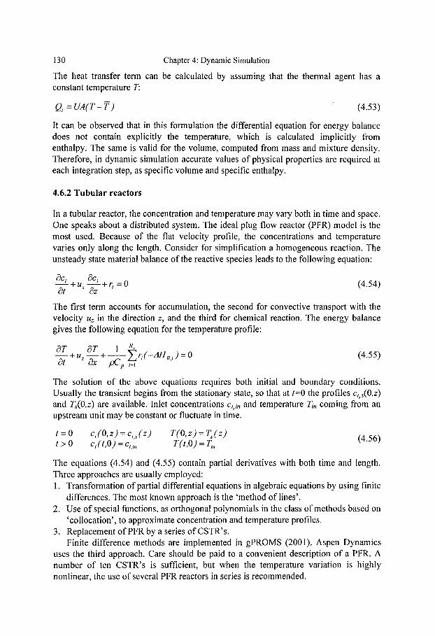
130 Chapter 4: Dynamic Simulation
The heat transfer term can be calculated by assuming that the thermal agent has a constant temperature T:
Q, = U A ( T - T ) (4.53)
It can be observed that in this formulation the differential equation for energy balance does not contain explicitly the temperature, which is calculated implicitly from enthalpy. The same is valid for the volume, computed from mass and mixture density. Therefore, in dynamic simulation accurate values of physical properties are required at each integration step, as specific volume and specific enthalpy.
4.6.2 Tubular reactors
In a tubular reactor, the concentration and temperature may vary both in time and space. One speaks about a distributed system. The ideal plug flow reactor (PFR) model is the most used. Because of the fiat velocity profile, the concentrations and temperature varies only along the length. Consider for simplification a homogeneous reaction. The unsteady state material balance of the reactive species leads to the following equation:
C~C i ~C i Ot + u, -~z + ri = 0 (4.54)
The first term accounts for accumulation, the second for convective transport with the velocity Uz in the direction z, and the third for chemical reaction. The energy balance gives the following equation for the temperature profile"
c3T c3T 1 Nr ~ + u= ~ + ~ ~ - ' r , ( -AHR, i ) = 0 (4.55) Ot Ox pCp i:1
The solution of the above equations requires both initial and boundary conditions. Usually the transient begins from the stationary state, so that at t -0 the profiles ci, s(O,z) and Ts(O,z) are available. Inlet concentrations ci, i, and temperature Tin coming from an upstream unit may be constant or fluctuate in time.
t = 0 ci(O,z ) = C,,s(Z ) T (O , z ) = Ts(z ) (4.56) t > 0 c,(t ,O) = c,,,, T(t ,O) = T~,
The equations (4.54) and (4.55) contain partial derivatives with both time and length. Three approaches are usually employed: 1. Transformation of partial differential equations in algebraic equations by using finite
differences. The most known approach is the 'method of lines'. 2. Use of special functions, as orthogonal polynomials in the class of methods based on
'collocation', to approximate concentration and temperature profiles. 3. Replacement of PFR by a series of CSTR's.
Finite difference methods are implemented in gPROMS (2001). Aspen Dynamics uses the third approach. Care should be paid to a convenient description of a PFR. A number of ten CSTR's is sufficient, but when the temperature variation is highly nonlinear, the use of several PFR reactors in series is recommended.

Chapter 4: Dynamic Simulation
4.7 PROCESS CONTROL TOOLS
131
4.7.1 Implementation of controllers
The majority of controllers in industry are based on Single Input Single Output (SISO) loops. The implementation of such controllers consists of a succession of operations, as follows:
�9 Select the process variable (PV) that has to be controlled. This may be a stream or unit variable, usually pressure, temperature, concentration, mass or volumetric flow rates, as well as the liquid level. The variation can be expressed as a percentage from the range (PVma x - PVmin). Setpoint SP is the PV value that should be kept at a desired value. Usually the setpoint is positioned close to the midrange.
�9 Define the controller output (OP) as the manipulated variable. This is usually a stream flow rate or heat duty. The steady state design supplies the nominal value. The maximum output may be taken as twice the nominal value. The minimum output may be set to zero or to a non-zero safe value.
�9 Implement controller. The PID (proportional-integral-derivative) controllers are mostly used in practice. A PID controller modifies the manipulated variable following the algorithm:
1 ~ i de(t) OP = OP~ s + Kc[e(t ) + c(t)dt + r D ] (4.57) rio dt
In the above relation OPss is the steady state value, or the bias of the manipulated variable, and ~ is the error defined as difference between PV and setpoint:
c : s P ( t ) - Pv( t ) (4.58)
A PID controller has three adjustable parameters Kr ri, Zb, which define proportional (P), integral (I) and derivative (D) actions. The most important is the controller gain Kr Usually Kc is dimensionless, and is expressed as the ratio of scaled output to input, %OP/%PV. Higher gain gives faster response, but also more oscillatory behaviour. P-controller has always a steady state error. The error is reduced by integration over a time r~ known as reset time. The derivative component may be considered for faster response, the parameter XD being known as rate time. Determining the above parameters implies a tuning procedure, as discussed later in this section.
�9 Define the mode of action. In direct action, when the process variable PV is above the setpoint (negative error) the manipulated variable (OP) is increased (negative gain), and vice versa. For instance, consider level control by outlet flow. When the level rises above the setpoint the outlet flow must increases too. In reverse action, when PV increases above SP (negative error), the manipulated variable decreases. Here we may give as example the control of purity by reflux. When the purity of the product increases above the setpoint, the reflux flow rate must diminish.
�9 Prepare the controller view and recorder settings.

132 Chapter 4: Dynamic Simulation
4.7.2 Tuning of PI controllers
PI is the most used controller. The tuning consists of a Pl-controller the finding the dynamic characteristics called 'ultimate gain' (Ku) and 'ultimate period' (Pu). A step disturbance is introduced, and the gain of controller in P mode is slowly increased. The value where sustained bounded oscillations appear designates the ultimate gain Ku. The ultimate period Pu can be measured directly.
In another method, called ATV (auto-tune variation), the controller is replaced by a relay of amplitude +h%. The period is divided in each cycle by two up to the occurrence of oscillations. If a is the amplitude of oscillations, the ultimate gain can be calculated as:
K~ = 4h / ~ra (4.59)
By knowing Ku and Pu, the parameters of a PI controller can be calculated with simple relations as given in the Table 4.1, according to Ziegler-Nichols (ZN) or Luyben-Tyreus (LT). It is considered that the ZN tuning is somewhat aggressive, while LT is rather soft. Note that the values of tuning parameters determined as above should be seen only as initial values. The tuning should continue up to the point where the performance of controller is satisfactory (see Chapter 12).
Another problem is the use of the tuning parameters for SISO loops in a multi-input multi-output (MIMO) environment. The influence of interactions between loops can be dumped in some cases only by 'detuning' the parameters, usually by diminishing the gains and increasing the reset times.
Table 4.1 Tuning rules for PI controllers
Tuning rule Kc (%/%) P~ (min) Ziegler-Nichols (ZN) Ku/2.2 Pu/1.2 Luyben-Tyreus (TL) Ku/3.2 2.2 Pu
EXAMPLE 4.4 Closed loop dynamic simulation of a flash
Switch on automatic the controllers for level and pressure used for the flash discussed in the Example 4.2, and examine the closed-loop response.
Solution. We use the default tuning parameters, as follows: LC 1 with Kc=20 %/% and ri = 10 min., and PC2 with Kc=20 %/%. Fig. 4.8 displays the closed loop response for the same scenario of disturbances as in Example 4.2. This time the liquid level is kept around the set point with small deviations. The response of the output streams is different from open loop dynamics: the outlet liquid flow rate decreases at increasing temperature, and vice versa. An inverse response is noted in both cases. Hence, keeping constant the liquid level will produce disturbances in the outlet flows, which might be undesirable

Chapter 4: Dynamic Simulation 133
for the downstream unit. A looser level control would be more profitable. In fact, besides the separation in liquid and vapour, the role of a flash vessel is to dump disturbances in flows arriving from the upstream units. In conclusion, except chemical reactors, for the level control of units with liquid inventories, as reservoirs, flash drums and reboilers, a simple P-controller is convenient.
Figure 4.8 Dynamic response of a flash in closed loop
4.8 F U R T H E R R E A D I N G
As general reference for mathematical modelling in chemical engineering we recommend the newest edition of the acclaimed textbook of Bird, Lightfoot & Stewart (2001). A classical guide for writing equations for deterministic systems is the book of Himmelblau & Bischoff (1968), probably now difficult to find. A refreshing retrospective of mathematical modelling has been revealed recently by Aris (2001).
Mathematical formulation of dynamic models and their linearisation is treated in books dealing with process dynamics and control. Here we mention the textbooks of Stephanopoulos (1984), Ogunnaike & Ray (1994), Luyben (1995), and Marlin (1995). Very useful theoretical and practical insights in dynamics and control of distillation processes, with so many implications in dynamic simulation, can be found in the monograph edited by Luyben (1992) with contribution of specialists in different areas. A useful presentation of process dynamics from a practical viewpoint can be found in the book of Ingham et al. (1994).
Nonlinear dynamics is becoming an important topic in design, since implied not only in safety aspects, but also in design for flexibility. Some applications will be presented in Chapter 13. An advanced treatment of nonlinear dynamics can be found in the book of Bequette (1998). More complex dynamic phenomena, as the occurrence of multiple steady states and chaotic behaviour, are presented in accessible but rigorous manner. Numerous examples built in Matlab illustrate the mathematical issues.

134
4.9 R E F E R E N C E S
Chapter 4: Dynamic Simulation
Aris, R., 2001, Modelling principles, Academic Press Bequette, R. W., 1998, Process Dynamics, Modelling, Analysis and Simulation,
Prentice Hall, New Jersey Bird, Lightfoot, Stewart, 2001, Transport Phenomena, Wiley, New York, 2 nd Edition Himmelblau, D., K. Bishoff, 1968, Process Analysis and Simulation. Deterministic
Systems, Wiley, New York Ingham, J., I. J. Dunn, E. Heinzle, J. E. Prenosil, 1994, Chemical Engineering
Dynamics. Modelling with PC Simulation, VCH-Wiley, Weinheim Luyben, W., 1989, Process Modelling, Simulation and Control, 2 nd Edition,
McGraw Hill, New York Luyben, W. L., 1996, Design and control design of freedom, Ind. Eng. Chem. Res., 35,
2204-2214 Grassi, V. G., 1992, Rigorous modelling and conventional simulation, in Practical
Distillation Control, Van Nostrand Reinhold, New York, p. 29-46 Marlin, T. E., 1995, Process Control, Mc Graw Hill, New York Ogunnaike, B. A., W. H. Ray, 1994, Process Dynamics, Modelling and Control,
Oxford University Press Pantelides, C. C., P. I. Barton, 1992, Equation-Oriented dynamic simulation,
Comp. & Chem. Eng., ESCAPE-2, $263-$285 Practical Distillation Control, 1992, edited by W. L. Luyben, Van Nostrand Reinhold Stephanopoulos, G., 1984, Chemical Process Control, An Introduction to Theory and
Practice, Prentice-Hall International
SOFTWARE MANUALS
Aspen Dynamics User Manual, version 10.2, Aspen Tech, 2001 g-Proms, User Manual, version 2.1,2001

PART 11
THERMODYNAMIC METHODS

This Page Intentionally Left Blank

Chapter 5
GENERALISED COMPUTATIONAL METHODS IN THERMODYNAMICS
5.1 PVT behaviour of fluids 5.1.1 Phase diagrams 5.1.2 Equations of state 5.1.3 Principle of corresponding state
5.2 Fundamentals of thermodynamics 5.2.1 Laws of thermodynamics 5.2.2 Free energy functions 5.2.3 Phase equilibrium condition 5.2.4 Gibbs-Duhem equation 5.2.5 The network of thermodynamic properties
5.3 Fugacity 5.3.1 Def'mition 5.3.2 Computation of fugacity
5.4 Equations of state 5.4.1 Virial family of equations of state 5.4.2 Cubic equations of state
5.5 Generalised computational methods using PVT relationship 5.5.1 Departure functions 5.5.2 Evaluation of the departure functions 5.5.3 Generation of thermodynamic property charts
5.6 Summary
5.7 References

13 8 Chapter 5: Generalised Computational Methods
This chapter deals with the fundamental concepts that allow a unified approach of the thermodynamic computations in process simulation, both in the field of physical properties and of phase equilibria. The last aspect is examined in more detail in the Chapter 6. The material is presented as a synthesis of a much more elaborated treatment that may be found in dedicated textbooks on Chemical Engineering Thermodynamics, as Smith and van Ness (1997), Kyle (2000), Sandler (2001). The description of the major methods for estimating fundamental properties, mostly being implemented in simulation packages, may be found in the thesaurus book of Reid and al. (1987) updated recently by Poling, Prausnitz and O'Connell (2001).
The chapter starts by examining the P VT behaviour of process fluids, as gases and liquids. We will introduce generic models, as the equations of state and the principle of corresponding states, which dominate nowadays the thermodynamic calculations by computer methods. Then we will review the laws of thermodynamics in order to ensure a coherent presentation of the fundamental equations. Particular attention will be given to the network of thermodynamic relations that makes possible to navigate between different properties, mostly not accessible by measurements, only on the base of very limited experimental information. We will formulate the general conditions of phase equilibrium. In this context, we will highlight the concept of fugacity and its calculation. A distinct section will be devoted to a more ample presentation of the equations of state, particularly of cubic type, which at presently are the default models in flowsheeting packages. We will end the chapter by describing the generalised computational methods for generating charts and tables for various properties.
5.1 P V T B E H A V I O U R O F F L U I D S
5.1.1 Phase diagrams
Pc
supercritical fluid
~ 1 critical - 7 C
E I liquid .~,~o / solid / o~q '~U
,~9~,/ . . . . . ., / ~ vapour
5 ~ i p l e point
v . . . . . . . ) ,
Tc T
Figure 5.1 Generalised phase diagram

Chapter 5: Generalised Computational Methods 139
Figure 5.1 presents the behaviour of a pure species that can exist as solid, liquid or vapour in a pressure-temperature diagram. We may have three types of two-phase equilibrium: solid/liquid, vapour/liquid and solid/vapour. There is a point where all three phases coexist, designated by the triple poin t . Here the phase rule gives F = C + 2 - P = 1 +2-3=0 degrees of freedom. Neither pressure nor temperature can be used to modify the equilibrium. If only two phases can be found at equilibrium F - 1 +2-2= 1, and either pressure or temperature can vary. The most important equilibrium in process engineering is v a p o u r - l i q u i d equi l ibr ium, abbreviate as VLE. It may be observed that the two phases will coexist up to a point where it is difficult to make a distinction between vapour and liquid. This is the cri t ical po in t , a fundamental physical property characterised by cri t ical p a r a m e t e r s Pc, Tc and V c . Above the critical point the state of the fluid is supercr i t ical . Actually, the properties of a supercritical fluid are quite different from a super-dense gas or a light liquid.
If the pressure P is represented as function of the molar specific volume V of a pure component at constant temperature, the isotherms have the aspect given in Fig. 5.2, where the state variables (reduced values) are scaled by reference to the critical point:
Zr __ ~Z ," Pr -- ~ P " V -- ~V (5.1) Vc Pc v~
At the critical point the difference between liquid and vapour volumes approaches zero, suggesting that the energy needed for phase transition, in other words the enthalpy of vaporisation, should diminish to zero. The above observation illustrates in a simple manner the link between the P VT behaviour of a fluid and the energy implied in its physical changes.
Figure 5.3 presents the generic P VT relationship for a pure component in a 3D diagram. This representation captures both the temperature evolution of the phase boundaries at equilibrium, as well as their volumetric behaviour. The 2D representation for different cases is straightforward.
Figure 5.2 Pressure-Volume curves Figure 5.3 Generalised PVT diagram

140 Chapter 5: Generalised Computational Methods
5.1.2 Equations of state
An algebraic equation relating the fundamental state variables of a fluid P, V and T is known as an equation o f state, abbreviated here by EOS. The simplest EOS is the ideal gas law P V=RT. The models based on equations of state are widespread in simulation because allow a comprehensive computation of both thermodynamic properties and phase equilibrium with a minimum of data. EOS models are applied not only to hydrocarbon mixtures, as traditionally, but also to mixtures containing species of the most various chemical structures, including water and polar components, or even to solutions of polymers. The most important equations of state are presented briefly below, but they will be examined in more detail in other sections.
a. Virial EOS
The non-ideality of a gas can be expressed by the compressibility factor Z, defined as:
P V Z = ~ (5.2) R T
One of the simplest forms, called Virial equation o f state, express the compressibility factor Z as a power series of molar volume or pressure:
P V B C Z = - 1 + - - + - - 7 + ...... (5.3)
R T V V
Z = __PV = 1 + B ' P + C' p2 + ..... (5.4) R T
Note that the Virial coefficients B, C, or B', C', are function only of temperature. Virial EOS has a theoretical basis in statistical mechanics. For example, the B/V term accounts for interactions between pairs of molecules; C/V 2 describes three molecule interactions, etc. The form Z=I +B/V called the second virial coefficient has found wide applications, but it is restricted to gas phase calculations at moderate pressures up to 20 bar.
Much more sophisticated is the form known as the BWR-EOS, proposed by Benedict, Webb and Rubin (1940) 1. This model represents a more complex dependency of pressure as function of volume:
R T BoRT - A o - C O / T 2 b R T - a act c 7 - 7 P
~ ~ V 2 --]- ~ 3 - ~ + V 3 T 2 ( I + - -~ ) exp V2 (5.5)
The constants A, B, C, a, b, c, a and [3 are characteristic for a given fluid. BWR-EOS and its recent modifications permit accurate calculations of physical properties of light gases, non-polar or slightly polar components medium pressure. BWR-EOS can be used for both thermodynamic properties, as enthalpy and entropy, and phase equilibrium. It is also suited for light hydrocarbon processes, including rich methane and hydrogen mixtures, as well as in gas liquefaction.
1 For complete references on EOS's see the book of Poling, Prausnitz and O'Connel (2001)

Chapter 5: Generalised Computational Methods 141
b. Cubic equation of state
The cubic EOS are based on the famous van der Waals equation (1873):
RT a P : - - (5.6)
V - b V 2
The term a/V 2 accounts for increasing attractive forces between molecules at higher pressure, while b is a measure of the co-volume of molecules at infinite pressure. Note that both parameters a and b are functions only of critical pressure and temperature.
Long time the original van der Waals EOS did not found industrial applications. Redlich and Kwong (1949) discovered that a modified form was convenient for describing the hydrocarbon mixtures. The model, abbreviated here by RK-EOS, is represented by the relation:
RT a P = T 1 / 2 V ( V + V - b b) (5.7)
In fact, RK-EOS introduced an important modification in the formulation of van der Waals equation, the temperature dependency of the a parameter, such as:
a(T) = a~(T~,P~ ) a ( T ) (5.8)
The correction factor of the parameter a is designated often by alpha function. For the
RK-EOS this factor is a ( T ) = 1/~V~.
Much later Soave (1972) proposed a new modification, known as Soave-Redlich- Kwong EOS, abbreviated here SRK-EOS, in which the model incorporates another important molecular parameter, the acentric factor co (see later the equation 5.12). The result was that the accuracy of VLE computations improved considerably. In the case of SRK-EOS the alpha function is"
a ~ - 1 + ~c(1- T ~ ) (5.9)
The factor xis a polynomial function of co, ~c = f ( co ) .
Another equation, due to Peng and Robinson (1976), denoted by PR-EOS, has proved similar accuracy, but more robustness near the critical point. The form is:
RT a(T) P : - - (5.10)
v - b v ( v + b) + b(V - b)
The function a is given by Eq. (5.9) but with different dependency x = f ( co ) .
With the arrival of commercial simulators the cubic equations of state have become standard thermodynamic options. This fact may be attributed both to their simplicity and robustness in calculating thermodynamic properties and phase equilibrium. For example, a cubic EOS distinguishes without ambiguity between mono-phase and multi- phase systems. New modifications and mixing rules enlarged the field of applications from hydrocarbons to all (non-electrolytic) mixtures, including non-polar and polar components, over a large range of pressures and temperatures.

142 Chapter 5: Generalised Computational Methods
5.1.3 Principle of corresponding states
The principle o f corresponding states was the first attempt toward a universal method for correlating thermodynamic properties. This is expressed as following: The equilibrium properties that depend on intermolecular forces are related to critical properties in a universal way. In two parameters formulation (van der Waals, 1873), the compressibility factor is a function only of the reduced temperature and pressure:
Z = f(Tr,Pr) (5.11)
A major improvement in generalising the correlation of the compressibility factor was obtained with a three-parameters formulation. The third parameter is the acentric factor co, which is a thermodynamic measure of the shape and size of a molecule. A mathematical definition is based on the slope of vapour pressure curve at T~=0.7"
co = 1.0-log(P s~'/Pc)Tr=0.7 (5.12)
Following Pitzer (1955) 2, the compressibility factor Z may be expressed by
g = g ~ (T,., Pr ) +c~ (Tr, Pr ) (5.13)
Hence, the computation of Z is split in two parts: Z ~ term for an ideal spherical molecule, and Z 1 - deviation function accounting for non-sphericity. A large number of generalised predictive methods for physical properties exploit this formulation, as for example the Lee-Kesler s method (see later the section 5.4).
5.2 FUNDAMENTALS OF THERMODYNAMICS
5.2.1 Laws of thermodynamics
Thermodynamics is the science that studies the changes in the state or condition of a system when changes in its internal energy are important. Internal energy designates all forms of energy associated with motions, interactions and bonding of molecules forming a material body. This is quite different from forms of external energy, as kinetic and potential energy, which are of primary interest in mechanics. In this book the sign conventions are: - Energy: positive in, negative out.
- Work dW = - p d V : compression positive (dV<0), expansion negative (dV>0). - Capital letters designates molar values of properties, as volume (V), internal energy
(U), enthalpy (H), entropy (S) and free energy functions (A, G). Consequently, extensive values for a system containing n moles will be noted by (nV), (nU), etc.
2 Pitzer, K.S., Curl, R. F., J. Am. Chem. Soc., 79, 2369, 1957 3 Lee, B.I., Kesler, M.G., AIChEJ, 21,510, 1975

Chapter 5: Generalised Computational Methods 143
First law of thermodynamics
The first law postulates the conservation of energy. The system is the part of the space where the process occurs. Everything not included in the system is considered surroundings. Let's consider a system, where work (W) and heat (Q) are the only forms of energy passed between system and surroundings. Moreover, the system is closed, such as no mass exchange takes place. Thefirst law of thermodynamics is:
A (energy of the surroundings) + A (energy of the system) =0 (5.14)
The first term is given by the net amount of heat and work exchanged Q + W. The second term should take into account the change in energy of the system itself. This can be decomposed in several contributions. The most significant is the internal energy U, which includes all forms of energy associated with the activity of atoms and molecules forming a system, except those related to macroscopic movement (kinetic energy) or change in position (potential energy). Internal energy is a state function. Its absolute value cannot be known, but its variation AU between two states is always the same regardless the path followed.
In differential form, the first law postulates that in a closed system the internal energy U can be varied only by exchange of heat and/or of work:
dU=~+~v (5.15)
The differential dU is 'exact', depending only on the initial and final states (pressure, volume, temperature, composition). Contrary, both 6Q and 6/I/ are not exact differentials, depending on the path of transformation.
An important measurable physical property is the constant-volume heat capacity Cv, defined as:
v v
Because most of the industrial operations take place at fairly constant pressure, it is useful to associate U and P V in a new state function enthalpy (H), whose definition is:
H = U + P V (5.17)
By differentiation of (5.17) and combination with (5.15) leads to:
dH = 6Q + VdP (5.18)
Equation (5.18) is the first law expressed in differential form. From this we can define an important measurable physical property, the constant-pressure heat capacity Cp :
(OH] = c ~ P = C p (519) - - ~ p OF
C z and Cp are functions of temperature. For an ideal gas C ~ = C o + R.

144 Chapter 5: Generalised Computational Methods
The energy balance in industry is usually formulated as an enthalpy balance. For open (flowing) systems, when thermal effects predominate, the first law becomes:
AH : Q + W s (5.20)
The mechanical energy W s is exchanged as shaft work. Note that the volumetric work is incorporated directly in the computation of enthalpy. If only change in temperature is involved, and no phase change occurs, the variation of the (sensible) enthalpy is:
A H = H ( T e ) - H(T~ ) = ~ C e ( T ) d T (5.2 1)
The above formula is acceptable for condensed phases, as solid or liquids, without phase transition, but not for real gases, where the influence of pressure has to be accounted for. Consequently, the formula (5.21), so much used in hand calculations, is of relatively minor importance in process simulation. Instead, computations of enthalpy based on equations of state or corresponding states principle are used.
An ideal gas is taken usually as reference for the thermodynamic properties of a real fluid. Because the enthalpy of an ideal gas does not depend on pressure, its variation between two states depends only on temperature. It is convenient to define an arbitrary
reference state 4. The enthalpy of an ideal gas H ~ can be set at zero for T = T O . A
convenient reference temperature is the absolute zero Kelvin. In this case the enthalpy of an ideal gas can be calculated simply as
H ~ = ~rC~ =-aT +bT 2 /2 +cT 3 /3+ (522)
As it will be demonstrated later in this chapter, the difference in enthalpy between a real fluid and an ideal gas, at the same T and a reference P0, noted usually as departure
funct ion ( H - H ~ can be determined only from P VT information. Hence, the enthalpy of a real fluid, including contributions of both sensible heat and phase transition, may be found simply with the relation:
H = H ~ + ( H - H ~ (5.23)
This approach can be extended to other thermodynamic properties.
Second law the thermodynamics
The second law deals with the spontaneous evolution of a thermodynamic process and the efficiency of conversion between different forms of energy, particularly between work and heat. It is intimately linked with the notion of entropy. The work can be transformed spontaneously and integrally in heat, such that W = JQ. On the contrary, the conversion of heat in work is never spontaneous.
4 A reference state may be different from a standard state, a concept used in equilibrium reactions.

Chapter 5: Generalised Computational Methods 145
The second law of thermodynamics postulates: It is impossible for a device operating in a cyclic manner to completely convert heat into work. If the heat flows spontaneously from higher to lower temperature, the opposite process requires a heat engine. Camot demonstrated that the maximum work from a heat engine is given by a cycle formed by two adiabates and two isotherms whose efficiency is:
17 = Q1 - Q___..._____.A_: = T1 - T2 (5.24) Q1 r,
T 1 is the absolute temperature at which the heat Q1 is injected, and T 2 the temperature at which the heat Q2 is rejected. It follows that we can write:
Q1 Q2 =0 (5.25) Vl T2
Equation (5.25) suggests that the ratio between the heat (received or rejected) and the temperature might be a system property that might characterise the reversibility 5of the heat exchange in a cyclic process. By more rigorous reasoning, this observation leads to a new state function, entropy, defined as:
dS = 6Qrev (5.26) T
where @rev is the infinitesimal amount of heat exchanged in a reversible process at the temperature T.
Entropy plays a central role in evaluating the reversibility of processes. For the transformation from the point A to the point B the following relation is valid:
S 8 - $ 4 = IdQT'48 >_0 (5.27)
The equation (5.27) defines the following possibilities: (1) AS - 0 , the process is reversible and adiabatic, (2) AS > 0, the process is irreversible, and (3) AS < 0 the process is impossible.
Third law of thermodynamics
The third law allows the calculation of an absolute value for entropy. By definition the entropy o f a perfect crystalline substance is zero at zero absolute temperature. For a pure component ideal gas at the temperature T we may write:
AHf.s~o.~~~C~'l A H ~ p ~ C t ' . S r = ~ Cp's dT + ~ + ' dT + + ' dT (5.28)
r r r v r
5 A reversible process proceeds with infinitesimal gradients within the system. The direction can be reversed at any point by an infinitesimal change in external conditions.

146 Chapter 5" Generalised Computational Methods
Tfand Tv are the fusion and vaporisation temperatures, whereas AOfusion and AHvap are the enthalpies of the respective phase transitions.
5.2.2 Free energy functions '
Free energy functions A and G are more appropriate for the computation of physical and chemical equilibrium than the primary functions U and S. The def'mitions are: �9 He lmho l t z f r ee energy (A):
A = U - T S (5.29)
�9 Gibbs f ree energy (G)"
G = H - T S = U + P V - T S = A + P V (5.30)
The functions A and G are called 'potentials' because allow the calculation of the maximum work Wma~ only from initial and final states. Consider a reversible process in a closed system. The maximum work can be produced only by a reversible transformation. Eqs (5.15) and (5.26), can be combined to give the following relation:
d U = TdS + 6Wm~ (5.31)
The total work W takes into account the volumetric work P V, as well as other forms of
useful work (shaft, electrochemical), noted here by W # . The volumetric work is accounted as a change in volume at constant pressure. For an infinitesimal change the
total work is 6 W - - P d V + 6 W # . Hence, the following relation can express the maximum useful work:
~ ' r # a x -- d U - T d S + P d V (5.32)
For a process at (T, V) constant we obtain:
6 W # - d ( U - T S ) (5.33) m a x
Hence, the quantity A = U - T S is a potential at (V, 7) constant, because it gives the maximum work for finite variation:
m#ax -AA (5.34)
Similarly G=H-TS is a potential at (P, 7) constant, because:
m#ax =AG (5.35) The Gibbs free energy is preferred in technical calculations because most of industrial processes take place at fairly constant pressure.
Equation (5.31) can be extended to include irreversible processes being known as Clausius inequality."
A U - T A S + P A V - W # < 0 (5.36)

Chapter 5" Generalised Computational Methods 147
The equality sign is valid for reversible processes, while the inequality applies for irreversible processes. Since the first three terms represents AGr, P we can write:
A G r , e <_ W # (5.37)
If there is only volumetric work then W # = 0, and consequently:
AGr, v < 0 (5.38)
At equilibrium we have AGr, p = 0. On the other hand, a chemical process occurs
spontaneously when AGr, v < 0 .
The first and the second law of thermodynamics may be combined in the form of differential equations. Let's consider one mole of pure gaseous component in a closed system. The first law in a reversible process can be written as d U = 6Qrev--6Wre v .
Replacing 6QrevbY the equation (5.26) and considering only volumetric work such as 6Wre ~ = P d V leads to:
d U = T d S - P d V ( 5 .39)
Similar expressions can be obtained by differentiating the other state functions"
d H = T d S + VdP (5.4 O)
dA = - P d V - S d T (5.41)
d G = VdP - S d T (5.42)
The equations (5.39) to (5.42) are fundamental in thermodynamics, and the starting point to derive the network of thermodynamic properties.
Pressure and temperature dependency of Gibbs free energy
From the equation (5.42) at constant temperature we obtain:
d G = VdP or = V (5.43) T
Hence, G depends strongly on pressure for gases, but only slightly for liquids. Note that G can be obtained experimentally from volumetric measurements. In the case of an ideal gas the integration of (5.43) between P and P0 at constant Tleads to:
G = G o + R T ln (P / 1 arm) (constant T) (5.44)
This relation can be generalised for real gases by means of the fugacity concept. Similarly, at constant pressure but variable temperature we have:

148 Chapter 5" Generalised Computational Methods
d G = - S d r or = - S (5.45) P
Therefore, phase transitions give important changes in the slope of Gibbs free energy versus temperature, because of the large entropy variation.
5.2.3 Phase equilibrium condition
Pure Components
Figure 5.4 shows the variation of the Gibbs free energy G for a pure species going from solid to liquid, and further to gas, at constant pressure but variable temperature. The reference is an ideal gas state. At phase transition the functions U, H, S change abruptly with the temperature, the slope becoming infinite. On the contrary, the Gibbs free energy has a remarkable mathematical property, being continuous everywhere. At phase transitions, the slope of the G - T curve changes significantly but remains finite.
~ . ' , . ~ . "-L~,'--.. ' " "'--.... solid
~ ' , , vapour
Tsl Tsv TIv T
Figure 5.4 Gibbs free energy as function of temperature
The equilibrium condition for a pure species distributed between two phases c~ and 13 at the same and uniform P and T can be expressed as the equality of the Gibbs free energy in each phase:
[ Ga = G ~ ]v,r (5.46)
Equation (5.46) leads to an important thermodynamic relation that links the properties of phases at equilibrium. Assume an inf'mitesimal variation of temperature and pressure
around the equilibrium, such as we can write dG a - d G p . We may apply for each infinitesimal variation the equation (5.42) and obtain:
d P S 'a - S a = (5.47) d T V p - V a

Chapter 5: Generalised Computational Methods 149
From the Gibbs free energy def'mition and the equilibrium condition (5.46) it is easy to found that S p - S a = ( H p - H ~ ) / T . Replacing it in the relation (5.47) leads to the famous Clapeyron equation"
dP H ~ - H a - - = (5.48) dT T(V p - Z a)
The relation (5.48) is valid for any phase transition. More specifically, at vapour-liquid phase transition it becomes:
dP ) - ZHvap (5.49) - ' ~ equil- TAV
where AV = V v - V t , V v and Vtbeing the molar specific volumes of vapour and liquid. The relation (5.49) can be extended for other phase equilibria, as melting and sublimation. If the vapour is ideal V v - V t .~ V v = RT / P , and the equation (5.49) leads to the Clausius-Clapeyron equation:
d In P AHv,,p d In P AHvap . . . . or . . . . (5.50) d ( 1 / T ) R d ( 1 / T ) g
Hence, the enthalpy of vaporisation can be determined from vapour pressure data. Conversely, the vapour pressure may be estimated more accurately if the enthalpy of vaporisation is considered among experimental data. Details for estimating these two fundamental physical properties can be found in the monograph of Poling et al. (2001).
M i x t u r e s
We can introduce a composition dependency in the analysis of any state function U, H, A or G. Thus for multi-component system the equation (5.42) may be formulated in extensive manner as:
d(nG) = (n W)dP - ( n S ) d r (5.51)
For single-phase closed system without reaction we may write for an infinitesimal variation in P and T:
gP Jr,, P,,
The comparison with the equation (5.52) leads to:
I I O(nG) =(nV) and Or ~,. N T ,n
For single-phase open system the mixture composition may vary, and in consequence nG = g ( P , T , n~,n2, .... ,nj, . . . .) . Thus, we may write the more general relation:

150 Chapter 5: Generalised Computational Methods
d(nG) : D(nG) dP + d r + ~i OP T,. OT P,n " P,T,nj dlq i (5.54)
We introduce partial derivatives with the composition of the Gibbs free energy function for mixture (nG), which by definition are called chemicalpotentials:
:[O(nG)] (s.SS ]'li L OFli P,T,nj
As a result, the generic relation (5.54) takes the more practical form:
d(nG) = ( n V ) d P - ( n S ) d r + ~ ( j u i d ~ i ) (5.56)
Equation (5.56) is fundamental for calculations regarding multi-component mixtures, which are designated in thermodynamics by P VTx systems. From this we can obtain the generalisation of the phase equilibrium condition as follows:
[]'li ~ -- ]'lift -- ]'li y = " . . . . . . = ]'li zc ]P,T (5.57)
To apply Eq. (5.57) we need models for chemical potentials, as function of temperature, pressure and composition. The next section presents a fundamental equation that defines a theoretical constraint for formulating such thermodynamic models.
5.2.4 Gibbs-Duhem equation
Chemical potential was introduced as a partial property of the Gibbs free energy to solve the phase equilibrium problem. Similar partial properties may be considered for other extensive properties, as volume, enthalpy, entropy, etc. It would be useful to generalise the approach. Let's consider again that M represents the mean molar value of a property. For the whole system we have n M = f ( T , P , nl,n2,n 3 .... ). The derivation of the (nM) as function of T, P, and composition gives:
d ( n M ) : a ( n M ) dT "3 I- d P .-[- Z ~l,l i dt'li (5.58) aT p,, OP T,n P.T,nj
We may define as before a partial molar property:
2Q = [a(nM) 1 (5.59) ani JP,r,.j
The relation (5.58) can be re-written as:
c3M dT + n - ~ dP + Z Midrti (5.60) d ( n M ) = n - ~ ,,x r,,
Because n i = xin , dn i = x idn + ndx i , and by replacing in the relations (5.60) gives:

Chapter 5: Generalised Computational Methods
n dM + Man = n aT + n dP 3v Z ~'[i (rldxi Or. X i dl"l) P ,x T,x
Isolating the terms and multiplying by n and dn leads to:
151
(5.61)
OM dT - - ~ [ d M - - ~ e,x T,x
d P - Z M i d x i ] r t + [ M - Z x i M i ] d n = O
The above equation is valid only when the both terms in brackets are zero. So we have:
( ) I OM d r - ~p- d P - Z Midxi = 0 (5.62) d M - - ~ e,x r,x
M = Z x i M i (5.63)
The first condition is true because equivalent with (5.60). The second equation is important because states that a property of a mixture may be calculated from partial molar properties weighted by molar fractions. By differentiation we get:
dM - ~ xidM i + Z Midxi (5.64)
By replacing (5.64) into (5.62) leads to the relation:
c3M d r + - ~ dP -- Z (xidMi ) = 0 (5.65) - - ~ P,x T,x
The relation (5.65) known as Gibbs-Duhem equation is valid for any thermodynamic property in a homogeneous phase. At 7', P constant it becomes:
Z (xid~li ) -" 0 (5.66)
This simplified Gibbs-Duhem equation is widely used, as for example in deriving models for liquid activity coefficients.
5.2.5 The network of thermodynamic properties
Thermodynamic state functions, as U, H, S, F, G, have the remarkable property that the variation between two states depends only on the state-variables (P, V, 7) characterising the initial and the final state, but not on the path followed between these states, be real or hypothetical. It is said that the differential of a state functions is exact. Consider the function z=f(x,y). We may write:
dz = Oz dx + dy = Mdx + Ndy Y x
The function z is an exact differential if the following relation holds:

152 Chapter 5: Generalised Computational Methods
x Y
Not only P, V, 7', but also S may be considered as state variables. Useful relations between the state variables (P, V, 7', S) and state functions (U, H, A, G) can be obtained from the fundamental equations (5.39) to (5.42). These are:
V P s T
S T S P
The derivatives of the state variables are interrelated by Maxwell equations as follows:
S V S P
The assembly of the fundamental equations (5.39) to (5.42) together with (5.67) to (5.70) and (5.71) to (5.74) defines the thermodynamic network. These relations are the starting point for finding generalised computational methods for non-measurable thermodynamic properties from other measurable properties.
For instance, let's see how to calculate the variation of enthalpy of a real fluid as function of pressure. From the fundamental equation (5.40) we have:
T T
(5.75)
The derivative of entropy with pressure at constant temperature, (3S /d P)r, is not available experimentally. We may replace it with -(3V/dT)p, the derivative of volume with temperature at constant pressure, as justified by the equation (5.74). This may be available experimentally, or may be computed by an equation of state. Finally, the variation of enthalpy with pressure can be calculated by the relation6:
() = 7 ' ' ~ + v (5.76)
In this way, we can draw the isotherm curves in a property chart enthalpy-pressure.
6 The reader may check that for an ideal gas the enthalpy does not depend on pressure

Chapter 5: Generalised Computational Methods 153
EXAMPLE 5.1 Enthalpy and entropy as functions of T and P
Develop a computational method for enthalpy and entropy using only PVT data and ideal gas heat capacity.
Solution. Both H and S are function of T and P as follows:
dH= dH dT+ dP P T
(i)
( / / ) d T + --~ dP (ii) dS- -~p T
The first term in equation (i) is the heat capacity at constant pressure. For the second term we may use the equation (5.76). The result is:
dH = Cpdr + F - --~ p dP (iii)
In similar way we obtain for entropy:
dS =Cp d T - ( ~ - ~ dP (iv) T ~, dir ) p
How can we use these equations? Suppose that we want to compute the variation in enthalpy and entropy between the states (P1, T1 ) and (P2, T2 ). In both states the gas is not necessary ideal. Suppose that P2 >> P1. We may imagine two paths (Fig. 5.5):
real gas
P],T]
P0, T] P0, 12
ideal gas
Figure 5.5 Computational paths for enthalpy and entropy

154 Chapter 5: Generalised Computational Methods
(A) Medium/high pressure ( P1, T1 )--+ ( P2, T1 ) -+ ( P2, T2 ) (B) Low/high pressure ( P1, T1 ) -+ ( P0, T1 ) --+ ( P0, T2) -+ ( P2, T2) Clearly, the second path is more convenient, because the change in temperature takes place at low pressure, where the gas is ideal and accurate heat capacity is available. The computation follows the steps:
Step I: isothermal expansion to an ideal gas state, ( P1, T1 ) -+ ( Po, T1 )
Po c~V l~d-[ 1 -" H po ,T 1 -- H pI ,T 1 = I VTI d E -- T 1 d e (v)
p r~
AS~ = S,,o, ~ - S4,v, = - - - ~ d P (vi) p
Both enthalpy and entropy variations can be determined, since an equation of state can be used to describe the variation of volume with pressure at constant temperature, as well as the variation of volume with temperature at constant pressure.
Step II: isobaric heating, ( Po, T1 ) -+ ( Po, T2 )
T, A H 2 = Hpo,r, -Hpo,r , = I C ~ ( T ) d T (vii)
11,
T, o = [ C v ( T ) d T (viii) AS2 = S P~ m' - S P~ "~ T
Here, all we need is the ideal gas heat capacity.
Step HI: isothermal compression ( P0, T2 ) ~ ( P2, T2 ). The relations are similar with step I:
A H 3 = He=,r 2 - Hpo,T ~ VT= d P - d P (ix)
= - = - ,
This example demonstrates that reliable P V T correlation and constant-pressure heat capacity of an ideal gas are sufficient to determine a variety of thermodynamic properties, as enthalpy, entropy, Gibbs free energy, etc., and built comprehensive charts. This approach will be extended by means of departure functions.

Chapter 5: Generalised Computational Methods
5.3 F U G A C I T Y
155
5.3.1 Definition
The fugacity concept was introduced initially to account for the non-ideal behaviour of real gases. Later the concept was generalised to phase equilibrium calculation. Let us go back to the equation describing the variation of Gibbs energy with the pressure at
constant temperature dG = VdP. For an ideal gas we have dG ig = v igdP = R T d p , P
from which it follows:
dG ig = R T d l n P (5.77)
The equation (5.77) suggests similar relation for a real fluid, but where the pressure would be substituted by a more general property. Thus, by definition we may link the variation of Gibbs free energy with a thermodynamic property of a real fluid, called fugaci ty f , by the following differential equation:
dG = R T d In f (5.78)
It may be observed that fugacity has the meaning of a real pressure that a fluid would have when obeying different thermodynamic changes. Fugacity is in general different from the external (measurable) pressure. The reference state is 1 atm, where Gibbs free energy is function only of temperature G o (T). The integration between the state of a real fluid and the reference state leads to the expression:
G(T, P) = G o (T) + R T ln(f / 1 atm) (5.79)
Note that equation (5.79) applies equally to gases, liquids and solids. A better perception of the fugacity concept can be obtained by relating it to
pressure. Thus, by subtracting the equations (5.77) and (5.78) leads to the expression:
d ( G - G ig ) : d G R : R T d l n ( f / P) - R T d In qk (5.80)
At this point we may introduce an important class of thermodynamic functions called residual or departure functions. In this case, the residual Gibbs f ree energy may be def'med as:
GR(T,P):G(~P)-G~g(~,P) (5.81)
Further, we may introduce the fugaci ty coefficient qk, defined by:
~b= f (5.82) P
Note that at low pressures f = P or ~b = 1. Another interpretation of fugacity may come by integrating the relation (5.80)
between a state of an ideal gas, where GR=0 and ~b = 1, and a real state. The result is:

156 Chapter 5" Generalised Computational Methods
G R
R T ~ = t n O (5.83)
Hence, the fugacity coefficient may be seen as a measure of the residual Gibbs free energy. It is also interesting to note that the equation (5.83) shows how to compute a non-measurable thermodynamic function, as Gibbs free energy, via an indirect measurable physical property, as fugacity. In fact, the opposite is used in practice. By appropriate modelling of GR the fugacity may be calculated in various conditions of temperature and pressure, reducing considerably the experiments.
The above concepts can be applied to mixtures. Thus, we may define the fugacity of a component in a mixture by the equation:
dpi = dG_ = R T d ln f (constant T) (5.84)
This time pidesignates the chemical potential of the component i, identical with the
partial Gibbs free energy ~ . The circumflex sign emphasises that f is a property in a mixture, but not a partial property. The corresponding equation for an ideal gas is:
d/.ti ig - dGi ig - R T d ln(Py~) (constant T) (5.85)
Hence, we may define a fugac i ty coeff icient in a mixture as:
~i = ~/ (5.86) YiP
The combination of the equations (5.84) and (5.86) gives the relation:
lnqb, = (G- 7 - G~ 'g ) / R T - ~1~ / R T (5.87)
It can be observed that now the quantity ( ln~i ) is a partial property. Therefore, we may write the following relations:
In~i = [c3(nln~b)] (5.88) G~ni /',r
In ~b : ~ x i In ~i (constant P, T) (5.89)
x~d In ~ = 0 (constant P, 7) (5.90)
The Eq. (5.90) is a form of the Gibbs-Duhem equation with In ~ as partial property. Fugacity is a thermodynamic property intensively used in chemical engineering, the
most important being chemical equilibrium of gases at high pressures, and vapour- liquid equilibrium. The first subject is not covered here, but second topic will be discussed in detail in Chapter 6. Therefore, the problem is how to calculate fugacities

Chapter 5: Generalised Computational Methods 157
from direct measurable quantities, as pressure, volume, temperature and composition. This problem is analysed in the next section.
5.3.2 Computation of fugacity
Pure components
Consider a process at a constant temperature. From the equations (5.78) and (5.43) we may formulate the following relation for Gibbs free energy:
dG = R T d In f = VdP (5.91)
By adding and subtracting R T dlnP we get:
R T d l n f = ( v - R~Tp ) d P = d ( G - G ig (5.92)
The integration between zero pressure (ideal gas) and actual pressure leads to"
- - = V - dP = G - G ig (5.93) P
An immediate result is that the fugacity can be computed with any P VT relationship. Replacing Z = P V / R T i n (5.93) leads to a formulation based on compressibility:
P
lnqk : I ( Z - 1) dP (5.94) P
o
Changing the integration variable in equation (5.93) from P to V gives another useful expression for practical calculations:
ln f ( T , p ) 1 ~ R T / P [ _ ~ ) : l n ~ b : - ~ = - P V - ln Z + (Z - 1 ) (5.95)
It is interesting to examine the fugacity dependency with pressure and temperature. From the definition, one gets:
Of' T T
Consequently, the pressure dependency of fugacity is much higher for a gas than for a liquid, because the difference in phase volumes.
The variation of fugacity with the temperature can be found by examining the derivative of the equation (5.93):
5Y RT

158 Chapter 5: Generalised Computational Methods
Taking into account that G = H - TS and (OG / OT)p = - S we obtain:
0 ( l n f [ H-H~g ] O---T --fi) ~ = R T ~
(5.98)
Note the similarity between the relation (5.98) and the Clausius-Clapeyron equation.
1. Gases
The basic relation is the equation (5.95), rewritten in this case as:
In f v (T,P) l z =lnr k V - P V - l n +(ZV-1)
For an ideal gas Z v = 1 and f v (T, P) = P. Hence, we f'lnd again that at low pressure the fugacity of a pure species is just the total pressure.
At moderate pressures we may consider the Virial EOS. Using the form with the second coefficient Z = 1 + B ( T ) / V , leads to the following simple expression:
BP ln~b = ~ (5.99) RT
The computation of the second virial coefficient B can follow different ways. Here we illustrate the use of three-parameter corresponding states law. The following equations can be conveniently represent the behaviour of non-polar molecules:
BPc - B (~ + coB (1) (5.100) RT~
with
B (~ =0.063 0.422 . B ~ =0.139 0.172 (5 101) Tr 16 Tr 12
Similar relations have been proposed for polar molecules (Poling et al., 2001). higher pressure, the use of a cubic EOS is recommended. PR-EOS gives:
At
[z 4 bP/RT 1 fg bP a + (1 + In = (Z v - 1)- ln(Z g - ~ l n = P ---~)- 2~t2bRT Z V + (1- ~-~bP/-~
= (ZV _ I)_ ln(ZV _ B)_ A [ ZV + (I + v/-2) B ] 2x/-2B In Z v +(1-q~)B
(5.102)
where the EOS parameters are A = aP bP
(RT) 2 ; B = RT

Chapter 5: Generalised Computational Methods 159
E X A M P L E 5.2 Fugacity of a pure gas
Calculate the fugacity of C O 2 at 37.7 ~ and 13.8 bar with the following methods: (a) from experimental pressure-volume data (Kyle, 1999), (b) from a graphical correlation, (c) with a cubic EOS, and (d) with Virial EOS. The experimental data are:
P, (kPa) 689.5 68.95 137.9 275.8 551.6 827.4 1103.2 1379.0 V, (m3/mol) 0.375181 0.037381 0.018616 0.009237 0.004551 0.002988 0.002206 0.001751
Solution.
The evaluation of the integral ff (V- R~Tp)dP leads to the values In(f/P)= a) ~010692~ 3 [
f/P = 0.93314 a n d f = 12.85 bar. Note that the deviation between the calculated fugacity and measured pressure is about 1 bar.
b) For C O 2 w e know Tc = 304.2 K, Pc = 72.9 bar, co = 0.239. It follows Tr =1.023 and Pr = 0.1866. From Fig. 3.1 from Reid et al. (1987) we find f/P = 0.955 andf=13.22
c) Using our program (Dimian and Groenendijk, 1994) gives f/P=0.935 andf=12.95 bar with PR-EOS. The same result is obtained with SRK-EOS. The agreement of prediction by calculation with the experiment is excellent. Note that the solution of the equation (5.102) is possible with a spreadsheet.
d) With Tf l .023, P70.1866, c0=0.239 we obtain from (5.102) and (5.103): B ~~ =-0.34392, B ~ =-0.02837 and BPc/(RTc) = 0 = -0.3507
From Z=I + BP/RT= 1 +O(Pr/Tr) = 0.936 one gets f = 12.86 bar. The results indicate close values between experimental data and different models
based on equation of states. However, the pressure is moderate. At higher pressure the comparison could change, and probably the Virial EOS would show larger deviation.
2. Liquids The fugacity of a pure liquid component is close, but not identical, to its vapour pressure. By assuming the liquid incompressible, by combining the equations (5.43) and (5.79), and by integrating at constant temperature between the saturation pressure p~a~ and the system pressure P, gives the relation:
fL RTln = VL(P-P sat) (5.103)
fL, sat

160 Chapter 5: Generalised Computational Methods
V L is the liquid molar volume that may be taken equal with the liquid volume in saturation conditions at psat. Replacing fL,sat = ~sat psat leads to following equation:
v L ( p psat f L = qksat psat exp - ) (5.104)
RT
The exponential term gives the influence of pressure on liquid fugacity being known as Poynting correction. At moderate pressures the Poynting correction is negligible. Therefore, the fugacity of a liquid is practically independent on pressure but strongly dependent on temperature.
At equilibrium the component fugacities in liquid and vapour phases must be equal:
f L = f V (5.105)
It is important to note that in calculating fugacity coefficients with a cubic EOS the same expression holds for both vapour and condensed phase.
EXAMPLE 5.3 Phase equilibrium from fugacity computation
Find the equilibrium temperature for propane at 10 bar. Use PR-EOS.
Solution. Because we deal with a pure component the equilibrium is reached when the fugacity coefficients in each phase are equal ~b v = ~b L . The computation is presented graphically in Fig. 5.6. The equilibrium temperature is of 27.2 ~ The vapour fugacity shows little variation with the temperature. However, the fugacity coefficient is far from one; the non-ideality is obvious. On the contrary, the fugacity of the liquid varies strongly with the temperature, similarly with the vapour pressure.
Figure 5.6 Liquid and vapour fugacity for propane

Chapter 5: Generalised Computational Methods 161
Mixtures
The computation of component fugacity in a mixture follows the same conceptual path as for pure species, but with a notable difference" there is necessary to account for the influence of composition. This aspect is taken into consideration by means of mixing rules for the parameters entering in the equation of state model. The approach will be illustrated in this section with Virial and cubic EOS. Chapter 6 contains more material about this topic, of greatest importance in phase equilibria.
If the equation of state is explicit in pressure, the computation of component fugacity coefficient in mixture is based on the expression:
v,v*,,j V* V* -
where V* denote the total mixture volume. If the equation of state is explicit in compressibility, then the following relation may be applied:
ha ~i : ~P (~ -1) dP (5.107) P
As first example we will illustrate the application of mixing rules with the Virial EOS. If only the second term is kept, then we may write Z = 1 + a m (T)/V, exactly as for a pure component. However, this time the coefficient Bm is function of temperature as well as of composition. It can be demonstrated by statistical mechanics that the following mixing rule applies:
B m = Z Z y i Y j B i j (5.108) i j
where Yi designate the molar composition. The computation of Bm implies virial coefficients B O. characterising bimolecular interactions. It can be demonstrated that the fugacity coefficients of components can be related with the virial coefficients by the relation (Smith, van Ness, 1997):
PIcO(nB)l (5.109)
and finally computed with the equation:
ln~/= ~ 2 yjBo - B,,, (5.110)
The equation (5.110) involves pure-species values Bii and Bjj, as well as cross coefficients BO.. These can be calculated from pure component data, but incorporates also binary interaction parameters ko.. Details can be found in Poling et al. (2001).

162 Chapter 5" Generalised Computational Methods
The second application presents the common mixing rules used with a cubic EOS, called also geometric or one-fluM van der Waals mixing rules. The parameters a and b are averaged with the composition in the following manner:
a = Z Z xixja~j with a/j = (1- kij).Jaiiajj (5.111)
b = Z xibi (5.112)
It is important to note that the above formulas contain interaction parameters k 0 that
account for the non-ideal behaviour of the mixture. The parameters k0can be determined by regression of experimental data, as shown in Chapter 6. As illustration, we present the result of integrating the equation (5.107) with PR-EOS model by using the geometric mixing rules (5.111). The component fugacity coefficient is:
In fv B~ (Z v _ 1)-ln(Z v bP a y,P = -B - - ~ ) 2x/2bRT
2~'yj~j, B~ 1 [ ZV+(I+~f-~bP/RT ] l n A B Z v +(1-x/-~bP/RT
(5.113)
Note that the parameters a and b are dimensionless: A = aP/(RT) 2 and B = bP/RT. The same formula is valid for the fugacity in a liquid mixture, with the difference that fugacity coefficient is ln(f~ L / xiP ) and compressibility factor is Z L .
The above geometric mixing rules do not have a theoretical basis. However, they are suitable for applications involving hydrocarbons where the components are of comparable size, but not accurate enough for mixtures with strong non-ideal behaviour. More complex mixing rules, as well as predictive methods for non-ideality with EOS models will be presented in the Chapter 6.
EXAMPLE 5.4 Fugacity of components in a mixture
Consider an equimolar mixture of propane(l) / n-butane (2) at 10 bar. Find bubble- point and dew-point temperatures, and the corresponding phase compositions. Use PR-EOS neglecting the interaction parameters.
Solution. The equilibrium condition is the equality of the fugacity of each component in vapour and liquid phases. In addition, we consider the constraints of phase composition. The equations are:
ylP~ = x1P~[ (i)
yEP~2 = x2P~ (ii)

Chapter 5: Generalised Computational Methods 163
Y~ + Y2 = 1 (iii)
x~ + x 2 = 1 (iv)
Bubble point condition is expressed by the constraint (iii), while dew point condition by the constraint (iv). By taking into account (i) and (ii) these can be written as:
- 1 : 0 (v) x 1 + - - : - x 2 C v
o r
m n - - yl+ -y2 1 0 (vi)
Note that the fugacity coefficient is a function of temperature, pressure and phase composition, ~f = (T,P,x i v y i ) . Consequently, the determination of the equilibrium temperature implies an iterative solution of the equations (v) or (vi). In this case the fugacity coefficients are computed with the relation (5.113). Results are given below. Note the differences in the variation of fugacities for vapour and liquid. As before, the temperature affects more the liquid than the vapour. The concentration has here only a slight influence, but for other systems it could be different.
T, ~ ~ ~ ~ ~ Xl Yl
Bubble point 47.2 0.873 0.784 1.274 0.427 0.500 0.736 Dew point 59.5 0.886 0.806 1.550 0.565 0.286 0.500
5.4 E Q U A T I O N S O F S T A T E
5.4.1 Virial family of equations of state
The standard form of the Virial EOS formulates the compressibility as an infinite series of the inverse molar volume or pressure, as shown by the equations (5.3) and (5.4). In the low-pressure region, up to 15 bar, Virial EOS is the most accurate. The formulation known as 'second virial coefficient' is sufficient for technical computations. Virial EOS is able to handle a variety of chemical classes, including polar species. Hayden and O'Connell have proposed one of the best correlations for the second virial parameter 7. The method is predictive, because considers only physical data, as dipole moment, critical temperature, critical pressure, and the degree of association between the interacting components. Usually Virial EOS it is an option to describe the vapour phase
7 Hayden J. G., O'Connell, Ind. Eng. Chem. Proc. Des. Dev. 14, 209, 1975

164 Chapter 5: Generalised Computational Methods
non-ideality with liquid activity coefficient models. It gives good results up to 20-30 bar.
The original Virial EOS was applicable only to the gas phase. This limitation incited the development of extended forms, as the Benedict-Webb-Rubin (BWR) correlation (equation 5.5). This equation may contain sophisticated terms with a large number of parameters, mostly between 10 and 20, and need substantial experimental data for tuning. The extended Virial-type EOS's have lost much of their interest after the arrival of various cubic EOS in the last decades. Some formulations are still used for special applications, notably in gas processing and liquefaction, as BWR-Lee-Starling (BWR- LS) equation 8, one of the most accurate for hydrogen rich hydrocarbon mixtures. Note that extended Virial EOS may calculate not only volumetric properties, but also VLE.
One of the most interesting applications in this class is the method of Lee-Kesler (LK). The compressibility factor is described by three-parameter corresponding states correlation of the form:
Z = Z (0) 4- ( Z (r) -- Z ( 0 ) ) - co (r)
(5.114)
The contributions Z (~ and Z (r) are represented by generalised functions containing as parameters the reduced temperature and pressure. These have been obtained by using a special form of the BWR-EOS. Mixture critical parameters and acentric factor are calculated by means of mixing rules, which do not have interaction parameters. Tables of values for hand calculations may be found in Reid et al. (1987). Graphical representations of contributions are presented in Perry (1997). Note that this method can be used to compute phase properties (specific volume, enthalpy, entropy) for both vapour and liquid phase. It has been accepted as accurate option for enthalpy and entropy of hydrocarbons and slightly polar components.
Lee-Kesler method has been extended to oil and petrochemical type mixtures, as for example hydrocarbons and alcohols with CO2, H2, CH4 and HzS , and it is known as Lee- Kesler-Ploecker (LKP) 9. Special mixing rules are designed to describe both symmetric (non-polar) and symmetric (polar) molecules. More details can be found in Poling et al. (2001).
5.4.2 Cubic equations of state
As mentioned, cubic EOS models are often default options in flowsheeting software. The reason is that these make possible to execute most of the basic engineering calculations involving thermodynamic properties and phase equilibria with the minimum amount of data. The intensive research in this domain enlarged considerably the area of applications. Among specialised works in this field we recommend the review of Sandler (1993), as well as the monograph on equations of state edited by IUPAC Commission on Thermodynamics (2000).
8 Brul6, M.R., Lin, C.T., Lee, L.L., Starling, K.E., AIChEJ, 29, 616, 1982 9 Ploecker, V., Knapp, H., Prausnitz, J. M., Ind. Eng. Chem. Proc. Des. Dev., 17, 324, 1978

Chapter 5: Generalised Computational Methods 165
a. Hydrocarbon mixtures
The origin of the cubic equations of states goes back in history to the famous van der Waals equation (VdW EOS), which corrects the ideal gas law by an attraction term on pressure and a repulsion term on volume. Van der Waals equation is explicit in pressure and implicit (cubic) in volume. It contains two parameters, a and b, which can be expressed as function of Tc and Pc. We write it here again as:
a (p+-yT)(v-b) = R r (5 .115)
The parameters a and b, can be found from the conditions set for the critical point, as (1) maximum pressure, and (2) inflection point of the isotherms. Both are expressed mathematically by the conditions:
~ - Tc (, 3V2 )T~ =0 (5.116)
For der original Waals EOS the parameters are only function of critical properties, such as a = 27RZTc 2 /64P~ and b = RT~ / 8 P c .
A remarkable feature of van der Waals equation is its ability to calculate with reasonable accuracy the volumes of both liquid and vapour phases at equilibrium. This property made it attractive for some technical calculations, but a real breakthrough arrived only because of computer simulation. Slightly modifications have shown a surprising capacity to be adapted to various applications.
Modified van der Waals equations of state may be written in a general manner as"
R T 0 P = ~ + A with A= (5.117) V - b V 2 + 6 V + c
Table 5.1 presents the most representative cubic EOS. It should also be remembered that an important feature is the temperature dependency of parameters. Thus, the parameter a can be expressed as a product of its value at the critical point ac, and a dimensionless correction function a ( T ) , such as expressed by the equation (5.8). Table 5.2 gives more details about the temperature dependency.
It is important to note that a cubic EOS can be written as third-degree polynomial of compressibility factor:
Z 3 q-- a Z 2 -I- ~ Z q- y -" 0 (5.118)
The coefficients Gt, [3, ~/can be expressed as functions of the dimensionless parameters A and B. They depend on the particular cubic EOS, as shown in the Table 5.2.

166 Chapter 5: Generalised Computational Methods
Table 5.1 General expression for some cubic equations of state
Author Year 0 6 e A
van der Waals 1873 a 0 0
Redlich- 1949 a / f T b 0
Kwong
a
V 2
a / ~ T
V(V+b) O~(T)
Soave 1972 Os (T) b 0 V(V + b)
Peng- Robinson 1976 OeR (T) 2b -b 2 OpR (T)
V(V + b) + b(V - b)
Patel-Teja 1981 01,7- (T) b+c -cb OpT(T) v ( v + b) + c(v - b)
Table 5.2 Parameters for SRK and PR equations of state
Parameter Soave-Redlich-Kwong Peng-Robinson u 1 2 w 0 -1
-1 -I+B [3 A-B-B2 A-3B2-2B y -AB -AB+B 2 +B 3
0"45724RZT2 [1 + to(l- Tr~ 2 ] 0.42748R2T2 [1+ x(l_ TrO.5)2] PcT o.5
a Pc T~ tr = 0.48 + 1.574o9- 0.176o9 2 tc = 0.37464 + 1.54226o9 - 0.26992o9 2
A=aP/(RT) 2 and B=bP/(RT).
0.0866RT c 0.07780RT~
Pc
Taking into account the general formulation (5.117) the fugacity coefficients for a pure species calculated by SRK or PR EOS may be expressed by a single relation:
In q~ = (Z - 1) - ln(Z - B) + A In 2Z + B(u + ~ju 2 - 4 w
B~/u 2 - 4 w 2Z + B~/u 2 - 4 w (5.119)
Note that the same expression holds for vapour and liquid phase, but Z is different. As mentioned, a weakness of a cubic EOS consists of an inaccurate computation of
liquid density. A significant improvement has been obtained by the introduction of a

Chapter 5" Generalised Computational Methods 167
new parameter Cm on volume (Penelouxl0). Thus, for SRK EOS the volume correction
is: VI~ = VI~ ( S R K ) - c m . The parameter Cm may be estimated with by:
c m = 0.40768(0.29441 - Z R A ) ~ R T
C
P C
ZRA is the Rackett compressibility factor, computed with the equation:
(5.120)
ZRA = 0.29056 - 0.08775co (5.121)
It is notable that the Peneloux correction does not affect phase equilibrium. At this level it is useful to mention the Rackett method itself that is one of the most
accurate to calculate liquid densities. The following a equation recommended in Reid(1987):
V t'sat - RTc 7[1+(1-T~)2/7] (5 122) L.,RA Pc
EXAMPLE 5.5 Volumetric properties by cubic EOS
Estimate the specific volume of iso-butane at equilibrium at 300 K, where the vapour pressure is 3.704 bar. Use SRK-EOS and PR-EOS, with the Penneloux correction. Compare the computed liquid density with the estimation given by Rackett equation. The experimental values are: V L = 105.9 cm3/mol, V v = 6031 cm3/mol.
Solution. From tables, Reid et al. (1987), we find Tc = 408.2, Pc = 36.5 bar, co = 0.183, which gives ZRA = 0.27569.
a) SRK-EOS At fixed temperature we may use a trial-and-error procedure to find the equilibrium
pressure. We start with a first guess P', then we solve the cubic EOS to find Z v and
Z L , and finally we the fugacity coefficients ~b v and ~b L . The new trial will be at the
pressure P " = P ' ~bL/~b v . The computation proceeds by successive iterations until the
ratio ~bL/q~ v is less than an acceptable error. In this case we find an equilibrium pressure of 3.704 bar, which signifies that the pressure does not influence the fugacity. At this pressure and at the temperature of 300 K the SRK-EOS equation takes the form:
10 Peneloux, A., Rauzy, E., Freeze, R., Fluid Phase Eq., 8, 7-23, 1982

168 Chapter 5: Generalised Computational Methods
Z 3 - Z 2 + 0.09668Z - 0.0011825 = 0. The largest and the smallest roots correspond to Z v =0.9057 and Z t =0.01687. These values give:
V v = (0.9057)(83.14-300/3.706) - 6096 cm3/mol (1.1% error);
V t = (0.01687)(83.14.300/3.706) - 113.5 cm3/mol (7.2% error).
The estimation is good for vapour, but poor for liquid (it could be worse!).
b) Penneloux correction From (5.130) Cm-(0.40768)(83.14/408.2/36.5)(0.29441-0.27569)=7.1 cm3/mol. V L= 113.5-7.1=106.4 cm3/mol (error 0.5%). The improvement in the estimation of the liquid specific volume is spectacular.
c) PR EOS Applying the same procedure leads to a saturation pressure of 3.683 bar. Now we have Z 3- 0.9893Z 2 + 0.08025Z - 0.0009738 = 0, which gives Z v =0.9015 and Z L =0.01479.
One gets V v = 6089 cm3/mol (1.2% error); V t = 100.2 cm3/mol (5.4% error). There is an improvement in estimating liquid specific volume, but the error is still not negligible.
d) Rackett By replacing the known values in the equation (5.122) one obtains:
v L R T c 7[l+(l_Tr] 2/7 83.14• 408.2 0 27569 [1+(1-~ - 106.15cm 3 ~tool (error 0.2%) ~ - L a R A - - . n
Pc 36.5
b. Polar fluids
The first modified EOS for polar fluids have been proposed by Soave ll (1979). The modification called SRK2-EOS consists of two adjustable parameters in the alpha function:
a ( T ) = 1 + m ( 1 - T r ) + n ( 1 / T r -1) (5.123)
The parameters m and n, characteristic for each pure component, can be determined by regression of experimental vapour pressure data. SRK2 EOS is very convenient for the simulation of separation processes involving hydrocarbon and highly non-ideal mixtures, including azeotropes (Dimian & Crico, 1985). The program Thermowin (Dimian & Groenendijk, 1994) contains a database of 250 pure components and a database with interaction coefficients for geometric and Vidal-Huron mixing rules. The accuracy of SRK2 EOS is typically better as an order of magnitude than the classical SRK-EOS over a broad range of chemical classes. Table 5.3 illustrates this spectacular
11 Soave, G., Ind. Chem. Eng. Symp. Series, 1979, No. 56; also in Chem. Eng. Sci., 1984, 39, 357

Chapter 5: Generalised Computational Methods 169
improvement in terms of vapour pressure for some relevant components. It is also interesting that the accuracy of liquid density prediction improves too.
Table 5.4 shows the capacity of SRK2 EOS to estimate accurately the density of vapour and liquid, as well as the enthalpy of vaporisation, for a strong non-ideal component as the freon 1,1-CC12F 2. The agreement between predictions and experimental data is excellent.
Table 5.3 Accuracy of SRK and SRK2 EOS models (% std. dev in Pv)
SRK2 SRK Methane 0.187 1.741 1-butyne 1.988 44.52 Methanol 0.245 6.00 D i-methy 1- amine 0.692 7.53 1,1-difluoroethane 1.544 26.36 Bromo-ethane 1.754 32.9 Water 0.682 12.88 Hydrogen 3.080 9.79 Ammonia 1.909 5.72 HCN 0.244 9.16
Table 5.4 Estimation of properties with SRK2 EOS for 1,1-CC12F 2 (Freon 12)
T Computed values Experimental values P d liq. d. vap Hv P d liq. d. vap Hv
~ bar kg/m3 kg/m 3 kJ/kg bar kg/m3 kg/m3 kJ/kg -20 1.555 1458.2 9.36 163.5 1.56 1460 9.84 163.8 -10 2.267 1426.3 13.33 158.8 2.27 1433 12.8 160.0
0 3.198 1397.7 18.46 153.9 3.19 1389 17.7 155.0 10 4.384 1361.0 24.98 148.7 4.38 1365 23.8 150.0 20 5.863 1327.3 33.12 143.1 5.86 1331 31.5 145.0
SRK2 EOS has incited the research of other modifications of vdW EOS accurate for polar components. Thus, Strijek and Vera (1986) proposed modified formulations based on PR EOS. In the simplest modification, called PRSV 12, the factor a is still given by the equation (5.8), but the temperature dependency is:
a ~ = k o + k 1 (1 - rr ~ )(0.7 - T r) (5.124)
The parameter k 0 is a general function of the acentric factor co, while k 1 is a parameter to be found by regression. The evaluation of accuracy showed an error in correlating the vapour pressure under 1%, typically between 0.2 and 0.3%. The accuracy of PRSV is by an order of magnitude better as PR EOS and the same as Antoine equation. SRK2 and PRSV are of comparable accuracy.
12 Strijek, R., Vera, J. H., Can. J. Chem. Eng., 1986, p. 64

170 Chapter 5: Generalised Computational Methods
Another form, called PRSV213, more accurate, has three adjustable parameters k 0, kz, k3. The improvement in accuracy over the classical PR is even more spectacular. High accuracy in predicting vapour pressure data is an advantage when treating phase equilibrium. PRSV and PRSV2 EOS are implemented in HYSYS.
Similarly, other EOS for polar components, this time implemented in Aspen Plus, makes use of variations in the alpha function. Among these we may cite: �9 Mathias and Copemanl4
a(T) = [1 + K(1 - Tf 5 ) + c 2 (1 - T ~ + c 3 (1 - T ~ )12 (5.125)
�9 Schwartzentraub, Renon, Watanasiri 15 (SR POLAR)
a(T) =[1 + x(1-Tr~176 + PzTr + P3T~2)] 2 (5.126)
The parameter tc can be computed either with SRK or PR EOS. The parameters c2 and c3, and p,, P2, P3, respectively, must be identified from experimental data.
As mentioned, the ability of a cubic equation of state to describe accurately the physical properties and behaviour of a fluid depends both on the alpha function and the mixing rules (see Chapter 6). A discussion about the last development in commercial simulators, namely in Aspen Plus and Hysys, can be found in a recent article written by Twu, Sim and Tassone (2002).
We may conclude that there are significant advantages in using cubic EOS is simulation:
�9 They enable a comprehensive simulation of a problem with a minimum of input data, for both phase equilibrium and energy balance purposes.
�9 They can handle mixtures of various chemical species, from non-polar to very polar molecules. The mixing rules should be carefully selected.
�9 Cubic EOS models make possible a unified treatment of both supercritical and sub- critical components, removing the inconvenience of using Henry constants and asymmetric convention in computing K-values. There are also some disadvantages:
�9 A cubic equation of state model cannot predict all the properties with equal accuracy. Usually there is a non-negligible error in estimating liquid volume, which produces also errors in computing enthalpies, frequently underestimated. More accurate methods for enthalpy and entropy are based on corresponding states correlation (Lee-Kesler).
�9 VLE and LLE calculations at lower pressure are by far more accurate with a liquid activity approach.
13 Strijek, R., Vera, H., Can. J. Chem. Eng. 1986, p. 323 14 Mathias, P. M., Copeman, T. W., Fluid Phase Eq., 1983, p.91 15 Scwartzentrauber, J., Renon, H., Watanasiri, S., Chem. Eng., 1990, (March), p. 118

Chapter 5: Generalised Computational Methods 171
5.5 G E N E R A L I S E D C O M P U T A T I O N A L M E T H O D S U S I N G P V T R E L A T I O N S H I P
5.5.1 Departure functions
P2
P0
�9
Figure 5.7 Paths for enthalpy computation
The computation of thermodynamic properties in computer simulation is based largely on generalised methods using P VT relationship. Let examine how we could calculate the variation of enthalpy of a fluid when going from (7'1, P1) to (T2, P2). As with any thermodynamic function the variation is independent of path. There are several possibilities (Fig. 5.7). A first one could be an isothermal compression at 7'1 followed by an isobaric heating at P2 (ACD):
OH dP + - ~ d r (5.127) H2-H'= -~v, P2
while the second could be an isobaric heating at P1 followed by an isothermal compression at T2 (ABD):
2 DH dP+ - ~ dT (5.128) H E - H~ = - - ~ r2 pt
We may try another path, as AEFGHD, which includes now a phase transition. All these routes are feasible, but not practical: partial derivatives of enthalpy with pressure and temperature should be available at different isotherms or isobars. We can imagine another way by a sufficient low pressure Po, where the gas is ideal. We may write:
H E - H, = ~;io -~aH T1 dP + T1 ~C~ + - - ~ T2 d r (5.129)

172 Chapter 5: Generalised Computational Methods
rE z~t = (H~ - Hpl )TI + I C ~ 1 7 6 (5.130)
T1
The first and the third term consider the variation of enthalpy between a real fluid, at given P and 7', and an ideal gas state, at the same T, but a reference pressure Po. These may be designated by the function ( H - H ~ called the departure enthalpy. More generally, we may define the departure function for a property M as:
( M - M ~ = M ( P , T ) - M i g (Po,T ) (5.131)
Now we may write the equation (5.130) in a more convenient way:
T2 l~ I = IC~ + { ( S p 2 - -S~ - ( S p l --S~ } (5.132)
Tl
Hence, the enthalpy change between T1, P~ and T2, P2 may be computed from the variation for an ideal gas plus the variation of the departure function, which accounts for non-ideality. The big advantage of the departure functions is that they can be evaluated with a P VT relationship, including the corresponding states principle. Moreover, the use of departure functions leads to a unified framework of computational methods, both for thermodynamic properties and phase equilibrium.
A similar treatment may follow the concept of residual property. By definition, a residual property M R is the difference between a molar value of any extensive thermodynamic property (V, U, H, S, G) of a real fluid, M, and its counterpart as an ideal fluid, M ig , at the same P and T. Thus, in general we may consider:
M R ( p , T ) = M ( P , T ) - M i g ( P , T ) (5.133)
Note that the difference between residual and departure functions comes only from the quantity M ~g (P, T ) - M ig (Po, T). Thus, residual and departure functions are identical for U and H, but slightly different for S and G. Hence, for the last function the difference is G R = ( G - G ~ - R l n ( P / P o ) , where Po is the reference pressure.
5.5.2 Evaluation of the departure functions
Consider the Helmholtz free energy. At constant temperature this can be calculated as:
A - A ~ = - ~o PdV (5.134)
Note that the reference ideal gas state is taken at the same temperature T, but at the pressure Po, where the volume has value V0. As previously, we may consider a path passing by a very low pressure (infinite volume):
A - A ~ : - ~" PdV - ~'o PdV (5.13 5) ,rv,,

Chapter 5: Generalised Computational Methods 173
Adding and subtracting ~ ( R T / V ) d V , and replacing P - R T / V in the second integral,
leads to the expression:
R T V A - A ~ = - ~ ( P - - - ~ - ) d V - R T l n vO (5.136)
Other departure functions come out in a straightforward manner:
= - - - ~ ( A - A~ = --~ v - V + Rln V----g-
H - H ~ = (A - A ~ + T(S - S ~ + R T ( Z - 1) (5.138)
U - U ~ - ( A - A ~ ~ (5.139)
G - G ~ = ( A - A ~ + R T ( Z - 1) =
= - ~ ( P - - - R - ~ - ) V + R T ( Z - 1 ) - R T I n 17 Zo
(5.140)
Note that the value of (A-AO), (G-GO) and (S-SO) depend on the choice of the reference state V0! Contrary, (U-UO) and (H-HO) are independent. The fugacity coefficient may be found by starting from the definition relation:
R T l n ( f / P ) = G ( T , P ) - G ig ( T , P ) (5.141)
The right term is the residual Gibbs energy. Further we obtain:
G ( T , P ) - G ~g (T ,P) = G ( T , P ) - G ~g (T ,P o ) - [G 'g ( T , P ) - G 'g (T, Po)l =
= ( G - G ~ ( G - G ~ - R T l n Z - R T l n V~ p V
(5.142)
The equations (5.131) to (5.133) and (5.127) leads to the following expression for the fugacity coefficient:
Equations of state
Any equation of state may be used to generate analytical expressions for residual or departure functions. In the case of PR-EOS the results for enthalpy and entropy are:
a [ 1 k, d T ) Z + (1 + ,f2)B
H ( T , P ) - H ~ = R T ( Z - 1 ) + 2qr~ b In (5.144) Z + (1- ,,/~)B

174 Chapter 5: Generalised Computational Methods
I Yf
S(T,P)-S~ Rln(Z-B)+ 2~f~ b In Z+(I_4r~)B j (5.145)
with : (5.146)
The equation (5.105) has already presented the result for fugacity.
Corresponding states law
Lee and Kesler (reference cited) found an accurate representation for compressibility of both gases and liquids by combining BWR-EOS with corresponding states law. They generated departure functions for enthalpy, entropy, fugacity coefficient and heat capacity. Tables are given in Reid et al. (1987), whereas illustrative graphs are presented in Perry (1997). The method is similar to that developed for compressibility. As an example, the enthalpy departure function may be calculated with the relation:
(H~176 (~ + c~ H~ H ) (1) (5.147)
Lee-Kesler method is considered more accurate for enthalpy and entropy than those based on cubic EOS. It is preferred in cryogenics or gas processing.
EXAMPLE 5.6 Departure functions
Calculate values for enthalpy by departure functions for propylene at P-20 bar by means of several P VT methods. Compare with values available in Perry (1997).
Solution. Table 5.5 presents values calculated with ASPEN Plus for the following quantities: vapour enthalpy Hv, liquid enthalpy HI, enthalpy of vaporisation AHvap, ideal gas enthalpy H ~ departure enthalpy vapour (H-H~ departure enthalpy liquid (H-H~ all in kJ/kg, as well as the boiling point T b in ~ Several P VT methods have been tried: PR and SRK EOS, Virial BWR-LS, as well as Lee-Kesler (LK) and Lee-Kesler-Ploecker (LKP) method based on corresponding states principle.
In Perry (1997) both tabular and graphical values for enthalpy of propylene are available. The key property for comparison is the enthalpy of vaporisation. From tables one obtains (AHvap) tab= 342.4 kJ/kg. From a chart (different source) one gets a value of (AHvap) gr ~ 357 kJ/kg.

Chapter 5" Generalised Computational Methods 175
Table 5.5 Comparison in accuracy between different methods for enthalpy estimation*
n v n 1 z~-/v a p n 0 (H-H~ (H-H~ Tb, ~ PR EOS 431.9 84.1 359.7 459.8 -27.9 -375.6 19.3 SRK EOS 431.7 80.1 363.4 459.3 -27.6 -379.3 19.1 LK 436.2 123.3 323.7 461.2 -25.1 -337.9 20.3* LKP 427.2 81.6 360.1 460.2 -33.9 -376.9 19.6 BWR-LS 428.1 85.2 357.9 459.3 -27.6 -379.2 20.9
* Phase equilibrium calculated with Grayson-Streed method
It can be seen that except LK, all the other methods give closed results, in good agreement with the graphical value, but not with the tabular value. The L K estimation seems inaccurate when compared with other estimation methods, but is more acceptable when compared with the tabular value. Two comments could be of interest:
�9 The computation of liquid departure enthalpy (H-H~ is determinant for the accuracy. Its value is typically an order of magnitude greater than the vapour departure enthalpy.
�9 Departure function methods are accurate to calculate thermodynamic properties.
5.5.3 Generation of thermodynamic property charts
Thermodynamic diagrams have been used for years in chemical engineering in design processes based on thermodynamic computations, as gas processing and refrigeration. These tools allow the designer to determine key properties, as enthalpy, entropy, and specific volume, and to execute by simple graphical representations some essential calculations, as adiabatic transformations. Large-scale charts are available for technical important substances as water, methane, oxygen, CO2, NH3, freons, etc. The most common property diagrams are:
�9 T-S: temperature/entropy �9 P-H: pressure/enthalpy �9 H-S: enthalpy/entropy or Mollier diagram.
Charts and tables may be found in handbooks (Perry, 1997), or in specialised publications. The tables are more accurate than small-scale diagrams 16. All these representations have been obtained with great effort by combining experimental data and correlation methods. In the computer simulation era charts and tables might be seen as obsolete. To answer this issue we should take into account the followings:
�9 Thermodynamic diagrams and computer simulation have in common the same body of thermodynamic network. In other words, they are consistent at the methods' level. However, they might be different at the correlation level, namely with respect to the P VT representation and the available experimental data.
16 Comprehensive tables have been published in International Tables of the Fluid State, Pergamon Press. See also the compilations of the U.S. Bureau of Standards.

176 Chapter 5" Generalised Computational Methods
�9 Specialised representations contain more experimental information as generic computer routines, and should be more accurate. For some technically important components, as water, the general accepted property tables are implemented as special options in process simulators 17.
�9 In general, the accuracy of results produced by generic computer method cannot be guaranteed. More important is the availability of accurate parameters. Over a limited range, the accuracy of computer methods can be greatly improved by tuning the parameters on experimental data. This is particularly necessary for mixtures.
�9 The possibility of data regression in simulation is a key feature. Consequently, the customisation of generic computer methods is a determinant advantage over traditional methods, which are fixed by the knowledge of the authors.
In conclusion, generic simulation methods can replace successfully the use of specialised charts and tables, if the accuracy is managed. By this we mean: 1) selection of the most appropriate method, 2) validation over the range of interest, and 3) calibration of parameters, if necessary. The following example illustrates the construction of property charts by means of generalised computational methods developed in this chapter.
EXAMPLE 5.7 Thermodynamic charts for R-123 with PR EOS
R- 123 (2,2-dichloro-, 1,1,1-trifluoroethane) is considered a more environmental friendly refrigerant. Generate property charts. Fundamental physical properties are available in Polling et al. (2001).
Solution. The data are" Mw-152.9; Tc=456.9 K; Pc=36.74 bar; Vc=278.05 m3/kmol. Zc=0.269, co=0.282. The ideal gas heat capacity is: Cv/R = 2.996 + 39.49• 10-3T - 2.743• 10-5T2-0.122+0.572• 10liT 4 J/kmolK.
1) Phase equilibrium
First consider the vapour-liquid equilibrium below the critical point. The equilibrium
condition is f ~ - f t . Temperature or pressure may be specified. Because the relation between fugacity and pressure is implicit, the solution is obtained as follows:
The compressibility Z is found by the solution of the following cubic equation:
Z 3 - ( - 1 + B)Z 2 + ( A - 3 B z - 2 B ) Z +(-AB + B 2 + B 3) = 0 (el)
with B = bP ;A = ~ a P (e2) a(T) = 0.45724 RzTcz Rr (Rr) pc
a(T) ; b(T) : 0.07780 RT (e3)
17 NBS steam tables are usually available as a separate option for water.

Chapter 5" Generalised Computational Methods 177
[a(T)] '/2 = 1 + to(1- x/T / T c ) (e4) tc = 0.37464 + 1.54226co - 0.26992co 2 (e5)
Two real roots are obtained, the smallest for liquid, the highest for vapour. Then the fugacity coefficient (vapour or liquid) calculated by
z fv A ln[z +(1++(1_ In P = (Z v - 1) - ln(Z v - B) - 2xf2B x/2'--)B ] (e6)
2) P-V relation in the monophase region
In this region F=I +2-1=2, so T and P must be fixed. The equation (e 1) has only one real root. In the ideal gas region the plot V-T is liniar.
3) Enthalpy and entropy
T
�9 Enthalpy H = ( H - H ~ ~ C~ T=298.15
�9 Entropy S = (S - S ~ + d T - R l n ~ T lbar T=298.15
The following diagrams have been calculated with EXCEL. The results are plotted in Fig. 5.8 to 5.10. Comparison with the data from Perry (1997) shows good agreement.
100 'oo"k\ 1~176176 K
L \ ~ 5 0 0 K
/ 4ooK
10 I 375 K
1 , 0.1 1 10 100
Volume, m3/kmol
Figure 5.8 Pressure-volume chart for R-123 with PR EOS

178 Chapter 5" Generalised Computational Methods
500
450 x, '
400 E
F--
350
300 -350
lO01~ar/ / / / / 5 0 bar / / / /
~~/ - 10 bar
i
/ , 5bar ...... / / / / / /
/ 2bar / ..... 2 bar. ...... : .b ar ......
-300 -250 -200 Entropy, J/kmol/K
Figure 5.9 Pressure-entropy chart for R-123with PR EOS
100
t-~ v 10
t _
t~ t~ t _
13.
1 -780
/ /
/
/ /
\ 5~o K 475 K ~
,/! 32
-760 -740 Enthalpy (kJ/mol)
Figure 5.10 Pressure-enthalpy chart for R-123 with PR EOS
-720

Chapter 5: Generalised Computational Methods
5.6 S U M M A R Y
179
This chapter reviews the fundamental concepts in thermodynamics that a user should master to obtain reliable results in simulation. The thermodynamic network (equations 5.39 to 5.42, and 5.68 to 5.74) links the fundamental thermodynamic properties of a fluid, as enthalpy, entropy, Gibbs free energy and fugacity, with the primary measurable state parameters, as temperature, pressure, volumes, concentrations. The key consequence of the thermodynamic network is that a comprehensive computation of properties is possible with a convenient P VT model and only a limited number of fundamental physical properties, as critical co-ordinates and ideal gas heat capacity.
Two types of P VT representation are used in simulation: equation of state and corresponding states principle. The equations of state are today the most applied. Particularly advantageous are the cubic equations of state, since they offer a consistent computation of both thermodynamic properties and phase equilibria. However, there is no single equation of state that could predict accurately the properties of all components, from hydrogen and methane up to polar species and polymers. That is why there are many models, each being accurate for a particular application.
Fugacity is a key concept in phase equilibria. The phase equilibrium condition consists of the equality of fugacities of a component among coexistent phases. The computation of fugacities implies two routes: equation of states, for both pure components and mixtures, and liquid activity coefficients for non-ideal liquid mixtures. The methods based on equations of state are more general.
Cubic EOS, as Soave-Redlich-Kwong and Peng-Robinson are today standard options in flowsheeting, but are suitable only for processes involving hydrocarbons. On the contrary, modified cubic EOS with several adjustable parameters can be used also for polar components. The improvement in accuracy is determined by the form of the 'alpha function that corrects the attraction term, namely by the number of parameters and their dependency on temperature. In addition, the capability of a particular EOS in calculations involving mixtures depends greatly on the 'mixing rules' applied to average the parameters by composition. Simple geometrical mixing rules can be used for hydrocarbon, but not for the treatment of non-ideal mixtures (see Chapter 6).
Generalised methods for calculating thermodynamic properties of fluids are based on the concept of 'departure functions'. A departure function designates the difference between the property of a real fluid and its counterpart as ideal fluid, at given pressure and temperature. On this basis a complete set of thermodynamic properties can be determined, as enthalpy, entropy, Gibbs free energy and fugacity. The integration of the closed-form equations for different functions makes necessary the availability of an accurate P VT relationship. Therefore, the generalised computer methods are competitive in accuracy with specialised tables and charts if the parameters of models have been carefully calibrated by regression.
Many thermodynamic options and routes of methods are possible when performing a simulation. Model compatibility with the physical situation, as well as the availability of parameters, should guide the user's choice.

180 Chapter 5: Generalised Computational Methods
5.7 R E F E R E N C E S
Aspen Plus, Physical Property Models and Methods, 2001, release 10.2 Dimian, A. C., A. Crico, 1985, Microcomputer software in chemical engineering,
Information Chimie & G6nie Chimique (F), No. 285, Novembre, p. 177-184 Dimian, A. C., A. J. Groenendijk, 1995, Thermowin - Thermodynamic Calculations
Software, University of Amsterdam Kyle, B. G., Chemical and Process Thermodynamics, 1999, McGraw-Hill, third edition Perry, R. H., Green, D. W., Chemical Engineer's Handbook, 1997, 7 th edition,
McGraw-Hill Reid, R. C., J. M. Prausnitz, B. E. Poling, 1987, 4 th edition, The Properties of Gases and
Liquids, McGraw-Hill B. E. Poling, J. M. Prausnitz, J. O'Connell, 2001, 5 th edition, The Properties of Gases
and Liquids, McGraw-Hill Sandier, S., 1993, Equations of State, in Models for Thermodynamics and Phase
Equilibria Calculations, Marcel Dekker Sandler, S., Chemical and Engineering Thermodynamics, 1999, third edition, Wiley Smith, J. M., H. C. Van Ness, 1997, Introduction in Chemical Engineering
Thermodynamics, 5 th edition, McGraw-Hill Twu, C. H., W. D. Sim, V. Tassone, 2002, Get handle on advanced cubic equations of
state, Chem. Eng. Progress, November, p. 58-65

Chapter 6
PHASE EQUILIBRIA
6.1 Computation of vapour-liquid equilibrium 6.1.1 Ideal solution concept 6.1.2 Equation of state approach 6.1.3 Liquid activity coefficient approach
6.2 Models for liquid activity 6.2.1 Modelling excess Gibbs free energy 6.2.2 Correlation models for liquid activity 6.2.3 Predictive methods for liquid activity
6.3 Regression of parameters in thermodynamic models 6.3.1 Thermodynamic consistency 6.3.2 Methodology 6.3.3 Evaluation of models
6.4 Special topics in phase equilibrium 6.4.1 Gas-Liquid equilibrium 6.4.2 Partial miscible systems
6.5 Further reading
6.6 References

182 Chapter 6: Phase Equilibria
Selecting the appropriate thermodynamic model and supplying correct parameters is a key step in solving a simulation problem. The purpose of this chapter is to review the fundamentals of phase equilibria in process simulation. Modem thermodynamic methods make possible the treatment of very complex mixtures, including supercritical and subcritical components, hydrocarbons or polar species, water, etc. Such calculations are impossible by hand or even with spreadsheets. However, the user should be aware that only a good understanding of theoretical bases could ensure reliable results.
The material of this chapter is devoted mainly to vapour/liquid (VLE), vapour liquid/liquid (VLLE) and gas/liquid (GLE) equilibria of various mixtures including hydrocarbons, functional organic species, water and soluble gases. These equilibria cover the largest part of the industrial applications. Two basic approaches are presented based on liquid activity and equations of state models. Special attention is paid to the regression of interaction parameters. Phase equilibrium with electrolytes is not covered here. Similarly, we will not deal with specific methods for oil and gas processing, although some general models may be applied in these areas. Supplementary references are given at the end of the chapter.
6.1 C O M P U T A T I O N O F V A P O U R - L I Q U I D E Q U I L I B R I U M
6.1.1 Ideal solution concept
The concept of ideal solution signifies no interactions between molecules. The only information regards pure component properties and mixture composition. Following the Lewis & Randall rule, the component fugacity in an ideal solution is obtained by multiplying the pure species fugacity at given T and P by its molar fraction. Thus, for the vapour phase we may write:
fiv = f i~ (6.1)
Note that ~v and for are the fugacities of the species i in mixture, and as pure component, respectively. Note the analogy with the Dalton law p~ = P~y~. Similarly, in
an ideal liquid solution the component fugacity ~L can be found by multiplying the
value as pure liquid fO.L by its molar fraction xi:
~L = fiO,Lxi (6.2)
At equilibrium the component fugacities in both phases are equal, so we may write"
Replacing (6.1) and (6.2) into (6.3) leads to the following expression for ideal K-values:

Chapter 6: Phase Equilibria 183
Kid Yi f i O'L . . . . (6.4) X i f i O'V
Hence, ideal K-values can be determined as the ratio of fugacity of the pure components in liquid and vapour phase, and these depend only on T and P. The result is similar with ideal mixtures defined by the Raoult-Dalton law, where K i = Pi / P , Pi being the vapour pressure and P the total pressure. A notable difference is that equation (6.4) may be used at high pressures, where the fugacity concept is more suitable.
There is a substantial analogy between the concepts of ideal solutions and ideal gases. Table 6.1 presents formulas for averaging some properties. Some are additive, as volume and enthalpy, while others, as entropy and free Gibbs energy, need correction for composition. Let's examine the entropy of an ideal gas. Due to mixing the component pressure goes from the system pressure P to the partial pressure Pi. Since at constant temperature dS] g = - R d In P , the integration from P to Pi gives:
(r,P)-Sj (r, p,) = -Rha(p/ p,) = Rln y,
As a result, for one mole of mixture the entropy is:
S ig : ~ y i g S f g ( T , p i ) : Z y i s ; g ( T , P ) - R Z y i l n y i
Table 6.1 Analogy between ideal gas and ideal solution
Ideal gas Ideal solution Volume
Enthalpy
Entropy
Gibbs free energy
Chemical potential
v'g = X y , V,
H'g -Zy, H:g S ig = Z y i S : g - R E y i l n y i
G ig = Z y i G : g + R T Z y , In Yi
: + a r ln yi
v = H 'd = ~_~xiH] d
S id = Z x i s !d - R Z x i In x i
G id = Zy iG~ d + RT E xi lnx i
: o ~ + R r l n x ,
6.1.2 Equation of state approach
A cubic equation of state model is capable to calculate the fugacity for both phases at equilibrium. We need a relation correlating fugacity and composition. The derivation starts by writing the variation of the chemical potential as"
= (O- nV / alP= Rraha T,P ,nj
(6.5)
A term RTd( ln Pi) containing the partial pressure Pi may be subtracted from the both sides to account for a reference ideal state. This operation leads to the relation:

184 Chapter 6: Phase Equilibria
R Td ln f i = ( ~ / ) dP - R Td In p i Pi T,P,nj
(6.6)
We have R T d In Pi = R T d In P + R T d In Z = R T d In P , because d In yi = 0. It follows:
Pi r,e,n; P (6.7)
The inversion property of thermodynamic functions allows to change the volume variation by the pressure variation, such as"
T,P,nj T,V,nj (6.8)
Further, we may introduce in analysis the fugacity coefficient. For vapour phase by
definition we have ~v _ f (T, P, Yi) . Combining (6.7) and (6.8) leads to the relation: t'Yi
lnr - - ~ - '~ i T,V,Nj
- ] R T ~lV - In Z v V J
(6.9)
Similarly, one gets for the liquid phase
R T ~ V - ln (6.10)
The above equations require the knowledge of pressure dependency on composition via mixing rules.
Replacing the fugacity coefficients in the condition (6.3) leads to the relation:
~iVyip : ~ x i P (6.11)
from which the calculation of real K-values is straightforward:
Yi ~i L K i . . . . (6.12)
X i ~i V
Hence calculating K-values with an EOS model consists of determining the ratio of the fugacity coefficients. The essential difference with the equation (6.4) is that besides T and P the fugacity coefficients incorporate the effect of composition.
The EOS method, particularly when using cubic EOS's, gives very good results for the most hydrocarbon systems, especially at medium and high pressures. It can be extended to polar components by using modified EOS's with appropriate mixing rules.

Chapter 6: Phase Equilibria 185
Mixing rules
Mixing rules are relations used to calculate mean values for the parameters of an equation of state from pure component values and mixture composition. Note that the accuracy of predictions for pure component properties is a necessary but not sufficient condition for the accuracy for mixture properties. Equally important is the type of mixing rules, as well as the quality of the interaction parameters used in these relations.
This section continues the discussion from Chapter 5. We presented simple geometric mixing rules for cubic EOS. With more than one adjustable parameter and temperature dependency, these mixing rules could handle also some non-ideal mixtures. As example, the following relations are implemented in ASPEN Plus with the option SR-POLAR (Schwartzentruber and Renon 1, 1989):
am = Z Z xixj(aiaj )~ - kaij - l i j (x , - X j )] i j
(6.13)
b~ + bj bm = Z Z xixj (1 - kbi j) (6.14)
2 i j
However, modem mixing rules for high non-ideal mixtures are founded on a more rigorous approach. Huron and Vidal 2 (1979) obtained the first significant advance by making use of excess Gibbs free energy. The starting point is the following equality:
Excess Gibbs free energy of mixing calculated with EOS approach = Excess Gibbs free energy of mixing from activity coefficient model
High-dense phase should be considered to make compatible the two models, in other words infinite pressure. The above condition becomes:
ex (T,P = m, xi) = G ex(T,P = m, xi) GEos (6.15)
The basic assumption is that G ex may be replaced by the Helmholtz free energy A ex , such that we may write:
G ex = A ex + P V ex ~ A ex (6.16)
where V ex is the excess volume. Since for a liquid phase A ex is practically independent of pressure it follows that V ex =0, and further:
V ex = V - Z xiVi = b - Z xibi = 0 (6.17)
1 Schwartzentruber, J., H. Renon, Fluid Phase Eq., 52,127-134, 1989
2 Huron, M.J., J. Vidal, Fluid Phase Equil., 3,255-271, 1979

186 Chapter 6: Phase Equilibria
From (6.17) we can obtain a mixing rule for the parameter bm as:
b m : Z x i b i (6.18)
Note that equation (6.18) is identical with one-fluid van der Waals mixing rule presented in Chapter 5. Further, a mixing rule for the parameter am is obtained by solving the equation (6.15), leading finally to the following relation:
am ai G ex
RTbm = Z xi (6.19) R T b i CRT
It is important to note that in the equation (6.19) G ex is excess Gibbs free energy. This function can be calculated accurately by means of liquid activity models. C is a constant depending on the particular type of EOS. Note also that in the mixing rules of Huron & Vidal the parameters in the liquid activity model are not equal with those found at other pressures, and must be regressed again from experimental data.
Wong & Sandler (1992) reviewed the approach, and proposed more thermodynamic consistent mixing rules. Thus, the first mixing rule sets a constraint on both a and b as follows:
bm am aij . RT = Z Z xixj(bij - - ~ ) (6.20)
where
bo aij 1 bii - + bjj (6.21) R T - 2 RTJ ---R-T
The second mixing rule remains unchanged, as given the equation (6.19). By combining (6.19) with (6.20) the following mixing rules are obtained:
am =Q D~ ., bm = Q-~ (6.22) RT 1 - D 1 - D
with
ai GeX(xi) (6.23) Q= Z Zxixj(bi j aij ) " D= Z x i + - - RT- ' biRT CRT
This time the mixing rules proposed by Wong & Sandier can make use of the interaction parameters already identified for liquid activity models, such as no supplementary regression is needed. In this way, a huge existing experimental information can be re-used. Moreover, if UNIFAC is used to express G ex , then the mixing rules of Wang & Sandier become purely predictive.

Chapter 6: Phase Equilibria 187
EXAMPLE 6.1 Interaction parameters for cubic equations of state
Bubble pressure found experimentally for a mixture of 50.2% C O 2 and 49.8 % n-butane at 344.2 K is 64.8 bar. Specific volume of saturated liquid is 99.13 cm3/mol. The interaction coefficients are: O2 (1)/n-butane (2): k12 = 0.143 for SRK and k12 = 0.133 for PR EOS. Compare bubble point pressure values estimated by the two equations of state, as well as the prediction of the liquid volume, and compare it with the value calculated by Rackett equation. The critical data are"
T o K Pc, bar V c co CO 2 304.15 73.8 93.9 0.2373 n-butane 425.18 38.0 255 0.2008
Solution. We use our program (Dimian and Groenendijk, 1994). Bubble point pressures, equilibrium K-factors and densities are presented in Table 6.2. Values calculated using interaction coefficients are marked by star. The differences between properties with and without binary interaction parameters are considerable.
Table 6.2 Equilibrium computations with EOS model
Bubble pressure Kco2 V V V L % Error in Method Kbu t bar cm 3/mol cm3/mol V L SRK 64.8 * 1.552 0.443 276.9 116.9 16.9
51.0 1.589 0.406 380.0 108.6 10.5 PR 66.13' 1.539 0.456 257.8 104.1 6.01
52.14 1.581 0.414 361.1 97.1 -2.0
This example highlights some important aspects related to the use of EOS models. 1. Interaction parameters are essential for accurate prediction of phase equilibrium.
Here SRK gives exactly the experimental bubble pressure, but PR is also accurate. 2. The improvement in K-values does not automatically ensure accuracy of other
properties. In this example the estimation of liquid volume is poor for SRK, but acceptable for PR. Without interaction coefficients the prediction of the liquid volume is even better! Note that when the volumetric properties are important, as in reservoir engineering, special equation of state or mixing rules should be applied, as Teja-Sandler EOS given in Chapter 5. The same observation holds for the enthalpy of vaporisation, which could be in serious error. Another method for enthalpy/entropy computation should be used, as for example based on the principle of corresponding states.
The next example deals with an important application of EOS modelling, the calculation of a phase envelope of a natural gas mixture. Phase envelope is a thermodynamic tool intensively used in the exploration of oil and gas fields, as well as in designing pipelines for natural gas transportation.

188 Chapter 6: Phase Equilibria
EXAMPLE 6.1 Phase envelope of a natural gas
Construct a phase envelope for a hydrocarbon mixture with the molar composition: C H 4 - 9 0 % ; ethane - 2%; propane - 3%; n-butane - 4%, C5+ 1%. Use PR EOS.
Solution. A phase envelope maps the equilibrium behaviour of a complex mixture in a P-T space at constant composition. Figure 6.1 displays the plot obtained with ASPEN Plus with curves of constant vapour fraction, from bubble (V=0) to dew points (V- 1).
Figure 6.1 Phase envelope of a rich natural gas
The examination of the above phase envelope allows some remarks: 1. The critical point (CP) of the mixture is located at P=83 bar and T=220 K, much
lower than the maximum pressure (cricodenbar) that is at 115 bar. There is also a maximum temperature (cricodenterm) at about 290 K.
2. The curves of constant vaporisation show large asymmetry. In the boiling region (V=0 to 0.5) they are practically indistinguishable. Contrary, in the condensation region (V=0.5 to 1) the curves span a considerable area, where large variation in temperature or pressure occurs for small amount of condensed phase.
3. Multiple states may occur. Let's consider an initial state represented by the point a. By lowering the temperature the dew point curve is intersected at two different pressures (segment ab). Firstly the gas condenses, producing a small amount of liquid, but vaporises again by lowering the temperature. A similar behaviour may be noted by

Chapter 6: Phase Equilibria 189
dropping the pressure (segment ac). On the same isotherm we may have two condensation pressures. This phenomenon, called retrograde condensation, is fundamental in the exploration of gas and oil.
6.1.3 Liquid activity coefficient approach
The application of the Raoult-Dalton law fails for non-ideal mixtures. An efficient method to cope with this problem is to use a correction method based on the l iquid activity coefficient. The starting point in analysis is the equality of component fugacity
in each phase, f / v = f/L. The computation of the vapour phase fugacity can follow a method based on fugacity coefficient, so we may write:
f i v = y i P ~ V (6.24)
For the computation of ~v we may chose any appropriate P VT relationship. Beside an equation of state, as SRK or PR, the method of Hayden and O'Connell 3 (1975) based on virial EOS can be applied, which in addition could consider the association of molecules. More material about the chemical theory of VLE may be found in the book of Prausnitz et al. (1980).
For the liquid phase the computation of fugacity we can follow another route based on the concept of l iquid activity coefficient. This is theoretically founded by the concept o f excess Gibbs energy. G ex is the difference between the actual Gibbs free energy and the value corresponding to an ideal solution, in the same conditions. Thus, by definition we have:
G ex (T, P, x i) = G(T, P, x i) - G ia (T, P, x i) (6.25)
The above relation is valid for one mole of mixture. After multiplication by n (moles of mixture) and differentiation with respect to n i, we obtain:
=E OH P,T,nj P,T,nj P,T,nj
(6.26)
o r
Gi ex = G i - Giia (6.27)
3 Hayden, J. G., J. P. O'Connell, A Generalised Method for Predicting Second Virial Coefficients, Ind. Eng. Chem. Proc. Des., 14, 209, 1975

190 Chapter 6: Phase Equilibria
Here the notation G i designates the partial Gibbs energy of the component i in the
mixture. By definition we have dG i = d~ti = R T d l n f . The state of a pure l iquid can
be chosen as reference, for which G-~ = G ~ ( T , P ) a n d f i = f i ~ By integrating at constant T and P between the reference state and the actual state we obtain:
G i - G i = R T In f/0~L_. (6.28)
For an ideal solution we may apply the Lewis-Randall rule and write the fugacity as
f i = f i ~ xi . It follows that:
~/d _ G~ - R T In x~ (6.29)
By combining the equations (6.27) to (6.29) leads to the following expression for the excess Gibbs energy of a component in a mixture:
e x w ~ id f i G i = G i - G i -- R T l n ~ (6.30)
x i f i OL
By definition, the activity coefficient a~ indicates the deviation of the activity of a species from its measured concentration. If molar fraction is chosen as composition variable, we may write:
ai y~ = - - (6.31) x~
On the other hand activity may be defined by the ratio of component fugacity in the mixture to its standard-state value as pure liquid at system' s T and P:
f~ (6.32) a i -- f i o , L
By combining (6.31) and (6.32) we obtain:
f~ (6.33) r i = x i f iO , L
Consequently, the fugacity of a component in the liquid phase may be formulated as"
j~i L -- 7 i x i f i O'L (6.34)
Finally, combining the equations (6.24) and (6.34) leads to the fundamental relation:
yip~bi v = 7ixi f i ~ (6.35)
It follows that real K-values can be obtained by:

Chapter 6" Phase Equilibria 191
Yi f i O'L K i = p~bV (6.36)
The equation (6.36) combines the fugacity description for the vapour phase with liquid activity modelling, but needs the pure liquid fugacity f oL as function of more accessible properties. In Chapter 5 the following relation was demonstrated:
f0L = p~.i#,v ~ (6.37) ,i R T
Ps.i represents the vapour pressure at the saturation temperature T, while qksV, i is the
fugacity of the saturated vapour. For an ideal vapour ~bs, v = 1. The last term is known as the Poynting correction. Its computation makes use of the variation of the partial molar liquid volume of the component. In many situations the Poynting correction is negligible. Therefore, at low pressures the fugacity of the pure liquid is practically the vapour pressure, f/0,L ~ p/, and in consequence the equation (6.35) becomes:
y i P q f = YiXiPi (6.38) Equation (6.38) finds large applications in the simulation of separations.
The above relation show also that the accuracy of the vapour pressure is determinant in VLE calculations. A more general Antoine-type correlation can be written as:
C2 + C4T + C 5 In T + C6 TC7 (6.39) lnPs =C1 + C 3 +T
For accurate results at least the constants C1, C2 and C3 should be available. In the case of hydrocarbon mixtures the Chao-Seader 4 (1961) method is often used.
The fugacity coefficients may be calculated by a corresponding states formulation, as the sum of two contributions, for spherical molecule and deviation from sphericity:
f0,L v} ~ v} l) In = In + co i In (6.40) P
v} ~ and U} 1) are semi-empirical functions of reduced temperature and pressure.
Excess Gibbs free energy and activity coefficients
Excess Gibbs energy and activity coefficients are linked. From the equations (6.30) and (6.33) the following fundamental relation is obtained:
Gi ex = RT In Yi (6.41)
4 Chao, K,C., J. D. Seader, AIChEJ, 7, 598, 1961

192 Chapter 6: Phase Equilibria
Since Gi ex is a partial property of G ex , it follows that In Yi is also a partial property. The total excess Gibbs free energy becomes:
G ex / R T = Z xi In Yi (6.42) i
Hence, the total excess Gibbs energy can be easily determined from experimental values of activity coefficients, as it will be shown in the next section. Because In Yi is a partial property, the following relation may be written:
( Z x i d In Yi = 0)e,7" (6.43) i
The relation (6.43) is a form of the Gibbs-Duhem equation. Let's examine the case of a binary mixture, for which we have:
xldln 71 + x2dln }"2 -- 0 (6.44)
For an infinitesimal variation d x 1 it follows:
d In y 1 dIn}" 2 x I + x 2 ~ = 0 (6.45) dx, dx,
Because dx 1 = - d x 2 we obtain further:
O In Yl O In 7'2 0 In 7"2 (6.46) X 1 - - = - - X 2 - - = X 2 - -
OX 1 tYqXl tYqX 2
Hence, the liquid activity coefficients in a binary mixture are interdependent. In y~ and In Y2 have opposite slopes approaching pure component comer with zero slope.
6.2 M O D E L S F O R L I Q U I D A C T I V I T Y
6.2.1 Modelling excess Gibbs free energy
Let's consider some experimental data, as those presented in the Table 6.3 for the binary methyl-ethyl-ketone (1) / toluene (2) at 50~ (Smith and Van Ness, 1987). Activity coefficients may be computed with (6.38), then ln y~ and In Y2, and finally excess Gibbs free energy by the relation (6.42). Figure 6.4 presents the plot. A quasi-parabolic shape is obtained with maximum deviation of 0.075RT at x 1 = 0.5.
In a second step, we attempt to linearise the model. A suitable function is
G ex / RTxlX 2 . By least square fitting the following equation is obtained:

Chapter 6: Phase Equilibria 193
G e X
R T _ _ = X l X 2 ( O . 1 9 8 X 1 + 0.372X2)
Therefore, we may assume that the following correlation model is appropriate:
G e x
X l x 2 R T
(6.47)
= A21x 1 + A12x 2 (6.48)
Relation (6.48) is consistent because satisfies Gibbs-Duhem equation.
Table 6.3 VLE for the system MEK(1)/Toluene (2) at 50 ~
P/kPa Yl In 7"1 In ?'2 Gex/RT Gex/RTxlx2
12.3 0 0 0 0 15.51 0.0895 0.2716 0.266 0.009 0.032 0.389 18.61 0.1981 0.4565 0.172 0.025 0.054 0.342 21.63 0.3193 0.5934 0.108 0.049 0.068 0.312 24.01 0.4232 0.6815 0.069 0.075 0.072 0.297 25.92 0.5119 0.744 0.043 0.1 0.071 0.283 29.96 0.6996 0.805 0.023 0.127 0.063 0.265 30.12 0.7135 0.8639 0.01 0.151 0.051 0.248 31.75 0.7934 0.9048 0.003 0.173 0.038 0.234 34.15 0.9102 0.999 -0.003 0.237 0.019 0.227 36.09 1 1 0 .... 0
F igure 6.2 Variation of excess Gibbs free energy with composition
We may generalise the above treatment: we can use any form of functional dependency for excess Gibbs energy, if it respects de Gibbs-Duhem equation. Two

194 Chapter 6: Phase Equilibria
types of series expansion have proved to be the most suitable: power series and Legendre functions.
The power expansion consists of the following expression:
G ex
R T = X 1 X 2 (a + bx 1 + cx~ + ..... )
An alternative form is known as Redlich-Kister expansion:
(6.49)
G ex
R T : x l x 2 [ A + B ( x 1 - x2) + C ( x 1 - x2 ) 2 + ..... ] (6.50)
A direct application of the power series is the development of Margules equations. If B=C=0 then one gets a two-suf f ix equat ion, because G ex is a second degree function:
G ex
R T = A x l x 2 (6.51)
The equation (6.51) has only one constant, but it may be used for qualitative computations. If both A and B are non-zero, then one gets a three-suf f ix equat ion:
G ex
R T - - = x lx2 (A21xl + A12x2) (6.52)
There is also an accurate four-suffix formula that may be employed to test the thermodynamic consistency of VLE data.
Another expansion accurate for data correlation is:
G ex
R T - - = x lx2[Po + p l ( 2 x l -1 )+ P 2 ( 6 x 2 - 6 x 1 + 1)+ ..... ] (6.53)
The terms in parenthesis are L e g e n d r e po lynomia l s . Their advantage over the ordinary polynomial expansion is that the coefficients Pk are orthogonal. This means that the values ofpk found by regressing experimental data are independent of each other, and in consequence the accuracy can be adapted to the number of data points.
At this point is worthy to mention DECHEMA database (Nagata, Gmehling and Onken, 1977), as a thesaurus of interaction parameters with various liquid activity models. This database has been updated several times, and may be accessed from some software systems, as Aspen Plus.
6.2.2 Correlation models for liquid activity
Firstly we present classical models, as Margules and van Laar, traditionally used in hand-calculations. These are still applicable when the accuracy is not crucial, or for local models in dynamic simulation. Then we will discuss in more detail accurate models suited for computer simulation, as Wilson, NRTL and UNIQUAC. Here we present only formulas for binary mixtures. Extension to multi-component mixtures is given in textbooks on thermodynamics (Smith et al., 1997)

Chapter 6: Phase Equilibria 195
1. Margules
Margules-type correlation has been already derived before. The most used form is:
ln?q = x22[A12 + 2(A21-A12)Xl] ln?" 2 = x12[A21 + 2 ( A 1 2 - A21)x2] (6.54)
Margules model can be used for both VLE and VLLE computations.
2. Van Laar
Van Laar model is simple, gives good results, and can be used for both VLE and VLLE. The model has two adjustable parameters:
In Yl = B12 In Y2 = B21 (6.55) [1 + (B12x 1 / B21x2)] 2 [1 + (B21x 2 / B12Xl)] 2
Note that van Laar allows direct calculation of binary interaction parameters from a single data, as for example the azeotropic point, where we have simply Yl =P/PI(Taz) and 7"2 =P/P2(Taz) �9 Binary parameters can be calculated with the following equations:
x 2 In 7'2 x 1 In y~ B12 = In 7"1 1 + -- Bal = In Y2 1 + (6.56)
x 1 In 7'1 x 2 In Y2
3. Wilson
Wilson 5 (1964) brought the first major contribution in the field of modem liquid activity models by developing the local composition concept. This is related to the segregation caused by different interaction energies between pairs of molecules. Thus, the probability of finding a species 1 surrounded by molecules of species 2, relative to the probability of being surrounded by the same species 1, is given by the expression:
X12 X 2 exp(-212 /RT) - - m
xll xl exp(-211 / RT) (6.57)
The quantities 212 and 211 signify interaction energies between molecules. The quantity x12 has the meaning of a local composition. Furthermore, a local volume fraction of the component 1 can be formulated as:
~1 -- V1LXll (6.58) V1L X11 + V2L Xl 2
The quantities vlL and V2L are the molar liquid volumes of the two components. The following relation can describe the excess Gibbs free energy:
5 Wilson, G. M., Vapour-Liquid Equilibrium. XI. A new expression for the Excess Free Energy of Mixing, J. Amer. Chem. Soc. 86, 127, 1964

196 Chapter 6: Phase Equilibria
G e X
-- X 1 In (1 + X2 In (2 R T x 1 x 2
(6.59)
Binary interaction constants may be defined as"
= I (';L12 - ";]'11) ] A12 Vzc exp - (6.60) A21 = VlL R T
Y1L expI_ ( & l - - & 2 ) ] (6.61) V2L R T
The energies of interaction are "~,12 "-/],21 but 211 :r ~'22" After substitution of (6.60-61) in (6.62) the excess Gibbs energy becomes"
G e x
R T - - = --X 1 ln(x 1 + A 1 2 x 2 ) - x 2 ln(x 2 + A21x1) (6.62)
Finally, the following equations for the activity coefficients are obtained:
In }/1 = -- ln(Xl + x2A12) + x2 ( A12 x 1 + x2A12
A21 x 2 + x1A21
) (6.63)
In }/2 = -- ln(x2 + x1A21 ) - Xl ( - - A12 - A21 ) (6.64) x 1 + x2A12 x2 + XlA21
Wilson model describes very accurately the VLE of strong non-ideal mixtures, but unfortunately is not convenient for liquid/liquid equilibrium.
If infinite-dilution yff data are available from chromatographic measurements, the interaction parameters can be found readily by solving the following algebraic system:
oo lnyl = 1- lnA12 - A21 (6.65) oo
In 7"2 = 1 - In A21 - A12 (6.66)
The interaction parameters from 7~ ~ may be used over the whole concentration range.
4. NRTL
NRTL (non-random two-liquids) model developed by Renon and Prausnitz 6 (1968) is an extension of the local composition concept that accounts for the non-randomness of interactions. The following expression for Gex is obtained:
/ / = X1X 2 r21G21 + /'12G12 (6.67) R T x 1 + x2G21 x 2 4- x1G12
6 Renon, H., Prausnitz, J. M., Local Compositions in Thermodynamic Excess Functions for Liquid Mixtures, AIChEJ, 14, 135, 1968

Chapter 6: Phase Equilibria 197
Quantities r U express differences in interaction energies, rj~ = (gji - gii) / R T . The
parameters G~ take into account the non-randomness of interactions such as
G/j = exp(-a%.). The parameter a can be treated as adjustable, although better it
should be fixed. Some recommendations are:
- cz=0.20 for saturated hydrocarbon with polar non-associated species; - cz =0.30 for non-polar compounds, but also for water and non-associated species; - ~ =0.40 for saturated hydrocarbon and homologue per-fluorocarbons; - a =0.47 for alcohol and other self-associated non-polar species.
Binary activity coefficients are given by the following equations:
In Z1 = x22[ "r21G21 )2 + /12G12 )2 ] (6.68) (x 1 + x2Gxl (x2 + XlG12
In 7'2 = x12[ r12G22 )2 + r21G21 )2 ] (6.69) (x 2 + XlG21 (Xl + x2G12
In three parameter formulation we have to regress ~12, ~21 and a. Even if -t-z2 and v21 account implicitly for the effect of temperature, it is possible to introduce temperature dependency explicitly, as for example r U =a~j + b U / T . NRTL model is somewhat sensitive in computation, but it can be used to describe very accurately both VLE and VLLE of high non-ideal mixtures.
5. UNIQUAC
UNIQUAC stands for UNiversal QUAsi-Chemical model, and has been developed by Abrams and Prausnitz (1978). Unlike Wilson and NRTL, where local volume fraction is used, in UNIQUAC the primary variable is the local surface area fraction 0 U . Each molecule is characterised by two structural parameters: r, the relative number of segments of the molecule (volume parameter) and q, the relative surface area (surface parameter). Values of these parameters have been obtained in some cases by statistical mechanics. There is also a special form of UNIQUAC for systems containing alcohols, where a third surface parameter q' can increase significantly the accuracy (Prausnitz et al., 1980).
In UNIQUAC the excess Gibbs free energy is computed from two contributions. The first called combinatorial part represents the influence of the structural parameteFs, as size (parameter r) and shape (area parameter q). The second called the residualpart account for the energy of interactions between segments. In the case of a binary mixture the expression for the excess Gibbs free energy is: - Combinatorial part:
ex z I 0l 02) Gc = x 1 In ~ + x 2 In ~__22 + _ qlxl In + In (6.70) RT X 1 X 2 2 --~ q2x2 ~2

198 Chapter 6: Phase Equilibria
- Residual part:
cTg RT - - = - q l X l ln(01 +02Z'21)-q2x 2 ln(0 2 +01/'12 )
The parameters in the above equations have the following significance:
�9 ~1- average segment fraction, ~b 1 = xlrl xlr 1 + x2r 2
�9 01- average surface area fraction, 01 = Xlql xlq 1 + x2q 2
�9 r/j- binary interaction energy rji = e x p ( - ujiRT-uii 1
�9 z - lattice co-ordination number, set equal to 10.
(6.71)
Size and area parameters can be computed from other two quantities, van der Waals area A W and volume V W . This information is usually stored in the database for pure component properties. Finally, UNIQUAC has only two adjustable parameters, r12 and r21, but these rise to four if temperature dependency is considered.
UNIQUAC is as accurate as Wilson's model, but it may be applied to liquid/liquid equilibrium. Despite its apparent complexity the UNIQUAC model is robust in computations.
As conclusion to this section, it is useful to mention two observations regarding the multi-component mixtures:
�9 Only binary interaction parameters are sufficient for accurate simulation of VLE based operations, as distillation. However, accurate simulation of LLE based operations, as liquid-liquid extraction, might need ternary data.
�9 The quality of the binary interaction parameters is crucial for the reliability of results. By consequence, special attention must be given to parameter regression. This aspect will be discussed in detail in a separate section.
6.2.3 Predic t ive methods for liquid activity
Predictive methods make possible to treat the non-ideality of a liquid mixture without the knowledge of binary interaction parameters fitted from experimental data. Obviously, the predictive should be used only for exploratory purposes. Here we present two approaches. The first one, called the regular solution theory, requires information only about pure components. The second one, UNIFAC, is based on group contributions, and makes use indirectly of experimental data.
1. Regu lar solution theory
The regular solution concept is based on two assumptions: molecules of equal size and no heat of mixing. Scatchard and Hildebrand (for more details see Sandler, 1999) arrived at the following simple relation for the activity coefficient:

Chapter 6: Phase Equilibria 199
o,,L(s, (6.72) In Yi,L = RT
~i is the volume fraction of the component i, which can be found from the component molar liquid volumes oil by
XiOi'L = XiOi'L (6.73)
6 i is called solubility parameter can be determined by the relation:
I 11/2 S i : b J 7 7 - R T Oi, L
(6.74)
Hence, the key information in calculating the liquid activity is the partial volume and A H vap enthalpy of vaporisation of components - - - i �9
2. UNIFAC
UNIFAC is an extension of UNIQUAC, in which the interaction parameters are estimated by means of contributions of groups. Firstly, the molecules are decomposed in characteristic structures, as functional groups and subgroups. Some small molecules are considered separately for more accuracy. Then the parameters involved in UNIQUAC-type equations are determined, as follows:
�9 Molecular volume and area parameters in the combinatorial part are replaced by:
ri = Z v(k i)Rk ;qi = Z v(k i)Qk (6.75) k k
v~ i) is the number of functional group of type k in the molecule i, while Rk,Qk are volume and area parameters of the functional group.
�9 Residual term is replaced by:
In gff = ~ v~ i) (In F k - In F~ i)) (6.76) k 1-" k is the residual activity coefficient of the functional group k in the actual mixture.
/-'kci) is the residual activity coefficient of the functional group k in a reference mixture which contains only i molecules. The activity coefficient for the group k in molecule i depends on the molecule i in which the k group is situated. The following relation gives the activity coefficient of each group:

200 Chapter 6: Phase Equilibria
lnFk =Okl- ln(ZOmTmk - ~m ~nOnTnmOmTkm (6.77)
XmOm 0,, is the area fraction of group m, given by the equation: 0 m = ~ XmQm n
X m is the mole fraction of group m in the solution: X m = Z V(im)Xj/Z Z (Y(J)xj) i j n
There are also group interaction parameters Trek expressed by the
equation Trek = exp( - amk ) where is amk :/: akm but a,, k = 0 when m=k. T " '
Table 6.4 illustrates some UNIFAC groups. For example, for the group 1 (alcane) there are four subgroups" CH3, CH2, CH, C, each characterised by Rk and Qk values. A number of polar molecules are counted as groups, as H20, CH3OH, CS2, furfural, DMF, acrylonitrile, etc.
Table 6.4 Example of UNIFAC decomposition
No. group Group name Sub-group Formula Rk Qk 1 CH 2 alcane 1 CH 3 . . . . . . . . . .
2 CH 2 3 CH 4 C
2 C=C alcene 5 CHz=CH 5 Alcohol 15 OH 7 17 Water 8 18 AcOH
47 88 CON(Me)2
For instance, ethanol CH3-CH2-OH can be considered as 1 • l•215 But if we consider the binary acetone/n-hexane, the system would behave as a mixture from the groups CH3, CH 2 and CH3-C=O. For an equimolar mixture acetone/n-hexane we have: 3 groups CH3, 4 groups CH2 and 1 group CH3CO. It should be kept in mind that the precision of UNIFAC depends on the available experimental information used for the subsequent groups. Some remarks"
�9 UNIFAC is recommended only for exploratory purposes. A true liquid activity model should replace it when experimental data becomes available. Sometimes the predictions by UNIFAC are surprisingly good, when sufficient experimental data was available.
�9 UNIFAC is not reliable for LLE, which is more difficult for modelling than VLE. Note that VLE and LLE make use of different UNIFAC parameters.

Chapter 6" Phase Equilibria 201
�9 Modem software has built-in UNIFAC automatic decomposition algorithms. Check the availability of the UNIFAC parameters when the molecule decomposition is not obvious, or it contains less common atoms. Note also that there are several updates of UNIFAC parameters.
EXAMPLE 6.2 Prediction of phase equilibrium by UNIFAC
Examine the accuracy of estimation for VLE by UNIFAC and by other LACT methods for the following non-ideal binaries: water/1-propanol and water/acid acetic. Compare with experimental data from Perry (1997).
Solution. Here we present results obtained with ASPEN Plus. Let's examine first the behaviour of the binary water/1-propanol at normal pressure. We select among options the model UNIFAC with ideal vapour phase. 1-propanol can be decomposed in the following subgroups: 1.CH3+2.CH2+I.OH. Water is stand-alone component. Figure 6.3a presents the result of a Txy analysis at constant pressure. It may be observed that UNIFAC predicts an azeotrope with the water mol fraction of 0.525 at 81.15 ~ Now, the computation is repeated by using NRTL with ideal vapour phase, drawn as full line. Note that this time the calculation makes use of binary interaction parameters stored in the internal database. The results are similar, although shifted slightly to lower temperatures. For comparison experimental values are plotted, and these are reproduced with high accuracy by NRTL. However, UNIFAC gives also good results, being able to predict correctly the azeotrope.
For the second mixture, water/acetic acid, UNIFAC predicts an azeotrope, but the comparison with experimental data reveals that the prediction is completely wrong! There is no azeotrope, although the binary shows a high non-ideal behaviour toward diluted acid solutions. We may try with Wilson, changing the option for the vapour phase to Hayden-O'Connell method. Now the estimation is very accurate (not shown). We may retry to use UNIFAC with Hayden-O'Connell. In fact, the azeotrope disappears, but the accuracy is rather modest.
This example demonstrates that UNIFAC is useful but not always accurate for design. Even with more accurate models the reliability of predictions has to be carefully examined. For instance, the analysis of the binary water/1-propanol with another set of NRTL or UNIQUAC parameters could predict immiscibility, which in fact is a false indication.
We will end this example with a recommendation: when checking high non-ideality specify two liquid phases. If the software does not find two phases the immiscibility is highly improbable, so the system is homogeneous.

202 Chapter 6: Phase Equilibria
Figure 6.3 Prediction of phase equilibrium by UNIFAC
6.3 T H E R E G R E S S I O N O F P A R A M E T E R S IN T H E R M O D Y N A M I C M O D E L S
The most accurate thermodynamic model could fail without good parameters. That is why the validation of parameters in thermodynamic models should be a systematic activity in process design.
Binary interaction parameters involved in liquid activity (LACT) models are described by the following general relation:
7"i = f i (xi, T; Oij) (6.78)
The function f depends on the type of model, and incorporates a number of parameters, here designated by 0 U , which should be found by regression.
Similarly, in the equation of state (EOS) approach the problem consists of fitting parameters involved in the mixing rules, following the generic relation:
q~i = g(Yi,T,P;O~j ) (6.79)
The quality of the experimental data is essential. It is desirable to cover the experimental space with a large number of data, but experiments are expensive. The simulation may help a lot to guide and reduce the experimental effort. It is worthy to mention that industrial data may be used for the calibration of thermodynamic models for design purposes.
The following type of equilibrium data can be considered: 1. PTxy data contain the maximum of information. Isobaric data are preferable in
design because incorporate the temperature effect. Indeed, the activity coefficients are much more dependent on temperature than pressure. Isothermal data are preferred in scientific studies. Vapour composition data are less accurate than liquid composition.

Chapter 6" Phase Equilibria 203
2. Bubble pressure (P-x) or temperature (T-x) is the easiest information to obtain. In this category we may include industrial data consisting of sampling temperature and tray liquid composition of running distillation columns.
3. Azeotropic points are available for a great number of binary mixtures. The information can be extrapolated via a liquid activity model over the whole concentration range, but the accuracy is not guaranteed.
4. Infinite dilution activity coefficients can be measured accurately by chromatographic methods. There are studies claiming that the extrapolation of data is reliable for homogeneous mixtures over the whole range of composition.
5. Reciprocal solubility. This information is necessary for treating liquid/liquid systems. The knowledge of the azeotropic point and of reciprocal solubility may be considered sufficient for design purposes.
6. Solubility o f gases in liquids. The thermodynamic treatment is subtler in the region of concentrated solutions. This aspect will be analysed in the section 6.4.
6.3.1 Thermodynamic consistency
The quality of experimental data can be assessed before regression by a test for thermodynamic consistency. The treatment is based on the Gibbs-Duhem equation written here as:
Arm AHm dT + dP + x l d l n y 1 + x2dlnT" 2 = 0 RT 2 RT
(6.80)
AH m and A V m are molar enthalpy and molar volume of mixing, respectively. The heat of mixing is negligible in most cases. In an isobaric system the second term vanishes, and the Gibbs-Duhem equation takes the form:
x ld lny 1 + x2dlny 2 =0 (6.81)
The following relation is obtained for the thermodynamic consistency test:
~ :~ In Y___L dx 1 = 0 (6.82) i 7'2
Thus, the test consists of plotting the logarithm of the activity coefficients ratio versus molar fraction of one component. The integral should be close to zero.
However, the above test is necessary but not sufficient, since the ratio of activity coefficients eliminates the effect of pressure, which should be checked for correctness. The calculated value of the pressure can be obtained from the relation:
p, Xlr y,~ : - - - - (6.83)
where the asterisk marks the estimated (computed) values. Consequently, there is ,
necessary a pre-correlation of the activity coefficients Yi, for instance by Legendre polynomials or four-suffix Margules type model. Note that the correction for vapour

204 Chapter 6" Phase Equilibria
non-ideality ~b i should be included. Equally important is the accuracy of liquid
fugacities f o,L.
The parameters entering in the pre-correlating of Ti can be obtained by minimising the following objective function:
Q=~-'~(P-P*)I (6.84) i=1
, The next step is to compute values for the vapour phase molar fractions Yi from the previous estimated quantities, as:
y, = XlY~ f~ (6.85)
Accurate consistency test is passed if two conditions are satisfied (Gess et al., 1991):
�9 Average deviation Ay = 1 ~"~I(Y- Y*)i] below 0.01. n i = 1
�9 Deviation Ay y~ y~ evenly distributed, as measured by the bias 1 m - - * - - A y .
H i = 1
6.3.2 Methodology
The regression of parameters from experimental data can follow two statistical techniques: least square (LSQ) and maximum likelihood (ML).
Least square regression
LSQ method consists in finding the set of model parameters that minimise the square error between measured and experimental values. As mentioned, two type of regression may be encountered: LACT and EOS models.
In the LACT approach the equilibrium equations for a binary system are:
ylP~ = XlYlfl ~ , y2P~2 - x272f ~ (6.86)
Direct measured variables are x, y, P, and T, while ), may be seen as an indirect measurable quantity. Different formulations of the objective function have been studied. The following two alternatives are recommended:
�9 Bubble pressure7:
n
Q = Z (P / - P~')2 (6.87) i = 1
7 Often referred as Baker's (BM) method

Chapter 6: Phase Equilibria 205
�9 Vapour composition and bubble pressure:
Q = (Yl - Yl )2 + (Y2 - Y2) 2 + (P - P* )2 (6.88) i=1 e
An objective function formulated in terms of K-values has proved good results for fitting interaction parameters from EOS models"
n - * K2 -K2 (6.89) Q = ~ K1 gl + i=1 K1 K2
Note that the experimental and calculated values are K i = yi / x~ and K~ = ~b ( / ~b~.
Maximum likelihood approach
The basic assumption in the ML approach is that all measured and calculated variables are subject to random errors. Moreover, the errors are normally distributed and independent. Data errors may be characterised by a variance cy 2, either globally or individually. The numerical method consists of finding a suitable set of parameters that maximise the likelihood between true values and measured data.
Several types of objective function may be considered. One of the most efficient that has a least-square formulation consists of minimising the deviations in T, P, x, y weighted by the variance of errors.
S = Z ( e i ~ Pie)2 + (T/~ T/e)2 + (x; -2 Xe)2 + (yO _2Y;)2 (6.90) i=1 P,i T,i O'x,i O'y,i
The superscripts m and c designate measured and calculated values, respectively. The 2 represents the standard deviation of measurements in pressure, temperature notation Crx.i
and compositions. A problem in ML approach is the estimation of experimental errors, seldom reported
in original articles. Recommended values are AT= 1 K, AP= 133 Pa (lmmHg), Ax=0.005, Ay=0.015.Note that in the ML approach the equilibrium equations are considered as constraints of the optimisation algorithm.
It is interesting to compare the two approaches. ML method should produce better estimates than LSQ, if the errors are random and not systematic. When the errors are systematic, the graphical representation is the simplest way for detection. With good quality data the two approaches give similar results. If the data are inaccurate, the regression procedure plays an important role.
The quality of data regression should be checked systematically by inspecting the deviation of individual points with respect to model prediction, as the statistical significance of parameters. As Prausnitz noted (1980), 'the choice of a model is not as important as the procedure used to obtain the parameters from limited and inaccurate experimental data'.

206 Chapter 6: Phase Equilibria
EXAMPLE 6.3 Thermodynamic consistency of experimental data
VLE data for the binary methanol (1)/water (2) mixture at 760 mmHg are given below:
T,~ 196.4 93.5 91.2 89.3 87.7 84.4 81.7 78 75.3 73.1 71.2 69.3 67.5 66 65 xl [0.02 0.04 0.06 0.08 0.1 0.15 0.2 0.3 0.4 0.5 0.6 0.7 0.8 0.9 0.95 Yl 10.134 0.23 0.304 0.365 0.418 0.517 0.579 0.665 0.729 0.779 0.825 0.87 0.915 0.958 0.979
Antoine equation's constants lgP-- A-B/(T+C), with T in ~ and P in mmHg, are:
A B C Methanol 8.07131 1730.63 233.426 Water 8.08097 1582.271 239.726
Examine the thermodynamic consistency of the experimental data. Evaluate the capacity of van Laar model to correlate the data by means of LSQ and ML techniques.
Solution. Figure 6.4 displays the VLE experimental data. Asymmetric lens shape suggests non- ideal behaviour, confirmed by the comparison with a virtual ideal system. Experimental liquid activity coefficients are shown by marked values in Fig. 6.5.
Figure 6.4 Experimental values Figure 6.5 Activity coefficients
As discussed, some liquid activity models can be put in a linear form by means of the function Q = x I In ?'1 + x2 ln y2, in fact the excess Gibbs free energy. The linearisation of the van Laar model may be formulated as follows:

Chapter 6: Phase Equilibria 207
x l x 2 1 B12 - B21 ~ = - - t x 1 ( i ) Q B12 B12B21
The regression of parameters by least-squares regression can be done with EXCEL TM. The values obtained by LSQ are: B12=0.9646 and B21=0.6058 (fig. 6.6).
The quality of regression seems to be modest. Note the scatter of data at low methanol concentration. Figure 6.5 presents calculated against experimental values for liquid activity coefficients. The fit is good at high methanol concentration, but gives systematically higher values at low methanol concentration.
The comparison of vapour composition is a better measure for accuracy, and is given in Fig. 6.7. The correlation seems satisfactory, although not very accurate. Indeed, the mean deviation of vapour molar fraction is 0.025, greater than the default error in regressions of 0.015.
1.80
1.60
1.40 o
1.20 x x
1.00
0.80
0.60
van Laar
1.0
0.8
0.6
~0 .4
0.2
0.0 i . _ t . . . . t . . . . . . . ~ . . . . . . . . . . . . | 1 i r
0 0.2 0.4 0.6 0.8 1 0 0.2 0.4 0.6 0.8 1 Xl Xl
Figure 6.6 Least- square regression Figure 6.7 Accuracy of regression
The analysis presented so far shows that the least-squares procedure cannot distinguish between the inaccuracy of data and the model capacity to describe a particular system. We need a deeper insight. Firstly, we apply the test of activity coefficients found from experimental data by means of the equation (6.82). Figure 6.8 presents the plot of ln(y 2 / Yl) against x 1 . Two areas are formed around x-axis. Data are consistent if the following condition is satisfied (Sandier, 1999):
]A eall-]A e11 I -0.02 < iAre a ii + iAre a II I <_ 0.02 (ii)
Evaluation of the integral gives: AreaI=-O. 15332 and ArealI=O. 18708. The area test is"
0.18708-0.15332 0.1878+0.15332
= 0.099 > 0.02

208 Chapter 6: Phase Equilibria
Hence, the consistency test suggests that the data are not accurate. In a second attempt, we treat the same problem by the maximum likelihood method
by using the Data Regression System available in Aspen Plus. The results are: B12=0.8449 and B21=0.5274.
Figure 6.9 shows a comparison between the two methods as the deviation in vapour phase composition between experimental and computed values. The distribution of is odd, almost all negative, indicating possible systematic errors. However, the difference in accuracy by the two regression techniques is significant. LSQ gives poor results, the deviation being particularly large at small concentration of methanol, or large concentration of water. ML gives much better results. The deviations are now below 0.01 and uniform distributed. Even if the original data might contain errors, the model can spread them out over the interval of concentrations.
Thus, this example illustrates that in parameter regression the most important features are the quality of data and the regression procedure. The model should be accurate, but it cannot alone determine the quality of regression.
Figure 6.8 Thermodynamic consistency Figure 6.9 Accuracy of data reduction
6.3.3 Evaluation of models
The monograph of Gess, Danner and Nagvekar (1991) contains a comprehensive evaluation of the adequacy of different thermodynamic models. A number of 104 binaries covering a large variety of chemical classes have been selected. The components were assigned to the following categories: non-polar (NP), weakly polar (WP), strongly polar (SP), aqueous. Typical systems have been formed by combining components with different polarity from different chemical classes, as described in the Table 6.5. They have been completed with mixtures containing carboxylic acids and immiscible systems. A special attention was paid to the quality of the VLE data.
The authors propose a simple method to distinguish between ideal and non-ideal systems. This consists in correlating excess Gibbs free energy with a simple one-suffix Margules equation of the form G e x / R T = A x l X 2 . Theoretically A=0 for non-ideal mixtures, but practically this limit may be set to A=0.6. Note that ideal systems may be

Chapter 6: Phase Equilibria 209
formed not only from non-polar components, but also from the combination of some polar components, as alcohols.
The conclusions of the above study are: �9 For slightly non-ideal systems there is little difference between models. Simpler
models, as van Laar or Margules, may be used. �9 UNIQUAC is the best for NP/WP, WP/WP, WP/SP combinations, although the
other models are very close. �9 Wilson seems the best for NP/SP mixtures, but UNIQUAC and Margules are the
most accurate in some cases. Note that in one case UNIQUAC was the worst! �9 In the case of SP/SP systems the above research did not draw a conclusion.
Sometimes simple models, as van Laar and Margules, behave much better than local composition models. UNIQUAC and Margules may be here recommended.
�9 For aqueous miscible systems UNIQUAC and Wilson behave the best. �9 EOS models are in general of lower accuracy than LACT models, particularly for
systems containing SP components. However, for NP/WP combinations the EOS models were in some cases among the best. Huron-Vidal mixing rules produce better results than conventional geometrical mixing rules. For NP/NP systems there is no difference. Note that modified EOS for polar species and mixing rules of Wong-Sandler type have not been used.
�9 At higher pressure EOS models should be always considered. On the contrary, at lower pressure LACT models are superior over EOS models.
�9 Immiscible systems can be handled only by NRTL, UNIQUAC, van Laar, and Margules. The first two models are the best.
Table 6.5 summarises the recommendations regarding liquid activity models. UNIQUAC gives good results in most cases. For mixtures of strong polar molecules all LACT models should be checked. Wilson is a good choice for homogeneous organic mixtures. NRTL and UNIQUAC are recommended for immiscible systems.
Table 6.5 Recommendations on liquid activity models
Non-polar (NP) Weakly polar (WP) Strong polar (SP) Non-polar (NP) All models - -
Weakly polar ( W P ) UNIQUAC UNIQUAC - Strong polar (SP) Wilson UNIQUAC None Aqueous miscible - - UNIQUAC
Aqueous immiscible NRTL or UNIQUAC
EXAMPLE 6.4 Comparison of liquid activity and equation of state models
Study the ability of different thermodynamic models to describe the VLE for the binary mixture 1-propanol/water. Experimental data are from Perry (1977). Check the accuracy of the following models: (1) liquid activity: Wilson, Uniquac, NRTL, UNIFAC, and (2) equations-of-state: SRK, SR-Polar.

210 Chapter 6: Phase Equilibria
Solution. The ideality of vapour phase is taken as a working hypothesis. Experimental data together with calculated 7i and K-values are presented in Table 6.6. The regression of the interaction parameter has been done with Aspen Plus. Note that the program performs automatically a thermodynamic consistency test.
Table 6.6 Experimental data, activity coefficients and K-values
x y P P 712 721 K1 K2 T P 1-prop 1-prop 1-prop water 1-prop water 1-prop water
~ bar - - bar bar . . . . 98.59 1 .013 0.0030 0.0544 1 .066 0 . 9 6 3 17.23 1.00 18.13 0.95 95.09 1 .013 0.0123 0.1790 0.934 0.848 15.78 0.99 14.55 0.83 91.05 1 .013 0.0322 0.3040 0.798 0.729 11.98 1.00 9.44 0.72 88.96 1 .013 0.0697 0.3650 0.734 0.674 7.22 1.03 5.24 0.68 88.26 1 .013 0.1390 0.3840 0.714 0.656 3.92 1.10 2.76 0.72 87.96 1 .013 0.2310 0.3970 0.705 0.648 2.47 1.23 1.72 0.78 87.79 1 .013 0.3110 0.4060 0 .701 0.644 1.89 1.36 1.31 0.86 87.66 1 .013 0.4120 0.4280 0.697 0.641 1.51 1.54 1.04 0.97 87.83 1 .013 0.5450 0.4650 0.702 0.645 1.23 1.85 0.85 1.18 89.34 1 .013 0.7300 0.5670 0.746 0.684 1.06 2.38 0.78 1.60 92.3 1.013 0.8780 0.7210 0.838 0.764 0.99 3.03 0.82 2.29
Liquid activity models.
The computation takes into account the following assumptions: �9 Wilson and UNIQUAC models have an explicit temperature dependency of the form ln(A U) = a U + b/j / T +c# In T + d#T. By default the regression considers the
terms b•. Here we select a four parameter formulation with both a U and b U .
�9 Five parameters for NRTL model with the formulation:G U = e x p ( - a u r u )
with rij = aij + bij /T +e# lnT + f i jT , whereao =cij + d u ( T - 2 7 3 . 1 5 ) . Beside the
pairs a U and bu, the fifth parameter a = a U = aji is fixed at 0.3.
Table 6.7presents the values of binary interaction parameters obtained by regression, and used in the back calculation of liquid activity coefficients.
Table 6.7 Parameters of liquid activity models issued from regression
Comp. 1 Comp. 2 Wilson UNIQUAC NRTL aj 2 1-prop water 12.8268 -11.1626 13.19915
a21 water 1-prop 4.454137 6.193759 -4.33146
bl 2 1-prop water -5772.21 3990.636 -4805.76
b21 water 1-prop -1754.01 -2436.78 2603.956
a . . . . 0.3

Chapter 6: Phase Equilibria 211
Table 6.8 presents the comparison of experimental versus calculated data with four liquid activity models. The results given by Wilson, NRTL and UNIQUAC activity seem good, although some errors can be detected with UNIFAC. Figure 6.10-1eft presents a graphical comparison between experimental and calculated values for liquid activity coefficients. No clear advantage of a particular model can be seen in this type of representation. However, the difference becomes visible in a plot of vapour phase errors against liquid composition (Fig. 6.10-right). Clearly the Wilson model is the most accurate. Errors are larger in the dilute region, but after x1=0.2 they become very small. UNIQUAC and NRTL are less accurate, but still good. Also UNIFAC gives satisfactory results, except in the dilute region where the error climbs to 15%.
Table 6.8 Experimental and calculated liquid activity coefficients
Experimental values
x 7'1
Calculated Yl Wilson NRTL UNIQUAC UNIFAC
0.0000 - 17.460 18.875 18.426 16.131 0.0030 17.225 17.362 17.909 17.671 15.423 0.0123 15.785 15.980 15.322 15.359 13.461 0.0322 11.984 11.553 11.422 11.475 10.273 0.0697 7.223 6.838 7.366 7.343 6.695 0.1390 3.919 3.824 4.138 4.108 3.781 0.2310 2.468 2.462 2.493 2.482 2.330 0.3110 1.887 1.920 1.853 1.852 1.793 0.4120 1.510 1.540 1.442 1.446 1.439 0.5450 1.231 1.267 1.188 1.193 1.209 0.7300 1.055 1.078 1.049 1.051 1.065 0.8780 0.992 1.014 1.009 1.009 1.0141
Figure 6.10 Liquid activity models

212 Chapter 6: Phase Equilibria
EOS models The following cubic equation of state are tested:
�9 SRK equation, with geometrical mixing rules, with one interaction parameter, k U . �9 SR-Polar, with mixing rules given by equation (6.13) and (6.14).
We have chosen to identify only the two parameters regarding the attraction term, ka0 and 10., neglecting the correction on the b parameter. The results are: SRK: k/j --0.118156; SR-Polar ka~j= -0.082925 and l/j = 0.0384094 Figure 6.11 shows the comparison between experimental and calculated K-values. As expected, the SRK EOS is not accurate. On the contrary, SR-Polar gives excellent results, as good as the more capable Wilson model.
Figure 6.11 Equation of state models
6.4 S P E C I A L T O P I C S IN P H A S E E Q U I L I B R I U M
6.4.1 Gas-liquid equilibrium
Gas-liquid and vapour-liquid equilibria display similarities, but also significant differences. Let's consider a component i in a gaseous mixture dissolved in a solvent, at equilibrium at constant temperature. If the solution is very diluted and there is no chemical reaction, then the Henry law expresses a simple proportionality between the solute partial pressure pi and its molar fraction in liquid xi:
HiA = Pi / xi (6.91)
Henry constant HiA is characteristic for a pair component-solvent, depends strongly on temperature, and has the dimension of a pressure. Similarly with VLE the gas-liquid equilibrium may be described by an equilibrium constant Ki, as"

Chapter 6: Phase Equilibria 213
Ki = Y__2_ = H u (6.92) x i P
However, the Henry law is not valid at higher solute concentration. Since important gas absorption processes take place at higher pressure, the influence of the pressure should be accounted for. Here we present two approaches. The first one is based on the asymmetric definition of the K-values. The second one takes profit from the ability of cubic equations of state to handle simultaneously sub-critical and supercritical components. They are examined in more detail below.
Asymmetric definition of equilibrium constants
O
O
O Lewis & Randall rule - " ' ; ; ; Iii I# i I
~ ~,slll~. ~'II'~'I iplll IIII
real fluid -" "
0 molar fraction of solute 1
Figure 6.12 Asymmetric definition of the reference states
Hi
The approach is illustrated in Figure 6.12, where the fugacity of a solute in liquid ~t is displayed as function of its molar fraction x i . A Henry constant H i may be defined as
the limit of component fugacity ~t at infinite dilution (left comer of the diagram):
f / ( T , P , xi) H i ( T , P ) = limxi_~0 (6.93)
Xi
Henry constant H i depends on the pair solute-solvent, but the last will be omitted from notations for clarity reasons. The temperature dependency of H i may be expressed similarly with the vapour pressure as:
lnH i = A + B / T + C l n T + D T 2 (6.94)

214 Chapter 6: Phase Equilibria
A relation similar with liquid fugacity can describe the pressure dependency of H i �9
H i (T, P) = Hi (T, P , / ) exp dP (6.95) ~ R T
The reference pressure P,/ is usually 1.013 bar. In the correction term, analogue with
the Poynting factor, V/is the solute liquid molar volume, found in tables or estimated by different methods (Reid et al., 1987). The Poynting correction is small at low pressures, but necessary at higher pressures.
Another reference-state for the solute i may be its pure liquid fugacity, f 0 . This state is a virtual one, because in practice x~ << 1. If the actual liquid mixture has as reference an ideal solution obeying the Lewis-Randall rule, we may define the
reference-state f0 as the limit of component fugacity at x i --~ 1 :
l imx~l f i ( T ' P ' x i ) = f i ~ (T ,P ) (6.96) Xi
Obviously, the values of the two standard states are different, so that H~ ~ f 0 . Ideal solution is often chosen as reference in analysis. In this case we may write for
the fugacity of a component the r e l a t i o n s fi id (HL) = x iH i a n d f i id (LR) = x i f i ~ , where HL stands for Henry law and L-R for Lewis-Randall assumption. The problem is now how to express the phase equilibrium? A possible approach would be to use Henry law for solute, and Lewis-Randall rule for solvent. For this reason such definition of K-values is considered asymmetric.
The examination of a binary system involving a solute (1) and solvent (2) allows more insight into the problem (Figure 6.13). For the solvent the reference-state fo may be seen as real, because this is always a liquid with negligible vapour pressure at the working temperature. The fugacity of the component 2 can be approximated by an ideal
~el,id = x 2 f O For a non-ideal liquid solution obeying the Lewis-Randall rule, as J2
behaviour, we may consider an activity coefficient model, such as Y2 = f2 t / ~t,id J 2 "
Therefore, the fugacity of the solvent component may be written as j~J = y 2 x 2 f ~ .
As discussed, for the solute 1 it is rational to take as reference state an ideal solution obeying the Henry law. Therefore, we may define a 'virtual' activity coefficient y~ having as reference the infinite diluted solution, as expressed by the equation:
Y~ = ~z (6.97) XlHi

Chapter 6: Phase Equilibria 215
Note the boundary condition Yl (xi ~ 0)= 1. On the other hand a 'normal' activity
coefficient )'1 may be defined with reference to an ideal solution obeying the Lewis- Randall rule (see also equation 6.33):
~t (6.98) Yl = Xlfl 0
At infinite dilution 7'lW~ take the value y~. It is easy to find that the following relation links the two fictitious reference states for the solute:
= ~
It follows that the two type of the activity coefficient are linked by the relation:
(6.99)
Yl Yl (6.100) oo
Yl
o
El)
/ f l , / "
/ /
.., H 1
0 Xl
Figure 6.13 Asymmetric definition of the gas-liquid equilibrium
Taking into account the above reasoning, we may write the following relations for the phase equilibrium of solute and solvent, respectively:
ylPr V = XlHly 1 and y 2 P ~ = x2f~ (6.101)
Because for low pressure ~b v --1, the solvent fugacity is usually equal with its vapour
pressure, f2 ~ = P2. The K-values become:
K 1 = y~H] / P , K2 = yzP2 / P (6.102)

216 Chapter 6: Phase Equilibria
Hence, following the asymmetric convention the K-values are defined by two references:
�9 Solute, by a Henry constant (x l ~ 0 ). �9 Solvent, by a liquid fugacity (x 2 ~ 1 ).
The important fact is that we may use a standard liquid activity model, as van Laar or NRTL, to describe the non-ideality of the interaction solute-solvent. Example 6.6 will illustrate this topic.
Summing up, the asymmetric convention for K-values is a powerful approach useful in solving difficult industrial problems, among which we may cite: 1. Absorption in various solvents of gases containing both sub-critical and supercritical
components. For instance, by the absorption in water of a gas containing CO2, H2, CH4 and CH3OH, the first three species may be treated as Henry components, while for CH3OH is subcritical. By asymmetric convention applied to all components the thermodynamic treatment is consistent and accurate.
2. Absorption of sour gases (NH3, SO2, CO2)in water at low pressures. Here gas/liquid equilibrium should be described correctly over a large concentration interval. Use of Henry constants without correction for concentration effects gives large errors.
3. Describing gas-liquid processes with very concentrated solutions, as the concentration of ammonia-water solutions, and more generally, processes with strong interactions solute-solvent.
4. Design of stripping columns of volatile organic components (VOC). This is a counter-illustration of the above examples. Here a VLE model has difficulty to describe accurately the process, while the description of light species in the dilute region by Henry law is easier and more reliable.
EXAMPLE 6.5 Gas-liquid equilibrium by asymmetric convention
Ammonia is considered a gas at normal pressure and ambient temperature, although is not supercritical (Tc=405.5 K, Pc=I 1.3 atm). Traditionally, the design of an absorption column for ammonia in water makes use of the Henry law, but this approach may be justified only when the solution is very diluted. Investigate the possibility to handle more concentrated NH3 solutions by using symmetric and asymmetric convention.
Solution. Experimental data found in Perry are solubility S (g NH3/100g H20 ) function of ammonia partial pressure PNH3 at different temperatures. Equilibrium data are:
XNH s -" S/17/(S/17 + 100/18) (i)
P = PNH 3 + PH20 = P N H 3 + pOll2 0 (1 - XNH 3 )7H20
Y N H s --" PNHs / P
(ii)
(iii)

Chapter 6: Phase Equilibria 217
As a good approximation 7HzO ~1. Figure 6.14 shows experimental curves
PNI~, VS. XNI~, for 20 ~ and 40 ~ Note that the solutions are relatively concentrated.
Figure 6.14 Partial pressure of ammonia versus molar fraction
The plots indicate that the non-ideality is significant at higher concentrations. Consequently, liquid activity coefficients should be used. Because NH3 is subcritical, there is a choice between symmetric and asymmetric conventions. In the first case, Antoine equation is necessary for both components. In the second case, Henry constant for ammonia-water pair is required, but this may be obtained from the slope of the experimental curves plotted in Fig. 6.14. Vapour pressures and Henry constants are:
T (~ p0 NH 3 (torr) H NH 3 (torr) 20 6409.6 566.6 40 11623.7 1405.5
The following relations give the experimental liquid activity coefficients for ammonia:
�9 Symmetric convention 7"NH 3 = PNH3 /(pOH3XNH3 )
�9 Asymmetric convention ?'NH 3 = 7"NH 3 / 7"NH 3
where 7';~ is the infinite dilution activity coefficient by symmetric convention at zero
molar fraction. In this case 7'N/43 can be determined by extrapolating 7'NH, values. Figure 6.15 displays the experimental values for liquid activity coefficients defined
above. The non-ideality is significant. Note also that the shape of curves seems to indicate some errors in the high concentration domain.
The next step is the regression of experimental data with a liquid activity model. As illustration we select van Laar, with temperature dependency, a0 = a~j + b 0 / T.

218 Chapter 6: Phase Equilibria
Figure 6.15 Liquid activity coefficients for ammonia in water. Left - symmetric convention; Right- asymmetric convention
Symmetric convention
Figure 6.16 shows a comparison between calculated and experimental data, with Antoine parameters from the database, and Maximum Likelihood objective function. The accuracy is sufficient for technical computations, but it could be better when Antoine parameters are simultaneously regressed.
Figure 6.16 Data regression with symmetric convention
Asymmetric convention
The procedure follows the same route, with the difference that NH 3 is defined as a Henry component. The Henry-constant can be obtained from the slope at zero concentration. The back computation of data gives very closed results with the symmetric convention; therefore they are not given again. Note that the Henry coefficients can be simultaneously regressed. A temperature dependency may be

Chapter 6" Phase Equilibria 219
considered as lnH i = A + B / T . Figure 6.17 presents the relative deviation on the variables T, P, x and y. The accuracy is remarkable. Hence, simultaneous regression of Henry-constant and interaction parameters of liquid activity can lead to high accuracy in gas-liquid equilibrium over the large range of concentration and temperature.
Figure 6.17 Simultaneous regression of interaction parameters and Henry constant. Absolute deviations in T (~ P (mmHg), X (molar fraction), and Y (molar fraction)
The values of the regressed parameters are presented in the following table (SI units):
a12 a21 b12 b21 A B ammonia water ammonia water ammonia ammonia
water ammonia water ammonia water water Symmetric convention 1.7855 11.3862 -1271.37 -4114.03 - - Asymmetric convention -7.1831 -46.3283 818.76 1000 26.2744 -4134.26
Cubic equations of state approach
Cubic equations of state, particularly modified van der Waals equations for polar species, are also suitable for computing the phase equilibrium of gas-liquid systems. The EOS approach enables elegant and efficient simulation of processes at higher pressures. The remarkable advantage is that all components, supercritical or sub-critical, are treated by the same equation of state. Here the key problem is the selection of appropriate mixing rules, as well as the regression of binary interaction parameters. Sufficient data should be available. After the conversion of solubility data in PTxy data, the regression of binary interaction parameters can follow the usual way. The method gives good results if the variation of solubility with the concentration is moderately non-linear.

220 Chapter 6: Phase Equilibria
6.4.2 Partial miscible systems
The occurrence of immiscibility may be explained by means of Gibbs free energy of mixing AGmi x . This quantity can be expressed by the relation:
AGmi x / R T = (x 1 In x 1 + X 2 In x 2 ) + (x 1 In Yl + x2 In 72 ) (6.103)
The first term describes the contribution of the ideal mixing itself, while the second one describes the excess energy due to interactions The variation can exhibit a particular shape, as illustrated by a numerical example in the Figure 6.18, where the activity coefficients have been calculated by Margules model with A~2=2 and A21=1.5. It may be observed that in the immiscibility region a-b the value AGmix, resulting by combining the distinct phases a and b, is lower than the value which would be obtained by extrapolating the curve's shape from the homogeneous region. In other words, phase splitting contributes to minimise the Gibbs free energy of mixing.
Figure 6.18 Mixing Gibbs energy and immiscibility
The computation of phase immiscibility involves two steps, (1) estimating the occurrence of immiscibility, and (2) determining the solubility limits. The first aspect may be solved by observing that the curve AGmi x is concave in the two liquid phases region. This may be expressed mathematically as:
I 02Aamix.l ty~? T,P
< 0 (6.104)
By consequence, the test of phase splitting consists of checking if the excess Gibbs energy model satisfies somewhere the condition (6.104). Then, the immiscibility range

Chapter 6: Phase Equilibria 221
can be determined from the observation that at the limit solubility points both slopes of A G m i x against x~ are identical, such as:
=m at both x 1=xl, a and x l=xl , b (6.105) OX1 T,P
From the above explanation we can conclude that the simulation of separations with two liquid phases depends heavily both on the ability of the thermodynamic model and on the regression procedure. The next examples illustrate this problem.
EXAMPLE 6.6 Data regression with immiscible systems
Water (1) and 1-butanol (2) form a typical immiscible system. The normal boiling l~oints of pure components are 100 ~ and 117.5 ~ respectively. The heterogeneous azeotrope has the co-ordinates X,z=y~z=0.654 and Taz=92.7 ~ The following experimental data are known at a pressure of 1.043 at:
T (~ 110.95 106.4 100.85 96.65 94 93 92.8 95.4 95.8 Xl 0.05 0 . 0 9 7 0 .181 0 .291 0.417 0.55 0.98 0 . 9 9 1 0.992 Yl 0.253 0 . 4 0 2 0.556 0.66 0 . 7 2 4 0.753 0.76 0.839 0.85
Limiting solubilities of 1-butanol in water at 92.7 ~ are
X~,ma x = 0.975. Study the correlation of both VLE and LLE data.
Xl,mi n -- 0 . 5 6 5 a n d
Solution. We select NRTL model with 5 parameters. Note that the regression in Aspen Plus can handle simultaneously VLE and LLE data. The table below presents results obtained with ML function, and a weighting factor of 1:1 for each data set.
Parameter Comp. 1 Comp. 2 Value Std. Dev. a~2 WATER N-BUT-01 94.88852 123.1874 a21 N-BUT-01 WATER 209.0816 19.24899 bl2 WATER N-BUT-01 -7425.68 45078.14 b21 N-BUT-01 WATER - 10148.8 7101.122
N-BUT-01 WATER 0.452372 0.058497
Standard deviations show the range of values that would not affect the accuracy of computation. Thus, b~2 and b21 have large standard deviation, and by consequence little importance in fitting. Contrary, random parameter ot is of significance.
Figure 6.19 shows that the accuracy of regression is excellent, both for vapour- liquid and liquid-liquid equilibria. This is reflected in very small errors in estimating the solubility and the azeotropic point, as it may be seen from the following table.

222 Chapter 6: Phase Equilibria
X 1,min X 1,max Y az T az Experimental 0.5850 0.9750 0.7540 92.70 Estimated 0.5833 0.9765 0.7536 92.70 Errors (%) -0.283 0.154 -0.052 0.
Figure 6.19 Boiling diagram for water/1-butanol
Figure 6.20 Gibbs energy of mixing versus molar fraction of water

Chapter 6: Phase Equilibria 223
Figure 6.20 displays curves AGmi x versus x~ at normal pressure and several temperatures. The concave shape allows the detection of an immiscibility region located roughly between 0.55 and 0.975, diminishing with increasing temperature. The right limit, rich water solution with small amount of alcohol is accurately described. The left limit, 1-butanol-rich solution with significant amount of water, is more difficult to locate. This fact might be explained by less sharp slope dy/dx.
The next example presents an even more difficult problem when handling simultaneously immiscibility and azeotropy. Both the model selection and the regression procedure play a significant role.
EXAMPLE 6.7 Immiscibility and azeotropy
The binary mixture water (1) / butanone (2) exhibits an interesting phase behaviour: the azeotrope lies outside the immiscibility region. Study the ability of a liquid activity model to describe accurately both VLE and LLE.
Solution. We present results of regression obtained in ASPEN Plus with NRTL model. Experimental data comes from Landolt-B6rnstein. Fig. 6.21 displays the comparison of data at 1.033 at when both VLE and LLE data have been combined. The accuracy is excellent. Both immiscible region and position of the azeotrope are correctly described. Fig. 6.22 displays AGmix at the split temperature of 73.2 ~ The characteristic concave shape is reproduced. As before, the variation is sharper at the water-rich zone limit.
Figure 6.21 Mixture water/butanone-2: correlation of VLLE by NRTL

224 Chapter 6: Phase Equilibria
Figure 6.22 Phase splitting It is interesting to see how this approach may be extrapolated. With interaction
parameters from only LLE both immiscibility range and azeotropy are correctly predicted (comparison not shown). The correlation becomes excellent when azeotropic points are added (Fig. 6.23 left). If only VLE data were used then the prediction of LLE would have been possible, but with very poor results (Fig. 6.23 right).
Figure 6.23 Immiscibility and azeotropy

Chapter 6: Phase Equilibria
6.5 F U R T H E R READING
225
For a deeper understanding of various topics presented here some excellent books may be consulted. The main concepts in phase equilibria are clearly and rigorously explained in one of the most acclaimed books in chemical engineering thermodynamics written by Smith and Van Ness (1995), the 5 th edition being re-published in 1997. Other popular textbooks in thermodynamics have been republished in new editions, as by Kyle (1999) and Sandier (1999). These new editions make use of helping programs on CD-ROM. In this respect we could mention a good introductory textbook published by Elliott and Lira (1999) that employ spreadsheets.
However, more advanced material is necessary for subtle differentiations between models that could make the difference in an industrial application. The excellent book about phase equilibria edited by Sandier (1994) contains chapters written by experts, representing the main directions in the thermodynamic modelling for chemical process design, namely modelling excess Gibbs free energy, equations of state, thermodynamics of polymer solutions, group contribution estimation methods, molecular simulation methods, and models for electrolyte solutions. The last topic is quite specific and difficult, but increasingly important because environmental applications. The book of Zemaitis and al. (1986) remains the most comprehensive so far.
The field of equations of state remains one of the most active in phase equilibria. We should mention the two-volume treatise published recently (2000) under the auspices of the International Union of Pure and Applied Chemistry. Here the reader may found very advanced topics, as associating fluids, ionic fluids, polydisperse systems, or polymers.
6.6 R E F E R E N C E S
Abbott, M. M., J. M. Prausnitz, 1994, Modelling the Excess Gibbs Energy, in Models for Thermodynamic and Phase Equilibria, edited by S. Sandler, Marcel Dekker
Abrams, D. S., J. M. Prausnitz, 1978, Statistical thermodynamics of liquid mixtures. A new expression for Excess Gibbs Energy, AIChEJ, 20, p. 24
American Petroleum Institute, 1976, Technical Data Book, Petroleum Refining, 3 rd ed, API, Division of Refining, Washington
Elliot, J. R., C. T. Lira, 1999, Introductory Chemical Engineering Thermodynamics, Prentice Hall
Fredenslund, A., R.L. Jones, J. M. Prausnitz, 1975, AIChEJ, 21, 1086 Fredenslund, A., J. Gmehling, P. Rasmussen, Vapour-Liquid Equilibria Using
UNIFAC, Elsevier (Amsterdam), 1977 Gess, M.A., P.R. Danner, M. Nagvekar, 1991, Thermodynamic Analysis of Vapour-
Liquid Equilibria: Models and a Standard Database, DIPPR, AIChE Gmehling, J., J. Menke, J. Krafczyk, K. Fischer, 1994, Azeotropic Data, Part I and Part
II, VCH, Weinheim

226 Chapter 6: Phase Equilibria
Landolt-Boernstein, 1980, Zahlenwerte und Funktionen, Springer Verlag Kyle, B.G., 1999, Chemical and Process Thermodynamics, third edition, Prentice-Hall Nagata, I., 1977, in J. Ghmeling, U. Onken, W. Arlt, Vapour-Liquid Equilibrium Data
Collection, DECHEMA, Frankfurt, Perry's Chemical Engineers Handbook, 1997, 7 th edition Prausnitz, J. M., T. F. Anderson, E. A. Grens, C. A. Eckert, R. Hsieh, J. P. O'Connell,
1980, Computer Calculations for Multicomponent Vapour-Liquid and Liquid- Liquid Equilibria, Prentice-Hall
Rafal, M., J.W. Berthold, N.C. Scrivner, 1994, Models for Electrolyte Solutions, in Models for Thermodynamic and Phase Equilibria Calculations, edited by S. Sandler, Marcel Dekker
Reid, R. C., Prausnitz, J. M., Poling, B. E., 1987, The Properties of Gases and Liquids, Mc Graw-Hill, 4 th edition
Sandler, S., 1999, Chemical and Engineering Thermodynamics, third edition, Wiley Sandler, S. J., H. Orbey, B. Lee, 1994, Equation of States, in Models for
Thermodynamic and Phase Equilibria Calculations, edited by S. Sandler, Marcel Dekker
Smith, J. C., H. C. Van Ness, Abott, M., 1997, Introduction to Chemical Engineering Thermodynamics, McGraw-Hill, 5th edition, McGraw-Hill
Wong, H., Sandler, S., 1992, AIChEJ, 38, p. 671-680 Swan Arons, J., T. W. de Loos, 1994, Phase Behaviour: Phenomena, Significance and
Models, in Models for Thermodynamic and Phase Equilibria Calculations, edited by S. Sandler, Marcel Dekker
Zemaitis, J.F., D.M. Clark, M. Rafal, N. C. Scrivner, 1986, Handbook of Aqueous Electrolyte Thermodynamics, AIChE Publ.

PART 111
PROCESS SYNTHESIS

This Page Intentionally Left Blank

Chapter 7 PROCESS SYNTHESIS
BY HIERARCHICAL APPROACH
7.1 Introduction 7.2 Outline of the Hierarchical Approach 7.3 Data and requirements 7.4 Input/Output analysis
7.4.1 Number of simple plants 7.4.2 Input/Output structure 7.4.3 Economic Potential
7.5 Reactor design and recycle structure 7.5.1 Number of recycle streams 7.5.2 Material balance with recycles 7.5.3 Reactor design issues 7.5.4 Economic Potential with recycles
7.6 General structure of the separation system 7.6.1 Phase condition of the reactor effluent 7.6.2 First phase split 7.6.3 Superstructure of the separation system 7.6.4 Knowledge-based synthesis approach
7.7 Vapour recovery and Gas separation systems 7.7.1 Selectors and separation methods 7.7.2 Sector analysis and split sequencing
7.8 Liquid separation system 7.8.1 Application issues 7.8.2 Liquid split manager 7.8.3 Separation methods 7.8.4 Selector analysis 7.8.5 Split sequencing
7.9 Separation of zeotropic mixtures by distillation 7.9.1 Alternative separation sequences 7.9.2 Heuristics for sequencing 7.9.3 Complex columns 7.9.4 Sequence optimisation
7.10 Enhanced distillation 7.11 Alternatives to distillation 7.12 Reactive Distillation 7.13 Economic Potential after separations 7.14 Summary 7.15 References

230 Chapter 7: Process Synthesis
The goal of this chapter is to present a systematic approach in developing flowsheets for chemical processes. The methodology designated by Hierarchical Approach has been developed by Douglas in the decade of 1980, and presented in his now classical book on Conceptual Design of Chemical Processes (Douglas, 1988). The methodology was intended initially for petrochemical type processes. The engineering experience has revealed a much broader interest, most of all as a strategy for solving a process synthesis problem. Combined with intelligent programming the methodology can be used as working frame for the automatic generation of flowsheets (Han et al., 1994).
Hierarchical Approach is based on physical reasoning. Some steps might be perceived as 'obvious'. This is rather a merit than a weakness, because once understood the methodology can be easily applied into a variety of situations, independently of a computing tool. Actually, the construction of the whole methodology, as a coherent paradigm of structured levels and design decisions represents a contribution of high conceptual value in chemical engineering.
In the subsequent sections, we will explain the approach in detail illustrated by examples. To learn it properly, it is important that the reader goes through all the steps. Because of the complexity of the overall synthesis problem, some issues regarding the synthesis of subsystems, as chemical reactors, azeotropic distillations, or heat exchangers networks, will be presented in separate chapters.
7.1 I N T R O D U C T I O N
The development of a flowsheet following the Hierarchical Approach is essentially a top-down analysis organised as clearly defined sequence of tasks grouped in levels. Each level contains a decision-making mechanism based on the identification of dominant design decisions that will generate flowsheet alternatives. An evaluation procedure eliminates unfeasible alternatives. By keeping only the best alternative at each level, the solution proceeds through a depth-first approach. Finally, the procedure leads to a base-case flowsheet, which will serve for more detailed analysis and refinement. The above presentation may be completed by two comments: 1. The hierarchical evolution of the design is a necessary condition for getting a
computational tractable problem. 2. The procedure can guarantee the identification of the optimal design space. This is
possible for the following reasons: - Design decisions set bounds in searching the optimal solution at each level. - The design space is progressive reduced, by retaining only feasible solutions that
include always the optimal one. - Few alternatives are selected for optimisation. - Systematic techniques can perform structural refinement of subsystems, as well as
the pre-optimisation of operational parameters and equipment sizing. We adopt here the principle of 'learning by example'. The methodology will be
illustrated by developing flowsheet alternatives for the process known as the Hydrodealkylation of Toluene, commonly abbreviated as HDA. This example, already

Chapter 7: Process Synthesis 231
introduced in Chapter 3, has been selected by Douglas to support his methodology. HDA process has been used also extensively in the scientific literature to illustrate different topics in process synthesis and plantwide control.
EXAMPLE 7.1 HDA process
HDA process converts alkylbenzenes and alkylnaphtalenes to their aromatic rings. As typical example, toluene is transformed to benzene in the presence of hydrogen, following the reaction:
Toluene + H 2 ~ Benzene + C H 4 (1 )
In the case of a thermal process, the conditions are: temperature 620-700 ~ pressure 25-35 bar. Here we consider as raw materials toluene and H2 with 5 % C H 4. A ratio H2/Toluene approximately 5/1 must be ensured at the reactor entry to prevent coke formation. By-products are diphenyl, naphtalene and other heavy hydrocarbons. Here we consider only the formation of diphenyl, following the reversible reaction:
2 Benzene ~-, Diphenyl + H 2 (2)
Figure 7.1 presents an intuitive flowsheet. After the dissolution of hydrogen in toluene at high pressure, the mixture is evaporated and heated to the reaction temperature. The reactor outlet stream is cooled and separated in gas and liquid streams by simple flash. The gas stream containing excess hydrogen and methane is recycled, a purge preventing the accumulation of methane. The liquid stream is sent to the separation system.. In the first column, the liquid mixture is 'stabilised' by removing dissolved gases. The second column delivers benzene in top, while the third column recovers toluene from diphenyl and other heavies.
H2,CH4 ~ g e 1 Reactor - IiFlash I T Toluene
Diphenyl 1
B e n z e n e ~2,CH4
~ _~-~Stab
Figure 7.1 HDA process: non-integrated plant

232 Chapter 7: Process Synthesis
The above flowsheet has a major drawback: inefficient use of energy. Indeed, the heating and cooling make use exclusively of external utilities. It is obvious that energy can be saved by appropriate combination of hot and cold streams. This could be found by using intuition or previous experience, and then checking the solution by simulation. However, this approach requires extensive work and can never guarantee that the solution is the best.
Figure 7.2 presents the optimal solution found by Douglas (1988) by applying Hierarchical Approach for flowsheet synthesis and Pinch Point Analysis for energy saving. The flowsheet requires some explanations. Reactants are pre-heated through successive heat exchangers, in counter current with the reactor-exit. Then the reaction mixture is passed through a furnace and heated-up to the required reaction temperature. Note that the enthalpy of the outlet mixture is used not only for preheating reactants, but also to drive the reboilers of the distillation columns. By recovering energy, no external steam is necessary for the distillation section. Only cold utilities are required for condensers. Note also that the distillation columns for benzene production and toluene recycle are thermally integrated. However, some questions may arise:
1. Is this flowsheet really 'the best' solution? 2. Why do we need a furnace, when the reaction is exothermic? 3. What about the control and operation of this high-integrated plant? 4. Could the plant handle a mixture of toluene with other alkylbenzenes?
Diphenyl
I ,--4
o o
o 3
~ Furnace ~ Reactor ~ ~ ~
( ~ ~ Liquid recycle Benzene.._ ! product
I ! Purge
** Toluene~ feed
Figure 7.2 HDA plant, maximum energy recovery (after J. Douglas, 1988)
, H 2 feed

Chapter 7: Process Synthesis 233
Another solution is given in Fig. 7.3 (Dimian, 1996). This time the heat integration considers a more global viewpoint based on 'site integration'. Excess heat available at high temperature is exported to the utility system. The heat needed to drive the distillation columns is imported from the steam network, at a temperature level compatible with the site policy. Exported energy as high-pressure steam is more valuable, and can be used to produce electricity in a combined heat and power cycle. Therefore, heat recovery is more efficient if treated as a plantwide problem.
The controllability properties of the two flowsheets are also different. In a very tight integrated plant, as in Fig. 7.2, disturbances in the reactor system will strongly affect other parts, namely the separation system. On the contrary, for the plant in the Fig. 7.3 the disturbances will be quickly compensated by the buffering effect of the utility system. A finer analysis will reveal that despite the exothermal heat effect, the presence of a heater before the reactor is necessary to prevent unstable reactor operation.
H2 []
~ Compressor Purge
Steam Flash Steam ! - ~ .. g . . . . t iok\ ~ i-urnace generation
RCC
Toluene
I
Diphenyl
Cooler
CH4
olumn
steam 18 bar
Figure 7.3 Energy Integrated HDA plant (site integration)
Summing up, a conceptual design problem is always open-ended. The result is never unique. The optimality of a flowsheet depends not only on the definition of the objective function and constraints, but also on numerous design decisions that the designer must consider. Moreover, only static evaluation of the design performances (steady-state behaviour) is not sufficient. Dynamic characteristics and flexibility in manufacturing should be also considered in assessing the optimality.

234 Chapter 7: Process Synthesis
7.2 O U T L I N E O F T H E H I E R A R C H I C A L A P P R O A C H
Hierarchical Approach is a methodological flame for the conceptual synthesis of process systems. The overall strategy is organised in a number of levels, each level being decomposed in a number of tasks. The approach presented below is organised in eight levels as follows (Douglas and Stephanopoulos, 1995):
Level 0 - Input information
Collect data on chemistry, raw materials, product specifications, economic constraints and legal regulations.
Level 1 - Number of Plants
Determine the number of plants for multi-step reactions.
Level 2 - Input-Output Structure and Plant Connections
Specify feed, exit and recycle streams for each plant. Specify interconnections between plants. Estimate minimum capital and operation costs.
Level 3 - Recycle structure of the simple plants
For each plant specify reactor type, recycle streams and flows. Set upper and lower limits for conversion by taking into account the cost of recycles.
Level 4 - Separation systems of the simple plants
For each plant specify the separation system and estimate its annualised cost. Additional hierarchical refinement reveals seven sub-levels.
4a. General separation structure: identify specific separation subsystems. 4b.Vapour separation and recovery system: separate gaseous products and
recover valuable liquid components. 4c. Solid recovery system: recover valuable solids from solutions. 4d. Liquid separation system(s); separate products from liquid mixtures. 4e. Solid separation system: separate solid products. 4f. Combine separation systems in the whole flowsheet, and study interactions.
Level 5. Process Integration
5a. Pinch Point Analysis: Heat Exchanger Network (HEN) design for optimal heat and power saving.
5b. Water Minimisation: design an efficient system for the recycling of water. 5c. Solvent Minimisation: design an efficient system for the recycling of
solvents.
Level 6. Evaluate Alternatives
6a. Examine alternative design decisions. 6b. Examine alternatives for the reactor design. 6c. Consider more efficient separation systems.

Chapter 7: Process Synthesis
Level 7. Hazop analysis
7a. Identify sources of hazards and risks. 7b. Perform hazard and operability study.
Level 8. Control system synthesis
8a. Plantwide Control: develop the control strategy of the whole plant. 8b. Control structure for units: design control structures for individual units.
235
Consistency of the Hierarchical Approach
The activities involved at each level may be grouped in the following categories"
1. Synthes& tasks: generate structural alternatives by using heuristic reasoning, systematic methods or numerical procedures.
2. Analys& tasks: solve material and energy balances, design equipment by short-cut methods or by computer simulation, and generate cost estimates.
3. Evaluation Tasks: evaluate flowsheet alternatives by means of performance indices of economic nature or technical significance. An alternative is rejected as unfeasible when one of several indices violates predefined bounds. On the contrary, an alternative is retained for further evolution and refinement if satisfies the constraints and shows potential for optimality.
Because the Hierarchical Approach keeps only the best design or a short list of the most promising candidates, it is considered a depth-first search.
4. Constraint Propagation Tasks. Setting constraints ensures proper bounding of the feasible design region. The propagation of constraints can take place by the following mechanism"
- Propagation of constraint values. For instance, Input/Output material balance must be consistent at each level, within percentage of errors for impurities and losses. Here we may add design variables that propagate as set values, as conversion, reactants' ratio, reaction temperatures, product purity, etc.
-Induction of new constraints. Some constraints may change if new information becomes available. This is the case of the Economic Potential.
-Generation of context-dependent constraints. Design decisions at one level may generate a context of constraints for subsequent levels. For example, a non- condensable reactant identified at the Level 0 (input information) will determine the use of a gas recycle and a purge at the Level 2 (Input/Output structure), of a plug flow reactor at the Level 3 (recycle structure), and of a flash drum at the Level 4 (separation system).
The following subchapters will present the methodology in more detail. However, some more complex subjects will be developed in separate chapters, particularly the energy integration and the synthesis of distillation sequences for non-ideal mixtures.

236 Chapter 7: Process Synthesis
7.3 D A T A A N D R E Q U I R E M E N T S
The reliability of a project depends greatly on the amount and quality of the available design information. Usually the project schedule is tight and the time insufficient for an extensive research. The input data required by a design project may be collected in a systematic manner, following the checklist presented below.
Product rate
Product rate should be expressed in both mass and molar units. Consider an annual working time of 8000 hours. Decide if the process will be continuous or batch. Continuous processes are suitable for commodities, while batch processes are more advantageous for specialities, the boundary being around 10000 tones/year.
C h e m i c a l R e a c t i o n E n g i n e e r i n g
The most important aspects in this category are" a. Stoichiometry
- Express the stoichiometric equations for the main components that can be associated with reaction steps in the manufacture of the desired product(s). Include intermediates that can be separated and recycled. At each step indicates the phase of reaction, and the range of feasible temperatures and pressures.
- List the thermal effect for each reaction. Identify high exothermal reactions, as well as temperature sensitive reactions with high activation energy.
- List technological constraints, as the reactants' ratio at the reactor inlet, maximum allowable concentrations, flammability and explosion limits.
b. Selectivity - List secondary reactions leading to by-products, in the range of temperatures and
pressures mentioned above. - Find data about selectivity, and its variation with conversion. This information is
essential in conceptual design. Data about product distribution in different conditions can be also of interest.
- Pay special attention to the formation of impurities in chemical reactors. Include reactions involving impurities entered with raw materials.
c. Chemical equilibrium - Identify reversible reactions. When chemical equilibrium is important, a preliminary
study is strongly recommended. d Catalyst
- List potential catalysts. Estimate their costs. - Examine the effect of temperature and of impurities on catalyst activity. -Examine the environmental problems raised by regeneration, as the need for
solvents or special chemicals. Estimate the cost of regeneration and disposal. e. Reactor Engineering
- Describe alternative reactor types. Collect information about the reactor design; minimum data are residence time, and operating temperature and pressure.

Chapter 7: Process Synthesis 237
- List reaction constraints: minimum feed temperature, maximum temperature and pressure, as well as safety aspects.
- Search information about the kinetics of main reactions, as well as about selectivity. The last is crucial for developing a realistic process.
E c o n o m i c d a t a
a. Product price versus purity. Identify impurities that affect the price of the product. Find information regarding the price variation with purity. Here you may list downstream applications and potential markets. Search also prices for valuable by-products and intermediates.
b. Raw materials prices Get reliable information about the prices of raw materials as function of purity. Consider intemal prices, if the process could be integrated on an existing platform. For remote sources include transport fees and storage costs.
c. Prices o f utilities List prices for utilities: fuel, steam (high, medium and low pressure), cooling water, chilled water, brines, electricity, and refrigeration. Specify limitations in supply.
d. Price of waste disposal List the prices of by-products disposal, as well as the price to treat volatile organic components (VOCs), polychlorinated biphenyls (PCBs), and other impurities forbidden by the environmental regulations.
P l a n t a n d s i t e d a t a
it The site selection has a strong impact on feasibility. Hereafter we list some key aspects: a. Location.
Proximity to the source of raw materials is preferable. Consider as first choice the integration on an existing industrial platform, where other processes could supply reactants or intermediate at lower costs. Consider also a location favourable for shipping the products.
b. Storage facilities. The costs for storage of raw materials, products and intermediates are significant in the case of large-scale commodities.
c. Climate. Get data about minimum and maximum temperatures, humidity, wind and meteorological variability. These data are necessary in designing the insulation of equipment and in examining the possibility of using air-coolers.
d. Utility system. Determine the type of utility available on the selected industrial site, particularly the levels of process steam (high, medium and low pressure), the temperature of the cooling water (recycled from cooling towers), inert gas, refrigeration facilities.
e. Environmental legislation. List specific requirements that the process must fulfil with respect to the environmental legislation, as greenhouse gases, soil and water pollution.

238 Chapter 7: Process Synthesis
Physical properties
Fundamental physical properties must be known at the beginning of a design, both for raw materials and for products and sub-products. Minimal data are: physical state at normal pressure and temperature, vapour pressure, and density in storage conditions.
Safety and Health Considerations
A list with safety and hazard problems must be supplied at the beginning of any design. These can be the reasons of important design decisions. The following elements deserve attention: a. Explosions risks. List potential explosive mixtures involving the components in
reactors and storage facilities. Specify concentration and temperature range, particularly for the gas-air mixtures.
b. Fire risks. Find information about the flash point, auto-ignition temperature and flammability limits.
c. Toxicity. Specify the toxic or non-toxic character of the main chemicals involved in the process. The indication of volatility of liquid toxic components is compulsory. Information over toxicity and hazard effects can be found on the websites of national agencies for public environment and health, as for example Environmental Protection Agency of US (EPA). The engineering aspect regarding environmental protection and safety are
specialised topics that cannot be treated properly here. As general introduction in environmental engineering we recommend the book of Allen and Rosselot (1996). In the field of process safety the book of Crowl and Louvar (1989) is very popular. The topics of hazard and operability (Hazop), as well as hazard analysis (Hazan) are covered in a book due to Kletz (1992). A concise presentation of these issues sufficient for a student project may be found in Coulson & Richardson vol. 6 (Sinnott, 1993).
7.4 I N P U T / O U T P U T A N A L Y S I S
7.4.1 Number of simple plants
The main steps in the reaction network determine the number of reactors and the number of simple plants. The following approach may be used: 1. Consider a plant for each reactor system. 2. If the reaction network involves intermediate species produced in different reactor,
consider the possibility of common separations for some components. The separations become simpler, but interactions between recycles may occur.
3. In a first attempt, do not consider large recycle loops due to the recovery of some helping materials, as water, solvents or hydrogen.

Chapter 7" Process Synthesis 239
EXAMPLE 7.2 Number of simple plants in a VCM process
Vinyl Chloride (VCM) is produced by the thermal cracking of di-choroethane (DCE) following the reaction:
C2H4C12 (DCE) -* CEHsC1 (VCM) + HC1 (i)
We have to consider a plant for manufacturing the intermediate DCE. This can be obtained directly from ethylene and chlorine, as described by the reaction:
CEH 4 + C12 --~ C2H4C12 (ii)
Because selling HC1 is not profitable, a third plant can reconverted it to DCE by oxidative reaction with ethylene:
C2H 4 + 2HC1 + 0.502 ~ C2H4C12 + H20 (iii)
Alternatively, HC1 can produce C12 by direct oxidation:
2HC1 + 0.502 -'~ C12 + H20 (iv)
Hence, a balanced process can be described by the overall stoichiometry:
2C2H 4 + C12 + 0.502 "~ 2C2H3C1 + H20 (v)
At this point, we have the choice between two alternatives: 1. Consider three separate plants, chlorination, cracking and oxy-chlorination, each
with its separation section. 2. Combine two reaction steps, as direct chlorination and cracking, in a single plant
(VCM), and treat separately the recovery of HC1. Thus, DCE coming from the oxy- chlorination, becomes an external feed for the VCM plant, which has two distinct reactors, but a common part for the separation system. The conceptual design should consider not only the behaviour of individual plants,
but also their interaction through recycles. This is the case in the VCM manufacturing. These aspects will be covered in Chapter 17 by the Case Study 3.
I C!2 I
C2H41 I I
Direct chlorination
DCE
02 C284 4~... �9 O 2 Q ~ j uxy-c mo rinat ion
Separat ion sys tem 1
Separat ion sys tem 3
Cracking
HC!
VCM "1" . . . . . t 1 i
i Separat ion t
sys tem 2 t I
t ' I . . . . ,
Figure 7.4 Number of plants in VCM manufacturing

240 Chapter 7: Process Synthesis
7.4.2 Input/Output structure
Input/Output structure defines the overall material balance boundary of the flowsheet. A golden rule for any steady-state material balance requires that the total mass flow of all components entering the process must be equal with the total mass flow of all components leaving it. The recycles affect only internal process streams, but not the overall Input/Output material balance! It is recommended to start with a simplified approach, in which only feeds, products and sub-products are considered. As a rule of thumb, we may recover more than 99 % of all valuable materials. From this point of view, there could be at least two flowsheet alternatives (Fig. 7.5):
- Recovery of all reactants (process A). - Loss of some reactants because of purge of gaseous streams (process B).
A typical example is the synthesis of ammonia. Here the reactants, N2 and H2, are relatively inexpensive. Purge is necessary to avoid the accumulation of inert gases. If a membrane technique is competitive, the reactants may be recovered almost completely from purge, reducing the overall material consumption.
Feed streams PROCESS A
Products
By-products
Feed streams v
PROCESS B
Figure 7.5 Input-Output structures of a flowsheet
"- Purge
] Products
I By-pr'-oducts
Design decisions at the level of Input/Output structure are sources of flowsheet alternatives (Douglas, 1988). These decisions are briefly commented below.
a. Feed Purification
The following guidelines help to decide if a feed purification is necessary. 1. If an impurity is not an inert but in significant amount, remove it. Otherwise, the
cost of separation may be higher. 2. If an impurity is present in a gas feed, as first choice let the impurity enter the process. 3. If an impurity in a liquid feed stream is also a by-product or a product component,
usually is better to pass the feed through a separation system. 4. If an impurity is present as azeotrope with the reactant, often is better to process it. 5. If a feed impurity is an inert that can be separated easier from the product than from
the feed, it is better to let it pass through the process.

Chapter 7: Process Synthesis 241
6. Impurities affecting catalyst activity must be removed. Evaluate the cost of an extra purification system for feeds, as well as the cost of recycling some harmful impurities, including equipment fouling and maintenance.
b. Recycling of reversible by-products
The recycling of by-products in reversible reactions leads to over-sizing, but may also produce undesirable side reactions. In addition, the removal of by-products needs supplementary investment in separation equipment or special reactors. There are no heuristics for such issue, but a sensitivity analysis may help to take a decision.
For example, in the HDA process the by-product (diphenyl) can be removed in the separation system or recycled to the reactor. The first alternative requires a supplementary distillation column. The second option leads to an accumulation of diphenyl in the plant that could create troubles in long-time operation. Hence, a wise design decision is not to recycle a by-product that would create troubles in operation.
c. Purge and bleed streams
Gas-phase reactions may lead to gaseous by-products and impurities. Similarly, a gaseous reactant may contain light impurities that will pass through the reaction system or produce other impurities. As result, processes with gas recycles need the placement of one or several purges to prevent the accumulation of some gaseous components. The above observation may be extended to heavy components, for which exit points (bleeds) must be provided.
The above topic illustrates the fact that environmental issues should be examined at early design stages. The following preventive actions are recommended: 1. Minimise purge and bleeding streams by producing a material balance with raw
materials consumption close to the stoichiometric requirements. 2. Examine the post-treatment of purges and other emissions, for example by physical
operations (ex: adsorption) or by chemical conversion (ex: combustion). 3. Consider the transformations of light impurities by chemical conversion in more
heavy components that can be easy eliminated as bleed streams. Note that new separation techniques, as membranes, could recover efficiently valuable components from purges and bleeds. For non-valuable species these techniques are rather expensive.
d. Non-recycled components
Many industrial reactions make use of excess air, as for example in hydrocarbon oxidation. Moreover, combustion reactions can be used to supply 'in situ' the heat needed for endothermic reactions. Because of low cost, the air is not normally recycled. The exit point of gases is the flare.
Oxygen has replaced air in many processes. Besides a significant reduction in the volume of emissions, the reaction rate and selectivity may also greatly improve.
Unlike air, the recycling of water is imperative. Water can be used as reactant, as in hydrolysis reactions. Water can be also a direct heat transfer agent, as steam for supplying heat by some endothermic reactions (dehydrogenation of hydrocarbons), or to remove heat (polymerisation of styrene by suspension process).

242 Chapter 7: Process Synthesis
Because water treatment implies substantial expenses, it must be considered as negative term in the Economic Potential at the Input/Output level. If the economic analysis is negative, then alternative reactors should be considered.
e. Number of outlet streams
An important aspect in the discussed methodology is the number of streams leaving the process. Some guidelines are given below: 1. Examine carefully the reactor outlet and list all the components. 2. Assign a destination code to each component. Table 7.1 gives more details. 3. Order the components by their normal boiling points. 4. Group neighbouring components with the same destination. The number of all groups minus the recycle streams gives the number of the outlet streams. Be careful with azeotropes or solid components that may change the rule.
The correct assignment of the product streams ensures the consistency of the Input/Output material balance. At each stage of the flowsheet synthesis be certain that all products, by-products and impurities leave the process!
Table 7.1 Destination codes and component classification
f Design variables
Design variables arise from assumptions regarding the design decisions. These decisions are mostly of technological and economical nature, but also justified by the respect of environmental or legal constraints. At the Input/Output level, the design variables define also the degrees of freedom for the overall material balance. That is why it is impossible to develop a unique material balance for a process. Table 7.2 lists some possible choices.

Chapter 7: Process Synthesis
Table 7.2 Design variables at the Input/Output level
243
Reaction system �9 level of conversion and selectivity �9 molar ratio of reactants �9 reaction temperature and/or pressure
. . . . . . . . . . . . . . . . . . . . . . . . . . . . . . . . . . . . . . . . . . . . . . . . . . . . . . . . . . . . . . . . . . . . . . . . . . . . . . . . . . . . . . . . . . . . . . . . . . . . . . . . . . . . . . . . . . . . . . . . . . . . . . . . . . . . . . . . . . . . . . . . . . . . . . . . . . . . . . . . . . . . . . . . . . . . . . . . . . . . . . . . . . . . . . . . . . . . . . . . . . . . . . . . . . . . . . . . . . .
Reactants �9 need for feed purification �9 reactants not recovered �9 use of gas recycle and purge
. . . . . . . . . . . . . . . . . . . . . . . . . . . . . . . . . . . . . . . . . . . . . . . . . . . . . . . . . . . . . . . . . . . . . . . . . . . . . . . . . . . . . . . . . . . . . . . . . . . . . . . . . . . . . . . . . . . . . . . . . . . . . . . . . . . . . . . . . . . . . . . . . . . . . . . . . . . . . . . . . . . . . . . . . . . . . . . . . . . . . . . . . . . . . . . . . . . . . . . . . . . . . . . . . . . . . . . . . . .
By-products �9 separation or recycling �9 waste treatment
g. Overall Material Balance
The overall material balance gives the relation between the input streams (raw materials) and the output streams (products, by-products, purge) of the process. In the first attempt, a simplified approach is sufficient. Usually the assumptions are:
- Consider only product and by-products, but neglect sub-products and impurities. - Consider 100% recovery of all recycled components.
Thus, in the first stage it is more important to find the variation range of the variables of significance in the overall material balance, than to include all losses. The result is a kind of ideal reference material balance. The procedure given below requires only a spreadsheet. The steps are: 1. Identify the inlet and outlet streams (Input/Output structure). 2. Express the production rate in convenient units. 3. Determine the flow rates for every component implied in the chemical reaction
network. 4. Express the formation of by-products in terms of design variables (conversion,
molar ratio, etc.). For complex reactions, consider correlations for product distribution.
5. Determine the flow rates for excess reactants that are not recycled, and include them in outlet streams.
6. Determine the inlet flow rates for impurities entered with some reactant streams. 7. Calculate outlet flow rates for impurities in purge or bleed streams.
E X A M P L E 7.3 Overall material balance of the HDA process
Figure 7.6 shows the Input/Output structure of the HDA process. Input streams are toluene and hydrogen. Outlet streams are benzene, diphenyl and purge. Toluene is pure, but hydrogen has 5% methane. The design decisions are: (1) not purify the feed, (2) recycle hydrogen, and (3) consider purge for methane.
a. Simplified material balance
In a first approximation, we may neglect the by-product formation and consider a stoichiometric reactant ratio. However, the impurities introduced with feeds are

244 Chapter 7: Process Synthesis
accounted for. Table 7.3 presents the Input/Output material balance for a production of 100 kmol/h. Note that the internal recycles do not change the Input/Output material balance, as long as the reaction selectivity is not affected!
H2+CH4 FH YFH 1
T o l u e n e
FT l
H D A PROCESS
P u r g e P c YPH
"-PM
B e n z e n e ~ P B
D i p h e n y / --- PD
Figure 7.6 Input/Output structure of the HDA process
Note also that the per-pass conversion of toluene is not necessarily one, but it will not influence the Input/Output material balance in this case, because we neglected the by- product formation.
Table 7.3 Sim9lified Input/Output material balance for HDA process
Component
H2 CH4 Benzene Toluene Diphenyl Total kmol/h Mw Total kg/h
Input Output Hydrogen Toluene Total Benzene Diphenyl Purge Total
100 5.26
- 100
105.26 100 2.7 92
- - 105.26 100 - -
100 0 105.26 78 154 16
284.21 9200 9484.21 7800 0 1684 .21 9484.21
b. Rigorous material balance
Now we consider the formation of by-products, as well as the possibility to feed some reactants in excess. The selectivity of the main reaction is given by the following relation (Douglas, 1988):
S=1-0 .0036 / (1 -x v (7.1) 1.55
where x T is the toluene conversion to benzene. Graphical representation (Fig. 7.7) shows that the selectivity is high up to a conversion of 0.5, but drops rapidly after. Clearly, the conversion is an important design variable at the Input/Output level.
The next step in procedure is to formulate the material balance as a function of dominant design variables, toluene conversion, and excess of hydrogen. In this case, it is possible to examine the problem analytically (for notations see Fig. 7.6).
�9 P~, PD, PM, Pc : molar rate of benzene, diphenyl and methane, and purge flow. �9 FT. , F H : molar feed of toluene and hydrogen.

Chapter 7: Process Synthesis 245
" YFH, YPH " hydrogen mole fraction in feed and purge. The following equations describe the material balance for a given production rate.
FT = P8 (i) PM = P8 (ii) PD = P8 1- S S S S 2
(iii)
ymF~ = P~ - PB ( 1 - S ) + PGy m S 2S
P~ =(1 )PG (1 - YFH )FH + ~ - YPH
(iv)
(v)
O95o9 iiiiiiiiiiiiiiiiiiiiiiiiiiiiiiiiiiiiiiiiiiiiiii 0.85 . . . . . . . . . . . . . . . . . . . . . . . . . . . . . . . . . . . . . . . . . . . . . . . . . . . . . . . . . . . . .
0 9 0.8 . . . . . . . . . . . . . . . . . . . . . . . . . . . . . . . . . . . . . . . . . . . . . . . . . . . . . . . . . . . . .
0.75 . . . . . . . . . . . . . . . . . . . . . . . . . . . . . . . . . . . . . . . . . . . . . . . . . . . . . . . . . . . . . .
0 . 7 . . . . . . . . . . . . . . . . . . . . . . . . . . . . . . . . . . . . . . . . . . . . . . . . . . . . . . . . . . . . . .
0.65 . . . . . . . . . . . . . . . . . . . . . . . . . . . . . . . . . . . . . . . . . . . . . . . . . . . . . . . . . . . . . . .
0.6 0 012 014 016 018 1
C o n v e r s i o n
Figure 7.7 Selectivity of as function of conversion
The combination of equations (iv) and (v) gives the purge flow rate for given production, selectivity and input of hydrogen"
p . 1- S Pc = FH + - " (vi)
S 2
From (v) and (vi) the following relation for the make-up hydrogen can be found:
Ps[1 - (1 - YpH) 1 - S] 2 F H = (vii)
S ( Y F H -- Y P H )
Because hydrogen concentration in feed YF/4 is fixed, it might be concluded that the purge concentration Yt'H might be another design variable. However, equation (vii) indicates that Yen cannot be set independently of the hydrogen feed. The result is

246 Chapter 7: Process Synthesis
important for the process control strategy. Controlling both make-up hydrogen and hydrogen concentration in purge is not possible for the simple reason that the problem is over-specified at steady state.
Table 7.4 presents the material balance for the following design variables: conversion 0.75 giving selectivity 0.969, and hydrogen excess of 40%. Comparison with simplified analysis shows an increase of material consumption with 4.3%. This is due mainly to the formation of by-product, but the purge rate increases too.
The main conclusion from this simple example is that important design decisions can be taken at the Input/Output level. Material balance analysis must consider the reaction selectivity. Impurities present in raw materials or formed by reactions generate environmental problems that must be detected at very early stages.
Table 7.4 Rigorous Input/Output material balance for HDA process Input Output
Component Hydrogen Toluene Total Benzene Diphenyl Purge Total H2 CH4 Benzene Toluene Diphenyl Total kmol/h Mw Total kg/h
140 0 7.37 0
0 0 0 103.20 0 0
147.37 103.20 2.7 92
397.89 9494.70 9892.60
0 0 38.40 0 0 110.57
100 0 0 0 0 0 0 1.60 0
100 1.60 148.97 78 154 12.39
7800 2 4 6 . 6 5 1845.94 9892.60
7.4.3 Economic Potential
At each level of the Hierarchical Approach the feasibility of design altematives are evaluated by means of an Economic Potential (EP). This index is a measure of profitability representing the difference between earnings and expenses on yearly basis. EP must be high enough to accept further reduction at the other levels of flowsheet development. If EP is not positive and high enough, the analysis stops. It is worthy to note that the raw material costs dominate the operation costs in chemical process industries by more than 60%, particularly in commodities.
Uncertainties in costs can have a major impact in evaluating the feasibility of a process. Fluctuations of product prices are easier to manage, because they are regulated by the market. The prices of raw materials are more uncertain. These should consider the transportation costs, whose contribution is significant for remote sources. Intemal prices of commodity chemicals are much more advantageous on an integrated platform.
An important observation is that in a highly uncertain environment the computation of an Economic Potential at I/O level can put minimum/maximum targets for selling and acquisition prices, respectively. As a rule of thumb, the ratio of product selling price to raw materials purchasing price should be greater than two (see an explanation in Chapter 15). If the economic environment is highly uncertain, the comparison of

Chapter 7: Process Synthesis 247
alternatives could be done on the basis of only cumulative operating costs, excluding raw materials.
Sensitivity analysis can estimate the risks with respect to each cost element. Although the procedure varies for each organisation, the values in the Table 7.5 may be used as reasonable (Gary and Handwerk, 1994):
Table 7.5 Range of variables for a sensitivity analysis of the Economic Potential
Decrease by % Increase by % Product prices 5 5 Raw materials costs 3 5 Investment costs 15 20 Operating volumes 5 2
In conclusion, at the Input~Output stage (Level 2) the computation of the Economic Potential considers only material costs, including the treatment of waste generated by by-products and impurities, following the relation:
EP 2 = {Product value} + {By-product value} - {Raw material costs} - - { Waste treatment cost}
(7.2)
In the case of the HDA process we get:
EP 2 = {Benzene cost} + {Fuel value ofdi-phenyl} + {Fuel value ofpurge} -
- {Yoluen cost} - {Make-up gas cost}
Table 7.6 Prices for HDA process
Materials Cost Utilities Unit Cost Toluene S/tone 170 Hydrogen S/tone 350 Benzene S/tone 570 Diphenyl (fuel) S/tone 100 Purge (fuel) S/tone 50
Electricity S/kWh 0.5 Fuel (methane) $/GJ 2.5 Water (chilled 10 ~ $/m 3 0.15 (0.30) Steam (boilers) S/tone 15 Refrigeration $/GJ 400
Plotting EP 2 as function of conversion can bound the domain of feasible designs. Fig. 7.8 presents curves for 10%, 30% and 70% excess of hydrogen. If H2,ex is the
excess of hydrogen, the purge concentration should be H2,ex/(1 + H2,ex), but it varies slightly with the conversion because of the secondary reaction. The examination of the results reveals that EP 2 is very sensitive with the excess of hydrogen. Optimal hydrogen/toluene should be close to the stoichiometric ratio, because the purge value is much lower than the hydrogen price. In this case, the maximum conversion is limited at approximately 0.8, but there is no indication about the lower bound. The lower bound will be set by evaluating the cost of recycles.

248 Chapter 7" Process Synthesis
Figure 7.8 Economic Potential at the Input/Output level
7.5 R E A C T O R D E S I G N A N D R E C Y C L E S T R U C T U R E
The behaviour of the reactor determines the recycle structure of a flowsheet. In this respect, the following aspects have to be analysed (Douglas, 1988): 1. Number of recycle streams. 2. Excess of some reactants at the reactor inlet. 3. Chemical equilibrium. 4. Cost of the reactor system. 5. Cost of recycles, particularly of gas compression 6. Energy management around the reactor system. The next sections will examine each aspect in more detail.
7.5.1 Number of recycle streams
Finding the recycle streams consists of the following steps: �9 Firstly, associate reaction steps with reactor numbers. �9 Then, associate feed streams and recycle streams with reactor numbers, taking into account
the path of individual components. To do this, consider the list of all components leaving the reactor ranked by their normal boiling point.
�9 Group recycle components with neighbouring boiling points, if they have the same reactor destination. The number of recycle streams is merely the number of groups identified above. The following heuristic should be obvious: Do not separate two components and
then remix them at a reactor inlet. We must also have in mind the significant difference between the cost of recycling a gas or a liquid. Compressors are very expensive and the cost of compression is very high, whereas the cost of pumping is much lower, except in special applications (viscous liquids, slurries, aggressive solutions, etc).

Chapter 7: Process Synthesis 249
As illustration, consider the definition of product and recycle streams in HDA process. The design decision is: not recycle diphenyl. Table 7.7 presents the analysis following the above procedure. The result is that there are two recycle streams, gas recycling hydrogen and methane, and liquid recycling toluene.
Table 7.7 Product and Recycle streams in HDA process
Component Normal Boiling Point, ~ Destination Code Hydrogen -253 Gas Recycle
Purge Methane - 161 Gas Recycle
Purge Benzene 80 Primary product Toluene 111 Recycle-liquid Diphenyl 253 Fuel by-product
, , ,
7.5.2 Material balance with recycles
The central issue in performing the material balance with recycles is the behaviour of the reaction system. Besides conversion, a design variable inherited from the previous level, the molar reactant ratio becomes now a design variable, which will affect the flow rate of the recycle streams. Note that the assumption of 100% overall recovery of unconverted reactants is maintained.
Excess reactant
Use of a reactant above the stoichiometric ratio can bring some advantages, as: �9 Shift the maximum conversion for equilibrium controlled reactions. �9 Shift the component distribution by kinetic effects. �9 Help to convert completely an unrecoverable reactant. �9 Increase the rate of heat and mass transfer. �9 Prevent undesired secondary reactions.
As mentioned, the excess of a reactant at the reactor inlet should be realised by means of recycles, and not by feeding fresh reactant above the stoichiometric ratio! However, if this happens, because of technological reasons, as difficult recovery or low reactant price, the excess must be removed in purge or bleed stream. In this case, the excess of reactant becomes an optimisation variable.
Material balance
In general, the material balance problem can be solved simply by means of a flowsheeting simulator replacing the whole separation section by a single black-box. In some cases, the problem can be solved analytically, as for HDA process (Fig. 7.9). If FT and FR are fresh feed and recycled toluene then the reactor feed F0 is:
F o = F~ + F R (7.3)
The recycle flow and the conversion of toluene are related by the relation:

250 Chapter 7: Process Synthesis
F R = F r (1 - x r ) / x r (7.4)
Note that when the conversion approaches zero the recycle flow becomes infinitely large, while at total conversion the recycle is zero.
Gas recycle ~ ~ Purge ._
H 2 fee d _ . . ~ ~ l Benzene ,~. ~ Reactor . _ . , = . fSeparator~~"
70 1 or- o ooy, Toluene I
feed ] FI(I'XT)IXT Toluene recycle
Figure 7.9 Recycle structure of the HDA plant
After estimating the recycle of the limiting reactant, we may use the specification for the molar ratio(s) of reactants to obtain the flows of the other component(s). We may write the following equation for hydrogen balance at the reactor inlet:
YFH F~I + Yl~H R e - M R ( Fr ) (7.5) x T
/ ~ is the flow rate of the gas recycle and M R the molar ratio hydrogen/toluene at the reactor inlet. Equation (7.5) gives the gas recycle if the input of hydrogen and toluene are specified. Further, we may work out the relation that links the feed of toluene Fr and of hydrogen F/-/as function of production, selectivity and purge concentration in hydrogen (see Example 7.3). Finally, for the gas recycle we obtain the relation:
(MR y e H 1 S . ) RG = sYP~tt Xr YFtc -- YeH 2 (7.6)
The Equation (7.6) indicates that as design variables we may choose x r (conversion), yp~/(fraction of hydrogen in purge) and M R (molar ratio). Unfortunately, there are no design heuristics to guide their selection. This issue is in fact a constraint optimisation problem, the objective function being the Economic Potential at the level of recycle stricture Level 3 (see later in this chapter).
It is worthy to note that we could be tempted to set these values as specifications when designing the plant control structure. However, some specifications might be in conflict. As it can be seen from the relation (7.5), it is not possible to control simultaneouslygas recycle flow, ratio hydrogen/toluene and hydrogen concentration in purge. Normally, it is recommended to fix the recycle flow rate /~ at the maximum capacity of the compressor. If M R is imposed since technological reasons, it comes out that yp~/must be let free. This is again an important plantwide control decision that can

Chapter 7: Process Synthesis
be obtained by analysing only the input/output material balance! analyse this issue in more detail.
251
Chapter 13 will
7.5.3 Reactor design issues
Stoichiometry and kinetics
The chemical reactor has a determinant role on both the material balance and the structure of the whole flowsheet. It is important to stress that the downstream levels in the Hierarchical Approach, as the separation system and heat integration, depend entirely on the composition of the reactor exit stream. However, a comprehensive kinetic model of the reaction network is hardly available at an early conceptual stage. To overcome this shortcoming, in a first attempt we may neglect the interaction between the reactor and the rest of the process, and use an analysis based on stoichiometry. A reliable quantitative relationship between the input and the output molar flow rates of components would be sufficient. This information is usually available from laboratory studies on chemistry. Kinetics requires much more effort, which may be justified only after proving that the process is feasible. Note that the detailed description of stoichiometry, taking into account the formation of sub-products and impurities is not a trivial task. The effort is necessary, because otherwise the separation system will be largely underestimated.
Heat effects
A good measure of the heat effects associated with a chemical reaction is the adiabatic temperature change, dTad. This can be computed from the relation:
-AHR (7.7) ATad = TRout -- TR in =
' ' F C p
TR,in and TR,ou t are the input and output temperatures, AH R being the heat of reaction,
F the molar feed, and C e the mixture heat capacity. The adiabatic change of temperature may serve to compare different alternatives regarding the reaction system, even if the reactor itself is not an adiabatic one. Some design guidelines are as follows" 1. Exothermic reactions. If ATad >0 is too high, then"
- Increase the flow rate and/or lower the per-pass conversion. - Use a heat carrier to remove heat (example excess hydrogen). - Consider the heat transfer to a cold source.
2. Endothermic reactions. If A T a d <0 is tOO high, then: - Preheat the reactants at sufficiently high temperature. - Consider the heat transfer from a hot source. - Use a direct heat carrier to supply heat (example steam). -Consider the possibility of internal heat generation by exothermic reactions
(example in-situ combustion).

252 Chapter 7: Process Synthesis
Equilibrium limitations
1. Reversible exothermic reactions In this situation it is necessary to optimise the temperature profile. Higher temperature is advantageous for the reaction rate, but not for equilibrium conversion, while lower temperature has the opposite effect. For this reason, the reaction should start at a higher temperature and end at a lower one. 2. Reversible endothermic reactions The reaction temperature should be set as high as the technological constraints allow. Use of heat carriers may be considered, as steam, hot gas or solid inert. If the number of moles increases by reaction, the dilution with inert shifts the equilibrium conversion to higher values. However, more energy is needed for inert recycling. Therefore, the molar ratio inert/hydrocarbon is an optimisation variable. 3. Equilibrium reaction with separation (distillation, extraction) Removal of a by-product by means of a separative operation (distillation, stripping, extraction, membrane) can bring the conversion to completition. An important application is the Reactive Distillation, discussed later in this chapter.
Reactor selection, design and simulation
The selection and design of a chemical reactor is covered in Chapter 8. As mentioned, in an early stage of process development a detailed stoichiometric description is sufficient. Kinetics is necessary only when the recycles have significant influence on products' distribution and in consequence on separations. In this case, accurate modelling of the whole reaction system is required, which often is not a simple matter.
A practical way to overcome the above shortcoming is to combine a kinetic simulation mode for the main reaction(s) with a stoichiometric description of by- products and impurities. The recycle flow rates will reflect the performances of the reaction system for a given design, but the separation system will be not underestimated. This approach is very advantageous when assessing the plant flexibility to large variations in throughput or when studying the process dynamics.
7.5.4 Economic Potential with recycles
Level 3 includes the first elements of the flowsheet structure. The central issue is the cost of recycles. However, only some elements can be expressed quantitatively. The easiest is the cost for recycling fluids, as gases via compressors. Because the recycle flow rate varies inverse proportionally with the conversion, the cost of recycling fluids introduces the first element setting a lower bound for conversion. The next element is the cost of the reactor, including devices for feed conditioning. Because kinetic information is hardly available in an evaluation project, the reactor cost can be estimated only loosely. The cost of separations that deliver the recycle streams is yet not known. Hence, the formula for computing the Economic Potential at the Level 3 is:
EP 3 - {Product value}+{By-product value}- {Raw-mat. costs} - (7.8) - {Waste costs} - {Reaction system costs} - {Recycle costs}

Chapter 7: Process Synthesis 253
The rationale of computing an economic potential at the Level 3 is to consolidate the design of the reaction system. There are three aspects of interest" a) Evaluate alternatives for the selection of the reactor type. For example, a gas-phase
catalytic reactor can be compared against a slurry gas/liquid reactor. b) Evaluate alternatives for the reactor design. For example, we may have interest to
compare a heat carrier versus a heat transfer system. c) Define the optimality range for design variables characterising the reactor system.
These are usually temperature, pressure, conversion, and reactant ratio. The central issue is the optimal domain for conversion. Because the conversion determines both the nature and the flow rates of the chemical species, this variable affects decisively the separation system.
The cost of recycles
The cost of recycles considers only the transport and the conditioning of the fluid between the separation section and reactor. Gas recycling is expensive because needs a compressor. On the contrary, the cost of pumping liquids is in most cases negligible.
Usually the compressor is multi-staged with intermediate cooling. The number N of stages can be calculated with the formula:
N = log(P N / P0) / log K (7.9)
P0 and PN are the initial and final pressures. K is the compression factor, typically between 3 to 4 for piston compressors, and 1.1 to 1.5 for turbo-compressors. The cost of the equipment can be estimated based on the power for adiabatic compression. For multistage stage compression with intermediate cooling at the inlet temperature To the compression power W is given by the relation:
W = N y GRT~ [g (y-1)/y - 1] (7.10) 7"--1 Mw
G is the mass flow rate, Mw the gas molecular weight, R universal gas constant, and 7 the isentropic compression coefficient. The effective work can be obtained dividing W by the compressor efficiency, usually between 0.8 and 0.9.
The cost of gas recycle can be expressed as an operation cost, proportional with the compressor power, plus the installed cost IC expressed on an annualised basis. A reasonable payback time is three years. The annual cost of gas recycle is:
TAC gas = 8150*W*e + IC/3 (7.11)
In the relation (7.11) e is the cost of electricity and 8150 the annual hours of operation. Because the cost of the compression is high, the pressure drop in the gas recycle loop should be minimised. Another solution is exploring the possibility of producing power internally, as for example by gas or steam turbines.
Note that the cost of expensive equipment for thermal conditioning of reactants should be accounted for, as furnaces, as well as the cost of heat carriers, or devices needed for conditioning solid recycled reactants.

254 Chapter 7: Process Synthesis
r
EXAMPLE 7.4 Economic Potential with recycles for HDA process
The Economic Potential at the Level 3 is:
EP 3 =Benzenecost + Fuel value of diphenil+Fuel value of purge -Toluen cost- Makeup gas cost-Compresor cost- Furnace cost- Reactor cost
(7.12)
The design decision is to set the hydrogen/toluene molar ratio at the reactor inlet at 5"1. We fix also the purge concentration in hydrogen, Yell. Consequently, the make-up hydrogen is left free.
Tables of material balance with recycles have been prepared for different conversions of toluene with Yen as parameter. Fig. 7.10 displays gas-recycle flow rate against conversion for hydrogen purge concentration of 0.1, 0.4 and 0.7. The plot shows a large variation of the gas flow rate with conversion, over several orders of magnitude, for the concentration of/-/2 in purge between 0.1 and 0.7. Therefore, it is rational to work at higher conversion, but also with substantial excess in hydrogen.
Figure 7.10 Gas recycle versus conversion with hydrogen in purge as parameter
The next step is to evaluate the cost of recycles. In a first attempt we consider only the gas recycle. The compressor power is computed with the equation 7.10, taking a pressure ratio in the gas loop of 1.15. The cost of the compressor can be estimated by the factorial method (see Chapter 15). Generally, the cost correlation has the form:
Cost,$ = (M&S/280)x(constant)x(capacity) ~ x(correctionfactor)
M&S is an inflation factor for the chemical equipment. More information is given in the section 15.4.3. M&S was 1060 in mid 1998. Next, the cost of gas recycle is computed by lumping the contributions of capital and operating costs. We consider a payback

Chapter 7: Process Synthesis 255
time of three years as generally acceptable. The total annual recycle cost becomes: Recycle Cost = 0.333xlnstalled Cost + Operating Costs.
Figure 7.11 Economic Potential with recycle
We proceed with a first evaluation of EP 3 for the prices given in Table 7.8. Fig. 7.11 displays EP 3 against conversion for hydrogen concentration in purge of 0.4. The first plot shows only the influence of gas recycle. It may be observed that the conversion range has been reduced to 0.4-0.8. The Economic Potential is sufficiently high, so we may proceed with the Level 4. Nevertheless, it would be interesting to examine other elements that might modify this analysis.
Therefore, we consider the cost of the reaction system. We have seen that a furnace is necessary to preheat the reaction mixture. A more careful analysis will indicate that this equipment is also necessary to 'stabilise' the reactor operation against possible multiple steady states (Bildea and Dimian, 1998). We can again apply the factorial method, where the duty is the measure of the equipment capacity. The furnace duty can be determined by considering a temperature increase from 520 ~ to 620 ~ As before, annual-basis investment and costs are calculated. Fig. 7.12 presents the result as a second EP3 plot. It can be seen that the optimum conversion is around 0.7.
7.6 GENERAL STRUCTURE OF THE SEPARATION SYSTEM
Level 4 of the Hierarchical Approach deals with the synthesis of the Separation System. A separation problem can be formulated as follows:
For given data (flow rate, composition, product specifications, and potential separation methods) find at least a separation sequence that fulfils the product requirements with minimum costs.

256 Chapter 7: Process Synthesis
The methodology that we develop in this section consists of decomposing the complex problem in sub-problems, for which partial solutions can be found easier. By analysing the generic problem of separations, Douglas (1988) found the following sub- levels:
Level 4a- General structure. Level 4b - Vapour Recovery System and Gas Separations. Level 4c - Solid Recovery System and Solid Separations. Level 4d- Liquid Separation System. Level 4e - Combine the separation systems for multiple plants.
The methodology for flowsheet synthesis presented in this book combines the Hierarchical Methodology of Douglas with a knowledge-based approach, proposed by Barnicki and Fair (1990, 1992). Since distillation is the main separation method, the reader should be familiar with modem design concepts described in specialised books as written by Kister (1992), and more recently by Stichlmair & Fair (1999) and Doherty & Malone (2001). For a more detailed treatment of separation techniques, we recommend the book of Seader and Henley (1998).
The structure of the separations is determined by the composition and the thermodynamic properties of the mixture leaving the reactor. The first phase-split is essential, because it enables the decomposition of the separation problem in sub- problems or subsystems, where specific systematic procedures can be applied. Therefore, we will start the flowsheet development by examining this key topic.
7.6.1 Phase condition of the reactor effluent
We will analyse some simple cases, after which their generalisation in the frame of a superstructure will be easier to understand.
1. Liquid reactor effluent
A liquid reactor effluent may be of the following types: (1) Homogeneous organic or aqueous fluid. (2) Homogeneous fluid that can split in two liquid phases by further cooling. (3) Homogeneous fluid that can separate a second solid phase by crystallisation. (4) Three phase liquid/liquid/solid mixture. Fig. 7.12 displays the structure of the separation problem of type 1 with a single liquid separation system.
r
Feeds Reactor Lq. Separation Products system I ~-
I Liquid recycle
Figure 7.12 Recycle structure for liquid reactor effluent

Chapter 7: Process Synthesis 257
2. Two-phase (vapour and liquid) reactor effluent
A heterogeneous gas/liquid reactor illustrates a two-phase effluent (Fig. 7.13). The two phases are already present inside the reaction space. Vapour phase may undergo a new phase-split after condensation. The secondary vapour enters the vapour separation system. Gaseous reactants are recycled to the reactor, but purge may be necessary to eliminate gaseous products or avoid the accumulation of inert. The liquid streams from phase split and vapour recovery are sent to the liquid separation system, from which the liquid reactant is recycled.
Gas recycle Purge I "
~ P h a s e ~ Vapor split recovery
Feed Reactor Liquid ~ system ,
t I Liquid recycle
Figure 7.13 Recycle structure for two-phase reactor effluent
3. Vapour-phase reactor effluent
The effluent reactor mixture is normally submitted to condensation. Two situations will be examined following the thermodynamic behaviour of the components.
a. Condensable~non-condensable components
Firstly, the mixture must be condensed and split in gas and liquid phases in a flash vessel (Fig. 7.14). The condensable components are sent to the liquid separation system, while the non-condensable components are treated in the gas separation system. Another solution is applying a quench to the reactor outlet with recycled solvent.
The phase-split block can be a single flash, a series of flashes, or a combination of flash and absorption/stripping columns. Flash temperature and pressure are design variable that may be optimised to fulfil a separation objective, as sharp gas/liquid split or recovery of some components. For water-driven condensers the recommended condensation temperature is of about 35 ~ Vapour components can be condensed and sent to the liquid separation system. The supercritical components carried in the liquid phase can be recovered in a stabiliser column (see later in this section). Further, these can be sent to the gas separation system, used as fuel, or purged.
b. Non-condensable (supercritical) components
In this case, there is only a gas separation system. The separation of valuable product, from the reaction mixture can take place by appropriate methods, as selective adsorption/desorption with solvents, described later in this chapter. An example is the separation and purification of acetylene with various solvents, as NMP or DMF.

258 Chapter 7: Process Synthesis
" - Purge Vapor recycle [ Vapor recovery [
tv i1 Fee~ Reactor ~ 35~[ Phase split "-' l ~ L Liquid
Liquid recycle Liquid recovery[ Products._ I
Figure 7.14 Recycle structure for a vapour phase reactor effluent
EXAMPLE 7.5 Separation subsystems in the HDA process
The reactor effluent in the HDA process contains both condensable components and non-condensable species. Examine the separation of these components by a first split.
Solution. Fig. 7.15 illustrates the structure of the separation system, where the first separation step is a simple gas-liquid flash. The gas outlet contains H 2 and CH 4 with traces of benzene and toluene, while the liquid outlet consists of benzene and toluene, with small amounts of H 2 and CH4.
a 2
Toluene y
Liquid Separation System
H2 i r _1 t i Gas I I I Separation I
V _ i ~ 1 System I
I ' ' L - - I,
I Compressor i i Purge I
Reactor
[ -----~ Benzene
L---~Diphenyl
Figure 7.15 Separation subsystems of HDA process

Chapter 7: Process Synthesis 259
Table 7.8 presents K-values and phase compositions computed by Aspen Plus with Peng-Robinson EOS. The following remarks are useful:
- L a r g e differences in K-values between condensable and non-condensable components give sharp condensation temperature.
- K-values vary significantly with the pressure for supercritical components, but only slightly with the temperature. The trend is opposite for condensable components.
- Flash temperature and pressure are optimisation variables, which should ensure a compromise between the losses of benzene and hydrogen in the gas and liquid streams, respectively. The cost of recycling hydrogen sets a lower bound for pressure, while the temperature is constraint by the available cooling agent.
- After solving the first separation step the solution of the whole problem is greatly simplified. Hydrogen-rich gas is recycled, but alternatively it can be sent to the gas separation system for methane recovery. The synthesis of the liquid separation system can be also examined separately.
Table 7.8 Split of components in a flash (mole fraction/K-value)
P Components (bar)
H2 30 40
CH4 30 40
C6H6 30 40
C7H10 30 40
T=20 ~ T=40 ~ , ,
x y K x y K 3.74E-03 0.400 106.9 5.06E-03 0.401 79.1 4.48E-02 0.596 13.3 5.83E-02 0.596 10.2
0.648 3.64E-03 5.62E-03 0.639 3.12E-03 4.88E-03 0.296 5.13E-04 1.73E-03 0.290 4.51E-04 1.56E-03
4.07E-03 0.397 97.7 5.50E-03 0.398 72.5 4.13E-02 0.593 14.4 5.40E-02 0.594 11.0
0.640 7.95E-03 1.24E-02 0.634 6.69E-03 1.06E-02 0.306 1.30E-03 4.23E-03 0.298 1.10E-03 3.69E-03
7.6.2 First phase split
1. Gas/Liquid systems
A first evaluation of phase separation may be obtained by performing a flash at 35 ~ K-values larger than 10 are characteristic for gas-phase components, while K-values smaller than 0.1 indicate condensing components. Another method is ranking the components by normal boiling points. Table 7.9 shows the relation between the normal boiling point To and the pressure needed to separate the component by simple distillation (Barnicky & Fair, 1992). Gases are components with Tb <-20 ~ which would require a distillation pressure higher than 25 bars. In general, the condensable components have boiling points above 50 ~ and can be separated by distillation at pressures below five bars. For the intermediate range, there is no obvious choice. The component will be shared between gas and liquid separations. Note that if complete condensation can be obtained by acceptable temperature and pressure combination, the distillation is in many cases the best separation method.

260 Chapter 7: Process Synthesis
Table 7.9 Grouping of components by distillation separation
The following techniques can be used as the first separation step (Fig. 7.16): - Simple V/L flash or sequence of flashes. - Physical or chemical absorption. - Reboiled stripping.
Figure 7.16 Techniques for the first separation step
Simple flash is suitable in a large number of cases, when the difference in K-values between light and heavies is quite large, over 10 (Fig. 7.16a). Pressure and temperature are optimisation variables against recovery specifications. Better separation can be obtained in more stages with intermediate heating/cooling, in which the temperatures and pressures are also subject to optimisation (Fig. 7.16b).
Advanced recovery can be realised by means of a gas-absorption device. The absorbent can be a process stream or a recycled solvent (Fig. 7.16c). When reactive components are present in the gas phase the separation can involve absorption with chemical reaction. If the pressure of the original stream is not sufficient, vapour recompression could be used to improve the separation after a first flash (Fig. 7.16d).

Chapter 7: Process Synthesis 261
Reboiled stripping is an efficient first-step technique for mixtures containing an important amount of light and intermediate components. An example is the separation of C2/C3 components from a mixture issued from fluid catalytic cracking. The original stream serving is sent to the top of a distillation column that is provided only with reboiler. The top product contains gases and light components stripped-out by the vapour produced in the reboiler, while the bottoms collect the remaining heavy components. Note that the temperature of the inlet mixture stream should be low enough to prevent the entrainment of heavier components in the top product. A recycled heavy solvent may be used to increase the efficiency of the separation, in which case the mixture to be separated is fed in a lower position.
2. Gas/Liquid/Solid systems
Solid particles can be present in the reactor liquid effluent or generated by deeper cooling. Another method is precipitation of solids by means of a suitable Mass Separation Agent (MSA). This technique is more expensive than simple cooling, because it introduces a new recycle loop. Adding water might lead to waste treatment problem. After precipitation, the suspension is sent to filter or centrifuge. In general, two liquid recovery systems are generated, for reactant and solvent, respectively.
7.6.3 Superstructure of the separation system
The separation systems studied so far can be assembled in a 'superstructure', as presented in the Fig. 7.17 (Douglas, 1995). It may be observed that the subsystems are interconnected. Because recycling is not economical, a challenge for designer is to minimise the number and the flow rates of recycles. Special attention should be paid to accumulation of by-products and impurities, because of interactions through recycles. Some methods will be presented when discussing the gas recovery & separation system. Here we only mention that the chemical conversion of impurities accumulated in recycles is often a better solution than the physical treatment. As an example, we may cite the combustion of organic components or the selective hydrogenation of non- saturated hydrocarbons.
Regarding the strategy, in the first place should be considered the synthesis of the vapour recovery and gas separation systems, from which recovered condensable components are sent to the liquid separation system. For the same reason, the synthesis of the solid recovery and solid separation systems should be placed in the second place. The subsystems for gas and solid separations are largely uncoupled, and can be treated as stand-alone. Thus, the synthesis of liquid separation system is the last, but by far the most difficult. Its decomposition in subsystems is again the best approach.
The inspection of the superstructure illustrated by the Fig. 7.17 emphasises again the role of the first-separation step. Sharp recovery will minimise the interactions between subsystems. On the other hand, the selection of the separation techniques and the design of units should bring flexibility to prevent bottlenecks. For example, adsorption or membranes should not be used in the first split, but could be certainly considered in the synthesis of the subsystem for gas separations.

262 Chapter 7" Process Synthesis
I Gas Separation t
Vapor [ Recovery
T
Purge Liquid Recycle
i Liquid I Product
Separation[ Byproduct
T J I q Re'~176 I
T I Dissolve
Flash
Product or Byproduct -"
Product Byproduct
Solvent Recycle
I Filter I
I Recovery
I SoHd
Separation
-[ Decanter
[ Liquid [Product
q Separation[ Byproduct
Figure 7.17 Superstructure of the separation system (after Douglas, 1995)
7.6.4 Knowledge-based synthesis approach
The principle of the knowledge-based approach for the synthesis of separation systems (Bamicki & Fair, 1990, 1992) is displayed in Fig. 7.18. On the top of we place the generation of the superstructure of separations depicted in Fig. 7.17, where three separation subsystems have been identified: 1) Vapour Recovery & Gas Separation. 2) Liquid separations. 3) Solid separations. Thus, the overall problem can be decomposed in smaller problems, namely the synthesis of separation subsystems. This activity can be done by means of specialised 'managers', in this case designated by Gas Split Manager (GSM), Liquid Split Manager (LSM) and Solid Split Manager (SSM).
The next step is a secondary decomposition of the separation problem of each subsystem by means of so-called 'selectors'. These designate groups of separation methods capable of splitting the initial mixture in sub-mixtures by a procedure that generates a separation sequence. For example, LSM can operate on two selectors: zeotropic and azeotropic separations. GSM can operate on three selectors: enrichment, purification, and sharp split.
The decomposition in selectors has as effect a significant reduction in the searching space of all possible separations. The managers are supported by a number of specialised 'designers' bringing the expertise necessary to implement the required task. Roughly, the designers can be identified with standard unit operations.

Chapter 7: Process Synthesis 263
Figure 7.18 Separation synthesis hierarchy of a knowledge-based system
The synthesis of subsystems can be described by a logical diagram in Fig. 7.19. The steps are briefly explained below.
1. Split generation. Starting with the mixture composition and product specifications possible splits are proposed by making use of specific heuristics. Then the selected splits are placed in corresponding selectors.
2. Selector analysis. In each selector, a logical diagram will guide the identification of the suitable separation method. A split becomes 'potential' if it can be accomplished by at least one separation method. The selection of a separation method is supported by a ranked list of characteristic properties. For example, the relative volatility is a characteristic property for the separation of a mixture by simple distillation. However, it can be used only in for zeotropic mixtures, but not for azeotropic mixtures.
3. Split sequencing. The potential splits identified above are compared to decide the best to perform next. For instance, in the case of zeotropic mixtures the split sequencing may be assisted by heuristics, On the contrary, for azeotropic mixtures a more sophisticated approach is necessary, based on Residue Curve Maps.
4. Separator design. The goal of this activity is to determine the basic sizing elements of the unit operation performing the split, as well as the distribution of components in the resulting sub-mixtures. Each potential split selected at the step 3 is subject to a design procedure that may be of shortcut type or based on rigorous simulation.
5. Sub-mixture analysis. The composition of intermediate streams generated in each split is confronted against product specifications. The steps 1 to 4 are repeated for all the intermediate mixtures, until the generation of all products is accomplished.

264 Chapter 7: Process Synthesis
Figure 7.19 Logical diagram of a separation manager
Remarks: 1. The procedure does not necessarily lead to an unique solution, but rather to a
number of alternatives, from which an optimal solution could be developed by more elaborated methods.
2. The synthesis of the liquid separation system is better founded by systematic methods as for vapour-phase or solid-phase separations. Computer simulation can be used to support the procedure, namely when distillation is the preferred method.
7.7 V A P O U R R E C O V E R Y A N D G A S S E P A R A T I O N S Y S T E M S
Vapour Recovery system aims to recover valuable condensable components from a gas stream or to remove undesired components as corrosive, toxic, bad-odour, polymerisable, freezable, etc. The Gas Separation system has to separate recycled gaseous reactants, and to deliver purified products and by-products.
The location of the Vapour Recovery System is an important practical issue. Douglas (1988) recommends the following heuristics:
�9 On purge, if significant product amount is being lost. �9 On the gas-recycle stream, if impurities could affect the reactor. �9 On the vapour stream after flash, if both items 1 and 2 are valid. �9 Do not use vapour recovery if neither item 1 nor 2 is important.
7.7.1 Selectors and separation methods
The Gas Separation Manager presented in this section includes both Vapour Recovery and Gas Separation systems. The flowsheet synthesis can be decomposed in subsystems following the following split selectors:

Chapter 7: Process Synthesis 265
1) Enrichment separations. 2) Sharp separations. 3) Purifications. Table 7.10 presents characteristic properties used for the sequencing of separations, as well as suitable separation methods.
Table 7.10 Methods used in vapour recovery and gas-phase separations
The separation methods need some brief comments.
1. Condensation. This is the simplest separation, making use of higher pressure or lower temperature, or the combination of both. When the condensation temperature is bellow ambient, there is need for refrigerant. The temperature and pressure in a condensation operation are optimisation variables.
Heuristic: Separation by condensation may be considered when the relative volatility between the key components is greater than 7, or boiling point difference bigger as 40 ~
2. Desublimation. Sometimes a solid phase can be obtained directly by desublimation, as for example the separation of phtalic anhydride by the oxidation of ortho-xylene.
3. Physical Absorption. The separation is based on differences in solubility of gases in a solvent. The selectivity index is defined as the ratio of liquid-phase mole fractions of
abs two competing gaseous solutes, S o = x i / x j . Normally, physical absorption is commonly combined with stripping. The common applications are in the area of enrichment and sharp separations.

266 Chapter 7" Process Synthesis
Heuristic: If the selectivity is greater than 3 for enrichment, or than 4 for sharp separation, then the separation by physical absorption is feasible technique.
4. Chemical Absorption. In this operation, the separation involves a true chemical reaction between the gas solute and a solvent. Examples:
- Amine systems (MEA, DEA) for purification of gases CO2 and H2S, - Sour gases absorption in alkaline water solutions, - Special solvent formulation for gas purification (Solexol).
Chemical absorption is recommended for advanced purification of diluted gases, when ppm purity is required. Note that the use of a chemical solvent is costly.
Heuristic: If the species to be separated contain different acid-base functional groups (or if one contains neither), then chemical absorption, based on acid-base reaction, may be a feasible alternative.
5. Adsorption. Gaseous components (adsorbates) can be removed and recovered by selective adsorption/desorbtion by means of appropriate solid separation agents (adsorbents), as activated carbon, aluminium oxide, silica gel, synthetic zeolites (molecular sieves). Two types of adsorption may be distinguished: Equilibrium Limited Adsorption, and Molecular Sieve Adsorption. Both adsorption and regeneration are operated periodically. The following methods can be considered for regeneration: Thermal Swing Adsorption (TSA), Pressure Swing Adsorption (PSA), inert gas stripping, and displacement desorption.
6. Membrane separation. Here the separation takes place by a selective diffusion of one or more gaseous components across a semi-permeable barrier. In most applications, the membrane is a micro-porous solid, but there are also liquid membranes. The feasibility may be evaluated by using an index ofperselectivity aij defined by means of solubility (Si) and diffusivity (Di) ratios as follows:
it~ 1 = L JL J
Heuristic: Membrane permeation can be feasible if a/j is greater than 15.
7. Cryogenic distillation. Because of high pressures and low temperatures cryogenic distillation is feasible at higher throughput, usually more than 10-20 tons/day.
Heuristic: Consider cryogenic distillation only for bulk, sharp or enrichment separations involving high throughput, if the relative volatility of key components is greater than two.
8. Catalytic conversion. The most efficient way to prevent the accumulation of impurities that are difficult to remove is chemical conversion. Here we consider only two types of reactions: catalytic combustion and hydrogenation. By catalytic combustion, a gaseous impurity is destroyed to CO2, SO2, N2 and H20. For safety reasons, the impurity concentration should be kept well below the lower explosion limit. By catalytic hydrogenation, unsaturated organic components are transformed in species easier to remove. High catalyst selectivity is required.

Chapter 7" Process Synthesis 267
Here we mention as advanced technique the use of supercritical water oxidation (SCWO) for destroying organic impurities. Note that organic species become highly soluble in supercritical water. For example, highly harmful PCBs can be converted in benign small molecules, as CO2, HC1 and NH by oxidation is supercritical water. However, this is a typical end-of-pipe antipollution measure.
Heuristic: Consider catalytic oxidation to remove volatile organic impurities in concentration below 10% of the lower flammability point. Do not use it to destroy halogenated organics.
7.7.2 Sector analysis and split sequencing
Gas Separation Manager considers three selectors: enrichment separations, sharp separations and purifications. The selectors and suitable separation methods are described below. Table 7.11 presents a list of separation methods that may be used in each of the selectors.
1. Enrichment separation consists of increasing the concentration of one or several species in a desired stream. This operation does not mean high recovery or purity. The following separation techniques are convenient: condensation, physical absorption, membrane permeation, cryogenic distillation, and adsorption.
2. Sharp separation consists of obtaining two high-purity, high-recovery product streams from one input stream. The concentration of components in input is not restrictive. The split sharpness is defined as the ratio of key component concentrations in products:
S = c l / c 2 > 9 - 9 . 5 ifcl >c2or S=Cl/C 2 >0.111-0.115 ifcl < C 2.
Potential techniques in sharp separations are: physical absorption, cryogenic distillation, molecular sieve adsorption, and equilibrium adsorption (when the molar fraction of adsorbate is less than 0.1). Chemical absorption may be also considered, but it is applicable when the component concentration is low.
3. Purification separation is meant here as the removal of one or more impurities from a stream to achieve very high concentration (purity) of the dominant component. The initial concentration of impurity in mixture should be lower than 2% or 2000 ppm. The final concentration of impurity in product should be less than 100 ppm. Separation methods suitable for purification are: equilibrium adsorption, molar sieve adsorption, chemical absorption and catalytic conversion.
Split generation and their sequencing can be managed by means of heuristics. General heuristics are presented in Table 7.12, which are inspired by the use of distillation. Firstly must be removed corrosive, hazardous, and any troublesome materials. This is particularly true for gas phase separations. For example, components that freeze, as water and CO2, may foul the equipment in cryogenic distillation. Then, the next should be splits that separate directly a product. The same priority is valid for the removal of the most plentiful component, which reduces the cost of downstream operations. Finally, if possible, a 50/50 split is the best solution for further sequencing.

268 Chapter 7: Process Synthesis
Table 7.11 Gas Separation Manager: separation methods used in selectors
Table 7.12 General sequencing heuristics for the Gas Split Manager
Table 7.13 displays other heuristics, more specific for gas separations (Bamicki and Fair, 1992). Note those regarding the removal of small amounts of water, as well as the catalytic conversion of impurities. Removal of impurities that may accumulate or generate other troublesome impurities by interactions of recycles is an important issue in operation and control (see the Case Study 3 in Chapter 17).
Table 7.13 Special sequencing heuristics for Gas Split Manager

Chapter 7: Process Synthesis 269
EXAMPLE 7.6 Synthesis of a gas separation system
This example adapted from Bamicki & Fair (1992) presents the separation and purification of a typical landfill gas produced by anaerobic decomposition of municipal waste. This contains approximately 200 kg organics/ton waste. The gas composition is 40-60 mol% CH4, 40-50 mol% CO2 and 5000 ppm various impurities. A medium-size plant can produce between 50000-60000 m3/day methane. Table 7.14 shows the initial landfill gas composition, as well as product specifications.
Table 7.14 Gas composition and product specifications
Component Gas mol% Purity CO2 Purity methane Methane 47.5 - 99.98 mol% Carbon dioxide 47.0 99.985 mol% - Nitrogen 3.70 - - Oxygene 0.99 - - Hydrogen sulfide 0.01 0.3 ppm max 1.25g/100SCF Aromatics (benzene) 0.30 5 ppm max - Halohydrocarbons (chloroethane) 0.50 - 0.25g/100 SCF
The analysis starts by ordering the components by composition, as given in Table 7.14. The first split suggested is the removal of the last three trace components: hydrogen sulfide, benzene, and chloro-ethane. This split would correspond to the second heuristic in Table 7.12: remove troublesome trace impurities. The appropriate selector is of purification type. Four methods could be considered: chemical absorption, catalytic conversion, molecular sieve adsorption and physical adsorption.
Table 7.15 Ranked property list for purification separation
Chemical absorption Molecular sieve adsorption Equilibrium adsorption
Component
CO2 H2S Nitrogen Oxygen Chloroethane Benzene Methane
, .
Chemical family
acid gas acid gas inert gas inorg, gas chloride aromatic n-alkane
Component
Oxygen Nitrogen H2S CO2 Methane Chloroethane Benzene
Kinetic diameter
(A) <3 <3 <4 <4 <4 <5 <8
Component
Oxygen Nitrogen Methane CO2 Benzene H2S Chloroethane
Loading (mol/g ads)
0 0
0.0005 0.0035 0.0046 0.0069 0.0070
In order to select the separation method, Table 7.15 lists some characteristic properties of components. Chemical absorption is not feasible, because all the trace

270 Chapter 7: Process Synthesis
components belong to different chemical families. For the same reason, we eliminate the catalytic conversion. To evaluate the molecular sieve adsorption, we compare the kinetic diameter of components. Since benzene has the largest size, this method would imply the absorption of other components. Finally, we examine the feasibility of equilibrium adsorption. The values regarding the loading capacity of adsorbent indicates that all the trace components can be conveniently removed, and therefore this method can be applied.
The remaining gas mixture has now the composition: oxygen 3.7 mol%, nitrogen 1.0 mol%, methane 47.9 mol%, CO2 47.4 mol%. These values suggest sharp splits for the products, either CO2 or methane, or the separation of nitrogen/oxygen from the rest. Consequently, the suitable selector will be of 'sharp separation' type. Potential methods are: absorption (physical or chemical), cryogenic distillation, molecular sieve adsorption and equilibrium-limited adsorption. The corresponding lists of ranked properties are presented in Table 7.16.
The first method, absorption, is feasible. It is known that CO2 can be absorbed in water or solvents, as amines or Selexol. Because high purity is required, physical absorption should be followed by chemical absorption. Cryogenic distillation is not feasible because the condenser would freeze in the presence of CO2. Molecular sieves of 3 A allow the separation of the mixture oxygen/nitrogen from the bulk gas mixture, CO2/methane. The equilibrium-limited adsorption on activated carbon would give poor separation. In conclusion, at this step there are two potential splits: physical/chemical absorption of CO2 and molecular sieve adsorption of nitrogen/oxygen. Application of the third heuristics, 'favour separations which match the desired products', gives preference to the first split.
After CO2 removal, the remaining mixture has the composition 91mol % CH4, 7.1mo1% oxygen and 1.9 % nitrogen. The examination of the Table 7.16 indicates that the separation of methane by cryogenic distillation might be considered in competition with molecular sieve adsorption. Cryogenic distillation is expensive and unsafe in this case. Molecular sieve adsorption remains the only possibility.
Table 7.16 Ranked lists of properties for sharp separations selector
Absorption
Comp. Family
Oxygen inorg gas Nitrogen inorg gas CO2 acid gas Methane n-alkane
Cryogenic Distillation
Relative Comp. Volatility
Mol. Sieve Adsorption Kinetic diam. (A)
Comp.
Equil. Adsorption
Loading Comp. (mol/g)
Nitrogen 1.13 Oxygen 2.73 Methane 1 CO2 freeze
Oxygen <3 Nitrogen <3 CO 2 <4 Methane <4
Nitrogen ~ 0 Oxygen .~ 0 Methane 0.005 CO2 0.0035
Fig. 7.20 presents the final flowsheet. Firstly, the landfill gas enters an equilibrium adsorption unit, where the trace impurities H2S, aromatics and halo-hydrocarbons are removed. The next step is the separation of CO2 by physical or chemical absorption.

Chapter 7: Process Synthesis 271
The residual gas containing CH4, N 2 and O2 could be used as fuel, or be purified further by using molecular sieve adsorption.
mixture
CO2, CH4, N2, Oz CH 4 , N2,02 CH4
2 3
omp s
Equilibrium Physical & Chemical Molecular Sieve Adsorption Absorption Adsorption
Figure 7.20 Example synthesis of a gas separation system
7.8 L I Q U I D S E P A R A T I O N S Y S T E M
The synthesis of a flowsheet for the separation of a liquid mixture is a difficult activity, the main reason being the complexity of the thermodynamic behaviour. In the most cases, there is an interaction between the selection of the separation method and the processing conditions, as the concentration of components and the required recovery and purity. Except ideal or slight non-ideal mixtures, it is difficult to find the optimal sequencing of operations involving complex phase equilibria, as azeotropic distillation, liquid/liquid extraction, crystallisation or adsorption. In this subchapter we analyse only issues regarding the global strategy. More elaborated topics, as systematic methods for azeotropic mixtures, will be treated in the Chapter 9.
7.8.1 Application issues
The overall objective of the liquid separation system is to deliver purified products and by-products, and to recover recycled reactants and solvents. Questions regarding design decisions at this level are"
�9 How to remove the light ends (gaseous components dissolved in liquids)? �9 How to recycle components that form azeotropes with the reactants? �9 What separations can be made by distillation? �9 What is the sequence of distillation columns? �9 Alternatives if the distillation is not feasible?

272 Chapter 7: Process Synthesis
The first question addresses more a technical detail than a separation principle. The other four questions are more fundamental, and will be handled in the frame of the synthesis strategy explained further on. Before entering the subject we must emphasise that distillation remains the most applied and reliable technique for the separation of liquid mixtures. When distillation is feasible, it should be immediately adopted. Other methods that may be applied should be rated against distillation.
Removal of light-ends
If the first split is a vapour/liquid flash at high pressure, some light components remain dissolved in the liquid phase. The removal of gases and lights is recommended before other separations. Several possibilities may be considered 1. Successive flashes, by dropping the pressure or/and increasing the temperature. 2. Vapour distillate. Several possibilities could exist (Figure 7.21). In a partial
condenser column, both vapour and liquid distillate are overhead products. In a stabiliser column, only vapour distillate is taken-off, while the liquid is returned in the column as reflux. In a pasteurisation column, the gases are removed as top vapour distillate, while the purified product is obtained as liquid-side stream, few stages below the condenser. In all cases the top temperature depends on available cooling agent. Column pressure is optimised against losses in valuable components.
3. Reboiled stripping. The vapour needed to strip-out gaseous and light components is produced internally by the reboiler. The initial mixture is fed at sufficiently low temperature on the top stage.
Figure 7.21 Alternatives for removing lights
Removal of heavy-ends
High molecular components may be found in the effluent of some reactors, as for cracking, oxidation, etc. Because there is a danger of fouling downstream units, these heavies should be removed before other separators. Fig. 7.22 presents some solutions. An adsorption device, as for example a clay tower, could solve partially the problem.

Chapter 7" Process Synthesis 273
The inconvenient is that the retention capacity of the absorbent change with time, which must be cleaned or changed.
Another solution is the use of a flash as pre-separator of lights from heavies, while the purification of the bulk component takes place in a second side-stream column. This device offers the simultaneous removal of lights and heavies. A practical example is the purification of phtalic anhydride (Dimian, 1997).
Figure 7.22 Altematives for removing heavies
7.8.2 Liquid split manager
The logic diagram of the Liquid Split Manager follows the pattem from the Fig. 7.18: (1) Study the mixture. Identify all known and potential azeotropes. Decide product
streams and their specifications. Prepare ranked lists of characteristic properties. (2) Identify possible splits in the ranked lists by using heuristics. (3) Identify appropriate selector and separation methods. (4) Examine the split sequencing. Decide the next split to be performed. (5) Consult the designer and check the feasibility of the separation method by rigorous
simulation. If the design is not feasible go back to the point (4) and select another split. If the split is acceptable, find the component distribution in the product streams. Do not optimise the design at this stage.
(6) Compare the composition of intermediate mixtures with the specifications of products. Restart the procedure from the point 2, until all the products are found.
(7) Assembly the final flowsheet from the partial separations. Optimise the design. It is clear that the above procedure does not produce a unique design. In practice the
number of altematives is limited because of the heuristics and physical constraints.

274 Chapter 7: Process Synthesis
Liquid separation methods and corresponding characteristic physical properties are presented in Table 7.17. Note that besides distillation, stripping and extraction, other unit operations, as melt crystallisation, adsorption and membranes can be used.
Table 7.17 Separation methods included in Liquid Separation Manager
7.8.3 Separation methods
Here we discuss only basic features of separation techniques suitable for the synthesis of a liquid separation system. The nomenclature is compatible with the monograph of Seader and Henley (1998), recommended for deeper insight.
1. Simple Distillation. In this category, we include the separation of ideal or slightly non-ideal mixtures that do not form azeotropes, based on the differences in the relative volatilities of components. A simple column designates a device that separates one or several feeds in only two products: top distillate and bottoms. Complex columns are can deliver more than two products. In this category we include columns with side-streams, columns equipped with auxiliary devices, as prefractionators, side-strippers and side- rectifiers, as well as thermally integrated columns.
Two heuristics are worth to mention: Heuristic 1 (Relative volatility a). For c~ > 1.5 the simple distillation is the most economical separation. For c~ < 1.1 distillation is not feasible. For 1.1 < a < 1.5 the column requires very large number of stages and/or very high reflux. Other separation methods could be more appropriate. Heuristic 2 (Slope of the vapour pressure curves). The relative volatility may be improved by selecting an appropriate operating pressure. Low pressures enhance the relative volatility, but increases the energetic consumption.

Chapter 7" Process Synthesis 275
2. Stripping. The separation by striping is still based on relative volatility, but the vapour/liquid flows are realised by means of an external separating agent. A simple stripping column uses the injection of gas or steam to remove the light components. This method is appropriate when the bottom product is thermally sensitive. In reboiled stripping the vapour flow is created by means of an external reboiler, as in a simple distillation, but the condenser for the top vapour is missing. There is also a refluxed stripping, used to separate light organics by direct steam injection (steam distillation). Then the top vapour is condensed and sent to phase separation by decanting.
3. Azeotropic distillation. Azeotropes could exist in the initial mixture or created by means of an entrainer. The synthesis of separation sequences involving azeotropes is a complicated matter, but systematic methods based on Residue Curve Maps are available. These methods will be developed in larger extent in Chapter 9.
4. Extractive distillation. In extractive distillation the solvent, usually a high boiler, is added near the top of the column to enhance selectively the volatility between the components to be separated. This method could be considered both in zeotropic and azeotropic selectors.
5. Liquid-liquid extraction. A mass separation agent MSA (solvent) is added to extract selectively the desired component (solute) in a phase (extract) from another phase (raffinate). Because the solvent selection is a central issue, a screening method is of great help. Table 7.18 presents a group interaction method for solvent selection proposed by Cusack et al (1991). UNIFAC method can be used to detect potential solvents, but should be used with caution for simulating extraction devices.
6. Liquid Adsorption. Adsorption takes place selectively because of (1) polarity differences between adsorbate and unadsorbed liquid, or (2) differences in size and structural characteristics of molecules. In the first category we may mention activated carbon, in the second one the molecular sieves. Liquid adsorption is suitable for both recovery of small amounts from dilute solutions, and for bulk separations. Purification is feasible with very selective adsorbent. Recovery of adsorbate and regeneration of the adsorbent may be performed by (1) Thermal Swing Adsorption, (2) Pressure Swing Adsorption, (3) inert-purge swing, or (4) displacement desorption.
7. Melt crystallisation. Differences of 20-30 ~ are typically required between the freezing points of the components to be separated and the bulk of the solution. Note that low temperature requires expensive refrigeration system and operating costs.
8. Membranes. Despite intensive research, the use of membranes is viewed an emerging technology. Most of applications are small-scale oriented. The availability of suitable membranes are still problematic and can explain the reluctance of designers. The most interesting for large-scale separations are pervaporation and reverse osmosis. Pervaporation was successfully employed for the purification of organic solvents containing small amounts of water, for breaking the azeotrope ethanol-water, and to remove volatile organic components (VOC) from wastewater. The enrichment of gases by membrames is another successful application. More information about membranes can be found in specialised works, as Strathmann (1990) and Seader & Henley (1998).

276 Chapter 7" Process Synthesis
Table 7.18 Solvent selection method for L-L extraction (after Cusak, 1991)
Note: To use Table 7.18, place the solute in row and choose the solvent from the column groups that lowers the activity coefficient. Sign (+) means that the column group component tends to increase the activity coefficient, sign (-) means decrease, while sign (0) means no effect.
7.8.4 Selector analysis
Liquid Split Manager incorporates two split selectors: zeotropic (ideal or slightly non- ideal) mixtures, and azeotropic mixtures. Each selector is divided further as function of two criteria: mixture composition and sensitivity to the effect of temperature. The first generates other two categories: dilute and bulk separations. The second demarcates between temperature sensitive and temperature insensitive separations.
A separation is considered dilute when distillate (D) or bottom product (B) is less than 5% weight of the feed (F). The separation of a dilute mixture by distillation (simple, extractive or azeotropic) is not economical, and other methods, as liquid-liquid extraction, stripping, crystallisation, adsorption, or membrane permeation, should be applied (Barnicki and Fair, 1990). It is obvious that the decision depends on the mixture composition and the nature of components. However, even in the case of dilute mixtures, distillation may be interesting, for example as indirect sequence (see later in this section).
In a bulk separation, the products to be separated are in significant amounts in the initial mixture, more than 5%. Distillation is the most interesting separation method, but the vapour/liquid phase behaviour of the mixture is essential. The logic diagrams for the separation method selection can follow two patterns" zeotropic mixtures, and azeotropic mixtures. The first is relative easy to handle, the second is much more difficult. Chapter 9 will be entirely devoted to this topic.
When the components to be separated are temperature sensitive, the separation should occur at a sufficient low temperature to prevent thermal decomposition. In this

Chapter 7: Process Synthesis 277
respect appropriate methods are stripping, liquid-liquid extraction, adsorption and crystallisation. Note that vacuum distillation may be also used, because it can supply high purity products. This is the case of monomers used in polymerisation processes.
The above classification is summarised in Table 7.19. Note that the synthesis procedure follows the logical diagram illustrated in Fig. 7.19
Table 7.19 Liquid Separation Manager: selectors and separation methods
* Vacuum distillation
7.8.5 Split sequencing
Without a systematic approach, the number of separations to investigate could be enormous. It can be demonstrated that for N components mixture to be separated by M potential methods the number of separation sequences S can be determined by the following relation (Thompson & King, 1972):
S = [2(N - 1)]! MU_ , (7.14) N! (N-1) t
Thus, for six components mixture with five separation methods there are 13125 possible sequences. If only two methods are applicable the choice reduces to 1344 alternatives. Even with only one method, the analysis of all sequences for more than five components would be still prohibitive, as indicated in Table 7.20.
Table 7.20 The number of separation sequences using simple distillation columns
Components 2 3 4 5 6 Sequences 1 2 5 14 42
Thus, a mixture of six components can be separated in 42 different sequences. If a first sharp split may isolate 2 mixtures each of 3 components, then the number of sequences diminish to 1+2• Note that the decision to remove only one component reduces considerably the number of alternatives. Consequently, we need

278 Chapter 7: Process Synthesis
methodological tools for sequencing. There are two approaches: 1) the use of heuristics, and 2) algorithmic methods. The last requires programming tools that are not available for commercial use. That is why the heuristic methods are still the most practical and easy to combine with simulation tools.
Table 7.23 presents generic heuristics for sequencing the separation of liquid mixtures. More rules, specific for the separations of zeotropic mixtures by distillation, will be shown later. The separation for azeotropic mixtures is treated in Chapter 9, although the emphasis is on the solvent selection and not on the number of splits.
Table 7.21 General heuristics for separation sequencing
Some comments might be of interest: 1. The first heuristic eliminates troublesome problems early. Safety and environmental
aspects have priority. 2. The second heuristic is a 'golden rule' in industry, but other end-purification
methods could be competitive. The components to be recycled to reactors should be of good purity with respect to undesirable species.
3. Distillation remains the most reliable separation technique. If it is feasible, it is unlikely that other method could be competitive.
4. The isolation of zeotropic and azeotropic mixtures simplifies tremendously the analysis. If some components are distributed then the systems may be still treated separately, but they will be coupled by recycle and bridge separations.
5. Difficult zeotropic separations demand large number of stages and very high reflux ratio. Energy integration system should be investigated (see Chapter 10). Other methods, as crystallisation, could be competitive.
6. The separation of azeotropes requires special analysis (Chapter 9). The use of entrainers and combined separation methods are the best solutions.
7. The removal of the most plentiful component will reduce drastically the cost of separation for the next column.
8. When the components are evenly distributed, 50/50 split leads to a drastic reduction of the number of splits.

Chapter 7: Process Synthesis 279
EXAMPLE 7.7 Selection of methods to separate a liquid mixture
Liquid-phase oxidation of n-butane to acetic acid gives formic acid as by-product and some impurities, as listed in Table 7.22 (Barnicky & Fair, 1990). Propose a separation sequence to recover the acetic and formic acids as pure products.
Solution. We start by ranking the components function of composition and some characteristic properties. The most important is the normal boiling point (nbp). Thus, it can be seen that formaldehyde is a gas, and acetaldehyde vaporises at room temperature. The next four components with boiling points in the range 329-352 K are lights that can be lumped in a single fraction. The first six components are only 7.0 %mole. The separation may be considered as diluted. Potential azeotropes between these species are not of significance. On the other side, the formic acid gives maximum boiler azeotrope with water at 107.65 ~ with 22.6% water.
Table 7.22 Composition and component properties of a liquid mixture Freezing Dipole Kinetic
Component mol% Mw nbp, K Point, K moment diameter 1 Formaldehyde 0.5 30 254 - - -
...... .2 . ................ . A c e . t . a ! ~ e ~ . . . y . . . ~ . e ................ . 0 . . 5 ........................ . 4 . 4 . .......................... . . .2..9.4 ............................. - .................................................... - ............................................. - ..........................................
3 Acetone 1.0 58.8 329.2 178.2 1.71 5.2 ...... ~ ................. ~ e i ~ a n o i ................................... f 3 ........................ ~ ~ 1 6 ................... ~ ~ ~ i ~ ...................... i ~ ~ i ~ ................................. i i ~ i .............................. ~ i i ..................................
....... ~ ................. ~ a ~ e r ................................................. 3616 ................... i ~ ........................... ~ ~ ~ i ~ .................... ~ ~ ~ i ~ ................................. i i 8 ~ .............................. ~ i i5 .................................
....... 8 ................. ~ o ~ i c a c ~ i ......................... i i i ~ .................. ~iig .......................... ~ ~ / ~ i 8 .................... ~ 8 i i 3 ................................. i i 3 ~ .............................. ~ i ~ .................................
....... ~ ................. ~ c e i ~ i e a c ~ i ........................... ~ ~ 1 3 .................. ~ ~ ........................... ~ ~ i i i ...................... ~ ~ ~ i 8 ................................. i i ~ i ............................. ~ i ~ .................................
The application of the heuristics indicates that the gaseous components should be removed in the first split. This separation can be done by a simple flash, which will be the first step in the sequence. The second split should take as lights the four next components, up to water. This split corresponds also to the heuristics three and four. A suitable separation technique could be the reboiled stripping.
The next mixture contains formic acid (11.9 %), acetic acid (31.4%) and water (56.7%). The difference of freezing points of water and acids is too close (9 and 16 ~ respectively), so that the separation by crystallisation is not feasible. If distillation is applied, one can separate two binary mixtures, formic acid/water and acetic acid/water. The separation of these mixtures is known, and it can be solved by standard techniques. Figure 7.23 shows the final sequencing that will consists from a flash, a distillation column, and a special device of extractive azeotropic distillation.

280 Chapter 7: Process Synthesis
Figure 7.23 Synthesis of a Liquid Separation System
7.9 S E P A R A T I O N O F Z E O T R O P I C M I X T U R E S B Y D I S T I L L A T I O N
7.9.1 Alternative separation sequences
A simple column performs the separation of a single feed into two products. The simplest case is the separation of a ternary mixture ABC, with components ordered by decreasing volatility. Figure 7.24 shows the alternatives. In the direct sequence, the components are separated in the order of volatilities, firstly A and then B as overhead products. In the indirect sequence, the first split delivers the heaviest component C as bottoms from the first column, followed by the A-B separation in the second column.
A
t A,B,C ..I
"IT
B A
t I
B c A Bo IlT
C C B
direct indirect sequence sequence
Figure 7.24 Direct and indirect sequences of simple distillation columns

Chapter 7: Process Synthesis 281
In the case of a four-component mixture ABCD there are five possible sequences, each of three columns, as shown in Table 7.23. In 'direct' sequence all the components except the heaviest are taken as top products, while in 'indirect' sequence all the components are obtained as bottom products except the lightest component. In 'equal split' A and C are obtained as overhead products, while B and D as bottoms. There also two mixed sequences, 'direct/indirect' and 'indirect/direct' depending on the second split, while the third split is the same.
Table 7.23 Sequences for separating four-component mixture by simple columns
A five-component mixture can be separated following 14 sequences, as shown in Table 7.24. The sequences are similar with those commented before, although with one more column.
Table 7.24 Sequences for separating five-component mixture by simple columns
7.9.2 Heuristics for sequencing
The procedure explained bellow, known equally as the list processing method, allows the designer the identification of feasible sequences in separating ideal or slightly non- ideal zeotropic mixtures using simple distillation columns. Table 7.25 presents the list of more specific heuristics that can be used for sequencing, supplementary to those in Table 7.21. The first heuristic indicates that the most difficult problem should be isolated and pushed the last in the sequence. The second heuristic favours the separation

282 Chapter 7: Process Synthesis
of the lightest components leading to the direct sequence. The third rule considers in the first place the separation of the majority component. When none of the before mentioned heuristics applies, dividing the mixture in nearly equal amounts leads to a more advantageous situation for the next split. The next example presents an application.
Table 7.25 Heuristics for separation sequencing of zeotropic mixture
E X A M P L E 7.8 Separation of an aromatic mixture
Examine suitable separation sequences for the mixture of alkanes given in Table 7.26 (Smith, 1995).
Table 7.26 Data for sequencing a separation of alkanes
Component Flowrate Nbp, K Relative Adjacent relative kmol.h-~ volatility volatility
................................................. 4 . 5 . . 4 ................................ 2 3 . ! . ................................. 7. : .9.8. ......................................................................
B. i-Butane 136.1 261 3.99 2 . . . . . . . . . . . . . . . . . . . . . . . . . . . . . . . . . . . . . . . . . . . . . . . . . . . . . . . . . . . . . . . . . . . . . . . . . . . . . . . . . . . . . . . . . . . . . . . . . . . . . . . . . . . . . . . . . . . . . . . . . . . . . . . . . . . . . . . . . . . . . . . . . . . . . . . . . . . . . . . . . . . . . . . . . . . . . . . . . . . . . . . . . . . . . . . . . . . . . . . . . . . . . . . . . . . . . . . . . . .
C. n-Butane 226.8 273 3.0 1.33 . . . . . . . . . . . . . . . . . . . . . . . . . . . . . . . . . . . . . . . . . . . . . . . . . . . . . . . . . . . . . . . . . . . . . . . . . . . . . . . . . . . . . . . . . . . . . . . . . . . . . . . . . . . . . . . . . . . . . . . . . . . . . . . . . . . . . . . . . . . . . . . . . . . . . . . . . . . . . . . . . . . . . . . . . . . . . . . . . . . . . . . . . . . . . . . . . . . . . . . . . . . . . . . . . . . . . . . . . . .
D. i-Pentane 181.4 301 1.25 2.40 . . . . . . . . . . . . . . . . . . . . . . . . . . . . . . . . . . . . . . . . . . . . . . . . . . . . . . . . . . . . . . . . . . . . . . . . . . . . . . . . . . . . . . . . . . . . . . . . . . . . . . . . . . . . . . . . . . . . . . . . . . . . . . . . . . . . . . . . . . . . . . . . . . . . . . . . . . . . . . . . . . . . . . . . . . . . . . . . . . . . . . . . . . . . . . . . . . . . . . . . . . . . . . . . . . . . . . . . . . .
E. n-Pentane 317.5 309 1.0 1.25
Solution. Table 7.26 lists the normal boiling points and the relative volatilities of components. The sequence starts by examining potential splits for the first column C-1. The results are as follows:
All four heuristics give contradictory results. For example, the most difficult split D/E that should be done last is recommended as first by the heuristic 3. Heuristics 2 and 4 would imply the design with the A/B or C/D keys, respectively. We take the decision to accept the heuristic recommending the split A/BCDE. We apply again the heuristics sequentially for the split C-2. The results are:

Chapter 7: Process Synthesis 283
The results are again in conflict, but the heuristic 4 is acceptable, because the split B/C is more difficult. Thus, the full sequence is: A/BCDE, BC/DE, B/C, D/E. Similar reasoning would be valid with other heuristics in the first and the second split (given in parenthesis). In this way, few candidates are obtained, as given in Table 7.27.
Table 7.27 Candidate sequences for separating a mixture of alkanes
At this point a question arises: which sequence is the best? Intuitively, a ranking method could be the amount of feed vaporised in each split, which is a measure of the total energy consumption. From this viewpoint, the sequence (3) from Table 7.27 is the best. Later in this chapter, we will try to check this result by a more rigorous method.
7.9.3 Complex columns
By complex column, we mean a distillation set-up that can handle a mixture of at least three components, and deliver more than two products. The arrangement consists of a main distillation column surrounded by additional devices, as prefractionator, heaters, inter-coolers, side-strippers and side-rectifiers. Figure 7.25 presents seven design alternatives for separating a temary mixture ABC. Note that direct and indirect two- column sequences are included in this list, since they may be seen as reference altematives. The operation of different types may be summarised as follows: 1. Side-stream rectifier: take A and C from the main column, but B as top product of a
side rectifier. 2. Side-stream stripper: A and C as before, but take offB as bottom product of a side stripper. 3. Prefractionator: pre-separate AB and BC mixture in a first column (sloppy separation), then
take the pure components A, B, and C as products in a second column. 4. Side-stream low position: take off B as side stream below the feed. 5. Side-stream high position: take off B as side stream above the feed.

284 Chapter 7: Process Synthesis
A I - - ~ A
e l !.
B
r
~ A
C
A ~ A
Figure 7.25 Types of complex columns
The key advantage of a complex column over a sequence of simple columns is more compact equipment and substantial reduction of costs, as investment, instrumentation, manpower and maintenance. A salient example is the topping column in oil refining. Another outstanding application is the production of oxygen, nitrogen and other inert gases by air distillation. However, complex columns have known relatively few applications in chemical process industries. This situation is changing rapidly because of recent advances in simulation, dynamics and control.
Heuristics for the selection of complex columns have been proposed by Tedder & Rudd (1978). The selection is based on the 'ease-of-separation' (ESI) index, defined as:
E S I = a A___& = K A / K_.......__~8 (7.15) a s c K8 / K c
If E S I > 1 then splitting A/B split is easier than B/C, and conversely if ESI < 1 then splitting A/B is harder than B/C. The rules are:
�9 For ESI < 1.6 then: 1. If 0.4 < B < 0.8 and A ~ B use prefractionator (D3). 2. If B > 0.5 and C < 0.05 use side-stream low position (D4). 3. If B > 0.5 and A < 0.05 use side-stream high position (D5). 4. If B < 0.15 and A - B use side-stream rectifier (D 1). 5. Otherwise favour the sequence that removes the most plentiful first.
�9 For ESI > 1.6 1. If C >0.6 then indirect sequence. 2. If B > 0.5 and 0.05 < C < 0.20 then prefractionator D3. 3. If B > 0.5 and C < 0.05 then side-stream low position (D4). 4. If B > 0.5 and A < 0.05 then side-stream high position (D5). 5. Otherwise favour side-stream stripper (D2). Other heuristics may be added as : 1. Thermally coupled design 1 and 2 should be considered as alternatives to two- column design, if less than half of the feed is middle product. 2. Designs 1, 2, 4 and 5 should be considered for separating all mixtures where a low middle purity is acceptable.

Chapter 7: Process Synthesis 285
A rational strategy in applying complex columns is to reduce the separation of a mixture of n-components to a sequence of pseudo-ternary splits, where the most difficult separation will be the last. However, this heuristic does not guarantee structural optimality, neither explicitly consider all complex column alternatives.
EXAMPLE 7.9 Liquid separation system of the HDA process
Develop the liquid separation system for the HDA. Table 7.28 gives the composition of the stream that leaves the flash at 306 K and 35 bar.
Table 7.28 Mixture to be separated by HDA process
We start by ordering the components by increasing boiling points. The gaseous components, H2 and CH4, should be removed before any other separation. This corresponds also to the general first heuristic for separations (Table 7.21). The first separation is a stabilisation column. The pressure will be determined such as the condenser temperature not exceed 33 ~ simultaneously with minimal losses in benzene and toluene. In this case, a pressure of 10 to 11 bar is suitable.
Now, we have to separate the ternary mixture benzene, toluene and diphenyl. Application of the special heuristics from Table 7.25 gives the following sequencing"
The direct sequence is favoured. Moreover, high purity benzene is taken-off as distillate. Figure 7.26 presents the flowsheet.
In the second part of this problem, we will examine the possibility to separate the ternary mixture benzene/toluene/diphenyl in a complex column. The relative volatility of the components is approximately 2.5/1/0.3. For the composition from Table 7.28 we obtain ESI<I.6, and A<0.72, B <0.26, C-~0.02. Consequently, a side-stream draw of toluene below the feed position is recommended. This design ensures high purity of benzene, but only moderate purity of the toluene to be recycled, which in addition may tolerate small amounts of diphenyl.

286 Chapter 7" Process Synthesis
Figure 7.26 Liquid Separation System of HDA
7.9.4 Sequence optimisation
The above heuristics may produce a feasible but not always optimum sequence. In principle, the sequences can be compared by means of operation and capital costs. The first depends on the total utility consumption, proportional with the vapour rate. The second depends on the number of stages. Glinos & Malone (1988) demonstrated that optimal sequencing depends less on the total number of stages, but near-optimum sequences are those minimising the total vapour rate of key components. Therefore, when the relative volatility of keys differs considerably the estimation of total vapour flow based only on partial feeds is in large error. It is worth to mention that the method described before can be used for ranking of sequences, but not to determine the effective optimal vapour flow.
A true optimal sequencing can be found by a mathematical programming approach. A thorough treatment of this topic can be found in the book of Biegler, Grossmann & Westerberg (1998). Earlier attempts proposed the optimisation of a superstructure including all the possible sequences and using detailed modelling of columns. However, finding the solution is hindered by various non-linear and non-convex elements, making this method unpractical for process synthesis studies.
More efficient is a generic tree representation of the separations based on 'tasks'. The sequencing can be formulated as a structural optimisation problem where standard techniques based on Mixed Integer Linear Programming (MILP) apply. The tasks consist of simple distillation columns, as well as of hybrids for complex column arrangements, modelled by appropriate shortcut or semi-rigorous methods. Details can be found in Doherty and Malone (2001).
The progress in simulation allows, however, a rapid and accurate solution of the sequencing problem for zeotropic mixtures. We recommend the following procedure:

Chapter 7: Process Synthesis 287
1. Generate a (large) list of candidates by using general and specific heuristics, as given in Table 7.21 and 7.25.
2. Produce a shortlist of few candidates by ranking the alternatives following the total vapour rate. The accuracy of minimum reflux calculation should be sufficiently good. Some approximations of the Underwood method based on key components are in large errors when applied to multicomponent mixtures. We recommend the use of the original Fenske-Underwood-Gilliland method, which is relatively easy to program in a spreadsheet.
3. Evaluate the best candidates by paying attention to heat integration problem and to other technological constraints.
4. Select the optimum sequence. Use rigorous simulation for the final assessment.
EXAMPLE 7.10 Sequence optimisation for alkane separation
Examine the optimisation of the separation of alkanes discussed in Example 7.8.
Solution. The sequences identified by heuristics (Table 7.26) are evaluated by simulation with Aspen Plus using short cut model DSTWU, based on the Underwood method for minimum reflux. In all cases the initial mixture is at 6 bar and 300 K. The pressure in all columns is also at six bar. No intermediate heat exchangers are considered. The thermodynamic option is 'ideal', based only on vapour pressure data. The measure for total vapour is the reboiler duty.
Table 7.29 indicate that the results obtained by shortcut calculations are quite different with those predicted by heuristics (see Table 7.27). It can be seen the sequences can be classified in two groups: higher energetic consumption (3, 8, 9) and lower energetic consumption (11,12). The best is the sequence 12 where the first split is 'indirect' removing the most plentiful as bottoms. The second is the sequence 11 that has the same first split. Sequence 12 is only slightly better because 50/50 second split. Third is the sequence 9 based on 50/50 first split, but well behind the first two in term of total duty. The other two sequences gives very close results.
Table 7.29 Total vapour flow rate for alternative sequences
* Duty in MW

288 Chapter 7: Process Synthesis
To find an explanation Table 7.30 present comparative results regarding the sequences 9 and 12. It can be observed that the sequence 9 handles the most difficult separation D/E as the last, while sequence 12 treated it as the first. We would expect the first solution to be more advantageous. The results shows practically the same duty, 16.15 versus 16.76, although we would expect much more energetic consumption when the four components ABCD are taken as overhead distillate instead just D. Actually, the presence of the other components has as effect a considerable reduction of the minimum reflux, 3 instead 12! Thus, minimum reflux calculation based only on key components would give false predictions. This result reinforces the statement made before that the minimum vapour flow in sequencing should be determined by accurate methods.
Table 7.30 Comparision between two representative distillation sequences
* Duty in MW; ** Temperature in K
The above sequencing methods valid for zeotropic systems cannot be applied in the case of mixture with strong non-ideal character and displaying distillation boundaries, as those in the case of breaking azeotropes. Fortunately, the sequencing problem in this case has a different character. Most of the separations of multi-component non-ideal mixtures can be reduced by appropriate splits to the treatment of ternary mixtures, for which two or three columns are normally sufficient. The separation sequence follows direct or indirect sequence. The energetic consumption due to the recycle of entrainer dominates the economics. From this viewpoint preferred is that sequence in which the entrainer is recycled as bottoms. Hence, in azeotropic distillation the main problem is the solvent selection and not columns' sequencing.

Chapter 7: Process Synthesis
7 .10 E N H A N C E D D I S T I L L A T I O N
289
This term designates a class of distillation techniques used to separate non-ideal azeotropic mixtures or zeotropic systems with very low relative volatility. In most cases the presence of a mass separation agent (MSA) is necessary.
Azeotropic distillation
In broader sense, the azeotropic distillation may handle the separation of azeotropic systems without and with a MSA. In the first situation, the entrainer originates from the process. In the second case the entrainer is recycled. In the past, this problem was solved by means of experience and intuition. Nowadays this it handled by means of systematic methods based on the representation in Residue Curve Maps (RCM). This topic will be developed in more extent in Chapter 9.
Extractive distillation
Extractive distillation is based on the ability of an entrainer to increase selectively the relative volatility of components. The choice of entrainer is based on its chemical affinity with one of the components to be separated. Extractive distillation can be used to separate both zeotropic and azeotropic mixtures. Table 7.31 presents a list of industrial applications.
Table 7.31 Industrial examples of extractive distillation
The entrainer (solvent) is fed near the top of the column when the mixture is zeotropic or forms a minimum-boiling azeotrope. In the case of a maximum-boiling azeotrope the solvent is introduced with the feed. The separation sequence has normally two columns. The first separates the non-extracted components in top, while the second column recovers the useful component. Normally the solvent is a heavy component that is recycled as bottoms. Chapter 9 gives more explanations about this technique.
Fig. 7.27 presents the separation of the ethanol-water mixture using ethylene glycol. Column C-1 removes the excess of water and supplies a mixture with the composition close to azeotrope with 90% mol ethanol. The top distillate is sent to the second column

290 Chapter 7: Process Synthesis
C-2 near the base, while the solvent enters near the top. The behaviour of this column seems more close to absorption than distillation (Stichlmair & Fair, 1999). Ethanol is recovered in the top of the column C-2, The third column C-3 separates water in top and ethylene glycol in bottoms for recycling.
Figure 7.27 Separation of a binary mixtures by extractive distillation
Salt distillation
This technique is similar with extractive distillation, but the solvent is an ionic salt. For example, acetone distillates easier from a solution with methanol in the presence of a concentrated solution of calcium chloride. The salt can be also a complex organic molecule. An example is the use of sulfonates of alkyl-aromatics to separate more heavy organic molecules, as phenols.
Pressure-Swing Distillation
When the composition of an azeotrope is sensitive to moderate changes in pressure, then pressure-swing distillation may be used to separate almost pure components. The flowsheet displayed in the Fig. 7.28 consists of two columns operated at different pressures. The first column separates pure A in top or in bottom, if this is a minimum or maximum boiler, respectively. The second feed is placed on the other side of the azeotrope, which makes possible the separation of pure B. The other product is recycled to the first column. Some industrial separations may be cited as hydrochloric, hydrofluoric and formic from water solutions.

Chapter 7: Process Synthesis 291
Figure 7.28 Pressure Swing Distillation
7.11 A L T E R N A T I V E S T O D I S T I L L A T I O N
Extraction
Usually extraction implies distillation, because of solvent recycling. Fig. 7.29 displays a typical application, the separation of acetic acid from an aqueous solution with isopropyl-ether. After extraction, the organic phase is sent to the column C-1 where the acetic acid is recovered as bottoms. The distillate separates in two phases in decanter. The organic phase is sent back to C-1 as reflux and as solvent to the extractor, while the water-rich phase goes to the second column C-2. The raffinate from the extraction column is sent to C-2, from which wastewater is recovered in bottom, while the solvent separating in top is sent to the decanter of C-1 and recycled to the extraction unit.
Figure 7.29 Combined extraction and distillation

292 Chapter 7: Process Synthesis
Supercritical extraction
Supercritical extraction (SCE) is a modem separation technique that uses the dramatic increase in solubility of some solutes in supercritical fluids. Important applications have been found in food industry, as the extraction of caffeine from coffee, fats from butter, etc. Ethanol may be also recovered by extraction with CO2. We should also mention the use of supercritical water to solve environmental problems, as the destruction of poly-chloro-benzenes (PCBs) by oxidation in supercritical water.
7.12 R E A C T I V E D I S T I L L A T I O N
Combining reaction and separation in the same device leads in principle to the most compact and economic design. For this reason Reactive Distillation (RD) has raised a high interest, both from industrial and scientific point of view. A synonym term is Catalytic Distillation, because only a catalyst can enhance the reaction rate at values compatible with the separation requirements.
A salient application of RD is the manufacture of methyl-acetate. The conventional process consisted of a reactor and 10 separation units: eight distillation columns, one liquid extraction unit, and one decanter. An innovative process developed by Eastman Chemical Company (Agreda et al., 1990) and displayed in Fig. 7.30 replaces the whole flowsheet by a single RD unit. The economic advantage is impressive, five times reduction both in capital and operation costs (Siirola, 1996).
Figure 7.30 Reactive Distillation and conventional process for methyl acetate synthesis
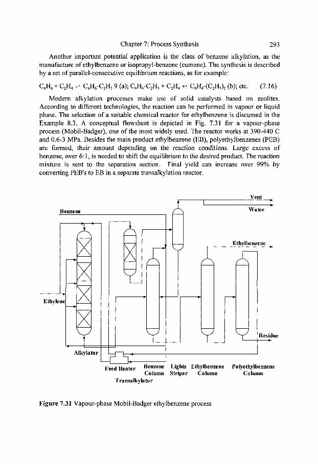
Chapter 7: Process Synthesis 293
Another important potential application is the class of benzene alkylation, as the manufacture of ethylbenzene or isopropyl-benzene (cumene). The synthesis is described by a set of parallel-consecutive equilibrium reactions, as for example:
C6H 6 + CEH 4 ~ C6H6-CEH 5 9 (a); C6H6-CEH 5 + CEH 4 ~ C6H4-(CEHs)2 (b); etc. (7.16)
Modem alkylation processes make use of solid catalysts based on zeolites. According to different technologies, the reaction can be performed in vapour or liquid phase. The selection of a suitable chemical reactor for ethylbenzene is discussed in the Example 8.3. A conceptual flowsheet is depicted in Fig. 7.31 for a vapour-phase process (Mobil-Badger), one of the most widely used. The reactor works at 390-440 C and 0.6-3 MPa. Besides the main product ethylbenzene (EB), polyethylbenzenes (PEB) are formed, their amount depending on the reaction conditions. Large excess of benzene, over 6"1, is needed to shift the equilibrium to the desired product. The reaction mixture is sent to the separation section. Final yield can increase over 99% by converting PEB's to EB in a separate transalkylation reactor.
Benzene
Ethylen
Aikylator
v
Vent
Water
r
Feed Heater Benzene Lights Ethylbenzene Column Striper Column
Transalkylator
Ethylbenzene
/ ~ ....
Y Residue
Polyethylbenzene Column
Figure 7.31 Vapour-phase Mobil-Badger ethylbenzene process

294 Chapter 7: Process Synthesis
The above flowsheet can be simplified tremendously by catalytic distillation. Figure 7.32 depicts a conceptual configuration. The RD column consists of a reactive zone at the top, and a distillation section at the bottom. The reaction mixture is sent to a purification column, from which ethylbenzene is obtained as top distillate. A side- stream containing PEB is sent to transalkylation for EB recovery. Obviously, the feasibility of this process depends largely on the availability of an active and selective catalyst. For zeolites the optimal operating conditions are about pressure around 3 MPa, temperature less than 200 ~ and reaction rate capable to give a space-time of-~5 h -1 for almost complete ethylene conversion.
Figure 7.32 Reactive distillation column for ethylbenzene production.
The development of reactive separation processes is a complex activity that requires advanced knowledge in various domains, as catalysis, computer modelling, hydraulics of internals, etc. The state-of-the art in reactive distillation can be found in recent reviews (Taylor & Krishna, 2000), as well as in specialised books, as Doherty & Malone (2001), and Stichlmair & Fair (2000).
7.13 ECONOMIC POTENTIAL AFTER SEPARATIONS
After developing the separation system, the computation of the Economic Potential at the Level 4 becomes:
Economic Potential for Level 4
EP 4 = {Product value} + {By-product value} - {Raw-mat. costs}- - {Reactor costs} - {Recycle costs} - {Separation costs}
(7.17)

Chapter 7: Process Synthesis 295
The Economic Potential at Level 4 can be used to optimise the performances of the reaction and separation subsystems with respect to raw material consumption and the reactor conversion. Lower conversion gives in general better selectivity, but means higher recycle rates and higher cost of separations, as well as for the transport of fluids. Higher conversion gives lower costs for operations depending on throughput, as transportation and heating/cooling, but gives more sub-products and impurities. Therefore, at higher conversion the cost of separations increases sharply since more constraints on purity specifications, and more separation units necessary to remove impurities. The difficulty in optimisation consists of finding simple but reliable cost estimation of different units as function of throughput and separation performance. Case Study in Chapter 17 presents such calculation for the HDA process.
After completing the flowsheet, it is useful to reconsider the discussion about optimisation. In this respect, the key design variable is the conversion of the main reaction. Figure 7.33 illustrates the variation of the Economic Potential during the flowsheet synthesis at different stages. A minimum EPmi n is necessary to continue the flowsheet development. At the Level 2 (input/output), an upper boundary on conversion can be set because sharp decrease in selectivity afterwards. At this point, it would be interesting to consider other reaction conditions, or other catalyst. At the Level 3 (reactor and recycles) a low bound of conversion can be set, because of the cost of recycles, particularly high when transporting gases. At Level 4, where the cost of separations is accounted for, the two bounds get closer to each other. A feasible domain can be defined, where the optimal conversion is located.
Typical for the chemical processes is that the region around optimum is rather flat. Thus, the effort to locate accurately this optimum is not essential at the process synthesis stage. Here we just state that steady state optimum is not always the most convenient from operability and controllability viewpoint. A certain back-off from optimum is necessary to ensure flexibility in production rate, as well as robust control faced to different disturbances. This issue will be handled in Chapter 13.
Figure 7.33 Optimal conversion at different levels of the process synthesis by the Hiearchical Approach

296 Chapter 7" Process Synthesis
Hence, at the level Reactor-Separators-Recycles the material balance can be brought in a narrow optimal region. On this basis can be started the process integration steps regarding the optimal management of energy, mass separation agents, process water, waste minimisation, etc.
7.14 S U M M A R Y
Hierarchical Approach is a simple but powerful methodology for the synthesis of process flowsheets. It consists of a top-down analysis organised as a clearly defined sequence of tasks grouped in levels. Each level solves a fundamental problem as, number of plants, input/output structure, reactor design and recycle structure, separation system, energy integration, environmental analysis, safety and hazard analysis, and plantwide control. At each level, systematic methods can be applied for the synthesis of subsystems, as chemical reaction, separations, or heat exchangers network.
In applying the methodology, the designer has to identify dominant design variables and take design decisions. As a result, a number of alternatives are produced that are submitted to an evaluation procedure based on economical and technological criteria. In principle, at each level only one alternative could be retained for further development, so that the procedure leads finally to a good 'base-case'. This serves for improvement and optimisation, namely by applying Process Integration techniques.
Thus, the major merit of the Hierarchical Approach is that it offers a consistent frame for developing alternatives rather than a single design. The final solution is never unique, depending on a number of design decisions and constraints.
The key result of the Hierarchical Approach is the development of the basic flowsheet structure, formed by Reactor-Separations-Recycles. This structure defines the material balance envelope. In this respect of highest importance is the behaviour of the reaction system, which should deliver a realistic image of the reaction mixture. Other constraints regarding the reactor operation, as molar ratio of reactants, or safety requirements, are determinant for the structure of recycles. Optimal conversion represents a complex optimisation problem between the valorisation of raw materials and the cost of reactor, separators and recycles.
The Hierarchical Approach developed in this chapter incorporates a knowledge- based procedure for the synthesis of separations. This consists of dividing the separation section in three subsystems: gas & vapour, liquid and solid separations. Each subsystem is further managed by selectors, which makes use of unit operations. Split sequencing is based mainly on heuristics, although may include algorithmic or optimisation techniques. This chapter describe in more detail the synthesis of distillation trains for zeotropic distillations, the non-ideal case being left for the Chapter 9.
After solving the material balance problem, the next step is the energy integration. Here we can apply a powerful systematic methodology, Pinch Point Analysis, which will be the object of Chapters 10 and 11. Integration of controllability and operability will form the object of Chapters 12 and 13. Integrating other elements of design, may

Chapter 7: Process Synthesis 297
require the revision of some elements of the material balance, namely the operation parameters, but, in principle, not the basic structure of the flowsheet.
Finally, the flowsheet structure and the performances of the integrated design have a determinant role on process profitability. The heat and material balance built upon supplies the key elements for investment and operation costs.
7.15 R E F E R E N C E S
Agreda, V.H., L. R. Partin, W.H. Heise, 1990, High-purity methyl acetate via Reactive Distillation, Chem. Eng. Progr., 86, February, 40-46
Allen, D.T., K., S. Rosselot, 1996, Pollution Prevention for Chemical Processes, Willey Bildea, C. S., A. C. Dimian, 1998, Stability and Multiplicity Approach to the Design of Heat-Integrated PFR, AIChE J, vol. 44, 2703-2712 Barnicki, S.D., J.R. Fair, 1990, Separation System Synthesis: A knowledge based
approach: 1. Liquid Mixture Separations, Ind. Eng. Chem. Res., 29, 431-439 Barnicki, S.D., J.R. Fair, 1992, Separation System Synthesis: A knowledge based
approach: 2. Gas/Vapour mixtures, Ind. Eng. Chem. Res., 31, 1679-1694 Barnicki S. D., J. J. Siirola, 1997, Separation system synthesis, in Kirk-Othmer
Encyclopedia of Chemical Technology, 4 th edition, vol. 21,923-962 Crowl, D., J. F. Louvar, 1989, Chemical Process Safety: Fundamentals with
Applications, Prentice Hall, Cusack, R. W., 1991, Chem. Eng., 98(2), 66-71 Dimian, A. C., 1996, Process Integration course, University of Amsterdam, Dimian, A. C., 1997, Compact distillation system, in Distillation & Absorption '97,
IChemE, Symp. Ser. 142, 279-288 Douglas, J. M., 1988, Conceptual Design of Chemical Processes, McGraw-Hill Publ. Douglas, J. M., 1995, Synthesis of separation system flowsheets, AIChEJ, 41,252 Doherty, M.F., G.A. Caldarola, 1985, Design and synthesis of homogeneous azeotropic
distillation, Ind. Eng. Chem. Fundam., 24, 474-485 Doherty, M., M. Malone, 2001, Synthesis of Distillation systems, McGraw-Hill Douglas, J., G. Stephanopoulos, 1995, Hierarchical Approaches in Conceptual Design:
framework and computer implementation, Foundations of Computer Applications in Process Design (FOCAPD), AIChE Publ.
Gary, J.H., G.E. Handwerk, 1994, Petroleum Refining, Marcel Dekker Glinos, K., Malone, M., 1988, Optimality regions for complex column alternatives in
distillation systems, Chem. Eng. Res. Des., 66, 229-240 Han, C., G. Stephanopoulos, J. M. Douglas, 1994, Automation in design: The
conceptual synthesis of chemical processing schemes, in Paradigms of Intelligent Systems in Process Engineering, Advances in Chemical Engineering Series, Academic Press
Ho, W. S., K. K. Sirkar, 1990, Membrane Handbook, Van Nostrand-Reinhold Kister, H. Z., 1992, Distillation Design, McGraw-Hill

298 Chapter 7: Process Synthesis
Kletz, T., 1999, Hazop and Hazan: Identifying and Assessing Process Industry Hazards, Hemisphere Publ.
Malone, M. F., M. F. Dogerthy, 1996, Separation system synthesis for non-ideal liquid mixtures. Foundations of Computer Aided Process Design, p. 9-18
Perry's, 1997, Chemical Engineers Handbook, 7th edition Schweitzer, P. A (editor), 1988, Handbook of Separation Techniques, Mc-Graw Hill Seader, J. D., E. J. Henley, 1998, Separation Process Principles, John Wiley Siirola, J.J., 1996, Industrial applications of chemical process synthesis, in Advances in
Chemical Engineering, vol. 23, Process Synthesis, Academic Press Sinnott, R. K., 1993, Coulson and Richardson's Chemical Engineering, vol. 6,
Pergamon Press Smith, R., 1995, Chemical Process Design, McGraw-Hill Stichlmair, J., J.R. Fair, J. L. Bravo, 1989, Separation of azeotropic mixture via
enhanced distillation, Chem. Eng. Progress, 85(1), 63-69 Stichlmair, J., J. R. Herguijuela, 1992, Separation regions and processes of zeotropic
and azeotropic ternary distillation, AIChEJ, 38, p. 1523-1535 Stichlmair, J. G., J. R. Fair, 1999, Distillation, Principles and Practice, Willey-VCH Strathmann, H., 1990, Membrane and Membrane Separation Processes, Ullmann's
Encyclopaedia of Industrial Chemistry, vol. A16 Taylor, R., Krishna, R., 2000, Modelling reactive distillation, Chem. Eng. Sci., 52,
993-1005 Tedder, D. W., D. F Rudd, 1978, Parametric studies in industrial distillation, AIChEJ
24,303-334 Thompson, R., W., C. J. King, 1972, Systematic synthesis of separation systems,
AIChEJ, 18, 941 Westerberg, A.W., O. M. Wahnshaft, 1996, Synthesis of distillation based separation
processes, in Advances in Chemical Engineering, vol. 23, Process Synthesis, Academic Press
Widago, S., W. D. Seider, 1996, Azeotropic distillation, AIChEJ, 42(1), 96-130

Chapter 8
SYNTHESIS OF REACTION SYSTEMS
8.1 Chemical reaction network 8.1.1 Stoichiometry 8.1.2 Reaction rate 8.1.3 Kinetics 8.1.4 Conversion and selectivity
8.2 Chemical equilibrium 8.2.1 Equilibrium constant 8.2.2 Equilibrium composition
8.3 Reactors for homogeneous systems 8.3.1 Reactor volume 8.3.2 Performance of ideal reactors in simple reactions 8.3.3 Performance of ideal reactors in complex reactions 8.3.4 Non-ideal reactor models
8.4 Reactors for heterogeneous systems 8.4.1 Solid catalysed reactions 8.4.2 Heterogeneous fluid/fluid reactors
8.5 Thermal design issues 8.5.1 Temperature profile 8.5.2 Stability of the thermal regime 8.5.3 Types of thermal design
8.6 Selection of chemical reactors 8.6.1 Reactors for homogeneous systems 8.6.2 Reactors for heterogeneous systems
8.7 Synthesis of chemical reactor networks 8.7.1 Attainable Region concept 8.7.20ptimisation methods
8.8 Further reading
8.9 Summary
8.10 References

300 Chapter 8: Synthesis of Reaction Systems
The reaction system is the core of a chemical process. It is also the starting point in process design. By proper selection and design of the chemical reaction system, the modem process plants must cope with large flexibility with respect to production rate and selectivity. A greater attention should be paid to the formation of by-products and impurities. The selection and the design of the reactor system must be done in the context of interactions with the whole process, particularly with the separation system.
The goal of this chapter is to analyse elements from chemical reaction engineering necessary to consider in the conceptual design of a process as a system. The chapter is organised as follows. Preliminary sections will review basic concepts with regard to stoichiometry and chemical equilibrium, as compulsory steps in evaluating the feasibility of a chemical process. Then, we will discuss design principles in the field of homogeneous reactions, with reference to the two ideal reactor models, mixed and plug flow reactors. These will be followed by heterogeneous reactors, where we will point- out the problems rather than to enter in detailed analysis. A larger attention will be paid to thermal design issues, related to safety and heat integration, both essential for flowsheet development. On this basis we will present some guidelines for the reactor selection. A final section is devoted to new systematic methods developed by the process systems community, in particular to the concept of Attainable Region.
8.1 C H E M I C A L R E A C T I O N N E T W O R K
8.1.1 Stoichiometry
The chemical transformation between the components involved in a network of chemical reactions can be described quantitatively by means of stoichiometric relations. In the case of multiple reactions, the stoichiometric relations form a system of linear algebraic equations:
S
Zvi.jAj = 0, i:1,.... , R (8.1) i=l
vij is the stoichiometric coefficient in the reaction i of the species j, the network consisting of S components and R independent reactions. The relation (8.1) may be extended to the atomic balance. If the atomic species are Ek (k = 1 .. . . ,N) and the atomic coefficients ~k, the material balance is constrained by the atomic balance as follows"
N
A, = e# j= 1,...., S (8.2) k=l
S
~j"vjejk = 0 , k=-l, ...., N (8.3) j= l

Chapter 8: Synthesis of Reaction Systems 301
It is worthy to note that only i ndependen t reac t ions must be employed to express the composition of a reaction mixture. This is usually the case of complex reactions, as the cracking of hydrocarbons, where much more stoichiometric equations may be written than strictly necessary. The number of independent reactions can be simply determined as the rank of the matrix of stoichiometric coefficients.
EXAMPLE 8.1 Stoichiometric independent reactions
The following reactions can be written for the catalytic reforming of methane with water, at high temperature:
C H 4 + H 2 0 - - - ~ C O + 3 H 2
C H 4 + 2 H 2 0 - - - ~ C 0 2 + 4 H 2
C O + H20----}CO 2 + n 2
C H 4 - - , C + 2 H 2
C O 2 + C --+ 2 C O
C + H 2 0 - + C O + H 2
Find the number of stoichiometric independent reactions.
(i) (ii) (iii) (iv) (v) (vi)
Solution. The species are: CH4, H 2 0 , H2, C O , CO2, and C. By convention, the stoichiometric coefficients for reactants are negative, and positive for products. The matrix of stoichiometric coefficients of the reactions (i) to (vi) is:
CH 4 H20 H 2 CO CO 2 C _
- 1 - 1 3 1 0 0 - 1 - 2 4 0 1 0
v = 0 - 1 1 - 1 1 0
0 0 0 2 - 1 - 1 0 -1 1 1 0 -1
-
The rank of the above matrix may be found by standard methods, for example by triangulation. After algebraic manipulations of rows and columns the final matrix is:
V =
-1 -1 - 3 -1 0 -1 1 -1 0 0 0 0 0 0 0 - 2 0 0 0 0 0 0 0 0
0 0 1 0
0 0 0 0 0 0 0 0

302 Chapter 8: Synthesis of Reaction Systems
There are three non-zero diagonal elements, so the rank of the matrix is three. As a result, there are three independent reactions, which might be for example the reactions (i), (ii) and (iv).
8.1.2 Reaction rate
In extensive manner the reaction rate can be defined as the rate of reactant consumption or product formation. Let's consider the singular reaction A--+products. By reference to the reactant A the reaction rate might be seen simply as-dN A /d t , being expressed in (moles of A transformed/time). More useful for design is an intensive definition, in which we may introduce an element characterising the reaction device itself, as volume, mass or contact surface. Here we adopt the convention that the reaction rate is positive for products and negative for reactants. Selecting the product j as reference, the following definitions of the reaction rate may be written (Levenspiel, 1999):
1 dNj moles j formed rj = -~-ff~- = (volum of fluid)(time) (8.4)
1 dNj moles j formed rj = - ~ - - ~ = (mass of solid)(time) (8.5)
1 dNj moles j formed = ( 8 . 6 )
rj = S dt (surface of contact)(time)
Equation (8.4) is suitable for homogeneous system, equation (8.5) is useful for fluid/solid catalyst reactors, while equation (8.6) is applicable for gas/liquid or liquid/liquid reactors.
We may express the variation of the number of moles in a reaction system in a generic manner by means of the molar extent of reaction ~, as:
Nj =Njo - v j~ (8.7)
Note that ~ characterises the reaction itself and not a particular component. Thus, for the stoichiometric independent reaction i we may define an equivalent reaction rate, as:
1 d~: i r i = - - ~ (8.8)
V d t
This time (i defines the molar extent of the reaction i. If the component j is implied in several reactions, the net reaction rate is given by:
R
rj = ~ v~,jr~ j=l,2, . .... ,S (8.9) i=1

Chapter 8: Synthesis of Reaction Systems 303
or in matrix notation:
[rj] = [vi,j][r~] (8.10)
The relation (8.10) can be used also to analyse kinetic experimental data in the case of complex reactions. Usually the number of species is much larger than the number of independent reactions. Therefore, it is sufficient to choose a number of R key species among the components that can be measured with good accuracy. Let's denote by 9tj the known measured reaction rates. Then the system can be solved to find the
rates of the individual reactions r~ as:
[F i ] __ [~j~j ][Vi,j ]-I (8.1 1)
The other species may be determined easily from the remaining set of equations (8.10). As example, we consider the following consecutive-parallel reactions, often found
in organic chemistry processes, as nitration, alkylation, chlorination, etc:
A + B--~ C + S r 1
C + B---> D + R r 2
D + B--+ E + F r 3
(8.12)
There are six chemical species and three reactions. We select A, B and C as key components. The matrix of stoichiometric coefficients is:
Ii' 111 1 [vq]= -1 -1 [vi3]-l= 0 0 -1
-1 0 0 -1 1 (8.13)
The equation (8.12) becomes:
[rl r2 r3 ]= [r,4 r8 rc 0 1
- 1
(8.14)
from which one gets:
r 1 =rA; r 2 = - r A - r c ; r 3 = 2 r A - r B +r c (8.15)
The reaction rates of the other species can be obtained from the relation (8.10) as:
r ]-[rl 1I!0,1 r 3 0 1 1 1 1
(8.16)
r~ = r 2 - r 3 ; r E =r~; r s =r~ + r 2 + r 3

304 Chapter 8: Synthesis of Reaction Systems
8.1.3 Kinetics
The reaction rate is a function of concentration, temperature and pressure. In a large number of practical cases, the reaction rate may be expressed as function of only temperature and concentration, as follows:
r, : f , ( T ) f 2 ( c j ) (8.17)
The dependency on temperature is given by the Arrhenius law:
f (T) = k 0 exp(-E / R T ) (8.18)
where ko is the pre-exponential factor and E the activation energy. The dependency on concentration can be formulated as a power-law function:
a p (8 19) . . . . . . .
In the relation (8.19) a,/3, ... are partial orders of reaction. Their sum gives the global order of reaction n = a + ,8 + .... If the reference component is A then the reaction rate is expressed in general by the following relation:
. . - E / RT . .a .~fl r A : ko~ ~A~ ... (8.20)
Note that the partial orders of reaction a, /3, ... correspond to the stoichiometric coefficients only for elementary reactions. In the case of non-e lementary react ions the apparent orders of reactions are different from stoichiometric coefficients, and more than one reaction step must be considered to explain the reaction mechanism.
It is worthy to note that there is a thermodynamic constraint in formulating kinetic expressions for reversible reactions: the partial reaction orders must be consistent at equilibrium. Let's examine the reversible reaction aA + bB ~-~ p P + r R , for which the following reaction rate expression is proposed:
a f t r: p - k 2 Cp c R r A =lqcAc ~ (8.21)
Since at equilibrium p r a b cec n = KccAcs , reaction orders and stoichiometric coefficients should respect the condition:
a : fl___ : ~ : p__ (8.22) a b p r
8.1.4 Conversion and selectivity
The molar extent of reaction ~: introduced previously has the disadvantage of an extensive variable, since depends on the amount of reactants. It is often more convenient to use convers ion as an intensive measure of a chemical transformation. The use of a re ference reactant is compulsory. If NAo is the initial molar amount of the
reactant A, and N A the amount after reaction, the conversion X A is by definition:

Chapter 8: Synthesis of Reaction Systems 305
. S A NAo - NA
NA0 (8.23)
The number of moles of other species can be expressed as function Of XA, as follows"
vj (8.24) Nj = Njo + ~ N A o X A a
The total number of moles in the system is:
A v Nt = N O + NAO X A (8.25)
a
From (8.7) and (8.24) it follows that the link between conversion and molar extent of reaction is simply:
a X A = ~A0 ~: (8.26)
The use of conversion is suited for simple reactions, while the molar extent of reaction is more convenient for multiple reactions. In this case a molar extent of reaction ~i can be attributed to each independent reaction. The number of moles of component j involved in R reactions is:
R
Nj = Njo + ~ vi,j~ji (8.27) i=1
The total number of moles becomes"
S R R
Art = N O + ~ ~ v,.j~ i = N O + ~ A vi~: , (8.28) j=l i=1 i=1
where Av i is the variation of the number of moles in the reaction i. Selectivity and yield are important concepts when dealing with multiple reactions.
Three types of components are of interest: reactants, including the reference, main product, and by-products. In this book we use the following definitions:
Amount of useful product formed Selectivity (o) = (8.29)
Amount of reference reactant transformed
Amount of useful product formed Yield (rl) = (8.30)
Initial amount of reference reactant
Let's consider the simple reaction a A + b B ~ p P + r R, where A is the reference reactant and P the desired product. Note that the above relations must take into account the stoichiometric coefficients. The following relations define selectivity and yield:

306 Chapter 8: Synthesis of Reaction Systems
a N e Crp/A = (8.31)
P NAo - N4
a Np r/p/A = - - ~ (8.32)
P NAo
Yield, selectivity and conversion are linked by the relation:
rip/A = cre/AX A (8.33)
EXAMPLE 8.2 Selectivity of complex reactions
The following reactions may be considered at the catalytic burning of ammonia:
4NH 3 +502 ~ 4NO+6H20 (i) 2NO+O 2 ~ 2NO 2 (ii) 2NO ---> N 2 + 0 2 (iii) 4NH 3 +302 ---> 2N 2 +6H20 (iv) 4NH 3 +6NO ---> 5N 2 +6H20 (v) N 2 +O 2 ---> 4NO+6H20 (vi)
The feed reaction mixture has the following composition: N H 3 - 20%, N O 2 - 2%, NO - 3%, N2- 5%, 02 - 35%, H20 - 5%, the rest being other inert gases. The following molar fractions have been measured at the reactor exit: YNH3=0.086, YNo2 = 0.1075, YN2=0.064. Determine the conversion of ammonia. Calculate the amounts of NO and NO2 for 2000 Nm3/h initial mixture. Determine yield and selectivity in nitric oxides, the reference reactant being ammonia.
Solution. Following the example 8.1 three reactions are stoichiometric independent. We select the reactions (i), (ii) and (iii) with the extent of reaction ~1, ~2, ~:3, The numeber of moles of each component is: NH3: N1 = N~o - 4~ NO2: N2: N3 = N3o + ~3 02: H=: Ns = Ns0 + 6~1 NO: Inert: N7 = NT0 Total flow: Nt = Nt0 + ~l - ~2 The molar fractions at the reactor exit are:
N== + - - +
N6 = N6o + 4 { , - 2{2- 2~3
N~o - 4 ~ N2o + 2S>l Yl = Y2 =
N,o N,o Y3 - -
N3o +~3 N,0

Chapter 8: Synthesis of Reaction Systems 307
It is convenient to use as variable the extent of reaction referred to the initial number of moles ~ni = ~i / N to . The above equations becomes:
0 . 2 0 - 4~n 1 0.02 + 2~,,2 0.05 + ~,1 Yl = =0.086 Y2 = =0.1075 Y3 = =0.064
By solving the system it comes: ~:n1=0.0288, ~n2=0.0428 and ~nl=0.0131. The other molar fractions are y4=0.1788, y5=0.226, y6=0.0334, y7=0.3043. The ammonia conversion is from definition: XNH3 = 1-N1/N10 = 1-(Yl0 -4~:,1)/y~o = 0.576.
The molar flow rates are:
Input: Fo = 2000/22.4 - 89.285 kmol/h.
Output: F = Fo (1 + ~.1 - ~n2) = 88.036 kmol/h. The flow rates of the main components are:
Input Output Change N H 3 17.857 7.571 -10.386 NO 2.678 2.940 0.262 N O 2 1.786 9.460 7.678
By definition the yield is obtained as the amount of product formed divided by the initial reference reactant: In molar units the yield for NO and NO2 is respectively"
0.262 7.678 = ~ 100 = 1, 47% , rkvo2/NH3 =
tiN~ 17.857 17.857 100=43%
The selectivity in the two products is obtained dividing the amount of product formed by the amount of reference reactant transformed. One gets:
0.262 7.678 = ~ 1 0 0 = 2.522% O'NO2/UH 3 -- 100 = 73.93%
crN~ / N~/3 10.386 ' 10.386
The above values verify the relation between conversion, yield and selectivity.
8.2 C H E M I C A L E Q U I L I B R I U M
Chemical equilibrium is a key issue in process design. Chemical equilibrium might set in many cases an upper limit for the achievable conversion, if nothing is done to remove one of the products from the reaction space. Because the equilibrium conversion is independent of kinetics and reactor design, it is also convenient to use it as reference. Note that important industrial reactions take place close to equilibrium, as the synthesis of ammonia and methanol, esterification of acids with alcohols, dehydrogenations, etc, particularly when the reaction rate is fast. Therefore, the investigation of chemical equilibrium should be done systematically in a design project.

308 Chapter 8: Synthesis of Reaction Systems
8.2.1 Equilibrium constant
The analysis of chemical equilibrium is based on the concept of chemical potential (Chapter 5). Consider a homogeneous gaseous system. The chemical potential fij of a componentj in a mixture is given by:
~tj (P, T, yj ) = ,u ~ (T) + RT In ~ (8.34)
o pj is the chemical potential of the pure component, function only of temperature, j"j is the fugacity of the component j in mixture, depending on pressure, temperature and composition. The over-hat designates a component property in a mixture. In the case of singular reaction involving S components the following relation describes the chemical equilibrium:
s
A a ~ = ~ h , = 0 (8.35) j=l
In the case of R multiple reactions a similar expression is:
R S
A a ~ - = 0 (8.36) i=1 j= l
From (8.36) we find the following definition for the equilibrium constant:
A G ~ (8.37)
where AG o is the variation of Gibbs free energy of the system given by: 0 o
A c ~ ( r ) = Z ~j~,o = (~j~,)~o~u~,~ - (~j~,,)ro.o,~,~ (8.38)
The equilibrium constant K f based on fugacity is given by:
S
K f = I - - [ ) 2 j (8.39) j= l
By convention the stoichiometric coefficients vj are positive for products and negative for reactants. Similarly with (8.37) for multiple reactions we obtain a system of equilibrium relations"
AG ~ (V) = - R T l n KI, , i=l,2,...R (8.40)
Now, the problem is to express fugacity as function of P, T and composition, and on this basis to determine the equilibrium composition. Two possibilities exist: assume ideal or real solutions.

Chapter 8" Synthesis of Reaction Systems
a. Ideal solutions.
In the case of ideal solutions the Lewis-Randall approximation can be used:
309
L :joy =
The equilibrium constant becomes:
K f = K y K ~ P Av
(8.41)
(8.42)
s s
where Ky = H Y~J' K~ = H (r176 and A v = ~ Vj,p~od~c,~ - ~ Vj,reactants �9 j= l j=l
Note that the equilibrium constant of fugacity coefficients of pure components K~ is independent of composition, and can be calculated with a suitable equation of state, as Viral or cubic EOS. The pressure correction pay depends on the variation of the number of moles. It follows that the equilibrium composition may be calculated from Ky, by expressing the composition of each species as function of conversion or of the molar extent of reaction.
b. Real solutions
In this case the component fugacity is j~j = ~jPyj , where r is the fugacity coefficient of the component that now considers the effect of composition. This can be accounted for by means of mixing rules (see Chapters 5 & 6). Equation (8.42) remains formally valid, but takes now into account the equilibrium constant of fugacity coefficients
s Kd = H ( ~ j ) vj . For liquid phase reactions the treatment is similar, by replacing
J=l
fugacity with activity. Because the relation a j =yjx~links the activity with
composition, we obtain:
K a = K r K x (8.43)
s
The equilibrium constant of the activity coefficients K r = H Y~J can be calculated by j= l
means of a liquid activity model (see Chapter 6). The case of heterogeneous equilibrium is more difficult, but less frequent in
practice. Supplementary material may be found in more specialised books on thermodynamics.

310 Chapter 8: Synthesis of Reaction Systems
8.2.2 Equilibrium composition
In the case of simple reactions, the equilibrium composition can be calculated by solving the equation (8.39) with conversion as variable for chemical transformation. On the contrary, the extent of reaction is more suitable for multiple reactions. The solution may be obtained by solving a system of algebraic equations of type (8.40).
A second possibility to calculate the equilibrium composition is by Gibbs free energy minimisation. The starting point is the system of equations generated by the relation (8.36). Phase equilibrium may be included in analysis. This method is particularly powerful, because it does not imply necessarily the knowledge of the stoichiometry. However, the user should consider only species representative for equilibrium. As in any optimisation technique, this approach might find local optimum. Specifying explicitly the equilibrium reactions is safer.
The effect of temperature on equilibrium is given by van 't Hoffequation:
d ln K AH n = (8.44) dT RT 2
K stands for either Kf or Ka, while AH n is the heat of reaction. If the reaction is exothermic (negative heat effect) then both equilibrium constant and conversion decreases with increasing temperature. On the contrary, in endothermic reactions the equilibrium conversion increases with the temperature (Fig. 8.1).
The above discussion has important practical consequences. In endothermic reactions the operating temperature must be kept as high as possible, while in exothermic reactions the temperature should follow an optimal profile, which should start at higher temperature and ends-up at lower temperature.
Irreversible reaction . . . . . . . . . . . . . . . . . . . . . . . . . . . . . . . . . . . . . . . . . . . . . . . . . . . .
E x o t h ~ - E~"~nd othermic XA e reac
0 Temperature
Figure 8.1 Effect of temperature on equilibrium conversion
8.3 R E A C T O R S F O R H O M O G E N E O U S S Y S T E M S
In this section we will review basic equations for calculating the reaction volume necessary to achieve a given conversion for simple reactions.

Chapter 8" Synthesis of Reaction Systems 311
8.3.1 Reactor volume
We may distinguish between two approaches in calculating the volume of a chemical reactor: kinetic and shortcut design. In kinetic design, at least the kinetics of the main reaction must be known. Perfect mixing and plug flow are known as 'ideal models', as CSTR and PFR, respectively. Real models, with intermediate degree of mixing, can be described as combinations of ideal models.
a. Continuous Stirred Tank Reactor (CSTR).
In a CSTR the reaction rate is uniform in space and constant in time, at the level of exit concentrations (Fig. 8.2). At constant volume V the material balance of the reactant A is:
v dcA = FA, o - F A - ( - r A ) V (8.45) dt
At steady state the following 'characteristic equation' is obtained:
V XA I V cAoXAj (8.46) - - = ~ or r = ~ = ~ FAo -rAi Qvo - rAi
where the subscript f refers to the outlet conditions. The equation (8.46) can be used to calculate the reaction time r and the reaction volume V for a given conversion.
Figure 8.2 Illustration of a Continuous Stirred Tank Reactor
For multiple reactions, the solution of the characteristic equation involves a system of algebraic equations as follows"
V cj -Cjo cj -Cjo r . . . . . R (8.47)
Qvo rj E vi,jri i=1
R
We may write c j - c j 0 = ~ Vi,j~vi , making use of the extent of reaction with reference i=1
to the reaction volume, ~'~ = ~'~ / V . The equation (8.47) becomes:
R R
r~-' vi jr ~ = ~ vi,j~:vi , j = l , 2 , . ..... ,S (8.48) i=1 i=1

312 Chapter 8" Synthesis of Reaction Systems
The equation (8.48) is equivalent with the following system of algebraic equations:
~vi = r ri(~vl,~v 2 ...... $:v,) , i=1,2,...., R (8.49)
The system (8.49) is non-linear but can be solved by means of standard techniques.
b. Plug Flow Reactor (PFR).
In a PFR the component concentrations and the reaction rate vary continuously along the reactor length (Fig. 8.3). A component balance on an infinitesimal volume gives:
FAo dX A = -rAdV (8.50)
The elementary volume is dV = Sdz, where S = 7fi5/2 / 4 and d the reactor diameter. By
introducing the specific molar flux of the reference reactant A, FAo = FAo/S , the characteristic equation of a PFR can be written in differential form as:
dX-----A-A = -rA ( X ) (8.51) dz FAo
The equation (8.51) can be integrated analytically or numerically for simple reactions in isothermal conditions to get the reactor volume or the space-time defined as r = V / Qvo.
x A.~ dX A x ~~ dX A (8.52) = or r = CAo
V FAo _r~-(-~A ) o - r A ( X A )
Figure 8.3 Illustration of a Plug Flow Reactor
For multiple reactions, the set of the stoichiometric independent reactions must be integrated simultaneously. Molar extent of reaction is more convenient as reaction variable, at best by reference to the total mass flow $:mi = ~ i / m . The mass balance equations become:
d~m, ri(~m,,~m2 ..... ) dz G
, i = 1,2, ...., R (8.53)
where G - G / S = pu z is the mass flux, G being the total mass flow rate, also the

Chapter 8: Synthesis of Reaction Systems 313
product between mass density p and linear velocity u~. For non-isothermal operation the heat balance equation must be considered. It is
easy to demonstrate that the equation giving the temperature profile may be written as:
dT 1 n 4U ( T _ L ) (8.54) : L./L.. p"~'r~ Zi=l ( - r , ) ( -MEn,,) - ,J~Cp d
The heat involved in each independent reaction is the product of reaction rate (-r~) by the heat of reaction (-AHR. i ). The heat transferred is proportional with the overall heat transfer coefficient U and the temperature difference (T-T a) between the reaction mixture and the thermal agent. Hence, the solution of the equations (8.53-54) will produce profiles of concentrations and temperature.
The computation methods described above require the knowledge of reaction kinetics. Unfortunately, this is not the case in a large number of cases, particularly in an evaluation project. In this case shortcut methods are handy, in which the reactor volume may be estimated from information about the residence time. The following definitions of the reaction time are mostly used:
�9 Space-time r as the ratio of reactor volume V by the inlet volumetric flow Qv.o
~ : V / Q~,o (8.55)
�9 Space-velocity as the reciprocal of the space time:
S V : I / r (8.56)
Three measures for space-velocity (measured in hour -I ) in are commonly used: �9 LHSV (liquid) = (inlet liquid flow rate at STP~/reactor volume); �9 GHSV (gas space velocity) -- (inlet gas flow rate at STP/reactor volume); �9 WHSV (weight space velocity) = (inlet mass flow rate / mass of catalyst).
In order to avoid severe errors attention has to be paid to the units used in the above definitions. If the reaction volume can be reasonably estimated by short-cut calculation, then some hydrodynamic constraints, as the allowable pressure drop, or minimum / maximum fluid velocities, are other elements used to asses the final sizing.
8.3.2 Per formance of ideal reactors in simple reactions
Let's consider the reaction A -->products with the kinetics - r A - kc" A . Figure 8.4 shows a graphical qualitative comparison between the volumes of a CSTR and a PFR needed to reach the same conversion. It may be observed that for a n-th order reaction a PFR needs always a smaller volume than a CSTR, the difference being significant at high conversion of A. The explanation is that in a CSTR the reaction rate is lower than in a PFR, being limited at the value of the final concentration.
l STP stands for standard temperature an pressure

314 Chapter 8: Synthesis of Reaction Systems
Figure 8.4 Qualitative comparison of CSTR and PFR reactors
Figure 8.5 presents a quantitative comparison for first-order and second-order reactions. It may be observed that at low conversions, say below 30%, the difference in volumes is small. The choice between CSTR and PFR is determined by other considerations, as the need of mixing for a better contact, heat transfer rate, safety, or mechanical technology. However, the difference in reaction volumes becomes considerable at conversions larger than 90%. For a first-order reaction at XA=0.99 the ratio Vcs'rp,/VpFR is 10, while for a second-order reaction this ratio becomes 100.
100
VCsTRNpFR
10
i !!!!1 ! !; !!! !i!!!ii ! . . . . . . I. ' _ _ L _ L _ ' _ L _ , r ) _l , , ~ ,.
0.01 0.1 1-XA 1
Figure 8.5 Comparison of CSTR and PFR for first and second-order reactions
A question arises: how to reduce this difference? The solution consists of using a series of CSTRs instead a single PFR. Since the reaction rate is higher in each intermediate volume, finally a much higher productivity than in a single equivalent reactor is obtained (Fig. 8.6). At limit, an infinite series of CSTRs behaves as a single PFR of the same volume.

Chapter 8: Synthesis of Reaction Systems 315
Figure 8.6 Series of CSTRs
Let's examine an isolated reactor l in a series. The characteristic equation is:
cA,t-1 Qv,I-1 = 1 + (-rA,t) rt (8.57) C A,l Qv,! CA,1
For first-order reaction and constant density mixture the analytical solution is:
N
= i - i ( 1 + k , , , ) (8.58) CA,N l=1
A graphical method can solve elegantly the design of a series of CSTR for any kinetics in the case of a single reaction. In a diagram - r A = f(c4 ) lines with the slope
- 1 / r t are drawn starting from CA0. The segments needed to reach the final concentration CAr give the number of reactors.
100
VnCSTRNpFR
lO
1 0.01 0.1 1-XA 1
Figure 8.7 Comparison of performance of a series of n equal-size CSTRs and a PFR

316 Chapter 8: Synthesis of Reaction Systems
Figure 8.7 illustrates the difference between a series of CSTRs and PFR for first-order reaction. Similar results may be shown for second-order reactions. Diagrams are presented in standard textbooks (Levenspiel, 1999). It may be observed that the improvement is considerably already starting with only two reactors. Hence, a series of CSTRs can replace advantageously a single large reactor, particularly when high conversions are desirable. The series of CSTRs may consist of individual units, or compartments arranged in the same unit.
8.3.3 Performance of ideal reactors in complex reactions
The relative performances discussed before, valid for single reactions, consider only the productivity as comparison criteria. In the case of multiple reactions the issue is the selectivity to the desired product.
a. Parallel reactions
Consider the following parallel reactions:
a A--->P , r p - k l C A
A --~ R , r R - k z c ~
P is the desired product, while R is a waste. The relative rate of formation of P to R is:
r e : k, c,~_ p (8.59) rn k2
The selection of a suitable reactor can be analysed by means of the following heuristics: �9 If the desired reaction has a higher reaction order than unwanted reaction ( a >/3 ) a
high reactant concentration is favourable; PFR or batch reactors are suitable. �9 If the desired reaction has lower reaction order than the unwanted reaction ( a </5' ),
the reactant concentration should be kept low. CSTR at high conversion should be chosen, although the required reaction volume is large.
�9 If a = tithe concentration has no effect. The only way to control the product distribution is by modifying the ratio k 1 / k 2 . The activation energies of the competing reactions should be examined. If E1 > E 2 the reaction temperature should be maximised. If E~ < E 2 the reaction temperature should be kept low. However, in this situation much more efficient is to search a suitable catalyst.
b. Series reactions kl ks
Consider the first-order reactions A---> P---> R, where P is the main product and R the by-product. The formation of P or of any other intermediate is maximised when fluids of different compositions at different stages of conversion are not allowed to mix.

Chapter 8" Synthesis of Reaction Systems 317
Therefore, PFR or batch reactor will give a better yield of P as CSTR. In the first case, the maximum concentration of P is given by:
Cp,m~ / C~o = (kl / k2 )k2/(k2-k,) (8.60)
as well as the optimum residence time:
r p,op, = ln( k 2 / k~ ) / ( k 2 - k~ ) (8.61)
t , ~ 0 . 6 !
t , ~ 0 . 4 v
O
1
�9 kz/kl=(l.~'~ 0.8 " ' , .
"k21kl = 1 ~ ',
0 . 2 . . . .
I t t i
0 0.2 0.4 0.6 0.8 XA 1
Figure 8.8 Comparison of selectivity in CSTR and PFR
Figure 8.8 gives a comparison of selectivity in CSTR and PFR models. PFR gives always a better selectivity. The advantage is significant if the secondary reaction is slower than the main reaction. When the by-product formation is fast then the mixing pattern has less importance. Low conversions give always better yield in intermediates. However, a large amount of unconverted reactant has to be recovered and recycled. The cost of separations may be determinant in the overall plant economics. Thus, the reactor selection should be evaluated against the cost of separations.
e. Series-parallel reactions
As example, we examine the reactions:
kt
A + B - - + P (8.62)
k2
P + B---~R
The designer has a wide choice in manipulating variables and mixing patterns. However, these reactions can be analysed in terms of their constituent reactions. The optimum contact device for favourable product distribution is the same as for the constituent reactions. (Levenspiel, 1999). If P is desired, the above reaction system can be analysed by analogy with the series reaction A ~ P ~ R. In this case PFR gives always a higher yield in intermediate, the feeding policy of B being irrelevant.

318 Chapter 8: Synthesis of Reaction Systems
As mentioned, selectivity is the key issue in selecting a chemical reactor for multiple reactions. Typically, high selectivity might be obtained at low conversion, but this implies a large amount of reactant to be recycled. Heuristics do not offer simple solutions. Again, the design of the reactor should be seen not isolated, but in the context of the separations with recycles The type and the size of reactor, as well as the operating parameters should be optimised against the cost of separations. This is possible by taking advantage from the optimisation capabilities offered by the flowsheeting programs.
8.3.4 Non-ideal reactor models
Continuous stirred tank and plug flow are ideal mixing patterns. Real reactors may deviate considerably from these models. The following aspects could affect the behaviour of a real reactor:
�9 Residence time distribution (RTD). �9 The state of aggregation (micro- and macro-fluids). �9 The earliness and lateness of mixing.
The two latest factors are difficult to handle, so that we may assume as workable hypotheses micro-fluid state and perfect mixing of reactants at the reactor inlet. It remains the problem of the residence time distribution. This can be solved by adopting one of the following methods:
�9 Compar tment model. A real reactor may be approximated by the combination of zones with ideal mixing patterns, as perfect mixing or plug flow, connected by streams (Figure 8.9). The volume of different zones and the corresponding flows can be optimised to fulfil some criteria of productivity or selectivity. The idea has been developed in the recent years in a much more sophisticated manner. Ideal models may be assembled in a 'superstructure', from which the final configuration are determined by means of optimisation techniques. This topic will be discussed later in this chapter. �9 Tank-in-series model. A series of CSTRs can be used to describe moderate deviations from the plug flow. The approach is much simpler than dispersion models, and can be easy implemented in a process simulator.
Figure 8.9 Modelling of a real reactor by compartments with ideal mixing pattern

Chapter 8" Synthesis of Reaction Systems
8.4 R E A C T O R S F O R H E T E R O G E N E O U S S Y S T E M S
319
In the case of a heterogeneous reaction the overall process rate must consider the kinetics of both chemical and physical steps. If a very slow step can be identified, this controls in generally the global reaction rate. More often, the analysis should consider several limiting steps, both of physical and chemical nature. Therefore, the computation of the reaction rate in heterogeneous systems requires information that is hardly available at the conceptual stage.
Flow modelling of each phase is another difficult problem. Simplified assumptions are often not realistic. The hold-up of the reacting phase is particularly important, depending on the design and hydrodynamic characteristics of the reaction device.
Therefore, the analysis of heterogeneous reactions is a complex topic, out of the scope of this book. We limit the discussion only at basic aspects regarding the selection of the reactor, as well as the simulation of the reactor system at conceptual design stage.
8.4.1 Solid catalysed reactions
1. Kinetics
a. Rate of catalysed reaction
A catalysed reaction is a result of several steps involving adsorption on active sites, reaction between sites and desorption from sites. Following Langmuir-Hinselwood- Hougen-Watson (LHHW) approach, the reaction rate has the form:
(kinetic term)(driving force) --rA= (8.63)
adsorption term
In design is more rational to replace a multi-constant formula by a local valid first-order kinetics, which can be combined easy with other rate controlling steps.
b. Pore diffusion combined with surface kinetics
The pore diffusion can affect the reaction rate. Let's consider an isothermal particle. The actual reaction rate can be found by correcting the above surface reaction by an effectiveness factor c defined as:
c= actual reaction rate (8.64) surface reaction rate
The effectiveness factor can be determined as function of particle geometry L, effective pore diffusion coefficient Deffand the kinetic constant k. These can be put together in a
physical parameter called 'Thiele modulus' defined as L4k/De~. Analytical
expressions and graphical representations are available elsewhere (Levenspiel, 1999).

320 Chapter 8: Synthesis of Reaction Systems
c. Film temperature resistance
Exothermic reactions might display effectiveness factors larger than one because of the temperature gradient across the gas film. The calculation is complicated, but the assumption of isothermal particle is conservative for conceptual design.
d. Mass transfer resistance
Mass transfer across an external film may play a role in the case of very fast reactions, as combustions, or in the case of catalyst coated on surface. Correlations based on dimensionless number are available for a large spectrum of physical situations.
2. Types of reactors
a. Gas-solid catalytic reactors
Fixed bed reactors
Figure 8.10 presents various types: (a) single packed bed (b) multi-bed arrangements, (c) multi-tubular reactor. Single-bed type is suited for adiabatic operations, preferably for endothermic reactions. Multi-bed reactor is better suited for reversible exothermal reactions, as methanol or ammonia synthesis, where after-stage cooling is necessary to move away from equilibrium. Multi-tubular heat exchanger enables better temperature control, and is recommended in the case of high exothermal reactions.
The design of such gas-solid catalytic reactors can be approximated by a pseudo- homogeneous model with gas phase in plug flow. In the case of very exothermic reactions accounting for radial dispersion of heat and mass might be useful to prevent excessive particle overheating. The reaction time must find a compromise with the hydrodynamic design, namely the maximum gas velocity and pressure drop.
Figure 8.10 Types of fixed-bed catalytic reactor
Fluidised bed reactors
Intense mixing in a fluidised bed gives high mass & heat transfer rates, leading to good temperature control. Figure 8.11 presents two types: (a) stable catalyst, and (b) catalyst that needs regeneration. The last type is used in Fluid Catalytic Cracking (FCC) of hydrocarbon. The description of different models can be found in Levenspiel (1999).

Chapter 8: Synthesis of Reaction Systems 321
Figure 8.11 Fluid bed reactors
b. Gas/Liquid reactors on solid catalyst
The following discussion refers to the reaction:
A(gas) + bB(liquid) cat,,tyst > products (8.65)
Figure 8.12 presents the main types. Packed-bed reactor (a) is similar with an absorption column, where the packing can posses catalytic properties (coated catalyst), or host catalyst in special arrangements, as for example tea-bags. In the trickle-bed reactor (b) the gas dissolved or dispersed in liquid flows downwards through the bed of catalyst in co-current with the liquid phase. This reactor is suited for high-pressure operation and large ratios gas/liquid. In the last two devices, the catalyst dispersed in liquid as very fine particles is brought in contact with the gas either in a slurry bubble column (c), or in an agitated slurry reactor (d).
Figure 8.12 Types of gas/liquid reactions catalysed by solids

322 Chapter 8: Synthesis of Reaction Systems
8.4.2 Heterogeneous fluid/fluid reactors
Here we will pay attention to the gas-liquid reactors. The reaction takes place usually in the liquid phase. Three main types of contact may be distinguished following the phase ratio: (1) gas bubbles dispersed in liquid, (2) liquid drops dispersed in gas, and (3) gas and liquid in film contact. In the first category we may cite gas-liquid bubble columns, plate or packed absorption columns, agitated tanks, agitated columns, static mixer columns, pump-type reactors. As examples in the second class we may name spray columns or liquid injection systems. The third category can be used with very exothermic reactions or viscous liquids.
The heterogeneous process can be seen as a combination of physical absorption with chemical reaction. The reaction zone can penetrate in the liquid phase, if the reaction is relatively slow, or takes place only at the interface, if the reaction rate is infinite. The chemical reaction can accelerate considerably the pure physical process. The ratio of actual process rate by the physical process rate is known as enhancement factor E. In the case of a bimolecular reaction the enhancement factor can be expressed as function of Hatta number Ha = ~kcsDA//kAt , where k is the chemical kinetic constant, c8 the liquid-phase concentration of the reactant B, DAt the diffusivity of gas through the liquid film, and kAl the film mass transfer coefficient in the liquid phase.
8.5 T H E R M A L DESIGN ISSUES
8.5.1 Temperature profile
a. Optimum temperature profile
Reversible Irreversible & b reversible endothermic exothermic
1 t' - 1 ~---------- ...... ~-~ir~-~ .....
m
T Tma x T
Figure 8.13 Optimal temperature profiles
The temperature profile should maximise the reaction rate to ensure maximum productivity, but respecting safety and other technological constraints. For simple reactions the best path is the isothermal profile, both for irreversible reactions and

Chapter 8" Synthesis of Reaction Systems 323
endothermic reversible reactions (Figure 8.13-a). As mentioned, in the case of the reversible exothermic reactions the equilibrium conversion decreases with the temperature. Consequently, the reaction should start at the maximum allowable temperature, and decrease continuously or stage-wise along a path that gives a reaction rate close to optimum (Figure 8.13-b). For this reason the design of reactor for exothermic reversible reactions is a challenging optimisation problem.
The treatment of multiple reactions is more complex, because it involves not only the objective of optimal productivity, but also the desired selectivity. The optimal temperature path in a reactor can be found by computer simulation. As a qualitative guideline, it should be kept in mind that high temperature favours reactions with higher activation energy, while low temperatures is recommended for reactions with low activation energy. Let's consider the following consecutive-series first-order reactions:
A k,.K, >p k~.E~ ;S
P is the desired product. If EI>E 2 and E~>E3, high temperature is recommended. If E~ is the lowest, then low reaction temperature should be applied. If El>E 2 but E~<E3 the reaction should start at higher temperature, and decrease with conversion. If E~<E 2 but E~>E 3 then the reaction should start at lower temperature, and increase afterwards.
b. Adiabatic operation
In an adiabatic operation, there is a simple relation between the variation of temperature rise and conversion. In addition, this is independent of the type of reactor. Consider a homogeneous reaction of the type A ~ products. The feed with the mass throughput G enters the reactor at T~. The mixture leaves the reactor at T2. The inlet molar flow rate of the reactant A is FAo =(G/p)CAo, where p is the density, and cA0the initial concentration. The following energy balance may be written:
GClp ( T 1 - T O ) = GC~ (T z - T O ) + FAoXA (-AHI~ ) (8.66)
To is a reference temperature, not very far from 7'1 and T2. Further we assume that the 1 2 mass heat capacity is almost constant, so we may write Cp =Cp = Cp. It follows
immediately the relation:
AT = ATaaX A (8.67)
where ATad is the adiabatic temperature change defined by:
( - M / R ) ATad = - - C A o (8.68)
p C P
Hence, a good approximation in an adiabatic operation is that the temperature variation is proportional with the adiabatic temperature change multiplied by conversion.

324 Chapter 8: Synthesis of Reaction Systems
The adiabatic temperature change ATaa is an important characteristic in designing chemical reactors. As the relation (8.68) indicates, ATaddepends on the heat of reaction, the heat capacity of the mixture, as well as on the reactant concentration in feed. Fig. 8.14 presents typical temperature profiles. For both endothermic and exothermic reactions, the use of a large amount of inert brings the operation close to an isothermal regime, but the reactor productivity decreases by dilution. Therefore, use of inert may be uneconomical. Another solution could be imagined, as the use of intermediate heating (endothermic reactions) or intermediate cooling (exothermic reactions).
XA
Isothermal . . . . . . . . . . . . . . . . . . . .
Less inert "'"--...~ .,';/ ..... I~'e';'s inert v
T O T Figure 8.14 Temperature profiles for adiabatic operation
The heat of reaction developed by an exothermal reaction in an adiabatic reactor can save energy by means of a feed-effluent-heat exchanger (FEHE) device, as in the case of the HDA process. Even if PFR is stable as stand-alone unit, it may become unstable in such energy recovery loop. This problem will be analysed in Chapter 13 as an example of interaction between reactor design, energy saving and control.
c. Non-adiabatic operation
The polytropic mode makes use of a thermal agent. The temperature profile inside the reactor can deviate more or less from the (ideal) constant temperature, depending on the rate of the heat transfer to the cooling agent. If the heat transfer is too low, a hot spot may occur, which in general is dangerous for operation.
A useful representation of the thermal regime is the XA-T diagram. By dividing the relation (8.54) by (8.51), and by taking into account (8.68), the following equation is obtained for the conversion-temperature profile:
dX A 1 dT 4UcAo ATaa - ( T - L ) (8.69)
pcpd[-rA(XA,T)]
Figure 8.15 displays several trajectories for an exothermic reversible reaction. The optimal reaction rate is located close to the equilibrium curve. The points A, E, G, H

Chapter 8" Synthesis of Reaction Systems 325
correspond to several feed temperatures. Let's consider a higher feed temperature (point A). Initially the reaction rate is high, the second term in the denominator of the equation (8.69) is nearly zero, so that the slope d X A / d T is close to 1/ATad. As a result, the temperature increases with an initial adiabatic trend. As the reaction advances the difference between the two terms becomes smaller, while the slope dX A /dTbecomes larger. When the two terms are equal, the slope goes to infinity the temperature reaching a maximum. The profile exhibits a hot-spot given by the relation:
,ocp d T - T a = ~ ( - r A)AT.d (8.70)
4Uc Ao
After reaching the maximum, the second term becomes larger than the first one, and the slope dX A /dTbecomes negative. The temperature decreases steadily, although the conversion still increases, up to the final point D. It may be observed that a trajectory of type ABCD is close to the optimum reaction rate. If the inlet temperature is somewhat lower (point E) the temperature profile still shows a maximum, but the reactor is operating globally at a lower reaction rate. If the feed temperature is low, as indicated by the points G or H, the temperature profile decreases monotonically. The profile is almost isothermal, but globally the reaction rate is low, and in consequence a large reactor volume is needed.
Hence, trajectories exhibiting maximum temperature, as ABCD or EFD, are more economical than isothermal profiles. This should be obtained not by less intensive heat transfer, but by selecting suitable temperatures for the feed and the thermal agent. Naturally, the maximum reactor temperature should be acceptable. But more important is to check that the proposed design does not exhibit an excessive parame t r i c sensitivity,
which can lead to a complete destabilisation of the operation. This aspect, together with other safety topics, will be discussed in the next section.
XA
D
T,
equilibrium
H G E
maximum rate
/
A
Figure 8.15 Conversion-temperature trajectories for exothermic reversible reaction in non-adiabatic operation

326 Chapter 8: Synthesis of Reaction Systems
8.5.2 Stability of the thermal regime
In this section we will discuss basic aspects regarding the stability of the thermal regime of chemical reactors. More material could be found in specialised books, as in the monograph of Carrbery and Varma (1987).
1. Parametric sensitivity
The concept of parametric sensitivity designates the behaviour of a plug flow reactor in the case of high exothermic reactions with respect of some parameters characterising its thermal regime. As typical parameters we may cite initial concentration of the reactant(s), feed temperature To, and cooling agent temperature Ta. Figure 8.16 shows qualitatively the behaviour of a PFR. The temperature profiles correspond to a feed temperature of 340 K, and the thermal agent temperature between 300 and 342.5 K. Up to 335 K, the temperature profiles shows a gradual variation. If Ta has lower values, say below 330 K, the temperature decreases further, meaning that in fact there is no reaction. Contrary, higher Ta can start the reaction and give a satisfactory conversion over the whole reactor length. However, above a certain value of Ta the temperature profile becomes very sensitive with the feed temperature. Thus, when Ta increases from 335 to 337.5 K an excessive temperature rise (hot-spot) appears at 420 K. In this case a modification of Ta with 2.5 K gives an increase in the reactor temperature of 80 K. For 5 K variation in Ta the hot-spot rise is of 100 K! The situation described above is not acceptable for operation. Therefore, hot-spot occurrence is very likely with high exothermic reactions, and must be avoided by a proper design and selection of operating parameters. Computer simulation is a powerful method that can be used to detect such behaviour.
440
T,K
340
............. -~----342.5 / )~ 340
" - ~
330 T.= 32 0-20----~
Z, m
Figure 8.16 Parametric sensitivity of a PFR
2. Multiple steady states
The intersection of the material balance and energy balances gives the stationary operation points of a chemical reactor. In the most cases, there is a single operating point, or a single stable steady state. However, there are a number of cases displaying

Chapter 8: Synthesis of Reaction Systems 327
multiple steady states. In other words, the reactor could operate in several points, depending on the variation of some parameters during the operation. Some states could be stable, but some states could be unstable. The reactor design should be adapted such to ensure that the desired stable-state will be always reached, even for large variations in the operating parameters. The operation around unstable points should be avoided. Working in an unstable point is in principle possible, but the stabilisation implies a costly control and safety system. Note that safety is more important than any other economic or performance consideration in designing chemical reactors. The occurrence of multiple steady states should not be limited to only stand-alone analysis, but incorporating the effect of recycles. Chapter 13 will discuss this topic in more detail.
The occurrence of multiple steady states can be illustrated at best by a CSTR in which a high exothermic reaction takes place. A simple method is to examine separately the behaviour of the two terms of the energy balance: heat generated by reaction, and heat transferred from the reactor. The heat generated is proportional with the reaction rate and the thermal effect:
Q~ = V(-~IR,A)[-rA(XA,7")] = (- -~R,A)FAoXA (8.71)
For a first-order reaction - r A = kCAo(1- X A ) = k o exp(-E / RT)CAo(1 - XA) . From the characteristic equation of a CSTR we obtain:
XA = kor exp( -E /RT) (8.72) 1 + k or exp(-E / RT)
where r = VcAo/FAo is the residence time. It follows that the heat generated can be expressed as function of temperature and conversion by the relation:
QG "-- FAO (--~-tr,A) k~ "I" exp(-E / RT) (8.73) 1 + k or exp(-E / RT)
k I
Similarly, in the case of a first-order reversible reaction A ~ we find: k2
Q~ = FAo(_AHr,.4) koreXp(-E / RT) (8.74) 1 + k~, 0r exp(-E~ / RT) + k2, 0r exp(-E 2 / RT)
Numerical exploration of the equations (8.73-74) shows that the curves Qc-T have a S-shape for irreversible reactions, and a maximum for reversible reactions (non- represented). The shape is more complex in the case of multiple reactions, because simultaneously exothermic or endothermic reactions in the individual steps.
The heat transferred displays a much simpler trend, being in general a linear function of temperature. We may distinguish two contributions:
�9 Sensible heat of the reaction mixture QT~ = Gcp(T-To) .
�9 Heat transferred to the thermal agent QT2 = UA, (T - T a), with Ta constant. Hence, the heat transferred is given by:

328 Chapter 8: Synthesis of Reaction Systems
Qr = Gcp (T - T O ) + UA, (T - T~) (8.75)
Plotting Qx against T shows a family of lines that can be shifted up and down by means of To or Ta. Modifying the heat transfer coefficient and the heat transfer area makes change the slope. With these elements we may examine how multiple steady states might occur. The intersection of Qc and Qx gives the temperature of the stationary states, which can be further used to compute conversion and concentrations. Figure 8.17 presents three typical situations:
�9 Low conversion state, when either the temperature Ta is too low, or the product UA~ is too high.
�9 High conversion state, which may occur at higher ira or lower UAt. �9 Three or more steady states. In the case of a first-order reaction there are three
steady states, while in the case of a first-order consecutive reaction there are up to five stationary points. It is important to note that the behaviour of these steady states is not identical with
respect to inherent disturbances in operating conditions, as for example feed reactor temperature, composition or flow rate of the feed, or temperature and flow rate of the cooling agent, etc. Some are insensitive to such variations, in the sense that after the disturbance vanishes the system comes back naturally in the original state. These are stable stationary states, as the points A and C in Fig. 8.17. In the case of the point B the situation is essentially different. This is an unstable stationary state because in the absence of a control action small disturbances will move the system either to the high conversion state (reaction ignition), or to the low conversion state (reaction extinction). This type of behaviour is dangerous for operation and must be avoided.
Figure 8.17 Stationary steady-states for a CSTR for an irreversible exothermic reaction
A physical explanation of the multiple steady states occurrence can be found by examining the slope of the curves QG and QT against T in the stationary points, as presented in Figure 8.18. Consider the low conversion point A (Figure 8.18a). If a disturbance makes decrease the reactor temperature, such as T<TA, then the heat generated becomes larger than the heat transferred, QG>QT. If the disturbance disappears, then the reactor comes back naturally to the point A. Contrary, if T> TA then QG<QT, and the reactor cools down. Thus, the point A is stable, because it recovers itself after a disturbance. The same demonstration is valid for the point C. Generalising the above result, the necessary condition for stability is that the slope of the heat transferred to be larger than the slope of the heat generated:

Chapter 8: Synthesis of Reaction Systems 329
dQ~ dQr ~ < ~ (8.76) dT dT
The behaviour of the mid-state (point B) is different. If the temperature decreases below TB with a small amount AT it can be seen that the heat generated by reaction is unable to bring the temperature back when the disturbance disappears. Because Q6<QT. the temperature has the tendency to decrease even more. The operating point will move finally in the low conversion point. It is said that the reaction dies out. On the contrary, when the reaction temperature increases by AT, because Q6>QT the temperature will increase steadily up to reaching the stationary point of high conversion. It may be observed that the unstable point is characterised by the condition that the slope of heat generated by reaction be larger than the slope of heat transferred:
dQT dQ~ > (8.77) dT dT
The above analysis regards only the steady state behaviour. In consequence, no indication is given about the evolution of the system in time. The time behaviour is important particularly in the case of the unstable steady states. Therefore, a more rigorous analysis of stability must take into account a dynamic model. Two approaches can be applied. The first one is to study the behaviour to small disturbances by using a linearised model developed around the stationary point. The model consists of differential equations for which standard numerical methods can be used. The second approach consists of studying the influence of parameters that may affect significantly the qualitative behaviour of the system over a larger range of variation by using the techniques of bifurcation analysis. Chapter 13 presents some results obtained by applying this last technique in studying the behaviour of chemical reactors in recycle systems (Bildea and Dimian, 1998).
Figure 8.18 Stable and unstable steady states: the slope condition
Note that the auto-thermal PFR reactor (preheat of inlet reactant by the outlet reaction mixture) exhibits similar behaviour with CSTR. Even if the PFR alone is stable, the positive feedback of heat through the recovery heat exchanger makes the system unstable. The stabilisation can be obtained by introducing a heat source that keeps constant the feed reactor temperature (see also the Chapter 13).

330 Chapter 8" Synthesis of Reaction Systems
8.5.3 Types of thermal design
This section deals with issues regarding the thermal design of chemical reactors, which will be examined following the two main types, mixed and plug flow reactors.
a. Mixed reactors
Figure 8.19 Heat transfer devices for mixed reactors
The main advantage of a mixed reactor is high intensity of heat and mass transfer. Constant temperature is the usual way of conducting a reaction in laboratory. There are many reasons to extrapolate this mode of operation at industrial scale. Fig. 8.19 illustrates two solutions are applicable to liquid-phase reactions.
The transfer of the heat of reaction may be achieved by means of an external jacket, or/and by the use of an internal heating/cooling coil. In a more efficient set-up the thermal agent circulates in a semi-closed loop, in which the temperature of the thermal agent is regulated by make-up from a constant temperature source. In some very exothermic reactions, as polymerisation, the operation at the bubble point of the mixture is possible. The cooling takes place by the vaporisation of a solvent or of a reactant. The vapour phase is condensed in an external heat exchanger and refluxed back.
A very efficient heat transfer may be achieved by pumping the reaction mixture via an external heat exchanger. This solution is also applicable to a plug flow reactor. If the recycle rate is high, the global behaviour will be close to a mixed reactor.
b. Plug flow reactor
Plug flow reactors are applied mainly for gas-phase reactions. Heat transfer coefficient inside the reactor tube usually controls the overall heat transfer. High turbulent flow regime is recommended. However, the fluid velocity is constrained by the allowable pressure drop, by the feasible reactor length, catalyst attrition, etc. Figure 8.20

Chapter 8: Synthesis of Reaction Systems 331
illustrates two types, pipe-tube and heat exchanger reactor. Pipe reactor is suitable when the gas velocity should be high, as in the case of cracking of hydrocarbons, typically between 30 to 50 m/s. Fixed bed and tubular heat exchanger is recommended when the gas velocity should be kept low, as when using solid catalysts. In this case the superficial gas flow rate is typically between 10 to 30 cm/s.
Figure 8.20 Types of thermal design for PFR
8.6 S E L E C T I O N O F C H E M I C A L R E A C T O R S
A central issue in process design is the selection of the best reactor that could meet the process requirements before to start the flowsheet development. An 'ideal' reactor configuration should conciliate process operability with productivity requirements. In this respect we may mention:
�9 Safe operation within the feasible space of temperature, pressure, concentration and residence time.
�9 Environmental acceptability. �9 Good controllability properties: stable operation and easy rejection of disturbances. �9 Acceptable flexibility to feedstock quality. Capacity to handle large variations in
throughput. �9 Maximum selectivity to desired products and minimum waste production. �9 Constant product quality. �9 Low capital and operating costs.
Some preliminary information should be collected before starting the evaluation. The following checklist may be of help.
�9 Write down the network of chemical reactions. �9 Determine the number of independent reactions. �9 List by-products and impurities. �9 List quality requirements, minimum tolerable impurities. �9 Compile physicochemical data: physical state of reactant, reaction enthalpy and
Gibbs free energy in standard conditions. �9 Specify the operating conditions, as temperature and pressure.

332 Chapter 8" Synthesis of Reaction Systems
�9 List safety problems, as flammability and explosion limits. �9 Study chemical equilibrium issues, as conversion, effect of temperature and
pressure, reactants' ratio. �9 Study selectivity issues linked with conversion.
8.6.1 Reactors for homogeneous systems
Taking into account the elements discussed before, we may formulate some guidelines for reactor selection. The strategy may be applied also for heterogeneous reactions described by pseudo-homogeneous models, as some gas-solid catalyst reactors, or gas- liquid reactions with reaction in the liquid phase.
1. Continuous versus batch reactors. Continuous processes are preferred for large-scale production of commodities or intermediates, as in basic organic, inorganic, petrochemical and polymer industries. The boundary might be placed between 5000 to 10000 tonne/year. Batch reactors are more difficult to control. Therefore, continuous processes might be suitable even for small rates of dangerous products, which could be at best produced and consumed on site, and not stored and transported. Semi-batch processes may also be suitable for temperature sensitive reactions.
2. CSTR versus PFR reactors CSTR can offer intense heat and mass transfer. Beside, this reactor is compatible with the manner of which most of the reactions are carried out in laboratory. PFR brings the advantage of productivity, but here the mixing is detrimental. Thus, PFR is not the best when high heat and mass transfer is required. Hence, the designer is confronted with the dilemma "to mix or not to mix"! To answer this question, two aspects should be examined mainly: 1) the contact mode of reactants, and 2) the magnitude of the heat of reaction. The first aspect may be solved by pre-mixing, either in separate devices, or when feeding the reactor. The second problem is solved in principle better in a mixed reactor, but it can be treated also conveniently in a PFR if sufficient specific heat transfer area is available (small tube diameter).
With respect to an isothermal operation we may formulate the following rules (adapted from Levenspiel, 1999):
Rule 1. For single reactions, minimise the reaction volume by keeping the concentration as high as possible for reactant whose order is n>0, otherwise keep the concentration low. Some application tips may be distinguished:
a. For normal reactions where n>0, CSTR requires a larger volume than PFR. The difference increases with the conversion, particularly in the region of high conversions, and is also larger for higher reaction orders. b. The use of a series of CSTRs, either as individual units, or assembled in a compact construction, can diminish the required total reaction volume, bringing closer to the volume of a PFR for a sufficient large number of units. c. One of two CSTRs followed by a PFR might also be seen as an interesting alternative that minimises the reaction volume.

Chapter 8: Synthesis of Reaction Systems 333
d. At low conversions, up 30%, the difference between CSTR a PFR is not relevant as performance. The selection can be done on the base of cost, but also on controllability and safety reasons. Hence, in a PFR the reaction can be stopped easier, but simply cutting the feed and flushing the reactor with inert. A CSTR would require much more time.
Rule 2. For reactions in series, to maximise any intermediate, do not mix fluids that have different concentrations of the reactant and intermediates. PFR gives the most of all intermediates. Rule 3. For parallel reactions to get the best product distribution, keep in mind that low reactant concentration CA favours the reaction of lowest order, while high CA favours the reaction of highest order. If the desired reaction is of intermediate order then cA should be intermediate. If the reaction orders are the same, the product distribution is not affected by concentration, and the only solution is to search a suitable catalyst. Rule 4. Complex reactions can be analysed by means of simple series and parallel reactions. In the case of series-parallel reactions of first-order, the behaviour as series reactions dominates. A PFR reactor is more advantageous for the production of the intermediate component.
Rule 5. High temperature favours the reaction with larger activation energy. Reactions with small activation energy are slightly affected, so that low temperature is preferred.
3. T h e r m a l d e s i g n .
The technical solution depends on the sign of the thermal effect, endothermic or exothermic, as well as of its magnitude. The following systematisation may be applied.
a. Endothermic reactions. The reaction temperature should be maximised to ensure high reaction rate. The following reactor types may be considered:
�9 Adiabatic reactors. Premix the reactant with an inert heat carrier, fluid or solid, which can be recovered and recycled.
�9 Non-adiabatic reactors. Use heating from an external source, as for example: - Preheat and reaction coil placed in a furnace, as for hydrocarbon cracking; - Shell-and-tube heat exchanger, usually the reaction taking place in tubes.
b. Exothermal reactions. In the case of CSTR the designer should ensure that the operation does not occur in an unstable steady state (except special cases), or there is not danger of runaway in the case of PFR. The following solutions may be considered:
�9 CSTR with cooling by external jacket and/or cooling coil. �9 CSTR operating at the mixture boiling point and external condenser. �9 CSTR or PFR with external cooling loop. �9 Adiabatic PFR with inert dilution. Provide quench after reactor to prevent
overheating and thermal decomposition. �9 PFR with external cooling, either as long length/diameter tube (coil) or as shell-and-
tube heat exchanger.

334 Chapter 8: Synthesis of Reaction Systems
8.6.2 Reactors for heterogeneous systems
The selection of a reaction system for multiphase reactors is a complicated matter that cannot be covered in the limited space of this book. Here we mention the comprehensive paper of Krishna and Sie (1994) addressing this topic.
Figure 8.21 Strategy for multiphase reactor selection (after Krishna & Sie, 1994)
The three-level strategy (Fig. 8.21), consists of the following type of activities: �9 Catalyst design strategy. �9 Injection and dispersion strategies. �9 Choice of hydrodynamic flow regime. The first phase, called 'catalyst design', studies the kinetic problem, namely the rate-
limiting step and measures to enhance it. For example, in the case of a solid catalyst the design variables are the particle size, its shape, porous structure and distribution of active material. For gas-liquid systems the decisions concern the choice between gas- dispersed or liquid-dispersed systems, and provisions of an appropriate ratio between liquid-phase bulk flow and liquid-phase diffusion layer.
The second level deals with the contact of reactants. It consists of several strategies" �9 Reactant and energy injection strategy, as one-shut (batch), continuous pulsed
injection, reversed flow, staged injection, and use of a membrane. �9 Choice of the optimum state of mixedness. �9 Choice between in-situ separation of products and post-reaction treatment. �9 Injection of energy against in-situ production. �9 Contacting flow pattem as co-, counter-, and crosscurrent contacting of phases. The third level deals with issues regarding the details of heat and mass transfer
phenomena. Here the choice is between different hydrodynamic regimes in multi-phase flows, as dispersed bubbly flow, slug flow, or chum-turbulent flow for gas-liquid systems, or dense-phase transport vs. dilute-phase transport for gas-solid systems.

Chapter 8: Synthesis of Reaction Systems 335
The application of this strategy is worthwhile particularly for exploring innovative reaction systems that goes beyond the combination of classical mixed and plug flow models. From the above presentation, it can be observed that more attention is paid to the problem of combining the reaction and separations in a compact device (process intensification), as reaction with distillation, extraction, membrane diffusion, etc.
EXAMPLE 8.1 Selection of a chemical reactor
Ethylbenzene (EB) is currently produced by alkylation of benzene with ethylene, primarily via two routes: liquid-phase with A1C13 catalyst, or vapour-phase in catalytic fixed bed reactor (Ullmann, 2001). Examine the differences, as well as advantages and disadvantages of these routes. List pros and cons in selecting suitable reactors.
Solution.
1. Chemical reaction network
The alkylation of benzene with ethylene is described by a network of complex reactions. The main reaction is:
0 O + CH2=CH2 ~ -- k-1
The reaction needs Lewis-acid type catalysts. Higher polyalkylbenzenes are formed by successive series reactions, as for example the formation of diethylbenzene.:
k2 C6H 6 + C2H4 ~ "--- C6Hs_(C2H5) 2
k.2
Note that diethylbenzene has three isomers in orto-, meta-, and para- ring positions. Up to six substitutions at the benzene ring might be theoretically possible. Propylene present in ethylene as impurity may also produce cumene and higher alkylates as by- products. Using an excess of benzene can improve the yield by converting the polyalkylbenzene into ethylbenzene, as for example:
-..-- 2C6H5-CaH 5 C6H5-(C2H5)2 + C6H 6 k- 3
Hence, the alkylation of benzene with ethylene consists of a complex network of reversible reactions. Globally the reaction may be seen as parallel with respect of ethylene and benzene, and series with respect of polyalkylbenzenes.
2. Chemical equilibrium
Modem simulators can calculate the equilibrium of complex reactions by the minimisation of Gibbs free energy of the reaction mixture. Here we present results obtained with the module RGibbs of Aspen Plus. An appropriate thermodynamic model is a cubic equation of state, as Peng-Robinson.

336 Chapter 8: Synthesis of Reaction Systems
Let's start with the equilibrium of the main reaction for a molar ratio 1:1. Figure 8.22A presents the equilibrium conversion on the interval 500-700 K, and pressures of 1, 10, 20, and 40 atm. It may be observed that almost complete conversion of benzene is possible, but the temperature should be kept lower than 500 K. The equilibrium conversion decreases with the temperature, because the reaction is exothermic. Higher pressure can increase significantly the equilibrium conversion, allowing higher reaction temperature and higher reaction rate.
. . . . . . . . . . . . . ,-3~-, ................................................................................ . ..................................................................................................................
~ .=_o 1 conversion "~>e 0.95 latm ~ 2 0 4 0 "-i ~ 0.8 ........................ . I
0.9 ~" ~, ;5 8 0.6 enzene 0.85 r
P atm, R r 0 . a 0.8 .~
0.75 ~ 0.2 ~_Diethylb.enzen.~; ......... ii! uJ
0.7 0 . . . . 500 550 600 650 700 500 550 600 650 700
Temperature, K Temperature, K
A B
" 1 O
o 0.8 ( 3 .
E o 0.6 O
E .=_ 0.4 i . .
. . Q
= 0.2 1 3 "
w 0
...................................................................................................... 0.02 C o . m
*- Ethylbenzene 0.016 .~ 0.9 > ( -
P=20atm R5:1 0.012 o o 0.8 D i e t h y l b e n z e ~ I E
. . _ ~ ~ f f " 0.008 .== .-g 0.7 conversion
- 0 .004 "5 LU
, , , 0 0.6
. . . . . . . . . . . . . . . . . . . . . . . . . . . . . . . . . . . . . . . . . . . . . . . . . . . . . . . . . . . . . . . .
. . . . . . . . . . . v a p o u ~ !
l i q u i d / ~ ' R : i i
R 1 : 1 i
500 550 600 650 700 400 420 440 460 480 500
Temperature, K Temperature, K
C D
Figure 8.22 Chemical equilibrium by the alkyklation of benzene with ethylene
Now we consider a mixture of four components: benzene, ethylene, ethylbenzene and diethylbenzene. Figure 8.22B presents the equilibrium composition at a ratio of reactants 1"1 and 20 atm. The above picture changes considerably. The equilibrium conversion of benzene drops under 80%. The amount of ethyl-benzene at equilibrium drops also significantly, because of diethylbenzene. On the contrary, the temperature seems not to play a role. Hence, we must include in our analysis secondary reactions. The problem is that we would need kinetic data to assess the selectivity.

Chapter 8: Synthesis of Reaction Systems 337
Fortunately, the thermodynamics can help again. What happens if we would consider an excess of benzene? Figure 8.22C presents results for a benzene/ethylene ratio of 5:1 at 20 atm. It may be seen that the selectivity in ethyl-benzene increases considerably, over 98%. The benzene conversion per pass is low, of 20%, signifying high recycle, but this is the price for high selectivity.
Improving the yield can be obtained by treating the recycled poly-alkyl-benzenes with an excess of benzene. Figure 8.22D illustrates that a ratio benzene /di-ethyl- benzene of 1:1 is insufficient, but at 2:1 an equilibrium conversion higher than 95% may be obtained. Note that at 20 bar and below 200 ~ the reaction takes place in a single liquid phase, after which a second vapour phase appears.
Summing up, the thermodynamics teaches us that the following elements should be taken into account when selecting and designing a reactor system for EB synthesis:
�9 To get high conversion use higher pressures, larger than 20 bar, and lower temperatures, under 500 K.
�9 Use an excess of benzene (4:1 to 5:1) to improve the selectivity. Consider complete consumption of ethylene.
�9 If poly-alkyl-benzenes are formed, further improvement in the yield of EB can be obtained by reversible conversion with benzene.
3. Catalyst
Firstly, Lewis acid catalyst as A1C13, FeC13, or ZrC14 can be considered. Aluminium chloride catalyst is a complex of A1C13 in benzene with ethyl chloride as promoter, and gives fast reaction rates. The problem is that the removal of A1C13 from the final product and its recycle implies costly steps and waste formation. Another catalyst in this category is BF3/alumina commercialised by UOP Alkar process. Solid-phase silica- alumina catalysts, as zeolite ZSM-5 developed by Mobil, can be successfully applied. Note that the reaction mechanism is different from the A1C13 catalysis. Ethylene molecules are adsorbed onto Broensted acid sites, and the activated complex reacts further with benzene. This reaction mechanism gives less polyethylbenzenes, so that a transalkylation reaction is not necessary. Vapour phase, as well as liquid phase zeolite may be applied, depending on the catalyst properties.
4. Kinetics
The first alkylation step is much faster than the subsequent steps, because the alkyl groups decrease the activity of the aromatic ring. As an order of magnitude, the reaction rates for the first, second and further substitutions are of 1: 0.5: 0.25:0.1: 0.1: 0.1.
5. Heat effect and thermal regime
The reaction is moderate exothermic with AHn-- -114 kJ/mol. A measure of exothermicity is the adiabatic temperature rise. Table 8.1 gives some values calculated for an inlet temperature of 400 K and 1 arm. The adiabatic temperature rise for the stoichiometric mixture is considerable (441.6 K), but the dilution with benzene in the ratio 5:1 makes drop it to 144.6. If diluted ethylene feedstock is considered, the

338 Chapter 8: Synthesis of Reaction Systems
adiabatic rise diminishes further, but less compared with benzene dilution, because much lower molecular weight. Hence, the reaction needs a heat transfer device, except for very diluted ethylene feedstock and high benzene recycle.
Table 8.1 Adiabatic temperature rise by the benzene alkylation
Case Feed composition F (kmol/h) G (kg/h) Cp (kJ/kg/K) Tout-Tin 1 R =1 2 106.5 2.24 441.6 2 R=5 6 418.6 1.74 144.6 3 R=5, 25% ethane 7 448.7 1.77 132.5 4 R=5, 75% ethane 9 508.8 1.82 113.6
6. Secondary reactions and product specifications
Ethylbenzene is used mainly for the manufacture of styrene. Among impurities, diethylbenzene is very important, because dehydrogenation to divynilbenzene, which is harmful in polymerisation. It is worth to keep in mind that the formation of troublesome impurities should be prevented by the design of the reaction system. In this respect the catalyst plays a determinant role. Zeolite-type catalysts should give less polyalkylbenzene. The use of an excess of reactant can help to shift the product distribution to higher yield in ethylbenzene. Another possibility is to use a separate reactor for transalkylation. The trade-off between of a larger recycle of benzene and the use of a secondary reactor is a matter of optimisation.
7. Reactor selection
With the above elements the following reaction systems may be considered: A. Liquid-phase alkylation using A1C13 catalyst (heterogeneous or homogeneous system). B. Vapour-phase alkylation with BF3/alumina catalyst. C. Vapour-phase zeolite catalyst. D. Liquid-phase zeolite catalyst.
Table 8.2 presents comparatively the four reactor types proposed above. Liquid-phase alkylation was practiced in the past, but is nowadays completely obsolete, mainly because of pollution problems. Vapour-phase alkylation (UOP Alkar process) was popular up to 1970, when Mobil/Badger process based on ZMS-5 synthetic zeolite catalyst was launched. This process dominates the market nowadays, but is in competition with the liquid-phase process based equally on zeolite catalyst proposed by UOP/Lummus. The two processes have similar performances. The selection depends greatly on the catalyst behaviour, price and regeneration cost. We would prefer the last, for the following reasons:
�9 Lower temperature is more favourable from equilibrium viewpoint, implying less benzene recycle;
�9 Liquid-phase reaction gives also higher productivity compared with a gas-phase reactor; �9 A simpler flowsheet and a better heat integration, because the absence of
vaporisation/condensation steps before and after the reactor.
Table 8.2 Reactor selection by the benzene alkylation

Chapter 8: Synthesis of Reaction Systems 339
We are tempted to proceed a little bit further, and examine the development of the whole flowsheet in relation with the reaction system. Let's suppose that the feedstock is of high purity ethylene and benzene. Because recycling a gas is much more costly than a liquid, we consider as design decision the total conversion of ethylene. The benzene will be in excess in order to ensure higher conversion rate, but also to shift the equilibrium. The equilibrium calculation can predict with reasonable accuracy the composition of the product mixture for given reaction conditions. Then polyalkylates, mainly diethylbenzene can be reconverted to ethylbenzene in a second reactor.
Hence, the reaction section will have two reactors, alkylation and transalkylation. The alkylation reactor should be operated at higher pressure where the solubility is high enough to ensure a homogeneous reaction. The reaction temperature may be selected such to allow cooling by steam generation. In this case a temperature in the range of 130-150 ~ can produce low-pressure steam of 3 to 6 bar. Higher temperature would be more interesting, because higher value of the medium pressure steam, and its possible utilisation as heating agent for the distillation section. Thus, the process might be designed to be energetically self-sufficient.
For the development of the separation section we will examine the composition and the thermodynamic behaviour of the outgoing reaction mixture. This contains benzene, ethylbenzene and polyethylbenzenes. The separation sequencing is simple because the mixture is zeotropic and the difference in the normal boiling points of components is large. A first distillation column takes off benzene for recycle, a second one separates

340 Chapter 8: Synthesis of Reaction Systems
the main product, and a third column recovers polyethylbenzenes for transalkylation. Figure 8.23 present the final flowsheet.
In conclusion, this example emphasises important issues in selecting a reactor: 1. Before any other consideration, the analysis of stoichiometry is necessary. This must include secondary reactions, as well as reactions generated by the existing impurities in the original feed. The analysis of chemistry should take into account constraints regarding the purity specifications in the final product. 2. Chemical equilibrium calculations may reveal essential features in design, particularly the feasible pressure/temperature range, as well as achievable composition space. 3. The selection of the operating conditions and the reactor design is subordinated to high selectivity, not only by maximising the amount of desired product, but also minimising or preventing the formation of components difficult to remove later.
Figure 8.23 Ethylbenzene manufacture by liquid-phase alkylation of benzene
8.7 S Y N T H E S I S O F C H E M I C A L R E A C T O R N E T W O R K S
The methods described so far for developing a reactor system start with the proposal of a device, either as single reaction space or as combination of zones. The solution is further evaluated by design and performance calculations. This approach is suitable in the case of simple reactions, where the difference between the two limiting models, mixed flow and plug flow is easy to express quantitatively. In more complex cases, as multiple reactions in homogeneous systems or multi-phase reactions, the selection and the design of an optimal reaction system is not easy. High productivity, requesting high per-pass conversion, is usually in conflict with low selectivity, which increases the cost of separations. The trade-off depends on a large number of variables, and is guided by heuristics rather than by rigorous evaluation. Without a systematic approach the evaluation of a large number of alternatives is necessary.

Chapter 8: Synthesis of Reaction Systems 341
The synthesis problem of a chemical reactor network may be defined as follows. Given the reaction stoichiometry and kinetic expressions, initial feeds, reactor targets (productivity, selectivity, flexibility), technological constraints, find the optimal reactor network structure, as well as sub-optimal alternatives. The following elements should be determined:
�9 Feasible design space in term of temperature, pressure and concentrations �9 Flow pattern, system's elements (zones), and their connection �9 Size of zones and optimal distribution of flows �9 Energy requirements and optimal temperature profile. Therefore, in the first place the process synthesis should solve a structural problem,
the configuration of the optimal reactor system. Then detailed design and refinement can follow. If there are several candidates close to optimum, these could be assembled in a superstructure and submitted to structural optimisation.
As it can be observed from the above discussion, the objective of such approach would be not to replace the principles of designing chemical reactors, but to facilitate the invention of more complex reaction systems. Some researches started in the recent years, but a real breakthrough in the design practice has not been achieved yet. This area is at the edge of the advanced research. Here we present only a brief description of two advanced topics, Attainable Region concept and Optimisation methods. For more details the reader is referred to the book of Biegler, Grossman and Westerberg (1998).
8.7.1 Attainable Region concept
Attainable Region (AR) is a systematic geometric method for the synthesis of a complex chemical reactor network. The concept has been developed in the last 15 years, starting with the pioneering works of Glaser and Hildebrand (1987). The visit of the website www.wits.ac.za (University of Witwatersrand, South Africa) may serve both as introduction and update in this topic.
The synthesis problem is the following: given a feed state and a number of fundamental processes, as mixing, chemical reactions, heating or cooling, find the best combination of these processes that will built-up the optimal chemical reactor, as well as the optimal operating conditions. Note that the objective function is usually of economic nature, but it may include safety or environmental elements.
The traditional way is to consider a (large) number of combinations of units, usually CSTRs or PFRs, and compute their performances for various designs. This method is tedious and never ensures that the best reactor has been found. Contrary, AR tries to give an answer from a different perspective. Firstly, it looks at the fundamental processes that may occur in the reacting system. The analysis enables to find a region where all the possibilities for conducting the reaction could be found. This is used to obtain the optimum layout and the optimum operating conditions. Then designing and sizing the chemical reactor is a downstream activity.
Before entering into the presentation of conceptual issues, some introductory elements are necessary.
�9 The fundamental processes that may be considered in synthesis of a reaction system are physical and chemical phenomena as, mixing, reaction, separation, and heat or

342 Chapter 8: Synthesis of Reaction Systems
mass transfer. Later these phenomena can be materialised in reactors or unit operations that are already available, but also as innovative designs.
�9 The state of the system is characterised by state variables. These describe the fundamental processes, but it may include also variables from the objective function.
�9 Process vectors give the instantaneous change in state variables if a fundamental process occurs.
�9 Attainable Region has the property of convexity. Figure 8.24 gives a geometrical explanation. It is said that a region is convex if containing two points A and B, contains all the points of the segment A-B. The region is concave if the segment connecting A and B goes through the complement of the region. In other words, in a convex region all the vectors point-out into the region, or they are tangent at most to its boundary, or zero. A concave region can be transformed in a convex one by adding a 'convex hull'.
Convex region Concave region n A
Figure 8.24 Convex and concave regions
In the discussion that follows we will consider a homogeneous reaction system where three types of fundamental processes are the most interesting:
�9 Mixing. By this operation two fluids of states c and c* produces a fluid with the state b- given by the lever arm rule, as ~-= ac + (1 -a )c* . a is a weighting factor
such that0 < a _< 1. We can describe also a mixing by a vector v = c - c * that points-out from the state c to the state c*. As state variables obeying a mixing law we may cite composition, enthalpy and residence time. Note that mixing as defined before can take place only in a convex region.
�9 PFR. The reaction rate at constant density is a vector tangent to the trajectory of component concentration, because the length variation can be translated in time.
�9 CSTR. The mixing vector v is collinear with the scaled reaction vector because c - c : rr(c).
The construction of the Attainable Region
It is important to note that when using AR technique we are interested in constructing only the boundary of AR (DAR). Any other interior point can be achieved by mixing points from the boundary. Sometime an interior point could be preferred because of

Chapter 8: Synthesis of Reaction Systems 343
economic optimisation or technical feasibility. However, OAR will represent always the best performance.
A def'mite methodology to find the Attainable Region for given fundamental processes is not available. A trial and error procedure is necessary. However, the AR technique is supported by a powerful test procedure. The candidate region must respect the following necessary conditions, as demonstrated by the works of Glasser, Hildebrand (1997):
1. The region includes all the feed points. 2. No process vectors on the boundary of the region point out of the region. 3. No stationary point with mixing as process exists in the complement of the attainable region. The first condition states that the feed must be included in the AR, because it will
deliver a product even without processing. Other possibility is by-pass the feed around the reactor. This operation modifies the residence time, and in consequence can shift the performance of the reactor system.
The second condition ensures that a candidate AR is convex. The process vector must point inwards, be tangent or zero. If a process vector points out of the region, then a possible extension could be imagined. This condition is particularly powerful when mixing is allowed as fundamental process. If by mixing boundary points the resulting vector points out then the region is not AR, and must be extended.
The third condition can help to extend a candidate region that might fulfil the first two conditions. The stationary point with mixing is in fact a CSTR. If such point can be found outside the candidate region, this means that the Attainable Region has not been yet found, and an extension is possible. This condition can be satisfied if the system feed and maximum rate reactors (both absolute and relative) have been considered.
Example
The concept of AR will be illustrated by means of an example developed originally by Glasser and Hildebrand (1987). The problem consists of finding the best reactor network that maximises the amount of B product formed by the following reaction scheme (van de Vusse):
A< kl,k2 >B k~ >C
2A k, >D (8.78)
The desired product B is formed by a reversible reaction from A, and consumed by a consecutive irreversible reaction to C, and is also in competition with the by-product D. Hence, only the species A and B are of interest.
The kinetic constants are as follows: k~=0.01 s-~; k2=5 s -1, k3=10 s~; k4=100 m3/kmol.s. As fundamental processes we consider mixing, perfect mixed reaction (CSTR) and reaction with no mixing (PFR).

344 Chapter 8: Synthesis of Reaction Systems
1.40E-04
1.20E-04
03 K- 1.00E-04 \ / o / ~ \ = \",,
o 8.00E-05 / nr,-, , �9 .~ [ r-rr,, ~ \ SSTR
6.00E-05 ~ ",.~ / 8 / \ \ o 4.00E-05 X~,~ ~"~ O
2.00E-05 , , ~ ,
0.00E+00 0 0.2 0.4 0.6 0.8 1
Concentration of A
Figure 8.25 State-space representation of van der Vusse reaction for PFR and CSTR
In a first attempt, we will analyse the design problem based on the classical chemical reaction engineering. Note that the equilibrium of the reaction A- ~ B is shifted to the left, such that a small amount of B would appear. Because of the series reaction B ~ C the amount of B would be even smaller. It may be observed that the reaction rate A to D is very high compared with ,4 to B. From this point of view, a small concentration of A (high conversion) would give a higher concentration of B. A CSTR would be suitable, but it will require a much larger volume than a PFR.
The analysis can be performed quantitatively by means of methods explained in the section 8.3. We consider individual PFR and CSTR with the pure ,4 as feed of CA0 " - - 1 kmol/m 3. The concentration of all species can be obtained as function of residence time. With this information we can plot a state-space diagram CB-CA, as shown in Figure 8.25. It may be seen that a PFR gives a somewhat higher concentration of B at CA around 0.15 (conversion 0.85), while CSTR gives an optimum concentration of B at CA around 0.3 (conversion 0.7). Thus, taking into account the performance of ideal reactors it comes out that a PFR is preferred. Now the question is if we can find a better reaction system.
Let's examine in more detail the behaviour of a single PFR, as shown in Fig. 8.26, where the scale has been modified for better visibility. The trajectory of the reaction in the CB-CA space may be found directly from the obvious relation:
dc B / dc A = r 8 / ( - r A ) (8.79)
In other words, the tangent to the reaction trajectory of species B and A in a PFR is given by the ratio of the corresponding reaction rates. It may be seen that at the left side, up to the point X, the region seems to obey the property of convexity. Vectors linking two points of the boundary point inwards the region. If for example two PFRs are connected in parallel, as figured by the points a and c, then the amount in B in the mixed product is inferior to that produced by a single PFR, as indicated by the point b. At the right of the point X the situation is different: better selectivity can by obtained in

Chapter 8: Synthesis of Reaction Systems 345
two parallel PFRs (points d and f), compared with a single PFR (point e) The conclusion is that the PFR region is concave, and may be extended.
Figure 8.26 Correction of concavity by means of a 'convex hull'
We may consider the extension of the region by means of segments that fill-in in the concave domain. The full correction to convexity can be obtained by building what could be called a 'convex hull'. This can be obtained graphically by means of the segment OX. Note that X may be located as the point where the maximum rate of formation of B is recorded. It may be also observed that a point on the segment OX represents a PFR with bypass, the position depending on the fraction of feed split. It can be seen that a PFR with bypass gives a better selectivity than any PFR or combinations of PFRs up to the point X. Summing up, we have obtained a candidate AR. This obeys the first two conditions, because it contains the feed, and is convex. The question is if it satisfies also the third condition? The answer is no. Indeed, we have seen that a CSTR starting from the feed gives a better selectivity than a PFR. Thus, we should consider firstly a CSTR.
We will re-examine the Figure 8.25, where PFR and CSTR trajectories are displayed starting from the same feed. It may be seen that there is a large overlap in the behaviour of the two reactors. However, CSTR gives a better selectivity at lower conversion, while PFR gives a higher selectivity at higher conversion. We can proceed as before by adding a convex hull at the right of the CSTR region, starting with the feed. This can be obtained by drawing the tangent OP, as indicated in the Figure 8.27A. Moreover, the vector OP represents in fact a CSTR, because of the relation:
(C8o - c 8 ) / ( C A o - cA ) = rA / r8 (8.80)
The point P is located as the maximum rate of formation of B related with the consumption of A in a CSTR. Points on the line OP represent a CSTR with by-pass, where the ratio of the direct feed and by-pass may be found by the lever rule.

346 Chapter 8" Synthesis of Reaction Systems
1.5E-04
- - x
/ ~ , ' \ X ~ Convex hull i
1.0E-04
5.0E-05
0.0E+00
0 0.5 1
Concentration of A
A
1.5E-04
1.0E-04
5.0E-05
0.0E+00
PFR region
Q P /
0 0.5 1
Concentration of A
B
Figure 8.27 Construction of the Attainable Region
However the region at the left of the point P is not convex. But we may continue from the point P with a PFR, as indicated in Fig. 8.27B. The computation is done by simply integrating the differential equations of a PFR, this time input concentrations supplied by the exit of the CSTR. The new augmented region is convex. This time all three conditions are fulfilled. No other mixed reactors can be found above the boundary that could give a higher amount of B. This is the final Attainable Region.
After obtaining the Attainable Region, in fact drawing only its boundary, the synthesis of the reaction network is easy. Figure 8.28 displays possible configurations. Up to 60% a single CSTR with by-pass gives the best selectivity. The highest selectivity of the all reaction systems is obtained with a combination CSTR-PFR. The graphical construction gives the intermediate conversion, and enables to determine the size of the two reactors. The CSTR has to be sized to reach a conversion of 60 %, followed by a PFR to complete the reaction up to a conversion of 78%.
m F 0 ~Q p r 1.0E - 04 o ~ / �9 - ~ I
0 5.0E 05 j c O O
0.0E+00 0 0.5 1
Concentration of A
Figure 8.28 Possible configurations for the reaction system

Chapter 8" Synthesis of Reaction Systems 347
Hence, the combination CSTR-PFR gives a higher yield in B that could be obtained with either single CSTR or PFR, as well as with other CSTRs or PFRs arrangements, in series or parallel. In general, the proposed combination is the best configuration of the all-imaginable combinations of CSTR and PFR reactors. The last result is important, and illustrates the power of the Attainable Region approach. Now we are sure that a better reactor cannot be obtained, and the search of other systems is not necessary.
As it has been shown, in AR approach the construction of the boundary is essential. Feinberg and Hidebrandt (1997) demonstrated that the boundary of attainable region could be assembled only by means of combinations of PFRs, CSTRs, and DSRs (differential side-stream reactors). The calculation of these elementary reactors is simple. The construction of an AR is not complicated, if the analysis is restricted at two dimensions. Moreover, 3-D representation could be visualised relatively easy with an appropriate computer tool. In the case of systems of higher dimensions the method relies rather on numerical techniques, and is not easy to apply.
The AR method has been extended to more complex system, as non-isothermal reactions, catalytic reactions, polymerisation reactors, or combination with separations. Other important applications of Attainable Region are in the field of optimisation and planning of experiments. More information can be found by consulting the above cited website.
8.7.20ptimisation methods
The synthesis of chemical reactors by means of optimisation methods is another systematic approach in the field of chemical reaction engineering developed by process systems community. The synthesis problem consists of finding the optimal reactor network and its flow pattern, as well as the best energetic policy, for given chemistry, rate laws and systems constraints. This research area is relatively recent. Among representative papers, we can mention Kokossis & Floudas (1990, 1994, 1995), as well as Biegler and co-workers (1997). As mentioned in Chapter 7, when making use of structural optimisation there are two problems: generate a superstructure imbedding the optimal network, and find the true global optimum.
The first problem is the key issue. The immediate approach is to see the reactor synthesis as the inverse problem of the decomposition of a real reactor in compartments of ideal mixing patterns. Thus, the chemical reaction network would consists of a combination of ideal models, CSTR's and PFR with connections and by-pass streams.
In addition, we can consider the differential stream reactor (DSR) as a generalisation of PFR model, in which the inlet and outlet streams enter or leave at different side points. In practice DSR can be met as cold-shot reactors for methanol and ammonia synthesis, or as multi-feed tubular reactor for gas-phase ethylene polymerisation. However, the approach is not restricted to homogeneous systems. In fact, the most incentive is the field of heterogeneous reactor when several phases (gas, liquid, solid) are involved.
In an early attempt Kokossis and Floudas (1990, 1994) proposed the use of a redundant MINLP superstructure that includes several CSTR's, and recycles. Integer variables are used to manage the selection of reactors and their connections. It is clear

348 Chapter 8: Synthesis of Reaction Systems
that the solution of the problem is extremely difficult, because of high non-linearities typically for reaction systems.
To progress in the generality of the approach the combinatorial dimension of the problem should be kept reasonable. Balakrishna and Biegler (1992) had the idea to use the AR method for rationalising the generation of superstructure by an approach that the authors call "M1NLP targeting method". In this way two problems are solved, the extension of AR approach to more than two dimensions, and a drastic simplification of the superstructure. It is worthy that the superstructure has no recycles but only a series- parallel structure, and contains just two types of reactors, CSTR and DSR. The principle of this approach is illustrated in Fig. 8.29. The superstructure consists of assembling modules of fixed configuration. The number of modules is increased successively and the new superstructure is solved. The procedure stops when no further improvement in the objective function is obtained. In this way the reactor network is developed starting with a simple description, and adding elements of complexity up to achieving the optimal structure. This is a fundamental difference with earlier approaches, where the superstructure was super redundant. In addition, the construction of the superstructure avoids non-monotonic behaviour protecting against premature termination of the algorithm.
~ v
Figure 8.29 The superstructure of a MINLP targeting model
The algorithmic methods for reactor synthesis can be extended, in principle to the whole flowsheet. Two directions have been investigated:
�9 Simultaneous synthesis of the reactor/separator/recycle system. The cost of separations and recycle affects the economic trade-offs. The optimal reactor would be somewhere between maximum yield (minimum recycles) and maximum selectivity (minimum separations).
�9 Simultaneous optimisation of reactor design and heat integration around it. The optimal reaction temperature profile inside and around the reaction system should take into consideration opportunities for heat integration.
For more detail about these topics, and in general about the use of optimisation method in Process Synthesis, the reader could consult the book of Biegler et al. (1997). The books of Floudas (1995) and Grossmann (editor, 1996) are recommended as introduction in the field of optimisation methods including MINLP techniques.

Chapter 8: Synthesis of Reaction Systems
8.8 FURTHER READING
349
The material offered in this chapter is only a condensed treatment of basic elements of chemical reactor engineering needed to approach a process design problem. The reader should have already a good knowledge of this discipline. As study or refreshment material, we recommend in the first place the classical textbooks due to Levenspiel (recent edition in 1999) and Fogler (1992). Other remarkable books have been published by Carberry (1976), Westerterp, van Swaaij and Beenackers (1984), as well as by Froment and Bishop (new edition in 1990). More advanced treatment of different subjects in chemical reaction engineering can be found in the monograph edited by Carberry and Varma (1987) with contributions of experts in each field.
Practical insights, calculation methods and numerical examples can be found in the books of Rase (1977) and Rose (1981), as well as in Walas (1995). Regarding chemical kinetics issues, important both for process development and design, we recommend the books of Smith (1981) and Walas (1995).
8.9 REFERENCES
Carbery, J. J., 1976, Chemical and Catalytic Reactor Engineering, McGraw-Hill Carrberry, J. J., A. Varma, 1987, Chemical Reaction and Reaction Engineering,
Marcel Dekker Biegler, L. T., I. E. Grossmann, A. W. Westerberg, 1997, Systematic Methods of
Chemical Process Design, Prentice Hall Doraiswamy, L. K., M. M. Sharma, 1983, Heterogeneous Reactions" Analysis,
Examples and Reactor design, two volumes, Wiley Feinberg, M., D. Hildebrandt, 1997, Optimal reactor design from a geometric
viewpoint, Chem. Eng. Science, 52(10), 1637-1665 Floudas, C. A., 1995, Non-linear and Mixed-Integer Optimisation: Fundamentals and
Applications, Oxford University Press Froment, G. F., K. B. Bischoff, 1990, Chemical Reactor Analysis and Design, Wiley Fogler, H. S., 1992, Elements of Chemical Reaction Engineering, Prentice-Hall Glasser, D., C. Crowe, D. Hildebrandt, 1987, A geometric approach to the steady flow
reactors. The attainable region and optimisation in concentration space, I&EC Research, 26(9), 1803
Glasser, D., D. Hildebrandt, 1997, Reactor and process synthesis, Computers Chem. Engng., Vol. 21, s775
Grosmann, I. E. (Editor), 1996, Global Optimisation in Engineering Design, Kluwer Publ.
Hildebrandt, D., D. Glasser, C. Crowe, 1990, The geometry of attainable region generated by reaction and mixing, I & EC Research, 20(1), 49-58
Hildebrandt, D., L.T. Biegler, 1995, Synthesis of reactor network, FOCAPD '94, AIChE Symp. Series
Levenspiel, O., Chemical Reaction Engineering, 3rd edition, Wiley, 1999

350 Chapter 8" Synthesis of Reaction Systems
Kokossis, A. C., C. A. Floudas, 1990, Optimisation of complex reactor networks, I. Isothermal operations, Chem. Eng. Sci., 45(3), 593; 1994, II. Non-isothermal operations, 1994, Chem. Eng. Sci., 49(7), 1037
Krishna, R., S. T. Sie, Strategies for multiphase reactor selection, 1994, Chem. Eng. Sci., vol. 49, 24A, 4029-4065
Rase, H. F., 1977, Chemical Reactor Design for Process Plants, 2 volumes, Wiley Rose, L. M., 1981, Chemical Reactor Design in Practice, Elsevier Smith, R., 1981, Chemical Engineering Kinetics, McGraw-Hill Ullmann, 2001, Encyclopedia of Chemical Technology Walas, S. M., 1989, Reaction Kinetics for Chemical Engineers, Butterworths Walas, S. M., 1995, Chemical Engineering Handbook of Solved Problems,
Gordon & Breach Westerterp, K. R., W. P. M. van Swaaij, A. A. Beenackers, 1984, Chemical Reactor
Design and Operation, Wiley

Chapter 9
SYNTHESIS OF AZEOTROPIC SEPARATION SYSTEMS
9.1 Graphical representations for ternary mixtures 9.1.1 Residue Curves Map 9.1.2 Distillation Curves Map 9.1.3 Right-angle triangle diagrams 9.1.4 Separation regions
9.2 Homogeneous azeotropic distillation 9.2.1 Separations in one distillation field 9.2.2 Extractive distillation 9.2.3 Separation in two distillation fields
9.3 Heterogeneous azeotropic distillation
9.4 Combined processes 9.4.1 Distillation combined with extraction 9.4.2 Distillation combined with adsorption 9.4.3 Distillation combined with membrane permeation
9.5 Design issues 9.5.1 Shortcut method for zeotropic mixtures 9.5.2 Minimum reflux in ternary distillation 9.5.3 Design methods for non-ideal systems
9.6 Further reading
9.7 Summary
9.8 References

352 Chapter 9: Azeotropic separation systems
The separation of mixtures involving azeotropes has been considered until recently a difficult problem. Today systematic methods are available, which can stimulate greatly the designer's creativity in discovering new entrainers and novel flowsheets, or by combining distillation with other separation techniques.
As shown in the Chapter 7, the separation of a complex liquid mixture can be split in two large sub-problems: zeotropic and azeotropic mixtures. In the last case the problem can be reduced to the treatment of ternary mixtures, the azeotrope plus the entrainer. Therefore, we may define the following elementary separation problem:
Given the mixture AB, forming min imum or maximum azeotrope, find a suitable entrainer E and f eas ib le separat ion sequences that can deliver A and B of high purity, at least one operation being distillation. The entrainer may be present already in the mixture, or being added and recycled.
It is clear that the above problem adopts a systems viewpoint focusing on the feasibility of the separation, and not on the detailed design of separators.
We start the chapter by explaining the graphical thermodynamic representations for ternary mixtures known as Residue Curve Maps. The next section deals with the separation of homogeneous azeotropes, where the existence of a distillation boundary is a serious obstacle to separation. Therefore, the choice of the entrainer is essential. We discuss some design issues, as entrainer ratio, optimum energy requirements and finite reflux effects. The following subchapter treats the heterogeneous azeotropic distillation, where liquid-liquid split is a powerful method to overcome the constraint of a distillation boundary. Finally, we will present the combination of distillation with other separation techniques, as extraction or membranes.
9.1 G R A P H I C A L R E P R E S E N T A T I O N S F O R T E R N A R Y M I X T U R E S
9.1.1 Residue Curves Map
Let's consider the following experiment: a ternary mixture of composition x A , x~, x c is submitted to simple differential distillation at constant pressure, as depicted in Figure 9.1-1eft. The time-evolution of the liquid composition describes a residue curve.
Suppose that at the time t, the pot contains L moles of liquid of composition xi. If the vapour with the equilibrium composition Yi is removed at the rate V, then the component material balance over the time dt gives:
d ( L x i ) - L dxi dL - + x i = - V y i (9 1)
dt dt - -~
Further, we introduce the dimensionless time 0 = V t / L . Since d L / d t = - V ,
Yi = Kix~, the liquid composition is described by the relation:

Chapter 9: Azeotropic separation systems 353
dxi
dO ~ = ( K i -1 )x i (9.2)
Vj-1 Yj-l,i I ~ I I
I J I ~j+l Yj+l,i l ~ LJ xj, i
I I
Figure 9.1 Residue curves and distillation lines analogy
The integration of the equation (9.2) is easy, but in each point the equilibrium constants Ki has to be calculated by a suitable thermodynamic model, as function of pressure, temperature and composition. The trajectory obtained in this way starting with an arbitrary initial concentration describes a residue curve. The assembly of trajectories of liquid composition forms a Residue Curves Map (RCM).
Figure 9.2 presents a RCM for an ideal zeotropic system: benzene/toluene/ethyl- benzene ~ in the form of an equilateral triangle. Pure components are set in vertices, while the sides describe binary mixtures. The space inside the triangle contains all possible ternary mixtures. Note that the boiling points of the pure components at the pressure of separation are marked in vertices. On the contrary, the boiling temperatures of the intermediate mixtures cannot be given explicitly, but their evolution during the distillation is clearly indicated by arrows.
We adopt here the convention that the direction of a trajectory points-out from lower to higher temperatures. For example, on the segment representing the binary mixture the trajectory is oriented from the light to the heavy component. The shape of the residue curves depends on the relative volatility of components. It may be observed that in Fig. 9.2 all the residue curves have the same vertices as origin and terminus. More specifically, all the trajectories emanate from the benzene comer and terminate in the ethyl-benzene vertex. These species are the lowest and the highest boilers, respectively. The vertex of toluene is only an intermediate destination, where the residue curves enter from the benzene and leave to the ethyl-benzene. Note that the residue curves do never intersect each other.
The assembly of residue curves having as origin and terminus the same points forms a distillation region. Hence, a zeotropic mixture displays always a single distillation region. On the contrary, if azeotropes are present several distillation regions can exist.
1 The RCMs in this chapter have been computed by Aspen Plus and exported to EXCEL.

354 Chapter 9: Azeotropic separation systems
Toluene
138 ~ , 80.1
Ethyl -benzene
Figure 9.2 Residue Curve Maps for a zeotropic system
o C
Benzene
After this example, we may introduce the characteristic points of a RCM (Fig. 9.3). Node is a point where the residue curves can start or terminate. Saddle is an intermediate destination, in which the trajectories enter from one direction and leave to another one. We adopt here the convention that a node is stable if the residue curves converge on it. Thus a stable node designates implicitly a high boiler. A node is unstable if the trajectories diverge from it, and therefore designates a low boiler. Saddle points are intermediate boilers. In Figure 9.2, benzene is an unstable node, ethyl- benzene is a stable node, while toluene is a saddle. The behaviour of nodes and saddles can be treated theoretically by analogy with non-linear systems. The concept of characteristic points is important in classifying the azeotropic mixtures.
Figure 9.3 Types of characteristic points
Figure 9.4 displays RCMs for some typical azeotropic mixtures. Figure 9.4a presents the mixture acetone (56.2 ~ / benzene (80.1 ~ / heptane (98.4 ~ Acetone and heptane form a minimum boiling azeotrope with nbp of 55.1 ~ which is the lowest boiler. It may be observed that the residue curves emanate from the azeotropic point, take the direction to the benzene/heptane edge, and then deflect to the heptane vertex. Binary azeotrope and heptane are unstable and stable nodes, respectively. Acetone and benzene are saddles. In this case there is a single distillation region, as for zeotropic mixtures, but the shape of the residue curves is peculiar.

Chapter 9" Azeotropic separation systems 3 5 5
Benzene
9 8 , 4 ~ o, ,,, | ~ ~ 56,2
55.1 ~ Heptane Acetone
oc
iso-Propanol
100 ~ 97.8 - v , -
Water 87.7 ~ n-Propanol
oc
Toluene ~ .9 ~
64.7 o C Acetone Chloroform
.2 ~
Methanol
II.
53.9
61.2 ~ 56.2 ~ . v
Chloroform 64.6 ~ Acetone
Figure 9.4 Residue Curve Map for some azeotropic systems
Figure 9.4b displays the RCM for the mixture acetone (56.2 ~ / chloroform (61.2 ~ / toluene (110.8 ~ The first two components give a maximum-azeotrope (nbp 64.7 ~ but boiling lower than toluene. There are two unstable nodes (acetone and chloroform), one stable node (toluene), and a saddle (azeotrope acetone-chloroform). The residue curves can emanate either from the acetone or from the chloroform vertices, but all terminate in the toluene vertex. The direction of trajectories shows clearly the separation of the

356 Chapter 9: Azeotropic separation systems
concentration space in two regions: Region I formed by the curved triangle acetone/toluene/azeotrope, and Region II in the remaining part.
Hence, the family of all residue curves that originate from one fixed composition point and terminate into another fixed composition point defines a distillation region. Two adjacent regions are separated by a separatrix. In this book we called it simply dist i l lat ion boundary.
Distillation boundaries appear because of the existence of one or several azeotropes between the components of a mixture. A distillation boundary links a node with a saddle. Note that in Figure 9.4b the boundary has a noticeable curved shape. The curvature of distillation boundaries plays a decisive role in the feasibility of the potential separation sequences.
Figure 9.4c presents the RCM for the mixture iso-propanol (82.5 ~ / n-propanol (97.8 ~ / water (100 ~ The two alcohols give minimum-boiling azeotropes with water, the boiling points being 80.7 ~ and 87.7 ~ Now there are five characteristic points. A distillation boundary appears between the two azeotropes, the first being (unstable) node, the second being a saddle. N-propanol and water are stable nodes, but located in different distillation regions, while iso-propanol is a saddle.
Finally, Figure 9.4d illustrates a more complex situation, the mixture acetone/ chloroform/methanol, with four azeotropes (three binaries and one ternary). There are four distillation regions. Note that the ternary azeotrope is a saddle.
From the above examples, it may be concluded that simple thermodynamic information, as boiling points of pure components and azeotropes, is sufficient to sketch the main features of a RCM, as the direction of trajectories and distillation boundaries. However, drawing correctly the curvature of boundaries needs accurate knowledge of phase equilibrium.
The geometric properties of a RCM allow its simple sketch. Figure 9.5 shows the construction for the mixture methyl-isopropyl-ketone (MIPK), methyl-ethyl-ketone (MEK) and water. Firstly, the position of the binary azeotropes and of the ternary azeotrope is located. Then the boiling points for pure components and azeotropes are noted (Fig. 9.5a). The behaviour of characteristic points (node or saddle) is determined by taking into account the direction of temperatures. Finally, straight distillation boundaries are drawn by connecting saddles with the corresponding nodes (Fig. 9.5b).
The consistency of a RCM with the azeotropic data can be verified by a theoretical test (Doherty and Malone, 2001), expressed by the following relation:
4 ( N 3 - $3) + 2 ( N 2 - 8 2 ) + ( N 1 - S , ) = 1 (9.3)
N~ and Si are the number of nodes and saddles, respectively, involving exactly i species from the ternary mixtures. For example, in Figure 9.4c N3=0, $3=0, N2=l, $2=1, N1=2, S1 = 1, and 4(0-0)+2(1 - 1)+(2-1)=0+0+ 1 = 1. In the Figure 9.4d we have N3=0, $3 = 1, N2=3, $2=0, N,=I, S~=2, and 4(0-1)+2(3-0)+(1-2)=-4+6-1=1.
In this way, qualitative diagrams for the assessment of distillation regions can be drawn. A complete classification can be found in Perry (Seader et al., 1997).
Before closing this topic, we must stress the importance of the thermodynamic data in getting reliable RCMs. The adequacy of models and the accuracy of interaction parameters must be checked always. Wilson is very accurate for homogeneous

Chapter 9" Azeotropic separation systems 357
mixtures. UNIQUAC and NRTL are sufficiently accurate in a large number of cases�9 A supplementary advantage is that these models can be applied for both VLE and LLE. Specifying systematically VLLE as option for flash calculation avoids unreliable azeotrope prediction. Different sources of equilibrium data should be tested. UNIFAC should be used only for exploratory purposes.
MIPK 95.3 ~
Water 73.6 ~ MEK Water 100 ~ 79.6 ~ 100 ~
MIPK 95.3 ~
73.6 ~
a b
MEK 79.6 ~
Figure 9.5 Sketching a Residue Curve Map from characteristic points
9.1.2 Distillation Curves Map
We can imagine another experiment, in which a distillation column equipped with trays is operated at total reflux (Fig. 9.1b). The component material balance between two successive trays gives:
V,+ly,,+l,i = L , x , , i (9.4)
Because at total reflux V,+~ = L , , one gets"
Y,+l,i = x, . i (9.5)
Hence, for each component the concentration of a vapour rising from the tray (n+ 1) equals the concentration of the liquid flowing from the tray n. This relation defines a d i s t i l l a t i o n c u r v e as the locus of the tray compositions at total reflux. A d i s t i l l a t i o n
c u r v e m a p (DCM) can be generated easily by choosing a tray liquid composition x , , i ,
and stepping up and down by a series of bubble and dew points. As before, tracing the DCM of a ternary mixture involving azeotropes may lead to
one of more distillation regions. Numerical investigation demonstrates that distillation and residue curves are, in general, close to each other. In fact, both are related with the variation of concentration in a distillation column operated at infinite reflux, RCM for a packed column, and DCM for a trayed column.

358 Chapter 9: Azeotropic separation systems
When the distillation boundary is almost straight the difference between RCM and DCM is negligible. When the distillation boundary exhibits a high curvature, the differences might be of significance. Because neither RCM nor DCM offers a safe basis to predict the extent of boundary crossing, this difference has no practical consequence when using methods based on the equilibrium-stage concept.
9.1.3 Right-angle triangle diagrams
A RCM can be represented as a right-angular triangle, more practical for sketching separation sequences. The following convention is adopted (Doherty & Malone, 2001): a. Pure components: lowest-boiler on top, intermediate-boiler on bottom-left, highest-
boiler on bottom-right. b. Azeotropes. A binary azeotrope is represented by a number, which is:
0: no azeotrope, 1: binary minimum-boiling azeotrope, node; 2: binary minimum-boiling azeotrope, saddle; 3" binary maximum-boiling azeotrope, node; 4: binary maximum- boiling azeotrope, saddle. Ternary azeotrope: m (minimum), M (maximum) or S (intermediate).
Acetone
64.5
61.2 64.7
Chloroform 53.9 Methanol
Figure 9.6 Residue Curve Map in a right-angle ternary diagram
Figure 9.6 shows the RCM for the mixture acetone/chloroform/methanol, for which the class is 311-S. The first digit represents the max-azeotrope acetone/chloroform, the second the minimum-azeotrope chloroform/methanol, the third the minimum-azeotrope acetone/methanol. The letter S signifies the temary saddle azeotrope. More RCMs are presented in Perry (1997), from a total of 125 configurations.

Chapter 9: Azeotropic separation systems
9.1.4 Separation regions
359
A separation region defines the part of a RCM where the separation of a mixture in products is feasible. Figure 9.7 presents the generation of separation alternatives for the zeotropic mixture benzene, toluene, and ethyl-benzene. Point F is the initial feed. Figure 9.7-1eft shows the 'direct sequence', in which the first column recovers the light component (benzene) in top. The separation is represented by the segment bld~. Note that the position of d~, close to the vertex of benzene, denotes high purity, while the position of b~, practically on the edge toluene/ethyl-benzene, indicates high recovery. A second split separates the medium-boiler (toluene) in top from the high-boiler (ethyl- benzene) in bottoms.
The graphical representation makes use of the following rules: �9 Feed F and products, dl and bl, must be collinear, �9 The ratio distillate to bottoms respects the lever rule, that is D/B = Fb I /Fd I .
A second alternative, called 'indirect sequence', is depicted in the Figure 9.7-right. In the first split the pure high-boiler is recovered completely as bottoms, followed by the separation of the light and medium components. Note that the two alternatives make use of simple distillation columns, with one feed and two products. A suitable design can fulfil any type of feed composition and purity specifications.
Let's examine another alternative. For example, the first split might be 'sloppy', meaning that both distillate and bottoms contain a large amount of the intermediate component. This would imply two more splits, in total three simple columns, obviously uneconomical. In consequence, the second column should deliver all three components, including the intermediate as side-stream. This scheme seems unusual, but it may be in fact more economically when the two columns are heat-integrated.
Toluene Toluene 110.8 ~ ~ _ ~ ~ 0.8 ~
138 o 0.1 ~ 138 ~ 80.1 ~ dl Ethyl-benzene Benzene Ethyl-benzene Benzene
Figure 9.7 Direct and indirect distillation sequences
Hence, the RCM representation allows the designer to identify the feasible
separations. In the case of zeotropic mixtures if the separation is possible at total reflux, then it is certainly feasible at finite reflux, the problem being only finding a

360 Chapter 9" Azeotropic separation systems
suitable column design, as number of stages and reflux. This reasoning is not in general valid for azeotropic separations! For azeotropic mixtures the effect of reflux and of the mass transfer on the separation of azeotropic mixtures is an issue not yet satisfactory understood, but of the greatest importance in practice. For instance, in azeotropic distillations there is a minimum and a maximum reflux to achieve a given product purity. This topic will be developed later (see Example 9.2).
Figure 9.8 presents the separation of a zeotropic ternary mixture in somewhat more detail. A feasible solution is obtained when the material balance line dl-F-bl intersects a residue curve passing through the points dl and b 1. This is the case with the couple dl-b~, but also with the couple dE-b E. The couples d'-b' (direct sequence) and d"-b" (indirect sequence) represent limiting situations in which one pure component is completely recovered, either as the most volatile, or as the heaviest.
These limiting points allow the definition of separation regions as the space of attainable products (Fig. 9.9). Thus, the region of all possible concentrations for the top product may be visualised by the shaded curved triangle Afd". The top distillate can vary between pure A (d'-direct sequence) and the mixture A/B (d"-indirect sequence), the other limit being the residue curve passing through the feed. Similarly, the region of attainable bottoms is delimited by the curved triangle CFb'.
Hence, it is important to keep in mind that in the case of zeotropic ternary mixtures the feasibility of separations does not depend on the feed composition. This can be performed in a sequence of two simple columns, either as 'direct' or as 'indirect' sequences. The choice is a matter of optimisation or constrained by technological reasons.
B d'~A) B
d"(A+B) A
F , F �9
d"
direct Z ) ~ ~ ~ '- ~'~~,'.,~, d, b"(C) B sequence / , . : ~ ~ ~ - ~ \ - indirect
sequence
b d' C A
Figure 9.8 Separation alternatives in a Residue Curve Map

Chapter 9: Azeotropic separation systems 361
Figure 9.9 Separation regions for a ternary zeotropic mixture
When the components A and B form a homogeneous azeotrope the situation is fundamentally different. It is clear that the recovery of both high purity A and B in a single column is not possible. The use of an entrainer is necessary. This will change the relative volatility of components creating opportunities for separation. Obviously, the entrainer must be recycled, if it is not a component already present in significant amount in the original mixture. It may be observed that at least two distillation columns are necessary: a first one to recover the first pure component, and the second one to recover the other component and recycle the entrainer.
At this point, it is important to make a clear distinction between homogeneous and heterogeneous azeotropic distillation. In the first situation, at every separation step all the azeotropes are homogeneous. In the second case, the process involves a second liquid phase, usually in the separation of the top distillate by liquid-liquid decanting. Intuitively, the separation by homogeneous azeotropic distillation would be preferable, so we will examine it in the first place.
The trajectories of the residue curves in homogeneous azeotropic distillation can give two pictures:
�9 No distillation boundary. �9 One or more distillation boundaries. The absence of a distillation boundary seems rather uncommon, but it may be
encountered in practice (see Example 9.1). The occurrence of distillation boundaries in the RCM is more likely. The feasibility of the separation of pure components will depend on the type of RCM. Moreover, the shape of the distillation boundary plays a crucial role in feasibility.
Figure 9.10 illustrates a situation in which A and B form a maximum azeotrope, with C the highest boiler. A and B are unstable nodes, C is a stable node, while the AB azeotrope is saddle. Consider an AB mixture rich in A as represented by the point f~.

362 Chapter 9: Azeotropic separation systems
After mixing with the entrainer C, the new feed becomes the point m~. The mixing operation is represented by the segment fl-C, the position of ml depending on the ratio entrainer/initial mixture given by the lever rule. Suppose that we would like to separate A of good purity by a first split. The distillate is described by the point dl close to the vertex of A. The bottom product is marked by the point b~ collinear with dl and m~. Both dl and b~ will be situated on the same residue curve. In addition, the position of b~ must obey a hard constraint imposed by the distillation boundary: it cannot go beyond. Thus, high purity A can be obtained, but the maximum recovery is dictated by the distillation boundary.
Now, the second split, represented by the segment d2-b2 has no other choice as to separate the azeotrope AB in the top and the entrainer C in the bottom. Thus, it is not possible to obtain pure component B by this technique. Similarly, it is not possible to obtain pure A from a feed rich in component B (point f2). The separation regions are represented by shaded curved triangles.
Figure 9.10 Distillation regions when components A and B are separated by a straight distillation boundary
At this point, a question arises. Could we overcome the constraint of a distillation boundary? The answer is not easy. In any case, the selection of a suitable entrainer is the key element. The number of columns involved in the separation sequence is not very important, because it can be either two or three. On the contrary, the recycle policy of the entrainer and of intermediate mixtures plays a major role. Sometimes the location of feeds, as for example the original mixture and the entrainer in the first column, may have also an effect on the overall feasibility. These issues will be developed in a lager extent in the next sections.
If a suitable solvent cannot be found, the problem should not be abandoned. The combination of azeotropic distillation with other separation techniques can offer better solutions than painful separation by only distillation.

Chapter 9" Azeotropic separation systems
9.2 H O M O G E N E O U S A Z E O T R O P I C D I S T I L L A T I O N
363
The problem is finding feasible separation sequences for breaking the binary azeotrope AB by using only homogeneous distillation. There are two possibilities:
1. Both pure products A and B belong to the same distillation field. There is no distillation boundary between the components to be separated.
2. The pure products A and B are separated by a distillation boundary, and they belong to different distillation fields. The distillation boundary must be sufficiently curved, such that one split can cross it.
9.2.1 Separations in one distillation field
9.2.1.1 Entrainer selection
In the subsequent presentations, we will consider that A is more volatile as B. The entrainer must be selected such that both components to be separated belong to the same distillation field. The AB azeotrope must be a node, stable or unstable, or in other words does not belong to a distillation boundary. Criteria for entrainer selection have been proposed by Doherty & Caldarola (1985), and are given in Table 9.1. The choice is organised as function of the azeotrope type and the relative volatility of the entrainer. Note that the mentioned requirements are minimum. Additional azeotropes may exist.
A first choice, valid for both minimum and maximum azeotropes, would be a medium-boiler entrainer. Such condition is difficult to fulfil in practice because in the most cases the species forming azeotropes have close boiling points. However, such entrainers can be found (see Example 9.1).
In addition, for a minimum AB azeotrope the entrainer may be: 1) low boiler that forms medium-boiling maximum azeotrope with A, and 2) maximum boiler. The last case is quite special, and it is known as extractive distillation. For maximum AB azeotrope, the entrainer may be high-boiler that forms medium-boiling minimum azeotrope with B. It should be noted that is difficult to find entrainers giving opposite azeotropes with A or B with respect to the original AB azeotrope. Hence, the choice of an entrainer generating separations in one distillation field is in practice limited.
Table 9.1 Criteria for entrainer selection for separations in one distillation field
Examples of suitable RCMs for azeotropic separation in a single field are given in Fig. 9.11. For a feasible sequence, A and B but not both must be a saddle, except in extractive distillation, when both A and B are saddles. Two columns are sufficient for

364 Chapter 9" Azeotropic separation systems
separation, either as direct or indirect sequence. The first column separates one product and a mixture with the entrainer. The second column allows the separation of the second component, and the recycle of the entrainer, either pure or as azeotrope with A or B. In general, the entrainer and the original mixture can be merged in the same feed. A notable exception is the extractive distillation.
Minimum AB azeotrope Maximum AB azeotrope L=C
I=A
Medium boiler no new azeotrope
Medium boiler new azeotropes
High boiler
~, w v
m H=B
Low boiler
L=A
m
v
I=C H=B
L=A
m
M
I=C; H=B
L=A
m
I=B H=C
L=A
I=C
' M
H=B
L=A
M
I=C m H=B
L=A
I=B H=C
Figure 9.11 Feasible Residue Curve Maps for separating AB azeotrope with the entrainer E by azeotropic distillation in a single field

Chapter 9: Azeotropic separation systems 365
9.2.1.2 Sequencing of splits
Let's consider the separation of a binary minimum azeotrope AB with a medium boiling entrainer C (Fig. 9.12). Note that the AB azeotrope and the component B are nodes, while both A and C are saddles. The separation regions for the first split are delimited by direct and indirect sequences, respectively. If the boiling points of A and AB azeotrope are not too close, A can be obtained as distillate, even if it is a saddle! Rooks et al. (1998) has given recently a consistent explanation; the split is feasible when the concentration profiles of both rectification and stripping zones points to the same common saddle, in this case the component C.
As an exercise, the reader could examine the separations based on the RCM's drawn in Fig. 9.11, either as direct or as indirect sequence. Note that the products are always of type node-saddle, with the notable exception of the case f (extractive distillation), where the both products are saddles. The entrainer can be recycled either as overhead or as bottoms. The last alternative should be preferred from an energetic viewpoint.
Figure 9.12 Separation of an azeotropic mixture in one distillation region
EXAMPLE 9.1 Separation of the azeotrope acetone/heptane using benzene
Acetone and heptane give at normal pressure a minimum-boiling azeotrope with 89.8 % mole acetone and nbp 55.1 ~ Examine the feasibility of separation with benzene as entrainer by both direct and indirect sequences. Compare the attainable purity.
Solution. Let's consider a mixture acetone/heptane of azeotropic composition. The RCM acetone/heptane/benzene has been presented already in the Figure 9.4a. There is only one distillation region. The heavy component, heptane, is a stable node. The other

366 Chapter 9: Azeotropic separation systems
node (unstable) is the binary azeotrope acetone/heptane. The entrainer benzene is medium-boiler and saddle.
Split sequencing follows the representation sketched in Figure 9.12. Direct sequence gets acetone as distillate in the first split, and heptane as bottom product in the second split. In indirect sequence heptane can be recovered as bottoms from the first split, while acetone is obtained as top distillate from the second split.
At the first sight, the direct sequence should be more favourable as energetic consumption, because of the large amount of acetone in the initial mixture. On the other hand, the indirect sequence should give higher purity acetone, because the second split is a zeotropic binary acetone/benzene. Note that in both sequences the entrainer is recycled as bottoms.
Computer simulation gives more insights. Table 9.2 presents some results obtained with ASPEN Plus. The direct sequence is more difficult, particularly the first split, where about 80 stages are necessary to get 99.8% purity acetone.
It is important to observe that in the direct sequence the first column has two feeds: binary mixture in lower position, and entrainer in higher position, somewhat similar with an extractive distillation! Thus, the feasibility of the first split illustrates the rule of 'common saddle' mentioned. Both distillate and bottom products point to the same saddle, in this case the benzene. Surprisingly, high purity products can be achieved with a relatively low entrainer ratio of 0.4.
In indirect sequence, the first split is much easier (35 trays), and the amount of entrainer is lower (0.08). In the second split, however, the situation is less favourable. Equilibrium diagram y-x shows difficult separation of pure acetone, because very low relative volatility with respect to benzene. However, the same high purity of 99.8% acetone can be obtained. It is important to note that the feed should be placed near to the reboiler, so that the second column is practically a stripper. The recycled entrainer benzene may contain a small amount acetone, which helps to get high purity products. The energetic consumption is slightly below the direct sequence, because low amount of entrainer. Hence, contrary to expectations, the indirect sequence has better indices, both as hardware and energetic consumption.
Table 9.2 Simulation results for the separation acetone/heptane with benzene
Direct sequence Indirect sequence Ratio entrainer/mixture 0.4 0.08 Column 1: - stages 80 35 - location azeotrope/entrainer 55/35 22 - reflux ratio 4 1.9 Column 2: - stages (feed location) 50 (40) 35(33) - reflux ratio 9 4.43 Purity acetone 99.8 99.8 Purity heptane 99.99 99.99 Reboiler duty 0.134+0.124=0.258 MW 0.086+0.145=0.231 MW

Chapter 9" Azeotropic separation systems
9.2.2 Extractive distillation
367
Extractive distillation is the most used separation method of azeotropes by homogeneous distillation with important applications in industry (see Table 7.31). Extractive distillation consists of using a high boiling component as mass separation agent (entrainer or solvent). The separation is of type direct-sequence (Fig. 9.13). The main product is obtained from the first column as top distillate, while the other component (co-product) leaves in the bottoms with the solvent. The second column distillate the co-product and recover the entrainer. Note that the product is not always the most volatile species. In fact, the role of entrainer is to change significantly the relative volatility of the components to be separated.
The extractive distillation column has always two feeds: the entrainer is sent to the upper position, few stages below the top, eventually slightly sub-cooled, while he mixture is fed in the lower position. The entrainer flows downwards in counter-current with the vapour, absorbing selectively the component that will leave in bottoms.
Let's examine the case of breaking the azeotrope ethanol/water with ethylene glycol. The flowsheet was given in Fig. 7.28. The RCM plot is given in Fig. 9.13-1eft. It can be observed that both products are saddles, which is typical for extractive distillation.
1
0.9
Water t~ 0.8 t- :,~ 0.7
~_.0.6 (D
"~0.5 E 320.4 .o'0.3 ._1
0.2
0.1
Glycol Ethanol 0
--$- ETHANOL �9 --"- WATER ---~- GLYCOL /
.~-- -L~-,~-~..~t_,---.~--,:~ _,, /~.. /
/
[ ~ _ ...m""q" ,L Mixture k~.
0 5 10 15 20 Stages
Figure 9.13 Concentration profiles in an extractive distillation column
The behaviour of an extractive distillation column (Fig. 9.13-right) shows notable differences with respect to a simple column. The concentration profiles show that the column can be divided in three zones" rectification, mid-section and stripping. In the top section, the separation takes place between the product (ethanol) and the entrainer. Because large differences in boiling points only few stages are necessary. In the mid- section is the co-product (water) whose concentration changes significantly. In fact, water from the vapour-phase is absorbed into glycol. For this reason Stichlmair (1999) suggests that more appropriate would be to designate this method by 'extractive- absorption'. Note also that in extractive distillation the reflux has minimum and maximum values. More information can be found in Doherty & Malone (2001).

368 Chapter 9: Azeotropic separation systems
9.2.3 Separation in two distillation fields
The process can take place in two distillation fields when the distillation boundary between the components to separate is highly curved. An important issue is the location of feasible products. Figure 9.14 illustrates the case when AB gives maximum-boiling azeotrope, but lower than the entrainer C. There is a curved distillation boundary connecting the vertex C (node) with the AB azeotrope (saddle). Consider a ternary feed F close enough to the concave side. At infinite reflux both top and bottom products must be located on the same residue curve, and in the same distillation field, either on the concave or on the convex side of the separatrix. In Fig. 9.14 these can be the couples dl-b~ or dE-bE, but not dl-b2! Note that crossing the boundary is possible, but only from the concave side!
C distillation / ~ 1 boundary b2
A max. az. B
Figure 9.14 Feasible products by crossing a curved distillation boundary at infinite reflux
Figure 9.15 Separation regions with a curved distillation boundary

Chapter 9" Azeotropic separation systems 369
Let's see a separation at very high reflux. The separation regions are depicted in Figure 9.15, bounded by the direct and indirect sequences, as well as by the residue curve passing through the feed. In direct sequence after the first split the bottoms, figured by the point bl, is on the separatrix. Then, the second split using bl as feed can cross the boundary, since it is on the concave side, leading finally to recover A and B (see later Fig. 9.16). However, note the boundary can be crossed already in the first split at finite reflux, giving a bottom product designated here by b2. In this way, at finite reflux the feasibility region may be larger than predicted by the analysis at infinite reflux! Therefore, the infinite-reflux design may be considerate as conservative.
9.2.3.1 Entrainer selection
The selection of an entrainer with boundary crossing is based on the observation that in a RCM both constituents A and B are nodes, stable or unstable. In other words, both A and B can be separated either as overhead or bottom products. Table 9.3 gives a list of recommended heuristics for entrainer selection (Stichlmair and Fair, 1999). In all cases, the distillation boundary must be highly curved, although 'how much curved' is not exactly known at the present time. The simplest choice is a low boiler for a minimum AB azeotrope, and a high boiler for a maximum AB azeotrope.
Table 9.3 Criteria for entrainer selection for systems with boundary crossing
9.2.3.2 Sequencing of splits
The feasibility of a separation process with boundary crossing is still a subject of research. Although numerous simulation studies predict that a highly curved distillation boundary could be easily crossed, the experimental material to prove it is very insufficient. A more conservative approach (Doherty & Malone, 2002) asserts that schemes with boundary crossing would require a large number of stages and high entrainer ratio. On the other hand, Springer & Krishna (2002) demonstrated experimentally the possibility of crossing the distillation boundary at finite reflux in many situations, including almost straight boundaries. They give a theoretical explanation by means of non-equilibrium stage modelling. In the absence of systematic studies a more careful position seems logical. However, the search of innovative solutions should take into account that crossing boundary may be possible.

370 Chapter 9: Azeotropic separation systems
Infinite reflux design
The design based only on the assumption of total reflux and of large (theoretically infinite) number of plates is called usually oo/oo analysis. The sequencing requires the following rules when crossing the distillation boundary (Doherty et al., 1985, Stichlmair, 1992): 1. Feed must be sufficiently close to the distillation boundary, on the concave side. 2. Both products A and B must belong to the same residue or distillation curve, which can be either on the same side with the feed, or on the other side. On this basis, separation alternatives with maximum three or minimum two columns can be generated.
9.2.3.3 Three columns alternative
Figure 9.16 presents a first sequence for breaking a maximum boiling azeotrope (AB) with a high boiler C when the mixture AB is richer in A. The initial mixture is fl. After mixing with C, the feed ml is obtained. In the first split, the distillate d~ can recover A at high purity. The bottoms b~ will consist of a mixture B/C with some A. Note again that d~, m~, and bl are located on the material balance line. In addition, d~ and b~ belong to the same residue curve, in the left distillation field. Therefore, this split has not crossed the distillation boundary, but the point b~ can be pushed very close to it.
dl(A) d2 d3(B) t
C
b 2 f! m~ 3
i b3(az)
m'
dl d3 A f~ max. az. B
Figure 9.16 Separation of acetone and chloroform with toluene (Alternative 1).
Three columns sequence for separation in two distillation fields. The first split is sharp.
On the contrary, the second split will cross the boundary, so that the products d 2 and b E jump on the convex side. The column can be designed to deliver C as bottoms and an AB mixture as top product. Further, the component B can be recovered at high purity as top distillate, while the azeotrope AB is recycled. Thus, the sequence has three columns.

Chapter 9: Azeotropic separation systems 371
Both components are recovered as top distillate, because they are the origin of the residue curves. The entrainer is recycled as bottoms.
As an exercise the reader could examine the situation when the initial feed has an excess of B. The first split will take place in the right-side region. By clever recycle of the entrainer and mixing with the B-rich mixture from the first split, again a three- column sequence can be generated.
Figure 9.17 displays a second alternative. The first column may be designed to give a 'sloppy' split. The points b~ and d~ are on the same residue curve, and inside the same distillation region. Because d~ can be brought practically on the side AB, the next binary split will produce high purity A and AB azeotrope, which is recycled. The point b~ is at a small distance from the side BC, depending on the shape of the distillation border. As a result, the third split can recover B and deliver the entrainer to be recycled. Hence, this alternative seems to be interesting, but limited with respect to achievable purity. Fortunately, crossing the distillation boundary already in the first split can increase the purity, as it will be demonstrated later in this section.
C ~ b3
,.i: i /
A f~ max. az.
d2(A) d3(B) d
f~ m[
- ( c )
B
Figure 9.17 Separation of acetone and chloroform with toluene (Alternative 2). Three columns sequence for separation in two distillation fields. First split sloppy.
Two columns sequence
The process may be simplified to a sequence with only two columns, as displayed in Figure 9.18, leading to a third alternative. The feed m~ may be shift close to the vertex C by increasing the amount of solvent. The point b~ will move very near to the side BC, making possible a quasi-binary separation b2-d2.
A convincing application of two columns sequence is the split of the azeotrope ethanol (A) / water (B) with tetrahydrofurane (C), as proposed by Stichlmair (1999). Figure 9.19 depicts qualitatively the split sequencing. The entrainer is a low-boiler forming a minimum azeotrope with water (az~, nbp 64.2 ~ below the boiling point of the original water-ethanol azeotrope (az2, nbp 78.2 ~ There is also an azeotrope tetrahydrofurane-ethanol (az3, nbp 65.9 ~ but this is not essential. Water and ethanol,

372 Chapter 9" Azeotropic separation systems
as well as the water-tetrahydrofurane azeotrope, are nodes. The entrainer self and the water-ethanol azeotrope are saddles. The rules of feasibility given in Table 9.3 are respected. In this case, water and ethanol can be taken as bottom products, while the entrainer is recycled as azeotrope with water. Note that the distillate dl is on the concave side of the boundary, while the products d2 and b2 are on the other side.
dl(A) d2(B)
~//~bl fl ml~ ~
d 1 d ) max. az.
A �9 B
Figure 9.18 Separation of acetone and chloroform with toluene (Alternative 3). Two columns sequence for a separation in two distillation fields.
d2(az 2)
d2 C't/~ az 3 d 1
fl ml
i bl(B ) b2(A)
Y~" ~. ~ b 2 f~ az~ A
Figure 9.19 Breaking the ethanol-water azeotrope with tetrahydrofurane by a two columns sequence. The process takes place in two distillation regions.

Chapter 9: Azeotropic separation systems 373
Finite reflux design
Feasible separation alternatives identified at total reflux remain valid for finite reflux. However, if the distillation boundary at inf'lnite reflux has a strong curvature, it can be crossed at finite reflux (Wahnschafft and Westerberg, 1992). This means that the top and bottom products may belong to different residue curves in different distillation regions. Thus, it seems that we might speak about an effective distillation border that is a function of reflux. There is no simple way to predict it, but its extent can be flamed by simulation. This topic will be illustrated in the next example.
EXAMPLE 9.2 Split of the azeotrope acetone/chloroform with toluene
Acetone and chloroform forms a maximum-boiling azeotrope. Toluene, a high boiler, seems to be a suitable entrainer following the criteria given in Table 9.3. Examine by simulation the feasibility of different altematives. Evaluate the influence of different design elements on product purity. Consider 50 kmol/h mixture with 30% chloroform and 70% acetone.
Solution. Here we present results obtained with ASPEN Plus version 10.1. Figure 9.4b presented already the RCM drawn with the NRTL model. Acetone and chloroform are both unstable nodes, toluene is a stable one, the maximum-boiling azeotrope acetone- chloroform being a saddle. The distillation boundary shows a strong curvature.
The tree alternatives have been already presented for the separation of such mixture. Alternative 1 (see Fig. 9.16) has three columns. Figure 9.20 presents the concentration profiles in the first column after flowsheet convergence. The column has 50 theoretical stages, with the feed mixture-entrainer on stage 20, and the entrainer/feed ratio of two. The reflux is set at 3.5. The distillation takes place in a single distillation field, at the left of the distillation bondary. The rectification part works mainly to separate the binary acetone-chloroform, the entrainer concentration being negligible. A jump in concentration takes place around the feed. Below, over several stages in the stripping zone the toluene remains constant, while the acetone decreases significantly. By approaching the distillation boundary, the profile bows to toluene.
The concentration profile of the second column shows that this works completely on the right side of the distillation border, even if the feed seems to be on the left side. The concentration profile follows closely the residue curves. The third column is a binary separation, without much interest. Hence, the simulation indicates that the separation sequence designed in a RCM by oo/oo analysis is feasible and leads to high purity products. Sizing and optimisation of columns can be done by standard procedures.
The flowsheet convergence deserves a comment. Closing the recycle has to cope with the accumulation of different components. Make-up of the recycled component is always necessary to get convergence. For example, a splitter may remove completely the toluene, while an external feed gets it back. A controller could manipulate the external flow such the difference between exit and make-up toluene goes to zero.

374 Chapter 9: Azeotropic separation systems
Figure 9.20 Separation of acetone and chloroform with toluene (Alternative 1) The first split is sharp. The process takes place in two distillation regions, but the concentration profiles do not cross the simple distillation border.
Alternative 2 has also three columns, as depicted in Fig. 9.18. From oo/ooanalysis we expect the presence of a small amount of acetone in chloroform, because of the constraint set by the separatrix. Fortunately, chloroform purity is better at f'mite reflux. In fact, the distillation border can be crossed in the first column, as demonstrated by the concentration profile in Fig. 9.21. The bottom product is free of acetone, high purity chloroform being obtained by a simple binary distillation.
Figure 9.21 Separation of acetone and chloroform with toluene (Alternative 2).
Three columns, first split sloppy. The simple distillation border is crossed in the first column.

Chapter 9: Azeotropic separation systems 375
Alternative 3 (see Fig. 9.16) has only two columns. The first split could deliver high purity acetone, while the second split would give chloroform with acetone as impurity. The graphical representation predicts that chloroform purity would not exceed 98% for a reasonable amount of entrainer. Again, computer simulation gives a much better solution. The concentration profile for the first column (Fig. 9.22) shows clearly that the distillation border is crossed at finite reflux, and high purity can be obtained in the second split.
Figure 9.22 Separation of acetone and chloroform in two columns (Altemative 3). The simple distillation border is crossed in the first column.
Elements affecting purity. Purity can be managed mainly by means of two factors: entrainer and reflux ratios. For given purity there is a minimum entrainer ratio. This can be determined from a RCM plot. The influence of reflux is subtler. In the case of azeotropic systems, we may have a minimum and a maximum reflux ratio giving the same purity.
Figure 9.23a displays curves of constant purity as function of reflux ratio and entrainer flow rate, when distillate rate and number of stages are constant. The sequence has two columns (Altemative 3). Two situations are examined, low and high purity of chloroform. It can be observed that there is a minimum entrainer ratio to achieve a given purity. For the same entrainer ratio there are minimum and maximum reflux ratios. At low purity, there is a wider range for reflux, while at high purity the variation is limited.
Figure 9.23b shows curves at constant purity as function of reflux and number of stages, keeping the entrainer ratio constant. The existence of a minimum number of stages for desired purity is clearly indicated. When the column has more stages than minimum, there are two steady states for the reflux necessary at given purity. The above behaviour is unusual, in contrast with zeotropic systems, where the purity improves always by increasing the reflux. The explanation may be found in a dilution effect by solvent at higher reflux, making that its effect on the relative volatility of components drops too.

376 Chapter 9: Azeotropic separation systems
20
18
16
14
o 12
x 10
re 8
6
4
2
0
N=50 j
i l i i i I i i i i i t i i i i i
60 70 80 90 100 110 120 130 140 150
1 0 . . . . . . . . . . . . . . . . . . . . . . . . . . . . . . . . . . . . . . . . . . . . . . . . . . . . . . . . . . . . . . . . . . . . . . . . . . . . . . . . . . . . . . . . . . . . . . . . . . . . . . . . . . . . . . . . . . . . . . . . . . . . . . . . . . . . . . . . . . . . .
9 E/F=2
8
7
.9 6
5
w 4
3
2
1
0 20
- -Low purity 99% ----High purity 99.9% .-,,. . . . . . . --..
. . . . " . . . . i f f - J
L , , I ' ' J I ' ' ' I ' ' ' I ' ' '
40 60 80 100 120
Toluene flow rate (kmol/hr) Stages
a b
Figure 9.23 Dependence of chloroform purity on entrainer, reflux and number of stages. Mixture acetone/chloroform with 70% acetone, feed rate 50 kmol/h, two columns sequence.
Figure 9.24 Capital and operation costs for three separation altematives
Economic evaluation.
Finally, it is interesting to compare the three altematives from economic point of view. Figure 9.24 presents capital and operation costs. The most expensive columns in term of capital are those crossing the boundary, as well as for separating the binary chloroform/toluene. The alternative with two columns is the cheapest. It has also the lowest operation costs. The first altemative is the most expensive in operation.
With these elements, the altematives can be compared on the basis of Total Annual Cost (Fig. 9.23). By far, the best altemative has only two columns. The altemative with a sloppy split is ranked in the second place, because of cheaper operation.

Chapter 9: Azeotropic separation systems 377
Figure 9.25 Total Annual Cost for three separation alternatives
9.3 HETEROGENEOUS AZEOTROPIC DISTILLATION
In heterogeneous azeotropic distillation liquid-liquid phase splitting helps to overcome the constraint of the distillation boundary. As example we will handle ethanol recovery from a water/alcohol mixture by using a generic entrainer.
Figure 9.26 shows the RCM. There are three minimum-boiling azeotropes, as well as a ternary azeotrope, the lowest-boiler. Pure components and ternary azeotrope are stable nodes, while binary azeotropes are saddles. Ethanol and water are both nodes, but in different distillation regions. The distillation boundary being almost straight, it cannot be 'crossed' by homogeneous distillation. Other strategy should be investigated.
E
Et W az 2
Figure 9.26 General Residue Curve Map for a ternary ethanol-water-entrainer

378 Chapter 9: Azeotropic separation systems
It may be observed that the ternary azeotrope m falls inside the heterogeneous region. Thus, an overhead vapour of this composition splits by decantation in two phases, one rich in entrainer ol, other in water wl, the ethanol being distributed in both. Moreover, ol and wl are in different distillation regions. By clever mixing with other streams, these streams can produce feasible feeds for ethanol and water recovery columns, by overcoming the constraints of the distillation boundaries. Hence, liquid- liquid decantation creates opportunities for the separation of an azeotropic mixture.
With these elements, we can sketch a separation sequence (Fig. 9.27). We may start with an initial feed close to the azeotropic composition (point F). The column receives as reflux the organic phase Ol and recycled mixture FR such to produce the overall feed fl situated in the distillation region I. Ethanol and temary azeotrope are nodes. The top distillate is a vapour of composition Yl that must fall in the heterogeneous region. The liquid-phase composition of the top stage should be in the homogeneous region.
[ _ ~ Yl
Et
Et
E
azl
fl /
. J . . . . . . . . . . . . . . . . . . . . . �9
az 2 z
Figure 9.27 Separation of ethanol by azeotropic distillation
W
E
az I az3
Et W E t a z 2
Figure 9.28 Alternatives for water removal
E
/" 'S II ~ b 2 az 2 W

Chapter 9: Azeotropic separation systems 379
The other stream wl is located in the region II, where water and temary azeotrope are nodes. Here, two possibilities appear. A sequence of two columns can be used (Fig. 9.28-1eft), the first taking the ternary azeotrope as top distillate, and the second split separating water and binary azeotrope az2. In the second alternative (Fig. 9.28- right), with appropriate design a single column is necessary in which the water can be obtained directly as bottom product. The top distillate is a mixture enriched in ethanol containing some water and entrainer that can be recycled either in decanter or as feed in the ethanol column.
On this basis several flowsheet alternatives can be depicted. Figure 9.29 depicts only the alternative with two columns, one for ethanol recovery, whereas the other one is for water removal and alcohol concentration. Note that this flowsheet accepts relatively concentrated solutions. The concentration can be done in a separate column, so that the flowsheet contains a maximum of three columns.
From the above discussion it can be observed that the initial diluted feed can be sent to the water-column and not to the ethanol recovery column (azeotropic distillation). In consequence, this alternative has only two columns, and has been occasionally presented as innovative. Doherty & Malone (2001) discusses in detail all the alternatives discovered along the time using benzene as entrainer. The tw0-column sequence is not the most economical because of large entrainer recycle and expensive columns. It seems that the two-column sequence with prefractionator, in total three units, offers the best compromise between investment and operation (solvent recycle) costs.
Figure 9.29 Flowsheet for separating ethanol from water by heterogeneous azeotropic distillation
We mention also that this type of separations could exhibit high non-linear behaviour, as multiple steady-states (Widago and Seider, 1996). This might explain some difficulties to obtain robust convergence in simulation.

380 Chapter 9: Azeotropic separation systems
EXAMPLE 9.3 Recovery of ethanol by heterogeneous azeotropic distillation
The azeotrope ethanol/water can be broken by azeotropic distillation with benzene. Examine by simulation the feasibility of a two-column alternative. Study the influence of different design elements on the achievable purity.
Solution. Ethanol (nbp 78.4 ~ and water (nbp 100 ~ form a minimum boiling azeotrope (nbp 78.2 ~ and 10 % mole water). If benzene (nbp 80.1 ~ is selected as entrainer, the new azeotropes have the following characteristics at normal pressure: - Binary homogeneous minimum boiling with ethanol (67.7 ~ 44.6 % mole E); - Binary heterogeneous minimum boiling with water (69.3 ~ 29.8 % mole W); - Ternary heterogeneous minimum boiling (64.1 ~ 27.5 % mole E, 19.4 % mole W). The RCM (Fig. 9.30) was calculated by ASPEN Plus version 10.2 using UNIQUAC with interaction parameters from both VLE and LLE. The azeotropes are predicted with good accuracy. However, LLE computations show some difficulties near the plait point. The simple distillation boundary has moderate curvature, bowed to the ternary azeotrope, with the concavity to the water region. Ethanol is stable node in the region I, where the unstable node is the ternary azeotrope. These are potential products of the column (C-l). A temperature difference of about 14 ~ is sufficient for economic separation. However, the azeotrope water/ethanol (saddle) is at only 0.2 ~ from the boiling point of ethanol, so we expect difficulties. In the region II, the nodes are water and ternary azeotrope. Here should work the column (C-2). The only way to bridge the two distillation regions is by liquid-liquid splitting.
Ethanol
67.7 ~
�9 "- . ' . . . " ' , . . . . . ~:r-
.... L.__..::-,--;-----:-~" - ) ..... ::' ~,~/
�9 . , ....J-.: ,. / /., �9
�9 " " ~ ' "~ " / : " ~ 0 100 ~ ' - ........ :"' , .... ;, ........ �9 i 8 .
Water 69.3 ~ Benzene
1 ~
Figure 9.30 RCM for the mixture ethanol/water/benzene
Consider 1000 kg/h alcohol/water mixture of 90% weight fraction ethanol. The flowsheet is the same as in Fig. 9.29. The simulation of the ethanol column has to cope

Chapter 9: Azeotropic separation systems 381
with the difficulty of L-L splitting. For this reason, it was simulated as a stripping column, combined with a three-phase decanter. The thermodynamic option was UNIQUAC with VLE parameters for column, and LLE parameters for decanter. Accurate LLE is the key feature in convergence. Also, the feed of the column (C-l) should be very close to the simple distillation boundary, or inside the region I.
The ethanol column (C-l) has practically only stripping zone. Fig. 9.31-1eft shows composition profile both for liquid and vapour phase. The examination of the composition profiles highlights the role of the entrainer. In the zone close to the top the benzene extracts the ethanol in the liquid phase, and as a result increases the volatility of water, so that on lower stages the water is completely removed. In the lower part practically only the binary ethanol/benzene remains. The distillation trajectory starts from the ternary azeotrope, goes along the ethanol/benzene saddle and terminates in the ethanol vertex. Because the boiling point of the azeotrope ethanol-water is close to the pure ethanol, the profile could easily jump to the ethanol/water azeotrope. Consequently, the design and operation of the column (C-1) is very sensitive.
Column (C-2) removes the excess of water in bottoms and delivers a concentrated mixture ethanol/water with small amounts of entrainer as top distillate. The column is fed near the top with the water-phase mixture from the decanter. The concentration profile (Fig. 9.31-right) shows clearly the role of this column as simply concentrator of ethanol. Therefore, if the feed is diluted it would be rational to enter it directly into the water column. Thus, a two-column alternative is workable. Note that in this flowsheet (Fig. 9.29) the top distillate from (C-2) is returned into the first column and not into the decanter! This operation is more efficient saving about 50% entrainer amount. The above process delivers high recovery and high purity ethanol (99.812%, 280 ppm benzene, 1600 ppm water). The ratio entrainer/ethanol is 9.44 mol/mol.
Figure 9.31 Composition profile for azeotropic separation ethanol/water with benzene

382 Chapter 9" Azeotropic separation systems
9.4 C O M B I N E D P R O C E S S E S
The combination of distillation with other separation techniques can overcome the difficulty in f'mding a suitable entrainer. Some methods will be analysed hereafter. The book of Stichlmair and Fair (1999) may be consulted for more information.
9.4.1 Distillation combined with extraction
Liquid-liquid extraction can be used to recover one of the components to be separated, as well as the entrainer to be recycled. A typical process is the separation of cyclohexane/benzene, with nbp's at 80.8 ~ and 80.1 ~ and minimum-boiling azeotrope at 77.6 ~ (Seader and Henley, 1998). If acetone is used as entrainer (nbp 56.2 ~ then an azeotrope appears between acetone and cyclohexane (nbp 53.1 ~ RCM shows a distillation boundary between the components to be separated (Fig. 9.32). To simplify the process, consider an initial azeotropic mixture. After mixing with entrainer the feed f~ is separated in two products, benzene in bottoms and acetone-cyclohexane azeotrope in top. From the last mixture cyclohexane can be extracted with water. Finally acetone and water are separated by simple distillation.
acetone 56.2 ~
bl 80.8 ~ 77.6 80.1 ~
cyclohexane benzene
1
benzene
acetone
E-1
!
water"
cyclohexane
Figure 9.32 Combining distillation and extraction for the separation of cyclohexane and benzene
9.4.2 Distillation combined with adsorption
Adsorption is an effective technique to break an azeotrope. The separation makes use of molecular sieve adsorption, and can take place either in vapour or in liquid phase. Unlikely a process using a MSA that could contaminate the final product, here absolute purity product is obtained. Figure 9.33 depicts a process for pharmaceutical-grade ethanol (Stichlmair and Fair, 1999). After pre-concentration in the column C-1 operating at a pressure slightly above normal, the vapour distillate with the azeotropic composition is fed to the adsorption device. Here the water is retained, producing a vapour that consists of pure ethanol. This may be used to heat the second distillation

Chapter 9" Azeotropic separation systems 383
column C-2, which operates under vacuum and receives the water-rich effluent from the regeneration phase. Hence, the absorption is conducted in a cycle of three phases: adsorption, regeneration and pressure built-up.
feed
azeotrope
r
I
C-1
water
azeotrope 1
1.2 bar
I 'A-1
A I
I I
A-3 1 C-2
ethanol water Figure 9.33 Distillation combined with adsorption
vacuum
~ 0 . 2 bar
9.4.3 Distillation combined with membrane permeation
Membrane permeation is an emerging technique that can be efficient in breaking azeotropes. As example, we can give again the separation of ethanol from water. A suitable flowsheet is presented in Fig. 9.34. After pre-concentration in the column C-1, the azeotrope is fed to a membrane. The pressure on the inlet-side is higher, while the other side is connected to a vacuum line. Several stages are necessary to go beyond the azeotropic composition, with intermediate heating to compensate the vaporisation through permeation. The final ethanol-rich retentate is fed in a second column C-2 for advanced purification by distillation. Ethanol is recovered as a bottom product, while the top distillate having azeotropic composition is recycled to membrane permeation.
Figure 9.34 Distillation and membrane permeation (Stichlmair and Fair, 1999)

384 Chapter 9: Azeotropic separation systems
9.5 D E S I G N I S S U E S
9.5.1 Shortcut method for zeotropic mixtures
The two important design elements of a distillation column are the number of theoretical stages N, and the reflux R ratio. If the mixture is zeotropic, they are related, as illustrated in Fig. 9.35-a. There is a minimum number of theoretical stages Nmin, as well as a minimum reflux Rmin, both depending on the sharpness of separation. For zeotropic mixtures with n-components, the shortcut design procedure known as Fenske- Underwood-Gilliland (FUG) method is well-established (Perry's handbook, 1997).
| - - - - 1 . . . . . . . . . . . . . . . . . . . . . . . . . . . . . . . . .
i |
Nmin
Rmi n R
Cost
Nopt
Nmin
b
/~lnvestment \~ Operation . . . . .
i t i
Rmi n Rop t R
Figure 9.35 The relation between the number of stages and reflux
FUG procedure consists of the following steps: 1. Formulate specifications. For a new column these are usually the split on the key
components and R/Rmin, ratio of reflux to minimum reflux. 2. Calculate the minimum number of stages. Specifications are formulated as distillate and bottom rates and compositions, denoted by D, B, xo and x~, respectively from which the Fenske equation gives:
I/OX /"X r"X /OX 1''O o where a is the mean relative volatility of key components. 3. Determine the minimum reflux by the Underwood method:
(9.6)
~i ai(xi'D)m = R m i n + 1 �9 a i - - 0
(9.7)
~i aiXi'F -- 1-- q (9.8) �9 a ~ - O

Chapter 9" Azeotropic separation systems 385
In the above equations a i is relative volatility with respect to a reference component, and q is the thermal condition of the feed (1 for bubble-point, 0 for dew- point). Because the feed composition is known, 0 may be found by iterations from the second equation. Then Rmin is determined directly from the first equation. 4. Use Gilliland correlation to calculate N from R, or R from N:
:1 expEI'+'44 1/] N + 1 11 + 117.2~ ~o.5 (9.9)
where �9 = (R - Rmi n)/(R + 1). Optimum reflux can be in principle determined by taking into account investment
and operation costs. The column cost is roughly proportional with the number of stages N. The cost of utilities depends on the maximum vapour flow in the column, proportional with R+ 1. Consequently, the optimisation of the function N(R+ 1) versus R can supply a good estimation of actual optimum reflux, as shown in the Fig. 9.35-b. In practice, the optimal reflux takes values between 1.2-1.5 Rmin. Alternatively, the actual number of theoretical stages may be considered twice the minimum one.
9.5.2 Minimum reflux in ternary distillation
The concept of minimum reflux is more complex in azeotropic distillation, because of the high non-ideal behaviour and distillation boundaries. For the special case of ternary distillation, the analysis may be simplified. It is useful to mention that the minimum reflux is linked with the concept of distillation pinch. This represents a zone of constant phase composition, so that the driving force becomes very small. Consequently, the number of necessary stages for separation goes to infinite. Similarly, there is a minimum reboil rate. In this respect, three classes of limiting separations may be distinguished (Stichlmair and Fair, 1999). Figures 9.36 to 9.38 present concentration profiles obtained by simulation with an ideal system benzene-toluene-ethyl-benzene.
�9 D,X D
min imum a ! ~ reflux
lv//~ml double / ~ F, X F S D, /._")('Y "'F..:!"~ ::.:::~o:,)..@':.;,;~!" .~ . B, x B
�9 . . . . . . . . . . . . ~ - . . . - ..... "....- .....-
B, XBi XTs b
Figure 9.36 Preferred separation of a ternary mixture

386 Chapter 9: Azeotropic separation systems
In the first class, called preferred separation, the mid-component is distributed approximately evenly between the two products. There is a double pinch zone, above and below the feed (Fig. 9.36). Material balance line and concentration profile intersect at the feed point. The reflux ratio has the lowest value of all possible separations. Hence, the preferred separation is the most favourable in ternary systems.
In the second class, the distillate is of high purity in low boiler. The rectification section operates at a reflux above minimum, while the stripping section may operate at minimum reboil. There is only one pinch, below the feed (Fig. 9.37). The concentration profile does not intersect the mass balance line, the pinch being shifted upwards to the right. This situation is characteristic for the first column in direct sequence.
In the third class of separations (Fig. 9.38), the bottom product is enriched in high boiler. Now, the stripping section operates at higher reboil, while the rectifying section may be kept at minimum reflux. There is a pinch zone above the feed. Both the concentration profile and the pinch shift downwards. This situation is typical for the first column of an indirect sequence.
�9 D,X D
a ~ R>Rmi n I I single ~ XDi F, X~l ~ I pinch
B,x B
B, XBi XTs b
Figure 9.37 Separation of an overhead fraction rich in low boiler
~ XD
a Rmin ,
o,
B, XBi XTs b Figure 9.38 Separation of a bottom product rich in high boiler

Chapter 9: Azeotropic separation systems 387
When the ternary mixture is an azeotropic one, supplementary aspects must be considered, as the strong variation of volatilities with composition, as well as the existence of distillation boundaries. The design of such distillation column can be handled better by means of new tray-by-tray methods, as it will be explained below.
9.5.3 Design methods for non-ideal systems
Among the new methods for designing distillation columns dealing with non-ideal systems the Boundary Value (BV) method has received a large acceptance (Doherty & Malone, 2001). The principle is explained in Fig. 9.39, where the components A, B. C are in the decreasing order of volatility. Consider a simple column one-feed two- products. The calculation consists of tray-by-tray solution of the material and energy balances starting from the composition specifications on distillate and bottoms. Supplementary specifications are the reflux ratio L/D and the reboil V/B. In this way, separate profiles for stripping and rectification and stripping sections can be obtained (Fig. 9.39-1eft). If the profiles intersect then the column is feasible. By minimising the distance between profiles the number of stages and feed location can be obtained.
The BV method can be used to calculate the minimum flows. In Fig. 9.39-right the reflux and boilup ratios has been reduced close to minimum values. Pinch zones can be identified where the composition changes very little on successive stages. In this case the profiles just intersects at the feed position. Below minimum flows the profiles will not intersect. In Fig. 9.39-right a saddle pinch can be identified in the rectifying profile. This profile corresponds to the minimum reflux in a 'direct sequence', since the distillate is practically pure component A. The minimum reflux is practically independent of the bottoms composition. Similarly, a minimum reboil ratio can be identified. The determination of the minimum number of stages is subtler, since the composition of the top distillate and bottoms are not independent.
Hence, the BV method can be used for the design of the distillation columns dealing with the separation of non-ideal mixtures. The method is implemented in some software, as Aspen Split (AspenTech) and Distil (Hyprotech).
Figure 9.39 Drawing composition profiles by the Boundary Value Method

388 Chapter 9: Azeotropic separation systems
9.6 F U R T H E R R E A D I N G
The conceptual design of distillation systems has received a particular attention in the recent years, by the publication of some remarkable books. The first that we mention is Separation Process Principles by Seader & Henley (1998), a significant upgrade of an already remarkable textbook on equilibrium-staged separations. However, modem RCM methods are explained only in a succint manner with emphasis on applications. The reader will find more information about new separation methods that are complementary to distillation, or can replace it in some cases.
A noteworthy book devoted exclusively to distillation has been published recently by Stichlmair & Fair (1999). Both authors are known as major scientific contributors in the field of distillation and absorption, the first in the area of conceptual design methods, the second in the are of internals design. The topics are very clearly explained and application oriented. The concise manner allows sufficient space to scientific issues regarding unsolved problems.
Another recent book dedicated to the conceptual design of distillation systems has been published by Doherty and Mallone (2001). The authors are well-known by outstanding contributions in the field. Emphasis is given to process synthesis aspects, namely to the new methods based on residue curve maps, as well as to the innovative use of Reactive Distillation.
In the area of process synthesis we may mention also two large reviewers due to Westerberg and Wahnshafft (1996), from a scientific perspective, and of Siirola (1996), from a practical perspective.
The presentation in this chapter was based on equilibrium-stage concept. Actually, there is a debate about the usefulness of such concept against more realistic rate-based models. At least the screening of alternatives can be done with the equilibrium-stage methods presented here. However, the designer should be aware that the solution of an industrial problem involves the consideration of the mass-transfer and hydrodynamics aspects. Therefore, each time when possible rate-based models should be used for final column design. These models involve detailed knowledge of sizing, geometrical characteristics and transport properties that is not usually available at a conceptual design stage. Reliable data are available only for standard internals and usual mixtures. The extrapolation of such data to innovative solutions should be carefully examined. Commercial programs are available for using rate-based models in the design of distillation columns, as for example ChemSep (Taylor & Kooijman) distributed by CACHE and Ratefrac from AspenTech. The theoretical basis of these models can be found in the excellent book of Taylor & Krishna (1996).
In the area of engineering practice the outstanding monographs of Kister dedicated to design (1992) and operation (1993) remain among the most comprehensive works.
The above references demonstrates that the old field of distillation still offers good subjects for research and development. Distillation remains the most used separation technique in chemical engineering.

Chapter 9: Azeotropic separation systems 389
9.7 S U M M A R Y
The conceptual design of distillation systems involving high non-ideal mixtures can be managed nowadays by means of systematic methods. These new methods combine the insight capabilities of graphical thermodynamic tools based on Residue Curve Maps with the power of computer simulation. The main ideas are: Residue Curve Map (RCM) is a suitable thermodynamic representation for the conceptual design of distillation systems, particularly for ternary mixtures involving azeotropes. Residue curves represent the time evolution of the liquid-phase composition in a batch distillation still, being similar with the liquid-concentration profile in a packed distillation column at infinite reflux. Similarly, a Distillation Curve Map (DCM) describes the concentration profile on the stages of a distillation column operated at infinite reflux. RCM and DCM representation give similar results in conceptual design. RCM is characterised by fixed composition points, which are the pure components and the azeotropes. The family of all residue curves that originate from one fixed composition point and terminate at another fixed composition point defines a distillation region. Two adjacent distillation regions are separated by a distillation boundary. The curvature of the boundary plays an important role in designing separation sequences. 3. Pure components and azeotropic data are sufficient to sketch the main characteristics of a RCM. However, accurate thermodynamic modelling is needed for design. Erroneous prediction of azeotropes will compromise the whole conceptual work. A typical fault is the confusion between homogeneous and heterogeneous azeotropes when interaction parameters from VLE and LLE data are mismatched. Because the curvature of the distillation boundary plays a major role, its accurate draw requires high quality thermodynamic data. 4. The elementary problem analysed in a RCM is the separation of high-purity components from an A/B binary mixture by means of a Mass Separation Agent (entrainer). The key issue is the entrainer selection that will produce a favourable RCM for breaking the azeotrope. In this respect a major decision is the application of only homogeneous azeotropic distillation, or considering also heterogeneous azeotropic distillation. 5. The separation by homogeneous azeotropic distillation is severely constrained by distillation boundaries. The major concern is the place where the process takes place, namely in one or two distillation regions. The first situation is similar with zeotropic systems, but finding a suitable entrainer is problematic. In the second case, the distillation boundary has to be crossed. Since insufficient theoretical and experimental research is available, this is not guaranteed by only simulation. Heuristics have been formulated for the both situations for the proper entrainer selection. 6. Heterogeneous azeotropic distillation offers in principle wider possibilities. Liquid- liquid split helps to cross the distillation boundary. However, the process might be very sensitive, because of a more complex thermodynamic behaviour. 7. When the distillation is not feasible or uncertain, the combination with other separation techniques is recommended.

390 Chapter 9: Azeotropic separation systems
9.8 R E F E R E N C E S
Bossen, B. S., S. B. Jorgensen, R. Gani, 1993, Simulation, design, and analysis of azeotropic distillation operations, Ind. Eng. Chem. Res., 32, 620-633
Doherty, M., F., G., A. Caldarola, 1985, Design and synthesis of homogeneous azeotropic distillations, Ind. Eng. Chem. Fundam., 24, 474-485
Doherty, M., F., M. Malone, 2001, Conceptual design of distillation systems, Mc Graw-Hill
Fidkowski, Z.T., M.F. Doherty, M. F. Malone, 1993, Feasibility of separations for distillation ofnonideal ternary mixtures, AIChEJ, 39(8), 1303-1321
Fien, G., Y.A. Liu, 1994, Heuristic synthesis and shortcut design of separation processes using Residue Curve Maps: A rewiew, Ind. Eng. Chem. Res., 33, 2505-2522
Laroche, L., N. Bekiaris, H.W. Andersen, M. Morari, 1992, Homogeneous azeotropic distillation: separability and flowsheet synthesis, I. E. Chem. Res., 31, 2190-2209
Kister, H.Z., 1990, Distillation Operation, McGraw-Hill Kister, H.Z., 1992, Distillation Design, McGraw-Hill Koehler, J., P. Poellmann, E. Blass, 1995, A review on minimum energy calculation for
ideal and nonideal distillations, AIChEJ, 43 (4), 1003-1020 Rooks, R. E., Julka, V., Doherty, M. F., Malone, M. F., 1998, Structure of distillation
regions for multicomponent azeotropic mixtures, AIChEJ, 44(6), 1382-1391 Springer, P. A. M, S. van der Molen, R. Baur, R. Krishna, 2002, Experimental
verification of the Maxwell-Stefan formulation in describing composition trajectories during azeotropic distillation, Trans IChemE, vol. 80, Part A, 654-665
Seader, J. D., E. J. Henley, 1998, Separation Process Principles, Wiley Seader, J. D., J. J. Siirola, S. D. Barnicki, 1997, Distillation, in Perry's Chemical
Engineers Handbook, 7 th edition, McGraw-Hill Sirola, J. J., 1996, Industrial applications of chemical process synthesis, Adv. Chem.
Engng. Vol. 23, 1-62 Stichlmair, J. G., J. R. Fair, 1999, Distillation, Principles and Practice, Wiley-VCH Stichlmair, J. G., J. R. Herguijuela, 1992, Separation regions and process for zeotropic
and azeotropic ternary distillation, AIChEJ, 38 (10), 1523-1535 Taylor, R., Krishna, R., 1993, Multicomponent Mass Transfer, Wiley Wanshafft, O. M., J. W. Koehler, E. Blass, A. W. Westerberg, 1992,
The product composition regions of single-feed azeotropic distillation columns, Ind. Eng. Chem. Res., 31 (10), 2354-2362
Westerberg, A., W., O. Wahnshafft, 1996, The synthesis of distillation-based separation systems, Advances in Chemical Engineering, vol. 23, Academic Press
Widago, S., W. D. Seider, 1996, Azeotropic distillation, AIChE J, 42(1), 99-130

PART IV
PROCESS INTEGRATION

This Page Intentionally Left Blank

Chapter 10
PINCH POINT ANALYSIS
10.1 Introduction 10.1.1 Basic concepts 10.1.2 The overall approach
10.2 Targets for energy recovery 10.2.1 Composite Curves 10.2.2 Pinch Point Principle 10.2.3 Balanced Composite Curves 10.2.4 Stream segmentation 10.2.5 Data extraction 10.2.6 Targets for energy and capital
10.3 Placement of utilities 10.3.1 Threshold problems 10.3.2 Multiple utilities 10.3.3 Variable temperature utilities
10.4 Design of the Heat Exchanger Network 10.4.1 Topological analysis 10.4.2 HEN design in the grid diagram 10.4.3 Stream splitting 10.4.4 Reducing the HEN 10.4.5 Network optimisation
10.5 Mathematical programming
10.6 Design evolution
10.7 Extensions of the pinch principle
10.8 Summary of Pinch Point Analysis
10.9 References

394 Chapter 10: Pinch Point Analysis
10.1 I N T R O D U C T I O N
Energy saving is a major issue in sustainable development. Thanks to the effort of several researchers, a methodology was developed in the decade 1980-90 under the label Pinch Point Technology. Some key concepts have been published at the end of 1970, but Linnhoff and co-workers have the merit of the most important contributions. They published the first 'Guide for Optimal Use of Energy in Process Industries' in 1982 (republished in 1994) where the concept of Process Integration was introduced. Since, Process Integration evolved to a paradigm of process design, which addresses not only energy saving but other important systemic issues (see Chapter 1). Today the label Pinch Point Analysis designates the systematic research of innovative solutions in the area of energy saving (Linnhoff et al., 1994).
P i n c h P o i n t A n a l y s i s
Pinch Point Analysis (PPA) is an extension of the second principle of Thermodynamics to the energy management of the whole plant. PPA deals with the optimal structure of the heat exchange between the process streams, as well as the optimal use of utilities. Among benefits we mention: 1) Assess the reference basis of an energy saving project, namely: - Minimum Energy Requirements (MER), as heating and cooling loads for utility
system, for a minimum temperature approach ATmi n assumed at Pinch; - Maximum energy saving by process/process heat exchange; - Capital and operation costs needed by MER. 2) Set optimal targets before the detailed design of the heat exchanger network: - Design targets for the Heat Exchangers Network (HEN), as the total heat exchange
area and the number of units for achieving MER; - Nature and amount of utilities needed for satisfying the optimal loads; - Integration on heat saving with power generation. 3) Suggest modifications in technology and process design with significant impact on saving energy, as: - Optimisation of the operating parameters of reactors and separators; - Heat integration of distillation columns; - Optimal placement of heat engines and heat pumps, etc.
PPA makes use intensively of conceptual graphical tools. The concept of Pinch has proved a generic value, being extended to the management of other valuable resources, as water, solvents and hydrogen (Linnhoff et al., 1994).
In parallel with PPA, a different approach was developed, based on Mathematical Programming (MP). Grossman, Floudas and co-workers have brought significant contributions (see the references). Nowadays the two approaches are largely complementary, PPA as conceptual tool while MP as automatic design tool.
Specialised packages for implementing Pinch Point Analysis are available, as SUPERTARGET TM (Linnhoff/KBC), ASPEN Pinch TM, HEXTRANTM(Simsci). The synthesis of a heat exchanger network by mathematical programming may be handled by means of packages based on the generic environment GAMS TM.

Chapter 10: Pinch Point Analysis 395
10.1.1 Basic concepts
Composite and Grand composite curves
The most fundamental concepts in Pinch analysis are Composite and Grand Composite Curves. Composite Curves (Fig. 10.1-1eft) visualises the flow of heat between the hot and cold process streams selected for heat integration. A composite curve is obtained by plotting the cumulative enthalpy of streams, cold or hot, against temperature. The relative position of the composite curves depends on the minimum temperature difference ATmi n between cold and hot streams. This sets also the Pinch position as the place where the heat transfer between the hot and cold streams is the most constrained.
Composite Curves enable to determine directly the Minimum Energy Requirements (MER) from stream data without ever calculate heat exchangers. These are the minimum hot Qh and minimum cold Qc utility required for driving the heat exchanger network, with a minimum driving force of ATmi n at Pinch.
The Pinch principle states that any design where heat is transferred across the Pinch will require more energy than minimum requirements. Consequently, the heat recovery problem is divided into two subsystems, above and below the Pinch.
The same information can be used for drawing the diagram Grand Composite Curve (Figure 10.1-right). Here the difference between the enthalpy of the hot and cold streams is plotted against a conventional shifted temperature scale. This representation identifies the possibilities of heat recovery by intemal process/process exchange, as well as the optimal selection and placement of utilities.
Figure 10.1 Composite Curves, Pinch Point, and Minimum Energy Requirements
Supertargeting
Energy costs increases roughly proportional with ATmi., while capital costs (heat exchangers) decrease more sharply than proportional (Fig. 10.2). Supertargeting consists of setting design targets for the whole process by an overall optimisation procedure well ahead the detailed sizing of heat exchangers.

396 Chapter 10: Pinch Point Analysis
Costs ~ 1 Annual Costs
E n ~ a p i t a ! |
i
ATmi, Figure 10.2 Targeting of energy and capital costs before HEN design
Grid Diagram
Grid diagram (Fig. 10.3) designates a working frame for developing the Heat Exchanger Network (HEN). The bubbled stick linking two streams in Fig. 10.3 symbolises a heat exchanger. The development of HEN is based on feasibility rules that form the Pinch Design method. HEN developed for MER is optimal when both energy and capital costs are considered. Additional reduction in capital costs may be obtained by removing small units. This operation might transfer heat across the Pinch, and as a results makes increase the total consumption of utilities.
Figure 10.3 The Grid Diagram enables to develop the Heat Exchanger Network
Appropriate Placement
To ensure energy saving, the position of unit operations with respect to Pinch must respect the rules of the Appropriate Placement. For example, a heat engine has to be placed either above or below the Pinch, but not across it. Distillation columns should not be placed across the Pinch. Contrary, a heat pump is optimally placed across the Pinch. This subject will be discussed in more detail in the Chapter 11.

Chapter 10: Pinch Point Analysis 397
Plus/Minus Principle
The visualisation of heat exchange opportunities by the composite curves, combined with the rules of Appropriate Placement, can suggest changes in process design with significant effects on the energetic efficiency. In this way, Pinch Point Analysis becomes an empowering tool for Process Synthesis. Plus/Minus principle consists of some rules that can reduce the consumption of both hot and cold utilities. Figure 10.4 presents an example. Originally a distillation column is placed across the Pinch, the reboiler above, and the condenser below (dotted curves). Note that the reboiler is considered a cold stream! By lowering the pressure, the reboiler moves from above to below the Pinch. Thus, a cold stream is removed from above the Pinch (minus) and placed below (plus). Hence, a reduction in both hot and cold utilities is obtained. Consequently, the distillation column can run at zero net utility consumption, compared with the previous situation.
Pinch Qh Utility X ~ ~ / - ~ saving
condenser ~ ] // / '
\ ,~" ~/ ~reboiler - / . ~ //(~ ..... initia! .design. r K , , r modified design < >
q~ Figure 10.4 Plus/Minus principle
Balanced Composite Curves and Grid Diagram
Balanced composite curves are similar with those discussed above, with the difference that now the utilities are considered as streams. Since the utilities covers any imbalance between the streams selected for integration, the enthalpy balance is closed. Moreover, the design of the heat exchangers is done in the balanced grid diagram.
10.1.2 The overall approach
Pinch Point Analysis starts with the input of data. The first step is the extraction of stream data from a flowsheet simulation, which describes typically the material balance envelope (Reactors and Separators). Proper selection and treatment of streams by segmentation is a key factor for efficient heat integration. The next step is the selection of utilities. Additional information regards the partial heat transfer coefficients of the different streams and segments of streams, and of utilities, as well as the cost of utilities and the cost laws for heat exchangers.

398 Chapter 10: Pinch Point Analysis
After the input of data the next step is targeting, which consists of finding the optimal ATmi n as a trade-off between energy and capital costs. On this basis targets for MER can be determined, as well as the overall heat exchange area and the number of units. If the economic data are not reliable, selecting a practical ATm~n is recommended.
Then, the Appropriate Placement of unit operations is checked. This may suggest some design modifications by applying the Plus/Minus principle. Utility options are tested again. Capital costs are trade-off against energy costs. The procedure may imply iteration between targeting and process revision. Significant modifications could require reviewing the flowsheet simulation.
The iterative procedure is ended when no further improvement can be achieved. Note that during different steps of the above procedure the individual heat exchangers are never sized, although information about the heat transfer coefficients of participating streams are required. Only after completing the overall design targets the detailed sizing of the Heat Exchanger Network can take place. Optimisation can be used to refine the design. Then the final solution is checked by rigorous simulation.
Summing-up, Pinch Point Analysis consists of a systematic screening of maximum energy saving that can be obtained in a plant by internal process/process exchange, as well as the optimal use of the available utilities. The method is capable to assess optimal design targets for Heat Exchanger Network well ahead the detailed design of the equipment. Furthermore, PPA may suggest improvements in the original design that could enhance significantly the energetic performance of the process, from changes in the parameters of the operational units to structural modifications in the flowsheet.
Figure 10.5 Overall approach in designing a Heat Exchanger Network by Pinch Point Analysis

Chapter 10: Pinch Point Analysis
10.2 TARGETS FOR ENERGY RECOVERY
399
10.2.1 Composite Curves
Stream data
Table 10.1 presents the stream data chosen to illustrate the construction of the Composite Curves. The following minimum elements are necessary: - Stream or segment temperatures: supply Ts, and target Tt. - Heat capacity of each stream or segment, defined as CP=AH/AT, where AH is the enthalpy variation over the temperature interval AT. Conversely, the enthalpy change of a stream segment is"
AH = CP x (T t -Ts) (10.1)
The hypothesis of constant CP is fundamental in PPA. If the enthalpy-temperature relation is not linear, then the stream must be 'segmented'. Note that in the relation (10.1) CP is in fact the term FxCP (mass flow rate by the mass heat capacity).
Table 10.1 Stream data for Composite Curves
rs rt c e At-I Stream Name oC oC kW/C kW
1 hotl 220 60 100 -16000 2 hot2 180 90 200 -18000 3 coldl 50 150 150 15000 4 cold2 130 180 400 20000
Total 1000
The heat balance of the streams in the Table 10.1 shows an excess of 1000 kW. However, adding 1000 kW cold utility is not sufficient. The second law of Thermodynamics requires a minimum temperature difference between hot and cold streams. Consequently, the real energetic consumption is much higher.
Composite Curves
Composite Curve (CC) displays the cumulated enthalpy of all streams, hot or cold, available in a temperature interval between the extreme supply and targets temperatures. The formula to calculate the relation enthalpy-temperature is:
H :/-/o + Z [Z (cpj)li_l AV, (10.2) i j
CPj's a r e the heat capacities of the active streams in the temperature interval ATe. The value H0 can shift the position of the composite curve. The partition in temperature intervals is based on the analysis of stream population. For the streams in Table 10.1, there are three intervals for the hot streams, and three for the cold streams (Fig. 10.6).

400 Chapter 10" Pinch Point Analysis
240 ..h..o.....~... ..C..O..!..d...! .C...O,.[d...2.. L 240 220 . . . . . . . . . . . . hot1 .................................... .................................... ................................... ........ 220 200 200 180 180
160 160
o 140 ........................................................................................................................................................................... 140 ~- 12o ................................................................................................................................................ } ....................................................................... 12o
i loo ................................................................................................................................................ 1~ ................................................ i ......................................................................... loo
,o,o i iii iii I :iiii i: 6o80 40 40
20 20 0 1 2 3 4
s t reams
Figure 10.6 Temperature intervals of hot and cold streams
Figure 10.7 explains the graphical construction of the hot Composite Curve. The two streams, hotl and hot2, are represented by the segments ab and cd with CP,=100 and CP2=200 kW/~ respectively. The total enthalpy variation is AHh=AH,+AH2 = 16000+18000=34000 kW. The interval between the target and supply temperatures is divided in three subintervals: 60-90, 90-180 and 180-220 ~ In each interval the overall CP can be obtained simply by adding the CP's of the active streams. For instance, in the first and third interval there is only hotl, so that CP-100. In the second interval both hotl and hot2 are active, therefore CP=CPI+CP2=300. Thus, each change in the slope of the composite curve corresponds to the entry or to the exit of a stream. Slope close to zero (horizontal position) means very high CP, as in the case of phase transitions.
250 F - * - - ho t1 . ~ Y t l
~ ....... ~ , o ; 2 ................ ~ ; ..................................... " 7 ... . . . . . . . . . ~ ~ 1 7 6 f ....... ~ , o t c ~ .... f ....... ~ ........................... ~ : ~ ....... ~
!--" t- / ~ ! ................ i ! Ts2 100 ~_ . . . . . . . . . . . . . . . . . . . I c' i C I ', t / , , i i Ts,
50 . i /_ . ~ . , _LI ................................. ~ J.," ....................... AH-~- ....... != "=
o ~'' '! . . . . . . . . . . . . . i . . . . . . . . . . . . . , ! , , i . . . . .
0 5000 10000 15000 20000 25000 30000 35000 40000
H, k W
F i g u r e 10.7 Cons t ruc t i on o f a hot C o m p o s i t e Cu rve

Chapter 10: Pinch Point Analysis 401
The same method can be applied to draw the cold Composite Curve (Fig. 10.8). There are three temperature intervals, 50-130, 130-150, and 150-180 ~ where CP3 =150, CP3+CP4=550 and CP4=400. The enthalpy is AHc=AH3+AH4= 15000+20000=35000 kW.
Figure 10.8 Construction of a cold Composite Curve
Both composite curves can be plot on the same diagram (Fig. 10.9). The hot CC may keep the original position. The cold CC shifts to the right by adding an amount of heat such to achieve ATtain. For ATmin = 10 ~ Qc = 6000 kW and Qh=7000 kW. The Pinch is situated between 130 and 140 ~
Figure 10.9 Composite Curves

402 Chapter 10: Pinch Point Analysis
In this way, the graphical representation has identified two fundamental elements of a heat integration problem:
1. Minimum temperature approach at Pinch, ATm~n. 2. Minimum Energy Requirements (MER) as utility targets for heat recovery.
MER and ATmi n are interdependent as illustrated in the Fig. 10.10. If ATmi n is set to 15 ~ the hot CC keeps the same place, while the cold CC shifts to the right. One gets graphically Qc=7500 and Qh=8500 kW. The Pinch is located at 130-145 ~ Note that both utility requirements have increased with 1500 kW. In the first case the heat available for recovery was 28000 kW, while in the second case 26500 kW. Hence, increasing ZITmi n makes necessary more utilities and diminishes the energy saving.
Figure 10.10 Shifting the composite curves modifies ATmi n and utility targets
Problem Table algorithm
When investigating the heat integration between hot and cold streams available in a temperature interval, we must ensure that the driving force is at least equal with ATmin. Linnhoff and Flower (1978) solved elegantly this problem by means of a method designated by Problem Table algorithm.
Firstly, the temperature scale is modified such to accommodate a minimum driving force ATmi n (Fig. 10.11). Hot streams are represented on the left scale. Cold streams are plotted on the right scale, where the temperature is shifted with ATmin, say by convenience with 10~ Both hot and cold streams can be referred to shifted temperature scale, where the hot stream temperatures are moved down with ATmin/2 , and the cold stream temperatures shifted up with ATmJ2.

Chapter 10: Pinch Point Analysis 403
Secondly, temperature intervals for heat integration are identified. In the above example, there are six temperature intervals. The first is delimited by the supply temperature of hotl (220 ~ as well as by the target temperature of cold2 (180 ~ The shift temperatures are 215 ~ and 185 ~ corresponding to an interval AT=30 ~ The next interval appears because of the entry of stream hot2. The shift temperature varies from 185 ~ to 175 ~ The third interval corresponds to the exit of coldl, etc.
240220 ........................................................................................................................................................................................................................... .......................... �9 ........ ......_.h~ ............. . ............ . ......... hot2...... ......... 2: ~ ............ - - c~ .......... . ..... ...~..... ....... _ ............... cold2.~.... ....... ...._.... ..... i
200180 i):iii-_- - . . . . . . . . . . . . . . . . . . . . . . . . . . ............................................................................................................................................................................................................... , .... ~ - 7 ' -'1-85 . . . . . . . . . . . . . . . . . . . . . . . . . . . . . . . . . . ~. ............................ -------------
160 ~- . . . . . . . -t~ i5- . . . . . . . . . . ~. ! - cO 140 . . . . . . . . . . . . . . . . . . . . . . . . . . . -1-: ;5. ,L . . . . . . . . . . . . . . o
...................... Q . . . . . . . . . . . . . . . . . . . . . . . . . . . . . . . . . . . . . . . . . . . . . . . . . . . . . . . . . . . . . . . . . . . . . . . . . . . . . . . . . . . . . . . . . . . . . . . "i ................................................................ i ....................................................................................................
10080 ~[ 7090
60 5 0
,o i ................................................................ i ................................................................... i ................................................................... i .................................................................... i ............................... 2 0 1 0
0 1 2 3 4
Figure 10.11 Shifted temperature scale
The next step is the set-up of the 'Problem Table'. Figure 10.12 gives a sample from an EXCEL TM workbook. The first three columns contain hot and cold stream temperatures, as well as shifted temperatures. Column four gives the temperature intervals. Column five gives the AT~.'s. Columns five to nine indicate the active streams necessary for CP calculation: zero for inactive streams, -1 for hot active streams, and 1 for cold active streams. This information can be related to the Table 10.1 for computing the CP's of each interval, as given in the column CPin. Finally, the enthalpy variation of each interval is found by multiplying each CP by ATin.
The last column gives a qualitative message: negative value signifies heat surplus, positive value means deficit. Excess heat can be removed by cold utility, while deficit heat can be covered by hot utility. Obviously, this approach would mean poor use of energy. Instead, we should try to combine the heat content of different temperature intervals. Thus, the deficit of cold streams can be covered with the surplus of the hot process streams, and only the unbalanced amount by hot utilities. Finally, this strategy allows the identification of the maximum recoverable energy by process-process heat exchange, and of the minimum amount of hot and cold utilities needed to cover the heat balance. It is important to note that the condition of a minimum temperature approach between coupled hot and cold streams must be fulfilled, but only in a restricted zone, of the Pinch. Far from the Pinch, the temperature difference could be larger than ATmin.

404 Chapter 10: Pinch Point Analysis
Figure 10.12 Problem Table algorithm
The coupling of intervals can be found by organising the flow of heat in a cascade manner. In a first trial (Fig. 10.13-1eft) we assume that no heat is transferred from the hot utility. The first interval has an excess of 3000 kW that can be transferred to the second one, resulting in a net enthalpy flow of 0-(-3000)=3000 kW. The second interval has a deficit of 3000 kW, so that the net heat flow after this interval becomes zero. Consequently, the first and second intervals match perfectly each other. The third interval has a deficit of 2000 kW, and at its exit a net heat flow deficit of 2000 appears, which would increase a t -7000 kW on the fourth interval. Clearly, a negative heat flow cannot be cascaded further. Therefore, this solution is not feasible.
In a second trial we may consider a hot utility load of 7000 kW that could compensate the deficit noted before. The result of cascading heat flow can be seen in the Figure 10.13 right. After the first interval the net heat flow is 7000-(-3000)=10000 kW. The second interval delivers 10000-3000=7000 kW. The cascade of heat flow goes on until the lowest interval is reached. As it can be seen, now all the net flows but one are positive. The location where the heat flow is zero is the Pinch Point! The shifted temperature is of 135 ~ or 130-140 ~ expressed in real stream temperatures.
Figure 10.13 Cascade diagram

Chapter 10: Pinch Point Analysis 405
Grand Composite Curve
With the information issued from the Problem Table, we can draw the Grand Composite Curve (GCC). A composite curve is obtained by plotting the heat content of each temperature interval (x-axis) against shifted temperature scale (y-axis). As mentioned, the shifted temperature scale takes into account a difference of ATmi, between hot and cold streams. Figure 10.14 presents GCC corresponding to the streams given in Table 10.1 for ATtain = 10 ~ The following observations are of interest: 1. The Pinch Point divides the diagram in two regions, above and below the Pinch, in
which the heat recovery problem can be analysed separately. 2. Above the Pinch there is need only for hot utilities. Below the Pinch only cold
utilities must be used. 3. The 'pockets' of the grand composite curve designate possible heat recovery by
process-process exchange.
0 o
250
200
150
100
50
Qh i
- H O W l :
/ Recovery _s
f COLD UTILITY i
Qc :: I I I
0 2000 4000 6000 8000 10000 12000 Differential Enthalpy, kW
Figure 10.14 Grand Composite Curve
10.2.2 Pinch Point Principle
From the above example we learned that the Pinch separates the space of heat recovery into distinct regions, as represented in Fig. 10.15. The original problem is decomposed in two sub-problems, above and below the Pinch. Consequently, a Pinch Point principle can be formulated as follows (Linnhoff and Hindmarsh, 1982): 1. Do not transfer heat across the Pinch. 2. Do not use cold utility above the Pinch. 3. Do not use hot utility below the Pinch.

If there is heat flow across the Pinch, then the energy consumption is higher than minimum necessary. Both hot and cold utility consumption will increase with the same amount XP above the minimum targets. The Pinch equation is:
Actual Energy (A) = Target (T) + Cross-Pinch Energy flow (XP) (10.3)
Zero heat flow
Minimum Minimum+XP
406 Chapter 10" Pinch Point Analysis
Minimum
Figure 10.15 Pinch Point Principle
Minimum+XP
Thus, transferring heat across the Pinch is a double loss in energy. However, during the effective design of the heat exchanger network, the initial targets must be revised to accommodate constrains, as for example smaller number of units, or some imposed loads. The actual energy consumption could increase above the minimum targets, but the designer should try to keep the pinch violation as small as possible.
The temperature approach ATmi n is a key variable in PPA. Recommended values are 10 to 20 ~ in petrochemical industry, 20 ~ in refining, but only 5 ~ in cryogenics. More rigorously, ATmi n can be determined by a super-targeting procedure, which performs an optimisation between the costs of utilities and of capital, as explained by the Fig. 10.2. Beside stream data, supplementary information is needed as: �9 Type, temperature and costs of utilities. �9 Partial heat transfer coefficients of streams (or of segments) and of utilities. �9 Maximum heat transfer area of the heat exchangers.
As mentioned, because the energy targets increase linearly with ATmin, the cost of utilities follows the same trend. On the contrary, the capital cost decreases non-linearly with ATmi n. Note that the cost function exhibits a jump when the number of units changes. Therefore, it is important to keep in mind that reduction in the number of units is by far more important for overall costs optimisation than the incremental reduction of heat transfer area.
10.2.3 Balanced Composite Curves
In balanced composite curves (Fig. 10.16) both utility and process streams are considered as usual streams. When more than one hot or cold utility is used, each

Chapter 10: Pinch Point Analysis 407
supplementary utility introduces a new pinch. Hence, we may have a main process Pinch and several utility Pinches. The selection of utilities may be guided by some heuristics. The simplest recommendations are:
1. Add heat at the lowest temperature level relative to the process Pinch. 2. Remove heat at the highest temperature level relative to the process Pinch.
HP
f J v ~ __Utility Pinch
- ~ \ Util ity Pinch
Figure 10.16 Balanced composite curves
10.2.4 Stream segmentat ion
The hypothesis of constant CP is the fundamental assumption in Pinch Point Analysis. In fact, the stream enthalpy is not strictly a linear function of temperature. This is particularly true for mixtures undergoing phase change. In this case we should decompose a T-H curve in segments of constant CP's by an operation called stream segmentation. Let's examine the vaporisation/condensation of a pure component. We may define a virtual CP by considering a small temperature change, say 1 K (Fig. 10.17). Thus, the phase transition of a pure component stream may be represented by a (large) horizontal segment. In the case of a mixture we, can divide the stream in segments on which the CP's are constant. Note that the segmentation has to be done always on the 'safe side', meaning that the segments should be placed below a hot stream, or above a cold stream (Fig. 10.18).
T ' T
....................... _ ,~vapour 8 T = 1 . . . . . ,
I I
| i liquid}< I i . ~
AHv.p H
S / /
.~~afe side "j H
Figure 10.17 Phase transition Figure 10.18 Stream segmentation

408 Chapter 10: Pinch Point Analysis
10.2.5 Data extraction
The selection of streams is determinant for efficient heat integration. Most of the studies are based on results issued from a process simulator. Automatic transfer of data to the Pinch software is a current feature of many simulation systems, commonly called 'data extraction', which sometimes is assisted by an expert system. However, the user should be aware about possible problems in heat integration caused by inappropriate stream extraction, even if it is computer-assisted. Hereafter some recommendations: a. Check the accuracy of the thermodynamic model used for enthalpy calculation.
Equations of state models often underestimate the enthalpy of phase transition. b. Consider the plant decomposition in sections. The proximity of streams selected for
integration is an important practical constraint. Furthermore, short path of the energy avoid time delays in control.
c. List carefully the process constraints. These must include controlled temperatures, as for example before reactors, separation flashes and distillation columns, for which heaters (furnaces) or coolers (refrigerant driven) are necessary. Some imposed heat exchangers may be eliminated from analysis.
d. 'Implicit' duties unimportant in simulation could become significant for heat integration, as those included in flashes.
e. Evaluate carefully the integration of chemical reactors, particularly for high exothermic reactions. Avoid the feedback of energy that might lead to multiple steady states and unstable behaviour.
f. In a first attempt do not consider the condensers and reboilers of the distillation columns, except if there is a particular incentive to save utilities by using process streams. These duties have a high energetic potential. However, the heat integration of separators with other process streams is limited by serious constraints on controllability. Use the plant or site utility system for such exchange.
10.2.6 Targets for energy and capital
As it was previously demonstrated, the Pinch Point principle enables to determine in a simple manner the load and cost of utilities for a given ATmi,. These are minimum requirements that become targets in an energy saving project. The capital cost forms the other part of the targeting procedure. This is controlled by the following elements: equipment type, number of units, heat exchange area, number of shells, material of construction, pressure and pressure drop, piping and equipment layout.
Number of Heat Exchange Units
It can be demonstrated (see later in this chapter) that the number of the heat exchangers involving S streams, including utilities, is given by the simple relation"
Ntj : S - 1 (10.4)
If the Pinch is disregarded, then the above formula gives the total minimum number of units. For example for the streams given in the Table 10.1 we have Nu=(4+2)-1=5. If

Chapter 10: Pinch Point Analysis 409
the Pinch is considered, above the Pinch No=(3+1)-1=3, while below the Pinch Nv=(4+l)-l=4, in total 7 units. The difference is explained by the existence of two loops. The subchapter 10.3 will develop this topic.
Heat Exchange Area
Heat exchange area can be estimated from the balanced composite curves. The simplest is adopting the hypothesis of counter-current, as well as vertical heat transfer driving force. The total area A~.I is obtained by summing the differential heat-exchange area in different temperature intervals, as expressed by the relation:
intervals l l ~ q i co~jq~j] A,_, : Z AT -#,, + ( l o.5 k LMk i In the above relation qi or qj are enthalpy variations over a temperature interval with a mean-logarithmic temperature difference ATI.Mk. The notation hi or hj designates partial heat transfer coefficients, including fouling. Note that ATm~n for process-utility heat exchangers may be different than for process-process heat exchangers.
Number of Shells
The number of shells can be determined simply by dividing the target of total area by the area of the selected type of heat exchanger. Shell-and-tube heat exchangers are sill the most used in process industries. The simplest is 1-1 type (1 shell pass, 1 tube pass), where the relation (10.5) is valid. There are situations when multi-pass heat exchangers are more advantageous, the most common being of type 1-2 (1 shell pass, 2 tube passes). The deviation from purely counter-current flow can be accounted for by means of the FT factor. A practical value is FT=0.9. Values lower than 0.75 should be avoided. The overall heat exchange area can be computed with the relation:
intervals~k l~i qi co~ q~il "4'-2 : A T -1- F~ . -~-/+ (10.6)
The calculated area is increased by an oversizing factor of 10-20%. Then the number of shells can be found simply by knowing the area of single shell. The manufacture of shell-and-tubes heat exchangers is regulated by standards, the most known being the TEMA standards. Chapter 16 gives some guidelines.
Capital cost law
Simple cost law can be used to estimate the capital of a heat exchanger, such as:
Capital = A + B(Area) n (10.7)
The constants A, B, and n are function of the type of exchanger, pressure and material. The installed costs include insulation, piping and instrumentation. A usual assumption is that the network heat transfer area is divided evenly in a number of units, constrained by the

410 Chapter 10" Pinch Point Analysis
maximum shell area. Note that the capital costs must be aligned with the energy costs on annual basis. The simplest way is the assumption of a payback time, usually three years.
The above method gives reasonable results within 10% errors providing that the variation of the heat transfer coefficients is less than an order of magnitude (Smith, 1995). The search of preliminary targets can be summarised as follows"
1. Screen design options in conceptual design reflected in alternative material and energy balances.
2. Try different utility options with implications in both energy and capital costs. 3. Start preliminary process optimisation. Thus, the targeting procedure makes possible a rapid estimation of energy and
capital targets. This idea can be extended for designing a complete heat exchanger network by decomposing the plant in subsystems, where local integration may be applied (Polley & Heggs, 1999). The reduced number of streams leads finally to simple but reliable solutions, even if these might be considered as sub-optimal.
EXAMPLE 10.1 AT.~. and minimum energy targets
Determine the optimal ATmin and the targets for energy recovery with the streams listed in the Table 10.1. Consider as utilities cooling water at 20 ~ and steam at 250 ~
Solution.
1. Capital costs.
We use the values A-16000, B=3600, n=0.7 (Polley and Heggs, 1999), the cost being expressed in S/year. The area will be estimated as 1-1 shell-and-tube heat exchangers. We assume that the process streams have h~ of 0.5 kW/m2K, plus 2.0 kW/m2K for cooling water and 4 kW/m2K for steam, all values including fouling resistances. Thermal effectiveness is 0.9. Maximum exchanger size is 500 m2/shell. In addition we consider a payback time of 3 years and interest rate of 7.5%.
2. Utility costs.
The prices of utilities can be expressed on annual basis, for instance in $/(kWyear). From steam tables (Appendix F) at 250 *C the saturation pressure is 39.76 bar and the vaporisation enthalpy AHv=1715.7kJ/kg. Consequently, the ton of steam has 1.716 GJ. The energy unit (kWyear) is equivalent with lkJ/s•215 = 28.8 GJ. Thus, the annual steam cost is 28.8/1.715=16.78x(cost of 1 ton steam). A price of 10 $/t gives 167.8 $/(kW year). This value might be compared with 0.0218 $/kWh=174.4 $/(kWyear) reported in reference. The price of water is 0.0015 $/kWh=12 $/(kWyear). However, in this example we consider the following prices: for steam 125 $/(kWyear), and for water 12.5 $(kWyear). Figure 10.19 presents the results of targeting obtained with SUPERTARGET TM.

Chapter 10: Pinch Point Analysis 411
In this case the optimum A Tmi n is between 9 and 10 ~ The reader can check the values found for the energy targets, and verify that they increase linearly with A Tmin. The capital costs decrease non-linearly.
This example gives the opportunity to draw some useful remarks: - Targeting is sensitive to the cost data, particularly to the most expensive utility and to the exponent in the capital cost relation. - In many cases when only area is variable the optimum is almost fiat. Contrary, the objective function shows a sharp decrease by reducing the number of units.
2.2
2.0
1.8
1.6 >,
=E "-" 1.4 dk.m
o tO 1.2
1.0
8.0
6.0
Energy Cost 1-1 Area Cost 1-1 Total Cost
/Y" . . . . I . . . . i . . . . I . . . . ! . , , t t
5 10 15 20 25
ATmi n [C]
Figure 10.19 Targeting ofATmi . by minimisation of capital and utility costs
10.3 P L A C E M E N T O F U T I L I T I E S
This subchapter emphasises the advantage of selecting utilities well ahead the detailed design of heat exchangers. Again, a number of design decisions with great impact on the process economics can be taken at the targeting level.
10.3.1 Threshold problems
Not all heat recovery problems have a Pinch. Sometimes only hot or cold utility is required. Figure 10.20a illustrates a typical situation. Initially (right case), the analysis indicates a pinched problem with both hot and cold utilities. By lowering ATmi n the cold composite curve shifts to the left up to a position where there is no need for hot utility. The value of A Tmi n when this situation occurs is called threshold. Lowering ZITmi n below the threshold leads to the need of a second cold utility, this time at the hot end. Similarly,

412 Chapter 10" Pinch Point Analysis
a problem with both hot and cold utility can turn into a problem that needs only hot utility below a threshold value of A Tmin (Figure 10.20b). The above situations can be understood since utility requirements vary proportionally with A Tmi .. Hence, a problem apparently with both cold and hot utilities might hide a threshold problem.
Below the threshold ATtar. the cost of energy remains constant. As a result, the trade- off between capital and energy can be considered only at A Tmi, values equal or above the threshold. Because the occurrence of utility at the opposite end increases the number of units, the probability of optimum near A Tm~, at threshold is more likely.
kJ-t
"x
I. Iv m / H ~ H ;
t
, /
"x t , / "x t i // �9 , ~,, , '., i: Oc, min ~.
' i ~ ,,
t h r e s h o ~ i ' ,.. w,-
ATrn~
r - v /" "ft H ., . /
i, \ / \ /
"l ! ;
' , / Qh,n~n ~
o threshold
ATtain
a b
r - H
Figure 10.20 Threshold problems
Note that a threshold problem may turn into a pinch problem when multiple utilities are used. Figure 10.21 gives a graphical explanation. In Fig. 10.21 left the cold utility is covered by both cooling water (CW) and steam generation. A new utility Pinch occurs at steam-generation side. In Fig. 10.21 right, only hot utility is required. If the utility is covered by both high-pressure (HP) and low-pressure (LP) steam, then a new Pinch occurs at LP-process side. The only utility above this Pinch is HP steam. The design of HEN in a threshold problem keeps the same rules as for a normal pinch problem.
Utility
,,, C ~ W / / / W ~ ' Ste:erma t, on I �9 = = = = = = :
iv H
HP Steam
Pinch
b.. m H
Figure 10.21 Threshold problem turned into a problem with utility Pinch

Chapter 10: Pinch Point Analysis 413
EXAMPLE 10.2 Threshold problem
Examine the targeting of the following streams:
Ts, ~ Tt, ~ Duty, kW CP, kW/~ hi, kW/m2K
hotl 220 60 16000 100 0.5 hot2 180 90 18000 200 0.5 eoldl 40 150 38500 350 0.5
Utility and cost data are the same as for Example 10.1.
Solution. We use SUPERTARGET TM for targeting by varying ATmin. The plots indicate a threshold problem. Figure 10.22-1eft displays the utility consumption. Up to a ATm~ . = 20, the threshold, there is no need for cold utility. Hot utility remains constant at 4500 kW. For AT > ATmin a certain amount of cold utility is necessary, proportionally
with the difference AT-ATmi n . For example, for ATm~,=25 ~ Qh=5000 kW and Qc=500 kW, the difference remaining at 4500 kW.
Figure 10.22-right illustrates the costs of capital and energy, as well as the total cost. Capital cost is calculated as purely counter-current. Up to threshold both capital and energy costs are constant. There are three units: two process/process heat exchangers, plus a heater. After this point, a sudden increase in capital occurs due to a new unit, a cooler. From this point on, the problem is pinched. Capital cost decreases with ATmi, because of larger driving force. Hence, it is advantageous to work below the threshold. HEN design will be solved in the Example 10.4.
6000 . . . . . . . .
l Hot Uti l i ty 5000
.L = = _ = _ = .......... =_~.-.~ - - ' ' ' w - - ' = ' ' ' ' ' ~
4000 . . . . . . . . . . . . . . . . . . . . . . . . . . . . . . . . . . . . . . . . . . . . . .
.~ 3 o 0 0 . . . . . . . . . . . . . . . . . . . . . . . . . . . . . . . . . . . . . . . . . . . . . .
2000 . . . . . . . . . . . . . . . . . . . . . . . . . . . . . . . . . . . . . . . . . . . . .
1000 . . . . . . . . . . . . . . . . . . . . . . . . . . . . . . . . . . . . . . . . . . . . . .
Cold Uti l i ty .,,.__~,,___~ . . . .
5 16 17 18 19 20 21 22 23 24 25
ATmi,, deg. C
1.4E+06
................... . . . . . . . . . . . . . . . . . . .
1.0E+06 . . . . . . . . . . . . . . . . . . . . . . . . . . . . . . . . . . . . . . . . . . .
8.0E+05 . . . . . . . . . . . . . . . . . . . . . . . . . . . . . . . . . . . . . . . . . . . .
Utilities ~ . f - I " - 6.0E+05 ~ ' ~ ' ~ : C . L Z _ Z
Capital
4.0E+05 10 12 14 16 18 20 22 24 26 28 30
AT,,j,, deg. C
Figure 10.22 Targeting in the case of a threshold problem

414 Chapter 10: Pinch Point Analysis
10.3.2 Multiple utilities
Several hot or cold utilities may be used in a heat recovery project. GCC is the appropriate conceptual tool. Let's review the heat integration of the streams presented in Table 10.1. The same hot load as in Fig. 10.14 can be shared between two steam levels: high-pressure (HP) and low-pressure (LP) steam. In the GCC the solution is simple represented by horizontal segments placed at temperatures corresponding to their pressures, as in Fig. 10.23 for three steam levels. This feature makes possible to specify exactly the amount required by each utility. Simple targeting can be applied to optimise their amount if the prices are significantly different.
Similarly, the cold utility can be split into cold water and other cold utilities, as brine solution or refrigerant. Rising low-pressure steam is another possibility of cooling at temperatures above 100 ~ In this case, boiling feed water (BFW) is used to recover a part of energy by preheating. LP-steam can be upgraded at higher temperature by thermal compression. Each additional utility above the highest and coldest utilities introduces a new utility Pinch. A minimum temperature approach is required for each.
Figure 10.23 Multiple utilities
10.3.3 Variable temperature utilities
In this category we can consider flue gases, hot oil or other thermal fluids. The main problem is that the use of such utilities is more constrained with respect to the temperature level. Figure 10.24 illustrates two situations encountered when using flue gases for heating. Firstly, larger ATtain contribution utility-process must be assumed, say of 50 ~ because of poor heat transfer on the gas-side. Figure 10.24a presents the case when the constraint is the exit gas temperature. The graphical representation permits to visualise easily the stack losses. Increasing the theoretical flame temperature by air preheating or by low air excess can reduce the heat losses. Note that other factors as the Pinch can limit the flue gas temperature. This can be the process away from the Pinch,

Chapter 10" Pinch Point Analysis 415
as illustrated by the Fig. 10.24b, or the dew point of the acid components in the gas stack. As an exercise the user may examine the use of hot oil as thermal agent.
Figure 10.24 Flue gas as variable temperature utility, a) Constraint by process Pinch; b) limitations by a process away from the Pinch
10.4 D E S I G N O F T H E H E A T E X C H A N G E R N E T W O R K
The systematic procedure for designing the Heat Exchanger Network based on Pinch principle is designated as the Pinch Design method (Linnhoff et al., 1978, 1983). The methodology consists of the following steps: 1. Select streams for integration. Only streams useful for effective energy integration
should be considered. Some simple rules could be mentioned: a. Examine the heat integration of reactors separately. b. In a first approximation do not consider reboilers and condensers. c. In the case of a larger flowsheet decompose the problem in subsystems, taking
into account the proximity of streams. 2. Select utilities. 3. Estimate process/process saving and process/utility loads. 4. Construct Composite Curve and Grand Composite Curve. Identify process and
utility pinches. 5. Determine targets for design: A Tmin, Minimum Energy Requirements, number of
units, capital and utility costs. 6. Construct the grid diagram. 7. Find the matches of heat exchangers by applying the rules of Pinch Design method. 8. Improve the design by eliminating small heat exchangers.

416 Chapter 10: Pinch Point Analysis
9. Optimise the Heat Exchanger Network. The points 1 to 5 belong to the targeting procedure already presented. The points 6 to 9 form the core of the Pinch Design method that will be explained in the subsequent sub- chapters. Particularly the point 7 deserves more attention.
10.4.1 Topological analysis
Number of matches
It can be demonstrated that the minimum number of units (matches) NE necessary to recover the energy between Ns process streams using N U utilities is (Linnhoff, 1994):
NE = N s + N u -1 (10.8)
If loops are presents in the network then the number of heat exchangers is given by the formula:
NE--Ns + Nu-1 + (loops) (10.9)
Paths and Loops
The concepts of paths and loops are very useful for optimising a heat exchanger network. As noted, the application of the Pinch Design method generates redundancy in the number of units. Actually, reducing the number of heat exchangers can contribute more significantly in the cost saving than the incremental optimisation of the exchange area. Merging some units could violate the Pinch principle in the sense of increasing both hot and cold energy loads. In a number of cases an important reduction in capital may be obtained only with a marginal increase of energy above minimum requirements. This problem can be solved effectively by the approach explained below.
Qh Q
Q Qc Q-X Qc+X A
I
Qh+X Q-X
a b
Figure 10.25 Concept of paths
Path means a physical connection through streams and heat exchangers for shifting energy between hot and cold utilities. Consequently, a path allows the modification of the temperature difference between the hot and cold streams. Figure 10.25 illustrates the idea. Initially the utility loads are Qc and Qh. In between there is a heat exchanger of duty Qc (Fig. 10.25a). By rising Qh with X units, the cold utility duty Qr must rise

Chapter 10: Pinch Point Analysis 417
exactly with the same amount. Consequently, the heat exchanger duty becomes (Q-X), as in Fig. 10.25b. The outlet temperature of the hot side will decrease. The same happens with the outlet temperature of the cold side. Thus, the temperature differences at both ends are enlarged. Note that the heat exchangers outside the path are not affected, but well the utility heat exchangers.
Loop is a closed trajectory passing through several heat exchangers (Figure 10.26). Note that a loop can link several heat exchangers with the same utility. Changing a duty with X modifies the duties of the other exchangers with exactly the same amount, because conservation of energy. Setting the duty to zero eliminates the heat exchanger. The operation will change the temperatures of the units involved in the loop, and might lead to infeasible temperature profiles. Feasible AT can be restored if the loop is connected with both hot and cold utilities through a path. Example 10.4 will illustrate the approach, but after learning how to perform matches.
,~L A W
w
Q1
QI-X Q3+X
t " �9 "t . . . . o2+x
.~ Q3 Q4 Q3+X Q4-X
Q2 QI-• Q2+X
a b
Figure 10.26 Concept of loops
10.4.2 HEN design in the grid diagram
The design of the Heat Exchanger Network takes place in the balanced grid diagram. This means that the utilities have been placed on the Grand Composite Curve. As illustrated by the Fig. 10.3, the hot streams run from left to right at the top, and cold streams run counter-currently at the bottom.
The Pinch split the diagram in two regions: above (at the left) and below (at the right) the Pinch. A vertical 'bubble headed' stick linking two streams represents a heat exchanger. Temperature and/or duty and area are also normally displayed.
The design starts at the Pinch, where the heat transfer is the most constrained. The match procedure has to respect some feasibility rules. Remember that in this context CP means (flowrate)x(specific heat capacity).
For a match above the Pinch, the following heuristic has to be respected:
CP~o, <- CPco,~ (lo.lo)
Intuitively, the rule can be justified by the fact that above the Pinch there is need only for hot utility, such that the CP's of cold streams must be greater than the CP's of hot streams. A more accurate reason can be found in the fact that the temperature difference

418 Chapter 10" Pinch Point Analysis
(Th-Tc) at the end looking to the Pinch is always smaller, at most equal to the temperature difference on the other side. It is also clear why the above rule is not so strict for a match away from the Pinch.
Similarly, below the Pinch the following heuristic holds:
CPho , > CPcotd (10.11)
Finally, the following relation can capture both heuristics:
UPs, < CPo, , ( 10.12)
Thus, for a match close to the Pinch, CP of the incoming stream must be smaller that the CP of the outgoing stream.
EXAMPLE 10.3 Heat Exchange Network design
Consider the streams given in the Table 10.1. Develop the Heat Exchanger Network in a grid diagram for Minimum Energy Requirements.
Solution. Figure 10.27 presents the grid diagram, on which stream supply and target temperatures, as well as the CP's are marked. In Example 10.2 the Pinch was located at 130-140 ~ for ATmi, = 10 ~ We recall that the heat loads of streams were:
hotl AHI= 100x(220-60)=16000 hot2 AH2=200x (180-90)=18000 coldl AH3=150x (50-150)=-15000 cold2 AH4=400x (130-180)=-20000
The targeting procedure found Qh=7000 and Q&-6000 units. The process-process heat exchange can recover a maximum of 28000 units.
220 140 hot1 -
180 140 hot2 "
150 130 cold1 -"
.,180 130 cold2 ~
6O
9O
5O A v
100
200
150
400
Figure 10.27 Grid diagram for Example 10.3

Chapter 10: Pinch Point Analysis 419
a. Region above the Pinch.
Figure 10.28 illustrates the approach. The investigation begins near the Pinch, keeping in mind the rule CP h < CPc. Matches that could tick-off streams completely are preferred. Let's consider firstly the streams hotl and eoldl. The match rule is fulfilled. Moreover, the stream eoldl is completely recovered. Hence, the first match E1 looks as follows:
E1 CP T' T" ATstream Duty Hot side Cold side AT
100 170 140 30 3000 150 150 130 20 3000
20 10
Note that at the cold-end facing the Pinch, AT' '=ATmin=l 0 ~ while at the hot-end the temperature approach is sensible larger. Similarly, we can take the second match E2 as hot2/eold2, because CPh=200 < CPr Again, the whole stream hot2 is recovered. Because duty is Q2=400x(150-130)=8000 units, the exit temperature of hot2 is 140 ~ The third match takes the remaining of hotl with cold2. CP rule is respected, CPh=100 < CPr Heat balance gives Q3 =100x(220-170)=400x(162.5-150)=5000 units. Because this match is far from Pinch, the temperature approach is larger than ATmi, at the both ends. Finally, to close the heat balance we must place a heater on the stream cold2. The total enthalpy is AH4=400x(180-130)=20000, and the heater load becomes Q4=20000-(8000+5000)=7000 units. Summing up, there are four units above the Pinch.
220 hot1 @ "
180 hot2 �9
E3 150
cold1
E4 180 162.5
cold2 ~
Q:7000
Figure 10.28 HEN above the Pinch
170
150 w
Q:5000 Q:80(X)
140 CP
- ~. 100
,, E 140 i ' 200
- .~ 1,50
Q:~ i 130 1
~r 400 |
b. Region below the Pinch
The graphical construction of the network is given in Fig. 10.29. As before, we start at Pinch by keeping in mind that this time the matching rule is CP c <_ CP h . Firstly, we try to tick-off the stream hotl. The only available stream is eoldl. Unfortunately, in this case the feasibility rule is not respected, because CPc=150 > CPh=100. Therefore, we have to consider the other stream hot2. Now CPc = 150 < CPh=200, the match is feasible. We may tick-off the residual load of the stream hot2, such the match duty becomes 10000. The heat balance of E5 is Qs=200x (140-90)=150x (130-63.3)=10000.

420 Chapter 10: Pinch Point Analysis
The remaining 2000 units of coldl can be matched against hotl in E6, even if the CP rule is not respected. This is because the previous match has lowered the temperature of the cold outlet corresponding to the hot inlet (located at Pinch). For this heat exchanger the heat balance is Q6=100• Finally, the residual load of hotl is rejected to the cooler E7 with the duty Q7=6000 units. Note that the placement of the cooler may create another alternative, by exchanging the place with E6. This choice may be motivated by technological reasons. In this case the cooler Q7 could be coupled with a closed-loop heating system using pressurised water that could work between 70 and 130 ~
CP , 1 4 0 , 140
100 e
140 200 -
" I I
I , E5 ! I
I 1 3 0 63. 150 ,-", w
I
I Q:IO000 !
Q:6000 120
i E7 90
1 " E6
50 w v
Q:2000
Q:6000
Q E7
140
i E 5 130 63.3
! !
' Q:10000 i
80 60
T " 90
50 A
~ v
Q:2000
a b
Figure 10.29 HEN below the Pinch
The Heat Exchanger Network assembling the subsystems is given in Fig. 10.30. This HEN corresponds to the maximum energy recovery thermodynamically possible for a given ATm~n. However, this is not the most economical network, if the costs of both energy and heat exchangers are taken into account. The network can be further reduced.
hot1 ~.
hot2 180 A
150 cold1 -"
220 170 I F
E3 E2
E4 180 cold2 ~
Q:7000 Q:5000 Q:8000
Q:3000
Pinch 14o
' i i ,,', ,,',
140',', i |
I ' �9 ! i ,,', i |
13o',', I ' , , ,
130
E5 63.3
120
i !
,Q:10000 Q:2000 ,, i
Q:6000 CP 60 ~ loo
E7 90
200 E6
50 I
Figure 10.30 Overall Heat Exchanger Network (alternative 1)
150
400

Chapter 10: Pinch Point Analysis 421
Note that the solution is not unique. Figure 10.32 presents another alternative. Consider that the match E5 (below the Pinch) involving eoldl and hot2 has a duty of only 4000. The remaining enthalpy of eoldl is taken-off completely against hotl in the unit E6. Note that for this match the CP rule is not respected, since CP1 < CP2. This is possible if the hot end is far from the Pinch. The remaining part of hot2 is finally cooled in E7. The cooler E7 moves from the stream hotl to the stream hot2. The change in temperatures can be read on the figure.
220 170 hot1 w ,,
hot2 180 A 1 .
E3 E2
150 cold1 -"
Q:3000
Pinch 1 4 0
i i i i ,,,
E 1 | |
140 120 i i i i
" E 5 | |
130" 103.4: �9 I I �9 J =
Q:4000 Q:8000 E4
180
cold2 ~
Q:7000 Q:5000 Q:8000
130
CP 60 ,.- 100
E7
@ Q:6000
E6
90 200
50 - - 150
O' , 400
Figure 10.31 Overall Heat Exchanger Network (alternative 2)
10.4.3 Stream splitting
By stream splitting we can find practical solutions for cases where, apparently, the matches at Pinch are not feasible because the rules for CP's do not hold. Some common situations are depicted in Figs. 10.32. The following explanations address the subsystem above the Pinch. Two situations will be examined: a) The number of hot streams smaller than the number of cold streams. In Fig. 10.32a-left there are two hot streams against one cold streams. Whatever CP's might be, there are not sufficient cold streams, because above the Pinch we cannot use cold utility. Thus, in addition to CP's rule a 'count rule' regarding the pairing of streams at Pinch must be satisfied. Above the Pinch, this rule is"
N hot <- N cotd ( 10.13)
By splitting the cold stream in two segments two matches become possible. Moreover, the split must be done such to respect the CP's rule, as in Fig. 10.32a-right. b) Count rule is satisfied, but not the CP's rule. Figure 10.32b-left illustrates this situation by one hot stream and two cold streams. The hot stream must be split in two parts such as the CP's of hot streams becomes smaller than CP's of the corresponding cold streams, as in the Fig. 10.32b-right.
It may appear also that the 'count rule' is satisfied, but the CP's rule fulfilled only partially. In this case the largest cold stream should be split.

422 Chapter 10: Pinch Point Analysis
The analysis can be extended below the Pinch, where the 'count rule' becomes:
N~ozU < Nho , (10.14)
Considering that the hot and cold streams are in and out respectively, we may formulate the 'count rule' more generally as:
No, ' <_ Ni, (10.15)
CP
1
2
CP
5 ISI,
3 r
4
CP
T 1 m T . ,
, a J . \ . 3b I
,q I ! |
CP
4 • ! ! i[-3]
Figure 10.32 Principle of stream splitting at Pinch
X Stream data / at Pinch
~ A b o v e / / / ~ Below
Y e ~ ~ ~ Split Cold ~ " ' x ' ~ ~ Yes "l Stream I" I
21 SplitHot [. I "[ Stream 1-~
x• Place Heat / Exchanger /
Figure 10.33 General HEN design procedure at Pinch

Chapter 10: Pinch Point Analysis 423
The above rules can be put together into a general design procedure at Pinch, as illustrated by the Fig. 10.33. Firstly, the stream count rule is checked. If not fulfilled, a first stream split is performed to balance streams, cold stream above the Pinch, or hot stream below the Pinch. Then the CP's rule is checked for matches close to the Pinch. If not fulfilled, again stream splitting is executed, this time opposite to the first. Note that the above rules might be not respected away from Pinch.
E X A M P L E 1 0 . 4 S t r e a m s p l i t t i n g
Develop a heat exchanger network for the streams given in the Example 10.2.
Solution. Figure 10.34 presents the grid diagram. We notice that there is only a cold stream, but three hot streams including the hot utility. There is no process Pinch. However, we may consider a utility Pinch on the cold side. In this case we select ATmi n =15 ~ a lower value that the threshold of 20 ~ as calculated in the Example 10.2. Hence, we are at the left of the cold utility Pinch.
We may apply the same design method by starting with the matches at Pinch. The CP rule is respected, because the CP's of the hotl and hot2 streams entering the Pinch are smaller than the CP of the eoldl leaving the Pinch. However, the stream count gives a problem: there are not enough cold streams. Because two hot streams, we need at least one cold stream more. The stream eoldl should be split in two branches proportionally with the duty of streams hotl and hot2 used for matching. Hence, the split fractions are 16/34 and 18/34 respectively. After matching, a mixer is necessary to recompose the stream coldl. Figure 10.34 presents the matches, with three units, as predicted by the topological analysis.
steam
hot 1
1250 249.9 1 0 . . . . . . , D,I i i
! 2 2 0 60~ CP:100 i
hot2 180
. . . . . . .
|
i
~ 150 i i
|
i
coldl
E3 Q: 16000
T E1 Q:18000 | 90 ~
. . . . . . . . . . . . . . . . . . . . . . . . .
. . . . . . - . . . . . .
! 3_ .7.1,: :,: .......... 3_ . i:: , ..... 40
Q:4500 .47
CP:200
CP:350 !40 20 ~4 . . . . . . . . . . . . . . . * CW i
Figure 10.34 Example 10.4" streams and matches

424 Chapter 10" Pinch Point Analysis
10.4.4 Reducing the HEN
The synthesis of the heat exchanger network for Minimum Energy Requirements ensures the best energy recovery from thermodynamic point of view. However, taking into account the cost of heat exchangers could change the analysis substantially. The decomposition of the system in subsystem increases the number of units above those required by the first law analysis. The difference is given by the loops crossing the Pinch. Further reduction is paid by increasing both heating and cooling requirements. The trade-off depends on the costs of energy and of hardware in a particular situation. As a rule of thumb, the following two heuristics are recommended:
1. Break firstly the loop including the smallest heat exchanger. 2. Remove the unit with the smallest load in a loop.
The explanation is that the capital reduction for small units is by far more important for the same incremental area than for large units. For small heat exchangers the contribution of the fixed capital term, which accounts for installation, instrumentation, control, supervising and maintenance costs, can largely overcome the cost of area.
EXAMPLE 10.5 Reduction of the Heat Exchanger Network
The maximum energy recovery network found in the Example 10.3 has seven heat exchangers. First law analysis indicates a minimum number of five units because of four streams and two utilities. Two units could be removed. Identify the loops and redesign the network for ATmi n =10 ~
Solution. The original network is presented in Fig. 10.35. The smallest unit E6 has a duty of 2000. Visual inspection can identify a loop passing through the units E1 and E6. The next step is to suppress the unit E6 by shifting its load to El. The unit E1 becomes Ela, its duty going from 3000 to 5000. This operation keeps constant the enthalpy balance of the streams hotl and coldl, but modifies the temperatures.
Q:6000 CP 220 170 140 120 60
hot1 . , , , L _~ ~ v ~ 100
E7
hot2 180 A w
150 cold1
cold2
E3 E2
E4
@7000 Q:5000
E1
I I i i140 i I I i i130
I
loop1 I
E5
63.3 . , L . . . . . ~ m ,m i
Q:3000 Q: 10000 Q:2000
130
9 0 "- 200 y
E6
50 ~L
Q:8000
150
400
Figure 10.35 Network with minimum energy requirements

Chapter 10: Pinch Point Analysis 425
Figure 10.36 shows the situation after breaking the first loop. A simple heat balance around E1 shows that the exit temperature of hotl changes from 140 to 120 ~ while the inlet temperature of coldl passes from 120 to 116.7 ~ The approach temperature at the cold-end becomes 3.3 ~ thus smaller than 10 ~ Restoring ATm~n can be achieved by increasing simultaneously the utility loads, as depicted in Fig. 10.37. Indeed, there is a path linking the cooler E7 with the heater E4 through E3. It may be observed that by adding a duty of 1000 to E7 will restore the exit temperature of Ela to 130 ~ while the temperature of the cold side remains unchanged. In this way a value of AT larger than 10 ~ is achieved, such the match is feasible. Note that the duty of E3 has been reduced with 1000, while the inlet temperature of E3 passed from 162.5 to 160 ~ Hence, the reduction of a unit has been paid by reducing the amount of recovered energy by (1000/27000) • 100=3.7%.
hot1 220 Q:6000 60 CP
�9 �9 ,. 100
E7
hot2 180 e
150 cold1 �9
E3
E4
cold2
Q:7000 Q:5000
170 120!
Q:5000 Q: 10000
130 �9
Q:8000
90 �9 200
50 �9 150
400
Figure 10.36 Breaking the first loop
180 130 220 -1..7G
!l . . . . t
1Rf) _~_s 1Kn Ii 130 cold2 ~ �9
n-r-,nnn Q: 8000 Q:8000 Q:4000
Figure 10.37 Restoring the temperature difference
Q:7000 C~.~ t ' ,~
�9 E7a
60 v
90
50 0
CP
100
200
150
400

426 Chapter 10" Pinch Point Analysis
The smallest unit is now the E3a. This is involved in a loop passing through the units E3a-Ela-ES-E2. We may combine E3a with Ela. Figure 10.38 shows the new temperatures after this operation. Note that the units E2 and E5 became E2a and E5a, because changed duties. The reader can check that the enthalpy balance is conserved. It may be seen that an infeasible temperature difference appeared at the cold-end of E2a, such as AT became -10 ~ For restoring it an increase in utilities is needed. It is easy to see that a supplementary load of 4000 will restore AT of E2a at 10 ~ Figure 10.39 displays the final network. There are now three process/process heat exchangers of loads 5000, 8000 and 10000, in total 23000 units. The utility consumption is 11000 units for cooling and 12000 units for heating. Hence, the loss in heat recovery is (4000/27000) x 100-14.8%.
As an exercise the user is encouraged to reduce the alternative 2 from Fig. 10.31. The f'mal result is a HEN with 5 units, E2=8000, E3=1000, ES=15000, Qc=10000 and Qh-- 11000, with a ATmin = 10 ~ in E2.
Q:7000 220 ~ 60
hot1 �9
E7a hot2 180 90
�9 �9
150 cold1 �9
E2a
180 E4a 1 ~ 6 0 130! cold2 d �9
Q:8000 Q:12000
170
Elb l 120!
Q:9000 Q:6000
E5a
50
CP
100
200
150
400
Figure 10.38 Breaking the second loop Q:11000 220 130 hot,. T �9
Elc E7b
hot2 180
E2b E5b
150 cold1 �9
Q:5000 Q:IO000
180 130 cold2 ~ �9
Q:12000 Q:8000
Figure 10.39 Final network with the minimum number of units
6O
90
50
CP
100
200
150
400

Chapter 10: Pinch Point Analysis
10.4.5 Network optimisation
427
As explained, the Pinch Design method generates a network with a certain degree of redundancy. The reduction of units can contribute to major saving in capital costs. However, more energy is necessary to inject into the network to restore infeasible driving forces. This task can be treated elegantly by optimisation.
Another application is the split of streams at Pinch in order to fulfil the feasibility criteria of matches. Some insights can be obtained from the grid diagram. However, the exact split fraction is a typical optimisation problem. The same is valid for splitting streams far from Pinch. Note that bypasses of streams around heat exchangers can be used for temperature control.
The above description shows that optimisation is a powerful method in handling the design of a heat exchangers network. Because the whole approach is founded on a linear enthalpy-temperature relation, the problem can be solved by Linear Programming (LP). The optimisation is essentially a parametric one, because the network structure is not affected. If the streams involved in matches are not longer constraint by the CP's rule, as for matches away from the Pinch, then the optimisation becomes structural, and the problem is of type Mixed Integer Linear Programming (MINLP).
Optimisation is also a powerful manner for designing networks submitted to constraints. Usually these can be duties, inlet/outlet temperatures, area, heat transfer coefficients, and split and bypass fractions of streams. The approach is particularly powerful for revamping existing networks, where the number of old exchangers is by far larger than the new units to be inserted.
EXAMPLE 10.6 Network optimisation
Optimise the network for minimum energy requirements developed in Example 10.3 as Alternative 1 with data from the Example 10.1. The objective function is the total annual cost of both energy and capital.
Solution.
220 175.6 CP hot1 �9 100
hot2 180
150 cold1 41
i E3
J Q:4474 Q:10526 Q:0 I A:1153 A:1448
Q:4438 Q:7474 A:453 ~1500
E4 180 cold2
Q:8088 A:229
130.9 E7 60
E 1 1 !' Q:6000 142.6 ~ A:306 90
200
Figure 10.40 Optimised network for the Example 10.5
50 �9 150
400

428 Chapter 10: Pinch Point Analysis
The heat exchanger area can be calculated in the hypothesis of counter-current 1-2 heat exchangers, as expressed by the relation 10.6. Then the cost of capital can be computed by considering a cost law. The number of shells is found straightforward by assuming a maximum area per unit of 500 m 2. The optimisation variable is the minimum temperature approach.
Figure 10.41 displays the optimised HEN found by using the design software SUPERTARGET TM. A reduction in cost of about 10% is possible with respect of the MER network for ATmin=10 ~ but with the penalty of increasing the utility consumption with 15%. The reduction in total cost is explained by lower capital obtained by eliminating the heat exchanger E6. Note that ATmi n is practically the same at 10.7 ~ but shifted between 130.7 and 120.2 ~
10.5 M A T H E M A T I C A L P R O G R A M M I N G
Generally speaking, Mathematical Programming represents a class of alternative techniques that can be employed to solve energy saving problems. Numerous researches have been devoted to this subject. A good introduction in this area can be fund in the Chapter 16 of he book written by Biegler, Grossmann, and Westerberg (1998). He distinguished between sequential and simultaneous approaches.
The sequential method makes possible the development of partial optimised networks that satisfy one of the criteria among minimum utility, minimum investment or minimum number of units. Note that the solution of the minimum utilities may be seen analogue with the transhipment problem in linear programming (LP). Hot streams can be regarded as sources and cold streams as destinations. The heat can be transferred from sources to destinations through some intermediates exchange places, where a ATmi n driving force must be ensured. This is equivalent with temperature intervals in the Problem Table algorithm, as it was formulated in the subchapter 10.2. The energy starts to flow from the hot utility source. The excess energy that cannot be transferred to cold streams can be cascaded at lower temperature intervals, and finally, to the cold utility. The result is a fully targeting of the recovery problem, as it was developed in section 10.3, where a Pinch can be clearly defined. Further, the problem can be extended to take into account physical matches by means of a Mixed Integer Linear Programming (MILP) algorithm. It is important to note that the solution may be not unique. There might be several networks for the same cost of utility and hardware. Conversely, the same network may have different distributions of heat loads if loops are present. It is worthy that the method can treat directly forbidden or imposed matches.
In the simultaneous method an existing superstructure is optimised rigorously by a Mixed Integer Non-linear Programming (MINLP). The modelling is based on a stage- wise build-up of the superstructure for each temperature interval. Within each stage potential heat exchange between any pair of hot and cold streams may take place. Accordingly, each stream is split and directed to match all cold streams, and reciprocally. In a first approximation the outlets of the exchangers are well mixed.

Chapter 10: Pinch Point Analysis 429
These are also optimisation variables. The number of stages can be put equal to the temperature intervals. Finding the number of matches is similar with the extended transhipment model. However, the constraint of the Pinch can be removed easier, and by consequence, leading to networks that minimise simultaneously units, capital and energy. Other structural features, as steam splitting and bypassing, can be considered.
In the past, Pinch Analysis and Mathematical Programming have been seen often as opposite. They are in fact highly complementary. Pinch Analysis remains an invaluable systematic investigation method, solidly anchored in Thermodynamics and based on simple intuitive graphical tools. It offers a step-wise global picture of the problem to be solved, suggest intermediate solutions, and therefore stimulate greatly the creativity. On the other hand, when the computations become tedious or excessive, the use of an automatic algorithmic tool is highly desirable. Hence, embedding Mathematical Programming into packages based on Pinch Point Analysis is the most efficient way to solve conceptual design problems in the field of energy saving.
10.6 D E S I G N E V O L U T I O N
The most radical way to obtain substantial energy saving is to review the basic process design, namely the material balance envelope given by Reactor and Separators. Conversely, energy saving projects should also seen as an opportunity to bring important changes to the original process, from the revamp of some units to the debottlenecking of the whole plant.
Replacing the reactor is a hard decision, unlikely in an energy saving project. However, changing the reactor's parameters, particularly the temperature, might be possible when new operation mode can be envisaged, as for example switching on a new catalyst. Increasing the operating temperature of reactors is better for energy integration, particularly in the case of exothermal reactions.
The next important step is the revision of the distillation trains, above all the duties of reboilers and condensers, as well as the pressures and temperatures in top and bottoms. A simple list of these variables can identify possible thermal couplings between reboilers and condensers. If the thermal coupling is possible, the direct integration in the frame of a more complex distillation device should also be checked.
It should be keept in mind that only energy saving is never the ultimate goal. In fact, any process change should be investigated as a trade-off of both energy and capital costs. From a practical viewpoint, the targeting of subsystems based on the proximity principle can lead rapidly to a good integration that can be finally optimised without excessive effort. The last but not the least, the solution of a heat integration problem must always be examined from the point of view of operability and controllability.
There are two theoretical principles to consider in bringing conceptual changes with energy saving impact: Appropriate Placement and Plus~Minus Principle (Linnhoff et al., 1982, 1994). The first ensures an optimal use of energy provided that the placement of the unit operations in with respect to Pinch respects some rules. Chapter 11 will

430 Chapter 10: Pinch Point Analysis
present this topic in more detail. The second is based on the examination of the composite curves, and will be briefly comment here.
Plus/Minus principle states that a reduction in the utility requirements can be obtained if the following actions are taken (Smith, 1995):
�9 Increase the total hot stream load above the Pinch. �9 Increase the total cold stream load below the Pinch. �9 Decrease the total cold stream heat duty above the Pinch. �9 Decrease the total hot stream heat duty below the Pinch.
An example has been given in the introductory part (Fig. 10.6). Figure 10.41 presents another example. A cold stream is removed from the region above the Pinch and placed below the Pinch. The shape of the cold composite changes accordingly. By removing a hot stream, the hot utility diminishes, and by exactly the same amount the cold utility load. Similarly, by moving a hot stream from the region below to above the Pinch reduces the cold utility load, and as a result the hot utility consumption. We may generalise the above observation as a generic heuristic in energy integration:
�9 Shift hot streams from below above the Pinch. �9 Shift cold stream from above to below the Pinch.
/I i i
tion after modification
H
Figure 10.41 The use of Plus/Minus principle for energy saving
10.7 E X T E N S I O N S O F T H E P I N C H P R I N C I P L E
By analogy with the energy saving, the Pinch concept has been extended to the treatment of other valuable resources in process industries as water, hydrogen or solvents. Saving process water is one of the most important issues in industry. Much more efficient use of water can be achieved by recycling it to the places for which is sufficiently clean, and not send it to the wastewater re-treatment. How to handle this in a systematic manner can be investigated by a method analogue to the thermal Pinch. The systematic investigation of wastewater management by Water Pinch has been

Chapter 10: Pinch Point Analysis 431
started with the paper of Wang & Smith (1994) and continued since with other co- workers. Similar with temperature-enthalpy composite curves, composite concentration curves can be built having as co-ordinate the concentration in contaminant versus the mass of contaminant (Fig. 10.42 left). The slope of each segment is inverse proportional with the stream flow rate; steeper slope means lower water flow rate. By taking into account the variation of contaminant in all the process streams, the water Pinch can be located. The slope of the line passing through this Pinch allows the identification of a minimum feasible overall water flow needed to supply the system (Fig. 10.42 right), which becomes a target for design. In this way the saving in process water can be precisely quantified. The water Pinch method has been developed to a mature technology that can be applied to industrial problems, namely by combination with MILP optimisation methods.
I concentration
m a s s
concentration
I Pinch / ~ / ~'~'~
m a s s
Figure 10.42 Water Pinch principle: concentration composite curve (left), targeting water consumption (right)
Another important application of the Pinch concept is the hydrogen management in refineries. Again, recycling hydrogen of convenient purity instead of high-purity hydrogen, can lead to important saving. The problem has been addressed recently by Towler et al. (1996) by means of Hydrogen Pinch.
The above examples suggest that mass-exchange operations could be treated by Pinch-modelling. However, unlike thermal Pinch, where the temperature is a general measure of the energy content, the identification of a unique measure of mass-exchange is difficult, because of large dimensionality of the problem. A general approach has been proposed by E1-Halwagi and Manousiouthakis (1989) by means of the Mass Exchange Network concept, but its application in engineering calculations is difficult. However, practical solutions can be found in situations where lumping of components is possible, as in wastewater or emissions. These topics are developed in by E1-Halwagi (1997) in this book over Process Integration in solving environmental problems.
The waste minimisation can take profit from Pinch Point Analysis. This issue is not mentioned here, but the reader can found more information in specialised works, as in

432 Chapter 10: Pinch Point Analysis
the series of articles of Petela and Smith (1991-92), as well as in the book written by Smith (1995).
However, the application of Pinch principle for optimising mass exchange networks cannot be so powerful as in heat integration, because of higher dimensionality of the problem in term of chemical species. On the contrary, this area is an example where optimisation techniques are more suitable, particularly of mixed integer non-linear programming (MINLP) type. The number of structural alternatives is rather limited by problem definition itself, whereas the number of streams and of components can be very large. In addition, a global optimisation can handle better the optimisation of costs of different operations and equipment involved in the mass exchange network. An example of such approach for waste minimisation has been published by Papalexandri, Pistikopoulos and Floudas (1994).
10.8 S U M M A R Y O F P I N C H P O I N T A N A L Y S I S
1. Pinch Point Analysis is a systematic process design methodology consisting of a number of concepts and techniques that ensure an optimal use of energy. The Pinch is characterised by a minimum temperature difference ATmi n between hot and cold streams, and designates the location where the heat recovery is the most constraint.
2. The fundamental computational tool is the Problem Table algorithm. This tool allows the identifications of the Pinch, as well as of targets for hot and cold utilities.
3. The net heat flow across Pinch is zero. Consequently, the system can be split into two stand-alone subsystems, above and below the Pinch. Above the Pinch there is need only for hot utility, while below the Pinch only cold utility is necessary. For given ATtain the hot and cold utility consumption identified so far becomes Minimum Energy Requirements (MER). No design can achieve MER if there is a cross-pinch heat transfer.
4. The partition of the original problem in subsystems may introduce redundancy in the number of heat exchangers. When the capital cost is high, it might be necessary to remove the Pinch constraint in order to reduce the number of units. The operation will be paid by supplementary energetic consumption, which has to be optimised against the reduction in capital costs. The result is that heat recovery problem becomes an optimisation of both energy and capital costs, constraint by a minimum temperature approach in designing the heat exchangers.
5. Stream selection and data extraction are essential in Pinch Analysis for effective heat integration.
6. The key computational assumption in Pinch Point Analysis is constant CP on the interval where the streams are matched. If not, stream segmentation is necessary.
7. The counter-current heat flow of the streams selected for integration may be represented by means of Composite Curves (CC). Another diagram, Grand Composite Curve (GCC) allows the visualisation of the excess heat between hot and cold streams, against temperature intervals. This feature helps the selection and placement of utilities, as well as the identification of the potential process/process matches.

Chapter 10" Pinch Point Analysis 433
8. The synthesis of a Heat Exchanger Network consists of three main activities: a. Targeting. Set a reference basis for energy integration, namely:
�9 Minimum Energy Requirements (MER). �9 Utility selection and their placement. �9 Number of units and heat exchange area. �9 Cost of energy and hardware at MER.
b. Synthesis of heat exchanger network (I-~N) for minimum energy requirements and maximum heat recovery. Determine matches in subsystems and generate alternatives.
c. Network optimisation. Reduce redundant elements, as small heat exchangers, or small split streams. Find the trade-off between utility consumption, heat exchange area and number of units. Consider constraints.
9. The improvement of design can be realised by Appropriate Placement and Plus/Minus principle. Appropriate Placement defines the optimal location of individual units against the Pinch. It applies to heat engines, heat pumps, distillation columns, evaporators, furnaces, and to any other unit operation that can be represented in terms of heat sources and sinks.
10. The Plus/Minus principle helps to detect major flowsheet modifications that can improve significantly the energy recovery. Navigating between Appropriate Placement, Plus/Minus Principle and Targeting allows the designer to formulate near-optimum targets for the heat exchanger network, without ever sizing heat exchangers.
11. Pinch Point principle has been extended to operations involving mass exchange. Saving water can be treated systematically by Water Pinch methodology. Similarly, the inventory of hydrogen in refineries can be efficiently handled by Hydrogen Pinch. Other applications of industrial interest have been developed in the field of waste and emissions minimisation. The systematic methods in handling the integration of mass-exchange operations are still in development. In this area the methods based on optimisation techniques are very promising.
10.9 REFERENCES
Biegler, L., I. E. Grossmann, A. Westerberg, 1998, Systematic Methods of Chemical Process Design, Prentice Hall
Duran, M. A., I. E. Grossmann, 1986, Simultaneous optimisation and heat integration of chemical processes, AIChEJ, 32, 123
Floudas, C. A., A. R. Ciric, I. E. Grossmann, 1986, Automatic synthesis of optimum heat exchanger network configuration, AIChEJ, 32, 276
E1-Halwagi M. M., V. Manousiouthakis, 1989, Synthesis of mass exchange networks, AIChEJ, 35 (8), 1233-1244
E1-Halwagi M. M., 1997, Pollution prevention through Process Integration. Systematic design tools, Academic Press
Linnhoff, B., B. Hindmarsh, 1983, The Pinch design method of heat exchanger networks, Chem. Engng. Sci., 38, 745

434 Chapter 1 O: Pinch Point Analysis
Linnhoff, B., D. W. Townsend, D. Boland, G. F. Hewitt, B. Thomas, A. R. Guy, R. H. Marsland, 1982 (1 th edition), 1994 (2 th edition), User Guide on Process Integration for the Efficient Use of Energy, The Institution of Chemical Engineers, UK
Linnhoff, B., 1993, Pinch Analysis. A-state-of-the-art overview, Trans. Inst. Chem. Eng., September, 501-522
Linnhoff, B., J. R. Flower, 1978, Synthesis of heat exchanger networks: Part I: Systematic generation of energy optimal networks, AIChEJ, 24(4), p. 633-642. Part II: Evolutionary generation of networks with various criteria of optimality, AIChEJ, 24(4), 642-654
Papalexandri, K. P., E. N. Pistikopoulos, A. Floudas, Mass exchange networks for waste minimisation, 1994, Trans IChemE, vol. 72, Part A, May, 279-294
Polley, G. T., P. J. Heggs, 1999, Don't let the Pinch pinch you, Chem. Eng. Progress, December, 27-36
Smith R., 1995, Chemical Process Design, McGraw-Hill Smith, R., E. A. Petela, 1991-1992, Waste minimisation in process industries, The
Chemical Engineer (UK), ibid. 1. The problem, 24-25, Oct. 1991, ibid. 2. Reactors. 17-23, Dec. 1991, ibid 3. Separation and recycle systems, 24-28 Febr. 1992, ibid 4. Process operations, 21-23, April 1992, ibid 5. Utility waste, 32-35, July, 1992
Towler, G. P., R. Mann, A. J. Serriere, C. M. D. Gabaude, 1996, Refinery hydrogen management: cost analysis of chemically-integrated facilities, Ind. Eng. Chem. Res., 35 (78), 2378-2388
Wang, Y. P., R. Smith, 1994, Wastewater minimisation, Chem. Eng. Sci., vol. 49, 981-1006

Chapter 11 PRACTICAL ENERGY INTEGRATION
11.1 Heat and Power Integration 11.1.1 Heat engines 11.1.2 Combined Heat and Power (Cogeneration) 11.1.3 Heat pumps 11.1.4 Refrigeration cycles
11.2 Distillation systems 11.2.1 Single columns 11.2.2 Heat pumps driven systems 11.2.3 Heat integrated columns 11.2.4 Thermally coupled columns
11.3 The integration of chemical reactors
11.4 Total Site integration
11.5 Summary
11.6 References

436 Chapter 11: Practical Energy Integration
After the theoretical principles of Pinch Point Analysis this chapter continues with some major applications. We will develop the idea that the energetic performance of a unit operation in a process depends not only on its performance as stand-alone piece of equipment, but also upon the interactions with the other units.
The optimal behaviour of a unit operation in the context of a process can be formalised by means of the concept of Appropriate Placement. This concept consists of some rules regarding the position of a unit operation with respect to Pinch. In the subsequent sections we will analyse this topic for some major unit operations. A first section will be devoted to the integration of heat pumps and heat engines. An important issue is the combined production of heat and power. Then, we will present energy saving techniques for stand- alone and integrated distillation columns. In the case of high exothermal reactions the heat integration of chemical reactors offers good opportunities for supplying most of the energy needed in the plant or/and exporting the excess. The last topic is the concept of site integration, namely the optimisation of utilities and refrigeration loads.
11.1 H E A T A N D P O W E R I N T E G R A T I O N
11.1.1 Heat engines
Thermodynamic background
A heat engine makes use of thermal energy to produce mechanical energy, designated usually as shaft work. Steam and gas turbines are the most important applications of heat engines in process industries.
Heat engine is a device that takes an amount of heat Q1 from a source at the temperature T1 and produces an amount of work W by rejecting an amount of heat Q2 to a sink at the temperature T2. The first law of thermodynamics states that the mechanical work delivered is simply:
W=Q~ -Q2 (11.1)
In practice a heat engine operates in a cycle between a heat source and a heat sink. The second law states that the conversion of heat into work is never 100%. The maximum yield is achieved in a Carnot reversible cycle that consists of two adiabatic and two isothermal transformations. For such cycle the amount of work Wproduced from the heat source Q~ is:
W = rlcQ, (11.2)
The thermal efficiency r/c depends only of the absolute temperatures of the hot source and cold sink, as described by the simple relation (see Chapter 5):
qc = l-T2/T1 (11.3)
More generally, the overall efficiency of a heat engine is"
~7 = W / Q1 (11.4)
Because of various losses the real efficiency is much lower than the real one, r/< r L .

Chapter 11" Practical Energy Integration 437
For describing applications involving steam turbines the Rankine cycle is suitable, as represented in Fig. 11.1 in a T-S diagram. Initially, the hot source produces superheated steam at P1-T1 (point 1) submitted to expansion to produce shaft work. With appropriate design of the turbines, the expansion can be brought close to adiabatic (point 2). The conditions may be chosen to bring the point 2 near saturation, but preventing free-water. Then the vapour is totally condensed in a heat exchanger, which is the cold sink (point 3). The cycle is closed by rising the liquid water pressure to the original value P1 (point 4), followed by pre-heating (point 5), and finally evaporation and superheating to the initial state (point 1). Note that the condensation step may be coupled with the heating of some unit operations, as distillation or evaporation. Therefore, the Rankine cycle is very attractive for energy integration.
Figure 11.1 Rankine cycle
Figure 11.2 Appropriate placement of a heat engine

438 Chapter 11: Practical Energy Integration
Appropriate placement
The correct placement of a heat engines is either above or below the Pinch, but not across it. Figure 11.2 gives the explanation. Initially the utility loads are Qm and Qout. If Qin+W is supplied to the heat engine, it is possible to deliver W shaft work and simultaneously Qin heat. Because the injected energy is used entirely in the process, its efficiency becomes 100%! The same is valid for a heat engine placed below the Pinch.
When the heat engine is placed across the Pinch, an amount of heat Qe supplied above the Pinch can be converted into the work W, but the rejected part Qe-W is lost with the cold utility below the Pinch. Therefore, the placement of a heat engine across the Pinch must be avoided.
11.1.2 Combined Heat and Power (Cogeneration)
The combined production of heat and power in the frame of the same process is called co- generation. This technique offers opportunities for very efficient energy integration. The generated mechanical work or electricity can be used to drive compressors or heat pumps, while the heat can be used as hot utility. Two major applications will be examined.
1. Steam turbines
A steam turbine can be integrated as shown in Fig. 11.3. Initially, the boiler house generates high-pressure steam of duty Q/_/p. This amount can be split into Q~p and Q[v,
the last term being converted into work and low-pressure steam, such as W = Q[v - Q~P.
Because the actual hot utility load is Qh = Q'He + Q*Le one gets the amount of work:
w = Q . , . - + = Q . p - ( 1 1 . 5 )
Without co-generation the utility consumption would be QHP" Therefore, the work W is get for free! The transformation of high-pressure steam in work has a theoretical efficiency of 100% when the rejected heat is used inside a process. Co-generation has proved to be cost effective in processes involving high exothermal reactions, but also as a method for valorisation of process waste.
HP Steam A . . , i
,~W Boiler i house
Condensate
T HP : |
' 1
LP
~...~---Pinch
Figure 11.3 Combined power generation and heating with a steam turbine
H

Chapter 11" Practical Energy Integration 439
2. Gas turbines
In the case of a gas turbine the process is not reversible. Figure 11.4 illustrates the principle of use. Hot gas produced by combustion is expanded through a gas turbine, which in turn drives a compressor or a power generator. For better efficiency the air is compressed and preheated. The overall engine efficiency depends on the gas temperature, process Pinch position, as well as on the shape of the composite curve.
Figure 11.4 Combined power generation and heating with a gas turbine
EXAMPLE 11.1 Combined heat and power cycle
Examine the efficiency of a combined heat & power cycle that should supply the load required in the Example 10.3. Consider superheated steam at 60 bar and 540 ~ The stream for heating is extracted at a 50% ratio. Assume ideal Rankine cycle with steam exit pressure at 3 bar.
Solution. The hot load is of 7000 kW, the hottest stream being at 180 ~ If A Tn~n=30 ~ is assumed for utility/process exchange, the minimum steam temperature is 210 ~ or a saturation pressure of approximately 20 bar. Thermodynamic properties of steam in different conditions as required by the problem are given below (see also Annex F):
T, ~ Enthalpy (kJ/kg) Entropy (kJ/kg/~ Hv HI Hvap Sv $1
Superheated steam 60 bar 540 3517.0 - - 6.9999 - Saturated steam, 20 bar 212.4 2799.5 908.8 1 8 9 0 . 7 6.3409 2.4235 Saturated steam, 3 bar 180 2725.3 561.5 2163.8 6.9919 2.1379
Figure 11.5 presents the layout of a power & heat system following an ideal Rankine cycle. Consider 2 kg/s total steam at 60 bar split in the ratio 1:1 between only power and heat & power co-generation (point 1). After isentropic expansion from 60 to 20 bar the exhaust steam remains superheated at 360 ~ the enthalpy being h2=3159.3 kJ/kg (point 2). The power delivered is Wc = hl-h2 = 3517.0-3159.3 = 357.7 kW.

440 Chapter 1 l" Practical Energy Integration
Figure 11.5 Co-generation and Rankine cycle for the Example 11.1
The heat available by condensation is Qh = l*(h2-h6)= 3159.3-908.8 = 2250.5 kW, so that the steam necessary for process heating is 7000/2250.5=3.33 kg/s.
If co-generation is taken into account, the useful energy per kg steam is Wc+Qh = 357.7+2250.5=2608.2 kW (we neglect the power consumption for water recompression). The total heat consumed to bring the steam to the original state is: Q~=3517-908.8=2608.2. Thus, for this part of the process the heat efficiency in an ideal cycle is 100%!
On the other hand, only power generation by steam expansion from 60 to 3 bar gives the work Wp = 3517-2725.3 =791.7 kW (point 1 to point 3, constant S). The thermal energy flow is Q2=3517.0-561.5 = 2955.5 kW, so that the thermal efficiency for only power generation is: r/p=791.7/2955.5=0.268.
By cogeneration the total useful heat flow is Qu = Wc+Wp+Qh = 357.7+791.7+2250.5 = 3399.9 kW. The heat consumed is Qt = QI+Q2 = 2608.2+2955.5 = 5563.7 kW, so that the global thermal efficiency becomes ~Th+p = 3399.9/5563.7 = 0.611>>0.268.
Thus, the above figures demonstrate that co-generation of heat and power could improve tremendously the energetic efficiency of an industrial process.
11.1.3 Heat pumps
Thermodynamic background
A heat pump is a device that operates in an opposite manner to a heat engine: takes the amount of heat Q2 from a source at T2 and delivers an amount Q1 to a source at T1 by spending W mechanical energy. Without losses the heat balance indicates that Q1 = Q2 + w . Classical examples are the domestic refrigerator, or the air-conditioning system. A heat pump can operate as a reversible cycle, so that Eq. (11.3) still holds.
The efficiency of a heat pump is characterised by a coefficient of performance, defined as:
C O P : Q , / w : ( o 2 + w ) / w (11.6)
COP gives the amount of useful heat delivered by unit of mechanical work. Higher values means better heat pumping efficiency.

Chapter 11: Practical Energy Integration 441
Figure 11.6 shows a typical vapour-compression cycle in a T-S diagram. Initially, the working fluid in liquid state (point 3) absorbs the amount of heat Qa from a source (evaporator) at P2 and T2 producing a vapour (point 4). Then the vapour is compressed to P1 and T1 by spending W work (point 1). Note that the point 1 is a superheated vapour. Then the vapour is cooled and transformed in liquid by condensation at constant pressure (point 2). During this operation an amount of heat Q1 is rejected to a sink (user). The cycle continues by restoring the low pressure and temperature state by expansion through a valve (point 3). This operation gives a partial vaporised fluid. The liquid part passes again through evaporator delivering a saturated vapour (point 4). The vapour goes again to the compression in the next cycle.
Note that the fluid used in a vapour compression cycle should have large vaporisation enthalpy, moderate vapour pressure, as well as acceptable usage properties, as non-toxic, non-inflammable and non-corrosive.
Figure 11.6 Representation of a heat pump
Figure 11.7 Appropriate placement of heat pumps

442 Chapter 11" Practical Energy Integration
Appropriate placement
The best placement of heat pumps is across the Pinch (Fig. 11.7). If the heat pump is placed above the Pinch, the amount Qe + W is reintroduced into the process, and the hot utility load decreases by W. This supplementary energy is more expensive than the thermal energy. On the contrary, if the heat pump is placed across the Pinch the device can take an amount Qe from below the Pinch and bring it above the Pinch, such that both utility loads diminish by the same amount Qe.
11.1.4 Refrigeration cycles
The industrial refrigeration systems are based on vapour compression cycles, and operate normally in more than one stage. Heat is absorbed at low temperature and rejected to the environment, or to another process. The only utilities are shaft work as source of energy, and water or air as cooling agents. The design of the refrigeration systems as stand-alone units is described in specialised books in Engineering Thermodynamics (Moran and Shapiro, 2000). However, Pinch Point Analysis can detect significant opportunities for energy saving and set optimal targets for shaft work directly from the process stream data (Linnhoff et al., 1994).
The performance of a refrigeration system can be characterised by a coefficient of performance COPr that gives the ratio between the heat extracted Qe and the shaft work consumed W:
COPr = QF. (11.7) W
An ideal refrigeration cycle could be based on a Carnot cycle, for which the ideal coefficient of performance is:
C O P i a = T c - TF" (11.8) rE
Tc and Te are condenser and evaporator temperatures on the side of the working fluid. As a rule of thumb, the ratio of ideal to actual coefficient of performance is around 0.6, so that the shaft work target for rejecting the amount of heat Qe can be estimated roughly with the relation:
W = QE Tc -TE (11.9) 0.6 T~:
The energy integration of low-temperature processes may follow the general pattern of Pinch Point Analysis, namely the identification of the heat load targets and the placement of refrigeration levels. Then the power necessary to drive the refrigeration devices may be evaluated by applying established design rules. The above approach has the disadvantage of hiding opportunities for energy saving, this time in its high value form, for instance as electrical or mechanical energy.
A more efficient approach makes use of the concept of exergy (Linnhoff and Dhole, 1992). The CC or GCC plots can be redrawn into exergy composites by replacing the

Chapter 11" Practical Energy Integration 443
temperature scale with the Carnot factor rlc = 1-T 0 /T . The use of Grand Exergy Composite is displayed in Fig. 11.8. The refrigeration system supplies to the Heat Exchanger Network (HEN) the amount of exergy AExr by means of a multi-level refrigeration system. The amount of exergy AExp is supplied to the process. Clearly, AExr must be larger than AExp. The difference, denoted here by (aTo)HEN, is the exergy loss in the HEN (including utility heat exchangers), proportional with the shaded area in Fig. 11.8. Thus the above graphical method allows a simple visualisation of opportunities for shaft work saving for different design alternatives.
Figure 11.8 Exergy analysis in low-temperature systems
11.2 D I S T I L L A T I O N S Y S T E M S
Distillation remains the most used separation method, but is penalised by low thermodynamic efficiency in stand-alone operation. Therefore, energy saving in distillation is a priority topic in integrated process design. In this subchapter we present a number of techniques that can be applied to improve the energetic efficiency of distillation systems by integration with the whole process.
The efficiency of a distillation process can be rated against the minimum energy of separation. Consider a generic separation process in which j single-phase inlet streams containing i components are separated in k single-phase product streams. Let's denote the stream molar flow rate by F and the molar composition by zi. The minimum (reversible) work of separations Wmin is equal with the work that should be done by the surroundings on the system, when both would be at the temperature To. This may be expressed in terms of Gibbs free energy variation as:
-Wmi . = ~FkGk - Z F j G j (11.10) out in
Taking into account that partial Gibbs free energy is given by G i =/.t o + RT In f~ one gets: i

444 Chapter 11" Practical Energy Integration
Several cases will be examined. Thus, for an ideal mixture at low pressure the minimum work of separation is:
For a non-ideal liquid mixture at near atmospheric pressure a similar expression is obtained, the molar fractions z~ being corrected by activity coefficients ~,i:
-Wmi n =RToI~o~tFk(~-'zi,kln(?'i,kzi,k)l-~Fj(Zzi,jln(yi,kzi,j)lli . ~ (11.13)
The equation (11.13) indicates that a non-ideal mixture with positive deviations (yi > 1 ) requires less separation work than a mixture with negative deviations (yi < 1 ).
For the separation of a mixture in pure components the minimum separation work is:
-Wmi n = RTo~-'z j ln(yjzj) (11.14) J
For a binary mixture the relation (11.14) becomes:
-Wmi n = R T o [ z 1 l n Y l Z l + ( 1 - Z l ) l n Y 2 ( 1 - z 2 ) ]
Numerical computations can show that the minimum separation work is rather small. For example, for a binary equimolar mixture the minimum ideal separation work in pure components at 298 K is Wmin=0.6931 RTo = 1718 J/mol.
The actual separation process receives energy mainly as heat. The ability of heat to be converted into work is expressed by the exergy E, as the maximum amount of work that could be developed by a reversible Camot engine receiving heat Q at Tb and rejecting the residual heat to the environment at To. The exergy associated to the heat transfer is:
F: = Q(1- ~ ) (11.15)
For example, for a simple column receiving QR at the bottom temperature T~ and rejecting Qc at the top temperature Tc the net separation work W~et is:
Wnet = E R - ['::C = Qlc (1- ~ ) - Qc (1- '~-f ) (11.16) l . J ~ . ,
The thermodynamic efficiency of the separation can be obtained as:
Wmin r / = - - (11.17) Whet
In many cases QR = Qc, so that the relation (11.17) becomes:

Chapter 11" Practical Energy Integration 445
Wne , = QRTO(Tc TB )
The temperature difference ( T R - T c ) is usually between 5 and 30 C, so from this point of view the losses in exergy are limited. In practice the temperature difference is even larger, because the heat is supplied from a source at T h > T B and rejected to a cooling agent for which T c > T c . Moreover, if cooling water is used, then we may assume Tc=To, and the following approximate formula may be used:
Wnet _~ Q R (1- To / Th ) (11.18)
From the above presentation it may be concluded that the increasing the thermodynamic efficiency of separations by distillation should consist primarily of reducing the heat requirement QR, as for example by optimising the reflux and the flow rate of mass- separation agents. Rejecting heat to the environment by condensation, as for example by cooling with air and water, represents important exergy losses. Therefore, the integration of distillation operations with the rest of the process should be systematically investigated.
EXAMPLE 11.2 Efficiency of a simple distillation process
Consider the separation of an equimolar mixture of 100 kmol/h methanol-water. The column is operated at normal pressure, and has 15 stages with the feed on the stage 7. The reflux ratio is 1.3. Examine the thermodynamic efficiency of this separation. Hot source is steam at 406.15 K, cold sink is cooling water at 298 K. How the energetic efficiency of separation could be improved?
Solution. Firstly, a simulation in ASPEN Plus is run, with Wilson as liquid activity option. Heat exchangers for feed preheating and product cooling are considered. The results are given below (component 1 methanol).
Condenser Reboiler Temperature, K 337.8 377 Pressure, atm 1.0 1.20 Composition, xl 0.997 0.008 Duty, kW -1125 1147
The other heater/coolers are:
Ts, K Tt, K Duty, kW Feed preheat 298 351 138 Distillate cooler 337.8 298 -58 Bottoms cooler 377 298 -82

446 Chapter 11" Practical Energy Integration
The activity coefficients in the initial mixture are ~,~= 1.11 and )t2= 1.14. For the minimum work of separation one gets: Wm~,,=(lO0/3600) •215 kW In the most favourable situation the work for separation could be obtained by means of a Carnot engine operating between Ts, Tc and T0=298 K. The net work would be:
Wnet, o--1147x (1-298/377)-1125(1-298/337.8)=107.8 kW
The best thermodynamic efficiency for the given design would be:
17o=Wmin/Wnet, o = 3 9 . 6 3 / 1 0 7 . 8 = 0 . 3 6 7
The above value is not bad. In reality much more exergy is destroyed because of irreversibilities, particularly due to the cooling. For example, if we take into account only the hot utility for separation (feed preheating and reboiler) the total heat is Q~ = 138 + 1147 = 1285 kW. This could be extracted virtually from surroundings and converted by means of a Camot cycle working between 298 and 406.15 K, for which the following work can been obtained:
W n e t , 1 - - 1285• kW
Thus, the thermodynamic efficiency in terms of availability of hot utility is:
r/l= Wmi./Wnetl = 39.63 / 342.2 = 0.116
This more realistic value is much lower than the previous one. We will search to improve it. Heat integration of feed and product streams could reduce the heat preheating. For ATtar,, = 10 ~ one gets Qh=32.8 kW and Qc=22.5 kW. The total heat for separation can be reduced to 32.8+1147=1179.8 kW, giving W,,et=1179.8(1-298/406.15) = 314 kW, and as result r/= 0.126. The increasing in efficiency is about 10%, so that the improvement obtained by heat integration around the stand-alone column is marginal. Next, we will examine another solution. Because the duty of reboiler and condenser are approximately equal, it could be interesting to use a heat pump. Suppose that the heat pump is designed with a very low temperature approach to reboiler and condenser, of 5 K. Hence, the heat pump works between 332.8 and 382 K. Using again a Carnot cycle, the energy of separation would be given by the relation (11.18)"
Whet, 2 - - 1147x298x(1/332.8-1/382) = 134 kW
As a result, the energetic efficiency would rise to r/2 = 0.295, a significant improvement, close to the upper limit 0.367 determined above. In practice we should count a mechanical efficiency of 70%, so that the overall efficiency will drop to 0.21, still interesting.
Pumping over a large temperature interval is expensive in term of capital, as well as in term of energy, when this is exclusively from imported electricity. However, when cheap mechanical energy can be found, the use of heat pumping in distillation becomes a viable solution for energy saving.

Chapter 11" Practical Energy Integration 447
11.2.1 Single columns
Consider a simple distillation column, one-feed two-products with total condenser. In a temperature-enthalpy diagram this can be depicted as a rectangular 'box' (Fig. 11.9). The upper and lower sides represent bottom and top products respectively, the segments being proportional to the reboiler and condenser duties. The inspection of temperatures and duties of simple columns gives a rapid idea about possible thermal coupling just by shifting the pressures. For example, the vapour distillate of a high-pressure column can supply heat to the reboiler of a low-pressure column, the same heat exchanger serving as condenser and reboiler.
Figure 11.9 Representation of a simple distillation column
Appropriate Placement
The correct placement of a distillation column with respect to the background process is either above or below the Pinch, (Fig. 11.10). If the column is completely above the Pinch, the process can supply the heating load, while the condenser duty can be rejected back into the process at lower temperature. This operation does not modify the energetic requirements, but the distillation column will operate at zero energy cost! The same demonstration is valid when placing a colmnn completely below the Pinch. On the contrary, both hot and cold utility consumption is increased for a distillation column placed across the Pinch. From practical viewpoint a distillation column can be moved in a direction compatible with better heat integration just by shifting the pressure.
Figure 11.10 Appropriate placement of distillation columns

448 Chapter 11" Practical Energy Integration
Column Profiles
A more refined approach consists of using the concept of Column Profiles (Dhole and Linnhoff, 1993). The counter-current vapour and liquid enthalpy traffic in a distillation column has large analogy with the Composite Curves. As a result, there is a Column Grand Composite Curve (CGCC), as is illustrated by the Fig. 11.11-1eft. Note again that the bottom and top products are placed at the highest and lowest position, respectively. These composite curves can be built from the enthalpy profiles obtained by rigorous simulation. Note that for a simple column the Pinch point is located in at the column feed. Fig. 11.11-right shows that the hot and cold utility loads can be placed at intermediate temperature levels as side-reboilers or side-coolers, similarly with placing multiple utilities on Grand Composite Curve. This possibility is exploited in the industry, the most salient example being the topping column in refining.
Column Profiles can be used to detect opportunities for energy saving, both with stand-alone and integrated units. The method is available in some packages, as in SuperTarget TM. Some techniques for heat saving will be presented in the next sections.
Reboiler T T
Condenser 11,
H
Reboiler
J reboiler
/Side
Condenser
Figure 11.11 Enthalpy profiles and Composite Curves
1. Reducing the reflux.
CGCC can indicate if a reduction in reflux is possible (Fig. 11.12). At minimum reflux the Pinch touches the vertical axis. Obviously, both reboiler and condenser duties are reduced in the same proportion. Note that the reduction in reflux might be justified from a stand-alone operation point of view, but not necessarily when the integration with other units is considered, such as in the case of the heat integrated distillation columns (see later in this chapter).
2. Feed conditioning.
Inappropriate feed condition can be visualised by a large enthalpy variation near the feed. Excessively superheated feed could develop a large amount of vapour because of a flashing effect, dangerous for the hydrodynamics of internals. The same consequence may have an excessive sub-cooled feed, this time by a quenching effect. These situations can be easily

Chapter 11" Practical Energy Integration 449
detected by examining the column profiles. Figure 11.13 depicts a situation where feed pre- heating would lead to a reduction in the load of reboiler.
However, the feed conditioning might affect the purity too. Partially vaporised feed increases both condenser duty and reflux in the rectification zone, and consequently gives higher purity of the top product. Sub-cooled feed will improve the purity of the bottom product by increasing the vapour flow rate in the stripping zone. Hence, partially vaporised feed will improve the separation of a heavy impurity by increasing the reflux, while sub-cooled feed gives a better removal of light impurities from bottoms by means of a higher vapour flow available for stripping! This effect is counterintuitive, since it would be expected that the partial vaporisation of the feed will help the separation of a light species.
Reflux excess
Reboiler
Condenser
H
Figure 11.12 Scope for reflux reduction
Feed preheat
Reboiler
Condenser
H
Figure 11.13 Feed conditioning
3. Side-stream heat exchangers: heaters, coolers, reboilers or condensers.
Heating and cooling at only the extreme sides of a distillation column is not always economical, particularly in the case of very high or very low temperatures. Appropriate placed side-stream heat exchangers can take over significant parts of the heating or cooling loads, with the advantage of using process streams or cheaper utilities.
The approach may be extended to detect opportunities for energy integration when several columns are considered, as illustrated by the Fig. 11.14. The traditional approach by T-H boxes suggests increasing the pressure of A, and using a side condenser in B (Fig. 11.14-1eft). The first modification could be not acceptable because implies further rise in the bottom temperature of the column A. The examination of column profiles may suggest other solutions. In the Figure 11.14-right the GCCC curves of the three columns are superimposed, with the profile of the column B reversed. It comes out that it is more rational to consider the condenser of the column A as a side-reboiler for the column B, as well as a part of the condenser of B as side- reboiler for the column C. In this case the integration of columns does not require changing the pressures. The solution can be optimised by rigorous simulation.

450 Chapter 11" Practical Energy Integration
Figure 11.14 Column profiles help to develop complex distillation set-up
11.2.2 Heat pumps driven systems
Heat pumping can be a cost-effective solution for energy saving. A now classical example is the cryogenic purification of propylene by distillation (see Example 11.3). Several solutions will be examined.
A first possibility consists of using an external heat pump (Fig. 11.15). The heat taken from the condenser is raised at a sufficient high temperature by means of a compressor. Note that the working fluid may be chosen independently of separation mixture. It is easy to imagine another solution where the heat pump would connect not condenser and reboiler, but an intermediate cooler or reboiler (side integration). This combination would enable to manage better the temperature difference, as well as the variation of internal heat streams.
Figure 11.15 External heat pump

Chapter 11: Practical Energy Integration 451
If the product is a high purity component, this can be used as working fluid. Two possibilities are offered. In the altemative with heat pump of vapour distillate (Fig. 11.16) the vapour overhead is heated-up by compression, and used to drive the reboiler. In the alternative with heat pump of reboiler liquid (Fig. 11.17), the bottom product is vaporised by expansion through a valve, evaporated by passing through the condenser, recompressed and injected as vapour in the base of the column. Hence, the first alternative has only reboiler, the second one only condenser. Note that the insertion of a cooler on the trajectory of the pumping fluid is necessary to ensure appropriate temperature before flashing and phase separation. Supplementary heat exchangers might be necessary to complete the thermal balance, but also for start-up and shut down.
Figure I 1.16 Heat pump with vapour distillate
Figure 11.17 Heat pump with reboiler liquid

452 Chapter 11: Practical Energy Integration
The implementation of a heat pump depends greatly on the local economic elements. The cost of the shaft-work is the most critical. Electricity is typically expensive, unless a special price is agreed. More attractive is the use of a gas turbine driven by low cost recovered fuel, as well as shaft work produced in combined heat and power cycles.
E X A M P L E 11.3 Heat pump driven system
The separation of propylene from propane is difficult, the difference in the boiling points being of about 5 K, and the relative volatility below 1.1. In conventional cryogenic distillation the column is operated at 16-19 bar with water condenser, or at 21-26 bar with air cooler. Large number of stages is required, between 150 and 200, as well as large reflux ratios, between 10 and 20. Propylene purity is of polymerisation grade over 99%. Examine the thermodynamic efficiency of heat pumping for saving energy.
Solution. We select the scheme with vapour distillate recompression. The following data are assumed: - Feed: 100 kmol/hr C3/C3 = with 40% C3 =, T=298 K, P=12 bar. - Column: 120 theoretical stages. - Pressure: top 10 bar, column pressure drop 1.2 bar.
SPl00 ~
HX1
- O0
- - E 5
o
CP
VIO0
HX2
Figure 11.18 Simulation of a heat pump driven separation of propane/propylene

Chapter 11" Practical Energy Integration 453
Figure 11.18 presents the flowsheet simulated with Aspen Plus. The distillation column C100 has only reboiler, linked by an energy stream with the heat exchanger REB. The compressor COMP increases the propylene pressure from 10 to 18 bar, sufficient to rise the temperature from 292 K to 328 K. In this way a gradient of about 24 K is created between the working fluid and reboiler. After condensation the propylene passes through a trim heat exchanger HX2. Its role is important in ensuring robust convergence, but also in practice for process control, because the suppression of the condenser removes a degree of freedom. Controlling the temperature of stream 12 at 306 K (33 ~ ensures sufficient liquid after the valve V100. The phase separation that takes place in the flash vessel supplies reflux for C 100 and vapour distillate.
Table 11.1 presents some key results, as purity, energetic consumption and temperatures. Power consumption increases more than linearly with the purity. It is remarkable to note that the reboiler duty is by an order of magnitude higher than the power introduced by the compressor, in this case the only source of energy for separation. The ratio between heat duty used in the reboiler and the external mechanical work spent by the compressor is about 11. We may conclude that there is a real advantage to use heat pumping in this separation. A necessary condition is that the cost of mechanical energy should be low enough. This can be found in other sources than electricity, as for example gas turbines drives by recovered fuel.
Table 11.1 Key results by the simulation of propylene separation Reboil T Reboiler Isentropic Tr im duty T top bottom Tcompr Tout
Reboil Propylene d u t y , power, kW to K K reboiler ratio purity kW kW K
power
12 0 . 9 8 1 2 2 9 0 0 . 5 250.0 11.6 292.3 304.1 3 2 7 . 7 313.3 191.7
14 0 . 9 9 0 2 3384.3 294.2 11.5 292.3 304.1 3 2 7 . 6 314.1 252.9 16 0 . 9 9 3 5 3865.8 338.1 11.4 292.2 304.2 3 2 7 . 6 314.7 314.0
18 0.9954 4 3 4 9 . 6 382.2 11.4 292.2 304.2 3 2 7 . 6 315.2 375.2
11.2.3 Heat integrated columns
The methods for saving energy discussed so far were suited for the separation of essentially binary mixtures. In this section we will enlarge the treatment to multi- component mixtures. In Chapter 7 we discussed two altematives, direct and indirect sequence. The unbalanced temary mixtures can be better treated in sequences of heat- integrated columns. An interesting solution is a prefractionator followed by side- product column. The first column performs a separation in two binaries, A/B and B/C, sent as feeds to the second column. Here all three pure components are obtained, A and C as top and bottom products, and B as side-stream. It is interesting to note that the non- integrated prefractionator set-up needs roughly 30% less energy compared with the two- columns conventional arrangements (Smith, 1995). The reason is that the separation in

454 Chapter 11" Practical Energy Integration
the prefractionator is not penalised by remixing effects, as it is the case with direct or indirect sequence. Further energy saving can be achieved by developing heat-integrated schemes, as it will be illustrated by the next example.
As general comment, we should add that the controllability of the heat-integrated scheme needs careful examination. By the coupling of units some manipulating variables disappear, as reboiler duty, or reflux flow rate. In addition, energy feedback could introduce unstable behaviour. When several alternatives offer similar energy consumption, the selection should be based on controllability properties rather on marginal energy saving. The next example illustrates this important topic.
EXAMPLE sequence
11.4 Design and controllability of a heat-integrated distillation
Consider the separation of an equimolar mixture of pentane (A)/hexane (B)/heptane (C) with a total flow rate of 150 kmol/h. The desired purity for A, B and C is of 0.99, 0.98 and 0.99. Study the design of a heat-integrated distillation scheme with prefractionator.
Solution.
Base case As reference we consider the direct separation scheme. The design of columns was done in Aspen Plus by means of shortcut methods followed by rigorous simulation. The energetic consumption depends on the reflux ratio. We assume that the optimal RfRmi n is 1.3, and column pressures of 2 and 1 bar with 0.2 bar pressure drop. Table 11.2 presents the results. Note that the initial feed temperature is 298 K, and therefore the reboiler duty of the first column includes feed preheating.
Table 11.2 Base case design (direct sequence) for separation of a ternary mixture Column 1 Column 2 Total
Stages (feed) 20 (8) 22 (10) 42 Reflux ratio (minimum) 1.3 (0.97) 1.8 (1.35) - Condenser duty, MMkcal/h 0.675 0.972 1.647 Reboiler duty, Mmkcal/h 1.228 0.840 2.068
Heat integration schemes.
In the forward heat integration scheme (FHI) the top vapour of the prefractionator is used to heat the reboiler of the main column, and after condensation split in reflux and secondary feed for the main column (Fig. 11.19). The pressure in the prefractionator has to be high enough to ensure a temperature difference of minimum 10 K in the reboiler of the main column. In the reverse heat integration scheme (RHI) displayed in Fig. 11.20, the top vapour from the main column is used to drive the reboiler of the prefractionator. Note that this vapour is practically the pure component A. After condensation this stream is split in top product and reflux of the main column.

Chapter 11" Practical Energy Integration 455
I BCl C ~ ~ I1~1 , 1
, i l ................... ....... ,
B
Figure 11.19 Forward heat integration
I ABC ( ~ PF
j-
~f AB
C
BC
l [
A
Figure 11.20 Reverse heat integration

456 Chapter 11" Practical Energy Integration
It may be observed that in both cases the thermal coupling takes place by combining one condenser with one reboiler. Perfect matching of duties arises problems. A first solution is to install additional heat exchangers, but the capital cost increase could cancel the energy saving, because even small units have a non-negligible fixed-part cost. A second solution is to change the design of the column in a way that enables a perfect match of duties. Moreover, fewer trays for separation are needed. This solution was adopted here. Additional energy saving can be obtained by combining the feeds and products, as shown in the Figures 11.20-21.
Design alternatives.
Note that the amount of A (or C) that leaves the prefractionator with the bottom (or top) stream will end-up in the side-stream of the main column. Consequently, the maximum amount of A and C in the prefractionator bottom and top is 0.5 kmol/h, respectively. Therefore, the design of the prefractionator is critical for the achievable purities. Several specifications are possible.
Table 11.3 displays four design alternatives. In Design I the prefractionator performs a sharp separation A/C. In Design II, the amount of A and C in bottom and top of the prefractionator are closed to their maximum values, and as a consequence a sharp A/B and B/C split is required in the main column. Other options are: Design III, with high recovery of the heavy component, and low recovery of the light component, and Design IV, with low recovery of the heavy component and high recovery of the light component.
Table 11.3 Design alternatives for the prefractionator Design I Design II Design III Design IV
Distillate (kmol/h) A 49.975 49.525 49.525 49.975 C 0.025 0.475 0.025 0.475
Bottom (kmol/h) A 0.025 0.475 0.475 0.025 C 49.975 49.525 49.975 49.525
The four design alternatives have different sizing characteristics, as given in Table 11.4. The pressure difference is of about 6 bar in FHI and 5 bars in RHI. In the both schemes the first design alternative has the tallest prefractionator, while the second one the shortest, the main column having practically the same number of stages. There is a difference in the theoretical number of stages required in each altemative, but this is not significant at industrial scale. We may observe that the total heating duty does not vary too much, being around 1.5 MMkcal/h. The maximum heating duty saving is of 30%.
However, if the above altematives are similar with respect to energy consumption, they are very different as dynamic behaviour. It can be demonstrated by controllability analysis (see the section 13.6.2) that the forward heat-integration scheme is much easier to control, using only temperature measurements (Bildea and Dimian, 1999). The reversed heat-integration scheme needs a composition analyser of the side stream. The low-cost design with small prefractionator (Design I) has the best closed-loop performance.

Chapter 11: Practical Energy Integration 457
This example demonstrates that the evaluation of controllability properties of a heat- integrated scheme is necessary. Very often the differences in energy saving between alternatives are marginal, while the differences in dynamics might be considerable.
Table 11.4 Characteristics of prefractionator/side stream column heat integrated system Design I Design II Design III Design IV
PF C PF C PF C PF C Forward heat integration Reflux ratio 2. Total stages 24 Feed tray (from 12 top) Side-stream tray Top stage pressure 7.3 (bar) Reboiler duty, 1.138 Mkcal/h Condenser duty, 1.052 Mkal/h Feed preheat duty 0.455 Total duty, 1.593 Mkcal/h
3.39 1.96 2.35 2.14 2.40 1.55 2.17 28 12 30 15 28 19 28 6, 20 6 6, 23 10 5, 20 8 6, 20
12 12 12 12 1 7.1 1 7.4 1 7.0 1
1.052 1 . 1 5 0 1 . 0 6 8 1 . 1 4 9 1 . 0 8 1 1 . 0 8 7 1.008
1.052 1 . 0 6 8 1 . 0 4 6 1 . 0 8 1 1 .061 1 . 0 0 8 0.988
0.442 0.493 0.432 1.592 1.642 1.440
Reverse heat integration Reflux ratio Total stages Feed tray (from top) Side-stream tray Top stage pressure (bar) Reboiler duty, Mkcal/h Condenser duty, Mkal/h Total duty, Mkcal/h
0.891 20 10
2.588 0.980 2.568 1 . 0 1 6 2.568 0.828 2.5 34 10 35 15 35 15 35 7, 25 5 6, 26 9 6, 25 6 7, 26
15 15 15 15 5.95 1 5.4 1 5.6 1 5.75
0.911 1 . 5 5 8 0.922 1 . 5 4 2 0.916 1 .543 0.895 1.539
0.858 0 . 9 1 1 0.886 0.922 0.869 0.916 0 . 8 5 3 0.895
1.558 1.542 1.543 1.539
11.2.4 T h e r m a l l y coupled co lumns
By thermal coupling the heat is transferred by direct contact between vapour and liquid flows that connect sections of different columns. This is a major difference with 'heat integrated columns', where the heat exchange takes place by condenser/reboilers. Hence, thermal coupled columns have a more complex behaviour. Figure 11.21 illustrates two basic arrangements with side-columns. The first is the side-rectifier, derived from a direct sequence. The second one is the side-stripper that corresponds to

458 Chapter 11: Practical Energy Integration
an indirect sequence. In both cases a side-stream is picked-up from the main column and treated in a second column to separate the intermediate component B. The side- rectifier is placed below the feed, while the side-stripper is located above the feed to avoid the contamination with B of the product A and C, respectively. These thermal coupled arrangements are more efficient as conventional direct and indirect sequence.
Figure 11.21 Thermally integrated side-stream columns
The prefractionator scheme can generate a thermal coupling arrangement. A first possibility known as the Petlyuk column is illustrated in Fig. 11.22 (left). The prefractionator performs enriching in A and C delivering two secondary feeds, vapour and liquid, for the main column. This receives also liquid reflux and vapour boil-up from the main column. Note that the prefractionator can be included physically in the separation space producing a dividing wall column, as depicted in Fig. 11.22 (right).
Figure 11.22 Thermally coupled columns
Petlyuk column has been extensively studied. The energy saving may be estimated roughly at 30% compared with simple columns, being more efficient than side-rectifier and side-stripper arrangements. However, the industry is reluctant. A reason is the difficulty to manage mechanical problems, as the split of the flows and the pressure drop between columns. More fundamental reasons seem to be the limitation in

Chapter 11: Practical Energy Integration 459
achieving high purity, as well as the occurrence of multiple steady-states. By thermal coupling the pressures, temperatures and flows in columns become highly interdependent, making the design and control more difficult as with simple columns. It seems that the best application of a Petlyuk column is the separation of a ternary mixture with a large amount of middle component, when the purity is not crucial.
Contrary to expectations, it is divided-wall column that have received more attention from industry. Some dozen of applications have been recorded in the last years all over the world.
11.3 T H E I N T E G R A T I O N O F C H E M I C A L R E A C T O R S
An exothermic reaction is a heat source. Accordingly to the general principle the appropriate placement is above the Pinch (Figure 11.23a). The minimum hot utility can be reduced by the amount of heat developed by the reaction, s o OH, min -- O H - OR. The minimum cold utility remains the same because no heat transfer across Pinch occurs. In contrast, the placement of an exothermic reaction below the Pinch is inappropriate, because leads to an increasing in the consumption of cold utility. Note also that in the case of an exothermic reaction the operating temperature should be maximised, in order to offer the highest driving force for the integration with the rest of the process.
Figure 11.23 Appropriate placement of chemical reactors
In a similar way, the recommended placement of an endothermic reaction is below the Pinch (Figure 11.23b). This time the minimum cold requirements will diminish by the heat of reaction, such a s Oc, min -- Q c - OR. The integration should be done at the lowest temperature that still gives an economical reaction rate.
If the reactor placement is not appropriate, it is in general easier to change the process. Otherwise the revision of the whole reactor design is necessary. In this case the

460 Chapter 11" Practical Energy Integration
system behaviour will be a significant factor in the reactor selection. The principle of local integration plays even a greater role. Safety and controllability requirements are much more harder for reactors than for separation units. It is therefore rational to use standard heat integration techniques with utility driven heat exchangers, which can act also as interface for export/import from the utility system. If the integration with process streams is feasible, providing trim heat exchangers for control ensures a more robust operation.
11.4 T O T A L S I T E I N T E G R A T I O N
The concepts of Pinch Point Analysis can be extended from a single plant to an industrial site. Usually, several plants share the utility system, namely steam and water, and the same electricity supplier. The export/import of utilities via the site utility system is a simple way for integration, with significant economic advantages. For example, further expansion of the energy supply can be done in the central utility plant and distributed via the existing network. The optimisation of steam levels in individual plants is more profitable when the total site is considered.
The analysis of a site integration problem can be executed in diagrams known as Total Site Profiles (Linnhoff et al., 1994). Figures l l.24a-b present the Grand Composite Curves of individual plants. The GCC's are drawn in the classical T-H diagram, by freezing the 'pockets' where process-process recovery takes place, and by shifting the sink (above Pinch) and source (below Pinch) elements with 1/2 ATmi, up and down, respectively. Then the shifted segments are combined in a Total Site Grand Composite Curve, with site source profile and site sink source profile, as shown in Fig. 11.24c.
T.Nhn a
"t t l o
m r /" 'Pocket '
. [ ~ } 4/2 ATtaIn
-I-
T, Mbd b c T(RNI)
l ' / (,A,D) J
/ + k< Tota l S i te P ro f i l es tB,F) ~ . " (B)~I (,j,.~l I site S i n k W r o m e l
(c)
~ H ~ . . . . . = H �9 4 m -liO ~ -40 ~ 0 mn 40 I 0 80 l m
m
~ w 4o ~ I'1 o n 4o m
Figure 11.24 Total Site integration: constructing Source and Sink profiles from individuals GCCs (after Dohle and Linnhoff, 1993)
The representation of Total Site profiles can give a central view of the targets for fuel, turbine loads, and cooling, as it is shown in Fig. 12.25. The central cogeneration

Chapter 11" Practical Energy Integration 461
plant supplies VHP steam that produces an amount of power W and HP steam, which further is fed in different processes noted here 1 to 6. In addition, there is a MP steam facility that recovers heat from certain processes and supplies to others. The excess heat is rejected to the site cooling water, which in turn is conditioned via cooling tower system.
Note that on the secondary right vertical axis, not the temperature, but the equivalent Carnot efficiency r/c = 1 - T / T o has been plotted. This second graph allows the designer the visualisation of the shaft work co-generated, proportional with the shaded area. This type of plot can be used to evaluate the benefit of integrating individual plants on site, before undergo major investments or process modification that can lead to significant saving in capital and energy.
Similarly, the problem of emissions can better be handled as a site integration problem. It is worth to note that the reduction in waste and effluents could increase the consumption in fuel, and as a consequence to increase gaseous emissions. The explanation is that larger steam consumption is needed for waste separations, which in turn is produced in fired boilers. Hence, there is a trade-off between process emissions and fuel related emissions.
Figure 11.25 Total site targets for fuel, steam and power (after Dohle and Linnhoff, 1993)

462
11.5 S U M M A R Y
Chapter 11" Practical Energy Integration
The most efficient energy saving can be obtained by examining the integration of different units in the context of the whole process rather than by improving individual performances. Appropriate Placement of units with respect to Pinch is the key concept in saving energy. Unit operations involving both sink and sources, as distillation columns and heat engines, must be placed on the same side of the Pinch, either above or below. Heat pumps should be placed across the Pinch. Otherwise, the correct placement for energy sources is above the Pinch, and of sinks below the Pinch.
Distillation is a major energy consumer. Saving opportunities can be obtained starting with the optimisation of energy around and inside the column, as by optimising the reflux, by appropriate feed conditioning, placement of side-heaters and coolers, etc. A finer assessment of different saving opportunities can be obtained by means of Column Grand Composite Curves. Heat pumping is a viable option for smaller temperature differences, and when cheap shaft work is available.
Thermal integrated columns offer significant savings, typically between 20-30%. The schemes with prefractionator are particularly interesting. Thermal coupled columns are promising, but still in research, although divided-wall column has known some success recently.
Exothermic reactions should be placed above the Pinch, while endothermic reactions below the Pinch, at the highest temperature possible. The appropriate placement should be considered among the criteria for chemical reactor selection.
Saving energy by very tight integration might enter in conflict with operability and controllability. The integration of design and control should be carefully examined.
Total Site Integration allows the identification of major opportunities for saving both energy and capital investment in new infrastructures. The approach involves careful analysis of the integrated plants by process simulation. Significant saving can be obtained by structural flowsheet modifications, or by reconsidering the site policy regarding energy and utilities.
11.6 R E F E R E N C E S
Bildea, C. S., A. C. Dimian, 1999, Interaction between design and control of a heat integrated distillation system with prefractionator, Trans. Inst. Chem. Engnrs., ChERD, vol. 77, Part A, 597-607
Dhole, V. R., B. Linnhoff, Distillation column targets, 1993, Comp. & Chem. Engng., vol. 17, No. 5/6, 549-560
Linnhoff, B., D. W. Townsend, D. Boland, G. F. Hewitt, B. Thomas, A. R. Guy, R. H. Marsland, 1994, User guide on process integration for the efficient use of energy, The Institution of Chemical Engineers, UK
Moran M. J., H. N. Shapiro, 2000, Fundamentals of Engineering Thermodynamics, 4 th Edition, Wiley
Smith R., 1995, Chemical Process Design, McGraw-Hill

Chapter 12
CONTROLLABILITY ANALYSIS
12.1 Introduction
12.2 Modelling of dynamic systems 12.2.1 Mathematical models 12.2.2 Linear models 12.2.3 Linearization and perturbation variables 12.2.4 Laplace transform 12.2.5 Frequency response
12.3 Controllability analysis of SISO systems 12.3.1 Definitions 12.3.2 Characteristics of feedback control
12.4 Controllability analysis of MIMO systems 12.4.1 Stability 12.4.2 Directions in MIMO systems 12.4.3 Controllability measures
12.5 Decentralized control 12.5.1 Controllability measures for decentralised control 12.5.2 Methodology for input/output controllability analysis
12.6 References

464 Chapter 12: Controllability Analysis
12.1 I N T R O D U C T I O N
This chapter presents fundamental elements from the process control theory necessary in assessing the controllability of a design. It prepares also the computational tools used in Chapter 13 devoted to plantwide control. Prior knowledge is welcome. If the material is too difficult, the reader should go back to specialized undergraduate books. A concise presentation of the process control essentials viewed from process engineer's perspective has been recently published by Luyben & Luyben (1998). In the field of feedback control of multivariable systems with emphasis on controllability analysis we recommend the book of Skogetsad and Postletwhite (1998).
The controllability tools presented in here are based on the theory of linear systems, which is valid for relatively small disturbances around the stationary state. A non-linear approach, more suited for investigating the effect of large variations, will be developed in Chapter 13. The chapter starts with a brief introduction in process dynamics, followed by the properties of linear systems. The controllability analysis begins with SISO (single input/single output) systems and reviews the major concepts in feedback control. Then, the analysis is extended to MIMO (multi input/multi output) systems, with emphasis on decentralised control systems (multi SISO control loops), which is the most encountered in plantwide applications.
The preparation of a control strategy begins with a thorough steady-state analysis. Its objective is to investigate potential control structures (pairings), and to correct some weak points in the design, particularly in the magnitude of the manipulated variables. However, this is not sufficient. A dynamic controllability analysis is necessary to ensure a robust behaviour and satisfactory dynamic performance faced with given disturbances.
Naturally, the type of controller plays an important role. In this chapter we limit the analysis to classical PID controllers. These form over 90% of the control loops in industry. As mentioned, from a plantwide control viewpoint multi-SISO controllers are the most adapted. Naturally, we do not exclude more sophisticated MIMO control systems, as DMC or Model Based Control systems, but these are typically applied to stand-alone complex units, as FCC reactors, complex distillation units in refining, etc. Hence, the controllability analysis presented here aims more to get a conceptual insight in the dynamics of a process related to its design than to offer a high-performance control solution.
Outline of control system design
In the process control language the object upon a control system is applied is called often a 'plant'. This can be a single unit, or an assembly of several units, as two heat-integrated distillation units. However, when the control system design embodies the whole process and regards the interrelation between different units, we speak about plantwide control.
The design of a control system of a plant can be formulated as a procedure of several steps (Skogestad and Postletwaite, 1996): 1. Study the plant to be controlled and determine the control objectives. 2. Model the system and simplify the model, if necessary. 3. Analyse the model and determine its dynamic properties. 4. Decide which variables can be measured, which must be controlled, and which are
manipulated variables. The last aspect implies an analysis of the available degrees

Chapter 12: Controllability Analysis 465
of freedom. In the most cases, the manipulated variables are the valves that can be inserted to vary flows of material streams or duties of energy streams.
5. Select the control configuration. In the case of multi SISO systems this step consists in the determining the pairing between controlled and manipulated variables.
6. Decide the type of controller to be used, for example P, PI or PID. 7. Specify the required performance of the control system. 8. Design the controller. In the case of a PID controller this step is equivalent to
tuning the parameters. 9. Simulate the behaviour of the resulting controlled system. 10. Choose hardware and software for control system implementation. 11. Implement the control system, test and retune the control loops on-line.
Steps 8 and 9 are subject of process control courses. In practice, control systems are often designed considering only steps 1, 4, 5, 6, 10 and 11. This chapter focuses on systematic tools to assist the designer during steps 3 (input-output controllability analysis), 4, 5 and 6 (control structure design). Input-output controllability can be def'med as the ability to achieve acceptable performance. For chemical plants, "performance" is regarded as reaching and maintaining desired equilibrium (set-point) values.
It should be noted that controllability is a property of the plant. Controllability can be improved by design changes. Therefore, the design of control systems might include a step 0, involving the design of the process itself. Controller and process should be considered as a unit. However, the process is more important. As Luyben noted (1998), we should see the Process Control with capital P and small c. A simple controller is often able to perform acceptable on a process that is easy controllable. By contrary, the f'mest controller could fail when applied to a poor design.
12.2 M O D E L L I N G O F D Y N A M I C S Y S T E M S
Manipulated variables
Disturbances
Controlled System
Controller
t Reference r variables
Controlled variables
Figure 12.1 General structure of control systems

466 Chapter 12: Controllability Analysis
A dynamic system is described by a set of state variables. We are interested to keep some controlled (output) variables as constant as possible (the regulator problem), or to make them follow some desired trajectory in time, (the servo problem). We achieve these goals by changing some manipulated (input) variables. The device for adjusting the manipulated inputs to keep the controlled outputs at their desired values (references or setpoints) is called controller. There are also external variables that are not manipulated, but may influence the process dynamics by their inherent variations. They are called disturbances. The main job of a control system is to rejecting disturbances.
Throughout this chapter, we will use the following notations: x - state variables, u - manipulated inputs, d- disturbances, y - controlled variables, r - references.
12.2.1 Mathematical models
Nonlinear, distributed parameter systems are described by partial differential equations of the following form:
( Ox(~i't) d2x(~i't) u(t),d(t),~ ) 0 x(~i,t ) = f x, , ~ , 0 t 0~, d~, 2 (12.1)
y(t) = g(x(~,,t))
The variables x are of intensive nature characterising the 'state' of a system, as temperature, pressure, and concentrations. The state variables are function of time, as well as of spatial coordinates ~i. The functions fand g are in general nonlinear.
The integration of the system 12.1 needs appropriate initial and boundary conditions (see also Chapter 4). For simulation purposes, the spatial coordinates in distributed parameter models must be discretised, for example, by finite differences, finite elements, or other techniques.
Lumped parameter systems are described by nonlinear differential-algebraic equations of the general form:
0 x(t____))= f(x(t),u(t),d(t)) 0 t (12.2)
y(t) = g(x(t) )
with the initial condition x(0)= x 0 . Because the mathematical theory of nonlinear dynamic systems is complex, such
models are used more for dynamic simulation purposes than for the analysis and design of control systems. Simpler models can be obtained by linearisation around a nominal operating point.
12.2.2 Linear models
Some issues from the theory of linear systems with immediate application in controllability analysis are further discussed. More details can be found in textbooks over control theory. The general form of linear models is:

Chapter 12: Controllability Analysis 467
dx(t__~) = A . x( t ) + B . u(t) + B d �9 d( t ) d t (12.3)
y( t ) : C . x( t )
x(O) = Xo
where A, B, Bd, and C are real matrices of appropriate dimension.
Sometimes both manipulated and disturbances are included in the input variables u. In this case, a simpler form of (12.3) is obtained:
d x( t ) - A . x ( t ) + B . u ( t )
d t (12.4) y = C . x ( t )
In the particular case of single-input/single-output (SISO) systems, the B and C matrices become column and row vectors, respectively:
d x(t) - A . x ( t ) + B . u ( t )
d t (12.5) y : c T "x(t)
12.2.3 Linearization and perturbation variables
The nonlinear differential equations
d x(t_____~)= f ( x ( t ) , u ( t ) , d ( t ) ) O t (12.6)
y(t) = g ( x ( t ) )
can be transformed into linear differential equations by the following steps:
1. Find the nominal, steady-state operating point (xs, us, ys) by solving:
f ( X s ' U s ) = O (12.7) y~=g(x~)
2. Expand in Taylor series the nonlinear functions f and g, keeping only the linear factors:
q I O f ( x - x ~ ) + ( u - u ~ ) + f (x, u) = f (x~, u s) +--~x s -~--ffu s ...
(12.8)

468 Chapter 12: Controllability Analysis
g ( x ) = g ( x s ) + ~ x s (X - Xs ) + ...
3. Substitute (12.8) in (12.9), observing that d ( x ( t ) - x s ) = dx(t.____~) d t d t
d ( x - x s ) _ 0 f ( x _ x s ) + ( u _ u s )
o-7 and
y-y (X-Xs) s
4. Introduce the perturbation (deviation) variables"
x = x - x , , u = u - u s , y = y - y s
5. The linear model is:
(12.9)
(12.10)
(12.11)
d ;c(t) = A . Yc(t) + B . ~ ( t )
d t (12.12) y = C . Yc(t)
where A = = = are Jacobian-type matrices. O X s s s
Note: From now on, we will work with perturbation (deviation) variables. We will use the normal notation (x, u, d, y, without tilde-~).
Scaling
Consistent results in controllability analysis demand the use of s c a l e d variables (~,ct,)3,1:). Scaling consists of evaluating the magnitude of expected disturbances and reference changes, of available manipulated inputs, and of the allowed deviation of controlled outputs. Scaling is achieved by dividing each variable by its maximum expected or allowed change: A d - diagonal matrix containing the largest expected change in disturbances, &/i,max
A u - diagonal matrix containing the largest allowed input changes, 6 U i.ma ~
A, - diagonal matrix containing the largest allowed control errors, & i,m~
m r " d i a g o n a l matrix containing the largest e ~ change of the reference values, f i r i , m a x .
The scaled model is obtained by expressing the unscaled variables in term of the scaled ones:

Chapter 12: Controllability Analysis 469
u = A,fi , d : And , y : A,,~ , r : A - 1 A r / ~ (12.13)
The scaled model (A,/~,C)is given by:
A : A , B - B . A , , /}u =Bu.A u , d : A - 2 . C (12.14)
From now on, for more comfort, we will discard the sign ^ over the scaled variables. In terms of scaled variables, the control objective is to keep the control error I ~(r I y ( t ) - r ( t ) l _< 1, in spite of disturbances I d(01 _< land of reference changes
I r (t) l <_ 1, by using manipulated inputs [u (t)[ _< 1.
12.2.4 Laplace transform
Laplace transformation allows an easier solution of ordinary differential equations. The Laplace transform of a function of time flt) is defined by:
oo
L[f(t)] : I f ( t ) . e - " d t (12.15) 0
By this operation a time-dependent function is transformed into a function depending on the complex variable s.
Transfer matrix
When perturbation (deviation) variables are used, and the system is initially at steady state, the transfer function can be interpreted as the ratio between the Laplace transforms of the output and input variables:
y(s) : G(s) . u(s) (12.16)
A practical expression for the transfer matrix is obtained by applying the Laplace transform to the linear system (A, B, C):
s x ( s ) - x o = Ax(s)+ Bu(s) (12.17) y(s ) = Cx(s)
After some algebraic manipulation, the Laplace transform of output vector is obtained as:
y(s) = C . ( s I - a ) -1 .x o + C . ( s I - A ) -1 .B .u(s ) (12.18)
If the system is initially at steady state (x0 = 0), the ratio between the Laplace transforms of output and input variables (the transfer matrix) becomes:
G(s) =C(sI-A ) I B (12.19)
The following observations are of significance: 1. For SISO systems, the transfer function can be calculated as G(s)=cr(sI - A)-lb. 2. For SISO systems, the transfer function is a strictly proper rational function, i.e. is ratio of two polynomials, the order of the denominator being larger than the order of the

470 Chapter 12: Controllability Analysis
numerator (!ifnG(s)=O). For MIMO systems the transfer matrix contains strictly
proper rational functions. 3. The disturbance transfer function (matrix), Ga(s), can be def'med in a similar manner. Then, the output of the liniar system
d x(t___~) = A.x(t)+ B.u(t)+ B d .d (t) (12.20) dt
y(t)=C.x(t)
is given by:
y(s) = G(s)" u(s)+ Ga(s ). d(s) (12.21)
4. After transforming the equation into the Laplace domain and solving for output variables in term of s, we can transform back in the time domain by inverting the Laplace transform:
y(t) : L-l[V(s)] (12.22)
The most common method is called partial fraction expansion. The function to be inverted is written as a sum of simple functions:
y ( s ) : Z y k ( s ) (12.23) k
and y(t) : E L-l [v, (s)] : E y, (t)
k k
Often, y(s) appears as the ratio of two polynomials:
y(s) = ~(s) = (s - Pl - PN) (12.24)
which can be expressed as:
_A'p, )' lim[(s k ) F ( s ) ] (12.25) y(s) = ~ Z (s where A k = - p s--> pk
12.2.5 Frequency response
To give a physical interpretation of the transfer function, let consider a sinusoidal input to a linear and stable SISO system:
u ( t ) : u o sincot (12.26)
where u0 and co are the magnitude and frequency, respectively. The output is also a sinusoid with the same frequency but shifted in phase (delayed) from the input:
y(t) : Yo sin(cot + q)) (12.27)

Chapter 12: Controllability Analysis 471
The ratio Yo/Uo and the phase shift ~p can be obtained from the transfer function by inserting s=jco and evaluating the magnitude and phase of the resulting complex number G(jco):
Y~ ) and (p=LG(jco) (12.28) U 0
G(jco) is called the frequency response of the system described by G(s). It shows how the system responds to sinusoidal inputs of frequency co.
The magnitude of the frequency response, IG(jco)l is called the system gain. Sometimes, the gain is given in units of decibel (dB) def'lned as A [dB] = 20 loglo A. The argument of the complex number q~= ZG(jco) is called phase. A graphical representation is obtained by plotting the gain and the phase of the transfer function versus frequency (Bode diagram). As an example, Fig. 12.2 presents the Bode diagram
s+2 for the transfer function G ( s ) = s3 + 2s 2 + 3s + 4 "
I0
0 C~ ,x:;I -10 r
-20
-30
-40 0~
-45 r
-90
~ -135
-180 10 -1
Figure 12.2. Bode diagram
Bode Diagram �9 . �9 , . . . . .
10 ~ Frequency (rad/sec)
101
When interpreting the frequency response, we will adopt the following point of view: high frequency means fast changing inputs; low frequency (in particular co = 0) signifies steady state. In the case of MIMO sistems, G(jco) is a matrix. Its elements, gij(jco) represent the sinusoidal response from input j to output i. The overall response to simultaneous input signals with the same frequency in several input channels is equal to the sum of individual responses:

472 Chapter 12: Controllability Analysis
Y, (co) = g,1 (Jco)ul (co) + gi2 (Jco)u2 (co)+" '= E gij ( jco)uj (co) J
where y(co) denotes a sinusoidal signal with frequency co.
(12.29)
12.3 C O N T R O L L A B I L I T Y A N A L Y S I S O F S I S O S Y S T E M S
12.3.1 Definitions
Figure 12.3 presents the block diagram of a real process in open loop. The plant is characterised by the transfer function G that links the inputs u and the outputs y', so that y '= Gu. A real process is also characterised by disturbances d. Their action on the output can be formally expressed by a transfer function Gd so that y"= GdU. The total
output is y = y' + y". It is desired to keep the output y at the reference r, whose values might change in order to fulfil operational requirements. The action of a setpoint change is similar to a disturbances characterised by a transfer function R. In consequence, the contro l error e may be written as:
e = y - r = Gu + G d d - Rr (12.30)
With these elements the definition of input-output controllability can be formulated as follows: Controllability is the ability to achieve acceptable control performance; that is, to keep the outputs (y) within specified bounds or displacements from their references (r), in spite of unknown but bounded variations, such as disturbances (d) and plant changes, using available inputs (u) and available measurements (Ym and dm). In other words, a plant is controllable if a controller exists (connecting plant measurements
and plant inputs) that gives acceptable performance for all expected plant variations. It should be kept in mind that the controllability is independent of the controller type, but is a property of the plant (process) alone. It can only be affected by design changes.
The above definition of controllability does not specify the allowed bounds for the displacements or the expected variations in the disturbances; that is, no definition of the desired performance is included.
When we discuss controllability, we assume that the variables and models have been scaled as previously outlined, so the acceptable performance is def'med as:
�9 Keep the control error ] y ( t ) - r ( t ) l _< 1, in spite of disturbances I d(t)l _< land
reference changes I r(t)] _< l using manipulated inputs I u(t)[ _< 1. This definition can be interpreted from a frequency response point of view, i.e. considering sinusoidal disturbance d(t)=dosin cat. We then have: �9 At each frequency the performance requirement is to keep the control error l e(co)l <1, for any disturbance [d(co)[ _< 1 and any reference ]r(co)[ _< 1, using an
input I u( o) I_<1

Chapter 12: Controllability Analysis 473
1 ~ I r R
1 t ; " "
Figure 12.3 Block diagram of the plant
Feedback c o n t r o l
Figure 12.4 illustrates the principle of a feedback control system. The control system compares the value of the controlled variable (y) with the desired one (r). The control error is used to calculate the manipulated variable u that will bring the controlled variable y as close as possible to the setpoint r. The action of controller can be characterised by the transfer function K, so that the controller output / plant input is:
~ =K(~X~-y) ~12.31~
K l u l l G I 1
% l d
y
Figure 12.4 Block diagram of the control system
The plant model without control is
y = G(s)u + Gd(s)d (12.32)
After replacing y - r, the Eq. 12.32 can be solved for the required value of the manipulated variable u as follows:
u=G-~Gdd+G-~r (12.33)

474 Chapter 12: Controllability Analysis
From Eq. 12.33 it seems that perfect control is possible, if the disturbances d are known, and the models Gd and G are available. However, the disturbances Gd can not be measured, and a perfect plant model G is never available. Moreover, the plant model G must be inverted. For this reason, all factors that make difficult the calculation of G -~ (for example, a near-singular matrix G) are detrimental for control.
When the controller is implemented, the open-loop response becomes:
y = GKr + Gdd (12.34)
The closed-loop response under feedback control becomes:
y - (I +GK)-IGKr +(I +GK)-IGad (12.35)
The following notation and terminology are used:
�9 Loop transfer function: L = GK (12.36)
�9 Sensitivity function: S = (I + GK)-' : (I + L)-' (12.37)
�9 Complementary sensitivity function: r = (I + GK)-' GK = (I + L)-lL (12.38)
The comparison of open and closed-loop responses (12.37) and (12.38) reveals that the sensitivity function S gives the reduction of sensitivity to disturbances, achieved by feedback control. It is evident that S =0 and T = 1 are desirable. In this way, the output follows perfectly the setpoint, and the process is not affected by disturbances. Both can be achieved by large controller gain, that is K ~ ~ . However, large controller gain leads to instability, which sets limits on the achievable closed-loop performance.
12.3.2 Characteristics of feedback control
Bandwidth and crossover frequency
Loosely speaking, bandwidth may be def'med as the frequency range [c~, co2] over which control is effective. In most cases we require tight control at steady state. Since ah=0 we call co2 the bandwidth. The word 'effective' may be interpreted in different ways, giving rise to different definitions of bandwidth. The interpretation we use is that control is effective if we obtain some benefit in terms of performance. For example, considering the interpretation of the sensitivity function S, we arrive at the following definition:
�9 The closed-loop bandwidth cob is the frequency where IS(/'co)[ first crosses
1/,q~ = 0.707 (~ -3dB) from below. �9 The gain crossover frequency, toe, defined as the frequency where ILfjco)l first
crosses 1 from above, is also used to def'me closed-loop bandwidth. It has the advantage of being simple to compute, and usually gives a value close to coB.

Chapter 12: Controllability Analysis 475
Stability
Here we adopt the following definition valid for linear systems: a system is 'stable' if bounded input variations produce bounded output variations as t ---~oo; otherwise the system is unstable (Ogunnaike & Ray, 1994). One of the main issues in designing feedback controllers is stability. Let consider the response of a closed-loop system under proportional control, as deviation in output y vs. time (Fig. 12.5). If the controller gain is moderate (Kc<Ku) then y goes to zero after some oscillations. By increasing gain the oscillations intensify up to a point where they become sustained. This point correspond to the ultimate gain Kc=Ku. For K~>Ku the system becomes unstable.
.................................................................................................................................................... .................... 1 ] Kc=Ku
1
~, o
-1
-2
Figure 12.5 Typical time-domain response of stable and unstable systems
Two methods are commonly used to determine closed-loop stability: 1. Evaluate the poles of the closed-loop system, i.e. the roots of the function 1 +L(s)=0). The system is stable if and only if all the closed-loop poles are in the open Left Half Plane (LHP). 2. Plot the frequency response of L(/'co) in Bode diagram (Fig. 12.6). For open-loop stable systems ZL(jco) falls with frequency such that ZL(jco) crosses-180 ~ only once at the frequency ~80. Bode's stability criterion says that the closed-loop system is stable if and only if the loop gain ILl is less than 1 at this frequency.
[L(jco180~ < 1 (12.39)
�9 The gain margin GM is defined as:
GM = I/IL(jcO,~o ~ (12.40)
Thus GM is the factor by which the loop gain IL(jco)l may be increased before the closed-loop system becomes unstable. The GM is thus a safeguard against steady-state gain uncertainty. Typically, we require GM>2.

476 Chapter 12: Controllability Analysis
�9 The phase margin is defined as:
PM =/L( jmc)+ 180 (12.41)
PM tells how much phase-lag (time delay) we can add to L(s) at frequency ~ before the phase at this frequency becomes-180 o, which corresponds to closed-loop instability. Typically, we require PM>30 o. It is important to note that by decreasing ~ (resulting in a slower response) the system can tolerate larger time delay errors.
= 1 .........
Frequency (0c (~
-180
E
Frequency
Figure 12.6 Bode diagram showing gain and phase margin
Performance of the control systems
Figure 12.7 shows some common measures used to assess the closed-loop performance, when a step setpoint change is applied. The offset represents the difference between the final, steady state values of the setpoint and the controlled variable. The rise time is the time from the change of the setpoint, until the controlled variable reaches the first time the new setpoint. The overshoot shows by how much the deviation exceeds the setpoint during the initial transient period. The decay ratio is the ratio between the magnitudes of two neighbour peaks in the response. The settling time is the time needed for the output to attain a nearly constant value, for example the final value +/- 2%. For a well- designed control system, the offset is zero, the decay ratio is about 1/4, and the rise time, overshoot andsettling time have small values.
In addition, the performance may be evaluated by integrated the squared control oo
error over some time interval, ISE = ~[y(t)- r(t)~ dt 0

1 �9 5
il rise i /T,,,,o vershoot steady state errori
"~ decay ratio i 0.5 !
settling time i
0 i
0 5o time 100 150
Figure 12.7. Performance of control systems
Limitations imposed by Right-Half-Plane (RHP)-zeros and time delays
RHP-zeros typically appear when we have competing effects of slow and fast dynamics. For example, the plant:
G(s)- . . . . 1 2 _ _ - s + 8 s + l s+10 ( s+ lXs+lO) (12.42)
has a RHP-zero at z = 8.
0.8
For a stable plant with nz RHP-zeros, it may be proven that the output in response to a step change in input will cross zero (its initial value) nz times. We have inverse response that is detrimental for control, because the controlled variable moves, initially, in the wrong direction. Therefore, in this case fast control is impossible.
0.6
= 0.4 4-J " . ~
E < 0.2
nverse response
Chapter 12" Controllability Analysis 477
Figure 12.8 Inverse response
1 2 3 4 5 Time (sec.)

15
Chapter 12" Controllability Analysis
It is well known from classical root-locus analysis that as the feedback gain increases towards infinity, the closed-loop poles migrate to the positions of open-loop zeros. Thus, the presence of RHP-zeros implies high-gain instability.
I I
10
5
0 ~
-5
-10
-15 -10
Figure 12.9 Root-locus plot
478
0 10 20
The polynomial approximation of the time delay (Pad6) contains a RHP zero:
o 0
G ( s ) = e_se = e-Sg 1 - s - ~ ~ _______~2 (12.43) s ~ 0
e 2 l + s - 2
showing that time delays have detrimental effects, similar to RHP-zeros.
Limitations imposed by input constraints
In all physical systems there are limits to the changes that can be made to the manipulated variables. We want to know if the expected disturbances can be rejected and if we can track the reference changes, while maintaining luUOI < 1 ?
We replace y = Rr in plant model y = G(s)u + G a (s)d and solve for the required input:
u - G-1Rr - G-1Gad (12.44)
For disturbance rejection (r=O, d(co)=l) the requirement lu(co)l < 1 is equivalent to:
(12.45)
For setpoint tracking (r=l , d=0) the requirement lu(~l < 1 is equivalent to:
<, ~'(-.0 < (.0 r (12.46)
In addition, for an unstable plant with a real RHP-pole at s=p we approximately need:

Chapter 12: Controllability Analysis 479
IGI > IG l < p (12.47)
Otherwise, the input will saturate when there is a sinusoidal disturbance d( t )= sincot, and we may not be able to stabilize the plant. Note that the
frequency p may be larger than the frequency cod at which [G a ( j o a I = 1.
EXAMPLE 12.1 Controllability analysis of a chemical reactor
In this exercise, we will evaluate the controllability of a CSTR with heating jacket (Fig. 12.10). The reaction A --+ B is first-order, irreversible and moderate exothermic. Since the heat of reaction is not enough to achieve a temperature that gives high conversion, heat is provided by pressurised hot water (inlet temperature 383 K). Temperature measurements follow a first order dynamics with a time constant of 60 s. Valve dynamics is represented by first order elements with a time constant of 30 s. Study the controllability property of the SISO loop keeping the reactor temperature at set-point by manipulating the hot-water flow rate. Disturbances in reactor inlet temperature and reactor inlet concentration are expected. The nominal values of the input variables are: F o = 0.006 m 3 / s feed flow rate, c o = 0.84 kmol /m 3 feed concentration
T O = 333 K feed temeperature, F c = 0.003 m 3 / s heating agent flow rate
The following design data are known; V = 2 m 3 reactor volume, p = 670 kg / m 3 density
E k 0 = 3.547.109 s -~ pre-exponential factor, - - = 10000 K Arrhenius temperature
R AH n = -72.95.106 J / kmol, heat of reaction, Cp = 2445 J / (kg. K) specific heat
V c = 0.2 m 3 jacket volume, UA = 5438 W / K heat-transfer capacity
Cpc = 4185 J / ( k g K ) heating agent specific heat, Pc = 1000 kg /m 3 heating agent density
T~,~, = 383 K heating agent inlet temperature
Figure 12.10 Physical scheme and notations for the control of a CSTR

480
S o l u t i o n
Chapter 12" Controllability Analysis
The dynamic model consists of mass and energy balance:
dt= F~176176 exp - ~ - ~ C
aT I E I c pCpV--d-t-= FoPCp(To-T)+ V(-AHr)ko exp - - -~ +UA(Tc-T )
aTr
The steady state operating point is obtained by setting the time derivatives to zero, and solving the resulting set of algebraic equations, flx, u,d) = 0: c s = 0.397 kmol/m 3, reactor concentration
T s = 361.2 K, reactor temperature
To. s = 376.4 K, jacket temperature
Linearization around steady state gives the linear model:
Icl • v =A. dt dtTc
y = T = C . T r~
where
I -6.3.10 3 -1.19.10 -4
A = 0.149 -1.23.10 -4 0 6.5.10 -3 I:l' B ' - ~
33.0
II Ic~ +~.[F~]+8~ L To
01 1.66-10 -3
-2.15.10 -2
I -1 3.10 -3 0 B a= 0 3.10 -3 ; C = [ 0
0 0
1 0]
Using scaled variables, the transfer function representation is given by:
Y(s)=G(s)u(s)+Gd(S)d(s)
where
Au c(~)-~C(s~-AF B- 6.84.10 -5 s + 4.34.10 -7 s 3 + 2.79.10-2s 2 + 1.44.10-4s + 2.75.10 -7

Chapter 12" Controllability Analysis 481
I 1.5 �9 10-2 s + 4 . 1 8 . 1 0 -4 s + 2 . 0 5 . 1 0 -6 ]
Ad L 1.88" 10-SS + 4.03" 10 -7 J G d ( s ) = - ~ C ( s I - A)- 'B d = s~-+-~2.-7~k:~+ii-~:i-~_q--~s+-~.-7-~:i~_7 where
A =2K A =O.O025m3/s Ad=IIOK 0 1 ' " ' 0 0.084 kmol/m 3 are matrices containing the
scaling factors.
The magnitude of the transfer functions G and G d is plotted in Fig. 12.11 as function of frequency. At steady state, the magnitude of the both disturbance transfer functions exceed 1, therefore feedback control is necessary. The rejection of disturbance in feed concentration seems to be possible although with some difficulties, because IGI > IGd.2 ! but the difference is very small. In exchange it can be seen that the manipulated variable is not big enough to reject disturbances in feed temperature (IGI < IGd,1 [). The analysis predicts problems with the rejection this disturbance, and the necessity to review the design. Figure 12.12 shows the closed loop response, when the feed temperature is reduced from 333 K to 328 K. The controller succeeds to reduce the error to less than 2 K. However, the heating flow rate has to be increased from 0.003 m3/s to 0.09 m 3 / s, that is by a factor of 30! This cannot be realized in practice.
8 .............................................................................................................................................................................................
"13
(.9 - - 4
(.9
G
G d 2 . . . . . . . . . .
1 .E-04 1 .E-03 1 .E-02 1 .E-01
o~ / [rad/s]
Figure 12.11 Magnitude of transfer functions for reactor cooling system, and disturbances (1- reactor inlet temperature, 2- reactor inlet concentration) vs. frequency

482
362
Chapter 12: Controllability Analysis
0.10
361
360 g
359
358
357
0.08
,--, 0.06
, e 0.o4
0.02
0.00
y f
0 1000 2000 3000 0
t ime / [S] time / [s]
~ooo 2000 ~ooo
Figure 12.12 Left: Closed-loop response of the reactor temperature to a disturbance of 5 K in feed temperature; Right: Variation of the hot-water flow rate
In the second part we will demonstrate that the controllability can be improved by changing the design. Instead hot water we use hot oil with the temperature To,in = 473 K. Fig. 12.13 shows the new situation. Now both disturbances transfer functions are under the process function up to moderate frequencies. Disturbance rejection is possible, meaning that there is power enough in the external heating source that is less vulnerable to disturbances in feed temperature. However, fast temperature disturbance cannot be
rejected at frequencies co > 5.10 -3 rad/s where IGI < l, but unlikely in practice.
8 ...................................................................................................................................................................
6 G
o_ - 4
o_
Gd2 -.. ---... 2
0
1.E-05 1.E-03 1.E-01
co / [rad/s]
Figure 12.13 Process and disturbances transfer functions with hot oil as thermal agent

Chapter 12: Controllability Analysis 483
Hence, the process becomes controllable. Fig. 12.14 shows closed-loop simulation for 10 K decrease in the feed temperature. The results confirm the controllability analysis
384
383
Z 382
381
380 0 500 1000 1500 2000 2500 3000
t ime / [s]
E
,o
0.02
0.01
0.01
0.00 0 500 10t30 1500 2000 2500 3000
t ime / [s]
Figure 12.14 Closed-loop simulation results, for decrease of 10 K in the feed temperature.
12.4 CONTROLLABILITY ANALYSIS OF MIMO SYSTEMS
U 1
K I u 2 G I
T
.... l .d
G d
Yl
Figure 12.14 MIMO control system

484 Chapter 12: Controllability Analysis
In a multi-input multi-output (MIMO) control system (Fig. 12.14), there are several controlled variables (vector y) that should be kept on set-points (vector r) faced to disturbances (vector d) by means of appropriate manipulated variables (vector u). The feedback controller K provides the algorithm that will ensure the link between the manipulated (inputs) and controlled (outputs) variables. In this chapter we will consider a decentralised control system that makes use of multi-SISO control loops, which means that a single controlled variables is controlled by a single manipulated variable. This arrangement is typical for plantwide control purposes. However, there will be interactions between different loops. These interactions can be detrimental, or can bring advantages. Therefore, the assessment of interactions is a central issue in the analysis of MIMO systems.
12.4.1 Stability
The input/output dependency in a linear MIMO system can be described by the following relation:
y ( s t - G ( s ) u ( s t + G d ( s l d (s ) (12.48)
This time G(s) and Gd(S) are matrices that define the gain function of outputs with respect to the inputs and disturbances. If a multivariable controller is used the closedloop equation for (12.35) becomes:
y = (I +GK) -1GKr +(I +GK) -1Gdd (12.49)
where now K designates a multivariable controller. Again, poles and zeros are important for evaluating stability and controllability
properties of the physical system. To find the poles of an open-loop MIMO system one can use the transfer function matrix or the state-space description. They are related by:
G(s) = [CAdj(s I- A)B] i( z_A)l (12.50)
The poles of the transfer function and the eigenvalues of the equivalent system matrix in the state-space form are the same. The knowledge of poles is linked with stability. A multivariable system is stable if all the poles of the transfer function matrix lie in the left-half (LHP) plane; otherwise it is unstable.
The calculation of zeros is more subtle. Suppose that the transfer function matrix is square. The appropriate definition is that multivariables zeros are the poles of the inverse of the transfer function matrix (Ogunnaike & Ray, 1994):
AdjG(s) (12.51) G-1 (s)-IG I Thus, the roots of the equation IG<s)l-0 are the zeros of the determinant transfer
function matrix G(s). For a non-square matrix the zeros of G(s) are those values that reduce its rank.
For closed-loop systems the characteristic equation for finding the poles is"
det[l + G(s)K(s)] = 0 (12.52)

Chapter 12: Controllability Analysis 485
If any of the roots of the above equation are in the RHP the system is closed-loop unstable. The treatment of this problem by Nyquist or root locus plot is can be found in Luyben (1990).
To illustrate the topics of this section we will use as example a distillation column for the high purity separation of a benzene/toluene mixture. The following transfer function model in scaled variables represents the column's dynamics (Dimian, Bildea & Kiss, 2001):
Ixo]: 1 F=,I x, 7.9s + 1 L-2387
-3045] [~] I [403 l �9 + ~ .[F] (12.53) 3495 7.9s + 1L-469J
The system is stable because it has only one pole at-1/7.9 in LHP.
12.4.2 Directions in MIMO systems
For a SISO system for which y = Gu the gain at a given frequency is:
ly( o)l = I G(jco)l (12.54) l u( o)l l u( o)l Thus, in a SISO system the gain depends on frequency, but is independent of the input magnitude.
For MIMO systems, the inputs and outputs are vectors, and therefore we need to "sum up" the magnitudes of the elements. If we select the vector 2-norm:
IlY (c~ II a0 ~ ~/y20 + y22 +"" = = ( 1 2 . 5 5 )
Ilu II u ((t)) i I ~u120 + y220 +...
The gain depends on frequency co, it is independent of the input magnitude Ilu(co)ll2, but it depends on the d i rec t ion of the input. For the above distillation process, the steady state (s - 0) transfer matrix is
[ 2115 -3045] G = �9 Consider the following inputs, having the same magnitude
-2387 3495 ' Ilul12 =1, but different directions:
[I0] [01] [0017071 [0"707 1 Ul = ; u2 = ; u3 = 7071 ; U4 -'- L-- 0. 707J
The corresponding output vectors are:
= I 2115 1 ;Y2 = F-3045] ;Y3 = 1-657l, =F 3648 1 Yl L -2387 L 3495 L 783 _i ;y4 L--4159J
with the 2-norms:
Ily, ll~ = 3189; Ily~ll~ = 4635; Ily~ll~ = 1022; Ily41l~ = 5532

486 Chapter 12: Controllability Analysis
12.4.3 Controllability measures
The controllability measures described in this section have a more general character. Measures applicable for square plants and decentralised control will be discussed in the next subchapter. The operations on matrices described below can be done easily with MATLAB, a specialised tool for analysing process control problems.
A. Singular Value Decomposition
Any matrix G ~ C t• may be factorised by s ingu lar value decompos i t i on (SVD):
G = U . Y,. V H (12.56)
where the matrices U ~ C t• and V ~ C m• are unitary ( U -~ = U z ). The matrix Z ~ C t• has the following structure:
:Iol l>m (12.57)
Z=[Z, 0] l < m
Z l = d i a g { c r l , c r z , . . . , c r k } , k - m i n ( l , m ) (12.58)
cr k ~ R +
()" ~ O" 1 _>O" 2 >__..._> O" k = O "
The unitary matrices U and V form orthonormal bases for the column (output) space and the row (input) space of G. The column vectors of u, denoted ui are called ou tpu t
s ingu lar vectors . The columns of V, denoted vi, are called input s ingu lar vectors .
Because:
G . V = U . Z (12.59)
for the i-th column:
G . v i = cr i . u i (12.60)
In other words, if the input has the direction of the i-th input singular vector vi, then the output is in the direction of the corresponding output singular vector ui, and the gain is equal to the corresponding singular value ~. Hence, the highest gain (for any input direction) is given by the maximum singular value (~-), while the lowest gain is given by the minimum singular value ( cr ). For the distillation column example:
: 066 075][5 6 0 7r057 0.82] G(0) ~ 0.75 0.66 21.95_][_ 0.82 0.57

Chapter 12: Controllability Analysis 487
This makes sense from physical point of view. The purity of products is sensitive (large singular value crl - 5626) to simultaneous decrease of reflux and increase of boilup (input direction [-0.57 0.82] T ), which results in decreasing top purity and increasing bottom purity (output direction [-0.66 0.75] T ). However a simultaneous increase of reflux and boilup (in the input direction [0.57 0.82] T ) does not contribute much to purity increase (output direction [0.66 0.75] T, singular value (o-1 = 21.95) ).
Minimum singular value
The minimum singular v a l u e l of the plant, cr(G(jco)) is a useful measure for evaluating the feasibility to achieve acceptable control without input saturation. For scaled variables, we can achieve an output magnitude of at least o-(G) in any output direction, with a manipulated input of unit magnitude.
The requirement is that o- (G)> 1 and preferably as large as possible. Minimum singular value can be used for the selection of the controlled outputs from a list of candidates paired with given inputs. It is desirable to have as outputs those that correspond to the highest minimum singular value.
Bandwidth in MIMO systems
We defined the bandwidth as the frequency up to which control is effective. For MIMO systems the bandwidth depends on directions. We have a bandwidth region between a lower frequency where the minimum singular value or(S) reaches 0.707 (the low gain or worst-case direction) and a higher frequency where the maximum singular value ~ (S) reaches 0.707 (the high-gain or best direction). If we want to associate a single bandwidth frequency for a multivariable system, then we consider the worst-case direction. The bandwidth def'med this way is approximately equal to the frequency
(L(j o))Crosses l( om above).
Condition number
The condition number ~/of a G matrix is defined as the ratio between the maximum and minimum singular values:
o-(G) (12.61)
The larger is the condition number, the poorer the conditioning of the matrix. The condition number depends strongly on the scaling of inputs and outputs. Thus, we may consider a minimized condition number, def'lned by:
7* =minT(D~GD2) (12.62) Dl ,D2
The condition number is a measure of input-output controllability. If the condition number is small, then the multivariable effects of uncertainties are not likely to be
1 Minimum singular value is designated in some works by 'Morari Resiliency Index'.

488 Chapter 12" Controllability Analysis
serious. Large condition number might indicate sensitivity to uncertainties. When comparing several alternatives we would prefer those with smaller condition number.
B. Relative Gain Array
RGA provides a measure of interactions caused by decentralized control. Let assume that the input u; controls the output y,. Let the corresponding gain be" go when the other loops are open, and gu when the other loops are closed, so that the other outputs are constant, except for the considered loop. By definition the element 2ij of the RGA is given by:
J all loops open _ gu _ (12.63)
all loops closed except for the uj loop
Mathematically, the relative gain array (RGA) of a non-singular matrix G is defined as:
A H RGA(G)= A ( G ) = G | -1) (12.64)
where | denotes 'element-by-element multiplication'. (G-~) H is the complex-conjugate transpose of the inverse of G matrix.
RGA has the following properties: 1. RGA is independent on input and output scaling. 2. The rows and columns of RGA sum to one.
3. The sum-norm of the RGA, I[All~.m = Zl 01, is very close to the minimized i , j
i - - i
condition number. This means that plants with large RGA elements are always ill-conditioned.
Consider a 2x2 system for which at steady-state the gains are Kij. We may write:
Yl = KllUl + K12u2 (12.65)
Y2 = K21Ul + K22u2
It can be demonstrated that in the case of a 2x2 system the elements in the steady state RGA can be calculated by the following relation:
1 211 = (12.66)
1 - KlzK21 KllK22
The other elements are A~2 = )~11 , /291 - - ~ 1 2 - - 1-All .

Chapter 12: Controllability Analysis 489
C. Disturbance direction and disturbance condition number
Consider a single (scalar) disturbance and let the vector gd represent its effect on the outputs. The disturbance condition number ~d or DCN is def'med as:
II
DCN provides a measure of how a disturbance is aligned with the plant. It may vary between 1 (disturbance in the "good" direction g ), and 7(G) (disturbance in the "bad" direction _u ), g and u_ being the output directions in which the plant has its largest and smallest gain, respectively. For the distillation column example, we obtain a disturbance condition number DCN = 2.63. This is close to 1, and very small compared to condition of the plant (CN = 256), meaning that the effect of the disturbance is well aligned with high gain direction of the plant (corresponding to maximum singular value)
D. Inputs for perfect control
For a square plant the input needed for perfect disturbance rejection is"
u = - G - 1 G a d (12.68)
The worst-case single disturbance is ]d(co)[ = 1. Then, input saturation is avoided if all the elements of u are less than 1 in magnitude, that is"
l ll~
12.5 DECENTRALIZED CONTROL
A multivariable controller computes the value of each manipulated input based on the value of all controlled outputs�9 The design of multivariable controllers is not an easy task. Moreover, multivariable controllers requite accurate plant models. Therefore, most of process systems make use of a simpler structure, where the value of one manipulated is computed based on the value of one controlled output. This is called decentralized control, or multi-SISO. The decentralized controller has the following diagonal structure:
k,(s)
X(s)-diag{ki(s)}- k~(s)
k,,,(s)
(12.70)

490 Chapter 12: Controllability Analysis
The design of a decentralized control systems involves two steps: �9 The choice of pairings �9 The design of each controller.
I I I I
r] II + II U I [
1"2 I I U2
I I I I I ! I I I I I I l_
l d
Figure 12.15 Decentralized control of MIMO systems
12.5.1 Controllability measures for decentralised control
RGA number
RGA is often presented as the method for pairing controlled and manipulated variables. In this respect some comments are useful:
1. If ,;qj is close to 1, then there is almost no interaction between control loops. The system is almost decoupled. Note that interactions are not necessarily bad, because interacting loops may help each other in rejecting disturbances.
2. Pairing on negative values 2ij(0) < 0 is highly undesirable, because it means that the steady-state gain in "our" loop changes the sign when the other loops are closed.
3. Very large values of RGA indicate that the system can be quite sensitive to model parameters. The linearisation of the model should be checked carefully.
Luyben (1999) noted that RGA should be not considered as an effective tool in recommending pairing, but it can be seen more useful in avoiding poor pairing.
The RGA vs. frequency can be used to measure the diagonal dominance in multi- SISO control systems, by means of the simple quantity:
RGA_number = [[A(G)- ILm (12.71)
Suitable pairings should give an RGA_number close to 0 at crossover frequency.
Niederlinski index
A simple method for avoiding poor pairing is based on the computation of the Niederlinski index. Note that integral action must be used in all controllers. It needs only the knowledge of the steady-state gains Ko. The formula is:

Chapter 12: Controllability Analysis 491
NI= det[K0" ] (12.72)
1-Ij l, The necessary but not sufficient condition for stability is that NI for the selected pairing be positive. For a 2 x 2 system, the RGA and Niederlinski index are equivalent. This is not true, however, for larger systems.
Performance Relative Gain Array
Let G =diag(g;i ) be the matrix containing the diagonal elements of G. The decentralized controller is diagonal K(s)= diag(ki) and each loop has the transfer function L; = giiki.
At frequencies where feedback is effective, the sensitivity function is S ~ S F, where 06 is the sensitivity of individual loops and
A
F= G(s)G-l(s) is called Performance Relative Gain Array (12.73)
F is important when evaluating the performance with decentralized control. Consider a change in reference for the output j of magnitude Rj. Then, for acceptable reference tracking we must require for each loop i:
I1+ > I L. I. 74) Consequently, for performance is desirable to have small PRGA elements, at least at frequencies where feedback is effective. However, at frequencies close to crossover, stability is the main issue and we prefer to have 7~, close to 1.
Closed Loop Disturbance Gain
Similarly to PRGA, the closed loop disturbance gain (CLDG) is defined as:
A
. c - ' ( s ) . C (s) (12.75) Consider a single disturbance ga and let gd; denote the i-th element of gal. Then, for acceptable disturbance rejection ( le;I < 1 ), we must require for each loop i:
II+L,I>I ' I Vi (12.76)
In other words, ~ gives the "apparent" disturbance gain as seen from loop i when the system is controlled using decentralized control. Thus, the condition to avoid input constraint follows directly:
Ig.I vk (12.77)
Taking the ratio between the closed loop disturbance gain gai (CLDG) and the disturbance gain gui we obtain the relative disturbance gain, giving the change of disturbance gain caused by decentralized control.

492 Chapter 12: Controllability Analysis
(12.78)
12.5.2 Methodology for input/output controllability analysis
The methodology presented hereafter regards a MIMO system that can be handled by a combination of multi SISO loops. It is an input/output controllability being based on linear analysis tools. It can be applied to a stand-alone complex unit, as a distillation column, or to a flowsheet. In this later case it has the character of a decentralised (integral) plantwide control problem.
I. Problem definition
�9 Control objectives. It should be clear what are the control objectives, as for example, production change, quality specifications of products, minimisation of waste and emissions, etc. The basic inventory control (pressures, levels) should not be among the objectives, although this could interfere with the higher level control objectives, as mentioned.
�9 Process constraints. These constraints are defined by safety requirements, environmental regulations, product quality and equipment protection.
�9 Controlled variables (outputs). The selection of the controlled variables should be based on process engineering judgement, as well as the type and location of the measurements. In this case the controlled variables refer to quality control, as the purity of products from distillation columns, or having a plantwide character, as the concentration of key impurities on selected process streams, or temperatures regarding the reaction system, etc.
�9 Manipulated variables (inputs). These are available degrees of freedom left after considering the basic control. The selection of manipulated variables could also be the object of a local controllability analysis. A typical example is the use of SVD for the selection of the sensitive stage for inferential quality control in a distillation column.
�9 Disturbances. Disturbances must be defined in term of amplitude and frequency range. Setpoint changes, due to optimisation or/to design modifications could also be included.
�9 Scaling of variables and disturbances. Proper scaling is necessary for a meaningful computation of controllability indices.
2. Steady state controllability analysis
�9 Determine steady-state gains for plant, as well as for disturbances. An important problem here is the linearity and sensitivity of the inputs with outputs. This feature should be careful investigated by simulation. Good linearity over the control range

Chapter 12: Controllability Analysis 493
should be ensured. If the manipulated variables have not sufficient power on the controlled variables, they are excluded, or the design has to be changed.
�9 Try to get a global picture of the system behaviour, by computing the dependence of the state variables vs. operating parameters. You may find multiple steady states. Be aware that some of them are unstable.
�9 Estimate feasible pairing by relative gain array (RGA). Keep in mind some simple rules:
1. Do not pair on negative RGA elements. 2. Avoid pairing on high RGA positive elements, although this could mean rather high sensitivity to model than problems in controllability. 3. Avoid very interactive loops, as RGA element close to 0.5 in a 2x2 system.
�9 Eliminate unfeasible pairing that gives a negative Niederlinski index. �9 Evaluate the power of manipulated variables by SVD analysis. The best set is that
giving the highest low singular value (MRI) and lowest condition number CN. Consistent scaling has to be used in comparing different alternatives.
�9 Rank the control alternatives. Prefer alternatives where the controlled and manipulated variables are physically close.
3. Dynamic flowsheeting
The job is not finished with steady state controllability analysis. Only dynamic simulation enables a reliable assessment of the control problem. The solution of the dynamic modelling depends on the dynamics of units involved in the control problem. Detailed models are necessary for the key units. The simplification of the steady-state plant simulation model to a tractable dynamic model, but still able to represent the relevant dynamics of the actual problem, is a practical altemative. Steady-state models can be used for fast units, as heat exchangers, or even chemical reactors with low inventory.
Before performing a controllability analysis, ensure the stability of the plant. The first step is to close all inventory control loops, by means of level and pressure controllers. Then, check the stability, by dynamic simulation. If the plant is unstable, it will drift away from the nominal operating point. Eventually, the dynamic simulator will report variables exceeding bounds, or will fail due to numerical errors. Try to identify the reasons and add stabilizing control loops. Often a simple explanation can be found in uncontrolled inventories. In other situations the origin is subtler. Some units are inherently unstable, as with CSTR's or the heat-integrated reactors. The special case when the instability has a plantwide origin will be discussed in Chapter 13.
4. Dynamic controllability analysis
Based on the non-linear plant model, a linear dynamic model is derived, either as a set of transfer functions (identification method), or as a state-space description. The last alternative is offered in advanced packages as ASPEN Dynamics TM.
�9 Check once again the stability of the plant, by computing the eigenvalues of the A matrix in state space description or the poles of the transfer function.
�9 Check the pairing by computing the frequency-dependent RGA-number. If the pairing is correct, the RGA-number should drop to small values at high frequencies.

494 Chapter 12: Controllability Analysis
A value close to zero means quasi-independent SISO controllers. �9 Scale the model. For each disturbance, obtain the frequency response. The range of
frequencies to be considered in further analysis corresponds to disturbance transfer function larger than 1 in magnitude.
�9 Compute and plot comparatively the frequency-dependent closed loop disturbance gain (CLDG) and the magnitude of the transfer functions connecting manipulated inputs to outputs. Assess the "power" and "speed" of the manipulated variables.
�9 The previous step gives an indication of the controller tuning: the closed-loop disturbance gain (CLDG) should be smaller than the loop transfer function [1 +g,,(s)k,(s)] for each disturbance, where g, (s) is the open-loop input/output transfer function, and k,(s) the controller model.
�9 Calculate the frequency-dependent disturbance condition number, and compare with the plant condition number.
�9 Optionally, the controllability performances can be estimated by performance relative gain array (PRGA) and relative disturbances gain (RDG).
5. Closed loop simulation
The control structures identified by the controllability analysis are tested by full non- linear simulation. Here the first task consists of implementing and tuning of controllers. The use of prescribed local control structures, or setting perfect control for fast loops simplifies this task and preserves the plantwide character of the analysis.
6. Design alternatives
If there are design alternatives, the procedure should be repeated and alternatives ranked. Design modifications may concern:
�9 (Re)sizing of units. �9 Alternative flowsheet (recycle) structures.
A similar controllability analysis can be applied to solve various plantwide control problems, as the handling of impurities in a complex plant (see Case Study 3 in the Chapter 17). The next example will illustrate the main aspects of a controllability analysis by means of a distillation column.
EXAMPLE 12.2 Controllability analysis applied to distillation column
Analyse the feasibility of different control structures by a controllability analysis for a distillation column methanol-water. Consider the data of the EboAkademi pilot-scale column (Haggblom & Waller, 1992). Solution Firstly, a steady state simulation is built in AspenPlus. The feed stream consists of F = 200 kg/h containing 19.41% mol methanol. The column has 15 trays. At the nominal operating point, reflux and reboiler duty are R = 60 kg/h and Q = 41.84 kW,

Chapter 12: Controllability Analysis 495
respectively. This gives X D -- 90.76 % mol methanol in distillate, and xB = 98.68 % mol water in bottom. Disturbance of +/- 40 kg/h in feed flow rate are expected.
We consider sieve trays with a diameter d = 0.13 m. Reflux drum and column sump are sized by assuming residence times of 5 min and 10 min, respectively.
Steady state controllability analysis
Small disturbances of 0.5% around the nominal operating point are considered in distillate (D), reflux flow rate (L), reboiler duty (V), bottom product (B), and feed (F). The gain matrix is given below, where scaled values are marked by a star:
A XD
A x B
A XD*
A XB*
AD AL AV AB AF -0.01395 0.00686 -0.00455 0.00476 -0.00451 0.00168 -0.00082 0.00863 -0.00306 0.00197 -279.150 137.375 -73.823 214.616 -90.2017 33.719 -16.593 47.454 -137.957 39.4014
RGA is calculated from the gain matrix as RGA = G | T. SVD analysis gives MRI, condistion number and disturbance condition number. MRI is the minimum value of E: G = u. X. v ; M R / = Crn~ n �9 Condition number is y = O'ma x / O'mi n .
For example, in the case of the LV structure the calculations are:
1-16.593 47.454 0.0139 0.0259J -0.2313
-0.2313
J 1.2313
= I-0.97039 0.24152].I160.5028 G Iy = u . X . v [_ 0.24152 0.970393 0
O'ma x Therefore: MRI Lv= O'mi n ' - 32.98 and Y = O"mi n
0 ]E085553 0.517741 32.984 0.51774 0.85553 160.50
= 4.86 32.98
The steady-state controllability analysis for several structures is briefly given below:
Alternative DV LB LV RV
RGA MRI ~ ),* 0.55 34.26 9.16 7.36 0.81 58.14 4.55 1.089 1.23 32.98 4.86 4.67 1.28 34.25 6.40 6.20
The altemative DV has an RGA-element close to 0.5 meaning strong interaction, so this can be excluded. The other three structures behave somehow similar. RGA-element is close to 1, MRI is high, while ~/ is low but still higher than ),*. From steady-state controllability indices it seems that LB structure is the most suitable. The LV structure has very similar characteristics, although it seems to have some difficulties to reject feed disturbances. For this reason we will examine this structure in dynamic mode also.

496 Chapter 12: Controllability Analysis
Control structures
A one-feed two-product distillation column has five degrees of freedom, corresponding to five valves available: condenser duty and reboiler duties, as well as reflux, distillate, and bottom flows. Three degrees of freedom are used for inventory control. In one possible control configuration: condenser duty for pressure, distillate for level in the reflux drum, bottom flow for level in the sump.
The remaining two degrees of freedom can be used for composition control. In LV configuration the reflux rate controls the distillate purity, and reboiler duty controls the bottoms purity.
Dynamic Simulation
When exporting the steady-state solution file for dynamic simulation, Aspen dynamics provides inventory (i.e., level and pressure) controllers. However, the tuning of P level controllers is too tight, and need to be changed to 1%/%.
Linear Model
Aspen Dynamics generates automatically a linear model by means of a Control Design Interface (CDI). The state space matrices A, B, C, D are saved as sparse matrices in ASCII files. These can be imported in MATLAB TM and used for further calculations.
Scaling
The following table is of help in defining the scaling factors"
Variables Nominal value Maximum/expected deviation Controlled variables
% methanol in distillate 0.9076 0.002 % water in bottoms 0.9868 0.002
Manipulated variables reflux flow rate (kg/hr) 60 40 reboiler duty (kW) 46.57 20
Disturbances feed flow rate (kg/hr) 200 40
Steady-state linear controllability analysis
The steady state transfer matrix obtained from dynamic simulation is: 1 /137.37 -73.82/
G(0) = - C ~-16.59 47.45 J " �9 A- �9 B = It may be observed that the result is identical
with the steady state analysis obtained by linearisation in Aspen Plus. The scaled disturbance~ain matrix at steady state is:
1 F0.90 -] Ga(O)=-C'A- "Ba =[-19.16J"
Since one element is larger than 1 in magnitude, implementing control for disturbance rejection is necessary.

Chapter 12: Controllability Analysis 497
The magnitude of inputs can be determined as follows:
F0 61 u = G(0) -1 .G e (0) [_0.49J
Both inputs are less than 1; the manipulated variables are powerful enough. For pairing the RGA at steady state is calculated:
1 RGA(O)=G(O)| [-0.231 1.231 "
The same values from steady state analysis are obtained, which confirm the pairing xD-L and xB-V. In addition the 'RGA elements are small, so the effect of modelling errors is not serious. The SVD analysis gives the results:
E J 160.50 0 O'ma x G (0) = u. Y~. v with E = and 2' = ~ = 4.86
' 0 32.98 O'mi n "
The smallest value t J m i n = 32.98 value is large, so that the plant is well-conditioned.
Dynamic controllability analysis
The primary information in dynamic controllability analysis is similar to the steady- state analysis, namely the gains for manipulated variables and disturbances on the controlled variables, this time plotted against frequency. This can be obtained from a state-space description (matrices A, B, C, D) or by identification.
Figure 12.16-1eft illustrates the open loop gain for manipulation, L and V, on the controlled variables xD and xs. Figure 12.16-right shows the scaled gains produced by a disturbance in feed. On the range where [GoI is less than one the rejection do not need control. In this case the disturbance in feed [Gd, l['-'l seems not to affect the distillate composition, but [Gd,2[>> 1 indicates that control for purity of bottoms is needed. Indeed, from the control problem definition the distillate purity is loose, while the purity of bottoms is much more strict.
Another insight can be obtained by examining closed loop disturbances gain (CLDG) elements against the corresponding open loop gain, as illustrated by the Fig. 12.17. For both controlled variables the open-loop gain is much higher that the closed- loop disturbance gain, therefore the disturbances should be easily rejected.
The ability to the proposed pairing to handle the disturbance can be investigated by means of RGA-number. RGA-number is below one over a large frequency range, showing that the control by the proposed pairing is effective (Fig. 12.18-1eft). The same conclusion can be drawn by plotting condition number 7' and disturbance condition number 7'* against frequency (Fig. 12.18-right). Condition number is higher than disturbance condition number, suggesting a good control structure.

498 Chapter 12: Controllability Analysis
1000 100
G1,1 100 G1,2
LS? ?
. . . . . . . , . . . . . . . . . . . . . . . . . . . .
10 " ' . . "<i
I . . . . . . . . . . . . . . . . . . . . . . . . . . . . . . . . . . . . . . . . . . . . . . . . . . . . . . . . . . . . . . . . . . .
0.1 0.1 0.001 0.01 0.1 1 10 0.001 0~01 0.1 1 10
/ [rad/min] co / [rad/min]
Figure 12.16 The gains in open loop for manipulated variables and feed disturbance
Gd,2
. . . . . . . . . . . . . . . . 9 ; ; ~ . . . . . . . . . . . . . . .
, , , ,
lOO
1000
100
G1,1
CLDG 1,1
1 , ,
0.001 0.01 0.1 / [rad/min]
i
100
G2,2
CLDG 1,2
1 10 0.001 0.01 0.1 1 10 m / [rad/min]
Figure 12.17 Closed loop disturbance gain against loop gain
1 6
0.8
0.6
0.4
0.2
RGA number
0 0 0.001 0.01 0.1 1 10 0.001
/ [rad/min]
Condition i number y
0.01 0.1 1 m / [rad/min]
Figure 12.18 RGA number and Condition number against frequency

Chapter 12: Controllability Analysis 499
Finally, the results of controllability analysis are checked by closed loop dynamic simulation. Figure 12.19 displays the time variation of the distillate and bottom purity as fraction from the full scale for a disturbance of 40 kg/h (20%) in the feed flow rate. Both controllers are of PI-type with Kc=l and reset time of 20 minutes. It may be observed that both disturbances are rejected conveniently, despite a very large disturbance. Controlling the purity of distillate is easier than of the bottoms, which confirms the controllability analysis.
The above example was limited to a single disturbance, the feed flow rate. Other disturbances could be feed composition, or feed temperature, etc. When several disturbances arrive in the same time then we may speak about 'directions'. It could happen that the control system would reject easier (or more difficult) a combination of disturbances. A convenient measure of the ability of the control system to handle such situations is the 'cost of disturbances' (Lewin, 1996).
0.15
0.1
0.05 XD
. . . . .
0
-0.05
-0.1
-0.15 i i
0 30 60 90 120 Time / [min]
Figure 12.19 Closed loop response of methanol-water distillation column
In conclusion, this chapter reviews the basics of the controllability analysis in view of a better use of steady state and dynamic simulation for integrating design and control. The measures presented makes use of information that is easy to obtain by simulation, providing that the modeling is realistic and accurate for the purpose of investigation.
For a deeper insight in control aspects the reader is invited to consult some of the references given hereafter, at least the concise book of Luyben & Luyben (1997). Considering controllability as a built-in element of design is a new approach in process engineering, as well in teaching design. Beside this work, the only book dealing with this issue has been published by Seader, Seder, & Lewin (1999).

5OO
12.6 R E F E R E N C E S
Chapter 12: Controllability Analysis
Dimian, A. C., C. S. Bildea, A. Kiss, 2001, Advanced Process Integration, postgraduate course, University of Amsterdam
Haggblom, K. E., Waller, K. V., 1992, Control structures, consistency, and transformations in Practical Distillation, ed. W. Luyben, Van Nostrand Reinhold
Lewin, D. R., 1996, A simple tool for disturbance resiliency diagnosis and feed forward control design, Comp. & Chem. Engng., 1, 13-25
Luyben, W. L., 1990, Process Modelling, Simulation and Control for Chemical Engineers, 2 nd edition, McGraw-Hill
Luyben, W.L., M.L. Luyben, 1997, Essentials of Process Control, McGraw-Hill, New York Moore, C. F., 1992, Selection of controlled and manipulated variables, in Practical
Distillation, ed. W. Luyben, Van Nostrand Reinhold Marlin, T., 1995, Process Control: Designing processes for dynamic performance,
McGraw Hill Ogonnaike, B., W. H. Ray, 1998, Modelling and Process Control, Academic Press
Seader, Seider, W. D., J. D. Seader, D. R. Lewin, 1999, Process Design Principles: Synthesis,
Analysis and Evaluation, Wiley Skogestad, S., I. Postlethwaite, 1996, Multivariable Feedback Control, Analysis and
Design, Wiley

Chapter 13
INTEGRATION OF DESIGN AND CONTROL
13.1 Introduction
13.2 Steady state design and controllability
13.3 Dynamic effects in recycle systems 13.3.1 Effects of recycles on the overall dynamics 13.3.2 Dynamics of interdependent units 13.3.3 Snowball effects 13.3.4 Feasibility of control structures in recycle systems
13.4 Control of component inventory 13.4.1 Make-up policy of reactants 13.4.2 Control of impurities
13.5 Steady state nonlinear effects of material recycle 13.5.1 Modelling 13.5.2 Isothermal CSTR- Separator- Recycle 13.5.3 Two-reactants, second-order reaction 13.5.4 Adiabatic CSTR- Separator- Recycle
13.6 Dynamic effects of energy recycle 13.6.1 Heat integrated reactors 13.6.2 Heat integrated distillation
13.7 Plantwide control procedure 13.7.1 Outline 13.7.2 Application
13.8 Integrating plantwide control in Hierarchical Conceptual Design 13.8.1 Basic flowsheet structures 13.8.2 Approach
13.9 Summary
13.10 References

502 Chapter 13: Integration of Design and Control
13.1 INTRODUCTION
Modem plants are characterised by complicated recycle structures due to high valorisation of raw materials and waste minimisation, as well as to energy integration. Conceptual process design must guarantee good inherent controllability characteristics.
The traditional approach in designing the control system of a process is to develop firstly an optimised steady state design, and then to implement control loops unit-by- unit, in a way that inspired the expression 'like the candles on a Christmas tree'. Often in the past, plants that looked wonderful on paper failed in operation, requiring costly revision of the conceptual basis. Therefore, an integrated approach of design and control is needed, which should begin at an early conceptual stage. The advent of powerful computation systems integrating both steady state and dynamic simulation capabilities makes today this wish realistic.
This chapter is devoted mainly to the control philosophy of the whole plant, what nowadays is called 'plantwide control'. Clearly, it is desirable to make use, as much as possible, of standard control loops at the unit level, because the global control strategy should be independent of the implementation and tuning of local controllers.
Plantwide control problems arise in the context of plants with recycles of mass and energy. Positive feedback effects complicate the dynamics because of interactions and non-linear phenomena, as multiple steady states and chaotic behaviour.
In the past, inserting large buffering capacities has been used to solve dynamic problems, as interactions between different plant sections, or variations in raw materials and throughput. In this way, the units should behave much as stand-alone with almost constant inflow, and their control could be assessed individually. The price of such approach was slow dynamics and higher operation costs. In addition, large storage capacities were potential sources of safety problems.
Nowadays the designers should try to eliminate unnecessary storage and surge capacities, but with clear understanding of implications on the operability of the whole plant. It might be expected that reduced buffers accelerate the dynamics, but increase sensitivity to disturbances. Thus, the assessment of interactions between units and the optimisation of inventories are key issues in modem process design. In addition, in modem design the plant should be responsive to large variations in throughput. Ideally, the plant should work smoothly 'on-demand' and avoid the storage of products waiting for a virtual client. This operating mode becomes imperious for hazardous chemicals.
The current practice has shown that there is a gap between process and control engineers. Filling this gap is a challenge for education. Only very recently plantwide controllability issues have been included in a book dealing with process design (Seider, Seader & Lewin, 1999). This chapter aims to give another perspective on the same subject, with emphasis on integrating controllability aspects in flowsheet synthesis.
The first topic developed in this chapter is the interrelation between steady state design and controllability. Particular attention will receive the generic structure Reactor- Separator-Recycle. We consider that material balance has priority in establishing the plantwide control strategy. That is why we will examine in the first place the effects induced by the recycle of mass. Particular attention will receive the feed policy of the reactants, as well as the handling of impurities, both fundamental plantwide control issues. Then we will examine the effect of recycling energy, with emphasis on heat

Chapter 13: Integration of Design and Control 503
integrated reactors and heat integrated distillation columns. The last part will handle the development of plantwide control structures. Firstly, we will present a recent methodology that is applicable to existing plants (Luyben & Tyreus, 1999). Then we will exemplify a workable procedure for new designs based on the identification of basic flowsheet structures and their connection in a flowsheet.
It is assumed that the reader is familiar with the fundamentals of process control of the key unit operations, as reactors, distillation columns, etc. A concise description of essential topics in Process Control can be found in the recent book of Luyben & Luyben (1998). We also strongly recommend the recent monograph of Luyben and Tyreus on plantwide control (1999). Basic issues in dynamics and process control can be found in the classical textbooks of Stephanopoulos (1984), Luyben (1990), Marlin (1995) and Ray & Ogunnaike (1998).
It is useful to remember here three 'common sense' laws in process control (Luyben & Luyben, 1998):
1. The best control is the simplest one that will do the job. 2. You must understand the process before you can control it. 3. Liquid levels must always be controlled. However, the liquid surge level in a recycle system may float up and down between safe limits.
13.2 S T E A D Y S T A T E D E S I G N A N D C O N T R O L L A B I L I T Y
It has been recognised for long time that the performance of a plant depends much more on its design characteristics than on the sophistication of the control algorithms. The practice showed also that the optimal steady state design is not always the best in operation. Only slightly more expensive alternative could posses much better dynamic properties, and become more profitable when the 'cost of time' is taken into account. Hence, there is always a trade-offbetween steady state economics and controllability.
From steady state point of view, the size of equipment should be kept as small as possible in order to minimise the capital cost and prevent safety risks. However, a too small volume increases the sensitivity to disturbances, and in the worst case can upset the operation. Therefore, the design should provide sufficient capacity to dump fluctuations, although an excessive value would give too long transients. Hence, the design of capacities is a matter of optimisation, both from steady state and dynamic viewpoint.
The capacity of a unit in mass-exchange or reactive operations is designated often in process dynamics by holdup or inventory. This can be expressed globally, or per components. As a rule of thumb, the volume of a liquid surge should be designed with a residence time between 5 and 10 minutes.
The trade off between design and controllability can be illustrated simply by an example from chemical reaction engineering. From textbooks we learn that a series of CSTR's is more advantageous than a single CSTR, because it needs a smaller total volume to reach a given conversion. Thus, steady state optimisation would consist of replacing a single large CSTR by a number of smaller CSTR's. This apparent advantage should be reviewed if the dynamic behaviour is examined. Figure 13.1 compares the time evolution of temperature for a single large reactor of 20 m 3 and a series of three

504 Chapter 13: Integration of Design and Control
smaller reactors (3x 1.85 m 3) at a step change in the heat release. The overshoot in a single large reactor can be limited to 1.5 ~ while the hot-spot in the first CSTR is of about 20 ~ It is obvious that this aspect must be considered in process design if the product quality depends strongly on temperature, as in the case of polymerisations. Thus, the optimal steady state design could be not the best from control viewpoint.
1CSTR (20m3) 3 CSTR (3x1.85m3) 351.5 360
v 351.0 g "~ 350.5 o E o 350.0
349.5 1.5 2.0
358
356
354
~352 ~ 350 F-
348 346
R1
2.5 3.0 3.5 4.0 .5 2.0 2.5 3.0 Time, h Time, h
3.5 4.0
Figure 13.1 Temperature variation in one large CSTR and a series of smaller CSTR
Another important observation is that the design of a stand-alone unit and incorporated in recycle might be very different. We refer again to chemical reactors. Traditionally, the design considers fixed inlet conditions (flow rates, inlet temperature and concentrations) and desired performance (usually conversion and product distribution). The result is a reaction volume according to a desired mixing pattern. However, the design objective can change significantly when the reactor is examined in the context of a plant with recycles. The reactor must cope not only with small variations around the nominal operation point, but also with large variations in the plant throughput corresponding to a desired flexibility. The reactor inlet flow rate, including recycles, could vary significantly, but the reactor must ensure the transformation of each fresh reactant molecule entering the process. If not, accumulation of materials that occurs in various places can generate operation and control problems.
Therefore, a systemic approach is necessary in designing chemical reactors. In this chapter, we will demonstrate that a minimum reactor volume is required in a recycle system for flexible operation. Moreover, the nominal design should be placed sufficiently far away from the maximum sensitivity region of the relation conversion-reactor volume. It is worthy to note that multiple steady states are possible in the case of several recycles of reactants. The recycle of heat gives an even more complicated behaviour. Moreover, the stability and performance of the reactor system depends also on the control structures of other units. Hence, reactor design and feasibility of the control structures at the plant level should be examined simultaneously.
The example of CSTR reactor might suggest the idea that 'large is beautiful' from controllability point of view. This is not true, in general. When positive feedback is present because of a recycle of mass or energy, very efficient equipment might be not the most suitable. Typical example is the recovery of reaction heat for feed preheating by means of a feed-effluent heat exchanger (FEHE). A high-efficiency heat exchanger will increase the chance of unstable behaviour because of a stronger positive feedback of heat. Thus, the notion of 'small' or 'large' equipment should be seen as context dependent. This chapter will illustrate a quantitative treatment by non-linear analysis.

Chapter 13" Integration of Design and Control
13.3 D Y N A M I C E F F E C T S I N ~ C Y C L E S Y S T E M S
505
13.3.1 Effects of recycles on the overall dynamics
The presence of recycles affects greatly the dynamic behaviour of a process compared with a sequential flowsheet. In general, the overall dynamic response shows longer time-constant and higher steady state gain than the individual elements.
z +
x
Forward process
Recycle process
v
Figure 13.2 Plant with recycle
Let's consider coupled forward and recycle processes, as depicted in Fig. 13.2. In the absence of recycle, the forward process receives u as input and delivers y as output. With recycle the input becomes z=u+x, where x is the output of the recycle process. We assume that the dynamics of both processes is described by first-order ODE, as follows:
dy Z" F ~-t+ y = KF(U + X) (13.1)
dr - - + x = KRy (13.2)
rR dt
KF, KR and rF, rR are gains and time-constants for the forward and recycle process respectively. By differentiating the first equation and replacing the derivative dx/dt from the second, leads to a second-order linear ODE, whose characteristic equation is:
Z'F Z'R 2 r F + Z'R s + s + l = 0 (13.3) 1 - K F K R 1 - K F K R
This relation can be put in a more convenient form as:
r2s 2 + 2~:rs + 1 = 0 (13.4)
In this way two dynamic characteristics of a process can be identified: the time-constant r and the dumping factor ~:. For the first we get the expression:
l 7yF.l. R r = (13.5) 1 - K F K R
As it may be observed, the overall process time-constant depends on the total gain through the recycle loop, which is the product of individual gains of the forward and

506 Chapter 13" Integration of Design and Control
recycle processes. If KFKR <<1 (small loop gain) then ris simply the geometric mean of individual rF and rR. If KFKR approaches unity, then the global time-constant increases rapidly. For KFK R >_ 1 the process becomes unstable. The system is always stable for a negative recycle gain.
Figure 13.3 shows the time-domain response to a step change in input u for different values of recycle gain KR, as well as KF=I, T F =rR=I. It can be seen that increasing the recycle gain lead to more sluggish response. For larger recycle gain (KR = 1.2), the system is unstable and the output y increases infinitely.
................................................................... 7 ........................................................................................................................................
KR= 1.2 / K R = 0.8
/ ........................... i / f .............. i
/ ............ i / t ' " i
/ ...... i / . . . . . . . " K.=0s !
// , / . . i / / - / " i
A ~
T i m e
Figure 13.3 Effect of recycles on plant dynamics
Representing the roots of the characteristic equation in the complex domain offers a simple way to perform a stability analysis. The system is stable if and only if all the poles are located in the open left-half-plane (LHP). If there is at least one pole in the right-half-plane (RHP), the system is unstable. The representation is similar with the well- known root-locus plot used to evaluate the stability of a closed-loop system.
Open-Loop System with Recycle E . . . . . . . . . . . . . . . . . . . . . . . . . . . . . . . . . . . . . . . . . . . . . "~ . . . . . . . . . . . . . . . . . . . . . . . . . . . . . . . . . . . . . . . . . . . . . 1 . . . . . . . . . . . . . . 8 . . . . . . . . . . . . . . . . . . . . . . . . . . r . . . . . . . . . . . . . . . . . . . . . . . . . . . . . . . . . . . . . . . . . . . . . . . . . . . . . . . . . . . . . . . . . . . . . . . . . . . . . . . . . . . . . . . . . . . . .
! . . . . 7 . . . . . . . . . . . . . . . . . . . . . . . . . . . . . . . . . . . . . . . k
L . . . . . . . . . . . . . . . . . . . . . . K;:--:5o- . . . . 6 . . . . . . . . . . . . . . . . . . . . . . . . . . . . . . . . . . . . . . .
�9 I~ ~- . . . . . . . . . . . . . . . . . . . . . . . . . . . . . , ~. i- . . . . . . . . . . . . . . . , . . . . . . . . . . . . . . . . . . 5-
L . . . . . . . . . . . . . . . . . . . . . . . . . . . . . =! ! O11 . . . . . . K R = - 1 0
_E
I KR= -2 KR= +10 KR= 0 ,~,
i . . . . . . . . . . . . . . . . . . . . . . . . . . . . . . . . . . . . . .
-5 -3
. . . . - 4 - . . . . . . . . , . . . . . . . . . . . . . . . i . . . . . . . . . . . . . . .
.... 3 ......... i ............... i ...............
. . . . 2 . . . . . . . . . . . . . . . . . . . . . . . . i . . . . . . . . . . . . . . .
KR= +1 KR= +10 - ;0 ............. i ....... : ......... ;
-' 1 3 5 R e a l p a r t
Figure 13.4 Analysis of the open-loop stability in the s-plane
Figure 13.4 presents the system discussed above, where both forward and recycle processes can be described by a first order lag. Without recycle (KR=0), there is one pole

Chapter 13: Integration of Design and Control 507
situated in the LHP at s = -1. When recycle is introduced, the system becomes second- order, and there are two poles. Increasing further KR moves one of the negative poles closer to zero. Correspondingly, the time constant becomes larger and larger. When KR=I, one pole reaches zero, and the system behaves as pure integrator. This pole shifts further in the RHP for recycle gains larger than unity, and the system becomes unstable. For negative values of KR the poles become complex conjugate, the system is stable, and exhibits under-damped behaviour.
The above simple analysis highlights an important issue in process dynamics: the influence of positive and negative feedback on system's stability. Instability can occur in recycle systems due to positive feedback when the gain is larger than unity. We may give as example the recycle of energy developed by an exothermal reaction in an adiabatic PFR for feed preheating. Instability may occur because of the exponential increase in reaction rate with the temperature when this cannot be properly controlled (Bildea & Dimian, 1998). Another example is the recycle of impurities in a plant with recycles, whose inventory cannot be kept at equilibrium by the separation system (Dimian et al., 2000).
On the other hand, negative feedback can contribute to stabilise the system. Similar examples may be given, but now with negative gains. Thus, the temperature of high exothermal reactions can be controlled by recycling a part of the reaction mixture through an external cooler, or by partial vaporisation/condensation in an external condenser. The positive feedback due to accumulation of impurities can be eliminated by means of catalytic conversion.
13.3.2 Dynamics of interdependent units
Based on the above analysis we may state that the units involved in a recycle system are dynamically interdependent. As a result, their design, sizing, and control are correlated. For instance, a control structure that is perfectly valid for standalone operation might be inappropriate when the same unit is placed in a recycle structure. Further, we will examine this important issue by means of some examples.
A case of practical interest is a chemical reactor coupled with a separation section, from which the unconverted reactants are recovered and recycled. Let's consider the simplest situation, an irreversible reaction A---~B taking place in a CSTR coupled to a distillation column (Fig. 13.5). Here we present results obtained by steady state and dynamic simulation with ASPEN Plus and ASPEN Dynamics. The reader is encouraged to reproduce this example with his/her favourite simulator. The species A and B may be defined as standard components with adapted properties. In this case, we may take as basis the properties of n-propanol and iso-propanol, and assume ideal phase equilibrium. The relative volatility B/A increases at lower pressures, being approximately 1.8 at 0.5 atm. We consider the following data: nominal throughput of 100 kmol/hr of pure A, reactor volume 2620 1, and reaction constant k=-10 s -1. For stand-alone operation the reaction time and conversion are r = 0.106 hr and xA = 0.36.
The design of the distillation column must take into account the operation in recycle. In a first approximation we use a shortcut design imposing as specifications in top 95% recovery of B and 0.01% of A. The purity of B in distillate is better than 99.8 %, while the fraction of B in bottoms is kept at less than 5 %. A number of 35 theoretical stages is found for 1.3Rmin, but we consider 40 stages to ensure some flexibility.

508 Chapter 13" Integration of Design and Control
, . . . . . . .~ r _ _ ~ , , - - ~ CC_TOP
r , PC T - ',
i i i i ~ . . . . . i|
. . . .
Figure 13.5 Control structure for the reactor/distillation recycle system
With these elements, ASPEN Plus can perform a sizing run and determine initial values for dynamic simulation, particularly the holdup on each tray. We select a diameter of 2.2 m and sieve trays with 50 mm weir height. Then the operation parameters, sizing elements and initial values are exported to ASPEN Dynamics.
In the first approach, we may consider a 'classical' standalone control structures, as displayed in Fig. 13.5. Reactor feed is on flow control (PI), and outlet stream on level control (PI). For the distillation column a classical inventory control is: column pressure with condenser cooling (PI), base level with bottom product (P), and reflux drum level with distillate (P). Quality control loops are top composition with reflux and bottom composition with reboiler duty, both as PI controllers.
Figure 13.6 presents the dynamic response for a 10% decrease of the feed flow rate. For comparison, the same response of a series reactor/column without recycle is depicted. Time constants can be estimated of about 2.5 hr and 8 hr, respectively. It is clear that the dynamics of the recycle system is much slower.
Distillate (product)flow rate
105 ................................................................................................................................................ i i
E 95 Reactor - Distil lation i
�9 . ~ Reactor - Distil lation - Recycle u. 90 !
I 85 j
0 2 4 6 8 tim e I [ h ]
Bottoms flow rate
200 ............................................................................................................................................... .
, - , ~ Reac tor - Distillation r- _____ 150 O Reactor - Dist i l lat ion- Recycle E
100 ul.
5O
0 2 4 6 8
tirne / [ h ]
Figure 13.6 Closed loop response of a reactor- distillation column series
A simulation exercise can show the distillation column has more effect on the response than the reactor, because of higher order dynamics. Modifications on reactor, as increasing the kinetics and simultaneously reducing the volume, will improve only

Chapter 13" Integration of Design and Control 509
marginally the whole dynamics. More efficient is to accelerate the dynamics of the distillation column by reducing the capacitive elements, as the number of stages. High efficiency trays bring only a limited improvement on dynamics. On the contrary, packed columns give faster dynamics but higher sensitivity to disturbances.
Another important aspect that we can learn from this example is the optimisation of a recycle system. If only the steady state operation is studied, the optimal plant consists from a small reactor coupled with a tall column, because usually the reactor is more expensive. If the cost of transient operation and off-spec products is taken into account, the steady state optimisation is no longer valid. Other sub-optimal designs might offer better dynamic performances, as for example somewhat larger reactor and shorter distillation column. The solution can be found by dynamic optimisation (Luyben, 1999).
13.3.3 Snowball effects
Snowball effect designates the situation in which small variations of a flowsheet variable, generally a flow rate at the inlet or outlet of a process with recycles, generates large variations of streams around some units inside the process (Fig. 13.7). It is worthy to note that snowball is essentially a steady state effect, and not a dynamic one, because at finite disturbance the amplification remains finite. However, some units cannot tolerate large fluctuations in flows, particularly the distillation columns. Therefore, the designer should avoid snowball effects already at the conceptual stage.
o , . , i k O
O t . O
.'- . . . . . . . . . . . . . ominal . . . . . . . . l
~~~ point
Feed flow rate
Figure 13.7 Increase in the recycle flow rate due to a snowball effect
Based on the analysis of several recycle systems, Luyben has formulated a useful heuristic: A stream somewhere in a liquid recycle loop should be flow controlled. This rule has proved a significant practical importance, particularly in recycle systems involving the control of inventory of several components. However, its implementation as control principle deserves more studies.
13.3.4 Feasibility of control structures in recycle systems
A perfect workable control structure for a stand-alone unit can become unfeasible because of interactions with other units by recycles. The opposite might also be true" an infeasible stand-alone control structure can become feasible when the interactions along

510 Chapter 13: Integration of Design and Control
recycles are exploited. Clearly, when linking units in a structure, controlling the whole is different that just by adding the control of components. Strategies for the plantwide control will be discussed later in this chapter. Here we point out only some qualitative aspects regarding the influence of recycles on the two types of major equipment items" reactors and distillation columns.
Chemical reactors
The classical control structure for a CSTR presented in Fig. 13.5 (flesh reactant on flow control and reaction mixture on level control) is usual in stand-alone operation. However, it might be unfeasible in recycle systems (Luyben et al., 1999). It was found that fixing the outlet flow and allowing variable reaction volume between some limits could lead to better control. But as demonstrated in the section 13.5 the explanation is merely in too small reactor volume. Hence, the design of the reactor working in a recycle system should incorporate the effect of recycles.
Another remarkable example is the recycle of energy developed in an adiabatic PFR for reactants' preheating. Although the stand-alone PFR reactor is stable, in recycle it may become unstable. Consequently, control is needed to stabilise it. Moreover, the stabilisation depends on the design of the units involved in recycle. Section 13.6 develops more this issue.
Distillation columns
Let's consider a simple one-feed two-product distillation column. When examined as stand-alone item with a fixed feed, its control is typically a 5x5 multivariable problem. Among the five controlled variables three are for the basic inventory: pressure, level in reflux drum and reboiler. The two remaining are for quality control: purity of distillate and bottom products. The five manipulated variables are: distillate flow D, bottom product B, boilup V or reboiler duty Qr, condenser duty Qc and reflux flow L. The combination of controlled and manipulated variables may lead to several control structures. Here we present some typical situations useful for dynamic simulation.
Usually the column pressure is controlled by the condenser duty Qc. Reflux drum level can be hold by either distillate D or reflux L. Here the so-called 'Richardson rule' is useful: use the largest flow to control a level. Base level can be hold with either the bottoms, or with the boilup (reboiler duty). Finally, there are two compositions left, of top xD and of bottoms xa, respectively, which can be controlled by the remaining manipulated variables. If both are simultaneously controlled, we speak about dual composition control. If only one is held constant, we have single-end composition control. Basic structures are depicted in Fig. 13.8. The first input controls x/~ and the second xa.
1. R-V: Reflux and Boilup. The levels in reflux drum and base are kept by distillate and bottoms. This structure may be interactive as dual composition control. As a single-end composition control it is one of the most used. In this case either reflux or boilup are kept constant at a value sufficient to ensure an acceptable variation in the composition of the uncontrolled product. 2. D-V: Distillate and Boilup. The levels are hold by reflux and bottom product, respectively. This structure is justified at high reflux ratio, when the distillate is too

Chapter 13" Integration of Design and Control 511
small to control the level in the reflux drum. Because the composition is determined by reflux, it is desirable to accelerate the action of the level control loop. This can be achieved by setting the reflux on ratio with distillate and use the level controller to change this ratio. 3. RR-V: Reflux ratio (L/D) and Boilup. This structure is similar with R-V, but works better in dual composition control. 4. R-B: Reflux and Bottoms. In this case the base level is controlled by the heat input, which might create some problems because of inverse response. 5. RR-BR: Reflux ratio and Boilup ratio (V/B).
. . . .
F
v ~ . . . . . * v
B B i
_2
Reflux-Boilup
, @. ~ I - - Q c
~ - ( ~ ....... ,
. . . . . . -~ m ~ �9 D
I R~io ~-- A F~__~ [ ....................
--~ ,
v
i i
Distillate-Boilup ( ~ - - - i
i Qc
I
~ ~ ' - ~ ~ Q , ...... ' v
i
Reflux Ratio-Boilup
Figure 13.8 Control structures for distillation columns
Reflux-Bottpms

512 Chapter 13: Integration of Design and Control
When the distillation column is placed in a recycle, the interaction with other units must be taken into account, particularly with the reactor. The reactor is the place where significant changes in composition occur, which can lead to even larger variations in recycles. If these variations are too large, the disturbances sent to separators could reach magnitudes and frequencies that cannot be rejected properly. Thus, controlling the recycle streams can improve the dynamic behaviour of both reactor and separators.
EXAMPLE 13.1 Control of the distillation section of the HDA plant
Examine the control structure for the separation section of the HDA plant from plantwide perspective.
Solution. Fig. 13.9 presents the flowsheet for the separation section of a HDA process. The first column is a stabiliser. The vapour distillate - a mixture of H2, CH4 with traces of benzene and toluene - can be used to hold constant the pressure. The quality of the bottom product is ensured by controlling a sensitive temperature in the top zone (inferential control) with the reboiler duty. Reflux and bottoms flow rates control the levels in reflux drum and sump, respectively.
The second column supplies benzene of high purity. One-point composition control is more robust in a recycle system. In inferential mode the heat input in reboiler controls a 'sensitive temperature' in the column. If the sampling point is placed in the stripping section, this control loop ensures good composition control of the bottom product. The reflux is set in ratio with the feed flow rate. For moderate disturbances, this allows good purity of distillate simultaneously with high recovery. The levels in the flash drum and in the base are hold by manipulating distillate rate and bottom product, respectively.
Finally, the control of recycle column is quite simple: distillate is taken-off by level control, reboiler duty is used to control the losses of toluene in bottom, and a bleed stream is paired on the reboiler-level control for the removal of the heavy impurities.
Toluene
Heavies
Figure 13.9 Control of distillation section in the HDA plant
From flash
|

Chapter 13: Integration of Design and Control
13.4 C O N T R O L O F C O M P O N E N T I N V E N T O R Y
513
We recall that in process dynamics the material content of a given volume is usually called 'inventory'. In recycle systems with chemical reactions the control of the components' inventory is a central issue in developing a plantwide control strategy. From this point of view we can distinguish two important aspects:
�9 Make-up policy of reactants. �9 The handling of impurities.
13.4.1 Make-up policy of reactants
At steady state the chemical species must enter and leave the plant in a manner that satisfies perfectly the material balance. If chemical reactions are present, the make-up policy of the reactants must fulfil the stoichiometry of various chemical reactions. However, in practice the material balance of components has always a dynamic character. When several reactants are involved, not all can be fed on flow control. Firstly, because of inherent measurement errors and variability of raw materials, the reactants cannot be exactly counted in the stoichiometric ratio. Secondly, the reaction conditions are not constant. Accumulation will take place, and over longer period could lead to dysfunctions or even to plant upset. Somewhere in the plant the inventory of the reactants and products should be measured or estimated, and the make-up policy adapted accordingly.
The issue of reactant feed policy in recycle systems has been raised by Bill Luyben. Complete references and ampler presentation can be found in his recent book (1999). Here we will examine two typical situations involving a bimolecular reaction. In the first the reference reactant is completely converted, while the other one is recycled. The second case considers that both reactants are incompletely converted and recycled.
13.4.1.1 Incomple te reactant convers ion
Let's consider a recycle system where a reaction of the type A + B---~C takes place. The reaction rate is bimolecular and has the form:
vR. A = kcAc 8 (13.6)
Suppose that the reactant A is totally consumed. If the reaction rate is not infinite, the reactant B must be recycled at a convenient rate, in such a way that the resulting reaction rate leads to the total consumption of A. Therefore, we may speak about total conversion of the one-pass reactant, and partial conversion of the recycled reactant. Because the feed of fresh reactants must respect the stoichiometry, the feed policy of B must be adapted to fulfil the dynamic material balance. The above situation can be found often in industry, as for instance the synthesis of ethers from alchene-oxides and alcohols, the alkylation of benzene with ethylene or propylene to ethylbenzene or cumene, the addition of HCN to ketones, etc.
Figure 13.10 presents a first alternative. Both A and B feeds are on flow control according to the stoichiometric ratio. This control structure seems feasible on paper. In practice, as well as in simulation, it will not work. The reason is that the input/output material balance cannot be hold, even when small disturbances occur. Contrary, the

514 Chapter 13: Integration of Design and Control
make-up policy displayed in Fig. 13.11 gives good results. Now only the reactant A (completely converted) is set on flow control. The fresh reactant B is fed in recycle after separation in a manner that fulfils the reaction stoichiometry. Therefore, the recycle flow rate of B can be set at a constant value, sufficient to ensure complete consumption of A, while the flesh B is fed on level control in a buffer tank. This control structure can handle moderate variations in throughput, of order of +/- 10%, depending on the reactor volume. At larger change the fixed recycle flow rate must be adapted accordingly. The next example will illustrate this feed strategy.
Figure 13.10 Feed policy for a recycle system with incomplete bimolecular reaction. Alternative A: both reactants on feed control
Figure 13.11 Feed policy for a recycle system with incomplete bimolecular reaction. Alternative B: make-up of partially converted reactant in recycle

Chapter 13: Integration of Design and Control 515
EXAMPLE 13.2 Make-up control of addition of methanol to propylene-oxide
Consider the reaction of propylene-oxide with methanol leading to 2-methoxy-propanol:
(CIt~ - CH)O - CI~3 + CI-I3 - OH --, C H~ OH - CI-Z (OCH3 ) - CH~ (A) (8) (c)
Examine alternative feed policies for a fresh feed of 10 kmole/h of A and B.
Solution. Propylene-oxide is a volatile hazardous species (nbp 35 ~ that cannot be recycled. The boiling points of the other two components are 63.5 ~ for methanol and 129 ~ for 2-methoxy-propanol. These can be separated easily by distillation. Thermodynamic analysis shows that the VLE behaviour is ideal. The reaction constant in Aspen is formulated a s : k=ko(T/To)"exp(-E/R(1/T-1/To) ). For this exercise we
consider k 0 = 2.107 s-l, E-30000 cal/mol, To =1000 K and n=0. These values are realistic for an industrial plant.
We start by examining the feasibility of alternative feeding policies by steady state simulation in Aspen Plus. Figure 13.12 depicts the flowsheet. The key units are the reactor and the distillation column. We chose a PFR model, with 100% per-pass conversion of A. The reactant B is converted exactly in the same proportion as the amount of fresh A, but the excess is recovered by distillation and recycled. Further, we consider a distillation column with 10 stages and feed in the middle.
In the first alternative, both flesh reactants are set on flow control. This arrangement can be simulated simply by setting each flow rate at 10 kmol/hr. In this case the control of the reactor (plug flow) is not of significance. On the contrary, implementing control structures for the distillation column is necessary, because it determines the behaviour of the exit and recycles streams. Only two specifications are allowed. The first may be the quality of the bottom product, achieved by manipulating the boilup. The second one should be related to the overall material balance. The specification of the flow rate of the bottom product is unfeasible, because this cannot exactly match the input of reactants, unless its purity is extremely high. Another solution is to specify the ratio distillate/feed, and let the flow rates of the streams to be adapted by the convergence procedure. In this case we may define a ratio distillate/feed of 0.35, which gives about 50% recycle of B. If the purity in bottom is set at 99.9% the simulation fails. The same happens for 99.99%. Convergence is obtained only at very high purity, but because the amount of B tolerated in product is under the convergence error of the tear stream. This behaviour is unlikely in practice. Hence, the steady state simulation shows clearly that setting both fresh feeds on flow control does not lead to a controllable flowsheet.
Now, we try the second feeding alternative: the fresh input of the reactant B is adapted to fulfil the overall material balance. At steady-state, the amount of B supplied must be exactly the feed of A plus the loss in the bottom product. For this purpose the reactant B is fed now in recycle. A mixer unit is added to the flowsheet. The make-up of B is set such to achieve a constant partial flow rate of B at the mixer outlet, say at 15 kmole/hr. The column specifications have to be adapted to this situation. The specification of the bottom product purity can be kept. On the other hand, specifying the distillate flow rate would be in conflict with the fixed recycle. Another alternative is to

516 Chapter 13" Integration of Design and Control
specify the flow rate of the bottom product, by considering the required purity. These specifications work well, suggesting a feasible plantwide control alternative.
!
H E A T E R
IVID[
---~PDISTJ P ~ P ~ ' - - ]
"1 I LCf ' ', , LCt J
- ~ - J
Lag
. . . .
' !
- "-----! ~ODUCr J , I
, " - ~ - ' : , : ! I i ! I| . . . . . . . . . . . . . . . . . J
Figure 13.12 Flowsheet for bimolecular reaction with complete one-pass conversion of limiting reactant
Before starting the dynamic simulation, the sizing of units must be considered. The reactor is a long serpentine tube of 0.05 m diameter and 1000 m length. The high exothermic reaction develops an adiabatic temperature rise of 240 ~ The reactor temperature is kept between acceptable limits by means of hot water at 4 bar in co- current. A simulation exercise shows high sensitivity of the temperature profile inside the reactor with the inlet temperature of both reactant and thermal agent. Cold inlet temperatures, as well as too cold thermal agent can lead to severe hot spot on the first 50 m. This aspect, although highly interesting, is not developed here. Convenient results can be obtained by taking the inlet temperature of the thermal agent at 120 ~ and heat transfer coefficient of 2000 w/maK. The temperature-rise is under 20 ~ while the reaction is kept at a good rate along the whole length. Complete conversion is achieved for propylene-oxide.
The reactor simulation with Aspen Dynamics sets some modelling constraints. In dynamic mode a PFR is transformed in a series of CSTR's. In order to get a reasonable model size, the number of elements is limited at 10 to 20. Therefore, we consider two PFR's in series. Because the temperature variation is the most important in the first zone, the first reactor has 100m and 20 elements. In the second zone the variations are almost linear, so that 10 elements for 900 m are sufficient.
Dynamic simulation of distillation column needs also tray sizing. We considered sieve trays with 0.4 m diameter of and 0.05 m static liquid height.
Manage properly the pressure is a key aspect in dynamic simulation. As shown in Chapter 4, Aspen Dynamics offers two possibilities: flow driven or pressure driven simulations. We selected the first possibility. We take care to specify all the items needed in dynamic simulation: pressure change units (pumps, valves), mixers and heat

Chapter 13" Integration of Design and Control 517
exchangers. After performing the sizing in Aspen Plus, the results are exported to Aspen Dynamics. Figure 13.12 presents the flowsheet for dynamic simulation.
Let's take a look at the control loops. Now the make-up stream of reactant B is fed on level controller LCf of the buffer tank. The flow rate of the exit stream (Recycle) is set at a constant value by a simple specification on the stream's script. There are also two level controllers LCt and LCb for the top and bottom inventories of the distillation column, which manipulate the distillate and bottom products, respectively. Besides, the top column pressure is kept constant by means of the condenser duty. Quality control is implemented only for the bottom product, the reflux being fixed. We considered a composition measure with a first- order lag transmitted to a controller that manipulates the reboiler duty.
As it can be observed, we did not implement controllers on reactor. This is not necessary, because of the self-regulating mode of operation ensured by design and the choice of operating conditions. An important role in self-regulation plays the internal vaporisation of liquid mixture that protects the reactor from runaway. This situation was checked in steady state simulation by selecting an appropriate flash option. Unfortunately, this option was not available in dynamic simulation. However, the design was robust enough to ensure moderate temperature profile and very high conversion ofpropylene-oxide.
The tuning of controllers has been done by standard procedures, with final adjustment in the dynamic run. The proposed control structure shows remarkable robustness faced to different disturbances. The plant can face large changes in throughput for at least +/- 20%. However, the overall dynamics is slow. Figure 13.13 displays some trends.
10.8 Concen t ra t i on
~10.6 i ',, ,"'~'., / .................................. E ~10 .4 Ik
10.2
10 . ~ . , ,
20 20 .5 21 21 .5 22
.......................................................................................................................................... 0 .992 F low rote
f
0 .9915 c 0 ._
0.991 ~
" " .... Concen tm~on c
............................................................................................. 0.9905 ~
0 .99
22 23 24 25 26 27 28 29 30
Time, hr
Figure 13.13 Time-profiles for flow and product concentration at large changes in throughput
Summing up, the above example demonstrates that the feed policy is a plantwide control problem. When several reactants are involved, only one can be set on flow control. The make-up of the other reactants must be implemented in a way that prevents a permanent accumulation (positive or negative) in the dynamic material balance. Thus, fixing the recycle flow of the second partner in a bimolecular reaction has proved to be an efficient method to stabilise the variability of recycle streams. However, this is not the panacea for feeding the reactants. The next section will bring supplementary insights.

518 Chapter 13: Integration of Design and Control
13.4.1.2 Second order reaction with incomplete conversion of both reactants
This time both reactants are only partially converted. As before, we assume that distillation is the best separation method. There will be one of two recycles depending on the relative volatility of components.
1. Both reactants A and B are more volatile than the product C. Only one distillation column is needed. At the first sight, because the consumption of the reactants in reactor follows the stoichiometry, their ratio would remain constant also in recycles. Consequently, one might think that both can be fed on flow control, taking care to respect the stoichiometry. As before, this control structure will not work in practice. Because the reactants are linked by the separation, their inventory cannot be determined separately. Moreover, the strategy consisting in putting one reactant on flow control and adjusting the make-up of the other one will not work either.
Figure 13.14 presents a suitable control structure for feeding. This time the reactant A is put on concentration control, while B is fed on level control. This structure keeps the advantage of measuring directly the production rate by integrating the feed variation over a period of time. However, a continuous measurement of concentration of A is needed, and this is not always obvious. Note also that the outlet reactor stream is held on flow control, in order to prevent a snowball effect. Increase or decrease in production can be achieved at best by manipulating the reactor temperature, which in turn will determine an automatic adjustment of the reactant feeds.
Figure 13.14 Feed policy for a second order reaction with recycle of both reactants from a single distillation column
2. The volatility of the product C is intermediate between A and B. Two distillation columns are needed. Suppose that s A > (~c > (~B. Reactant B can be recycled as bottom product from the first column (indirect sequence), while the reactant A is recycled as top product from the second column. The product is obtained as

Chapter 13" Integration of Design and Control 519
bottoms from the second separator. Luyben et al. (1999) have identified four control structures, which will be briefly commented.
Figure 13.15 Control structure for bimolecular reaction with both reactants fed in recycles
Control structure CS 1 shown in Fig. 13.15 makes use of the feed in recycles of both reactants. Recycles flow rates are also fixed on flow control. Note that the make-up of A and B may be done directly in the reflux drum and in the reboiler sump, respectively. The reactor outlet is put on level control. Single-point composition control and fixed reflux are used for distillation columns. Composition controllers can be co-ordinated by the composition measurement for the end product. This structure works well, but has the disadvantage of an indirect setting of production.
Another control structures can be developed. The structure called CS2 consists of feeding A on flow control, while B is set on level control. Although appealing and logical at the first sight, this structure does not work. This can handle only small disturbances in feed, of order of +/- 2%, but not larger variations. An imbalance in inventory occurs that lead to an upset of the system after a number of hours. Control structure CS3 keeps A on flow control, but replaces the input of B with the composition control. Again, this structure does not work. Finally, the control structure CS4 adds A on concentration control and B on level control, the reactor outlet being on flow control. This structure works well, but as CS1 it has the disadvantage of an indirect measure of production rate and requires a composition analyser.
A finer analysis permits to understand why CS2 and CS3 do not work. It may be observed that at constant temperature in the case of a bimolecular reaction the same reaction rate can be reached for different concentrations of z A and zB. The locus of constant reaction rate is a hyperbole (Fig. 13.16 left). Accordingly, for the same reactor inlet flow F we can have two steady states (Fig. 13.16 right). These are:
- Large concentration in A corresponding to a large recycle flow of A (stream Dz), and small concentration of B, corresponding to small recycle of B (stream B1). - Opposite, small concentration in A corresponding to a small recycle flow of A (stream D2), and large concentration of B, corresponding to large recycle of B (stream B1).

zA
Chapter 13: Integration of Design and Control
A stability analysis can show that the first situation leads to unstable behaviour. Consequently, when the limiting reactant is on flow control, its concentration in reactor should be small enough. Note that the control structure CS2 can be improved by introducing ratio control elements that can account for the amount of reactants in the two recycles.
V R
520
0 m
LI.
Z B ZB
Figure 13.16 Multiple steady-states for bimolecular reaction
The above examples demonstrate in a simple manner that the feed policy of reactants in a plant is a plantwide control problem, particularly important for complex reactions with several recycles. Ideally the reactants should be introduced in amounts corresponding to the stoichiometry, including the formation of by-products and impurities. This is impossible by setting all the feeds by flow control in given ratios, not only because the measurements errors, but mainly because of variations in the reaction rate of different species due to various factors, temperature, catalyst activity, purity of feeds, etc. To this, it should be added the positive feedback of recycles. It can lead to excessive steady state sensitivity manifested by snowball effects, damageable for the operation of separation units, or in some cases to dynamic unstable behaviour. These phenomena are interrelated with the design of chemical reactor. When flexibility in production is required, the reactor volume should be sufficient large to cope with important variations in the reaction conditions. In addition for safety reasons the operating point should avoid regions where multiple steady states could exist, but ignored by designer. We reach again the conclusion that the design of a reactor should take into account the effect of recycles.
13.4.2 Control of impurities
The management of impurities is an issue of greatest significance in Process Design. Impurities affect the product quality, but also can generate troubles in operation and maintenance, and cause environmental damages. The inventory of impurities is a plantwide control problem, because it involves reactors and separators connected through recycles. Ideally, each component should be followed in each unit and each stream. Downs (1992) pointed out that the material balance must be preserved not only from an overall viewpoint, but also for each component. He presented a qualitative

Chapter 13: Integration of Design and Control 521
method to solve this problem known as 'Downs drill'. This consists of preparing material balance tables for each component following the rule:
{Input} + {Generation} - { Output} - {consumption} = {accumulation}
The control of the accumulation can occur by self-regulation, or by manipulating process flows and operating conditions of units.
Figure 13.16 illustrates the difference between non self-regulating and self- regulating processes by means of a simple example. Suppose that a water supply system is fed through a storage tank. The feed F1 is on flow control. In case a the flow F2 to the process is pumped out at constant rate. Because the tank can become flooded or empty, the system is not self-regulating. In other words, the system integrates any imbalance between input and output. The process becomes controlled self-regulating if a level controller LC is put in place. If the inflow increases or decreases, the outflow will follow these variations perfectly at steady state, although dynamically with some delay and fluctuations. If the tank has an overflow then the process is naturally self- regulating. Note that putting both input and output on flow control, and setting their ratio to 1 as feed-forward controller is not practical, because of measurement errors.
F1
A - N o n se l f - regu la t ion B - C o n t r o l l e d s e l f - r e g u l a t i o n
F 1
C - Natura l s e l f - r e g u l a t i o n
Figure 13.17 Principle of self-regulation
In a similar manner, the accumulation term can be driven to zero in gas-phase operations by means of controlled self-regulation that makes use of a pressure controller. Chemical reactions can also act as self-regulating when the accumulated component is a reactant, or if this is involved in an equilibrium reaction. When the accumulated component is a product, there is no mean to limit its inventory, except to manipulate an exit stream, or to cancel its generation. The above procedure is intuitive, and may be used for small-scale problems. However, it does not indicate how to solve systematically this problem, and how to include design elements in analysis.
A quantitative approach of the plantwide control of impurities has been proposed by Dimian et al. (2000). They demonstrate that the inventory of impurities in a large plant is a plantwide control problem that can be solved efficiently by managing positive and negative feedback effects, as well as by taking profit from interactions through recycles.

522 Chapter 13: Integration of Design and Control
Chemical conversion is an effective way to counteract the accumulation of impurities due to positive feedback. Also, changing the connectivity of units may be used to modify the effect of interactions, for example by preventing an excessive increase in recycles due to snowball effects. Effective plantwide control structures may imply controlled and manipulated variables belonging to different but dynamically neighbouring units. The methodology to evaluate the dynamic inventory of impurities consists of a combination of steady state and dynamic flowsheeting with controllability analysis. This is used to assess the best flowsheet alternative and propose subsequent design modifications of units. Case Study 3 in Chapter 17 will present this problem in more detail.
13.5 STEADY STATE NONLINEAR EFFECTS OF MATERIAL RECYCLE
The nonlinearity of chemical processes received considerable attention in the chemical engineering literature. A large number of articles deal with stand-alone chemical reactors, as for example continuously stirred tank reactor (CSTR), tubular reactor with axial dispersion, and packed-bed reactor. The steady state and dynamic behaviour of these systems includes state multiplicity, isolated solutions, instability, sustained oscillations, and exotic phenomena as strange attractors and chaos. In all cases, the main source of nonlinearity is the positive feedback due to the recycle of heat, coupled with the dependence of the reaction rate versus temperature.
Nonlinear phenomena can be induced by material recycles. For examples, the plug- flow reactor (PFR) with recycle of a fraction of reactor's effluent can exhibit state multiplicity, sustained oscillations around a unique steady state and chaotic behaviour. If the material recycle has the temperature equal to the reactor effluent the true cause of the nonlinear phenomena is the material feedback.
Fig. 13.18 depicts reaction systems involving material recycles that are common in the industrial practice. The plant receives the feed Fo of concentration Co. The reactor effluent (F2, c:) is firstly processed by a separation section, and only afterwards recycled. Fixed composition of product (4) and recycle (3) streams is achieved by local control of the separation units. Hence, the composition at reactor inlet is not directly dependent on the reactor effluent. The temperature at the reactor inlet has a constant value by an upstream heat exchanger. This excludes the energy feedback. Such plant will be designated here by Reactor-Separator-Recycle system.
The analysis presented in this chapter is motivated by several plantwide control studies, which reported control difficulties due to the "snowball effect", when production changes were required. Moreover, the behaviour of Reactor-Separator- Recycle systems is relevant for integrating conceptual design and plantwide control because. Early during conceptual design, one reaches the stage when the recycle structure of the flowsheet is established. Accordingly, the reactor is the first unit to be examined in detail, because the chemical species present in the reactor effluent determine the separation section. Hence, reactor modelling, sizing, and control should be considered before separation is addressed. Thus, kinetic-reactor / black-box separation/recycle is the first quantitative model available.

Chapter 13" Integration of Design and Control 523
Figure 13.18 C S T R - Separator- Recycle systems
13.5.1 Modelling
The model used in this section neglects the time delays due to recycles and the capacity of the mixing vessels. Consequently, the model is obtained by the combination of the differential equations describing the dynamics of the reactor and the closed-loop separation. F and c are molar flow rate and reactant concentration, respectively. Dimensionless values are denoted by f=C/Co and z=F/Fo with reference to process inlet. Subscripts follow the numbering explained in Fig. 13.18. When two reactants are involved, a second subscript is used. Because high purity product Ca = z4 = 0.
Reactor model
A dynamic model of a CSTR can be derived based on unsteady mass and energy balance (see Chapters 4 and 8). The model contains a few nonlinear differential equations, being amenable to analytic or numerical investigation. When nth-order reaction is considered, the mass and heat balance equations can be written in the following dimensionless form:
dz----L2 = l--~El+ f3z3-(l+ Da 170 !+0 (13.7)
Le d--~O l + f 3 0 + Bzz exp I D a 170+0 I-fl(O-O~) (13.8)
The variables of the dimensionless model are: reactor outlet concentration ( z 2 ), reactor temperature (69, and time r. The model parameters represent the activation energy (y), adiabatic temperature rise (B), heat-transfer capacity (fl), coolant temperature (0r and Lewis number (Le). The recycle flow rate ~ ) and concentration (z3) are state variable and

524 Chapter 13: Integration of Design and Control
parameter of the separation model, respectively. The new and the most important parameter in this analysis is theplant DamkOhler number (Da) given by:
Da = k (Tref ] V--~-c n ] Fo ref (13.9)
Note that Eq. 13.9 makes use of Fo, the plant feed flow rate, and not of the reactor inlet flow rate.
Closed-loop separation model
In a simplified approach we consider a separation section where all the units are lumped in a black-box. The composition of the outlet streams is constant due to the local control. In practice, this is achieved by manipulating internal flow rates or by heat duties. Changing the flow rate or composition of the inlet streams is reflected by a gradual change of the flow rate of outlet streams. When complete reactant recovery is assumed (z4 = 0), the simple model describing the dynamic behaviour of the recycle consists of a first-order differential equation:
df3 = ( l + f 3 ) . z 2 - f 3 .z 3 (13.10) 2"S " Z3 -~T
where j~ and rs are dimensionless recycle flow rate and time constant, respectively. The composition of the recycle stream z3 is fixed by the local control system. Here we make the following remarks conceming the dimensionless model (Eqs. 13.7 to 13.10): �9 Flow rate (F~) and composition (c~) of the reactor-inlet depend on the flow rate (F3)
and composition (c3) of the recycle, and therefore cannot be used as references. For this reason, the dimensionless quantities are defined using the flow rate (F0) and concentration (Co) at the plant inlet. The plant Damk6hler number obtained in this way is different from the classical definition that makes use of reactor inlet as reference.
�9 When a control loop keeps constant the reaction temperature, this can be used as reference, Tref = T2. When there is no reactor temperature control, but reactor-inlet temperature control, then r r e f - - r 1.
�9 We consider the plant Damk6hler number to be a varying parameter. The overall mass balance requires the equality of the feed (Fo) and product (F4) flow rates, Fo = F4. Consequently, the plant Damk6hler number accounts for production (F0), reactor volume (V) and design uncertainty (k(Tr~f) ).
�9 Each of the following variables appears in only one dimensionless variable: feed flow rate (Fo), heat transfer capacity (UA), coolant temperature (T~), recycle concentration (c3), reaction activation energy (EA), and reaction enthalpy (-AH). Thus, the effect of each one can be easily investigated.
�9 The reaction conversion (X) is a key result. It can be calculated as:
X=l- O+L)z (13.11 1 + f3z3

Chapter 13" Integration of Design and Control
13.5.2 Isothermal CSTR- Separator- Recycle
525
For nth-order reaction A--> products taking place in an isothermal CSTR-Reactor- Separator system, the dimensionless model Eqs. 13.7 and 13.10 reduces to:
dz2 dr
I [ l+f3z3-( l+f3)z2]-zz Da
(13.12)
dr3 : ( l + f 3 ) . z 2 _f3 .z 3 T S �9 z 3 (13.13)
The steady state model, obtained after dropping the time derivatives in Eqs. 13.12 and 13.13, has two steady state solutions:
( 1 ) ( ' (Z2)1,2. "-- Z 3 , ~ (13.14) (f3),,z. = 0%
"4-b-S " f f f S - 1 (13.15)
The steady state conversion is given by:
l z 3~Da - 1 ) (X)l,2 = O, z3(l + ~ ) - I (13.16)
Figure 13.19 presents the conversion vs. plant Damk6hler number, for two different reaction orders and different values of the recycle concentration. Solid and dashed lines refer to stable and unstable steady states, respectively. It is obvious that one solution is unfeasible, corresponding to zero conversion and infinite recycle flow rate (its stability is presented for z3 = 1). The other one is feasible (0 < X< 1, finite recycle) if, and only if the following condition is fulfilled:
z3.VDa>l (13.17)
0.5
1 1
x 0
-0.5
0.5
0
-0.5
.... ~ i .................... ,:'i":" n,
!;i i;i i/! ill
;il i i i i
1 2 3 4 0 5 0 5
Z3=1 0.9 0.8
/ " , / " . , ~
t o" . " t ; �9
I , i
: 2 : " e ~
�9 ~ ,
, ,
i i i i
1 2 3 4 Da Da
n -order reaction in isothermal CSTR-Separator-Recycle system Figure 13.19 One- reactant, ~

526 Chapter 13: Integration of Design and Control
Such a feasibility constraint, characteristic to recycle systems, does not appear for stand-alone reactors. It can be explained by simple material balance reasons. The separation section does not allow the reactant to leave the process. Therefore, for a given a reactant input (F0) either large reactor volume (V) or fast kinetics (k(Tref)) are necessary to consume entirely the reactant fed and avoid accumulation. These three variables are conveniently grouped in the plant Damk6hler number. The factor z 3 accounts for the degradation of reactor performance due to impure reactant recycle. We note that a similar feasibility conditions also holds when the concentration of the reactant in the product stream is nonzero. Moreover, systems containing a purge stream of fixed flow rate have the same qualitative behaviour as the simple system described here. Finally, we remark that the condition 13.17 applies also to the system P F R - Separator- Recycle.
Interaction between design and control
The set of specifications used in the previous section (F0, V, z3, z4) can be viewed as a conventional plantwide control structure, as displayed in Fig. 13.20a. Plant throughput is set by the reactant feed, the reaction volume is kept constant, and the separation section is dual-composition controlled. For this control structure, the feed disturbances affect the flow rate and composition of the reactor outlet/separation inlet. Hence, manipulated variables internal to separation section are used to reject the disturbances. As a result, disturbances are rejected mainly by changing the reaction conditions.
(a) (b)
I 1 1 z4=0
Figure 13.20 CSTR-Separator-Recycle: control structures
The CSTR-separator-recycle system was previously analysed in several plantwide controllability studies. Luyben (1994) pointed out that the conventional control structure exhibits high sensitivity to feed disturbances. He proposed as alternative (Fig. 13.20b) to keep the reactor outlet on flow control and to modify the plant throughput by changing the reaction conditions, either by allowing larger variation of the reactor volume or by modifying the temperature. This control structure is equivalent to the following set of design specifications: Fo, F2, z3, z4. When disturbances affect the process, the load of the separation section changes only due to composition modification. In order to compare the conventional and Luyben's control structures, we perform a steady state sensitivity analysis for different values of the design parameters.
Let's Fo* and V* represent nominal feed flow rate and reaction volume. For the conventional control structure, Fig. 13.21-1eft displays the flow rate to separation vs.

Chapter 13: Integration of Design and Control 527
reactant feed flow rate, for different values of the nominal Damk6hler number ( D a * = k.V*.co/Fo) and recycle stream purity (z3). In the case of Luyben's I
structure, Fig. 13.21-right presents reactor volume ( V ~ V* ) vs. reactant feed flow rate. A sensitivity study demonstrates that systems with small reactor or slow reaction
rate (Da* < 2) are better controlled by the Luyben's structure. However, systems with large reactor or fast reaction rate (Da > 3) are better controlled by the conventional structure. To explain this fact, we recall that close to Da=l the system is sensitive to Da. For the conventional control structure, the plant Da number represents a disturbance, as it contains F0. Because low sensitivity is required, designs with Da large perform better. For the Luyben control structure, the plant Da number is a manipulated variable through the reaction volume V. Consequently, disturbances can be rejected with small effort if Da is small. It should be also noted that high purity separation (z3 = 1) improves the performance of the conventional control structure. It is worthy to mention that the design analysed by Luyben (1994) had Da-l .12. Hence, poor performance of the conventional control structure is expected.
Conventional control structure
~ i ;Ay:o:9; i , ..................................... ..................................
4 ~ Da "=2
0
07 ~ FJF'0 ~3
Luyben control structure 10 "ZA.Y-(};w ............................. Da':i-/
Da *=3
0 ' ' I ' '
0.7 1 Fd/-'o-- 1.3
4
o 3
t~2
1
5 ............................................................................................................................................. : IDa "=3, ~ ,
" d 6 % 4
Z A,y=0.95 ZAY:~
0 : 0
0.7 1 FolF*o 1.3 0.7 1 FoIF*o 1.3
Figure 13.21 First-order reaction in CSTR-Separator-Recycle" sensitivity analysis for different control structures
The implementation of a variable-volume reactor could be seen as not practical, because the reactor is an expensive equipment item whose volume should be effectively used. In fact, sizing properly the reactor should ensure by design the required flexibility to large variations in throughput. However, the rule of limiting the variation of recycles

528 Chapter 13: Integration of Design and Control
keeps its importance, but other solutions than controlling the reactor's outlet can be imagined.
13.5.3 Two-reactants, second-order reaction
This section analyses the second order reaction A + B ~ P taking place in an isothermal CSTR-Separator-Recycle system. When the reactants are completely recycled, feasible operation is possible only if the ratio of reactants in the feed matches exactly the stoichiometry. For this reason, only one reactant feed may be on flow control 0CA,0=I), while the feed flow rate of the second reactant (fB,0) must be used to control its inventory. Two possible control structures are discussed (Fig.13.22): flow control of the recycle stream of one reactant, or of the reactor effluent, respectively.
fee..~ ,~ar-(~ A recycle A B r~ecycle ~ (f3' ZA'3) I
I CS1 I CS I A recycle ~, zA.3)
f2, a,2, ~3,2 -]
B recycle .~.
Figure 13.22 Two-reactants, second-order reaction in CSTR-Separator-Recycle system
The steady state model includes reactor and separation equations, as well as the relation for the feed flow rate of second component imposed by the control structures:
r 1: f.,o = Ao ,. - L (13.18)
CS 2: fa,o = f2 --0 + f3 + f5 -- Da. ZA, 2 �9 ZB,2) (13.19)
In both cases, two steady state solutions are possible. They have complex analytical expressions, not reproduced here.
The conversion of the key component, XA, is presented in Fig. 13.23 for high purity separation (ZA, 3 = ZB, 5 = 1 ). For given values of the fixed flow rate (fRec,B or j~) and separation performance (zA,3 and ZB,5), twO feasible steady states exist when the plant Damk6hler number exceeds the critical value corresponding to the turning point of the D a - XA diagram. The following feasibility conditions can be derived:
CS 1" D a > Da cr =4 fRec, B Za, 3 �9 ZB,5 (fRe~,B --1) (13.20)

CS 2: D a > D a cr = ~
Chapter 13" Integration of Design and Control
4 L ZA,3"zB,s f ~ - I
529
(13.21)
XA
0.8
0.6
0.4
0.2
cs,I
1.2
5 : i
0 5 10 Da 15 20 25
XA
0.8
0.6
0.4
0.2
cs2] 3 ..................................
5 "~"~ ...........................................................
10 " ................................................................................ f2=2
0 5 10 Da 15 20 25
Figure 13.23 Multiple steady states of two-reactants, second-order reaction in isothermal CSTR-Separator-Recycle system
An important result of the above analysis is that a recycle system in which the reactor is designed near critical D a cr can suffer from serious operability problems. If the reaction kinetics is over-estimated, or the feed flow rate deviates from the nominal design value, the operating point falls at the left of the turning point in the D a - XA map, in the region where no steady state exists. Inf'mite reactant accumulation occurs and the plant has to be shut down. This behaviour was confirmed by dynamic simulation using a more detailed model. We remark that is very likely to get a design in this high sensitivity region by steady state optimisation.
In Fig. 13.23 the lower steady state is unstable and has unusual behaviour: larger reactor gives lower conversion. The instability can be proved based on steady state considerations only, showing that the analogue of CSTR's slope condition is not fulfilled. Note that the low-conversion state is c l o s e d - l o o p unstable. Moreover, it is independent on the dynamic separation model. Because this instability cannot be removed by control, operation is possible when the following requirements, necessary but not sufficient, are met:
1 CS 1: X A > (13.22)
zB,s "fRec,B + 1
2 CS 2: X a > (13.23) 2 + ZA,3 . ( f 2 i)
A dynamic model is needed to prove the stability of the upper solution branch, which is not guaranteed by Eqs. 13.22 and 13.23. More precisely, differences in the dynamics of recycles might lead to oscillatory behaviour, because of the violation of a dynamic stability condition. To check stability, a dynamic model is needed.
The lower limit of the conversion achievable at a stable operating point decreases as the flow rates increase (Eq. 13.22, 13.23) and D a er increases (Eq. 13.20, 13.21). Hence,

530 Chapter 13: Integration of Design and Control
for a second-order reaction in isothermal CSTR there is a lower limit of the reactor size in a recycle system given by:
Da. ZA,3. ZB,5 > 4 (13.24)
13.5.4 Adiabatic CSTR- Separator- Recycle
Steady state behaviour
We start by recalling some results concerning the stand-alone adiabatic CSTR. Its steady state can be described by the following dimensionless equation, where the Damk/3hler number (Da*) and adiabatic temperature rise (B*) are calculated using the reactor-inlet flow rate (F~) and concentration (c~) as reference values.
- X + Oa* . ( l - X ) . exp 1 + B*X
It can be proven that Eq. 13.25 admits three solutions for yB* > 4(l+B*). Because
usually B* has small values, an approximate criteria for state unicity is 7' B* < 4. The steady state model of the adiabatic CSTR-Separator-Recycle system is obtained
by setting f l= 0 and dropping the time derivatives in Eqs. 13.7 and 13.8. After some algebraic manipulations, the model can be reduced to one equation with one state variable X (the recycle of A is pure component so that z 3 = 1 ):
I ( X , Da, B,y) = - X + Da .X . (1 -X) . exp 1 + BX = (13.26)
: X . g ( X , Da, B ,z ) :O
Equation 13.26 has X = 0 as trivial solution, which will be disregarded in the following. The multiplicity features of the expression
( y B X I = o (13.27) g(X, Da, B,z) : - 1 + Da.(1-X) .exp 1+ BX
are summarised below: �9 The dependence of X vs. Da (including the unfeasible domain of negative conversion) is S-shaped. Therefore, for fixed values of B and 7, a range of Da values for which Eq. 13.27 admits three solutions (not necessarily with physical significance) does exist. The range of multiple steady states is bounded by two turning points. �9 Multiple feasible states exist if at least one of the turning points is located in the region of positive conversion and the following condition is fulfilled:
Br>l (13.28)

Chapter 13" Integration of Design and Control 531
0.8
0.6
X O.4
0.2
0
-0.2
i
* 0.5 t \ Unfesible ~
Da
Figure 13.24 First-order reaction in adiabatic CSTR- Separator- Recycle system
Figure 13.24 presents X vs. Da, for fixed value of the activation energy y= 25, and different values of the adiabatic temperature rise B. When B y > 1, zero, two or one feasible steady state exist for Da < Da F, Da F < Da < l/z3, and Da > 1, respectively. When B y < 1, a unique feasible steady state exists for Da > 1/z 3 , which is exactly the feasibility condition obtained for isothermal reactor operation. Note that the multiplicity region of the adiabatic CSTR- Separator- Recycle system ( B y > 1) is larger compared to the stand-alone adiabatic CSTR (B'y > 4). An optimisation procedure might suggest a small reactor, corresponding to an operating point close to the turning point, but such system will be faced with operability problems.
, 2 . . . . . . . . . . . . . . . . . . . . . . . . . . . 1 steady state; is0thermal and adiabatic operation are feasible
= ,= =
' \ \ ~ 2 steady states ~ ~ ~ adiabatic operation is feasible
I Z3=1 0.2 - no steady state ~ . ~
operation is unfeasqbl~ ~ I I I
0 0.1 0.2 B 0.3
0.8
Da 0.6
0.4
Figure 13.25 First-order reaction in adiabatic CSTR- Separator- Recycle system: Effect of activation energy (y) and adiabatic temperature rise (B) on the extent of feasibility region

532 Chapter 13: Integration of Design and Control
Figure 13.25 presents the locus of the turning points in a Da vs. B diagram, for different values of y and z3 = 1. For reactions with sufficiently high activation energy or adiabatic temperature rise (By > 1), the range of Da values for feasible operation (Da > Da F) is larger, compared to the isothermal CSTR operation (Da > l/z3). This happens due to the occurrence of feasible steady states at the turning point. However, only one of the new steady states is stable, as discussed in the next section.
Dynamic behaviour
When multiple steady states exist, the low-conversion one is unstable (dashed-line in Fig. 13.24). This is independent of the dynamic separation model, but does not guarantee the stability of the high-conversion branch.
Instability of the low-conversion branch restricts the conversion that can be achieved in an adiabatic reactor. This can have practical consequences when low conversion is desired, for selectivity reasons. Stability condition is presented in Fig. 13.26 left, where the influence of recycle purity and activation energy on the coordinates (B, At) of the turning point are shown. For a given reaction (fixed B and y), one can design an adiabatic reactor to operate in a stable Reactor- Separator- Recycle system only if the required conversion is in the upper part of the diagram. Note that the performance of the separation section (z3) has a small influence, as illustrated in Fig. 13.26 right.
1
0.8 - = ~ Stable Y
0.6 15 X
0.4 10
0.2 Unstable
0 0 0.05 0.1 0.'15 012 0.25 B
0.8
0.6 X
0.4
0.2
0
.................................................. ...... o : 9 ............. o .......... o 1 7 ......................
/ / Unstable
i , i , l 0.05 0.1 B 0.15 0.2 0.25
Figure 13.26 First-order reaction in adiabatic CSTR- Separator- Recycle system: Conversion achievable at stable operating points
Summing up, we may state that the interaction between Reaction and Separation systems through material recycles generates nonlinear phenomena. For all reactors a zero-conversion inf'mite-recycle steady state exists, but obviously, this is not realistic. Feasible steady states at conversion greater than zero appear when the reactor volume exceeds a critical value. Feasibility rules regarding the design of reactors in recycle systems can be formulated in term of dimensionless number that takes into account the reaction kinetics, the thermal effects, as well as the specifications of the recycle composition. Attention should be paid in designing chemical reactors to steady state stability in recycle systems. This aspect could set hard constraints to the conversion level for which the reactor should be designed.

Chapter 13: Integration of Design and Control
13.6 D Y N A M I C E F F E C T S O F E N E R G Y R E C Y C L E
533
Saving energy by integration must be analysed also from the point of view of its effect on dynamics and control. Industrial practice showed that excessive heat integration could lead to poor dynamics or even inoperable plants. Hence, considering controllability aspects in designing energy saving systems is an essential topic.
The coupling of units creates new paths for the propagation of disturbances, while reducing the number of the degrees of freedom. The positive feedback of energy through recycle may lead to unstable systems even if the stand-alone units are stable.
Luyben et al. (1999) presented an interesting analysis of the relation between thermodynamics and process control by means of the exergy destruction principle. Thus, a responsive control is achieved when the control system can alter significantly the rate of exergy destruction (entropy generation). Here we have to solve a contradiction. Tight heat integrated systems are not likely to be responsive, when the control is ensured only by transferring the excess of energy from one location to another. On the other hand, quick responsive processes can be obtained at the expense of high entropy generation, or in other words of high inefficiency. Consequently, there is an optimal trade-off between the thermodynamic efficiency and operability, which is a task of an integrated design. For example, significant improvement in responsiveness can be obtained by using some (usually small) auxiliary utility-driven heat exchangers. From operability point of view, the utility system can manage control problems by cutting the paths for the propagation of disturbances when energy is recycled.
Similarly with the recycle of mass, the recycle of energy can induce non-linear phenomena that affect the whole plant. Practical solutions can be obtained by examining these aspects at the level of sub-systems. The next sections present two examples of practical significance" heat integrated reactors and heat integrated distillation columns.
13.6.1 Heat integrated reactors
In the case of highly exothermic reactions, the heat exchange between the effluent of an adiabatic reactor and the feed stream may be used for energy saving. A feed-effluent heat exchanger, abbreviated often as FEHE, is placed before the reactor. There are several reasons to include additional units as follows: - A heater, as for example fumace, is required for start-up. Because positive feedback
due to heat integration may lead to state multiplicity, the fumace duty can be manipulated in a temperature control loop to ensure stable operation.
- The heat excess must be removed in a cooler (steam-generator). Placing the steam- generator before the FEHE allows heat recovery at higher temperature and is therefore preferable in view of exergetic considerations.
In this way another structure is obtained, as presented in Fig. 13.27, which is more general for industrial applications. This will be called heat-integrated PFR. This generic structure has been studied by Bildea & Dimian (1998, 2000) from the point of state- multiplicity, stability, and controllability. The investigation has put in evidence the close link between design and controllability.

534 Chapter 13: Integration of Design and Control
qc ~ S T E A M GENERATOR
l" I To I FEHE REACTOR
FURNACE
Figure 13.27 Heat-integrated plug-flow reactor
Four design alternatives of the heat-integrated HDA plant have been considered (Table 13.1). Design 1 has low-efficiency FEHE and operates in the unicity region, but close to the unicity/rnultiplicity boundary. Design 2 has high-efficiency FEHE, and therefore operates in the multiplicity region, at an unstable operating point. Each design has two alternatives. In alternatives 1A and 2A both the steam generator and the furnace duties are large. In the altematives 1B and 2B, a small steam-generator is considered. Thus, the energy saving, expressed by the FEHE duty, increases from design 1A to 2B.
Table 13.1 Design alternatives of the HDA heat-integrated reactor Design 1A Design 1B Design 2A Design 2B
Furnace duty, large large large moderate Steam-generator duty large small large small FEHE Hot side inlet (~ 297 588 297 588 Efficiency, e 0.28 0.28 0.745 0.745 Area small small large large Hot side outlet temperature, T~ (~ 104.7 186 212.8 445.5 Cold side outlet temperature 7'5 (~ 223.8 435.6 102.7 181.9 Duty small moderate moderate large
Three control structures are considered: �9 CSI: reactor temperature~furnace duty �9 CS2: reactor temperature/bypass around FEHE �9 CS3: reactor temperature/furnace duty, inlet furnace temperature/bypass FEHE. The disturbances are (1) reactor feed, (2) steam generation duty, and (3) overall heat transfer coefficient because of the fouling of FEHE.
A linear controllability analysis can be performed using the measures presented in Chapter 12. The necessary condition to ensure control with given inputs is that for every disturbance the loop gain has to be greater than disturbances gains, such as:
Igii[ > ]gdik{, Vk (13.29)

Chapter 13: Integration of Design and Control 535
As illustration of the approach, Fig. 13.28 presents loop and disturbance gains when furnace duty is the manipulated variable (control structure CS 1). At low frequency, the condition 13.29 is fulfilled for the designs 1A and 2A. For the designs 1B and 2B, it is necessary to increase slightly the maximum allowed control action to avoid input saturation. In all cases, fast disturbances cannot be rejected at high frequencies. Feed flow rate is the most difficult disturbance. When steam-generator is designed for large load, a disturbance in its duty (design 1A and 2A) is difficult to reject. Because a fast change in FEHE heat transfer coefficient is not expected, we are concerned with only low frequency response, where the disturbance is easy to reject.
When bypass around FEHE is the manipulated variable (control structure CS2), the simulation shows that disturbances in the feed flow rate cannot be rejected. Disturbances in steam-generator duty can be handled only if the steam-generator duty is small (design 1B and 2B). Only designs 2A and 2B can cope with FEHE fouling.
Taking into account the overall behaviour, the design 2B with moderate furnace duty, small steam-generator and efficient FEHE performs the best.
This example demonstrates that the controllability of the heat-integrated reactors must be investigated in more detail before other design steps are undertaken. Non- linear behaviour puts serious constraints on conversion range and operating parameters, particularly on the temperature. The optimal conversion is not only a matter of trade-off between separation and recycle costs, but also a problem of control and operation.
100
~1o
100
=: ~o
1
1 0.0001
1000 1000
1 0 0
~ lO
1 0.01 m I [rad/s] 1 0.0001 0.01 m / [rad/s] 1
0.0001 0.01 m / [radls]
IOO
=~IO
I 0.0001 0.01 m / [radls] 1
Figure 13.28 CS 1 �9 Frequency-dependent loop and disturbance gains , g (loop gain); =, A, x, gdk (disturbances gain), k = 1 (feed), 2 (duty), 3(heat transfer).
13.6.2 Heat integrated distillation
Heat integration of distillation columns can lead to significant energy saving. However, this should not penalise operability. In this section we will show how simultaneous design and control can solve conveniently this problem (Bildea and Dimian, 1999).

536 Chapter 13: Integration of Design and Control
The integrated system discussed consists of prefractionator coupled to a side-stream main column. Figure 13.29 presents forward heat-integration with prefractionator at higher pressure. Vapour distillate is sent to heat-up the reboiler of the second column. In reverse integrated scheme the pressure in the second column is higher, the top vapour being used as heating agent in the reboiler of the first column.
U . . . . . . . . . . . . . . . . . . . . . . . . . . . . . . . . . . . . . . . . . . . . . . . . . . . . . . . . . . . .
Figure 13.29 Preffactionator/side stream column with forward integration
As example, we consider the separation of an equimolar mixture of pentane/hexane/heptane with moderate purity requirements. Four designs are investigated for both forward and reverse heat-integration. Energy integration takes into account total match of reboiler and condenser of the first/second and second/first columns, respectively, as well as feed preheating with excess enthalpy of products. Design I considers tall prefractionator for sharp light/heavy split. Design II has shorter prefractionator for moderate light/heavy split. In the other cases, the prefractionator is designed for high recovery of the light, or of the heavy component, respectively. In all designs the number of stages varies significantly for prefractionator, but remains practically constant for the main column. The results can be summarised as follows:
�9 In all cases, the total energy consumption varies only slightly. Therefore, energy recovery cannot be a selection criterion between alternatives. However, the dynamic behaviour shows significant differences.
�9 Controllability indices, as Closed Loop Disturbance Gain (CLDG) and Performance Relative Gain Array (PRGA) predict in all situations better dynamic properties for the forward heat-integration scheme, compared with the reverse one. This behaviour is verified by closed loop simulation with the full non-linear model.
�9 For the preferred forward integration scheme an efficient control structure using only temperature measurements can be developed as shown in Fig. 13.291 .
�9 The design with short prefractionator has, by far, the best performance. �9 Reverse heat-integration scheme does not work with only temperature
measurements. The system is controllable only if the concentration of the side-
1 YC denotes ratio controller.

Chapter 13: Integration of Design and Control 537
stream can be measured. Moreover, better disturbance rejection is possible with a sharp light/heavy split in the prefractionator. It may be concluded that in general the forward heat-integration scheme is easier to
control. A possible explanation may be the absence of a positive feedback of energy, which is very likely in the reverse heat-integration scheme.
Q
I
r compositionu c~176
i . Q
Figure 13.30 Control structure for forward heat-integration.
13.7 P L A N T W I D E C O N T R O L P R O C E D U R E
In this section we present a heuristic plantwide control procedure proposed by Luyben and Tyreus (1999). The methodology is founded on considerable industrial experience, and it is illustrated in the original reference by relevant case studies. The procedure is applicable for existing flowsheets. The synthesis of flowsheets for desirable controllability patterns remains an open research topic.
13.7.1 Outline
The plantwide control procedure consists of nine steps briefly presented hereafter.
1. Establish control objectives
Assess steady state design and dynamic control objectives. The manipulations must have sufficient power to reject disturbances and drive the set points. The choice of the control objectives is essential, because different objectives may lead to different structures. Typically the plantwide control objectives could include reactor and separation yields, quality specifications, product grades, as well as constraints set by

538 Chapter 13: Integration of Design and Control
environmental restrictions and safe operation. The nominal operation point must be selected preferably in the mid-range of the allowed variations.
2. Determine control degrees of freedom
Count the control valves. The number of control valves available in a process equals the degrees of freedom for control. Most of the valves will be allocated to the basic control features, as production rate, control of inventories (gas and liquid), product quality control, as well as safety and environmental constraints. The remaining valves can be used to enhance steady state economics or improve dynamic controllability. Additional manipulations can be obtained by bypassing heat exchangers or some separators.
3. Establish energy management system
In term of plantwide control the energy management has to fulfil two functions: 1. Remove exothermic heats of reaction. The elimination of excess heat directly to utility could lead to a more responsive but inefficient process. Transfer to another unit(s) via process stream(s) improves the energy efficiency, but might affect controllability. After all the excess heat will be dissipated to the utility system. 2. Prevent the propagation of thermal disturbances in the case of process-process heat integration. Excessive heat-integration might have as consequence long paths for disturbances and poor dynamic performance. The insertion of trim utility heat exchangers, as heaters or coolers, may help to solve this problem.
4. Set production rate
Establish the variables that dominate the productivity of the reactor and determine the most appropriate manipulator to control the production rate. A desired production rate can be achieved only by altering the reaction conditions, either directly or indirectly, and simultaneously by changing the fresh feed. To obtain higher production the overall reaction rate must increase too. By far, the temperature has the most important effect. When this cannot be modified, we can try other manipulators, as reactant concentration for liquid-phase reactions, or reactor pressure, for gas-phase reactions. The reaction rate can be also manipulated by catalysts or initiators.
The reactor can handle large variations in throughput if it has sufficient volume. A certain degree of oversizing will help the controllability. As we demonstrated, a minimum reaction volume is necessary for reactors involved in recycles.
The control strategy of feeds must ensure the amount of fresh reactants needed by stoichiometry. If the reaction is monomolecular, reactant on feed control may be feasible only if the reactor is large (high conversion). For bimolecular reactions, only one (limiting) reactant could be on flow control. The make-up policy for the other reactant should be adapted dynamically, preferably by feeding in recycle after separation.
5. Control product quality and handle safety, operational, and environmental constraints
Select the 'best' valves to control each of the product-quality, safety, and environmental variables. The above quantities must be tightly controlled for economic and operational reasons. The selection of the manipulated variables has to ensure good dynamic characteristics with respect to the controlled variables: small time-constants and dead- times, as well as large steady state gains. Considering quality control loops before overall material balance inventory is a distinctive feature of this plantwide control

Chapter 13: Integration of Design and Control 539
methodology. The effect of magnitude of flow rates on variables defining product quality and vital process constraints must be carefully evaluated.
6. Fix a flow in every recycle loop and control inventories
Fix a flow in every recycle loop and then select the best manipulated variables to control inventories. A simple and effective way to prevent large changes in recycle flows (snowball) is fixing a flow in every control loop. Whenever level controllers set all flows in a recycle loop, wide excursions can occur in these flows because the total system inventory is not regulated.
Once fixed a flow in each recycle loop, one can determine what valve should be used to control each inventory variable. Inventory may be controlled with fresh reactant make-up streams but also with streams leaving the units. Liquid streams may be added to a location where the level varies with the amount of that component in the process. Similarly, gas fresh feed streams may be added to a location where the pressure gives a measure of the amount of that material in the process.
7. Check component balances
Identify how chemical components enter, leave and are generated (or consumed) in the process. Accumulation of chemical components in recycle streams can be a major reason of failure in control. A preventing method consists in tracing the paths and evaluating inventories for reactants, products and inert, as well as for sub-products and main impurities. This accounting operation can be done by means of a component table where input, generation, output and accumulation region are noticed.
Because the reactants are not allowed to leave the process with the product, they accumulate, if not consumed by the reaction. Excess reactant above stoichiometry at the reactor inlet must be ensured by recycle policy and not by fresh feed.
All products must have exit points from the system. Recycling a limited amount of products is allowed. As a consequence, tight control of purity of recycle streams is not in general a plantwide control issue.
Inert accumulation might be also a source of troubles. Typically, the inert is removed by purging a small fraction of a recycle stream. The purge rate is adjusted to keep the recycle composition between acceptable limits.
The flow rate of gaseous recycles is limited by the high costs of compressors. For this reason a gas recycle should be set constant at the highest value.
In the case of complex flowsheets with interaction between recycles, the handling of impurities can be formulated as a plantwide control problem and solved by means of controllability analysis.
8. Control individual unit operations
The control of units can be treated following effective structures proven by the industrial practice. However, if a unit is involved in a recycle, the control scheme should be reviewed and adapted. For example, dual-concentration control of distillation columns in recycles can be replaced by more flexible one-point concentration control.
9. Optimise economics or improve dynamic controllability
Establish the best way to use the remaining control degrees of freedom. After satisfying the basic control requirement described above, there are some degrees of freedom left.

540 Chapter 13: Integration of Design and Control
These can be used either to optimise stead-state economic performance or to improve the dynamic response of the plant.
13.7.2 Application
HDA process will illustrate the above methodology. Figure 13.31 presents the flowsheet with control implementation, as suggested by Luyben and Tyreus (1999).
Step 1. Control objective: desired production rate of high-purity benzene. Constraints" feed ratio hydrogen/aromatics greater than 5, and reactor effluent quenched at 620 ~
Step 2. There are 23 valves for control: two for fresh feed toluene and hydrogen; purge; furnace fuel; liquid quench; cooling water; two for gas and liquid outlets from flash; five for each distillation columns (steam, reflux, distillate, bottoms, cooling water).
Step 3. The reaction is exothermal. After process/process energy saving for feed preheating, the excess energy is rejected to the cooling water. Because the only reason of the furnace is to ensure constant inlet reactor temperature the first control loop is inlet reactor temperature/fuel inflow. To prevent the thermal decomposition of the product, a second loop keeps constant outlet reactor temperature by manipulating the quench stream.
Step 4. Production may be set by either supply or demand. Controlling the input of reactants (direct mode) is dynamically more convenient than setting the plant output (indirect mode). Here we prefer to control the production by the supply of reactants.
We have to identify dominant variables for changing the reaction rate. These may be inlet reactor temperature, pressure, and toluene concentration. Changing pressure is not recommended for safety reasons. Manipulating the inlet reaction temperature is also restricted. Changing the toluene inlet concentration would remain the only solution. At constant temperatm'e, pressure and ratio hydrogen/toluene, the inlet concentration of toluene is also constant. Thus, apparently there is no way to manipulate the reaction rate!
A deeper insight shows that in this case there is no possibility to isolate the effect of temperature and concentration. In fact, both have a significant contribution in the reaction rate, and must be examined not at the reactor inlet, but inside the process. For example, increasing the reaction rate means that in the given reaction volume the reaction rate must be in average higher. Measuring 'directly' the reaction rate in the reactor would imply to measure several temperatures and concentrations inside the reactor, and apply a correlation model. This is not practical.
Fortunately, there is another possibility: use an indirect measure by means of the separation system itselfl In fact, the separation system will recycle the amount of non- reacted toluene, which is a function of conversion. Thus, the solution is adding in the recycle an amount of fresh feed compatible with the achievable conversion. Hence, fixing the flow rate of a reactant in recycle proportional with the desired production is a feasible mean to change the production.
Thus, changing the production will consist of setting on flow control the valve for the recycle of toluene, but setting the make-up toluene on level control in the drum of the recycle column.
Step 5. The quality of the product, benzene, is determined by the amount of lights transferred from the stabiliser, as well as by the contamination with heavies. Therefore, the quality control in stabiliser is the advanced removal of lights from bottoms. The

Chapter 13: Integration of Design and Control 541
separation is easy, and therefore the reflux may be simple set at a convenient value. Sensitive stage temperature(s) with bottoms purity may be found and coupled with the reboiler duty. The same is valid to control the purity of benzene and recycled toluene. Simple one-point concentration control with fixed reflux can be applied in all three columns. Note that steady state simulation must check a good linearity and sufficient magnitude of the input (reboiler duty). The control of benzene purity could work more efficient as cascade control configuration, where the set-point of the (secondary) sensitive temperature controller is supervised by the (primary) composition controller.
Step 6. The recycle flow rate of toluene, after separations and make-up, can be fixed at a value compatible with the achievable production. Similarly, the gaseous recycle can be set at fixed flow rate. This solution is also advantageous for compressor operation. Therefore, make-up of hydrogen can be set on pressure control.
Step 7. The material balance of toluene has been already discussed. Recycling toluene will not create accumulation as long as the reactor can convert the fresh feed. Small amounts can leave with heavies in the recycle column, but should be kept as low as possible. These losses will be compensated automatically by make-up in recycle.
Because benzene is a product, it is desirable to separate it completely. Small amounts might be recycled, and should not give troubles as long as the control of the distillation columns is robust. Small amounts are lost in purge and in the top of the stabiliser, where minimal losses can be achieved by low condenser temperature.
Methane is sub-product, but enters also as feed impurity. It goes almost completely in the purge. Small amounts dissolved in liquid after flash must be removed in the stabiliser. The inventory of hydrogen is subtler. The minimum amount to be fed is the stoichiometric amount relative to toluene. This ratio cannot be fulfilled, because there is no separation methane/hydrogen before recycling. Moreover, there is a hard constraint at the reactor inlet regarding the ratio hydrogen/toluene. Steady state simulation shows that specifying both excess of hydrogen and purge flow rate is incompatible with a strict control of the hydrogen/toluene ratio. In this case putting the purge on composition control will limit the accumulation of methane.
Di-phenyl is generated as by-product in a secondary reaction. The net amount formed in reaction must be removed as bottoms in the recycle column.
Table 13.2 summarises the material balance of components as discussed above.
Table 13.2 Component inventory table in HDA process Component Input Genera t ion Output Cons. Accumulation Toluene Fresh feed 0 0 R1 LC in recycle
column Benzene 0 R1 Product R2 CC in product
(Stabiliser) column Hydrogen Fresh feed 2"R2 Purge R1 PC in recycle gas
(excess) (Stabiliser) loop Methane Fresh feed R1 Purge 0 CC on gas purge
(Stabiliser) Di-phenyl 0 R2 Bottoms 0 TC in recycle
column

R e a c t o r
Chapter 13" Integration of Design and Control
Step 8. The control of distillation column can be implemented mainly by stand-alone considerations. Liquid inventories in the flash and separation columns have classical structure: base flow on level control. The liquid level in the flash drum is kept by the condenser cooling duty. Pressure is controlled by condenser duty in the production and recycle columns, but by vapour distillate in stabiliser.
Note that the reflux flow rate has been fixed in the all three columns. This solution avoids interactions that could occur if dual-composition control would be implemented.
Step 9. The above control loops represented the basic regulatory control. The remaining valves could be used for improving the yield or optimisation. In this case there is no remaining valve left. However, we may imagine a supervisory level of some controllers that can be effective in optimisation. Thus, the optimisation of yield can be realised only in the reactor. The inlet reactor temperature can be related with the quality of the hydrocarbon feedstock in order to give the best selectivity. Flash temperature is also an optimisation variable for limiting the losses in volatile components, as benzene and toluene. The set point of purge controller can also be related with the purity of the hydrogen fresh feed.
542
f
V F u m a ~ ~ ']
I '
I. 1 O.n.n. , �9 . . . . . . . . . . . . . . _1 (
" - I ~ 1 | . . . . . , > i ._" l@ . . . . , ~1: 0 ' E" , --(~ ~ - - I I | - ! ~ l r ' 3 I i r - - : g I~ = : ' :
T ! L - ~ ' L__]-,- ~ i v
H 2 feed
SP ,-(~ !
~ h e n y l
Figure 13.31 HDA process control strategy (after Luyben and Tyreus, 1999)

Chapter 13" Integration of Design and Control
13.8 I N T E G R A T I N G P L A N T W l D E C O N T R O L IN H I E R A R C H I C A L C O N C E P T U A L D E S I G N
543
Using Hierarchical Approach for flowsheet synthesis as conceptual frame for implementing the process control structure has been initiated by Douglas et al. (1988), and continued by other researchers as Ponton & Liang (1993), and Lyman & Georgekis (1995). More recent Zheng et al. (1999) have reconsidered the hierarchical procedure for plantwide control system synthesis. However, because of richness of issues the integration of design and control in flowsheet development is still a research topic.
This chapter presents a simple synthesis-oriented approach methodology for integrating plantwide control in hierarchical conceptual design (Bildea, 2001). Two ideas are central: 1. Process plants can be represented by means of subsystems, called basic flowsheet
structures (BFS). These can interact through material and energy streams. This representation reveals two steps for integrating conceptual design and plantwide control: design controllable BFS's, and couple the BFS's in such a way that a controllable system is obtained.
2. The main objective of plantwide control is to maintain the mass & energy balance of the plant. We remark that energy imbalances can be easily directed towards the utility system. Mass balance is more difficult to manage, because every species entering or formed in reactions (even traces!) must be consumed in reactions or find a way to leave the plant. Therefore, the mass balance must take into consideration the interactions throughout the whole plant, easier to handle at the level of subsystems. On the other hand, the control of energy integration can be solved locally, and/or by exchange with the plant utility system. The earliest stage where controllability can be considered is when the recycle
structure of the flowsheet has been designed. Design decisions concem the performance of reaction (conversion, selectivity) and separation sections (purity, recovery), as well as recycle policy. These will freeze the most important elements of the mass balance. At this level the reactor modelling, sizing, and control may be considered in more detail. Hence, the plant may be viewed as a Reactor-Separator-Recycle super-system.
13.8.1 Basic flowsheet structures
We consider that a process plant consists of several subsystems interconnected through material and energy streams (Figure 13.32) called basic flowsheet structures (BFS). Here local control objectives can be achieved using only manipulated variables that are interior to the BFS. Delimiting the BFS depends on what design and modelling details are available and how the control objectives are assigned. We consider that the basic flowsheet structure can be identified based on engineering judgment. Examples are heat-integrated reactors, complex distillation arrangements, azeotropic distillation with solvent recycle, etc.
The task of plantwide control is to harmonise the BFS's in such a way that the whole system operates in a required manner. This is achieved by changing the control objectives of the BFS. The controllability of the BFS is a necessary (but not sufficient)

544 Chapter 13: Integration of Design and Control
condition for the controllability of the entire plant. Consequently, our approach to integrate design and control consists of two steps:
1. Design basic flowsheet structure with good controllability properties. This is possible for unit operations, where a lot of industrial experience exists. However, it is an open field of research more complex sub-systems.
2. Couple the BFS in such a way that a controllable system is obtained.
Figure 13.32 Systemic representation of chemical plants
13.8.2 Approach
1. Initial data
The design initial data concerns reactions' chemistry, raw materials, production rate, product specifications and economic constraints. Control-related data must specify the required production range, the product grades, and the variability of the raw materials.
2. Input-output Typical design decisions at input/output regard feed purification, gas purge and recycle of by-products. They establish the number and the composition of product streams. One could be tempted at this stage to decide how to control the production rate. The analysis presented before demonstrated that setting all reactants on flow control gives difficulties. Moreover, the strategy depends on reactor design, separation performance and recycles. Hence, it is too early to take plantwide control decisions.
3. Recycle structure of the flowsheet After the selection of the reactor and the specification of its performance the structure of recycles can be established. Separation sections are specified as product recovery or

Chapter 13: Integration of Design and Control 545
purity. Additional units for recycling and conditioning fluids may be considered. Flow rate and composition of the streams are expressed in terms of several design variables, as conversion, recycle flow rate or composition, etc. In the hierarchical procedure, the values of these design variables are determined at the next level, when the cost of recycles and separations can be calculated more accurately. However, plantwide control structure may be considered.
First, several candidates for plantwide controlled variables may be identified. These are not assigned to a particular basic flowsheet structure, and therefore they have a true plantwide character. Examples are production rate, recycle composition, ratio between reactants at reactor inlet, etc.
Secondly, candidates for manipulated inputs can be found. When they are flow rates connecting BFS's, the choice affect the control of both upstream and downstream. As an example, it was proposed to keep reactant recycle on flow control and to change the setpoint of this loop when production changes are required. This implies that the inventory control of the upstream unit is in direction opposite to flow, while the inventory control of the downstream unit is in the direction of flow. Manipulated flows should be chosen with care to avoid over-specification with respect to plant mass balance. The set-points of the BFS's form another category of plantwide manipulated variables. Examples are reaction conversion, separation performance, etc.
The choice of the controlled and manipulated variables can be based on engineering judgement, or on methods that are more systematic. In any case we recommend those that regard in the first place the material balance. This gives valuable insight into the number of control degrees of freedom, functional controllability, I/O pairing for decentralized control.
The proposed control structures may be analysed by steady state simulation. In commercial simulators, unit operation input data or flow rate and composition of feed streams can be varied in order to meet some 'design specifications'. Although the design specifications are apparently similar to SISO feedback controllers, it does not mean that the final control structure has to be decentralized or the I/O pairing must be preserved. This approach is advantageous because the nonlinear character of the process remains intact.
Sensitivity analysis can show which plantwide manipulated inputs (setpoints of BFS control) are necessary. Variability of the streams connecting BFS indicates which disturbances must be rejected. In this way, the designer can identify control objectives of the basic flowsheet structures, and set them as explicit targets for design.
4. Separation system
Because of problem complexity, the separation system is usually decomposed into sub- systems, as vapour, liquid and solid separations. For each sub-system, there are systematic procedures to generate design altematives. For many separation operations, there are procedures, supported by industrial experience, that lead to economical optimal design with good controllability properties. However, there are also many cases where design procedures for robust controllability are still needed.
5. Heat integration
Pinch Point Analysis can be used to develop heat integration schemes. Some could be optimal from the viewpoint of energy saving, but inoperable in practice. We adopt the

546 Chapter 13: Integration of Design and Control
position that the heat-integration should be performed locally. When energy cannot be recovered by integration in one plant section, it should be used to generate steam or power, and exported this way to other sections. In any case, the designer should check that heat integration does not affect the process controllability.
The next example will revisit the plantwide problem of HDA plant, this time viewed as a process synthesis problem where flowsheet design and controllability are examined at the same levels of the hierarchical methodology.
EXAMPLE 13.3 Development of a control structure for HDA plant
Examine the development of a control structure for HDA plant discussed in Chapter 7. Supplementary data on design and steady state simulation are given in Case Study 1. The nominal production rate is 120 kmol/h benzene at a purity exceeding 99.8%. The feed streams are pure toluene and hydrogen. Production flexibility of +25% is required
Solution. We have seen that the analysis of a plantwide control problem can begin at the level three, the recycle structure. In this case, two recycles have been identified: �9 Gas recycle. Non-reacted hydrogen and methane is recycled to the reactor by means
of a gas compressor. Purge is necessary to prevent methane build-up. The flow rate of the gas recycle is determined by the reaction conversion, as well as by the constraint of a strict ratio hydrogen/hydrocarbon at the reactor inlet.
�9 Liquid recycle. Non-reacted toluene is recycled to the reactor, after separating dissolved gases, benzene product and by-product (diphenyl).
At this level, considering an adiabatic tubular reactor and a furnace for feed heating up to the reaction temperature completes the flowsheet.
Further we will discuss the selection of controlled and manipulated variables. The recycle structure is presented in Fig. 13.33. At this level a simple mass balance with perfect separations and negligible side reactions can give valuable insight to the plantwide control problem. The equations are:
F~ = F1 (13.30)
F1 (13.31) YI-ze = YH2 --~2 = YH2 Fp
YJ--L3 = X " (FR "Yi-ie + F2 " Y/42) (13.32) YT3 F1
1 - X F v = F ~ . ~ (13.33)
X
F e = F 2 (13.34)

Chapter 13: Integration of Design and Control 547
Fj and ykj denote the flow rate of stream j and the molar fraction of the k component ( H - hydrogen, T - toluene) in the stream j, while X is the reaction conversion.
If production rate and hydrogen/toluene ratio at the reactor inlet (YH3/YT3) are set, Eqs. 13.30 to 13.34 have two degrees of freedom. Hence, two design variables must be specified, but not any combination is feasible. Douglas (1988) considers reactor conversion and purge composition as design variables and optimises the economic potential. We use his results (X = 0.78, YHP = 0.424) as a starting point.
Next we will examine potential controlled and manipulated variables. There are five potential controlled variables: production (Fs), hydrogen/toluene ratio (YH3/YT3), pressure, purge composition (YHP), and conversion (X). However, some of them might be left uncontrolled. For example, conversion control is difficult, because of dead-time associated with a PFR. Moreover, it requires on-line composition analyser, which is not available or expensive. For these reasons, it would be desirable to develop a control structure in which controlling the reactor inlet temperature would be sufficient.
The following manipulated variables are available: toluene feed (F1), hydrogen feed (F2), gas recycle (FR), purge (Fv) and furnace duty (qh). Furnace duty may be used to control the reactor inlet temperature. The setpoint of this control loop may be coupled, in a cascade manner, with other variable from the previous list.
H 2 feed (2) _~_ v-.,
(R)
! Toluene feed T(T) ..(1) ~ >l
/oluene . ~ oncentrafi7 |
(3)
power
Compressor ["
~ressure > >tFurnace~-~[ Reactor [ [
i <, onvor ,on)
omp0sit@ ] �9 (P)
l ~- r- Purge
/ onzone \ .... ~oncentrati7 >1 G-L separation .... I
~ 7 Liquid separation section 1" . . . .
I Aoluene ~ ~/Purity % ~~Benzene .~ "---" concentration,2 ~ ~Flowrat~," ~Xk~oncentrati 7 Oip e 7 enzono (D) (B) (M)
Figure 13.33 Recycle structure of the HDA plant
It should be observed that it is not rational to vary the gas recycle flow rate, because operating the compressor under its capacity is not economical. Moreover, hydrogen loss is minimized when the gas recycle is at maximum. For these reasons we consider in all control structures constant gas recycle.
Inspection of the mass balance equations gives more insight into control issues: �9 The only way fed toluene can leave the system is as benzene. Hence, any strategy
that will try to set the production rate without modifying the toluene feed will fail.

548 Chapter 13: Integration of Design and Control
�9 The purge composition can be controlled using either the hydrogen feed or purge flow rate, but not both.
�9 The pressure is constant if the gas holdup remains constant. Because the number of moles of gaseous components does not change in the reaction, hydrogen feed and purge flow rates must be equal. Consequently, assigning one for purge composition control leaves the other for pressure control. The remaining manipulated variable (set-point of the furnace duty) can be used to
control either the conversion or the hydrogen/toluene ratio. Both controlled variables seem to be important. Low conversion means more utility consumption for separation, while high conversion affects reaction selectivity. Low hydrogen/toluene ratio leads also to undesirable by-products.
This way, a large number of control structures have been excluded from further analysis. Table 13.3 presents five control structures that were considered, denoted CS 1 to CS5.
Table 13.3 HDA plant: candidate control structures. Control Hydrogen/Toluene Purge Conversion structure ratio composition
CS 1 Hydrogen feed CS2 Hydrogen feed
CS3 - Hydrogen feed CS4 Hydrogen feed
CS5 Setpoint of the furnace Hydrogen feed duty-reactor inlet temperature loop
Setpoint of the furnace duty- reactor inlet temperature loop
Setpoint of the furnace duty- reactor inlet temperature loop
In all control structures, gas recycle flow rate is constant; toluene feed is used to set the production; purge flow rate is used to keep constant pressure.
The control structures have been evaluated by steady state sensitivity analysis with ASPEN PLUS, by means of design-specifications. Figure 13.34 presents the most important results. �9 Without control, hydrogen/toluene ratio deviates considerably from the optimal
value (Fig. 13.34a). Controlling purge composition (CS3, CS4) reduces the variability, but it is still bellow target at higher production rates.
�9 For all control structures, the hydrogen lost in purge is proportional with the production (Fig. 13.34b). When purge composition is controlled (CS3, CS4 and CS5), the hydrogen loss is less sensitive to production changes.
�9 Conversion (Fig. 13.34c) and reactor outlet temperature (Fig. 13.34d) strongly depend on the production when both YH/YT and YPH are controlled (CS5). This may affect negatively the selectivity.
�9 For the design considered, CS5 requires high flexibility of separations (Fig. 13.34e). At the lowest production, the liquid separation section handles 90 kmol/h benzene, 55 kmol/h toluene. At the highest production, the mixture consists of 150 kmol/h benzene, 15 kmol/h toluene. However, the variability of the stream entering the separation section

Chapter 13" Integration of Design and Control 549
can be reduced if the system is designed for lower conversion, for example X=0.5, as illustrated in Fig. 13.34f.
(a) 1 0 ...........................................................................................................
-4,- CS 1, 2 and 5 i 8 - i -CS 3 I
Z -x- CS 4 , i -O- No control i
.9 6 i v
T
2 ~ . . . . . ~
90 120 150 Production / [kmol/h]
,...., t- "5 120 E
m 8 8 0
"r-
40 90
(b) 160 ....................................................................................................................
-~-CS 1 t C S 2
120 150 Production / [kmol/h]
(c) 1 .......................................................................................................................................
-~-CS 1 - !-CS 2 and 4
Z -A-CS 3 o ~ c s ~ �9 ~ 0.8 _
e,- o
0
O . 6 =,
90 120 150 Production / [ k m o l / h ]
(d) 7 1 0
, . i
I-~690 | -~CS3_x_CS 4 ~ ' ~ ' ~ ~
6 7 0 |
90 120 150 Production / [kmol/h]
(e) "c" 160
~ ' 'X-s .................................................................................................. -~)-- CS 1 i "{: o ~ t CS 2 and 4 ! o E ~ - i -CS 3 i E
>, ~>120
t - e-
0 "5 10 . . . . . . . . . . . . . . . . . . i ~ 80 90 120 150
Production / [ k m o l / h ]
(0 x - o : 5 ................................ ~ c s ~ .................................................................... !
t CS 2 and 4 ~ / I
90 120 150 Production / [kmol/hr]
Figure 13.34 HDA plant. Control structure evaluation by steady state simulation
It may be concluded that there is no incentive to control the reactor conversion. Either the purge composition or the hydrogen/toluene ratio (but not both!) should be controlled. In the first case, the whole plant must be over-designed to work at a hydrogen/toluene ratio higher than necessary. In the second case, increased hydrogen loss at high production must be accepted. To control both variables, the plant must be designed for lower conversion and higher load of the distillation columns. Hence, the control structure CS 1 has a minimum of disadvantages and will be further considered.

550 Chapter 13: Integration of Design and Control F R/[kn~ol/h] = 0 400 100 700 0.8_ \i ,.7, 0.6 -
x 0 .4 -
F1 0 . 2 - a lone Y H3 / y T3 = 5
0 \ , , 0 50 100
1000 1300
1600
150 V / [m 3]
Figure 13.35 Conversion vs. reactor volume, for fixed hydrogen / toluene ratio and different values of the gas recycle flow rate
One could arrive at control structure CS 1 based only on the mass balance equations and by the fact that conversion control is difficult. In this case, the requirement of good plantwide controllability is a constraint for further design optimisation. To illustrate this idea, the dependence of the conversion versus reactor volume is presented in Fig. 13.35, for fixed values of the gas recycle flow rate and hydrogen / toluene ratio. It is interesting to note that the system exhibits state multiplicity! The turning points of the volume/conversion diagrams represent the stability limit. The upper branch (high conversion) is stable, while the lower branch (low conversion is trustable). Note that it is possible to have moderate conversion (good selectivity) at stable operating point only if the gas recycle is large enough.
When the operating point is chosen by optimisation, the locus of the turning point should be seen be considered as a feasibility limit. Designs near the turning points are dangerous. Consider the stable operating point X=0.55, FR=700 kmol/h. The reactor volume can be calculated, but the kinetic data is always uncertain. When the reaction rate is over-estimated, the real operating point falls at the left of the volume-conversion line, in the region where no feasible operating point exists. Then, although the control system does a perfect job, toluene accumulation occurs, leading to infinite recycle.
Separation system The control of the distillation columns has been discussed in the Example 13.2. It
should be remarked that the range of feed disturbances affecting the separation section was obtained as a result of the sensitivity analysis performed at the previous design level. This way, disturbance rejection can be set as a distinct design specification.
Heat-integration Heat integration issues have been discussed in the section 13.6.1. Because one heat- balance constraint, two design decisions should be taken, for example FEHE efficiency and steam generator duty. They can be found by optimisation according to some economic criteria. However, it is known that auto-thermal reactors have complex, nonlinear behaviour, including state multiplicity, isolated solution branches and

Chapter 13" Integration of Design and Control 551
sustained oscillations. Consequently, the design and control of the heat-integrated PFR should be analysed in a greater detail, as we did.
Dynamic simulation Te mentioned control loops have been implemented in Aspen Dynamics (Fig. 13.37) that includes the control of the heat integration loop around the reactor (Fig. 13.27) and of the separation system (Fig. 13.9). The following scenario was used to evaluate the performance of the control system: initially, the production rate is set to 120 kmol/h, after 2 hours, increased to 150 kmol/h, later, reduced in two steps to 90 kmol/h.
Figure 13.38 presents the results of the dynamic simulation. Large production increase or decrease can be easily achieved, while the product purity is held on specification. Reaction selectivity remains high, so that the production of heavies is minimised. The constraint related to hydrogen / toluene ratio is satisfied most of the time. Note that the reactor design is such that the operation point is on the upper stable branch in Fig. 13.35. In contrast, if the design is on the unstable branch, close to the turning point, then operability problems appears (Bildea et al., 2002).
Compressor
(2)
(I)
, (R5) ~ ~ Steam generator ~ ~ t6) (R4) Quench
FEHE / ~ Furnace
(T) (R6) C ~ 1 7 6 ~'~
(!1) I I --
"- (D) ~- ) ' (~ ~ 1 ! '~ 9 ) ~ (7) ~
r~
Purge (P)
Figure 13.36 Plantwide control of the HDA plant
The example demonstrates that the interaction between reaction and separation systems through recycles can lead to steady state multiplicity and instability even if the stand-alone reactor has a unique stable state. Non-linear analysis is a powerful method to investigate this behaviour.

552 Chapter 13" Integration of Design and Control
Product ~, 15o i
,... lOO ]
i 51 I , , , -
0 5 10 15 t ime I[h]
0.999
O.mSS ~ - "r" g~
0.998
Heavies 10 0.6 ,.~
."r 6 mde fracion ,~ "~ 0.4
2 o ~
o 0 2 0 5 10 15
t ime lib]
Purge 350
25o
~
IO0
5o 0 ,
0 5 10 15 t ime / [h ]
O6 ~o
o~ 4= _=
0.4 ~ ."e.
0 2
G a s
12 ~ 0.025 ..~
0.01 E
c 2 -
0 , 0 0 5 10 15
t ime / [h ]
Figure 13.37 Dynamic simulation results
13 .9 S U M M A R Y
Integrating controllability in design is more a process design issue than a process control problem. Optimum steady state design might be not the best for controllability. This situation could occur if the manipulated variables have not sufficient power, or if the holdup of reactors and of other capacitive items involved in recycles are too small. Controllability tools based on linear control theory can serve for examining controllability issues for small variations. For larger variations a non-linear analysis is more suited, since it allows the identification of multiple steady states or of regions of maximum sensitivity, where control difficulties could be met.
The recycle of mass and energy have important effects on the dynamics and control of complex plants. Positive feedback increases the time constant of units placed in recycle, the effect depending on the recycle gain. Larger gains can lead even to unstable behaviour. On the contrary, negative feedback has always a stabilising effect.
Snowball effects designate high sensitivity of recycle flows to small changes in input/output flows or in some parameters of units. The snowball is essentially a steady state effect, but the large magnitude of variations and the duration of transients can affect seriously the operation and control, leading eventually to plant upset. Therefore, the snowball effects must be avoided by design.
The feed policy of reactants is a plantwide control problem. Setting all reactants on flow control leads typically to conflicts in the dynamic material balance. Control problems can be identified even for monomolecular reactions carded out in the simple flowsheet CSTR-

Chapter 13: Integration of Design and Control 553
separator-recycle, where the classical control structure based on the level control of reaction volume could not always work. The problem turns out to be in fact a combined reactor design and control strategy.
More elaborated make-up schemes are necessary for multi-reactant processes. If one reference reactant may be set on flow control, the make-up of others should be done in a way that satisfies the dynamic material balance. In this respect is important to note the Luyben's rule that 'a stream somewhere in a liquid recycle loop should be flow controlled'.
A fundamental aspect highlighted in this chapter is that the design of chemical reactors has to consider the non-linear effects due to recycles of mass and energy. Thus, there is a minimum reactor volume for feasible operation, which for simple reactions can be expressed as a function of a 'plant Damk/Shler number'. For multi-molecular reactions multiple steady states can occur even in isothermal conditions, the type of reactor being less important than the stoichiometry. For non-isothermal operation multiple steady states can occur not only when using a CSTR, which gives such behaviour already as stand-alone (see Chapter 8), but even with a PFR, which itself is stable as standalone. Furthermore, it should be avoided to design the reactor near the maximum sensitivity region of conversion vs. reactor volume.
The control of waste and impurities is a key issue in developing a plantwide control strategy. The accumulation of impurities must be avoided by providing exit points in purges after transformation in benign materials. Obviously, the amount of waste should be minimised by design. The control system can help to solve the waste minimisation problem by its capacity to measure and control the dynamic inventory of components. Controllability tools can be used to solve this plantwide problem.
Heat integration of units should be done in such way that avoids control troubles due to unstable behaviour. Particular attention should be paid to reactors dealing with very exothermal reactions. Excessive feedback of heat is detrimental for controllability. Using the utility network for exporting/importing energy gives simple and robust solutions that preserve both energy efficiency and controllability. Similarly, simultaneous analysis of design and control has to be included in the heat integration of distillation columns. It is demonstrated that feed-forward heat integration of two distillation columns can be realised by using simple temperature controllers, but with appropriate design of columns.
The implementation of a plantwide control structure on a given design can follow a step-wise procedure (Luyben & Tyreus, 1999). The actions with plantwide character regard energy management, production rate, product quality, safety and environmental protection, and control of impurities.
The synthesis of a flowsheet with desired controllability pattem is a more complicated problem still in research. A practical approach is proposed based on the concept of basic flowsheet structures (BFS's). These are subsystems whose control objectives can be fulfilled by using internal manipulated variables. Then the BFS's are coupled in a way that leads to a controllable process. The priority is given to material balance. The integration of BFS's can be studied by steady state simulation by means of sensitivity analysis and of flowsheet controllers (design specifications). The hierarchical approach of design (Douglas, 1988) is employed as the general frame in developing simultaneously the flowsheet structure and the plantwide control strategy. Controllability analysis can be used to assess the feasibility of control structures. Dysfunctions can be corrected by adopting alternative control strategies or/and by changing the design.

554 Chapter 13: Integration of Design and Control
13.10 R E F E R E N C E S
Bildea, C. S., A. C. Dimian, 1998, Stability and multiplicity approach to the design of heat-integrated PFR, AIChE Journal, vol. 44, 703-2712
Bildea, C. S., A. C. Dimian, 1999, Interaction between design and control of a heat- integrated distillation system with prefractionator, Chem. Eng. Research & Design (Trans. Inst. Chem. Eng.), vol. 77, A7, 597-609
Bildea, C. S., A. C. Dimian, P. Iedema, 2000, Interaction between design and control of heat-integrated PFR, Proceedings of ESCAPE-10, Elsevier, 169-175
Bildea, C. S., A. C. Dimian, P. Iedema, 2000, Nonlinear behaviour of Reactor- Separator-Recycle systems, Comp. & Chem. Engng., vol. 24, 209-217
Bildea, C. S., Integration of Design and Control by Nonlinear Analysis (PhD thesis), 2001, University of Amsterdam
Bildea, C. S., S. Cruz, Dimian, A. C., Iedema, P., 2002, Design of tubular reactors in recycle systems, Proceedings ESCAPE-12, Elsevier, 439-444
Dimian, A. C., A. J. Groenendijk, P. Iedema, 2001, Recycle interaction effects on the ontrol of impurities in a complex plant, 2001, Ind. Eng. Chem. Res., 40, 5784-5794
Downs, J., 1992, Distillation control in a plantwide control environment, in W. Luyben (ed), Practical Distillation Control, van Nostrand Reinhold, New York
Fisher, W. R., M. F. Doherty, J. M. Douglas, 1988, The interface between design and control, Ind. Eng. Chem. Res., 27, 597-611
Groenendijk, A. J., A. C. Dimian, P. Iedema, 2000, Systems approach for evaluating dynamics and plantwide control of complex plants, AIChE Journal, 41, 133
Luyben, W. L., 1990, Process Modelling, Simulation and Control for Chemical Engineers, McGraw-Hill, second edition
Luyben, W. L., M, L. Luyben, 1998, Essentials of Process Control, Mc-Graw Hill Luyben, W. L., Tyreus, B., 1999, Plantwide Process Control, Mc-Graw-Hill Lyman, P., C. Georgeakis, 1995, Plantwide control of Tennessee-Eastman problem,
Comp. Chem. Eng., 19, 321 Marlin, T., 1995, Process Control: Designing processes for control systems for dynamic
performance, McGraw Hill Ogunnaike, B., W. H. Ray, 1998, Modelling and Process Control, Academic Press Ponton, J. W., D. M. Liang, 1993, Hierarchical approach to the design of process
control system, Chem. Eng. Res. Des., 70, 181 Seider, W. D., J. D. Seader, D. R. Lewin, 1999, Process Design Principles: Synthesis,
Analysis and Evaluation, Wiley Skogestad, S., I. Postletwaite, 1998, Multivariable Feedback Control, Wiley Stephanopoulos, G., 1984, Chemical Process Control, Prentice Hall Zheng, A. R., R. V. Mahajanam, J. M. Douglas, 1999, Hierarchical procedure for
plantwide control system synthesis, AIChEJ, 45, 1255

P A R T V ....
DES,~I.GN P R O J E ~ : , C T ~

This Page Intentionally Left Blank

Chapter 14
PROCESS DESIGN PROJECT
14.1 Scope
14.20rganisation
14.3 Process Integration courses 14.3.1 Undergraduate Process Integration course 14.3.2 Postgraduate Process Integration course
14.4 Process Integration project
14.5 Plant Design Project 14.5.1 Outline 14.5.2 Subjects
14.6 References

558
14.1 S C O P E
Chapter 14: Process Design Project
This chapter presents a framework for teaching modem Process Design by an integrated approach of methods and tools. The main educational object is the Plant Design Project. Guidelines are provided for developing courses and projects at both undergraduate and postgraduate levels.
Creativity is the distinctive feature of an engineer, and particularly of a designer. Process Design (PD) project is the activity in the curriculum where the student develops creative skills, consolidates the knowledge in chemical engineering and learns to work in a team committed to reach an objective in short time with limited data. In most cases the PD project is the last activity before graduation where the student learns the rigour of the engineer's profession. Without much experience she/he has to find solutions that could stand against proven processes.
In the past the perfection of details was often the goal of the design exercise, the creativity being something that would come after years of experience. This attitude could be explained by a narrow specialisation on technologies, some having an innovative character, as petrochemical products and polymers in the 1960-70, but since entered in the field of commodities. The educational system followed the same trend. The situation changed radically in the last years. Nowadays a chemical engineer should be able to do "anything". This means to be able to work in any industry or social activity asking for its skills. And there are a lot of opportunities. The explanation of this versatility can be found in the fact that the education of chemical engineer is oriented to solving problems by a multidisciplinary approach.
In the latest years the curriculum of many universities has migrated from specialisation on technologies to a more fundamental approach under the slogan 'back to basics'. Indeed, only mastering the fundamental knowledge offers a long-term basis for professional evolution. Continuous education over the whole professional life is the only solution for keeping pace with the fast changes of the modem society.
The challenges for engineering companies are greater than ever. Adaptability and responsiveness to uncertainties of the global market are key factors for competitiveness. Strict environmental regulations and severe safety norms set hard constraints that must be integrated in the core of the design project. Hence, creativity and rigour are today's key features of the chemical engineer profession.
Process engineering changed dramatically in the last years, above all because of information technology. Nowadays individual engineers can perform sophisticated calculations that needed before large teams of specialists in different areas. Database technology expands dramatically the flow of information inside and outside a company. Time-consuming activities, as equipment sizing and drawing, can be done much easier, so that more effort may be spent in innovative tasks.
Computer-based engineering tools have a huge impact on the profession of designer. A large part from the sizing methods based on empirical correlations, mostly originated from the period 1950-1970, are nowadays obsolete. New correlations are in many cases proprietary of consulting companies or equipment suppliers. More efficient is a 'direct' approach based on first-principle methods, in other words on the fundamental equations

Chapter 14: Process Design Project 559
of chemical engineering. A salient example is the use of Computer Fluid Dynamics in designing new devices for process intensification and environment protection. The detailed sizing of internals has lost in interest because it can be done much better with specialised packages. In consequence, the problem of equipment design shifted from sizing to functional design. This has to take into account not only the performance of stand-alone items, but also the interactions with the other units by a systems approach of the whole design problem. Therefore, in conceptual design the emphasis is on the optimal selection of equipment items from a number of alternative types for which suppliers can be found. From this point of view the formulation of appropriate specifications sheets is a key issue.
Summing up, today a student design project should be directed primarily to the development of creative skills, but without scarifying the reliability of the engineering solution. The project should focus not only on technical performance and economic efficiency, but also on issues of social significance, as sustainability and environment protection.
Figure 14.1 Outline of the Design Project

560 Chapter 14: Process Design Project
The outline of a process design project is illustrated in Fig. 14.1. More details will be given in the subsequent chapters. The following steps can be distinguished:
1. Define the design problem and collect sufficient data. 2. Generate flowsheet alternatives by applying Process Synthesis methods. The
basic flowsheet structure is given by the Reactor and Separation systems. These form the material balance envelope that is the basis for further development. Use flowsheeting to get insights into different conceptual issues, as well to evaluate the performance of different alternatives.
3. From competing alternatives select a good 'base case' and improve it by using the techniques of Process Integration. Determine targets for utilities, process water and mass separation agents, as well as for the equipment design. Optimise the final flowsheet.
4. Select the equipment items, perform sizing, and collect the key characteristics as 'specification sheets'.
5. Examine plantwide control aspects, including safety, environment protection, flexibility with respect to production rate, and quality control.
6. Minimise waste and emissions. Assess process sustainability. 7. Estimate capital and operating costs. Execute the economic evaluation focused
on profitability. 8. Elaborate the design report. Defend it by public presentation.
More details about this approach will be given in the following sections. It is worthy to mention also some teaching principles, as for example:
�9 Make use of the systems viewpoint in defining a design problem. �9 Employ systematic methods in solving a design problem. �9 Stimulate the reasoning in terms of design decisions and alternatives. �9 Employ computer simulation as the main tool for analysis and design. �9 Make use efficiently of information technology through Internet. �9 Use representative applications for learning systematic methods. �9 Stimulate innovative solutions by challenging subjects.
1 4 . 2 0 R G A N I S A T I O N
The teaching of Process Design can be organised at two levels: - Develop creativity and teach systematic methods by means of a dedicated Process Design course and of an introductory project. - Consolidate the engineering skills in the frame of a full Plant Design project.
Many recent curricula in chemical engineering or industrial chemistry incorporate a course in Process Design. This course will be designated in this book by Process Integration, a label that reflects the modem trends in process engineering, as explained in Chapter 1. Some observations are of interest regarding the organisation of a design project:
- Working in small teams of 2/4 students is the most efficient. The assignment should provide a clear scheduling of tasks and strict follow-up.

Chapter 14: Process Design Project 561
- The projects should be customised taking into account the level and motivation of the students. The projects involving industrial subjects are the best. - The evaluation should be individual, although the group responsibility is required for the acceptance of the project. - The report has to fulfil the requirements of logic, concise and clear development. -The Plant Design project has to be defended by public presentation. Communication skills should be acquired by special training. Preliminary knowledge is necessary before application for PI course and design
project. The following courses could be considered as compulsory: �9 Chemical and Engineering Thermodynamics*. �9 Chemical Reaction Engineering *. �9 Transport Phenomena. �9 Separation Processes*. �9 Unit Operations*. �9 Process Dynamics and Control*. �9 Safety and Environment Protection. Courses marked by a star should have projects of smaller or larger extent.
Particularly important are the projects in Thermodynamics, Chemical Reaction Engineering and Separation Processes, where the use of a simulator is welcome. However, the student should keep the ability to develop basic chemical engineering calculations without making use of sophisticated simulation programs, but by employing spreadsheets or generic mathematical tools. Particularly important is to develop analytical skills in performing material and energy balances, as for example described in the book of Himmelblau (1996).
14.3 PROCESS INTEGRATION COURSES
In this section we share the experience in teaching Process Integration (PI) courses in The Netherlands at both undergraduate and postgraduate levels for about 10 years.
14.3.1 Undergraduate Process Integration course
The course described below is based on four weeks full time, corresponding to 4• hours. The split between lectures and working classes depends on the teacher's choice, but we found that the ratio 40/120 is convenient. The content of a typical Process integration course is outlined in Table 14.1, with indication to chapters in the present book. Hereafter we mention some pedagogical issues.
The course starts by teaching the fundamentals of the steady-state flowsheeting by means of a simple case study, as the Example 2.1. The emphasis should be not on the manipulation of the simulator, but on generic topics as, degree of freedom analysis, formulation of feasible specifications, flowsheet control structures and treatment of recycles. Tracing the inventory of components is a valuable method in debugging convergence problems, but also to highlight the relation between material balance and plantwide control problems.

562 Chapter 14: Process Design Project
The chapter on Integrated Process Design presents the features of the systems approach and of systematic design methods. This chapter offers also the opportunity to discuss social issues as Sustainable Development and Production-integrated environmental protection.
Process Synthesis deals mainly with the invention of flowsheets by the Hierarchical Approach. In teaching this topic care should be given to pass throughout all the steps of the procedure, emphasising the role of design decisions in generating alternatives. The same is valid for the Process Integration project, where each step in flowsheet development has to be supported by a design decision. A distinctive feature of the hierarchical methodology presented in this book is the application of a knowledge- based approach in developing the separation system. Because the key role of the reactor, supplementary material is given in Chapter 8 with respect to selection and design from a systems viewpoint. Similarly, the synthesis of distillation sequences for non-ideal mixtures is treated in a separate chapter. However, this chapter is meant mainly for a postgraduate level.
Pinch Point Analysis develops the basic principles in performing energy integration. The presentation should focus on the targeting approach before detailed design of heat exchangers, as well as on the role of the appropriate placement of units with respect to Pinch. The application of the Pinch design method could become cumbersome if the problem is not properly analysed, namely in term of streams selection. This part needs training before to be used in the project.
Finally, the Economic Evaluation should be oriented from the beginning to profitability analysis, by identifying the design elements that have impact on the profitability measures.
Table 14.1 Undergraduate Process Integration course Topics Lectures Working classes
Integrated Process Design Process Simulation Process Synthesis Pinch Point Analysis Practical Energy Integration Economic Evaluation
4 h (Ch. 1) 4h(Ch. 2 & 3) 12h (Ch. 7 & 8) s h (Oh. ~0) 8 h (Ch. 11) 4 h (Ch. 15)
Environmental measures Simulation exercises Project PI Working classes / Project PI Project PI Project PI
14.3.2 Postgraduate Process Integration course
A postgraduate education system for designers named "Two-year Advanced Design Study" has been developed in The Netherlands to respond the demands of modem process engineering (Grievink et al., 2002). The key objective is to learn the modem process design principles, including the systematic methods and computer tools. The course on Advanced Process Integration and Plantwide Control (Dimian et al., 2002) is an example. The course is followed optionally by a project between two and four weeks. Table 14.2 presents the outline with reference to chapters from this book.
In the present globalisation environment the students come from different countries with different backgrounds. For this reason a 'sequential' teaching system is not longer

Chapter 14: Process Design Project 563
appropriate. More efficient is a 'direct access' system, where the knowledge is adapted and customised to the classroom's needs. The distinctive feature of this postgraduate course is the integration of dynamics and control in the process design methodology. Particular attention is given to the use of controllability analysis as design tool, as well as to the development of a plantwide control strategy. The advanced investigation of these aspects becomes possible by the integration of simulation tools, namely of steady state and dynamic flowsheeting.
Table 14.2 Advanced Process Integration and Plantwide Control course
Day Topics Lectures Working classes Process Simulation Dynamic Simulation Process Synthesis. Non-ideal distillation systems Integration Design and Control Plantwide Control
Ch. 2 & 3 SS flowsheeting Ch. 4 Dynamic simulation Ch. 7 Azeotropic distillation Ch. 9 systems Ch. 11 Controllability analysis Ch. 12 Dynamic simulation
14.4 PROCESS INTEGRATION PROJECT
The scope of the Process Integration project is to develop an innovative approach of a process design problem. The teaching objective is to incite the students to produce original flowsheets rather than imitate proven technologies. The emphasis is on learning the methodology for flowsheet development and suitable systematic methods for the design of subsystems. The student should understand why several competing technologies could exist for the same process, and be able to identify the key design decisions that have been produced different flowsheets. Thus, the creativity is the major goal at this level. A more rigorous engineering approach will be trained during the Plant Design project.
A typical content of a Process Integration project is given in Table 14.3. The timing corresponds to 80 hours or two weeks full time for a group of two students. In preliminary stages of material balance the use of a spreadsheet should be encouraged. In later stages of flowsheet development the use of simulator is welcome, but taking care not transforming the project in the solution of a simulation problem.
Table 14.3 Content of a Process Integration project 1. Project definition
1.1 Product definition and commercial interest 1.2 Product specifications and plant capacity 1.3 Alternative chemical routes 1.4 Commercial competing processes 1.5 Product, raw materials and utilities costs 1.6 Safety and environmental requirements 1.7 Site selection

564 Chapter 14: Process Design Project
2. Reaction system 2.1 Chemistry and industrial stoichiometry 2.2 Heat of reaction 2.3 Chemical equilibrium 2.4 Catalyst and chemical kinetics 2.5 Reactor selection
3. Process synthesis 3.1 Input/Output material balance (S) 3.2 Input/Output Economic Potential (S) 3.3 Recycle structure of the flowsheet 3.4 Material balance with recycles (PS) 3.5.Economic Potential with recycles (S) 3.6 General structure of the separation system 3.7 Vapour separation system 3.8 Liquid separation system using splitters
4. Process simulation 4.1 Thermodynamic analysis (PS) 4.2 Reactor modelling (S, PS) 4.3 Preliminary simulation of the flowsheet (PS) 4.4 Separation system (PS) 4.5 Stream report
5. Energy integration 5.1 Selection of streams for heat integration 5.2 Selection of utilities 5.3 Input data: streams and utilities 5.4 Targets of energy integration (PPA) 5.5 Design of Heat Exchanger Network (PPA)#
6. Evaluation 6.1 Critical comparison with existing processes 6.2 Future improvements
S - spreadsheet; PS - process simulation; PPA- pinch point analysis; # - optional
14.5 PLANT DESIGN PROJECT
1 4 . 5 . 1 O u t l i n e
The objectives of a Plant Design Project (PDP) are: - Develop the conceptual design of a process at a level of feasibility and performance
close to the industrial reality. - Assess the environmental impact and propose measures to improve it. - Evaluate the economics and profitability. - Educate the teamwork and the management of time. - Improve the communication skills.
Unlike the PI project where the emphasis was on generating flowsheet alternatives, in the Plant Design Project the subject is selected from existing competing technologies. However, the rationale of the flowsheet design has to be retraced by a rigorous revision of the conceptual levels and of the appropriate design decisions at each design step.

Chapter 14: Process Design Project 565
Table 14.4 presents a typical content of a PDP, but this may be adapted to meet specific teaching needs. The efficiency and the robustness of the engineering solution are this time central features. The project is demanding both as content and intensity, so the work should be done at best by groups of 3-4 students. Typical duration is between 10 to 12 weeks full time. The tasks should be planned in such a way to allow parallel working. For example, writing the final report should start from the first week by incorporating the information at the right place in the outline. Sharing efficiently tasks and information allows the team to complete the project in time, despite difficulties.
Table 14.4 Content of a Plant Design project 1. Project Definition
1.1 Requirements: products, raw materials, production rate, specifications 1.2 Site selection 1.3 Altemative chemical routes 1.4 Commercial competing processes 1.5 Short description of the selected technology 1.6 Prices: products, raw materials, utilities
2. Chemical Reaction Analysis 2.1 Chemical reaction network 2.2 Thermo-chemistry 2.3 Chemical equilibrium analysis 2.4 By-products and impurities 2.5 Catalyst production and regeneration 2.6 Material Safety Data Sheets of main components 2.7 Process constraints: safety, toxicity, odour, waste
3. Thermodynamic Analysis 3.1 Physical properties of pure components 3.2 Phase equilibria of representative mixtures
4. Process Synthesis 4.1 Input/Output structure 4.2 Chemical reactor analysis 4.3 Recycle structure of the flowsheet 4.4 Separation systems 4.5 Preliminary Process Flow Diagram
5. Material and Energy balances 5.1 Input/Output material balance 5.2 Approximate material balance with recycles 5.3 Detailed simulation with rigorous units 5.4 Stream report
6. Energy Integration (Pinch Point Analysis) 6.1 Selection of utilities 6.2 Energy integration around the reaction system 6.3 Energy integration of distillation columns 6.4 Streams selection for heat integration

566 Chapter 14: Process Design Project
6.5 Heat and Power co-generation 6.6 Water cooling and refrigeration systems 6.7 Heating agent systems 6.8 Heat Exchanger Network design 6.8 Revised Process Flow Diagram
7. Equipment Selection and Sizing 7.1 Chemical reactor 7.2 Distillation columns 7.3 Heat exchangers 7.4 Transport of fluids 7.5 Cooling and refrigeration systems 7.6 Storage vessels 7.7 Handling of solids
8. Process Control and Instrumentation 8.1 Plantwide Control analysis 8.2 Process Control of main units
9. Safety and Loss Prevention 9.1 Main process hazards 9.2 Risk analysis
10. Environmental Analysis 10.1 Air pollution sources 10.2 Waste disposal 10.3 Wastewater treatment
11. Economic Evaluation 11.1 Market analysis 11.2 Total Capital Investment 11.3 Total Operating Costs 11.4 Profitability analysis
12. Critical evaluation 12.1 Summary of results 12.2 Sustainability measures 12.3 Conclusions
13. Documents and drawings 13.1 Process Simulation Diagram 13.2 Process Flow Diagram 13.3 Stream Report 13.4 Equipment specification sheets
14. Appendixes 14.1 Literature survey: articles, patents 14.1 Supplementary information: computer files, etc.
The project starts by an intensive research of data. Literature research is time consuming, although this is more efficient today because of Internet. The problems generated by the chemistry should be analysed before any design step. A comprehensive description of the chemical reaction network, as well as the availability

Chapter 14: Process Design Project 567
of data about the selectivity of different steps is of greatest importance. Most of the separation difficulties come from the removal of by-products and impurities that affect the specifications on product purity. In addition, the problems arisen by the use of auxiliary chemicals have to be analysed, as solvents, acid or basic neutralising agents, or catalyst. Health and safety properties of the main components and by-products must be listed as Material Safety Data Sheets, for which many data are available on Internet. Different physical properties of species and mixtures can be found in CRC Handbook (2000), as well as in the Landolt- B6rnstein collection of physical data.
Thermodynamic modelling is of crucial importance for reliable design. Our experience, shared by colleagues from other universities (Jimenez & Bafiares-Alc~ntara, 2002), shows clearly that there is a gap between the general knowledge taught in Physical Chemistry courses and the its application in the calculation of physical properties and phase equilibria by means of process simulation. That is why this book contains two chapters on generalised thermodynamic methods and phase equilibria, which can be used as material for a short course in Applied Thermodynamics, or for upgrading the knowledge by individual study. Other important preliminary issues in design are thermo-chemistry and chemical equilibrium.
As mentioned, the process synthesis section should retrace the rationale of flowsheet development by applying the Hierarchical Approach, as explained in Chapter 7. Deviations from the standard flowsheet are encouraged. This is necessary because often the flowsheets described in the open literature are either oversimplified or being based design decisions that could be not longer valid in the context of the actual design.
Developing a good material balance is a milestone of the project. Reliable and accurate simulation of Reactor-Separations-Recycle system is necessary. The simulation should start by combining stoichiometric models for reactor with shortcut models for separations. These can be upgraded in rigorous units after closing the recycle loops. In addition, considerations about the stability of the reaction system could be studied. Because of the importance of the chemical reactor, we recommend the study of Chapter 8 dealing with the reaction engineering from the viewpoint of Process Synthesis. Basic elements for the synthesis of separation systems are discussed in Chapter 7, namely for zeotropic mixtures. More advanced issues that address non-ideal mixtures are presented in Chapter 9. Note that the use of simple distillation columns is sufficient at this stage. The need for complex columns should be a result of process integration.
The next step is the energy integration by applying Pinch Point Analysis and techniques for energy saving. The selection of streams should be carefully examined from the point of view of their potential for heat exchange. Instead of listing all the streams, more efficient is the strategy of local integration. The analysis should start around the chemical reactor. If the reaction is highly exothermal, there are opportunities for saving energy for separations and/or exporting energy to other users on site. The analysis of distillation columns can identify potential thermal coupling or opportunities for making use of complex columns.
After solving the integration of key units, the analysis could proceed with other process streams by applying the targeting principle. As a result the Minimum Energy Requirements of the process can be identified. The analysis in Balanced Grand

568 Chapter 14: Process Design Project
Composite Curve could suggest modifications in the flowsheet design leading to energy saving. After completing the analysis by targeting approach, the design of the Heat Exchanger Network can follow by applying the Pinch design method. The whole analysis will lead to a revised flowsheet. This flowsheet should be simulated as a final proof for the correctness of design.
After flowsheet development, the next step consists of equipment selection and sizing. Chapter 15 contains guidelines about the design of the main equipment items, as reactors distillation columns and heat exchangers. More information about equipment design can be found in specialised books, as Coulson & Richardson (1993), Perry (1997), Woods (1995), Sandler & Luckewicz (1987), etc. Note that the flowsheeting systems incorporate sizing capabilities. However, the report should indicate clearly the assumptions in performing the calculations, as for example the type of tray and the position of the operating point with respect to flooding in the case of a distillation column. Accordingly, the sizing characteristics should be clearly described for each equipment item. We recommend the use of specification sheets in the format employed by the engineering companies (see examples in Coulson & Richardson, 1993).
For the correct estimation of capital investment a complete list of the equipment items is needed. Note that some units lumped in the simulation blocks or neglected as unimportant must be explicitly listed as equipment items, and sized accordingly. Typically these are storage tanks and reservoirs, furnaces and heating systems, special pumps and devices for the transportation of solids, dryers, filters, evaporators, centrifuges, cyclones, etc. These items should be added on the final Process Flowsheet Diagram.
The chapter on Process Control should focus on plantwide control problems as safety, change of the production rate and product quality. Control schemes for individual units are well documented, but these should be adapted to the particular situations.
Emphasise should be set on safety and loss prevention issues. The Hazop study could follow the guidelines from Coulson & Richardson (1993). More information about this topic may be found in Crowl & Lowvar (1990), and other specialised references.
The environmental analysis consists of evaluating the risks on health and environment, even if prevention measures have been incorporated in design. The requirements formulated in project definition should be examined on the base of the proposed solutions. For example, the cost of antipollution measures should be added to the operating costs, and their impact on profitability estimated. For this section we recommend the book of Allen & Rousselot (1997).
The economic evaluation of the project should be oriented to profitability analysis, as explained in Chapter 14. The estimation of capital investment and operation costs is necessary, but the figures are only intermediate steps to profitability measures. These should be compared with similar processes, or other industrial projects, on a longer- term vision based on a lifecycle analysis. The economic analysis can be done at best with a spreadsheet.

Chapter 14: Process Design Project 569
The project concludes with a synthesis of the main results, as material and energy consumption, capital-investment, profitability indices and sustainability measures. The critical analysis should review the main requirements and possible improvements.
Good quality graphics should be used to illustrate all the design issues. The tables should contain sufficient information to support the design, but not irrelevant data. A comprehensive plant stream table is compulsory. Reworking the tables provided by simulator is often necessary.
The Plant Design project should be defended by public presentation. The final mark should take into consideration both the quality of the technical work, as well as the capacity of the team to convince the audience and the examination commission about the merits of the project.
14.5.2 Subjects
Table 14.5 presents a sample of subjects that can be solved by means of public information. Most of the subjects are of petrochemical nature, more suited for the fully application of the methodology developed in this book. However, processes in speciality chemicals, biotechnologies or environmental engineering could be envisaged. The list contains also examples of design problems based on the internal scientific research.
The basic technological information for most of the subjects can be found in Encyclopaedias of industrial chemistry, as Ullmann's and Kirk-Othmer, or can be based on more specialised books, as Myers (1997) and Gary & Handwerk (1994). Efficient bibliographical research can be done nowadays on Internet, but the students should learn to search selectively and efficiently the information really needed.
Assigning a variety of subjects could arise some scepticism. However, our experience showed great interest and motivation of students. The results were surprisingly good even in the case when the students arrived with some weaknesses in the initial skills. The reason is that the design project is the occasion of a substantial revision of the knowledge acquired in fundamental chemical engineering courses, whose usefulness is now obvious. Particularly, the challenging character of the design problem produces a substantial improvement in motivation, and a net enhance of the individual performance. Care should be paid to keep the computer use focused on solving the design problem. Failure and frustration could arrive for various reasons, as interruption in work, communication gap between team members and insufficient staff support. Teamwork management is another useful element that the students appreciate during this high value educational activity.
Table 14.5 Student projects No. 1 2 3 4
Process Observations Acetone/Phenol via Cumene Acetylene purification Absorption in methanol/n-octane/NMP Acrylonitrile by Propylene amonoxidation Sohio process Benzene alkylation to Ethylbenzene and Several processes: Vapour-phase, Iso-propylbenzene Liquid-phase or Reactive Distillation

570 Chapter 14: Process Design Project
5 6 7 8 9 10
11 12 13 14 15 16 17
18 19 20
Benzene and Xylenes from Toluene Toray process Butadiene by selective oxidation Innovative process Benzoic acid by tar upgrading Research Cyclohexanone from Phenol Research Dimethylterephtalate by Xylene oxidation Huels/Witte process from p-xylene Polymer-grade ethylene by pyrolysis of Stone& Webster, ABB Lummus, hydrocarbon feedstocks Etylene Oxyde Shell Chemicals Butadiene extraction from C4 f rac ion Comparative study of several solvents Fatty esters hydrogenation Research (Brands et al., 2001) HF Alkylation of C3/C4 fractions UOP and Philips Petroleum processes Methanol from synthesis gas Low and medium pressure process Selective butadiene hydrogenation DSM process Polymerisation processes: PE, PP, PVC, Use Aspen-Polymer Plus TM for Polystyrene, SAN specific polymerisation reaction models PCB supercritical water oxidation Internal research Vinyl Acetate synthesis Acetic acid/ethylene/oxygen process Vinyl Chloride Monomer 1. Balanced process, see Case Study 3
2. Stauffer process
14.6 REFERENCES
Allen, D. T., K. S. Rosselot, 1997, Pollution prevention for Chemical Processes, Wiley Brands D, A. C. Dimian, A. Bliek, 2002, Supercritical hydrogenolysis of fatty esters. 1.
Thermodynamics. 2. Process development, J. Am. Oil. Chem. Soc., vol, 79, 75-91 Crowl, D. A., Lowvar, J. F., 1990, Chemical Process Safety, Prentice Hall CRC Handbook of Chemistry and Physics, 2000, CRC Press Himmelblau, D. M., 1996, Basic Principles and Calculations in Chemical Engineering,
Prentice Hall Gary, J. H., Handwerk, G. E., 1994, Petroleum Refining. Technology and Economics,
3nd Ed., Marcel Dekker, NY Kirk-Othmer Encyclopaedia for Chemical Technology, 1991, 4 th Ed., Wiley Landolt-B~rnstein, Zahlenwerte and Functionen, Springer Verlag Meyers, R. A., 1997, Handbook of Petroleum Refining Processes, 2 nd Ed., McGraw-Hill Perry's Chemical Engineer's Handbook, 1995, 7 th edition Sandler, H, J, Luckewicz, E. L., Practical Process Engineering, 1987, McGraw-Hill Sinnott, R. K, in Coulson & Richardson, 1993, Chemical Engineering, vol. 6, Pergamon
Press Ullmann's Encyclopaedia of Chemical Technology, 2000 Woods, D. R., 1995a, Process Design and Engineering Practice, Prentice Hall Woods, D. R., 1995b, Data for Process Design and Engineering Practice, Prentice Hall

Chapter 15
ECONOMIC EVALUATION OF PROJECTS
15.1 Introduction
15.2 Basic concepts 15.2.1 Prices 15.2.2 Capital and operating costs 15.2.3 Cash flow
15.3 Time-value of money 15.3.1 Compound interests 15.3.2 Annuities 15.3.3 Annualised capital costs 15.3.4 The effect of inflation
15.4 Capital costs 15.4.1 Elements of capital costs 15.4.2 Estimation of capital investment 15.4.3 Cost indexes 15.4.4 Capital depreciation
15.5 Operating costs 15.5.1 Elements of operating costs 15.5.2 Estimation of operating costs 15.5.3 Simplified model for estimating operating costs
15.6 Profitability Analysis 15.6.1 Traditional profitability indices 15.6.2 Simplified profitability analysis 15.6.3 Modem profitability measures 15.6.4 Discounted Cash Flow Rate of Return 15.6.5 Summary of profitability measures
15.7 Further reading
15.8 References

572 Chapter 15: Economic Evaluation of Projects
15.1 I N T R O D U C T I O N
The moment of truth of any design is the economic analysis. A good project should ensure rapid return of the investment and good profitability over the expected lifetime, comparable with other industrial or financial projects. Characteristic for the modem process design is the fact that the conceptual design itself incorporates the basic elements of the economic analysis. For example, in the synthesis of flowsheet by Hierarchical Approach explained in Chapter 7, the Economic Potential is used to eliminate unfeasible routes in early stages, and for ranking flowsheet alternatives in later stages. Moreover, the economic optimality is imbedded in the objective function that controls the synthesis of subsystems, as the separation system or heat exchanger network. In other words, the paradigm of modem Process Integration allows the development of an optimal design both from technical and economical point of view.
From the perspective of integrated design the economic analysis of a project should be seen in the first place as an assessment of process profitability. This should not require the revision of the flowsheet structure and of the basic equipment items. If this happens, the conceptual design methodology was not properly applied.
Nowadays, sophisticated computer packages interfaced with process simulation and engineering database systems can support the economic analysis of a design project from initial stages to its completion. These tools contain capabilities for design and mechanical sizing of process equipment, databases with information about materials of construction, as well as data about suppliers and prices. In this way rapid and accurate estimation of capital-investment is possible for smaller or larger projects, at any level of detail required. The engineer can focus on the conceptual and decisional aspects of his work. One of the most known software in the economic analysis of design projects is ICARUS Process Evaluator| interfaced with Aspen Plus.
As with process simulation, however, complicated economic computations might obscure basic features, and most of all the decisional levels and the sources of uncertainty of different elements. That is why is important to know the fundamentals of an economic analysis and to pass throughout the main steps before let a computer to do an essential sophisticated job.
The conceptual design of a process is the most responsible for the success or failure of the whole project. Therefore, an unfortunate decision at this stage will be paid later at much higher cost. The economic evaluation of the conceptual design stage is often called preliminary cost estimation. This is also the object of the present chapter.
The chapter starts by introducing the basic concepts of an economic analysis, as prices, breakdown of the capital and manufacturing costs, profit, as well as the formation of cash flow. Because the time-value of money plays a central role the next section presents some basic elements of financial methods. Two other sections deal with the detailed estimation of capital and operation costs. Simplified equations based on typically cost ratios can be used for quick estimations. These ratios are also helpful for the control of more detailed computations. The chapter ends with a more detailed description of the profitability analysis, both by traditional and modem methods. Note that the methods developed in this chapter can be applied using spreadsheets.

Chapter 15" Economic Evaluation of Projects
15.2 B A S I C C O N C E P T S
573
15.2.1 Prices
The economic analysis of a design project starts early in the conceptual design with the evaluation of an Economic Potential (EP). Thus, at the Input/Output level this is"
EP (Input/Output) - value of products- cost of raw materials- environmental expenses = selling-price x production rate - purchasing-price x raw materials a m o u n t - environmental expenses
This first step involves crucial cost elements, as the selling price of products and purchasing price of raw materials, which by far dominate the profitability of any chemical process. If this information is not reliable from the beginning, it will blur the whole analysis, whatever the accuracy of other costs could be.
Characteristic for Chemical Process Industries is the burden of raw materials in the manufacturing costs, typically between 50 and 60%. As a result, the profit of chemical processes depends heavily on the market of raw materials. In addition, the weight of the shipping fees in the product cost must be also carefully examined for remote suppliers.
In the case of commodities, as fuels, plastics or fertilisers, the raw materials are intermediate chemicals produced from more basic raw materials, as oil, natural gas or minerals. For example, the production of polyolefin is integrated on a petrochemical platform with refining and other basic chemicals. The combination of several processes on a large industrial site is a typical feature of chemical industry that determines in large extent the profitability of a particular plant.
Selling prices for existing products are controlled by the market and easier to estimate. They are more stable on a longer period. It should be stressed that the price of a chemical product depends on its application properties, mainly of purity. Ensuring high-value product specifications by design can bring a significant commercial advantage even with relatively expensive raw materials.
15.2.2 Capital and operating costs
From the point of view of a designer the costs involved in a project can be classified in two major categories: (1) Capital costs and (2) Operating costs.
Capital costs regard the equipment and the infrastructure needed to realise physically the plant. The main part is the fixed-capital ( F c ). Here we count the cost of the land and site development, the expenses necessary to design the plant, to purchase the equipment, to erect the plant and ancillary buildings, as well as various contingencies. Besides working-capital (Fw) is necessary for starting-up the production including manufacturing expenses for the first months of production.
Operating costs are linked directly with process operation. Here the most important position is the cost of raw materials. The second large expenses are the energetic utilities. Operating costs include also the maintenance of equipment, as well as

574 Chapter 15: Economic Evaluation of Projects
manpower, labour, administrative overhead, sales, provisions, etc. Detailed description and estimation methods for both categories will be given later in this chapter.
Another classification, more appropriate for accounting, divides the costs associated with the manufacturing process in two types: (1) Fixed costs and (2) Variable costs.
Fixed costs are independent of the production rate, as capital charges, labour and overhead salaries, insurance, periodic maintenance and taxes.
Variable costs are proportional with the production rate, as raw materials, various chemicals, utilities and transport costs, but also some royalties and maintenance costs.
The common measure of different costs is money. Therefore, a profitability analysis must take into account the time-value o f money. The practical way to evaluate the profitability is to forecast the evolution of the cash flow over a longer period of time, theoretically over the plant lifecycle. The next section will discuss in more detail the formation of the cash flow.
1 5 . 2 . 3 C a s h f l o w
Different elements describing the formation of the cash flow are shown in Fig. 15.1. These originate from three categories: - Capital sources and sinks, - Total Capital Investment, - Operating costs.
Capital sources include credits and loans from banks, stocks, etc., as well as the net cash flow from selling the products. The sinks are the repayment of credits and of different debts, as well dividends to shareholders.
Total Capital Investment (TC1) contains fixed and working-capital. The first is recovered over several years by means of a depreciation charge D. The second is consumed in the first year of operation. It is important to note that depreciation of the fixed-capital is regulated by law and depends on the taxation system of each country. The depreciation charge is typically 10-20% of the fixed-capital. This topic of particular importance in cash flow formation will be developed in the section 15.3.4.
Operating costs Co include all expenses regarding the manufacturing process, as raw materials, utilities, manpower, contingencies, etc. (see later in this chapter), excluding the depreciation of the fixed-capital.
With these elements, the cash flow calculation can follow the procedure outlined below. The definition of the terms could be slightly different, and should always be checked for comparative studies. In this text we adopt the approach of Peters & Timmerhaus (1991). A more elaborated treatment written by Holland & Wilkinson can be found in Perry (1997).
1. Firstly, the gross profit GP can be calculated as the difference between revenue from sales S and operating costs C O :
G P = S - C ~ (15.1) Following the above definition the gross profit excludes the depreciation. 2. Next, a net profit before tax Pbt may be determined by deducting the depreciation from the gross profit:

Chapter 15" Economic Evaluation of Projects 575
Pbt = G P - D = S - (C O + D) (15.2)
3. Because tax must be paid for every profit, the net profi t after tax Pat is:
Pat = P6, (1 - t) : IS - (C O + D)](1 - t) (15.3)
where t denotes the legal tax rate. 4. Finally, the depreciation must be reintegrated. The net ca sh f l ow CF becomes:
CF : Pat + D = [ S - ( C o + D)](1- t) + D : ( S - C o ) ( 1 - t ) + D • (15.4)
The result shows that the cash flow can be calculated simply as the gross profit after tax ( S - C)(1- t) plus the depreciation multiplied by the tax rate, the term Dxt. That is why the last term is often seen as a tax credit on capital depreciation.
Income taxes I,d tax rate t
Net profit after tax Pat=[S-(Co+D)](I-t)
"" I Net profit before tax Pbt=S-(Co+D) Depreciation D I~ ,
Gross profit GP=S-C ~
Total Income _ ~ ~ ) _ ~ Cost for operations C o from sales Operations (not including depreciation)
I I I i
,' Total capital investment TCI=Fc+F W I . . . . . . Working capital F w
['Fixed-capital Fc ]
Depreciation[
lit Cash r c e s ,, "~176
Figure 15.1 Formation of profit and cash flow (after Peters & Timmerhaus, 1991)
As the relation (15.4) suggests, the depreciation of the fixed-capital might be an important source of cash flow, although this is not created in the manufacturing process. Suppose that the sales are S=1000 kE and the operation costs C O =600 kE. The gross profit would be GP=400 kE. If the tax rate is 40% then the taxes on GP would be of

576 Chapter 15' Economic Evaluation of Projects
160 k•. Assume now fixed-capital depreciation of D=200 kE. The net profit before tax
is Pb~ =400--200 =200 kE~ The income tax is 0.4• kE. The tax reduction is 160- 80=80 kE. Therefore, capital depreciation could be a significant source of tax saving, particularly for short write-offs periods. The depreciation politics plays an important role in process profitability, as it will be discussed later in this chapter.
The above calculation method gives a 'spot' value of the cash flow, or averaged over time. In a profitability analysis it is necessary to estimate the evolution of the cash flow over a longer period of time, which inevitably should take into account the time value of money. Figure 15.2 presents the graph of cumulative cashflow over the project lifecycle 1. This starts by buying the land (AB). It follows the period of fixed-capital investment indicated by the segment BC. Working-capital (CD) is needed to start the production. The total capital investment is represented by the segment OD and includes working and fixed-capital, as well as the cost of the land.
Project start 2
Land
Working capital
Land, salvage and G working capital ~ ~ J o 6 recovery F t . .
8 ,..., I l l z 4 Cumulative cash flow ~
Project . / Break-even Pay-back time J _ . -. / < ....... _~ / ~ point /
4 8 Time, years 1
~ ~____. Investment
Figure 15.2 Cumulative cash flow over plant lifecycle
The repayment of the initial investment starts with the first production, which is considered the time zero. The cash flow will cumulate over the years up to the point where the production stops. The initial capital investment can be recovered at the end of the lifecycle as a salvage value. In the first phase of operation the cash flow is used
1 The term 'project' is used here in a larger sens than process design, including plant realisation and operation, in general a profit generation activity implying capital and operating costs.

Chapter 15: Economic Evaluation of Projects 577
to pay back the total investment. Consequently, the negative cumulative cash flow diminishes to zero at the break-even p o i n t (E). The time interval necessary for reimbursing the initial capital investment is an important economic index called the p a y b a c k time.
The above representation based on the cash flow analysis over a longer period gives a comprehensive image of the profitability from the point of view of the financial operations incurred by the manufacturing process. An important feature of cash flow is that it takes into account the variability in time of different cost elements, as prices, interest rate, market behaviour, depreciation politics, etc.
However, the above cash flow analysis is deterministic. Therefore, a more realistic treatment should include some elements of risk analysis. This consists of the identification, quantification, evaluation and acceptance of risks. The subject concerns more the management of projects and therefore it is out of the scope of this book. More material about risk analysis can be found in specialised references, as in Haimes (1998).
As an illustration of the above concepts we will examine the selling price that ensures a profitable operation. If the product price cannot be found from reliable market data, or when the product is new, then making use of simply profitability indicators, as Return On Investment (ROD, allows a quick estimation.
EXAMPLE 15.1 Estimation of a profitable selling price
A new plant for a speciality chemical is designed for a production of 1000 tonne/year. Estimate a profitable selling price that would give a R O I after tax of minimum 20%. The following data are assumed: - Total capital investment TCI =1000 kE, with fixed-capital F c =800 kE and working-
capital F W =200 kE. The depreciation is straight-line over eight years. - Annual operating costs C O =200 kE/year. - Tax rate t=0.35.
S o l u t i o n .
R O I after tax is defined as the ratio between the profit after tax and the total capital investment (fixed plus working-capital), as follows:
ROIat = eat / TCI = [S - (C o + D)](1 - t ) / ( F c + F w )
For the net profit after tax we get Pat = ROIat • TCI = 0.20• 1000 = 200 kE/year. Linear depreciation over 8 years gives D = 800000/8 = 100 kE/year. Applying eq. 15.3 leads to the relation: 200 - [S- (200+100]• We get S = 607692,- C. Hence, a profitable selling price should be at least 608 C/tonne.

578 Chapter 15: Economic Evaluation of Projects
15 .3 T I M E - V A L U E O F M O N E Y
Two major questions are of interest when examining the opportunity of an investment: - What is the value of an amount of money (capital or earnings) over a longer period
of time? - What is a good policy of reimbursing a credit?
15.3.1 Compound interests
To answer the first question consider a bank deposit whose present value is P. What is its value after n years? Suppose that the annual interest rate i is constant. After the first
year we get P(1 + i), after the second year P(1 + 02 , etc. After n years the future value F becomes"
F = P(1 + i) n (] 5.5)
Conversely, the present value of a future expense F is:
P = F/(1 + i)" (] 5.6)
The relation (15.5) is known as the compound-interest formula. The relation (15.6) is the reciprocal that allows the comparison of different options on the same basis, the present value. A simple numerical exploration shows that the variation of the future value F over years depends strongly on the interest rate. Figure 15.3 presents the evolution of a monetary unit over 20 years at different interest rates. The time-value of money change considerably, particularly for higher interest rates and longer times.
40
35
30
�9 25
�9 20 L , .
= 15 u _
10
:iii:iiiiiiiiii:iiiiiiiiiiiiiiiiii!iiiiiiiiiiiii:!:iiii!iii!!iiiiiiiii ............ 10 ~ ..... ~---_--_"_"_"_7"::
. . . . . . . . . . . . . . . . . . . . . . . . . . . . - 2 3 . : - ~ - " - - . : - : : = . . . . . . . . . . . . . : ._..::. . .: ..... :- ........ 7 . 5 ~ . . . . . ~ . . . . . _ _ . . ~ ~ . . . . . . . . . . . .7.:: ........................... ::::::::":::.:L . . . . . . . . . . . . . . . . . . . . . . . ~ - / o
_ _ , ~ ~ . ' ~ . ' - ' - - ~ . . : ~ . 7 . , - ' - ~ ........ : : : r - - - - ' r : : : r : " , " - : : -- " . . . . . . . . . . .
t I I
0 5 10 15 20
Years
Figure 15.3 Value of unit currency function of time at different interest rates

Chapter 15: Economic Evaluation of Projects 579
A more accurate illustration of the future and present values is presented in Table 15.1. Thus a placement at 10% brings 46.4 % more value after five years, while the same amount of money left sleeping has only a value of 0.683 after five years.
Table 15.1 Future and present values for a monetary unit at different interest rate
5%
10%
Yea 0 1 2 3 5 10 1 1.0500 1.1025 1.1576 1.2763 1.6289 1 0.9524 0.9070 0.8639 0.7835 0.6139 1 1.1000 1.2100 1.3310 1.4641 2.5937 1 0.9091 0.8264 0.7513 0.6830 0.3855
It is clear that large investments are rational when the interest rate is low enough in a stable macro-economic environment. This situation is typical for process plants that have a very long life, typically between 20-30 years. Contrary, smaller investments could accept higher interests, particularly for payback periods shorter than three years.
15.3.2 Annuities
The second question concerns the repayment of a loan or something equivalent, as mortgage or life insurance. Let's consider the opposite problem: what is the capital accumulated by investing regularly an amount R for which an interest rate i is received? The accumulated value consists of a series of n regularly payments, called annuity. In an ordinary annuity the payments occur at the end of each period, so it will accumulate interests on ( n - 1 ) periods. Thus the partial capital generated by the first payment is R(1 + i),-1. The second payment brings R(1 + 0 "-2 , etc. The lumped sum accumulated after the last payment is:
S = R(1 + i),,-1 + R(1 + i) n-2 + ..... + R(1 + i)1 + R
Multiplying both terms by (1 + i) and subtracting the original expression leads to:
S = R ( l + i ) n - 1 (15.7) i
The term [(1 + i) n -1 ] / i is designated commonly as series compound-amoun t factor .
For example, saving in a bank account a monthly deposit of 100 E at an annual rate of 5% over 40 years will bring a cumulative amount of 152602 E. This amount is by far more substantial than 48000 E saved over the sane period in a 'piggybank'. Referred to the initial time, this would be worth only 21676 E if the inflation rate is 5%.
The analysis presented above is also important to evaluate the depreciation of equipment. Let's denote by S is the difference between the purchasing and scrapping values. By assuming an interest rate i and a depreciation period n, the annual charge of depreciation as constant payments R can be computed as follows:

580 Chapter 15: Economic Evaluation of Projects
[ i 1 R = S (1+ i)" - 1 (15.8)
EXAMPLE 15.2 Equipment depreciation
An equipment has been purchased for 12000,- E with the intention of selling it after five years. A scrap value of 2000 E is expected. Calculate the profitability of renting the tool at 300,- E/month. The annual interest rate is of 10%.
Solut ion. The annual depreciation rate calculated with the equation (15.8) is:
R=[12000-2000]• = 1638 E/year
This value shows that 1638 E/yr should be accumulated yearly in a depreciation fund at annual interest of 10% to account for the decrease in the equipment value. For this reason this type of depreciation is known as sinking-fund method. Note that the purchasing and scrap value are referred to the same present value. Thus, rent the equipment could bring 300• 12= 3600 E/year, an amount that would cover largely the depreciation.
15.3.3 Annua l i s ed capital costs
In the accounting practice the operating and capital costs must be expressed on a common basis. The first are normally reported on yearly basis. With the capital the situation is different. We may consider that the capital is borrowed over a period of time, usually between five and ten years, the repayment will be done following a fixed sum called annuity. Suppose that the present value of the invested capital is P. If invested at a fixed interest rate i over n years, this will produce an equivalent amount F, as given by the equation (15.6). The reimbursement by yearly payments A can be expressed by the equation (15.7), so we may write F = P(1 + i)n= A[((1 + i) n - 1)/i]. It follows that the present value of the invested capital is:
p = A ( l + i ) n - 1 (15.9)
i(1 + i) n
Conversely, the annual reimbursement becomes:
A = P i(1 + i) n (15.10) (1+ i)" -1
The term multiplying A in equation (15.9) is called present-value series factor, while the term multiplying P in (15.10) is called annualisation or capital-recovery factor.

Chapter 15: Economic Evaluation of Projects 581
Table 15.2 presents some illustrative values. For example, to get revenue of 1000 each year over five years an amount of 4329.5 must be initially invested at 5%. For a mortgage of 1000 at 5% over five years the reimbursement is 231/y.
Table 15.2 Present-value series and capital-recovery factors
Present-value series factor Interest rate / year 1 2 3 5 10 5% 0.9524 1.8594 2.7232 4.3295 7.7217 10% 0.9091 1.7355 2.4869 3.7908 6.1446 15% 0.8696 1.6257 2.2832 3.3522 5.0188
Capital-recovery Interest rate / year 1 2 3 5 10 5% 1.0500 0.5378 0.3672 0.2310 0.1295 10% 1.1000 0.5762 0.4021 0.2638 0.1627 15% 1.1500 0.6151 0.4380 0.2983 0.1993
Table 15.3 presents a synthesis of financial calculations at 5% annual interest rate. Let's see the situation after three years. The significance of figures is: - A single deposit of 100 will produce a value of 115.8 after three years. - An amount of 100 is only 86.3 8 as present value after three years. - An annuity of 100 will produces a future value of 315.3 after three years. - To accumulate a capital of 100 after three years the annuity saving is 31.72. - Annuity of 100 gives after three years a present worth of 272.3. - A mortgage of 36.72 paid at the end of each year reimburses a credit of 100.
Table 15.3 Financial computations
Years Single payment Uniform series of payments Compound- Present- Compound- Sinking-fund Present-value Capital- amount value amount factor factor recovery factor factor factor factor P - + F F - + P A - + F F - + A A - + P P - + A
(1 + i)" (1 + i)-" (1 + i)" - 1 i (1 + i)" - 1 i(1 + i)" i (1 + i )" - 1 i(1 + i )" (1 + i )" - 1
1
2 3 5 10 15 20
1.050 0.9524 1.0 1.0 0.952 1.05 1.103 0.9070 2.050 0.4878 1.859 0.5378 1.158 0.8638 3.153 0.3172 2.723 0.3672 1.276 0.7835 5.526 0.1809 4.329 0.2309 1.629 0.6139 12.578 0.0794 7.722 0.1295 2.079 0.4810 21.579 0.0463 10.380 0.0963 2.653 0.3769 33.066 0.0302 12.462 0.0802

582 Chapter 15: Economic Evaluation of Projects
EXAMPLE 15.3 Invest or reimburse a loan
A revamping project needs 1000000,- E investment. Someone has the idea to put the whole money in a bank account at 10% annual interest rate and ask for a loan at the same rate, but with monthly payments. Examine the feasibility of this proposal.
Solution. Firstly, let's see what a placement in a bank account can earn. Suppose that a placement at 10% for 5 years is found. The future value of the sum can be calculated with the Eq. 15.5 as F - 1.0E6x(1 +0.1)5= 1.464E6 E. On the other hand, we may consider a credit of one million paid monthly at an yearly interest rate of 10 % over five years (10/12 monthly interest over 60 months). The equation (15.9) can be used to calculated the annuity as follows:
A = 1.0E6 • +(0.1/12))6~ +(0.1/12)) 6~ ] • 12:1.0E6• E/year
Note that 0.25496 is the annualised factor that should be used to spread a present value over five years. The payments will give a lump sum of F'=254960x5=l.2748E6 E. The difference F-F' is the gain 1.464-1.275=0.189 million E. It may be observed that borrowing might be more advantageous than spending the own money, at the condition that the interest rate of return be equal or greater than the credit. Unfortunately, the banks know the answer to the above question.
15.3.4 The effect of inflation
Inflation affects considerably an economic analysis. Higher inflation rate is dissuasive for investors because the time-value of money declines rapidly. However, over a longer period of time a parallel trend between inflation and banking interest rate has been observed. This effect leads to a much more stable trend of the effective rate ief f = i - i h , f . For example, in Western Europe the decade 1990-2000 has been characterised by low inflation rate, between 1.5 and 3 %, and credits between 5.5 and 7%. The difference gives an effective interest rate almost constant of 4%.
The time-value of money is lowered by the effect of inflation. The future value becomes:
F = P (l+i)n = P[(l + ieff ) n] (15.11) (l + ilnf )"
The relation (15.11) is similar with (15.9), but the interest rate is diminished by the inflation rate. Contrary, the zero-time value is different, as follows:
F P = _= F[1 +(i + ii,,f)]-" (15.12)
(l + i)"(l + ii,,f )"

Chapter 15: Economic Evaluation of Projects 583
In this case the inflation is cumulative with the interest rate. The inflation diminishes the revenues, but accelerates the reimbursement of credits. The last effect discourages the investors, so finally both effects are negative.
15.4 CAPITAL COSTS
15.4.1 Elements of capital costs
A grass-root plant is defined as a complete plant erected on a new site. The area confining the plant is designated by the battery limit (BL). This area excludes facilities for large storage, general utilities and administrative buildings. Total Capital Investment (TCI) designates the amount of funds needed to design, build, and operate the plant, and is the contribution of two main categories, fixed-capital and working-capital.
Fixed-capital
The capital for designing and building the plant ready for start-up represent the fixed- capital, and includes direct costs and indirect costs. Table 15.4 presents the details.
Table 15.4 Breakdown of fixed-capital items (after Peters & Timerhaus, 1991)
Direct costs 1. Purchased equipment
All equipment listed on flowsheet, surplus equipment, and spare parts. Inflation cost allowance.
2. Purchased-equipment installation. 3. Instrumentation and Control
Purchase, installation, calibration, computer system. 4. Piping, valves and insulation. 5. Electrical equipment. 6. Buildings
Process buildings, auxiliary buildings, maintenance, shops, building services. 7. Yard improvements
Site development, roads, railroads. 8. Service facilities
Utility plant and distribution, refrigeration plants, waste disposal, water treatment, fire protection. Non-process equipment and services. Distribution packaging.
9. Land Indirect costs 1. Engineering and supervision.
Design and engineering fees, administration, etc. 2. Construction expenses.
Temporary constructions, personnel fees 3. Contractor's fees. 4. Contingency.

584 Chapter 15: Economic Evaluation of Projects
Working-capital
A plant needs working-capital in the first months of the manufacturing process. Typical elements are the costs for start-up, raw materials and other chemicals, work in progress and finished product inventories, accounts receivable from shipments, cash on hand for payroll and other debts. Raw material inventory should ensure approximately one- month production. The inventory of products should be limited to some days. Just-in- time production would mean only the storage of products waiting for shipment.
In preliminary estimations the working-capital may be approximated as a fraction of fixed-capital:
F W = k F c (15.13)
The coefficient k depends on the type of product. It might be taken 0.05 for simple products, 0.15 for petrochemicals, and 0.30 for sophisticated products. In some contractor estimations a coefficient of 0.10 is added for start-up costs. Hence, the following formula can be used for calculating the total capital investment (TCI):
TCI = F c + F W = (1 + k )F c (15.14)
The result is that only the fixed-capital needs to be determined more accurately.
15.4.2 Estimation of capital investment
The methods used to estimate the capital investment depends on the degree of accuracy required by the project and on the available data. An accuracy of +/- 5% can be achieved by means of a detailed-item estimation, in which equipment costs are computed from detailed sizing and material specifications. This method can be applied at best by using specialised computer package, as ICARUS TM.
Hereafter we present a simpler method, used in preliminary cost estimations, known as percentage o f delivered-equipment cost (Peters & Timmerhaus, 1991), or detailed factorial method (Sinnott, 1993). The fundamental element is the cost of basic equipment identified at the conceptual design stage, which includes the main items as reactors, mixers, separators, heat exchangers, intermediate storage vessels, compressors, pumps, filters, centrifuges, furnaces, dryers, etc.
The cost of an individual equipment item C e may be estimated by means of a factorial relation of type"
c ; = c,, o x Fm x • s, (15.15)
e Ci, o is the reference price of the standard type, usually manufactured from carbon steel
and designed for moderate temperatures and pressures. The reference price can be determined by means by means of public correlations or from vendor information. Generalised diagrams for cost estimation are presented in the Appendix A for some major equipment items, as vessels, internals of distillation columns, heat exchangers, etc. Note that correction factors account for material ( F m ), pressure (Fp), and

Chapter 15: Economic Evaluation of Projects 585
temperature ( F t ). Table 15.5 presents values that might be considered when specific information is missing.
For example, the cost of a distillation column can be assembled from the cost of elements" vertical cylindrical vessel, plus internals (trays or packing), reboiler, condenser, and reflux drum. The height of the shell can be determined from the number of trays and inter-stage height. The column diameter can be found by hydraulic calculations based on the flooding point. In this way, the volume of the cylindrical part can be easily evaluated. The volume of auxiliary vessels, as drum and reboiler, can be estimated from the residence time, typically of 10 minutes.
The cost of more complex equipment items, as reactors, furnaces, dryers, or filters can be estimated for preliminary design by means of a global quotation called the capacity ratio method. The cost is expressed by a power-law correlation as:
C~ = C~ (S 2/$1) n (15.16)
C~ and C~ are the costs at the capacities S 1 and S 2 , respectively. The exponent n depends on the type of equipment. It is closed to 0.6 for vessels and heat exchangers, but can rise to 1 or greater for more sophisticated mechanical devices, as centrifuges. The value of 0.6 is accepted as a rough rule for extrapolation.
Table 15.5 Correction factors for material, pressure and temperature
Material Fm Pressure, Fp Temperature, ~ FT atm
Carbon steel 1.0 0.005 1.3 -60 : 600 1.3 Bronze 1.05 0.015 1.2 0 - 300 1.0 Aluminium 1.075 0.05 1.1 100 - 200 1.05 Cast steel 1.11 0.5-5 1.0 600 1.1 Stainless steel 1.28-1.5 50 1.1 2000 1.2 Hastelloy C 1.54 200 1.2 2000 1.0 Monel 1.65 400 1.3 2000 1.0 Nickel/Inconel 1.71 400 1.3 1000 1.0 Titanium 2.0 400 1.4 2500 1.0
The central element in fixed-capital estimation is the Purchased Cost of Equipment (PCE). This can be determined simply by the addition of costs of individual items:
P C E = Z C e (15.17) i
The other cost contributions, either as direct or indirect costs, are expressed by means of factors f~ relative to the purchasing cost of basic equipment. Table 15.6 presents some mean values, ordered by the type of process: fluids, fluids and solids, or solids (Peters & Timerhaus, 1991). The reference year is 1990. The factors F 1 to F9 designate direct costs, while the factors F10 and F11 regard indirect costs. The factors F12 and F 13 allow the estimation of contractor fees and unforeseen events. The factors F6 to F9 considers only plant extensions and improvement of an existing site, and not grass-root

586 Chapter 15: Economic Evaluation of Projects
investments. In consequence, the method presented is valid for the estimation of capital costs in the area known as Internal Site Battery Limits (ISBL). The application of the ratios leads finally that the TCI can be obtained simply with the relation:
TCI = F c + F w = ( ~ f )x PCE (15.18) i
The interesting result is that the total cost of the investment can be expressed simply by a constant multiplying the purchasing cost of equipment PCE:
TCI = Kp x PCE (15.19)
The constant Kp depends on the type of process. Following the figures assumed, Kp is
5.69 for processes involving only fluids, as in petrochemistry and refining, 4.87 for processes with fluid/solid operations, and 4.55 for processes with only solids.
Table 15.6 Ratio factors for estimating fixed-capital investment based on purchasing cost of basic equipment PCE (after Peters & Timmerhaus, 1991)
Item Fluids Fluids-Solids Solids F 1 - purchase cost of basic equipment F2 - equipment installation F3 - instrumentation and control# F4 - piping # F5 - electrical# F6 - building, including services* F7 - yard improvement* F8 - service and utilities facilities* F9- land*
1.0 1.0 1.0 0.47 0.39 0.45 0.18 0.13 0.09 0.66 0.31 0.16 0.11 0.10 0.10 0.18 0.29 0.25 0.10 0.10 0.13 0.70 0.55 0.40 0.06 0.06 0.06
Direct costs 3.46xPCE 2.93• 2.64• F 10 - engineering and supervision 0.33 0.32 0.33 F 11 - construction expenses 0.41 0.34 0.39 Indirect costs 0.74• 0.66• 0.72• F 12 - contractor fee (- 5% fixed costs) 0.21 0.18 0.17 F13 - contingency (- 5% fixed costs) 0.42 0.36 0.34 Fixed-capital 4.83• 4.13xPCE 3.87•
Working-capital (-15% total capital) 0.86 0.74 0.68 Total capital investment 5.69• 4.87• 4.55•
# including installation; * omitted for minor extensions or retrofitting
Table 15.7 presents order-of-magnitude investment costs for some chemical process plants at the horizon of 1990. The scaling-rule based on the 0.6 power is reasonable and suggests that large-scale capacities are more advantageous. Small added value chemicals, as sulphuric acid and methanol, need considerable less specific investment compared with higher value products, as polymers. In refining large units are favoured, particularly for FCC, delayed coking and alkylation.

Chapter 15: Economic Evaluation of Projects 587
Table 15.7 Typical investments for process plants (after Peters & Timmerhaus, 1991)
Process Capacity Fixed-capital $/tonne Power, n
1000t/year Millions $
Chemical commodities Sulphuric acid 100 Methanol (steam reforming of methane) 60 Ammonia (steam reforming of methane) 100 Ethylene (refinery gases) 50 Chlorine (electrolysis) 50 Acetic acid (carboxylation of methanol) 10 Ethylene oxide 50 Glycol (ethylene and chlorine) 5 Polyethylene (high-density) 5
3 32 0.65 13 200 0.60 24 240 0.53 13 260 0.83 28 550 0.45 6 650 0.68 50 1000 0.78 15 2900 0.75 16 3200 0.65
Refining Distillation vacuum (65% vap.) 100 19 200 0.70 Distillation atm. (65% vap.) 100 32 320 0.90 Hydrotreating 10 3 320 0.65 Thermal cracking 10 5 500 0.70 FCC 10 16 1600 0.42 Alkylation (H2SO4) 10 19 1900 0.60 Coking (delayed) 10 26 2600 0.38 Reforming (catalytic) 10 29 2900 0.60
15.4.3 Cost indexes
The economic data fluctuates strongly. However, over a longer period of time some trends can be characterised by curves or equations. The update of the cost data can be done in a simple manner by means of cost indexes, as follows:
Present value = Reference value (actual index~reference index) (15.2o)
Two of the most used cost indexes are briefly presented below.
1. Marshall and Swift equipment cost. This index can be used for updating the cost of individual equipment items. Weighting factors take into account the contribution of eight industries, where chemicals have a weight of 48, refining 22, and rubber & plastics 8. The value of 100 is the basis for 1926. This index is updated monthly and published in Chemical Engineering magazine. M & S index was 1095 for mid 2002. Table 15.8 gives some values, while Fig. 15.4 gives the trend over the last 13 years, together with linear and quadratic regression equations. R 2 value closer to one indicates a better correlation. Although quadratic regression is statistically better, the linear extrapolation is safer.
Table 15.8 The evolution of Marshall & Swift cost index
Year 1926 1969 1988 ....... ] 990 1992 1998 2000 2001 M&S 100 280 852 915 943 1061 1098 1095

588 Chapter 15: Economic Evaluation of Projects
2 0 0 ........................... 1 ............................ r ........................... 1
y = - 0 . 6 3 4 4 x 2 + 2 5 4 9 x -
R 2 = 0 . 9 9 1 2 100
000
ooo
8 0 0
1988
3 E + 0 6
y = 1 8 . 4 3 3 x 3 5 7 7 3
R 2 = 0 . 9 7 9 4 , ,,
i
1990 1992 1994 1996 1998 2000 2002
Figure 15.4 The evolution of Marshall & Swift factor in the period 1988-2001
2. Chemical Engineering Plant cost. This index contains information about the construction costs. Four major components are weighted by factors accounting for equipment, installation, engineering and supervision. The equipment is further sub-divided in fabricated equipment, process machinery, pipes and valves, instrumentation and control, pumps and compressors, support, insulation and paint. The reference is 100 in 1957. As its name indicates, this index is updated monthly in the journal Chemical Engineering. It can be seen that the cost evolution on longer term is not linear, although on shorter time this could be assumed as a working hypothesis. The correlation equation is given only as an illustration.
450
400
350
300
250
200
150
100
50
0
/
y = 3E -05x s - 0 .2623x 4 + 1037 .4x 3 - 2 E + 0 6 x 2 + 2 E + 0 9 x - 8 E 1
R l = 0 . 9 9 2 4 , | , , , , ,
t I I I t I
1950 1955 1960 1965 1970 1975 1980 1985 1990 1995 2000 2005
Figure 15.5 Chemical Engineering Plant Cost index from 1950 to 2002 (after Chemical Engineering magazine, Jan. 2002, pp. 62-70)

Chapter 15: Economic Evaluation of Projects
15.4.4 Capital depreciation
589
Depreciation is the procedure that takes into account the contribution of the fixed- capital in the cost of the final product. In the same time depreciation is a manner to consider the obsolescence of the working tool. The value of an equipment item starts to decline right from the moment when it has been paid. This phenomenon can be expressed quantitatively by a specific allowance, which is called depreciation. Another interpretation is that the depreciation is a manner to transfer the value of the capital into the cost of products or services. For this reason the depreciation should be included in a certain way in the operating costs.
The consideration of depreciation as a cost has several advantages. Firstly, it enables to determine realistically the expenses and the amount of profit that can be saved from taxation. Secondly, it provides an accounting procedure to recover the initial capital investment. Thirdly, it allows for the replacement of the obsolete capital by new investments. In this respect an accelerated depreciation stimulates the renewing of the production tools and can contribute to improve greatly the competitiveness.
On the other hand, the shareholders, who see the value of their property diminishing rapidly, perceive rapid capital depreciation less favourably. Thus for investors a long- term depreciation is more desirable. On the other hand, the authorities could see very fast depreciation rate as an attempt to escape paying taxes. Therefore, the depreciation is subject of legal regulations, but also subject of political decisions. The accounting system has its procedures too. Shortly, depreciation is a complicated issue in practice.
We should also note that maintenance and repairs of capital goods is not normally incorporated in depreciation, but well in the operating costs.
A manufacturing tool or property has a residual value at the end of its service, and might be sold to another user. The money obtained by sale is denoted as the salvage value. When the tool cannot be sold but only disposed or dismantled one speaks about the scrap value. Because of environmental reasons, the scrap value should be negative. It might be very high, as in the case of nuclear plants or very toxic chemicals.
The procedure for accounting the depreciation follows rules specific to each country. However, from conceptual viewpoint we may consider two categories, linear and accelerated depreciations.
In the straight-line method, the depreciable capital is split in equal parts over the estimated service life. The value of depreciation is simply given by:
D=(Vi -Vs)/n (15.21)
V~ and V~ are initial and salvage values, respectively, and n is the time of operation. This form of depreciation is preferred in quick estimation computations.
Accelerated depreciation can be obtained by the declining-balance method. This consists of applying a fixed-percentage factor f on the property value each year. For example, the depreciation in the first year is d 1 = V/f, in the second year d 2 = Vlf,
etc. After n years the salvage values becomes V~ = V/(1- f ) " , from which we get for the fixed-percentage factor the relation:

590 Chapter 15: Economic Evaluation of Projects
f = (1 - Vs / Vi) 1In (15.22)
The application of the declining method could lead to depreciation rates that might be seen too high by the legal authority. A method that avoids this drawback, called double- declining method, consists of puttingftwice the straight-line depreciation factor. In this way a sharper depreciation in the early years of service occurs. This method might be useful to account for the downgrading of high-tech equipment, as automation and computer hardware.
Depreciation of capital falls under the authority of governmental tax agencies. The assets are categorised in classes of different lifetimes, as for example 3, 5, 7, 10, 15 and 20 years. The depreciation factors are adapted to reflect the most rational replacement policy from taxation viewpoint. As illustration, in USA the tax reform act from 1986 defined a Modified Accelerated Cost Recovery System (MACRS). Process equipment falls in 5-year class, as shown in the following table:
Year J)
1 2 3 4 5 6 0.20 0.32 0.192 0.1152 0.1152 0.0576
Half years are considered at the beginning and the end of the project. The depreciation is the strongest in the first three years, when 70% of capital is written-off.
EXAMPLE 15.4 Depreciation costs
A piece of equipment has a purchase value of 50000 E. After a service of 10 years, it could be sold at a present value of 5000 E. Determine the book value after 5 years of service by straight-line, declining balance and double declining methods.
Solution.
a. By straight-line the annual depreciation is: d=(50000- 5000)/10 - 4500 E/year. After five years the asset value is Va = 50000-5x4500=22500 E.
b. By declining-balance method the fixed-percentage factor is ' i-1-(5000/50000 )-vl~ 0.2589. The book value after five years is Va = 50000• E, much lower than previously.
c. By the double-declining method the linear depreciation factor is doubled. Thus f=0.2. The book value after five years becomes Va = 50000x(1-0.2) 5 = 16383 6'. This value is somewhat intermediate between the first two.

Chapter 15: Economic Evaluation of Projects
15.5 O P E R A T I N G C O S T S
591
The fees necessary to manufacture and deliver the product give the second big category of costs, called here operating costs. Similar denomination is 'total product costs' (Peters and Timmerhaus, 1991), or manufacturing costs in other books. There are different levels of accuracy in estimating the operation costs.
15.5.1 Elements of operating costs
The operating costs may be divided in two main parts: manufacturing costs and general expenses. Manufacturing costs can be broken further into direct production costs, fixed charges, and plant overhead costs. Sometimes the term operating costs designates only manufacturing costs. General expenses include administration, distribution and marketing, research and development, as well as financial charges.
I. Manufacturing costs A. Direct costs
1. Raw materials. 2. Operating labour. 3. Direct supervisory and clerical labour. 4. Utilities. 5. Maintenance. 6. Operating supplies. 7. Laboratory charges. 8. Patents and royalties.
B. Fixed costs 1. Depreciation. 2. Local taxes. 3. Insurance. 4. Rent.
C. Plant overhead costs: Safety and protection, Plant and payroll overhead, Control laboratory, Packaging, Storage facilities. II. General expenses (supplementary costs) A. Administrative costs
1. Executive salaries and clerical wages 2. Engineering and legal costs 3. Communications. 4. Office maintenance.
B. Marketing, distribution and selling 1. Sales office. 2. Marketing and advertising. 3. Shipment.
C. Research and Development D. Financial interests

592 Chapter 15: Economic Evaluation of Projects
More details about individual items can be found in specialised works. Here we will discuss only some key positions.
Raw materials could represent up to 50-60% of the total operation costs. The cost of raw materials is time variable and highly uncertain. Sources of prices are specialised journals as Chemical Market Reporter, and more recently on Internet sites. Freight and transportation fees should be included.
Utilities (steam, water, refrigerants, natural gas, liquid fuel, electricity, etc.) can be determined accurately from the material and energy balance obtained by simulation. The heat integration study can estimate the lowest energetic consumption. Then the real consumption can be determined to allow a margin for operation, typically by using an oversizing of 20-25%. Electricity consumption must be included in the case of compressors, blowers, high pressure pumps, vacuum systems, very viscous liquids, pneumatic transportation, mixing vessels, and in general for power intensive operations. The prices of utilities depend heavily on the country, as well on the facilities offered by the industrial site. Combined heat and power production could offer much lower prices. As a rough approximation, the costs of utilities might represent 10 to 20% of the total operating costs. Appendix B contains more information about utility prices.
Operating labour designates the cost of human operators involved in plant operation. Chemical industry employed many people in 1960-70, but nowadays much less because of automation and supervision by computers. Estimation from old sources is obsolete. At best, the manning of a process may be estimated by inspecting the flowsheet, and paying attention to different operations, as reaction, separation, filtration, waste water treatment, etc. Table 15.9 presents some guidelines. The working time is 40 hr/week. In practice due to different events, illness, vacation, training, etc., five shifts should be provided for each operator position.
Wages are difficult to estimate. The situation is very variable from country to country, particularly regarding the special allowances for employees, but also the employer contributions to social security. The reference for social contribution is often the minimum salary. Table 15.10 gives some data for European countries. The computation should also take into account different allowances, as well as social security charges paid by the company.
Table 15.9 Direct labour requirements
Unit operation Worker/unit/shift Reactor: batch, continuous Distillation columns Dryers: spray, rotary Filter (vacuum) Centrifuge Evaporator
1,�89 1/3-1/2 1,�89 �88 1/4-1/2 �88

Chapter 15: Economic Evaluation of Projects
Table 15.10 Minimum and median monthly salary in some European countries#
593
Country ' Minimum salary, E ' Average salary, E Ratio Netherlands 1057 2157 0.49 France 1030 1716 0.60 Spain 414 ......... 1150 0.36 UK 922 2316 0.3 98
# OECD sources, basis 01/01/1999
15.5.2 Estimation of operating costs
Table 15.11 presents data for the estimation of operating costs based on the above decomposition. The basis is the material and heat balance from flowsheeting, as well as the operating labour. This checklist can be used to compute the operating costs for profit and cash flow calculation. Note that the depreciation charge should be excluded, if it is accounted separately.
Table 15.11 Estimation of the total operating costs (after Peters & Timmerhaus, 1991)
Costs Typical values Manufacturing costs = direct costs + fixed charges + plant overhead costs (MC)
1. Direct costs (DC) Raw materials Operating labour (OL) Direct Supervisory Utilities Maintenance and repairs Operating supplies Laboratory charges Patents and royalties
From material balance (10-50% )TOC From manpower (10-20% TOC) 20% OL From energy balance (10-20% TOC) 10% F C
1 % F C (6%0L) 10-20% OL O-6% TOC
Total DC -~ 60% TOC 2. Fixed costs (FC) Depreciation# Local taxes Insurance Rent
10% F c for equipment, 2-3% F c for buildings
1-4% F C
0.5-1% F C
8-12% from rented land and buildings Total FC -~ 10-20% TOC 3. Plant overhead (OVHD)
Total manufacturing costs = DC+FC+OVHD
50-70 % from operating labour or 5-15 % TOC It includes general and payroll overhead, medical and safety services, restaurant, lab, storage, etc. 80-90% TOC

594 Chapter 15' Economic Evaluation of Projects
General expenses (SARE)## Administrative Costs
Distribution and selling Research and Development Financial interests
15% OL, or 2-6 % TOC (executive salaries, clerical wages, legal fees, office supplies, communications) 2-20% TOC 5% TOC 0-10 % F c
SARE 10-20% TOC or 2.5% from Revenue Total operating costs TOC = MC+SARE Product cost = Annual operating cost/Annual production rate
# Do not include in operating costs if accounted separately in the cash flow ## Sales, Administration, Research and Engineering
15.5.3 Simplified model for estimating operating costs
A simplified cost model can be deducted based on the breakdown of costs shown in Table 15.11. The total operating cost TOC can be expressed as the sum of manufacturing costs (MC) and general expenses (SARE):
TOC=MC+SARE (15.23)
The first term is calculated as the contribution of direct costs (DC), fixed costs (FC) and plant overhead (OVHD) as
MC=DC+FC+O VHD (15.24)
Direct costs are composed from the costs of raw materials (RM), utilities (Ut), operating labour (OL), direct supervision and clerical labour (Ds), maintenance and repairs (Mt), operating supplies (Os), laboratory charges (Lab), patents and royalties. We may neglect the last term. By using the factors in Table 15.10 we obtain:
DC = RM+Ut+OL+O.2OL+O.1Fc+O.O1Fc+O.150L = RM+Ut+l.350L+O.11Fc (15.25)
Fixed costs are given by depreciation (excluded in this case), local taxes (ignored), insurance and rent. For the last two terms we take the approximation
FC = 0.03Fc (15.26)
The plant overhead include management and payroll overhead that cam be related with the operating power OL, as well as safety and maintenance fees that can be related with the fixed-capital. For the first we may take 60% from the charges involved in direct costs, while for the second 2.5% from fixed-capital. So we have approximately
0 VHD=0.810L+O.O25F c (15.27)
SARE costs can be approximated by 2.5% from the revenue (S). Summing the terms in equation 15.23 leads to
TOC=RM+Ut+2.16OL+0.165Fr 0.025S (15.28)
The cost of operating labour can be further ref'lned taking into account that 4.5 shifts are needed for an operator position. The average salary of a Dutch worker in year 2000 can

Chapter 15: Economic Evaluation of Projects 595
be found from the Table 15.10 by considering 12 months plus one month extra allowance, and 2.5% annual increase 2000/1999. One gets a gross salary of 28750 E, or 129340 E for an operator position. The labour cost can be approximated by
OL=28750• (E/yr) (15.29)
For even simpler calculations the estimation of the labour costs could be eliminated by assuming 10% of TOC. The relation (15.28) becomes:
TOG = 1.11 (RM+Ut)+O. 183Fc+ 0.028S (15.30)
It is clear that the accuracy of the simplified equations is limited by the uncertainty in the numerical values of factors assumed for different costs. 15.6 PROFITABILITY ANALYSIS
Before entering into the subject it is worthy to review the definition of the terms in the computation of cash flow and profitability measures (Table 15.12). The profitability measures should be calculated on after-tax basis (net values) to ensure a consistent comparison. A typical tax rate is 35%.
The revenue is the total income from sales, or the total savings. Gross profit is revenue minus cash expenses without accounting for depreciation. All expenses are the cash expenses adding the depreciation. The net profit before tax is the revenue minus all expenses. Income taxes are paid on the net profit. Accordingly, the cash flow has to reintroduce the depreciation. This is done in practice by an internal transfer of value in the accounting system. The net cash flow is the net profit after tax plus the depreciation.
Thus, again the depreciation plays an important role in cash flow calculation. Presenting the results in terms of gross profit without depreciation gives the impression of a better profit margin. On the other hand considering higher depreciation rate allows more tax saving and larger cash flow. It can be shown that the profitability is maximised when the depreciation can be done quickly.
Table 15.12 Definition of elements entering in a profitability analysis
Revenue = Total income (or total savings) Gross profit = Revenue- Cash expenses (w/o depreciation) All expenses = Cash expenses + Depreciation Income tax = (Revenue - All expenses) xtax Net profit before tax = Revenue - All expenses
Net profit after tax = Revenue - All expenses - Income tax = (Revenue - All expenses)x(1-tax rate)
Cash flow = Net profit + Depreciation = Revenue- Cash expenses- Income tax Cash flow - (Revenue- All expenses) x (1.tax rate) + Depreciation Cash flow = (Revenue - Cash expences) x (1.tax rate) + Depreciationxtax rate=
= Gross profit + Depreciationxtax rate

596 Chapter 15" Economic Evaluation of Projects
15.6.1 Traditional profitability indices
Rate of Return measures
Rate of Return on Investment (ROI) is defined as the annual profit generated by a unit of invested capital, as expressed by the relation:
% R O I = (Annual Net Profit/Invested Capital) x 100 (15.31)
The terms can be expressed in different ways, which might create confusion. The annual net profit may be considered before or after tax. Sometimes the net profit in the third year after start-up is used. The invested capital may be referred to the original total capital investment, fixed-capital, depreciated investment, average investment, or something else. The operating costs could include the depreciation in the fixed costs.
Sometimes a minimum profit on capital is required before the investment becomes worthwhile. The minimum profit is included as a fictitious expense. The return should be larger than zero to make the investment attractive.
If fixed-capital is taken as reference the rate of return of the fixed-capital is:
N P S R O I c = ~ . ~ -(Earnings as percentage sales) x(Turnover ratio) (15.32)
s Fc
Turnover ratio = S / F c represent the ratio of gross sales to the fixed-capital investment. The reciprocal CR = F c / S is called capital ratio. For chemical industries the turnover ratio is about one. Values up to 5 are common for very efficient processes. Reducing both fixed and working-capital can increase the turnover ratio. More productive fixed- capital can be obtained by more compact flowsheet design and higher productivity of equipment by process intensification. Lower working-capital implies reducing inventories by Computer Integrated Manufacturing and 'Just-In-Time' delivery.
EXAMPLE 15.5 Rate of Retum on Investment
A project requires fixed-capital of 850 kE and working-capital of 150 kE. It is expected that the annual income will be of 900 kE and the expenses (including depreciation) of 600 kE. Consider a tax rate of 35%. Calculate the rate of return before and after taxes. How R O I would change when a minimum annual return on investment before taxes of 15% is required?
Solution. a. The total capital is 850 + 150 = 1000 kE The profit before taxes is 9 0 0 - 600 = 300 kE/year. The rate of return before taxes is given by ROIbt = 300/1000 = 30%. b. After taxes the net profit is 300x(1-0.35) = 195 kE/year. The rate of return after tax becomes ROIat = 195/1000 = 19.5%. It can be noticed that between the two modes of R O I there is a considerably difference. c. The minimum profit required is 0.15• 1000 = 150 kC/year.

Chapter 15: Economic Evaluation of Projects 597
The expenses are 600 + 150 = 750 kE/year. The profit before taxes is 900-750=150 kE, and after taxes 150x(1-0.35) = 97.5 kE/year. We get for the return rate of investment 97.5/1000 = 9.75%. This value shows that the investment could bring much more than 15% required, and therefore is very attractive.
Paybaek time
Payback time (PBT) is def'med as the minimum length of time theoretically necessary to recover the initial capital investment based on the average profit and average depreciation. The average profit is calculated from income minus operating costs excluding depreciation. The initial capital investment is generally the original depreciable fixed-capital. In a first approximation the effect of time-value of money may be neglected, so that computation can be done as follows:
PBT' = Fixed-capital / (avg. profit +avg. depreciation) (15.33)
By another method the objective of a minimum rate of return could be considered. A minimum interest rate is chosen, for example equal with the banking interest. The annual cash flow is corrected for the present value. The calculation formula becomes:
PBT ' '= (Depreciable fixed-capital + interests on total capital investment) / (profit + depreciation)ct, annuity (15.34)
The payback time including a target for the rate of retum will be longer, but more advantageous for projects making most of the profit in the early years.
The payback time can be identified more accurately on a cash flow diagram as the time interval from the plant first production to the break-even point. By definition, this index cannot measure the performance of a project after paying the initial investment. For large plants, as in petrochemistry and ref'ming, the payback time should be between seven and ten years. This measure is much smaller for high-tech processes, as in speciality chemicals biotechnologies. For small-scale projects, as revamping or energy saving, typical values for the payback time are 2 to 3 years, sometimes shorter.
EXAMPLE 15.6 Payback time
An energy integration project may save 500 kE/year in utility, but requires investment in new heat exchangers of 1000 kE. The project life is 10 years. Calculate the payback time with investment financed by internal resources, and when the capital is borrowed at 10% interest rate.
Solution. a. With linear depreciation the annual charge is 1000/10 = 100 kE/year. Payback time excluding interests is PBT'=1000/(500+ 100)=1.66 years.

598 Chapter 15: Economic Evaluation of Projects
b. The capital is reimbursed by annuity. Each year a factor of i(1 + i)"/[(1 + i ) " -1] is accounted for depreciation. From Table 15.2 an factor of 0.1627 is found. The annuity is 0.1627x1000=162.7 kE/year. The actual money paid is 1627 kC. The payback time with payment of interests becomes" P B T " = 1627 / (500 + 162.7)- 2.46 years. Although gives a somewhat longer payback time the second solution is viable.
15.6.2 Simplified profitability analysis
The simplified cost models developed for total capital investment and operating costs allows a quick analysis of profitability. For instance, the gross profit before taxes can be obtained by subtracting total operating costs TOC (Eq. 15.30) from sales S:
GP = S - TOC = 0.972S - 1.11(RM + Ut) -0 .183F c (15.35)
The equation 15.35 can be further simplified by using the following ratios:
Ut F c R M D a = - - /3= 7 = - - 6 = - - (15.36)
TOC S S F c
The factors defined before have the following significance: c~: maximum fraction of utilities from the total operating costs, 13: capital ratio, or reciprocal of turnover ratio (see equation 15.32), 7: raw material to sales ratio, d: depreciation charge. From the equation (15.35)-(15.36) we obtain:
G__p_P = 0.972-1.1 l a - l . 1 1 7 - 0.183,B (15.37) S 1-1.11a
The left member of the above equation is the gross profit reported to sales, also designated by prof i t margin. Let us consider some typical values, as a = 0.1, fl = 1, 7' = 0.40. For these values we obtain GP / S = 0.3092 or 30.92%.
The ratio between the prices of selling products and of raw materials is a subject of debate in an economic analysis. It would be desirable to have an idea about the minimum feasible ratio for given operating costs. A simple measure is the payback time. By applying the Eq. 15.33 we get:
P B T = TCI = ( l + k ) F c (15.38) PB + D PB + 6F c
We may consider k =- 1.25 that includes working capital and plant start-up expenses. 6 is the capital charge depending on the depreciation policy. Dividing by S and denoting PBT= r leads to the equation:

Chapter 15: Economic Evaluation of Projects 599
1.25fl 1.25fl 2"- -
GP 0.972 - 1 1 la - 1 1 ly - O. 183fl S 1-1.11a
(15.39)
and finally:
y : 0.8757 - a - 0.165fl - (0.9 - ct)fl( 1.25
- 6 ) (15.40/ 2"
Feasible ratios sales to raw materials can be explored for different payback periods. Selecting a = 0.1 and fl = 1 leads to the results in Table 15.13.
Table 15.13 Price ratio of products to raw materials
r 2 3 4 5 6
S/RM=I/z 5.24 2.8 2.27 2.04 1.91
It may be seen that payback times shorter than three years requires S/RM ratios higher than three, while for payback times greater than five, as for large petrochemical or refinery plants, S/RM ratios less than two can be obtained. Equation (15.10) indicates also that the minimum ratio S/RM can be reduced by increasing the sales at fixed-capital (raising the turnover ratio) or by diminishing other variables costs, as the cost of utilities.
15.6.3 Modern profitability measures
The representation of the cash flow over the project's lifecycle, as depicted in Fig. 15.1, gives a more convenient image of the process profitability as the static measures described before. In the first stage - design, plant erection and start-up - the project creates the basis for the future earnings, but accumulates debts. In the second stage, operation, the plant starts to supply products and receive income. The revenues must overcome the expenses and deliver an acceptable profit. A first objective is to payback the initial investment. The second one is to obtain a good profit, which in practice means a higher rate of return, better if the money was invested in another operation, say in a saving account or in low-risk shares.
Thus, a more modem concept of the profitability analysis should consider the project as a source of profit as any other business. Capital and operating costs are only intermediate figures as inputs of a profitability analysis.
Net Present Value
By net present value analysis the cash flow C F n eamed in different years n is brought to the present value CFn,o by using a compound-interest formula:
CF,, CFn, o- (15.41)
(l+i)"

600 Chapter 15: Economic Evaluation of Projects
Besides the current expenses, the cash flow must pay the total capital investment TCI. If the project lifetime is T and the interest rate is i, the cumulative cash flow expressed as net present value (NP V) will be:
~ CF, NP V = (-i-~t)n TCI (15.42)
n=l
The interest rate i in Eq. 15.42 can be selected as representative for the company, close to similar projects, or imposed as minimum acceptable. From profitability point of view the objective of a project is to maximise the net present value NPV. This implies not only recovering the initial investment, but also generating sufficient added value after the breakeven point. In this way NP V appears as a measure of the total value that could be achieved over a longer time. However, the analysis depends on the assumed value of the interest rate. This limitation can be removed by reference to the maximum achievable performance, the discounted rate of retum.
A profitable project should realise a positive NP V for a sufficient high interest rate, say 10%. When several projects are compared, the best is the one bringing the highest NP V. If NP V is negative, the economic analysis should review the elements of the cash flow and identify saving measures. NPV evolution can also indicate when the project does not bring sufficient value, and therefore the plant should be retrofitted or stopped.
15.6.4 Discounted Cash Flow Rate of Return
Discounted cash flow rate of retum (DCFRR) is a measure of the maximum interest rate that a project could afford just by paying the total capital investment at the end of its life. Other synonyms are used, the most popular being the Internal Rate of Return (Ie, R) ~.
Mathematically, DCFRR can be determined as the interest rate for which the Net Present Value at the end of the project lifetime becomes zero:
n~ CFn NP V = ~_~ - TCI = O (15.43) n=l (1 -I- r) n
In equation (15.43) r denotes DCFFR. This may be found by trial-and-error, easy to do with a spreadsheet. Higher DCFRR means more profitable project.
Intuitively, DCFRR might be seen equivalent with the maximum interest rate of money borrowed to finance the project under the condition that the net cumulative cash flow over the project lifetime would be just sufficient to pay all principal and accumulated interests. In order to obtain consistent comparison, it is recommended to use after-tax values corrected for inflation. Hence, DCFRR is a synthetic measure of process profitability.
2 Other similar methods or names are Profitability Index, Interest Rate of Retum, True Rate of Retum, Investor's Rate of Retum

Chapter 15: Economic Evaluation of Projects 601
Capitalised costs
Reduction of capital costs is a strong incentive in design practice. When competitive projects have similar NPV and DCFRR, the projects having the lowest capital investment should be preferred. This measure is useful in conceptual design when competitive processes might have similar flowsheets, but with alternatives for some key items. A typical example is the chemical reactor, a heavy investment normally subcontracted, for which different technology suppliers could be considered.
Capitalised costs represent the amount of money that should be available for the initial capital investment plus the funds necessary to generate sufficient interest accumulation for the perpetual replacement of the equipment. If the operating costs do not vary, the alternative giving the lowest capitalised costs will be selected.
The computation of capitalised costs can follow the pattern of annuity payment. The following equation is obtained:
C R C R (1 + i)" + Vs (15.44) K =C v + = (l+i)n -1 (l+i)n -1
K is the capitalised costs, Cv the original cost of equipment, CR the replacement cost, and Vs the salvage value. Note that (1 + i) n/[(1 + i) n - 1] is the capitalised-cost factor.
15.6.5 Summary of profitability measures
It is worthwhile to review the advantages and shortcomings of the controllability measures presented before, and to make some comments and recommendations.
The fixed-capital investment is an (rough) indication of the technical performance of the process design. Comparison with competitive and similar processes is necessary. Lower capital investment is a definite advantage, but it does not in itself a guarantee for profitability in operation.
Rate of return indices gives an indication over the performance of an investment. It shows the fraction of the invested capital that can be recovered by the annual profit. Care should be taken in the definition of terms, as the profit before or after tax, including or excluding depreciation. The disadvantage is that it is only a static measure, at a given time or in average conditions, but it says nothing about the time evolution of profitability. This index can be used for assessing small projects.
Payback time shows the shortest period for capital recovery. It has the same disadvantage of rate of retum index, giving no information about later years. For small projects payback period bellow three years is typical.
The indices based on discounted cash flow, as NPV and DCFRR, are more suitable for assessing the long-term profitability, as in the case of grass-root plants or significant retrofitting. However, the assessment will be not better than the accuracy of forecasting the cash flow. However, since the cash flows for the later years are highly discounted, the overall figures will be less affected by longer-term uncertainty. NPV has the advantage of showing clearly the real profit in each year, and when the project should be stopped. DCFRR is a synthetic measure of the maximum profitability, but has the disadvantage of ignoring the capital and cash flows as amounts and history.

602 Chapter 15: Economic Evaluation of Projects
The influence of different factors subject to uncertainty can be assessed by a sensitivity analysis. The most probable values are attributed to the base case. Then alternatives are generated by allowing errors in each factor, as for example variations in prices for raw materials, products or utilities, or different interest rates. The discounted cash flow analysis can determine which are the cost elements having the strongest influence on the NP V and DCFRR, and which are unimportant. This type of analysis is relatively simple to be done with a spreadsheet. The formulation of the problem in term of ratios can bring useful insights.
Risk analysis methods should be also considered in long-term projects or/and involving a large amount of capital. The forecast of cash flows can make use of statistics. Details can be found in Holland & Wilkinson (Perry, 1997).
EXAMPLE 15.7 Economic evaluation of a project
A feasibility study estimated a capital of 100 million E, from which 10% working- capital and 90% fixed-capital spread over three years as follows: 30, 50, and 10 million E. The plant lifetime is 15 years. Table 15.2 gives the forecast of revenue and operating costs (excluding depreciation) in millions E. The revenue in the last year includes the salvage of capital. Consider a tax rate of 35%. Analyse the profitability of this project.
S o l u t i o n .
Table 15.14 presents the computations done with a spreadsheet. Revenue and operation costs (excluding depreciation) are given in columns two and three. The depreciation is assumed straight-line, in this case 90/15 = 6 mil. E/year. The gross profit GP is obtained by subtracting operation costs from revenue. The net profit NP-bt (before tax) is the gross profit minus depreciation. The net profit NP-at (after tax) is calculated by applying the factor 0.65 on the NP-bt. The cash flow is obtained from the net profit after tax by adding the depreciation. Column eight presents the cumulated cash flow, plotted in Fig. 15.14. The break-even point is reached after three years.
Column nine presents the discounted cash flow (present value) for an interest rate of 15%. The highest profit is reached in the third year, but it declines rapidly later. Already after nine years the linear trend in cash flow starts to fall. Retrofitting the plant would be rational after 12 years, or it should be closed.
The last two columns show how to determine DCFRR. By trial-and error it is found DCFRR of 32.1%. This is the maximum interest rate that this project could deliver, a rather high figure that predicts that the project would be very profitable, namely because of the high profit in the early years. The profitability indices are: - Rate of return. The annual net profit after tax is the average of the column six,
respectively 23.4 mil E, so that we have: ROI=23.4/(90+ 10) = 0.2346 or 23.4%. - Payback time. The net profit before tax is in average 36 mil. C. PBT = 90/(36+6) =
2.14 years. With the net profit the payback time is PBT= 100/(23.4+6)=3.06 years, a value close to that determined from the cash flow diagram.

Chapter 15" Economic Evaluation of Projects 603
T a b l e 15.14 Profitabili ty analysis
1 2 3 i4 Year Rev. oP. GP
Costs -3
-2
1 70 40 2 100 ! 60 3 120 60 4 130 70 5 140 80 6 150 90 7 160 90 8 150 90 9 140 90 10 130 90 11 120 90 12 120 901 13 110 90 14 100 90 15 100 9O
5 6 NP-bt NP-at
10 NP V 15%
0 0 -30 -30 -30 -50 -80 -80
,
-2O -100 -100 30 24 15.6 21.6 -78.4 18.78 -81.22 16.35 40 34 22.1 28.1 -50.3 21.25 -59.97 16.10 60 54 35.1 41.1 -9.2 27.02 -32.95 17.83 60 54 35.1 41.1 31.9 23.50 -9.45 13.50 60 54 35.1 41.1 73 20.43 10.99 10.22 60 54 35.1 41.1 114.1 17.77 28.76 7.73 70 64 41.6 47.6 161.7 17.89 46.65 6178 60 54 35.1 41.1 202.8 13.44 60.09 4.43 50 44 28.6 34.6 237.4 9.84 69.92 2.82 40 34 22.1 28.1 265.5 6.95 76.87 1.74 30 24 15.6 21.6 287.1 4.64 81.51 1.01 30 24 15.6 21.6 308.7 4.04 85.55 0.76 20 14 9.1 15.1 323.8 2.45 88.00 0.40 10 4 2.6 8.6 332.4 1.22 89.22 017 10 4 2.6 8.6 341 1.06 90.27 0.13
7 8 9 CF CCF P V
15%
11 12 PV NPV 32.1% 32.1%
-100 -83.65 -67.55 -49.72 -36.22 -26.00 -18.27 1 i149
-7.06 -4.23 -2.49 -1.48 -0.72 -0.31 -0.14 -0.01
400
350
300
250 o N,,.
x: 200
150 0 "0 r 100
50 E ::= 0 0
-50
-100
-150 -
..................................................................... 3~.;,--';'-"-':'- -~- ..........
......................................................... ~.-~- ............................
/ i l t I I l / L _ _ t 1 I t t t I I t r
....... o_ ...... .............. 6 ............. _9_ ............. ............
i - .=/
....... _ _~_ _ _~_ .~.._~_ i . . . . . . . . . . . . . . . . . . . . . . . . . . . . . . . . . . . . . . . . . . . . . . . . . . . . . . . . . . . . . . . . . . . . . . . . .
Years
F i g u r e 15.6 Cash flow forecast over the plant lifetime

604 Chapter 15: Economic Evaluation of Projects
15.7 F U R T H E R READING
A thorough presentation of fundamentals of an economic analysis for process design can be found in the classical book of Peters and Timmerhaus (1991). In addition this book contains detailed information about the cost of chemical equipment. A concise but useful treatment can be found in Coulson & Richardson volume 6 (1993). The part on economics in Douglas (1987) is particularly well written from the viewpoint of a designer. The chapter written by Holland & Wilkinson for Perry's Handbook 7 th
edition (1997) contains an extended description of the modem concepts of profitability, a comprehensive estimation of manufacturing and fixed-capital costs, as well as an introduction in the accounting and cost control concepts. The economic evaluation of projects from the perspective of the Institution of Chemical Engineers-UK may be found in Allen (1991).
15.8 R E F E R E N C E S
Allen D. H., Economic Evaluation of Projects, 1991, Institution of Chemical Engineers Douglas, J. M., Conceptual Design of Chemical Processes, 1988, McGraw-Hill Holland, F. A., Wilkinson, J. K., Process Economics, 1997, in Perry's Chemical Engineers Handbook, 7 th edition, McGraw-Hill Guthrie, K. M., Data and Techniques for Preliminary Cost Estimation, March 1964, Chemical Engineering, 76, 114-142 Guthrie, K. M., 1974, Process Plant Estimating, Estimation and Control, Craftsman Haimes, Y., 1998, Risk Modelling, Assessment and Management, Wiley Peters M. S., Timmerhaus, K. D., 1991, Plant Design and Economics For Chemical Engineers, 4 th edition, McGraw-Hill Sinnott, R. K., in Coulson & Richardson's Chemical Engineering, vol. 6, second edition, 1993

Chapter 16
EQUIPMENT SELECTION AND DESIGN
16.1 Reactors 16.1.1 Flow reactors 16.1.2 Stirred tank reactors 16.1.3 Mechanical design of vessels
16.2 Separators 16.2.1 Distillation columns 16.2.2 Absorption columns 16.2.3 Sizing separation columns 16.2.4 Extraction equipment 16.2.5 Membrane separation processes
16.3 Heat exchangers design 16.3.1 Heat transfer fluids 16.3.2 Heat transfer coefficients 16.3.3 Pressure drop calculation 16.3.4 Temperature driving force 16.3.5 Shell-and-tubes heat exchangers 16.3.6 Air cooled heat exchangers 16.3.7 Compact heat exchangers
16.4 Transport of fluids 16.4.1 Compressors 16.4.2 Pumps
16.5 References

606 Chapter 16: Equipment Selection and Design
The use of simulators has changed dramatically the design of process equipment. Traditional short-cut methods have been replaced by computer methods that can be executed in a fraction of second on PC's. For equipment design a large number of specialised packages are available either as stand alone or interfaced with the flowsheeting systems. However, the designer should be aware at any time about the modelling and sizing principles, and be capable to diagnose pitfalls and shortcomings. These are also situations in which the designer should be able to get quick but reliable estimations of equipment sizing with little data and without simulator.
This chapter is limited to key process equipment regarding chemical reactors, separators and transport of fluids, which cover the largest part of a design project. More material can be found in general purpose works as Perry (1997), Coulson & Richardson vol. 6 (Sinnot, 1994), Ullmann's Encyclopedia (1993), or in design books mentioned as references.
16.1 R E A C T O R S
Reactor selection and computational methods have been discussed in Chapter 8. The design of chemical reactors consists of the following steps:
�9 Selection of the type of reactor. �9 Volume calculation based on reaction kinetics or on known residence time. �9 Geometrical arrangement of intemals in a convenient manner for hydrodynamics. �9 Hydraulic calculations such to match allowable pressure drop, velocity of fluids, and
residence time.
16.1.1 Flow reactors
In shortcut methods the reactor volume may be approximated from information about the residence time, expressed either as LHSV, GHSV or WHSV (see section 8.3.1). Technological constraints, as allowable pressure drop, heat and mass transfer, catalyst attrition, etc., are other elements that lead to the final geometric characteristics. An important design parameter is the fluid superficial velocity (phase volumetric flow divided by cross-area). Recommended values are:
�9 Gas-phase reactions: 30-50 m/s (low pressures), 10-20 m/s (high pressures); �9 Gas over catalytic bed: 0.10-0.30 m/s depending on catalyst size, allowable pressure
drop, attrition resistance of catalyst pallets; �9 Fluid bed: usually twice the minimum fluidisation velocity; �9 Gas in absorption columns: 1 m/s in sieve or packing tray �9 Gas in trickle bed reactors: 0.10-0.20 cm/s; �9 Liquids or supercritical fluids in tubular reactors: 0.5-3 m/s; �9 Liquid in trickle bed reactors: > 1 cm/s.
Table 16.1 gives some examples of residence time and/or space velocities. A larger list compiled by Walas can be found in Perry (1997). Useful information about different processes and sizing methods are given in Ullmann's Encyclopedia.

Chapter 16: Equipment Selection and Design 607
Table 16.1 Residence times in industrial reactors (adapted from Perry, 1997)
Consider the case of a catalytic reactor characterised by a recommended value of WHSV to achieve a commercial conversion. By the definition we have:
W H S V - G o / W C (16.1)
where G O is the total mass flow rate at the reactor inlet, and W C the amount of catalyst. The mass of catalyst can be easily calculated, and further the reaction volume as
VR = Go/(Pc x W H S V ) (16.2)
where Pc is the catalyst bulk density. The geometry of the reaction volume should be arranged in a manner compatible with the hydrodynamics. Assuming an inlet gas velocity u the geometric characteristics as cross-area A T , diameter D and length L R can be calculated as:

608 Chapter 16: Equipment Selection and Design
A T : G O I pcu , D = ~I4AT Ire and L, = V R / A T (16.3)
where Pc is the gas density at the inlet conditions. The next step is to check if the fluid velocity is acceptable for the
minimum/maximum pressure drop, as well as for good mass and heat transfer. For fixed bed reactors a practical particle diameter is between 3 and 5 mm. The pressure drop across a bed of particles can be calculated by means of the general equation:
dP = f Pc u2 az gd.
f i s a friction factor that can be estimated by the Ergun ~ equation:
(16.4)
1 - c A 1 - c f = - - 7 ( + B ) (16.5)
Rep
The Reynolds number is def'med as Re p = dpG/r/c, c being the void fraction of the
catalytic bed. For non-spherical particles an equivalent diameter is defined as dp =6Vp/Sp , where Vp and Spare volume and surface. In the absence of
experimental data the void fraction of packed bed of spheres can be estimated by:
c : 0 . 3 8 + 0 . 0 7 3 1+ (D/dp) 2 (16.6)
The constants in the Ergun's equation depend on the hydrodynamic regime. For example, if Re/(1-e) < 500 then A=1.75 and B=150. For larger Reynolds values the correlation of Hicks z (1970) can be used:
f = 6.8 (1 - e) 1"2 Re_0.2 (16.7) 3
The minimum pressure drop to ensure uniform distribution of reactants is of about 0.02 bar/m for fixed beds, and of 0.07 bar/m for trickle beds.
For industrial pellets the heat and mass transfer coefficients can be calculated simply by relations valid for spherical particles in static conditions: Nu = 2 and Sh = 2. The obtained values are conservative for preliminary design.
16.1.2 Stirred tank reactors
Geometry The geometry of a stirred tank is determined by the aspect ratio H/D (height by diameter). The ratio H/D is typically 2 to 3. The actual reactor volume is calculated by
1 Ergun, S. Fluid through packed beds, Chem. Eng. Progr., 48(2),89, 1952 2 Hicks, R. E., Pressure drop in packed beds of sphere, Ind. Eng. Chem. Fundam., 9, 500, 1970

Chapter 16: Equipment Selection and Design 609
considering a filling factor of 0.7 to 0.8. The vessel diameter can be approximated from
the volume of the cylindrical part V = (re/4)D2H. For more accurate calculation the volume of the head should be considered (Table 16.2).
Table 16.2 Volume of heads for tank reactors
Head type Height Volume Ellipsoidal Hemispherical Conical
D / 4
D / 2
zcD 3 / 24 zcD 3 / 12 ~h(D 2 + d 2 + Dd) / 12 h - height, d- diameter of the small end
Mechanical mixing
The mixing device is an important element in designing stirred tank reactors. Perry's handbook or the monograph of Tatterson (1991) can be consulted for the selection of mixers. A good presentation can be found in McCabe et al. (1992).
The following types are commonly applied: �9 Radial mixers: flat-blade impellers and turbines �9 Radial/axial mixers: pitched bladed and marine propeller �9 Low viscosity mixers" paddle, anchor and helical ribbon. Turbines are smaller multi-blades mixers, which can be hub-mounted flat-blade
type, straight or curved, or disc-mounted flat blade (Rushton) type, of generally six blades.
Impellers and paddle are larger slower-speed mixers with two or four blades. Both mixer types are almost universal for low and moderate viscosity. The flat-blade turbine has a predominant radial action being suited for turbulent mixing, as in the case of gas- liquid dispersions. The pitched-blade mixer and the marine propeller are appropriate for axial mixing.
The speed of such mixers is between 1800 and 400 rpm, higher for smaller volume, and lower for larger volumes. Baffles can be used to reduce the vertex formation that diminishes the active volume. For low viscous liquids (10 -3 to 1 Ns/m 2) turbines, impellers and propellers are suitable. For viscous liquids, above 102 Ns/m 2, anchor and helical ribbon agitators are recommended.
The power consumption of a mixer is characterised by the power number N e
defined as:
P Ne n3DSaP
The power number can be correlated as function of dimensionless numbers as:
Np = g(Re, Fr, $1, S2 , ...S n )
(16.8)
(16.9)

610 Chapter 16: Equipment Selection and Design
Dimensionless groups are Reynolds - Re = nD~ p / rl , Froude - F r - n 2 D a / g , while S 1 to S n are geometrical similarity ratios. The notations are: Da - mixer diameter, n- rotation speed, p - liquid density and r/- viscosity.
The flow in mixed tanks can be characterised by two distinct regimes: laminar (Re < 10), and fully turbulent (Re > 10000). In laminar flow there is a linear relation between power and viscosity expressed by N e = K L / R e . As a result the power can be determined with the following relation:
P = X L n 2 D ] r l (16.10)
In un-baffied stirred tanks, a vortex formation occurs at Reynolds larger than 300. This phenomenon should be avoided by working in laminar regime, or by using baffles in turbulent mixing (Re > 104). Because N p = Kp the following relation is obtained:
3 3 ( 1 6 . 1 1 ) P - K T n D~,p
Note that for Newtonian fluids in turbulent regime the mixing power is independent of viscosity.
Table 16.3 Constants for calculating mixing power in baffled tanks
Mixer type K L K T Geometry
Turbines Six-blade disk 3 65 5.75 $3=0.25, $4=0.2 Six-curved blades 4 70 4.80 $4=0.2 Four-pitched blades of 45 ~ 3 44.5 1.27 $4-0.2
Propeller three blades Pitch 1.04 41 0.32 Pitch 1.53 55 0.87
Flat paddle, two blades 4 36.5 1.70 $4-0.2 Anchor 3 300 0.35
The constants K L and K T are constants specific to each type of mixer, for laminar and turbulent regime, as given in Table 16.3. The conditions of geometrical similarity are given by means of ratios S I = D a / Dt , S 2 = h a / D t , S 3 - L / D a ,
S 4 = W / D a , S 5 = B / D t and S 6 = H / D t . Da and Dt are the diameters of mixer and of tank, respectively. H and ha are height of the liquid, and of the distance of mixer with respect to bottom. L is the horizontal length of the turbine blade of width W. B is the baffle width. Recommended values for S 1 are 0.33 for turbines and propellers, 0.6 for paddle and 0.95 for anchor mixers. Usually $2=0.33, $3=0.25, $4-0.2, Ss=0.1, $6 =1.
30ldshue, J.Y., Fluid Mixing Technology, 1983, McGraw-Hill, 1983 4 Rushton, J. H., Ind. Eng. Chem., 1952, vol. 44, p. 2931

Chapter 16: Equipment Selection and Design 611
Heat transfer
The partial heat transfer coefficient bulk-liquid/wall in an agitated vessel can be calculated by means of relations similar to the following:
Nu =CRe~ 0"33 /7 (16.12)
C is 0.36 for jacketed vessels and 0.87 for cooling coils. (r//r/w ) is a correction factor for viscosity variation between bulk and wall, usually negligible.
16.1.3 Mechanical design of vessels
A chemical reactor is a vessel manufactured from metal, often stainless steel or high resistant alloys. A minimum wall thickness is required to resist to different loads, and mainly to internal pressure. Accurate mechanical calculation of process equipment is a matter of mechanical engineering, and out of the scope of this book. Here we present only simple relations that permit the evaluation of weight and cost of vessels in a preliminary economic analysis. More information about mechanical design can be found in Coulson & Richardson (1993).
For a cylindrical shell of diameter D the minimum thickness 6 for an internal design pressure Pi can be found with the relation:
6 = P~D (16.13) 20 d -P/
The design stress cr d can be obtained from tables as function of temperature, as the Table C 1 in Appendix C. Alternatively, the design stress can be estimated as the tensile strength crr divided by a safety factor S, for which typical values are from 2.5 to 4. The tensile strength crr is about 360 N/mm 2 for carbon steels and 500 N/mm 2 for stainless steels.
For spherical vessels the minimum thickness is given by
6 = P/D (16.14) 40" d -P/
The design pressure Pi is 10% above the working pressure. In the case of vessels subject to vacuum, the shell buckling could occur because of
elastic instability. A critical pressure Pb can be approximated by:
Pb = 2.2E(t / Do ) (16.15)
where E is the Young modulus, t the wall thickness and D o the outside diameter. Stiffness rings are welded to prevent the collapse of the metal sheet.
Beside the resistance to intemal pressure, a minimum wall thickness is required to ensure that the vessel resists to deformation due to its own weight, to incidental loads,

612 Chapter 16: Equipment Selection and Design
as well as safety margin against corrosion, as given in Table 16.4. Note that for low pressures the minimum thickness calculated by the resistance to pressure could be much less than the values recommended in Table 16.4. Thus, minimum thickness is sufficient to ensure the resistance to internal pressure.
Table 16.4 Minimum thickness of cylindrical vessels
Vessel diameter (m) Minimum thickness (mm) 1 5 1 to2 7 2 to 2.5 9 2.5 to 3 10 3.0 to 3.5 12
16.2 S E P A R A T O R S
16.2.1 Distillation columns
The two important design elements of a distillation column are the number of theoretical stages N, and the reflux R ratio. For a zeotropic mixture there is a minimum number of theoretical stages Nmi n at infinite reflux, as well as a minimum reflux Rmin, at inf'mite number of stages, as illustrated in Fig. 9.3 5. For binary mixtures the classical McCabe method gives useful insights into design. For n-components mixtures the Fenske-Underwood-Gilliland (FUG) procedure is the standard shortcut design method. However, the final solution should always be tested by rigorous simulation.
Optimum reflux can be in principle determined as a trade-off between investment and operation costs. The column cost is roughly proportional with the number of stages N. The cost of utilities depends on the vapour flow, proportional with the reflux plus distillate, R + 1. Consequently, the optimisation of the function F R = N(R + 1) versus R leads to a convenient approximation of the optimum reflux. In practice, the optimal reflux takes values between 1.1-1.5Rmin, the most probable being 1.2-1.3. Alternatively, the actual number of theoretical stages may be taken twice the minimum number N m i n .
In the case of azeotropic and extractive distillation there is a minimum and maximum reflux to achieve a given purity. Design issues for such mixtures have been presented in Chapter 9.
McCabe-Thiele method for binary mixtures
The classical McCabe-Thiele method can be applied for the preliminary design of columns separating quasi-ideal binary mixtures in products with moderate purity when the volatility is larger than 1.5. It is also suitable for multi-component mixtures when the key components are adjacent. The method is based on the assumption of constant molar overflow.

Chapter 16: Equipment Selection and Design 613
0 X B X F
B
X D 1 0 X B X F X D 1
Figure 16.1 McCabe-Thiele graphical method
Left: Drawing the feed line: a - cold feed, b - liquid saturated feed, c - partial vaporized feed, d - saturated vapour feed, e - superheated vapour; Right: Finding the number of equilibrium stages; A B C - top plate with total condenser.
The standard McCabe method that consists of the following steps (Fig. 16.1): 1. Trace the equilibrium diagram y-x . Place the points charactering feed x F , distillate
x D and bottoms x B .
2. Determine the feed condition q. This signifies the moles of liquid going to the stripping zone from one mole of feed, and can be found as follows:
- Liquid at bubble point q = 1, - Vapour at dew point q = 0, - Mixture with vaporised fractionf q = 1 - f , and therefore 0 < q < 1, - Cold feed q = 1 + C p L ( T b - T F ) / A H V > 1,
- Superheated feed q = - C p . v ( T F - T d ) / A H v < O.
In the above relations Cp, L and Cp, v are the molar heat capacity of liquid and vapour,
AHvis the molar vaporisation enthalpy, while T F , T b , T d a r e the actual feed temperature, feed bubble point and feed dew point. 3. Trace the feed-line as the equation
q XF y = - - - x + - -
1 - q 1 - q
Make use of the property that the q-line cross the diagonal at x = x F and has the slope - q / ( 1 - q) , as illustrated by Fig. 16.1-1eft. If the feed is at bubble point (recommended) the feed line is a vertical passing through x F . If the feed is saturated vapour the feed
line is a horizontal passing through y p - x F .

614 Chapter 16: Equipment Selection and Design
4. Determine the minimum reflux ratio. This can be located by the position of the operating line from x D that intersects the feed-line on the equilibrium curve. The slope
of this line is emi n/(emi n + 1) and the ordinate at Yei,,ch = XD/(gro in + l) 5. Assume an operating reflux ratio by using the rule R = (1.2 + 1.3)Rmi n 6. Trace the operating lines. For a liquid feed at saturation the equations are:
R __ - - ( X - - X D ) - Rectification zone: y XD - R + 1
R - Stripping zone: y - x w = - - ( x - x w )
R + F
The simplest method is to start with the rectification zone by drawing the corresponding line from the point x = x D and find the intersection with the q-line. Then the operating line for the stripping zone is simply joining this point with x w .
7. Determine the number of theoretical stages by as the number of segments of a stepwise line that can be traced between the operating lines and the equilibrium curve starting from the top or from the bottom of the column. The graphical construction allows also the identification of the feed plate.
As example Fig. 16.1-right shows the determination of the number of stages when the feed is partially vaporised.
McCabe-Thiele method helps the identification of design troubles that could arrive with non-ideal mixtures when the equilibrium curve shows inflection points, as displayed in Fig. 16.2.
0 Xtp XD, c 1 0 XF, A XF, B X D 1
Figure 16.2 McCabe-Thiele method for mixtures showing equilibrium curves with tangent pinch. Left: Position of tangent pinch and critical distillate composition. Right: Minimum reflux and feed composition; A - feed pinch control, B - tangent pinch control
At the inflection point, designated by t a n g e n t p i n c h , the composition is x~p, and the tangent intersects the diagonal at X D , c ( F i g . 16.2-1eft). This composition is the

Chapter 16: Equipment Selection and Design 615
maximum purity that can be obtained without be affected by the inflection of the equilibrium curve. For purities higher than xD,cthe minimum reflux and feed composition are interrelated (Fig. 16.2-right). In the case A the minimum reflux is controlled by the feed pinch. In the case B the minimum reflux at feed pinch is infeasible. The minimum reflux is controlled by the tangent pinch, as indicated by the point B p , actually much larger than with reference to feed pinch. In conclusion, it is
problematic to achieve high purity with a mixture displaying tangent pinch. Distillation should be coupled with other operation, as for example with liquid-liquid extraction.
Low volatility binary mixtures: Smoker equation
When the relative volatility is low, below 1.3, the number of theoretical stages could become very large, above 100. Graphical methods are tedious. In this case an algebraic method can be applied known as the Smoker method. The derivation starts with the assumption that the operation line is straight:
y = s x + c
and phase equilibrium can be described the Fenske equation
y = ax/[(1 + (a - Ix)]
cz being the relative volatility. By eliminating y leads to the relation:
s ( a - 1)x 2 + [s + b ( a - 1) - a ] x + b = 0 (16.16)
The second-degree equation (16.16) has a positive root k = x + between 0 and 1. By
setting x* - x - k it can be demonstrated that the number of stages is given by:
I* I Xo(1- flx~) a N = log , / log xn(1- flx~)
where
c = l ( a - 1 ) k (16.18)
Then the number of stages can be calculated for each section as follows:
a. Rectifying section
x o = x D - k , x n = x F - k , s = R / ( R + 1), b = x D / ( R + 1)
b. Stripping section
�9 �9 Rz F + x D - ( R + 1)x B x o = x F - k , x n = x B - k , s = , b =
(R + 1)(x F - x B )
(16.17)
f l = s c ( a - 1) 2 (16.19) a - s c
(Z F -- X D ) X B
(R + 1)(x F - x B )
(16.20)
(16.21)

616 Chapter 16: Equipment Selection and Design
If the feed is not liquid at saturation the feed composition is replaced by �9 b + z F / ( q - 1)
Z F = q / ( q - 1 ) - s
Multicomponent mixtures: Fenske-Gilliland-Underwood method
The procedure consists of the following steps:
1. Formulate specifications. For a new column these are usually the split of the key components and R/Rmi n o r N / Nmi n .
2. Calculate the minimum number of stages with the Fenske equation.
N re=log BxB t Dxo h (16.22)
where D , B , x o and x B are formulated distillate and bottoms flow rates rates and compositions, while ct is the mean relative volatility of key components. 3. Determine the minimum reflux by solving the equation (Underwood method):
Z ai (xi'D)m = Rm + 1 (16.23) i ai mO
~i aixi'F = 1 - q (16.24) �9 a i - O
In the above equations a/ is relative volatility with respect to a reference component, and q is the thermal condition of the feed (1 for bubble-point, 0 for dew-point). Because the feed composition is known, 0 may be found by iterations from the second equation. Then R m i n is determined directly from the first equation. 4. Use the Gilliland correlation to calculate N from R, or R from N:
E/1+544 1/1 N Nm 1 exp 11 117.2W ~p0.5
m
N + I + (16.25)
where ~F : ( R - R m ) / ( R + 1).
16.2.2 Absorption columns
Shortcut calculation for designing absorber and stripper can be performed by using group methods. The contact device is seen as counter-current cascades of N adiabatic stages (Fig. 16.3). The component vapour and liquid flow rates leaving and entering a stage at equilibrium are vi =Vyi and li--Lxi, while L and V are the flow rates of vapour and liquid phase, respectively. The system has no degrees of freedom. Consider an adsorption column. The problem is to determine the fraction of the gas absorbed by a

Chapter 16: Equipment Selection and Design 617
given solvent flow rate in a device of N stages, or to f'md the number N of stages for a desired absorption fraction. The original derivation is designated as the Kremser method, but there are several improvements documented in specialised references.
The non-absorbed fraction of the solute ~b4 is related with the number of stages by the relation:
A e -1 (16.26) = _ 1
Ae=L/KV is the average effective absorption factor of each component, whereas K=y/x
is the gas-liquid equilibrium constant.
Liquid
Lo, Io
VN+ 1 , VN+ 1' Gas or va
Iv, v, 1
2 3
I-2 I-1 N ....
LN, IN ,. I v
)our
Figure 16.3 Cascade of stages for absorption or stripping operations
An analogue equation holds for stripping of volatiles components from a liquid stream by means of an inert. The non-stripped component fraction #s is given by
S e -1 (16.27) CS = SeN+l _ 1
This time an average stripping factor is defined as S~=KV/L. Group methods are limited to dilute systems, where K-values could be considered as
constant. In the case of more concentrated mixtures we recommend the use of computer methods. Attention has to be paid care to correct description of gas-liquid equilibrium. The use of asymmetric convention for K-values could overcome the drawback of using the Henry-law for concentrated solution (see Chapter 6). In the case of absorption with chemical reaction the methods based on the integration of mass transfer equations are recommended. Some specialised simulation packages have capabilities in this area.

618 Chapter 16: Equipment Selection and Design
16.2.3 Sizing separation columns
Tray or packed columns
Tray columns are used generally for diameters larger than 1 m. They accept a large variation of turndown, defined as the ratio of vapour flow rate at normal operating point to the minimum throughput, as well as large variation in the ratio vapour to liquid. In this respect valve trays are preferred over sieve trays. Tray columns can operate at very variable liquid load, from very low to very high. The holdup on trays can be designed to be low, as for thermal unstable chemicals or vacuum operation, or high, as for reactive distillation columns. Occasionally, heaters or coolers can be mounted on trays. Because of larger liquid holdup the tray columns are less sensitive to disturbances in flows and composition, and more robust in control than packed columns. The dynamics is however, slower. The features mentioned are significant advantages. Probably the most important disadvantage of plate columns is the pressure drop, typically 6-7 mbar per tray, which becomes critical at a large number of trays and low pressure. This aspect is also to consider for systems showing tendency to foaming.
Three types of trays dominate the market: sieve, valves and bubble-cap. Numerous commercial shapes exist. Sieve trays are low-cost in purchasing and maintenance, and robust in operation, can be designed for high throughput, but are penalised by a relatively low turndown, of about 2:1. The resistance to fouling is good, the entrainment moderate. The pressure drop can be lowered below down to 3 to 4 mbar. The market share of sieve trays is about 25%.
Valve trays keeps the feature of sieve trays, but have the important advantage of a higher vapour turndown of 4 to 5 or more. They are not suitable for separations where high probability of fouling exists. Valve trays dominate the market with about 70% of the applications, although they are 2-3 times more expensive than sieve trays.
Bubble-cap trays are considered obsolete, but still used in some occasions, for example at extremely low liquid load, or for conducting reactive distillation, where high holdup and longer residence time are necessary. They are very sensitive to fouling and expensive in maintenance.
Random packed columns are traditionally employed for low throughput applications when the diameter is below 1 m. New structured packings have pushed this limit to much larger values. The small pressure drop, typically 0.5-1 mbar per HETP is a significant advantage over tray columns. The low liquid holdup allows the treatment of thermally sensible components, but has a disadvantage of higher sensitivity to disturbances in control. The operation is flexible with respect to gas load, but it is very constrained with respect to the liquid flow rate. Packed column operate between a minimum liquid load required for uniform distribution, and a maximum load imposed by the flooding limit. The resistance of packed columns to fouling is limited, but in turn they behave better against foaming. Ceramic or plastic packing resist better to corrosion. New structured packing is available today in a variety of shapes, covering a large area of applications, as in fine chemicals processes and reactive distillation.

Chapter 16: Equipment Selection and Design
Real number of stages
619
In the approach based on equilibrium stages the number of real stages can be found by dividing the number of theoretical plates N T by an overall efficiency E o :
N = N T / E o (16.28)
A very conservative value for overall efficiency is 0.5. More realistic values are in the range 0.7 to 0.8. There are a lot of correlations for overall efficiency. Doherty & Malone (2001) give the following equation based on O'Connell 5 experimental data:
/
E o = 0.24 + 0.76 exp(- /a r/ V r/o
(16.29)
where a is the relative volatility and r/the relative viscosity of the liquid referred to water (r/0=10 "3 Ns/m2). Note that the relation has been developed originally for bubble cap trays, and is slightly conservative for sieve and valve trays. It can be applied equally for distillation and absorption. Kister (1992) found that the O'Connell correlation is the most convenient for preliminary design.
For packed columns the stages can be converted in equivalent packing by means of the height equivalent to a theoretical plate (HETP). Following Eckert (1988) for random packing the value of HETP is practically independent of the physical properties of fluids, but depends on the size of packing. For example, for Pall packing the HETP is 0.3 m for 25-mm, 0.45 for 38-mm and 0.6 m for 50 mm rings. A safety factor of 30 to 50% should be considered to account for the maldistribution of liquid. For hydraulic and efficiency reasons the packed columns are used for tower diameters less than 1 m.
Hydraulic design of trays columns
The hydraulics of a tray column shows a complex picture (Fig. 16.5). The ratio of vapour to liquid flow rates should be situated in a region of satisfactory operation. This region is constrained by undesired phenomena, as weeping, entrainment, entrainment flooding, and downcomer flooding. Weeping and flooding set lower and upper bounds for vapour velocity. It is desirable to work at high vapour velocity to reduce both diameter and column cost.
The hydraulic design of distillation columns consists primarily in determining the f l o o d i n g po in t , where the vapour velocity becomes excessive such that leads to a dramatic increase in pressure drop. Usually the hydraulic design of trayed columns regards only the flooding of the active bubbling area. The operating point is selected typically at 70-80% with respect to the maximum load. Note that at higher pressures, when the density of vapour phase becomes important, there is a danger of flooding in downcomer, in the sense that the liquid could be pushed back and prevent to flow downwards. Provide larger downcomer area is necessary in such situation.
5 Connell, H. E. Trans. AIChE 42, 741-755, 1946

620 Chapter 16: Equipment Selection and Design
~Excessive entrainment Entrainment
Downcomer oding
Weeping
Figure 16.4 Tray hydraulics
Liquid flow rate
The flooding mechanism is complex, depending on the type of tray. The L/V ratio and the column's pressure are the key factors. As illustrated in Fig. 16.5 at low pressures the entrainment flooding is the main limiting factor of column capacity, while at higher pressures the flooding in downcomer should be taken into consideration. More details about this issue can be found in Kister (1992).
10~ ~ Downcomer
L/V ratio
1 ~ ~ Entrainment or ~ ] ".~wncomer flood ]Spray
0.1 [ entrainment I
0.1 1 10 Pressure, bar
Figure 16.5 Flooding mechanism (after Kister, 1992)
Entrainment flooding is the most common. Among different methods the correlation proposed by Fair (1961)6 found a wide acceptance. Fig. 16.7 presents a generalised plot in terms of capacity factor CF that includes the flooding velocity unf
CF - unf ~PZ /(PL -- PV )~0"5 (20 / 0") 0.2 (16.30)
6 Fair, J. R., Petro/Chem Eng. 33 (10), p. 45, 1961

Chapter 16: Equipment Selection and Design 621
versus a flow factor defined by
0 .5 FLy = L / V ( P v / PL (16.31)
The gas velocity at flooding u,,y is referred to the net area, which is the tower cross-
section A T minus the area occupied by downcomer. In the above correlation PL and Pv are the density of the liquid vapour and phase, L and V being the flow rates in mass units. The correlation includes a correction for superficial tension cr with respect to a reference value of 20 dyn/cm. The flooding in downcomer is more difficult to capture. The downcomer should be sized such to ensure a good hydraulic seal and sufficient liquid aeration. In practice this condition is fulfilled by taking the downcomer area as 10 to 12% from the cross-section, as well as the tray spacing of about 0.6 m.
The pressure drop can be determined as the contributions of dry plate, static liquid height, weir liquid crest and residual head. For approximate design the following relation is sufficient:
Ap = 1.5hwpzg (16.32)
where hwis the weir height. The weir height is typically 40 to 60 mm for columns above atmospheric pressures, but much lower for vacuum operation (6 to 12 mm).
The manufactures of internals can supply devices of higher performance than the usual sieve and valve trays, optimised for given liquid/vapour traffic and physical properties of phases.
i i t j
i . _
o ,4.,I O
u.. 0.1 > , ,
,.i..i
0 t~ f a . m o
0.01 0.01
0.~il .....
iJ ~Lf-i
Tray sp;acing h=0.91r~
....
0.1 Flow Factor F
Figure 16.6 Flooding correlation for trays (adapted from Perry, 1997)

622 Chapter 16: Equipment Selection and Design
Hydraulic design of packed columns
Table 16.5 shows geometric and hydraulic characteristics of some common random packing, as Raschig and Pall rings, Intallox saddles, but including more modern shapes as IMTP and Mellapack. Note that the use of appropriate internals for support and fluid distribution could be more important for the overall efficiency than HETP (Kister, 1992). A single packing zone should not be higher than 8-10 times the tower diameter.
Table 16.5 Characteristics of some common packings (after Perry, 1997)
Structured packing is nowadays largely used in industry because of lower pressure drop and higher mass transfer efficiency. There are numerous types. Following Kister (1992), structured packing has a definite advantage over modem random packing only at low liquid loads (< 20 gpm/ft2).
A generalised pressure drop correlation for determined the flooding point has been proposed by Eckert (1988), and is displayed in Fig. 16.8. The ordinate is expressed as
2 0.1 ,-, capacity at flooding Cy=uyqt rp/Pv(Pt-Pv)g. The packing behaviour is
characterised by the packing factor Fp. Metric units are used with liquid viscosity in
centipoise and g=9.81 m/s z. The abscise is formulated as a flow factor given by
(L/V)/~/Pv/(Pt-Pv), where L and V are in mass units. The plot allows the
calculation of the superficial gas velocity at flooding uf. For the same packing size smaller Fp signifies higher capacity. For example IMTP
of 25 mm has Fp = 135 while Raschig rings of 25 mm have Fp = 492. It comes out that IMTP packing allows 1.9 times more throughput.

Chapter 16: Equipment Selection and Design 623
. 1 . . . . . . .
"-----30 ~ - - . _ . - . . . . 2 0 ~ "
Zl F p r ] L "1 ' ~ "" " ' " ~ 2 0 ~ - . . . _ _
P v ( P L - P v ) g ' " " " ~ ' - " 12 ~
0 . 0 1 6 - - - - - _
0.001
4 "~ ~ " - ' - " - - - - . . . . . . . _
- - - - - 3 1 ~ - " " - ~ "-'--
2 ~ . . . . . . ~_.
--F-T-T-VTC~---T---Z--Z-Z-q--r-T7 Parameter of curves is pressure
_ ~ _ drop in millimeters of ~ water/meter of packed height
" b , ",, '%2 x'x,
\ >,
/ ~ 0.1 pv pL-~
X
0.01 1 10
Figure 16.7 Flooding correlation for packed columns (after Eckert, 1988)
Condenser and reboiler
The duties of condenser and reboiler of a distillation column fed with liquid at saturation are approximately equal if the molar enthalpy of vaporisation of components is not too different. The condenser duty can be calculated as:
Q : D(R + 1)AH c (16.33)
where D is the distillate rate, R the reflux ratio and AH c the enthalpy of condensation. The sizing of the vessels around the column is based on allowable residence times.
For the reflux drum and reboiler sump the residence these are of 5 to 10 minutes. The choice between kettle and thermosiphon reboilers could be justified by the observation that the last gives less trouble in operation (Kister, 1992).
16.2.4 Extraction equipment
The design of separators based on L-L extraction should be done outside the flowsheeting calculations, except situations where relatively diluted solutions are handled. Both LLE prediction and the calculation of the number of stages is more difficult as with distillation or absorption systems. The methods are essentially graphical and based on representations in triangular diagrams. These methods are well documented in specialised references, as Seader & Henley (1998). Note that shortcut methods for extraction devices have been developed by analogy with the Kremser method for adsorption-stripping columns.

624 Chapter 16: Equipment Selection and Design
The equipment for liquid-liquid extraction shows a large diversity. The following categories can be identifies:
1. Stage-wise equipment (mixer-settlers). 2. Continuous (differential) contact devices:
a. Spray towers b. Packed columns c. Perforated plate columns d. Mechanically agitated columns: rotary-disk contactor (RDC), Scheibel,
Ktihni tower, Karr-reciprocating plate tower e. Pulsed columns f. Centrifugal extractors.
From these types the most interesting for industry are mixer-settlers, perforated plate columns, and mechanically agitated columns. In selecting the device attention should be paid to difference in density of phases, variation of superficial tension, and viscosity. Mixer-settlers can be designed as compacted vessels combining mixing and settling zones. The design of continuous contact systems is much more complex, but it can be done taking into account the hydrodynamics of the dispersed flows and the mass transfer kinetics from and to drops. The mass transfer factors define the capacity and performance of the extraction device. For details see Seader & Henley (1998), as well as the L-L extraction chapter written by Robins & Cusack in Perry (1997).
16.2.5 Membrane separation processes
The separations of gas and liquid mixtures by using membranes are emerging techniques. These include gas permeation, perevaporation, reverse osmosis, dialysis and electrodialysis. The membranes can be classified in two large categories, porous and non-porous materials. Gas permeation is the most interesting for large scale applications, as separation of hydrogen from refinery gases, adjustment of H2/CO ratio in synthesis gas, air separation in oxygen and nitrogen rich gases, recovery of methane from biogas, etc.
In principle, the sizing of membranes consists of determining the cross-sectional area needed to achieve specifications with respect to recovery and selectivity of components. The mass flux calculation of a component Ni follows the expression:
Ni = PMi x (driving force) (16.34)
PMi is the permeance, which is defined as the ratio of permeability PM, to membrane
thickness IM :
In commercial applications the permeability is expressed in barrers defined as
(16.35)
1 barrer = 10 -1~ cm 3 (STP).cm/(cm2.s.cmHg)

Chapter 16: Equipment Selection and Design 625
Permeability depends both on the adsorptive properties of the component and the diffusion through support. As an approximation the following relation to estimate the permeability of porous membrane when Knudsen diffusivity prevails:
PMi = RTr l I D i + l /Dr ,
where D i is the molecular diffusion coefficient, Dr, is Knudsen diffusivity, e the
porosity, and r the tortuosity. The calculation of membranes is based on a number of empirical data regarding
both membrane and fluid properties. More information can be found in Seader & Henley (1998), as well in the chapter devoted to alternative separations in Perry (1997).
Again, we should recall that membranes should not be used for high purity and large throughput, where other techniques are superior, mainly cryogenic distillation or Pressure Swing Adsorption. The energetic calculation has shown that the energy consumption for separating gases by membranes is not inferior compared with distillation, except when the gas is already at high pressure and low purity of product is acceptable.
16.3 H E A T E X C H A N G E R S D E S I G N
The design of heat exchangers is based on the general equation:
Q = UAATmF (16.36)
where the notations have the following significance: Q- heat exchanger duty (kW); U- overall heat transfer coefficient (kW/m2K); A - heat exchange area (m2); A Tm- mean-temperature differences between the hot and cold fluids (K) FT- correction factor that accounts for crossing driving force effects.
Heat exchanger design by hand is tedious. Very convenient are computer programs as B-JAC, HTRI/HTFS or HEXTRAN interfaced with flowsheeting software. The understanding of some basic design principles is necessary, which is the scope of this section. Besides standard textbooks more technical information can be found in the monograph of Hewitt et al. (1994), as well as in the well-known guide of Linnhoff et al. (1994).
16.3.1 Heat transfer fluids
Water Water is the most used heat transfer fluid. Critical pressure and temperature of water are 220 bar and 373.14 ~ As steam water is a valuable heating agent below 200 ~ where the saturation pressure is about 24 bar. Superheated steam can be used above the saturation limit. Liquid water is excellent for cooling purposes, and sometimes is used

626 Chapter 16: Equipment Selection and Design
for heating at mild temperature, below 100 ~ For higher temperatures special thermal fluids are more suitable than water.
Salt brines Brines designate liquids used as heat transport agents between a remote heat source and the refrigeration systems. Salt brines are water solutions of inorganic salts. For example, NaC1 solutions could be used down to -10 ~ but these are corrosive. Instead aqueous CaC12 solutions (concentration of maximum 25%) are preferable down to -20 ~ Salt brines have low purchase cost but are expensive in operation. Antifreezes described below are preferable.
Glycol solutions Ethylene and propylene glycols as aqueous solutions of different concentrations are suitable for lower temperature applications. Ethylene glycols can be used in principle down to -35 ~ but in practice is limited to the range 10 ~ / - 10 ~ because of high viscosity. Propylene glycol has the advantage to be non-toxic. Other antifreeze fluids, as methanol and ethanol solutions arise safety and toxicity problems.
Thermal fluids The category of thermal fluids designates special molecules or mixtures for carrying out heat transfer operations over a large temperature interval but at reasonable operating pressures. As example, Table 16.6 shows the properties of some thermal fluids produced by Dow Chemicals. The most known Dowtherm A is a mixture of diphenyl oxide/diphenyl capable of working as liquid or vapour up to 400 ~ at a maximum pressure of 10 bar. Other fluids are based on mixtures of heavy hydrocarbons. Silicones are excellent liquid heating/cooling media over a wide temperature range, as for example between-100 ~ and 400 ~ More information can be found on the Internet sites of producers.
Table 16.6 Properties of some thermal fluids
Fluid Composition Temperature range
~
Psat Cp # p # q# max.temp.
bar kJ/kgK kg/m3 cP Dowtherm A (C6H5)20 / L 15 + 400
(C6H5)2 V 257+ 400 Dowtherm J Alkylated -80 + 315
aromatics Dowtherm Q Alkylated L-35 + 330
aromatics Syltherm 800 Siloxane -40 + 400
Syltherm XLT Siloxane -100 + 260
10.6 1.556 1062 5 2.702 680 0.13
11.9 1.571 933.6 9.98 3.012 568.2 0.16
3.4 1.478 1011 46.6 2.586 734 0.2
13.7 1.506 990 51 2.257 547 0.25
5.2 1.343 947 78 2.264 563 0.18
# - values at minimum and maximum temperatures

Chapter 16: Equipment Selection and Design 627
Inorganic salts The most used salt is molten mixture of the eutectic NaNO2 (40%)/NaNO3 (7%)/KNO 3 (53%). The service temperature is between 146 ~ (melting point) and 454 ~
Refrigerants Refrigerants are substances that can remove heat from a body or process fluid by vaporisation. Ammonia (R717) seems to be again a popular refrigerant after years of decline in favour of chlorinated hydrocarbons (CFC's). Because of damaging the ozone layer, the CFC's are nowadays banned. New refrigerants based on hydrochlorofluorocarbons (HCFC) have been developed in the recent years, although these are not completely inoffensive. Thermodynamic properties of new HCFC can be found in Perry (1997). One of the most recommended is R 134a for replacing R12.
16.3.2 Heat transfer coefficients
The overall heat transfer coefficient between two fluids separated by a wall is the reciprocal of the overall resistance to heat transfer, obtained as the sum of individual resistances. These include the heat transfer through the fluid films (inside and outside), conductive heat transfer through the wall, as well as the resistance of fouling deposits on the both sides. Accordingly, the following relation can be used to calculate the overall heat transfer coefficient for a cylindrical tube"
1 1 do ln(do/d i ) d o 1 = - - + + ~ - - (16.37) Uo hi 2Aw di hi
U0 is the overall heat transfer coefficient based on the outside area, h i and h o are inside and outside heat transfer coefficients including fouling, d i and d o inside and outside diameter, while 2 w is the thermal conductivity of the tub wall material. Diameter correction can be neglected for thin walls.
The partial heat transfer coefficients depend on the hydrodynamic regime of the flow (turbulent, laminar, intermediate), as well as on the physical property of the system, particularly viscosity and thermal conductivity. The partial heat transfer coefficients h is obtained from the Nusselt number as:
h= N u • (16.38)
where / is a characteristic length, as for example the tube diameter d , and ~ is the thermal conductivity of the fluid. Nusselt is given by the general equation:
y 6 Nu = C Re a Pr/~ FgFp (16.39)
Reynolds number is an indication of the hydrodynamic regime and can be calculated as:
Re = ulp (16.40)

628 Chapter 16: Equipment Selection and Design
where u is the fluid velocity, p the density and r/the dynamic viscosity. Prandtl number includes only physical properties:
Pr = Cprl / 2 (16.41)
Fg and Fp are invariants of geometry and physical properties. For other geometries the general formula (16.39) holds, but the characteristic length is replaced by a hydraulic diameter de = 4 • (cross-sectional area for flow) / (wetted perimeter).
For fully turbulent regime in pipes Re should be larger than 104 . The hydraulic design should be such to ensure turbulent regime with reasonable pressure drop. This is possible by adapting the geometry of the heat exchange device, as for example the number of passes through tubes or the baffle spacing in a shell-and-tubes exchanger. When Re < 2300 the hydrodynamic regime is laminar and the heat transfer is governed by conduction.
The heat transfer coefficient for flow of liquids and gases in pipes in turbulent regime can be estimated accurately by means of the equation:
/ / TM
Nu = 0.027 Re~ Pr~ 7? (16.42)
By taking into account the relation 16.11 it follows that the heat transfer is inverse proportional with the viscosity to the power 0.47 (-~r/-~ and to thermal conductivity to the power 0.67 (22/3). High viscosity liquids have lower heat transfer coefficients, and therefore increasing the temperature has a favourable effect. For gases temperature the effect is opposite, since the viscosity of gases increases with temperature. A gas of exceptional conductivity is hydrogen, which gives coefficients higher by an order of magnitude than the usual gases. Note that for liquids in convection the heat transfer coefficient is in the range 300-3000 W/m/K, while for gases the values are in the range 30-300 W/m2K, function of pressures from lower to higher values.
In the laminar regime the following relation is convenient:
183, e r,033
For the condensation of vapours the following relation can be applied:
he = C/],[ PL (PLqFv- PV ) g ]
(16.43)
where h c is heat transfer coefficient of the condensation film, , q and 2 are the viscosity and thermal conductivity of the condensate, while p~. and Pv are the densities of liquid and vapour. F v is the mass loading per tube and per unit of wetted perimeter in kg/m s. This is calculated as follows:
�9 F v = G/L t for condensation outside horizontal tubes;
(16.44)

Chapter 16: Equipment Selection and Design 629
�9 F v = G / ~2/e for condensation outside vertical tubes. The constant C is 0.95 for horizontal single tubes, 0.75 for tubes in a bundle, and 0.926 for vertical tubes.
For condensers and evaporators where counter-current vapour/liquid flow occurs, the tube diameter should be checked against flooding (Sinnott, 1993):
[ul/2p 1/4 + ul/2pl/4]< 0.6[gdt(PL - pv)] 1/4 (16.45)
where u v and u L are the superficial velocity of vapour and liquid. Table 16.7 shows typical values for partial heat transfer coefficients that can be used
in preliminary design. The assumed values should be checked in the final design. Particularly attention should be given to the situations involving two-phase mixtures, hydrogen-rich gases and condensation of vapours with non-condensable gases.
Table 16.7 Partial heat transfer coefficients
Fluid h (W/m2K) Fluid h (W/m2K) Gases
Gases low pressure 20-80 Gases high pressure 100-300 Hydrogen-rich gases 80-150
Liquids Water turbulent regime 1500-3000 Dilute aqueous solutions 1000-2000 Light organic liquids 1000-1500 Viscous organic liquids 500-800 Heavy-ends 200-500 Brines 800-1000 Molten salts 500-700
Boiling liquids Boiling water Boiling organics
1500-2000 800-1300
Condensing vapour Condensing steam 4000-5000 Thermal fluids 2000-3000 Organics 800-2000 Organics with NC 500-1500 Refrigerants 1500
NC: non-condensables
Taking the fouling into consideration is important in designing heat exchangers. Table 16.8 gives values for the fouling resistance expressed as equivalent partial transfer coefficients. Note that for thicker walls from stainless steel the resistance across the metal is significant and should be included in the overall heat transfer coefficient.
Table 16.8 Fouling as equivalent heat transfer coefficient

630 Chapter 16: Equipment Selection and Design
The combination of different situations leads to the overall heat transfer coefficient listed in Tables 16.9-12. Note that fouling is included.
Table 16.9 Overall heat transfer coefficients for Shell-and-tubes heat exchangers

Chapter 16: Equipment Selection and Design 631
Table 16.10 Overall heat transfer coefficients for aft-cooled heat (bare tube basis)
Table 16.11 Overall heat transfer coefficients for jacketed vessels
Table 16.12 Overall heat transfer coefficients for immersed coils in agitated vessels
16.3.3 Pressure drop calculation
Pressure drop calculation in heat exchangers is based on the Fanning-Darcy equation:
Ap = ~x L_~ u2,o (16.46) deq 2

632 Chapter 16: Equipment Selection and Design
The equivalent diameter is given by deq = 4S / P, where S is the cross section and P the
perimeter of the flow, L is the path length, and ~ is a friction factor expressed as function of Reynolds number and device geometry. Heat transfer and pressure drop calculations are interrelated. Higher fluid velocity is necessary to ensure intensive heat transfer, but this could lead to excessive pressure drop. As a rule of thumb the velocity should be in the order of 1-3 m/s for liquids with normal viscosity and density, and between 10-30 m/s for gases at normal pressures.
16.3.4 Temperature driving force
T1 t vl
TI "
- - - - - - - - - - - -
vl
Length Length
Figure 16.8 Temperature profiles in 1-1 heat exchanger
The temperature difference in a heat exchanger varies from point-to-point. Ideally the basic design equation dA = dQ/UAT should be integrated over different heat exchange zones to obtain the total heat exchange area. This is indeed done in CAD packages by methods based on zone analysis. For preliminary design the heat exchange area is determined by taking into account a logarithmic-mean temperature difference ATm, called also LMTD, and a correction factor FT-as shown by Eq. 16.36. The computation of AT m is based on the temperature differences at the two ends of the heat exchanger,
the hot side AT' = t i - t ' 2 and the cold side AT" =t~-t2. Fig. 16.8 displays the temperature profiles for ideal counter-current (left) and co-current (right) flows. The following formula is valid for both arrangements.
AT' -AT" AT m = , . (16.47)
In(AT / AT )
The correction factor FT-accounts for the deviation from the ideal pattern due to reversed or cross-flow, when the hot fluid outlet temperature is below the cold fluid outlet temperature (for profiles see Fig. 16.9). FT is less than 1. Graphical correlations are available in specialised books, as in Perry (1997). For 1-2 shell-and-tubes exchangers the following analytical formula can be applied:
I ....... 1 F T =~JR 2 +lln[(1-S)/(1-RS)]I(R-1)ln 2-S[R+I-x[R2 +1]
2-S[R+1-#R2+11 (16.48)

Chapter 16: Equipment Selection and Design 633
where R= AT 1 ~AT 2 =G2Cp, 2/G1Cp, 1 , and S :(Ts 1' -Ts
Figure 16.9 Temperature profiles for 1-2 heat exchanger
16.3.5 Shell-and-tubes heat exchangers
The shell-and-tube heat exchangers share more than 60% from the heat exchangers market. The design is well established. Figure 16.11 displays the American TEMA (Tubular Exchanger Manufacture Association) standards that are largely accepted (for details see Perry, 1997). The codification makes use of three letters that indicates the type of stationary head, shell and rear head, respectively. One of the most common type is AES or AEL that designate removable channel and cover (A), one-pass shell (E) and fixed tube sheet (L) or floating-rear (S). A similar type is BEM but with bonnet-type cover. The type A is preferred when fouling in tubes is likely. The types NEN designates channel integral with tube sheets and removable cover.
In preliminary design the problem is the selection of the right type of exchanger and its sizing that complies with design specifications. Conversely, the design should be developed such to use as much as possible standard heat exchangers. The designer should decide which side, shell or tube, is appropriate for each fluid, and find a compromise between heat-transfer intensity and maximum pressure drop. For example, cooling water passes usually through tubes in low-pressure condensers. When the flow velocity is insufficient to ensure high transfer coefficient more than one-pass is recommended, as 2, 4, or 6 passes. However, at higher pressures the tubes are more appropriate for condensing, while the cooling water is better fed in the shell side, where the fluid velocity can be manipulated by means of baffles.
Some rules for fluid allocation are mentioned briefly: 1. Corrosion: most corrosive fluid to the tube-side. 2. Fouling: fouling fluids in tubes. 3. Fluid temperatures: high temperature fluid in tubes. 4. Pressure" high-pressure fluids in tubes. 5. Pressure drop: lower pressure drop can be obtained in one or two passes. 6. Condensing steam and vapour at low pressures: shell side. 7. Condensing gas-liquid mixtures: tube-side with vertical position. 8. Stainless and special steels: corresponding fluid in tubes.

634 Chapter 16: Equipment Selection and Design Allowable pressure drop is one of the key design parameters. This is in general of
0.5 to 0.7 bar for liquids, occasionally larger for tube-side flow, and of 0.1 for gases. The shell diameter depends on the number of tubes housed, as well as the limitations
set by pressure and temperature. The diameter may vary between 0.3 and 3 m. High values are valid for fixed-tube sheet. If removable bundle is necessary then the shell diameter is limited to 1.5 m.
FRONT END
STATIONARY HEAD TYPES i , , I
CHANNEL AND REMOVABLE COVER
d_~-, BONNET (INTEGRAL COVER)
C i'~M.., ..... olqur _.. ~ .
CHANNEL INTEGRAL WITH TUBE- SHEET AND REMOVABLE COVER
CHANNEL INTEGRAL WITH TUBE- SHEET AND REMOVABLE COVER
L p L'_':
SPECIAL HIGH PRESSURE CLOSURE
SHELL TYPES
ONE PASS SHELL
TWO PASS SHELL WITH LONGITUDINAL BAFFLE
_L SPLIT FLOW
_L .L DOUBLE SPLIT FLOW
,t ~ ' 1 1 i DIVIDED FLOW
�9 KETTLE TYPE REBOILER
REAR END HEAD TYPf.S
FIXED TUBESHEET LIKE "A" STATIONARY HEAD
FIXED TUBESHEET LIKE "O" STATIONARY HEAD
r,T-"l ~
FIXED TUBESHEET LIKE '1r STATIONARY HEAD
OUTSIDE PACKED FLOATING HEAD
: : : :~J~l~ . . . . "~X L , �9 ,-":~e.r--a-
FLOATING HEAD WITH BACKING DEVICE
_,~[~. . . . . . . . . . ~==%,
PULL THROUGH FLOATING HEAD
I ' 1
12J -
U-TUBE BUNDLE
CROSS FLOW EXTERNALLY SEALED FLOATING TUBESHEET
Figure 16.10 Type of shell-and-tubes heat exchangers following TEMA standards (reproduced from Perry's Chemical Engineers Handbook)
Tube size is designated by outside diameter O.D.) x thickness x length. Diameters are normalised in inch or mm. Examples are 1/4, 3/8, 1/2, 5/8, 3/4, 1, 1�88 and 1�89 inches. Tubes of 3/4 in or schedule 40 (19/15 mm), as well as 1 in (25/21 mm) are the most used. Tube lengths may be at any value up to 12 m, the more common values being of 6, 9, and 10 m.

Chapter 16: Equipment Selection and Design 635
Triangular layout of tubes is the most encountered. The tube pitch is 1.25 times the outside diameter. Exact tube counting can be obtained by means of specialised design programs. For preliminary calculations the number of tubes can be found by means of relations based on the factor C = ( D / d ) - 3 6 , where D and d are bundle and tube outside diameters, respectively. The total number of tubes Art can be calculated by means of the following relations (Perry, 1997):
1 tube pass" N t = 1298 + 74.86C + 1.283C 2 - 0.0078C 3 - 0.0006C 4
2 tube pass: N~ = 1266 + 73.58C + 1.234C 2 - 0.0071C 3 - 0.0005C 4
4 tube pass: N t = 1196 + 70.79C + 1.180C 2 - 0.0059C 3 - 0.0004C 4
6 tubes pass: N t = 1166 + 70.72C + 1.269C 2 - 0.0074C 3 - 0.0006C 4 As illustration Table 16.13 shows some layouts for 3/4 and 1 inch O. D. tubes.
Table 16.13 Shell and tubes layout
Shell One pass Two-pass Four pass I. D., in 3/4 in O.D. 1 in O.D. 3/4 in O.D. 1 in O.D. 3/4 in O.D. 1 in O.D.
8 37 21 30 16 24 16 12 92 55 82 52 76 48
15 �88 151 91 138 86 122 80 21 �88 316 199 302 188 278 170
25 470 294 452 282 422 256 31 745 472 728 454 678 430 37 1074 674 1044 664 1012 632
Note that double-pipe heat exchangers are widely used for smaller flow rates. When the heat transfer coefficient outside is too low, a solution consists of using longitudinal finned tubes as extended surface.
16.3.6 Air cooled heat exchangers
Air-cooled heat exchangers are employed on large scale as condensers of distillation columns or process coolers. The approach temperature - the difference between process outlet temperature and dry-bulb air temperature - is typically of 8 to 14 ~ above the temperature of the four consecutive warmest months. By air-humidification this difference can be reduced to 5 ~ Air cooled heat exchangers are manufactured from finned tubes. Typical ratio of extended to bare tube area is 15:1 to 20:1. Finned tubes are efficient when the heat transfer coefficient outside the tubes is much lower than inside the tubes. The only way to increase the heat transferred on the air-side is to extend the exchange area available. In this way the extended surface offered by fins increases significantly the heat duty. For example, the outside heat transfer coefficient increases from 10-15 W/m2K for smooth tubes to 100-150 or more when finned tubes are used. Typical overall heat transfer coefficients are given in Table 16.10. The correction factor Fv for LMTD is about 0.8.

636 Chapter 16: Equipment Selection and Design
16.3.7 Compact heat exchangers
Compact heat exchangers (CHEs) are characterised by high efficiency in reduced volume, but much higher cost. If area density of the shell-and-tubes heat exchangers can achieve 100mZ/m 3, the compact heat exchangers have significantly higher values, between 200 and 1500 mZ]m 3. However, because of higher cost, the CHEs are employed in special applications. Some common types are briefly presented.
Plate heat exchangers
These devices are similar with plate filters. Because of small cross section, intensive heat transfer can be realised, as for example from 400 W/m2K with viscous fluids up to 6000 W/m 2 K for water. Gasket plate devices are the most common. The effective area per plate can be larger than 1 m 2. Up to 400 plates can be assembled in a frame. However, the operation is limited to 30 bars and 250 ~ Plate heat exchanger are intensively used in food and pharmaceutical industry, but less in chemical industries. Welded plate heat exchangers are similar. The operation can rise to 80 bars and 500 ~ but cleaning is problematic.
Plate-fin heat exchangers are manufactured by assembling plates separated by corrugated sheets, which form the fins. The plates are made from aluminium sealed by brazing. The operation of these devices requires clean fluids. The main applications can be found in cryogenic and natural gas liquefaction for pressures and temperatures up to 60 bars and 150 ~
Spiral plate exchangers
Spiral plate exchangers are usually of two types: spiral-plate and spiral-tubes. Very intensive heat transfer can be achieved, with transfer area per unit up to 250 m 2. The operation is limited to 20 bars and 400 ~ However, the cost of such devices is high.
16.4 TRANSPORT OF FLUIDS
16.4.1 Compressors
In computer simulation the (ideal) compression work in adiabatic operation is calculated usually as the variation in enthalpy of the gas mixture between initial state /]1, T1 and final state P2, T2 (see also eq. 5.20):
W s = F a [H(Pz,T2)- H(P~,T~) ] (16.49)
where F a is the mass gas flow rate and H is the mass gas enthalpy. Eq. 16.49 is completed with the condition of isentropic compression S~(P1,T~)=S2(P2T2). The enthalpy and entropy of a gas mixture in different conditions of pressure and

Chapter 16: Equipment Selection and Design 637
temperature can be determined accurately from a PVT relation, for example by using an equation of state or three-parameter corresponding states law (see Chapter 5).
Another possibility used for shortcut calculations with unary gases is based on the analogy with an ideal gas. The first law for an open system gives d H = 6 Q + VdP. If the transformation is adiabatic fiQ = 0 and dH = VdP = dW,. The shaft work becomes
= ~)[" VdP . Introducing the heat capacity ratio 7" = Cp / C v the theoretical power for w, a single stage compressor can be obtained as:
W, = F aRT~ Y _ 1 [~ " P~ ) - 1 (16.50)
The temperature variation is given by-~- 1 =,-~-1) "
For larger pressure differences multi-stage compression are needed. The overall work in staged compression with intermediate cooling is significantly lower than in a single stage. The pressure interval between the initial pressure P0 and the final pressure
PN can be split in N equal compression ratios such as R = (Pu / po)IlN. If after each stage the gas is cooled at T1, then the total power is obtained by summing the partial power of stages, leading to:
= -1 (16.51) r- LtP, j
The real shaft power is obtained by dividing the theoretical power by compression efficiency, generally 0.75, and by transmission efficiency, generally 0.8 to 0.9.
The selection of the type of compressor depends on pressure drop, type of fluid and gas flow rate (Table 16.14). For low pressures and smaller flow rates blowers and centrifugal fans are used. Multistage turbo-compressors are applied for higher pressures and larger flow rates. For very high pressures reciprocating compressor are used. The cost of a reciprocating compressor is about 30% more expensive than similar centrifugal type. For a more complete discussion see Perry (1997).
Table 16.14 Guidelines for compressor selection
Type Maximum Maximum Compression Maximum Speed (rpm) capacity (m3/h) ratio pressure, bar
Axial flow fan 1000 150000 0.35 2 Turbo blower 3000 10000 0.3 1.5 Turbo compressor 10000 150000 3.5 100 Reciprocating 300 100000 3.5 5000

638 Chapter 16: Equipment Selection and Design
For vacuum production reciprocating, rotary positive displacement and liquid ring pumps can be used to pressures from 200 to 10 mmHg. Alternatively steam ejectors can be used when water self is a product, as in evaporation of aqueous solutions. The residual pressures can be lowered under 1 mmHg by using several ejectors in series.
16.4.2 Pumps
The power for pumping can be found by multiplying the volumetric flow rate Qv by the total pressure head AP~: P : QvAPt (16.52) The pressure head includes the pressure difference between the supply and storage points, the pressure due to height difference, as well as the pressure drop due to friction:
L 8 Qv 2 (16.53) AP = (P2 - P1) + (h2P2 - h l p l ) g + 2 d5 :r 2 PL
The friction coefficient in the transmission lines is given in general by the relation: 2, = C R e m (16.54) Recommended values for Newtonian liquids are C-0.16 and m=-0.20.
16.5 R E F E R E N C E S
Doherty, M., M. Malone, 2001, Synthesis of Distillation Systems, McGraw-Hill McCabe, W. L., Smith, J. C., Harriott, P., 1992, Unit Operations of Chemical
Engineering, 5 th ed., McGraw-Hill Eckert, J. S., 1988, Design of Packed Columns, in Handbook of Separation Techniques
(editor A. Schweitzer), McGraw-Hill Kister, H. Z., 1992, Distillation Design, McGraw-Hill Linnhoff, B., D. W. Townsend, D. Boland, G. F. Hewitt, B. Thomas, A. R. Guy, R. H Marsland, 1982, 1994 (2th edition), User Guide on Process Integration for the Efficient Use of Energy, The Institution of Chemical Engineers Hewitt, G. F., Shires, G. L., Bott, T. R., 1994, Process heat transfer, CRC Press Perry's, Chemical Engineers Handbook, 7 th ed., 1997 Seader, J. D., Henley, E. J., 1998, Separation Process Principles, Wiley Sinnot, R.K, Coulson & Richardson's Chemical Engineering vol. 6, 1993 Stichlmair, J. G., J. R. Fair, 1999, Distillation, Principles and Practice, Willey-VCH Taterson G. G., 1991, Fluid Mixing and Gas Dispersion in Agitated Tanks,
McGraw-Hill Ullmann's Encyclopaedia of Industrial Chemistry, 1990 Walas, S., 1977, Chemical Reactors, in Perry's Handbook of Chemical Engineers

Chapter 17
CASE STUDIES
17.1 Design and simulation of HDA plant 17.1.1 Flowsheet development 17.1.2 Preliminary design and simulation 17.1.30ptimisation of material balance 17.1.4 Energy integration 17.1.5 Rigorous steady-state simulation
17.2 Dynamic simulation of the HDA plant 17.2.1 Plantwide control strategy 17.2.2 Control of the heat integrated reaction loop 17.2.3 Control of the separation section 17.2.4 Control of the flash 17.2.5 Plantwide control of the HDA plant
17.3 Control of impurities in a complex plant 17.3.1 Methodology 17.3.2 Process description 17.3.3 Plant Simulation Model 17.3.4 Plantwide control problem 17.3.5 Steady state controllability analysis 17.3.6 Dynamic controllability analysis
17.4 References

640 Chapter 17: Case Studies
17.1 D E S I G N A N D S I M U L A T I O N O F H D A P L A N T
HDA process has been used in several chapters of this book, particularly in developing the hierarchical approach of process synthesis. Here we present a complete treatment of the aspects raised before, which may serve also as a guide on how to use simulation throughout a design project.
17.1.1 Flowsheet deve lopment
The main reaction is the transformation of toluene to benzene in the presence of hydrogen. By-products are diphenyl, naphtalene and other heavy hydrocarbons.
Toluene (T) + H 2 (H) ~ Benzene (B) + CH 4 (M) (17.1)
Benzene +--> Diphenyl (D) + H 2 (17.2)
The reaction conditions are temperature 620-700 ~ and pressure 25-35 bar. High excess of H2 is necessary at the reactor entry to prevent coke formation. Here we consider that keeping a constant ratio hydrogen/toluene of 5/1 is a requirement of technology. Raw materials are pure toluene and H2 with 5 % CH4. Benzene product should be over 99.9 % purity.
t H2,CH 1 ~ I
Toluene
Diphenyl ~ 9 1 . m
~ ge
Reactor I ~ IFlash[
Benzene ] I _~ 2'CH4 - tab
Figure 17.1 Simplified flowsheet for the HDA process
Figure 17.1 presents a simplified flowsheet, as developed in Chapter 7. Fresh raw materials mixed with recycled toluene and hydrogen is heated up to the reaction temperature. The reaction takes place in an adiabatic plug flow reactor. The reactor outlet is quenched with recycled hydrocarbon to prevent coke formation. Finally, the reaction mixture is cooled at 33 ~ and separated in a flash vessel in gas and liquid.
The gaseous stream contains hydrogen and methane with traces of benzene and toluene. The secondary product, methane, should be recovered before recycling hydrogen. This would imply a costly cryogenic distillation or membrane unit. In this case a simpler solution is to use a purge. However, the loss in hydrogen must be completed with an excess in feed. The recycle of hydrogen must also ensure a constant

Chapter 17: Case Studies 641
ratio hydrogen/hydrocarbon at the reactor inlet. Thus, the excess of hydrogen in feed and the loss in purge are linked through the material balance. This feature has important consequences on both design and control of the whole plant.
The liquid stream contains benzene and toluene, as well as heavy impurities, mainly diphenyl, with traces of dissolved gases. The gaseous components are removed in a stabiliser, followed by the separation of the liquid mixture by distillation either as two- column sequence (benzene production and toluene recycling), or as single side-stream column.
The existence of two recycles sets an optimum for the reaction conversion. Higher conversion minimises the gas recycle cost, but increases the cost of liquid separations because of by-products and impurities. Economic Potential indicates that the optimal conversion should be between 70 and 80%.
17.1.2 Preliminary design and simulation
Energy integration is not necessary in preliminary design, so that the analysis can handle only the material balance.
17.1.2.1 Reaction section
The simulation of the reactor can be treated based on 1) stoichiometry and/or yield correlation, 2) kinetics for the main reaction and chemical equilibrium for the second, and 3) kinetics for the main reaction, followed by stoichiometry or yield correlation for secondary reactions. We considered the following kinetic equation for the main reaction (Douglas, 1988)"
k c c 1/2 = 6.3e + lOexp(- 5 2 0 0 0 / R T ) r l ~ i T n
Selectivity of the secondary reaction is:
S = 1 - O . O 0 3 6 / ( 1 - x T ) T M
kmol/m 3 s (17.3)
(17.4)
S being the fractional amount of benzene transformed in di-phenyl, and xT toluene conversion.
The reaction rate becomes commercially interesting above 620 ~ but the reaction temperature is limited to 710 ~ Because the adiabatic temperature rise is of about 70~ the maximum inlet temperature is considered 640 ~
17.1.2.2 Separations
There is no short-cut method for stabiliser, but this can be easily simulated as a distillation column with vapour distillate. The feed should be sent close to the top. For the separation benzene/toluene and toluene/di-phenyl a short-cut method as Fenske- Underwood-Gilliland can be used. R/Rmin=l.2 or N/Nmin=2 may be taken in a preliminary design. Note that the use of design models in preliminary simulation makes converge easier the recycles by guarantying the specifications. Obviously, the short-cut design must be reliable in order to fulfil later the specifications in rating mode.

642 Chapter 17" Case Studies
17.1.2.3 Simulation
This case study has been simulated with ASPEN Plus TM and Aspen Dynamics TM version 10.1, but the approach remains valid for other software (Fig. 17.2).
A first issue is the thermodynamic modelling. For the high-pressure part including the stabiliser, an equation-of-state model is appropriate, as for example Peng-Robinson or Soave-Redlich-Kwong. A specific model for hydrocarbons, as Chao-Seader or Grayson-Streed, may be used equally for the low-pressure part.
The PFR model is built-up by using a kinetics for the main reaction followed by selectivity computation by inline-FORTRAN. Preliminary design considers an inlet temperature of 630 ~ and the conversion per pass of 0.7. By taking into account the effect of recycles, a reaction time of about 80 seconds and a volume of about 100 m 3 is found. The following geometry is proposed: diameter 2.8 m, length 16m. These values indicate that the reaction rate is very slow compared with other thermal cracking reactions. The linear velocity is of about 0.2 m/s, a very low value for homogeneous gas reaction, but normal for a solid catalyst reactor. Altematively, several reactors in parallel might be considered.
Heating and cooling of streams to and out the reactor are simulated in preliminary design by simple heat exchangers. Quench has been simulated by a 'design- specification' that keeps the temperature at 620 ~ by manipulating the flow rate of a splitter after the flash. A pressure drop of 3 bars is assumed for the whole gas line.
The liquid separation section may be simulated initially as a black-box. Rigorous units can be considered later after convergence of recycles.
K-I
HEATER REACTOR
sP
I
Figure 17.2 Preliminary Process Simulation Diagram

Chapter 17: Case Studies 643
An important feature in this problem is that the material balance of the recycle system must be adapted to fulfil the constraint of a given ratio hydrogen/toluene at the reactor inlet. This has been done by means of a design specification, where the manipulated variable is the fresh feed of hydrogen.
A debatable point is the specification of purge. Fixing a purge flow rate or composition is not feasible, because of incompatibility with the overall material balance (see feasible specifications in Chapter 3). On the contrary, setting the purge as split ratio leads always to convergence. Note that in this study we have chosen to keep constant the flow rate of the gas recycle. This is rational, because the compressor is an expensive piece of equipment, which operates preferably at constant flow rate, close to the maximum capacity.
17.1.2.4 Preliminary material balance
The objective of preliminary simulation is to obtain a good operation point from material balance viewpoint. Table 17.1 presents the main streams of the simplified flowsheet. Fresh feed toluene of 125 kmol/h corresponds to a production of about 120 kmol/h benzene. The gas recycle has been set at 1500 kmol/h. With the constraint of a hydrogen/toluene ratio mentioned, the flesh hydrogen flow is 223.9 kmol/h. The feed of reactor is simply obtained by adding the first four columns of the Table 17.1. Thus the partial flow rate of toluene before the reactor is 0+125+1.22+48.63=174.8 kmol/h. Hence, the toluene conversion is (174.8-50.1)/174.8=0.713. The above hydrogen excess gives a molar fraction of hydrogen in purge of 0.434.
Table 17.1 Preliminary material balance Feed H Feed T Rec. H Rec. T R out Product Heavies Purge Gas
Temp. C 37.90 50 42.6 33 677.3 33 33 33 Pres. bar 37.5 37 35 32 34 32 32 32 Flow, kmol/h 235.7 125 1500 48.634 1909.3 120.24 1.61 230.43
Toluene 0 125 1.22 48.63 50.1 0.01 0.05 0.19 Hydrogen 223.91 0 650.36 0 749.52 0 0 99.91 Benzene 0 0 9.086 0 133.84 120.23 0 1.40 Methane 11.78 0 839.33 0 975.87 0 0 128.94 Diphenyl 0 0 0 0 0 0 1.56 0
33 32
8.42 0
0.80 0.01 7.60
0
17.1.30ptimisation of material balance
At this point we may proceed by introducing more rigorous units, and refine the material balance. However, it will be interesting to consider the optimisation problem. There is obviously a trade-off of conversion, recycle flow rate and fresh-hydrogen feed that should be examined with respect to the Economic Potential. A preliminary screening of the optimal conversion has been presented in Chapter 7. The degradation of selectivity at conversion above 0.8 sets an upper limit already at the Level 2 of the Hierarchical Methodology. At the Levels 3 and 4 the cost of recycles sets a lower limit. Consequently, the objective function is the Economic Potential at the Level 4, with gas and liquid recycles, the optimisation variables being those affecting the production, as reactor length and reaction inlet temperature, as well as the gas recycle flow rate and the fresh hydrogen feed.

644 Chapter 17: Case Studies
17.1.3.1 Objective function
Economic Potential is the income obtained from selling products and by-products, minus expenses, which include both the cost of raw materials and operating costs. Material costs are determinant, but submitted to large uncertainty. The difference between the prices of toluene and benzene should be sufficient to ensure a profitable process (Table 17.2). As noted in Chenier ~, the price of toluene should be at least of 132 $/tonne. In the 1990 decade the price of benzene oscillated between 1 and 2 S/gallon, or between 260 and 520 S/ton. Sub-products, heavies, gas purge and gas distillate, may be used as fuel in the process itself. It is rational to consider prices comparable with the replaced commercial fuel.
Table 17.2 Prices for HDA process
Heavies Purge Gas Benzene Toluene H2 (liquid fuel) (Gas fuel)
Price, 350 170 1000 50 50 50 $/tonne
We consider an annual operation time of 8150 h. With the above data the Economic Potential regarding only the materials is 6.741.469 S/yr.
In the second step we introduce cost elements sensitive to recycles. For gas recycle we should account for the cost of compression plus compressor depreciation, both on annual basis. For liquid recycle we should consider the operating costs of the distillation column plus the recovery of investment. Preliminary heat integration around the chemical reactor has a feed-effluent heat exchanger (FEHE), as well as a furnace, necessary for start-up and control (Figure 17.3). A rigorous analysis will be present in the next section.
Furnace
Reactor
Figure 17.3 Preliminary heat integration around the chemical reactor
Equations suitable for analytical computation of installed cost of vessels, heat exchangers, compressors, and column internals may be found in the Annexe A. We consider a Marshall & Swift factor XMS=(M&S/280)=3.786, corresponding to year 1999. Three years payback time is assumed. In-line FORTRAN instructions given
Chenier, P. J., Survey of industrial chemistry, 2nd edition, VCH, 1992

Chapter 17: Case Studies 645
below (Table 17.3) illustrate the approach. Note that the retrieved values are in metric units, while the cost equations are originally in English units. As explained in Chapter 3, in the optimisation procedure the design-specification 'hydrogen/toluene ratio equal to five' has been transformed in constraint, another manipulated variable (hydrogen feed) being added to the list of the optimisation variables.
Table 17.3 Cost equations introduced as in-line Fortran in the optimisation procedure
17.1.3.2 Sensitivity
Before any optimisation, it is highly recommended to investigate the feasibility by a sensitivity study. Figure 17.4 presents the variation of the economic potential as function of gas recycle and reactor length. It may be observed that the optimum is reached at the maximum reactor length and high recycle flow rate. It is interesting to note that the purge concentration does not vary too much, floating around 0.4. This confirms that there is not need to design the plant for constant purge concentration, but rather for constant (high) gas recycle flow.

646 Chapter 17: Case Studies
Figure 17.4 Sensitivity of objective function with respect of gas recycle and reactor length
17.1.3.30ptimisation
ASPEN Plus makes use of an SQP algorithm for optimisation. The f'mal results are:
Optimal economic potential: EP=6.35E6 $ Reactor length: RL= 19 m (maximum) Temperature: TR=640 C (maximum) Recycle flow rate: RH=2191.4 kmol/h (2300 max) Hydrogen flow rate: FH=201.62 kmol/h
The optimal reaction conversion is 0.646, and the purge hydrogen concentration of 0.35. Note that higher operation costs bring the optimum to higher conversion, lower recycle rate and higher fresh hydrogen flow rate, but the effect is limited. Thus, if the operation costs increase by a factor of four, then the optimal values are RL=19 m, TR=633.5 ~ RH=1615 kmol/h, FH=214.4 kmol/h, which corresponds to a conversion of 0.75, and a purge concentration of 0.386.
The robustness of the solution may be checked by means of sensitivity analysis. An important issue is that the 'optimal' design should be able to handle large variations in throughput. Table 17.4 presents three cases: the nominal operating point and +/- 12% variation in throughput. When increased production is required, the inlet reactor temperature must be to maximum, the recycle flow rate going to the upper boundary, while the flesh hydrogen feed increases more than proportional. Thus, increase in throughput is paid by more hydrogen loss in purge. Two situations are presented when the throughput decreases: a shorter reactor and lower gas recycle, but a higher consumption of hydrogen (column three), as well as a longer reactor with a larger recycle, but smaller hydrogen excess (column four). The last is compatible with the optimal design.

Chapter 17: Case Studies 647
In conclusion, the optimal plant design should have a reactor length of 19 m, maximum inlet temperature of 640 ~ and gas recycle flow rate of 2300 kmol/h. The compressor should be operated at its maximum capacity, but the distillation columns should be sized to cope with higher loads at increased throughput. There is not necessary to keep constant the purge concentration in hydrogen. A sensitive manipulated variable in changing the production is the make-up of hydrogen. Setting the compressor at its maximum capacity will contribute to minimise the excess of hydrogen. Note that an increased production is realised by a lower conversion per pass! This result is somewhat counterintuitive.
Table 17.4 Optimal design and flexibility Feed toluene kmol/h 125 140 110 110 Reactor length m 19 19 16 19 Inlet temperature ~ 640 640 630.2 640 Feed hydrogen kmol/h 201.6 234.4 200.0 170.9 Recycle hydrogen kmol/h 2191.4 2300 1690.6 2000 Conversion - 0.646 0.641 0.6 0.66 Hydrogen in purge - 0.35 0.374 0.42 0.328
The above analysis reveals some special features of process optimisation. 1. In a multi-variable optimisation problem most of the variables are on the
boundary of constraints or very close to it. 2. Because the material costs play the most important role, the optimal solution
moves to the region in which the loss in selectivity is the lowest. 3. If the cost of recycles is not excessive, the optimum moves to lower conversions.
The cost of gas recycles could be higher than of liquid recycles. 4. A relatively big reactor is necessary to ensure a good flexibility in production.
The units involved in recycles should be oversized accordingly. The problem of the proper reactor size in recycles, and particularly in the HDA process, has been treated rigorously by Bildea et al. (2002). The design of the reactor should avoid the region of maximum sensitivity situated around the turning point in a conversion-DamkOhler Diagram (see Chapter 13).
5. A compressor in a recycle should be operated at its maximum capacity.
17.1.4 Energy integration
Here we adopt the principle of integration of sub-systems. We do not consider the heat integration of the reactor loop with the liquid separation system for controllability reasons. The excess of heat can be exported to the utility network, eventually to be re- imported as steam for the distillation section at adequate pressure levels.
17.1.4.1 Reactor system
In the first step we examine the possibility of heat integration of streams around the reactor. In a first approach we may disregard the quench. Table 17.5 presents the stream population for an operating point at a conversion of about 77 %.

648 Chapter 17: Case Studies
Table 17.5 Stream population for heat integration around the reactor
Ts, ~ Tt, ~ AH kW MCP (W/kg/~ Reactor inlet 42.5 630 18600 31.74 Reactor outlet 677.5 33 -20100 31.18
The overall balance gives an excess of 1500 kW, so the problem does not require hot utility. There is need only for cold utility (cooling water). Thus, feed preheating may be covered exclusively by the exothermic reaction and save a significant amount of energy. However, a furnace is necessary before reactor to ensure constant temperature. The reactor outlet is quenched at 620 ~ Assume that the furnace has to preheat the reaction mixture from 520 ~ to a reaction temperature of 630 ~ By simulation we find a duty of 3800 kW. The new stream population for heat integration becomes"
Table 17.6 Streams for integration without furnace
Ts, ~ Tt, ~ DH (kW) CP (W/kg/~ R_preheat 43.5 520 14800 31.0 R outlet 620 33 20100 33.7
m
The problem requires again only cold utility. Besides cooling water we may consider steam generation at 250 ~ (40 bar). For ATmi,=lO ~ the targeting procedure leads to cold utility requirements of 5300 kW. This is exactly the furnace duty plus the initial cooling duty (3800+ 1500=5300).
Figure 17.5 presents the heat network design in a grid diagram with SUPERTARGET TM. Note that a Pinch is introduced at 250/260 ~ by the hot utility. On the left side there are two matches: the steam generator (SG), and the first feed pre- heater (HX1). On the right side there are also two matches: a second feed pre-heater (HX2), and a final cooler (COOL). Figure 17.6 shows more clearly the flowsheet of the heat integrated loop around the chemical reactor (alternative A).
630. 380.9 ....... ~ . X l ......... (
520. FL 250. . . . . . . . ~ ~ - 8386:1 . . . .
251. . . . . . . . . . . . . . . . . . . . . . . .
I
................. cF?31.P?__ ~ / .....
i -k_ff Qf 6741-3.9 - - - 1
30. y l ~ . . . . . . . . . . . . . . . . . L . J Qf12~
1250. Q f 4071.-1- . . . . . . . . . . . . . . . . . . ' I
R2
R1
~.9
Figure 17.5 Heat exchanger network design around the reactor

Chapter 17: Case Studies 649
There is also an alternative B with only a single pre-heater HX1 and a steam generator (SG). Both alternatives have been simulated successfully, the operating points being very close. Table 17.6 presents duties and temperatures for the heat exchangers. In both cases the process/process heat exchange is of about 14800 kW. Alternative A delivers 4000 kW high-pressure steam, and requires cooling water of about 1270 kW. In alternative B the steam production is lower of about 22%, while the cooling duty increases in the same proportion. Hence, the first alternative offers better heat integration, by a better use of the driving force between the hot and cold streams.
SG
Furnace
Reactor
COOL
Figure 17.6 Heat integrated reactor loop
Table 17.7 Comparison of alternatives for heat integration of the chemical reactor
Alternative A Alternative B Feed preheating HXI: HX2: HXI:
620--~387~ 267 ~ 72~ 533~91.2~ 244 ~-- 529 ~ 43.5 4-- 244 ~ 43.5 4- 520 ~ Q: 8370 kW Q:6400 kW Q: 14790 kW
Furnace 520 ~ 630 ~ Q: 3800 kW 520 ~ 630 ~ Q: 3800 kW Steam generator 620 ~ 533 ~ Q: 3275 kW 387 ~ 257.5 ~ Q: 4000 kW Cooler 72 ~ 33 ~ Q: 1270 kW 91.2 --~ 33 ~ Q: 2050
17.1.4.2 Liquid separation section
The synthesis of the liquid separation system for the HDA process has been discussed in Chapter 7. The flowsheet consists of three columns: C-1 (stabiliser), C-2 (production), and (C-3) recycle. For the same operation point discussed before Table 17.8 presents some characteristics of the three columns. Note that a cooler (duty 730 kW) should be inserted before the column C-2 to bring the feed at its bubble point. The design is valid for a benzene purity of 99.8 %, as well as for a loss of toluene in Heavies of about 0.4%, imposed by the limitation of reboiler temperature in the recycle column below 200 ~

650 Chapter 17: Case Studies
Table 17.8 Simulation results for the separation section
C-1 C-2 C-3 Nstages 6 31 7 R/D R=200 kg/h 1.136 0.167 Pc, bar 11 1.1 1.1 To, ~ 32 82.9 113.5 Tr, ~ 193 124.9 189 Qe, kW 35 2200 370 Qr, kW 1160 2190 360
Let us examine the potential heat integration of the columns C-2 and C-3. The temperature difference between the reboiler of the first and the condenser of the second is small. Actually, the fluid in both units is practically the toluene. Rising the pressure of the column C-3 at 2 bar would ensure a difference of 20 ~ for the thermal coupling. The saving is of about 16%. More advantageous is to consider a column with side- stream. If low purity benzene is accepted this is the best solution. If high purity benzene should be produced, the solution with two columns is more suitable.
17.1.5 Rigorous steady-state simulation
The above presentation leads to the flowsheet shown in Fig. 17.7. The scheme can be simulated now with rigorous units. The sizing of units is also of interest both for the economic evaluation, as well as for preparing the dynamic simulation. Results are available as stream table for the whole process, performance characteristics for units, as well as sizing elements. They can be exported to a spreadsheet, for editing specification sheets or for design purposes. The complete results are not shown here, but the user is encouraged to reproduce the above steps with his favourite simulator.
K-I
SP
,~ SG
QUENCH
I ~.11 FEHE FR REACTOR RSEC
Figure 17.7 Steady-state flowsheet of the HDA plant

Chapter 17: Case Studies
17.2 D Y N A M I C S I M U L A T I O N O F T H E H D A P L A N T
651
After developing a robust steady-state simulation, the next step is the sizing of units whose dynamics is considered. Typically these are units with a significant material inventory, as flash vessels, distillation columns, and liquid-phase reactors. Heat exchangers, pumps and compressors may be considered in many situations as reaching fast steady state.
17.2.1 Plantwide control strategy
The plantwide control philosophy has been discussed already in Chapter 13, and illustrated by Fig. 17.8. The following plantwide control structures is proposed: 1. Production. In a first approach, toluene feed is set on flow control. This is the
simplest solution that may work faced to a wide disturbance spectrum, if the reactor is large enough (see Chapter 13). Altematively, the toluene may be fed in the liquid recycle as a make-up stream for keeping constant recycle rate. This solution may accommodate large throughput variations, but the production is set indirectly by modifying the set-point of the recycle accordingly. An even better solution is to keep constant the flow before the reactor, which now includes both flesh and recycled toluene.
2. Hydrogen make-up: hydrogen/toluene ratio kept on setpoint with the flesh hydrogen feed. 3. Reaction system: inlet reactor temperature with the fumace duty. 4. Gas recycle: keep constant the recycle flow rate close to the maximum compressor capacity. 5. Gas loop pressure: keep constant the gas pressure after flash by manipulating the purge flow.
C6H - C H 3 + H 2 ~ C6H 6 + CH41
l power ~omposition~ (R) I COmpressOr ] < .~., (P) - - ~ "~ Purge
(2; ed }1 ~enzene .~ .l~ < , Toluene~ <~ress(e ~ N~oncentra 7
o'ue e ee r , 00' 00' ~oneentratl 7
/oluene . ~ N~ncentrat~/ ' [ Liquid separation section 1' [ /oluene ~ ~Purity "~ L/enzene ~
He .~CCavie s OxnCentratm~~ ~iBenzene Flowrate/~-~Methane concentration~/~ (D) (B) (M)
Figure 17.8 Plantwide Control of HDA plant

652 Chapter 17: Case Studies
The control of units may follow the standard control structures applicable for stand- alone units. The HDA plant has been decomposed in several parts for an easier control implementation in Aspen Dynamics, as follows:
1. Heat integrated reaction loop. 2. Separation section. 3. Make-up of reactants.
17.2.2 Control of the heat integrated reaction loop
The flowsheet (Figure 17.9) contains a feed-effluent heat exchanger (FEHE), furnace, reactor, quench unit and steam generator. The following controllers can be considered: �9 TC 1: inlet reactor temperature with furnace duty, �9 TC2: outlet reactor temperature with quench flow, �9 PC 1" outlet reactor pressure with outlet flow rate
- [] QUEI
PCI
TC
r
Figure 17.9 Control structure of the reaction section
The tuning may follow a simplified procedure. Let As and AUmax be the maximum allowed control error and control action, respectively. Then the variable ranges are y + ACm~ and u + Aura, ~ , PI-controllers are used, with the gain Kp = Aumax / As and integration time TI = 20 min. Table 17.9 presents the nominal operating point of the three controllers, at a nominal toluene plant throughput of 125 kmol/h.
Table 17.9 Nominal operating point of the reaction loop control PC1 TC1 TC2
y (output) 33.8 bar 630 ~ 620 ~ A~;ma x 1 bar 5 ~ 5 ~ u (input) 1984.6 kmol/h 3.46 Mkcal/h 59.5 kmol/h AUmax 1000 kmol/h 1.7 Mkcal/h 30 kmol/h
The robustness of the control scheme can be tested against disturbances. Steady- state simulation enable to define the spectrum of disturbances corresponding to different operation policies, as given in Table 17.10, for +/- 25 kmol/h, around the nominal value.

Chapter 17: Case Studies
T a b l e 17.10 Disturbances definition at the reactor inlet
653
125 kmol/h 150 kmol/h 100 kmol/h (nominal case)
Component molar flow rates (kmol/h) Toluene 167.83 192.56 142.75 Hydrogen 839.18 962.84 713.75 Benzene 10.34 10.61 9.973 Methane 967.31 908.77 1035.08 Diphenyl 0.001 0.001 0
The performance of the control system is presented in Figure 17.10 for two disturbances, production increase to 150 kmol/h, as well as production decrease to 100 kmol/h.
631 ~ . . . . . . . . . . . . . . . . . . . . . . . . . . . . . . . . . . . . . . . . . . . . 622 631] ...................................................................................................... 622 E ~. ~ / Reactor inlet ~.
"~ E 630-~-~ t r~ ~ 1 620 ~ .-~ e.., 630 620 Q) ~ / 'React~ [ ~ ~ ~ o u e ~ n c h (~ [ ~ a) O ~ a) r- -,
ee rr 6 2 9 ~ . . . . i 618 629 ~ , , , 618
0 1 2 3 4 S 0 1 2 3 4 5 t ime / [h] time / [h]
F i g u r e 17.10 Response of the reaction system to disturbances in throughput
17 .2 .3 C o n t r o l o f the s e p a r a t i o n s e c t i o n
The control of the separation section is developed unit by unit by applying the standard control schemes for distillation units adapted to take into account the behaviour of the distillation column in a recycle environment.
S t a b i l i s e r . The control objective is the stripping of gases from liquid, but with minimum loss of benzene. A suitable control structure is:
- Reboiler level with bottom product. - Reflux drum level with reflux flow rate. - Column pressure with vapour distillate. - Composition (inferential control) with reboiler duty.
B e n z e n e column. The purity of distillate has to be over 99.9%, but no benzene is allowed in bottoms that could accumulate in recycle. One-point control of purity gives good results if the reflux flow rate is high enough. Setting a feed-forward scheme for reflux divided by feed allows good behaviour at large variations in throughput. The control configuration for the benzene column is:
- Level in reflux drum with distillate. - Level in reboiler with bottoms. - Condenser pressure with cooling water. - Ratio reflux/feed constant with reflux flow rate. - O n e point quality control: inferential concentration measurement (sensitive
temperature in the rectification region) with reboiler duty.

654 Chapter 17: Case Studies
Recycle column. This column operates more as a stripping. One-point quality control is sufficient. - Level in reflux drum with distillate. - Level in reboiler with bottom product. - Condenser pressure with cooling water. - O n e point quality control: inferential concentration measurement (sensitive
temperature in the rectification region) with reboiler duty. Aspen Dynamics provides implicit pressure PI-controllers, and sets the range of manipulated
and controlled variables to [0, twice the nominal value]. Controller gain of 20 %/~ and integration time of 12 min are used. These values are suitable. Contrary, the P level controller gain of 10 %/0,4 seems too aggressive, and may be changed to 1%%.
" T
F i g u r e 17.11 Control structure of the HDA separation section
Figure 17.11 presents the flowsheet with control implementation. Dynamic simulation showed that is essential to control the pressure after valve V2. Hence, a pressure controller PC_I 0 was added. It was difficult to control the condition of stream 34 using the heat exchanger HX3. For this reason, the temperature controller TC_4 is on "manual". Table 17.11 summarises the control structure of the separation section.
T a b l e 17.11 Control structure for the separation section of the HDA plant
Item
LC1
PC2 LC3
LC4
Controlled variable Variable
C- 1 reflux drum level C-1 pressure C-1 sump level C-1 reflux drum level
Nominal value Range
, , ,
0.925 0-1.85
11 0-22 1.25 0-2.5
1.875 0-3.75
Manipulated Input Nominal Variable value Range
Reflux 200 0-400
Vapour flow rate 8.63 0-17.25 Bottom flow rate 13500 0-27000
Distillate f low 9271 .4 0-18542 rate
TI Kp (min)
20 1
12

Chapter 17: Case Studies
PC5 C-2 pressure 1.1 0-2.2 LC6 C-2 sump 1.625 0-3.25
level LC7 C-3 reflux 1.3 0-2.6
drum level PC8 C-3 pressure 1.1 0-2.2 LC9 C-3 sump 1.625 0-3.25
level PC 10 pressure 2 1.9-2.1 TC 1 C-1 tray 2 115.55 113.5-
temperature 117.5 TC 2 C-2 tray 24 108.01 106-
temperature 110 TC_3 C-3 tray 6 117.22 115-
temperature 119
Condenser duty - 1.909 Bottom flow rate 4233
Distillate flow 3849.1 rate
Condenser duty -0.433 Bottom flow rate 384.51
-3.82-0 20 0-8467.2 1
0-7698.2 1
-0.866-0 20 0-769 1
Reboiler duty Valve opening 50 0-100
1.051 0.5-1.5
Reboiler duty 1.899
0.417 Reboiler duty
655
12
12
1 20 1 20
0.95-2.85 1 20
0.21-0.63 1 20
The disturbances seen at inlet of the separation section are available from steady state simulation. These are presented in Table 17.12. The following variables are of interest:
- Product flow rate and purity. - Losses: benzene in stabiliser, and toluene in heavies. - Product recycled (benzene in recycle).
Table 17.12 Disturbances for separation section of the HDA plant 125 kmol/h 150 kmol/h
(nominal case) 100 kmol/h
Component molar flow rates (kmol/h) Toluene 43.065 41.965 43.505 Hydrogen 0.701 0.851 0.551 Benzene 118.752 142.275 94.878 Methane 7.827 8.379 7.152 Diphenyl 1.742 2.731 1.048
Firstly, the performance of the control system is tested for a throughput increase with 20% (Fig. 17.12). The purity is only slightly affected, decreasing from 99.85% to 99.75%. However, the losses in benzene and toluene increase more than proportionally. This can be explained by an increased amount of sub-products that makes necessary to remove more useful components to respect specifications. Further reduction could be obtained by improving both the design and the control.
0 . 9 9 9 .................................................................................................................. 1 6 0
.m.
~ . 0 .998 "E
flow rate
0 . 9 9 7
p u r i t y
f -
140 E
120 ~ 0
1 0 0 _o
80 15
4 ................................................................................................................................ 0 . 3
' o 3
" 2 ==
o
0
enzene
0 5 10 0 '5 1'0 15 time I [h] time I [h]
O 0.2 E
,.....,
O [,- 0.1 R e
C .Q
o
Figure 17.12 Response of the HDA separation section to an increase in production

656 Chapter 17: Case Studies
Secondly, the effect of throughput decrease with 20% is investigated (Fig. 17.13). This time the purity is not affected, and the losses diminish.
0.999 ..................................................................................................................... 160
. ~ 0.998 L_
0.997
v /
purity
flow rate
2 ................................................................................................................................. 0.2
1,o =z = =o �9 - - , , . ~
' - ' 1 120 ~ g
g ~~176 8 0 0
5
zen tOUene
1 |
5 10 0 5 10 0 time I [h] time / [h]
Figure 17.13 Response of the HDA separation section to a decrease in production
am
o E
0.1 - ~
e~ O N
J~
0
17.2.4 Control of the flash
The last subsystem to be analysed is the cooler and the flash vessel. This makes the connection between the reaction and separation sections. Figure 17.14 displays the control structure.
TC_I
T-I
LCI
1 sP
Figure 17.14 Control structure of the flash section of the HDA plant
For unknown reasons, Aspen Dynamics 10.1 does not allow the purge flow rate to be manipulated. Hence, vapour flow rate is used for pressure control. However, the gas recycle flow rate (stream 11) is set to the nominal value of 1600 kmol/h. The maximum

Chapter 17: Case Studies 657
allowed control action (stream 10) is set to 100 kmol/h, which is about 50% of the purge flow rate. This ensures that the purge flow rate is always positive.
Table 17.13 Control structures of the flash section of the HDA plant Controlled variable Manipulated Input T~
Item Variable Nominal Range Variable Nominal Range Kp (min) value value
LCI Level 2.065 0-4.125 Liquid 18330 0-36660 1 flow rate
PC2 Pressure 32 31-33 Vapour 1812 1712-1912 1 flow rate
TC_I Temperature 33 28-38 Cooling -1.92 -3/-1 1 duty
12
20
As before, the disturbances seen at flash inlet are available from the steady state simulation. Control of level, temperature and pressure is excellent. No input saturation occurs. Trends of interest are the amounts of benzene in the vapour stream and methane in the liquid stream. They follow the increase or decrease in plant throughput almost proportionally.
17.2.5 Plantwide Control of the HDA plant
In a first altemative the toluene may be set on feed control, giving a direct measure of the achievable production. Hydrogen is added such to keep constant hydrogen/toluene ratio at reactor inlet. This solution implies a composition analyser, which should not arise problems. For this controller we have the following characteristics: �9 Process variable range: 4.9 ... 5.1 �9 Manipulated variable range: 100 ... 300 kmol/h �9 Controller gain: 1%/% �9 Integration time: 20 min.
Steady-state analysis have shown that one cannot set simultaneously the ratio hydrogen/toluene and the purge flow rate, because of material balance inconsistency. For this reasons the proposed control structure let free the output.
Alternatively (Luyben, 1999), the make-up of toluene can be done in the recycle of toluene, whose flow rate can be set constant for a given production. The flow rate of flesh hydrogen can be controlled with the pressure on the gas recycle line. The purge flow can be manipulated to keep constant the amount of methane purged from the plant.
The above structures can be assembled in the control structure of the whole plant. The flowsheet has been already illustrated in Fig. 13.36. The closed-loop response of some key variables is displayed in Figure 13.37 for a nominal throughput in toluene of 125 kmol~ with increase/decrease variation of 25 kmol/h (20%) respectively. It may be seen that the plant reacts smoothly at these large variations. Note that at higher production the product purity decreases only very slightly from 0.9986 to 0.9984, but the production of Heavies is practically doubled from 3 to 6 kmol/h, mainly because more toluene lost. The same is valid for benzene lost in purge. Therefore, if the environmental regulations are regarded, the control of these two columns should be improved.

658 Chapter 17: Case Studies
17.3 C O N T R O L O F I M P U R I T I E S IN A C O M P L E X P L A N T
The management of impurities is an important issue both in Process Design and Operation. A key point is the interaction between these two aspects. Strict environmental regulations forbid the dump of harmful materials in the environment. Therefore waste minimisation, aiming to zero effluents, is a fundamental feature of sustainable process design. The increased number of recycles in integrated plants, makes the control and the operation much more difficult.
The inventory of impurities is a plantwide control problem, because it involves both the reaction and separation subsystems through recycles. Ideally, the inventory of each component should be traced from the source to its final destination. Recent systematic studies on the dynamics and control of the recycle systems have been started, as described in the Chapter 13. Luyben and Tyreus (1998) proposed a ten steps plantwide control design procedure (section 13.7). The step 7 consists of 'Checking component balances: identify how chemical components enter, leave, and are generated or consumed in the process. At this stage it is necessary to find the specific mechanism or control loop to guarantee that there will be no uncontrollable build-up of any chemical component within the process'.
The present case study will show how to solve quantitatively this problem. It will be demonstrated that in the case of large complex plants the inventory of the main components and of impurities cannot be managed separately, because they are coupled through recycles. The interactions can hinder or help the solution of the problem, depending on the competition between positive and negative feedback effects. The implementation of a control structure based on the viewpoint of stand-alone units can lead to conflicts. Hence, a systemic approach based on a quantitative evaluation of the recycle effects is needed (Dimian et al., 2000, 2001).
17.3.1 Methodology
The methodology presented below is suitable to handle complicated material balance problems. Moreover, this approach enables to develop design alternatives that are not visible at the process synthesis stage. The procedure (Figure 17.15) can be summarised in the following steps:
1. Problem definition. Firstly the key components are identified. These are products, sub-products and intermediates, as well as impurities with significant effect on product quality and operation. Then the impurities are traced by means of 'tables' containing sources, sinks, exit streams, transit units and process streams. Formation and depletion of impurities must be supported by a consistent stoichiometry. Then an operating window is defined in terms of production rate, operation parameters and technological constraints. In principle, this step may identify a number of flowsheet alternatives, but supplementary alternatives may arise during the application of the procedure.
2. Calibration of a steady state Plant-Simulation-Model. This activity might be the most time consuming. For an existing plant, it can be combined with data reconciliation' although this can be applied with reasonable accuracy only for the main components.

Chapter 17: Case Studies 659
The tuning of the stoichiometry, as well as the identification of parameters in the thermodynamic models could be done in a systematic manner by applying a V-lifecycle modelling (Chapter 2).
Figure 17.15 Methodology for the control of impurities in a complex plant
3. Plantwide control problem. a. Control objectives. The strategic plantwide control objective is the minimisation of the total process waste. Potential toxic material must be converted in benign material, or to be stored and sent to post-treatment. Key impurities are considered those that are object of analytical control procedures, both in reactants and products, as well as internal process streams. b. Process constraints. These are maximum tolerable amounts or/and concentrations of impurities in products and process effluent streams (purges, vents, and bleeds), as well as in internal streams or inventory of selected units. In addition, we have to consider maximum tolerable losses of reactants and products in effluent streams. These constraints are defined by environmental regulations, product quality and equipment protection. c. Controlled variables (outputs). Type and location of the measurements is based on process engineering judgement. These are typically quality requirements of intermediate reactants, and concentration of key impurities on selected internal process streams. d. Manipulated variables (inputs). These are available degrees of freedom left after considering the inventory control of the main components. They may include manipulated variables left for quality control of selected separation units, as well as

660 Chapter 17" Case Studies
streams belonging to the input/output structure of the process, as make-up, purge or bleed streams. e. Disturbances. These may be flow rates and concentrations of key impurities produced by the process, or introduced with the inflow of reactants. Disturbances must be defined in term of amplitude and frequency range. Setpoint changes, due to optimisation or/to design modifications, as re-routing of some streams, have also to be considered. f. Scaling of variables and disturbances. Proper scaling is necessary for a meaningful computation of controllability indices (see Chapter 12).
4. Steady state controllability analysis. A simple and efficient plantwide control structure can be built with multi-SISO PID controllers. This step enables to evaluate the control structures of decentralised (integral) feedback control. The main actions are: Determine steady-state gains for plant and disturbances. Evaluate the feasibility of input/output combinations by single value decomposition (SVD) analysis. Estimate feasible pairing by relative gain array (RGA) and Niederlinski index.
5. Dynamic flowsheeting. The detail of modelling depends on the dynamics of units involved in the plantwide control problem. However, the availability of suitable dynamic models for the wide variety of unit operations involved in practice is questionable. The simplification of the steady-state Plant Simulation Model to a tractable dynamic model, but still able to represent the relevant dynamics of the actual problem, is a practical alternative. In this case detailed models are necessary for the key units, where impurities are generated and eliminated, as kinetic models for reactors and dynamic models for some distillation columns. For other units, steady-state models are sufficient.
6. Dynamic controllability analysis. Based on the non-linear plant model, a linear dynamic model is derived, either as a set of transfer functions (identification method), or as a state-space description (matrices A, B, C. D). The last alternative is offered in some advanced packages, as Aspen Dynamics TM, but the applicability to very large problems should be verified. Then a standard controllability analysis versus frequency can be performed. The main steps are: - Compute RGA and RGA-number. Check the pairing suggested by the steady-state
analysis over the frequency range where control is needed. Evaluate the effect of interactions.
- Check input constraints by means of closed loop disturbances gain (CLDG). Modify the design if necessary.
- Estimate controllability performances of the selected structures by performance relative gain array (PRGA) and relative disturbances gain (RDG).
Repeat the procedure for each alternative decentralised control structure. For details about different controllability measures see the Chapter 12 from this book, or the Chapter 10 of the book of Skogestad and Postlethwaite (1996).
7. Closed loop simulation. Here the first task consists of implementing and tuning the controllers. The use of prescribed local control structures, or setting perfect control for fast loops simplifies this task and preserves the plantwide character of the analysis. Here

Chapter 17: Case Studies 661
the plantwide control structures identified by the controllability analysis are tested by full non-linear simulation. Evidently, this step is time-consuming and should be applied only to the most promising design altematives only.
8. Design alternatives. For each flowsheet alternative identified at the point 1 the procedure should be repeated and alternatives ranked. Supplementary alternatives may arise during the analysis by design evolution. The generation of a base-case is recommended, against which the other alternatives can be evaluated. Design modifications may concern the (re)sizing of unit operations, and alternative flowsheet (recycle) structures. Some alternatives can be rejected during the steps 4-6 when controllability analysis indicates clearly inferior dynamic behaviour. However, some design improvements can be suggested by the controllability measures, as described at the points 4 and 6. Essentially, they should ensure: 1) The effect of interactions should not prevent the implementation of a decentralised control system (RGA and RGA number), 2) The magnitude of inputs must be effective in controlling the outputs at steady-state (SVD and CLDG analysis).
9. Design actions. The results of such study are: -Identification of the best flowsheet alternative and suggestions for plantwide control strategy. -Design and sizing modifications of units, as for example the replacement of obsolete internals of distillation columns by material with better performance.
17.3.2 Process description
A balanced VCM process produces only vinyl-cloride by combining three reaction steps: direct ethylene chlorination to 1,2-dichloroethane (DCE), cracking of DCE to VCM, and recovery of HC1 by oxychlorination with ethylene. The global stoichiometry may be described by the simplified scheme:
Chlorination: C2H 4 + Cl 2 ~ 1,2 - C2H4Cl 2 (DCE) + impurities (1)
Cracking: DCE---~C2H3CI (VCM) + HCl + impurities (2)
Oxychlorination: C 2 H 4 + 2 HCl + 1/202 ~ DCE + H20 + impurities (3)
The above steps are conducted in three different reactors. Differences of individual VCM licensers are mainly due to the reaction systems. The reactors determine the amount of impurities, and consequently the purification equipment and energy requirements. Details about technology may be found in Ullmann (vol. A6, 1986). Proper handling of impurities is a crucial for sustainability of a VCM process. This problem is a complex combination of chemistry, thermodynamics, design and control, whose solution has a generic value for large-scale complex processes.

662 Chapter 17: Case Studies
17.3.2.1 Base-ease flowsheet
Figure 17.16 presents a simplified flowsheet, which concentrates the essential features of an industrial process, but does not reproduce a particular technology. The chlorination of ethylene to DCE takes place in a gas-liquid type reactor (R1), working at near atmospheric pressure and 353 K, using FeC13 as catalyst. After purification, the thermal cracking of DCE takes place in a tubular reactor (R2) at high temperature (500 to 600 K) and pressure (0.5 to 1.5 MPa). The by-product HC1 is recovered as DCE by oxyclorination of ethylene in a fluid bed type (R3). Note that the flowsheet may consider the processing of an external DCE stream. Thus, the amount of ethylene and chlorine is 'balanced' to consume the entire HC1 produced in the cracking section.
. ~ D4Lights .
C2H4 ~ _ ~ SS2 Q ' "~'= ~R1 D 2
$1 $6
2y
Figure 17.16 Base case flowsheet of a balanced VCM process
Despite a good selectivity, the amount of impurities in a VCM process is considerable due to the large scale. As an order of magnitude the waste production is of 25 kg/tonne lights and heavies.
The removal of impurities in a VCM process is known to be difficult. These may accumulate in the recycle loops and cause unstable operation. Among the large number of impurities, three are of particular importance: (I1) chloroprene (nbp 332.5 K), (12) trichloroethylene (nbp 359.9 K), and (13) tetrachloromethane (nbp 349.8). Both I1 and 12 are 'bad' for operation, being non-saturated components. The first can easy polymerise above 8% and plugs the equipment. The second favours coke formation in the cracking reactor. Contrary, 13 is a 'good' impurity, having a catalytic action in the cracking reactor by reducing the temperature and improving the selectivity. In some patents it is introduced deliberately.
The source of chloroprene (I~) is the cracking section, trichloroethylene (I2) appears mainly in the oxychlorination, while tetrachloromethane (I3) is produced both in chlorination and oxy-chlorination, but may be present as impurity in the initial feed.

Chapter 17" Case Studies 663
These impurities must be removed selectively from DCE (nbp 356.8 K) sent to cracking. Both I~ and 12 must be kept low, while 13 must be kept close to an optimal value. This is the incentive of the plantwide control problem.
Crude DCE produced in the reactors R1 and R3 are sent to SO, a black-box unit that simulates the washing/drying operation. A first amount of dissolved gases and very light impurities is removed in the unit S1, and sent further to the distillation column $4, which is the exit of light impurities.
After pre-treatment, the crude DCE is sent to purification in the distillation column $2, the key unit of the separation system. This column receives DCE from three reactor systems, and is the place where three large recycle loops cross. The top distillate of $2 should remove the light impurities mentioned above. The purification from heavies is continued in the distillation columns $3 and $5.
The separation of impurities in $2 is affected by volatility constraints. At 350 K, the top temperature, the volatility of 11, 12, and 13 relative to DCE is of about 1.9, 0.94 and 1.6. Therefore, the top distillate of $2 can remove easily I1 and 13, but not 12. Note also that the top distillate of $2 cannot contain more than 8% 11.
To prevent the accumulation of 12, a side stream drawn from $2 is sent to the reactor R1, where chlorination to heavies takes place. Because of constraint on I1, the top distillate of $2 carries with a significant amount of DCE, which has to be recovered and recycled by the column $4. By recycling the bottom of $4 to the reactor R1, some amounts of impurities I1 and 12 are converted in heavies. This operation helps to reduce the accumulation of undesired impurities, particularly of 12, but affects the operation of the reactor R1.
Therefore, there is rational to introduce a specialised reactor for the conversion of non-saturated impurities in heavies by liquid-phase chlorination. This new reactor, designated by R4, placed between $2 and $4, gives the opportunity for flowsheet alternatives as described in the next section.
Note that all the heavy impurities, produced by the process or by converting lights to heavies, are removed by the distillation columns $3 and $5. They work in tandem in order to limit the losses in DCE. Unlike the distillation of light impurities, there is no heavy impurity that constraints the purification of DCE.
Note that $2 is a large distillation column, with about 50 theoretical stages, operating at high reflux. The separation in $3 is easy, and requires only few stages, Note that $4 and $5 are small units, but of particular importance, because of their function: $4 is the only exit of light impurities (Lights), while $5 is the only exit of the heavy impurities (Heavies).
After thermal cracking the reaction mixture is quenched and cooled (non-presented). The recovery of HC1, and the separation of VCM from un-reacted DCE takes place in the units $6 and $7, respectively.
17.3.2.2 Alternatives flowsheets
Chemical conversion of impurities in R4 makes possible altemative recycle structures by keeping the same equipment, but changing the stream connections. The recycle of impurities to R1 may cancel. Figure 17.17 shows three supplementary alternatives to the base-case.
In alternative A, the bottom of $4 is sent directly to the column $5. The removal loop of lights $2-R4-$4-$5-$2 crosses the removal loop of heavies $2-$3-$5-$2 in the

664 Chapter 17: Case Studies
column $5. This modification diminished heavies both in R1 and $2. Because of higher throughput the design of $5 requires revision.
In alternative B, the bottom of $4 returns directly to $2. The loop for removal lights is shorter, but a larger amount of heavies increases the danger of fouling of the column $2.
In alternative C, the bottom of $4 goes directly to the finishing column $3, which is now subject to more fouling. Moreover, a fault of $4 will affect immediately the cracking section.
From the three alternatives, A is technologically the safest, but implies the revamp of $5. Altemative B is simpler, but needs to review the internals of $2, which is an expensive column. The alternative C is the simplest, but less safe in operation. It may be expected that each alternative will have distinct controllability properties. The final selection must take into account this important feature, as well as the cost of modifications.
Summing up, the tracing mechanism of key impurities is as follows: - 11: generated in R2, converted to heavies in R1 and R4, concentrated in $2 to leave
by $4 in Lights. - 12: generated in R3, converted to heavies in R1 and R4, concentrated in $2, leaves
by the path $2-$3-$5 in Heavies. - 13: appears in R1, and R3, leaves the process by the path $2-$4 in Lights.
Lights Lights
alternative A alternative B alternative C
Figure 17.17 Flowsheet alternatives
17.3.3 Plant Simulation Model
A steady-state Plant Simulation Model of an existing plant helped to calibrate the base- case model on a representative operating point. Some details of an industrial process were skipped, but the omission of these details does influence neither the plantwide material balance nor the process dynamics. The units SO, $6 and $7 may be considered black-boxes. Contrary, S1 to $5 are rigorous distillation columns, modelled as sieve trays. In steady-state all the reactors are described by stoichiometric approach, but kinetic models are used for R1 and R4 in dynamic simulation.

Chapter 17: Case Studies 665
Note that the reaction network has been formulated such to use a minimum of representative components, but to respect the atomic balance. This approach is necessary because yield reactors can misrepresent the process. Details enabling a full simulation are given in Dimian et al. (2001).
17.3.4 Plantwide control problem
The quality of the intermediate DCE must fulfil strict purity specifications. Low impurity levels imply high energetic consumption, but higher impurity amounts are not desired for operation. The intermediate DCE is conditioned mainly in the distillation column $2. In the bottom product the concentration of the two 'bad impurities' I1 and 12 must not exceed an upper limit, of 100 and 600 ppm, respectively, while the concentration of the good impurity I3 must be kept around optimal value of 2000 ppm. Because these impurities are implied in all three reaction systems through recycles that cross in the separation system, their inventory is a plantwide control problem. The problem is constraint by technological and environmental constraints, as mentioned.
The advanced removal of 11 and 12 must f'md a compromise with optimal concentration of I3 in the bottom product of column $2. These contradictory requirements cannot be fulfilled by any stand-alone design of $2. The control of impurities becomes possible only by exploiting the positive feedback effects of the recycle loops balanced by the negative feedback effects of chemical conversion and exit streams.
Hence, the plantwide control objective is the quality of DCE sent to the cracking section, for which three specifications are required: These are the outputs of the plantwide control problem. We assume that they are available by direct concentration measurements, as by IR spectroscopy or on-line chromatography.
An analysis of the degrees of freedom indicates as a first choice manipulated variables belonging to the column $2, used for quality control: D2- distillate flowrate, SS2 - side stream flowrate, and Q2 - reboiler duty. We may also consider manipulated variables belonging to the column $4, adjacent and connected with $2 by a recycle, but dynamically much faster. Thus, supplementary outputs are: D4-distillate flow rate, and Q4-reboiler duty. Hence, the inputs are the variables D2, SS2, Q2, D4 and Q4.
The scaling for outputs has considered a maximum error of (100-nominal value) for 11, (600-nominal value) for 12, and 500 for 13. The inputs have been scaled with 25% of nominal values.
A major disturbance of the material balance simulated here by a step variation in the external feed (FDcE), a disturbance of 75 kmol/h. The plant throughput is of 1000 kmol/h equivalent DCE, while the load of the column $2 is of about 2000 kmol/h. A second significant disturbance is XI3 , the fraction of impurity I3 introduced by the external DCE feed. A molar fraction of 0.012 has been considered, about 20% from the 13 inventory. The most probable range of frequencies for disturbance rejection is 0.1-1 rad~ for throughput, and 0.1-10 rad/h for impurities.
17.3.5 Steady state controllability analysis
Because of different recycle structures, the base-case and the alternatives A, B and C will have slightly different nominal operating points. Table 17.14 shows the scaled static gains for the base-case. The reboiler duty (Q2) has the highest influence on the all

666 Chapter 17: Case Studies
outputs, particularly on I~. The distillate D2 affects m o r e 13, but D4 and Q4 give even higher gains. 12 is more sensitive to SS2. The system is sensitive to disturbances, particularly to DCE flow rate (FDcE). The examination of the static gains indicates some coupling possibilities, as Q2-I~, SS2-I2, and D2-I3 or D4-I3, but also the existence of strong interactions (high negative values).
Table 17.14 Scaled static gain matrix of the base-case D2 SS2 Q2 D4 Q4 Fl)cw XI3
ll - 0 . 0 7 6 - 0 . 1 8 4 -4.325 -0.154 -0.041 3.303 0.096 12 -0.140 - 0 . 3 0 2 - 2 . 2 9 8 -0.215 -0.061 2.061 0.157 13 0.737 0.156 -0.908 - 2 . 1 3 6 -0.727 2.237 1.853
Da will affect all the impurities, but preferentially I3 in the base-case and the alternatives A and B, while in the alternative C the effect is more important on 12. Similarly, the static gains of other manipulated variables can be examined. However, a one-by-one investigation is not able to quantify the effect of interactions. Therefore it is necessary to perform an RGA analysis.
17.3.5.1 R G A analysis
Table 17.15 presents the RGA diagonal elements for the three most promising combinations. All diagonal control structures are feasible at steady-state, but with different pattern of interactions. Niederlinski index NI was used to assess the stability of pairing. This index is positive in all the control structures, but results are not reported here. The loops Q2-I~ and SS2-I2 are more interactive than the loop controlling 13 with either D2, D4 or Q4. The use of D4 offers the best de-coupling. Note that the RGA elements of the loops with I1 and I2 are always larger than one, while the RGA elements of the loops with 13 are in some cases less than one. We recall that RGA element larger than one means that the open loop gain exceeds the closed loop gain, so the interactions work in an opposite direction. It can be concluded that the effect of Q2 and SS2 on the control of I~ and 12 are reduced by the other loop controlling 13.
Thus, the effect of interactions on the control of 13 depends both on the recycle structure and the manipulated variable. Distillate rate D2 gives more interactions compared with the case where the manipulated variable belongs only to $4 (either D4 or Q4). The use of manipulated variables from different units should not be a surprise when these are, dynamically speaking, close enough, as it is the case with $2 and $4. In the base-case and alternative B the effect of the $4 variables on 13 is enhanced by closing the other loops, while in alternatives A and C this effect is hindered.
However, at this point there is not a clear distinction between the base-case and alternatives, although we expected a difference because of the very different units involved in recycles. A dynamic controllability analysis is needed.
Table 17.15 RGA diagonal elements 11, 12, 13 Base-case alt A alt B alt C Q2, SS2, D2 1.47, 2.01, 1.34 1.58, 1.27, 1.10 1.37, 1.27, 0.89 1.63, 0.96, 0.83 Q2, SS2, D4 1.43, 1.35, 0.96 1.51, 1.38, 1.13 1.43, 1.29, 0.92 1.61, 1.43, 1.06 Q2, SS2, Q4 1.43, 1.36, 0.97 1.65, 1.48, 1.25 1.43, 1.30, 0.93 1.74, 1.57, 1.19

Chapter 17: Case Studies 667
17.3.5.2 Dynamic simulation
The dynamic simulation model has been adapted to meet the constraints of a large scale problem and of the equation solving mode of Aspen Dynamics. The final model contained more than 6000 equations. Since the change in material balance (inventory) takes place at long time scales, some substantial simplifications of the local control of units can be considered. Finally, the plantwide control problem is reduced to analyse a 3x7 system, where three outputs (concentration of impurities I1, 12, and I3) should be controlled with three among five inputs (D2, SS2, Q2, D4, and Q4), in the presence of two disturbances (FDcE, Xi3). Because of decentralised control, at most three SISO controllers should be physically implemented.
17.3.5.3 Step responses for the Base-Case
The responses to perturbations for the base-case are illustrates by the Figure 17.18. Increasing the distillate flow rate D2 of column $2 diminishes the impurities 11 and 12, and increases 13 (Figure 17.18a). More distillate from D2 to the reactor R4 reduces the conversion of impurities in Heavies. A higher load of column $4 makes distillate more light-impurity I1. The other two impurities I2 and 13 are recycled to reactor R1. Here I2 is transformed into heavies, further removed through $5, but I3 will accumulate. Initially, the accumulation of I3 is fast, taking approximately 1�89 hour. Because at higher concentration more I3 distillates through the path $2-$4, its accumulation slows down to zero. Steady state is reached for I1 and I2 after 10 hours, while I3 needs six time more. Note that the largest steady state effect is for I3, followed by I2 and I1. Because of a faster response, a controller would affect mainly I~ and I3, but only slightly I2. This first insight suggests that the steady state and the dynamic behaviour would be different.
Increasing the side stream flow rate SS2, stimulates the accumulation of I3 but diminishes both Ii and I2. The strongest effect is on I2. By increasing the recycle flow through R1, more impurities I1 and I2 are transformed into heavies, and their inventories decreases (negative feedback). Note that at shorter time, a faster accumulation of I3 (positive feedback) takes place, compensated later by the exit through the column $4 (negative feedback). The dynamics is fast for I~ and I3, and slow for I2, which in turn gives the largest steady-state response.
The reboiler duty Q2 has a strong and fast effect on all impurities (Figure 17.18b). The curves show two competing effects, stripping-out and accumulation through recycles. The first is faster at very short time, but is balanced by the second at longer times. The most important effect is on the impurity Ii, both dynamically and at steady-state.
The column $4, the exit point of light impurities, has an essential role on the plantwide dynamics. The positive feedback effect of recycles can be better exploited to compensate the loss in the good impurity I3. This time the effect is much stronger and opposite at steady state: triple steady-state gain, but manipulated variable smaller by an order of magnitude. The distillation rate D4 can produce a snow-ball effect on the impurity I3. This phenomenon might happen if the maximum magnitude of D4 is set too low to restrict the losses in DCE. Hence, D4 is a good candidate as a plantwide manipulated variable, but the design of the column $4 must be adapted to work is synergy with column $2.
Summing up, the dynamic simulation shows that the dynamic response at shorter times is qualitatively different from the steady-state behaviour. Because of higher initial

668 Chapter 17: Case Studies
dynamic gains, the control of loops for I~ and 13 will dominate the control of 12, even when the steady-state gain of the last would be much larger. The time scale of the plantwide dynamics is two order-of-magnitude slower than of local control loops. The open loop response shows the behaviour of a stable system, although a strong steady- state non-linear effect (snow-ball) can occur if the exit rates of impurities (streams Lights or Heavies) are pushed to very low bounds.
a b
0.8 0 ..................................................................................................................................
0.6 0.4
0.2 E
0
-0.2
,~\ 13
11 / 12 , /
-1
~ - 2
-5
-6
[ . . . . . . . . . ,,,,,,,
t3
f
\t~, /1~
0 2 4 6 8 10 0
time [h]
Figure 17.18 Open loop dynamic responses in the base case
2 4 6 8 10 time [h]
17.3.5.4 Step responses for Alternatives
It should be remembered that the alternative flowsheets have been obtained by re- routing the bottom product of the column $4 after suppressing the recycle to R1. Different recycle paths are created. As before, the response of 13 with D2 or D4 is of greatest interest. Because the dynamic simulation shows similar profiles for the alternatives A and B with the base-case, they are not presented. However, they are different in the alternative C (Figure 17.19a). Remember that in the first two altematives the bottom product from $4 is sent to the column $2, either via $5 or directly, while in the third case there is not such loop. If D2 rises suddenly, in the beginning there is a fast accumulation of 13, because the amount leaving the system through $4 is still small. After reaching a higher concentration, the impurity becomes more volatile and leaves easier the plant. As a result, the negative feedback effect increases. The compensation of two effects takes a relatively long time. Because the negative feedback is not longer delayed, the shape of the time profiles and the steady-state values in the alternative C are different compared with other alternatives.
Figure 17.19b presents a direct comparison of all alternatives with respect of impurity I~. It may be seen that the effect depends on the recycle structure: deflation for the base-case and inflation in altematives A and C, while in the altemative B the steady state effect is almost negligible. The explanation can be found in the negative feedback effect of reactor R1, where I1 is destroyed in heavies. In altematives, by suppressing the back flow from $4 to R1, the converted I1 diminishes and the accumulation becomes positive. The effect is maximum in alternative C and minimum in the altemative B, corresponding to differences in the path of the recycle loops.
Again, the short time and long time dynamics are quite different. This phenomenon can be explained by the fact that the removal of impurities through the column $4 can

Chapter 17: Case Studies 669
reach a quasi steady-state value only after a sufficient accumulation (positive or negative) takes place.
0.8 base case
0.6
�9 "~ 0.4
0.2
0 - ! | l
0 2 4 6 time [h]
0.4
0.3
~ 0.2 ~ 0.1
0
-0.1
0 . 5 ............................................................................................................................................
/alternative C
/ alternative A
/alternative B i \~. .___ ,_ . " \ r . . . . . . J
t
i i i i I
8 10 0 2 4 6 8 10 time [h]
Figure 17.19 Open loop dynamic responses in the three alternatives
17.3.6 Dynamic controllability analysis
A scaled linearised state-space description around the nominal operating point of the dynamic model has been generated. The matrices A, B, C, and D have been exported in MATLAB | where a controllability analysis as function of frequency has been performed. Alternatively, transfer functions have been generated. The results are similar.
The steady-state analysis indicated good sensitivity of the controlled variables to inputs and the possibility to reject disturbances with a diagonal multi-SISO control structures, as for example Q2-I1, SS2-I2, D2-I3 (see also Table 4). Although there are some differences in the open loop behaviour of flowsheet alternatives as compared to the base-case, these do not justify a net preference. On the other hand, the steady state RGA analysis predicted that a control structure using D2 to control I3 should be more affected by interactions as by manipulating D4 or Q4, but the differences cannot be evaluated only by the inspection of numerical values. Because a steady-state analysis cannot predict how the real disturbances would be handled by the control system, a deeper controllability analysis is necessary in the frequency domain. The battery of indices has been tried in each case, as described by Groenendijk et al.(2000). Here we give only representative results.
17.3.6.1 RGA-number
RGA-number, defined as [IRGA- Ills~n, gives a quantitative measure of the interactions in a diagonal decentralised control structure. The lower RGA-number the more preferred is the control structure. A value close to zero means quasi-independent SISO controllers. Note that a good controllability can be obtained up to the frequency where the RGA number does not exceed 1. Consequently, graphical representations versus frequency enable to evaluate the robustness of control faced to a certain frequency range of disturbances.
Figure 17.20a shows the evaluation of three control structures in the base-case: (1) Q2-I1, SS2-I2, D2-I3, (2) Q2-I1, SSa-I/, D4-I3, and (3) Qa-I1, SS2-I2, Q4-I3. All show quasi-constant low values at lower frequencies, up to 0.5 rad/h, in agreement with the steady-state analysis. Rapidly increased RGA-number at higher frequencies indicates a

670 Chapter 17: Case Studies
degradation of controllability, because of negative off-diagonal RGA elements. Note that the structures using manipulations from the column $4, namely D4 and Q4, are somewhat less affected. Consequently, the control of all three impurities might be difficult for disturbances above 0.5 rad/h.
If the loop SS2-I2 is removed, the situation improves considerably. Indeed, the steady-state analysis suggested that best pairing is Q2-I1 and D4-I3. Figure 17.20b presents RGA number for the base-case and alternatives with these combinations, when the control becomes a simple 2x2 structure. In the first place, the plot indicates that base-case and alternative B are practically unaffected by interactions at low frequencies. They behave much better compared to alternatives A and C. The mentioned pairing is feasible for the base-case and the flowsheets A and C up to 10 red/h, while in alternative B the upper bound is somewhat lower. This frequency range is realistic from plantwide point of view. Hence, the above control structures seem to have good properties. This fact has been verified by closed loop simulation.
(D .t2 E = 10 c-
< (.9 n,'
100 .......................................................................................................................................... I1-Q2,12-SS2,13-D4-..._..
~ i
1 ~
0.01 0.10 1.00 10.00 frequency [red/h]
10.00 I alternative B ../ ,.. [ alternative A " " ~ / ==E 1 " 0 0 ~ S
~ 0.10~ alternativeC , .
0 .01 I . . . . . . . , ba~se case
0.01 0.10 1.00 10.00 frequency [rad/h]
Figure 17.20 RGA number, a) control alternatives in the base-case b) structure I l-Q2 and I3-D4 in all alternatives
17.3.6.2 Closed loop performance
After evaluating feasible pairing, we can estimate their performance by using Closed Loop Disturbances Gain (CLDG) index. To keep the control error between acceptable bounds, the closed loop disturbance gain should be smaller than the loop transfer function (1 +g,(s)ki(s)), for each disturbance, where g,(s) is the open loop input-output transfer function and/q(s) is the controller model.
Figure 17.2 l a shows the closed loop disturbance gain and loop transfer function for the control of 13 with D2 for XI3 as disturbance. The loop transfer function with a proportional controller of gain 1 is insufficient to overcome the CLDG element at lower frequencies. To keep 13 between bounds, the loop transfer function should be larger, but the effect cannot be achieved by increasing the scaled controller gain, constrained at maximum 1. The situation is worse in the other alternatives. This analysis has been confirmed by closed loop simulation. The situation can improve if D4 is used instead D2.
RGA analysis has shown that leaving 12 uncontrolled would improve the rejection properties of the remaining controllers. When the interactions between the controllers are taken into account, only two controllers, Q2-I1 and D4-I3, are sufficient to keep 12 between bounds, because the disturbances affect the outputs in the same direction. In

Chapter 17: Case Studies 671
this case the reboiler duty and the side draw also affect the impurities I] and I2 in the same direction. So both controllers are supporting each other in rejecting the disturbance. Because the power of Q2 is much larger than SS2, the controller Q2-I~ is dominating, and the controller SS2-I2 is not needed.
Closed loop simulations with only the controller Q2-I1 implemented show that the effect of the disturbance FDCE on I2 is reduced by 80% (Figure 17.2 l b). 12 is below its maximum and further reduction is not needed. Still, a controller would be required only if I2 must be kept on setpoint, but this operation would create more problems that it solves. Hence, leaving I2 free, but having the guarantee of a bounded variation, is a rational compromise that preserves the robustness of the control system. Hence, the plantwide control objective can be achieved with only two control loops, Q2-I1 and D4-I3. As we have demonstrated, over a practical range of frequency these are almost de-coupled.
2.5 ~ ........................................................................ ~----]-3 ............................................................. i 2.5 ~ ~ .........................................................................................................................................
2 ] - ~ K , - - l +kg i t ; o en,oo0 . . . . . . . . . . . . . . . . . . . . .
1.5 = "~ "~ 1 2_11 Q2-11
E 0.5
0.5 T = [] [] = " ~ = = ==~=-=-==='==~ "=~'="~-,-4 0 / I 1 "=m w _ i
0 r - '~ . . . . . . . . . . . . . . . . . "w~/-It"~' -0.5 , , ,
0.001 0.010 0.100 1.000 0 10 20 30 40 50 f requency [tad/h] t ime [h]
Figure 17.21 Closed Loop Performance Gain a) controllers I1-Q2, 12- SS2 and I3-D2 b) I1-Q2; I2-SS2 and I3-D4
17.3.6.3 Closed loop simulation
Firstly, the implementation of three PI controllers has been tried. Figure 17.22a shows the results obtained in attempting to control the good impurity 13 with the structure Q2- I1, SS2-I2 and D2-I3. The attempt failed, the system cannot be stabilised because of heavy interactions. As shown, the impurity 13 accumulates and exceeds its bound. The input magnitude of D2 is indeed too small to control 13, as was indicated by the analysis of the closed loop performance. Changing D2-I3 with D4-I3 does not change fundamentally the situation. Thus, the simultaneous control of the three impurities is not possible. This result was not predictable from the steady-state analysis, but it has been foreseen by the dynamic controllability analysis. Thus, it was decided to let the loop SS2-I2 on manual.
Figure 17.22b shows the result obtained by implementing the controllers Q2-I1 and D4-I3, where only the P component has been considered, with the scaled gains from the CLDG plot. The impurities I1 and 13 can be kept between bounds. The interactions enable to keep equally the impurity 12 between bounds, such as its control is not needed. Hence, the use of only two PI controllers to control three impurities is possible, because it takes profit from the co-operative effect of interactions. Note that using manipulated variables from different units is not a current practice. However, the principle of

672 Chapter 17: Case Studies
proximity is preserved, because the columns $2 and $4 are dynamically adjacent. Moreover, the dynamics of the impurities is dominated by the effect of recycles.
0.3
�9 1.5 " 0 :::3
E 0.5
0
-0.5
2 .5 .............................................................................................................................................. 1
2
l , | ,
X13
0.2
0.1 r
0 E
-0.1
-0.2
FDCE
- - - 4
0 10 20 30 40 50 0 5 10 15 20 25 30 time [h] time [h]
Figure 17.22 Closed loop simulation, a) controllers I1-Q2, I2- SS2 and I3-D2 for feed disturbance b) I2-SS2 and I3-D4 for both feed and concentration disturbances
17.3.6.4 Selection of the best alternative
The plantwide controllability analysis enables a rational decision regarding the optimal management of the inventory of impurities in the case of a complex plant. The case study of VCM plant has shown that the most significant improvement came from the chemical conversion of impurities that diminishes the positive feedback of recycles. This alternative was the base-case examined in this study. The other flowsheet alternatives were obtained by re-routing the recycles. Controllability study and close loop simulations has shown that the base-case and the alternative B have the best dynamic properties. Remember that the last consists in re-routing the bottom of the exit column of impurities, not to the reactor R1 but to the purification column $2. This modification has a definite advantage: let R1 working cleaner. Thus, the alternative B is preferred. Moreover, it offers the shortest path of impurities, and consequently a faster dynamics, together with protection against the failure of other units. The revamp consists only in re-piping, and optionally in replacing the internals in the lower part of the column $2 with fouling-resistant trays or packing.
Another interesting design measure that becomes necessary after such study is the insertion of a reservoir to damp disturbances higher than 10 rad/h. In like manner, the choice of measuring devices and of sampling rate should be made in agreement with the above plantwide dynamics.
17.3.6.5 Conclusions
If the inventory of main components can be handled by local control loops, the inventory of impurities has essentially a plantwide character. The rates of generation, mainly in chemical reactors, and of depletion (exit streams and chemical conversion), as well as the accumulation (liquid phase reactors, distillation columns and reservoirs) can be balanced by the effect of recycles in order to achieve an acceptable level. Because

Chapter 17: Case Studies 673
several units with large holdup may be involved, as liquid-phase reactors and distillation columns, this problem can be solved only by a systems approach.
Interactions through recycles can be exploited to create plantwide control structures that are not possible when a stand-alone approach is adopted. In this case, acceptable control of three key impurities can be achieved with only two control loops.
Chemical conversion of impurities is an efficient way to counteract the accumulation of impurities by a positive feedback effect of recycles. Re-routing the connection of separation units can generate flowsheet alternatives with different controllability properties.
In this case study, the steady-state controllability analysis was not able to make a clear distinction, but the frequency analysis showed that two alternatives offered a better rejection of disturbances. The analysis, based on steady-state and dynamic controllability measures, requires only a limited closed loop non-linear simulation.
This investigation can be applied preferably in revamping projects, where the information about the material balance can be exploited by tuning a rigorous plant simulation model. The approach is recommended also for designing new plants, but a detailed description of the chemical reaction network producing impurities is needed.
17.4 R E F E R E N C E S
Bildea, C. S., S. Cruz, Dimian, A. C., Iedema, P., 2002, Design of tubular reactors in recycle systems, Proceedings ESCAPE-12, Elsevier, 439-444 Dimian, A. C, Process Integration course, 1996, University of Amsterdam Dimian A. C., A. J., Groenendijk, P. Iedema, 1996, System analysis in handling
impurities, ESCAPE 6, Computers & Chem. Engng., vol. 20 Suppl., p. s805-810 Dimian A. C., A. J., Groenendijk, P., Iedema, 2001, Recycle interaction effects on the
control of impurities in a complex plant, Ind. Eng. Chem. Res., p. 5784-5794 Douglas, J. M., Conceptual Design of Chemical Processes, 1988, McGraw-Hill Groenendijk, A. J., A. C., Dimian, P. Iedema, 2000, Systems approach for evaluating
dynamics and plantwide control of complex plants, AIChEJ, vol. 46, p. 119-132 Luyben, W. L., B. D., Tyreus, M. L., Luyben, 1998, Plantwide Process Control,
McGraw-Hill Ullmann's Encyclopedia of Industrial Chemistry, VCH Publ., Weinheim, vol. A6, 1986, 263.

This Page Intentionally Left Blank

APPENDICES

This Page Intentionally Left Blank

677
APPENDIX A:
ESTIMATION OF BASIC EQUIPMENT COST
1. Purchased Cost of E q u i p m e n t (PCE)
The correlations given below are based on data from Coulson & Richardson (1993) updated from mid 1992 to mid 2002 by considering an annual inflation rate of 3% (multiplication factor 1.3439) and an exchange rate 1 s = 1.831 6.
1.1 Pressure vessels.
1000
100
10
/ i f /
.............. I ......... T ....... r T T T i
~ j 3: y = 5.1468e ~
1 I I I I 1 1 2: y = 3.7113e ~ j - / -
/ / / I I I l l l ' r / , / / I I I I I I I I I I I I
1: y = 1 . 7 9 0 5 x u ~
1 10 100
Vessel lenght, m
Figure AI Horizontal pressure vessels. Diameters (m): 1 - 0.5; 2 - 1; 3 - 2.0; 4 - 3.0
1000
100
10 - - 3
10
Vessel height, m
3: y : 5.7194x ~ -
1 0 0
Figure A2 Vertical pressure vessels. Diameters (m): 1 - 0.5; 2 - 1; 3 - 2.0; 4 - 3.0

678
Table AI Correction factors for pressure vessels
Material Fm Carbon steel (CS) 1 Stainless steel (SS) 2 Monel 3.4 SS clad 1.5 Monel clad 2.1
Pressure 1-5 bar 5-10 20 40 60
1 1.1 1.2 1.6 2.2
1.2 Heat exchangers (shell-and-tubes)
1000 ..................................................................
I I 0 0
I 0
I 10
1 i
- - 3 : y = 2 .1621x ~176
- - 4 : y = 4.5361x~
100 1000
Heat t ransfer area, m 2
Figure A3 Shell & tubes heat exchangers 1-CS/CS; 2-CS/brass; 3-CS/SS; 4 -SS/SS
1.3 Internals of distillation columns.
10000
0
,o r
0 u 1000 C
E
W
[ _ I t I 1 I 1 1 | 1 _ 2 y=,660.88x, ,'393"47x, , , ,,,+795"22---- J
y = 3 7 5 . 4 5 x 2 - 3 3 5 . 8 4 x + 5 2 4 . 5 9 -- - / " /
_ _ . r i - f - - - . f j -
- - 1 " y = 2 1 4 . 5 3 x 2 - 1 1 1 . 2 6 x + 2 9 9 . 5 3 -
I I l r l l l . . . . . 100
0.1 1 10 Plate diameter, m
Figure A4 Cost of trays: 1-sieves, 2-valves, 3-bubble cap. Multiply by 1.7 for SS.

679
Table A2 Column packing cost
Packing size (mm) 25 38 50 Saddles, ceramic 1770 1300 1230 Pall rings, plastic 1380 840 520 Pall rings, stainless steel 3130 1820 1750
1.4 Other major equipment items
The cost of other equipment items may be estimated by using the relation
P C E = C S n with the constants C and S as given in Table A3.
Table A3 Cost of equipment, mid 2002 (adapted from Coulson & Richardson, 1993)
Equipment Size Size Constant C,E Index n Comment unit, S range
Agi ta tors Power, 5-75 Propeller kW 2600 0.5 complete Turbine 8200 0.5 unit
Boilers Steam, 1-10 bar kg/h <50000 30 0.8 oil, gas fired 10-60 bar 50 0.8
Conveyers Length, m Belt 0.5 m 2-40 2500 0.75 Belt 1 m 3800 0.75
Compressors Power, electric Centrifugal kW 20-500 1300 0.8 max. press Reciprocating 1800 0.8 50 bar
Centr i fuge Diameter, Horizontal m 0.5-1.0 75000 1.3 Vertical 75000 1.0
Crushers Flow Cone t/h 20-200 5000 0.85 Pulverisers kg/h 4400 0.35
........................................................................................... Dryers A r e a ; m ~ ...........................................................................................................................................................................................................................
Rotary 5-30 15000 0.45 carbon steel Pan 2-10 10000 0.35
....... ' gv a -po~a i o ;:s .................................. ~ r e a T m ~ ........................ i 6 - i ( i 6 ( i ..................................................................................................................................................................................................
Vertical tube 15000 0.45 carbon steel Falling film 28000 0.35
........................................................................................ Fil ters X r e a ] m ~ ...........................................................................................................................................................................................................................
Plate and frame 5-30 6000 0.60 carbon steel Vacuum drum 1-10 23000 0.60
Furnaces Duty, kW Cylindrical box 103-104 190 0.77 carbon steel
103.105 290 0.77 SS=2.5 CS Reactors Capacity,
Jacketed m 3 3-30 20000 0.40 carbon steel Agitated 26000 0.45 glass lined

680
Table A3 - continuation
Tanks Capacity, atmospheric Vertical m 3 1-50 3200 0 .60 pressure Horizontal 10-100 3800 0 .60 carbon steel
Storage Capacity, Floating roof m 3 50-8000 3800 0.55 SS = 2.5CS Cone roof 50-8000 3100 0.55
2. Cost equations
Alternatives equations for the purchased and installed cost of equipment are given below. These have been adapted from Douglas (1988), which in turn originate from the data of Guthrie (1969) 1. The capacity data are expressed in metric units. The values are more suited for US market. The M&S factor for mid 2002 was 1095.
2.1 Pressure vessels, column and reactors
Purchased Cost ($) = (M&S/280) (957.9 D 1.o66 HO.82 Fc) (A1)
Installed Cost ($) = (M&S/280) (957.9 D 1.o66 H ~ (A2)
with both D (diameter) and H (height) expressed in meter. The factor F~=Fm Fp takes into account material Fm and pressure Fp. The last can be correlated by the expression:
Fp : 1 + 0.0074(P - 3.48) + 0.00023(P - 3.48) 2 (A3)
with P in bar. The material factor can be determined from the Table A4.
Table A4 Material factors for pressure vessels
Shell material Carbon steel Stainless steel Monel Titanium Fm clad 1.00 2.25 3.89 4.25 Fm solid 1.00 3.67 6.34 7.89
2.1 Trays
Installed Cost ($)= (M&S/280) 97.2 D ~55 H Fc
For standard 24 in. tray spacing the overall correction factor is Fc=F1+Fm. Tray factor Ft is 0 for sieve trays, 1.8 for bubble cap, and about 3 for more complicated trays. Material factor Fm is 1.0 for carbon steel, 1.7 for stainless steel, but much higher for high alloys.
Guthrie, K. M., Chem. Eng. 76(6), March 24 (1969)

681
2.1 Heat exchangers (shell-and-tubes)
Purchased Cost ($)= (M&S/280)(474.7 A 0.65 Fc ) (A4)
Installed Cost ($)= (M&S/280)(474.7 A ~ (A5)
The heat exchange area A is in m 2, and 20 < A < 500 m//shell. F~ =Fro (Fa+Fp) where Fro, Fd and Fp are correction factors for material, design type and design pressure given in the Tables A5 and A6.
Table A5 Material factors for shell & tubes heat exchangers
Shell/ CS/ CS/ CS/ CS/ SS/ Monel/ CS/ Tubes CS Brass Monel SS SS Monel Titanium Fm 1.0 1.30 2.15 2.81 3.75 4/25 8.95
Table A6 Correction factors for shell & tubes heat exchangers
Design type Fd Design pressure, bar Fp Kettle reboiler 1.35 Floating head 1.00 U-tube 0.85 Fixed-tube sheet 0.80
<10 0.0 20 0.10 30 0.25 60 0.52 75 0.55
2.4 Furnaces
A-flame construction with multiple tube banks, field erected.
Purchased cost ($) = (M&S/280)(15668Q 0.85 Fc)
Installed cost ($) = (M&S/280)(15668Q o.85)(1.27+Fc)
(A6)
(A7)
Q is the duty expressed in MW, with 20<Q<300. The correction factor Fc=Fa+Fm+Fp is given in Table A7.
Table A7 Correction factors for furnace cost
Design type Fd Radiant tube Fm Design pressure, Fp material bar
Process heater 1.0 Carbon steel 0 < 40 0 Pyrolysis 1.1 Chrome/Molibden 0.35 100 0.15 Reformer (no 1 .35 Stainless 0.75 150 0.30 catalyst)
200 0.60

682
2.5 Gas Compressors
Centrifugal machine, motor drive, base plate and coupling.
Purchased cost ($) = (M&S/280)(664.1P 0.82 Fc) (A8)
P is the brake power in kW, with 25<P<750 kW. The correction factor F~ is given in Table A8.
Table A8 Correction factor for compressors
Design type Fc Centrifugal, motor 1.00 Reciprocating, steam 1.07 Centrifugal, turbine 1.15 Reciprocating, motor 1.29 Reciprocating, gas engine 1.82
Turbo Blowers
Purchased cost ($) = (M&S/280) CQ m
The capacity Q is expressed in m3/s. Constant C and exponent m depend on the maximum discharge pressure drop as follows:
(A9)
Discharge pressure drop, bar 0.2 0.6 2 Constant C 2282 7271 4821 Exponent m 0.529 0.598 0.493 Q range, m3/s 0.05-5 0.5-15 1-7.5

683
A P P E N D I X B:
COST OF UTILITIES
Table B lshows indicative values for the cost of some major utilities for The Netherlands (2001), comparatively with data for USA as given in Peters & Timmerhaus (1991). No attempt was made to account for the effect of inflation since the price of energy does not follow necessarily the general trend of consumer prices.
Table BI Cost of utilities
The oil & gas market has a strong influence on the price of utilities. A consistent method for estimating the cost of utilities can be developed based on thermo-chemical calculations and typical efficiency of industrial processes, as power plants, boilers, turbines, refrigeration cycles, etc. Each utility can be related to its equivalent fuel value, as indicated by the Table B2 (Douglas, 1988). Once the cost of fuel known, the price of other utilities can be easily determined. Note that the prices in Table B2 are only for illustration purposes.
A common unit in energy production is BFOE (barrel fuel oil equivalent) based on a low heating value (LHV) of 6.05E6 Btu or 6.38GJ (1Btu=l.055 kJ). Note that lbarrel is 42 gallon or 1.5898E-lm 3. For estimations it may be considered that 1200 Btu LHV is necessary per lb steam, as well as an investment of $80 lb/hr steam. For heating fuel
1 Gary, J., Handwerk, G., Petroleum Ref'ming, third edition, Marcel Dekker, 1994

684
oils can be used, as No. 1 fuel (35 oAPI or 850 kg/m 3) similar to kerosene, or No.2 fuel (30 oAPI or 876 kg/m 3) comparable to diesel. 2
2 Gary, J., Handwerk, G., Petroleum Refining, third edition, Marcel Dekker, 1994

685
APPENDIX C:
M A T E R I A L S OF CONSTRUCTION
Here we discuss only some basic aspects regarding the preliminary selection of materials with respect to equipment design and costing evaluation. More information can be found in engineering handbooks, as Perry (1997), Coulson & Richardson (1993) and Ullmann's Encyclopedia (1992). The following criteria should be kept in view:
1. Resistance to process conditions, as corrosion, erosion, stress variation, as well as extreme temperatures.
2. Processibility of material in the form of parts used in equipment manufactures, as sheets, piping, profiles, including welding properties.
3. Contamination properties regarding the interaction between material and fluid and its consequence on both process and mechanical behaviour of the equipment.
4. The cost of materials and of processing. The materials of construction can be classified as follows:
1. Ferrous metals and alloys, as cast iron, low-alloy steels, stainless steel and higher alloy steel.
2. Nonferrous metals and alloys, as nickel and nickel alloys, copper and alloys, titanium, zirconium, etc.
3. Inorganic non-metallic, as glass and glassed steel, porcelain and stone. 4. Plastic and thermoplastic material, as PVC, PE, rubber and thermosetting
plastics. Here we refer only to the first two categories that dominate process equipment manufacture, more particularly to ferrous metals and alloys.
Resistance to fluid corrosion is by far the most important aspect. This topic is discussed in detail in the mentioned references, where extensive corrosion tables are given. From this point of view process fluids can be classified as follows"
1. Hydrocarbon mixtures, usually non-aggressive for carbon and low-alloy steel, but aggressive for plastics.
2. Non-oxidising and reducing media a. Acid solutions excluding hydrochloric, phosphoric, sulphuric. b. Neutral solutions, as non-oxidising salts, chlorides, sulphates. c. Ammonium hydroxide and amines.
3. Oxidising media a. Acid solutions, e.g. nitric acid, b. Neutral or alkaline solutions, e.g. persulfates, peroxides, chromates, c. Pitting media, as acid ferric chloride solutions.
4. Neutral waters a. Fresh water supplies, slow moving or turbulent. b. Seawater, low moving or turbulent.
5. Gases a. Steam, dry or wet. b. High-temperature (furnace) gases with oxidising effect. c. Hydrogen-rich gases with pitting effect. d. Halogens and halide acids.

686
Besides fluid corrosion a particular attention has to be given to extreme temperature conditions in which the equipment should work or ensure safety operation. Temperatures higher than 600 ~ require special high-temperature steels. The same is valid for cryogenic conditions, where material still should have good toughness at low temperatures. The mechanical strength of steels degrades significantly with increasing temperature, particularly near to the creep limit.
When wall thickness is calculated, care should be given to correct estimation of the tensile strength (stress) at the design temperature. This aspect is important when selecting high-alloy and special steels that are much more expensive than carbon steel and mild alloy (see Table 2). Note that the thermal conductivity of stainless steels is considerably lower than of carbon steel, implying much higher heat transfer resistance. For example, thermal conductivity of carbon steel is about 50 W/m K, but only 10-15 W/m K for stainless steels.
Commonly metallic materials of constructions are discussed briefly below. Specific information about properties and applications can be found in quality standards practiced in each country, as for example SAE, AISI, ASTM (USA), BS (UK), DIN (Germany), NF (France), UNI (Italy), NEN (The Netherlands), etc.
A. Iron and carbon steel Low carbon steel (CS) is the most used and cheapest engineering material. It is suitable for hydrocarbon and organic solvents, except chlorinated solvents. Concentrated sulphuric acid and caustic alkalies can be stored occasionally in CS. High silicon irons can be used for storing acids. Surface treatment (quenching, tempering, nitriding, age hardening) can be used to improve the resistance to corrosion resistance or higher temperature. Coating with protected sheets of more resistant materials can be also applied, leading to important cost reduction.
B. Stainless steels A wide range is available in a great variety of compositions that can be tailored for specific application. According to their microstructure the stainless steels can be classified in three main categories:
1. Ferric steels, with 13-20% Cr, < 0.1% C, but no nickel 2. Austenitic steels, with 18-29% Cr, > 7% Ni 3. Martensitic, with 10-12%Cr, 0.2-0.4%C, and up to 2% Ni.
The class of austenitic stainless steels is by far the most used. Adding nickel improves considerably the resistance to corrosion, which can enhanced further by adding molibden. Both ferric and austenitic alloys cannot be hardenable by heat treatment. Among different types of stainless steels the most used in process industries are of austentic types. The main are briefly described.
1. Type 18Cr/8Ni SS type (304 in USA, 801B in UK, and by X5CrNil8 9 in Germany) is the most used in process industry. It is suitable for most of the applications except furnace gases, static see water, and pitting media. It has a fair to good resistance to acids solutions. The low carbon variant 304L is recommended for thicker welded parts. The version 321 stabilised with titanium is more suitable for higher temperatures. 2. Type 18Cr/8Ni/2Mo (316 in USA, 845B in UK, X5 Cr NiMo 18 12) where molibden has been added to improve the resistance to reducing media, and dilute

687
acid solutions, is almost an universal steel. However, mechanical processing is more difficult. For welding thick parts the low carbon version 316L is more suitable.
Table 1 shows some typical values for the stress that may be considered in mechanical design calculation as function of temperature. It can be seen that a safety factor of about is taken into account at higher temperatures compared with the nominal tensile strength. Although the corrosion resistance of standard steels 304 and 316 types is good, their thermal resistance above 600 ~ is not satisfactory. Heat-resistant steels for furnaces and cracking units are discussed in Ullmann (1992).
C. Nickel alloys Three classic nickel alloys are the most known in process industry. Monel, a nickel- copper alloy in the ratio 2:1, is after stainless steel the most popular. It stands better than stainless steel against ferric chloride, acid solutions, alkalies, reducing media and see water. Inconel (76%Ni, 7% Fe, 15% Cr) can be used for high temperature applications and furnace gases (sulphur free). Hastelloy alloys are high resistant to strong mineral acids, as HC1, and strong oxidising media. However, all these materials are more expensive than the stainless steel, so their use should be restricted to strictly necessary.
Table CI Typical design stress (adapted after Coulson & Richardson, 1993)
Material Tensile Design stress at temperature ~ in N/mm 2 strength 100 200 300 400 500 (N/mm 2 )
Carbon steel 360 125 105 85 70 Low alloys steel 550 240 240 235 220 Stainless steel series 340 510 145 115 105 100 (18Cr/8Ni) Stainless steel series 316 520 150 120 110 105 (18Cr/8Ni/2Mo)
170 90
95
Table 2 gives a price scale with reference to carbon steel. The price of steel is very variable depending on country, process, shape, etc. Example of mean prices on the period 1997-2001 recorded by the inspection of several Internet sites are: 250/350 E/tonne for hot rolled sheets, 350/500 E/tone for cold rolled sheets, 400 E/tonne for coiled plates. A reasonable composite steel price for process industries purposes would be about 400 E/tonne.
Table C2 Relative cost of material of construction Carbon steel Low alloy steels (Cr-Mo) Austentic steel type 304 (18/8 CrNi) Austentic type 316 Copper Monel Titanium
1 2 2 - 6 2.5 - 8 5.7 25 26

688
Appendix D: Saturated Steam Properties
Specific volume Enthalpy Entropy
T P Vl Vv H1
*C kPa m3/kg m 3 / k g kJ/kg
AHv
kJ/kg
HV
kJ/kg
S1
kJ/kg.K
ASv
kJ/kg.K
SV
kJ/kg.K
0 0.6106 0.000999 206.42 -0.017 2501.3 5 0.8724 0.001000 147.09 20.432 2490.2 10 1.2287 0.001000 106 .3 41.105 2478.8 15 1.7071 0.001001 77.846 61.946 2467.2 20 2.3414 0.001002 57.726 82.909 2455.5 25 3.1728 0.001003 43.313 103.96 2443.5 30 4.2505 0.001004 32.862 125.06 2431.5 35 5.6330 0.001006 25.196 146.18 2419.4 40 7.3890 0.001008 19.511 167.32 2407.2 50 12.355 0.001012 12.028 209.56 2382.7 60 19.946 0.001017 7.6696 251.71 2358.0 70 31.196 0.001023 5.0418 293.76 2333.1 80 47.404 0.001029 3.4067 335.73 2308.0 90 70.169 0.001036 2.3600 377.66 2282.5 100 101.33 0.001044 1.6722 419.61 2256.5 110 143.38 0.001052 1.2095 461.65 2230.0 120 198.70 0.001061 0.8912 503.85 2202.7 130 270.34 0.001070 0.6680 546.26 2174.5 140 361.64 0.001080 0.5084 588.93 2145.2 150 476.30 0.001091 0.3924 631.92 2114.8 160 618.38 0.001102 0.3068 675.25 2083.2 170 792.32 0.001114 0.2426 718.96 2050.0 180 1002.9 0.001127 0.1939 763.07 2015.4 190 1255.2 0.001141 0.1564 807.60 1979.0 200 1554.7 0.001156 0.1273 852.59 1940.8 210 1907.3 0.001172 0.1044 898.05 1900.5 220 2319.1 0.001189 0.0861 944.05 1858.2 230 2796.6 0.001208 0.0715 990.63 1813.4 240 3346.6 0.001228 0.0597 1037.9 1766.0 250 3976.2 0.001251 0.0501 1086.0 1715.7 260 4692.8 0.001275 0.0421 1135.0 1662.1 270 5504.3 0.001302 0.0356 1185.1 1604.8 280 6418.7 0.001332 0.0301 1236.6 1543.3 290 7444.6 0.001366 0.0255 1289.6 1476.8 300 8591.0 0.001404 0.0216 1344.7 1404.6 310 9867.7 0.001447 0.0183 1402.0 1325.6 320 11286 0.001499 0.0155 1462.0 1238.4 330 12858 0.001560 0.0130 1525.4 1140.7 340 14599 0.001637 0.0108 1593.7 1028.6 350 16527 0.001740 0.0088 1669.8 894.27 360 18668 0.001895 0.0069 1760.9 720.17 370 21052 0.002219 0.0049 1895.5 438.99 374 22090 0.003155 0.0031 2099.3 0
2501.3 2510.6 2520.0 2529.2 2538.4 2547.5 2556.6 2565.6 2574.5 2592.2 2609.7 2626.9 2643.7 2660.2 2676.1 2691.6 2706.5 2720.7 2734.2 2746.8 2758.4 2769.0 2778.4 2786.6 2793.3 2798.6 2802.2 2804.0 2803.9 2801.6 2797.1 2789.9 2779.8 2766.4 2749.3 2727.6 2700.4 2666.1 2622.2 2564.0 2481.1 2334.5 2099.3
-0.0031 0.07178 0.14592 0.21916 0.29143 0.36265 0.43278 0.50180 0.56971 0.70220 0.83041 0.95460 1.07510 1.19220 1.3062 1.4175 1.5263 1.6328 1.7373 1.8399 1.9408 2.0401 2.1379 2.2343 2.3295 2.4235 2.5166 2.6088 2.7005 2.7918 2.8831 2.9745 3.0665 3.1595 3.2538 3.3499 3.4484
3.55 3.6572 3.7744 3.9133 4.1202 4.4298
9.1572 8.9528 8.7545 8.5624 8.3761 8.1957 8.0208 7.8513 7.6871 7.3733 7.0779 6.7991 6.5354 6.2853 6.0473 5.8201 5.6026 5.3937 5.1924 4.9979 4.8093 4.626
4.4474 4.2729 4.1018 3.9337 3.768
3.6041 3.4415 3.2795 3.1175 2.9546 2.7899 2.6224 2.4507 2.2732 2.0879 1.8913 1.6775 1.4351 1.1374 0.6826
0
9.1541 9.0246 8.9005 8.7815 8.6676 8.5583 8.4536 8.3532 8.2568 8.0755 7.9083 7.7537 7.6105 7.4774 7.3535 7.2376 7.1289 7.026.S 6.9297 6.8378 6.7501 6.6661 6.5853 6.5072 6.4312 6.3572 6.2845 6.2129 6.1420 6.0714 6.0006 5.9291 5.8565 5.7819 5.7045 5.6232 5.5362 5.4413 5.3347 5.2094 5.0507 4.8028 4.4298

A N N E X E E - V A P O U R P R E S S U R E OF S O M E H Y D R O C A R B O N S
689
: M e t h a n e - E thane , P ropane • n -Bu tane x n - P e n t a n e _- n -Hexane a n - H e p t a n e ~ n -Oc tane
o n - D e c a n e - B e n z e n e T o l u e n e ~ Xy lene
- - . - - E t h y l b e n z e n e ...~... E thy lene ....... P ropy lene ....... 1 -Hexene ........ 1 -Pen tene ....... 1 -Bu tene ....... 1,2-B u tad iene ....... 1 ,2 ,3-Tr imethy l benzen e
....... ~ . . . . . . . . . . i i i i i
.............. = ....... i ............ i .................. ~ ................. i - - - : i-----------------ii....--..-..-....-L.....--.....-i i .......................... i .........................
.......... ~ : ....... ; ......................... ,..-. ............... ! ....... . , .......... ;.,. ....................... i ...................... i . . . . . . . . . . . ', ......................... i ..........................
.... ..' ! . . - : : ............... i ................... .,:: ........................ . i" . . ' . " 5 : ...,..,L ........ #,:5 ................. § .............. ii .......... Z ~ . . i l ................... ,:. .....................
ii!iiiiiiiil!i::il!il, i .iii!))!!i!i. i!ii!!!
...'"i 100 150 200 250 300 350 400 450 500 550 600 650 700
T e m p e r a t u r e (K)

690
A P P E N D I X F - V A P O U R P R E S S U R E OF S O M E
O R G A N I C C O M P O N E N T S
100 -
__,_ Methanol _ ,_ Propanol __,,_ 1-Pentanol __,_ Acetic Acid _ ~ Methyl-Ethyl-Ketone ....... Carbon-Tetrachloride ..... Acrylonitri le
Benzoic-Acid ...m.. Benzaldehyde
--o- Ethanol __._ N-Butanol ...... Formic-Acid
, Acetone Water
___,,_ 1,2-Dichloroethane _+_ Cyclohexanol ...... Aniline ___._ Ethylene-Glycol
.Q v
L _
t~ erj
1 0 - Q. L _
O c~
>
.
3 0 0
�89 S ~ i . ~ 1 i'X3~'"
I I F ~ /1; '1 ,='Z ,,/ r / " ,(" , / I ! I IXla,~ ..'1 I I I 1~ /
f d
i z i l / . . " / / / / .,,'7 I 1 / W t ' / / 7 1 / I .~',," ,1"
////A
f
f
3 5 0 4 0 0 4 5 0 5 0 0 5 5 0 6 0 0 6 5 0 7 0 0 7 5 0
T e m p e r a t u r e (K)

Appendix G: Conversion factors to SI Units
691
To convert from unit To SI unit Multiply by Length
in m 2.5400• 10 2 ft m 0.3048
Mass lb kg 0.45359
Force lbf N 4.4482 kgf N 9.81
Tempera ture ~ K ~ ~ K (~ ~ K ~
Pressure in. of water (60 ~ Pa 2.4884• 102 atm Pa 1.0133x10⁵ psi Pa 6.8948• torr (mmHg, 0 ~ Pa 1.3332•
Volume ft 3 m 3 2.8317x10 -2 in 3 m 3 1.6387• -3 gal m 3 3.7854• 10 -3 bbl (42 gal) m 3 0.15899
Density lb/in 3 kg/m 3 2.7680x 10 4
lb/ft 3 kg/m 3 16.018 Energy
Btu J 1.0544x 10³ Btu/lb J/kg 2.3244x 10³ Btu/lb/~ J/kg/K 4.1840x 10³ kcal J 4180
Power HP (550 ft.lbf/s) W 7.457x 10² Btu/hr W 0.2931 kcal/h W 1.1622 ton of refrigeration kW 3.517
Heat t ransfer coefficient Btu/h/ft 2/~ W/m2/s 5.6783 kcal/h/m2/~ W/m2/K 1.162
Pressure drop psi/ft kPa/m 2.2621 x 101

This Page Intentionally Left Blank

693
INDEX
A
Adiabatic temperature change, 324 Air-cooled heat exchangers, 635 Alkylation processes, 293 Alpha function in EOS, 141 Alternatives of design, 9 Ammonia/water phase equilibrium, 216 Annuity, 579 Appropriate Placement, 394, 428, 442 Attainable Region, 341 Azeotropic distillation, 289
- heterogeneous, 373 - ethanol dehydration, 376 - homogeneous, 359 - boundary crossing, 365 - entrainer selection, 359, 364 - feasibility, 361 - three-column alternatives, 366 - two-column sequence, 367
Azeotropic mixtures - classification, 354 - right-triangle diagrams, 354 - ternary diagrams, 350
Balanced composite curves, 395 Bandwidth in MIMO systems, 487 Basic flowsheet structures, 543 Batch reactor, 76 Battery limit, 583 Boundary Value method, 383 BWR EOS, 164
Capacity ratio method, 585 Capital-cost law, 407 Capital recovery factor, 580 Capitalised costs, 601 Carnot cycle, 436 Cascade diagram, 402 Cash flow, 574 Chemical Engineering Plant cost, 588 Chemical Process Industries, 2 Closed Loop Disturbance Gain, 491 Co-generation, 438 Column Profiles, 448
Combined processes, 291 Combined separation processes, 378 Compact heat exchangers, 636 Complementary sensitivity function, 474 Complex columns, 283 Composite Curves, 393, 397 Compound interests, 578 Compressors selection, 253,636 Computed Aided Process Engineering, 34 Computer Aided Design, 51 Computer Aided Operation, 51 Computer simulation
- applications, 35 - approach, 41 - definition, 34 - historical view, 40 - main software, 56 - software selection, 55
Conceptual Process Design, 7, 13 Condition number, 487, 497 Control of distillation columns, 510 Control of impurities, 520
- analysis, 659 - methodology, 662
Control of reactants in recycles, 518 Control structures in recycle systems, 509 Control systems
- performance, 476 - stability, 475, 484
Controllability analysis - chemical reactor, 479 - distillation column, 494 - MIMO systems, 483 - SISO systems, 472
Controllability measures, 486 Controllability
- heat-integrated reactors, 533 - heat-integrated columns, 454
Controllers in flowsheeting, 79 Convexity, 342 Correction factor for LMTD, 632 Cost indexes, 587 Cost of recycles, 253 Costs of a project, 573 Critical parameters, 139 Continuous Stirred Tank Reactor, 311 Cubic Equations of State, 141, 164 Cumulative cash flow, 576

694
DAE systems, 119 DamkShler-number (plant), 524 Data extraction in Pinch Analysis, 406 Data regression, 202 Databases for physical properties, 77 Decentralized control, 489 Degrees of freedom analysis, 81-89 Degrees of freedom
- flowsheet, 89 - unfeasible specifications, 90
Departure functions, 171, 176 Depreciation, accounting methods, 589 Depreciation of equipment, 580, 590 Design and controllability, 503 Design decisions, 8, 18, 242 Design of equipment
- chemical reactors, 606 - distillation columns, 612 - extraction equipment, 623
Detailed factorial method, 584 Direct sequence, 280 Discounted Cash Flow Rate of Return, 600 Distillation
- batch distillation, 73 - inside-out algorithm, 72 - interlinked columns, 73 - refining columns, 73 - shortcut design, 380, 612
Distillation boundary, 352 Distillation Curves Map, 353 Distillation pinch, 381 Distillation regions, 349 Disturbance Condition Number, 489 Dividing-wall column, 458 Dynamic controllability analysis, 493 Dynamic effects
- energy recycle, 533 - material recycle, 522
Dynamic flowsheeting, 114, 117, 493, 651 Dynamic modelling
- distillation, 125 - flash, 121 - model formulation, 115
Dynamic simulation - controllers, 131 - distillation, 128 - flash, 123 - stirred tank reactor, 115, 129 - tubular reactor, 130
Economic evaluation, 602 Economic Potential, 246, 252, 294, 573 Effects of recycles on dynamics, 505 Efficiency of trays, 619 Engineering method, 8 Enhanced distillation, 289 Enthalpy/entropy departure functions, 174 Enthalpy/entropy computation, 153 Environmental protection, measures 24 Environmental protection, 6, 22 Equations of state
- cubic, 140, 164 - polar fluids, 168 - virial, 140, 163
Ethanol dehydration, entrainer - hydrocarbon, 373 - tetrahydrofurane, 367 - glycol, 289
Excess Gibbs energy - activity coefficients, 191 - modelling, 181,192
Extractive distillation, 289, 363
Feed control - one limiting reactant, 513 - two limiting reactants, 518
Feed Effluent Heat Exchanger design, 533 Feed policy of reactants, 513 Feed purification, 240 Feedback control, 473 Feedback effects, 507 Fenske-Underwood-Gilliland (FUG), 380, 612 Financial computations, 581 Fixed capital breakdown, 583 Flooding point, 619 Flowsheeting
- analysis tools, 106 - calculation sequence, 96 - convergence, 103 - definition, 34 - in-line programming, 80 -methodology, 41, 44 - optimisation of a gas plant, 109 - optimisation, 107 - results, 105 - software architecture, 46 - thermodynamic options, 77
Flowsheeting, steady state, 59, 87, 642

Free energy functions, 146 Frequency response characteristics, 474 Fugacity
- computation, 157 - definition, 155 - mixtures, 161, 162 - pure components, 159
Gas-Liquid Equilibrium, 212 Gas Separation Manager, 267 Gas Separation system, 264 Gas turbine, 439 Gibbs-Duhem equation, 137, 150, 203 Gibbs free energy minimisation, 75 Gibbs free energy, 146 Grand Exergy Composite, 443 Graphical User Interface (GUI), 41-49 Grid diagram, 394
H
HDA process - description, 60, 231,640 - dynamic simulation, 651 - energy integration, 232, 641 - infeasible specifications, 93 - liquid separation section, 285, 649 - material balance, 243 - optimisation, 231,643 - plantwide control, 512, 546, 651 - steady state simulation, 642 - subsystems, 258
Heat engines, 436 Heat exchangers, design of, 625 Heat Exchangers Network, 392 Heat integrated columns, 453 Heat integrated PFR, 533 Heat integration
- chemical reactors, 459 - distillation, 443 - heat & power, 436 - topological analysis, 414 - Total Site profiles, 460
Heat integration, controllability issues, 454 Heat pumps, placement, 440 Heat pumps driven distillation, 450 Heat transfer coefficients, 629 Heat transfer fluids, 625 Heat transfer in mixed vessels, 610 Heat Exchanger Network design
695
- evolution, 427 - general approach, 415 - optimisation, 425 - reduction of units, 422 - stream splitting, 419
Henry constant, 212 Heterogeneous reactions, 319 Heuristics
- liquid separations, 278 - vapour & gas separations, 268 - zeotropic mixtures, 282
Hierarchical Approach - data & requirements, 236 - input/output-analysis, 238 - number of plants, 239 - outline, 234 - reactor design issues, 251 - recycle structure, 248 - separation system, 255
Hydraulic design of columns, 619 Hydrogen Pinch, 429
Ideal solution, 182 Immiscibility and azeotropy, 223 Immiscible systems, 220 Independent reactions, 301 Index problem, 119 Indirect sequence, 280 Inflation, 582 Input constraints, 478 Input/Output controllability analysis, 492 Input/Output structure, 240 Inputs for perfect control, 489 Integrated Process Design, 3, 15
- trends, 19 - systematic methods, 17
Integrated systems, 52-57 Integration of control and design, 533,543 Integration of simulation tools, 50 Interaction parameters, 185, 187 Internal Site Battery Limits (ISBL), 586 Internet simulation, 55 Inventory, 503 Inverse response, 477
K
K-values - asymmetric definition, 213 - EOS approach, 183, 219

696
- ideal, 182 - liquid activity approach, 189 - real, 184
Kremser's method, 617
L-L extraction, 291 Laws of thermodynamics, 142 Least-square regression, 204 Lee-Kesler method, 164 Lewis & Randall rule, 182, 214 Life Cycle Analysis, 28 Life cycle modelling, 11-15 Liquid activity models, 195-199 Liquid Separation Manager, 273 Liquid Separation system, 271 List processing method, 281 LNG/LPG plant, 101 Local models, 120 Loop transfer function, 474
M
Management of impurities, 659 Marshall & Swift cost index, 587 Mass Exchange Network, 430 Material balance with recycles, 249 Mathematical Programming, 392 Maximum-likelihood regression, 205 McCabe-Thiele method, 613 Membrane separation, 624 Methanol process, 41 Minimum energy of separation, 443 Minimum Energy Requirements (MER), 392 Minimum reflux, 381 Minimum singular value, 487 Mixed Integer Linear Programming (MILP), 427 Mixed Integer Non linear Programming (MINLP), 427 Mixing rules, 185 Mixing, power of, 609 Modelling liquid activity, 194 Multiple steady states, 326 Multiple steady states in control
- adiabatic reactor in recycles, 530 - plantwide control, 520 - second-order reaction, 528
N
Net Present Value (NPV), 599 Network of thermodynamic properties, 151 Niederlinski index, 490
Onion diagram, Process Integration, 15 Operating costs, 573, 591 Optimisation of conversion, 295 Optimisation, 107 Optimisation, HDA process example, 644 Overall heat transfer coefficients, 630 Overall material balance, 243
Packing characteristics, 622 Pad6 approximation, 478 Parametric sensitivity, 326 Payback time, 597 Peneloux correction, 167 Peng-Robinson EOS, 141, 166 Performance Relative Gain Array, 491 Petlyuk column, 458 Phase diagrams, 139 Phase envelope, 188 Phase equilibrium
- calculation from fugacity, 160 - condition, 148
PID controller, 131 Pinch Design method, 413 Pinch Point Analysis, 392, 395 Pinch Point principle, 393,403 Plant Design project, 564 Plant Simulation Model, 38, 57 Plantwide control
- HDA process, 651 - integration with flowsheet synthesis, 537 - VCM process, 667
Plantwide control of impurities, 658 Plate heat exchangers, 636 Plug Flow Reactor, 312 Plus/Minus principle, 395, 428 Preferred separation, 382 Preliminary cost estimation, 572 Pressure-swing distillation, 290 Pressure drop calculation, 631 Principle of corresponding states, 142 Problem Table algorithm, 400 Process Design creative aspects, 7

Process Design project, 558 Process Flow Diagram, 43 Process Integration concept, 13,392, 430 Process Integration teaching
- course, 561 - project, 563
Process Intensification, 9, Process Simulation Diagram, 43, 44 Process Simulation, 13 Process Synthesis Hierarchical Appr., 230 Process Systems Engineering, 11 Profit formation, 574 Profitability analysis, 595 Profitability measures, 599 Property charts, 175 Propylene-oxide methylation, 515 Propylene purification, heat pump, 452 Pump selection, 638 Purchased Cost of Equipment, 585 PVT behaviour, 138
R
Rackett method, 167 Rankine cycle, 437 Raoult-Dalton law, 183 Rate of Return on Investment, 596 Reaction kinetics, 304 Reaction rate, 302 Reaction systems
- Attainable Region, 341 - optimisation methods, 347
Reactive Distillation, 292 Reactor-Separator-Recycle systems, 522 Reactor-separator system, 507 Reactor control in recycle systems, 526 Reactor design
- gas/liquid-reactors 322 - heat transfer, 330 - kinetic approach, 311 - non-ideal models, 318 - optimum temperature profile, 322 - performance, 313 - shortcut methods, 313 - solid catalysed reactions, 319 - stability, 326
Reactor selection, benzene alkylation, 335 Reactor simulation
- equilibrium reactor, 75, 84 - kinetic model, 76
Reactors, ideal models, 75 Redlich-Kwong EOS, 141
697
Refrigeration cycles, 442 Relative Gain Array (RGA), 488, 491 RGA number, 490 Removal of lights & heavies, 272 Residual property, 172 Residue Curves Map, 348 Right-Half-Plane (RHP) zeros, 477 Road map of the book, 3
Salt distillation, 290 Selection of reactors, 331 Selectivity, 305 Self regulation, 521 Sensitivity analysis, 602 Sensitivity function, 474 Separation methods,
- gas mixtures, 265 - liquid mixtures, 274
Separation regions, 355 Separation sequence
- alternatives, 280 - optimisation, 286
Separation system synthesis, 259-262 Sequential-Modular flowsheeting, 96 Shell and tube heat exchangers, 633 Shifted temperature scale, 400 Simulation of complex plants, 33, 38 Singular Value Decomposition (SVD), 486 SISO controllers, 131 Sizing of separation columns, 618 Smoker method, 615 Snowball effect, 509 Soave-Redlich-Kwong EOS, 141, 166 Software architecture
- Equation-Oriented, 49 - open software, 54 - Sequential-Modular, 47
Space velocity, 313 Split sequencing
- gas separations, 267 - liquid separations, 276
Steam turbines, 438 Stirred Tank Reactor, 311 Stirred tank reactors, 608 Stoichiometry, 300 Stream report, 105 Stream segmentation, 405 Successive Quadratic Programming, 108 Supercritical extraction, 292 Supertargeting, 393,406

698
Sustainable Development, 3, 6, 27 Synthesis of reaction systems, 340 Systems Approach
- analysis, 4, 8, 11 - synthesis, 3, 8, 15
Systems Engineering, 2, 11
Tearing of recycle loops, 99 TEMA standards, 633 Temperature driving force, 632 Thermal coupling, 447 Thermally coupled columns, 457 Thermodynamic consistency, 203 Thermodynamic separation efficiency, 445 Thermodynamic models, comparison, 209 Thermodynamic options, 77 Threshold problems, 409 Time value of money, 578 Total Capital Investment, 574 Total Site targets, 461 Transhipment problem, 426 Typical investments, 587
UNIFAC, prediction accuracy of, 201 Unit Operations in simulation, 69-76 Utilities
- multiple levels, 412 - placement, 409 - variable temperature, 412
Van de Vusse reaction, 343 Van der Waals EOS, 165 Vapour-Liquid Equilibrium, 182 Vapour compression cycle, 441 Vapour Recovery system, 264 VCM process, case study, 662 Vessels, mechanical design of, 611
W
Waste minimisation, 430 Water Pinch, 429, 431 Working capital, 584