Insights into the influence of priors in posterior mapping of discrete morphological characters: a...
13
Insights into the Influence of Priors in Posterior Mapping of Discrete Morphological Characters: A Case Study in Annonaceae Thomas L. P. Couvreur 1,2 *, Gerrit Gort 3 , James E. Richardson 4 , Marc S. M. Sosef 2 , Lars W. Chatrou 5 1 The New York Botanical Garden, New York City, New York, United States of America, 2 Biosystematics Group, Netherlands Centre for Biodiversity Naturalis (Section Nationaal Herbarium Nerderland), Wageningen University, Wageningen, The Netherlands, 3 Biometris, Wageningen University, Wageningen, The Netherlands, 4 Royal Botanic Garden Edinburgh, Edinburgh, United Kingdom, 5 Biosystematics Group, Wageningen University, Wageningen, The Netherlands Abstract Background: Posterior mapping is an increasingly popular hierarchical Bayesian based method used to infer character histories and reconstruct ancestral states at nodes of molecular phylogenies, notably of morphological characters. As for all Bayesian analyses specification of prior values is an integrative and important part of the analysis. He we provide an example of how alternative prior choices can seriously influence results and mislead interpretations. Methods/Principal Findings: For two contrasting discrete morphological characters, namely a slow and a fast evolving character found in the plant family Annonaceae, we specified a total of eight different prior distributions per character. We investigated how these prior settings affected important summary statistics. Our analyses showed that the different prior distributions had marked effects on the results in terms of average number of character state changes. These differences arise because priors play a crucial role in determining which areas of parameter space the values of the simulation will be drawn from, independent of the data at hand. However, priors seemed to fit the data better if they would result in a more even sampling of parameter space (normal posterior distribution), in which case alternative standard deviation values had little effect on the results. The most probable character history for each character was affected differently by the prior. For the slower evolving character, the same character history always had the highest posterior probability independent of the priors used. In contrast, the faster evolving character showed different most probable character histories depending on the prior. These differences could be related to the level of homoplasy exhibited by each character. Conclusions: Although our analyses were restricted to two morphological characters within a single family, our results underline the importance of carefully choosing prior values for posterior mapping. Prior specification will be of crucial importance when interpreting the results in a meaningful way. It is hard to suggest a statistically sound method for prior specification without more detailed studies. Meanwhile, we propose that the data could be used to estimate the prior value of the gamma distribution placed on the transformation rate in posterior mapping. Citation: Couvreur TLP, Gort G, Richardson JE, Sosef MSM, Chatrou LW (2010) Insights into the Influence of Priors in Posterior Mapping of Discrete Morphological Characters: A Case Study in Annonaceae. PLoS ONE 5(5): e10473. doi:10.1371/journal.pone.0010473 Editor: Dorian Q. Fuller, University College London, United Kingdom Received January 8, 2010; Accepted April 9, 2010; Published May 10, 2010 Copyright: ß 2010 Couvreur et al. This is an open-access article distributed under the terms of the Creative Commons Attribution License, which permits unrestricted use, distribution, and reproduction in any medium, provided the original author and source are credited. Funding: These authors have no support or funding to report. Competing Interests: The authors have declared that no competing interests exist. * E-mail: [email protected] Introduction Bayesian inference of character evolution is a novel way to map characters along phylogenies [1,2,3,4]. It attempts to summarize unobserved character histories that could have given rise to the observed data on the tips of a phylogeny. A character history reveals more information about the evolution of a specific character than just the reconstruction of ancestral states at the nodes of the tree. Additionally, it provides information about the number of changes, the timing and placement, and the type of change that occurred along the tree(s) [1,4]. In contrast to the widely used maximum parsimony optimization method, which optimizes characters by minimizing the number of state changes across a fixed topology (or on a sample of topologies, e.g. MrBayes), the Bayesian approach simultaneously accommodates for both mapping as well as phylogenetic uncertainty, i.e. alternative reconstructions within and between equally likely trees respectively [4,5,6]. In addition, it also allows for character states to change along a branch instead of just at the nodes, which is especially important for long branches for which the probability of change is much higher [1,4,7]. Two main methods of Bayesian inference of character evolution have been advanced differing generally by the underlying model of trait evolution: that of Pagel et al. [2] and that of Huelsenbeck et al. [4]. In this study we shall focus on the latter method termed posterior mapping as introduced by Huelsenbeck et al. [4]. Posterior mapping was originally developed for DNA sequence data [3] but its use has since been extended to morphological characters [4]. For discrete morphological characters, which are the main focus of this study, the posterior mapping approach using a continuous-time Markov PLoS ONE | www.plosone.org 1 May 2010 | Volume 5 | Issue 5 | e10473
-
Upload
independent -
Category
Documents
-
view
0 -
download
0
Transcript of Insights into the influence of priors in posterior mapping of discrete morphological characters: a...
Insights into the Influence of Priors in Posterior Mappingof Discrete Morphological Characters: A Case Study inAnnonaceaeThomas L. P. Couvreur1,2*, Gerrit Gort3, James E. Richardson4, Marc S. M. Sosef2, Lars W. Chatrou5
1 The New York Botanical Garden, New York City, New York, United States of America, 2 Biosystematics Group, Netherlands Centre for Biodiversity Naturalis (Section
Nationaal Herbarium Nerderland), Wageningen University, Wageningen, The Netherlands, 3 Biometris, Wageningen University, Wageningen, The Netherlands, 4 Royal
Botanic Garden Edinburgh, Edinburgh, United Kingdom, 5 Biosystematics Group, Wageningen University, Wageningen, The Netherlands
Abstract
Background: Posterior mapping is an increasingly popular hierarchical Bayesian based method used to infer characterhistories and reconstruct ancestral states at nodes of molecular phylogenies, notably of morphological characters. As for allBayesian analyses specification of prior values is an integrative and important part of the analysis. He we provide anexample of how alternative prior choices can seriously influence results and mislead interpretations.
Methods/Principal Findings: For two contrasting discrete morphological characters, namely a slow and a fast evolvingcharacter found in the plant family Annonaceae, we specified a total of eight different prior distributions per character. Weinvestigated how these prior settings affected important summary statistics. Our analyses showed that the different priordistributions had marked effects on the results in terms of average number of character state changes. These differencesarise because priors play a crucial role in determining which areas of parameter space the values of the simulation will bedrawn from, independent of the data at hand. However, priors seemed to fit the data better if they would result in a moreeven sampling of parameter space (normal posterior distribution), in which case alternative standard deviation values hadlittle effect on the results. The most probable character history for each character was affected differently by the prior. Forthe slower evolving character, the same character history always had the highest posterior probability independent of thepriors used. In contrast, the faster evolving character showed different most probable character histories depending on theprior. These differences could be related to the level of homoplasy exhibited by each character.
Conclusions: Although our analyses were restricted to two morphological characters within a single family, our resultsunderline the importance of carefully choosing prior values for posterior mapping. Prior specification will be of crucialimportance when interpreting the results in a meaningful way. It is hard to suggest a statistically sound method for priorspecification without more detailed studies. Meanwhile, we propose that the data could be used to estimate the prior valueof the gamma distribution placed on the transformation rate in posterior mapping.
Citation: Couvreur TLP, Gort G, Richardson JE, Sosef MSM, Chatrou LW (2010) Insights into the Influence of Priors in Posterior Mapping of Discrete MorphologicalCharacters: A Case Study in Annonaceae. PLoS ONE 5(5): e10473. doi:10.1371/journal.pone.0010473
Editor: Dorian Q. Fuller, University College London, United Kingdom
Received January 8, 2010; Accepted April 9, 2010; Published May 10, 2010
Copyright: � 2010 Couvreur et al. This is an open-access article distributed under the terms of the Creative Commons Attribution License, which permitsunrestricted use, distribution, and reproduction in any medium, provided the original author and source are credited.
Funding: These authors have no support or funding to report.
Competing Interests: The authors have declared that no competing interests exist.
* E-mail: [email protected]
Introduction
Bayesian inference of character evolution is a novel way to map
characters along phylogenies [1,2,3,4]. It attempts to summarize
unobserved character histories that could have given rise to the
observed data on the tips of a phylogeny. A character history
reveals more information about the evolution of a specific
character than just the reconstruction of ancestral states at the
nodes of the tree. Additionally, it provides information about the
number of changes, the timing and placement, and the type of
change that occurred along the tree(s) [1,4]. In contrast to the
widely used maximum parsimony optimization method, which
optimizes characters by minimizing the number of state changes
across a fixed topology (or on a sample of topologies, e.g.
MrBayes), the Bayesian approach simultaneously accommodates
for both mapping as well as phylogenetic uncertainty, i.e.
alternative reconstructions within and between equally likely trees
respectively [4,5,6]. In addition, it also allows for character states
to change along a branch instead of just at the nodes, which is
especially important for long branches for which the probability of
change is much higher [1,4,7]. Two main methods of Bayesian
inference of character evolution have been advanced differing
generally by the underlying model of trait evolution: that of Pagel
et al. [2] and that of Huelsenbeck et al. [4]. In this study we shall
focus on the latter method termed posterior mapping as
introduced by Huelsenbeck et al. [4]. Posterior mapping was
originally developed for DNA sequence data [3] but its use has
since been extended to morphological characters [4]. For discrete
morphological characters, which are the main focus of this study,
the posterior mapping approach using a continuous-time Markov
PLoS ONE | www.plosone.org 1 May 2010 | Volume 5 | Issue 5 | e10473
chain and implementing the Mk model of Lewis [8] has been
proposed [1,4]. The continuous-time Markov chain contains a
transition matrix defined by two parameters: the rate of
transformation of the morphological character (h) and a bias
parameter governing the direction of change between each
character state ( ). These Markov evolutionary model parameters
(h and ) are drawn from their posterior distribution. The prior
probability distribution of the rate of transformation h is modelled
as a gamma distribution with parameters aS and bS, while a beta
distribution with parameters aB and bB is placed on the directional
bias . In both cases the values of the parameters a and b refer to
the shape and inverse scale parameters of the gamma distribution
defining the mean (E) and the standard deviation (SD) of the
distributions [4,9]. The characterisation of two prior values
(directional bias and rate of transformation h) is the main
difference with the other method of Bayesian inference of
character evolution as introduced by Pagel et al. [2]. Indeed, in
the Pagel et al. method there is only one rate parameter that is
modelled as a beta distribution [2]. Finally, ancestral state
characters are then estimated based on their marginal posterior
probability [4], which is calculated by integrating over the
uncertainty in all of the other model parameters (tree topology,
branch lengths, etc.).
As for all Bayesian analyses specifying prior values can be
problematic and many researchers feel uneasy in doing so
[10,11,12]. This apprehension could come from a lack of
understanding of the effect of the priors on the final results.
Moreover, in recent studies that apply posterior mapping to study
the evolution of morphological and ecological characters, the
values of the parameters are generally not reported
[13,14,15,16,17] or their impact on the final results is not
addressed [18]. The nature of the beta distribution placed on
the directional bias prior ( ) allows for the use of a so-called flat or
uninformative prior (aB = bB = 1). Probabilities are uniform over
the whole parameter space providing an adequate and widely used
alternative to the lack of prior knowledge. For this study the
influence of the prior on the directional bias ( ) will not be
addressed. In contrast, and most importantly, the gamma
distribution placed on the rate of transformation h cannot
accommodate for uniform priors. Any combination of the two
parameters, aS or bS, will define the mean E(T) and the standard
deviation SD(T) of the prior distribution. For morphological
character evolution, the impact of this prior distribution on the
realizations has received meagre attention and to our knowledge
has not been thoroughly assessed using empirical data. Schultz and
Churchill (1999), using simulated data, showed that certain
combinations of priors on h and can influence the outcome of
simulations. Huelsenbeck et al. [4], applied different transforma-
tion rate priors, a slow and fast mean rate E(T), with a flat prior on
the directional bias ( ), on two different empirical datasets. They
noticed that the posterior probabilities of the character histories
were independent of the prior used. How the priors affect the
outcome of the realizations in terms of average number of
transformations and the posterior probability of a character history
remains unclear. With the advent of user-friendly software like
SIMMAP [19], enabling a more widespread application of this
method, it is important to renew awareness of this issue.
To this end we undertook an empirical study of two
morphological characters found within the flowering plant family
Annonaceae of the early diverging magnoliids [20]. Recent
molecular phylogenetic studies [21,22,23] revealed a well
supported clade with on average twice the level of sequence
divergence (the so-called long branch clade, LBC) when compared
to a second major clade with lower levels of sequence divergence
(the so-called short-branch clade). The LBC is generally
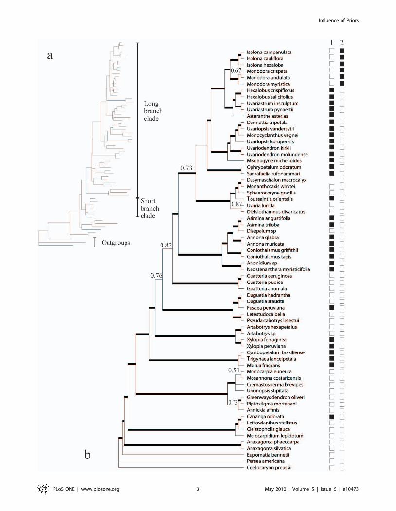
characterized by long branches (Figure 1 a) subtending species-
rich clades [24]. The long branches of the LBC offer an ideal
situation for applying posterior mapping to the study of the
evolution of morphological characters, given the flaws that might
be expected when applying maximum parsimony optimization to
character reconstruction. Two contrasting morphological charac-
ters found within the LBC were selected (Figure 1 b). (1) A
potentially slow evolving character, carpel fusion, which has two
states: apocarpy and syncarpy. Syncarpy is defined as the
congenital fusion of the female reproductive units of the flower
termed carpels [25,26], and has only rarely evolved within the
magnoliids. In Annonaceae, however, syncarpy has evolved in the
ancestor of two strongly supported African sister genera Isolona and
Monodora [25,27,28]. Syncarpy was specifically chosen because one
can ‘intuitively’ infer from the tree that this character evolved
once, and thus allows us to evaluate in a more informed way how
different priors can or can not influence the results. (2) A
potentially faster evolving character: pollen unit, again with two
states: single (pollen composed of a single grain) and compound
(pollen composed of two, four or numerous grains). The single
state is considered ancestral within Annonaceae with reversals
being fairly common [29].
The aim of the present study was to investigate, within
Annonaceae and for the two characters described above, how
prior selection of the transformation rate h can influence certain
important values (e.g. the average number of transformations or
the marginal posterior probability of each ancestral character
states) by subjecting empirical data to the posterior mapping
method. Thus, this study was not designed to compare results
between alternative methods of character optimization. For such
comparisons the reader is referred to Huelsenbeck et al. [4] or
Ekman et al. [30].
Results
PhylogenyThe partition strategy strongly supported under the Bayes factor
was run for five million generations with three independent runs.
The posterior probabilities of all splits were indistinguishable
between independent runs as visualized with AWTY (results not
shown), suggesting convergence between them. In addition, all
three runs reached stationarity after 250,000 generations with all
of the parameters converging to the same values as visualized with
Tracer. The majority rule consensus tree was generally well
resolved and well supported (Fig. 1). For details about the MrBayes
analysis and discussion about the phylogenetic relationships in
Annonaceae resulting from this analysis see Couvreur et al. [28].
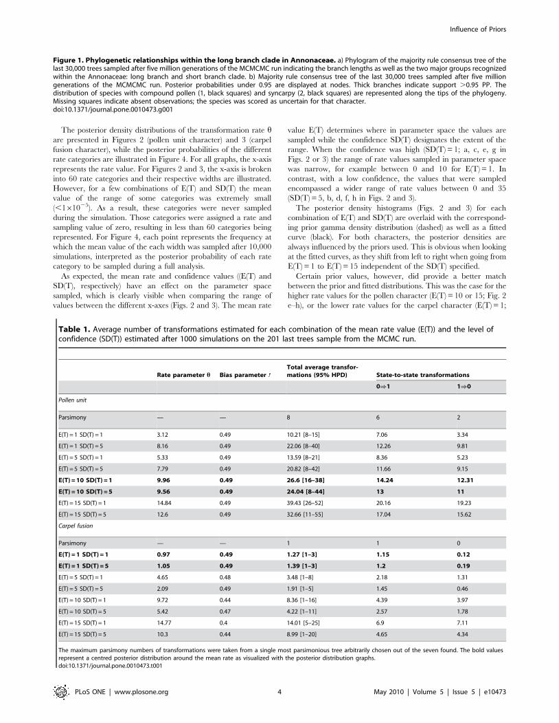
Influence of the Rate Prior hThe average number of total transformations as well as the
average number of transformations from one state to another, for
each of the two characters under eight different combinations of
E(T) and SD(T), are summarized in Table 1. For both characters
the average number of total transformations as well as state-to-
state changes is higher with the faster rate prior, i.e. higher E(T).
Thus, for carpel fusion the average total number of transforma-
tions changed from 1.39 (prior set at a low rate: E(T) = 1,
SD(T) = 5) to 8.99 (prior set at a high rate: E(T) = 15, SD(T) = 5). If
SD(T) is narrowed to one, the differences are even greater (1.27 to
14.01). Finally, averages for similar values of E(T) showed marked
differences according to the different values of SD(T), except for
two cases indicated in Table 1 (highlighted in), when the averages
did not differ greatly.
Influence of Priors
PLoS ONE | www.plosone.org 2 May 2010 | Volume 5 | Issue 5 | e10473
Influence of Priors
PLoS ONE | www.plosone.org 3 May 2010 | Volume 5 | Issue 5 | e10473
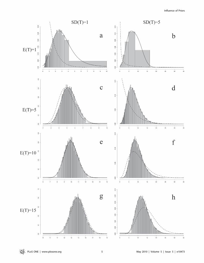
The posterior density distributions of the transformation rate hare presented in Figures 2 (pollen unit character) and 3 (carpel
fusion character), while the posterior probabilities of the different
rate categories are illustrated in Figure 4. For all graphs, the x-axis
represents the rate value. For Figures 2 and 3, the x-axis is broken
into 60 rate categories and their respective widths are illustrated.
However, for a few combinations of E(T) and SD(T) the mean
value of the range of some categories was extremely small
(,161025). As a result, these categories were never sampled
during the simulation. Those categories were assigned a rate and
sampling value of zero, resulting in less than 60 categories being
represented. For Figure 4, each point represents the frequency at
which the mean value of the each width was sampled after 10,000
simulations, interpreted as the posterior probability of each rate
category to be sampled during a full analysis.
As expected, the mean rate and confidence values ((E(T) and
SD(T), respectively) have an effect on the parameter space
sampled, which is clearly visible when comparing the range of
values between the different x-axes (Figs. 2 and 3). The mean rate
value E(T) determines where in parameter space the values are
sampled while the confidence SD(T) designates the extent of the
range. When the confidence was high (SD(T) = 1; a, c, e, g in
Figs. 2 or 3) the range of rate values sampled in parameter space
was narrow, for example between 0 and 10 for E(T) = 1. In
contrast, with a low confidence, the values that were sampled
encompassed a wider range of rate values between 0 and 35
(SD(T) = 5, b, d, f, h in Figs. 2 and 3).
The posterior density histograms (Figs. 2 and 3) for each
combination of E(T) and SD(T) are overlaid with the correspond-
ing prior gamma density distribution (dashed) as well as a fitted
curve (black). For both characters, the posterior densities are
always influenced by the priors used. This is obvious when looking
at the fitted curves, as they shift from left to right when going from
E(T) = 1 to E(T) = 15 independent of the SD(T) specified.
Certain prior values, however, did provide a better match
between the prior and fitted distributions. This was the case for the
higher rate values for the pollen character (E(T) = 10 or 15; Fig. 2
e–h), or the lower rate values for the carpel character (E(T) = 1;
Table 1. Average number of transformations estimated for each combination of the mean rate value (E(T)) and the level ofconfidence (SD(T)) estimated after 1000 simulations on the 201 last trees sample from the MCMC run.
Rate parameter h Bias parameterTotal average transfor-mations (95% HPD) State-to-state transformations
0)1 1)0
Pollen unit
Parsimony — — 8 6 2
E(T) = 1 SD(T) = 1 3.12 0.49 10.21 [8–15] 7.06 3.34
E(T) = 1 SD(T) = 5 8.16 0.49 22.06 [8–40] 12.26 9.81
E(T) = 5 SD(T) = 1 5.33 0.49 13.59 [8–21] 8.36 5.23
E(T) = 5 SD(T) = 5 7.79 0.49 20.82 [8–42] 11.66 9.15
E(T) = 10 SD(T) = 1 9.96 0.49 26.6 [16–38] 14.24 12.31
E(T) = 10 SD(T) = 5 9.56 0.49 24.04 [8–44] 13 11
E(T) = 15 SD(T) = 1 14.84 0.49 39.43 [26–52] 20.16 19.23
E(T) = 15 SD(T) = 5 12.6 0.49 32.66 [11–55] 17.04 15.62
Carpel fusion
Parsimony — — 1 1 0
E(T) = 1 SD(T) = 1 0.97 0.49 1.27 [1–3] 1.15 0.12
E(T) = 1 SD(T) = 5 1.05 0.49 1.39 [1–3] 1.2 0.19
E(T) = 5 SD(T) = 1 4.65 0.48 3.48 [1–8] 2.18 1.31
E(T) = 5 SD(T) = 5 2.09 0.49 1.91 [1–5] 1.45 0.46
E(T) = 10 SD(T) = 1 9.72 0.44 8.36 [1–16] 4.39 3.97
E(T) = 10 SD(T) = 5 5.42 0.47 4.22 [1–11] 2.57 1.78
E(T) = 15 SD(T) = 1 14.77 0.4 14.01 [5–25] 6.9 7.11
E(T) = 15 SD(T) = 5 10.3 0.44 8.99 [1–20] 4.65 4.34
The maximum parsimony numbers of transformations were taken from a single most parsimonious tree arbitrarily chosen out of the seven found. The bold valuesrepresent a centred posterior distribution around the mean rate as visualized with the posterior distribution graphs.doi:10.1371/journal.pone.0010473.t001
Figure 1. Phylogenetic relationships within the long branch clade in Annonaceae. a) Phylogram of the majority rule consensus tree of thelast 30,000 trees sampled after five million generations of the MCMCMC run indicating the branch lengths as well as the two major groups recognizedwithin the Annonaceae: long branch and short branch clade. b) Majority rule consensus tree of the last 30,000 trees sampled after five milliongenerations of the MCMCMC run. Posterior probabilities under 0.95 are displayed at nodes. Thick branches indicate support .0.95 PP. Thedistribution of species with compound pollen (1, black squares) and syncarpy (2, black squares) are represented along the tips of the phylogeny.Missing squares indicate absent observations; the species was scored as uncertain for that character.doi:10.1371/journal.pone.0010473.g001
Influence of Priors
PLoS ONE | www.plosone.org 4 May 2010 | Volume 5 | Issue 5 | e10473
Influence of Priors
PLoS ONE | www.plosone.org 5 May 2010 | Volume 5 | Issue 5 | e10473
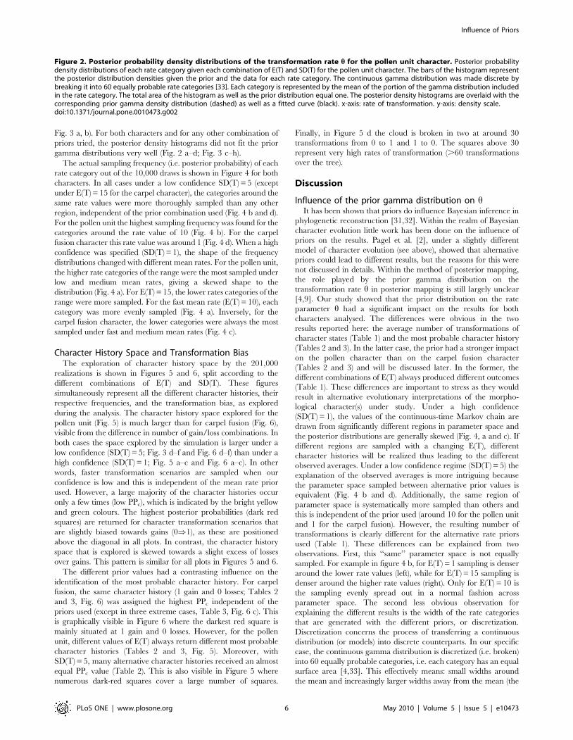
Fig. 3 a, b). For both characters and for any other combination of
priors tried, the posterior density histograms did not fit the prior
gamma distributions very well (Fig. 2 a–d; Fig. 3 c–h).
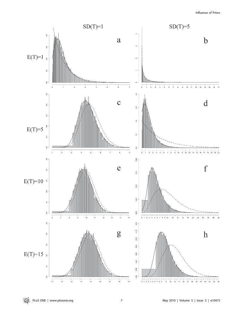
The actual sampling frequency (i.e. posterior probability) of each
rate category out of the 10,000 draws is shown in Figure 4 for both
characters. In all cases under a low confidence SD(T) = 5 (except
under E(T) = 15 for the carpel character), the categories around the
same rate values were more thoroughly sampled than any other
region, independent of the prior combination used (Fig. 4 b and d).
For the pollen unit the highest sampling frequency was found for the
categories around the rate value of 10 (Fig. 4 b). For the carpel
fusion character this rate value was around 1 (Fig. 4 d). When a high
confidence was specified (SD(T) = 1), the shape of the frequency
distributions changed with different mean rates. For the pollen unit,
the higher rate categories of the range were the most sampled under
low and medium mean rates, giving a skewed shape to the
distribution (Fig. 4 a). For E(T) = 15, the lower rates categories of the
range were more sampled. For the fast mean rate (E(T) = 10), each
category was more evenly sampled (Fig. 4 a). Inversely, for the
carpel fusion character, the lower categories were always the most
sampled under fast and medium mean rates (Fig. 4 c).
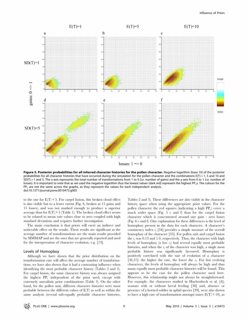
Character History Space and Transformation BiasThe exploration of character history space by the 201,000
realizations is shown in Figures 5 and 6, split according to the
different combinations of E(T) and SD(T). These figures
simultaneously represent all the different character histories, their
respective frequencies, and the transformation bias, as explored
during the analysis. The character history space explored for the
pollen unit (Fig. 5) is much larger than for carpel fusion (Fig. 6),
visible from the difference in number of gain/loss combinations. In
both cases the space explored by the simulation is larger under a
low confidence (SD(T) = 5; Fig. 3 d–f and Fig. 6 d–f) than under a
high confidence (SD(T) = 1; Fig. 5 a–c and Fig. 6 a–c). In other
words, faster transformation scenarios are sampled when our
confidence is low and this is independent of the mean rate prior
used. However, a large majority of the character histories occur
only a few times (low PPc), which is indicated by the bright yellow
and green colours. The highest posterior probabilities (dark red
squares) are returned for character transformation scenarios that
are slightly biased towards gains (0)1), as these are positioned
above the diagonal in all plots. In contrast, the character history
space that is explored is skewed towards a slight excess of losses
over gains. This pattern is similar for all plots in Figures 5 and 6.
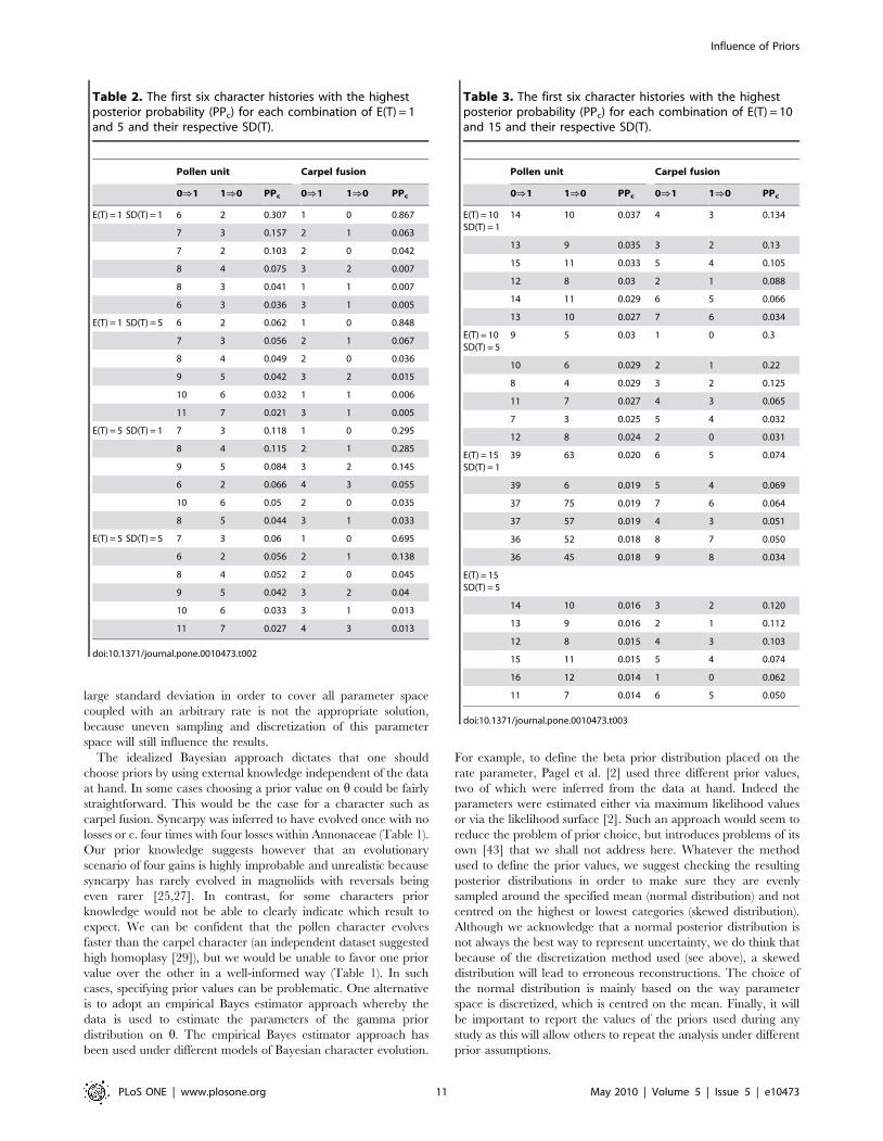
The different prior values had a contrasting influence on the
identification of the most probable character history. For carpel
fusion, the same character history (1 gain and 0 losses; Tables 2
and 3, Fig. 6) was assigned the highest PPc independent of the
priors used (except in three extreme cases, Table 3, Fig. 6 c). This
is graphically visible in Figure 6 where the darkest red square is
mainly situated at 1 gain and 0 losses. However, for the pollen
unit, different values of E(T) always return different most probable
character histories (Tables 2 and 3, Fig. 5). Moreover, with
SD(T) = 5, many alternative character histories received an almost
equal PPc value (Table 2). This is also visible in Figure 5 where
numerous dark-red squares cover a large number of squares.
Finally, in Figure 5 d the cloud is broken in two at around 30
transformations from 0 to 1 and 1 to 0. The squares above 30
represent very high rates of transformation (.60 transformations
over the tree).
Discussion
Influence of the prior gamma distribution on hIt has been shown that priors do influence Bayesian inference in
phylogenetic reconstruction [31,32]. Within the realm of Bayesian
character evolution little work has been done on the influence of
priors on the results. Pagel et al. [2], under a slightly different
model of character evolution (see above), showed that alternative
priors could lead to different results, but the reasons for this were
not discussed in details. Within the method of posterior mapping,
the role played by the prior gamma distribution on the
transformation rate h in posterior mapping is still largely unclear
[4,9]. Our study showed that the prior distribution on the rate
parameter h had a significant impact on the results for both
characters analysed. The differences were obvious in the two
results reported here: the average number of transformations of
character states (Table 1) and the most probable character history
(Tables 2 and 3). In the latter case, the prior had a stronger impact
on the pollen character than on the carpel fusion character
(Tables 2 and 3) and will be discussed later. In the former, the
different combinations of E(T) always produced different outcomes
(Table 1). These differences are important to stress as they would
result in alternative evolutionary interpretations of the morpho-
logical character(s) under study. Under a high confidence
(SD(T) = 1), the values of the continuous-time Markov chain are
drawn from significantly different regions in parameter space and
the posterior distributions are generally skewed (Fig. 4, a and c). If
different regions are sampled with a changing E(T), different
character histories will be realized thus leading to the different
observed averages. Under a low confidence regime (SD(T) = 5) the
explanation of the observed averages is more intriguing because
the parameter space sampled between alternative prior values is
equivalent (Fig. 4 b and d). Additionally, the same region of
parameter space is systematically more sampled than others and
this is independent of the prior used (around 10 for the pollen unit
and 1 for the carpel fusion). However, the resulting number of
transformations is clearly different for the alternative rate priors
used (Table 1). These differences can be explained from two
observations. First, this ‘‘same’’ parameter space is not equally
sampled. For example in figure 4 b, for E(T) = 1 sampling is denser
around the lower rate values (left), while for E(T) = 15 sampling is
denser around the higher rate values (right). Only for E(T) = 10 is
the sampling evenly spread out in a normal fashion across
parameter space. The second less obvious observation for
explaining the different results is the width of the rate categories
that are generated with the different priors, or discretization.
Discretization concerns the process of transferring a continuous
distribution (or models) into discrete counterparts. In our specific
case, the continuous gamma distribution is discretized (i.e. broken)
into 60 equally probable categories, i.e. each category has an equal
surface area [4,33]. This effectively means: small widths around
the mean and increasingly larger widths away from the mean (the
Figure 2. Posterior probability density distributions of the transformation rate h for the pollen unit character. Posterior probabilitydensity distributions of each rate category given each combination of E(T) and SD(T) for the pollen unit character. The bars of the histogram representthe posterior distribution densities given the prior and the data for each rate category. The continuous gamma distribution was made discrete bybreaking it into 60 equally probable rate categories [33]. Each category is represented by the mean of the portion of the gamma distribution includedin the rate category. The total area of the histogram as well as the prior distribution equal one. The posterior density histograms are overlaid with thecorresponding prior gamma density distribution (dashed) as well as a fitted curve (black). x-axis: rate of transformation. y-axis: density scale.doi:10.1371/journal.pone.0010473.g002
Influence of Priors
PLoS ONE | www.plosone.org 6 May 2010 | Volume 5 | Issue 5 | e10473
Influence of Priors
PLoS ONE | www.plosone.org 7 May 2010 | Volume 5 | Issue 5 | e10473
marginal regions). Each category is then assigned a fixed rate value
equal to the mean of the range. Thus, these widths are directly
dependent on the shape of the prior probability distribution, and
therefore on the values assigned to the parameters aS and bS. It is
the generation of different width ranges within an equal parameter
space for different prior values that also produce the observed
disparities in the average number character transformations. For
example, for the pollen character, categories around the rate value
10, which is the most frequently sampled category for any value of
E(T), present large widths for E(T) = 1 (Fig. 2 b), medium widths
for E(T) = 5 (Fig. 2 d) and smaller widths for E(T) = 10 (Fig. 2 f).
Because each width is represented by its mean, the different
discretizations around the most frequently sampled rate value will
have a direct effect on the average number of transformations as
shown by the results.
Finally, discretization is also responsible for another counterin-
tuitive result. For the pollen unit, a higher average number of
transformations was returned under the small mean rate prior
when compared to the medium one (Table 1), although we would
expect a lower average for the small rate. Figure 2 b shows the
ranges of the two last rate categories generated under E(T) = 1 and
SD(T) = 5, which encompassed a large range of values and were
represented by their mean of 11.78 and 32.24. The latter rate
value is the largest rate category generated. Although it had a low
posterior probability (sampled 65 times out of 10,000 draws), this
was still enough during the course of a long simulation to produce
a few high transformations (.60). These high transformations are
clearly visible in Figure 5 d, where character history space is split
into two at around 30 gains and 30 losses. These high generated
transformations are responsible for returning an average superior
Figure 3. Posterior probability density distributions of the transformation rate h for the carpel fusion character. Posterior probabilitydensity distributions of each rate category given each combination of E(T) and SD(T) for the carpel fusion character. The bars of the histogram representthe posterior distribution densities given the prior and the data for each rate category. The continuous gamma distribution was made discrete bybreaking it into 60 equal probable rate categories [33]. Each category is represented by the mean of the portion of the gamma distribution included inthe rate category. The total area of the histogram as well as the prior distribution equal one. The posterior density histograms are overlaid with thecorresponding prior gamma density distribution (dashed) as well as a fitted curve (black). x-axis: rate of transformation. y-axis: density scale.doi:10.1371/journal.pone.0010473.g003
Figure 4. Posterior probabilities for both pollen unit and carpel fusion characters. Posterior probabilities for each rate prior E(T) given astandard deviation S(T) for both pollen unit and carpel fusion characters. x-axis: rate of transformation. y-axis: sampling frequency ( = posteriorprobability) of each discrete rate category.doi:10.1371/journal.pone.0010473.g004
Influence of Priors
PLoS ONE | www.plosone.org 8 May 2010 | Volume 5 | Issue 5 | e10473
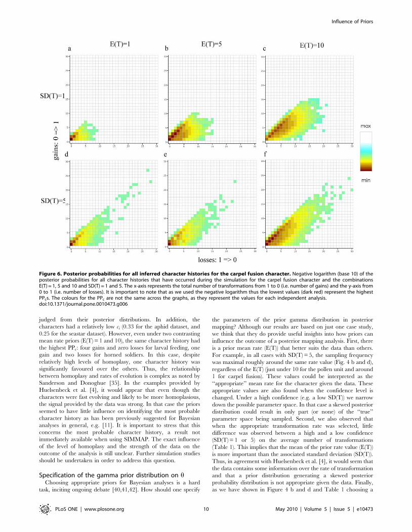
to the one for E(T) = 5. For carpel fusion, this broken cloud effect
is also visible but to a lesser extent (Fig. 6, broken at 15 gains and
15 losses), and was not marked enough to produce a superior
average than for E(T) = 5 (Table 1). The broken cloud effect seems
to be related to mean rate values close to zero coupled with high
standard deviations and requires further investigation.
The main conclusion is that priors will exert an indirect and
noticeable effect on the results. These results are significant as the
average number of transformations are the main results provided
by SIMMAP and are the ones that are generally reported and used
for the interpretation of character evolution, e.g. [13].
Levels of HomoplasyAlthough we have shown that the prior distribution on the
transformation rate will affect the average number of transforma-
tions, we have also shown that it had a contrasting influence when
identifying the most probable character history (Tables 2 and 3).
For carpel fusion, the same character history was always assigned
the highest PPc independent of the prior used, except with
extremely unrealistic prior combinations (Table 3). On the other
hand, for the pollen unit, different character histories were most
probable between the different values of E(T) as well as within the
same analysis (several sub-equally probable character histories,
Tables 2 and 3). These differences are also visible in the character
history space when using the appropriate prior values. For the
pollen character the red squares (indicating a high PPc) cover a
much wider space (Fig. 5 c and f) than for the carpel fusion
character which is concentrated around one gain - zero losses
(Fig. 6 c and f). One explanation for these differences is the level of
homoplasy present in the data for each character. A character’s
consistency index ci [34] provides a simple measure of the overall
homoplasy of the character [35]. For pollen unit and carpel fusion
the ci was 0.13 and 1.0, respectively. Thus, the character with high
levels of homoplasy (a low ci) had several equally most probable
histories, and when the ci of the character was high, a single most
probable history was significantly favoured. Homoplasy is
positively correlated with the rate of evolution of a character
[36,37]: the higher the rate, the lower the ci. For fast evolving
characters, the levels of homoplasy will always be high and thus
many equally most probable character histories will be found. This
appears to be the case for the pollen character used here.
However, this relationship might not always be straightforward.
For example, the characters studied in Huelsenbeck et al. [4],
seastars with or without larval feeding [38] and, absence or
presence of a horned soldier in aphid species [39], were also shown
to have a high rate of transformation amongst states (E(T) = 10), as
Figure 5. Posterior probabilities for all inferred character histories for the pollen character. Negative logarithm (base 10) of the posteriorprobabilities for all character histories that have occurred during the simulation for the pollen character and the combinations E(T) = 1, 5 and 10 andSD(T) = 1 and 5. The x-axis represents the total number of transformations from 1 to 0 (i.e. number of gains) and the y-axis from 0 to 1 (i.e. number oflosses). It is important to note that as we used the negative logarithm thus the lowest values (dark red) represent the highest PPcs. The colours for thePPc are not the same across the graphs, as they represent the values for each independent analysis.doi:10.1371/journal.pone.0010473.g005
Influence of Priors
PLoS ONE | www.plosone.org 9 May 2010 | Volume 5 | Issue 5 | e10473
judged from their posterior distributions. In addition, the
characters had a relatively low ci (0.33 for the aphid dataset, and
0.25 for the seastar dataset). However, even under two contrasting
mean rate priors (E(T) = 1 and 10), the same character history had
the highest PPc: four gains and zero losses for larval feeding, one
gain and two losses for horned soldiers. In this case, despite
relatively high levels of homoplasy, one character history was
significantly favoured over the others. Thus, the relationship
between homoplasy and rates of evolution is complex as noted by
Sanderson and Donoghue [35]. In the examples provided by
Huelsenbeck et al. [4], it would appear that even though the
characters were fast evolving and likely to be more homoplasious,
the signal provided by the data was strong. In that case the priors
seemed to have little influence on identifying the most probable
character history as has been previously suggested for Bayesian
analyses in general, e.g. [11]. It is important to stress that this
concerns the most probable character history, a result not
immediately available when using SIMMAP. The exact influence
of the level of homoplasy and the strength of the data on the
outcome of the analysis is still unclear. Further simulation studies
should be undertaken in order to address this question.
Specification of the gamma prior distribution on hChoosing appropriate priors for Bayesian analyses is a hard
task, inciting ongoing debate [40,41,42]. How should one specify
the parameters of the prior gamma distribution in posterior
mapping? Although our results are based on just one case study,
we think that they do provide useful insights into how priors can
influence the outcome of a posterior mapping analysis. First, there
is a prior mean rate (E(T)) that better suits the data than others.
For example, in all cases with SD(T) = 5, the sampling frequency
was maximal roughly around the same rate value (Fig. 4 b and d),
regardless of the E(T) (just under 10 for the pollen unit and around
1 for carpel fusion). These values could be interpreted as the
‘‘appropriate’’ mean rate for the character given the data. These
appropriate values are also found when the confidence level is
changed. Under a high confidence (e.g. a low SD(T)) we narrow
down the possible parameter space. In that case a skewed posterior
distribution could result in only part (or none) of the ‘‘true’’
parameter space being sampled. Second, we also observed that
when the appropriate transformation rate was selected, little
difference was observed between a high and a low confidence
(SD(T) = 1 or 5) on the average number of transformations
(Table 1). This implies that the mean of the prior rate value (E(T))
is more important than the associated standard deviation (SD(T)).
Thus, in agreement with Huelsenbeck et al. [4], it would seem that
the data contains some information over the rate of transformation
and that a prior distribution generating a skewed posterior
probability distribution is not appropriate given the data. Finally,
as we have shown in Figure 4 b and d and Table 1 choosing a
Figure 6. Posterior probabilities for all inferred character histories for the carpel fusion character. Negative logarithm (base 10) of theposterior probabilities for all character histories that have occurred during the simulation for the carpel fusion character and the combinationsE(T) = 1, 5 and 10 and SD(T) = 1 and 5. The x-axis represents the total number of transformations from 1 to 0 (i.e. number of gains) and the y-axis from0 to 1 (i.e. number of losses). It is important to note that as we used the negative logarithm thus the lowest values (dark red) represent the highestPPcs. The colours for the PPc are not the same across the graphs, as they represent the values for each independent analysis.doi:10.1371/journal.pone.0010473.g006
Influence of Priors
PLoS ONE | www.plosone.org 10 May 2010 | Volume 5 | Issue 5 | e10473
large standard deviation in order to cover all parameter space
coupled with an arbitrary rate is not the appropriate solution,
because uneven sampling and discretization of this parameter
space will still influence the results.
The idealized Bayesian approach dictates that one should
choose priors by using external knowledge independent of the data
at hand. In some cases choosing a prior value on h could be fairly
straightforward. This would be the case for a character such as
carpel fusion. Syncarpy was inferred to have evolved once with no
losses or c. four times with four losses within Annonaceae (Table 1).
Our prior knowledge suggests however that an evolutionary
scenario of four gains is highly improbable and unrealistic because
syncarpy has rarely evolved in magnoliids with reversals being
even rarer [25,27]. In contrast, for some characters prior
knowledge would not be able to clearly indicate which result to
expect. We can be confident that the pollen character evolves
faster than the carpel character (an independent dataset suggested
high homoplasy [29]), but we would be unable to favor one prior
value over the other in a well-informed way (Table 1). In such
cases, specifying prior values can be problematic. One alternative
is to adopt an empirical Bayes estimator approach whereby the
data is used to estimate the parameters of the gamma prior
distribution on h. The empirical Bayes estimator approach has
been used under different models of Bayesian character evolution.
For example, to define the beta prior distribution placed on the
rate parameter, Pagel et al. [2] used three different prior values,
two of which were inferred from the data at hand. Indeed the
parameters were estimated either via maximum likelihood values
or via the likelihood surface [2]. Such an approach would seem to
reduce the problem of prior choice, but introduces problems of its
own [43] that we shall not address here. Whatever the method
used to define the prior values, we suggest checking the resulting
posterior distributions in order to make sure they are evenly
sampled around the specified mean (normal distribution) and not
centred on the highest or lowest categories (skewed distribution).
Although we acknowledge that a normal posterior distribution is
not always the best way to represent uncertainty, we do think that
because of the discretization method used (see above), a skewed
distribution will lead to erroneous reconstructions. The choice of
the normal distribution is mainly based on the way parameter
space is discretized, which is centred on the mean. Finally, it will
be important to report the values of the priors used during any
study as this will allow others to repeat the analysis under different
prior assumptions.
Table 3. The first six character histories with the highestposterior probability (PPc) for each combination of E(T) = 10and 15 and their respective SD(T).
Pollen unit Carpel fusion
0)1 1)0 PPc 0)1 1)0 PPc
E(T) = 10SD(T) = 1
14 10 0.037 4 3 0.134
13 9 0.035 3 2 0.13
15 11 0.033 5 4 0.105
12 8 0.03 2 1 0.088
14 11 0.029 6 5 0.066
13 10 0.027 7 6 0.034
E(T) = 10SD(T) = 5
9 5 0.03 1 0 0.3
10 6 0.029 2 1 0.22
8 4 0.029 3 2 0.125
11 7 0.027 4 3 0.065
7 3 0.025 5 4 0.032
12 8 0.024 2 0 0.031
E(T) = 15SD(T) = 1
39 63 0.020 6 5 0.074
39 6 0.019 5 4 0.069
37 75 0.019 7 6 0.064
37 57 0.019 4 3 0.051
36 52 0.018 8 7 0.050
36 45 0.018 9 8 0.034
E(T) = 15SD(T) = 5
14 10 0.016 3 2 0.120
13 9 0.016 2 1 0.112
12 8 0.015 4 3 0.103
15 11 0.015 5 4 0.074
16 12 0.014 1 0 0.062
11 7 0.014 6 5 0.050
doi:10.1371/journal.pone.0010473.t003
Table 2. The first six character histories with the highestposterior probability (PPc) for each combination of E(T) = 1and 5 and their respective SD(T).
Pollen unit Carpel fusion
0)1 1)0 PPc 0)1 1)0 PPc
E(T) = 1 SD(T) = 1 6 2 0.307 1 0 0.867
7 3 0.157 2 1 0.063
7 2 0.103 2 0 0.042
8 4 0.075 3 2 0.007
8 3 0.041 1 1 0.007
6 3 0.036 3 1 0.005
E(T) = 1 SD(T) = 5 6 2 0.062 1 0 0.848
7 3 0.056 2 1 0.067
8 4 0.049 2 0 0.036
9 5 0.042 3 2 0.015
10 6 0.032 1 1 0.006
11 7 0.021 3 1 0.005
E(T) = 5 SD(T) = 1 7 3 0.118 1 0 0.295
8 4 0.115 2 1 0.285
9 5 0.084 3 2 0.145
6 2 0.066 4 3 0.055
10 6 0.05 2 0 0.035
8 5 0.044 3 1 0.033
E(T) = 5 SD(T) = 5 7 3 0.06 1 0 0.695
6 2 0.056 2 1 0.138
8 4 0.052 2 0 0.045
9 5 0.042 3 2 0.04
10 6 0.033 3 1 0.013
11 7 0.027 4 3 0.013
doi:10.1371/journal.pone.0010473.t002
Influence of Priors
PLoS ONE | www.plosone.org 11 May 2010 | Volume 5 | Issue 5 | e10473

Many more questions remain to be answered and especially how
exactly will the priors affect the results in certain situations still
needs to be explored: for example how will the priors affect the
results with different degrees of homoplasy, rate heterogeneity of a
morphological character, tree shape, sampling of taxa and
characters. Answering these questions using simulated data would
allow for a better understanding of the precise role priors play in
posterior mapping.
Materials and Methods
Phylogenetic analysesThe results presented here are derived from a DNA sequence
data matrix of the Annonaceae family [28] totalling 66 taxa
sampled across the family. The dataset was composed of six
chloroplastic markers, three non-coding (trnL-trnF, trnS-trnG and
psbA-trnH) and three coding (ndhF, rbcL and partial matK), totalling
7945 characters. Gaps were coded as separate characters. All
phylogenetic analyses were run using the Metropolis-coupled
Monte Carlo Markov chain (MCMCMC) algorithm implemented
in MrBayes, ver. 3.1.2 [44], under the best partitioning strategy
identified using the Bayes factor [45] and following Brandley et al.
[46]. For each partition, the best performing evolutionary model
was identified using the Akaike information criterion (AIC [47])
using MrModeltest [48]. Three separate runs (with one cold and
three hot chains) of five million generations each were undertaken
and stationarity as well as convergence between the MCMC runs
was checked using both Tracer v. 1.3 [49] and the online program
AWTY [50].
Influence of the Transformation Rate PriorThe impact of alternative prior distributions on the transfor-
mation rate (h) was studied by subjecting the carpel fusion and
pollen characters to the posterior mapping method as implement-
ed in the program SIMMAP version 1.0 beta 2.3 (build 12092006
[19]). Both characters were scored for each taxon following
Couvreur et al. [28]. Both characters were unordered.
SIMMAP allows the user to specify two parameters (aS and bS)
that define the prior gamma distribution placed on the
transformation rate h and one parameter (aB) for the beta
distribution placed on the directional bias . For the latter, a flat
prior was used in all analyses (aB =bB = 1). To compare the effect
of the prior distributions on h we must be sure to compare them
equally, i.e. make sure they have either the same mean (E(T)) or
standard deviation (SD(T)). For the prior gamma distribution we
have E(T)~aS
bS
and SD(T)~
ffiffiffiffiffiffiffiaS
bS2
r[4,33]. Formulating these
equations as a function of aS and bS leads to aS~E(T)2
SD(T)2and
bS~E(T)2
SD(T)2. This formula allows us to find the values of the
parameters aS and bS for any required combination of E(T) and
SD(T).
The simulation of the continuous-time Markov chain was
realized 1,000 times over the last 201 trees imported from the
MrBayes analysis for both characters. Eight different combinations
of E(T) and SD(T) for the prior distribution on h were analysed. A
slow, medium, fast and very fast mean rate (E(T) = 1, 5, 10 and 15
respectively) were each combined with a high and low confidence
(SD(T) = 1 and 5, respectively). Note that these values and
associated terminology were chosen relative to the biology of the
morphological characters considered for this specific analysis. The
total number of character transformations, and the number of
transformations between each state were averaged over all
realizations. Finally, the actual number of times a particular
character history occurred throughout the 201,000 realizations
was calculated (for example, how many times was ‘‘one gain and
one loss’’ simulated). A perl script (Vriesendorp and Couvreur,
unpublished) was written in order to extract that information from
the SIMMAP output files. Dividing the number of occurrences by
the total number of realizations gives the posterior probability of
each character history (abbreviated as PPc, not to be confused with
the PP of the nodes in the phylogenetic tree). To reduce the large
range of values between PPcs (5e26 to 0.9) the negative logarithm
of the PPc for each of the characters histories was plotted on a 2D
graph using Kyplot (Koishi Yoshioka, v.2 beta 15, www.
woundedmoon.org/win32/kyplot.html).
We also evaluated the influence of the priors on the posterior
distribution. The posterior distribution for each combination of
E(T) and SD(T) was estimated by undertaking 10,000 realizations
using the ‘‘number of realizations sampled from priors’’ function
in SIMMAP. This approach estimates the posterior distribution of
the parameters by sampling the prior without undertaking the full
length analysis. The posterior distribution for each combination
was then visualized in Tracer v. 1.3 [49] by converting the
SIMMAP output file to a Tracer file using the python script
‘‘convert2tracer.py’’ found on the SIMMAP website (Bollback,
http://www.simmap.com). The prior gamma distribution was
broken or discretized into 60 rate categories, each of which
represents an equal probability density [33]. As the areas under
the probability curve are equalized, the resulting categories have
different widths. For each combination of E(T) and SD(T) two
different graphs were produced. A posterior density histogram was
normalized by dividing the number of counts within each rate
category by the width of that category, with the total surface area
of the rectangles equalling one. This representation allows for the
overlay of the prior gamma probability density as a reference.
Smooth curves were fitted using the software in R and based on
Eilers [51]. Moreover, this provides a visualization of how
parameter space is discretized (broken down) given each
combination of E(T) and SD(T).
A second graph was generated that represents the number of
times each rate category (represented by its mean) was sampled
out of 10,000 draws, i.e. the posterior probability of each
category following Huelsenbeck et al. [4]. This graph differs from
the previous one in that we no longer take the width of the rate
into account, and by overlapping the posterior distribution for
each E(T) we can clearly identify the regions of parameter space
that are more sampled than other under the alternative priors
chosen.
Maximum parsimony optimization results were also provided as
a reference only. The majority rule consensus tree from the
Bayesian analysis was used for subsequent analyses using Mesquite
v. 1.11 [52]. Both characters were treated as unordered.
Acknowledgments
Timo van der Niet is deeply thanked for critically reading and significantly
improving earlier versions of the manuscript. Jonathan Bollback is thanked
for comments and discussions around the posterior mapping method and
suggestions for improving the manuscript. Bastienne Vriesendorp is also
thanked for her help in writing the perl scripts. Finally, Pieter Pelsen and
several anonymous reviewers are also thanked for their useful comments
and critics.
Author Contributions
Conceived and designed the experiments: TLPC JER MS LC. Performed
the experiments: TLPC. Analyzed the data: TLPC GG. Contributed
Influence of Priors
PLoS ONE | www.plosone.org 12 May 2010 | Volume 5 | Issue 5 | e10473
reagents/materials/analysis tools: GG MS. Wrote the paper: TLPC LC.
Provided significant help at the final stages of the article: JER MS.
References
1. Bollback JP (2005) Posterior mapping and posterior predictive distributions. In:
Nielsen R, ed. Statistical methods in molecular evolution. New York: Springer.pp 439–462.
2. Pagel M, Meade A, Barker D (2004) Bayesian estimation of ancestral character
states on phylogenies. Systematic Biology 53: 673–684.3. Nielsen R (2002) Mapping mutations on phylogenies. Systematic Biology 51:
729–739.4. Huelsenbeck JP, Nielsen R, Bollback JP (2003) Stochastic mapping of
morphological characters. Systematic Biology 52: 131–158.5. Ronquist F (2004) Bayesian inference of character evolution. Trends in Ecology
& Evolution 19: 475–481.
6. Schluter D, Price T, Mooers AO, Ludwig D (1997) Likelihood of ancestor statesin adaptive radiation. Evolution 51: 1699–1711.
7. Cunningham CW, Omland KE, Oakley TH (1998) Reconstructing ancestralcharacter states: a critical reappraisal. Trends in Ecology & Evolution 13:
361–366.
8. Lewis PO (2001) A likelihood approach to estimating phylogeny from discretemorphological character data. Systematic Biology 50: 913–925.
9. Schultz TR, Churchill GA (1999) The role of subjectivity in reconstructingancestral character states: A Bayesian approach to unknown rates, states, and
transformation asymmetries. Systematic Biology 48: 651–664.10. Huelsenbeck JP, Larget B, Miller RE, Ronquist F (2002) Potential applications
and pitfalls of Bayesian inference of phylogeny. Systematic Biology 51: 673–688.
11. Alfaro ME, Holder MT (2006) The posterior and the prior in Bayesianphylogenetics. Annual Review of Ecology, Evolution, and Systematics 37:
19–42.12. Buschbom J, Barker D (2006) Evolutionary history of vegetative reproduction in
Porpidia s. l. (lichen-forming ascomycota). Systematic Biology 55: 471–484.
13. Smedmark JEE, Swenson U, Anderberg AA (2006) Accounting for variation ofsubstitution rates through time in Bayesian phylogeny reconstruction of
Sapotoideae (Sapotaceae). Molecular Phylogenetics and Evolution 39: 706–721.14. McLeish MJ, Chapman TW, Schwarz MP (2007) Host-driven diversification of
gall-inducing Acacia thrips and the aridification of Australia. Bmc Biology 5.15. Lewis LA, Lewis PO (2005) Unearthing the molecular phylodiversity of desert
soil green Algae (Chlorophyta). Systematic Biology 54: 936–947.
16. Chaverri P, Bischoff JF, Evans HC, Hodge KT (2005) Regiocrella, a newentomopathogenic genus with a pycnidial anamorph and its phylogenetic
placement in the Clavicipitaceae. Mycologia 97: 1225–1237.17. Jones WJ, Won YJ, Maas PAY, Smith PJ, Lutz RA, et al. (2006) Evolution of
habitat use by deep-sea mussels. Marine Biology 148: 841–851.
18. Leschen RAB, Buckley TR (2007) Multistate characters and diet shifts:Evolution of Erotylidae (Coleoptera). Systematic Biology 56: 97–112.
19. Bollback JP (2006) SIMMAP: Stochastic character mapping of discrete traits onphylogenies. BMC Bioinformatics 7: 88–94.
20. APGII (2003) An update of the Angiosperm Phylogeny Group classification for
the orders and families of flowering plants: APG II. Botanical Journal of theLinnean Society 141: 399–436.
21. Richardson JE, Chatrou LW, Mols JB, Erkens RHJ, Pirie MD (2004) Historicalbiogeography of two cosmopolitan families of flowering plants: Annonaceae and
Rhamnaceae. Philosophical Transactions of the Royal Society of London B series359: 1495–1508.
22. Mols JB, Gravendeel B, Chatrou LW, Pirie MD, Bygrave PC, et al. (2004)
Identifying clades in Asian Annonaceae: monophyletic genera in thepolyphyletic Miliuseae. American Journal of Botany 91: 590–600.
23. Pirie MD, Chatrou LW, Mols JB, Erkens RHJ, Oosterhof J (2006) ‘Andean-centred’ genera in the short-branch clade of Annonaceae: testing biogeograph-
ical hypotheses using phylogeny reconstruction and molecular dating. Journal of
Biogeography 33: 31–46.24. Pirie MD (2005) Cremastosperma (and other evolutionary digressions): Molecular
phylogenetic, biogeographic, and taxonomic studies in Neotropical Annonaceae.Utrecht: Utrecht University. pp 1–256.
25. Endress PK (1990) Evolution of reproductive structures and functions inprimitive angiosperms (Magnoliidae). Memoires of the New York Botanical
Garden 55: 5–34.
26. Carr SGM, Carr DJ (1961) The functional significance of syncarpy.Phytomorphology 11: 249–256.
27. Endress PK (1982) Syncarpy and alternative modes of escaping disadvantages of
apocarpy in primitive angiosperms. Taxon 31: 48–52.
28. Couvreur TLP, Richardson JE, Sosef MSM, Erkens RHJ, Chatrou LW (2008)Evolution of syncarpy and other morphological characters in African
Annonaceae: a posterior mapping approach. Molecular Phylogenetics andEvolution 47: 302–318.
29. Doyle JA, Le Thomas A (1996) Phylogenetic analysis and character evolution in
Annonaceae. Bulletin du Museum Natlurelle d’Histoire Naturelle, B, Adansonia
18: 279–334.
30. Ekman S, Andersen HL, Wedin M (2008) The limitations of ancestral statereconstruction and evolution of the Ascus in the Lecanorales (Lichenized
Ascomycota). Systematic Biology 57: 141–156.
31. Yang Z, Rannala B (2005) Branch-length prior influences Bayesian posterior
probability of phylogeny. Systematic Biology 54: 455–470.
32. Zwickl DJ, Holder MT (2004) Model parameterization, prior distributions, andthe general time-reversible model in Bayesian phylogenetics. Systematic Biology
53: 877–888.
33. Yang Z (1994) Maximum likelihood phylogenetic estimation from DNA
sequences with variable rates over sites: Approximate methods. Journal ofMolecular Evolution V39: 306–314.
34. Farris JS (1969) A successive approximations approach to character weighting.
Systematic Zoology 18: 374–385.
35. Sanderson MJ, Donoghue MJ (1996) The relationship between homoplasy andconfidence in a phylogenetic tree. In: Sanderson MJ, Hufford L, eds.
Homoplasy: The recurrence of similarity in evolution. San Diego: Academic
Press. pp 67–89.
36. Archie JW (1996) Measures of homoplasy. In: Sanderson MJ, Hufford L, eds.Homoplasy: The recurrence of similarity in evolution. San Diego: Academic
Press. pp 153–188.
37. Donoghue MJ, Ree RH (2000) Homoplasy and developmental constraint: A
model and an example from plants. American Zoologist 40: 759–769.
38. Hart MW, Byrne M, Smith MJ (1997) Molecular phylogenetic analysis of life-history evolution in Asterinid starfish. Evolution 51: 1848–1861.
39. Stern DL (1998) Phylogeny of the tribe Cerataphidini (Homoptera) and the
evolution of the horned soldier aphids. Evolution 52: 155–165.
40. Van Dongen S (2006) Prior specification in Bayesian statistics: Three cautionary
tales. Journal of Theoretical Biology 242: 90–100.
41. Kass RE, Wasserman L (1996) The selection of prior distributions by formalrules. Journal of the American Statistical Association 91: 1343–1370.
42. Carlin BP, Louis TA (2000) Bayes and empirical bayes methods for data
analysis. London: Chapman & Hall.
43. Yang Z (2006) Computational Molecular Evolution: Oxford University Press,
Oxford.
44. Ronquist F, Huelsenbeck JP (2003) MrBayes 3: Bayesian phylogenetic inferenceunder mixed models. Bioinformatics 19: 1572–1574.
45. Nylander JAA, Ronquist F, Huelsenbeck JP, Nieves-Aldrey JL (2004) Bayesian
phylogenetic analysis of combined data. Systematic Biology 53: 47–67.
46. Brandley MC, Schmitz A, Reeder TW (2005) Partitioned Bayesian analyses,
partition choice, and the phylogenetic relationships of scincid lizards. SystematicBiology 54: 373–390.
47. Akaike H (1973) Information theory as an extension of the maximum likelihood
principle. In: Petrov BN, Csaki F, eds. Second International Symposium on
Information Theory Akademiai Kiado. Budapest . pp 267–281.
48. Nylander JAA (2004) MrModeltest v2. Program distributed by the author.Evolutionary Biology Centre, Uppsala University.
49. Rambaut A, Drummond AJ (2003) Tracer. Version 1.4. Available: http://
evolve.zoo.ox.ac.uk/.
50. Nylander JAA, Wilgenbusch JC, Warren DL, Swofford DL (2008) AWTY (are
we there yet?): a system for graphical exploration of MCMC convergence inBayesian phylogenetics. Bioinformatics 24: 581–583.
51. Eilers PH (2007) Ill-posed problems with counts, the composite link model and
penalized likelihood. Statistical Modeling 7: 239–254.
52. Maddison WD, Maddison DR (2006) Mesquite: a modular system for
evolutionary analysis. Version 1.11. Available: http://mesquiteproject.org,editor.
Influence of Priors
PLoS ONE | www.plosone.org 13 May 2010 | Volume 5 | Issue 5 | e10473