INFORM ATION TO USERS

This manuscript has been reproduced from the microfilm master. UMI films the text directfy from the original or copy submitted. Thus, some thesis and dissertation copies are in typewriter face, while others may be firom any type of conq)uter printer.

H ie quality of this reproduction is détendent upon the qnali^ of the copy submitted. Broken or indistinct print, colored or poor quality illustrations and photographs, print bleedthrough, substandard margins and inq)roper alignment can adversefy affect reproduction.

In the unlikely event that the author did not send UMI a complete manuscript and there are missing pages, these will be noted. Also, if unauthorized copyright material had to be removed, a note wül indicate the deletion.

Oversize m aterials (e.g., maps, drawings, charts) are reproduced by sectioning the original, beginning at the upper left-hand comer and continuing from left to right in equal sections with small overlaps. Each orig inal is also photographed in one exposure and is included in reduced form at the back of the book.

Photographs included in the original manuscript have been reproduced xerographically in this copy. Higher quality 6” x 9" black and white photographic prints are available for any photogr^hs or illustrations appearing in this copy for an additional charge. Contact UMI direct^ to order.

UMIA Bell & Howell Information Company

300 North Zeeb Road. Ann Arbor. Ml 48106-1346 USA 313.'761-4700 800,'521-0600

LIQUID MOLDING OF TEXTILE REINFORCEMENTS: ANALYSIS OF FLOW INDUCED VOIDS AND EFFECT OF POWDER COATING ON

PREFORMING AND MOLDABÏLITY

DISSERTATION

Presented in Partial Fulfillment of the Requirements for the

Degree Doctor of Philosophy

in the Graduate School of The Ohio State University

By

Vivek Rohatgi

ooooooThe Ohio State Univesily

1995

Dissertation Committee:

Dr. L. James Lee

Dr. James F. Rathman

Dr. Kurt W. Koelling

Approved by

AdvisorDepartment of Chemical Engineering

OHI Number: 9612267

Copyright 1995 by Rohatgi, Vivek

All rights reserved.

DHI Microform 9612267 Copyright 1996, by DMI Company. All rights reserved.

This microform edition is protected against unauthorized copying under Title 17, United States Code.

UMI300 North Zeeb Road Ann Arbor, MI 48103

Copyright by

Vivek Rohatgi

1995

This dissertation is dedicated

to

My wife, Vidhi

ACKNOWLEDGMENTS

I would like to express my gratitude to my advisor. Dr. Ly James Lee for his advice

throughout this project. I would also like to acknowledge Drs. James Rathman and Kurt

Koelling as members of the dissertation committee for their valuable time, suggestions and

comments. I also wish to thank Mr. Jim Barron, Dr. Asjad Shafi and Dr. Dexter White of

Dow Chemical for the various useful discussions I had with them. My appreciation goes to

Mike Kukla and Shoujie Li for their technical assistance.

Finally, I wish to thank my parents, sister and my wife for their encouragement and

constant emotional support throughout this seemingly everlasting endeavor.

m

VTTA

Septem ber 26, 1966..........................................Bom, Patna, India

July 1985 - May 1989............................................ B. Tech, Chemical EngineeringInstitute of Technology, BHU Varanasi, India

September 1989 - September 1990.................. Polymer Engineering Research FellowDepartment of Chemical Engineering The Ohio State University Columbus, Ohio, USA

September 1990 - August 1991.......................Graduate Research AssociateDepartment of Chemical Engineering The Ohio State University

August 1991...........................................................M.S., Chemical EngineeringThe Ohio State University

September 1991 - present..................................... Graduate Research AssociateDepartment of Chemical Engineering The Ohio State University

Publications

"Influence of material and processing variables on resin-fiber interface in glass fiber reinforced polymeric composites", V. Rohatgi, M.S. Thesis, The Ohio State University (1991).

"Influence of processing and material variables on resin-fiber interface in liquid composite molding". Polymer Composites, 14 (2), April 1993, N. Patel, V. Rohatgi and L. J. Lee.

"Macro and microvoid formation in liquid composite molding", 9th ASM/ESD Conference, Dearborn, MI, November 1993, V. Rohatgi, N. Patel and L. J. Lee.

IV

"Permeability measurement of braided graphite fiber preforms and kinetic/rheological measurement and modeling of a BMI resin". Collaborative Core Research Program, Ohio Aerospace Institute, Cleveland, OH, January 1994, V. Rohatgi, M. Perry and L. J. Lee.

"Microflow analysis in resin transfer molding". Proceedings of the NSF Design and Manufacturing Grantees Conference, Jan. 1994, L. J. Lee, V. Rohatgi and N. Patel.

"Flow characterization and air entrapment and removal during impregnation of fiber reinforcements in liquid composite molding". Report No. ERC/NSM - P- 94-19, The Ohio State University, May 1994, V. Rohatgi, N. Patel and L. J. Lee.

"Microscale flow behavior and void formation mechanism during impregnation through a unidirectional stitched fiberglass mat". Polymer Engineering and Science, 35 (10), May 1995, N. Patel, V. Rohatgi and L. J. Lee.

"Effect of reactive tackifier on preforming and molding in RTM", AIChE Annual Meeting, November 1995, V. Rohatgi, S. Li and L. J. Lee.

"Experimental investigation of flow induced microvoids during impregnation of unidirectional stitched fiberglass mat". Polymer Composites, December 1995, V. Rohatgi, N. Patel and L. J. Lee.

Fields of Study

Major Field: Chemical Engineering

Minor Field: Polymers/Composites Science and Engineering1. Interfacial phenomena2. Two-phase flow in porous media3. Chemo-rheology of polymeric resins4. Preforming of powder coated textile reinforcements5. Material Characterization (Chemical, Physical, Thermal and

Mechanical) of polymeric resins & composites

TABLE OF CONTENTS

DEDICATION............................................................................................................................. ii

ACKNOWLEDGMENT............................................................................................................ iii

VITA .................................................................................................................................... iv

TABLE OF CONTENTS........................................................................................................... vi

LIST OF TABLES...................................................................................................................... xi

LIST OF FIGURES....................................................................................................................xii

CHAPTER PAGE

I. INTRODUCTION

1.1 Fiber Reinforced Polymer Composites...................................................................I

1.2 Polymer Composite Processes................................................................................ 5

1.2.1 Hand Lay - up and Spray - u p ...................................................................... 5

1.2.2 Prepreg Vacuum Bagging and Autoclaving............................................... 6

1.2.3 Filament Winding and Pultrusion................................................................6

1.2.4 Compression Molding of Sheet Molding Compound...............................7

1.2.5 Liquid Composite Molding (LCM)............................................................. 8

1.2.5.1 Resin Transfer molding (RTM )......................................................8

1.2.5.2 Structural Reaction Injection molding (SRIM)........................... 12

1.3 Resin Systems for LCM......................................................................................... 14

1.4 Reinforcements for LCM....................................................................................... 16

1.5 Tooling and Design Consideration for LCM ...................................................... 20

vi

1.6 Pumping/Dispensing Unit for L C M ....................................................................21

1.7 Scope of Study....................................................................................................... 22

II. LITERATURE REVIEW

2.1 Mold Filling and Fiber Wetting in LCM ............................................................ 29

2.1.1 Darcy's Law................................................................................................. 29

2.1.2 Equilibrium Contact Angle........................................................................31

2.1.3 Dynamic Contact Angle............................................................................. 32

2.1.4 Capillary Pressure.......................................................................................35

2.1.5 Wicking Phenomena.................................................................................. 38

2.2 Contact Angle and Surface Tension Measurements..........................................39

2.2.1 Direct Observation of Contact Angle....................................................... 39

2.2.2 Wetting Force Measurements................................................................... 43

2.2.3 Bundle Contact Angle................................................................................ 43

2.2.4 Surface Tension Measurements................................................................48

2.2.4.1 Capillary Rise M ethod...................................................................48

2.2.4.2 Ring M ethod...................................................................................49

2.2.4.3 Drop Volume and Drop Weight Methods................................... 49

2.2.4.4 Pendant Drop M ethod....................................................................50

2.2.4.5 Wilhelmy Technique...................................................................... 50

2.3 Void Formation Studies........................................................................................ 50

2.3.1 Experimental Studies on Void Formation................................................50

2.3.2 Modeling of Void Formation.....................................................................52

2.4 Measurement of Void Content..............................................................................58

2.4.1 Density Determination................................................................................58

2.4.2 Water Absorption........................................................................................ 59

vii

2.4.3 Micrography................................................................................................59

2.4.4 Confocal Scanning Optical Microscopy................................................. 61

2.4.5 Ultrasonic C - Scan.................................................................................... 61

2.4.6 Radiography................................................................................................ 62

2.5 Effect of Voids on Mechanical Properties............................................................62

2.6 Application of Polymer Powders in Composites................................................ 66

2.7 Tack and Drape Characteristics of Prepregs/Preforms...................................... 70

2.8 Modeling of Fiber Consolidation..........................................................................75

2.9 Rheo-kinetic Characterization of Bismaleimide Resins.................................... 77

in. ANALYSIS OF FLOW INDUCED VOIDS DURING FIBER IMPREGNATION

3.1 M aterials.................................................................................................................. 85

3.2 Instrumentation and Experimental Procedure.....................................................85

3.2.1 Liquid Properties and Contact Angle Measurements............................ 85

3.2.2 Flow Visualization of Macro and Micro V oids...................................... 89

3.3 Flow visualization of Macro voids Formation......................................................93

3.3.1 Axial Flow................................................................................................... 93

3.3.2 Transverse Flow........................................................................................ 101

3.4 Flow visualization of Micro voids Formation.................................................... 103

3.4.1 Axial Flow..................................................................................................103

3.4.2 Transverse Flow........................................................................................ 114

3.5 Mobilization of Macro and Microvoids..............................................................123

3.6 Vacuum Assisted Liquid Injection......................................................................124

V lll

IV. FIBER CONSOLIDATION AND SPRINGBACK IN POWDER (TACKIFIER) COATED PREFORMS

4.1 M aterials............................................................................................................... 125

4.2 Equipment and Experimental Procedure.......................................................... 125

4.2.1 Differential Scanning Calorimetry.........................................................125

4.2.2 Preforming Experiments......................................................................... 132

4.2.2.1 U-Shape Bending..........................................................................132

4.2.2.2 Vacuum Debulking...................................................................... 134

4.2.2.3 Lateral Compression.................................................................... 136

4.2.3 Scanning Electron Microscopy...............................................................139

4.2.4 Rheometrics Dynamic Analyzer.............................................................139

4.3 Results and Discussion....................................................................................... 142

4.3.1 Characterization of Reaction Kinetics...................................................142

4.3.2 Fiber Preforming ..................................................................................... 145

4.3.2.1 U-Shape Bending..........................................................................145

4.3.2.2 Vacuum Debulking.......................................................................148

4.3.2.3 Lateral Compression.................................................................... 154

4.3.3 Phenomenological Approach for Springback Control under Lateral Compression............................................................................................... 169

V. MECHANICAL PROPERTIES OF MOLDED COMPOSITES AND FLO\^^ CHARACTERISTICS OF TEXTILE REINFORCEMENTS

5.1 Effect of Voids on Fiberglass/UP Composites.................................................191

5.1.1 Dynamic Mechanical T est...................................................................... 192

5.1.2 Freeze-Thaw Cycling ..............................................................................197

5.1.3 Ultrasonic C-Scan ................................................................................... 199

IX

5.2 Mechanical Properties of Tackified Samples.................................................. 203

5.3 Flow Characteristics of Textile Reinforcements............................................. 212

5.3.1 Permeability of Fiber Preforms............................................................... 212

5.3.1.1 Braided Preforms......................................................................... 218

5.3.1.2 Tackified Woven Preforms.........................................................225

5.3.2 Effect of tackifier on fiber wetting in woven preform s....................... 229

5.3.2.1 Wicking Experiments...................................................................229

5.3.2.2 Measurement of capillary pressure vs. saturation....................231

VI. CONCLUSIONS AND RECOMMENDATIONS....................................................237

REFERENCES........................................................................................................................243

APPENDICES

A. Operational procedure for in-plane permeability measurements................... 250

B. Flexural properties of tackified (1 wt.%) BMI res in .......................................253

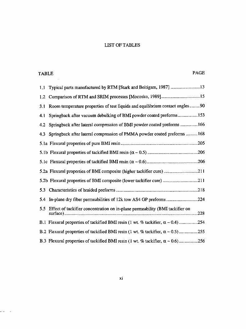
LIST OF TABLES

TABLE p a g e

1.1 Typical parts manufactured by RTM [Stark and Beitigam, 1987].............................13

1.2 Comparison of RTM and SRIM processes [Mocosko, 1989].................................... 15

3.1 Room temperature properties of test liquids and equilibrium contact angles........ 90

4.1 Springback after vacuum debulking of BMI powder coated preforms..................153

4.2 Springback after lateral compression of BMI powder coated preforms............... 166

4.3 Springback after lateral compression of PMMA powder coated preform s.......... 168

5.1a Flexural properties of pure BMI resin.......................................................................205

5.1b Flexural properties of tackified BMI resin (a ~ 0 .5 ).............................................. 206

5.1c Flexural properties of tackified BMI resin (a ~ 0.6)............................................... 206

5.2a Flexural properties of BMI composite (higher tackifier cure)...............................211

5.2b Flexural properties of BMI composite (lower tackifier cure)................................211

5.3 Characteristics of braided preforms...........................................................................218

5.4 In-plane dry fiber permeabilities of 12k tow AS4 GP preforms............................ 224

5.5 Effect of tackifier concentration on in-plane permeability (BMI tackifier onsurface)........................................................................................................................... 228

B.l Flexural properties of tackified BMI resin (1 wt. % tackifier, a ~ 0.4)................254

B.2 Flexural properties of tackified BMI resin (1 wt. % tackifier, a ~ 0.5)................255

B.3 Flexural properties of tackified BMI resin (1 wt. % tackifier, a ~ 0.6)................256

XI

LIST OF FIGURES

FIGURE PAGE

1.1 Schematic of the resin transfer molding process.......................................................... 9

1.2 Schematic of the braiding, weaving and the knitting process....................................19

1.3 The resin injection step in LCM processes : governing phenomena and processissues............................................................................................................................... 25

1.4 Overview of resin transfer molding of polymer powder coated fiber preforms... 26

1.5 Fiber deformation modes : (a) U-shape bending and (b) lateral compression........ 28

2.1 Three phase equilibrium contact angle [Miller, 1977]............................................... 33

2.2 Schematic of the image analysis set - up for contact angle measurement of asessile drop [Neumann, 1992]...................................................................................... 40

2.3 Graph of Cosine 6 vs. 0 [Cahn's Manual DCA 322,1992].......................................42

2.4 Concept of the Wilhelmy technique [Miller, 1977]....................................................44

2.5 A typical curve illustrating the weight changes with time in a wickingexperiment [Hsieh and Yu, 1992]................................................................................47

2.6 Schematic of the flow front progression and the air entrapment processduring transverse flow [Pamas and Phelan, 1991].....................................................54

2.7 Schematic depiction of the channeling flow from larger to smallercapillary [Chan and Morgan, 1993 b ] ......................................................................... 56

2.8 Normalized shear strength as a function of void content[Feldgoise et al., 1991].................................................................................................. 65

2.9 Types of powder coating in composites [Cochran and Pipes, 1991]........................68

2.10 Schematic of the surface of a prepreg [Bonhomme, 1986]........................................ 73

2.11 Squeezing flow of a Newtonian liquid [Bonhomme, 1986] .....................................73

XU

2.12 Reaction mechanisms of a BMI resin : (a) Michael addition of diamine tobismaleimide and (b) bismaleimide homopolymerization....................................... 79

3.1 Schematic of the Dynamic Contact Angle Analyzer [DCA 322].............................87

3.2 Typical trace of force readings obtained in a surface tensionmeasurement experiment (e.g. UP resin)....................................................................88

3.3 Schematic of the flow visualization set-up; video assisted microscopy(VAM).............................................................................................................................94

3.4 Photograph showing the lead - lag at the flow front for axial flow:capillary number < 10"^............................................................................................... 95

3.5 Schematic of formation of macrovoids during axial flow .........................................98

3.6 Photograph of macrovoids trapped in the fiber m at....................................................99

3.7 Percent area macrovoids for flow along the fiber tows (axial flow).......................100

3.8 Percent area macrovoids for flow normal to the fiber tows (transverse flow) ... 102

3.9 Photographs showing the lead - lag at the flow front for axial flow and capillaiynumber > 10'^ : (a) overall view and (b) zoom v iew ............................................. 104

3.10 Schematic of formation of microvoids during axial flow ....................................... 105

3.11 Photograph of coagulated microvoids formed by joining of adjacent wickingstream s..........................................................................................................................107

3.12 Photographs of microvoids : (a) capillary number ~ 0.36 and(b) capillary number ~ 0.004....................................................................................108

3.13 Percent area microvoid content as a function of injection velocity for axialflow .............................................................................................................................. 109

3.14 Percent area macro and microvoids for axial flow : (a) silicone oil, 200 cs ,(b) DOP oil, (c) ethylene glycol and (d) master curve of all three liquids.........110

3.15 Photographs showing the optical transparency of composite samples :(a) good fiber wetting and (b) poor fiber wetting....................................................113

3.16 Percent area macro and micro voids during transverse flow of DOP oil.................115

3.17 Schematic of flow front progression and the formation of microvoids duringtransverse flow (mechanism I, capillary number < 10"2).......................................116

xin

3.18 Photograph illustrating lead-lag at the flow front during transverse flow(mechanism I, capillary number < 10'^)................................................................. 117

3.19 Photograph of microvoids formed during transverse flow of DOP oil :capillary number ~ 0.003 (2(X)X)...............................................................................118

3.20 Photographs showing the dynamics of microvoid formation and movement during transverse flow : (a) formation of microvoids, (b) and (c) movementwith change in shape and s iz e ................................................................................... 120

3.21 Schematic of the flow mechanism (II) for transverse flow : (a) an enlarged side view of flow in and around a fiber tow and (b) microvoid at the edgeof the fiber tow............................................................................................................. 122

4.1 Schematic of 6k, 4 HS woven fiber reinforcement................................................... 126

4.2 Structure of two components of Bismaleimide resin based tackifier...................... 127

4.3 Schematic of the Differential Scanning Calorimetry set-up.................................... 128

4.4 Scanning electron micrograph showing distribution of tackifier powder in"undebulked" fiber preform ........................................................................................133

4.5 Schematic of the U-shape bending device..................................................................133

4.6 Schematic of preform lay-up prior to debulking........................................................135

4.7 Schematic of the lateral compression device............................................................. 137

4.8 Calibration curve for the LVDT used in lateral compression experiments 138

4.9 Schematic of parallel plate set-up for theological measurements............................141

4.10 Scanning reaction rate profile for BMI tackifier........................................................143

4.11 Isothermal conversion profiles for BMI tackifier......................................................144

4.12 Glass transition temperatures of BMI tackifier under different cureconditions......................................................................................................................146

4.13 Springback in U-shape bending of fiber preforms as a function of tackifierconversion at different concentration levels.............................................................147

4.14 Photographs showing springback in U-shape bending of fiber preforms fordifferent debulking conditions................................................................................... 149

4.15 Photomicrograph showing powder coagulation and tackifier location forpreforms subjected to U-shape bending.................................................................... 150

XIV

4.16 Sintering of tackifier particles : (a) upon melting and (b) coagulation intodeformed droplets........................................................................................................ 151

4.17 Photomicrographs of the fiber preform with BMI tackifier applied usingthe solvent technique (a) low magnifications and (b) high magnification 152

4.18 Photomicrograph of surface of fiber preform with BMI tackifier and vacuumdebulked at94°C .......................................................................................................... 155

4.19 Consolidation behavior of BMI tackified preforms under lateral compression :(a) compacted thickness, (b) springback and (c) uncompacted thickness .......... 156

4.20 Viscoelastic behavior of tackified preforms : (a) change in strain as a function of time at constant pressure and (b) change in strain during springbackat zero stress..................................................................................................................158

4.21 Photomicrographs of surface of laterally compressed preforms with BMItackifier : (a), (b) showing interlayer coverage and (c) droplet possibly coexisting with a "manchon"......................................................................................160

4.22 Change in viscosity and viscoelastic properties of BMI tackifier as a function of temperature : (a) dynamic viscosity, (b) G* and (c) G' & G "................................ 163

4.23 Dynamic viscosity of PM M A...................................................................................... 167

4.24 Photomicrographs of surface of PMMA tackified preforms compressed at220°C : (a) low magnification and (b) high magnification.....................................170

4.25 Photomicrographs of surface of PMMA tackified preforms compressed at250°C : (a) low magnification and (b) high magnification.....................................171

4.26 Photomicrographs of surface of PMMA tackified preforms compressed at~287°C : (a) low magnification and (b) high magnification...................................172

4.27 Viscoelastic properties of PMMA : (a) G* and (b) G" and G "................................173

4.28 Phenomenological approach for springback control under lateralcompression..................................................................................................................174

4.29 Consolidation behavior of untackified fiber preform under lateral compression :(a) 8 layers and (b) 16 layers.......................................................................................176

4.30 Photomicrographs showing the consolidation of inter and intralayer gaps with increasing fiber volume fraction : (a) Vf = 0.32, (b) Vf = 0.45 and(c) Vf = 0.67............................................................................................................... 177

XV

4.31 Comparison of experimental vs. consolidation model for lateral compressionof 4HS preforms : (a) 8 layers and (b) 16 layers...................................................... 181

4.32 Viscoelastic properties of BMI tackifier under isothermal conditions :(a) 94°C, (b) 120°C and (c) 150°C............................................................................. 183

4.33 Overview of the phenomenological approach for springback control underlateral compression......................................................................................................186

4.34 Photomicrographs showing cross-section of laminates after springback :(a), (b) preforms with PMMA powder heated at ~287°C and (c) preformwith BMI tackifier vacuum debulked at 94°C ......................................................... 188

5.1 Torsion rectangular fixtures with the loaded sample [RDA InstructionManual, 1994]...............................................................................................................193

5.2 Drop in the dynamic stiffness of unidirectional stitched fiberglass mat reinforced UP composite samples with increased immersion times in hotwater : (a) no void, (b) ~ 7% macrovoid and (c) ~ 3% m icrovoid........................195

5.3 Formation of microcracks in unidirectional stitched fiberglass mat reinforced reinforced UP composite samples: (a) cracks on the surface, macrovoidsample and (b) cracks in the fiber tow, micro void sam ple.....................................198

5.4 Components of the SONOTEK Ultrasonic C - scan system................................... 199

5.5 Ultrasonic C - scan image of unidirectional stitched fiberglass mat reinforced UP composite samples : (a) Vg = 0.04 cm/sec., (b) Vg = 1.0 cm/sec. and(c) Vs = 3.9 cm/sec.................................................................................................... 201

5.6 Schematic of the 3-pt bending test............................................................................. 203

5.7 Configuration of the mold set-up for preparing clear castings...............................204

5.8 Comparison of mechanical properties of pure BMI resin and with 3 wt.%tackifier : (a) mean flexural strength and (b) mean % strain at break................... 208

5.9 Four clover leaf pattern indicative of residual microstresses at the tackifierparticle/resin matrix interface.................................................................................... 209

5.10 Scanning electron micrographs of the fracture surface : (a) pure BMI resinand (b) tackified BMI resin.........................................................................................210

5.11 Schematic of the in-house developed permeability set-up...................................... 213

XVI

5.12 Schematic of the Ashcroft Dead Weight Gauge Tester...........................................215

5.13 Calibration curves of the pressure transducers used for permeabilitymeasurements : (a) 100 psi range and (b) 500 psi range........................................ 216

5.14 Pressure rise vs. time curves for brmded preforms : (a) 3 layers [0/0/0](b) 2 layers [0/0] and (c) 2 layers [0/90] ...............................................................221

5.15 Pressure drop as a function of tackifier concentration and locationfor 4HS graphite fiber preforms................................................................................ 227

5.16 Permeability as a function of tackifier concentration for 4HS graphite fiberpreforms with BMI tackifier and vacuum debulked at 94°C.................................228

5.17 Comparison of wicking behavior of solvent and powder coated 4HS graphitefiber preforms.............................................................................................................. 230

5.18 Schematic of the centrifuge device.............................................................................232

5.19 Configuration of the fiber sample in the centrifuge device.................................... 235

5.20 Comparison of capillary pressure as a function of saturation for 4HSgraphite fiber samples with and without tackifier................................................... 236

xvii

CHAPTER I

INTRODUCTION

1.1 Fiber Reinforced Polymer Composites

The demand for light weight high strength materials in almost all walks of life has

brought about an increased usage of composite materials. Composites offer high strength

and stiffness, resistance to hostile environments as well as ability to be formed into

complex shapes.

Composite materials evolve from combining two or more physically distinct and

mechanically separable component materials. The key, however, lies in combining the

components in a synergistic way so as to enhance the properties of the final product.

Composite materials can include steel reinforced concrete, straw reinforced mud bricks,

linoleum, fiber reinforced ceramic / polymer or for that matter any other combination that

falls under the definition of a composite material. This text, however, will focus only on

methods, materials and applications of polymer composites, more specifically fiber

reinforced polymer composites.

Fiber reinforced polymer composites (FRP's) have been in use since World War II. In the

late 1940s and early 1950s, FRP's were used largely in the marine industry. However,

they have come a long way since then, and today, they are being used in a wide range of

applications. Polymer composites are used in the transportation industry (automotive,

tmck, ships and railway vehicles), in aerospace, defense and outer space applications, in

1

2

the recreational and sporting goods industries, in electronics, and in commercial

industries. As an example. Corvette, Fierro, and Avanti automobiles have had body

structures made of polymer composites for over 25 years. Another spectacular

application in the automotive industry is the sports car, the Dodge Viper that has all its

external panels with a total weight of about 77 kg made of polymer composite. In 1987,

Ford Motor Company completed a prototype replacing the 90 piece steel front stmcture

of an Escort automobile with a two piece composite structure [Johnson, 1987]. An all

composite chassis for Bugatti BE 110 automobile has been developed by Composites

Aquitaine, a French Company [High performance composites, 1993]. Another example

is the All Terrain Vehicle (Bandvagnen) designed and manufactured in Sweden.

Recently, a 175 ft tall polymer composite mast was fabricated for the Zeus luxury super

yacht, the largest boat of its type to be certified by the American Bureau of Shipping

[Stover, 1993]. Trains, such as the BART (the San Francisco Bay Area Transit System),

use composites for interior panels, and several trains have fully formed compartments

made of composites [Strong, 1989]. Rail vehicles in Europe are now also being made of

polymer composites. The Voyager, which circled the world without stopping, was an all

composite aircraft. Boeing's 767 commercial aircraft has over 30% of its structure, from

its nose landing gear doors to its vertical fin tip, based on polymer composite materials.

In October 1993, the first set of horizontal and vertical stabilizers were fabricated with

fiber reinforced plastics for Boeing's new 777 wide body passenger jet [Modern Plastics,

1994]. B - IB stealth bombers, DC - X missiles, and F -18 fighter jets make use of high

performance advanced polymer composites. The Solar and Heliospheric Observatory

(SOHO) spacecraft which was due to launch in July 1995, will have an all composite

Telescope Structure Assembly (TSA) mounted on it [McConell, 1993]. The sporting

goods and recreational industry uses composites for tennis racquets, golf clubs, baseball

bats, skis, snowmobiles etc. The most common uses for composites in electrical

3applications utilize the non conductive nature of composite materials. Typical examples

include printed circuit boards (PCBs), insulators, and radomes [Strong, 1989].

Commercial industries employ polymer composites for the manufacture of storage tanks,

bathtubs, kitchen sinks, compressed gas cylinders, medical equipment, building panels

etc. The success of polymer composites in today's globally competitive market is

primarily due to the large number of advantages they offer as compared to other

materials. The advantages are [Moritz, 1993]:

1. Higher strength / stiffness to weight ratio than most metals

2. Design flexibility

3. Thermal stability

4. Dimensional stability

5. Increased fatigue life

6. Improved corrosion and wear resistance

7. Finishing (Long lasting with minimum maintenance)

8. Parts consolidation &

9. Significant cost advantages (Low tooling costs)

As with all other materials, composites are not without their disadvantages. Perhaps the

greatest disadvantages are the lack of well - defined and easy to employ design rules and

lack of highly productive manufacturing methods. The resolution of these issues is the

overriding concept behind the extensive research efforts being directed towards

composite manufacturing processes, both in academia and in industry.

A fiber reinforced polymer composite consists of a fiber reinforcement, a matrix resin,

and an interface between the two. Fiber reinforcement provides strength and stiffness.

The matrix protects the reinforcement from adverse environmental effects and binds the

fibers, while the interface serves to transfer stress from the matrix to the fibers. Fiber

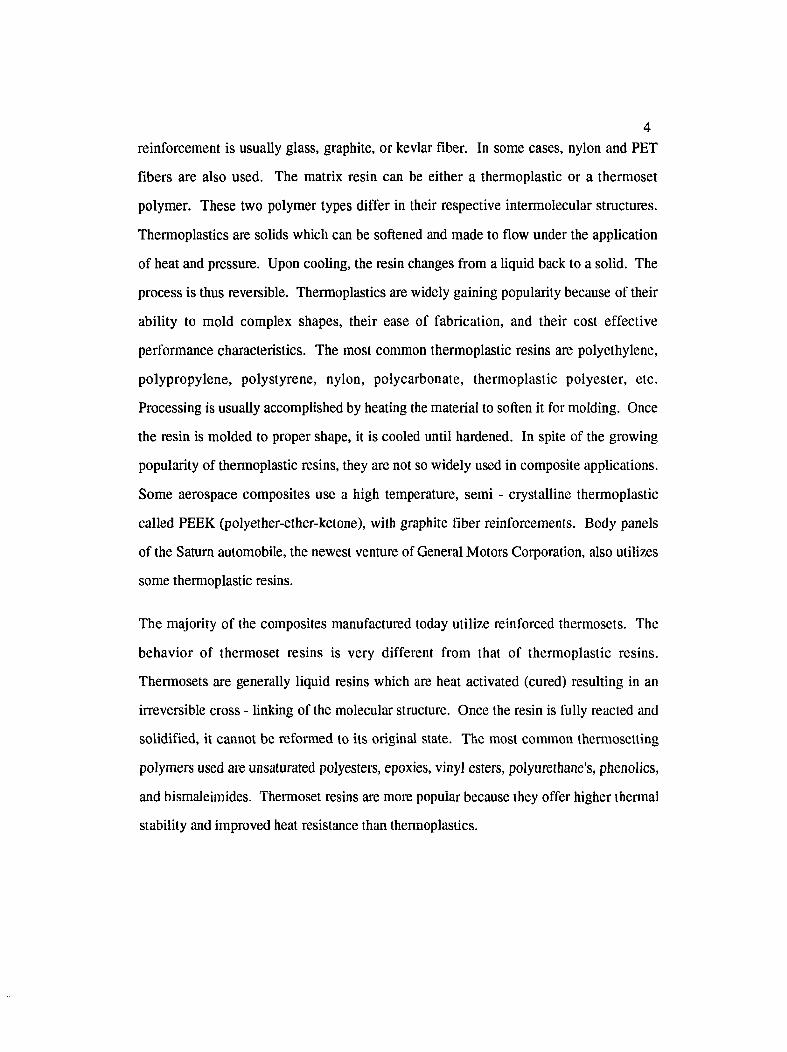
4reinforcement is usually glass, graphite, or kevlar fiber. In some cases, nylon and PET

fibers are also used. The matrix resin can be either a thermoplastic or a thermoset

polymer. These two polymer types differ in their respective intermolecular structures.

Thermoplastics are solids which can be softened and made to flow under the application

of heat and pressure. Upon cooling, the resin changes from a liquid back to a solid. The

process is thus reversible. Thermoplastics are widely gaining popularity because of their

ability to mold complex shapes, their ease of fabrication, and their cost effective

performance characteristics. The most common thermoplastic resins are polyethylene,

polypropylene, polystyrene, nylon, polycarbonate, thermoplastic polyester, etc.

Processing is usually accomplished by heating the material to soften it for molding. Once

the resin is molded to proper shape, it is cooled until hardened. In spite of the growing

popularity of thermoplastic resins, they are not so widely used in composite applications.

Some aerospace composites use a high temperature, semi - crystalline thermoplastic

called PEEK (polyether-ether-ketone), with graphite fiber reinforcements. Body panels

of the Saturn automobile, the newest venture of General Motors Corporation, also utilizes

some thermoplastic resins.

The majority of the composites manufactured today utilize reinforced thermosets. The

behavior of thermoset resins is very different from that of thermoplastic resins.

Thermosets are generally liquid resins which are heat activated (cured) resulting in an

irreversible cross - linking of the molecular structure. Once the resin is fully reacted and

solidified, it cannot be reformed to its original state. The most common thermosetting

polymers used are unsaturated polyesters, epoxies, vinyl esters, polyurethane's, phenolics,

and bismaleimides. Thermoset resins are more popular because they offer higher thermal

stability and improved heat resistance than thermoplastics.

1.2 Polymer Composite Processes

Fiber reinforced polymer composites are manufactured by a large number of processing

methods which include hand lay - up, spray - up, prepreg vacuum bagging and autoclave

curing, filament winding, pultrusion, compression molding of sheet molding compound

(SMC) and its derivatives (BMC, TMC etc.), and liquid composite molding (LCM),

which includes processes like resin transfer molding (RTM), structural reaction injection

molding (SRIM), and their variants. The following is a brief overview of the common

methods employed in the industry to manufacture fiber reinforced polymer composites.

However, since the objective of this study is the experimental investigation of the issues

related to the LCM process, it is discussed in much greater detail.

1.2.1 Hand Lay - up and Spray - up

Hand lay - up technique started in the forties and has been used since then to make

models, prototypes, and other parts that have low production volume. In this method,

layers of dry fiber mat are laid in the mold and the liquid resin is poured manually on

each layer. Entrapped air is removed by squeegees, rollers, and / or brush dabbing

[Schwartz, 1984]. The "lay - up" is made by building layer upon layer to obtain the

desired thickness. Curing is usually done at room temperature, and catalysts are often

added to speed up the reaction. This method uses mostly polyester resin and occasionally

epoxies. The reinforcement, however, is always fiberglass.

Hand lay - up technique is labor intensive and very time consuming. Thus, in an effort

to mechanize the hand lay - up process, spray - up technique was devised. In this

method, the fiber reinforcement (chopped rovings) and the catalyzed resin are

simultaneously deposited in the mold from a combination of a chopper and a spray gun.

Additional layers of the rovings and resin may be added to obtain the desired thickness.

6

Traditionally spray guns use pressurized air to spray the resin. More recently, "airless"

spray guns which dispense resin under hydraulic pressure through special nozzles have

been developed. They are preferred as they provide more controlled spray patterns and

reduce emission of volatiles [Moritz, 1993]. Typical applications of lay -u p /sp ray - up

processes include boat and boat hulls, truck roofs and housings, bathtubs, furniture etc.

1.2.2 Prepreg Vacuum Bagging and Autoclaving

In the prepreg method, wetting of the fibers occurs outside the mold. The fiber

reinforcement, usually arranged in a unidirectional tape or a woven fabric, is impregnated

with a partially cured resin. The resulting product is called a prepreg and is stored in a

freezer until molding when layers of prepregs are cut and laid into the mold. The prepreg

method allows a better control over the processing variables and thus, is a more precise

method than the hand lay - up method. However, the prepreg method usually involves

two additional steps, vacuum bagging and autoclaving. Vacuum bagging involves laying

pieces of prepreg and other materials onto a mold and enveloping the assembly with a

bag. Vacuum is pulled on the bag, which serves the dual purpose of compressing

(debulking) the prepreg plies and simultaneously withdrawing entrapped air. Further

debulking and curing is done in an autoclave pressure oven. Prepreg vacuum bagging /

autoclave curing is the traditional method for manufacturing high performance graphite /

epoxy composites for aerospace applications.

1.2.3 Filament Winding and Pultrusion

Filament winding draws fiber tows or bundles through a resin bath and wraps the

continuous tow onto a mandrel to form the part. Successive layers are added at the same

or different winding angles until the required thickness is reached. The mandrel is then

placed in an oven for curing. This process is called wet winding. Dry filament winding.

7which is less common, uses prepregs as the winding medium. Most standard composite

resins (polyesters, epoxy, phenolic etc.) can be used for filament winding. Continuous

reinforcements commonly used are glass (for price), carbon (for strength and modulus),

and aramid (for toughness and lightweight). Composite suspension leaf springs and

pressure vessels are usually filament wound [Strong, 1989].

Pultrusion is quite similar to filament winding in that it also involves passing a

continuous fiber reinforcement through a resin bath. However, instead of wrapping the

resin rich fibers onto a mandrel, the part is formed by passing the fibers through a heated

die. Resins and reinforcements used in filament winding are used in pultrusion too. The

largest market for pultruded parts is translucent building panels made from fiberglass and

polyester resin. Other applications include supports and panels for tmck trailers, door

supports for automobiles, ladder rails etc. [Strong, 1989].

1.2.4 Compression Molding o f Sheet Molding Compound

Sheet molding compound (SMC) is a complex composite of unsaturated polyester resin

to which thickeners, inorganic fillers, fiber reinforcements (usually chopped glass fibers),

catalyst, pigment, and other additives are added to form a paste like material. This paste

like material is stored for several days between layers of a carrier film, typically

polyethylene, until proper molding viscosity has been attained. Once ready, the carrier

film is removed from the charge, which is then molded in a heated matched metal mold

mounted in a hydraulic press [Moritz, 1993]. The SMC process is a reactive polymer

process in which part curing and shaping occur together. It is used extensively in the

automotive and truck industry. General Motors uses SMC for body panels of its AFV

minivans like the Pontiac Trans Sport, the Chevrolet Lumina, and the Oldsmobile

Silhouette. Each van uses approximately 320 lbs. of SMC [Wigotsky, 1989; Wood,

8

1988; Wood, 1990]. SMC is also used for roofs, rear decks, and outer door panels in

GM's redesigned F-body cars for 1993, the Chevrolet Camaro and Pontiac Firebird.

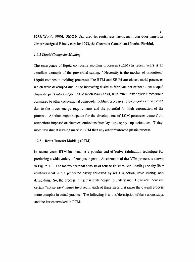
1.2.5 Liquid Composite Molding

The emergence of liquid composite molding processes (LCM) in recent years is an

excellent example of the proverbial saying, " Necessity is the mother of invention."

Liquid composite molding processes like RTM and SRIM are closed mold processes

which were developed due to the increasing desire to fabricate net or near - net shaped

disparate parts into a single unit at much lower costs, with much lower cycle times when

compared to other conventional composite molding processes. Lower costs are achieved

due to the lower energy requirements and the potential for high automation of the

process. Another major impetus for the development of LCM processes came from

restrictions imposed on chemical emissions from lay -up /sp ray - up techniques. Today,

more investment is being made in LCM than any other reinforced plastic process.

1.2.5.1 Resin Transfer Molding (RTM)

In recent years RTM has become a popular and effective fabrication technique for

producing a wide variety of composite parts. A schematic of the RTM process is shown

in Figure 1.1. The modus operandi consists of four basic steps, viz., loading the dry fiber

reinforcement into a preheated cavity followed by resin injection, resin curing, and

demolding. So, the process in itself is quite "easy" to understand. However, there are

certain "not so easy" issues involved in each of these steps that make the overall process

more complex in actual practice. The following is a brief description of the various steps

and the issues involved in RTM.

FIBERLOADING

RESININJECTION

CUREREACTION

COMPOSITEDEMOLDING

Figure 1.1 Schematic of the resin transfer molding process

10

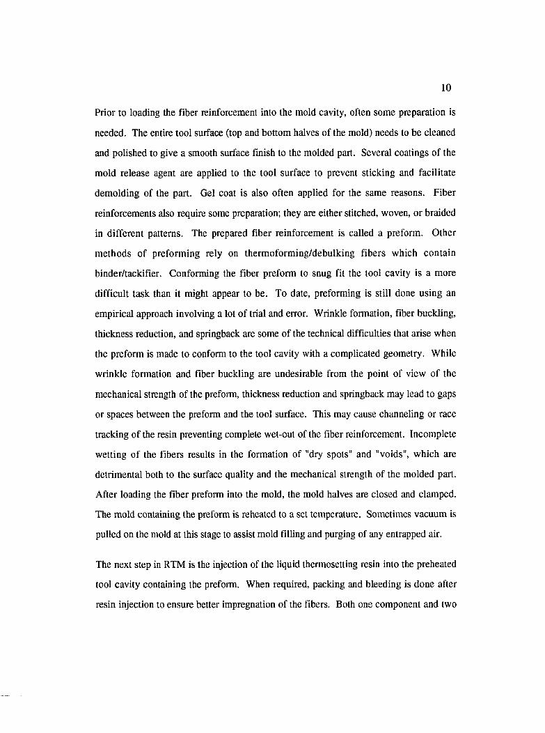
Prior to loading the fiber reinforcement into the mold cavity, often some preparation is

needed. The entire tool surface (top and bottom halves of the mold) needs to be cleaned

and polished to give a smooth surface finish to the molded part. Several coatings of the

mold release agent are applied to the tool surface to prevent sticking and facilitate

demolding of the part. Gel coat is also often applied for the same reasons. Fiber

reinforcements also require some preparation; they are either stitched, woven, or braided

in different patterns. The prepared fiber reinforcement is called a preform. Other

methods of preforming rely on thermoforming/debulking fibers which contain

binder/tackifier. Conforming the fiber preform to snug fit the tool cavity is a more

difficult task than it might appear to be. To date, preforming is still done using an

empirical approach involving a lot of trial and error. Wrinkle formation, fiber buckling,

thickness reduction, and springback are some of the technical difficulties that arise when

the preform is made to conform to the tool cavity with a complicated geometry. While

wrinkle formation and fiber buckling are undesirable from the point of view of the

mechanical strength of the preform, thickness reduction and springback may lead to gaps

or spaces between the preform and the tool surface. This may cause channeling or race

tracking of the resin preventing complete wet-out of the fiber reinforcement. Incomplete

wetting of the fibers results in the formation of "dry spots" and "voids", which are

detrimental both to the surface quality and the mechanical strength of the molded part.

After loading the fiber preform into the mold, the mold halves are closed and clamped.

The mold containing the preform is reheated to a set temperature. Sometimes vacuum is

puUed on the mold at this stage to assist mold filling and purging of any entrapped air.

The next step in RTM is the injection of the liquid thermosetting resin into the preheated

tool cavity containing the preform. When required, packing and bleeding is done after

resin injection to ensure better impregnation of the fibers. Both one component and two

1 1

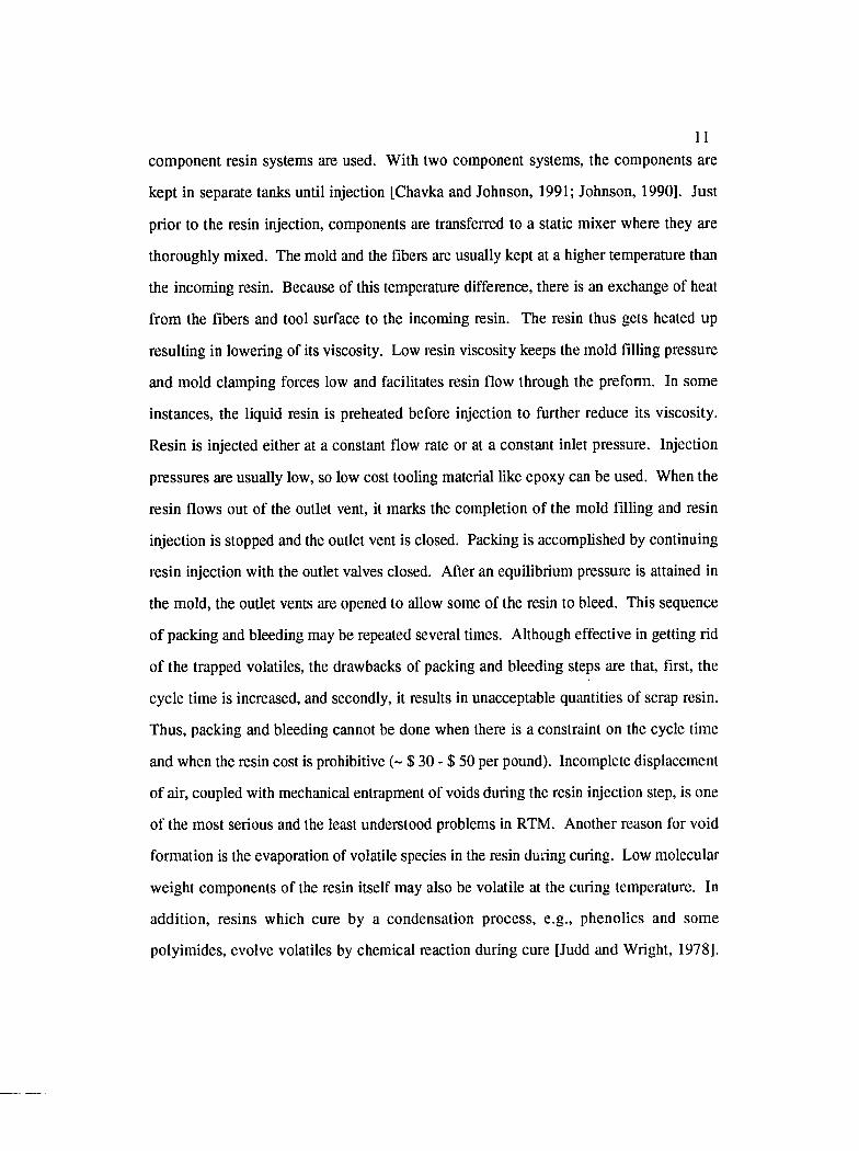
component resin systems are used. With two component systems, the components are

kept in separate tanks until injection [Chavka and Johnson, 1991; Johnson, 1990]. Just

prior to the resin injection, components are transferred to a static mixer where they are

thoroughly mixed. The mold and the fibers are usually kept at a higher temperature than

the incoming resin. Because of this temperature difference, there is an exchange of heat

from the fibers and tool surface to the incoming resin. The resin thus gets heated up

resulting in lowering of its viscosity. Low resin viscosity keeps the mold filling pressure

and mold clamping forces low and facilitates resin flow through the preform. In some

instances, the liquid resin is preheated before injection to further reduce its viscosity.

Resin is injected either at a constant flow rate or at a constant inlet pressure. Injection

pressures are usually low, so low cost tooling material like epoxy can be used. When the

resin flows out of the outlet vent, it marks the completion of the mold filling and resin

injection is stopped and the outlet vent is closed. Packing is accomplished by continuing

resin injection with the outlet valves closed. After an equilibrium pressure is attained in

the mold, the outlet vents are opened to allow some of the resin to bleed. This sequence

of packing and bleeding may be repeated several times. Although effective in getting rid

of the trapped volatiles, the drawbacks of packing and bleeding steps are that, first, the

cycle time is increased, and secondly, it results in unacceptable quantities of scrap resin.

Thus, packing and bleeding cannot be done when there is a constraint on the cycle time

and when the resin cost is prohibitive (~ $ 30 - $ 50 per pound). Incomplete displacement

of air, coupled with mechanical entrapment of voids during the resin injection step, is one

of the most serious and the least understood problems in RTM. Another reason for void

formation is the evaporation of volatile species in the resin dunng curing. Low molecular"

weight components of the resin itself may also be volatile at the curing temperature. In

addition, resins which cure by a condensation process, e.g., phenolics and some

polyimides, evolve volatiles by chemical reaction during cure [Judd and Wright, 1978].

12For most resin systems however, the main reason for void formation is mechanical

entrapment. The information available on the micro mechanics of this process is very

little compared to what is known about wetting and void formation in autoclave type

processes. It should be pointed out that in some applications it is desirable to have voids.

This is typically true when a premium is put on light weight and the composite is not

expected to perform structurally, as in foam core panels. In general however, voids are

an undesirable material defect which should be minimized or eliminated whenever

possible [Ghiorse, 1993].

After the resin injection step, the resin is cured during which the mold temperature is set

at a higher temperature in order to drive the reaction to completion. The length of the

cure cycle depends on several factors which include resin type, catalyst type and amount

used, part thickness, and curing temperature. Problems during the cure cycle include

incomplete and non - uniform cure in the part. These problems occur either due to low

cure temperature, localized variations in mold heating, localized heat generation due to

reaction exotherm, or a combination of all of these. When required, post curing is done at

a temperature higher than the cure temperature to achieve greater conversion. Post curing

may be done after the part has been demolded. The part however, must develop "green

strength" (strength a composite exhibits after resin gelation, but prior to complete cure)

before it can be demolded. Premature demolding results in inferior mechanical

properties. Typical parts manufactured using RTM are shown in Table 1.1

1.2.5.2 Stmctural Reaction Injection Molding (SRIM)

One of the variants of RTM is SRIM. The steps involved in the SRIM process are similai'

to RTM. However, there are some key differences in the resin injection and curing steps.

SRIM is a much faster process than RTM. Resin injection and curing steps get over in a

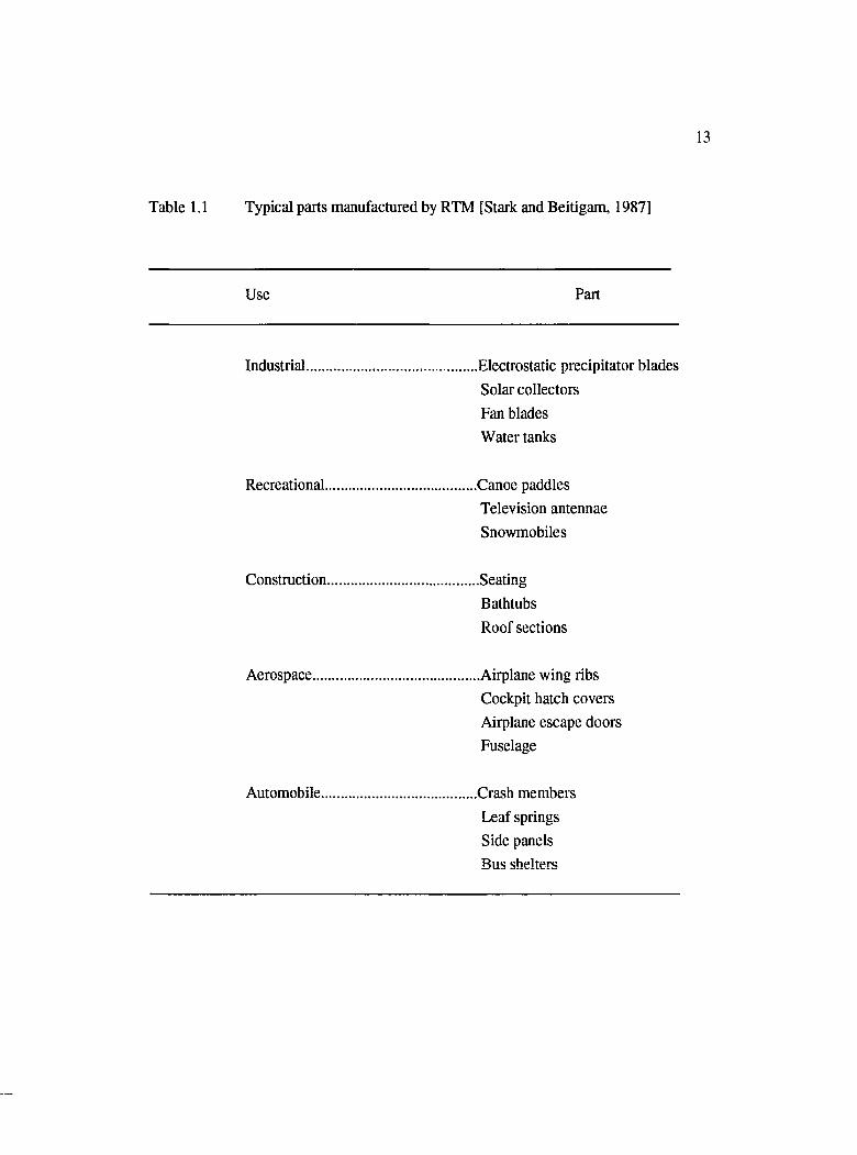
Table 1.1 Typical parts manufactured by RTM [Stark and Beitigam, 1987]

Use Part

Industrial........................Solar collectors Fan blades Water tanks

Recreational................... ................... Canoe paddlesTelevision antennae Snowmobiles

Construction................... ....................SeatingBathtubs Roof sections

Aerospace....................... ....................Airplane wing ribsCockpit hatch covers Airplane escape doors Fuselage

Automobile....................Leaf springs Side panels Bus shelters

14

matter of seconds as opposed to several minutes in the case of RTM. SRIM resins are

two component thermosetting liquid resins. They are highly reactive in comparison to

RTM resins and require very fast, high pressure impingement mixing to achieve thorough

mixing before injecting into the mold. Because of the high injection pressures used, steel

molds held together by a hydraulic press are used. The cure reaction is mixing activated

and is complete shortly after the resin reaches the outlet vent. Thus, no packing or

bleeding is possible, and if there is any air present, it remains trapped. After curing

reaction is complete, the part is removed from the mold and the process is completed.

Generally, no post cure is carried out. Typical applications of SRIM include electric

scooter frames [Ohmura et al., 1993], automotive bumper beams, instrument panels, load

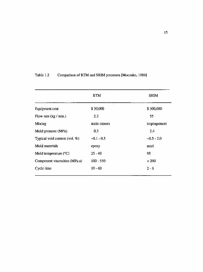
floors and cross members [Babbington et al., 1990]. Table 1.2 compares the features of

the SRIM process with those of RTM [Mocosko, 1989].

1.3 Resin Systems for LCM

The selection of a resin system is primarily based on the cost and performance

requirements of the end - use application [Stark and Beitigam, 1987]. A resin system

includes, apart from the resin, other components like the curing agent, catalysts, fillers,

pigments, promoters, and inhibitors. An ideal resin is one which can stay at very low

viscosity for a long period and yet cure quickly. A long pot life allows resin injection at

lower pressures, improves fiber wet - out, and yields faster cycle times. Once cured, the

resin should have good structural and mechanical properties. Structural properties

include shrinkage characteristics, microcrack resistance, etc. Flexural modulus, tensile

strength, impact strength, and strength after impact, are some of the mechanical

properties that are taken into consideration while choosing a resin system. Other

considerations include chemical resistance, electrical properties, and fire characteristics.

15

Table 1.2 Comparison of RTM and SRIM processes [Mocosko, 1989]

RTM SRIM

Equipment cost $ 30,000 $ 500,000

Flow rate (kg / min.) 2.3 55

Mixing static mixers impingement

Mold pressure (MPa) 0.3 2.4

Typical void content (vol. %) -0.1 -0.5 -0.5 - 2.0

Mold materials epoxy steel

Mold temperature (°C) 25-40 95

Component viscosities (MPa.s) 100-550 <200

Cycle time 10-60 2 - 6

16

Thermoset RTM resins can be divided in general into two broad categories, viz.

aerospace and non - aerospace type resins. Aerospace resins include high performance,

high cost epoxies, bismaleimides, phenolics, and polyimides. Non - aerospace

applications use low cost epoxies, unsaturated polyester, vinyl ester, and hybrid resins

like blends of unsaturated polyesters and isocyanates. Typical SRIM resins are

polyurethanes, polyurethane/isocyanurates, polyurethane/polyester IPNs, and

polyurethane/urea hybrids [Lee, 1989; Mocosko, 1989].

1.4 Reinforcements for LCM

As with the resin system, the selection of the appropriate reinforcements is primarily

governed by the cost and the performance requirements of the end use application.

However, there are several other important mechanical, processing, and fiber

characteristics that also influence the choice of reinforcement. Apart from its mechanical

strength, a fiber reinforcement is characterized by four additional attributes, viz. (1) bulk

factor, which is the ratio of the volume of the given mass of "loose" reinforcement to the

volume of the same mass after forming; (2) drapeability or the ability of a fabric to

conform to the contours of the mold cavity; (3) wash resistance, or the ability to resist

movement during resin injection; and (4) wettability, or the ability to allow maximum

access to the resin to all the pores in the reinforcement.

Predominant fiber materials are glass (E and S types), graphite and kevlar. Glass fibers

are often used in parts with lower cost and performance requirements. This encompasses

most of the non - aerospace type applications. Graphite fibers provide the best property

performance with respect to their weight, and are mostly used in aerospace applications

where reduced weight and high performance characteristics are dominant factors. Kevlar

fibers are used in high temperature applications (upto 400 °C), and where high impact

17strength is required. Typical applications include aircraft and missile products, helmets,

bicycle frames, etc.

In order to enhance the physical and chemical interaction between the fibers and the

matrix resins, glass fibers are often treated with sizings. A typical commercial sizing may

include a film former, a silane coupling agent, lubricants, and additives such as anti -

statics, defoamers, and surface tension reducers [Plueddemann, 1974]. Surface

modification of graphite fibers is usually done by plasma treatment or chemical etching.

Kevlar fibers are used as is without any surface treatment.

Finally, the manner in which the fiber reinforcements are held together to form a fiber

mat or a preform is important in many ways. Many single fiber filaments are brought

together in the form of a bundle also called a roving or a tow. The most common method

for holding the fiber tows and maintaining the orientation is by using a continuous stitch.

Benefits of stitching include better interlaminar shear properties, damage tolerance, and

fiber alignment [Stark and Beitigam, 1987]. However, the use of stitches has one serious

disadvantage. Stitches interfere with the flow and result in the formation of voids. This

was found to be the case in the experiments that were conducted in this study. To avoid

this problem, other ways have been devised to hold the fiber tows. These include

weaving, knitting, and braiding the fiber tows in different patterns to obtain a self

supporting structure. Typical fiber reinforcements are formed as random chopped

strands, random continuous strands, unidirectional or bidirectional stitched mats,

unidirectional rovings, bidirectional wovens, and various other combinations using

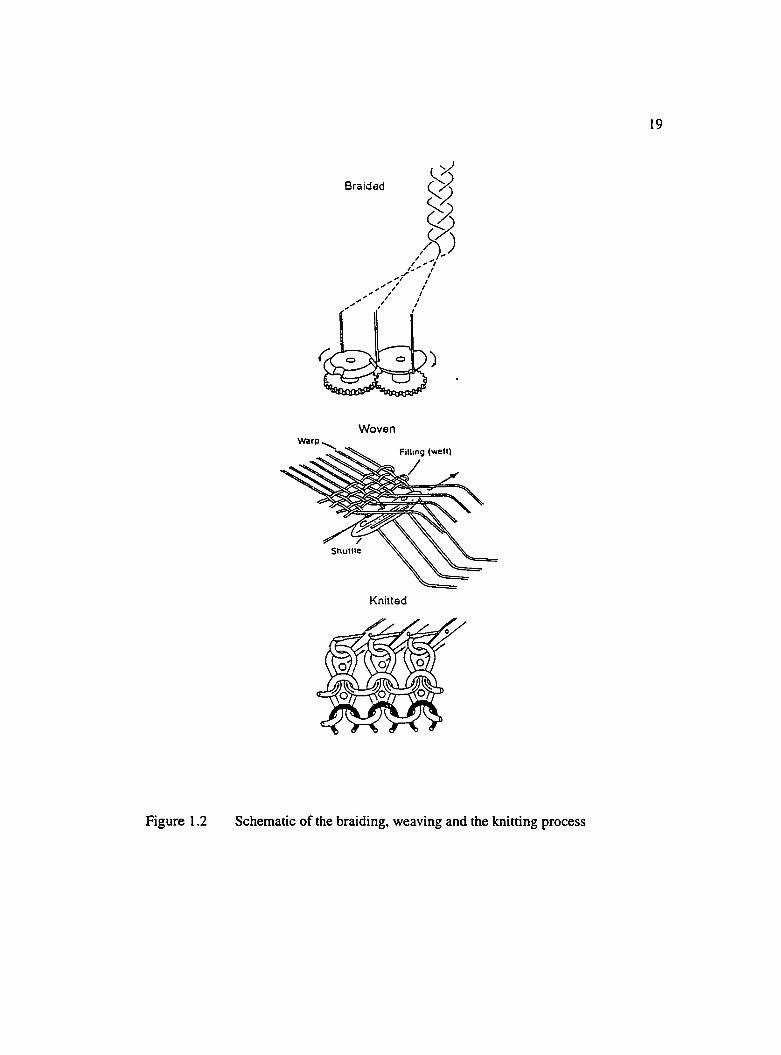
stitching, weaving, knitting, braiding and filament winding. Weaving is done by

interlacing fiber tows of one set over and under the fiber tows of the other set. Depending

on the under over pattern, different harness types are obtained, e.g., 3 HS, 4 HS, 8 HS,

etc. The main characteristic of woven fibers is the fonnation of crimp caused by the

18under and over weave pattern at the intersection of weft and warp fibers. In knitting, the

interlacing is done by loops formed between neighboring tows in one set. Knitted fabrics

eliminate crimp and result in less bulky reinforcement. In braiding, fibers are interlaced

over a mandrel. Typical braid patterns are either two over and two under or one over and

one under. Triaxial braiding is one technique for introducing unidirectional fibers into a

braid. Woven materials have good drapeability. Non woven knitted reinforcements have

even better drapeabilty and wet-out and carry load more evenly [Margolis, 1988].

Braiding is specially suited for parts with complex shapes and is the most economical

preforming method [Becker, 1990]. Figure 1.2 shows a schematic of the braiding,

weaving and the knitting process.

Other methods employed in the industry to maintain the shape of the preforms involve

the use of binders or tackifiers. Binders are more common in automotive industry while

the use of tackifiers is specially common in the aerospace industry. These are normally

thermoplastic or thermoset resins that are solid at room temperature and are randomly

sprayed on the preform in the form of a fine powder. The preform is then heated either

by thermoforming or by debulking depending upon whether the preforms have binder or

tackifier on them. The binder / tackifier melts or reacts upon heating and solidifies either

by reacting in the case of thermosets or by cooling in the case of thermoplastics, thus

imparting rigidity to the preform. The choice of a binder / tackifier is governed by the

compatibility with the matrix resin. Usually, the tackifying material is an advanced form

of the matrix resin which can co-cure with the resin. Typical examples are epoxy,

polyester, phenolic, and bismaleimides. The amount sprayed is usually about 4 to 7

percent by weight of the preform [Hansen, 1990].

Random spraying of the binder/tackifier on the preform causes high concentration in

localized areas which results in poor wetting due to an increased resistance to resin flow.

1 9

Braided

WovenW a rp

F illin g (w e lt)

Shuttle

Knitted

Figure 1.2 Schematic of the braiding, weaving and the knitting process

20

Recently, Shields and Colton [1993] proposed a method for improving the wettability of

powder coated preforms. Instead of applying the powdered resin onto the preform itself,

they applied it to the fiber tows using an electrostatic powder fusion coating process.

They found that spreading the fiber tows during the coating process resulted in a much

improved fiber wet - out. Powdered fiber tows were then woven to obtain the preforms.

There are several different ways of applying the powder on the fiber reinforcements. One

approach, which is also investigated in this study, utilizes spraying individual layers with

a powdered tackifying material, and then stacking up the layers one on top of the other.

When heat and pressure are applied, the tackifier powder bonds the layers together into

shape. This technique is especially suited for large parts with complicated geometries. It

facilitates easier handling of the preform as a single unit, reduces bulk factor, and

improves drapeability. Moreover, it also helps in better control of the prefomi shape and

thickness. Net-shape preforms are critical to the fabrication of high performance RTM

parts. Wrinkles in the reinforcing fabric are often created when oversized preforms are

compressed into the molding tool, ultimately resulting in structural failure of the

composite [Barron, 1995].

The powder technique has historically been used to manufacture thermoplastic matrix

based prepregs. Powder coating techniques for making prepregs mainly fall into two

main categories; 1) wet powder coating that involves impregnation of fibers from a slurry

of polymer powder, and 2) a dry coating process, typically performed in a fluidized bed

with or without the aid of electrostatic deposition [Hirt et al., 1990].

1.5 Tooling and Design Considerations for LCM

The workman's adage, "if you want to do the job right, you need the right tool," was

never more apt as it is for the growing field of LCM [Monks, 1993]. A typical LCM tool

21can be broken down into five major areas, viz. the injection port(s), the air vent(s), the

guide pins, the mold cavity, and the gasket. The injection port(s) and air vent(s) provide

resin access to the mold and a means for removing volatiles and trapped air from the part.

The guide pins ensure proper alignment of the mold halves. The mold cavity imparts the

desired shape to the part, while the gasket seals the mold and prevents resin leakage

[Stark and Beitigam, 1987]. Other important considerations include a smooth surface to

minimize sticking, good temperature control, and ease of part removal.

A variety of tooling material can be used for RTM. Very low cost, unsophisticated

plastic tools can be used for extremely low volumes and prototype work [Butryn, 1991].

For low to medium volume production, epoxy, nickel, aluminum or even laminated

plastic tools with heating elements and thermocouples can be used at a relatively low

tooling cost. Steel molds with sophisticated heating arrangements are required for high

volume production.

When sizing the stiffness and thickness of a mold which is to be bolted together, internal

mold pressures must be carefully calculated. Also, the mold must be rigid enough to

compress the lofted preform without tool distortion. In the case of metal molds, hardened

shear edges to trim excess reinforcement from the preform in the pinch - off areas as the

mold is closed, reduces post molding finishing time and also provides a good seal

[Johnson, 1987].

1.6 Pumping / Dispensing Unit for LCM

Pressure pot and metering / mixing units are the two basic choices for resin injection.

Pressure pot equipment uses air pressure or a gear pump to transfer resin from the pot to

the mold. The drawback of using pressure pot equipment is that it is limited to one

component resin systems. The metering / mixing unit is more versatile and is capable of

22handling two or more component resin systems. Metering is done by a positive

displacement pump, usually a piston type, which maintains a constant volumetric ratio

between the components. Mixing is done either by static mixers in the case of RTM or

by impingement mixers in the case of SRIM. A flushing system is also used to prevent

resin gelation in the transfer system [Stark and Beitigam, 1987].

1.7 Scope of Study

Although liquid composite molding processes like RTM and SRIM have been in use in

the last several years, RTM was quoted as "the new kid on the block" [Stover, 1993]. So,

although LCM processes are increasingly being used to make composite parts, some

skepticism still exists in the minds of the people, which prevents a wider application of

these processes to make even more diverse structural components. In addition, the

numerous choices available for fiber reinforcement, resin, tooling material, and

processing conditions make it even more difficult to have a complete and an updated

database. This could explain why relatively very few people have a thorough

understanding of all the relevant issues or know how to make the most effective use of it.

As mentioned in an earlier section, one of the most serious problems is inadequate fiber

wetting and mechanical entrapment of voids during the resin injection step. Although the

problem of void formation is generic to all polymer composite manufacturing processes,

it is most serious and the least understood problem in LCM processes. The reason for

this is stringent requirements for low cycle times coupled with the complex nature of

resin flow through the fiber reinforcement. In most of the traditional processes like

prepreg vacuum bagging and autoclaving and compression molding of sheet molding

compound, etc., the fibers and the resin are in contact with each other for a prolonged

period of time. This provides intimate contact between the fiber and the resin leading to

good interface wetting and bonding. LCM processes are different in the sense that the

23fibers are initially in an unimpregnated form, and it is the complete impregnation of the

fibrous network in the shortest possible time, that is the ultimate goal. The resin injection

step in LCM processes involves two types of flow which occur simultaneously. One is

mold filling or the advancement of the bulk flow front through the larger gaps between

the fiber tows of the preform, and the other is impregnation, the local penetration of the

resin into the smaller gaps within the fiber tows. During the injection of resin into the

mold, the resin must quickly fill the mold and wet all the individual fibers before much

reaction occurs. However, this does not always happen as the resin injection step is

completed very fast (in an order of seconds for SRIM and minutes for RTM). This gives

very little time for the resin to displace all the air out of the preform. Also, depending on

the fiber architecture, injection flow rate, and resin properties, voids are trapped during

resin injection. Presence of voids result in poor wetting, and, consequently, poor bonding

yielding composite parts with non - uniform mechanical strength and / or inferior surface

quality. Excess void content (> 1%) decreases the composite's durability and fatigue

resistance and increases its susceptibility to weathering and moisture absorption.

Consistent production of high strength and good surface quality composites by LCM is

difficult and requires a much better understanding of the controlling material and

processing variables. In an earlier work [Rohatgi, 1991], influence of some of the

material and processing variables on resin - fiber bonding was studied using single

filament composites. In that study, it was assumed that the single filament was

completely wetted by the resin with no voids at the interface. Hence, the observed

differences in the behavior of composite samples was attributed to the difference in the

degree of interface bonding. Since in actual practice, a preform consisting of thousands

of single filaments is used, perfect wetting is never achieved. There are always some

amount of voids formed during resin injection. However, a better understanding of the

process and the issues involved can help minimize the problem of void formation.

24Figure 1.3 shows the governing phenomena and the process issues involved in the resin

injection step. Understanding the two type of flows during the resin injection step and

the formation of voids was the objective of the first part of this study. A new technique,

video assisted microscopy (VAM), was developed for this purpose, which is described in

Chapter ffl. The effects of flow rate, flow pattern, and liquid properties were correlated

to the microscale flow behavior and the formation of macro and micro voids in

unidirectional stitched fiberglass mats. In the past, there have been very few studies that

have systematically investigated the influence of all these factors on formation of voids.

In this text, air pockets trapped in the larger gaps between the fiber tows are referred to as

macro voids, while those trapped in the smaller gaps within the fiber tows are referred to

as micro voids. The knowledge gathered was used to construct processability diagrams.

Such diagrams can be used for selection of important material, and processing variables

for manufacturing nearly void free composites.

Another objective of this work as discussed in Chapter IV, was to study the effectiveness

of using a reactive tackifier powder to obtain "net-shape" preforms and investigate some

of the associated side effects of using the same during mold filling and curing stages.

The idea of using a reactive tackifier powder for making fiber preforms is relatively new.

The current practice in the composite industry using this technique is to mold parts by

trial and error, which is evidently very ineffective and costly. Since this is the first

scientific study that looks into all aspects of the process in detail, the results obtained

would be very useful in developing guidelines to optimize the process. The study would

be also helpful in identifying the relative importance of the relevant processing variables

that affect the different stages of molding tackified preforms.

Figure 1.4 summarizes the processing variables investigated and their role in affecting the

various processing issues. A commercial Bismaleimide (BMI) resin was used as the

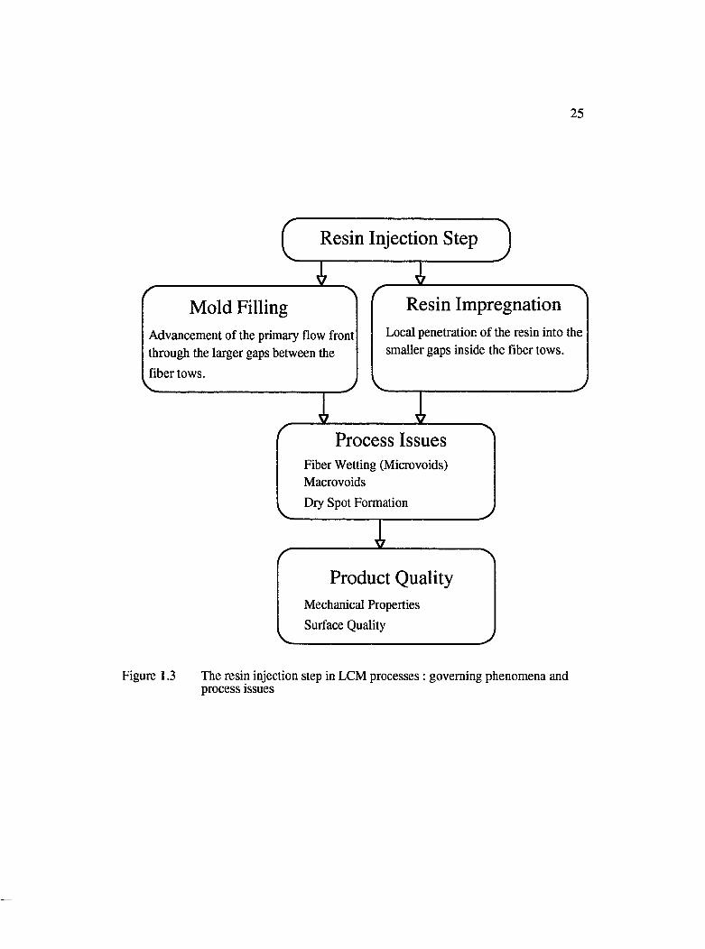
25

^ R esin Injection Step ^

Process IssuesFiber Wetting (Microvoids)MacrovoidsDry Spot Formation

Product QualityMechanical Properties Surface Quality

M old Filling

Advancement of the primary flow front through the larger gaps between the fiber tows.

R esin Impregnation

Local penetration of the resin into the smaller gaps inside the fiber tows.

Figure 1.3 The resin injection step in LCM processes : governing phenomena and process issues

P rocess variab les

Concentration of Size of tackifier Application technique Debulking temperaturetackifier powder powder

(e.g. powder vs. solvent) Debulking time

Powder Coagulation

Net-shape compaction Interply adhesion & Springback

Viscoelasticproperty

Rheo - kinetics

Dissolution of tackifier in the resin

Permeability Fiber wetting

Mechanical properties of composite

Figure 1.4 Overview of resin transfer molding of polymer powder coated fiber preformsWON

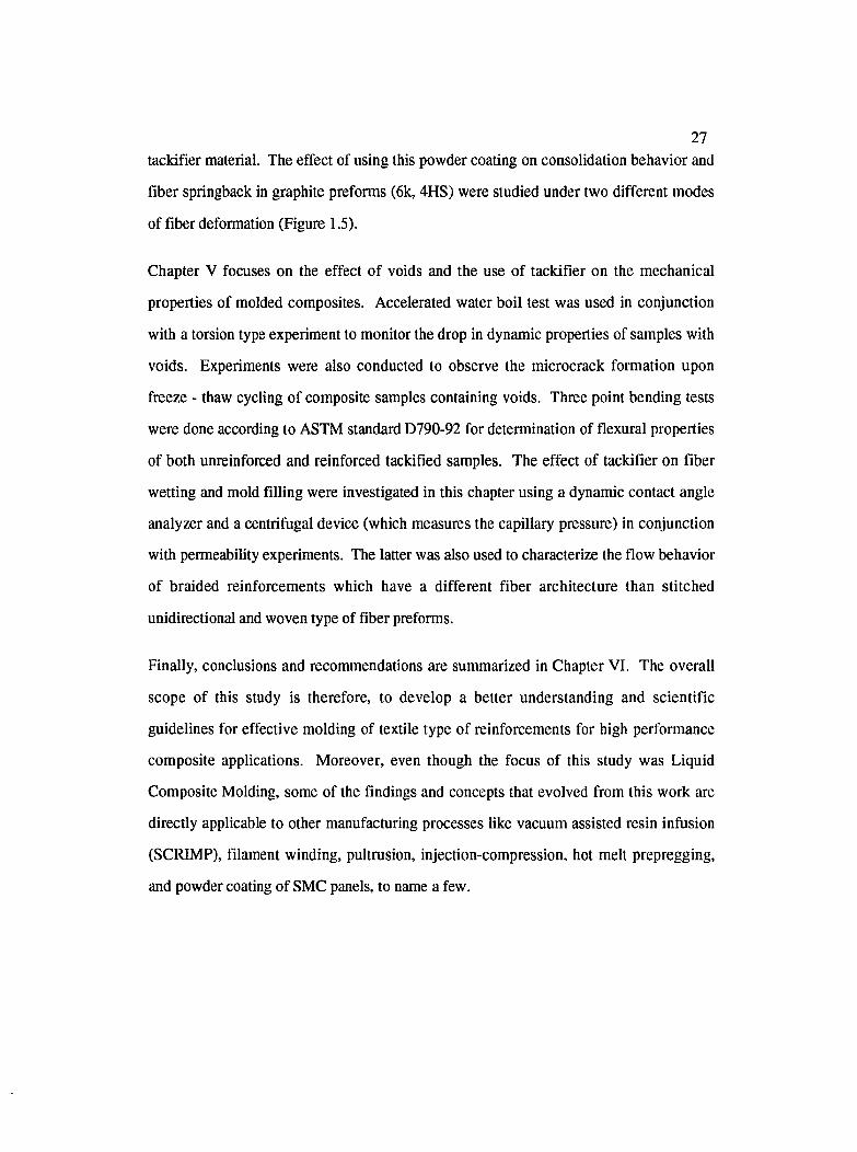
27tackifier material. The effect of using this powder coating on consolidation behavior and

fiber springback in graphite preforms (6k, 4HS) were studied under two different modes

of fiber deformation (Figure 1.5).

Chapter V focuses on the effect of voids and the use of tackifier on the mechanical

properties of molded composites. Accelerated water boil test was used in conjunction

with a torsion type experiment to monitor the drop in dynamic properties of samples with

voids. Experiments were also conducted to observe the microcrack formation upon

freeze - thaw cycling of composite samples containing voids. Three point bending tests

were done according to ASTM standard D790-92 for determination of flexural properties

of both unreinforced and reinforced tackified samples. The effect of tackifier on fiber

wetting and mold filling were investigated in this chapter using a dynamic contact angle

analyzer and a centrifugal device (which measures the capillary pressure) in conjunction

with permeability experiments. The latter was also used to characterize the flow behavior

of braided reinforcements which have a different fiber architecture than stitched

unidirectional and woven type of fiber preforms.

Finally, conclusions and recommendations are summarized in Chapter VI. The overall

scope of this study is therefore, to develop a better understanding and scientific

guidelines for effective molding of textile type of reinforcements for high performance

composite applications. Moreover, even though the focus of this study was Liquid

Composite Molding, some of the findings and concepts that evolved from this work are

directly applicable to other manufacturing processes like vacuum assisted resin infusion

(SCRIMP), filament winding, pultrusion, injection-compression, hot melt prepregging,

and powder coating of SMC panels, to name a few.

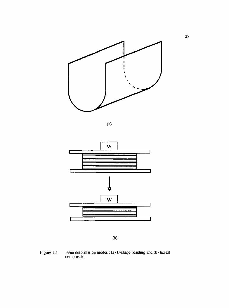
28

(a)

W

1

w

(b)

Figure 1.5 Fiber deformation modes : (a) U-shape bending and (b) lateral compression

CHAPTER H

LITERATURE REVIEW

2.1 Mold Filling and Fiber Wetting in LCM

The nature of flow of resin through the porous fiber preform in LCM is very much

similar to that of soil mechanics. In both processes, a wetting fluid flows through an

unsaturated, i.e., dry, porous medium, initially containing a non - wetting phase i.e. air.

However, one difference is that while soil mechanics is purely an infiltration type

process, LCM is not. The resin injection step in LCM processes consist of two types of

flow. One is macroflow or mold filling, which involves flow in the larger gaps between

the fiber tows. The other is microflow or resin impregnation, which involves infiltration

into the smaller gaps between the filaments of the fiber tows. Macro flow can be

considered to be an induced process in that it is initiated by an externally applied

mechanical pressure and is, thus, governed by viscous forces. Microflow, on the other

hand, can be considered to be a spontaneous process in which the driving force is the

cause of interaction between the liquid and solid phase. Microflow is mostly controlled

by the capillarity and the surface tension effects.

2.1.1 Darcy's Law

Darcy's law has often been used to model the steady state macroflow process. It states

that flow rate is directly proportional to the pressure gradient and is given by

29

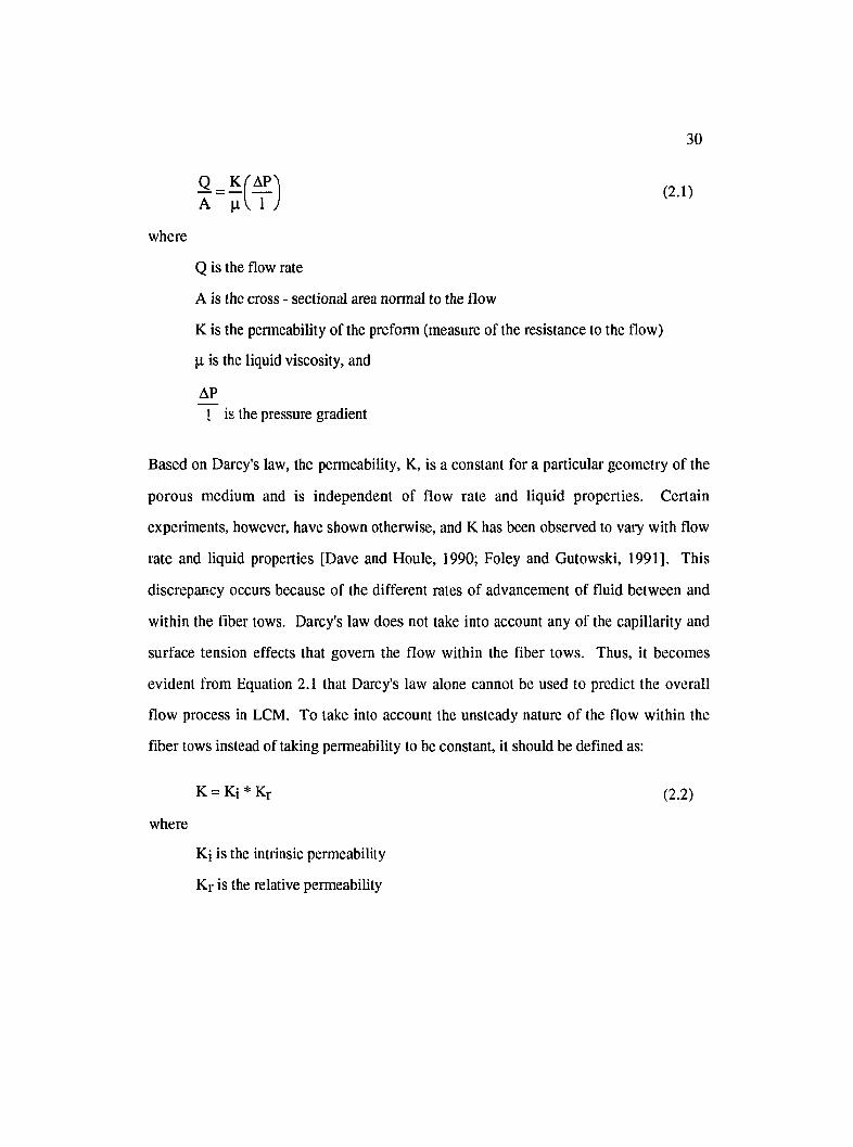
30

where

Q is the flow rate

A is the cross - sectional area normal to the flow

K is the permeability of the preform (measure of the resistance to the flow)

|i is the liquid viscosity, and

1 is the pressure gradient

Based on Darcy’s law, the permeability, K, is a constant for a particular geometry of the

porous medium and is independent of flow rate and liquid properties. Certain

experiments, however, have shown otherwise, and K has been obsei’ved to vary with flow

rate and liquid properties [Dave and Houle, 1990; Foley and Gutowski, 1991]. This

discrepancy occurs because of the different rates of advancement of fluid between and

within the fiber tows. Darcy's law does not take into account any of the capillarity and

surface tension effects that govern the flow within the fiber tows. Thus, it becomes

evident from Equation 2.1 that Darcy's law alone cannot be used to predict the overall

flow process in LCM. To take into account the unsteady nature of the flow within the

fiber tows instead of taking permeability to be constant, it should be defined as:

K = Ki * Kr (2.2)

where

Ki is the intrinsic permeability

Kr is the relative permeability

31Ki is obtained from the Kozeny - Carman equation, and Kr varies from 0 to 1 depending

on the saturation of the porous medium [Dave and Houle, 1990]. In the following

sections, some of the theoretical and empirical models and correlations relevant to the

microflow process are discussed.

2.1.2 Equilibrium Contact Angle

When a liquid comes in contact with a solid surface, the equilibrium condition for wetting

is determined by the three phase equilibrium of solid, liquid, and vapor. As shown in

Figure 2.1, the equilibrium point of contact is described as the intersection of three

interfaces: solid - liquid, liquid - vapor and solid - vapor. The equilibrium condition is

given by the Young - Dupre' equation [Miller, 1977] as

Ysv ~ Y s l “ Y l v Cos0 (2.3)

where

Ysv is the solid surface energy

Ysl is the solid - liquid interface tension

Ylv is the liquid surface tension, and

Cos 9 is the cosine of the equilibrium contact angle 0

Contact angle is usually considered to be a measure of the wettability or degree of

wetting. Based on the magnitude of the contact angle, the liquid can be classified as

either one of the three, viz., spreading (6 = 0), wetting (O<0<9O°), or non - wettingO O

(90 <0<18O ). When a wetting liquid penetrates the empty capillaries, the solid - air

interface is replaced by the solid - liquid interface. The higher the value of the adhesion

tension ( Ylv Cos0), the more readily the wetting proceeds [Carino and Mollet, 1975]. In

general, in order to ensure wetting, the liquid phase should have a surface free energy or

surface tension lower than the solid surface free energy. Measuring the contact angles

32with liquids of known surface tension also provides a means of quantifying the

interaction between solids and liquids. The physical property that determines the extent

of this interaction is the work of adhesion between the solid and the liquid given by

[Kamath et a l, 1987]

W a = Y L v ( l + Cos0) (2.4)

2.1.3 Dynamic Contact Angle

When the liquid is in motion with respect to the solid or vice versa, the solid - liquid -

vapor interface is under transient conditions. The value of the contact angle then differs

from its equilibrium value and a dynamic contact angle develops. Even at very low

velocities, the dynamic contact angle is considerably larger than the equilibrium value.

Dynamic contact angle could be either advancing or receding depending on whether one

surface is advancing or receding over the other. Usually the values of the advancing and

receding contact angles are not the same except in cases of perfect wetting (Cos 0 = 1).

Advancing contact angles are greater than or equal to the receding contact angles. The

difference is termed as the contact angle hysteresis. Some of the sources of hysteresis

include surface roughness, surface heterogeneity, increased liquid penetration due to

diffusion, and surface deformation/relaxation effects [Domingue, 1992]. Since the nature

of LCM processes is to make the resin advance through the fiber preform advancing

contact angles are more relevant. Thus, any mention of the contact angle hereafter refers

to the advancing dynamic contact angle, unless stated otherwise.

The dynamic contact angle is influenced by the resin viscosity and surface tension.

Several studies have been undertaken to describe the effects of viscosity and surface

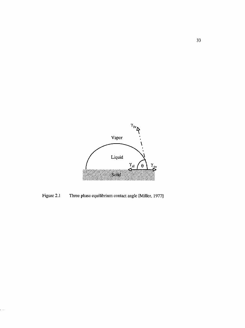
33

' I v ,

Vapor

Liquid

sv

Figure 2.1 Three phase equilibrium contact angle [Miller, 1977]

34

tension on the measured dynamic contact angle. This phenomenon is usually described

by the dimensionless capillary number (Ca#), defined as:

Ca# = ^ (2.5)Y l v

where

H is the viscosity of the impregnating resin, and

V is the relative velocity of the resin past the dry fibers

In general, the dynamic contact angle is reported to remain constant at sufficiently low

values of the capillary number, and then increase as Ca # increases. This was attributed

to the distortion of the meniscus shape due to viscous effects. The dependence of the

contact angle on the viscous drag was observed in the range of 10'^ < Ca # < 10*5 [Ahn

and Seferis, 1991].

Elmendorp and During [1991] obtained a relation between the dynamic contact angle and

the capillary number based on the precursor film model. This model explains the physics

behind the spreading of a liquid over a solid substrate. According to this model, the

liquid closest to the solid experiences the largest molecular attraction and so tends to

move faster than the bulk liquid. This causes a concavity in the liquid surface. Away

from the solid surface, the shape of the liquid surface, which determines the dynamic

contact angle, is governed by the balance of surface tension and viscous forces. The

correlation between the dynamic contact angle, equilibrium contact angle, and Ca # was

given as:

e / - e / = 53*C a# (2.6)

35Another correlation for dynamic contact angle may be described by the Friz equation for

resins with viscosities in the range of 10 -1000 mPas moving at velocities of the order of

0 .1 -1 0 cm/sec [Hayward and Harris, 1990]

tanOj = mV Y lv y

(2.7)

where

m and n are constants

Contact angle analysis is further complicated by the nature of the resin system and the

fiber surface. Resin systems usually consist of a mixture of compounds. Selective

adsorption of a certain species out of the resin or even a chemical reaction with the fiber

surface would create a composition gradient and may lead to changes in the contact

angle. In the same token, changes in fiber wettability would occur if the sizing or the

binder on the fiber interacts either physically or chemically with the resin. In addition to

these, chemical reaction and evaporation of volatile chemical species may also affect the

surface energies at the interface altering the dynamic contact angle. The effect of fiber

sizing on the contact angle was quantified in a recent study by Larson and Drzal [1992].

In the same study it was observed that evaporation of styrene from a vinyl ester resin

substantially increased the surface free energy of the resin and changed the fiber - liquid

interaction from favorable to unfavorable. Contamination of glass fibers with styrene

vapor and liquid resulted in an increase in contact angle, and zones of poor wetting with

increased porosity were observed in the molded composite [Hayward and Harris, 1990].

2.1.4 Capillary Pressure

In addition to the dynamic contact angle, another fundamental parameter to be considered

in flow through porous media is the capillary pressure (Pc). Capillary pressure is defined

36as the difference in the pressure between the wetting and the non - wetting phase at the

liquid - air interface.

Pc = Pnw - Pw = Ylv

r 1

1--------- (2 .8)

Equation 2.8 is the Laplace equation of capillarity. ri and r% are the principal radii of

curvature of the meniscus. The quantity is sometimes referred to as the mean curvature

of the interface, and depends on the shape and size of the capillary [Corey, 1986].

In soil mechanics, capillary pressure is termed as "suction". This is not surprising as it

provides the driving force for the liquid to impregnate the porous media. Capillary

pressure is a function of saturation. It is an increasing function of the non - wetting phase

saturation or, alternately, a decreasing function of the wetting phase saturation. The two

functions however, are not the same, and capillary pressure, like contact angle exhibits

hysteresis. Saturation is defined as the ratio of the volume of the fluid phase to the total

accessible pore volume. Thus, the capillary pressure is at the maximum when the fibers

are dry, and then decreases as the fibers get more and more wet or the wetting phase

saturation increases.

Assuming the filaments in the fiber tows to be cylindrical capillaries, a simple

relationship for evaluating the capillary pressure was obtained [Skartsis et al., 1992]:

(2.9)

where

d is a measure of the size of the capillary or the flow channel

The above equation is known as the Young - Laplace equation. The problem in using

Equation 2.9 is that it is very difficult to obtain realistic estimates for d. This is so

37because a typical fiber preform consists of a large number of capillaries of varying shapes

and sizes. One approach to estimate d utilizes the concept of hydraulic diameter, Dh.

This concept is identical to the one used to derive the Blake - Kozeny - Cannan equation

for flow through porous media [Skartsis et al., 1992]. In another approach, d was treated

as a function of porosity and the diameter of a single fiber (Df). In the same study,

another factor, the form factor (F), based on fiber alignment and flow direction, was

incorporated into the definition of the capillary pressure given by

P, = — Cos e (2.10)Df <})

where

<t> is the fiber porosity

For unidirectional fibrous preforms, it was found that F assumes a value of 4 for flow

along the fiber direction and a value of 2 for flow normal to the fiber direction. For

complex fiber alignment such as in woven fiber preforms, the study mentioned that F

could be determined from permeability measurements [Ahn and Seferis, 1991]. Typical

capillary pressures measured by Ahn et al. was in the order of 5 - 6 psi. Since in actual

production of composite parts by say an RTM process, injection pressures are usually of

the order 100 - 200 psi, one might argue the role played by the capillary pressure and the

research efforts being directed towards its determination. It should be noted that even

though the magnitude of the injection pressure or the applied mechanical pressure at the

inlet is many times higher than the capillary pressure, the situation is reversed at the flow

front. At the flow front, the mechanical pressure is zero, and it is the magnitude of the

capillary pressure that governs the resin impregnation. The importance of capillary

pressure is even more significant in low pressure processing, such as prepregging,

filament winding, and resin infusion processes [Ahn and Seferis, 1991].

38

2.1.5 Wicking Phenomena

Spontaneous liquid penetration of porous materials under the influence of capillary forces

is termed as wicking. The wicking phenomenon is commonly described by the theory of

Lucas and Washburn, which models the porous media as a bundle of cylindrical capillary

tubes and assumes a quasi steady creeping flow [Hodgson and Berg, 1988]. Substituting

the expression for Pc into the Hagen-Poiseuille equation, the following expression was

obtained to relate the rate of capillary penetration as a function of liquid properties and

effective capillary dimensions:

dh 1dt 8[ih

2yCos8- p g h *r‘ (2 .11)

Equation 2.11 was developed to model capillary flow in the vertical direction. Since

resin injection in LCM processes is done with the mold kept horizontally, the

gravitational forces can be neglected and Equation 2.11 reduces to

dh 1dt 8 |ih

2 y C os6 * r (2 .12)

Equation 2.12 can be readily integrated to yield the expression for distance traveled (h) as

a function of time (t).

h = ryCosG 2\i .

VF (2.13)

Although the above equation has been substantiated by wicking experiments with pure

liquids in several porous media, deviations have been obsei^ved for very short wicking

distances and in media which are swollen by the penetrating liquid. The theory also

shows some deviations for multi component penetrating liquids like suifactant solutions

[Hodgson and Berg, 1988]. The Lucas - Washburn theory would also not be applicable if

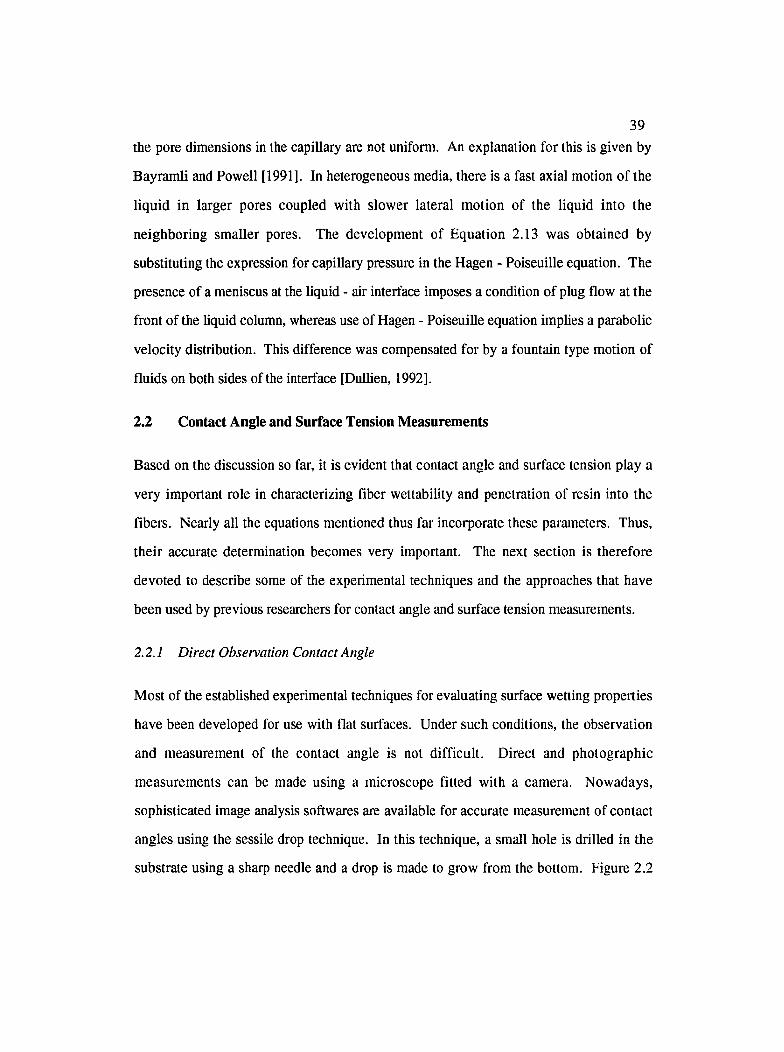
39the pore dimensions in the capillary are not uniform. An explanation for this is given by

Bayramli and Powell [1991]. In heterogeneous media, there is a fast axial motion of the

liquid in larger pores coupled with slower lateral motion of the liquid into the

neighboring smaller pores. The development of Equation 2.13 was obtained by

substituting the expression for capillary pressure in the Hagen - Poiseuille equation. The

presence of a meniscus at the liquid - air interface imposes a condition of plug flow at the

front of the liquid column, whereas use of Hagen - Poiseuille equation implies a parabolic

velocity distribution. This difference was compensated for by a fountain type motion of

fluids on both sides of the interface [Dullien, 1992].

2.2 Contact Angle and Surface Tension Measurements

Based on the discussion so far, it is evident that contact angle and surface tension play a

very important role in characterizing fiber wettability and penetration of resin into the

fibers. Nearly all the equations mentioned thus far incorporate these parameters. Thus,

their accurate determination becomes very important. The next section is therefore

devoted to describe some of the experimental techniques and the approaches that have

been used by previous researchers for contact angle and surface tension measurements.

2.2.1 Direct Observation Contact Angle

Most of the established experimental techniques for evaluating surface wetting properties

have been developed for use with flat surfaces. Under such conditions, the observation

and measurement of the contact angle is not difficult. Direct and photographic

measurements can be made using a microscope fitted with a camera. Nowadays,

sophisticated image analysis softwares are available for accurate measurement of contact

angles using the sessile drop technique. In this technique, a small hole is drilled in the

substrate using a sharp needle and a drop is made to grow from the bottom. Figure 2.2

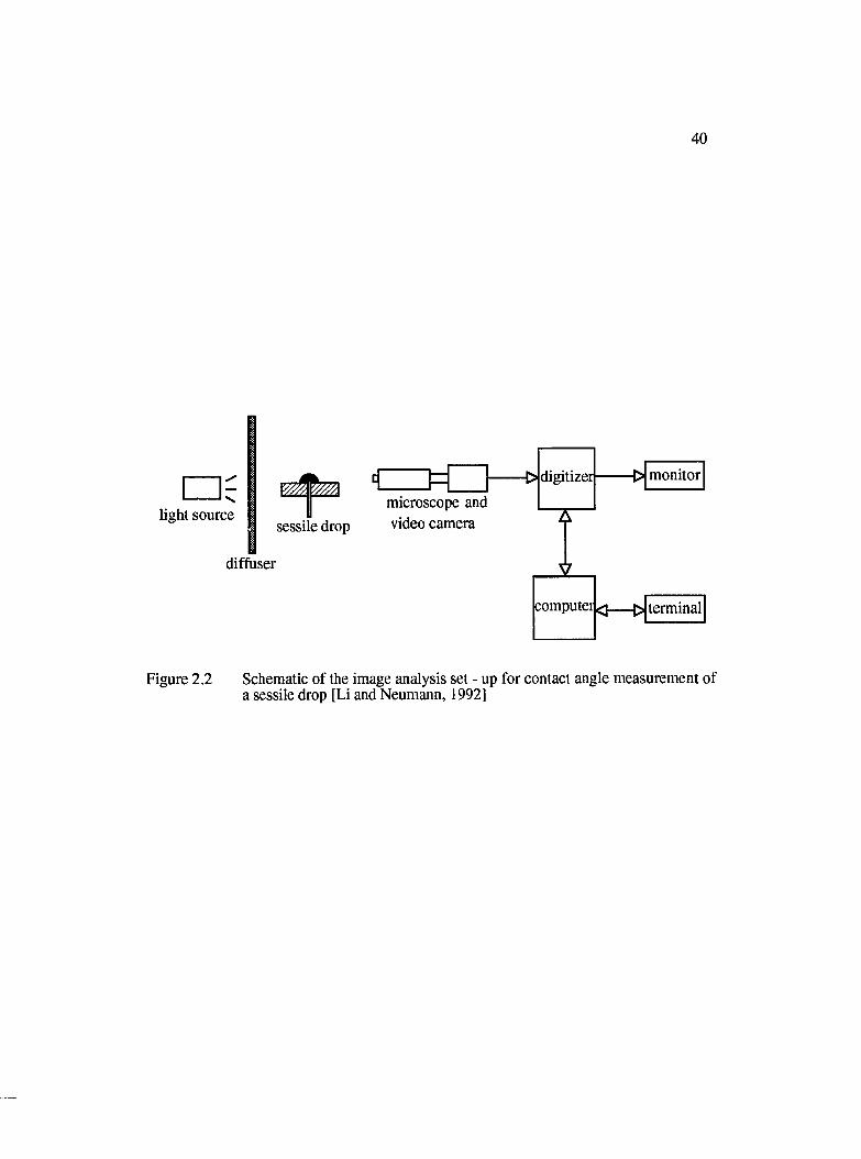
40

light sourcesessi e drop

microscope and video camera

diffuser

> monitordigitizer

computer < 3-----0 terminal

Figure 2.2 Schematic of the image analysis set - up for contact angle measurement of a sessile drop [Li and Neumann, 1992]

41

shows the block diagram of a typical digital image processing set - up for sessile drop

measurements. The video signal of the drop is transmitted to a digitizer which performs

the frame grabbing and digitization of the image to 512 by 512 pixels with 256 gray

levels each, where 0 represents black and 255 represents white. The digitized image is

transferred to the computer for image analysis and computation. Advancing contact

angles can also be obtained using this method by forming the drop using a motor driven

syringe.

Making contact angle measurements on single filaments is a much more difficult

experimental task. The direct approach requires that a drop of liquid be placed on a

horizontally mounted sample, and the contact angle be observed from a point in the same

horizontal plane and perpendicular to the long axis of the sample. However, this type of

experiment has several pitfalls. This is so because certain liquids have the tendency to

completely surround a single fiber and form a symmetrical unduloid shape, while others

can remain on one side of a fiber with a "clamshell" profile. In some instances, the same

liquid could be made to adopt either of these configurations depending upon how it was

deposited. Thus, this approach requires considerable precaution to make sure that the

true contact angle is observed and measured. The reason why such precision is required

is explained in the plot of Cos 0 as a function of 0 as shown in Figure 2.3. The plot

demonstrates the percentage uncertainty in the former due to a ± 1 ° error in measuring 0

between 0° and 90°.

Due to the inherent difficulties involved in accurate measurement of contact angles on

single fibers using direct methods, an indirect method was devised and successfully

adapted. This method is based on the Wilhelmy principle and is discussed next.

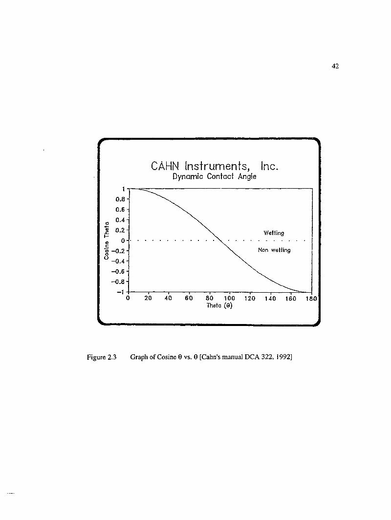
42

CÀHN Instruments, Inc.Dynamic Contact Angle

0 .8-1

0.6 -

o 0.4- 0 .2 -CJC

I -W ettin g

I -0.2-“ - 0 .4 -

— 0.6 -

- 0 . 8 -

Non w etting

0 20 40 60 80 100 120 140 160 180T h ê ta ( 0 )

Figure 2.3 Graph of Cosine 0 vs. 0 [Cahn's manual DCA 322, 1992]

43

2.2.2 Wetting Force Measurements

Since the development of the Wilhelmy technique, it has been applied extensively to

study the dynamic wetting behavior of fibers for various liquid / fiber systems. Lee and

Seferis [1988] used this technique to characterize the effect of surface treatment of carbon

fibers with a silicone oil and a low surface tension epoxy. This method is an indirect

method for determining contact angles as it does not involve direct observation of the

shape of the liquid surface on the solid. Rather, this technique involves measuring the

force that a liquid exerts on the fiber surface and calculating the contact angle based on

force values. According to the formula of Wilhelmy, the pull exerted on the fiber

inserted into a liquid is expressed by

Fw = P *Ylv *Cos6 (2.14)

P is the perimeter of the fiber along the three phase boundary line, and the other terms

have their usual meaning. If the perimeter and the surface tension are known, the contact

angle can be evaluated from Fw- The determination of the wetting force Fw can be

carried out by measuring the change in weight of a vertical fiber (with a microbalance)

that occurs when it is placed in contact with a liquid. Figure 2.4 illustrates this concept in

terms of the forces acting on the fiber before and after contact [Miller, 1977].

2.2.3 Bundle Contact Angle

For composite manufacturing processes, ideally the contact angle of fiber tows should be

measured instead of the contact angle with single fibers. Two different approaches have

been employed to do so. Chwastiak [1973] used wicking experiments to determine

bundle contact angles from changes in the surface free energy which occurs during the

wetting process. Another approach uses the same technique as that used for measuring

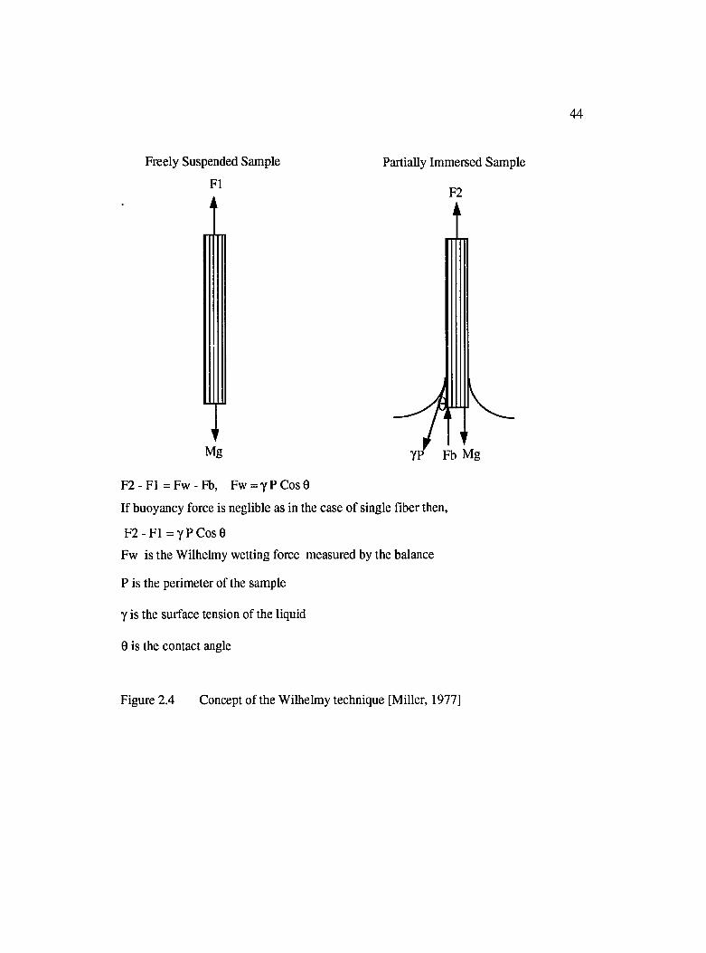
44

Freely Suspended Sample

FI

Partially Immersed Sample

F2

Mg

F 2 - F l = F w - F b , F w = y P C o s 9

If buoyancy force is neglible as in the case of single fiber then,

F2-F1 = y P C o s e

Fw is the Wilhelmy wetting force measured by the balance

P is the perimeter of the sample

Y is the surface tension of the liquid

0 is the contact angle

Fb Mg

Figure 2.4 Concept of tbe Wilhelmy technique [Miller, 1977]

45

contact angles with single fibers. The latter approach is much simpler. However, with

fiber tows, in addition to wetting, liquid uptake due to wicking also occurs. Thus, for

contact angle measurements, the two effects need to be decoupled.

Chwastiak obtained the following equation for change in the surface free energy by

neglecting the inertial term in comparison to the gravitational and viscous forces:

128(1Ay = ^ g P r A Ü ( m ) (2.15)

H is the total height of the fiber bundle, pf is the fiber density, df is the fiber diameter, p

is the liquid viscosity, (]) is the porosity, Kh is the hydraulic constant, V j is the total

volume of the bundle, Wf is the weight of the filaments in the fiber bundle, m is the

weight of the liquid wicked in time t, and X is the slope of the wicking data m vs. t on a

log - log plot.

All the terms on the right hand side of equation were readily obtained except for the

hydraulic constant. The porosity of the bundle was kept fixed by enclosing them tightly

in a tube. Thus, the accuracy of Equation 2.15 depends upon the accuracy with which the

hydraulic constant is determined. Once the free energy of wetting was obtained, the

contact angle was evaluated as follows

Cos0 = - ^ (2.16)Y lv

Hsieh and Yu [1992] used the Wilhelmy technique to determine the contact angle of

water on woven fabric strips. The experimental protocol used by them is explained as

follows. A strip of woven fabric was hung from a microbalance. The surface of the

liquid reservoir resting on a traveling stage was then brought close to the edge of the

fabric just enough to touch it. The force reading was recorded until a steady - state in the

46measurement was reached. The liquid surface was then pulled away from the strip and

the drop in the force readings was recorded until a steady state was achieved. Figure 2.5

is a schematic of a typical curve illustrating the weight changes during the experiment.

Point A to B is the zero baseline prior to the fabric - liquid contact. Point B to D shows

the force increase from the liquid contacting the fabric and the simultaneous wicking

action. The initial sharp force increase from point B to point C is mostly due to wetting

with some contribution from liquid uptake. The subsequent wicking is indicated by the

slower force change from point C to point D before reaching the steady state. Point D to

E records the separation process of the wetted fabric from the liquid. As the liquid level

moved away from the fabric edge, the liquid surface remained in contact with the lower

edge of the fabric. The slight increase in the force detection during this process was

attributed to the change in the fabric edge configuration and / or change in the contact

angle at the meniscus. At point F, the fabric is completely separated from the liquid. The

residual weight recorded indicates the total liquid retention (Wt) in the fabric.

The B - D section of the curve shown in Figure 2.5 results from simultaneous wetting and

wicking. The amount wicked into the fabric was obtained from Wt, The advance steady -

state force at point D was denoted as (A st) , and the wetting force was obtained as;

Fw = Ast -Wt (2.17)

The perimeter of the fabric was obtained from a similar experiment, but with a perfectly

wetting liquid with known surface tension, such as Hexadecane which made a zero

contact angle with the fabric. Once the perimeter of the fabric was known the contact

angle was calculated from the Wilhelmy equation after inputting the value of the surface

tension of water.

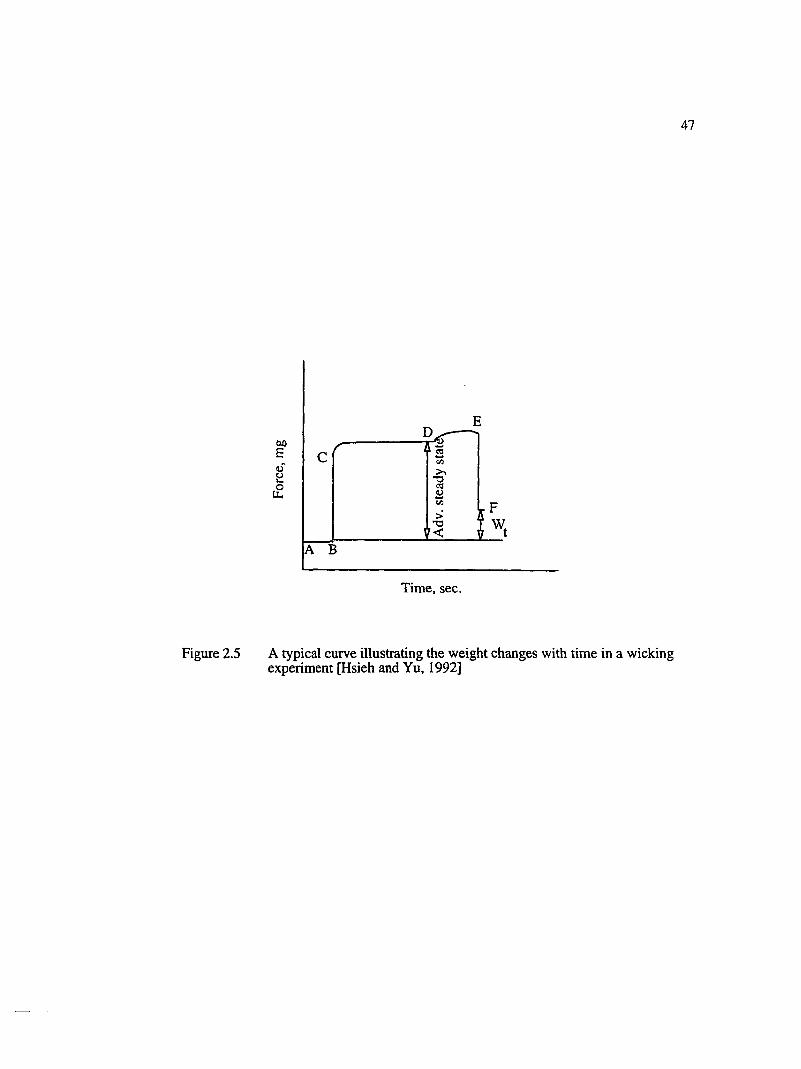
47

bû

-O

Time, sec.

Figure 2.5 A typical curve illustrating the weight changes with time in a wicking experiment [Hsieh and Yu, 1992]

48

2.2.4 Surface Tension Measurements

Surface tension of a liquid is a thermodynamic property, and for pure liquids depends

only on temperature, with respect to which it shows a monotonie decrease [Ahn and

Seferis, 1991]. Surface tension of polymer resins have been observed to change with

reaction. This was explained by Larson and Drzal [1992] as due to the evaporation of

volatile species. The following methods are used for its determination [Shaw, 1980].

2.2.4.1 Capillary Rise Method

This method is based on the measurement of the height of liquid column (h) in a capillary

of radius r immersed in a liquid. Since the measurements do not involve disturbance of

the liquid surface, slow time effects can be followed. Surface tension is given by the

expression

which for zero contact angle reduces to

(2 .1 9 )

where

Ap is the difference in the density of the liquid and vapor

For accuracy, corrections should be made for very narrow and wide capillaries. In

practice, the capillary rise method should only be used when the contact angle is zero,

owing to the uncertainty in measuring contact angles correctly. A variation of this

method is to measure the difference in capillary rise for capillaries of different sizes, thus

eliminating reference to the flat surface of the reservoir liquid. In this case, surface

tension is given by Equation 2.20:

49

A p £ iv ^ (2.20)2(ri-r,)

where

Ah is the difference in the height of the liquid meniscus in the two capillaries

2.2A.2 Ring Method

In this method the force required to detach a ring from a surface or interface is measured

either by suspending the ring from the arm of a balance or by using a torsion wire

arrangement (du Nouy tensiometer). The detachment force is related to the surface

tension by the expression

F is the puU on the ring, R is the mean radius of the ring, and p is a correction factor. To

ensure zero contact angle, platinum rings should be cleaned with a strong acid or by

flaming. The correction factor allows for the non vertical direction of the tension forces

and for the complex shape of the liquid supported by the ring at the point of detachment.

The value of P can be calculated from the equation of Zuidema and Waters [Shaw, 1980].

2.2.4.3 Drop Volume and Drop Weight Methods

Drops of liquid are allowed to detach themselves slowly from the tip of a vertically

mounted narrow tube, and either they are weighed or their volume is measured. At the

point of detachment

(2 .22)' 27ir 27ir

50

P is a correction factor which is required because on detachment, (a) the drop does not

completely leave the tip, and (b) the surface tension forces are seldom exactly vertical. P

is empirically shown to depend on the ratio

2.2.4A Pendant Drop Method

A pendant drop of the liquid is photographed, and its image is projected on to a graph

paper. From the dimensions of the drop, the surface tension can be computed using the

same image analysis software as that used in the sessile drop method for calculating

contact angles [Li and Neuman, 1992].

2.2.4.5 Wilhelmy Technique

In this method, a heat cleaned glass cover plate or a platinum plate is immersed vertically

in the liquid. The force exerted by the liquid on the plate is monitored using a

microbalance. If the perimeter of the plate is known, surface tension can be calculated

using the Wilhelmy Equation 2.14. The underlying assumption in this method is that the

plate makes a zero contact angle with the liquid whose surface tension is to be measured.

Wilhehny technique was used in this study, and details are given in the next chapter.

2.3 Void Formation Studies

2.3.J Experimental Studies on Void Formation

Bascom and Romans [1968] were first to report the formation of voids between the

filaments of fiber tows of glass fiber reinforced polyester resin composites produced by

filament winding. Microscopic observation of small composite samples showed 10^ to

10^ voids per cubic centimeter. They found that reducing the contact angle to zero, and

51causing the strands to oscillate as they passed through the resin markedly reduced the

number of voids.

Peterson and Robertson [1991 & 1992] studied the formation of voids in fiber rovings.

The primary factors in the generation of voids were attributed to the heterogeneity both

on bulk and local scales. They explained that heterogeneity on bulk scale results in

channeling causing void formation. Heterogeneity on the local scale results in trapping

of voids by coalescence of wicking streams. They also explained why changes in the

void size and distribution occurs during the mold filling process in terms of viscous

forces. The viscous action of the resin can free formerly trapped voids allowing them to

flow out with the resin. Viscous forces may also move a void lodged in a constriction by

reducing its size. Under static conditions, changes in void size occurs by coalescence due

to surface tension.

Mahale et al. [1992] used the refractive index matching technique and image analysis to

quantify void formation during radial impregnation of random continuous glass fiber

mats. They reported a critical value of capillary number (Ca # = 2.5 x 10"3), below

which void contents increased exponentially with decreasing capillary numbers. Above

this critical value negligible entrapment of voids was observed. Chen et al. [1993] used a

similar approach to visualize void formation using an oil with the same refractive index

as the fibers. Based on the sizes and location of the voids, they classified them as (1)

small cylindrical micro voids inside the fiber bundles, mesovoids encompassing several

filaments inside the fiber bundles, and spherical macro voids outside the fiber bundles.

They found that low viscosity, zero contact angle, high mold temperature, and high

pressure resulted in minimal void formation. Also, increasing the fiber volume fraction

reduced the amount of voids trapped. They reported that if capillarity is dominant,

surfactants can help in reducing voids by reducing the wetting contact angle.

52Hayward and Harris [1990] studied the effect of vacuum on void formation in glass fiber

reinforced polyester resin system. They found that resin injection with the assistance of

vacuum resulted in substantial improvements in composite quality (i.e., reduced void

formation). Their experiments showed that the effects of vacuum assistance occurred

only at the point of initial contact of the resin front with the glass preform. Subsequent

resin injection using vacuum did not lead to improvement in previously poorly wet - out

portions of the preform. A similar study on the effect of vacuum has also been perfonned

by Lundstrom et al. [1992]. They reported that most of the voids were concentrated to a

small area close to the flow front. With increasing vacuum, the maximum void content

and the size of the region of detectable voids decreased. The void volume fraction was

detemiined with optical microscopy and image analysis. Stabler et al. [1992] studied

drag induced void formation in braided graphite prefonn and epoxy system. They

observed that most of the voids were located in the indention regions where the fiber tows

crossed each other. They explained that voids were trapped because indention regions

were low pressure regions. Once the air bubble was lodged at the notch, it was very

difficult to move. They reported that for conditions of light mold surface waxing with

buffing, low initial bubble content, and mold vibration frequency of 10 Hz, void

formation was minimized.

2.3.2 Modeling o f Void Formation

Several theoretical models have been proposed for void formation. Although these

models are formulated using several simplifying assumptions and for simplified

geometry, they indicate some of the physical phenomena that takes place on the micro

scale.

Elmendorp and During [1990] developed a model for void formation during transverse

flow in aligned hexagonal array of fibers. The shape of the liquid surface advancing

53through the fiber bundles was determined based on the precursor film model. They

assumed that the viscous forces do no not influence the shape of the liquid surface other

than altering the value of the static contact angle. Their model predicted that if upon

coalescence of two flow fronts the dynamic contact angle was greater than tc/2, a void

would be formed downstream of the fiber. They reported that for capillary number

greater than 0.05, voids can be trapped due to dynamic effects. This implied a critical

impregnation velocity of 1.5 micron/sec. Also, at a particular volume fraction, void

content increased with increasing capillary number. The capillary number at which void

formation started (critical capillary number) decreased with increase in fiber volume

fraction.

Void formation during flow perpendicular to unidirectional fiber tows has been modeled

by Parnas and Phelan [1991]. Darcy's law was used to describe both macro and micro

flow. Consideration of capillary forces was neglected. The concept of this model is

based on the premise that as the advancing flow front encounters a fiber bundle, it fiows

around it, entrapping a pocket of air as it does so. After the front surrounds and bypasses

a fiber bundle, the fiber bundle is slowly impregnated with the fluid. The basis for the

assumed entrapment mechanism is that the interstitial space within the fiber bundles is

much smaller than the spaces between the fiber bundles that make up the preform. Thus,

the permeability of a fiber bundle, k%, is much less than the permeability of the space

between the bundles, ki. Considering the flow geometry depicted in Figure 2.6, when

ki/k2 equals 1.0, the flow front penetrates the fiber bundles at the same rate as it advances

through the space between the bundles and no air is trapped. However, as the fiber

bundles become successively less permeable and the ratio ki/k] tends to infinity, the rate

of fiber impregnation relative to the motion of the advancing front becomes negligible.

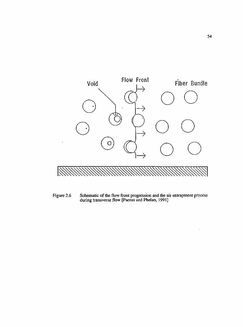
54

\/nîH F l o w Front F i b e r B u n d l e

Figure 2.6 Schematic of the flow front progression and the air entrapment process during transverse flow [Pamas and Phelan, 1991]

55

When a point is reached where the flow front splits into two upon reaching a fiber bundle

and then recoalesces downstream of the bundle before all the air in the bundles can be

forced out, air is trapped within the bundles and remains trapped.

Chan and Morgan [1992] have developed some simple models for void formation under

different scenarios. One of their models predicted void formation for axial flow in the

unidirectional fiber preform. Again Darcy's law was used to model resin flow. The flow

was characterized by a global flow front advancing through the larger pores between the

fiber bundles with subsequent radial penetration into the smaller pores within the bundles.

Because of the differences in time scales associated with the two types of filling, voids

were trapped at the flow front. Chan and Morgan [1993a] used a similar approach to

model void formation for circular, elliptical and rectangular cross - sectioned tows

oriented either along or normal to the global resin flow direction. The model was used to

estimate the void size and distribution in fabric preforms. Another work by Chan and

Morgan [1993b] focuses on the formation of microvoids within the fiber tows. Figure 2.7

depicts a schematic of two capillaries lying adjacent to each other, but of unequal sizes.

The model assumes that at time equals zero (t = 0), the resin front in the two capillaries

coincide in the axial direction. A net capillary pressure, which is the difference in

capillary pressures between the two fronts, exists. The net capillary pressure causes the

resin to flow forward in the smaller capillary. This forward flow leads to a transverse

flow of resin from the larger to the smaller capillary. The forward flow in the smaller

capillary is accompanied by a reverse flow in the larger capillary. They suggested that

this forward - reverse capillary flow leads to the possibility for void formation in two

ways. The forward moving resin front in the smaller capillary can merge with another

such forward moving front to enclose a void resulting in a void length of approximately L

(Figure 2.7). Voids can also form when the surrounding resin flows transversely across

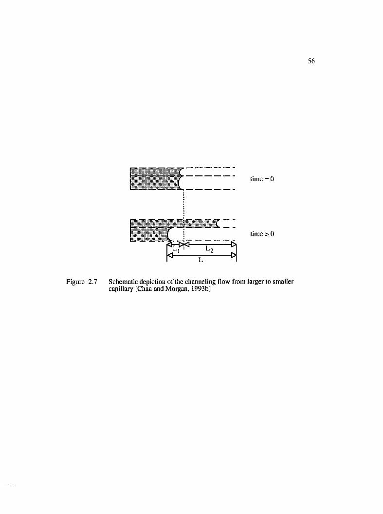
56

II

U l ­

time = 0

time > 0

Figure 2.7 Schematic depiction of the channeling flow from larger to smaller capillary [Chan and Morgan, 1993b]

57

to enclose the void region left by the receding front in the larger capillary. This leads to a

void of length L].

Chen et al. [1993] also proposed a model based on the concept of two levels of porosity

of fiber mats. One outside the fiber tows, and the other within the fiber tows. Their

model includes liquid bypassing with initial air trapping, subsequent capillary invasion of

fiber bundle with air compression, and mobilization to explain air entrapment

phenomena. The concept of liquid bypassing and initial air trapping is similar to that of

Pamas and Phelan and Chan and Morgan. During flow, most of the liquid will pass

through the space between the bundles bypassing the space within the bundles. However,

some of the liquid will penetrate into the fiber bundles owing to capillary suction and the

external pressure. The amount of air entrapped within the fiber bundles will depend upon

the speed of the advancing flow front and the magnitude of the capillary forces. A

modified Lucas - Washburn type equation was suggested for liquid penetration given by

U =

where

Kb is the permeability of the fiber bundles

<t>b is the bundle porosity &

AP is the external pressure drop from the bulk flow

After initial air trapping, the model takes into account the effect of pressure difference

inside and outside the fiber bundle on the size of the trapped voids. Finally, the

mobilization step was modeled based on the relative magnitudes of the viscous and

capillary forces. The criteria for mobilization was that the viscous forces should be

greater than the capillary forces. An engineering approach was used to estimate the

overall void content given by Equation 2.24:

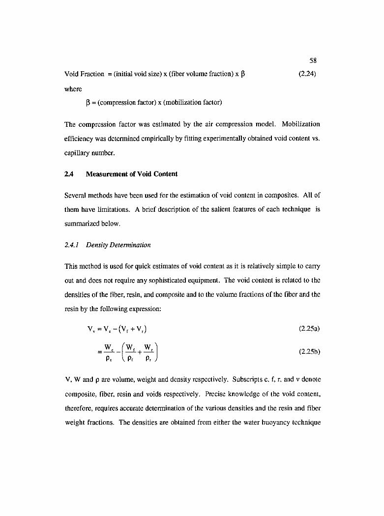
58

Void Fraction = (initial void size) x (fiber volume fraction) x P (2.24)

where

P = (compression factor) x (mobilization factor)

The compression factor was estimated by the air compression model. Mobilization

efficiency was determined empirically by fitting experimentally obtained void content vs.

capillary number.

2.4 Measurement of Void Content

Several methods have been used for the estimation of void content in composites. All of

them have limitations. A brief description of the salient features of each technique is

summarized below.

2.4.1 Density Determination

This method is used for quick estimates of void content as it is relatively simple to carry

out and does not require any sophisticated equipment. The void content is related to the

densities of the fiber, resin, and composite and to the volume fractions of the fiber and the

resin by the following expression:

Vv = V , - ( V f + V j (2.25a)

(2.25b)Pc P f Pr

V, W and p are volume, weight and density respectively. Subscripts c, f, r, and v denote

composite, fiber, resin and voids respectively. Precise knowledge of the void content,

therefore, requires accurate determination of the various densities and the resin and fiber

weight fractions. The densities are obtained from either the water buoyancy technique

59ASTM D792 or the density gradient technique ASTM D1505. The fiber / resin content is

usually obtained from chemical or thermal methods. The former involves acid digestion

of the resin, whilst in the latter, the resin is removed by thermal degradation and weight

changes are monitored by gravimetry. A variation of 0.1% in pc, Pf, pr, Vf or Vr results

in a variation of 2.5% in the estimated void content [Judd and Wright, 1978]. Also, this

technique only estimates the overall void content based on small samples, and provides

no information on the size, shape, location, or distribution of voids.

2.4.2 Water Absorption

This method requires the determination of the equilibrium water uptake of pure resin and

composite. Void volume is given as

Vv = Wc - Wr (2.26)

Wei s the water absorbed by the composite, and Wr is the water absorbed by the pure

resin. Its validity depends upon complete saturation of the voids. Analysis is also

complicated from the fact that resin swelling, hydrolysis, or leaching may occur. Thus,

this method is limited to cases where such reactions do not occur. The accuracy of this

method is estimated to be no greater than the density determination method.

2.4.3 Micrography

This technique is adapted from metallography in which a reflecting type microscope is

used for analyzing metallurgical specimens. A small section of the composite is cut and

mounted on a block, e.g., bakelite. It is then polished sequentially on silicon carbide

abrasive disks with increasing grit size. This is followed by polishing using a diamond or

alumina paste [Olsen et al., 1992]. In some cases the surface of the specimen may be

coated with a substance such as isopropylbiphenyl to reduce scattering of light from

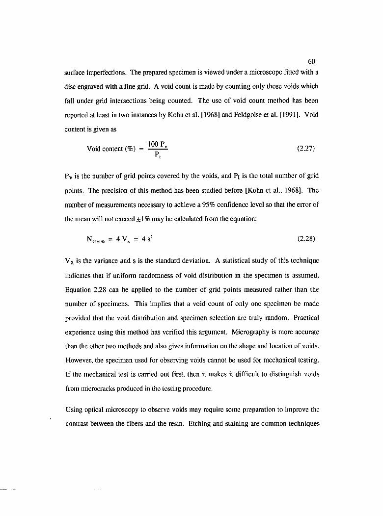
6 0

surface imperfections. The prepared specimen is viewed under a microscope fitted with a

disc engraved with a fine grid. A void count is made by counting only those voids which

fall under grid intersections being counted. The use of void count method has been

reported at least in two instances by Kohn et al. [1968] and Feldgoise et al. [1991]. Void

content is given as

inn pVoid content (%) = (2.27)

?v is the number of grid points covered by the voids, and ?t is the total number of grid

points. The precision of this method has been studied before [Kohn et al., 1968]. The

number of measurements necessary to achieve a 95% confidence level so that the enor of

the mean will not exceed ±1% may be calculated from the equation:

== 4 == 4 s= (2.28)

Vx is the variance and s is the standard deviation. A statistical study of this technique

indicates that if uniform randomness of void distribution in the specimen is assumed.

Equation 2.28 can be applied to the number of grid points measured rather than the

number of specimens. This implies that a void count of only one specimen be made

provided that the void distribution and specimen selection are truly random. Practical

experience using this method has verified this argument. Micrography is more accurate

than the other two methods and also gives information on the shape and location of voids.

However, the specimen used for observing voids cannot be used for mechanical testing.

If the mechanical test is carried out first, then it makes it difficult to distinguish voids

from microcracks produced in the testing procedure.

Using optical microscopy to observe voids may require some preparation to improve the

contrast between the fibers and the resin. Etching and staining are common techniques

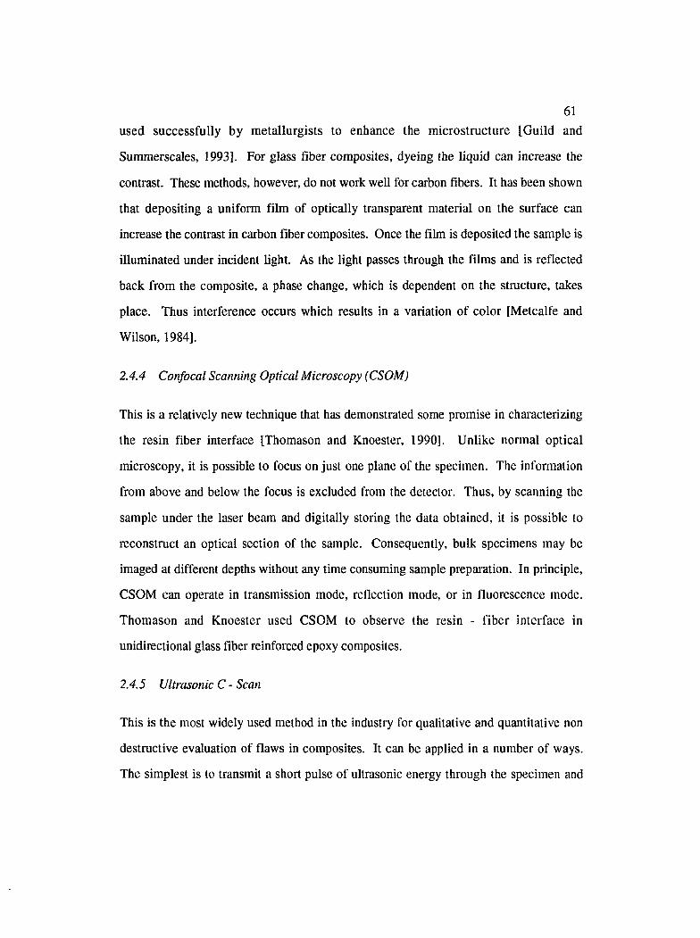
61

used successfully by metallurgists to enhance the microstructure [Guild and

Summerscales, 1993]. For glass fiber composites, dyeing the liquid can increase the

contrast. These methods, however, do not work well for carbon fibers. It has been shown

that depositing a uniform film of optically transparent material on the surface can

increase the contrast in carbon fiber composites. Once the film is deposited the sample is

illuminated under incident light. As the light passes through the films and is reflected

back from the composite, a phase change, which is dependent on the structure, takes

place. Thus interference occurs which results in a variation of color [Metcalfe and

Wilson, 1984].

2.4.4 Confocal Scanning Optical Microscopy {CSOM)

This is a relatively new technique that has demonstrated some promise in chaiacterizing

the resin fiber interface [Thomason and Knoester, 1990]. Unlike normal optical

microscopy, it is possible to focus on just one plane of the specimen. The information

from above and below the focus is excluded from the detector. Thus, by scanning the

sample under the laser beam and digitally storing the data obtained, it is possible to

reconstruct an optical section of the sample. Consequently, bulk specimens may be

imaged at different depths without any time consuming sample preparation. In principle,

CSOM can operate in transmission mode, reflection mode, or in fluorescence mode.

Thomason and Knoester used CSOM to observe the resin - fiber interface in

unidirectional glass fiber reinforced epoxy composites.

2.4.5 Ultrasonic C - Scan

This is the most widely used method in the industry for qualitative and quantitative non

destructive evaluation of flaws in composites. It can be applied in a number of ways.

The simplest is to transmit a short pulse of ultrasonic energy through the specimen and

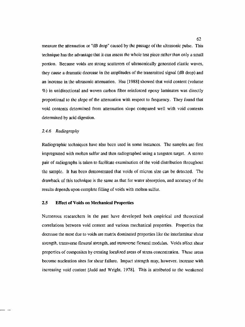
6 2

measure the attenuation or "dB drop" caused by the passage of the ultrasonic pulse. This

technique has the advantage that it can assess the whole test piece rather than only a small

portion. Because voids are strong scatterers of ultrasonically generated elastic waves,

they cause a dramatic decrease in the amplitudes of the transmitted signal (dB drop) and

an increase in the ultrasonic attenuation. Hsu [1988] showed that void content (volume

%) in unidirectional and woven carbon fiber reinforced epoxy laminates was directly

proportional to the slope of the attenuation with respect to frequency. They found that

void contents determined from attenuation slope compared well with void contents

determined by acid digestion.

2.4.6 Radiography

Radiographic techniques have also been used in some instances. The samples are first

impregnated with molten sulfur and then radiographed using a tungsten target. A stereo

pair of radiographs is taken to facilitate examination of the void distribution throughout

the sample. It has been demonstrated that voids of micron size can be detected. The

drawback of this technique is the same as that for water absorption, and accuracy of the

results depends upon complete filling of voids with molten sulfur.

2.5 Effect of Voids on Mechanical Properties

Numerous researchers in the past have developed both empirical and theoretical

correlations between void content and various mechanical properties. Properties that

decrease the most due to voids are matrix dominated properties like the interlaminar shear

strength, transverse flexural strength, and transverse flexural modulus. Voids affect shear

properties of composites by creating localized areas of stress concentration. These areas

become nucléation sites for shear failure. Impact strength may, however, increase with

increasing void content [Judd and Wright, 1978]. This is attributed to the weakened

63bonding contribution to the formation of a more extensive yielding zone at the

propagating crack tip. Greater toughness then arises because of debonding and pulling

out of fibers and to a limited extent by delamination.

For a void free composite, the three factors which determine shear strength are the

ultimate shear strength of the reinforcement, the matrix material, and the bond at the resin

- fiber interface. In an ideal case, the lower bound on composite shear strength Xc is the

shear strength of the matrix, Xm. Chamis [1969] developed the following semi -

empirical relationship based on the assumption that shear strength of the composite was

related to the maximum shear strain in the matrix;

(2.29)Pv

where

Pf is the experimental - theoretical correction factor

(pm is the limiting matrix shear strain

Gc, Gm and Gf are the shear moduli of the composite, matrix, and fiber

respectively

Vv is the void volume

Pv is the void correction factor = --------------^ —

■ ^ k{\ - V J

Noyes and Jones [1968] developed Equation 2.30 for cases where voids have a

significant effect on failure characteristics

KV„11 + V,(K - 1)

(2.30)

K is an empirical constant, and Vf is the fiber volume fraction.

64

Greszczuk [1967] has developed equations to correlate the shear strength of composites

with spherical and cylindrical voids to the shear strength with no voids [Bowles and

Frimpong, 1992].

for spherical voids6V„

7C(1 - V,)(2.31a)

for cylindrical voids — = 1 -X

4V..7C(1 - V,)

(2.31b)

From Equations 2.31a and 2.31b, it can be readily seen that for the same void content,

cylindrical voids causes a greater drop in the shear strength than spherical voids. Figure

2.8 shows the plot of Equations 2.29, 2.30, and 2.31 (a) normalized against the shear

strength values at zero void content. Ghiorse [1992] measured the interlaminar shear

strength, flexural strength and flexural modulus as a function of void content in graphite

fiber/epoxy systems. Interlaminar shear strength was measured using a three point

loading fixture in accordance with ASTM D - 2344. Flexural strength and modulus were

measured using three point flexural tests in accordance with ASTM D - 790. He reported

that for every 1% increase in void content upto 5 %, there was a 9.7% drop in the

interlaminar shear, 10.3% drop in the flexural strength and a 5.3% drop in the flexural

modulus. Bowles and Frimpong [1992] obtained similar results for the interlaminar shear

and flexure strength as a function of void content in a graphite fiber/polyimide matrix

system.

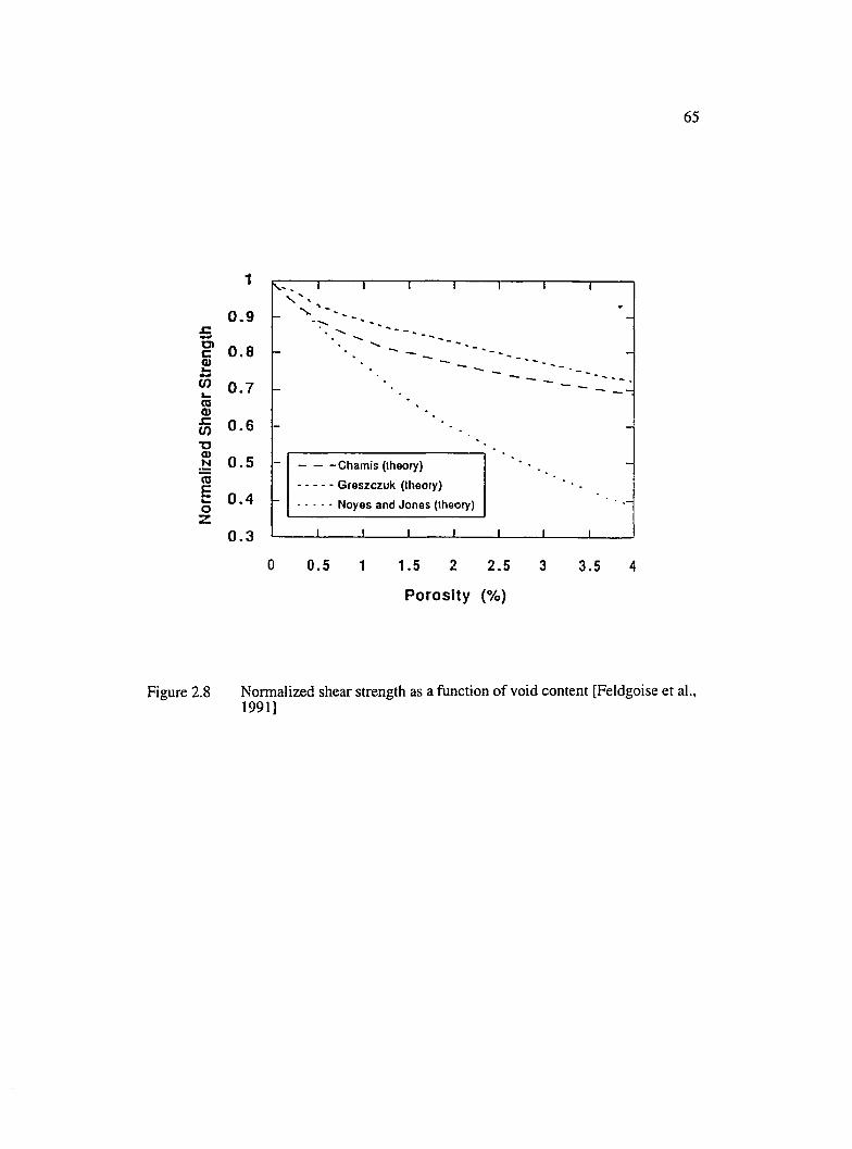
65

o>c2toswTJ<uNmEoz

1

0.90.8

0.70.6

0.50.40.3

■v

C ham is (Iheory)

G reszczu k (Iheory)

■ ■ • N oyés and Jo n e s (theory)

0.5 1 1.5 2 2.5

Porosity (%)

3.5 4

Figure 2.8 Normalized shear strength as a function of void content [Feldgoise et al., 1991]

6 6

Fan [1993] developed Equation 2.32 to predict the flexural strength as a function of void

content.

F = F„(Fv+V,)

1 • MIp.JI" (1 - F. - V.) J

(2.32)

where

F is the flexural strength of the composite

Fo is the flexural strength of the composite with no voids

Fv is the fiber volume fraction

P r and pm are the densities of the fiber reinforcement and the resin matrix

respectively

Vv is the void content (vol. %)

This theoretical correlation was found to agree quite well with the experimental results

obtained by Ghiorse [1992]. The suggested formula, Equation 2.32, has also been found

to be quite accurate for the prediction of reduction in the modulus of elasticity.

2.6 Application of Polymer Powders in Composites

One of the earliest references to the incorporation of powdered resin in fiber tows is the

patent by Price [1973]. Many other workers have subsequently discussed or patented

different versions of the technique [Gibson and Manson, 1992]. The idea of using

powders was developed to provide an alternative means to produce composites from

thermoplastic resins that are difficult to prepreg due to their high melt viscosity or due to

the need to use high boiling point precursor solvents which are difficult to remove.

67Several different forms of powder coated composites are available. Figure 2.9 shows

three of them. These include sheathed materials, melt fused materials and binder

materials. This nomenclature is based on the method used to hold the powder on the

fiber. In a sheathed system, the polymer powder is impregnated into the fiber tow, and

then the tow is coated with molten polymer to hold the powder on the fibers.

The hot melt system utilizes a fluidized bed to impregnate the tow and then a heat source

to melt the particles to fuse them onto the fiber. Successful impregnation of powders

relies on pins or rollers to open up and spread the fiber tow in order to present as large an

area as possible for the incorporation of powder into the strand. However, in alternative

versions of the process, an air knife [Muzzy et al., 1990] and a venturi [de, Jager G, 1987]

have been proposed to open up the yarn. Some studies describe the incorporation of the

powder into the tow solely in terms of mechanical effects while others have emphasized

the importance of electrostatic attraction [Throne and Soh, 1990]. Once the tows have

been filled with the resin, the next step is to pass them through an oven to melt the

powder and complete the impregnation process. Infra-red heating has been found to be

useful, especially in the early stages of heating in order to achieve a high rate of

temperature increase. Typical oven residence times are in the range of 10 -100 seconds.

The binder system uses a polymer to bind the powder particles on the fibers. This

method produces the most flexible and drapeable prefrom. However, complete removal

of the binder can become difficult. In this process, the polymer powder (having a

particle size < 20 pm) is mixed with a binder in a solution. The fibers are then passed

through a bath containing this solution, where they are coated with the polymer powder.

The amount of polymer powder deposited on the fibers depend upon the powder

concentration in the solution and the rate at which the fibers are pulled through the bath.

Cochran and Pipes [1991] studied the feasibility of this approach for making Poly-ether-

6 8

Sheathed Melt Fused Binder

Figure 2.9 Types of powder coating in composites [Cochran and Pipes, 1991]

69

ether-ketone (PEEK) powder coated preforms. In another study by Vodermayer et al.

[1993], impregnation of carbon fiber rovings was investigated using a similar approach,

but with an aqueous polymer powder dispersion process. The advantage of using an

aqueous dispersion being lesser health hazards. However, there is still the need to

remove the water after impregnation of the fiber rovings. Thus, dry powder coating of

fiber tows is often the preferred approach as it circumvents a lot of inherent difficulties

associated with removal of liquids, resulting in faster line speeds.

There are several types of thermoplastic powder suitable of use in powder impregnation

technique. Candidate resin include the high performance materials, PEEK,

polyethersulfone (PES), polyphenylene sulfide (PPS) and polyetherimide (PEI), but there

is also considerable potential for using the commodity "engineering thermoplastics", such

as nylon 12 and polypropylene.

Some composite applications require the use of textile type (stitched, knitted, woven,

etc.) preforms for improved mechanical properties. However, to obtain good mechanical

properties, it becomes necessary to obtain full consolidation of bulky textile type

preforms. Consolidation is an important issue as bulk factors (the ratio of preform

thickness to final part thickness) are on the order of 5:1 for 2D textiles and 3:1 for 3D

textiles [Hugh et al., 1993]. To facilitate consolidation, polymer powders based preforms

were developed. Full consolidation of powder coated textile preforms entails a two-step

process. It involves an initial debulking step to obtain the wetting needed for intimate

contact of resin and fiber, followed by final "net-shape" consolidation. Initial debulking

is done by any of the common forming methods such as, rubber molding, hydroforming,

diaphragm forming, and matched die molding. Final consolidation is usually

accomplished by standard autoclave or heat-press procedures. Several studies focusing

on the flexural rigidity and consolidation behavior of thennoplastic powder coated

70preforms have been undertaken in recent years at the NASA Langley Research Center

[Hirt et al., 1990 & Hugh et al., 1993]. In aerospace industry, usually a reactive material

(tackifier) is used for consolidation of fiber preforms. The reactive material can either be

uncatalyzed or catalyzed thermoset resin with generally the same cure chemistry as the

matrix resin. Some of the common methods of tackifier application utilize veils, solvent

spray and powder [Kittelson and Hackett, 1994]. Veils can be placed between adjacent

plies of broad goods followed by fusing the ply stacks with heat and pressure to form a

preform. Tackifiers can also be applied from solvents by spraying onto each broad good.

However, for the same reasons as in the case of thermoplastic resins, the preferred

approach is to use powders which can be applied onto the broad goods by a sifter type

apparatus. Application of heat and pressure causes the powder to melt and flow between

the layers of the fiber preform. Since the powder concentration typically ranges from 4 to

7% by weight of the fibers, tackified preforms can be thought of as very low content

prepregs. Again, one of the important issues in using thermoset powder coated preforms

is the need for significant debulking during the consolidation process. It is important to

note that since the density of the fibers is nearly twice that of the resin, 4 to 7 weight

percent of tackifier equates to about 8 to 14 percent of the total resin in the finished part.

Thus, tackifier can become a major component in the matrix resin and can significantly

affect the mechanical properties of the molded part. It is because of this reason, that the

chemistry of the tackifiers is chosen so as to be compatible with the matrix resin.

2.7 Tack and Drape Characteristics of Prepregs /Preforms

One of the major concerns in using prepregs and preforms is insufficient tack and poor

drape characteristics. Tack is the property that allows the layers of the fiber mat to stick

to one another so that the whole fiber stack can be handled as a single unit with reduced

slippage between the layers. Drape refers to the ability to conform to the tool surface.

71Often prepregs and preforms need to be deformed in order to fit the shape and curvature

of the tool surfaces. If the elastic energy stored during this deformation is high, the fibers

will overcome the adhesion forces due to tack during relaxation, and the prepreg/preform

will "springback" to its undeformed state. The springback phenomenon is also referred to

as non-conformance to the tool surface [Gutowski and Bonhomme, 1988], and is a

manifestation of the elastic stresses stored in the fibers.

Several attempts have been made to measure and model the phenomenon of tack

adhesion. Although there is no universally accepted technique for measuring tack,

various methods exist ranging from the primitive to the more sophisticated. One of the

older methods of measuring tack involves sticking a piece of prepreg on a vertical steel

surface, and stating that the tack is high enough if the prepreg does not fall in thirty

seconds [Meissonnier, 1988]. The newer methods derived from two main ASTM

standards [D 2979-71 & D 3121-73] are used mostly by the pressure sensitive adhesives

industry [Bonhomme, 1986].

Meissonnier [1988] developed a simple test to study tack and drape characteristics of

bismaleimide resin based graphite fiber prepregs. The experimental technique used was

similar to the flatwise compressive/tensile test. Prepreg samples were glued to the

crossheads of an Instron machine using special tabs, and subjected to a compression-

tension cycle. First, the samples were brought in contact with a constant cross-head

speed, held in contact under a constant load for a given "hold-time", and then pulled apart

in the opposite direction with the same speed till the samples came apart. The significant

parameters of the test were : rate of loading and unloading, the maximum pressure, hold

time and temperature. The measured quantities were : tension modulus, energy absorbed

during tension loading, strain and creep compliance under the maximum pressure during

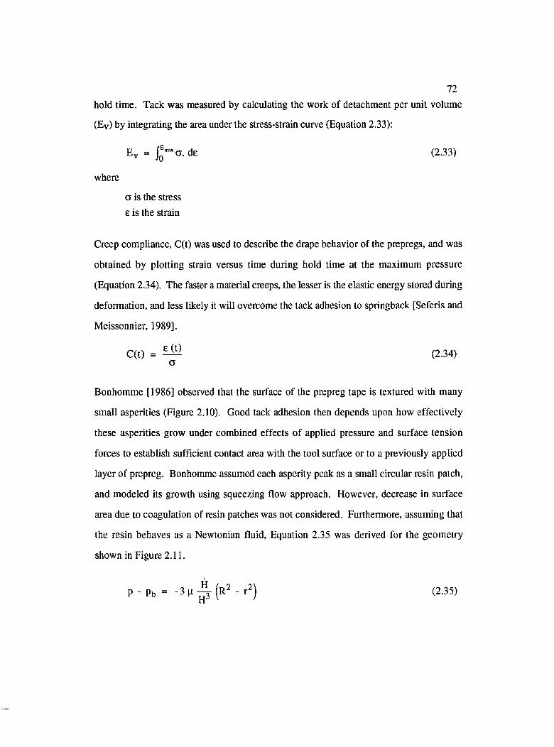
72hold time. Tack was measured by calculating the work of detachment per unit volume

(Ev) by integrating the area under the stress-strain curve (Equation 2.33):

Ev = Jq"“ ct. de (2.33)

where

a is the stress e is the strain

Creep compliance, C(t) was used to describe the drape behavior of the prepregs, and was

obtained by plotting strain versus time during hold time at the maximum pressure

(Equation 2.34). The faster a material creeps, the lesser is the elastic energy stored during

deformation, and less likely it will overcome the tack adhesion to springback [Seferis and

Meissonnier, 1989].

C(t) = ^ (2.34)a

Bonhomme [1986] observed that the surface of the prepreg tape is textured with many

small asperities (Figure 2.10). Good tack adhesion then depends upon how effectively

these asperities grow under combined effects of applied pressure and surface tension

forces to establish sufficient contact area with the tool surface or to a previously applied

layer of prepreg. Bonhomme assumed each asperity peak as a small circular resin patch,

and modeled its growth using squeezing flow approach. However, decrease in surface

area due to coagulation of resin patches was not considered. Furthermore, assuming that

the resin behaves as a Newtonian fluid. Equation 2.35 was derived for the geometry

shown in Figure 2.11.

P - Pb - ^ (2 3 5 )

73

actual surface texture

idealizedsurfacetexture

resin patch model

Figure 2.10 Schematic of the surface of the prepreg [Bonhomme, 1986]

H(t)777777777

R(t)

Figure 2.11 Squeezing flow of a newtonian liquid [Bonhomme, 1986]

74

Equation 2.35 was then rewritten in terms of the applied force with pressure at the

boundary pb = 0 (i. e. neglecting the surface tension effects), the volume of the patch, V =

HA, and A = 7i r 2-

t2 . H,f p d t = - — iiV^ f H ' ^ d H (2.36)J 0 -TT Jt, H

For F = Fa = constant, ti = 0, t% = t. Hi = Hq, and H% = H, the following result was

obtained for the wetted area of the patch as a function of time

A(t) 1 + —

1

(2.37)

where

N is = 4 for a Newtonian fluid and

To is the time constant given by Equation 2.38

3 IX8 n F,

(2J8)

where

Ao and Hq are the starting area and height of the resin patch

For surface tension driven squeezing flow, the expression for area growth was derived

similar in form to Equation 2.37 by substituting patm - Pc for the boundary pressure py.

where• ,u -11 / 2 Yr Cos 0

P c is the capillary pressure ( = —*—^ ------)

However, for this case, N = 2 and time constant x is given by Equation 2.39:

X =4% yCosG y

75

(139)

2.8 Modeling of Fiber Consolidation

In order to better understand the "deconsolidation" or the springback phenomena in

composites, a conceptual mathematical model for transverse stiffness of a bundle of

confined fibers was developed by Gutowski [1985]. The model assumes that the

deflection behavior of a fiber is given by the strength of material solutions for a beam of

span length li and diameter d (Equation 2.40). Also, that the fiber is arched with a height Cl, but ^ is large and so the arch length and span length are very close.Cl

pAf

n Eld j c i ;

(2.40)

where

P is the applied pressure

Af is area of the fibers exposed to pressure p

E is the modulus of elasticity

I is the moment of inertia

C is a constant and depends on the assumed end conditions

5 is the beam deflection

The final equation arrived at for transverse stiffness was obtained as given by Equation

2.41 :

P = ^

J _

vVo Vf64 a p

I Vo

(2.41)

a y

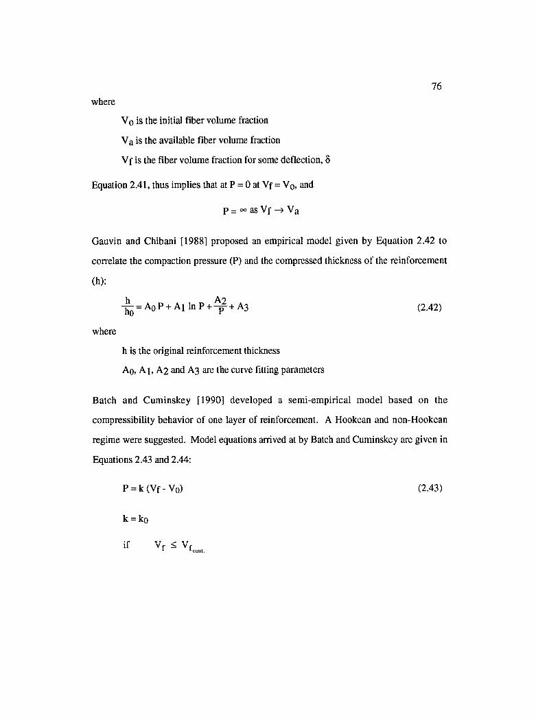
76where

Vo is the initial fiber volume fraction

Va is the available fiber volume fraction

Vf is the fiber volume fraction for some deflection, 8

Equation 2.41, thus implies that at P = 0 at Vf = Vq, and

p = oo as Vf Va

Gauvin and Chibani [1988] proposed an empirical model given by Equation 2.42 to

correlate the compaction pressure (P) and the compressed thickness of the reinforcement

(h):

- ^ = AqP + Ai l n P + ^ + A3 (2.42)

where

h is the original reinforcement thickness

Ao, A i, A2 and A3 are the curve fitting parameters

Batch and Cuminskey [1990] developed a semi-empirical model based on the

compressibility behavior of one layer of reinforcement. A Hookean and non-Hookean

regime were suggested. Model equations arrived at by Batch and Cuminskey are given in

Equations 2.43 and 2.44:

P = k ( V f - V o ) (2.43)

k = ko

if Vf < Vf* ^cont.

77

and

J _ J _

k = ko Y ---- T " (2.44)

■ vT

if Vf > Vf* ^cont.

where

k is the fiber compaction spring constant

ko is the fiber compaction spring constant for the Hookean regime

T| is the fiber packing efficiency

V is the ultimate fiber fraction at maximum pressure

V f is the volume fraction at the transition between Hookean and non-Hookean cont.

Claus and Loos [1989] expressed the compaction behavior of textile prefoiTns in terms of

a logarithmic series. Their model is given by Equation 2.45:

d = ai + a2 In P + a3 (In P)2 + 3 4 (In P)3 + ........ (2.45)

where

d is the deflection of the fiber bed, and P the compaction pressure

The number of terms in the series were chosen to give the desired level of correlation

with experimental results.

2.9 Rheo-kinetic Characterization of Bismaleimide Resins

Bismaleimide resins are used mostly as matrix resins for high performance composite

applications. They exhibit low moisture absorption, excellent chemical stability, and

thermal and mechanical properties superior to most epoxy resins. Low moisture

78absorption comes from the fact that the imide functionality has lower capacity for

hydrogen bonding than either -OH or -NH2 containing polymers.

Due to the aromatic nature and high crosslink density of the cured network, the fully

cured resins are brittle. Thus, bismaleimide resins are often reacted with aromatic

diamines, which reduce the crosslink density by increasing the distance between the

crosslinks [Tungare and Martin, 1993]. However, the addition of diamines results in a

slight decrease in the thermal stability of bismaleimide resins.

Another approach to reduce brittleness is to create an interpenetrating network by

modifying the resin with a silicone monomer such as diphenylsilanediol. Properties of

silicone modified bismaleimide resins have been studied by Voit and Seferis [1987].

They observed that the silicone additive provided important morphological modification

to the resin matrix by improving impact toughness while, at the same time, retaining the

high temperature properties of the resin.

The curing behavior of bismaleimide resins using formulations containing different

stoichiometric ratios of 1,1' - (methylene - 4,1 - phenylene) bismaleimide and 4,4' -

methylenedianiline (MDA) was studied by Tungare and Martin [1992]. Their study

revealed that curing can take place via two reaction pathways (Figures 2.12 a and b).

They are amine addition to the maleimide double bond of the bismaleimide, which occurs

readily at low temperatures (> 75 °C), and the homopolymerization of the bismaleimide

double bonds, which occurs at high temperatures (> 155 °C). At lower temperatures, the

two reactions are in a sequential order, but at high temperatures, both of them occur

simultaneously.

The maleimide double bonds of the bismaleimide resin are weakened by the electron

withdrawing nature of the adjacent carbonyl groups, and hence, nucleophilic addition of

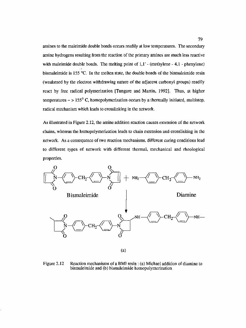
79amines to the maleimide double bonds occurs readily at low temperatures. The secondary

amine hydrogens resulting from the reaction of the primary amines are much less reactive

with maleimide double bonds. The melting point of 1,1'- (methylene - 4,1 - phenylene)

bismaleimide is 155 °C. In the molten state, the double bonds of the bismaleimide resin

(weakened by the electron withdrawing nature of the adjacent carbonyl groups) readily

react by free radical polymerization [Tungare and Martin, 1992]. Thus, at higher

temperatures ~ > 155° C, homopolymerization occurs by a thermally initiated, multistep,

radical mechanism which leads to crosslinking in the network.

As illustrated in Figure 2.12, the amine addition reaction causes extension of the network

chains, whereas the homopolymerization leads to chain extension and crosslinking in the

network. As a consequence of two reaction mechanisms, different curing conditions lead

to different types of network with different thermal, mechanical and rheological

properties.

N

OBismaleimide

-i- nh2— ■NH,

oDiamine

N-

O

.NH NH—

(a)

Figure 2.12 Reaction mechanisms of a BMl resin : (a) Michael addition of diamine to bismaleimide and (b) bismaleimide homopolymerization

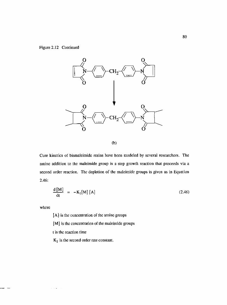
Figure 2.12 Continued

80

o

N

o

N- y \ '

OX

o> -

OX

I— ] S ^

(b)

Cure kinetics of bismaleimide resins have been modeled by several researchers. The

amine addition to the maleimide group is a step growth reaction that proceeds via a

second order reaction. The depletion of the maleimide groups is given as in Equation

2.46:

^ = - K , t M l [ A ]dt

(2.46)

where

[A] is the concentration of the amine groups

[M] is the concentration of the maleimide groups

t is the reaction time

Kj is the second order rate constant.

81

The maleimide and amine conversions, and a/^ are given by Equations 2.47 and

2.48:

_ K 1 - [ m ]

^ ■ [Mol

_ [Aq] - [A ]

^

(2.47)

(2.48)

where

[Mq] is the initial concentration of maleimide groups

[Aq]. is initial concentration of the amine groups

Equation 2.46 can be written in terms of the maleimide conversion, using Arrhenius

temperature dependence for Kj , as in Equation 2.49:

[M o f= Ai exp d t ‘

-E lRT

X [l -ajvi] 1 -

[Ao][Ao] (2.49)

The kinetic model developed by Tungare and Martin [1992] for BMI

homopolymerization has the following form:

d[M]dt

= k2t Ml -k2i[M]-k2p[M] Ml - k2p[M] M (2.50)

Ml

dtMl k2p[M] Ml

- k 2p

2Ml - k ] p Ml M (2.51)

82

M

dt= k2p[M] Ml ^2p M, M (2.52)

where

Ml

M

is the concentration of the maleimide radicals

is the concentration of the polymer formed

k 2 i is the reaction rate constant for the initiation step

k 2 p is the reaction rate constant of the propagation step

k 2 t is the reaction rate constant of the termination step

Tungare and Martin [1992] found that in the multistep homopolymerization, the chain

propagation step is an order of magnitude slower than the initiation and the termination

reactions and is the rate controlling step. The single step amine addition reaction occurs

much more rapidly than the chain propagation reaction during the homopolymerization of

BMI. This model, however, does not consider the interactions between the two reactions

and the diffusion effect on reaction rate.

The change in viscosity as a function of conversion for BMI resins has not been modeled

as extensively as the reaction kinetics. Meissonnier [1988] proposed an empirical model

for two different formulations of BMI (Kerimid 70003 and 70015) based on the WLF

(William-Landel-Ferry) equation given as:

A ( T - T g )L ogn(T) = Log^Tgo ■

B + T - T„(Z53)

where

|i is the viscosity

T is the temperature

Tg is the glass transition temperature of the resin at any conversion

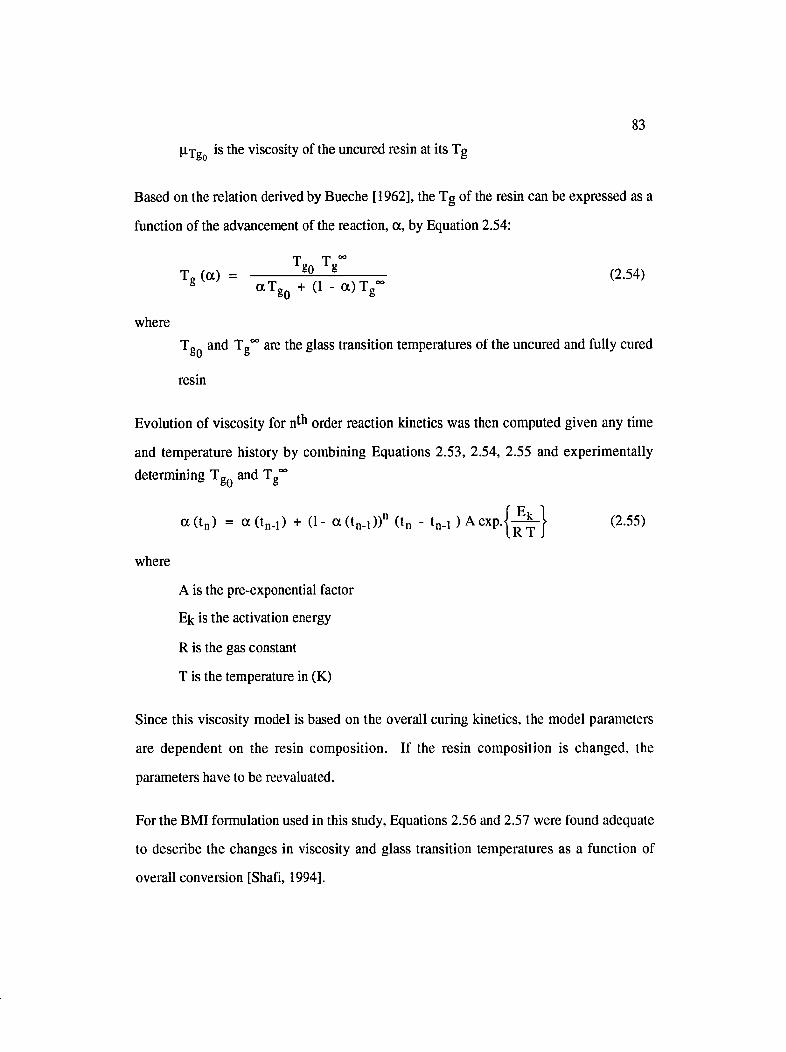
83is the viscosity of the uncured resin at its Tg

Based on the relation derived by Bueche [1962], the Tg of the resin can be expressed as a

function of the advancement of the reaction, a , by Equation 2.54;

whereTgQ and Tg” are the glass transition temperatures of the uncured and fully cured

resin

Evolution of viscosity for n^h order reaction kinetics was then computed given any time

and temperature history by combining Equations 2.53, 2.54, 2.55 and experimentally determining Tg^ and Tg”

a ( t n ) = a ( t n . i ) + ( 1 - a ( t n - i ) ) " B n - t n - i ^ ^ ( 2 5 5 )

where

A is the pre-exponential factor

Ek is the activation energy

R is the gas constant

T is the temperature in (K)

Since this viscosity model is based on the overall curing kinetics, the model paiameters

are dependent on the resin composition. If the resin composition is changed, the

parameters have to be reevaluated.

For the BMI formulation used in this study. Equations 2.56 and 2.57 were found adequate

to describe the changes in viscosity and glass transition temperatures as a function of

overall conversion [Shafi, 1994].

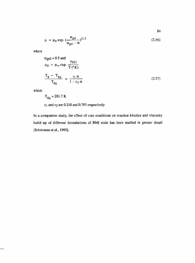
84

[ 1 = Ho exp. (-----^ (2. 56)Otgel " GO

where

ttgel = 0.5 and7161

Ho = HooCxp.T(°K)

~ ^gp ^ Cl « T„^ 1 - C2 a

(2.57)Bp

whereTgo= 281.7 K

Cl and 0 2 are 0.218 and 0.793 respectively

In a companion study, the effect of cure conditions on reaction kinetics and viscosity

build up of different formulations of BMI resin has been studied in greater detail

[Srinivasan et al., 1995].

CHAPTER III

ANALYSIS OF FLOW INDUCED VOIDS DURING FIBERIMPREGNATION

3 .1 Materials

For flow visualization experiments, several non-reactive liquids having different surface

tensions and viscosities were used. These include water, DOP oil (diphenyl-octyl-

phthalate), silicone oils (dimethylpolysiloxane, Dow Coming), glycerin, and ethylene

glycol.

There are numerous choices of fiber reinforcements for LCM processes. However, most

of them can be characterized by two types of pores; one between the fiber bundles and the

other within the bundles. In this work, a unidirectional stitched fiberglass mat (CoFab

AO 108) was used as it was easier to analyze the observed flow behavior because of the

simple fiber architecture. It is a non-woven type of reinforcement with fiber bundles

oriented in one direction only, and held together by continuous stitches.

3 .2 Instrumentation and Experimental Procedure

3.2.1 Liquid Properties and Contact Angle Measurements

The viscosities and surface tensions of the experimental liquids were either measured or

obtained from handbooks. Viscosity measurements were made using the Brookfield

viscometer, while for surface tension and contact angle measurements, a Dynamic Contact

85

8 6

Angle Analyzer (DCA 322) was used. DCA 322 (Figure 3.1) is based on the Wilhelmy

principle. In this technique, a solid sample suspended from a balance is partially immersed

in a liquid and the force exerted by the liquid on the solid is monitored. To recall, the

Wilhelmy wetting force is given by

Fw = P ylCOs(0) (3.1)

where

P is the perimeter of the sample

is the surface tension of the liquid, and

0 is the contact angle made by the liquid on the sample

The value of Fw is obtained from the balance. Thus, it follows that if two of the three

quantities on the r.h.s. of Equation 3.1 are known, it can be solved for the third quantity.

For contact angle measurements, it was necessary to know the surface tension of test

liquids. For surface tension measurements, a heat cleaned glass cover slip of known

perimeter was used as the sample. It was suspended from the arm of the microbalance via

a hangdown wire. The test liquid was contained in a beaker resting on a motor driven

traveling stage. The liquid was slowly raised by moving the stage upwards. At the first

contact of the liquid with the sample, there was an increase in the force. The force then

decreased due to buoyancy as more and more of the sample was immersed in the liquid.

After a sufficient length of the sample was traversed by the liquid, the direction of the stage

was reversed to obtain the data for the receding cycle. The wetting force was obtained by

extrapolating the force reading to zero depth of immersion to account for the buoyancy

factor. This is a point when the sample first comes in contact with the liquid. The value of

the contact angle is assumed to be close to zero. This assumption is usually valid when

there is no hysteresis between the advancing and the receding cycles. Figure 3.2 shows a

typical trace of the curves obtained from a surface tension experiment. In this case, the

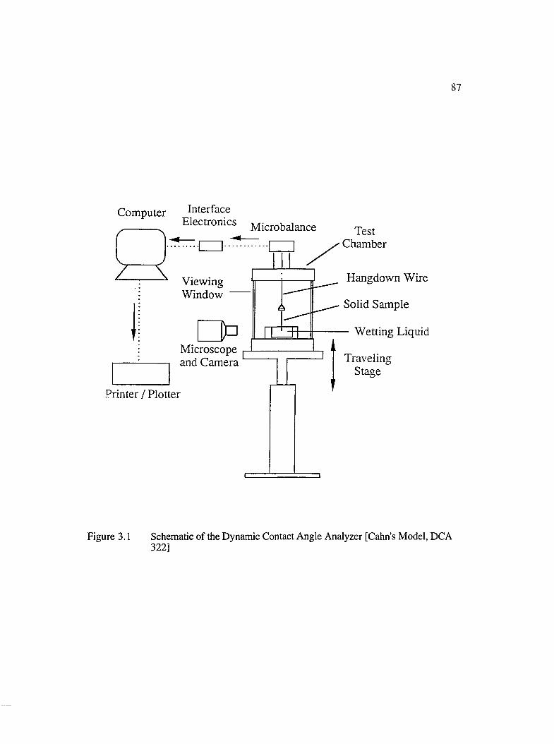
87

Computer Interface Electronics

/ \

V , J/ \

Microbalance

Printer / Plotter

ViewingWindow

Microscope and Camera

TestChamber

Hangdown Wire

Solid Sample

Wetting Liquid

TravelingStage

Figure 3.1 Schematic of the Dynamic Contact Angle Analyzer [Cahn’s Model, DCA 322]

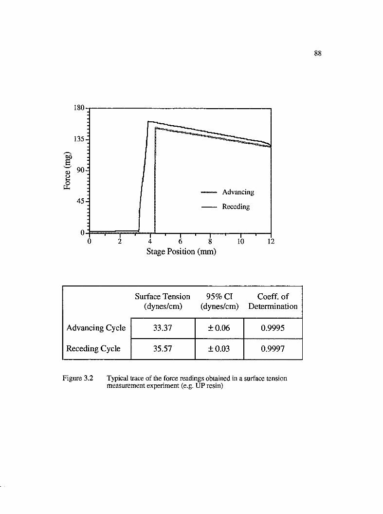
88

180

135-

B : ^ 9 0 -

I ;Advancing

Receding4 5 -

40 2 6 8 10 12Stage Position (mm)

Surface Tension 95% Cl Coeff. o f(dynes/cm) (dynes/cm) Determination

Advancing Cycle 33.37 ± 0 .0 6 0.9995

Receding Cycle 35.57 ±0 .03 0.9997

Figure 3.2 Typical trace of the force readings obtained in a surface tension measurement experiment (e.g. UP resin)

89

curve represents the force values from which the surface tension of unsaturated polyester

resin was calculated.

After obtaining the surface tension of test liquids, contact angles were measured in a similar

fashion. However, a single filament was used as the sample instead of the cover slip. The

perimeter of the filaments was measured using wetting liquids like Hexane and Hexadecane

which gave nearly zero contact angles. In a parallel study, contact angles between fiber

bundles and sample liquids were also measured [Patel et al., 1994]. The physical

properties of the liquids and the corresponding contact angles with the fibers are given in

Table 3.1.

3.2.2 Flow Visualization o f Macro and Micro Voids

A transparent acrylic mold with a light source underneath was used as a flow cell for

visualization experiments. The mold dimensions were 5.7" x 3.54" (1 x w). A rectangular

cavity having dimensions 3.35" x 1.97" (1 x w) was created using a lexan gasket. Strips of

fiber mat were cut so that its edges were flush with the side« of the rectangular cavity. This

was done to ensure that no race - tracking or channeling occurred from the sides. Also, a

gap of about 0.4" was kept between the fiber mat and the inlet so that the liquid reached the

fiber mat as a plug flow. Liquid was injected at a constant flow rate using a Harvard

apparatus infusion / withdrawal pump (Model 919). It is a positive displacement pump

with a piston cylinder type mechanism for injection. The highest superficial velocity

achieved in the mold was 3.9 cm/sec. Care was taken to remove all the air bubbles from

the source liquid and the transparent tube connecting the pump to the mold. Flow behavior

was observed for both flow along and normal to the fibers for different injection flow rates.

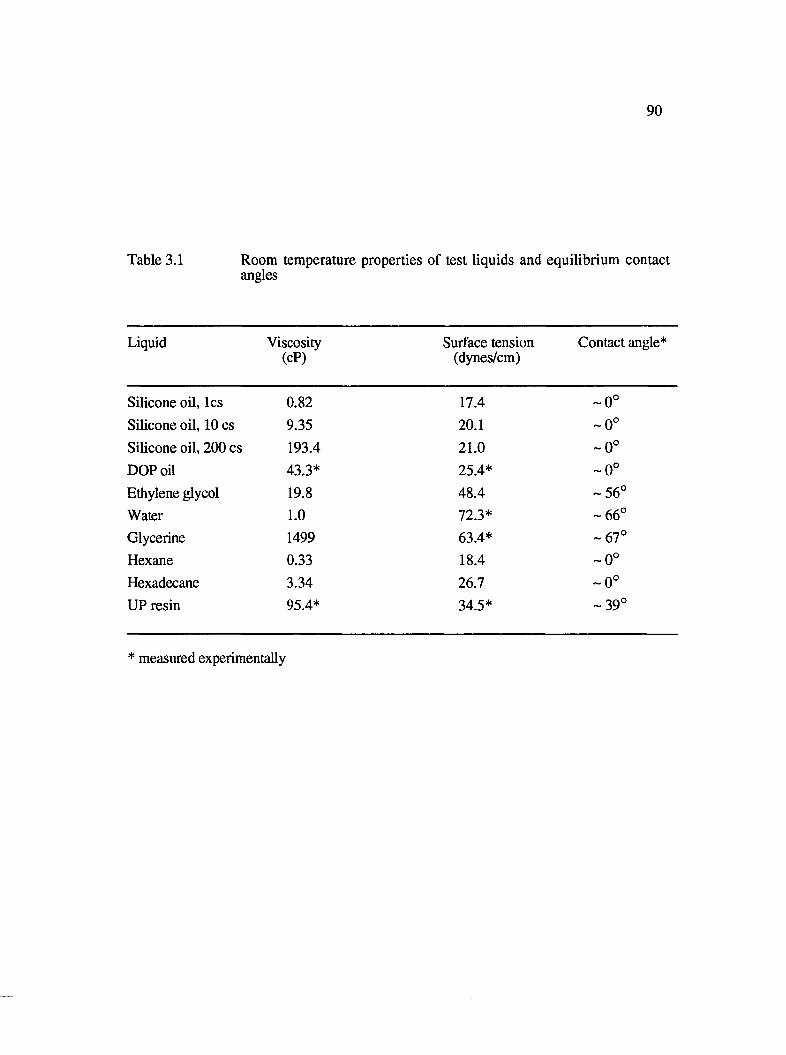
90

Table 3.1 Room temperature properties of test liquids and equilibrium contactangles

Liquid Viscosity(cP)

Surface tension (dynes/cm)

Contact angle*

Silicone oil, les 0.82 17.4 - 0 °Silicone oil, 10 cs 9.35 20.1 - 0 °Silicone oil, 200 cs 193.4 21.0 - 0 °

DOP oil 43.3* 25.4* - 0 °Ethylene glycol 19.8 48.4 -5 6 °Water 1.0 72.3* - 6 6 °Glycerine 1499 63.4* - 6 7 °Hexane 0.33 18.4 - 0 °Hexadecane 3.34 26.7 - 0 °UP resin 95.4* 34.5* -3 9 °

* measured experimentally

91

The fiber volume fraction for these experiments, as calculated from Equation 3.2, was

43%.

(3.2)1- f Vf ] = 1 -n

I V cJ t

where

(|) is the porosity

Vf is the volume of the fibers

Vc is the volume of the cavity

% is the surface density of the fiber mat (ML'2)

p is the density of the glass fiber (ML"3)

n is the number of layers of the fiber mat

t is the final gap or the cavity thickness

The flow pattern of the liquid through the fiber mat and the formation of macrovoids during

liquid injection were viewed on a 13" T.V. monitor using a CCD video camera (Cohu

Model 4915-2001) and recorded on an S-YHS recorder (Panasonic Model AG 1960).

Macrovoids were viewed at a magnification of 16 times. After liquid injection was

completed, the mold was scanned for voids. A representative number of photographs were

taken for each run and the area fraction of macrovoids was computed.

Observation of formation of microvoids in the smaller gaps (~ 1pm) between the 13pm

diameter filaments in the fiber tows posed quite a challenge. This is so because it required

a magnification of greater than 200 times to see the filaments and the trapped microvoids.

Achieving a high magnification was not a problem as most commercial microscopes offer

magnifications greater than or up to 1000 times. However, at such high magnifications,

the working distance between the sample and the objective lens is in the order of a few

millimeters. Thus, for proper focusing of the sample at high magnifications (> lOOX), the

92sample must be only a few millimeters from the lens. This is where the problem arises.

Such a requirement on the proximity of the sample to the lens makes it impossible with

most microscopes to put a flow cell under the lens and focus on the filaments of the fiber

mat. Thus, in - situ observation of formation and movement of microvoids during liquid

injection becomes impossible with conventional microscopes.

Several different approaches were tried to tackle the problem before finally meeting with

success. Some of the approaches tried included using an Infinity lens, a reflecting

microscope (used in metallurgical microscopy), scanning electron microscopy (SEM), and

confocal laser microscopy. Both metallurgical microscopy and confocal laser microscopy

have been used in the past to observe the microstructure of fiber reinforced polymer

composites. The major limitation of these techniques is that they are off - line techniques in

the sense that they cannot be used for in - situ observations.

After a lot of experimentation and unsuccessful attempts at solving the problem, a

combination of the Cohu video camera (having a 1/2" view detector area), the T.V.

monitor, and more importantly, a 6.5 X Zoom lens (D. O. Industries) with a 5X adapter

and a 2X eyepiece finally did the trick. With this set - up, high magnifications of greater

than 400 X were achieved at a working distance of more than an inch, hence the name,

video assisted microscopy (YAM). This allowed the transparent acrylic mold to be placed

between the Zoom lens and the brightfield/darkfield stage for on-line viewing of the

formation of microvoids during liquid injection.

One last problem that needed to be solved was to improve the contrast between the

transparent injection liquids and the translucent white glass fibers. Some techniques like

etching and staining have been tried by previous researchers to improve the contrast. In

this work, a tint of red dye was added to the liquids which helped in defining the edges of

93the voids more clearly. The amount added was well below the critical concentration of

about 1% and was just enough to improve the contrast without altering the physical

properties of the liquids. The brightfield/darkfield stage was used for the same purpose.

In the darkfield mode, the reflections at the glass-air interfaces disappear resulting in a

better contrast

As in the case of macrovoids, after liquid injection, a representative number of photographs

were taken for each run and the area fraction of microvoids was computed using the Point

count technique [Kohn et al., 1968; Feldgoise et al., 1991]. Thus, void (both macro and

micro) fraction is reported as percentage detected area voidage. The schematic of the flow

visualization set - up developed in this study is shown in Figure 3.3.

3.3 Flow visualization of Macrovoids Formation

3 .7 ./ Axial Flow

A t low flow rates (v ~ < 0.1 cm / sec.), it was observed that the liquid penetrated through

the fiber mat at unequal rates, as shown in Figure 3.4. The same behavior was observed at

even higher flow rates (v > 0.1 cm / sec.) for some liquids like water, which have very

high surface tension and vei"y low viscosity. Thus, in essence, it is the capillary number

that governs how the liquid flows through the fiber mat.

The capillary number is usually defined as the ratio of viscous force (product of viscosity

and velocity) to capillary force:

C a # = ^ 1 0 - - (3.3)Ylv

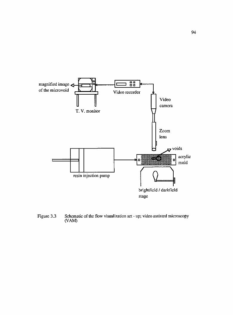
94

magnified image of the microvoid Video recorder

Videocamera

T. V. monitor

Zoomlens

voids

acrylicmold

resin injection pump

□ □

brightt'ield / darkfield stage

Figure 3.3 Schematic of the flow visualization set - up; video assisted microscopy (VAM)

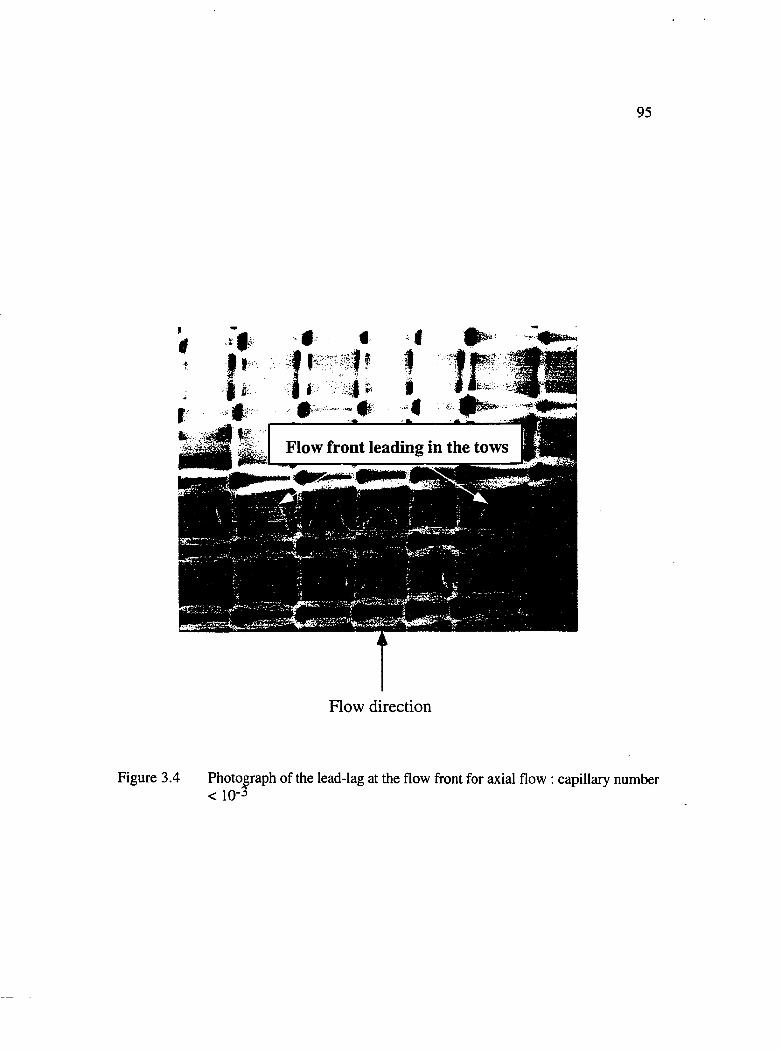
95

Flow front leading in the tows

Flow direction

Figure 3.4 Photograph of the lead-lag at the flow front for axial flow ; capillary number < 10-^

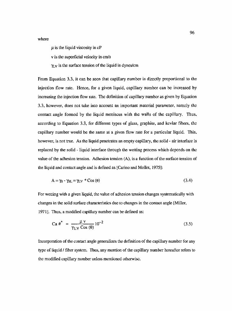
96where

|i is the liquid viscosity in cP

V is the superficial velocity in cm/s

T l v is the surface tension of the liquid in dynes/cm

From Equation 3.3, it can be seen that capillary number is directly proportional to the

injection flow rate. Hence, for a given liquid, capillary number can be increased by

increasing the injection flow rate. The definition of capillary number as given by Equation

3.3, however, does not take into account an important material parameter, namely the

contact angle formed by the liquid meniscus with the walls of the capillary. Thus,

according to Equation 3.3, for different types of glass, graphite, and kevlar fibers, the

capillary number would be the same at a given flow rate for a particular liquid. This,

however, is not true. As the liquid penetrates an empty capillary, the solid - air interface is

replaced by the solid - liquid interface through the wetting process which depends on the

value of the adhesion tension. Adhesion tension (A), is a function of the surface tension of

the liquid and contact angle and is defined as [Carino and Mollet, 1975]:

A = Ys - Ysl = TLv * Cos (0) (3.4)

For wetting with a given liquid, the value of adhesion tension changes systematically with

changes in the solid surface characteristics due to changes in the contact angle [Miller,

1971]. Thus, a modified capillary number can be defined as:

C a#* = --------------^ 10~^ (3.5)Ylv Cos (0)

Incorporation of the contact angle generalizes the definition of the capillary number for any

type of liquid / fiber system. Thus, any mention of the capillary number hereafter refers to

the modified capillary number unless mentioned otherwise.

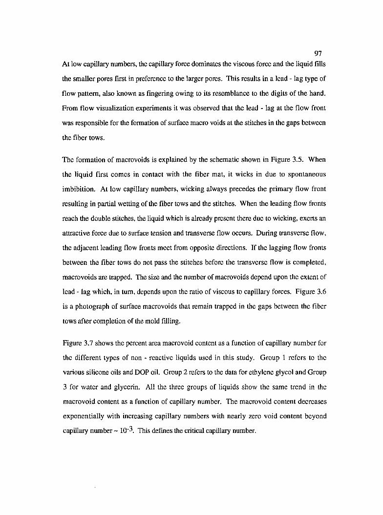
97At low capillary numbers, the capillary force dominates the viscous force and the liquid fills

the smaller pores first in preference to the larger pores. This results in a lead - lag type of

flow pattern, also known as fingering owing to its resemblance to the digits of the hand.

From flow visualization experiments it was observed that the lead - lag at the flow front

was responsible for the formation of surface macro voids at the stitches in the gaps between

the fiber tows.

The formation of macrovoids is explained by the schematic shown in Figure 3.5. When

the liquid first comes in contact with the fiber mat, it wicks in due to spontaneous

imbibition. At low capillary numbers, wicking always precedes the primary flow front

resulting in partial wetting of the fiber tows and the stitches. When the leading flow fronts

reach the double stitches, the liquid which is already present there due to wicking, exerts an

attractive force due to surface tension and transverse flow occurs. During transverse flow,

the adjacent leading flow fronts meet from opposite directions. If the lagging flow fronts

between the fiber tows do not pass the stitches before the transverse flow is completed,

macrovoids are trapped. The size and the number of macrovoids depend upon the extent of

lead - lag which, in turn, depends upon the ratio of viscous to capillary forces. Figure 3.6

is a photograph of surface macrovoids that remain trapped in the gaps between the fiber

tows after completion of the mold filling.

Figure 3.7 shows the percent area macrovoid content as a function of capillary number for

the different types of non - reactive liquids used in this study. Group 1 refers to the

various silicone oils and DOP oil. Group 2 refers to the data for ethylene glycol and Group

3 for water and glycerin. All the three groups of liquids show the same trend in the

macrovoid content as a function of capillary number. The macrovoid content decreases

exponentially with increasing capillary numbers with nearly zero void content beyond

capillary number ~ 10"3. This defines the critical capillary number.

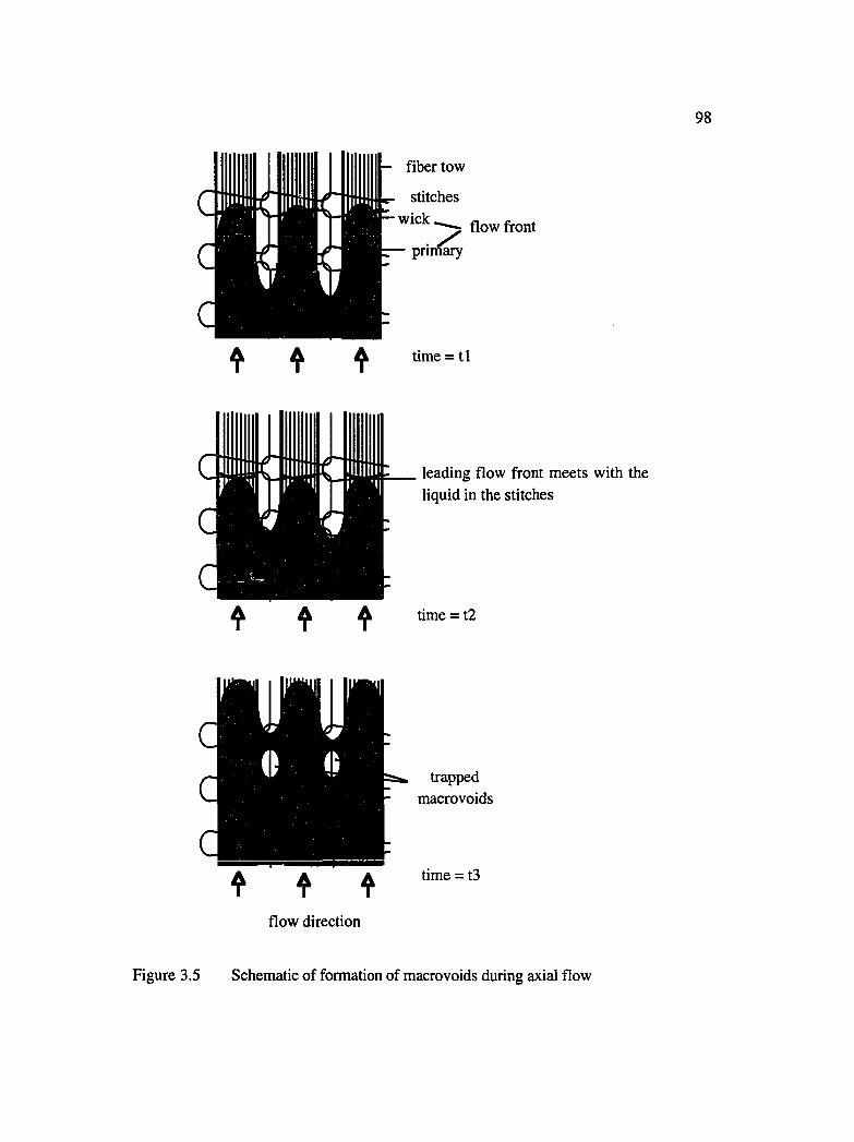
98

— fiber tow

stitches w ick^

p r ir i î^flow front

time = t l

leading flow front meets with the liquid in the stitches

time = t2

f f fflow direction

trappedmacrovoids

time = t3

Figure 3.5 Schematic of formation of macrovoids during axial flow

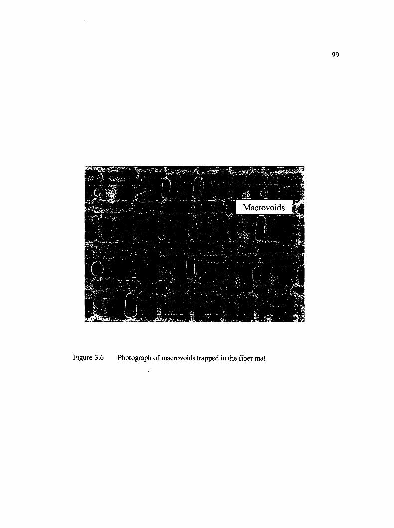
99

Macrovoids

Figure 3.6 Photograph of macrovoids trapped in the fiber mat

100

iII

> q□ Group I

• Group II

X Group III

40.0

35.0

30.0 P ^ o: X

25.0

20.0

15.0

10.0

5.0

0.0 0.000001 0.00001 0.0001 0.001 0.01 0.1

Modified capillary number

£

XX

I I m i l t t i - i IIuL

# ]

□ B □

Figure 3.7 Percent area macrovoids for flow along the fiber tows (axial flow)

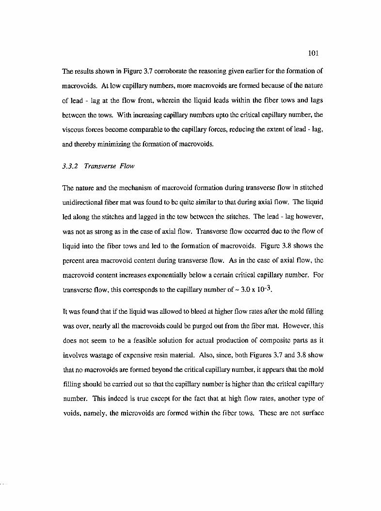
101

The results shown in Figure 3.7 corroborate the reasoning given earlier for the formation of

macrovoids. At low capillary numbers, more macrovoids are formed because of the nature

of lead - lag at the flow front, wherein the liquid leads within the fiber tows and lags

between the tows. With increasing capillary numbers upto the critical capillary number, the

viscous forces become comparable to the capillary forces, reducing the extent of lead - lag,

and thereby minimizing the formation of macrovoids.

3.3.2 Transverse Flow

The nature and the mechanism of macrovoid formation during transverse flow in stitched

unidirectional fiber mat was found to be quite similar to that during axial flow. The liquid

led along the stitches and lagged in the tow between the stitches. The lead - lag however,

was not as strong as in the case of axial flow. Transverse flow occurred due to the flow of

liquid into the fiber tows and led to the formation of macrovoids. Figure 3.8 shows the

percent area macrovoid content during transverse flow. As in the case of axial flow, the

macrovoid content increases exponentially below a certain critical capillary number. For

transverse flow, this corresponds to the capillary number of ~ 3.0 x 10'3.

It was found that if the liquid was allowed to bleed at higher flow rates after the mold filling

was over, nearly all the macrovoids could be purged out from the fiber mat. However, this

does not seem to be a feasible solution for actual production of composite parts as it

involves wastage of expensive resin material. Also, since, both Figures 3.7 and 3.8 show

that no macrovoids are formed beyond the critical capillary number, it appears that the mold

filling should be carried out so that the capillary number is higher than the critical capillar}'

number. This indeed is true except for the fact that at high flow rates, another type of

voids, namely, the microvoids are formed within the fiber tows. These are not surface

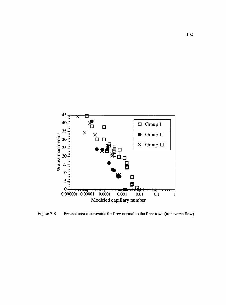
102

4 5

4 0 - j

3 5 - j

3 0 - :

2 5 J

2 0 - j

15-j

1 0 4

540

X X □ □• n i la

□ Group I

• Group II

X Group III

T I 11 iiii|0.001

□s

□0 ,

0.000001 0.00001 0.0001Modified capillary number

HBjl I I I I ITilfJ I III III!0.01 0.1

Figure 3.8 Percent area macrovoids for flow normal to the fiber tows (transverse flow)

103

voids and are more difficult to purge. The following sections describe formation of

microvoids at high flow rates for both axial and transverse flows.

3 .4 Flow Visualization of Microvoids Formation

3.4.1 Axial Flow

As in the case of macrovoids, the formation of microvoids during axial flow can be

correlated to the nature of lead - lag at the flow front. When the viscous force dominates

the capillary force, the nature of lead - lag at the flow front is reversed. Under such a

situation, the liquid leads in the gaps between the fiber tows and lags within the tows.

Figures 3.9 (a) and (b) depict the flow front wherein the silicone oil (200 cs.) is injected at

a superficial velocity of 3.9 cm / sec. No wicking was observed in this case. This is so

because at high flow rates, the primary flow front progresses at a rate equal to or faster than

the wicking rate. Also, the lead - lag is not very uniform. This is because of the non

uniformity in the gaps due to unequal spacing between the fiber tows.

A plausible mechanism to explain the formation of microvoids is shown by the schematic in

Figure 3.10. As can be seen in Figures 3.9 (a) and (b) and in the schematic in Figure 3.10,

the leading flow fronts diffuse inward from the larger gaps into the fiber tows. After

diffusing into the tows, the liquid meets with the lagging flow fronts moving in the flow

direction within the tows. When flow fronts meet from opposite directions, microvoids are

trapped. These microvoids may remain at the site of their formation or may move along

with the flow with gradual change in their shapes and sizes. The shape, size, and the

mobility of microvoids depend on the balance of the air pressure inside the microvoids,

surface tension forces, and the hydrodynamic pressure. Geometric factors like the non

uniformities within the fiber tows and stitches also play important roles in governing the

final shape and size of the microvoids.

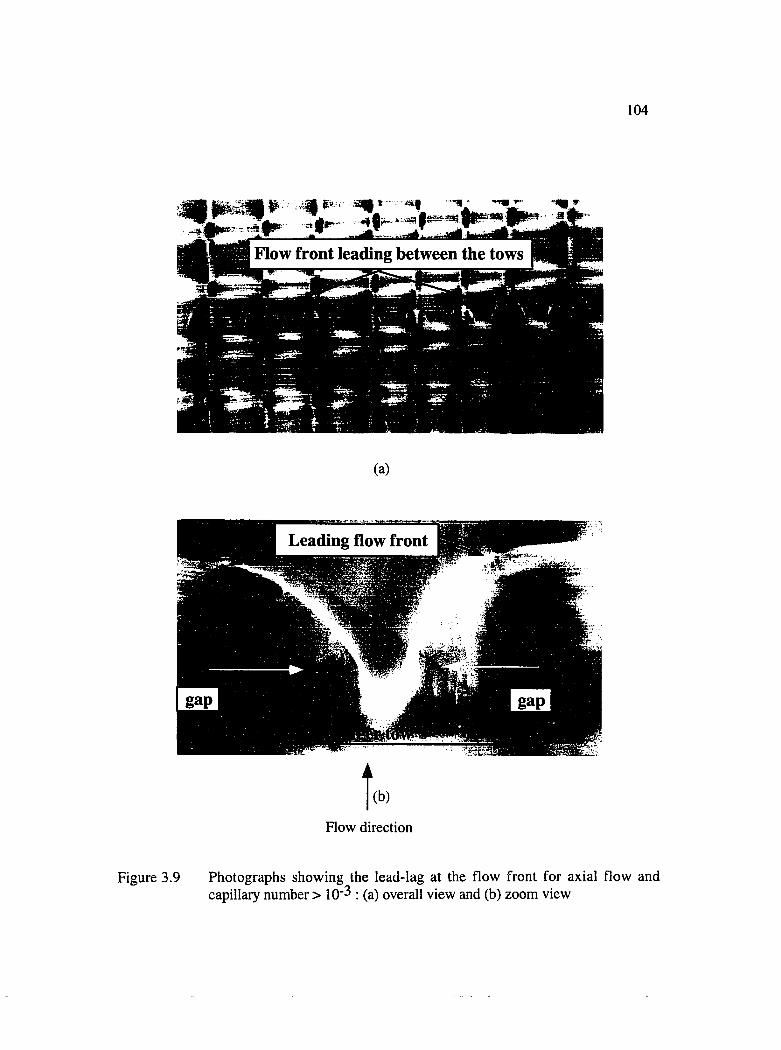
104

Flow fron t leading between the tows

(a)

Leading flow fron t

Flow direction

Figure 3.9 Photographs showing the lead-lag at the flow front for axial flow and capillary number > 10"3 : (a) overall view and (b) zoom view

105

Q

d

fiber tow

fTi \stitches

— flow front

time = tl

trappedmicrovoids

time = t2

flow direction

Figure 3.10 Schematic of formation of microvoids during axial flow

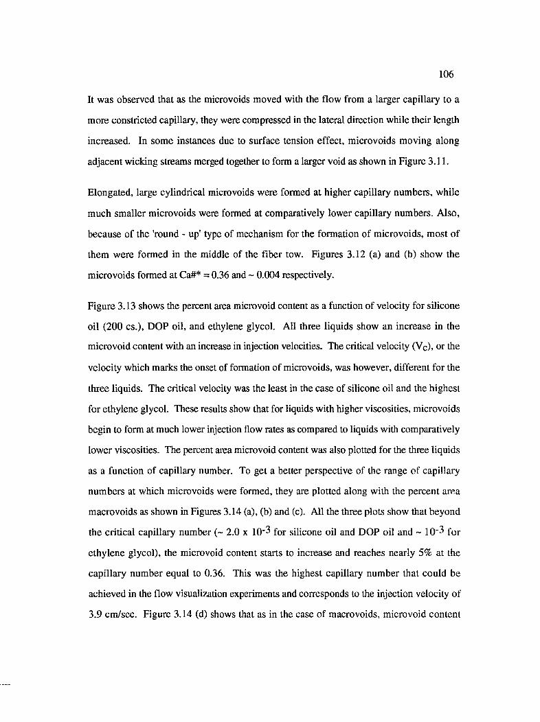
106

It was observed that as the microvoids moved with the flow from a larger capillary to a

more constricted capillary, they were compressed in the lateral direction while their length

increased. In some instances due to surface tension effect, microvoids moving along

adjacent wicking streams merged together to form a larger void as shown in Figure 3.11.

Elongated, large cylindrical microvoids were formed at higher capillary numbers, while

much smaller microvoids were formed at comparatively lower capillary numbers. Also,

because of the 'round - up' type of mechanism for the formation of microvoids, most of

them were formed in the middle of the fiber tow. Figures 3.12 (a) and (b) show the

microvoids formed at Ca#* = 0.36 and ~ 0.004 respectively.

Figure 3.13 shows the percent area microvoid content as a function of velocity for silicone

oil (200 cs.), DOP oil, and ethylene glycol. All three liquids show an increase in the

microvoid content with an increase in injection velocities. The critical velocity (Vc), or the

velocity which marks the onset of formation of microvoids, was however, different for the

three liquids. The critical velocity was the least in the case of silicone oil and the highest

for ethylene glycol. These results show that for liquids with higher viscosities, microvoids

begin to form at much lower injection flow rates as compared to liquids with comparatively

lower viscosities. The percent area microvoid content was also plotted for the three liquids

as a function of capillary number. To get a better perspective of the range of capillary

numbers at which microvoids were formed, they are plotted along with the percent area

macrovoids as shown in Figures 3.14 (a), (b) and (c). All the three plots show that beyond

the critical capillary number (~ 2.0 x 10'3 for silicone oil and DOP oil and ~ 10'3 for

ethylene glycol), the microvoid content starts to increase and reaches nearly 5% at the

capillary number equal to 0.36. This was the highest capillary number that could be

achieved in the flow visualization experiments and corresponds to the injection velocity of

3.9 cm/scc. Figure 3.14 (d) shows that as in the case of macrovoids, microvoid content

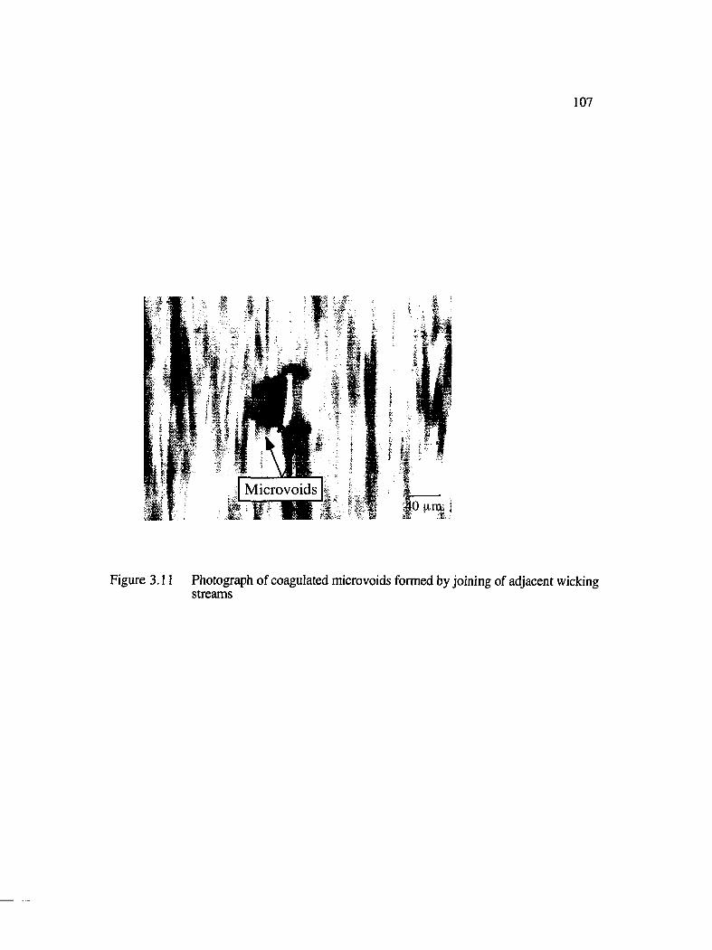
107

I I

Microvoids I10 wm. s

Figure 3.11 Photograph of coagulated microvoids formed by joining of adjacent wicking streams

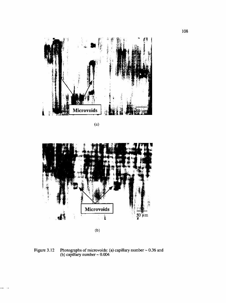
108

f

M icrovoids

(a)

M icrovoids

(b)

Figure 3.12 Photographs of microvoids: (a) capillary number ~ 0.36 and (b) capillary number ~ 0.004

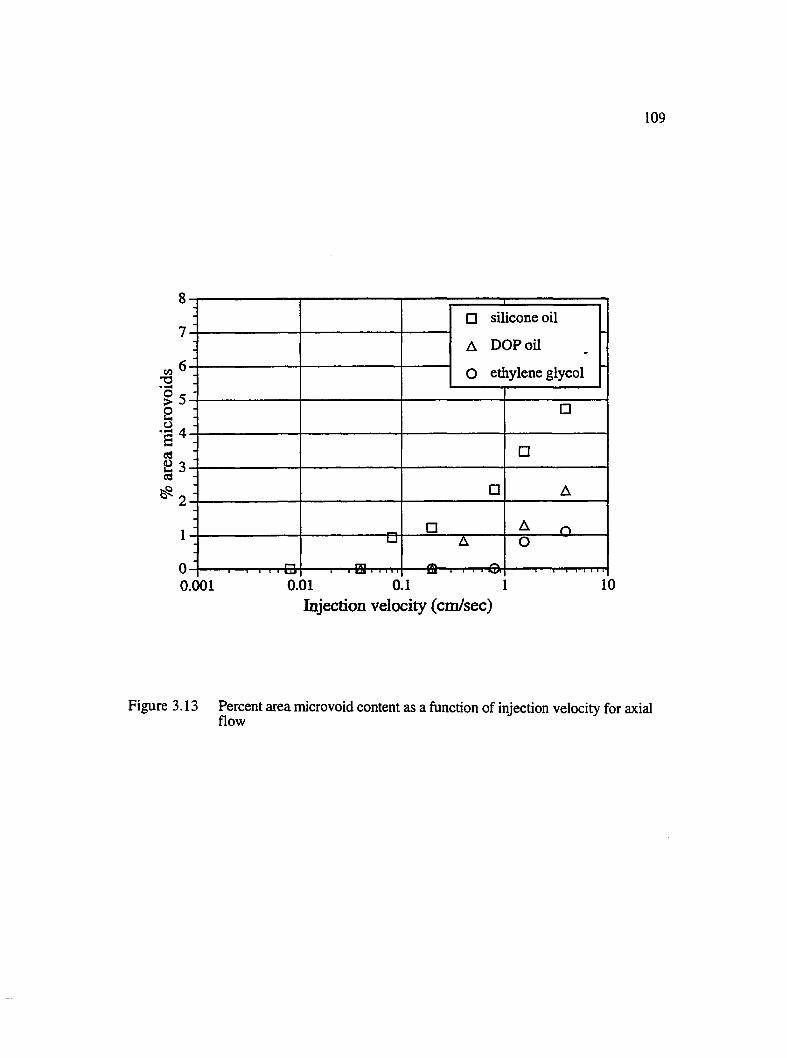
109

8q

7□ silicone oil

A DOP oil

O ethylene glycol

/

f i lCO ^ .

□

□as

^ o ■ □ A

1 □ ^ nX

A

----- Q A O

o.cK)1 0. 01 0 1 1Injection velocity (cm/sec)

Figure 3.13 Percent area microvoid content as a function of injection velocity for axial flow

110

18 .

16- □ □ macrovoids14- □12- □ ■ microvoids

c/3T3

OÜ 104e

I8-:6-i4-j

2-io J 0.0001

30.

12 204§ , | 1 5 ^

a 1 0 4cd

□

0.001-B il T-n n p

0.01- I — I I i l I I I

0.1

1816

• 1 4 ^■12 ‘I

§10864

42

0

Modified capillary number

(a)

A macrovoids

A microvoids

5 4

0 - j ------------1— I I I j h i i | r

0.0001 0.001

A A A ^ ....... .........1— I I ï n ii|0.01 0.1

4253

4 2 0 ^P

-15 •

410 §4 5

0

Modified capillary number

(b)

Figure 3.14 Percent area macro and microvoids for axial flow : (a) silicone oil, 200 cs and (b) DOP oil, (c) ethylene glycol and (d) master curves for all three liquids

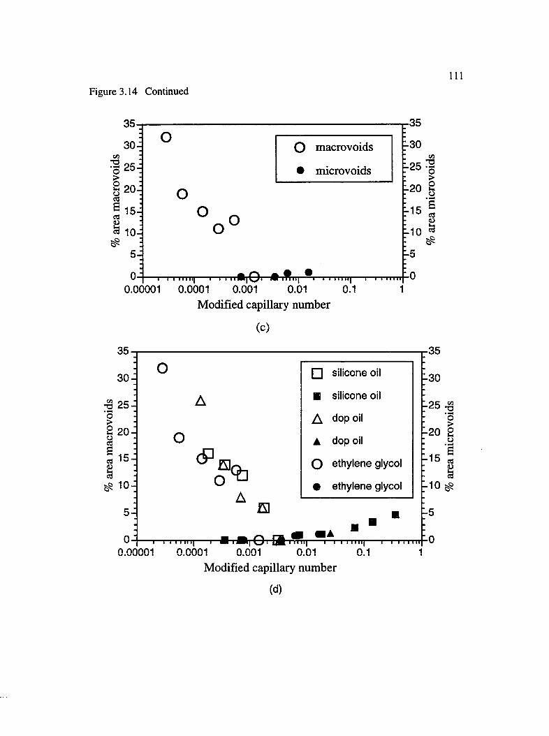
Figure 3.14 Continued111

CO1I§

353 0 :

2 5 -I

2 0 -i

1 5 :

1 0 :

5:0

0.00001

o o macrovoids

• microvoids

oo

o o

“I—I 1 111 lll0.0001 0.001 0.01

1— I I 111 l l l —

0.1T — I I M i l l

-20

35

30CA

25 1

I'i10 ^

50

Modified capillary number

(c)

35.

30 :

-Q 25: "o

§ 20-1

I i a . §

# 1 0 :

5:

0

O

d ?%

□ silicone oil

■ silicone oil

A dop oil

A dop oil

o e thy lene glycol

• e thy lene glycol

£3

I I I I M l i |

0.00001 0.00010 1 - *

0.001TTTTTf

0.011— I ' l 11 I I I ]

0.1

■35

-30

■25 ‘o

■20 2 s

I■10 ^

-5

■0

:15

Modified capillary number

(d)

1 1 2

for all the three liquids bunched together when plotted against the capillary number. The

plot also shows that both the macro and the microvoid content is nearly zero percent within

a certain range of the capillary numbers. Such plots can be used as effective tools for

designing optimal processing windows in actual production of composite parts to minimize

void content of either type.

It should be pointed out that the microvoid content reported here represents an average of

only those areas in the fiber tows with microvoids in them. Thus, the overall void content

would be lower. However, for structural parts, depending upon their end use, local void

content could be more significant than the overall void content because it is these localized

weak spots that become regions of stress concentration at the fiber / matrix interface and

provide opportunity for crack propagation under external loading. Apart from affecting the

structural integrity of the part, these localized voids can also cause optical inhomogeneity

due to the refractive index mismatch between the matrix and the reinforcing fibers. With

glass canopies of the fighter jets being replaced by fiber reinforced composite materials, a

great deal of effort is being directed towards making composite canopies as transparent as

the currently used polycarbonate sheets.

The effect of fiber wetting on optical transparency of composite samples can be seen from

Figures 3.15 (a) and (b). A grid was placed underneath the composite samples with good

and poor fiber wetting and photographs were taken under identical lighting conditions.

Although the sample with good fiber wetting (Figure 3.15 a) is not completely transparent,

the grid is more clearly visible when compared to the sample with poor wetting (Figure

3.15b).

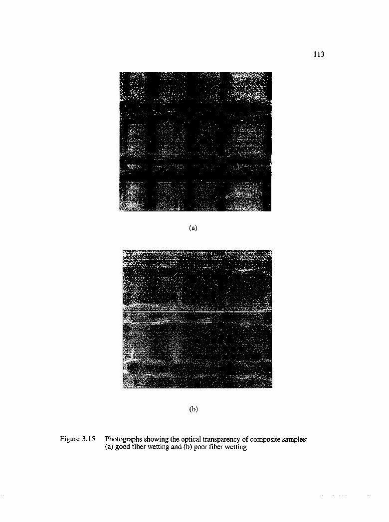
113

(a)

(b)

Figure 3.15 Photographs showing the optical transparency of composite samples; (a) good fiber wetting and (b) poor fiber wetting

114

3.4.2 Transverse Flow

Formation of microvoids during transverse flow was also studied. It was observed that for

the same capillary number, the microvoid content was higher in the case of transverse flow

as compared to the axial flow. Also, unlike the case of axial flow, microvoids were formed

even at lower flow rates (capillary number -10"^). Figure 3.16 shows that for transverse

flow, there does not exist a range of capillary number within which the void content is

zero. Both macro and microvoids were formed across a broad range of capillary numbers.

The reason for this can be explained by two types of flow mechanisms, both of which can

lead to the formation of microvoids during transverse flow. However, depending on the

injection flow rate, more microvoids were formed by one mechanism than the other. At

lower flow rates, or for capillary number upto < ~10'2, Mechanism I shown by the

schematic in Figure 3.17 was more dominant. For the sake of clarity, the sequence of

events leading to microvoid formation is shown in three separate fiber tows. In reality, this

sequence occurs in each of the fiber tows as the flow progresses through the fiber mat.

When the main flow front or the primary flow front reaches the edge of the fiber tow, the

liquid first wicks into the stitches causing a lead-lag at the flow front (Figure 3.18).

Transverse flow or cross-flow then occurs wherein the liquid present in the stitches wicks

into the fiber tows by capillary action. When these wicking streams move towards each

other from opposite directions, they either collapse into one another or trap microvoids.

Microvoids are trapped if the surrounding hydrodynamic pressure gradient is smaller than

the sum of the capillary pressure due to surface tension forces and the air pressure inside

the voids. Figure 3.19 shows the photograph of microvoids trapped in the fiber tow

during transverse flow at a capillary number of 0.0033.

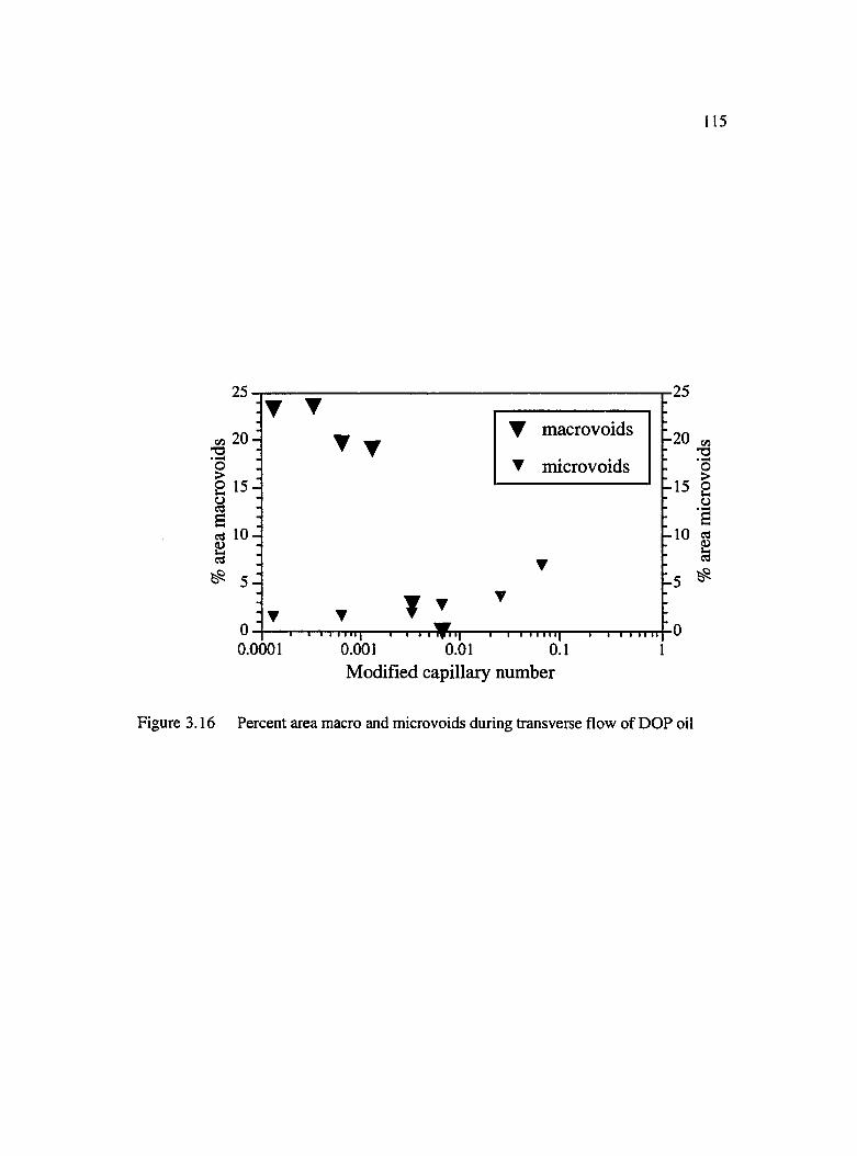
15

▼ macrovoids

▼ microvoids

10

0.0001Modified capillary number

Figure 3.16 Percent area macro and microvoids during transverse flow of DOP oil

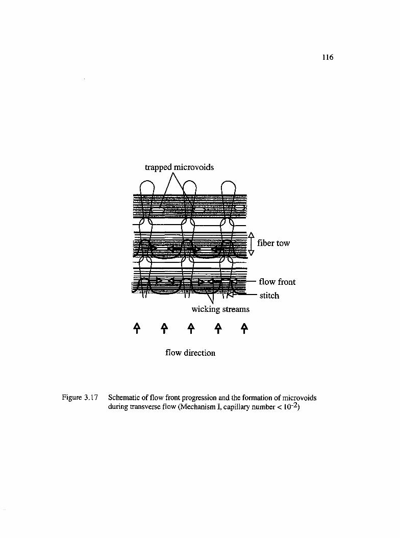
1 1 6

trapped microvoids

Îfiber tow

flow front

stitch

wicking streams

f f f f f

flow direction

Figure 3.17 Schematic of flow front progression and the formation of microvoids during transverse flow (Mechanism I, capillary number < 10'2)

117

flow front leading in the stitches

Flow direction

Figure 3.18 Photograph illustrating lead-lag at the flow front during transverse flow (Mechanism I, capillary number < 10‘2)

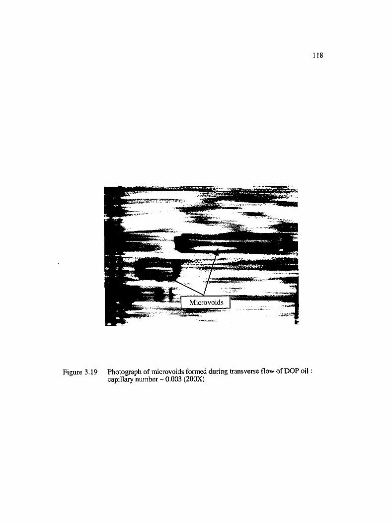
118

Microvoids

Figure 3.19 Photograph of microvoids formed during transverse flow of DOP oil capillary number ~ 0.003 (200X)

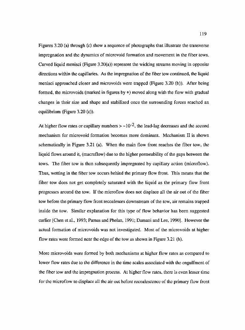
119

Figures 3.20 (a) through (c) show a sequence of photographs that illustrate the transverse

impregnation and the dynamics of microvoid formation and movement in the fiber tows.

Curved liquid menisci (Figure 3.20(a)) represent the wicking streams moving in opposite

directions within the capillaries. As the impregnation of the fiber tow continued, the liquid

menisci approached closer and microvoids were trapped (Figure 3.20 (b)). After being

formed, the microvoids (marked in figures by *) moved along with the flow with gradual

changes in their size and shape and stabilized once the surrounding forces reached an

equilibrium (Figure 3.20 (c)).

At higher flow rates or capillary numbers > ~10"2, the lead-lag decreases and the second

mechanism for microvoid formation becomes more dominant. Mechanism II is shown

schematically in Figure 3.21 (a). When the main flow front reaches the fiber tow, the

liquid flows around it, (macroflow) due to the higher permeability of the gaps between the

tows. The fiber tow is then subsequently impregnated by capillary action (microflow).

Thus, wetting in the fiber tow occurs behind the primary flow front. This means that the

fiber tow does not get completely saturated with the liquid as the primary flow front

progresses around the tow. If the microfiow does not displace all the air out of the fiber

tow before the primary flow front recoalesces downstream of the tow, air remains trapped

inside the tow. Similar explanation for this type of flow behavior has been suggested

earlier [Chen et al., 1993; Pamas and Phelan, 1991; Damani and Lee, 1990]. However the

actual formation of microvoids was not investigated. Most of the microvoids at higher

flow rates were formed near the edge of the tow as shown in Figure 3.21 (b).

More microvoids were formed by both mechanisms at higher flow rates as compared to

lower flow rates due to the difference in the time scales associated with the engulfment of

the fiber tow and the impregnation process. At higher flow rates, there is even lesser time

for the microflow to displace all the air out before recoalescence of the primary flow front

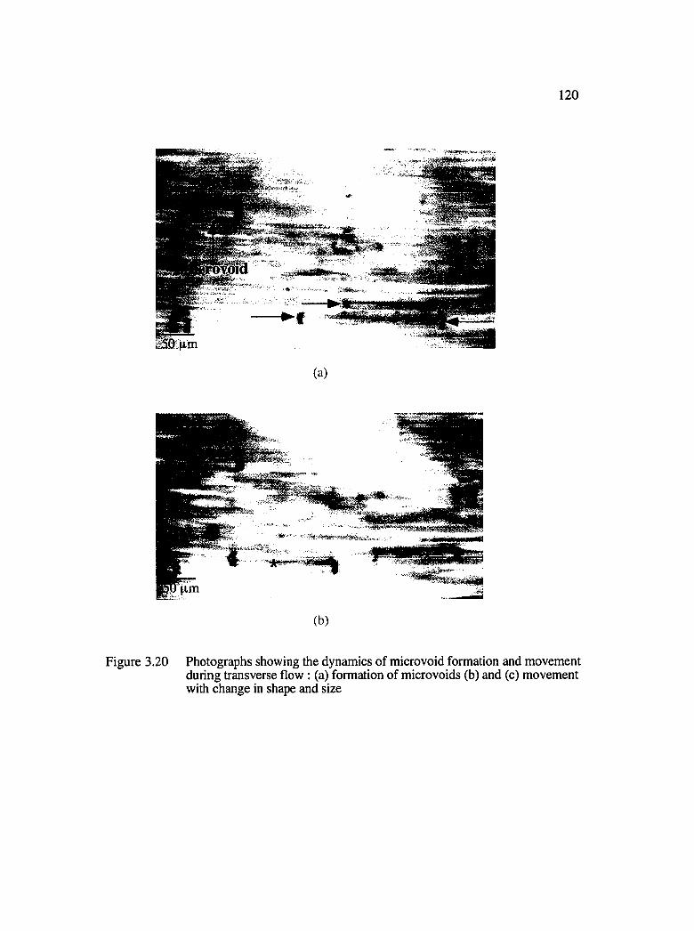
120

iSôl+im

(a)

ÈSoea*;

..

(b)

Figure 3.20 Photographs showing the dynamics of microvoid formation and movement during transverse flow : (a) formation of microvoids (b) and (c) movement with change in shape and size

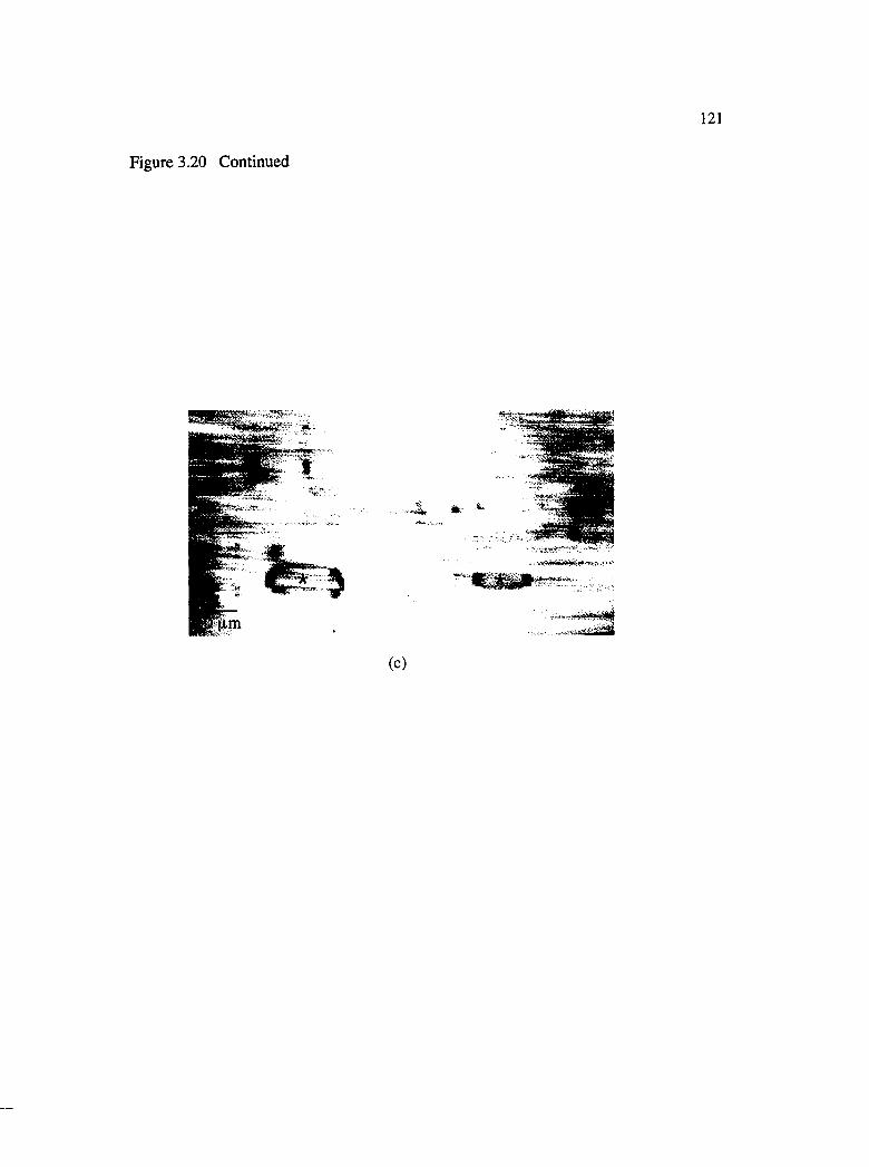
Figure 3.20 Continued

121

(c)

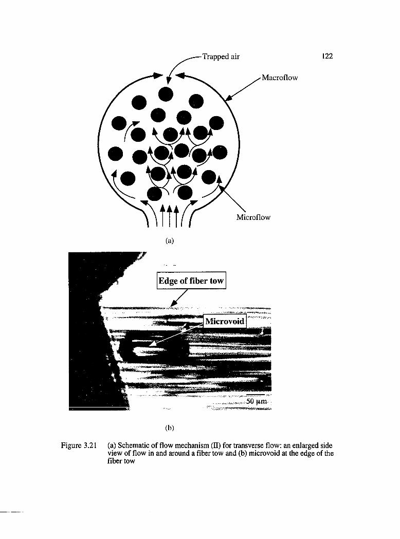
Trapped air 122

Macroflow

Microflow

(a)

Edge of fiber tow

7m m em T SIlM Microvoid

fSsStt

. 50 p,m

(b)

Figure 3.21 (a) Schematic of flow mechanism (II) for transverse flow: an enlarged sideview of flow in and around a fiber tow and (b) microvoid at the edge of the fiber tow

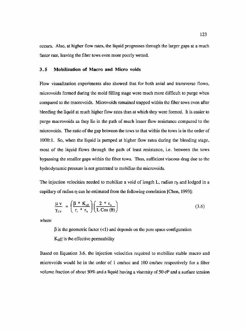
123

occurs. Also, at higher flow rates, the liquid progresses through the larger gaps at a much

faster rate, leaving the fiber tows even more poorly wetted.

3 .5 Mobilization of Macro and Micro voids

Flow visualization experiments also showed that for both axial and transverse flows,

microvoids formed during the mold filling stage were much more difficult to purge when

compared to the macrovoids. Microvoids remained trapped within the fiber tows even after

bleeding the liquid at much higher flow rates than at which they were formed. It is easier to

purge macrovoids as they lie in the path of much lesser flow resistance compared to the

microvoids. The ratio of the gap between the tows to that within the tows is in the order of

1000:1. So, when the liquid is pumped at higher flow rates during the bleeding stage,

most of the liquid flows through the path of least resistance, i.e. between the tows

bypassing the smaller gaps within the fiber tows. Thus, sufficient viscous drag due to the

hydrodynamic pressure is not generated to mobilize the microvoids.

The injection velocities needed to mobilize a void of length L, radius ry and lodged in a

capillary of radius rt can be estimated from the following correlation [Chen, 1993]:

(3.6)[tv _ r 2 * r, ^Ylv I n * r, ; l^LCos (0)^

where

P is the geometric factor (<1) and depends on the pore space configuration

Keff is the effective permeability

Based on Equation 3.6, the injection velocities required to mobilize stable macro and

microvoids would be in the order of 1 cm/sec and 100 cm/sec respectively for a fiber

volume fraction of about 50% and a liquid having a viscosity of 50 cP and a surface tension

124of 50 dynes/cm. Thus, much higher flow rates are required to completely remove the

microvoids as compared to macrovoids.

3 .6 Vacuum Assisted Liquid Injection

VALI (vacuum assisted liquid injection) was also tried in this study. It was found that both

the macro and the micro void contents were reduced considerably when the liquid was

injected into the fiber mat with the assistance of vacuum. Pulling vacuum during liquid

injection helped to increase the flow rate and so minimal macrovoids were formed.

Microvoid content was low because of reduction in pressure in the air pockets trapped

inside the fiber tows, resulting in improved tow impregnation. To obtain a part with 'zero'

voids however, requires a perfect vacuum applied uniformly in the mold cavity, and a very

good seal to prevent ;y leakage of vacuum. This may not be an easy task for a large mold

used in the actual production of composite parts. Moreover, the use of vacuum may not be

feasible when there are constraints on the cycle time (e.g. SRIM process), and in cases in

which the resin contains volatile species (e.g. UP and vinyl ester resins).

CHAPTER IV

FIBER CONSOLIDATION AND SPRINGBACK IN POWDER (TACKIFIER) COATED PREFORMS

4.1 Materials

A commercial bismaleimide (BMI) resin was used as the tackifier material, while graphite

preforms with satin weave (6k, 4HS) were used as the fiber reinforcement (Figure 4.1).

Although the exact formulation of the resin is proprietary, it is believed that the two major

components are 4, 4'-bismaleimido-diphenylmethane and 0, O' - diallyl bisphenol A

[Perry, 1993] whose structures are shown in Figure 4.2. A thermoplastic powder,

polymethyl-methacrylate (PMMA, Mw = 250, 000), was also used as a substitute for the

reactive BMI powder in some cases to decouple the effects of increase in modulus due to

reaction and tackifier location on springback of consolidated laminates.

4.2 Equipment and Experimental Procedure

4.2.1 Differential Scanning Calorimetry

TA Instruments' DSC 2910 was used to obtain the chemical reaction kinetics of BMI

tackifier. A DSC is designed on an enthalpy change method. It operates by recording the

difference in the energy required as a function of time to maintain the same programmed

temperature profile for the sample being studied and an empty reference container. Figure

4.3 shows the schematic of the set-up used. Test conditions and sample parameters are

125

Warp tows Fill tows

Gap between warp tows

Crossdirection

Machinedirection Crimps

Gap between fill tows

Figure 4.1 Schematic of 6k, 4HS woven fiber reinforcement

127

O OIl II

[ T ^ N —

a ü

4,4' - bismaleimido-diphenylmethane

CHz= CHCHj ^ CH3 / CHjCH = CH;

CH;

0 ,0 ' - diallyl Bisphenol A

Figure 4.2 Structure of two components of Bismaleimide resin based tackifier

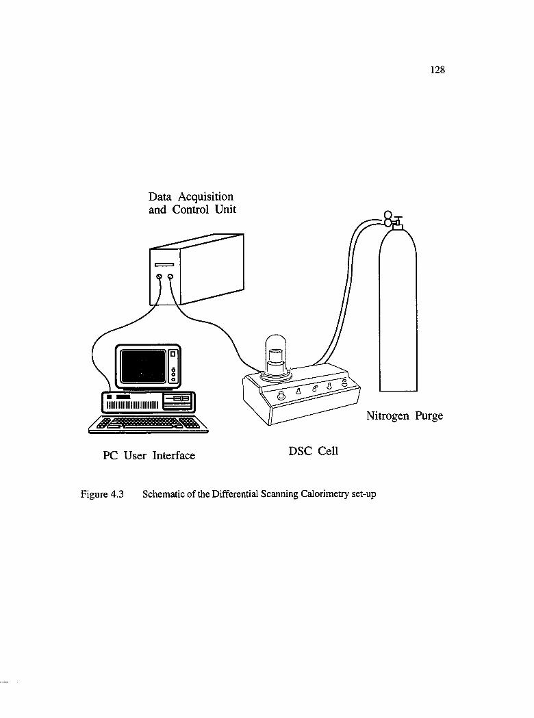
128

Data Acquisition and Control Unit

Nitrogen Purge

PC User Interface DSC Cell

Figure 4.3 Schematic of the Differential Scanning Calorimetry set-up

129

input into an interface computer before the start of each run. The computer is linked to the

data acquisition and control unit which is connected to the DSC cell. The DSC cell consists

of the sample and the reference pans placed on a cast constantan metal disc. Welded to the

base of the disc are a pair of chromel-alumel thermocouple wires. One set of wires

measures the temperature of the sample pan, while the other measures that of the reference

pan. An average temperature circuit measures and controls the temperature of the sample

and reference holders to conform to a predetermined time-temperature program. At the

same time, a temperature difference circuit compares the temperatures of the sample and

reference pans and proportions the power to the heaters under each pan so that the

temperature remains equal. When the sample undergoes a thermal transition, the power to

the heaters is adjusted to maintain thermal equilibrium between the pans, and a signal

proportional to the power difference appears as either an exothermic or an endothermie

peak [Billmeyer, 1984].

The operating temperature can be programmed either in the ramp mode (heat/cool at a fixed

rate), isothermal mode, step mode, or any combination of these. Hermetically sealed

aluminum pans capable of withstanding an internal pressure of 0.2 MPa (2 atm) were used.

These pans had an average volumetric capacity of about 10 mm^. Thus, depending on the

density of the material, the weight of the samples typically range from 5 to 20 mg.

To characterize the resin reaction kinetics, both scanning and isothermal experiments are

required. The scanning experiments are used to determine the total heat which can be

generated from a fresh sample. This is done by subjecting the sample under ramp

conditions twice. The second scan is done to get the baseline. A flat baseline indicates that

the material has reacted completely. By subtracting the baseline from the first curve, the

rate of reaction can be computed as a function of temperature. Integrating this curve over

the whole temperature range, the total heat of reaction can be obtained using Equation 4.1:

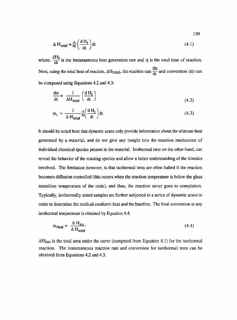
130

(4.1)

where, is the instantaneous heat generation rate and tf is the total time of reaction.

Next, using the total heat of reaction, AHtotal, the reaction rate and conversion (a) can

be computed using Equations 4.2 and 4.3:

1 r d H t ^dt AHtotai I dt J (4.2)

It should be noted here that dynamic scans only provide information about the ultimate heat

generated by a material, and do not give any insight into the reaction mechanism of

individual chemical species present in the material. Isothermal runs on the other hand, can

reveal the behavior of the reacting species and allow a better understanding of the kinetics

involved. The limitation however, is that isothermal tests are often halted if the reaction

becomes diffusion controlled (this occurs when the reaction temperature is below the glass

transition temperature of the resin), and thus, the reaction never goes to completion.

Typically, isotherm ally tested samples are further subjected to a series of dynamic scans in

order to determine the residual exotherm heat and the baseline. The final conversion at any

isothermal temperature is obtained by Equation 4.4:

“ rmal = (4.4)^ " to ta l

AHiso is the total area under the curve (computed from Equation 4.1) for the isothermal

reaction. The instantaneous reaction rate and conversion for isothermal tests can be obtained from Equations 4.2 and 4.3.

131MDSC (Modulated DSC) was used to measure the glass transition temperatures of the resin

cured under different conditions. This was done to see if the reaction pathway affected the

properties of the final network formed. MDSC offers several advantages over conventional

DSC. These include, increased sensitivity, improved resolution of closely occurring and

overlapping transitions and separation of reversing and non-reversing heat flow. In this

technique, a Liquid Nitrogen Cooling device (LNCA) is used to superimpose a sinusoidal

ripple (modulation) on a linear heating profile (underlying heating rate). The overall

heating profile thus depends on the underlying heating rate, the amplitude, and frequency

of modulation. The total heat flow comprises of two components as given by Equation 4.5

[MDSC Manual, 1993]. The reversing part being dependent on the heating rate and the

non-reversing dependent only on the absolute temperature.

^ [Cp + fR (t,T)] + fA (t,T) (4.5)

reversing non-reversingwhere

^ = heat flowf f . .= heating rate

Cp = sample heat capacity

t = time

fR (t, T) = kinetic response of any physical transition, and

fA (t, T) = kinetic response of any chemical transition

The MDSC software uses the Discrete Fourier Transformation (DPT) technique for signal

deconvolution to separate the non-reversing and reversing parts of the total heat flow. This

technique determines the measured amplitude of the sample temperature and heat flow

modulation by comparing the raw modulated data to a reference sine wave of the same

frequency. Any portion of the raw signal which follows the reference sine wave is the

132reversing part, and is "in phase" with the modulation. The remaining "out of phase"

portion constitutes the non-reversing part After determining the heat flow and temperature

amplitudes, the heat capacity is computed from Equation 4.6:

C p = -K ., *Qamp

\^am p j * ( ^ )

where

Cp = heat capacity Kcp = heat capacity constant Qamp = heat flow amplitude Tamp = temperature amplitude

Period = modulation period

Reversing heat flow is calculated by multiplying the heat capacity by the underlying heating

rate. This is then subtracted from the total heat flow to yield the non-reversing heat flow.

4.2.2 Preforming Experiments

4.2.2.1 U-Shape Bending

Figure 4.4 shows the initial distribution of the BMI powder prior to the preforming stage.

Eight layers of these tackified woven graphite fiber mats were placed between two plates

(Figure 4.5), which were then bent into a U shape and then held in that position with a

clamp. The gap between the two plates was controlled to keep the fiber volume fraction

equal to 55%. The whole bending device was then placed for different intervals of time in

a preheated oven set at a desired temperature. After a certain conversion of the tackifier

was achieved (obtained from DSC experiments), the oven was shut off and the samples

were allowed to cool down to room temperature. The preform was then taken out of the

bending device, and springback angles were measured.

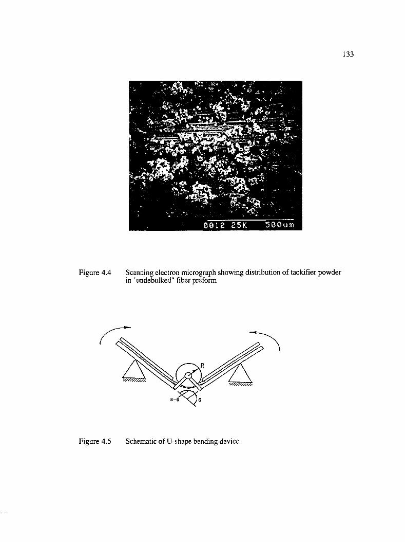
1 3 3

5 0 0 U m0 0 1 2

Figure 4.4 Scanning electron micrograph showing distribution of tackifier powder in "undebulked" fiber preform

Figure 4.5 Schematic of U-shape bending device

134

4.2.2.2 Vacuum Debulking

Vacuum debulking involves placing the fiber stack in a vacuum bag and pulling vacuum on

the sample. Prior to starting the debulking process however, certain preparatory steps are

needed. First, the desired amount of tackifier was applied to each layer. The layers were

stacked one on top of the other as illustrated schematically in Figure 4.6, and the whole

stack was then sandwiched between two Teflon release plies (Release Ease 234 TFP). The

"sandwich" was placed in the center of an aluminum plate. The temperature of the fiber

stack was controlled using a thermocouple connected to an Omega on-off controller. A

strip of jute fabric was placed as a runner from the vacuum tube to the ply stack. Tacky

tape was placed around the edges of the aluminum plate and around the vacuum tube and

thermocouple wire. The whole assembly was then sealed with an "envelope". The

envelope material was VAC-PAK HS -8171 co-extruded nylon 6 film with additives for

heat stabilization up to 205°C. To ensure a good vacuum seal, the envelope was pressed

against the Tacky Tape using a metal roller caster. The vacuum bag assembly was then

placed in a preheated oven and the vacuum hose connected to a vacuum pump. A vacuum

of 29 in Hg was pulled for different amounts of time at a constant temperature of 94°C.

The sample was then allowed to cool to room temperature, with the vacuum still being

pulled during the cooling period. After cool down, vacuum was stopped, the sample taken

out and the thickness of the fiber stack measured using vernier calipers. The samples were

left overnight and the thickness measured again. Springback was calculated by taking the

difference in sample thickness between the two readings. Thus, the values obtained and

reported here for vacuum debulking experiments reflect the long term relaxation behavior of

compressed fibers, rather than instantaneous springback.

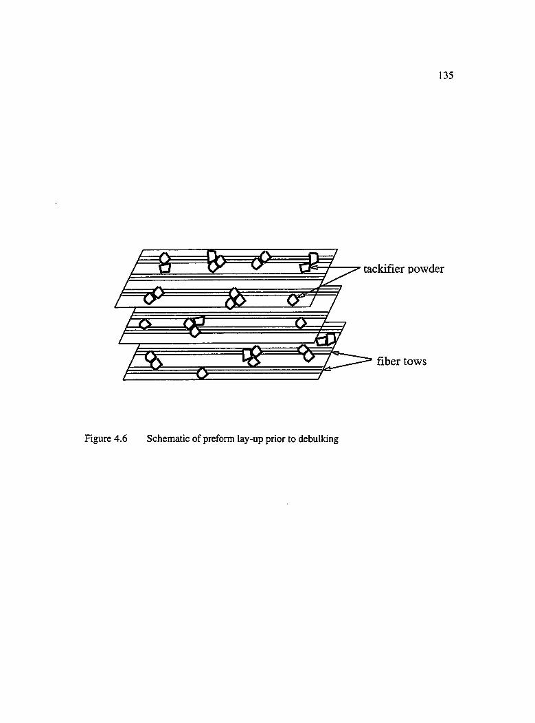
135

tackifier powder

fiber tows

Figure 4.6 Schematic of preform lay-up prior to debulking

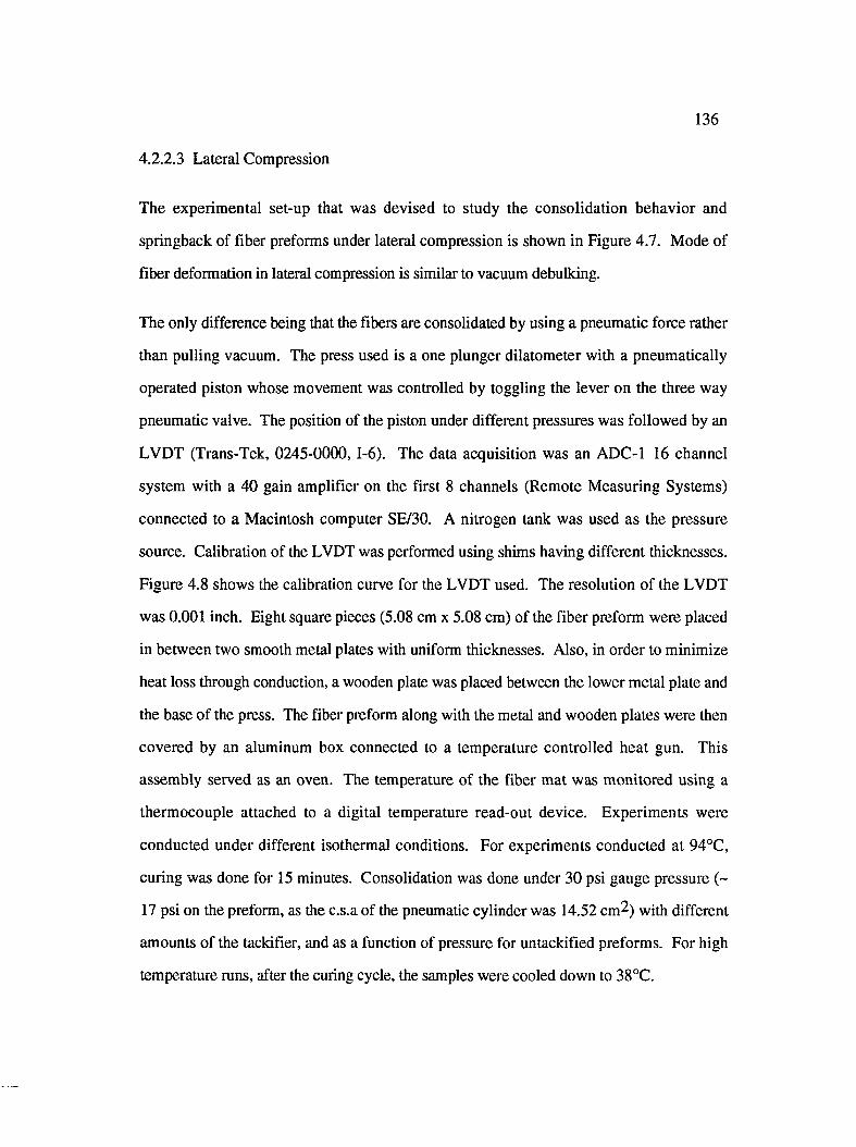
136

4.2.2.B Lateral Compression

The experimental set-up that was devised to study the consolidation behavior and

springback of fiber preforms under lateral compression is shown in Figure 4.7. Mode of

fiber deformation in lateral compression is similar to vacuum debulking.

The only difference being that the fibers are consolidated by using a pneumatic force rather

than pulling vacuum. The press used is a one plunger dilatometer with a pneumatically

operated piston whose movement was controlled by toggling the lever on the three way

pneumatic valve. The position of the piston under different pressures was followed by an

LVDT (Trans-Tek, 0245-0000, 1-6). The data acquisition was an ADC-1 16 channel

system with a 40 gain amplifier on the first 8 channels (Remote Measuring Systems)

connected to a Macintosh computer SE/30. A nitrogen tank was used as the pressure

source. Calibration of the LVDT was performed using shims having different thicknesses.

Figure 4.8 shows the calibration curve for the LVDT used. The resolution of the LVDT

was 0.001 inch. Eight square pieces (5.08 cm x 5.08 cm) of the fiber preform were placed

in between two smooth metal plates with uniform thicknesses. Also, in order to minimize

heat loss through conduction, a wooden plate was placed between the lower metal plate and

the base of the press. The fiber preform along with the metal and wooden plates were then

covered by an aluminum box connected to a temperature controlled heat gun. This

assembly served as an oven. The temperature of the fiber mat was monitored using a

thermocouple attached to a digital temperature read-out device. Experiments were

conducted under different isothermal conditions. For experiments conducted at 94°C,

curing was done for 15 minutes. Consolidation was done under 30 psi gauge pressure (~

17 psi on the preform, as the c.s.a of the pneumatic cylinder was 14.52 cm2) with different

amounts of the tackifier, and as a function of pressure for untackified preforms. For high

temperature runs, after the curing cycle, the samples were cooled down to 38°C.

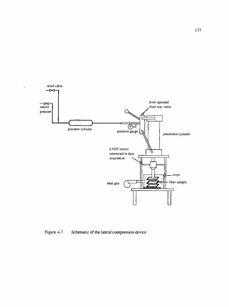
137

relief valve

lever operated three way valvesource

pressure

pressure gaugepressure cylinderpneumatic cylinder

LVDT mount connected to data acquisition N

:----- oven

fiber sampleheat gun

Figure 4.7 Schematic of the lateral compression device

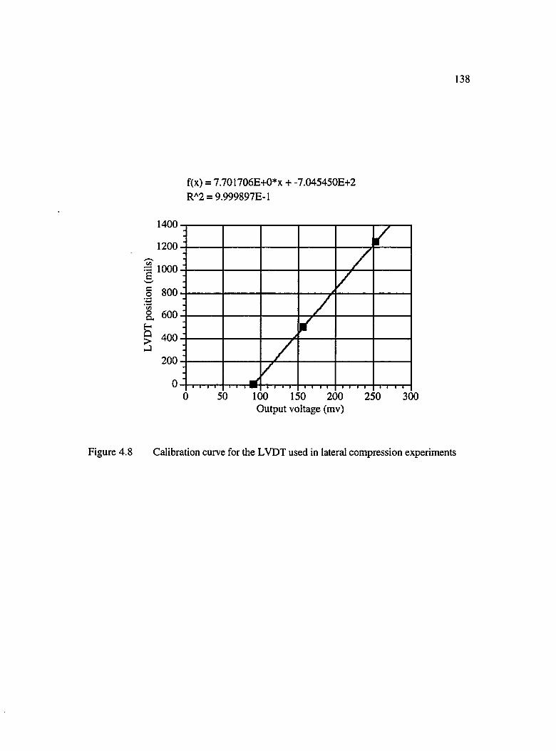
f(x) = 7.701706E+0*x + -7.045450E+2 RA2 = 9.999897E-1

1 3 8

1400

1200

= 1000

800

400

200

100 150 200 250Output voltage (mv)

300

Figure 4.8 Calibration curve for the LVDT used in lateral compression experiments

139

Springback was then obtained by taking the difference in the laminate thickness without

and with applied pressure.

4.2.3 Scanning Electron Microscopy

A Hitachi S-510 scanning electron microscope with a resolution of 70 Â , magnification

upto 150,000X, and an accelerating voltage of 25 KV was used to observe the distribution

of the tackifier powder in the fiber preform and to qualitatively describe the consolidation

and springback phenomenon. A carbon based ink was used to glue the sample onto the

holder. All samples were gold coated to provide a conductive layer. Photomicrographs

were taken using an installed Polaroid camera.

4.2.4 Rheometrics Dynamic Analyzer

A dynamic analyzer developed by Rheometrics, Inc. (a modified RDA II) was used to

monitor the changes in viscosity and viscoelastic properties G’ (elastic or storage modulus)

and G" (viscous or loss modulus) of BMI and PMMA powders as a function of

temperature and time.

The spectrometer part of the RDA consists of three subsystems: the actuator, transducer

and environmental control subsystems. The control computer synchronizes, generates, and

directs test instructions to, and processes raw data received from, all subsystems. The user

inputs commands such as type of mode, test sequence, strain rate, etc. in the test

control/analysis station (computer) which are transferred to the actuator controller through

the control computer. The actuator subsystem is comprised of electro-mechanical

components that apply a precise deformation to the test sample. The transformer "reads"

the response of the sample in mechanical energy form and converts it to electrical energy

before sending it to the control computer from where it is then transferred to the personal

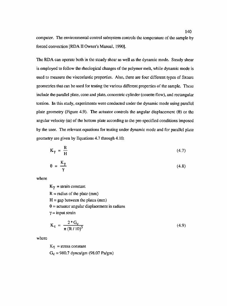
140computer. The environmental control subsystem controls the temperature of the sample by

forced convection [RDA II Owner's Manual, 1990].

The RDA can operate both in the steady shear as weU as the dynamic mode. Steady shear

is employed to foUow the rheological changes of the polymer melt, while dynamic mode is

used to measure the viscoelastic properties. Also, there are four different types of fixture

geometries that can be used for testing the various different properties of the sample. These

include the parallel plate, cone and plate, concentric cylinder (couette flow), and rectangular

torsion. In this study, experiments were conducted under the dynamic mode using parallel

plate geometry (Figure 4.9). The actuator controls the angular displacement (6) or the

angular velocity (to) of the bottom plate according to the pre-specified conditions imposed

by the user. The relevant equations for testing under dynamic mode and for parallel plate

geometry are given by Equations 4.7 through 4.10:

K , = I (4.7)

Ky0 = —^ (4.8)

Y

where

Ky = strain constant

R = radius of the plate (mm)H = gap between the plates (mm)8 = actuator angular displacement in radians y = input strain

2* G

where

Kx = stress constant

Gc = 980.7 dynes/gm (98.07 Pa/gm)

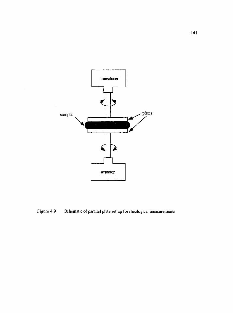
141

transducer

sample

\ iplates

actuator

Figure 4.9 Schematic of parallel plate set up for rheological measurements

142

The transducer measures the torque (M) on the upper plate which can be converted to stress

(t ), using the following equation:

X = M * Kx (4.10)

where

M = transducer torque in gm-cm

The viscoelastic properties (G' and G" ) are calculated from the values of shear stress and

strain from Equations 4.11 and 4.12 respectively.

G' = cos 5 ^ -1 (4.11)

G" = s i n ô f - l (4.12)y y )

where

S = phase angle between stress and strain

4.3 Results and Discussion

4.3.1 Characterization o f Reaction Kinetics

The scanning reaction rate profile and the isothermal conversion profiles for the BMI

tackifier used in this study are shown Figures 4.10 and 4.11 respectively. Scanning was

done from room temperature to 350°C at 5°C/min. The two reaction peaks in Figure 4.10 is

indicative of more than one reaction occurring. The first small peak at 125°C is probably

due to amine addition, while the second peak at 225°C due to BMI homopolymerization.

The isothermal conversion profiles shown in Figure 4.11 were obtained using Equation

4.4. With increasing temperatures, the reaction proceeds much faster and conversion

increases more rapidly with time. However, in all cases, the conversion profiles leveled

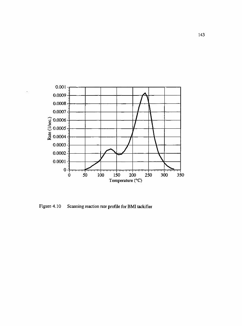
1 4 3

0.001

0.0009

0.0008

V

I 0.00044

0.00034

0.00024

0.00014

150 200 250 300Temperature (°C)

350100

Figure 4.10 Scanning reaction rate profile for BMI tackifier

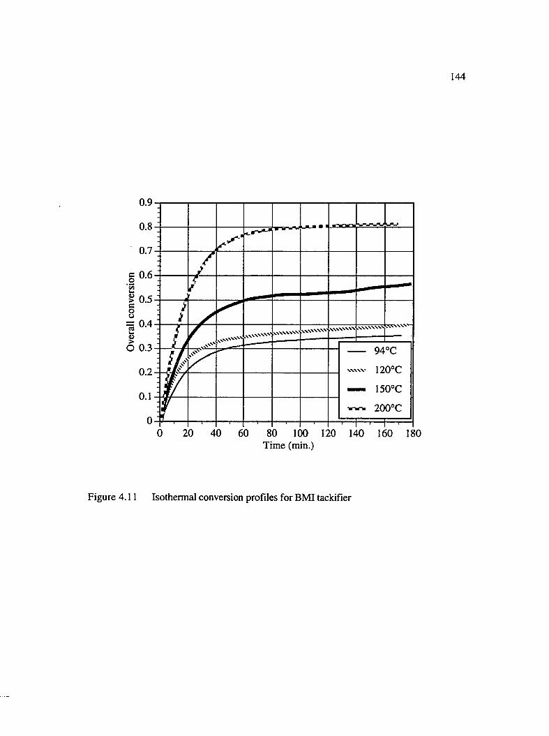
144

0.9

o2

§u& 4 : ,W N N V V V \< V .W W V '.U ^I

o 94°C

120°C

150°C

200°C

0 20 40 60 80 100 120 140 160 180Time (min.)

Figure 4.11 Isothermal conversion profiles for BMI tackifier

145

off indicating slowing down of the reaction due to diffusion controlled reaction kinetics. It

should be mentioned here that since the starting material is already cured to -35% , the

conversions reported here represent the amount reacted from the remaining unreacted 65%.

In cases where more than one reaction occur, different final products are formed depending

upon the cure history. This is also substantiated by Figure 4.12 which shows different

ultimate Tg (glass transition temperature) values for three different temperature profiles.

TPl represents scanning at 5°C/min. from room temperature to 350°C, TP2 is an isothermal

run at 130°C for 8 hours followed by an isothermal run at 220°C for 3 hours, and TP3

represents an isothermal run at 220°C for 3 hours and 20 minutes. The point of intersection

of the tangent to the lines on the heat capacity curves is usually taken as the glass transition

temperature, and is marked by an arrow in Figure 4.12.

4.3.2 Preforming Experiments

4.3.2.1 U-shape bending

Figure 4.13 shows the effect of tackifier concentration and degree of cure on the amount of

recovery or springback. As shown in the plot, at any particular concentration level,

increasing the degree of cure reduces the amount of springback. Also, for the same

conversion, increasing the tackifier concentration results in lower springback. Increasing

the concentration from 3 wt.% to 8 wt.% reduced the conversion required for no

springback, from .57 to .35. Ideally, for the tackifier to be soluble in the incoming matrix

resin during mold filling, the conversion should be less than .25 (of the tackifier) as the gel

conversion of the fresh BMI resin is around 0.5. Once the resin gels, the highly cross -

linked network formed does not permit the diffusion of significant amount of the solvent,

thereby drastically decreasing the solubility.

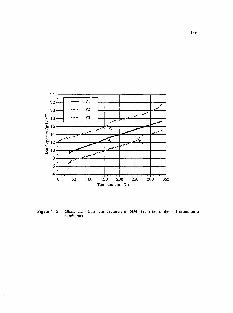
146

TPI

TP2

TP3

E 16

•n 14

12

S 10

0 50 100 150 200 250 350300Temperature (°C)

Figure 4.12 Glass transition temperatures of BMI tackifier under different cure conditions

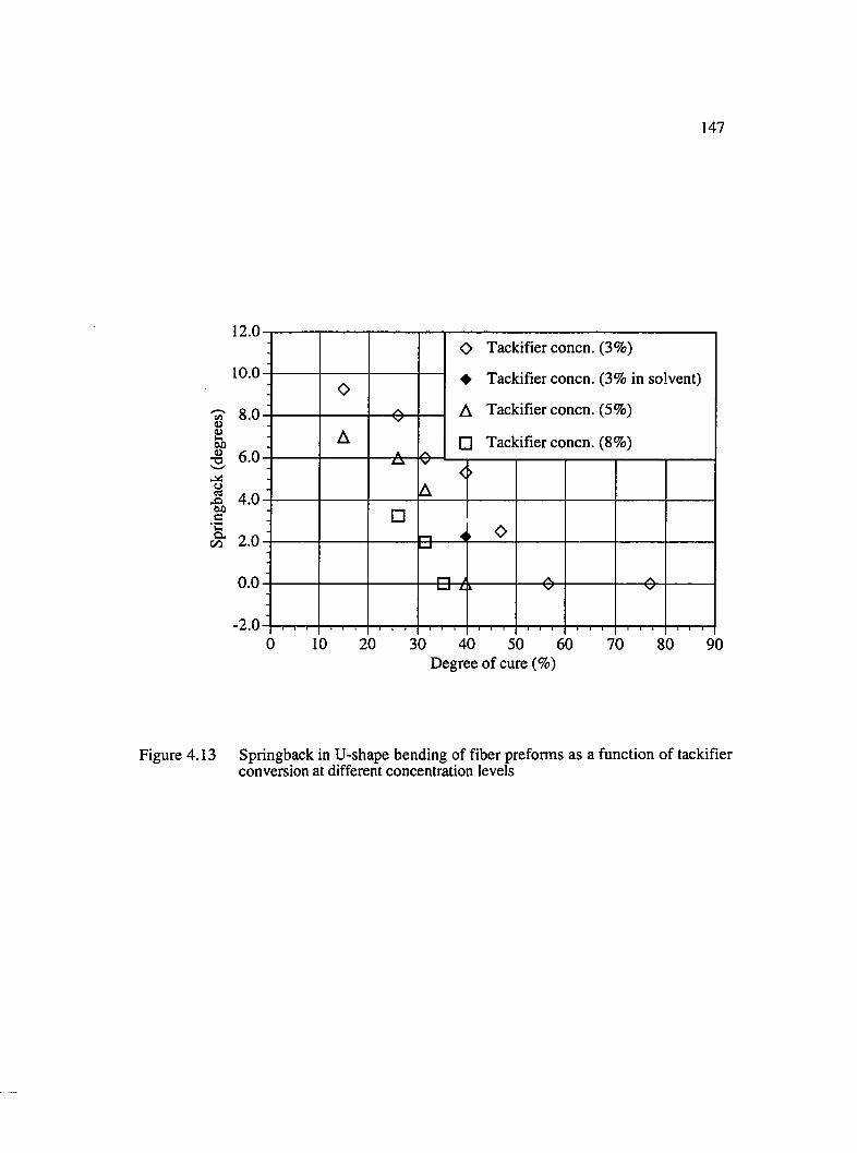
1 4 7

III

12. 0 -

10.0

8.0

6.0

4.0

2.0

0.0

- 2 . 0 -

- O Tackifier concn. (3%)

♦ Tackifier concn. (3% in solvent)

A Tackifier concn. (5%)

□ Tackifier concn. (8%)

o

A-A- A...

<A

>

- □n ^ . 0LI

n A

----1—1—1— 1 1 1 1 1 1

1—1 L k

" 1 "T" 1

V

1 1 1 1

----

1 1 10 10 20 30 40 50 60 70 80 90

Degree of cure (%)

Figure 4.13 Springback in U-shape bending of fiber preforms as a function of tackifier conversion at different concentration levels

148

This implies that an even higher tackifier concentration (> 8 wt. %) is required to achieve

zero springback at conversions less than .25. The trade-off is that at higher concentrations,

the preform becomes "boardy" and stiff, which is undesirable. Another side effect of

increasing tackifier concentration discussed in Chapter V, is reduced permeability due to

less free volume available for resin flow. Figures 4.14 (a) through (c) are photographs of

the front view of the preforms depicting springback under different cure conditions.

Figure 4.15 shows the photomicrograph of the surface of the U-shaped preform. When

compared with the initial distribution of the tackifier (Figure 4.4), this figure exhibits

substantial powder coagulation. The reason for this can be attributed to coalescence of

adjacent tackifier particles during melting and subsequent coagulation due to spreading of

liquid droplets. Coalescence of powder particles upon melting is known as sintering, and

eventually all contiguous particles flow into a deformed sphere representing a minimization

of surface and gravitational energy. The sintering phenomena and formation of deformed

droplets over a heated glass substrate are shown in Figures 4.16 (a) and (b).

An interesting result that was observed from these experiments was that when 3 wt. % of

the tackifier was applied dissolved in acetone, springback reduced from 5.3° to 2.2°. One

reason for this can be attributed to the increase in the elastic modulus of the fibers from a

more uniform coating of the tackifier on the filament surface (Figure 4.17). Springback

then decreases because the resistance to bending increases with increase in the tensile

modulus.

4.3.2.2 Vacuum Debulking

The results from vacuum debulking experiments are shown in Table 4.1. Both solvent and

powder methods were used to apply the tackifier powder on the fiber preforms.

Springback was observed to be the least when all the layers were soaked together in

1 4 9

94°C- 12 min.

(a)

94°C - 30 min.

(b)

150°C-46m in.

(c)

Figure 4.14 Photographs showing springback in U-shape bending of fiber preforms for different debulking conditions

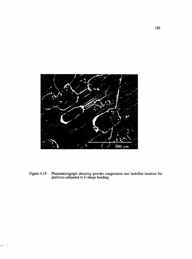
150

Figure 4.15 Photomicrograph showing powder coagulation and tackifier location for preforms subjected to U-shape bending

151

(a)

(b)

Figure 4.16 Sintering of tackifier particles : (a) upon melting and (b) coagulation into deformed droplets

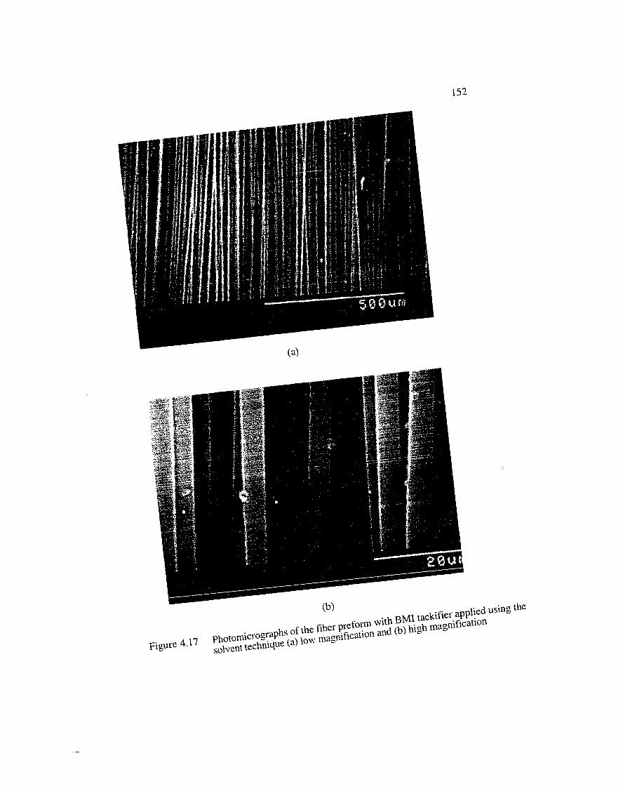
152

(b)

FiEUi 4.17 Photomicmgraphs of the fiber preform with BMI tackifier applied using thesolvent technique (a) low magnification and (b) high magnification

Table 4.1 Springback after vacuum debulking of BMI powder coated preforms

Experimentalconditions

Tackifier application technique

Thickness before debulking

(mm)

Thickness after debulking

(mm)

Thickness, overnight (mm)

8 layers

Tackifier concn. 3 wt%

-30" Hg vacuum

&94 °C, 30 min.

Solvent

individuallayers

4.087 2.109 2.526

sb = 0.417

all layers together

3.119 2.158 2.197

sb = 0.039

Powder

Run 1 3.688 2.258 2.379

sb = 0.121

Run 2 3.785 2.158 2.224

sb = 0.066 KJ\W

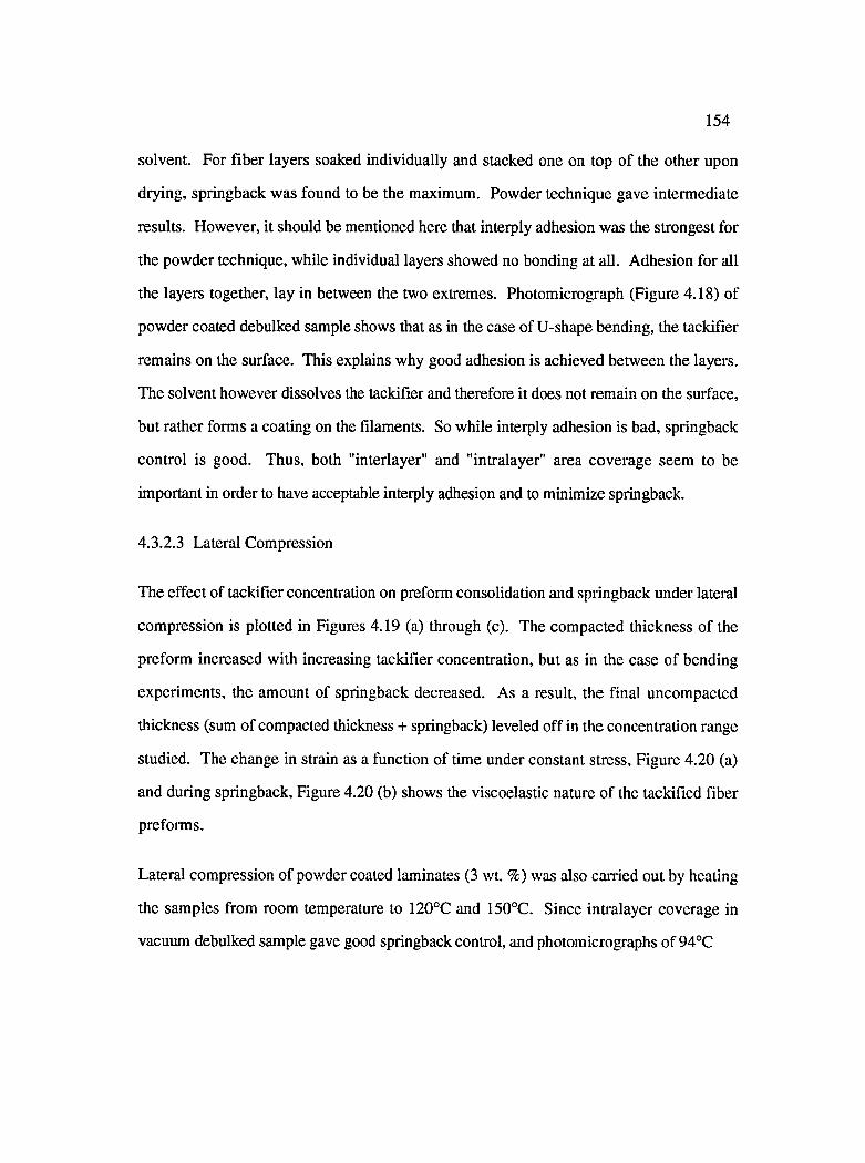
154

solvent. For fiber layers soaked individually and stacked one on top of the other upon

drying, springback was found to be the maximum. Powder technique gave intermediate

results. However, it should be mentioned here that interply adhesion was the strongest for

the powder technique, whUe individual layers showed no bonding at all. Adhesion for all

the layers together, lay in between the two extremes. Photomicrograph (Figure 4.18) of

powder coated debulked sample shows that as in the case of U-shape bending, the tackifier

remains on the surface. This explains why good adhesion is achieved between the layers.

The solvent however dissolves the tackifier and therefore it does not remain on the surface,

but rather forms a coating on the filaments. So while interply adhesion is bad, springback

control is good. Thus, both "interlayer" and "intralayer" area coverage seem to be

important in order to have acceptable interply adhesion and to minimize springback.

4.S.2.3 Lateral Compression

The effect of tackifier concentration on preform consolidation and springback under lateral

compression is plotted in Figures 4.19 (a) through (c). The compacted thickness of the

preform increased with increasing tackifier concentration, but as in the case of bending

experiments, the amount of springback decreased. As a result, the final uncompacted

thickness (sum of compacted thickness + springback) leveled off in the concentration range

studied. The change in strain as a function of time under constant stress. Figure 4.20 (a)

and during springback. Figure 4.20 (b) shows the viscoelastic nature of the tackified fiber

preforms.

Lateral compression of powder coated laminates (3 wt. %) was also carried out by heating

the samples from room temperature to 120°C and 150°C. Since intralayer coverage in

vacuum debulked sample gave good springback control, and photomicrographs of 94°C

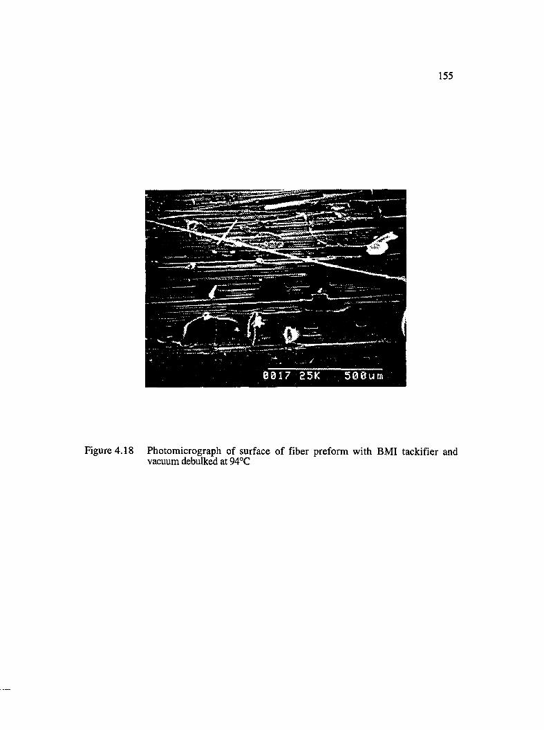
155

Figure 4.18 Photomicrograph of surface of fiber preform with BMI tackifier and vacuum debulked at 94°C

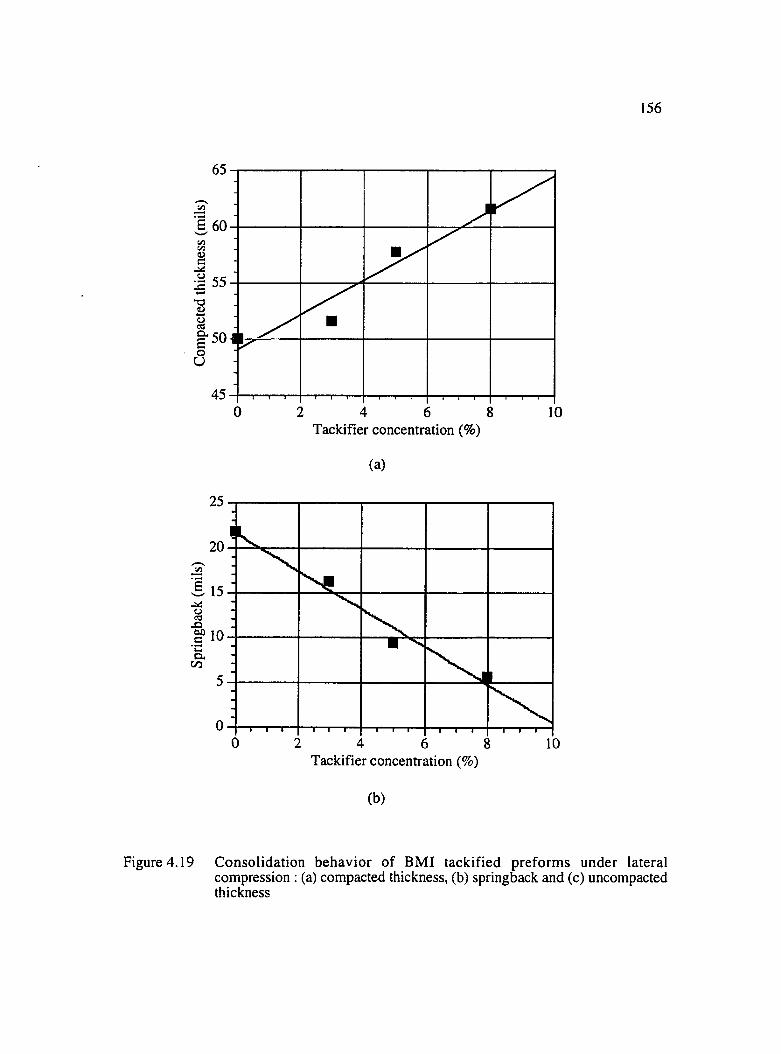
1 5 6

§ 6 0(/)

Tackifier concentration (%)

(a)

25

20

15

5

0

Tackifier concentration (%)

(b)

Figure 4.19 Consolidation behavior of BMI tackified preforms under lateral compression : (a) compacted thickness, (b) springback and (c) uncompacted thickness

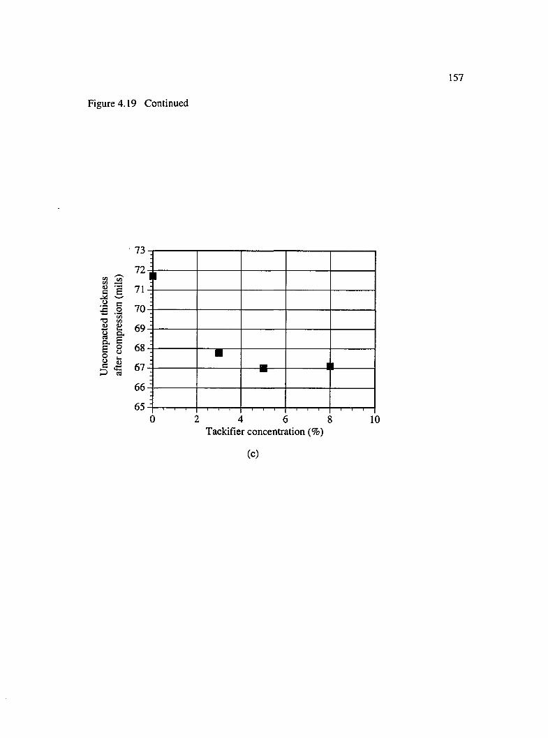
157

Figure 4.19 Continued

1I•5 I

II

73 n

79 -!

71 '1

70^

68^

67^H

1I■

65^c) : () 1(

Tackifier concentration (%)

(c)

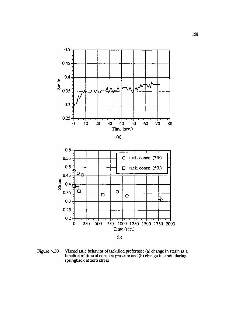
158

0.5

0.45 H

0.4-^IüCO

0.25-0 10 20 30 40 50 60 70 80

Time (sec.)

(a)

c

I00

0.6

0.55

0.5

0.45

0.4

0.35

0.3

0.25

0.2

1 1 1 O tack, concn. (3%)

:u lacK. con cn. '0)

------ W-

ou 0=b

:

0 250 500 750 1000 1250 1500 1750 2000Time (sec.)

(b)

Figure 4.20 Viscoelastic behavior of tackified preforms : (a) change in strain as a function of time at constant pressure and (b) change in strain during springback at zero stress

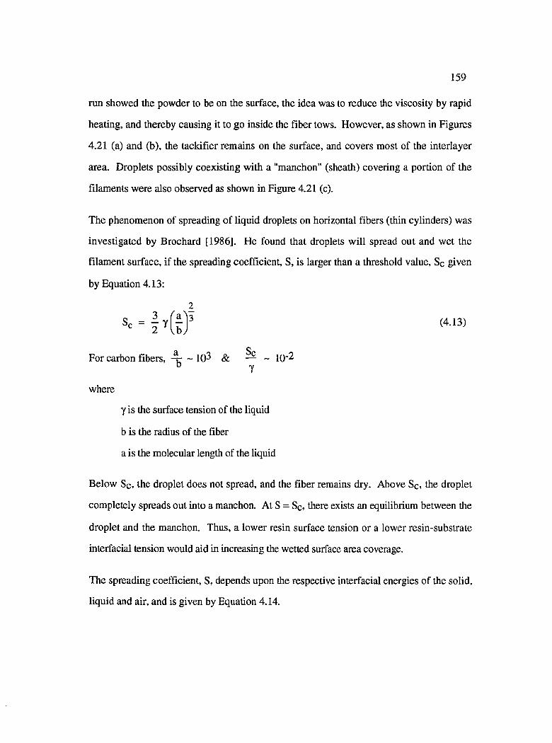
159

run showed the powder to be on the surface, the idea was to reduce the viscosity by rapid

heating, and thereby causing it to go inside the fiber tows. However, as shown in Figures

4.21 (a) and (b), the tackifier remains on the surface, and covers most of the interlayer

area. Droplets possibly coexisting with a "manchon" (sheath) covering a portion of the

filaments were also observed as shown in Figure 4.21 (c).

The phenomenon of spreading of liquid droplets on horizontal fibers (thin cylinders) was

investigated by Brochard [1986]. He found that droplets will spread out and wet the

filament surface, if the spreading coefficient, S, is larger than a threshold value. Sc given

by Equation 4.13:

S , = | y ( f ) ï (4.13)

For carbon fibers, - 10^ & — ~ 10‘2D y

where

Y is the surface tension of the liquid

b is the radius of the fiber

a is the molecular length of the liquid

Below Sc, the droplet does not spread, and the fiber remains dry. Above Sc, the droplet

completely spreads out into a manchon. At S = Sc, there exists an equilibrium between the

droplet and the manchon. Thus, a lower resin surface tension or a lower resin-substrate

interfacial tension would aid in increasing the wetted surface area coverage.

The spreading coefficient, S, depends upon the respective interfacial energies of the solid,

liquid and air, and is given by Equation 4.14.

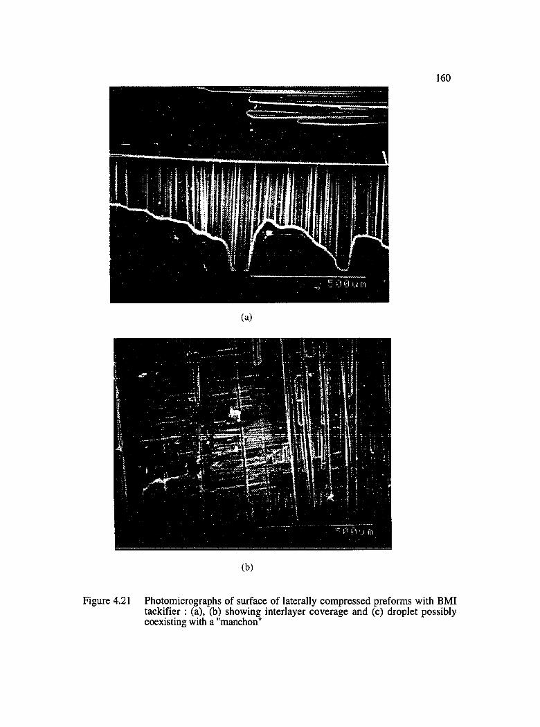
160

(a)

(b)

Figure 4.21 Photomicrographs of surface of laterally compressed preforms with BMI tackifier : (a), (b) showing interlayer coverage and (c) droplet possibly coexisting with a "manchon"

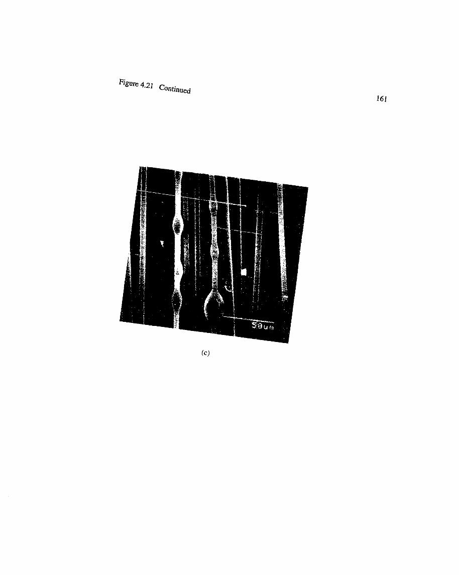
"'*“'* ‘'•21 C o n t i n u e

161

(c)

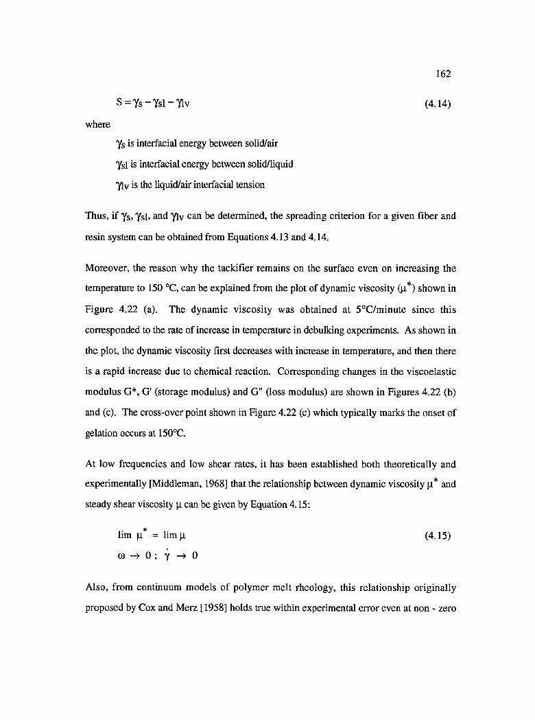
162

S = Ys - Ysl “ Ylv (4.14)

where

Ys is interfacial energy between solid/air

Ysl is interfacial energy between sobd/Uquid

Ylv is the bquid/air interfacial tension

Thus, if Ys, Ysl, and Ylv can be determined, the spreading criterion for a given fiber and

resin system can be obtained from Equations 4.13 and 4.14.

Moreover, the reason why the tackifier remains on the surface even on increasing the

temperature to 150 °C, can be explained from the plot of dynamic viscosity (|i*) shown in

Figure 4.22 (a). The dynamic viscosity was obtained at 5°C/minute since this

corresponded to the rate of increase in temperature in debulking experiments. As shown in

the plot, the dynamic viscosity first decreases with increase in temperature, and then there

is a rapid increase due to chemical reaction. Corresponding changes in the viscoelastic

modulus G*, O' (storage modulus) and G" (loss modulus) are shown in Figures 4.22 (b)

and (c). The cross-over point shown in Figure 4.22 (c) which typically marks the onset of

gelation occurs at 150°C.

At low frequencies and low shear rates, it has been established both theoretically and

experimentally [Middleman, 1968] that the relationship between dynamic viscosity |i* and

steady shear viscosity |l can be given by Equation 4.15:

lim |i* = limp. (4.15)

CO 0 ; y 0

Also, from continuum models of polymer melt rheology, this relationship originally

proposed by Cox and Merz [1958] holds true within experimental error even at non - zero

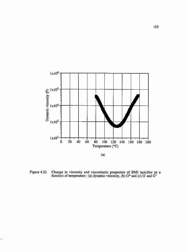
163

1x10

Temperature (°C)

(a)

Figure 4.22 Change in viscosity and viscoelastic properties of BMI tackifier as a function of temperature : (a) dynamic viscosity, (b) G* and (c) O' and G"

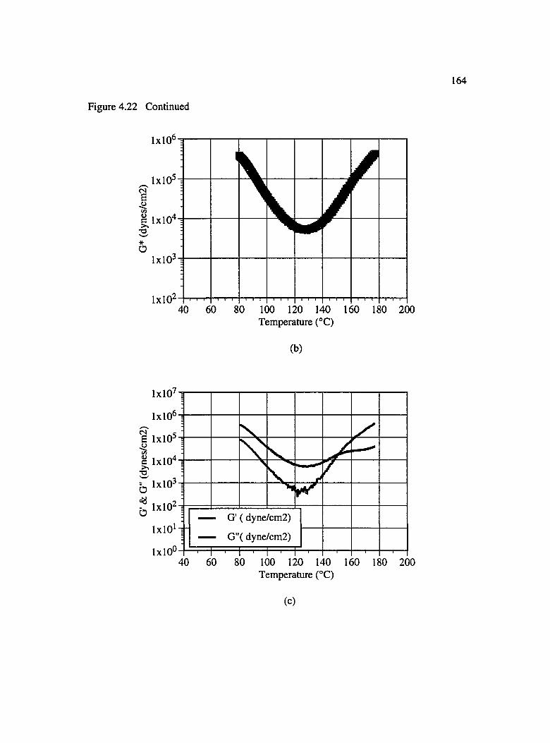
Figure 4.22 Continued

164

c IxlO'^

80 100 120 140 160 180 200Temperature (°C)

(b)

1x10'

c 1x10'

1x10G' ( dyne/cm2)

G"( dyne/cm2)1x10

1x10'

Temperature (°C)

(c)

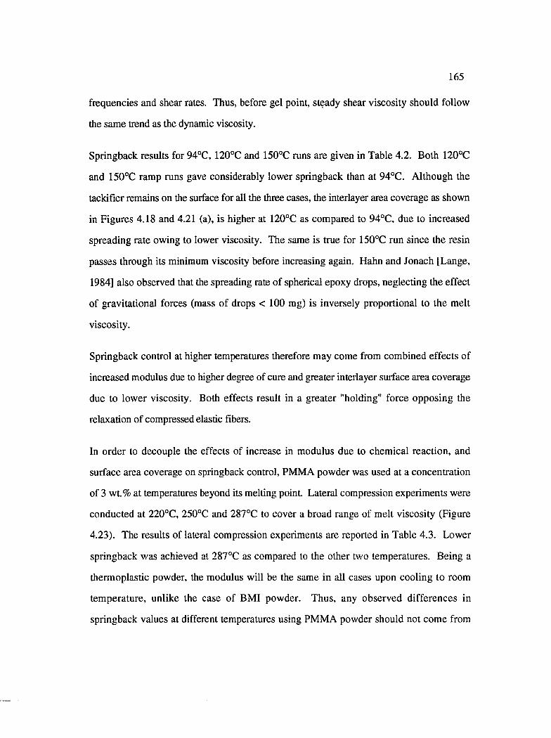
165

frequencies and shear rates. Thus, before gel point, steady shear viscosity should follow

the same trend as the dynamic viscosity.

Springback results for 94°C, 120°C and 150°C runs are given in Table 4.2. Both 120°C

and 150°C ramp runs gave considerably lower springback than at 94°C. Although the

tackifier remains on the surface for all the three cases, the interlayer area coverage as shown

in Figures 4.18 and 4.21 (a), is higher at 120°C as compared to 94°C, due to increased

spreading rate owing to lower viscosity. The same is true for 150°C run since the resin

passes through its minimum viscosity before increasing again. Hahn and Jonach [Lange,

1984] also observed that the spreading rate of spherical epoxy drops, neglecting the effect

of gravitational forces (mass of drops < 1 0 0 mg) is inversely proportional to the melt

viscosity.

Springback control at higher temperatures therefore may come from combined effects of

increased modulus due to higher degree of cure and greater interlayer surface area coverage

due to lower viscosity. Both effects result in a greater "holding" force opposing the

relaxation of compressed elastic fibers.

In order to decouple the effects of increase in modulus due to chemical reaction, and

surface area coverage on springback control, PMMA powder was used at a concentration

of 3 wt.% at temperatures beyond its melting point. Lateral compression experiments were

conducted at 220°C, 250°C and 287°C to cover a broad range of melt viscosity (Figure

4.23). The results of lateral compression experiments are reported in Table 4.3. Lower

springback was achieved at 287°C as compared to the other two temperatures. Being a

thermoplastic powder, the modulus will be the same in all cases upon cooling to room

temperature, unlike the case of BMI powder. Thus, any observed differences in

springback values at different temperatures using PMMA powder should not come from

166

Table 4.2 Springback after lateral compression of BMI powder coated preforms

DebulkingTemp.(°C)

PowderLocation

Springback(mm)

94 w/o pulse Interlayer 0.38-0.41

ramp to 120 Mostly Interlayer 0.16-0.23

ramp to 150 Mostly Interlayer 0.15-0.25

94 w. pulse

(40psi.)

Interlayer 0.35-0.37

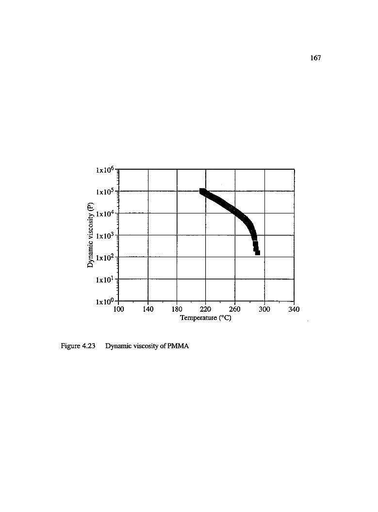
167

>. 1x10^

I 1x103

e ixiQZ

180 220 260 Temperature (°C)

340

Figure 4.23 Dynamic viscosity of PMMA

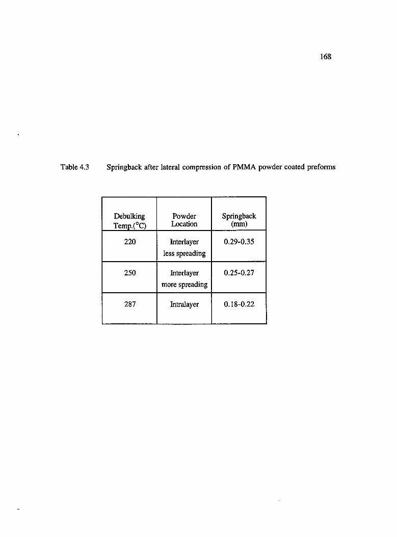
168

Table 4.3 Springback after lateral compression of PMMA powder coated preforms

DebulkingTemp.(°C)

PowderLocation

Springback(mm)

220 Interlayer less spreading

0.29-0.35

250 Interlayer more spreading

0.25-0.27

287 Intralayer 0.18-0.22

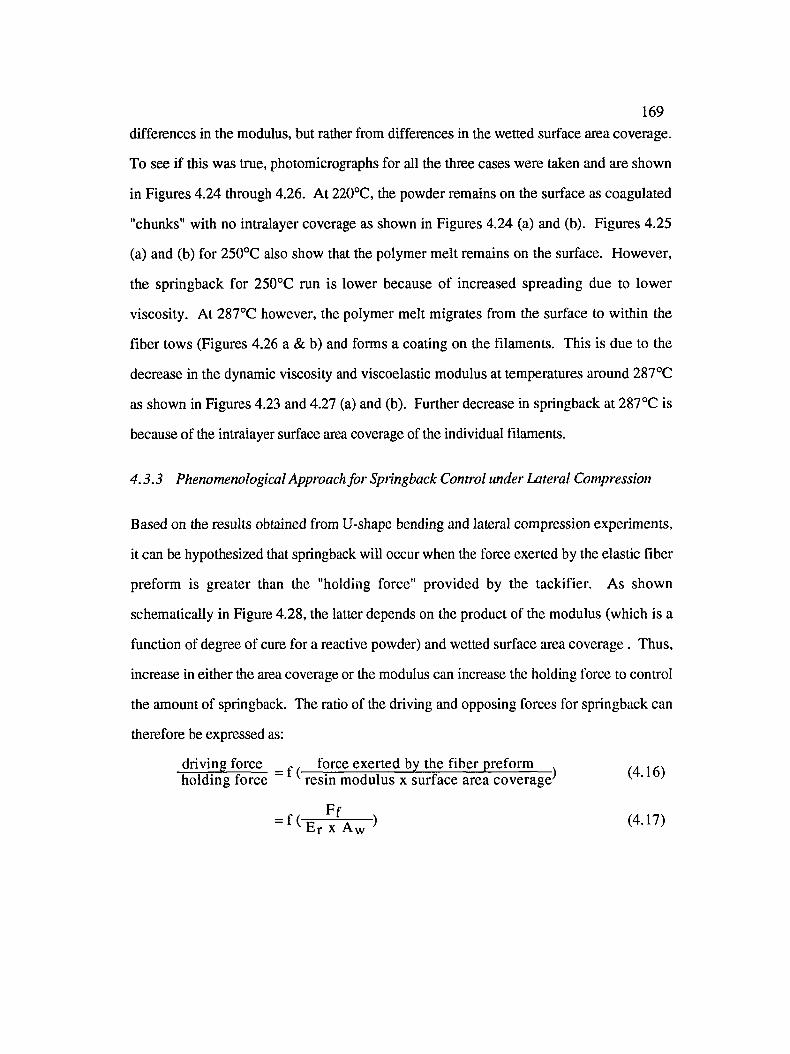
169differences in the modulus, but rather from differences in the wetted surface area coverage.

To see if this was true, photomicrographs for all the three cases were taken and are shown

in Figures 4.24 through 4.26. At 220°C, the powder remains on the surface as coagulated

"chunks" with no intralayer coverage as shown in Figures 4.24 (a) and (b). Figures 4.25

(a) and (b) for 250°C also show that the polymer melt remains on the surface. However,

the springback for 250°C run is lower because of increased spreading due to lower

viscosity. At 287°C however, the polymer melt migrates from the surface to within the

fiber tows (Figures 4.26 a & b) and forms a coating on the filaments. This is due to the

decrease in the dynamic viscosity and viscoelastic modulus at temperatures around 287°C

as shown in Figures 4.23 and 4.27 (a) and (b). Further decrease in springback at 287°C is

because of the intraiayer surface area coverage of the individual filaments.

4.3.3 Phenomenological Approach for Springback Control under Lateral Compression

Based on the results obtained from U-shape bending and lateral compression experiments,

it can be hypothesized that springback will occur when the force exerted by the elastic fiber

preform is greater than the "holding force" provided by the tackifier. As shown

schematically in Figure 4.28, the latter depends on the product of the modulus (which is a

function of degree of cure for a reactive powder) and wetted surface area coverage. Thus,

increase in either the area coverage or the modulus can increase the holding force to contr ol

the amount of springback. The ratio of the driving and opposing forces for springback can

therefore be expressed as:

driving force _ , force exerted by the fiber preform .. .holding force “ resin modulus x surface area coverage^ ^

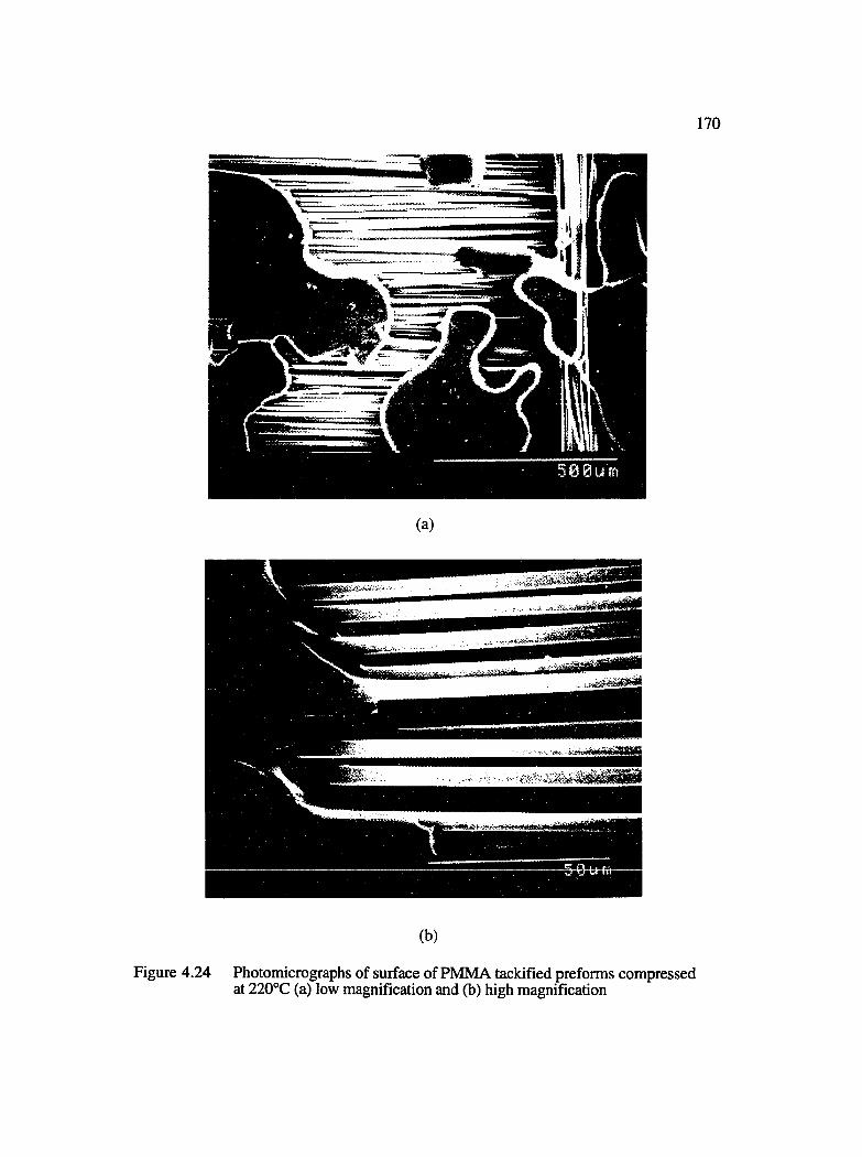
170

masm

(a)

5 0 0 urn

(b)

Figure 4.24 Photomicrographs of surface of PMMA tackified preforms compressed at 220°C (a) low magnification and (b) high magnification

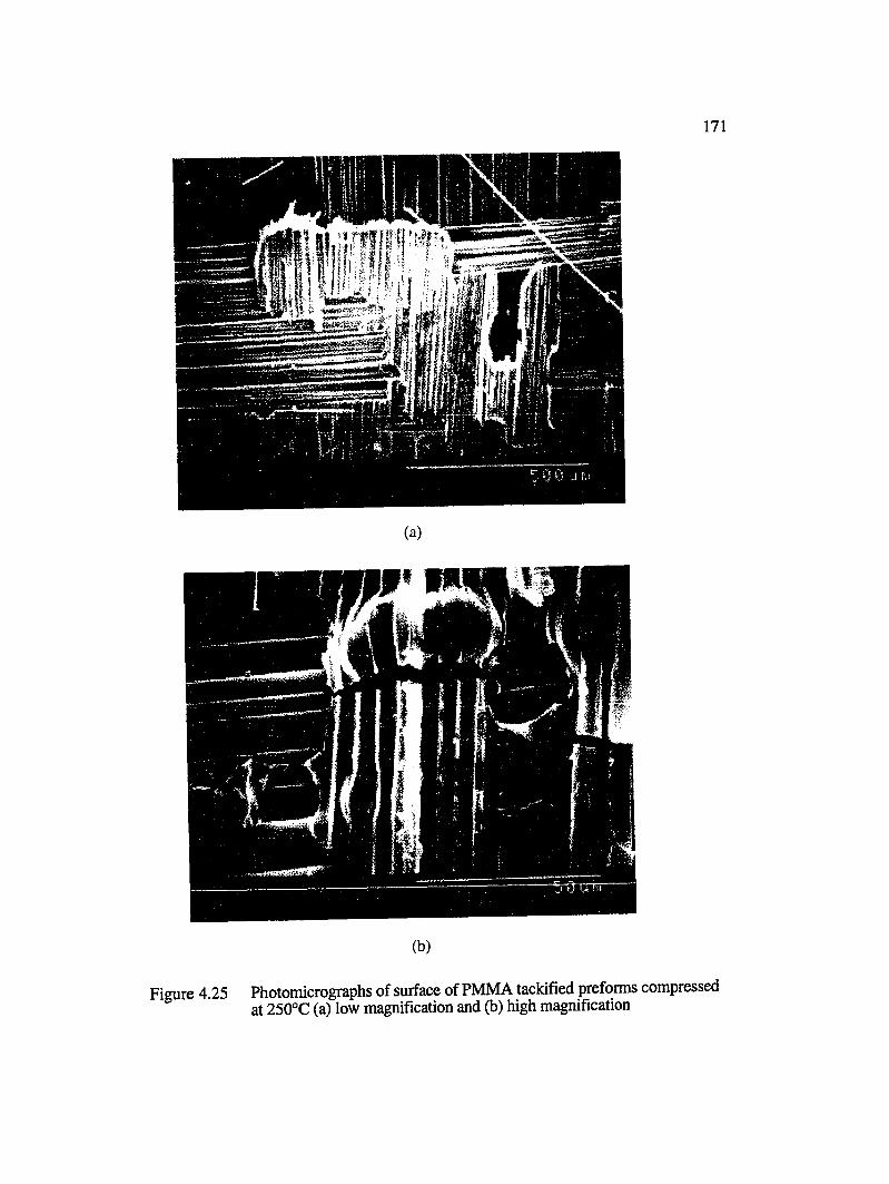
171

(a)

1

(b)

Figure 4.25 Photomicrographs of surface of PMMA tackified preforms compressed at 250°C (a) low magnification and (b) high magnification

172

I «nwm

i

(a)

(b)

Figure 4.26 Photomicrographs of surface of PMMA tackified preforms compressed at ~287°C (a) low magnification and (b) high magnification

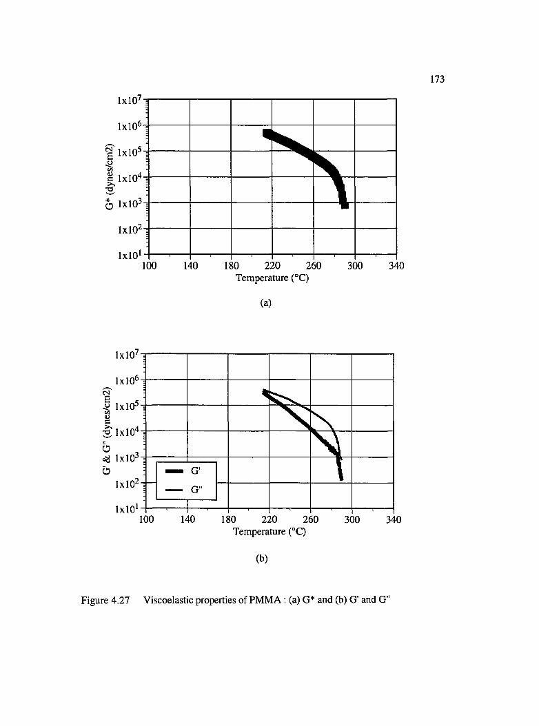
173

1x10

<N

C 1 x 1 0 ' 30 1 x 1 0

1 x 1 0220

Temperature (°C)100 180 260 340300

(a)

1 x 1 0 *100 140 220

Temperature (°C)180 260 300

(b)

Figure 4.27 Viscoelastic properties of PMMA : (a) G* and (b) O' and G"

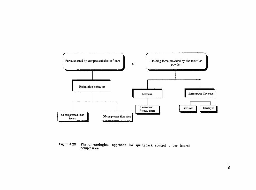
Force exerted by compressed elastic fibers Holding force provided by the tackifier powder

Relaxation behavior

SurfaceArea CoverageModulus

Conversion f(temp., lime)

Interlayer Intralayer

Of compressed fiber layers Of compressed fiber tows

Figure 4.28 Phenomenological approach for springback control under lateral compression

A

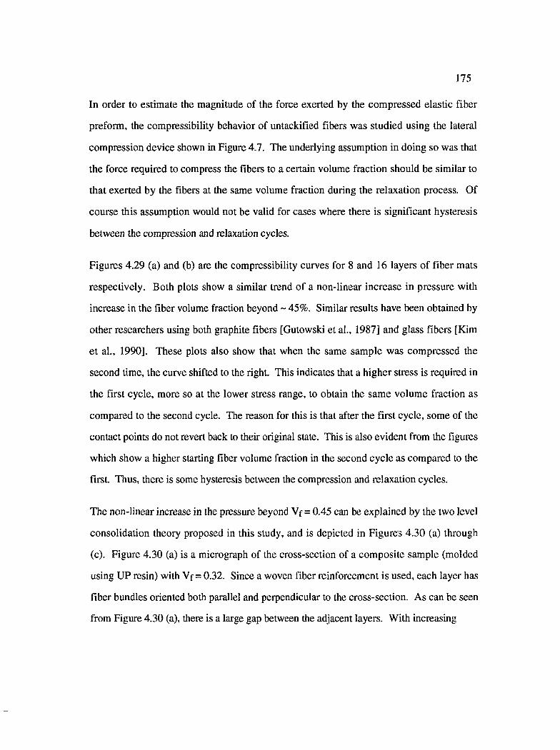
175

In order to estimate the magnitude of the force exerted by the compressed elastic fiber

preform, the compressibility behavior of untackified fibers was studied using the lateral

compression device shown in Figure 4.7. The underlying assumption in doing so was that

the force required to compress the fibers to a certain volume fraction should be similar to

that exerted by the fibers at the same volume fraction during the relaxation process. Of

course this assumption would not be valid for cases where there is significant hysteresis

between the compression and relaxation cycles.

Figures 4.29 (a) and (b) are the compressibility curves for 8 and 16 layers of fiber mats

respectively. Both plots show a similar trend of a non-linear increase in pressure with

increase in the fiber volume fraction beyond ~ 45%. Similar results have been obtained by

other researchers using both graphite fibers [Gutowski et al., 1987] and glass fibers [Kim

et al., 1990]. These plots also show that when the same sample was compressed the

second time, the curve shifted to the right. This indicates that a higher stress is required in

the first cycle, more so at the lower stress range, to obtain the same volume fraction as

compared to the second cycle. The reason for this is that after the first cycle, some of the

contact points do not revert back to their original state. This is also evident from the figures

which show a higher starting fiber volume fraction in the second cycle as compared to the

first. Thus, there is some hysteresis between the compression and relaxation cycles.

The non-linear increase in the pressure beyond Vf = 0.45 can be explained by the two level

consolidation theory proposed in this study, and is depicted in Figures 4.30 (a) through

(c). Figure 4.30 (a) is a micrograph of the cross-section of a composite sample (molded

using UP resin) with Vf = 0.32. Since a woven fiber reinforcement is used, each layer has

fiber bundles oriented both parallel and perpendicular to the cross-section. As can be seen

from Figure 4.30 (a), there is a large gap between the adjacent layers. With increasing

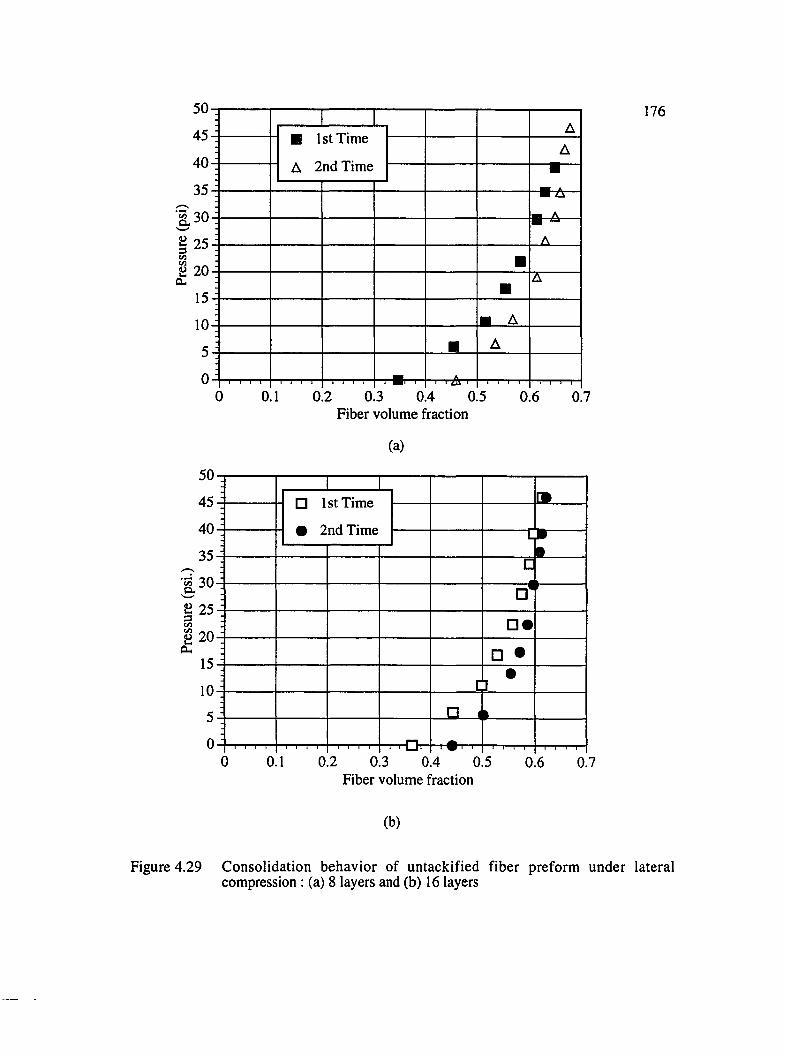
50

45-

40

35

U s o ­

il) 25-

20

15-

10 -

50

45-

40-

35-

•S30-

I 25-

S 20-

15-

10 -

5-

0 -

■ 1st Time

A 2nd Time

rA-0.1 0.2 0.3 0.4 0.5

Fiber volume fraction

(a)

0.6

I□ 1st Time

• 2nd Time

I I 1 I I I I I

[B

dr

□ •

0.1 0.2 0.3 0.4 0.5Fiber volume fraction

0.6

0.7

0.7

1 7 6

(b)

Figure 4.29 Consolidation behavior of untackified fiber preform under lateral compression : (a) 8 layers and (b) 16 layers

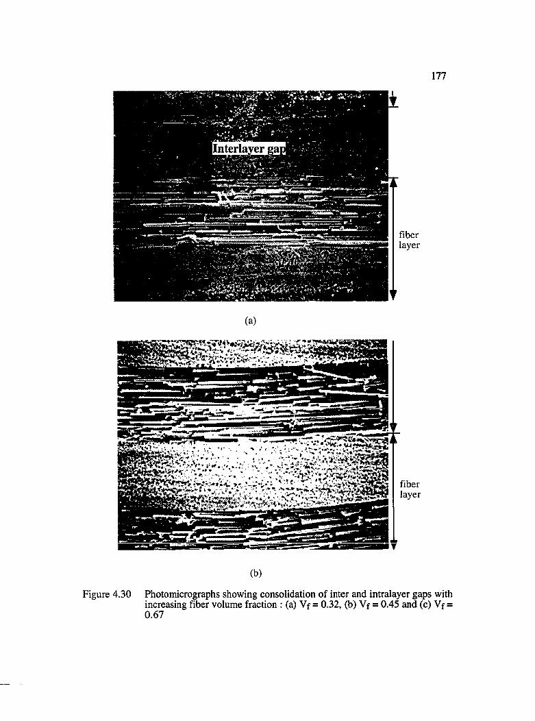
177

In terlaver ea

gijZ mZ wrr.

(a)

(b)

Figure 4.30 Photomicrographs showing consolidation of inter and intralayer gaps with increasing fiber volume fraction : (a) Vf = 0.32, (b) Vf = 0.45 and (c) Vf = 0.67

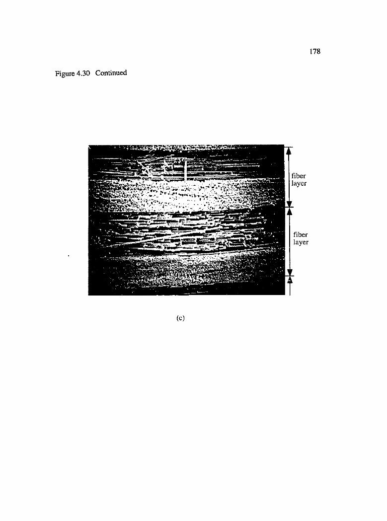
178

Figure 4.30 Continued

i f l B . H é

a

(c)

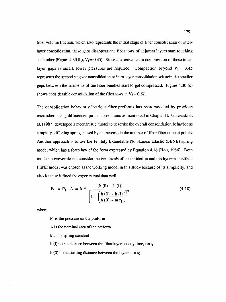
179

fiber volume fraction, which also represents the initial stage of fiber consolidation or inter­

layer consolidation, these gaps disappear and fiber tows of adjacent layers start touching

each other (Figure 4.30 (b), Vf = 0.45). Since the resistance to compression of these inter­

layer gaps is small, lower pressures are required. Compaction beyond V f= 0.45

represents the second stage of consolidation or intra-layer consolidation wherein the smaller

gaps between the filaments of the fiber bundles start to get compressed. Figure 4.30 (c)

shows considerable consolidation of the fiber tows at Vf = 0.67.

The consolidation behavior of various fiber preforms has been modeled by previous

researchers using different empirical correlations as mentioned in Chapter II. Gutowski et

al. [1987] developed a mechanistic model to describe the overall consolidation behavior as

a rapidly stiffening spring caused by an increase in the number of fiber-fiber contact points.

Another approach is to use the Finitely Extendable Non-Linear Elastic (FENE) spring

model which has a force law of the form expressed by Equation 4.18 [Hou, 1986]. Both

models however do not consider the two levels of consolidation and the hysteresis effect.

FENE model was chosen as the working model in this study because of its simplicity, and

also because it fitted the experimental data well.

Ff = Pf . A = k * (h (0) - h (i)) (4.18)'h (O ) - h ( i)

1 -

h (0) - m rf

where

Ff is the pressure on the preform

A is the nominal area of the preform

k is the spring constant

h (i) is the distance between the fiber layers at any time, t = ti

h (0) is the starting distance between the layers, t = to

m and rf are the number of layers and the radius of the tows in each layer

(h (0) - m rf) represents the maximum compressible distance achievable

n is an empirical constant

180

Also since

Vf (i) ^ MO)V f (0) h (i)

(4.19)

Substituting Equation 4.19 in Equation 4.18 yields the relationship between applied

pressure and fiber volume fraction as given by Equation 4.20:

P f = k f

1 -

Vf (i) - V f(0)Vf (i)

Vf (i) - Vf (0 )""Vf (i)

Vf": - V f (0)Y m

(4.20)

where

kf = kh(0)

Vf is the maximum fiber volume fraction achievable

The experimental data was fitted using Equation 4.20 for an assumed maximum fiber

volume fraction Vf” = 0.901, and are shown by solid lines in Figures 4.31 (a) and (b). k

and n are the model parameters and are obtained using non-linear regression. The values of

k and n for 8 layers and 16 layers are:

k = 12.7 & n = 1.35

k = 13.11 & n = 1.86

(for 8 layers)

(for 16 layers)

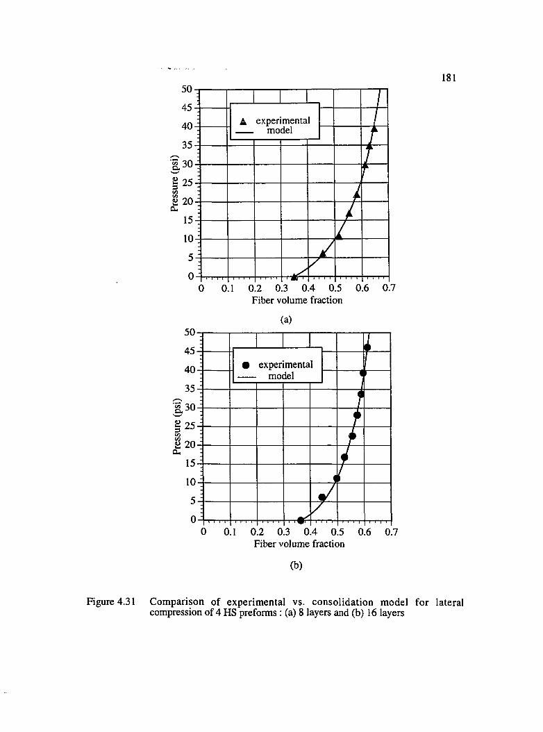
181

A experimental — model4 0 -

3

ICL

0 0.1 0.2 0.3 0.4 0.5 0.6 0.7Fiber volume fraction

(a)

45-:# experimental — model40

8 304

0 0.1 0.2 0.3 0.4 0.5 0.6 0.7Fiber volume fraction

(b)

Figure 4.31 Comparison of experimental vs. consolidation model for lateral compression of 4 HS preforms : (a) 8 layers and (b) 16 layers

182

Build up of viscoelastic modulus during preform consolidation can be obtained using RDA.

For EMI tackifier, changes in the viscoelastic properties with time at 94°C, 120°C and

150°C are shown in Figures 4.32 (a) through (c). Measurements were made using parallel

plates of 7.9 mm diameter at a frequency of 5 rad/sec. and a strain of 0.1. For both 94 °C

and 120°C, the values of G" are greater than O', which indicates that the resin did not reach

its gel point till 60 minutes for 94°C and 30 minutes for 120°C. However, Figure 4.32 (c)

shows a reversal in the trend for 150 °C, with G' being greater than G" from the beginning.

This is due to gelation which occurs within 20 seconds at 150°C. Before the gel point, the

material exhibits more liquid like characteristics, and hence G" is higher than G'. Beyond

gelation, G" levels off, and G' crosses over.

The wetted surface area coverage depends upon the tackifier location. Scanning electron

micrographs of the surface of tackified preforms showed that depending upon the

processing conditions, the area coverage could be both interlayer, i.e. between the layers,

or intralayer, i.e. within the fiber tows. The maximum interlayer coverage would be equal

to the nominal area of the preform, while the magnitude of the intralayer coverage would

depend upon the fraction of the total filament surface area covered. Since quantification of

the actual surface area coverage is difficult owing to the complex nature of spreading of a

viscoelastic melt over a porous substrate, the area coverage was studied qualitatively.

The criterion for intralayer coverage can be obtained by an order of magnitude analysis of

the forces favoring and resisting impregnation into the fiber tows. The main force favoring

impregnation into the tows would be the capillary pressure, Fc, while the resistance to

deformation would come from the force due to the viscoelastic modulus of the polymer

melt, Fg . Thus, the driving force, Fd for bundle impregnation (neglecting effects of

gravity and static friction) can be expressed by Equation 4.21.

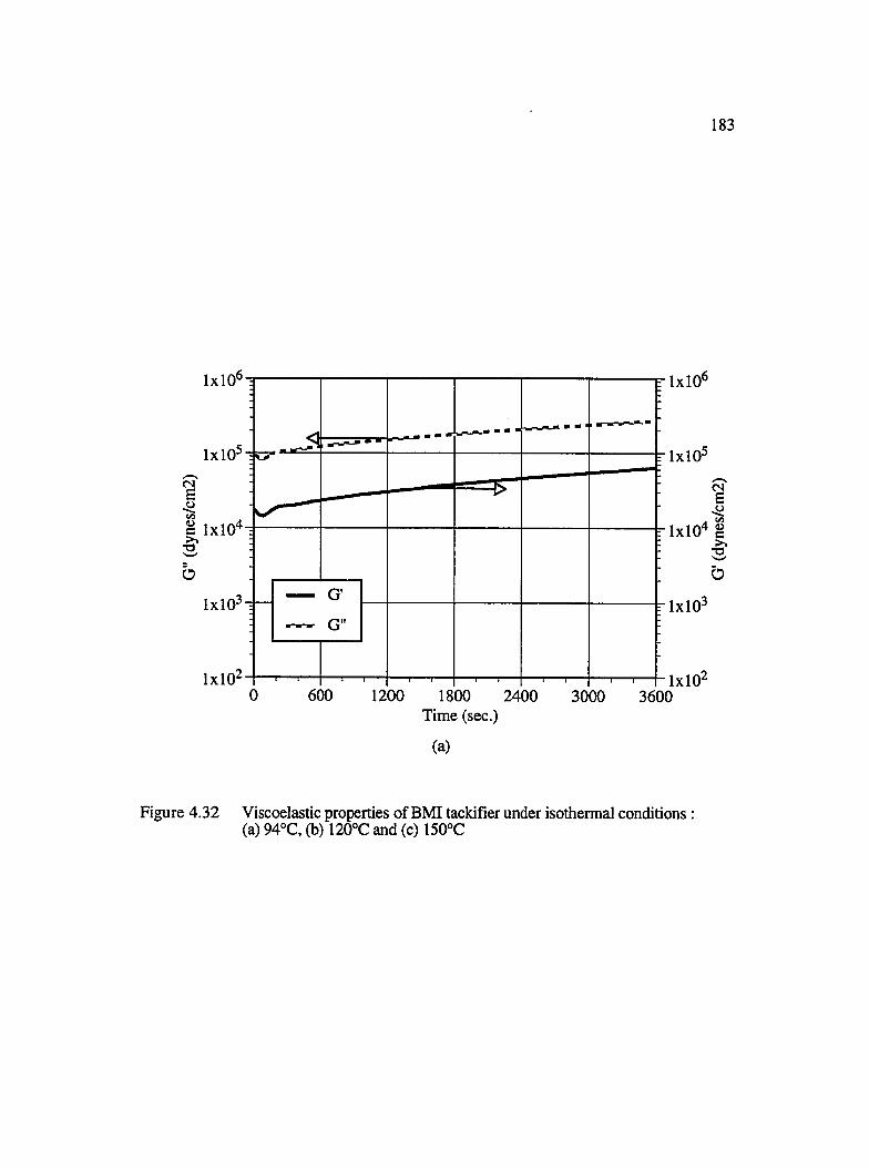
183

F 1x10'

TTTr 1x10

es

r lx lO '

r 1x10

1x10 1x100 600 1200 1800 2400 3000 3600

Time (sec.)

(a)

îêÜ

Figure 4.32 Viscoelastic properties of BMI tackifier under isothermal conditions :(a) 94°C, (b) 120°C and (c) 150°C

184

Figure 4.32 Continued

1x10' r i x i C

r 1x10(S

r lxlO'

1x10 r 1x10

1x10 1x100 200 400 600 800 1000 1200 1400 1600 1800

IÜ

Time (sec.)

(b)

1x10 F 1x10

1x10' rlx lO '

P 1x10

^ 1x10'

1x10 r 1x10

1x10 1x100 200 400 600 800 1000 1200 1400 1600 1800

Time (sec.)

(c)

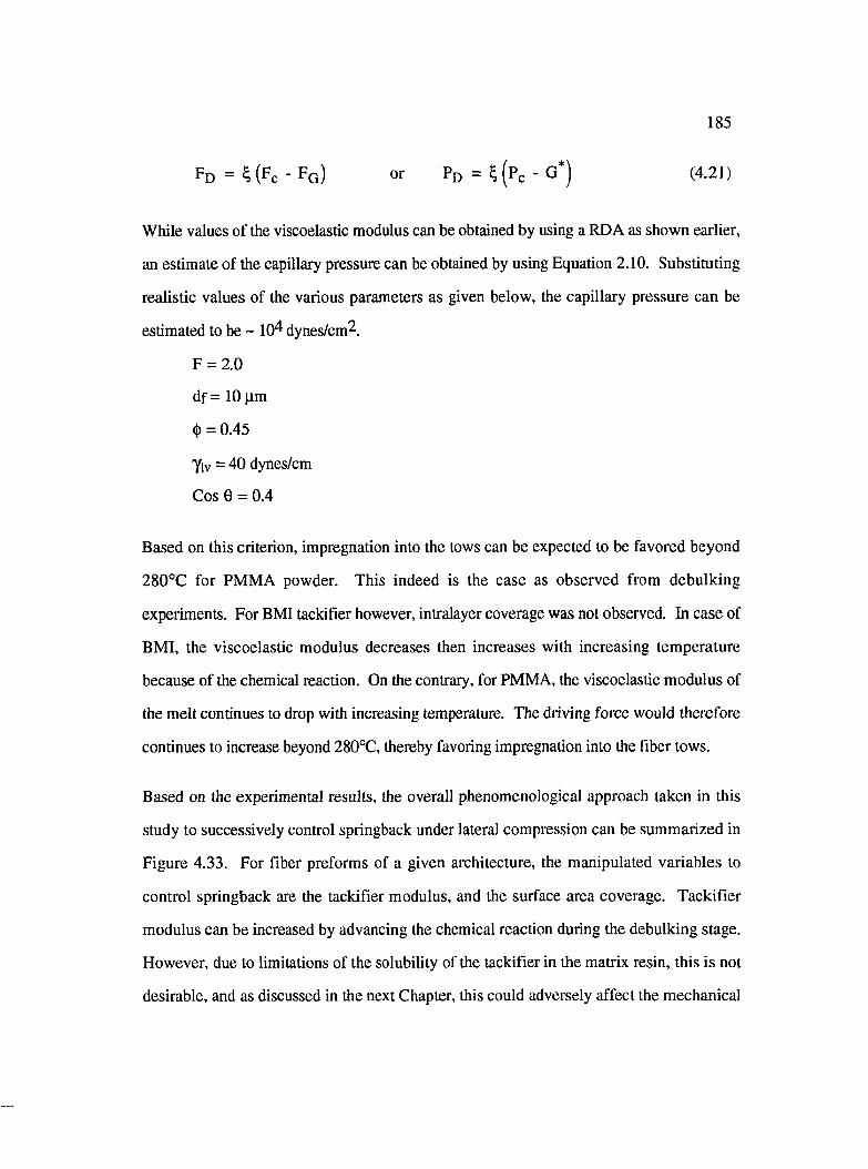
185

Fd = 4 (Fc - Fg ) or Pn =% (Pc - G*) (4.21)

While values of the viscoelastic modulus can be obtained by using a RDA as shown earlier,

an estimate of the capillary pressure can be obtained by using Equation 2.10. Substituting

realistic values of the various parameters as given below, the capillary pressure can be

estimated to be ~ 10^ dynes/cm^.

F = 2.0

df = 10 |im

(|) = 0.45

Ylv = 40 dynes/cm

Cos 0 = 0.4

Based on this criterion, impregnation into the tows can be expected to be favored beyond

280°C for PMMA powder. This indeed is the case as observed from debulking

experiments. For BMI tackifier however, intralayer coverage was not observed. In case of

BMI, the viscoelastic modulus decreases then increases with increasing temperature

because of the chemical reaction. On the contrary, for PMMA, the viscoelastic modulus of

the melt continues to drop with increasing temperature. The driving force would therefore

continues to increase beyond 280°C, thereby favoring impregnation into the fiber tows.

Based on the experimental results, the overall phenomenological approach taken in this

study to successively control springback under lateral compression can be summarized in

Figure 4.33. For fiber preforms of a given architecture, the manipulated variables to

control springback are the tackifier modulus, and the surface area coverage. Tackifier

modulus can be increased by advancing the chemical reaction during the debulking stage.

However, due to limitations of the solubility of the tackifier in the matrix resin, this is not

desirable, and as discussed in the next Chapter, this could adversely affect the mechanical

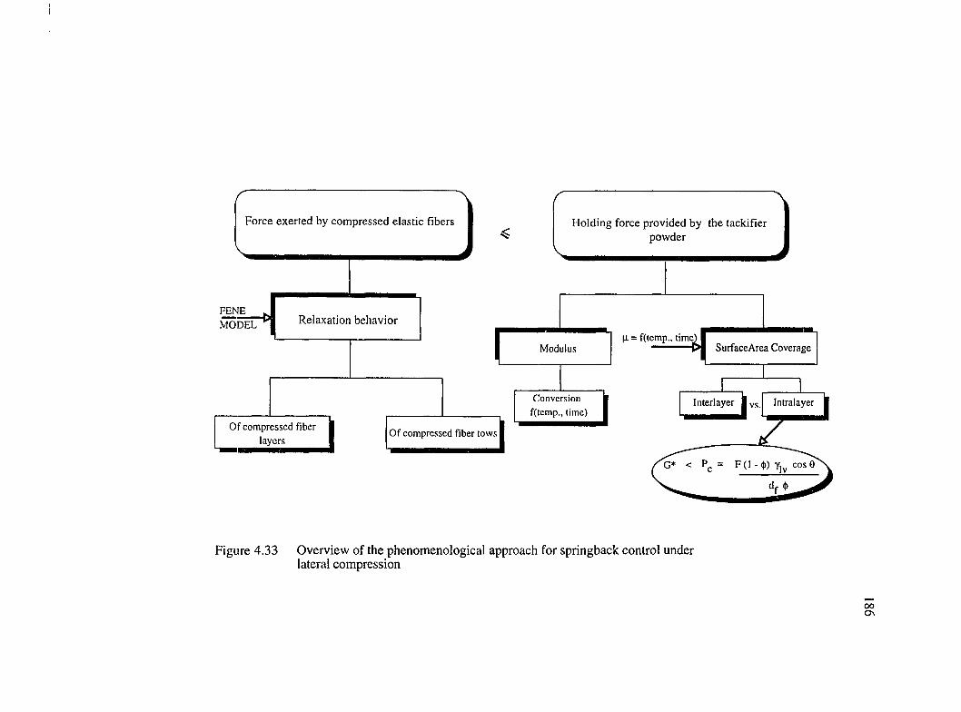
Force exerted by compressed elastic fibers Holding force provided by the tackifier powder

FEME

MODEL Relaxation behavior

SurfaceArea CoverageModulus

Conversion f(temp., time)

Interlayer Intralayervs.

Of compressed fiber layers Of compressed fiber tows

Figure 4.33 Overview of the phenomenological approach for springback control under lateral compression

00o\

187properties of the molded composite. Thus, a better alternative is to increase the surface area

coverage, and this can be achieved by increasing both the interlayer and intralayer

coverage, as there are two levels and consolidation, and consequently two levels of

springback.

Further proof o f this can be seen from Figure 4.34 (a), (b) and (c). These

photomicrographs represent the cross-section of the samples after springback, and figure

(a) and (b) corresponds to the case in which intralayer coverage was achieved using PMMA

powder at ~ 287°C. Figure (c) shows the cross-section of the sample with BMI tackifier at

94°C, and in which the tackifier remains on the surface. Figure (a) shows that the fiber

tows are compressed much more as compared to Figure (c). However in case of PMMA

heated at -287 °C, some gaps between the layers were observed (Figure b) showing

interlayer springback. These gaps are not present in the case of BMI, indicating that

springback results mostly from deconsolidation of fiber tows.

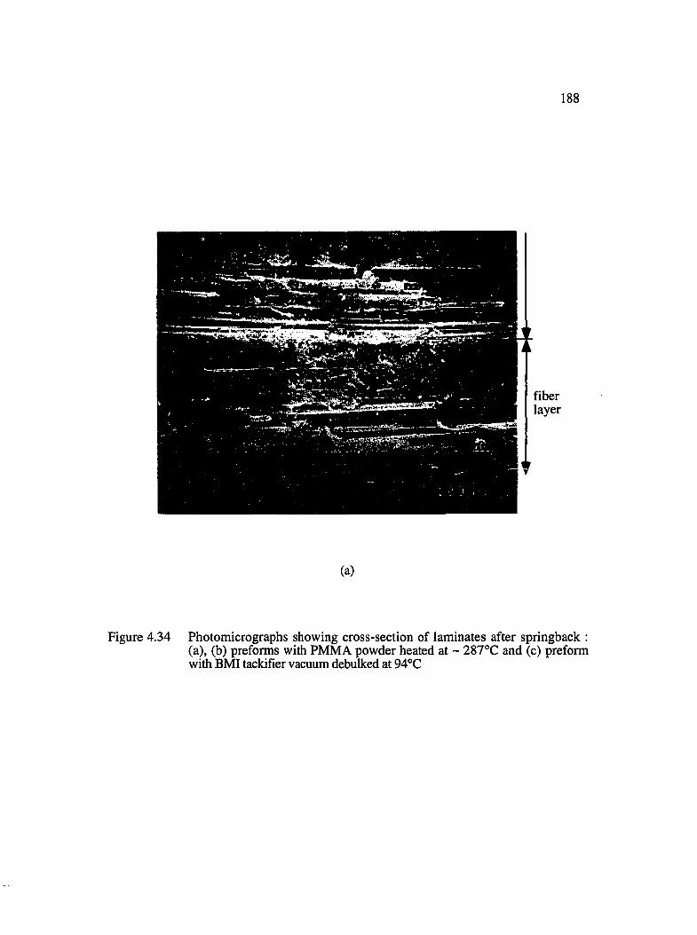
188

(a)

Figure 4.34 Photomicrographs showing cross-section of laminates after springback :(a), (b) preforms with PMMA powder heated at ~ 287°C and (c) preform widi BMI tackifier vacuum debulked at 94°C

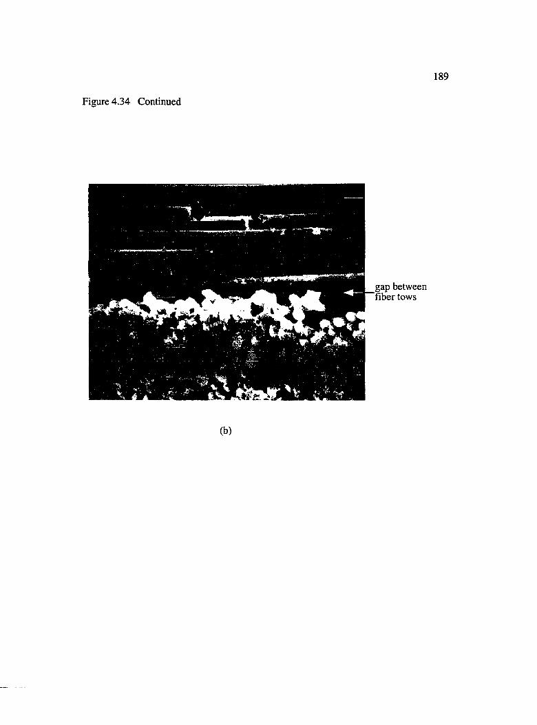
189

Figure 4.34 Continued

gap between fiber tows

(b)

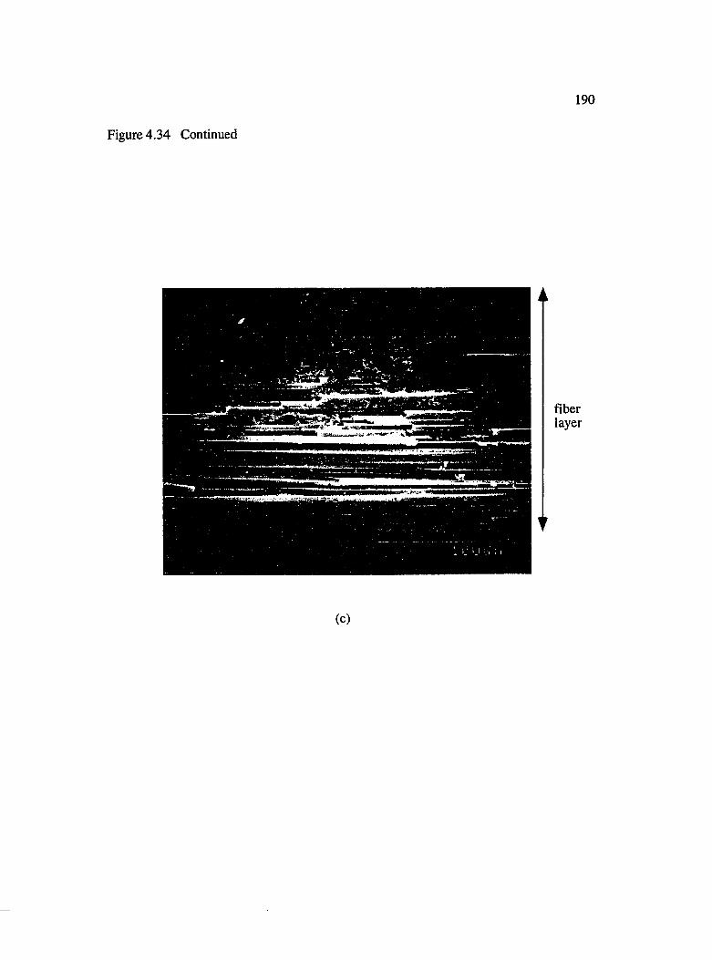
Figure 4.34 Continued

190

fiberlayer

(c)

CHAPTER V

MECHANICAL PROPERTIES OF MOLDED COMPOSITES AND PERMEABILITY CHARACTERISTICS OF TEXTILE REINFORCEMENTS

5 .1 Effect of Voids on Fiberglass/UP Composites

Stitched unidirectional fiberglass mat (CoFab AO 108) reinforced unsaturated polyester

(UP) resin composite samples were prepared using one layer of fiber reinforcement and

under similar conditions and same fiber volume fraction as mold filling experiments

described in Chapter III. The unsaturated polyester resin (Q 6585, Ashland Chemical)

used is a 1:1 mixture of propylene glycol and maleic anhydride containing 35% by weight

of styrene. The structure of the two constituents is shown below

O?

CH

~ C ” C H = CH“ C-------- O —Œ — CH 2 “O —

Maleic Anhydride Propylene Glycol

The unsaturated polyester resin has an average of 10.13 vinylene groups per polyester

molecule. The average molecular weight is 1580 gm/gm-mole, and the equivalent

molecular weight/(mole C=C) is 156 gm/gm mole. Additional styrene was added to make

the molar ratio of styrene to unsaturated polyester equal to 2.0.

191

192The initiator, USP 245 (2,5 dimethyl-2,5 bis (2-ethyl-hexanoyI-peroxy) hexane) was

added at 1% by weight of styrene and UP resin. Both unsaturated polyester resin and

styrene monomer were used as received without removing the inhibitor. In order to avoid

batch to batch variations, a large quantity of the resin (without the initiator) was prepared

and stored in the freezer. When required for molding experiments, a small amount was

taken out and the appropriate amount of initiator was added. Curing was done overnight at

130°C.

5.1.1 Dynamic Mechanical Test

A Rheometrics Dynamic Analyzer (RDA) was used in the torsion mode to monitor the drop

in the dynamic properties of composite samples immersed in hot water for up to 48 hours.

Consideration of dynamic properties become important when the structural configuration of

a part is dictated by flutter and vibration characteristics [Maymon et al., 1978].

Test samples used were rectangular strips having dimensions of 5.3 cm x 1.1 cm (1 x w).

Three strips were cut from composite samples with no voids, with ~ 3% microvoids and

with -7 % macrovoids. These strips were then immersed in hot water at 95°C successively

for 1 hr, 2 hrs, 4 hrs, 8 hrs and 48 hrs. After each immersion time, the sample was taken

out and placed between the top and bottom fixtures of the RDA as shown in Figure 5.1.

The top fixture was held stationary, while a cyclic twist was applied to the bottom fixture

during the experiment. All readings were taken at room temperature over a frequency

sweep from 0.1 rad/sec. to 25 rad/sec. at a maximum strain of 0.1%. The values of elastic

modulus G' were computed from Equations 4.10 and 4.11 along with 5.1:

Kx = 1000

t 3 + 1.8 ( - ) ________ w

wt-(5.1)

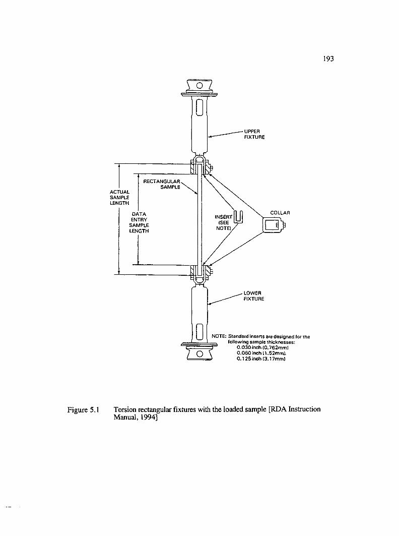
1 9 3

UPPERFIXTURE

RECTANGULARSAMPLE

ACTUALSAMPLELENGTH

COLLARDATAENTRY

SAMPLELENGTH

INSERT(SEE

NOTE).

LOWERFIXTURE

NOTE; S tandard Inserts are designed for the — . following sam ple th icknesses:j 0 .0 3 0 Inch (0 .7 6 2 m m |

0 .0 6 0 Inch (1 .5 2 m m l ) 0 .1 2 5 Inch (3 .17mm)

Figure 5.1 Torsion rectangular fixtures with the loaded sample [RDA Instruction Manual, 1994]

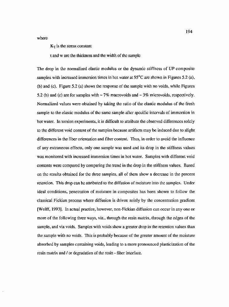
194where

Kx is the stress constant

t and w are the thickness and the width of the sample

The drop in the normalized elastic modulus or the dynamic stiffness of UP composite

samples with increased immersion times in hot water at 95°C are shown in Figures 5.2 (a),

(b) and (c). Figure 5.2 (a) shows the response of the sample with no voids, while Figures

5.2 (b) and (c) are for samples with ~ 7% macrovoids and ~ 3% microvoids, respectively.

Normalized values were obtained by taking the ratio of the elastic modulus of the fresh

sample to the elastic modulus of the same sample after specific intervals of immersion in

hot water. In torsion experiments, it is difficult to attribute the observed differences solely

to the different void content of the samples because artifacts may be induced due to slight

differences in the fiber orientation and fiber content. Thus, in order to avoid the influence

of any extraneous effects, only one sample was used and its drop in the stiffness values

was monitored with increased immersion times in hot water. Samples with different void

contents were compared by comparing the trend in the drop in the stiffness values. Based

on the results obtained for the three samples, all of them show a decrease in the percent

retention. This drop can be attributed to the diffusion of moisture into the samples. Under

ideal conditions, penetration of moisture in composites has been shown to follow the

classical Fickian process where diffusion is driven solely by the concentration gradient

[Wolff, 1993]. In actual practice, however, non-Fickian diffusion can occur in any one or

more o f the following three ways, viz., through the resin matrix, through the edges of the

sample, and via voids. Samples with voids show a greater drop in the retention values than

the sample with no voids. This is probably because of the greater amount of the moisture

absorbed by samples containing voids, leading to a more pronounced plasticization o f the

resin matrix and / or degradation of the resin - fiber interface.

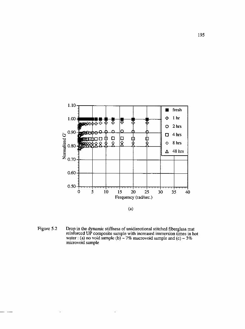
1 9 5

1. 10 -

1.00 -

^ 0 .9 0 -

1 ,

0.70

0.60

0.50-

-I H H 1 ■ ■ 1 1I

■ fresh

* 1 hr

O 2 hrs

□ 4 hrs

O 8 hrs

A 48 hrs

■> *

\ m O (

1 1=■

1 t

I>

]□ □ [ ] □ □ c] [> < \ !

]

:

-

---I'T 1 1 i l l 1 1' 1 1 1 -T-l 1"!0 5 10 15 20 25 30 35 40

Frequency (rad/sec.)

(a)

Figure 5.2 Drop in the dynamic stiffness of unidirectional stitched fiberglass mat reinforced UP composite sample with increased immersion times in hot water : (a) no void sample (b) ~ 7% macro void sample and (c) ~ 3% microvoid sample

Figure 5.2 Continued

196

- 0.90

= 0.80

m-m

OO (p o

■4-

m □

o.Æ

*

□

< >

A

■ fresh

O 1 hr

O 2 hrs

□ 4 hrs

O 8 hrs

A 48 hrs

0.50 [ I I T I I I i I I )■! I - I I - j i r "i |"| I I I I j I - I I 1 I I - I I I I r - r I - I '

0 5 10 15 20 25 30 35 40Frequency (rad/sec.)

(b)

- 0.90

3 0.80

M - * - *

<gijSi A OO O (b O

□ □ CD □

A A A A

m m

■ fresh

O 1 hr

O 2 hrs

□ 4 hrs

O 8 hrs

A 48 hrs

10 15 20 25 30 35Frequency (rad/sec.)

40

(c)

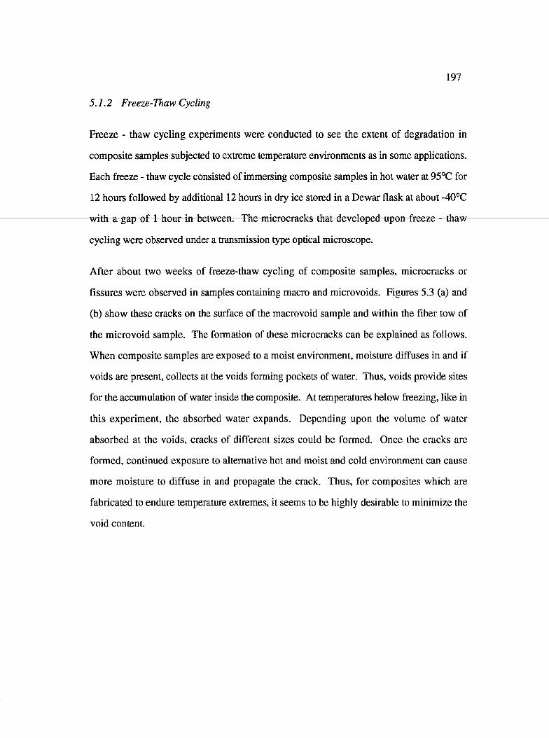
197

5.1.2 Freeze-Thaw Cycling

Freeze - thaw cycling experiments were conducted to see the extent of degradation in

composite samples subjected to extreme temperature environments as in some applications.

Each freeze - thaw cycle consisted of immersing composite samples in hot water at 95°C for

12 hours followed by additional 12 hours in dry ice stored in a Dewar flask at about -40°C

cycling were observed under a transmission type optical microscope.

After about two weeks of freeze-thaw cycling of composite samples, microcracks or

fissures were observed in samples containing macro and microvoids. Figures 5.3 (a) and

(b) show these cracks on the surface of the macrovoid sample and within the fiber tow of

the microvoid sample. The formation of these microcracks can be explained as follows.

When composite samples are exposed to a moist environment, moisture diffuses in and if

voids are present, collects at the voids forming pockets of water. Thus, voids provide sites

for the accumulation of water inside the composite. At temperatures below freezing, like in

this experiment, the absorbed water expands. Depending upon the volume of water

absorbed at the voids, cracks of different sizes could be formed. Once the cracks are

formed, continued exposure to alternative hot and moist and cold environment can cause

more moisture to diffuse in and propagate the crack. Thus, for composites which are

fabricated to endure temperature extremes, it seems to be highly desirable to minimize the

void content.

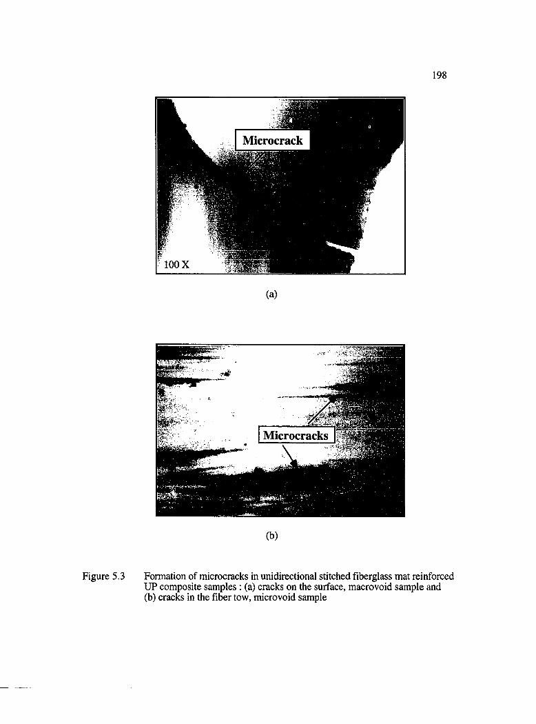
198

M icrocrack

100 X

(a)

M icrocracksm \

(b)

Figure 5.3 Formation of microcracks in unidirectional stitched fiberglass mat reinforced UP composite samples : (a) cracks on the surface, macrovoid sample and(b) cracks in the fiber tow, microvoid sample

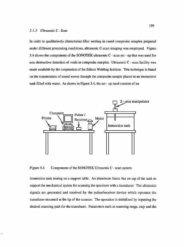
1995.1.3 Ultrasonic C - Scan

In order to qualitatively characterize fiber wetting in cured composite samples prepared

under different processing conditions, ultrasonic C-scan imaging was employed. Figure

5.4 shows the components of the SONOTEK ultrasonic C - scan set - up that was used for

non-destructive detection of voids in composite samples. Ultrasonic C - scan facility was

made available by the cooperation of the Edison Welding Institute. This technique is based

on the transmission of sound waves through the composite sample placed in an immersion

tank filled with water. As shown in Figure 5.4, the set - up used consists of an

Z - axis manipulator

Computer Printer

\ \ HSE

Puiser / Receiver.

i

. ^ Motor

¥Immersion tank

Figure 5.4 Components of the SONOTEK Ultrasonic C - scan system

immersion tank resting on a support table. An aluminum frame lies on top of the tank to

support the mechanical system for scanning the specimen with a transducer. The ultrasonic

signals are generated and received by tbe puiser/receiver device which operates the

transducer mounted at the tip of the scanner. The operation is initialized by inputting the

desired scanning path for the transducer. Parameters such as scanning range, step and the

200threshold level above which the echo signals are to be sampled are all initialized. After the

required input information is entered, the scanner stepping motor control sequence is

activated. The motor controls the motion of the transducer in both X and Y directions. The

distance of the transducer from the composite specimen was adjusted by the Z axis

manipulator at the start of the experiment. All the electronics are interfaced with a

computer. The C - scan images were viewed on the computer screen, and hard copies were

obtained from the printer attached to the computer.

Ultrasonic C-scan images for unidirectional stitched fiberglass reinforced UP composites

molded using two layers of the reinforcement and using axial flow at different flow rates

are shown in Figures 5.5 (a), (b) and (c). Figure 5.5 (a) is the C-scan image of the

composite molded at a flow velocity of 0.04 cm/sec. For UP resin, this injection velocity

corresponds to a capillary number of 1.37 x 10'3. Based on the flow visualization

experiments using non - reactive liquids, this capillary number lies in the range where no

voids are formed within the tows. This seems to correlate nicely with the C-scan image in

which the tows appear as parallel dark bands. The uniform shading of the tows indicates

very little scattering of the transmitted signal characteristic of high level of impregnation of

fibers.

Figure 5.5 (b) is the C-scan image of the composite sample molded at a velocity of 1.0

cm/sec. This corresponds to a capillary number of 3.47 x 10'3 where some microvoids

start to form. These microvoids show up in the image as white spots within the fiber tows.

Figure 5.5 (c) shows a much different image than the other two. This is the scan of the

composite sample molded at a velocity of 3.9 cm/sec. The fiber tows are barely visible.

Also, the entire image has very light colors which show up as gray areas in this black and

white photograph.

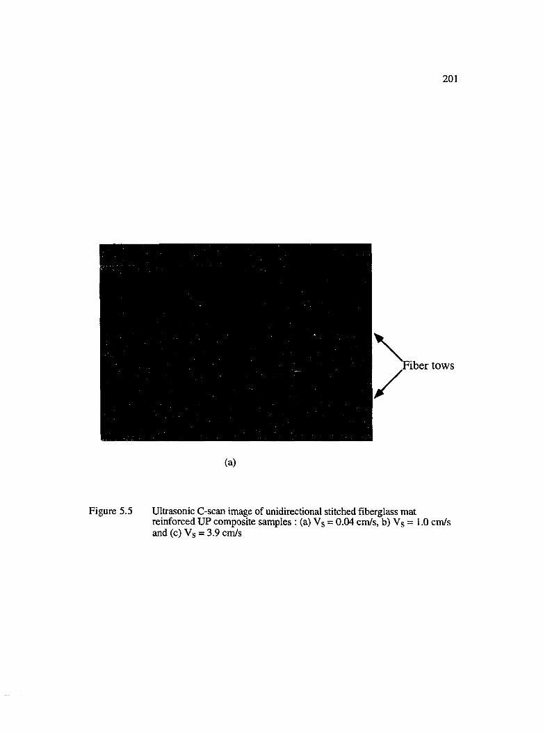
201

iber tows

(a)

Figure 5.5 Ultrasonic C-scan image of unidirectional stitched fiberglass matreinforced UP composite samples ; (a) Vs = 0.04 cm/s, b) Vs = 1.0 cm/s and (c) Vs = 3.9 cnVs

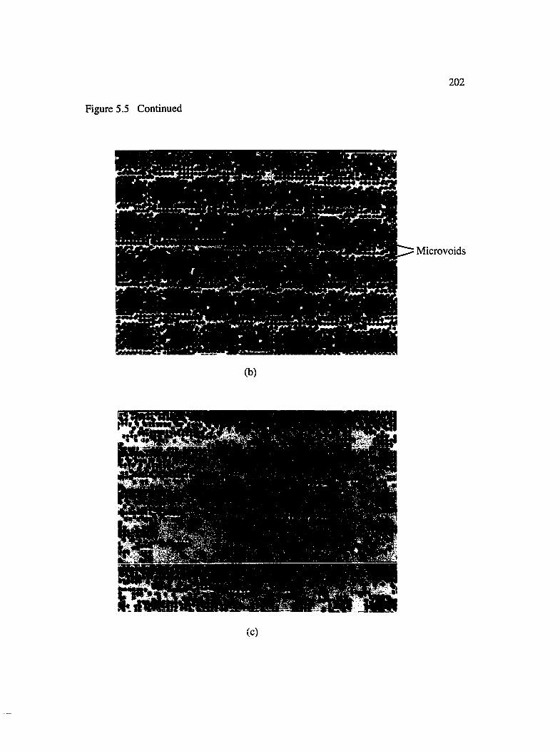
Figure 5.5 Continued

202

Microvoids

(b)

(c)

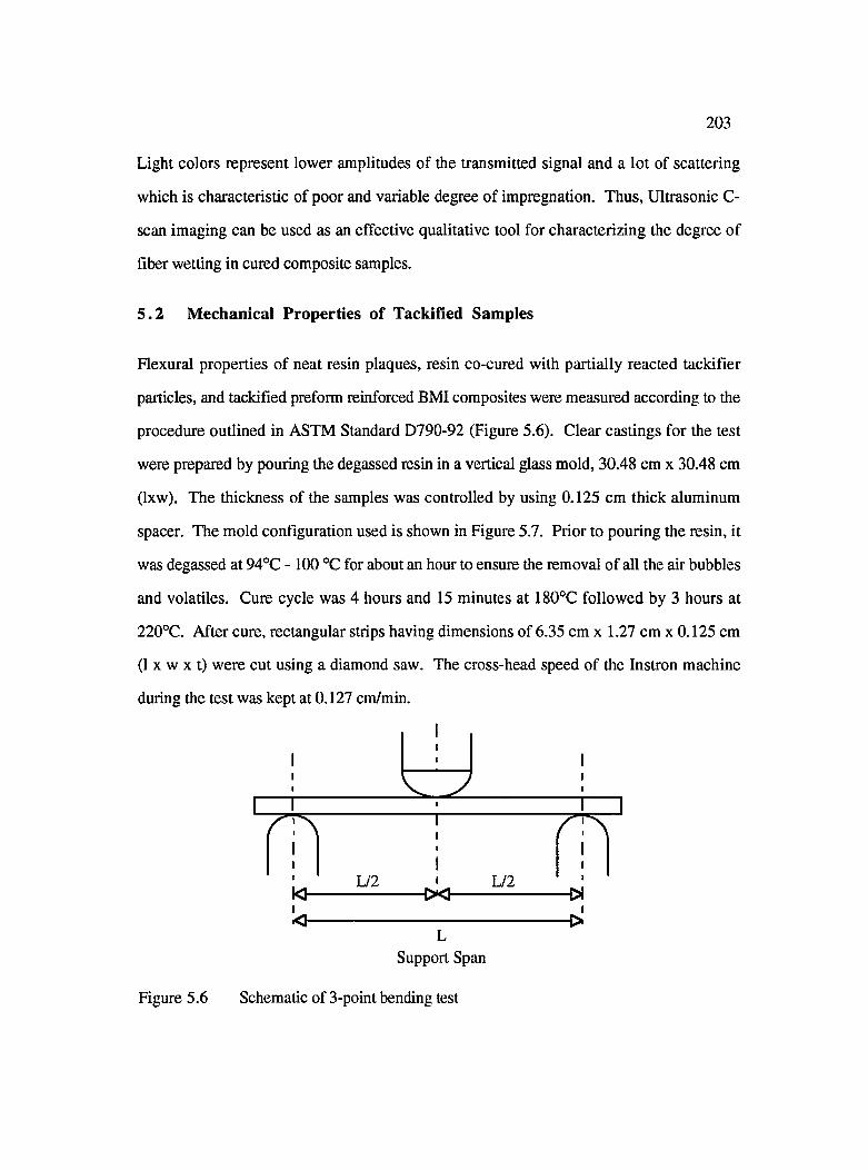
203

Light colors represent lower amplitudes of the transmitted signal and a lot of scattering

which is characteristic of poor and variable degree of impregnation. Thus, Ultrasonic C-

scan imaging can be used as an effective qualitative tool for characterizing the degree of

fiber wetting in cured composite samples.

5 .2 Mechanical Properties of Tackified Samples

Flexural properties of neat resin plaques, resin co-cured with partially reacted tackifier

particles, and tackified preform reinforced BMI composites were measured according to the

procedure outlined in ASTM Standard D790-92 (Figure 5.6). Clear castings for the test

were prepared by pouring the degassed resin in a vertical glass mold, 30.48 cm x 30.48 cm

(Ixw). The thickness of the samples was controlled by using 0.125 cm thick aluminum

spacer. The mold configuration used is shown in Figure 5.7. Prior to pouring the resin, it

was degassed at 94°C - KX) °C for about an hour to ensure the removal of all the air bubbles

and volatiles. Cure cycle was 4 hours and 15 minutes at 180°C followed by 3 hours at

220°C. After cure, rectangular strips having dimensions of 6.35 cm x 1.27 cm x 0.125 cm

(1 X w X t) were cut using a diamond saw. The cross-head speed of the Instron machine

during the test was kept at 0.127 cm/min.

L/2 L/2X .

Support Span

Figure 5.6 Schematic of 3-point bending test

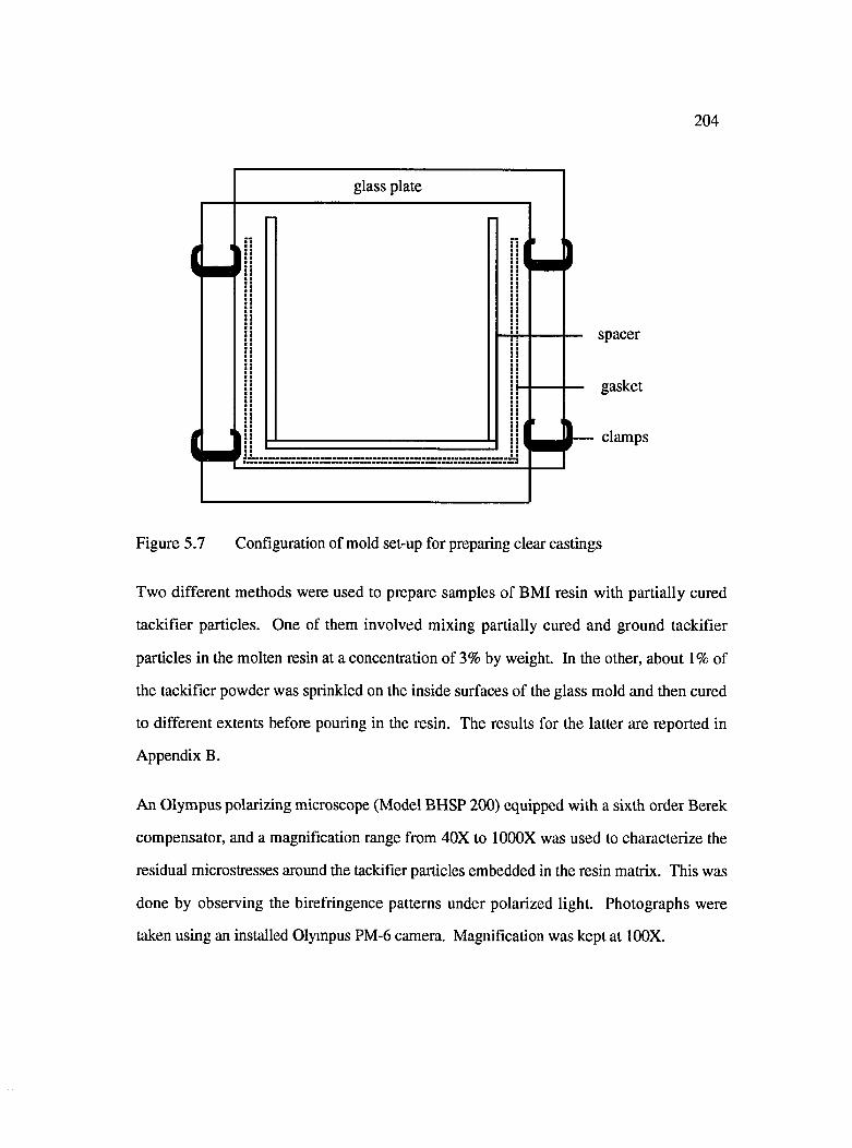
204

glass plate

(-1 Lspacer

gasket

clamps

Figure 5.7 Configuration of mold set-up for preparing clear castings

Two different methods were used to prepare samples of BMI resin with partially cured

tackifier particles. One of them involved mixing partially cured and ground tackifier

particles in the molten resin at a concentration of 3% by weight. In the other, about 1% of

the tackifier powder was sprinkled on the inside surfaces of the glass mold and then cured

to different extents before pouring in the resin. The results for the latter are reported in

Appendix B.

An Olympus polarizing microscope (Model BHSP 200) equipped with a sixth order Berek

compensator, and a magnification range from 40X to lOOOX was used to characterize the

residual microstresses around the tackifier particles embedded in the resin matrix. This was

done by observing the birefringence patterns under polarized light. Photographs were

taken using an installed Olympus PM-6 camera. Magnification was kept at lOOX.

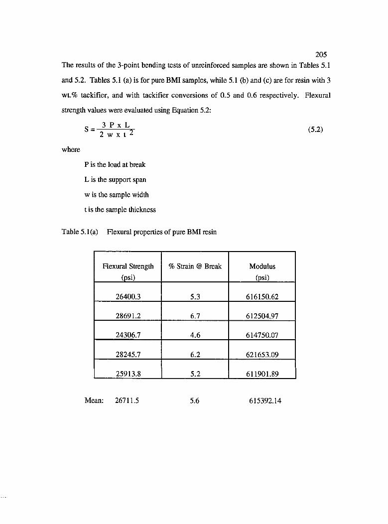
205The results of the 3-point bending tests of unreinforced samples are shown in Tables 5.1

and 5.2. Tables 5.1 (a) is for pure BMI samples, while 5.1 (b) and (c) are for resin with 3

wt.% tackifier, and with tackifier conversions of 0.5 and 0.6 respectively. Flexural

strength values were evaluated using Equation 5.2:

3 P X LS =2 w X t

where

P is the load at break

L is the support span

w is the sample width

t is the sample thickness

Table 5.1(a) Flexural properties of pure BMI resin

(5.2)

Flexural Strength

(psi)

% Strain @ Break Modulus(psi)

26400.3 5.3 616150.62

28691.2 6.7 612504.97

24306.7 4.6 614750.07

28245.7 6.2 621653.09

25913.8 5.2 611901.89

Mean: 26711.5 5.6 615392.14

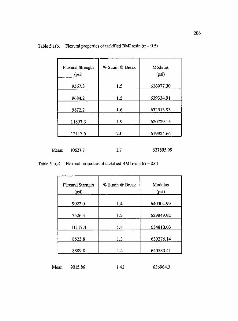
Table 5.1(b) Hexural properties of tackified BMI resin (a ~ 0.5)

206

Flexural Strength

(psi)

% Strain @ Break Modulus(psi)

9567.3 1.5 626977.30

9684.2 1.5 639334.91

9872.2 1.6 632513.93

11897.3 1.9 620729.15

12117.5 2.0 619924.66

;an: 10627.7 1.7 627895.99

c) Flexural properties of tackified BMI resin (a ~ 0.6)

Flexural Strength

(psi)

% Strain @ Break Modulus(psi)

9022.0 1.4 640304.99

7526.3 1.2 629849.92

11117.4 1.8 634810.03

8523.8 1.3 639276.14

8889.8 1.4 640580.41

Mean: 9015.86 1.42 636964.3

207As shown in Table 5.1 and in Figures 5.8 (a) and (b), both the mean flex strength and the

mean percent strain at break for pure resin samples were found to be higher than the

corresponding values of tackified resin samples. One reason for this could be due to the

insolubility of the tackifier particles in the matrix resin resulting in a two phase system.

Due to this heterogeneity, residual microstresses (Figure 5.9) develop probably due to the

mismatch in the thermal expansion and contraction of the two phases. Thus, when the

applied stress and the residual stress reach a certain critical level, premature fracture occurs.

The fracture surface of both pure resin (Figure 5.10 a) and tackified resin (Figure 5.10 b)

were also observed. The latter figure shows voids at the fracture surface which can also

explain the poor mechanical properties exhibited by the tackified resin samples. This

observed morphology is similar to the one observed in some rubber modified epoxy and

bismaleimide fracture surfaces [Voit and Seferis, 1987]. It was hypothesized that the

reason for this is due to cavitation, crazing, or debonding of the rubber particles that were

phase separated during the curing stage.

Tables 5.2 (a) and (b) compares the flexural strength, percent strain at break and modulus

of composite samples made from preforms coated with 3 wt.% tackifier powder debulked

at 145°C for 1 hour and 80°C for 20 minutes respectively to achieve two different cure

levels. The samples with lower degree of tackifier cure show slightly higher values for the

flexural strength, although the difference is not as drastic as in the case of unreinforced

sample. This is probably due to the masking effect of the fibers.

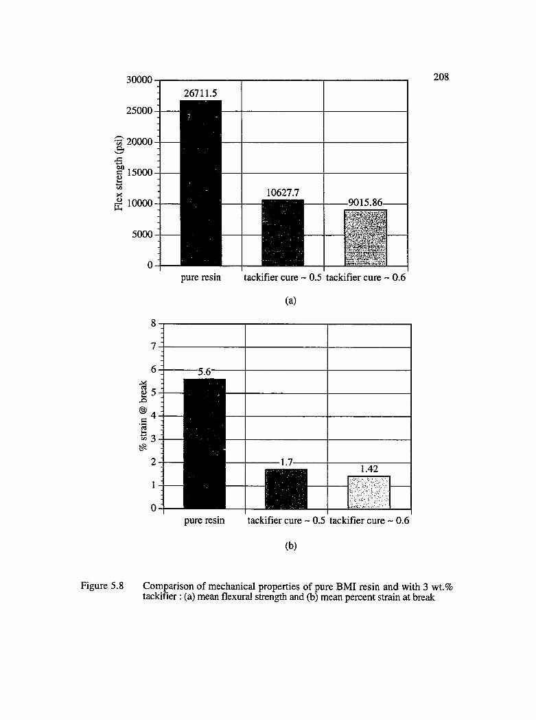
30000

25000

-a 20000 &.

c 15000II 10000

5000

26711.5

10627.79015.86-

pure resin

*

tackifier cure ~ 0.5 tackifier cure ~ 0.6

208

(a)

@1

pure resin tackifier cure ~ 0.5 tackifier cure ~ 0.6

(b)

Figure 5.8 Comparison of mechanical properties of pure BMI resin and with 3 wt.% tackifier ; (a) mean flexural strength and (b) mean percent strain at break

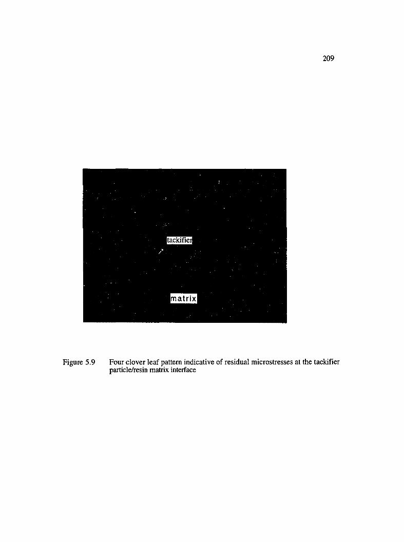
209

tackifie

matrix

Figure 5.9 Four clover leaf pattern indicative of residual microstresses at the tackifier particle/resin matrix interface

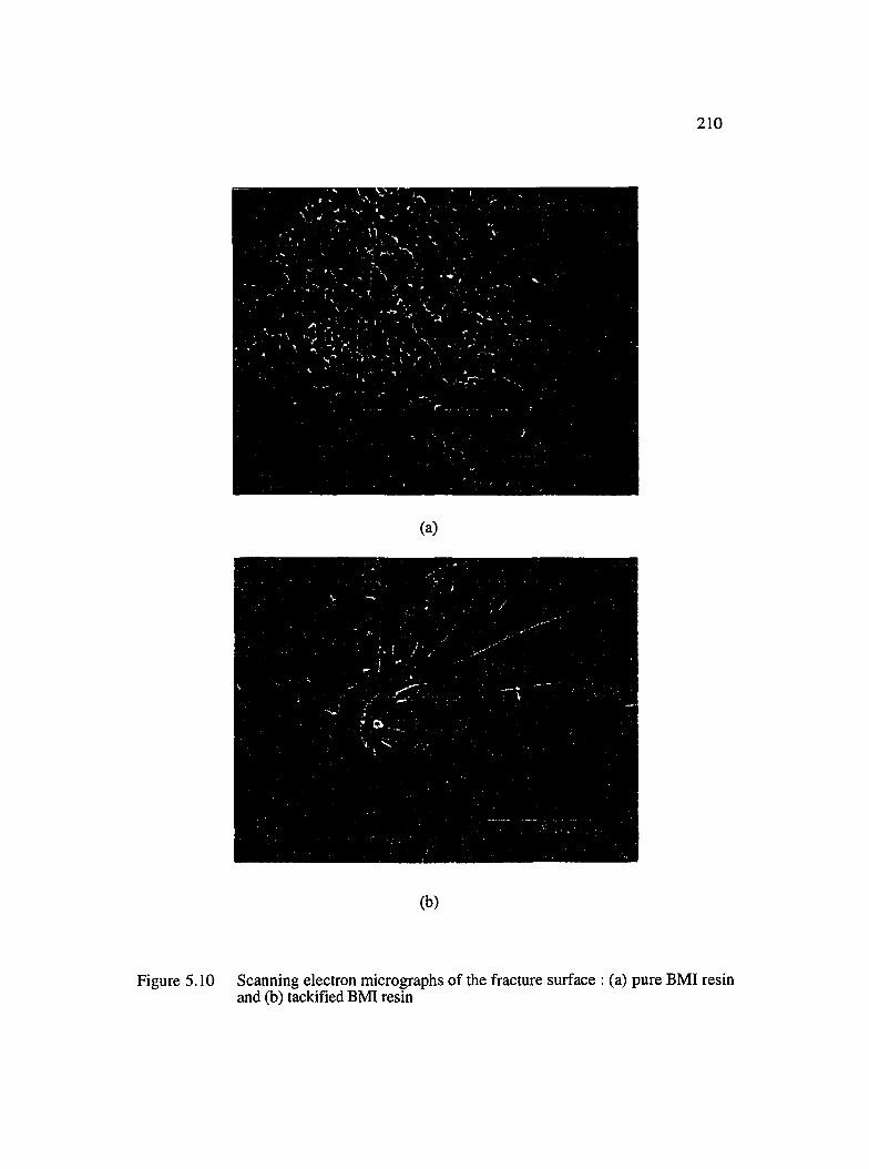
210

(a)

(b)

Figure 5.10 Scanning electron micrographs of the fracture surface : (a) pure BMI resin and (b) tackified BMI resin

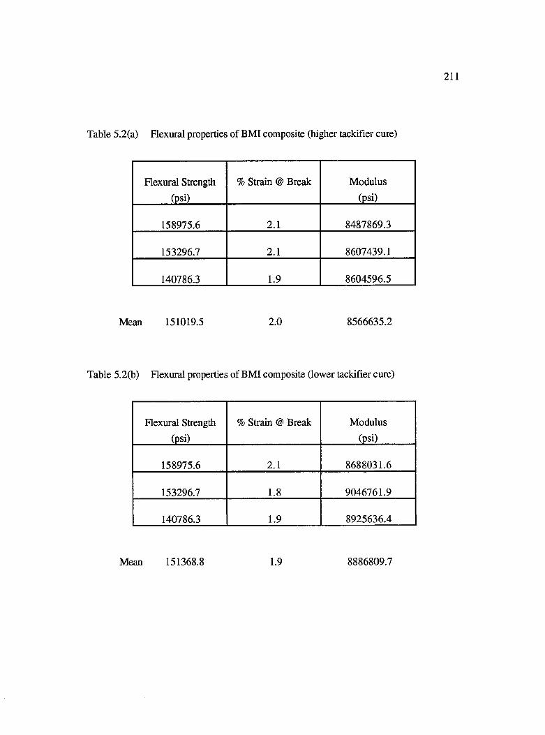
211

Table 5.2(a) Flexural properties of BMI composite (higher tackifier cure)

Flexural Strength % Strain @ Break Modulus

(psi) (psi)

158975.6 2.1 8487869.3

153296.7 2.1 8607439.1

140786.3 1.9 8604596.5

Mean 151019.5 2.0 8566635.2

Table 5.2(b) Flexural properties of BMI composite (lower tackifier cure)

Flexural Strength % Strain @ Break Modulus

(psi) (psi)

158975.6 2.1 8688031.6

153296.7 1.8 9046761.9

140786.3 1.9 8925636.4

Mean 151368.8 1.9 8886809.7

212

5 .3 Flow Characteristics of Textile Reinforcements

5.3.1 Permeability o f Fiber Preforms

Permeability measurement characterizes the flow resistance of a fiber reinforcement. Since

pressure drop and mold filling times during the resin injection stage are governed by

permeability values, their measurement becomes important from processing point of view.

Also, these values can vary over a wide range depending upon the fiber structure.

Moreover, fabrics with anisotropic structure would have varying permeability values in

different flow directions. Thus, permeability is a tensor quantity having both magnitude

and direction. The use of binder or tackifier material further complicates the issue, and

therefore warrants a systematic investigation.

Since permeability measurements of stitched unidirectional fiberglass mat were conducted

in a companion study [Wu, 1995], this work focuses on braided and 4HS tackified

reinforcements. The experimental set-up used for in-plane permeability measurements is

shown in Figure 5.11. Using a liquid of known viscosity and injecting it at a constant flow

rate, the pressure drop can be monitored as the liquid flows through the fabric.

Permeability values for an isotropic fiber mat can then be determined by Darcy's law given

by Equation 2.1. To recall, Darcy's law states that permeability is inversely proportional to

the pressure drop as given by Equation 5.3:

K = f ( ^ ) (5.3)AP~ T

where, all the terms have their usual meaning as defined earlier in this text.

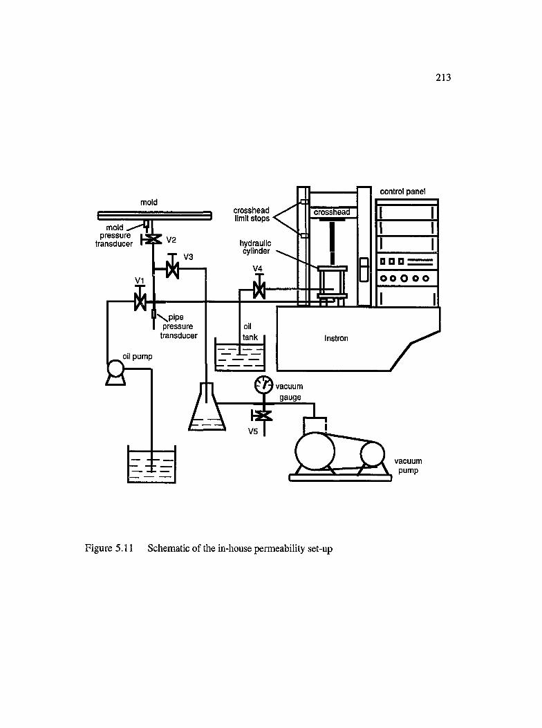
213

control panelmold

crosshead limit stops

crosshead

mold ^ pressure

transducer hydrauliccylinder

V4nonoo o o o

l \ p i p epressure

transducer tank Instron

oii pump

vacuumgauge

V5

vacuumpump

Figure 5.11 Schematic of the in-house permeability set-up

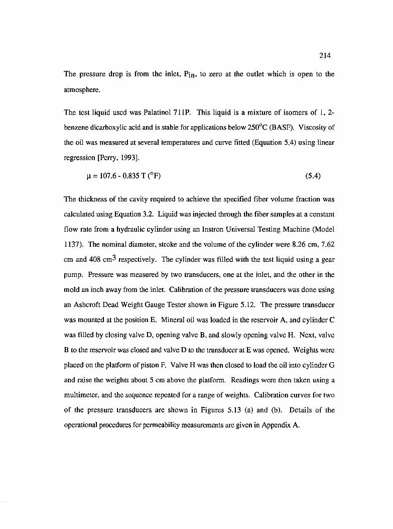
214

The pressure drop is from the inlet. Pin, to zero at the outlet which is open to the

atmosphere.

The test liquid used was Palatinol 7 IIP . This liquid is a mixture of isomers of 1 ,2 -

benzene dicarboxylic acid and is stable for applications below 250°C (BASF). Viscosity of

the oil was measured at several temperatures and curve fitted (Equation 5.4) using linear

regression [Perry, 1993].

|l = 107.6 - 0.835 T (°F) (5.4)

The thickness of the cavity required to achieve the specified fiber volume fraction was

calculated using Equation 3.2. Liquid was injected through the fiber samples at a constant

flow rate from a hydraulic cylinder using an Instron Universal Testing Machine (Model

1137). The nominal diameter, stroke and the volume of the cylinder were 8.26 cm, 7.62

cm and 408 cm3 respectively. The cylinder was filled with the test liquid using a gear

pump. Pressure was measured by two transducers, one at the inlet, and the other in the

mold an inch away from the inlet. Calibration of the pressure transducers was done using

an Ashcroft Dead Weight Gauge Tester shown in Figure 5.12. The pressure transducer

was mounted at the position E. Mineral oil was loaded in the reservoir A, and cylinder C

was filled by closing valve D, opening valve B, and slowly opening valve H. Next, valve

B to the reservoir was closed and valve D to the transducer at E was opened. Weights were

placed on the platform of piston F. Valve H was then closed to load the oil into cylinder G

and raise the weights about 5 cm above the platform. Readings were then taken using a

multimeter, and the sequence repeated for a range of weights. Calibration curves for two

of the pressure transducers are shown in Figures 5.13 (a) and (b). Details of the

operational procedures for permeability measurements are given in Appendix A.

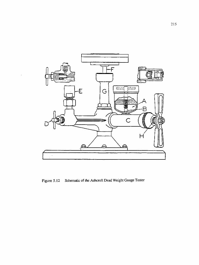
215

cm

Figure 5.12 Schematic of the Ashcroft Dead Weight Gauge Tester

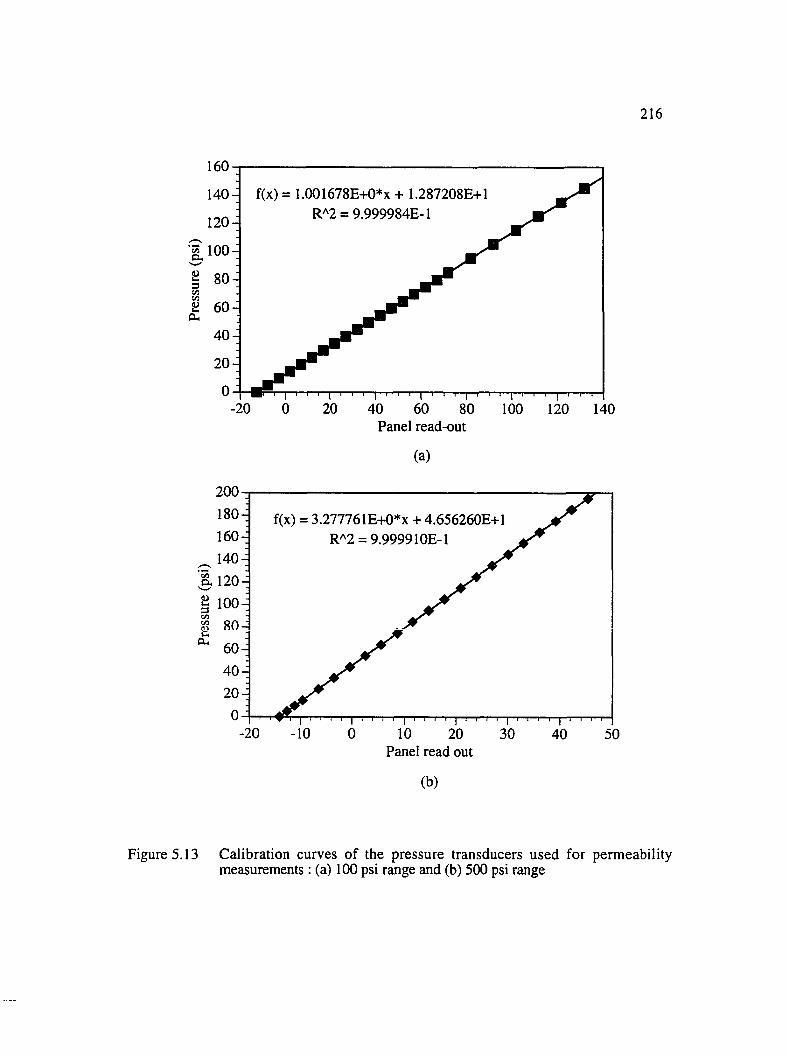
216

160

f(x)= 1.001678E+0*x+ 1.287208E+1 RA2 = 9.999984E-1

140-

120 -

•g 100-

8 0 -

6 0 -

4 0 -

20 -

60-20 0 20 40 80 100 120 140Panel read-out

(a)

7,00-180-^160

140 H

a 120^e3 100^

2 8 0 -O h 60^

40^20^

0-J

f(x) = 3.277761E+0*x + 4.656260E+1 RA2 = 9.999910E-1

I 1

10 20 Panel read out

(b)

Figure 5.13 Calibration curves of the pressure transducers used for permeability measurements : (a) 100 psi range and (b) 500 psi range

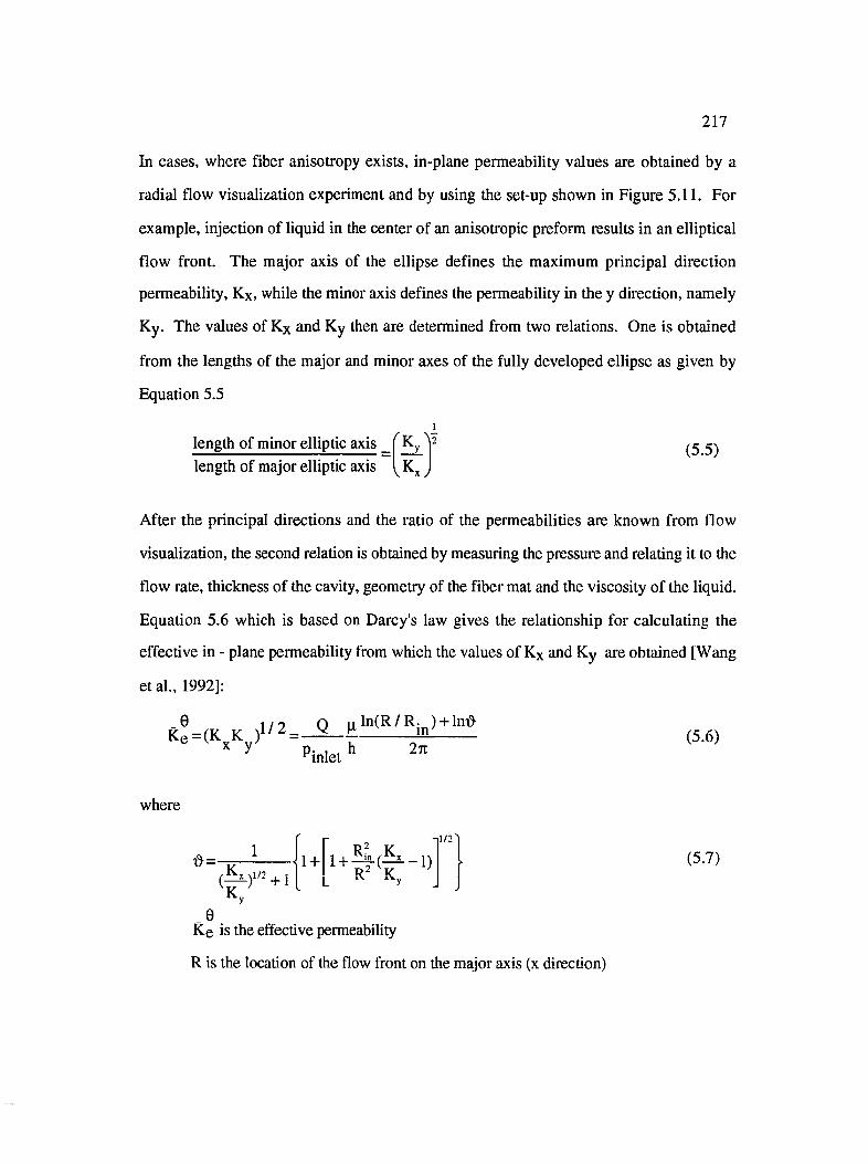
I l l

In cases, where fiber anisotropy exists, in-plane permeability values are obtained by a

radial flow visualization experiment and by using the set-up shown in Figure 5.11. For

example, injection of liquid in the center of an anisotropic preform results in an elliptical

flow front. The major axis of the ellipse defines the maximum principal direction

permeability, K%, while the minor axis defines the permeability in the y direction, namely

K y . The values of K x and K y then are determined from two relations. One is obtained

from the lengths of the major and minor axes of the fully developed ellipse as given by

Equation 5.5

length of minor elliptic axis K, ^length of major elliptic axis y

(5.5)

After the principal directions and the ratio of the permeabilities are known from flow

visualization, the second relation is obtained by measuring the pressure and relating it to the

flow rate, thickness of the cavity, geometry of the fiber mat and the viscosity of the liquid.

Equation 5.6 which is based on Darcy's law gives the relationship for calculating the

effective in - plane permeability from which the values of K x and K y are obtained [Wang

et al., 1992]:

Ke=(K^Ky)1 /2 Q pln(R/R;^) + lnû

P inlet

in"2 %

(5.6)

where

1( ^ ) i / : + lKy

' , R“„ xK1/2'

14- (5.7)

_0Ke is the effective permeability

R is the location of the flow front on the major axis (x direction)

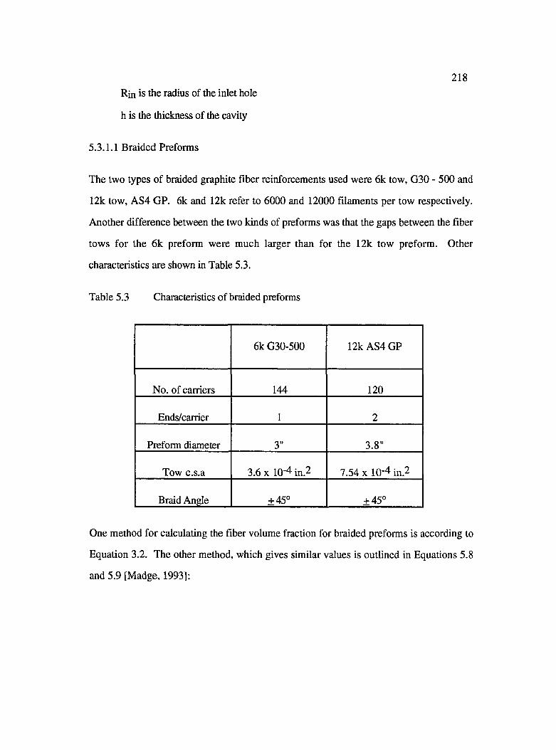
218Rin is the radius of the inlet hole

h is the thickness of the cavity

5.3.1.1 Braided Preforms

The two types of braided graphite fiber reinforcements used were 6k tow, G30 - 500 and

12k tow, AS4 GP. 6k and 12k refer to 6000 and 12000 filaments per tow respectively.

Another difference between the two kinds of preforms was that the gaps between the fiber

tows for the 6k preform were much larger than for the 12k tow preform. Other

characteristics are shown in Table 5.3.

Table 5.3 Characteristics of braided preforms

6k G30-500 12k AS4 GP

No. of carriers 144 120

Ends/carrier 1 2

Preform diameter 3" 3.8"

Tow c.s.a 3.6 X 10‘4 in.2 7.54 X 10-4 in.2

Braid Angle ±45° ±45°

One method for calculating the fiber volume fraction for braided preforms is according to

Equation 3.2. The other method, which gives similar values is outlined in Equations 5.8

and 5.9 [Madge, 1993];

219

V f = - î ^ (5.8)

where

where

where

n = number of layers

Af = total fiber area in cross-section of braid

Ab = cross - sectional area of braided structure ( = t x 7 1 D)

t = ply thickness

D = preform diameter

^ ^ ^ M N ç A j , (5 ,9 )C O S 0

M = number of ends per carrier

Nc = number of carriers

Ay = tow cross - sectional area (c.s.a)

0 = tow braid angle

The results for pressure rise vs. time curves showed an S shape in the initial part for 6k

preforms, whereas Darcy's law predicts it to be linear. This discrepancy was due to

"system elasticity" which arose from the fact that the tygon tube used to convey the liquid

from the Instron machine to the mold was not totally incompressible. So, although the

liquid was pumped from the Instron at a constant flow rate, the flow rate might not have

been constant at the mold inlet thereby causing the artifact. The permeability equipment

was therefore modified by replacing the tygon tube by a metal tube. In addition, the

pipeline and the liquid were degassed prior to liquid injection to remove any trapped and

dissolved air. Permeability experiments for only 12k, AS4 GP preforms however were

conducted using the modified equipment, which are discussed next.

220Permeability measurements using unidirectional flow were tried, but were not very

successful. It is suspected that this was probably because the liquid flowed faster from the

sides of the cavity resulting in severe 'race -tracking'. This phenomenon seems to be more

pronounced when only a small number of fiber mats are used. Another reason could be the

"flexible" structure of the braided preforms. These preforms can be distorted more easily

as compared to other fiber types where the tows are held in place either by stitches or are

woven in such a way that their structural integrity is maintained. In order to circumvent the

problem of 'race - tracking', the radial flow method was used wherein the liquid was

injected through a small hole in the center of the circular fiber preforms. Fiber samples

with 10.16 cm diameter and 2.286 cm hole in the center were used for radial flow

measurements.

The pressure vs. time curves for three and two layers of fiber preforms are shown in

Figures 5.14 (a) through (c), and the permeability values are summarized in Table 5.4.

The orientation of the fiber layers are denoted in the parenthesis. As an example, [0/0/0]

denotes that each layer is oriented with its axis parallel to the other layer. In the case of

three layers, the porosity was 34%, while for two layers the porosity was 31%.

It is interesting to note that the injection pressure does not level off even after the liquid

reaches the edge of the fiber sample. One plausible explanation for this is that for braided

fiber preforms, the fiber structure is quite flexible and the preform is highly deformable.

Thus, during mold filling the orientation of the fiber tows may change, resulting in a

change of perm eability, and consequently, a change of the pressure drop.

221

120 -

100 -

80

a

ie

60

40

20

\

1

1

1

— Dry

— W etl

- - Wet2

1

111

-

11

1

— ■•■'■I , ■ ■ ■ ' V I 1 1 1 1 ■ ' 1 1 — 1 1 1- - - - - - - - - -

400 800 1200 Time (sec.)

1600 2000

(a)

Figure 5.14 Pressure rise vs. time curves for braided preforms : (a) 3 layers [0/0/0], (b) 2 layers [0/0] and (c) 2 layers [0/90]

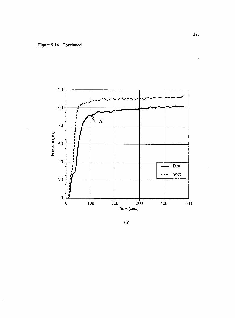
Figure 5.14 Continued

222

120

100

Cue

CL,

Dry

Wet

100 200 300 400 500Time (sec.)

(b)

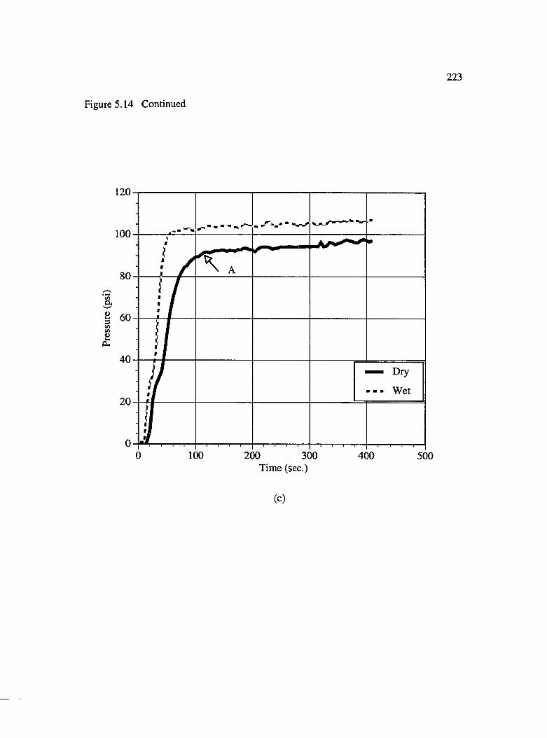
223

Figure 5.14 Continued

120

100

I40

Dry

Wet

100 200 300 400 500Time (sec.)

(c)

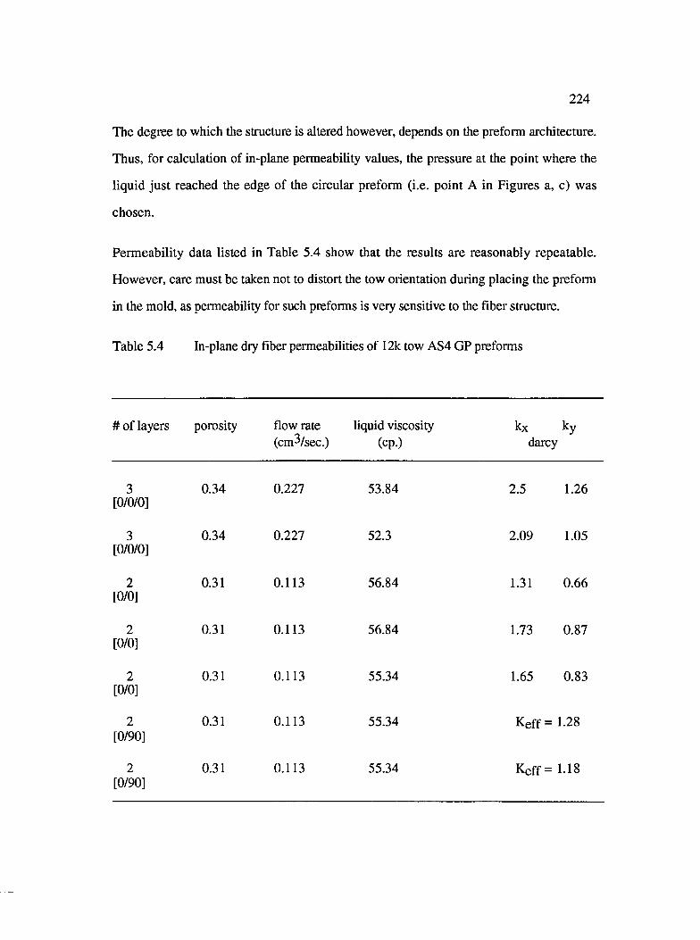
224

The degree to which tlie structure is altered however, depends on the preform architecture.

Thus, for calculation of in-plane permeability values, the pressure at the point where the

liquid just reached the edge of the circular preform (i.e. point A in Figures a, c) was

chosen.

Permeability data listed in Table 5.4 show that the results are reasonably repeatable.

However, care must be taken not to distort the tow orientation during placing the preform

in the mold, as permeability for such preforms is very sensitive to the fiber structure.

Table 5.4 In-plane dry fiber permeabilities of 12k tow AS4 GP preforms

# of layers porosity flow rate (cm^/sec.)

liquid viscosity (cp.)

k x k y

darcy

3[0/0/0]

0.34 0.227 53.84 2.5 1.26

3[0/0/0]

0.34 0.227 52.3 2.09 1.05

2[0/0]

0.31 0.113 56.84 1.31 0.66

2[0/0]

0.31 0.113 56.84 1.73 0.87

2[0/0]

0.31 0.113 55.34 1.65 0.83

2[0/90]

0.31 0.113 55.34 Keff = 1.28

2[0/90]

0.31 0.113 55.34 Keff = 1.18

225

5.3.1.2 Tackified Woven Preforms

As discussed in Chapter IV, preforming experiments showed that increasing the tackifier

concentration resulted in reduced springback. Also, better springback control was achieved

with intralayer surface area coverage or when the tackifier was inside the fiber tows. The

free volume available in the larger gaps between the fiber tows and in the smaller gaps

between the filaments of the fiber tows would decrease with increase in the tackifier

concentration. Thus, the actual free volume for resin flow in a tackified preform would be

lesser than the sample with no tackifier. This could result in a higher flow resistance or

decreased permeability for the tackified sample.

To see if this indeed was true, four different sets of samples were prepared to study the

effect of tackifier concentration and location on permeability of 4HS graphite fiber

preforms. One set comprised of preforms debulked at 94°C and having 3, 5 and 8 wt.% of

BMI tackifier (Set 1). The conditions of the second set were the same as the first set, but

were prepared using the solvent technique (Set 2). The third set of preforms were made

using the same concentrations as the other two, but with PMMA powder and at 287°C (Set

3). The control sample was the one with no tackifier (Set 4).

As in the case of braided preforms, radial flow was used instead of axial flow to measure

in-plane permeabilities of the tackified fiber preforms. To prepare the samples for the

experiment, 16 layers ((j) = .45) of the fiber were first cut into squares, 12.7 cm x 12.7 cm

(1 X w). The squares were then placed on a 10.16 cm diameter die cutter with a steel rule

knife edge [Grandon Manufacturing]. The die cutter and the stack of fibers were put

between two thick wooden plates and placed in a Carver Laboratory hydraulic hand press

to cut the circular fiber samples. A 1.905 cm steel punch was used to cut the center hole in

226the fiber stack. The fiber stack was then debulked using the vacuum debulking procedure

described in Chapter IV.

The pressure drop for the three sets and the control sample are shown in Figure 5.15. The

plot illustrates several interesting features. Firstly, for samples of Set 1, in which the

tackifier remains on the surface, the pressure drop increases with increasing tackifier

concentration. For samples of the other two sets in which the powder goes inside the fiber

tows, there is no significant change in the pressure drop with increasing tackifier

concentration. Secondly, the pressure drop for untackified sample is similar to samples of

Set 3. These results indicate that permeability is affected more by the blockage of the larger

gaps between the fiber tows as compared to the blockage of the smaller gaps within the

tows. Thirdly, the pressure drop values for Set 3 are much higher than that of Set 2, but

lower than samples of Set 1. The much lower pressure drop values obtained for samples

of Set 2 are due to the shrinking of fiber tows (due to the capillary effect of the solvent in

which the fibers were soaked in) causing an increase in the larger gaps between the tows,

and thereby decreasing the flow resistance.

Based on the increase in pressure drop for samples of Set 1, permeability values were

calculated using Darcy’s law, and are shown in Figure 5.16. Table 5.5 shows the percent

decrease in permeability with successive increase in tackifier concentration (or percent

decrease in porosity).

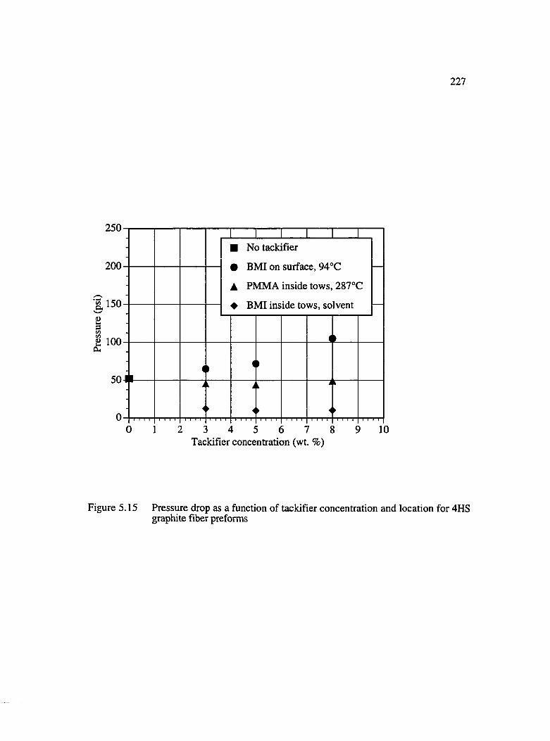
227

250

200

150

I 100.eu

50

0

I I I .. J. I ..I■ No tackifier

• BMI on surface, 94°C

▲ PMMA inside tows, 287°C

♦ BMI inside tows, solvent

5 6 7Tackifier concentration (wt. %)

10

Figure 5.15 Pressure drop as a function of tackifier concentration and location for 4HS graphite fiber preforms

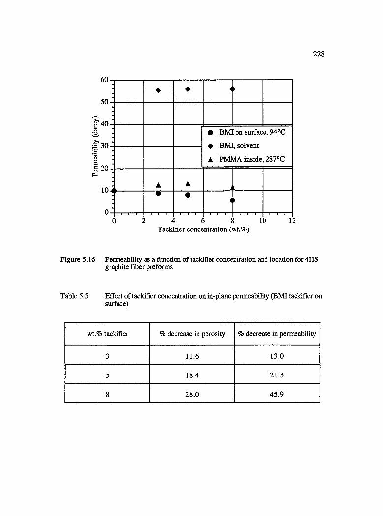
228

60

50

2 40IS 30

1eu

20

10

0

♦ <►

# BMI on surface, 94°C

A PMIklA inside 287°C

▲ A i 1'# •

1

0 :i (5 { 10 1Tackifier concentration (wt.%)

Figure 5.16 Permeability as a function of tackifier concentration and location for 4HS graphite fiber preforms

Table 5.5 Effect of tackifier concentration on in-plane permeability (BMI tackifier on surface)

wt.% tackifier % decrease in porosity % decrease in permeability

3 11.6 13.0

5 18.4 21.3

8 28.0 45.9

229

5 .3.2 Ejfect o f Tackifier on Fiber Wetting in Woven Preforms

5.3.2.1 Wicking Experiments

Dynamic Contact Angle Analyzer (DCA) described in Chapter III was used to study the

effect of tackifier application technique (powder vs. solvent) on wetting characteristics of

tackified preforms. This was done by comparing the amount of liquid retained by the fiber

preform treated by the two different techniques.

In these experiments, first a small piece of the fiber preform was placed on the balance loop

of the DCA. Next, the test liquid contained in a beaker resting on a traveling stage is

brought in contact with the edge of the preform. As the liquid starts to wick in, the force

changes are recorded on a computer. After the force reached the steady state, the fiber mat

was separated from the liquid. The force dropped until a steady state was achieved. Since

the initial weight of the preform was tared, the force readings recorded are the sum of the

Wilhelmy wetting force and the weight of the liquid wicked into the fiber tows. The final

steady state weight indicates the total liquid retention. Figure 5.17 shows the curves for

change in weight with time for the two samples. The segment AB is the baseline prior to

the contact between the fiber and the liquid. The segment BC shows an increase in force

readings. This is mostly due to wetting, with some contribution from liquid uptake. The

segment CD shows a slower change in force until it reaches a steady state. The segment

DE records the separation process of the wetted fabric from the liquid. The slight increase

in the force detection during this process was attributed to the change in the fabric edge

configuration and/or change in the contact angle at the meniscus. At point F, the fabric is

completely separated from the liquid. The residual weight recorded indicates the total liquid

retention (W,) in the fabric.

230

2003% in solvent180-3% powder

160-

140-

120 -

% 100- Ü :^ 8 0 -

6 0 -

4 0 -

20 -

0 500 1000 1500 2000 2500 3000 3500Time (sec.)

Figure 5.17 Comparison of wicking behavior of solvent and powder coated 4HS graphite fiber preforms

231

As shown in Figure 5.17 the liquid retention for the powder technique for 3 wt.% tackified

fiber preforms is greater than for the solvent technique. As liquid uptake due to wicking

occurs solely by capillary forces, the higher liquid retention in case of the powder sample

indicates more free volume in the capillaries for the liquid to wick in as compared to the

solvent sample. This is to be expected since the powder remains on the surface, while the

solvent causes the powder to go inside the fiber tows thereby blocking the interstitial

capillaries between the filaments of the fiber tows.

In order to study the effect of tackifier concentration, and the effect tackifier application

technique on wetting characteristics of fiber tows, a centrifugal device was used to

determine the relationship between capillary pressure, Pc and saturation, S. Since these

experiments involve starting with a completely wet sample, the ?c vs. S curves really

exhibit the drainage characteristics of the fiber samples rather than imbibition which occurs

during mold filling in Liquid Composite Molding. However, it has been observed by

several researchers for a wide variety of porous media, that although the magnitude of

capillary pressure at any saturation may be different for imbibition and drainage, the trend

remains the same. Thus, either curve can be used for comparative purposes. The

measurement technique and results obtained from centrifuge experiments are discussed

next.

5.3.2.2 Measurement o f Capillary pressure V5. saturation

The set up of the centrifuge device is shown in Figure 5.18 [Han, 1994]. It consists of a

metal container 44 cm in diameter and 30 cm in height mounted on a stand. The fiber

samples were placed on an aluminum beam connected to an axle which was rotated by a

multi speed motor. A wide range of angular velocities could be generated using this motor,

and the speed of rotation was measured by a Tachometer - Process Time Indicator. Fiber

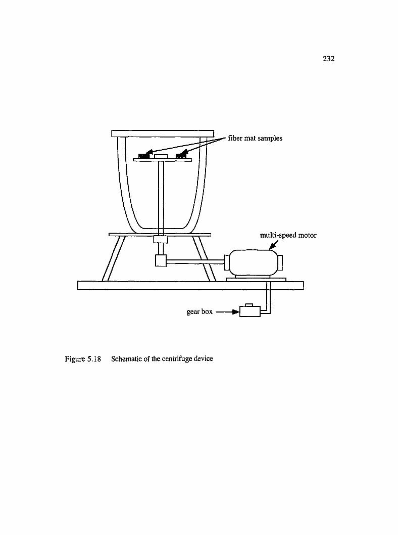
232

fiber mat samples

multi-speed motor

gear box

Figure 5.18 Schematic of the centrifuge device

233

samples were kept in an acrylic mold 2.54 cm x 2.54 cm x 0.5 cm (1 x w x t) enclosed in a

plastic box with the front end open. The actual size of the cavity was varied using spacers

depending upon the number of fiber layers and porosity. A porous tissue was placed at the

front end to collect the liquid thrown out by the centrifugal forces during the experiment.

The experimental procedure for a typical run is as follows. The number of fiber layers

required to attain the desired porosity were cut, placed inside the mold and weighed. Test

liquid was then injected into the mold till the fibers were completely saturated. The mold

with the wet fibers was weighed again to determine the weight of the liquid at 100%

saturation. The mold was placed in the plastic box and then mounted on the aluminum

beam. During rotation, the centrifugal force tries to drive the liquid out of the pores, while

the capillary pressure tries to retain it. At equilibrium the two forces are balanced. Thus,

each rotation was carried out for several minutes till equilibrium was reached. After each

rotation at successively increasing speeds, the mold was taken out and weighed to

determine the amount of liquid remaining in the fiber mat. This process was repeated at

several speeds to obtain a relationship between saturation and capillary pressure which

were calculated according to Equations 5.10 and 5.11:

' =

where

m is the mass of the liquid retained at any speed of rotation

p is the density of the lest liquid

t is the cavity thickness

(|) is the porosity

Pc = (5.11)

234where

A p is the difference in the wetting and the non-wetting fluids

oi is the angular velocity

ri and X2 are the inner and outer radii of rotation (Figure 5.19)

The porosity (<])), for the different cases was calculated using Equation 5.12:

<t> = 1

/ ( \mf m,+I P f J I p. J (5.12)(2.54)- X t

where

mf is the mass of the fiber

Pf is the density of carbon fiber (~ 1.8 g/cm^)

mt is the mass of the tackifier

Pt is the density of the tackifier (~ 1.0 g/cm^)

Equation 5.11 is based on the assumption that at any cross-section of the sample normal to

the radius of rotation, the saturation is uniform [Collins, 1961]. Figure 5.20 shows the

capillary pressure vs. saturation curves for various samples. PMMA powder was used

because previous experiments described in Chapter IV showed that it was easier to control

the location of this powder as compared to BMI tackifier. All the curves show the same

trend of non linear increase in capillary pressure with decrease in saturation. At the start of

the experiment, capillary pressure is small because the saturation is high. With increasing

speeds of rotation, the liquid first starts to come out from the larger gaps and then from the

interstitial gaps between the filaments. This is why capillary pressure increases gradually

till a saturation of about 0.8 - 0.75, and then increases rapidly as the saturation decreases

further. So although the general trend is the same, the capillary pressure at any given

saturation is different for each condition under which the samples were made. Capillary

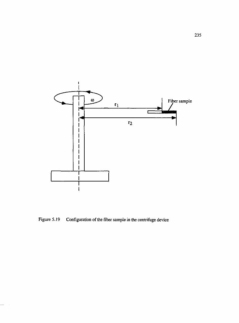
235

Fiber sample

Figure 5.19 Configuration of the fiber sample in the centrifuge device

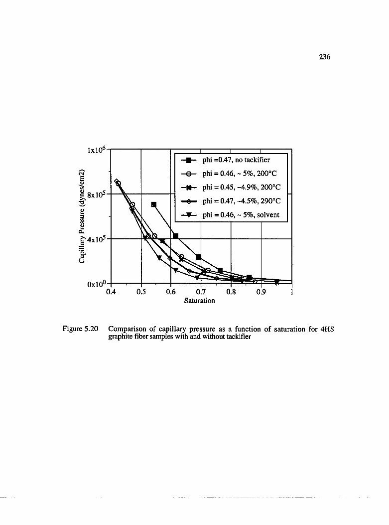
236

phi =0.47, no tackifier

phi = 0.46, - 5%, 200°C

phi = 0.45, -4.9% , 200“C

phi = 0.47, -4.5%, 290°C

phi = 0.46, - 5%, solvent

ë 8x105

\

0.6 0.7Saturation

Figure 5.20 Comparison of capillary pressure as a function o f saturation for 4HS graphite fiber samples with and without tackifier

237

pressure is the highest for the sample without any tackifier, followed by the ones in which

it remains on the surface (i.e. 200°C case), and then in which the tackifier goes inside the

tows (i.e. 290°C and solvent cases). These results indicate that since the capillary pressure

is lower, resin impregnation into fiber tows is hindered by the presence of tackifier. From

results obtained in Chapter III, it can be inferred that since the stability of a void depends

upon the relative magnitudes of hydrodynamic and capillary pressures, mobilization of

voids would be easier when the capillary pressure is lower. However, blockage of the

capillaries by the tackifier particles could provide hindrance to void movement. Thus, the

effect of both tackifier concentration and location on void formation and mobilization

should be further investigated.

CHAPTER VI

CONCLUSIONS AND RECOMMENDATIONS

6.1 Analysis of Flow Induced Voids

Air bubbles or voids are formed during the resin injection step in liquid composite molding

processes because of two simultaneous and competing flows. One is the flow through the

larger gaps between the fiber tows, and the other is the local penetration of the resin in the

fiber tows. A 2D flow visualization technique was therefore developed and successfully

implemented to observe the competing micro flows during liquid injection. From flow

visualization experiments, mechanisms of formation of macro voids and microvoids in

unidirectional stitched fiberglass preforms were proposed in this study. The results

obtained revealed that void formation during mold filling can be correlated to the relevant

processing variables by the dimensionless modified capillary number (Ca#*). Modified

capillary number depends on the liquid properties, injection flow rate, and liquid/fiber

contact angle. Large voids or macrovoids are formed between the fiber tows at low flow

rates corresponding to the capillary numbers < 10"3. Smaller voids or microvoids are

formed within the fiber tows at higher flow rates. Void formation for both axial and

transverse flows were studied. In both cases, two types of microflows are necessary for

macrovoid formation; one is fingering or the lead-lag at the flow front, and the other is the

transverse or cross flow. Mechanisms for the formation of microvoids is however

different for axial and transverse flow. During axial flow, microvoids are formed by a

'round - up' type of mechanism wherein the leading flow fronts loop back to meet the

238

239lagging flow fronts. In case of transverse flow, microvoids were formed by two types of

flow mechanisms, both of which resulted in microvoid formation across a wide range of

capillary numbers. For capillary number < ~10"2, microvoids were formed primarily due

to the lead-lag at the flow front, followed by cross-flow of the liquid leading in the stitches

into the fiber tows by capillary action. At higher capillary numbers (> ~10‘2), microvoids

were trapped mostly due to the macroflow around the fiber tow being completed before the

microflow could displace all the existing air witliin the tows.

For the same capillary number, void content was higher for transverse flow as compared to

the axial flow. Moreover, flow visualization experiments showed that for flow along the

fiber tows, minimal voids of either type were formed when the capillary number ranged

from 0.001 - ~ 0.005. However, no such process window was observed for transverse

flow. This indicates that in addition to the modified capillary number, fiber architecture and

flow pattern can also affect the selection of suitable molding conditions so as to minimize

the overall void content of a molded part. The size of trapped macro voids ranged from

IQ-l - 10 3 cm2, while that of microvoids ranged from 10"6 - lQ-4 cm2. Although,

vacuum assisted liquid injection helped to reduce the formation of both macro and

microvoids, the latter are more difficult to purge during regular mold filling.

Due to the complex nature of the microscale flow pattern, unidirectional stitched fiberglass

mat was chosen because of its simple architecture. However, as stated eai lier in Chapter 1,

fiber reinforcements with different structures and materials are being used in actual

production of composite parts, and is worth to carry out visualization experiments with

other fiber types in order to have a more complete database. Also, since the current

visualization set-up is limited to only one or two layers of the preform, a 3D visualization

and imaging technique should be developed to obtain information about formation of voids

in thicker fiber preforms. One approach for doing so would be to scan through the

240thickness of the preform using a laser source, much like the confocal scanning optical

microscopy.

Dynamic mechanical tests of aged composite samples showed that presence of macro and

micro voids result in reduced stiffness. Voids provide a path for diffusion of moisture

which causes plasticization of the resin matrix and degradation of the matrix/fiber interface.

Also, freeze-thaw cycling of voided composite samples showed significant microcrack

formation. Thus, it becomes imperative to minimize the formation of voids, and this

warrants a proper choice of the molding conditions. Although, the results obtained in this

study showed that voids indeed affect the properties o f the molded composite samples,

further investigation should be carried out to investigate which of the two kinds of voids

(macro or micro) have a more deteriorating effect on mechanical properties like flexural

strength and modulus, interlaminar shear and strength after impact.

6.2 Analysis of Powder Coating on Preforming and Moldability

A 4 HS type of textile reinforcement was also used in this study. The advantages of using

a woven preform includes better drapeability, and elimination of the use of stitches, a

structural inhomogeniety which results in formation of voids. The disadvantage however

is the need for considerable debulking or consolidation due to the high bulk factor. In

order to avoid high clamping pressures (one of the advantages of LCM over other

processes like SMC), a powder coating (tackifier) can be used to control deconsolidation or

springback of compressed fiber preforms. Since the current approach used in the

composite industry is to obtain "net-shaped" preforms by trial and error, which is evidently

very ineffective, the findings of this study will help in improving the understanding of the

issues involved in preforming and molding of tackified fabrics.

241The processing variables that were observed to affect dimensional changes in U-shape

bending and lateral compression of tackified preforms include powder concentration,

application technique (powder vs. solvent), location of application (between the layers vs.

within the fiber tows), and debulking temperature. A two level consolidation theory is

proposed to explain the mechanism of fiber springback, viz., interlayer consolidation or

compression of the gaps between the fiber tows, and intralayer consolidation or

compression of interstitial gaps within the fiber tows. Based on the experimental results, it

can also be hypothesized that fiber springback will occur when the force exerted by the

compressed elastic fibers upon release of an externally applied load, is greater than the

"holding" force provided by the tackifier. The latter depends upon the tackifier modulus

and the wetted surface area of the preform. Increasing the tackifier modulus and/or the area

coverage can therefore help in reducing the amount of springback. Experiments with a

reactive BMI powder and a non-reactive PMMA powder showed that area coverage can be

either interlayer or intralayer, depending upon the rheological properties of the viscoelastic

polymer melL A phenomenological approach was used in this study for springback control

under lateral compression. For a more quantitative analysis, models for increase in the area

coverage during the debulking stage and increase in the resin modulus as a function of

debulking temperature and time should be developed. For BMI resin, modeling of increase

in modulus as a function of conversion becomes quite complex due to two competing

reaction mechanisms, one leading to a linear polymer chain, and the other resulting in a

cross-linked network due to homopolymerization.

For the same tackifier concentration, better springback control is achieved from intralayer

coverage as compared to interlayer coverage. Increasing the degree of cure, and tackifier

concentration also resulted in lower springback. The drawback of advancing the chemical

reaction during the debulking stage comes from the limitations of tackifier solubility in the

incoming fresh resin during mold filling. Incomplete dissolution of the tackifier particles in

242the resin can adversely affect the mechanical properties due to residual microstresses at the

tackifier/resin interface.

Scanning electron micrographs (SEM) showed that during the debulking process, the

tackifier powder melts, coagulates and flows along the capillaries blocking the pore spaces

within the preform. Since mold filling is governed primarily by macro flow, blocking of

the larger gaps by the tackifier powder results in lower permeability or increased flow

resistance. Blocking of the interstitial pore spaces however affects fiber wettability by

lowering the capillary pressure which is a function of saturation. From results obtained in

Chapter III, it can be inferred that since the stability of a trapped void depends upon the

relative magnitudes of the hydrodynamic and capillary pressures, mobilization of

microvoids would be easier when the capillary pressure is lower. However, blockage of

the interstitial gaps could provide hindrance to void movement. Thus, it would be

interesting to further investigate how the tackifier concentration and location affects both the

formation and movement of macro and microvoids.

REFERENCES

K. J. Ahn and J. G. Seferis, Polymer Composites, 12 (3), 146, June (1991).

D. A. Babbington, J. K. Fielder, and D. P. Waszeciak, 33 ^ Annual PolyurethaneTechnical Marketing Conference, 620, Sept./Oct. (1990).

J. Barron, Dow Chemical Company, Freeport, Texas, Private Communication (1995).

G. L. Batch and S. Cuminskey, 4 5 * Annual Conference Composites Institute, The Society of Plastics Industry, Session 9-A (1990).

W. D. Bascom and J. B. Romans, Product and Development, 7 (3), 172 (1968).

E. Bayramli and R. L. Powell, Colloids and Surfaces, 56, 83 (1991).

W. Becker, SME Composites in Manufacturing, 9 (1990).

F. Brochard, Journal of Chem. Phys., 84 (8), 15 (1986)

F. W. Billmeyer, Textbook o f Polymer Science, 3rd ed., John Wiley and Sons, New York (1984).

L. R. L. Bonhomme, "Tack and Conformance o f Prepreg Tapes during Automatic Tape Layup ", M.S. Thesis, MIT, June (1986).

K. J. Bowles and S. Frimpong, Journal of Composite Materials, 26 (10), 1487 (1992).

F. Bueche, Physical properties o f polymers , Interscience publishers. New York (1962).

T. F. Butryn, 36th International SAMPE Symposium, 546 (1991).

L. Carino and H. Mollet, Powder Technology, 11, 189 (1975).

C. C. Chamis, NASA Technical Note D5367 (1969).

A. W. Chan and R. J. Morgan, SAMPE Quarterly, 23,48, April (1992).

A. W. Chan and R. J. Morgan, Proc. of 51®t SPE ANTEC, 844 (1993a).

243

244A. W. Chan and R. J. Morgan, SAMPE Quarterly, 24 (4), 49, July (1993b).

N. G. Chavka and C. F. Johnson, Proc. of a SM/ESD Adv. Composites Conference, 115 (1991).

Y. T. Chen, "Resin Transfer Molding o f Polycyanate: Chemorheology, Molding Experiment and Wetting Visualization", Ph. D., Dissertation, Department of Chemical Engineering, University of Minnesota (1993).

Y. T. Chen, H. T. Davis and C. W. Macosko, AIChE J., 41, 2261 (1995).

S. Chwastiak, Journal of Colloid and Interface Science, 42 (2), 298, February (1973).

S. J. Claus and A. C. Loos, Proc. of the American Society for Composites (1989).

R. Cochran and R. B. Pipes, 23rd International SAMPE Technical Conference, 1169(1991).

R. E. Collins, Flow o f Fluids through Porous Materials , Van Nostrand, Reinhold Publishing Corporation, New York (1961).

A. T. Corey, Mechanics o f Immiscible fluids in porous media. Water Resources Publishers (1986).

W. P. Cox and E. H. Merz Jr., Journal of Polymer Science, 28, 619 (1958).

S. G. Damani and L. J. Lee, Polymer Composites, 11 (3), 174 (1990).

R. Dave and S. Houle, Proc. of the American Society for Composites, 5 ^h Technical Conference, 539, June (1990).

J. Domingue, "The Phenomena o f Contact Angle Hysteresis", Cahn's Manual,(1992).

S. Dong and R. Gauvin, Polymer Composites, 14 (5), 414, October (1993).

F. A. L. Dullien, Porous media, flu id transport and pore structure, 2 ed.. Academic Press Inc., (1992).

J. J. Elmendorp and F. During, Proc. of 4 9 *h SPE ANTEC, 1361 (1991).

T. C. Fan, SAMPE Quarterly, 29 (4), 15, July/Aug. (1993).

S. M. Feldgoise, F. Foley, D. Martin and J. Bohan, 23^^ Intn'l SAMPE Technical Conference, 259, October (1991).

R. Gauvin and M. Chibani, 43^^ Annual Conference Composites Institute, The Society of Plastics Industry, Session 22-C (1988).

245

S. R. Ghiorse, SAMPE Quarterly, 24 (2), pp. 54, January (1993).

A. G. Gibson and J. A. Manson, Composites Manufacturing 3 (4), 223 (1992).

L. B. Greszczuk, Annual Conference Composites Institute, The Society of Plastics Industry, 22 (1967)

F. J. Guild and J. Summerscales, Composites, 24 (5), 383 (1993).

T. G. Gutowski, SAMPE Quarterly, 16 (4), 58 (1985).

T. G. Gutowski and L. Bonhomme, Journal of Composite Materials, 22, 204 (1988).

K. Han, Ph. D. Dissertation, The Ohio State University, Columbus, Ohio (1994).

M. J. Hannon, D. Rhum and K. F. Wissbrun, Journal of Coatings Technology, 48 (621), 42(1984).

R. S. Hansen, SME Technical Papers EM 90-214 (1990).

J. S. Hayward and B. Harris, Composites Manufacturing, 1 (3), 161, Sept. (1990).

High Performance Composites, 6, Nov ./Dec. (1993).

D. E. Hirt, J. M. Marchello and R. M. Baucom, 22nd International SAMPE Technical Conference, 360 (1990).

K. T. Hodgson and J. C. Berg, Journal of Colloid and Interface Science, 121 (1), 22 Jan. (1988).

Y. L. Hsieh and B. Yu, Textile Research Journal, 62 (11), 677 (1992).

D. Hsu, Proc. of the 46th sPE ANTEC, 1273 (1988).

M. K. Hugh, J. M. Marchello, R. M. Baucom and N. J. Johnston, 25th International SAPilPE Technical Conference, 812 (1993).

de. G. Jager, "Method and apparatus for applying powdered materials to filaments", WO 87/00563 (1987).

C. F. Johnson, Engineered Materials Handbook, 1, ASM, 564 (1987).

C. F. Johnson, Composite Materials Technology - Processes and properties , Ch 5, P. K. Mallick and S. Newman, Ed., Hanser Publishers, New York (1990).

N. C. W. Judd and W. W. Wright, SAMPE Journal, 14 (1), 10, Jan./Feb. (1978).

Y. K. Kamath, C. J. Dansizer, S. Hornsby and H. D. Weigmann, Textile Research Journal, 205, April (1987).

246J. L. Kittleson and S. C. Hackett, 39th International SAMPE Symposium, 83

(1994).

B. J. Kohn, A. G. Sands and R. C. Clark, Product and Development, 7 (3), 178 (1968).

Peter G. de Lange, Journal of Coatings Technology, 56 (717), 23 (1984).

B. K. Larson and L T. Drzal, Proc. of 50^^ SPE ANTEC, 752 (1992).

L. J. Lee, Fundamentals of reaction injection molding, Ch 4, 4 (2), Comprehensive Polymer Science, Pergamom Press (1989).

W. J. Lee and J. C. Seferis, Polymer Composites, 9 (1), 36 Feb. (1988).

D. Li, and A. W. Neumann, Journal of Colloid and Interface Science, 148 (1), 190, Jan. (1992).

T. S. Lundstrom, B. R. Gebart and C. Y. Lundemo, 4 7 ^ Annual Conference Composites Institute, The Society of Plastics Industry, Session 16-F, 1(1992).

J. Madge, General Electric Aircraft Engines Division, Cincinnati, OH, Private Communication (1994).

A. D. Mahale, R. K. Prud'homme and L. Rebenfeld, Polymer Engineering andScience, 32 (5), 319 (1992).

Cahn's Instruction Manual, Cahn Instruments, Inc., Cerritos, CA (1993).

J. M. Margolis, Proc. of 43*' Annual SPI Composites Institute Conf., Session 9-E (1988).

G. Maymon, R. P. Briley and L. W. Rehfield, Advanced Composite Materials - Environmental Effects , ASTM STP 658, 221 (1978).

V. P. McConnell, High Performance Composites, 22, Nov./Dec. (1993).

MDSC 2910, Modulated Differential Scanning Calorimeter Operator's Manual, TA Instruments, New Castle, Delaware (1993).

J. Meissonnier, "Processing Optimization o f Bismaleimide Matrix Composites", M.S. Thesis, University of Washington, January (1988).

B. L. Metcalfe and R. J. Wilson, Journal of Material Science Letters, 4, 235(1985).

S. Middleman, The Flow of High Polymers , Chapter 5, Interscience, N. Y. (1968)

B. Miller, Surface Characteristics o f Fibers and Textiles, Part II, Ch. 11,417, M. J. Schick, Ed., Marcel Dekker (1977).

247C. W. Mocosko, RIM : Fundamentals o f reaction injection molding, Hanser

Publisher (1989).

Modem Plastics, 24, January (1994).

R. Monks, Plastic Technology, 40, March (1993).

K. H. Moritz, The Composites Industry - An Overview (1993).

I. Muzzi, B. Varrughese and P. H. Yang, SPE ANTEC Proceedings, 48, (1990).

J. V. Noyés and B. H. Jones, AIAA, 68 (1968).

Y. Ohmura, Takao Uematsu, Tohru Imanara, Shoichi Sato, Takayoshi Imai, and Naomi Yamashita, Proc. of the 9^^ ASM/ESD Advanced Composite Conference, 69 (1993).

J. R. Olsen, D. E. Day and J. G. Stoffer, Journal of Composite Materials, 26 (8), 1181 (1992).

R. S. Pamas and F. J. Phelan Jr., SAMPE Quarterly, 53, Jan. (1991).

N. Patel, V. Rohatgi and L. J. Lee, Proc. of 49^^ Annual SPI Composites Institute Conf., Session 10-D (1994).

M. J. Perry, Ph. D. Dissertation, The Ohio State University, Columbus, Ohio(1993).

R. C. Peterson and R. E. Robertson, Proc. of the 7*^ ASM/ESD Advanced Composite Conference, 203 (1992).

R. C. Peterson and R. E. Robertson, Proc. of the 8^h ASM/ESD Advanced Composite Conference, 63 (1992).

E. P. Plueddemann, Ed., Composite materials: interfaces in Polymer Matrix Composites , vol. 6, Academic Press (1974).

R. V. Price, "Production of impregnated roving", US Patent 3742105 (1973).

Rheometrics Dynamic Analyzer, RDA II Owners Manual, Rheometrics Inc., Piscataway, NJ (1990).

V. Rohatgi, "Influence o f Material and Processing Variables on Resin - Fiber Interface in Glass Fiber Reinforced Polymeric Composites", M.S. Thesis, Department of Chemical Engineering, The Ohio State University, (1991).

V. Rohatgi, N. Patel and L. J. Lee, ERC Report ERC/NSM-P-94-19, May (1994).

A. J. Salem and R. S. Pamas, Proc. American Soc. Composites, 1012 (1991).

248M. M. Schwartz, Composite Materials Handbook, Ch 4, McGraw Hill Publication

(1984).

J. C. Seferis and J. Meissonnier, SAMPE Quarterly, 20 (3), 55 (1989).

A. Shafi, Dow Chemical Company, Freeport, Texas, Private Communication,(1994).

D. J. Shaw, Introduction to Colloid and Surface Chemistry, 3 ^ éd., Butterworths,(1980).

K. Shields and J. Colton, Polymer Composites, 14 (4), 341, Aug. (1993).

L. Skartsis, B. Khomami and J. L. Kardos, SAMPE Journal, 28 (5), 19, Sept./Oct. (1992).

R. Srinivasan, T. J. Wang and L. J. Lee, SPE ANTEC Proceedings, 53, (1995).

W. R. Stabler, G. B. Tatterson, R. L. Sadler and A. H. M. El-Sheikh, SAMPE Quarterly, 23 (2), 38 (1992).

E. B. Stark and W. V. Beitigam, Engineered Materials Handbook, 1, ASM, 168(1987).

D. Stover, High Performance Composites, 38, Nov. / Dec. (1993a).

D. Stover, High Performance Composites, 54, Sept./Oct. (1993b).

A. B. Strong, Fundamentals o f Composite Manufacturing: Materials, Methods and Applications, Society of Manufacturing Engineers, (1989).

J. L. Thomason and A. Knoester, Journal of Material Science Letters, 9, 258 (1990).

J. L. Throne and M.S. Soh, 35th International SAMPE Symposium, 2086 (1990).

A. V. Tungare and G. C. Martin, Journal of Applied Polymer Science, 46, 1125(1992).

A. V. Tungare and G. C. Martin, Polymer Engineering and Science, 33 (10), 614(1993).

A. M. Vodermayer, J. C. Kaerger and G. Hinrichsen, Composites Manufacturing, 4 (3), 123 (1993).

J. F. Voit and J. C. Seferis, Journal of Applied Polymer Science, 34, 1459 (1987).

T. J. Wang, C. H. Wu and L. J. Lee, Polymer Composites, 15 (4), 278 (1994).

V. Wigotsky, Plastics Engineering, 23, Sept. (1989).

249

E. G. Wolff, SAMPE Journal, 29 (3), 11, May/June (1993).

A.S. Wood, Modem Plastics, 50, October (1990).

A.S. Wood, Modem Plastics, 46, October (1988).

C. H. Wu, Ph. D. Dissertation, The Ohio State University, Columbus, Ohio (1995).

APPENDIX A

O PERATIO N A L PROCEDURE FOR IN-PLANE PERM EA BILITY

M EASUREM EN TS

250

251

A .l In-Plane Permeability Measurements

The following sequence of steps describe the procedure to be followed during a permeability experiment (see Figure B1 for details):

1) Degass completely the liquid to be used to remove any air bubbles or trapped volatiles. Turn on the INSTRON at least 30 minutes prior to starting the experiment. This is the recommended warm-up period.

2) Close valves V2 and V3, and open valves VI and V4.

3) Turn on the oil pump and let it circulate through the hydraulic system for 2 minutes.

4) After about two minutes of circulation, turn off the pump. Close valve VI and move the piston rod to the lowest position in order to drive out all the air bubbles in the hydraulic cylinder.

5) Repeat steps 2-4 several times until no air bubbles are observed.

6) With the piston in the lowest position, close valve V4.

7) Open valve V5 and turn on the vacuum pump. Then close valve V5 andopen valve V3 slowly to its maximum position. Hold the vacuum level at more than 28" for about 1 minute to purge all the air from the connecting tubings.

8) Close valve V3, open valve V5 and turn off the vacuum pump.

9) Set the upper and lower crosshead limit stops at appropriate positions.

10) Move the crosshead to the upper position.

252

11) Open valve VI and the oil pump. After the hydraulic cylinder is full of oil and the piston does not rise any further, turn off the oil pump. Close valveVI.

12) Move the crosshead down till it almost touches the piston rod.

13) Open valve V2 and let the oil flow through the inlet by moving the crosshead against the piston of the cylinder. This is done to purge any remaining air in the system. When no air bubbles are observed, stop the oil flow and wipe off the mold.

14) Set the desired velocity of the crosshead on the INS TRON panel.

15) Place the fiber sample into the mold. Close the mold and then tighten the bolts evenly so that the thickness of the mold is the same as that without the fiber sample. A vernier caliper can be used to check the thickness before and after loading the fiber sample. It is time now to start the experiment.

16) Watch closely the increase in pressure as the experiment progresses. If the pressure readings get close to the upper limit of pressure transducer range, change the velocity of the crosshead to a lower value to reduce the pressure drop, or stop the experiment by pressing the STOP button on the INSTRON panel.

17) Repeat liquid injections if "wet-fiber" permeability values are required.

APPENDIX B

FLEX URAL PRO PERTIES O F TA CK IFIED (1 wt. % ) BM I RESIN

253

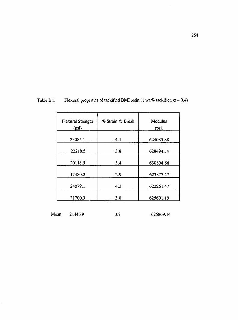
254

Table B. 1 Flexural properties of tackified BMI resin (1 wt.% tackifier, a ~ 0.4)

Flexural Strength (psi)

% Strain @ Break Modulus(psi)

23085.1 4.1 624085.88

22218.5 3.8 628494.34

20118.5 3.4 630894.66

17480.2 2.9 623877.27

24079.1 4.3 622261.47

21700.3 3.8 625601.19

Mean: 21446.9 3.7 625869.14

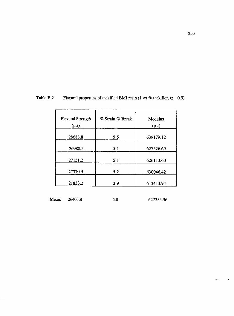
255

Table B.2 Flexural properties of tackified BMI resin (1 wt.% tackifier, a ~ 0.5)

Flexural Strength (psi)

% Strain @ Break Modulus(psi)

28683.8 5.5 639179.12

26980.5 5.1 627526.69

27151.2 5.1 626113.60

27370.5 5.2 630046.42

21833.2 3.9 613413.94

Mean: 26403.8 5.0 627255.96

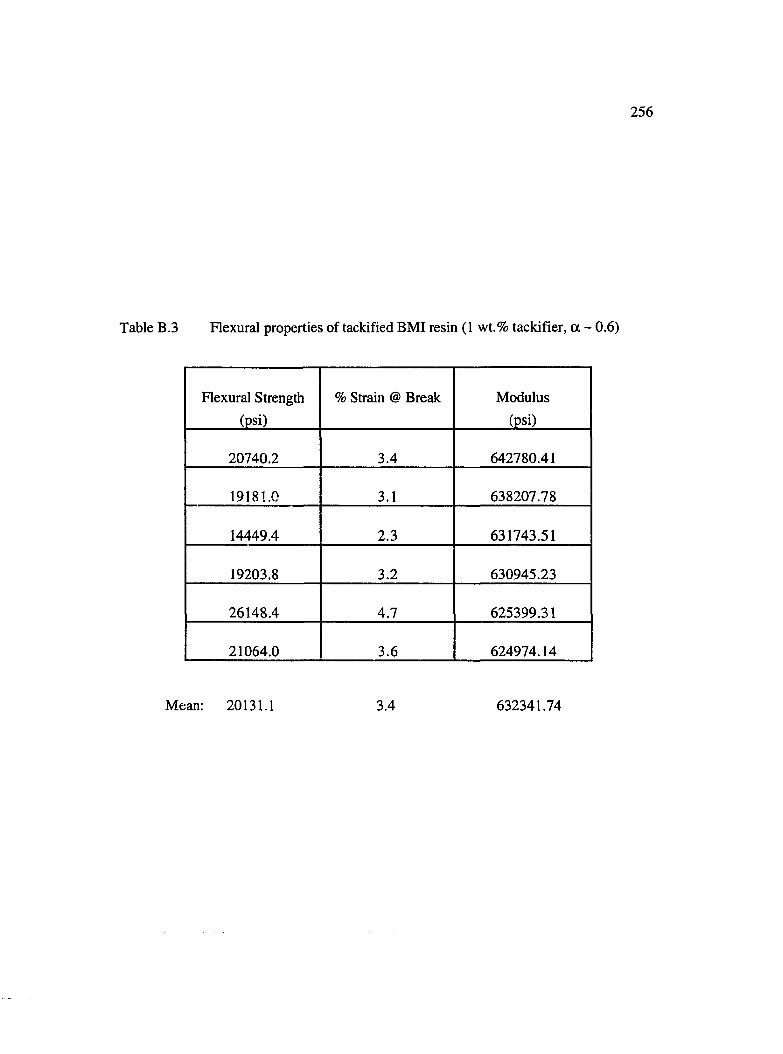
256

Table B.3 Flexural properties of tackified BMI resin (1 wt.% tackifier, a ~ 0.6)

Flexural Strength (psi)

% Strain @ Break Modulus

(psi)

20740.2 3.4 642780.41

19181.0 3.1 638207.78

14449.4 2.3 631743.51

19203.8 3.2 630945.23

26148.4 4.7 625399.31

21064.0 3.6 624974.14

Mean: 20131.1 3.4 632341.74