Accepted Manuscript

Multi-Objective Test Case Prioritization in Highly ConfigurableSystems: A Case Study

Jose A. Parejo, Ana B. Sanchez, Sergio Segura,Antonio Ruiz-Cortes, Roberto E. Lopez-Herrejon, Alexander Egyed

PII: S0164-1212(16)30193-5DOI: 10.1016/j.jss.2016.09.045Reference: JSS 9857

To appear in: The Journal of Systems & Software

Received date: 23 December 2015Revised date: 8 September 2016Accepted date: 25 September 2016

Please cite this article as: Jose A. Parejo, Ana B. Sanchez, Sergio Segura, Antonio Ruiz-Cortes,Roberto E. Lopez-Herrejon, Alexander Egyed, Multi-Objective Test Case Prioritization in HighlyConfigurable Systems: A Case Study, The Journal of Systems & Software (2016), doi:10.1016/j.jss.2016.09.045

This is a PDF file of an unedited manuscript that has been accepted for publication. As a serviceto our customers we are providing this early version of the manuscript. The manuscript will undergocopyediting, typesetting, and review of the resulting proof before it is published in its final form. Pleasenote that during the production process errors may be discovered which could affect the content, andall legal disclaimers that apply to the journal pertain.

ACCEPTED MANUSCRIPT

ACCEPTED MANUSCRIP

T

Highlights

• A multi-objective test case prioritization real-worldcase study is presented

• Seven objective functions based on functional andnon-functional data are proposed

• Comparison of the effectiveness of 63 combinationsof up to three objectives

• NSGA-II evolutionary algorithm to solve the multi-objective prioritization problem

• Multi-objective prioritization is more effective thanmono-objective approaches

1

ACCEPTED MANUSCRIPT

ACCEPTED MANUSCRIP

T

Multi-Objective Test Case Prioritization in Highly Configurable Systems:A Case Study

Jose A. Parejoa, Ana B. Sancheza, Sergio Seguraa, Antonio Ruiz-Cortesa, Roberto E. Lopez-Herrejonb, AlexanderEgyedb

aETS Ingenierıa Informatica Universidad de Sevilla, SpainbInstitute for Software System Engineering Johannes Kepler University, Austria

Abstract

Test case prioritization schedules test cases for execution in an order that attempts to accelerate the detection offaults. The order of test cases is determined by prioritization objectives such as covering code or critical components asrapidly as possible. The importance of this technique has been recognized in the context of Highly-Configurable Systems(HCSs), where the potentially huge number of configurations makes testing extremely challenging. However, currentapproaches for test case prioritization in HCSs suffer from two main limitations. First, the prioritization is usually drivenby a single objective which neglects the potential benefits of combining multiple criteria to guide the detection of faults.Second, instead of using industry-strength case studies, evaluations are conducted using synthetic data, which providesno information about the effectiveness of different prioritization objectives. In this paper, we address both limitationsby studying 63 combinations of up to three prioritization objectives in accelerating the detection of faults in the Drupalframework. Results show that non–functional properties such as the number of changes in the features are more effectivethan functional metrics extracted from the configuration model. Results also suggest that multi-objective prioritizationtypically results in faster fault detection than mono-objective prioritization.

1. Introduction

Highly-Configurable Systems (HCSs) provide a com-mon core functionality and a set of optional features totailor variants of the system according to a given set of re-quirements [9, 69]. For instance, operating systems such asLinux or eCos are examples of HCSs where functionalityis added or removed by installing and uninstalling pack-ages, e.g. Debian Wheezy offers more than 37,000 availablepackages [13]. Content management systems are also ex-amples of HCSs were configuration is managed in termsof modules, e.g. the e-commerce platform Prestashop hasmore than 3,500 modules and visual templates [63]. Re-cently, cloud applications are also being presented as con-figurable systems, e.g. the Amazon Elastic Compute Cloud(EC2) service offers 1,758 different possible configurations[27].

HCSs are usually represented in terms of features. Afeature depicts a choice to include a certain functionalityin a system configuration [69]. It is common that not allcombinations of features are allowed or meaningful. In thiscase, additional constraints are defined between them, nor-mally using a variability model, such as a feature model.

Email addresses: japarejo@us.es (Jose A. Parejo),anabsanchez@us.es (Ana B. Sanchez), sergiosegura@us.es (SergioSegura), aruiz@us.es (Antonio Ruiz-Cortes),roberto.lopez@jku.at (Roberto E. Lopez-Herrejon),alexander.egyed@jku.at (Alexander Egyed)

A feature model represents all the possible configurationsof the HCS in terms of features and constraints amongthem [40]. A configuration is a valid composition of fea-tures satisfying all the constraints. Figure 1 depicts afeature model representing a simplified family of mobilephones. The model illustrates how features and relation-ships among them are used to specify the commonalitiesand variabilities of the mobile phones. The following setof features represents a valid configuration of the model:{Mobile Phone, Calls, Screen, HD, GPS, Media, Camera}.

HCS testing is about deriving a set of configurationsand testing each configuration [54]. In this context, a testcase is defined as a configuration of the HCS under test(i.e. a set of features) and a test suite is a set of test cases[54]. Henceforth, the terms test case and configurationare used indistinctly. Testing HCSs is extremely challeng-ing due to the potentially huge number of configurationsunder test. As an example, Eclipse [13] has more than1,650 plugins that can be combined (with restrictions) toform millions of different configurations of the developmentenvironment. This makes exhaustive testing of HCSs in-feasible, that is, testing every single configuration is tooexpensive in general. Also, even when a manageable setof configurations is available, testing is irremediably lim-ited by time and budget constraints which requires makingtough decisions with the goal of finding as many faults aspossible.

Typical approaches for HCS testing use a model-based

Preprint submitted to Elsevier Monday 26th September, 2016

ACCEPTED MANUSCRIPT

ACCEPTED MANUSCRIP

T

approach, that is, they take an input feature model rep-resenting the HCS and return a valid set of feature con-figurations to be tested, i.e. a test suite. In particular,two main strategies have been adopted: test case selectionand test case prioritization. Test case selection reducesthe test space by selecting an effective and manageablesubset of configurations to be tested [16, 34, 50]. Test caseprioritization schedules test cases for execution in an or-der that attempts to increase their effectiveness at meetingsome performance goal, typically detecting faults as soonas possible [2, 45, 75]. Both strategies are complementaryand are often combined.

Test case prioritization in HCSs can be driven by differ-ent functional and non–functional objectives. Functionalprioritization objectives are those based on the functionalfeatures of the system and their interactions. Some exam-ples are those based on combinatorial interaction testing[75], configuration dissimilarity [2, 33, 60] or feature modelcomplexity metrics [59, 60]. Non–functional prioritizationobjectives consider extra–functional information such asuser preferences [21, 39], cost [75], memory consumption[45] or execution probability [15] to find the best orderingfor test cases. In a previous work [59], we performed a pre-liminary evaluation comparing the effectiveness of severalfunctional and non–functional prioritization objectives inaccelerating the detection of faults in an HCS. Results sug-gested that non–functional properties such as the numberof changes or the number of defects in a previous versionof the system were among the most effective prioritizationcriteria.

Challenges. Current approaches for test case prioritiza-tion in HCSs follow a single objective approach [2, 39, 15,21, 33, 45, 59], that is, they either aim to maximize or min-imize an objective (e.g. feature coverage) or another (e.g.suite size) but not both at the same time. Other works[70, 75] combine several objectives into a single functionby assigning them weights proportional to their relativeimportance. While this may be acceptable in certain sce-narios, it may be unrealistic in others where users maywish to study the trade-offs among several objectives [44].Thus, the potential benefits of optimizing multiple pri-oritization objectives simultaneously, both functional andnon–functional, is a topic that remains unexplored.

A further challenge is related to the lack of HCSs withavailable code, variability models and fault reports thatcan be used to assess the effectiveness of testing approaches.As a result, authors typically evaluate their contributionsin terms of performance (e.g. execution time) using syn-thetic feature models and data [2, 34, 56, 76]. This in-troduces significant threats to validity, limit the scope oftheir conclusions and, more importantly, it raises questionsregarding the fault–detection effectiveness of the differentalgorithms and prioritization objectives.

Contributions. In this paper, we present a case studyon multi–objective test case prioritization in HCSs. In

particular, we model test case prioritization in HCSs asa multi–objective optimization problem, and we present asearch–based algorithm to solve it based on the classicalNSGA-II evolutionary algorithm. Additionally, we presentseven objective functions based on both functional andnon–functional properties of the HCS under test. Then,we report a comparison of 63 different combinations of upto three objectives in accelerating the detection of faults inthe Drupal framework. Drupal is a highly modular opensource web content management system for which we havemined a feature model and extracted real data from itsissue tracking system and Git repository [59]. Results re-veal that non–functional properties, such as the number ofdefects in previous versions of the system, accelerate thedetection of faults more effectively than functional prop-erties extracted from the feature model. Results also sug-gest that multi-objective prioritization is more effective ataccelerating the detection of faults than mono-objectiveprioritization.

The rest of the paper is structured as follows: Section2 introduces the concepts of feature models and multi-objective evolutionary algorithms. Section 3 presents theDrupal case study used to perform this work. In Section4 and Section 5 we respectively describe the overview anddefinition of our approach and the multi-objective opti-mization algorithm proposed. Section 6 defines seven ob-jective functions for HCSs based on functional and non-functional goals. The evaluation of our approach is de-scribed in Section 7. Section 8 presents the threats tovalidity of our work. The related work is discussed in Sec-tion 9. Finally, we summarize our conclusions and outlineour future work in Section 10.

2. Background

2.1. Feature Models

A feature model defines all the possible configurationsof a system or family of related systems [6, 40]. A featuremodel is visually represented as a tree–like structure inwhich nodes represent features, and edges denote the re-lationships among them. A feature can be defined as anyincrement in the functionality of the system [5]. A con-figuration of the system is composed of a set of featuressatisfying all the constraints of the model. Figure 1 showsa feature model describing a simplified family of mobilephones. The hierarchical relationship among features canbe divided into:

• Mandatory. If a feature has a mandatory relation-ship with its parent feature, it must be included inall the configurations in which its parent feature ap-pears. In Figure 1, all mobile phones must providesupport for Calls.

• Optional. If a feature has an optional relationshipwith its parent feature, it can be optionally included

3

ACCEPTED MANUSCRIPT

ACCEPTED MANUSCRIP

T

Figure 1: Mobile phone feature model

in all the configurations including its parent feature.For example, GPS is defined as an optional feature ofmobile phones.

• Alternative. A set of child features has an alterna-tive relationship with their parent feature when onlyone of them can be selected when its parent feature ispart of the configuration. In Figure 1, mobile phonescan provide support for Basic or HD (High Defini-tion) screen, but not both of them at the same time.

• Or. A set of child features has an or-relationshipwith their parent when one or more of them can beincluded in the configurations in which its parent fea-ture appears. In Figure 1, software for mobile phonescan provide support for Camera, MP3 or both in thesame configuration.

In addition to the hierarchical relationships betweenfeatures, a feature model can also contain cross-tree con-straints. These are usually of the form:

• Requires. If a feature A requires a feature B, theinclusion of A in a configuration implies the inclu-sion of B in such configuration. In Figure 1, mobilephones including the feature Camera must includesupport for a HD screen.

• Excludes. If a feature A excludes a feature B, bothfeatures cannot appear in the same configuration.

The following is a sample configuration derived fromthe feature model in Figure 1: {Mobile Phone, Calls,Screen, HD, Media, Camera}. This configuration includesall the mandatory features (Mobile Phone, Calls, Screen)and some extra features (HD, Media, Camera) meeting all

Feature Changes Faults Size

Basic 1 0 270Calls 6 10 1,000Camera 11 8 680GPS 8 6 460HD 3 3 510Media 9 5 1,100MP3 11 8 390Screen 2 4 930

Table 1: Mobile phone feature attributes

the constraints of the model, e.g. Camera requires HD. Fea-ture models can be automatically analysed to extract allits possible configurations or to determine whether a givenconfiguration is valid (it fulfils all the constraints of themodel), among other analysis operations [6]. Some toolsupporting the analysis of feature models are FaMa [24],SPLAR [53] and FeatureIDE [66].

Feature models can be extended with additional infor-mation by means of feature attributes, these are called at-tributed or extended feature models [6]. Feature attributesare often defined as tuples < name, value > specifyingnon–functional information of features such as cost or mem-ory consumption. As an example, Table 1 depicts threedifferent feature attributes (number of changes, number offaults and lines of code) and their values on the featuresof the model in Figure 1.

Feature models are often used to represent the testspace of an HCS where each configuration of the modelrepresents a potential test case. Since typical HCSs canhave thousands or even millions of different configurations,several sampling techniques have been proposed to reducethe number of configurations to be tested (e.g. [46, 50,55]). Salient among them is pairwise testing whose goal isto select test suites that contain all possible combinationsof pairs of features [46]. As an example, Table 3 shows theset of configurations obtained when applying pairwise test-ing to the model in Figure 1. The test suite is reduced from13 (total number of configurations of the feature model) tofive in the pairwise suite. Once a set of configurations areselected for testing, their behaviour has to be tested usingstandard testing mechanisms, e.g. executable unit tests.However, in this article we focus only on the first step:obtaining a set of high-level test cases respect to differenttesting objectives. In Section 4 we present in further detailthe role of feature models in our work.

2.2. Multi–objective evolutionary algorithms

Evolutionary algorithms are a widely used strategy tosolve multi–objective optimization problems. These algo-rithms manage a set of candidate solutions to an optimiza-tion problem that are combined and modified iteratively toobtain better solutions. This process simulates the natu-ral selection of the better adapted individuals that surviveand generate offspring improving species. In evolution-

4

ACCEPTED MANUSCRIPT

ACCEPTED MANUSCRIP

T

Figure 2: Working scheme of evolutionary algorithm

ary algorithms each solution is referred to as individualor chromosome, and objectives are referred to as fitnessfunctions.

The working scheme of an evolutionary algorithm is de-picted in Figure 2. Initialization generates the set of indi-viduals that the algorithm will use as starting point. Suchinitial population is usually generated randomly. Next,the fitness functions are used to assess the individuals. Inorder to create offspring, individuals need to be encoded,expressing its characteristics in a form that facilitates itsmanipulation during the rest of the algorithm. Then, themain loop of the evolutionary algorithm is executed untilmeeting a termination criterion as follows. First, individu-als are selected from current population in order to createnew offspring. In this process, better individuals usuallyhave higher probability of being selected resembling thenatural evolution where stronger individuals have morechances of reproduction. Next, crossover is performed tocombine the characteristics of a pair of the chosen individ-uals to produce new ones in an analogous way to biologicalreproduction. Crossover mechanisms depend strongly onthe scheme used for the encoding. Mutation generatesrandom changes on the new individuals. Changes are per-formed with certain probability where small modificationsare more likely than larger ones. In order to evaluate thefitness of new and modified individuals, decoding is per-formed and fitness functions are evaluated. Finally, thenext population is conformed in such a way that individu-als with better fitness values are more likely to remain inthe next population.

Multi–Objective Evolutionary Algorithms (MOEAs) area specific type of evolutionary algorithm where more thanone objective are optimized simultaneously. However, ex-cept in trivial systems, there rarely exist a single solutionthat simultaneously optimizes all the objectives. In thatcase, the objectives are said to be conflicting, and there ex-ists a (possibly infinite) number of so-called Pareto optimalsolutions. A solution is said to be a Pareto optimal (a.k.a.non-dominated) if none of the objectives can be improvedwithout degrading some of the others objectives. Analo-gously, the solutions where all the objectives can be im-proved are referred to as dominated solutions. The surfaceobtained from connecting all the Pareto optimal solutionsis the so-called Pareto Front. Among the many MOEAsproposed in the literature, the Non-dominated Sorting Ge-netic Algorithm-II (NSGA-II) [12] has become very popu-lar due to its effectiveness in many of the benchmarks inmulti–objective optimization [11, 81].

3. The Drupal case study

In this section, we present the Drupal case study fullyreported by the authors in a previous work [59]. Drupalis a highly modular open source web content managementframework written in PHP [8, 67]. This tool can be usedto build a variety of websites including internet portals,e-commerce applications and online newspapers [67]. Dru-pal has more than 30,000 modules that can be composedto form valid configurations of the system. The size ofthe Drupal community (more than 630,000 users and de-velopers) together with its extensive documentation arestrengths to choose this framework as our empirical casestudy. More importantly, the Drupal Git repository andthe Drupal issue tracking systems are publicly availablesources of valuable functional and non-functional informa-tion about the framework and its modules.

Figure 3 depicts the feature model of Drupal v7.23.Nodes in the tree represent features where a feature cor-responds to a Drupal module. A module is a collection offunctions that provides certain functionality to the system.Some modules extend the functionality of other modulesand are modelled as subfeatures, e.g. Views UI extendsthe functionality of Views. The feature model includesthe core modules of Drupal, modelled as mandatory fea-tures, plus some optional modules, modelled as optionalfeatures. In addition, the cross-tree constraints of the fea-tures in the model are depicted in Figure 3. These areof the form X requires Y, which means that configurationsincluding the feature X must also include the feature Y. ADrupal configuration is a combination of features consis-tent with the hierarchical and cross-tree constraints of themodel. In total, the Drupal feature model has 48 features,21 non-redundant cross-tree constraints and it represents2.09E9 different configurations [59].

In this paper, we model the non-functional data fromDrupal as feature attributes, depicted in Table 2. Thesedata were obtained from the Drupal website, the Drupal

5

ACCEPTED MANUSCRIPT

ACCEPTED MANUSCRIP

T

Figure 3: Drupal feature model

Git repository and the Drupal issue tracking system [59].In particular, we use the following attributes:

• Feature size. Number of Lines of Code (LoC) of thesource code associated to the feature (blank linesand test files were excluded from the counting). Thesizes range from 284 LoC (feature Ctools custom

content) to 54,270 LoC (feature Views).

• Number of changes. Number of commits made bythe contributors to the feature in the Drupal Gitrepository1 during a period of two years, from 1 May2012 to 31 April 2014. As illustrated, the number ofchanges ranges from 0 (feature Blog) to 90 (featureBackup migrate).

• Single faults. Number of faults reported in the Dru-pal issue tracking system2. Faults were collected fortwo consecutive versions of the framework v7.22 andv7.23 in a period of two years, from 1 May 2012 to31 April 2014. For instance, we found 19 reportedbugs related to the Drupal module Taxonomy (fea-ture Taxonomy) in Drupal v7.23. The number of totalfaults ranges from 0 in features as Options to 1,091in the feature Views.

• Integration faults. List of features for which inte-gration faults have been reported in the Drupal is-sue tracking system. In total, we identified threefaults triggered by the interaction of four features,25 caused by the interaction of three features and132 faults triggered by the interaction between twofeatures. These faults have been computed on thefeatures that triggered them in Table 2. For in-stance, the fault caused by the interaction of Blog

and Entity API is computed as one integration faultin the feature Blog and one integration fault in thefeature Entity API. We refer the reader to [59] fordetailed information about the bug mining processin Drupal.

4. Approach overview

In this section, we define the problem addressed andour approach illustrating it with an example.

4.1. Problem

The classical problem of test case prioritization con-sists in scheduling test cases for execution in an order thatattempts to increase their effectiveness at meeting someperformance goal [57]. A typical goal is to increase theso-called rate of fault detection, a measure of how quicklyfaults are detected during testing. In order to meet a goal,

1http://drupalcode.org/project/drupal.git2https://drupal.org/project/issues

6

ACCEPTED MANUSCRIPT

ACCEPTED MANUSCRIP

T

Feature Size ChangesFaults (v7.22) Faults (v7.23)

Single Integration Single Integration

Backup migrate 11,639 90 80 4 80 4

Blog 551 0 1 3 0 3

Captcha 3,115 15 17 1 17 1

CKEditor 13,483 40 197 11 197 9

Comment 5,627 1 10 19 13 15

Ctools 17,572 32 181 31 181 31

Ctools acc. rul. 317 0 0 0 0 0

Ctools cus. con. 284 1 10 1 10 1

Date 2,696 9 44 3 44 3

Date API 6,312 11 41 1 41 1

Date popup 792 4 30 1 30 1

Date views 2,383 6 25 1 25 1

Entity API 13,088 14 175 18 175 18

Entity tokens 327 1 22 6 22 6

Features 8,483 72 97 9 97 9

Field 8,618 7 45 18 48 17

Field SQL sto. 1,292 2 3 2 3 2

Field UI 2,996 3 13 2 11 1

File 1,894 1 10 5 11 5

Filter 4,497 3 19 5 19 5

Forum 2,849 2 6 4 5 4

Google ana. 2,274 14 11 1 11 1

Image 5,027 3 10 8 9 6

Image captcha 998 0 3 0 3 0

IMCE 3,940 9 9 5 9 5

Jquery update 50,762 1 64 12 64 12

Libraries API 1,627 7 11 0 11 0

Link 1,934 11 82 4 82 4

Node 9,945 4 26 29 24 23

Options 898 1 0 0 0 0

Panel nodes 480 2 16 1 16 1

Panels 13,390 34 87 24 87 24

Panels IPE 1,462 20 19 2 19 2

Path 1,026 20 3 1 2 1

Pathauto 3,429 2 54 9 54 9

Rules 13,830 5 240 15 240 15

Rules sch. 1,271 4 13 0 13 0

Rules UI 3,306 1 26 0 26 0

System 20,827 16 35 5 35 4

Taxonomy 5,757 4 15 22 19 22

Text 1,097 1 6 3 5 3

Token 4,580 10 37 7 37 7

User 8,419 12 20 25 19 22

Views 54,270 27 1,091 51 1,091 51

Views content 2,683 5 23 2 23 2

Views UI 782 0 12 4 12 4

WebForm 13,196 46 292 0 292 0

Total 336,025 573 3,231 3,232

Table 2: Non–functional feature attributes in Drupal

prioritization can be driven by one or more objectives. Forinstance, in order to accelerate the detection of faults, asample objective could be to increase the code coverage inthe system under test at a faster rate, under the assump-tion that faster code coverage implies faster fault detec-tion.

Inspired by the previous definition, we next define themulti-objective test case prioritization problem in HCSs.Given the set of configurations of an HCS represented bya feature model fm, we present the following definitions.

Test case. A test case is a set of features of fm, i.e.,a configuration. A test case is valid if its features satisfythe constraints represented by the feature model. As anexample the following set of features represent a valid testcase of the model presented in Figure 1: {Mobile Phone,

Calls, Screen, Basic, Media, MP3}.

Test suite. A test suite is an ordered set of test cases.Table 3 depicts a sample test suite of the model presentedin Figure 1.

Objective function. An objective function represents agoal to optimize. In this work, objective functions receivean attributed feature model (fm) and a test suite as inputsand return a numerical value measuring the quality of thesuite with respect to the optimization goal.

ID Test Case

TC1 Mobile Phone,Calls,Screen,Basic,Media,MP3TC2 Mobile Phone,Calls,Screen,HD,GPS,Media,Camera,MP3TC3 Mobile Phone,Calls,Screen,HD,Media,CameraTC4 Mobile Phone,Calls,Screen,HDTC5 Mobile Phone,Calls,Screen,Basic,GPS

Table 3: Mobile phone test suite

Given a feature model representing the HCS under testand an objective function, the problem of test case prior-itization in HCSs consists in generating a test suite thatoptimizes the target objective. This problem can be gen-eralized to a multi–objective problem by considering morethan one objective. In this case, the problem may havemore than one solution (i.e., test suites) if there not ex-ist a single solution that simultaneously optimizes all theobjectives.

4.2. Our approach

Our approach can be divided in two parts described inthe next sections.

4.2.1. Multi–objective test case prioritization

We propose to model the multi–objective test case pri-oritization problem in HCSs as a multi–objective optimiza-tion problem. Figure 4 illustrates our approach. Givenan input attributed feature model, the problem consists infinding a set of solutions (i.e., test suites) that optimize the

7

ACCEPTED MANUSCRIPT

ACCEPTED MANUSCRIP

T

Figure 4: Our multi–objective test case prioritization approach forHCSs

target objectives. In this paper, we propose seven objec-tive functions based on both functional and non–functionalproperties of the HCS under test.

4.2.2. Comparison of prioritization objectives

We propose to compare the effectiveness of differentcombinations of prioritization objectives at acceleratingthe detection of faults in the Drupal framework. To thatpurpose, we used historical data collected from a previousversion of Drupal as detailed in Section 3. In particular,we propose using the Average Percentage of Faults De-tected (APFD) [19, 57, 65] metric to check which one ofthe Pareto optimal solutions obtained accelerates the de-tection of faults more effectively. This enables the selectionof a global solution and makes it possible to identify theobjectives that lead to better test suites.

The Average Percentage of Faults Detected (APFD)[19, 57, 65] metric measures the weighted average of thepercentage of faults detected during the execution of thetest suite. To formally define APFD, let T be a test suitewhich contains n test cases, and let F be a set of m faultsrevealed by T. Let TFi be the position of the first test casein ordering T’ of T which reveals the fault i. The APFDmetric for the test suite T’ is given by the following equa-tion:

APFD = 1− TF1+TF2+...+TFn

n×m + 12n

APFD value ranges from 0 to 1. The closer the valueis to 1, the better is the fault detection rate, i.e., the fasteris the suite at detecting faults.

4.3. Illustrative example

Table 4 shows the information of four test suites, us-ing the test cases of Table 3. Note that the order of testcases matters. Along with the test cases that composeeach suite, the table also shows the value of the objec-tive functions Changes and Faults defined in Section 6.Roughly speaking, these functions measures the ability ofthe suite to test those features with a greater number ofcode changes or reported bugs as quickly as possible.

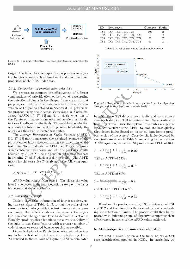
Figure 5 depicts the Pareto front obtained when try-ing to find a test suite that maximizes both objectives.As denoted in the call-out of Figure 5, TS4 is dominated

ID Test cases Changes Faults

TS1 TC4, TC1, TC5, TC3 109 49TS2 TC1, TC2, TC3, TC4, TC5 80 52TS3 TC3, TC4, TC5, TC2, TC1 77 57TS4 TC5, TC4, TC2, TC3, TC1 59 53

Table 4: A set of test suites for the mobile phone

Figure 5: Test suites of table 4 as a pareto front for objectivesChanges and Faults (both to be maximized)

by TS3, since TS3 detects more faults and covers morechanges faster; i.e. TS3 is better than TS4 according toboth objectives. Once the optimal test suites are gener-ated, we calculate their APFD to evaluate how quicklythey detect faults (based on historical data from a previ-ous version of the system). Consider the faults detected byeach test case shown in Table 5. According to the previousAPFD equation, test suite TS1 produces an APFD of 46%:

1− 2+2+4+4+1+34×6 + 1

2×4 = 0.46,

TS2 an APFD of 57%:

1− 1+1+2+3+4+55×6 + 1

2×5 = 0.57

TS3 an APFD of 80%:

1− 1+1+1+1+2+35×6 + 1

2×5 = 0.8

and TS4 an APFD of 53%:

1− 3+4+3+4+2+15×6 + 1

2×5 = 0.53

Based on the previous results, TS3 is better than TS1and TS2 and therefore it is the best solution at accelerat-ing the detection of faults. The process could then be re-peated with different groups of objectives comparing theireffectiveness in terms of the APFD values achieved.

5. Multi-objective optimization algorithm

We used a MOEA to solve the multi–objective testcase prioritization problem in HCSs. In particular, we

8

ACCEPTED MANUSCRIPT

ACCEPTED MANUSCRIP

T

Tests/Faults F1 F2 F3 F4 F5 F6

TC1 X XTC2 X XTC3 X X X XTC4 XTC5 X

Table 5: Test suite and faults exposed

adapted NSGA-II due to its popularity and good perfor-mance for many multi-objective optimization problems. Inshort, the algorithm receives an attributed feature modelas input and returns a set of prioritized test suites opti-mizing the target objectives. In the following, we describethe specific adaptations performed to NSGA-II to solve themulti–objective test case prioritization problem for HCSs.

5.1. Solution encoding

In order to create offspring, individuals need to be en-coded expressing their characteristics in a form that facil-itates their manipulation during the optimization process.To represent test suites as individuals (chromosomes) weused a binary vector. The vector stores the information ofthe different test cases sequentially, where each test caseis represented by N bits, being N the number of featuresin the feature model. Thus, the total length of a test suitewith k test cases is k ∗N bits, where the first test case isrepresented by the bits between position 0 and N − 1, thesecond test case is represented by the bits between posi-tion N and 2∗N −1, and so on. The order of each featurein each test case corresponds to the depth-first traversalorder of the tree. A value of 0 in the vector means thatthe corresponding feature is not included in the test casewhile a value of 1 means that such feature is included. Forefficiency reasons, mandatory features are safely removedfrom input feature models using atomic sets [62]. Figure6 illustrates a test suite with its corresponding encodingbased on the feature model showed in Figure 1 (includingmandatory features). Note that the length of the vectorthat encodes the solutions may differ depending on thenumber of test cases contained in the test suite.

5.2. Initial population

The generation of an appropriate set of initial solu-tions to the problem (a.k.a. seeding) may have a strongimpact to the final performance of the algorithm. In [44],Lopez-Herrejon et al. compared several seeding strategiesfor MOEAs in the context of test case selection in soft-ware product lines and concluded that those test suitesincluding all the possible pairs of features (i.e. pairwisecoverage) led to better results than random suites. Basedon their finding, our initial population is composed of dif-ferent orderings of a pairwise test suite generated by theCASA tool [28, 29] from the input feature model.

Figure 6: Test suite encoding as a binary vector

Figure 7: Crossover operator

5.3. Crossover operator

The algorithm uses a customized one–point crossoveroperator. First, two parent chromosomes (i.e. test suites)are selected to be combined. Then, a random point ischosen in the vector (so-called crossover point) and a newoffspring is created by copying the contents of the vectorsfrom the beginning to the crossover point from one par-ent and the rest from the other one. To avoid creatingtest suites with non-valid test cases, the crossover point isrounded to the nearest multiple of N in the range [1, SP ],being N the number of features in the model and SP thesize of the smallest parent. Figure 7 illustrates a samplecrossover operation between two chromosomes of differentsizes.

5.4. Mutation operators

We implemented three different mutation operators de-tailed below.

9

ACCEPTED MANUSCRIPT

ACCEPTED MANUSCRIP

T

• Test case swap. This mutation operation exchangesthe ordering of two randomly chosen test cases.

• Test case addition/removal. This mutation opera-tion adds (or removes) a random test case at a ran-domly chosen index multiple of N in the suite, beingN the number of features in the model.

• Test case substitution. This mutation operation sub-stitutes a randomly chosen test case from the testsuite by another valid test case randomly generated.

Note that all three operators generate feasible solu-tions, that is, vectors that encode test cases fulfilling allthe constraints of the input feature model. Test suites in-cluding duplicated test cases as a result of crossover andmutation are discarded.

6. Objective functions

In this section, we propose and formalize different ob-jective functions for test case prioritization in HCSs. Allthe functions receive an attributed feature model repre-senting the HCS under test (fm) and a test suite (ts) asinputs and return an integer value measuring the qualityof the suite with respect to the optimization goal. Notethat the following functions will be later combined to formmulti-objective goals (see Section 7). To illustrate eachfunction, we use the feature model in Figure 1 as fm andthe test suite ts = [TC1, TC2] with two of the test casesshown in Table 3, which we reproduce next:

TC1 = {Mobile Phone,Calls,Screen,Basic,Media,MP3}

TC2 = {Mobile Phone,Calls,Screen,HD,GPS,Media,Camera,MP3}

6.1. Functional objective functions

We propose the following functional objective func-tions based on the information extracted from the featuremodel.

Coefficient of Connectivity-Density (CoC). This met-ric calculates the complexity of a feature model in termsof the number of edges and constraints of the model [4]. Inour previous work [60], we adapted CoC to HCS configura-tions achieving good results in accelerating the detectionof faults. Now we propose to measure the complexity offeatures in terms of the number of edges and constraintsin which they are involved. This function calculates andaccelerates the CoC of a test suite, giving priority to thosetest cases covering features with higher CoC more quickly.Formally, let the function coc(fm, ts.tci) return a value in-dicating the complexity of the features included in the testcase tci at position i in test suite ts, considering only thosefeatures not included in preceding test cases tc1..tci−1 oftest suite ts. This objective function is defined as follows:

Connectivity(fm, ts) =

|ts|∑

i=1

coc(fm, ts.tci)

i(1)

As example, test case TC1 has a CoC of 13 computed asfollows: 4 edges in Mobile Phone, 1 edge in Calls, 3 edgesin Screen, 1 edge in Basic, 3 edges in Media and 1 edgein MP3. Let us now consider TC2. Notice that the selectedfeatures in TC2 that have not already been considered byTC1 are HD, GPS, and Camera. Hence TC2 has a value of5 computed as follows: 2 edges in HD, 1 edge in GPS, and2 edges in Camera. Now considering that TC1 is placedin the position 1 and TC2 in position 2, we calculate thefunction Connectivity as follows:

Connectivity(fm, ts) = (13/1) + (5/2)

= 13 + 2.5 = 15.5

Dissimilarity. Some pieces of work have shown that twodissimilar test cases have a higher fault detection rate thansimilar ones since the former ones are more likely to covermore components than the latter [33, 60]. This functionfavors a test suite with the most different test cases inorder to cover more features and improve the rate andacceleration of fault detection. Formally, let the functiondf(fm, tci) return the number of different features foundin the test case tci that were not considered in precedingtest cases tc1..tci−1. This objective function is defined asfollows:

Dissimilarity(fm, ts) =

|ts|∑

i=1

df(fm, ts.tci)

i(2)

Test case TC1 has a Dissimilarity value of 6 because itconsiders the following features: Mobile Phone, Calls,Screen, Basic, Media and MP3. Test case TC2 has Di-ssimilarity value of 3 because it considers the followingfeatures that were not part of TC1: HD, GPS and Camera.Now considering that TC1 is placed in the position 1 andTC2 in position 2, we calculate the function Dissimilarityas follows:

Dissimilarity(fm, ts) = (6/1) + (3/2)

= 6 + 1.5 = 7.5

Pairwise Coverage. Many pieces of work have used pair-wise coverage based on the evidence that a high percentageof detected faults are mainly due to the interactions be-tween two features (e.g. [26, 32, 60]). This objective func-tion measures and accelerates the pairwise coverage of atest suite, giving priority to those test cases that cover ahigher number of pairs of features more quickly. Formally,let the function pc(fm, tci) return the number of pairs offeatures covered by the test case tci that were not coveredby preceding test cases tc1..tci−1. This objective functionis defined as follows:

Pairwise(fm, ts) =

|ts|∑

i=1

pc(fm, ts.tci)

i(3)

Test case TC1, covers 36 different pairs of features such asthe pair [Calls,¬GPS] that indicates the feature Calls is

10

ACCEPTED MANUSCRIPT

ACCEPTED MANUSCRIP

T

selected in TC1 and the feature GPS is not selected. Testcase TC2 covers 27 different pairs of features such as thepair [HD, GPS] which indicates that both features HD andGPS are selected. Now considering that TC1 is placed in theposition 1 and TC2 in position 2, we calculate the functionPairwise as follows:

Pairwise(fm, ts) = (36/1) + (27/2)

= 36 + 13.5 = 49.5

Variability Coverage and Cyclomatic Complexity.From a feature model, Cyclomatic Complexity measuresthe number of cross-tree constraints [4], while VariabilityCoverage measures the number of variation points [22]. Avariation point is any feature that provides different vari-ants to create a product, i.e. optional features and non-leaf features with one or more non-mandatory subfeatures.These metrics have been jointly used in previous works asa way to identify the most effective test cases in exposingfaults, i.e. the higher the sum of both metrics, the betterthe test case [22, 60]. Now, we propose a function that cal-culates these metrics and gives priority to those test casesobtaining higher values more quickly. Formally, let func-tion vc(fm, tci) return the number of different cross-treeconstraints and the number of variation points involvedon the features included in the test case tci that were notincluded in preceding test cases tc1..tci−1. This objectivefunction is defined as follows:

V Coverage(fm, ts) =

|ts|∑

i=1

vc(fm, ts.tci)

i(4)

The features in test case TC1 have 3 variation points inMobile Phone, Screen and Media features. The featuresin test case TC2 that were not included in test case TC1 areGPS, HD and Camera. From these three features: GPS hasone variation point (adds 1), and HD and Camera are in-volved in a cross-tree constraint (add 2). Now consideringthat TC1 is placed in the position 1 and TC2 in position 2,we calculate the function V Coverage as follows:

V Coverage(fm, ts) = (3/1) + (3/2)

= 3 + 1.5 = 4.5

6.2. Non-functional objectives functions

We propose the following non–functional objective func-tions based on extra–functional information of the featuresof an HCS.

Number of Changes. The number of changes has beenshown to be a good indicator of error proneness and canbe helpful to predict faults in later versions of systems(e.g. [30, 79]). Our work adapts this metric for featuresin HCSs. This objective function measures the numberof changes covered by a test suite and the speed coveringthose changes, giving a higher value to those test casesthat exercise the features with greater number of changes

earlier. Therefore, this objective function uses historicaldata of the HCS under test. Formally, let the functionnc(fm, tci) return the number of code changes covered byfeatures of the test case tci at position i that were notcovered by preceding test cases tc1..tci−1. Note that weconsider a test case to cover a change if it includes the fea-tures where the change was made. This objective functionis defined as follows:

Changes(fm, ts) =

|ts|∑

i=1

nc(fm, ts.tci)

i(5)

Please refer to Table 1. Test case TC1 covers the follow-ing number of changes: 6 changes in the feature Calls, 2changes in Screen, 1 change in Basic, 9 changes in Media

and 11 in the feature MP3. In total TC1 covers 29 changes.Test case TC2 considers three new features HD, GPS andCamera, which respectively cover 3, 8, and 11 changes. Intotal TC2 covers 22 changes. Now considering that TC1 isplaced in the position 1 and TC2 in position 2, we calculatethe function Changes as follows:

Changes(fm, ts) = (29/1) + (22/2)

= 29 + 11 = 40

Number of Faults. Earlier studies have shown that thedetection of faults in an application can be acceleratedby testing first those components that showed to be moreerror-prone in previous versions of the software. This is re-ferred to as history-based test case prioritization [36, 64].Our work adapts this metric for features in HCSs. Thisobjective function calculates the number of faults detectedby a test suite and its speed revealing those faults, givinga higher value to those test cases that detect more faultsfaster. This objective uses historical data about the faultsreported in a previous version of the HCS under test. For-mally, let function nf(fm, tci) return the number of faultsdetected by the test case tci that were not detected bypreceding test cases tc1..tci−1. Note that we consider atest case to detect a fault if it includes the feature(s) thattriggered the fault. This objective function is defined asfollows:

Faults(fm, ts) =

|ts|∑

i=1

nf(fm, ts.tci)

i(6)

Please refer to Table 1. Test case TC1 detects: 10 faultsin the feature Calls, 4 faults in feature Screen, 0 faultsin feature Basic, 5 faults in feature Media and 8 faults infeature MP3. The total number of faults detected by TC1

is 27. Test case TC2 considers three new features HD, GPSand Camera which respectively detect 3, 6 and 8 faults. Intotal TC2 detects 17 faults. Now considering that TC1 isplaced in the position 1 and TC2 in position 2, we calculatethe function Faults as follows:

Faults(fm, ts) = (27/1) + (17/2)

= 27 + 8.5 = 35.5

11

ACCEPTED MANUSCRIPT

ACCEPTED MANUSCRIP

T

Feature Size. The size of a feature, in terms of its num-ber of Lines of Code (LoC), has been shown to provide arough idea of the complexity of the feature and its errorproneness [41, 52, 59]. This objective function measuresthe size of the features involved in a test suite, giving pri-ority to those test cases covering higher portions of codefaster. Formally, let function fs(fm, tci) return the sizeof the features included in the test case tci that were notincluded in preceding test cases tc1..tci−1. This objectivefunction is defined as follows:

Size(fm, ts) =

|ts|∑

i=1

fs(fm, ts.tci)

i(7)

Please refer to Table 1. The size contributed by test caseTC1 is 3, 690 LoC computed by adding: 1000 for featureCalls, 930 for feature Screen, 270 for feature Basic, 1100for feature Media and 390 for feature MP3. The new fea-tures that test case TC2 considers are: feature HD with size510, feature GPS with size 460 and feature Camera with size680. Hence, the total for test case TC2 is 1, 650 LoC. Nowconsidering that TC1 is placed in the position 1 and TC2 inposition 2, we calculate the function Size as follows:

Size(fm, ts) = (3690/1) + (1650/2)

= 3690 + 825 = 4515

7. Evaluation

This section explains the experiments conducted to ex-plore the effectiveness of multi–objective test case priori-tization in Drupal. First, we introduce the target researchquestions and the general experimental setup. Second, theresults of the different experiments and the statistical re-sults are reported.

7.1. Research questions

In previous works, we investigated the effectiveness offunctional [60] and non–functional [59] test case prioritiza-tion criteria for HCSs from a single–objective perspective.In this paper, we go a step further in order to answer thefollowing Research Questions (RQs):

RQ1: Can multi-objective prioritization with functionalobjective functions accelerate the detection of faults in HCSs?

RQ2: Can multi-objective prioritization with non-functionalobjective functions accelerate the detection of faults in HCSs?

RQ3: Can multi-objective prioritization with combina-tions of functional and non-functional objective functionsaccelerate the detection of faults in HCSs?

RQ4: Are non-functional prioritization objectives (eitherin a single or multi-objective perspective) more, less orequally effective than functional prioritization objectives in

accelerating the detection of faults in HCSs?

RQ5: What is the performance of the proposed MOEAcompared to related algorithms?

7.2. Experimental setup

To answer our research questions, we implemented thealgorithm and the objective functions described in Sections5 and 6 respectively. To put it simply, our algorithm takesthe Drupal attributed feature model as input and gener-ates a set of prioritized test suites according to the targetobjective functions. In particular, the algorithms were ex-ecuted with all the possible combinations of 1, 2 and 3 ofthe objectives functions described in Section 6, yielding 63combinations in total. In all cases, the goal was to gen-erate prioritized test suites that maximize each objectivefunction, e.g. max(Changes) and max(VCoverage). Foreach combination of objectives, the algorithms were exe-cuted 40 times to perform statistical analysis of the data.The configuration parameters of the NSGA-II algorithmare depicted in Table 6. These were selected based on therecommended parameters for NSGA-II [12] and the resultsof some preliminary tuning experiments. Note that therecommended default mutation probability for NSGA-IIis 1/N , where N is the number of variables of the prob-lem, i.e. number of test cases in the suite. The averagenumber of test cases in the pairwise suites generated byCASA and used as seed was 13.

Parameter Value

Population size 100Number of generations 50Crossover probability 0.9Test case swap mutation probability 0.4 ∗ (1/N)Test case addition/removal mutation probability 0.3 ∗ (1/N)Test case substitution mutation probability 0.3 ∗ (1/N)

Table 6: Parameter settings for the evolutionary algorithm

The search-based algorithms were implemented usingjMetal [18], a Java framework to solve multi–objective op-timization problems. The non-functional objective func-tions were calculated using the Drupal feature attributesreported in Table 2. In particular, the objective functionFaults was calculated on the basis of the faults detectedin Drupal v7.22. The function Pairwise was implementedusing the tool SPLCAT [38] which generates all the pos-sible pairs of features of an input feature model. Randomvalid products (used in one of our mutation operators)were generated using the tool PLEDGE [33], which inter-nally uses a SAT solver.

The prioritized test suites generated by the algorithmwere evaluated according to their ability to accelerate thedetection of faults in Drupal. To that purpose, we usedthe information about the faults reported in Drupal v7.23(3,392 in total, including single and integration faults) to

12

ACCEPTED MANUSCRIPT

ACCEPTED MANUSCRIP

T

measure how quickly they would be detected by the gen-erated suites. More specifically, we created a list of faultyfeature sets simulating the faults reported in the bug track-ing system of Drupal v7.23. Each set represents faultscaused by n features (n ∈ [1, 4]). For instance, the list{{Node},{Views, Ctools}} represents a fault in the fea-ture Node and another fault triggered by the interactionbetween the features Views and Ctools. We consideredthat a test case detects a fault if the test case includesthe feature(s) that trigger the fault. As a further example,consider the list of faulty features {{Media},{HD},{Camera,GPS}} and the following test case for the feature model inFig. 1: {Mobile Phone,Calls,Screen,HD,Media,Camera}.The test case would detect the fault in Media and HD butnot the interaction fault between Camera and GPS sinceGPS is not included in the configuration.

In order to evaluate how quickly faults are detectedduring testing (i.e., rate of fault detection) we used theAverage Percentage of Faults Detected (APFD) metric de-scribed in Section 4.2.2. Given a prioritized test suite, thismetric was used to measure how quickly it would detectthe faults in Drupal v7.23. For comparative reasons, wemeasured the APFD values of both, the prioritized suitesgenerated by our adaptation of NSGA-II and the initialpairwise suite generated by the CASA algorithm [28, 29]on each execution.

In addition to the comparison between NSGA-II andCASA, we compared NSGA-II with a random search al-gorithm and a deterministic state of the art prioritizationalgorithm. The details of this comparison are presented inSection 7.7.

We ran our tests on an Ubuntu 14.04 machine equippedwith INTEL i7 with 8 cores running at 3.4 Ghz and 16 GBof RAM.

7.3. Experiment 1. Functional objectives

In this experiment, we evaluated the rate of fault de-tection achieved by each group of 1, 2 and 3 functionalobjectives, 14 combinations in total. The results of theexperiment are shown in Table 7. For each set of objec-tives, the table shows the results of 40 different executionsof NSGA-II and CASA respectively. For NSGA-II, the ta-ble depicts the average APFD value of all the test suitesgenerated (i.e., Pareto optimal solutions), average of themaximum APFD value achieved on each execution andmaximum APFD value obtained in all the executions re-spectively. For CASA, the table shows the average andmaximum APFD values achieved in all the executions.The top three best average and maximum APFD valuesof the table are highlighted in boldface. We must remarkthat all the test suites generated detected at least 99% ofthe emulated faults. Thus, we omit the results related tothe number of faults detected and focus on how quicklythey were detected.

The results in Table 7 show that all the functional pri-oritization objectives, single or combined, outperformedCASA on both the average and maximum APFD values

Figure 8: Box plot of the maximum APFD achieved on each execu-tion (40 in total)

obtained. In total, NSGA-II achieved an average APFDvalue of 0.918 while CASA achieved 0.872. This was ex-pected since CASA was not conceived as a test case priori-tization algorithm. It is also noteworthy that the Pairwiseobjective produced the worst results. This finding is alsoobserved in the box plot of Figure 8 which illustrates thedistributions of the maximum APFD values found on eachexecution of NSGA-II (40 in total). The Pairwise ob-jective function obtained the lowest minimum, maximumand median values. This is lined with the results of CASAand it suggests that pairwise coverage is not an effectiveprioritization criterion. Interestingly, however, despite thebad performance of Pairwise as a single objective, itscombination with other objectives provides good results ingeneral, since it is involved in the objective combinationswith better medians and averages. It is also observed thatmulti-objective combinations provide better distributionsof APFD values than single objectives.

In order to accurately answer the research questions weperformed several hypothesis statistical tests. Specifically,for each single functional objective (e.g. Connectivity)and combination of two or three functional objectives (e.g.Pairwise and Dissimilarity) we stated a null and alter-native hypothesis. The null hypothesis (H0) states thatthere is not a statistically significant difference betweenthe results obtained by both sets of objectives while thealternative hypothesis (H1) states that such difference isstatistically significant. Statistical tests provide a proba-bility (named p-value) ranging in [0, 1]. Researchers haveestablished by convention that p-values under 0.05 are so-called statistically significant and are sufficient to rejectthe null hypothesis. Since the results do not follow a nor-mal distribution, we used the Mann-Whitney U Tests forthe analysis [48]. Additionally, a correction of the p-valueswas performed using the Holms post-hoc procedure [35] asrecommended in [14]. The tables of specific p-values are

13

ACCEPTED MANUSCRIPT

ACCEPTED MANUSCRIP

T

ObjectivesNSGA-II CASA

Avg Avg Max Max Avg Max

Connectivity 0.923 0.936 0.957 0.874 0.939Dissimilarity 0.905 0.928 0.956 0.865 0.934Pairwise 0.887 0.887 0.951 0.862 0.934VCoverage 0.888 0.934 0.956 0.874 0.946

Connectivity + Pairwise 0.932 0.951 0.959 0.883 0.939Connectivity + Dissimilarity 0.906 0.935 0.960 0.863 0.947Connectivity + VCoverage 0.919 0.936 0.957 0.874 0.944Dissimilarity + Pairwise 0.941 0.952 0.958 0.888 0.948Dissimilarity + VCoverage 0.909 0.934 0.959 0.865 0.944Pairwise + VCoverage 0.933 0.948 0.957 0.867 0.941

Connectivity + Dissimilarity + Pairwise 0.933 0.953 0.957 0.878 0.946Connectivity + Dissimilarity + VCoverage 0.908 0.935 0.957 0.872 0.937Connectivity + Pairwise + VCoverage 0.935 0.951 0.959 0.876 0.940Dissimilarity + Pairwise + VCoverage 0.937 0.953 0.959 0.865 0.937

Average 0.918 0.938 0.957 0.872 0.941

Table 7: APFD values achieved by functional prioritization objectives

provided as supplementary material.As a further analysis, we used Vargha and Delaney’s

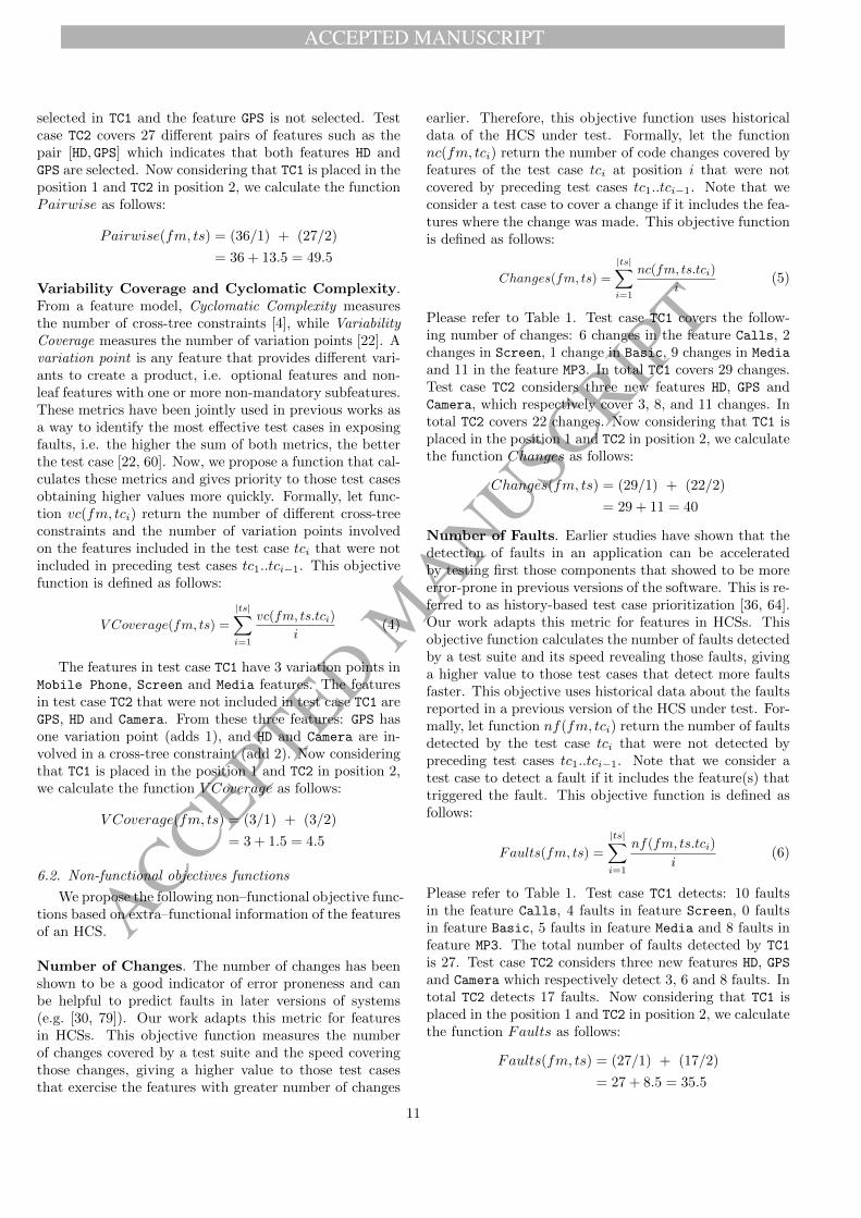
A12 statistic [3] to evaluate the effect size, i.e., determinewhich mono or multi–objective combinations perform bet-ter and to what extent. Table 8 shows the effect sizestatistic. Each cell shows the A12 value obtained whencomparing the single objectives in the columns against thecombination of objectives in the rows. Note that CASAwas considered as another prioritization objective in ouranalysis. Vargha and Delaney [68] suggested thresholds forinterpreting the effect size: 0.5 means no difference at all;values over 0.5 indicates a small (0.5-0.56), medium (0.57-0.64), large (0.65-0.71) or very large (0.72-1) difference infavour of the multiple objective in the row; values below0.5 indicates a small (0.5-0.44), medium (0.43-0.36), large(0.36-0.29) or very large (0.29-0.0) difference in favour ofthe single objective in the column. Cells revealing verylarge differences are highlighted in light grey (in favour ofthe row) and dark grey (in favour of the column). Values inboldface are those where hypothesis test revealed statisti-cal differences (p-value <0.05). Statistical results confirmthe bad performance of CASA and the Pairwise objectivefunction compared to the rest of objectives. Since values intable 8 are in general above 0.5 and most of the cells areshaded in light gray, general results confirm that multi–objective prioritization provides better results for the rateof fault detection than mono–objective prioritization whenusing functional objectives.

The average execution time of NSGA-II for all the func-tional objectives was 12.1 minutes, with a maximum av-erage execution time of 3.6 hours for the combination ofobjectives Connectivity + Pairwise + VCoverage, anda minimum execution time of 69 seconds for the objectiveDissimilarity. It is noticeable that all the executions in-cluding the objective Pairwise took an average executiontime longer than 20 minutes, due to the overhead intro-

duced by the calculation of the pairwise coverage. Theaverage execution time of CASA was 5 seconds.

7.4. Experiment 2. Non–functional objectives

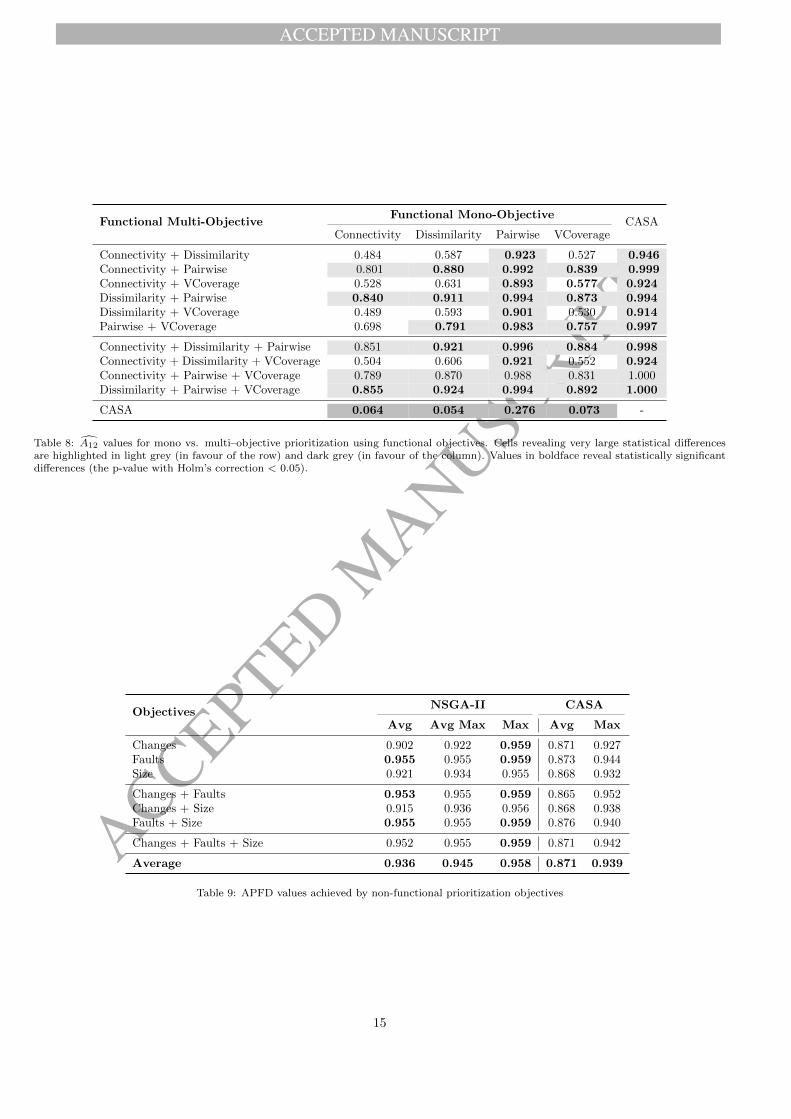
In this experiment, we evaluated the rate of fault detec-tion achieved by each group of 1, 2 and 3 non–functionalprioritization objectives, 7 combinations in total. Table9 presents the APFD values achieved by NSGA-II andCASA with each set of objectives. As in the previous ex-periment, the average and maximum APFD values achievedby NSGA-II (with any objective) were higher than thoseachieved by CASA. This confirms the poor performanceof pairwise coverage as a prioritization criterion. Interest-ingly, the Faults objective function is involved in the bestaverage and maximum APFD values. This suggests thatthe number of faults in previous versions of the systemis a key factor to accelerate the detection of faults. Allthe test suites generated detected more than 99.9% of theemulated faults.

Figure 9 depicts a box plot of the distributions of themaximum APFD value achieved on each execution of NSGA-II. The graph clearly shows the dominance of the Faults

objective function, both in isolation and in combinationwith other objectives. This was confirmed by the statis-tical tests, where p-values revealed significant differencesbetween the groups of objectives including Faults and therest of objectives.

Table 10 shows the values of the A12 effect size. CASAis excluded from the table since it was clearly outperformedby all other objectives. Again, the results show the supe-riority of Faults, either in isolation or combined, whencompared to any other group of objectives. As in the pre-vious experiment, all the multi–objective combinations im-prove the results obtained by single objectives, with A12

values over 0.5 in all cells except one. No clear differences

14

ACCEPTED MANUSCRIPT

ACCEPTED MANUSCRIP

T

Functional Multi-ObjectiveFunctional Mono-Objective

CASAConnectivity Dissimilarity Pairwise VCoverage

Connectivity + Dissimilarity 0.484 0.587 0.923 0.527 0.946Connectivity + Pairwise 0.801 0.880 0.992 0.839 0.999Connectivity + VCoverage 0.528 0.631 0.893 0.577 0.924Dissimilarity + Pairwise 0.840 0.911 0.994 0.873 0.994Dissimilarity + VCoverage 0.489 0.593 0.901 0.530 0.914Pairwise + VCoverage 0.698 0.791 0.983 0.757 0.997

Connectivity + Dissimilarity + Pairwise 0.851 0.921 0.996 0.884 0.998Connectivity + Dissimilarity + VCoverage 0.504 0.606 0.921 0.552 0.924Connectivity + Pairwise + VCoverage 0.789 0.870 0.988 0.831 1.000Dissimilarity + Pairwise + VCoverage 0.855 0.924 0.994 0.892 1.000

CASA 0.064 0.054 0.276 0.073 -

Table 8: A12 values for mono vs. multi–objective prioritization using functional objectives. Cells revealing very large statistical differencesare highlighted in light grey (in favour of the row) and dark grey (in favour of the column). Values in boldface reveal statistically significantdifferences (the p-value with Holm’s correction < 0.05).

ObjectivesNSGA-II CASA

Avg Avg Max Max Avg Max

Changes 0.902 0.922 0.959 0.871 0.927Faults 0.955 0.955 0.959 0.873 0.944Size 0.921 0.934 0.955 0.868 0.932

Changes + Faults 0.953 0.955 0.959 0.865 0.952Changes + Size 0.915 0.936 0.956 0.868 0.938Faults + Size 0.955 0.955 0.959 0.876 0.940

Changes + Faults + Size 0.952 0.955 0.959 0.871 0.942

Average 0.936 0.945 0.958 0.871 0.939

Table 9: APFD values achieved by non-functional prioritization objectives

15

ACCEPTED MANUSCRIPT

ACCEPTED MANUSCRIP

T

Figure 9: Box plot of the maximum APFD achieved on each execu-tion (40 in total)

were found between the use of multi–objective prioritiza-tion with two or three objectives.

The average execution time of NSGA-II for all thecombinations of non-functional objectives was 3.7 minutes,with a maximum average execution time of 4.6 minutes forFaults + Size and a minimum average execution time of2.5 seconds for Size.

Non-FunctionalMono-Objective

Multi-Objective Changes Faults Size

Changes + Faults 0.955 0.565 0.968Changes + Size 0.670 0.084 0.549Faults + Size 0.960 0.597 0.978

Changes + Faults + Size 0.951 0.536 0.960

Table 10: A12 values for mono vs. multi-objective prioritizationusing non–functional objectives. Cells revealing very large statisticaldifferences are highlighted in light grey (in favour of the row). Valuesin boldface reveal statistically significant differences (the p-value withHolms correction < 0.05).

7.5. Experiment 3. Functional and non–functional objec-tives

In this experiment, we evaluated the rate of fault de-tection achieved by each mixed combination of 2 and 3functional and non–functional prioritization objectives, 48combinations in total. The results of the experiment arepresented in Table 11. The cells with the top three bestaverage, average maximum, and global maximum APFDvalues of the table are highlighted in boldface. The resultsshow that all the multi–objective combinations greatly im-proved CASA on the average, average maximum, and globalmaximum APFD values obtained. As in the previous ex-periment, 10 out of the 12 top best APFD values wereachieved by multi–objective combinations including the

objective Faults, which confirms the effectiveness of faulthistory in accelerating the detection of faults in Drupal.Analogously, 6 out of the 10 best APFD values includethe objective Dissimilarity which confirms the findingsof previous studies on the effectiveness of promoting thedifferences among test cases to detect faults more quickly.As in the previous experiments, all the test suites gener-ated detected at least the 99% of the seeded faults.

Table 12 shows the values of the A12 effect size on thecomparison between single and multi–objective combina-tions of functional and non–functional objectives. Valuesindicate a better performance of multi–objective prioriti-zation compared to single–objective prioritization with theexception of Faults where most cells were under 0.5. Theoverall dominance, however, was observed in the combina-tion of objectives Dissimilarity + Faults followed byDissimilarity + Faults + VCoverage, with values over0.6 in all cells and over 0.93 in 6 out of 7 columns.

Table 13 depicts the effect size on the comparison be-tween multi–objective prioritization using functional ob-jectives and multi–objective prioritization using both func-tional and non–functional objectives. In general, A12 val-ues show statistical differences in favour or the combina-tion of functional and non-functional objectives, especiallythose including Faults. Interestingly, all the cells reveal-ing differences in favour of functional-objectives includethe objective Pairwise, which supports its potential whencombined with other prioritization objectives, as observedin Experiment 1.

Finally, Table 14 depicts the effect size on the com-parison between multi–objective prioritization using non–functional objectives and multi–objective prioritization us-ing both functional and non–functional objectives. A12

values reveal that when Faults is present in the combi-nation of non–functional objectives, mixed combinationsare outperformed in general, showing large effect sizes andstatistically significant differences. On the contrary, mixedobjective combinations including Faults clearly outper-form Changes + Size, but behave slightly worse than theother combinations of non-functional objectives. There-fore, the objective Faults seems to have a key influencein the performance of prioritization providing slightly bet-ter result when combined with other non-functional ob-jectives. It is remarkable, however, that some mixed com-binations of objectives such as Dissimilarity + Faults

provided the best overall results of this experiment.The average execution time of NSGA-II for the mixed

combinations of functional and non–functional prioritiza-tion objectives was 9.2 minutes. The maximum averageexecution time was 23.6 minutes reached by the objectivesConnectivity + Faults + Pairwise. The minimum ex-ecution time, 73.8 seconds, was obtained by the combina-tion of objectives Connectivity + Size + VCoverage.

16

ACCEPTED MANUSCRIPT

ACCEPTED MANUSCRIP

T

ObjectivesNSGA-II CASA

Avg Avg Max Max Avg Max

Changes + Connectivity 0.911 0.936 0.959 0.871 0.942Changes + Dissimilarity 0.905 0.935 0.959 0.873 0.943Changes + Pairwise 0.938 0.952 0.959 0.878 0.950Changes + VCoverage 0.919 0.940 0.958 0.867 0.941Connectivity + Faults 0.954 0.955 0.959 0.884 0.935Connectivity + Size 0.915 0.941 0.959 0.881 0.946Dissimilarity + Faults 0.954 0.956 0.959 0.871 0.947Dissimilarity + Size 0.904 0.930 0.957 0.858 0.921Faults + Pairwise 0.944 0.954 0.959 0.868 0.944Faults + VCoverage 0.954 0.955 0.959 0.869 0.940Pairwise + Size 0.940 0.953 0.960 0.878 0.943Size + VCoverage 0.914 0.937 0.958 0.876 0.948

Changes + Connectivity + Dissimilarity 0.908 0.938 0.958 0.873 0.935Changes + Connectivity + Faults 0.950 0.955 0.959 0.875 0.935Changes + Connectivity + Pairwise 0.936 0.953 0.958 0.862 0.933Changes + Connectivity + Size 0.914 0.942 0.959 0.878 0.929Changes + Connectivity + VCoverage 0.916 0.942 0.959 0.876 0.947Changes + Dissimilarity + Faults 0.952 0.955 0.959 0.880 0.936Changes + Dissimilarity + Pairwise 0.939 0.954 0.958 0.874 0.936Changes + Dissimilarity + Size 0.911 0.941 0.957 0.867 0.943Changes + Dissimilarity + VCoverage 0.910 0.946 0.957 0.869 0.945Changes + Faults + Pairwise 0.944 0.954 0.958 0.874 0.941Changes + Faults + VCoverage 0.951 0.955 0.959 0.883 0.946Changes + Pairwise + Size 0.941 0.955 0.963 0.866 0.952Changes + Pairwise + VCoverage 0.937 0.954 0.958 0.875 0.947Changes + Size + VCoverage 0.909 0.940 0.957 0.874 0.940Connectivity + Dissimilarity + Faults 0.954 0.956 0.960 0.877 0.941Connectivity + Dissimilarity + Size 0.913 0.941 0.959 0.879 0.941Connectivity + Faults + Pairwise 0.944 0.954 0.964 0.867 0.932Connectivity + Faults + Size 0.954 0.955 0.959 0.876 0.947Connectivity + Faults + VCoverage 0.953 0.955 0.959 0.858 0.925Connectivity + Pairwise + Size 0.937 0.954 0.962 0.870 0.937Connectivity + Size + VCoverage 0.908 0.936 0.959 0.881 0.954Dissimilarity + Faults + Pairwise 0.944 0.955 0.959 0.871 0.947Dissimilarity + Faults + Size 0.953 0.955 0.959 0.875 0.938Dissimilarity + Faults + VCoverage 0.953 0.956 0.964 0.876 0.947Dissimilarity + Pairwise + Size 0.940 0.954 0.959 0.868 0.944Dissimilarity + Size + VCoverage 0.913 0.941 0.957 0.873 0.936Faults + Pairwise + Size 0.942 0.955 0.959 0.863 0.937Faults + Pairwise + VCoverage 0.944 0.954 0.958 0.866 0.938Faults + Size + VCoverage 0.953 0.956 0.959 0.874 0.931Pairwise + Size + VCoverage 0.941 0.954 0.959 0.877 0.938

Average 0.934 0.949 0.959 0.873 0.940

Table 11: APFD values achieved by functional and non-functional prioritization objectives

17

ACCEPTED MANUSCRIPT

ACCEPTED MANUSCRIP

T

Mixed Multi-ObjectiveFunctional Objectives Non-Functional Objectives

Connectivity Dissimilarity Pairwise VCoverage Changes Faults Size

Changes + Connectivity 0.550 0.639 0.902 0.588 0.693 0.124 0.596Changes + Dissimilarity 0.518 0.614 0.906 0.573 0.671 0.118 0.563Changes + Pairwise 0.814 0.893 0.993 0.856 0.899 0.298 0.858Changes + VCoverage 0.530 0.633 0.954 0.571 0.701 0.131 0.583Connectivity + Faults 0.924 0.967 1.000 0.946 0.948 0.556 0.966Connectivity + Size 0.566 0.684 0.956 0.616 0.736 0.092 0.630Dissimilarity + Faults 0.951 0.967 0.999 0.958 0.962 0.686 0.971Dissimilarity + Size 0.455 0.553 0.879 0.481 0.601 0.108 0.497Faults + Pairwise 0.885 0.947 0.997 0.914 0.931 0.418 0.931Faults + VCoverage 0.936 0.964 0.999 0.949 0.956 0.589 0.972Pairwise + Size 0.863 0.931 0.994 0.903 0.914 0.336 0.893Size + VCoverage 0.542 0.631 0.924 0.584 0.685 0.101 0.580

Changes + Connectivity + Dissimilarity 0.534 0.634 0.939 0.570 0.681 0.128 0.578Changes + Connectivity + Faults 0.918 0.961 0.998 0.938 0.944 0.509 0.953Changes + Connectivity + Pairwise 0.877 0.939 0.995 0.907 0.921 0.370 0.911Changes + Connectivity + Size 0.593 0.693 0.958 0.646 0.744 0.143 0.644Changes + Connectivity + VCoverage 0.573 0.673 0.960 0.623 0.743 0.176 0.633Changes + Dissimilarity + Faults 0.932 0.965 0.999 0.948 0.952 0.570 0.963Changes + Dissimilarity + Pairwise 0.873 0.936 0.995 0.911 0.925 0.384 0.910Changes + Dissimilarity + Size 0.541 0.639 0.963 0.589 0.728 0.121 0.600Changes + Dissimilarity + VCoverage 0.677 0.761 0.970 0.731 0.812 0.189 0.730Changes + Faults + Pairwise 0.910 0.948 0.996 0.930 0.941 0.471 0.942Changes + Faults + VCoverage 0.926 0.963 0.999 0.944 0.950 0.554 0.964Changes + Pairwise + Size 0.909 0.953 0.996 0.930 0.939 0.494 0.938Changes + Pairwise + VCoverage 0.888 0.947 0.997 0.917 0.932 0.429 0.925Changes + Size + VCoverage 0.573 0.682 0.943 0.620 0.729 0.093 0.625Connectivity + Dissimilarity + Faults 0.940 0.963 0.999 0.956 0.959 0.624 0.973Connectivity + Dissimilarity + Size 0.558 0.659 0.951 0.606 0.728 0.133 0.622Connectivity + Faults + Pairwise 0.899 0.946 0.998 0.922 0.938 0.457 0.931Connectivity + Faults + VCoverage 0.929 0.970 0.999 0.949 0.949 0.616 0.961Connectivity + Faults + Size 0.934 0.964 1.000 0.948 0.954 0.577 0.968Connectivity + Pairwise + Size 0.903 0.949 0.997 0.926 0.939 0.450 0.942Connectivity + Size + VCoverage 0.521 0.626 0.919 0.548 0.665 0.144 0.570Dissimilarity + Faults + Pairwise 0.915 0.957 0.998 0.934 0.942 0.496 0.947Dissimilarity + Faults + Size 0.936 0.968 0.999 0.953 0.955 0.620 0.971Dissimilarity + Faults + VCoverage 0.940 0.963 0.998 0.957 0.960 0.637 0.968Dissimilarity + Pairwise + Size 0.895 0.950 0.998 0.921 0.931 0.391 0.926Dissimilarity + Size + VCoverage 0.572 0.680 0.953 0.622 0.742 0.123 0.628Faults + Pairwise + Size 0.914 0.958 0.999 0.938 0.946 0.479 0.953Faults + Pairwise + VCoverage 0.905 0.951 0.997 0.930 0.938 0.442 0.935Faults + Size + VCoverage 0.937 0.968 0.999 0.956 0.959 0.616 0.969Pairwise + Size + VCoverage 0.887 0.946 0.997 0.914 0.931 0.447 0.932

Table 12: A12 values for mono vs. multi–objective combinations of functional and non-functional objectives. Cells revealing very largestatistical differences are highlighted in light grey (in favour of the row) and dark grey (in favour of the column). Values in boldface revealstatistically significant differences (the p-value with Holm’s correction is < 0.05)

18

ACCEPTED MANUSCRIPT

ACCEPTED MANUSCRIP

TMixed Multi-ObjectiveFunctional Multi-Objective

Con+Dis Con+Pai Con+VCo Dis+Pai Dis+VCo Pai+VCo Con+Dis+Pai Con+Dis+VCo Con+Pai+VCo Dis+Pai+VCo

Changes + Con 0.556 0.267 0.529 0.221 0.559 0.386 0.203 0.547 0.284 0.208Changes + Dis 0.518 0.242 0.489 0.198 0.531 0.363 0.187 0.513 0.268 0.199Changes + Pai 0.800 0.523 0.792 0.463 0.827 0.703 0.418 0.810 0.551 0.438Changes + VCo 0.536 0.245 0.488 0.211 0.541 0.338 0.200 0.517 0.248 0.201Con + Faults 0.900 0.738 0.921 0.713 0.938 0.893 0.667 0.909 0.753 0.683Con + Size 0.573 0.242 0.534 0.189 0.580 0.388 0.168 0.571 0.271 0.178Dis + Faults 0.915 0.823 0.947 0.811 0.956 0.919 0.778 0.924 0.803 0.769Dis + Size 0.463 0.208 0.424 0.176 0.467 0.294 0.156 0.442 0.216 0.162Faults + Pai 0.864 0.641 0.878 0.600 0.910 0.830 0.560 0.879 0.676 0.580Faults + VCo 0.906 0.780 0.932 0.754 0.956 0.907 0.721 0.916 0.767 0.719Pai + Size 0.834 0.571 0.849 0.519 0.878 0.790 0.473 0.854 0.637 0.503Size + VCo 0.544 0.239 0.515 0.196 0.549 0.363 0.175 0.537 0.272 0.180

Changes + Con + Dis 0.528 0.253 0.492 0.220 0.540 0.367 0.198 0.519 0.270 0.214Changes + Con + Faults 0.888 0.730 0.917 0.694 0.940 0.877 0.654 0.900 0.736 0.668Changes + Con + Pai 0.849 0.618 0.864 0.563 0.896 0.798 0.508 0.869 0.651 0.543Changes + Con + Size 0.602 0.281 0.559 0.238 0.606 0.420 0.217 0.592 0.318 0.227Changes + Con + VCo 0.585 0.293 0.540 0.256 0.586 0.394 0.244 0.573 0.299 0.237Changes + Dis + Faults 0.898 0.758 0.927 0.736 0.947 0.898 0.688 0.908 0.761 0.701Changes + Dis + Pai 0.849 0.621 0.864 0.570 0.896 0.802 0.524 0.865 0.648 0.543Changes + Dis + Size 0.557 0.224 0.497 0.189 0.548 0.323 0.181 0.526 0.231 0.171Changes + Dis + VCo 0.674 0.373 0.645 0.319 0.690 0.517 0.296 0.669 0.389 0.298Changes + Faults + Pai 0.877 0.708 0.902 0.672 0.933 0.854 0.622 0.890 0.707 0.643Changes + Faults + VCo 0.901 0.754 0.933 0.735 0.946 0.898 0.687 0.912 0.761 0.705Changes + Pai + Size 0.876 0.706 0.900 0.662 0.924 0.848 0.624 0.893 0.716 0.634Changes + Pai + VCo 0.859 0.650 0.874 0.603 0.906 0.823 0.549 0.876 0.678 0.580Changes + Size + VCo 0.581 0.242 0.549 0.189 0.590 0.395 0.171 0.585 0.277 0.171Con + Dis + Faults 0.911 0.798 0.944 0.783 0.957 0.914 0.742 0.922 0.780 0.745Con + Dis + Size 0.570 0.268 0.520 0.227 0.569 0.388 0.213 0.554 0.278 0.215Con + Faults + Pai 0.868 0.689 0.891 0.645 0.920 0.844 0.604 0.887 0.700 0.619Con + Faults + Size 0.906 0.772 0.935 0.753 0.954 0.909 0.713 0.917 0.770 0.722Con + Faults + VCo 0.900 0.757 0.925 0.742 0.938 0.894 0.706 0.917 0.772 0.718Con + Pai + Size 0.875 0.698 0.888 0.646 0.927 0.846 0.604 0.888 0.700 0.620Con + Size + VCo 0.519 0.268 0.495 0.236 0.537 0.372 0.216 0.524 0.284 0.220Dis + Faults + Pai 0.886 0.719 0.911 0.689 0.936 0.871 0.643 0.898 0.727 0.664Dis + Faults + Size 0.907 0.779 0.941 0.764 0.951 0.907 0.723 0.917 0.779 0.734Dis + Faults + VCo 0.909 0.792 0.936 0.779 0.950 0.906 0.736 0.917 0.777 0.738Dis + Pai + Size 0.866 0.655 0.883 0.602 0.914 0.838 0.543 0.878 0.688 0.576Dis + Size + VCo 0.584 0.257 0.540 0.213 0.588 0.399 0.199 0.578 0.284 0.198Faults + Pai + Size 0.883 0.716 0.915 0.676 0.936 0.876 0.628 0.898 0.723 0.649Faults + Pai + VCo 0.872 0.691 0.901 0.647 0.924 0.856 0.595 0.885 0.707 0.619Faults + Size + VCo 0.908 0.783 0.937 0.765 0.950 0.910 0.729 0.923 0.780 0.737Pai + Size + VCo 0.871 0.663 0.891 0.632 0.911 0.835 0.586 0.876 0.691 0.606

Table 13: A12 values for combinations of functional objectives vs. mixed combinations of functional and non–functional prioritizationobjectives. Cells revealing very large statistical differences are highlighted using dark grey (in favour of the column) or light grey (in favourof the row). Values in boldface reveal statistically significant differences (the p-value with Holm’s correction is < 0.05)

19

ACCEPTED MANUSCRIPT

ACCEPTED MANUSCRIP

T

Mixed Multi-ObjectiveNon-Functional Multi-Objective

Changes + Faults Changes + Size Faults + Size Changes + Faults + Size

Changes + Connectivity 0.098 0.549 0.087 0.116Changes + Dissimilarity 0.100 0.517 0.093 0.110Changes + Pairwise 0.239 0.807 0.222 0.273Changes + VCoverage 0.117 0.543 0.105 0.126Connectivity + Faults 0.470 0.924 0.438 0.514Connectivity + Size 0.063 0.569 0.055 0.083Dissimilarity + Faults 0.643 0.947 0.571 0.639Dissimilarity + Size 0.078 0.451 0.072 0.095Faults + Pairwise 0.343 0.882 0.318 0.391Faults + VCoverage 0.555 0.932 0.473 0.548Pairwise + Size 0.269 0.853 0.251 0.314Size + VCoverage 0.083 0.535 0.073 0.094

Changes + Connectivity + Dissimilarity 0.113 0.528 0.100 0.118Changes + Connectivity + Faults 0.454 0.917 0.408 0.480Changes + Connectivity + Pairwise 0.290 0.865 0.269 0.350Changes + Connectivity + Size 0.113 0.595 0.108 0.130Changes + Connectivity + VCoverage 0.165 0.584 0.149 0.167Changes + Dissimilarity + Faults 0.528 0.929 0.469 0.537Changes + Dissimilarity + Pairwise 0.327 0.866 0.302 0.359Changes + Dissimilarity + Size 0.122 0.547 0.101 0.113Changes + Dissimilarity + VCoverage 0.166 0.680 0.136 0.173Changes + Faults + Pairwise 0.443 0.904 0.392 0.446Changes + Faults + VCoverage 0.505 0.929 0.458 0.523Changes + Pairwise + Size 0.435 0.903 0.394 0.467Changes + Pairwise + VCoverage 0.367 0.882 0.330 0.401Changes + Size + VCoverage 0.077 0.578 0.067 0.088Connectivity + Dissimilarity + Faults 0.598 0.941 0.535 0.589Connectivity + Dissimilarity + Size 0.097 0.563 0.095 0.124Connectivity + Faults + Pairwise 0.424 0.891 0.378 0.434Connectivity + Faults + Size 0.548 0.933 0.476 0.546Connectivity + Faults + VCoverage 0.565 0.929 0.520 0.578Connectivity + Pairwise + Size 0.404 0.897 0.348 0.418Connectivity + Size + VCoverage 0.111 0.521 0.106 0.134Dissimilarity + Faults + Pairwise 0.444 0.913 0.403 0.469Dissimilarity + Faults + Size 0.567 0.942 0.515 0.583Dissimilarity + Faults + VCoverage 0.607 0.942 0.548 0.595Dissimilarity + Pairwise + Size 0.295 0.884 0.279 0.364Dissimilarity + Size + VCoverage 0.096 0.584 0.082 0.111Faults + Pairwise + Size 0.419 0.914 0.373 0.452Faults + Pairwise + VCoverage 0.388 0.901 0.348 0.419Faults + Size + VCoverage 0.590 0.937 0.531 0.586Pairwise + Size + VCoverage 0.388 0.893 0.359 0.434

Table 14: A12 values for combinations of non-functional objectives vs. mixed combinations of functional and non–functional prioritizationobjectives. Cells revealing very large statistical differences are highlighted using dark grey (in favour of the column) or light grey (in favourof the row). Values in boldface reveal statistically significant differences (the p-value with Holm’s correction is < 0.05)

20

ACCEPTED MANUSCRIPT

ACCEPTED MANUSCRIP

T

7.6. Experiment 4. Functional vs non–functional objec-tives

In this experiment, we performed a further statisticalanalysis of the data obtained in previous experiments tomeasure the effect size on the comparison of functionalobjectives against non–functional objectives, both singleand combined. Table 15 shows the values of the A12 effectsize. A majority of cells show A12 values under 0.5 indi-cating that non-functional objectives are in general moreeffective than functional objectives for test case prioriti-zation in HCSs. As observed in Experiment 2 and 3, theobjective Faults, and those combinations including it con-sistently show the largest differences. Also, as observed inExperiment 1, the objective Pairwise is consistently out-performed by all non-functional objectives, but it providesthe best results in favour of functional objectives whencombined with others.

7.7. Experiment 5. Algorithm comparison

In this experiment, we compared the performance ofNSGA-II with a random search algorithm and a determin-istic test case prioritization algorithm. The experimentalsetup and results of both comparisons are described in thefollowing sections.

7.7.1. Comparison with Random Search

The pseudo-code of our implementation of RandomSearch (RS) algorithm is described in Algorithm 1. Thealgorithm takes an input attributed feature model afmand returns a set of test suites optimizing the target ob-jectives. The algorithm has two configuration parameters:the number of iterations to be performed nIterations, andthe maximum size of the random test suites to be gener-ated maxSize. We set maxSize to the ceiling for theaverage size of the pairwise suites generated by CASA (13test cases). Regarding the value of nIterations, we set itsvalues to 5000, in order to ensure a fair comparison withNSGA-II, which performs 50 iterations with a populationof 100 individuals (50 ∗ 100 = 5000 evaluations).

Three functions are invoked in the pseudo-code of Al-gorithm 1: i) randomSuite, that generates a suite of ran-dom size (between 1 and maxSize), comprising of ran-dom products generated using the PLEDGE tool [33]; ii)isNotDominated that checks if the solution sol providedas parameter is not dominated by any solution in thePareto front estimation pFront; and iii) notDominatedthat returns the solutions from pFront that are dominatedby sol.

Table 16 shows the results of the comparison. For eachgroup of objectives and algorithm under comparison, thetable shows the execution time, average and maximumAPFD value of the test suites in the Pareto front. Thebest values of each metric on each row are highlighted inboldface. As illustrated, NSGA-II outperforms RS in 58out of the 63 combinations of objectives in terms of aver-age APDF value. Interestingly, there is not a clear winner

Algorithm 1 Random search algorithm

1: procedure RS(afm)2: i← 13: pFront← {}4: while i ≤ nIterations do5: sol← randomSuite(afm,maxSize)6: if isNotDomiated(sol, pFront) then7: pFront← notDominated(pFront, sol)

⋃sol

8: end if9: i← i + 1

10: end while11: return pFront12: end procedure

in terms of execution time: RS was faster in 36 out of the63 objective groups (57.2%) meanwhile NSGA-II achievedlower average execution times in 42.8% of the objectives.We found that the overhead in the RS algorithm was dueto the cost of generating random valid test cases. In termsof fault detection, NSGA-II detected slightly more faultsthan RS. However, both algorithms detected more than99.5% of the emulated faults and thus the differences arenot significant.

Table 7.7.1 shows the average, standard deviation andmaximum values of the hypervolume achieved by each al-gorithm and objective group under comparison. The hy-pervolume is the n-dimensional space contained by a setof solutions with respect to a reference point [7]. Thehypervolume metric is widely used to compare the perfor-mance of multi-objective algorithms, where solutions witha larger hypervolume provide a better trade-offs among ob-jectives than solutions with a smaller hypervolume. Thebest values of each metric on each row are highlighted inboldface. NSGA-II provides better results for the major-ity of executions both in terms of average hypervolume (38out of 63 objective sets) and maximum hypervolume (41out of 63 objective sets). Interestingly, RS provides bet-ter results than NSGA-II for a fair percentage of objectivesets. This is probably because NSGA-II mainly focuses onre-ordering the test cases in the initial population, whileRS performs a wider exploration of the search space gen-erating solutions with different (random) test cases. It isnoteworthy, however, that a larger hypervolume does notnecessarily implies a better rate of fault detection, as ob-served in Table 16.

In summary, NSGA-II outperforms RS in acceleratingthe detection of faults in HCSs since NSGA-II provideshigher average and maximum APFD values, it usually gen-erates Pareto fronts approximations with better hypervol-umes, and both algorithms have similar executions times.

7.7.2. Comparison with a coverage-based prioritization al-gorithm

For a further validation, we compared the results ofour MOEA with the deterministic coverage-based priori-tization algorithm for software product lines proposed by

21

ACCEPTED MANUSCRIPT

ACCEPTED MANUSCRIP

T

Functional ObjectivesNon-Functional Objectives

Changes Faults Size Changes + Faults Changes + Size Faults + Size Changes + Faults + Size

Connectivity 0.675 0.083 0.550 0.060 0.509 0.057 0.078Dissimilarity 0.583 0.037 0.442 0.036 0.403 0.035 0.037Pairwise 0.166 0.000 0.083 0.000 0.076 0.000 0.000VCoverage 0.637 0.061 0.509 0.051 0.463 0.045 0.056

Connectivity + Dissimilarity 0.657 0.115 0.536 0.093 0.493 0.087 0.108Connectivity + Pairwise 0.895 0.278 0.851 0.212 0.802 0.201 0.265Connectivity + VCoverage 0.704 0.088 0.589 0.070 0.541 0.054 0.080Dissimilarity + Pairwise 0.912 0.314 0.887 0.242 0.838 0.225 0.290Dissimilarity + VCoverage 0.654 0.064 0.534 0.039 0.497 0.039 0.058Pairwise + VCoverage 0.848 0.116 0.741 0.090 0.697 0.081 0.108

Connectivity + Dissimilarity + Pairwise 0.915 0.363 0.898 0.289 0.849 0.274 0.342Connectivity + Dissimilarity + VCoverage 0.688 0.104 0.553 0.089 0.516 0.079 0.097Connectivity + Pairwise + VCoverage 0.891 0.273 0.831 0.234 0.792 0.221 0.261Dissimilarity + Pairwise + VCoverage 0.918 0.342 0.896 0.286 0.848 0.258 0.322

Table 15: A12 values for functional vs. non–functional prioritization objectives. Cells revealing very large statistical differences are highlightedin dark grey (in favour of the column). Values in boldface reveal statistically significant differences (the p-value with Holm’s correction is <0.05)

Sanchez et al. [60]. The algorithm takes an attributedfeature model afm as input, generates a pairwise suitefrom the model and re-arranges its products in descend-ing order of pairwise coverage using bubble search. Forthe deterministic generation of a pairwise suite, we usedthe SPLCAT tool [38]. The pseudo-code of our imple-mentation is described in Algorithm 2. Two functions areinvoked in the pseudo-code of this algorithm: i) ICPLwhich represents the ICPL algorithm for generating pair-wise suites as implemented by the tool SPLCAT, and covthat is equivalent to the PairwiseCoverage objective func-tion defined in section 6 assuming that the suite has asingle test case, specified as a parameter.

Algorithm 2 Coverage-based prioritization algorithm

1: procedure PWCMax(afm)2: suite← ICPL(afm)3: size← size(suite)4: repeat5: swapped← false6: for i← 2, size do7: if cov(suite[i − 1], afm) <

cov(suite[i], afm) then8: aux← suite[i]9: suite[i]← suite[i− 1]

10: suite[i− 1]← aux11: swapped← true12: end if13: end for14: until ¬swapped15: return suite16: end procedure

The APFD value achieved by the coverage-based algo-rithm is 0.946, which is less than the average AFPD valueof the best solution in the Pareto front found by NSGA-IIfor 38 out of the 63 objective sets, i.e. column “Avg Max”

in Table 16. More importantly, NSGA-II achieved betterresults than the coverage-based algorithm in all the 40 ex-ecutions for 29 out of the 63 objective sets. This meansthat, for almost half of the objective sets, our algorithmwas always better than the coverage-based algorithm. Itis noteworthy, however, that the differences between theAPFD values of NSGA-II and the coverage-based algo-rithm are small, probably due to the size of the gener-ated suites (13 test cases on average). We conjecture thatthese differences would be larger when dealing with big-ger test suites (e.g. 3-wise), but this is something thatrequires further research. In terms of execution time, thecoverage-based algorithm was executed in less than 2 sec-onds, which makes it appropriate when fast response timesare required.

7.8. Discussion

We now summarize the results and what they tell usabout the research questions.

RQ1: Mono vs. multi–objective prioritization us-ing functional objectives. Experiment 1 revealed thatmulti–objective prioritization outperforms mono-objectiveprioritization when using functional objectives. The su-periority was especially noticeable in the comparison withPairwise as a single-objective, which consistently achievedthe worse rate of fault detection. Interestingly, however,Pairwise performed very well when combined with otherfunctional objectives. In the light of these results, RQ1 isanswered as follows:

Multi–objective prioritization using functional ob-jectives is more effective than mono–objective pri-oritization with functional objectives in acceleratingthe detection of faults in HCSs.

22

ACCEPTED MANUSCRIPT

ACCEPTED MANUSCRIP

T

NSGA-II Random Search

Objectives Ex.Time Avg Avg Max Ex.Time Avg Avg Max

Connectivity 77251.6 0.923 0.935 119627.9 0.911 0.915Dissimilarity 75856.1 0.912 0.931 112480.8 0.885 0.894Pairwise 1478882.8 0.880 0.880 714078.2 0.913 0.913VCoverage 79107.7 0.888 0.933 102457.4 0.893 0.918Connectivity + Dissimilarity 83767.4 0.912 0.937 106497.4 0.898 0.914Connectivity + Pairwise 1421967.3 0.938 0.951 709398.8 0.933 0.952Connectivity + VCoverage 78199.5 0.914 0.934 120115.3 0.891 0.899Dissimilarity + Pairwise 1400685.8 0.941 0.952 715289.6 0.931 0.953Dissimilarity + VCoverage 77182.5 0.916 0.936 128498.2 0.900 0.919Pairwise + VCoverage 1453296.7 0.936 0.948 714764.8 0.927 0.952Connectivity + Dissimilarity + Pairwise 1414754.9 0.929 0.954 711827.3 0.927 0.953Connectivity + Dissimilarity + VCoverage 80922.4 0.906 0.929 111031.5 0.917 0.933Connectivity + Pairwise + VCoverage 1434254.1 0.932 0.949 720098.3 0.928 0.953Dissimilarity + Pairwise + VCoverage 1405714.7 0.938 0.952 715958.6 0.926 0.952

Changes 154553.9 0.902 0.915 255249.5 0.907 0.907Faults 266983.7 0.955 0.955 311060.0 0.953 0.953Size 147161.1 0.917 0.931 267076.5 0.917 0.917Changes + Faults 267046.7 0.953 0.955 315937.0 0.933 0.954Changes + Size 150685.2 0.918 0.942 250050.4 0.909 0.942Faults + Size 266313.0 0.955 0.956 317911.9 0.941 0.954Changes + Faults + Size 267405.4 0.951 0.955 319803.3 0.935 0.954

Changes + Connectivity 89517.2 0.916 0.939 134150.5 0.907 0.944Changes + Dissimilarity 89095.0 0.907 0.939 143702.3 0.905 0.940Changes + Pairwise 1174272.6 0.937 0.952 602875.9 0.928 0.951Changes + VCoverage 86759.7 0.917 0.936 133983.3 0.906 0.950Connectivity + Faults 248148.2 0.953 0.955 221543.1 0.944 0.954Connectivity + Size 95670.1 0.915 0.944 134395.5 0.910 0.948Dissimilarity + Faults 253215.6 0.954 0.955 219950.5 0.940 0.954Dissimilarity + Size 85769.7 0.903 0.923 129575.3 0.913 0.946Faults + Pairwise 1328146.5 0.943 0.954 681334.3 0.938 0.954Faults + VCoverage 258827.7 0.955 0.956 211328.7 0.944 0.954Pairwise + Size 1190707.6 0.942 0.953 608338.8 0.932 0.953Size + VCoverage 82624.5 0.913 0.935 148241.0 0.908 0.950Changes + Connectivity + Dissimilarity 90333.7 0.912 0.939 141020.4 0.899 0.947Changes + Connectivity + Faults 242090.7 0.951 0.955 213817.3 0.932 0.955Changes + Connectivity + VCoverage 91098.6 0.915 0.943 147589.7 0.904 0.942Changes + Dissimilarity + Faults 258500.8 0.952 0.955 237274.7 0.932 0.954Changes + Dissimilarity + VCoverage 79023.9 0.912 0.948 149348.8 0.887 0.946Changes + Faults + Pairwise 1314596.2 0.942 0.954 685275.2 0.929 0.955Changes + Faults + VCoverage 253188.5 0.952 0.955 227043.4 0.927 0.954Changes + Pairwise + Connectivity 1159383.0 0.935 0.954 609231.8 0.926 0.954Changes + Pairwise + Dissimilarity 1156172.8 0.935 0.953 608587.6 0.923 0.953Changes + Pairwise + VCoverage 1154166.3 0.936 0.954 601289.3 0.924 0.954Changes + Size + Connectivity 81688.1 0.911 0.939 131841.9 0.903 0.947Changes + Size + Dissimilarity 87032.2 0.913 0.942 131280.7 0.913 0.950Changes + Size + Pairwise 1185686.4 0.940 0.955 609731.4 0.925 0.955Changes + Size + VCoverage 93134.0 0.908 0.940 138131.6 0.906 0.952Connectivity + Dissimilarity + Faults 254147.6 0.954 0.955 232744.1 0.938 0.954Connectivity + Dissimilarity + Size 77954.7 0.910 0.944 130562.3 0.902 0.945Connectivity + Faults + Pairwise 1324924.1 0.942 0.954 689787.5 0.935 0.955Connectivity + Faults + Size 254000.3 0.954 0.955 221594.3 0.925 0.954Connectivity + Faults + VCoverage 245731.1 0.951 0.955 217372.5 0.941 0.954Connectivity + Size + Pairwise 1167713.3 0.938 0.955 604217.1 0.924 0.955Connectivity + Size + VCoverage 83282.2 0.914 0.944 156937.0 0.904 0.951Dissimilarity + Faults + Pairwise 1324060.1 0.945 0.955 677402.6 0.929 0.954Dissimilarity + Faults + Size 243985.7 0.952 0.955 226250.4 0.931 0.954Dissimilarity + Faults + VCoverage 251145.3 0.952 0.955 225094.4 0.934 0.954Dissimilarity + Pairwise + Size 1130349.7 0.942 0.954 607200.3 0.927 0.953Dissimilarity + Size + VCoverage 95906.8 0.912 0.945 137942.8 0.906 0.949Faults + Pairwise + VCoverage 1299913.7 0.944 0.955 682123.5 0.935 0.954Faults + Pairwise + Size 1315391.8 0.942 0.955 686569.3 0.939 0.954Faults + Size + VCoverage 246233.0 0.953 0.956 218511.5 0.924 0.955Pairwise + Size + VCoverage 1169411.1 0.939 0.955 603278.3 0.923 0.953

Average 552301.4 0.930 0.946 351709.2 0.920 0.945

Table 16: APFD values and execution times achieved by NSGA-II and Random Search (40 executions in total).

23

ACCEPTED MANUSCRIPT

ACCEPTED MANUSCRIP

T

NSGA-II Random Search

Objective Avg HV StdDev HV Max HV Avg HV StdDev HV Max HV

Connectivity 0.062 0.031 0.144 0.026 0.007 0.060Dissimilarity 0.055 0.024 0.129 0.036 0.006 0.050Pairwise 0.151 0.003 0.157 0.318 0.004 0.324VCoverage 0.062 0.026 0.115 0.021 0.003 0.033Connectivity + Dissimilarity 0.103 0.040 0.166 0.068 0.014 0.107Connectivity + Pairwise 0.217 0.034 0.303 0.349 0.006 0.360Connectivity + VCoverage 0.108 0.047 0.206 0.049 0.010 0.071Dissimilarity + Pairwise 0.206 0.032 0.261 0.355 0.008 0.374Dissimilarity + VCoverage 0.109 0.039 0.185 0.060 0.010 0.089Pairwise + VCoverage 0.218 0.026 0.257 0.344 0.007 0.364Dissimilarity + Pairwise + VCoverage 0.269 0.049 0.356 0.379 0.009 0.396Connectivity + Dissimilarity + Pairwise 0.281 0.062 0.428 0.379 0.010 0.398Connectivity + Dissimilarity + VCoverage 0.167 0.062 0.297 0.083 0.012 0.105Connectivity + Pairwise + VCoverage 0.278 0.052 0.393 0.372 0.014 0.407

Changes 0.110 0.025 0.178 0.082 0.008 0.103Faults 0.157 0.017 0.188 0.166 0.015 0.201Size 0.065 0.015 0.093 0.050 0.003 0.058Changes + Faults 0.260 0.026 0.308 0.245 0.015 0.273Changes + Size 0.169 0.044 0.299 0.133 0.009 0.160Faults + Size 0.207 0.025 0.251 0.213 0.017 0.248Changes + Faults + Size 0.305 0.040 0.404 0.290 0.019 0.330

Changes + Connectivity 0.168 0.039 0.304 0.113 0.009 0.137Changes + Dissimilarity 0.165 0.038 0.291 0.115 0.008 0.131Changes + Pairwise 0.245 0.028 0.311 0.386 0.008 0.400Changes + VCoverage 0.173 0.037 0.266 0.106 0.007 0.124Connectivity + Faults 0.214 0.041 0.309 0.197 0.019 0.254Connectivity + Size 0.129 0.043 0.256 0.083 0.006 0.097Dissimilarity + Faults 0.199 0.031 0.295 0.201 0.016 0.244Dissimilarity + Size 0.111 0.028 0.179 0.087 0.009 0.106Faults + Pairwise 0.293 0.019 0.360 0.435 0.012 0.470Faults + VCoverage 0.204 0.040 0.298 0.194 0.023 0.249Pairwise + Size 0.213 0.022 0.256 0.360 0.004 0.373Size + VCoverage 0.124 0.033 0.196 0.077 0.004 0.092Changes + Connectivity + Dissimilarity 0.212 0.054 0.385 0.147 0.014 0.182Changes + Connectivity + Faults 0.317 0.044 0.416 0.273 0.019 0.315Changes + Connectivity + Pairwise 0.324 0.039 0.415 0.418 0.009 0.433Changes + Connectivity + Size 0.226 0.043 0.341 0.162 0.011 0.188Changes + Connectivity + VCoverage 0.221 0.053 0.346 0.134 0.009 0.158Changes + Dissimilarity + Faults 0.297 0.042 0.421 0.283 0.018 0.319Changes + Dissimilarity + Pairwise 0.307 0.048 0.425 0.419 0.009 0.445Changes + Dissimilarity + Size 0.211 0.041 0.303 0.164 0.009 0.181Changes + Dissimilarity + VCoverage 0.212 0.040 0.334 0.145 0.012 0.189Changes + Faults + Pairwise 0.374 0.034 0.452 0.499 0.012 0.530Changes + Faults + VCoverage 0.303 0.043 0.391 0.271 0.017 0.303Changes + Pairwise + Size 0.300 0.051 0.417 0.423 0.007 0.435Changes + Pairwise + VCoverage 0.323 0.039 0.410 0.412 0.008 0.430Changes + Size + VCoverage 0.226 0.051 0.364 0.160 0.009 0.183Connectivity + Dissimilarity + Faults 0.256 0.044 0.366 0.237 0.021 0.279Connectivity + Dissimilarity + Size 0.166 0.046 0.249 0.115 0.012 0.138Connectivity + Faults + Pairwise 0.340 0.054 0.444 0.462 0.014 0.489Connectivity + Faults + Size 0.266 0.046 0.368 0.249 0.019 0.288Connectivity + Faults + VCoverage 0.252 0.057 0.394 0.218 0.018 0.258Connectivity + Pairwise + Size 0.281 0.053 0.388 0.391 0.007 0.410Connectivity + Size + VCoverage 0.184 0.046 0.288 0.107 0.009 0.127Dissimilarity + Faults + Pairwise 0.342 0.040 0.422 0.471 0.015 0.514Dissimilarity + Faults + Size 0.265 0.044 0.435 0.251 0.020 0.282Dissimilarity + Faults + VCoverage 0.248 0.058 0.403 0.231 0.020 0.290Dissimilarity + Pairwise + Size 0.267 0.034 0.359 0.394 0.008 0.412Dissimilarity + Size + VCoverage 0.166 0.030 0.215 0.113 0.010 0.157Faults + Pairwise + Size 0.339 0.021 0.382 0.473 0.013 0.497Faults + Pairwise + VCoverage 0.345 0.029 0.392 0.456 0.009 0.479Faults + Size + VCoverage 0.263 0.045 0.375 0.246 0.017 0.273Pairwise + Size + VCoverage 0.275 0.030 0.350 0.390 0.007 0.404

Table 17: Comparison of hypervolumes obtained by NSGA-II and Random Search.

24

ACCEPTED MANUSCRIPT

ACCEPTED MANUSCRIP

T

RQ2: Mono vs. multi–objective prioritization us-ing non–functional objectives. The results of experi-ment 2 showed significant differences in favour of multi–objective prioritization over mono–objective prioritizationusing non–functional objectives. It also revealed a clearsuperiority of the objective function Faults, single or incombination with other objectives, over the rest of the non-functional objectives. We conjecture that this result couldbe caused by the nature of the case study. In particular,we used the bugs detected in Drupal v7.22 to acceleratethe detection of faults in Drupal v7.23. Being two consecu-tive versions of the framework, we found that some of thefaults in Drupal v7.22 remained in Drupal v7.23, whichmeans that the prioritization could be overfitted. Whilethis is a realistic scenario, we think the results could not begeneralizable to non–consecutive versions of the frameworkand thus the results must be taken with caution. Basedon the global results, however, RQ2 is answered as follows:

Multi–objective prioritization using non–functionalobjectives is, in general, more effective than mono–objective prioritization with non–functional objec-tives in accelerating the detection of faults in HCSs.

RQ3: Combination of functional and non–functionalobjectives. Experiment 3 revealed that the multi–objectiveprioritization using functional and non–functional objec-tives outperform prioritization driven by a single objec-tive, either functional or non-functional. Similarly, mixedcombinations of objectives achieved better results than thecombination of functional objectives, but slightly worsethan the combination of non-functional objectives. It wasobserved that the objective Faults has a key influencein the results of prioritization, probably explained, as de-tailed above, by the use of two consecutive versions of theframework. It is remarkable, however, that the best overallresults were achieved by the combination of the functionalobjective Dissimilarity and the non-functional objectiveFaults. In the light of these results, RQ3 is answered asfollows:

Multi–objective prioritization driven by functionaland non–functional objectives perform better thanmono–objective prioritization, and better thanmulti–objective prioritization using functional ob-jectives, but slightly worse than multi–objective pri-oritization using non–functional objectives in accel-erating the detection of faults in HCSs.

RQ4: Functional vs non–functional objectives. Theresults of experiment 4 show a clear dominance of non–functional objectives over functional objectives, especiallynoticeable when these are combined in a multi-objectiveperspective. This is consistent with our previous results onmono–objective comparison of functional and non–functional

objectives [59]. Based on these results, RQ4 is answeredas follows:

Non–functional prioritization objectives are moreeffective in accelerating the detection of faults inHCSs than functional objectives, especially whenthey are combined in a multi-objective perspective.

RQ5: What is the performance of the proposedMOEA compared to related algorithms?. The re-sults of experiment 5 reveal that NSGA-II outperformsRandom Search and coverage-based prioritization in termsof hypervolume and rate of detected faults. Although thecoverage-based algorithm provides solutions with a gooddetection speed in a short execution time, our adapta-tion of NSGA-II outperforms it with 60% of the objectivesets under comparison. More importantly, our algorithmachieved better results than the coverage-based approachin all the executions for 29 out of 63 objective groups. Thismeans that, for almost half of the objective sets, NSGA-II was always better than the coverage-based algorithm.Based on these results, RQ5 is answered as follows:

NSGA-II outperforms random search and coverage-based prioritization in accelerating the detection offaults in HCSs, although coverage-based prioritiza-tion is significantly faster.

8. Threats to validity

The factors that could have influenced our case studyare summarized in the following internal and external va-lidity threats.

Internal validity. This refers to whether there is sufficientevidence to support the conclusions and the sources ofbias that could compromise those conclusions. Inadequateparameter setting is a common internal validity threat.In this paper, we used standard parameter values for theNSGA-II algorithm [12]. Furthermore, to consider the ef-fect of stochasticity, the algorithm was executed multipletimes with each combination of objective functions andtheir results analysed using statistical tests.

For the evaluation of our approach we seeded our al-gorithm with pairwise test suites from the Drupal featuremodel in Fig. 3. Each pairwise was composed of 13 testcases on average. The output test suites generated by theprioritization algorithms under study had a similar size.Due to the small number of test cases in the suites, wefound that the absolute differences among the APFD val-ues achieved by different algorithms and objectives wheresmall, which may suggest that their performance is sim-ilar. We remark, however, that the observed differencesare statistically significant showing the superiority of our

25

ACCEPTED MANUSCRIPT

ACCEPTED MANUSCRIP

T

approach. Results also suggest that the observed differ-ences would be noticeably larger when prioritizing largertest suites, but that is something that requires further re-search. Finally, we may remark that the main goal ofour work is to compare the effectiveness of different prior-itization objectives for HCSs, rather than comparing theperformance of different prioritization algorithms.

External validity. This can be mainly divided into lim-itations of the approach and generalizability of the con-clusions. Regarding the limitations, the Drupal featuremodel and their attributes were manually mined from dif-ferent sources and therefore they could slightly differ fromtheir real shape [59]. Other risk for the validity of our workis that a number of the faults in Drupal v7.22 remainedin Drupal v7.23, which may introduce a bias in the fault–driven prioritization. Note, however, that this is a realisticscenario since it is common in open-source projects thatunfixed faults affect several versions of the system.

The statistical and prioritization results reported arebased on a single case study and thus cannot be gen-eralized to other HCSs. Nevertheless, our results showthe efficacy of using combinations of functional and non-functional goals in a multi-objective problem as good driversfor test case prioritization in open–source HCSs as theDrupal framework.

9. Related work

In this section we summarize the pieces of work thatmost closely relate to us. We divide them into HCSs test-ing and general software testing.

HCSs testing. Within the context of HCSs, therehas been a stark and recent interest in the area of Soft-ware Product Lines (SPLs) testing as evidenced by severalsystematic mapping studies (e.g. [10, 17, 20]). These stud-ies focus on categorizing SPL approaches along criteriawithin the realm of SPLs such as handling of variabilityand variant binding times, as well as other aspects liketest organization and process. Among their findings, allidentified Combinatorial Interaction Testing (CIT), as theleading approach of SPL testing. Recent work by Yilmazet al. divides CIT approaches in two big phases [77]: i)what phase whose purpose is to select a group of productsfor testing, and ii) how phase whose purpose is to performthe test on the selected products. When CIT is applied toSPLs the goal is to obtain a sample of products, i.e. fea-ture combinations, as representative exemplars on whichto perform the testing tasks. Recently, we performed asystematic mapping study to delve into more detail onthe subject [46]. This mapping study identified over fortydifferent approaches that rely on diverse techniques, suchas genetic and greedy algorithms, that were evaluated alsowith multiple problem domains of different characteristics.Among other findings, this study revealed that the largemajority of approaches focuses only on computing the sam-ples of products based purely on variability models (e.g.

feature models), that is, the main focus is the what phaseof CIT.

In addition, most of the approaches found focus onpairwise testing and only few have higher coverage strengths(i.e. t>3). A salient example is the work of Henard et al.who compute covering arrays of up to 6 features (i.e. t=6)for some of the largest variability models available [33].They employ an evolutionary algorithm with an objec-tive function based on Jaccard’s dissimilarity metric, andcompute samples of fixed size within certain fixed con-straints regarding computation time and number of iter-ations. For their larger case studies and for the smallercase studies from 3-wise upwards, they analyze the effec-tiveness of their approach based on the estimated numberof feature interactions (i.e. t-sets) as the actual numberis intractable to compute. To the best of our knowledge,this and other approaches that consider higher coveragestrengths for SPLs do not provide empirical evidence thathigher coverage strengths are in fact more effective for faultdetection to actually pay off for their typically more ex-pensive computation. This is so, because for their analysisthey do not consider actual faults found in actual systemslike our work does with Drupal.

Our study also revealed very few instances of priori-tization in SPL testing. Salient among them is our pre-vious work that studied different approaches to prioritizetest suites obtained with a single-objective greedy algo-rithm and their impact for fault detection [60]. Anotherapproach was proposed by Johansen et al. who attach ar-bitrary weights to products to reflect for instance marketrelevance and compute the covering arrays using a greedyapproach [39]. This approach was formalized by Lopez-Herrejon et al. who also propose a parallel genetic algo-rithm that achieved better performance in a larger num-ber of case studies [45]. In sharp contrast with these ap-proaches, our current work employs a multi-objective al-gorithm to analyze different combinations of metrics andtheir impact for detecting faults in a real-world case study.

Devroey et al. proposed a model-based testing ap-proach to prioritize SPL testing [15]. Their approach relieson a feature model, a feature transition system (a tran-sition system enhanced with feature information to indi-cate what products can execute a transition), and a usagemodel with the probabilities of executing relevant transi-tions. This approach computes the probabilities of exe-cution of products which could be used to prioritize theirtesting. It was empirically evaluated on logged informationof a web-system. In contrast with our work, their prior-itization is based on statistical probabilities per product(not on functional and non-functional data), and does notconsider multiple optimization objectives.

Recent work by Wang et al. use a preference indicatorto assign different weights to objective functions depend-ing on their relevance for the users [74]. They modify theNSGA-II algorithm by substituting its crowd distance in-dicator with their preference indicator. In contrast withour work, their focus is on finding more effective weight as-

26

ACCEPTED MANUSCRIPT

ACCEPTED MANUSCRIP

T

signments that reflect user preference rather than focusingon different combinations of objective functions to speedup fault localization. Also recent work by Epitropakis etal. study multi-objective test case prioritization but focuson standard software systems (i.e. not on HCSs), and usea different set of objective functions [23].

Similar to test prioritization, only a few studies havebeen conducted on employing multi-objective optimiza-tion of SPL testing. The work by Wang et al. describean approach to minimize test suites using three objec-tives [70], namely, test minimization percentage, pairwisecoverage, and fault detection capability that works by as-signing weights to these objectives – a process called scalar-ization [82]. Their work was extended to generate weightsfrom a uniform distribution while still satisfying the user-defined constraints [71]. More recently, they have extendedthis work to consider several multi-objective algorithmsthat also includes resource awareness [73].

Work by Henard et al. presents an ad-hoc multi-objectivealgorithm whose fitness functions are maximizing cover-age, minimizing test suite size, and minimizing cost [34].However, they also use scalarization. This is importantbecause there is an extensive body of work on the down-sides of scalarization in multi-objective optimization [51].Among the shortcomings are the fact that weights mayshow a preference of one objective over the other and, mostimportantly, the impossibility of reaching some parts of thePareto front when dealing with convex fronts.

In contrast, work by Lopez-Herrejon et al. propose anapproach for computing the exact Pareto front for pairwisecoverage of two objective functions, maximization of cov-erage and minimization of test suite size [43]. Subsequentwork also by Lopez-Herrejon et al. studied four classi-cal multi-objective algorithms and the impact of seedingfor computing pairwise covering arrays [44]. These ap-proaches have in common that they do not consider prior-itization and are not evaluated with actual real-world casestudies. Closets to our work, Wang et al. compare SPLtesting techniques that include different weight-assignmentapproaches for scalarization into single objective problems,multi-objective evolutionary algorithms, swarm particle al-gorithms, and hybrid algorithms [72]. In contrast withour work, they use a different set of objective functions,and their industrial case study considers only a handfulof products for which they aim to minimize the cost ofselecting already existing test cases. Multi-objective tech-niques have also been used at other stages of the SPLdevelopment life cycle, for instance for product configu-ration. For a summary please refer to a recent mappingstudy on the application of Search-Based Software Engi-neering techniques to SPLs [47].

Drupal is, to the best of our knowledge, the first doc-umented case study that provides detailed information re-garding faults and their relation to features and their in-teractions based on developers’ logs. Recent work by Abalet al. collected a database with similar information forseveral versions of the Linux kernel [1]. We plan to look at

this case study to further corroborate or refute our find-ings.

General software testing. In the general context ofsoftware testing there is extensive literature that relates toour work in the sense of using multi-objective algorithmsor prioritization schemes but not particularly applied toHCSs. For example, Harman et al. provide an overviewof the area of Search-Based Software Engineering whichshows the prevalence of testing as the development activ-ity where search-based techniques are commonly used [31].Similarly, Yoo and Harman present a general overview ofregression testing that includes prioritization [80]. Amongtheir findings is the work by Li et al. that applied andcompared several metaheuristics for test case prioritiza-tion [42]. They show that even though genetic algorithmswork well, greedy approaches are also effective.

Regarding multi-objective algorithms, Sayyad and Am-mar performed a survey on pareto-optimal SBSE whichidentified the growing interest and use of classical multi-objective algorithms [61]. The articles that they identifiedin the testing area do not, however, deal with HCSs. Yooand Harman propose treating test case selection as a multi-objective problem with a Pareto efficient approach [78].Islam et al. propose an approach that uses traceabilitylinks among source code and system requirements, recov-ered via the Latent Semantic Indexing (LSI) technique, asone of the multi-objective functions to optimize [37]. Morerecently, Marchetto et al. [49] extend on this work to pro-vide a more thorough analysis and evaluation of using LSIin combination with more metrics for test case prioritiza-tion.

10. Conclusions

This article presented a real–world case study on multi–objective test case prioritization in Drupal, a highly con-figurable web framework. In particular, we adapted theNSGA-II evolutionary algorithm to solve the multi-objectiveprioritization problem in HCSs. Our algorithm uses sevennovel objective functions based on functional and non-functional properties of the HCS under test. We performedseveral experiments comparing the effectiveness of 63 dif-ferent combinations of up to three of these objectives inaccelerating the detection of faults in Drupal. Results re-vealed that prioritization driven by non-functional objec-tives, such as the number of faults found in a previous ver-sion of the system, accelerate the detection of bugs moreeffectively than functional prioritization objectives. Fur-thermore, it was observed that the prioritization objectivebased on pairwise coverage, when combined with otherobjectives, is usually effective in detecting bugs quickly.Finally, results showed that multi-objective prioritizationperforms better than mono-objective prioritization in gen-eral. To the best of our knowledge, this is the first compar-ison of test case prioritization objectives for HCSs usingindustry–strength data.

27

ACCEPTED MANUSCRIPT

ACCEPTED MANUSCRIP

T

Several challenges remain for future work. First, thedevelopment of similar case studies in other HCSs wouldbe a nice complement to study the generalizability of ourconclusions. Also, the result of combining more than threeobjectives is a topic that remains unexplored and for whichother algorithms (so-called many–objectives algorithms)are probably more suited. Finally, we may remark thatpart of the results of this work have been integrated intosmarTest [25], a Drupal test prioritization module devel-oped by some of the authors and recently presented at theInternational Drupal Conference [58] with very positivefeedback from the community.

Material

For the sake of replicability, the source code of our al-gorithm, the Drupal attributed feature model, experimen-tal results and statistical analysis scripts in R are publiclyavailable at http://exemplar.us.es/demo/SanchezJSS2016(100Mb).

Acknowledgments

This work has been partially supported by the Euro-pean Commission (FEDER) and Spanish Government un-der CICYT project TAPAS (TIN2012-32273) and BELI(TIN2015-70560-R), the Andalusian Government projectCOPAS (P12-TIC-1867) and the Austrian Science Fund(FWF) projects P25513-N15.

References

[1] I. Abal, C. Brabrand, and A. Wasowski. 42 variability bugsin the linux kernel: a qualitative analysis. In I. Crnkovic,M. Chechik, and P. Grunbacher, editors, ACM/IEEE Inter-national Conference on Automated Software Engineering, ASE’14, Vasteras, Sweden - September 15 - 19, 2014, pages 421–432. ACM, 2014.

[2] M. Al-Hajjaji, T. Thum, J. Meinicke, M. Lochau, and G. Saake.Similarity-based prioritization in software product-line testing.In Software Product Line Conference, pages 197–206, 2014.

[3] A. Arcuri and L. Briand. A hitchhiker’s guide to statisticaltests for assessing randomized algorithms in software engineer-ing. Software Testing, Verification and Reliability, 24(3):219–250, 2014.

[4] E. Bagheri and D. Gasevic. Assessing the maintainability ofsoftware product line feature models using structural metrics.Software Quality Control, 2011.

[5] D. Batory. Feature models, grammars, and propositional for-mulas. In Software Product Lines Conference (SPLC), vol-ume 3714 of Lecture Notes in Computer Sciences, pages 7–20.Springer–Verlag, 2005.

[6] D. Benavides, S. Segura, and A. Ruiz-Cortes. Automated anal-ysis of feature models 20 years later: A literature review. In-formation Systems, 35(6):615 – 636, 2010.

[7] N. Beume, C. M. Fonseca, M. Lopez-Ibanez, L. Paquete, andJ. Vahrenhold. On the complexity of computing the hypervol-ume indicator. IEEE Transactions on Evolutionary Computa-tion, 13(5):1075–1082, Oct 2009.

[8] D. Buytaert. Drupal Framework. http://www.drupal.org, ac-cessed in October 2015.

[9] M. B. Cohen, M. B. Dwyer, and J. Shi. Constructing interac-tion test suites for highly-configurable systems in the presenceof constraints: A greedy approach. Transactions on softwareengineering, 2008.

[10] P. A. da Mota Silveira Neto, I. do Carmo Machado, J. D. Mc-Gregor, E. S. de Almeida, and S. R. de Lemos Meira. A sys-tematic mapping study of software product lines testing. Infor-mation & Software Technology, 53(5):407–423, 2011.

[11] K. Deb and K. Deb. Multi-objective optimization. In E. K.Burke and G. Kendall, editors, Search Methodologies, pages403–449. Springer US, 2014.

[12] K. Deb, A. Pratap, S. Agarwal, and T. Meyarivan. A fast andelitist multiobjective genetic algorithm: Nsga-ii. EvolutionaryComputation, IEEE Transactions on, 6(2):182–197, 2002.

[13] Debian 7.0 wheezy released, May 2013. Accessed November2013.

[14] J. Derrac, S. Garca, D. Molina, and F. Herrera. A practical tu-torial on the use of nonparametric statistical tests as a method-ology for comparing evolutionary and swarm intelligence algo-rithms. Swarm and Evolutionary Computation, 1(1):3 – 18,2011.

[15] X. Devroey, G. Perrouin, M. Cordy, P.-Y. Schobbens, A. Legay,and P. Heymans. Towards statistical prioritization for softwareproduct lines testing. In Proceedings of the Eighth InternationalWorkshop on Variability Modelling of Software-Intensive (VA-MOS), 2014.

[16] X. Devroey, G. Perrouin, and P. Schobbens. Abstract test casegeneration for behavioural testing of software product lines.In Software Product Line Conference, volume 2, pages 86–93.ACM, 2014.

[17] I. do Carmo Machado, J. D. McGregor, Y. C. Cavalcanti, andE. S. de Almeida. On strategies for testing software productlines: A systematic literature review. Information and SoftwareTechnology, 56(10):1183 – 1199, 2014.

[18] J. J. Durillo and A. J. Nebro. jmetal: A java framework formulti-objective optimization. Advances in Engineering Soft-ware, 42:760–771, 2011.

[19] S. Elbaum, G. Rothermel, S. Kanduri, and A. G. Malishevsky.Selecting a cost-effective test case prioritization technique. Soft-ware Quality Journal, 2004.

[20] E. Engstrom and P. Runeson. Software product line testing - asystematic mapping study. Information and Software Technol-ogy, 53(1):2–13, 2011.

[21] A. Ensan, E. Bagheri, M. Asadi, D. Gasevic, and Y. Biletskiy.Goal-oriented test case selection and prioritization for productline feature models. In Conference Information Technology:NewGenerations, 2011.

[22] F. Ensan, E. Bagheri, and D. Gasevic. Evolutionary search-based test generation for software product line feature models.In Conference on Advanced Information Systems Engineering(CAiSE’12), 2012.

[23] M. G. Epitropakis, S. Yoo, M. Harman, and E. K. Burke. Em-pirical evaluation of pareto efficient multi-objective regressiontest case prioritisation. In International Symposium on Soft-ware Testing and Analysis, 2015.

[24] FaMa Tool Suite. http://www.isa.us.es/fama/, AccessedNovember 2013.

[25] SmarTest. http://www.isa.us.es/smartest/index.html, ac-cessed October 2015.

[26] J. Ferrer, F. Chicano, and E. Alba. Evolutionary algorithmsfor the multi-objective test data generation problem. SoftwarePractice and Experience, 2012.

[27] J. Garcıa-Galan, O. Rana, P. Trinidad, and A. Ruiz-Cortes.Migrating to the cloud: a software product line based analy-sis. In 3rd International Conference on Cloud Computing andServices Science (CLOSER’13), 2013.

[28] B. Garvin, M. Cohen, and M. Dwyer. Evaluating improvementsto a meta-heuristic search for constrained interaction testing.Empirical Software Engineering, 16(1):61–102, 2011.

[29] B. J. Garvin, M. B. Cohen, and M. B. Dwyer. An improvedmeta-heuristic search for constrained interaction testing. In

28

ACCEPTED MANUSCRIPT

ACCEPTED MANUSCRIP

T

Search Based Software Engineering, 2009 1st InternationalSymposium on, pages 13–22. IEEE, 2009.

[30] T. L. Graves, A. F. Karr, J. S. Marron, and H. Siy. Predictingfault incidence using software change history. Technical report,National Institute of Statistical Sciences, 653–661, 1998.

[31] M. Harman, S. A. Mansouri, and Y. Zhang. Search-based soft-ware engineering: Trends, techniques and applications. ACMComput. Surv., 45(1):11, 2012.

[32] C. Henard, M. Papadakis, G. Perrouin, J. Klein, P. Heymans,and Y. L. Traon. Bypassing the combinatorial explosion: Usingsimilarity to generate and prioritize t-wise test suites for largesoftware product lines. Technical report, 2012.

[33] C. Henard, M. Papadakis, G. Perrouin, J. Klein, P. Heymans,and Y. L. Traon. Bypassing the combinatorial explosion: usingsimilarity to generate and prioritize t-wise test configurationsfor software product lines. IEEE Transactions on Software En-gineering, 40:1, 2014.

[34] C. Henard, M. Papadakis, G. Perrouin, J. Klein, and Y. L.Traon. Multi-objective test generation for software productlines. In International Software Product Line Conference(SPLC), 2013.

[35] S. Holm. A simple sequentially rejective multiple test procedure.Scand. J. Statist., 6(2):65–70, 1979.

[36] Y.-C. Huang, C.-Y. Huang, J.-R. Chang, and T.-Y. Chen. De-sign and analysis of cost-cognizant test case prioritization usinggenetic algorithm with test history. In Computer Software andApplications Conference, 2010.

[37] M. Islam, A. Marchetto, A. Susi, and G. Scanniello. A multi-objective technique to prioritize test cases based on latent se-mantic indexing. In T. Mens, A. Cleve, and R. Ferenc, edi-tors, 16th European Conference on Software Maintenance andReengineering, CSMR 2012, Szeged, Hungary, March 27-30,2012, pages 21–30. IEEE Computer Society, 2012.

[38] M. F. Johansen, O. Haugen, and F. Fleurey. Properties of real-istic feature models make combinatorial testing of product linesfeasible. In MODELS, 2011.

[39] M. F. Johansen, O. Haugen, F. Fleurey, A. G. Eldegard, andT. Syversen. Generating better partial covering arrays by mod-eling weights on sub-product lines. In International ConferenceMODELS, 2012.

[40] K. Kang, S. Cohen, J. Hess, W. Novak, and S. Peterson. Fea-tureoriented domain analysis (foda) feasibility study. In SEI,1990.

[41] K. S. Lew, T. S. Dillon, and K. E. Forward. Software complexityand its impact on software reliability. Transactions on softwareengineering, 14:1645–1655, 1988.

[42] Z. Li, M. Harman, and R. M. Hierons. Search algorithms forregression test case prioritization. IEEE Trans. Software Eng.,33(4):225–237, 2007.

[43] R. Lopez-Herrejon, F. Chicano, J. Ferrer, A. Egyed, andE. Alba. Multi-objective optimal test suite computation forsoftware product line pairwise testing. In Proceedings of the29th IEEE International Conference on Software Maintenance,2013.

[44] R. E. Lopez-Herrejon, J. Ferrer, F. Chicano, A. Egyed, andE. Alba. Comparative analysis of classical multi-objective evo-lutionary algorithms and seeding strategies for pairwise testingof software product lines. In Proceedings of the IEEE Congresson Evolutionary Computation, CEC 2014, Beijing, China, July6-11, 2014, pages 387–396. IEEE, 2014.

[45] R. E. Lopez-Herrejon, J. Ferrer, F. Chicano, E. N. Haslinger,A. Egyed, and E. Alba. A parallel evolutionary algorithm forprioritized pairwise testing of software product lines. In D. V.Arnold, editor, GECCO, pages 1255–1262. ACM, 2014.

[46] R. E. Lopez-Herrejon, S. Fischer, R. Ramler, and A. Egyed.A first systematic mapping study on combinatorial interactiontesting for software product lines. In Eighth IEEE InternationalConference on Software Testing, Verification and Validation,ICST 2015 Workshops, Graz, Austria, April 13-17, 2015, pages1–10. IEEE Computer Society, 2015.

[47] R. E. Lopez-Herrejon, L. Linsbauer, and A. Egyed. A systematic

mapping study of search-based software engineering for softwareproduct lines. Journal of Information and Software Technology,2015.

[48] H. B. Mann and D. R. Whitney. On a test of whether one of tworandom variables is stochastically larger than the other. Ann.Math. Statist., 18(1):50–60, 03 1947.

[49] A. Marchetto, M. Islam, W. Asghar, A. Susi, and G. Scan-niello. A multi-objective technique to prioritize test cases. IEEETransactions on Software Engineering, PP(99):1–1, 2015.

[50] D. Marijan, A. Gotlieb, S. Sen, and A. Hervieu. Practical pair-wise testing for software product lines. In Proceedings of the17th International Software Product Line Conference, SPLC’13, pages 227–235, New York, NY, USA, 2013. ACM.

[51] R. Marler and J. Arora. Survey of multi-objective optimiza-tion methods for engineering. Structural and MultidisciplinaryOptimization, 26(6):369–395, 2004.

[52] S. Matsumoto, Y. kamei, A. Monden, K. Matsumoto, andM. Nakamura. An analyses of developer metrics for fault pre-diction. In International Conference on Predictive Models inSoftware Engineering, number 18, 2010.

[53] M. Mendonca, M. Branco, and D. Cowan. S.P.L.O.T.: SoftwareProduct Lines Online Tools. In Companion to the 24th ACMSIGPLAN International Conference on Object-Oriented Pro-gramming, Systems, Languages, and Applications (OOPSLA),pages 761–762, Orlando, Florida, USA, October 2009. ACM.

[54] G. Perrouin, S. Oster, S. Sen, J. Klein, B. Budry, andY. le Traon. Pairwise testing for software product lines: com-parison of two approaches. Software Quality Journal, 2011.

[55] G. Perrouin, S. Sen, J. Klein, B. Baudry, and Y. le Traon. Au-tomated and scalable t-wise test case generation strategies forsoftware product lines. In Conference Software Testing, Verifi-cation and Validation, 2010.

[56] X. Qu, M. B. Cohen, and G. Rothermel. Configuration-awareregression testing: An empirical study of sampling and priori-tization. In International Symposium in Software Testing andAnalysis, 2008.

[57] G. Rothermel, R. Untch, C. Chu, and M. Harrold. Prioritiz-ing test cases for regression testing. IEEE Transactions andSoftware Engineering, 27:929–948, 2001.

[58] A. B. Sanchez, S. Segura, and A. R. Cortes. Smartest: Accel-erating the detection of faults in drupal. In DrupalConEurope2015, 09/2015 2015.

[59] A. B. Sanchez, S. Segura, J. A. Parejo, and A. Ruiz-Cortes.Variability testing in the wild: The drupal case study. Softwareand Systems Modeling Journal, pages 1–22, Apr 2015.

[60] A. B. Sanchez, S. Segura, and A. Ruiz-Cortes. A comparisonof test case prioritization criteria for software product lines. InIEEE International Conference on Software Testing, Verifica-tion, and Validation, pages 41–50, March 2014.

[61] A. S. Sayyad and H. Ammar. Pareto-optimal search-based soft-ware engineering (POSBSE): A literature survey. In 2nd In-ternational Workshop on Realizing Artificial Intelligence Syn-ergies in Software Engineering, RAISE 2013, San Francisco,CA, USA, May 25-26, 2013, pages 21–27. IEEE Computer So-ciety, 2013.

[62] S. Segura. Automated analysis of feature models using atomicsets. In First Workshop on Analyses of Software Product Lines(ASPL), pages 201–207, Limerick, Ireland, September 2008.

[63] S. Segura, A. B. Sanchez, and A. Ruiz-Cortes. Automated vari-ability analysis and testing of an e-commerce site: An experi-ence report. In International Conference on Automated Soft-ware Engineering, pages 139–150. ACM, 2014.

[64] C. Simons and E. C. Paraiso. Regression test cases prioritizationusing failure pursuit sampling. In International Conference onIntelligent Systems Design and Applications, pages 923–928,2010.

[65] H. Srikanth, M. B. Cohen, and X. Qu. Reducing field failures insystem configurable software: Cost-based prioritization. In 20thInternational Symposium on Software Reliability Engineering,pages 61–70, 2009.

[66] T. Thum, C. Kastner, F. Benduhn, J. Meinicke, G. Saake, and

29

ACCEPTED MANUSCRIPT

ACCEPTED MANUSCRIP

T

T. Leich. Featureide: An extensible framework for feature-oriented software development. Science of Computer Program-ming, 79:70–85, Jan. 2014.

[67] T. Tomlinson and J. K. VanDyk. Pro Drupal 7 development:third edition. 2010.

[68] A. Vargha and H. D. Delaney. A critique and improvementof the cl common language effect size statistics of mcgrawand wong. Journal of Educational and Behavioral Statistics,25(2):101–132, 2000.

[69] A. von Rhein, A. Grebhahn, S. Apel, N. Siegmund, D. Beyer,and T. Berger. Presence-condition simplification in highly con-figurable systems. In International Conference on Software En-gineering, 2015.

[70] S. Wang, S. Ali, and A. Gotlieb. Minimizing test suites insoftware product lines using weight-based genetic algorithms. InGenetic and Evolutionary Computation Conference (GECCO),2013.

[71] S. Wang, S. Ali, and A. Gotlieb. Random-weighted search-based multi-objective optimization revisited. In C. L. Gouesand S. Yoo, editors, Search-Based Software Engineering - 6thInternational Symposium, SSBSE 2014, Fortaleza, Brazil, Au-gust 26-29, 2014. Proceedings, volume 8636 of Lecture Notes inComputer Science, pages 199–214. Springer, 2014.

[72] S. Wang, S. Ali, and A. Gotlieb. Cost-effective test suite min-imization in product lines using search techniques. Journal ofSystems and Software, 103:370–391, 2015.

[73] S. Wang, S. Ali, T. Yue, Ø. Bakkeli, and M. Liaaen. En-hancing test case prioritization in an industrial setting withresource awareness and multi-objective search. In L. K. Dil-lon, W. Visser, and L. Williams, editors, Proceedings of the38th International Conference on Software Engineering, ICSE2016, Austin, TX, USA, May 14-22, 2016 - Companion Vol-ume, pages 182–191. ACM, 2016.

[74] S. Wang, S. Ali, T. Yue, and M. Liaaen. Upmoa: An improvedsearch algorithm to support user-preference multi-objective op-timization. In ISSRE, 2015.

[75] S. Wang, D. Buchmann, S. Ali, A. Gotlieb, D. Pradhan, andM. Liaaen. Multi-objective test prioritization in software prod-uct line testing: An industrial case study. In Software ProductLine Conference, pages 32–41, 2014.

[76] Z. Xu, M. B. Cohen, W. Motycka, and G. Rothermel. Con-tinuous test suite augmentation in software product lines. InSoftware Product Line Conference, 2013.

[77] C. Yilmaz, S. Fouche, M. B. Cohen, A. A. Porter, G. Demiroz,and U. Koc. Moving forward with combinatorial interactiontesting. IEEE Computer, 47(2):37–45, 2014.

[78] S. Yoo and M. Harman. Pareto efficient multi-objective testcase selection. In D. S. Rosenblum and S. G. Elbaum, editors,Proceedings of the ACM/SIGSOFT International Symposiumon Software Testing and Analysis, ISSTA 2007, London, UK,July 9-12, 2007, pages 140–150. ACM, 2007.

[79] S. Yoo and M. Harman. Regression testing minimisation, selec-tion and prioritisation: A survey. In Software Testing, Verifi-cation and Reliability, volume 22, pages 67–120, 2012.

[80] S. Yoo and M. Harman. Regression testing minimization, selec-tion and prioritization: a survey. Softw. Test., Verif. Reliab.,22(2):67–120, 2012.

[81] A. Zhou, B.-Y. Qu, H. Li, S.-Z. Zhao, P. N. Suganthan, andQ. Zhang. Multiobjective evolutionary algorithms: A surveyof the state of the art. Swarm and Evolutionary Computation,1(1):32 – 49, 2011.

[82] E. Zitzler. Evolutionary multiobjective optimization. In Hand-book of Natural Computing, pages 871–904. 2012.

30

ACCEPTED MANUSCRIPT

ACCEPTED MANUSCRIP

T

Jose A. Parejo received his Ph.D. (with honors) from University of Sevilla in 2103, where he

currenly works as Senior Lecturer of software engineering. He has worked in the industry as

developer, architect and project manager from 2001 to 2007. His research interests include

metaheuristic optimization and software engineering, focusing mainly on search-based software

engineering. He serves regularly as reviewer for international journals and conferences.

Ana B. Sanchez received her Ph.D. (with honors) from University of Seville in May 2016. She has

worked as a research assistant in the Applied Software Engineering research group

(ISA, www.isa.us.es) at the University of Seville in the area of automated testing of highly-

configurable systems. Contact her at anabsanchez@us.es.

Sergio Segura received his Ph.D. in Software Engineering (with honours) from Seville University,

where he currently works as a Senior Lecturer. His research interests include software testing,

software variability and search-based software engineering. He has co-authored some highly cited

papers as well as tools used by universities and companies in various countries. He also serves

regularly as a reviewer for international journals and conferences.

Antonio Ruiz-Cortés is an accredited Full Professor and Head of the Applied Software Engineering

research group at the University of Seville, in which he received his Ph.D (with honours). and M.Sc.

in Computer Science. His research interests are in the areas of service oriented computing, software

variability, software testing, and business process management. Further information about his

publications, research projects and activities can be found at www.isa.us.es

Roberto Erick Lopez-Herrejon is an Associate Professor at the Department of Software

Engineering and Information Technology of the École de Technologie Supérieure of the University

of Quebec in Montreal, Canada. Prior he was a senior postdoctoral researcher at the Johannes Kepler

University in Linz, Austria. He was an Austrian Science Fund (FWF) Lise Meitner Fellow (2012–

2014) at the same institution. From 2008 to 2014 he was an External Lecturer at the Software

Engineering Masters Programme of the University of Oxford, England. From 2010 to 2012 he held

an FP7 Intra-European Marie Curie Fellowship sponsored by the European Commission. He

obtained his Ph.D. from the University of Texas at Austin in 2006, funded in part by a Fulbright Fellowship. From 2005

to 2008, he was a Career Development Fellow at the Software Engineering Centre of the University of Oxford. His

main expertise is in software customization, software product lines, and search based software engineering.

roberto.lopez@etsmtl.ca Department of Software Engineering and IT. École de Technologie Supérieure, (ÉTS),

Notre-Dame Street Ouest. 1100, H3C 1K3. Montreal, Canada

Alexander Egyed heads the Institute for Software Engineering and Automation at the Johannes

Kepler University, Austria. He is also an Adjunct Assistant Professor at the University of Southern

California, USA. Before joining the JKU, he worked as a Research Scientist for Teknowledge

Corporation, USA (2000–2007) and then as a Research Fellow at the University College London, UK

(2007–2008). He received a Doctorate degree in 2000 and a Master of Science degree in 1996, both in

Computer Science, from the University of Southern California, USA under the mentorship of Dr.

Barry Boehm. His research interests include software design modeling, requirements engineering,

consistency checking and resolution, traceability, and change impact analysis. He is a member of ACM, ACM SigSoft,

IEEE, and IEEE Computer Society.