International Journal of Forecasting ( ) –

Contents lists available at ScienceDirect

International Journal of Forecasting

journal homepage: www.elsevier.com/locate/ijforecast

Information rigidities: Comparing average and individualforecasts for a large international panelJonas Dovern a, Ulrich Fritsche b, Prakash Loungani c,∗, Natalia Tamirisa d

a University of Heidelberg, Germanyb University of Hamburg, Germanyc Research Department, IMF, 700 19th Street, NW, Washington DC, 20431, United Statesd IMF, United States

a r t i c l e i n f o

Keywords:Rational inattentionAggregation biasGrowth forecastsInformation rigidityForecast behavior

a b s t r a c t

We study forecasts of real GDP growth using a large panel of individual forecasts from 36advanced and emerging economies over the period 1989–2010.We show that the degree ofinformation rigidity in average forecasts is substantially higher than that in individual fore-casts. Individual-level forecasts are updated quite frequently, a behavior which is more inline ‘‘noisy’’ information models (Woodford, 2002; Sims, 2003) than with the assumptionsof the sticky informationmodel (Mankiw & Reis, 2002).While there are cross-country vari-ations in information rigidity, there are no systematic differences between advanced andemerging economies.© 2014 International Institute of Forecasters. Published by Elsevier B.V. All rights reserved.

1. Introduction

The way in which people form expectations is a cen-tral concern inmacroeconomics. Over the past decade, twomain classes of theories on the formation of expectationshave emerged. The first, due to Mankiw and Reis (2002),states that forecasters update their information sets infre-quently because there are fixed (‘‘menu’’) costs of acquir-ing information. In the second, developed by Woodford(2002) and Sims (2003), forecasters update their informa-tion sets continually, but receive noisy signals of the truestate of the economy. Both theories generate informationrigidities, that is, departures from full information rationalexpectations. In an important pair of papers, Coibion andGorodnichenko (2010, 2012) showed that canonical ver-sions of both theories – dubbed the ‘sticky information’ and

∗ Corresponding author.E-mail addresses: jonas.dovern@awi.uni-heidelberg.de (J. Dovern),

ulrich.fritsche@wiso.uni-hamburg.de (U. Fritsche), ploungani@imf.org(P. Loungani), ntamirisa@imf.org (N. Tamirisa).

‘imperfect information’ models respectively – predict thataverage forecast errors should be correlatedwith past fore-cast revisions.

In this paper, we begin by showing that there is anequivalent way to document information rigidities, whichis to look at the correlation between the current forecastrevision and past forecast revisions. Because our test doesnot require the construction of forecast errors, it has theadvantage that the econometrician does not have to takea stand on, or collect, various versions of the ex post data(e.g., initial releases of GDP vs. final estimates). This is par-ticularly helpfulwhen evidence for a large number of coun-tries is being analyzed, as is the case in this paper. We findthat, for most countries, the degree of information rigidityin average forecasts using our approach is similar to thatreported by Coibion and Gorodnichenko.

A second contribution of our paper is to try to distin-guish between the sticky information and noisy informa-tion explanations of information rigidity. We do this bylooking not just at average or consensus forecasts (i.e., fore-casts aggregated across a number of forecasters), but also

http://dx.doi.org/10.1016/j.ijforecast.2014.06.0020169-2070/© 2014 International Institute of Forecasters. Published by Elsevier B.V. All rights reserved.

2 J. Dovern et al. / International Journal of Forecasting ( ) –

at individual-level forecasts. We find that individual-levelforecasts tend to be updated quite frequently, which ismore consistent with the noisy information class of the-ories than with the forecaster behavior assumed under thesticky information model, where agents keep their fore-casts unchanged for extended periods due to menu costs.1

The broad country coverage of our study also providesan opportunity to compare the extent of forecast smooth-ing for advanced and emerging economies. We find that,for both average and individual-level forecasts, the degreeof information rigidity varies across countries. However,there is heterogeneity within both advanced countries andemerging market economies; we do not find any system-atic differences in the extent of information rigidity be-tween the two groups of countries.

The paper is organized as follows: Section 2 discussesthe methodology for testing for the degree of forecastsmoothing using average and individual forecast data. Sec-tion 3 describes our data on international growth forecasts,and highlights some important stylized facts. Section 4presents the empirical results. The last section concludes.

2. Methodology for testing for forecast smoothing

2.1. Average forecasts

The test for forecast smoothing (forecast efficiency) ex-ploits the fact that we have a sequence of forecasts for thesame event, viz., annual real GDP growth, i.e., we have a se-quence of (average) forecasts F̄i,t,h for country i and targetyear t made at horizons h = 24, 23, . . . , 1. Furthermore,let r̄i,t,h = F̄i,t,h−F̄i,t,h+k∗ denote the revision of the averageforecast computed over k∗ months.We set k∗

= 3 through-out this paper; this value is a reasonable choice given thetrade-off between losing too much of the high frequencydynamics (for larger values of k) and sampling too many‘‘zero-revisions’’ due to the fact that some forecasters up-date their forecasts only quarterly (for lower values of k).

Under the null of full information rational expectations,the sequence of forecasts for one event must follow amartingale process. Nordhaus (1987) proposed a test thatis based on regressing the contemporaneous revision onlagged forecast revisions:

r̄i,t,h = βi + λ r̄i,t,h+k + ui,t,h, (1)

where k ≥ k∗ has to hold in order to avoid moving av-erage effects in the residuals of the regression.2 If λ = 0,forecasts are (weakly) efficient. Otherwise, forecast revi-sions are correlated, and the null hypothesis of forecast ef-ficiency is rejected.

Reis (2006) shows that under sticky information, the av-erage forecast for an event xi,t is a weighted average of the

1 Many of the underlying theories for forecast smoothing are formu-lated at the level of the individual forecaster. Although their aggregateimplications are often drawn based on averaging across individual fore-casters, themean estimate of forecast smoothing based on individual dataneed not be the same as the estimate of forecast smoothing based on theconsensus data. The bias induced by aggregation is well recognized in theliterature (Crowe, 2010), but can be avoided by using individual data (An-drade & Le Bihan, 2013).2 We assume k = 3(=k∗) throughout this paper.

lagged average forecast and the current rational expecta-tion of the event:

F̄i,t,h = λF̄i,t,h+k + (1 − λ)xi,t + vi,t,h

, (2)

wherevi,t,h is the rational expectations error. It follows that

r̄i,t,h = F̄i,t,h − F̄i,t,h+k

= λr̄i,t,h+k + (1 − λ)vi,t,h − vi,t,h+k

= λr̄i,t,h+k + ui,t,h. (3)

Thus, the regression coefficient from Eq. (1) translates di-rectly into the degree of information rigidity in the stickyinformation framework (e.g., Mankiw& Reis, 2002; or Reis,2006).

Similarly, in the ‘‘noisy’’ information framework (e.g.,Sims, 2003, and Woodford, 2002), the degree of informa-tional rigidity can be inferred directly from the parame-ter estimates of Eq. (1). Coibion and Gorodnichenko (2012)show that, under the assumption of a standard loss func-tion, agents optimally use the Kalman filter to update theirforecasts in each period as

F̄i,t,h = (1 − G)F̄i,t,h+k + Gxi,t + ωi,t,h

, (4)

whereωi,t,h is the noise component of the information thatagents have about the event xi,t at a particular point intime. Evidently, the formulation is very similar to Eq. (2). Itfollows that the parameter λ is equal to the degree of infor-mational rigidity in the imperfect information frameworkas well, with this being given by 1 − G in the theoreticalmodel.

An alternative test of forecast efficiencywhichwas sug-gested by Nordhaus (1987) is to regress the forecast er-rors – rather than contemporaneous revisions as in Eq. (1)– on past revisions. The two tests are equivalent, i.e., thealternative test equation also yields estimates of the de-gree of informational rigidities (Coibion & Gorodnichenko,2010). However, the main advantage of using our specifi-cation is that it does not rely on the actual outcomes, and,hence, side-steps the issue of what vintage of the actualdata should be used when computing the forecast error.

It is reasonable to expect that information rigidities willvary over the forecast horizon. For instance, they might bemore pronounced at longer horizons because (under stickyinformation) agents might have reduced resources avail-able for obtaining the information required for forecastupdating3 at a high frequency, and/or (under imperfectinformation) they may face noisier signals, leading themto place less weight on new information. While these twoarguments suggest that the degree of information rigid-ity will increase monotonically with the forecast horizon,theremay be other effects at work that are non-monotonicfunctions of the forecast horizon (e.g., differences across in-stitutions in their forecast cycles).

To examine empirically the way in which the degreeof forecast smoothing changes over the forecast horizon,

3 Note that in the original version of the sticky information framework(Mankiw & Reis, 2002), the degree of forecast rigidity is assumed to be anexogenously given constant.

J. Dovern et al. / International Journal of Forecasting ( ) – 3

we add interaction terms between forecast horizons andlagged revisions in Eq. (1). The resulting specification is:

r̄i,t,h = βi + λr̄i,t,h+k +

m

λmI (hm) r̄ i,t,h+k + ui,t,h, (5)

where all variables are defined as above,m is the index forthe interaction terms of forecast revisions and horizons,and I(hm) is an indicator function that equals 1 if thehorizon of an observation is equal to hm and 0 otherwise.The coefficients on the interaction terms are expected tobe positive and rising with the forecast horizon.

We estimate the fixed-effect panel data model usingthe ordinary least squares (OLS) estimator. Since our dataset potentially has a complicated correlation structure dueto the three dimensions of the data, we correct standarderrors by the method suggested by Driscoll and Kraay(1998), which does not require strong assumptions on theform of the cross-sectional and temporal correlation in theerror terms. Since the time dimension of our panel data setis large, the Nickell (1981) bias, which is of the order 1/T ,is likely to be of only modest size.

2.2. Individual forecasts

The test for the efficiency of individual forecasts is anal-ogous to that for average forecasts. An individual forecastversion of Eq. (5) is given by:

rj,i,t,h = βj,i + λrj,i,t,h+k

+

m

λmI (hm) rj,i,t,h+k +uj,i,t,h, (6)

where rj,i,t,h is the revision of an individual forecast by fore-caster j for country i and target year t at horizon h.4 Again,if λ + λm = 0, the forecast revisions at horizon hm are ef-ficient. Otherwise, this null hypothesis is rejected.

When estimated on individual forecasts, the autocorre-lation coefficient λ should be interpreted as a general mea-sure of the degree of forecast smoothing, which reflectsbehavioral features or deviations from efficiency. It can-not be linked directly to the parameters of the theoreticalmodels discussed above. In the case of sticky information,there is no correlation between the current forecast revi-sions and the last period’s forecast revisions at the levelof an individual agent, because agents either fail to up-date their forecast or update it by moving directly to thefull information rational expectations forecast. In the caseof imperfect information, the error term in the regressionof the current revision on past revisions will (most likely)be correlated with the current forecast revision (Coibion &Gorodnichenko, 2010, p. 7), and the OLS estimator will bebiased in this case. An instrumental variable (IV) approachmay be a solution, but there are no obviously good instru-ments. Lagged revisions are inappropriate as instrumentsunder the null hypothesis, which implies that individualforecast revisions are uncorrelated over time.

In any case, we also estimated the model in Eq. (1)using the general method of moments (GMM) approach

4 As for average forecasts, we set k∗= k = 3 for the analysis of

individual forecasts as well.

suggested by Arellano and Bond (1991) and Arellano andBover (1995) as a robustness check. We allowed standarderrors to be correlated between any observations that referto the same country and the same forecasting period.5Overall, the results indicated that the differences betweenthe estimates based on the OLS estimator and those basedonGMMare small, and that the set of instruments is invalidor weak in most cases. Thus, we focus on OLS estimates inthe remainder of this paper.

Although the autocorrelation coefficients λ cannotbe linked to the degree of information rigidities di-rectly, one can measure the extent of the rigidities non-parametrically, owing to sticky information, by recoveringthe rate of information updating from the individual fore-casts directly. An estimator for the probability of forecastupdating is given by the fraction of individuals that updatetheir forecasts (Andrade & Le Bihan, 2013). In our setting,these fractions can be calculated as the share of forecasterswho revised their forecasts at least once during the threemonths prior to a given point in time. This approachmakesthe fractions comparable to the coefficients on the laggedrevisions from Eq. (5), where we calculate revisions of theaverage forecasts over k∗

= 3 months.

3. Data and descriptive statistics

Our analysis is based on forecasts of annual GDP growthfrom a cross-country survey data set compiled by Con-sensus Economics Inc. This data set contains a variety ofmacroeconomic forecasts made by public and private eco-nomic institutions, mostly banks and research institutes.Starting in October 1989, the survey has been being con-ducted at a monthly frequency in a growing number ofcountries. The survey process is the same in all countries:the forecasters send their responses during the first twoweeks of each month, and the data are published in themiddle of each month. Thus, when the panelists are mak-ing their forecasts, they are likely to be aware of each oftheir competitors’ forecasts from one month ago.

Because it covers a large number of countries (and vari-ables), this data set has been used in a number of empiricalstudies; among others, by Ager, Kappler, and Osterloh(2009), Batchelor (2007), Dovern, Fritsche, and Slacalek(2012), Dovern and Weisser (2011), Gallo, Granger, andJeon (2002), Isiklar, Lahiri, and Loungani (2006), Lahiri andSheng (2008), Loungani (2001) and Loungani, Stekler, andTamirisa (2013). Only the last four studies, however, makeuse of the fact that the data set provides all of the individ-ual forecasts of the panel of forecasters for each country, inaddition to the central forecast tendency, which has beenused in the other studies.

Due to the fact that Consensus Economics Inc. asks theforecasters to report their forecasts for the annual GDPgrowth rates of the current and the next calendar year,the data set has a three-dimensional panel structure ofthe kind formalized by Davies and Lahiri (1995). For each

5 We use both the first lag of the revision and the first lag of theunderlying forecast as instruments in the two-step system GMM withWindmeijer (2005) corrected standard errors, taking into account apossible downward bias in two-step GMMestimations. Themaximum laglength for the transformed model was set to two.

4 J. Dovern et al. / International Journal of Forecasting ( ) –

Table 1Basic features of the forecast data.

Full sample Advanced economies Emerging economies

Number of target years 23 23 23Number of countries 36 14 22Number of individual forecast observations 188639 104894 83745Average number of forecasts per country per target year 15.5 17.2 13.7

Average forecastMean 3.2 2.1 4.6Median 3.0 2.4 4.8

Average forecast errorsMean 0.0 −0.1 0.1Median 0.2 0.1 0.4

Note: The advanced economies in our sample are: Australia, Canada, France, Germany, Italy, Japan, The Netherlands, New Zealand, Norway, Spain, Sweden,Switzerland, the United Kingdom and the United States. The emerging economies in our sample are: Argentina, Brazil, Chile, China, Colombia, Hong Kong,India, Indonesia, Malaysia, Mexico, Peru, Philippines, Singapore, South Korea, Taiwan POC, Thailand and Venezuela.Source: Authors’ estimates.

Full sample Advanced economies Emerging economies

Fig. 1. Root mean squared forecast errors over forecast horizons.

target year, the data set contains a sequence of 24 forecastsfrom each panelist, made between January of the yearbefore the target year and December of the target year.

We include all countries in our sample for whichConsensus Economics Inc. reports individual forecasts. Weinclude only those forecasters who reported growth fore-casts at least 10 times. The data were retrieved directlyfrom Consensus Economics Inc. and cleaned in the follow-ing way. First, since forecasters are identified in the dataset, not by a unique ID, but by (sometimes different ver-sions of their) names, we concatenated those forecast se-ries that belonged to a single forecaster who showed upunder different names (e.g., we treat forecasts correspond-ing to ‘‘Mortgage Bankers Assoc’’, ‘‘Mortgage Bankers’’ and‘‘Mortgage Bankers Association’’ as coming from the sameforecaster). Second, when there were mergers or acquisi-tions, we kept the forecasts when it was evident whichforecaster continued to produce the forecasts after themerger (e.g., we treated forecasts corresponding to ‘‘FirstBoston’’, ‘‘CS First Boston’’, ‘‘Credit Suisse First Boston’’ and‘‘Credit Suisse’’ as coming from the same forecaster). Theother forecaster involved in the merger or acquisition wasassumed to leave the panel after the merger.

In total, we end up with 188,639 individual forecastsfrom 36 different countries, of which 104,894 are from14 advanced economies (Table 1). The forecasts are madefor target years between 1989 and 2011, with the numberof observations increasing towards the end of the sampleas more and more countries were covered by the surveyand the average number of panelists per country increased.On average, our data set includes nearly 16 individualforecasts per period for each country. The forecasts seem

to have a tendency to overestimate growth in the emergingeconomies slightly when measured against the currentdata vintages for GDP growth. (Real-time data vintages arenot available for all countries in the sample.)

As expected, the average root mean squared forecasterror (RMSFE) declines with the forecast horizon (Fig. 1).In otherwords, the forecast errors become smaller towardsthe end of the target year (as the horizon, h, approaches 1).On average, the RMSFEs for emerging economies are morethan twice as high as those for advanced economies forlong forecast horizons, and are still almost 75% higher atthe end of the target year.

The size of forecast revisions evolves differently overthe forecast horizons for advanced and emerging eco-nomies (Fig. 2). Although the relationships are not mono-tonic for either country group, their patterns differ. Foradvanced economies, the revisions are larger around theturn of the year than at either much earlier or very shortforecast horizons, and in general the average size of the re-visions does not vary much with the forecast horizon. Foremerging economies, the revisions are much smaller forvery long forecast horizons and much higher during thetarget year (h ≤ 12). At the end of the target year (h = 1),the average revision in emerging economies is about twiceas large as that for advanced economies. This indicates thatuncertainty about the actual data just before the end ofthe forecasting horizon is substantially higher in emergingeconomies than in advanced economies, possibly owing tolags in statistical data collection and the poor quality of ini-tial data releases.

The distribution of forecast revisions shows that fore-casts are frequently changed only a little or not at all (as is

J. Dovern et al. / International Journal of Forecasting ( ) – 5

Fig. 2. Mean absolute revisions over forecast horizons.

Fig. 3. Distribution of forecast revisions.

indicated by the high density around zero, Fig. 3). Exceptfor the large spikes at zero, the distributions at all horizonsfollowaneat unimodal bell-shapeddistribution. The distri-bution of revisions is flatter for emerging economies thanfor advanced economies; here, large forecast revisions aremore frequent, reflecting higher volatilities of the targetvariables, and presumably also larger revisions to the pre-liminary official statistics, as well as the fact that forecastsremain unchanged initially more often than in advancedeconomies (the fraction of small or zero revisions is muchhigher than in advanced economies).

The data show a skewed distribution of the revisions foremerging economies and advanced economies: they aresignificantly negatively skewed for all horizons, i.e., thereis a tendency for negative revisions to be less frequent thanupward revisions, but larger—reflecting the asymmetricnature of business cycles.

The forecasts become more clustered as the forecasthorizon shrinks (Table 2). Deviations from the average

forecast followaunimodal distribution for all forecast hori-zons, with most of the forecasts being close to the aver-age forecast (Fig. 4). For the advanced economies, very fewdeviations are larger than half a percentage point. In con-trast, the dispersion is considerably larger for the emergingeconomies, with the data showing a considerable degree ofdisagreement across forecasters even at the end of the tar-get year (h = 1). Again, this is a reflection of the fact thatuncertainty about the actual data release is substantiallylarger here than in advanced economies.

4. Empirical findings

4.1. Average forecasts

The left-hand side of Table 3 provides the results of es-timating Eq. (5) on average forecasts. As was stated above,we choose k = 3 as the horizon over which revisions

6 J. Dovern et al. / International Journal of Forecasting ( ) –

Fig. 4. Distribution of the deviation of individual forecasts from the average (consensus).

are calculated. This is in line with a quarterly frequencyof updating forecasts. (Using one-month horizon results inmany zero values.) The horizons we pick for our estima-tions are h = 1, 4, 7, 10, 13 and 16.6

We find strong and consistent evidence of informationrigidities in consensus forecasts. There is a strong posi-tive correlation between the current forecast revision andits first lag for all country groups and for both estimationmethods. The coefficients on the lagged revisions arehighly statistically significant in all cases.

The extent of information rigidities appears to bebroadly similar in forecasts for advanced and emergingeconomies. The coefficient on lagged revisions for emerg-ing economies at very short forecast horizons is 0.41, com-pared to 0.37 for advanced economies.

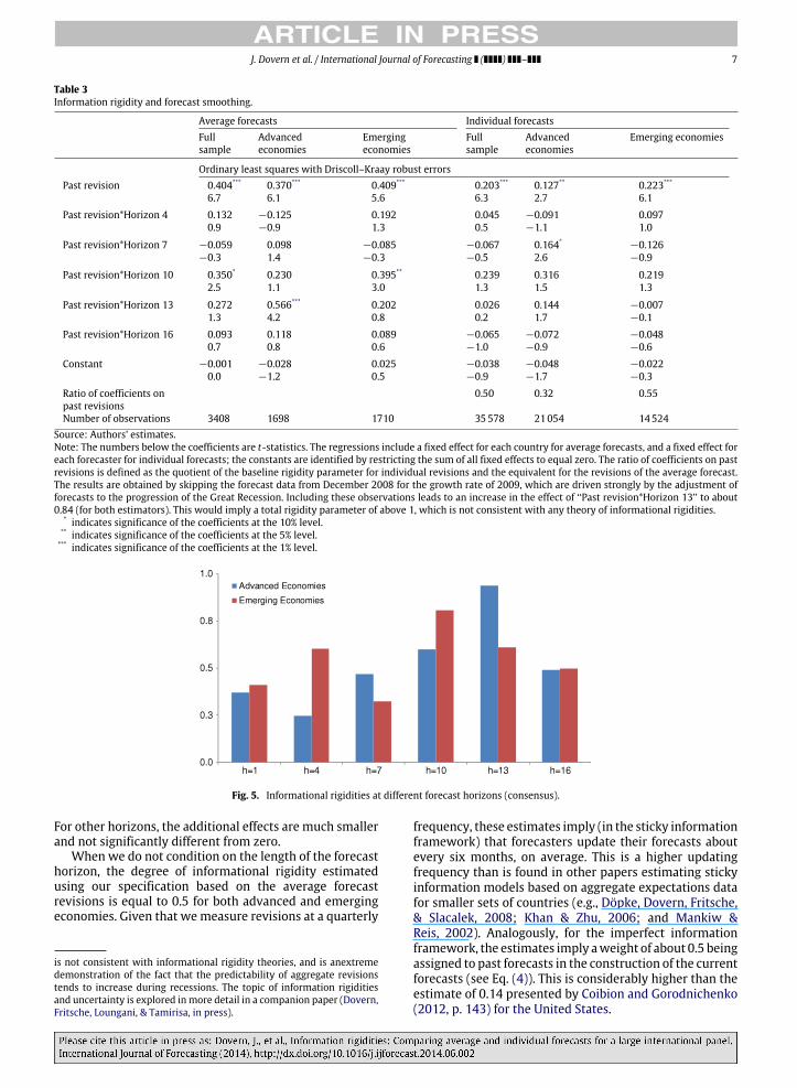
Information rigidities tend to be larger at around theturn of the year, i.e., at forecast horizons between 13 and 10(Fig. 5). Possible explanations for this pattern could relateto the fact that the quarter-on-quarter growth rates for thelast quarter of a year have a particularly large effect on theannual growth rate of the following year. Theremay also beinstitutional or behavioral explanations, where forecasters

6 Since all specifications include lagged revisions as an explanatoryvariable, we ‘‘lose’’ one observation per target year (h = 19) for theestimation. Our results are robust to the choice of horizons; that is, if weinstead pick h = 2, 5, 8, etc., for example.

Table 2Revisions and deviations from the average forecast.

Horizon (in months)h = 18 h = 12 h = 6 h = 1

Mean absolute deviation fromconsensus

Full sample 0.29 0.26 0.19 0.10Advanced economies 0.24 0.22 0.15 0.07Emerging economies 0.36 0.32 0.28 0.15

Variance of deviation fromconsensus

Full sample 0.42 0.39 0.31 0.17Advanced economies 0.33 0.29 0.21 0.11Emerging economies 0.56 0.52 0.45 0.25

Source: Authors’ estimates.

switch their focus from the current year forecasts to thenext year forecasts at around the turn of the year. However,the coefficients on the interaction terms between laggedrevisions and the horizon-indicator function are only pos-itive and statistically significant for horizons 10 (emergingeconomies) and 13 (advanced economies) respectively.7

7 As was noted in the footnote to Table 3, if we do not exclude forecastsmade in December 2008 for the growth rate of 2009, which are drivenstrongly by the adjustment of forecasts in the aftermath of the Lehmancollapse, we even obtain an estimate of the total degree of informationalrigidity (for advanced economies and h = 13), which is larger than 1. This

J. Dovern et al. / International Journal of Forecasting ( ) – 7

Table 3Information rigidity and forecast smoothing.

Average forecasts Individual forecastsFullsample

Advancedeconomies

Emergingeconomies

Fullsample

Advancedeconomies

Emerging economies

Ordinary least squares with Driscoll–Kraay robust errorsPast revision 0.404*** 0.370*** 0.409*** 0.203*** 0.127** 0.223***

6.7 6.1 5.6 6.3 2.7 6.1

Past revision*Horizon 4 0.132 −0.125 0.192 0.045 −0.091 0.0970.9 −0.9 1.3 0.5 −1.1 1.0

Past revision*Horizon 7 −0.059 0.098 −0.085 −0.067 0.164*−0.126

−0.3 1.4 −0.3 −0.5 2.6 −0.9

Past revision*Horizon 10 0.350* 0.230 0.395** 0.239 0.316 0.2192.5 1.1 3.0 1.3 1.5 1.3

Past revision*Horizon 13 0.272 0.566*** 0.202 0.026 0.144 −0.0071.3 4.2 0.8 0.2 1.7 −0.1

Past revision*Horizon 16 0.093 0.118 0.089 −0.065 −0.072 −0.0480.7 0.8 0.6 −1.0 −0.9 −0.6

Constant −0.001 −0.028 0.025 −0.038 −0.048 −0.0220.0 −1.2 0.5 −0.9 −1.7 −0.3

Ratio of coefficients onpast revisions

0.50 0.32 0.55

Number of observations 3408 1698 1710 35578 21054 14524Source: Authors’ estimates.Note: The numbers below the coefficients are t-statistics. The regressions include a fixed effect for each country for average forecasts, and a fixed effect foreach forecaster for individual forecasts; the constants are identified by restricting the sum of all fixed effects to equal zero. The ratio of coefficients on pastrevisions is defined as the quotient of the baseline rigidity parameter for individual revisions and the equivalent for the revisions of the average forecast.The results are obtained by skipping the forecast data from December 2008 for the growth rate of 2009, which are driven strongly by the adjustment offorecasts to the progression of the Great Recession. Including these observations leads to an increase in the effect of ‘‘Past revision*Horizon 13’’ to about0.84 (for both estimators). This would imply a total rigidity parameter of above 1, which is not consistent with any theory of informational rigidities.

* indicates significance of the coefficients at the 10% level.** indicates significance of the coefficients at the 5% level.*** indicates significance of the coefficients at the 1% level.

Fig. 5. Informational rigidities at different forecast horizons (consensus).

For other horizons, the additional effects are much smallerand not significantly different from zero.

When we do not condition on the length of the forecasthorizon, the degree of informational rigidity estimatedusing our specification based on the average forecastrevisions is equal to 0.5 for both advanced and emergingeconomies. Given that wemeasure revisions at a quarterly

is not consistent with informational rigidity theories, and is anextremedemonstration of the fact that the predictability of aggregate revisionstends to increase during recessions. The topic of information rigiditiesand uncertainty is explored inmore detail in a companion paper (Dovern,Fritsche, Loungani, & Tamirisa, in press).

frequency, these estimates imply (in the sticky informationframework) that forecasters update their forecasts aboutevery six months, on average. This is a higher updatingfrequency than is found in other papers estimating stickyinformation models based on aggregate expectations datafor smaller sets of countries (e.g., Döpke, Dovern, Fritsche,& Slacalek, 2008; Khan & Zhu, 2006; and Mankiw &Reis, 2002). Analogously, for the imperfect informationframework, the estimates imply aweight of about 0.5 beingassigned to past forecasts in the construction of the currentforecasts (see Eq. (4)). This is considerably higher than theestimate of 0.14 presented by Coibion and Gorodnichenko(2012, p. 143) for the United States.

8 J. Dovern et al. / International Journal of Forecasting ( ) –

Fig. 6. Fractions of revised individual forecasts.

4.2. Individual forecasts

4.2.1. Information stickinessNext, we measure the frequency of forecast updating

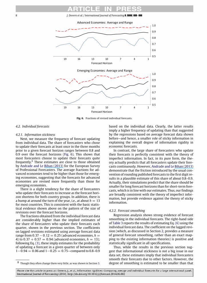
from individual data. The share of forecasters who choseto update their forecasts at least once in the three monthsprior to a given forecast horizon ranges between 0.8 and0.9 over the forecast horizons (Fig. 6). This shows thatmost forecasters choose to update their forecasts quitefrequently.8 These estimates are close to those obtainedby Andrade and Le Bihan (2013) for the European Surveyof Professional Forecasters. The average fractions for ad-vanced economies tend to be higher than those for emerg-ing economies, suggesting that the forecasts for advancedeconomies are revised more frequently than those foremerging economies.

There is a slight tendency for the share of forecasterswho update their forecasts to increase as the forecast hori-zon shortens for both country groups. In addition, there isa hump at around the turn of the year, i.e., at about h = 13for most countries. This is consistent with the basic statis-tical evidence shown above on the pattern of the size ofrevisions over the forecast horizons.

The fractions obtained from the individual forecast dataare considerably higher than the implied estimates ofthe share of forecasters who update their forecasts eachquarter, shown in the previous section. The coefficientson lagged revisions estimated using average forecast datarange from 0.37− 0.12 = 0.25 (advanced economies, h =

4) to 0.37 + 0.57 = 0.94 (advanced economies, h = 13);following Eq. (3), these imply estimates for the probabilityof updating a forecast in a given quarter of between only1−0.94 = 0.06 and 1−0.25 = 0.75—compared to 0.8–0.9

8 Though they often change them very little, as was shown in Section 3.

based on the individual data. Clearly, the latter resultsimply a higher frequency of updating than that suggestedby the regressions based on average forecast data shownbefore—and hence, a smaller role of sticky information inexplaining the overall degree of information rigidity ineconomic forecasts.

In contrast, the large share of forecasters who updatetheir forecasts is perfectly consistent with the theory ofimperfect information. In fact, in its pure form, the the-ory actually predicts that all forecasters update their fore-casts continuously. However, Andrade and Le Bihan (2013)demonstrate that the friction introduced by the usual con-vention of rounding published forecasts to the first digit re-sults in a plausible estimate of this share of about 0.8–0.9.Actually, their simulations predict that the share should besmaller for long forecast horizons than for short-term fore-casts, which is in linewith our estimates. Thus, our findingsare broadly consistent with the theory of imperfect infor-mation, but provide evidence against the theory of stickyinformation.

4.2.2. Forecast smoothingRegression analysis shows strong evidence of forecast

smoothing in the individual forecasts. The right-hand sideof Table 3 reports the results of estimating Eq. (6) using theindividual forecast data. The coefficient on the lagged revi-sion (which, as discussed in Section 2, provides a measureof general forecast smoothing, rather than an exact map-ping to the existing information theories) is positive andstatistically significant in all specifications.

Thus, while the results in the previous section sug-gest that informational stickiness is not a big issue in ourdata set, these estimates imply that individual forecasterssmooth their forecasts due to other factors. However, thedegree of smoothing is estimated to be smaller than that

J. Dovern et al. / International Journal of Forecasting ( ) – 9

Fig. 7. Distribution of information rigidity coefficients across countries.

for the consensus forecasts. The magnitude of the differ-ence is given in the row labeled ‘‘Ratio of coefficients onpast revisions’’ in Table 3, which shows the ratio of the co-efficient on lagged revisions estimated on individual fore-casts to that estimated on average forecasts; the estimateof the persistence in forecast revisions is about halved. Thissuggests that theprocess of averaging forecasts induces ad-ditional stickiness.

As with consensus forecasts, we find differences in theextent of smoothing in forecasts for advanced and emerg-ing economies. The coefficients on lagged revisions arehigher in the case of emerging economies (0.23 versus0.13). These results are consistent with the graphical evi-dence discussed in Section 3 (Fig. 4), and suggest that infor-mation rigidities are more pronounced in the forecasts foremerging economies, possibly owing to greater lags in datareleases, the weaker quality of economic statistics, and thefact that, probably, less resources are spent in the produc-tion of these forecasts relative to those spent on the fore-casts for advanced economies.

Also, similarly to the regressions based on average fore-casts, those based on individual forecast data suggest thatforecast smoothing is non-monotonic over forecast hori-zons. For advanced economies, the coefficients on theinteraction terms between lagged revisions and horizonvariables are strongly positive for horizons 7, 10 and 13;the largest size of the coefficients on the interaction termsis obtained at h = 13. The Driscoll–Kraay standard errors,however, show that the effects are not significantly dif-ferent from zero in most cases. For emerging economies,the results pertaining to the interaction terms are evenweaker; we do not report any significant effects. Overall,the conclusion is that, while forecast smoothing at the in-dividual level increases somewhat for the medium-rangeforecast horizons, the evidence for the horizon effect iseven weaker than in the regressions based on aggregateforecast data.

Lookingmore closely at the distribution of forecast per-sistence across countries reveals a substantial degree ofvariation. Table 4 shows estimates from country-specificestimates of Eq. (1) based on revisions of average forecasts

and summary statistics (for each country) for forecaster-specific estimates of the same model based on individ-ual forecast revisions.9 The results in this table provide astrong confirmation of our previous findings. For 29 coun-tries out of 31, the smoothing parameter from the averageforecasts is higher than that from the individual forecasts,and by a substantial margin in most cases.10 In some rarecases, the variation in individual forecast revisions is ex-plained to a substantial degree by lagged revisions (basedon the average R2 from the regressions, e.g., in Germany(0.35) or Italy (0.44)); but in general, revisions seem to bequite unpredictable at the individual level based on pastrevisions.

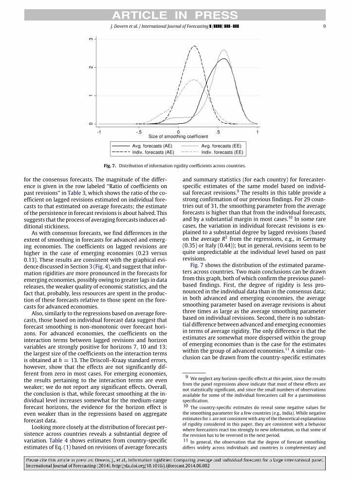
Fig. 7 shows the distribution of the estimated parame-ters across countries. Two main conclusions can be drawnfrom this graph, both of which confirm the previous panel-based findings. First, the degree of rigidity is less pro-nounced in the individual data than in the consensus data;in both advanced and emerging economies, the averagesmoothing parameter based on average revisions is aboutthree times as large as the average smoothing parameterbased on individual revisions. Second, there is no substan-tial difference between advanced and emerging economiesin terms of average rigidity. The only difference is that theestimates are somewhat more dispersed within the groupof emerging economies than is the case for the estimateswithin the group of advanced economies.11 A similar con-clusion can be drawn from the country-specific estimates

9 We neglect any horizon-specific effects at this point, since the resultsfrom the panel regressions above indicate that most of these effects arenot statistically significant, and since the small numbers of observationsavailable for some of the individual forecasters call for a parsimoniousspecification.10 The country-specific estimates do reveal some negative values forthe smoothing parameter for a few countries (e.g., India). While negativeestimates for λ are not consistentwith any of the theoretical explanationsof rigidity considered in this paper, they are consistent with a behaviorwhere forecasters react too strongly to new information, so that some ofthe revision has to be reversed in the next period.11 In general, the observation that the degree of forecast smoothingdiffers widely across individuals and countries is complementary and

10 J. Dovern et al. / International Journal of Forecasting ( ) –

Table 4Country-specific estimates.

Country Average forecasts Individual forecastsλ sd N R2 Avg. λ Avg. sd Avg. N Avg. R2 K Avg. Frac.

Australia 0.337 0.052 365 0.10 0.065 0.057 131.1 0.02 36 0.86Canada 0.414 0.049 364 0.16 0.165 0.098 165.0 0.19 29 0.73France 0.527 0.047 364 0.26 0.179 0.132 118.5 0.12 40 0.85Germany 0.613 0.044 364 0.35 0.337 0.103 200.3 0.35 42 0.78Italy 0.534 0.046 364 0.27 0.170 0.196 126.3 0.44 32 0.86Japan 0.492 0.048 364 0.22 0.216 0.174 109.2 0.06 38 0.92Netherlands 0.615 0.044 363 0.35 0.187 0.175 96.3 0.00 23 0.83New Zealand 0.389 0.056 341 0.13 −0.019 0.063 110.6 0.04 28 0.89Norway 0.494 0.048 363 0.22 0.118 0.100 88.9 0.00 18 0.92Spain 0.695 0.038 363 0.48 0.251 0.078 108.7 0.13 28 0.85Sweden 0.666 0.045 363 0.38 0.246 0.393 100.3 0.00 31 0.95Switzerland 0.631 0.047 363 0.34 0.298 0.068 124.9 0.16 19 0.79UK 0.699 0.041 364 0.45 0.310 0.264 144.9 0.28 60 0.79USA 0.330 0.051 364 0.10 0.037 0.339 121.4 0.02 60 0.84

Argentina 0.545 0.063 151 0.33 0.123 0.664 49.2 0.00 42 0.87Brazil 0.512 0.078 151 0.22 0.021 0.136 57.3 0.00 42 0.81Chile 0.570 0.065 151 0.34 0.281 0.098 64.8 0.23 38 0.82China 0.577 0.052 277 0.31 0.032 0.276 106.4 0.00 39 0.66Colombia 0.627 0.076 151 0.32 −0.002 0.314 50.5 0.02 30 0.75Costa Rica 0.499 0.072 147 0.25 – – – – – –Dominican Republic 0.572 0.076 147 0.28 – – – – – –Ecuador 0.335 0.087 147 0.09 – – – – – –Hong Kong 0.543 0.049 350 0.26 0.237 0.113 92.1 0.52 38 0.72India −0.079 0.058 277 0.01 −0.243 0.154 63.3 0.02 30 0.83Indonesia 0.624 0.041 350 0.40 0.102 0.027 76.1 0.01 39 0.67Malaysia 0.717 0.039 350 0.49 0.331 0.348 77.3 0.15 44 0.72Mexico 0.638 0.060 151 0.43 0.141 0.146 67.4 0.20 44 0.83Panama 0.395 0.077 147 0.15 – – – – – –Paraguay 0.526 0.081 147 0.22 – – – – – –Peru 0.702 0.063 151 0.45 0.461 0.088 56.9 0.12 25 0.79Philippines 0.390 0.065 277 0.12 −0.135 0.190 15.6 0.01 14 0.86Singapore 0.699 0.050 350 0.36 0.372 0.112 84.8 0.14 38 0.79South Korea 0.528 0.048 365 0.25 0.173 0.069 87.7 0.05 36 0.83Taiwan POC 0.559 0.049 365 0.26 0.310 0.080 103.4 0.03 32 0.80Thailand 0.616 0.045 350 0.35 0.203 0.135 68.9 0.19 41 0.81Venezuela 0.119 0.085 151 0.01 0.227 0.259 60.8 0.04 33 0.82

Note: The estimates in the left part of the table refer to country-specific estimations based on the revision of the average forecast for each country. Thosein the right part of the table are average figures based on separate estimations for each individual forecaster in each country. All country- and forecaster-specific models were estimated without any forecast-horizon controls. λ denotes the estimated coefficient for the first lag of the 3-month revision (Avg.λ refers to the average across all individual estimates for each country). Sd (Avg. sd) is the corresponding (average) standard deviation. N (Avg. N) showsthe (average) number of observations for each estimation. K denotes the number of different forecasters in each country for which an estimate is obtained.Avg. Frac. displays the fraction of forecasters that, on average, adjust their forecasts at least once during a three-month period (computed across all forecasthorizons).Source: Authors’ estimates.

for the fraction of forecasters that, on average, update theirgrowth forecasts at least once during a three-month pe-riod: the average estimate for advanced economies (0.85)is somewhat higher than the corresponding estimate foremerging economies (0.79), but this difference is statis-tically insignificant given the standard deviation acrosscountries (approximately 0.06 in both cases).

5. Conclusion

This paper has provided evidence on the dynamicsof forecast revisions of real GDP growth using a largepanel data set of individual forecasters in 36 advanced andemerging market economies over the period 1989–2011.The data set used in the paper is far larger than any panel of

similar to Dovern’s (2013) finding that the frequency of forecast updatingdiffers substantially across individuals, countries and time.

individual forecasts previously used in the literature, andcovers a wide range of different countries.

Previous work has documented that forecasts are char-acterized by a significant degree of smoothing or rigidity(Coibion & Gorodnichenko, 2010; Nordhaus, 1987), and anumber of theories have been offered to explain this phe-nomenon. In particular, Coibion and Gorodnichenko showthat finding a correlation between the forecast errors andpast forecast revisions is consistentwith two of the leadingexplanations for forecast smoothing, viz., the sticky infor-mation model and the ‘‘noisy’’ information model.

Using an equivalent test of forecast revisions on pastforecast revisions, we confirm the finding of persistence inaverage forecast revisions. We also contribute novel per-spectives on forecasters’ behavior, drawing on our large setof individual forecasts for advanced and emerging coun-tries.

In particular, we provide evidence against the useful-ness of the sticky information model for describing the

J. Dovern et al. / International Journal of Forecasting ( ) – 11

dynamics of growth forecasts. We show that the esti-mates of informational rigidity based on consensus (av-erage) forecasts overstate the true degree of forecasters’inattentiveness.When consensus forecasts are used, as hasbeen the common practice in previous studies, the esti-mates suggest that forecasts are updated every six monthson average. Our analysis of the fractions of forecasters whoupdate their forecasts, however, points to a higher fre-quency of updating. Hence, the evidence based on fractionssuggests only aminor role of sticky information in explain-ing the overall degree of information rigidity in economicforecasts. The predictability of individual forecast revisionsalso casts some doubt on the validity of the sticky informa-tion theory.

Many interesting issues are left for the future research.In particular, herding, another prominent feature of fore-casters’ behavior (Gallo et al., 2002), and its interactionwith forecast smoothing, deserve a closer look. In addition,our sample shows evidence of nonlinearities in forecastsmoothing.12 Further topics that merit exploration are theimplications of uncertainty for the dynamics of macroeco-nomic forecasting and the evolution of forecast rigiditiesover the business cycle.

Acknowledgments

We thank Angela Espiritu and Jair Rodriguez for excel-lent research assistance.We are also grateful toOli Coibion,Yuriy Gorodnichenko, Tara Sinclair and an anonymous ref-eree for valuable suggestions on an earlier draft, as wellas participants in the 2014 AEA meetings, 2012 George-Washington-University-IMF Forecasting Forum, the 2011International Symposium on Forecasting, the 2012 Econo-metric Society’s Australasian Meeting, and seminars at theGeorge Washington University and Hamburg Universityfor helpful comments.

References

Ager, P., Kappler, M., & Osterloh, S. (2009). The accuracy and efficiencyof the consensus forecasts: a further application and extension of thepooled approach. International Journal of Forecasting , 25(1), 167–181.

Andrade, P., & Le Bihan, H. (2013). Inattentive professional forecasters.Journal of Monetary Economics, 60(8), 967–998.

Arellano, M., & Bond, S. (1991). Some tests of specification for panel data:Monte Carlo evidence and an application to employment equations.Review of Economic Studies, 58, 277–297.

Arellano,M., & Bover, O. (1995). Another look at the instrumental variableestimation of error-components models. Journal of Econometrics, 68,29–51.

12 Smoothing is less pronounced in the tails of the distribution of indi-vidual forecast revisions than in themain body of the distribution (see theworking paper version of this paper for preliminary evidence). However,it remains an open question as to how these nonlinearities can be linkedto the different theories of forecast generation mentioned in this paper.

Batchelor, R. (2007). Bias in macroeconomic forecasts. InternationalJournal of Forecasting , 23(2), 189–203.

Coibion, O., & Gorodnichenko, Y. (2010). Information rigidity and theexpectations formation process: a simple framework and new facts. NBERworking papers 16537, National Bureau of Economic Research, Inc.

Coibion, O., & Gorodnichenko, Y. (2012). What can survey forecasts tellus about information rigidities? Journal of Political Economy, 120(1),116–159.

Crowe, C. (2010). Consensus forecasts and inefficient information aggrega-tion. IMF working paper WP/10/178, July.

Davies, A., & Lahiri, K. (1995). A new framework for analysing surveyforecasts using three-dimensional panel data. Journal of Econometrics,68, 205–227.

Döpke, J., Dovern, J., Fritsche, U., & Slacalek, J. (2008). Sticky informationPhillips curves: European evidence. Journal of Money, Credit andBanking , 40(7), 1513–1519.

Dovern, J. (2013).When areGDP forecasts updated? Evidence froma largeinternational panel. Economics Letters, 120, 521–523.

Dovern, J., Fritsche, U., Loungani, P., & Tamirisa, N. (in press). Areinformational rigidities of macroeconomic forecasts influenced by thebusiness cycle? Unpublished manuscript.

Dovern, J., Fritsche, U., & Slacalek, J. (2012). Disagreement amongforecasters in G7 countries. Review of Economics and Statistics, 94(4),1081–1096.

Dovern, J., & Weisser, J. (2011). Accuracy, unbiasedness and efficiency ofprofessional macroeconomic forecasts: an empirical comparison forthe G7. International Journal of Forecasting , 27(2), 452–465.

Driscoll, J. C., & Kraay, A. C. (1998). Consistent covariance matrixestimation with spatially dependent panel data. Review of Economicsand Statistics, 80, 549–560.

Gallo, G. M., Granger, C. W. J., & Jeon, Y. (2002). Copycats and commonswings: the impact of the use of forecasts in information sets. IMFStaff Papers, 49(1), 4–21.

Isiklar, G., Lahiri, K., & Loungani, P. (2006). How quickly do forecastersincorporate news? Journal of Applied Econometrics, 21, 703–725.

Khan, H., & Zhu, Z. (2006). Estimates of the sticky-information Phillipscurve for the United States. Journal of Money, Credit and Banking ,38(1), 195–207.

Lahiri, K., & Sheng, X. (2008). Evolution of forecast disagreement in aBayesian learning model. Journal of Econometrics, 114(2), 325–340.

Loungani, P. (2001). How accurate are private sector forecasts? Cross-country evidence from consensus forecasts of output growth.International Journal of Forecasting , 17, 419–432.

Loungani, P., Stekler, H., & Tamirisa, N. (2013). Information rigidity ingrowth forecasts: some cross-country evidence. International Journalof Forecasting , 29(4), 605–621.

Mankiw, G., & Reis, R. (2002). Sticky information versus sticky prices:a proposal to replace the new Keynesian Phillips curve. QuarterlyJournal of Economics, 117(4), 1295–1328.

Nickell, S. (1981). Biases in dynamic models with fixed effects.Econometrica, 49(6), 1417–1426.

Nordhaus, W. (1987). Forecasting efficiency: concepts and applications.The Review of Economics and Statistics, 69, 667–674.

Reis, R. (2006). Inattentive producers. Review of Economic Studies, 73(3),793–821.

Sims, C. (2003). Implications of rational inattention. Journal of MonetaryEconomics, 50(3), 665–690.

Windmeijer, F. (2005). A finite sample correction for the variance of linearefficient two-step GMM estimators. Journal of Econometrics, 126(1),25–51.

Woodford, M. (2002). Imperfect common knowledge and the effects ofmonetary policy. In P. Aghion, R. Frydman, J. Stiglitz, & M. Woodford(Eds.), Knowledge, information, and expectations in modern macroeco-nomics: in honor of Edmund S. Phelps. Princeton University Press.