Working Paper

Hans-Böckler-Straße 39 D-40476 Düsseldorf Germany Phone: +49-211-7778-331 IMK@boeckler.de http://www.imk-boeckler.de

Sustainable Capitalism: Full-Employment Flexicurity Growth with Real Wage Rigidities

Toichiro Asada, Peter Flaschel, Alfred Greiner, Christian Proaño

April 27, 2010

5/2010

Sustainable Capitalism: Full-Employment Flexicurity Growth

with Real Wage Rigidities

Toichiro Asada,

Faculty of Economics, Chuo University,

Tokyo, Japan

Peter Flaschel,∗ Alfred Greiner

Department of Business Administration and Economics,

Bielefeld University, Bielefeld, Germany

Christian R. Proano

Macroeconomic Policy Institute (IMK)

Dusseldorf, Germany

April 27, 2010

Abstract

In this paper we present a model of flexicurity capitalism that exhibits a second labormarket with the government as an employer of first resort, where all workers not employedby firms in the private sector find meaningful employment. We show that the model exhibitsa unique interior steady state which is asymptotically stable under real wage adjustmentdynamics of the type considered in Blanchard and Katz (1999), and under a type of Okun’sLaw that links the level of utilization of firms to their hiring and firing decision. Theintroduction of a company pension fund can be shown to contribute to the viability of theanalyzed economic system. However, when credit is incorporated in the model, in placeof savings-driven supply side fluctuations in economic activity, investment-driven demandside business cycle fluctuations (of a probably much more volatile type) can take place.———————Keywords: Flexicurity, employer of first resort, Solovian growth, company pension funds,

sustainability.JEL CLASSIFICATION SYSTEM: E3, E6, H1

∗Corresponding author. E-mail: pflaschelwiwi.uni-bielefeld.de

1

1 Introduction

In the US unemployment rates had been relatively low until the beginning of the financial crisisin the late 2000’s, in contrast to Europe where a great many countries have been suffering fromhigh and persistent unemployment over the last decades. But there are also European countriesthat were successful in maintaining high employment rates. These are, on the one hand, theNetherlands and the Nordic Welfare states, such as Denmark, Finland and Sweden, and, onthe other hand, Great Britain and Ireland. While Great Britain and Ireland have pursued anAnglo-Saxon approach with respect to its economic policy, mainly characterized by flexiblehiring and firing conditions and by few social spending, the Nordic Welfare states and theNetherlands have followed a different policy. The latter allow flexible hiring and firing, too,but they have adopted high standards of social security. Thus, these countries demonstrate thatflexibility and security need not be contradictory but may well be compatible and that socialsecurity does not necessarily lead to high unemployment rates or instability of the economicsystem. Often, the Nordic welfare system is referred to as the flexicurity model, with the termflexicurity obtained by merging the terms flexibility and security.It is in particular in public debates, that the flexicurity model has attracted great attention,although there is no clear consensus on its definition (cf. Zhou (2007). According to Wilthagen(1998) the concept of flexicurity was launched by the sociologist and member of the DutchScientific Council for Government Policy Hans Adriaansens in speeches and interviews. Ac-cording to Adriaansens flexicurity means a shift from ’security within a job’ toward ’securityof a job’ (cf. Wilthagen, 1998, p. 13). In any case, an important aspect as regards flexibilityon the labor market is that there is both external flexibility, i.e. hiring and firing, as well asinternal flexibility, such as flexible working hours and the possibility of working overtime andpart-time work (see Wilthagen et al., 2004a,b). Essential characteristics with respect to secu-rity are income security that is income protection in the event of job loss and after retiring fromwork, on the one hand, and the ability to combine paid work with other social responsibilitiesand obligations, on the other hand. Our goal in this paper is to integrate some ideas of theflexicurity model into the basic neoclassical growth model as presented by Solow (1956) andto analyze the resulting model with respect to its dynamic properties.Solow’s (1956) model of economic growth provides the basis for a variety of subsequent modelsanalyzing the phenomenon of economic growth in Western capitalist economies. An importantaspect in Solow’s growth model is the assumption of a neoclassical production function withsmooth factor substitution characterizing the input-output relationship that determines thelaws of motion of the economy, in place of a fixed proportions technology. Solow assumed fullemployment and considered homogenous labor as one of the factors of production. In contrastto that, Goodwin’s (1967) growth cycle model had quite a different starting point (Marx’sreserve army mechanism): It assumed – as in Marx (1954, ch. 23) – a real wage Phillipscurve and considered its interaction assuming an extreme variant of classical savings behaviorin a technological framework with fixed proportions in production. Instead of monotonicconvergence to the steady state, the Goodwin model gave rise to persistent cycles aroundits steady state position of a structurally unstable center dynamics type that could be easily

2

modified towards the occurrence of stable limit cycles (as in Rose’s (1967) employment cyclemodel).1

It is not difficult to combine the Solow growth model with the Goodwin growth cycle model,since the latter only introduces real wage rigidities into the Solovian framework (or smoothfactor substitution into the Goodwin growth model). The resulting model features dampedoscillations (close to Goodwinian cycles if the elasticity of substitution between capital andlabor is low) and even monotonic convergence of the state variables (labor intensity and realwage) to the steady state in the opposite case. However, one problem of this integrated modelis – if it creates periods of mass unemployment – that it implies the possibility of unemployedworkers losing their skills and, thus, leading to labor market segmentation, with older workerssubject to long-term or never ending unemployment and workers’ families becoming degradedin their social and emotional status (a situation that is difficult to reverse). Further, theremay be counteracting unemployment benefits, low wages for the degraded part of the workforce and more that must be analyzed with respect to their consequences for the evolution ofcapitalist economies.In this paper we will not engage into such an analysis of the consequences of mass unemploy-ment but we will augment the above Solow-Goodwin synthesis by an employer of first (notlast) resort, where all workers (and even pensioners) find reasonable employment if they aretemporarily dismissed from the private sector of the economy, the sector of capitalist firms. Inour model economy, that is to be seen as ideal in that respect, we only allow for two types ofskill characteristics: skilled and high-skilled labor instructed in primary/secondary educationand in tertiary education, respectively. Thus, by speaking of an employer of first resort weintend to underline that the skilled or high-skilled work profiles are employed in the publicsector as well as in the private sector. Hence, we abstract from an employer of last resort andfrom the corresponding labor market where all labor is employed that is either unwilling orunable to work as skilled or high-skilled worker. By modeling the government as an employerof first resort we want to emphasize that the government needs qualified employees in order toorganize the complex social security system in a flexicurity economy. This fact holds true forindustrialized countries and, therefore, for Nordic countries as well so that one cannot call thegovernment an employer of last resort. The model we build on this basis is providing a stylizedtheoretical basis for the Nordic Welfare approach to flexicurity, but one that is not subjectto the pejorative reformulation of flexicurity as ’flexploitation’ as it is sometimes referred toin evaluations of the concept of flexicurity in the political debate. Instead, we use the Solowmodel with the Goodwin real wage rigidity to construct full employment in this framework bymeans of (decentralized) government actions, with wage bargaining in the private sector andwith two implied laws of motion (for employment and for the real wage) that will guaranteeeven monotonic convergence to the steady state in such a framework with flexible hiring andfiring.We view this model as an ideal economic system, a democratic and egalitarian society shouldaspire to, and towards which progress paths have to be found, confirmed by elections in a

1See also Solow (1990) for an interesting discussion of the Goodwin (1967) growth cycle model.

3

democratic society introducing ratchet effects when some parties propose to abolish such anevolution (if it has been by and large successful). It is ideal in that it combines flexible hiringand firing (and job discontinuities in the first, the private labor market) with income andemployment security through a pension scheme and a second labor market that preserves theskills of the workforce and prevents their human degradation. Although being an ideal systemsome elements have already been integrated in real-world economies. For example, in Europethe three main pillars on which the social security system rests are the health care system, theunemployment insurance and the pension system. In our model we will take into account twoof these pillars, the unemployment insurance and the pension system while neglecting healthinsurance. Thus, we present a model where the aspect of income security is modeled withrespect to unemployment and with respect to the old age. By demonstrating that our modeleconomy is stable, meaning that it converges to a steady state, we can show that an economywith a relatively elaborate social security system may well be a sustainable one.We think that modern market economies are currently experiencing progress paths towards theflexicurity model, sometimes on a very low pace as the current discussion about minimum wagesin Germany demonstrates. Yet, even such a discussion can be reflected from the perspectiveof the concept of flexicurity and may be interpreted as a step forward towards flexicurityif a general minimum level of (real) wages can be established in Germany. We have shownin Flaschel and Greiner (2009) in the context of Goodwin’s growth cycle mechanism thatminimum and also maximum wages (of workers) could dampen the employment fluctuationsof the economy and could thus contribute to its stability after a transitory period of lowemployment.Flexicurity – properly understood – may be the modern equivalent to Solow’s growth modeland may – in the same ideal way – provide a perspective for the future of capitalism whichis compatible with the social structure of democratic societies. To demonstrate the workingof flexicurity capitalism we will provide in section 2 the accounting framework for such aneconomy. In section 3 we will consider the behavior of the agents in such a framework in verybasic terms and show on this basis the global asymptotic stability of – and even monotonicconvergence to – its steady state position with respect to its central state variables, the realwage in the first labor market and the utilization rate of the workforce of firms. In section4 we study the law of motion and the steady state positions of the (extra) company pensionpayments this model type allows for and, thus, consider conditions for the viability of theeconomy (which should allow for pension payments above the level of base pension payments).Yet, if we consider credit financing in nominal terms the investment behavior can departfrom savings behavior such that the coordination of these two magnitudes leads to Keynesianeffective demand problems giving rise to demand driven business cycles. This is the stagewhere flexicurity capitalism must prove its superiority, since there are existing business cyclefluctuations of a much larger extent than those that can originate from supply side driven fullcapacity growth. Such problems must however be left for future research here.

4

2 Flexicurity societies

The flexicurity concept – primarily discussed with respect to the Nordic economies and theNetherlands – intends to combine two labor market components which – as many economistsmight argue – cannot be reconciled with each other, namely workplace flexibility in a verycompetitive environment with income and employment (but not job) security for workers inthis economy. The problem here is to find the appropriate mix between the two aspects oflabor market institutions, intended to overcome both the case of flexibility without security(free hiring and firing capitalism) as well as the case of security without flexibility (past Easternsocialism).In this section we first consider some basic features of a flexicurity economy. Thereafter, thebudget equations and the economic behavior within these equations are presented. On thisbasis we investigate the stability of balanced growth paths of such an economy and also itssustainability concerning the generation of sufficient income and pension payments.

2.1 Full-employment capitalism: Ideal, status-quo and compromises

Let us start here from a definition of the concept of flexicurity as it is discussed in the EuropeanUnion.

The concept of ’flexicurity’ attempts to find a balance between flexibility for employers (andemployees) and security for employees. The Commission’s 1997 Green Paper on ’Partner-ship for a new organization of work’ stressed the importance of both flexibility and securityto competitiveness and the modernization of work organization. The idea also featuresprominently in the ’adaptability pillar’ of the EU employment guidelines, where ’the so-cial partners are invited to negotiate at all appropriate levels agreements to modernize theorganization of work, including flexible working arrangements, with the aim of making un-dertakings productive and competitive and achieving the required balance between flexibilityand security.’ This ’balance’ is also consistently referred to in the Commission’s SocialPolicy Agenda 2000-2005 COM (2000) 379 final, Brussels, 28 June 2000).2

The concept of ‘flexicurity’ was introduced in Denmark on the political level by the socialdemocratic prime minister Poul Nyrup Rasmussen in the 1990’s3 and it was introduced into theacademic literature by Ton Wilthagen, see Wilthagen (1998) and Wilthagen et al. (2004a,b)on the Dutch origins of the flexicurity model. The role of the flexicurity approach in theperformance of the Danish economy is critically investigated in Anderson and Svarer (2007);for further critical assessments of the proposals for and the discussion on a flexicurity economythe reader is moreover referred to recent contributions by Funk (2008) and Viebrock and J.Clasen (2009).We stress in this context that our following approach to flexicurity is an abstract and primarilymacroeconomic one that neglects the difficulties of how to implement flexicurity coordinationand incentive principles on the microlevel from the economic, the social and the juristic pointof view.

2http://www.eurofound.europa.eu/areas/industrialrelations/dictionary/definitions/flexicurity.htm

3See http://www.eurofound.europa.eu/areas/industrialrelations/dictionary/definitions/FLEXICURITY.htm

5

Our approach to labor market institutions of the flexicurity type differs significantly from thebasic income guarantee (BIG) and Employer of Last Resort (ELR) approaches of the literatureas they are compared for example in Tcherneva and Wray (2005), though the intention ofthese and our approaches have many things in common. Our approach can be characterizedas an abstract modeling of a full-employment economy comparable in intention to the TableauEconomique of Quesnay. It therefore represents an ideal economy to be compared with thestatus-quo of actual developed capitalist economies. Such a comparison should then allow usto formulate compromises between the ideal and the status-quo of actual economies, like theUnited States of America or Australia, as described in Tchernova and Wray in the first caseand in Quirk et al. (2006) with respect to Job Guarantee (JG) principles in the second case.We would however argue here that these latter approaches are presenting compromises withoutreally formulating an ideal on the basis of which these compromises can be designed.We thus just do the opposite here which may therefore be considered as complementary tothe ELR and JG approaches, though we do not assume job guarantees, but only employmentsecurity. Moreover, however, in the ideal we have dismissed the concept of un- or low-skilledlabor as representing a significant portion of the working population, since we believe that anideal schooling system can overcome this factual situation to a large degree.

2.2 Flexicurity: Basic principles and problems

Basic aspects and problems of such a combination are:

• How much flexibility in:

1.1 hiring and firing and job discontinuities?

1.2 wage and price setting?

1.3 technical change?

1.4 globalization and financial markets?

• How much security in:

2.1 base income?

2.2 employment?

2.3 location of employment?

2.4 atypical employment?

Moreover, in order to get social acceptance for such a combination of the interests of capitalowners and those of workers, basic aspects of social cohesion in a modern democratic marketeconomy must be given. Thus, the following problems must also find a positive solution:

• Is there a consent-based cooperation between capital and labor?

• Does a proper citizenship education and democratic evolution exist?

• Is the existence of equal opportunities assured?

6

• Is there a reflected and controlled evolution of institutions?

In this paper we will provide a model which reconciles the aspects 1.1/2 with the problems2.1/2, where the other aspects of the enumerated points remain excluded. Further, we shallsimply assume that the societal issues in the last block have been developed to such an extentthat the proposed model is not only transparent to the citizens of the considered capitalistsociety, but have indeed led to basic agreements on how the economy is to be organized andhow the society should be developed further.

2.3 Budget equations, consumption and investment

Against this background, we next design the accounting framework (formulate the budgetequations) of a growth model that combines ideas of Solow (1956) and Goodwin (1967). Incontrast to Goodwin, our model takes into account a second labor market which, through itsinstitutional setup, guarantees full employment in its interaction with the first labor market,the highly flexible and competitive private sector of the economy. It goes without sayingthat, to start with, the model must be formulated in as simple a way as possible, however,incorporating the essential components which underlie a flexicurity economy and society. Wefirst consider the sector of firms in such an economy:

Firms

Production and Income Account:

Uses Resources

δK δK

ω1Ld1 C1 + C2 + Cr

ω2Lw2f G

Π (= Y f ) I (= Y f )

Y Y

δ1R + R S1

This account is a very simple one. Firms use their capital stock K (at profit-maximizing fullcapacity utilization) to employ the amount of labor (in hours): Ld

1 in its operation, at the realwage ω1, the law of motion of which is to be determined in the next section from a model of thewage-price dynamics in the private sector. They in addition employ labor force Lw

2f = αfLd1

(in heads4) from the second labor market at the wage ω2, which is a constant fraction αω ofthe real wage in the first labor market. This labor force Lw

2f is working the normal hoursof a standard workday, while the workforce Lw

1 from the first labor market may be workingovertime or undertime depending on the size of the capital stock in particular. Therefore therate uw = Ld

1/Lw1 gives the utilization rate of the workforce Lw

1 in the first labor market, theprivate sector of the economy (all other employment comes from the working of households

4to be determined in the next section.

7

occupied in the second labor market). Note finally that the capital stock depreciates at therate δ.

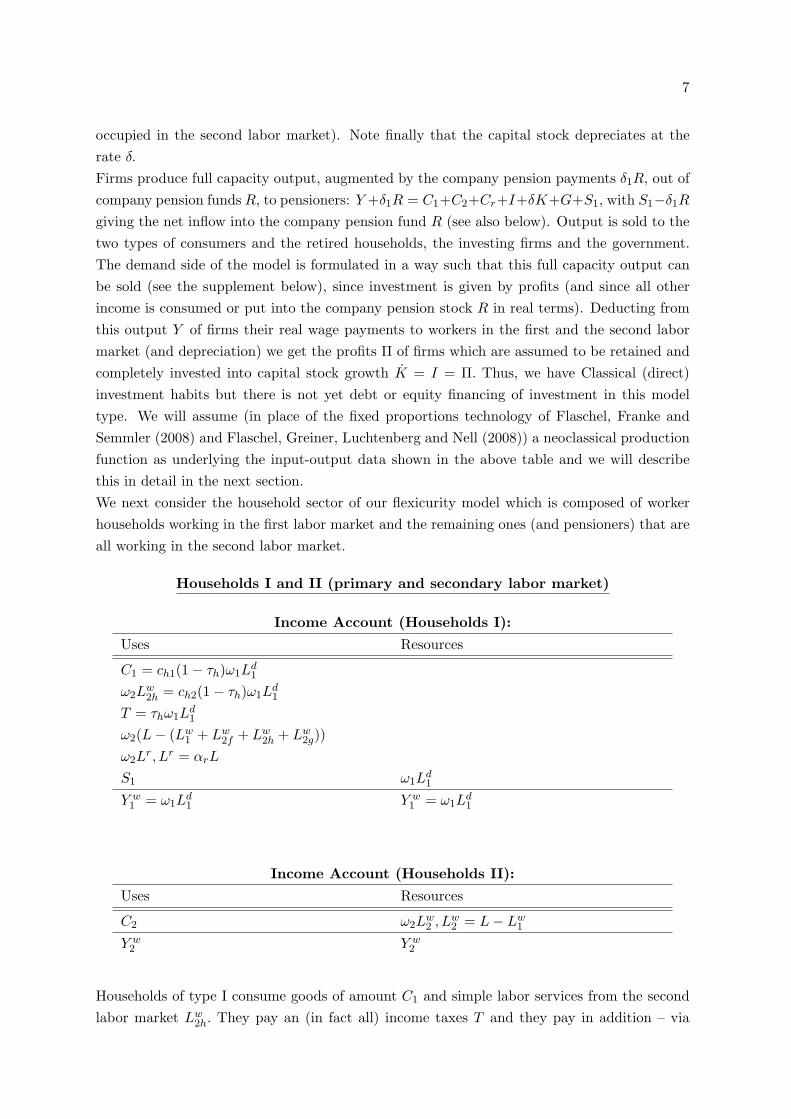
Firms produce full capacity output, augmented by the company pension payments δ1R, out ofcompany pension funds R, to pensioners: Y +δ1R = C1+C2+Cr+I+δK+G+S1, with S1−δ1R

giving the net inflow into the company pension fund R (see also below). Output is sold to thetwo types of consumers and the retired households, the investing firms and the government.The demand side of the model is formulated in a way such that this full capacity output canbe sold (see the supplement below), since investment is given by profits (and since all otherincome is consumed or put into the company pension stock R in real terms). Deducting fromthis output Y of firms their real wage payments to workers in the first and the second labormarket (and depreciation) we get the profits Π of firms which are assumed to be retained andcompletely invested into capital stock growth K = I = Π. Thus, we have Classical (direct)investment habits but there is not yet debt or equity financing of investment in this modeltype. We will assume (in place of the fixed proportions technology of Flaschel, Franke andSemmler (2008) and Flaschel, Greiner, Luchtenberg and Nell (2008)) a neoclassical productionfunction as underlying the input-output data shown in the above table and we will describethis in detail in the next section.We next consider the household sector of our flexicurity model which is composed of workerhouseholds working in the first labor market and the remaining ones (and pensioners) that areall working in the second labor market.

Households I and II (primary and secondary labor market)

Income Account (Households I):

Uses Resources

C1 = ch1(1− τh)ω1Ld1

ω2Lw2h = ch2(1− τh)ω1L

d1

T = τhω1Ld1

ω2(L− (Lw1 + Lw

2f + Lw2h + Lw

2g))ω2L

r, Lr = αrL

S1 ω1Ld1

Y w1 = ω1L

d1 Y w

1 = ω1Ld1

Income Account (Households II):

Uses Resources

C2 ω2Lw2 , Lw

2 = L− Lw1

Y w2 Y w

2

Households of type I consume goods of amount C1 and simple labor services from the secondlabor market Lw

2h. They pay an (in fact all) income taxes T and they pay in addition – via

8

further tax transfers – all workers’ income that is not coming from firms, from them and thegovernment (which is equivalent to an unemployment insurance). Moreover, they pay thepensions of the retired households (ω2L

r) and accumulate their remaining income S1 in theform of a company pension into a fund R that is administrated by firms (with inflow S1 andoutflow δ1R). Thus, we have a pay-as-you-go pension system and a company pension fundthat assure the income of retired persons.The transfer ω2(L − (Lw

1 + Lw2f + Lw

2h + Lw2g) can be considered as solidarity payments, since

workers from the first labor market that lose their job will automatically be employed in thesecond labor market where full employment is guaranteed by the government. We considerthis employment as skill preserving, since it can be viewed as ordinary office or handicraft work(subject only to learning by doing when such workers return to the first labor market, i.e, toemployment in the production process of firms).The second sector of households is modelled in the simplest way that is available: Householdsemployed in the second labor market, i.e, Lw

2 = Lw2f + Lw

2h + Lw2g pay no taxes and totally

consume their income. We have thus Classical saving habits in this household sector, whilehouseholds of type I may have positive or negative savings S1 as residual from their income andtheir expenditures. We assume that they can accumulate these savings (or dissave in case of anegative S1) from the stock of commodities they have accumulated as pension fund inventoriesin the past. In order to have a coherent distribution of the funds R that are accumulated byhouseholds of type I on the basis of their savings S1, we have to formulate the law of motionof such funds R as follows:

R = S1 − δ1R

where δ1 is the rate by which these funds are depreciated through company pension paymentsto the ’officially retired’ workers Lr, assumed to be a constant fraction of the ’active’ workforceLr = αrL. These worker households are added here as not really inactive, but offer workaccording to their still existing capabilities that can be considered as a (voluntary) additionto the supply of work organized by the government L − (Lw

1 + Lw2f + Lw

2h), i.e. the workingpotential of the officially retired persons remains an active and valuable contribution of theworking hours that are supplied by the members of the society. We consider this principleof ‘active aging’ an important feature of a flexicurity economy. It is obvious that the properallocation of the work hours under the control of the government needs thorough reflectionfrom the microeconomic and the social point of view, which however cannot be a topic in apaper on the macroeconomics of such an economy.As the income account of the retired households shows (see below) they receive pension pay-ments as if they would work in the second labor market and they get in addition individualtransfer income (company pensions) from the accumulated funds R in proportion to the timethey have been active in the first labor market and as an aggregate household group of thetotal amount δ1R by which the pension funds R are reduced in each period.

9

Income Account (Retired Households):

Uses Resources

Cr ω2Lr + δ1R, Lr = αrL

Y r Y r

There is finally the government sector which is also formulated in a very basic way:

The Government

Income Account: Fiscal Authority / Employer of First Resort

Uses Resources

G = αgT T = τhω1Ld1

ω2Lwg2 = (1− αg)T

ω2(L− (Lw1 + Lw

2f + Lw2h + Lw

2g)) ω2Lwr

ω2Lr ω2αrL

Y g Y g

The government receives income taxes, the solidarity payments (employment benefits) for thesecond labor market paid from workers in the first labor market and old-age pension payments.It uses the taxes to finance government goods demand G and the surplus of taxes over thesegovernment expenditures to actively employ the core workers in the government sector. Inaddition it employs the workers receiving employment benefits from the households in firstlabor market and it in fact also employs the ’retired’ persons to the extent they are willingand can still contribute to the various employment activities. We thus have that the totallabor force in the second labor market is employed by firms, by households of type I and theremainder through the government as is obvious from the solidarity payments of householdsworking in the first labor market. The income payments to workers in the second labormarket (ω2L

w2 ) that are not originating from their services to firms, to households of type I or

through an excess of income taxes over government commodity expenditures (base governmentemployment) are paid out of transfers from the household sector I that works in the privatesector to the government under competitive conditions. On the basis of these payments theremaining work in the second labor market is organized by government (in the way it does thisin the administration of the state in all modern market economies).In sum we get that workers are employed either in the first labor market and if not therethen by doing auxiliary work within firms, services for households of type I or services inthe government sector concerning public administration, infrastructure services, educationalservices or other public services. In addition there is a potential labor supply αrL from theretired households, which due to their long life-expectancy in modern societies can remaineffective suppliers of specific work over a considerable span of their life time after their officialretirement. In this way the whole workforce is always fully employed in this model of socialgrowth (and the retired persons according to their willingness and capabilities) and, thus, doesnot suffer from human degradation through prolonged unemployment in particular. Of course,

10

there are a variety of issues concerning state organized work that point to (incentive) problemsin the organization of such work, but all such problems exist also in actual industrializedmarket economies in one way or another.We have formulated in this section the skeleton of a flexicurity growth model of the economywhere full employment is not assumed, but actively constructed. The next sections augment theaccounts of the considered economy by basic behavioral relationships concerning production,employment and the law of motion of real wages.

3 Smooth factor substitution, Okun’s law and real wage rigidi-

ties

Our synthesis of the growth models of Solow (1956) and Goodwin (1967) into a model of theflexicurity variety consists of three basic building blocks, the three factor production functionof the private sector, Okun’s law that relates the utilization of the workforce Lw

1 to the hiringand firing decision of firms and the dynamic of the real wages of the workers in the first labormarket, describing the degree of labor market rigidity existing in the private sector of theeconomy.The module that describes the growth dynamics of the model therefore consists of the followingthree structural equations:

Y = F (K, Ld1, L

w2f ), ω1 = F2(K, Ld

1, Lw2f ), ω2 = F3(K,Ld

1, Lw2f ) (1)

Lw1 = βe(Ld

1 − Lw1 ) + nLw

1 (2)

w1 = βw(uw − 1) + p, uw = Ld1/Lw

1 (3)

The first (set of) equation(s) provide a three factor neoclassical production function, built onstandard assumptions, coupled with the conditions for profit maximization with respect to itstwo variable inputs, the labor hours worked by workers Lw

1 in the first labor market segmentand the normal working hours supplied by the workforce Lw

2f that is employed by firms fromthe second labor market. We stress that workers Lw

1 of type I are providing over- or under-timework according to the needs of profit-maximizing firms (who will recruit additional workers ordismiss employed ones in view of the discrepancy Ld

1−Lw1 described by Okun’s law later on).5

We should also like to point out that there is one good in this economy that is produced withtwo types of labor input supplied by households of type I and of type II, respectively.The second equation describes, as already indicated, Okun’s law in the given environmentwhere only Lw

1 is over- or under-employed (since capital is always fully employed and since wehave an employer of first resort with respect to the second labor market). The time rate ofchange Lw

1 is following the excess measure Ld1 − Lw

1 with an adjustment speed described byβe, taking into account that the natural growth rate n, a constant, of the total workforce L

must be used as trend term in this law of motion to provide a steady state solution later on (iffurther adjustment equations are to be avoided in this baseline model for reasons of simplicity).

5We assume that the normal supply of labor by individual workers is measure by ‘1’ for notational simplicity.

11

The third equation is a standard money-wage Phillips curve, solely based on the actual insideemployment of workers working on the first labor market, and on myopic perfect foresightconcerning price inflation.6 This latter assumption avoids the explicit consideration of a pricePhillips curve, since we can then reduce the wage-price dynamics of this model type to a realwage dynamics ω1, ω1 = w1/p and need not consider nominal effects in the chosen framework.For the real wage of workers in the second labor market we simply assume that it is a constantfraction of the real wage ω1, which means that income distribution is driven by the insidersin the first labor market solely. Outsiders (the second labor market) play no role in the wagebargaining process.Since aggregate demand is always equal to aggregate supply in the chosen framework, sinceall savings is product-oriented and since all profits are invested (i.e., Say’s law holds), we havethat actual output can be and is supply driven, depending on the level of real wages ω1, ω2

and on the capital stock K.

Supplement: On the validity of Say’s law in Solovian flexicurity growth.

In our social growth model, we have assumed that workers of type II consume their wholeincome (they pay no taxes). With respect to the other type of workers we have assumed thefollowing consumption function

C1 = ch1(1− τh)ω1Ld1, ch propensity to consume, τh tax rate

ω2Lw2h = ch2(1− τh)ω1L

d1 consumption of household services

Savings of households of type I is, on the basis of our accounting relationships, given by:

S1 = ω1Ld1 − C1 − ω2L

w2h − ω2(L− (Lw

1 + Lw2f + Lw

2h + Lw2g))− ω2L

r

due to the assumed solidarity contribution they provide to the second labor market.Since the government, workers from the second labor market and pensioners do not save andsince all tax transfers are turned into consumption and the savings of households of type I intocommodity inventories of firms from which company pensions are to be deducted and sincefinally all profits are invested it can easily be shown that we must have at all times:

Y + δ1R = C1 + C2 + Cr + I + δK + G + S1, C1 = ch1(1− τh)ω1Ld1,

if firms produce at full capacity Y (which they can and will do in this case). Thus, there areno demand problems on the market for goods and, therefore, no need to discuss a dynamicmultiplier process as in Keynesian type models. Note, moreover, that we have by constructionfor our social growth model at all points in time:

L = Lw1 + Lw

2f + Lw2h + Lw

2g + Lwr = Lw

1 + Lw2 Lr = αrL

6See Blanchard and Katz (1999) for its micro-foundation and note that we do not use Blanchard and Katz

(1999) error correction terms here which however – when added – would not modify our stability results obtained

in this paper.

12

We have assumed that households of type I must pay a solidarity contribution (employmentbenefits) to those workers of type II, whose wages are not paid by firms, through services ofhouseholds of type II to households of type I and through the core employment in the govern-ment sector. The government employs in addition as administrative workers and infrastructureworkers (public work and education) the remaining workforce in the second labor market (plusthe Lr services from pensioners). This completes the discussion of the behavioral equations ofthe social growth model.

4 Global convergence towards balanced reproduction

Normalizing level magnitudes by dividing through the capital stock K, as usual, and usinglower case letters for the ratios thereby obtained, we get the reduced form equations as:

y = F (1, ld1, lw2f ), ω1 = F2(1, ld1, l

w2f ), ω2 = F3(1, ld1, l

w2f ) (4)

lw1 = βe(ld1/lw1 − 1) + n− K, K = ρ = Π/K (5)

ω1 = βw(ld1/lw1 − 1) (6)

Since ω2 is a constant fraction of ω1 we get from the profit maximization condition of firmsthe following proposition (due to ρ = y − δ − ω1l

d1 − ω2l

w2f ):

Proposition 1:

Assume that the production function F satisfies:

F2 > 0, F3 > 0, F22 < 0, F33 < 0, F23>= 0, ∆ = F22F33 − (F23)2 > 0.

Then, the profit maximizing behavior of firms implies the relationships:7

ld1 = ld1(ω1), (ld1)′(ω1) < 0 (7)

lw2f = lw2f (ω1), (lw2f )′(ω1) < 0 (8)

y = y(ω1), y′(ω1) < 0 (9)

ρ = ρ(ω1), ρ′(ω1) < 0 (10)

Proof: See the mathematical appendix.

Given proposition 1, the dynamics implied by the model can be reduced to two nonlinear lawsof motion for the state variables ω1, l

w1 > 0 of the type:

ω1 = βw(ld1(ω1)/lw1 − 1) (11)

lw1 = βe(ld1(ω1)/lw1 − 1) + n− ρ(ω1) (12)

7In case of a Cobb-Douglas production function Kα(Ld1)

β1 (Lw

2 )β2 we have:

lw2f =β2

β1αωld1 , ld1 = [

β2αω

β1

β2

β1

β

2

ω1]1

β1+β2−1 .

13

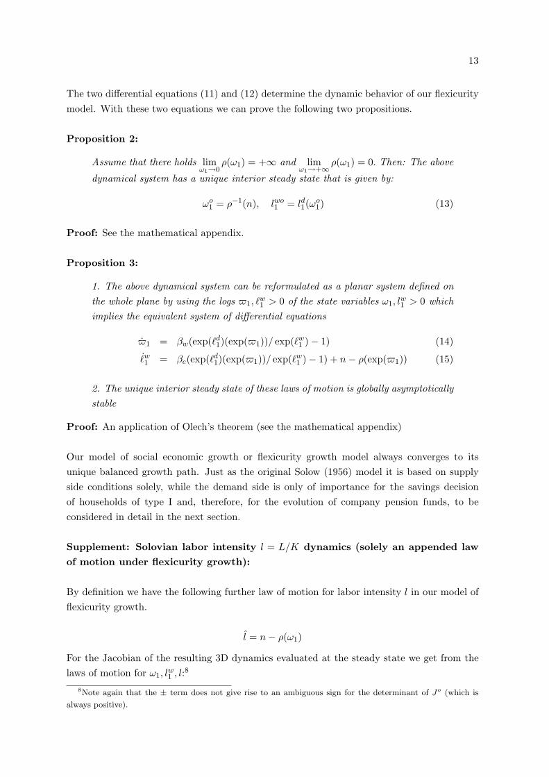
The two differential equations (11) and (12) determine the dynamic behavior of our flexicuritymodel. With these two equations we can prove the following two propositions.

Proposition 2:

Assume that there holds limω1→0

ρ(ω1) = +∞ and limω1→+∞ ρ(ω1) = 0. Then: The above

dynamical system has a unique interior steady state that is given by:

ωo1 = ρ−1(n), lwo

1 = ld1(ωo1) (13)

Proof: See the mathematical appendix.

Proposition 3:

1. The above dynamical system can be reformulated as a planar system defined onthe whole plane by using the logs $1, `

w1 > 0 of the state variables ω1, l

w1 > 0 which

implies the equivalent system of differential equations

$1 = βw(exp(`d1)(exp($1))/ exp(`w

1 )− 1) (14)˙w1 = βe(exp(`d

1)(exp($1))/ exp(`w1 )− 1) + n− ρ(exp($1)) (15)

2. The unique interior steady state of these laws of motion is globally asymptoticallystable

Proof: An application of Olech’s theorem (see the mathematical appendix)

Our model of social economic growth or flexicurity growth model always converges to itsunique balanced growth path. Just as the original Solow (1956) model it is based on supplyside conditions solely, while the demand side is only of importance for the savings decisionof households of type I and, therefore, for the evolution of company pension funds, to beconsidered in detail in the next section.

Supplement: Solovian labor intensity l = L/K dynamics (solely an appended lawof motion under flexicurity growth):

By definition we have the following further law of motion for labor intensity l in our model offlexicurity growth.

l = n− ρ(ω1)

For the Jacobian of the resulting 3D dynamics evaluated at the steady state we get from thelaws of motion for ω1, l

w1 , l:8

8Note again that the ± term does not give rise to an ambiguous sign for the determinant of Jo (which is

always positive).

14

Jo =

− − 0± − 0+ 0 0

Proposition 4:

The above 3D dynamics are globally asymptotically stable, but exhibits zero roothysteresis with respect to the state variable l.

Proof: See the mathematical appendix.

5 Monotonic adjustment processes through flexible hiring and

firing

We now derive a local condition for the occurrence of monotonic convergence to the steadystate of our model of flexicurity growth. According to the last proposition, we basically onlyhave to investigate the first two laws of motion. It suffices therefore to consider the followingmatrix with respect to its eigenvalues:

Jo =

(Jo

11 Jo12

Jo21 Jo

22

)=

(− −± −

)

where the ± sign reduces to + in the calculation of the determinant of this matrix. It is obviousthat we always have locally asymptotically stable dynamics (i.e. trace Jo < 0,det Jo > 0).Furthermore, the condition trace Jo = 4detJo, i.e.

(Jo11 + Jo

22)2 = 4(Jo

11Jo22 + Jo

21Jo12)

separates monotonic convergence (for parameters βe sufficiently large) from cyclical conver-gence (parameters βe sufficiently small). Reformulated, this condition reads:

|Jo22| = |Jo

11|+ 2√|Jo

21Jo12|, i.e. signβH

e = sign[|Jo11|+ 2

√|Jo

21Jo12|]

Figure 1: The case of a small parameter βe

15

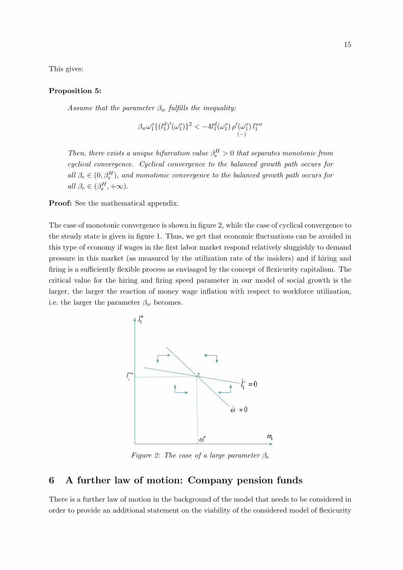
This gives:

Proposition 5:

Assume that the parameter βw fulfills the inequality:

βwωo1{(ld1)′(ωo

1)}2 < −4ld1(ωo1) ρ′(ωo

1)(−)

lwo1

Then, there exists a unique bifurcation value βHe > 0 that separates monotonic from

cyclical convergence. Cyclical convergence to the balanced growth path occurs forall βe ∈ (0, βH

e ), and monotonic convergence to the balanced growth path occurs forall βe ∈ (βH

e , +∞).

Proof: See the mathematical appendix.

The case of monotonic convergence is shown in figure 2, while the case of cyclical convergence tothe steady state is given in figure 1. Thus, we get that economic fluctuations can be avoided inthis type of economy if wages in the first labor market respond relatively sluggishly to demandpressure in this market (as measured by the utilization rate of the insiders) and if hiring andfiring is a sufficiently flexible process as envisaged by the concept of flexicurity capitalism. Thecritical value for the hiring and firing speed parameter in our model of social growth is thelarger, the larger the reaction of money wage inflation with respect to workforce utilization,i.e. the larger the parameter βw becomes.

Figure 2: The case of a large parameter βe

6 A further law of motion: Company pension funds

There is a further law of motion in the background of the model that needs to be considered inorder to provide an additional statement on the viability of the considered model of flexicurity

16

capitalism. This law of motion describes the evolution of the pension fund per unit of thecapital stock η = R

K and is obtained from the defining equation R = S1 − δ1R as follows:

η = R− K =R

K

K

R− ρ =

S1 − δ1R

K/η − ρ, i.e. :

η =S1

K− (δ1 + ρ)η = s1 − (δ1 + ρ)η

For reasons of simplicity we now assume a Cobb-Douglas production function. Then, we knowthat there is a constant αf > 0 such that lw2f = αf ld1 holds. Savings of households of type Iand profits of firms per unit of capital are given by:

s1 = (1− (ch1 + ch2)(1− τh)− τh)ω1ld1(ω1)− αωω1(lwx + lr)

lwx = l − (lw1 + lw2f + lw2h + lw2g)

lr = αrl, i.e. due to the financing of the employment terms lw2h + lw2g :

s1 = (1− ch1(1− τh)− αgτh)ω1ld1(ω1)− ((1 + αr)l − (lw1 + lw2f ))αωω1, lw2f = αf ld1(ω1)

ρ = y − (1 + αωαf )ω1ld1(ω1)]− δ

For reasons of analytical simplicity we also assume that the economy has already reachedits steady state with respect to the variables ω1, l

w1 and that we also have a given ratio l =

L/K = const. This is a simplifying assumption that must be accompanied later on by theassumption that the actual value of l = l must be chosen in a neighborhood of a base valuelo (see below). The above of course also provides us with a steady state value for the rate ofprofit ρ(ω1) = ρo(ωo). Moreover we also assume for simplicity δ1 = δ for the depreciation ratesof the capital stock and for the stock of pension funds.This gives for the law of motion of the pension fund per unit of capital the following differentialequation:

η = (1− ch1(1− τh)− αgτh)ω1ld1(ω1)− ((1 + αr)l − (lw1 + αf ld1(ω1)))αωω1 − (δ + ρ)η

which gives a single linear differential equation for the ratio η. This dynamical equation isglobally asymptotically stable around its steady state position given by:

ηo =(1− ch1(1− τh)− αgτh)ω1l

d1(ω1)− ((1 + αr)l − (1 + αf )ld1(ω1))αωω1

δ + ρ

In this case we have monotonic adjustment of the pension-fund capital ratio to its steady stateposition, while in general we have a non-autonomous adjustment of this ratio that is driven bythe real wage and employment dynamics of the first labor market. The steady state level of η

is positive iff there holds for the full employment labor intensity ratio:

l <(1− ch1(1− τh)− αgτh)ω1l

d1(ω1) + ((1 + αf )ld1(ω1))αωω1

(δ + ρ)(1 + αr)αωω1

We assume in addition that the additional company pension payments to pensioners shouldadd the percentage 100αc to their base pension ω2αr l per unit of capital. This gives as afurther restriction for the steady state position of the economy:

δηo = αcω2αr l, ω2 = αωω1

17

Inserting the value for ηo then gives

αc = δ(1− ch1(1− τh)− αgτh)ω1l

d1(ω1)− ((1 + αr)l − (1 + αf )ld1(ω1))αωω1

(δ + ρ)ω2αr l

In this way, we get that a target value for αc demands a certain labor intensity ratio l and viceversa. For a given total labor intensity ratio there is a given percentage by which companypensions compare to base pension payments. This percentage is the larger the smaller the ratiolw1 /l due to the following reformulation of the αc formula:

αc = δ[(1− ch1(1− τh)− αgτh)ω1 + (1 + αf )αωω1]lw1 /l − (1 + αr)αωω1

(δ + ρ)αrαωω1(16)

If this value of the total employment labor intensity ratio prevails in the considered economy(where it is of course as usually assumed that ch1(1− τh) + αgτh < 1 holds) we have that corepension payments to pensioners are augmented by company pension payments by a percentagethat is given by the parameter αc and that these extra pension payments are distributed topensioners in proportion to the time that they have worked in the private sector of the economy.This implies a trade-off between the ratios l, αc, as expressed by the relationship (16). It alsoshows that the total working population must make a certain ratio of the capital stock in orderto allow for a given percentage of extra company pension payments.Due to δηo = αcω2αr l and so

1 = (δ+ ρ)ηo we also have the equivalence between positive savingsper unit of capital of households of type I and positive values for αc, ηo. Moreover, these valuesare indeed positive if the following holds:9

l <(1− ch1(1− τh)− αgτh)ω1l

d1(ω1) + (1 + αf )ld1(ω1))αωω1

(δ + ρ)(1 + αr)αωω1

This inequality set limits to the total labor-supply capital-stock ratio l which allows for positivesavings of households of type I in the steady state and thus for extra pension payments to themlater on. Households of type I are by and large financing the second labor market throughtaxes and employment benefits (besides their contribution to the base income of the retiredpeople). Since firms have a positive rate of profit in the steady state, since the governmentbudget is always balanced and since only households of type I save in this economy, we havederived the condition under which such an economy accumulates not only capital, but alsopensions funds to a sufficient degree – under appropriate restrictions on labor supply.

7 Conclusion and outlook

We have shown in this paper that a model of flexicurity capitalism can be formulated, exhibit-ing a second labor market (and an employer of first resort) where all workers not employedby private firms find meaningful employment. This economy is characterized by viable andattracting balanced reproduction schemes. Hence, we have been able to demonstrate that a

9Note that the numerator is easily shown to be positive and even larger than 1 under standard Keynesian

assumptions on expenditure and taxation rates.

18

capitalistic system which is characterized by both flexibility and social security is a stable and,thus, sustainable system. Social security in our model means that retired workers get pensionsfrom a pay-as-you-go system and from firms that administer a pension fund that is built upthrough savings of active workers. In addition, workers not employed by firms receive soli-darity payments and meaningful occupation from the government. This shows that our socialsecurity system is rather complex but, nevertheless, allows convergence to a steady state. Incase of a sufficiently flexible labor market the convergence is even monotonic implying thattransitory business cycle fluctuations can be avoided.In technical terms, the model exhibits a unique interior steady state which is globally asymp-totically stable. We could show this by concentrating on the private sector of the economy,the dynamics of which are characterized by insider real wage adjustment dynamics of the typeconsidered in Blanchard and Katz (1999),10 and on a type of Okun’s Law that linked the levelof utilization of the insiders of firms to their hiring and firing decision. Since both of these lawsof motion only refer to the first labor market and, thus, only to a part of the whole workforce,the fundamental equation of the Solow (1956) growth model has appeared only as an appendixto this core dynamics, describing the evolution of the total labor supply per unit of capital inaddition.A further fundamental law concerning the viability of the economy was the law of motion ofcompany pension funds per unit of capital which was shown to lead to a viable steady statelevel of it when the labor-supply capital ratio is bounded by above in an appropriate way. Theexistence of such pension funds allows in principle to add credit (out of these funds) to theconsidered flexicurity model which, when such credits are delivered in physical form, wouldnot question the supply side orientation of the model, see Flaschel, Greiner, Luchtenberg andNell (2008) for details.This, however, changes when paper credit is added to the model implying that investmentdemand can now depart from the supply of savings in which case we get an IS-equilibrium onthe market for goods that generally differs from the supply of goods through profit-maximizingfirms. In place of savings-driven supply side fluctuations in economic activity we then haveinvestment driven demand side business cycle fluctuations of a probably much more volatiletype. This situation is modeled and analyzed in Flaschel et al. (2008). It represents one litmustest for the proper working of flexicurity capitalism, since supply side growth may be too stablea situation in order to really test the strength of economies that are designed on the basis of theflexicurity approach. In such a situation it has to be tested in detail, also numerically (since theresulting 5D dynamics are of a fully interdependent type), how the hiring and firing parameterβe influences the performance of the economy. In addition, prudent fiscal and monetary policymay then be needed in order to preserve the stability features we have shown to exist for oursupply side version of flexicurity growth in this paper. The investigation of such topics mustbe left for future research here however.

10if myopic perfect foresight is added to their discussion of a wage Phillips curve and its theoretical under-

pinnings.

19

References

Andersen, T.M. and Svarer, M. (2007), Flexicurity - Labor Market Performance in Den-mark, CESifo Working Paper 2108.

Blanchard, O.J. and L. Katz (1999): Wage dynamics: Reconciling theory and evidence.American Economic Review, 89. Papers and Proceedings, 69 – 74.

Flaschel, P. (1984): Some stability properties of Goodwin’s growth cycle model. Zeitschriftfur Nationalokonomie, 44, 63-69.

Flaschel, P. and A. Greiner (2009): Employment Cycles and Minimum Wages: A MacroView. Structural Change and Economic Dynamics, 20, 279-287.

Flaschel, P., Franke, R. and W. Semmler (2008): Kaleckian investment and employ-ment cycles in postwar industrialized economies. In: Flaschel, P., Landesmann, M. (eds.):Mathematical Economics and the Dynamics of Capitalism. London, Routledge.

Flaschel, P., Greiner, A., Luchtenberg, S. and E. Nell (2008): Varieties of capi-talism: The flexicurity model. In: Flaschel, P., Landesmann, M. (eds.): MathematicalEconomics and the Dynamics of Capitalism. London, Routledge.

Funk, L. (2008), European Flexicurity Policies: A Critical Assessment, The InternationalJournal of Comparative Labour Law and Industrial Relations, 24, 349-384.

Gandolfo, G. (1996): Economic Dynamics. Springer: Berlin.

Goodwin, R. (1967): A growth cycle. In: C.H. Feinstein (ed.): Socialism, Capitalism andEconomic Growth. Cambridge: Cambridge University Press, 54 – 58.

Marx, K. (1954): Capital. A Critique of Political Economy, Vol.I. New York: Lawrenceand Wishart.

Quirk, V. et al. (2006): The job guarantee in practice. The University of Newcastle,Australia: Center of Full Employment and Equity, working paper no. 06-15.

Rose, H. (1967): On the non-linear theory of the employment cycle. Review of EconomicStudies, 34, 153-173.

Solow, R. (1956): A contribution to the theory of economic growth. Quarterly Journal ofEconomics, 70, 65-94.

Solow, R. (1990): Goodwin’s growth cycle: Reminiscence and rumination. In: K.Velupillai(ed.): Nonlinear and Multisectoral Macrodynamics. London: Macmillan, 31-41.

Tchernova, P. and Wray, L.R. (2005): Can basic income and job guarantees deliver ontheir premises. University of Missouri-Kansas City: Center for Full Employment andPrice Stability, working paper no. 42.

20

Viebrock, E. and Clasen, J. (2009), Flexicurity and Welfare Reform: A Review, Socio-Economic Review, 7, 305-331

Wilthagen, T. (1998): Flexicurity: A new paradigm for labour policy reform? Flexicurity

Research Programme FXPaper Nr. 1.

Wilthagen, T., Tros, F. and van Lieshout, H. (2004a): Towards ’flexicurity’?: Balanc-ing flexibility and security in EU member states. European Journal of Social Security,6, 113-36.

Wilthagen , T. and Tros, F. (2004b), The Concept of ’Flexicurity’: A New Approach toRegulating Employment and Labour Markets, Transfer 2: 166-186.

Zhou, J. (2007): Danish for all? Balancing flexibility with security: The Flexicurity model.IMF Working Paper, WP/07/36.

21

Mathematical Appendix

A. Proof of Proposition 1

Since ω2 is a constant fraction of ω1, we set ω2 = αω1, where α is a positive constant. We canexpress then the rate of profit ρ as follows:

ρ = y − δ − ω1ld1 − ω2l

w2f = F (1, ld1, l

w2f )− ω1l

d1 − αω1l

w2f (A1)

The first order conditions for the maximization of ρ with respect to ld1 and lw2f are given bythe following set of equations:

∂ρ/∂ld1 = F2(1, ld1, lw2f )− ω1 = 0 (A2)

∂ρ/∂lw2f = F3(1, ld1, lw2f )− αω1 = 0 (A3)

where F2 = ∂F/∂ld1 and F3 = ∂F/∂lw2f . The second order conditions for the maximization of ρ

can be written as follows:

F22 < 0, F33 < 0, ∆ =

∣∣∣∣∣F22 F23

F23 F33

∣∣∣∣∣ = F22F33 − (F23)2 > 0 (A4)

where F22 = ∂2F/∂ld21 , F33 = ∂2F/∂lw2

2f , and F23 = ∂2F/∂lw2f∂ld1 = ∂2F/∂ld1∂lw2f .

Assumption A1

F2 > 0, F3 > 0, F22 < 0, F33 < 0, F23>= 0, ∆ = F22F33 − (F23)2 > 0.

Remark A1.Suppose that the production function is of the Cobb-Douglas type such that

Y = AK1−β1−β2(Ld1)

β1(Lw2f )β2 (0 < β1 < 1, 0 < β2 < 1).

We then havey = A(ld1)

β1(lw2f )β2 , y = Y/K.

In this case, all of the inequalities in Assumption 1 are satisfied (and F23 > 0).

Proposition 1All of the relationships (7) – (10) in the text are satisfied under Assumption A1.

Proof: Solving equations (A2) and (A3), we have ld1 = ld1(ω1) and lw2f = lw2f (ω1). Totallydifferentiating equations (A2) and (A3), we get

(F22 F23

F23 F33

)(dld1/dω1

dlw2f/dω1

)=

(1α

)(A5)

22

Solving this equation, we obtain the following inequalities.

(ld1)′(ω1) = dld1/dω1 =

∣∣∣∣∣1 F23

α F33

∣∣∣∣∣ /∆ = (F33(−)

−α F23(−or0)

)/ ∆(+)

< 0 (A6)

(lw2f )′(ω1) = dlw2f/dω1 =

∣∣∣∣∣F22 1F23 α

∣∣∣∣∣ /∆ = (α F22(−)

−F 223)/ ∆

(+)< 0 (A7)

Therefore, we have y = F (1, ld1(ω1), lw2f (ω1)) = y(ω1) andy′(ω1) = dy/dω1 = F2

(+)(dld1/dω1)

(−)

+ F3(+)

(dlw2f/dω1)(−)

< 0. (A8)

It follows from eq. (A1) that ρ is a linear decreasing function of ω1 for any given values ofld1 > 0 and lw2f > 0. Therefore, the graph of the function ρ = ρ(ω1) becomes the outer envelopeof downward sloping straight lines. This means that we have ρ′(ω1) = dρ/dω1 < 0.

Next, let us consider the phase diagram for the system (11), (12) in the text (see there figure1). The locus of ω1 = 0 is given by the following equation:

ld1(ω1) = lw1 (A9)

Totally differentiating this equation and rearranging terms, we get

dlw1dω1

∣∣∣ω1=0

= (ld1)′(ω1) < 0 (A10)

The locus of lW1 = 0 is given by

{ld1(ω1)/lw1 − 1}+ {n− ρ(ω1)}/βe = 0 (A11)

Totally differentiating this equation and rearranging terms, we obtain the following relation-ship.dlw1dω1

∣∣∣lw1 =0

= {(ld1)′(ω1)− ρ′(ω1)lw1βe

}( lw1ld1(ω1)

) (A12)

Since (ld1)′(ω1) < 0 and ρ′(ω1) < 0, we have the following results from equations (A11) and

(A12):

(1) dlw1dω1

∣∣∣lw1 =0

is a continuous decreasing function of the parameter value βe > 0.

(2) limβe→0

dlw1dω1

∣∣∣lw1 =0

= +∞

(3) limβe→+∞

dlw1dω1

∣∣∣lw1 =0

= (ld1)′(ω1) < 0

In other words, the slope of the locus of lw1 = 0 is positive for all sufficiently small values of βe,and it is negative for all sufficiently large values of βe, and the locus of lw1 = 0 coincides withthat of ω1 = 0 if βe is infinitely large. On the other hand, we can easily see that ∂ω1/∂ω1 < 0and ∂lw1 /∂lw1 < 0. Therefore, we obtain two types of the phase diagrams (see the figures 1 and

23

2 in the text) depending on the magnitude of the parameter value βe.

B. Proof of Proposition 2

Assumption B1.

limω1→0

ρ(ω1) = +∞ and limω1→+∞ ρ(ω1) = 0.

Remark B1.The Assumption B1 is in fact satisfied if the production function is of Cobb-Douglas type.

Proposition 2

The two-dimensional dynamical system that is described by equations (11) and (12) has aunique interior steady state that is given by Eq. (13) in the text.

Proof: The equilibrium solution of this dynamical system is characterized by the followingset of equations with the two unknowns ω1 and lw1 :ld1(ω1) = lw1 (B1)ρ(ω1) = n (B2)Eq. (B2) has the unique solution ωo

1 = ρ−1(n) > 0 because of Assumption B2 and the factthat the function ρ(ω1) is a decreasing function. Substituting ω1 = ωo

1 into Eq. (B1), wemoreover get lwo

1 = ld1(ωo1) > 0.

C. Proof of Proposition 3

Let us defineω1 = ln ω1, ld1 = ln ld1, lw1 = ln lw1 . (C1)We can then transform the dynamical system that is given by equations (11) and (12) in thetext as follows:˙ω1 = βw{exp(ld1)(exp(ω1))/ exp(lw1 )− 1} = G1(ω1, l

w1 ) (C2)

˙lw1 = βe{exp(ld1)(exp(ω1))/ exp(lw1 )− 1}+ n− ρ(exp(ω1)) = G2(ω1, l

w1 ) (C3)

This system is well-defined for all (ω, lw1 ) ∈ R2. The Jacobian matrix of this system is given by

J1 =

(G11 G12

G21 G22

)(C4)

where G11 = ∂G1∂ω1

= βw{ ∂(exp(ld1))∂(exp(ω1))

exp(ω1)

exp(lw1 )} < 0, G12 = ∂G1

∂lw1= −βw{ exp(ld1)

exp(lw1 )} < 0, G21 =

∂G2∂ω1

= [βe{ ∂(exp(ld1))∂(exp(ω1))

1exp(lw1 )

} − dρd(exp(ω1) ] exp(ω1), and G22 = −βe{ exp(ld1)

exp(lw1 )} < 0 for all (ω1, l

w1 ) ∈

R2.

24

Therefore, we have the following set of inequalities for all (ω1, lw1 ) ∈ R2 :

traceJ1 = G11(−)

+G22(−)

< 0 (C5)

detJ1 = G11G22 −G12G21 = G12(−)

(exp(ω1)) (dρ/d(exp(ω1))(−)

> 0 (C6)

G11G22 6= 0 (C7)

This set of inequalities implies that all of Olech’s sufficient conditions for global asymptoticstability of the two-dimensional system of differential equations are satisfied (cf. Gandolfo,1996, 354 – 355). This proves all assertions of Proposition 3.11

D. Proof of Proposition 4

Let us consider the global stability of the system of dynamical equations (11) and (12) in thetext when appended by the following law of motion for l.

l = n− ρ(ω1) (D1)This system is a decomposable system, and we already know that the unique equilibriumpoint (ωo

1, lwo1 ) of the independent subsystem that consists of equations (11) and (12) is

globally stable (cf. Proposition 3). In other words, we have limt→+∞ω1(t) = ωo

1 so that we have

limt→+∞ ρ(ω1(t)) = ρ(ωo

1) = n (cf. Proposition 2). Therefore, we obtain

limt→+∞ l(t) = n− lim

t→+∞ ρ(ω1(t)) = n− n = 0. (D2)This means that the whole system is globally stable in the sense that l also converges to somevalue although lim

t→+∞ l(t) depends on the initial condition l(0). We can prove the dependency

of limt→+∞ l(t) on l(0) as follows. Let us define l = ln l. Then, we can rewrite eq. (D1) as

˙l = n− ρ(ω1). (D3)Integrating this equation with respect to time, we obtain

l(t) = l(0) +∫ t0 {n− ρ(ω1(τ)}dτ (D4)

so that we havelim

t→+∞ l(t) = l(0) +∫∞0 {n− ρ(ω1(τ)}dτ. (D5)

This proves the assertion.

E. Proof of Proposition 5

We can rewrite the system of dynamical equations (11) and (12) in the text as follows:

ω1 = ω1βw{ld1(ω1)/lw1 − 1} = G1(ω1, lw1 ) (E1)

lw1 = lw1 [βe{ld1(ω1)/lw1 − 1}+ n− ρ(ω1)] = G2(ω1, lw1 ) (E2)

11See also Flaschel (1984) for the application of Olech’s theorem in the context of models of economic growth.

25

The Jacobian matrix of this system at the equilibrium point (ωo1, l

wo1 ) can be written as follows:

Jo =

(Jo

11 Jo12

Jo21 Jo

22

)(E3)

where Jo11 = ωo

1βw(ld1)′(ωo

1)/lwo1 < 0, Jo

12 = −ωo1βwld1(ω

o1)/(lwo

1 )2 < 0, Jo21 =

lwo1 [βe{(ld1)′(ωo

1)}/lwo1 − ρ′(ωo

1)], and Jo22 = −βel

d1(ω

o1)/lwo

1 < 0.

Then, the characteristic equation of this system becomes

Γo(λ) = |λI − Jo| = λ2 + a1λ + a2 = 0 (E4)

wherea1 = −traceJo = −Jo

11 − Jo22 = [−ωo

1βw(ld1)′(ωo

1)}+ βeld1(ω

o1)]/lwo

1 > 0, (E5)a2 = detJo = Jo

11Jo22 − Jo

12Jo21 = −ωo

1βwld1(ωo1)ρ

′(ωo1)/lwo

1 > 0. (E6)

The discriminant(D) of this system can be written asD = a2

1 − 4a2 = D(βe). (E7)It is now obvious that cyclical fluctuations around the equilibrium point occur if and only ifD < 0 holds true.

Assumption E1The parameter βw is so small that we have the following inequality (E8):βwωo

1{(ld1)′(ωo1)}2 < −4ld1(ω

o1) ρ′(ωo

1)(−)

lwo1 (E8)

Proposition 5

Under Assumption E1, we get for the uniquely determined bifurcation value that separatesmonotonic from cyclical convergence the inequality βH

e > 0. Cyclical convergence to thebalanced growth path occurs for all βe ∈ (0, βH

e ), and monotonic convergence to the balancedgrowth path occurs for all βe ∈ (βH

e ,+∞).

Proof: We can easily see that D(βe) is a monotonically increasing continuous function of βe

with the following properties.

limβe→+∞

D(βe) = +∞ (E9) D(0) = (ωo1βw/lwo

1 )[βwωo1(l

d1)′(ωo

1)2/lwo

1 + 4ld1(ωo1)ρ

′(ωo1)] (E10)

Assumption E1 implies that D(0) < 0. In this case, there exists unique positive value βHe

such that we have D(βHe ) = 0, D(βe) < 0 for all βe ∈ (0, βH

e ), and D(βe) > 0 for allβe ∈ (βH

e , +∞). This proves the assertion because we already proved the global convergenceof the solution to the balanced growth path(cf. Proposition 3)

Publisher: Hans-Böckler-Stiftung, Hans-Böckler-Str. 39, 40476 Düsseldorf, Germany Phone: +49-211-7778-331, IMK@boeckler.de, http://www.imk-boeckler.de IMK Working Paper is an online publication series available at: http://www.boeckler.de/cps/rde/xchg/hbs/hs.xls/31939.html ISSN: 1861-2199 The views expressed in this paper do not necessarily reflect those of the IMK or the Hans-Böckler-Foundation. All rights reserved. Reproduction for educational and non-commercial purposes is permitted provided that the source is acknowledged.