GEE Paper

138

Dezembro 2019

The Financial Channels of Labor Rigidities:

Evidence from Portugal

Edoardo M. Acabbi | Ettore Panetti| Alessandro Sforza

Gabinete de Estratégia e Estudos do Ministério da Economia Office for Strategy and Studies of the Ministry of Economy Rua da Prata, n.º 8 – 1149-057 Lisboa – Portugal www.gee.gov.pt ISSN (online): 1647-6212

The Financial Channels of Labor Rigidities: Evidence from Portugal 1

Edoardo M. Acabbi2, Ettore Panetti3, Alessandro Sforza 4

Abstract:

How do credit shocks affect labor market reallocation and firms’ exit, and how does their propagation depend onlabor rigidities at the firm level? To answer these questions, we match administrative data on worker, firms, banksand credit relationships in Portugal, and conduct an event study of the interbank market freeze at the end of2008. Consistent with other empirical literature, we provide novel evidence that the credit shock had significanteffects on employment dynamics and firms’ survival. These findings are entirely driven by the interaction of thecredit shock with labor market frictions, determined by rigidities in labor costs and exposure to working-capitalfinancing, which we label “labor-as-leverage” and “labor-as-investment” financial channels. The credit shock explainsabout 29 percent of the employment loss among large Portuguese firms between 2008 and 2013, and contributes toproductivity losses due to increased labor misallocation.

JEL Classification Codes: D24, D25, E24, G21Keywords: Financial crises, Credit, Firm dynamics, Labor rigidities, Productivity

Note: This article is the sole responsibility of the authors and does not necessarily reflect thepositions of GEE or the Portuguese Ministry of Economy.

1Edoardo M. Acabbi thanks Gabriel Chodorow-Reich, Emmanuel Farhi, Samuel G. Hanson and Jeremy Stein for their extensive adviceand support. The authors thank Martina Uccioli, Andrea Alati, António Antunes, Omar Barbiero, Diana Bonfim, Andrea Caggese,Luca Citino, Andrew Garin, Edward L. Glaeser, Ana Gouveia, Simon Jäger, Sudipto Karmakar, Lawrence Katz, Chiara Maggi,Carlos Robalo Marques, Fernando Martins, Luca Mazzone, Simon Mongey, Steven Ongena, Luca Opromolla, Matteo Paradisi, AndreaPassalacqua, Pedro Portugal, Gianluca Rinaldi, Stefanie Stantcheva, Ludwig Straub, Adi Sunderam and Boris Vallée, and the seminarparticipants at the briq workshop on “Firms, Jobs and Inequality”, Barcelona GSE Summer Forum in “Financial Shocks, Channelsand Macro Outcomes”, the Petralia job-market 2019 bootcamp and Harvard macroeconomics, finance and public economics, and fiscalpolicy lunches. The authors also thank Paulo Guimarães, Pedro Próspero, Fátima Teodoro, Maria Lucena Vieira and the staff of the“Laboratório de Investigação com Microdados” at Banco de Portugal (BPLim). Pedro Moreira and Antonio Santos provided excellentresearch assistance. The analyses, opinions and findings of this paper represent the views of the authors, and are not necessarily thoseof Banco de Portugal or the Eurosystem.

2Harvard University (eacabbi@g.harvard.edu)3Banco de Portugal, UECE-ISEG and Suerf (etpanetti@bportugal.pt)4University of Bologna and CESifo (alessandrosforza87@gmail.com)

Contents

1 Introduction 1

2 Conceptual framework 5

3 Data and sample selection 7

3.1 The credit shock in Portugal in 2008-2009 . . . . . . . . . . . . . . . . . . . . . . . . . . . . . . . . . . . . 7

3.2 Data . . . . . . . . . . . . . . . . . . . . . . . . . . . . . . . . . . . . . . . . . . . . . . . . . . . . . . 9

3.3 Sample selection and descriptives . . . . . . . . . . . . . . . . . . . . . . . . . . . . . . . . . . . . . . . . . 9

4 Empirical strategy 10

4.1 Characterizing banks’ credit supply . . . . . . . . . . . . . . . . . . . . . . . . . . . . . . . . . . . . . . . . 10

4.2 Testing the channel . . . . . . . . . . . . . . . . . . . . . . . . . . . . . . . . . . . . . . . . . . . . . . . 12

5 Average firm-level results 15

5.1 Labor outcomes . . . . . . . . . . . . . . . . . . . . . . . . . . . . . . . . . . . . . . . . . . . . . . . . . 15

5.2 Firm exit . . . . . . . . . . . . . . . . . . . . . . . . . . . . . . . . . . . . . . . . . . . . . . . . . . . . 19

5.3 Financial outcomes . . . . . . . . . . . . . . . . . . . . . . . . . . . . . . . . . . . . . . . . . . . . . . . 20

6 Heterogeneity results 21

6.1 The role of labor rigidities . . . . . . . . . . . . . . . . . . . . . . . . . . . . . . . . . . . . . . . . . . . . 21

6.1.1 Labor as leverage, labor as investment . . . . . . . . . . . . . . . . . . . . . . . . . . . . . . . . . . 24

6.2 Labor rigidities and non-cleansing effects . . . . . . . . . . . . . . . . . . . . . . . . . . . . . . . . . . . . . 27

6.2.1 Heterogeneity results by labor share and productivity . . . . . . . . . . . . . . . . . . . . . . . . . . . 29

7 Labor rigidities and macroeconomic effects 30

7.1 The credit shock and aggregate employment . . . . . . . . . . . . . . . . . . . . . . . . . . . . . . . . . . . 30

7.2 Firm survival and factor reallocation throughout the financial crises . . . . . . . . . . . . . . . . . . . . . . . . 31

7.3 The credit shock and aggregate misallocation . . . . . . . . . . . . . . . . . . . . . . . . . . . . . . . . . . . 32

7.3.1 The credit shock and misallocation in labor . . . . . . . . . . . . . . . . . . . . . . . . . . . . . . . . 32

7.3.2 Aggregate productivity effects . . . . . . . . . . . . . . . . . . . . . . . . . . . . . . . . . . . . . . 34

8 Conclusion 36

9 References 38

10 Tables 44

11 Figures 57

A A model of the financial channels of labor rigidities 65

B Data description and cleaning 67

B.1 Available datasets . . . . . . . . . . . . . . . . . . . . . . . . . . . . . . . . . . . . . . . . . . . . . . . . 67

B.1.1 Labor market data: Quadros de Pessoal . . . . . . . . . . . . . . . . . . . . . . . . . . . . . . . . . 67

B.1.2 Firm level financial statement data: Central de Balanços . . . . . . . . . . . . . . . . . . . . . . . . . 68

B.1.3 Credit exposure level dataset: Central de Responsabilidades de Crédito . . . . . . . . . . . . . . . . . . 69

i

B.1.4 Banks balance sheet dataset: Balanço das Instituições Monetárias e Financeiras . . . . . . . . . . . . . . 69

B.1.5 Banks balance sheet dataset: Sistema Integrado de Estatísticas de Títulos . . . . . . . . . . . . . . . . . 70

B.1.6 Commuting zone definitions . . . . . . . . . . . . . . . . . . . . . . . . . . . . . . . . . . . . . . . 70

B.1.7 Labor market data: Occupational Information Network . . . . . . . . . . . . . . . . . . . . . . . . . . 70

B.2 Sample selection . . . . . . . . . . . . . . . . . . . . . . . . . . . . . . . . . . . . . . . . . . . . . . . . . 70

C Production function estimation 71

C.1 Productivity and output elasticities estimation . . . . . . . . . . . . . . . . . . . . . . . . . . . . . . . . . . 71

C.2 Markups and marginal products . . . . . . . . . . . . . . . . . . . . . . . . . . . . . . . . . . . . . . . . . 74

D Appendix Tables 76

E Appendix Figures 99

ii

List of Figures

1 Credit dynamics in Portugal . . . . . . . . . . . . . . . . . . . . . . . . . . . . . . . . . . . . . . . . . . . 57

2 Balance checks . . . . . . . . . . . . . . . . . . . . . . . . . . . . . . . . . . . . . . . . . . . . . . . . . 57

3 Employment and wage bill regressions: event study . . . . . . . . . . . . . . . . . . . . . . . . . . . . . . . . 58

4 Employment adjustment by tenure . . . . . . . . . . . . . . . . . . . . . . . . . . . . . . . . . . . . . . . . 59

5 Regressions by labor-share bins . . . . . . . . . . . . . . . . . . . . . . . . . . . . . . . . . . . . . . . . . . 60

6 Balance sheet items and sales regressions by labor-share bins . . . . . . . . . . . . . . . . . . . . . . . . . . . 61

7 Regressions by quartiles of otj training scores . . . . . . . . . . . . . . . . . . . . . . . . . . . . . . . . . . . 62

8 Regressions by labor-share and CD-ACF-productivity bins . . . . . . . . . . . . . . . . . . . . . . . . . . . . . 63

9 Reallocation and TFP by labor share - full dataset . . . . . . . . . . . . . . . . . . . . . . . . . . . . . . . . 64

10 Credit dynamics in Portugal . . . . . . . . . . . . . . . . . . . . . . . . . . . . . . . . . . . . . . . . . . . 99

11 Unemployment rate . . . . . . . . . . . . . . . . . . . . . . . . . . . . . . . . . . . . . . . . . . . . . . . 99

12 Bank concentration by total regular credit . . . . . . . . . . . . . . . . . . . . . . . . . . . . . . . . . . . . 100

13 Number of credit relationships . . . . . . . . . . . . . . . . . . . . . . . . . . . . . . . . . . . . . . . . . . 100

14 Distribution of nominal base-wage growth in Portugal . . . . . . . . . . . . . . . . . . . . . . . . . . . . . . . 101

15 Balance checks (Borusyak et al., 2019) . . . . . . . . . . . . . . . . . . . . . . . . . . . . . . . . . . . . . . 101

16 Employment and wage-bill regressions: event study, reduced form . . . . . . . . . . . . . . . . . . . . . . . . . 102

17 Wage bill adjustment by tenure: event study . . . . . . . . . . . . . . . . . . . . . . . . . . . . . . . . . . . 103

18 Qualifications regressions, event study . . . . . . . . . . . . . . . . . . . . . . . . . . . . . . . . . . . . . . 104

19 Age regressions, event study . . . . . . . . . . . . . . . . . . . . . . . . . . . . . . . . . . . . . . . . . . . 105

20 Employment regressions by labor-share bins, survivors sample . . . . . . . . . . . . . . . . . . . . . . . . . . . 106

21 Regressions by labor-share bins, reduced form . . . . . . . . . . . . . . . . . . . . . . . . . . . . . . . . . . . 107

22 Regressions by labor-share quartiles . . . . . . . . . . . . . . . . . . . . . . . . . . . . . . . . . . . . . . . 108

23 Regressions by residualized labor-share bins . . . . . . . . . . . . . . . . . . . . . . . . . . . . . . . . . . . . 109

24 Regressions by labor-share bins (alternative measure) . . . . . . . . . . . . . . . . . . . . . . . . . . . . . . . 110

25 Regressions by labor-share quartiles in sales . . . . . . . . . . . . . . . . . . . . . . . . . . . . . . . . . . . . 111

26 Regressions by labor-share bins (2007-2008 averages) . . . . . . . . . . . . . . . . . . . . . . . . . . . . . . . 112

27 Regressions by leverage bins . . . . . . . . . . . . . . . . . . . . . . . . . . . . . . . . . . . . . . . . . . . 113

28 Regressions by labor-share and productivity bins, reduced form . . . . . . . . . . . . . . . . . . . . . . . . . . 114

29 Regressions by residualized labor-share and productivity bins . . . . . . . . . . . . . . . . . . . . . . . . . . . 115

30 Regressions by labor-share in sales and productivity bins . . . . . . . . . . . . . . . . . . . . . . . . . . . . . 116

31 Regressions by labor-share and TSLOG-ACF-productivity bins . . . . . . . . . . . . . . . . . . . . . . . . . . 117

32 Regressions by labor-share and CD-productivity bins, OLS . . . . . . . . . . . . . . . . . . . . . . . . . . . . 118

33 Regressions by labor-share and TSLOG-productivity bins, OLS . . . . . . . . . . . . . . . . . . . . . . . . . . 119

34 Labor MRP-cost gap regressions by labor-share quartiles . . . . . . . . . . . . . . . . . . . . . . . . . . . . . 120

iii

List of Tables

1 Sample representativeness, 2005 firms with credit, QP . . . . . . . . . . . . . . . . . . . . . . . . . . . . . . 44

2 Firm level descriptive statistics, sample of analysis . . . . . . . . . . . . . . . . . . . . . . . . . . . . . . . . 45

3 Loan level regressions . . . . . . . . . . . . . . . . . . . . . . . . . . . . . . . . . . . . . . . . . . . . . . 46

4 Employment regressions . . . . . . . . . . . . . . . . . . . . . . . . . . . . . . . . . . . . . . . . . . . . . 47

5 Wage bill regressions . . . . . . . . . . . . . . . . . . . . . . . . . . . . . . . . . . . . . . . . . . . . . . 48

6 Employment - wage bill regressions: Manufacturing . . . . . . . . . . . . . . . . . . . . . . . . . . . . . . . . 49

7 Heterogeneous employment regressions: Qualifications . . . . . . . . . . . . . . . . . . . . . . . . . . . . . . 50

8 Heterogeneous employment regressions: Age cohorts . . . . . . . . . . . . . . . . . . . . . . . . . . . . . . . 51

9 Exit regressions . . . . . . . . . . . . . . . . . . . . . . . . . . . . . . . . . . . . . . . . . . . . . . . . . 52

10 Correlations of observables with labor share . . . . . . . . . . . . . . . . . . . . . . . . . . . . . . . . . . . 53

11 Balance sheet and financials regressions . . . . . . . . . . . . . . . . . . . . . . . . . . . . . . . . . . . . . 54

12 Reallocation and TFP - full dataset . . . . . . . . . . . . . . . . . . . . . . . . . . . . . . . . . . . . . . . 55

13 Marginal revenue products - cost gaps regressions . . . . . . . . . . . . . . . . . . . . . . . . . . . . . . . . . 56

14 Average prevailing interest rates on non-financial bank loans . . . . . . . . . . . . . . . . . . . . . . . . . . . 76

15 Share of secured credit, firm level . . . . . . . . . . . . . . . . . . . . . . . . . . . . . . . . . . . . . . . . 77

16 Firm level descriptive statistics, sample of analysis - workforce composition . . . . . . . . . . . . . . . . . . . . 78

17 Robustness: instrument effects on credit post-2010 . . . . . . . . . . . . . . . . . . . . . . . . . . . . . . . . 79

18 Employment regressions, first stage . . . . . . . . . . . . . . . . . . . . . . . . . . . . . . . . . . . . . . . 80

19 Employment regressions, reduced form . . . . . . . . . . . . . . . . . . . . . . . . . . . . . . . . . . . . . . 81

20 Hours regressions . . . . . . . . . . . . . . . . . . . . . . . . . . . . . . . . . . . . . . . . . . . . . . . . 82

21 Employment - wage bill regressions . . . . . . . . . . . . . . . . . . . . . . . . . . . . . . . . . . . . . . . 83

22 Heterogeneous employment regressions: Contracts . . . . . . . . . . . . . . . . . . . . . . . . . . . . . . . . 84

23 Heterogeneous employment regressions: Education . . . . . . . . . . . . . . . . . . . . . . . . . . . . . . . . 85

24 Robustness: Almeida et al. (2011) identification, effects on fixed investments . . . . . . . . . . . . . . . . . . . . 86

25 Average wage regressions . . . . . . . . . . . . . . . . . . . . . . . . . . . . . . . . . . . . . . . . . . . . 87

26 Regressions by attachment . . . . . . . . . . . . . . . . . . . . . . . . . . . . . . . . . . . . . . . . . . . 88

27 Loan level regressions: productivity . . . . . . . . . . . . . . . . . . . . . . . . . . . . . . . . . . . . . . . 88

28 Regressions by CD productivity bins (Ackerberg et al. (2015)) . . . . . . . . . . . . . . . . . . . . . . . . . . 89

29 Regressions by OLS CD productivity bins . . . . . . . . . . . . . . . . . . . . . . . . . . . . . . . . . . . . 90

30 Regressions by OLS TSLOG productivity bins . . . . . . . . . . . . . . . . . . . . . . . . . . . . . . . . . . 91

31 Regressions by TSLOG productivity bins (Ackerberg et al. (2015)) . . . . . . . . . . . . . . . . . . . . . . . . . 92

32 Reallocation and TFP by labor share - full dataset . . . . . . . . . . . . . . . . . . . . . . . . . . . . . . . . 93

33 Marginal revenue products - cost gaps regressions . . . . . . . . . . . . . . . . . . . . . . . . . . . . . . . . . 94

34 Wedge regressions . . . . . . . . . . . . . . . . . . . . . . . . . . . . . . . . . . . . . . . . . . . . . . . . 95

35 Revenue elasticities and markups, PIM capital . . . . . . . . . . . . . . . . . . . . . . . . . . . . . . . . . . 96

36 Revenue elasticities and markups, book v. of capital . . . . . . . . . . . . . . . . . . . . . . . . . . . . . . . 97

37 MRPs, user costs and gaps, full CB . . . . . . . . . . . . . . . . . . . . . . . . . . . . . . . . . . . . . . . 98

iv

1. Introduction

How do credit shocks affect labor market reallocation and firms’ exit, and how does their propagation depend onlabor rigidities at the firm level? Do credit shocks reinforce or hinder productivity-enhancing reallocation dynamics?We answer these questions by using an event study of the real effects of the interbank market freeze during theglobal financial crisis, and dissect how the shock to short-term credit supply spread to the corporate sector.

The recent global financial crisis (2008–2009) and the EU joint bank and sovereign debt crisis (2010–2012)revamped the interest of politicians, policy-makers and the general public in how financial markets affect the realeconomy. The severity of these recessionary episodes make it of paramount importance for economists and policy-makers to provide an accurate analysis of the implications and propagation of financial shocks. Moreover, thecentral role of the financial system in channeling funds across different sectors of the economy may have non-trivialimplications for the overall productive system; financial frictions can hamper productive reallocation of resourcesand limit long-run growth.

We document how the responsiveness of firms to credit shocks is determined by their own financial flexibility,and in particular by their ability to adjust their labor costs. Labor costs constitute a sizable fraction of firms’ coststructure, as in many advanced economies the labor share, albeit declining, is still above 50 percent (Karabarbounisand Neiman, 2014). Despite their large share in total costs, labor costs are often overlooked as a source of financialrisk, and most macroeconomic models assume that labor is a flexible input in production. However, there are atleast two important financial channels through which intrinsic labor inflexibility can amplify the effect of creditshocks and put firms’ operations at risk. We label these channels “labor-as-leverage” and “labor-as-investment”.

Labor-as-leverage refers to the operating leverage that results from the rigidity of compensation owed toincumbent workers. It is determined by significant adjustment costs at the firm level, in the form of hiring, searchand firing costs, together with wage rigidity. Labor-as-leverage exposes the firm to greater liquidity risk, given thefirm’s inability to adjust partially fixed operating costs. Should it be hit by an unexpected adverse liquidity shock,a firm with relatively greater pre-commitments to labor, which is senior to many other expenses, might have to cutemployment of its least protected workers and existing investments in order to honor these pre-commitments. Thepresence of institutional adjustment costs in the labor market, and/or internal incentives to retain workers with thegreatest human capital (Oi, 1962), would then lead the firm to cut its most liquid investments, hiring, and separatefrom the least protected workers. Eventually, if the liquidity drought is too intense, the firm might not be able tohonor its debt and workforce commitments, and exit the market.

In parallel, the labor-as-investment channel arises because of the possible mismatch in the timing of paymentsto workers and the cash flows from production, which makes workers akin to an investment good. This channelwould be stronger in firms that need to employ a more qualified workforce, the hiring of which is likely to be costlierif these workers are a scarce input of production. The same channel would be present if firms have to pay trainingcosts in order for the workers to be productive. As firms incur these labor-related costs in advance of realizingrevenue cash flows, they become subject to a working-capital channel, through which the labor costs are directlyaffected by the costs of external financing. As a consequence, an increase in credit spreads, by giving rise to a creditsupply shock, increases the marginal costs of hiring, thus leading to hiring and investment cuts.5

5There is another potential indirect channel, closely related to labor-as-investment, that might explain the employment effects thatwe identify. If a firm does not finance labor through credit, but is subject to a borrowing constraint on financing capital, the effectsthat we identify would directly impact capital investment, and by the complementarity of production inputs would affect employmentdecisions, too (Fonseca and Van Doornik, 2019). While we do not rule out this channel, we argue that many features in our resultspoint to the existence of labor-as-investment and labor-as-leverage. Complementarity effects, likely present in our results, do notundermine the validity of our conceptual framework.

1

We use the conceptual framework underlying these two channels to address our research questions. We analyzethe impact and the propagation on labor-market reallocation, real outcomes for firms and firm survival of theinterbank market freeze in 2008 in Portugal, which led to a sharp decrease in the supply of short-term liquidity toPortuguese firms. This event represents a unique opportunity to analyze the real effect of credit shocks and theirinteraction with labor-market rigidities for several reasons. First, the failure of Lehman Brothers was sudden andunexpected, and plausibly exogenous to the Portuguese economy. Second, the event led to a considerable dry-up ofthe interbank market, which Portuguese banks heavily relied on to finance their corporate short-term credit. SincePortuguese firms are highly dependent on bank credit (especially short-term) to cover their labor costs the shockhas a strong potential to generate sizable real effects.6

We combine detailed administrative data on banks’ and firms’ balance sheets, a matched employer-employeedataset, and a credit register covering the universe of banks loans in Portugal to trace out the heterogeneouspropagation of the credit shock across the corporate sector. We obtain a causal identification by leveraging ashift-share instrument for credit growth, calculated as the weighted exposure of a firm to the interbank marketfreeze through the banks with which it holds loan relationships. Our results highlight that the credit shock hadstatistically and economically significant effects on employment dynamics, the average likelihood of firms’ survivaland other firm level real outcomes.

More importantly, the estimated average effects hide substantial heterogeneity across different firms. The findingsare in fact driven by our two financial channels of labor rigidities. In the presence of adjustment costs and wagerigidities, consistent with the labor-as-leverage story, firms are unable to alter their overall incumbents’ wage bill.At the same time the requirement for some firms to pay search and hiring costs or part of the payroll in advance,exposes the firm to liquidity risk, consistent with the labor-as-investment channel. If firms use bank short-termcredit to smooth liquidity outflows and inflows to pay labor costs, or to finance fixed operating costs, then wagepolicies, incumbents’ wage bills and hiring and training expenses will constrain their responses and adjustments toshocks. Firms characterized by relatively more generous commitments to employees will experience higher cash-flowsensitivities of hiring, employment and investment as a consequence of both the labor-as-investment and labor-as-leverage channels.

We estimate different treatment effects across firms with relatively greater labor costs exposure than otherwiseobservationally similar firms. We show that reliance on labor in production appears to constrain firms’ abilityto respond to unexpected credit shocks, through pre-commitments to labor and upfront labor-related costs. Theaverage effects are predominantly determined by the firms most exposed to labor costs. Interestingly, we observestronger treatment effects for labor-intensive firms that employ a more specialized workforce and correspondinglyoffer more generous compensation, thus suggesting that leverage effects induced by labor costs might be correlatedwith the investment in workers’ human capital. Our findings highlight that the disruption in the operations ofconstrained firms triggered by the credit shock can be so severe that more labor-intensive firms are also more likelyto fail, irrespective of their productivity ranking.

Our results show that, conditional on firms’ exposure to labor financing and pre-commitments to incumbents,overall total factor firm productivity does not seem to meaningfully affect the ability of firms to respond to shocks.The dynamics that we identify are consistent with a “non-cleansing” effect of credit shocks at the micro level,meaning that we do not observe a strengthening of existing productivity-enhancing reallocation dynamics as aconsequence of the shock. In fact, the intensity of the credit shock transmitted by banks is evenly distributed across

6Administrative data indicate that the labor share in value added in Portugal is around 60 percent. According to the employment lawsindex by Botero et al. (2004) and several other international employment protection legislation (EPL) indexes, Portugal has amongthe strictest employment protection laws among advanced economies.

2

firms, and thus the shock appears to be as good as randomly assigned across the corporate sector. As such, theheterogeneous results are plausibly not flawed by reverse causality, and we can successfully tie the observation ofnon-cleansing effects to labor rigidity. Put differently, the credit shock idiosyncratically spreads to the real economythrough bank-firm linkages, and has the potential to prompt non-cleansing effects, driven by firms’ endogenousexposure to liquidity risk through the financial channels of labor rigidity.

The credit shock explains 29 percent of the employment loss among large Portuguese firms between 2008 and2013, and the burden of the estimated loss entirely falls on firms with relatively greater exposure to employee-relatedexpenditures in their cost structure. A negative shock also exacerbates labor misallocation at the firm level, thusimpairing productive labor reallocation in the economy. By conducting an aggregate productivity growth accountingexercise, we find that our shock explains approximately 4.3 percent of the overall deterioration in productivity duringthe period of analysis, entirely through labor misallocation. Moreover, the rigidities in labor adjustments seem todisproportionately harm younger cohorts of workers, who suffer a greater likelihood of undergoing job separations.This result points to an important potential source of productivity losses in the long run, since younger generationsaccumulate lees human capital. These findings point to interesting new avenues of research in the interactionsbetween financial and labor frictions.

Our findings indicate that credit shocks tend to increase misallocation, weaken productivity growth and diminishthe cleansing effect of recessions. We attribute these effects to the presence of financial frictions, which we identifyas driven by the financial channels of labor rigidities.

Contribution to the Literature Our work contributes to several strands of the academic literature. First,we contribute to the strand of the literature in corporate finance that analyzes the real effects of financial frictions,both at the microeconomic and macroeconomic level, with a particular focus on the propagation of different kindsof financial shocks, chiefly credit shocks.7 Our research relates to the analysis of the propagation of financialshocks through banks’ credit supply, such as in Peek and Rosengren (2000), Khwaja and Mian (2008), Ivashina andScharfstein (2010) and especially Chodorow-Reich (2014), who focuses on the financial crisis following the demiseof Lehman Brothers.8 We contribute to this line of research by using a dynamic event study to trace out thepropagation of a credit shock on large firms in a small open economy, providing results on firms’ propensities toadjust the employment of different kinds of workers, and the reaction of related investment decisions at the firmlevel. We highlight that the effects of a short-term credit shock on employment growth and firms’ survival areheterogenous, and give rise to interesting dynamics depending on firms’ endogenous exposure to liquidity risk.

Second, our study is related to a literature in corporate finance analyzing capital structure determination inconnection with financial frictions (Froot et al., 1993; Rampini and Viswanathan, 2013).9 The literature hasmostly focused on financial leverage and capital financing, whereas our study is closer to a more recent strand ofliterature focusing on the financial frictions that might emerge in relationship to labor composition and financing.We especially relate to the literature analyzing the characteristics of labor that can make it akin to a quasi-fixedfactor in production and an investment good from the firm’s standpoint, which should in turn require long term

7Among the very first examples of this strand of literature are Bernanke and Gertler (1989), Gertler and Gilchrist (1994) and Bernankeet al. (1999), who theorized the existence of a “financial accelerator” in the propagation of both real and financial shocks, and Fazzariet al. (1988) and Kaplan and Zingales (1997), who focus on the cash-flow sensitivities of firms in relation to measures of financialfrictions.

8For more recent studies along the same line of research, see Pagano and Pica (2012) and Jermann and Quadrini (2012), who provide atheoretical analysis of the working-capital financial propagation channel, and Paravisini et al. (2015), Paravisini et al. (2017), Bertonet al. (2018), Bentolila et al. (2017), Giroud and Mueller (2017), Manaresi and Pierri (2018), Huber (2018), Bottero et al. (2018), Amitiand Weinstein (2018), Barbosa et al. (2019), Blattner et al. (2019) and Barrot et al. (2019) for empirical works.

9See for instance Froot et al. (1993) on the relationship with dynamic risk hedging and investment decisions, or more recently Rampiniet al. (2014), Rampini and Viswanathan (2013) and Rampini (2019), especially in relationship to capital financing.

3

financing (Oi, 1962; Hamermesh, 1989; Hamermesh and Pfann, 1996; Benmelech et al., 2015, 2019). In this context,some recent papers have focused on the increasing importance of analyzing the financing of firm intangible capital,especially in the form of human capital (Danthine and Donaldson, 2002; Xiaolan, 2014; Simintzi et al., 2015; Serfling,2016; Favilukis and Lin, 2016b,a; Sun and Xiaolan, 2018; Favilukis et al., 2019; Caggese et al., 2019).10 We contributeto this line of research by showing how labor rigidities become a sizable constraint on firms’ internal funds, throughthe two financial channels of propagation that we define, labor-as-investment and labor-as-leverage.11,12

Third, we complement the literature on firm dynamics along the business cycle and the cleansing propertiesof recessions. Based on the seminal argument by Schumpeter (1942), there has been a general consensus thatrecessions have the positive by-product of cleansing low-productivity firms out of the market, thus improving theallocation of resources. Davis and Haltiwanger (1990, 1992) revamped interest in this subject and confirmed theexistence of a cleansing, by analyzing job flows and dynamics using US Census data. In contrast, some authors suchas Barlevy (2003), Ouyang (2009), Osotimehin and Pappadà (2015) and Kehrig (2015) question the unconditionalexistence of the cleansing effect, and argue that financial frictions might attenuate or even reverse it, possibly eventurning it into a “scarring” effect. Along those lines, Foster et al. (2016) observe that the Great Recession featuredless productivity-enhancing inputs’ reallocation and a weaker cleansing effect in firms’ exit. They argue (but donot provide causal evidence) that the fact that that recessions started as a financial crisis could rationalize thisfinding, consistent with the possible “scarring” effects of financial shocks. We directly contribute to this literatureby showing that, in the context of the propagation of the financial crisis to Portugal from 2008 onwards, there is noevidence of increased cleansing. We employ a causally identified event study, and document that financial shocksgenerate non-cleansing dynamics, which appear to be correlated with the specific financial friction we identify.13

Finally, we contribute to the literature analyzing productivity growth and factors’ misallocation at themacroeconomic level, and the relationship between productivity growth, financial development and financial factorsin general.14 We adopt the methodology from some recent studies in productivity estimation (De Loecker andWarzynski, 2012; Ackerberg et al., 2015; Lenzu and Manaresi, 2018) to measure firm-level distortions, and connect

10Xiaolan (2014) describes how, in order to provide incentives for workers to invest in human capital and not leave the firm, firmshave an incentive to insure risk-averse workers against income risk, thus promising stable compensation and implicitly generating aleverage effect in downturns. Guiso et al. (2005) also analyze workers’ insurance against income risk provided by firms, and findsthat firms tend not to transmit idiosyncratic adverse shocks to workers. Favilukis et al. (2019) shares our focus on labor financingas a fundamentally important source of risk for firms, and call labor obligations “the elephant in the room” for explaining firm riskand credit spreads. See Matsa (2019) for a review of the literature regarding the relationship between labor composition and firmfinancing.

11For an outline of theoretical macroeconomic models addressing the impact on labor and financial frictions, see among others Petrosky-Nadeau (2014); Schoefer (2015). Schoefer (2015) provides one of the first instances of a theoretical setting in which business cyclesamplification is modeled to stem from rigidities in incumbents’ wage rigidity, and not new hires’ rigidity, which has been the focusof the literature on macroeconomic fluctuations and wage rigidity (Gertler and Trigari, 2009; Gertler et al., 2016). The Portuguesesetting provides some of the best available empirical evidence on the different wage cyclicality between new and incumbent workers(Martins et al., 2012; Carneiro et al., 2012).

12We implicitly relate also to the literature in labor economics analyzing the relevance of firm specific or general human capital inturnover decisions (Oi, 1962; Becker, 1962; Jovanovic, 1979b,a), wage setting under monopsony (Manning, 2011), rent-sharing withinthe firm (Card et al., 2017; Kline et al., 2019), and workers’ substitutability (Jäger, 2019). Garin and Silverio (2018) provide an analysisof rent-sharing around the same period of our analysis in Portugal, as a consequence of unexpected demand shocks determined bythe exposure of different trade flows at the firm level.

13Dias and Robalo Marques (2018) apply methods from this strand of literature (Davis and Haltiwanger, 1990; Melitz and Polanec,2015; Foster et al., 2016) to show that the period of the EU sovereign debt crisis was more cleansing than previous periods for thePortuguese economy. We show that if one takes into account the period after the Lehman Brothers failure as the “crisis” period aswell and considers the years before as “normal times” there is actually no evidence of enhanced cleansing.

14Seminal studies in this literature are Hulten (1986) for the first theorization of an aggregation result from individual firm orestablishment to aggregate productivity, and Hall (1988), Restuccia and Rogerson (2008) and Hsieh and Klenow (2009) for theformal definition of misallocation through the measurement of wedges between marginal costs and prices of input utilization andoutput. Seminal studies analyzing firms productivity and size distributions as a function of the presence of adjustment costs are,among others, Hopenhayn (1992); Hopenhayn and Rogerson (1993); Gomes (2001). More recent studies providing advancements inmethodologies in order to identify and compute aggregate productivity growth and misallocation are Levinsohn and Petrin (2012),Petrin and Sivadasan (2013), Bartelsman et al. (2013), Baqaee and Farhi (2019b), Baqaee and Farhi (2019a).

4

their evolution to the impact of a financial shock, as in Bai et al. (2018), Fonseca and Van Doornik (2019) and Bauand Matray (2019). To the best of our knowledge, our work provides the first analysis of the impact of a negativecredit supply shock on misallocation in the context of a causally identified event study.15 Furthermore, we are thefirst to show the existence of a perverse non-cleansing selection mechanism in firm exit and inputs reallocation,which we show is related to the degree of labor rigidities measured at the firm level.

Section 2 briefly summarizes the conceptual framework that will guide our empirical analysis. Section 3 describesthe data and sample selection, and section 4 describes the empirical strategy we employ to identify the credit shock.Section 5 reports the average firm-level results, and section 6 the heterogeneous results. Section 7 analyzes themacroeconomic effects of labor rigidities.

2. Conceptual framework

We start our analysis with a brief description of the conceptual framework underlying the financial channels oflabor rigidities and their real effects at the firm level.

A firm may need to finance part of its payroll and other production inputs with credit (i.e. a form of workingcapital) because of the possible time mismatch between cash inflows and outflows due to the nature of its economicactivity or to the presence of upfront training and search costs. In this case the marginal costs of output and inputsincorporate the cost of credit, and variations in the cost of credit feed back into inputs demand. Hence, labor costsdirectly depend on the cost of credit, and a sudden increase in credit spreads demanded by banks would decreasethe amount of labor demanded by firms.

In the most extreme cases, firms may have to forgo any working capital and only finance production inputsout of retained earnings. In general, any firm that discounts future profits and does not hire its labor on thespot market in each period (due to hiring and firing costs, search costs, and long-term labor training cycles) willincorporate credit rates into the long-term value of hiring, exactly as for any investment good. Then, if a firmdoes not match the maturity of the investment with its financing, and finances long-term investment in labor withshort-term credit exposures or fungible credit lines, it will be subject to liquidity risk in the short run, and to thevolatility of short-term credit rates in credit markets. A rise in these credit spreads will thus immediately decreaselabor demand. This is the labor-as-investment channel.

This channel would manifest itself in firms that need to employ a more qualified and selected workforce, thehiring of which is costlier if these workers possess specific skills or education that make them a scarce input ofproduction. Moreover, the same channel would be present if there are significant training costs that firms have toincur for the workers to be employable in the production process.

A credit supply shock not only affects labor demand by changing the effective cost of labor, but it also drainsthe firm of liquidity to finance current expenditures. In such a scenario, rigidities in compensation and employmentadjustments might impair firm production and ultimately cause it to exit the market. We label this channel labor-as-leverage. The partial fixity of labor expenditures related to incumbent workers creates a channel of operatingleverage, which impacts the firm’s ability to adjust costs following unexpected shocks to productivity or liquidity.Given that pre-committed payments to labor are generally senior to other committed payments, this kind of labor-induced operating leverage becomes a source of financial risk for the firm, similarly to (if not more pressing than)financial leverage itself.

This transmission channel for credit shocks is conceptually distinct from labor-as-investment, which predomi-

15Blattner et al. (2019) use the 2012 EBA capital requirements exercise as a natural experiment to show that Portuguese banks distortedthe allocation of credit towards firms with underreported loan losses, which led to negative productivity effects.

5

nantly matters for hiring and investment decisions. In fact, labor-as-leverage amplifies the effects of a shock, andhas the potential to impact firing decisions and firm survival itself. The rigidity in incumbents’ costs might affectfirm outcomes through the working-capital channel, if a share of the whole workforce compensation has to be paid inadvance, but might also result from the need for firms to finance other sources of fixed costs to continue operating.In turn, labor-as-leverage can be determined by the presence of institutional rigidities in the labor market thatfirms need to comply with, or by dynamics of human capital accumulation at the firm level. In fact, the firms’need to employ a skilled and highly trained workforce makes labor a quasi-fixed input in production (Oi, 1962;Jovanovic, 1979a) which determines rigidities in employment and cost adjustment even without explicit firing costsand downward wage rigidity in the labor market. Thus, it is important to notice that labor-as-leverage and labor-as-investment can depend on and reinforce each other in many cases. If workers with greater hiring and trainingcosts command higher wages because of their lower substitutability with outside workers, it is reasonable to expectthat labor-as-investment would give rise to labor-as-leverage. On the other hand, if firms can use higher salariesand overall compensations to attract and retain workers of higher quality, labor-as-leverage might lead to morelabor-as-investment, too. In other words, the two channels are very likely to coexist in the same firm, and interactand reinforce each other.

If these dynamics are present, they give rise to sharp predictions regarding how firms with different exposuresto labor rigidities through the two channels should respond to an unexpected shock to short-term credit, which isakin to a cash-flow shock.

Prediction 1 A negative credit shock will lead to lower hiring and employment, and will reduce otherexpenditures at the firm level.

A direct link between the cost of credit and the marginal cost of hiring through labor-as-investment, or thedirect and indirect influence of rigidities in compensation adjustment and fixity in labor through labor-as-leverage,would directly impact hiring. The amplification of the liquidity shock through cost fixity could also affect currentemployees, especially the least expensive to fire. The pecking order of firings would likely be LIFO (last-in-first-out),because of firing costs that are increasing in incumbents’ tenure (which is indeed part of the story in Portugal) orthe possibility that tenured incumbents accumulate firm-specific human capital through which they hold up thefirm’s operations, or general skills that they could use to increase their bargaining power and obtain employmentprotection and higher salaries. This conceptual experiment highlights the fact that both channels might interact,and that investment in labor inputs might support the labor-as-leverage channel, too.

The two channels might also impact other outcomes at the firm level: firms might try to overcome the liquidityshortage by extracting liquidity through other means, such as trade credits or debt towards suppliers, dependingon their market power in the supply chain. They might have to reduce the investment in current assets or,by amplification through leverage or by complementarity through the investment channel, even decrease capitalinvestment.

Prediction 2 A negative credit shock will decrease the value of the firm, and in the presence of fixed costs willincrease firm exit.

Following the same logic as in Prediction ??, the distortion in production inputs demand and allocation willnecessarily decrease firm value. In the presence of fixed operating costs this means that there is an increased chancefor a firm hit by a negative credit shock to have a productivity too low to satisfy its fixed commitments. Given thatlabor-as-leverage amplifies the effects of credit shocks, it is reasonable to attribute the increased probability of firm

6

failure to this channel.16

Prediction 3 The effects of Predictions ?? and ?? will be stronger in firms more exposed to labor costs, in thepresence of rigidities in compensation and adjustment costs.

This is the main contribution of our paper. We isolate the variation related to firms’ reliance on labor costs intheir operating-cost structure. We show that firms more exposed to labor costs through their own compensationand wage policy decisions over time end up having greater elasticities of employment and investment, and eventuallya greater likelihood to fail. This finding implies that it is more likely to observe exits of relatively high productivityfirms if these firms are particularly exposed to labor rigidities, which underlies the logic of the non-cleansinghypotheses for financial shocks. Section 6 provides a detailed description of how we identify labor rigidity throughlabor costs, and how we think the two channels of labor rigidities determine the results and affect each other.

Appendix A develops a simple model of a firm’s credit and labor demand subject to a working-capital constraint,which formalizes and provides intuition regarding some of the channels that we state here. The model also providesproofs of Predictions ??, ??, ?? in that simple setting.

3. Data and sample selection

We start with a summary of Portugal and its economy in 2008–2009. Then, we describe the data and the criteriaaccording to which we define the sample of analysis, and reports some descriptive statistics relative to firm andworkforce characteristics. We refer the interested reader to Appendix B for a more detailed description of eachdataset and the sample-selection criteria.

3.1. The credit shock in Portugal in 2008-2009

We aim to analyze the firm response to variations in credit supply around the end of 2008, when the USinvestment bank and global financial services firm Lehman Brothers filed for bankruptcy, thus initiating a globalfinancial crisis that spread internationally through the banking system and financial networks. In our empiricalexercise we refer to the years between 2006 and 2008 as the “pre-period”, and to the years from 2008 to 2013 as the“post-period”.

The global financial crisis and the ensuing credit shock to the Portuguese banking system feature some peculiarcharacteristics, which make them particularly apt for analyzing the impact of credit shocks on real variables, theeffects on firm survival and in general the ability of firms to cope with unexpected liquidity shocks. First, Portugal isa small open economy, predominantly characterized by medium- and small-size firms, heavily reliant on bank creditas in other southern European countries. Firms are not likely to be able to access alternative means of financingduring a financial crisis, as very few of them are able to issue bonds (which can in any case be controlled for by theeconometrician). Moreover, firms are likely to be involved in relationship lending with their banks, which makesit difficult for them to switch to different banks in case of a shock.17 Second, the fact that the decrease is mostlydriven by short-term credit is particularly interesting for the analysis of employment decisions and firm dynamics,as such shortages are likely to be unexpected for firms, and to be directly related to their day-to-day liquiditymanagement. Given the need to smooth liquidity mismatches between cash-flows and revenues, this form of credit

16A firm that, absent other fixed commitments, is unable to operate profitably after the shock is likely to be ex-ante unproductive, andwe would thus not define this an instance of firm exit as a result of the credit shock per se. The fact that in our results we identifyhigh productivity firms failing as a result of the credit shock should at least partly dismiss this story. Moreover, in our sample thereis no evidence that firms with high incumbents’ turnover face higher exit rates as a consequence of the credit shock, a finding whichwould be an instance of failure determined directly by labor-as-investment. Results are not reported but are available upon request.

17See Bonfim and Dai (2017) for evidence on relationship lending in Portugal. Iyer et al. (2014) document that firms, in the context ofthe same credit shock we study, did not seem able to compensate for the lost credit supply with other forms of credit.

7

is commonly used as a mean of financing current expenditures, such as stipends, labor costs and in general workingcapital, and a shortage would likely impair a firm’s smooth functioning.18 Third, the shock originated outside thereal economy and the Portuguese economy altogether. Thus, conditional on controlling for possible endogeneityor selection in banks’ portfolios, our setting offers the best conditions for causally identifying an exogenous creditshock for banks.

Before the end of 2008, the Portuguese economy did not suffer from the global financial crisis directly, but ratherthrough indirect channels, such as the collapse in global export demand (Garin and Silverio, 2018). Moreover, unlikethe United States or Spain, Portugal did not suffer from the burst of a housing bubble (Fradique Lourenço andRodrigues, 2015), had in place regulations discouraging the set-up of off-balance-sheet vehicles for banks, whichwould have likely been used to get exposure to US commercial paper and subprime lending from the US (Acharyaand Schnabl, 2010), and aggregate credit supply was stable if not mildly increasing. The failure of Lehman Brothersin September 2008 led to a worldwide confidence crisis in the banking sector, and to a dramatic decrease in theliquidity available to the Portuguese financial sector. At that time, Portuguese banks relied heavily on very short-term interbank loans for financing and managing their day-to-day liquidity needs.19 The fact that liquidity suddenlydried up, that these financial instruments were often unsecured and, consequently, that the market for them wasbased on trust across financial institutions effectively determined a collapse in the volume of funds exchanged.Figure 1b reports the aggregate volume of foreign interbank liabilities in the Portuguese banking system, measuredas the sum of short-term deposits (up to 1 year) and repos where the counterparty is a foreign financial institution(excluding central banks). The volume of credit intermediated in this market started shrinking in 2007, but thefall substantially accelerated after 2008, so that by 2013 the total volume was approximately 40 percent of its peak2007 value.20

Given the inability to easily obtain liquidity for their own day-to-day operations in a period of global financialturmoil during which capital injections were arguably hampered as well, banks around the world had to increasespreads and required collateral, and reduce the amount of credit that they supplied to the real economy andnon-financial businesses, as shown for instance by the ECB “Bank Lending Surveys” at the time. Iyer et al. (2014)document these dynamics in Portugal, and analyze how credit supplied at the credit exposure and firm level changedas a function of the exposure of Portuguese banks to interbank funds at the beginning of 2007.21 Figure 1a showsthe aggregate trends for regular (neither overdue nor under renegotiation) short-term (with maturity less than oneyear, or liquid credit lines with no defined maturity) and foreign short term interbank funds (for banks in our finalsample).22 Credit supply was still increasing after the first signs of financial distress in 2007, and rapidly fell from2009 onwards, primarily because of a strong decrease in the supply of short-term credit and credit lines. AppendixFigure 10 shows analogous aggregate trends for long-term and total regular credit. Overall, from the start of the

18See the ECB “Survey on the Access to Finance of Small and Medium Enterprises” (SAFE) and the “Bank Lending Survey” (BLS)for information on firms’ use of banks’ external finance and especially short-term debt. We also address this point in the empiricalanalysis, where we show that the shock seems to be mostly correlated with working capital dynamics, but not with long-term financingof capital investment.

19See for instance Upper (2006). Cocco et al. (2009) show that interbank lending relationships were quite important for the Portuguesebanking sector. As regards the dynamics of the dry-up of the interbank funds market, see the ECB Financial Integration Report ofApril 2009 (ECB, 2009).

20A similar trend is observed for the overall interbank funds. We focus on foreign interbank exposures because at the time of the failureof Lehman Brothers banks were particularly worried about counterparty risk, and it is plausible to assume that this concern wasespecially prevalent vis-à-vis foreign counterparties. All our results are robust if we consider total interbank funds instead of justforeign ones.

21The first episode of distress associated to the global financial crisis was BNP Paribas’ decision in August 2007 to freeze redemptionson three of its money market funds, due to the inability to price the assets in the portfolios exposed to the US subprime housingmarket.

22We group credit lines with no defined maturity as “short-term” because in the dataset this category comprehends all those exposuresthat, once withdrawn by the customer, should undergo renegotiation with the bank in order to be rolled-over.

8

financial crisis to the end of 2013 the total volume of credit under consideration shrank by 30 percent (regularcredit) and 40 percent (short-term credit). In this way, the financial crisis originated in the banking system in theUS spread to the Portuguese real economy. Figure 11 documents how the unemployment rate started to steadilyincrease in 2008, especially for the youngest workers, reaching a peak at above 16 percent in 2013 (40 percent forworkers under 25).

3.2. Data

Our analysis combines four main datasets. These are confidential administrative datasets provided by the Bankof Portugal, featuring: a matched employer-employee dataset, covering almost the universe of firms and attachedworkforce in manufacturing and services in Portugal; a firms’ balance-sheet dataset, covering the universe of firms;a bank-firm matched credit registry, with data at the exposure level for the universe of loans; a banks’ balancesheets’ dataset. The period covered in our analysis spans from 2003 to 2013.

Our employer-employee dataset, containing detailed data at the worker and firm level, is the Quadros de Pessoal(henceforth QP). It is a dataset collected and managed by the Ministry of Labour, Solidarity and Social Security,that draws on a compulsory annual census of all firms employing at least one worker at the end of October eachyear. The dataset covers approximately 350,000 firms and 3 million employees per year. The dataset featuresdetailed data at the firm level (location, industry, annual revenues, structure of ownership and total employment),at the establishment level, and at the worker level (age, gender, occupation, qualification, level of education, typeof contract, date of hire and last promotion, hours worked, base stipend and extra compensation).

The firms’ balance-sheet database is the Central de Balanços (henceforth CB), managed by the Bank of Portugal.It consists of a repository of yearly economic and financial information on the universe of non-financial corporationsoperating in Portugal from 2005 to 2013. It includes information on sales, balance-sheet items, profit and lossstatements, and cash flow statements (after 2009). It is the most reliable dataset in terms of coverage of firms activein Portugal; we also use it also to determine firm exits.

We construct the bank-firm matched credit dataset from the Bank of Portugal’s own credit registry, the Centralde Responsabilidades de Crédito (henceforth CRC), which features the universe of bank-firm monthly exposures byPortuguese credit institutions. The dataset contains detailed information on the number of credit relationships, thecorresponding amounts and the kind of exposure: short- or long-term, credit granted but still not in use (potential),credit overdue, written-off or renegotiated.

Finally, we also access one of the Bank of Portugal’s proprietary datasets with balance sheets for the universeof financial institutions operating in the country (henceforth, BBS). For each balance-sheet item (liability or asset)it is possible to see the kind of counterparty involved (i.e. the kind of institution, government, private or non-governmental body, creditor or debtor), the maturity of the item in question if relevant (time deposits, on-demanddeposits, interbank long-term or short-term exposures) and the nationality of the counterparty (extra-EU or eachEU country separately).

Throughout the analysis we resort to some other minor datasets, both confidential and publicly available. Werefer the reader to Appendix B for a detailed description of their features, what variables we use and what proceduresor computations we perform.

3.3. Sample selection and descriptives

Our main analysis consists of an event study in which we estimate the adjustment of real outcomes at the firmlevel to an unexpected variation in short-term credit supply.

9

We combine all the four administrative datasets to obtain a complete picture of firms’ and workers’ conditionsand their linkages to banks through credit. We restrict our attention to firms in mainland Portugal, and exclude theagricultural sector, the fishing sector, the energy sector (extraction, mining and distribution), the construction sectorand the financial sector itself. To study firms’ response to the shock, we consider firms with a credit relationshipwith any bank in 2005 (before the shock), and condition on their survival until 2009 (after the shock). Moreover,we focus on firms with at least 9 employees, which is approximately the threshold for the fourth quartile (75th

percentile) in the distribution of firms’ sizes in the years before 2009, and covers more than 60 percent of theworkforce in the QP in the pre-period. Finally, we exclude firms with gaps in employment data in QP for theentirety of the pre-period (from 2006 to 2008).

We consolidate banks into banking-groups.23 Our final sample spans 14,846 firms and 31 banking groups, evenif most of the regressions that require also balance-sheet variables features a sample of 13,806 firms. Given that thelevel of observation for workers’ and balance-sheet data at the firm level is yearly, we collapse banks’ balance sheetsand the credit dataset to the yearly level.Credit exposures are averaged over the entire year. Table 1 summarizesthe representativeness of our sample with respect to the set of active firms in 2005 with bank credit. Our samplehas an approximate coverage between 60 and 70 percent of the QP’s workforce and revenues in the pre-period.Tables 2 and 16 present firm level descriptive statistics for the firms included in our sample for the pre-period.24

The average firm in our sample has 55 employees and a turnover of approximately EUR6.4 million. However, thedistribution is heavily skewed to the right, as the median firm has 22 employees and a turnover of around EUR2.1million. For the average firm, the leverage ratio —intended as regular credit over total assets —is 26 percent, andthe ratio of short-term credit to wage bill —intended as liquid credit with less than one year of maturity or creditlines over wage bill —is 1.24 (median 0.47).

Figure 12 shows credit market concentration in Portugal over the years, in terms of the regular credit of thelargest banks in the country. The figure clearly shows how the credit market in Portugal is heavily concentrated, asalso found by Amador and Nagengast (2016). Figure 13 shows the distribution of the number of credit relationshipsby firm in 2005, both for firms in our sample and in the full dataset. The figures provide further evidence that thePortuguese credit market tends to be concentrated, and a lot of firms only have a single relationship with one bank.However, our sample consists of relatively bigger and more organizationally sophisticated firms, and thus featuresa substantially lower share of firms with single banking relationships.

4. Empirical strategy

4.1. Characterizing banks’ credit supply

In this section, we present our empirical strategy to causally identify the impact of a variation in short-termcredit supply on different real measures at the firm level, such as employment and other forms of real investment,and on the probability of failure. We analyze firms survival with a linear probability model, and other firms’ realadjustments with a difference-in-differences empirical strategy.

The complication with measuring the causal impact of a variation in credit supply on any firm-level realvariable, which is in itself the equilibrium outcome of a firm-level decision, is that the simple observation of creditvariation does not convey any information on the unobserved effective willingness of a bank to supply credit vis-à-vis the unobserved credit demand by the firm. As long as the firm’s credit demand is correlated with a firm’sinvestment decision, and with idiosyncratic investment opportunities, the econometrician needs some way to isolate

23We use the term “banks” throughout the text, even though they refer to consolidated banking groups.24We deflate all nominal values in the analysis by the 2013 CPI, except for the productivity and marginal products estimation.

10

the component of credit variation that is only related to banks’ supply decision. In the presence of a credit shockthat affects the ability of a bank to supply credit to firms regardless of their credit demand, the econometricianalso needs to also find an indirect measure of the bank’s credit supply decision. We use an instrument to identifybanks’ supply decisions. 25

In order for an instrument to be valid in disentangling the exogenous variation in credit supply, it must correlateto firms’ real outcomes only through credit variation. Moreover, its assignment to firm-bank pairings must be asgood as random conditional on observables. In the case of firms’ real investment decisions, this implies that theeconometrician should verify that there are parallel trends in firms’ behavior absent the treatment, in our case thecredit shock. It is also necessary to avoid bias in the estimates stemming from endogenous non-random matchingof banks and firms in the years leading to 2008. Relationship ties between banks and firms in Portugal are sticky,and the average duration of a relationship is around 9 years Bonfim and Dai (2017). Nonetheless, it is possible thatfirms and banks re-sorted themselves in anticipation of the credit shock. To indirectly control for these dynamics,we measure our instrument while referring to the bank-firm network in 2005, which is outside of our sample ofanalysis. If switching across firms and banks in anticipation of the shock is relevant, it is possible that firms in 2008are no longer associated with the same banks from 2005. Thus, observing a strong first stage in the regressionsshould lend credibility to our strategy and mitigate any concern of endogenous switching or re-sorting between firmsand banks.

Finally, to further control for other sources of observed and unobserved heterogeneity that might affect ourestimates, we saturate the model with multiple fixed effects and firm level observables interacted with a timevariable, to explicitly allow for differential trends in the outcome variables. As a consequence, our estimateseffectively compare variations across firms with similar starting characteristics, and allow for differential trendsdepending on a firm’s location, industry and many other observables. In this way, we can identify the effect ontofirms as similar as possible to each other, but attached to banks with differential exposure to the credit shock..

In our empirical exercise the endogenous treatment variable that we instrument, labeled Dji , is the variation in

the average short-term credit of firm i in period j, where j is either two years in the pre-period (between 2006 and2007) or in the post-period (between 2009 and 2010). We leave out 2008 because some signs of financial distresswere already present but the financial crisis had not yet escalated. In a similar fashion we calculate the shock upuntil 2010, in order to avoid considering credit dynamics pertaining to the EU sovereign debt crisis. Following theliterature analyzing firm-level employment flows with micro-data (Davis et al., 1996) and the more recent one onthe real effect of financial shocks (Chodorow-Reich, 2014) we measure the credit shock Si to a firm i as a symmetricgrowth rate:26

Si =Dpost

i −Dprei

12 (Dpost

i +Dprei )

. (1)

This measure ranges between -2 and 2. It is a particularly appealing measure in this context because it allows us toconsider credit variation that ranges from the creation of a credit relationship (value 2) to its complete termination

25Several empirical works in the recent years (Khwaja and Mian, 2008; Chodorow-Reich, 2014; Amiti and Weinstein, 2018) address theendogeneity issue by exploiting the fact that firms tend to have multiple bank relationships at the same time. By observing howmuch banks vary credit supply to other attached firms, while controlling for each firm’s demand through firm-level fixed effects, theseworks indirectly obtain a measure of the predicted variation in credit that a firm should expect, independently of its own idiosyncraticdemand. However, this strategy has the weakness that it does not allow to compute a measure of the credit-supply shock for firms withonly one lending relationship. Thus, it would not be particularly appropriate in our setting (see Figure 13) but would better applyto the analysis of big and financially sophisticated firms which optimally choose to diversify their credit exposures among differentfinancial intermediaries.

26This is a second order approximation of the log variation in credit around 0, and can also be interpreted as the growth rate relativeto the midpoint instead of the starting point.

11

(value -2). Moreover, it generally limits the influence of outliers on empirical specifications.27

Following Iyer et al. (2014), we propose an instrument for credit supply based on banks’ exposures to theinterbank market as a means of financing: the ratio of foreign interbank liabilities to total assets at the bank levelin the year 2005, a year out of sample. Foreign interbank liabilities are measured as the sum of short-term deposits(up to 1 year) and repos where the counterparty is a foreign financial institution (excluding central banks). Asthis is defined at the bank level, we need to compute a measure of firm indirect exposure to the interbank marketthrough its bank networks. We build a shift-share instrument at the firm level, in which the shift component is thebank’s exposure to the foreign interbank market and the shares are the shares of a firms’ short-term credit witheach bank in 2005. Formally, define the foreign exposure of bank b as FDb and firm i’s share of short-term creditwith bank b in 2005 as ωi,b. Then, the instrument Zi is defined as

Zi =∑b∈Bi

ωi,bFDb, (2)

where Bi is the set of banks with a credit relationship with firm i in 2005 and∑

b∈Bi ωi,b = 1.28

In order for such an instrument to disentangle a causal effect, we need to verify that it is quasi-randomlyassigned, i.e. it’s distribution across firms is plausibly random conditional on the observables that the econometriciancan control for. Passing this test guarantees that the estimated effects are not the spurious by-product of otherdynamics stemming from the non-random matching between a firm and a bank based on the bank’s foreign fundingexposure. Figure 2 shows pairwise correlations of the instrument Zi with firm-level observable characteristics,conditional on the set of fixed effects that we include in the main empirical difference-in-differences specification.The instrument appears to be as good as randomly distributed conditional on most of the observables we consider(and the fixed effects in the regressions).29 In almost all cases coefficients are very small and close to 0. Still, giventhat some observables are significantly correlated with the instrument, we control explicitly for trends related tothese observables in our regressions, plus other observables that we include to improve precision and robustness.30,31

4.2. Testing the channel

Before analyzing the impact of the credit shock on firm real outcomes, we show how accurate our proposedinstrument is at characterizing exposure-level credit dynamics around the Lehman Brothers’ failure.32

27We still eliminate the outliers in the credit-growth data, dropping the 2.5 percent greatest positive variations.28We extensively scrutinize BBS data before admitting banks to the estimation sample. For instance, we exclude all intra-group fundingbetween subsidiaries of foreign banking groups, and harmonize the dataset to account for all bank mergers between 2003 and 2013.For confidentiality reasons, we cannot disclose any information on the position of any specific bank.

29The instrument remains balanced even when some of the fixed effects are removed. As we stick to specifications with the full set offixed effects in our analyses, these alternative correlations are not reported, but are available upon request.

30Given that the years preceding the financial crisis were years of sustained credit growth, also fueled through interbank liquidityfinancing, it is not surprising to see a strong positive correlation between the indirect exposure of a firm to the foreign interbankmarket and credit growth until 2005. Even so, we control for pre-2005 credit growth in all specifications.

31In a recent influential paper on the identification properties of shift-share instruments, Borusyak et al. (2019) highlight that theexogeneity of the instrument could stem from the quasi-randomness of the underlying shifts with respect to firm characteristics, butdoes not per se stem from the overall shift-share structure. They show that the standard shift-share IVs can be implemented througha re-weighted shock-level specification. We show for completeness in Figure 15 that the interbank exposures at bank level are notsignificantly correlated to weighted bank exposures to firm-level observables (where the weights are shares of bank-level short-termcredit exposures with a firm). The absence of any significant correlation lends credibility to the assumption that our identificationstems from shocks quasi-randomness. In concurrent work, Goldsmith-Pinkham et al. (2019) show that the identification can come fromexogeneity in the shares, too. We present balance checks both for the bank level shocks and the full shift-share, as it is likely that aslong as it is possible that banks specialize in some firms or industries, the latter assumption is less likely to hold exactly. Nonetheless,results in Table 3 in section 4.2 seem to indicate that match-specific characteristics do not significantly affect the transmission of thecredit shock, which might be consistent with the validity assumptions in Goldsmith-Pinkham et al. (2019).

32The structure of the CRC for the years of interest does not allow us to track loans over time, but more broadly defines firm-bankexposure types. We use the terms exposure and loan interchangeably, if not otherwise specified. We refer the reader to Appendix Bfor a description of exposure categories in the CRC.

12

The exposure-level analysis of the shock is important for providing evidence that banks did not selectively cutcredit to some firms in response to the liquidity shortfall. If that is true, we can be confident that any differencein firms’ reaction to the shock is the by-product of the firms’ own decisions. For this empirical analysis, whichresembles the exposure-level first stage of the firm-level analyses that we perform in section 5, we run the followingspecification:

Si,b = f(FDb) + µi + εi,b, (3)

where Si,b is the symmetric growth rate of credit variation for each credit exposure of firm i to bank b between2006–2007 and 2009–2010 averages, calculated as the endogenous treatment in Equation (1) but at the firm-bankexposure level, and f(FDb) represents different functions of bank foreign exposure. The definition of the outcomevariable allows us to simultaneously consider extensive and intensive margins of the treatment effect. In the baselinespecification we also add firm-level fixed effect µi so that we are effectively controlling for the within-firm variationin credit supply, i.e. the change in lending to the same firm by banks with different levels of exposure. This featureallows us to control for any firm-specific time-invariant heterogeneity, but but we are only able to implement thisexposure-level specification only on firms with multiple banking relationships (Khwaja and Mian, 2008).

Table 3 shows the results of multiple specifications testing the robustness of the exposure-level relationship.33

We find highly significant negative (semi-)elasticities of firm short-term credit to our measure of a bank’s exposureto the foreign interbank funds’ market. In our preferred specification, in column 1, a 1 percentage point increasein a bank’s exposure determines approximately a 2.1 percentage points decrease in the amount of short-term creditprovided by that bank until 2010.34 Columns 2 and 3 show analogous results for different functions of the levelof interbank exposure (firms above the mean or median banks’ exposure). Given that one might be concernedabout the effects of omitted variable bias, which might imply that the estimated effects are biased by unobservablefirm-level characteristics of effects specific to the matching between firms and banks, we perform several robustnesschecks to show that the estimated effect is very stable and quite precisely estimated. In column 1 we report abounding set to evaluate coefficient stability, following Oster (2017), which should give the reader an idea of howmuch one would expect the estimated coefficient to move because of the presence of match-specific unobservableinfluences. We use the results of the specification in column 1, which control for firm specific trends in short-termcredit dynamics determined by unobservable characteristics through firm fixed-effects, as benchmark results, andcompare them to results obtained when an analogous regression is run on the same sample with no controls at all.The bound between the estimated and the “bias-corrected” coefficients is tight and far from 0, which is stronglyreassuring.35

In order to show that the credit channel proxied by the interbank foreign funds exposure is not influenced bythe dynamics of the sovereign debt crisis, we perform a robustness exercise in columns 4 and 5 in which we addcontrols for the exposure of banks to sovereign debt by the Portuguese government. In column 4 we control for the

33Borusyak et al. (2019) and Adão et al. (2019) recently expressed concerns on clustering standard errors in shift-share designs at thelevel of the unit of analysis (which would be the firm in our case), given that the variation in the treatment actually comes from“shifts” at a more aggregate level (in our case banks). To speak to that, we cluster standard errors by bank-by-industry pair, where theindustry is defined as 3-digits CAE (Codificaçao de Actividades Económicas). The results are robust, if not more precise, to differentclustering choices, namely straight industry clustering or double-clustering by industry and commuting zone. We maintain this choiceof clustering throughout the analysis (we use main bank in firm-level estimations), and we always admit potentially different industry-related trends in credit and outcomes in all specifications. In results available upon request we found evidence that, controling bybank specialization as in Paravisini et al. (2017), banks seemed to be supplying credit while discriminating across industries, but notwithin.

34In our dataset, reasonable values of foreign interbank exposure range from 10 percent to slightly more than 25 percent.35Oster (2017) developed a framework to evaluate coefficient stability by observing how much estimated coefficients and R2 vary inregressions when one varies the amount of observable controls. The framework builds on the work by Altonji et al. (2005), and isbased on the logic according to which, if a researcher includes relevant observable controls in a linear regression and the coefficient ofinterest does not vary, it is unlikely that omitted unobservable controls are significantly biasing the results.

13

ratio of the average amount of sovereign debt on a bank’s balance sheet over total assets in 2009, and in column 5we control for the same measure from the last quarter of 2009, which is the period when the sovereign debt crisisdynamics started to unfold. Even if these controls are highly significant in these specifications at the exposure level,our estimated coefficients for the effect of exposure to foreign interbank funds remain stable and are not statisticallydistinguishable from the estimated coefficient in column 1.36 As a further check, we test whether our instrumentZi computed at the firm level as in Equation (2) predicts credit dynamics after 2010, after controlling for creditvariation up to that year. We run the following regression at the firm level on the set of firms active in 2010:

∆Di;st,2013−2010 = β∆Di;st,2010−2006 + γZi + ΓXi + εi. (4)

Results are shown in Table 17. From columns 1 to 5 we gradually add controls, including the fixed effects, 2005observable firm characteristics and controlling for weighted exposure of firm to sovereign holding of their banks (withshares of short term loans with each bank, as for the instrument in Equation (2) as weights), either consideringmatched banks in 2005 or in the fourth quarter of 2009 (for the banks that have active regular short-term loans), incolumns 4 and 5. In all specifications our instrument does not predict short-term debt dynamics after 2010, lendingcredibility to our proposed identification channel.

Following Khwaja and Mian (2008) and Chodorow-Reich (2014) we perform further robustness tests in columns6 to 9 of Table 3. By removing the firm level fixed effect and observing how much the semi-elasticity of credit to thebank shock varies across specifications, we can indirectly asses whether the match between firms and banks is notas good as random. This can be done if the firm characteristics affecting loan demand, which would normally beabsorbed by the firm fixed effect, are additively separable in the empirical specification under consideration (Altonjiet al., 2005; Khwaja and Mian, 2008). The variation in the estimate should proxy the amount of bias implied bythe not as-good-as-random matching determined by firm-specific unobservable characteristics. In columns 6 and 7we replicate the exposure-level regression with no controls, while in columns 8 and 9 we saturate the model witha series of fixed effects characterizing the firm operations, such as industry, location and other characteristics. Incolumns 7 and 9 we run the regressions on the full sample of firms that we use in the firm-level specifications in oursample of analysis, including firms with only a single bank relationship. The estimates are remarkably stable acrossspecifications, with a range of variation for our preferred specifications (columns 1 and 8) of around 2–3 percent ofthe base estimate of column 1. All estimates are statistically indistinguishable at standard confidence levels.

Finally, to lend further credibility to our estimates, in column 10 we run a regression analogous to thespecifications by Iyer et al. (2014), and analyze the impact on total credit of the banks’ exposure to the interbankmarket as a whole (both domestic and foreign exposures are accounted for in this specification, to adhere closelyto the specification in Iyer et al., 2014). Our estimate with the 2005 exposure is on the same order of magnitudeas theirs (-0.432 versus -0.556), despite the fact that they have estimates from a different set of firms, with a morerecent measure of exposure, and a wider set of banks, given that Iyer et al. (2014) do not consolidate banks intobanking groups. Our estimates also show that the credit shock had an immediate and very strong impact on thevolume of short-term credit, as the semi-elasticities imply that most of the variation in total credit determined bythe Lehman shock comes from relatively fickle short-term exposures.

36In our dataset, the exposure of banks to sovereign-issued financial liabilities is one order of magnitude smaller than the exposure toforeign interbank exposure. Exposures rates are rarely above 4 percent.

14

5. Average firm-level results

In this section, we present average results on the effect of our identified credit shock on firms’ real outcomes,employment, other forms of investment and adjustment of balance-sheet aggregates, and ultimately the decision tooperate vis-à-vis exiting the market. We also highlight how firms present different propensities to adjust employmentdepending on worker characteristics, such as education, qualification, tenure within the firm and age. We provideevidence that firms appear to be constrained in their ability or willingness to adjust employment of their longer-tenured employees. This finding, together with the presence of substantial downward nominal-wage rigidity inPortugal (see Figure 14) lends support to the likely presence of operating-leverage channel through financial frictions(Schoefer, 2015). We also show that firms’ employment adjustment is stronger in industries with time lags betweenthe moment when (labor) costs are paid out and the moment when revenues are realized and cash-flows are received,namely manufacturing. Employment adjustment is also concentrated on more skilled, specialized workers, who arelikely to be more expensive to hire and train.. These findings point to the existence of a labor-as-investment channel,possibly coexisting with and complementing the labor-as-leverage channel.

5.1. Labor outcomes

Before analyzing the interaction of the effects of the credit shock on firm employment, financial outcomes andsurvival with the influence of labor rigidities, we show average results on employment to give a sense of the averagemagnitude of the dynamics caused by the credit shock. This exercise is useful both to validate our results andto present a dynamic event study showing the absence of a pre-trend in our employment dynamics, which lendscredibility to our identification strategy.

Our baseline empirical specification follows a standard difference-in-differences design. We collapse our datasetat a pre- and post-period level, by averaging our outcome variables over the two periods. Then, we run the followingregression:

log(Yi,t) = γi + τt + (βSi + ΓXi,pre) · 1{t = Post}+ FEi,t + εi,t t ∈ {Pre, Post}. (5)

In the specification, Yi,t is the average outcome variable in the period of consideration, γi is a firm fixed effect, τtis a time fixed effect, Si is the treatment variable that we instrument in the 2SLS regression with the instrumentZi, Xi,pre are a set of out-of-sample controls at the firm level in 2005, and FEi,t is a further set of fixed effects bypre/post period. We interact controls with a dummy equal to 1 for the post-period years (from 2009 to 2013) toallow differential trends over the post-period (their baseline effect is captured by the firm fixed effect γi). Fixedeffects in the pre-period are absorbed by the firm fixed effect, and thus their influence captures differential group-specific trends in the post period. Consistent with the loan level specifications in Table 3, we cluster the standarderrors at the main bank-industry pair level.

Table 4 reports the results from estimating Equation (5) with the logarithm of the number of employees as anoutcome variable, while Tables 18 and 19 in the Appendix show the first stage and the reduced-form estimates.The first column of Table 4 reports the results of a standard difference-in-differences with no additional controls. Inthe second column we add the set of fixed effects that we use in all regressions throughout the empirical analysis.In column 3 we add as controls all the variables for which the balance-check test fails (see Figure 2) and in column4 we get to the main specification that we will use throughout the paper, with the full set of controls. Results incolumns 3 and 4 show that the correlation of the instrument in 2005 with some observables does not have a relevanteffect on the coefficient of interest. Given that we are averaging the outcome variable over a different number ofobservations in the post period due to firm exit or attrition from the QP, in column 5 we report the estimated

15

coefficient over a sample of survivor firms. This last estimated coefficient more precisely characterizes the intensivemargin of firm adjustment.37 The first stage effective F-statistic is always above 30 and not far from the 5% Nagarbias thresholds (which is at 37.42 according to the methodology in Montiel Olea and Pflueger, 2013), showing thatthe instrument very strongly predicts the variation in credit.38

Our preferred estimates range from 0.071 (column 4, full sample) to 0.086 (column 5, survivors). To add contextto the magnitude of our estimates, in the post-period the predicted treatment after the first stage regressionhas an average of -0.183 (median -0.204), a standard deviation of 0.565 and a 10–90 percentile range of 1.532.39

A one negative standard-deviation variation in the treatment would decrease the average firm employment byapproximately 4 percentage (log) points (4.9 percentage points according to the survivors’ estimate). Given thatthe average employment variation in our sample is -0.044 (median -0.040) and the standard deviation in employmentis 0.288, the shock has significant economic size. The economic impact is even more prominent, given that in thelater years in our sample Portgual was suffering form the EU sovereign debt crisis. The debt crisis dynamics mayhave been correlated with our shock, but they are unlikely to have been predominately determined by it.40 Onestandard deviation in our shock explains between 14 and 17 percent of the standard deviation in employment. Eventhough our estimated elasticity is approximately between one quarter and one sixth of the estimated correspondingvalues in other studies (Bentolila et al., 2017; Mocetti et al., 2018), the amount of variation explained by the shockis comparable.41

Table 5 shows the estimates of the elasticity of the wage bill (either full or base wage) in specifications wherewe control for the full set of controls and fixed effects, and consider both the full sample and the survivors. Theestimates have a similar degree of precision as the employment ones, and the wage bill appears to have a higherelasticity to the shock with respect to employment. This might indicate that wages were being cut, or that therewere compositional effects in firing/hiring. The flexible components of pay do not display a different volatility tothe shock compared to base pay, indicating that firms cannot cut extra compensation more easily than base wages.This finding is confirmed by results in Table 20, which shows that estimated elasticities of work hours to the shockare almost identical to the elasticities of employment. Moreover, elasticities are indistinguishable between the casesreferring to total hours worked and the ones referring to normal hours (with no extra-ordinary or over-time hours).In the last two columns in Table 5, we show the results of estimating a euro-to-euro sensitivity of payroll with respectto the cash-flow shock generated by the credit-supply variation. We scale the level variation in salaries between thepre- and post-periods and the variation in credit at the numerator of Si in Equation (1) by the pre-period averagelevel of sales. The estimated euro-to-euro sensitivity is 0.17 for the full sample and 0.23 for the survivor sample,which should deliver more precise estimates for the wage bill and employment for the entirety of the post-period.These values are close to standard values estimated in the literature.42

37Given that we do not add zeros to the panel to balance it, estimation on the full sample does not simultaneously capture extensiveand intensive margins adjustment. At the same time, estimating the elasticity on the sample of survivors is only potentially subjectto bias due to self-selection into survival.

38In an acid regression the instrument is not significant, whereas the variation in credit obviously is. Results available upon request.39Recall that the baseline growth rate takes values between -2 and 2, and nothing prevents the treatment predicted by the first stagefrom taking values outside this domain.

40Consistently with the evidence presented in Table 3, the coefficients in these regressions hardly move if we add direct controls forfirm-level weighted exposure to sovereign debt at the end of 2009.

41The corresponding share of one standard-deviation variation in employment explained by the shock in Mocetti et al. (2018) is 18percent. However, in our study credit is much more volatile than in the other cited studies, which might imply that the differencein the estimated elasticities could be a by-product of the non-linear relationship between the credit-supply variation and the realvariables, and the fact that short-term credit is likely much more volatile than total credit. Interestingly, the reduced-form estimatesare quite consistent with similar analyses in a similar period (Cingano et al., 2016).

42Schoefer (2015) provides a review of the values of the cash-flow dollar-to-dollar sensitivity estimated in the literature. Plausibleestimates range from 0.2 to 0.6, and he calibrates his model for the US economy to obtain a 0.25 sensitivity, close to our intensivemargin estimate. In contemporaneous works on how exchange rate shocks affect French firms, Barbiero (2019) estimate cash-flow

16

In Table 6 we show the results of estimating our difference-in-differences specifications only on the firms inmanufacturing. For most production activities labor is not immediately paid on the moment in which a revenueis generated, and this timing mismatch is particularly strong in manufacturing industries. Consistently with thisreasoning, the estimated employment and wage bill elasticities are highly significant, between 60 and above 80

percent higher, and estimated with a very similar degree of precision in the manufacturing sector despite the factthat the sample of analysis is approximately half the size of the full sample. The results are a clear sign of theexistence of a labor-as-investment channel in our sample, at least for manufacturing firms.

To assess the timing and persistence of the effects of the credit shock, we run a dynamic specification of theprevious difference-in-differences:

Yi,t = γi + τt +∑

k 6=2008

(βkSi + ΓkXi,pre) · 1{t = k}+ FEi,t + εi,t (6)

where a different treatment coefficient is estimated for each year k. We normalize the treatment to be 0 in 2008,so that all the other treatment coefficients in the regressions can be interpreted as variation in the outcome withrespect to its level in 2008. In this specifications the outcome variables are always expressed as ratios of the levelof the outcome over its average in the pre-period. This means that the regressions are performed on the percentagechange with respect to the average pre-period level of the outcome.43 We run these event-study regressions onsurvivor firms only, whom we identify through the CB.

As evident from Figure 3, the treatment does not show pre-trends. Moreover, it has persistent effects thataccumulate over time, weakly waning only in 2013. Interestingly, the only year in which the point estimates foremployment and wage bill are clearly different is 2010, when Portugal briefly exited the recession and the EUsovereign debt crisis dynamics had not fully materialized. This is the only year in our sample in which we havesome weak evidence that firms adjusted employment through temporary contracts, and it is plausible that someof the terminated workers were substituted with new hires at lower wages. These dynamics would explain why,despite wage rigidity, we observe a higher elasticity of the wage bill with respect to employment.

Figures 4a, 4b and 17 show that firms are constrained in how they adjust to the credit shock, and tend toconcentrate their employment and wage-bill adjustments on the least attached workers, possibly as a consequenceof wage rigidity. The results highlight a pecking order of firm adjustment along the extensive margin similar to aLIFO (last-in-first-out) logic, where less protected workers are disproportionately impacted. However, the evidenceis inconclusive on whether the results are determined by firing costs increasing with tenure (Lindbeck and Snower,1986), the presence of a dual labor market (Boeri and Jimeno, 2016) or the firms’ revealed-preference unwillingnessto separate from their most skilled and expert workers (Jovanovic, 1979a,b), consistent with the view that labor isa costly investment good.

In these dynamic specifications, we regress the ratio of each category of workers (attached incumbents and nethires) over the pre-period level of employment (or analogously their wage bill over the average pre-period wage bill),and plot the series of estimated coefficients along with the overall total employment and wage-bill effect. We defineattached incumbents as the workers present in the firm for the entirety of the pre-period, whereas all the otherworkers are either less attached workers (present in the firm for less than three years, or discontinuously present

sensitivities between 0.2 and 0.3.43This specification is very convenient for the dynamic model, as it allows to graphically depict how the treatment effect is subdividedacross subgroups of workers, which we are going to exploit to show tenure dynamics within the firm. Running this specification does notpresent particular problems in terms of handling outliers. We present in Appendix Table 21 the results of the difference-in-differencesin specification (5) run on these outcome variables, and show that they are closely consistent with the log specification.

17

in the firm) or net hires throughout the period. Given that each worker is assigned to a category, their estimatedcoefficients must by construction sum up to the total effect. Therefore, we are not estimating the own-elasticityof employment for each kind of worker, but we are allocating the treatment to the two different categories. Bydividing the estimated share of treatment going to a category by the share that it represents in the pre-period,one can indirectly obtain the implied elasticity. If the share of apportioned treatment corresponded closely to thepre-period share represented by the category, one could conclude that the workers’ category exhibits the sameelasticity of employment adjustment as for the average employee.44 It is important to keep in mind that theattached incumbents represent approximately 70 percent of employment in the pre-period, and they are always atleast double the size of the less-attached workers. Figures 4a, 4b and 17 provide evidence that that firms pass thetreatment effect to workers’ employment and labor costs asymmetrically. Attached workers, less attached workersand net hires have very different implied elasticities of employment and compensation: only a small fraction of thetreatment impacts attached workers, whereas less attached workers and net hires seem to bear the brunt, if notalmost the entirety, of the treatment effect, coherently for instance with the logic of results in Buhai et al. (2014).The evidence on the different adjustment channels depending on attachment and tenure within the firm indirectlysupports the existence of a hiring effect through labor-as-investment but, perhaps more relevantly, also supports theargument that incumbents’ wages and overall labor costs constrain firms’ choices in reaction to shocks, consistentwith labor-as-leverage. In fact, the higher implied elasticity for the less attached workers with respect to attachedones implies that separations take place as a consequence of the shock, and these separations are more commonprecisely for for workers whose separation is plausibly cheaper.45 In other words, incumbents’ costs act as a sluggishoperating-leverage factor to which firms do not easily adjust, which makes the most attached workers in the firm aquasi-fixed factor (Oi, 1962).

In Tables 7, 8, 22 and 23 we calculate the elasticities of employment to the credit shock for subgroups of workersbased on their qualification within the firm, age cohort in 2008, contract type and education level.46 In theseregressions the dependent variable is the ratio of the number of employees in a specific category over their averagenumber in the pre-period. This effectively amounts to performing the regressions on the percentage variationbetween the pre- and post-periods.47 We define the categories as follows: for qualifications, we subdivide the 9-levelhierarchy defined by the Portuguese law into managers, specialized workers and skilled professionals or semi-skilledand unskilled professionals and trainees; for age cohorts, we define young workers as those younger than 30 in 2008,prime workers between 31 and 55, and old workers between 56 and 65; for contracts, we distinguish between workerswith permanent or fixed-term contracts; finally, for education, we define low educated workers as those who did notcomplete a high school or equivalent schooling level, as medium educated those who did not get any undergraduatedegree or specialized secondary education, and as high educated those with any higher level of schooling.

The results show high and significant elasticities for specialized workers/team-leaders, and high but noisierestimates for low-skilled generic workers. Sforza (2018) argues that the observed adjustment dynamics are likelyrelated to the complementarity of specialized workers with some specific forms of capital, such as specific equipment,

44See for instance Mocetti et al. (2018) for a similar decomposition methodology for different types of workers.45Table 26 in the Appendix reports elasticities of the employment of attached and less attached workers through the difference-in-differences specification analogous to the one in Equation (5). The estimated elasticity for the less attached workers is more thandouble the elasticity for attached workers.

46Additional results on heterogeneous effects for workers in different kind of occupations (routine vs. non-routine, manual vs. cognitive)along the lines of Autor et al. (2003) and Autor and Dorn (2013) are available upon request.

47We use this particular measure because it allows us to admit 0 values in the post-period, as the measure is defined only if a firm has apositive number of workers in the firm of the specific category in the pre-period. The dependent variable is always winsorized at thetop 1-percent level. We prefer this measure to the asinh() or the log(1 +x), which are very similar in practice, because in many caseswe are dealing with small numbers of workers, hence adding one “fictitious” worker to the estimation could make a material differencein the estimated coefficients.

18

that are directly affected by the credit shock. He argues that these workers are a layer in firms’ organization, thatwould likely be cut as a consequence of a credit shock downsizing the firm. As shown in section 6.1, these workersseem to be relatively prevalent in more labor-intensive firms, featuring a more specialized and highly paid workforce.Thus, part of the higher elasticity of employment that we detect in relation to the credit shock is arguably relatedto the implicit constraint that their compensation imposes on these firms’ liquidity management. More importantly,the hiring and training of these kinds of workers is likely to entail greater costs. As a consequence, firms are likelyto consider these workers investment goods. If firms pay wages and employment costs out of short-term loans orcredit lines, a maturity mismatch in their financing can generate an implicit exposure to cash-flow shocks.

In line with the previous tenure-related findings (Figures 4a and 17), we estimate the highest elasticity ofemployment for young workers, and non significant elasticities with respect to older workers. This finding isparticularly relevant for the long-term effects on growth and productivity, if human-capital investment requirestime and there are persistent “scarring” effects on workers belonging to cohorts that were at some point in timehighly exposed to unemployment and recessions.48 Regarding contracts, temporary workers have a higher estimatedelasticity of employment than permanent workers, but the estimates are noisy and not significant.49 Finally,regarding education, we find that the credit sock effects, coherently with the previous results, are concentrated onmedium education workers.50,51

5.2. Firm exit

In order to analyze firm survival we estimate a linear probability model on the probability of exiting the marketas a consequence of our instrumented treatment. We use the CB for all the firms in which the merged QP-CB existsin order to identify firm exit (as explained in Appendix B.1.2).

We run the following linear probability model specification:

P (exiti,t) = τt + βSi + ΓXi,pre + FEi,t + εi,t, (7)

where the outcome variable, defined at the yearly level, is a dummy variable equal to 1 if a firm exited in any yearbetween 2009 and 2013, and τt is a year fixed effect. Table 9 shows estimates of Equation (7). The fixed effects arethe same as for the empirical specifications in Table 4, interacted with yearly dummies and controls fixed at their2005 levels (not interacted with year dummies). The set of controls Xi,pre is the same as for the specifications inTable 4, but here we add to the controls the share of credit that a firm gets from micro-banks (i.e. excluding thethe 10 largest banks) and the share of credit that the firm is getting from the banks failing before 2014, as we tryto control indirectly for the unobservable characteristics related to these kinds of matching.52 In column 2 we show48In a recent paper Caggese et al. (2019) show similar results, both theoretically and empirically, and argue that financial frictions andadjustments costs in hiring and firing distort the firing choices of firms. We plan to analyze the possible long-term adverse effects onproductivity and growth determined by these dynamics in the future research.

49A common anecdotal explanation for the fact that the estimates of the elasticity of temporary employment are not statisticallydifferent from 0 is that, during the crisis and especially from 2011 onwards, the Portuguese government enacted some ad-hoc measuresto allow firms to retain temporary workers beyond their contractual duration. Given that these workers are in general paid lessthan permanent workers, many firms actually exploited this concession to retain them at lower relative cost (See OECD (2017), page33). Another candidate explanation might be that firms performed a large part of the replacement hires that they could afford withtemporary contracts instead of permanent ones, and given that we only see a snapshot of firm employment every year in Octoberthe overall numbers do not vary much. Finally, the reforms to the Employment Protection Legislation following the Memorandumof Understanding with the International Monetary Fund led to a reduction in the costs related to permanent contracts vis-à-vistemporary ones. For more details on the Portuguese labor laws and the reforms during the EU sovereign debt crisis we refer thereader to OECD (2017).

50Several workers carrying out non-trivial specialized tasks, especially if older in the workforce, would not possess an advanced schoolingdegree, despite the recent progresses in Portugal’s average level of schooling (Cardoso et al., 2018).

51In Appendix Figures 18 and 19 we report the breakdown, in a dynamic event study specification analogous to the ones underlyingFigures 4a and 17, of the treatment effects across workers with different qualification levels and different ages respectively.

52For confidentiality reasons, we are not allowed to discuss the position and role of any specific bank, firm and in general any unit of

19

results on the restricted sample for which we can reliably calculate the TFP.53

The credit shock has a substantial impact on the chances of firm survival, especially in the sub-sample of firms forwhich we have enough data to estimate productivity. According to the estimates, a one-percent standard-deviationdrop in the predicted treatment would increase the probability of firm exit between 0.63 and 0.76 percentagepoints per year, against an average exit rate of approximately 5 percent. The difference in the likelihood of firmexit for a firm exposed to the 10th percentile of treatment as opposed to the 90th would be between 1.6 and 1.9percentage points per year. Interestingly, the estimated coefficient for TFP is very close to 0 and not significant:high productivity three years before the crisis does not seem to unconditionally protect firms from the shock, despitethe fact that TFP is very persistent over time.54 The estimated effect, far from having a “scarring effect”, does notseem to be “cleansing” on average either.

5.3. Financial outcomes

In this section, we document the effects of the credit shock on firms adjustment over balance-sheet variables. Wefocus on short-term credit and identify a liquidity shock that impairs the short-term liquid finances of a firm andthus its ability to manage its day-to-day activities. We argued that the financing of the so-called “working capital”of the firm is most likely to be affected by the dynamics of short-term credit supply to the firm. In contrast, onewould not expect fixed capital investment to be directly affected by this type of shock, as such kind this investmentis the result of advanced planning by the firm, and it is probably financed through long-term credit. Any effect oncapital investment, in this setting, should come as a result of complementarity of production function inputs.

Table 11 shows the results of estimating Equation (5) on balance-sheet and other financial variables for oursample of survivor firms. The outcome variables are total assets, fixed assets (sum of tangible and intangible assets)and current assets, cash, sales, trade credits and debts to suppliers. We take the logarithm of the variables with onlypositive support, and the asinh of the variables that can take negative values, because defined in net terms. Totalassets appear strongly responsive to the shock, with an estimated coefficient of 0.098, which has similar magnitudeas the employment and wage bills coefficients. When we break down the effects by fixed and current assets, we seethat the result is entirely driven by current assets, whereas the elasticity of fixed assets is not significantly differentfrom 0, despite the fact that its magnitude is quite comparable to the employment estimate. In a similar fashion,we estimate a sizable and significant (at the 10-percent level) elasticity of trade credits to the credit shock, possiblyindicating that negatively hit firms ran down their existing trade credits over time while positively hit firms werewilling to let their trade credits stock grow vis-à-vis their customers. We do not identify a significant elasticity forsales, cash or debt with respect to suppliers, possibly indicating that this alternative means of extracting liquidityfrom suppliers up the production chain was not readily available to affected firms.

Our results show that fixed assets growth, i.e. capital investment, is not significantly affected by the shock onaverage. This average result is reasonable if long-term credit is the relevant variable for predicting an effect oncapital investment. To verify this, we use an empirical strategy similar to the one in Almeida et al. (2011). Giventhat from 2009 onwards the CRC features more precise measures of a loan’s original and residual maturity, wemeasure the value of long-term credit maturing for a firm in the first two quarters of 2009. Then, we rerun thedifference-in-differences model of Equation (5) adding as further control the dummy exp_lti, which is equal to 1 if afirm has more than 20 percent of its long-term credit maturing in that period (the same threshold used in Almeida

observation in the empirical specifications.53Our preferred TFP specification follows the estimation technique by De Loecker and Warzynski (2012) and Ackerberg et al. (2015),also used on the QP by Caliendo et al. (2016). For further details about the estimation techniques we refer the reader to theaforementioned papers and to Appendix C.

54The correlation coefficient between TFP in 2008 and 2005 is between 0.9 and 0.97 depending on the different TFP specifications.

20

et al. (2011), corresponding roughly to the 75th percentile in the distribution of the variable), and estimate thefollowing specification:

log(Yi,t) = γi + τt+ (βSi + λexp_lti + δSi · exp_lti + ΓXi,pre) · 1{t = Post}+

+FEi,t + εi,t t ∈ {Pre, Post},(8)

in which the dummy is added as a control and interacted with our treatment (which implies that the interaction isalso instrumented by the interaction of the dummy with the instrument).

We report our results in Table 24. The credit shock has no significant effect on capital investment on average,even when the firm has a large portion of its long-term credit maturing and it is hard to roll it over with banks. Thisconsiderable share of long-term credit maturing for the firm has a strong significant effect on capital investment, asany firm in this category experiences between 5.75 and 6.13 percentage (log) point smaller increase in fixed assetsover the period. These results support our hypothesis that the credit shock is predominantly a liquidity shock, andfirms’ longer term investment decisions do not seem to depend on short-term liquid sources of financing (at least aslong as the shock does not impair their overall operations in a definitive way and/or the firm is strongly exposedto liquidity risk though labor costs, as we show in section 6.1).55 It is thus sensible to consider inputs that needfinancing on a more frequent basis and by means of short-term liquidity for our analysis on firms adjustment to theshock.

6. Heterogeneity results

In this section, consistent with the conceptual framework in section 2, we present heterogeneous results showinghow labor rigidities affect the propagation of the credit shock and amplify its effects. The first section focuseson labor rigidities, how we define them and which frictions underlie them and their financial channels. We thenshow that the propagation of the shock through labor rigidities takes place regardless of firms’ productivity levels.The dynamics of the shock thus appear to have a “non-cleansing” connotation, in that the shock affects high- andlow-productive firms similarly, depending on the degree to which they are subject to labor rigidities.

6.1. The role of labor rigidities

Our goal is to show that the empirical results of the previous sections are driven by rigidities related to laborfinancing and firms’ inability to adjust their workforce in response to unexpected credit shocks. Consistent withrecent research in labor and finance, we argue that the rigidities we aim to identify can generate real effects throughfirms’ financing channels.

We present evidence on the overall influence of labor rigidities on the propagation of the credit shock acrossfirms and the relevance of its effects. Controlling for how much labor compensation matters in the cost structureof the firm is likely to proxy for both how much a firm needs to finance labor as an investment good and how muchit is likely to be constrained by rigidity in labor adjustments and costs in case of a sudden liquidity drought.

Our results are based on the variation of the labor share at the firm level that is determined by the variation, sizeand generosity of wage and compensation policies intrinsic in the firm economic activity. We measure the degreeto which labor costs constrain cost-structure adjustments by ranking firms by their labor shares, i.e. the share ofemployment costs in value added. The ideal experiment is to identify the effect of a difference in the relevance oflabor and labor costs in the firm cost structure for otherwise observationally similar firms. For instance, even within

55In Section 6.1 we find that firms more subject to labor rigidities, for which we indeed detect significant elasticities of capital investmentadjustment, are also firms that have a relatively higher share of short-term financing to start with. Consequently, the average effecton capital investment is also plausibly a by-product of compositional differences in financing across firms.

21

the same industry, firms producing different varieties of the same product which require a different input mix canend up having similar degrees of productivity and profitability, but a different reliance on labor costs in production.Given that we argue that labor costs would in many instances need to be financed with external liquidity, andwould also be partially rigid to adjust in the short-term, this variation in the cost structure would capture exactlythe channels we describe in section 2.56

Different factors might determine a firm’s labor share: for instance, observing a high labor share might indicatethat a firm is very inefficient at using its labor (that is, it has a very low value added per employee), that itis temporarily unproductive (value added is low because of a temporary shock) or that, given a certain level oflabor productivity, it has a cost structure that compensates labor more than other factors of production. Thesource of variation we want to isolate pertains to this last component of labor share characterizing the firm overallcompensation policy, which likely changes slowly over time. We address this point and employ two strategies toisolate a source of variation in the generosity of compensation and the relative importance of labor costs for thecost structure of the firm: either we control for the level of value added per employee in our main specifications or,in robustness exercises, we first regress the labor share on value added per employee and then use the residuals as acounterfactual labor share based only on the wage-policy component.57 Moreover, we control for the labor share byusing its average level between 2005 and 2006 in base results, but confirm the results in specifications with averagelabor share for the entire pre-period or just 2007 and 2008. Given that the robustness exercises always qualitativelyconfirm our findings we are less worried that the base results are just driven by temporary shocks in productivityor profitability, or by persistently low productivity. As a further robustness check, we compute labor shares in twoways: by considering total costs related to labor as reported in the CB in our main specification, or just wagesfrom QP. As a final robustness check, given that utilization of intermediate inputs might be an additional choiceaffecting firms’ ability to adjust the cost structure in response to unexpected shocks, we also report results with thelabor share computed as the ratio of labor costs to total sales.

We partition firms by labor-share quantiles, and perform regressions measuring a different coefficient for thecredit shock for each quantile.58 We run specifications by splitting firms into 7 equally sized bins (for the mainspecifications) or 4 quartiles (for most robustness exercises and the specifications on financial variables). We controlfor baseline effects linearly, but the results are qualitatively unchanged if we control with a polynomial. Thespecification for exit is:

P (exit)i,t = τt +

n∑k=1

βkSi · 1{LabShbin = k}+ ΓXi,pre + FEi,t + εi,t, (9)

56One might think, for instance, about a generic example with two manufacturers producing different varieties of a good, say furniture.Even within the same industry, the degree to which a firm relies on labor, and more importantly specialized labor, with respect toother inputs, might vary. A manufacturer of generic furniture on a large scale might have very different labor needs from a producerof design, very specific, furniture. The degree of skill and specialization required in the workforce is likely to be very different too,even if eventually the productivity per worker might be similar. In this very simple example, though, the firm reliance on labor mightbe different, and the compensation per worker is very likely to differ depending on the specific skills employed. It is clear that thefirm more skilled-labor dependent will generate greater labor financing needs, susceptible to possible liquidity shocks. We actuallyconfirm this hypothesis on average in our data, in section 6.1.1.

57Some recent studies (Schoefer, 2015; Donangelo et al., 2019; Favilukis et al., 2019) highlight the importance of labor share as anindicator of the degree to which labor costs inflexibility constrain firms’ operations, especially in presence of wage rigidity.

58The results are the same regardless of whether we rank firms within sector. For the reported results we did not rank within sector.All regressions feature an industry fixed effect, so all results should be interpreted as within industry.

22

while the specification for employment is:

log(Yi,t) = γi + τt+

(n∑

k=1

βkSi · 1{LabShbin = k}+ ΓXi,pre

)· 1{t = Post}+

+FEi,t + εi,t t ∈ {Pre, Post},

(10)

where n ∈ {4, 7} depending on the specification.

Figures 5a and 5b (for 7 quantiles) and Figures 22a and 22b (for quartiles) show estimates for the baselinespecifications of labor share, for both exit and employment. Both the estimated elasticity of employment andthe effect on the probability of firm exit as a consequence of a (negative) credit shock are almost monotonicallyincreasing across the labor-share bins, as labor-rigidity channels would imply. Importantly, the estimated coefficientsare statistically different across far bins in the distribution. For instance, focusing on the specifications with 7 bins,the sixth and fifth bins in the employment specification are statistically different (significance between 5 and 10percent) from the second and the first. For the exit regression the sixth and seventh bins are statistically differentfrom the first and the second (with significance ranging from 1 to 10 percent depending on the bins). There issubstantial heterogeneity across bins, with the lowest labor-share bins virtually unaffected by the shock. Consistentwith the results in the previous section and our conceptual framework in section 2, these results confirm that thecomponent of the variation in labor share determined by the generosity in labor compensation increases firms’exposure to a working-capital channel, which affects the hiring margin, and acts as a leverage/risk factor for thefirms as regards total employment and firm survival. As a consequence, firms with high labor shares experience arelatively more volatile employment adjustment and a greater likelihood to fail following a negative credit shock. Theestimated coefficients for most affected firms have substantial economic relevance, with the magnitude approximately33 percent greater than the average or more for employment, and more than 2 times larger for exit for the mostextreme labor-share bins. In Appendix Figures from 20 through 25b, we report the employment specification ofthe “survivors” sample and the reduced forms and robustness checks with alternative measures of the labor share(residual from the regression of labor share on value added per employee, alternative definition with wage bill onlyand labor share in sales). The results are qualitatively coherent and quantitatively very close to the main onesacross all specifications.

In order for the exercise to make empirical sense, we also need the labor share to be a firm’s persistent feature.The correlation between the average labor share between 2007 and 2008 and the average lavor share between 2005and 2006, which we use in the main specifications, is higher than 0.7, and we should actually expect the compensationcomponent to be more persistent than the productivity component. As a robustness check we show in Figures 26aand 26b the results obtained by estimating the exit and employment specifications on quartiles of average laborshare in 2007 and 2008. The results are very similar and confirm the findings in our main specifications, validatingour results and indicating that labor share is a slowly changing firm characteristic. Nonetheless, we prefer not touse this as our main specification because the evolution of labor share during the pre-period might be endogenousto firms’ contemporaneous outcomes, or to the possible anticipation of idiosyncratic outcomes, which might becorrelated with having obtained credit from banks through the 2005 sorting process.

In Figures 6a through 6c we report the results of running the specification on quartiles of financial variables, in thesample of firms not exiting the market. There is a very strong similarity in how total assets, current assets and salesrespond to the shock with respect to the employment specification. Even in these cases, there is an upward trendin the estimated elasticities with respect to the labor-share quartiles, and the magnitudes of amplification of theelasticities for the highest labor share bins are approximately double the average estimated effect. Regarding fixed

23

assets, we showed in section 5.3 that we do not find any significance on average, and that fixed capital investment ismuch more reactive to shocks to long-term credit supply. Nonetheless, comparing estimated elasticities between thetwo lowest and the two highest quartiles, elasticities in higher quartiles are generally larger, possibly indicating thatthere are complementarities in the adjustment of employment and fixed capital investment for the most exposedfirms.59 We observe similar, albeit less significant, results and trends regarding specification with total sales as thedependent variable.

In this section we showed that the share of (arguably inflexible) labor costs in the firm cost structure amplifiesthe effect of a shock to short-term debt, which firms use to finance current operations, such as compensating labor,on real outcomes. We now dissect the financial channel of labor rigidities into the two main channels underlying it,the labor-as-leverage and the labor-as-investment channels.

6.1.1. Labor as leverage, labor as investment

From the previous analyses we can see that the variation in labor shares determined by compensation policiescan both create an alternative source of leverage for firms and expose them to mismatches in the timing of cash-flow receipt and payouts. The evidence implicitly shows that firms do not sufficiently correct for these time andmaturity mismatches, as many firms finance their current expenses with short-term liquidity even when theseexpenses underlie longer-term predictable liquidity needs, which is surely the case for some kinds of labor. Thus,inflexible labor costs can be a strong source of financial frictions during a liquidity shock.

There is likely no clear-cut way to definitely separate the two channels that give rise to these results in ourempirical setting, because they likely support and reinforce each other.60 Nevertheless, we can show that numerousempirical findings and results in our data point to their existence.

First of all, there is abundant descriptive evidence supporting our hypotheses on the financial channels of laborrigidities. As reported in Figure 14, Portugal seems to be subject to a considerable degree of nominal wage rigidity,as demonstrated by the observed spike in the share of contracts from 2009 onwards that are subject to wage freezes(and not cuts). As previously stated, the Portuguese labor market is generally considered as one of the mostinflexible among advanced economies in terms of rigidity of contractual agreements and severance costs, as shownfor instance by Botero et al. (2004) or by indicators of the strictness of Employment Protection Legislation (EPL),such as those by the OECD or the ILO.

Furthermore, we regress some 2005 or full pre-period observables on the full set of controls and fixed effects inthe main empirical specifications plus labor share, and analyze which of these characteristics are strongly correlatedwith the average labor share after controlling for the average value added per employee for 2005 and 2006. Thisexercise does not identify any inherently causal relationship, but it can indicate what firms’ characteristics correlatewith the effects that we estimate, or which stylized facts might explain them. Table 10 displays the signs of the

59In a recent study Fonseca and Van Doornik (2019) analyze the adjustment of both labor and fixed-capital investment following areform of the bankruptcy law in Brazil, which effectively increased recovery rates from bankruptcy for lenders and eased firms’ financialconstraints. They show how capital investment and high-skill employment react to exogenous variations in credit availability by virtueof their complementarity in production. If a firm does not finance labor through credit, but is subject to a borrowing constraint onfinancing capital, the effects that of a credit shock would directly impact capital investment at first, and then by the complementarityof production inputs it would affect employment decisions as well. Importantly, Fonseca and Van Doornik (2019) argue that theirfindings are consistent with our financial channels, which they cannot set apart from their proposed complementary channel (page 3,footnote 2). Our results seem to confirm that the channel identified by Fonseca and Van Doornik (2019) is in place, but also suggestthat whether a firm is hit by a shock or not crucially depends on the prevalent means of financing. In other words, while we do notrule out this channel, we argue that many features in our results point to the existence of labor-as-investment and labor-as-leverage.

60The model in Appendix A also conveys this intuition, as it highlights how the exposure to a working-capital channel through labor-as-investment also gives rise to labor-as-leverage if incumbents’ salaries must be paid in advance and are subject to some form ofrigidity. In contrast, labor-as-leverage does not necessarily require a labor-as-investment channel to exist, as discussed in Section 2,but is plausibly determined by it in practice.

24

correlations for these regressions, along with the significance level of the statistical estimate.

Firms with high labor shares are similar in terms of employment size to the most productive firms with lowlabor shares, but have a lower level of total assets. In regressions where we do not control for the average 2005wages, which are strongly persistent, the labor share is strongly positively correlated with the firm fixed effectestimated through an AKM model (Abowd et al., 1999) on the full QP dataset for pre-period years, even aftercontrolling for labor force composition (share of managers, specialized workers). The labor share is almost bydefinition positively correlated with average wages: firms with high labor shares (especially if productive) seemto be paying their workers more, even after conditioning on workers’ ability (share of highly educated or highlyqualified workers). These correlations are consistent with the existence of labor-as-leverage, possibly correlatedwith the labor-as-investment channel, but likely going beyond it. In fact, it appears plausible that relatively morelabor-intensive firms actively use their compensation policies as a means of attracting qualified workers. However,given labor costs rigidity, these same compensation policies likely constrain firms’ use of internal funds, especiallywhen liquidity is scarce. We also observe that the shares of older workers in the firm, of managers, of specializedworkers and highly educated workers are strongly positively correlated with the labor share. Consistent with thisfinding, firm-level median tenure of permanent workers positively correlates with labor share. This fact indicatesthat, despite a firm’s workforce being more inflexible at high labor shares, the preserved matches might be of higherquality (Jovanovic, 1979a). We also observe a negative correlation with the share of temporary workers, who mightbe used by firms to alleviate the influence of labor-as-leverage.

We might also expect a negative correlation between measures of financial leverage and the component of laborshare representing generosity of compensation if the labor-as-leverage channel is active (Simintzi et al., 2015; Matsa,2019; Favilukis et al., 2019). Indeed this correlation is present in the data, which supports the view that firms realizethat labor costs can generate operating leverage, which needs to be traded off against financial leverage. Given theidentified results on the credit shock, it is also evident that firms do not sufficiently take the necessary steps toisolate themselves from cash-flow shocks. We do not find evidence of greater collateralization in short-term credit(see Table 15), which is the prevalent form of financing for those firms with a highly inflexible cost structure relatedto labor costs, and we actually find lower cash holdings per employee. To further show that our results are notconsistent with a standard amplification through financial leverage, we show in Appendix Figures 27a and 27bthat performing regressions by financial-leverage bins instead of labor-share ones does not reveal any clear trend orrelationship between the response to the shock and financial leverage. The estimated coefficients are mostly flat,and noisily estimated. Therefore, despite this negative correlation with financial leverage, our results show that therigidity determining the labor-as-leverage channel represents a risk factor for firms’ operations and survival that isdistinct from the standard financial-leverage channel. Our results complement the recent results in Favilukis et al.(2019). We find that after controlling for measures of technical and labor productivity, the variation in labor sharedetermined by the generosity in labor compensation policies is strongly positively correlated with measures of risk,such as the default probabilities for Portuguese firms estimated by Antunes et al. (2016). This correlation does notstem from the labor productivity component of labor share, which is independently accounted for.

The results in section 5 implicitly support the existence of the two channels of labor-as-leverage and labor-as-investment. We see that most of the employment adjustment takes place with respect to specialized workers (Table7), whose abundance is heavily correlated with a firm’s exposure to rigid labor costs.

The results in Figures 4a, 4b and 17, and Tables 8 and 26, are also consistent with rigidities in firm adjustmentwith respect to incumbents, which might be the result of firing costs that are increasing in tenure, as surely is thecase in Portugal, or by the reluctance of firms to part away with employees with greater general and firm-specific

25

human capital (Jovanovic, 1979a), as one would expect if labor is a long-term investment. It is important tostress two points. First, the higher employment elasticities of the less-attached workers imply that separation as aconsequence of the shock is possible, which reinforces the intuition that the employment effect is at least partiallydetermined by the leverage channel, and not just the investment channel, which should primarily impact hiring.Second, the insiders/outsiders dynamics (Lindbeck and Snower, 1986) that we observe towards young workers isvery likely to have implications for the long-run trajectory of labor productivity and the stock of human capital inthe economy.

Additional results partially support the two channels as well. Table 25 reports the results of running ourdifference-in-differences regressions on average wages at the firm level, either for all employees or for the remainingincumbents from 2008. We do not find any evidence of meaningful adjustments in the average wages in either case,as one would expect if wages were rigid.61

Finally, in section 5 we showed stronger effects in manufacturing industries, which is consistent with the labor-as-investment channel. We perform a further check to identify effects plausibly driven by labor-as-investment. Weverify that, as the existence of the channel would imply, we should measure stronger employment effects in firmsthat employ workers with greater hiring and training costs. We exploit the detailed information available at theworker level in the QP. We match profession definitions for each worker in the QP to profession definitions andcharacteristics in the Occupational Information dataset O*NET. This is a widely used dataset in labor economicsthat categorizes professions according to different criteria. For instance, it has information on the educationalrequirements and training necessary to master a task, and the complexity of performing it. We use scores from the“education, training and experience” tables, and more specifically the “on-the-job training required” (otj) score, toclassify each worker by the amount of on-the-job training that he or she is supposed to require given the job thathe or she performs. We aggregate these scores at the firm level taking averages of the scores for each employee, andpartition the firms in quartiles based on the scores in 2005. Then, we run our difference-in-differences specificationsfor employment and firm survival, estimating a different coefficient for each quartile. Figures 7a and 7b showthe results of these estimations. Consistent with the labor-as-investment channel, we find greater elasticities ofemployment to credit in firms that employ workers with higher training costs, as proxied by the average otj score,and a correspondingly stronger effect on the probability of exiting for those firms, even if the results for exit arenoisier and do not allow to detect statistically significant differences across coefficients of interest.

In Table 10, we report the significance of correlations of the O*NET variables with the portion of variation inthe labor share determined by workers’ compensation. We consider the firm-level otj score, and the “zone” score,which is a score provided by O*NET itself that serves as a summary index for all the scores in the “education,training and experience” tables scores, namely required education, required experience, amount of training on-siteand the otj score itself. We find very strong positive correlations of these measures with our measure of cost rigiditythrough labor costs.

The fact that our results are determined by both investment and leverage effects lends credibility to thehypothesis that labor-as-investment can over time create labor-as-leverage. By accumulating skills, workers becomea source of high and rigid costs for the firm. On top of that, because of a possibly long training process forreplacements, workers become quasi-fixed inputs from which firms do not want to separate (Oi, 1962). This is away in which labor-as-investment plausibly turns into labor-as-leverage even in absence of explicit labor marketrigidities.

61This piece of evidence is not conclusive, as any significant effect might indicate that the adjustment took place through either theintensive (wages) or the extensive (hirings and firings) margin. Not finding any significant effect is however consistent with thepossibility that wage adjustments did not take place because of wage rigidity.

26

6.2. Labor rigidities and non-cleansing effects

In the previous section, we showed that how the credit shock propagates and which firms are affected the mostcrucially depend on the firms’ exposure to illiquidity risk, as proxied by their exposure to labor costs. Either becauselabor costs or a rigid component of firm costs or because firms must expose themselves to liquidity risk to pay wages(or plausibly both), we find stronger effects of a credit shock for firms with relatively greater labor costs. We nowtackle a related question about the effects of the shock on the productivity of firms, which has been the subject ofrecent research in macroeconomics.

There is a hypothesis in macroeconomics, dating back as far as Schumpeter (1942), that recessions are periodsof enhanced creative destruction, and the worst, least productive agents in the economy are more easily weeded outby economic forces. According to the “cleansing” hypothesis, one should expect a greater likelihood of failure for theleast productive firms in recessions, and a stronger productivity-enhancing reallocation of resources from the leastto the most productive firms. This hypothesis has generally been confirmed in the data, especially regarding laborreallocation in post-war recessions during the 20th century (Davis and Haltiwanger (1990), Davis and Haltiwanger(1992), Davis et al. (1996)). However, some empirical studies have questioned whether this cleansing effect shouldarise, especially if financial frictions hinder resource reallocation (Barlevy, 2003), with some studies arguing thatthe cleansing effect could actually be weaker in recessions than in normal times (Osotimehin and Pappadà, 2015) oreven reverse itself and turn into a “scarring” effect (Ouyang, 2009). In an influential study about the employmentdynamics and reallocation in the US, Foster et al. (2016) argue that the Great Recession was “less cleansing”than previous downturns, with less productivity-enhancing labor reallocation. They argue (but do not prove) thatfinancial frictions might be relevant explanatory factors for justifying their findings.

We put this argument to test, and show that the credit shock that we identify affects both productive andunproductive firms in similar ways. Moreover, we show that productivity by itself is not a strong driver of the shockpropagation, as opposed to our measures of labor rigidities: conditional on those measures, total factor productivitydoes not determine any heterogeneity in firms’ reactions to the shock.62

In order to evaluate the effects of the credit shock on firms with different productivities, we compute TFP at thefirm level, by 2 digit industrial sector. Our preferred methodology follows De Loecker and Warzynski (2012) andAckerberg et al. (2015), which adopt the control-function approach of Olley and Pakes (1996) and Levinsohn andPetrin (2003) and provide updates to the estimation techniques. Our main specification features TFP calculatedthrough a gross-output three-factor Cobb-Douglas production function. We measure capital both as the net bookvalue or by the perpetual inventory method (PIM), but present results based on the latter measure in our mainanalysis. Labor is measured as the wage bill, which should capture differences in quality more precisely than theheadcount, and intermediate inputs are measured as the cost of intermediate goods and services reported in incomestatements.63 Input costs are deflated by appropriate price indexes at the industry level.62We already partly tested this theory in Table 9, where we showed that the 2005 level of TFP, even if very persistent across time andup to 2008, does not seem to be positively correlated in a significant way to the probability of survival in our sample of relatively bigfirms.

63We conducted several robustness tests, by also estimating a gross-output production function as a three-factors Cobb-Douglas (byOLS) or a translog (by OLS or again following De Loecker and Warzynski (2012); Ackerberg et al. (2015)). In the main text, we showresults where TFP is computed as the “transmitted” component of productivity, which is the part of productivity predictable by thefirm, which affects input choices. This is computed as the difference between output predicted through a regression on a third orderpolynomial of all inputs of production (first stage) and the predicted output after the (consistent) estimation of all relevant coefficientsof the production function (second stage). All the results presented in the paper are qualitatively robust to different specifications ofthe production function or to using as TFP the overall residual after the second-stage estimation (without purging the error from thefirst stage). The full residual, as opposed to the transmitted component, might include unexpected productivity innovations, but alsosome measurement error and to some extent the influence of prices, given that we perform a revenue TFP estimation. See AppendixC for details about the estimation, and see Tables 35 and 36 for descriptive statistics on output elasticities according to the differentestimation methods.

27

To test for the cleansing effect of the credit shock, we check that banks did not transmit the shock differentlyacross firms. If this was the case, any possible heterogeneity that we detect in the firm real outcomes might bedetermined by the different strength with which banks decided to transmit the credit shock depending on firmscharacteristics, and not by non-cleansing dynamics determined by a shock with the same intensity on differentfirms. In Table 3 we showed that there is no evidence that banks are on average transmitting the shock differentlyto different firms, and we offered evidence supporting this view by showing that estimated exposure-level semi-elasticities of credit to the instrument are stable across specifications with and without firm-level fixed effects, andacross samples with firms with more than one loans and with all firms. We now go one step further, and test directlywhether the same semi-elasticities vary by productivity level.

In order to directly inspect the relationship between the credit shock and productivity levels, we partition firmsinto terciles of productivity within their own 2 digit sector, and label the terciles low, medium and high productivity.Then, we jointly estimate an effect for each tercile by running the following regression at the exposure level:

Si,b =∑

k∈{L,M,H}

βkFDb · 1{TFPbin = k}+ µi + εi,b, (11)

where, as in Equation (3), Si,b is the symmetric growth rate of credit variation for each credit exposure of firm i

to bank b between 2006–2007 and 2009–2010, calculated as the endogenous treatment in (1) but at the firm-banklevel, and FDb represents bank foreign exposure. We again control for the baseline effects linearly, through resultsare unchanged with polynomial controls or fixed effects. We estimate the specification in (11) with firm fixedeffects for the multi-loan sample (first two columns) and with fixed effects included in the empirical specificationsthroughout the paper as in columns 8 and 9 in Table 3 for the full sample (second two columns). The results ofthese specifications reported in Appendix Table 27 show that across all specifications we cannot rule out the nullhypothesis that banks transmit the shock to firms with different productivity in the same way. We are howeverunable to argue whether this was the case because of “evergreening” incentives, as Blattner et al. (2019) argue forthe later period of the EU bank and sovereign crisis, or because, when the unexpected liquidity drought hit them,banks could not afford to discriminate among borrowers in cutting short-term credit.

We also estimate analogous specifications at the firm level, similar to what we did for the analysis of laborrigidities. We run the following specification for firm exit:

P (exit)i,t = τt +∑

k∈{L,M,H}

βkSi · 1{TFPbin = k}+ ΓXi,pre + FEi,t + εi,t, (12)

and the following specification for employment:

log(Yi,t) = γi + τt +

∑k∈{L,M,H}

βkSi · 1{TFPbin = k}+ ΓXi,pre

· 1{t = Post}+

+ FEi,t + εi,t t ∈ {Pre, Post},

(13)

and again control for baseline effects linearly.

Table 28 reports the results of the estimation by productivity bins. The estimated coefficients across productivitylevels are not significantly different across each other in either specifications, more evidently so in the case of theemployment specifications. Regarding exit, we find a significant effect for low-productivity firms, whereas medium-and high-productivity firms seem to be less affected by the credit shock. Regarding employment, the effects

28

are relatively evenly distributed across productivity levels. This seems to indicate that labor reallocation is notnecessarily benefiting high-productivity firms at the expenses of lower-productivity ones. The estimates are notprecise enough to yield any definitive conclusion on the presence of a cleansing effect. Still, labor reallocation doesnot seem to be stronger for the worst firms in the economy, and even the results on firm exit do not clearly indicatethat highly productive firms fare better after being hit by an unexpected shock.

6.2.1. Heterogeneity results by labor share and productivity

How do labor rigidities interact with the propagation of the shock across firms at different productivity levels? Wecombine the previous analyses, and estimate coefficients for different combinations of labor-share and productivitytiers. We keep three terciles of TFP, and consider quartiles of labor share: we define as low and high labor share thelower and upper quartiles respectively, and as medium labor share anything in between. We estimate the followingspecification for firm exit:

P (exit)i,t = τt +∑∑

k,j∈{L,M,H}

βk,jSi · 1{LabShbin = k, TFPbin = j}+ ΓXi,pre + FEi,t + εi,t, (14)

and the following specification for employment:

log(Yi,t) = γi + τt+

∑∑k,j∈{L,M,H}

βk,jSi · 1{LabShbin = k, TFPbin = j}+ ΓXi,pre

·· 1{t = Post}+ FEi,t + εi,t t ∈ {Pre, Post}.

(15)

We estimate a different coefficient for each bin, while controlling for the baseline effects linearly and by interactinglabor share and productivity.

We show the results from this empirical exercise in Figures 8a and 8b for TFP estimated according to theAckerberg et al. (2015) method from a Cobb-Douglas production function, while in Figures 31a and 31b we provideas robustness the same specifications with TFP estimated according to Ackerberg et al. (2015) but with a translogproduction function. Three considerations emerge. First, within labor-share bins different levels of productivityacross firms do not seem to determine remarkable differences in the estimated coefficients, consistent with thepredictions of Table 28. Second, the results from section 6.1 on the labor-share heterogeneous effects carry overin a very stark way to this empirical exercise, as evident from the different magnitudes of the coefficients acrosslabor-share bins. Moreover, the coefficients for the high and low labor-share bins across productivity levels arestatistically different from each other, at the 5 to 10% level of significance depending on the specification and thespecific productivity bin. Third, although there is no significant effect on high-productivity firms for most bins, wedo find strong significant effects on high-productivity firms with high labor share, both for employment and, unlikethe results in Table 28, for firm exit. In other words, if we consider the detection of similar effects across differentlevels of firm productivity as evidence of a non-cleansing effect of the credit shock, we can readily conclude that theestimated effect is not cleansing.64

Our results strengthen the argument in Foster et al. (2016) that, at least during the last financial crisis, thecleaning dynamics that are typically observed in recessions were weakened. Moreover, our results show that labor

64In Figures 28a and 28b we report the reduced form estimates. In Figures 29a, 29b, 30a, 30b, 32a, 32b, 33a and 33b we again providerobustness evidence, through the specifications with residualized labor share, labor share in sales and specifications with CD andTSLOG TFP estimated by OLS. Additional robustness exercises with TFP estimated as the full residual of the production function,or with capital as the net book value of assets, in all the interactions of production functions and estimation methods are availableupon request.

29

rigidities are a fundamental driver of the propagation of the credit shock across the economy, and might ultimatelybe the source of financial frictions that hindered productivity-enhancing resource reallocation. In the next sectionwe try to verify this conjecture, and revisit recent empirical evidence on the cleansing effects of the financial crisisin our Portuguese sample.

7. Labor rigidities and macroeconomic effects

Do the labor rigidities that we identify have effects on an aggregate scale? In this section we address this question,and show evidence that suggests the macroeconomic relevance of the financial channels of the labor rigidities.

First, we show results on the overall share of employment loss that the credit shock explains for the post-period,by means of a back-of-the-envelope calculation on the event-study sample. We aggregate the implied effects of thecredit shock at the firm level through the reduced-form estimates from the event study, following a counterfactualpartial-equilibrium approach. The counterfactual we consider is the variation in employment that would haveoccurred, per the event study reduced form estimates, had the credit shock not hit the Portuguese economy.

Second, we revisit the evidence in Foster et al. (2016), and show that it appears their story is confirmed inPortugal, as the cleansing effect we detect around the Lehman shock is present but weaker than in normal times.65

For this aggregate exercise, we consider all firms in a CB-QP matched dataset, excluding the industries outside theevent study. Put differently, we are considering a much bigger set of firms, many of which are much smaller thanthose in our the event study.

Finally, we show that our shock impacts labor misallocation at the firm level, by measuring the variation inthe gaps between the marginal product of labor and the cost of labor. We use this result to perform an aggregateproductivity decomposition exercise along the lines of Levinsohn and Petrin (2012) in our sample of large firms. Wethen show, again by means of a counterfactual partial-equilibrium approach, that labor misallocation at the firmlevel explained by our shock accounts for slightly less than 5 percent of the aggregate productivity loss in Portugalfrom 2008 to 2012.66

7.1. The credit shock and aggregate employment

We showed in section 5 that a standard deviation in the credit shock can explain approximately between 14and 17 percent of the standard deviation in employment growth over the period. In this section, we aggregate thereduced-form estimates and show that our identified credit shock can explain a substantial share of employmentvariation in the post-period. We do so by estimating the counterfactual aggregate employment variation assumingthat the treatment effect of the credit shock was uniformly equal to zero. Because of the nature of the aggregationexercise, we implicitly ignore general-equilibrium effects, the imputation of which would require a fully specifiedstructural model.

We estimate Equation (5) in first differences, with the variation in log employment between the pre- and post-periods as outcomes, and obtain the estimated employment growth rate for each firm given the average treatmenteffect (T):

gi,E |T = βSi + γi + τpost + ΓXi,pre + FEi,post (16)

65In a recent paper, Dias and Robalo Marques (2018) show that the 2010–2012 EU bank and sovereign debt crisis was more cleansingthan previous years for Portugal, albeit not for all firms. We do not think their results are at odds with ours, given that we findthat shifting back two years the timing that they label as “crisis” considerably weakens their result, which stands given their choiceof reference years to define the “crisis” period. However, our results are instrumental in showing one of the possible channels throughwhich financial frictions weaken, but do not necessarily eliminate, cleansing effects (Osotimehin and Pappadà, 2015; Foster et al.,2016).

66For the Levinsohn and Petrin (2012) decomposition, we implicitly only consider incumbent firms in 2008 surviving until 2012.

30

Then, we obtain the analogous predicted employment growth rate assuming that the treatment effect of the creditshock is uniformly 0 (NT):

gi,E |NT = γi + τpost + ΓXi,pre + FEi,post (17)

We can thus compute the implied employment growth rate due to the treatment effect, by aggregating the treatmenteffects across all firms:

GE |T =

∑i ∆Ei,Post|T∑

iEi,Pre=

∑iEi,Pre[exp(gi,E |T )− exp(gi,E |NT )]∑

iEi,Pre(18)

The credit shock explains between 1.1 and 1.2 percentage points of the 3.9 percent aggregate employment loss inour sample of medium to large Portuguese firms, depending on whether one uses the estimate for the full sample oronly the survivor firms. Put differently, we account for approximately 29 percent of employment losses in relativelybig firms in Portugal.67 The entirety of these employment losses comes from the firms in the highest labor-sharequartiles, as showed by the estimation of Equation 10. These estimates show that the credit shock is critical forexplaining employment losses between 2008 and 2013, a period which was characterized by a global trade collapseand a Europe-wide financial crisis, which seem to be driving factors of neither the estimated credit shock nor itseffects.68

7.2. Firm survival and factor reallocation throughout the financial crises

We revisit the evidence in Foster et al. (2016) and show that in the period around the financial crisis followingthe collapse of Lehman Brothers the cleansing dynamics were weaker than in normal times, both as regards firmssurvival and the reallocation of factors of production. Moreover, we show that even at the aggregate level laborrigidities seem to drive the weakening of cleansing effects. We run the following regressions at the firm-year level:

yi,t+1 = τt + βTFPi,t + γTFPi,t · 1{t ∈ Post}+ FEi + εi,t, (19)

where Post ≡ {2009, 2010, 2011, 2012}. In the exit regression, the dependent variable is a dummy equal to 1 if thefirm exits in year t and is not in the dataset anymore at t+1, while it is equal to ∆log(x)i;t+1,t for the regressions ofemployment growth, full-time-equivalent employment growth and capital growth. All outcome variables come fromthe CB. We estimate a coefficient for TFP that reports the average effects for the pre-period years, and a variationof slope for the crisis years. The sample includes all firms for which we can compute the TFP, measured on the fullresidual of the estimation of a Cobb-Douglas production function with the Ackerberg et al. (2015) methodology. Wecontrol for year fixed effects and 3-digits industry fixed effects, and cluster standard errors at the 3-digits industrylevel.69

We report our results in Table 12. Productivity seems to underlie a cleansing dynamic on average: higher-productivity firms have relatively lower probability of exit and greater input growth on average. In all cases,however, the effect seems to be weaker in the post-Lehman years, with a variation in the effect always significantat the 5% level. This is true for all the results related to exit, employment growth and fixed-capital growth. Thereis thus evidence, consistent with Foster et al. (2016) or Osotimehin and Pappadà (2015), that the cleansing effect67We do not explicitly account for firm exit in this bank-of-the-envelope calculation, and use average employment levels in the pre- andpost periods for the calculations, even in the case of failed firms. The estimate of employment loss is stable if we restrict our attentionto survivor firms.

68An analogous back-of-the-envelope calculation for total assets predicts a loss in the aggregate stock of slightly more than 1 percent,even if in our sample total assets actually increased by almost 2 percent. This is probably due to capital-intensive firms, which wefind are mostly unaffected by the credit shock.

69The exit regression is not run on the year 2005 because, as explained in Appendix B, the way in which the CB is structured is suchthat firms present in 2005 are surely active in 2006. See Appendix B for more details on the CB structure.

31

during the financial crisis was weaker, which could be plausibly related to the financial channels and frictions weanalyzed in the event study.

We then analyze whether our measure of labor rigidities affects these aggregate results. We again split thefirms by labor-share quartiles and, while controlling for the underlying effects of labor share and value added peremployee, we estimate a different effect of productivity on our outcomes in both normal times and the crisis periodfor each quartile. We run the following empirical specifications:

yi,t+1 = τt +

4∑k=1

(βkTFPi,t + γkTFPi,t · 1{t ∈ Post}) · 1{LabShbin = k}+ FEi,t + εi,t, (20)

where Post ≡ {2009, 2010, 2011, 2012}. We control for labor-share quartile-by-pre/post-period fixed effects togetherwith industry fixed effects, and for the average effect of value added per employee. We report our results in Figure9 and Table 32 in the Appendix. In all cases, in normal times the cleansing effects are stronger in firms with agreater labor share and labor rigidity. At the same time, the prevalence of the cleansing effect falls most sharply forfirms with a high labor share and thus stronger frictions in costs’ adjustment. This finding is valid both in absoluteterms, for all specification under consideration, and in relative terms, apart from results for the second and forthbins in the capital specification. In relative terms, the greatest weakening in correlation ranges from low values forthe exit specification (around 6 percent of the pre-period level) to relatively large and significant values (slightlyless than 25 percent of the pre-period value for headcount employment, slightly less than 40 percent for capital).

These results indicate that in the post-Lehman period the cleansing effect was particularly weak with respect tothe pre-period for the firms with the most rigid cost structure with respect to labor, both in terms of firm survivaland inputs reallocation. In other words, despite the inherent lack of causal identification underlying this exercise,our evidence lends credibility to the relevance of the financial channels of labor rigidity from the event study inimpacting reallocation at an aggregate level.

7.3. The credit shock and aggregate misallocation

Having established a connection between the real effects of the credit shock and labor rigidities, we finally turnto the direct imputation of an aggregate productivity effect of the shock. The exercise consists of two parts. First,we analyze the direct effect of the shock on the misallocation of factors of production at the firm level. Second, weuse our imputed partial-equilibrium effects to calculate an aggregate productivity effect. Given the nature of ourevent study, we restrict ourselves to analyzing aggregate productivity in our sample of relatively large Portuguesefirms. The logic behind our calculation of counterfactual productivity is similar to the exercise we conducted foraggregate employment variation in section 7.1.

7.3.1. The credit shock and misallocation in labor

In order to obtain firm-level measures of misallocation, we directly analyze the effect of our identified credit shockon the gaps in marginal revenue products and user costs (MRP-cost gaps). In efficient economies the first-orderconditions for the optimal input demand would yield zero MRP-cost gaps. As a consequence, any friction in theadjustment process and imperfections in the inputs market might lead to positive or negative gaps. Following theliterature on misallocation (Hsieh and Klenow, 2009; Bartelsman et al., 2013; Petrin and Sivadasan, 2013; Askeret al., 2014; Lenzu and Manaresi, 2018) we estimate MRP-cost gaps by measuring wedges in implicit first-orderconditions.

In order to compute MRP-cost gaps, we obtain plausible measures of input costs from our dataset, and estimates

32

of output elasticities from the parameters in the estimation of the production function. Before computing the gapsfrom the data, given that we do not observe prices, we estimate markups following De Loecker and Warzynski(2012).70 Define MRP-cost gaps as:

MRPK-cost gapi,t = θki,tPi,tYi,tKi,t

1

µi,t−Ri,t, (21)

MRPL-cost gapi,t = θli,tPi,tYi,tLi,t

1

µi,t−Wi,t, (22)

for capital and labor, respectively. We obtain the marginal-revenue product part of the gap by multiplying therelevant output elasticity from production function estimation (θxi,t, where x ∈ {L,K}) by the inverse of therevenue share of the input and the estimated price markup (µi,t). The marginal-cost part depends on whether weconsider capital or labor. For capital, the marginal cost consists of Ri,t, that summarizes the depreciation rate,which we keep at 7 percent (as for the PIM computations), and the average interest rate paid by the firm on itsdebt, which is the ratio of interest expenditures to total debt.71 For labor the marginal costs is instead the averagewage Wi,t, for which we divide the total wage bill by the number of employees (taken from the QP when available,or as the full-time equivalent count in the CB).

Table 10 reports the correlation of the estimated gaps with the labor share, after controlling for laborproductivity. Even if the labor share by itself, almost by construction, correlates negatively with the MRPL-cost gap, the portion of variation attributable to variation in labor costs and wage policies correlates positively withit. This correlation indicates that those firms with a more rigid cost structure because of labor costs are also theones that would benefit the most by reallocating labor more efficiently, and for which the marginal product of laboris above marginal costs despite wage policies. This finding suggests that these firms employ a more generous wagepolicy to attract high-quality labor, but these wages are dangerous double-edged sword when unexpected liquidityshocks hit, as losing workers for these firms hurts aggregate productivity growth.72

We reinforce this intuition by showing the direct effect of the shock on misallocation at the firm level. Werun the difference-in-differences specification from Equation (5) with the average MRP-cost gaps in the pre- andpost-periods as outcomes. We report our results in Table 13, where the dependent variables are the gaps calculatedwith elasticities from a translog production function with the Ackerberg et al. (2015) methodology, using both PIMand book value of capital.73

These effects are predominantly determined by an increase in marginal products of labor, and not by variationsin wages. In Appendix Table 33 we decompose the labor-gaps effects into MRPL and average wages effects and findthat after a negative credit shock the MRPL tends to increase at the firm level. This suggests that it is implausiblethat firms are firing exclusively the most inefficient workers in response to the shock.

The identified shock does not have any meaningful effect on capital misallocation, whereas it has sizable effects

70As Lenzu and Manaresi (2018) and Fonseca and Van Doornik (2019) show, the gaps can also be used to obtain an implicit index ofinput allocation distortion across firms, and thus which firms are credit-constrained or which firms have more problematic labor/capitalwedges that prevent them from optimizing their employment choices.

71When the information is missing, similarly to Fonseca and Van Doornik (2019) we impute interest rates as the average yearly interestrate at the 2-digit industry level.

72Consistent with Fonseca and Van Doornik (2019), we show that labor rigidities strongly characterize constrained firms, for whichlabor allocation seems to be heavily distorted. This is especially true for highly productive firms (the correlation of both gaps withTFP, not shown, is always significant and positive at the 0.1% level).

73We use this methodology as it implicitly allows firm-specific elasticities that vary with input utilization, a more empirically generalassumption. In contrast, with Cobb-Douglas the elasticities are fixed at the industry level and the elasticity of substitution acrossinputs in production is fixed to 1, as inputs are neither complements nor substitutes. Hence, in that case the variation in gaps wouldonly come from variation in revenue shares and markups.

33

(albeit significant only at the 10% level) on the labor gaps, with negative shocks considerably worsening laborallocation. Taking into account that the labor gaps are in thousand of euros, a negative standard deviation shockwould increase labor gaps by approximately EUR500, which is slightly more than 20 percent of the average andaround 40 percent of the median of the MRPL-cost gap distributions.

Finally, we run the specification from Equation (10) on the MRPL-cost gap to determine whether there areheterogeneous treatment effects through labor rigidities. Figure 34 shows that even in this case our measure oflabor rigidity is strongly correlated with the estimated treatment effects, as we detect the strongest effect in thehighest labor-share quartile. Nonetheless, even if not significant, the estimates of the effect are stably negative inthree out of four quartiles, which might indicate that the misallocation effects are present in most of the firms inthe economy. In Appendix Table 34 we show analogous results when the outcome variable is the difference (wedge)between output elasticity and revenue share. In these specifications the shock had a significant effect on the laborwedge, and a close to significant effect on the intermediate inputs wedge. These wedge measures can be used tocalculate overall allocative efficiency component of aggregate productivity growth as in Levinsohn and Petrin (2012),as we proceed to do in the next section.

7.3.2. Aggregate productivity effects

In order to aggregate the previous results and estimate the share of productivity variation explained by thecredit shock, we follow Levinsohn and Petrin (2012) and define aggregate productivity growth (APG) as the changein aggregate demand minus the change in expenditures in production inputs (the usual Solow residual). Moreformally,

APG =∑i

PidYi −∑i

∑Xi∈{L,K,M}

Wi,XidXi, (23)

where Yi is final output (total sales), Xi is an input in production (either labor L, capital K or intermediate inputsM) and Wi,Xi are costs of inputs (either the wage Wi or the user cost of capital Ri, which includes depreciationand interest rates on debt-financing capital, or the price of intermediate inputs Pm

i ). The previous relationship canbe re-written in growth rates as:

APG =∑i

Did logAi +∑i

Di

∑Xi∈{L,K,M}

(θXi − sXi )d logXi, (24)

where Ai is technical efficiency (i.e. firm-level TFP), Di = (PiQi)/(∑

i V Ai) are the Domar weights, θXii are theoutput elasticities of input Xi obtained through the production function estimation and sXii are revenue shares foreach input Xi.74 The first term in Equation (24) defines variation in technical efficiency at the aggregate level andthe second term represents the effect of input reallocation. This term, beyond the technical-efficiency effect (whichwould be APG in efficient economies (Hulten, 1986) incorporates the benefit from reallocating inputs from firms inwhich the marginal product of the input is relatively smaller with respect to the cost to firms in which the marginalproduct is relatively higher.

We perform an aggregate-productivity growth-accounting exercise between 2008 and 2012 by using a discretetime (Tornquist-Divisia) approximation of Equation(24), using averages across periods for the Domar weights,elasticities and revenue shares. We use TFP and output elasticities calculated according to the Ackerberg et al.(2015) method on a translog production function. The exercise is carried out on the sample of relatively largefirms that we use for most of the causal empirical analysis, as we aim to use the estimates of wedge effects from

74The Domar weights are the ratio of sales to total value added at the firm level. They thus can sum to more than 1, and dependingon value added can also be negative.

34

section 7.3.1 to compute the contribution of the shock. For this part of the exercise we implicitly assume thatour sample represents the whole Portuguese economy.75 We estimate an overall −12.37 percent APG for Portugalbetween 2008 and 2012, due to variation in TFP not explained by input reallocation. The combined contributionof alocative efficiency is on the other hand close to a positive 1-percenage point variation (due to labor reallocationin the aggregate).76

Then, we perform a counterfactual exercise similar to the one for aggregate employment in section 7.1, followingthe derivations in the second decomposition of Baqaee and Farhi (2019a).77

For the aggregation exercise, we assume that the technical productivity variations are not correlated with ourreduced-form estimates from the event study.78 Thus, reduced form estimates identify a source of variation inaggregate productivity stemming only from input misallocation, and we can adopt decomposition 2 from Baqaeeand Farhi (2019a), which is a generalization of the results in Levinsohn and Petrin (2012), under the assumption ofno TFP changes (due to the shock), and compute the amount of aggregate productivity growth attributable to theshock only through misallocation. As regards labor variation, we use the estimates from Section 7.1, specificallyEquations 16 and 17. As regards variation in the labor wedge, we take averages between the 2008 labor wedge andthe 2012 wedges implied by the reduced form estimates variation. Specifically, the relevant wedge in the case thetreatment effect is accounted for is, according to results in Appendix Table 34,

θLi − sLi |T = βSi + γi + τpost + ΓXi,pre + FEi,post, (25)

whereas the counterfactual wedge had the shock not hit is

θLi − sLi |NT = γi + τpost + ΓXi,pre + FEi,post. (26)

According to the use of the Tornquist-Divisia approximation, the wedges to be used in the aggregation exerciseare thus

θLi − sLi |j =1

2((θLi − sLi )2008 + (θLi − sLi )|j) j ∈ {T,NT} (27)

The portion of aggregate productivity growth exclusively attributable to the shock is thus

APG|T∑i

Di

((θLi − sLi )|T dlogLi|T − (θLi − sLi )|NT dlogLi|NT

), (28)

where Di is the firm level average Domar weight between the years 2008 and 2012, which is used as firm levelweight in both scenarios (treatment and counterfactual scenario with no treatment). The first term on the righthand side of Expression (28) is the allocative efficiency aggregate productivity variation variation implied by reducedform estimates. The second term represents the same measure in a counterfactual scenario where treatment effects

75See Appendix Table 1 for the sample representativeness.76Baqaee and Farhi (2019b) show that the decomposition by Levinsohn and Petrin (2012) might be incorrect because in the aggregationthey use the wrong Domar weights (that is, the “right” Domar weights should be cost, and not revenue weights). However, we stilluse the results of Levinsohn and Petrin (2012) to provide at least suggestive evidence of the decomposition of productivity growth,and its overall size, over the period. See Baqaee and Farhi (2019a,b) for a discussion.

77Bau and Matray (2019) use the same decomposition to calculate the productivity effects determined by decreases in misallocation asa consequence of liberalizations in India over the 2000s.

78We do not find any direct effect of our shock on TFP. However, the assumption here is actually stronger, because it also implies thatTFP variations are not directly or indirectly (through general-equilibrium adjustments) correlated with our estimated inputs andwedge variations.

35

are uniformly set to 0.

We find that the misallocation attributable to labor would increase by 4 percent absent the shock, whereas theeffect of the shock further increases misallocation by 0.52 percentage points, i.e. 13 percent of the estimated partial-equilibrium effect. In aggregate terms, the implied variation attributable to the shock corresponds to approximately4.2 percent of the total. Moreover, implied misallocation according to the invent study reverses the conribution ofallocative efficiency to aggregate productivity growth, from positive to negative.

The effect that we identify has economic significance, but the methodology used is based on a partial-equilibriumexercise that has some caveats and would call for caution when interpretating results. This is especially true giventhat the general-equilibrium exercise does not detect a large change in misallocation, whereas the partial-equilibriumestimates from the event study imply an increase in misallocation, at least for labor. The analysis of the financialchannels of labor rigidities through the lens of a structural model of the economy, in this sense, would provide a morecomplete characterization of the productivity dynamics and the underlying propagation channels. We argue thatour exercise provides evidence that the financial channels that we identify have plausible macroeconomic relevancefor part of the productivity dynamics observed at the aggregate level.79

8. Conclusion

We study how credit shocks affect labor market reallocation, firms’ exit and other real outcomes, howlabor-market rigidities impact the propagation of credit shocks, and whether in turn this propagation reinforcesproductivity-enhancing reallocation dynamics. To answer these questions, we conducted an event study to analyzethe real effects of the interbank market freeze in Portugal following the failure of Lehman Brothers at the end of2008, and dissected the way in which the credit shock generated by that episode spread to the corporate sector.Our main results highlight that the credit shock has significant effects on employment dynamics and firms’ survival,irrespective of firms’ measured productivity. These findings are entirely driven by the interaction of the creditshock with labor-market frictions, determined by rigidities in labor costs and exposure to working-capital financing,which we label “labor-as-leverage” and “labor-as-investment” financial channels. The credit shock explains about 29percent of the employment loss among large Portuguese firms between 2008 and 2013, and contributes to slightlyless than 5 percent of the productivity losses due to labor misallocation. Our findings also support the argumentthat the presence of financial frictions, as determined by the financial channels of labor rigidities, weakens thecleansing effect of recessions.

The relevance of labor obligations for financial risk and real activity of firms has recently been the focus ofempirical research in finance and macroeconomics (Serfling, 2016; Donangelo et al., 2019; Favilukis and Lin, 2016a).Our study sheds light on the macroeconomic relevance of financial frctions at the firm level determined by laborrigidities, and poses interesting questions about how policy-makers should think about regulating their influence.The fact that several of our results are determined by both labor-as-investment and labor-as-leverage channelslends credibility to the hypothesis that labor-as-investment can over time create labor-as-leverage, given that, byaccumulating skills, workers become a source of high and rigid costs for firms (Oi, 1962). In that sense, it isparamount to deepen our understanding of the workings of the two financial channels by developing a structural

79Blattner et al. (2019) perform an analogous exercise in their paper. Cumulating their estimated APG over the years, one obtainsa productivity decrease of approximately 16.4 percent, with an overall 7 percent coming from TFP and most of the rest comingfrom capital misallocation. We obtain a number in the same ballpark of theirs, but have most of the decrease coming from TFP(13 percent) with no significant contributions from capital misallocation. However, it is hard to compare the results, as we limitourselves to a smaller sample of relatively bigger firms, where it is reasonable to expect a smaller productivity decrease overall. Wealso use different techniques in order to estimate the production function elasticities (they use cost-shares for the APG, whereas weuse Ackerberg et al. (2015) control function methods on a translog, which is a more flexible production function specification) andeven the sample of analysis varies, as we only focus on incumbent firms in 2008 that are alive until 2012.

36

model, more so to study their general-equilibrium effects and elaborate counterfactuals that would allow theevaluation of policy responses. In fact, the two conceptually distinct financial channels that we identify, despite theirintrinsic connection, demand different policy responses. The labor-as-leverage financial channel calls for policiesthat alleviate labor market frictions, and especially wage rigidity. This channel would by itself call into question theefficacy of hiring credits in recessions in order to preserve employment levels. Instead of facilitating new hiring, itshould actually motivate policy-makers to evaluate measures that alleviate the burden of firms’ current employmentcosts.80

The existence of the labor-as-investment financial channel, in contrast, is deeply ingrained in how firms carry outsome production processes, and its relevance will only increase over time as intangible human capital becomes moresalient in both manufacturing and services (Xiaolan, 2014; Sun and Xiaolan, 2018). These trends make it essentialfor economists to improve their understanding of labor financing, and rationalize why firms expose themselves tothe risk inherent in the maturity mismatch in financing an investment good as high-skill labor with short-termcredit. In turn, this understanding will enable policy-makers to develop policies to support more stable forms oflabor financing, or alleviate the exposure of firms to the liquidity risk of incurring upfront costs.81

Our findings point to a pivotal role of labor compensation and financing in affecting firms’ performance. Therelevance of labor costs in input cost structure at the firm level constrain internal funds and liquidity managementin periods of scarce liquidity, and impair firms’ productive activities, leading to weakened cleansing in the economy.Our results show that, because of frictions in labor adjustment, employment losses and productivity distortionsresulting from credit shocks can be significant. Our mechanisms also help providing an explanation for why theeffects of credit shock can be persistent over time. As the amplification of the shock through cost rigidity aggravateseconomic downturns, many firms end up either dramatically down-scaling or exiting the market altogether. Futureresearch should thus continue to analyze these frictions, their determinants, and most importantly policies toalleviate their influence.

80Recent evidence in empirical macroeconomics and labor point exactly to this direction. Among others, Giupponi and Landais (2018)and Cahuc et al. (2018) show that short-term-work schemes in Italy and France were particularly helpful during the Great Recessionto subsidize labor hoarding and attenuate the employment effects of the recession. Our results imply that these programs, on top ofpreserving employment, might also have beneficial effects on productivity. Moreover, the attenuation of the adjustment frictions inlabor and labor costs implied by these scheme might allow to distinguish cases in which a firm wants to fire unproductive workersbut is constrained by explicit labor-market rigidites from cases in which it does not want to fire any worker given their potentialproductivity in the future. This is likely to be helpful for young workers (see Caggese et al., 2019).

81An interesting piece of evidence on this issue is Barrot and Nanda (2019), who show that accelerating payments in arrears on thepart of the US government in 2011 led to an alleviation in creditor firms financing constraint, which benefited employment.

37

9. ReferencesAbowd, J. M., F. Kramarz, and D. N. Margolis (1999). High Wage Workers and High Wage Firms. Econometrica 67 (2),

251–333.

Acharya, V. V. and P. Schnabl (2010). Do global banks spread global imbalances? Asset-backed commercial paper duringthe financial crisis of 2007-09. IMF Economic Review 58 (1), 37–73.

Ackerberg, D. A., K. Caves, and G. Frazer (2015). Identification Properties of Recent Production Function Estimators.Econometrica 83 (6), 2411–2451.

Adão, R., M. Kolesár, and E. Morales (2019). Shift-Share Designs: Theory and Inference. The Quarterly Journal ofEconomics forthcoming.

Afonso, A. and A. Venâncio (2016). The relevance of commuting zones for regional spending efficiency. AppliedEconomics 48 (10), 865–877.

Almeida, H., M. Campello, B. Laranjeira, and S. Weisbenner (2011). Corporate Debt Maturity and the Real Effects of the2007 Credit Crisis. NBER Working Paper No. 14990 .

Altonji, J. G., T. E. Elder, and C. R. Taber (2005). Selection on observed and unobserved variables: Assessing the effectivenessof Catholic schools. Journal of Political Economy 113 (1), 151–184.

Amador, J. and A. J. Nagengast (2016). The Effect of Bank Shocks on Firm-Level and Aggregate Investment. ECB Workingpaper series No. 1914 .

Amiti, M. and D. E. Weinstein (2018). How Much do Idiosyncratic Bank Shocks Affect Investment? Evidence from MatchedBank-Firm Loan Data. Journal of Political Economy 126 (2), 525–587.

Antunes, A., H. Gonçalves, and P. Prego (2016). Firm default probabilities revisited. Banco de Portugal EconomicStudies 2 (2), 21–45.

Asker, J., A. Collard-Wexler, and J. De Loecker (2014). Dynamic Inputs and Resource (Mis)Allocation. Journal of PoliticalEconomy 122 (5), 1013–1063.

Autor, D. H. and D. Dorn (2013). The growth of low-skill service jobs and the polarization of the US Labor Market. AmericanEconomic Review 103 (5), 1553–1597.

Autor, D. H., F. Levy, and R. J. Murnane (2003). The Skill Content of Recent Technological Change: An EmpiricalExploration. The Quarterly Journal of Economics 118 (4), 1279–1333.

Bai, J. J., D. Carvalho, and G. M. Phillips (2018, dec). The Impact of Bank Credit on Labor Reallocation and AggregateIndustry Productivity. Journal of Finance 73 (6), 2787–2836.

Baqaee, D. R. and E. Farhi (2019a). A Short Note on Aggregating Productivity. NBER Working Paper No. 25668 .

Baqaee, D. R. and E. Farhi (2019b). Productivity and Misallocation in General Equilibrium. NBER Working Paper No.24007 .

Barbiero, O. (2019). The valuation effects of trade. Working paper.

Barbosa, L., C. Celerier, and A. Bilan (2019). Credit Supply Shocks and Human Capital: Evidence from a Change inAccounting Norms. SSRN Electronic Journal .

Barlevy, G. (2003). Credit market frictions and the allocation of resources over the business cycle. Journal of MonetaryEconomics 50 (8), 1795–1818.

Barrot, J.-N., T. Martin, J. Sauvagnat, and B. Vallée (2019). Employment Effects of Alleviating Financing Frictions:Worker-level Evidence from a Loan Guarantee Program.

Barrot, J.-N. and R. Nanda (2019). Can Paying Firms Quicker Affect Aggregate Employment? Journal ofFinance forthcoming.

Bartelsman, E. J., J. C. Haltiwanger, and S. Scarpetta (2013). Cross-country differences in productivity: The role of allocationand selection. American Economic Review 103 (1), 305–334.

38

Bau, N. and A. Matray (2019). Misallocation and Capital Market Integration: Evidence From India. mimeo.

Becker, G. S. (1962). Investment in Human Capital: A Theoretical Analysis. Journal of Political Economy 70 (5), 9–49.

Benmelech, E., N. K. Bergman, and A. Seru (2015). Financing Labor.

Benmelech, E., C. Frydman, and D. Papanikolaou (2019). Financial frictions and employment during the Great Depression.Journal of Financial Economics 133 (3), 541–563.

Bentolila, S., M. Jansen, and G. Jiménez (2017). When Credit Dries Up: Job Losses in the Great Recession. Journal of theEuropean Economic Association 16 (3), 650–695.

Bernanke, B. and M. Gertler (1989). Agency costs, net worth, and business fluctuations. American Economic Review 79 (1),14–31.

Bernanke, B. S., M. Gertler, and S. Gilchrist (1999). The Financial Accelerator in a Quantitative Business Cycle Framework.Handbook of Macroeconomics.

Berton, F., S. Mocetti, A. Presbitero, and M. Richiardi (2018). Banks, Firms, and Jobs. Review of Financial Studies 31 (6),2113–2156.

Blattner, L., L. Farinha, and F. Rebelo (2019). When losses turn into loans: the cost of undercapitalized banks. Banco dePortugal Working Paper No. 2018-16 .

Boeri, T. and J. F. Jimeno (2016). Learning from the Great Divergence in unemployment in Europe during the crisis. LabourEconomics 41, 32–46.

Bonfim, D. and Q. Dai (2017). Bank size and lending specialization. Economic Notes 46 (2), 329–380.

Borusyak, K., P. Hull, and X. Jaravel (2019). Quasi-Experimental Shift-Share Research Designs.

Botero, J. C., S. Djankov, R. La Porta, F. Lopes-de Silanes, and A. Shleifer (2004). The regulation of labor. The QuarterlyJournal of Economics 119 (4), 1339–1382.

Bottero, M., S. Lenzu, and F. Mezzanotti (2018). Sovereign debt exposure and the bank lending channel: impact on creditsupply and the real economy.

Buera, F. and S. Karmakar (2017). Real Effects of Financial Distress: The Role of Heterogeneity.

Buhai, S., M. Portela, C. Teulings, and A. van Vuuren (2014). Returns to Tenure or Seniority? Econometrica 82 (2), 705–730.

Caggese, A., D. Metzger, and V. Cunat (2019). Firing the Wrong Workers: Financing Constraints and Labor Misallocation.Journal of Financial Economics 133, 589–607.

Cahuc, P., F. Kramarz, and S. Nevoux (2018). When Short-Time Work Works.

Caliendo, L., G. Mion, L. D. Opromolla, and E. Rossi-Hansberg (2016). Productivity and Organization in Portuguese Firms.NBER Working Paper No. 21811 .

Card, D., A. R. Cardoso, J. Heining, and P. Kline (2017, dec). Firms and Labor Market Inequality: Evidence and SomeTheory. Journal of Labor Economics 36 (S1), S13–S70.

Cardoso, A. R., P. Guimarães, P. Portugal, and H. Reis (2018). The returns to schooling unveiled. IZA Discussion PaperNo. 11419 .

Carneiro, A., P. Guimarães, and P. Portugal (2012). Real Wages and the business cycle: Accounting for worker, firm, andjob title heterogeneity. American Economic Journal: Macroeconomics 4 (2), 133–152.

Chodorow-Reich, G. (2014). The Employment Effects of Credit Market Disruptions: Firm-level Evidence From the 2008-9Financial Crisis. Quarterly Journal of Economics 129 (1), 1–59.

Cingano, F., F. Manaresi, and E. Sette (2016). Does Credit Crunch Investment Down? New Evidence on the Real Effects ofthe Bank-Lending Channel. Review of Financial Studies 29 (10), 2737–2773.

Cocco, J. F., F. J. Gomes, and N. C. Martins (2009). Lending relationships in the interbank market. Journal of FinancialIntermediation 18 (1), 24–48.

39

Danthine, J.-P. and J. B. Donaldson (2002). Labor Relation and Asset Returns. Review of Economic Studies 69, 41–64.

Davis, S. J. and J. Haltiwanger (1990). Gross job creation and destruction: Microeconomic evidence and macroeconomicimplications. NBER Macroeconomics Annual 5, 123–168.

Davis, S. J. and J. Haltiwanger (1992). Gross job creation, gross job destruction, and employment reallocation. The QuarterlyJournal of Economics 107 (3), 819–863.

Davis, S. J., J. C. Haltiwanger, and S. Schuh (1996). Job creation and destruction. MIT Press.

De Loecker, J. and F. Warzynski (2012). Markups and Firm-Level Export Status. American Economic Review 102 (6),2437–2471.

Dias, D. A. and C. Robalo Marques (2018). Every cloud has a silver lining: micro-level evidence on the cleansing effects ofthe portuguese financial crisis. Banco de Portugal Working Paper No. 2018-18 .

Donangelo, A., F. Gourio, M. Kehrig, and M. Palacios (2019). The Cross-Section of Labor Leverage and Equity Returns.Journal of Financial Economics 132, 497–518.

ECB (2009). Financial integration report. Technical report.

Favilukis, J. and X. Lin (2016a). Does wage rigidity make firms riskier? Evidence from long-horizon return predictability.Journal of Monetary Economics 78, 80–95.

Favilukis, J. and X. Lin (2016b). Wage Rigidity: A Quantitative Solution to Several Asset Pricing Puzzles. Review ofFinancial Studies 29 (1), 148–192.

Favilukis, J., X. Lin, and X. Zhao (2019). The Elephant in the Room: The Impact of Labor Obligations on Credit Risk.American Economic Review forthcoming.

Fazzari, S. M., G. R. Hubbard, and B. C. Petersen (1988). Financing Constraints and Corporate Investment. BrookingsPapers on Economic Activity 1 (1), 141–195.

Fonseca, J. and B. Van Doornik (2019). Financial Development, Labor Markets, and Aggregate Productivity: Evidence fromBrazil. mimeo.

Foster, L. S., C. Grim, and J. C. Haltiwanger (2016). Reallocation in the Great Recession: Cleansing or Not? Journal ofLabor Economics 34 (1, pt. 2), S293 – S331.

Fradique Lourenço, R. and P. M. M. Rodrigues (2015). House prices: bubbles, exuberance or something else? Evidence fromeuro area countries. Banco de Portugal Working Paper No. 2015-17 .

Froot, K. A., D. S. Scharfstein, and J. C. Stein (1993). Risk management: coordinating corporate investment and financingpolicies. The Journal of Finance 48 (5), 1629–1658.

Garin, A. and F. Silverio (2018). How Does Firm Performance Affect Wages? Evidence from Idiosyncratic Export Shocks.

Gertler, M. and S. Gilchrist (1994). Monetary policy, business cycles, and the behavior of small manufacturing firms.Quarterly Journal of Economics CIX (2), 309–340.

Gertler, M., C. Huckfeldt, and A. Trigari (2016). Unemployment Fluctuations, Match Quality, and the Wage Cyclicality ofNew Hires. NBER Working Paper No. 22341 .

Gertler, M. and A. Trigari (2009). Unemployment Fluctuations with Staggered Nash Wage Bargaining. Journal of PoliticalEconomy 117 (1), 38–86.

Giroud, X. and H. M. Mueller (2017). Firm leverage, consumer demand, and employment losses during the great recession.Quarterly Journal of Economics 132 (1), 271–316.

Giupponi, G. and C. Landais (2018). Subsidizing Labor Hoarding in Recessions: the Employment and Welfare Effects ofShort Time Work. CEP Discussion Papers No. 1585 .

Goldsmith-Pinkham, P., I. Sorkin, and H. Swift (2019). Bartik Instruments: What, When, Why, and How. NBER WorkingPaper No. 24408 .

Gomes, J. F. (2001). Financing Investment. The American Economic Review 91 (5), 1263–1284.

40

Guiso, L., L. Pistaferri, and F. Schivardi (2005). Insurance within the Firm. Journal of Political Economy 113 (5), 1054–1087.

Guiso, L., L. Pistaferri, and F. Schivardi (2013). Credit within the firm. Review of Economic Studies 80 (1), 211–247.

Hall, R. E. (1988). The relation between price and marginal cost in u.s. industry. Journal of Political Economy 96 (5),921–947.

Hamermesh, D. S. (1989). Labor demand and the structure of adjustment costs. American Economic Review 79 (4), 674–689.

Hamermesh, D. S. and G. A. Pfann (1996). Adjustment Costs in Factor Demand. Journal of Economic Literature 34 (3),1264–1292.

Hardy, W., R. Keister, and P. Lewandowski (2018). Educational upgrading, structural change and the task composition ofjobs in europe. Economics of Transition and Institutional Change 26 (2), 201–231.

Hopenhayn, H. A. (1992). Entry, Exit, and firm Dynamics in Long Run Equilibrium. Econometrica 60 (5), 1127–1150.

Hopenhayn, H. A. and R. Rogerson (1993). Job Turnover and Policy Evaluation: A General Equilibrium Analysis. Journalof Political Economy 101 (5), 915–938.

Hsieh, C.-T. and P. J. Klenow (2009). Misallocation and manufacturing TFP in China and India. The Quarterly Journal ofEconomics 124 (November), 1403–1448.

Huber, K. (2018). Disentangling the Effects of a Banking Crisis: Evidence from German Firms and Counties. AmericanEconomic Review 108 (3), 868–898.

Hulten, C. R. (1986). Productivity change, capacity utilization, and the sources of efficiency growth. Journal ofEconometrics 33 (1-2), 31–50.

Ivashina, V. and D. S. Scharfstein (2010). Bank lending during the financial crisis of 2008. Journal of FinancialEconomics 97 (3), 319–338.

Iyer, R., J.-L. Peydró, S. da Rocha-Lopes, and A. Schoar (2014). Interbank liquidity crunch and the firm credit crunch:Evidence from the 2007–2009 crisis. Review of Financial studies 27 (1), 347–372.

Jäger, S. (2019). How Substitutable Are Workers? Evidence from Worker Deaths.

Jermann, U. and V. Quadrini (2012, feb). Macroeconomic effects of financial shocks. American Economic Review 102 (1),238–271.

Jovanovic, B. (1979a). Firm-specific Capital and Turnover. Journal of Political Economy 87 (6), 1246–1260.

Jovanovic, B. (1979b). Job Matching and the Theory of Turnover. Journal of Political Economy 87 (5), 972–990.

Kaplan, S. N. and L. Zingales (1997). Do Investment-Cash Flow Sensitivities Provide Useful Measures of FinancingConstraints? The Quarterly Journal of Economics February, 169–215.

Karabarbounis, L. and B. Neiman (2014). The global decline of the labor share. The Quarterly Journal of Economics,61–103.

Kehrig, M. (2015). The Cyclical Nature of the Productivity Distribution. mimeo.

Khwaja, A. I. and A. Mian (2008, September). Tracing the impact of bank liquidity shocks: Evidence from an emergingmarket. American Economic Review 98 (4), 1413–42.

Kline, P., N. Petkova, H. Williams, and O. Zidar (2019). Who Profits from Patents? Rent-Sharing at Innovative Firms. TheQuarterly Journal of Economics forthcoming.

Lenzu, S. and F. Manaresi (2018). Do Marginal Products Differ from User Costs? Micro-Level Evidence from Italian Firms.mimeo.

Levinsohn, J. and A. Petrin (2003). Estimating production functions using inputs to control for unobservables. Review ofEconomic Studies 70 (2), 317–341.

Levinsohn, J. and A. Petrin (2012). Measuring aggregate productivity growth using plant-level data. RAND Journal ofEconomics 43 (4), 705–725.

41

Lindbeck, A. and D. J. Snower (1986). Wage setting, unemployment and insider-outsider relations. The American EconomicReview, Papers and Proceedings 76 (2), 235–239.

Manaresi, F. and N. Pierri (2018). Credit Constraints and Firm Productivity: New Evidence from Matched Bank-Firm Data.

Manning, A. (2011). Imperfect competition in the labor market. In Handbook of Labor Economics, Volume 4, pp. 973–1041.Elsevier.

Martins, P., G. Solon, and J. P. Thomas (2012). Measuring What Employers Do about Entry Wages over the Business Cycle:A New Approach. American Economic Journal: Macroeconomics 4 (4), 36–55.

Matsa, D. A. (2019). Capital Structure and a Firm’s Workforce. Annual Review of Financial Economics forthcoming.

Melitz, M. J. and S. Polanec (2015). Dynamic Olley-Pakes Decomposition with Entry and Exit. The RAND Journal ofEconomics 46 (2), 362–375.

Mocetti, S., A. F. Presbitero, M. Richiardi, and F. Berton (2018). Banks, Firms and Jobs. Review of Financial Studies 31 (6),2113–2156.

Montiel Olea, J. L. and C. Pflueger (2013). A Robust Test for Weak Instruments. Journal of Business and EconomicStatistics 31 (3), 358–369.

OECD (2017). Labour Market Reforms in Portugal 2011-15.

Oi, W. J. (1962). Labor as a quasi-fixed factor. Journal of Political Economy 70 (6), 538–555.

Olley, S. G. and A. Pakes (1996). The dynamics of productivity in the telecommunications equipment industry.Econometrica 64 (6), 1263–1297.

Osotimehin, S. and F. Pappadà (2015). Credit Frictions and The Cleansing Effect of Recessions. Economic Journal 127 (602),1153–1187.

Oster, E. (2017). Unobservable Selection and Coefficient Stability: Theory and Evidence.

Ouyang, M. (2009). The scarring effect of recessions. Journal of Monetary Economics 56 (2), 184–199.

Pagano, M. and G. Pica (2012). Finance and employment. Economic Policy 27 (69), 5–55.

Paravisini, D., V. Rappoport, and P. Schnabl (2017). Specialization in Bank Lending: Evidence from Exporting Firms.NBER Working Paper No. 21800 .

Paravisini, D., V. Rappoport, P. Schnabl, and D. Wolfenzon (2015). Dissecting the Effect of Credit Supply on Trade:Evidence from Matched Credit-Export Data. The Review of Economic Studies 82 (1), 333–359.

Peek, J. and E. S. Rosengren (2000). Collateral Damage: Effects of the Japanese Real Estate Collapse on Credit Availabilityand Real Activity in the United States. American Economic Review 90 (1), 30–45.

Petrin, A. and J. Sivadasan (2013). Estimating lost output from allocative inefficiency, with an application to chile and firingcosts. Review of Economics and Statistics 95 (1), 286–301.

Petrosky-Nadeau, N. (2014). Credit, vacancies and unemployment fluctuations. Review of Economic Dynamics 17 (2),191–205.

Rampini, A. A. (2019). Financing durable assets. American Economic Review 109 (2), 664–701.

Rampini, A. A., A. Sufi, and S. Viswanathan (2014). Dynamic risk management. Journal of Financial Economics 111 (2),271–296.

Rampini, A. A. and S. Viswanathan (2013). Collateral and capital structure. Journal of Financial Economics 109 (2),466–492.

Restuccia, D. and R. Rogerson (2008). Policy distortions and aggregate productivity with heterogeneous establishments.Review of Economic Dynamics 11 (4), 707–720.

Schoefer, B. (2015). The Financial Channel of Wage Rigidity. mimeo.

Schumpeter, J. A. (1942). Socialism, capitalism and democracy. Harper and Brothers.

42

Serfling, M. (2016). Firing Costs and Capital Structure Decisions. Journal of Finance 71 (5), 2239–2286.

Sforza, A. (2018). Shocks and the organization of the firm: Who pays the bill? mimeo.

Simintzi, E., V. Vig, and P. Volpin (2015). Labor protection and leverage. Review of Financial Studies.

Sun, Q. and M. Z. Xiaolan (2018). Financing intangible capital. Journal of Financial Economics forthcoming.

Upper, C. (2006). Contagion due to interbank credit exposures: What do we know, why do we know it, and what should weknow? mimeo.

Xiaolan, M. Z. (2014). Who Bears Firm-Level Risk? Implications for Cash Flow Volatility. mimeo.

43

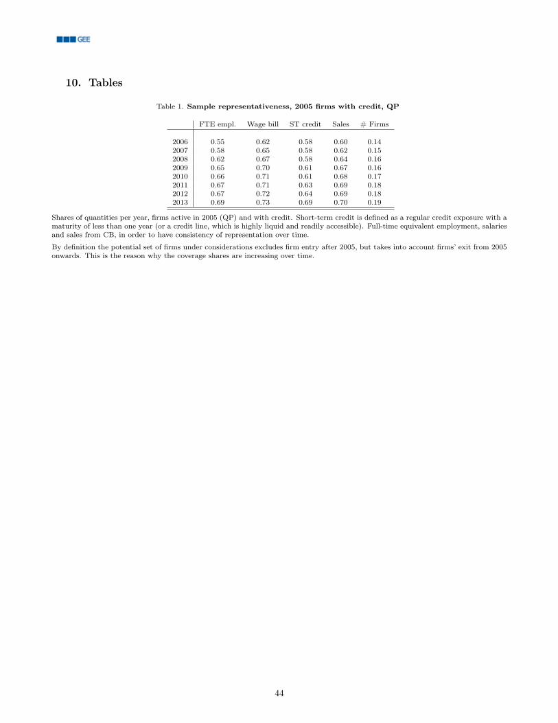
10. Tables

Table 1. Sample representativeness, 2005 firms with credit, QP

FTE empl. Wage bill ST credit Sales # Firms

2006 0.55 0.62 0.58 0.60 0.142007 0.58 0.65 0.58 0.62 0.152008 0.62 0.67 0.58 0.64 0.162009 0.65 0.70 0.61 0.67 0.162010 0.66 0.71 0.61 0.68 0.172011 0.67 0.71 0.63 0.69 0.182012 0.67 0.72 0.64 0.69 0.182013 0.69 0.73 0.69 0.70 0.19

Shares of quantities per year, firms active in 2005 (QP) and with credit. Short-term credit is defined as a regular credit exposure with amaturity of less than one year (or a credit line, which is highly liquid and readily accessible). Full-time equivalent employment, salariesand sales from CB, in order to have consistency of representation over time.

By definition the potential set of firms under considerations excludes firm entry after 2005, but takes into account firms’ exit from 2005onwards. This is the reason why the coverage shares are increasing over time.

44

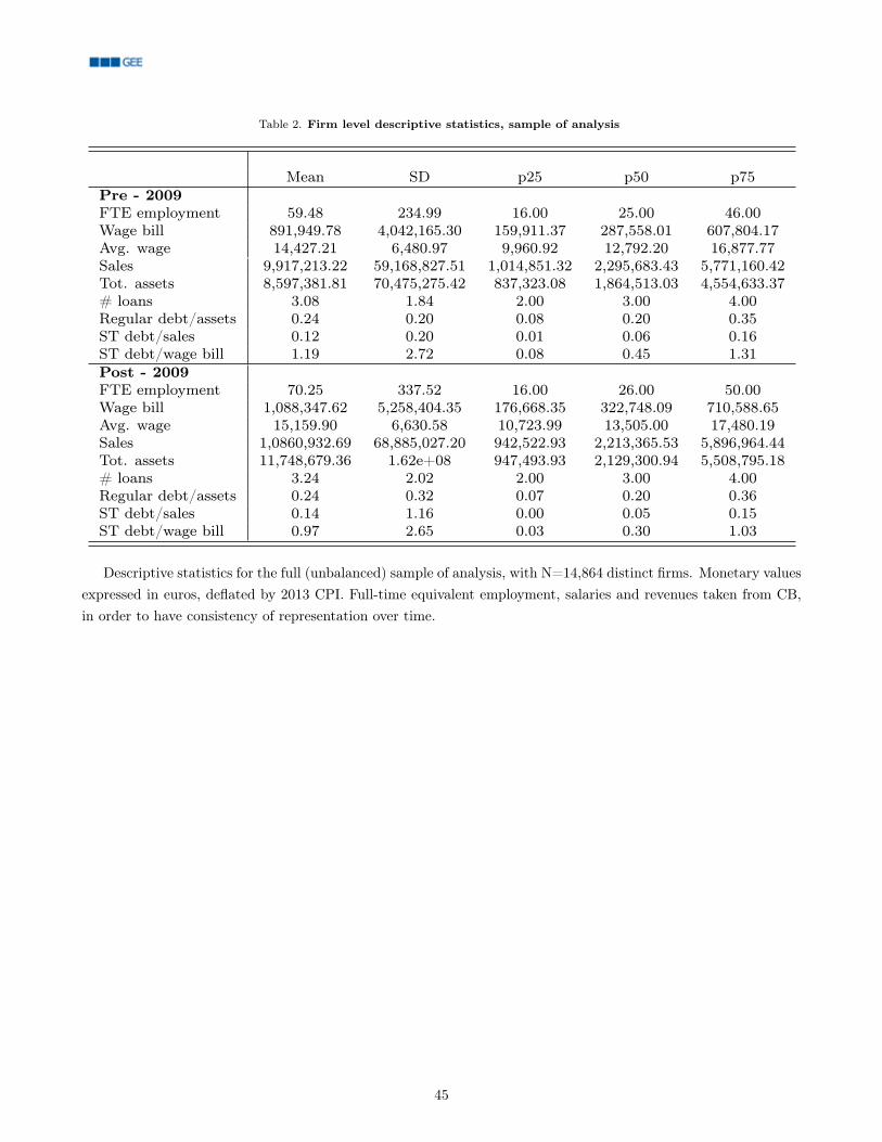
Table 2. Firm level descriptive statistics, sample of analysis

Mean SD p25 p50 p75Pre - 2009FTE employment 59.48 234.99 16.00 25.00 46.00Wage bill 891,949.78 4,042,165.30 159,911.37 287,558.01 607,804.17Avg. wage 14,427.21 6,480.97 9,960.92 12,792.20 16,877.77Sales 9,917,213.22 59,168,827.51 1,014,851.32 2,295,683.43 5,771,160.42Tot. assets 8,597,381.81 70,475,275.42 837,323.08 1,864,513.03 4,554,633.37# loans 3.08 1.84 2.00 3.00 4.00Regular debt/assets 0.24 0.20 0.08 0.20 0.35ST debt/sales 0.12 0.20 0.01 0.06 0.16ST debt/wage bill 1.19 2.72 0.08 0.45 1.31Post - 2009FTE employment 70.25 337.52 16.00 26.00 50.00Wage bill 1,088,347.62 5,258,404.35 176,668.35 322,748.09 710,588.65Avg. wage 15,159.90 6,630.58 10,723.99 13,505.00 17,480.19Sales 1,0860,932.69 68,885,027.20 942,522.93 2,213,365.53 5,896,964.44Tot. assets 11,748,679.36 1.62e+08 947,493.93 2,129,300.94 5,508,795.18# loans 3.24 2.02 2.00 3.00 4.00Regular debt/assets 0.24 0.32 0.07 0.20 0.36ST debt/sales 0.14 1.16 0.00 0.05 0.15ST debt/wage bill 0.97 2.65 0.03 0.30 1.03

Descriptive statistics for the full (unbalanced) sample of analysis, with N=14,864 distinct firms. Monetary valuesexpressed in euros, deflated by 2013 CPI. Full-time equivalent employment, salaries and revenues taken from CB,in order to have consistency of representation over time.

45

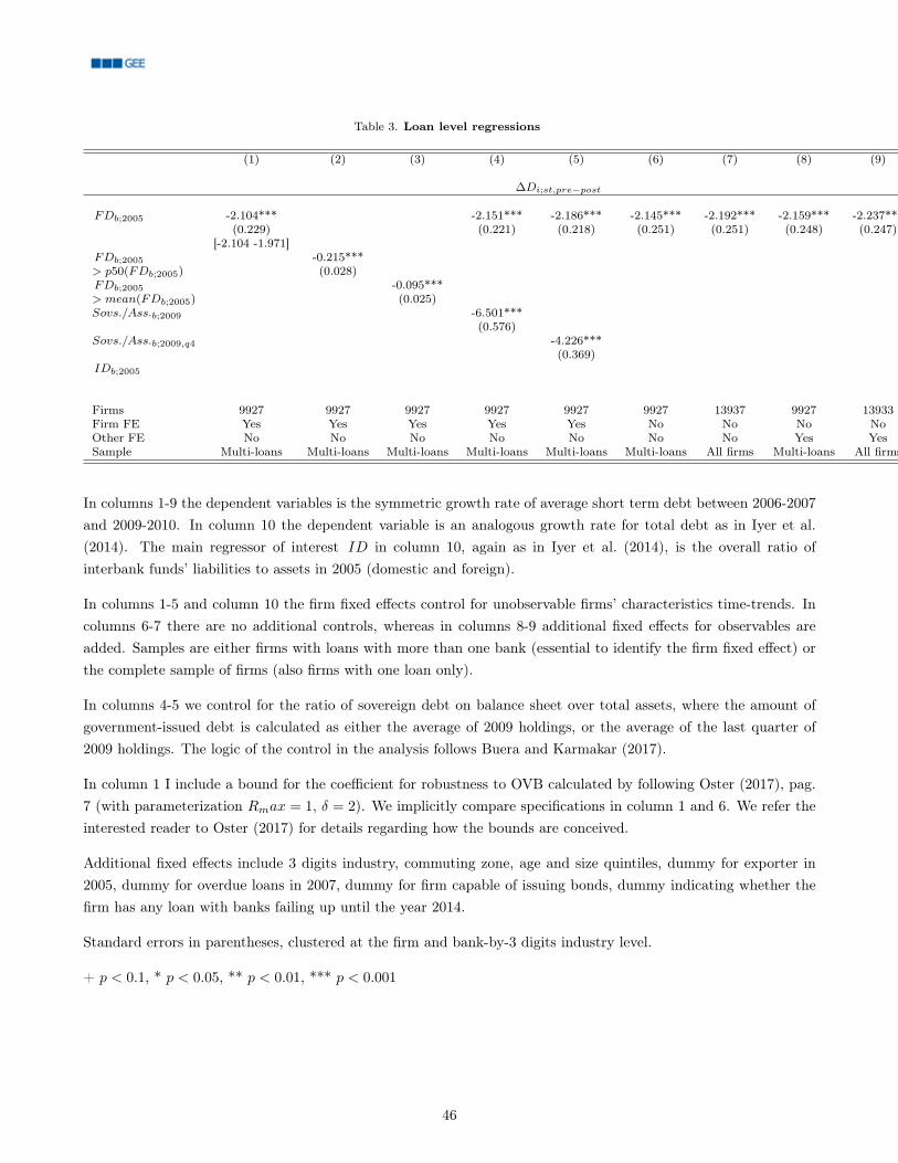
Table 3. Loan level regressions

(1) (2) (3) (4) (5) (6) (7) (8) (9) (10)

∆Di;st,pre−post ∆Di;tot,pre−post

FDb;2005 -2.104*** -2.151*** -2.186*** -2.145*** -2.192*** -2.159*** -2.237***(0.229) (0.221) (0.218) (0.251) (0.251) (0.248) (0.247)

[-2.104 -1.971]FDb;2005 -0.215***> p50(FDb;2005) (0.028)FDb;2005 -0.095***> mean(FDb;2005) (0.025)Sovs./Ass.b;2009 -6.501***

(0.576)Sovs./Ass.b;2009,q4 -4.226***

(0.369)IDb;2005 -0.432***

(0.121)

Firms 9927 9927 9927 9927 9927 9927 13937 9927 13933 10413Firm FE Yes Yes Yes Yes Yes No No No No YesOther FE No No No No No No No Yes Yes NoSample Multi-loans Multi-loans Multi-loans Multi-loans Multi-loans Multi-loans All firms Multi-loans All firms Multi-loans

In columns 1-9 the dependent variables is the symmetric growth rate of average short term debt between 2006-2007and 2009-2010. In column 10 the dependent variable is an analogous growth rate for total debt as in Iyer et al.(2014). The main regressor of interest ID in column 10, again as in Iyer et al. (2014), is the overall ratio ofinterbank funds’ liabilities to assets in 2005 (domestic and foreign).

In columns 1-5 and column 10 the firm fixed effects control for unobservable firms’ characteristics time-trends. Incolumns 6-7 there are no additional controls, whereas in columns 8-9 additional fixed effects for observables areadded. Samples are either firms with loans with more than one bank (essential to identify the firm fixed effect) orthe complete sample of firms (also firms with one loan only).

In columns 4-5 we control for the ratio of sovereign debt on balance sheet over total assets, where the amount ofgovernment-issued debt is calculated as either the average of 2009 holdings, or the average of the last quarter of2009 holdings. The logic of the control in the analysis follows Buera and Karmakar (2017).

In column 1 I include a bound for the coefficient for robustness to OVB calculated by following Oster (2017), pag.7 (with parameterization Rmax = 1, δ = 2). We implicitly compare specifications in column 1 and 6. We refer theinterested reader to Oster (2017) for details regarding how the bounds are conceived.

Additional fixed effects include 3 digits industry, commuting zone, age and size quintiles, dummy for exporter in2005, dummy for overdue loans in 2007, dummy for firm capable of issuing bonds, dummy indicating whether thefirm has any loan with banks failing up until the year 2014.

Standard errors in parentheses, clustered at the firm and bank-by-3 digits industry level.

+ p < 0.1, * p < 0.05, ** p < 0.01, *** p < 0.001

46

Table 4. Employment regressions

(1) (2) (3) (4) (5)log(#emp)i,t

Si 0.066+ 0.072* 0.070* 0.071* 0.086*(0.040) (0.033) (0.033) (0.034) (0.035)

Firms 14846 14830 13833 13806 11802EFF. WID F 34.15 37.29 36.52 34.56 35.55Sample Complete Complete Complete Complete SurvivorsFixed effects No Yes Yes Yes YesControls No No Fail b.c. Yes Yes

The regressions refer to the empirical specification in equation (5) in the text. All regressions feature firm and timefixed effects.

We refer to as the estimation sample in which only the controls for which the balance checks have failed are includedand controlled for.

Additional fixed effects are 3-digit industrial sector, commuting zone, quintiles of firm age and size in 2005, anddummies for: exporter, firm with overdue loans in 2007, banking relationship with the banks failed before 2014,firm capable of issuing bonds, firm with a single banking relationship.

Additional controls include the 2005 values of: log level of short-term credit, financial leverage, log of total assets,short-term credit growth betweeen 2004 and 2005, debt towards suppliers over assets, number of loans, (weighted)length of banking relationships, cash over assets, share of temporary workers, trade credits over assets, log numberof employees, asinh of the value added per employee, log of sales, firm age, share of short-term credit in regularcredit, share of fixed tangible assets in total assets, ROA, ROS, log of the average wage, average workers’ turnoverrate between 2003 and 2005. All controls and fixed effects are interacted with a post-period dummy.

The number of firms in the regressions change depending on the missing values in the balance-sheet variables.

Standard errors clustered at the bank-industry pair level.

+ p < 0.10, * p < 0.05, ** p < 0.01, *** p < 0.001

47

Table 5. Wage bill regressions

(1) (2) (3) (4) (5) (6)log(wage bill)i,t log(base wage bill)i,t wage billi,t/salesi,pre

Si 0.090* 0.114** 0.093* 0.111** 0.163+ 0.233**(0.038) (0.041) (0.038) (0.040) (0.084) (0.083)

Firms 13806 11802 13806 11802 13806 11802WID F 35.63 36.33 35.63 36.33 42.37 46.45Sample Complete Survivors Complete Survivors Complete Complete

The dependent variables are either the total wage bill (columns 1 and 2) or the base wage bill, which does notcomprehend extraordinary or overtime payments (columns 3 and 4). In columns 5 and 6 the dependent variableis the ratio of wage bill to the pre-period average value of sales, whereas the treatment is the variation in averageshort term credit (as for the standard treatment) scaled by the pre-period average value of sales. The coefficientsin columns 5 and 6 should be interpreted as dollar-on-dollar cash-flow pass through.

See the table 4 for the list of controls and fixed effects in the regressions. All regressions feature the full set of fixedeffects and controls.

Standard errors clustered at the bank-industry pair level.

+ p < 0.10, * p < 0.05, ** p < 0.01, *** p < 0.001

48

Table 6. Employment - wage bill regressions: Manufacturing

(1) (2) (3) (4) (5) (6)log(#emp)i,t log(Wage bill)i,t log(Base wage bill)i,t

Si 0.118** 0.136** 0.165** 0.186** 0.153** 0.169**(0.041) (0.047) (0.056) (0.062) (0.052) (0.057)

Firms 6348 5404 6348 5404 6348 5404EFF. WID F 24.06 22.27 24.06 22.27 24.06 22.27Sample Complete Survivors Complete Survivors Complete Survivors

See the table 4 for the list of controls and fixed effects in the regressions. All regressions feature the full set of fixedeffects and controls.

Regressions estimated only on the subsample of firms in manufacturing industries.

Standard errors clustered at the bank-industry pair level.

+ p < 0.10, * p < 0.05, ** p < 0.01, *** p < 0.001

49

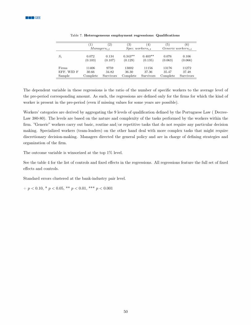
Table 7. Heterogeneous employment regressions: Qualifications

(1) (2) (3) (4) (5) (6)Managersi,t Spec. workersi,t Generic workersi,t

Si 0.072 0.134 0.343** 0.403** 0.076 0.106(0.103) (0.107) (0.129) (0.135) (0.063) (0.066)

Firms 11406 9759 13002 11156 13176 11272EFF. WID F 30.66 34.82 36.30 37.36 35.47 37.48Sample Complete Survivors Complete Survivors Complete Survivors

The dependent variable in these regressions is the ratio of the number of specific workers to the average level ofthe pre-period corresponding amount. As such, the regressions are defined only for the firms for which the kind ofworker is present in the pre-period (even if missing values for some years are possible).

Workers’ categories are derived by aggregating the 9 levels of qualification defined by the Portuguese Law ( Decree-Law 380-80). The levels are based on the nature and complexity of the tasks performed by the workers within thefirm. ”Generic” workers carry out basic, routine and/or repetitive tasks that do not require any particular decisionmaking. Specialized workers (team-leaders) on the other hand deal with more complex tasks that might requirediscretionary decision-making. Managers directed the general policy and are in charge of defining strategies andorganization of the firm.

The outcome variable is winsorized at the top 1% level.

See the table 4 for the list of controls and fixed effects in the regressions. All regressions feature the full set of fixedeffects and controls.

Standard errors clustered at the bank-industry pair level.

+ p < 0.10, * p < 0.05, ** p < 0.01, *** p < 0.001

50

Table 8. Heterogeneous employment regressions: Age cohorts

(1) (2) (3) (4) (5) (6)Y oung w.i,t Prime age w.i,t Old w.i,t

Si 0.170+ 0.223* 0.087** 0.101** 0.079 0.040(0.098) (0.102) (0.030) (0.032) (0.058) (0.054)

Firms 13210 11315 13806 11802 10679 9124EFF. WID F 30.70 31.64 34.56 35.55 28.76 34.81Sample Complete Survivors Complete Survivors Complete Survivors

The dependent variable in these regressions is the ratio of the number of specific workers to the average level ofthe pre-period corresponding amount. As such, the regressions are defined only for the firms for which the kind ofworker is present in the pre-period (even if missing values for some years are possible).

The age categories are: young workers (between 16 and 30), prime age workers (between 30 and 55) and old workers(between 56 and 65). Age cohorts are fixed over the period of analysis and defined depending on the age of theworker in 2008.

The outcome variable is winsorized at the top 1% level.

See the table 4 for the list of controls and fixed effects in the regressions. All regressions feature the full set of fixedeffects and controls.

Standard errors clustered at the bank-industry pair level.

+ p < 0.10, * p < 0.05, ** p < 0.01, *** p < 0.001

51

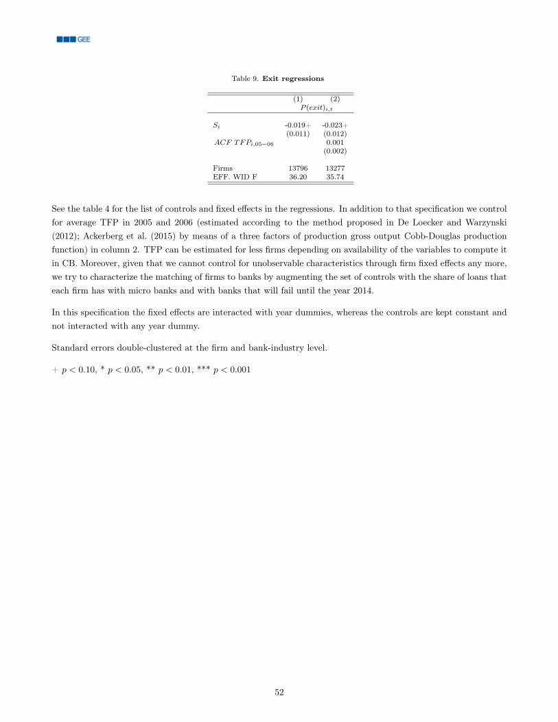
Table 9. Exit regressions

(1) (2)P (exit)i,t

Si -0.019+ -0.023+(0.011) (0.012)

ACF TFPi,05−06 0.001(0.002)

Firms 13796 13277EFF. WID F 36.20 35.74

See the table 4 for the list of controls and fixed effects in the regressions. In addition to that specification we controlfor average TFP in 2005 and 2006 (estimated according to the method proposed in De Loecker and Warzynski(2012); Ackerberg et al. (2015) by means of a three factors of production gross output Cobb-Douglas productionfunction) in column 2. TFP can be estimated for less firms depending on availability of the variables to compute itin CB. Moreover, given that we cannot control for unobservable characteristics through firm fixed effects any more,we try to characterize the matching of firms to banks by augmenting the set of controls with the share of loans thateach firm has with micro banks and with banks that will fail until the year 2014.

In this specification the fixed effects are interacted with year dummies, whereas the controls are kept constant andnot interacted with any year dummy.

Standard errors double-clustered at the firm and bank-industry level.

+ p < 0.10, * p < 0.05, ** p < 0.01, *** p < 0.001

52

Table 10. Correlations of observables with labor share

Labor shareWorkforce variables (pre 2009)Avg. wage (+)***AKM firm FE (+)***Sh. managers (+)***Sh. specialized workers (+)***Sh. temporary workers (-)**Median tenure (perm.) (+)***Sh. workers 55+ (+)***Sh. high education workers (+)***OJT score (+)***ONET zone score (+)***Financial variablesFinancial leverage (debt/ass.) (2005) (-)***ST debt/ass. (2005) (-)***Financial leverage (2008) (-)***ST debt/ass. (2008) (-)+Credit growth (06-08) (-)***Cash per worker (2005) (-)***Sh. ST credit (2005) (+)***Sh. ST debt fully secured (2009) .MRP - gapsLabor gap (+)***Capital gap .

Correlations are measured in regressions controlling by the full set of fixed effects and controls in the diff-in-diff specifications, whichimplies that we are also always controlling for value added per employee. Labor share and value added for employee are calculated asaverages for the years 2005 and 2006.

When controlling for a variable post-2006, its previous level in 2005 is excluded from the controls.

Abowd et al. (1999) (AKM) firm fixed effects obtained from regressing (full) individual wages in the pre-period on individual fixed effects,firm fixed effects, year fixed effects, gender dummy, educational level fixed effects (less than high school, high school and undergraduatedegree and higher), a third order polynomial of age.

Results for AKM FE and avg. wage robust to controlling for workforce composition variables (share of specialized workers and managers,shares of workers with different education levels).

See appendix C.2 for details regarding the estimation of MRP - cost gaps.

* p < 0.10, ** p < 0.05, *** p < 0.01

53

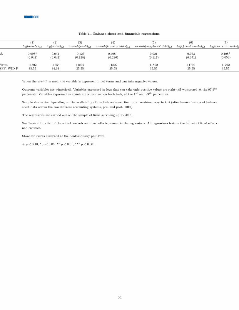
Table 11. Balance sheet and financials regressions

(1) (2) (3) (4) (5) (6) (7)log(assets)i,t log(sales)i,t arsinh(cash)i,t arsinh(trade credits)i,t arsinh(suppliers′ debt)i,t log(fixed assets)i,t log(current assets)i,t

Si 0.098* 0.041 -0.123 0.408+ 0.021 0.063 0.108*(0.041) (0.044) (0.128) (0.226) (0.117) (0.071) (0.054)

Firms 11802 11554 11802 11802 11802 11799 11792EFF. WID F 35.55 34.93 35.55 35.55 35.55 35.55 35.55

When the arsinh is used, the variable is expressed in net terms and can take negative values.

Outcome variables are winsorized. Variables expressed in logs that can take only positive values are right-tail winsorized at the 97.5th

percentile. Variables expressed as arsinh are winsorized on both tails, at the 1st and 99th percentiles.

Sample size varies depending on the availability of the balance sheet item in a consistent way in CB (after harmonization of balancesheet data across the two different accounting systems, pre- and post- 2010).

The regressions are carried out on the sample of firms surviving up to 2013.

See Table 4 for a list of the added controls and fixed effects present in the regressions. All regressions feature the full set of fixed effectsand controls.

Standard errors clustered at the bank-industry pair level.

+ p < 0.10, * p < 0.05, ** p < 0.01, *** p < 0.001

54

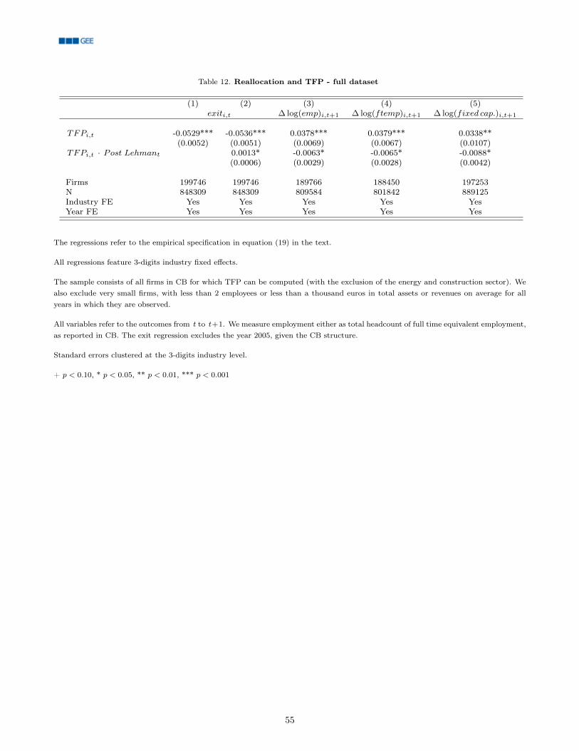
Table 12. Reallocation and TFP - full dataset

(1) (2) (3) (4) (5)exiti,t ∆ log(emp)i,t+1 ∆ log(ftemp)i,t+1 ∆ log(fixed cap.)i,t+1

TFPi,t -0.0529*** -0.0536*** 0.0378*** 0.0379*** 0.0338**(0.0052) (0.0051) (0.0069) (0.0067) (0.0107)

TFPi,t · Post Lehmant 0.0013* -0.0063* -0.0065* -0.0088*(0.0006) (0.0029) (0.0028) (0.0042)

Firms 199746 199746 189766 188450 197253N 848309 848309 809584 801842 889125Industry FE Yes Yes Yes Yes YesYear FE Yes Yes Yes Yes Yes

The regressions refer to the empirical specification in equation (19) in the text.

All regressions feature 3-digits industry fixed effects.

The sample consists of all firms in CB for which TFP can be computed (with the exclusion of the energy and construction sector). Wealso exclude very small firms, with less than 2 employees or less than a thousand euros in total assets or revenues on average for allyears in which they are observed.

All variables refer to the outcomes from t to t+1. We measure employment either as total headcount of full time equivalent employment,as reported in CB. The exit regression excludes the year 2005, given the CB structure.

Standard errors clustered at the 3-digits industry level.

+ p < 0.10, * p < 0.05, ** p < 0.01, *** p < 0.001

55

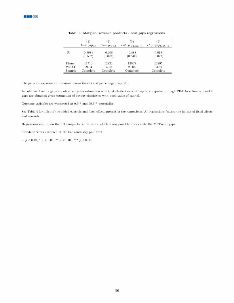
Table 13. Marginal revenue products - cost gaps regressions

(1) (2) (3) (4)Lab. gapi,t Cap. gapi,t Lab. gapbook;i,t Cap. gapbook;i,t

Si -0.968+ -0.008 -0.888 0.019(0.537) (0.027) (0.547) (0.022)

Firms 11710 12823 12005 12895WID F 29.34 35.37 29.06 34.99Sample Complete Complete Complete Complete

The gaps are expressed in thousand euros (labor) and percentage (capital).

In columns 1 and 2 gaps are obtained given estimation of output elasticities with capital computed through PIM. In columns 3 and 4gaps are obtained given estimation of output elasticities with book value of capital.

Outcome variables are winsorized at 0.5th and 99.5th percentiles.

See Table 4 for a list of the added controls and fixed effects present in the regressions. All regressions feature the full set of fixed effectsand controls.

Regressions are run on the full sample for all firms for which it was possible to calculate the MRP-cost gaps.

Standard errors clustered at the bank-industry pair level.

+ p < 0.10, * p < 0.05, ** p < 0.01, *** p < 0.001

56

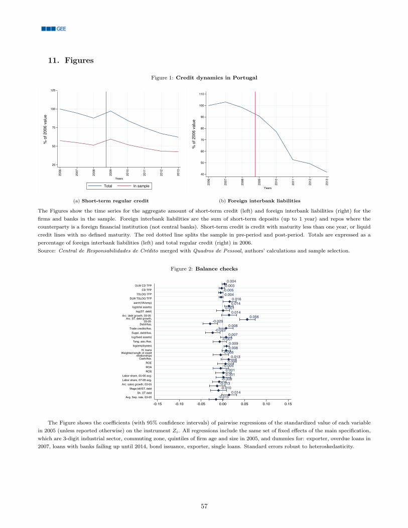
11. Figures

Figure 1: Credit dynamics in Portugal

25

50

75

100

125

% o

f 2006 v

alu

e

2006

2007

2008

2009

2010

2011

2012

2013

Years

Total In sample

(a) Short-term regular credit

40

50

60

70

80

90

100

110

% o

f 2006 v

alu

e

2006

2007

2008

2009

2010

2011

2012

2013

Years

(b) Foreign interbank liabilities

The Figures show the time series for the aggregate amount of short-term credit (left) and foreign interbank liabilities (right) for thefirms and banks in the sample. Foreign interbank liabilities are the sum of short-term deposits (up to 1 year) and repos where thecounterparty is a foreign financial institution (not central banks). Short-term credit is credit with maturity less than one year, or liquidcredit lines with no defined maturity. The red dotted line splits the sample in pre-period and post-period. Totals are expressed as apercentage of foreign interbank liabilities (left) and total regular credit (right) in 2006.Source: Central de Responsabilidades de Crédito merged with Quadros de Pessoal, authors’ calculations and sample selection.

Figure 2: Balance checks

0.004-0.003-0.005-0.004

0.0160.014

0.0010.014

0.056-0.029

0.008-0.023

0.007-0.007

0.0090.008

-0.0050.013

0.006-0.005

0.0010.001

-0.008-0.013-0.010

0.014-0.015

DLW CD TFPCD TFP

TSLOG TFPDLW TSLOG TFP

asinh(VA/emp)log(total assets)

log(ST. debt)Arc. debt growth, 03-05

Arc. ST. debt growth,03-05

Debt/Ass.Trade credits/Ass.

Suppl. debt/Ass.log(fixed assets)Tang. ass./Ass.log(employees)

N. loansWeighted length of credit

relationshipsCash/Ass.

ROEROAROS

Labor share, 05-06 avg.Labor share, 07-08 avg.Arc. sales growth, 03-05

Wage bill/ST. debtSh. ST debt

Avg. Sep. rate, 03-05

-0.15 -0.10 -0.05 0.00 0.05 0.10 0.15

The Figure shows the coefficients (with 95% confidence intervals) of pairwise regressions of the standardized value of each variablein 2005 (unless reported otherwise) on the instrument Zi. All regressions include the same set of fixed effects of the main specification,which are 3-digit industrial sector, commuting zone, quintiles of firm age and size in 2005, and dummies for: exporter, overdue loans in2007, loans with banks failing up until 2014, bond issuance, exporter, single loans. Standard errors robust to heteroskedasticity.

57

Figure 3: Employment and wage bill regressions: event study

-.35

-.3

-.25

-.2

-.15

-.1

-.05

0

.05

.1

2006 2007 2008 2009 2010 2011 2012 2013Year

Employees Wage bill Base wage bill

The dependent variables in these regressions are the ratio of the number of employees (wage bill) over the average of their level inthe pre-period (2006-2008). In the specifications the coefficient for the year 2008 are normalized to 0, so that all the other coefficientshave to be interpreted as the effect on the percentage variation of employment or wage bill with respect to the 2008 level.The sample includes only survivor firms (N = 11,801), but is not balanced. The graph displays the effect of a negative shock.See Table 4 for the list of controls and fixed effects in the regressions. All regressors and fixed effects are interacted with a year dummy.95% confidence intervals displayed, standard errors clustered at the bank-industry pair level.

58

Figure 4: Employment adjustment by tenure

-.3

-.25

-.2

-.15

-.1

-.05

0

.05

.1

2006 2007 2008 2009 2010 2011 2012 2013Year

Employees Attached incumbents Net hires and less attached

(a) Attached incumbents vs. all other workers

-.3

-.25

-.2

-.15

-.1

-.05

0

.05

.1

2006 2007 2008 2009 2010 2011 2012 2013Year

Employees Attached incumbentsLess attached incumbents Net hires

(b) Attached incumbents vs. less attached incumbents and net hires

The dependent variables in these regressions are the ratio of the number of employees of the specific category over the averagenumber of employees in the pre-period (2006-2008). By construction, the sum of the coefficients of each regression should be equal tothe overall employment effect. In the specifications the coefficients for 2008 are normalized to 0, so that all the other coefficients shouldbe interpreted as the effect on the percentage variation of each kind of employment with respect to the 2008 level.Attached incumbents are defined as workers present at the firm for the entirety of the pre-period. Less attached incumbents are allother incumbents in 2008, whereas net hires are all the other workers (hires/separations in the post period). In order to get a sense ofthe implied elasticities of adjustment, one should divide the estimated coefficient by the share of workers in the pre-period. Attachedworkers constitute more than 67% of the workforce in the pre-period. The share of less attached incumbent is the remaining share ofworkers in 2008, and is always less than half of the attached incumbents share throughout the post-period.The sample includes only survivor firms (N = 11,801), but is not balanced. The graph displays the effect of a negative shock. See Table4 for the list of controls and fixed effects present in the regressions. All regressors and fixed effects are interacted with a year dummy.95% confidence intervals displayed, standard errors clustered at the bank-industry pair level.

59

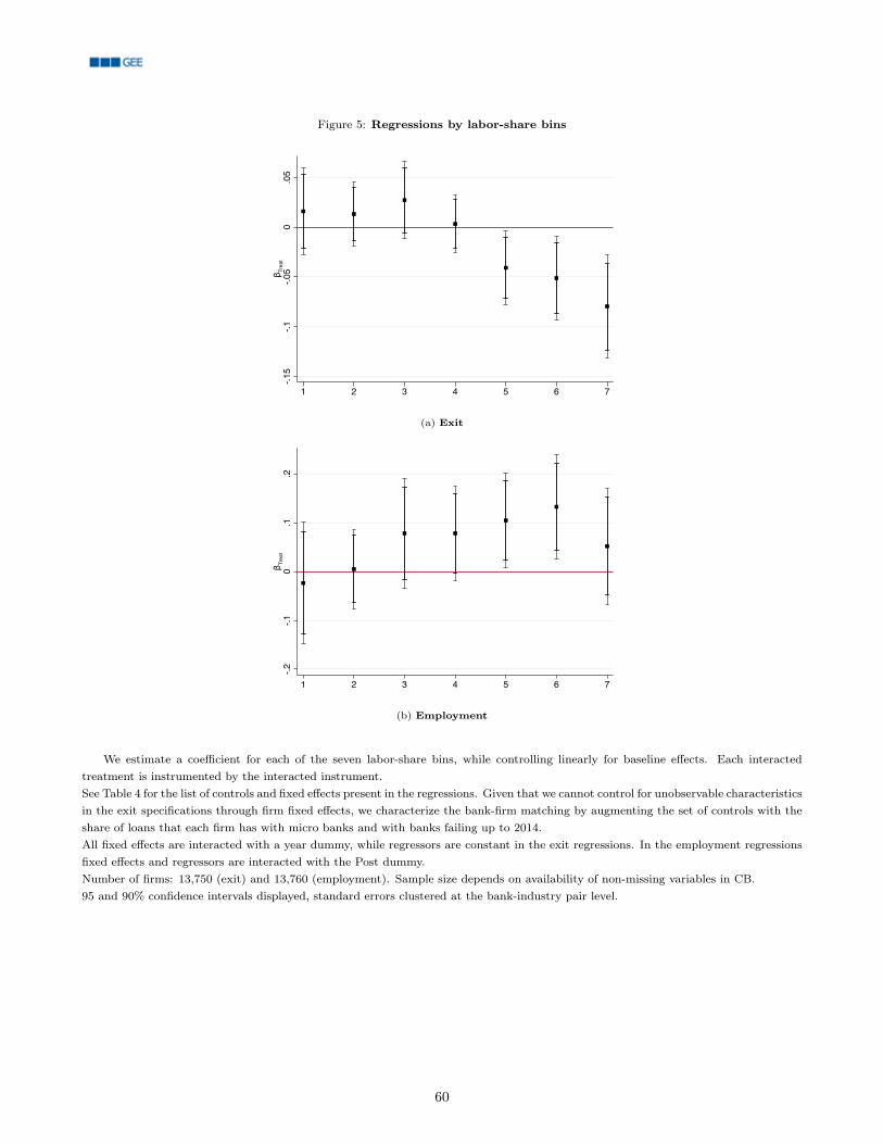
Figure 5: Regressions by labor-share bins

-.15

-.1-.05

0.05

β Treat

1 2 3 4 5 6 7

(a) Exit

-.2-.1

0.1

.2β T

reat

1 2 3 4 5 6 7

(b) Employment

We estimate a coefficient for each of the seven labor-share bins, while controlling linearly for baseline effects. Each interactedtreatment is instrumented by the interacted instrument.See Table 4 for the list of controls and fixed effects present in the regressions. Given that we cannot control for unobservable characteristicsin the exit specifications through firm fixed effects, we characterize the bank-firm matching by augmenting the set of controls with theshare of loans that each firm has with micro banks and with banks failing up to 2014.All fixed effects are interacted with a year dummy, while regressors are constant in the exit regressions. In the employment regressionsfixed effects and regressors are interacted with the Post dummy.Number of firms: 13,750 (exit) and 13,760 (employment). Sample size depends on availability of non-missing variables in CB.95 and 90% confidence intervals displayed, standard errors clustered at the bank-industry pair level.

60

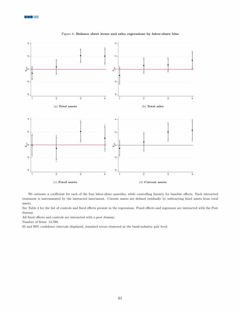
Figure 6: Balance sheet items and sales regressions by labor-share bins

-.4-.2

0.2

.4β T

reat

1 2 3 4

(a) Total assets

-.4-.2

0.2

.4β T

reat

1 2 3 4

(b) Total sales

-.4-.2

0.2

.4β T

reat

1 2 3 4

(c) Fixed assets

-.4-.2

0.2

.4β T

reat

1 2 3 4

(d) Current assets

We estimate a coefficient for each of the four labor-share quartiles, while controlling linearly for baseline effects. Each interactedtreatment is instrumented by the interacted instrument. Current assets are defined residually by subtracting fixed assets from totalassets.See Table 4 for the list of controls and fixed effects present in the regressions. Fixed effects and regressors are interacted with the Postdummy.All fixed effects and controls are interacted with a post dummy.Number of firms: 13,760.95 and 90% confidence intervals displayed, standard errors clustered at the bank-industry pair level.

61

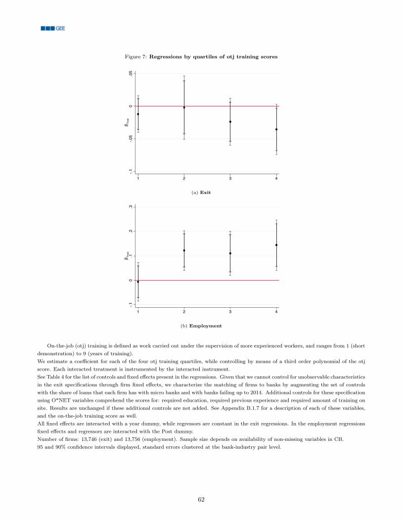
Figure 7: Regressions by quartiles of otj training scores

-.1-.05

0.05

β Treat

1 2 3 4

(a) Exit

-.10

.1.2

.3β T

reat

1 2 3 4

(b) Employment

On-the-job (otj) training is defined as work carried out under the supervision of more experienced workers, and ranges from 1 (shortdemonstration) to 9 (years of training).We estimate a coefficient for each of the four otj training quartiles, while controlling by means of a third order polynomial of the otjscore. Each interacted treatment is instrumented by the interacted instrument.See Table 4 for the list of controls and fixed effects present in the regressions. Given that we cannot control for unobservable characteristicsin the exit specifications through firm fixed effects, we characterize the matching of firms to banks by augmenting the set of controlswith the share of loans that each firm has with micro banks and with banks failing up to 2014. Additional controls for these specificationusing O*NET variables comprehend the scores for: required education, required previous experience and required amount of training onsite. Results are unchanged if these additional controls are not added. See Appendix B.1.7 for a description of each of these variables,and the on-the-job training score as well.All fixed effects are interacted with a year dummy, while regressors are constant in the exit regressions. In the employment regressionsfixed effects and regressors are interacted with the Post dummy.Number of firms: 13,746 (exit) and 13,756 (employment). Sample size depends on availability of non-missing variables in CB.95 and 90% confidence intervals displayed, standard errors clustered at the bank-industry pair level.

62

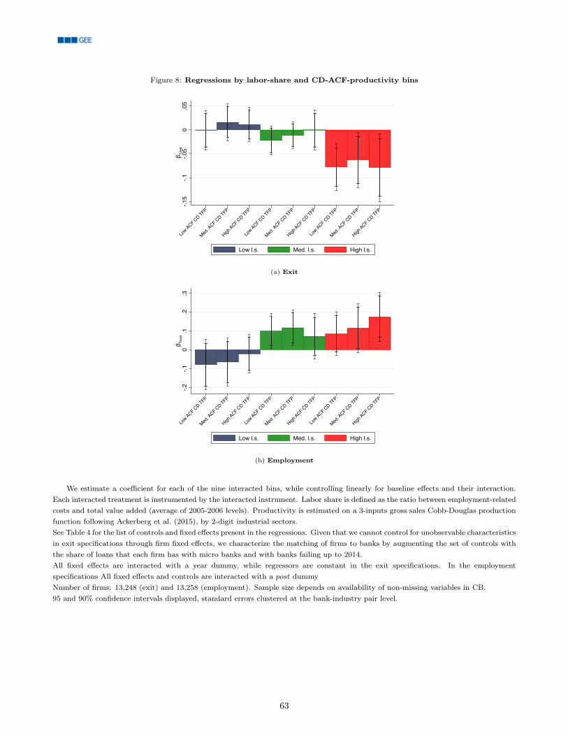
Figure 8: Regressions by labor-share and CD-ACF-productivity bins

-.15

-.1-.0

50

.05

β Tre

at

Low ACF CD TFP

Med. A

CF CD TFP

High ACF CD TFP

Low ACF CD TFP

Med. A

CF CD TFP

High ACF CD TFP

Low ACF CD TFP

Med. A

CF CD TFP

High ACF CD TFP

Low l.s. Med. l.s. High l.s.

(a) Exit

-.2-.1

0.1

.2.3

β Tre

at

Low ACF CD TFP

Med. A

CF CD TFP

High ACF CD TFP

Low ACF CD TFP

Med. A

CF CD TFP

High ACF CD TFP

Low ACF CD TFP

Med. A

CF CD TFP

High ACF CD TFP

Low l.s. Med. l.s. High l.s.

(b) Employment

We estimate a coefficient for each of the nine interacted bins, while controlling linearly for baseline effects and their interaction.Each interacted treatment is instrumented by the interacted instrument. Labor share is defined as the ratio between employment-relatedcosts and total value added (average of 2005-2006 levels). Productivity is estimated on a 3-inputs gross sales Cobb-Douglas productionfunction following Ackerberg et al. (2015), by 2-digit industrial sectors.See Table 4 for the list of controls and fixed effects present in the regressions. Given that we cannot control for unobservable characteristicsin exit specifications through firm fixed effects, we characterize the matching of firms to banks by augmenting the set of controls withthe share of loans that each firm has with micro banks and with banks failing up to 2014.All fixed effects are interacted with a year dummy, while regressors are constant in the exit specifications. In the employmentspecifications All fixed effects and controls are interacted with a post dummyNumber of firms: 13,248 (exit) and 13,258 (employment). Sample size depends on availability of non-missing variables in CB.95 and 90% confidence intervals displayed, standard errors clustered at the bank-industry pair level.

63

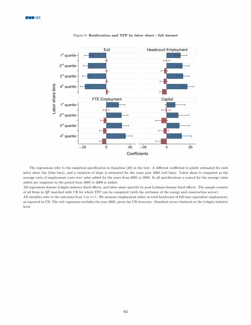
Figure 9: Reallocation and TFP by labor share - full dataset

1st quartile

2nd

quartile

3rd quartile

4th quartile

1st quartile

2nd

quartile

3rd quartile

4th quartile

−.05 0 .05 −.05 0 .05

Exit Headcount Employment

FTE Employment Capital

Labor

share

bin

s

Coefficients

The regressions refer to the empirical specification in Equation (20) in the text. A different coefficient is jointly estimated for eachlabor share bin (blue bars), and a variation of slope is estimated for the years post 2008 (red bars). Labor share is computed as theaverage ratio of employment costs over value added for the years from 2005 to 2008. In all specifications a control for the average valueadded per employee in the period from 2005 to 2008 is added.All regressions feature 3-digits industry fixed effects, and labor share quartile by post-Lehman dummy fixed effects. The sample consistsof all firms in QP matched with CB for which TFP can be computed (with the exclusion of the energy and construction sector).All variables refer to the outcomes from t to t+1. We measure employment either as total headcount of full time equivalent employment,as reported in CB. The exit regression excludes the year 2005, given the CB structure. Standard errors clustered at the 3-digits industrylevel.

64

A. A model of the financial channels of labor rigiditiesThe aim of the present section is to provide a conceptual framework for the emergence of the financial channels of labor rigidities,

which are at the core of the empirical analysis of the paper. To this end, it develops a simple model of firm decision of credit and labordemand, subject to a working-capital constraint.

The economy lives for two periods, and is populated by a profit-maximizing firm. The firm has a constant returns-to-scale technologyF that employs capital and labor to produce a consumption good to be sold at price P = 1.82 The firm starts the initial period withsome retained earnings Π, a fixed amount of capital K and incumbent workers I (a share of the workforce of the previous period) whoreceive a salary wI .83 The firm has to choose whether to adjust the workforce by hiring new workers N in a competitive labor market.84

To this end, it offers to them a salary wN and incurs in a training/vacancy cost c in order for them to be productive in the final period.The firm has to pay a share λ of the total wage bill of the final period in advance, together with the full training cost c. We are assumingthat, given the natural of the production activity carried out, there might be time gaps between cash inflows and wage payouts, or thatit takes time for workers to become productive and the training has to be financed in advance.85 For this reason, it needs to borrow anamount D of working capital from a banking sector.

For the present exercise, we assume that the firm starts in an unconstrained condition, in which bank credit D is available at a rateR = 1/β, where β is an intertemporal discount factor and is equal to 1 for simplicity. The firm incurs a fixed cost of operation f , andexits if is unable to honor it. In that sense, credit is only useful to transfer resources across periods, but absent any unexpected shockwould have no effect on the unconstrained equilibrium. Hence, we assume for simplicity that the firm takes external credit only up tothe amount needed to finance its current expenditures, but no more. Formally, the firm maximizes its value V :

maxN,D

V = AF (N + I, K)− wNN − wII − cN − f, (29)

subject to the working-capital constraint:D + Π ≥ cN + λ(wNN + wII), (30)

where A is the firm TFP, and Π are retained earnings.

In normal times, when the working-capital constraint is not binding, the first-order condition with respect to new hires yields:

AFL(N + I, K) = wN + c. (31)

This relationship defines the optimal level of new hires N∗ and as a consequence the optimal amount of credit D∗ to achieve it fromthe working-capital constraint (30).86

Now suppose that the bank unexpectedly cuts its credit supply and the firm can only obtain a level D.87 In this case, the firm’sworking-capital constraint yields the firm’s labor demand as:

N =(D + Π)− λwII

c+ λwN. (32)

The credit tightening has a negative impact on the firm’s value, summarized by the shadow value of credit.

Result 1 A negative credit shock decreases firm value:

∂V

∂D

∣∣∣∣D=D

= µ =AFL(N + I, K)− wN − c

c+ λwN, (33)

82This market setting comes at no loss of generality, and can be easily extended to a monopolistically competitive environment.83We do not model the determination of the incumbents’ salary. That would arguably depend on current market wages, past wagelevels in case of downward wage rigidity and some incurred training cost.

84De facto, this amounts to analyzing a setting with decreasing returns to scale in the short run, and necessarily ignores any feedbackeffect on fixed capital investment through labor-capital complementarity in production.

85Another way to rationalize this constraint is by limited enforcement in labor contracts. Before production takes place, the firmpromises salaries wI and wN to incumbents and new hires, respectively. However, it can renege on the promise and defaults on hispayroll, in which case the workers are able to seize only a fraction of the production. To relax this problem, the firm pays a fractionof the wage bill upfront.

86Notice that in this case the incumbents’ salaries have no effect on the optimal level of hiring. Moreover, we do not allow the firm tofire incumbents. We discuss the effect of this assumption below.

87Remember that in our empirical analysis we do not have a direct measure of credit spreads at the loan level. Hence, we model thecredit shock as a decrease in credit supply below the level that would be optimally demanded by firms. In any case, the two settingsare isomorphic in our simple model, as any suboptimal level of credit supplied by banks can rationalize an increase in credit spreadsthrough the shadow value of liquidity for the firm.

65

where µ is the shadow value of the working-capital constraint (30).

The effect on firm’s value through new hires:

∂N

∂D=

1

λwN + c−

λ

λwN + c

(∂wI

∂DI +

∂I

∂DwI)

(34)

highlights that a credit tightening can affect them not only directly, but also through the effect on incumbents wages and employment.Yet, if we assume that the incumbents’ wages are fully inflexible (which, at least in nominal terms, is almost entirely the case in Portugal)and that firings are not feasible or optimal (see discussion below), then the term in parentheses of the previous expression cancels out,and we can state the following:

Result 2 The elasticity of employment to credit around the optimal undistorted quantities is:

εL,D =∂ logL

∂ logD=

N∗

N∗ + I+

λwII −Π

(λwN + c)(N∗ + I). (35)

We interpret the first term as the labor-as-investment channel, which depends on how much the firm wants to extend its workforcewith respect to the current one (the elasticity of new hires to credit is always 1 in this setting). The second term represents insteadthe labor-as-leverage channel: The greater the incumbents’ wages wI , or the greater the share of the wage bill λ that has to be paidin advance, or the smaller the retained earnings Π from the previous period, the stronger the amplification of a credit shock from thelabor-as-leverage channel will be on new hires.88 The leverage effect through a firm’s exposure to the compensation-policy componentof its labor share, which we identify in the empirical analysis, exactly proxies this leverage effect in the model through the greaterincumbents’ wage level.

As a matter of fact, this amplification result might not be per se a signal of firm unprofitability, as it is possible that retainedearnings Π do not fall too much for greater levels of labor share in the past, if the firm has a good operating margin in the aggregateafter taking capital costs and other costs into account. In the data, the labor share is indeed negatively correlated with past profits.The variation in labor costs conditional on a certain level of profitability is exactly what the empirical exercise measures. What mattersfor the leverage effect to materialize is that a firm is exposed to rigid labor costs that it has to honor. Controlling for different degreesof productivity, such as value added per employee and overall TFP, helps distinguishing whether what one observes in the data is theresults of simple overpayment or a leverage effect on an otherwise productive firm.89

Result 3 Given Π, a greater incumbents’ labor share to finance (proxied by λwII) amplifies the employment elasticity to credit,and further raises the TFP threshold below which a firm exits the market.

Discussion Given the necessary complication that analyzing the discontinuity in the hiring/firing decision would entail with respectto the discontinuity in adjustment costs at the 0 point, our model does not include optimal firing due to TFP shocks or market conditions.In principle, the presence of implicit or explicit firing costs would arguably determine a pecking order from the least to the most protectedworkers. A way to rationalize this could be either by assuming firing costs that are increasing in tenure (which is for sure part of thestory in Portugal) or the possibility that tenured incumbents accumulate firm-specific human capital through which they hold up thefirm’s operations, or general skills that they could use in increasing their bargaining power with the firm. However, these dynamicswould not eliminate the leverage effect, given that the workers creating the most leverage are at the same time the most skilled andlikely essential to the firm operations.

Incumbents wages wI can be high for different reasons, which are left unmodeled here given the static nature of the model.Consistently with Card et al. (2017) or Kline et al. (2019), one would expect wages to incorporate part of the training costs in whichthe firm had incurred in order for the workers to be productive, given their implicit lower substitutability with outsiders. Moreover,risk-sharing consideration between firms and workers might affect wage dynamics (Guiso et al., 2005, 2013). For example, Xiaolan(2014) shows that the optimal contract to provide insurance to workers against negative productivity shocks, while at the same timeproviding the incentives for high-skill workers to remain in the firm, necessarily implies a degree of downward wage rigidity and anincreasing trajectory over time as a function of human capital accumulation. In other words, in Xiaolan’s setting downward rigidity incompensation is not determined by explicit firing costs, but by risk-sharing considerations. These kinds of dynamics are exactly whatone should have in mind regarding the way in which labor-as-investment turns into labor-as-leverage in our framework.

From the empirical analysis, it is clear that the amplification of a credit shock, which in this setting is isomorphic to a cash-flow

88Keep in mind that λ and Π do not affect the optimal amount of hiring in the undistorted state.89Keep in mind that the employment elasticity does not directly depend on future profitability and is not attenuated by it. If anything,future profitability would lead to a greater effect on impact through the investment channel, as firms would hire more in the optimalundistorted case.

66

shock, is predominantly driven by leverage.90 Thus, the effects on exit can almost surely be attributable to the labor-as-leveragechannel.91 The labor-as-investment channel instead, absent any non-convexity in training costs, should at most eliminate new hiresbut, given the presence of capital in place and incumbent workers, it is unlikely to drive exit. Labor-as-investment plausibly createsamplification through the effect that it has on wage dynamics over time, which is not captured in this static model, but does not perse generate a greater volatility of firms’ employment and investment decisions to cash-flow shocks. Put differently, in this very simplemodel working capital is needed to create the leverage effect through incumbents wages, but does not create amplification per se. Infact, training and vacancy costs expose the firms to financing costs, but firms might react to cash-flow shocks by scaling them backin a proportionate way. For example, a firm having to finance 80 percent of the wage bill in advance will exhibit the same elasticityof employment as a firm having to finance only 20 percent, provided that they receive the shock in a similar proportional amount.Hence, the elasticity of hiring to cash-flow, absent other channels, should be 1 in the simple model, which is why the overall elasticityof employment is the hiring share itself.

It is important to point out that, even if one would generally expect the labor-as-investment and labor-as-leverage channels tofrequently coexist and possibly reinforce each other, these two channels are separate on a substantive level, and it is conceivable thatthey can exist independently. In the model, labor-as-leverage implicitly depends on the presence of the working-capital constraint,which makes labor akin to an investment good. However, it is possible to conceive other situations in which its effects would materializeeven in the absence of an investment channel. In fact, it is possible that the presence of other fixed or complementary costs at firm levelwould set the leverage effect in motion, even if workers immediately generate the cash flow needed for their payments. In a similar way,if a firm had projects or other expenses that need priority financing for the firm to operate, the need to finance them would determinea real effect on employment and other forms of investments if costs are rigid. As long as the cash inflows that the workers generateare used by the firm to finance other prioritized payments, the quasi-fixity of labor will once again reverberate on new hiring and evenfiring decisions for the less attached workers.

All these arguments do not dismiss the labor-as-investment channel as irrelevant: to some extent, the channel creates an exposureto credit fluctuations through investment costs (which might have a leverage effect later on), and the fact that firms do not seem toinsure themselves against the exposure to short-term liquidity risk is still puzzling, given that training costs are possibly long-term andeasily predictable.

B. Data description and cleaning

B.1. Available datasets

B.1.1. Labor market data: Quadros de Pessoal

The Quadros de Pessoal (henceforth QP) is a longitudinal matched employer-employee dataset, containing detailed data at theworkers’ and firms’ level on employment composition for the firms and individual worker characteristics. The data are collected andmanaged by the Ministry of Labour and Social Solidarity, that draws on a compulsory annual census of all the firms employing at leastone worker at the end of October each year. It does not cover the public administration and non-market services, whereas it coverspartially or fully state-owned firms, provided that they offer a market service. The dataset covers approximately 350,000 firms and 3million employees per year. In 2010 the structure of the survey was reformed and the QP was incorporated into the Relatório Único,an integrated reporting system to enable employers to easily provide more extensive information on workers to the Ministry. As aconsequence, some very small entrepreneurial firms were exempted from filing compulsorily the questionnaire, which is why after 2009the coverage of QP is less complete than in previous years.92

The dataset is available at the Bank of Portugal from 1982 to 2013, and is hierarchically made up by a firm-level dataset, anestablishment-level dataset and a worker-level dataset. The firm level dataset contains information on the firm location (from regionalto very narrowly defined parish level, which roughly corresponds to a neighborhood, industry of operation (CAE rev. 2.1 until 2006 andCAE rev. 3, based on NACE-Rev. 2 Statistical classification of economic activities in the European Community), total employment,total sales, ownership structure and legal incorporation. Analogous information is available on the establishment-level dataset.

90An alternative possibility is that the firm is hit by the credit shock at a point in time when it needs to replace a high share of itsincumbent workers, and the credit shock makes it impossible to pay the training costs for new hires, thus leaving the firm in theimpossibility to produce. Through such a mechanism, exit would also depend on the labor-as-investment channel. However, in oursample there is no evidence that firms with high incumbents’ turnover face higher exit rates. Results are available upon request.

91The effect of the credit shock might also translate into a greater volatility of capital investment and eventually a greater exit probability,given that the decrease in D diminishes firm value. In turn, stronger leverage effects from past rigid costs, by distorting more a firmemployment decision, might amplify the effect on V , consistently with the empirical results.

92Despite this inconvenience, we use the firms’ balance sheet dataset, the Central de Balanços, which covers all non-financial corporationsin Portugal, to correctly disentangle firms’ failures. This also means that in our analysis the “survivors” sample is not necessarily abalanced sample.

67

The worker level dataset provides detailed information on worker characteristics and contracts. Information included comprehendsworkers’ gender, age, detailed occupational code (the Classificação Nacional de Profissões (CNP94) up to 2009 and the ClassificaçãoPortuguesa das Profissões (CPP2010) from 2010 onward, which is based on ISCO08 International Occupational Classification Codes),detailed educational level, qualification within the firm (managerial qualification, specialized workforce or generic workers, besidestrainees). At the contract level it is possible to know the precise hiring date, the kind of contract (various typologies that generallydefine the contract as fixed-term or open-ended), the hours arrangement (full-time versus part-time), the effective number of hoursworked, and information on the compensation. More specifically, for each worker it is possible to obtain information on the base pay,any extra paid in overtimes or other extra-ordinary payments and other irregularly paid components. In contrast, there is no informationon social security contributions. We winsorize the extreme 0.5% tails of the distribution of wages.93

The unique worker identifier is based on the workers’ social security number, and given the extensive work on the part of theMinistry to control and certify the quality of the data in this administrative dataset, the coverage and reliability of the data is quitehigh (except for the discrete break in coverage for only a subset of firms in 2010 due to the new reporting requirement in the RelatórioÚnico. Given that other datasets in our analysis cannot cover the same time-span, we only focus on years from 2005 to 2013 (butpotentially control for observables up to 2003 in some empirical exercises).

We use the QP to extract information regarding wage policies at the firm level. This is the dataset we use in order to computeAKM firm level fixed effects, which describe what component of workers’ compensation is firm specific and pertains to average firmwage policy. We compute AKM fixed effects thourgh an AKM regression, which is a wage regression at the worker level on firm andworker fixed effects and other workers’ characteristics. The firm fixed effect captures overall generosity of payments while the individualfixed effect should capture unobservable skills. In our AKM specifications we control for sex, a third polynomial of age and educationalcategories dummies, all variables present in QP itself. We run the AKM regressions on worker level data from 2003 to 2008.

B.1.2. Firm level financial statement data: Central de Balanços

The Central de Balanços (henceforth CB) is a firms level balance-sheet and income statements database, managed by the Bankof Portugal. It consists of a repository of yearly economic and financial information on the universe of non-financial corporationsoperating in Portugal from 2005 to 2013. It includes information on sales, balance-sheet items, profit and loss statements, and cash flowstatements (after 2009) for all private firms in Portugal.The CB builds on the Informaçào Empresarial Semplificada, an administrativefirms’ balance-sheet dataset managed by the Ministry of Finance and Public Administration. The Bank of Portugal obtains the datafrom the Ministry and performs extensive consistency checks to guarantee that the data are reliable and consistent over the years.The dataset in its present form covering the universe of firms is based on information reported in the starts in 2006, even if almost theentirety of firms already existing in 2005 provided balance sheet data for that year as well together with the 2006 filing. For this reason,we actually have a very high coverage of firms’ balance sheets for 2005 as well. Before 2005 the CB maintained by the Bank of Portugalwas actually a survey only for the biggest firms in the country. However, given the substantially lower coverage of the population offirms before 2005, we do not rely on that data.After 2009, in order for the data to comply with international accounting standards, there has been a major overhaul of the variablesdefinitions in the dataset, from the Plano Oficial de Contabilidade (POC) to the Sistema de Normalização Contabilística (SNC). In allour computations, unless otherwise noted, we have personally gone through a variables’ harmonization process, in collaboration with thestatistics department managing the administrative datasets for researchers at the Bank of Portugal, BPLim, to guarantee comparabilityacross periods.

The dataset contains a great amount of information on firms’ balance sheets and income statements, even if the harmonizationprocess between 2009 and 2010 makes it at time difficult if not impossible to keep consistent records for all balance sheet variables in thedataset. We use the dataset to obtain information on total assets, fixed assets, current assets total debt (not just bank debt) and interestexpenditures, cash-flow and capital expenditures (after 2009), cash balances, exports and export status, trade credits, debt towardssuppliers, inventories, return on equity, assets and sales, salaries, total employee related , revenues, costs and breakdowns (among whichintermediate inputs, materials and services), profits. We computer value added from this dataset by adding back employee relatedexpenditures to the firm EBITDA (which should correspond to subtracting expenditures on intermediate goods from total sales).

Given the dataset time-consistent coverage of firms operating in Portugal, we use it to identify firm exits as well. The procedureto identify a firm exit combines different criteria. Firstly, we rely on the CB on categorization of whether a firm is active, suspendedactivity or closed down. Secondly, we flag all the cases in which the firm will end up having 0 employees the next year but does havea positive number of employees in a given year. Thirdly, we actually check whether a firm disappears from the dataset in any given

93As regards the qualification categories, the Portuguese Decree-Law 380/80 established that firms should indicate the qualificationlevel as in the Collective Agreement. If this is not available, firms should select the qualification level of the worker. These categoriesare based on the degree of complexity of tasks that the worker performs within the firm (from more basic, routine tasks to morediscretionary managerial ones). The categories are defined within a 9 levels hierarchy, that we simplify into three broad categories.

68

year that is not 2013 and does not re-appear at any time (and does not simply have, consequently, a gap in the data). Lastly, we labelas exits the instances in which a firm disappears for more than two years, as it is likely that if the identifier reappears later it has justbeen reassigned to another firm (an assumption that seems to be validated by the observation that when such instance takes place thefirm seems different in terms of size and sector between the two periods). In all the cases we select the criterion of exit, in case a firmmatches more than one at different points in time, by looking at the case in which the firm “closed down” with the highest number ofemployees or, if ties are not resolved, with the lowest EBITDA.

B.1.3. Credit exposure level dataset: Central de Responsabilidades de Crédito

The Central de Responsabilidades de Crédito (henceforth CRC), is the credit registry of the Central Bank of Portugal. The datasetfeatures available for our period of analysis (up to 2013) features bank-firm exposures above EUR50 by the universe of Portuguese creditinstitutions at the monthly level. The dataset does not contain credit exposure by foreign banks towards Portuguese firms, but canobviously contain credit from Portuguese banks to foreign owned firms residing and operating in Portugal.94

The dataset is regularly employed for supervisory purposes, and by the credit institutions themselves to obtain information onpotential debtors. It contains detailed information on the number of credit relationships, the corresponding amounts and the kind ofexposure: short- and long-term, credit granted but still not materialized (potential), credit overdue, written-off or renegotiated. From2009 onwards, but unfortunately not before, it is possible to obtain information closer to loan-level (i.e. it is possible to keep trackof exposures which consist into the sum of loans with very detailed similar characteristics instead of seeing an aggregate number bykind of coarsely defined exposure) and more details about the exact maturity of each exposure and the collateral posted by each firm,if any (real collateral or guarantees, fraction of the value of the loan backed by it). Given the nature of our analysis and the periodof interest, we mostly focus on obtaining a consistent representation of the information available in the dataset before 2009. For ouranalysis and given the time frequency in other data sources we average debt exposures at the yearly level. We use “regular” credit in ourspecifications as measure of credit, which corresponds to credit in good standing and in use by the firm. Credit is defined as short-termif the maturity is below 1 year or it is a credit line with undefined maturity (post-2009 data) or is categorized as commercial, discountor other funding short-term pre-2009. We group together short-term loans, credit lines with defined short-term maturity and creditlines with underfined maturity because the latter category of credit lines comprehends all those exposures that, once withdrawn by thecustomer, should undergo renegotitation with the bank in order to be rolled-over. This feature makes them very liquid instrumentsthat, similarly to short-term loans, is subject to short-term credit rates volatility and rollover risk. Credit lines always constitute above3/4 of short-term credit as we define it. Long-term credit is thus obtained as the remainder in regular credit.

B.1.4. Banks balance sheet dataset: Balanço das Instituições Monetárias e Financeiras

The “Balanço das Instituições Monetárias e Financeiras” (henceforth BBS) is the balance-sheet dataset for credit institutions thatwe employ. It is a proprietary dataset of the Bank of Portugal with the balance sheets of the universe of financial monetary institutionsoperating in the country. The dataset is utilized by officers of the bank in order to monitor the health of financial monetary institutionsoperating in the country and the overall stability of the system. In the dataset, for each balance-sheet item (liability or asset) itis possible to see which is the kind of counterparty involved (i.e. the kind of institution, government, private or non-governmentalbody, creditor or debtor), the maturity of the item in question if relevant (time deposits, on demand deposits, interbank long-term orshort-term exposures) and the nationality of the counterparty (extra-EU or each EU country separately). The data are reported at themonthly level.

The measure of interbank funding which is the basis of our instrument is computed from this dataset as the ratio of the average(yearly) short-term foreign interbank borrowing by the bank over total assets. Foreign short-term interbank borrowing is computed asthe sum of short-term deposits with maturity up to 1 year and repos where the counterparty if a foreign financial institution (obviouslynot a central bank).

In matching the BBS and the CRC, we also took care of harmonizing and making bank definitions consistent across datasets giventhe existence of many mergers and acquisitions in the Portuguese banking system during the period. Each M&A event between 2000and 2013 (for institutions with at least 1 percent of total credit in a given month) was taken into consideration in order to make sure thatcredit flows across institutions were rightly accounted for, and definitions of bank codes across datasets and across time were consistent.

94We do not believe that this fact could be a source of significant bias in any of our results, as the Portuguese economy mostly featuresrelatively small and arguably bank-dependent firms, and for the biggest firms it is more likely for them to access directly debt marketsinstead of creating ties with foreign banks. Most foreign banks, moreover, operate Portugal incorporated subsidiaries in the country,the credits of which would regularly appear in the CRC.

69

B.1.5. Banks balance sheet dataset: Sistema Integrado de Estatísticas de Títulos

The Sistema Integrado de Estatísticas de Títulos (henceforth SIET) is a proprietary dataset of the Bank of Portugal. It includesdebt securities (i.e. banknotes, commercial papers, bonds, etc.) with maturity both short term (up until 1 year) and long term (morethan 1 year), and capital (i.e. shares and other means of participations) but neither derivatives nor REPOs. For both debt securitiesand capital, SIET collects data about emissions and portfolio holdings. For emissions, SIET collects flows and stocks relative to nationalissuers, on a title-by-title and issuer-by-issuer bases. For portfolio holdings, SIET collects flows and stocks on an investor-by-investorand title-by-title basis. Through SIET we obtain holdings of sovereign debt, or more in general any government-issued debt instrumentheld by banks on their balance sheet.

B.1.6. Commuting zone definitions

Given the relevance of the concept of commuting zone, especially for the analysis of labor market reallocation, we obtained data onthe definition of commuting zones for Portugal from Afonso and Venâncio (2016).

B.1.7. Labor market data: Occupational Information Network

Given the availability of definitions of occupations at the worker level in the QP, we were able to obtain occupation characteristicsthrough the Occupational Information Network (O*NET) database. The O*NET database is a widely used database in labor economicsand is the primary source of data in the United States for categorization of occupation characteristics. It is based on the combinationof the analysis of responses to questionnaires on occupations administered to sampled employers and employees, and is updated fourtimes a year with new data or updates to current categorizations.

We used O*NET in order to create indexes on job categorizations in terms of education, experience and training requirements. Foreach occupation a categorization is provided regarding the level of experience required (with possible scores ranging from 1 to 12, fromless than high-school to post-graduate level), the level of previous experience (from 1 to 11, from none to more than 10 years), the levelof on-site training (classes, courses, instructions sessions organized by the employer) or on-the-job training (that is, work carried outunder the supervision of more experienced workers) required to being able to carry out the required tasks (from 1 to 9, from a shortdemonstration to years of training). Moreover, we also extracted for each occupation the categorization of the “job zone” (with a scorefrom 1 to 4 in ascending order of “sophistication” of required vocational preparation levels), which is a further categorization created byexpert O*NET analysts that combines all the previous four categories in a unique index. We obtained a separate occupational index aswell for each category by averaging the scores, taking into account the frequency of each score for each response.

In order to combine the data, we first worked on making profession definitions consistent across time in our dataset, and thenmerged our occupational code to O*NET through a ISCO08-ONETSOC10 crosswalk. Given the change in occupational codes from theClassificação Nacional de Profissões (CNP94) to the new Classificação Portuguesa das Profissões (CPP2010) in 2010 in order to updatethe categorization and making in compliant to the International Standard Classification of Occupations (ISCO2008) categorization, wecreated a crosswalk based on the frequency of cross-occupational code changes from 2009 to 2010 in the QP within the same firms. Weused the cross-walk in Hardy et al. (2018) to merge our ISCO08 codes to (ONET)SOC10 (Standard Occupational Codes). We thenaveraged all the occupational scores and indexes obtained from ONET across occupations in order to obtain a time consistent 3-digitsISCO08 occupational categorization.95

We used O*NET version 23.3, and more specifically the education, training and experience files.96

B.2. Sample selection

In order to prepare the data for the analysis in our event-study, we need to combine all the different sources of data available, andperform cleaning checks to obtain a relevant sample of analysis depending on variables availability and firms’ and banks’ characteristics.

Given that the focus of our analysis is predominantly the adjustment of employment and other real variables as a function of thedifferent measures that we label as different sources of “labor rigidities” in the text, the main firm-level dataset around which we combinethe other datasets is the QP.

First, we perform some quality checks on the QP and remove workers’ for which identifiers are not consistent over time.97 We then

95The fact that obviously the occupational categorizations are neither bijections nor injections across sets made it difficult in some casesto reassign the occupational codes. We tried to use the official crosswalk at first, but noticed that it created very big discontinuitiesfor the frequency of observation of some professions. We noticed on the other hand that within firms changes in occupational codesseemed to be very consistent, and as such a more valid “revealed preference” categorization on the part of employers of their employeesactual occupation. We then decided to limit ourselves to a 3-digits categorization in order to have a meaningful number of workers foroccupation, and in order to minimize the inconsistencies in the cross-categorizations of occupational codes between CNP and CPP.

96https://www.onetcenter.org/dictionary/23.3/excel/education_training_experience.html97For the period 2005-2013 the problem is actually marginal.

70

select only workers listed as “employees”, full-time, between 16 and 65 years of age, and receiving a full wage in the October of everyyear (e.g. not on sick leave or other forms of leave).98 As regards monetary balance-sheet variables, wages and credit variables, wedeflate all nominal values in the analysis by the 2013 consumer price index.99

In order to define the final sample of analysis we merge all datasets and select firms based on some defined criteria. Given thatwe are interested in both firm dynamics and employment adjustment, we mostly consider firms present both in QP and CB.100 Werestrict our attention to firms in mainland Portugal, and exclude from the sample industries like agriculture, fishing, energy (extraction,mining and distribution), the construction sector and the financial sector itself. For the event study we only consider firms with a creditrelationship with any bank in 2005, which of course must survive until 2009 to be present in the period of time after the credit shock.We focus on firms with at least 9 employees, which is approximately the threshold for the fourth quartile in the distribution of firms’sizes in the years before 2009, and covers more than 60 percent of the workforce in the QP matched to CRC in the pre-period. In orderto reduce measurement noise, we consider only firms with no gaps in the data in the pre-period.101102

We also perform some consistency and sanity checks in selecting the relevant banks to be included in the analysis. More precisely,we exclude from the analysis the very small banks that disappear from the dataset before 2009. We also exclude from the set of banksfor which the instrument is computed those banks for which foreign interbank funding is actually intra-banking-group funding from theforeign headquarter to the Portuguese subsidiary.103

To limit the influece of outliers in the regressions, we drop firms in the top 2.5 percentile of positive credit variation between the pre-and post-periods. For the same reason we drop all the firms with a percentage of exposure-amount growth above the top 2.5 percentof the distribution in the exposure level specifications. This effectively amounts to eliminating more than 2.5 percent of firms for thoseparticular regressions, but we still think that this kind of cut is more sensible than leaving the firms in the estimation sample withoutaccounting for all their loans.

Our final sample spans 14,846 firms and 31 banks.104

C. Production function estimation

C.1. Productivity and output elasticities estimation

For the estimation of output elasticities, markups and ultimately revenue total factor productivity (TFPR) we use differentmethodologies. First of all, we consider a three-factors of production gross output (y) function, where factors are labor (l), physicalcapital (k) and an intermediate input (m). We consider both a simple Cobb-Douglas specification where the elasticity of substitutionamong the factors of production is restricted to be 1 and a translog specification, which relaxes the above assumption. The (log-)production function is thus expressed as a function of log-inputs as:

yi,t = f(li,t, ki,t,mi,t) + ωi,t + εi,t (36)

where f(li,t, ki,t,mi,t) isβlli,t + βkki,t + βmmi,t (37)

in the Cobb-Douglas case, and:

βlli,t + βkki,t + βmmi,t +∑

x∈{l,k,m}βxxx

2i,t +

∑j∈{l,k,m},j 6=x

∑x∈{l,k,m}

βjxji,txi,t (38)

98We also remove records with unreasonable number of hours worked and perform other sanity checks or within-worker’s recordsharmonization on other variables, such as date of birth, hiring dates, workers’ characteristics.

99For the productivity estimation the deflation of nominal values is performed at a much greater level of detail and precision dependingon each item and industry. We refer the reader to Appendix C for the details of the estimation.

100Most of the firms with partial state ownership are not in CB. Hence, they can be included in the most basic analyses, but not inthose that feature firm balance-sheet controls.

101Considering firms already existing in 2005 allows us to have at least 3 years of pre-period in our event study framework. We implicitlyexclude entrants in the three years before 2009 from the event study analysis.

102We focus on relatively big firms, at least by Portuguese standards, as we are interested in measuring employment adjustment atthe firm level, which becomes increasingly noisy and lumpy for very small firms, and because of the fact that the QP coverage ofPortuguese firms is full for relatively big firms but decreases for very small firms after 2009.

103The cases for which this happens are very few and do not represent more than 1 percent of total credit at any point time. We cannotdisclose any detail on the names of the banks in question.

104Most of the regressions which require also balance-sheet variables consists of 13,804 firms, while the sample of surviving firms consistsof 11,802 firms. At least for the employment and balance-sheet items regressions, though, results are virtually unchanged if we justrestrict our attention to specifications in which fixed effects that do not require the CB are utilized (see 4), and cover the entiresample.

71

in the translog case. ω in the equation represents the firm’s level of technical efficiency (or total factor productivity, TFP).105

In our estimation gross output is measured as total firm sales (coming from QP when available and using CB firm revenues, whichcorrespond to the QP definition of sales, for all other firms), deflated by 2-digit industry gross output deflators. Labor is measured as thefirm wage bill (coming from QP when available or using CB total salaries for all other firms), which differently from total headcount (orfull-time equivalent count) partially accounts for labor quality, and is deflated by the consumer price index. The intermediate input isthe sum of the cost of intermediate goods and supplied services, deflated by 2-digit industry intermediate inputs deflators. For physicalcapital we use a capital series that we constructed following the perpetual inventory method (PIM) in the baseline specifications or thebook value of (net) fixed assets (both tangible and intangible). In the latter case the book value of (net) fixed assets is deflated by2-digit industry capital goods formation deflator.106 For the PIM on the other hand we estimate the following equation:

Ki,t = (1− δi,t)Ki,t−1 +Ii,t

deft(39)

at the firm level. Instead of using the book value of yearly depreciation for fixed assets, we use a level of 7 percent for all firms.107 From2009 onwards we can measure directly firm level capital investment form the cash-flow statement (unavailable for earlier years) as thetotal yearly capital expenditure in both tangible and intangible capital formation. For the other years, or when the variable is missing,we use the variation in book fixed assets, deflated by the yearly capital goods formation deflator, as a measure of investment. We takethe earliest year available level of fixed assets, deflated by the industry capital goods formation deflator, as starting value for the series.For incumbents firms in the dataset, the earliest year is 2005, and their starting value of real capital is thus just an approximation. Weuse the results based on PIM capital as our baseline.108

The estimation is carried out yearly, for all firms in the CB from 2005 to 2013, at a level of aggregation that is close to the 2-digitindustry level.109 For the estimation of output elasticities we remove from the dataset firms with a revenue labor share lower than orgreater than 1 percent, firms with a revenue material labor share lower than 10 percent or greater than 1, and the firms with a sum oflabor and material shares above 1.2. We also drop the lowest and highest 1-percent quantiles of labor and material shares. We are leftwith 275,093 unique firms and 139,735 firm-year observations on average.

Firm level (log) TFP is calculated as the residual from the estimation of the production function according to the variousspecifications. The estimated residual, the productivity shock, can be written as

ξi,t = ωi,t + νi,t = ωi,t + εi,t (40)

where ω represents the “transmitted” component of productivity (that is, the one that the firm takes into account while making inputdecisions) and νi,t should represent an unexpected shock. Given that the residual νi,t in the estimation might also arise because ofany measurement error in output, inputs and prices, we calculate productivity either as the full residual from the production functionestimation, or the residual

ωi,t = yi,t − f(li,t, ki,t,mi,t) (41)

where yi,t is obtained as the estimated gross output from a regression of output on a third order polynomial of all inputs of production.The latter form aims to eliminate any component of the realization of gross output that appears not to be related to the planned inputchoice, and remains unexplained by it, thus limiting the concern on the influence of measurement error. In the main text we showresults based on this latter measure of productivity, but our results are qualitatively unchanged regardless of the measure we use. Weuse the full residual, as standard in the literature, for the productivity decomposition.110

The estimation of output elasticities and productivity generally presents problems related to the nature of input choice itself. Onthe one hand, input choice is likely to be very strongly correlated with (expected) productivity itself, and as such the direct estimation

105The CES production function is a specific case of the general translog production function, and can be obtained by applying asecond order Maclaurin approximation (which implies the parameterization of the Cobb-Douglas case as point around which theapproximation is performed) to the log of y =

(∑axx

ρi

) νρ . The CES entails some specific parameters restrictions with respect to

an unconstrained translog specification, which should thus be considered as a more general specification.106All the price indexes for Portugal, apart from the CPI, are obtained from the OECD STructural ANalysis Database (STAN)

(http://www.oecd.org/sti/ind/stanstructuralanalysisdatabase.htm).107 7% is less than the maximum level of depreciation tax deduction that firm would get by deflating capital the most each year. For this

reason, even if imperfect, it is a plausible measure of yearly depreciation. Given that we are unable to decompose in a time-consistentway the subcomponents of capital formation, the approximation is necessary.

108Our results are qualitatively insensitive to the measure of fixed capital that we used for the estimation of output elasticities andproductivity, and in many cases are also almost quantitatively indistinguishable.

109Given that there is a change in industry definitions in QP (see Appendix B) and some subgroups are small, we aggregate some ofthe subgroups. The resulting industry definitions are conceived to be time-consistent across the different CAE versions of industrialdefinitions.

110See Petrin and Sivadasan (2013) for a similar exercise.

72

of the log production function by OLS would very likely be subject to biases given endogeneity determined by simultaneity.111 On theother hand, there is generally an implicit selection bias for the firms observed in the dataset, given that more productive firm tend tobe more resilient in normal times.

We address the first issue by following the literature in industrial organization on the identification by means of proxy variables(Olley and Pakes (1996); Levinsohn and Petrin (2003)).112 This methodology consists into substituting unobserved productivity in theproduction function by a proxy variable, a choice variable assumed to have an invertible mapping with productivity itself. In our case,we use the intermediate input as the proxy variable (as in Levinsohn and Petrin (2003)).

The estimation is subdivided in two stages: in the first stage output is non-parametrically regressed on the inputs (and importantly,the proxy variable, which is an input in our case), in order to retrieve expected output and an estimate of the residual:113

yi,t = φ(li,t, ki,t,mi,t) + εi,t (42)

We follow De Loecker and Warzynski (2012) and Ackerberg et al. (2015) in the estimation of all the relevant output elasticities at thesecond stage, which allows for consistent estimation even in presence of dynamic effects of the labor choice on the other inputs. Thesecond stage estimation relies on the assumption that productivity at the firm level follows a Markov process:

ωi,t = g(ωi,t−1) + ηi,t (43)

For a given guess of parameters β one can obtain an estimate of productivity:

ωi,t(β) = φ− (βlli,t + βkki,t + βmmi,t) (44)

for the Cobb-Douglas case of

ωi,t(β) = φ−

βlli,t + βkki,t + βmmi,t +∑

x∈{l,k,m}βxxx

2i,t +

∑j∈{l,k,m},j 6=x

∑x∈{l,k,m}

βjxji,txi,t

(45)

in the translog case. One can thus non-parametrically regress ωi,t on its own lag and obtain the estimated innovation to productivityνi,t(β)). It is then possible to estimate all the output elasticities and subsequently TFP by GMM relying on moment conditions of theform:

E[ηi,t(β)zj ] = 0 j ∈ {l, k,m} (46)

in the Cobb Douglas case and

E[ηi,t(β)zj ] = 0 j ∈ {l, k,m} (47)

E[ηi,t(β)zjzh] = 0 j, h ∈ {l, k,m} (48)

in the translog case. The z variables are instruments for the various inputs. Given the standard assumptions on input dynamics, kcan be a valid instrument of itself, whereas we use lags of labor and intermediate inputs as instruments, and according interactions forhigher order terms.114115116

We address the problem of possible selection bias of firms into the dataset by trying to control for the probability of survival in thelaw of motion of productivity, as suggested in Olley and Pakes (1996). We actually augment the estimation of Equation (43) by addingthe estimated survival probability obtained by fitting a probit model on year dummies and input levels.117

111Given Portugal’s labor market institutional features, it would not look unreasonable to consider labor as a quasi-fixed input inproduction, with a greater degree of flexibility than capital but still less flexible. Our method of estimating labor elasticity isconsistent regardless of this matter, but if labor not a fully flexible input in production it cannot be utilized to estimate firms’markups.

112The proxy-variable approach is the most frequently used in the industrial organization literature. Alternatives are fixed effects, firstorder conditions, the dynamic panel approach or the use of plausible instruments.

113We use a third order polynomial of inputs in this first stage regression.114In order for lags of wage bill and intermediate inputs to be valid instrument for their respective current values, one would need the

prices to be correlated over time, an assumption that is quite plausible and surely confirmed in our data as regards the dynamics ofwages.

115In the Cobb Douglas case we also add orthogonality conditions for the lag of capital and the second lag of intermediate inputs. Giventhe amount of parameters to estimate and the computing time required for the procedure, we do not add overidentifying restrictionsin the translog case.

116If labor was indeed a dynamic input, the estimation of its elasticity would remain consistent anyway, as the orthogonality conditionwould a fortiori be valid for its lag.

117We carried out a the same procedure by augmenting Equation (43) with the estimated failure probability as in Antunes et al. (2016),

73

We compute productivity and elasticities for robustness by estimating the Cobb-Douglas and translog productions functions bystraight OLS as well, adding year fixed effects to the estimation. All results in the main body of the paper are qualitatively (andquantitatively) robust to these different estimation procedures.

In the Cobb-Douglas case the estimated coefficients for each input are also output elasticities, which are consequently fixed withineach industry (the Cobb-Douglas specification does not admit any variation in input revenue shares and elasticities across firms withinthe same estimation sample). In the translog case, on the other hand, the elasticity of substitution across any inputs is not restrictedto be 1 and elasticities can vary depending on each firms’ input mix utilized. For any input x, given the other two inputs j and h, theestimated output elasticity can be obtained as:

θxi,t = βx + 2βxxxi,t + βxjji,t + βxhhi,t (49)

Tables 35 and 36 show average estimates of input elasticities using all the different estimation methodologies, and with differentmeasures of the capital input. Reassuringly, the estimated elasticities and markups are in line with the recent studies performing similarestimations ( Blattner et al. (2019) for Portugal, Fonseca and Van Doornik (2019) for Brazil and Lenzu and Manaresi (2018) for Italy).

C.2. Markups and marginal products

The estimation of output elasticities makes it possible to also estimate firms’ markups and evaluate the marginal revenue productof inputs in production.

In order to estimate firm level markups, we rely on the procedure laid out by De Loecker and Warzynski (2012), who use thefirst-order condition of the flexible inputs to impute the ratio of prices to costs. We use the intermediate input for this task, given that,as discussed above, labor is likely to be a dynamic input in our context, and is surely subject to some degree of adjustment costs. Themarkup can be obtained as

µi,t = θmi,t

(Pi,tQi,t

Pmi,tMi,t

)(50)

As in De Loecker and Warzynski (2012), we can only imperfectly measure the expenditure share of materials in gross output, giventhe likely presence of measurement error in the estimation of Equation (36). For this reason, we divide gross output in equation(50) by exp(εi,t), the residual from the first stage regression in the production function estimation procedure. Per De Loecker andWarzynski (2012) this correction helps eliminating any variation in expenditure shares coming from variation in output not correlatedwith φ(li,t, ki,t,mi,t), that is “output variation not related to variables impacting input demand”.118

Given the estimated markups and elasticities, it is possible to obtain estimates of the distortion in labor and capital utilization,namely the differences (gaps) between their estimated marginal products and their cost. Taking into account a model in which firmscompete monopolistically and choose their input demand level at each period, we can derive revenue marginal product (MRP) as

MRPXi,t ≡∂(Pi,t(Qi,t)Qi,t)

∂Xi,t= Pi,t

∂Qi,t

∂Xi,t︸ ︷︷ ︸VMPXi,t

1 +Qi,t

Pi,t

∂Pi,t

∂Qi,t︸ ︷︷ ︸

µ−1i,t

= θXi,tPi,tQi,t

Xi,t

1

µi,t(51)

and as such MRP - cost gaps as

MRPK-cost gapi,t = θki,tPi,tYi,t

Ki,t

1

µi,t−Ri,t (52)

MRPL-cost gapi,t = θli,tPi,tYi,t

Li,t

1

µi,t−Wi,t (53)

Ri,t consists of the depreciation rate, which we keep at 7 percent as in the PIM exercise, and the average interest rate paid by the firmon its debt, which is the ratio of interest expenditures to total debt. When the information is missing, similarly to Fonseca and VanDoornik (2019) we impute interest rates as the average yearly interest rate at the 2-digit industry level.119 For the average wage Wi,t,we divide the total wage bill by the number of employees (either taken from the QP when available, or as the full-time equivalent countin the CB for the remaining firms).120

but did not notice any material difference in final outcomes.118We mainly focus on the estimates of markups and marginal products coming from the Ackerberg et al. (2015) translog specification,

as in the Cobb-Douglas case elasticities do not vary within industry, and as such markups for instance are solely determined by theranking in corrected expenditure shares, and not by possible variation in output elasticities and inputs utilization.

119It is not possible to obtain more precise interest rates estimates for different kind of loans and credit instruments for the years of theanalysis. The variation in results is minimal if using finer definitions of industry.

120For this estimation, one would ideally want to have more precise estimates of the marginal costs of inputs of production than the

74

These gaps convey information on how much a firm is constrained in the demand for an input (in case the gap is positive) or isoverusing it and likely the optimal downward adjustment in its usage is hindered by adjustment costs (negative gaps).

Table 37 displays our estimates of costs, marginal revenue products and gaps. Even in this case, quite reassuringly, our estimates ofgaps are in the same ballpark of magnitude of recent studies performing similar exercises (Blattner et al. (2019) for Portugal, Fonsecaand Van Doornik (2019) for Brazil and Lenzu and Manaresi (2018) for Italy).

average yearly estimates of firm wage and user cost of capital. Reassuringly, studies in which data allow to gauge the distinctionbetween average and marginal cost levels do not seem to find dramatic differences in gaps estimated according to the different costsdefinitions (see Lenzu and Manaresi (2018) for the difference in estimated gaps using average versus marginal wages.

75

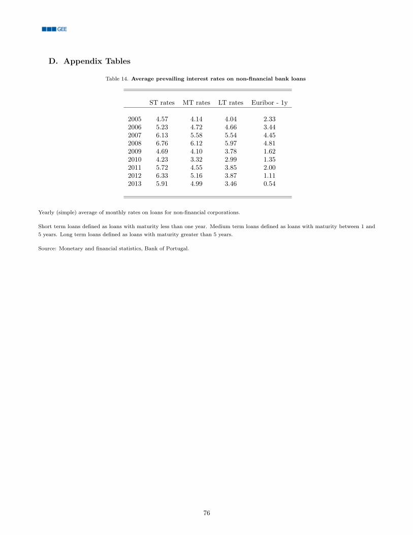
D. Appendix Tables

Table 14. Average prevailing interest rates on non-financial bank loans

ST rates MT rates LT rates Euribor - 1y

2005 4.57 4.14 4.04 2.332006 5.23 4.72 4.66 3.442007 6.13 5.58 5.54 4.452008 6.76 6.12 5.97 4.812009 4.69 4.10 3.78 1.622010 4.23 3.32 2.99 1.352011 5.72 4.55 3.85 2.002012 6.33 5.16 3.87 1.112013 5.91 4.99 3.46 0.54

Yearly (simple) average of monthly rates on loans for non-financial corporations.

Short term loans defined as loans with maturity less than one year. Medium term loans defined as loans with maturity between 1 and5 years. Long term loans defined as loans with maturity greater than 5 years.

Source: Monetary and financial statistics, Bank of Portugal.

76

Table 15. Share of secured credit, firm level

(1) (2) (3)ST LT Diff.

Sh. secured loans 0.25 0.50

Sh. secured credit 0.40 0.62 0.22∗∗∗(0.43) (0.40) 138.46

Sh. fully secured credit 0.21 0.38 0.17∗∗∗(0.33) (0.40) 122.03

Sh. financial collateral 0.04 0.07 0.03∗∗∗(0.18) (0.21) 33.11

Sh. real collateral mortgage 0.07 0.21 0.14∗∗∗(0.23) (0.35) 121.83

Sh. personal guarantee 0.37 0.50 0.14∗∗∗(0.42) (0.42) 83.50

N 140592 131845

The table refers to all firms in a CRC-QP match in the sectors of analysis (excluding, agriculture, mining, energy production anddistribution and construction). The share of secured loans refers to the actual share of loans that have any sort of collateralizationbacking it. All other statistics are aggregated at the firm level and refer to shares of total regular credit available to firms.

Column (3) shows the results of t-test for the difference of the means, T-stats reported.

77

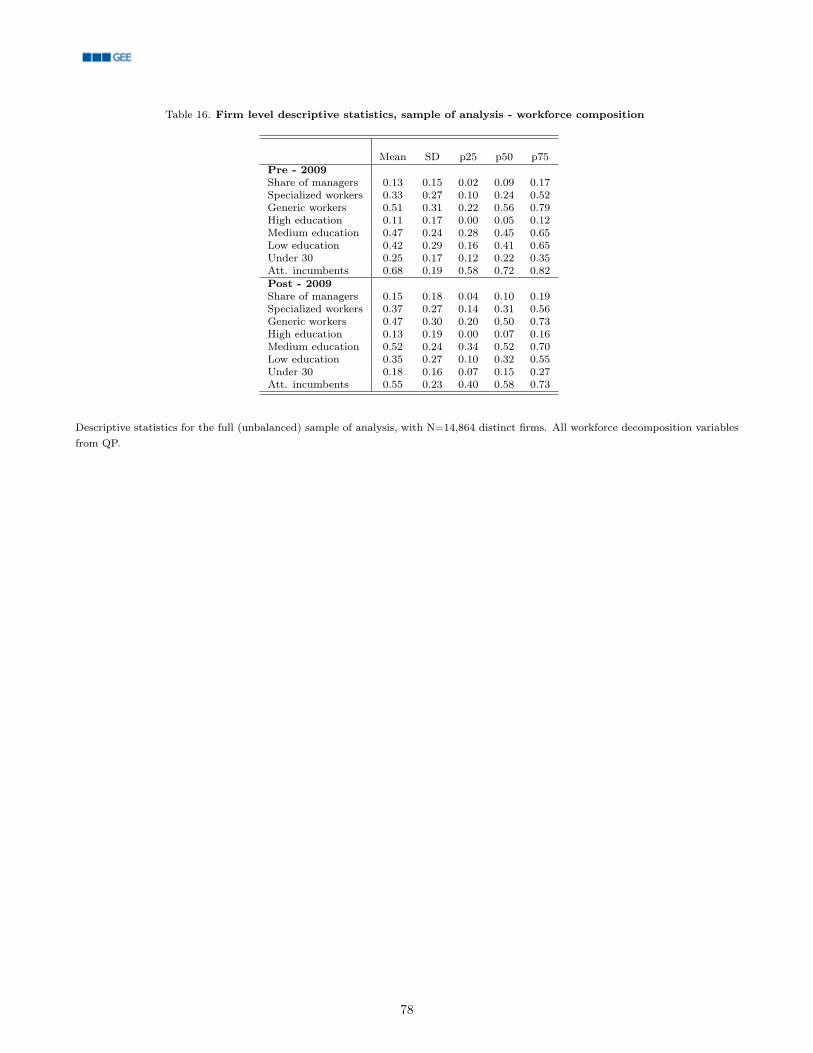
Table 16. Firm level descriptive statistics, sample of analysis - workforce composition

Mean SD p25 p50 p75Pre - 2009Share of managers 0.13 0.15 0.02 0.09 0.17Specialized workers 0.33 0.27 0.10 0.24 0.52Generic workers 0.51 0.31 0.22 0.56 0.79High education 0.11 0.17 0.00 0.05 0.12Medium education 0.47 0.24 0.28 0.45 0.65Low education 0.42 0.29 0.16 0.41 0.65Under 30 0.25 0.17 0.12 0.22 0.35Att. incumbents 0.68 0.19 0.58 0.72 0.82Post - 2009Share of managers 0.15 0.18 0.04 0.10 0.19Specialized workers 0.37 0.27 0.14 0.31 0.56Generic workers 0.47 0.30 0.20 0.50 0.73High education 0.13 0.19 0.00 0.07 0.16Medium education 0.52 0.24 0.34 0.52 0.70Low education 0.35 0.27 0.10 0.32 0.55Under 30 0.18 0.16 0.07 0.15 0.27Att. incumbents 0.55 0.23 0.40 0.58 0.73

Descriptive statistics for the full (unbalanced) sample of analysis, with N=14,864 distinct firms. All workforce decomposition variablesfrom QP.

78

Table 17. Robustness: instrument effects on credit post-2010

(1) (2) (3) (4) (5)∆Dst,2013−2010

∆Di;st,2010−2006 -0.220*** -0.231*** -0.253*** -0.254*** -0.251***(0.011) (0.011) (0.012) (0.012) (0.012)

Zi 0.240 -0.041 -0.148 -0.176 -0.154(0.277) (0.257) (0.260) (0.262) (0.261)

W. Sov. -0.980+share in Q4-2009, 2005 banks (0.588)W. Sov. -1.242*share in Q4-2009, 2009 banks (0.629)

Firms 12883 12865 12061 12061 11882Fixed effects No Yes Yes Yes YesControls No No Yes Yes Yes

The regressions refer to the empirical specification in equation (4) in the text.

All regressions feature firm and time fixed effects. See the table 4 for the list of further controls and fixed effects in the regressions.

The sample consists of firms with (short-term) credit relationships in 2010.

Columns 4 and 5 control directly for firms (weighted) exposure to banks average sovereign debt holdings over assets in 2009 (Q4), eitherconsidering banks with which the firms has a relationship in 2005 (4) or 2009 (5).

Standard errors clustered at the bank-industry pair level.

+ p < 0.10, * p < 0.05, ** p < 0.01, *** p < 0.001

79

Table 18. Employment regressions, first stage

(1) (2) (3) (4) (5)Si

Zi -1.761*** -1.706*** -1.716*** -1.702*** -1.766***(0.301) (0.276) (0.280) (0.285) (0.293)

Firms 14846 14830 13833 13806 11802Sample Complete Complete Complete Complete SurvivorsFixed effects No Yes Yes Yes YesControls No No Fail b.c. Yes Yes

The table shows the estimation results of the first stage regressions of the credit variation Si on the instrument Zi. All regressionsfeature firm and time fixed effects.

See the table 4 for the list of controls and fixed effects in the regressions.

Standard errors clustered at the bank-industry pair level.

+ p < 0.10, * p < 0.05, ** p < 0.01, *** p < 0.001

80

Table 19. Employment regressions, reduced form

(1) (2) (3) (4)log(#emp)i,t

Zi -0.123** -0.120** -0.120** -0.152***(0.051) (0.052) (0.053) (0.054)

Firms 14830 13833 13806 11802Sample Complete Complete Complete SurvivorsFixed effects Yes Yes Yes YesControls No Fail b.c. Yes Yes

All regressions feature firm and time fixed effects. See the table 4 for the list of controls and fixed effects in the regressions.

Standard errors clustered at the bank-industry pair level.

+ p < 0.10, * p < 0.05, ** p < 0.01, *** p < 0.001

81

Table 20. Hours regressions

(1) (2) (3) (4)log(# hours)i,t log(# base hours)i,t

Si 0.067* 0.085* 0.067* 0.085*(0.034) (0.035) (0.034) (0.035)

Firms 13806 11802 13806 11802EFF. WID F 34.56 35.55 34.56 35.55Sample Complete Survivors Complete Survivors

The dependent variables are either the total amount of work hours (columns 1 and 2) or the total amount of normal contract hours,which does not comprehend extraordinary or overtime hours of work.

See the table 4 for the list of controls and fixed effects in the regressions. All regressions feature the full set of fixed effects and controls.

Standard errors clustered at the bank-industry pair level.

+ p < 0.10, * p < 0.05, ** p < 0.01, *** p < 0.001

82

Table 21. Employment - wage bill regressions

(1) (2) (3) (4) (5) (6)Employeesi,t Wage billi,t Base wage billi,t

Si 0.069* 0.083* 0.100** 0.122** 0.102** 0.116**(0.031) (0.033) (0.038) (0.041) (0.038) (0.040)

Firms 13806 11802 13806 11802 13806 11802EFF. WID F 34.56 35.55 34.56 35.55 34.56 35.55Sample Complete Survivors Complete Survivors Complete Survivors

The dependent variable in these regressions is the ratio of the number of workers (or the wage bill) to the average level of the pre-periodcorresponding amount.

The outcome variable is winsorized at the top 1% level.

See the table 4 for the list of controls and fixed effects in the regressions. All regressions feature the full set of fixed effects and controls.

Standard errors clustered at the bank-industry pair level.

+ p < 0.10, * p < 0.05, ** p < 0.01, *** p < 0.001

83

Table 22. Heterogeneous employment regressions: Contracts

(1) (2) (3) (4)Permanent w.i,t Temporary w.i,t

Si 0.098+ 0.158* 0.174 0.145(0.057) (0.062) (0.147) (0.150)

Firms 13657 11681 11829 10129EFF. WID F 37.00 38.37 31.02 32.94Sample Complete Survivors Complete Survivors

The dependent variable in these regressions is the ratio of the number of specific workers to the average level of the pre-periodcorresponding amount. As such, the regressions are defined only for the firms for which the kind of worker is present in the pre-period(even if missing values for some years are possible).

Temporary workers are workers hired with a fixed-term contract.

The outcome variable is winsorized at the top 1% level.

See the table 4 for the list of controls and fixed effects in the regressions. All regressions feature the full set of fixed effects and controls.

Standard errors clustered at the bank-industry pair level.

+ p < 0.10, * p < 0.05, ** p < 0.01, *** p < 0.001

84

Table 23. Heterogeneous employment regressions: Education

(1) (2) (3) (4) (5) (6)High educ.i,t Medium educ.i,t Low educ.i,t

Si 0.030 -0.048 0.222** 0.271*** 0.057 0.065+(0.138) (0.133) (0.071) (0.080) (0.036) (0.036)

Firms 9539 8228 13699 11710 12679 10833EFF. WID F 30.45 32.25 33.01 34.07 38.51 41.89Sample Complete Survivors Complete Survivors Complete Survivors

The dependent variable in these regressions is the ratio of the number of specific workers to the average level of the pre-periodcorresponding amount. As such, the regressions are defined only for the firms for which the kind of worker is present in the pre-period(even if missing values for some years are possible).

High educated obtained at least an undergraduate degree. Medium educated workers completed high school or an equivalent levelprofessional school. Low educated workers did not complete high school or an equivalent professional school.

The outcome variable is winsorized at the top 1% level.

See the table 4 for the list of controls and fixed effects in the regressions. All regressions feature the full set of fixed effects and controls.

Standard errors clustered at the bank-industry pair level.

+ p < 0.10, * p < 0.05, ** p < 0.01, *** p < 0.001

85

Table 24. Robustness: Almeida et al. (2011) identification, effects on fixed investments

(1) (2)log(fixed assets)i,t

Si 0.017 0.031(0.074) (0.120)

Si · exp_lti -0.025(0.119)

exp_lti -0.090*** -0.095***(0.015) (0.026)

Firms 11799 11799Sample Survivors Survivors

The regressions refer to the empirical specification in equation (8) in the text.

The treatment is interacted with a dummy variable equal to 1 if the firm has long-term debt maturing in the first two semester of 2009.As a consequence, we instrument the interacted treatment with the interaction of the same dummy and the baseline instrument Zi.We also control for the dummy variable itself, interacted with the post-period dummy to allow for different rends depending on thelong-term debt maturing soon after the credit shock.

The regressions are carried out on the sample of firms surviving up to 2013.

See Table 4 for a list of the added controls and fixed effects present in the regressions. All regressions feature the full set of fixed effectsand controls.

Standard errors clustered at the bank-industry pair level.

+ p < 0.10, * p < 0.05, ** p < 0.01, *** p < 0.001

86

Table 25. Average wage regressions

(1) (2)log(Avg. wage)i,t log(Avg. wage)inc08;i,t

Si 0.018 0.023(0.015) (0.017)

Firms 13806 13804EFF. WID F 34.56 34.56Sample Complete Complete

The dependent variable for column 1 is the logarithm of the average wage for all employees. The dependent variable for column 3 is thelogarithm of the average wage for incumbent workers in 2008 who remain in the firm.

See the table 4 for the list of controls and fixed effects in the regressions. All regressions feature the full set of fixed effects and controls.

Standard errors clustered at the bank-industry pair level.

+ p < 0.10, * p < 0.05, ** p < 0.01, *** p < 0.001

87

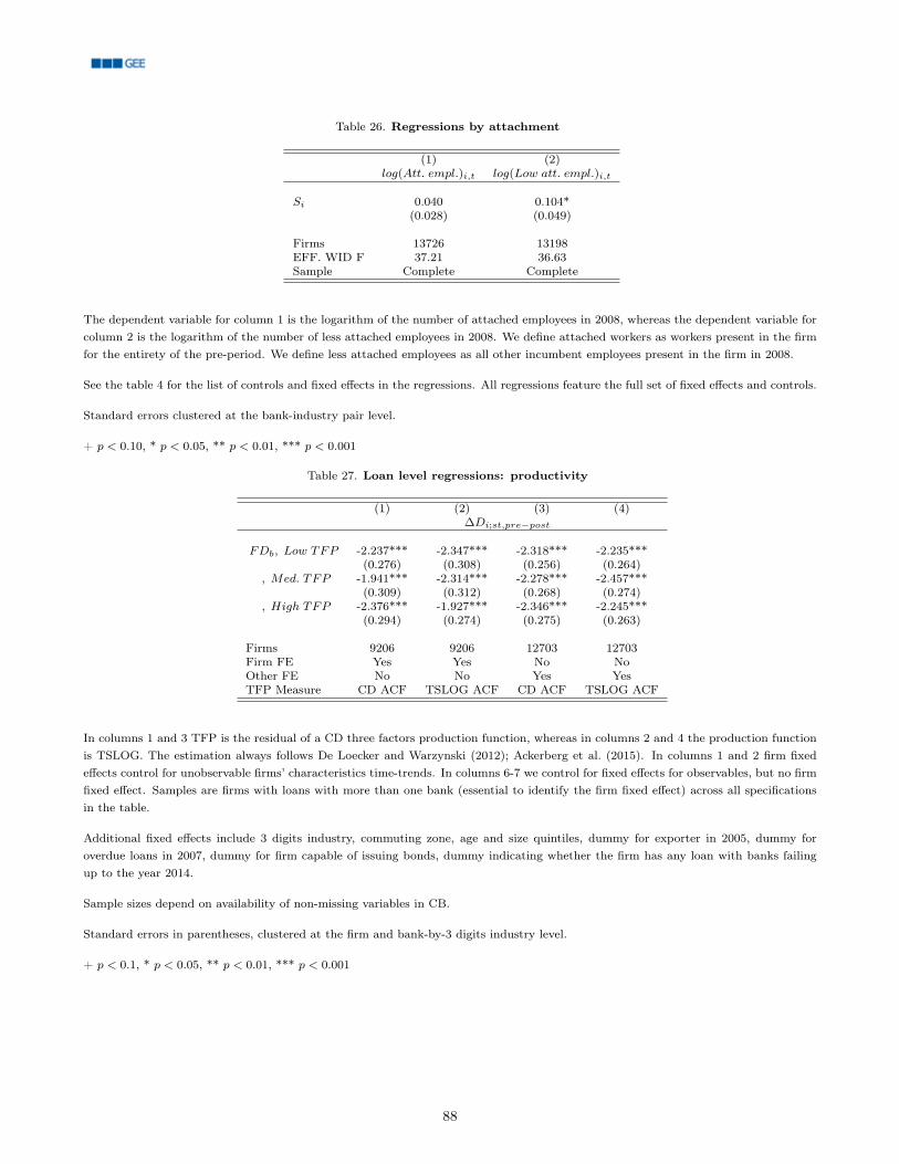
Table 26. Regressions by attachment

(1) (2)log(Att. empl.)i,t log(Low att. empl.)i,t

Si 0.040 0.104*(0.028) (0.049)

Firms 13726 13198EFF. WID F 37.21 36.63Sample Complete Complete

The dependent variable for column 1 is the logarithm of the number of attached employees in 2008, whereas the dependent variable forcolumn 2 is the logarithm of the number of less attached employees in 2008. We define attached workers as workers present in the firmfor the entirety of the pre-period. We define less attached employees as all other incumbent employees present in the firm in 2008.

See the table 4 for the list of controls and fixed effects in the regressions. All regressions feature the full set of fixed effects and controls.

Standard errors clustered at the bank-industry pair level.

+ p < 0.10, * p < 0.05, ** p < 0.01, *** p < 0.001

Table 27. Loan level regressions: productivity

(1) (2) (3) (4)∆Di;st,pre−post

FDb, Low TFP -2.237*** -2.347*** -2.318*** -2.235***(0.276) (0.308) (0.256) (0.264)

, Med. TFP -1.941*** -2.314*** -2.278*** -2.457***(0.309) (0.312) (0.268) (0.274)

, High TFP -2.376*** -1.927*** -2.346*** -2.245***(0.294) (0.274) (0.275) (0.263)

Firms 9206 9206 12703 12703Firm FE Yes Yes No NoOther FE No No Yes YesTFP Measure CD ACF TSLOG ACF CD ACF TSLOG ACF

In columns 1 and 3 TFP is the residual of a CD three factors production function, whereas in columns 2 and 4 the production functionis TSLOG. The estimation always follows De Loecker and Warzynski (2012); Ackerberg et al. (2015). In columns 1 and 2 firm fixedeffects control for unobservable firms’ characteristics time-trends. In columns 6-7 we control for fixed effects for observables, but no firmfixed effect. Samples are firms with loans with more than one bank (essential to identify the firm fixed effect) across all specificationsin the table.

Additional fixed effects include 3 digits industry, commuting zone, age and size quintiles, dummy for exporter in 2005, dummy foroverdue loans in 2007, dummy for firm capable of issuing bonds, dummy indicating whether the firm has any loan with banks failingup to the year 2014.

Sample sizes depend on availability of non-missing variables in CB.

Standard errors in parentheses, clustered at the firm and bank-by-3 digits industry level.

+ p < 0.1, * p < 0.05, ** p < 0.01, *** p < 0.001

88

Table 28. Regressions by CD productivity bins (Ackerberg et al. (2015))

(1) (2)log(#emp)i,t P (exit)i,t

Si, Low TFP 0.070+ -0.033*(0.037) (0.013)

, Med. TFP 0.087* -0.015(0.042) (0.013)

, High TFP 0.080+ -0.017(0.042) (0.016)

Firms 13287 13277WID F 10.84 11.47Sample Complete CompleteFirm FE Yes NoOther FE Yes Yes

See Table 4 for a list of the added controls and fixed effects present in the regressions. All regressions feature the full set of fixedeffects and controls. In addition to that specification we control for average TFP in 2005 and 2006 (estimated according to to themethod proposed in De Loecker and Warzynski (2012); Ackerberg et al. (2015) by means of a three factors of production gross outputCobb-Douglas production function). TFP can be estimated for less firms than the full samples depending on availability of the variablesto compute it in CB. Moreover, given that we cannot control for unobservable characteristics in the exit specification through firm fixedeffects any more, we try to characterize the matching of firms to banks by augmenting the set of controls with the share of loans thateach firm has with micro banks and with banks failed up until the year 2014.

We control linearly for the baseline effect of productivity.

In the exit specification the fixed effects are interacted with year dummies, whereas the controls are kept constant and not interactedwith any year dummy. In the employment specifications all variables are interacted with a post-period dummy.

Sample sizes depend on availability of non-missing variables in CB.

Standard errors clustered at the bank-industry pair level.

+ p < 0.10, * p < 0.05, ** p < 0.01, *** p < 0.001

89

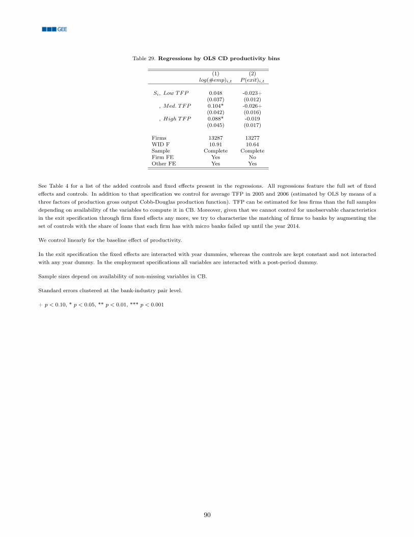
Table 29. Regressions by OLS CD productivity bins

(1) (2)log(#emp)i,t P (exit)i,t

Si, Low TFP 0.048 -0.023+(0.037) (0.012)

, Med. TFP 0.104* -0.026+(0.042) (0.016)

, High TFP 0.088* -0.019(0.045) (0.017)

Firms 13287 13277WID F 10.91 10.64Sample Complete CompleteFirm FE Yes NoOther FE Yes Yes

See Table 4 for a list of the added controls and fixed effects present in the regressions. All regressions feature the full set of fixedeffects and controls. In addition to that specification we control for average TFP in 2005 and 2006 (estimated by OLS by means of athree factors of production gross output Cobb-Douglas production function). TFP can be estimated for less firms than the full samplesdepending on availability of the variables to compute it in CB. Moreover, given that we cannot control for unobservable characteristicsin the exit specification through firm fixed effects any more, we try to characterize the matching of firms to banks by augmenting theset of controls with the share of loans that each firm has with micro banks failed up until the year 2014.

We control linearly for the baseline effect of productivity.

In the exit specification the fixed effects are interacted with year dummies, whereas the controls are kept constant and not interactedwith any year dummy. In the employment specifications all variables are interacted with a post-period dummy.

Sample sizes depend on availability of non-missing variables in CB.

Standard errors clustered at the bank-industry pair level.

+ p < 0.10, * p < 0.05, ** p < 0.01, *** p < 0.001

90

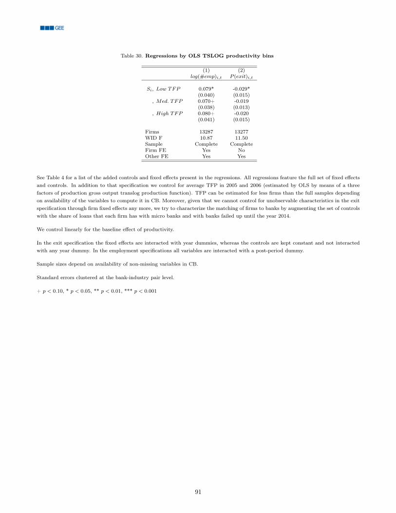
Table 30. Regressions by OLS TSLOG productivity bins

(1) (2)log(#emp)i,t P (exit)i,t

Si, Low TFP 0.079* -0.029*(0.040) (0.015)

, Med. TFP 0.070+ -0.019(0.038) (0.013)

, High TFP 0.080+ -0.020(0.041) (0.015)

Firms 13287 13277WID F 10.87 11.50Sample Complete CompleteFirm FE Yes NoOther FE Yes Yes

See Table 4 for a list of the added controls and fixed effects present in the regressions. All regressions feature the full set of fixed effectsand controls. In addition to that specification we control for average TFP in 2005 and 2006 (estimated by OLS by means of a threefactors of production gross output translog production function). TFP can be estimated for less firms than the full samples dependingon availability of the variables to compute it in CB. Moreover, given that we cannot control for unobservable characteristics in the exitspecification through firm fixed effects any more, we try to characterize the matching of firms to banks by augmenting the set of controlswith the share of loans that each firm has with micro banks and with banks failed up until the year 2014.

We control linearly for the baseline effect of productivity.

In the exit specification the fixed effects are interacted with year dummies, whereas the controls are kept constant and not interactedwith any year dummy. In the employment specifications all variables are interacted with a post-period dummy.

Sample sizes depend on availability of non-missing variables in CB.

Standard errors clustered at the bank-industry pair level.

+ p < 0.10, * p < 0.05, ** p < 0.01, *** p < 0.001

91

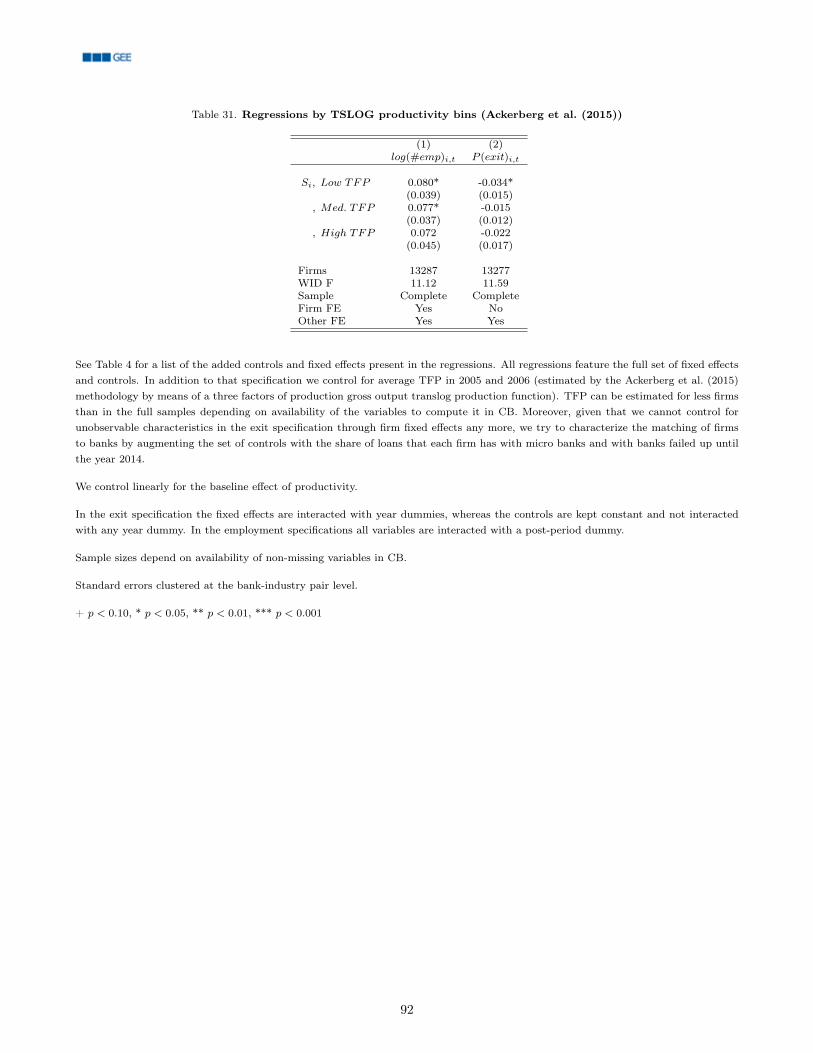
Table 31. Regressions by TSLOG productivity bins (Ackerberg et al. (2015))

(1) (2)log(#emp)i,t P (exit)i,t

Si, Low TFP 0.080* -0.034*(0.039) (0.015)

, Med. TFP 0.077* -0.015(0.037) (0.012)

, High TFP 0.072 -0.022(0.045) (0.017)

Firms 13287 13277WID F 11.12 11.59Sample Complete CompleteFirm FE Yes NoOther FE Yes Yes

See Table 4 for a list of the added controls and fixed effects present in the regressions. All regressions feature the full set of fixed effectsand controls. In addition to that specification we control for average TFP in 2005 and 2006 (estimated by the Ackerberg et al. (2015)methodology by means of a three factors of production gross output translog production function). TFP can be estimated for less firmsthan in the full samples depending on availability of the variables to compute it in CB. Moreover, given that we cannot control forunobservable characteristics in the exit specification through firm fixed effects any more, we try to characterize the matching of firmsto banks by augmenting the set of controls with the share of loans that each firm has with micro banks and with banks failed up untilthe year 2014.

We control linearly for the baseline effect of productivity.

In the exit specification the fixed effects are interacted with year dummies, whereas the controls are kept constant and not interactedwith any year dummy. In the employment specifications all variables are interacted with a post-period dummy.

Sample sizes depend on availability of non-missing variables in CB.

Standard errors clustered at the bank-industry pair level.

+ p < 0.10, * p < 0.05, ** p < 0.01, *** p < 0.001

92

Table 32. Reallocation and TFP by labor share - full dataset

(1) (2) (3) (4)exiti,t ∆ log(emp)i,t+1 ∆ log(ftemp)i,t+1 ∆ log(fixed cap.)i,t+1

TFPi,t · 1(labsh_q. = 1) -0.0370*** 0.0298*** 0.0267*** 0.0183+(0.0049) (0.0069) (0.0067) (0.0105)

· 1(labsh_q. = 2) -0.0390*** 0.0339*** 0.0325*** 0.0249*(0.0051) (0.0070) (0.0069) (0.0115)

· 1(labsh_q. = 3) -0.0400*** 0.0352*** 0.0334*** 0.0274*(0.0053) (0.0069) (0.0070) (0.0110)

· 1(labsh_q. = 4) -0.0454*** 0.0444*** 0.0413*** 0.0322**(0.0049) (0.0069) (0.0070) (0.0105)

·Post Lehmant · 0.0005 -0.0001 0.0000 -0.0014· 1(labsh_q. = 1) (0.0010) (0.0035) (0.0032) (0.0048)· 1(labsh_q. = 2) 0.0005 -0.0049 -0.0055 -0.0107

(0.0008) (0.0036) (0.0034) (0.0066)· 1(labsh_q. = 3) 0.0011 -0.0059 -0.0064 -0.0062

(0.0010) (0.0042) (0.0041) (0.0056)· 1(labsh_q. = 4) 0.0027+ -0.0095*** -0.0087** -0.0119*

(0.0015) (0.0027) (0.0028) (0.0056)asinh(V A/emp)2005−2008 -0.0112*** -0.0031* 0.0014 0.0077+

(0.0011) (0.0013) (0.0013) (0.0040)

Firms 178294 170044 169324 176376N 802568 767934 762156 845980Industry FE Yes Yes Yes YesLabor share quartileby post-Lehman FE Yes Yes Yes Yes

The regressions refer to the empirical specification in equation (20) in the text. A different coefficient is jointly estimated for each laborshare bin, and a variation of slope is estimated for the years post 2008.

Labor share is computed as the average ratio of employment costs over value added for the years from 2005 to 2008. In all specificationsa control for the average value added per employee in the period from 2005 to 2008 is added.

All regressions feature 3-digits industry fixed effects, and labor share quartile by post-Lehman dummy fixed effects.

The sample consists of all firms in QP matched with CB for which TFP can be computed (with the exclusion of the energy andconstruction sector).

All variables refer to the outcomes from t to t+1. We measure employment either as total headcount of full time equivalent employment,as reported in CB. The exit regression excludes the year 2005, given the CB structure.

Standard errors clustered at the 3-digits industry level.

+ p < 0.10, * p < 0.05, ** p < 0.01, *** p < 0.001

93

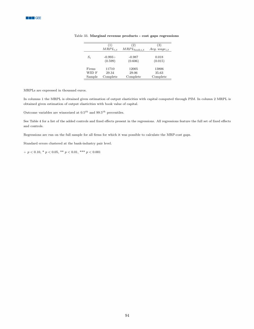
Table 33. Marginal revenue products - cost gaps regressions

(1) (2) (3)MRPLi,t MRPLbook;i,t Avg. wagei,t

Si -0.993+ -0.987 0.018(0.599) (0.606) (0.015)

Firms 11710 12005 13806WID F 29.34 29.06 35.63Sample Complete Complete Complete

MRPLs are expressed in thousand euros.

In columns 1 the MRPL is obtained given estimation of output elasticities with capital computed through PIM. In column 2 MRPL isobtained given estimation of output elasticities with book value of capital.

Outcome variables are winsorized at 0.5th and 99.5th percentiles.

See Table 4 for a list of the added controls and fixed effects present in the regressions. All regressions feature the full set of fixed effectsand controls.

Regressions are run on the full sample for all firms for which it was possible to calculate the MRP-cost gaps.

Standard errors clustered at the bank-industry pair level.

+ p < 0.10, * p < 0.05, ** p < 0.01, *** p < 0.001

94

Table 34. Wedge regressions

(1) (2) (3)Lab. wedgei,t Cap. wedgei,t Mat. wedgei,t

Si -0.0080+ 0.0023 -0.0081(0.0047) (0.0049) (0.0092)

Firms 11710 12823 12988WID F 29.34 35.37 34.90Sample Complete Complete Complete

Outcome variables are winsorized at 0.5th and 99.5th percentiles.

See Table 4 for a list of the added controls and fixed effects present in the regressions. All regressions feature the full set of fixed effectsand controls.

Regressions are run on the full sample for all firms for which it was possible to calculate the input wedges.

Standard errors clustered at the bank-industry pair level.

+ p < 0.10, * p < 0.05, ** p < 0.01, *** p < 0.001

95

Table 35. Revenue elasticities and markups, PIM capital

CD TSLOG ACF CD ACF TSLOG

Mean IQR Mean IQR Mean IQR Mean IQR

θL 0.20 0.13 0.21 0.18 0.22 0.11 0.21 0.19(0.0001) (0.0003) (0.0001) (0.0003)

θK 0.03 0.02 0.03 0.03 0.02 0.01 0.03 0.02(0.00003) (0.00005) (0.00001) (0.00004)

θM 0.74 0.19 0.73 0.21 0.71 0.14 0.72 0.21(0.0002) (0.0003) (0.0002) (0.0003)

RS 0.97 0.04 0.97 0.05 0.96 0.02 0.96 0.04(0.0001) (0.0001) (0.0002) (0.0001)

µ 1.33 0.34 1.26 0.16(0.0009) (0.0003)

The table displays descriptive statistics regarding firm-level production function parameters, returns to scale and markups. Mean,interquartile ranges and block bootstrapped standard errors (by firm) for the mean. We show estimates for the two specifications ofthe gross production function (Cobb-Douglas and translog) and two methodologies we use. The first two columns are estimated bysimple OLS, whereas the second two are estimated following the method by Ackerberg et al. (2015), which accounts for endogeneity inthe choice of inputs use and we correct for firm selection. See appendix C for details regarding the estimation procedure. Returns toscale are computed as

∑X θXi,t X ∈ {L,K,M}. Markups are estimated according to the method laid out by De Loecker and Warzynski

(2012), see appendix C.2 for details regarding the estimation procedure.

The table results are based on estimates of the production function where capital is measured according to the perpetual inventorymethod (PIM).

96

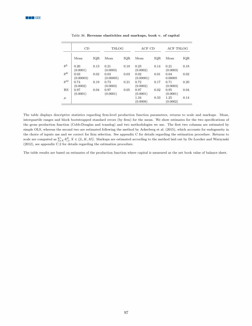
Table 36. Revenue elasticities and markups, book v. of capital

CD TSLOG ACF CD ACF TSLOG

Mean IQR Mean IQR Mean IQR Mean IQR

θL 0.20 0.13 0.21 0.18 0.23 0.14 0.21 0.18(0.0001) (0.0003) (0.0002) (0.0003)

θK 0.03 0.02 0.03 0.03 0.02 0.01 0.04 0.02(0.00003) (0.00005) (0.00001) 0.00005

θM 0.74 0.19 0.73 0.21 0.72 0.17 0.71 0.20(0.0002) (0.0003) (0.0002) (0.0003)

RS 0.97 0.04 0.97 0.05 0.97 0.02 0.95 0.04(0.0001) (0.0001) (0.0001) (0.0001)

µ 1.34 0.33 1.25 0.14(0.0008) (0.0002)

The table displays descriptive statistics regarding firm-level production function parameters, returns to scale and markups. Mean,interquartile ranges and block bootstrapped standard errors (by firm) for the mean. We show estimates for the two specifications ofthe gross production function (Cobb-Douglas and translog) and two methodologies we use. The first two columns are estimated bysimple OLS, whereas the second two are estimated following the method by Ackerberg et al. (2015), which accounts for endogeneity inthe choice of inputs use and we correct for firm selection. See appendix C for details regarding the estimation procedure. Returns toscale are computed as

∑X θXi,t X ∈ {L,K,M}. Markups are estimated according to the method laid out by De Loecker and Warzynski

(2012), see appendix C.2 for details regarding the estimation procedure.

The table results are based on estimates of the production function where capital is measured as the net book value of balance sheet.

97

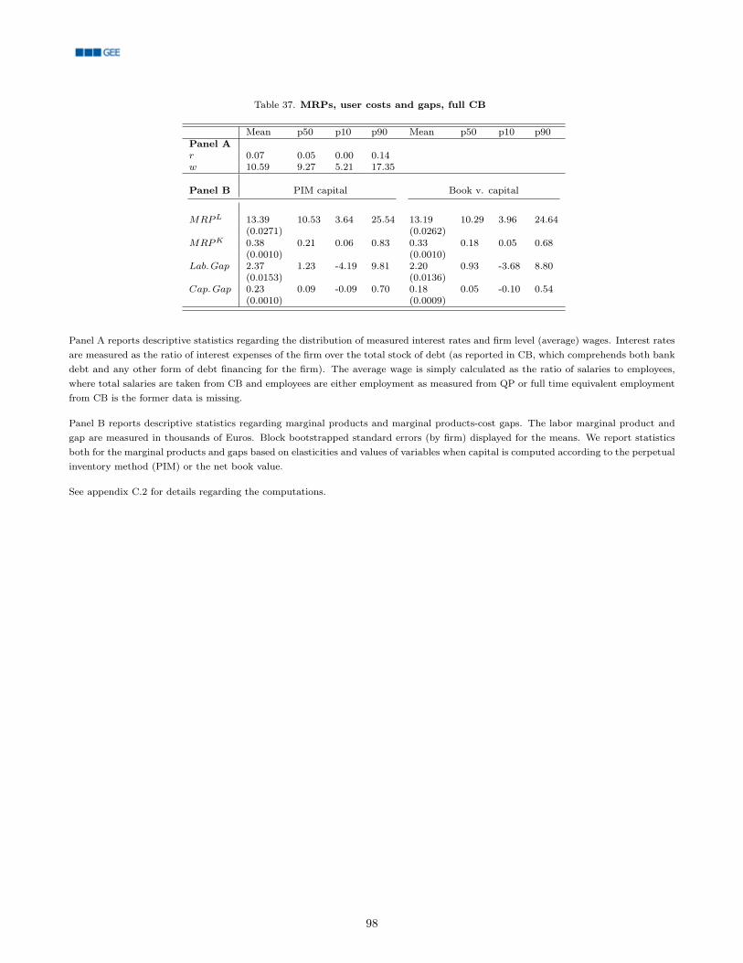
Table 37. MRPs, user costs and gaps, full CB

Mean p50 p10 p90 Mean p50 p10 p90Panel Ar 0.07 0.05 0.00 0.14w 10.59 9.27 5.21 17.35

Panel B PIM capital Book v. capital

MRPL 13.39 10.53 3.64 25.54 13.19 10.29 3.96 24.64(0.0271) (0.0262)

MRPK 0.38 0.21 0.06 0.83 0.33 0.18 0.05 0.68(0.0010) (0.0010)

Lab.Gap 2.37 1.23 -4.19 9.81 2.20 0.93 -3.68 8.80(0.0153) (0.0136)

Cap.Gap 0.23 0.09 -0.09 0.70 0.18 0.05 -0.10 0.54(0.0010) (0.0009)

Panel A reports descriptive statistics regarding the distribution of measured interest rates and firm level (average) wages. Interest ratesare measured as the ratio of interest expenses of the firm over the total stock of debt (as reported in CB, which comprehends both bankdebt and any other form of debt financing for the firm). The average wage is simply calculated as the ratio of salaries to employees,where total salaries are taken from CB and employees are either employment as measured from QP or full time equivalent employmentfrom CB is the former data is missing.

Panel B reports descriptive statistics regarding marginal products and marginal products-cost gaps. The labor marginal product andgap are measured in thousands of Euros. Block bootstrapped standard errors (by firm) displayed for the means. We report statisticsboth for the marginal products and gaps based on elasticities and values of variables when capital is computed according to the perpetualinventory method (PIM) or the net book value.

See appendix C.2 for details regarding the computations.

98

E. Appendix Figures

Figure 10: Credit dynamics in Portugal

25

50

75

100

125

% o

f 2006 v

alu

e

2006

2007

2008

2009

2010

2011

2012

2013

Years

Total In sample

(a) Total regular credit

25

50

75

100

125

% o

f 2006 v

alu

e

2006

2007

2008

2009

2010

2011

2012

2013

Years

Total In sample

(b) Long-term regular credit

The Figures show the time series for the aggregate amount of total regular (left) and long-term credit (right) for the firms andbanks in the sample. Total regular credit is credit not overdue or in renegotiation available to the firm. Long-term credit is any creditexposure with maturity greater than one year, with the exclusion of credit lines with no maturity. The red dotted line splits the samplein pre-period and post-period. Totals are expressed as a percentage total regular credit in 2006.Source: Central de Responsabilidades de Crédito merged with Quadros de Pessoal (left), Central de Responsabilidades de Créditomerged with Quadros de Pessoal and banks’ balance sheets (right), authors’ calculations and sample selection.

Figure 11: Unemployment rate

5

10

15

20

25

30

35

40

Ra

te

2006

2007

2008

2009

2010

2011

2012

2013

Years

Unemployment rate Youth unemployment rate

The Figure shows the time series of the unemployment rate in Portugal, both for all workers (blue) and for workers below 25 yearsold (red).Source: OECD.

99

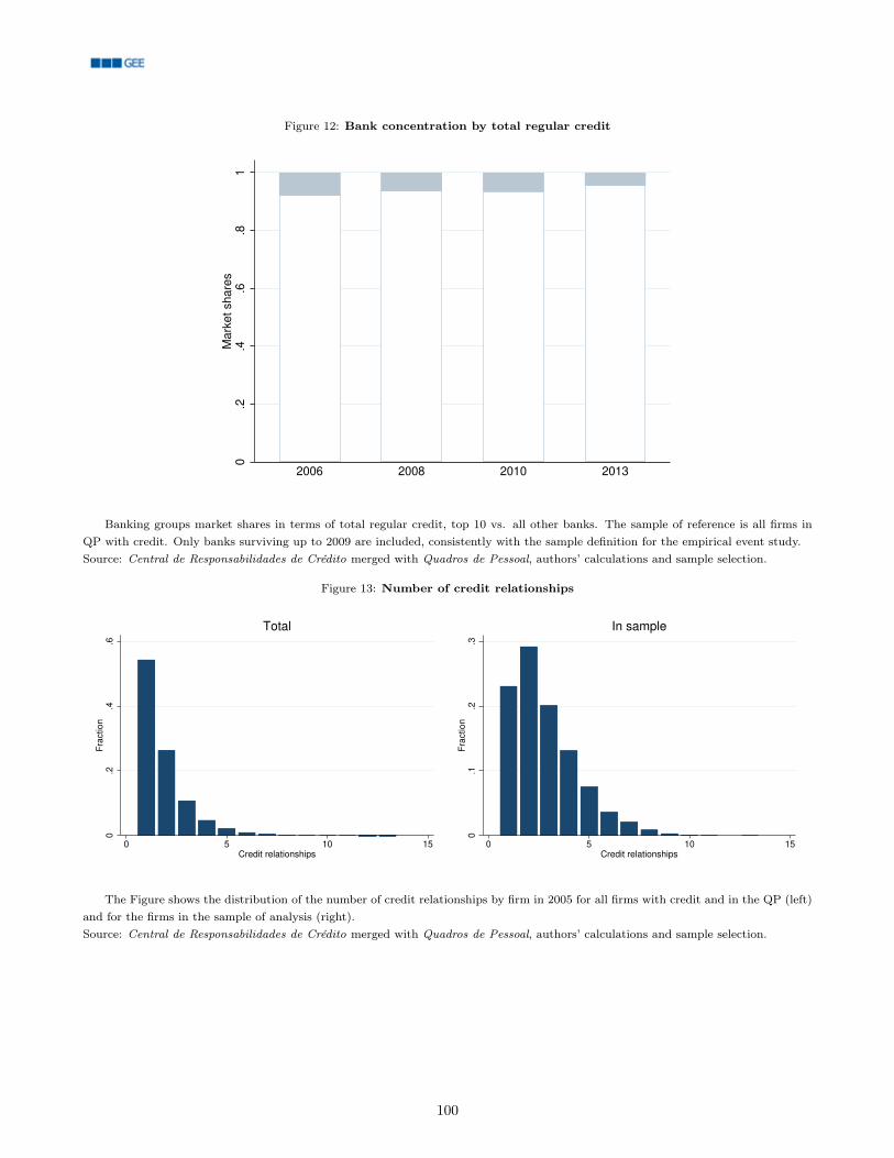
Figure 12: Bank concentration by total regular credit

0.2

.4.6

.81

Ma

rke

t sh

are

s

2006 2008 2010 2013

Banking groups market shares in terms of total regular credit, top 10 vs. all other banks. The sample of reference is all firms inQP with credit. Only banks surviving up to 2009 are included, consistently with the sample definition for the empirical event study.Source: Central de Responsabilidades de Crédito merged with Quadros de Pessoal, authors’ calculations and sample selection.

Figure 13: Number of credit relationships

0.2

.4.6

Fra

ctio

n

0 5 10 15Credit relationships

Total

0.1

.2.3

Fra

ctio

n

0 5 10 15Credit relationships

In sample

The Figure shows the distribution of the number of credit relationships by firm in 2005 for all firms with credit and in the QP (left)and for the firms in the sample of analysis (right).Source: Central de Responsabilidades de Crédito merged with Quadros de Pessoal, authors’ calculations and sample selection.

100

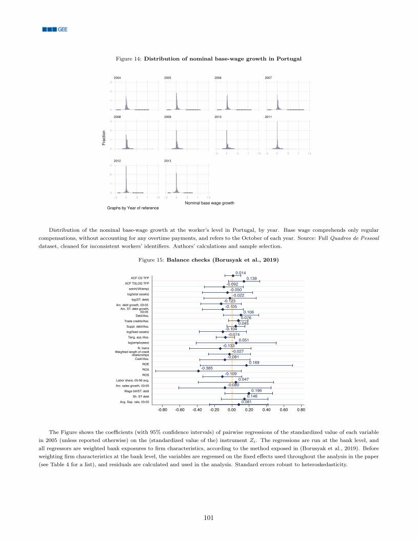
Figure 14: Distribution of nominal base-wage growth in Portugal

0

.1

.2

.3

0

.1

.2

.3

0

.1

.2

.3

−.5 0 .5 1 1.5 −.5 0 .5 1 1.5

−.5 0 .5 1 1.5 −.5 0 .5 1 1.5

2004 2005 2006 2007

2008 2009 2010 2011

2012 2013

Fra

ction

Nominal base wage growth

Graphs by Year of reference

Distribution of the nominal base-wage growth at the worker’s level in Portugal, by year. Base wage comprehends only regularcompensations, without accounting for any overtime payments, and refers to the October of each year. Source: Full Quadros de Pessoaldataset, cleaned for inconsistent workers’ identifiers. Authors’ calculations and sample selection.

Figure 15: Balance checks (Borusyak et al., 2019)

0.0140.139

-0.092-0.050

-0.022-0.123-0.105

0.1060.076

0.045-0.104

-0.0740.051

-0.133-0.027

-0.0810.169

-0.385-0.109

0.047-0.080

0.1960.146

0.081

ACF CD TFPACF TSLOG TFP

asinh(VA/emp)log(total assets)

log(ST. debt)Arc. debt growth, 03-05

Arc. ST. debt growth,03-05

Debt/Ass.Trade credits/Ass.

Suppl. debt/Ass.log(fixed assets)Tang. ass./Ass.log(employees)

N. loansWeighted length of credit

relationshipsCash/Ass.

ROEROAROS

Labor share, 05-06 avg.Arc. sales growth, 03-05

Wage bill/ST. debtSh. ST debt

Avg. Sep. rate, 03-05

-0.80 -0.60 -0.40 -0.20 0.00 0.20 0.40 0.60 0.80

The Figure shows the coefficients (with 95% confidence intervals) of pairwise regressions of the standardized value of each variablein 2005 (unless reported otherwise) on the (standardized value of the) instrument Zi. The regressions are run at the bank level, andall regressors are weighted bank exposures to firm characteristics, according to the method exposed in (Borusyak et al., 2019). Beforeweighting firm characteristics at the bank level, the variables are regressed on the fixed effects used throughout the analysis in the paper(see Table 4 for a list), and residuals are calculated and used in the analysis. Standard errors robust to heteroskedasticity.

101

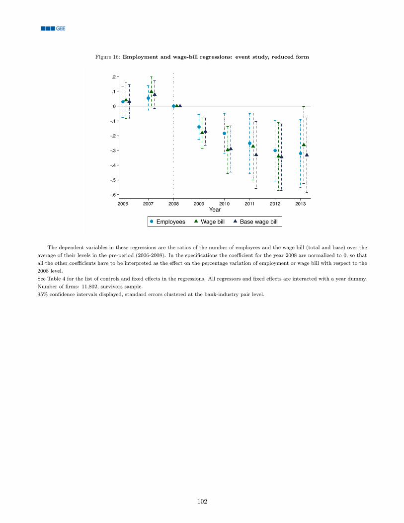
Figure 16: Employment and wage-bill regressions: event study, reduced form

-.6

-.5

-.4

-.3

-.2

-.1

0

.1

.2

2006 2007 2008 2009 2010 2011 2012 2013Year

Employees Wage bill Base wage bill

The dependent variables in these regressions are the ratios of the number of employees and the wage bill (total and base) over theaverage of their levels in the pre-period (2006-2008). In the specifications the coefficient for the year 2008 are normalized to 0, so thatall the other coefficients have to be interpreted as the effect on the percentage variation of employment or wage bill with respect to the2008 level.See Table 4 for the list of controls and fixed effects in the regressions. All regressors and fixed effects are interacted with a year dummy.Number of firms: 11,802, survivors sample.95% confidence intervals displayed, standard errors clustered at the bank-industry pair level.

102

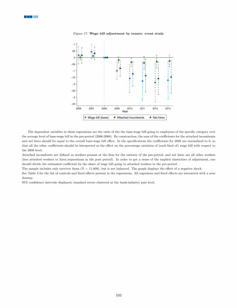
Figure 17: Wage bill adjustment by tenure: event study

-.35

-.3

-.25

-.2

-.15

-.1

-.05

0

.05

.1

2006 2007 2008 2009 2010 2011 2012 2013Year

Wage bill (base) Attached incumbents Net hires

The dependent variables in these regressions are the ratio of the the base-wage bill going to employees of the specific category overthe average level of base-wage bill in the pre-period (2006-2008). By construction, the sum of the coefficients for the attached incumbentsand net hires should be equal to the overall base-wage bill effect. In the specifications the coefficients for 2008 are normalized to 0, sothat all the other coefficients should be interpreted as the effect on the percentage variation of (each kind of) wage bill with respect tothe 2008 level.Attached incumbents are defined as workers present at the firm for the entirety of the pre-period, and net hires are all other workers(less attached workers or hires/separations in the post period). In order to get a sense of the implied elasticities of adjustment, oneshould divide the estimated coefficient by the share of wage bill going to attached workers in the pre-period.The sample includes only survivor firms (N = 11,809), but is not balanced. The graph displays the effect of a negative shock.See Table 4 for the list of controls and fixed effects present in the regressions. All regressors and fixed effects are interacted with a yeardummy.95% confidence intervals displayed, standard errors clustered at the bank-industry pair level.

103

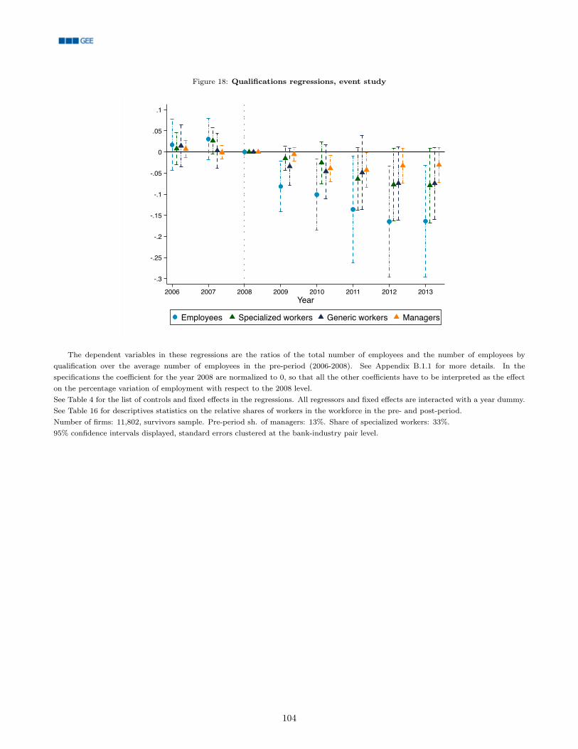
Figure 18: Qualifications regressions, event study

-.3

-.25

-.2

-.15

-.1

-.05

0

.05

.1

2006 2007 2008 2009 2010 2011 2012 2013Year

Employees Specialized workers Generic workers Managers

The dependent variables in these regressions are the ratios of the total number of employees and the number of employees byqualification over the average number of employees in the pre-period (2006-2008). See Appendix B.1.1 for more details. In thespecifications the coefficient for the year 2008 are normalized to 0, so that all the other coefficients have to be interpreted as the effecton the percentage variation of employment with respect to the 2008 level.See Table 4 for the list of controls and fixed effects in the regressions. All regressors and fixed effects are interacted with a year dummy.See Table 16 for descriptives statistics on the relative shares of workers in the workforce in the pre- and post-period.Number of firms: 11,802, survivors sample. Pre-period sh. of managers: 13%. Share of specialized workers: 33%.95% confidence intervals displayed, standard errors clustered at the bank-industry pair level.

104

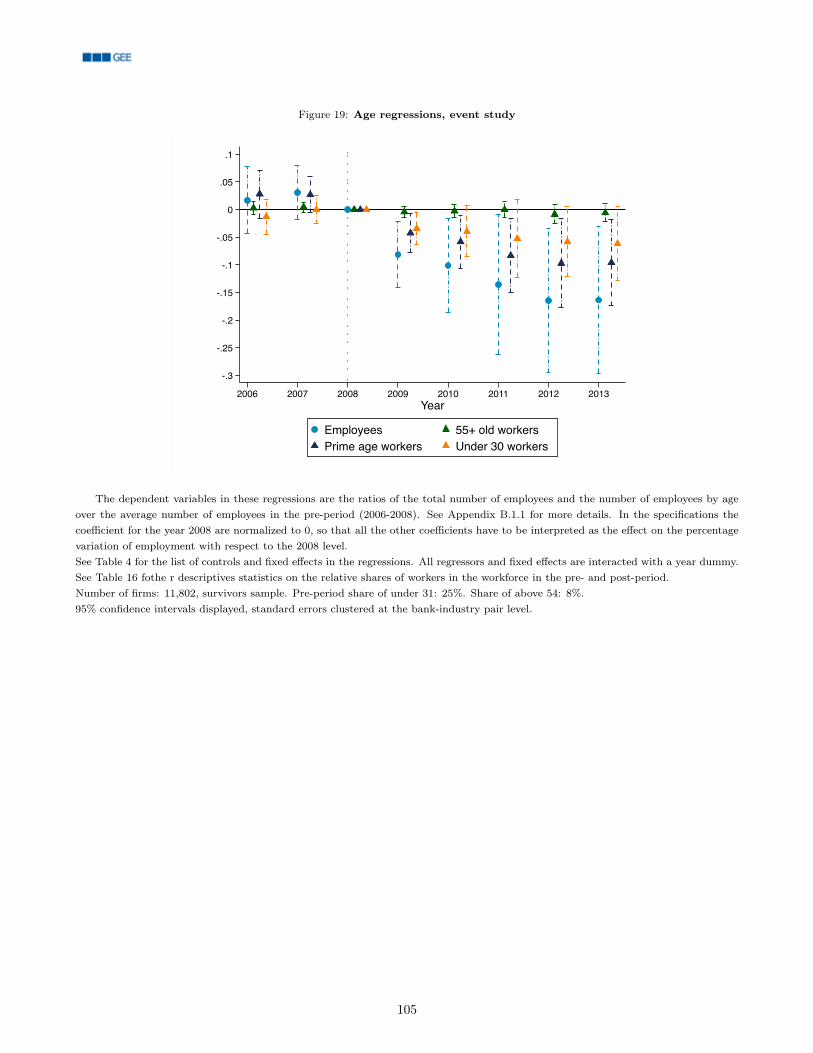
Figure 19: Age regressions, event study

-.3

-.25

-.2

-.15

-.1

-.05

0

.05

.1

2006 2007 2008 2009 2010 2011 2012 2013Year

Employees 55+ old workersPrime age workers Under 30 workers

The dependent variables in these regressions are the ratios of the total number of employees and the number of employees by ageover the average number of employees in the pre-period (2006-2008). See Appendix B.1.1 for more details. In the specifications thecoefficient for the year 2008 are normalized to 0, so that all the other coefficients have to be interpreted as the effect on the percentagevariation of employment with respect to the 2008 level.See Table 4 for the list of controls and fixed effects in the regressions. All regressors and fixed effects are interacted with a year dummy.See Table 16 fothe r descriptives statistics on the relative shares of workers in the workforce in the pre- and post-period.Number of firms: 11,802, survivors sample. Pre-period share of under 31: 25%. Share of above 54: 8%.95% confidence intervals displayed, standard errors clustered at the bank-industry pair level.

105

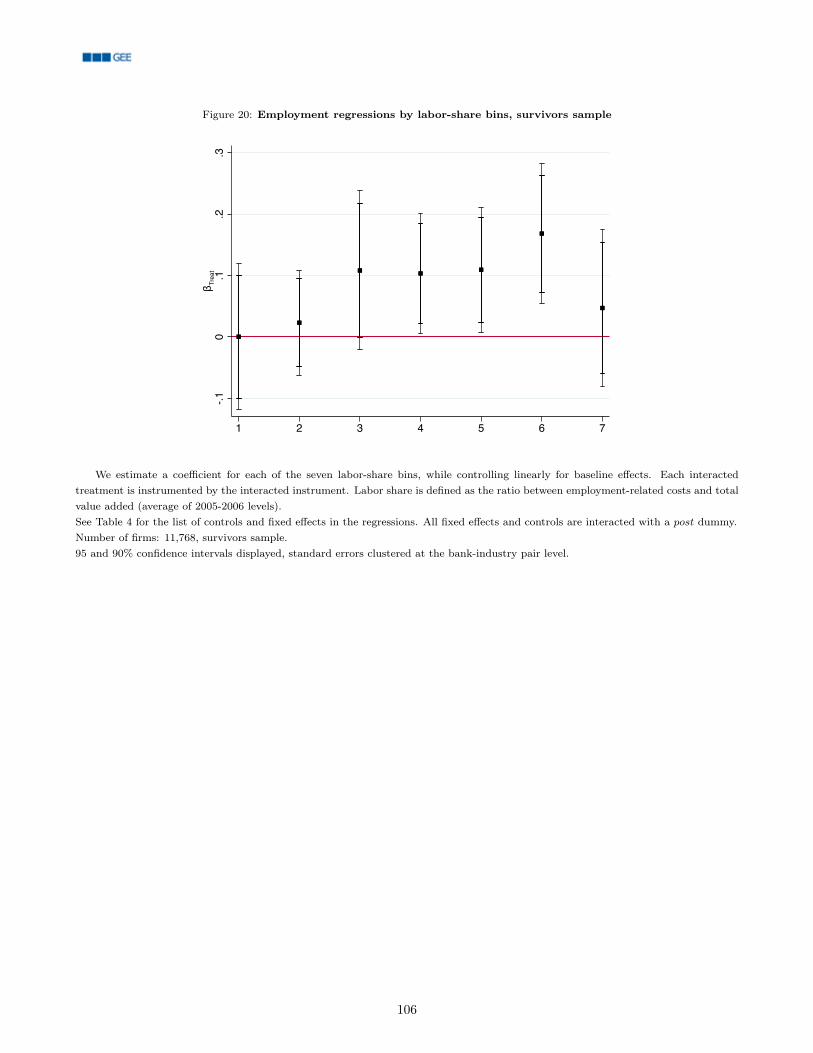
Figure 20: Employment regressions by labor-share bins, survivors sample

-.10

.1.2

.3β T

reat

1 2 3 4 5 6 7

We estimate a coefficient for each of the seven labor-share bins, while controlling linearly for baseline effects. Each interactedtreatment is instrumented by the interacted instrument. Labor share is defined as the ratio between employment-related costs and totalvalue added (average of 2005-2006 levels).See Table 4 for the list of controls and fixed effects in the regressions. All fixed effects and controls are interacted with a post dummy.Number of firms: 11,768, survivors sample.95 and 90% confidence intervals displayed, standard errors clustered at the bank-industry pair level.

106

Figure 21: Regressions by labor-share bins, reduced form

-.05

0.05

.1.15

.2β T

reat

1 2 3 4 5 6 7

(a) Exit

-.4-.2

0.2

β Treat

1 2 3 4 5 6 7

(b) Employment

We estimate a coefficient for each of the seven labor-share bins, while controlling for baseline effects linearly and for the interactedinstruments. Labor share is defined as the ratio between employment-related costs and total value added (average of 2005-2006 levels).See Table 4 for the list of controls and fixed effects in the regressions. Given that we cannot control for unobservable characteristics inthe exit specifications through firm fixed effects any more, we characterize the bank-firm matching by augmenting the set of controlswith the share of loans that each firm has with micro banks and with banks failing up to 2014.All fixed effects are interacted with a year dummy, while regressors are constant in the exit specification. In the employment specificationall fixed effects and controls are interacted with a post dummy.Number of firms: 13,750 (exit), 13,760 (employment). Sample size depends on availability of non-missing variables in CB.95 and 90% confidence intervals displayed, standard errors clustered at the bank-industry pair level.

107

Figure 22: Regressions by labor-share quartiles

-.1-.05

0.05

β Treat

1 2 3 4

(a) Exit

-.10

.1.2

β Treat

1 2 3 4

(b) Employment

We estimate a coefficient for each of the four labor-share quartiles, while controlling linearly for baseline effects. Each interactedtreatment is instrumented by the interacted instrument.See Table 4 for the list of controls and fixed effects present in the regressions. Given that we cannot control for unobservable characteristicsin the exit specifications through firm fixed effects, we characterize the bank-firm matching by augmenting the set of controls with theshare of loans that each firm has with micro banks and with banks failing up to 2014.All fixed effects are interacted with a year dummy, while regressors are constant in the exit regressions. In the employment regressionsfixed effects and regressors are interacted with the Post dummy.Number of firms: 13,750 (exit) and 13,760 (employment). Sample size depends on availability of non-missing variables in CB.95 and 90% confidence intervals displayed, standard errors clustered at the bank-industry pair level.

108

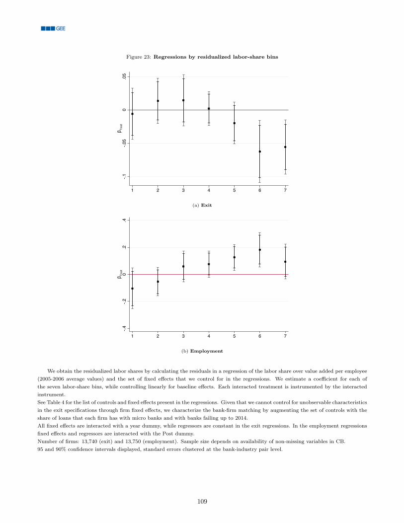
Figure 23: Regressions by residualized labor-share bins

-.1-.05

0.05

β Treat

1 2 3 4 5 6 7

(a) Exit

-.4-.2

0.2

.4β T

reat

1 2 3 4 5 6 7

(b) Employment

We obtain the residualized labor shares by calculating the residuals in a regression of the labor share over value added per employee(2005-2006 average values) and the set of fixed effects that we control for in the regressions. We estimate a coefficient for each ofthe seven labor-share bins, while controlling linearly for baseline effects. Each interacted treatment is instrumented by the interactedinstrument.See Table 4 for the list of controls and fixed effects present in the regressions. Given that we cannot control for unobservable characteristicsin the exit specifications through firm fixed effects, we characterize the bank-firm matching by augmenting the set of controls with theshare of loans that each firm has with micro banks and with banks failing up to 2014.All fixed effects are interacted with a year dummy, while regressors are constant in the exit regressions. In the employment regressionsfixed effects and regressors are interacted with the Post dummy.Number of firms: 13,740 (exit) and 13,750 (employment). Sample size depends on availability of non-missing variables in CB.95 and 90% confidence intervals displayed, standard errors clustered at the bank-industry pair level.

109

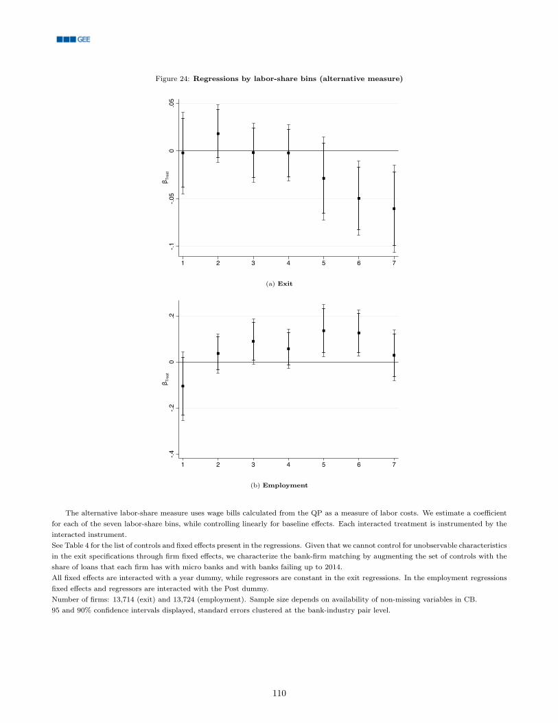
Figure 24: Regressions by labor-share bins (alternative measure)

-.1-.05

0.05

β Treat

1 2 3 4 5 6 7

(a) Exit

-.4-.2

0.2

β Treat

1 2 3 4 5 6 7

(b) Employment

The alternative labor-share measure uses wage bills calculated from the QP as a measure of labor costs. We estimate a coefficientfor each of the seven labor-share bins, while controlling linearly for baseline effects. Each interacted treatment is instrumented by theinteracted instrument.See Table 4 for the list of controls and fixed effects present in the regressions. Given that we cannot control for unobservable characteristicsin the exit specifications through firm fixed effects, we characterize the bank-firm matching by augmenting the set of controls with theshare of loans that each firm has with micro banks and with banks failing up to 2014.All fixed effects are interacted with a year dummy, while regressors are constant in the exit regressions. In the employment regressionsfixed effects and regressors are interacted with the Post dummy.Number of firms: 13,714 (exit) and 13,724 (employment). Sample size depends on availability of non-missing variables in CB.95 and 90% confidence intervals displayed, standard errors clustered at the bank-industry pair level.

110

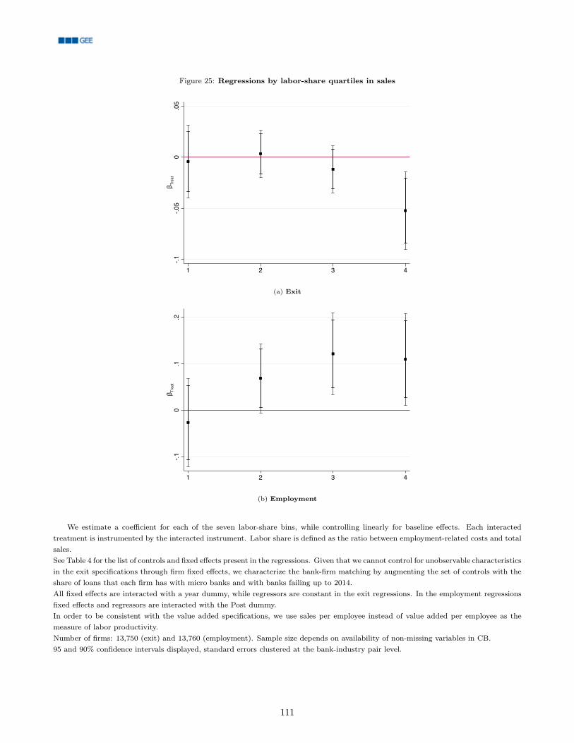
Figure 25: Regressions by labor-share quartiles in sales

-.1-.05

0.05

β Treat

1 2 3 4

(a) Exit

-.10

.1.2

β Treat

1 2 3 4

(b) Employment

We estimate a coefficient for each of the seven labor-share bins, while controlling linearly for baseline effects. Each interactedtreatment is instrumented by the interacted instrument. Labor share is defined as the ratio between employment-related costs and totalsales.See Table 4 for the list of controls and fixed effects present in the regressions. Given that we cannot control for unobservable characteristicsin the exit specifications through firm fixed effects, we characterize the bank-firm matching by augmenting the set of controls with theshare of loans that each firm has with micro banks and with banks failing up to 2014.All fixed effects are interacted with a year dummy, while regressors are constant in the exit regressions. In the employment regressionsfixed effects and regressors are interacted with the Post dummy.In order to be consistent with the value added specifications, we use sales per employee instead of value added per employee as themeasure of labor productivity.Number of firms: 13,750 (exit) and 13,760 (employment). Sample size depends on availability of non-missing variables in CB.95 and 90% confidence intervals displayed, standard errors clustered at the bank-industry pair level.

111

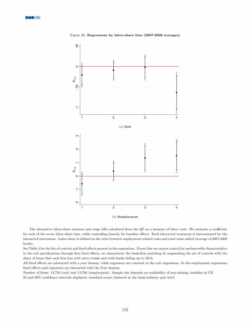
Figure 26: Regressions by labor-share bins (2007-2008 averages)

-.1-.05

0.05

β Treat

1 2 3 4

(a) Exit

-.2-.1

0.1

.2.3

β Treat

1 2 3 4

(b) Employment

The alternative labor-share measure uses wage bills calculated from the QP as a measure of labor costs. We estimate a coefficientfor each of the seven labor-share bins, while controlling linearly for baseline effects. Each interacted treatment is instrumented by theinteracted instrument. Labor share is defined as the ratio between employment-related costs and total value added (average of 2007-2008levels).See Table 4 for the list of controls and fixed effects present in the regressions. Given that we cannot control for unobservable characteristicsin the exit specifications through firm fixed effects, we characterize the bank-firm matching by augmenting the set of controls with theshare of loans that each firm has with micro banks and with banks failing up to 2014.All fixed effects are interacted with a year dummy, while regressors are constant in the exit regressions. In the employment regressionsfixed effects and regressors are interacted with the Post dummy.Number of firms: 13,750 (exit) and 13,760 (employment). Sample size depends on availability of non-missing variables in CB.95 and 90% confidence intervals displayed, standard errors clustered at the bank-industry pair level.

112

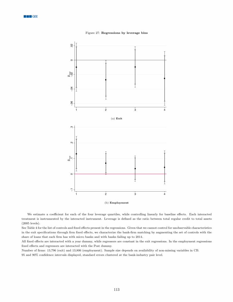
Figure 27: Regressions by leverage bins

-.06

-.04

-.02

0.02

β Treat

1 2 3 4

(a) Exit

-.10

.1.2

.3β T

reat

1 2 3 4

(b) Employment

We estimate a coefficient for each of the four leverage quartiles, while controlling linearly for baseline effects. Each interactedtreatment is instrumented by the interacted instrument. Leverage is defined as the ratio between total regular credit to total assets(2005 levels).See Table 4 for the list of controls and fixed effects present in the regressions. Given that we cannot control for unobservable characteristicsin the exit specifications through firm fixed effects, we characterize the bank-firm matching by augmenting the set of controls with theshare of loans that each firm has with micro banks and with banks failing up to 2014.All fixed effects are interacted with a year dummy, while regressors are constant in the exit regressions. In the employment regressionsfixed effects and regressors are interacted with the Post dummy.Number of firms: 13,796 (exit) and 13,806 (employment). Sample size depends on availability of non-missing variables in CB.95 and 90% confidence intervals displayed, standard errors clustered at the bank-industry pair level.

113

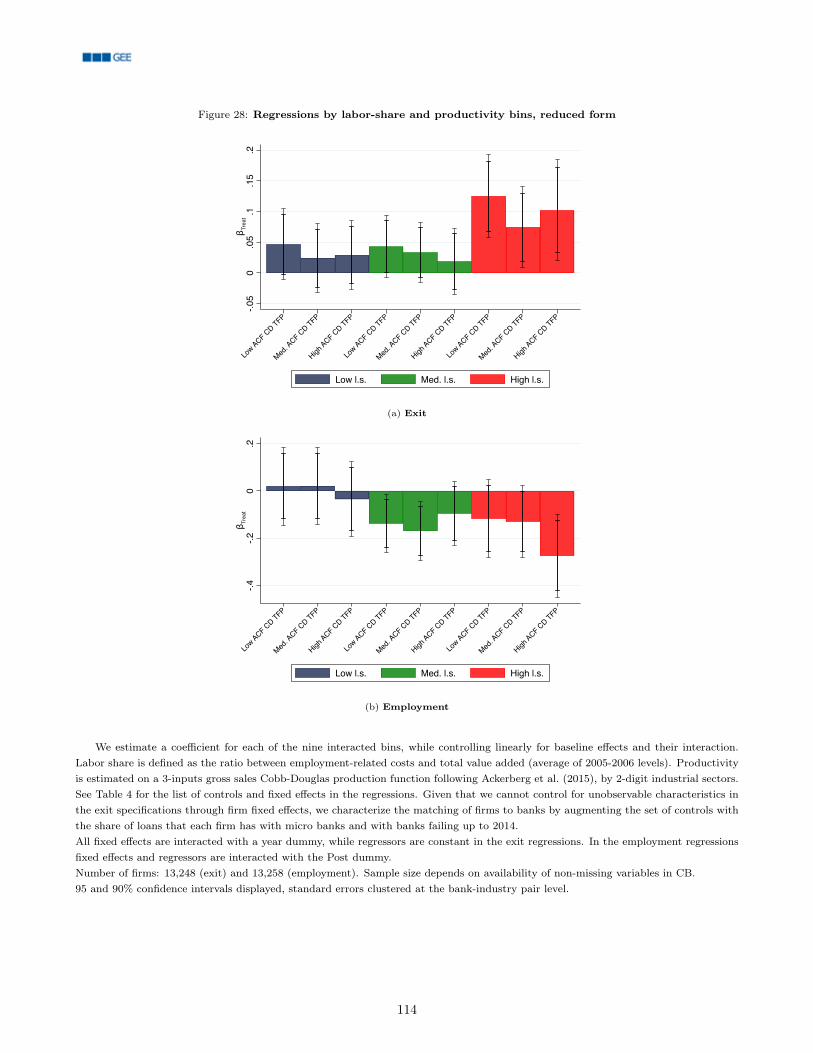
Figure 28: Regressions by labor-share and productivity bins, reduced form

-.05

0.0

5.1

.15

.2β T

reat

Low ACF CD TFP

Med. A

CF CD TFP

High ACF CD TFP

Low ACF CD TFP

Med. A

CF CD TFP

High ACF CD TFP

Low ACF CD TFP

Med. A

CF CD TFP

High ACF CD TFP

Low l.s. Med. l.s. High l.s.

(a) Exit

-.4-.2

0.2

β Tre

at

Low ACF CD TFP

Med. A

CF CD TFP

High ACF CD TFP

Low ACF CD TFP

Med. A

CF CD TFP

High ACF CD TFP

Low ACF CD TFP

Med. A

CF CD TFP

High ACF CD TFP

Low l.s. Med. l.s. High l.s.

(b) Employment

We estimate a coefficient for each of the nine interacted bins, while controlling linearly for baseline effects and their interaction.Labor share is defined as the ratio between employment-related costs and total value added (average of 2005-2006 levels). Productivityis estimated on a 3-inputs gross sales Cobb-Douglas production function following Ackerberg et al. (2015), by 2-digit industrial sectors.See Table 4 for the list of controls and fixed effects in the regressions. Given that we cannot control for unobservable characteristics inthe exit specifications through firm fixed effects, we characterize the matching of firms to banks by augmenting the set of controls withthe share of loans that each firm has with micro banks and with banks failing up to 2014.All fixed effects are interacted with a year dummy, while regressors are constant in the exit regressions. In the employment regressionsfixed effects and regressors are interacted with the Post dummy.Number of firms: 13,248 (exit) and 13,258 (employment). Sample size depends on availability of non-missing variables in CB.95 and 90% confidence intervals displayed, standard errors clustered at the bank-industry pair level.

114

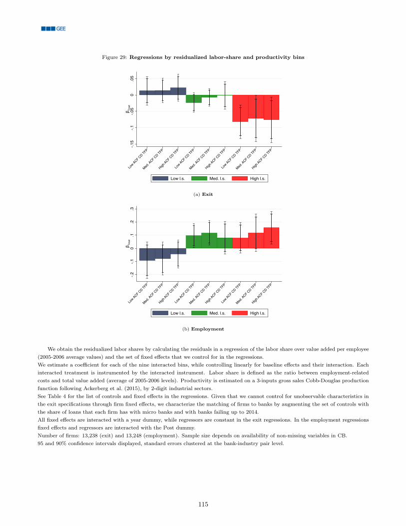
Figure 29: Regressions by residualized labor-share and productivity bins

-.15

-.1-.0

50

.05

β Tre

at

Low ACF CD TFP

Med. A

CF CD TFP

High ACF CD TFP

Low ACF CD TFP

Med. A

CF CD TFP

High ACF CD TFP

Low ACF CD TFP

Med. A

CF CD TFP

High ACF CD TFP

Low l.s. Med. l.s. High l.s.

(a) Exit

-.2-.1

0.1

.2.3

β Tre

at

Low ACF CD TFP

Med. A

CF CD TFP

High ACF CD TFP

Low ACF CD TFP

Med. A

CF CD TFP

High ACF CD TFP

Low ACF CD TFP

Med. A

CF CD TFP

High ACF CD TFP

Low l.s. Med. l.s. High l.s.

(b) Employment

We obtain the residualized labor shares by calculating the residuals in a regression of the labor share over value added per employee(2005-2006 average values) and the set of fixed effects that we control for in the regressions.We estimate a coefficient for each of the nine interacted bins, while controlling linearly for baseline effects and their interaction. Eachinteracted treatment is instrumented by the interacted instrument. Labor share is defined as the ratio between employment-relatedcosts and total value added (average of 2005-2006 levels). Productivity is estimated on a 3-inputs gross sales Cobb-Douglas productionfunction following Ackerberg et al. (2015), by 2-digit industrial sectors.See Table 4 for the list of controls and fixed effects in the regressions. Given that we cannot control for unobservable characteristics inthe exit specifications through firm fixed effects, we characterize the matching of firms to banks by augmenting the set of controls withthe share of loans that each firm has with micro banks and with banks failing up to 2014.All fixed effects are interacted with a year dummy, while regressors are constant in the exit regressions. In the employment regressionsfixed effects and regressors are interacted with the Post dummy.Number of firms: 13,238 (exit) and 13,248 (employment). Sample size depends on availability of non-missing variables in CB.95 and 90% confidence intervals displayed, standard errors clustered at the bank-industry pair level.

115

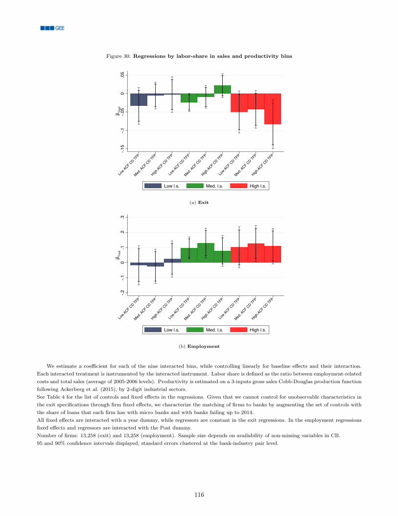
Figure 30: Regressions by labor-share in sales and productivity bins

-.15

-.1-.0

50

.05

β Tre

at

Low ACF CD TFP

Med. A

CF CD TFP

High ACF CD TFP

Low ACF CD TFP

Med. A

CF CD TFP

High ACF CD TFP

Low ACF CD TFP

Med. A

CF CD TFP

High ACF CD TFP

Low l.s. Med. l.s. High l.s.

(a) Exit

-.2-.1

0.1

.2.3

β Tre

at

Low ACF CD TFP

Med. A

CF CD TFP

High ACF CD TFP

Low ACF CD TFP

Med. A

CF CD TFP

High ACF CD TFP

Low ACF CD TFP

Med. A

CF CD TFP

High ACF CD TFP

Low l.s. Med. l.s. High l.s.

(b) Employment

We estimate a coefficient for each of the nine interacted bins, while controlling linearly for baseline effects and their interaction.Each interacted treatment is instrumented by the interacted instrument. Labor share is defined as the ratio between employment-relatedcosts and total sales (average of 2005-2006 levels). Productivity is estimated on a 3-inputs gross sales Cobb-Douglas production functionfollowing Ackerberg et al. (2015), by 2-digit industrial sectors.See Table 4 for the list of controls and fixed effects in the regressions. Given that we cannot control for unobservable characteristics inthe exit specifications through firm fixed effects, we characterize the matching of firms to banks by augmenting the set of controls withthe share of loans that each firm has with micro banks and with banks failing up to 2014.All fixed effects are interacted with a year dummy, while regressors are constant in the exit regressions. In the employment regressionsfixed effects and regressors are interacted with the Post dummy.Number of firms: 13,258 (exit) and 13,258 (employment). Sample size depends on availability of non-missing variables in CB.95 and 90% confidence intervals displayed, standard errors clustered at the bank-industry pair level.

116

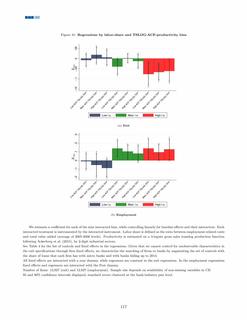
Figure 31: Regressions by labor-share and TSLOG-ACF-productivity bins

-.15

-.1-.0

50

.05

β Tre

at

Low ACF TSLO

G TFP

Med. A

CF TSLOG TFP

High ACF TSLO

G TFP

Low ACF TSLO

G TFP

Med. A

CF TSLOG TFP

High ACF TSLO

G TFP

Low ACF TSLO

G TFP

Med. A

CF TSLOG TFP

High ACF TSLO

G TFP

Low l.s. Med. l.s. High l.s.

(a) Exit

-.2-.1

0.1

.2.3

β Tre

at

Low ACF TSLO

G TFP

Med. A

CF TSLOG TFP

High ACF TSLO

G TFP

Low ACF TSLO

G TFP

Med. A

CF TSLOG TFP

High ACF TSLO

G TFP

Low ACF TSLO

G TFP

Med. A

CF TSLOG TFP

High ACF TSLO

G TFP

Low l.s. Med. l.s. High l.s.

(b) Employment

We estimate a coefficient for each of the nine interacted bins, while controlling linearly for baseline effects and their interaction. Eachinteracted treatment is instrumented by the interacted instrument. Labor share is defined as the ratio between employment-related costsand total value added (average of 2005-2006 levels). Productivity is estimated on a 3-inputs gross sales translog production functionfollowing Ackerberg et al. (2015), by 2-digit industrial sectors.See Table 4 for the list of controls and fixed effects in the regressions. Given that we cannot control for unobservable characteristics inthe exit specifications through firm fixed effects, we characterize the matching of firms to banks by augmenting the set of controls withthe share of loans that each firm has with micro banks and with banks failing up to 2014.All fixed effects are interacted with a year dummy, while regressors are constant in the exit regressions. In the employment regressionsfixed effects and regressors are interacted with the Post dummy.Number of firms: 12,927 (exit) and 12,927 (employment). Sample size depends on availability of non-missing variables in CB.95 and 90% confidence intervals displayed, standard errors clustered at the bank-industry pair level.

117

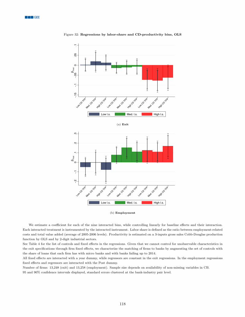
Figure 32: Regressions by labor-share and CD-productivity bins, OLS

-.15

-.1-.0

50

.05

.1β T

reat

Low CD TFP

Med. C

D TFP

High CD TFP

Low CD TFP

Med. C

D TFP

High CD TFP

Low CD TFP

Med. C

D TFP

High CD TFP

Low l.s. Med. l.s. High l.s.

(a) Exit

-.2-.1

0.1

.2.3

β Tre

at

Low CD TFP

Med. C

D TFP

High CD TFP

Low CD TFP

Med. C

D TFP

High CD TFP

Low CD TFP

Med. C

D TFP

High CD TFP

Low l.s. Med. l.s. High l.s.

(b) Employment

We estimate a coefficient for each of the nine interacted bins, while controlling linearly for baseline effects and their interaction.Each interacted treatment is instrumented by the interacted instrument. Labor share is defined as the ratio between employment-relatedcosts and total value added (average of 2005-2006 levels). Productivity is estimated on a 3-inputs gross sales Cobb-Douglas productionfunction by OLS and by 2-digit industrial sectors.See Table 4 for the list of controls and fixed effects in the regressions. Given that we cannot control for unobservable characteristics inthe exit specifications through firm fixed effects, we characterize the matching of firms to banks by augmenting the set of controls withthe share of loans that each firm has with micro banks and with banks failing up to 2014.All fixed effects are interacted with a year dummy, while regressors are constant in the exit regressions. In the employment regressionsfixed effects and regressors are interacted with the Post dummy.Number of firms: 13,248 (exit) and 13,258 (employment). Sample size depends on availability of non-missing variables in CB.95 and 90% confidence intervals displayed, standard errors clustered at the bank-industry pair level.

118

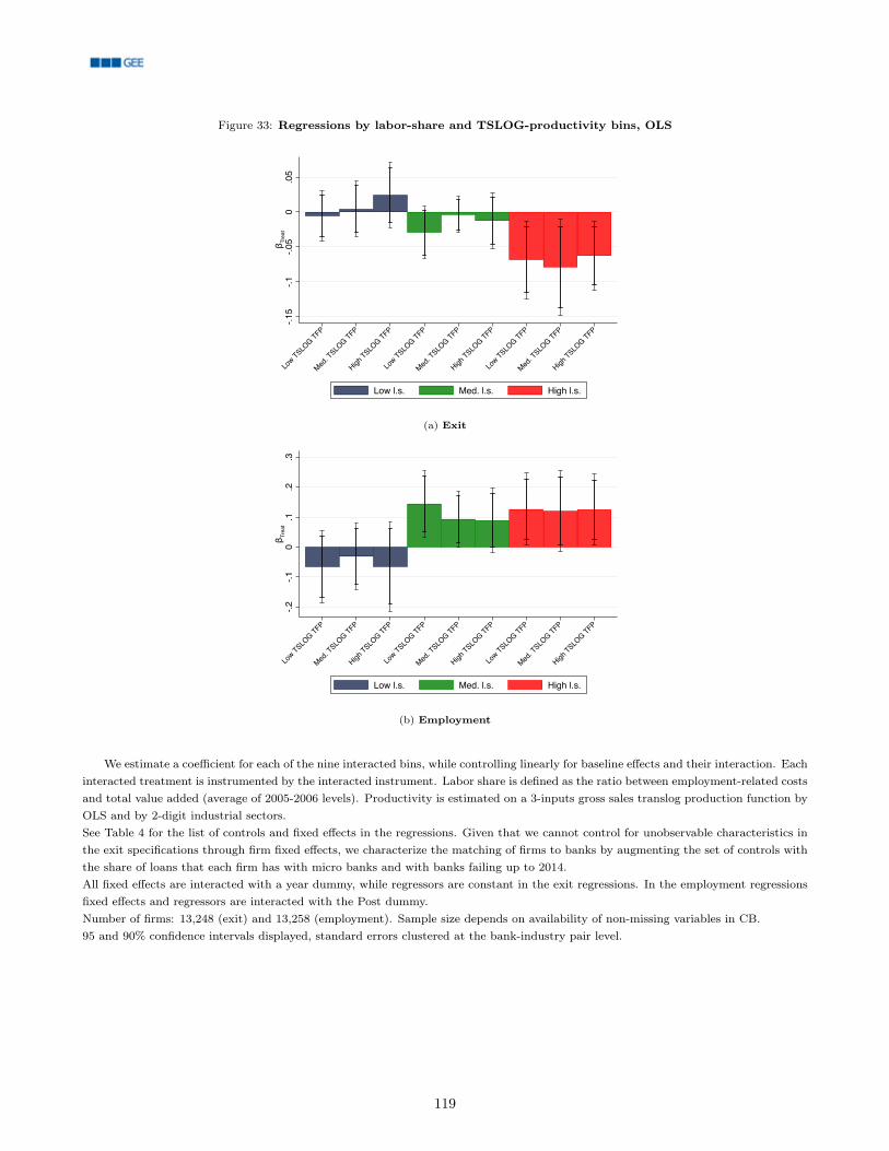
Figure 33: Regressions by labor-share and TSLOG-productivity bins, OLS

-.15

-.1-.0

50

.05

β Tre

at

Low TSLO

G TFP

Med. T

SLOG TFP

High TSLO

G TFP

Low TSLO

G TFP

Med. T

SLOG TFP

High TSLO

G TFP

Low TSLO

G TFP

Med. T

SLOG TFP

High TSLO

G TFP

Low l.s. Med. l.s. High l.s.

(a) Exit

-.2-.1

0.1

.2.3

β Tre

at

Low TSLO

G TFP

Med. T

SLOG TFP

High TSLO

G TFP

Low TSLO

G TFP

Med. T

SLOG TFP

High TSLO

G TFP

Low TSLO

G TFP

Med. T

SLOG TFP

High TSLO

G TFP

Low l.s. Med. l.s. High l.s.

(b) Employment

We estimate a coefficient for each of the nine interacted bins, while controlling linearly for baseline effects and their interaction. Eachinteracted treatment is instrumented by the interacted instrument. Labor share is defined as the ratio between employment-related costsand total value added (average of 2005-2006 levels). Productivity is estimated on a 3-inputs gross sales translog production function byOLS and by 2-digit industrial sectors.See Table 4 for the list of controls and fixed effects in the regressions. Given that we cannot control for unobservable characteristics inthe exit specifications through firm fixed effects, we characterize the matching of firms to banks by augmenting the set of controls withthe share of loans that each firm has with micro banks and with banks failing up to 2014.All fixed effects are interacted with a year dummy, while regressors are constant in the exit regressions. In the employment regressionsfixed effects and regressors are interacted with the Post dummy.Number of firms: 13,248 (exit) and 13,258 (employment). Sample size depends on availability of non-missing variables in CB.95 and 90% confidence intervals displayed, standard errors clustered at the bank-industry pair level.

119

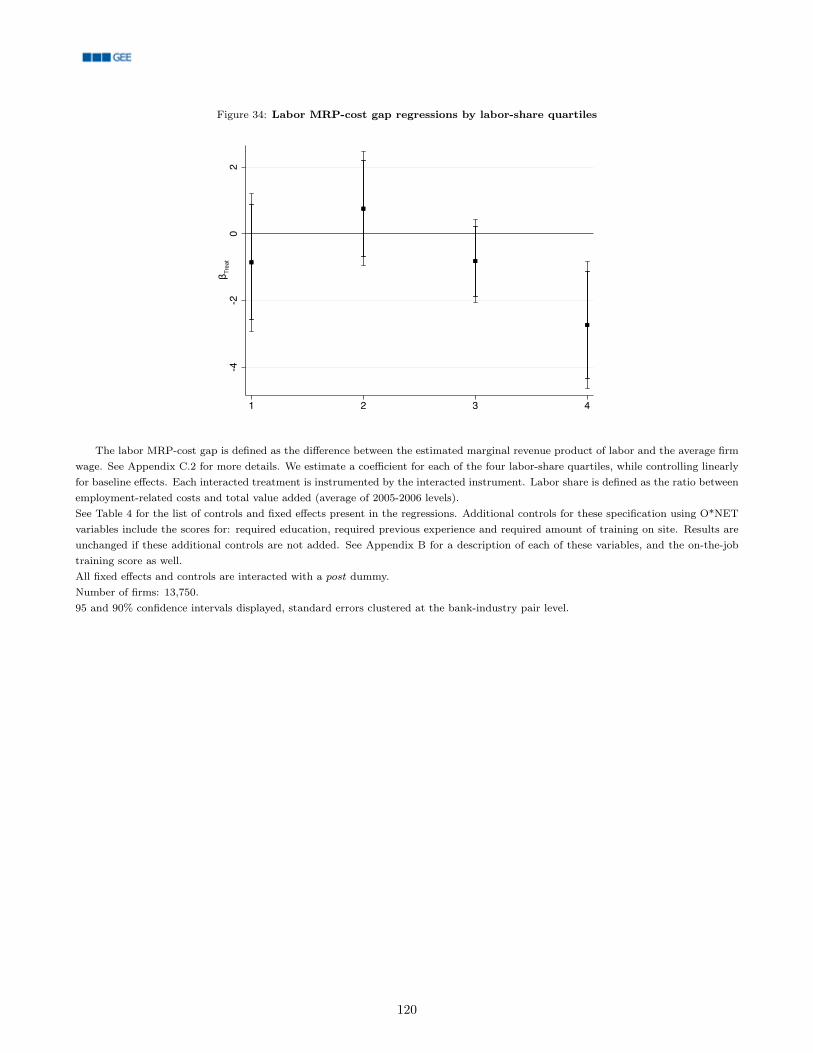
Figure 34: Labor MRP-cost gap regressions by labor-share quartiles

-4-2

02

β Treat

1 2 3 4

The labor MRP-cost gap is defined as the difference between the estimated marginal revenue product of labor and the average firmwage. See Appendix C.2 for more details. We estimate a coefficient for each of the four labor-share quartiles, while controlling linearlyfor baseline effects. Each interacted treatment is instrumented by the interacted instrument. Labor share is defined as the ratio betweenemployment-related costs and total value added (average of 2005-2006 levels).See Table 4 for the list of controls and fixed effects present in the regressions. Additional controls for these specification using O*NETvariables include the scores for: required education, required previous experience and required amount of training on site. Results areunchanged if these additional controls are not added. See Appendix B for a description of each of these variables, and the on-the-jobtraining score as well.All fixed effects and controls are interacted with a post dummy.Number of firms: 13,750.95 and 90% confidence intervals displayed, standard errors clustered at the bank-industry pair level.

120

121

GEE Papers 1: Evolução do Comércio Externo Português de Exportação

(1995-2004)

2: Nowcasting an Economic Aggregate with Disaggregate Dynamic Factors: An Application to Portuguese GDP

3: Are the Dynamics of Knowledge-Based Industries Any Different?

4: Competitiveness and convergence in Portugal

5: Produtividade, Competitividade e Quotas de Exportação

6: Export Diversification and Technological Improvement: Recent Trends in the Portuguese Economy

7: Election Results and Opportunistic Policies: An Integrated Approach

8: Behavioural Determinants of Foreign Direct Investment

9: Structural Transformation and the role of Foreign Direct Investment in Portugal: a descriptive analysis for the period 1990-2005

10: Productive experience and specialization opportunities for Portugal: an empirical assessment

11: The Portuguese Active Labour Market Policy during the period 1998-2003 - A Compive Conditional Difference-In-Differences Application

12: Fiscal Policy in a Monetary Union: Gains from Changing Institutions

13: Coordination and Stabilization Gains of Fiscal Policy in a Monetary Union

14: The Relevance of Productive Experience in the Process of Economic Growth: an Empirical Study

15: Employment and Exchange rates: the Role of Openness and Technology

16: Aggregate and sector-specific exchange rate indexes for the Portuguese economy

17: The Macroeconomic Determinants of Cross Border

Mergers and Acquisitions and Greenfield Investments

18: Does the location of manufacturing determine service sectors’ location choices? Evidence from Portugal

19: A hipótese do Investment Development Path: Uma Abordagem por Dados em Painel. Os casos de Portugal e Espanha

20: Outward FDI Effects on the Portuguese Trade Balance, 1996-2007

21: Sectoral and regional impacts of the European Carbon Market in Portugal

22: Business Demography Dynamics in Portugal: A Non-Parametric Survival Analysis

23: Business Demography Dynamics in Portugal: A Semi-parametric Survival Analysis

24: Digging Out the PPP Hypothesis: an Integrated Empirical Coverage

25: Regulação de Mercados por Licenciamento

26: Which Portuguese Manufacturing Firms Learn by Exporting?

27: Building Bridges: Heterogeneous Jurisdictions, Endogenous Spillovers, and the Benefits of Decentralization

28: Análise comparativa de sobrevivência empresarial: o caso da região Norte de Portugal

29: Business creation in Portugal: Comparison between the World Bank data and Quadros de Pessoal

30: The Ease of Doing Business Index as a tool for Investment location decisions

122

31: The Politics of Growth: Can Lobbying Raise Growth and Welfare?

32: The choice of transport technology in the presence of exports and FDI

33: Tax Competition in an Expanding European Union

34: The usefulness of State trade missions for the internationalization of firms: an econometric analysis

35: The role of subsidies for exports: Evidence from Portuguese manufacturing firms

36: Criação de empresas em Portugal e Espanha: análise comparativa com base nos dados do Banco Mundial

37: Economic performance and international trade engagement: the case of Portuguese manufacturing firms

38: The importance of Intermediaries organizations in international R&D cooperation: an empirical multivariate study across Europe

39: Financial constraints, exports and monetary integration - Financial constraints and exports: An analysis of Portuguese firms during the European monetary integration

40: FDI and institutional reform in Portugal

41: Evaluating the forecast quality of GDP components

42: Assessing the Endogeneity of OCA conditions in EMU

43: Labor Adjustment Dynamics: An Application of System GMM

44: Corporate taxes and the location of FDI in Europe using firm-level data

45: Public Debt Stabilization: Redistributive Delays versus Preemptive Anticipations

46: Organizational Characteristics and Performance of Export Promotion Agencies: Portugal and Ireland compared

47: Evaluating the forecast quality of GDP components: An application to G7

48: The influence of Doing Business’ institutional variables in Foreign Direct Investment

49: Regional and Sectoral Foreign Direct Investment in Portugal since Joining the EU: A Dynamic Portrait

50: Institutions and Firm Formation: an Empirical Analysis of Portuguese Municipalities

51: Youth Unemployment in Southern Europe

52: Financiamento da Economia Portuguesa: um Obstáculo ao Crescimento?

53: O Acordo de Parceria Transatlântica entre a UE e os EUA constitui uma ameaça ou uma oportunidade para a Economia Portuguesa?

54: Prescription Patterns of Pharmaceuticals

55: Economic Growth and the High Skilled: the Role of Scale Eects and of Barriers to Entry into the High Tech

56: Finanças Públicas Portuguesas Sustentáveis no Estado Novo (1933-1974)?

57: What Determines Firm-level Export Capacity? Evidence from Portuguese firms

58: The effect of developing countries' competition on regional labour markets in Portugal

59: Fiscal Multipliers in the 21st century

60: Reallocation of Resources between Tradable and Non-Tradable Sectors in Portugal: Developing a new Identification Strategy for the Tradable Sector

61: Is the ECB unconventional monetary policy effective?

62: The Determinants of TFP Growth in the Portuguese Manufacturing Sector

123

63: Practical contribution for the assessment and monitoring of product market competition in the Portuguese Economy – estimation of price cost margins

64: The impact of structural reforms of the judicial system: a survey

65: The short-term impact of structural reforms on productivity growth: beyond direct effects

66: Assessing the Competitiveness of the Portuguese Footwear Sector

67: The empirics of agglomeration economies: the link with productivity

68: Determinants of the Portuguese GDP stagnation during the 2001-2014 period: an empirical investigation

69: Short-run effects of product markets’ deregulation: a more productive, more efficient and more resilient economy?

70: Portugal: a Paradox in Productivity

71: Infrastructure Investment, Labor Productivity, and International Competitiveness: The Case of Portugal

72: Boom, Slump, Sudden stops, Recovery, and Policy Options. Portugal and the Euro

73: Case Study: DBRS Sovereign Rating of Portugal. Analysis of Rating Methodology and Rating Decisions

74: For Whom the Bell Tolls: Road Safety Effects of Tolls on Uncongested SCUT Highways in Portugal

75: Is All Infrastructure Investment Created Equal? The Case of Portugal

76: Why Virtuous Supply-Side Effects and Irrelevant Keynesian Effects are not Foregone Conclusions: What we Learn from an Industry-Level Analysis of Infrastructure Investments in Portugal

77: The Role of Gravity Models in Estimating the Economic Impact of Brexit

78: Infrastructure Investment in Portugal and the Traded/Non-Traded Industry Mix

79: Goods and Factor Market Integration: A Quantitative Assessment of the EU Enlargement

80: Understanding productivity dynamics:a task taxonomy approach

81: On the Effects of Infrastructure Investments on Industrial CO2 Emissions in Portugal

82: Assessing Competition With the Panzar-Rosse Model: An empirical analysis of European Union banking industry

83: Health Care Investments and Economic Performance in Portugal: An Industry Level Analysis

84: Is deregulation of product and labour markets promoting

employment and productivity? A difference-in-differences approach

85: Foreign acquisition and internal organization

86: Learning, Prices, and Firm Dynamics

87: The Diffusion of Knowledge via Managers’ Mobility

88: Empresas Zombie em Portugal - Os sectores não transacionáveis da Construção e dos Serviços

89: Collective bargaining through the magnifying glass: A comparison between the Netherlands and Portugal

90: A Lower VAT Rate on Electricity in Portugal: Towards a Cleaner Environment, Better Economic Performance, and Less Inequality

91: Who Seeks Re-Election: Local Fiscal Restraints and Political Selection

92: Assessing the Competitiveness of the Metalworking Sector

93: The efficiency of Portuguese Technology Transfer Offices and the importance of university characteristics

94: Persistence in innovation and innovative behavior in unstable environments

124

95: The effect of entrepreneurial origin on firms’ performance - The case of Portuguese academic spinoffs

96: Absorptive Capacity and Firms’ Generation of Innovation - Revisiting Zahra and George’s Model

97: Innovations in digital government as business facilitators: implications for Portugal

98: Innovation and the economic downturn: Insights from Portuguese firms

99: European Funds and Firm Dynamics: Estimating Spillovers from Increased Access

100: Corporate Leverage and Investment in Portugal

101: The effects of official and unofficial information on tax compliance

102: Competition effect on innovation and productivity - The Portuguese case

103: Measuring the Welfare of Intermediation in Vertical Markets

104: Of course Collusion Should be Prosecuted. But Maybe...

Or (The case for international antitrust agreements)

105: Product market competition and gender discrimination

106: Integration of Small Technology-Based Firms in Aeronautics

107: The Effects of Highway Tolls on Private Business Activity – Results from a Natural Experiment

108: Competition and Firm Productivity: Evidence from Portugal

109: Do Exchange Traded Funds (ETFs) Outperform the Market? Evidence from the Portuguese Stock Index

110: Assessing the Competitiveness of the Portuguese Chemical Sector

111: A General Equilibrium Theory of Occupational Choice under Optimistic Beliefs about Entrepreneurial Ability

112: O Mercado Segurador em Portugal: O Papel dos Gestores na Constituição de Provisões

113: Exploring the implications of di erent loan-to-value macroprudential policy designs

114: The Determinants of TFP Growth in the Portuguese Service Sector

115: Agglomeration and Industry Spillover Effects in the Aftermath of a Credit Shock

116: Entrepreneurial Human Capital and Firm Dynamics

117: Global Value Chains and Vertical Specialization: The case of Portuguese Textiles and Shoes exports

118: Firm heterogeneity and exports in Portugal: Identifying export potential

119: Vantagens Comparativas Reveladas e suas determinantes: Uma Aplicação à Economia Portuguesa

120: A Look at the main channels of Potential Impact of Brexit on the Portuguese Economy

121: How internationalization and competitiveness contribute to get public support to innovation? The Portuguese case

122: Grande Guerra e Guerra Colonial: Quanto Custaram aos

Cofres Portugueses?

123: Financing a Renewable Energy Feed-in Tariff with a Tax on Carbon Dioxide Emissions: A Dynamic Multi-Sector General Equilibrium Analysis for Portugal

124: Brown Sugar, how come you taste so good? The impact of a soda tax on prices and consumption

125: ARFIMA Reference Forecasts for Worldwide CO2

Emissions and the National Dimension of the Policy Efforts to Meet IPCC Targets

125

126: Reference Forecasts for CO2 Emissions from Fossil-Fuel Combustion and Cement Production in Portugal

127: Regulated Early Closures of Coal-Fired Power Plants and Tougher Energy Taxation on Electricity Production: Synergy or Rivalry?

128: Picking Our Environmental Battles: Removal of Harmful Subsidies or Carbon Taxation?

129: Financing Future Feed-in Tariffs from Currently Installed RES-E Generating Capacity

130: Foreign Direct Investment, Income Inequality and Poverty

in Portugal, 1973-2014: What does cointegration analysis tell us?

131: On the Spillover Effects of CO2 Taxation on the Emissions of other Air Pollutants

132: On the Macroeconomic and Distributional Effects of the

Regulated Closure of Coal-Operated Power Plants

133: The China Shock and Employment in Portuguese Firms

134: Energy Taxation Reform with an Environmental Focus

135: ARFIMA Reference Forecasts for Worldwide CO2 Emissions and the Need for Large and Frontloaded Decarbonization Policies

136: Exporter Firms Behaviour, Evidence From Portuguese

Firms Using Microdata

137: Collateral Value and Entrepreneurship: Evidence from a

Property Tax Reform

138: The Financial Channels of Labor Rigidities: Evidence from

Portugal