Research in Computing Science vol. 138, 2017

Advances in Computing Science

Research in Computing Science

Series Editorial Board

Editors-in-Chief:

Grigori Sidorov (Mexico) Gerhard Ritter (USA)

Jean Serra (France)

Ulises Cortés (Spain)

Associate Editors:

Jesús Angulo (France)

Jihad El-Sana (Israel) Alexander Gelbukh (Mexico)

Ioannis Kakadiaris (USA)

Petros Maragos (Greece) Julian Padget (UK)

Mateo Valero (Spain)

Editorial Coordination: Alejandra Ramos Porras

Research in Computing Science es una publicación trimestral, de circulación internacional, editada por el Centro de Investigación en Computación del IPN, para dar a conocer los avances de investigación científica

y desarrollo tecnológico de la comunidad científica internacional. Volumen 138, noviembre 2017. Tiraje:

500 ejemplares. Certificado de Reserva de Derechos al Uso Exclusivo del Título No. : 04-2005-121611550100-102, expedido por el Instituto Nacional de Derecho de Autor. Certificado de Licitud de Título

No. 12897, Certificado de licitud de Contenido No. 10470, expedidos por la Comisión Calificadora de

Publicaciones y Revistas Ilustradas. El contenido de los artículos es responsabilidad exclusiva de sus respectivos autores. Queda prohibida la reproducción total o parcial, por cualquier medio, sin el permiso

expreso del editor, excepto para uso personal o de estudio haciendo cita explícita en la primera página de

cada documento. Impreso en la Ciudad de México, en los Talleres Gráficos del IPN – Dirección de Publicaciones, Tres Guerras 27, Centro Histórico, México, D.F. Distribuida por el Centro de Investigación

en Computación, Av. Juan de Dios Bátiz S/N, Esq. Av. Miguel Othón de Mendizábal, Col. Nueva Industrial

Vallejo, C.P. 07738, México, D.F. Tel. 57 29 60 00, ext. 56571.

Editor responsable: Grigori Sidorov, RFC SIGR651028L69

Research in Computing Science is published by the Center for Computing Research of IPN. Volume 138,

November 2017. Printing 500. The authors are responsible for the contents of their articles. All rights reserved. No part of this publication may be reproduced, stored in a retrieval system, or transmitted, in any

form or by any means, electronic, mechanical, photocopying, recording or otherwise, without prior

permission of Centre for Computing Research. Printed in Mexico City, in the IPN Graphic Workshop – Publication Office.

Volume 138

Advances in Computing Science

Juan Carlos Chimal Eguía

Horacio Rodríguez Bazán

Christian E. Maldonado (eds.)

Instituto Politécnico Nacional, Centro de Investigación en Computación

México 2017

ISSN: 1870-4069

Copyright © Instituto Politécnico Nacional 2017

Instituto Politécnico Nacional (IPN)

Centro de Investigación en Computación (CIC)

Av. Juan de Dios Bátiz s/n esq. M. Othón de Mendizábal

Unidad Profesional “Adolfo López Mateos”, Zacatenco

07738, México D.F., México

http://www.rcs.cic.ipn.mx

http://www.ipn.mx

http://www.cic.ipn.mx

The editors and the publisher of this journal have made their best effort in

preparing this special issue, but make no warranty of any kind, expressed or

implied, with regard to the information contained in this volume.

All rights reserved. No part of this publication may be reproduced, stored on a

retrieval system or transmitted, in any form or by any means, including

electronic, mechanical, photocopying, recording, or otherwise, without prior

permission of the Instituto Politécnico Nacional, except for personal or

classroom use provided that copies bear the full citation notice provided on the

first page of each paper.

Indexed in LATINDEX, DBLP and Periodica

Printing: 500

Printed in Mexico

http://www.ipn.mx/

http://www.ipn.mx/

http://www.cic.ipn.mx/

Editorial

Computer Science is pervasive to the scientific endeavor. There is no area or field of

study which, nowadays, can thrive without the use of computational resources, models

and algorithms to analyze ever growing amounts of data in increasingly complex

ways. This trend is clearly reflected in the selection of papers included in this volume

of Research in Computing Science.

This issue presents both new and improved algorithms and methods as well as ap-

plications to other fields of study. Accepted works range from improved algorithms

for solving classical computational problems, to the application of known models and

techniques on biomedical challenges.

All submitted papers were reviewed by two or more independent members of the

editorial committee. This volume contains revised and corrected versions of the 16

accepted papers.

Our deepest gratitude goes to all the parties involved in the creation of this volume:

Foremost to the authors of the articles for their dedication to the excellence of the

works presented. We are also grateful for the hard labor the members of the editorial

board invested in the evaluation and selection of the highest quality papers amongst

many others of high value. We are also indebted to the Sociedad Mexicana de Inteli-

gencia Artificial (SMIA) for their collaboration towards the completion of this jour-

nal. Our special and profound gratefulness to the Centro de Investigación en Compu-

tation of the Instituto Politecnico Nacional (CIC-IPN) for their invaluable collabora-

tion in the publishing of this issue. The submission, review, and selection processes

were enabled by the widely adopted tool EasyChair, (www.easychair.org) free of

charge.

Juan Carlos Chimal Eguía

Horacio Rodríguez Bazán

Christian E. Maldonado

CIC-IPN, Mexico

Guest Editors

November 2017

5

ISSN 1870-4069

Research in Computing Science 138 (2017)ISSN 1870-4069

Table of Contents Page

Numerical Analysis of a Diffusion Flame Under Water Mist Jet

Influence ...................................................................................................................... 9

M. De la Cruz-Ávila, E. Martínez-Espinosa, G. Polupan

Priority Data Transmission Schemes for a Wireless Sensor Network on

BAN ............................................................................................................................ 19

Sergio Martínez, Mario Rivero, Laura Garay, Issis Romero

Modelo foveal rectangular a partir de un sensor de imagen comercial ............... 29

José Antonio Loaiza Brito, Luis Niño de Rivera y Oyarzábal

Computational Intelligence Algorithms Applied to the Pre-diagnosis of

Chronic Diseases ....................................................................................................... 41

Mariana Dayanara Alanis-Tamez, Yenny Villuendas-Rey,

Cornelio Yáñez-Márquez

Hybrid CW-GA Metaheuristic for the Traveling Salesman Problem ................. 51

Irma Delia Rojas Cuevas, Santiago Omar Caballero Morales

Transmission of Digital Audio with Visible Light.................................................. 61

Sergio Sandoval-Reyes, Arturo Hernandez-Balderas

Implicaciones computacionales de los aeromanipuladores ................................... 69

Julio Mendoza-Mendoza, Baltazar Jiménez-Ruiz,

Víctor Javier González-Villela, Mauricio Méndez-Martínez,

Leonardo Fonseca-Ruiz, Erick López Alarcón

Lumped Parameter Estimation of a Stochastic Process of Second

Order Using the Second Moment and Recursiveness ............................................ 79

Romeo Urbieta Parrazales, José de Jesús Medel Juárez,

Karen Alicia Aguilar Cruz, Rosaura Palma Orozco

A Survey on Computer Science Techniques in the FOREX Market:

Models and Applications .......................................................................................... 89

Diego Aguilar, Ildar Batyrshin, Oleksiy Pogrebnyak

Armagedroid, APKs Static Analyzer Software ...................................................... 99

Luis Enrique Héctor Almaraz García, Eleazar Aguirre Anaya,

Ponciano Jorge Escamilla Ambrosio, Raúl Acosta Bermejo

7

ISSN 1870-4069


Experimental Comparison of Bioinspired Segmentation Algorithms

Applied to Segmentation of Digital Mammographies ......................................... 109

David González-Patiño, Yenny Villuendas-Rey,

Amadeo J. Argüelles-Cruz

Sequence Prediction with Hyperdimensional Computing ................................... 117

Job Isaias Quiroz Mercado, Ricardo Barrón Fernández,

Marco Antonio Ramírez Salinas

Designing New CAPTCHA Models Based on the Cognitive Abilities of

Artificial Agents ...................................................................................................... 127

Edgar D. García-Serrano, Salvador Godoy-Calderón,

Edgardo M. Felipe-Riverón

Estimation and Identification Process Using an Exponential Forgetting

Factor ....................................................................................................................... 137

Karen Alicia Aguilar Cruz, José de Jesús Medel Juárez,

Romeo Urbieta Parrazales, María Teresa Zagaceta Álvarez

Análisis de readmisión hospitalaria de pacientes diabéticos mediante

aprendizaje computacional .................................................................................... 147

Germán Cuaya-Simbro, Elias Ruiz, Angélica Muñoz-Meléndez,

Eduardo F. Morales

The Mexican Magical Towns Traveling Salesman Problem:

Preliminary Results ................................................................................................ 159

Sandra J. Gutiérrez, Nareli Cruz, Hiram Calvo, Marco A. Moreno-

Armendáriz

8Research in Computing Science 138 (2017) ISSN 1870-4069

Numerical Analysis of a Diffusion Flame Under Water

Mist Jet Influence

M. De la Cruz-Ávila1, E. Martínez-Espinosa2, G. Polupan1

1 Instituto Politécnico Nacional, LABINTHAP, ESIME, CDMX,

Mexico

2 UNAM Ciudad Universitaria, Instituto de Ingeniería, CDMX,

Mexico

[email protected]

Abstract. A water mist jet for a steam generator of direct contact with a diffu-

sion flame is numerically analyzed in this paper. Numerical simulation is con-

ducted for an 8 Lug-Bolt array in a confined system. The diffusion flame is

modelled in the Eulerian - Eulerian multiphase approach where the reaction

species are oxygen which is injected by a 16.9 mm central nozzle, methane by

four peripheral 5.86 mm nozzles as the water mist and with a droplet size of

10μm. Numerical simulations are developed with the Reynolds Averaged Na-

vier-Stokes and the Realizable k-ε turbulence model is considered. The Eddy

Dissipation Model is implemented in order to calculate the effect of turbulent

chemical reaction rate. Predictions show some instabilities that are located with-

in the flame structure as long as the fuel moisture percentage is less than 1%. If

the mist fraction for vaporization increases, the instabilities do not affect the in-

ternal flame structure but instabilities becomes relevant to the end of the calcu-

lus domain. The decrement about 60% of the water mist velocity due to a vapor

gap around the micro droplets is the mean cause of the instabilities. Therefore, a

very precise control of the numerical parameters is so important for multiphase

approximations.

Keywords: Eulerian - Eulerian multiphase approach, multiphase combustion,

water mist injection, direct vaporization.

1 Introduction

In the open literature there are many studies focused on two gas streams, which con-

sider an annular fuel and oxidizer injection shape. For example, the study carried out

by Fossa [1], and Cioncollini [2] analyze two-phase mixture flows. Grech [3], Cu-

trone [4], and Smith [5] conducted numerical simulations with Reynolds-Averaged

Navier-Stokes (RANS) method for diffusion combustion process in jet propulsion

rockets and gas turbines. Lopez-Parra and Turan [6] have simulated a methane turbu-

lent jet diffusion flame with the Eddy Dissipation Model (EDM) [7] and the standard

9

ISSN 1870-4069

Research in Computing Science 138 (2017)pp. 9–18; rec. 2017-09-11; acc. 2017-10-25

k-ε turbulence model with satisfactory results. Finally, the mixing fluids process in

diffusion flame systems is extremely important because the fuel and oxidizer are in-

jected independently and combustion starts when the mixture reaches flammability

limits (upper or lower) [8].

However, all this studies are focused on the flame development but not on the nu-

merical control for a multiphase combustion-vaporization scheme. Therefore, this

paper is focused on the numerical control settings for the numerical diffusion flame-

water mist in a multiphase scheme approximation. The water mist injection flow for

three cases are analyzed in order to compare its influence over development during

the steam generation. This work allows to be applied to further numerical studies in

turbulent combustion, water drops vaporization and quenching flames.

2 Numerical Details

Numerical simulations are conducted for 8 Lug-Bolt system where oxygen is injected

in a 16.9 mm central nozzle, methane and water mist by four peripheral 5.86 mm

nozzles respectively. The simulations used the standard methane, water and oxygen

properties for mixture species. Jets are under atmospheric conditions of 1atm and

298K in a confined system as shown in Fig. 1.

Fig. 1. Computational domain, settings and mesh.

The combustion chamber has 101.6mm diameter (Dc) and 1500mm of total length

(L). The aim of the numerical approximations is to analyse the influence of the water

mist affecting the mixture process for three flow Cases. An Eulerian-Eulerian ap-

proach was implemented for representing multiphase phenomenon and combustion

species were modelled as the continuous phase (p phase 1) and the water mist as the

dispersed phase (q phase 2). Simulations consider mean velocity profile of 10m/s for

every stream. The water mist droplets are analysed for three different cases. The mi-

cro-droplet diameter remains constant with 10 µm while the injection mist flow is

10


Research in Computing Science 138 (2017) ISSN 1870-4069

0.005, 0.010 and 0.015 kg/s. Pressure outlet to air was use for boundary outlet a non-

slip and adiabatic treatment for the calculus domain wall was use. A mesh with

3232854 cells (Fig.1.), which is based on the proper resolution of the micro-droplets

dynamics with a size of 10 microns and the gas phase flow coupling was used as de-

scribed by Yuval Dagan et al [9]. Both phases are proposed as unreactive fluids to

ensure a good tracking of properties at the interphase.

2.1 Constitutive Equations

In first instance, the numerical analysis of the oxygen-methane mixture process is of

the physical nature. This implies that the equations to be solved are mass conserva-

tion, the momentum quantity, energy and chemical. These equations in multiphase

Eulerian-Eulerian approach model solution are defined by the following expressions.

Mass conservation.

∂

∂t(αqρq )+∇∙(αqρq v q

)=∑(mpq -mqp

)+Sq

n

p=1

, (1)

where αq is the volume fraction, 𝑣 𝑞 is the velocity of phase q and ��𝑝𝑞 characterizes

the mass transfer from the pth to qth phase, and ��𝑞𝑝 characterizes the mass transfer

from the phase q to phase p, ρ is the phase density and Sq is the source term.

Momentum.

∂

∂t(αqρq v q

)+∇∙(αqρq v qv q)=-αq∇p+∇∙τ q

ρq g +

∑(Kpq(v p -v q

)+mpq v pq

-mqp v qp

)+(F q +F lift,q

+F td,q )

n

p=1

, (2)

where (Kpq (=Kqp)) is the interphase momentum exchange coefficient and 𝑣 𝑞,𝑝 are the

phase velocities. Note that represents the mean interphase momentum exchange and

does not include any contribution due to turbulence. The turbulent interphase momen-

tum exchange is modelled with the turbulent dispersion force term 𝐹 𝑡𝑑,𝑞 and 𝐹 𝑞 the

external body forces which is equal to 0. 𝜏�� is the qth phase stress tensor p and g are

the pressure ante gravity respectively.

Conservation of Energy. To describe the conservation of energy in Eulerian mul-

tiphase applications, the equation can be written in terms of each phase:

∂

∂t(αqρq hq)+∇∙(αqρq v q

hq)=

αq

∂pq

∂t+τ q

:∇v q -∇∙q q

+Sq+∑(Qpq+mpq hpq-mqp

hqp).

n

p=1

(3)

Conservation of Species. The chemical species conservation equation for a multi-

phase mixture can be represented in the following form:

11

Numerical Analysis of a Diffusion Flame Under Water Mist Jet Influence


∂

∂t(ρqαqYi

q) +∇∙ (ρqαqv

qYi

q) =

-∇∙αqJ i

q+αqRi

q+αqSi

q+ ∑(mpiqj-mqjpi)+R

n

p=1

, (4)

where ℛ is the reaction rate and 𝜏 𝑞 = 𝜌𝑞 𝑣 𝑞𝑣 𝑞

− 𝜌𝑞 𝑣 𝑞𝑣 𝑞

, 𝑞 𝑞 = 𝜌𝑞 𝑣 𝑞ℎ𝑞

− 𝜌𝑞 𝑣 𝑞ℎ�� ,

𝐽 𝑖��

= 𝜌𝑞 𝑣 𝑞𝑌𝑖𝑞 − 𝜌𝑞 𝑣 ��𝑌𝑖

��, are the average fluctuations of Reynolds stresses, heat flux-

es and mass fluxes respectively, with the sign ‘‘¯’’ denoting time average and ‘‘~’’

denoting Favre average.

The transport momentum equation averaging result into the appearance of terms

containing the average fluctuations. Turbulence model involved in this paper (the

Realizable k-ɛ model) is based on the Boussinesq hypothesis, which means, the Reyn-

olds stress tensor must be modelled in order to close the RANS equations and be pro-

portional to the mean deformation rate tensor. The Realizable k-ɛ turbulence model

describes a two scalar transport, the turbulent kinetic energy (k) and its dissipation

rate (ε). The model has been validated experimentally for many reactive flows simula-

tions with satisfactory results [10-12]. Numerical simulations are developed with the

alternative RANS technique and considers the Realizable k-ε [13] turbulence model

for the equations system closure.

2.2 Constitutive Combustion Kinetics and Combustion Modelling

The energy production by the methane combustion has been well established by the

next overall reaction:

CH4 + 2O2 = CO2 + 2H2O, ΔH298 = - 802.7 kJ/mol. (5)

This overall equation is a gross simplification by the actual reaction mechanism,

which involves free radical chain reactions. The numerical simulation considers a

stoichiometric reaction neglecting all other subsequent reaction in the chain reaction

mechanism. Nevertheless, this work main purpose is not to analyze the secondary

chemical reactions. For this reason, a single-step irreversible chemical reaction was

used in order to redirect computational resources to the flow development.

The species are characterized through the involved mass fractions Yi for i=1 to N,

where N is the number of species in the reacting mixture. The mass fractions Yi are

defined by:

𝑌𝑖 =𝑚𝑖

𝑚, (6)

where mi is the mass of species i present in a given volume V and m is the total mass

of gas in the volume. The numerical study of turbulent-reactive flows depends upon

the combustion model adequate selection. The high non-linear production term for the

species’ conservation equation closure is one of the most challenging aspects when

modeling turbulent combustion. The Eddy Dissipation Model (EDM) is used to calcu-

late the turbulent chemical reaction rate effect. The EDM is based on the infinitely

12



fast chemistry hypothesis and assumes that the reaction rate is controlled by the turbu-

lent mixing [14]. A generalized formulation of the EDM has been proposed in order

to take into account finite-rate chemistry effects. A stoichiometric relation describing

chemical reactions of arbitrary complexity can be represented by the rth reaction equa-

tion [15]. The turbulent mixing rate is related to the turbulent eddies timescale present

in the flow. The timescale used for this purpose is the so-called eddy lifetime, τ=k/ε,

with k being the turbulent kinetic energy, ε the turbulent dissipation rate and the

chemistry typically described by relatively simple single or two-step mechanism. The

species i production net-rate due to reaction r, Ri, r is given by the smaller (limiting-

value) of the two expression below.

Base on reactants mass fraction:

Ri,r=v'i,rMw,iAρ ε

kminR (

YR

v'R,rMw,R

). (7)

Base on products mass fraction:

Ri,r=v'i,rMw,iABρε

k

∑ YPP

∑ v''j,rMw,jNj

, (8)

where Yp and YR the species mass fraction, A and B are Magnussen [14] constant for

reactants (4.0) and products (0.5) respectively. Mw, i molecular weight R and P reac-

tants and products respectively.

2.3 Numerical Fluid Reconstruction

A 3rd order Quadratic Upstream Interpolation for Convective Kinematics (QUICK)

scheme for the convective and viscous terms was considered. However, this high-

order scheme is not easy to apply to unstructured grid directly. The Leonard’s QUICK

scheme [16] uses a quadratic fit through two upwind nodes and one downwind cell

center. To find the exact location of the next upwind cell nodes would increase the

geometrical complexity and consume relatively more memory and CPU time.

In a uniform grid (Fig. 2. for definitions of points WW, W, P, E, EE), the Quick

scheme at the east cell-face can be written as:

ϕe=

1

2(ϕ

P+ϕ

E)-

1

8(ϕ

w-2ϕ

P+ϕ

E) (u≥0),

ϕe=

1

2(ϕ

P+ϕ

E)-

1

8(ϕ

EE-2ϕ

E+ϕ

P) (u<0).

(9)

Fig. 2. QUICK scheme for a uniform grid.

13



This scheme is 2nd-order accurate if the definition of the truncation error is based

on approximating the spatial derivative at cell centers in the linear convection equa-

tion. Other authors [14, 15] have chosen alternative definitions of the truncation error,

according to which QUICK becomes 3rd-order accurate. Consequently, the imple-

mentation of both specifications (mesh/scheme) provides better approximation results

in comparison to those in which use is posed separately.

The 3rd-order Modified High Resolution Interface Capturing Scheme (M-HRIC) for

the viscous terms. For simulations using the multiphase model, upwind schemes are

generally unsuitable for interface tracking because of their overly diffusive nature.

Central differencing schemes, while generally able to retain the sharpness of the inter-

face, are unbounded and often give unphysical results. In order to overcome these

deficiencies, it is better to use the modified version of the High Resolution Interface

Capturing (HRIC) scheme. The modified HRIC scheme is a composite normalized

variable diagram (NVD) scheme that consists of a nonlinear blend of upwind and

downwind differencing. First, the normalized cell value of volume fraction, ��𝑐 is

computed and is used to find the normalized face value, ��𝑓 as follows:

ϕc=

ϕD

-ϕU

ϕA

-ϕU

, (10)

where A is the acceptor cell, D is de donor cell, and U is the upwind cell and

ϕf= {

ϕc ϕ

c<0 orϕ

c>1,

2ϕc 0≤ϕ

c≤0.5,

1 0.5≤ ϕc≤1.

(11)

Fig. 3. Cell Representation for Modified HRIC scheme.

3 Results

The heat released of the combustion process directly affect the water mist flow chang-

ing its enthalpy and as a consequence the vaporization process take places. The water

vapour temperature contours for the three Cases are presented in Fig.4. In Case A, the

global vapour temperature ascends to 2921 K because its mass flow is 0.005 kg/s

(50% less than case B and 75% less than C) and the vaporization starts in a zone near

or in the flame front. Vaporization Enthalpy direct affects the micro droplet due to its

proximity size (less mas flow = lager distance between droplets). The global vapour

temperature for Case B is 2489 K which represents a 14.7% variation respect Case A

because its droplets proximity is shorter. Then, the vaporization energy needs to be

higher to reach all droplet surroundings. Thus for Case C, the global vapour tempera-

ture is 1541 K which represent a 47% respect Case A and 39% respect Case B. This

14



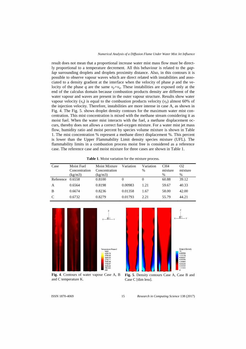
result does not mean that a proportional increase water mist mass flow must be direct-

ly proportional to a temperature decrement. All this behaviour is related to the gap-

lap surrounding droplets and droplets proximity distance. Also, in this contours it is

possible to observe vapour waves which are direct related with instabilities and asso-

ciated to a density gradient at the interface when the velocity of phase p and the ve-

locity of the phase q are the same vp=vq. These instabilities are exposed only at the

end of the calculus domain because combustion products density are different of the

water vapour and waves are present in the outer vapour structure. Results show water

vapour velocity (vq) is equal to the combustion products velocity (vp) almost 60% of

the injection velocity. Therefore, instabilities are more intense in case A, as shown in

Fig. 4. The Fig. 5. shows droplet density contours for the maximum water mist con-

centration. This mist concentration is mixed with the methane stream considering it as

moist fuel. When the water mist interacts with the fuel, a methane displacement oc-

curs, thereby does not allows a correct fuel-oxygen mixture. For a water mist jet mass

flow, humidity ratio and moist percent by species volume mixture is shown in Table

1. The mist concentration % represent a methane direct displacement %. This percent

is lower than the Upper Flammability Limit density species mixture (UFL). The

flammability limits in a combustion process moist free is considered as a reference

case. The reference case and moist mixture for three cases are shown in Table 1.

Table 1. Moist variation for the mixture process.

Case Moist Fuel

Concentration

(kg/m3)

Moist Mixture

Concentration

(kg/m3)

Variation Variation

%

CH4

mixture

%

O2

mixture

%

Reference 0.6558 0.8100 0 0 60.88 39.12

A 0.6564 0.8198 0.00983 1.21 59.67 40.33

B 0.6674 0.8236 0.01358 1.67 58.00 42.00

C 0.6732 0.8279 0.01793 2.21 55.79 44.21

Fig. 4. Contours of water vapour Case A, B

and C temperature K. Fig. 5. Density contours Case A, Case B and

Case C [dim less].

15



The fuel-oxygen mixture is produced by the turbulence induced in the methane-

oxygen stream at the outlet burner and the density difference between the central jet

and surroundings (mixture layer around the oxygen jet potential core). On one hand,

numerical predictions show a drag effect on methane jet by the oxygen flow because

the oxygen jet core has a greater amount of flow. The same behaviour is present in the

three cases. Therefore, for the most relevant zone to the species mixture is located

between the methane jets and oxygen stream where the flammability limits are

reached. The flammability limits are represented by a methane-oxygen mixture densi-

ty an optimal composition that is reached for combustion reaction. Since this global

mixture have 0.8% of moist, the global density mixture increases its value in 1.21% to

reach the UFL and the reaction zone is extended in the combustion chamber (repre-

sented through the iso-surfaces in Fig. 6). Whilst the reaction zone increases, the re-

circulation zones remain unchanged. But on the other hand, the drag effect and the

recirculation also affect the water mist flow. Besides the drag effect, the velocity con-

traflow product of the vortex has a direct impact on the jets momentum reducing the

velocity of the eight jets flow as the streamlines exhibit in Fig 7. For the three case the

most affected is the case A with a water mist velocity reduction in a 60%.

Considering two fluid regions, vp>vq. The fluid p has uniform velocity vp=10 m/s

while q vq= 4 m/s although the fluid injection V=10 m/s for both phases. The velocity

difference mentioned before is a direct consequence of the water vapour gap sur-

rounding every droplet as mentioned by Korlie [17]. This velocity gradient causes a

special offset between the mixture interfaces. It is assumed that the flow is inviscid at

Tpq<Tsat in this case Tpq<TReact where Tpq is the mean temperature between phases and

TReact is the mean exothermic reaction temperature. Therefore it can suffer a tangential

velocity discontinuity at the interfacial area concentration, 𝐴𝑝𝑖 and 𝐴𝑝𝑗 just before the

methane and oxygen potential cores. Those discontinuities are shown in Fig 8. Since

the velocity gradient is sufficient to inflict a shear at the fluid interface, is possible to

define a shear velocity or friction velocity.

Fig. 6. Iso-surfaces of mixture components Case

A, B and C.

Fig. 7. Streamlines and recirculation zones

Cases A, B and C.

16



Fig. 8. Contours of tangential velocity of

water mist phase [m/s].

Fig. 9: Contours of ush [dim less].

This kind of shear stress may be re-written in units of velocity. It is useful method

to compare true velocities, such as the velocity of a mist flow in a stream and the

shear between layers of flow and it is shown that in many case this velocity is

ush≈1/10 vp. Before the flickering zone the outer instabilities at the outer flame layer

are present. In most cases the inner instabilities are present within flame-mist layer.

The Fig. 9. demonstrates the instabilities by means of waves. The waves destabi-

lize the structure of the oxygen jet. The outer waves destabilize the vapour-

combustion products mixture structure. With the increment of mist flow the inner

waves tend to diminish and the outer instabilities tends to increase.

4 Conclusions

The vaporization starts in a zone near the flame front and vaporization Enthalpy direct

affects the micro droplet due to its proximity stablishing the relation less mass flow

equal to lager distance between droplets. Then, the vaporization energy needs to be

higher to reach all droplet surroundings which means a flame front temperature reduc-

tion. All this behaviour is related to the “gap-lap” surrounding droplets and droplets

proximity distance. Since the mean velocity of both phases are the same vp = vq, the

outer instabilities are intense by water vapour and combustion products mixing pro-

cess.

Furthermore, in a fuel moisture percentage less than 1%, the instabilities are con-

served within the flame structure. If the vaporization mist fraction increases, the in-

stabilities do not affect the internal structure where the methane-oxygen mixing pro-

cess occurs. However, these instabilities are transferred to the outer structure of the

flame by means of waves since the density variation between water vapour and com-

bustion products is emphasized. Even the methane-oxygen reaction zone increases its

value (distance) in a 68% is not a participant cause for any both kind of instabilities.

The direct mechanism for these instabilities is an intensified vaporization process

affecting directly the velocity of the water mist injection jets. Therefore, the vaporiza-

tion effect is the leading cause of both types of instabilities.

17



References

1. Fossi, M.: A Simple Model to Evaluate Direct Contact Heat Transfer and Flow Character-

istics in Annular Two-Phase Flow. International Journal of heat and mass flow vol. 16,

272–279 (1995)

2. Cioncollini, A., Thome J., Lombardi C.: Algebraic Turbulence Modelling in Adiabatic

Gas–Liquid Annular Two-Phase Flow. International Journal of Multiphase Flow vol. 35,

pp. 580–596 (2009)

3. Grech, N., Mehdi, A., Zachos, P. K., Pachidis, V., Singh, R.: Effect of Combustor Geome-

try on Performance of Airblast Atomizer Under Sub-Atmospheric Conditions. Engineering

Applications of Computational Fluid Mechanics vol. 6, pp. 203–213 (2012)

4. Cutrone, L., Ihme, M., Herrmann, M.: Modelling of High Pressure Mixing and Combus-

tion in Liquid Rocket Injectors. Center for Turbulence Research, pp. 269–281 (2006)

5. Smith J. J., Schneider G., Suslov D., Oschwald M., Haidn O.: Steady-State High Pressure

LOx/H2 Rocket Engine Combustion. Aerospace Science and Technology vol. 11, pp. 39–

47 (2007)

6. Lopez-Parra, F., Turan A.: Computational Study on the Effects of Non-Periodic Flow Per-

turbations on the Emissions of Soot and NOx in a Confined Turbulent Methane/Air Diffu-

sion Flame. Combustion Science and Technology 179 (7): 1361–1384 (2007)

7. Magnussen, B. F.: On the Structure of Turbulence and a Generalized Eddy Dissipation

Concept for Chemical Reaction in Turbulent Flow. AIAA Paper 1981-42 (1981)

8. De la Cruz, M., Polupan, G., Martínez, E., Carvajal, I.: Estudio Numérico del Efecto de la

Presión en el Proceso de Mezcla Metano-Oxígeno en un Arreglo de Chorros 4-Lug Bolt.

Información Tecnológica, CIT Chile, vol. 26, no. 2, pp. 153–162 (2015)

9. Dagan, Y., Arad, E., Tambour Y.: On the Dynamics of Spray Flames in Turbulent Flows.

In: Proceedings of the Combustion Institute vol. 35, issue 2, pp. 1657–1665 (2015)

10. Vicente, W., Salinas-Vázquez, M., Martinez, E., Rodriguez, A.: Numerical Simulation of a

Turbulent Lean, Premixed Combustion with an Explicit Algebraic Stress Model. J. Math.

and Statistics: 1, 86–90 (2005)

11. Lin, Z. Q., Wei, F., Jin, Y.: Numerical Simulation of Pulverized Coal Combustion and No

Formation. Chemical Engineering Science: 58, 5161–5171 (2003)

12. Herrmann, M.: Numerical Simulation of Turbulent Bunsen Flames with a Level Set

Flamelet Model. Combustion and Flame: 145, 357–375 (2006)

13. Shih, T.-H., Liou, W. W., Shabbir, A., Yang, Z., Zhu, J.: A New k-e Eddy-Viscosity Mod-

el for High Reynolds Number Turbulent Flows Model Development and Validation. Com-

puters and Fluids 24(3): 227–238 (1995)

14. Waterson, N.P., Deconinck, H.: A Unified Approach to the Design and Application of

Bounded Higher-Order Convection Schemes. In: Proceedings of the 9th International Con-

ference on Numerical Methods in Laminar and Turbulent Flow, Pineridge Press, Swansea,

p. 203, Atlanta (1995)

15. Gaskell, P.H., Lau, A.K.C.: Curvature-Compensated Convective Transport: Smart, a New

Boundedness-Preserving Transport Algorithm. International Journal for Numerical Meth-

ods in Fluids, Vol. 8, p. 617 (1988)

16. Leonard, B.P., Leschziner, M.A., McGuirk, J.: The QUICK algorithm: a uniformly 3rd-

order finite-difference method for highly convective flows. In: Numerical methods in lam-

inar and turbulent flow: proceedings of the first international conference, p. 807, Swansea,

(1978)

17. Korlie, M.S.: Three-Dimensional Computer Simulation of Liquid Drop Evaporation.

Computers and Mathematics with Applications 39, pp. 43–52 (2000)

18



Priority Data Transmission Schemes for a Wireless

Sensor Network on BAN

Sergio Martínez1, Mario Rivero2, Laura Garay1, Issis Romero1

1 Instituto Politécnico Nacional,

Unidad Profesional Interdisciplinaria en Ingeniería y Tecnologías Avanzadas,

CDMX, Mexico

2 Instituto Politécnico Nacional, Centro de Investigación en Computación,

CDMX, Mexico

[email protected], [email protected],

[email protected], [email protected]

Abstract. Among the most recurrent Wireless Sensor Network (WSN)

employment is the biopotential signals monitoring (e.g. electrocardiograms,

electroencephalograms, electrogastrograms) that allows transmitting the

body organ response from a person. Within the WSN’s focused on

bioelectrical studies, the energy analysis is essential indeed, given that

sensors are devices of minimal dimensions and implies batteries tend to be

small and have short-lifetime. In the present research we proposed two

priority schemes to enhance the network performance by giving transmission

priority to certain nodes. In a first scheme, nodes have different priorities

according to the data type they are reporting on. Hence, nodes that sense

more relevant data have higher priority to use the channel compared to nodes

reporting less important data. For the second scheme, the aim is to prolong

the system lifetime by assigning higher transmission probability to nodes

with higher residual energy levels while nodes with little energy left, perform

fewer transmissions. We show that the performance of the system is indeed

enhanced by the introduction of such schemes.

Keywords: Wireless Sensor Network (WSN), Body Area Network (BAN),

Cognitive Ratio (CR).

1 Introduction

Nowadays, the implementation of wireless and ambulatory technologies in medical

applications has important relevance [1]. Take into consideration, the multiple

areas joint effort to work on e-health applications, which primary goal is to increase

life quality of people. Within e-health, it is required the gauge of constant signals

emitted by the body. That is why tools are required that are capturing the electrical

measures generated by the human being. These are known as bioelectrical studies.

For biopotential signals monitoring, different solutions have emerged and an

alternative relies on wireless sensor networks [2].

However, based on [3] and [4] the WSN confront an inherent conflict that

intrinsically depends on batteries dimensions and capacities. In this context,

batteries require an important energy performance analysis given that life-battery 19

ISSN 1870-4069


mailto:[email protected]


is shorter than current energy systems [5]. Nevertheless, studies of network energy

behavior focus either on the adaptation of protocols [6], packet size optimization

[7] or materials properties analysis giving greater capacity [8]. The present research

proposed to design and simulate the energy performance of a WSN focused on the

study of biopotential signals.

We analyze that in practical applications two common situations are presented,

in one there are sensors that have priority over others because they are giving

attention to a specific body area, consequently exist nodes that have more

importance than others generating the priority based scheme. In other case, there

are medical applications where the aim is to extend the lifetime batteries as much

as possible. This second scheme requires an analysis of the remaining battery

energy giving rise to the residual energy based scheme.

2 System Design and Parameters Description

A wireless sensor network is a set of devices placed in a certain area capable of

performing basic operations, sensing and communicate with other sensors [9]. Let

both describe a bioelectrical potential as the representation of the ion flow through

the cell membrane and can be measured by invasive or non-invasive nodes for

nerves and muscles in the human body [10].

The proposed system is composed of a set of nodes in sensors that measure

bioelectrical signals assuming that all are placed in the body of a single person. The

intercommunication distance responds to less than 3.28 ft, thus the sensors work on

a body area network (BAN) [5] with e-health application. The system is designed

considering that any biopotential study cited in the table bellow can be transmitted.

Table 1. Most used bioelectrical studies [11].

Study Description Voltage Frequency(Hz)

ECG Electrocardiogram. Representation of heart electrical

signals 0.5–4 mV 0.01–250 Hz

EEG Electroencephalogram. Depiction of electrical signals

produced by the brain. 5–300 µV 150 Hz DC

EGG Electrogastrogram. It is the representation of the

electrical signals produced by the stomach. 10µV–1mV 1 Hz DC

EMG Electromyogram. Measures the electrical activity of

muscles. 0.1–5 mV 10 KHz

2.1 Communication Parameters

The following describes the general properties of the communication scheme used

in the network:

– The communication scheme or protocol is TDMA since it requires a minimum

hardware-software processing for its implementation and considers a

deterministic system assuring the information transmission of each node in its

respective slot.

– A hybrid network is understood in this project when it is used two different

kinds of networks. The primary network consists of sensors that transmit

continuously. On the other hand, the secondary network will transmit

sporadically (i.e. event monitoring) [12]. 20



– The cognitive radio in the communication system network design is presented

in the inclusion of on/off processes that, represent a method of modeling traffic

in stationary communications networks. To consider on/off processes, the

following premises must be considered:

• The nodes of the continuous monitoring network (primary network) will

be on for a specific period called time on.

• There will also be time periods for primary network nodes where they will

be ‘turned off’. In this sense, these periods are known as time off. When

primary network has some turned off node, the respective slot will be free

to transmit information that is generated from secondary network nodes. It

is very important to indicate that the sensors work all the time and implies

energy consumption at any time.

The communication protocol has as reference the work done in [12] and [13] where

both focus on epilepsy, however at the present design is open to any biopotential

study cited in Table 1.

3 Energy Analysis

There is clearly a great compromise between the information amount tolerance that

can be lost from continuous monitoring and the energy consumption reduction. We

estimate results for knowing in detail the network behavior and to carefully analyze

this dependence. We consider M as the number of slots for each frame.

To specify the quantitative analyzes, it is considered to evaluate the data in

specific values. Let the primary network be an electroencephalogram composed of

a set of 22 nodes. The secondary network will be monitoring a 4-channel

electrogastrogram. Thus: M = 22 nodes and ne = 4 event monitoring nodes

(secondary network nodes).

3.1 Energy Consumption And Packet Loss For WSN

In the primary network there are in total M nodes and the information will be

transmitted continuously. In this case, it is remembered that it is a deterministic

protocol so that each of the nodes of the electroencephalogram has a reserved slot

to transmit. However, when the on/off processes are included, there is a change in

the energy consumption derived from the on and off times. Therefore, the energy

in the primary network is analyzed through two cases:

– Case 1. The node is active. The node is on (i.e. slot is related to an on time) and

the usual energy transmission is taken. This energy will be evaluated by

E[tx] referring to the unit of energy consumption per packet transmission.

– Case 2. The node is in sleep mode. It refers to the node being switched off and

therefore not transmitting EEG information. However, when the sensor is on

(even if not send data), a certain amount of energy is being used which is much

smaller than the active node. The energy is determined by:

Es = 0.1E[tx], (1)

where

Es = Sleep node energy consumption, 21

Priority Data Transmission Schemes for a Wireless Sensor Network on BAN


E[tx] = Active node energy consumption.

The WSN performance is evaluated by variables E[tx] (for energy consumption)

and Packets (for system loss). In both cases, there is a probability that the packet

has been successfully transmitted. This is defined as the probability of successful

packet transmission.

The secondary network is based on the ne nodes occupied. In numerical terms,

for this analysis are four. In order to be able to relate the energy used by the primary

network.

However, the applications of bioelectrical studies are variable, depending on

the medical requirement, the analysis must be adapted. On the one hand, we have

the circumstance where the study has a set of nodes that monitor a specific area.

Consequently, the priority of some sensors is greater than the rest. In this way, the

communication and analysis scheme focuses on the priority that each sensor has.

In the other hand, there is a primordial interest on the network energy

optimization. In that case, it is much more convenient to modify the perspective so

that the analysis is applied on the lifetime of the batteries and their respective

residual energy.

3.2 Priority Based Scheme Model

There are scenarios where one sensor has more importance than the others. For

example, in an EGG, there is an area with greater gastric movement and takes

precedence over the rest. For this case, the first scheme based on priorities is

proposed.

This scheme considers an amount of M continuous monitoring nodes and ne

event-monitoring. In each frame, on and off time will be generated. When some

node in the primary network is off, then secondary network information can be

transmitted through one of the four nodes that monitor the stomach. Each of these

nodes will have an assigned priority. Only two priorities are presented: high or low.

To differentiate them, each of them will have an assigned transmission probability,

the one of high priority will be greater than the others. Therefore, it is proposed:

Transmission probability of high priority node = 0.85 and Transmission probability

of low priority node = 0.25.

Each node will have its own transmission probability determined by its

respective priority, so ρi represents the probability of transmission of an i-event

monitoring node. Based on the above, there will be three possible cases:

1 . One high priority node and three low priority nodes (ρ0 = 0.85, ρ1 = 0.25, ρ2 =

0.25 and ρ3 = 0.25)

2 . Two high priority nodes and two low priority nodes (ρ0 = 0.85, ρ1 = 0.85, ρ2 =

0.25 and ρ3 = 0.25)

3 . Three high priority nodes and only one low priority node (ρ0 = 0.85, ρ1 = 0.85,

ρ2 = 0.85 and ρ3 = 0.25)

It is necessary to indicate that the transmission probability of high or low

priority is independent of the probability of successful transmission of the

packet 22



3.3 Residual Energy Based Scheme Model

When nodes that are monitoring are equally important, all nodes can transmit with

the same priority. However, depending on the case, there are sensors that monitor

much more than others, so the battery-lifetime of these becomes shorter. In other

words, its efficiency and probability of sending the data will depend on how much

energy is available from the battery. In this way the residual energy scheme is

proposed. This second scheme shares the same basis as the priority scheme, it has

a primary network of M nodes and a secondary network composed of ne nodes. In

this case, we will consider a transmission probability dependent of the energy still

holding the battery for each sensors. This is called residual energy and is directly

related to the probability of transmission of each of the event-monitoring node.

ρi = γe−γE0/ER, (2)

where ρi = transmission probability for i-node, γ = Battery decay factor, E0 = Initial

battery energy, ER = Residual battery energy

It is again emphasized that the probability of transmission by residual energy is

independent of the probability of successful transmission ().

4 WSN Performance Simulations And Results

The network performance was applied by discrete event simulations. The results

will be display for the primary and secondary network divided into the two

proposed schemes (by priority and by residual energy). The scale for energy

consumption depends on lifetime battery of 1 ∗ 109E[tx].

All the graphs shown below are determined by the variables: PON which

represents the on time probability per frame and which indicates the probability

that an event is successfully transmitted.

4.1 Priority Based Scheme Model

Fig.1. Primary Network Energy consumption (active nodes). 23



Fig.2. Primary Network Energy consumption (sleep mode nodes).

In these first figures it is possible to show the behavior of the primary network

respect to the energy consumption for active and sleep nodes. These graphs show

the three possible cases identified in section 3.2. Specifically, it can be considered

that as the on time probability increases, the amount of energy consumption

increases. It can also be denoted that for the minimum turned-on time and a

maximum probability of successful packet transmission, the scheme that has three

high priority nodes and one low one presents the least amount of energy consumed.

It is important to remind that Case 1: ρ0 = 0.85, ρ1 = 0.25, ρ2 = 0.25 and ρ3 = 0.25,

Case 2: ρ0 = 0.85, ρ1 = 0.85, ρ2 = 0.25 and ρ3 = 0.25 and Case 3: ρ0 = 0.85, ρ1 = 0.85,

ρ2 = 0.85 and ρ3 = 0.25

Fig.3. Secondary Network Total Energy Consumption.

For the secondary network it can be seen that the system has a maximum energy

consumption when the on time is very low and the probability of successful

transmission is high. Although within the three cases, the scheme of three high

priority and one low node is the one that requires the maximum energy

consumption, so this scheme is not optimum when there is a large amount of

monitoring per event. 24



Fig.4. Network Packet Loss (non reported packets).

In the subsequent figure, it can be seen the loss of packets due to a lack of

reporting (i.e., not falling into the probability of transmission by priority, they are

not transmitted.) In this sense, it can be denoted that the maximum number of lost

packets are when there is only one high priority sensor.

4.2 Residual Energy Based Scheme

Fig.5. Primary Network Energy consumption (active nodes).

Fig.6. Primary Network Energy consumption (sleep mode nodes). 25



In these figures we present a behavior quite similar to the system by priorities,

where at greater on time probability, successful transmission of more packets is

shown and the energy used in active nodes is greater. However, unlike the priority

scheme, the energy consumption for this network is lower.

Fig.7. Secondary Network Total Energy Consumption.

The secondary network in this case shows a considerable difference with

respect to the decay factor of the battery, where the higher the factor, the higher the

energy consumption obtained by the secondary network.

Fig.8. Network Packet Loss (non reported packets).

Regarding the loss of packets, it can be denoted that the behavior for the

different battery decay factor is practically the same, where the greatest loss occurs

when there is the maximum information transmission request and the minimum

amount of on time probability. It should be considered that the packet loss here

involves the packets of the primary network.

5 Conclusions

In the present research a WSN focused on biopotential studies was proposed that

works with TDMA deterministic protocol and uses cognitive radio through on/off 26



processes to reduce the number of slots used on each frame. Energy performance

was evaluated through two schemes: priorities based scheme where sensors have

different importance (some body parts are more important than the others) and

residual energy scheme where the aim is to decrease the battery energy

consumption. The network is represented by discrete event simulations.

Therefore, a priority scheme can be considered to generate lower energy

consumption in the primary network, more variable consumption in the secondary

network but more losses than the residual energy scheme. If the application requires

few monitoring per event, it is advisable to use a scheme based on priorities,

otherwise the residual energy scheme is recommended.

References

1. Nakajima, T.: Aspects of Information Communications Technology for Better Medical

Control, International Journal of E-Health and Medical Communications (IJEHMC).

1, 18–27, (2010)

2. Mahmoudi, R., Inievski, K.: Low power emerging wireless technologies, 2, CRCPress,

(2012)

3. Dargie, W., Poellabauer, C.: Fundamentals of Wireless Sensor Network. Chichester:

John Wiley & sons Ltd, p. 34, (2010)

4. Castillejo, P., Martínez, J., Rodríguez, M.: Integration of wearable Devices in a

wireless sensor network for an e-health application. Institute of Electrical and

Electronics Engineers, 13, 38–49 (2013)

5. Shaikh, A., Pathan, S.: Research on Wireless Sensor Network Technology.

International Journal of Information and Education Technology, 2, 476–479 (2012)

6. Chatzigiannakis, I., Kinalis, A., Nikoletseas. S.: Wireless sensor networks protocols

for efficient collision avoidance in multi-path data propagation. In: Proceedings of the

1st ACM international workshop on Performance evaluation of wireless ad hoc,

sensor, and ubiquitous networks (PE-WASUN ’04), ACM, 8–16 (2004)

7. Sankarasubramaniam, Y., Akyildiz, I., McLaughlin, S.: Energy Efficiency Based

Packet Size Optimization. In: Wireless Sensor Networks IEEE International

Workshop on Sensor Network Protocols and Applications, 1–8 (2003)

8. Rodriguez, J.: Digital Advances in Medicine, E-health, and communication

technologies. Digital: IGI Global, p. 12 (2013)

9. Dargie, W., Poellabauer, C.: Fundamentals of Wireless Sensor Network. JohnWiley &

sons Ltd: Chichester, p. 24 (2010)

10. Ganong, W.: Review of Medical Physiology. McGrawHill: New York, p. 576 (2005)

11. Enderle, J., Blanchard, S., Bronzino, J.: Introduction to biomedical engineering.

Elsevier academic press: California, p. 323 (2004)

12. Martinez, S., Rivero, M., Garay, L.: Design of hybrid wireless sensor network to

monitor bioelectric signals focused on the study of epilepsy. Research in Computing

Science, 75, 43–49 (2014)

13. Martinez, S., Rivero, M., Garay, L.: Performance Analysis of Preemptive and Non-

Preemptive Schemes in Hybrid Wireless Sensor Networks focused on the study of

epilepsy. Research in Computing Science, 101, 29–42 (2015)

27



Modelo foveal rectangular a partir de un sensor de

imagen comercial


Instituto Politécnico Nacional, Sección de Estudios de Posgrado e Investigación,

ESIME Culhuacan, México


Resumen. Este trabajo propone la implementación del modelo foveal tipo rec-

tangular a la imagen generada en un sensor convencional. La principal proble-

mática en los sensores foveales basados en el modelo log polar es que cada foto-

sensor está diseñado con geometrías y tamaños diferentes. Los sensores conven-

cionales tienen una distribución de M por N pixeles en un arreglo rectangular, en

tanto que en los modelos foveales, los elementos de imagen se encuentran distri-

buidos en círculos concéntricos. El diseño de cada sensor debe ser específico de

acuerdo a la aplicación que se requiera. Esto ocasiona una limitación en el desa-

rrollo de sistemas con distintas configuraciones de retinas, debido a que es nece-

sario cambiar los diseños para diferentes aplicaciones con el respectivo análisis.

La propuesta consiste en una nueva estrategia para generar una imagen foveal

desde un sensor de imagen convencional, que utiliza un algoritmo de transforma-

ción log polar en un modelo rectangular, donde se promedian los valores de los

elementos fotosensores vecinos en una regla de crecimiento geométrico. Los re-

sultados muestran las imágenes obtenidas desde un sensor de imagen comercial,

aplicando el algoritmo de transformación log polar a un esquema de rectángulos

circunscritos con crecimiento geométrico.

Palabras clave: modelo foveal, modelo log polar, sensor de imagen, visión fo-

veal.

Foveal Rectangular Model from a

Commercial Image Sensor

Abstract. This work proposes the implementation of the rectangular model fo-

veal to the image generated in a conventional sensor. The main problem in foveal

sensors based on the log polar model is that each photosensor is designed with

different geometries and sizes. Conventional sensors have a distribution of M by

N pixels in a rectangular array, whereas in foveal models, the elements of ima-

gen are distributed in concentric circles. The design of each sensor must be spe-

cific according to the application that is required. This causes a limitation in the

development of systems with different configurations of retinas, because it is ne-

cessary to change the designs for different applications with the respective

29

ISSN 1870-4069


analysis. The proposal consists of a new strategy to generate a foveal image from

a conventional image sensor, which uses a log polar transformation algorithm in

a rectangular model, where the values of the neighboring photo-sensor elements

are averaged in a geometric growth rule. The results show the images obtained

from a commercial image sensor, applying the log polar transformation algorithm

to a scheme of circumscribed rectangles with geometric growth.

Keywords: foveal model, log polar model, image sensor, foveal vision.

1. Introducción

El modelo foveal está inspirado en los sistemas de visión de los animales debido a

que se trata de emular el comportamiento de la retina biológica, basándose en la distri-

bución geométrica de las células fotorreceptoras en humanos o animales [1,2,3]. En la

retina biológica se tiene la mayoría de los fotorreceptores concentrados en la zona fo-

veal y disminuyen en número en dirección a la periferia [4,5,6]. Esta organización de

los fotorreceptores tiene propiedades significativas debido a la variación en la resolu-

ción en el campo visual. A esto se le conoce como visión espacio-variante [5,7]. Existen

numerosos estudios en que han desarrollado sensores con estructuras foveales, desta-

cando la tecnología CMOS debido a sus capacidades y calidad en resolución [6,7,8].

Sin embargo, el diseño y fabricación de este tipo de sensores aún tienen problemas que

deben ser resueltos.

Aunque algunos autores han sugerido una aplicación ingeniosa en VLSI, éstas aún

requieren un proceso de fabricación no estándar [7,8]. Pardo et al. presentaron el diseño

de un sensor foveal CMOS utilizando ajustes en la geometría de cada fotosensor de

acuerdo a la ubicación desde el centro hasta la periferia, utilizando una rotación de ejes,

los cuales, van creciendo en tamaño en los diferentes niveles de la fóvea para producir

corrientes fotogeneradas proporcionales al área de incidencia [7,8,9]. Sin embargo, ésta

se debe compensar debido al crecimiento de los sensores. Nuevas soluciones se encuen-

tran en la literatura especializada que proponen la construcción de elementos de detec-

ción de tipo logarítmico para compensar dichos problemas [4,5,7,8].

F. Pardo, B. Dierickx, D. Schaffer, F Paillet y P. Zeferino analizaron en detalle el

procedimiento de diseño de una celda básica para un fotodiodo con tecnología CMOS

[7,8,9,10]. El Patrón de Ruido (FPN), debido al factor de escala en la fabricación y los

efectos de canal angosto, es un gran reto que todavía no está resuelto. Pardo et al. pro-

ponen reducir el FNP generado por la escala de diseño, utilizando una estructura carte-

siana de píxeles para la región de mayor resolución y posteriormente una transforma-

ción log polar en la región periférica. P. Pardo muestra una transformación de ejes car-

tesianos para rotar los polígonos [7]; sin embargo, al momento de realizar el diseño de

todo el sensor, es necesario construir un modelo de anillos concéntricos con un factor

de escalamiento geométrico. Es por ello que sería necesario rotar la célula básica y

escalarla, (figura 1). El modelo foveal representa la base de los sistemas de visión fo-

veal; sin embargo, el problema principal para poder llevar diversos análisis de estruc-

turas foveales, representa el inconveniente de su fabricación.

30



Fig. 1. Diseño de una celda básica de fotodetección. a) Celda original con sus líneas de acceso.

b) Rotación establecida para el campo receptivo, en la que se muestran los ejes modificados [7].

2. El modelo foveal

El modelo foveal es una transformación matemática de una imagen desde un plano

polar a un plano rectangular a través de un mapeo logarítmico y luego regresarla para

su interpretación. La representación log-polar [7,8,11,12,13] es el mapeo de puntos del

plano polar o también llamado plano retínico (ρ, η) a un plano complejo logarítmico,

nombrado plano cortical (ξ, γ).

De acuerdo con [11,14], la imagen foveal es, en resumen, una representación en un

plano discreto de la transformación log-polar. Esto es, una imagen es representada en

coordenadas rectangulares de acuerdo con:

𝑧 = 𝑥 + 𝑗𝑦, (1)

𝑧 = 𝜌𝑒𝑗𝜂, (2)

donde:

𝜌 = √𝑥2 + 𝑦2, (3)

𝜂 = 𝑡𝑎𝑛−1 (𝑦

𝑥). (4)

Por lo que las coordenadas x, y se pueden expresar como:

𝑥 = 𝜌 𝐶𝑜𝑠(𝜂), (5)

𝑦 = 𝜌 𝑆𝑒𝑛(𝜂). (6)

Lo anterior representa la ubicación de un elemento de imagen en el plano rectangu-

lar. Cualquier pixel queda perfectamente ubicado bajo estas coordenadas. De la inves-

tigación de Volker Krüger, una imagen cortical quedaría representada a través de un

mapeo al plano logarítmico complejo por la siguiente regla de correspondencia:

31

Modelo foveal rectangular a partir de un sensor de imagen comercial


𝑤 = 𝑙𝑛(𝜌𝑒𝑗𝜂). (7)

El origen del plano x-y no se puede mapear por la singularidad presentada en ρ=0.

Por lo que es necesario definir un intervalo muy cercano al origen de la imagen. La

representación de la imagen tiene un crecimiento geométrico o exponencial, por lo que

se utiliza un logaritmo arbitrario de base “a” [14]. Así, para el mismo punto de ima-

gen z:

𝑧 = 𝜌 𝑎𝑗𝜂 . (8)

La base “a” es la contraparte del factor de magnificación cortical. Entonces:

𝑤 = log𝑎(𝜌) + 𝑗𝜂. (9)

Para realizar el proceso de visión por computadora o utilizar un procesador digital,

los componentes radiales y angulares deberán ser digitalizados. Por ello se consideran

las siguientes coordenadas: ξ = Componente radial, γ = Componente angular.

Las variables Nr y Na definen la resolución máxima radial y angular del plano log

polar, respectivamente. El mapeo de las coordenadas polares (ρ, η) a las coordenadas

(γ, ξ) en el plano log polar, está dada por [14]:

𝜉 = log𝑎 (𝜌

𝜌0) , (10)

𝛾 =𝑁𝑎

2𝜋(𝜂 +

𝜋

2). (11)

La figura 2 muestra una representación de la transformación con las coordenadas de

(10) y (11). El plano cortical aún sigue siendo un plano rectangular en donde queda

representada la imagen en coordenadas logarítmicas. Para obtener la representación fo-

veal de dicha imagen, es necesario obtener la transformación inversa, que es en reali-

dad, la transformación log polar. Las coordenadas se definen como:

𝑥 = 𝜌0𝑎𝜉𝐶𝑜𝑠(𝜂), (12)

𝑦 = 𝜌0𝑎𝜉𝑆𝑒𝑛(𝜂), (13)

donde los valores de las coordenadas quedan en un intervalo de 0 ≤ 𝜉 ≤ 𝑁𝑟, 0 ≤ 𝛾 ≤𝑁𝑎. De igual manera, en [13,14], se establece lo siguiente:

𝜌0𝑎𝑁𝑟 = 𝜌𝑚𝑎𝑥 , (14)

donde es posible observar que el tamaño de la imagen transformada queda relacionado

por el factor “a”. La forma de la ecuación es una función de crecimiento geométrico.

3. Metodología

En este trabajo se discute la manera de utilizar la transformación log polar para ge-

nerar un modelo rectangular e implementarlo desde un sensor de imagen comercial.

32



Así, cualquier elemento de fotodetección queda especificado por un pixel, llamado

celda básica, (figura 2). La propuesta consiste en realizar agrupaciones de celdas bási-

cas para hacer crecer zonas de incidencia hacia la periferia. La distribución en un plano

polar (figura 2a.) queda determinada por medio de campos receptivos. Así, al colocar

agrupaciones de celdas básicas, éstas pueden cubrir áreas completas si se realiza una

distribución rectangular o cuadros concéntricos. Los campos receptivos se presentan

como rectángulos con crecimiento geométrico.

Una primera evaluación consiste en superponer el conjunto de celdas rectangulares

sobre la estructura polar, generando diferentes zonas blancas sobre el plano polar. Sin

embargo, las zonas blancas decrecen cuando se trata de rectángulos concéntricos. Este

nuevo enfoque reduce las zonas blancas y produce una mejor distribución sobre el di-

seño.

Las trayectorias rectas concéntricas en la figura 2-b se mueven gradualmente hacia

la periferia siguiendo el modelo log polar conocido. Lo relevante es que la ubicación

de cada celda básica sigue las ecuaciones (12) y (13) haciendo posible reorganizar los

pixeles de una imagen en una nueva estructura foveal, pero rectangular. Esta agrupa-

ción respeta el modelo espacio-variante del sensor foveal estudiado. El ajuste se realiza

utilizando asociaciones de elementos de imagen siguiendo una función polinomial:

𝑓(𝑘) = 𝑏𝑘, (15)

donde “b” es la base en la que se trabaja la serie y “k” equivale al número de capas o

niveles en los que dividirá la imagen foveal.

En esta propuesta, se establece la base 2, debido a que las asociaciones serán en

grupos de dos, cuatro o más celdas básicas, como se puede observar en la figura 2-b.

Este nuevo modelo es equivalente al modelo log polar convencional, ya que las

trayectorias se extienden por la misma ley de crecimiento geométrico de los círculos de

la estructura espacio-variante. Es importante mencionar que la ley de crecimiento de

las celdas que componen cada rectángulo circunscrito en la nueva distribución foveal

está controlada por el Factor de Crecimiento S.

De acuerdo con (14) y (15), se propone que, el elemento de imagen más pequeño se

designa como W0, el cual tiene un crecimiento geométrico rectangular con un factor de

crecimiento S. El tamaño del i-ésimo elemento de imagen está dado por:

𝑊𝑖 = 𝑆𝑖𝑊0. (16)

Por lo que el tamaño semi radial del sensor será:

𝑟𝑑 = ∑ 𝑊𝑖𝑁𝑖=0 , (17)

𝑟𝑑 = 𝑊0 (𝑆𝑁+1−1

𝑆−1), (18)

donde N es el número de capas del modelo foveal. Sin embargo, si se toma como centro

el elemento mínimo de imagen, se presentará una singularidad (cuando S=1). Es por

ello, que se deberá tomar lo siguiente:

𝑟𝑑𝑚𝑎𝑥 = 𝑟𝑑0 + 𝑊0 (𝑆𝑁+𝑆−2

𝑆−1), (19)

33



rdmax queda determinado por la suma del radio del elemento mínimo de imagen ubicado

en el centro más el radio (rd) de todo el sensor. Cada elemento rectangular de tamaño

Wi queda representado en el plano rectangular, como se observa en la figura 3.

Fig. 2. Correspondencia entre un modelo de círculos concéntricos y uno rectangular. En (a) se

muestra la distribución de celdas básicas en los diferentes anillos. En (b) se puede observar una

propuesta de distribución de celdas en un formato rectangular basado en agrupaciones de acuerdo

al área de incidencia.

La magnitud de W0 tiene valores reales positivos que dependen de la tecnología de

fabricación para el fotodetector o simplemente adquieren valores enteros positivos

cuando se trata de una imagen en pixeles. El crecimiento geométrico de los elementos

de imagen, sirve de base para la transformación de la imagen original en un modelo

polar, visto desde un plano rectangular.

Una vez definida la celda básica, es posible generar toda la retina y la fóvea en una

matriz concéntrica rectangular distribuyendo los pixeles. Los fotorreceptores están re-

presentados con cuadros distribuidos en polígonos concéntricos alrededor del centro

del sensor cuya separación aumenta de forma exponencial. Lo anterior posibilita que

cualquier circuito de fotodetección sea una celda básica, evitando una rotación de ejes

en el diseño de la estructura.

La figura 4 representa la forma de agrupar los elementos de imagen para llevar a

cabo la distribución foveal de la imagen. La selección de filas y columnas es necesaria al

tratarse de un arreglo matricial; sin embargo, la línea de selección de “anillo” es fundamental

34



para seleccionar un contorno cuadrado similar a los anillos o circunferencias en una repre-

sentación polar.

Fig. 3. Representación de la transformación por agrupación de celdas utilizando el modelo rec-

tangular.

Fig. 4. Estructura del modelo foveal rectangular donde las coordenadas X, Y son para seleccio-

nar cada pixel. La variable r representa la manera con la cual se agrupan los elementos de ima-

gen.

35



El modelo conecta celdas básicas formando un contorno. Por ejemplo, la celda bá-

sica central es individual y se selecciona mediante las líneas (r0, X2, Y2). El contorno

siguiente puede seleccionarse mediante (r1, X1-X2-X3, Y1-Y2-Y3), lo anterior signi-

fica que se pueden generar las siguientes coordenadas para seleccionar cada una de las

celdas (r1, X1, Y1), (r1, X2, Y1), (r1, X3, Y1), etc. Para el siguiente contorno, se realiza

de la misma manera (r2, X0-X1-X2-X3-X4, Y0-Y1-Y2-Y3-Y4).

4. Resultados

El modelo propuesto presenta que es posible realizar agrupaciones de celdas con el

objeto de tener áreas de incidencia mayores sin modificar el tamaño del pixel. La salida

será la suma de las corrientes fotogeneradas o del valor promedio de los pixeles en las

celdas agrupadas. De acuerdo con (18) y (19) y considerando el elemento mínimo igual

1 y 480 como el máximo, se obtienen los valores correspondientes al Factor de Creci-

miento S, (figura 5).

Fig. 5. Gráfica del número de capas (resolución en pixeles) contra el factor de crecimiento (es-

calamiento).

Al aproximarse a los 480 pixeles el factor de crecimiento varía muy poco. Aplicando

el procedimiento a las imágenes de prueba es posible obtener una imagen foveal como

se muestra en la figura 6.

El valor de N=240 se toma como un valor máximo de acuerdo a la resolución de la

imagen original que es de 480 pixeles. Las figuras en 6(a) son imágenes tomadas por

un sensor de imagen comercial OV7670 con una resolución de 640x480 pixeles. Desa-

rrollando el procedimiento de transformación foveal rectangular (figura 3 y 4), es posi-

ble observar que se mantiene una alta resolución en el centro de la imagen y que decrece

hacia la periferia.

El cuadro blanco en el centro de la imagen se debe a que se consideró como el ele-

mento más pequeño a un grupo de pixeles para conformar la fóvea; sin embargo, eso

no es necesario ya que es completamente viable considerar a un pixel como el elemento

0

1

2

3

4

1

31

61

91

12

1

15

1

18

1

21

1

24

1

27

1

30

1

33

1

36

1

39

1

42

1

45

1

48

1Factor de Crecimiento

36



básico de imagen. Lo anterior se puede observar en la primera figura foveal, en la que

el cubo tiene un intervalo de área central de pixeles.

Fig. 6. Transformación Foveal Rectangular. a) Imágenes originales tomadas del sensor comer-

cial. b) Imágenes que han sido transformadas siguiendo la estructura de la figura 4.

Fig. 7. Conversión foveal rectangular con una imagen tomada desde el sensor OV7670 con una

resolución de 640x480 pixeles. (a) S=10, N=120. (b) S=10, N=240. (c) S=50, N=120. (d) S=50,

N=240. (e) S=100, N=120. (f) S=100, N=240.

37



El valor se toma considerando un pixel a la derecha e izquierda de un punto central.

De igual manera, un pixel superior e inferior. Debido al escalamiento, esto se ve refle-

jado en un cuadro blando notorio en el centro de la imagen. Para la imagen inferior,

solo se tomó un pixel como intervalo central. Nótese que el área blanca se encuentra

reducida.

Las imágenes de la figura 7, muestran el efecto con diferentes valores de S y un valor

constante del número de capas en 120 y 240.

5. Conclusiones

Los resultados muestran que la estructura propuesta basada en fotosensores rectan-

gulares funciona correctamente para implementar sensores de visión foveal a partir de

estructuras de sensores convencionales. Este nuevo enfoque de los sensores foveales

preserva las propiedades de la transformada log polar. Además, es posible trabajar con

diseños VLSI convencionales y sin requisitos previos de fabricación de sensores están-

dar. Por el contrario, los chips foveales (que son de fabricación no estándar) son una de

las razones que han dificultado la aplicación en la visión foveal. Este modelo puede

aplicarse a nuevos chips fóveales dedicados basados en fotodiodos, fototransductores

CMOS convencionales o fototransistores.

La celda básica puede ser cualquiera que haya sido empleada en diferentes modelos

retinales, estableciendo un modelo foveal ortogonal con cuadros concéntricos y agru-

pación de elementos de imagen del mismo tipo sin realizar ninguna transformación de

ejes. El punto clave es asegurar que esas estructuras sean capaces de tener un acceso

independiente a cada píxel a través de una lógica de control apropiada.

La transformación log polar a través de software dedicado ha visto una aplicación

limitada debido a los tiempos de transformación y procesamiento impuestos por la ló-

gica de programación. El modo de transformación propuesto en este artículo, que utiliza

un espacio variable rectangular, permite realizar la transformación foveal directamente

sin llevar a cabo una transformación previa cortical y así obtener de forma directa una

reducción en la cantidad de información que podrá ser procesada posteriormente.

Referencias

1. Palanker, D., Vankov, A., Huie, P., Baccus, S.: Design of a high resolution optoelectronic

retinal prosthesis. Department of Ophthalmology and Hansen Experimental Physics Labor-

atory, Stanford University, Institute of Physics Publishing 2 S105–S120 (2002)

2. Weber, C., Trisch, J.: Implementations and Implications of Foveated Vision. Recent Patents

on Computer Science 2, 75–85 (2009)

3. Bolduc, L.: A review of biologically motivated space variant data reduction models for ro-

botic vision. Computer Vision and Image Understanding, vol. 69, 170–184 (February 1998)

4. Traver, V. J., Pla, F.: Designing the lattice for log-polar images. Discrete Geometry for com-

puter Imagery, Proceedings, vol. 2886, 164–173 (2003)

5. Melnyk, P.: Biologically Inspired Composite Image Sensor for Deep Field Target Tracking.

Thesis. University of New Hampshire.

38



6. Niño-de-Rivera, L., Calzada Salas, R., Duchen Sánchez, G., Loaiza Brito, J.A.: Visual Sim-

ulation of Retinal Images Through Microstructures. Microelectronic Engineering. Vol. 90,

pp. 159–162 (2012)

7. Pardo, F., Dierickx, B., Scheffer, D.: Space-Variant Nonorthogonal Structure CMOS Image

Sensor Design. IEEE Journal of Solid-State Circuits, Vol. 33, No. 6 (June 1998)

8. Pardo, F., Dierickx, B., Scheffer, D.: CMOS foveated image sensor: Signal scaling and small

geometry effects. IEEE Transactions on Electron Devices, Vol. 44, No. 10 (October 1997)

9. Paillet-Damien, F., Thierry, M., Bernard, M.: Second Generation Programmable Artificial

Retina. CTA/GIP ENSTA/LEI. 32. 75015 Paris, France (2000)

10. Zeferino-Tomas, P. F.: Bio-Inspired Processing Module for the development of an artificial

retina. Universidade Tecnica de Lisboa. Instituto Superior Tecnico. Licenciatura em Engen-

haria Electrotecnica e de Computadores. Relatorio de Trabalho Final de Curso 157/2002/M

(Setembro de 2003)

11. Pardo-Carpio, F.: Sensor Retínico Espacio Variante basado en Tecnología CMOS. Tesis.

Departamento de Informática y Electrónica Universidad de Valencia (24 de septiembre de

1997)

12. Christos-Savvas, D. B.: Reconfigurable Foveated Active Vision System. In: 3rd Interna-

tional Conference on Sensing Technology, Taiwan (2008)

13. Javier-Traver, V., Bernardino, A.: A review of log-polar imaging for visual perceptions in

robotics. Robotics and Autonomous Systems 58 (2010)

14. Volker, K.: Optical Flow Estimation in the Complex Logarithmic Plane. Instituts für In-

formatik und Praktische Mathematik der Christian Albrechts Universität zu Kiel (1995)

39



Computational Intelligence Algorithms Applied to the

Pre-diagnosis of Chronic Diseases

Mariana Dayanara Alanis-Tamez1, Yenny Villuendas-Rey2,

Cornelio Yáñez-Márquez1

1 Instituto Politécnico Nacional, Centro de investigación en Computación,

Mexico

2 Instituto Politécnico Nacional, Centro de Innovación y Desarrollo Tecnológico en Cómputo,

Mexico

Abstract. Classification models applied to medicine have become an increasing

area of research worldwide. Such as, the application and development of known

models and algorithms for disease diagnosis and prediction have been an active

research topic. The present article is a study of the classification algorithms

most used in the literature, and its application to the diagnosis of chronic dis-

eases. More specifically, we tested five classification models, over medical da-

ta. The application of the supervised classification algorithms is done over the

Knowledge Extraction based on Evolutionary Learning (KEEL) environment,

using a Distributed optimally balanced stratified 5-fold cross validation scheme.

In addition, the experimental results obtained were validated to identify signifi-

cant differences in performance by mean of a non-parametric statistical test (the

Friedman test). The hypothesis testing analysis of the experimental results indi-

cates which supervised classification model outperforms others for medical di-

agnosis.

Keywords: classification models, medical informatics, disease prediction and

diagnosis, computational intelligence.

1 Introduction

For medical diagnosis, computational applications have been developed mainly in two

principal areas: algorithm development and system development for supporting diag-

nosis. Among others, several web-based systems, as well as tools for telediagnosis

and telemedical devices can be mentioned [1, 2, 3].

Chang et al. [1] developed a Web-based decision support system that considers the

sensitivity analysis as well as the optimal prior and posterior decisions applied for

some chronic diseases. The purpose of their work is to review several approaches and

to develop a Web-based decision support system (DSS).

Sanchez-Santana et al. [2] introduced another computational approach for medical

diagnosis. They propose a new telediagnosis environment for the detection of cardio-

vascular problems and allows medical staff to semi-automatically identify and quanti-

fy a patient's potential cardiovascular complications.

41

ISSN 1870-4069


In addition, Havlik et al [3] propose a solution for remote monitoring, rapidly de-

veloping devices for telemedical applications and assistive technologies. The ap-

proach used was to design and realize a modular system consisting of input modules

for signal acquisition, a control unit for signal pre-processing, handshaking of data

communication, controlling the system and providing the user interface and commu-

nication modules for data transmission to a superordinate system.

In this paper, for assisting medical diagnosis, several algorithmic solutions have

been proposed in recent years (section 2). We study the different classification algo-

rithms most used in the literature, and its application to the diagnosis of chronic dis-

eases (section 3). The different datasets have: imbalanced data, mixed categorical and

numerical attributes, and missing values. In addition, we used 15 medical related da-

tasets (section 4) to test all the classification models and the numerical experiments

performed in the comparison between the different classification algorithms applied

to the medical diagnosis. Finally, we offer the conclusion and some lines of future

work (section 5).

2 Background

For medical diagnosis, several algorithmic solutions have been proposed in recent

years.

Aiping Lu et al. [4] used pattern classification as a guideline in disease classifica-

tion in Traditional Chinese medicine (TCM) practice and has been recently incorpo-

rated with biomedical diagnosis. They describe the historical evolution on the integra-

tion of the TCM pattern classification and disease diagnosis in biomedicine, the

methodology of pattern classification for diseases

Timothy J. W. Dawes et al. [5] used a machine-learning survival model that uses

three-dimensional cardiac motion which predicts outcome independent of conven-

tional risk factors in patients with newly diagnosed pulmonary hypertension. It is used

to determine if patient survival and mechanisms of right ventricular failure in pulmo-

nary hypertension could be predicted by using supervised machine learning of three-

dimensional patterns of systolic cardiac motion.

Yu Sun et al. [6] used the performance of a support vector machines (SVM) algo-

rithm to predict prostate tumor location using multi-parametric MRI (mpMRI). They

used a Gaussian kernel SVM which was trained and tested on different patient data

subsets. Parameters were optimized using leave-one out cross validation.

Fazekas [7] addressed the examination of the periodicity of the childhood leukemia

in Hungary using seasonal decomposition time series. The dataset used was from the

Hungarian Pediatric Oncology Workgroup, and contained the data of all the patients

with lymphoid leukemia diagnosed between 1988 and 2000. These data highlight the

role of the environmental effects, like viral infections, epidemics, among others on the

onset of the disease.

To sum up, Zheng et al. proposed a data informed framework for identifying sub-

jects with and without Type 2 Diabetes Mellitus from Electronic Health Records via

feature engineering and machine learning [8]. The objective of this work is to develop

42

Mariana Dayanara Alanis-Tamez, Yenny Villuendas-Rey, Cornelio Yáñez-Márquez


a semi-automated framework based on machine learning as a pilot study to liberalize

filtering criteria to improve recall rate with a keeping of low false positive rate.

3 Datasets and Algorithms

In this section, a summary of the classification algorithms applied and the datasets

related to medical diseases are presented.

3.1 Datasets Related to Medical Diseases

The used datasets include information about different diseases, such as breast cancer,

thyroid diseases, heart diseases, liver disorders, diabetes, and others, all related to

mainly with chronic diseases. The datasets used in this paper were taken from online

information provided by KEEL dataset repository [9]. We used the medical related

standard classification datasets.

In the following, a description of each of the datasets used is shown.

Breast Cancer dataset: It is one of three domains provided by the Oncology Insti-

tute, which has repeatedly appeared in the machine learning literature. This dataset

has two classes, 201 instances of one class and 85 instances of another class. The

instances are described by nine attributes, some of which are linear and some are

nominal.

Liver Disorders (BUPA) dataset: It analyzes some liver disorders that might be-

cause of the excessive alcohol consumption. The objective is to select if a given indi-

vidual suffers from alcoholism.

Heart Disease (Cleveland) dataset: It is a part of the Heart Disease Dataset (the part

obtained from the V.A. Medical Center, Long Beach and Cleveland Clinic Founda-

tion), using a subset of 14 attributes. The objective is to detect the presence of heart

disease in the patient.

Haberman's Survival dataset: It contains cases from a study that was conducted be-

tween 1958 and 1970 at the University of Chicago's Billings Hospital on the survival

of patients who had undergone surgery for breast cancer. The objective is to deter-

mine if the patient survived 5 years or longer (positive) or if the patient died within 5

years (negative).

Statlog (Heart) dataset: The objective is to detect the absence or presence of heart

disease.

Hepatitis dataset: It contains a mixture of integer and real valued attributes, with

information about patients affected by the hepatitis disease. The objective is to predict

if these patients will die or survive.

Mammographic Mass dataset: It can be used to predict the severity (benign or ma-

lignant) of a mammographic mass lesion from BI-RADS attributes and the patient's

age. The data was collected at the Institute of Radiology of the University Erlangen-

Nuremberg between 2003 and 2006.

Thyroid Disease (New Thyroid) dataset: It is one of the several databases about

Thyroid available at the UCI repository. The objective is to detect is a given patient is

normal or suffers from hyperthyroidism or hypothyroidism.

43

Computational Intelligence Algorithms Applied to the Pre-diagnosis of Chronic Diseases


Pima Indians Diabetes dataset: The diagnostic, binary-valued variable investigated

is whether the patient shows signs of diabetes according to World Health Organiza-

tion criteria

Post-Operative dataset: The classification objective of this database is to determine

where patients in a postoperative recovery area should be sent to next. Because hypo-

thermia is a significant concern after surgery, the attributes correspond roughly to

body temperature measurements.

South African Hearth dataset: A retrospective sample of males in a heart-disease

high-risk region of the Western Cape, South Africa. The class label indicates if the

person has a coronary heart disease: negative or positive.

SPECTF Heart dataset: It describes diagnosing of cardiac Single Proton Emission

Computed Tomography (SPECT) images. Each of the patients is classified into two

categories: normal or abnormal.

Thyroid Disease (thyroid0387) dataset: The objective is to detect is a given patient

is normal or suffers from hyperthyroidism or hypothyroidism. This dataset is one of

the several databases about Thyroid available at the UCI repository.

Breast Cancer Wisconsin (Diagnostic) dataset: It contains 30 features computed

from a digitized image of a fine needle aspirate (FNA) of a breast mass. The objective

is to determine if a found tumor is benign or malignant.

Breast Cancer Wisconsin (Original) dataset: It contains cases from a study that was

conducted at the University of Wisconsin Hospitals, Madison, about patients who had

undergone surgery for breast cancer. The objective is to determine if the detected

tumor is benign or malignant.

Table 1. Description of the datasets used.

Datasets Attributes Imbalance analysis Missing

values Classes

Numeric Categorical Instances IR

1. breast 0 9 277 2.420 Yes 2

2. bupa 7 0 345 1.379 No 2

3. cleveland 13 0 297 12.308 Yes 5

4. haberman 3 0 306 2.778 No 2

5. heart 13 0 270 1.250 No 2

6. hepatitis 19 0 80 5.154 Yes 2

7. mammographic 6 0 830 1.060 Yes 2

8. newthyroid 5 0 215 5.000 No 3

9. pima 8 0 768 1.866 No 2

10. post-operative 0 8 87 62.000 Yes 3

11. saheart 8 1 462 1.888 No 2

12. spectfheart 44 0 267 3.855 No 2

13. thyroid 21 0 7200 40.157 No 3

14. wdbc 30 0 569 1.684 No 2

15. wisconsin 9 0 683 1.858 Yes 2

In table 1, a summary of the description of the datasets is given. The summary in-

cludes the amount of numerical and categorical attributes, the number of instances,

the Imbalance Ratio (IR) among majority and minority classes, the presence or not of

missing values, and the number of classes.

44



For validation purposes, we used the Distributed optimally balanced stratified cross

validation procedure (dob-scv) with five folds, introduced by [10] and recommended

for imbalanced scenarios.

3.2 Performance Measures and Statistical Tests

Firstly, when imbalanced datasets were used for classification, the usual performance

measures become inadequate [11]. This is because of the bias that such measures have

towards the majority class, which in turn may yield to misleading conclusions. For

evaluating the performance over imbalanced datasets with multiple classes, the use of

the average True Positive Rate for each class [11] have been raised.

Therefore, in a two classes problem, the true positive rate (TPR) (as well-known as

recall or sensitivity) considers the total of positive instances correctly classified, rela-

tive to the total of instances of the positive class, considering True Positives (TP),

True Negatives (TN), False Positives (FP), and False Negatives (FN). See equa-

tion (1).

Classification Sensitivity = TPR = Recall =TP

TP + FN . (1)

In fact, in a problem with k classes, the classification sensitivity takes into con-

sideration the total of correctly classified instances from class j, relative to the total of

instances of the j-th class. Therefore, the classification sensitivity for class j calculate

the probability of correctly classifying an instance from class j. For the computation

of such classification sensitivity, let 𝑛𝑗 be the number of correctly classified instances

(in a confusion matrix of k classes), and let 𝑡𝑗 be the total of instances belonging to

class j. So, for this reason the classification sensitivity (also recall or true positive

rate) of class j, denoted by 𝑆𝑗, is computed as follows:

Sj = Recallj = TPRj = nj

tj. (2)

The minimum classification sensitivity is given by [7]:

Minimum = minj=1..k

{Sj}. (3)

Although minimum classification sensitivity allows handling multiple classes, it

only considers the lesser of the correctly classified rates among the classes. That is

why in this paper, a measurement of performance is giving the same weight to each of

the classes, independently from the number of samples each has, was chosen. The

performance measure used here is the average classification sensitivity per class [10]

which is defined as:

Average = 1

k∑ Sj.

k

i=1

(4)

In the previous equation k is the number of classes and 𝑆𝑗 is the classification sensi-

tivity for the j-th class. This performance measure allows us to evaluate the global

performance of classification algorithms over all the classes in the problem, not only

45



over the minority class. The use of the average classification sensitivity per class al-

lows taking into consideration all the classes, without bias towards any one. Figure 3

presents an example of how the minimum classification sensitivity and the average

classification sensitivity are computed, with k = 3 classes:

𝑆𝐴 =2

10= 0.2, 𝑆𝐵 =

3

10= 0.3, 𝑆𝐶 =

2

10= 0.2

a) 𝐴𝑣𝑒𝑟𝑎𝑔𝑒 =0.2+0.3+0.2

3=

0.7

3 b) 𝑀𝑖𝑛𝑖𝑚𝑢𝑚 = 𝑚𝑖𝑛{0.2, 0.3, 0.2} = 0.2

Fig. 1. An example of computation of performance measures given a confusion matrix for three

classes taking in consideration the average classification sensitivity and the minimum classifi-

cation sensitivity.

To determine which classification algorithms got the better experimental results while

predicting voting intentions and hypothesis testing was used. Statistical hypothesis

tests evaluate whether there is a significant difference in the performance given by

different classification algorithms, talking about their prediction of the voting inten-

tions. Regarding the works of [12,13], non-parametric tests were chosen for the cur-

rent research. Particularly, the Friedman test is widely recommended for this kind of

works so it was selected.

In addition, the Friedman test is a statistical non-parametric test developed by

Friedman [14], which turns out to be the non-parametric equivalent to the two-way

ANOVA analysis. The Friedman test consists of ordering the samples and replacing

them by their respective ranks like: the best result corresponds to rank 1, the second

best to rank 2, the third to rank 3 and so on. After that, the existence of identical sam-

ples is taken into consideration, in which case they are assigned an averaged rank.

3.3 Classification Algorithms

Firstly, a decision tree [15] is a predictor that indicates the label associated with an

instance by traveling from a root node of a tree to a leaf, the leaf will be the assigned

class. At each node on the root to leaf, the successor child in the tree is chosen based

on a splitting of the input space. C4.5 is a decision tree which is an extension of the

ID3 algorithm, this algorithm is almost always referred to as a statistical classifier.

Another algorithm used is kNN [15] or k nearest neighbor algorithm, it is a super-

vised classification method whose training phase consists of storing the characteristic

vectors and class labels of training examples. The distance between the stored vectors

is calculated and the “k” nearest instances are selected; the selected instance is sorted

with the most repeating class.

46



Logistic [15] or Logistic Regression, is a type of regression analysis used to pre-

dict the outcome of a categorical variable as a function of independent or predictor

variables. However, logistic regression is used for classification tasks: We can inter-

pret h(x) as the probability that the label of x is 1.

MLP [15] or Multilayer Perceptron is a network of simple “neurons” or “percep-

trons”. It has its neurons grouped in layers of distinct levels. Each of the layers is

formed by a set of neurons and three different types of layers are distinguished: the

input layer, the hidden layers and the output layer.

Finally, SMO [16] or Sequential minimal optimization is an algorithm for solving

the quadratic programming problem that arises during the training of support vector

machines, it was implemented by John Platt's for the machines learning tool called

WEKA (Waikato Environment for Knowledge Analysis).

The classification algorithms described in this section were used to evaluate the da-

tasets proposed in the next section.

4 Experimental Results and Discussion

This section presents the experimental results obtained for medical diagnosis, using

the classification models proposed, as well as other state of art models. Figure 2 illus-

trates the schematics of the experiment design carried out.

Fig. 2. Schematic of the experimental design.

Five state-of-the-art classification algorithms were selected. All of them can deal with

mixed and incomplete data. This selection includes Nearest Neighbor (NN) (using

k=3), Multilayer Perceptron (MLP), C4.5, SMO and Logistic. For MLP, C4.5, Logis-

tics and SMO, we used the default parameter values offered in the KEEL software

package.

For the Nearest Neighbor classifier, the HEOM dissimilarity was used [17] which

handles mixed and incomplete data descriptions. Considering that 𝑚𝑎𝑥𝑎 and 𝑚𝑖𝑛𝑎 are

the maximum and minimum values of the feature 𝑎, if it is a numerical attribute, the

HEOM dissimilarity is computed as:

HEOM(x,y) = √∑ da (xa,ya)

m

a=1

. (5)

Datasets

•Dob-scv

Classification

•Performance measures

•Stadisticalanalysis

Medical diagnosis

47



da{

1 if xa or ya are unknown,

overlap (xa,ya) if a is numerical

diff(xa,ya)if a is categorical,,

overlap (xa,ya)= {

0 if xa= ya,

1 otherwise,

diff (xa,ya) = |xa- ya| / maxa - mina .

Table 2 shows the results obtained by the analyzed classification algorithms, for

the medical diagnosis problems considered. Best results are highlighted in bold.

Table 2. Average True Positive Rate obtained by the classification algorithms.

Datasets C4.5 kNN Logistic MLP SMO

breast 0.591 0.605 0.595 0.659 0.632

bupa 0.614 0.652 0.659 0.535 0.500

cleveland 0.292 0.297 0.319 0.298 0.310

haberman 0.578 0.583 0.564 0.649 0.500

heart 0.775 0.803 0.835 0.833 0.833

hepatitis 0.679 0.732 0.641 0.820 0.693 mammographic 0.838 0.818 0.828 0.459 0.824

newthyroid 0.894 0.914 0.956 0.695 0.767

pima 0.687 0.690 0.730 0.708 0.714

post-operative 0.328 0.343 0.326 0.641 0.336

saheart 0.618 0.607 0.669 0.643 0.688 spectfheart 0.565 0.701 0.606 0.579 0.509

thyroid 0.976 0.593 0.724 0.447 0.518

wdbc 0.479 0.475 0.487 0.500 0.477

wisconsin 0.502 0.511 0.512 0.510 0.503

Times Best 2 1 6 5 1

To find the best classification algorithm is more appropriate for the correct diagno-

sis of diseases, the Friedman test [13] was applied.

Table 3. Algorithms rankings according to the Friedman: the best performer is Logistic.

No. Algorithm Ranking

1 Logistic 2.267

2 MLP 2.767

3 kNN 3.000

4 SMO 3.300

5 C4.5 3.667

The algorithms rankings according to the Friedman test are shown in table 3, where

the best classifier for this task is, apparently, Logistic.

Considering the results of the Friedman Test, it rejects the hypothesis having an ad-

justed value lower or equal than 0.05. The test indicates that the probability of Fried-

man is 0.149, this value is greater than 0.05 thus the result confirms that although the

Logistic model was the number one in the ranking, the Friedman test did not find

significant differences in the performance of the five classifiers analyzed.

48



5 Conclusions and Future Work

In this paper, it is proposed to study and evaluate the different classification algo-

rithms most used in the literature, in order to determine which of these is the best in

terms of medical diagnosis. These classification algorithms were selected because all

of them can deal with mixed and incomplete data.

The result was that among the selected algorithms, in the analysis of diagnosis of

several diseases, the logistic model obtained very good results; due to it significantly

outperform other classifiers in medical diagnosis. According to the Friedman test, the

best classifier in the experiments carried out is Logistic; but, considering the results of

the probability of Friedman that is 0.149 and this value is greater than 0.05 we con-

clude that although the Logistic model was the number one in the ranking, the Fried-

man test did not find significant differences in the performance of the five classifiers

analyzed.

As a future work, we would propose a new algorithm, different from those already

evaluated in the literature, that competes with the evaluated classifiers and that also

has significant differences against the others. This new algorithm should be proposed

taking into consideration that it is able of handling mixed, incomplete and multiclass

data.

Acknowledgements. The authors would like to thank the Instituto Politécnico Nacio-

nal (Secretaría Académica, COFAA, SIP, CIDETEC, and CIC), the CONACyT, and

SNI for their economic support to develop this work.

References

1. Chang, C. C., Cheng, C. S., Huang, Y. S.: A Web-Based Decision Support System for

Chronic Diseases. JUCS (Journal for Universal Computer Science), 12(1), 115–125

(2006)

2. Sanchez-Santana, M. A., Aupet, J. B., Betbeder, M. L., Lapayre, J. C., Camarena-

Ibarrola, A.: A tool for telediagnosis of cardiovascular diseases in a collaborative and

adaptive approach; JUCS (Journal for Universal Computer Science), 19(9), 1275–1294

(2013)

3. Havlik, J., Lhotska, L., Parak, J., Dvorak, J., Horcik, Z., Pokorny, M.: A Modular System

for Rapid Development of Telemedical Devices; JUCS (Journal for Universal Computer

Science), 19(9), 1242–1256 (2013)

4. Lu, A., Jiang, M., Zhang, C., Chan, K.: An integrative approach of linking traditional

Chinese medicine pattern classification and biomedicine diagnosis. Journal of eth-

nopharmacology, 141(2), 549–556 (2012)

5. Dawes, T. J., de Marvao, A., Shi, W., Fletcher, T., Watson, G. M., Wharton, J., Cook, S.

A.: Machine learning of three-dimensional right ventricular motion enables outcome pre-

diction in pulmonary hypertension: a cardiac MR imaging study. Radiology, 283(2), 381–

390 (2017)

6. Sun, Y., Reynolds, H., Wraith, D., Williams, S., Finnegan, M. E., Mitchell, C., Haworth,

A.: Predicting prostate tumor location from multiparametric MRI using Gaussian kernel

49



support vector machines: a preliminary study. Australasian physical & engineering sci-

ences in medicine, 40(1), 39–49 (2017)

7. Fazekas, M.: Analysing Data of Childhood Acute Lymphoid Leukaemia by Seasonal

Time Series Methods. JUCS (Journal for Universal Computer Science), 12(9), 1190–

1195 (2006)

8. Zheng, T., Xie, W., Xu, L., He, X., Zhang, Y., You, M., Chen, Y.: A machine learning-

based framework to identify type 2 diabetes through electronic health records. Interna-

tional Journal of Medical Informatics, 97, 120–127 (2017)

9. KEEL dataset repository Homepage, https://www.keel.es

10. López, V., Fernández, A., García, S., Palade, V., Herrera, F.: An insight into classifica-

tion with imbalanced data: Empirical results and current trends on using data intrinsic

characteristics. Information Sciences, 250, 113–141 (2013)

11. Fernández, A., López, V., Galar, M., Del Jesus, M. J., Herrera, F.: Analysing the classifi-

cation of imbalanced data-sets with multiple classes: Binarization techniques and ad-hoc

approaches. Knowledge-based systems, 42, 97–110 (2013)

12. Demšar, J.: Statistical comparisons of classifiers over multiple datasets. Journal of Ma-

chine Learning Research, 7, 1–30 (2006)

13. García, S., Fernández, A., Luengo, J., Herrera, F.: Advanced nonparametric tests for mul-

tiple comparisons in the design of experiments in computational intelligence and data

mining: Experimental analysis of power. Information Sciences, 180(10), 2044–2064

(2010)

14. Friedman, M.: A comparison of alternative tests of significance for the problem of m

rankings. Annals of Mathematical Statistics, 11, 86–92 (1940)

15. Duda, R. O., Hart, P. E., Stork, D. G.: Pattern classification. Wiley, New York (1973)

16. SMO Homepage, http://weka.sourceforge.net/doc.dev/weka/classifiers/functions/SMO.html

17. Wilson, D. R., Martinez, T. R.: Improved heterogeneous distance functions. Journal of

Artificial Intelligent Research, 1–34 (1997)

50



https://www.keel.es/

Hybrid CW-GA Metaheuristic for the Traveling

Salesman Problem


Universidad Popular Autónoma del Estado de Puebla A.C., Puebla, Puebla,

Mexico


Abstract. The Traveling Salesman Problem (TSP) is one of the most challenging

problems in Logistics and Supply Chain Management. Its relevance in routing

planning and distribution has significant impact on reduction of operative costs

for all enterprises. However, due to its NP-hard complexity, it is difficult to ob-

tain optimal solutions for TSP instances. This paper describes a hybrid approach

based on Clarke and Wright (CW) and Genetic Algorithms (GA) to provide near

optimal solutions for the TSP. Performance of this meta-heuristic was assessed

by comparing it with other well-known methods such as CW, GA and Tabu-

Search (TS). Results obtained from experiments with TSP instances corroborated

the suitability of the hybrid approach for the TSP.

Keywords: traveling salesman problem, tabu search, metaheuristics, Clarke and

Wright, genetic algorithms.

1 Introduction

The Traveling Salesman Problem (TSP) [1] is one of the most important and challeng-

ing problems in Logistics and Supply Chain Management. This is because operative

costs associated to transportation and distribution are correlated to the efficiency of

route planning, and TSP is focused on finding the route of minimum distance to cover

a set of customer points.

However, solving the TSP is a computational task of NP-hard complexity. Thus, it

is difficult to obtain exact or optimal solutions for large instances of the TSP (number

of customer points higher than 100). This is the reason why the TSP is one of the com-

binational optimization problems that has attracted many researchers to propose and

analyze metaheuristic algorithms to solve it in polynomial time. Among the algorithms

used for this purpose, the following can be mentioned: Genetic algorithms (GA) [2],

Tabu-Search (TS) [3], Clarke and Wright (CW) [4].

For GAs different strategies and implementations have been proposed. This has led

to different reported performance for the TSP: average errors from best-known solu-

tions between 1.56% and 7.64% for 14 TSP instances [5], 0.00% to 1.62% for 40 in-

stances [6], 0.00% to 2.54% for 22 TSP instances [7], 0.00% to 2.46% for 29 instances

51

ISSN 1870-4069



[8] and 0.00% to 0.61% for six TSP instances [9]. On the other hand, with TS, average

errors from best known solutions of 0.00% to 6.00% have been reported [10]. However,

in some cases, TS has provided better solutions than best-known solutions as reported

in [11].

This work is focused on providing a hybrid metaheuristic to provide near-optimal

solutions to different TSP instances. Based on work reported in the literature, the me-

taheuristic is aimed to provide solutions with an average error less than 7.64% [5]. The

metaheuristic is integrated by the CW algorithm and a GA (CW-GA metaheuristic).

This was performed in order to achieve sequential improvement on CW solutions by

means of evolutionary operators. Comparison with the hybrid CW-TS approach led to

confirm that GA can be a more suitable metaheuristic for hybridization with other meth-

ods for sequential improvement of TSP solutions.

The present work is structured as follows: in Section 2 the details of the CW, GA

and TS algorithms are presented. Then, in Section 3 the assessments of the CW, GA,

TS, CW-GA and CW-TS methods are presented and discussed. Finally, the conclusions

are presented in Section 4.

2 Development of the Metaheuristics

In this section, the metaheuristics used for the hybrid approach are described. In Section

2.1 the CW algorithm is described while in Section 2.2 the TS algorithm is described.

Then, in Section 2.3 the elements of the GA are described.

2.1 Clarke and Wright (CW)

Clarke and Wright is commonly used for Vehicle Routing Problems (VRP). In this case

it is used for the TSP (VRP is also known as the multiple TSP or mTSP). The CW

algorithm is described as follows:

- First the Euclidean distance between all customer points is computed:

𝑐𝑖𝑗 = √(𝑥𝑖 − 𝑥𝑗)2+ (𝑦𝑖 − 𝑦𝑗)

2, (1)

where (xi, yi) and (xj, yj) are the geographical locations of customer point i and j re-

spectively.

- Second, the saving value between customer i and j is computed as:

𝑠𝑖𝑗 = 𝑐𝐷𝑖 + 𝑐𝑗𝐷 − 𝑐𝑖𝑗, (2)

where cDi is the traveling distance between the Depot (start-end point for the TSP

route of minimum distance) and customer i, cjD is the traveling distance between cus-

tomer j and the Depot, and cij is the traveling distance between customer i and j. Eq.

(2) is not the original proposed by Clarke and Wright, it is the modified expression

proposed by Bodin [12]. After computation, all savings values are stored in a savings

list with its corresponding customer points.

52



- Third, the values in the savings list are sorted in decreasing order. Finally, the route

is constructed by continuous merging of customer points (i,j) with the highest saving

value. Thus, the merging procedure starts from the top of the savings list. Figure 1

presents an extension of the description of the CW algorithm.

Fig. 1. Description of the Clarke and Wright (CW) algorithm.

2.2 Tabu Search (TS)

TS considers a neighborhood search procedure to iteratively move from one potential

solution S0 to an improved solution sBest in the neighborhood of S0. In order to avoid

Start

Rank the savings

(savings list)

(i,j)

assigned

to a

route?

Start a new partial

route

Calculate the savings

s(i,j)

End

(No,No)

(Yes,No)

Is i or j at

the

start/end of

a partial

route?

(No,Yes)

(Yes,Yes)Do not include (i,j) in

the partial route

Complete the existing

partial route

No

Yes

Is i or j at the

start/end of

another

partial route?

Yes

No

Merge the partial

routes

1

Next pair (i,j)

in savings list

1

savings list

is empty

No1

Yes

3

2

2

Erase (i,j) in savings

list

3


list


list

53

Hybrid CW-GA Metaheuristic for the Traveling Salesman Problem


revisiting previous solutions a tabu list is considered. This list keeps the last movements

that led to a solution hidden from the search process during a number of iterations. The

overall TS process is as follows [13]: a tabu list of size N/4 is considered for a 2-opt

movement strategy with a Stop Condition of 1000 iterations. A generation of feasible

solutions (neighborhood) is obtained with the 2-opt strategy and assessment for the tabu

list is based on the minimum distance criteria. If the movement that led to the solution

of minimum distance is not in the tabu list and this solution is better than the best solu-

tion previously found then the movement is applied, the best solution is updated, and

the movement is added the tabu list. If the movement does not improve the quality of

the solution, the movement is just added to the tabu list. If the movement is already in

the tabu list then no change or update is performed. Figure 2 presents an extension of

the description of the TS algorithm.

Fig. 2. Description of the Tabu-Search (TS) algorithm.

2.3 Genetic Algorithm (GA)

In a GA, a population of candidate solutions for an optimization problem is evolved to

obtain better solutions. Each candidate solution has a set of properties which can be

Start

TabuList=[]

sNeighborhood=getNeighborgs(best Candidate)

sBest=S0

End

sBest=bestCandidate

Not tabuList.contains

(sCandidate &&

(fitness(sCandidate)>

fitness(bestCandidate)))

Yes

No

bestCandidate=sCandidate

Fitness(bestCandidate)

>fitness(sBest)

No

Yes

For i=1 to 1000

bestCandidate=sNeighbor.firstElem

For sCandidate in

sNeighborhood

tabuList.push(bestCandidate=40)

tabuList.decrementInOne()

sBest

54



mutated or be used to exchange information with other solutions. In this case, the prop-

erties are the sequences of nodes in a tour or route of minimum distance.

The GA begins with an initial population of A individuals which can be randomly

generated or be obtained by another method. Then, this population is evolved by pro-

ducing offspring from selected individuals (parents). Potential parents were selected

based on their fitness to solve the combinatorial problem. On each generation, the fit-

ness of every individual in the population is evaluated; the fitness is the value of the

objective function to be solved (in this case, the total distance of the TSP route). For

this case, parents were randomly selected from the best 50% of individuals.

Then, offspring were obtained by means of the reproduction operators known as

crossover and mutation. For this case, 0.80A offspring were produced with OX cross-

over, 0.05A were produced with CX crossover, and 0.15A were produced with 2-opt,

1-opt and shift mutation. Figure 3 presents the extended description of the GA.

Fig. 3. Description of the Genetic Algorithm (GA).

- 2-opt: Figure 4 presents the reproduction mechanism of this operator. In the first

step (a) two points are random selected. Then, in the second step (b) the points are

reconnected and the cost (total distance) of the route is computed. If the cost of this

Start

Initial_population

for i=1 to 1000

80% OX 5% CX 15% Mutation

opc=random()

opc

2 opt 1 opt shift

Total_pop= [initial_population + descendants]

Total_pop= sort(Total_pop)

Initial_population= Total_pop[1..size_pop]

size_pop=200

End

≤0.8 >0.8 && <0.9 ≥0.9

55



route is better than the previous cost, the two points remain in the new position,

otherwise, they return to their original position. With the 1-opt operator, a single

point is selected and it is moved to a randomly selected location.

Fig. 4. Sample tour with seven locations: (2, 7) are swapped.

- Shift: Figure 5 presents the two steps of this process. In the first step (a) two points

are randomly selected. Then, in the second step (b) the order of all points between

the two selected points (including these points) is reversed. If the cost of the new

route is better than the previous cost, the shifted points remain in their new posi-

tions, otherwise, they are returned to their original position.

Fig. 5. Sample tour with seven locations: (2,7) are shifted.

- Cycle Crossover (CX) and Order Crossover (OX): With these operators, points

between parent solutions can be exchanged, leading to offspring that contain route

information from different solutions.

3 Assessment

A set of 30 symmetric TSP instances were considered to assess the approach [14]. For

this case, GA and TS were initialized with randomly generated solutions. As shown in

56



Table 1, the constructive method CW has the lowest average error (8.39%) from well-

known solutions. GA follows with 47.50% and TS has the highest average error with

106.01%. Also, as presented in Figure 6, GA has better and faster convergence than

TS. However, none of them reach the optimal solution, or are close to the performance

of CW.

Fig. 6. Convergence of CW, TS, and GA algorithms.

In order to assess the hybrid approach, the initial solutions for TS and GA were

obtained with the CW algorithm. This led to the hybrid metaheuristics CW-TS and CW-

GA. As presented in Table 1, the CW-GA outperforms CW, TS, GA and the CW-TS

method by obtaining an average error of 5.57%. In contrast, CW-TS achieved an aver-

age error of 6.61%. Convergence of CW-GA and CW-TS is presented in Figure 7.

Fig. 7. Convergence of CW, CW-TS and CW-GA algorithms.

0

50000

100000

150000

200000

250000

1 101 201 301 401 501 601 701 801 901

To

tal D

ista

nce

Iterations

CW TS GA Best

37,500

38,000

38,500

39,000

39,500

40,000

40,500

41,000

41,500

42,000

42,500

1 101 201 301 401 501 601 701 801 901

To

tal D

ista

nce

Iterations

CW CW-TS CW-GA Best

57



Table 1. Comparative results of CW, GA, TS, CW-GA and CW-TS.

GA TS CW-GA CW-TS

Best CW % Value % Value % Value % Value %

Eil51 426 437 2.62 437 2.62 437 2.62 437.15 2.62 437.15 2.62

Berlin52 7,542 8,291 9.93 7,748 2.73 8,117 7.63 7747.9 2.73 8117.4 7.63

Eil76 538 574 6.73 595 10.52 817 51.82 574.21 6.73 570.58 6.06

pr76 108,159 113,930 5.34 115,340 6.64 171,630 58.68 111570 3.15 112590 4.10

kroA100 21,282 23,049 8.30 24,852 16.77 38,759 82.12 21784 2.36 22523 5.83

kroB100 22,141 24,392 10.17 24,747 11.77 41,775 88.68 23944 8.14 23958 8.21

kroC100 20,749 22,516 8.52 23,233 11.97 38,223 84.22 21997 6.01 22084 6.43

kroD100 21,294 22,902 7.55 25,477 19.64 37,072 74.10 22746 6.82 22720 6.70

kroE100 22,068 24,496 11.00 25,516 15.62 40,990 85.74 23619 7.03 23518 6.57

Eil101 629 691 9.85 679 7.87 683 8.64 678.5 7.87 683.37 8.64

Lin105 14,379 15,763 9.63 14,878 3.47 15,092 4.96 14878 3.47 15092 4.96

pr107 44,303 49,157 10.96 50,245 13.41 119,580 169.91 45872 3.54 47814 7.92

pr124 59,030 63,978 8.38 73,611 24.70 143,790 143.59 60389 2.30 62938 6.62

Bier127 118,282 124,030 4.86 121,530 2.75 122,830 3.85 121530 2.75 122830 3.85

Ch130 6,110 6,817 11.58 6,623 8.40 6,696 9.59 6623.1 8.40 6696 9.59

pr136 96,772 106,200 9.74 132,010 36.41 165,780 71.31 106000 9.54 105880 9.41

pr144 58,537 63,447 8.39 86,919 48.49 177,080 202.51 62085 6.06 62920 7.49

Ch150 6,528 6,972 6.81 6,927 6.11 6,931 6.17 6926.9 6.11 6930.9 6.17

kroA150 26,524 28,526 7.55 38,486 45.10 49,763 87.61 27879 5.11 27913 5.24

kroB150 26,130 27,833 6.52 36,831 40.95 52,699 101.68 27115 3.77 27078 3.63

pr152 73,682 78,221 6.16 101,870 38.26 270,850 267.59 77581 5.29 78068 5.95

D198 15,780 17,704 12.19 17,086 8.28 17,312 9.71 17086 8.28 17312 9.71

kroA200 29,368 32,115 9.35 31,377 6.84 31,641 7.74 31377 6.84 31641 7.74

kroB200 29,437 33,059 12.30 52,559 78.55 68,518 132.76 31724 7.77 32367 9.95

pr226 80,369 84,902 5.64 164,690 104.92 377,510 369.72 129600 2.33 129600 2.33

pr264 49,135 53,087 8.04 124,070 152.51 213,500 334.52 82180 2.25 84317 4.91

Ts225 126,643 129,600 2.33 315,920 149.46 338,180 167.03 52459 6.77 52658 7.17

A280 2,579 2,851 10.56 6,951 169.53 6,643 157.60 2798.7 8.52 2811 9.00

pr299 48,191 54,178 12.42 134,020 178.10 145,030 200.95 52160 8.24 52274 8.47

lin318 42,029 45,484 8.22 127,190 202.62 120,730 187.25 44676 6.30 44336 5.49

Average 8.39 47.50 106.01 5.57 6.61

4 Conclusions

Performance of individual metaheuristics was variable: GA obtained an average error

throughout 30 TSP instances of 47.50%. Meanwhile, TS obtained an average error of

106.01% from best known results. However, if CW is considered as the generator of

initial solutions, the hybrid CW-GA metaheuristic is able to obtain an average error of

5.57%. In comparison, the hybrid CW-TS obtained an average error of 6.61%. CW

obtained an average error of 8.39%.

Regarding convergence, initially TS has faster convergence than GA. However, after

400 iterations, the convergence of GA continues, achieving better results than TS.

Individual metaheuristics can provide very suitable solutions for routing problems

as the TSP. However, performance may vary significantly from one metaheuristic to

other. Better performance can be achieved if integration between metaheuristics is per-

formed. In this case, GA could improve the performance of the constructive CW algo-

rithm, and its evolutionary features were more competitive than the features of TS.

58



Thus, with an average error of 5.57%, the hybrid CW-GA may provide better solutions

than individual metaheuristics.

Acknowledgements. The main author would like to thank Tecnológico Nacional de

México/Instituto Tecnológico de Puebla and Consejo Nacional de Ciencia y Tecnología

(CONACYT) for the scholarship to pursue a Ph.D. degree.

References

1. Glover F., McMillan C.: The general employee scheduling problem: An integration of MS

and AI. Computers & Operations Research, 13(5), 563–573. doi: /10.1016/0305-

0548(86)90050-X (1986)

2. Holland, J. H., Adaptation in natural and artificial systems. An introductory analysis with

application to biology, control, and artificial intelligence. Ann Arbor, MI: University of

Michigan Press (1975)

3. Glover, F.: Future paths for integer programming and links to artificial intelligence. Com-

puters & Operations Research, 13(5), 533–549.doi: 10.1016/0305-0548(86)90048-1 (1986)

4. Clarke, G., & Wright, J. W. Scheduling of vehicles from a central depot to a number of

delivery points. Operations Research, 12(4), 568–581 (1964)

5. Albayrak, M., Allahverdi, N.: Development a new mutation operator to solve the traveling

salesman problem by aid of genetic algorithms. Expert Systems with Applications, 3(38),

1313–1320 (2011)

6. Antosiewicz, M., Grzegorz, K., & Kamiński, B.: Choice of best possible metaheuristic al-

gorithm for the travelling salesman problem with limited computational time: quality, un-

certainty and speed. Journal of Theoretical and Applied Computer Science, 7(1), 46–55

(2013)

7. Doyuran, T., Çatay, B.: A robust enhancement to the Clarke-Wright savings algorithm. The

Journal of the Operational Research Society, 62(1), 223–231 (2011)

8. He, Y., Qiu, Y., Liu, G., Lei, K.: A parallel adaptive tabu search approach for traveling

salesman problems. In: Natural Language Processing and Knowledge Engineering, IEEE

NLP-KE'05, Proceedings of IEEE International Conference on, 796–801 (2005)

9. Ma, J., Yang, T., Hou, Z., Tan, M., Liu, D.: Neurodynamic programming: A case study of

the traveling salesman problem. Neural Computing and Applications, 17(4), 347–355 (2008)

10. Marinakis, Y., Magdalene, M.: A hybrid multi-swarm particle swarm optimization algo-

rithm for the probabilistic traveling salesman problem. Computers & Operations Research,

37(3), 432–442 (2010)

11. Marinakis, Y., Athanasios, M., Panos, M. P.: A hybrid genetic—GRASP algorithm using

Lagrangean relaxation for the traveling salesman problem. Journal of Combinatorial Opti-

mization, 10(4), 311–326 (2008)

12. Yan, X., Liu, H. M., Yan, J., Wu, Q. H.: A fast evolutionary algorithm for traveling salesman

problem. In: Natural Computation, Third International Conference on IEEE, 4, 85–90 (2007)

13. Tsubakitani, S., Evans J. R.: Optimizing Tabu List size for the Traveling Salesman Problem.

Computers & Operations Research, 25(2), 91–97 (1998)

14. Yang, N., Ping, L., Baisha, M.: An angle-based crossover tabu search for the traveling sales-

man problem. In: Natural Computation ICNC 2007, Third International Conference on,

IEEE, 4, 512–516 (2007)

59



Transmission of Digital Audio with Visible Light


CIC, Instituto Politécnico Nacional, CDMX,

Mexico


Abstract. Communication by visual light or VLC by its acronym in English

(Visual Light Communication), uses visible light from fluorescent lamps, or

light from light emitting diode (LED) to transmit information. The transmission

of information is done by modulating the intensity of the LED light. In the re-

ceiver the information is initially recovered through a photo-detector, which is

usually connected to a device for the final recovering of the information. In this

article we describe an application based on VLC, to transmit audio stored in a

micro SD card using a shield mounted on an Arduino microcontroller, and sev-

eral modules (called bits) of LittleBits. The use of modular components that al-

low simple interconnection, facilitated the development of this application.

Keywords: visual light communications, audio, Arduino.

1 Introduction

Visible Light Communication (i.e. VLC). [1, 2], transmits data by intensity modula-

tion. It uses Light Emitter Diodes (LEDs) and light detectors at transmit and receive

ends respectively. It works in the 380 nm to 780 nm optical band which is visible light

and hence the name VLC [3, 4, 5].

VLC can be used as a communications medium to transmit data by visible light for

ubiquitous computing, because light-producing devices (such as indoor/outdoor

lamps, traffic signs, commercial displays and car headlight and taillights) are used

everywhere [6].

This paper describes a VLC application to transmit and receive digital audio using

an Arduino microcontroller connected to a LED, and a light sensor connected to a

speaker.

The remainder of this paper is organized as follows: Section 2 presents a summary

of works related to the transmission of digital audio using VLC. Section 3 describes

the design of our VLC application. Section 4 shows the results of the implementation.

Finally, our conclusions and future work are presented in Section 5.

2 Related Work

Several research works on VLC technologies have been proposed. The most im-

portant are described in the following.

61

ISSN 1870-4069


2.1 How LED based VLC Systems Works

Typical LED based VLC systems are implemented using an intensity modulation and

direct detection (IM/DD) scheme with a line-of-sight (LOS) configuration [7]. In the

transmitter, IM is implemented through the modulation of the transmitted signal into

the instantaneous optical power of the LED by controlling the radiant intensity with

the forward current through the LED (High modulation frequencies are used to avoid

flicker). In the receiver, the transmitted signal is recovered using direct detection

(DD). In this simple method, a photodiode is used to convert the incident optical sig-

nal power into a proportional current. Figure 1 shows a general VLC link structure for

an IM/DD based VLC system [8].

Fig. 1. A general VLC link structure.

2.2 VLC Transmitter

A typical LED based VLC transmitter contains a signal generator (information

source), and a modulator, followed by the LED driver and the LED optics, see Figure

1 [9]. The modulation methods available for VLC, particularly for indoor applica-

tions, must support dimming and provide flicker mitigation. The modulating signals

are used to switch LEDs at desired frequencies using LED drivers. These drivers rely

on transconductance amplifiers to convert voltage signals to corresponding current

signals to excite the light sources (LEDs) for both communication and illumination

purposes.

VLC Modulation

Although there are different modulation schemes for VLC, mainly, on-off keying

(OOK), variable pulse-position modulation (VPPM), color shift keying (CSK) and

orthogonal frequency division multiplexing (OFDM) [10], OOK is the most popular.

OOK (On-Off-Keying) is the most commonly used IM/DD modulation scheme in

VLC due to its simple implementation. In this method basically the LED intensity is

62



changed between two distinguishable levels corresponding to the data bits (1 or 0).

See Figure 2. A modified OOK, called Variable OOK (VOOK) can provide dimming.

It is achieved by changing the data duty cycle through pulse-width modulation

(PWM), with only 1 bit of information carried per symbol period

Fig. 2. On-Off Keying with PWM.

2.3 VLC Receiver

A typical optical receiver’s front end consists of a photo detector followed by an am-

plifier. The photo detector can be a photo diode or a Light Detect Resistor (LDR). In

both cases its impedance decreses in the presence of light and increses in its absense.

See Figure 3. A simple photo detector can be used as a receiver since VLC exhibits no

Doppler shift, and therefore it is not necessary a sophisticated receiver tracking algo-

rithm.

Fig. 3. A LDR photo detector followed by an amplifier.

63



3 Audio Streaming Using VLC

In the following we develop a VLC application to transmit and receive realtime audio

using light from a LED in the transmitter, and a photo detector in the receiver.

In order to do that, we will use in the transmitter as a data source, an Arduino mi-

crocontroller with a SD shield 3.0 [11] containing digital music in WAV format, and

two LittleBits modules [12]: A microphone/amplifier bit and a bright LED bit. See

Figure 4. The Arduino output ports produce OOK-PWM output signals, whose duty

cicles represent the audio intensity.

Fig. 4. An Arduino microcontroller with a SD Shield and two LittleBits modules.

While as in the receiver we will use two LittleBits components: A light sensor bit,

and a speaker bit. See Figure 5.

Fig. 5. Receiver components: Light sensor and speaker.

3.1 Transmitting Digital Audio via VLC

The Arduino (Master device) loads the WAV file from the micro-SD card (Slave

device) in .wav format throught out pins d4 (CS: Chip Select), d11 (MOSI: Master

Output Slave Input), d12 (MISO: Master Input Slave Output), and d13 (SCK: Signal

Clock). It then generates an On-Off PWM signal and outputs it (pin 9), toward the

microphone/amplifier component, which amplifies the On-Off PWM signal and feeds

it to the bright LED bit component. The .wav file stored in the SD card has the fol-

lowing specifications: 8 bits per sample; 22050 Hz sampling rate; mono channel; and

PCM unsigned 8-bit format. The Arduino code to execute the above mentioned is

shown in Figure 6.

64



Fig. 6. Arduino code to play the audio .wav file stored in the SD card.

In this code (modified from [13]), the library "SD.h" allows Arduino-SD card

communication; "TMRpcm" allows asynchronous playback of PCM/WAV files di-

rectly from the SD card; SPI (Serial Peripheral Interface) allows the transfer of audio

data through the MISO, MOSI and SCK signals between the Arduino and the SD

card.

3.2 Receiving Digital Audio via VLC

As it was mentioned, the streaming music sent as a LED light is received through a

light sensor module which then sends it to the speaker module. This speaker module

no only filters the audio signal but also amplify it. Using these LittleBits components

makes these tasks very simple. See Figure 7.

Fig. 7. Receiving digital audio via VLC.

65



4 Experiments and Results

For the experiments we use as was mentioned an Arduino microcontroller with a SD

card and several LittleBits components. The whole setup is shown in Figure 8.

Fig. 8. Setup for the transmission and reception of digital audio using VLC.

Figure 8 shows the Arduino microcontroller with a SD shield. The shield contains

a micro SD card which in turn contains the .wav file. The output from the Arduino is

sent to the Mic-Amp-LED modules through an audio connector. Note that the audio

connector has only two wires (digital audio signal and ground), because the audio has

just one channel. Note also that both the Arduino and the LittleBits modules are ener-

gized with 9 V batteries.

This Figure 8 also shows the light coming from the LED and in the lower part of

this figure, the backward face of the light sensor and the speaker modules. Naturally if

an object blocks the light from the LED, the light sensor ceases of receiving this light

and the music reproduced by the speaker, is interrupted.

4.1 Discussion of Results

The setup for the transmission and reception of audio using VLC worked well, alt-

hough with a little noise. Naturally, this noise increases when the distance between

the LED and the light sensor is greater. Also the brightness of the LED and the align-

ment between LED and light sensor also influence the performance.

66



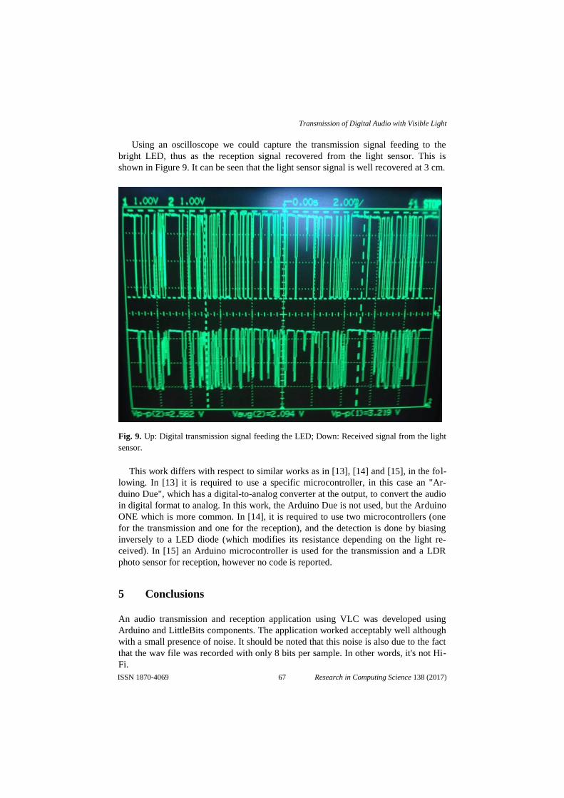
Using an oscilloscope we could capture the transmission signal feeding to the

bright LED, thus as the reception signal recovered from the light sensor. This is

shown in Figure 9. It can be seen that the light sensor signal is well recovered at 3 cm.

Fig. 9. Up: Digital transmission signal feeding the LED; Down: Received signal from the light

sensor.

This work differs with respect to similar works as in [13], [14] and [15], in the fol-

lowing. In [13] it is required to use a specific microcontroller, in this case an "Ar-

duino Due", which has a digital-to-analog converter at the output, to convert the audio

in digital format to analog. In this work, the Arduino Due is not used, but the Arduino

ONE which is more common. In [14], it is required to use two microcontrollers (one

for the transmission and one for the reception), and the detection is done by biasing

inversely to a LED diode (which modifies its resistance depending on the light re-

ceived). In [15] an Arduino microcontroller is used for the transmission and a LDR

photo sensor for reception, however no code is reported.

5 Conclusions

An audio transmission and reception application using VLC was developed using

Arduino and LittleBits components. The application worked acceptably well although

with a small presence of noise. It should be noted that this noise is also due to the fact

that the wav file was recorded with only 8 bits per sample. In other words, it's not Hi-

Fi.

67



Also, the performance of the application depends on the brightness of the emitter

LED and the sensitivity of the photo sensor with respect to the light received from the

LED and the surrounding light (in Figure 5 it can be seen that the light sensor has a

control for graduating the sensitivity in the presence of high or low light). Additional-

ly, the alignment between the LED and the light sensor influences the reception, and

consequently the quality of the audio reproduction. This work could be improved by:

1) Increasing the emission power of the LED to increase the reception distance; and

2) Include video transmission by adding another LED light source to encode video.

Acknowledgements. This work was supported by the Instituto Politecnico Nacional;

Project SIP 20171260.

References

1. Haas, H.: Wireless data from every light bulb. TED Ideas worth spreading,

http://www.ted.com/talks/harald_haas_wireless_data_from_every_light_bulb (2011)

2. Tsonev, D., Videv, S. Haas, H.: Light fidelity (Li-Fi): towards all-optical networking. In:

Proc. SPIE (Broadband Access Communication Technologies VIII) 9007(2) (2013)

3. Sherman, J.: How LED Light Bulbs could replace Wi-Fi. Digital Trends.

http://www.digitaltrends.com/mobile/light-bulb-li-fi-wireless-internet/, last accessed

2016/05/01

4. Haas, H.: High-speed wireless networking using visible light. SPIE Newsroom (2013)

5. Vincent, J.: Li-Fi revolution: internet connections using light bulbs are 250 times faster

than broadband. http://www.independent.co.uk/news/science/li-fi-revolution-internet-

connections-using-light-bulbs-are-250-times-faster-than-broadband-8909320.html (2013)

(last accessed on March 2016)

6. Jovicic, A., Li, J., Richardson, T.: Visible light communication: opportunities, challenges

and the path to market. IEEE Communications Magazine, 51(12), 26–32 (2013)

7. Kamsula, P.: Desing and implementation of a bi-directional visible light communication

testbed. University of Oulu, Department of Electrical and Information Engineering, Mas-

ter’s Thesis, 59 p. (2015)

8. He, Y., Ding, L., Gong, Y., Wang, Y.: Real-time audio & video transmission system based

on visible light communication. Optics and Photonics Journal, 3(02), 153 (2013)

9. Lee, K., Park, H.: Modulations for visible light communications with dimming control.

IEEE photonics technology letters, 23(16), 1136–1138 (2011)

10. Arduino Homepage, https://www.arduino.cc/, last accessed 2017/09/01

11. LittleBIts Homepage, https://littlebits.cc/ last accessed 2017/09/01

12. Banzi, M., Fitzgerald, S., Guadalupi, A.: Simple Audio Player. (2015)

13. Jpiat, J.: Arduino Simple Visible Light Communication. https://github.

com/jpiat/arduino/wiki/Arduino-Simple-Visible-Light-Communication, last accessed

2017/09/01

14. Yıldırım, G., Özen, Ö., Yüksel, H., İnci, M.: A Low-Cost Li-Fi Communication Setup.

(2017)

68



https://www.arduino.cc/

https://littlebits.cc/

Implicaciones computacionales de losaeromanipuladores

Julio Mendoza-Mendoza1, Baltazar Jimenez-Ruiz2,Vıctor Javier Gonzalez-Villela1, Mauricio Mendez-Martınez3,

Leonardo Fonseca-Ruiz3, Erick Lopez Alarcon3

1 Centro de Ingenierıa Avanzada, Facultad de Ingenierıa, UNAM,Mexico

2 Escuela Superior de Computo, Instituto Politecnico Nacional,Mexico

3 Unidad Profesional Interdisciplinaria en Ingenierıa y Tecnologıas Avanzadas,Instituto Politecnico Nacional,

Mexico

[email protected]

Resumen. Este documento presenta las necesidades computacionalesimplıcitas en el diseno y operacion de manipuladores de robots aereos;para este proposito, se identifican y verifican diferentes consideracionesen el estado de la tecnica actual y muy reciente. Se inicia con el calculo re-querido para las unidades UAS individuales, y continua con la operacionde estructura completa, que se divide en 4 modos de operacion cıclicos:vuelo hacia el area de trabajo y transformacian a manipulador; despeguede aeronaves; control en modo manipulador y finalmente aterrizaje. A lolargo del texto, hay un ejemplo de aplicacion, un brazo de robot voladordesarrollado por los autores.

Palabras clave: manipuladores aerias roboticos, dise˜o, operacion.

Computational Implications of Aeromanipulators

Abstract. This document presents the computational needs implicit inthe design and operation of aerial-robot manipulators, for this purpose,different considerations are identified and verified in the current and veryrecent state of the art. It is started with the computation required forthe individual UAS units, and continue with the full-structure operationwhich is divided into 4 cyclic modes of operation: flight towards thework area and transformation to manipulator; aircraft take off; controlin manipulator mode and finally landing. Along the text, there is anexample of application, a flying robot arm in development by the authors.

Keywords: aerial-robot manipulators, design, operation.

69

ISSN 1870-4069


1. Introduccion

La tecnologıa de aeromanipuladores como estructuras voladoras de tipo brazorobot, tanto en configuraciones seriales como paralelas (Figura 1) data de 2012[1,2,3,4,5,6,7,8,9].

Basicamente se trata de estructuras aereas donde los UAVs (acronimo inglespara vehıculo aereo no tripulado) que las transportan, funcionan tambien co-mo los elementos de manipulacion robotica, para comprender las implicacionescomputacionales relacionadas a estos mecanismos, es necesario subdividirlas enla siguientes areas: 1 consideraciones computacionales generales de los UAVs; 2consideraciones de transformacion y vuelo hacia la zona de operacion del sistemade manipulacion aerea conjunta; 3 implicaciones computacionales de ascenso; 4implicaciones computacionales de control en el modo de manipulacion aerea; 5implicaciones computacionales de descenso.

En nuestra aplicacion particular, cada una de estas implicaciones es satisfechavıa hardware por el sistema embebido de vuelo Pixhawk y vıa software mediantelas librerıas APM [10,11], sin embargo, este texto resultara de utilidad para quiendesee hacer su propio sistema con microprocesadores, FPGAS, DSPs, microcon-troladores o tarjetas de desarrollo de altas prestaciones. Para el correspondientemodelado y condiciones de operacion ver [9].

2. Implicaciones generales

Las implicaciones computacionales generales de los vehıculo aereo no tripu-lado, se recogen en [12,13,14,15].

Cada uno de los elementos descritos posee distintas frecuencias de operacionpor lo cual es necesario un sistema de administracion RTOS (real time operatingsystem) que dictamine la adecuada lectura, procesamiento, almacenamiento,jerarquıa y ejecucion, estos consisten en:

Lectura de sensores de orientacion, posicion planar y altura: Lamanera estandar es utilizar IMUs, magnetometros, barometros, acelerometrosy GPS o camaras, todos operando en distintos protocolos de comunicacion yfrecuencias de muestreo, en algunos casos por construccion del sensor y en otrospor prioridad de medicion.

Escritura a propelas y mecanismos de ejecucion mediante servo-motores: Lo primero es el uso directo con motores generalmente brushless(sin escobillas) y lo segundo consiste en utilizar motores auxiliares, para tareassecundarias al vuelo, por ejemplo estabilizadores de camara, alerones y meca-nismos de thrust vectoring (vectorizacion del empuje principal) [16,17,18]. Estoes importante porque la escritura a los primeros debe ser en frecuencias muchomayores a los segundos, basicamente porque de los primeros depende que nocaiga la aeronave y estan sujetos a altas vibraciones, estos por lo general debenoperar a PWMs (acronimo ingles para modulacion por ancho de pulsos) de 490Hz mientras que los secundarios a 50Hz.

Control retroalimentado de orientacion, posicion planar y altura:De manera general, se subdivide la tarea de movimiento de un UAV en estos tres

70

Julio Mendoza-Mendoza, Baltazar Jiménez-Ruiz, Víctor Javier González-Villela, et al.


modos de ejecucion, el prioritario es mantener una altura de operacion tambienconocido como hovering; el de rango de prioridad intermedia es controlar laorientacion o actitud de la aeronave y finalmente su posicion planar, tambienconocida como steering [19,20,21,15,22].

Procesamiento de imagenes: Esta tarea se vuelve necesaria en aquellascondiciones donde no funcionan los sistemas de posicionamiento global satelital(por ejemplo en interiores, o zonas rocosas o boscosas).

Comunicacion interna de datos de entrada y salida: Esta por logeneral se realiza en un bus de topologıa serial, como se indica consiste en laforma en la cual se comparten y procesan los datos de los sensores hacia elprocesador principal y a la vez el modo en el que este decide su escritura a losdiversos sistemas de actuadores.

Almacenamiento de datos de vuelo y telemetrıa: Es el modo en el queel sistema almacena los datos para su uso e interaccion y el modo de comunicacioninalambrica entre el mando de control autonomo principal.

Lectura de mandos de control remoto: Consiste en la lectura de unida-des de teleoperacion, las cuales establecen el vinculo entre la unidad en vuelo yla base manual en tierra, como puede verse, junto con la telemetrıa existen dosdistintos modulos de mando inalambrico, el reto aquı es garantizar que operencon precision en frecuencias distintas y en multiples canales independientes.

Lectura de unidades analogicas y digitales tipo GPIO: Consiste enla habilitacion, interaccion, lectura y escritura de los puertos analogicos o bienaquellos digitales de proposito general (general purpose input/output).

Filtrado de senales: La adicion de ruido a los UAVs esta implıcita en lavibracion de los motores y su interaccion electrica, de esta forma, es necesarioun algoritmo de filtrado de senales, el cual generalmente es mediante tecnicas.

Fusion sensorial: Cuando el medio cambia de manera constante, es ne-cesario utilizar combinacion de sensores de geolocalizacion, un ejemplo es entretareas donde el dron pase de un ambiente externo a un interno y se deba tambienintercambiar entre la lectura de un sistema de vision artificial y un sensor GPS.

Planificacion de tareas: Es necesario obtener datos de velocidad y acele-racion para disponer de movimientos suaves, mas aun, hay autores que indican ydemuestran que es necesario incluir snap (segunda derivada de aceleracion) [23],como los sensores se limitan a lectura de velocidades posiciones y aceleracionesy en la mayorıa de los casos es parcialmente, es necesario incluir estimadoresque implican observadores, estimacion neuronal, estimacion difusa y a su vezalgoritmos de planificacion de trayectorias entre puntos, lo cual, tambien vuelvenecesario incluir algoritmos de optimizacion de productos matriciales.

Prioridad de tareas en tiempo real: Dadas las diferentes frecuencias deoperacion de sensores, actuadores, sistemas y sub-lazos de control, es necesariopriorizar las tareas de ejecucion, las de mayor prioridad suelen ser aquellas deescritura a motores y lectura de altura; las intermedias las de lectura planar yorientacional y finalmente en menor rango las de comunicacion serial, lectura demandos remotos y almacenamiento de datos de vuelo, ahora bien dentro de lasprioritarias relacionadas a escritura de motores, las jerarquıa es altitud, actitud,

71

Implicaciones computacionales de los aeromanipuladores


movimiento de plano y trayectoria espacial, el Pixhawk dispone para ello deun sistema RTOS para asignar prioridades y tiempos, sin embargo en caso dedisenar su propia controladora de vuelo, es necesario establecer un sistema detiempo real para ejecucion de eventos.

3. Maquina de estados del vuelo de un aeromanipulador,caso particular aerobrazo

Antes de proseguir con las areas de implicaciones computacionales es ade-cuado indicar la maquina de estados relacionada a la operacion del aerobrazo[9], para ello se subdivide la operacion conjunta en dos etapas: 1 traslado ytransformacion: es decir la operacion conjunta del sistema de UAVs para llegara la zona de operacion y una vez ahı transformarse en manipulador aereo; 2manipulacion aerea: es decir anclar su posicion en la zona de operacion deseaday funcionar como brazo robotico flotante:

A la izquierda de la Figura 3 se ilustra la ejecucion de la maquina de estados,el lazo mas externo es la transformacion entre aeronave y brazo volador el cualcorresponde a la activacion o desactivacion de un sistema tipo clutch, cuandoel clutch esta activo, los UAVS tienen un comportamiento de estructura rıgiday solo contribuyen al traslado de la misma, una vez que esta desactivado elclutch, lo cual esta en funcion de la zona de operacion donde se desea el modode manipulador aereo, se inicia el modo de manipulacion aerea.

El modo de manipulacion aerea, es decir el lazo interno de la maquina deestados, esta basado en el hecho de que se poseen dos controles remotos ypuede compartirse su mando auxiliar entre ambos drones mediante protocolosalambricos o inalambricos Figura 2, de esta manera cada boton auxiliar tienedos estados 1 o encendido y 0 o apagado, al ser dos mandos existen entonces 4combinaciones (00), (01), (11 )y (10), que respectivamente indicarıan la secuenciade apagado, ascenso, control y descenso respectivamente, la maquina de estadosdeseable para nuestros propositos es la siguiente: estando en el modo apagado(00) solo se admite trasladarse al estado de ascenso (01), cualquier otra combina-cion mantiene al sistema en el modo de apagado. Una vez ascendiendo (01) solose admite el paso al modo de control de altura (11) y angulos de hombro y codoo bien al modo de descenso (10). En el modo de control (11) solo es admisiblepasar al modo de descenso (10). Del modo de descenso (10) solo es admisiblecambiar al modo de apagado (00).

4. Implicaciones computacionales de vuelo ytransformacion hacia la zona de trabajo, modoaeronave

Coordinacion y programacion paralela de vuelo fısicamente res-tringido de multiples UAVS: La cual puede ser centralizada si se usa unsolo procesador y se ve al sistema no como un conjunto de UAVS sino como un

72



conjunto de helices o bien descentralizada (multiprocesador) si cada UAV usasu respectivo procesador y se ve al sistema como un grupo coordinado de UAVsautonomos, la tarjeta Pixhawk es capaz de realizar ambos modos de operacioncon UAVs de hasta 4 rotores para una configuracion de aerobrazo de 8 helices(es decir 2 cuadrotores o bien 4 coaxiales de dos helices u ocho monocopteros).El problema de la operacion centralizada es la sobrecarga de tareas de actuaciony control para un solo procesador.

Estimacion de perturbaciones en vivo: Aunque todo el vuelo poseeperturbaciones, la parte critica es aquella de larga duracion, es decir en modoaeronave, donde se vuelve necesario estimar y contrarrestar los efectos del viento,la presion y temperatura, esto es computacionalmente complicado a cielo abiertopues el aire representa un flujo laminar y varia con modelos diferenciales parcialesque inciden sobre variaciones de una viga (la aeronave se considera como unaviga multiplemente apoyada sobre sus helices).

Lectura simultanea de multiples puntos para determinar parame-tros de inercia y masa en un punto virtual: Dicho punto virtual es el centrode gravedad o de masas el cual es virtual porque puede o no estar fısicamente enel cuerpo del sistema, pero es de suma importancia para el control del mismo,como este punto dependen de la configuracion de cada UAV, un buen algoritmopara determinarlo esta en [24] el cual implica calcular las variaciones inerciales decada UAV y/o punto intermedio de union y transferirlas a una central de mandopara calcular ası el punto inercial equivalente, esto computacionalmente implicael envio de datos sensoriales simultaneos a una central de procesamiento donde seprocesan y a su vez se devuelve el punto resultante a cada UAV para que tengannocion de la operacion conjunta, ello implica envio por protocolos alambricos oinalambricos, generalmente seriales y a su vez metodos para asegurar la adecuadatransferencia de la informacion (el mas basico es el cheksum).

Interaccion de transformacion: En este punto, es necesario un metodo pa-ra transformar la estructura aerea desde un modo de vuelo estandar y coordinado(por ejemplo un helicoptero o un ala volante) a uno de vuelo independiente peroigualmente coordinado (es decir un brazo volador), la implicacion computacionales la conmutacion de frecuencias de operacion de las helices las cuales debenapagarse y encenderse en una secuencia precisa mientras el sistema vuela (helibotpatente MX/a/2016/014595) o bien [6,9], vase Figura 1.

5. Implicaciones computacionales de ascenso modocompartido

El ascenso es la parte mas simple pero peligrosa de la operacion de un sistemaaereo, esto es porque primero se debe garantizar un despegue el cual no ocurrede manera inmediata a la activacion de las helices, es decir existe un bias en elcual las helices giran pero el sistema no consigue elevacion, mas aun cada heliceposee su propio bias de despegue en dependencia del adecuado centrado de todoel sistema o bien el balanceo de cada propela, la implicacion computacional enesta parte consiste en monitorear un valor optimo para la elevacion conjunta sin

73



Fig. 1. Aeromanipuladores: De arriba a abajo y de izquierda a derecha: Hai-Nguyen2015; Julio Mendoza 2015; Alexandros Nikou 2015; Moju Zhao 2016; Sangyul Park2016; Mendoza MX/a/2016/014595 MX/a/2015/015160.

Fig. 2. Comunicacion alambrica entre UAVs hombro y codo.

74



Fig. 3. Maquina de estados del aerobrazo.

llegar al nivel de apagado y tambien dictaminar un valor en el cual se mude alestado de control.

6. Implicaciones computacionales de control modoaeromanipulador

Restricciones de giro en los motores: Una vez activado el modo de con-trol, surgen dos importantes implicaciones computacionales, la primera guardarelacion al cambio de giro de los motores, es decir mientras el control puedealcanzar cotas positivas y negativas, algunas aeronaves como los cuadricopterosexigen que sus motores no cambien de sentido de giro (para evitar efectos deautorotacion), por lo tanto se debe recurrir al problema de optimizacion descritoen [8,5]:

El cual simplemente expresa eso, el control aplicado a los motores debemantenerse positivo pese a la variacion del error y el control de vuelo.

Ahora bien en caso de disponer variacion de sentido de giro, esta no puederealizarse arbitrariamente y sigue consignas de absorcion de resultantes, unamanera es agregar un motor adicional que contrarreste vectorialmente todas lasvariaciones negativas de la senal de control de los demas motores [3].

Jerarquıa y calculo en linea del control: La segunda consiste en recal-cular el propio control, el cual como se dijo es de tres tipos, elevacion, actitudy plano y saber en que situaciones resulta adecuado dotar de mas importanciaa uno respecto a otro, como se dijo el control mas importante es el de altura,pero paradojicamente en la elevacion del dron, dada la desigualdad en el bias deempuje de cada motor, el mas importante es el de actitud, otro ejemplo es en lastareas acrobaticas y agresivas [25,23] en este caso se debe discernir y disenar si

75



la tarea tiene prioridad por la conservacion de angulo o por la de posicion planar[26].

Optimizacion de sobreactuacion: Otra implicacion computacional decontrol es la de sobreactuacion (mas motores que grados de libertad): en estecaso la matriz que transfiere el control cartesiano 6D (3 dimensiones de traslaciony 3 de rotacion), debe transformarse a control de velocidades en cada propela,si por ejemplo tenemos un sistema de 2 cuadricopteros, son 8 propelas por locual las matrices de transformacion exigen metodos de optimizacion como losbasados en pseudoinversas y ademas respetar las restricciones descritas en losparrafos precedentes.

7. Implicaciones computacionales de descenso modocompartido

El descenso es otra operacion simple pero delicada, consiste en apagar pau-latinamente los motores pero cuidando que estos se mantenga en su modo desustentacion (es decir que posean suficiente fuerza para garantizar que el sistemano se desplome), como fue dicho, los motores no tienen un bias homogeneo por locual el control de orientacion cobra mayor prioridad en este modo de operacion,tal y como es exagerado en el cine y la tv, el proceso implica escalones deencendido y apagado, cuando se nota un desplome severo, se aplica un impulsode elevacion y ası hasta tocar suelo, la complejidad computacional consiste enmantener operativos los sensores y actuadores en tiempos precisos que garanticenun descenso suave y ademas no destructivo.

8. Conclusiones

En este documento se muestran las implicaciones computacionales mas fre-cuentes encontradas en el diseno del aerobrazo y tambien encontradas en pro-yectos semejantes [3,5,6], estas se subdividen en distintas tareas y se muestranal lector como un conjunto de modulos a considerar y resolver si se pretenderealizar manipulacion aerea coordinada.

Asimismo se da enfasis en la necesidad de poseer sistemas RTOS desde nivelmoderado hasta estricto en funcion de la tarea a ejecutarse, de esta forma sesugiere utilizar sistemas aereos de navegacion embebida como el Pixhawk, Erle-brain o NavIO, microcontroladores dedicados o bien FPGAs o microprocesadoresy decantar opciones de tarjetas de desarrollo basicas (Arduino, Raspberry), dehecho este fue el motivo de la evolucion del APM al Pixhawk, el primero basadoen un Arduino y el segundo basado en un microprocesador Cortex M4F.

Agradecimientos. Los autores agradecen a la Secretarıa de Investigacion yPosgrado del Instituto Politecnico Nacional, y sus correspondientes proyectosSIP y BEIFI, asimismo a la DGAPA-UNAM y a COFAA-IPN.

76



Referencias

1. Tognon, M., Franchi, A.: Control of motion and internal stresses for a chain oftwo underactuated aerial robots. In: Control Conference (ECC), 2015 European,IEEE (2015) 1620–1625

2. Naldi, R., Forte, F., Marconi, L.: A class of modular aerial robots. In: Decisionand Control and European Control Conference (CDC-ECC), 2011 50th IEEEConference on, IEEE (2011) 3584–3589

3. Nikou, A., Gavridis, G.C., Kyriakopoulos, K.J.: Mechanical design, modelling andcontrol of a novel aerial manipulator. In: Robotics and Automation (ICRA), 2015IEEE International Conference on, IEEE (2015) 4698–4703

4. Mellinger, D., Shomin, M., Michael, N., Kumar, V.: Cooperative grasping andtransport using multiple quadrotors. In: Distributed autonomous robotic systems.Springer (2013) 545–558

5. Park, S., Her, J., Kim, J., Lee, D.: Design, modeling and control of omni-directionalaerial robot. In: Intelligent Robots and Systems (IROS), 2016 IEEE/RSJ Interna-tional Conference on, IEEE (2016) 1570–1575

6. Zhao, M., Kawasaki, K., Chen, X., Kakiuchi, Y., Okada, K., Inaba, M.: Transforma-ble multirotor with two-dimensional multilinks: Modeling, control, and whole-bodyaerial manipulation. In: International Symposium on Experimental Robotics,Springer (2016) 515–524

7. Nguyen, H.N., Park, S., Lee, D.: Aerial tool operation system using quadrotorsas rotating thrust generators. In: Intelligent Robots and Systems (IROS), 2015IEEE/RSJ International Conference on, IEEE (2015) 1285–1291

8. Choi, F.: Modeling and control of asymmetrically coupled quadrotor uavs. Master’sthesis, Seoul National University (2015)

9. Mendoza-Mendoza, J., Sepulveda-Cervantes, G., Aguilar-Ibanez, C., Mendez, M.,Reyes-Larios, M., Matabuena, P., Gonzalez-Avila, J.: Air-arm: A new kind offlying manipulator. In: Research, Education and Development of Unmanned AerialSystems (RED-UAS), 2015 Workshop on, IEEE (2015) 278–287

10. authors, S.: Pixhawk webpage. https://pixhawk.org/ (2010) Acces 18-08-2017.11. authors, S.: Ardupilot libraries webpage. http://ardupilot.org/dev/docs/apmcopter-

programming-libraries.html (2010) Acces 18-08-2017.12. Meier, L., Tanskanen, P., Fraundorfer, F., Pollefeys, M.: Pixhawk: A system for

autonomous flight using onboard computer vision. In: Robotics and automation(ICRA), 2011 IEEE international conference on, IEEE (2011) 2992–2997

13. Fresk, E., Nikolakopoulos, G., Gustafsson, T.: A generalized reduced-complexityinertial navigation system for unmanned aerial vehicles. IEEE Transactions onControl Systems Technology 25(1) (2017) 192–207

14. Santana, L.V., Brandao, A.S., Sarcinelli-Filho, M.: Outdoor waypoint navigationwith the ar. drone quadrotor. In: Unmanned Aircraft Systems (ICUAS), 2015International Conference on, IEEE (2015) 303–311

15. Quan, Q.: INTRODUCTION TO MULTICOPTER DESIGN AND CONTROL.Springer (2017)

16. Pascoa, J., Dumas, A., Trancossi, M., Stewart, P., Vucinic, D.: A review of thrust-vectoring in support of a v/stol non-moving mechanical propulsion system. OpenEngineering 3(3) (2013) 374–388

17. Rajappa, S., Ryll, M., Bulthoff, H.H., Franchi, A.: Modeling, control and designoptimization for a fully-actuated hexarotor aerial vehicle with tilted propellers. In:Robotics and Automation (ICRA), 2015 IEEE International Conference on, IEEE(2015) 4006–4013

77



18. Ryll, M., Bulthoff, H.H., Giordano, P.R.: Modeling and control of a quadrotoruav with tilting propellers. In: Robotics and Automation (ICRA), 2012 IEEEInternational Conference on, IEEE (2012) 4606–4613

19. Carrillo, L.R.G., Lopez, A.E.D., Lozano, R., Pegard, C.: Quad rotorcraft control:vision-based hovering and navigation. Springer Science & Business Media (2012)

20. Valavanis, K.P., Vachtsevanos, G.J.: Handbook of unmanned aerial vehicles.Springer Publishing Company, Incorporated (2014)

21. Schafroth, D., Bermes, C., Bouabdallah, S., Siegwart, R.: Micro helicopter steering:Review and design for the mufly project. In: Mechtronic and Embedded Systemsand Applications, 2008. MESA 2008. IEEE/ASME International Conference on,IEEE (2008) 216–221

22. Torenbeek, E., Wittenberg, H.: Flight physics: essentials of aeronautical disciplinesand technology, with historical notes. Springer Science & Business Media (2009)

23. Mellinger, D., Kumar, V.: Minimum snap trajectory generation and controlfor quadrotors. In: Robotics and Automation (ICRA), 2011 IEEE InternationalConference on, IEEE (2011) 2520–2525

24. Al-Rawashdeh, Y.M., Elshafei, M., Al-Malki, M.F.: In-flight estimation of centerof gravity position using all-accelerometers. Sensors 14(9) (2014) 17567–17585

25. Lee, T., Leoky, M., McClamroch, N.H.: Geometric tracking control of a quadrotoruav on se (3). In: Decision and Control (CDC), 2010 49th IEEE Conference on,IEEE (2010) 5420–5425

26. Mellinger, D., Michael, N., Kumar, V.: Trajectory generation and control forprecise aggressive maneuvers with quadrotors. The International Journal ofRobotics Research 31(5) (2012) 664–674

78



Lumped Parameter Estimation of a Stochastic Process

of Second Order Using the Second Moment and

Recursiveness

Romeo Urbieta Parrazales1, José de Jesús Medel Juárez1, Karen Alicia Aguilar Cruz1,

Rosaura Palma Orozco2

1 Centro de Investigación en Computación - Instituto Politécnico Nacional, CDMX,

Mexico

2 Escuela Superior de Cómputo - Instituto Politécnico Nacional, CDMX,

Mexico

[email protected], [email protected], [email protected],

[email protected]

Abstract. In this article, a stochastic algorithm is briefly presented based on the

one of second moment applied to a stochastic process model of second order.

The design initially consisted in formulating the state equation model and the

stochastic outputs, in order to apply the second moment using the internal prod-

uct of Martingale and the stochastic operators of the expectation, variance and

covariance. The design results generated the formulas on: the covariances and

the internal product variances to calculate the lumped estimation parameters,

the error functional based on the mean quadratic error, the output variable as a

function of the estimation parameters obtained. Furthermore, the recursive form

was formulated in this design starting from the premise of the obtained results

using the second stochastic moment. The main interest lays on the recursive

form, because this is the one capable of being implemented in a digital system.

In order to observe the precision and the convergence of the estimation parame-

ters and the output variables, Matlab-based figures are shown.

Keywords: Linear stochastic systems, parameter estimation, second moment.

1 Introduction

The random input and output variables of a noisy process can be modeled by means

of experimental data obtained from measurements carried out during time intervals T.

These models are called Black Box Models (Fig. 1) [1, 2].

The Black Box Models are called this way, because their internal states are not

known. One method to determine these unknown states starting from observable

states are the so called methods of identified states based on the mean quadratic er-

ror [3].

79

ISSN 1870-4069



Fig. 1. Stochastic Estimation based on the second moment.

The method relies on turning the unknown or non-measurable states 𝑥𝑘 into an

identified state ��𝑘 by means of the stochastic conditions of the observable state 𝑦𝑘 ,

based on the identified error (1):

𝛿𝑘 = 𝑦𝑘 − ��𝑘 . (1)

The error can lead to different methods of stochastic estimation and is hereby

known as the innovation process.

The error functional from the identification error 𝛿𝑘 using the second moment of

probability, is defined as the expected value of the Euclidean norm of 𝛿𝑘 [4, 5, 6]:

𝐽𝑘(𝛿𝑘) = E {𝛿𝑘𝑇

𝛿𝑘} = (𝑦𝑘 − ��𝑘)𝑇 (𝑦𝑘 − ��𝑘). (2)

On the other hand, within the linear stochastic model, the observable state was repre-

sented by means of finite differences equations of 2nd order (3):

d2f(y)

dy2 ≅ (f(y) − 2f(y(k − 1)) + f(y(k − 2)). (3)

As it can be observed in (1) a system of this type has two delays and a negative

sign in one of its parameters [7, 8, 9, 10, 11].

As we mentioned before, based on a second order state and a quadratic mean of

second moment, the main purposes of this work are to design the estimation state

based on this second moment, further on, to identify the stochastic output variable and

finally, to determine the precision by means of the error functional. Additionally, the

parameters and the variables of interest will be plotted.

This article was structured in the following manner: abstract, second moment, sto-

chastic recursive algorithm, quadratic mean error functional, experiment, conclusions

and bibliography.

2 Simplified Stochastic Output Model.

Like it was said in this introduction, a stochastic system based on noisy output and

input measurements taken during a certain number of time intervals T, can adopt the

following linear model in differences like the state equation (4) with stochastic output

(5) [9, 10]:

80

Romeo Urbieta Parrazales, José de Jesús Medel Juárez, Karen Alicia Aguilar Cruz, et al.


𝑥𝑘+1 = 𝑎1𝑥𝑘 + 𝑎2𝑥𝑘−1 + 𝑏𝑤𝑘 , (4)

𝑦𝑘 = 𝑐𝑥𝑘 + 𝑑𝑣𝑘. (5)

Delaying (4) and (5) we have (6) and (7) respectively

𝑥𝑘 = 𝑎1𝑥𝑘−1 + 𝑎2𝑥𝑘−2 + 𝑏𝑤𝑘−1, (6)

𝑦𝑘−1 = 𝑐𝑥𝑘−1 + 𝑑𝑣𝑘−1. (7)

Now, solving for the delayed state from (7) yields (8), and delaying (8) gives (9):

𝑥𝑘−1 = 𝑐−1𝑦𝑘−1 − 𝑑𝑐−1𝑣𝑘−1, (8)

𝑥𝑘−2 = 𝑐−1𝑦𝑘−2 − 𝑑𝑐−1𝑣𝑘−2. (9)

Substituting (8) and (9) in (6) gives (10). Besides, substituting (10) in (5) yields

(11):

𝑥𝑘 = 𝑎1𝑐−1𝑦𝑘−1 + 𝑎2𝑐−1𝑦𝑘−2 − 𝑎1𝑑𝑐−1𝑣𝑘−1 − 𝑎2𝑑𝑐−1𝑣𝑘−2 + 𝑏𝑤𝑘−1, (10)

𝑦𝑘 = 𝑎1𝑦𝑘−1 + 𝑎2𝑦𝑘−2 − 𝑎1𝑑𝑣𝑘−1 − 𝑎2𝑑𝑣𝑘−2 + 𝑏𝑐𝑤𝑘−1 + 𝑑𝑣𝑘. (11)

And from (11) the noise is (12) leading to the simplified stochastic output (13):

𝑉𝑘 = −𝑎1𝑑𝑣𝑘−1 − 𝑎2𝑑𝑣𝑘−2 + 𝑏𝑐𝑤𝑘−1 + 𝑑𝑣𝑘 , (12)

��𝑘 = 𝑎1𝑦𝑘−1 + 𝑎2𝑦𝑘−2 + 𝑉𝑘. (13)

3 Stochastic Algorithm Based on the Second Moment

The second moment is a technique used in probability theory to demonstrate that a

random variable (RV) has a positive probability. Generally, the method consists in

delimiting the probability that a RV fluctuates away from its mean. The method in-

volves a comparison of the second moment of the RV and the square of the first mo-

ment. Hence: 𝜇2 = 𝐸((𝑌 − 𝜇)2), where Y is the RV and μ is the mean [12].

From (13), we can obtain (14), that is (15), where �� = [𝑎1 𝑎2], and 𝑧��−1 =[𝑦𝑘−1: 𝑦𝑘−2 ]𝑇:

𝑦𝑘 = ��𝑧��−1 + 𝑉𝑘, (14)

𝑦𝑘 = [𝑎1 𝑎2][𝑦𝑘−1 𝑦𝑘−2 ]𝑇 + 𝑉𝑘, (15)

Taking the second moment of probability from (14) for the variable 𝑧𝑘−1𝑇 [13, 14],

we have (16), that once solved gives (17):

𝐸{𝑦𝑘𝑧��−1𝑇 } = ��𝐸{𝑧��−1𝑧��−1

𝑇 } + 𝐸{𝑉𝑘𝑧��−1𝑇 }, (16)

𝐸{𝑦𝑘𝑧��−1𝑇 } − 𝐸{𝑉𝑘𝑧��−1

𝑇 } = ��𝐸{𝑧��−1𝑧��−1𝑇 }. (17)

Here is the estimated parameter based on the second moment (18):

81

Lumped Parameter Estimation of a Stochastic Process of Second Order ...


��𝑘 = (𝐸{𝑦𝑘𝑧��−1𝑇 } − 𝐸{𝑉𝑘𝑧��−1

𝑇 })(𝐸{𝑧��−1𝑧��−1𝑇 })+. (18)

From (18), the stochastic estimated parameter is defined as a direct function to the

covariance 𝑝𝑘, and inverse to the covariance 𝑞𝑘 as indicated in (19):

��𝑘 ≜𝑝𝑘

𝑞𝑘, (19)

where, ��𝑘, 𝑝𝑘 , 𝑎𝑛𝑑 𝑞𝑘 are vectors of 1x2, 1x2 and 2x2 dimensions, respectively.

To calculate the covariances pk and qk, the stochastic covariance is represented by

the expectation of the internal products of the output variable, which is convoluted

with the same output, but now with a delay, (20) [11]:

[��1,𝑘 ��2,𝑘] = 𝐸({𝑦𝑘𝑧��−1𝑇 } − {𝑉𝑘𝑧��−1

𝑇 }). (20)

The stochastic expectation comes represented as a sequence from zero to k samples

and is expressed by means of a sum [15] as it can be seen in (21):

[��1,𝑘 ��2,𝑘] =1

𝑘[∑ ([ 𝑦𝑖𝑦𝑖−1 𝑦𝑖𝑦𝑖−2] − [ 𝑉𝑖𝑦𝑖−1 𝑉𝑖𝑦𝑖−2])𝑘

𝑖=0 ]. (21)

Solving the sums from 0 to k samples, the two vectors of the covariances [13]

𝑝1,𝑘 and 𝑝2,𝑘 , are obtained as in (22):

[��1,𝑘 ��2,𝑘] =

1

𝑘2 [ 𝑦𝑘𝑦𝑘−1 − 𝑉𝑘𝑦𝑘−1 + (𝑘 − 1)2��1,𝑘−1 𝑦𝑘𝑦𝑘−2 − 𝑉𝑘𝑦𝑘−2 + (𝑘 − 1)2��2,𝑘−1]. (22)

While the covariance 𝑞𝑘 comes expressed as a quadratic matrix of 2x2 (23), in this

case, the matrix turns out to be singular yielding into a pseudoinverse matrix.

[��11,𝑘 ��12,𝑘

��21,𝑘 ��22,𝑘] = 𝐸{𝑧��−1𝑧��−1

𝑇 }

= 𝐸 {[𝑦𝑘−1

𝑦𝑘−2] [𝑦𝑘−1 𝑦𝑘−2]} = 𝐸 [

𝑦𝑘−12 𝑦𝑘−1𝑦𝑘−2

𝑦𝑘−2𝑦𝑘−1 𝑦𝑘−22

]. (23)

Solving for the expectation operator over the internal product, the covariances ma-

trix 𝑞𝑘 is obtained in (24):

[𝑞11,𝑘 𝑞12,𝑘

𝑞21,𝑘 𝑞22,𝑘] =

1

𝑘2 ∑ [𝑦𝑖−1

2 𝑦𝑖−1𝑦𝑖−2

𝑦𝑖−2𝑦𝑖−1 𝑦𝑖−22

]𝑘𝑖=0 . (24)

Now, by inserting the sums into each one of the terms within the pseudoinverse

matrix, the result is (25).

Developing the samples in each one of the sums from 0 to k samples leads to ob-

tain the sequential form of each one of the components of the pseudoinverse matrix

(26) of the covariance 𝑞𝑘.

82



[��11,𝑘 ��12,𝑘

��21,𝑘 ��22,𝑘] =

1

𝑘2 ([∑ 𝑦𝑖−1

2 𝑘𝑖=0 ∑ 𝑦𝑖−2𝑦𝑖−1

𝑘𝑖=0

∑ 𝑦𝑖−1𝑦𝑖−2 𝑘𝑖=0 ∑ 𝑦𝑖−2

2𝑘𝑖=0

]), (25)

[��11,𝑘 ��12,𝑘

��21,𝑘 ��22,𝑘] =

1

𝑘2 ([𝑞11,𝑘 𝑞12,𝑘

𝑞21,𝑘 𝑞22,𝑘]), (26)

where the components of the pseudoinverse matrix are (27):

𝑞11,𝑘 = 𝑦𝑘−12 + (𝑘 − 1)2𝑞11,𝑘−1 ; 𝑞12,𝑘 = 𝑦𝑘−2𝑦𝑘−1 + (𝑘 − 1)2𝑞12,𝑘−1, (27)

𝑞21,𝑘 = 𝑦𝑘−1𝑦𝑘−2 + (𝑘 − 1)2𝑞21,𝑘−1; 𝑞22,𝑘 = 𝑦𝑘−22 + (𝑘 − 1)2𝑞22,𝑘−1.

The equation (25) can be divided into two components as in (28):

(1

𝑘2) ([𝑦𝑘−1

2 𝑦𝑘−1𝑦𝑘−2

𝑦𝑘−1𝑦𝑘−2 𝑦𝑘−22

] + (𝑘 − 1)2 [��11,𝑘−1 ��12,𝑘−1

��21,𝑘−1 ��22,𝑘−1]). (28)

The estimated parameter using the second moment expressed in (18), (21) and (26) is

presented in (29):

��𝑘 = [��1,𝑘 ��2,𝑘] = [��1,𝑘 ��2,𝑘] [��11,𝑘 ��12,𝑘

��21,𝑘 ��22,𝑘]

+

, (29)

where ��𝑘 and 𝑝𝑘 , are matrices of dimensions: 1x2, while 𝑞𝑘 is a matrix of dimension:

2x2, and is also a pseudoinverse [16]. Then, the simplified stochastic output ��𝑘 of

(13) respect to the estimation parameter of second moment ��𝑘 ends up being (30):

��𝑘 = ��1𝑦𝑘−1 + ��2𝑦𝑘−2 + ��𝑘. (30)

4 Recursive Stochastic Estimation Algorithm

From (19), the covariance 𝑝𝑘 can be obtained as the matrix (31) of 1x2 being a func-

tion of the covariance 𝑞𝑘.

[��1,𝑘 ��2,𝑘] =1

𝑘( 𝑦𝑘𝑦𝑘−1− 𝑉𝑘𝑦𝑘−1 𝑦𝑘𝑦𝑘−2 − 𝑉𝑘𝑦𝑘−2

+(𝑘 − 1)[��1,𝑘−1��1,𝑘−1 ��2,𝑘−1��2,𝑘−1]). (31)

Using (18) to calculate the estimation parameter, together with (22) and (25) we

get (32), then, the stochastic output based on the recursive second moment is (33).

��𝑘 = [��1,𝑘 ��2,𝑘] = [��1,𝑘 ��2,𝑘] [��11,𝑘 ��12,𝑘

��21,𝑘 ��22,𝑘]

+

, (32)

��𝑘 = ��1𝑦𝑘−1 + ��2𝑦𝑘−2 + ��𝑘. (33)

83



5 Functional of Mean Quadratic Error

The mean quadratic error functional is a measurement to accurately know about the

estimation parameter convergence by means of the errors between the normal parame-

ter and the one from the second stochastic moment [18]. Considering the parametric

error 1 (34), parametric error 2 (35), error functional 1 (36), and error functional

2 (37):

��1,𝑘 = 𝑎1,𝑘 − ��1,𝑘 , (34)

��2,𝑘 = 𝑎2,𝑘 − ��2,𝑘, (35)

J1,𝑘 = (1

𝑘2) [��1,𝑘2 + (k − 1)2𝐽1,𝑘−1], (36)

J2,𝑘 = (1

𝑘2) [��2,𝑘2 + (k − 1)2𝐽2,𝑘−1]. (37)

The recursive form has utmost importance, because it generally gives proof of pre-

cision between the stochastic estimation parameters and the ones based on the second

moment, which are meant to be implemented in a digital system. Considering parame-

tric error 1(38), parametric error 2 (39), error functional 1 (40), error functional

2 (41).

��1,𝑘 = 𝑎1,𝑘 − ��1,𝑘, (38)

��2,𝑘 = 𝑎2,𝑘 − ��2,𝑘, (39)

J1,𝑘 = 𝐸{��1,𝑘2 } = (

1

𝑘2) [��1,𝑘2 + (k − 1)2𝐽1,𝑘−1], (40)

J2,𝑘 = 𝐸{��2,𝑘2 } = (

1

𝑘2) [��2,𝑘2 + (k − 1)2𝐽2,𝑘−1]. (41)

6 Experiment

The stochastic estimation algorithm based on the second moment is meant to be

placed as an example.

For the stochastic process the considered parameters are a1=0.1+i0.05i; a2=-

0.1+0.05; b=0.002; c=1; d=0.003.

The identification of the system variable is presented by means of the Fig. 2 and

Fig. 3. Where the first fifteen samples of the output responses are matched and hence,

tend to be confused with each other. For the recursive case, the identification of the

output variables is achieved more quickly. The graphs of the experiment were carried

out using Matlab [19, 20].

For a second stage the initial conditions of the recursive stochastic estimation algo-

rithm, for (26) and (27) are: pr1(2)=0.003; pr2(2)=0.001; anr1(2)=0.05; anr2(2)=0.05.

Implementing this values, the result for the parameter estimation is seen in Fig. 4.

84



Fig. 2. Stochastic simplified output variable identification.

Fig. 3. Stochastic recursive outputs variable identification.

Fig. 4. Estimated stochastic parameters based on the second moment ��1 and ��2 from Eq. (29)

and recursive stochastic calculated parameters ��1 and ��2 from Eq. (32).

To have a better idea of the convergence we use the error functional to measure the

convergence level for both estimated parameters. The initial conditions for the mean

quadratic error functional based on the second moment and the recursiveness, Eqs.

(30) and (31) together with (34) and (35), respectively are the following: second mo-

85



ment: J1(2)=0.0004; J2(2)=0.0004 and recursiveness: Jr1(2)=0.0004; Jr2(2)=0.0004.

Results are shown in Fig. 5 and Fig. 6.

Fig. 5. Graph 6. Error functional of second moment 𝐽1 in blue colour and 𝐽2 in red colour. Re-

mark: Here we deal with a Super Martingale.

Fig. 6. Graph 7. Error functional of second moment 𝐽 1 in green colour and 𝐽

2 in sky-blue col-

our. Remark: Here we deal again with a Super Martingale.

7 Conclusions

The main objective of making the convergence of the two estimation parameters of

states ��𝑘, based on the estimation algorithm using the second moment, into the value

lost by the parameters of the linearly modelled stochastic states was fulfilled.

The found estimation parameters for the second moment were only able to locate

the convergence, when they were subjected to a sign inversion, just as it is described

in (1). The convergence range of the estimation parameters did work only within 0 <

��𝑘 < 1. The paths of the estimation parameters were always of the Super Martingale

form.

The fireproof took place, when the estimation parameters of this proposed algo-

rithm were replaced at the output variable and it was noticed that the experimentally

measurable random data was perfectly compared with the a priori data.

86



Due to the previous acknowledgements, we come up with the conclusion that the

estimation algorithm based on the second moment applied to a random experimental

model and represented by a linear stochastic second order model worked out properly.

Also, it was possible to design and simulated experiment with a recursive estimator

model ��𝑘, starting with the estimator based on the second moment, whose objective in

the future is to be placed at the disposal of whomever wants to implement it on a digi-

tal system by only having experimental data of random systems.

Acknowledgments. The authors would like to thank the Instituto Politécnico Nacion-

al, through projects SIP20171418, SIP20170227, and CONACYT, for the support

given to carry out this project.

References

1. Abonyi, J.: Fuzzy Model Identification for Control. Editorial Birhausser, pp. 1–21 (2003)

2. Rivals, I., Personnaz, L.: Black Box Modeling with State Space Neural Networks. (1995)

3. Sinha, A:. Optimal and Robust Control. CRC Press, pp. 179–228 (2007)

4. Lewis, F. L., Xie, L., Popa, D.: Optimal Estimation, Optimal and Robust Estimation. CRC

Press, pp. 3–50 (2008)

5. Medel, J., García, C.V.: Estimación de Parámetros Usando la deconvolución y la Pseudo-

inversa:Descripción e Implementación Recursiva. Revista de Física 56 (1) 54–60 (2009)

6. Aguado, A., Martínez, M.: Identificación y Control Adaptivo. Cap 2. Prentice Hall (2003)

7. Schiavi, E., Muñoz, A. I.: Métodos en Diferencias Finitas para para la Resolución de Pro-

blemas de Contorno. (2007)

8. Rivero, R.: Identificacion de Sistemas de Segundo Orden.

9. Elliot, R. J., Aggoun, L., Moore, J. B.: Hidden Markov Models. Estimation and Control.

p. 19, Springer (2008)

10. Alavez, J.: Estimación de Parámetros en Ecuaciones Diferenciales Ordinarias. Cap. 1, pp.

1–34.

11. Heij, C., Ran A., van Schagen, F.: Introduction to Mathematical System Theory. In: Linear

Systems, Identification and Control, p. 75. Birkhauser Verlag (2007)

12. Hoel, P. G., Port, S. C., Stone, C. J.: Introduction to Probability Theory. Chapter 4, pp.

92–95. Houghton Mifflin Company (1971)

13. Domínguez, J. A., González-Farías, G., Rodríguez-Dagnino, R. M.: Un procedimiento

práctico para estimar el parámetro de forma de la distribución Gaussiana Generalizada. p.

6, Centro de Investigación de Matemáticas.

14. Wilfredo Dominguez C. Convergencia Aleatoria en Espacios de Hilbert. PESQUIMAT.

Revista de la F.C.M. de la Universidad mayor de San Marcos. Vol. II, No. 1, pp. 69–70.

Lima-Perú (Agosto 1999)

15. Debnath, L., Mikusinski, P.: Hilbert Spaces with Applications. Chap. 3, pp 93–135. Else-

vier Academy Press (2005)

16. Medel Juárez, J.J., Zagaceta Álvarez, M.T.: Estimación-Identificación como Filtro Digi-

tal Integrado: Descripción e Implementación Recursiva. Revista Mexicana de Física 56 (1)

1–8 (Feb. 2010)

17. Rengifo, C. F.: Una Herramienta para Identificación Recursiva de Sistemas Dinámicos.

pp. 1–12 (2004)

87



18. Santo Orcero, D.: La Matriz Fundamental y la Matriz esencial. Conceptos y aplicaciones.

(2002)

19. Lewis, F.L., Xie, L., Popa, D.: Optimal Estimation. In: Optimal and Robust Estimation.

Chapter 9, pp. 423–442. CRC Press (2008)

20. Rodríguez del Río, R.: Gráficas con MatLab. Madrid, España.

21. Dukkipatti, R.: Analysis and Design of Control Systems Using Matlab. New Age Interna-

tional (2006)

22. Lagunas, M.A.: Procesos Estocásticos y Estimación de Parámetros. Cap. II (2007)

23. Stroock, D.W.: Probability Theory: An Analytic View. Chapter 4. Cambridge University

Press (1994)

88



A Survey on Computer Science Techniques inthe FOREX Market: Models and Applications


Centro de Investigacion en Computacion, Instituto Politecnico Nacional,CDMX, Mexico

[email protected], [email protected], [email protected]

Abstract. In this paper a survey on computer science techniques such asnatural language processing, machine learning, data mining, associationrules, etc. which are applied on the FOREX market is presented. Themain objective of investing in FOREX market is to maximize the profitsgiven a certain period of time. This survey can be useful to researchersin this area, in order to compare and extend previous works.

Keywords: time series, Forex, data mining, natural language proces-sing.

1 Introduction

1.1 Foreign Exchange Market

The Foreign Exchange (FOREX)1 market is one of the biggest and most liquid2

markets for investors, trading in average $5.1 trillion dollars per day in April2016 [1]. It trades in pairs of currencies, the first coin of the pair is called basecurrency and is the one that an investor can sell or buy. The second coin is calledreference currency and it means the money that an investor is willing to pay orto receive for the base currency.

FOREX is a decentralized market, also know as an Over the Counter (OTC)market. OTC markets are not controlled by any government nor have a physicallocation, all transactions are made by computer, phone and email orders. OTCtrades a great number of listed securities, such as currencies, bonds, and shares ofcompanies that does not meet the requirements to be listed on exchanges suchas the New York Stock Exchange (NYSE) or the Bolsa Mexicana de Valores(BMV) exchange in Mexico. There are mainly two forms of trades, one wherea dealer trade with institutions or corporations and other intermediate tradesbetween different dealers.

Modeling the economic markets and currency pair market is a difficult task asstated by Rey [2], who published a paper in which the role of a vehicle currency

1 Some sources also use the FX abbreviation.2 A liquid asset is described as one that can be easily exchanged for money, i.e

currencies, shares, bonds, etc.

89

ISSN 1870-4069


is studied in order to explore the rise and fall of currencies through the evolutionof trades patterns between countries.

1.2 The Risk on OTC Markets

OTC markets such as FOREX are considered to have more risk implied on thetransactions, due to little or non existent regulations, which make OTC marketsless transparent; for this reason many advisors do not recommend this type ofmarket for small and unexperienced investors.

1.3 Mexico in the FOREX Market

According to the results given by Bank of Mexico (Banxico), in 2016 the Mexicanpeso (MXN) was the tenth currency with most trade in the world, and the secondone in the list of emerging countries3, only behind the Chinese renminbi.

It is recognizing patters using fuzzy logicalso important to notice that mostof the transactions made with the MXN currency are realized outside of Mexico,besides the US dollar (USD) is the main currency that is traded against theMXN [3].

1.4 Trading in FOREX

To make transactions in the FOREX market it is necessary to have an accountwith a brokerage company; as the OTC market works on networks, it is possibleto open an account from other country, but it is recommended to use the mosttrusty broker one can find, i.e. a broker with the biggest capital liquidity.

1.5 Spread

The spread is one of the main subjects in FOREX trading, it is described as thedifference between the bid and ask price of a currency4, is common to find it inpractice as the Bid-Ask Spread. Currency pairs usually have the lowest spread,movements around $0.00015 also known as Pip6.

Because there are no commissions on the FOREX transactions, brokers usethe spread as a way of making profit, this means the tighter a spread is, thebetter profit an investor can make. The competition between FOREX brokers isfierce, it is recommendable to shop around for the best prices in currencies7.

3 An emerging market economy is described as one who is progressing into becomingan advanced economy, i.e: Mexico, Brazil, Russia, India, Turkey and China.

4 The ask price is the money that a seller is asking to receive for a security, converselythe bid price is the money a buyer is willing to pay for a security.

5 Some currencies trade at movements of $0.016 A Pip is the equivalent of 1/100 of 1%.7 Many variables can affect the spread of a currency pair, such as volatility, high or

low demand and also affects the political issues on the base currency country.

90



1.6 Making a Profit on the FOREX Market

1.7 Two Strategies for Trading

There are mainly two strategies for trading in currencies, shares, bonds, etc. Thelong and the short position.

Long PositionThe long position is the most common among investors in markets, it follows

the principle “Buy low, sell high”, in the FOREX market is the same as buying acurrency which an investor thinks is going to appreciate in the future (in FOREXchanges may occur in relatively small intervals of time, such as minutes), ifthe currency price rise then the investor will sell it obtaining a profit from theoperation. On the other hand if the currency loss its value the investor could sellit at lower price taking losses.

Short SellingThe short selling is a strategy in which an investor predicts the value of an

asset, such as currency, will drop in the future. In practice an investor could“borrow currencies” from a margin account8, the short investor exchange thecurrency pair, if the prediction is true and the value of the base currency dropssuch investor could buy the same currency at a lower cost, finally returning itto broker in the margin account.

Short selling is seen as a highly risky strategy, because the maximum profitcan be achieved when a base currency drops down to near zero; however, themaximum losses tend to infinity since there is no limit for a currency to appreci-ate. Thus this strategy is recommended only for experienced investor. The mainidea behind short selling is to bet against a security.

2 Previous Related Surveys

In this section, previous survey related to FOREX and financial markets usingcomputer science techniques are described.

Most recently, Kumar et al. [4] performed a survey on applications of textmining in financial domain; it categorized the applications into FOREX rateprediction, stock market prediction, customer relationship management (CRM)and cyber security which were published in the period of 2000-2016. Theydivide the text mining task into four categories, namely classification, clustering,summarization, topic identification and association rule mining. The surveyconcluded that more efficient techniques are needed to handle and predict asignificant amount of data, also the most frequently used text mining task isclassification followed by prediction: one of the purposes is to standardize theperformance metrics to compare various works.

8 Brokerage firms offer margin accounts in which they lend money to investors in orderto purchase securities.

91

A Survey on Computer Science Techniques in the FOREX Market: Models and Applications


Batyrshin et al. [5] presented a survey paper on perception based patterns intime series. They discussed the importance of recognizing patterns using fuzzylogic on time series in order to support decision making processes. In this studythey found that most of the decision making procedures in problems on financialand economics are based on human decisions supported by statistics, data miningor data processing software.

The main contributions are the applications that uses fuzzy logic for thedescription of patterns such as sign derivatives, scaling trends, linguistic inter-pretations of patterns as result of clustering, relationship between patterns, etc.

This survey includes studies which use financial data, i.e stock prices, news,indicators as well as non-financial data, i.e climate conditions. They concludethat time series data mining along with natural language computation andcomputing with word and perceptions is an opportunity field for researchersto explore new method and publish new techniques.

Soft computing techniques applied on the stock market where reviewed byAtsalakis et al. [6]. In this research they stated that soft computing techniquesare candidate to capture stock market nonlinear relations returning significantforecasting results, the methods included in the survey are mainly neural net-works and neuro-fuzzy models with several types of training. The results werecompared against conventional models such as artificial neural networks, linearand multi-linear regression, ARIMA models, genetic algorithms, random walk,buy and hold, etc.

Data mining techniques with applications in the stock markets were surveyedby Hajizadeh et al. [7], they stated that data mining techniques in the financialdomain are gaining interest from the researchers. One of the most importantproblems is finding efficient ways tu summarize and visualize the stock marketdata in order to give useful information for investment decisions.

The survey categorized six data mining techniques and its applications onthe stock market, namely decision tree, neural networks, clustering, associationrules, factor analysis and time series. They conclude that the use of data miningtechniques in the financial domains has reached good results and they expectthe number of studies in this field increase.

3 Review of Computer Science Techniques for theFOREX market

This survey highlights some applications of computer science which have anapplication in the FOREX market. These applications are categorized mainlyinto FOREX rate forecast, up-down movements, trend analysis.

The FOREX rate predictions attempts to give an accurate price of a currencypair in the future, using available data, such as past values of bid/ask quotes.

Due to space limitations most of the mathematical framework of the studieswill not be presented.

Nassirtoussi et al. [8] published a research in 2015, in which they classifiedthe future of a currency pair; a binary classification was used, namely POS if a

92



currency pair will appreciate or NEG if the bid/ask price will drop. The studyincluded a novel system that used text mining, natural language processing,statistical pattern recognition as well as sentiment analysis that predicts thedirectional movement on currency pairs in the FOREX market on the wordsused in news headlines in previous hours. The forecast horizon for this studyis 1-2 hours as they were working with intra-day trading data, news headlineswere obtained from a financial news web page via web service and data fromEUR/USD currency pair.

Before the research of Nassirtoussi the idea of forecasting the FOREX ratesfrom news headlines was revised by Peramunetilleke and Wong [9], in their studythey proposed that the information contained in news was better in contrast tonumeric time series, because they not only contain the effect, but also the possiblecause of the event that affects the FOREX rates.

They implemented a new technique that relies on natural language proces-sing, which automatically evaluated the news. The system receives as an inputnews headlines from Reuters and the output is a categorical forecast divided inthree: the dollar moves up, remains steady or goes down within the next one,two or three hours.

The system generates weights for keywords on headlines, then it createsrules that can handle continuous attributes, rather than boolean expressions, tocreate the rules they use two methods, namely TFxIDF which consist in termfrequency, discrimination factor and normalization and the TFxCDF methodwhich uses category frequencies.

The results they obtained showed that the TFxCDF method reaches betterresults than other methods, it was also compared to a conventional time seriesanalysis tool and two different neural network approaches and outperformedthem.

Idvall et al. [10] in their master thesis investigated the use of Markov chainsin hidden Markov models with two implemented extensions: a Gaussian mix-ture model (GMM) and an exponentially weighted expectation maximization(EWEM) in order to create a new way of algorithmic trading which mainobjective is to increase the profit of the alpha returns on intra-day trading.

They concluded that the use of hidden Markov models on the FOREX mar-kets is still an area of opportunity for researchers. Their model in some settingswas able to obtain significance profit, whereas other settings the predictor lookedclose to a random generator, this was attributed to the great quantity of factorsthat have to be considered when setting up a model.

They propose that a different machine learning method and improving theinitial estimates of the parameters would produce better results. As for the modelitself it could be expanded in order to diversify the portfolio of HMM, includingdifferent currency pairs, since each pair might depend on different causes thushave different patterns, also the usage of leverage could be advantageous toenhance the profits.

Regarding the machine learning (ML) area, Baasher and Fakhr [11] publishedan article in which they used ML techniques to forecast the High exchange rate

93



daily trend; They represented the forecast problem as a binary classification taskwith the two possible outcomes being uptrend and downtrend. This article usedfour mayor currencies, namely USD/YEN, USD/EGP, EUR/EGP, EUR/SAR.

The ML algorithms used for classification were radial basis function (RBF),multilayer perceptron neural network (MLP) and support vector machines (SVM).The results for forecasting of the generalized autoregressive conditional hete-roscedasticity (GARCH) were used as part of the feature set, along with otherclassical technical analysis techniques for time series i.e momentum. Feature se-lection and extraction method were applied in order to optimize the results givenby the ML algorithms. For the comparison analysis, they used the percentageclassification performance and a novel function called percentage normalizedprofit (PNP), which represents the ratio between accumulated profits using thepredicted trends versus the accumulated profit using perfect predictions duringa test period.

The study concludes that a good feature selection along with regularizationon the ML techniques can provide good results, making a profit in the FOREXmarket.

Karuzzaman and Sarker [12,13] published a research on predictions of foreigncurrencies rates using neural networks with three different learning algorithms,namely Standard Backpropagation (SBP), Scaled Conjugate Gradient (SCG)and Backpropagation with Bayesian Regulation (BPR). They concluded thatthe SCG learning algorithm outperformed the other models.

In their tests they used moving averaged values to feed the neural networkto predict the following week, comparing six currencies against the Australiandollar (AUD), in terms of performance measure the SCG model achieves veryclose prediction in terms of NMSE and MAE metrics. The Figure 1 shows theresults obtained.

Batyrshin et al. [14] proposed a novel definition for a non-statistical measureof time series comovement called “local trend association measure” (lta), whichis based on a early work the “moving approximation transform” (mat) [15]. Thelta measures positive and negative shape associations between time series.

They conclude that the correlation coefficient is not an useful tool in theanalysis of time series shape similarity and shape associations. They realized acomparative analysis between exchange rates with data from Google Finance[16], Figure 2 shows the initial points where the local trends change sign andthis can be associated with business events. Also using the approach of “pairof stocks” (or currencies), one can associate pairs which move asynchronous(positively associated) or with inverse movements.

Garcıa et al. [17] proposed a method to choose a better sliding window in themoving approximation transform (MAT) [15]. This new method uses the lengthof a pattern instead of the cos function to measure the positive or negativesimilarity between time series; they also presented a new method to visualizethe associations between time series which is easier to understand than the oneused in [15,14].

94



Fig. 1: Forecasting of different currencies by SCG based neural network modelover 65 weeks.

Kayacan et al. [18] used gray systems theory-based approaches to predictFOREX rates, because gray systems are more robust with respect to noise whichmake them ideal to treat the non stationary, and nonlinear time series of FOREXrates.

They used six models in this study, namely GM(1,1), modified GM(1,1)model using modeling errors and Fourier series (EFGM), modified GM(1,1)model at time domain using Fourier series (TFGM), Grey Verhulst model usingmodeling errors and Fourier series (EFGVM) and Grey Verhulst model at timedomain using Fourier series (TFGVM).

The results they obtained were that GM(1,1) models are better on bothinterpolation and extrapolation when compared to GVM model without using afilter. On the other hand, using a moving average filter (MAF), the performances

95



Fig. 2: The initial points of positively associated (at the top) and negativelyassociated (on the bottom) of moving approximations (shown by bold) in slidingwindow of size 20 of time series 4-FRF and 9-ESP.

of GVM models were increased and the performance of the GM(1,1) model wasdecreased.

They conclude that the modified GM(1,1) using Fourier series in time domainis the best model fitting and forecasting.

Nieh and Lee [19] revised dynamic relationship between stock prices and ex-change rates of the G7 countries. They found that there is no long-run significantrelationship between them, on the short-run significant relationship was foundfor one day in some of G7 countries.

In their research they found that some studies have encountered limitedsuccess in identifying a significant correlation between stock prices and currency’sfluctuations. The authors implemented various test to explore the dynamic re-lationships, such as Engle-Granger (EG) and Johansen maximum likelihoodcointegration; they applied the vector error correction model (VECM) as anappropriate framework to assess both the short-run inter-temporal co-movementand their long-run equilibrium relationship.

The data they used consisted in stock prices and foreign exchange rates forthe G7 countries, namely Canada, France, Germany, Italy, Japan, UK and theUS. They concluded that these two financial variables do not have predictivecapabilities for more than two consecutive trading days; they stated that froma practical view the investors believed that stock prices and exchange rates canserve as instruments to predict the future of each other, but the VECM onlyshows that one day prediction power of these two financial assets for certain

96



G7 countries. Moreover, the significant long-run outlook implies that these twoassets share no common trends in their economy system.

A study in 2011 by Li, Bin et al. [20] showed the existence of seasonality inthe FOREX market, they studied eight currency, namely the Canadian dollar,EUR, Japanese yen, Swiss franc, Swedish krona, British pound, Australian dollarand New Zealand dollar; which are traded against the USD. They used staticallytest to measure the returns month by month of the currencies in the years from1972 to 2010.

The researchers found that five currencies exhibit significantly higher returnsin the month of December and a significant reversal in January, this is maybedue to the effect of the “January effect”; this is a commonly know effect in thestock market but this study also detects its presence in the FOREX market.

The study only used hard data and statistics to obtain these results, as forthe source of this seasonality effect in the months of December and January isremarked as an open opportunity for other researchers to provide new findings.

4 Conclusions

This survey presents a review of computer science techniques for the FOREXmarket from the year 2000 up to date. The presented applications are mainlyfocused to rates forecast using a diverse variety of techniques, from naturallanguage processing and statistical models to machine learning algorithms. Inour study we found that:

– Since 2000 many researchers have been gaining interest in analyzing theFOREX market in order to obtain better profits.

– Due to the FOREX market being an OTC market the studies we found usesdifferent databases, which makes difficult to compare results between them,so we propose to standardize the data used for benchmark, or even create apublic repository of FOREX rates and news in order to have a comparisonof results.

– The foreign exchanges rates are moistly noisy, non-stationary and chaotic,for this reason many researchers have choose to use machine learning anddata mining techniques.

– The main task in FOREX market is to forecast the exchange values in orderto generate a bigger profit, but since there are no official benchmarks isdifficult to compare results between studies.

References

1. Bank of International Settlement: Triennial Central Bank Survey - Foreign ex-change turnover in April 2016, Monetary and Economic Department (2016)

2. Rey, H.: International trade and currency exchange. The Review of EconomicStudies 68(2):443–464 (2001)

97



3. Banco de Mexico: Resultados de la encuesta realizada por el Banco de PagosInternacionales (BIS) sobre volumenes de operacion en los mercados cambiariosy de derivados durante abril de 2016 (2016)

4. Shravan, K., Ravi, V.: A survey of the applications of text mining in financialdomain. Knowledge-Based Systems 114. pp. 128–147 (2016)

5. Batyrshin, I. Z, Sheremetov, L., Herrera-Avelar, R.: Perception based patterns intime series data mining.Perception-based Data Mining and Decision Making inEconomics and Finance. pp. 85–118 (2007)

6. Atsalakis, G.S., Kimon P. V..: Surveying stock market forecasting techniquesPartII: Soft computing methods. Expert Systems with Applications 36(3):5932–5941(2009)

7. Hajizadeh, E., Ardakani, H. D., Shahrabi, J.: Application of data mining techniquesin stock markets: A survey. Journal of Economics and International Finance 2(7)(2010)

8. Nassirtoussi, A. K.: Text mining of news-headlines for FOREX market prediction:A Multi-layer Dimension Reduction Algorithm with semantics and sentiment.Expert Systems with Applications 42(1):306–324 (2015)

9. Peramunetilleke, D., Wong. R.: Currency exchange rate forecasting from newsheadlines. Australian Computer Science Communications 24(2):131–139 (2002)

10. Idvall, P., Jonsson, C.: Algorithmic trading: Hidden Markov models on foreignexchange data. Master Thesis, Department of Mathematics, Linkopings Universitet(2008)

11. Baasher, A., Fakhr, M. W.: Forex daily trend prediction using machine learningtechniques. In: 11th WSEAS Int. Conf. on Applied Computer Science (2011)

12. Kamruzzaman, J., Sarker, R.A.: ANN-based forecasting of foreign currency ex-change rates. Neural Information Processing-Letters and Reviews 3(2):49–58(2004)

13. Kamruzzaman, J., Sarker R. A.: Forecasting of currency exchange rates using ANN:A case study. In: Neural Networks and Signal Processing, Proceedings of the 2003International Conference on. Vol. 1. IEEE (2003)

14. Batyrshin, I. Z., Solovyev V., Ivanov V.: Time series shape association measuresand local trend association patterns. Neurocomputing 175, pp. 924–934 (2016)

15. Batyrshin, I. Z.: Moving approximation transform and local trend associations intime series data bases. In: Perception-based Data Mining and Decision Making inEconomics and Finance. Springer Berlin Heidelberg, pp. 55–83 (2007)

16. https://www.google.com/finance

17. Garcia-Lopez, F. J., Batyrshin I. Z., Gelbukh, A. F.: Similitud de series detiempo basada en longitud de patrones de la transformada por aproximacionmovil.Research in Computing Science 115. pp. 79–92 (2016)

18. Kayacan, E., Ulutas, B., Kaynak, O.: Grey system theory-based models in timeseries prediction. Expert systems with applications 37(2):1784–1789 (2010)

19. Nieh, C., Lee, C.: Dynamic relationship between stock prices and exchange ratesfor G-7 countries. The Quarterly Review of Economics and Finance 41(4):477–490(2002)

20. Li, B.: Monthly seasonality in currency returns. JASSA 3, pp. 1972–2010 (2011)

98



https://www.google.com/finance

Armagedroid, APKs Static Analyzer Software

Luis Enrique Héctor Almaraz García, Eleazar Aguirre Anaya,

Ponciano Jorge Escamilla Ambrosio, Raúl Acosta Bermejo

Instituto Politécnico Nacional, Centro de Investigación en Computación, CDMX,

Mexico

[email protected], [email protected],


Abstract. Armagedroid, a software for static analysis of Android APKs, arises

with the objective of assisting in the decision making by the user analyst, who

must evaluate, thanks to the metadata obtained by the program, if it is a reliable

package or a possible malware application, automating the procedures involved

in this type of analysis. Consistent phases of the Armagedroid analysis consider

the APK structure, its contents, its manifest file to extract the package,

permissions and archive activities using action modules. The result obtained

with the use of the tool is the gathered information from each module applied to

a benign APK and one with malware, which, once compared, distinguish that

the malicious package requests more permissions than the trusted APK and

with just having an activity. The contributions of Armagedroid in comparison

with other programs of static analysis are: the validation that the file loaded in

memory is really an APK, checking its size, obtaining its content and

generating the analysis report of the APK which consists of the information of

the metadata obtained from the APK: the name, size in bytes, integrity

checksums, which are MD5, SHA1 and SHA256, APK content , information of

the files it contains, the name of the package, the list of activities and

permissions of the APK in order to make the results known to the user.

Keywords: APKs, Android, mobiles, applications, static analysis, malware,

software.

1 Introduction

The rise of the Internet and recently the Internet of Things, it is estimated that there

are about 19 billion digital devices connected to it [1], has led to the growth of

malware development by cybercriminals, to pursue certain purposes, mainly: data

theft, cybercrime, espionage and hacktivism. Each quarter of 2016 found 600 million

new samples of malware [2]. Currently, there is malware for all operating systems of

personal computers like Windows, Linux and MacOS, to mention a few examples, but

also malware has been developed for operating systems of mobile devices, the most

attacked are Android and iOS [3].

99

ISSN 1870-4069




Malware analysts on different platforms employ 2 types of malware analysis, static

analysis and dynamic analysis. Static analysis identifies cryptographic hashes,

fingerprints and metadata for a malware, while in the dynamic analysis malware

execution is performed to study its behavior [4].

Android has become the operating system mostly used by smartphones, tablets,

watches, smart TVs and even some vehicles, so it has caught the attention of

malicious attackers to develop malware and take advantage of its users. A new

Android application with malware is discovered every 10 seconds [5], it is estimated

that by the end of this year 2017, the number of malware for this operating system

will reach 3,500,000 samples [5]. These applications are formed by a variant of the

Java JAR format, which is called APK [6]. An APK file contains the necessary

resources for the installation of APPS, specifically: the manifest file

(AndroidManifest.xml), the executable code (classes.dex) the compiled resources of

the application (resources.arsc) and the directories of the application.

This paper describes a new approach called Armagedroid that performs the

functions of a static analysis, obtaining: package name, size in bytes, integrity check

sums, the hash functions MD5, SHA1 and SHA256, APK content, the files it

contains, such as comments on them, last modified date, operating system in which

they were created, ZIP version used to compress them, their size once they have been

compressed and decompressed, the list of activities and permissions of the APK. The

development of Armagedroid allows a user to automate the tasks of performing the

static analysis of Android APKs that comprises the process of decompilation of the

APK, the extraction of its metadata, its directories and files.

The remaining of this document is organized as follows: Section 2 defines the main

concepts related to APKs: Android manifest file, package name, permissions, and

packaging activities. The existing related works about static analysis of APKs are

described in section 3, the phases of the software they developed and the results

obtained. The description of the modules of Armagedroid static analysis are presented

in section 4, which range from loading the APK, validating it, calculating its integrity

checksums, obtaining its contents, decompiling its resources, reading the file of the

packaging and the generation of the static analysis report. In section 5 the tests and

results obtained by applying the developed software on a benign application and on a

malicious APK are presented. Section 6 presents the conclusions reached in the

implementation and use of the software, as well as the future scope regarding the

improvement of the tool.

2 Android ApPlication PacKages

Applications are distributed and installed in the form of packaged application files,

called APKs. They are containers that include the code and the resources of the

application, as well as the manifest file (containing the permissions of the app).

APK is an extension of the JAVA JAR format, which in turn is an extension of the

ZIP format. The contents of an AKP are presented in Table 1 [7].

100

Luis Enrique Héctor Almaraz García, Eleazar Aguirre Anaya, et al.


Table 1. Contents of an APK and its description.

Content of an APK Description

AndroidManifest.x

ml

Declares the name of the application package, its version,

activities, services, message receivers and content providers

that integrate it [8].

Classes.dex Contains the executable code of the application in Dalvik VM

format which is the file with extension .dex.

Resources.arsc It has compiled application resources such as strings and

styles.

Assets directory It stores unprocessed resources, i.e. those that at the time of

generating the APK retain their name and characteristics,

Lib directory This directory is present in applications that use native

libraries via JNI (Java Native Interface).

Res directory

Group resources that are directly referenced from the Android

code, either directly using the android.content.res.Resources

class or indirectly through the high-level APIs, they are split

into separate subdirectories for each type of resource

(animations, images, menu definitions, etc.).

META-INF dir. It hosts the package manifest file and signature code.

2.1 Package that Contains the Android Application

It is the file that works as a unique identifier for the application and contains the

classes that implement a specific function once the APK is installed [9]. The example

of announcing a package is shown in Fig. 1, see that it begins with the <manifest

package = tag and the name of the package in quotation marks with its tag close >.

1. <manifest package=”com.example.project”>

2. ...

3. </manifest>

Fig. 1. Declaration of a package in an APK.

2.2 Permissions on Android for APKs

They define the access rights of the apps to the resources of the device to perform an

action, they can be used to access the hardware, to obtain connectivity to the Internet,

to use data of the user or the services of security, memory and processes. Once

installed the apps request these permissions through the file [10]. The declaration of a

permission is shown in Fig. 2, it should be noted that, in its construction, they start

with the label <uses-permission android: name = followed by the name of the

permission to which the app must access, finally the label is closed with >.

101



1. <manifest

xmlns:android=”http://schemas.android.com/apk/res

/android”

2. package=”com.android.app.myapp” >

3. <uses-permission

android:name=”android.permission.RECEIVE_SMS” />

4 ...

5. </manifest>

Fig. 2. Declaration of a permit in an APK.

2.3 Activities of an APK

An activity is a component of the application that contains the screens that are

presented to the user to interact and perform an action on it, thanks to the methods it

implements. The APK developer encodes an activity for each window that is shown

to the user.

All activities are declared in the AndroidManifest.xml file to be accessed by the

application [11]. Fig. 3 shows the declaration of an activity is done by adding an

element <activity Android: name plus the name of the activity in quotation marks and

the closing of the element with >.

1. <manifest ...>

2. <application ...>

3. <activity android:name=”.ExampleActivity”/>

4. ...

5. </application>

6. ...

7. </manifest>

Fig. 3. Declaration of an activity in an APK.

3 Works Related to Static Analysis APKs

There have been several publications related to using computational tools to perform

static analysis and dynamic analysis in the APKs, however, the focus of this

document and the Armagedroid software takes only static analysis as a reference.

A program that performs static analysis extracting the most relevant features of an

Android application [12] is performed by means of 4 stages: The first one involves

obtaining the APK and decompressing it through APKTool, stage 2 is responsible for

extracting the characteristics of the application through the manifest file

(AndroidManifest.xml), taking into consideration the actions That request other

actions of the different components of the application and also in the categories which

contain additional information on the type of component that action must handle, in

addition the software considers the permissions of the application, it is assigned a

102



category to the APK Analyzed in stage 3, according to a classification that the authors

previously made with the largest number of permissions present in several

applications and in stage 4 the user gives an assessment on the characteristics

obtained on the APK and the category that will be assigned. The results that they

obtained after analyzing several APKs were a list of categories: communications,

games, social networks, utilities, education, multimedia, widgets and trips.

At the University of Technology, they developed a framework that detects malware

in Android applications. They use the concept of machine-learning monitoring the

permissions of the application and events, in this way, the machine-learning classifier

is fed through 4 phases, the first is responsible for extracting the permissions

requested by the APK, the second uses the clustering algorithm K-Means to provide

information to the classifier, with the permits obtained before, the third phase applies

decision tree algorithms to determine if the APK is malware or is benign and in the

fourth phase evaluates the accuracy and accuracy of classification by means of true

positive, false positive, true negative, false negative, and general accuracy formulas.

They obtained 2 sets of data that differentiate between a malware APK and a benign

one, the database was composed of a total of 500 malware APK features, which were

extracted [13].

At the University of Luxembourg, authors used a set of 50,000 Android

applications to feed a machine-learning that classifies a group of features for malware

detection [14]. Firstly, the classifier is fed to the classifier with 2 types of sets, the set

of APKs obtained from Google Play with a module of the program that is responsible

for downloading them and the set of APKs with malware. They take the APK to

analyze from which their permissions are obtained, a prediction is obtained thanks to

the algorithms of RandomForest, J48, JRip and LibSVM, which, with the support of

the characteristics of the machine-learning information, informs if the APK is

malware or benign, together with the support of VirusTotal. As results obtained a

classification accuracy radius with mean values of 0.94, this implies a better

probability to differentiate between benign and malignant APKs.

4 Armagedroid System Modules

This section details the construction and operation of Armagedroid modules. The

overview of its components can be seen in Fig, 4 which describes that the software

currently has 7 modules of static analysis, which range from loading the APK into

memory, validating it, calculating checksums integrity, obtaining information from its

contents, Table 1, decompiling, reading the file AndroidManifest.xml and generating

the static analysis report.

a) Module of loading APK in memory: It is the first phase of the analysis, the user

selects the APK between their files; this is possible with the module of loading APK

in memory.

b) Module of validating APK: A feature that Armagedroid has before executing the

following phases of static analysis is to ensure that the selected file, in the previous

103



phase, is really an APK, for this, it observes the structure of the same and within its

content looks for the magic number of the packaging. The magic number of a file is a

numeric value that identifies it and associates it with a certain format. In the case of

APKs, the magic number is the value represented in hexadecimal as "PK \ x3 \ x4",

see the structure of an APK in Fig. 5. If the file does not contain this value, then

Armagedroid stops the analysis informing the user that the file is not APK, otherwise,

proceed to calculate the size of the it and the condition at this time to continue with

the analysis is to calculate its size in bytes, if it turns out to be 0 bytes, the analysis

stops and the user is told that the APK size does not allow the analysis.

Fig. 4. Modules of Armagedroid analysis.

c) Module of APK Integrity Checksum Calculation: As shown in Fig. 4, the

system determines 3 integrity check sums of the APK: MD5, SHA1, and SHA256

using the Integrity Checksum calculation module, it uses methods of the Python

language, in its version 3, with which the system was implemented, included in the

hashlib library, these are: hashlib.md5(), hashlib.sha1() and hashlib.256()

respectively, each one receives as input the byte set of the APK, Fig. 5, outputting a

128-bit alphanumeric string for MD5, 160 bits for SHA1 and 256 bits for SHA256.

d) Module of obtaining the content of the APK: This module obtains the contents

of the same one, the packaging contains the files of the Table 1 and of each one of

them are extracted: comments on the same, its last date of modification, operating

system in which they were created, version of the used ZIP to compress them, their

size once they have been compressed and decompressed. Armagedroid takes this data

informing the user analyst what the content of the APK, thus favoring the execution

of the module of obtaining its content without the need to add a decompression

function of it.

e) Module of APK decompilation: It uses the APKTool component for the APK

decompilation task, reading the decoded AndroidManifest.xml and obtaining the

name of the package, the permissions and activities corresponding to it, in the later

stages of the analysis. It results in a directory with the name of the APK and the

decompiled files in Table 1, if APKTool is not used, the files would not be readable.

104



f) Module of AndroidManifest.xml file reading: Reading module is responsible for

reading the Android manifest file, previously decoded, extracting the package name

from the APK, also gets the permissions and activities that compose it. The software

uses regular expressions to find the format in which the 3 elements are found before

the determination and thus their values, in the figures 1, 2 and 3 the declarations of a

package, a permission and an activity are described respectively.

Fig. 5. Structure of an APK.

g) Module of APK static analysis report generation: In its last execution,

Armagedroid performs a report in .txt file format containing the metadata obtained

from the APK: the name, size in bytes, checksum integrity checksums, which are

MD5, SHA1 and SHA256, APK content , information of the files it contains, such as

comments on them, last modified date, operating system in which they were created,

ZIP version used to compress them, their size once they have been compressed and

decompressed, also included name the package, the list of activities and permissions

of the APK, this task is performed by the module of generation of the report of static

analysis of the APK.

5 Tests and Results

Armagedroid software was tested with 2 APKs, one of which corresponds to a video

game of ships that destroy asteroids called Asteroides.apk and the second one is

malware, with the name badapk.apk, the purpose of analyzing these 2 APKs is to

105



know the scope that would have each one in the device once installed. Table 2 shows

the hardware and software features used for running Armagedroid.

Table 2. Hardware and software features used for running Armagedroid.

Software

Operating System Kali Linux 2017.1

Architecture 32 bits

Programming language Python 3

Hardware

RAM memory 3.8 Gb

Processor Intel® Pentium(R) CPU N3520 @

2.16GHz × 4

HDD 26.1 GB

Fig. 6. Permissions and activities from the APK Asteroides.apk.

Fig. 7. Permissions and activities from the APK badapk.apk.

As seen in Fig. 6, the permissions of the APK Asteroides.apk request access to

information storage and Internet access, are the permissions of a video game that

writes the scores obtained in the memory of the device and that has the capacity to

106



access the Internet. Also, in Fig. 6, provides an overview of the activities that the user

will see on the screen.

In the case of APK with malware, Armagedroid extracted the permissions of Fig.

7, in total there are 23, ranging from the request for Internet access, Wi-Fi network

state settings, user location, reading of your contacts, control over the sending and

receipt of both messages and phone calls, access to the camera and the microphone, to

change the background image of the device and write to memory. The software

detected a single activity, represented in Fig. 7, suggesting to the user that the APK is

analyzed, that it is a main activity that runs in the background avoiding raising

suspicions about their work.

6 Conclusions and future scope

Thanks to the implementation of Armagedroid, it was possible to create a tool that

automates the task of decompiling the APK, to extract its metadata, its directories and

files, procedures proper to a static analysis, the results of comparing a benign APK

with a malware resulted in a large difference in the permissions requested by the

malicious application as it requested a set of permissions on the configuration of the

wireless network, as well as the Internet, access to calls, messages and contacts on the

phone, also to write information in memory, manipulate the device's camera and

microphone, all give full scope to the tasks of the Android operating system and give

access to a cybercriminal to manipulate it.

As for benign APK, only two permissions were written in memory and Internet

access, which gives an idea that the application is what it claims to be, a video game.

An important point to say is that the tool does not yet predict probabilistically if the

APK is malware or benign, but only assists in the decision making, through the

obtained metadata, to the analyst user.

To get the APK valuation task, Armagedroid will be attached to the Garmdroid

web application, developed in the Cyber Security laboratory of the Computer

Research Center, which informs the user if the APK it analyzes is malware or benign.

Due to this interaction with the web platform, a communication component will be

created between both softwares, both Armagedroid and Garmdroid. In future tests

Armagedroid will be applied to a malware database of APKs to know the

characteristics that it obtains from them.

Aknowledgements. We thank the Instituto Politécnico Nacional and CONACyT who

have made possible the development of the Armagedroid project, both in support of

the necessary resources and in the provision of facilities for the realization of it.

References

1. Neely L.: Exploits at the Endpoint: SANS 2016 Threat Landscape Survey. (2016)

107



2. Universidad Internacional de Valencia: Ciberseguridad: Tendencias 2017. Jun 6, 2011,

from Universidad Internacional from Valencia (2011)

3. Case A., Golden R.: Advancing Mac OS X Rootkit Detection. In: Digital Forensic

Research Conference (2015)

4. Dunham K., Hartman S., Morales J., Quintans M., Strazzere T.: Android Malware and

Analysis. E.U.: Auerbach Publications, pp. 7, 51, 52, 91, 92 (2014)

5. Lueg, C.: 8,400 new Android malware samples every day. April 27, 2017, from G DATA.

https://www.gdatasoftware.com/blog/2017/04/29712-8-400-new-android-malware-

samples-every-day, last accessed 2017/08/14 (2017)

6. Elenkov N.: Android Security Internals: An In-Depth Guide to Android’s Security

Architecture. San Francisco, No Starch Press, pp. 51–52 (2014)



8. Developers Android: App Manifest, Developers Android. https://developer.android.com/

guide/topics/manifest/manifest-intro.html, last accessed 2017/08/14

9. Developers Android: Package, Developers Android, https://developer.android.com/

reference/java/lang/Package.html, last accessed 2017/08/14



11. Developers Android: Activities. December 4, 2016, https://developer.android.com/guide/

components/activities.html, last accessed 2017/08/14

12. Zuhair, M., Nisar, A., Ullah, H.: Automatic Feature Extraction, Categorization and

Detection of Malicious Code in Android Applications. Institute of Advanced Engineering

and Science (2013)

13. Aung, Z., Zaw, W.: Permission-Based Android Malware Detection. March 3, 2013, from

International Journal of Scientific & Technology Research (2013)

14. Allix K, Bissyandé T, Jérome Q, Klein J, State R, Le Traon Y. Large-Scale Machine

Learning-based Malware Detection: Confronting the 10-Fold Cross Validation Scheme

with Reality.University of Luxembourg (2014)

108



https://www.gdatasoftware.com/blog/2017/04/29712-8-400-new-android-malware-samples-every-day

https://www.gdatasoftware.com/blog/2017/04/29712-8-400-new-android-malware-samples-every-day

https://developer.android.com/

https://developer.android.com/

https://developer.android.com/guide/

Experimental Comparison of Bioinspired Segmentation

Algorithms Applied to Segmentation of Digital

Mammographies

David González-Patiño1, Yenny Villuendas-Rey2, Amadeo J. Argüelles-Cruz1

1 Centro de Investigación en Computación, Instituto Politécnico Nacional,

Ciudad de México, Mexico

2 Centro de Innovación y Desarrollo Tecnológico en Cómputo, Instituto Politécnico Nacional,

Ciudad de México, Mexico


Abstract. Breast cancer has affected people worldwide despite of age or eco-

nomic condition. In this paper, we explore the possibility of using bioinspired

algorithms, mainly designed for optimization, for segmentation of mammogra-

phies, which showed good performances in this task. The results showed useful

methods with promising results to segment digital mammographies using bioin-

spired algorithms.

Keywords: breast cancer, bioinspired algorithm, comparison, segmentation op-

timization.

1 Introduction

Breast cancer is one of the main causes of death in women all over the world [1]. This

is the main reason why researchers have been trying to detect breast cancer in early

phases using non-invasive techniques instead of invasive ones such as biopsies.

Mammographies studies are a useful tool for medics in order to diagnose breast

cancer in early phases since it allows them to get a digital image of the breast using a

low dose of x-rays. These studies are recommended to be done for women older than

26 years once a year [1].

A mammography is a digital image produced by a mammographic study and

typically, these images are gray scales which allows to differentiate the lesion in the

breast due to the texture and color [2]. To perform this task, the medic needs to segment

the region of interest (lesion) in order to split lesion and background and diagnose

accurately.

The bioinspired algorithm are inspired, as referred by their name, in natural and

biological processes and they have been used to solve optimization problems [3];

however this has not been the unique approach where they have been used.

109

ISSN 1870-4069





In this paper, we perform an experimental comparison using bioinspired algorithms

to segment mammography images and comparing the results with other algorithms used

for segmentation.

The paper is organized as follows. Section 2 is a review of some of the previous

works in automatic or semi-automatic segmentation processes in breast cancer

mammographies. In section 3, there is a little explanation of the algorithms used in this

work. Section 4 presents the results of the experiments got by the algorithms using them

in segmentation of mammography images and finally in Section 5, the conclusions and

future work is presented.

2 Previous Works

Mammographies are not the unique tool to help the expert medic to diagnose breast

cancer; however it has been the most commonly used technique.

Segmentation is a commonly used process after the mammography is taken, since it

allows to split the digital image into groups of pixels which are easier to analyze [4].

Although, there are many segmentation algorithms, which have showed good

performances; there is not a perfect algorithm for segmentation since many approaches

have been developed according to the necessities of each problem.

Some algorithms have been used for automatic diagnosis of breast cancer such as

the model proposed by Pena-Reyes and Sipper in 1999 [5] or the algorithm proposed

by Yan et al. in 2003 [6], which uses local entropy to segment images.

Timp and Karssemeijer [7], proposed in 2004 a segmentation method based on

dynamic programming to segment mammographies; this method showed to be

statistically significant between that method and other existing methods.

Cascio et al. [8] proposed an algorithm for mammogram segmentation using neural

networks. This algorithm also uses feature selection based on linear discriminating

analysis to choose the features which are able to distinguish lesions.

In 2012 [9], a method to split a mammographic image in lesion and background was

proposed; this algorithm was based on a maximum likelihood active contour which

showed good performances.

Later on, in 2016 [10], Dubrovina et al. presented a method using deep neural

networks for segment mammographies and in the same year, Sargent and Park [11]

implemented a method to segment mammographies using side-by-side comparisons.

Most of the works only focus on comparisons between classic algorithms, and,

bioinspired algorithms have not been compared with classic algorithms to segment, this

is why we addressed this problem in this paper.

3 Segmentation Algorithms

In this work, three algorithms were tested, a classic algorithm named Otsu method,

which is very used in segmentation tasks. The remaining two algorithms are genetic

algorithms and simulated annealing inspired in two different processes.

110

David González-Patiño, Yenny Villuendas-Rey, Amadeo J. Argüelles-Cruz


Otsu method [12] is a thresholding method based on selecting the optimal limit to

segment images into two regions. This method has been widely used in many

segmentation problems showing good performances. Even so, this method have

problems when one of the regions is significantly bigger, however this problem has

been solved in newer implementations of this method.

Genetic algorithms (GA) are a subclass of evolutionary algorithms which are

heuristics inspired on natural selection theory [13]. These algorithms generate random

populations at the beginning and improve their individuals each generation through

crossover and mutation in order to keep the best population according to a fitness

function.

Simulated Annealing (SA) [14] is a technique used to find the global optimum which

relies on the principle of annealing in metallurgy which involves heating and control

the cooling phase in order to reduce the defects.

Since most of the bioinspired algorithms are focused for optimization problems, in

this work there was a necessity to change the approach.

For this task, the Dunn index was used [15]; this index allows to evaluate clustering

algorithms, so, the higher the Dunn index, the better the clustering.

To represent a possible solution for the bioinspired algorithms in this work, we used

the representation of the individuals showed in figure 1.

Fig. 1. Representation of an individual.

This representation shows an individual with 3 components, which components are

represented as gray levels in the gray scale.

Table 1. Description of variables for equations 1 and 2.

Variable Description

N Number of regions

Sj Quantity of pixels in region j

SI Area of the image

N(b) Number of regions with exactly an area equal to b units

ej2 Squared color error of region j

Cx(p) Value of component x for pixel p

Cx(Rj) Average value of component x in the region j

To evaluate the segmentation done by each algorithm, we used the error measures

presented by Hui Zhang et al. in 2007 [16]. These measures were presented for image

segmentations using unsupervised methods. The two measures used were Average

squared color error, defined as F (equation 1) and F’ (equation 2), which is an improved

version of F which penalizes segmentations which contains lots of small regions:

150 50 240

111

Experimental Comparison of Bioinspired Segmentation Algorithms Applied to Segmentation ...


F = √𝑁 ∑𝑒𝑗2

√𝑆𝑗

𝑁𝑗=1 , (1)

F’ = 1

1000∗𝑆𝐼√∑ 𝑁(𝑏)1+

1

𝑏𝑀𝑎𝑥𝐴𝑟𝑒𝑎𝑏=1 ∑

𝑒𝑗2

√𝑆𝑗

𝑁𝑗=1 . (2)

The variables for each equation are defined in table 1.

4 Experiments

The images used in this work were provided by the Faculty of Medicine of the

University of Porto, Portugal in the dataset named Breast Cancer Digital Repository

[17], which is a repository that contains 200 lesions of 190 Portuguese women,

corresponding to 362 segmentations of mammographies identified by expert

radiologists.

The images are described by 38 attributes, representing several characteristics of the

lesions, such as clinical data, descriptors of the intensity of the lesion contour,

descriptors of the lesion texture and descriptors of location and shape of the lesion. In

addition, each image has associated the corresponding class (malign, benign). These

classes were corroborated by biopsy analysis, that is, we are certain about the

classification of each lesion.

The dataset contains some missing values (represented by NaN, Not a Number),

which were substituted by the attribute mean.

The three algorithms presented in this work processed all the images, and the error

measures were calculated for each image. The results are presented in this section.

Tables 2-4 show the segmentation of three lesions, as an example. In these tables,

we show the original image carried out by an expert radiologist, the lesion segmented

by the radiologist (Region of Interest, ROI), the ROI overlapped with the

mammography image, and then, the segmentation obtained by Otsu method, Genetic

Algorithm (GA) and Simulated Annealing (SA), respectively.

As shown, the algorithm that got the best segmentation was genetic algorithms,

eventhough the region of interest is not covered as much as in the other images, the

region which does not belong to the region of interest is not as much as in the other two

algorithms.

In the images is observed that Otsu method segmented the region of interest with a

bigger area compared to the other segmented images. This is relevant since the other

algorithms got a lower area and they had a bigger similarity to the original segmented

image carried out by an expert radiologist.

Genetic algorithms got a better segmentation comparing the produced image with

the original image carried out by an expert radiologist since the area in the image is

similar to the original segmented image carried out by an expert radiologist.

In this experiment can be observed that the three segmented images are visually

similar to the original segmented image carried out by an expert radiologist.

Eventhough the error measures in this image could be similar, the values for all the

images need to be calculated in order to obtain correct conclusions.

112



Table 2. (a) Original image, (b) ROI segmented by expert radiologist, (c) Overlap of the ROI

over original image, (d) Image segmented by Otsu method, (e) Image segmented by GA, (f)

Image segmented by SA.

(a)

(b)

(c)

(d)

(e)

(f)




(a)

(b)

(c)

(d)

(e)

(f)

113






(a)

(b)

(c)

(d)

(e)

(f)

All the 362 images were processed and the error measures were calculated for each

image by equations 1 and 2. The table 5 shows the measures calculated.

Table 5. Mean of the errors calculated for the segmentation of the 362 mammographies.

Algorithm F mean F’ mean

Otsu method 15.324 𝑥 106 12.880 𝑥 10−3

Genetic Algorithm 9.888 𝑥 106 8.313 𝑥 10−3

Simulated annealing 14.88 𝑥 106 12.519 𝑥 10−3

In addition, a comparison in running time was done for the 3 algorithms and the

results of the mean times are presented in table 6.

Table 6. Times calculated for the segmentation of the 362 mammographies.

Algorithm Mean time (secs.) Minimum time

(secs.)

Max. time

(secs.)

Otsu method 0.0515 0.022 0.590

Genetic Algorithm 170.830 126 278

Simulated annealing 130.406 97 211

As shown in tables 5 and 6, the algorithm having the best segmentation was Genetic

algorithm since the mean error calculated was lower compared to the other algorithms.

114



This could be due to the exploration and the capabilities of the algorithm for finding

better solutions which produce better segmentations.

Simulated annealing got a higher error compared with genetic algorithm, however

the error presented in Simmulated annealing is lower than the one calculated for Otsu

method.

With respect to computational cost Otsu method showed a very lower time compared

to the other algorithms, which showed to be a good implementation and a fast method

to produce binary images with the possibility to segment the region of interest.

5 Conclusions

The bioinspired algorithms tested in this work showed lower errors comparing them to

Otsu method, which is a very used method for thresholding. Although the genetic

algorithm got a lower error and Otsu got the highest error, in the running time test, the

genetic algorithm got the highest running times while the Otsu method got very little

running times.

This could be due to the implementation of the Otsu method in Matlab since this

algorithm is implemented and optimized in order to execute faster operations.

According to the error measures calculated, Genetic algorithms got a lower error

when segmenting the mammography images, this can be visually observed in the

segmented images since the regions of the segmented images are smaller and cover a

better portion of the original segmented image carried out by an expert radiologist.

In this comparison the best algorithm applied for segmentation was Genetic

algorithms according to the error measures, although Otsu got the lowest running time.

Acknowledgements. The authors would like to thank the Instituto Politécnico Nacional

(Secretaría Académica, Comisión de Operación y Fomento de Actividades

Académicas, Secretaría de Investigación y Posgrado, Centro de Investigación en

Computación, and Centro de Innovación y Desarrollo Tecnológico en Cómputo), the

Consejo Nacional de Ciencia y Tecnología (Conacyt), and Sistema Nacional de

Investigadores in México for their economical support to develop this work. Also

thanks to the support provided by the SIP project 20170362, for the economic support

and related work.

References

1. Ferlay, J., Héry, C., Autier, P., Sankaranarayanan, R.: Global burden of breast cancer. In:

Breast cancer epidemiology. pp. 1–19. Springer (2010)

2. Yaffe, M.J.: Digital mammography. In: PACS. pp. 363–371 (2006)

3. Yang, X.-S., Hossein Gandomi, A.: Bat algorithm: a novel approach for global engineering

optimization. Eng. Comput. 29, 464–483 (2012)

4. Pham, D.L., Xu, C., Prince, J.L.: Current methods in medical image segmentation 1. Annu.

Rev. Biomed. Eng. 2, 315–337 (2000)

115



5. Pena-Reyes, C.A., Sipper, M.: A fuzzy-genetic approach to breast cancer diagnosis. Artif.

Intell. Med. 17, 131–155 (1999)

6. Yan, C., Sang, N., Zhang, T.: Local entropy-based transition region extraction and

thresholding. Pattern Recognit. Lett. 24, 2935–2941 (2003)

7. Timp, S., Karssemeijer, N.: A new 2D segmentation method based on dynamic

programming applied to computer aided detection in mammography. Med. Phys. 31, 958–

971 (2004)

8. Cascio, D., Fauci, F., Magro, R., Raso, G., Bellotti, R., De Carlo, F., Tangaro, S., De

Nunzio, G., Quarta, M., Forni, G., others: Mammogram segmentation by contour searching

and mass lesions classification with neural network. IEEE Trans. Nucl. Sci. 53, 2827–2833

(2006)

9. Rahmati, P., Adler, A., Hamarneh, G.: Mammography segmentation with maximum

likelihood active contours. Med. Image Anal. 16, 1167–1186 (2012)

10. Dubrovina, A., Kisilev, P., Ginsburg, B., Hashoul, S., Kimmel, R.: Computational

mammography using deep neural networks. Comput. Methods Biomech. Biomed. Eng.

Imaging Vis. 1–5 (2016)

11. Sargent, D., Park, S.Y.: Automatic segmentation of mammogram and tomosynthesis

images. In: SPIE Medical Imaging. (2016)

12. Otsu, N.: A threshold selection method from gray-level histograms. Automatica 11, 23–27

(1975)

13. Banzhaf, W., Nordin, P., Keller, R.E., Francone, F.D.: Genetic programming: an

introduction. Morgan Kaufmann San Francisco (1998)

14. Khachaturyan, A.G., Semenovskaya, S. V, Vainstein, B.: A statistical-thermodynamic

approach to determination of structure amplitude phases. Sov. Phys. Crystallogr. 24, 519–

524 (1979)

15. Dunn, J.C.: A fuzzy relative of the ISODATA process and its use in detecting compact

well-separated clusters. (1973)

16. Zhang, H., Fritts, J.E., Goldman, S.A.: Image segmentation evaluation: A survey of

unsupervised methods. Comput. Vis. image Underst. 110, 260–280 (2008)

17. Moura, D.C., López, M.A.G.: An evaluation of image descriptors combined with clinical

data for breast cancer diagnosis. Int. J. Comput. Assist. Radiol. Surg. 8, 561–574 (2013)

116



Sequence Prediction with Hyperdimensional Computing

Job Isaias Quiroz Mercado, Ricardo Barrón Fernández,

Marco Antonio Ramírez Salinas

Instituto Politécnico Nacional (IPN), Centro de Investigación en Computación,

Mexico City, Mexico


Abstract. Hyperdimensional Computing is an emergent model of computation

where all objects are represented in high-dimensional vectors. This model in-

cludes a well-defined set of arithmetic operations that produce new high-

dimensional vectors, which, in addition to represent basic entities, can also rep-

resent more complex data structures such as sets, relations and sequences. This

paper presents a method for sequence prediction using Hyperdimensional Com-

puting and the Sparse Distributed Memory model. The proposed method is

based on the encoding, storage and retrieval of sequence vectors, which store

the k consecutive vectors of a sequence. The next element of a sequence is se-

lected by taking into account the current, as well as the k immediate preceding

elements of the sequence. Each vector is associated to a sequence vector that is

stored in memory; the way in which each vector is associated to its sequence

vectors is the main contribution of this paper. We present experimental results

for the encoding and prediction of randomly generated sequences and the re-

sults indicate that the method performs correct predictions.

Keywords: hyperdimensional computing, prediction methods, sequence repre-

sentation, sparse distributed memory.

1 Introduction

Sequence learning is essential to human intelligence, sequences are everywhere, go-

ing from low-level sensory-motor behavior up to high-level problem solving and rea-

soning. Sequential processes can also be found in fields such as robotics, finances,

language processing, etc.

Hyperdimensional Computing is an emergent model of computation. It is based on

the manipulation of high-dimensional vectors which are used not only to represent

variables and values, but also to represent relations, sets and sequences [2].

In this work, we use a Hyperdimensional Computing approach for sequence pre-

diction. We present the main idea behind the use of high-dimensional vectors as a

representation scheme, describe the operations used to manipulate these vectors and

propose a method for storage and prediction of sequences.

117

ISSN 1870-4069




The rest of the paper is organized as follows: Section 2 summarizes several works

related to the use of HD Computing for sequence representation. Section 3 explains

the main properties and operations used in HD Computing. In Section 4 we describe a

new method for storage and prediction of sequences, Section 5 presents the experi-

mental results and finally, Section 6 draws the conclusions and future work.

2 Related Work

2.1 Hyperdimensional Computing

The main difference between hyperdimensional computing (HD computing) and tra-

ditional computing relies on the type of elements used for computation. In HD com-

puting information is encoded in high-dimensional vectors (typically between 1,000

and 10,000 bits long). These vectors have no dedicated fields, information is distrib-

uted along all vector.

Kanerva [6] summarizes the main properties of HD Computing and explains three

applications where it can be used: language processing, learning from example and

analogy-making.

Hyperdimensional spaces can be binary, real or complex, in [9] Rahimi et al. give a

brief review of several frameworks for HD Computing, each framework having its

own set of symbols and operations. They also describe a hardware architecture for

operating high dimensional vectors.

HD Computing has been applied in different domains, such as visual character

recognition [3], cognitive software agents [14], robotics [5], biosignal processing

[10], and sequence prediction [1, 13].

2.2 Sequence Prediction with Hyperdimensional Computing

One of the first applications conceived for the Sparse Distributed Memory [7] was to

store and retrieve sequences, in order to learn a sequence the memory can be operated

in heteroassociative mode, where each location stores the next value of the sequence,

forming a chain of pointers. Even though this approach has several flaws, it was the

first idea to develop a prediction system based on HD Computing.

Kanerva proposed the use of several Sparse Distributed Memories for storing se-

quences, where each memory could store higher order sequential structures [7]. The

main limitation of this approach was the need of a very large memory system. This

type of learning has been applied in the modeling of service robot movement [22].

Bose et al. [1] proposed a framework for online sequence learning based on an associ-

ative memory model. In their approach, the prediction value is obtained as a result of

the sum of a set of history vectors.

In [13] Snaider and Franklin proposed a modification to the SDM model that al-

lows a more efficient way to store and retrieve sequences. These sequences are en-

coded using hyperdimensional operations (sums and permutations). Räsänen and

Saarinen propose a predictor based on HD Computing where, unlike the two previous

118

Job Isaias Quiroz Mercado, Ricardo Barrón Fernández, Marco Antonio Ramírez Salinas


approaches, there is no need of a special memory, “the idea is to represent the previ-

ously observed history of each possible sequence state using a single vector of very

large dimensionality” [12].

In this work we propose a prediction model based on HD Computing operators and

the original SDM model, without the need of increasing the size of the memory.

3 Hyperdimensional Computing Background

One of the most relevant properties of the high-dimensional spaces is that most of the

space is nearly orthogonal to any given point. This means that if two random vectors

are generated, it is highly probable (more than 99.999%) that they are mutually or-

thogonal. These properties where exploited in the SDM model developed by Kanerva

in 1988 [7]. However, the properties of high-dimensional spaces can also be used to

perform other type computations, for which is necessary to define a set of HD compu-

ting operators.

3.1 HD Computing Operations

HD Computing is based on three operations: addition, multiplication and permutation.

In this paper we use binary vectors, but these three operations can be defined for other

types of vectors [9]. A more detailed explanation of HD Computing operations can be

found in [6].

Addition

Addition is an element-wise binary average. The sum vector 𝑋𝑠 = ∑ 𝑥𝑘𝑛𝑘=1 is com-

puted by adding each component 𝑖 of each vector 𝑥𝑘 and then using the threshold

function Θ to maintain the values as 0 or 1:

𝑋𝑠,𝑖 = Θ (1

𝑛 ∑ 𝑥𝑘,𝑖

𝑛

𝑘=1

), (1)

where Θ(𝑢) = {1 𝑓𝑜𝑟 𝑢 > 0.5, 0 𝑓𝑜𝑟 𝑢 < 0.5, 𝑟𝑎𝑛𝑑𝑜𝑚 𝑜𝑡ℎ𝑒𝑟𝑤𝑖𝑠𝑒.

The components of the sum vector can be computed independently, which means

that it can be easily parallelized. The result vector 𝑋𝑠 is the concatenation of all the

corresponding components.

The sum vector has the property of being similar to the vectors added together;

therefore the addition operation is used to encode sets of vectors. The elements of the

sum are ‘visible’ in the representation of the set.

Multiplication

For binary vectors, multiplication is realized with an element-wise exclusive-or

119



(XOR); the resulting vector is dissimilar to the original ones. Multiplication is a

reversible operation; in fact, the XOR operator is its own inverse.

Multiplication is a mapping of points in space. Given two vectors A and B, it is

possible to generate C, and later retrieve either A or B.

𝐶 = 𝐴 ∗ 𝐵 ⟹ 𝐴 = 𝐶 ∗ 𝐵 ⟹ 𝐵 = 𝐶 ∗ 𝐴. (2)

Another interesting property of multiplication is that preserves distance, 𝑑(𝐴, 𝐵) =𝑑(𝐴 ∗ 𝑋, 𝐵 ∗ 𝑋), “it is like moving a constellation of points bodily into a different part

of the space while maintaining the relations (distances) between them” [6].

Permutation

Permutation randomly reorders the components of the original vector, and just as

multiplication, the resulting vector is dissimilar to the original one. Permutation is

invertible and it also maintains distance: 𝑑(𝐴, 𝐵) = 𝑑(ΠA, ΠB).

𝐵 = Π𝐴 ⇒ 𝐴 = Π−1𝐵. (3)

Unlike the two previous operations, permutation is not explicitly defined; it is pos-

sible to permute a vector by changing all its components to a different place, or only

some of them. An easy way to permute a vector is by performing a circular shift oper-

ation, which will change all the components and can easily be inverted. In this work

we implemented permutation as a shift right logical operation and the inverse permu-

tation as a shift left logical operation.

3.2 Clean-Up Memory

All previous operators allow us to encode, map and retrieve hyperdimensional patters,

but in most cases the retrieval is not going to be exact. For example, 𝑋 = 𝑋1 ∗ 𝐴 +𝑋2 ∗ 𝐵 is storing the association of 𝐴 with 𝑋1 and 𝐵 with 𝑋2. In order to retrieve 𝐴 we

can multiply 𝑋 by 𝑋1:

𝑋 ∗ 𝑋1 = (𝑋1 ∗ 𝐴 + 𝑋2 ∗ 𝐵) ∗ 𝑋1 (4)

⇒ 𝑋 ∗ 𝑋1 = 𝐴 + 𝑋1 ∗ 𝑋2 ∗ 𝐵.

The resulting vector contains the sum of the desire value (𝐴) and an unknown vec-

tor (𝑋1 ∗ 𝑋2 ∗ 𝐵). In order to discriminate this last vector we can use an auto-

associative memory that approximates 𝑋 ∗ 𝑋1 to 𝐴.

This auto-associative memory is called clean-up memory [8], its function is store

all the items that the system should recognize. When a noisy version of an item is

given as input, the memory must either output the most similar item or indicate that

the input is not close enough to any of the store items.

In the previous example is possible to obtain 𝐴 by performing a read operation

from memory.

𝐴 ≅ 𝑅𝑒𝑎𝑑(𝑋 ∗ 𝑋1) = 𝑅𝑒𝑎𝑑(𝐴 + 𝑛𝑜𝑖𝑠𝑒). (5)

120



Every time a pattern becomes meaningful it can be recorded in memory, which

becomes in “a catalog of meaningful patterns”.

In this work we use the Sparse Distributed Memory [7] as clean-up memory. The

SDM is an architecture that can store high dimensional binary vectors and retrieve

them based on partial matches. The storing of patters is distributed, meaning that a

single pattern is stored in many physical locations (called Hard Addresses).

3.3 Sequence Representation

A sequence is a complex structure that represents events that occur in certain order.

The ability to store and recall sequences is very important in a system that pretends to

have an intelligent behavior. There are several ways to represent sequences with HD

Computing [6], in this work we focus in the representation of sequences by permuting

sums.

The addition operation allow us to represent a set of vectors without a particular

order, this may not be useful to store sequences, unless the order of each vector is

somewhat codified. Permutations can be used for this purpose.

Since permutation generates a vector dissimilar from the original one, the order of

the vector can be encoded as the number of permutations performed to the vector

before the sum. For example, the sequence ABC, can be encoded as:

𝑆 = 𝐴 + Π𝐵 + ΠΠ𝐶. (6)

In order to retrieve each element we have to perform inverse permutations and use

the clean-up memory. Since all the permuted vectors are not stored in memory, they

are considered noise: 𝐴 ≅ 𝑅𝑒𝑎𝑑(𝑆) = 𝑅𝑒𝑎𝑑(𝐴 + 𝑛𝑜𝑖𝑠𝑒),

𝐵 ≅ 𝑅𝑒𝑎𝑑(Π−1𝑆) = 𝑅𝑒𝑎𝑑(𝐵 + 𝑛𝑜𝑖𝑠𝑒), (7)

𝐶 ≅ 𝑅𝑒𝑎𝑑(Π−1Π−1𝑆) = 𝑅𝑒𝑎𝑑(𝐶 + 𝑛𝑜𝑖𝑠𝑒).

The amount of vectors that can be encoded with this method manly is limited by its

dimensionality. For dimensions near 1,000 the limits is close to 4 to 5 vectors.

4 Prediction Model

The sequence prediction problem consists in that given 𝑥𝑛−𝑘+1, … , 𝑥𝑛−1, 𝑥𝑛, we want

to predict 𝑥𝑛+1. In this section we describe a prediction model based on HD Compu-

ting. The model is divided in two: a storage phase, where a set of sequences is stored

in memory, and a prediction phase, where the model provide the next value for a giv-

en sequence.

121



4.1 Encoding and Storage of Sequences

The first step is to associate each value of a sequence 𝑥𝑖 to a random binary vector 𝑋𝑖.

Due to the properties of high dimensional spaces, we can assume that all vectors 𝑋𝑖

are not only different, but also mutually orthogonal. All vectors 𝑋 are then stored in

memory in auto-associative mode.

Each vector 𝑋𝑖 must be associated with a sequence vector 𝑆𝑖, which encodes the k

future vectors 𝑋𝑖+1, … , 𝑋𝑖+𝑘.

𝑆𝑖 = 𝑋𝑖+1 + Π𝑋𝑖+1 + ⋯ + Π𝑘𝑋𝑖+𝑘 . (8)

Since 𝑋𝑖 has already been used as an address to memory, it is not possible to asso-

ciate the value 𝑋𝑖 to 𝑆𝑖 in a direct way. But we can map the address 𝑋𝑖 to another part

of the space where the association of 𝑋𝑖 and 𝑆𝑖 could take place. One way to imple-

ment such mapping is by multiplicate 𝑋𝑖 by a known random binary vector 𝑀. The

resulting vector 𝑋𝑖 ∗ 𝑀 is used as an address to store 𝑆𝑖:

𝑊𝑟𝑖𝑡𝑒(𝑀 ∗ 𝑋𝑖) = 𝑆𝑖 . (9)

In this prediction model the memory is not only used as a clean-up system (auto-

associative mode), but also as a way to associate symbols (hetero-associative mode).

Once that all 𝑋𝑖 vectors have been stored and mapped to its corresponding sequence

vectors, the storage phase is finished.

4.2 Prediction of Sequences

In order to predict the next value of a sequence, the systems needs to have as an input

at least k consecutive elements of the sequence: 𝑥𝑗−𝑘+1, … , 𝑥𝑗 . The system approxi-

mates each value 𝑥𝑗 to a known value 𝑥𝑖 and then associates a vector 𝑋𝑗 to each 𝑥𝑗.

Each vector 𝑋𝑗−𝑘+1, … , 𝑋𝑗 is associated with a sequence vector 𝑆𝑗−𝑘+1, … , 𝑆𝑗 which

can be read from memory as follows:

𝑆𝑗−𝑘+1 = 𝑅𝑒𝑎𝑑(𝑋𝑗−𝑘+1 ∗ 𝑀),

… (10)

𝑆𝑗 = 𝑅𝑒𝑎𝑑(𝑋𝑗 ∗ 𝑀).

Since each sequence vector has encoded a vector 𝑋𝑗+1𝑘 , the last step is to extract

each of these values in order to generate the final prediction vector 𝑋𝑗+1 from which is

possible to obtain the prediction value 𝑥𝑗+1, Fig 1.

𝑋𝑗+11 = 𝑅𝑒𝑎𝑑(Π−𝑘𝑆𝑗−𝑘+1),

…

𝑋𝑗+1𝑘 = 𝑅𝑒𝑎𝑑(𝑆𝑗−𝑘+1), (11)

122



𝑋𝑗+1 = ∑ 𝑋𝑗+1𝑟

𝑘

𝑟=1

→ 𝑥𝑗+1.

Fig. 1. Prediction model with Hyperdimensional Computing.

5 Experimental Results

We performed several simulations to test how the proposed method is able to store

and predict sequences. As stated before, we use binary vectors with length of 1,000

dimensions, these vectors have 50% ones and 50% zeros randomly distributed. We

also use the original Sparse Distributed Memory model.

For each simulation we vary the number of Hard Addresses of the memory to see

how the capacity of the memory increases. We also increment the value of k which

represents the number of vectors taken into account to form the sequence vector and

to make a prediction (see section 4.2).

Table 1. Prediction Rate for different values of k and N = 50 sequences

N = 50 sequences

Hard

Addresses

Successful Prediction

k = 1 k = 2 k = 3 k = 4

100,000 41.28% 26.40% 58.89% 33.25%

250,000 60.17% 51.36% 70.12% 51.12%

500,000 71.50% 59.85% 79.85% 70.78%

1,000,000 74.80% 64.98% 91.24% 74.98%

At the beginning of the experiment we generate random sequences, which are then

encoded and stored into memory. Then we take k consecutive points of each sequence

and try to predict the entire sequence. Each sequence consists of 20 points and we

consider a prediction to be successful if it has at most 5% of error. The number of

points and the criteria for a successful prediction was taken as in [13], so we can

compare the results. Table 1 summarizes the results from the experiments.

In the SDM model all the data is distributed along several physical locations, if the

capacity of the memory increases then the number of sequences that can be success-

123



fully predicted also increases. Unlike the system in [13] we do not modify the archi-

tecture of the memory, which results in a smaller size of memory, however, in this

method each element of each sequence takes two addresses, one for storing itself

(auto-associative mode) and one for storing its sequence vector (hetero-associative

mode).

Fig. 2. Percentage of successfully predicted sequences for different values of k.

The rate of successful predictions do not increase linearly with respect to the value

of k (Fig. 2), which might seem counterintuitive, because as the number of preceding

points increases the prediction is expected to get better. But one of the downsides of

the sum operation is that when the number of added vectors increases, the interference

between them increases as well. This interference mainly depends on the dimension-

ality of the vectors, for vectors with length 1,000 starts to be noticeable at approxi-

mately 4 to 5 vectors.

The results presented in [13] show that their system was capable of successfully

retrieve up to 49 sequences out of 50, but when the number of sequences increased to

100 none of the sequences could be restored. In this case the capacity of the memory

system was the limiting factor, since they only implemented 200,000 Hard Addresses.

Another interesting behavior from Fig. 2 is that the prediction rate for k = 1 is bet-

ter than for k = 2. As seen in Section 3.1, the sum operation returns a random value

when the sum of the components is equal to 0.5 (which prevents the sum vector to be

constantly filled with ones or zeros) and when k = 2 the probabilities for this to hap-

pen are much greater that when k = 1 or k = 3. This behavior was also observed

in [13].

20%

30%

40%

50%

60%

70%

80%

90%

100%

100,000 250,000 500,000 1,000,000

Su

cces

ful P

red

icti

on

Hard Addresses

k =

1k =

2k =

3

124



6 Conclusions and Future Work

This works presented some highlights of Hyperdimensional Computing, which is an

emergent model of computation based on the storage and manipulation of high-

dimensional vectors. This type of computation allows us to encode from single con-

cepts up to more complex data structures such as sequences.

We proposed a method for the encoding and prediction of sequences, based on

arithmetical operations and a Sparse Distributed Memory system. The main feature of

this method is the use of the multiplication operation as a way of mapping vectors in

space, in this particular case: mapping a vector to a sequence vector which allows us

to make predictions.

We presented experimental results for the prediction method and explain some of

its limitations, such as the restriction in the number of vectors to be added into a sin-

gle vector. One of the goals for future implementations is to increase the dimensional-

ity of the vectors in order to reduce the interference, not only in sums, but in all three

operations.

Another future modification is to develop a hierarchical model which allows us,

not only to predict single points, but also to predict sequences and other complex

structures, such as relations between concepts and sets.

References

1. Bose, J., Furber S., Shapiro, J.: An associative memory for the on-line recognition and

prediction of temporal sequences. In: Proc. IEEE International Joint Conference on Neural

Networks, Montreal, Canada, 1223–1228 (Jul./Aug. 2005)

2. Gallant, S., Okaywe T.: Representing Objects, Relations and Sequences. Neural Computa-

tion 25(8), 2038–2078 (2013)

3. Hong, Y., Chen S.: Character recognition in a Sparse Distributed Memory. IEEE Transac-

tions on Systems, Man and Cybernetics, 21(3), 674–678 (1991)

4. Jockel, S.: Crossmodal learning and prediction of autobiographical episodic experiences

using a Sparse Distributed Memory. Doctoral Thesis, University of Hamburg, Department

of Informatics (2010)

5. Jockel, S., Mendes, M., Zhang, J., Coimbra, P., Crisóstomo, M.: Robot navigation and ma-

nipulation based on a predictive associative memory. In: Proceedings IEEE 8th Internation-

al Conference on Development and Learning, Shanghai, China (June 2009)

6. Kanerva, P.: Hyperdimensional Computing: An Introduction to Computing in Distributed

Representation with High Dimensional Random Vectors. Cognitive Computation 1(2),

139–159 (2009)

7. Kanerva, P.: Sparse Distributed Memory. Cambridge, MA: Bradford/MIT Press (1988)

8. Plate, T.: Holographic reduced representation: distributed representation of cognitive struc-

ture. Stanfor: CSLI (2003)

9. Rahimi, A., Datta, S., Kleyko, D., Paxon, E., Olshausen, B., Kanerva, P., Rabaey, J.: High-

Dimensional Computing as a Nanoscalable Paradigm. IEEE Transactions on Circuits and

Systems: Regular Papers PP(99), 1–14 (2017)

10. Rahimi, A., Benatti, S., Kanerva, P., Benini, L., Rabaey, J.: Hyperdimensional Biosignal

Processing: A Case Study for EMG-based Hand Gesture Recognition. In: Proceedings of

125



the International Conference on Rebooting Computing, San Diego, CA, USE, pp. 1–8

(Oct. 2016)

11. Rao, R., Fuentes, O.: Hierarchical Learning of Navigational Behaviors in an Autonomous

Robot using a Predictive Sparse Distributed memory. Autonomous Robots 5(3–4), 297–

316 (1998)

12. Räsänen, O., Saarinen, J.: Sequence Prediction with Sparse Distributed Hyperdimensional

Coding Applied to the Analysis of Mobile Phone Use Patterns. IEEE Transactions on Neu-

ral Networks and Learning Systems 27(9), 1878–1889 (2016)

13. Snaider, J., Franklin, S.: Extended Sparse Distributed Memory and Sequence Storage.

Cognitive Computation 4(2), 172–180 (2012)

14. Snaider, J., Franklin, S.: Vector LIDA. Procedia Computer Science 41, 188–203 (2004)

126



Designing New CAPTCHA Models Based on the Cognitive

Abilities of Artificial Agents

Edgar D. García-Serrano, Salvador Godoy-Calderón, Edgardo M. Felipe-Riverón

Centro de Investigación en Computación, Instituto Politécnico Nacional, CDMX,

Mexico


Abstract. A CAPTCHA is a program that allows or denies access to services

by generating and grading test that humans can pass but current computer pro-

grams cannot. Captchas are generally used to protect free web services from au-

tomated programs. Also, they can provide an idea of which fields in artificial

intelligence are the most explored and which could be researched in the near fu-

ture. Most of the tests that are based on text recognition have been broken by

optical character recognition (OCR) techniques while those based on images are

vulnerable to machine learning attacks. Humans make use of cognitive abilities

to carry out tasks in daily life, even if they are not conscious which ones or how

they use them. The current state of technology is still not enough to reproduce

some human cognitive abilities, and the identification of those abilities is the

basis for the design of new CAPTCHA models. In this paper we introduce sev-

en new models of CAPTCHA to test some cognitive abilities that are supposed

to be beyond the capabilities of artificial agents. We use some APIs to proof

that images used in the proposals are extremely difficult to be recognized by ar-

tificial agents.

Keywords: CAPTCHA, human interaction proofs, Turing test, cognitive abili-

ties.

1 Introduction

CAPTCHA is acronym for Completely Automated Turing Test to Tell Computers and

Humans Apart [1], term that was introduced first time in the year 2000.

A CAPTCHA is a program that automatically generates a task or test that most hu-

mans can solve but artificial agents cannot. Captchas are based on a Turing test [2],

which is a question-answer game with a human judge and two participants; a human

and a computer program. The judge does not know which of the participants the com-

puter is, and by means of a question series the judge has to identify the computer

while both participants try to convince the judge that they are humans. In captchas,

the judge is a computer program, and instead of a question series, it generates a task.

If the task is completed successfully, the user is considered to be human, otherwise

127

ISSN 1870-4069




the user is considered an artificial agent. If a computer program correctly solves a

CAPTCHA, it is considered that the CAPTCHA model has been compromised or bro-

ken. Some uses for these tests are: online poll protection, web services registration

protection, dictionary attacks prevention, blog spam comment avoidance, and many

more.

Generally, captchas are used as a security measure known as question-answer au-

thentication, and its algorithms are totally public. For this reason, breaking a

CAPTCHA is an interesting artificial intelligence problem. In other words, it would be

difficult to make a program able to solve CAPTCHA even if it is known how it works

exactly. According to [1], a CAPTCHA is a win-win situation. On one side, if the

CAPTCHA is not broken, then we keep a way to differentiate humans from computers.

On the other side, if the CAPTCHA is broken, then a useful AI problem is solved.

Since its creation, captchas have motivated multiple researches in AI fields, from

OCR techniques as in [3], breaking classic text captchas or machine learning with

deep learning methods [4] to break semantic image captchas. In this research we left

out the security context and we use the CAPTCHA as an opportunity for some cogni-

tive computing researches. In this way, we consider some principles and features of

the set human cognitive abilities for designing seven new captcha models. The tests

present in these captchas are based on capabilities present in humans and which com-

puters cannot emulate yet. Furthermore, since these are new captcha models there is

no an artificial agent trained to solve them. Instead, we separately tested Google, Mi-

crosoft and IBM’s agents with the abstract images included in the proposed captcha

models.

2 Related Work

Given the wide variety of captchas currently around internet, it is possible to set a

taxonomy [5, 6] in which we can identify two main groups: visual captchas and audio

captchas.

Within the visual captchas class, we can find text-based captchas which are charac-

terized by displaying a set of characters with some transformations and distortions;

the user must input the characters that he can recognize. Text-based captchas are vul-

nerable to OCR and some examples are the classic CAPTCHA and ReCAPTCHA mod-

els [7]. Other kind of visual CAPTCHA are those based on images; it is generally a test

in which the user must identify some animals or objects and select them correctly

according to the instructions. An example of this is the ASIRRA captcha model [8]

that is a simple image categorization test. Another captcha model is based on videos,

known as video-captchas, where the task is to recognize and input the red characters,

part of the banner that crosses the screen in some direction. The NuCaptcha model [9]

was a pioneer in these tests, although it is vulnerable to more sophisticated OCR. The

next captcha models are mathematical in nature, this is to say, the user must solve a

basic arithmetic problem to get access. Finally, in the puzzle-captcha, like its name

suggest, it is necessary to complete a simple puzzle to complete the task. The last two

128



types of captchas are often difficult for humans, but they are even more difficult for

artificial agents.

Audio captchas, as an alternative for the existing captchas models, strictly require

only some eye-sighting abilities to pass the test. Visually handicapped persons gener-

ally fail the test and so they are denied the corresponding services that the CAPTCHA

was guarding. For this reason, it seems necessary to draw on other elements to design

captchas models, for example, sound. Audio captchas make use of sound to present

the instructions and the task to be solved. They consist in a fragment of audio in

which a person pronounces letters or numbers and the user must type the symbols

listened.

So far, webservers only use two of the CAPTCHA types above, most common are

the text-based ones (already broken by OCR techniques) and image based (broken by

deep learning algorithms). As they have been broken, a way of make them stronger is

searched. However, this leads to a more complex task even for humans. So this search

for stronger captcha models tend to create new tests to be implemented and that re-

quire the use of different types of cognitive abilities, for which artificial agents are

faced with bigger challenges.

Emotion identification requires an intense use of certain cognitive abilities, for that

reason a 2-layer CAPTCHA was proposed [10] where the first layer consists in a puz-

zle of an image describing an emotion. The second layer asks the user to select from a

menu, the word that better describes the presented image. The cognitive abilities re-

quired for solving this type of CAPTCHA are mainly visual processing.

To support the fact that human cognition plays an important role while solving

captchas, in [11] an experiment developed which faces many users with image based

captchas in varying difficulty levels. The author observes that a captcha modeling

design process that adapts models based on some cognitive factors could effectively

improve results.

In [12] the human ability of humor understanding is used; according to the author,

humor understanding is the most advanced cognitive ability of a human being. He

proposes a captcha model where the user is presented with four images that represent

different stages of some funny story, and the user has to sort these images in the prop-

er order.

There are some researches where the design of new tasks in captcha models is

strongly based on psychological principles. Such is the case of [13], where construc-

tivist theory and mental models are the base for such design. The main consideration

is that our brains do not perceive images pixel by pixel, instead, they are built with

models that sum up what the senses perceive (Gestalt laws). Captchas proposed in this

work are based on Gestalt laws and Geon’s theory of pattern recognition. Memory

and context play an important role in how humans visually interpret objects.

The captcha models proposed in our research are based on tasks that are still diffi-

cult for artificial agents to solve. For example: abstraction ability, common sense

reasoning, visual perception (Gestalt laws), and attention. Background knowledge

also plays an important role in the development of what we call Cognitive Captchas

(C-Captchas).

129

Designing New CAPTCHA Models Based on the Cognitive Abilities of Artificial Agents


3 Proposed Captcha Models

CAPTCHA models herein proposed are based in human cognition, conceived as the set

of all processes by which sensory input is collected, transformed, reduced, elaborated,

stored and used [14]. To identify exactly all of those processes is a difficult task in

which even psychologists have not come to an agreement. Following is the list of

human cognitive abilities required to solve these tasks in those captcha models:

Attention.

Short-term memory retention.

Visual/spatial processing.

Natural language understanding.

Fine grained motor skills.

Executive functions.

Common sense reasoning.

Even when there is not a formal definition of cognitive abilities for artificial

agents, certain techniques or algorithms exist that emulate some human abilities. Here

we list the artificial agents’ abilities that correspondingly take part in the knowledge

acquirement:

Pattern recognition

Natural Language processing.

Graphical interface interaction.

Machine Learning.

Associative binding.

We focus on those abilities where the artificial agents face greater problems than

humans. State of the art techniques in digital image processing are insufficient for

adequately emulating human perception abilities. Pattern recognition and machine

learning algorithms suitable for solving this kind of tasks usually require large

amounts of input data. For that reason, we selected a set of images that we identify as

abstract, because of their lack of textures, colors and closed outlines. All these images

show objects or characters in an indirect way, either with cartoons or suggested by

blurred strokes. Humans are usually able to recognize these images even with insuffi-

cient or simplified information thanks to a combination of perception, visual pro-

cessing, and background knowledge processing. We refer to this combination of abili-

ties as abstraction.

Another ability useful during the design process was common sense reasoning. It is

well known that artificial agents possess strong logical reasoning but not common

sense. Common sense is a set of knowledge that is acquired through experiences.

Research in this kind of reasoning has been carried out [15] but it is complex and

difficult to formalize; it is necessary to study the simplest cases to focus on the prob-

lems that we want to solve.

A set of minimum features is established for all captchas to keep a certain level of

difficulty. These features are:

130



Every CAPTCHA has three graphical regions: instructions, challenge and solution.

Instructions in natural language must present a common sense challenge.

All images must be abstract.

The user has just one chance to solve the CAPTCHA.

3.1 Model 1: Story Completion

This model contains two challenges. Firstly, the natural language challenge where a

simple instruction is provided to complete a story that entangles a random word repre-

senting an emotion (keyword). There are three rows (see Fig. 1) with two abstract

images and an empty frame; every row represents a different story. The goal is to

relate the keyword from natural language challenge with one of the three stories, se-

lect the ending frame from the solution region and complete the sequence by dragging

the chosen image to the empty frame of the corresponding story. This constitutes the

common sense reasoning challenge.

3.2 Model 2: Object-environment Association

The instructions in this captcha model simply tell the user to make proper associations

in each case but do not refer to specific objects nor they give more information. In the

challenge region three abstract images of animals are presented (drawn by line pat-

terns). In the solution region several abstract images representing places or environ-

ments can be found. The user is asked to use markers with specific shape to relate

each animal with its usual environment (see Fig. 1). Abstraction and background

knowledge processing are required in order to solve this captcha model.

3.3 Model 3: Differentiating Feature Identification

This captcha model is defined as a semantic classification challenge according to the

features of several animals presented in nine independent and abstract images (see

Fig. 1). All but one of the animal images share a specific feature and the remaining

image does not. The user is asked to select the image that does not share the common

feature and drag it to the solution region option that represents the feature in question.

In this case abstraction, natural language processing, pattern recognition and back-

ground knowledge processing are required.

3.4 Model 4: Foreground and Background Image Composition

The goal is to identify the foreground and background parts of a provided image,

select them among the images in the challenge region and drag them into the solution

region. The conceptual composition of the selected foreground element and back-

ground element images should result in the provided images (see Fig. 1). The images

that represent the foreground and background elements in the challenge region are not

131



exactly the same as the one provided even though the image conceptually. A high

level of abstraction is required for the resolution of this captcha model.

Model 1

Model 2

Model 3

Model 4

Fig. 1. Captchas from model 1 to model 4 showing the correct solutions and the correct places.

3.5 Model 5: Shared Features Identification

Abstraction is tested in this captcha model, a simple task in which the user needs to

drag and drop the answers that match with the feature mentioned in the instructions

region (see Fig. 2). The challenge region presents twelve images; from which the user

has to select three images whose associated entities share the common feature. Natu-

ral language processing, abstraction, common sense reasoning and background

knowledge processing are required for this challenge.

3.6 Model 6: Size Based Sorting

The goal is to sort, from smallest to biggest, four abstract images representing differ-

ent sized objects (see Fig. 2). After recognizing each abstract image, the size sorting

can only be performed by associating each image semantics with background

knowledge about its represented object size.

132



3.7 Model 7: Suggested and Explicit Object Relation

The abilities needed to complete this CAPTCHA are: pattern recognition, common

sense reasoning and abstraction. It is a simple test in which the user must drag the

abstract image from the challenge region that corresponds with the suggested object

shown in the solution region (see Fig. 2).

Model 5

Model 7

Model 6

Fig. 2. Captcha models 5 to 7 showing the correct solutions and their corresponding places.

4 Testing Artificial Agents

Since proposed captcha models are new there are no current artificial agents trained to

solve them. Therefore, the only possible test is to present the abstract images for

recognition to specialized cognitive agents. In order to make a comparison between

humans and artificial agents, some experiments were carried out using four types of

images: photography, realistic drawings, sketches and abstract images. The selected

agents were: Microsoft’s Computer Vision [16], IBM’s Visual Recognition API [17],

133



and Google’s Vision API [18]. Each agent is trained to input and image and processes

it to provide some information as the content, colors, size and semantics.

Fig. 3. Results of image recognition test: Microsoft ’s API (up left), IBM’s API (up right) and

Google’s API (below).

Fig. 4. Score comparison for each kind of images and its transformations

The first experiment used a corpus of 400 images, 100 images of every kind of im-

age above mentioned. The results in image recognition for each agent are shown in

87%

70%

54%

47%

86%

76%

5%

3%

PHOTO DRAW SKETCH ABS T

Confidence Score

91%

83%

90%

83%100%

84%

16%

4%

PHOTO DRAW SKE TCH ABS T

Confidence Score

94%

90%

85%

82%100%

92%

11%

15%

PHOTO DRAW SKE TCH ABS T

Confidence Score

90%

80%

80%

70%

60%

0%

100%

70%

80%

90%

90%

20%100%

80%

100%

100%

100%

20%

O R I G NEG 180… 4 5… - 4 5… ED .

PHOTOSMicrosoft IBM Google

90%

90%

50%

60%

40%

0%

100%

60%

40%

50%

60%

20%100%

100%

60%

90%

70%

20%

O R I G NEG 180… 45… - 4 5… ED .

DRAWINGSMicrosoft IBM Google

0% 10%

0%

0%

0%

0%30%

10%

10%

10%

0% 20%

10%

60%

0%

50% 70%

20%

O R I G NEG 180… 45… - 4 5… ED

SKETCHMicrosoft IBM Google

0% 10%

0%

0%

0%

0%10%

10%

0%

0%

0% 20%

20% 40%

0%

40% 60%

20%

O R I G NEG 180… 45… - 4 5… ED

ABSTRACT

Microsoft IBM Google

134



Fig. 3. The graphics show the number of correct classifications and the confidence

level; the latter is a mark that each agent provides assessing its own classification. All

agents can classify the photos and drawings with high confidence, but as the abstrac-

tion level increases the score gets reduced. When sketches and abstract images as

those used in C-Captchas are presented to the selected agents, the score gets lower

even when they show a high confidence.

In the second test, we took 10 images of each type and four transformations were

applied to them. The transformations were: inverted colors and rotations to 45 °, -45°

and 180°. Also, 10 photos were modified with Photoshop to make them look like

abstract images; the resulting images were added to the experiment. The agents were

tested with a total of a 170 images. The results were compared among them to support

the idea that abstractions and transformations make the task more difficult in case of

artificial agents (see Fig 4).

As it was expected, the transformed images were more difficult to recognize that

the original ones. In the case of abstract images, transformed images were almost

never correctly classified by agents. Strangely Google ’s agent better classifies

sketches and abstract images if they are in negative colors or with rotations of 45°.

This phenomenon could probably be explained with the image that Google ’s team

used as the training set for the agent. It should be mentioned that Google ’s agent had

the best performance when classifying the images, but it is still low with abstractions.

So we conclude that abstract images used in the proposed captcha models represent

great challenges to artificial agents as they have low rate of success in this experi-

ment. If an artificial agent tries to break this captchas, first it must understand the

instructions, recognize the images, and finally devise a solution to the test. Now, an

artificial agent that has low rate of success recognizing abstract images is expected to

have even a lower rate of success passing the whole test.

5 Conclusions

Advances in artificial intelligence have allowed traditional captchas to be broken,

motivating some research to improve currently used captcha techniques. To introduce

more sophisticated aspects of some cognitive abilities into captchas. Those abilities

include common sense reasoning, abstraction, and visual processing as explained by

Gestalt’s laws. For the moment it seems not possible to replicate those cognitive abili-

ties with artificial agents.

Abstract images, by themselves, represent a big problem for artificial agents, even

for those specialized in image recognition. Enterprises like Google, Microsoft or IBM

cannot handle high levels of abstraction yet.

If abstract images are added to a captcha model based on common sense and re-

quiring natural language processing or having a specific given context, the difficulty

in recognizing images increases. A future goal is to determine which areas of AI

could constitute new sources for future solutions, in order to create new captchas

principles that be easy for human beings and complex for artificial agents.

135



References

1. Von Ahn, L., Blum, M., Langford, J.: Telling humans and computers apart automatical-

ly. Communications of the ACM, 47(2), 56–60 (2004)

2. Turing, A. M.: Computing machinery and intelligence. Mind, 59(236), 433–460 (1950)

3. Baecher, P., B üscher, N., Fischlin, M., Milde, B.: Breaking reCAPTCHA: a holistic ap-

proach via shape recognition. Future challenges in security and privacy for academia and

industry, 56–67 (2011)

4. Sivakorn, S., Polakis, I., Keromytis, A. D.: I am robot: (deep) learning to break semantic

image captchas. In: Security and Privacy (EuroS&P), 2016 IEEE European Symposi-

um, pp. 388-403. IEEE (2016)

5. Sheheryar, M. A., Mishra, P. K., Sahoo, A. K.: A review on Captcha generation and evalu-

ation techniques. ARPN Journal of Engineering and Applied Sciences, 11(9), 5800–5811

(2006)

6. Kaur, K., Behal, S.: Captcha and Its Techniques: A Review. International Journal of

Computer Science and Information Technologies, 5(5), 6341–6344 (2014)

7. CAPTCHA Homepage, http://www.captcha.net, last accessed 2017/06/25.

8. Elson, J., Douceur, J. R., Howell, J., Saul, J.: Asirra: a CAPTCHA that exploits interest-

aligned manual image categorization. In: ACM Conference on Computer and Communica-

tions Security. (Vol. 7), 366–374 (2007)

9. Nu Captcha Homepage, http://www.nucaptcha.com, last accessed 2016/04/18.

10. Tanvee, M. M., Nayeem, M. T., Rafee, M. M. H.: Move & select: 2-layer CAPTCHA

based on cognitive psychology for securing web services. International Journal of Video

& Image Processing and Network Security, 11(5), 9–17 (2011)

11. Belk, M., Germanakos, P., Fidas, C., Holzinger, A., Samaras, G.: Towards the personaliza-

tion of CAPTCHA mechanisms based on individual differences in cognitive processing.

In: Human Factors in Computing and Informatics, 409–426 (2013)

12. Yamamoto, T., Suzuki, T., & Nishigaki, M.: A proposal of four-panel cartoon CAPTCHA.

In: Advanced Information Networking and Applications, 2011 IEEE International Confer-

ence, 159–166. IEEE (2011)

13. Rusu, A., Docimo, R.: Securing the web using human perception and visual object inter-

pretation. In: Information Visualisation, 13th International Conference, 613–618. IEEE

(2009)

14. Neisser, U.: Cognitive psychology: Classic Edition. Psychology Press, New York (2014)

15. Davis, E., Morgenstern, L.: Introduction: Progress in formal commonsense reasoning. Ar-

tificial Intelligence, 153(1–2), 1–12 (2004)

16. Computer Vision API Homepage, https://azure.microsoft.com/es-mx/services/cognitive-

services/computer-vision/, last accessed 2017/05/17.

17. IBM Watson Developer Cloud, https://visual-recognition-demo.mybluemix.net/, last ac-

cessed 2017/05/22.

18. Google Cloud Platform, https://cloud.google.com/vision/, last accessed 2017/05/22.

136



http://www.captcha.net/

http://www.nucaptcha.com/

https://azure.microsoft.com/es-mx/services/cognitive-services/computer-vision/

https://azure.microsoft.com/es-mx/services/cognitive-services/computer-vision/

https://visual-recognition-demo.mybluemix.net/

https://cloud.google.com/vision/

Estimation and Identification Process

Using an Exponential Forgetting Factor

Karen Alicia Aguilar Cruz 1, José de Jesús Medel Juárez1,

Romeo Urbieta Parrazales1, María Teresa Zagaceta Álvarez2

1 Centro de Investigación en Computación - Instituto Politécnico Nacional, CDMX,

Mexico

2 Escuela Superior de Ingeniería Mecánica y Eléctrica Unidad Azcapotzalco,

Instituto Politécnico Nacional, CDMX,

Mexico

[email protected], [email protected], [email protected],

[email protected]

Abstract. System identification and parameter estimation are important to obtain

information from systems which are difficult to model and that are usually pre-

sented as Black- Box models. This work presents a point to point parameter esti-

mation of a generalized non-deterministic system, whose results are variable

through time, by using an exponential Forgetting Factor (FF). An average ap-

proximation is used as base to add an exponential FF to modify and improve the

average results, without increasing the computational cost considerably. A com-

parison of the results applying the Least Square Method (LSM), the Recursive

Least Square (RLS) and FF is presented using a signal for tracking a simple tra-

jectory to prove the performance of the proposed method. As conclusion, it is

obtained an online estimation for a non-deterministic signal without needing a

previous training or Knowledge Base (KB).

Keywords: parameter estimation, system identification, exponential forgetting

factor, least square method.

1 Introduction

A system is an arrangement of different elements interacting together to accomplish an

objective [1, 2]. There are, for example, biological, physical, chemical systems or the

combination of them. For their analysis, representative models are created, whose com-

plexity depends on the number of considered details. To begin an analysis is necessary

to identify the known characteristics, which generally are the inputs and outputs seen

through measurable signals. Finally, a mathematical expression could be determined

based on the description of the behavior and the relation between the variables and

parameters.

137

ISSN 1870-4069


mailto:[email protected],%[email protected]

Models created considering the involved physical phenomena are difficult to obtain

because it is necessary to know what happens in the system, how it interacts with its

environment and what its boundaries are. A Black-Box (BB) description, shown in

Fig.1, is useful when only the input and output signals are known, and then the internal

dynamic is obtained by parameter estimation techniques [3, 4, 5, 6].

Fig. 1. Black-Box (BB) model for a Multiple Input Single Output (MISO) system.

System Identification (SI) and Parameter Estimation (PE) are related process, due to

the first one depends on the second. First it is necessary to determine, according to the

known signals, the parameters that describe the dynamic system. These parameters will

allow to identify, from an input signal, an output identified signal; which is supposed

to describe a reference system in an approximated form.

Different techniques have been developed and studied, such as a Fuzzy Logic (FL),

Lyapunov, Sliding Modes (SM) and Intelligent Systems (IS) or their combinations in-

tegrating Hybrid Estimation- Identification (HE-I) systems.

According to [7] and [8], hybrid methods not only require a high number of opera-

tions but also of computing time. In order to reduce these magnitudes, the mathematical

expectation is used. Nevertheless, a non-stationary system requiring a point to point

approximations will not be modeled adequately considering only an average estimation

because new parameters are necessary for each variation in the reference, and for these

cases the statistical information is not useful. So that, a Forgetting Factor (FF) must be

used in any method to reduce the convergence error between the reference and the iden-

tification results deleting unnecessary past information.

Within the stat of the art, FF has been represented through constant coefficients,

linear functions, and exponential functions considering the Euler number, by intervals

or with a specific sample time [9]; in almost all cases the FF is used to improve another

algorithm [10, 11, 12]. In [13] is mentioned that FF must be between 0 and 1, where

close to 0 values discard the information faster than those closer to 1.

In fact, real systems are variable, meaning their characteristic parameters too, creat-

ing the necessity developing algorithms that allow the calculation of parameters under

non-constant conditions within time restrictions. Thus, for variable systems, it is nec-

essary to determine also a variable FF to obtain an adaptive response.

In the present paper the effectiveness of an Exponential Forgetting Factor (EFF) ap-

plied to an average estimation is proved by implementing following steps: first, an

equivalent Multiple Input Single Output (MISO) system seen as a BB with variable

parameters; then, it is used a recursive description to obtain an online estimation, after

that, the error between the input and output is used to determine the necessary conver-

gence to reach a reference using the magnitude and sign properties as arguments in the

138

Karen Alicia Aguilar Cruz, José de Jesús Medel Juárez, Romeo Urbieta Parrazales, et al.


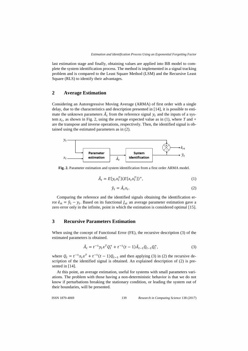
last estimation stage and finally, obtaining values are applied into BB model to com-

plete the system identification process. The method is implemented in a signal tracking

problem and is compared to the Least Square Method (LSM) and the Recursive Least

Square (RLS) to identify their advantages.

2 Average Estimation

Considering an Autoregressive Moving Average (ARMA) of first order with a single

delay, due to the characteristics and description presented in [14], it is possible to esti-

mate the unknown parameters ��𝑡 from the reference signal 𝑦𝑡 and the inputs of a sys-

tem 𝑥𝑡 , as shown in Fig. 2, using the average expected value as in (1), where T and +

are the transpose and inverse operations, respectively. Then, the identified signal is ob-

tained using the estimated parameters as in (2).

Fig. 2. Parameter estimation and system identification from a first order ARMA model.

��𝑡 = 𝐸{𝑦𝑡𝑥𝑡𝑇}(𝐸{𝑥𝑡𝑥𝑡

𝑇})+, (1)

��𝑡 = ��𝑡𝑥𝑡. (2)

Comparing the reference and the identified signals obtaining the identification er-

ror ��rt = ��𝑡 − 𝑦𝑡 . Based on its functional 𝐽𝑒𝑡 an average parameter estimation gave a

zero error only in the infinite, point in which the estimation is considered optimal [15].

3 Recursive Parameters Estimation

When using the concept of Functional Error (FE), the recursive description (3) of the

estimated parameters is obtained.

��𝑡 = 𝑡−1𝑦𝑡𝑥𝑇𝑄𝑡+ + 𝑡−1(𝑡 − 1)��𝑡−1𝑄𝑡−1𝑄𝑡

+, (3)

where 𝑄𝑡 = 𝑡−1𝑥𝑡𝑥𝑇 + 𝑡−1(𝑡 − 1)𝑄𝑡−1 and then applying (3) in (2) the recursive de-

scription of the identified signal is obtained. An explained description of (2) is pre-

sented in [14].

At this point, an average estimation, useful for systems with small parameters vari-

ations. The problem with those having a non-deterministic behavior is that we do not

know if perturbations breaking the stationary condition, or leading the system out of

their boundaries, will be presented.

139

Estimation and Identification Process Using an Exponential Forgetting Factor


4 EFF Estimation

From the average estimation, its low computational complexity is a remarkable ad-

vantage. In cases when a unique parameter is used in combination with an adequate FF

[16] it presents a better performance compared to other hybrid versions [7,17].

Within the state of the art, FF is implemented to modify the covariance from a system

state, but the descriptions are complex due to the number of operations, which increase

in order of the parameter matrix. Each FF affects with different intensity the estimation

results, having the exponential kind the most accepted, due to the past information tends

to lose weight through the evolution of the system following the tendency of the expo-

nential function (4) [18], whose base is the number e, and 𝐶 and 𝑎𝑟𝑔 the coefficient

and argument that affects its behavior.

exp = 𝐶𝑒𝑎𝑟𝑔 (4)

Two functions presented in different calculations, and that are not extensively used

to modify the Forgetting Factor (FF), are the sign (5) and the absolute (5). Each of them

gives different properties from magnitudes without increasing considerably the com-

plexity.

|𝑥| = {𝑥 𝑖𝑓 𝑥 ≥ 0,

−𝑥 𝑖𝑓 𝑥 < 0, (5)

𝑠𝑔𝑛(𝑥) = {

1 𝑖𝑓 𝑥 > 0,0 𝑖𝑓 𝑥 = 0,

−1 𝑖𝑓 𝑥 < 0. (6)

A comparison of both functions is developed to determine which is more useful for

the error correction in the estimation-identification process. Fig. 3 shows the results.

Fig. 3. Comparison of the sign and absolute function in the approximation of a signal.

140



As in shown in Fig. 3, comparing both functions to approximate a reference with

different magnitudes of variations, the sign function performs better, so this is the one

selected. It is also possible to see that when the reference tends to zero, both approxi-

mations are similar, obtaining a more remarkable variation when the error is different

from zero.

Considering the error identification as an innovation process and the principal argu-

ment for the exponential correction factor, as well as the characteristics given by the

sign function, it is proposed in [19] the use of the Exponential Forgetting Factor

(EFF) (7).

𝐸𝐹𝐹𝑡 = 𝑠𝑔𝑛(��𝑡)𝑒𝑠𝑔𝑛(𝐴𝑡)𝑒𝑟𝑡 . (7)

This factor is applied to modify the first average estimation and obtaining a second

estimation as indicated in (8)

��𝑡 = ��𝑡 + 𝐸𝐹𝐹𝑡 − 𝑠𝑔𝑛(��𝑡). (8)

To obtain the final identified output is necessary to apply (8) in (2); obtaining a cor-

rected estimation in two complete iterations. The block diagram in Fig. 4 summarizes

the procedure, where the dotted lines indicate the second estimation stage.

Fig. 4. Estimation-Identification block diagram, with two stages of correction using the sign

function and the Exponential Forgetting Factor (EFF).

141



5 Application Example

The estimation-identification process analyzed in time is focused on the shape of a sig-

nal. To visualize the effectiveness of the EFF correction, the method is applied in a

simple tracking trajectory problem.

According to [20], the initial trajectory assigned to a flight could be adjusted through

time to optimize the path with the objective of avoid accidents and to take advantage

of the wind flow [21]. Searching benefits in security, reduction of the fuel consumption

and environment pollution.

Being the reference signal a trajectory from one point to another given in latitude

and longitudinal coordinates, first the Recursive Least Square (RLS) and the Least

Square Methods (LSM) are compared.

To implement these first two methods is necessary to determine the longitude of the

filter and their initial parameter values. Longitude could be between 1 to n, being n the

biggest value, and the initial parameters between 0 and 1.

In Fig. 5 different filters size and their execution time are presented. This data was

obtained considering the input as a random signal and output signal from the reference

trajectory.

Fig. 5. Comparison in execution time between using the Least Square Method (LSM) and the

Recursive Least Square (RLS).

From Fig. 5 is easy to appreciate that an increment in the filter size implies increasing

the execution time. Thus, a second is performed to identify which filter, LSM or RLS

methods, approximates better the reference and with what size. Fig. 6 shows these per-

formances considering filters of size 1, 23 and 50.

The 23 size LSM was the best adapted to the reference, while any size of the RLS

method could not approximate the trajectory.

From previous results, it is decided to use the LMS (23) as reference to compare the

correction through the EFF estimation. Fig. 8 shows the approximation to the reference

comparison, and Fig. 9 the error obtained with each method, where the LSM has an

approximate of 2.5% error while the EFF 6%.

142



Fig. 6. Comparison of the LSM and RLS performance for different filter sizes.

Fig. 7. Performance in the tracking trajectory problem using the LSM and the EFF methods.

In addition to this, another comparison is performed, but now using the CPU-time from

the Matlab® interface to measure how much time they take to accomplish the estima-

tion. Fig. 9 presents the results, where the EFF estimation takes less time than the LSM

method.

6 Conclusions

With the development of the present paper, it was possible to compare a parameter

estimation - system identification process by using an Exponential Forgetting Factor

(EFF), reducing the influence of past data in comparison to the traditional Least Square

Method (LSM) and the Recursive Last Square (RLS).

The identification obtained with the LSM and the EFF was similar and better than

that one obtained with the RLS, for the considered signal reference. When using the

143



adequate size filter for the LSM the error tends to zero, nevertheless, when using the

EFF it is not necessary to define initial parameters and its execution time is 75%, ap-

proximately, lower than the one LSM presents.

Fig. 8. Error obtained when LSM and EFF methods are applied to identify a reference.

Fig. 9. Execution time taken from the cputime given by Matlab for the tracking trajectory prob-

lem, measured for different number of iterations and comparing the EFF and the LSM.

It is necessary to compare more Forgetting Factor (FF) configurations to determine

which is the best, but for now the combination of the sign function of the estimated

parameter, in average, and the error magnitude, as presented in this work, gives useful

results when time restrictions are presented.

References

1. Bakshi, U., Bakshi, V.: Automatic Control Systems. Technical Publications (2009)

2. García, R. P. Ñ.: Apuntes de sistemas de control. Editorial club Universitario (2003)

144



3. Ugalde, H., Carmina, J., Reyes, J., Mantilla, J.: Computational cost improvement of neural

network models in black box nonlinear system identification. Neurocomputing, 166, 96–108

(2015)

4. Godjevac, J. Neuro-fuzzy controllers: design and application. In: PPUR presses polytech-

niques (1997)

5. Qiu, F., Jensen, J. R.: Opening the black box of neural networks for remote sensing image

classification. International Journal of Remote Sensing, 25(9), 1749–1768 (2004)

6. Wnag, J.: Adaptive control for nonlinear systems using decomposed neural network. Cyber-

netics & systems 29 (1), 73–83 (1998)

7. Aguilar, K., Medel, J., Fernández, J., Vigueras, E.: Neural net gains estimation based on an

equivalent model. Computational Intelligence and Neuroscience 2016 (2016)

8. Aguilar, K., Zagaceta, M., Medel, J.; Adaptation of weights in a neuron using an integrated

filter. Research in Computing Science, 100, 139–147 (2015)

9. Parkum, J. Pulsen, N., Holst, J.: Recursive forgetting algorithms. Internacional Journal of

Control 55(1), 109–128 (1992)

10. Nishiyama, K.: A new approach to introducing a forgetting factor into the normalized least

mean squares algorithm. Signal Processing 114, 19–23 (2015)

11. Badoni, M., Singh, A., Singh, B.: Variable forgetting factor recursive least square control

algorithm for dstatcom. IEEE Transactions on Power Delivery 30(5), 2353–2361 (2015)

12. Yinling, J., Beiyan, J.: Multi-model neural network sliding mode control for robotic manip-

ulators. In: Mechatronics and Control (ICMC), International Conference on IEEE, 2431–

2435 (2015)

13. Chand, A., Kawanishi, M., Narikiyo, T.: Parameter estimation for the pitching dynamics of

a flapping-wing flying robot. In: IEEE International Conference on Advanced Intelligent

Mechatronics (AIM) IEEE, 1552–1558 (2015)

14. Aguilar, K., Urbieta, R., Medel, J.: Stochastic System Model Evaluated with First and Sec-

ond Order Filters. Research in Computing Science 118, 127–136 (2016)

15. Juárez, M., Parrazales, R., Orozco, R.: Estimador estocástico para un sistema tipo caja negra.

Revista mexicana de física 57(3), 204–210 (2011)

16. Albu, F.: Improved variable forgetting factor recursive least square algorithm. In: Control

Automation Robotics & Vision (ICARCV), 12th International Conference on IEEE, pp.

1789–1793 (2012)

17. Henwood, N.: Estimation en ligne de parametres de machines électriques pour véhicule en

vue d’un suivi de la température de ses composants. PhD thesis, Ecole Nationale Supérieure

des Mines de Paris (2014)

18. Antonio, N., Pedro, C., Manuel, M.: Conceptos básicos de filtrado, estimación e identifica-

ción. IEEE Transactions on Power Delivery 30(5), 2353–2361 (2015)

19. Aguilar, K.: Filtro digital para la estimación de parámetros variantes usando el factor de

olvido exponencial. Thesis, Centro de Investigación en Computación IPN (2015)

20. Altus, S.: Effective flight plans can help Airlines economize. Boeing Aero (2009)

21. Cattani, L., Eagle, P.: Aircraft identification, trajectory tracking and prediction. Tech. rep.

DTIC Document (1995)

145



Analisis de readmision hospitalaria de pacientesdiabeticos mediante aprendizaje computacional

German Cuaya-Simbro1, Elias Ruiz1, Angelica Munoz-Melendez2,Eduardo F. Morales2

1 Instituto Tecnologico Superior de Oriente del Estado de Hidalgo, Apan Hidalgo,Mexico

2 Instituto Nacional de Astrofısica, Optica y Electronica, Tonantzintla, Puebla,Mexico

{gcuaya, eruiz}@itesa.edu.mx, {amunoz,emorales}@inaoep.mx

Resumen. La disminucion de la taza de readmision hospitalaria tem-prana es una situacion de interes debido a que esto generalmente es de-bido a complicaciones de alguna enfermedad en los pacientes. En Mexicoes particularmente importante la prevencion de la readmision tempranade pacientes diabeticos, puesto que esto est asociado a complicacionesderivadas de la enfermedad, como pueden ser problemas en los ojos,riones, nervios, corazon, entre otros. Existen trabajos en donde se des-criben metodos computacionales para el diagnostico de diabetes [10,4],pero en estos trabajos no se hace un analisis de los factores relacionadosa las complicaciones de la enfermedad. En este artıculo, se presenta unanalisis basado en tecnicas de aprendizaje computacional para estimarlas variables mas importantes asociadas a la readmision hospitalaria enpacientes con diabetes. La metodologıa presentada contempla el uso demetodos de seleccion de atributos y seleccion de instancias mediantetecnicas supervisadas y no supervisadas, ası como la construccion declasificadores con la informacion obtenida, finalmente, se presentan y sediscuten los valores de precision y recuerdo de los clasificadores paramostrar la efectividad de estos en la prediccion de readmision tempranade pacientes diabeticos. Los resultados muestran las ventajas del uso de lametodologıa propuesta para la identificacion de la informacion relevanteasociada a la prevencion de readmision hospitalaria.

Palabras clave: seleccion de atributos, agrupamiento, clasificacion,readmision hospitalaria.

Hospital Readmission Analysis of Diabetic Patientsthrough Computational Learning

Abstract. The decrease in the rate of early hospital readmission is asituation of interest because this is usually due to complications of some

147

ISSN 1870-4069


disease in the patients. In Mexico, the prevention of early readmissionof diabetic patients is particularly important, since this is associatedwith complications derived from the disease, such as problems in theeyes, kidneys, nerves, heart, among others. There are works describingcomputational methods for the diagnosis of diabetes [10,4], but in theseworks an analysis of the factors related to the complications of thedisease is not done. In this article, we present an analysis based oncomputational learning techniques to estimate the most important va-riables associated with hospital readmission in patients with diabetes.The presented methodology contemplates the use of methods of selectionof attributes and selection of instances by means of supervised andunsupervised techniques, as well as the construction of classifiers withthe obtained information, finally, the values of precision and memoryof the classifiers are presented and discussed. to show the effectivenessof these in the prediction of early readmission of diabetic patients. Theresults show the advantages of using the proposed methodology for theidentification of relevant information associated with the prevention ofhospital readmission.

Keywords: attributes selection, grouping, classification, hospital read-mission.

1. Introduccion

Actualmente los modelos de inteligencia computacional son usados cada vezcon mayor frecuencia en el ambito medico, como herramientas para el diagnosticode enfermedades [6]. Sin embargo, es de especial interes usar las herramientas deinteligencia computacional en aplicaciones no solamente de diagnostico, sino deprediccion, en particular, es de suma importancia prevenir la aparicion o com-plicacion de enfermedades, lo cual generalmente implica una pronta (temprana)readmision hospitalaria de un paciente.

En los hospitales es importante tener un ındice bajo de readmision hospitala-ria [1] la cual es derivada de la complicacion de algun padecimiento, como puedenser cardiovascular, respiratorio, digestivo, diabetes, por mencionar algunos. Al-gunos paıses han creado programas para reducir la readmision hospitalaria [12],con el objetivo de reducir los costos de salud y de mejorar la calidad de vidade los pacientes. Es importante sealar que, el reducir la readmision hospitalariaimplica la prevencion y/o prediccion de esta.

La diabetes es una enfermedad con una incidencia cada vez mas alta en elmundo [5,11]. En particular, en Mexico es una enfermedad de alerta en hospitales[13]. Actualmente los hospitales se encuentran realizando esfuerzos en materia dediagnostico preventivo hacia la poblacion en general. Diagnosticar pre-diabeteso hacer recomendaciones de mejores habitos de alimentacion y ejercicio parapacientes con predisposicion a ella tiene un impacto en la reduccion de costospara las instituciones de salud y en una mejorıa para la calidad de vida delpaciente [2].

148

Germán Cuaya-Simbro, Elias Ruiz, Angélica Muñoz-Meléndez, Eduardo F. Morales


En contraste con lo anterior, poco se ha estudiado y discutido sobre aquellospacientes diagnosticados con diabetes y los cuales tuvieron que ser reingresadosal hospital en un corto tiempo por alguna complicacion de la enfermedad, lo cualtiene implicaciones graves para la salud del paciente, en ocasiones la muerte. Lamayorıa de estas situaciones son ocasionadas debido a que un paciente llegaa medicina general o a especialidades que no corresponden al tratamiento dela diabetes (endocrinologıa), lo que puede derivar en una complicacion de laenfermedad como pueden ser, problemas en riones, pies, ojos o piel, corazon,entre otras. Dichas complicaciones pueden ser evitadas, pero se requiere undiagnostico acertado y preventivo. Por este motivo, resulta importante contarcon estrategias que permitan ayudar a predecir posibles complicaciones asocia-das a la diabetes, lo cual generalmente deriva en una readmision hospitalariatemprana, y en especıfico determinar los factores que estan asociados a dichareadmision.

En este trabajo de investigacion se presenta un analisis de la informacionde una base de datos con registros de pacientes diagnosticados con diabetes loscuales fueron readmitidos en el hospital, determinando por medio de aprendizajecomputacional aquellas variables que estan asociadas a una readmision temprana(en un periodo de tiempo menor a 30 dıas) y mostrando como el uso de estetipo de tecnicas puede apoyar en la identificacion de factores asociados a lacomplicacion de enfermedades, en especıfico la diabetes.

2. Antecedentes

Debido a la importancia de la diabetes a nivel mundial, se han reportadodiversos trabajos que utilizan tecnicas de aprendizaje computacional para diag-nosticar diabetes en pacientes [10,4]. La mayorıa de dichos trabajos, utilizanreglas de decision o clasificadores SVM (Support Vector Machine) en un enfoquesupervisado. Sin embargo, su enfoque es principalmente el diagnostico, no laprediccion y/o prevencion de las complicaciones de alguna enfermedad.

Por otro lado, existen trabajos que reportan el analisis de informacion paraprevenir o predecir la readmision de pacientes, como se presenta en [19] don-de realizan un caso de estudio sobre una determinada raza para verificar lareadmision de pacientes pertenecientes a esta en un lapso menor a 30 dıas,utilizando un enfoque basado en un algoritmo de redes bayesianas. En [20] hacenun analisis del impacto de la hemoglobina glicosilada con respecto de los nivelesde reincidencia del paciente diabetico al hospital a lo largo de varios meses, losautores concluyen que la probabilidad de readmision esta ligada al diagnosticoprimario del paciente y a las acciones para mantener los niveles de hemoglobinaglicosilada bajo control. Igualmente, en [14] muestran la importancia de tener uncontrol glucemico al dar de alta al paciente para reducir el riesgo de reingreso enla poblacion mexicana, aunque la mayor razon de reingreso fue debido a infeccio-nes y enfermedades cardiovasculares. Los trabajos citados parten del analisis deinformacion a priori, proporcionada generalmente por los expertos (en particularla consideraciones de variables a utilizar), en contraste al trabajo realizado en

149

Análisis de readmisión hospitalaria de pacientes diabéticos mediante aprendizaje computacional


esta investigacion, se propone el analisis mediante aprendizaje computacional delos datos para determinar los factores o variables asociados a la complicacionde una enfermedad la cual derive en la readmision del paciente, en especıfico enpacientes diabeticos. La identificacion correcta de los factores de riesgo asociadosa complicaciones de cierta enfermedad propiciara un mejor pronostico.

Existen diversas tecnicas del aprendizaje computacional para analizar datosa fin de seleccionar atributos o variables de interes, seleccionar instancias o ejem-plos, mejorar la clasificacion a partir de datos entre otras, por ejemplo, [8,15]. Espor esto que en este trabajo se presentan resultados de la aplicacion de diferentesalgoritmos estandar de seleccion de variables, agrupamiento, y clasificacion, parala identificacion de factores de riesgo asociados a complicaciones de la diabetes,lo cual implica una readmision temprana del paciente. Los metodos de seleccionde variable, de agrupamiento y de clasificacion fueron aplicados a traves Weka,el cual es un software para minerıa de datos que permite realizar clasificacion yseleccion de atributos [7].

3. Metodologıa

En este trabajo se utilizo la base de datos descrita en [20]. Esta base de datoscuenta con 101,766 visitas de pacientes (registros) los cuales fueron hospitaliza-dos y a quienes se les asigno un numero de identificacion. Cada paciente tieneregistrado un numero determinado de visitas, esto es, un paciente en esta basede datos puede tener registradas 4 visitas, y otro paciente puede tener asociadosolo 1 visita. En una visita se toman la informacion de la Tabla 1 la cual cuentacon 55 atributos.

Tabla 1. Nombre y tipo de dato de los atributos de la base de datos. Informaciondetallada de la tabla puede ser consultada en [20].

Atr. Nombre del atributo Tipo Atr. Nombre del atributo Tipo1 Encounter ID Numerico 15 Num. of medications Numerico2 Patient number Numerico 16 Num. of outpatient visits Numerico3 Race Nominal 17 Num. of emergency visits Numerico4 Gender Nominal 18 Num. of inpatient visits Numerico5 Age Nominal 19 Diagnosis 1 Nominal6 Weight Numerico 20 Diagnosis 2 Nominal7 Admission type Nominal 21 Diagnosis 3 Nominal8 Discharge disposition Nominal 22 Number of diagnoses Numerico9 Admission source Nominal 23 Glucose serum test result Nominal10 Time in hospital Numerico 24 A1c test result Nominal11 Payer code Nominal 25 Change of medications Nominal12 Medical specialty Nominal 26 Diabetes medications Nominal13 Number of lab procedures Numerico 27 24 features for medications Nominal14 Number of procedures Numerico 28 Readmitted Nominal

Cada visita registrada indica si el paciente fue readmitido antes de 30 dıas(clase 1), despues de 30 dıas o ya no fueron readmitidos (clase 0), atributoreadmitted. El analisis desarrollado identifica informacion relevante asociada ala readmision temprana del paciente, y la relevancia de la informacion evaluada

150



mediante la construccion y evaluacion de clasificadores, posteriormente se uti-lizan tecnicas de agrupamiento para complementar o enriquecer la informacionrelevante. Este proceso es descrito con detalle a continuacion:

1. Se redujo el numero de instancias mediante un enfoque supervisado deeliminacion de registros incompletos.

2. Se realizo una conversion supervisada a datos numericos de todos los atri-butos nominales.

3. Se ordeno la base de datos de acuerdo al atributo “Identificador de visita”(Encounter ID).

4. Se separo la base de datos de acuerdo al numero de visitas de cada paciente,esto es, se creo una base de datos con la informacion de aquellos pacientescon unicamente 1 visita, M1, posteriormente se construye una nueva base dedatos con la informacion de los pacientes que tuvieron al menos 2 visitas,M2, cabe sealar que la informacion contenida en esta nueva base de datossolo esta la informacion de la segunda visita de los pacientes dado que lainformacion correspondiente a la primera visita ya se tiene almacenada enM1. Se continua con este proceso hasta tener por separada la informacionde cada una de las visitas de los pacientes. Una vez acabado este procesose obtuvo un total de 26 bases de datos, esto es, M1,M2, . . . ,M26, donde|M1| = 34321, |M2| = 6484, |M3| = 2259, . . ., |M26| = 1.

5. Se determino trabajar solamente con la informacion de los pacientes quetienen al menos 3 visitas registradas, esto es, se uso solo la informacion deM1, M2, y M3, debido a que el objetivo de este trabajo es prevenir lascomplicaciones de la diabetes, es decir, prevenir las readmisiones tempranasasociadas a esta enfermedad.

6. Se realizo un proceso de uniformidad de las bases de datos anteriores, bus-cando tener la misma informacion en cada una de ellas, tomando comoreferencias los elementos contenidos en M3, 2259, y eliminando los elementosdiferentes en M1 y M2. Ası, |M1| = |M2| = |M3| = 2259.

7. Se filtro la informacion de las bases de datos conservando unicamente aque-llos pacientes (instancias) que fueron diagnosticados con algun tipo de dia-betes, atributos Diagnosis 1, 2 o 3. Ası, |M1| = |M2| = |M3| = 485.

8. Se unio la informacion de las 3 bases de datos anteriores en una sola de talmodo que se obtuvo la base de datos con la que se trabajo, BDall, dondeDBall = M1 ∪M2 ∪M3, |DBall| = 1455.

9. Se realizo seleccion de atributos [8] mediante la regla Vsel =n⋃

j=1

Sj , donde Sj

es el conjunto de variables obtenidas por un metodo de seleccion de atributos.En los experimentos n = 5 y el umbral de cada Sj fue fijado a los seisprimeros resultados. Los metodos de seleccion de atributos utilizados fueron:metodo basado en correlacion [9], metodo basado en correlacion de Pearson,metodo basado en ganancia de informacion, y metodo basado en seleccion deatributos mediante el uso de reglas. Ası el conjunto de variables Vsel obtenidotiene 13 elementos los cuales son mostrados en la Tabla 2. De acuerdo a lasvariables seleccionadas se creo una base de datos conservando unicamentedichas variables DBsv.

151



Tabla 2. Variables escogidas por los metodos de seleccion de variables. Las variablescon el numero 27* corresponden a nombres de medicamentos consumidos por elpaciente.

No. Atributo Nombre del atributo No. Atributo Nombre del atributo18 Number of inpatient visits 27* glimepiride22 Number of diagnoses 8 Discharge disposition27* Insulin 26 Diabetes medications27* glipizide-metformin 17 Number of emergency visits27* metformin-rosiglitazone 19 Diagnosis 110 Time in hospital 20 Diagnosis 227* repaglinide

10. Se proceso la informacion de DBall con una tecnica de aprendizaje nosupervisado (k-medias de 2 grupos) para pesar de manera simple los ejemplosmas faciles de aprender y con ellos entrenar el modelo supervisado. Esteprocedimiento es una tecnica simplificada de boosting. De lo anterior seobtienen 2 bases de datos, instancias correctamente aprendidas DBcorr ylas incorrectamente aprendidas DBincorr.

11. Finalmente se realizo clasificacion de los datos utilizando tecnicas de apren-dizaje supervisado para cada conjunto de datos, tales como Redes Bayesianas[16], bagging [3], arboles [18] y vectores de soporte [17].

Un diagrama que ilustra el proceso de analisis de la informacion para determi-nar los factores relevantes asociados readmision temprana de pacientes diabeticosa causa de complicaciones es presentado en las Figuras 1 y 2.

Fig. 1. Diagrama del pre-procesamiento de la informacion. Al final se consideransolamente pacientes con diagnostico de diabetes.

4. Resultados y discusion

Para mostrar la efectividad del uso de la metodologıa propuesta en estetrabajo se construyeron 4 clasificadores, utilizando las diferentes bases de datosgeneradas durante el proceso de analisis de la informacion, DBall base de datoscon todos los atributos, DBsv base de datos con las variables de la Tabla 2,DBcorr base de datos con las instancias correctamente aprendidas en el procesode agrupamiento.

152



Fig. 2. Diagrama del proceso de analisis de la informacion el cual consiste en hacerseleccion de atributos, agrupamiento y clasificacion.

Las metricas que se usaron para evaluar cada uno de los clasificadores fueronprecision, recuerdo y medida F.

La precision se define como V PV P+FP , donde VP son los verdaderos positivos

(casos correctamente estimados y FP son los falsos positivos (casos erroneamenteclasificados como positivos). Esto es, es la proporcion de instancias relevantesobtenidas respecto a las instancias recuperadas.

Fig. 3. Valor de precision de los clasificadores con las diferentes bases de datos.

El recuerdo se define como V PV P+FN , donde FN son los falsos negativos (casos

erroneamente clasificados como negativos). Es decir, indica la proporcion deinstancias relevantes que se han recuperado sobre la cantidad total de instanciasrelevantes.

La medida F trata de establecer un compromiso entre la precision y elrecuerdo, evitando caer en una sobre representacion de alguno de los dos. Se

153



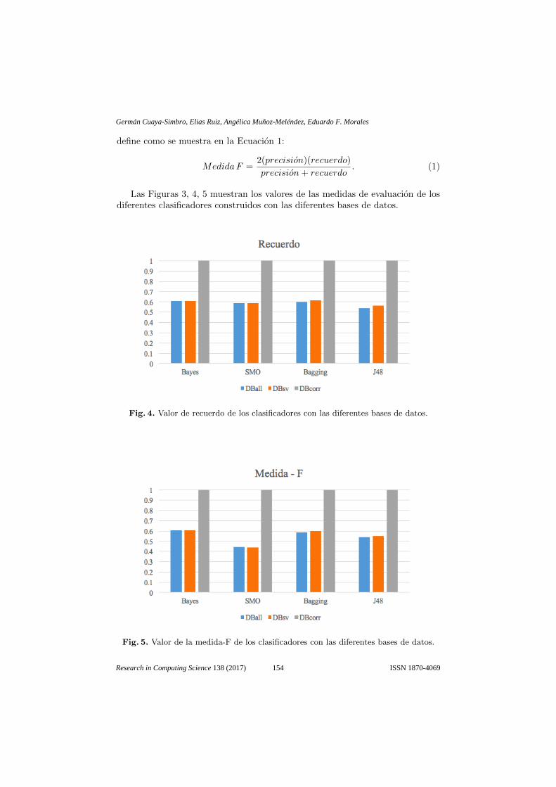
define como se muestra en la Ecuacion 1:

MedidaF =2(precision)(recuerdo)

precision + recuerdo. (1)

Las Figuras 3, 4, 5 muestran los valores de las medidas de evaluacion de losdiferentes clasificadores construidos con las diferentes bases de datos.

Fig. 4. Valor de recuerdo de los clasificadores con las diferentes bases de datos.

Fig. 5. Valor de la medida-F de los clasificadores con las diferentes bases de datos.

154



Como se puede observar los clasificadores construidos con las variables rele-vantes de la Tabla 2, tienen un desempeo similar a los clasificadores que fueronconstruidos utilizando todas las variables, esto es, se han determinado variablesrelevantes asociadas a la readmision temprana debido a complicaciones de ladiabetes.

Es de interes y de discusion los resultados obtenidos con la base de datosDBcorr, en principio esta base de datos es mas pequea que las bases DBall yDBsv, |DBcorr| = 723, el uso de agrupamiento permitio reducir el problema yanalizar la informacion mas relevante, debido a que las instancias consideras endicho conjunto de datos son muy similares y al momento de construir clasifica-dores con dicha informacion podemos determinar las relaciones y la relevanciade dichas variables, dado que obtenemos modelo mas efectivos en terminos deprecision, recuerdo y medida-F.

Con un analisis mas detallado de los modelos creados con DBcorr permitioobservar variables tales como la insulina la cual esta estrechamente asociada ala deteccion de un riesgo de readmision hospitalaria temprana, lo cual a partirde la simple seleccion de atributos no era posible determinar, ası debe tenerse encuenta que determinar subconjunto de forma supervisada ayuda en la explicacionde las relaciones de las variables respecto a la clase de interes, readmision.

Este analisis es complementario a la informacion mostrada en la Tabla 2y debe de ser considera por los expertos en el dominio para disear y conducirestudios mas especializados en donde solo se incorpore la informacion relevantey se descarte informacion que de acuerdo a los resultados no aporta informacionpara la determinacion de readmision en un periodo menor a 30 dıas.

5. Conclusiones y trabajo futuro

Se presenta una metodologıa la cual permite la identificacion de los factoresrelacionados a la readmision hospitalaria temprana debido a complicaciones enpacientes diabeticos.

La seleccion de atributos en conjunto con el agrupamiento de instancias simi-lares permite determinar las principales relaciones entre las variables y mejorarlos modelos de prevencion de readmision hospitalaria temprana.

Se discuten las posibles ventajas del uso de la metodologıa propuesta desdeel punto de vista computacional y ademas de las ventajas del uso de las variablesrelevantes desde el punto de vista clınico. Dando con ello un panorama de comotecnicas de aprendizaje automatico pueden apoyar en procesos de prevencionmedica, en este caso la prevencion de readmision temprana de pacientes diabeti-cos.

Como trabajo futuro, se extenderan el conjunto de pruebas para validar laefectividad de la metodologıa propuesta. Estas pruebas pueden involucrar el usode todo el conjunto de datos, uso de datos filtrados por edad, entre otras. Dela misma forma y con el objetivo de evaluar la efectividad de la metodologıase probara esta con diferentes bases de datos, tal como bases de datos medicas,climaticas o financieras, por mencionar algunas. Finalmente, con el objetivo de

155



medir la relevancia de la informacion se propone la validacion de los resultadosobtenidos, especıficamente la seleccion de variables, con expertos en el dominio,para verificar si los resultados encontrados tienen validez desde el punto de vistaclınico.

Referencias

1. Alonso Martinez, J.L., Llorente Diez, B., Echegaray Agara, M., Urbieta Echeza-rreta, M.A., Gonzalez Arencibia, C.: Reingreso hospitalario en Medicina Interna.Anales de Medicina Interna 18, 28 – 34 (05 2001)

2. Barquera, S., Campos-Nonato, I., Aguilar-Salinas, C., Lopez-Ridaura, R., Arre-dondo, A., Rivera-Dommarco, J.a.: Diabetes in mexico: cost and management ofdiabetes and its complications and challenges for health policy. Global Health 9,9 (2013), http://www.ncbi.nlm.nih.gov/pmc/articles/PMC3599194/

3. Breiman, L.: Bagging predictors. Machine Learning 24(2), 123–140 (1996),https://doi.org/10.1007/BF00058655

4. Fatima, M., Pasha, M.: Survey of machine learning algorithms for disease diag-nostic. Journal of Intelligent Learning Systems and Applications 9, 1–16 (2017),www.scirp.org/journal/PaperInformation.aspx?PaperID=73781

5. Forouhi, N.G., Wareham, N.J.: Epidemiology of diabe-tes. Medicine (Abingdon) 42(12), 698–702 (Dec 2014),http://www.ncbi.nlm.nih.gov/pmc/articles/PMC4282306/, s1357-3039(14)00271-0[PII]

6. Foster, K.R., Koprowski, R., Skufca, J.D.: Machine learning, medical diagnosis, andbiomedical engineering research - commentary. Biomed Eng Online 13, 94–94 (Jul2014), http://www.ncbi.nlm.nih.gov/pmc/articles/PMC4105825/, 1475-925X-13-94[PII]

7. Frank, E., Hall, M.A., Holmes, G., Kirkby, R., Pfahringer, B., Witten, I.H., Trigg,L.: Weka-a machine learning workbench for data mining. In: Maimon, O., Rokach,L. (eds.) Data Mining and Knowledge Discovery Handbook, 2nd ed., pp. 1269–1277. Springer (2010), https://doi.org/10.1007/978-0-387-09823-4 66

8. Guyon, I., Elisseeff, A.: An introduction to variable and featureselection. Journal of Machine Learning Research 3, 1157–1182 (2003),http://www.jmlr.org/papers/v3/guyon03a.html

9. Hall, M.A.: Correlation-based feature selection for discrete and numeric classmachine learning. In: Langley, P. (ed.) Proceedings of the Seventeenth InternationalConference on Machine Learning (ICML 2000), Stanford University, Stanford, CA,USA, June 29 - July 2, 2000. pp. 359–366. Morgan Kaufmann (2000)

10. Kavakiotis, I., Tsave, O., Salifoglou, A., Maglaveras, N., Vlahavas, I., Chou-varda, I.: Machine learning and data mining methods in diabetes research.Computational and Structural Biotechnology Journal 15, 104 – 116 (2017),http://www.sciencedirect.com/science/article/pii/S2001037016300733

11. Mayer-Davis, E.J., Lawrence, J.M., Dabelea, D., Divers, J., Isom, S., Dolan, L.,Imperatore, G., Linder, B., Marcovina, S., Pettitt, D.J., Pihoker, C., Saydah,S., Wagenknecht, L.: Incidence trends of type 1 and type 2 diabetes amongyouths, 2002-2012. New England Journal of Medicine 376(15), 1419–1429 (2017),http://dx.doi.org/10.1056/NEJMoa1610187, pMID: 28402773

12. McIlvennan, C.K., Eapen, Z.J., Allen, L.A.: Hospital readmis-sions reduction program. Circulation 131, 1796–1803 (May 2015),http://www.ncbi.nlm.nih.gov/pmc/articles/PMC4439931/

156



13. Meza, R., Barrientos-Gutierrez, T., Rojas-Martinez, R., Reynoso-Noveron, N., Palacio-Mejia, L.S., Lazcano-Ponce, E., Hernandez-Avila,M.: Burden of type 2 diabetes in mexico: Past, current and futureprevalence and incidence rates. Preventive medicine 81, 445–450 (2015),http://www.ncbi.nlm.nih.gov/pmc/articles/PMC4679631/

14. Molina-Corona, A., Zonana-Nacach, A.: Readmisin hospitalaria de pacientes diab-ticos: seguimiento de 12 meses. Revista Mdica del Instituto Mexicano del SeguroSocial 5, 469–474 (2010)

15. Olvera-Lopez, J.A., Carrasco-Ochoa, J.A., Martınez Trinidad, J.F., Kittler, J.: Areview of instance selection methods. Artif. Intell. Rev. 34(2), 133–143 (2010),https://doi.org/10.1007/s10462-010-9165-y

16. Pearl, J.: Probabilistic reasoning in intelligent systems - networks of plausibleinference. Morgan Kaufmann series in representation and reasoning, MorganKaufmann (1989)

17. Platt, J.C.: Sequential minimal optimization: A fast algorithm for training supportvector machines. Tech. rep., Advances in Kernel Methods - support Vector Learning(1998)

18. Quinlan, J.R.: C4.5: Programs for Machine Learning. Morgan Kaufmann (1993)19. Shameer, K., Johnson, K.W., Yahi, A., Miotto, R., Li, L., Ricks, D., Jebakaran, J.,

Kovatch, P., Sengupta, P.P., Gelijns, A., Moskovitz, A., Darrow, B., Reich, D.L.,Kasarskis, A., Tatonetti, N.P., Pinney, S., Dudley, J.t.: Predictive modeling ofhospital readmission rates using electronic medical record-wide machine learning:A case-study using mount sinai heart failure cohort. In: Pacific Symposium onBiocomputing. Pacific Symposium on Biocomputing. vol. 22, pp. 276–287 (2016),http://www.ncbi.nlm.nih.gov/pmc/articles/PMC5362124/

20. Strack, B., DeShazo, J.P., Gennings, C., Olmo, J.L., Ventura, S., Cios, K.J., Clore,J.N.: Impact of hba1c measurement on hospital readmission rates: Analysis of70,000 clinical database patient records. BioMed Research International 2014, 11(2014), http://dx.doi.org/10.1155/2014/781670

157



The Mexican Magical TownsTraveling Salesman Problem:

Preliminary Results

Sandra J. Gutierrez, Nareli Cruz-Cortes, Hiram Calvo,Marco A. Moreno-Armendariz

Instituto Politecnico Nacional, Centro de Investigacion en Computacion,CDMX, Mexico

[email protected], [email protected], [email protected],mam [email protected]

Abstract. The Traveling Salesman Problem (TSP) is a classical NP-hard combinatorial problem that has been intensively studied throughseveral decades. A large amount of literature is dedicated to this pro-blem. TSP can be directly applied to some real life problems, and tobe generalized to some other set of important combinatorial problems.Nowadays, a large collection of TSP instances can be found such asTSPLIB and National TSP webpage, among others. In this paper weexperiment with a different TSP instance, that is, a set of 111 Mexicantowns (called Magical Towns), by applying five different algorithms: (1)Ant Colony Optimization, (2) Particle Swarm Optimization, (3) GreedyMetaheuristic (4) Lin-Kernighan and (5) Hybrid Metaheuristic. The bestresults were obtained by the hybrid metaheuristic, with a final costfunction of 120.65.

Keywords: ant colony optimization, Lin-Kernighan, MAX-MIN antsystem, traveling salesman problem, magical towns.

1 Introduction

The Traveling Salesmen Problem (TSP) is one of the problems in mathematicsand computer science which is easy to understand and needs much effort to solve.The idea of the problem is to find the shortest path for a salesman starting froma given city, visiting n cities only once and finally arriving at the city of origin.

Much of the work on the TSP is motivated by its use as a platform foranalyzing the performance of general methods that can be applied to a widerange of discrete optimization problems. This is not to say, however, that theTSP does not find applications in many fields. Indeed, the numerous directapplications of the TSP bring life to the research area and help to direct futurework.

159

ISSN 1870-4069


A large collection of TSP instances can be found along the specialized li-terature, for instance TSPLIB1, National TSP webpage2, art constructed bysolving instances of the TSP3, among many others. However, there is almost nopublished work related to Mexican instances.

On the other hand, a Mexican Magical Town certificate is awarded to pla-ces that preserve and display tradition, beauty and culture through symbolicattributes, legends and history. The Magical Towns Program is a proposal madeby Mexico’s Ministry of Tourism launched in 2001 and, by 2017, a total of111 towns and villages in all 31 states have been awarded the title MagicalTown. The main objective of this program is to invite to visit this kind of townsthat provide a magical experience with a typical illustration of an authenticMexican village, natural beauty landscapes, folklore and historical sites, in orderto increase profits from travel and tourism.

In this paper we apply some heuristic algorithms in a specific TSP pro-blem, in this case Mexican Magical Towns. Specifically, a comparison among thefollowing algorithms is presented: two bio-inspired algorithms: Particle SwarmOptimization [1], Max-Min Ant System [2], besides the best-known algorithmfor TSP proposed by Lin & Kerninghan [3], a simple greedy strategy and anhybrid algorithm. Our comparative study shows that the algorithm with thebest results is the hybrid algorithm.

The rest of the paper will proceed as follows: the following section establishesthe TSP solved with different artificial intelligence (AI) techniques and describessome routing planning problems in Mexico. Some optimization metaheuristicsused in this paper are described in Section 3. The methodology for this investiga-tion is presented in Section 4. Computational results and discussion are presentedin Section 5. Finally, future work and conclusions are presented in Section 6.

2 Traveling Salesman Problem

The most used representation of TSP is an edge-weighted graph G = (V,E)with V being set of n = |V | nodes or vertices representing cities and E ⊆ V ×Vbeing set of directed edges or arcs. Each arc (i, j) ∈ E is assigned with a valueof length dij which is distance between cities i and j with i, j ∈ V . TSP can beeither asymmetric or symmetric in nature. In case of asymmetric TSP, distancebetween pair of nodes i, j is dependent on direction of traversing edge or arci.e. there is at least one arc(i, j) for which dij 6= dji. In contrast, in symmetricTSP the relation dij = dji holds for all arcs in E. The goal in TSP is thus tofind minimum length Hamiltonian Circuit of graph, where Hamiltonian Circuitis a closed path visiting each of n nodes of G exactly once. Thus, an optimalsolution to TSP is permutation π of node index 1, . . . , n such that length f(π)

1 https://www.iwr.uni-heidelberg.de/groups/comopt/software/TSPLIB95/2 http://www.math.uwaterloo.ca/tsp/world/countries.html3 http://www2.oberlin.edu/math/faculty/bosch/tspart-page.html

160

Sandra J. Gutiérrez, Nareli Cruz, Hiram Calvo, Marco A. Moreno-Armendáriz


is minimal, where f(π) is the objective or cost function, given by equation 1 [4]:

f(π) =

n−1∑i=1

dπ(i)π(i+1) + dπ(n)π(1). (1)

Besides the minimization of the total travel distance, other objectives couldbe considered too, for instance, minimization of travel time, minimization ofmoney (using free ways), etc.

TSP is a classical NP-hard combinatorial problem that has been intensivelystudied among several decades using heuristics like iterated-local search, branchand bound and graph coloring. Even evolutionary algorithms, ant colony opti-mization (ACO) algorithms and hybridization of techniques have been used [5].

2.1 Mexican TSP

To our knowledge, there have been only few studies about routing optimizationin Mexico. In [6] and [7] authors presents a novel method using ant colonies foroptimizing patrolling routes for personnel working in public security and the casestudy is municipality of Cuautitlan Izcalli in Mexico. Also in [8] authors design arouting planning software with the aim of distance minimization and travel costfor State of Puebla using dynamic programming and Floyd algorithm. Finally,in [9] authors use minimum spanning tree to collect trash across Atizapan deZaragoza, Mexico, while in [10], they use nearest neighborhoods to optimize thecollect of platforms across the country. These works are related to our paper,but there are not about Mexican TSP instances.

3 Optimization Heuristics and Metaheuristics

3.1 MAX - MIN Ant System (MMAS)

A main ant colony optimization algorithm (ACO) is Ant System (AS), a bio-inspired metaheuristic proposed by M. Dorigo [2]. In AS the real ant behavior isused as methaphor to get the best suitable path by artificial agents, its workingis based on a chemical substance called pheromone which is released by the antson their path, it helps ants to locate each other in order to get location of thenearest source of food. The higher the pheromone level, the greater the numberof ants following that path [11].

Each k ant generates a complete tour by choosing the cities according to aprobabilistic state transition rule given by equation 2, if cij ∈ N(sP ), otherwisepkij = 0 [2]:

pkij =ταij · η

βij∑

cil∈N(sP ) ταil · η

βil

, (2)

where τij is the pheromone associated with cities i and j, ηij = 1/dij , dij isthe distance between cities i and j, N(sP ) is the set of cities that remain to be

161

The Mexican Magical Towns Traveling Salesman Problem: Preliminary Results


visited, edges (i, l) where l is a city not yet visited. The parameters α and βcontrol the influence between pheromone and heuristic information ηij .

Ants prefer to move to cities which are connected by short edges with a highamount of pheromone. Once all ants have completed their tours the followingupdating rule is applied: a fraction of the pheromone evaporates on all edges(edges that are not refreshed become less desirable), and then each ant depositsan amount of pheromone on edges which belong to its tour in proportion to howshort its tour was.

In [12] authors include MAX - MIN AS, it is an improved version in whichonly the best ant updates the pheromone trails and the value of the pheromoneis bound. The pheromone update rule is shown in equation 3:

τij ← [(1− ρ) · τij +∆τ bestij ]τmaxτmin

, (3)

where ρ is the evaporation rate, ∆τ bestij is the quantity of pheromone laid onedge (i, j) by the best ant, τmin and τmax are the upper and lower bounds,respectively, which are typically obtained empirically and tuned on the specificproblem considered. If (i, j) belongs to the best tour ∆τ bestij is equal to 1/Lbest,otherwise it is equal to zero, and Lbest is the length of the tour of the best ant.There have been many works related to solving TSP using MM AS presented in[13] and [14].

3.2 Particle Swarm Optimization for TSP

The particle swarm optimization (PSO) is a popular metaheuristic based onsocial behaviour of flock of birds and school of fish; it was originally presented byKennedy and Eberhart [15]. In PSO, each particle represents a potential solutionwith an initial velocity and moves to a new position. At each iteration, everyparticle calculates its velocity and updates its position according to equations 4and 5, respectively [1]:

V(t)i = wV

(t−1)i ⊗ c1r1(Pi −X(t−1)

i )⊗ c2r2(G−X(t−1)i ), (4)

X(t)i = X

(t−1)i + V

(t)i . (5)

It is very important to mention that original PSO was only for continuoussearch spaces and because TSP is discrete, combinatorial problem, some mo-difications must be made. To solve TSP with PSO, each particle represents acomplete tour as a feasible solution and velocity is a measure to update the tourfor better solution. Many prominent PSO based methods use Swap Sequence(SS) for velocity. A SS is a collection of several Swap Operators (SOs) and eachone indicates two positions in a tour, those might be swapped. All SOs of a SSare applied on a particle’s tour maintaining order and hence implications of theSS transforms the TSP tour into a new one.

In equation 4, c1 and c2 are learning factors, r1 and r2 are random valuesbetween 0 and 1, Pi is the previous best tour, G is the best tour particles ever

162



encountered, Pi −X(t−1)i means to obtain SOs needed to make X

(t−1)i sequence

equal to Pi sequence, which is the same for G−X(t−1)i , c1r1(Pi−X(t−1)

i ) means

all SOs for (Pi − X(t−1)i ) should be maintained with the probability of c1r1,

which is the same for c2r2(G−X(t−1)i ), and w is the scaling factor of influence

of the previous velocity in present velocity. Each particle moves to a new tour

solution X(t)i applying all SS on its previous solution X

(t−1)i using equation 5.

A SS is the union of SOs, SS = (SO1, SO2, . . . , SOn).

The operator ⊗ defines the merging operation. If SS1 = SO(1, 2), SO(5, 2)and SS2 = SO(5, 3), SO(4, 1), the new swap sequence is:

SS(new) = SS1 ⊗ SS2 = SO(1, 2), SO(5, 2), SO(5, 3), SO(4, 1).

Finally if the new solution X(t)i is superior to Pi, update Pi, and do the same

for G. Some relevant works that used this metaheuristic were presented in [16]and [17].

3.3 Greedy Algorithms

A greedy algorithm is a mathematical process that follows the problem solvingheuristic of making the locally optimal choice at each stage, deciding whichnext step will provide the most obvious benefit with the aim of finding a globaloptimum, in this case chooses the nearest city no matter where it starts, butavailability of nearest cities it is important [18]. The advantage of using agreedy algorithm is that solutions to smaller instances of the problem can bestraightforward and easy to understand. The disadvantage is that it is entirelypossible that the most optimal short-term solutions may lead to the worstpossible long-term outcome [19].

3.4 Lin-Kernighan

The Lin-Kernighan (LK) algorithm belongs to the class called local search algo-rithms. It was first presented by Lin and Kernighan in [20]. This algorithm ishighly effective for generating optimal solutions for the symmetric TSP [21,22,23].However, the design and implementation of an algorithm based on this heuristicis not trivial. Basically, it is a generalization of the k-opt local search. The k-optneighborhood includes all the TSP tours that can be obtained by removing kedges from the original tour T and adding k edges such that the resulting tour isfeasible. Lin-Kernighan explores only parts of the k-opt neighborhood that seemto be most promising: it removes a edge from a given tour, then the resultingpath is rearranged looking for a minimization of its cost. To make the tourfeasible again, only one edge must be added to close up the tour. Then, it ispossible that the final aggregated edge does not minimize the total cost becausethis was not considered during the minimization process.

163



3.5 Hybrid Metaheuristics

Research in metaheuristics for combinatorial optimization problems has latelyexperienced a remarkable shift towards the hybridization of metaheuristics withother techniques for optimization. Simultaneously, the focus of research haschanged from being rather algorithm-oriented to being more problem-oriented.Nowadays the focus is on solving the problem at hand in the best way possible,rather than promoting a certain metaheuristic. This new approach is full ofa multitude of powerful hybrid algorithms that were obtained by combiningcomponents from several different optimization techniques [24].

4 Methodology

The algorithms to solve Mexican Magical Towns TSP were MMAS, PSO, LK,greedy and hybrid algorithms. All algorithms were implemented in Matlab R©.

The database of magical towns coordinates4 was incomplete, there weremissing towns5, so we manually completed it by searching in Google Maps thecoordinates of the missing towns6. At the end, the list contains 111 coordinates(latitude and longitude) of magical towns.

4.1 Experimental Setup

Experiments were run in a Personal Computer with Windows 10 Pro 64-bits,with processor [email protected] GHz and 8 GB RAM. The number of experimentsfor all algorithms was 30. Parameters for the AS and PSO algorithms are shownin Table 1 and Table 2, respectively, according to the most used parameters inthe state of the art.

Table 1. Algorithm parameters for AS.

Parameter m ρ α β Iterations

Value 111 0.1 1 2 100000

4 http://www.gpstec.mx/coordenadas-gps-de-los-pueblos-magicos-de-mexico-2014/5 http://hellodf.com/la-lista-definitiva-de-todos-los-pueblos-magicos-que-hay-que-

conocer-en-mexico/6 Available at (1)http://iarp.cic.ipn.mx/∼magicaltowns and

(2)https://www.dropbox.com/sh/dtqodj41x29tmxz/AABQPfo3xHD8M4n19wKkF-ha?dl=0

164



Table 2. Algorithm parameters for PSO.

Parameter Particles Neighborhoods Velocity Iterations c1 c2 w

Value 333 5 56 500 2 2 1

In Table 2, the velocity is the number of swap operators (SOs), i.e. the lengthof swap sequence (SS), in this case 56 random values between 1 and 111, whichrepresent the indexes to change in the corresponding tour.

5 Results and Discussion

In this section we present our results of applying five techniques to solve TSPsusing optimization metaheuristics. Table 3 shows the average performance of 30experiments of MAX-MIN AS, PSO, Greedy, LK and an hybrid (PSO and LK)algorithms.

Table 3. Cost function values of algorithms.

Algorithm Best Worst Average Time [s]

MMAS 134.14 228.68 136.81 37.27PSO 129.53 138.70 134.87 28.04

Greedy 140.83 168.06 154.39 0.32LK 121.81 693.22 138.67 0.31

PSO and LK 120.65 129.53 124.21 0.28

It is interesting to note that distance between best and worst tour in AS ismore significant than PSO, it shows that PSO has a faster convergence behaviorthan AS, maybe because ant system has an explorative tendency with theparameters selected and in PSO particles for a swarm in which, at the end, allhave similar solutions. In Figure 1(a) the obtained tour using MMAS algorithmis shown.

Moreover, in PSO the initial velocity, i.e. the length of SS, influences the po-pulation diversity, values between 10 and 111 were tested along the experiments,the higher the value of population diversity, the more influence has the particlevelocity. In Figure 1(b) the obtained tour using PSO algorithm is shown.

Furthermore in Figure 1(c) and 1(d) we shown the obtained tour using thegreedy and LK (k = 2) algorithms, respectively.

The optimal tour was found by applying an hybrid heuristic with PSO andLK algorithms, with a final cost function of 120.657. In Figure 2 the obtainedtour using hybrid heuristic is shown.

7 Available at (1) http://iarp.cic.ipn.mx/∼magicaltowns, and (2)https://www.dropbox.com/sh/dtqodj41x29tmxz/AABQPfo3xHD8M4n19wKkF-ha?dl=0

165



-120 -115 -110 -105 -100 -95 -90 -85

Longitude

14

16

18

20

22

24

26

28

30

32

34

Latit

ude

Optimal tour with MAX-MIN AS

citiestourMéxico

(a)

-120 -115 -110 -105 -100 -95 -90 -85

Longitude

14

16

18

20

22

24

26

28

30

32

34

Latit

ude

Optimal tour with PSO

citiestourMéxico

(b)

-120 -115 -110 -105 -100 -95 -90 -85

Longitude

14

16

18

20

22

24

26

28

30

32

34

Latit

ude

Currently optimal tour with greedy algorithm

citiestourMéxico

(c)

-120 -115 -110 -105 -100 -95 -90 -85

Longitude

14

16

18

20

22

24

26

28

30

32

34

Latit

ude

Optimal tour with LK

citiestourMéxico

(d)

Fig. 1. Best tours using metaheuristics: (a) MMAS, (b) PSO, (c) Greedy, (d) LK.

6 Future Work and Conclusions

The experimental results show that the Mexican Magical Towns Traveling Sa-lesman Problem could be solved applying different optimization metaheuristicslike MM AS, PSO, greedy, LK and an hybrid technique.

However, using two metaheuristic results in a powerful combinations thatfinds the optimal tour for the 111 Mexican Magical Towns, with a final costfunction value of 120.65. We think this results came from combining explorationsand explotation from PSO algorithm and then add LK algorithm which performslocally search and tries to improve the best solution from PSO algorithm.

As future work, the MMAS, PSO, LK and greedy algorithms can be analyzedfor future enhancement such that new research could be focused to investigatewhich parameters are the best according to the Mexican Magical Towns TSP.A series of hybrid AI algorithms still needs to be applied to the dataset, likegenetic algorithm, artificial bee colony, simulated annealing, etc.

On the other hand, the dataset only includes the euclidean distance betweencities and it is important to take into consideration the real distance according

166



-120 -115 -110 -105 -100 -95 -90 -85

Longitude

14

16

18

20

22

24

26

28

30

32

34

Latit

ude

Optimal tour with PSO and LK

citiestourMéxico

Fig. 2. Best tour using an hybrid metaheuristic.

to routes marked in a map. Nowadays, it is even possible to known the differentroutes, the traffic and estimated time through the different apps that use a GPS.

Acknowledgments. Work done under support Government of Mexico (Insti-tuto Politecnico Nacional, SNI, SIP-IPN, COFAA-IPN, BEIFI-IPN and CO-NACyT) for providing necessary support. The authors would like to thank thereviewers for the useful comments, their time, effort, and engagement to makingthis manuscript better.

References

1. Akhand, M. A. H., Akter, S., Rashid, M. A. and Yaakob, S. B.: Velocity TentativePSO: An Optimal Velocity Implementation based Particle Swarm Optimizationto Solve Traveling Salesman Problem. International Journal of Computer Science42(3):221–232 (2015)

2. Dorigo M., Gambardella L.C.: Ant Colony System: A Cooperative LearningApproach to the Traveling Salesman Problem. IEEE Transactions on EvolutionaryComputation, 1:1–24 (1997)

3. Karapetyana, D., Gutina, G.: Lin-Kernighan Heuristic Adaptations for the Gene-ralized Traveling Salesman Problem. European Journal of Operational Research208(3), 221–232 (2011)

4. Chahuan, C., Gupta, R., Pathak, K.: Survey of Methods of Solving TSP along withits Implementation using Dynamic Programming Approach. International Journalof Computer Applications, 52(4):12–19 (2012)

5. Blum, C., Puchinger J., Raidl, G.R., Roli A.: Hybrid metaheuristics in combina-torial optimization: A survey. Applied Soft Computing 11:4135–4151 (2011)

6. Calvo, H., Godoy-Calderon S., Moreno-Armendariz, M.A., Martınez-HernandezV.M.: Patrolling Routes Optimization Using Ant Colonies. In: 7th Mexican Con-ference on Pattern Recognition, pp.302–312, Mexico (2015)

167



7. Calvo, H., Godoy-Calderon S., Moreno-Armendariz, M.A., Martınez-HernandezV.M.: Forecasting, clustering and patrolling criminal activities, J. Intelligent DataAnalysis, 21(3):697–720 (2017)

8. Montiel R.: Un Planificador de Rutas Turısticas para el Estado de Puebla. In:7th Congreso Internacional de Computo en Optimizacion y Software, pp.221–232,M.A. Cruz-Chavez Press, Estado de Mexico (2011)

9. Reyes, R.: Diseno del programa de recoleccion de desechos solidos domiciliariospara el municipio de Atizapan de Zaragoza como aplicacion del problema del agenteviajero. Undergraduate dissertation, Instituto Politecnico Nacional (2005)

10. Soto, C.: Modelo para optimizar la recoleccion de tarimas en una empresa arren-dadora: Caso de estudio. Masters thesis, Instituto Politecnico Nacional (2008)

11. Raman, V., Singh, N.: Review of different heuristic algorithms for solving TravelingSalesman Problem. International Journal of Advanced Research in ComputerScience, 8(5):423–425 (2017)

12. Stutzle, T., Hoos, H.H.: MAXMIN Ant System. Future Generation ComputerSystems, 16(8):889–914 (2000)

13. Stutzle, T., Hoos, H.: MAX-MIN Ant System and Local Search for the TravelingSalesman Problem. In: IEEE International Conference on Evolutionary Computa-tion, pp. 309–314, Indianapolis (1997)

14. Dorigo, M., Maniezzo, V., Colorni, A.: Ant System: Optimization by a Colony ofCooperating Agent. In: IEEE Transactions on Systems, Man and Cybernetics-PartB: Cynernetics, 26(1):29–41 (1996)

15. Eberhart, R. C., Kennedy, J.: A new optimizer using particle swarm theory. In:6th International Symposium on Micromachine and Human Science, pp. 39–43,Nagoya, Japan (1995)

16. Yan, X., Zhang, C., Luo, W., Li, W.,Chen, W., Liu, H.: Solve Traveling SalesmanProblem Using Particle Swarm Optimization Algorithm. International Journal ofComputer Science, 9(6):264–271 (2012)

17. Zhang, J., Si, W.: Improved Enhanced Self-Tentative PSO Algorithm for TSP. In:6th IEEE International Conference on Natural Computing, pp.2638–2641, Yantai,Shandong (2010)

18. Gutin, G., Yeo, A., Zverovich, A.: Traveling salesman should not be greedy:domination analysis of greedy-type heuristics for the TSP. Discrete Applied Mat-hematics, 117(1):81–86 (2002)

19. Bang-Jensen, J., Gutin, G., Yeo, A.: When the greedy algorithm fails. DiscreteOptimization, 1(2):121–127 (2004)

20. Lin, S., Kernighan, B.W.: An effective Heuristic Algorithm for the Traveling-Salesman Problem. Operations Research, 21(2):498–516 (1973)

21. Helsgaun, K.: An effective implementation of K-opt moves for the Lin-KernighanTSP heuristic. Doctoral dissertation, Roskilde University (2006)

22. Applegate, D., Cook, W., Rohe, A.: Chained Lin-Kernighan for large travelingsalesman problems. INFORMS Journal on Computing, 15(1):82–92 (2003)

23. Helsgaun, K.: Solving the equality generalized traveling salesman problem usingthe LinKernighanHelsgaun Algorithm. Mathematical Programming Computation,7(3):269–287 (2015)

24. Blum, C., Puchinger, J., Raidl, G. R., Roli, A.: Hybrid metaheuristics in combi-natorial optimization: A survey. Applied Soft Computing, 11(6):4135–4151 (2011)

168



Impreso en los Talleres Gráficos

de la Dirección de Publicaciones

del Instituto Politécnico Nacional

Tresguerras 27, Centro Histórico, México, D.F.

noviembre de 2017

Printing 500 / Edición 500 ejemplares

Research in Computing Science vol. 138, 2017

Documents

Transcript of Research in Computing Science vol. 138, 2017