Influences on the Seismic Response of a Gravity Dam ... - MDPI

water

Article

Influences on the Seismic Response of a Gravity Dam withDifferent Foundation and Reservoir Modeling Assumptions

Chen Wang 1 , Hanyun Zhang 2,*, Yunjuan Zhang 1, Lina Guo 3, Yingjie Wang 1 and Thiri Thon Thira Htun 1

��

Citation: Wang, C.; Zhang, H.;

Zhang, Y.; Guo, L.; Wang, Y.; Thira

Htun, T.T. Influences on the Seismic

Response of a Gravity Dam with

Different Foundation and Reservoir

Modeling Assumptions. Water 2021,

13, 3072. https://doi.org/10.3390/

w13213072

Academic Editors: Miguel Á. Toledo,

Rafael Morán and Paolo Mignosa

Received: 8 August 2021

Accepted: 29 October 2021

Published: 2 November 2021

Publisher’s Note: MDPI stays neutral

with regard to jurisdictional claims in

published maps and institutional affil-

iations.

Copyright: © 2021 by the authors.

Licensee MDPI, Basel, Switzerland.

This article is an open access article

distributed under the terms and

conditions of the Creative Commons

Attribution (CC BY) license (https://

creativecommons.org/licenses/by/

4.0/).

1 College of Water Conservancy and Hydropower Engineering, Hohai University, Nanjing 210098, China;[email protected] (C.W.); [email protected] (Y.Z.); [email protected] (Y.W.);[email protected] (T.T.T.H.)

2 State Key Laboratory of Simulation and Regulation of Water Cycle in River Basin, Beijing 100048, China3 Development Research Center, The Ministry of Water Resource of P.R. China, Beijing 100038, China;

[email protected]* Correspondence: [email protected]; Tel.: +86-137-7095-7562

Abstract: The seismic design and dynamic analysis of high concrete gravity dams is a challengedue to the dams’ high levels of designed seismic intensity, dam height, and water pressure. In thisstudy, the rigid, massless, and viscoelastic artificial boundary foundation models were establishedto consider the effect of dam–foundation dynamic interaction on the dynamic responses of thedam. Three reservoir water simulation methods, namely, the Westergaard added mass method,and incompressible and compressible potential fluid methods, were used to account for the effectof hydrodynamic pressure on the dynamic characteristics and seismic responses of the dam. Theranges of the truncation boundary of the foundation and reservoir in numerical analysis were furtherinvestigated. The research results showed that the viscoelastic artificial boundary foundation wasmore efficient than the massless foundation in the simulation of the radiation damping effect of thefar-field foundation. It was found that a foundation size of 3 times the dam height was the mostreasonable range of the truncation boundary of the foundation. The dynamic interaction of thereservoir foundation had a significant influence on the dam stress.

Keywords: hydraulic structure; high gravity dams; dam-foundation-reservoir dynamic interaction;earthquake input mechanisms; hydrodynamic pressure; foundation size; reservoir length

1. Introduction

Concrete gravity dams have received increasing attention in recent years because oftheir reliable structures, simple design and construction techniques, and high adaptabilityto topographic and geological conditions. Several concrete gravity dams of over 200 m inheight are planned to be constructed in high seismic regions of Western China. However, itis still challenging to deal with problems such as high levels of designed seismic intensity,dam height, and high water pressure in the seismic design and seismic response analysisof concrete gravity dams.

The dam–foundation dynamic interaction needs to be carefully considered in theseismic response analysis of concrete gravity dams. Ghaedi et al. [1] compared the accelera-tion, displacement, stress, and dynamic damage of the 81.8 m high Kinta roller compactedconcrete (RRC) gravity dam in models of the dam, dam–reservoir, and dam–foundation–reservoir, and the results showed that foundation flexibility significantly affected theseismic response of the RCC dam–reservoir–foundation system. Bayraktar et al. [2] investi-gated the effect of base-rock characteristics on the dynamic response of dam–foundationinteraction systems subjected to three different earthquake input mechanisms, and thesimulation results with a 90 m high concrete gravity dam showed that the rigid-baseinput model was inadequate to describe the dynamic interaction of dam–foundation sys-tems, whereas the massless foundation input model could be used for practical analysis.

Water 2021, 13, 3072. https://doi.org/10.3390/w13213072 https://www.mdpi.com/journal/water

https://www.mdpi.com/journal/water

https://www.mdpi.com

https://orcid.org/0000-0001-9402-7084

https://doi.org/10.3390/w13213072

https://doi.org/10.3390/w13213072

https://creativecommons.org/

https://creativecommons.org/licenses/by/4.0/

https://creativecommons.org/licenses/by/4.0/

https://doi.org/10.3390/w13213072

https://www.mdpi.com/journal/water

https://www.mdpi.com/article/10.3390/w13213072?type=check_update&version=2

Water 2021, 13, 3072 2 of 22

Ghaemian et al. [3] compared the relative crest displacement and principal stress of the103 m high Koyna concrete gravity dam between rigid, massless, and massed foundationmodels, and concluded that the massless foundation input model overestimated the damdynamic response. Salamon et al. [4] compared the dam horizontal acceleration responsesbetween the massless foundation model and the massed foundation model. The resultsrevealed that the horizontal acceleration response at the dam crest obtained from a modelwith the massless foundation was about 1.5 times greater than the response from the modelwith the mass foundation. Chopra [5] revealed that seismic demands are considerablyoverestimated by assuming the foundation rock to be massless. Hariri-Ardebili et al. [6]investigated the seismic responses of the dam under near-fault and far-field ground mo-tion using three different types of foundation models, and revealed that considering theradiation damping (massed foundation) decreases the response values compared to thestandard massless model. Hariri-Ardebili et al. [7] also compared the seismic responses ofcoupled arch dam–reservoir–foundation systems with three types of foundation model.The results showed that the smaller seismic responses obtained from the massed foun-dation model compared with the massless foundation model, and the stress responsesobtained from either viscous boundary model or infinite elements model, were quitesimilar. Burman et al. [8] presented a simplified direct method incorporating the effectof soil–structure interaction (SSI), and carried out a time domain transient analysis of aconcrete gravity dam and its foundation in a coupled status. The 3D full dam models withdifferent foundation densities were used to analyze the seismic responses of a concretegravity dam [9], and the results indicated that the dynamic interaction between the damand the foundation significantly reduced the responses of the monoliths on the river bedbut increased the responses of the monoliths on the steep slopes of both banks.

Both foundation and dam are included in finite element models to analyze the seismicresponse of the concrete gravity dams considering dam–foundation dynamic interaction,but significant differences exist regarding the boundary simulated methods and the foun-dation range in the previous research. The radiation damping of an infinite foundation isan important factor affecting the structure–foundation interaction, which can be simulatedby setting artificial boundary conditions at the foundation truncation. Various artificialboundaries have been proposed to date, such as viscous boundary [10,11], viscous-springboundary [12,13], scaled boundary finite element method [14,15], infinite elements [7,16],and perfectly matched layers [17]. Hariri-Ardebili and Saouma [18] investigated the effectof different foundation numerical models and corresponding boundary conditions on theseismic responses of arch dam–foundation systems under near-fault and far-field groundmotions. The results indicated that the massed foundation model with infinite elements atfar-end boundaries would be a more appropriate method than the massless model, andthe rigid foundation model would not be suitable for simulating the seismic behaviorof arch dams. Pan et al. [19] proposed that installing a series of viscous dampers at thedam–foundation interface in the massless foundation model could accurately simulate theseismic response of the gravity dam. Salamon et al. [4] compared the seismic responses ofthe Pine Flat dam under free-field boundary and non-reflection boundary conditions, andthe results showed that the free-field boundary condition was essential to obtain realisticground motions. Chen et al. [20] investigated the influences of two boundary conditions(the viscous-spring boundary and the viscous boundary) in their earthquake input modelson the seismic analysis of the Pine Flat and Jin’anqiao gravity dam–foundation–reservoirsystems, and the results revealed that the agreement between the two boundary conditionswas good. Wang et al. [21] investigated the seismic damage development and potentialfailure pattern of the 142 m high Guandi concrete gravity dam using incremental dynamicanalysis (IDA), in which the massless foundation model was used to simulate the dam–foundation dynamic interaction, and the truncation boundary of the foundation was set to1.5 times the dam height in the upstream and downstream directions, and 2 times the damheight in the depth direction. Wang et al. [22] studied the seismic duration effect of thegravity dam–foundation–reservoir system under horizontal and vertical ground motions

Water 2021, 13, 3072 3 of 22

using the Koyna gravity dam as a numerical example. It was noted that the truncationboundary of the foundation was set to 2 times the dam height in the upstream direction,and 1 times the dam height in the downstream and depth directions. Gorai and Maity [23]investigated the seismic response of the concrete gravity dam–reservoir–foundation systemto near- and far-field ground motions, also using the Koyna gravity dam as a numericalexample. Here, the truncation boundary of the foundation was set to 1 times the widthat the dam base in the upstream and downstream directions, and 3 times the width at thedam base in the depth direction. Chen and Yang et al. [24] studied the damage processand potential damage modes of the 112 m high Jin’anqiao concrete gravity dam underseismic loads with different peak accelerations. The viscoelastic artificial boundary con-ditions and corresponding free-field input mechanisms were introduced to account forthe dam–foundation dynamic interaction and, in this case, the truncation boundary of thefoundation extended 3 times the dam height in each direction. Salamon et al. [4] revealedthat the variation of foundation length had a very limited influence on seismic responseswhen the free-field boundary condition was used. To locate the free field boundaries,Asghari et al. [25] modeled and analyzed several models with various foundation sizesfrom 2 to 10 h (where h is the height of the dam) in all directions, and the results showedthat 5 h can be interpreted as the relatively appropriate distance for truncating the bound-aries. The foundation was assumed to be massless [26], and the far-end boundary of thefoundation was at a distance from the dam of about 2 times the dam height in all directions.

The hydrodynamic pressure is another key factor that should also be considered in theseismic response analysis of concrete gravity dams. Westergaard [27] assumed that the damand foundation were rigid and then derived formulas of added masses for hydrodynamicpressures on the vertical upstream face of the dam. Chopra [5] revealed that using addedmass to simulate hydrodynamic effects ignores the water compressibility, which wouldlead to unreliable decisions in the seismic analysis of concrete dams. Khiavi et al. [28]investigated the hydrodynamic response of a concrete gravity dam and reservoir undervertical vibration using an analytical method. Amina et al. [29] conducted a series ofmodal analyses of the Brezina concrete arch dam based on the Lagrangian and added massapproaches. The results indicated that the higher coupled frequencies would be obtainedfrom the added mass approach as compared to the actual ones, whereas the more approx-imate coupled frequencies would be obtained from the Lagrangian approach. Altunisikand Sesli [30] used three different reservoir water modelling methods—Westergaard, La-grange and Euler—to calculate the dynamic hydrodynamic pressures on the 90 m highSariyar gravity dam. The reservoir length was 3 times the dam height in both the Lagrangeand Euler methods. It was concluded that more general results could be obtained by theWestergaard method, whereas the results obtained by the Lagrange and Euler methodswere closer to the actual behaviors of the dam. The Eulerian approach for hydrodynamicpressures was used to obtain the seismic performance of concrete gravity dam structures intheir research [31]. Bayraktar et al. [32] investigated the effect of reservoir length (1–4 timesthe dam height) on the seismic response of the 82.45 m high Folsom gravity dam to near-and far-fault ground motions using the Lagrange method. Given the similar maximumprincipal tensile stress and performance curves for 3 and 4 times the dam height, a reser-voir length of 3 times the dam height is sufficient to evaluate the seismic performance ofconcrete gravity dams. Kartal et al. [33] arrived at a similar conclusion for the cases oflinear and non-linear analysis of a 2D roller-compacted concrete dam. They showed thatthe reservoir with the length of 3 times the dam height was adequate to assess the seismicresponse of RCC dams. Moreover, Hariri-Ardebili et al. [6] claimed that the reservoir witha length of 3 times the dam height may be the computationally optimal model. Accordingto the hydrodynamic pressure distribution of the upstream dam surface under seismic loadin different reservoir length models, Pelecanos et al. [34] revealed that, for concrete gravitydams, the upstream reservoir length should be 5 times the height of the reservoir.

Studies have also been conducted on the seismic response of concrete gravity damsin which dam–foundation–reservoir dynamic interactions were simultaneously consid-

Water 2021, 13, 3072 4 of 22

ered. Mandal et al. [35] proposed a two-dimensional direct coupling method for the lineardynamic response analysis of the dam–foundation–reservoir system considering both soil–structure and fluid–structure interactions. They also concluded that the dynamic responsesof these respective subsystems would be affected by the dam–foundation–reservoir in-teraction. Løkke and Chopra [36] presented a direct finite element method for nonlinearearthquake analysis of concrete dams interacting with the fluid and foundation, wherethe semi-unbounded fluid and foundation domains were truncated by absorbing bound-aries with viscous dampers. This direct finite element method for earthquake analysis ofdam–reservoir–foundation systems was simplified for easy implementation in commercialfinite element software [37]. Chopra [38] revealed that the semi-unbounded size of thereservoir and foundation–rock domains, dam–foundation interaction, dam–reservoir inter-action, water compressibility, hydrodynamic wave absorption at the reservoir boundary,and spatial variations in ground motion at the dam–rock interface should be includedin the earthquake analysis of arch dams. A comprehensive procedure was proposed toanalyze the nonlinear earthquake response of arch dams [39], and the following factorswere considered: dynamic dam–reservoir and dam–foundation interactions, the semi-unbounded size of the foundation, compressible water, the opening of contraction joints,the cracking of the dam body, and the spatial variation of ground motions. Wang et al. [40]developed a nonlinear analysis procedure for earthquake response analysis of arch dam–reservoir–foundation systems, and the effects of the earthquake input mechanism, jointopening, water compressibility, and radiation damping on the earthquake response of theErtan arch dam were analyzed using the proposed procedure. The results showed thatsuch factors should be considered in the earthquake safety evaluation of high arch dams.Amini et al. [41] revealed that the consideration of dam–reservoir–foundation interactionin nonlinear analysis of concrete dams is of great importance.

Despite numerous studies on the seismic response of concrete gravity dams, it shouldalso be noted that a wide variety of models have been developed to simulate dam–foundation, dam–reservoir, and dam–foundation–reservoir dynamic interactions, andno consensus has been reached on the foundation and reservoir water simulation meth-ods and ranges of the truncation boundary of the foundation and reservoir in numericalanalysis. In this study, both dam–foundation and dam–reservoir dynamic interactionswere considered in the seismic response of concrete gravity dams. A 203 m high concretegravity dam in Southwest China was taken as the numerical example, and rigid, massless,and viscoelastic artificial boundary foundation models were established to account for theeffect of dam–foundation dynamic interactions on the dynamic characteristics and seismicresponse of the dam. Three reservoir water simulation methods, namely, the Westergaardadded mass method, the incompressible potential fluid method, and the compressiblepotential fluid method, were used in the massless foundation model and the viscoelasticartificial boundary model to account for the effect of dam–foundation–reservoir dynamicinteractions on the dynamic characteristics and seismic responses of the dam. The rangesof the truncation boundary of the foundation and reservoir in finite element models werefurther investigated.

2. Hydrodynamic Pressure Modelling Approaches2.1. Westergaard Added Mass Method

Westergaard [27] derived a theoretical solution to simulate the hydrodynamic pressureof reservoir water using added mass, which was later improved by Clough [42] in 1982.The generalized Westergaard formula can be expressed as Equation (1). It is applicable to ar-bitrarily shaped surfaces subjected to hydrodynamic pressure, and the seismic accelerationin three directions can be considered in this formula.

Mαi =78

ρw Ai

√Hi(Hi − Zi)λ

Ti λi (1)

Water 2021, 13, 3072 5 of 22

where i is a node on the structural surface subjected to hydrodynamic pressure, ρw is themass density of water, Ai is the effective area of i, Hi is the total water depth of the verticalsurface at which i is located, Zi is the height from i to the bottom of the structural surfacesubjected to hydrodynamic pressure, and λi is the normal vector of i, λi =

{λix, λiy, λiz

}.

2.2. Potential-Based Fluid Formulation

The following assumptions and constraints are made for the potential-based fluidelements in ADINA (Automatic Dynamic Incremental Nonlinear Analysis, a finite ele-ment analysis program) [43]: inviscid, irrotational flow with no heat transfer; slightlycompressible or almost incompressible flow; relatively small displacement of the fluidboundary; actual fluid flow with velocities below the sound speed or no actual fluid flow.The structure–fluid interaction is described as follows.

The finite element equation of motion for low velocity fluid is expressed as:[0 00 −MFF

][∆

..u

∆..φ

]+

[CUU CUFCFU −(CFF + (CFF)S)

][∆

.u

∆.φ

]

+

KUU KUF

KFU −(KFF + (KFF)S)

[ ∆u∆φ

]=

[00

]−[

FUFF + (FF)S

] (2)

where ∆u is the unknown displacement vector increment; ∆φ is the increment of theunknown potential vector; MFF is the fluid element mass matrix; CUU , CFU , CUF, CFFare the damping matrices of the structure, the fluid caused by the structure, the structurecaused by the fluid, and the fluid on the fluid–solid coupling interface, respectively;KUU , KFU , KUF, KFF are the stiffness matrices of the structure, the fluid caused by thestructure, the structure caused by the fluid, and the fluid on the fluid–solid couplinginterface, respectively; FU , FF, (FF)S are the fluid pressure on the structure boundary, thevolume integral term, and the area integral term corresponding to the fluid continuityequation, respectively.

Equation (2) does not include any structural system matrices, and it only gives thecontribution of the potential-based fluid elements to the system matrices. The contributionof the structural term is added to Equation (2) to obtain the finite element equation ofmotion for fluid–structure interaction, as follows:[

MSS 00 −MFF

][∆

..u

∆..φ

]+

[CUU + CSS CUF

CFU −(CFF + (CFF)S)

][∆

.u

∆.φ

]

+

[KUU + KSS KUF

KFU −(KFF + (KFF)S)

][∆u∆φ

]=

[00

]−[

FUFF + (FF)S

] (3)

In Equation (3), the structural element matrix of mass, damping, and stiffness, and theload vector, can be defined as:

MSS =∫VS

ρsNT NdV, CSS = αMSS + βKSS, KSS =∫VS

BT DBdV, FS =∫VS

NT PdV +∫S

NTTdS (4)

where VS is the solid region of the calculation; ρs is the density of the solid region; N isthe nodal shape function of the solid region; α and β are the structural mass and stiffnessmatrix coefficients, respectively; B and D are the displacement-strain matrix and the elasticstiffness matrix of the solid region, respectively; P, T, and S are the physical force, surfaceforce and boundary surface of the solid region, respectively.

3. Viscoelastic Artificial Boundary and Earthquake Input Mechanisms

The vibration energy of a dam subjected to earthquake will propagate through theinfinite foundation to the far field, causing a radiation damping effect on the dynamiccharacteristics of the dam. In this study, the radiation damping effect is simulated by

Water 2021, 13, 3072 6 of 22

imposing the viscoelastic artificial boundary condition at the foundation truncation, andthen converting the displacement and velocity time history of seismic wave motion intoequivalent nodal loads applied to the viscoelastic artificial boundary to complete the inputof ground motion.

3.1. Viscoelastic Artificial Boundary Condition

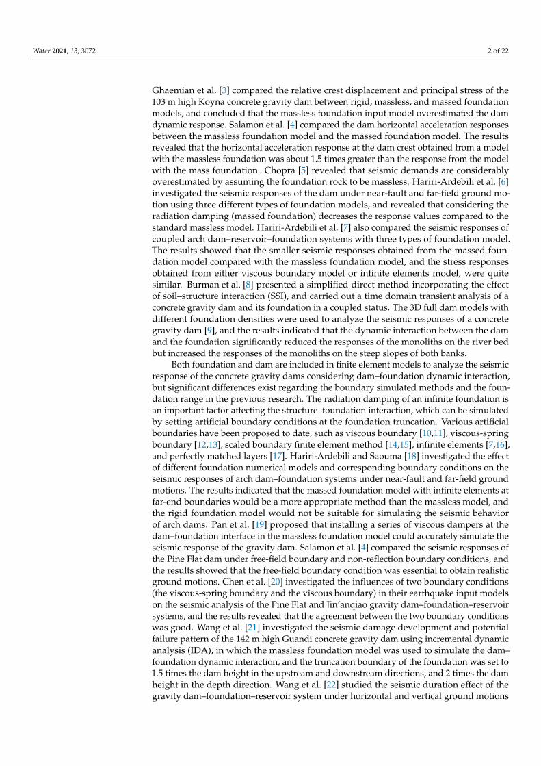
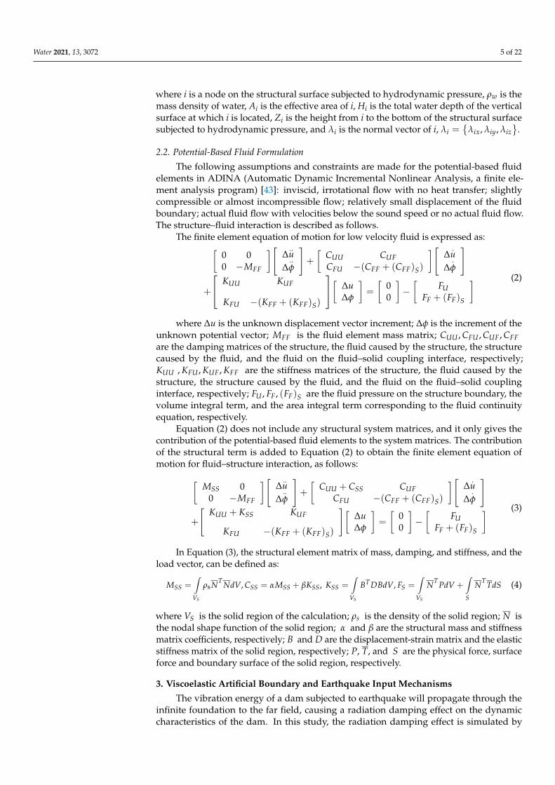
In this paper, the viscoelastic artificial boundary condition is implemented usinglinear spring-damping elements in ADINA. Figure 1 shows a schematic diagram of atwo-dimensional spring-damping element. The stiffness coefficient of the spring elementand the damping coefficient of the damper element are:{

KN = αNGr ∑ Ai, CN = ρcp∑ Ai

KT = αTGr ∑ Ai, CT = ρcs∑ Ai

(5)

where KN and KT are the normal and tangential stiffness of the spring, respectively; CNand CT are the normal and tangential damping coefficients of the damper, respectively;αN and αT are the normal and tangential correction coefficients of the viscoelastic artificialboundary, respectively, which are set to αN = 1.0 and αT = 0.5; cp and cs are the wavevelocities of the P-wave and S-wave, respectively; G and ρ are the shear modulus and massdensity of the medium, respectively; r is the distance between the wave source and thenode on the viscoelastic artificial boundary; ∑ Ai is the effective area of the node on theviscoelastic artificial boundary, which usually is the effective length for a two-dimensionalfinite element model.

Water 2021, 13, x FOR PEER REVIEW 6 of 23

3. Viscoelastic Artificial Boundary and Earthquake Input Mechanisms The vibration energy of a dam subjected to earthquake will propagate through the

infinite foundation to the far field, causing a radiation damping effect on the dynamic characteristics of the dam. In this study, the radiation damping effect is simulated by imposing the viscoelastic artificial boundary condition at the foundation truncation, and then converting the displacement and velocity time history of seismic wave motion into equivalent nodal loads applied to the viscoelastic artificial boundary to complete the input of ground motion.

3.1. Viscoelastic Artificial Boundary Condition In this paper, the viscoelastic artificial boundary condition is implemented using

linear spring-damping elements in ADINA. Figure 1 shows a schematic diagram of a two-dimensional spring-damping element. The stiffness coefficient of the spring element and the damping coefficient of the damper element are:

N N i N p i

T T i T s i

GK α A C ρc ArGK α A C ρc Ar

= = = =

，

，

(5)

where NK and TK are the normal and tangential stiffness of the spring, respectively;

NC and TC are the normal and tangential damping coefficients of the damper, respec-tively; Nα and Tα are the normal and tangential correction coefficients of the viscoe-lastic artificial boundary, respectively, which are set to 1.0Nα = and 0.5Tα = ; pc and

sc are the wave velocities of the P-wave and S-wave, respectively; G and ρ are the shear modulus and mass density of the medium, respectively; r is the distance between the wave source and the node on the viscoelastic artificial boundary; iA is the effec-tive area of the node on the viscoelastic artificial boundary, which usually is the effective length for a two-dimensional finite element model.

Figure 1. Schematic diagram of a two-dimensional spring-damping element.

3.2. Earthquake Input Mechanisms According to the characteristics of wave fields on different viscoelastic artificial

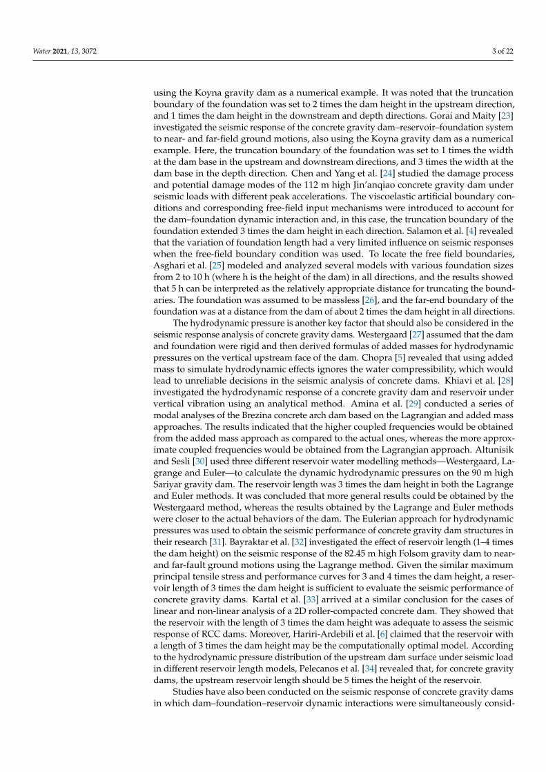
boundaries, the total wave field on the bottom boundary is decomposed into an incident field and a scattered field, whereas that on the side boundary is decomposed into a free field and a scattered field. The energy of the scattered field is absorbed by the viscoelastic artificial boundaries, whereas that of incident and free fields can be transformed into equivalent nodal loads and then applied to the boundaries. Figure 2 shows a schematic diagram of wave input for a viscoelastic artificial boundary.

Figure 1. Schematic diagram of a two-dimensional spring-damping element.

3.2. Earthquake Input Mechanisms

According to the characteristics of wave fields on different viscoelastic artificial bound-aries, the total wave field on the bottom boundary is decomposed into an incident field anda scattered field, whereas that on the side boundary is decomposed into a free field and ascattered field. The energy of the scattered field is absorbed by the viscoelastic artificialboundaries, whereas that of incident and free fields can be transformed into equivalentnodal loads and then applied to the boundaries. Figure 2 shows a schematic diagram ofwave input for a viscoelastic artificial boundary.

The displacement, velocity, and acceleration time history of wave fields are expressedas ui(t),

.ui(t), and

..ui(t), respectively, in which i = m denotes the total wave field, i = r

denotes the incident wave field, i = f denotes the free wave field, and i = s denotes thescattered field. According to the displacement continuity condition and the mechanicalequilibrium condition, the motion equation for node q on the bottom boundary can beexpressed as:

Mq..um

q (t) + Cq.um

q (t) + Kqumq (t) = Fr

q (t) + Fsq (t) (6)

Water 2021, 13, 3072 7 of 22


Figure 2. Schematic diagram of wave input for a viscoelastic artificial boundary.

The displacement, velocity, and acceleration time history of wave fields are ex-pressed as ( )iu t , ( )iu t , and ( )iu t , respectively, in which i m= denotes the total wave field, i r= denotes the incident wave field, i f= denotes the free wave field, and i s= denotes the scattered field. According to the displacement continuity condition and the mechanical equilibrium condition, the motion equation for node q on the bottom boundary can be expressed as:

m m m r sq q q q q q q qM u (t)+C u (t)+ K u (t)= F (t)+ F (t) (6)

The motion equation for node q on the side boundary can be expressed as: m m m f s

q q q q q q q qM u (t)+C u (t)+ K u (t)= F (t)+ F (t) (7)

where qK and qC are the artificial boundary parameters of q; rqF (t) , f

qF (t) and sqF (t) are the equivalent nodal loads to be applied at q to simulate the incident, free and

scattered wave field, respectively. For seismic wave motion input, only equivalent nodal loads r

qF (t) and fqF (t) need to be applied to the bottom and side boundary, which are

solved using Equations (6) and (7) based on the seismic wave motion propagation pattern and the stress state of wave fields, respectively. The equivalent nodal loads that should be applied at q are calculated as follows:

When the primary wave is incident:

1 2

1 1 2 2

( ) ( ) ( ) ( )

( ) ( Δ ) ( Δ )

( ) ( Δ ) ( Δ ) ( Δ ) ( Δ )

( ) ( ) (

r z r r rqz q qN qp qN qp p qp

f y r rqy q qp qp

p

f y r r r rqz q qT qp qT qp qT qp qT qp

f y f y f yqy qy qz

F t A K u t C u t ρc u t

λF t A u t t u t tc

F t A K u t t C u t t K u t t C u t t

F t F t F t

−

−

−

− + −

= + +

= − − −

= − + − + − + − = −

， ) ( )f yqzF t+

=

(8)

When the shear wave vibrating along the Y-axis is incident: z

3 3 4 4

3 4

( ) ( ) ( ) ( )

( ) ( Δ ) ( Δ ) ( Δ ) ( Δ )

( ) ( Δ ) ( Δ )

( ) ( ) ( )

r r r rqy q qT qs qT qs s qs

f y r r r rqy q qN qs qN qs qN qs qN qs

f y r rqz q s qs qs

f y f y f yqy qy qz

F t A K u t C u t ρc u t

F t A K u t t C u t t K u t t C u t t

F t A ρc u t t u t t

F t F t F t

−

−

−

+ − +

= + + = − + − + − + −

= − − − =

， ( )f yqzF t−

= −

(9)

in which

1 2 3 4Δ Δ 2 Δ Δ 2p s p s s st h c t H h c t h c t H h c= = − = = −，，， (10)

Figure 2. Schematic diagram of wave input for a viscoelastic artificial boundary.

The motion equation for node q on the side boundary can be expressed as:

Mq..um

q (t) + Cq.um

q (t) + Kqumq (t) = F f

q (t) + Fsq (t) (7)

where Kq and Cq are the artificial boundary parameters of q; Frq (t), F f

q (t) and Fsq (t) are

the equivalent nodal loads to be applied at q to simulate the incident, free and scatteredwave field, respectively. For seismic wave motion input, only equivalent nodal loads Fr

q (t)

and F fq (t) need to be applied to the bottom and side boundary, which are solved using

Equations (6) and (7) based on the seismic wave motion propagation pattern and the stressstate of wave fields, respectively. The equivalent nodal loads that should be applied at qare calculated as follows:

When the primary wave is incident:

Fr−zqz (t) = Aq

[KqNur

qp(t) + CqN.ur

qp(t) + ρcp.ur

qp(t)]

F f−yqy (t) = Aq

λcp

[ .ur

qp(t − ∆t1)−.ur

qp(t − ∆t2)]

F f−yqz (t) = Aq

[KqTur

qp(t − ∆t1) + CqT.ur

qp(t − ∆t1) + KqTurqp(t − ∆t2) + CqT

.ur

qp(t − ∆t2)]

F f−yqy (t) = −F f+y

qy (t) , F f−yqz (t) = F f+y

qz (t)

(8)

When the shear wave vibrating along the Y-axis is incident:

Fr−zqy (t) = Aq

[KqTur

qs(t) + CqT.ur

qs(t) + ρcs.ur

qs(t)]

F f−yqy (t) = Aq

[KqNur

qs(t − ∆t3) + CqN.ur

qs(t − ∆t3) + KqNurqs(t − ∆t4) + CqN

.ur

qs(t − ∆t4)]

F f−yqz (t) = Aqρcs

[ .ur

qs(t − ∆t3)−.ur

qs(t − ∆t4)]

F f+yqy (t) = F f−y

qy (t) , F f+yqz (t) = −F f−y

qz (t)

(9)

in which

∆t1 = h/cp, ∆t2 = 2Hs − h/cp, ∆t3 = h/cs, ∆t4 = 2Hs − h/cs (10)

where ρ, cp, cs, λ are the foundation density, P-wave velocity, S-wave velocity, and Lame constant,respectively; Hs is the vertical distance from the wave source to the bottom boundary; h is thevertical distance from q to the bottom boundary; ∆t1, ∆t2 , ∆t3, and ∆t4 are the time delay of theincident P-wave at q, the reflected P-wave at the foundation surface, the incident S-wave at q, and thereflected S-wave at the foundation surface, respectively. The subscripts of the equivalent nodal loadsrepresent the node number and component direction, and the superscripts represent the wave fieldfor calculating the equivalent nodal loads and the outer normal direction of the boundary surface at

Water 2021, 13, 3072 8 of 22

which q is located, which is positive if the direction is the same as the coordinate axis and negative ifthe direction is opposite to the coordinate axis.

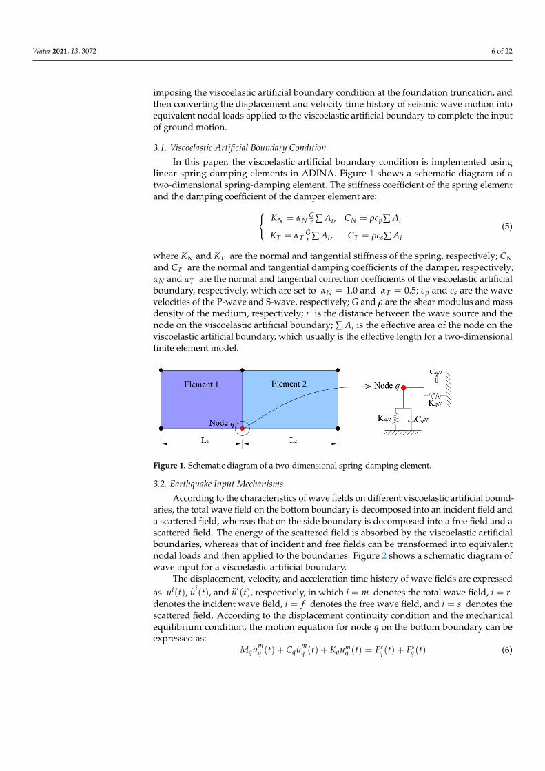
3.3. Verification TestThe viscoelastic artificial boundary is verified by a two-dimension test [44]. As shown in

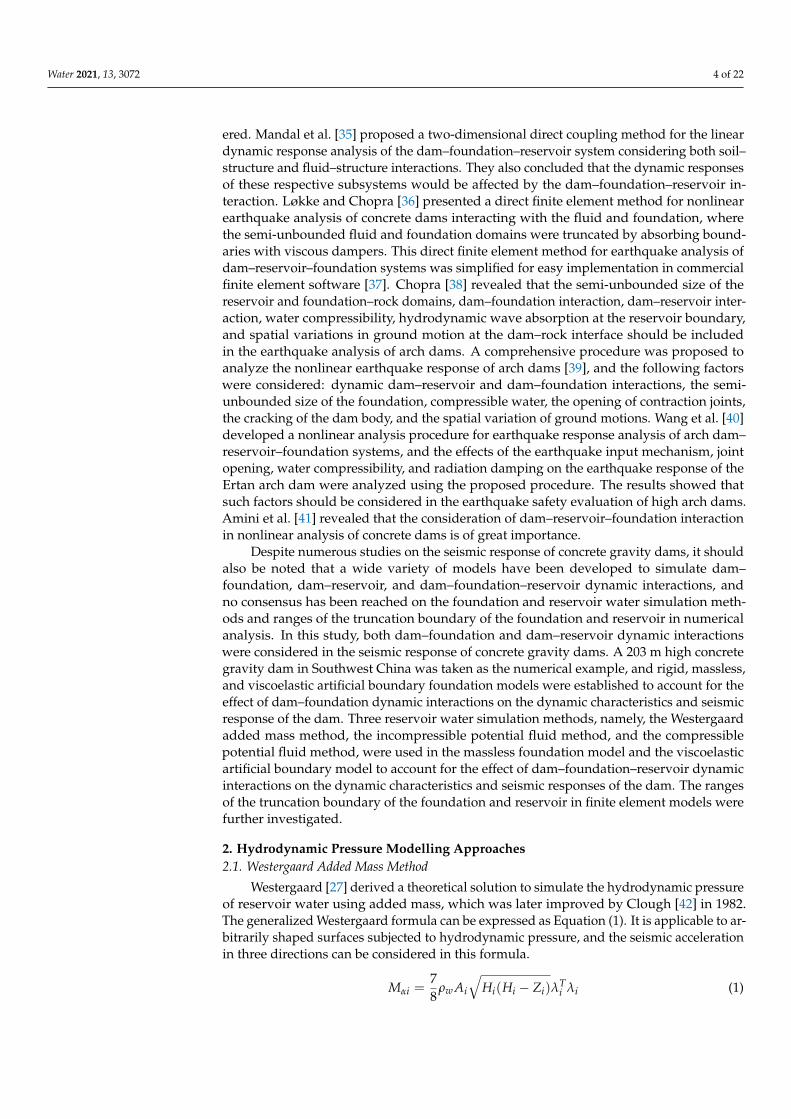
Figure 3, the model size is 905.5 m × 370 m, and the finite element mesh size is 5 m × 10 m. Themodulus of elasticity of the medium is 1.05 × 1010 N/m2, the mass density is 2777 kg/m3, thePoisson’s ratio is 0.23, the S-wave velocity is 1239.8 m/s, and the P-wave velocity is 2093.6 m/s. Thedynamic time-history analysis is performed with a total calculation time of 1 s and a time step of 0.01 s.The input displacement, velocity, and acceleration time history are determined by Equations (11)–(13)respectively, and their time-history curves are shown in Figure 4.

u(t) =

{t2 − sin(2π f t)

4π f t 0 ≤ t ≤ 0.250.125 t > 0.25

(11)

v(t) =

{12 − cos(2π f t)

2 0 ≤ t ≤ 0.250 t > 0.25

(12)

a(t) ={

π f sin(2π f t) 0 ≤ t ≤ 0.250 t > 0.25

(13)


where ρ, cp, cs, λ are the foundation density, P-wave velocity, S-wave velocity, and Lame constant, respectively; Hs is the vertical distance from the wave source to the bottom boundary; h is the vertical distance from q to the bottom boundary; 1tΔ , 2tΔ , 3tΔ , and

4tΔ are the time delay of the incident P-wave at q, the reflected P-wave at the foundation surface, the incident S-wave at q, and the reflected S-wave at the foundation surface, re-spectively. The subscripts of the equivalent nodal loads represent the node number and component direction, and the superscripts represent the wave field for calculating the equivalent nodal loads and the outer normal direction of the boundary surface at which q is located, which is positive if the direction is the same as the coordinate axis and nega-tive if the direction is opposite to the coordinate axis.

3.3. Verification Test The viscoelastic artificial boundary is verified by a two-dimension test [44]. As

shown in Figure 3, the model size is 905.5 m × 370 m, and the finite element mesh size is 5 m × 10 m. The modulus of elasticity of the medium is 1.05 × 1010 N/m2, the mass density is 2777 kg/m3, the Poisson’s ratio is 0.23, the S-wave velocity is 1239.8 m/s, and the P-wave velocity is 2093.6 m/s. The dynamic time-history analysis is performed with a total cal-culation time of 1 s and a time step of 0.01 s. The input displacement, velocity, and ac-celeration time history are determined by Equations (11)–(13) respectively, and their time-history curves are shown in Figure 4.

Figure 3. The finite element model of the verification test.

( )( )sin 2

0 0.252 40.125 >0.25

ftt tu t ft

t

ππ

− ≤ ≤=

(11)

( )( )cos 21 0 0.25

2 20 >0.25

fttv t

t

π− ≤ ≤=

(12)

( ) ( )sin 2 0 0.250 >0.25f ft t

a tt

π π ≤ ≤=

(13)

Figure 3. The finite element model of the verification test.Water 2021, 13, x FOR PEER REVIEW 9 of 23

Figure 4. The input time–history curves of displacement, velocity, and acceleration.

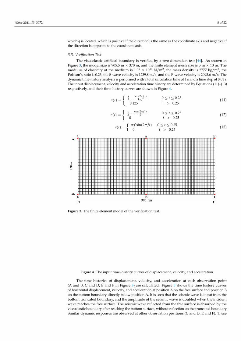
The time histories of displacement, velocity, and acceleration at each observation point (A and B, C and D, E and F in Figure 3) are calculated. Figure 5 shows the time history curves of horizontal displacement, velocity, and acceleration at position A on the free surface and position B on the bottom boundary directly below position A. It is seen that the seismic wave is input from the bottom truncated boundary, and the amplitude of the seismic wave is doubled when the incident wave reaches the free surface. The seismic wave reflected from the free surface is absorbed by the viscoelastic boundary after reaching the bottom surface, without reflection on the truncated boundary. Similar dy-namic responses are observed at other observation positions (C and D, E and F). These results indicate that the viscoelastic artificial boundary condition and the corresponding earthquake input mechanism are feasible.

Figure 5. The time–history curves of horizontal displacement, velocity, and acceleration.

4. General Description of the Numerical Example 4.1. General Information

A concrete gravity dam in Southwest China was selected as the study case. The concrete gravity dam block has a crest elevation of 1625 m, a heel elevation of 1422 m, a dam height of 203 m, a crest width of 16 m, and a normal water level of 1619 m. The calculation cross-section of the dam block is shown in Figure 6. In this study, the fol-lowing material parameters were considered. Dam: static modulus of elasticity = 2.5 × 1010

N/m2, mass density = 2400 kg/m3, Poisson’s ratio = 0.167 according to Design Code for Hydraulic Concrete Structures (SL 191-2008) [45], structural damping = 5%. Foundation: modulus of elasticity = 1.5 × 1010 N/m2, mass density = 2700 kg/m3, Poisson’s ratio = 0.24. Reservoir: mass density of water = 1000 kg/m3, acoustic wave speed = 1440 m/s.


The time histories of displacement, velocity, and acceleration at each observation point(A and B, C and D, E and F in Figure 3) are calculated. Figure 5 shows the time history curvesof horizontal displacement, velocity, and acceleration at position A on the free surface and position Bon the bottom boundary directly below position A. It is seen that the seismic wave is input from thebottom truncated boundary, and the amplitude of the seismic wave is doubled when the incidentwave reaches the free surface. The seismic wave reflected from the free surface is absorbed by theviscoelastic boundary after reaching the bottom surface, without reflection on the truncated boundary.Similar dynamic responses are observed at other observation positions (C and D, E and F). These

Water 2021, 13, 3072 9 of 22

results indicate that the viscoelastic artificial boundary condition and the corresponding earthquakeinput mechanism are feasible.



The time histories of displacement, velocity, and acceleration at each observation point (A and B, C and D, E and F in Figure 3) are calculated. Figure 5 shows the time history curves of horizontal displacement, velocity, and acceleration at position A on the free surface and position B on the bottom boundary directly below position A. It is seen that the seismic wave is input from the bottom truncated boundary, and the amplitude of the seismic wave is doubled when the incident wave reaches the free surface. The seismic wave reflected from the free surface is absorbed by the viscoelastic boundary after reaching the bottom surface, without reflection on the truncated boundary. Similar dy-namic responses are observed at other observation positions (C and D, E and F). These results indicate that the viscoelastic artificial boundary condition and the corresponding earthquake input mechanism are feasible.


4. General Description of the Numerical Example 4.1. General Information

A concrete gravity dam in Southwest China was selected as the study case. The concrete gravity dam block has a crest elevation of 1625 m, a heel elevation of 1422 m, a dam height of 203 m, a crest width of 16 m, and a normal water level of 1619 m. The calculation cross-section of the dam block is shown in Figure 6. In this study, the fol-lowing material parameters were considered. Dam: static modulus of elasticity = 2.5 × 1010

N/m2, mass density = 2400 kg/m3, Poisson’s ratio = 0.167 according to Design Code for Hydraulic Concrete Structures (SL 191-2008) [45], structural damping = 5%. Foundation: modulus of elasticity = 1.5 × 1010 N/m2, mass density = 2700 kg/m3, Poisson’s ratio = 0.24. Reservoir: mass density of water = 1000 kg/m3, acoustic wave speed = 1440 m/s.


4. General Description of the Numerical Example4.1. General Information

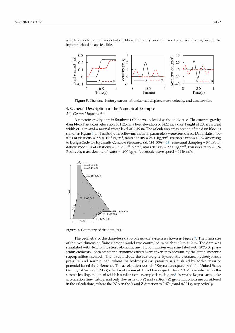
A concrete gravity dam in Southwest China was selected as the study case. The concrete gravitydam block has a crest elevation of 1625 m, a heel elevation of 1422 m, a dam height of 203 m, a crestwidth of 16 m, and a normal water level of 1619 m. The calculation cross-section of the dam block isshown in Figure 6. In this study, the following material parameters were considered. Dam: static mod-ulus of elasticity = 2.5 × 1010 N/m2, mass density = 2400 kg/m3, Poisson’s ratio = 0.167 accordingto Design Code for Hydraulic Concrete Structures (SL 191-2008) [45], structural damping = 5%. Foun-dation: modulus of elasticity = 1.5 × 1010 N/m2, mass density = 2700 kg/m3, Poisson’s ratio = 0.24.Reservoir: mass density of water = 1000 kg/m3, acoustic wave speed = 1440 m/s.Water 2021, 13, x FOR PEER REVIEW 10 of 23

Figure 6. Geometry of the dam (m).

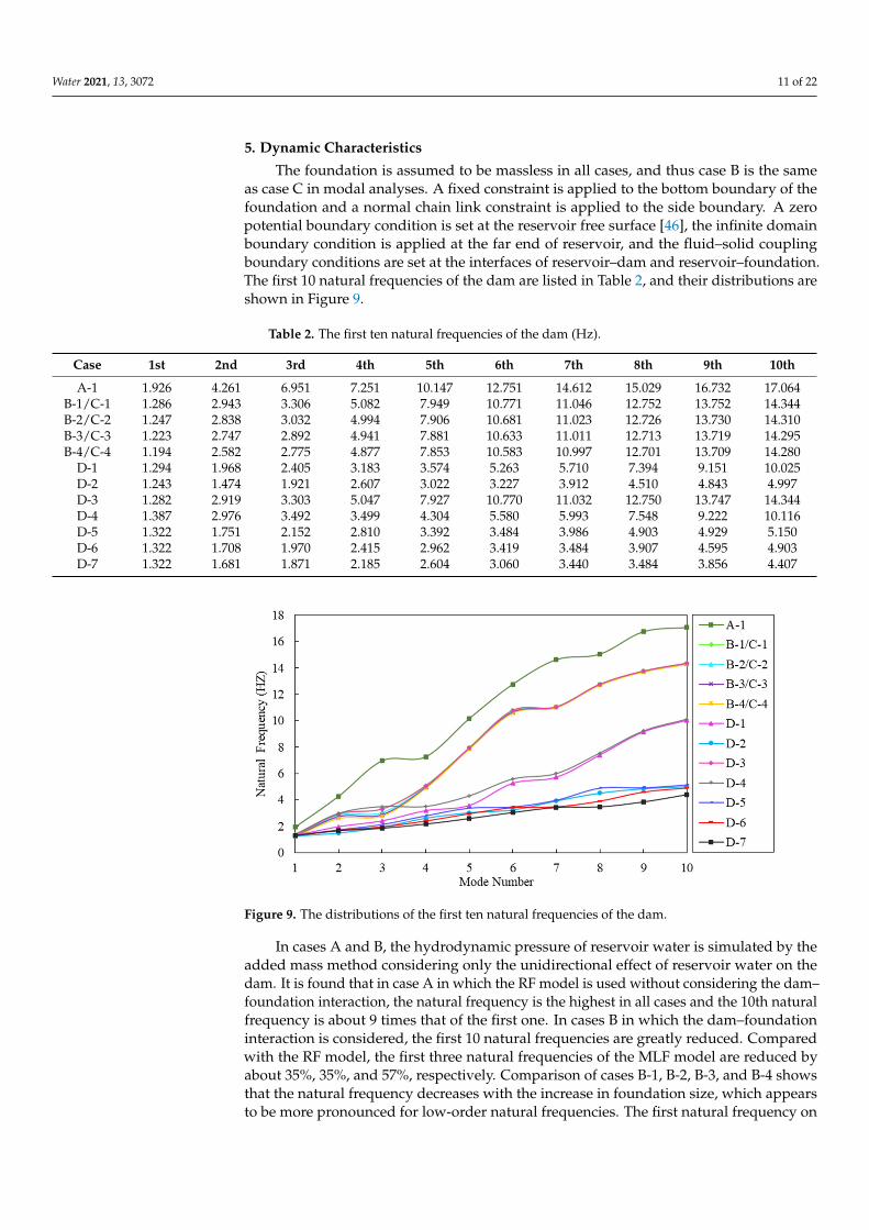
The geometry of the dam–foundation–reservoir system is shown in Figure 7. The mesh size of the two-dimension finite element model was controlled to be about 2 m × 2 m. The dam was simulated with 4640 plane stress elements, and the foundation was simulated with 207,900 plane strain elements. Both static and dynamic effects were taken into account by the static–dynamic superposition method. The loads include the self-weight, hydrostatic pressure, hydrodynamic pressure, and seismic load, where the hydrodynamic pressure is simulated by added mass or potential-based fluid elements. The acceleration record of Koyna earthquake with the United States Geological Survey (USGS) site classification of A and the magnitude of 6.3 M was selected as the seismic loading, the site of which is similar to the example dam. Figure 8 shows the Koyna earthquake acceleration time history, and only downstream (Y) and vertical (Z) ground motions are considered in the calculations, where the PGA in the Y and Z direction is 0.474 g and 0.304 g, respectively.

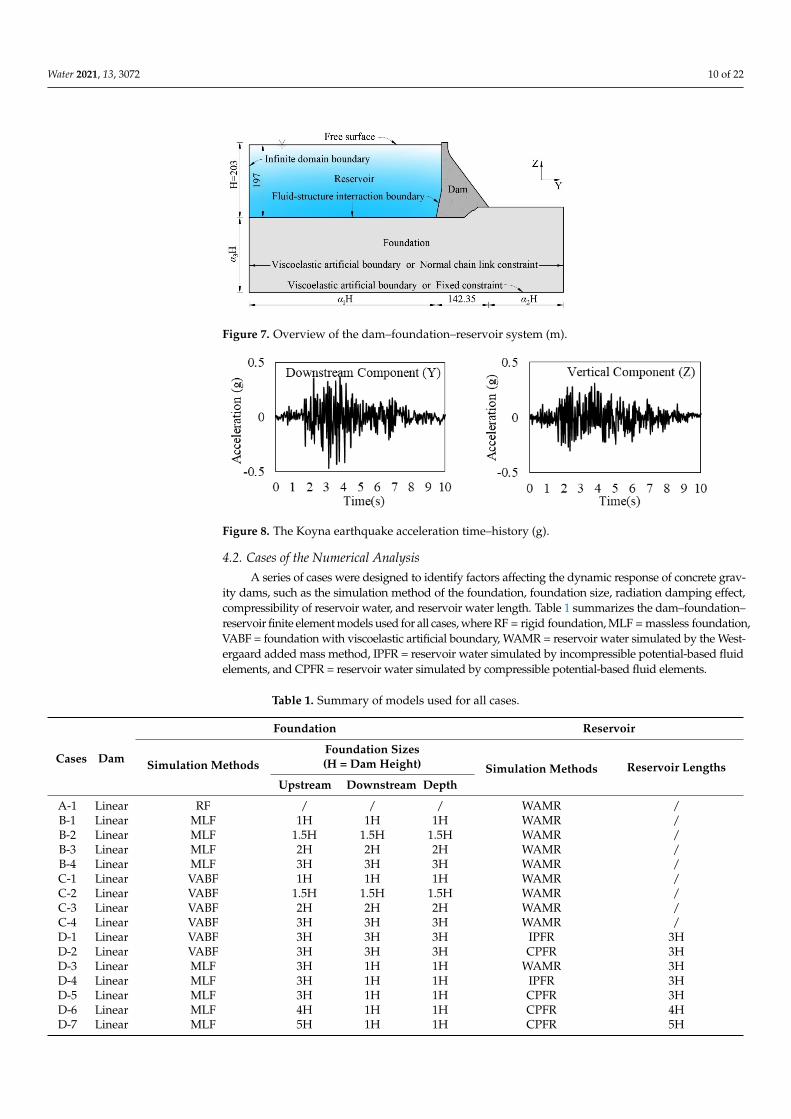
Figure 7. Overview of the dam–foundation–reservoir system (m).

Figure 8. The Koyna earthquake acceleration time–history (g).


The geometry of the dam–foundation–reservoir system is shown in Figure 7. The mesh sizeof the two-dimension finite element model was controlled to be about 2 m × 2 m. The dam wassimulated with 4640 plane stress elements, and the foundation was simulated with 207,900 planestrain elements. Both static and dynamic effects were taken into account by the static–dynamicsuperposition method. The loads include the self-weight, hydrostatic pressure, hydrodynamicpressure, and seismic load, where the hydrodynamic pressure is simulated by added mass orpotential-based fluid elements. The acceleration record of Koyna earthquake with the United StatesGeological Survey (USGS) site classification of A and the magnitude of 6.3 M was selected as theseismic loading, the site of which is similar to the example dam. Figure 8 shows the Koyna earthquakeacceleration time history, and only downstream (Y) and vertical (Z) ground motions are consideredin the calculations, where the PGA in the Y and Z direction is 0.474 g and 0.304 g, respectively.

Water 2021, 13, 3072 10 of 22













4.2. Cases of the Numerical AnalysisA series of cases were designed to identify factors affecting the dynamic response of concrete grav-

ity dams, such as the simulation method of the foundation, foundation size, radiation damping effect,compressibility of reservoir water, and reservoir water length. Table 1 summarizes the dam–foundation–reservoir finite element models used for all cases, where RF = rigid foundation, MLF = massless foundation,VABF = foundation with viscoelastic artificial boundary, WAMR = reservoir water simulated by the West-ergaard added mass method, IPFR = reservoir water simulated by incompressible potential-based fluidelements, and CPFR = reservoir water simulated by compressible potential-based fluid elements.

Table 1. Summary of models used for all cases.

Cases Dam

Foundation Reservoir

Simulation MethodsFoundation Sizes(H = Dam Height) Simulation Methods Reservoir Lengths

Upstream Downstream Depth

A-1 Linear RF / / / WAMR /B-1 Linear MLF 1H 1H 1H WAMR /B-2 Linear MLF 1.5H 1.5H 1.5H WAMR /B-3 Linear MLF 2H 2H 2H WAMR /B-4 Linear MLF 3H 3H 3H WAMR /C-1 Linear VABF 1H 1H 1H WAMR /C-2 Linear VABF 1.5H 1.5H 1.5H WAMR /C-3 Linear VABF 2H 2H 2H WAMR /C-4 Linear VABF 3H 3H 3H WAMR /D-1 Linear VABF 3H 3H 3H IPFR 3HD-2 Linear VABF 3H 3H 3H CPFR 3HD-3 Linear MLF 3H 1H 1H WAMR 3HD-4 Linear MLF 3H 1H 1H IPFR 3HD-5 Linear MLF 3H 1H 1H CPFR 3HD-6 Linear MLF 4H 1H 1H CPFR 4HD-7 Linear MLF 5H 1H 1H CPFR 5H

Water 2021, 13, 3072 11 of 22

5. Dynamic Characteristics

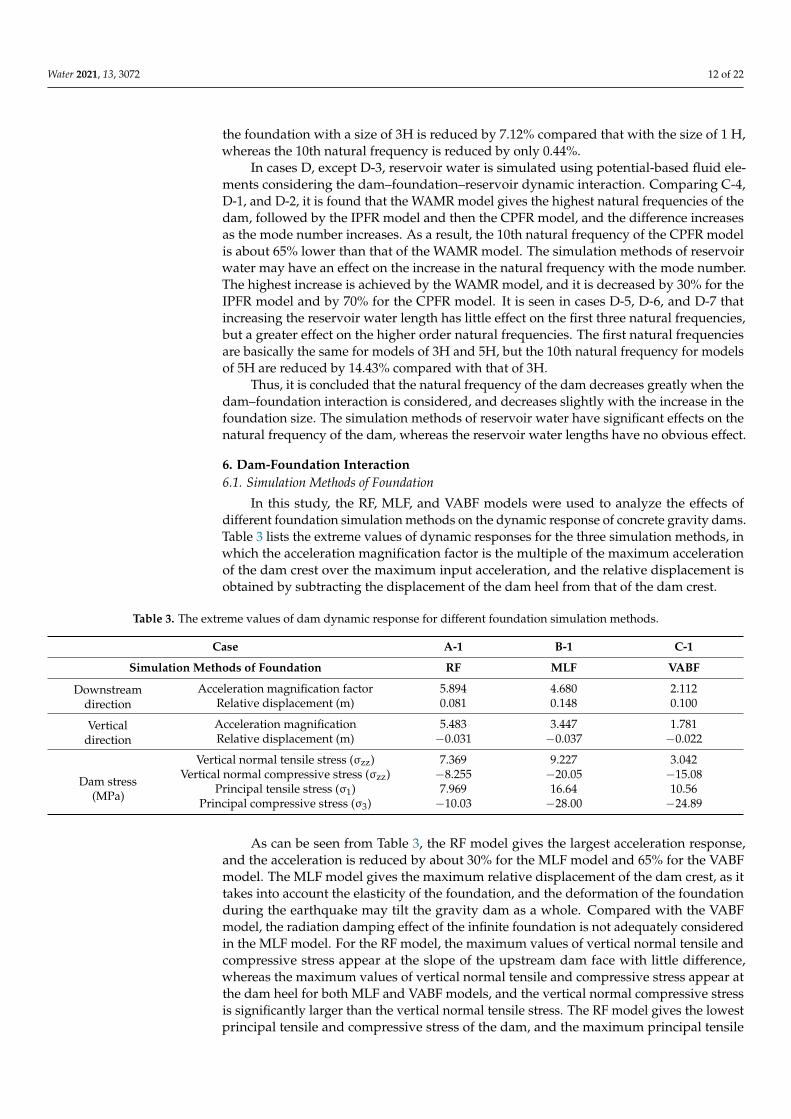
The foundation is assumed to be massless in all cases, and thus case B is the sameas case C in modal analyses. A fixed constraint is applied to the bottom boundary of thefoundation and a normal chain link constraint is applied to the side boundary. A zeropotential boundary condition is set at the reservoir free surface [46], the infinite domainboundary condition is applied at the far end of reservoir, and the fluid–solid couplingboundary conditions are set at the interfaces of reservoir–dam and reservoir–foundation.The first 10 natural frequencies of the dam are listed in Table 2, and their distributions areshown in Figure 9.

Table 2. The first ten natural frequencies of the dam (Hz).

Case 1st 2nd 3rd 4th 5th 6th 7th 8th 9th 10th

A-1 1.926 4.261 6.951 7.251 10.147 12.751 14.612 15.029 16.732 17.064B-1/C-1 1.286 2.943 3.306 5.082 7.949 10.771 11.046 12.752 13.752 14.344B-2/C-2 1.247 2.838 3.032 4.994 7.906 10.681 11.023 12.726 13.730 14.310B-3/C-3 1.223 2.747 2.892 4.941 7.881 10.633 11.011 12.713 13.719 14.295B-4/C-4 1.194 2.582 2.775 4.877 7.853 10.583 10.997 12.701 13.709 14.280

D-1 1.294 1.968 2.405 3.183 3.574 5.263 5.710 7.394 9.151 10.025D-2 1.243 1.474 1.921 2.607 3.022 3.227 3.912 4.510 4.843 4.997D-3 1.282 2.919 3.303 5.047 7.927 10.770 11.032 12.750 13.747 14.344D-4 1.387 2.976 3.492 3.499 4.304 5.580 5.993 7.548 9.222 10.116D-5 1.322 1.751 2.152 2.810 3.392 3.484 3.986 4.903 4.929 5.150D-6 1.322 1.708 1.970 2.415 2.962 3.419 3.484 3.907 4.595 4.903D-7 1.322 1.681 1.871 2.185 2.604 3.060 3.440 3.484 3.856 4.407


D-4 1.387 2.976 3.492 3.499 4.304 5.580 5.993 7.548 9.222 10.116 D-5 1.322 1.751 2.152 2.810 3.392 3.484 3.986 4.903 4.929 5.150 D-6 1.322 1.708 1.970 2.415 2.962 3.419 3.484 3.907 4.595 4.903 D-7 1.322 1.681 1.871 2.185 2.604 3.060 3.440 3.484 3.856 4.407

Figure 9. The distributions of the first ten natural frequencies of the dam.

In cases A and B, the hydrodynamic pressure of reservoir water is simulated by the added mass method considering only the unidirectional effect of reservoir water on the dam. It is found that in case A in which the RF model is used without considering the dam–foundation interaction, the natural frequency is the highest in all cases and the 10th natural frequency is about 9 times that of the first one. In cases B in which the dam–foundation interaction is considered, the first 10 natural frequencies are greatly reduced. Compared with the RF model, the first three natural frequencies of the MLF model are reduced by about 35%, 35%, and 57%, respectively. Comparison of cases B-1, B-2, B-3, and B-4 shows that the natural frequency decreases with the increase in foundation size, which appears to be more pronounced for low-order natural frequencies. The first natu-ral frequency on the foundation with a size of 3H is reduced by 7.12% compared that with the size of 1 H, whereas the 10th natural frequency is reduced by only 0.44%.

In cases D, except D-3, reservoir water is simulated using potential-based fluid ele-ments considering the dam–foundation–reservoir dynamic interaction. Comparing C-4, D-1, and D-2, it is found that the WAMR model gives the highest natural frequencies of the dam, followed by the IPFR model and then the CPFR model, and the difference in-creases as the mode number increases. As a result, the 10th natural frequency of the CPFR model is about 65% lower than that of the WAMR model. The simulation methods of reservoir water may have an effect on the increase in the natural frequency with the mode number. The highest increase is achieved by the WAMR model, and it is decreased by 30% for the IPFR model and by 70% for the CPFR model. It is seen in cases D-5, D-6, and D-7 that increasing the reservoir water length has little effect on the first three natural frequencies, but a greater effect on the higher order natural frequencies. The first natural frequencies are basically the same for models of 3H and 5H, but the 10th natural fre-quency for models of 5H are reduced by 14.43% compared with that of 3H.

Thus, it is concluded that the natural frequency of the dam decreases greatly when the dam–foundation interaction is considered, and decreases slightly with the increase in the foundation size. The simulation methods of reservoir water have significant effects on the natural frequency of the dam, whereas the reservoir water lengths have no obvious effect.

Figure 9. The distributions of the first ten natural frequencies of the dam.

In cases A and B, the hydrodynamic pressure of reservoir water is simulated by theadded mass method considering only the unidirectional effect of reservoir water on thedam. It is found that in case A in which the RF model is used without considering the dam–foundation interaction, the natural frequency is the highest in all cases and the 10th naturalfrequency is about 9 times that of the first one. In cases B in which the dam–foundationinteraction is considered, the first 10 natural frequencies are greatly reduced. Comparedwith the RF model, the first three natural frequencies of the MLF model are reduced byabout 35%, 35%, and 57%, respectively. Comparison of cases B-1, B-2, B-3, and B-4 showsthat the natural frequency decreases with the increase in foundation size, which appearsto be more pronounced for low-order natural frequencies. The first natural frequency on

Water 2021, 13, 3072 12 of 22

the foundation with a size of 3H is reduced by 7.12% compared that with the size of 1 H,whereas the 10th natural frequency is reduced by only 0.44%.

In cases D, except D-3, reservoir water is simulated using potential-based fluid ele-ments considering the dam–foundation–reservoir dynamic interaction. Comparing C-4,D-1, and D-2, it is found that the WAMR model gives the highest natural frequencies of thedam, followed by the IPFR model and then the CPFR model, and the difference increasesas the mode number increases. As a result, the 10th natural frequency of the CPFR modelis about 65% lower than that of the WAMR model. The simulation methods of reservoirwater may have an effect on the increase in the natural frequency with the mode number.The highest increase is achieved by the WAMR model, and it is decreased by 30% for theIPFR model and by 70% for the CPFR model. It is seen in cases D-5, D-6, and D-7 thatincreasing the reservoir water length has little effect on the first three natural frequencies,but a greater effect on the higher order natural frequencies. The first natural frequenciesare basically the same for models of 3H and 5H, but the 10th natural frequency for modelsof 5H are reduced by 14.43% compared with that of 3H.

Thus, it is concluded that the natural frequency of the dam decreases greatly when thedam–foundation interaction is considered, and decreases slightly with the increase in thefoundation size. The simulation methods of reservoir water have significant effects on thenatural frequency of the dam, whereas the reservoir water lengths have no obvious effect.

6. Dam-Foundation Interaction6.1. Simulation Methods of Foundation

In this study, the RF, MLF, and VABF models were used to analyze the effects ofdifferent foundation simulation methods on the dynamic response of concrete gravity dams.Table 3 lists the extreme values of dynamic responses for the three simulation methods, inwhich the acceleration magnification factor is the multiple of the maximum accelerationof the dam crest over the maximum input acceleration, and the relative displacement isobtained by subtracting the displacement of the dam heel from that of the dam crest.

Table 3. The extreme values of dam dynamic response for different foundation simulation methods.

Case A-1 B-1 C-1

Simulation Methods of Foundation RF MLF VABF

Downstreamdirection

Acceleration magnification factor 5.894 4.680 2.112Relative displacement (m) 0.081 0.148 0.100

Verticaldirection

Acceleration magnification 5.483 3.447 1.781Relative displacement (m) −0.031 −0.037 −0.022

Dam stress(MPa)

Vertical normal tensile stress (σzz) 7.369 9.227 3.042Vertical normal compressive stress (σzz) −8.255 −20.05 −15.08

Principal tensile stress (σ1) 7.969 16.64 10.56Principal compressive stress (σ3) −10.03 −28.00 −24.89

As can be seen from Table 3, the RF model gives the largest acceleration response,and the acceleration is reduced by about 30% for the MLF model and 65% for the VABFmodel. The MLF model gives the maximum relative displacement of the dam crest, as ittakes into account the elasticity of the foundation, and the deformation of the foundationduring the earthquake may tilt the gravity dam as a whole. Compared with the VABFmodel, the radiation damping effect of the infinite foundation is not adequately consideredin the MLF model. For the RF model, the maximum values of vertical normal tensile andcompressive stress appear at the slope of the upstream dam face with little difference,whereas the maximum values of vertical normal tensile and compressive stress appear atthe dam heel for both MLF and VABF models, and the vertical normal compressive stressis significantly larger than the vertical normal tensile stress. The RF model gives the lowestprincipal tensile and compressive stress of the dam, and the maximum principal tensile

Water 2021, 13, 3072 13 of 22

stress appears at the dam heel and the maximum principal compressive stress appears atthe neck of the downstream dam face. For both MLF and VABF models, the maximumprincipal tensile stress appears at the dam heel, and the maximum principal compressivestress appears at the dam toe. However, it is noted that the maximum principal tensilestress under the VABF model is smaller than that under the MLF model.

6.2. Sensitivity Analysis of Foundation Size

Cases B-1, B-2, B-3, and B-4 with different foundation sizes (1H, 1.5H, 2H, and 3H inthe upstream, downstream and depth directions) were analyzed to elucidate their effectson the dynamic response of gravity dams. Each of the four cases were modeled with theMLF model and calculated by applying fixed constraints to the bottom boundary of thefoundation and normal chain link constraints to the side boundary. The hydrodynamicpressure of reservoir water was simulated by the added mass method. Table 4 lists theextreme values of dam dynamic responses under for different foundation sizes.

Table 4. The extreme values of dam dynamic response for different foundation sizes (MLF).

Case B-1 B-2 B-3 B-4

Foundation Size 1H 1.5H 2H 3H

Downstreamdirection

Acceleration magnification factor 4.680 5.057 5.789 3.477Relative displacement (m) 0.148 0.150 0.154 0.141

Verticaldirection

Acceleration magnification 3.447 3.056 3.856 4.220Relative displacement (m) −0.037 −0.038 −0.048 −0.042

Dam stress(MPa)

Vertical normal tensile stress (σzz) 9.227 9.903 8.770 6.754Vertical normal compressive stress (σzz) −20.05 −20.79 −21.15 −18.72

Principal tensile stress (σ1) 16.64 16.37 13.70 10.66Principal compressive stress (σ3) −28.00 −29.52 −27.21 −28.01

Table 4 clearly shows that foundation size has a significant effect on the accelerationresponse. Specifically, the downstream acceleration at the dam crest reaches a maximumat a foundation size of 2H, which is 5.789 times that of the input; and a minimum at afoundation size of 3H, which is 3.477 times that of the input. The vertical acceleration at thedam crest reaches a maximum at a foundation size of 3H, which is 4.220 times that of theinput. However, foundation size has little effect on displacement, and both downstreamand vertical relative displacement at the dam crest reach a maximum at a foundationsize of 2H. The tensile stress can also be significantly affected by foundation size, andthe maximum tensile stress decreases with the increase in foundation sizes. As a result,the maximum vertical normal tensile stress and the maximum principal tensile stress at afoundation size of 3H are decreased by about 26.8% and 35.9% compared with that at afoundation size of 1H, respectively.

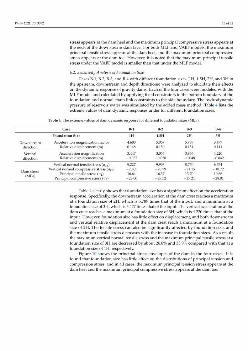
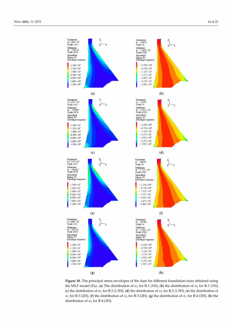
Figure 10 shows the principal stress envelopes of the dam in the four cases. It isfound that foundation size has little effect on the distributions of principal tension andcompression stress, and in all cases, the maximum principal tension stress appears at thedam heel and the maximum principal compressive stress appears at the dam toe.

Water 2021, 13, 3072 14 of 22


the input. However, foundation size has little effect on displacement, and both down-stream and vertical relative displacement at the dam crest reach a maximum at a foun-dation size of 2H. The tensile stress can also be significantly affected by foundation size, and the maximum tensile stress decreases with the increase in foundation sizes. As a re-sult, the maximum vertical normal tensile stress and the maximum principal tensile stress at a foundation size of 3H are decreased by about 26.8% and 35.9% compared with that at a foundation size of 1H, respectively.

Table 4. The extreme values of dam dynamic response for different foundation sizes (MLF).

Case B-1 B-2 B-3 B-4 Foundation Size 1H 1.5H 2H 3H

Downstream direction

Acceleration magnification factor 4.680 5.057 5.789 3.477 Relative displacement (m) 0.148 0.150 0.154 0.141

Vertical direction

Acceleration magnification 3.447 3.056 3.856 4.220 Relative displacement (m) −0.037 −0.038 −0.048 −0.042

Dam stress (MPa)

Vertical normal tensile stress (σzz) 9.227 9.903 8.770 6.754 Vertical normal compressive stress (σzz) −20.05 −20.79 −21.15 −18.72

Principal tensile stress (σ1) 16.64 16.37 13.70 10.66 Principal compressive stress (σ3) −28.00 −29.52 −27.21 −28.01

Figure 10 shows the principal stress envelopes of the dam in the four cases. It is found that foundation size has little effect on the distributions of principal tension and compression stress, and in all cases, the maximum principal tension stress appears at the dam heel and the maximum principal compressive stress appears at the dam toe.

(a) (b)

(c) (d) Water 2021, 13, x FOR PEER REVIEW 15 of 23

(e) (f)

(g) (h)

Figure 10. The principal stress envelopes of the dam for different foundation sizes obtained using the MLF model (Pa). (a) The distribution of σ1 for B-1 (1H), (b) the distribution of σ3 for B-1 (1H), (c) the distribution of σ1 for B-2 (1.5H), (d) the distribution of σ3 for B-2 (1.5H), (e) the distribution of σ1 for B-3 (2H), (f) the distribution of σ3 for B-3 (2H), (g) the distribution of σ1 for B-4 (3H), (h) the distribution of σ3 for B-4 (3H).

6.3. The Radiation Damping Effect of Infinite Foundation 6.3.1. Verification of the Foundation Model

The finite element model of the foundation (Figure 11) was analyzed using the method described in Section 3. The foundation sizes were also assumed to be 1H, 1.5H, 2H, and 3H, and the material properties are described in Section 4. The sinusoidal waves given by Equations (11)–(13) are input from the bottom boundary of the foundation with a peak of 12.542 m/s2 in both downstream and vertical directions. Three observation points are set on the foundation surface: point M which is closest to the upstream side, point N which is the intermediate point of the upstream side, and point O where there is the wave source. The PGA values at these three points are listed in Table 5. It is seen that the amplitude of the wave is almost doubled when it reaches the free surface of the foundation, which is consistent with the theory and further verifies the applicability of the viscoelastic artificial boundary and corresponding earthquake input mechanism.

Figure 10. The principal stress envelopes of the dam for different foundation sizes obtained usingthe MLF model (Pa). (a) The distribution of σ1 for B-1 (1H), (b) the distribution of σ3 for B-1 (1H),(c) the distribution of σ1 for B-2 (1.5H), (d) the distribution of σ3 for B-2 (1.5H), (e) the distribution ofσ1 for B-3 (2H), (f) the distribution of σ3 for B-3 (2H), (g) the distribution of σ1 for B-4 (3H), (h) thedistribution of σ3 for B-4 (3H).

Water 2021, 13, 3072 15 of 22

6.3. The Radiation Damping Effect of Infinite Foundation6.3.1. Verification of the Foundation Model

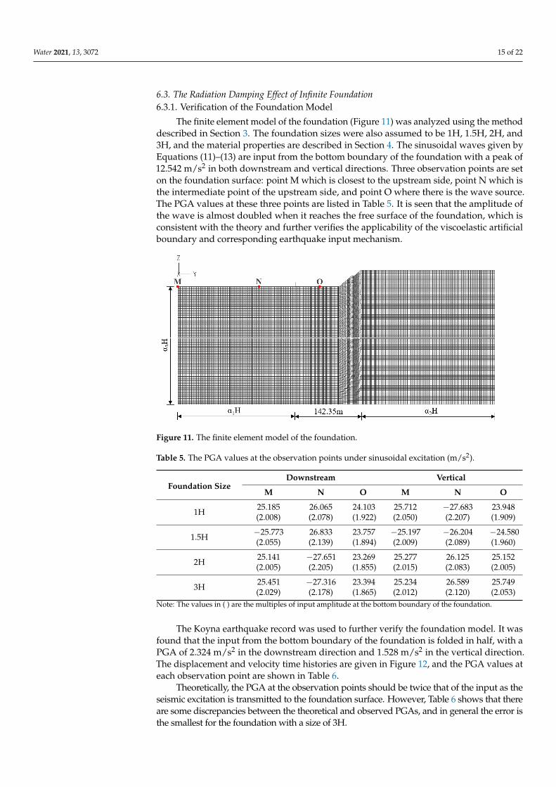
The finite element model of the foundation (Figure 11) was analyzed using the methoddescribed in Section 3. The foundation sizes were also assumed to be 1H, 1.5H, 2H, and3H, and the material properties are described in Section 4. The sinusoidal waves given byEquations (11)–(13) are input from the bottom boundary of the foundation with a peak of12.542 m/s2 in both downstream and vertical directions. Three observation points are seton the foundation surface: point M which is closest to the upstream side, point N which isthe intermediate point of the upstream side, and point O where there is the wave source.The PGA values at these three points are listed in Table 5. It is seen that the amplitude ofthe wave is almost doubled when it reaches the free surface of the foundation, which isconsistent with the theory and further verifies the applicability of the viscoelastic artificialboundary and corresponding earthquake input mechanism.Water 2021, 13, x FOR PEER REVIEW 16 of 23

Figure 11. The finite element model of the foundation.

Table 5. The PGA values at the observation points under sinusoidal excitation (m/s2).

Foundation Size Downstream Vertical

M N O M N O

1H 25.185 (2.008)

26.065 (2.078)

24.103 (1.922)

25.712 (2.050)

−27.683 (2.207)

23.948 (1.909)

1.5H −25.773 (2.055)

26.833 (2.139)

23.757 (1.894)

−25.197 (2.009)

−26.204 (2.089)

−24.580 (1.960)

2H 25.141 (2.005)

−27.651 (2.205)

23.269 (1.855)

25.277 (2.015)

26.125 (2.083)

25.152 (2.005)

3H 25.451 (2.029)

−27.316 (2.178)

23.394 (1.865)

25.234 (2.012)

26.589 (2.120)

25.749 (2.053)

Note: The values in ( ) are the multiples of input amplitude at the bottom boundary of the founda-tion.

The Koyna earthquake record was used to further verify the foundation model. It was found that the input from the bottom boundary of the foundation is folded in half, with a PGA of 2.324 m/s2 in the downstream direction and 1.528 m/s2 in the vertical di-rection. The displacement and velocity time histories are given in Figure 12, and the PGA values at each observation point are shown in Table 6.

Figure 12. The Koyna earthquake displacement and velocity time history.

Theoretically, the PGA at the observation points should be twice that of the input as the seismic excitation is transmitted to the foundation surface. However, Table 6 shows that there are some discrepancies between the theoretical and observed PGAs, and in general the error is the smallest for the foundation with a size of 3H.



Foundation SizeDownstream Vertical

M N O M N O

1H 25.185(2.008)

26.065(2.078)

24.103(1.922)

25.712(2.050)

−27.683(2.207)

23.948(1.909)

1.5H −25.773(2.055)

26.833(2.139)

23.757(1.894)

−25.197(2.009)

−26.204(2.089)

−24.580(1.960)

2H 25.141(2.005)

−27.651(2.205)

23.269(1.855)

25.277(2.015)

26.125(2.083)

25.152(2.005)

3H 25.451(2.029)

−27.316(2.178)

23.394(1.865)

25.234(2.012)

26.589(2.120)

25.749(2.053)

Note: The values in ( ) are the multiples of input amplitude at the bottom boundary of the foundation.

The Koyna earthquake record was used to further verify the foundation model. It wasfound that the input from the bottom boundary of the foundation is folded in half, with aPGA of 2.324 m/s2 in the downstream direction and 1.528 m/s2 in the vertical direction.The displacement and velocity time histories are given in Figure 12, and the PGA values ateach observation point are shown in Table 6.

Theoretically, the PGA at the observation points should be twice that of the input as theseismic excitation is transmitted to the foundation surface. However, Table 6 shows that thereare some discrepancies between the theoretical and observed PGAs, and in general the error isthe smallest for the foundation with a size of 3H.

Water 2021, 13, 3072 16 of 22




Foundation Size Downstream Vertical

M N O M N O

1H 25.185 (2.008)

26.065 (2.078)

24.103 (1.922)

25.712 (2.050)

−27.683 (2.207)

23.948 (1.909)

1.5H −25.773 (2.055)

26.833 (2.139)

23.757 (1.894)

−25.197 (2.009)

−26.204 (2.089)

−24.580 (1.960)

2H 25.141 (2.005)

−27.651 (2.205)

23.269 (1.855)

25.277 (2.015)

26.125 (2.083)

25.152 (2.005)

3H 25.451 (2.029)

−27.316 (2.178)

23.394 (1.865)

25.234 (2.012)

26.589 (2.120)

25.749 (2.053)

Note: The values in ( ) are the multiples of input amplitude at the bottom boundary of the founda-tion.

The Koyna earthquake record was used to further verify the foundation model. It was found that the input from the bottom boundary of the foundation is folded in half, with a PGA of 2.324 m/s2 in the downstream direction and 1.528 m/s2 in the vertical di-rection. The displacement and velocity time histories are given in Figure 12, and the PGA values at each observation point are shown in Table 6.


Theoretically, the PGA at the observation points should be twice that of the input as the seismic excitation is transmitted to the foundation surface. However, Table 6 shows that there are some discrepancies between the theoretical and observed PGAs, and in general the error is the smallest for the foundation with a size of 3H.


Table 6. The PGA values at the observation points under the Koyna earthquake excitation (m/s2).

Foundation SizeDownstream Vertical

M N O M N O

1H 3.506(−24.6%)

4.133(−11.1%)

4.121(−11.3%)

2.807(−8.1%)

3.410(+11.6%)

3.125(+2.3%)

1.5H −4.259(−8.4%)

−4.572(−1.6%)

−3.819(−17.8%)

3.541(+15.9%)

2.898(−5.2%)

3.178(+4.0%)

2H −4.200(−9.6%)

−4.716(+1.5%)

−5.092(+9.6%)

3.027(−0.9%)

3.031(−0.8%)

3.888(+27.2%)

3H 4.493(−3.3%)

−4.472(−3.8%)

4.509(−3.0%)

2.792(−8.6%)

−3.267(+6.9%)

3.405(+11.4%)

Note: The values in ( ) are the percentage changes compared with the theoretical value, − indicates decrease,+ indicates increase.

6.3.2. The Radiation Damping Effect

In contrast with the results of the MLF model in Section 6.2, four cases C-1, C-2, C-3,and C-4, which have the same foundation sizes as cases B-1, B-2, B-3, and B-4, respectively,were designed and analyzed. The viscoelastic artificial boundary condition is applied atthe truncation boundary of the foundation, and the hydrodynamic pressure of reservoirwater is simulated by added mass.

Comparison between Tables 4 and 7 indicates that the dynamic responses of the damobtained using the VABF model are significantly smaller than those obtained using theMLF model. Specifically, the VABF model leads to 45–67% reductions in acceleration,38–50% reductions in displacement, 28–56% reductions in principal tensile stress, and11–24% reductions in principal compressive stress. Figure 13 shows the principal stressenvelopes of the dam at different foundation sizes obtained using the VABF model. Ascompared with Figure 10, the high stress zone is significantly reduced, indicating thatmore conservative dynamic responses are obtained by the MLF model, whereas the damdynamic responses can be reduced effectively when the VABF model is used.

Table 7 shows that the downstream acceleration at the dam crest decreases as thefoundation size increases, and the minimum acceleration is 1.910 times that of the input at afoundation size of 3H. The vertical acceleration is 1.654 times that of the input at a foundationsize of 2H and 3H. However, the relative displacement at the dam crest is less affected byfoundation size. The downstream relative displacement decreases slightly with the increasein foundation size, and the displacement at a foundation size of 3H is 25.4% lower than thatat a foundation size of 1H. It should be noted that the tensile and compressive stresses ofthe dam decrease most significantly with the increase in foundation size. As a result, thefoundation size of 3H leads to a 22.1% decrease in the maximum vertical normal tensilestress, a 20.2% decrease in the maximum vertical normal compressive stress, a 55.5% decreasein the maximum principal tensile stress, and a 14.9% decrease in the maximum principalcompressive stress compared to the foundation size of 1H.

Water 2021, 13, 3072 17 of 22


25.4% lower than that at a foundation size of 1H. It should be noted that the tensile and compressive stresses of the dam decrease most significantly with the increase in founda-tion size. As a result, the foundation size of 3H leads to a 22.1% decrease in the maximum vertical normal tensile stress, a 20.2% decrease in the maximum vertical normal com-pressive stress, a 55.5% decrease in the maximum principal tensile stress, and a 14.9% decrease in the maximum principal compressive stress compared to the foundation size of 1H.

(a) (b)

(c) (d)

(e) (f)


(g) (h)

Figure 13. The principal stress envelopes of the dam for different foundation sizes obtained using the VABF model (Pa). (a) The distribution of σ1 for C-1 (1H), (b) the distribution of σ3 for C-1 (1H), (c) the distribution of σ1 for C-2 (1.5H), (d) the distribution of σ3 for C-2 (1.5H), (e) the distribution of σ1 for C-3 (2H), (f) the distribution of σ3 for C-3 (2H), (g) The distribution of σ1 for C-4 (3H), (h) the distribution of σ3 for C-4 (3H).

7. Dam–Reservoir Interaction 7.1. Simulation Methods of Reservoir

In the above cases, the hydrodynamic pressure of reservoir water was simulated using the Westergaard added mass method without considering its compressibility. In order to deal with this problem, the potential-based fluid elements in ADINA were used to simulate the incompressible and compressible reservoir water, as presented in this section. Accordingly, the free surface boundary condition is applied on the reservoir surface, the infinite domain boundary condition is applied at the far end of the reservoir, and the fluid–solid coupling boundary condition is applied at the junctions of reservoir–dam and reservoir–foundation. Table 8 shows the extreme values of dam dynamic re-sponses in the six cases, and Figure 14 shows the distributions of maximum hydrody-namic pressure along the dam–reservoir interface obtained by different reservoir simu-lation methods.

Table 8. The extreme values of dam dynamic responses for different reservoir simulation methods.

Case C-4 D-1 D-2 D-3 D-4 D-5 Simulation Method of Foundation VABF MLF

Simulation Method of Reservoir Water WAMR IPFR CPFR WAMR IPFR CPFR

Downstream direction

Acceleration magnification factor 1.910 2.429 2.219 4.575 4.833 5.249

Relative displacement (m) 0.074 0.069 0.068 0.149 0.112 0.172 Vertical

direction Acceleration magnification 1.654 1.822 1.715 3.433 4.085 2.660 Relative displacement (m) −0.022 −0.017 −0.018 −0.037 −0.032 −0.027

Dam stress (MPa)

Vertical normal tensile stress (σzz)

2.403 5.477 6.374 8.122 9.161 11.224

Vertical normal compressive stress (σzz) −12.03 −8.797 −9.121 −20.27 −11.84 −13.65

Principal tensile stress (σ1) 4.698 12.11 13.98 14.48 15.07 17.91 Principal compressive stress

(σ3) −21.19 −19.09 −19.50 −27.99 −22.55 −24.76

Hydrodynamic pressure of dam heel (KN/m2) 716.8 429.8 371.4 1188 1127 994.3

Figure 13. The principal stress envelopes of the dam for different foundation sizes obtained usingthe VABF model (Pa). (a) The distribution of σ1 for C-1 (1H), (b) the distribution of σ3 for C-1 (1H),(c) the distribution of σ1 for C-2 (1.5H), (d) the distribution of σ3 for C-2 (1.5H), (e) the distribution ofσ1 for C-3 (2H), (f) the distribution of σ3 for C-3 (2H), (g) The distribution of σ1 for C-4 (3H), (h) thedistribution of σ3 for C-4 (3H).

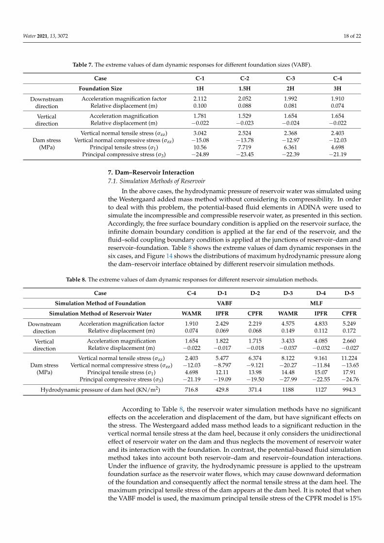
Water 2021, 13, 3072 18 of 22

Table 7. The extreme values of dam dynamic responses for different foundation sizes (VABF).

Case C-1 C-2 C-3 C-4

Foundation Size 1H 1.5H 2H 3H

Downstreamdirection

Acceleration magnification factor 2.112 2.052 1.992 1.910Relative displacement (m) 0.100 0.088 0.081 0.074

Verticaldirection

Acceleration magnification 1.781 1.529 1.654 1.654Relative displacement (m) −0.022 −0.023 −0.024 −0.022

Dam stress(MPa)

Vertical normal tensile stress (σzz) 3.042 2.524 2.368 2.403Vertical normal compressive stress (σzz) −15.08 −13.78 −12.97 −12.03

Principal tensile stress (σ1) 10.56 7.719 6.361 4.698Principal compressive stress (σ3) −24.89 −23.45 −22.39 −21.19

7. Dam–Reservoir Interaction7.1. Simulation Methods of Reservoir

In the above cases, the hydrodynamic pressure of reservoir water was simulated usingthe Westergaard added mass method without considering its compressibility. In orderto deal with this problem, the potential-based fluid elements in ADINA were used tosimulate the incompressible and compressible reservoir water, as presented in this section.Accordingly, the free surface boundary condition is applied on the reservoir surface, theinfinite domain boundary condition is applied at the far end of the reservoir, and thefluid–solid coupling boundary condition is applied at the junctions of reservoir–dam andreservoir–foundation. Table 8 shows the extreme values of dam dynamic responses in thesix cases, and Figure 14 shows the distributions of maximum hydrodynamic pressure alongthe dam–reservoir interface obtained by different reservoir simulation methods.

Table 8. The extreme values of dam dynamic responses for different reservoir simulation methods.

Case C-4 D-1 D-2 D-3 D-4 D-5

Simulation Method of Foundation VABF MLF

Simulation Method of Reservoir Water WAMR IPFR CPFR WAMR IPFR CPFR

Downstreamdirection

Acceleration magnification factor 1.910 2.429 2.219 4.575 4.833 5.249Relative displacement (m) 0.074 0.069 0.068 0.149 0.112 0.172

Verticaldirection

Acceleration magnification 1.654 1.822 1.715 3.433 4.085 2.660Relative displacement (m) −0.022 −0.017 −0.018 −0.037 −0.032 −0.027

Dam stress(MPa)

Vertical normal tensile stress (σzz) 2.403 5.477 6.374 8.122 9.161 11.224Vertical normal compressive stress (σzz) −12.03 −8.797 −9.121 −20.27 −11.84 −13.65

Principal tensile stress (σ1) 4.698 12.11 13.98 14.48 15.07 17.91Principal compressive stress (σ3) −21.19 −19.09 −19.50 −27.99 −22.55 −24.76

Hydrodynamic pressure of dam heel (KN/m2) 716.8 429.8 371.4 1188 1127 994.3

According to Table 8, the reservoir water simulation methods have no significanteffects on the acceleration and displacement of the dam, but have significant effects onthe stress. The Westergaard added mass method leads to a significant reduction in thevertical normal tensile stress at the dam heel, because it only considers the unidirectionaleffect of reservoir water on the dam and thus neglects the movement of reservoir waterand its interaction with the foundation. In contrast, the potential-based fluid simulationmethod takes into account both reservoir–dam and reservoir–foundation interactions.Under the influence of gravity, the hydrodynamic pressure is applied to the upstreamfoundation surface as the reservoir water flows, which may cause downward deformationof the foundation and consequently affect the normal tensile stress at the dam heel. Themaximum principal tensile stress of the dam appears at the dam heel. It is noted that whenthe VABF model is used, the maximum principal tensile stress of the CPFR model is 15%

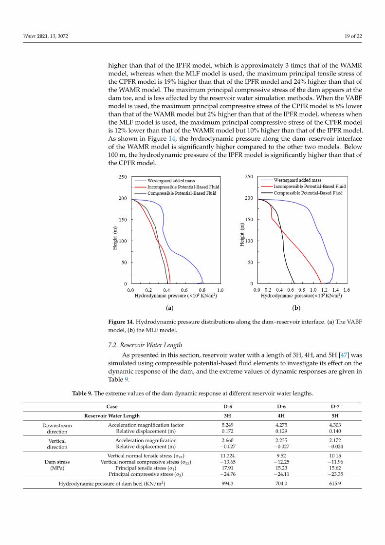
Water 2021, 13, 3072 19 of 22

higher than that of the IPFR model, which is approximately 3 times that of the WAMRmodel, whereas when the MLF model is used, the maximum principal tensile stress ofthe CPFR model is 19% higher than that of the IPFR model and 24% higher than that ofthe WAMR model. The maximum principal compressive stress of the dam appears at thedam toe, and is less affected by the reservoir water simulation methods. When the VABFmodel is used, the maximum principal compressive stress of the CPFR model is 8% lowerthan that of the WAMR model but 2% higher than that of the IPFR model, whereas whenthe MLF model is used, the maximum principal compressive stress of the CPFR modelis 12% lower than that of the WAMR model but 10% higher than that of the IPFR model.As shown in Figure 14, the hydrodynamic pressure along the dam–reservoir interfaceof the WAMR model is significantly higher compared to the other two models. Below100 m, the hydrodynamic pressure of the IPFR model is significantly higher than that ofthe CPFR model.


According to Table 8, the reservoir water simulation methods have no significant effects on the acceleration and displacement of the dam, but have significant effects on the stress. The Westergaard added mass method leads to a significant reduction in the vertical normal tensile stress at the dam heel, because it only considers the unidirectional effect of reservoir water on the dam and thus neglects the movement of reservoir water and its interaction with the foundation. In contrast, the potential-based fluid simulation method takes into account both reservoir–dam and reservoir–foundation interactions. Under the influence of gravity, the hydrodynamic pressure is applied to the upstream foundation surface as the reservoir water flows, which may cause downward defor-mation of the foundation and consequently affect the normal tensile stress at the dam heel. The maximum principal tensile stress of the dam appears at the dam heel. It is noted that when the VABF model is used, the maximum principal tensile stress of the CPFR model is 15% higher than that of the IPFR model, which is approximately 3 times that of the WAMR model, whereas when the MLF model is used, the maximum principal tensile stress of the CPFR model is 19% higher than that of the IPFR model and 24% higher than that of the WAMR model. The maximum principal compressive stress of the dam ap-pears at the dam toe, and is less affected by the reservoir water simulation methods. When the VABF model is used, the maximum principal compressive stress of the CPFR model is 8% lower than that of the WAMR model but 2% higher than that of the IPFR model, whereas when the MLF model is used, the maximum principal compressive stress of the CPFR model is 12% lower than that of the WAMR model but 10% higher than that of the IPFR model. As shown in Figure 14, the hydrodynamic pressure along the dam–reservoir interface of the WAMR model is significantly higher compared to the other two models. Below 100 m, the hydrodynamic pressure of the IPFR model is significantly higher than that of the CPFR model.

(a) (b)

Figure 14. Hydrodynamic pressure distributions along the dam–reservoir interface. (a) The VABF model, (b) the MLF model.

7.2. Reservoir Water Length As presented in this section, reservoir water with a length of 3H, 4H, and 5H [47]

was simulated using compressible potential-based fluid elements to investigate its effect on the dynamic response of the dam, and the extreme values of dynamic responses are given in Table 9.

The results show that the reservoir water length of 3H leads to a 7–23% increase in acceleration, a 9–33% increase in displacement, a 15–18% increase in the maximum prin-cipal tensile stress, a 3–6% increase in the maximum principal compressive stress, and a

Figure 14. Hydrodynamic pressure distributions along the dam–reservoir interface. (a) The VABFmodel, (b) the MLF model.

7.2. Reservoir Water Length

As presented in this section, reservoir water with a length of 3H, 4H, and 5H [47] wassimulated using compressible potential-based fluid elements to investigate its effect on thedynamic response of the dam, and the extreme values of dynamic responses are given inTable 9.

Table 9. The extreme values of the dam dynamic response at different reservoir water lengths.

Case D-5 D-6 D-7

Reservoir Water Length 3H 4H 5H

Downstreamdirection

Acceleration magnification factor 5.249 4.275 4.303Relative displacement (m) 0.172 0.129 0.140

Verticaldirection

Acceleration magnification 2.660 2.235 2.172Relative displacement (m) −0.027 −0.027 −0.024

Dam stress(MPa)

Vertical normal tensile stress (σzz) 11.224 9.52 10.15Vertical normal compressive stress (σzz) −13.65 −12.25 −11.96

Principal tensile stress (σ1) 17.91 15.23 15.62Principal compressive stress (σ3) −24.76 −24.11 −23.35

Hydrodynamic pressure of dam heel (KN/m2) 994.3 704.0 615.9

Water 2021, 13, 3072 20 of 22

The results show that the reservoir water length of 3H leads to a 7–23% increasein acceleration, a 9–33% increase in displacement, a 15–18% increase in the maximumprincipal tensile stress, a 3–6% increase in the maximum principal compressive stress, anda 41–61% increase in the maximum hydrodynamic pressure at the dam heel compared tothe reservoir water length of 4H and 5H.

8. Conclusions

In this study, some key factors, such as the dynamic interactions of dam–foundationand dam–reservoir, were considered in the dynamic numerical analysis of a 200 m highgravity dam. The rigid, massless, and viscoelastic artificial boundary foundation modelswere established to account for the effect of dam–foundation dynamic interaction on thedynamic responses of the dam. Three reservoir water simulation methods, namely, theWestergaard added mass method, and the incompressible and compressible potential fluidmethods, were used to account for the effect of hydrodynamic pressure on the dynamiccharacteristics of the dam. The ranges of the truncation boundary of the foundation andreservoir in numerical analysis were further investigated. The following conclusions canbe drawn:

(1) The natural frequency of the dam decreases greatly in numerical analysis when thedam–foundation interaction is considered, and decreases slightly with the increasein the foundation size. The simulation methods of reservoir water have significanteffects on the natural frequency of the dam, whereas the reservoir water lengths haveno significant effect.

(2) The dynamic interaction of the dam and the foundation cannot be ignored. Theradiation damping effect should be considered in the dynamic numerical analysis.The viscoelastic artificial boundary foundation is more efficient than the masslessfoundation in simulating the radiation damping effect of the far-field foundation. Itwas found that a foundation range of 3 times the dam height in all directions, suchas upstream, downstream, and depth, is the most reasonable range of the truncationboundary of the foundation.

(3) The methods used for reservoir water simulation have no significant effects on theacceleration and displacement of the dam, but have a significant effect on the stress.Compared with the Westergaard added mass method, the potential-based fluid simu-lation method simultaneously takes into account the reservoir–dam and reservoir–foundation interactions. The static and dynamic water pressure was applied to theupstream foundation surface as the reservoir water, which may cause downwarddeformation of the foundation and consequently increase the normal tensile stress atthe dam heel. It was found that a reservoir length of 3 times the dam height is feasiblefor the truncation boundary of the reservoirs.

Author Contributions: Conceptualization, H.Z.; methodology, H.Z.; validation, C.W., Y.Z., Y.W. andT.T.T.H.; resources, H.Z. and L.G.; data curation, C.W.; writing—original draft preparation, C.W.;writing—review and editing, H.Z. and C.W.; supervision, H.Z., L.G., Y.W. and T.T.T.H. All authorshave read and agreed to the published version of the manuscript.

Funding: This work was supported by the Open Research Fund of State Key Laboratory of Simulationand Regulation of Water Cycle in River Basin (China Institute of Water Resources and HydropowerResearch) (grant number IWHR-SKL-KF201816), the National Key Research and DevelopmentProgram of China (grant number 2017YFC0404903), and the Natural Science Foundation of JiangsuProvince (grant number BK20170884).

Institutional Review Board Statement: Not applicable.

Informed Consent Statement: Not applicable.

Data Availability Statement: The data presented in this study are available on request from thecorresponding author.

Water 2021, 13, 3072 21 of 22

Conflicts of Interest: The authors declare that they have no known competing financial interests orpersonal relationships that could have appeared to influence the work reported in this paper.

References1. Ghaedi, K.; Hejazi, F.; Ibrahim, Z.; Khanzaei, P. Flexible foundation effect on seismic analysis of roller compacted concrete (RCC)

dams using finite element method. KSCE J. Civ. Eng. 2017, 22, 1275–1287. [CrossRef]2. Bayraktar, A.; Hançer, E.; Akköse, M. Influence of base-rock characteristics on the stochastic dynamic response of dam–reservoir–

foundation systems. Eng. Struct. 2005, 27, 1498–1508. [CrossRef]3. Ghaemian, M.; Noorzad, A.; Mohammadnezhad, H. Assessment of foundation mass and earthquake input mechanism effect on

dam–reservoir–foundation system response. Int. J. Civ. Eng. 2019, 17, 473–480. [CrossRef]4. Salamon, J.W.; Wood, C.; Hariri-Ardebili, M.A.; Malm, R.; Faggiani, G. Seismic Analysis of Pine Flat Concrete Dam: Formulation and

Synthesis of Results; Springer International Publishing: Cham, Switzerland, 2020; pp. 3–97.5. Chopra, A. Earthquake analysis of concrete dams: Factors to be considered. In Proceedings of the Proceedings of the 10th

National Conference in Earthquake Engineering, Anchorage, AK, USA, 21–25 July 2014.6. Hariri-Ardebili, M.A.; Kolbadi, S.M.S.; Kianoush, M. FEM-based parametric analysis of a typical gravity dam considering input

excitation mechanism. Soil Dyn. Earthq. Eng. 2016, 84, 22–43. [CrossRef]7. Hariri-Ardebili, M.A.; Mirzabozorg, H. A comparative study of seismic stability of coupled arch dam-foundation-reservoir

systems using infinite elements and viscous boundary models. Int. J. Struct. Stab. Dyn. 2013, 13, 1350032. [CrossRef]8. Burman, A.; Nayak, P.; Agrawal, P.; Maity, D. Coupled gravity dam–foundation analysis using a simplified direct method of

soil–structure interaction. Soil Dyn. Earthq. Eng. 2012, 34, 62–68. [CrossRef]9. Wang, H.; Feng, M.; Yang, H. Seismic nonlinear analyses of a concrete gravity dam with 3D full dam model. Bull. Earthq. Eng.

2012, 10, 1959–1977. [CrossRef]10. Lysmer, J.; Kuhlemeyer, R.L. Finite dynamic model for infinite media. J. Eng. Mech. Div. 1969, 95, 859–878. [CrossRef]11. Hariri-Ardebili, M.A. Impact of foundation nonlinearity on the crack propagation of high concrete dams. Soil Mech. Found. Eng.

2014, 51, 72–82. [CrossRef]12. Liu, J.; Du, Y.; Du, X.; Wang, Z.; Wu, J. 3D viscous-spring artificial boundary in time domain. Earthq. Eng. Eng. Vib.

2006, 5, 93–102. [CrossRef]13. Liang, H.; Tu, J.; Guo, S.; Liao, J.; Li, D.; Peng, S. Seismic fragility analysis of a High Arch Dam-Foundation System based on

seismic instability failure mode. Soil Dyn. Earthq. Eng. 2020, 130, 105981. [CrossRef]14. Song, C.; Wolf, J.P. The scaled boundary finite-element method—alias consistent infinitesimal finite-element cell method—for

elastodynamics. Comput. Methods Appl. Mech. Eng. 1997, 147, 329–355. [CrossRef]15. Qu, Y.; Chen, D.; Liu, L.; Ooi, E.T.; Eisenträger, S.; Song, C. A direct time-domain procedure for the seismic analysis of dam–

foundation–reservoir systems using the scaled boundary finite element method. Comput. Geotech. 2021, 138, 104364. [CrossRef]16. Hariri-Ardebili, M.A.; Kianoush, M. Integrative seismic safety evaluation of a high concrete arch dam. Soil Dyn. Earthq. Eng.

2014, 67, 85–101. [CrossRef]17. Basu, U.; Chopra, A.K. Erratum to‘Perfectly matched layers for transient elastodynamics of unbounded domains’(Int. J. Numer.

Meth. Engng 2004; 59:1039–1074). Int. J. Numer. Methods Eng. 2004, 61, 156–157. [CrossRef]18. Harirri-Ardebili, M.A.; Saouma, V.E. Impact of near-fault vs. far-field ground motions on the seismic response of an arch dam

with respect to foundation type. Dam Eng. 2013, 24, 19–52.19. Pan, J.W.; Song, C.M.; Zhang, C.H. Simple model for gravity dam response considering radiation damping effects.

J. Hydraul. Eng. 2010, 41, 493–498. [CrossRef]20. Chen, D.; Hou, C.; Wang, F. Influences on the seismic response of the gravity dam-foundation-reservoir system with different

boundary and input models. Shock. Vib. 2021, 2021, 1–15. [CrossRef]21. Wang, G.; Wang, Y.; Lu, W.; Zhou, C.; Chen, M.; Yan, P. XFEM based seismic potential failure mode analysis of concrete gravity

dam–water–foundation systems through incremental dynamic analysis. Eng. Struct. 2015, 98, 81–94. [CrossRef]22. Wang, G.; Wang, Y.; Lu, W.; Yan, P.; Zhou, W.; Chen, M. A general definition of integrated strong motion duration and its effect on

seismic demands of concrete gravity dams. Eng. Struct. 2016, 125, 481–493. [CrossRef]23. Gorai, S.; Maity, D. Seismic response of concrete gravity dams under near field and far field ground motions. Eng. Struct. 2019,

196, 109292. [CrossRef]24. Chen, D.-H.; Yang, Z.-H.; Wang, M.; Xie, J.-H. Seismic performance and failure modes of the Jin’anqiao concrete gravity dam

based on incremental dynamic analysis. Eng. Fail. Anal. 2019, 100, 227–244. [CrossRef]25. Asghari, E.; Taghipour, R.; Bozorgnasab, M.; Moosavi, M. Seismic analysis of concrete gravity dams considering foundation mass

effect. KSCE J. Civ. Eng. 2018, 22, 4988–4996. [CrossRef]26. Mirzabozorg, H.; Akbari, M.; Hariri-Ardebili, M.A. Wave passage and incoherency effects on seismic response of high arch dams.

Earthq. Eng. Eng. Vib. 2012, 11, 567–578. [CrossRef]27. Westergaard, H.M. Water pressures on dams during earthquakes. Trans. Am. Soc. Civ. Eng. 1933, 98, 418–433. [CrossRef]28. Khiavi, M.P.; Sari, A. Evaluation of hydrodynamic pressure distribution in reservoir of concrete gravity dam under vertical

vibration using an analytical solution. Math. Probl. Eng. 2021, 2021, 1–9. [CrossRef]

http://doi.org/10.1007/s12205-017-1088-6

http://doi.org/10.1016/j.engstruct.2005.05.004

http://doi.org/10.1007/s40999-018-0325-9

http://doi.org/10.1016/j.soildyn.2016.01.013

http://doi.org/10.1142/S0219455413500326


http://doi.org/10.1007/s10518-012-9377-4

http://doi.org/10.1061/JMCEA3.0001144

http://doi.org/10.1007/s11204-014-9257-9

http://doi.org/10.1007/s11803-006-0585-2

http://doi.org/10.1016/j.soildyn.2019.105981

http://doi.org/10.1016/S0045-7825(97)00021-2

http://doi.org/10.1016/j.compgeo.2021.104364


http://doi.org/10.1002/nme.1137

http://doi.org/10.13243/j.cnki.slxb.2010.04.006

http://doi.org/10.1155/2021/6660145



http://doi.org/10.1016/j.engstruct.2019.109292

http://doi.org/10.1016/j.engfailanal.2019.02.018

http://doi.org/10.1007/s12205-017-0278-6

http://doi.org/10.1007/s11803-012-0142-0

http://doi.org/10.1061/TACEAT.0004496

http://doi.org/10.1155/2021/6669366

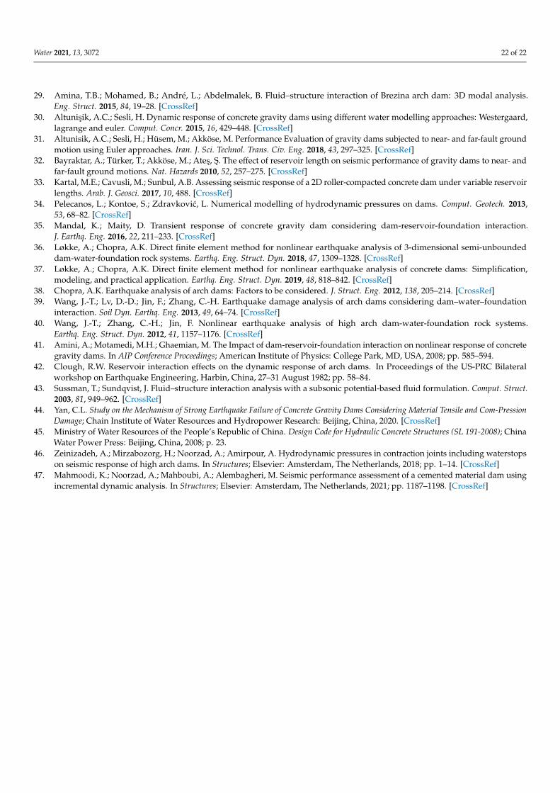
Water 2021, 13, 3072 22 of 22

29. Amina, T.B.; Mohamed, B.; André, L.; Abdelmalek, B. Fluid–structure interaction of Brezina arch dam: 3D modal analysis.Eng. Struct. 2015, 84, 19–28. [CrossRef]

30. Altunisik, A.C.; Sesli, H. Dynamic response of concrete gravity dams using different water modelling approaches: Westergaard,lagrange and euler. Comput. Concr. 2015, 16, 429–448. [CrossRef]

31. Altunisik, A.C.; Sesli, H.; Hüsem, M.; Akköse, M. Performance Evaluation of gravity dams subjected to near- and far-fault groundmotion using Euler approaches. Iran. J. Sci. Technol. Trans. Civ. Eng. 2018, 43, 297–325. [CrossRef]

32. Bayraktar, A.; Türker, T.; Akköse, M.; Ates, S. The effect of reservoir length on seismic performance of gravity dams to near- andfar-fault ground motions. Nat. Hazards 2010, 52, 257–275. [CrossRef]

33. Kartal, M.E.; Cavusli, M.; Sunbul, A.B. Assessing seismic response of a 2D roller-compacted concrete dam under variable reservoirlengths. Arab. J. Geosci. 2017, 10, 488. [CrossRef]

34. Pelecanos, L.; Kontoe, S.; Zdravkovic, L. Numerical modelling of hydrodynamic pressures on dams. Comput. Geotech. 2013,53, 68–82. [CrossRef]

35. Mandal, K.; Maity, D. Transient response of concrete gravity dam considering dam-reservoir-foundation interaction.J. Earthq. Eng. 2016, 22, 211–233. [CrossRef]

36. Løkke, A.; Chopra, A.K. Direct finite element method for nonlinear earthquake analysis of 3-dimensional semi-unboundeddam-water-foundation rock systems. Earthq. Eng. Struct. Dyn. 2018, 47, 1309–1328. [CrossRef]

37. Løkke, A.; Chopra, A.K. Direct finite element method for nonlinear earthquake analysis of concrete dams: Simplification,modeling, and practical application. Earthq. Eng. Struct. Dyn. 2019, 48, 818–842. [CrossRef]

38. Chopra, A.K. Earthquake analysis of arch dams: Factors to be considered. J. Struct. Eng. 2012, 138, 205–214. [CrossRef]39. Wang, J.-T.; Lv, D.-D.; Jin, F.; Zhang, C.-H. Earthquake damage analysis of arch dams considering dam–water–foundation

interaction. Soil Dyn. Earthq. Eng. 2013, 49, 64–74. [CrossRef]40. Wang, J.-T.; Zhang, C.-H.; Jin, F. Nonlinear earthquake analysis of high arch dam-water-foundation rock systems.

Earthq. Eng. Struct. Dyn. 2012, 41, 1157–1176. [CrossRef]41. Amini, A.; Motamedi, M.H.; Ghaemian, M. The Impact of dam-reservoir-foundation interaction on nonlinear response of concrete

gravity dams. In AIP Conference Proceedings; American Institute of Physics: College Park, MD, USA, 2008; pp. 585–594.42. Clough, R.W. Reservoir interaction effects on the dynamic response of arch dams. In Proceedings of the US-PRC Bilateral

workshop on Earthquake Engineering, Harbin, China, 27–31 August 1982; pp. 58–84.43. Sussman, T.; Sundqvist, J. Fluid–structure interaction analysis with a subsonic potential-based fluid formulation. Comput. Struct.

2003, 81, 949–962. [CrossRef]44. Yan, C.L. Study on the Mechanism of Strong Earthquake Failure of Concrete Gravity Dams Considering Material Tensile and Com-Pression

Damage; Chain Institute of Water Resources and Hydropower Research: Beijing, China, 2020. [CrossRef]45. Ministry of Water Resources of the People’s Republic of China. Design Code for Hydraulic Concrete Structures (SL 191-2008); China

Water Power Press: Beijing, China, 2008; p. 23.46. Zeinizadeh, A.; Mirzabozorg, H.; Noorzad, A.; Amirpour, A. Hydrodynamic pressures in contraction joints including waterstops

on seismic response of high arch dams. In Structures; Elsevier: Amsterdam, The Netherlands, 2018; pp. 1–14. [CrossRef]47. Mahmoodi, K.; Noorzad, A.; Mahboubi, A.; Alembagheri, M. Seismic performance assessment of a cemented material dam using

incremental dynamic analysis. In Structures; Elsevier: Amsterdam, The Netherlands, 2021; pp. 1187–1198. [CrossRef]


http://doi.org/10.12989/cac.2015.16.3.429

http://doi.org/10.1007/s40996-018-0142-z

http://doi.org/10.1007/s11069-009-9368-1

http://doi.org/10.1007/s12517-017-3271-y

http://doi.org/10.1016/j.compgeo.2013.04.003

http://doi.org/10.1080/13632469.2016.1217804

http://doi.org/10.1002/eqe.3019


http://doi.org/10.1061/(ASCE)ST.1943-541X.0000431



http://doi.org/10.1016/S0045-7949(02)00407-8

http://doi.org/10.27646/d.cnki.gsldy.2020.000025

http://doi.org/10.1016/j.istruc.2018.01.005

http://doi.org/10.1016/j.istruc.2020.12.015

Influences on the Seismic Response of a Gravity Dam ... - MDPI

Documents

Transcript of Influences on the Seismic Response of a Gravity Dam ... - MDPI