Influence of heterogeneity on the interpretation of pumping test data in leaky aquifers

Influence of heterogeneity on the interpretation of pumping test

data in leaky aquifers

Nadim K. Copty,1 Paolo Trinchero,2 Xavier Sanchez-Vila,2 Murat Savas Sarioglu,1

and Angelos N. Findikakis3

Received 28 April 2008; revised 9 September 2008; accepted 17 September 2008; published 15 November 2008.

[1] Pumping tests are routinely interpreted from the analysis of drawdown data and theirderivatives. These interpretations result in a small number of apparent parameter valueswhich lump the underlying heterogeneous structure of the aquifer. Key questions in suchinterpretations are (1) what is the physical meaning of those lumped parameters and (2)whether it is possible to infer some information about the spatial variability of thehydraulic parameters. The system analyzed in this paper consists of an aquifer separatedfrom a second recharging aquifer by means of an aquitard. The natural log transforms ofthe transmissivity, ln T, and the vertical conductance of the aquitard, ln C, are modeled astwo independent second-order stationary spatial random functions (SRFs). The MonteCarlo approach is used to simulate the time-dependent drawdown at a suite of observationpoints for different values of the statistical parameters defining the SRFs. Drawdown dataat each observation point are independently used to estimate hydraulic parameters usingthree existing methods: (1) the inflection-point method, (2) curve-fitting, and (3) thedouble inflection-point method. The resulting estimated parameters are shown to be spacedependent and vary with the interpretation method since each method gives differentemphasis to different parts of the time-drawdown data. Moreover, the heterogeneity in thepumped aquifer or the aquitard influences the estimates in distinct manners. Finally, weshow that, by combining the parameter estimates obtained from the different analysisprocedures, information about the heterogeneity of the leaky aquifer system may beinferred.

Citation: Copty, N. K., P. Trinchero, X. Sanchez-Vila, M. S. Sarioglu, and A. N. Findikakis (2008), Influence of heterogeneity on the

interpretation of pumping test data in leaky aquifers, Water Resour. Res., 44, W11419, doi:10.1029/2008WR007120.

1. Introduction

[2] In the analysis of pumping tests, drawdown data asfunction of space and/or time are normally used to inferrepresentative hydraulic parameters of the perturbed aquifervolume. Most existing pumping test analysis proceduresassume that the aquifer system is homogeneous, or at mostconsists of a few homogeneous deterministically locatedunits. Under such assumptions of homogeneity, it is possi-ble to devise graphical or analytical methods that canprovide the exact parameters of the system if noise-freedrawdown data are available (for example, Theis [1935] forconfined aquifers, Hantush and Jacob [1955] for leakyaquifers).[3] A salient characteristic of natural geologic formations

is that they are heterogeneous with complex patterns ofspatial variability. As a result, significant effort has beendevoted over the past four decades to address the problemof radially convergent flow toward a pumping well in

heterogeneous aquifers. A number of review papers havebeen published on this topic [e.g., Renard and de Marsily,1997; Rubin, 2003; Raghavan, 2004; Sanchez-Vila et al.,2006]. Some of the more relevant studies are summarizednext.[4] A number of published papers focused on the poten-

tial existence and determination of an effective hydraulicconductivity value, defined as the negative ratio between theexpected values of the flow and the hydraulic gradient atany given point [e.g.,Dagan, 1982, 1989;Gomez-Hernandezand Gorelick, 1989; Naff, 1991; Neuman and Orr, 1993;Indelman and Abramovich, 1994; Indelman et al., 1996;Sanchez-Vila, 1997; Riva et al., 2001; Dagan, 2001;Guadagnini et al., 2003; Indelman, 2003a, 2003b]. Whenthe effective hydraulic conductivity is constant throughoutthe domain, it can be considered an intrinsic property of themedium. However, for radially convergent flow, it wasshown as early as the study of Shvidler [1962] that such aconstant effective value does not exist. Rather, effectivehydraulic conductivity increases from the harmonic meannear the pumping well to the geometric mean at somedistance from the well, and this distance depends on thecorrelation length of the hydraulic conductivity field[Indelman and Abramovich, 1994; Sanchez-Vila, 1997].The effective hydraulic parameters are functions also ofthe flow dimensionality and time [Dagan, 1982].

1Institute of Environmental Sciences, Bogazici University, Bebek,Istanbul, Turkey.

2Department of Geotechnical Engineering and Geosciences, TechnicalUniversity of Catalonia, Barcelona, Spain.

3Bechtel National Inc., San Francisco, California, USA.

Copyright 2008 by the American Geophysical Union.0043-1397/08/2008WR007120

W11419

WATER RESOURCES RESEARCH, VOL. 44, W11419, doi:10.1029/2008WR007120, 2008

1 of 15

[5] Another group of papers focus on the estimation of anupscaled hydraulic conductivity that is averaged over afinite volume for an individual realization [e.g., Gomez-Hernandez and Gorelick, 1989; Oliver, 1990; Desbarats,1992; Durlofsky, 2000; Rubin, 2003; Copty et al., 2006].The upscaled hydraulic conductivity is a local, non-uniqueestimate, dependent on the flow conditions. In confinedaquifers the upscaled conductivity can be written as aweighted-average of the point values, with the weightsdecreasing with increasing distance from the pumping well[Sanchez-Vila et al., 1999a].[6] More recently, some researchers examined the prob-

lem of defining the statistical spatial structure from thedrawdown data [Copty and Findikakis, 2004a; Neuman etal., 2004, 2007; Firmani et al., 2006]. These studies showthat the variance and integral scale of the hydraulic conduc-tivity or transmissivity may be inferred when a large numberof pumping tests and observation points are available.[7] While all the papers cited so far provide a general

framework for the analysis of radially convergent flow inheterogeneous media, in practice most pumping tests areroutinely interpreted by simple methods based on a homog-enized conception of the system. The interpreted parameters(transmissivity and storativity in confined aquifers, plus theleakage factor in leaky aquifers) lump all the underlyingheterogeneity, providing some averaged value of the spa-tially dependent parameters. Although this is a commonlyencountered problem, relatively few papers can be foundthat assess the impact of the heterogeneity of the hydraulicparameters on the interpretation of pumping tests. Earlierstudies such as those of Barker and Herbert [1982], Butler[1988], and Butler and Liu [1993] examined this problemfor systems with deterministically defined high or lowpermeable inclusions embedded in a homogeneous back-ground T field. Serrano [1997] developed an analyticsolution that relates the mean and variance of the transmis-sivity of confined aquifers to the mean and variance of thedrawdown. Meier et al. [1998] and Sanchez-Vila et al.[1999b] evaluated the validity of the Cooper-Jacob method[Cooper and Jacob, 1946] for the interpretation of time-drawdown data in aquifers with heterogeneous transmissivityand uniform storativity. They showed that the transmissivityestimated using the Cooper-Jacob method does not dependon the observation point location, with a value close to thegeometric mean of the transmissivity distribution. However,the estimated storativity could significantly vary with thelocation of the observation point, which is indicative of theflow point-to-point connectivity between the pumping welland the observation point [see also Trinchero et al., 2008b].Copty and Findikakis [2004a, 2004b] used a Monte Carloapproach to study the effect of spatial heterogeneity on thetransient drawdown due to pumping in a confined aquifer,and on the conditions where the Cooper-Jacob assumptionswould be valid. Wu et al. [2005] used the Thies method toestimate flow parameters from time-drawdown data at asingle observation well in a highly heterogeneous aquiferwith log-Gaussian transmissivity and storativity fields.There results show that the estimated transmissivity andstorativity values estimated from the early drawdown datachange with time. The storativity estimate stabilize ratherquickly to a value that is function of the storativity of theaquifer volume between the pumping and the observation

wells. In contrast the estimated transmissivity at late times isfunction of the entire flow domain, and approach a valuethat is close but not equal the geometric mean. Knight andKluitenberg [2005] derived explicit analytic expressions forthe sensitivity of pumping tests and slug tests to variationsin the transmissivity and storativity, for the case when thepumping well and observation well are collocated and whenthe two wells are at different locations. Leven and Dietrich[2006] used sensitivity coefficients to study the effect ofspatial variability of the transmissivity and storativity ofconfined aquifer on the interpretation of single-well andtwo-well pumping tests.[8] Almost all the studies cited above have focused on the

problem of radially convergent flow in heterogeneousconfined aquifers. However, in natural geologic systems,confining layers overlying and/or underlying an aquiferoften leak. Aquifer-aquitard systems are found worldwide,particularly in multi-layer and more complex geologicformations such as alluvial aquifers. In such systems,drawdown values depend on the hydraulic properties ofboth the aquifer and the aquitard. Characterization ofaquifer and aquitard properties is then necessary for theproper modeling of groundwater flow and contaminanttransport. Despite that, to our knowledge there has beenno formal attempt to relate the parameters determined withconventional interpretation methods to the heterogeneousdistribution of the aquifer-aquitard parameters.[9] Specifically, we simulate pumping tests in syntheti-

cally generated aquifer-aquitard systems, considering sepa-rately the heterogeneity of the pumping aquifer and theconfining aquitard. Estimates of the apparent hydraulicparameters are obtained by analyzing each pumping testindependently for different distances from the pumping welland using common methods available in the literature andused extensively in computer codes developed for theanalysis of pumping tests. By combining the estimates ofthe apparent parameters obtained with the different analysismethods, it is shown that information about the heteroge-neity of the system may be inferred.[10] It is important to note that the interpretation of

pumping tests conducted in heterogeneous media can, inprinciple, be formulated as a geostatistical or inverse prob-lem. Over the past two decades several inversion modelingtools have been developed [see, for example, Rubin, 2003].Some authors have also proposed the use of hydrologicaltomography for the estimation of spatial distribution of theflow parameters [Yeh and Liu, 2000; Zhu and Yeh, 2005]However, the computational effort involved in these inter-pretation approaches can be intensive and quite complexbecause of the ill-posedness of the groundwater inverseproblem. The goal in this paper is to explore the possibilityof extending commonly used pumping tests analysis proce-dures to extract information about the underlying spatialvariability of leaky aquifer systems.

2. Problem Statement

2.1. Definition of the Heterogeneous Aquifer-AquitardSystem

[11] The vertical cross-section of the leaky aquifer systemconsidered in this study is similar to that analyzed byHantush and Jacob [1955]. The system consists of two

2 of 15

W11419 COPTY ET AL.: PUMPING TEST IN HETEROGENEOUS LEAKY AQUIFIERS W11419

horizontally unbounded aquifers, separated by an aquitard. Afully penetrating pumping well of infinitesimal radius isplaced in one aquifer and is fully isolated from the other.Before pumping, the system is assumed to be at equilibrium,with both aquifers and the aquitard having the samehydraulic head. The aquitard is assumed to have nostorage capacity. Because of the large contrast in hydraulicconductivity values, the flow induced by the pumping isapproximately vertical in the aquitard and horizontal in theaquifer. The mathematical equation describing flow in thepumped aquifer is:

@

@xT@s

@x

� �þ @

@yT@s

@y

� �� Cs ¼ S

@s

@tð1Þ

where T(x, y) [L2T�1] is the transmissivity of the (pumped)aquifer; C(x, y) [T�1] is the aquitard conductance, equal tothe vertical hydraulic conductivity of the aquitard divided byaquitard thickness; S [�] is the aquifer storativity; s(x, y, t)[L] is the drawdown. The leakage factor B [L] is definedas

B ¼ T=Cð Þ1=2: ð2Þ

[12] For a homogeneous aquifer-aquitard system thetransient drawdown is given by [Hantush and Jacob, 1955]:

s r; tð Þ ¼ Q

4pT0W u; r=Bð Þ; ð3Þ

where r is the radial coordinate, with origin at the pumpingwell, s(r, t) is the drawdown; Q is the constant pumpingrate, T0 is the spatially uniform transmissivity, andW(u, r/B)is the leaky well function:

W u; r=Bð Þ ¼Z1

u

1

yexp �y� r2

4B2y

� �dy ð4Þ

with u = r2 S0/4tT0, and S0 the spatially uniform storagecoefficient.[13] Because of leakage through the semi-confining layer,

the drawdown reaches a steady-state asymptotically. Thesteady drawdown, sm, is given by [de Glee, 1930]:

sm ¼ Q

2pT0K0 r=Bð Þ; ð5Þ

where K0 is the modified Bessel function of the second kindand of order 0.

2.2. Existing Parameter Interpretation Methods

[14] Two procedures are commonly used in the analysisof time-drawdown data in leaky aquifers: (1) the inflection-point method [Hantush, 1956], and (2) the curve-fittingmethod [Walton, 1962]. Both methods are based on theassumption of homogeneity of the system, plus a number ofadditional somewhat restrictive assumptions, such as nostorage released from the aquitard and constant head in theunpumped aquifer. Subsequent to the original study byHantush and Jacob [1955], a number of papers relaxed someof the assumptions listed above. For example, Hantush

[1960] accounted for the storage of the confining layer.Neuman and Witherspoon [1969a, 1969b] provided a moregeneral solution including drawdown in the overlyingaquifer. Moench [1985] incorporated the effect of theextraction well diameter and well bore skin on the transientdrawdown of leaky aquifers. Despite these improvements,the above-mentioned methods remain quite popular for theinterpretation of pumping test data in leaky aquifers becauseof their relative simplicity.[15] For completeness, the inflection-point method and

the curve-fitting method are described here briefly. Theinflection-point method [Hantush, 1956] uses analyticallyderived relationships of the drawdown versus log-timecurve to estimate the flow parameters. In particular, it isfound that the ratio between the drawdown, sp, and itsderivative at the inflection-point location, Dsp, is functionof the ratio r/B only [Hantush, 1956]:

2:3sp

Dsp¼ exp r=Bð ÞKo r=Bð Þ: ð6Þ

[16] The actual time where the inflection point takesplace, tp, can be written in terms of the different systemparameters:

tp ¼rSB

2T: ð7Þ

[17] Once the leakage factor, B, is estimated, the trans-missivity, T, and storativity, S, of the perturbed aquifer canbe determined sequentially from equations (5) and (7).[18] It is possible to demonstrate analytically that the

steady-state drawdown, sm, is twice the drawdown at theinflection point sm = 2sp. Hence, in real applications, thereare two different ways of applying the Hantush inflectionpoint method. First, from the steady-state drawdown (or itsextrapolation if the time-drawdown record is not sufficientlylong), one can estimate sp = 0.5sm. Then from the drawdowncurve, we estimate Tp and Dsp. Alternatively, one can locatethe inflection-point as the point where the derivative of thedrawdown vs log-time is maximum, and from that deter-mine sp and Dsp. While in homogeneous media bothmethods would render the same parameter values, in real(heterogeneous) media this is not necessarily true. The twovariants of the method will be compared and evaluated aspart of the present study.[19] The curve-fitting method [Walton, 1962] finds the

representative hydraulic parameters by comparing the ob-served time-drawdown data on a log-log plot to a family oftype curves developed based on the analytical solutiongiven in equation (3). In this paper, the best-fit parameterswere determined by a trial and error approach that mini-mizes the sum of squared differences between the simulateddrawdown and the theoretical drawdown:

Xi

s r; tið Þ � s r; tið Þ½ �2 ð8Þ

where s(r, ti) is the observed drawdown at distance r fromthe pumping well and time ti and s(r, ti) is the theoreticaldrawdown derived from the type curves.

W11419 COPTY ET AL.: PUMPING TEST IN HETEROGENEOUS LEAKY AQUIFIERS

3 of 15

W11419

[20] Recently, a third method for the interpretation ofpumping tests in leaky aquifers was developed, referred toas the double inflection-point (DIP) method [Trinchero etal., 2008a]. The DIP method requires the estimation of theratio t = ts1/2tp or t = ts2/2tp where tp is the timecorresponding to the inflection point (equation (7)) and ts1and ts2 are the times corresponding to the two inflection-points of the first derivative of the drawdown with respect tothe logarithm of time (Figure 1). Once t is estimated, theleakage factor is computed directly from [Trinchero et al.,2008a]:

B ¼ t2 � 1=4ð Þ2rt t2 þ 1=4ð Þ : ð9Þ

[21] After the leakage factor, B, is estimated, the other flowparameters (T, S, and C) are calculated from equations (5),(7) and (2), respectively. Because t can be based either on ts1or ts2, two sets of parameters are estimated with the DIPmethod.[22] The above methods provide the exact solution for the

hydraulic parameters (T, S, B) in a homogenous system,provided the drawdown data are noise-free. On the otherhand, each method provides a different set of parameters inreal (heterogeneous) systems, since each particular methodgives more weight to different portions of the time-draw-down data. The emphasis that each method gives to thedifferent portions of the drawdown curve is discussedfurther by Trinchero et al. [2008a] and section 3.3 of thispaper. One of the main conclusions of Trinchero et al. wasthat by comparing the estimates of B provided by theinflection-point method [Hantush, 1956] and the DIPmethod, it is possible to infer information about the localtransmissivity in the vicinity of the pumping well.[23] In this study Monte Carlo simulations are used to

assess what parameter values are given by the different

methods and whether it is possible to relate these parametersto some characteristic values of the heterogeneous system.

2.3. Numerical Setup

[24] We model the natural logarithms of the transmissiv-ity and aquitard hydraulic conductance as two independentmultivariate Gaussian SRF’s with stationary exponentialsemivariograms. Two sets of simulations are presented. Inthe first one the transmissivity of the pumped aquifer wasassumed spatially variable while the aquitard conductanceis assumed uniform. In the second set, the aquifer wasassumed to be homogeneous and the aquitard heteroge-neous. This allows us to evaluate the impact of the hetero-geneity of the aquifer and the confining layer on theestimated parameters independently.[25] For each set of parameters, 1000 realizations of the

spatially variable parameter (aquifer transmissivity or aqui-tard conductance) were generated using the turning bandsmethod [Mantoglou and Wilson, 1982]. The storativity ofthe pumped aquifer was assumed to be uniform equal to0.0001. The confining aquifer was assumed to have nostorage, which is consistent with the leaky aquifer systemanalyzed by Hantush and Jacob [1955]. The pumping wellis located at the center of a square aquifer, 481 m on eachside. The medium was discretized using square cells of size1 1 m2. At steady state, the equivalent well radius isapproximately 0.2 times the cell size [Desbarats, 1992]. Aprescribed head condition was imposed at the outer bound-ary, and the extraction well is treated as a prescribed sinkterm with steady rate of 2 m3/d. Drawdowns were simulatedusing the finite difference model MODFLOW [Harbaugh etal., 2000]. The test duration was 2 days, and a variable timestep was used in the simulations, starting with 1 s, andgradually increasing it as the test progressed.[26] Inspection of the results showed that steady state was

reached at the end of the 2-day period for all casesconsidered. Some simulations were repeated with a no-flowcondition at the outer boundary and the simulated draw-down data were identical, indicating that the outer boundaryhad no impact on the simulated drawdowns. The numericalsetup was also tested by simulating the pumping test in ahomogeneous leaky aquifer system and comparing thedrawdown data to equation (3).

3. Results

3.1. Impact of Aquifer Heterogeneity

[27] The first set of results corresponds to the case withspatially uniform aquitard conductance (Co = 0.001 d�1)and spatially variable aquifer transmissivity (with geometricmean, Tg = 1 m2/d, and ln T integral scale: I = 8 m, andvariance: s2 = 1). Figure 2 compares the aquifer transmis-sivity estimates (normalized by Tg) using the inflection-point and the curve-fitting methods at different distancesfrom the pumping well. Each point on the plots correspondsto one of the 1000 Monte Carlo realizations. Figure 2 alsoshows the correlation (Corr) and the mean absolute differ-ence (MAD) between the two sets of estimates as a functionof distance. From the two options of the inflection-pointmethod described in section 2.2, we selected to use theslope and drawdown at the point corresponding to half thesteady-state drawdown.

Figure 1. Drawdown and its first and second derivativesas a function of log time for Q = 2 m3/d, T = 1 m2/d, S =0.0001, C = 0.001 d�1, and r/B = 0.5 (adapted fromTrinchero et al. [2008a]).

4 of 15


[28] From Figure 2 we observe that overall the transmis-sivity estimates obtained with the two methods tend tospread around the 1:1 line. The differences between thevalues estimated with the two methods come from eachmodel weighing differently the T values within the domain.For larger distances from the pumping well, the estimateswith the two methods tend to converge, since the largeraquifer volume involved in the weighting process averagesout the effect of heterogeneities. The convergence in theestimates is also reflected in the increasing Corr toward 1and decreasing MAD toward zero with distance.[29] There is a significant difference between the behav-

ior of leaky and confined aquifers during pumping tests. Inthe latter, it was shown analytically by Sanchez-Vila et al.[1999b] that eventually all the estimated transmissivityvalues converge to a single T value which is close to thegeometric average of the random function T(x, y). On theother hand, for pumping tests conducted in leaky aquifers,each realization yields potentially different estimates. Thereason is that in confined aquifers steady-state conditionsare never reached, and so, all points in the domain areeventually affected by pumping. This is not the case inleaky aquifers, where steady-state conditions are eventuallyreached, and the drawdown is null everywhere exceptwithin a finite volume around the pumping well. Thus theweighted average of the local T values can be different foreach individual realization and, in particular, different fromthe overall mean value, Tg.

[30] Figure 3 displays scatter plots of the normalizedaquitard conductance estimates from both the inflection-point and the curve-fitting methods. For small distancesfrom the pumping well, the estimates with the two methodsmay differ significantly and the scatter of the estimatedaquitard conductance values is greater than the scatter of theaquifer transmissivity values. For large distances the esti-mates become independent of the interpretation method.However, for many simulations the estimated values can besignificantly different from the actual value used in thedrawdown simulation (i.e., C/Co 6¼ 1). These observationsare also confirmed by the values of Corr and MAD whichapproach one and zero, respectively with increase in dis-tance. A similar behavior is observed for the estimatedstorativity (The results are not presented here for brevity).[31] The main low-order statistics of the flow parameters

estimates are compiled in Table 1. The mean of the Testimates is found to be between the geometric and arith-metic mean of the transmissivity (in this case Ta/Tg = 1.65).Copty et al. [2006] observed a similar behavior in theequivalent transmissivity for steady-state radially conver-gent flow in leaky aquifers and associated this effect to eachrealization sampling only a portion of the domain centeredaround the pumping well, thus forcing the expected meantoward the arithmetic average. Table 1 also shows a slightincreasing trend in the mean of estimated transmissivitywith distance. This observation is discussed later.

Figure 2. Normalized transmissivity estimates using the inflection-point and the curve-fitting methodsfor different distances from the pumping well (heterogeneous aquifer with Tg = 1 m2 d�1, I = 8 m, ands2 = 1 and a uniform aquitard with Co = 0.001 d�1).


5 of 15

W11419

[32] The deviation of the estimated T values from theactual distributions causes a bias in the storativity andaquitard conductance estimates, which in the mean areslightly overestimated. The reason comes from the interpre-tation methods, all of them leading to estimates that are notindependent, but correlated. Thus errors in the estimation ofone parameter directly translate to errors in the remainingparameters. All methods have a large uncertainty, as mea-sured by the standard deviation (Table 1). For large dis-tances the variances decrease and the estimates becomemore consistent.[33] The probability density function (pdf) of the T/Tg

estimates from the inflection-point method (depicted in

Figure 2) is shown in Figure 4. The pdf of T/Tg is shownfor different r/I values. For comparison, the (lognormal)distribution of the transmissivity values used in the gener-ation of the heterogeneous T field is also shown. It isobserved that all distributions are asymmetric with positiveskewness. For observation points very close to the pumpingwell, the pdf of T/Tg is close to the log-normal distributionof the transmissivity field used in the pumping test simula-tion. As the value of r/I increases, the variance of T/Tgdecreases. However, even for large values of r/I, thevariance of T/Tg does not approach zero and, hence, theestimated transmissivity may differ from the geometricmean. As noted above, this is a significant difference in

Figure 3. Normalized aquitard conductance estimated using the inflection-point and the curve-fittingmethods for different distances from the pumping well (heterogeneous aquifer with Tg = 1 m2 d�1, I = 8m, and s2 = 1 and a uniform aquitard with Co = 0.001 d�1).

Table 1. Expected Value and Standard Deviation (Shown in Parenthesis) of the Flow Parameters Function of Distance From the Well—

Case of Spatially Variable Aquifer

Parameter Interpretation Method

Distance From the Well r/I

1/8 1/2 1 2 4 8

Normalized transmissivity Inflection point 1.06 (0.66) 1.07 (0.58) 1.07 (0.46) 1.07 (0.38) 1.11 (0.32) 1.24 (0.32)Curve fitting 1.07 (0.61) 1.08 (0.52) 1.08 (0.45) 1.08 (0.38) 1.12 (0.32) 1.24 (0.32)

Normalized leakage factor Inflection point 1.03 (1.01) 1.01 (0.49) 1.01 (0.40) 1.03 (0.33) 1.06 (0.26) 1.09 (0.19)Curve fitting 0.93 (0.49) 1.03 (0.43) 1.05 (0.40) 1.06 (0.35) 1.07 (0.27) 1.09 (0.20)

Normalized conductance Inflection point 2.48 (2.76) 1.34 (0.76) 1.20 (0.54) 1.13 (0.48) 1.07 (0.39) 1.08 (0.30)Curve fitting 1.74 (1.64) 1.22 (0.66) 1.15 (0.53) 1.11 (0.49) 1.08 (0.39) 1.08 (0.29)

Normalized storativity Inflection point 1.98 (2.88) 1.25 (0.47) 1.19 (0.37) 1.16 (0.42) 1.14 (0.39) 1.19 (0.34)Curve fitting 1.61 (1.68) 1.18 (0.33) 1.17 (0.37) 1.16 (0.42) 1.14 (0.39) 1.18 (0.33)

6 of 15


the behavior of leaky and confined aquifers where, in thelatter case, the cone of depression continues to grow withtime and a much larger aquifer volume contributes flowtoward the pumping well.[34] The distribution of the T/Tg estimates is dependent

on the parameters of the aquifer-aquitard system, namelythe values of C, I, and the s2. Figure 5 presents the pdfvalue of the T/Tg estimates for different sets of parametersand for r/I = 1. With increase in the s2, the variability of thetransmissivity field increases and consequently, the pdf ofthe estimated T displays larger variance and skewness. As Ior C increases, the aquifer radius perturbed by the pumpingtest relative to the characteristic length of the transmissivitydistribution diminishes. This yields estimates that are influ-enced more by the transmissivity near the pumping well

and, hence, the pdf becomes closer to the log-normaldistribution used in the generation of the T field.

3.2. Spatial Variability of the Estimated FlowParameters

[35] Figures 6a and 6b show the estimates of leakagefactor and transmissivity (normalized by Bg = (Tg/Co)

1/2 and

Figure 4. Probability density function of T/Tg estimatedusing the inflection-point method at different distances fromthe well. The lognormal ln(0, 1) distribution is also shown(heterogeneous aquifer with Tg = 1 m2 d�1, I = 8 m, ands2 = 1 and a uniform aquitard with Co = 0.001 d�1).

Figure 5. Sensitivity of the T/Tg pdf estimated using theinflection-point method to the conductance and log-transmissivity integral scale and variance. The lognormaldistribution ln(0, 1) is also shown.

Figure 6. (a) Leakage factor normalized by Bg = (Tg/Co)1/2

and (b) transmissivity normalized by Tg estimated using theinflection-point method for randomly selected simulationsas a function of distance from the well.


7 of 15

W11419

Tg respectively), for selected simulations and as a functionof distance of the observation well from the pumping well.Only the estimates which were obtained with the inflection-point method are shown (those with the curve-fittingmethod are qualitatively similar). The resulting estimatesare strongly dependent on the distance of the observationpoint from the pumping well and even for large distances(r/I = 8) generally display a noticeable variation for everyindividual realization. This behavior is very different to theconfined case, where for large distances all the values ofestimated transmissivities tend to converge to a single valuethat is close to the geometric mean of the T field [Meier etal., 1998; Sanchez-Vila et al., 1999a, 1999b].[36] These results can potentially have significant impli-

cations in real applications where flow parameters estimated

from pumping tests are used in geostatistical studies and fordefining input parameters of groundwater flow models.Specifically, pumping tests conducted in the same formationwould yield different flow parameters depending on theleakage into the pumped aquifer and on the location of theobservation point relative to the pumping well.[37] The spatial variability of the flow parameters is also

observed in the ensemble mean of the flow parameters,average over the 1000 Monte Carlo simulations. Figures 7aand 7b show a comparison of the mean estimates of theleakage factor and transmissivity obtained from the differentinterpretation methods as a function of distance. Close tothe pumping well, the mean leakage factors obtained withthe different interpretation methods show large variations.With increasing distance, the mean estimates converge to avalue slightly larger than the geometric mean, Bg. Thiseffect can be explained by physical considerations. Forheterogeneous leaky aquifers, the steady-state drawdowncan be expressed as an extension of equation (5):

sm ¼ Q

2pTmK0 r=Bmð Þ; ð10Þ

where sm is the steady-state drawdown and Tm and Bm arethe apparent transmissivity and leakage factor, respectively,at steady state. Similarly, the drawdown derivative at theinflection-point can be expressed using the analyticalsolution of Hantush [1956] as:

Dsp ¼2:3Q

4pTpexp �r=Bp

� �; ð11Þ

where Dsp is the slope of the drawdown curve at theinflection-point and Tp and Bp are the apparent transmissiv-ity and leakage factor, respectively, at the inflection point.Taking the ratio of equations (10) and (11) yields asomewhat modified version of equation (6):

2:3sm=2

Dsp¼ Tp

Tmexp r=Bp

� �Ko r=Bmð Þ: ð12Þ

[38] Whereas Tm and Bm result from drawdown data atlate times and, hence, are influenced by a larger aquifervolume, Tp and Bp are estimated from data at much earliertimes. For observation points located close to the well, Tpand Bp may significantly differ from Tm and Bm. As thedistance from the pumping well increases, the drawdowncurve involves a larger portion of the aquifer, with the ratiosTp/Tm and Bp/Bm moving progressively closer to one. Bothratios however do not necessarily converge to 1 because ofthe limited aquifer volume that influences pumping tests inleaky aquifer. Thus, for large distances the response of theheterogeneous system approaches somewhat that of anequivalent homogeneous system. A similar analysis couldalso be applied to the DIP method since it also combinesobservations of the drawdown curve and its derivatives atdifferent times.[39] Figure 7 also shows the expected value of the

normalized B and T estimates corresponding to the twovariants of the inflection-point method, namely (1) from theslope at the point corresponding to half the steady-statedrawdown (denoted as Inflection-point in the figure), and

Figure 7. Expected value of the (a) leakage factornormalized by Bg = (Tg/Co)

1/2 and (b) transmissivitynormalized by Tg as a function of distance from the well(heterogeneous aquifer with Tg = 1 m2 d�1, I = 8 m, ands2 = 1 and a uniform aquitard with Co = 0.001 d�1).

8 of 15


(2) from the maximum slope of the drawdown curve(Inflection-point 2 in the figure). In the latter case, thecorresponding expression relating the ratio of drawdown todrawdown slope at the inflection-point to the leakagefactor is:

2:3sp

Dsp¼ exp r=Bp

� �Ko r=Bp

� �: ð13Þ

[40] As evidenced by equation (12), the leakage factorestimated with the first variant of the inflection-pointmethod actually depends on the apparent parameters at bothintermediate and late (steady) time. On the other hand, fromequation (13) we see that estimates obtained with theInflection-point 2 are influenced by the apparent hydraulicparameters at intermediate times only. Hence the formerinterpretation (equation (12)) of the inflection-point method

is relatively less dependent on the local conditions aroundthe pumping well than Inflection-point 2.[41] Another point observed in Figure 7 is the increasing

trend in both the estimated leakage factor and transmissivitywith distance obtained regardless of the interpretationmethod (except for low values of r/I). The explanationbehind this trend for the inflection-point method is asfollows. Figure 8 shows the expected values of sm, Dsp,and sm/Dsp. All three quantities are normalized by theircounterparts sm,h, Dsp,h, and sm,h/Dsp,h corresponding to thehomogeneous aquifer with transmissivity equal to Tg. Forlarge distances both sm and Dsp are underestimated, but smconverges faster to its homogeneous counterpart, so that thenormalized ratio sm/Dsp is greater than 1 and increasesmonotonously in the range of distances explored. Fromequation (6), the direct consequence of overestimatingsm/Dsp is to overestimate B, and, subsequently, overestimateT (Figure 7b).[42] A similar increasing trend in the estimated transmis-

sivity of the pumped aquifer with distance between theobservation and pumping wells was also observed byNeuman and Witherspoon [1969b]. Their analysis howeverwas for the case of homogeneous media, with the apparentincrease in the estimated transmissivity with distance result-ing when the storage of the aquitard is neglected. As notedabove, the apparent increase in our case is due to theheterogeneity of the aquifer and the fact that data fromdifferent times are used in the data interpretation.

3.3. Identification of the Local Transmissivity atthe Pumping Well

[43] As indicated by Trinchero et al. [2008a], the DIPmethod can potentially be used to infer additional informa-tion on the local contrast of the transmissivity in the vicinityof the pumping well relative to the transmissivity spatialmean. To illustrate this, the DIP method and inflection-pointmethod are jointly applied to the Monte Carlo simulations.Figures 9 and 10 compare the transmissivity estimatesobtained from the inflection-point method with the twoestimates obtained from the DIP method (DIP1 and

Figure 8. Comparison of the mean steady-state drawdownand drawdown slope at the inflection-point for a case ofspatially variable transmissivity with that of the homo-geneous aquifer with transmissivity Tg.

Figure 9. Normalized transmissivity estimated using the inflection-point and the DIP1 (positive peak)methods for r/I = 1/2 and r/I = 2 (heterogeneous aquifer with Tg = 1 m2 d�1, I = 8 m, and s2 = 1 and auniform aquitard with Co = 0.001 d�1).


9 of 15

W11419

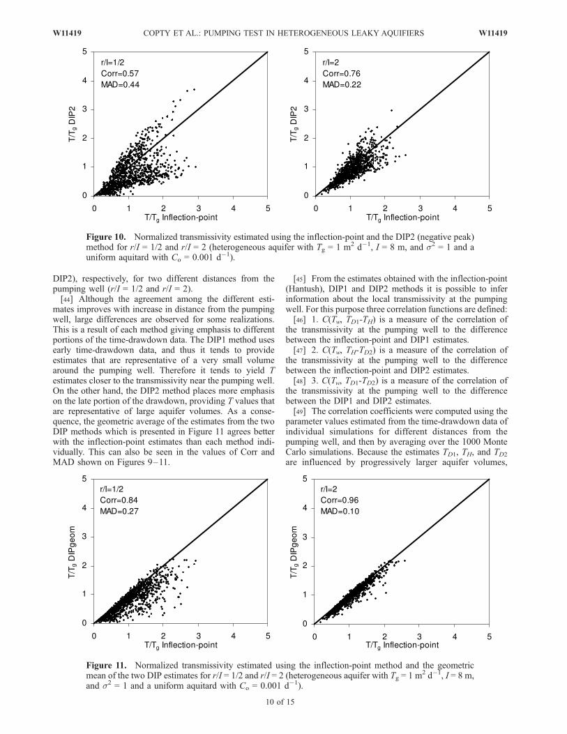
DIP2), respectively, for two different distances from thepumping well (r/I = 1/2 and r/I = 2).[44] Although the agreement among the different esti-

mates improves with increase in distance from the pumpingwell, large differences are observed for some realizations.This is a result of each method giving emphasis to differentportions of the time-drawdown data. The DIP1 method usesearly time-drawdown data, and thus it tends to provideestimates that are representative of a very small volumearound the pumping well. Therefore it tends to yield Testimates closer to the transmissivity near the pumping well.On the other hand, the DIP2 method places more emphasison the late portion of the drawdown, providing T values thatare representative of large aquifer volumes. As a conse-quence, the geometric average of the estimates from the twoDIP methods which is presented in Figure 11 agrees betterwith the inflection-point estimates than each method indi-vidually. This can also be seen in the values of Corr andMAD shown on Figures 9–11.

[45] From the estimates obtained with the inflection-point(Hantush), DIP1 and DIP2 methods it is possible to inferinformation about the local transmissivity at the pumpingwell. For this purpose three correlation functions are defined:[46] 1. C(Tw, TD1-TH) is a measure of the correlation of

the transmissivity at the pumping well to the differencebetween the inflection-point and DIP1 estimates.[47] 2. C(Tw, TH-TD2) is a measure of the correlation of

the transmissivity at the pumping well to the differencebetween the inflection-point and DIP2 estimates.[48] 3. C(Tw, TD1-TD2) is a measure of the correlation of

the transmissivity at the pumping well to the differencebetween the DIP1 and DIP2 estimates.[49] The correlation coefficients were computed using the

parameter values estimated from the time-drawdown data ofindividual simulations for different distances from thepumping well, and then by averaging over the 1000 MonteCarlo simulations. Because the estimates TD1, TH, and TD2are influenced by progressively larger aquifer volumes,

Figure 10. Normalized transmissivity estimated using the inflection-point and the DIP2 (negative peak)method for r/I = 1/2 and r/I = 2 (heterogeneous aquifer with Tg = 1 m2 d�1, I = 8 m, and s2 = 1 and auniform aquitard with Co = 0.001 d�1).

Figure 11. Normalized transmissivity estimated using the inflection-point method and the geometricmean of the two DIP estimates for r/I = 1/2 and r/I = 2 (heterogeneous aquifer with Tg = 1 m2 d�1, I = 8 m,and s2 = 1 and a uniform aquitard with Co = 0.001 d�1).

10 of 15


positive values of the three correlations TD1-TH, TH-TD2 orTD1-TD2 with Tw are indicative of a local Tw larger than theaquifer T spatial mean and vice versa. The three correlationfunctions are shown in Figure 12 as a function of distancefrom the pumping well. The correlation functions tend tovanish with distance, indicating that far from the well all theestimates are independent of the local T value at thepumping well. On the other hand, observation pointslocated at r < I would provide the greatest informationabout the local transmissivity.[50] Finally, we note that from previously published work

[e.g., Desbarats, 1992; Copty et al., 2006], one wouldexpect that the representative local transmissivity wouldbe a time-dependent weighted average of the point T valuessurrounding the pumping well, with weights decreasingwith distance. Since the correlations displayed in Figure 12are in terms of the single transmissivity value at thepumping well, Tw, only partial correlations are observed.

3.4. Impact of Aquitard Heterogeneity

[51] In this section we consider the scenario where theaquifer is assumed to be homogeneous with transmissivityTo = 1 m2/d, while the aquitard conductance is assumed tobe a multi-log-Gaussian SRF with a geometric mean Cg =0.001 1/d. The variance and integral scale of the natural logtransform of the conductance, ln C, are 1 and 8 m, respec-tively. For comparison purposes, these are identical to whatwas used earlier for the case of homogeneous aquitard andspatially variable transmissivity.[52] The normalized transmissivity and conductance esti-

mates obtained from the inflection-point and the curve-fitting methods for different distances from the pumpingwell are presented in Figures 13 and 14, respectively. Thevalues used for normalization are: To and Cg = 0.001 1/d.Table 2 provides the expected values and standard devia-tions of all the estimated flow parameters, including stor-ativity and leakage factor, at different distances.[53] In this scenario, both estimation methods yield very

similar transmissivity and storativity estimates, as seen also

in the values of Corr and MAD. Further, for short distances,normalized expected values of T and S are very close to 1with a very small standard deviation (Table 2). For largerdistances, although the estimates obtained with both meth-ods are in good agreement with each other, they deviate inmany instances from To (see Table 2 and Figure 13). Thisindicates that, as the distance between the observation pointand pumping well increases, the spatial variability of theaquitard conductance is expected to have a larger influenceon the estimation of the transmissivity.[54] The expected value of the estimated conductance on

the other hand is close to the arithmetic mean (Cgexp(s2/2) =

1.65 � 10�3 1/d), which translates into a mean estimatedleakage factor smaller than the geometric mean defined asLg = (T0/Cg)

1/2. The standard deviation tends to slightlydecrease with distance (Table 2 and Figure 14).[55] This behavior can be explained by looking at

the vertical fluxes through the semiconfining layer of ahomogeneous leaky aquifer system. We consider anobservation well at distance robs from the pumping well.The time corresponding to the inflection point for thisobservation well is given by: tp = robsSB/2T. At this momentin time (time of inflection), the leaky well function atany distance r from the pumping well is W(u, r/B)

where u =r2S

4tpT¼ r=Bð Þ2

2robs=B. A plot of W(u, r/B) as a function

r/B at Tp = robs/2T and for different values of robs/B is shownin Figure 15a. Integrating the leaky well function over theentire aquifer yields the ratio of the cumulative vertical flowthough the aquitard to the pumping rate at the well, which isshown in Figure 15b. For small values of robs/B, only a smallfraction of the pumpedwater is leakage through the confininglayer. As such, the pumping test is influenced by the localaquitard conductance only. That is, the pumping test is notinfluenced by the spatial variability of the aquitard conduc-tance, explaining why at short distances the expected value ofthe estimated transmissivity shows no spread around itsactual value (Figure 13a). As robs/B increases, the perturbedconfining layer volume increases and the vertical flow con-stitutes a larger fraction of the pumping rate. For suchconditions, the pumping test would yield a weighted spatialaverage of the aquitard conductance and as a result, thetransmissivity estimate would deviate from the actual values.

4. Conclusions

[56] This paper examines the impact of heterogeneity ofleaky aquifer systems on the flow parameters estimated withthree different methods, two of them commonly used in realapplications: the inflection-point [Hantush, 1956], thecurve-fitting [Walton, 1962] methods, plus the recentlydeveloped double inflection-point method [Trinchero etal., 2008a].[57] We simulate two framework scenarios whereby the

aquifer or aquitard are assumed homogeneous, while theother is defined as a multi-Gaussian SRF with given geo-statistical parameters. For the case of spatially variabletransmissivity and uniform aquitard conductance, the fol-lowing observations can be made:[58] 1. For observation points located relatively far from

the well, all interpretation methods yield similar estimates ofthe transmissivity, storativity and aquitard conductance.

Figure 12. Correlation of the difference in the estimatedtransmissivity values obtained from different methods to thetransmissivity at the well (heterogeneous aquifer with Tg =1 m2 d�1, I = 8 m, and s2 = 1 and a uniform aquitard withCo = 0.001 d�1).


11 of 15

W11419

[59] 2. The expected value of the transmissivity estimatesdepend on the geostatistical parameters of the T field, on theleakage factor, and the distance to the pumping well. Forthe Hantush inflection method and the Walton method theestimates are slightly larger than the geometric mean of thepoint T values.[60] 3. The T estimates from the individual realization are

dependent on the location of the observation point relativeto the pumping well, in contrast to the case of confinedaquifers where the estimated T is relatively insensitive to theobservation well location and tends to be close to thegeometric mean.[61] 4. A slight increasing trend is observed in the

expected value of the estimated leakage factor and trans-missivity with distance from the pumping well.[62] 5. Because the two DIP estimates rely on different

portions of the time-drawdown data, they may differ fromeach other. The geometric mean of the two DIP estimates isgenerally in good agreement with the estimate obtained

from the inflection-point method, particularly for distancesgreater than the integral scale of T. Moreover, differences inthe estimates of T obtained with the inflection-point and DIPmethods are correlated with the local value of T at thepumping well. This correlation tends to decrease withdistance from the pumping well. Therefore, using thedrawdown data at an observation point, located close tothe well (r < I), it is possible to infer local contrasts in thetransmissivity.[63] The second scenario assumes a uniform aquifer

transmissivity and a heterogeneous aquitard. On the basisof the results of these simulations we conclude:[64] 6. The heterogeneity of the aquifer and aquitard

influence the estimated hydraulic parameters in distinctmanners. For the case of spatially variable aquitard, theagreement in the transmissivity and storativity estimatesobtained with the inflection-point and the curve-fittingmethods is very good near the pumping well. The estima-tion of the aquitard conductance shows an opposite trend.

Figure 13. Normalized transmissivity estimated using the inflection-point and the curve-fitting methodsfor different distances from the pumping well (uniform aquifer with To = 1 m2d�1 and spatially variableaquitard with Cg = 0.01 d�1, I = 8 m, and s2 = 1).

12 of 15


With increasing distance, both T and S estimates exhibitlarger variability.[65] 7. The expected value of the aquitard conductance is

close to the arithmetic mean of the C values, indicating thatthe drawdown is most sensitive to the local conductance at

the pumping well, with the sensitivity rapidly decreasingwith distance.[66] Overall, this numerical exercise provides a frame-

work to understand the implications of the assumption ofhomogeneity in the estimates obtained with the different

Figure 14. Normalized aquitard conductance estimated using the inflection-point and the curve-fittingmethods for different distances from the pumping well (uniform aquifer with To = 1 m2d�1 and spatiallyvariable aquitard with Cg = 0.01 d�1, I = 8 m, and s2 = 1).

Table 2. Expected Value and Standard Deviation (Shown in Parenthesis) of the Flow Parameters Function of Distance From the Well—

Case of Spatially Variable Aquitard

Parameter Interpretation Method

Distance From the Well r/I

1/8 1/2 1 2 4 8

Normalized transmissivity Inflection point 0.98 (0.01) 1.00 (0.05) 1.01 (0.08) 1.04 (0.15) 1.13 (0.27) 1.39 (0.44)Curve fitting 0.98 (0.03) 1.00 (0.06) 1.02 (0.09) 1.05 (0.16) 1.13 (0.26) 1.34 (0.36)

Normalized leakage factor Inflection point 0.82 (0.15) 0.82 (0.13) 0.82 (0.11) 0.84 (0.10) 0.86 (0.08) 0.89 (0.06)Curve fitting 0.81 (0.13) 0.83 (0.12) 0.83 (0.11) 0.84 (0.09) 0.86 (0.08) 0.89 (0.06)

Normalized conductance Inflection point 1.63 (0.74) 1.61 (0.61) 1.59 (0.54) 1.56 (0.50) 1.58 (0.52) 1.78 (0.67)Curve fitting 1.65 (0.65) 1.57 (0.55) 1.56 (0.52) 1.55 (0.49) 1.59 (0.53) 1.76 (0.63)

Normalized storativity Inflection point 0.97 (0.01) 1.00 (0.01) 1.01 (0.02) 1.02 (0.07) 1.07 (0.17) 1.27 (0.33)Curve fitting 0.99 (0.02) 1.00 (0.02) 1.01 (0.03) 1.02 (0.08) 1.08 (0.17) 1.25 (0.28)


13 of 15

W11419

methods commonly used in the interpretation of pumpingtests in aquifer-aquitard systems. Since each method givedifferent emphasis to different portions of the drawdowncurve and, consequently to different volumes of the aquifer-aquitard system, we conclude that using all analysis meth-ods jointly may provide additional information (specifically,about contrasts in the local value of the transmissivity at thepumping well) than using each method independently.

[67] Acknowledgments. Nadim Copty acknowledges the financialsupport provided by the Scientific and Technological Council of Turkey(TUBITAK), project 104I130, and by the Bogazici University ResearchFund (BAP), project 06Y104. Paolo Trinchero and Xavier Sanchez-Vilaacknowledge support from CICyT (project PARATODO), the EU (projectGABARDINE), and the Agencia de Gestio d’Ajuts Universitaris i deRecerca of the Catalan Government. The constructive comments of ShlomoNeuman and Walter Illman are gratefully acknowledged.

ReferencesBarker, J., and R. Herbert (1982), Pumping tests in patchy aquifers, GroundWater, 20(2), 150–155.

Butler, J. J. (1988), Pumping tests in nonuniform aquifers: The radiallysymmetric case, J. Hydrol., 101(1–4), 15–30.

Butler, J. J., and W. Z. Liu (1993), Pumping tests in nonuniform aquifers:The radially asymmetric case, Water Resour. Res., 29(2), 259–269.

Cooper, H., and C. Jacob (1946), A generalized graphical method forevaluating formation constants and summarizing well-field history,Trans., Am. Geophys. Union, 27(4), 526–534.

Copty, N. K., and A. N. Findikakis (2004a), Stochastic analysis of pumpingtest drawdown data in heterogeneous geologic formations, J. Hydraul.Res., 42, 59–67.

Copty, N. K., and A. N. Findikakis (2004b), Bayesian identification of thelocal transmissivity using time-drawdown data from pumping tests,Water Resour. Res., 40, W12408, doi:10.1029/2004WR003354.

Copty, N. K., M. S. Sarioglu, and A. N. Findikakis (2006), Equivalenttransmissivity of heterogeneous leaky aquifers for steady state radialflow, Water Resour. Res., 42(4), W04416, doi:10.1029/2005WR004673.

Dagan, G. (1982), Analysis of flow through heterogeneous random aqui-fers. 2: Unsteady flow in confined formations, Water Resour. Res., 18(5),1571–1585.

Dagan, G. (1989), Flow and Transport in Porous Formations, Springer,Berlin, Germany.

Dagan, G. (2001), Effective, equivalent and apparent properties of hetero-geneous media, in Mechanics for a New Millenium, edited by H. Aref,and J. W. Phillips, pp. 473–485, Kluwer, Dordrecht, Netherlands.

de Glee, G. (1930), Over grondwaterstroomingen bij wateronttrekking doormiddle van putten, Ph.D. thesis, Delft Technische Hoogeschool, Delft.

Desbarats, A. J. (1992), Spatial averaging of transmissivity in heteroge-neous fields with flow towards a well, Water Resour. Res., 28(3),757–767.

Durlofsky, L. J. (2000), An approximate model for well productivity inheterogeneous porous media, Math. Geol., 32(4), 421–438.

Firmani, G., A. Fiori, and A. Bellin (2006), Three-dimensional numericalanalysis of steady state pumping tests in heterogeneous confined aqui-fers, Water Resour. Res., 42, W03422, doi:10.1029/2005WR004382.

Gomez-Hernandez, J. J., and S. M. Gorelick (1989), Effective groundwatermodel parameter values: Influence of spatial variability of hydraulic con-ductivity, leakance, and recharge, Water Resour. Res., 25(3), 405–419.

Guadagnini, A., M. Riva, and S. P. And Neuman (2003), Three-dimen-sional steady state flow to a well in a randomly heterogeneous boundedaquifer, Water Resour. Res., 39(3), 1048, doi:10.1029/2002WR001443.

Hantush, M. (1956), Analysis of data from pumping tests in leaky aquifers,Trans., Am. Geophys. Union, 37(6), 702–714.

Hantush, M. S. (1960), Modification of the theory of leaky aquifers,J. Geophys. Res., 65(5), 1634.

Hantush, M., and C. Jacob (1955), Non-steady radial flow in an infiniteleaky aquifer, Trans., Am. Geophys. Union, 36(1), 95–100.

Harbaugh, A., E. Banta, M. Hill, and M. McDonald (2000), Modflow-2000:The US Geological Survey modular ground-water model–user guide tomodularization concepts and the ground-water flow process, USGSOpen-File Report 00-92, p. 121 USGS, Reston, Va.

Indelman, P. (2003a), Transient well-type flows in heterogeneous forma-tions, Water Resour. Res., 39(3), 1064, doi:10.1029/2002WR001407.

Indelman, P. (2003b), Transient pumping well flow in weakly heteroge-neous formations, Water Resour. Res., 39(10), 1287, doi:10.1029/2003WR002036.

Indelman, P., and B. Abramovich (1994), Nonlocal properties of nonuni-form averaged flows in heterogeneous media,Water Resour. Res., 30(12),3385–3393.

Indelman, P., A. Fiori, and G. Dagan (1996), Steady flow towards wells inheterogeneous formations: Mean head and equivalent conductivity,Water Resour. Res., 32(7), 1975–1983.

Knight, J. H., and G. J. Kluitenberg (2005), Analytical solutions for sensi-tivity of well tests to variations in storativity and transmissivity, Adv.Water Resour., 28, 1057–1075.

Leven, C., and P. Dietrich (2006), What information can we get frompumping tests?—Comparing pumping test configurations using sensitiv-ity coefficients, J. Hydrol., 319(1–4), 199–215.

Mantoglou, A., and J. l. Wilson (1982), The turning bands method forsimulation of random-fields using line generation by a spectral method,Water Resour. Res., 18(5), 1379–1394.

Meier, P. M., J. Carrera, and X. Sanchez-Vila (1998), An evaluation ofJacob’s method for the interpretation of pumping tests in heterogeneousformations, Water Resour. Res., 34(5), 1011–1025.

Moench, A. (1985), Transient flow to a large-diameter well in an aquifer withstorative semiconfining layers, Water Resour. Res., 21(8), 1121–1131.

Naff, R. L. (1991), Radial flow in heterogeneous porous media: An analysisof specific discharge, Water Resour. Res., 27(3), 307–316.

Figure 15. Leaky well function and vertical flow throughthe aquitard as a fraction of the pumping rate vs. r/B at theinflection point tp = robsSB/2T for different values of robs/B.

14 of 15


Neuman, S. P., and S. Orr (1993), Prediction of steady state flow in non-uniform geologic media by conditional moments: Exact nonlocal form-alism, effective conductivity, and weak approximation, Water Resour.Res., 29(2), 341–364.

Neuman, S. P., and P. Witherspoon (1969a), Theory of flow in a confinedtwo-aquifer system, Water Resour. Res., 5(4), 803–816.

Neuman, S. P., and P. Witherspoon (1969b), Applicability of current the-ories of flow in leaky aquifers, Water Resour. Res., 5(4), 817–829.

Neuman, S. P., A. Guadagnini, and M. Riva (2004), Type-curve estimationof statistical heterogeneity, Water Resour. Res., 40, W04201,doi:10.1029/2003WR002405.

Neuman, S. P., A. Blattstein, M. Riva, D. M. Tartakovsky, A. Guadagnini,and T. Ptak (2007), Type curve interpretation of late-time pumping testdata in randomly heterogeneous aquifers, Water Resour. Res., 43,W10421, doi:10.1029/2007WR005871.

Oliver, D. S. (1990), The average process in permeability estimation fromwell-test data, SPE Form. Eval., 5(3), 319–324.

Raghavan, R. (2004), A review of applications to constrain pumping testresponses to improve on geological description and uncertainty, Rev.Geophys., 42, RG4001, doi:10.1029/2003RG000142.

Renard, P., and G. de Marsily (1997), Calculating the equivalent perme-ability: A review, Adv. Water Resour., 20(5–6), 253–278.

Riva, M., A. Guadagnini, S. P. Neuman, and S. Franzetti (2001), Radialflow in a bounded randomly heterogeneous aquifer, Transp. PorousMedia, 45(1), 139–193.

Rubin, Y. (2003), Applied Stochastic Hydrogeology, Oxford Univ. Press,New York.

Sanchez-Vila, X. (1997), Radially convergent flow in heterogeneous porousmedia, Water Resour. Res., 33(7), 1633–1641.

Sanchez-Vila, X., C. L. Axness, and J. Carrera (1999a), Upscaling trans-missivity under radially convergent flow in heterogeneous media, WaterResour. Res., 35(3), 613–621.

Sanchez-Vila, X., P. M. Meier, and J. Carrera (1999b), Pumping tests inheterogeneous aquifers: An analytical study of what can be obtainedfrom their interpretation using Jacob’s method, Water Resour. Res.,35(4), 943–952.

Sanchez-Vila, X., A. Guadagnini, and J. Carrera (2006), Representativehydraulic conductivities in saturated groundwater flow, Rev. Geophys.,44(3), RG3002, doi:10.1029/2005RG000169.

Serrano, S. E. (1997), The Theis solution in heterogeneous aquifers,Ground Water, 35(3), 463–467.

Shvidler, M. I. (1962), Filtration flows in heterogeneous media (in Rus-sian), Izv. Akad. Nauk SSSR Mech., 3, 185–190.

Theis, C. V. (1935), The relation between the lowering of the piezometricsurface and the rate and duration of discharge of a well using ground-water storage, Trans., Am. Geophys. Union, 16, 519–524.

Trinchero, P., X. Sanchez-Vila, N. K. Copty, and A. N. Findikakis (2008a),A new method to interpret pumping tests in leaky aquifers, GroundWater, 46(1), 133–143.

Trinchero, P., X. Sanchez-Vila, and D. Fernandez-Garcia (2008b), Point-to-point connectivity, an abstract concept or a key issue for risk assessmentstudies?, Adv. Water Resour., doi:10.1016/j.advwatres.2008.09.001.

Walton, W. (1962), Selected analytical methods for well and aquifer eva-luation, in Illinois State Water Survey Bulletin 49, 81 pp. Champaign, Ill.

Wu, C.-M., T.-C. J. Yeh, T. H. Lee, N.-S. Hsu, C. H. Chen, and A. F.Sancho (2005), Traditional aquifer tests: Comparing apples to oranges?,Water Resour. Res., 41(9), W09402, doi:10.1029/2004WR003717.

Yeh, T.-C. J., and S. Liu (2000), Hydraulic tomography: Development of anew aquifer test method, Water Resour. Res., 36(8), 2095–2105.

Zhu, J., and T. J. Yeh (2005), Characterization of aquifer heterogeneityusing transient hydraulic tomography, Water Resour. Res., 41,W07028, doi:10.1029/2004WR003790.

��N. K. Copty and M. S. Sarioglu, Institute of Environmental Sciences,

Bogazici University, Bebek, 34342 Istanbul, Turkey. ([email protected])A. N. Findikakis, Bechtel National Inc., 50 Beale Street, San Francisco,

CA 94105-1895, USA.X. Sanchez-Vila and P. Trinchero, Department of Geotechnical

Engineering and Geosciences, Technical University of Catalonia, C/JordiGirona 1-3, E-08034 Barcelona, Spain.


15 of 15

W11419

Influence of heterogeneity on the interpretation of pumping test data in leaky aquifers

Documents

Transcript of Influence of heterogeneity on the interpretation of pumping test data in leaky aquifers