mathematics

Article

Influence of Bloomberg’s Investor Sentiment Index: Evidencefrom European Union Financial Sector

Mariano González-Sánchez 1,* and M. Encina Morales de Vega 2

�����������������

Citation: González-Sánchez, M.;

Morales de Vega, M.E. Influence of

Bloomberg’s Investor Sentiment

Index: Evidence from European

Union Financial Sector. Mathematics

2021, 9, 297. https://doi.org/

10.3390/math9040297

Academic Editor: Miltiadis Chalikias

Received: 8 January 2021

Accepted: 30 January 2021

Published: 3 February 2021

Publisher’s Note: MDPI stays neutral

with regard to jurisdictional claims in

published maps and institutional affil-

iations.

Copyright: © 2021 by the authors.

Licensee MDPI, Basel, Switzerland.

This article is an open access article

distributed under the terms and

conditions of the Creative Commons

Attribution (CC BY) license (https://

creativecommons.org/licenses/by/

4.0/).

1 Department of Business and Accounting, Universidad Nacional de Educación a Distancia (UNED),Paseo Senda del Rey, 11, 28040 Madrid, Spain

2 Department of Business, Universidad San Pablo CEU, Julián Romea, 23, 28003 Madrid, Spain;memorales@ceu.es

* Correspondence: mariano.gonzalez@cee.uned.es

Abstract: A part of the financial literature has attempted to explain idiosyncratic asset shocks throughinvestor behavior in response to company news and events. As a result, there has been an increasein the development of different investor sentiment measurements. This paper analyses whetherthe Bloomberg investor sentiment index has a causal relationship with the abnormal returns andvolume shocks of major European Union (EU) financial companies through a sample of 85 financialinstitutions over 4 years (2014–2018) on a daily basis. The i.i.d. shocks are obtained from a factorialasset pricing model and ARMA-GARCH-type process; then we checked whether there is both indi-vidual and joint causality between the standardized residuals. The results show that the explanatorycapacity of the shocks of the firm Bloomberg sentiment index is low, although there is empiricalevidence that the effects correspond more to the situation of the financial subsector (banks, realestate, financial services and insurance) than to the company itself, with which we conclude that thesentiment index analyzed reflects a sectorial effect more than individual one.

Keywords: investor sentiment; idiosyncratic shocks; financial institutions; market risk

1. Introduction

The Investor Sentiment Index is a way of measuring the reaction of investors to the newspublished about events in companies. As stated by [1] the presence of investor sentimentpushes asset prices away from the equilibrium level justified by underlying fundamentals.For that reason, its construction and analysis have become increasingly important in theliterature, leading to the application of different methodologies and approaches.

Initially, work on investor sentiment was based on news about companies withoutdifferentiating good from bad news [2]. Later the literature identified an asymmetrybetween the effects of negative and positive news [3–15].

A temporal asymmetry was also identified when differentiating between times of reces-sion and of expansion [16–18]. In addition, its effect on volatility and trading volume has alsobeen analyzed, distinguishing between small and institutional investors [3,9,16,19–21].

In view of this increased interest in the explanatory capacity of investor sentiment,numerous empirical studies have developed investor sentiment indexes, although many ofthem have not corroborated their effectiveness outside the study sample [8,9,16,22]. Also,there is no consensus on how to build those indexes and which variables or informationto include [23]. As a result, some information providers and financial institutions haveattempted to respond to demand by producing reports and even developing their owninvestor sentiment indexes (both Reuters and Bloomberg have such indexes).

Another aspect related to this variety of applied methodologies has been to consideror not an asset valuation model when quantifying this index of investor sentiment. Thereis extensive financial literature on asset pricing that attempts to adjust the linear cross-sectional relationship between excess asset returns over the risk-free rate and exposure to

Mathematics 2021, 9, 297. https://doi.org/10.3390/math9040297 https://www.mdpi.com/journal/mathematics

Mathematics 2021, 9, 297 2 of 21

risk factors [24–27]. However, in some cases, the 5 results are not as significant as mightbe expected. So-called abnormal returns arise as a difference between the observed andexpected returns based on the pricing model used. In this way, there is a line of financialresearch that attempts to explain these idiosyncratic shocks or abnormal returns. One ofthe possible explanations for these shocks is how investors react to news published aboutthe companies, which can be identified as investor sentiment.

On the other hand, the financial literature has found that the economic and regulatoryenvironment affects performance as a result of the institutional quality and corporate gov-ernance of companies [28], the level of legal institutions and economic development [29],the level of integration and development of financial markets [11,30] and cultural differ-ences [31]. The sample selection is, for this reason, a factor that can condition the results ofthe study on the relationship between investor sentiment and financial asset price behavior.

Our aim is to test the usefulness of such investor sentiment indexes (in particular, theBloomberg investor sentiment index) offered by financial information providers to explainidiosyncratic return and volume shocks.

Related to our scope, reference [32] measures the effectiveness in predicting the Reuterssentiment index with respect to the Dow Jones Industrial Index, concluding that thatnegative Reuters sentiment shows more predictive power than positive Reuters sentiment.

Regarding the importance of sample selection stated previously, our empirical studyis focused on a group of listed financial companies (same industry and regulation) in theEuropean Union (same socio-economic environment). This sample has been chosen becausethis specific sector has suffered a large number of mergers and restructurings in recentyears and also it has been greatly weakened during the 2008 financial crisis along with anincrease in regulation. In this sense, we found very little literature focused on analyzingthe financial sector. Reference [33], for example, built a sentiment index for the Chinesefinancial market and find that it does not always influence the 45 quoted companies’ price.Reference [34] found a significant and negative relationship (asymmetric) between newssentiment (obtained from Thomson Reuters News Analytics) and changes in credit risk ofmajor international banks (measured by CDS spreads). More specifically, for the Spanishbanking system, reference [35] analyzed the relationship between stakeholders, Twitterposts and investors reactions in the market and find there is a positive impact on investor’sdecisions. Reference [36] analyzed the tone of news published on reputational events ina sample of European, American and Canadian financial institutions, concluding that anegative tone increases the implicit risk of default, while a more neutral tone decreases it.

Our results show that the Bloomberg investor sentiment index has a low causalrelationship with the abnormal returns and volume shocks of major EU financial companiesbut the empirical evidence indicates that the effects correspond more to the situation ofthe financial subsector (banks, real estate, financial services and insurance) than to thecompany itself, with which our contribution is that the sentiment index analyzed reflects asectorial effect more than individual one.

The rest of this paper is organized as follows—Section 2 reviews the literature, de-scribes the methodology followed in the study and presents the sample uses; Section 3shows the results obtained; and Section 4 explains the main conclusions of the study.

2. Materials and Methods2.1. Background

The main research of the financial literature seems to show a consensus on the existenceof a relationship between investor sentiment and the financial markets [8,20]. The marketvariable usually analyzed is the return on assets but the effect on trading volume [37,38]and volatility [17,31,39] has also been studied.

In contrast, there is no such consensus on how to measure investor sentiment (see [40]for an in-depth literature review and [15] for an analysis related to the financial sector). Afirst approach to investor sentiment is through building indexes that incorporate market

Mathematics 2021, 9, 297 3 of 21

variables (among others, [4,8,41]). A major problem with these is that they can includeother types of information unrelated to investor perceptions.

A second approach is to develop indexes using investor surveys [42]. There are severalrelevant indexes for the US market: University of Michigan Consumer Sentiment Index(a monthly index calculated from a consumer confidence survey of a random group offive hundred American households) [10,30,43–47]; the American Association of IndividualInvestor sentiment survey (an index that provides weekly information on the bullish,bearish or neutral perception of a pool of financial market surveys over the next sixmonths) [6,19,48–52]; and the Investor Intelligence and Daily Sentiment Index (an indexthat determines the balance between bull and bear investors) [53]. In the case of theEuropean Union, the European Commission’s monthly consumer confidence indicator hasbeen used [54].

In general, these empirical studies using surveys find relationships between thesentiment indexes and market variables, but, like the first of the approaches, it is notwithout its drawbacks, like its low observation frequency (monthly or quarterly) and,like [40] point out, these rates are less reliable when the non-response rate in surveys ishigh or the incentive to answer honestly is low.

A third approach is to build sentiment indexes from information provided by themedia. These indexes have several advantages, such as the increase in the frequency of datacompared to the previous ones (daily instead of monthly or quarterly in surveys), data arecheaper to obtain and they can be applied to a less restricted number of stocks. Within thisapproach, three different forms of application can be distinguished depending on where thenews is from—first, news published in specialized financial media, for example, [9] uses theWall Street Journal and [16] the New York Times; secondly, those obtained from an internetsearch engine, for example, [42] use Google keywords, while [55] use certain publicationson Google, although in this approach, the results should be interpreted with some degreeof caution due to the lack of transparency about how the data were created and uncertaintyabout the reason for the search [56]; and finally, the use of news from social media suchas Facebook, Twitter or LiveJournal [57,58]. In general, these empirical studies show thatthere is a relationship between investor sentiment as measured by media information andmarket variables. It should also be noted that this relationship is more important in the case ofcompanies whose shares show extreme returns or higher risk [10,11,41,59–62]. But, like withthe other two approaches, this one also presents problems since the relationship betweeninvestor sentiment and market returns has a different impact and direction depending onthe source of the information used.

As the use of investor sentiment indexes has become more widespread, empiricalstudies on this issue have begun to use high-frequency data, that is, daily and intradaydata [20,40,63], as opposed to less frequent data, such as monthly or weekly data fromsurveys [64–66]. The frequency effect of the data is relevant as indicated by [67] since whilethe relationship between short-term sentiment and portfolio returns is positive, in the longterm the relationship is the opposite.

At the same time as the investor sentiment indexes, the literature has developedthat attempts to explain return on assets through textual analysis of the news [13,68].There is no clear evidence of its explanatory capacity, since there are papers that argue ithas greater potential than sentiment indexes [39,69–71] but we also find papers arguingotherwise, as a consequence of the different linguistic perception of each investor, themarket where the news is from, the asymmetry between words with negative and positiveconnotations, the language in which the news is given and the analysis of words out ofcontext [14,19,32,33,35,36,62,66,71,72].

A final key element is the size of the investor whose sentiment is analyzed [37]. Thereis no consensus: some studies find there is a relationship between small investor sentimentand market prices [7,28,30,43–45,48,50,73–75] and others [6,54,70,76] conclude that thereis no significant relationship between retail investor sentiment and market returns, even

Mathematics 2021, 9, 297 4 of 21

finding that the explanatory power is in the opposite direction, that is, returns and volatilityvariations affect sentiment, not the other way around.

The role of institutional investor sentiment is not clear in the literature either [77], sincewhile some empirical studies show that this sentiment explains the behavior of marketprices [45,74,78], others conclude that its usefulness is limited or non-existent in explainingthe market returns of assets [6]. Some studies [53] show that although experienced analystsgive greater importance to their own information and less to public information when facedwith negative news, they tend to follow the herd behavior to a greater extent, while thoseothers who operate for investment banks or trade in high volumes do so to a lesser extent.Investor sentiment is not a thermometer unrelated to the investor’s size and knowledgeor expertise.

In summary, based on the literature reviewed, we can group the empirical studiestogether by two fundamental characteristics: on the one hand, those papers that do notconsider an asset valuation model to measure the relationship between investor sentimentand market returns of assets [12,17,28,37,79,80], versus those who do [7,9,11,62,64,66,67,81,82];and on the other, studies that develop their own sentiment indexes [11,35,41,71,82] versusthose using indexes developed by specialized investors or economic agents [9,36,64,82–84].

With regard to the first of these characteristics, it is clear that, to validate the effects ofany event on the financial variables, the empirical study must be carried out by adjustingan asset valuation model, that is, once the systematic risks arising from the risk factorshave been excluded. It will be the idiosyncratic shocks that might contain information oninvestor sentiment about each particular asset; otherwise the investor’s sentiment will notbe about a particular asset but about the market in general. Reference [85], for example,is a sample of empirical work on the effect of investor sentiment on market indexes orportfolios rather than on individual stocks: the analysis is, logically, less complex, as theshocks are smaller than if the study were conducted individually by companies. Our workis included in this group of studies.

As for the second characteristic, building an ad-hoc index for an empirical paper isobviously not exempt from a certain degree of subjectivity. The trend, for that reason,is to use information directly extracted from specialized media or with high data traffic(Twitter and Google) or Reuters sentiment index [32]. In the case of the data used in thispaper, Ref. [86] explains that the sentiment index has been put together taking into accountthe publication of news and tweets considered relevant to a given company and givingit a numerical valuation of investor sentiment. Bloomberg assigns a positive, negative orneutral valuation depending on how the published information would affect an investorwith a long position, that is, if she/he would react by taking a bullish, bearish or neutralstance. This assessment is then introduced into automatic learning models, resulting in theBloomberg sentiment index. The Bloomberg sentiment index is constructed in an aggregateway with all the news published daily for a company, unlike the Thompson Reuters NewsAnalytics index (TRNA).

2.2. Econometric Model for Analyzing Causality

In financial institutions, our field of study, it should be noted that [82] use the factorialmodel of [25] and information from the Wall Street Journal to examine the effect of mediasentiment on the market valuation of banks injected with liquidity by the US governmentwithin the Capital Purchase Program (CPP).

In our case, we use [24–27] five-factor model (we have opted for a factorial model,although others could be used (such as a hidden factors model), because it allows us toobtain in a simple way the idiosyncratic effect and abnormal returns from factors widelyused in the financial literature). In addition, the data used are presented in daily frequency,since, as noted above, the use of high-frequency data represents more reliably the influenceof the sentiment index on financial variables, unlike [32] which uses monthly frequencydata to measure the impact of the index provided by Reuters on the Dow Jones. This type

Mathematics 2021, 9, 297 5 of 21

of database does not take into account heteroscedasticity problems that, on the contrary,can be corrected with data on a daily basis.

In addition, some empirical works, which analyzed high frequency data (daily), con-sider the usual statistical properties of the series like heteroscedasticity [52], an issue we alsoconsider. In a first stage we extract the idiosyncratic shocks of the daily performance, thedaily variations of the log-volume and the log-average of Bloomberg’s investor sentimentindex, unlike [80].

The multivariate VAR-GARCH (Vector Autoregression with Multivariate-GARCH)methodology allows to jointly estimate the causality in mean and variance for a set of assetsbut it has some drawbacks: such as computational complexity, that happens when thenumber of assets increases; the difficulty to estimate returns that have a different univariateheteroscedastic behavior and multivariate GARCH process does not guarantee stationaryunivariate variance; specifying dependence on the multivariate GARCH is hard for non-normality series. Thus, if each return has different marginal probability distributions, thenthe estimation of the conditional distribution is difficult, with the consequent effect on theasymptotic behavior of the maximum likelihood estimator. Meanwhile, in the case of theCCF (Cross Correlation Function) methodology, it proves to be robust to non-symmetric andleptokurtic errors, although there are some disadvantages: the conditionality is estimatedby pairs, so for a set of assets, it does not allow to determine the common origin ofthe effects; the joint estimation of causality in mean and variance is not possible by thismethodology, since the results of the second are conditioned by the first; the causality invariance is sensitive to structural breaks in the parameters.

In short, neither methodologies outperform the other, both require a two-stage esti-mation and have different computational intensity and sensitivity to the stylized facts ofreturns. In this context, this paper chooses the CCF methodology for its robustness againstthe stylized facts. Thus, we apply a methodology to test the causality in mean and variancesimilar to [87].

We define ri,t as the excess of the daily return on asset i on day t over the risk-free rateon the same day (Rft), where the daily return is the first difference in the logarithm of thedaily price. Fm,t is the value of systemic risk factor m on day t. The asset pricing model isexpressed as:

ri,t = β0,i +M∑

m=1βm,i·Fm,t + ui,t

ui,t ∼ iid(

0, σ2i,t

),

(1)

where ui,t is the abnormal result with non-constant variance, so to obtain the i.i.d. shockswe model the variance based on a GARCH(1,1) process:

σ2i,t = δ0,i + δ1,i·u2

i,t−1 + δ2,i·σ2i,t−1. (2)

Then, the idiosyncratic shock is zi,t =ui,tσi,t

∼ iid(0, 1).Additionally and in order to contrast the robustness of the proposed factorial pricing

model (model of observable factors), we check its goodness of fit with respect to a modelof hidden or latent factors. For that, following [88], we use PCA (principal componentanalysis) to compare the results of latent (hidden) factors pricing model with observable

factorial pricing model. The latent factors (F) are estimate as: F = r·Λ·(

ΛT·Λ)−1

, where rare excess return on assets and Λ are eigenvectors of the largest (L) eigenvalues (at 95%explanatory level). Then, we estimate regression:

ri,t = α0 +L

∑j=1

β j·Fj,t + ξi,t. (3)

Mathematics 2021, 9, 297 6 of 21

To compare these approaches (latent vs. observed factors) we calculate two indicators

of accuracy level: first, root of mean alphas(

RMS_α =√

1N ∑N

i=1 α2i

), note that higher

values of RMS_α show higher anomalies and therefore, a worse accuracy level of pricing.

Second, we estimate the mean of asset idiosyncratic variances(

σξ =√

1N ∑N

i=1 σ2ξi

), so, if

σξ hidden factor model is higher than observed factor model then, hidden factor modelwould have a lower explanatory level of asset return than observed factor model, sincesystematic risk of hidden factors would be lower than observed factors.

For volume (Vi,t), we estimate the daily variations (vi,t = ln Vi,tVi,t−1

) and the relative

change in the volume of the EUROSTOXX-50 (vx,t = ln Vx,tVx,t−1

), so the idiosyncratic shock isextracted from the standardized residuals of an ARMA(P,Q)-GARCH(1,1) process:

vi,t = α0,i + αx,i·vx,t + ∑Pp=1 αp,i·vi,t−p + ∑Q

q=1 αP+q,i·ei,t−q + ei,t

σ2v,i,t = δ0,i + δ1,i·e2

i,t−1 + δ2,i·σ2v,i,t−1.

. (4)

The idiosyncratic shock of the volume is zvi,t =ei,t

σv,i,t∼ iid(0, 1).

Finally, we define the daily log-difference of the Bloomberg sentiment index as bi,t =

ln Bi,tBi,t−1

, which we model as an ARMA(P,Q)-GARCH(1,1) process:

bi,t = ω0,i + ∑Pp=1 ωp,i·bi,t−p + ∑Q

q=1 ωP+q,i·φi,t−q + φi,t

σ2b,i,t = δ0,i + δ1,i·φ2

i,t−1 + δ2,i·σ2b,i,t−1.

. (5)

And finally, the idiosyncratic shock of the variations in the investor sentiment indexwould be zbi,t =

φi,tσi,t

∼ iid(0, 1).Once the idiosyncratic shocks have been obtained, there are now different analysis

possibilities. First, since the systematic effects have been eliminated, it would be logical toexpect that each sentiment index would influence the abnormal returns and volume shocksof the stock itself. If we measure this influence in terms of Granger causality and, given thestatistical properties of the shocks, for each company we can estimate the following linearregression by Ordinary Least Squared (OLS) for each asset i:

yi,t = λ0 + ∑Hh=1 λh·zbi,t−h + ψi,t, (6)

where yt is both the abnormal returns (zt) and volume shock (zvt).As there could be an interrelation between companies in the same subsector, we carry

out a joint estimate by subsector by means of simultaneous equations applying the FullInformation Maximum Likelihood (FIML) method, then the expression to be estimated fora subsector s, with N firms, is: y1,t

...yN,t

=

ρ1,0...

ρN,0

+

ρ1,1 · · · ρ1,J...

. . ....

ρN,1 · · · ρN,J

· zb1,t−1 · · · zb1,t−J

.... . .

...zbN,t−1 · · · zbN,t−J

+

ε1,t...

εN,t

. (7)

If the results of estimate Expression-(7) showed companies with significant parametersthat, when estimating the Expression-(6) were not, then this would indicate that there is acontagion effect between shocks of companies from the same subsector and, consequently,we would analyzed the common effect of the shocks of the investor sentiment indexdifferentiating by subsectors.

For that, we define a dummy (Ds,i) which will be worth 1 if the institution i belongs tothe subsector s (banking, real estate, financial services and insurance) and zero otherwise. Tocorroborate the asymmetrical effect of the sentiment index found in the literature reviewed,we define a dummy assigned a 1 if on day (t − j) the original variable (excess returns orrelative change in volume) was negative, otherwise it will be zero, so for each institutionwe will obtain Dr,i and Dv,i. This way we avoid possible problems of endogeneity, since the

Mathematics 2021, 9, 297 7 of 21

value of the dummies does not depend on the sign of the shocks of the sentiment index.Finally, we estimate the following panel data model:

yi,t = γ0 + ∑Hh=1 γ+

h ·[Ds,i·

(1 − Dy,i

)·zbi,t−h

]+ ∑H

h=1 γ−h ·[Ds,i·Dy,i·zbi,t−h

]+ µi,t. (8)

From Expression-(7), we obtain the effect of the shocks of the investor sentiment indexaccording to the subsector over the abnormal returns and the shocks of the first difference ofthe volume logarithm, respectively. This effect will be obtained by differentiating whetherthe returns or volume changes were positive or negative in significant delays, that is, wecheck whether the effect is asymmetrical. The residuals (µi,t) may reflect the fixed or randomeffects of the model depending on the specific test for their selection (Hausman test).

2.3. Sample of Data

The sample used covers listed financial institutions in the EU. The period chosen runsfrom 1 April 2014 to 30 March 2018, on a daily basis. The sample has been subdivided intobanks, financial services, insurance and real estate, according to the ICB (Industry Classi-fication Benchmark) provided by Bloomberg. Each subsample is composed of the mostcapitalized (high market value) and largest (measured by assets) companies, that is, the setof companies that exceed 95% of the total subsector market and asset values at the sametime. There were 85 institutions listed in Appendix A and their subsectors are: banking(32), real estate (16), financial services (29) and insurance (8). Price, volume (includingEUROSTOXX-50) and investor sentiment index data are obtained from Bloomberg, whiledata on systemic factors are from the French data web (http://mba.tuck.dartmouth.edu/pages/faculty/ken.french/Data_Library/f-f_5developed.html).

3. Results3.1. Statistics

First, we show in Table 1 the statistics characteristics of the sample.Table 1 shows in two panels the statistical summary of factors and daily returns,

volume changes and investor sentiment index variations companies by subsectors. Panel Adisplays the statistics for the systemic factors included in Expression-(1). Panel B displaysthe statistics for the entire sample, showing the results for each variable by quartiles only(the rest of the statistics are available upon request.).

The results in Table 1 show that all series are stationary. In most cases, so-called styl-ized facts can be observed, including non-normality, autocorrelation of series in levels andsquared and conditional heteroscedasticity. The model proposed to obtain the independentshocks is therefore justified.

3.2. Adjustment of Econometric Models for Shock Extraction

First, we estimate econometric models for excess returns, changes of volume andsentiment Bloomberg index.

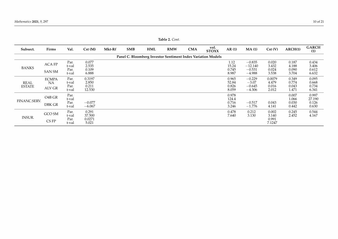
From Table 2 we verify that: regarding daily returns, we find that considering afactorial asset valuation model is essential to extract shocks; for volume and sentimentindices, we find that they follow both autoregressive and moving average processes and,finally, we note that in most variables show heteroscedasticity. In summary, not consideringthese statistical and financial characteristics of the data could mean that the results obtainedare biased. We then check that the shocks defined above as standardized residuals of themodels estimated above are i.i.d. The statistical summary is shown in Table 3.

Mathematics 2021, 9, 297 8 of 21

Table 1. Summary statistics.

Panel A. Statistical Summary of Systemic Factors

Factors #obs Min Mean Max std.dev Skewness Excess Kurtosis Jarque-Bera ARCH Box-Pierce Box-PierceSquared ADF

Mkt-Rf 1044 −0.0879 0.0002 0.0356 0.0091 −1.001 9.913 4448.8 24.97 19.88 166.66 −17.164var_VOL Eurostoxx 1044 −1.3493 −0.0019 1.2421 0.2792 −0.039 2.042 181.650 6.87 127.22 33.00 −18.085

SMB 1044 −0.1610 0.0001 0.0185 0.0043 −0.086 1.634 117.390 9.69 12.38 63.93 −14.861HML 1044 −0.0207 −0.0001 0.0175 0.0041 0.244 1.669 135.910 6.22 4.90 39.58 −14.284RMW 1044 −0.0151 0.0002 0.0161 0.0028 −0.290 2.290 240.810 4.45 12.45 27.14 −13.736CMA 1044 −0.0084 −0.3487 0.0107 0.0025 0.225 0.984 50.926 3.57 2.54 19.09 −14.274

Panel B. Statistical Summary for Companies

Return-Rf

Min. 1044 −1.1982 −0.0070 0.0527 0.0157 −8.302 1.363 82.008 0.01 1.95 0.06 −18.761Q1 1044 −0.2744 −0.0008 0.0930 0.0197 −0.889 3.973 698.010 4.03 8.18 24.84 −15.982Q2 1044 −0.2260 −0.0002 0.1187 0.0223 −0.384 6.779 2078.2 8.23 12.03 54.54 −15.583Q3 1044 −0.1591 0.0001 0.1706 0.0341 −0.065 11.668 5957.5 16.07 19.33 89.22 −14.956

Max 1044 −0.0771 0.0010 0.4940 0.0704 2.124 173.650 1,323.70 116.30 183.25 393.12 −13.161

Var. Volume

Min. 1044 −9.4171 −0.0016 1.4442 0.3364 −0.576 0.395 −0.5757 0.49 83.20 2.55 −24.6407Q1 1044 −2.8156 −0.0006 1.9098 0.3924 0.053 1.306 0.0531 9.14 123.64 45.22 −22.1418Q2 1044 −2.1977 −0.0002 2.5925 0.4999 0.172 2.455 0.1716 16.74 149.32 88.07 −21.2196Q3 1044 −1.8124 0.0004 3.2382 0.6015 0.286 4.429 0.2863 25.53 186.76 122.20 −20.4301

Max 1044 −1.1510 0.0063 11.0450 1.8481 0.855 139.740 0.8554 143.44 260.26 400.12 −18.7247

Bloomberg index

Min. 1044 −1.0000 −0.0442 0.0884 0.1180 −5.051 −1.492 −5.0508 5.94 70.63 32.17 −12.8279Q1 1044 −0.9911 0.0572 0.8579 0.2625 −0.623 0.504 −0.6232 77.91 627.47 464.13 −9.6259Q2 1044 −0.9733 0.0969 0.9218 0.2707 −0.274 1.074 −0.2736 307.85 1940.30 1791.53 −7.1652Q3 1044 −0.8682 0.1277 0.9624 0.3005 0.041 2.066 0.0414 1247.53 3901.94 3646.93 −4.8387

Max 1044 −0.6633 0.1958 0.9984 0.3544 3.724 30.047 3.7242 36079 5086.58 5131.81 −3.12748

Note: Return-Rf is daily return of stock market minus daily risk-free rate, Var. Volume is first difference of daily log-volume, Bloomberg index is the first difference of daily log-average value of the sentiment indexcalculated by Bloomberg. Jarque-Bera is normality test, ARCH (lag = 5) is LM-test on heteroscedasticity, Box-Pierce (lag = 5) is autocorrelation test on variable in level (mean equation) and in squared (varianceequation), ADF is Augmented Dickey-Fuller unit roots test. The critical values for the ARCH test (5) are 3.03 (1%) and 2.22 (5%) and it is an F distribution (lag, N-2*lag-1). For Box-Pierce it is Chi2(lag) and thecritical values are 15.09 (1%) and 11.07 (5%).

Mathematics 2021, 9, 297 9 of 21

Table 2. Estimate of the models to obtain the shocks.

Subsect. Firms Val. Cst (M) Mkt-Rf SMB HML RMW CMA vol.STOXX AR (1) MA (1) Cst (V) ARCH(1) GARCH

(1)

Panel A. Excess Returns Models

BANKSACA FP Par. 0.000 0.902 −0.991 0.392 −2.747 −0.849 0.280 0.006 0.815

t-val 0.427 14.210 −8.495 1.963 −10.100 −3.734 0.726 0.266 3.386

SAN SM Par. 0.000 0.862 −1.553 0.850 −2.200 −0.726 0.141 0.020 0.869t-val 0.717 10.750 −11.530 4.968 −7.484 −2.751 1.439 1.126 12.860

REALSTATE

ECMPANA

Par. 0.00009 0.5701 −0.2818 0.022 0.2435 −0.269 0.3648 0.128147 0.55897t-val 0.3279 10.58 −3.000 −0.130 1.302 −1.589 1.571 1.840 2.256

ALV GR Par. 0.000 0.534 −0.884 0.443 −0.395 −1.142 0.162 0.079 0.729t-val 1.580 8.213 −8.409 3.097 −1.876 −5.677 3.242 2.089 13.860

FINANC.SERV.O4B GR Par. 0.000 0.081 0.293 0.002 0.109 −0.089 −0.019 −0.218 1.139 0.224 0.316

t-val −0.511 1.419 2.054 0.007 0.289 −0.271 −0.11 −1.280 1.687 0.235 1.094

DBK GR Par. 0.000 0.592 −1.520 0.889 −2.876 −1.722 1.066 0.172 0.407t-val −0.291 5.623 −10.060 3.696 −7.590 −5.811 0.932 2.002 0.777

INSUR.GCO SM Par. 0.000 0.737 −0.108 0.089 −0.805 0.105 0.006 0.017 0.979

t-val 0.589 12.470 −0.919 0.434 −3.119 0.447 0.801 2.238 100.2

CS FP Par. 0.001 0.757 −1.328 −0.026 −2.141 −1.121 0.220 0.300 0.567t-val 1.442 8.534 −11.280 −0.153 −7.498 −4.269 0.833 1.440 1.682

Panel B. Volume Variation Models

BANKSACA FP Par. 0.001 0.890 0.193 −0.783 0.019 0.100 2.606

t-val 0.499 21.750 3.32 −16.94 3.436 0.677 9.190

SAN SM Par. 0.002 0.941 0.20 −0.766 0.027 0.084 0.773t-val 0.461 18.410 3.21 −18.37 1.930 2.865 8.546

REALESTATE

ECMPANA

Par. −0.0013 0.58978 0.291 −0.936 0.0140 0.065601 0.87627t-val −0.7922 9.597 7.684 −49.90 2.415 3.470 26.88

ALV GR Par. 0.000 0.988 0.34 −0.790 0.051 0.194 0.371t-val 0.033 26.440 3.51 −11.66 2.648 2.096 3.870

FINANC.SERV.O4B GR Par. 0.0034 −0.233 0.532 −0.949 0.497 0.145 0.592

t-val 0.605 −1.11 10.78 −50.33 1.496 1.494 2.402

DBK GR Par. −0.001 1.391 0.35 −0.907 0.611 0.112 −0.198t-val −0.261 7.281 4.51 −41.78 3.077 2.964 −3.504

INSUR.GCO SM Par. 0.001 0.640 0.12 −0.866 0.009 0.035 0.939

t-val 0.422 8.334 2.73 −34.21 0.822 1.433 17.720

CS FP Par. 0.000 0.984 0.21 −0.792 0.010 0.117 0.711t-val 0.193 27.200 4.06 −19.29 3.763 3.713 16.330

Mathematics 2021, 9, 297 10 of 21

Table 2. Cont.

Subsect. Firms Val. Cst (M) Mkt-Rf SMB HML RMW CMA vol.STOXX AR (1) MA (1) Cst (V) ARCH(1) GARCH

(1)

Panel C. Bloomberg Investor Sentiment Index Variation Models

BANKSACA FP Par. 0.077 1.12 −0.835 0.020 0.187 0.434

t-val 2.535 15.24 −12.140 3.432 4.188 3.406

SAN SM Par. 0.109 0.745 −0.531 0.024 0.090 0.612t-val 6.888 8.987 −4.988 3.538 3.704 6.632

REALESTATE

ECMPANA

Par. 0.3197 0.965 −0.229 0.0079 0.349 0.095t-val 2.850 52.84 −3.07 4.479 0.774 0.668

ALV GR Par. 0.211 0.826 −0.645 0.016 0.043 0.734t-val 12.530 8.059 −4.306 2.012 1.471 6.341

FINANC.SERV.O4B GR Par. 0.978 0.007 0.997

t-val 124.4 1.066 27.190

DBK GR Par. −0.077 0.716 −0.517 0.043 0.030 0.126t-val −6.067 3.246 −1.776 4.141 0.442 0.630

INSUR.GCO SM Par. 0.291 0.478 0.212 0.002 0.245 0.544

t-val 37.500 7.640 3.130 3.140 2.452 4.167

CS FP Par. 0.0271 0.991t-val 5.021 7.1247

Mathematics 2021, 9, 297 11 of 21

Table 3. Statistical summary of standardized shocks.

Subsector Firms #obs Value Mean std.dev Jarque-Bera ARCH Box-Pierce Box-PierceSquared

Panel A. Statistical Summary for Excess Returns Models

BANKSACA FP 1044 Test 0.001 1.001 3346.200 0.054 6.940 0.271

p-value 0.000 0.998 0.225 0.998

SAN SM 1044 Test 0.001 0.998 7916.800 0.056 8.600 0.284p-value 0.000 0.998 0.126 0.998

REALESTATE

ECMPANA

1044 Test 0.007 0.999 1369.300 0.460 3.101 2.185p-value 0.000 0.806 0.684 0.823

ALV GR 1044 Test 0.002 0.999 861.600 0.482 3.124 2.508p-value 0.000 0.790 0.681 0.775

FINANCSERV.

O4B GR 1044 Test 0.007 0.999 16,654.000 0.076 7.025 0.391p-value 0.000 0.996 0.219 0.996

DBK GR 1044 Test −0.007 0.999 521.110 0.197 0.869 1.045p-value 0.000 0.964 0.972 0.959

INSURANCEGCO SM 1044 Test −0.005 1.000 60.608 1.191 4.413 6.179

p-value 0.000 0.311 0.492 0.289

CS FP 1044 Test −0.013 1.000 0.273 9.252 1.365p-value 0.928 0.099 0.928

Panel B. Statistical Summary for Volume Variation Models

BANKSACA FP 1044 Test −0.010 1.001 1748.400 0.229 0.887 1.145

p-value 0.000 0.950 0.971 0.950

SAN SM 1044 Test −0.010 0.998 1064.300 0.459 3.439 2.364p-value 0.000 0.807 0.633 0.797

REALESTATE

ECMPANA

1044 Test 0.052 0.996 186.740 0.553 0.499 2.844p-value 0.000 0.736 0.992 0.724

ALV GR 1044 Test −0.071 1.000 74,747.000 0.036 3.501 0.179p-value 0.000 0.999 0.623 0.999

FINANCSERV.

O4B GR 1044 Test 0.0067 1.0002 849.39 0.2356 12.101 1.079p-value 0.000 0.947 0.0334 0.9559

DBK GR 1044 Test 0.006 1.000 472,210.000 0.024 6.870 0.125p-value 0.000 1.000 0.230 1.000

INSURANCEGCO SM 1044 Test 0.013 1.008 187.320 1.394 0.443 6.716

p-value 0.000 0.224 0.994 0.243

CS FP 1044 Test 0.001 1.000 2809.200 0.261 10.1842 1.31161p-value 0.000 0.934 0.065 0.934

Panel C. Statistical Summary for Bloomberg Investor Sentiment Index Variation Models

BANKSACA FP 1044 Test −0.006 0.999 289.360 0.514 0.172 2.611

p-value 0.000 0.766 0.999 0.760

SAN SM 1044 Test −0.003 0.999 34.887 0.819 6.759 4.187p-value 0.000 0.536 0.239 0.523

REALESTATE

ECMPANA

1044 Test −0.016 0.999 75,428.000 0.109 6.432 0.552p-value 0.000 0.990 0.266 0.990

ALV GR 1044 Test 0.002 0.999 28.541 0.936 2.737 4.646p-value 0.006 0.456 0.740 0.461

FINANCSERV.

O4B GR 1044 Test 0.060 0.889 76,348.000 0.491 6.538 2.466p-value 0.000 0.783 0.257 0.782

DBK GR 1044 Test −0.003 1.000 83.732 0.518 4.644 2.610p-value 0.000 0.763 0.461 0.760

INSURANCEGCO SM 1044 Test 0.000 1.000 324.86 0.0623 2.468 0.5386

p-value 0.000 0.9971 0.7812 0.99063

CS FP 1044 Test 0.0271 0.9914 1,3019,000 0.0029 0.103206 0.01476p-value 0.000 1.0000 0.9998 0.9999

Note: Normality test is Jarque-Bera test, ARCH (lag = 5) is LM-test on heteroscedasticity, Box-Pierce (lag = 5) is autocorrelation test on variablein level (mean equation) and in squared (variance equation).

Mathematics 2021, 9, 297 12 of 21

As we can see, the results of Table 3 indicate that the idiosyncratic shocks of thethree variables (returns, volume and sentiment index) do not display autocorrelation andheteroscedasticity, so they are i.i.d.

3.3. Comparison of Latent vs. Observable Factors Model

We extract latent factors from covariance matrix of excess returns on assets. Table 4show by subsectors: the total assets, the minimum number of factors necessary to explainat least 95% of the covariance matrix and the explanatory power of the first five factors (tocompare results with the model of the five observable factors):

Table 4. Principal Components of covariance matrix.

Sub-Sector Total Companies Factors % Explanation % Explanation of First 5 PC

Banks 32 23 95.38% 70.38%Real Estate 16 14 96.33% 62.87%

Financial Institutions 29 25 95.48% 43.09%Insurances 8 7 96.85% 87.87%

Table 5 shows the results of comparing the latent factors model against the observablefactors model. Specifically, we contrast which of the two models has lower RMS alpha andlower volatility of the idiosyncratic risk.

Table 5. Results of the comparison of the latent and observable factor models.

Observable Factors Model

Sub-SectorRMS Alpha Residual Deviation

Min Mean Max Min Mean Max

Banks 0.005% 0.053% 0.684% 0.298% 0.403% 1.957%Real Estate 0.001% 0.014% 0.058% 0.140% 0.194% 0.738%

Financial Institutions 0.004% 0.017% 0.099% 0.158% 0.265% 1.160%Insurances 0.008% 0.018% 0.045% 0.093% 0.224% 0.802%

Latent Factors Model for 95% Explanation

Sub-SectorRMS Alpha Residual Deviation

Min Mean Max Min Mean Max

Banks 0.026% 0.109% 0.744% 0.044% 0.512% 1.762%Real Estate 0.002% 0.037% 0.094% 0.006% 0.157% 0.602%

Financial Institutions 0.007% 0.048% 0.168% 0.022% 0.244% 1.004%Insurances 0.0124% 0.025% 0.072% 0.007% 0.191% 0.766%

Latent Factors Model for First 5 PC

Sub-SectorRMS Alpha Residual Deviation

Min Mean Max Min Mean Max

Banks 0.026% 0.109% 0.744% 0.737% 1.081% 2.243%Real Estate 0.002% 0.037% 0.094% 0.288% 0.352% 1.094%

Financial Institutions 0.007% 0.048% 0.168% 0.248% 0.329% 1.865%Insurances 0.0124% 0.025% 0.072% 0.185% 0.470% 0.894%

Note that the standard deviation of the residuals (idiosyncratic component of themodel) shows the lowest values for the latent factors model. However, when we comparethe model of 5 latent factors with the model of 5 observable factors, we find that thelatter shows a lower volatility of the idiosyncratic component. On the other hand, ifwe compare the intercept (alpha), we find empirical evidence that the latent modelspresent higher anomalies than the observable factors model (as [89] hidden factor modelsperformance more poorly). This is due to the fact that while the latent factor modelsexplain the covariances, the same does not occur with the mean, so that the constant showshigher values.

In addition to this evidence found, if we consider that the data are in daily frequencywith the consequent problem of behavior of the residuals (autoregressiveness, heteroskedas-

Mathematics 2021, 9, 297 13 of 21

ticity and heavy tails) then, we choose the estimation of the observable factors model andadjusting a GARCH process to the variance of the residuals, since CPA is more consistentwhen the data show Gaussian behavior (for example, asset returns in monthly frequency).

3.4. Comparison of the Influence of Investor Sentiment Index Shocks

First, using information criteria (AIC), it was determined that delay 3 was sufficient toadjust the model and then individual linear regressions were estimated. The results areshown in Table 6.

Table 6. Individual estimate of the influence of the investor sentiment index.

Subsectors Abnormal Returns Volume Shocks

Banks Lag-1 Lag-2 Lag-3 Lag-1 Lag-2 Lag-3

Portuguese commercial bank 0.0611 (*)Caixa Bank −0.0593 (*) 0.0167 (*)

National Bank of Greece −0.0632 (*)KBC Group 0.0054 (**)

Raiffeisen Bank 0.0125 (**)Banco Santander 0.0055 (*)

TCS Group Holding 0.0148 (*)Unicredit 0.0974 (**)

Real estate Lag-1 Lag-2 Lag-3 Lag-1 Lag-2 Lag-3

Ageas Group −0.0595 (*)Citycon −0.0639 (*)

Hanover Rueck −0.0853 (**) −0.0683 (*)Nexity 0.0737 (*)Talanx 0.0912 (**) −0.0761 (*)

Technopolis −0.0656 (*)

Finance Lag-1 Lag-2 Lag-3 Lag-1 Lag-2 Lag-3

ABC Arbitrage 0.0869 (**)Azimut Holding 0.0687 (*)

CIE du Bois Sauvage −0.0605 (*)Deutsche Beteiligungs 0.0617 (*)

Deutsche Bank AG 0.0689 (*)KAS Bank NV-CVA −0.0726 (*)

Natixis −0.0594 (*)Altamir −0.0639 (*)

MLP 0.0685 (*)Rothschild −0.0823 (**)

Insurance Lag-1 Lag-2 Lag-3 Lag-1 Lag-2 Lag-3

CNPFP Assurances −0.0610 (*) 0.0708 (*)MAPFRE 0.0618 (*)

Note: (*) and (**) indicate that the parameter is significant at the confidence level of 5% and 1% respectively.

As can be seen in Table 4, of the 85 companies in the sample, only 26 show anyeffect either on returns or volume or both. Thus, 31% of the sample shows effects and, bysubsector, it would be: 25% banks (mostly from countries where the financial crisis had agreater impact on the sector such as Spain, Portugal, Italy, Greece and Cyprus), 38% realestate, 34% finance and 25% insurance companies.

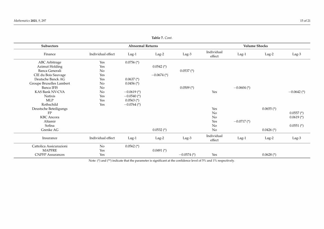
Next, to check the possible effect of contagion between companies in the same activitysubgroup, we estimated a system of equations using FIML (Full Information MaximumLikelihood). The goal is to check whether, when making a joint estimate, companies thatindividually did not show statistical significance (see Table 6), do so jointly. In that case, theresults would indicate that the sentiment index of these companies would be influencednot only by news about them but also by other companies in the subsector. Table 7 showsthe results obtained.

Mathematics 2021, 9, 297 14 of 21

Table 7. Subsectors estimate of the influence of the investor sentiment index.

Subsectors Abnormal Returns Volume Shocks

Banks Individ. effect Lag-1 Lag-2 Lag-3 Individ. effect Lag-1 Lag-2 Lag-3

Allied Irish Banks No No 0.0609 (*)Aareal Bank No −0.0498 (*)Banco BPM 0.0428 (*)

BBVA −0.0368 (*)Portuguese commercial bank Yes −0.0483 (*) 0.0738(**) No 0.0668 (*)

Bankia −0.0522 (*) No −0.0494 (*)Caixa Bank Yes −0.0682 (*) Yes 0.0141 (*)BPER Banca No −0.0508 (*)ING Groep No −0.0471 (*) No −0.0471 (*)

Banco de Sabadell No −0.0554 (*)Piraeus Bank No −0.0389 (*)

Intesa Sanpaolo No −0.0792(**)Raiffeisen Bank Yes 0.0679 (*)

Banco Santander Yes 0.0631 (*)TCS Group Holding Yes 0.0568 (*)

Unicredit Yes 0.0926(**) Yes 0.0568 (*)

Real estate Individual effect Lag-1 Lag-2 Lag-3 Individualeffect Lag-1 Lag-2 Lag-3

Ageas Group No 0.0526 (*) Yes −0.0563 (*)Citycon Yes −0.0530 (*)

Hanover Rueck Yes −0.0679(**) Yes −0.0485 (*)Muenchener Rueckver No −0.0773(**) No 0.0192 (*)

Nuerberger Beteilig No −0.1038(**)Vienna Insurance Group No −0.0591 (*) No −0.0507 (*)

Nexity Yes 0.0822(**)Talanx Yes 0.0815(**) −0.0652 (*)

Technopolis Yes −0.0724 (*)

Mathematics 2021, 9, 297 15 of 21

Table 7. Cont.

Subsectors Abnormal Returns Volume Shocks

Finance Individual effect Lag-1 Lag-2 Lag-3 Individualeffect Lag-1 Lag-2 Lag-3

ABC Arbitrage Yes 0.0756 (*)Azimut Holding Yes 0.0542 (*)Banca Generali No 0.0537 (*)

CIE du Bois Sauvage Yes −0.0674 (*)Deutsche Banck AG Yes 0.0637 (*)

Groupe Bruxelles Lambert No 0.0456 (*)Banca IFIS No 0.0509 (*) −0.0604 (*)

KAS Bank NV-CVA No −0.0619 (*) Yes −0.0642 (*)Natixis Yes −0.0540 (*)

MLP Yes 0.0563 (*)Rothschild Yes −0.0764 (*)

Deustsche Beteiligungs Yes 0.0655 (*)FP No 0.0557 (*)

KBC Ancora No 0.0619 (*)Altamir Yes −0.0717 (*)Sofina No 0.0551 (*)

Grenke AG 0.0532 (*) No 0.0426 (*)

Insurance Individual effect Lag-1 Lag-2 Lag-3 Individualeffect Lag-1 Lag-2 Lag-3

Cattolica Assicurazioni No 0.0562 (*)MAPFRE Yes 0.0491 (*)

CNPFP Assurances Yes −0.0574 (*) Yes 0.0628 (*)

Note: (*) and (**) indicate that the parameter is significant at the confidence level of 5% and 1% respectively.

Mathematics 2021, 9, 297 16 of 21

As can be seen in Table 7, the number of companies with significant effects frominvestor sentiment index shock has increased, that is, other companies have now beenadded to all those that were individually significant. It seems clear that there is an effectby subsector.

We then estimated the panel data model with asymmetric effect by subsector. Firstthe Hausman test was estimated, whose values were 17.07 (p-value of 0.846) for abnormalreturns and 11.36 (p-value of 0.986) for idiosyncratic volume shocks. As a result, theassumption of random effects is accepted in both cases. The within-between GLS estimateis chosen. Table 6 (Panel A and B) shows the results of the estimate of the panel data modelscorresponding to Expression (12), both for abnormal returns and for volume shocks. Theexplanatory power, measured by the coefficient of determination was 0.45% and 0.51%,respectively, which would indicate the limited influence of the shocks of the Bloombergsentiment index on the idiosyncratic shocks of returns and volume.

The results in Table 8 show that there is only an effect on abnormal returns when theprevious days’ returns were negative and, while for banks and real estate companies theeffect comes from the shock of the previous day’s sentiment index, for financial servicesand insurance companies the delay is slightly longer (three and two days, respectively).

Table 8. Estimate of the asymmetric and subsector influence of the investor sentiment index.

ParametersPanel A. Abnormal Returns Panel B. Volume Shocks

Coefficient Typ. Dev. p Value Coefficient Typ. Dev. p Value

Constant −0.0090 0.0043 0.0354 * 0.0037 0.0042 0.3755

news_bank_t-1 (+) 0.0028 0.0074 0.7034 0.0148 0.0072 0.0389 *news_bank_t-2 (+) −0.0058 0.0084 0.4925 0.0034 0.0080 0.6674news_bank_t-3 (+) 0.0060 0.0098 0.5401 0.0162 0.0078 0.0377 *

news_bank_t-1 (−) −0.0152 0.0076 0.0469 * 0.0026 0.0073 0.7242news_bank_t-2 (−) 0.0037 0.0088 0.6728 0.0010 0.0076 0.8920news_bank_t-3 (−) 0.0001 0.0089 0.9900 −0.0059 0.0077 0.4435

news_real estate_t-1 (+) −0.0050 0.0163 0.7612 0.0055 0.0111 0.6168news_real estate_t-2 (+) 0.0080 0.0106 0.4498 −0.0096 0.0122 0.4321news_real estate_t-3 (+) 0.0111 0.0116 0.3383 −0.0117 0.0147 0.4268

news_real estate_t-1 (−) −0.0170 0.0080 0.0353 * 0.0140 0.0114 0.2197news_real estate_t-2 (−) 0.0077 0.0114 0.4992 −0.0201 0.0102 0.0484 *news_real estate_t-3 (−) −0.0052 0.0115 0.6535 −0.0171 0.0187 0.3591

news_finance_t-1 (+) 0.0080 0.0094 0.3939 0.0013 0.0079 0.8723news_finance_t-2 (+) −0.0011 0.0082 0.8965 0.0064 0.0078 0.4148news_finance_t-3 (+) 0.0144 0.0079 0.0701 −0.0020 0.0080 0.8047

news_finance_t-1 (−) 0.0032 0.0087 0.7144 −0.0256 0.0085 0.0028 **news_finance_t-2 (−) −0.0026 0.0076 0.7305 0.0006 0.0074 0.9348news_finance_t-3 (−) 0.0134 0.0057 0.0185 * 0.0037 0.0083 0.6570

news_insurance_t-1 (+) −0.0080 0.0149 0.5930 −0.0210 0.0166 0.2045news_insurance_t-2 (+) −0.0036 0.0157 0.8211 0.0072 0.0174 0.6807news_insurance_t-3 (+) −0.0104 0.0160 0.5150 0.0063 0.0173 0.7165

news_insurance_t-1 (−) −0.0006 0.0163 0.9703 0.0051 0.0126 0.6869news_insurance_t-2 (−) 0.0255 0.0130 0.0491 * 0.0187 0.0152 0.2184news_insurance_t-3 (−) −0.0151 0.0178 0.3974 −0.0050 0.0159 0.7519

Note: * and ** indicate that the parameter is significant at the confidence level of 5% and 1% respectively.

The effects in terms of volume are more disparate. The effect is the greatest (one andthree previous days) in banking and only when the volume variation of the previous dayswas positive. For insurance companies the significant effect is the day before but only whenthe volume change on that date was negative. For real estate companies the effect has alonger delay (two days) and also when there is a drop in volume.

Mathematics 2021, 9, 297 17 of 21

4. Discussion

In recent years and in the empirical financial literature, research has been carried outto verify whether investor sentiment has any capacity to explain the behavior of financialassets. To analyzed this individual causal relationship, we carried out two prior tasks.

First and unlike some of the literature [12,17,37,88], we adjusted an asset pricing modelto extract so-called abnormal returns (idiosyncratic risk), because otherwise we wouldnot be analyzing the effect of investor sentiment on a given asset but rather includingsystematic risk.

Second, to avoid diluting the effect of shock on low frequency data [18,22,32,66] andthe subjectivity of the surveys (see [40]) an investor sentiment index had to be applied.As a result, the literature on fashioning sentiment indexes has proliferated, even incitingfinancial information providers, such as Bloomberg and Reuters, to build and publishtheir own.

In this context, this paper aims to analyzed the influence, measured as causality, ofBloomberg investor sentiment indexes for the EU financial sector. The selection of thesample is based on the results of previous research into the geographical, socio-economicand activity factors. The sample is composed of 85 EU financial institutions representingmore than 95% of the sector in capitalization (market value) and size (asset value).

The empirical results draw three main conclusions. First, the influence of the investorsentiment index shocks produced by Bloomberg is very low (R2 around 0.5%). Second,the effect of investor sentiment index shocks is asymmetric, that is, the effect is different ifreturn (volume) had risen or fallen in the previous days.

Thirdly, the effect is due more to a sectoral or activity aspect (banking, real estate,finance or insurance) than to individual characteristic of each firm.

These results provide a more accurate view of the influence of investor sentimentand a greater understanding of stock performance in reaction to this sentiment, as [86]states that different trading strategies based on this index outperform the benchmark ETFindex and [80] find a relationship between stock prices and their sentiment index when thecompany’s coverage in social networks is extensive. In summary, as a consequence of theevidence found, Bloomberg investor sentiment index has a slight influence (causality) onidiosyncratic shocks, possibly due to the construction of the index itself, which includesthe news published in an aggregated way instead of considering them individually, asin [38]. By contrast, at the level of activity or subsector, it would be advisable that sentimentindexes be calculated at the sectorial rather than individual level.

Regarding the limitations of empirical studies on sentiment indexes of investors, themain drawback is the opacity in the construction of the indexes. This lack of transparencymakes it difficult to contrast the relevance of index. So future researches should includea transparency section on the construction of these indices. Further, according to theconclusions obtained in this study, the calculation of indexes focused on sectors, instead ofindividual companies, would contain information more useful for inexperienced investors.

Author Contributions: M.G.-S. and M.E.M.d.V.; methodology, M.G.-S. and M.E.M.d.V.; software,M.G.-S. and M.E.M.d.V.; validation, M.G.-S. and M.E.M.d.V.; formal analysis, M.G.-S. and M.E.M.d.V.;investigation, M.G.-S. and M.E.M.d.V.; resources, M.G.-S. and M.E.M.d.V.; data curation, M.G.-S. and M.E.M.d.V.; writing—original draft preparation, M.G.-S. and M.E.M.d.V.; writing—reviewand editing, M.G.-S. and M.E.M.d.V.; visualization, M.G.-S. and M.E.M.d.V.; supervision, M.G.-S.and M.E.M.d.V.; project administration, M.G.-S. and M.E.M.d.V.; funding acquisition, M.G.-S. andM.E.M.d.V. All authors have read and agreed to the published version of the manuscript.

Funding: This work has been supported by the Spanish Ministry of Economics and Competitivenessunder grant MINECO/FEDER ECO2015-65826-P and C’atedra Universidad CEU San Pablo-MutuaMadrileña insurance company (grant ARMEG 060516-USPMM-01/17).

Conflicts of Interest: The authors declare no conflict of interest.

Mathematics 2021, 9, 297 18 of 21

Appendix A

The sample consists of the following financial institutions with ticker and countryinto parenthesis:

• Banking: BANCO SANTANDER (SAN SM, Spain), TCS GROUP HOLDING UCG IM-REG S (TCS LI, Cyprus), PIRAEUS BANK S.A (TPEIR GA, Greece), UBI BANCA SPA(UBI IM, Italy), UNICREDIT SPA (UCG IM, Italy), ALLIED IRISH BANKS PLC (ALBKID, Ireland), BANKINTER SA (BKT SM, Spain), CAIXABANK S.A (CABK SM, Spain),BNP PARIBAS (BNP FP, France), CREDIT AGRICOLE SA (ACA FP, France), ALPHABANK AE (ALPHA GA, Greece), AAREAL BANK AG (ARL GR, Germany), BANCOBPM SPA (BAMI IM, Italy), BANCO BILBAO VIZCAYA ARGENTA (BBVA SM, Spain),MEDIOBANCA SPA (MB IM, Italy), RAIFFEISEN BANK INTER- NATIONA (RBIAV, Austria), BANCO DE SABADELL SA (SAB SM, Spain), BANCO COMER- CIALPORTUGUES-R (BCP PL, Portugal), BANK OF IRELAND GROUP PLC (BIRG ID, Ire-land), BANKIA SA (BKIA SM, Spain), BANCA MONTE DEI PASCHI SIENA (BMPSIM, Italy), BPER BANCA (BPE IM, Italy), BANCA POPOLARE DI SONDRIO (BPSOIM, Italy), COMMERZBANK AG (CBK GR, Germany), CREDITO EMILIANO SPA(CE IM, Italy), ERSTE GROUP BANK AG (EBS AV, Germany), NATIONAL BANK OFGREECE (ETE GA, Greece), EUROBANK ERGASIAS SA (EUROB GA, Greece), SOCI-ETE GENERALE SA (GLE FP, France), ING GROEP NV (INGA NA, Netherlands),INTESA SANPAOLO (ISP IM, Italy), KBC GROUP NV (KBC BB, Belgium).

• Real estate: SPONDA OYJ (SDA1 FH, Finland), AGEAS (AGS BB, Belgium), AL-LIANZ SE-REG (ALV GR, Germany), CITYCON OYJ (CTY1S FH, Finland), EU-ROCOMMERCIAL PROPERTIE- CV (ECMPA NA, Netherlands), GRAND CITYPROPERTIES (GYC GR, Germany), HANNOVER RUECK SE (HNR1 GR, Germany),MUENCHENER RUECKVER AG-REG (MUV2 GR, Germany), NUERNBERGERBETEILIG-AKT ’B’ (NBG6 GR, Germany), NEXITY (NXI FP, France), RE- ALIA BUSI-NESS SA (RLIA SM, Spain), TALANX AG (TLX GR, Germany), TECHNOPOLIS OYJ(TPS1V FH, Finland), UNIQA INSURANCE GROUP AG (UQA AV, Austria), VIENNAINSUR- ANCE GROUP AG (VIG AV, Austria), WUESTENROT & WUERTTEMBERG(WUW GR, Germany).

• Financial services: NATIXIS (KN FP, France), ALTAMIR (LTA FP, France), LUXEM-PART SA (LXMP LX, Luxembourg), MLP SE (MLP GR, Germany), MUTARES AG(MUX GR, Germany), REINET INVESTMENTS SCA (REIN LX, Luxembourg), EU-RAZEO SA (RF FP, France), ROTH- SCHILD & CO (ROTH FP, France), SOFINA (SOFBB, Belgium), BANK OF GREECE (TELL GA, Greece), GRENKE AG (GLJ GR, Ger-many), DEUTSCHE BALATON AG (BBH GR, Ger- many), REINET INVESTMENTSSCA (O4B GR, Germany), VARENGOLD BANK AG (VG8 GR, Germany), ABC ARBI-TRAGE (ABCA FP, France), ACKERMANS & VAN HAAREN (ACKB BB, Belgium),AZIMUT HOLDING SPA (AZM IM, Italy), BANCA GENERALI SPA (BGN IM, Italy),BINCKBANK NV (BINCK NA, Netherlands), BANQUE NATIONALE DE BELGIQUE(BNB BB, Belgium), CIE DU BOIS SAUVAGE SA (COMB BB, Belgium), DEUTSCHEBETEILIGUNGS AG (DBAN GR, Germany), DEUTSCHE BANK AG-REGISTERED(DBK GR, Germany), FFP (FFP FP, France), GROUPE BRUXELLES LAMBERT SA(GBLB BB, Belgium), GIMV NV (GIMB BB, Belgium), BANCA IFIS SPA (IF IM, Italy),KAS BANK NV-CVA (KA NA, Netherlands), KBC ANCORA (KBCA BB, Belgium).

• Insurance: SCOR SE (SCR FP, France), CATTOLICA ASSICURAZIONI SC (CASSIM, Italy), MAPFRE SA (MAP SM, Spain), GRUPO CATALANA OCCIDENTE SA(GCO SM, Spain), AEGON NV (AGN NA, Netherlands), CNP ASSURANCES (CNPFP, France), AXA SA (CS FP, France), SAMPO OYJ-A SHS (SAMPO FH, Finland).

Mathematics 2021, 9, 297 19 of 21

References1. Smales, L.A. The importance of fear: Investor sentiment and stock market returns. Appl. Econ. 2017, 49, 3395–3421. [CrossRef]2. Bowman, R.G. Understanding and conducting event studies. J. Bus. Financ. Account. 1983, 10, 561–584. [CrossRef]3. De Long, J.B.; Shleifer, A.; Summers, L.H.; Waldmann, R.J. Noise trader risk in financial markets. J. Political Econ. 1990,

98, 703–738. [CrossRef]4. Lee, C.M.; Shleifer, A.; Thaler, R.H. Investor sentiment and the closed-end fund puzzle. J. Financ. 1991, 46, 75–109. [CrossRef]5. Pritamani, M.; Singal, V. Return predictability following large price changes and information releases. J. Bank. Financ. 2001,

25, 631–656. [CrossRef]6. Brown, G.W.; Cliff, M.T. Investor sentiment and the near-term stock market. J. Empir. Financ. 2004, 11, 1–27. [CrossRef]7. Kumar, A.; Lee, C.M. Retail investor sentiment and return co-movements. J. Financ. 2006, 61, 2451–2486. [CrossRef]8. Baker, M.; Wurgler, J.; Yuan, Y. Investor sentiment in the stock market. J. Econ. Perspect. 2007, 21, 129–152. [CrossRef]9. Tetlock, P.C. Giving content to investor sentiment: The role of media in the stock market. J. Financ. 2007, 62, 1139–1168. [CrossRef]10. Chung, S.L.; Hung, C.H.; Yeh, C.Y. When does investor sentiment predict stock returns? J. Empir. Financ. 2012, 19, 217–240. [CrossRef]11. Corredor, P.; Ferrer, E.; Santamaria, R. Investor sentiment effect in stock markets: Stock characteristics or country-specific factors?

Int. Rev. Econ. Financ. 2013, 27, 572–591. [CrossRef]12. Yuan, Y. Market-wide attention, trading, and stock returns. J. Financ. Econ. 2015, 116, 548–564. [CrossRef]13. Loughran, T.; McDonald, B. Textual analysis in accounting and finance: A survey. J. Account. Res. 2016, 54, 1187–1230. [CrossRef]14. Nardo, M.; Petracco-Giudici, M.; Naltsidis, M. Walking down Wall Street with a tablet: A survey of stock market predictions

using the web. J. Econ. Surv. 2016, 30, 356–369. [CrossRef]15. Heidinger, D.; Gatzert, N. Awareness, determinants and value of reputation risk management: Empirical evidence from the

banking and insurance industry. J. Bank. Financ. 2018, 91, 106–118. [CrossRef]16. García, D. Sentiment during recessions. J. Financ. 2013, 68, 1267–1300. [CrossRef]17. Smales, L.A. Asymmetric volatility response to news sentiment in gold futures. J. Int. Financ. Mark. Inst. Money 2014, 34, 161–172. [CrossRef]18. He, Z. Dynamic impacts of crude oil price on Chinese investor sentiment: Nonlinear causality and time-varying effect. Int. Rev.

Econ. Financ. 2020, 66, 131–153. [CrossRef]19. Verma, R.; Verma, P. Noise trading and stock market volatility. J. Multinatl. Financ. Manag. 2007, 17, 231–243. [CrossRef]20. Renault, T. Intraday online investor sentiment and return patterns in the US stock market. J. Bank. Financ. 2017,

84, 25–40. [CrossRef]21. Johnman, M.; Vanstone, B.J.; Gepp, A. Predicting FTSE 100 returns and volatility using sentiment analysis. Account. Financ. 2018,

58, 253–274. [CrossRef]22. Xiong, X.; Meng, Y.; Li, X.; Shen, D. Can overnight return really serve as a proxy for firm-specific investor sentiment? Cross-country

evidence. J. Int. Financ. Mark. Inst. Money 2020, 64, 1–14. [CrossRef]23. Chan, R.; Durand, F.; Khuu, J.; Smales, L.A. The validity of investor sentiment proxies. Int. Rev. Financ. 2017, 17, 473–477. [CrossRef]24. Fama, E.F. Efficient Capital Market II. J. Financ. 1991, 46, 573–617. [CrossRef]25. Fama, E.F.; French, K.R. The cross-section of expected stock returns. J. Financ. 1992, 47, 427–465. [CrossRef]26. Fama, E.F.; French, K.R. Common risk factors in the returns on stocks and bonds. J. Financ. Econ. 1993, 33, 3–56. [CrossRef]27. Fama, E.F.; French, K.R. Multifactor explanations of asset pricing anomalies. J. Financ. 1996, 51, 55–84. [CrossRef]28. Schmeling, M. Investor sentiment and stock returns: Some international evidence. J. Empir. Financ. 2009, 16, 394–408. [CrossRef]29. Guti’errez, J.A.; Martínez, V.; Tse, Y. Where does return and volatility come from? The case of Asian ETFs. Int. Rev. Econ. Financ.

2009, 18, 671–679. [CrossRef]30. Zouaoui, M.; Nouyrigat, G.; Beer, F. How does investor sentiment affect stock market crises? Evidence from panel data.

Financ. Rev. 2011, 46, 723–747. [CrossRef]31. Chiou, W.J.P.; Lee, A.C.; Lee, C.F. Stock return, risk, and legal environment around the world. Int. Rev. Econ. Financ. 2010,

19, 95–105. [CrossRef]32. Uhl, M.W. Reuters sentiment and stock returns. J. Behav. Financ. 2014, 15, 287–298. [CrossRef]33. Guo, K.; Sun, Y.; Qian, X. Can investor sentiment be used to predict the stock price? Dynamic analysis based on china stock

market. Phys. A Stat. Mech. Appl. 2017, 469, 390–396. [CrossRef]34. Smales, L.A. News sentiment and bank credit risk. J. Empir. Financ. 2016, 38, 37–61. [CrossRef]35. Gómez-Carrasco, P.; Michelon, G. The power of stakeholders’ voice: The effects of social media activism on stock markets.

Bus. Strategy Environ. 2017, 26, 855–872. [CrossRef]36. Barakat, A.; Ashby, S.; Fenn, P.; Bryce, C. On the time scale behavior of equity-commodity links: Implications for portfolio

management. J. Bank. Financ. 2019, 98, 1–24. [CrossRef]37. Piñeiro, J.R.; López, M.A.; Pérez, A.M. Examining the influence of stock market variables on microblogging sentiment. J. Bus. Res.

2016, 69, 2087–2092. [CrossRef]38. González-Sánchez, M.; Morales de Vega, M.E. Corporate reputation and firms’ performance: Evidence from Spain. Corp. Soc.

Responsib. Environ. Manag. 2018, 25, 1231–1245. [CrossRef]39. Antweiler, W.; Frank, M.Z. Is all that talk just noise? The information content of internet stock message boards. J. Financ. 2004,

59, 1259–1294. [CrossRef]

Mathematics 2021, 9, 297 20 of 21

40. Sun, L.; Najand, M.; Shen, J. Stock return predictability and investor sentiment: A high-frequency perspective. J. Bank. Financ.2016, 73, 147–164. [CrossRef]

41. Baker, M.; Wurgler, J. Investor sentiment and the cross-section of stock returns. J. Financ. 2006, 61, 1645–1680. [CrossRef]42. Da, Z.; Engelberg, J.; Gao, P. The sum of all FEARS investor sentiment and asset prices. Rev. Financ. Stud. 2014, 28, 1–32. [CrossRef]43. Fisher, K.L.; Statman, M. Consumer confidence and stock returns. J. Portf. Manag. 2003, 30, 115–127. [CrossRef]44. Lemmon, M.; Portniaguina, E. Consumer confidence and asset prices: Some empirical evidence. Rev. Financ. Stud. 2006,

19, 1499–1529. [CrossRef]45. Schmeling, M. Institutional and individual sentiment: Smart money and noise trader risk? Int. J. Forecast. 2007,

23, 127–145. [CrossRef]46. Ho, C.; Hung, C.H. Investor sentiment as conditioning information in asset pricing. J. Bank. Financ. 2009, 33, 892–903. [CrossRef]47. Stambaugh, R.F.; Yu, J.; Yuan, Y. The short of it: Investor sentiment and anomalies. Eur. Financ. Manag. 2012,

104, 288–302. [CrossRef]48. Fisher, K.L.; Statman, M. Investor sentiment and stock returns. Financ. Anal. J. 2000, 56, 16–23. [CrossRef]49. Kurov, A. Investor sentiment, trading behavior and informational efficiency in index futures markets. Financ. Rev. 2008,

43, 107–127. [CrossRef]50. Verma, R.; Soydemir, G. The impact of individual and institutional investor sentiment on the market price of risk. Q. Rev.

Econ. Financ. 2009, 49, 1129–1145. [CrossRef]51. Fong, W.M. Risk preferences, investor sentiment and lottery stocks: A stochastic dominance approach. J. Behav. Financ. 2013,

14, 42–52. [CrossRef]52. Johnk, D.; Soydemir, G. Time-varying market price of risk and investor sentiment: Evidence from a multivariate GARCH model.

J. Behav. Financ. 2015, 16, 105–119. [CrossRef]53. Frijns, B.; Huynh, T.D. Herding in analysts recommendations: The role of media. J. Bank. Financ. 2018, 91, 1–18. [CrossRef]54. Jansen, W.J.; Nahuis, N.J. The stock market and consumer confidence: European evidence. Econ. Lett. 2003, 79, 89–98. [CrossRef]55. Dimpfl, T.; Jank, S. Can internet search queries help to predict stock market volatility? Eur. Financ. Manag. 2016,

22, 171–192. [CrossRef]56. Nyman, R.; Kapadia, S.; Tuckett, D.; Gregory, D.; Ormerod, P.; Smith, R. News and Narratives in Financial Systems: Exploiting Big

Data for Systemic Risk Assessment; Bank of England Working Paper 74; Bank of England: London, UK, 2018.57. Siganos, A.; Vagenas-Nanos, E.; Verwijmeren, P. Facebook’s daily sentiment and international stock markets. J. Econ. Behav. Organ.

2014, 107, 730–743. [CrossRef]58. Siganos, A.; Vagenas-Nanos, E.; Verwijmeren, P. Divergence of sentiment and stock market trading. J. Bank. Financ. 2017,

78, 130–141. [CrossRef]59. Amihud, Y.; Mendelson, H. Asset pricing and the bid-ask spread. J. Financ. Econ. 1986, 17, 223–249. [CrossRef]60. D’Avolio, G. The market for borrowing stock. J. Financ. Econ. 2002, 66, 271–306. [CrossRef]61. Wurgler, J.; Zhuravskaya, E. Does arbitrage flatten demand curves for stocks? J. Bus. 2002, 75, 583–608. [CrossRef]62. Baker, M.; Wurgler, J. Global, local, and contagious investor sentiment. J. Financ. Econ. 2012, 104, 272–287. [CrossRef]63. Gao, B.; Liu, X. Intraday sentiment and market returns. Int. Rev. Econ. Financ. 2020, 69, 48–62. [CrossRef]64. Fang, L.; Peress, J. Media coverage and the cross-section of stock returns. J. Financ. 2009, 64, 2023–2052. [CrossRef]65. Hribar, P.; McInnis, J. Investor sentiment and analysts’ earnings forecast errors. Manag. Sci. 2012, 58, 293–307. [CrossRef]66. Frijns, B.; Verschoor, W.F.; Zwinkels, R.C. Excess stock return co-movements and the role of investor sentiment. J. Int. Financ.

Mark. Inst. Money 2017, 49, 74–87. [CrossRef]67. Ding, W.; Mazouz, K.; Wang, Q. Investor sentiment and the cross-section of stock returns: New theory and evidence. Rev. Quant.

Financ. Account. 2018, 53, 493–525. [CrossRef]68. Brigida, M.; Pratt, W.R. Fake news. N. Am. J. Econ. Financ. 2017, 42, 564–573. [CrossRef]69. Tumarkin, R.; Whitelaw, R.F. News or noise? Internet postings and stock prices. Financ. Anal. J. 2001, 57, 41–51. [CrossRef]70. Das, S.; Martnez-Jerez, A.; Tufano, P. e-Information: A clinical study of investor discussion and sentiment. Financ. Manag. 2005,

34, 103–137. [CrossRef]71. Zhang, Y.; Swanson, P.E.; Prombutr, W. Measuring effects on stock returns of sentiment indexes created from stock message

boards. J. Financ. Res. 2012, 35, 79–114. [CrossRef]72. Zhang, Y.; Swanson, P.E. Are day traders bias free? Evidence from internet stock message boards. J. Econ. Financ. 2010,

34, 96–112. [CrossRef]73. Verma, R.; Verma, P. Are survey forecasts of individual and institutional investor sentiments rational? Int. Rev. Financ. Anal. 2008,

17, 1139–1155. [CrossRef]74. Verma, R.; Soydemir, G. The impact of US individual and institutional investor sentiment on foreign stock markets. J. Behav. Financ.

2006, 7, 128–144. [CrossRef]75. Antoniou, C.; Doukas, J.A.; Subrahmanyam, A. Cognitive dissonance, sentiment, and momentum. J. Financ. Quant. Anal. 2013,

48, 245–275. [CrossRef]76. Wang, Y.H.; Keswani, A.; Taylor, S.J. The relationships between sentiment, returns and volatility. Int. J. Forecast. 2006,

22, 109–123. [CrossRef]

Mathematics 2021, 9, 297 21 of 21

77. Klemola, A.; Nikkinen, J.; Peltomki, J. Changes in investors’ market attention and near-term stock market returns. J. Behav. Financ.2016, 17, 18–30. [CrossRef]

78. Lee, W.Y.; Jiang, C.X.; Indro, D.C. Stock market volatility, excess returns, and the role of investor sentiment. J. Bank. Financ. 2002,26, 2277–2299. [CrossRef]

79. Kurov, A. Investor sentiment and the stock market’s reaction to monetary policy. J. Bank. Financ. 2010, 34, 139–149. [CrossRef]80. Teti, E.; Dallocchio, M.; Aniasi, A. The relationship between twitter and stock prices. Evidence from the US technology industry.

Technol. Forecast. Soc. Chang. 2019, 149, 1–14. [CrossRef]81. Sabherwal, S.; Sarkar, S.K.; Zhang, Y. Do internet stock message boards influence trading? evidence from heavily discussed stocks

with no fundamental news. J. Bus. Financ. Account. 2011, 39, 1209–1237. [CrossRef]82. Ng, J.; Vasvari, F.P.; Wittenberg-Moerman, R. Media coverage and the stock market valuation of TARP participating banks.

Eur. Account. Rev. 2016, 25, 347–371. [CrossRef]83. Sibley, S.E.; Wang, Y.; Xing, Y.; Zhang, X. The information content of the sentiment index. J. Bank. Financ. 2016,

62, 164–179. [CrossRef]84. Papakyriakou, P.; Sakkas, A.; Taoushianis, Z. The impact of terrorist attacks in G7 countries on international stock markets and

the role of investor sentiment. J. Int. Financ. Mark. Inst. Money 2019, 61, 143–160. [CrossRef]85. Fong, W.M.; Toh, B. Investor sentiment and the MAX effect. J. Bank. Financ. 2014, 46, 190–201. [CrossRef]86. Bloomberg. Bloomberg Embedded Value in Bloomberg News & Social Sentiment Data; Technical Report BloombergTM; Bloomberg:

New York, NY, USA, 2016.87. González-Sánchez, M. Asymmetric causality in-mean and in-variance among equity markets indexes. N. Am. J. Econ. Financ.

2016, 36, 49–68. [CrossRef]88. Lettau, M.; Pelger, M. Estimating latent asset-pricing factors. J. Econom. 2020, 28, 1–31. [CrossRef]89. Onatski, A. Asymptotics of the principal components estimator of large factor models with weakly influential factors. J. Econom.

2012, 168, 244–258. [CrossRef]