Inequality and relative saving rates at the top

Working Paper Series Inequality and relative saving rates at the top

Philipp Lieberknecht, Philip Vermeulen

Disclaimer: This paper should not be reported as representing the views of the European Central Bank (ECB). The views expressed are those of the authors and do not necessarily reflect those of the ECB.

No 2204 / November 2018

Household Finance and Consumption Network (HFCN) This paper contains research conducted within the Household Finance and Consumption Network (HFCN). The HFCN consists of survey specialists, statisticians and economists from the ECB, the national central banks of the Eurosystem and a number of national statistical institutes.

The HFCN is chaired by Ioannis Ganoulis (ECB) and Oreste Tristani (ECB). Michael Haliassos (Goethe University Frankfurt), Tullio Jappelli (University of Naples Federico II) and Arthur Kennickell act as external consultants, and Juha Honkkila (ECB) and Jiri Slacalek (ECB) as Secretaries.

The HFCN collects household-level data on households’ finances and consumption in the euro area through a harmonised survey. The HFCN aims at studying in depth the micro-level structural information on euro area households’ assets and liabilities. The objectives of the network are:

1) understanding economic behaviour of individual households, developments in aggregate variables and the interactionsbetween the two;

2) evaluating the impact of shocks, policies and institutional changes on household portfolios and other variables;3) understanding the implications of heterogeneity for aggregate variables;4) estimating choices of different households and their reaction to economic shocks;5) building and calibrating realistic economic models incorporating heterogeneous agents;6) gaining insights into issues such as monetary policy transmission and financial stability.

The refereeing process of this paper has been co-ordinated by a team composed of Pirmin Fessler (Oesterreichische Nationalbank), Michael Haliassos (Goethe University Frankfurt), Tullio Jappelli (University of Naples Federico II), Sébastien Pérez-Duarte (ECB), Jiri Slacalek (ECB), Federica Teppa (De Nederlandsche Bank) and Philip Vermeulen (ECB).

The paper is released in order to make the results of HFCN research generally available, in preliminary form, to encourage comments and suggestions prior to final publication. The views expressed in the paper are the author’s own and do not necessarily reflect those of the ESCB.

ECB Working Paper Series No 2204 / November 2018 1

Abstract

We estimate the long- and short-run relationship between top income and wealth shares

for France and the US since 1913. We find strong evidence for a long-run cointegration

relationship governed by relative saving rates at the top. For both countries, we estimate

a decline in the relative saving rates at the top – after 1968 in France and 1983 in the

US, equivalent to a reduction of the long-run gap between wealth and income inequality

compared to the period before. In the short-run, income inequality drives wealth inequality,

while the converse link is weaker and slower. Using counterfactual simulations, we find that

the recent rise in wealth inequality in the US is largely attributable to the contemporary

increase in income inequality. Modest income concentration dynamics and a stronger decline

in relative saving rates at the top than in the US contributed to a more subdued rise in

wealth inequality in France.

Keywords: Income inequality, wealth inequality, VECM, cointegration, top shares

JEL Classification: D31, E21, E25, N32, N34.


Non technical summary

The distribution of national income and wealth are key economic variables with broad eco-

nomic and societal implications. The recent development of the World Wealth and Income

Database (WID), a large-scale database featuring historical cross-country inequality measures,

allows for a long-term analysis of the relationship between income and wealth inequality. In-

come inequality and wealth inequality are related because the flow of income determines saving,

which in turn determines the accumulated stock of wealth. A look at French and US data, two

countries with the longest time span of data available, shows that in recent decades the share

of income that goes to the top 1% or the top 10% has been rising. Simultaneously, the share

of wealth owned by the top 1% and top 10% has been rising as well. Remarkably, over the last

century, the top shares of income and wealth have been evolving in broadly similar ways. This

paper provides an analysis of the strong co-movement of income and wealth inequality across

time.

We first show theoretically that the flow of income at the top translates income inequality

into stock (wealth) inequality. If individuals at the top of the distribution have a higher propen-

sity to save than the rest of population, a given increase in income inequality (i.e. a higher

share of national income going to the top of the distribution) leads to a corresponding rise in

wealth inequality (i.e. a higher share of wealth going to the top of the distribution). This mech-

anism explains the co-movement over long time periods. In technical terms, income and wealth

inequality form an error-correction relationship. We show that this relationship is governed by

the relative savings rate, i.e. the savings rate of the top relative to the average savings rate in

the economy.

Using the data from the WID, we estimate this relationship and recover the relative savings

rate for France and the US. We find that over the last 100 years, the top 1% saves more than twice

as much as the average, while the top 10% saves around 70% as much. We also empirically test

the stability of these relative savings rates. We find breaks in the relationship between income

and wealth inequality in both France (in 1968) and the US (in 1983). We find a decline of the

relative savings rate after the break dates. This decline in the relative savings rates at the top

in both France and the US imply that income and wealth inequality are closer together today

than they were historically.

Using our estimated error correction relationship, we further analyze the short-run relation

between wealth and income inequality. Where income inequality can causes wealth inequality

through saving, the reverse causality (from wealth to income inequality) is also possible as wealth

also creates (capital) income. Our results suggest that in the short-run, income inequality drives

wealth inequality, while the converse effect is estimated to be rather small. Finally, we interpret

the recent rise in income and wealth inequality through the lens of our estimates. We find that

a large fraction of the observed rise in wealth concentration in the US in recent decades can be

attributed to rising income concentration. In France, modestly increasing income inequality and

a declining relative saving rate muted the rise in wealth inequality.


1 Introduction

Wealth and income inequality have been rising in recent decades, bringing a new impetus to

inequality research. Since 1980, the income share of the Top 1% in the U.S. almost doubled

to reach 20% of total national income today, and the Top 1 % wealth share increased by 13

percentage points and now amounts to 39% of all wealth. While the remarkable development

of inequality itself has spurred a rich area of research, the joint evolution of income and wealth

inequality has received limited attention.

Figure 1 depicts the historical development (1913-2014) of income and wealth inequality in

France and the US, as measured by the Top 1% shares. What is most striking is the almost

uniform evolution of wealth and income inequality over this long time horizon. The strong

co-movement of income and wealth inequality across time – which can be observed in virtually

every country – raises a number of intriguing questions. Is there a stable long-term relationship

between wealth and income inequality? If so, what is the driving force of this stability over

time? And how fast does income inequality lead to wealth inequality and vice versa?

Figure 1: Historical Evolution of Inequality

(a) France Top 1%

10

20

30

40

50

60

1920 1930 1940 1950 1960 1970 1980 1990 2000 2010Year

Top 1% Income Top 1% Wealth

(b) US Top 1%

10

20

30

40

50

60

1920 1930 1940 1950 1960 1970 1980 1990 2000 2010Year


Note: Top 1% shares for pre-tax national income and net personal wealth. Data from the WorldWealth and Income Database.

In this paper, we aim to answer these questions and investigate the co-movement of wealth

and income inequality. Our first contribution is to show that simple budget equation accounting

implies an error correction relationship between wealth and income inequality. The core of

this relationship is a cointegration between the top wealth share and the top income share

that is stable over time as long as relative saving rates out of pre-tax income at the top are

stable. Intuitively, relative saving rates at the top translate “flow” (pre-tax income) inequality

into “stock” (wealth) inequality. If individuals at the top of the distribution have a higher

propensity to save than the rest of population (Dynan et al., 2004), a given increase in income

inequality will thus lead to a corresponding rise in wealth inequality in the long-run (Saez and

Zucman, 2016). The theoretical error correction framework thus provides the basis to analyze

the joint long- and short-run relationship between wealth and income inequality empirically.

The error correction framework therefore allows us to actually estimate the long-run relative


saving rate at the top, which is our second contribution. We use annual data on top income and

wealth shares for France and the US since 1913 from the Word Wealth and Income Database

(WID) by Atkinson et al. (2011) and Alvaredo et al. (2013). Using (vector) error correction

analysis over the whole sample 1913-2014, we estimate that the long-run relative saving rate of

the Top 1% is more than twice as high as the aggregate saving rate. The estimated long-run

relative saving rate for the Top 10% is lower and remarkably similar across both countries, at

around 1.75. Both results are in line with the theoretical framework and with previous literature

suggesting that the propensity to save increases in wealth/income (De Nardi and Fella, 2017;

De Nardi et al., 2010; Dynan et al., 2004; Quadrini, 1999).

Our third contribution is to empirically test the stability of relative saving rates at the top

over time. We find strong evidence of structural breaks in the cointegration between income and

wealth concentration, in 1968 in France and 1983 in the US. In line with the structural break

tests, we estimate a decline in the long-run relative saving rates (out of pre-tax income) at the

top in both countries around the break dates, equivalent to a structural break in the long-run

relationship between income and wealth inequality. We attribute the decline to a change in

household behavior at the top, since tax progressivity did not increase in the past decades. The

drop in the relative savings rates at the top in both France and the US implies that income

and wealth inequality are closer together today than they were historically. Yet, from a long-

run perspective, we find that the remarkably uniform co-movement between income and wealth

inequality can only be explained by relative saving rates at the top that are relatively stable over

long time periods.

As a final contribution, we use our vector error correction framework to analyze the short-run

relation between wealth and income inequality. Our results suggest that in the short-run, income

inequality drives wealth inequality, while the converse effect is estimated to be rather small. The

absence of a strong feedback loop from wealth inequality to income inequality provides a new

light on the work by Piketty (2014), in which high wealth inequality leads to higher income

inequality through the returns on capital, again leading to higher wealth inequality through

higher savings. Our results imply that only the effect of income on wealth is strong in the

short-run, but not vice versa. Using counterfactual simulations, we find that income inequality

responds rather sluggishly to higher wealth inequality. In contrast, a large fraction of the

observed rise in wealth concentration in the US in recent decades can be attributed to rising

income concentration. In France, modestly increasing income inequality and a declining relative

saving rate muted the rise in wealth inequality. Overall, income inequality emerges as the key

driver of wealth inequality in both short- and long-run, whereas lower relative saving rates at

the top may only partially attenuate rising wealth inequality over the medium- and long-run.

Our paper is mainly related to the work by Saez and Zucman (2016) and Garbinti et al.

(2017). Our theoretical framework is an extension of their budget equation accounting. We

similarly start from the individual wealth accumulation as specified in the budget equation

(where wealth is accumulated savings out of income plus capital gains) and follow their line


of reasoning to show that the long-run relationship between top wealth and income shares is

pinned down by the relative saving rate at the top. Saez and Zucman (2016) and Garbinti et al.

(2017) discuss this relationship in a strict accounting sense, and neither discuss nor analyze

the resulting implications for empirical applications. We extend their analysis by accounting

for mobility across the wealth distribution and showing that the framework implies an error

correction as long as the relative saving rate at the top is stable over time.

We also differ from these papers because we estimate the actual long-run relative saving

rates at the top using error correction methods. In contrast, Saez and Zucman (2016) and

Garbinti et al. (2017) construct annual synthetic relative savings rates as a residual from the

aggregated budget equation of households. Their constructed savings rates are hence necessarily

quite volatile across-time and prone to measurement error, in particular with respect to capital

gains. In contrast, we estimate the long-run steady state relative savings rate as implied by

the long run dynamics of the top wealth and income share, but do not derive annual savings

rates. We therefore see our findings as complementary to those of Saez and Zucman (2016) and

Garbinti et al. (2017).1 As we account for wealth mobility, our error correction framework also

allows us to estimate actual relative saving rates (instead of synthetic saving rates) and test their

stability over time. As such, we are able to disentangle short- and long-run dynamics between

income and wealth concentration and to isolate the effect of rising income inequality from a

changing long-run relative saving rate to explain the recent trend rise in wealth inequality by

counterfactual analyses.

Interestingly, the drop in the relative savings rate at the top we find through our error

correction analysis of income and wealth inequality seems to have happened rather close in time

to the drop in the aggregate savings rate. An earlier literature has investigated the puzzling

large drop in the aggregate saving rates of the U.S. that started in the eighties (See among others

Bosworth et al. (1991), Gokhale et al. (1996), Attanasio (1998) and Parker (1999), Browning and

Lusardi (1996) provide an early overview.) While this literature could not come to a conclusion

of what caused the large drop, our results are in line with more recent findings of Juster et al.

(2005) that those households with higher capital gains in corporate equities reduced savings

the most in the eighties. Juster et al. (2005) explain the large drop in the aggregate personal

savings rate by the capital gains that households received during the stock market boom of the

eighties and nineties. This is supported by Kuhn et al. (2018), who document the importance of

portfolio compositions and asset prices on the evolution of wealth concentration using household-

level data from 1949-2016 in the U.S. As large corporate equities holdings are mostly held by

households at the top of the wealth distribution, our findings of a reduced relative savings rates

for the top fit nicely with their findings and therefore provides indirect new evidence on why

the aggregate savings rate dropped so much from the early eighties onward.

Our paper is also related to the large literature on quantitative macroeconomic models

1A possible analogy, although imperfect, is that Saez and Zucman (2016) and Garbinti et al. (2017) look atrelative saving rates from a business cycle viewpoint, while we take a long-run growth perspective.


that analyze the determinants of individual and aggregate saving rates. Benhabib and Bisin

(2016), Quadrini and Rıos-Rull (2015) and De Nardi and Fella (2017) survey the mechanisms

and assumptions under which canonical models such as the Bewley-Huggett-Aiyagari framework

are able to generate saving rate distributions that are in line with empirical observations and

imply realistic wealth concentrations, in particular fat tails at the top.2 Piketty and Zucman

(2015) show that the long-run wealth concentration increases in r-g (the after-tax rate of return

on wealth minus the growth rate). Slacalek et al. (2012) show that the historical evolution of

aggregate saving rates in the US can be explained by a buffer-stock model of optimal consumption

and saving. Hubmer et al. (2016) employ the Bewley-Huggett-Aiyagari model to analyze the

rise in wealth inequality in the U.S. in recent decades and identify a substantial drop in tax

progressivity as the main driver.

The rest of our paper is organized as follows. In Section 2, we discuss the theoretical

relationship between wealth and income shares, which forms the basis for our econometric setup.

Section 3 discusses the data and shortly describes the historical evolution of inequality. Section

4 outlines the econometric specification and presents the empirical results. In Section 5, we

perform counterfactual simulations to disentangle the relative contribution of income inequality

and saving rates to wealth inequality dynamics. Section 6 concludes.

2 Theoretical Framework

In order to provide a theoretical framework for our analysis, this section derives the theoretical

relationship between the wealth share and the income share across the population distribution of

wealth. We build on the reasoning in Saez and Zucman (2016). We extend their framework and

derive an error correction relationship between income and wealth shares of a certain fractile f

of the wealth distribution.3

Let W it denote wealth (consisting of both non-financial and financial assets) and Y i

t denote

pre-tax income (both labor income and flow income out of wealth such as rent, interest and

dividends) at time t of individual i. Then, the wealth accumulation of individual i is given by:

W it+1 = (1 + qit)W

it + sit Y

it (1)

where qit denotes the asset price growth rate (or capital gain), and sit is the saving rate of

individual i out of pre-tax income.4 The first term thus captures valuation effects of existing

2De Nardi and Fella (2017) for example survey transmission of bequests and human capital, heterogeneity inpreferences and the individual rate of return, entrepreneurship, richer earning processes and medical expenses.

3When we bring this theoretical framework to the data we will use wealth share data for fractile f of the wealthdistribution and income share data for fractile f of the income distribution (i.e. in the data, top income sharesare not constructed from the wealthiest individuals but from the highest earners). We explain what this impliesin more detail in the data section.

4We assume current period savings do not have a capital gain qit. Saez and Zucman (2016) assume savings aremade before, i.e W i

t+1 = (1 + qit) (W it + sit Y

it ) and so on all current period savings there is also a capital gain.

Our assumption simplifies the analysis.


wealth, and the second term represents the savings flow contributing to wealth accumulation.

Note that the saving rate sit is defined as a rate applicable to pre-tax income. Similarly, we can

define an after-tax saving rate out of disposable income. Disposable income Y id,t is all income

left after income taxation, such that we can write

Y id,t ≡ (1− τ it )Y i

t (2)

whereby τ it is the average income tax rate across all income sources levied from individual i.

The wealth accumulation equation can then alternatively be written as

W it+1 = (1 + qit)W

it + sid,t (1− τ it )Y i

t (3)

where the saving rate out of disposable income is given by sid,t. The relationship between the

two saving rates is then given by:

sit ≡ sid,t(1− τ it ) (4)

In words, the saving rate out-of pre-tax income is determined by the saving rate out of disposable

income and income taxes themselves. In the following, we focus on the representation of wealth

accumulation as given by Equation (1), because it allows us to derive a relationship between

wealth inequality and pre-tax income inequality.

We measure inequality as the share of wealth and income accruing to a certain wealth

fractile of the population, say the top 1 percent or the top 10 percent when ranking individuals

according to their wealth level. Let us first derive the wealth accumulation of fractile f of the

wealth distribution. We first define Nft to be the set of individuals in fractile f at time t, and

sft and qft as their average saving rate and asset price growth rate, respectively:

sft ≡Nf

t∑i

sitY it∑Nft

i Y it

qft ≡Nf

t∑i

(1 + qit)W it∑Nf

ii W i

t

− 1 (5)

We may then sum the wealth accumulation Equation (1) over the individuals of fractile f to

obtain the relationship between total wealth in fractile f in period t and t+1

Nft+1∑i

W it+1 = (1 + qft )

Nft∑i

W it + sft

Nft∑i

Y it + cft+1 (6)

where we control for mobility of individuals across the wealth distribution via the churn term

cft+1, defined as the difference of wealth of individuals moving into fractile f and out of fractile f

in t+1:

cft+1 =

Nft+1\N

ft∑

i

W it+1 −

Nft \N

ft+1∑

i

W it+1 (7)


The first term in Equation (7) represents total wealth of new entrants in fractile f at time t+1.

The second term in Equation (7) represents total wealth of individuals exiting fractile f at time

t+1.5 To the extent that wealth mobility at the top of the distribution is fairly limited (Charles

and Hurst (2003); Boserup et al. (2014)), there likely is substantial overlap in Nft and Nf

t+1

such that the churn term is relatively small. The wealth accumulation of fractile f of the wealth

distribution is then given by:

W ft+1 = (1 + qft )W f

t + sft Yft + cft+1 (8)

where W ft and Y f

t are wealth and pre-tax income accruing to wealth group f . The average

capital gain of fractile f is given by qft and sft is the saving rate of fractile f . In contrast to

Saez and Zucman (2016), sft is the actual saving rate of people in wealth fractile f (in period t)

and not a synthetic saving rate. This is because keeping track of the churn allows to explicitly

account for mobility across wealth groups.6 We will see shortly that actual saving rates are key

to understand the joint evolution of wealth and income inequality.

Equivalent reasoning allows us to write the aggregate wealth dynamics for the entire popu-

lation as:

Wt+1 = (1 + qt)Wt + st Yt (9)

where Wt denotes aggregate wealth and Yt represents aggregate pre-tax income. The aggregate

saving rate is given by st. Note that the growth rate of aggregate wealth gt is simply the sum

of the aggregate asset price growth rate and the aggregate saving (St ≡ stYt) to wealth ratio:

gt ≡Wt+1

Wt− 1 = qt +

StWt

(10)

To arrive at our measure of inequality, let us denote the wealth share of wealth fractile f at time

t as shfW,t and its income share as shfY,t:

shfW,t ≡W ft

WtshfY,t ≡

Y ft

Yt(11)

We can then combine Equations (8) and (9) to obtain:

shfW,t+1 =(1 + qft )shfW,t + sft sh

fY,t

YtWt

+cft+1

Wt

1 + qt + stYtWt

(12)

5In Equation (7), Nft and Nf

t+1 are the sets of individuals in fractile f at time t and t+1 respectively. We have

that Nft+1 = (Nf

t+1\Nft ) ∪ (Nf

t+1 ∩Nft ) and Nf

t = (Nft \N

ft+1) ∪ (Nf

t+1 ∩Nft ), as individuals move in and out of

fractile f. Individuals moving into fractile f at time t+1 are in Nft+1\N

ft , those moving out are in Nf

t \Nft+1.

6A more detailed study of wealth distribution dynamics is beyond the scope of our paper. See Hurst et al.(1998), Charles and Hurst (2003) and Boserup et al. (2014) for studies documenting low wealth mobility in theUS and Denmark, respectively. Related, Chetty et al. (2014) document a low degree of income mobility in theUS and Ferrie et al. (2016) find similar evidence for educational mobility in the US. Black and Devereux (2011)provide an overview about the literature on inter-generational mobility.


This is a characterization of the wealth share of fractile f at time t + 1 as a function of eight

variables: The wealth and income share of fractile f at time t (shfW,t and shfY,t), fractile f

and aggregate asset price growth rates (qft , qt) saving rates (sft , st), the aggregate income to

wealth ratio ( YtWt) and churn as a fraction of aggregate wealth (

cft+1

Wt). This equation shows quite

intuitively that the fractile f wealth share is ceteris paribus increasing in the rate of asset price

changes, saving rate, churn, and income share of fractile f and is decreasing ceteris paribus in

the aggregate asset price change and aggregate saving rate.

Finally, defining the change in the wealth share of fractile f as ∆shfW,t+1 ≡ shfW,t+1 − sh

fW,t

and the excess asset price growth rate for fractile f above the aggregate as ∆eqt ≡ qft − qt, we

can rewrite Equation (12) in dynamic form as:

∆shfW,t+1 =Yt

Wt+1(sft sh

fY,t − st sh

fW,t) +

∆eqt(1 + gt)

shfW,t +cft+1

Wt+1(13)

This equation shows the equilibrating force of deviations of the income and wealth share of

fractile f . If the income share of fractile f multiplied by its saving rate rises above the wealth

share of fractile f multiplied by the aggregate saving rate, the wealth share will increase (and

vice versa). The wealth share also increases if there is positive excess asset price growth or

positive churn, as seen from the second and third term. Following mere wealth accumulation

accounting, we thus obtain a theoretical prediction on the intertemporal relationship between

wealth inequality and income inequality, as represented by the shares of wealth and income

accruing to a certain fractile of the population.

Let us now consider a steady state in which wealth shares, income shares and saving rates

are stable. Let us furthermore assume that excess asset price growth and churn are short-run

phenomena.7 Equation (13) then implies a long-run relation between the wealth share and the

income share:

shfW = sfr shfY (14)

with

sfr ≡sf

s(15)

In other words, the wealth share to income share ratio for fractile f is equal to the relative

saving rate sfr . Under the assumption of no long-run asset price growth differentials, wealth

accumulation accounting thus implies a direct stable long-run relationship between wealth and

income inequality, as long as relative saving rates are stable.8 Equation (14) thus highlights

the key role of saving rates in determining the long-run evolution of wealth inequality. In the

7In a steady-state without wealth mobility, the churn term is zero. A constant positive steady-state level ofchurn would only alter the long-run relationship up to a constant.

8When allowing for non-zero long-run asset price growth differentials, the long-run relationship between wealthand income inequality is given by

shfW = sfr

(1− W

S∆eqf

)−1

shfY (16)


long-run, the relationship between income and wealth inequality is solely governed by relative

saving rates at the top. To fix intuition, suppose that all individuals had the same saving rate.

Equation (14) then implies that wealth shares are equal to income shares, because everybody

saves at the same rate out of income. However, if wealthy individuals have higher saving rates,

relative saving rate at the top will exceed unity and the corresponding wealth shares are higher

than income shares in the long-run. In combination with existing findings that saving propensity

increases in wealth/income (De Nardi and Fella, 2017; De Nardi et al., 2010; Dynan et al., 2004;

Quadrini, 1999), Equation (14) also implies that ratio of the share of wealth to the share of

income should be larger at higher levels of the distribution (i.e. larger for Top 1% than for the

Top 10%).

The relative savings rate and income inequality are therefore two important long-run deter-

minants of wealth inequality. For instance, keeping the relative saving rate constant, an increase

in income inequality leads to higher wealth inequality. Similarly, an increase in the relative sav-

ing rate, holding constant income inequality, leads to higher wealth inequality. This relationship

is stable over time as long as the steady state relative saving rate is unchanged.

We now show that using the assumption of the existence of a steady state relative savings

rate and savings to wealth ratio, we can derive an error correction relationship between the

wealth share, income share and the steady state relative savings rate. We first define ut and vt

as the time t deviations from steady state of the savings to wealth ratio and relative savings

rate.

− StWt+1

= − S

W+ ut (17)

−sfr,t = −sfr + vt (18)

We can now rewrite Equation (13) as the sum of a steady state cointegration relationship and

temporary deviations,

∆shfW,t+1 = − S

W(shfW,t − sfr sh

fY,t) +

cft+1

Wt+1+ et (19)

where the error term is given by

et =[shfW,t − sfr,tsh

fY,t

]ut +

[shfY,t(−

S

W)

]vt +

[shfW,t

(1 + gt)

]∆eqft (20)

Note that if the temporary deviations from the steady state and the excess capital gain are zero

such that the long-term link is not solely captured by saving rates only. The term in brackets is equal to oneunder no asset price differentials. From a theoretical perspective, if this assumption is not fulfilled, there can onlybe one asset in the economy. It is thus intuitive to assume that all assets grow at the same rate in the long-run,with the rate being equal to consumer price inflation such that the wealth-to-income ratio does not go to infinity(Garbinti et al., 2017).


in expectation, it holds that

E [et] = E [ut] = E [vt] = E[(∆eqft )

]= 0 (21)

such that Equation (19) is an error correction. The cointegration relationship is governed by

the steady state relative saving rate, sfr . The short-run adjustments are captured by the term

in front of the cointegration equation, the steady state savings to wealth ratio − SW . Intuitively,

the larger steady state aggregate saving relative to wealth, the faster the adjustment, i.e. the

stock of wealth adjusts faster when savings are a larger fraction of wealth. Wealth mobility as

captured bycft+1

Wt+1causes temporary fluctuations of the wealth share. The last term et represents

temporary deviations from steady state caused by aggregate savings to wealth fluctuations ut,

relative saving rate fluctuations vt and asset price effects ∆eqft which are present if the magnitude

of capital gains from fractile f differ from the aggregate. In our empirical analysis, Equation

(19) is the key relationship we want to test.

The key insight here is that we can use data on top wealth and income shares to estimate

the steady state relative saving rates at the top as the key driver of wealth inequality in the

long-run from the data. To illustrate, assume the US is in steady state, then the current wealth

and income share of the top 1% (at 38.6% and 20% respectively) would imply that the wealthy

save at a rate almost twice as much as the general population (i.e. 38.6/20=1.93). Estimating

Equation (19) allows us to give answers to a number of questions: What relative saving rate does

the data imply? Is there a stable long term relationship between wealth and income inequality

which would be implied by a stable steady state relative saving rate? What are the short run

dynamics between those two, and in particular how fast does income inequality lead to wealth

inequality and vice versa?

The next section presents the data used for the empirical analysis and provides a short

description of the historical evolution of wealth and income inequality.

3 Data

We interpret the framework outlined above as providing a theoretical dynamic link between

income and wealth inequality. In other words, in line with much of the literature, we take

income and wealth shares accruing to a certain fraction of the population as inequality measures.

While there are many different ways to measure inequality, this measure follows directly from

straightforward wealth accumulation accounting and allows us to capture both long- and short-

run relationship between income and wealth.

Up to recently, the joint dynamics of wealth and income inequality could not be studied

due to a lack of long time series with annual observations. We use data from the World Wealth

and Income Database (WID), a large-scale database featuring historical cross-country inequality


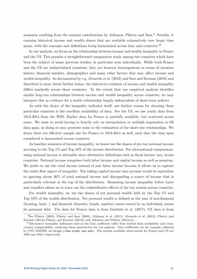
measures resulting from the seminal contributions by Atkinson, Piketty and Saez.9 Notably, it

contains historical income and wealth shares that are available exhaustively over larger time

spans, with the concepts and definitions being harmonized across time and countries.10

In our analysis, we focus on the relationship between income and wealth inequality in France

and the US. This permits a straightforward comparative study among two countries which have

been the subject of many previous studies, in particular seen individually. While both France

and the US are industrialized countries, they are however heterogeneous in terms of taxation

history, financial markets, demographics and many other factors that may affect income and

wealth inequality. As documented by e.g. Alvaredo et al. (2013) and Saez and Zucman (2016) and

described in more detail further below, the historical evolution of income and wealth inequality

differs markedly across these countries. To the extent that our empirical analysis identifies

similar long-run relationships between income and wealth inequality across countries, we may

interpret this as evidence for a stable relationship largely independent of short-term policies.

As with the choice of the inequality indicator itself, one further reason for choosing these

particular countries is the excellent availability of data. For the US, we use yearly data from

1913-2014 from the WID. Earlier data for France is partially available, but scattered across

years. We want to avoid having to heavily rely on interpolation or multiple imputation to fill

data gaps, as doing so may generate noise in the estimation of the short-run relationships. We

hence limit our effective sample size for France to 1913-2014 as well, such that the time span

considered is harmonized across countries.

As baseline measures of income inequality, we hence use the shares of pre-tax national income

accruing to the Top 1% and Top 10% of the income distribution. For international comparisons,

using national income is advisable since alternative definitions such as fiscal income vary across

countries. National income comprises both labor income and capital income as well as pensions.

We prefer to use the total income instead of just labor income because it allows us to capture

the entire flow aspect of inequality. Not taking capital income into account would be equivalent

to ignoring about 30% of total national income and disregarding a source of income that is

particularly relevant at the top of the distribution. Measuring income inequality before taxes

and transfers allows us to trace out the redistributive effects of the tax system across countries.

For wealth inequality, we use the shares of net personal wealth held by the Top 1% and

Top 10% of the wealth distribution. Net personal wealth is defined as the sum of non-financial

(housing, land...) and financial (deposits, bonds, equities) assets owned by an individual, minus

its personal debt. The data for France data is from Garbinti et al. (2017), US data is from

9See Piketty (2003), Piketty and Saez (2003), Atkinson et al. (2011), Alvaredo et al. (2013), Piketty andZucman (2014a),Piketty and Zucman (2014b) and Atkinson and Piketty (2014a,b).

10Alternative inequality indicators such as the Gini coefficient suffer from limited data availability and cross-country comparability, rendering them unattractive for our analysis. Gini coefficients are for example collectedby UNU-WIDER, see https://www.wider.unu.edu/. The earliest available observations for France and US are1956 and 1944, respectively.


Piketty et al. (2016, 2018b).11 As for income inequality, our main focus is on the Top 1% and

Top 10% since these measures are straightforward to interpret. At the same time, focusing on

the Top 1% and Top 10% strikes a balance between capturing inequality evolution at the tail

and being less subject to measurement errors that are likely more severe for higher percentile

shares (say Top 0.1% or Top 0.01%).

Figure 2: Historical Evolution of Inequality

(a) France Top 1%

10

20

30

40

50

60

1920 1930 1940 1950 1960 1970 1980 1990 2000 2010Year


(b) US Top 1%

10

20

30

40

50

60

1920 1930 1940 1950 1960 1970 1980 1990 2000 2010Year


(c) France Top 10%

20

30

40

50

60

70

80

90

1920 1930 1940 1950 1960 1970 1980 1990 2000 2010Year


(d) US Top 10%

20

30

40

50

60

70

80

90

1920 1930 1940 1950 1960 1970 1980 1990 2000 2010Year


Note: Top 1% and Top 10% shares for pre-tax national income and net personal wealth. Data fromthe World Wealth and Income Database.

Figure 2 shows the historical evolution of income and wealth inequality in France and the US,

for both the Top 1% and the Top 10% shares. The upper panels mirror Figure 1. There is a clear

downward trend for both income and wealth inequality in both countries, starting around 1920 in

France and post-WW2 in the US. The decline in inequality lasts until the 1970s, approximately,

with both countries experiencing a substantial final sharp decline of wealth concentration around

the 1970s. Since then, the US experienced a steady upward trend of inequality, almost reaching

historical peak levels in 2014. Inequality in France similarly increased after the 1970s until today,

although not as pronounced as in the US. For both countries, there is a substantial temporary

increase of wealth concentration during the dot-com-bubble in the late 1990s. What is most

striking is the remarkably close long-run co-movement of wealth and income inequality when

measured by top shares.

11For further details on the exact definitions, concepts and calculation methods underlying the income andwealth inequality measures employed here see Alvaredo et al. (2016).


It should be noted that our theoretical framework implies a link between wealth and income

shares at the top of the wealth distribution. In our empirical analysis, however, we use the income

shares at the top of the income distribution. It is important to recognize that, unfortunately,

joint distributions of income and wealth over very long periods are difficult to obtain. The

only study we are aware of is a very recent contribution by Kuhn et al. (2018), who assemble

household-level data from 1949-2016 for the U.S. Such data allows to construct income share

of certain wealth groups, e.g. the income share of the top 1 percent wealth holders. Over even

longer time periods, the closest existing data is top wealth share data constructed from wealth

distribution data and top income shares constructed from income distribution data, as available

from the WID. In practice, the top 1 percent wealth holders do not necessarily coincide with

the top 1 percent income earners – although the overlap might be substantial and is probably

even more considerable for the top 10 percent. Kuhn et al. (2018) show that the income share

of the Top 1% and the Top 10% of the wealth distribution are a bit lower than the income

share of the Top 1% and the Top 10% of the income distribution. Importantly for our analysis,

however, they document that the overall pattern and evolution over time are highly similar.

This allows us to extract long-run trends in the joint evolution of wealth and income inequality

despite the data limitations. Nevertheless, this caveat should be kept in mind when interpreting

the absolute magnitude of our estimated relative saving rates.

4 Empirical Results

In this section, we present and discuss our main empirical results on the joint short- and long-run

evolution of income and wealth inequality. We start by presenting and discussing the estimation

results using the whole sample period. We then perform structural break tests and sample

splits to investigate the stability of the estimated relative saving rates at the top. Lastly, we

decompose the determinants of the relative saving rates.

4.1 The Long- and Short-Run Relationship Between Wealth and Income In-

equality

As seen in the previous section, the historical evolution of income and wealth inequality shows

large changes over time. However, the remarkably uniform development of income and wealth

inequality seen in the data is in line with the theoretical framework and suggests that there

may exist a stable long-run relationship. We therefore explore whether income and wealth

inequality are cointegrated. As a basis for the cointegration analysis, we start by performing

(augmented) Dickey-Fuller tests to check whether our inequality indicators are non-stationary.

The augmented Dickey-Fuller test fails to reject the null hypothesis of a unit root for both income

and wealth shares, regardless of the selected lag length and in both countries. The results are

shown in the Appendix in Table A1. We therefore conclude that our preferred measures of

income and wealth inequality feature a unit root, rendering cointegration analysis appropriate.


Econometric Setup: Our main equation of interest is the dynamic relationship between

wealth shares and income shares at the top, as derived in Section 2:

∆shfW,t+1 = − S

W(shfW,t − sfr sh

fY,t) +

cft+1

Wt+1+ et (22)

which states that the change of fractile f ’s wealth share shfW,t+1 is a function of the current

wealth share, the current income share shfY,t, the relative saving rate sfr , short-term fluctuations

caused by churn and some temporary deviations et.

We are primarily interested in estimating the relative saving rate sfr governing the long-

run relationship between income and wealth inequality. For each country (France, US) and

both measures of inequality (Top 1% share, Top 10% share) we use three different approaches

to estimate relative saving rates at the top: (a) a Vector Error Correction Model (VECM),

(b) Canonical Correlation Regressions (CCR) following Park (1992) and (c) standard Ordinary

Least Squares (OLS) regressions.

For the VECM model, the empirical specifications is given by(∆shfW,t∆shfY,t

)=

(αW

αY

)(1 −sfr

)(shfW,t−1shfY,t−1

)+

p−1∑i=1

(γWW,i γWY,i

γYW,i γY Y,i

)(∆shfW,t−i∆shfY,t−i

)+

(εW,t

εY,t

)(23)

where shft = (shfW,t sh

fY,t)′ contains the wealth shares shfW,t and income shares shfY,t. The first

VECM equation captures Equation (22) – as we do not observe churn and as et will clearly be

autocorrelated and heteroskedastic, we capture the short-term fluctuations by lags in income

and wealth share changes. The second equation allows us to account for the contemporaneous

feedback of wealth concentration on income concentration. Given that our measure of income

contains capital income, this is one approach to control for possible simultaneity issues. Regard-

ing the long-run relationship, this VECM setup allows for up to one cointegration relationship

only, as we consider the joint evolution of two time series at a time – for example income and

wealth shares accruing to the Top 1% in France. Identification of the cointegration relationship

is straightforward by using the Johansen normalization. The VECM hence yields the estimated

relationship

shfW − sfr sh

fY ∼ I(0) (24)

and thus an estimate of the long-run relative saving rate at the top, which can be interpreted

as empirical test of the error correction representation in Equation (22). As byproduct of the

VECM, we also obtain estimates of the parameters αW and αY which capture the short-run

adjustment from imbalances in the cointegration relationship on wealth and income inequality,

respectively. The VECM hence allows us to characterize the joint short- and long-run evolution

of income and wealth inequality by disentangling short- and long-run adjustments.

In addition to the VECM, we can also obtain estimates of the long-run relative saving

rates only by using the CCR estimator and OLS. Essentially, these two approaches consist of


estimating – for each country and each measure of inequality separately – a single equation given

by:

shfW,t = sfr shfY,t + εt (25)

If wealth and income concentration are cointegrated, the simple OLS estimator of sfr is super-

consistent. However, in the present context, it is likely that there are common exogenous

forces driving both income and wealth shares simultaneously. This is equivalent to a non-

zero correlation between shocks that only affect income concentration and εt, in which case

the OLS estimates features non-Gaussian asymptotically biased and asymmetric distributions,

invalidating standard inference. We therefore employ the CCR approach proposed by Park

(1992) that uses a semiparametric correction to overcome these problems.12 The CCR estimator

is asymptotically unbiased and has fully efficient normal asymptotics, allowing for standard Wald

tests using asymptotic χ-squared statistical inference.13 The main drawback of CCR and OLS

is that they are by construction silent about short-run adjustments between income and wealth

inequality.

We assume that there are no linear time trends in the income and wealth shares per se. On

the one hand, this is motivated by graphical inspection, which suggests the absence of linear

time trends over the entire sample. On the other hand, this is also in line with the theoretical

framework outlined above. We therefore also abstract from time trends and a non-zero constant

mean in the cointegration equation. For the VECM setup, the appropriate lag length p is chosen

using the information criteria by Schwarz (SBIC), Hannan and Quinn (HQIC) and Akaike (AIC),

as reported in Table A2 in the Appendix.14

Baseline Results: Based on this econometric specification, our baseline results for France

and the US, using as inequality measures the share of wealth and income accruing to the Top

1% or Top 10% over the entire sample period 1913-2014, are presented in Table 1:

The estimates for the relative saving rates sfr as the cointegration relationship parameters

are highly significant and remarkably similar across estimators, indicating stationary linear

combinations of income and wealth inequality. For example using the Top 1% shares in France,

we obtain from the VECM that:

shW − 2.34 shY ∼ I(0) (26)

In other words, all estimators imply a statistically significant long-run relationship between

12Essentially, the CCR procedure transforms both regressand and regressor using estimates of one- and twosided long-run covariance-matrices between ε and regressor innovations. The estimates are then obtained byapplying OLS to the transformed variables.

13Alternative estimators are the fully-modified OLS by Phillips and Hansen (1990) and dynamic OLS by Saikko-nen (1992). In our analysis, we found only minuscule differences in both estimates and standard errors comparedto the CCR.

14The lag length tests favor parsimonious models, with for example both SBIC and HQIC indicating p = 1for the Top 1% shares in the US. For the remaining specifications, we strike a balance between the informationcriteria by setting p = 2.


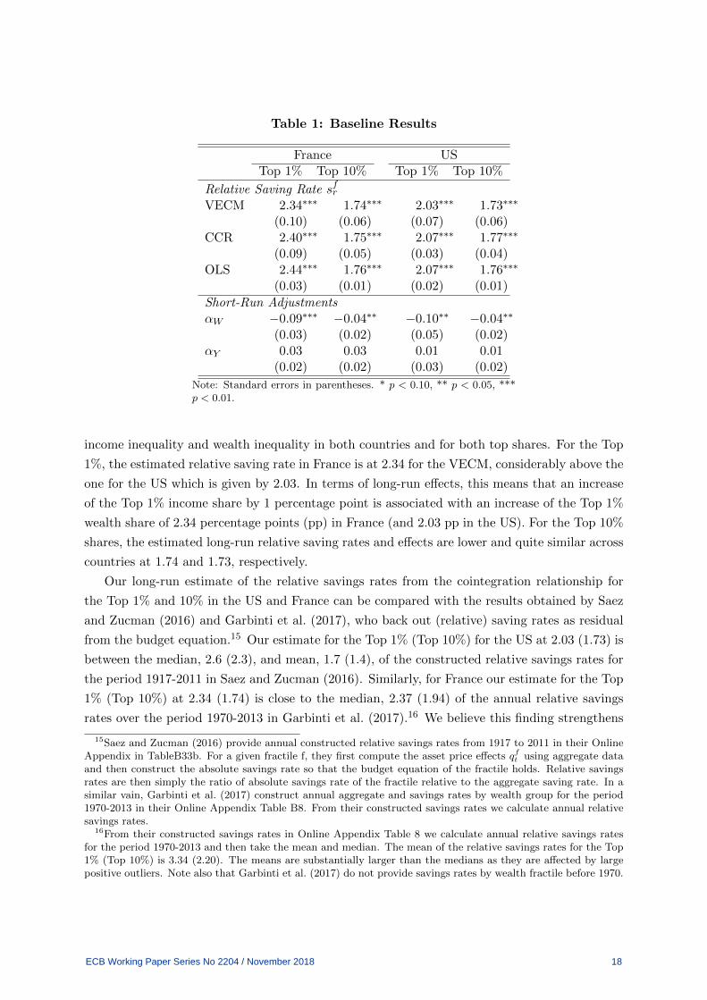
Table 1: Baseline Results

France USTop 1% Top 10% Top 1% Top 10%

Relative Saving Rate sfrVECM 2.34∗∗∗ 1.74∗∗∗ 2.03∗∗∗ 1.73∗∗∗

(0.10) (0.06) (0.07) (0.06)CCR 2.40∗∗∗ 1.75∗∗∗ 2.07∗∗∗ 1.77∗∗∗

(0.09) (0.05) (0.03) (0.04)OLS 2.44∗∗∗ 1.76∗∗∗ 2.07∗∗∗ 1.76∗∗∗

(0.03) (0.01) (0.02) (0.01)

Short-Run AdjustmentsαW −0.09∗∗∗ −0.04∗∗ −0.10∗∗ −0.04∗∗

(0.03) (0.02) (0.05) (0.02)αY 0.03 0.03 0.01 0.01

(0.02) (0.02) (0.03) (0.02)

Note: Standard errors in parentheses. * p < 0.10, ** p < 0.05, ***p < 0.01.

income inequality and wealth inequality in both countries and for both top shares. For the Top

1%, the estimated relative saving rate in France is at 2.34 for the VECM, considerably above the

one for the US which is given by 2.03. In terms of long-run effects, this means that an increase

of the Top 1% income share by 1 percentage point is associated with an increase of the Top 1%

wealth share of 2.34 percentage points (pp) in France (and 2.03 pp in the US). For the Top 10%

shares, the estimated long-run relative saving rates and effects are lower and quite similar across

countries at 1.74 and 1.73, respectively.

Our long-run estimate of the relative savings rates from the cointegration relationship for

the Top 1% and 10% in the US and France can be compared with the results obtained by Saez

and Zucman (2016) and Garbinti et al. (2017), who back out (relative) saving rates as residual

from the budget equation.15 Our estimate for the Top 1% (Top 10%) for the US at 2.03 (1.73) is

between the median, 2.6 (2.3), and mean, 1.7 (1.4), of the constructed relative savings rates for

the period 1917-2011 in Saez and Zucman (2016). Similarly, for France our estimate for the Top

1% (Top 10%) at 2.34 (1.74) is close to the median, 2.37 (1.94) of the annual relative savings

rates over the period 1970-2013 in Garbinti et al. (2017).16 We believe this finding strengthens

15Saez and Zucman (2016) provide annual constructed relative savings rates from 1917 to 2011 in their OnlineAppendix in TableB33b. For a given fractile f, they first compute the asset price effects qft using aggregate dataand then construct the absolute savings rate so that the budget equation of the fractile holds. Relative savingsrates are then simply the ratio of absolute savings rate of the fractile relative to the aggregate saving rate. In asimilar vain, Garbinti et al. (2017) construct annual aggregate and savings rates by wealth group for the period1970-2013 in their Online Appendix Table B8. From their constructed savings rates we calculate annual relativesavings rates.

16From their constructed savings rates in Online Appendix Table 8 we calculate annual relative savings ratesfor the period 1970-2013 and then take the mean and median. The mean of the relative savings rates for the Top1% (Top 10%) is 3.34 (2.20). The means are substantially larger than the medians as they are affected by largepositive outliers. Note also that Garbinti et al. (2017) do not provide savings rates by wealth fractile before 1970.


the case for our interpretation of the estimates from VECM, CCR and OLS as measuring the

long-run relative savings rate.

Turning to the short-run adjustments in the VECM, the parameter αW is estimated to be

statistically significant and around the same order of magnitude across the two countries. In

the VECM, αW governs the short-run change in wealth inequality as a reaction to imbalances

in the long-run relationship. To fix intuition, suppose that the share of Top 1% income is high

relative to wealth inequality, such that the cointegration equation is negative. The negative and

statistically significant coefficient αW then implies that the negative imbalance between the Top

1% shares creates a short-run adjustment of the wealth share. When the Top 1%’s share of

income increases by one percentage point above its long-run-consistent value, the Top 1% share

of wealth quickly rises as well by about approx. 0.09 · 2.34 = 0.21, about 10% of the long-run

effect. This suggests that short-run changes in income inequality are associated with rather

rapid short-run changes in wealth inequality. However, the effect is more pronounced for the

Top 1% shares than for the broader measure of inequality.

For the converse case, the estimates of the short-run effect αY from wealth inequality to

income inequality, have positive signs. This is in line with expectations. Let us suppose that

wealth inequality is high relative to income inequality, in which case the cointegration equation

is positive. A positive αY then implies that the high wealth inequality leads to a short-run

increase in income inequality. However, the estimated coefficients are not statistically significant

and considerably smaller than the estimates of αW . This suggests that the short-run link from

wealth inequality to income inequality is, if anything, weaker than the reciprocal effect. In

turn, we may conclude that wealth inequality leads to higher income inequality considerably

slower in the long-run. This is intuitive remembering that income inequality refers to a flow

concept, while wealth inequality is about a stock. We believe this finding to be quite important

in the discussion of the evolution of wealth inequality and on possible policy interventions. It

suggests wealth inequality is much driven by income inequality, but is not providing a strong

feedback loop back into income inequality. We investigate the short-run dynamics in more detail

in Section 5.

Given these results, we can also take a closer look at the historical evolution of inequality

through the lenses of our VECM. Figure 3 shows the estimated cointegration relationship and

associated deviations of top shares from the long-run equilibrium:

At the beginning of our sample, the estimated cointegration relationship is mainly positive,

indicating that wealth inequality was large relative to income inequality. The statistically signif-

icant negative αW indicates that such an imbalance leads to a decrease of wealth concentration

in the short-run, in line with the empirical observation: In both France and the US, substantial

decreases of wealth inequality occur around 1930 (coinciding with the Stock Market Crash of

1929) and 1939-1945 (the World War II years). At the same time, the VECM captures the high

volatility in inequality during that period of time. After 1945, the positive imbalance in the coin-

tegration equation persists, in line with the observed further decline of wealth inequality during


Figure 3: Inequality Imbalances

(a) France−

10

010

20

1920 1930 1940 1950 1960 1970 1980 1990 2000 2010Year

Top 1% Top 10%

(b) US

−10

010

20

1920 1930 1940 1950 1960 1970 1980 1990 2000 2010Year

Top 1% Top 10%

Note: The plots show the estimated cointegration relationship shfW − s

fr sh

fY resulting from the VECM

given in Equation (23).

that period of time. With income inequality remaining broadly stable or decreasing further until

the 1970s, the trend of falling wealth concentration continued until the 1970s, approximately.

In France, both income and wealth shares settled somewhat after the 1970s and increased

modestly thereafter, as indicated by the cointegration relationship being close but below zero.

This suggests that France experienced a slight upward pressure of income inequality on wealth

inequality in past decades. However, this effect is considerably more pronounced in the US,

where the estimated cointegration relationship quickly decreases after 1970 and stays negative

until today. With the exception of a short interruption during the climax of the global financial

crisis, the VECM results mirror the steadily upward trending income inequality in the US and

the associated snowballing effect on wealth inequality.

Summarizing the results from this section, we find evidence of a snowballing effect of income

inequality on wealth inequality, in line with the argument by Saez and Zucman (2016). Higher

income inequality elevates wealth inequality considerably in the short-run. In turn, a larger

concentration of wealth at the top of the distribution translates into rising capital income.

The latter effect is not particularly rapid and strong in the short-run. It is however highly

relevant in the long-run, as we provide evidence for a long-run link between income and wealth

concentration. Because relative saving rates at the top exceed unity, a rise in income inequality

yields an even higher increase in wealth inequality in the long-run.

4.2 Structural Breaks of Relative Saving Rates at the Top

Our baseline VECM analysis provides evidence that there exists a long-run relationship between

income and wealth inequality in both France and the US. We now investigate the stability of

relative saving rates at the top, which govern the long-run link. On the one hand, this is

motivated by graphical inspection of the raw inequality time series presented in Section 3.

While the ”distance” between income and wealth concentration (which can be seen as a rule-of-


thumb measure of the relative saving rate) is quite stable over time, it is by no means perfectly

constant. On the other hand, the changed path in the historical evolution of inequality suggests

that there may be structural breaks in long-run relative saving rates at the top. Post-estimation

diagnosis of the VECM using the whole sample period furthermore suggests that stability may

be concern: For all specifications, the Johansen (1995) Lagrange multiplier test indicates residual

autocorrelation, and for the Top 10% shares in the US, one eigenvalue is relatively close to 1

(compare Section C in the Appendix).

Testing for Stability: We thus check for the existence of a stable cointegration relationship

between income and wealth inequality by using the canonical Johansen (1991) test. For most

specifications, the Johansen cointegration test indicates a VECM rank of 0, as shown Table A4

in the Appendix. In other words, the Johansen test fails to detect a stable long-run relationship

between income and wealth inequality. In turn, this suggests that relative saving rates at the

top may not be entirely stable over time due to a structural break.

To detect the structural break dates of the relative saving rates at the top, we employ

standard supremum Wald tests (Andrews, 1993; Hansen, 1997) and cumulative sum stability

tests (Brown et al., 1975; Ploberger and Kramer, 1992). Both testing procedures indicate the

presence of a structural break in the long-run relationship between income and wealth inequality

occurring in 1968 in France, and in 1983 in the US. This suggests that long-run relative saving

rates at the top may have changed substantially around that point in time, both when looking

at the Top 1% and the Top 10%.17

Table 2: Structural Breaks in Relative Saving Rates


Supremum Wald1968*** 1968*** 1983*** 1983***(0.00) (0.00) (0.00) (0.00)

Cumulative sum1968*** 1968*** 1983*** 1983***(0.00) (0.00) (0.00) (0.00)

Note: Estimated break dates of relative saving rates at the top. p-values in parentheses.* p < 0.10, ** p < 0.05, *** p < 0.01.

Equivalently, this implies that the estimated relative saving rates presented in the previous

section may not be stable over time, as also implied by the Johansen test. We feed the estimated

break dates into the Pesaran et al. (2001) procedure to test whether income and wealth inequality

are nevertheless cointegrated after accounting for the structural break. That is, we estimate

single-equation autoregressive distributed lag (ARDL) models for income and wealth shares,

17We also perform univariate structural break tests on the individual time series. Table A3 in the Appendixshows that univariate structural breaks occur at around the same time as the breaks in the relative saving rate.


whose error correction model (ECM) representation is given by

∆shfY,t = α(shY,t−1 − βshW,t−1) +

p−1∑i=1

γY,i∆shfY,t−i +

q−1∑i=0

γW,i∆shfW,t−i + dt + et (27)

Note that we include dummies dt equal to 1 after and including 1968 for France and 1983

for the US to account for the structural breaks.

The hypotheses equivalent to no cointegration are

HF0 : α = 0 ∩ β = 0 Ht

0 : α = 0 (28)

where α is the short-run speed-of-adjustment coefficient and β is the long-run coefficient β.18

Following Pesaran et al. (2001), the existence of a long-run relationship is confirmed if both HF0

and Ht0 are rejected. Table 3 shows the results, which indicate that the null hypothesis of no

cointegration can be rejected at conventional confidence levels in all four cases after accounting

for the structural breaks. This constitutes evidence that a long-run relationship between income

inequality and wealth inequality exists, yet is not entirely stable because relative saving rates at

the top were subject to structural breaks.

Table 3: Pesaran-Shin-Smith Cointegration Tests

France USF-test t-test F-test t-test

Top 1% 6.24*** -3.18** 7.66*** -3.91***Top 10% 4.62** -2.60** 5.58** -3.33***

10% crit. value 3.28 -2.28 3.28 -2.285% crit. value 4.11 -2.60 4.11 -2.601% crit. value 6.02 -3.22 6.02 -3.22

Note: Critical values from Pesaran et al. (2001) using the whole samples and including time dummiesaccording to structural break tests. For I(1) regressors, HF

0 is rejected if F is larger than the criticalvalue, and Ht

0 is rejected if t is smaller than the critical value.p < 0.10, ** p < 0.05, *** p < 0.01.

Sample Splits: Given the results from the structural break tests and the Pesaran-Shin-Smith

cointegration test, we split our sample at the estimated break dates in 1968 for France and 1983

for the US. We then re-estimate our baseline regressions outlined above for the three estimators

VECM, CCR and OLS. Table 4 shows the corresponding estimates of relative saving at the top.

The estimated long-run relative saving rates continue to be estimated highly significantly

across samples. Moreover, all three estimators present strong evidence of a decline in relative

18The ARDL equation is estimated by OLS. Estimates of the short-run parameter are√T -consistent, while the

estimate of the long-run parameter is super-consistent if the variables are I(0). Both estimates are asymptoticallynormally distributed irrespective of the order of integration (Shin and Pesaran, 1999). The lag length of theARDL equations is chosen according to the information criteria by Schwarz and Akaike.


Table 4: Estimated Relative Saving Rates sfr

France US1913-2014 1913-1967 1968-2014 1913-2014 1913-1982 1983-2014

Top 1%

VECM 2.34∗∗∗ 2.53∗∗∗ 2.12∗∗∗ 2.03∗∗∗ 2.14∗∗∗ 1.90∗∗∗

(0.10) (0.11) (0.06) (0.08) (0.06) (0.02)CCR 2.40∗∗∗ 2.54∗∗∗ 2.11∗∗∗ 2.07∗∗∗ 2.16∗∗∗ 1.90∗∗∗

(0.09) (0.10) (0.02) (0.03) (0.02) (0.01)OLS 2.44∗∗∗ 2.54∗∗∗ 2.13∗∗∗ 2.07∗∗∗ 2.16∗∗∗ 1.90∗∗∗

(0.03) (0.04) (0.03) (0.02) (0.03) (0.02)

Top 10%

VECM 1.74∗∗∗ 2.01∗∗∗ 1.65∗∗∗ 1.73∗∗∗ 1.88∗∗∗ 1.53∗∗∗

(0.06) (0.10) (0.01) (0.06) (0.04) (0.03)CCR 1.75∗∗∗ 1.82∗∗∗ 1.65∗∗∗ 1.77∗∗∗ 1.84∗∗∗ 1.60∗∗∗

(0.05) (0.06) (0.01) (0.04) (0.04) (0.01)OLS 1.76∗∗∗ 1.81∗∗∗ 1.66∗∗∗ 1.76∗∗∗ 1.83∗∗∗ 1.61∗∗∗

(0.01) (0.02) (0.01) (0.01) (0.01) (0.01)

Note: Standard errors in parentheses. * p < 0.10, ** p < 0.05, *** p < 0.01.

saving rates after the structural breaks. In the first sample, relative saving rates at the top are

about 2.54 (1.82) for the Top 1% (Top 10%) in France and around 2.16 (1.84) in the US. This is

equivalent to roughly 1-2 VECM standard errors above the whole sample results. In the second

sample, relative saving rates decline compared to the first sample in both countries and both

measures of inequality. The drop is particularly pronounced for the Top 1% in France, where

the relative saving rates decreased by about 0.4 for the Top 1%. The relative saving rates of the

Top 10% in France decreased by 0.15 after 1968. In the US, the drop is comparable in size for

Top 1% and Top 10%, at roughly 0.25.

While these results are associated with the caveat of a substantially smaller sample size,

they support the structural break tests presented above.19 When performing a test for equality

of relative saving rates across samples, simple Wald tests strongly reject the null hypothesis of

equality in all cases. We therefore find evidence that long-run relative saving rates at the top

declined considerably and statistically significant around the 1970s/1980s in both France and

the US.

We may summarize our empirical findings as follows. First, we find strong econometric evi-

dence of a long-run cointegration relationship between income and wealth inequality. This holds

for both countries and both measures of inequality. Second, the associated estimated long-run

relative saving rates is higher for the Top 1% than for the Top 10%, in line with theoretical

considerations. Third, sample splits yield some evidence that the long-run relative saving rates

decreased after the structural breaks in both countries in the 1970s/1980s. Fourth, short-run

adjustments run mainly from income to wealth inequality, while the reciprocal effect is consid-

19The estimates of the short-run adjustment parameters are especially vulnerable to the small sample size.Section D in the Appendix provides more details of the short-run coefficient estimates in the two subsamples andsome economic interpretation.


erably slower. Overall, these findings underline the theoretical prediction from Equation (13):

To understand the historical evolution of wealth inequality, it is crucial to consider income

inequality dynamics and changes in relative saving rates at the top.

Why did the relative saving rates decline? To understand why the relative savings rates

declined in France and the US, we first check whether taxation could be the culprit. The

estimated relative saving rate are out of pre-tax income, which can be decomposed into a relative

savings rate out of disposable income and a relative tax ratio:

sfr =sfdsd

1− τ f

1− τ(29)

where sfd is the savings rate of fractile f out of disposable income, sd the aggregate savings

rate out of disposable income, τ f the average income tax rate of fractile f and τ the aggregate

average tax rate. A drop in the relative savings rate sfr could then e.g. be caused by a decline in

the relative saving rate out of disposable income (sfdsd

). Alternatively, even with constant savings

rates out of disposable income, an increase in the progressivity of the tax system (i.e τ f increases

relative to τ) reduces the relative tax ratio 1−τf1−τ and hence reduces the relative savings rate sfr .

To decompose the reduction in relative savings rates, we use available data on average and

fractile-specific income tax rates and aggregate saving rates. Saez and Zucman (2016) and

Piketty, Saez and Zucman (2018) provide average tax rates for different fractiles of the wealth

distribution in the US and absolute saving rates. Using their data, we construct average tax

rates over the two sample periods, before and after the break. For France, we use data from

Piketty and Saez (2007) who provide the tax rates and aggregate saving rates for 1970 and 2005.

We use their results for the first and the second sample, respectively.

We first compute the relative tax term 1−τf1−τ , for each country, fractile and sample separately.

We then calculate relative saving rates out of disposable income sfd,r by using Equation (22),

i.e. we use our estimated relative saving rates out of pre-tax income sfr and divide them by the

relative tax rate term. We can furthermore calculate absolute saving rates for the respective

fractile by simple multiplying the relative saving rates by the population-average saving rate in

the given year. The results are shown in Table 5.

For the top 1% rather than an increase in progressivity, we find that after 1968 in France

and 1983 in the US the average tax rates at the top relative to the aggregate actually declined

somewhat so that the relative tax factor increased. For the top 10% similarly the progressivity of

the tax system did not increase after the structural breaks. This is in contrast to earlier increases

in tax progressivity. For France, Piketty et al. (2018a) show that the rise of progressive taxation

on income was a crucial determinant of the decline in wealth inequality over the 1st and 2nd

World War, which is the beginning of our sample. We therefore attribute the decline of the

relative savings rate to a decline of the relative savings rate out of disposable income.

Interestingly the decline in the relative savings rate at the top coincides with a decline in


Table 5: Decomposing Estimated Relative Saving Rates

France US1913-1967 1968-2014 1913-1982 1983-2014

Top 1%Relative Saving RatesOut of disposable income sT1d,r 2.89 2.30 2.83 2.29

Out of pre-tax income sT1r 2.54 2.11 2.16 1.90Absolute Saving RatesOut of disposable income sT1d 0.48 0.21 0.28 0.17Out of pre-tax income sT1 0.40 0.18 0.19 0.12TaxesIncome tax rate τT1 0.17 0.12 0.31 0.28

Relative taxes 1−τT1

1−τ 0.88 0.92 0.76 0.83

Top 10%Relative Saving RatesOut of disposable income sT10r 1.82 1.65 1.84 1.60Out of pre-tax income sT10r 1.82 1.65 1.84 1.60Absolute Saving RatesOut of disposable income sT10d 0.31 0.15 0.20 0.12Out of pre-tax income sT10 0.29 0.14 0.16 0.09TaxesIncome tax rate τT10 0.06 0.05 0.20 0.21

Relative taxes 1−τT10

1−τ 0.99 0.99 0.89 0.92

AggregateSaving rate (disp. inc.) sd 0.17 0.09 0.10 0.07Income tax rate τ 0.05 0.04 0.09 0.14

Note: Data for the US is from Saez and Zucman (2016) and Piketty et al. (2018b). τ available from 1916-2014,τT1 and τT10 from 1960-2004. Data for France is from Piketty and Saez (2007). For the first sample, we usetheir results for 1970, and for the second the results for 2005.

the aggregate savings rate in both countries. In the US the aggregate private savings rate

declined from an average of 11.4% over the period 1959-1982 to 6.2% over the period 1983-

2014.20 In France, the aggregate private saving rate averaged 16.4% over the period 1950-1967,

and averaged 15.6% in the period 1968-2014.21

The drop in the US that started in the early eighties was so remarkable that an earlier

literature aimed to investigate the reasons behind this drop (see among others Bosworth et al.

(1991), Gokhale et al. (1996), Attanasio (1998) and Parker (1999)). To identify the reasons for

the declining aggregate saving rate, this literature was mainly concerned with finding the group

of people which reduced saving the most. This research was however seriously hampered by the

prevailing micro data at that time that could provide savings rates of different subgroups of the

population only with very low precision and many ad hoc assumptions. It seems that a consensus

20These averages are calculated using the personal saving rate, U.S. Bureau of Economic Analy-sis, Personal Saving Rate [PSAVERT], retrieved from FRED, Federal Reserve Bank of St. Louis;https://fred.stlouisfed.org/series/PSAVERT, July 5, 2018.

21These averages are calculated using the series Taux d’epargne des menages, retrieved from INSEE,https://www.insee.fr/fr/statistiques/2830268, July 5, 2018. The drop in the French savings rate is realy re-markable from the eighties onwards. Average savings rate was 14.3 % over the period 1980-2014.


view has never been reached. Browning and Lusardi (1996) provide an early overview of this

literature and list eleven (!) different possible explanations while concluding “[t]he variety of

proposed explanations is per se an indication that there exists little consensus on what underlies

the decline in saving rates.”

While this literature could not come to a conclusion of what caused the large drop, our

results are in line with more recent findings of Juster et al. (2005) using PSID micro data.

Juster et al. (2005) construct average saving rates for two groups of households: those that

own stock in 1984 and those that do not own stock. The average savings rate for stock owners

drops from 13.2% in 1984-1989 to 8.6% in 1989-1994, while those for non-stock owners barely

moves from 7.7% to 7.6% (see Table 2 in Juster et al. (2005)). In other words, in Juster et al.

(2005) the relative savings rate of stock owners versus non-stock owners drops from 1.71 to 1.13.

Our VECM estimates suggest a drop of the relative savings rate of the top 10 % from 1.88 to

1.53. Juster et al. (2005) further show that that those households with higher capital gains in

corporate equities reduced savings the most in the eighties.

The explanation of the large drop in the aggregate personal savings rate by the capital

gains that households received during the stock market boom of the eighties and nineties seems

plausible. As large corporate equities holdings occur mostly concentrated in households at the

top of the wealth distribution, our findings of a reduced relative savings rates for the top fit

nicely with their findings and provides new evidence on why the aggregate savings rate dropped

so much from the early eighties onward.

5 Counterfactual Simulations of Inequality

The rise in wealth inequality in recent years begs the question of what is the relative role of

rising income inequality versus movements in the relative savings rate. In this section, we aim

to disentangle the historical importance of the two causal channels of wealth inequality in the

past decades by performing counterfactual simulations. Let us reconsider the wealth evolution

Equation (19),

∆shfW,t+1 = − S

W(shfW,t − sfr sh

fY,t) +

cft+1

Wt+1+ et (30)

Absent large temporary deviations et, and churn, wealth dynamics for a certain fractile are

thus mainly driven by changes in their income fraction and their relative saving rates. On the

one hand, the previous VECM analysis indicates that there is a tight empirical short-run link

from income to wealth concentration. Given rising income inequality in recent decades, this

suggests an associated rapid increase in wealth inequality, as indeed observed empirically. On

the other hand, the estimated relative saving rates seem to have declined in recent decades.

The lower relative saving rates are expected to counteract the first channel of increasing income

inequality, and by that attenuating the increase in wealth inequality in the long-run. In the fol-


lowing, we therefore aim to decompose the observed evolution in wealth inequality into fractions

attributable to income inequality and relative saving rates, respectively.

Counterfactual Relative Saving Rates: We first perform counterfactual simulations of the

relative saving rates at the top to gauge the extent to which the observed decrease in saving rates

attenuated the first channel of increasing income inequality on the evolution of wealth inequality.

We use the estimates of the VECM from the beginning of our sample in 1913 until the structural

breaks in 1968 for France and 1983 for the US, respectively, as reported in Table 4. We then

use the corresponding estimates of the long-run relative saving rates at the top prior to the

structural break to perform out-of-sample model simulations, using the empirical income share

as exogenous input. In other words, the counterfactual scenario assumes that the relative saving

rates stayed constant at the 1968-level in France and the 1983-level in the US, and simulates

the evolution of wealth inequality for the observed development of income inequality.

Figure 4: Counterfactual Relative Saving Rates

(a) France Top 1%

10

20

30

40

1970 1980 1990 2000 2010Year

Empirical Relative Saving Rate Fixed in 1975

(b) US Top 1%

10

20

30

40

1970 1980 1990 2000 2010Year


(c) France Top 10 %

50

60

70

80

1970 1980 1990 2000 2010Year


(d) US Top 10%

50

60

70

80

1970 1980 1990 2000 2010Year


Note: Evolution of wealth inequality under constant relative saving rates after 1968 for France and1983 for US, using VECM results from Equation (23) for the time period 1913 until the respectivebreak.

As shown in the left panels of Figure 4, the estimated decrease of relative saving rates

substantially contributed to the evolution of wealth inequality in France. With relative saving

rates remaining constant at their 1968-level, wealth inequality would be higher today relative

to the empirical observations, at 27.1% (compared to 23.4%) and 63.4% (compared to 55.3%)


for the Top 1% and Top 10%, respectively. While increases in income inequality dynamics in

France were relatively subdued in recent decades, the non-negligible decline in relative saving

rates also attenuated the associated upward pressure on wealth inequality. This is in contrast to

the US, where the estimated relative saving rates are declined less after 1983. As a result, the

counterfactual simulations produce wealth inequality dynamics largely in line with the observed

increasing profile for the US, suggesting a negligible role of saving rates in recent decades. At

most, the attenuating effect seems to be stronger for the Top 10% compared to the Top 1%. The

results from the simulation using counterfactual saving rates suggests that the observed increase

in wealth inequality in the US seems to be largely attributable to the rise in income inequality.

In contrast, the subdued wealth inequality rise in France appears to be a joint result of lower

relative saving rates and modestly increasing income inequality.

Counterfactual Income Inequality: To provide further insights about the importance of

income shares for the evolution of wealth shares, we perform a second set of counterfactual

simulations. Again starting the simulations at the respective break dates, we first construct

counterfactual income shares for each country using income dynamics from the other country.

That is, we assume that the top income shares in France after 1968 featured the absolute changes

of the corresponding top income shares in the US. We do the same vice versa for the US, starting

in 1983. In other words, we obtain an increasing income inequality profile for France relative

to the observed subdued dynamics, and a relatively modest rise in income inequality for US

compared to actual outcomes. To give one example, this is equivalent to an increase of income

concentration from 9.1% in 1975 to 18.7% in 2014 instead of 10.8% for the Top 1% in France.

We use the counterfactual income inequality profile alongside the VECM estimates of post-break

relative saving rates at the top to perform simulations of wealth inequality dynamics. Figure 5

shows the results.

If France had experienced a rise in income inequality comparable to the US, wealth concen-

tration would be substantial higher in recent decades. Today, it would range at 37.9% for the

Top 1% and 66.3% for the Top 10%, only somewhat lower than the observed wealth inequality

in the US. Notably, this simulation includes the attenuating effect of declining saving rates in

France into account, such that some of the remaining difference attributable to this channel.

The converse scenario applies to the US: With a roughly constant income inequality profile,

wealth concentration for the Top 1% would have only risen by a bit to 25.1%, and the wealth

share of the Top 10% would have decreased from 67.3% to 59.7% in 2014.

Taken together, the results from the two counterfactuals simulation reiterate one key finding

of the VECM estimation as presented in the previous section: The short-run link from income

inequality to wealth inequality is rapid and relatively strong. While this effect may be partially

attenuated by adjustments in the relative saving rates at the top, it is sufficiently pronounced to

dominate the latter channel. As such, we may think of wealth inequality as being mainly driven

by income concentration, in particular in the short-run. In the long-run, the effect of relative


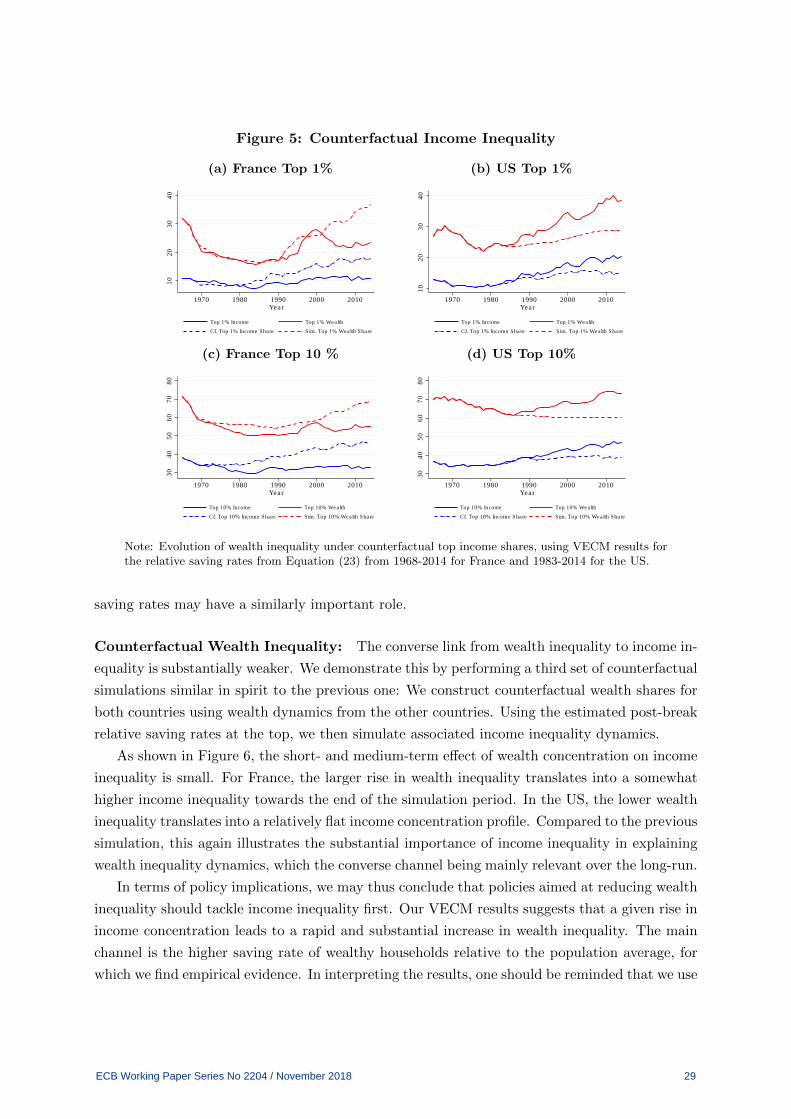
Figure 5: Counterfactual Income Inequality

(a) France Top 1%10

20

30

40

1970 1980 1990 2000 2010Year


Cf. Top 1% Income Share Sim. Top 1% Wealth Share

(b) US Top 1%

10

20

30

40

1970 1980 1990 2000 2010Year



(c) France Top 10 %

30

40

50

60

70

80

1970 1980 1990 2000 2010Year



(d) US Top 10%

30

40

50

60

70

80

1970 1980 1990 2000 2010Year



Note: Evolution of wealth inequality under counterfactual top income shares, using VECM results forthe relative saving rates from Equation (23) from 1968-2014 for France and 1983-2014 for the US.

saving rates may have a similarly important role.

Counterfactual Wealth Inequality: The converse link from wealth inequality to income in-

equality is substantially weaker. We demonstrate this by performing a third set of counterfactual

simulations similar in spirit to the previous one: We construct counterfactual wealth shares for

both countries using wealth dynamics from the other countries. Using the estimated post-break

relative saving rates at the top, we then simulate associated income inequality dynamics.

As shown in Figure 6, the short- and medium-term effect of wealth concentration on income

inequality is small. For France, the larger rise in wealth inequality translates into a somewhat

higher income inequality towards the end of the simulation period. In the US, the lower wealth

inequality translates into a relatively flat income concentration profile. Compared to the previous

simulation, this again illustrates the substantial importance of income inequality in explaining

wealth inequality dynamics, which the converse channel being mainly relevant over the long-run.

In terms of policy implications, we may thus conclude that policies aimed at reducing wealth

inequality should tackle income inequality first. Our VECM results suggests that a given rise in

income concentration leads to a rapid and substantial increase in wealth inequality. The main

channel is the higher saving rate of wealthy households relative to the population average, for

which we find empirical evidence. In interpreting the results, one should be reminded that we use


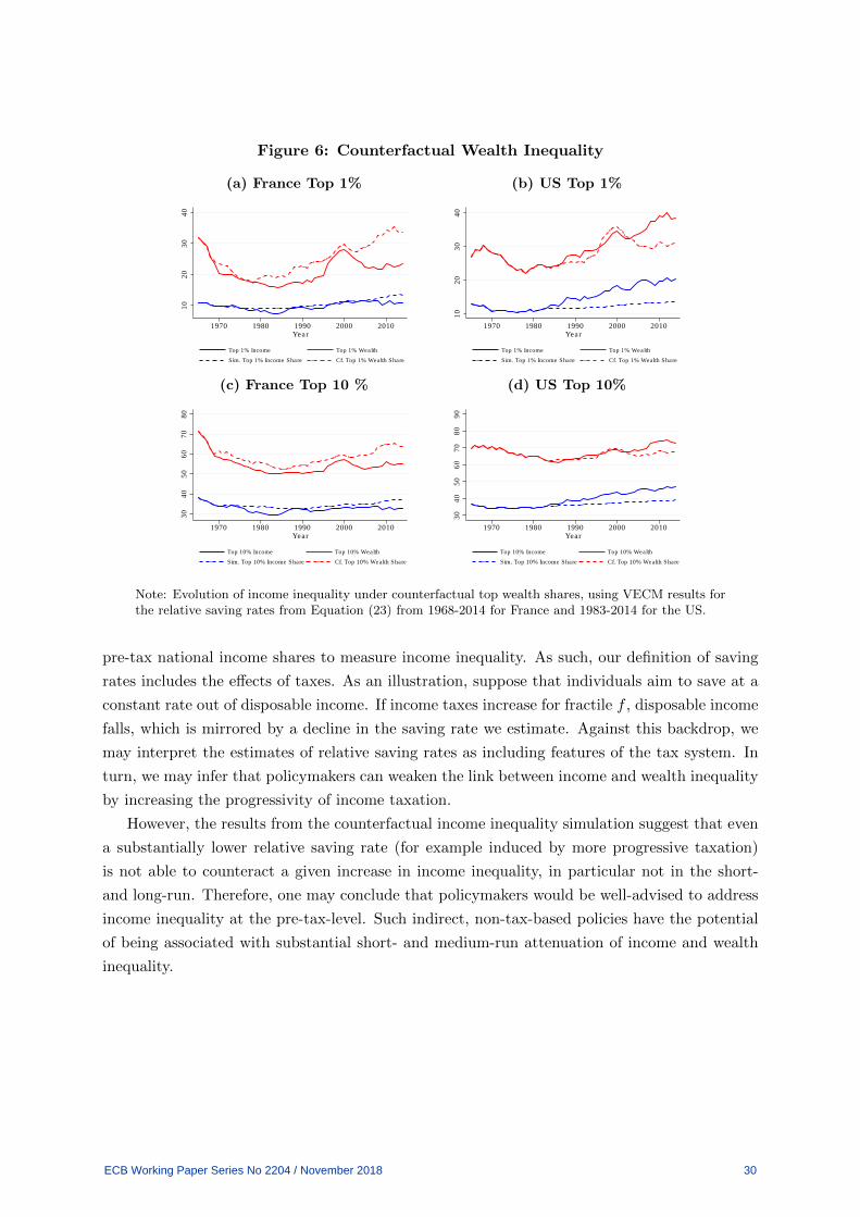
Figure 6: Counterfactual Wealth Inequality

(a) France Top 1%10

20

30

40

1970 1980 1990 2000 2010Year


Sim. Top 1% Income Share Cf. Top 1% Wealth Share

(b) US Top 1%

10

20

30

40

1970 1980 1990 2000 2010Year



(c) France Top 10 %

30

40

50

60

70

80

1970 1980 1990 2000 2010Year



(d) US Top 10%

30

40

50

60

70

80

90

1970 1980 1990 2000 2010Year



Note: Evolution of income inequality under counterfactual top wealth shares, using VECM results forthe relative saving rates from Equation (23) from 1968-2014 for France and 1983-2014 for the US.

pre-tax national income shares to measure income inequality. As such, our definition of saving

rates includes the effects of taxes. As an illustration, suppose that individuals aim to save at a

constant rate out of disposable income. If income taxes increase for fractile f , disposable income

falls, which is mirrored by a decline in the saving rate we estimate. Against this backdrop, we

may interpret the estimates of relative saving rates as including features of the tax system. In

turn, we may infer that policymakers can weaken the link between income and wealth inequality

by increasing the progressivity of income taxation.

However, the results from the counterfactual income inequality simulation suggest that even

a substantially lower relative saving rate (for example induced by more progressive taxation)

is not able to counteract a given increase in income inequality, in particular not in the short-

and long-run. Therefore, one may conclude that policymakers would be well-advised to address

income inequality at the pre-tax-level. Such indirect, non-tax-based policies have the potential

of being associated with substantial short- and medium-run attenuation of income and wealth

inequality.


6 Conclusion

We investigate the long- and short-run relationship between wealth and income inequality in

the US and France over more than a century. We first show that theoretical budget equation

accounting yields an error correction relationship between top wealth and top income shares.

This provides the basis to estimate relative saving rates at the top as the key driver of the long-

run cointegration between wealth and income inequality from the data. The empirical evidence

we provide shows that top wealth and income shares are indeed cointegrated. However, we find

that the relative saving rate at the top has declined after 1968 in France and after 1983 in the

US, which implies a shift in the cointegration relationship. Wealth inequality in the last few

decades has therefore been driven by two opposing forces. First, income inequality has increased,

implying a rising wealth inequality. Second, the lowering of the relative saving rate at the top

has reduced the degree to which income inequality leads to wealth inequality in the long run.

Our counterfactual analysis shows that with only modest declines in the relative saving rate

in the US, most of the rise in wealth inequality can be attributed to rising income inequality. In

contrast, a stronger decline in the relative saving rate in France combined with a more moderate

increase in income inequality led to a much slower rise in wealth inequality. With respect to

short-run dynamics, our estimates show that income inequality drives wealth inequality, while

the converse link is much weaker and slower. As such, our counterfactual simulations suggest that

even the substantial decline in relative saving rates observed in France would not be sufficient

to considerably attenuate a rise in wealth inequality associated with a US-type rising income

inequality profile.

From a broader perspective, our paper support the idea behind Piketty (2014) that a deeper

understanding of the dynamics of wealth and income inequality can only come through a joint

analysis of long-time series. Unfortunately, consistently defined time series measures of inequality

over more than a century, such as those of WID we use here, are very rare. As such, intensifying

the efforts to obtain more cross-country data, to overcome existing data gaps and to improve the

overall availability and quality of inequality measures emerges as a highly worthwhile and notable

contribution to inequality research, in particular for quantitative and econometric studies like

the one at hand.

Our analysis also underscores the importance of the relative saving rate for the joint evolution

of income and wealth inequality. In the long run, only the relative saving rates determine the

gap between top wealth and income shares. Today, they are closer together than in the 1920s

and 1930s. We show that the drop in the relative saving rate was not driven by changes in the

progressivity of income taxation, but coincides with a drop in aggregate savings rates. Earlier

research suggests that this drop might be explained by a reduced saving of those households

with equity gains. Such an explanation is consistent with our finding of a drop in the relative

savings rate at the top, where most equity is held.

Lastly, our results emphasize the key role of pre-tax income inequality in determining wealth


inequality. This suggest that policymakers would be well-advised to address income inequality

at the pre-tax-level. Such indirect, non-tax-based policies have the potential of being associated

with substantial short- and medium-run attenuation of income and wealth inequality.


References

Alvaredo, F., Atkinson, A., Chancel, L., Piketty, T., Saez, E., and Zucman, G. (2016). Distri-

butional National Accounts (DINA) Guidelines: Concepts and Methods used in WID.world.

Working Paper Series 2016/1, WID.world.

Alvaredo, F., Atkinson, A. B., Piketty, T., and Saez, E. (2013). The Top 1 Percent in Interna-

tional and Historical Perspective. Journal of Economic Perspectives, 27(3):3–20.

Andrews, D. W. K. (1993). Tests for Parameter Instability and Structural Change with Unknown

Change Point. Econometrica, 61(4):821–856.

Atkinson, A. B. and Piketty, T., editors (2014a). Top Incomes: A Global Perspective. Number

9780198727743 in OUP Catalogue. Oxford University Press.

Atkinson, A. B. and Piketty, T., editors (2014b). Top Incomes Over the Twentieth Cen-

tury: A Contrast Between Continental European and English-Speaking Countries. Number

9780198727750 in OUP Catalogue. Oxford University Press.

Atkinson, A. B., Piketty, T., and Saez, E. (2011). Top Incomes in the Long Run of History.

Journal of Economic Literature, 49(1):3–71.

Attanasio, O. (1998). Cohort Analysis of Saving Behavior by U.S. Households. The Journal of

Human Resources, 33(3):575–609.

Benhabib, J. and Bisin, A. (2016). Skewed Wealth Distributions: Theory and Empirics. NBER

Working Papers 21924, National Bureau of Economic Research, Inc.

Black, S. E. and Devereux, P. J. (2011). Recent Developments in Intergenerational Mobility.

volume 4 of Handbook of Labor Economics, chapter 16, pages 1487–1541. Elsevier.

Boserup, S. H., Kopczuk, W., and Kreiner, C. T. (2014). Stability and persistence of inter-

generational wealth formation: Evidence from Danish wealth records of three generations.

unpublished.

Bosworth, B., Burtless, G., and Sabelhaus, J. (1991). The decline in Saving: Evidence from

Household Surveys. Brookings papers on Economic Activity, I:183–256.

Brown, R. L., Durbin, J., and Evans, J. M. (1975). Techniques for Testing the Constancy

of Regression Relationships over Time. Journal of the Royal Statistical Society. Series B

(Methodological), 37(2):149–192.

Browning, M. and Lusardi, A. (1996). Household Saving: Micro Theories and Micro Facts.

Journal of Economic Literature, 34(4):1797–1855.


Charles, K. K. and Hurst, E. (2003). The Correlation of Wealth across Generations. Journal of

Political Economy, 111(6):1155–1182.

Chetty, R., Hendren, N., Kline, P., and Saez, E. (2014). Where is the land of Opportunity?

The Geography of Intergenerational Mobility in the United States. The Quarterly Journal of

Economics, 129(4):1553–1623.

De Nardi, M. and Fella, G. (2017). Saving and Wealth Inequality. Review of Economic Dynamics,

26:280–300.

De Nardi, M., French, E., and Jones, J. (2010). Why Do the Elderly Save? The Role of Medical

Expenses. Journal of Political Economy, 118(1):39–75.

Dynan, K. E., Skinner, J., and Zeldes, S. P. (2004). Do the Rich Save More? Journal of Political

Economy, 112(2):397–444.

Ferrie, J., Massey, C., and Rothbaum, J. (2016). Do Grandparents and Great-Grandparents

Matter? Multigenerational Mobility in the US, 1910-2013. Working Paper 22635, National

Bureau of Economic Research.

Garbinti, B., Goupille-Lebret, J., and Piketty, T. (2017). Accounting for Wealth Inequality

Dynamics: Methods, Estimates and Simulations for France (1800-2014). CEPR Discussion

Papers 11848, C.E.P.R. Discussion Papers.

Gokhale, J., Kotlikoff, L., and Sabelhaus, J. (1996). Understanding the Postwar Decline in U.S.

saving: A Cohort Analysis. Brookings papers on Economic Activity, I:315–407.

Hansen, B. E. (1997). Approximate Asymptotic P Values for Structural-Change Tests. Journal

of Business & Economic Statistics, 15(1):60–67.

Hubmer, J., Krusell, P., and Smith, Anthony A, J. (2016). The Historical Evolution of the Wealth

Distribution: A Quantitative-Theoretic Investigation. Working Paper 23011, National Bureau

of Economic Research.

Hurst, E., Luoh, M. C., Stafford, F. P., and Gale, W. G. (1998). The Wealth Dynamics of

American Families, 1984-94. Brookings Papers on Economic Activity, 1998(1):267–337.

Johansen, S. (1991). Estimation and Hypothesis Testing of Cointegration Vectors in Gaussian

Vector Autoregressive Models. Econometrica, 59(6):1551–1580.

Johansen, S. (1995). Likelihood-Based Inference in Cointegrated Vector Autoregressive Models.

Oxford University Press.

Juster, T., Lupton, J., Smith, J., and Stafford, F. (2005). The decline in household saving and

the wealth effect. The Review of Economics and Statistics, 87(4):20–27.


Kuhn, M., Schularick, M., and Steins, U. (2018). Income and Wealth Inequality in America,

1949-2016. Working Paper 6608, CESifo.

Park, J. Y. (1992). Canonical Cointegrating Regressions. Econometrica, 60(1):119–143.

Parker, J. (1999). Spendthrift in America? On two decades of decline in the U.S. saving rate.

NBER Macroeconomics Annual, 14:317–370.

Pesaran, M. H., Shin, Y., and Smith, R. J. (2001). Bounds testing approaches to the analysis

of level relationships. Journal of Applied Econometrics, 16(3):289–326.

Phillips, P. C. B. and Hansen, B. E. (1990). Statistical Inference in Instrumental Variables

Regression with I(1) Processes. Review of Economic Studies, 57(1):99–125.

Piketty, T. (2003). Income Inequality in France, 1901-1998. Journal of Political Economy,

111(5):1004–1042.

Piketty, T. (2014). Capital in the Twenty-First Century. Harvard University Press.

Piketty, T., Postel-Vinay, G., and Rosenthal, J.-L. (2018a). The End of the Rentiers: Paris

1842-1957. Working Paper Series 2018/1, WID.world.

Piketty, T. and Saez, E. (2003). Income Inequality in the United States, 1913-1998. The

Quarterly Journal of Economics, 118(1):1–41.

Piketty, T. and Saez, E. (2007). How Progressive Is the U.S. Federal Tax System? A Historical

and International Perspective. Journal of Economic Perspectives, 21:3–24.

Piketty, T., Saez, E., and Zucman, G. (2016). Distributional National Accounts: Methods and

Estimates for the United States. NBER Working Papers 22945, National Bureau of Economic

Research, Inc.

Piketty, T., Saez, E., and Zucman, G. (2018b). Distributional National Accounts: Methods and

Estimates for the United States. The Quarterly Journal of Economics, 133(2):553–609.

Piketty, T. and Zucman, G. (2014a). Capital is Back: Wealth-Income Ratios in Rich Countries

17002010. The Quarterly Journal of Economics, 129(3):1255–1310.

Piketty, T. and Zucman, G. (2014b). Wealth and Inheritance in the Long Run. CEPR Discussion

Papers 10072, C.E.P.R. Discussion Papers.

Piketty, T. and Zucman, G. (2015). Chapter 15 - Wealth and Inheritance in the Long Run. In

Atkinson, A. B. and Bourguignon, F., editors, Handbook of Income Distribution, volume 2 of

Handbook of Income Distribution, pages 1303 – 1368. Elsevier.

Ploberger, W. and Kramer, W. (1992). The cusum test with ols residuals. Econometrica,

60(2):271–285.


Quadrini, V. (1999). The importance of entrepreneurship for wealth concentration and mobility.

Review of Income and Wealth, 45(1):1–19.

Quadrini, V. and Rıos-Rull, J.-V. (2015). Chapter 14 - Inequality in Macroeconomics. In

Atkinson, A. B. and Bourguignon, F., editors, Handbook of Income Distribution, volume 2 of

Handbook of Income Distribution, pages 1229 – 1302. Elsevier.

Saez, E. and Zucman, G. (2016). Wealth Inequality in the United States since 1913: Evidence

from Capitalized Income Tax Data. The Quarterly Journal of Economics, 131(2):519–578.

Saikkonen, P. (1992). Estimation and Testing of Cointegrated Systems by an Autoregressive

Approximation. Econometric Theory, 8(1):1–27.

Shin, Y. and Pesaran, M. (1999). An Autoregressive Distributed Lag Modelling Approach to

Cointegration Analysis. In Strom, S., editor, Econometrics and Economic Theory in the 20th

century, pages 371–413. Cambridge University Press.

Slacalek, J., Sommer, M., and Carroll, C. (2012). Dissecting saving dynamics: measuring wealth,

precautionary and credit effects. Working Paper Series 1474, European Central Bank.


Appendix

A Econometric Setup

Table A1: Augmented Dickey-Fuller Tests

France USLags Y Top 1% W Top 1% Y Top 10% W Top 10% Y Top 1% W Top 1% Y Top 10% W Top 10%

0 0.36 0.23 0.33 0.56 0.59 0.36 0.80 0.691 0.40 0.27 0.35 0.55 0.45 0.37 0.74 0.712 0.46 0.29 0.39 0.58 0.50 0.32 0.69 0.573 0.12 0.25 0.20 0.55 0.46 0.32 0.71 0.544 0.18 0.22 0.22 0.54 0.68 0.51 0.75 0.425 0.37 0.24 0.43 0.55 0.78 0.71 0.76 0.386 0.20 0.28 0.25 0.56 0.68 0.57 0.77 0.287 0.35 0.35 0.34 0.60 0.80 0.70 0.71 0.308 0.37 0.37 0.43 0.62 0.80 0.66 0.53 0.38

Note: MacKinnon (1994) approximate p-values from (augmented) Dickey-Fuller tests for the top shares ofpre-tax national income (Y ) and net personal wealth (W ). A p-value larger than 0.05 indicates that the nullhypothesis that the respective variable follows a unit-root process cannot be rejected at the conventional5%-level.

Table A2: VECM Lag Length Selection

France USIC Top 1% Top 10% Top 1% Top 10%

SBIC 1 1 1 1HQIC 2 2 1 3AIC 2 2 5 3

Note: Preferred lag length p for a VECM involving the respective top shares of pre-tax national incomeand net personal wealth according to the SBIC, HQIC and Akaike’s information criterion (AIC).


B Structural Break Tests

The changed path in the historical evolution of inequality in the 1970s suggests the existence of

structural breaks. When modeling the time series as following a linear time trend, univariate

supremum Wald-tests strongly indicate structural breaks occurring at approximately the same

time in the 1970s, as shown in Table A3. In France, the structural break occurs around 1970,

while the US follows about a decade later in 1980. This provides evidence against the existence

of simple linear time trends in income and wealth inequality. It also confirms that income and

wealth inequality should not be seen as following trends that are merely a function of time,

but strongly depend on macroeconomic circumstances and associated policies. Notably, the

univariate breaks occur around the same dates as the structural breaks in relative saving rates.

Table 2 from the main text is shown in the lower panel to facilitate comparison.

Table A3: Structural Breaks in Inequality


Univariate Series Breaks

Income Y1973*** 1986*** 1978*** 1976***(0.00) (0.00) (0.00) (0.00)

Wealth W1970*** 1969*** 1978*** 1984***(0.00) (0.00) (0.00) (0.00)

Relative Saving Rates Breaks (Table 2)

Supremum Wald1968*** 1968*** 1983*** 1983***(0.00) (0.00) (0.00) (0.00)

Cumulative sum1968*** 1968*** 1983*** 1983***(0.00) (0.00) (0.00) (0.00)

Note: Estimated break dates of relative saving rates at the top (upper panel), pre-tax national income(Y ) and net personal wealth W . The univariate structural break tests are conducted using a supremumWald test. p-values in parentheses. * p < 0.10, ** p < 0.05, *** p < 0.01.


C VECM Diagnostics

Post-estimation diagnosis of the VECM companion matrix eigenvalues following Johansen (1995)

suggests that the cointegration relationships are stationary. However, the evidence for stability

of the US Top 10% cointegration relationship is somewhat uncertain, as one eigenvalue is at

0.94, relatively close to 1. Moreover, the Jarque-Bera test strongly rejects that the residuals

are normally-distributed, and for the US the Lagrange multiplier test following Johansen (1995)

indicates some residual autocorrelation.

Figure A1: VECM Residuals

(a) France

−6

−4

−2

02

4

1920 1930 1940 1950 1960 1970 1980 1990 2000 2010Year

Top 1% Top 10%

(b) US

−4

−2

02

4

1920 1930 1940 1950 1960 1970 1980 1990 2000 2010Year

Top 1% Top 10%

Note: The plots show the VECM residuals resulting from the VECM given in Equation (23).

As shown in Figure A1, the VECM residuals are large at the beginning of our sample,

coinciding with macroeconomic and financial market turmoil during the Great Depression and

World-War II. After the 1970s, the residuals are considerably smaller, but larger again at the

end of our sample during the global financial crisis. As our VECM focuses on income and wealth

inequality alone, these residual properties are to be expected. They represent exogenous effects

on income and wealth shares that are by design not captured in the VECM.

Table A4: Johansen Cointegration Test


Trace 1 0 0 0SBIC 0 0 0 0HQIC 1 0 1 0

Note: Estimated VECM rank using the Johansen cointegration test with the trace statistic, Schwarz’sBayesian information criterion (SBIC) and the Hannan and Quinn information criterion (HQIC). Rank= 1 indicates a stable long-run relationship between income and wealth inequality, while rank = 0hints at the presence of a structural break in our context.


D Sample Splits and Short-Run Adjustments

This section presents sub-sample estimates of the VECM short-run adjustment parameters. Con-

sidering the substantially smaller sample sizes, these estimates should generally be interpreted

with caution. Focusing first on the short-run adjustment from income to wealth inequality,

Table A5 shows the estimated coefficients for αW . The VECM sample splits indicates that the

short-run adjustment process from income to wealth inequality may have become more rapid

in recent decades, in particular in France for both Top 1% and Top 10%. A similar result is

detected for the Top 1% in the US, but not for the Top 10%. Overall, these results suggest that

a given increase in income inequality tends to lead to faster increase in wealth inequality. For

the US case, we may associate this with the decrease of the tax system progressivity induced by

the Reagan tax reforms in the 1980s.

Table A5: Short-Run Adjustment from Income to Wealth Inequality αW

France US1913-2014 1913-1967 1968-2014 1913-2014 1913-1982 1983-2014

Top 1% −0.09∗∗∗ −0.09∗∗ −0.15∗∗∗ −0.10∗∗ −0.06 −0.16(0.03) (0.04) (0.06) (0.05) (0.07) (0.13)

Top 10% −0.04∗∗ 0.00 −0.25∗∗∗ −0.04∗∗ 0.04 0.02(0.02) (0.02) (0.06) (0.02) (0.03) (0.03)


The short-run effects of wealth inequality on income inequality across samples are shown in

Table A6. We find some evidence that rapid short-run adjustments in this direction are mainly

a pre-break feature, in particular in France, but also for the Top 10% in the US. Again keeping

the caveat of the smaller sample size in mind, we may interpret the difference across samples for

France as indicating the effects of the wealth tax introduced in 1989. With such a tax in effect,

a given stock of wealth translates into less capital income in the next period, thus attenuating

the link between wealth and income inequality.

Table A6: Short-Run Adjustment from Wealth to Income Inequality αY

France US1913-2014 1913-1967 1968-2014 1913-2014 1913-1982 1983-2014

Top 1% 0.03 0.06∗∗ 0.04 0.01 0.06 0.11(0.02) (0.03) (0.03) (0.03) (0.04) (0.10)

Top 10% 0.03 0.05∗∗ 0.01 0.01 0.09∗∗∗ 0.10∗∗∗

(0.02) (0.02) (0.04) (0.02) (0.03) (0.03)



Acknowledgements The authors would like to thank Nicola Fuchs-Schündeln, Bertrand Garbinti, Wouter Den Haan, Tullio Jappelli, Hashem Pesaran, Giorgio Primiceri, Stefania Albanesi, Arthur Kennickell, Kevin Moore, Oreste Tristani, Pirmin Fessler, Alfonso Rosolia, Reamonn Lydon, Thomas Mathä, Junyi Zhu, Jirka Slacalek, and participants at the HFCS seminar for helpful comments and discussions. The views expressed in this paper only reflect those of the authors. They do not necessarily reflect the views of the European Central Bank. Any remaining errors are solely to be attributed to the authors. Philipp Lieberknecht Goethe University Frankfurt, Frankfurt am Main, Germany; email: [email protected] Philip Vermeulen European Central Bank, Frankfurt am Main, Germany; email: [email protected]

© European Central Bank, 2018

Postal address 60640 Frankfurt am Main, Germany Telephone +49 69 1344 0 Website www.ecb.europa.eu

All rights reserved. Any reproduction, publication and reprint in the form of a different publication, whether printed or produced electronically, in whole or in part, is permitted only with the explicit written authorisation of the ECB or the authors.

This paper can be downloaded without charge from www.ecb.europa.eu, from the Social Science Research Network electronic library or from RePEc: Research Papers in Economics. Information on all of the papers published in the ECB Working Paper Series can be found on the ECB’s website.

PDF ISBN 978-92-899-3309-4 ISSN 1725-2806 doi:10.2866/17297 QB-AR-18-084-EN-N

mailto:[email protected]

mailto:[email protected]

http://www.ecb.europa.eu/

http://www.ecb.europa.eu/

http://ssrn.com/

https://ideas.repec.org/s/ecb/ecbwps.html

http://www.ecb.europa.eu/pub/research/working-papers/html/index.en.html

Inequality and relative saving rates at the top

Documents

Transcript of Inequality and relative saving rates at the top