iIG2 %3

Patterns in HouseholdDemand and Saving

Aonstantino Lluch * Alan A. Powell * Ross A.Williams

. N.\ - __ . / XN

s V

, ..

1- V NN ff.

. 'S@ /

;~~^> AWorld Bank Research Publication

Pub

lic D

iscl

osur

e A

utho

rized

Pub

lic D

iscl

osur

e A

utho

rized

Pub

lic D

iscl

osur

e A

utho

rized

Pub

lic D

iscl

osur

e A

utho

rized

Patternsin Household Demandand Saving

Constantino LluchAlan A. PowellRoss A. Williams

Patterns in Household Demand

and Saving

with contributions byRoger R. Betancourt, Howard Howe, and Philip Musgrove

Published for the World BankOxford University Press

Oxford University PressNEW YORK OXFORD LONDON GLASGOW

TORONTO MELBOURNE WELLINGTON CAPE TOWN

IBADAN NAIROBI DAR ES SALAAM LUSAKA ADDIS ABABA

KUALA LUMPUR SINGAPORE JAKARTA HONG KONG TOKYO

DELHI BOMBAY CALCUTTA MADRAS KARACHI

(© 1977 by the International Bankfor Reconstruction and Development / The World Bank1818 H Street, N.W., Washington, D.C. 20433 U.S.A.

All rights reserved. No part of this publication may bereproduced, stored in a retrieval system, or transmittedin any form or by any means, electronic, mechanical,

photocopying, recording, or otherwvise, without the priorpermission of Oxford University Press. Manufactured in the

United States of America.

The views and interpretations in this book are those of theauthors and should not be attributed to the World Bank, to

its affiliated organizations, or to any individual actingin their behalf.

Library of Congress Cataloging in Publication Data

Lluch, Constantino.Patterns in household demnand and saving.Bibliography: p. 2611. Consumption (Economics) 2. Supply and demand.

3. Economic development. I. Powell, Alan A., jointauthor. II. Williams, Ross A., Joint author.Ill. International Bank for Reconstruction and Develop-ment. IV. Title.HB805.L58 339.4'1 77-3442ISBN 0-19-920097-1ISBN 0-19-920100-5 pbk.

Preface

IN 1972 A RESEARCH PROGRAM on patterns of demand and saving inthe development process was initiated at the Development ResearchCenter of the World Bank. The project was conceived as a system-atic examination of the consumption and savings behavior of house-holds in countries at different levels of development. It was believedthat inter- and intracountry comparisons of such behavior mightyield empirical regularities useful for broad characterizations of thedevelopment process.

The pioneering attempts to discover patterns in economic develop-ment (including household demand and saving) were those of Clark(The Conditions of Economic Progress, 1940) and Kuznets ("Quan-titative Aspects of the Economic Growth of Nations," I-X, EconomicDevelopment and Cultural Change, 1956-67). Later researchers haveattempted to extend this work to take advantage of improvements inthe data base and in econometric techniques over the past decade orso. The most notable recent contribution is that by Chenery andSyrquin (Patterns of Development, 1950-1970), who make inter-country comparisons of ten basic processes of accumulation, resourceallocation, and income distribution. The present work is more limitedin scope, but by concentrating on household demand and savingin some detail it complements the broader treatment of Cheneryand Syrquin. Our analvsis differs from previous work on householdbehavior in that it allows for a joint treatment of saving and theallocation of expenditure. This is made possible through the use ofLluch's extended linear expenditure system (ELEs).

v

vi Preface

The first phase of the project was devoted primarily to thedevelopment of methodology with some exploratory empirical work.Much of this has been published elsewhere. In the second phasethe adopted model, ELES, was fitted to time-series (national accounts)data for seventeen countries and cross-section data for eight countriesspanning the development spectrum. The results are presented inthis book; the theoretical model and estimation techniques are givenin chapter 2 in outline form only.

Intemational comparisons, particularly those which involve cross-section data on individual households, require the advice and assis-tance of a large number of people at various stages of inquiry: notleast in obtaining data, in carrying out computations, and in pre-senting results. Most of the cross-section studies represent theoutput of joint research with agencies in the various countries. Thework on the Republic of Korea in chapter 5 was undertaken incooperation with the Special Research Office of the Bank of Korea,and we are particularly indebted to the director, K. S. Park, forassistance. The Korean data themselves were generously provided byS. K. Chang, Director of the Bureau of Statistics, Economic Plan-ning Board, Korea, and we were also considerably helped by J. Y. Youof the bureau. The Mexican study in chapter 6 represents in part theoutput of joint research with Direccion General Coordinadora de laProgramaci6n Econ6mica y Social, Secretaria de la Presidencia,Mexico. We are greatly indebted to our collaborators Jose LuisAburto and Gabriel Vera for their assistance with data and analvsis ofresults and to Leopoldo Solis and Carlos Bazdresch for their constantsupport and encouragement. Chapter 7 was written in conjunctionwith the ECIEL program (Estudios Conjuntos sobre Integraci6nEcon6mica Latinoamericana). The Yugoslavian data were obtainedthrough the World Bank study, "Small Holder Development Strate-gies: A Case Study in Yugoslavia," undertaken by the Agricultureand Rural Development section of the World Bank's Central ProjectsStaff; Graham Donaldson and Peter Hazell of the World Bankprovided much assistance here. The national accounts data wereassembled by Rita Parrilli and Sandra Hadler; Richard Berner kindlyprovided disposable income estimates for Italy.

In carrying out computations we enjoyed the invaluable servicesof John Chang throughout the life of the project; Alexander Meerausprovided advice on ;computing problems. Orani Dixon assisted inthe preparation of the monograph with her usual combination ofcharm and skill.

Although all three authors have interacted on each chapter, the

PREFACE Vii

prime responsibility for authorship is as follows: chapters 1, 2, 3, and10, Lluch, Powell, and Williams; chapter 4, Lluch and Williamsexcept the section on Taiwan, which was written by Williamsassisted by John Chang; chapters 5 and 6, Lluch and Williams;chapter 9, Williams. Earlier versions of parts of chapters 3 and 5appeared in the Economic Record, Bank of Korea Quarterly Eco-nomic Review, and the Review of Economics and Statistics. Chapters7 and 8 were written by consultants-chapter 7 by Howard Howeand Philip Musgrove, chapter 8 by Roger Betancourt-who alsoprovided us with useful insights in writing our own chapters. Thebulk of the editorial work was done by Williams. Needless to say,the work does not necessarily reflect the views of the World Bank.

Some important acknowledgments remain. Monash Universitygenerously granted extended study leave to Powell and Williams,and throughout the life of the project we have benefited substantiallyfrom discussions with colleagues in the World Bank. Particularthanks are due to Montek Ahluwalia, Bela Balassa, Hollis Chenery,John H. Duloy, Roger Norton, Yung Rhee, Sang Mok Suh, andJean Waelbroeck. Other valuable comments have been provided byColin Clark, Ken Clements, and Nico Klijn. Jane Carroll editedthe final manuscript for publication.

CONSTANTINO LLUCH

ALAN POWELL

Ross WILLIAMS

February 1977

Contents

LIST OF TABLES Xii

GLOSSARY OF SYMBOLS XVii

GENERAL PERSPECTIVES XXi

The role of demand in economic development xxiPrinciple research findings xivLimitations of the study xxx

1. INTRODUCTION I

Previous studies 3Analytical framework 5Aggregation over consumers 8Plan of the book 9

2. METHODOLOGY 11

The extended linear expenditure system (ELES) 1)Stochastic specification and estimation methods 25

3. INTERNATIONAL PATTERNS IN DEMAND PARAMETERS AND

ELASTICITIES: EVIDENCE FROM THE NTATIONAL ACCOUNTS 36Data considerations 36

d Parameter estimates 39Total expenditure and price elasticities 53Key patterns in demand responses 64

4. SUBSISTENCE AND SAVING: FURTHER TIME-SERIES RESULTS 67

Subsistence expenditure 67Elasticities of the marginal utility of expenditure and income 74Average household savings behavior across countries 81Household saving in Korea 82

Permanent income, household demand, and saving in Taiwan 88

ix

x Contents

5. HOUSEHOLD DISAGGREGATION: EMPIRICAL RESULTS FOR KOREA 97

Reasons for disaggregating 97Rural-urban dualism 98Cross-section analysis of urban households 103Results at different levels of consumer disaggregation 113

6. CONSUMPTION AND SAVINGS BEHAVIOR IN MEXICO:

A CROSS-SECTION ANALYSIS 120

Data 120Empirical results 123An overview of findings 149

7. AN ANALYSIS OF ECIEL HOUSEHOLD BUDGET DATA FOR BOGOTA,

CARACAS, GUAYAQIJIL, AND LIMA

Howard Howe and Philip Musgrove 155

Methodology 156The data 157Empirical results: ELES parameter estimates 161Elasticity estimates 179Conclusions 195

8. HOUSEHOLD BEHAVIOR IN CHILE: AN ANALYSIS OF

CROSS-SECTION DATARoger Betancourt 199

Modifications of the model 200Permanent income compared with current income 202Current income results 215Consequences of aggregation 217Summary 222Appendix. The empirical implementation of the

permanent income model 223

9. CONSUMPTION AND SAVINGS BEHAVIOR OFFARMI HoUSEHOLDS IN YUGOSLAVIA 227

ELES parameter estimates 229Total expenditure and price elasticities 235

10. SUMMARY AND CONCLUSIONS 240

Savings responses 240Subsistence expenditure 242Demand responses to income changes 243The Frisch parameter and overall price responsiveness 248Specific price effects 250Comparison of the magnitudes of expenditure and

price elasticities 254Consumer disaggregation 255Future research 257

CONTENTS Xi

BIBLIOGRAPHY 261

AUTHOR INDEX 273

SUBJECT INDEX 275

FIGURES

1. ELES: The two-commodity case 132. Relation between , and GNP per capita 773. Household savings ratio, Korea, 1963-72 874. Household savings ratio, Taiwan, 1952-70 955. Regression lines for the marginal budget shares (p) for food 134

Tables2.1 LES and ELES elasticity formulas in terms of the

supernumerary ratio 172.2 Annotated formulas for demand elasticities in LES and ELES 183.1 Classification of eight commodities used in time-series analysis 373.2 Characteristics of the sample of seventeen countries 383.3 Average budget shares at sample mean values 403.4 Changes in average budget shares over the sample period 413.5 Changes in implicit price deflators and income over

the sample period 423.6 Estimated marginal propensity to consume (tt) and

marginal budget shares (3) 443.7 Estimated subsistence minimums (yi) 463.8 Estimates of per capita subsistence expenditure (Piy )

at sample midpoint in 1970 U.S. dollars 483.9 Coefficients of determination (R2) for fitted models 493.10 Durbin-Watson d statistics for fitted models 503.11 Relation between marginal budget shares (,Oi) and

level of GNP per capita 523.12 Total expenditure elasticities 543.13 Own-price elasticities 553.14 Cross-elasticities with respect to food price 563.15 Percentage of expenditure elasticity associated with

own-price and food-price responses 583.16 Mean income and price elasticities of total consumption

expenditure 603.17 Comparison of elasticity estimates from various studies 613.18 Regressions across countries of expenditure and price

elasticities against logarithm of GNP per capita 624.1 Estimates of y sum at sample midpoints in 1970 U.S. dollars

for different levels of commodity disaggregationfor fourteen countries 70

xii

TABLES Xiii

4.2 Estimates of annual per capita subsistence expenditure atsample midpoints in 1970 U.S. dollars, mixed aggregation 72

4.3 Double-log regressions of per capita subsistence expenditureon GNP per capita 73

4.4 Mean ELES estimates of d 754.5 Double-log regressions of on GNP per capita 764.6 Estimates of partial elasticities of substitution at per capita

GNP levels of $200 and $2,000 784.7 Mean ELES estimates of (&* 804.8 Double-log regressions of w* on GNP per capita 804.9 Mean household savings ratio and its elasticity with respect

to the price of food 824.10 The marginal propensity to consume and the y sum, Korea 844.11 Average household savings ratio and Frisch parameter, Korea 854.12 Prediction of household savings ratio, Korea 854.13 Estimates of marginal propensity to consume and permanent

income parameters, Taiwan, 1952-70 914.14 ELES estimates using current and permanent income,

Taiwan, 1952-70 924.15 Ability of models to predict household savings ratio over time,

Taiwan, 1952-70 965.1 Basic characteristics of aggregate survey data for urban and

farm households and comparison with nationalaccounts data, Korea, 1963-72 100

5.2 ELES estimates, annual time series of aggregate crosssections, Korea, 1963-72 101

5.3 ELES estimates of total expenditure and price elasticities,farm and urban households, Korea, 1963-73 102

5.4 Actual and predicted average household savings ratios,Frisch parameter, and food-price elasticity of savingsratio, Korea, 1963-72 103

5.5 Selected characteristics of urban households: Sample survey,Korea, 1971, first quarter 104

5.6 R2 values: ELES, cross-section data for urban households,Korea, 1971, first quarter 107

5.7 d values: ELES, cross-section data for urban households,Korea, 1971, first quarter 107

5.8 ELES estimates: Cross-section data for urban households,Korea, 1971, first quarter 108

5.9 Total expenditure elasticities: ELES, urban households,Korea, 1971, first quarter 109

5.10 Own-price elasticities and elasticity of average savings ratiowith respect to food price: ELES, urban households,Korea, 1971, first quarter 111

5.11 Cross-elasticities with respect to food price: ELES, cross-section data, urban households, Korea, 1971, first quarter 112

xiv Tables

5.12 ELES estimates: Cross-section data, Seoul households,1971, first quarter 114

5.13 Total expenditure elasticities: ELES, Seoul households,1971, first quarter 116

5.14 Own-price elasticities and elasticity of average savingsratio with respect to food price: ELES, Seoul households,1971, first quarter 116

5.15 Comparison of estimates of ELES parameters and elasticitiesusing different levels of consumer disaggregation, Korea 118

6.1 Mean income and sample size of socioeconomic classes,Mexico, 1968 123

6.2 Basic characteristics of household data, Mexico, 1968 1246.3 R2 values, ELES, Mexico, 1968 1266.4 Estimated values of marginal budget shares (pi) and

marginal propensity to consume (pu), ELES, Mexico, 1968 1286.5 Regressions of estimated values of marginal budget shares

(j3i) and the marginal propensity to consume (M) onhousehold characteristics, Mexico, 1968 132

6.6 Estimated values of subsistence parameters (-y*) andFrisch parameter (u), ELES, Mexico, 1968 136

6.7 Weighted regressions of estimated values of y* onhousehold characteristics, urban Mexico, 1968 140

6.8 Total expenditure elasticities, ELES, Mexico, 1968 1426.9 Regressions of estimated values of total expenditure

elasticities on household characteristics, Mexico, 1968 1446.10 Own-price elasticities, ELES, Mexico, 1968 1466.11 Regressions of price elasticities on household characteristics,

urban Mexico, 1968 1486.12 Food cross-price elasticities, Mexico, 1968 1506.13 Elasticity of average savings ratio with respect to food price,

urban Mexico, 1968 1526.14 Coefficient of variation for marginal budget shares (,ai) and

expenditure elasticities (?), Mexico, 1968 1526.15 Unweighted mean values of elasticities, Mexico, 1968 1547.1 Sample size of households in Bogota, Caracas,

Guayaquil, and Lima 1587.2 Mean quarterly income and expenditure, mean household

size, and average savings ratio in four South Americancities 162

7.3 Marginal propensity to consume (A) in fourSouth American cities 164

7.4 ELES parameter estimates, Bogota households, 1967-68 1687.5 ELES parameter estimates, Caracas households,

October-November 1966 1707.6 ELES parameter estimates, Guayaquil households, 1967-68 172

TABLES XV

7.7 ELES parameter estimates, Lima households, 1968-69 1747.8 Average committed expenditures on food and in total for

four South American cities 1787.9 Estimates of the Frisch parameter at mean expenditure for

four South American cities 1807.10 BogotA: Income and expenditure elasticities of demand

evaluated at point of means 1827.11 Caracas: Income and expenditure elasticities of demand

evaluated at point of means 1837.12 Guayaquil: Income and expenditure elasticities of demand

evaluated at point of means 1847.13 Lima: Income and expenditure elasticities of demand

evaluated at point of means 1857.14 Expenditure elasticities from double-log Engel curves 1867.15 Own-price elasticities for four South American cities 1887.16 Average own-price elasticities for four South American cities 1907.17 Cross-elasticities and elasticity of average savings ratio with

respect to food price ($,) for four South American cities 1927.18 Cross-elasticity with respect to food prices for four

South American cities 1947.19 Food cross-elasticities: Average of estimates for four

South American cities 1948.1 Regression results for the current income model:

Expenditure functions of urban and rural workers,self-employed, and employees, Chile 204

8.2 Structural estimates for current income model: Urban andrural workers, self-employed, and employees, Chile 208

8.3 Estimated values of marginal budget shares ($) and themarginal propensity to consume (/.), ELES, Chile, 1964 214

8.4 Estimated values of subsistence parameters (pip), scaleparameters (xi), household subsistence expenditures(p-yi), and Frisch parameter (w), ELES, Chile, 1964 218

8.5 Estimates of the price elasticities (%p), food cross-priceelasticities (f), expenditure elasticities (j), andelasticitv of the savings ratio with respect to food price(a), ELES, Chile, 1964 219

8.6 A comparison of the point estimates obtained with and-without disaggregating by occupational status,ELES, Chile, 1964 221

9.1 Basic characteristics of farm household survey,Yugoslavia, 1972 228

9.2 R2 values, ELES, farm households, Yugoslavia, 1972 2309.3 Estimated values of marginal budget shares (pi) and

marginal propensity to consume (,&), ELES, farmhouseholds, Yugoslavia, 1972 231

xvi Tables

9.4 Estimated values of subsistence parameters (yf ) andFrisch parameter (X), ELES, farm households,Yugoslavia, 1972 234

9.5 Double-log regressions of subsistence parameters on income,farm households, Yugoslavia, 1972 235

9.6 Total expenditure elasticities, ELES, farm households,Yugoslavia, 1972 236

9.7 Own-price elasticities and elasticity of average savings ratiowith respect to food price, ELES, farm households,Yugoslavia, 1972 237

9.8 Elasticity with respect to food price and clothing price,ELES, farm households, Yugoslavia, 1972 238

Glossary of Symbols

The symbols used throughout the book are identified here to facilitatereading the empirical results of chapters 3-10 without frequentcross-references to chapter 2. The general rule is that Greek lettersdenote parameters and elasticities, while Latin letters denote vari-ables. Except where explicitly noted, unsubscripted symbols in thetext refer to vectors, the typical elements of which are shown by thecorresponding subscripted symbols listed below. In the presentationof the empirical results, the use of a hat (^) indicates a parameterestimate, but in chapter 2 this symbol also indicates the operation ofconverting a vector into the corresponding diagonal matrix. Thefollowing list excludes notation for stochastic specification.

Greek symbols (parameters and elasticities)

as intercept for the ilh commodity in cross-section estimatingequations for ELES (extended linear expenditure system)

at intercept for the ith commodity in cross-section estimatingequations for LES (linear expenditure system)intercept in ELES cross-section aggregate consumption func-tion

/li marginal budget share for the ith commodityp3* marginal propensity to consume the ill commodityyi "origin" parameter for the ilh good in Klein-Rubin utilitv

function; may be interpreted as subsistence or committedconsumption of the ilh commodity

Yi' value of subsistence or committed consumption of ith good

xvii

xviii Glossary of Symbols

in cross-section analysis measured at the price prevailing atthe time of the household survey

a subjective rate at which consumers discount future utility^7 elasticity of total consumption expenditure with respect to

incomeB, elasticity of saving with respect to incomevi elasticity of total consumption expenditure with respect to

the price of the itl good-qi total expenditure elasticity of demand for the ith goodri income elasticity of demand for the ith good77ij uncompensated elasticity of demand for the ith good with

respect to the price of the jth good; total expenditure assumedfixed

?ij uncompensated elasticity of demand for the ith good withrespect to the price of the jth good; income assumed fixed

17 compensated elasticity of demand for the ith good with re-spect to the price of the jth good under LES

C compensated elasticity of demand for the ith good with re-spect to the price of ith good under ELES

O parameter used in calculating permanent income measures.It is used in two ways: in the appendix to chapter 8, as acorrection factor which converts the stock formulation intoa flow formulation; in the last section of chapter 4, as a scaleparameter

A parameter of extrapolative tendencies used in calculatingmeasures of permanent income; its interpretation in chapter8 differs from that in chapter 4

Ai parameter which, for the ith good, measures the effects offamily size on yj

p. marginal propensity to consume$ scale parameter used in defining permanent income in the

last section of chapter 4ei elasticity of the household savings ratio (and of saving) with

respect to the price of the ith good7r expected general rate of inflationp the market rate of interest

expected rate of growth of income (in the appendix tochapter 8)

-+ supemumerary ratio, that is, the ratio of uncommitted ex-penditure to total expendituretotal expenditure elasticity of the marginal utility of totalexpenditure, that is, the Frisch parameter

GLOSSARY OF SYMBOLS XiX

(o* income elasticity of the marginal utility of income

Latin symbols (variables)

f familv sizeth family size of hth household; fi in chapter 2 is the ill partial

utility within a directly additive utility frameworkpi price of the ith goodP index of general consumer pricesqi quantity purchased of the ith goods household savings' household savings ratiou( ) utility functionu value of utility functionU ( ) intertemporal utility functionvi expenditure on the ill good at current pricesv total consumption expenditure at current pricesv* total consumption expenditure in real termswi average budget share of the ilb goody personal disposable income at current pricesy* personal disposable income in real termsz permanent incomez* permanent income defined in terms of current and past real

incomeZf dummy variable representing household size; f = 1, 2 for

small and large households respectively

General Perspectives

THE WORLD BANK HAS FOR SEVERAL YEARS encouraged applied eco-nomic studies designed to facilitate the implementation of develop-ment policy in its less developed member countries. These studieshave sometimes focused on immediate problems specific to a par-ticular country or to groups of countries; at the other end of thespectrum, the Bank has also supported work designed to broaden anddeepen knowledge of the basic development process. The presentstudy falls into the latter category.

The Role of Demand in Economic Development

Economic development is best conceived as an economywide process.The distribution of growth over different types of economic activityand of income over socioeconomic groups is basic to this process.Quite apart from the direct interest which the detailed pictureundoubtedly will have for the policymaker, there is a growing con-sensus among economists that reliable perspectives on economicdevelopment are unlikely to be obtainable from models which do notdescribe the structure of basic demand and supply forces evolvingin the economy.

This book represents a broad attack on the role of demand ineconomic development. It is designed to complement the work ofthe Bank and other researchers on flexible economy-wide models ofdeveloping countries. In crudest outline, the domestic economy in

xxi

xxii General Perspectives

such models consists of a final demand sector and a productive (orinput-output) sector. Rewards to capital and labor (of different skilllevels) are determined by productivity. The possession of capital orskills thus determines the distribution of personal income, perhapswith modification by taxation and other government policies, suchas those designed to change the skill distribution through publicvocational training programs. The final demand due to privateconsumption expenditure is then determined by this personal incomedistribution and by prices, which are themselves determined by thecombined interaction of the myriad of forces at work within theeconomy. Together with investment demand and government spend-ing, personal consumption expenditures present final demands onthe productive sector, which, in meeting these demands, generateswages and profits, completing the cycle.

Household demand as a link in this chain is important for anumber of reasons: First, since the commodity composition ofpersonal demand varies with prices and income, it follows that aneconomy with growing per capita GNP may require a changingbalance among its productive activities. Economic planning mustcater to this change.

Second, because the import and export content of consumergoods varies, a changing pattem of demand may have implicationsfor external trade policy and for international financial management.

Third, governments may wish to redistribute income to improvegeneral welfare. Such a change will affect the structure of aggregateconsumer demand in ways that will need to be anticipated.

Fourth, domestic savings need to be mobilized to make feasiblethe growth targets of developing nations. Since savings are thesurplus of income over consumption, a proper understanding ofdemand behavior necessarily implies an addition to knowledge con-cerning savings behavior.

Fifth, until recently, the bulk of models of economic developmenthave been based on the assumption that commodity prices are oflittle or no significance in determining the crucial aspects of economicbehavior. The oil crisis may or mav not constitute a convincingrebuttal of this proposition, but investigation of the role of pricesremains high on the list of priorities in economic developmentmodeling. Prices cannot be investigated meaningfully without alsoexamining the structure of demand.

Sixth, the price of food is a politically sensitive issue in develop-ing countries. The behavior of food prices under various conditionsof shortage or glut depends on the responsiveness of consumers'

THE ROLE OF DEMAND IN ECONOMIC DEVELOPMENT XXiii

demand to the price of food. Used with due care, the results of thisstudy give some guidelines as to the likely orders of magnitude forthe relevant responses in a typical developing countrv at a givenstage of development.

The starting point for our characterization of demand and savingspatterns was the work of Clark (1940) and Kuznets (1962). On thebasis of data from several countries, these two authors documentedchanges in the commodity composition of demand as real per capitaincome grew. Clark (1957) drew some generalizations about thestructure of the demand for food and, in less detail, other consumergoods based on international as well as intracountry data. Houthakker(1965) made an exhaustive analysis of national accounts data forWestern European countries. This was followed by further inter-national comparison studies by Goldberger and Gamaletsos (1970),Weisskoff (1971), Gamaletsos (1973), and Parks and Barten (1973).These studies failed to detect systematic patterns in demand struc-ture which could be related to the stage of economic development.

The present monograph differs from previous work in two ways:first, savings and demand patterns are treated within a single inte-grated framework; second, all of the consumer's demand decisionsare modeled simultaneously, using the demand systems approach.Although this approach is not unique, none of the earlier works usedit in the context of a data base widely dispersed over the developmentspectrum. With the use of relativelv powerful techniques of estima-tion, this difference in approach was sufficient to reveal somesystematic tendencies in demand and savings behavior.

Specific questions of some importance were identified early inthe work. (a) Can the behavior of an average consumer be char-acterized in terms of a relatively small set of explanatory variables,and, if so, how important are relative prices as part of that set?(b) At different levels of per capita GNP are there systematic pat-terns in the responsiveness of the average consumer's demand be-havior to changes in prices and income? (c) Can "subsistenceexpenditure" be measured, and what are the implications of suchmeasures? (d) How many consumer "types" (groups of homogeneousconsumers with important differences in expenditure and savingsbehavior) emerge in the analysis of particular countries?

These questions were analyzed at various levels of generalitv andwith different bodies of data. Overall patterns were first ascertainedusing time series of per capita disposable income, per capita totalconsumption expenditure, its allocation over broad expenditure cate-gories, and prices from the United Nations national accounts for

xxiv General Perspectives

up to seventeen countries, covering a broad range of GNP per capita.More detailed intracountry pattems were ascertained from cross-section data for eight countries on the same variables, plus othersocioeconomic characteristics of the household relevant for con-sumption and savings behavior (for example, age and occupation ofhead of household, family size and location). In both overall andintracountry pattems, it was thought important to limit the scopeof analysis to larger categories of expenditure such as food, clothing,and housing. This decision was made partly for technical economicand econometric reasons, but in any event it is consistent with anemphasis on patterns of expenditure on basic human needs and, inparticular, with the central role that food expenditure must beassigned in any study of development.

Principal Research Findings

The results of our research are grouped below by the type of datafrom which they are obtained: national accounts, aggregated crosssections over time, and cross sections proper.

National Accounts

The research findings for aggregate data are summarized first, withoutregard for the effects of population size and composition. Nationalaccounts data have been used to fit systems of demand equationsfor an average consumer in the seventeen countries and sampleperiods given in table 3.2 for eight commodities. Estimates have beenobtained for eight marginal budget shares, giving the percentageallocation among commodities of an additional unit of total expendi-ture, and for the basic needs or subsistence level of consumption foreach commodity at base-year prices, as well as for the percentage ofan additional unit of disposable income that is consumed in thefourteen countries for which income data were available. The re-sponsiveness of consumer demand for each of the eight commoditygroups to income and price changes can be computed on the basisof these estimates.

As noted, our analysis allows for a joint treatment of saving andthe allocation of expenditure. The goodness of fit, precision ofestimates, and ability of the fitted system to predict the averagesaving ratio at mean sample values make the system an adequatetool to characterize broad tendencies in both household saving and

PRINCIPAL RESEARCH FINDINGS XXV

the allocation of expenditure. It is somewhat less reliable in char-acterizing savings than in eharacterizing demand behavior.

The key determinants of the demand for a good are total expendi-ture (or income), the price of the good, and the price of food.Other cross-price effects can be ignored for most practical purposes.

The results reported in chapter 3 indicate that: (a) If totalexpenditure or "income" per capita is increased by one currency unitin low-income countries, it is allocated approximately as follows:39 percent to food, 12 percent to housing, 9 percent to transport,and 7 percent to clothing, with a third going to other goods andservices. For high-income countries the comparable figures are: 21percent each to housing and transport, 17 percent to food, and8 percent to clothing, with a third again going to other goods andservices. (Low-income countries are defined as those with a GNP percapita of between $100 and $500 when expressed in 1970 U.S.prices, and high-income countries are those with a GNP per capitaof over $1,500.) (b) In low-income countries a 10 percent decreasein the price of food has about the same effect on the demand forfood as a 7 percent increase in total expenditure; in high-incomecountries the effect of such a price fall is equivalent to about an8 percent increase in total expenditure. (c) When the price of foodfalls this releases income for purchasing other goods. A 10 percentfall in the price of food in low-income countries would lead toan expansion in the demand for other goods equivalent to a riseof about 5 percent in total expenditure. The corresponding figurefor high-income countries is around 2.5 percent. (d) In low-incomecountries the demand for a commodity other than food is abouttwice as responsive to the price of food as it is to the price of thecommodity itself. The reverse is true for high-income countries.

Disposable income and the price of food are important determi-nants of savings behavior, as shown in chapter 4. The model yieldsadequate predictions of the household savings ratio, but it has asystematic tendency to underpredict by an average of 10 percent ofthe actual ratio. A pattem in the responsiveness of the averagehousehold saving ratio to changes in the price of food is quiteapparent. The percentage decline in savings expected to result froma one percent rise in the price of food has the following averagevalues at different levels of GNP per capita in 1970 U.S. dollars:$100-500, 1.8; $500-1,000, 1.0; $1,000-1,500, 0.8; $1,500-2,500, 0.6;$2,500 and over, 0.3.

Under certain assumptions (which cannot be accepted uncriti-cally), the estimated system yields also a measure of the subsistence

xxvi General Perspectives

consumption "bundle" in each country. For given levels of incomeand prices the subsistence consumption bundle determines theminimum level of consumption expenditures which an averageconsumer in each country studied regards as necessary. This basiclevel could obviously be used to define poverty: the poor part ofthe population would then include all households with per capitaincome below the subsistence consumption expenditure for theaverage consumer. Although our results are not robust enough tojustify their uncritical application to welfare analysis, the relativemagnitudes of estimated subsistence expenditures do offer someguidance on these issues, however qualified.

With these qualifications in mind, the following statements canbe made on the basis of work reported in chapter 4: (a) Totalsubsistence expenditure as a proportion of per capita GNP falls asGNP per capita increases. At different levels of GNP per capita, theaverage ratio is as follows: $100-500, 62 percent; $500-1,000, 56percent; $1,000-1,500, 46 percent; $1,500-2,500, 37 percent; $2,500and over, 25 percent. (b) Food subsistence expenditure is about63 percent of the total subsistence expenditure for the per capitaGNP interval $100-500. For all other values of GNP per capita it isabout 50 percent. (c) These relationships for food and for totalsubsistence expenditure fit the data well and can be used to infer theorder of magnitude of the cost of purchasing a socially acceptedminimal consumption bundle in countries lacking expenditure alloca-tion and price data in the national accounts.

Aggregated Cross Sections over Tinme

The degree of usefulness of a statistical average depends in partupon the homogeneity of its components. The concept of an averageconsumer (that is, one with an average income) is a major abstractionin dualistic economies: in the extreme, almost nobody receives theaverage income of an income distribution with two peaks. It followsthat different categories of consumers must be distinguished whendistributional considerations are a basic concern. The present projectreflects this concern through the analysis of bodies of data otherthan national accounts. In this part of the work, the concept of anaverage consumer for the economy as a whole is abandoned and thecomposition of the population is explicitly considered in its effectsupon demand and savings patterns.

The first body of evidence to bear on different patterns of expendi-ture and saving within an economy is contained in a series of annual

PRINCIPAL RESEARCH FINDINGS XXVii

averages of household expenditure data for different groups of thepopulation. Such data exist for a rural-urban breakdown for Korea.1

The relevant results, and their relation to the work based on nationalaccounts, are given in chapter 5. There is evidence of considerabledualism in demand and savings patterns of rural and urban consumersin Korea not accounted for by income differences alone. For farmers,the estimated responsiveness of food expenditure to changes in thetotal size of the consumer's budget is almost twice the value forurban dwellers. Farmers consume only about 46 percent of anyincrease in disposable income, whereas urban dwellers consume about81 percent, but the cost of subsistence is about 50 to 60 percent ofincome for both groups. The estimated system is shown to be a usefultool to predict the savings ratio of rural and urban consumers andits variation over time.

Economic analvsis of rural-urban migration and generation ofsavings in Korea can benefit from the work summarized above. Moregenerally, this work indicates that household disaggregation by loca-tion yields results on different pattems of expenditure and savingsthat are of practical importance and cannot be accounted for byincome differences alone.

Cross Sections

Purelv cross-section data on individual households are the basis ofadditional work on consumer types. Determinants of behavior otherthan income and prices can be explicitly considered. In some cases,price information is available in the form of territorial price indexes.But in general it is not available, and price effects have to be inferredeither from strong theoretical specification or from parallel workusing time-series data.

In all, household budget data (cross sections) were available forKorea, Mexico, Yugoslavia, and Chile and for one major city ineach of Colombia, Ecuador, Peru, and Venezuela. The scope andbudget of the project did not extend to the collection of householddata nor to the editing of existing raw data into a consistent formfor the computer. The selection of countries therefore dependedpartly on chance, partly on the degree of interest shown by therelevant officials in countries which had consumer surveys on record,and partly on the work of other researchers and research programs.

A summary of all the cross-section studies would defeat the aim

1. Throughout the book, references to Korea are to the Republic of Korea,otherwise known as South Korea.

xxviii General Perspectives

of this chapter of providing a succinct account of the entire work.The most noteworthy determinants of demand and savings behaviorare family size, location, and the socioeconomic class and age of thehousehold head. To illustrate these features and give the generalflavor of our findings the examples of Chile, Mexico, and Yugoslaviaare used here.

In chapter 8, different patterns of expenditure and savings for3,542 households included in the Cost of Living Survey for CentralChile, January 1964, have been analyzed. The households are classi-fied by urban-rural location and, within each locality, by age andoccupational status of head. Current income and family size are usedto explain demand patterns in each subclass.

To be emphasized are the independent roles of age and locationas determinants of consumption and savings behavior. In particularthe Chilean data suggested that, for urban households, with anyincrease in income the proportion saved decreases with income percapita for households with a relatively young head; it increases withincome per capita for households whose head is older. The averageratio of saving to income for the older category is more than twicethe value for the younger; in both cases, this average savings ratioincreases with income. For both urban and rural households totalsubsistence expenditure always increases with income for each agegroup considered separately. A similar but less pronounced phe-nomenon is observed for estimated subsistence expenditure on food.

In the case of Mexico, the 1968 nationwide survey of 5,608households was split into thirty-two relatively homogeneous groups.The variables used as the basis for these categories were, first, placeof residence (Mexico City, rural, or other urban); second, socio-economic class (workers, entrepreneurs, technocrats, and others);third, family size (large families are those with more than fivepersons; small have five or less); and finally, age of household head("young" is defined as less than 45 years of age; "old" as 45 orolder).

The following conclusions emerged: (a) Income and family sizeexert an important influence on the proportions in which an addi-tional unit of income would be allocated among the five commoditygroups distinguished (food, clothing, housing, durables, other). Theseincome effects are strong enough to show up even within socio-economic classes. (b) Some economies of size seem to accrue tofamilies in that subsistence expenses, per capita, are estimated to belower for large families than for small families. (c) Subsistence ex-penditures are lower for households in lower socioeconomic classes.

PRINCIPAL RESEARCH FINDINGS XXiX

(d) Place of residence (rural or urban) seems to exert only anegligible effect on the responsiveness of demand for the five com-modities to changes in income level. Some systematic differences inresponses to prices, however, may occur. (e) Place of residence doesexert a modest but significant influence on the percentage of anyincrease in disposable income which is consumed: 89 percent forrural households, as against 75 percent for urban households.

By contrast, the Yugoslavian data, which were drawn from the1972 annual farm survey, did not offer scope for analysis based onthe socioeconomic characteristics of households. The data did, how-ever, present an opportunity to explore the possibility of regionaldifferences in demand and savings behavior. The sample was cross-classified by region (Serbia, Voyvodina, and Kosovo) and by typeof farming activity. A six-commodity split of the consumption offarm households was available. A striking feature was the relativeuniformity of the structure of demand responsiveness across bothregions and farm types. This apparent uniformity of the behavior ofrural households suggests that the urban-rural dichotomy used else-where in the study may not be a bad approximation in capturingimportant sources of difference in demand behavior in developingcountries. Although savings behavior did vary across regions andfarm types, the variation was adequately explained by income differ-ences alone. In particular, as the per capita income of Yugoslavianfarm households increases from 5,000 to 10,000 dinars, on averagethe fraction of income saved increases from 28 to 43 percent. Thecomparatively high magnitudes of both these figures seems to reflectthe intemal financing of farm production and the difficulty ofseparating the production and consumption accounts in farm house-holds. This apparent tendency toward thrift on the part of farmhouseholds is confirmed by Korean evidence discussed in chapter 5.

All our cross-section work confirmed the following key findingsobtained using time-series data:

1. The percentage of an increase in income which is spent onfood is highest at low income levels.

2. The demand for a commodity is much more responsive tochanges in its own price at high income levels than at lowincome levels.

3. A change in the price of food has an effect on both savingand the allocation of expenditure, but this effect is much moreimportant at low income levels than at high income levels.

4. Estimates of total subsistence expenditure and subsistence

xxx General Perspectives

expenditure on food increase with income but at a slower ratethan income itself.

Limitations of the Study

The methodology followed throughout this study (that is, theextended linear expenditure system) leans heavily on certain de-velopments in the modern theory of demand. Although the imple-mentation is new, the basic ideas involved can be traced back toPigou (1910). Regarding consumer demand for a commodity hethought that its responsiveness to price changes would likely berelated in a fairlv straightforward wav to its responsiveness to changesin income. T,is'suggestion was followed up bv Friedman (1935) andfinally incorporated rigorously into demand theory by Houthaklker(1960). It needs to be emphasized here that this methodology isbased on rather strong assumptions about the underlying preferenceswhich determine the market behavior of consumers. There is aconsensus in the economics profession that this approach is valuablefor the interpretation of demands for broad groups of commodities,but undoubtedly conclusions based on an uncritical acceptance ofthe methodology would lead to error in some circumstances.

For many of the sets of data analyzed here, information on pricesis either lacking or of dubious qualitv. The advantage of theextended linear expenditure system in this context is that theincome responsiveness of demand for commodities and of savingis sufficient to imply how demand would respond to prices. To avery great extent it is this implicit responsiveness of demand toprices which is reported in this work, especially in the cross-sectionstudies. It follows that if more or better price data become availableour estimates should be checked for plausibility and either revised orabandoned, as iridicated. The degree of consistency evident betweenour estimates of the responsiveness of the demand for food to its ow-nprice and estimates from other studies based on different data andapproaches is relatively high, however, and this lends some modestsupport to the validity of the method.

There may be room for improvement among other aspects ofthe methodology-the treatment of the demand for durable goodscomes immediatelv to mind-but of at least equal importance arelimitations in the quality of the data. More or less by accident inour routine analysis of national accounts data we discovered caseswhere the data had been, to a large extent, fabricated. Household

LIMITATIONS OF THE STUDY Xxxi

budget studies conducted in highly literate developed countries andusing highly trained enumerators inevitably pose serious conceptualand practical problems in the manipulation, editing, and interpre-tation of data. This problem is ineluctably worse in less developedcountries. Lacking the detailed local knowledge necessary to dootherwise, however, we have had to take at face value the edited datasupplied to us, except in the case of the South American studiesreported in chapter 7. Because much of the cross-section data weresupplied to us with the helpful cooperation of local officials, themore obvious pitfalls have perhaps been avoided, but independentevaluations of the reliability of the data were generally not available.

To sum up: all due care has been taken, but no responsibilityaccepted for the uncritical application of our results.

Introduction

THE FOCAL POINT OF THIS STUDY is the evolution of the structure ofconsumer preferences as a function of economic development. Sinceper capita GNP iS the single most commonly used indicator of thelevel of economic development it is used as a classification index fordiscerning patterns in household demand and savings behavior.Economic development is, however, accompanied by phenomenasuch as urbanization, structural shifts in the composition of outputand employment, and changes in age structure and family com-position. To take into account the multidimensional nature ofeconomic development we also examine how demand and savingsparameters respond to changes in a number of socioeconomic anddemographic variables.

The demand and savings responses given most emphasis are:(a) the allocation of total consumption expenditure at the margin,that is, marginal budget shares, (b) price and total expenditure (orincome) elasticities, (c) marginal and average propensities to save(and consume), and (d) the elasticities of household saving withrespect to changes in relative prices. In addition, we estimateparameters which, with a generous interpretation, may be said torepresent subsistence expenditures.

All the measures mentioned are relevant for analyzing economicdevelopment. Hypotheses on household savings behavior occupy acentral role in growth models and in models of dualistic economicdevelopment, usually through altemative specification of savings

I

2 Introduction

pattems by source of income.' The response of the pattern ofconsumption to changes in income is an important element in thetheories of balanced growth developed by Rosenstein-Rodan (1943)and Nurkse (1959) and in the unbalanced growth models whichhave developed from Lewis (1954, 1955). Movements in consump-tion patterns are also incorporated into the more recent models ofstructural change of Chenery (1960, 1965), Taylor (1969), andKelley, Williamson, and Cheetham (1972). In the latter work thenotion of subsistence occupies a key role, as it does in Lewis's model.

Estimation of price elasticities of demand requires more justifi-cation because in development literature they are customarily assumedto be relatively unimportant. 2 This is so for the models of balancedand unbalanced growth discussed above. Mathematical programmingmodels of economic development have also traditionally assignedprices a low role.3 At an empirical level the importance of pricesdepends both on numerical estimates of elasticities and on observedor likely movements in relative prices. The substantial movementin relative consumer prices over the past few years suggests a greaterrole for price effects in development models. Theoretical and empiri-cal support for the importance of relative prices in economicdevelopment has recently been produced by Kelley, Williamson, andCheetham (1972) .4

Much information already exists on the relative shift in demandfrom primary to industrial goods as per capita incomes increase.5

It is recognized that this shift partially explains the increase in theshare of industrial goods in total output as incomes rise. Chenery(1960), while emphasizing the importance of supply considerations,noted that changes in final demand also have effects of some im-portance on intermediate demands for industrial goods. To theseincome effects, Kuznets (1966) added price effects, observing that

1. See, for example, Pasinetti (1962, 1974).2. For recent summaries of the literature which emphasize the role of this

assumption, see Chenery (1975) and Chenery and Syrquin (1975).3. Typically, piece-wise linearizations or informal iterative procedures are

needed to maintain the internal consistency of prices within programming models.For a particularly ingenious example of the former approach within a one-period agriculturally oriented linear program, see Duloy and Norton (1973). Anumber of representative programming models are contained in Chenery (1971);excellent surveys of the literature are contained in Blitzer, Clark, and Taylor(1975).

4. See also Cheetham, Kelley, and Williamson (1974).5. See Clark (1940), Houthakker (1957), Kuzxets (1962).

PREVIOUS STUDIES 3

the relative price changes brought about by technological advancemay produce differential effects on the various categories of finaldemand.

Kelley (1969), however, has argued that a simple comparison ofdemand patterns at different levels of income may mask the indi-vidual effects on demand of the various changes which accompanyeconomic development. Systematic changes in population growth,age structure, family size, and degree of urbanization may be atleast as important as income effects and, furthermore, may offsetthem. An aim of this study is to isolate these specific effects byusing detailed data on household budgets. Only by obtaining thesedisaggregated estimates is it possible to evaluate the (demand)effects on development of alternative policy mixes.

We would hope that, ultimately, our findings would be incorpo-rated into price-responsive economywide development models.6 Themodel used in this book facilitates such incorporation by endogeniz-ing saving: the choice between saving and consumption is directlylinked with the decision regarding allocation of expenditure. Thisfeature of the model permits an examination of the effect of changesin relative prices on saving.

Previous Studies

The two pioneering studies relating the level and structure of con-sumption to economic development are those of Clark (1940) andKuznets (1962). The latter confined his conclusions to broaddescriptive statements about the share of consumption in totalproduct. This share did not vary greatly, although there was atendency for it to be higher in low-income countries. Kuznets alsonoted marked cross-country differences in the structure of privateconsumption expenditures. These differences were similar to thosefound in intracountry cross-section studies but differed from resultsobtained using long time series within countries. Kuznets rationalizedhis findings in terms of basic social forces: urbanization and changesin technology, in organization of economic units, and in values.Clark attempted to detect systematic variations in demand elasticities

6. In addition to Kelley, Williamson, and Cheetham (1972), for recentdevelopments in this field see also Johansen (1974), Chenery and Raduchel(1971), Taylor and Black (1974), Lluch (1974a), Blitzer (1975), and Norton(1975).

4 Introduction

as a function of per capita GNP.7 He found that the income elasticityfor food declines as living standards rise.

Chenery and Syrquin (1975) have updated and extended thework of Clark and Kuznets, using more sophisticated statistical tech-niques and a much larger data base. They found that private con-sumption expenditure comprises a smaller proportion of GDP asincome levels rise, but this is more than accounted for by a substantialfall in the share of food, so that the share of nonfood privateconsumption in GDP increases. Gross domestic saving was found toform an increasing percentage of GDP as development proceeds, buthousehold saving was not considered separately.

In the studies by Clark, Kuznets, and Chenery and Syrquin, theanalysis of household demand and saving forms only a relativelysmall part of a larger search for the "stylized facts" about economicdevelopment. A number of other studies have been concemed solelywith intemational differences in the structure of demand. Com-parisons using national accounts data have been carried out byHouthakker (1965), Goldberger and Gamaletsos (1970), Weisskoff(1971), Gamaletsos (1973), and Parks and Barten (1973). Thesestudies failed to detect patterns in estimated parameters of demandwhich could be related to the stage of economic development.Working with double logarithmic models and Western Europeandata, Houthakker (1965, p. 287) concluded: "The price elasticities,in particular, show no uniformity at all." Goldberger and Gamaletsos(1970, p. 385), using similar data but a model derived from anadditive utility function, came to a similar conclusion: "The elastici-ties show considerable variation across countries, uniformity beingparticularly lacking for price elasticities." In none of these studies,however, did the selected countries span the development spectrum,and only Weisskoff included less developed countries in the sample.Patterns discerned bv cross-section studies of demand behavior havetended merely to confirm Engel's law, that is, income elasticities ofdemand for food are shown to be less than unity, althoughHouthakker (1957) noted some tendency for the expenditure elas-ticity of food to be lower at higher income levels.

Comparisons of aggregate consumption functions for countriesat all levels of economic development have been made by Yang(1964) and for developed countries by Oksanen and Spencer (1973).The literature on savings functions for developing countries has

7. See the 3d edition of Clark's The Conditions of Economic Progress(1957), cb. S.

ANALYTICAL FRAMEWORK 5been summarized by Mikesell and Zinser (1973). Their conclusionsare rather negative in that they find (p. 19) "no consensus in supportof any of the major hypotheses formulated (and tested) for thedeveloped countries," although they confirm the Kuznets andChenery and Syrquin finding that average saving tends to increasewith per capita income.8 Mikesell and Zinser conclude (p. 19) withthe plea that greater knowledge of saving propensities of differentcategories of transactors, such as households and farmers, is neededfor better policy guidance. An aim of the present work is to providesuch information for both savings and demand parameters.

Analytical Framework

The potential set of variables influencing demand and savingsparameters includes income, prices, the size and composition offamilies, age of household head, and the location and socioeconomicclass of households. Since we also want to measure all cross-priceeffects, a model in which all variables enter all equations in anunrestricted manner is clearly not feasible. The methodology usedthroughout the book is derived from the neoclassical theory ofconsumer choice. At a very general level, this confines the explanatoryvariables used in estimation to income and prices. Other relevantexplanatory variables (where allowed for) are introduced as criteriafor subdividing data prior to estimation.9 Thus a given set of esti-mates, such as price and income elasticities, will be interpreted inthe light of what other variables are being held constant.

Limiting explanatory variables to income and relative prices doesnot of itself reduce the problem of estimation to one of manageableproportions. A common approach to estimation at this stage is tofit demand equations one at a time-indeed, the earliest dawningof econometrics was in the attempts of Moore (1914) and Shultz(1938) to estimate single equations purporting to describe marketdemand. While this approach has the advantage of simplicity, thepresence in time-series samples of a large degree of collinearity amongrelevant predetermined variables-the price of the particular good,the prices of its substitutes and complements, and income-makesprecise estimation of coefficients difficult and often impossible.

8. They also note that the average savings rate is positivelv associated withrates of growth of GNP.

9. Except in chapters 7 and 8, where family size appears directly as anexplanatory variable in estimation.

6 Introduction

The present study follows the newer stream of development inwhich the demand relations for an exhaustive list of the items inthe consumer's budget are modeled simultaneously. In the oldersingle-equation approach, the basic difficultv is one of asking toomuch from too few data. To put it slightlv differently, the data arenot equal to the information load demanded by the estimationprocedure. The only solution possible is to increase the supply ofusable information. For this there are two sources: further observa-tions on the variables and a priori information generated by economictheory.

The collection of additional data is generally ruled out for manyreasons. First, and most obviously, data collection is always costly.Second, time-series data can be augmented only by the passage oftime, but usually the analvsis cannot be arbitrarily postponed. Third,with the near collinearity of time-series observations, data equal tothe task of estimation might involve impossibly long periods. In-eluctably, only one practical remedy remains, namely, the use ofextraneous information. For an economist the obvious source iseconomic theory, which contributes to the estimation process byimposing constraints among the parameters to be estimated.

But why should this information derived from economic theorybe tied to a systems rather than a single-equation approach? Inrmicroeconomic theory the constructs which tie economic relation-ships together are (a) an objective function or maximand and (b)a set of economic, financial, or institutional constraints. Behavioralrelations are seen as generated bv the optimization of (a) subjectto (b). Given their common parentage, it is no surprise that thevarious behavioral relations in a microeconomic model are highlyinterrelated. Two obvious examples are the interrelations amongfactor demands in the theory of the firm'0 and the interrelationsamong the demand functions for different goods in the theory of theconsumer." The latter provides the methodological focus of thisbook. Although some small part of the information coming fromeconomic theory could be implemented within a single-equationframework, efficient use of the information requires a systemsapproach.

A point still at issue in the literature is the degree of reliance tobe placed on a priori restrictions. At one end of the spectrum isthe view that such restrictions are a logical consequence of the way

10. The seminal woik is Marschak and Andrews (1944).11. See Slutsky (1915) and Hicks (1939).

ANALYTICAL FRAMEWORK 7

in which the model is specified, and consistency requires that theestimates adhere to them. At the other extreme, the restrictions aretreated with diffidence, even skepticism. Each economic theoreticalrestriction is regarded as a testable hypothesis. If the restricted modelfits "significantly" worse than an unrestricted one, the restrictions arescrapped. The trouble with this approach is that, by putting thestatus of the restrictions in doubt, it once again places a large (oftenimpossibly large) information load on the data-back to square one.12

A recent development by Byron (1974) takes an intermediateposition. The economic theoretical restrictions are assumed to becorrect on average. Stochastic terms now appear on the restrictionsas well as on the demand equations. Although Byron's approach isattractive it was beyond the resources available to the present studyand in any event became available very late in the life of thisproject. Economic theoretical constraints in this study, consequently,are uniformly treated as exact.

The restrictions we impose on the demand system are of threetypes. First are those which ensure that the "adding-up" propertyholds, that is, that the sum of expenditures on individual commoditiesis equal to total expenditure. These restrictions do not require thatconsumers maximize an objective function. A second set of restric-tions follows from maximization of a general utility function subjectto a budget constraint. These involve homogeneity of degree zero ofthe demand functions and symmetry of the income-compensatedcross-price effects.'3 The third set of restrictions depends on theassumption that the underlying utility function is directly additive.That is to sav, it is postulated that a "representative consumer's"utility function can be written (possibly after a monotonic trans-formation) as the sum of a set of individual partial utility functionseach having as its only argument the quantity of a particular good.It is assumed that the additional satisfaction or utilitv obtained fromconsuming an additional unit of a commodity does not depend onthe level of consumption of other commodities.

This tightly restricted analytical framework permits estimation of alarge number of demand and savings responses at the risk of im-posing incorrect a priori restrictions on the relations among them.In the light of our use of an additive system, the importance of theserestrictions is reduced by confining estimation to broad commodity

12. A variety of conflicting results have been obtained in empirical testing ofthe validity of restrictions. They are summarized in Barten (1975).

13. Sanderson (1974) has derived a similar set of restrictions without intro-ducing the concept of a utility function.

8 Introduction

groups, where the assumption of additive utility has greater validity.1 4

The maximum number of commodities considered here is eight.15

Experimental sensitivity analysis on the level of commodity aggrega-tion is reported in chapter 4.

Aggregation over Consumers

Neoclassical theory of demand refers to the optimizing behavior ofan individual consuming unit. Consistent aggregation of demandequations over consumers requires strong assumptions, unlikely to bemet in practice.1 6 Nevertheless, demand systems are most commonlyfitted to the most aggregate data, namely, time series of nationalaccounts aggregates. This procedure is usually j'ustified in terms ofobtaining average estimates of demand and savings parameters forthe "representative" consumer. This practice is followed in chapters3 and 4 where annual time-series data on a standard UN classificationof consumption expenditures are analvzed separately in each ofseventeen countries with per capita GNPS as widely disparate aspossible. Estimates of demand and savings behavior are thereforeobtained for representative consumers at different levels of economicdevelopment, as measured by real income.

National accounts data offer no scope for determining the effectsof income distribution, region, family size, or other socioeconomicfactors. These require household budget study data. But how finelyshould one disaggregate by consumers? If the disaggregation is toogreat the results become unwieldy, difficult to interpret and to in-corporate into economywide models. Stylized facts are what is soughtand not the measurement of fine differences in consumer preferences.Households with substantially different demand and savings behaviorshould be grouped separately, however, so that the effects of planned

14. In summarizing the empirical evidence Barten (1975) concludes (p. 51):"The various conditions [i.e., Testrictions] aTe more acceptable for a limited setof equations than for a finer breakdown."

15. Except in chapter 4, where results for Korea are presented for twelvecommodities solely for comparative purposes. Deaton (1974, 1975) has shownthat additivity is extremely restrictive at a high level of disaggregation (he usesthirty-seven commodities), and even for eight commodities care must be exer-cised in interpreting results.

16. See Theil (1954) and Green (1964). Barten (1974) adopts a moreoptimistic view and concludes (p. 8) that "there exists a prima facie case infavour of the analogy between the properties of derivatives of individual demandequations and those of average demand equations."

PLAN OF THE BOOK 9

or expected structural changes can be measured. Within Dixon's(1975) general equilibrium framework, for example, the number ofseparate representative consumers needed for accurate modelingdepends on identifying socioeconomic groups which are internallyhomogeneous with respect to marginal budget shares.

We proceed to throw light on the question of the optimum num-ber of representative consumers by sequentially breaking down thepopulation from the single representative consumer of chapters 3and 4. Since dualistic models form an important part of the theoreti-cal literature on economic development, the most natural first stepis to disaggregate into tvo representative consumers: rural and urban.In chapter 5 time series of cross-section aggregates for Korea are usedto determine whether any differences noted in the structure of con-sumer preferences between rural and urban consumers are statisticallyor economically significant. We also search for possible distortionsintroduced into the national accounts results as a consequence ofworking at a higher level of aggregation.

The rural-urban dichotomy is also explored for Mexico (chapter6) using a single budget study. Then household survey data forKorea, Mexico, and six other countries, mostly in Latin America,are examined at a more disaggregated level. These results are con-tained in chapters 5 to 9. Representative consumers are definedaccording to criteria such as socioeconomic class, family size and ageof household head, as well as location. In Mexico, for example, de-mand and savings responses for thirty-two different representativeconsumers are estimated. In all cases we look for systematic variationin demand and savings behavior among different representativeconsumers and note instances of similar behavior.

Plan of the Book

Chapter 2 sets out the basic economic model underlying the empiricalanalysis, namely, the extended linear expenditure system.17 Altema-tive interpretations of the estimating equations are offered. Forconvenience the expressions used throughout the book for calculatingelasticities and other economic measures are assembled in thischapter. The stochastic specification adopted is also set out here,and estimation procedures for both time-series and cross-section dataare briefly discussed.

17. See L]uch (1973a).

10 Introduction

Chapter 3 contains a comparison of separately fitted nationalaccounts time-series data for seventeen countries using an eight-commodity breakdown. The chapter commences with a discussionof the data base (the median sample size is fourteen years). Inpresenting empirical estimates, attention is concentrated on the basicparameters of the model and on total expenditure and price elastici-ties. In all cases we search for systematic movements in estimateswith the level of GNP per capita. In chapter 4 the results are extended;the same data base is used as in chapter 3, but the level of com-modity aggregation is varied. Estimates of subsistence expenditureare considered, as well as the ability of the model to predict house-hold saving. In addition, dynamic versions of the model are discussedand estimated using data from Taiwan.18

Korean data at three different levels of consumer disaggregationare discussed in chapter 5. The three sets of data analyzed are: atime series of national aggregates, a time series of cross-section meansfor rural and urban households respectively, and individual householddata at a point in time. Regional price indexes are used in estimatingprice responses from the household data.

Chapters 6, 7, 8, and 9 deal with household budget studies under-taken in a number of selected low-income countries in recent years.Estimates of income and price elasticities from budget studies areparticularly useful for less developed countries because frequently na-tional accounts data is either unavailable or unsuitable. Chapter 6 isdevoted to analyzing the 1968 nationwide survey in Mexico. Chapter7 compares results for large urban centers in selected Latin Americancountries: Colombia, Ecuador, Peru, and Venezuela. Chile is con-sidered separately in chapter 8. In chapters 7 and 8 there is somediscussion of the effects of introducing measures of permanent incomeinto the model. Finally, demand and savings behavior of farm house-holds in Yugoslavia is analyzed in chapter 9. In each country, house-holds in the surveys were cross-classified, to the extent allowed bythe data, by region and socioeconomic and demographic features.

Chapter 10 presents an overview and summary of our findingsplus our conclusions and perspectives for further research in the area.

18. The Republic of China is referred to throughout the book as Taiwan.

Methodology

IN THIS BOOK, THE BASIC TOOL to model household decisions on savingsand the allocation of expenditure is a single linear demand systemwith current disposable income and prices as the explanatorv vari-ables. The model is quite stringent, and its implications must beclarified from the outset. Also, it needs to be supplemented witheconometric specification and methods before it is applied to data.

The purpose of this chapter is to set out all these aspects of thebasic model. In the first section the system is analyzed in deterministicterms; in the second section the system is specified stochasticallyand the methods of estimation are given.

The Extended Linear Expenditure System (ELES)

To begin the formulation of ELES all possible determinants of savingand expenditure allocation are put aside except for current disposableincome and prices. Location, household size, and the age, education,and occupation of household members are among the factors thatare ignored for the moment. Some will be taken into account inlater chapters; others will not be considered in this book.

Formulation

Household decisions are assumed to be made on a per capitabasis, and the problem facing the household is put in the followingterms: Given a spendable amount per unit of time, to be called per

11

12 Methodology

capita disposable income (y), and a set of n commodities (whosequantities are denoted q1, ... , q,) with prices (ps, ..., p,), how muchis actually spent on each commodity, vi = piqi, (i = 1, ... , n), sothat total expenditure is v -vi; and how much is saved, s y - v.

We assume that the answer is given by

(2.1) Vi = Pi7i +A i7 (y- P,i )

for all (i = 1, ..., n), where (yi, ,B3t) are parameters to be estimated.System (2.1) will be called the extended linear expenditure system,ELES. Its counterpart in the applied demand literature (where v isconsidered exogenous), is the well-known linear expenditure system,LES.1 In fact (2.1) contains LES: Add all the expenditure equations,v7, to obtain

(2.2) v =O(- )1 mpj±yj + I.y

where /A= Y.#*; from (2.2) obtain an expression for y in terms of v,and substitute it into (2.1). The result is LES,

(2.3) vi = pi+Pi(V- pjyj)

where /=. /3'. The sense in which ELES iS "extended" relative toLES iS then apparent: ELES allows for the endogenous determinationof total consumption expenditure, v.

In LES the pi are marginal budget shares (Dvi/fv), that is,marginal propensities to consume out of total expenditure, so thatI#, = 1. In ELES the /3 are marginal propensities to consume out ofincome, so that /,8*. It, the aggregate marginal propensity to, con-sume. The yi parameters which appear in both LES and ELES may beinterpreted as representing basic needs, committed consumption, orsubsistence quantities, if they are positive, and Ipjyj as total com-mitted or subsistence expenditure. In LES the quantity (v - Ypjyj)may be thought of as "supernumerary" expenditure, which isallocated among commodities in the proportions fli (i = 1, ..., n).In ELES (y - Ypjyj) represents supernumerary income.

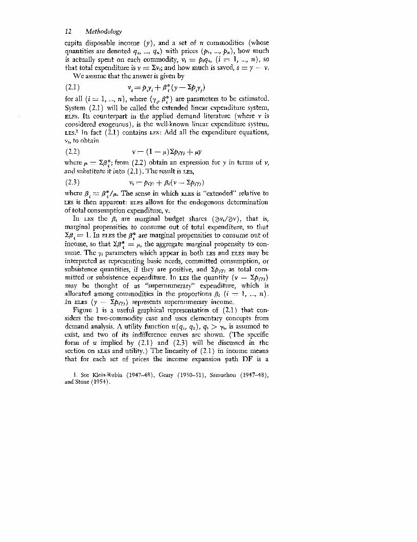
Figure I is a useful graphical representation of (2.1) that con-siders the two-commodity case and uses elementary concepts fromdemand analysis. A utility function u(q1, q2), qi > yi, is assumed toexist, and two of its indifference curves are shown. (The specificform of u implied by (2.1) and (2.3) will be discussed in thesection on ELES and utility.) The linearity of (2.1) in income meansthat for each set of prices the income expansion path DF is a

1. See Klein-Rubin (1947-48), Geary (1950-51), Samuelson (1947-48),and Stone (1954).

THE EXTENDED LINEAR EXPENDITURE SYSTEM (ELES) 13

Figure 1. ELES: The Two-Commodity Case

qY2

0'Y1 A B s/pt C

straight line from (7y,72, and the indifference map is homotheticto this point. If all income were spent on commodity 1, the amount

* OC would be consumed. According to (2.1), the value of BC is putaside for future consumption, and the value of OB is then allocatedamong the two commodities so that E is the chosen bundle, witha utility level it0 .

Why is the value of BC saved? It apparently results in a utilityloss; without saving, the utility level u, could be reached. The

14 Methodology

answer to this puzzle is simple. Figure 1 shows that maximizationof u(q,, q2 ) subject to the income constraint pjqj = y cannot yield(2.1) and therefore something else must be being maximized.

Two possibilities have been advanced. The first is that (2.1)represents optimal behavior at the beginning of a consumption plan(Lluch, 1973a). The plan is defined as the maximization of thepresent value of utility, u(t) = u(q 1 (t), q2 (t) ), 0 < t < oc, dis-counted at the fixed rate a > 0, subject to the constraint that thepresent value of expenditure cannot exceed initial wealth. This initialwealth has two components: nonhuman wealth that yields an incomeflow at the rate p, the rate of interest; and human wealth, the flowof expected labor income over the plan, discounted to the presentat the rate p. To justify the interpretation of (2.1) as behavior att = 0 the plan needs further restrictions: (a) u(t) is specified as anadditive logarithmic function of the Klein-Rubin type (see below);(b) expectations about prices and the interest rate are stationary;(c) the present value of expected changes in labor income is zero.

The second possibility was pointed out by Betancourt (1973) andelaborated independently by Howe (1975). Suppose that savingenters directly into the instantaneous utility function u(q1 , q2, s),which is also specified as a Klein-Rubin logarithmic function, butwvith committed saving set at zero (ys= 0).2 Instantaneous utilitymaximization, subject to the constraint pjqj + s = y, also yields(2.1 ) for any income concept, y.

From the point of view of this book, either of these possibilitiescan be chosen-or neither, in which case ELES iS considered just adescriptive device to organize data on household saving and expendi-ture allocation. We favor the first interpretation. It appears to givemore content to ELES3 and also to open avenues for further work.4

2. This has similarities with the original Klein-Rubin (1947-48) formula-tion. They state: "Some of the X, [our qi1 may be future commodities (savings),and the corresponding p, are the prices of the commodities properly discountedto the present" (p. 84n) .

3. For example, the marginal propensity to consume A is interpreted asa/p under the intertemporal derivation of (2.1). Thus if a = p, s = 0. Thecondition s > 0 is needed for the atemporal, but not the intertemporal, inter-pretation of ELES.

4. Some of which has already been carried out. See Kliin (1974) for alterna-tive ELES specifications allowing for time varying p and 8; for finite horizons,Klijn (1974), Mattei (1973); for discrete time formulations, Betancourt (1973),Powell (1974); for the introduction of adjustment costs, Clements, Evans,Ironmonger, and Powell (1975); for the treatment of durables, Dixon and Lluch(1975); for the introduction of accumulated consumption into the utilityfunction, Lluch (1974b).

THE EXTENDED LINEAR EXPENDITURE SYSTEM (ELES) 15

The second interpretation is a terminal one: Nothing much can besaid afterward.

Once BC in figure 1 is justified, questions about ELES begin inearnest. They boil down to the fact that ELES can be decomposedinto (2.2) and (2.3), and therefore combines the virtues and defectsof LES with a modified Keynesian consumption function:5

v/P = (I1- y) Y;yj + t, (Y/P),

which is just a rearrangement of (2.2) in which the price level isdefined as P = 1pj-yj/yj. In the consumption function, the marginalpropensity to consume appears in the intercept term as well as in itsconventional role as the coefficient of real income (y/P).

Why use ELES instead of LES in applied work? Or, for that matter,why apply either when more general and flexible demand systemsare available? The use of a linear system derived from an additiveutility function was elaborated upon in the Introduction. This bookdoes not deal with model generalizations for a given body of data.Rather the emphasis is on broad-based pattems and regularities asseen from the viewpoint of a fixed simple model, both in order tomake generalizations about the data and to learn more about thelimitations of the given model. Once the premium on simplicity isestablished, so is the use of the linear system without lags proposedhere.

The focus on ELES rather than LES in estimation is justified asfollows. One of the crucial concerns here is whether relative pricesmatter, and if so how much, in decisions regarding household savingand expenditure allocation. The effect of relative prices on savingcannot be measured at all with LES. The price effects on expenditureallocation, for a given total expenditure, would be identical in ELES

and LES if the parameter estimates coincided. But attaching astochastic specification to (2.1) rather than to (2.3) may alter theestimated values of parameters. Experience indicates that suchchanges in these values are substantial and that the y estimates are

* more stable and exhibit more regularities across countries under theELES specification (see chapter 3). Obtaining the best y estimatespossible is of particular importance because they determine priceeffects.

A further justification of ELES as against LES is that (2.2) enables

5. In the sense that total consumption expenditure is a function of currentincome. Notice that market disequilibrium and the distinction between notionaland actual demand are not necessary to obtain (2.2), which is therefore not aKeynesian function in the sense that Clower (1965) would have it.

16 Methodology

the identification of Ipjyj in the absence of price data (or variationin prices) if ,c #& 1. This fact will be amply used in chapters 5 to 9to obtain price elasticities from cross-section samples.

Some caveats remain, With a static Keynesian-type consumptionfunction and a linear system wvith no lags, no distinction betweenshort and long runs is possible.6 Also, in this linear system behavioris completely characterized by the focus D and the slope of DF infigure 1. The disadvantage of this simplicity is that there is limitedroom for price substitution. These linear systems are taken as localapproximations and are distinguished from the global as follows:In time-series applications, linearity is assumed to be good enoughfor per capita time series up to about fifteen years for each countryin the sample. In cross-section applications, linearity is consideredgood enough for homogeneous consumer groups, which are definedon the basis of a mixture of art, data, and preliminary empiricalresults. All applications are limited to broad commodity aggregates,in part so as not to stretch too much the additivity assumption (seethe section on ELES and utility), in part to focus on food expenditure,an important aspect of this work.

Elasticity Formulas

For convenience all relevant elasticity formulas for (2.1) are givenin this section together with their relationship to formulas for (2.3)-the ones obtained assuming constancy of total expenditure. Simplescalar transformations relate both sets of elasticities, and empiricalresults will focus on formulas relating to (2.3), for the purpose ofcomparison with those in the literature on consumer demand systems.Differences in results for the same body of data can, of course, beattributed solely to differences in the estimated values of parameters.

Each set of elasticities is expressed in two forms: in terms of afunction, the supernumerary ratio,-+,

(2.4) - ( = (v-Spjy 1 )/v,

and in terms of individual parameters and data (tables 2.1 and 2.2).7The following notation is used: w1 denotes the average budget share,v/v; ni, the expenditure elasticity of demand for the ith commodity;

q*. ), the uncompensated and expenditure-compensated price

6. Except for a brief departure in chapter 4. Note that in the time-serieswork only annual data are used.

7. Table 2.2 also includes other elasticity formulas developed in later sectionsof this chapter.

THE EXTENDED LINEAR EXPENDITURE SYSTEM (ELES) 17

Table 2.1. LES and ELES Elasticity Formulas in Termsof the Supernumerary Ratio

LES ELES

i = i/wi si= 'Mi

'?ii 77i-i(l + 11i, =j ini +(1)+ii=j

'1ij= 77tj=

-,qiwj(l + onj), t j tBj

7 3i(1 - Ai), i = j

- i ~~~~j'li = 7'7tj = i

(1 -. )( + Oni)W*

= - (1-A)

elasticities for a change in the jth price, with given total expenditure;(i, i7,j, $j), the corresponding income elasticity of demand and theuncompensated and income-compensated price elasticities, given dis-posable income; (y, ?), the elasticities of total consumption expendi-ture with respect to income and the ith price. The concepts ofexpenditure and income compensation under LES and ELES are dis-cussed in the next section.

The LES elasticity formulas (-q, , !) given in table 2.1 can beexpressed more compactly in matrix notation. Let {X}, {X} denotethe corresponding matrices. Then - -q(w' + f,l'), and{5t } = p (i - -2), where (-, w, p) are column vectors with typicalelements ( w4, 4i), and where a prime denotes transposition, whilea hat (^) indicates the corresponding diagonal matrix. Notice that

w = (, -i '), a symmetric matrix. Also, the following isimmediate,

(2.5)

so that the larger the value of 0, in absolute terms, the larger thesum of the substitution-effect components of own-price elasticities.In this sense ¢ measures the average price responsiveness in system(2.3).8

The rigidity in price responses allowed by LES is apparent from

8. See also Sato (1972).

Table 2.2. Annotated Formulas for Demand Elasticities in LES and ELES

Description Model Formula Comments

Elasticity of demnand forgood i with respect to:

Income ELES 77i- .i y/vt Always positive since no inferior goods are allowed. Would beunity if all 7i = 0 or if ,t = 1 and (#i/,5i) = (pieyjpjyj)for all i and j; see figure 2.1.

Total expenditure LES,ELES i7i = i/wi Always positive as above. Would be unity if all ey = 0 or if(Oilgi) = (Piyi/Pmyi) for all i and j.

PricesUncompensated

Pi-yico fLES 77ii= (1 - 0i)0 - 11 Strictly less than unity in absolute value except when yi is

Own vi negative and sufficiently large in absolute value. If "neces-sities" are associated with positive .Yi's, the own price elas-

ELES wii= (1-^.3i)- i -1 ticity of a necessity cannot exceed t in absolute value.ViJ

(LES 1ij = -0i3iyp/vi In the absence of negative y's, ordinary cross-price elasticitiesCross are negative, indicating that income effects swamp substi-

t ELES wi=nitution effects.Compensated

Own LES,ELES -(1 _ 0) -I Unambiguously negative provided actual spending on ith* \ vi J good, vi, exceeds subsistence expenditure, piyi.

Cross LES, ELES (. ) P~'~i'\ Unambiguously positive (indicating net substitutability)','~ \ v,} provided vi exceeds pi-yi.

Description Model Forinula Comminents

Elasticity of total ex-penditure with respect to

Income ELES X= y/v Ratio of marginal to average savings propensities.Price of good t ELES wi= (1 - p)piyi/v In the usual case, when y < 1 and yi > 0, has positive sign.Elasticity of saving

with respect to:Income ELES we = y/(y - p'Y) Unambiguously greater than 1 for p'y (cost of the subsistence

bundle) positive.Prices, ELES ti= -pi-yi(1 - A)/(y -v) Unambiguously negative provided the marginal and average

propensities to consume are less than 1.Frisch paramneter LES,ELES co -v/(v - p'-Y) The elasticity of the marginal utility of total expenditure with

respect to total expenditure, equal to the negative of the in-verse supernumerary ratio. With p'-y positive, asymptoticallyapproaches -1 from below as total expenditure gets larger.

Substitution elasticities LES,ELES o.ij = qi*j/wj = -sinj/lw Unambiguously positive, since no inferior goods are allowedand since to is required to be negative.

Note: A full glossary of symbols may be found at the front of the book. Symbols share of the ith commodity; y, income. In all cases, the commodity subscript i runs

used in this table are: as, the marginal budget share of the ith commodity in total from 1 through n.expenditure; yi, the basic needs or subsistence amount of the ith commodity; A, a. (i may also be interpreted as the price elasticity of the average savings ratio,

the marginal propensity to consume; pi, the price of the ith commodity; vi, the ex- (y - v)/y.penditure on the ith commodity; v, total expenditure; wi = vi/v, the average budget

20 Methodology

the formulas for price elasticities. If 0 < 0 and 0 < 8i < 1, con-ditions required by the utility specification (see the following section),then from the LES formulas in table 2.1 q* > 0, for all i 7 j, so thatall goods are net substitutes. In addition, if /i > 0 (i 1, ..., n)table 2.2 indicates that -1 < 1it < 0, and Bij < 0, i #z j, that is,demand is price inelastic and all goods are gross complements.Rigidity in income responses is also apparent. Marginal budgetshares are constant and, if pi > 0, inferior goods are ruled out.

All these restrictions imply that the model is to be used withcaution, because inferences from it should be adequate only forbroad commodity groups and a limited range of variability in totalexpenditure. It is argued here that this limited model is useful forthe purposes of this book. In particular, it focuses attention on aneglected contribution of demand analysis to the literature on de-velopment theory and planning: the influence of relative prices. Ifmuch of this influence consists of the income effects of price changes,there is no reason to ignore them. In particular, the price aspects ofEngel's law should be explored. One aspect is apparent from7i, = - i(1 + O- q)w 1 (where the subscript 1 denotes food), asgiven in table 2.1. Because the food budget share, w1, is large at lowlevels of income, yj, is likely to be relatively important in develop-ment planning.

Both the limitations and strengths of LES and ELES have their rootsin their implied utility specification. This aspect of the model isanalyzed in the next section.

ELES and Utility

It is well known that LES can be derived from utility maximizingbehavior, if the utility function is directly additive, namely,

It(q) =fi(q.1),

with the additional specification

fi (qi) = pi log (qi - y/); qi > -y;, ,Si > 0, ,Sfj =1

for all (i = 1, ..., n).9 Samuelson (1947-48) has emphasized thatthis is the only function that would yield (2.3). By implication,1fj[qj(t)] is also the only function that would yield ELES (2.1),when imbedded into an intertemporal utility maximization problem

9. See Geary (1950-51) and Samuelson (1947-48). The restriction q. > -yois required for the utility function to he defined. Then for marginal utilitiesto be positive the j3, must be positive.

THE EXTENDED LINEAR EXPENDITURE SYSTEM (ELES) 21

of the type specified in Lluch (1973a). The direct utility functionalassociated with this problem is

U[q(t)] f fo e- t1fi[qi(t)]dt

with

f4[qi(t) - pi log [q (t)- y]; qi (t) > yi, /3 > 0, i 1.

Notice that the y parameters are assumed to be constant in theconsumer plan.10

It follows that we are incurring all costs and benefits associatedwith additive utility functions, in particular that all price responsescan be expressed in terms of the income elasticities and just oneadditional term, (p. This implication of additivity was first noted byFrisch (1959) and Houthakker (1960), and emphasized by Sato(1972). For our purposes, it is reflected in the complete formalequivalence between formulas for 7ij in table 2.1 and the ones givenby Frisch and Sato. The difference in table 2.1 is, of course, one ofparameterization: what we consider constant over the relevant rangeof observations or which particular additive utility specification wechoose." Our choice is based on simplicity.'2 It is emphasized again

10. See Lluch (1974b), for a formulation in which the -y's are specifiedas linear functions of accumulated consumption of the it" commodity.

11. There are other additive utility specifications which produce more flexibledemand structures. The class has been explored by Pollak (1971), Johansen(1969), and Sato (1972); some have been applied empirically by Gamaletsos(1973) and Brown and Heien (1972). Sato's contribution is particularly note-worthy. He justifies the widely used double-log systems as approximations todemand systems obtained from an additive utility specification-a generalizedconstant elasticity of substitution function. He also presents a balanced discussionof pros and cons associated with alternative parameterizations. More recentlyDeaton (1974 and 1975) has argued against all additive utility specifications.Central to his argument is that nii/n, is approximately constant across com-modities under additivity (which requires w, and p,s to be of order I/n, wheren is the number of commodities); and the joint occurrence of n, < 0 and n., > 0for 9 of the 37 commodities considered. His use of the double-log form to testthe approximation overlooks Sato's contribution, where . is exactly constant.Deaton's results illustrate the difficulties that may arise with additive models atfine levels of commodity disaggregation, although he ignores the fact that theparameter estimates may violate the utility specification for many other reasons:use of total consumption as explanatory variable, assumption of no serial corre-lation in errors, estimation methods, or absence of lags, to list a few. See chapter3 below for additional evidence on the approximation.

12. For some extensions of ELES using alternative utility specifications, seeLluch (1973b).

22 Methodology

that, if , : 1, ELES permits identification of the additional term 0 inthe absence of price data or price variation, given that average andmarginal propensities to consume are related to 0 (using 2.2):v/y = [1 - (l-,b)/ ]- 1 , and therefore

(2.6) z 1-v/y _

v/y 1-I m

Under ELES the supernumerary ratio has then an added interpreta-tion as the ratio of the income elasticities of consumption, 9, andsaving, 78.

The choice of a specific form of the utility function raises severalquestions: How seriously do we consider (2.1) a device to estimateutility function parameters? How do we interpret changes in param-eter estimates across countries and within countries, and acrossconsumer groups? How much should we dwell upon the indirectutility implications of ELES (among them, for instance, the inter-pretation of 1/q as the expenditure elasticity of the marginal utilityof expenditure and the construction of true indexes of the cost ofliving)? The position taken on these questions is straightforward:ELES is a convenient tool, in applied consumption analysis, for atask parallel to parameter estimation in Cobb-Douglas productionfunctions. Both tasks can be accepted or rejected on similar groundsand are viewed as useful steps in the process of accumulatingempirical evidence. We therefore proceed to make statements onthe basis of (2.1) and its associated utility functional, making fulluse of the postulated model with some elementary cautions. Inkeeping with the limitations of linearity, its use is confined to broadcommodity groups and to the "center of gravity" of samples.

The empirical results that follow provide information for com-paring parameter values of the direct and indirect utility functionsassociated with ELES, both across and within countries. Referring tofigure 1, we shall analyze how D and the slope of DF change witheconomic development, in particular for the case of food and non-food. For a given level of development we shall be concerned withhow they change across homogeneous consumer groups.

An examination of the indirect utility function of ELES yieldsimportant theoretical results. First, all the well-known propositionsassociated with LES (treated exhaustively, for example, in Goldberger,1967, and Goldberger and Gamaletsos, 1970) hold. In particular,

4-?27ii = (i = 1, ..., n), so that the pi3's have both the inter-pretation of marginal budget shares and the own-price expenditurecompensation term. Also, the expenditure elasticity of the marginal

THE EXTENDED LINEAR EXPENDITURE SYSTEM (ELES) 23

utility of expenditure, t, which is a constant under many additiveutility specifications,13 is the function

(2.7) ,=

with k as defined in (2.4).Second, ELES contains also an income compensation concept,

which is equivalent to expenditure compensation in LES. The indirectutility function associated with the intertemporal interpretation ofELES is a linear transformation of the LES indirect utility function,with identical coefficients for the relevant differentials.14

Third, under ELES we can define the income elasticity of themarginal utility of income, cot, as the linear transformation of w,15

(2.8) co,* =M(0_ (1-)-

It follows from (2.8) and the definition of 7 in table 2.1 that theincome elasticity of total consumption expenditure can be expressed as

(2.9)

From (2.6) to (2.9) it follows also that the income elasticities ofsaving and of the marginal utility of income are the same in absolutevalue, that is, w(* -n, Both w'* and w will be used in the followingchapters for intercountrv comparisons of utility functions.

ELES and Saving

Hicks (1946, p. 177) wrote: "By eschewing utility we were able tosharpen the edge of our conclusions in economic statics; for thesame reason we shall be advised to eschew income and saving ineconomic dynamics. They are bad tools, which break in our hands."

Hicks's advice is ignored in this book, and this of course is doneat the cost of also ignoring all complications associated with thedefinition of income and saving. Pushed aside are problems associatedwith durable consumption goods, endogenous changes in tastes,unfulfilled expectations on prices and income, and uncertainty. Also,under the intertemporal interpretation of ELES, (2.1) is obtained only

13. See, again, Frisch (1959) and Sato (1972). We shall refer to w as theFrisch "parameter."

14. For details see Powell (1974), pp. 119-21.15. If the indirect utility functional G(y,p) is differentiated with respect to

y, GC = 31 (y - ,l'y)'. Expressing the marginal utility of income in flow termsand converting to elasticity form yields w* = -y (y - p',y)'. This can berewritten, using (2.2) and (2.7), as (2.8).

24 Methodology

if the present value of the time derivative of expected labor incomeis zero, an assumption whose empirical importance is not easy toevaluate.16

In spite of all this, we consider it fruitful to proceed to applica-tions as a first step toward a fuller integration of applied work ondemand systems and aggregate consumption functions. The resultingmodel of savings is static, since all intertemporal aspects of behaviorhave been reduced to relations at a given time and involve onlycurrent values of income and prices. The model is attractive for itssimplicity: Saving is positive, zero, or negative according to whetherthe marginal propensity to consume is smaller than, equal to, orlarger than one (see equation 2.10). The payoff is the identificationof price elasticities in cross sections, a payoff derived from the utilitystructure imposed and the ex post identity s = y - v.

The theory of saving put forwvard here is based on "impatience":the marginal propensity to consume is the ratio of the subjectiverate of discount to the rate of interest, that is, y = 8/p, so thats > 0 as 8 > p.17 This differs from Fisher's solution of the savingsproblem under certainty, which requires the equality of the rate ofinterest and the marginal rate of time preference as an equilibriumcondition. 18 It also differs from permanent income and life-cycleformulations, where zero interest rate and absence of time preferenceare compatible with positive saving.'9 We assume additivity overcommodities at a point in time and, intertemporally, over utilities;we then concentrate attention on behavior at the beginning of aconsumption plan, which is assumed to exist,20 with (real) time seenas the sequence of initial points of plans.

Whether the price paid is too high and the tools indeed break inour hands, can be judged after the empirical results are available.It is of interest to proceed to applications, given the added roleassigned to factors that traditionally were considered relevant onlyfrom the point of view of the allocation of total expenditure, whichpreviously was considered as exogenous. In particular, y estimates

16. An attempt is made in chapter 4 in the section on Taiwan.17. In ELES only if p > 8, that is, if A < 1, will the consumption of com-

modities along an optimal path increase over planning time. Yaari (1964)earlier showed this to be true in the context of a single-commodity optimalgrowth model.

18. See Fisher (1930), pp. 510-13.19. See, for example, Fama and Miller (1972), pp. 43-44.20. Existence in a broader context is shown by Uzawa (1968), who assumes

that a depends upon current utility.

STOCHASTIC SPECIFICATION AND ESTIMATION METHODS 25

are seen to be relevant also for savings behavior. Two examples of thisare given, both drawn from (2.2), which it is convenient to rewrite as

(2.10) s = (1 -A) (y- pjYj).I

If s' = - v/y, the average propensity to save, the following rela-tionship between s', IL, and U may be derived from (2.10):

1(2.11) s

Thus the Frisch parameter, which is a function of the y's, and themarginal propensity to consume jointly determine the average savingsratio under ELES.

The second example refers to the effect of changes in p1, theprice of food, on s'.21 The magnitude of this effect depends uponthe y1 estimate. The measure used is the elasticity of the averagesavings ratio with respect to the price of food as given by

Pi 's(2.12) s, = , p =- plY (I -A ,) /s =-Y (I -At) /S*

where s* = s/p,, that is, the real value of saving in terms of its pur-chasing power over food.2 2

The y, estimates play an important role in the subsistence bundle,as shown below, and this results in an important empirical regularityin e, as income increases.

Stochastic Specification and Estimation Methods

In outlining the economic assumptions which underly our chosenmodel, we eliminated subscripts for the unit of observation tosimplify presentation. Full econometric specification, however, re-quires precise statements as to which parameters are assumed to beconstant over the sample data and a complete description of theerror structure. In this section these requirements are met, and themethods used to obtain estimates of the parameters of the modelare then described.

21. The effect on saving of a change in import prices has been the subjectof considerable debate in the literature on international trade; for a convenientsummary see Johnson (1968), pp. 164-66.

22. Because income is exogenous the same formula applies for the elasticityof total saving with respect to food price.

26 Methodology

Stochastic Specification

In the stochastic specification of ELES we treat the deterministicformulation (2.1) as reflecting the mean value of commodity ex-penditures conditional on given values of the exogenous variables,prices and income. Thus we append to (2.1) additive errors withzero means.2 3 In general, variances and covariances of the error termsare assumed to be stationary.24 This stochastic representation ofELES may be written as

(2.13) Vit = pityi + fi3 (yt - Ypjtlj) + eitj=1

(2.14) E(et) = O, E(etet) =S,and E(etet,) = O, t =7 t'

where i denotes commodities (i = 1, ..., n), t denotes sample ob-servations (t = 1, ..., T), et is a vector of error terms (eit, ..., et)'and X is an n X n positive definite variance-covariance matrix oferrors across equations (commodities). In addition, et is assumedto come from a multivariate normal distribution. In the context of atime series t represents time periods (years), and assumption (2.14)rules out serial correlation in the errors.2 5 In a cross-section contextt represents households, and (2.14) rules out correlation of the errorsacross consumers. The explanatory variables (pit, yt) are taken to benonstochastic or, if stochastic, independent of eit.

Summing (2.13) over commodities yields the stochastic counter-part of the ELES aggregate consumption function (2.2):

(2.15) vt= (1 -) Pityi + ,MYt + etd=l

n

where et = E eit, E(c,) = 0, E(t=) = ', and c is a vector of units.i=1

23. In atemporal models such as LES, stochastic terms have sometimes beenincorporated into the utility function (see Pollak and Wales, 1969; Barten,1968). Byron (1974) has recently considered making stochastic the parameterrestrictions which are implied by utility theory. Our stochastic formulation, apartfrom being simpler to estimate, seems more appropriate in view of the fact that(2.1) may be derived from alternative problem formulations.

24. The exception is chapter 8 where the error terms are assumed to possessthese properties only after transformation of the variables.

25. The treatment of serial correlation is discussed in Lluch and Williams(1975a). For a thorough discussion of serial correlation in allocative modelssuch as LES, see Berndt and Savin (1975).

STOCHASTIC SPECIFICATION AND ESTIMATION METHODS 27In parameterizing the model the marginal propensity to consume,

c, is assumed to be constant over the sample data. If the inter-temporal utility-maximizing interpretation of ELES is adopted, thenconstancy of fx implies constancy of the ratio of the subjective rateof discount to the rate of interest, that is, of S/p. This would appear

* to be a valid assumption for our cross-section work, which considersonly groups of homogeneous consumers at a given time. With time-series data, however, the rate of interest will vary. Thus to assumeconstancy of A is to assume that 8 varies proportionally with p. Thisassumption may produce a misspecification bias if the model is fittedfor long periods, but the bias is likely to be less important for therelatively short periods considered in this analysis. In any event,our time-series results should be interpreted as pertaining to thesample mean values of 8/p.2 6

Following (2.13) and (2.14), the stochastic representation ofLES (2.3) is written as

(2.16) vit;=Pityi-+jp(vt- E; pjtyj) +-Itj=l

(2.17) E(ut) = O, E(utut) = A, and E(utuat4) = O, t # t'

w,Ahere i =1, ..., n; t,t' = 1, ..., T; ut = (Uit, ..., tlw)'; and A is ann X n singular variance-covariance matrix of errors. Singularity ofA follows from the property 'ut = 0. Joint normality of the errors isagain assumed.

In the first section of this chapter it was shown that deterministi-cally ELES may be decomposed into LES and an aggregate consumptionfunction. The stochastic version of LES obtained in this way is mosteasily seen by eliminating yt from (2.13) and (2.15). The error term

26. Powell (1973a) estimated an ELES consumption function using U.S.annual data in which a and p were estimated separately. The individual estimates

* of a and p were very sensitive to model specification but the ratio of a/p wasrelatively stable. Iacono (1976) has obtained similar findings in the context ofELES (and extensions) fitted to quarterly Australian data. An alternative param-eterization is to make the rate of interest a variable and the subjective rate ofdiscount a parameter to be estimated. Such an approach is adopted by Lluch(1974c). Using U.S. annual data for 1947-59 he finds that this parameterizationimproves the precision of the -y estimates compared with the parameterizationwhich treats g. as a constant. Lluch finds differences in the point estimates ofp and y for durables, but overall fit is similar for the two models. A difficultywith this approach for developing countries lies in choosing an appropriateinterest rate and obtaining time-series data.

28 Methodology

on LES now becomes

(2.18) uit = eit - iEt

for all i and t. If ELES (2.13) is the postulated model, equations(2.15) and (2.18) clearly imply that for LES there exists contempo-raneous correlation between ut and the stochastic explanatory vari-able vt, that is,

plim T- I v'ujt =7+ O (i =1..,n).t-l

Conventional maximum likelihood (ML) methods of estimation ofLES would therefore not be appropriate. Thus there are statisticalreasons for expecting the estimates of /3 and y obtained using ELES

(2.13) to differ from those obtained using LES (2.16).The maintained hypothesis in this book is ELES. The parameter

estimates reported are all obtained using this formulation, except fora few countries in chapter 3 where suitable time-series data on incomewere not available and LES estimates are given. In applications ofELES and LES to common sets of time-series data, ELES estimates werepreferred, for reasons discussed in chapter 3. In cross-section workthere are additional methodological reasons for preferring ELES whichare discussed below.

Time-Series Estimation

Both ELES (2.13) and LES (2.16) involve cross-equation restrictionson the parameters; in both cases all the yi occur in all equations. Thedemand systems must be estimated as a whole by methods whichimpose the cross-equation constraints. The procedure followed isdirect maximization of the likelihood functions associated with thesystems (2.13) and (2.16). In the case of ELES, the logarithm of thelikelihood function may be written as

nT T I T(2.19) L(e; p*, y, Q) n- ln27r - - Inill- EY e't-e,

2In the case of LES, an attempt to use (2.19) to write down thecorresponding likelihood function would involve replacing /3*, et,and 0-1 by ,3, ut, and A- respectively. Such a function is notdefined, however, since A is a singular matrix: 'ut = 0 and 'A = 0.A number of authors have shown that the solution is to omit oneequation (results being invariant to the equation dropped) and usethe constraint 1F - 1 to obtain the p estimate for the excluded

i

STOCHASTIC SPECIFICATION AND ESTIMATION METHODS 29equation.2 7 Thus if LES iS the maintained hypothesis, the log-likeli-hood function to be maximized is

(n-l)T T X IT(2.20) L(iu; #, y, A) = 2 1n27r- - In t 2 E tA-ut

where a tilde denotes deletion of entries for the nth equation; u and ,are n - I vectors and X is an (n - 1) X (n - 1) symmetricmatrix of error covariances.

The maximum likelihood estimates of 3*, y, and X are thosewhich maximize (2.19); the ML estimates of ,, y, and A are thosewhich maximize (2.20). The log-likelihood functions (2.19) and(2.20) are nonlinear in the parameters and were maximized usingthe modified Gauss-Newton method with analytical derivatives. Thebasic program used was the general nonlinear extremization packagewritten by Bard (1967) ,28

In this way maximum likelihood estimates of 3* and y areobtained for ELES and of 3 and y for LES. Under ELES, ML estimatesof M. and 3 are obtained from the relationships

n

(2.21) Y, 3Si=l

(2.22) (Si = 1])/E8@ $,t(i=1 ..., n).j=l

Asymptotic estimates of the variance-covariance matrices of esti-mated parameters in (2.13) and (2.16) were obtained from theHessian of the log-likelihood function evaluated at estimated param-eter values.29

27. See Barten (1969), Parks (1969, 1971), Powell (1969), Solari (1969,1971), and Deaton (1975). The problem is common to demand systems inwhich total expenditure, rather than income, is exogenous and the budgetconstraint holds exactly at all observations.

28. In earlier work (see Lluch and Powell, 1975). LES estimates wereobtained using LINEX, a LES specific program written by Carlevaro and Rossier(1970). The method used follows that of Solari (1969) and is similar to thatof Parks (1971). In test runs LES parameter estimates obtained using Bard'sprogram and LINEX were the same to five significant figures. There was sometendency for the standard errors of parameters to be a little smaller using Bard'smethod (of the order of 2 to 5 percent) owing to a slightly different specifi-cation of the Hessian. Although the likelihood functions for LES and ELES arevirtually isomorphic (see Powell, 1974, pp. 123-24), they are sufficiently differentto prevent the use of LINEX for the estimation of ELES.

29. See, for example, Dhrymes (1970), pp. 133-36. The procedure is spelledout in detail for LES in Parks (1971) and Deaton (1975).

30 Methodology

For ELES, let 10*p*, 3 and 1,, denote the asymptotic variance-covariance matrices of order n for the (Fe*, y) estimates. The (2n +1 ) asymptotic variance-covariance matrix of the (l,, ,, y) estimates isthen given by

L,:*3*!3S -11

L35

/J' L',,3*y

F -2tl* *J A y-

where J = (I - /3), and I is an n X n unit matrix.3 0

For LES, the variance of the omitted element of 8, 3,,, is obtainedfrom var ,, = I where the hat (^) denotes estimated valueand , is the (n- 1) asymptotic variance-covariance matrix forthe v?estimate.

In situations where the nonlinear procedure did not converge,ELES estimates were obtained by ruling out contemporaneous co-variances in the errors and assuming homoscedasticity across equa-tions, that is, we assume

(2.23) E(eret') = -oI.

In the case of LES estimates we assume

(2.24) E(ufit') = A o-z21I.

These procedures amount to a systems least squares (LS) approachand are in the tradition of earlier empirical work using LES.

3'

Cross-Section Estirnation with Price Variation

In a given economy at a given time, different consumers maypay different prices for the same goods. Regional differences may exist,for example, in the price of food or housing. Subgroups of consumers,however, are likely to face the same or very similar prices. The model

30. For the relevant asymptotic expression, see, for, example, Goldberger(1964),p. 125.

31. See Stone (1954) and Goldberger and Gamaletsos (1970). We estimateLES by systems least squares in a manner which permits a ML interpretation andtherefore direct calculation of standard errors of parameters (see Parks, 1971).The difficulty with the NIL interpretation is that since t'u, = 0, theoretically allcovariances cannot be zero. Specification (2.24) implies that the relationship

'A = 0 is preserved through nonzero covariances in the last row and columnof A. The parameter estimates we report for LES, LS, in chapter 3 are the sameas those obtained using the least squares option of LINEX, except for some smallchanges in the -y estimates for the Philippines.

STOCHASTIC SPECIFICATION AND ESTIMATION METHODS 31

estimated in chapter 5 assumes that households in the sample canbe divided into nine regional groupings. Within each group allhouseholds are assumed to face identical prices, but among groupsrelative price differentials are used. Thus for this application ELES

(2.13) may be written as

n

(2.25) Vih = Pih ,Yi +'T d(yh - E Pjh gyj) + eih=-1

where i denotes commodities (i = 1, ..., n), h denotes households(h = 1, ..., H), g denotes regions (g = 1, ..., G), and pih = pi, for

all hEg (i = 1, ... , n).32 Since all error covariances across householdsare already ruled out, the error specification (2.14) is unchanged,33as are the estimation methods for ELES described in the precedingsection.

Cross-Section Estimation in Absence of Price Data

As explained above, ELES enables all price elasticities to be estimatedin the absence of price data.3 4 The assumption that all consumersface identical prices is required, however, and for this reason werestrict estimation to groups of households where this assumptionis not likely to be grossly violated. In particular, we do not pool datafor urban and rural households.

Under the assumption that pih = pi (i = l, ... , n), where i denotesgoods and h households, the pjyi terms become independent of theunit of observation and may be replaced by y* (i - 1, ..., n), where-yi* measures subsistence expenditure in prices prevailing at the timeof the household survev. It should be noted that in comparing y *values across different groups of consumers, for example rural andurban, at a given time, the estimates will reflect any differences inprices paid by the various groups.

ELES (2.13) may now be written as

(2.26) Vih = ai + /8yh + eih

32. LES could be rewritten in a similar manner but it is not estimated.33. Replacing the subscript t by h.34. The estimation of ELES from household budget data was first implemented

by Belandria (1971); theoretical aspects of the procedure were systematized byPowell (1973b, 1974). Further contributions have been made by Betancourt(see chapter 8) and Howe and Musgrove (see chapter 7).

32 Methodology

where i = 1, ..., n goods; h - 1, ..., H households;35 and

n

ctj=y - /3* y*j.j=l

The error specification remains classical, that is, (2.14) with h re-placing t as a subscript.

The associated ELES aggregate consumption function is

(2.27) Vh = a + /yh + eh

n n n

where a = X ai = (I-') E y* and ch = E eih-

i=1 i=l i=l

Elimination of yt from (2.26) and (2.27) yields LES:

(2.28) Vih = a 3v + ±iVh + Uih

where ai' = ci/- Bia = *-fi I * and ui = ei- -fifh-

The system (2.26) is one of identical regressors in which everyleft-hand variable is regressed on the same set of exogenous variables.It follows that estimation of each of its equations by ordinary leastsquares (oLs), commodity by commodity, is equivalent to systemsmaximum likelihood estimationf36

Maximum likelihood estimates of fli (i = 1, ..., n) and /i are ob-tained from the estimates of ,*3 using (2.21) and (2.22);'7 ML esti-mates of y* and IyT are obtained from aj and ai* using the followingrelationships :-8

nt nn

(2.29) Y, yi* (1 s )- X as= (I1-,/)-E aii=1 i=1 i=l

(2.30) yai + [,i3(1 - I #3')- X af] =ai f3 + y*.j.=l j=1 j=1

35. The elasticity formulas in table 2.2 should also be reparameterized byreplacing pey with y9.

36. Retaining the assumption that the euh are joint normally distributed. Onall this see Zellner (1962); Goldberger (1964), pp. 207-12; and Dhrymes(1970), pp. 153-61.

37. This u estimate is identical to that obtained from estimating (2.27)by oLs.

38. Under LES it is not possible to unscramble estimates of the individual e.

STOCHASTIC SPECIFICATION AND ESTIMATION METHODS 33

The 2n variance-covariance matrix of (&, '*), which will be de-noted by a*, is obtained from

(2.31) n /V (X'X)-i

after appropriate rearrangement of the rows and columns, where Xis the H X 2 matrix of explanatory variables in (2.26) and g de-notes the Kronecker product. The elements, aij, of the error variance-covariance matrix f2 are estimated as

H6ej = (H - 2) - EF eile'jh (i,j = l..., n)

h=l

where e denotes estimated residuals from (2.26). The asymptoticvariance-covariance matrices of order n for , and y* are given by

E~~ ~~ =j3i'pt) Ei*s* (I - 43)

and

- (Njt y*N) YQ (* N'

where l* * is the (n X n) variance-covariance matrix for A* andN = [I + (1 - .) -1p*%']. It follows that var A ' t **, and varSYi*= The variances of A and 1y* may also be obtainedfrom ordinary least squares estimation of the aggregate consumptionfunction (2.27). The two methods yield identical estimates of thevariances.

In some empirical work we ignore covariances across equations(commodities) and assume that 0 in (2.31) is diagonal. The vari-ances across equations are, however, allowed to differ. That is, weassume

(2.32) E (eihejh) =Ovi i= j.=O i#j.

In this case the matric * is diagonal. The estimated variances ofthe estimates of / and lyj are no longer identical with those obtainedfrom OLS estimation of (2.27).

The basic cross-section equations (2.26) are, of course, linear Engelcurves with income as the explanatory variable. There has beenconsiderable discussion in the literature as to how the parameters ofEngel curves should be estimated to avoid bias. Summers' (1959, p.121) starting point is that "In estimating the parameters of Engelcurves, the assumption is made universally that a household's ex-

34 Methodology

penditure on the goods and services in its budget depend upon itsincome (and possibly other variables), but that its income does notdepend upon its expenditures." Hie then proceeds to formulate an(n + 2) simultaneous equation model, which is formally equivalentto our equations (2.26) and (2.27) plus the identity v = Evi. Usingthe arguments outlined by us in the section on stochastic specificationabove, he shows that ordinary least squares estimates of Engel curveswith total expenditure as the explanatory variable (our equation2.28) will yield parameter estimates which are biased and incon-sistent.3 9 In our terminology, ELES is the maintained hypothesis, fromwhich it follows that LES estimates are biased.

It is also argued, however, that measured or recorded income isnot the appropriate income variable to use in cross-section analysis.40

These arguments all reduce to one of errors in variables, whetherthey be based on the inaccuracy of household responses or failureto take account of normal or permanent income.

To overcome the problem of errors in variables, Liviatan (1961)proposed that consistent estimates of marginal budget shares beobtained by estimating Engel curves, with total expenditure as theexplanato,ry variable, using the method of instrumental variables withmeasured income as the instrument. But this method is identicalto our own, which estimates the f37 from Engel curves, with incomeas the explanatory variable, and ,. from the aggregate consumptionfunction, 41 and then divides to obtain estimates of 3,i. More formally,

E VihYh E Vihyh I Ey

h ~ ~~h h

where the expression after the first equality sign is Liviatan's instru-mental variable estimator of fli and the next expression correspondsto our method (all variables are now assumed to be deviated fromsample means). This provides a strong reason for concentrating onestimates of p. rather than p3t in presenting results. Of course the

39. Summers' article was a response to the classic work of Prais andHouthakker (1955). The latter were aware of such biases but deemed them tobe relatively unimportant (p. 63). Prais (1959) subsequently showed that thebiases average out over commodities; Powell (1973a) has derived a similarresult in the context of ELES and LES and worked out expressions for biases onindividual 7fT.

40. See, for example, Friedman (1957), Prais and Houthakker (1955),Liviatan (1961, 1964).

41. Recall that this is equivalent to using A = 2 S

STOCHASTIC SPECIFICATION AND ESTIMATION METHODS 35

argument regarding errors in variables still applies to estimates of ,and in the text we endeavor to point out where biases may be im-portant. Similarly, the presence of errors in variables implies theexistence of biases in the estimates of the yi, which should be bornein mind when considering estimates of price elasticities.42

42. In chapters 7 and 8 some comparisons are made with model estimatesobtained by directly introducing considerations of permanent income into thedefinition of income used as the explanatory variable in ELES.

3International Patterns in DemandParameters and Elasticities: Evidencefrom the National Accounts

As THE STARTING POINT for our empirical investigation we examine thedemand and savings behavior of the representative consumer for eachof seventeen countries spanning the development spectrum. To thiseffect we fit LES and ELES to aggregate national accounts data for eachcountry. Attention is focused on how marginal budget shares and theexpenditure and price elasticities vary with the level of GNP per capita.

Data Considerations

In order for intercountry comparisons of demand and savings be-havior to be useful for broad characterizations of the developmentprocess, it is necessary to include countries at all levels of economicdevelopment. Previous international comparisons using time-series datahave focused exclusively either on developed countries (Houthakker1965; Goldberger and Gamaletsos, 1970; Parks and Barten, 1973) oron developing countries (Weisskoff, 1971).

The basic data requirements for estimating models (2.13) and(2.16) are national accounts estimates in current and constant prices(in order to derive implicit price indexes) at the chosen eight-commodity level of aggregation (see table 3.1). In addition, personal

36

DATA CONSIDERATIONS 37

Table 3.1. Classification of Eight CommoditiesUsed in Time-Series Analysis

Commodity Commnodity title Commodities in UN nationalnumtber used in text accounts statisticsa

I Food Food, beverages, and tobacco2 Clothing Clothing and other personal effects3 Housing Household operation, rent, water, fuel,

and light4 Durables Furniture, furnishings, and household

equipment5 Personal care Personal care and health expenses6 Transport Transport and communication7 Recreation Recreation and entertainment8 Other services Miscellaneous services (financial services,

education and research, and other)

a. The definitions used are those given in the United Nations, Yearbook of National Accounts Statistics(1969). In the data for West Germany and Taiwan, commodities 3 and 4 are combined. Motor vehiclesare included in transport, and meals away from home are included in recreation.

disposable income data is required for ELES estimation.' The datamust be available for a sufficient number of years to permit econo-metric estimation. The basic data source was the United NationsYearbook of National Accounts Statistics, supplemented where neces-sary by national accounts publications of individual countries.2

Initially twenty-one countries were selected which satisfied theabove requirements and provided a reasonably even spread over thedevelopment spectrum. Two of these were subsequently found toexhibit hidden data peculiarities: Budget shares remained constantover the sample in Peru,3 and implicit price indexes were the samefor each good in Ecuador.4 Estimation problems led to dropping

1. In the empirical work presented in this chapter, permanent and measuredincome are assumed to be the same; in the context of Lluch (1973a) thepresent value of expected changes in labor income is zero. In chapter 4 wepresent results for Taiwan in which four different measures of permanent incomeare used. ELES estimates are similar in all cases.

2. Population figures were obtained from UN Demographic Yearbook andInternational Monetary Fund (IMF), International Financial Statistics, 1972Supplement.

3. Yielding expenditure elasticities of unity, own-price elasticities of minusone, and zero cross-price elasticities-a heaven for believers in Cobb-Douglasutility functions.

4. The price indexes for the Philippines also show very little differentialvariation, and model estimates should be treated with due care.

Table 3.2. Characteristics of the Sample of Seventeen Countries

Per capita personal Per capita private Implicit conver-disposable income at consumption at mid- sion ratio between

Per capita GNP midpoint of sample point of samnple NCU at sampleNational at midpoint of period period midpoint andcurrency sample period in 1970 U.S. dollars

Sample Sample unit 1970 U.S. 1970 U.S. 1970 U.S. (NCU perCountry period midpoint (NCU) dollars4 NCU'sb dollars NCU'sb dollars U.S. dollar)"

(1) (2) (3) (4) (5) (6) (7) (8) (9) (10)

Korea 1955-68 1962 Won 142 1080 115 112e 120 0.93660Thailand 1960-69 1964 Baht 148 1,952 115 1,729 102 16.96Philippines 1953-65d 1961 Peso 161 - - 407 125 3.248Taiwan 1955-68 1962 New Taiwan dollar 216 4,598 146 5,099 162 31.50Jamaica 1959-68 1964 Jamaican dollar 541 273 436 271 432 0.6266

c Panama 1960-68 1964 Balboa 564 - - 390 447 0.8723South Africa 1955-68 1962 Rand 596 260 461 226 401 0.5637Greece 1958-68 1963 Drachma 676 13,883 564 12,325 501 24.61Ireland 1955-68 1962 Irish pound 1,014 220 820 209 779 0.2682Puerto Rico 1955-67 1961 U.S. dollar 1,023 - - 683 828 0.8250Italy 1955-68 1962 Lira 1,207 4,124e 916 3,520e 782 4.5030Israel 1959-68 1964 Israeli pound 1,468 2,917 1,228 2,513 1,058 2.376United Kingdom 1955-68 1962 Pound 1,900 379 1,331 352 1,236 0.2847Australia 1955-66 1961 Australian dollar 2,192 1,015 1,622 932 1,489 0.6259West Germany 1955-68 1962 Deutsche mark 2,203 4,229 1,474 3,665 1,277 2.870Sweden 1955-68 1962 Krona 2,962 7,023 1,956 6,083 1,694 3.590United States 1955-68 1962 U.S. dollar 3,669 2,030 2,481 1,840 2,249 0.8182

- Data unavailable or unsatisfactory. c. Per capita GNP in NCU'S at sample midpoint divided by column 5. Source: Inter-a. Per capita GNP for 1970 as reported in World Bank Atlas 1972, projected back- national Monetary Fund, International Financial Statistics, 1972 SupPle,nent.

ward to sample midpoints using growth rates from the same source. Column 10 is used to derive columns 7 and 9.b. Sources: UN Yearbook of National Accounts Statistics, National Accounts of d. Years 1954, 1956, 1957, 1959 omitted.

OECD countries, 1953-69, and country national accounts. e. 102 NCU'S.

PARAMETER ESTIMATES 39

Sri Lanka and Chile from the sample.5 We thus report results forseventeen countries, which are listed in table 3.2 together with gen-eral characteristics of the data. The mean values of average budgetshares are given in table 3.3, changes in average budget shares intable 3.4, and price and income movements over sample periods intable 3.5. Suitable income data is available in thirteen cases.6 Thecountries are listed in order of GNP per capita at sample midpoints in1970 U.S. dollars. The level of per capita GNP covered by the dataranges from about $150 (Korea and Thailand) to near $4,000(United States). Table 3.2 also contains per capita estimates of totalconsumption expenditure and personal disposable income at samplemidpoints in both national currencies and 1970 U.S. dollars. Thereare of course well-known difficulties involved in converting values toa common currency unit,7 but here it is done for broad illustrativepurposes and as an aid in the interpretation of results. The modelsthemselves are always fitted separately for each country with dataexpressed in the national currency. In the majority of cases theperiod of estimation is 1955-68, giving fourteen observations. Allthe low-income countries are located in East Asia, a limitation incoverage that should always be bome in mind when making com-parisons of demand (and savings) behavior at different income levels.

Parameter Estimates

For the fourteen countries in table 3.2 for which personal incomedata exists, ELES (2.13) was fitted to national accounts data on percapita expenditures, per capita personal disposable income, and (im-plicit) prices using an eight-commodity breakdown. 8 The results ob-

5. LES estimates for Sri Lanka failed to converge; those for Chile wereobtained only for least squares, which produced extreme outliers for the yestimates and a supernumerary ratio greater than one (see Lluch and Powell,1975). Data limitations prevented ELES estimation in both cases.

6. Income data is available for Panama, but personal saving was foundto be negative in each year of the sample period. Because of concerns aboutthe data it was decided to estimate only LES.

7. See, for example, the interchange between Balassa (1973, 1974) andDavid (1972, 1973).

8. In Lluch and Williams (1975c) the estimates obtained on fitting ELES

are compared with LES estimates for the same or similar data. The two modelslead to similar levels of overall fit (as measured by R') and similar estimates ofthe marginal budget shares, p,, but ELES yielded y estimates which weretheoretically more acceptable (standard errors were roughly comparable). Forthese reasons we limit results to ELES, which in addition to estimates of 13 and eY

give insight into savings behavior. The detailed LES results are available in Lluchand Powell (1975).

Table 3.3. Average Budget Shares at Sample Mean Values

Commodity

Sample Personal OtherCountry period Food Clothing Housing Durables care Transport Recreation services

Korea 1955-68 0.599 0.104 0.114 0.028 0.042 0.047 0.044 0.022Thailand 1960-69 0.576 0.084 0.080 0.032 0.056 0.079 0.075 0.018Philippines 1953-65a 0.598 0.074 0.147 0.020 0.035 0.023 0.018 0.084Taiwan 1955-68 0.563 0.055 0.183 0.057 0.018 0.026 0.097Jamaica 1959-68 0.433 0.107 0.145 0.060 0.026 0.106 0.074 0.049Panama 1960-68 0.455 0.074 0.167 0.064 0.047 0.094 0.075 0.023South Africa 1955-68 0.368 0.118 0.167 0.078 0.048 0.132 0.047 0.041Greece 1958-68 0.468 0.122 0.183 0.039 0.036 0.069 0.061 0.023Ireland 1955-68 0.492 0.100 0.128 0.057 0.013 0.088 0.063 0.059Puerto Rico 1955-67 0.356 0.106 0.153 0.069 0.069 0.123 0.088 0.037Italy 1955-68 0.463 0.101 0.166 0.032 0.063 0.081 0.075 0.018Israel 1959-68 0.319 0.094 0.192 0.074 0.066 0.073 0.081 0.100United Kingdom 1955-68 0.397 0.107 0.183 0.066 0.023 0.109 0.075 0.040Australia 1955-66 0.333 0.110 0.127 0.078 0.057 0.131 0.043 0.121West Germany 1955-68 0.366 0.123 0.263 0.037 0.080 0.077 0.054Sweden 1955-68 0.366 0.115 0.159 0.070 0.037 0.142 0.089 0.024United States 1955-68 0.267 0.095 0.227 0.073 0.081 0.152 0.055 0.049

a. Excluding 1954, 1956, 1957, 1959.

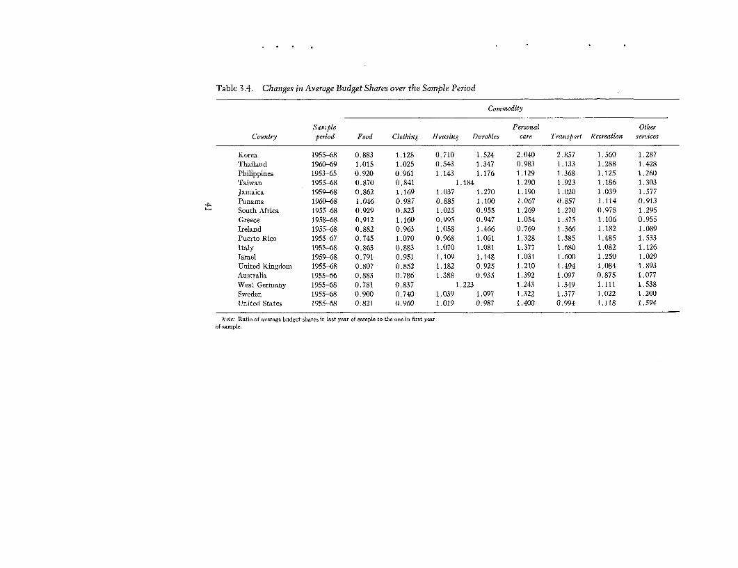
Table 3.4. Changes in Average Budget Shares over the Sample Period

Commodity

Sample Personal OtherCountry period Food Clothing Housing Durables care Transport Recreation services

Korea 1955-68 0.883 1.128 0.710 1.524 2.040 2.857 1.560 1.287Thailand 1960-69 1.015 1.025 0.543 1.347 0.983 1.133 1.288 1.428Philippines 1953-65 0.920 0.961 1.143 1.176 1.129 1.368 1.125 1.260Taiwan 1955-68 0.870 0.841 1.184 1.290 1.923 1.186 1.303Jamaica 1959-68 0.862 1.169 1.037 1.270 1.190 1.020 1.039 1.577Panama 1960-68 1.046 0.987 0.885 1.100 1.067 0.857 1.114 0.913South Africa 1955-68 0.929 0.825 1.025 0.955 1.269 1.270 0.978 1.295Greece 1958-68 0.912 1.160 0.995 0.947 1.054 1.375 1.106 0.955Ireland 1955-68 0.882 0.963 1.058 1.466 0.769 1.366 1.182 1.089Puerto Rico 1955-67 0.745 1.070 0.968 1.061 1.328 1.385 1.485 1.533Italy 1955-68 0.863 0.883 1.070 1.081 1.377 1.680 1.082 1.126Israel 1959-68 0.791 0.951 1.109 1.148 1.031 1.600 1.250 1.029United Kingdom 1955-68 0.807 0.852 1.182 0.925 1.210 1.494 1.084 1.893Australia 1955-66 0.883 0.786 1.388 0.935 1.392 1.097 0.875 1.077West Germany 1955-68 0.781 0.837 1.223 1.243 1.349 1.111 1.538Sweden 1955-68 0.900 0.740 1.039 1.097 1.322 1.377 1.022 1.200United States 1955-68 0.821 0.960 1.019 0.987 1.400 0.994 1.118 1.594

Note: Ratio of average budget shares in last year of sample to the one in first yearof sample.

Table 3.5. Changes in Implicit Price Deflators and Income over the Sample Period

Prices Income

Sample Personal Trans- Recrea- OtherCountry period Food Clothing Housing Durables care port tion services Total Money Real

Korea 1955-68 5.617 6.802 4.329 5.102 8.771 5.208 6.097 6.849 5.707 8.187 1.435Thailand 1960-69 1.338 1.017 0.789 0.863 1.127 1.005 1.245 1.199 1.183 1.599 1.351Philippines 1953-65 1.416 1.419 1.415 1.418 1.420 1.411 1.401 1.417 1.416 1.678, 1.185aTaiwan 1955-68 2.087 1.310 1.865 1.531 1.805 1.642 1.347 1.901 3.461 1.821Jamaica 1959-68 1.303 1.210 1.633 1.002 1.261 1.044 0.750 1.912 1.235 1.609 1.302Panama 1960-68 1.169 1.048 1.044 1.009 1.196 1.033 1.081 1.000 1.169 1.3753 1.1763South Africa 1955-68 1.344 1.027 1.577 1.042 1.661 1.366 1.383 1.555 1.327 1.657 1.249Greece 1958-68 1.293 1.127 1.172 1.069 1.282 1.206 1.057 1.071 1.207 2.144 1.776Ireland 1955-68 1.512 1.122 1.677 1.506 1.189 1.503 1.602 1.736 1.495 2.198 1.470Puerto Rico 1955-67 1.369 1.189 1.165 1.105 1.995 1.330 1.468 1.343 1.369 1.7773 1.298aItaly 1955-68 1.388 1.326 1.607 0.979 1.736 1,344 1.697 1.724 1.449 2.737 1.889Israel 1959-68 1.547 1.519 2.020 1.191 1.788 2.066 1.712 1.915 1.681 2.965 1.764United Kingdom 1955-68 1.315 1.248 1.838 1.246 1.494 1.464 1.824 1.639 1.484 2.011 1.355Australia 1955-66 1.291 1.165 1.709 1.054 1.414 1.240 1.379 1.394 1.316 1.593 1.211West Germany 1955-68 1.248 1.298 1.524 1.533 1.168 1.349 1.706 1.360 2.432 1.788Sweden 1955-68 1.683 1.340 1.650 1.262 1.449 1.569 1.730 1.618 1.574 2.276 1.446United States 1955-68 1.272 1.234 1.248 1.074 1.485 1.219 1.358 1.751 1.275 1.761 1.381

Note: Ratio of implicit price deflators and per capita personal disposable income in a. Per capita total consumption expenditure.last year of sample to first year of sample.

PARAMETER ESTIMATES 43

tained in this manner are supplemented by LEs estimates for the threecountries (Panama, Puerto Rico, and Philippines) in which suitableincome data are not available.

Table 3.6 contains estimates of the marginal propensity to con-sume, c, and marginal budget shares, p,s, together with estimates oftheir asymptotic standard errors. The method of estimation is givenin each case; systems least squares results (LS) imply that full ML

estimation failed to converge. Estimates of the y parameters andassociated standard errors are given in table 3.7. The units ofmeasurement are national currencies at base-year prices. In table 3.8these values are converted to 1970 U.S. dollars by using samplemidpoint prices and the conversion ratios given in table 3.2.

Overall fit is high, as is to be expected from time-series data: Thevalues of the coefficient of determination, R2 , exceed 0.95 in 103 ofthe 134 equations (see table 3.9).9 Values of the Durbin-Watsond statistic, however, show fairly marked positive first-order serialcorrelation in the residuals of individual equations, and reportedstandard errors should be interpreted with due care.10 Serial correlationis less marked on the equations for food and clothing (mean value ofd is 1.4 in each case) and most pronounced in the case of personalcare and other services (mean d values are around 0.9). Detailedresults are given in table 3.10.

Estimates of the marginal propensity to consume range from 0.58(Israel) to 0.93 (Korea); all are less than unity; all have relativelysmall standard errors. The values do not appear to move in anysystematic way with GNP per capita. There is some evidence that themarginal propensity to save out of current income is higher in thosecountries with higher rates of growth in income. The rank correlation

9. Calculated as R- = 1 - [z2d /z(v -v- )2] where u2 denotes residuals

from expenditure equations. It is to be interpreted solely as a descriptive indicatorof goodness of fit.

10. Again, the d statistic in this context is a descriptive indicator withunknown statistical properties. While LES and ELES tend to yield very similard values, it has been shown in Lluch and Williams (1975a) that, for U.S.data at least, allowance for serial correlation does not substantially affect thepoint estimates obtained using ELES, but it affects LES estimates markedly.

Another form of potential error misspecification is the assumption of constanterror variances over time, particularly as the dependent variables are in currentprices. Two sets of ELES estimates obtained for Korea using data for 1963-72in both current and real values yielded remarkably similar results for bothparameter estimates and standard errors (the current price results are containedin table 5.15). This result is noteworthy in that the ratio of the consumer priceindex at sample end to sample beginning was 3.35 (compare table 3.5).

Table 3.6. Estimated Marginal Propensity to Consume (y) and Marginal Budget Shares (,a,)

Marginal budget share (a)

Type of Personal Trans- Recrea- OtherCountry estinatel ,u Food Clothing Housing Durables care port tion services

Korea ELES, ML 0.928 0.434 0.069 0.085 0.077 0.074 0.146 0.078 0.0384. (0.028) (0.024) (0.011) (0.010) (0.006) (0.009) (0.007) (0.005) (0.005)

Thailand ELES, LS 0.759 0.482 0.101 0.013 0.052 0.052 0.123 0.150 0.028(0.035) (0.027) (0.014) (0.001) (0.001) (0.017) (0.014) (0.020) (0.018)

Philippines LES, LS - 0.311 0.055 0.267 0.044 0.060 0.056 0.030 0.176- (0.019) (0.019) (0.019) (0.019) (0.019) (0.019) (0.019) (0.050)

Taiwan ELES, ML 0.667 0.317 0.069 0.244 0.097 0.051 0.046 0.176(0.011) (0.017) (0.015) (0.009) (0.009) (0.003) (0.002) (0.007)

Jamaica ELES, LS 0.922 0.249 0.208 0.103 0.159 0.060 0.161 0.150 -0.090(0.018) (0.036) (0.031) (0.057) (0.023) (0.027) (0.024) (0.023) (0.067)

Panama LES, LS - 0.418 0.081 0.113 0.113 0.044 0.085 0.127 0.019- (0.023) (0.018) (0.017) (0.017) (0.021) (0.016) (0.019) (0.039)

South Africa ELES, ML 0.621 0.295 0.164 0.066 0.115 0.049 0.206 0.046 0.059(0.083) (0.036) (0.025) (0.013) (0.030) (0.013) (0.049) (0.006) (0.011)

Greece ELES, LS 0.810 0.341 0.168 0.175 0.050 0.048 0.107 0.083 0.028(0.051) (0.028) (0.006) (0.007) (0.007) (0.011) (0.009) (0.005) (0.007)

Ireland ELES, ML 0.846 0.315 0.134 0.108 0.114 0.014 0.170 0.075 0.070

(0.018) (0.011) (0.007) (0.005) (0.005) (0.002) (0.007) (0.005) (0.007)

Puerto Rico LES, ML - 0.177 0.112 0.144 0.068 0.114 0.176 0.137 0.072

- (0.009) (0.004) (0.004) (0.004) (0.007) (0.007) (0.004) (0.004)

Italy ELES, ML 0.790 0.401 0.087 0.171 0.069 0.066 0.117 0.070 0.019

(0.034) (0.017) (0.005) (0.018) (0.019) (0.025) (0.016) (0.010) (0.003)

Israel ELES, LS 0.577 0.210 0.103 0.172 0.119 0.066 0.116 0.117 0.097

(0.020) (0.011) (0.011) (0.014) (0.010) (0.013) (0.014) (0.013) (0.014)

United Kingdom ELES, ML 0.890 0.120 0.067 0.258 0.076 0.030 0.277 0.066 0.106(0.011) (0.016) (0.007) (0.039) (0.017) (0.003) (0.011) (0.010) (0.020)

4 Australia ELES, LS 0.796 0.143 0.050 0.220 0.082 0.133 0.224 0.009 0.138(0.021) (0.011) (0.010) (0.024) (0.009) (0.013) (0.011) (0.012) (0.013)

West Germany ELES, ML 0.807 0.243 0.096 0.321 0.045 0.116 0.085 0.094

(0.014) (0.018) (0.006) (0.016) (0.003) (0.003) (0.001) (0.007)

Sweden ELES, ML 0.810 0.278 0.071 0.145 0.079 0.052 0.253 0.097 0.024

(0.004) (0.027) (0.014) (0.014) (0.007) (0.005) (0.014) (0.014) (0.008)

United States ELES, MI 0.836 0.090 0.108 0.206 0.106 0.137 0.174 0.065 0.113(0.025) (0.008) (0.007) (0.014) (0.009) (0.013) (0.011) (0.003) (0.015)

- Parameter does not occur in model. a. Ls: least squares; ML: maximum likelihood.Note: Asymptotic standard errors are given in parentheses.

Table 3.7. Estimated Subsistence Minimums (yi)

Base Personal Other Sum ofCountry year Food Clothing Housing Durables care Transport Recreation services

Korea 1965 130.5 22.8 21.0 3.9 7.6 4.3 7.2 3.2 200.5(1.5) (0.6) (0.6) (0.5) (0.5) (0.4) (0.3) (0.2) (2.1)

Thailand 1962 623.5 68.0 179.2 15.6 57.8 37.9 6.5 8.7 977.2(82.5) (20.3) (12.4) (13.9) (18.6) (22.0) (31.1) (17.6) (175.4)

Philippines 1955 192.3 23.1 40.6 5.2 9.8 6.0 5.0 22.7 304.8(22.7) (4.1) (19.5) (3.3) (4.5) (4.1) (2.3) (13.0) (73.0)

Taiwan 1966 2,562.9 175.6 588.8 157.2 20.8 71.9 228.9 3,806.1(37.8) (4.9) (22.4) (16.6) (5.4) (4.9) (14.9) (73.0)

Jamaica 1960 72.2 -0.5 20.0 -6.2 -1.5 5.9 -1.2 20.8 109.5(8.0) (6.6) (7.3) (3.9) (4.0) (4.1) (3.0) (6.2) (27.9)

Panama 1960 86.4 12.3 42.2 1.2 8.9 18.9 2.7 4.9 177.5(28.2) (6.4) (7.2) (6.2) (5.3) (5.4) (9.1) (8.8) (62.0)

South Africa 1958 71.3 22.2 33.5 13.8 8.3 22.0 8.7 6.6 186.3(3.9) (2.4) (1.0) (2.3) (0.8) (3.6) (0.6) (0.8) (14.5)

Greece 1958 3,000.0 277.2 936.9 107.4 73.6 57.5 137.0 69.3 4,658.8

(870.8) (398.8) (409.6) (155.4) (171.0) (275.5) (209.2) (112.2) (2,572.0)

Ireland 1963 84.5 12.6 21.1 5.1 1.7 8.3 8.8 8.6 150.8

(3.1) (1.0) (1.1) (1.2) (0.2) (1.7) (0.9) (0.8) (9.5)

Puerto Rico 1963 156.8 11.4 27.6 10.2 -17.9 -13.4 -17.1 -15.7 141.9

(13.6) (6.4) (7.3) (3.5) (10.1) (11.2) (9.0) (4.3) (60.0)

Italy 1963 844.9 182.1 245.5 -46.6 98.6 50.1 129.3 24.3 1,528.2

(169.9) (37.7) (112.1) (27.1) (86.2) (79.8) (50.6) (15.3) (515.0)

Israel 1964 652.3 165.0 397.1 117.4 122.5 116.5 136.4 190.1 1,897.2

(10.7) (8.2) (12.9) (8.2) (9.0) (10.7) (9.9) (10.5) (52.8)

United Kingdom 1963 117.2 24.7 12.4 7.7 1.8 -18.8 13.5 -7.5 151.1

(3.6) (1.4) (12.1) (3.6) (0.6) (4.8) (2.6) (5.1) (20.9)

4 Australia 1966 302.9 93.3 58.0 46.0 10.3 52.8 43.7 79.4 686.5

(7.7) (4.5) (18.7) (4.1) (8.6) (8.7) (5.3) (8.8) (52.2)

West Germany 1954 579.1 164.5 96.0 13.4 -10.4 44.9 -32.7 854.7

(65.2) (22.5) (69.5) (9.8) (20.8) (14.3) (22.9) (194.8)

Sweden 1959 973.3 379.5 360.8 101.4 12.2 -140.4 136.1 43.4 1,866.3

(331.0) (45.7) (180.5) (69.2) (6.2) (277.5) (131.2) (53.1) (1,107.4)

United States 1963 416.1 67.2 224.3 28.0 12.4 110.2 38.5 -25.2 871.6

(18.9) (14.3) (47.3) (12.0) (36.3) (33.3) (13.6) (35.2) (20.1)

Note: Measured in national currency units (NCTU'S) per capita in base-year prices, are given in parentheses.except for Korea and Italy where the units are 102 NCU'S. Asymptotic standard errors

Table 3.8. Estimates of per Capita Subsistence Expenditure (p3 y7 ) at Sample Midpoint in 1970 U.S. Dollars

Sample Personal OtherCountry midpoint Food Clothing hlousing Durables care Transport Recreation services Total -¢

Korea 1962 68.7 11.7 13.7 1.9 3.7 3.6 4.2 2.7 110.3 0.097Thailand 1964 36.9 3.9 7.2 0.9 3.4 2.2 0.4 0.5 55.5 0.467Philippines 1961 69.1 8.3 15.4 1.9 3.5 2.2 1.8 8.2 110.3 0.096Taiwan 1962 74.3 5.4 17.5 4.9 0.7 2.1 7.5 112.3 0.241Jamaica 1964 127.7 -1.1 39.9 -10.1 -2.4 8.8 -1.8 41.2 202.5 0.520Panama 1964 105.8 14.1 49.1 1.4 11.2 22.9 3.1 5.6 213.2 0.536

*, South Africa 1962 133.9 38.9 66.9 25.0 17.4 42.8 17.2 14.0 356.0 0.151x Greece 1963 137.1 11.5 41.7 4.5 3.3 2.6 5.6 2.9 209.2 0.583

Ireland 1962 309.8 45.9 76.1 18.6 6.3 29.8 31.7 30.9 549.2 0.269Puerto Rico 1961 183.0 13.6 32.5 12.2 -20.6 -16.7 -20.0 -18.5 165.5 0.794Italy 1962 172.6 38.1 51.8 -10.1 19.8 10.7 26.5 4.9 314.3 0.569Israel 1964 274.5 69.4 167.1 49.4 51.6 49.0 57.4 80.0 798.5 0.189United Kingdom 1962 405.3 85.7 41.4 27.0 6.3 -67.1 46.0 -25.6 519.5 0.574Australia 1961 424.3 141.1 76.1 75.6 14.1 77.0 59.9 108.6 976.7 0.351West Germany 1962 230.4 65.7 40.9 6.1 -3.9 18.7 -15.8 342.2 0.701Sweden 1962 313.4 116.5 106.5 31.1 3.8 -43.1 43.3 13.3 584.8 0.649United States 1962 501.5 81.9 270.8 34.3 14.9 134.9 46.1 -29.5 1,055.0 0.539

Note: Conversions made by multiplying each -yi in table 3.7 by the value of the sion factors given in the last column of table 3.2.corresponding pi at the sample midpoint and then dividing by the implicit conver-

Table 3.9. Coefficients of Determination (Re) for Fitted Models

Commodity

Personal OtherCountry Food Clothing Housing Durables care Transport Recreation services

Korea 0.9988 0.9945 0.9959 0.9896 0.9866 0.9928 0.9914 0.9698Thailand 0.9791 0.9581 0.9720 0.9184 0.9253 0.9510 0.9595 0.9209Philippines 0.9958 0.9830 0.9891 0.9663 0.9940 0.9627 0.9968 0.9625Taiwan 0.9950 0.9927 0.9933 0.9289 0.9516 0.9786 0.9852Jamaica 0.9313 0.9453 0.9734 0.9598 0.8475 0.9292 0.9304 0.9520Panama 0.9762 0.9273 0.9334 0.9142 0.9289 0.6882 0.9575 0.8473South Africa 0.9876 0.8645 0.9948 0.8162 0.9711 0.9040 0.9834 0.9640Greece 0.9966 0.9907 0.9834 0.8908 0.8571 0.9792 0.9698 0.5700Ireland 0.9975 0.9772 0.9954 0.9868 0.7656 0.9898 0.9875 0.9756Puerto Rico 0.9929 0.9911 0.9952 0.9698 0.9841 0.9870 0.9937 0.9702Italy 0.9957 0.9807 0.9969 0.5283 0.9268 0.9439 0.9892 0.9803Israel 0.9980 0.9795 0.9960 0.8401 0.9944 0.9879 0.9900 0.9925United Kingdom 0.9983 0.9925 0.9869 0.9178 0.9963 0.9638 0.9948 0.8773Australia 0.9938 0.9531 0.9797 0.8687 0.9724 0.9804 0.8974 0.9882West Germany 0.9774 0.9850 0.9890 0.9864 0.9954 0.9983 0.9847Sweden 0.9980 0.9751 0.9913 0.9700 0.9835 0.9914 0.9917 0.8887United States 0.9923 0.9855 0.9813 0.9695 0.9834 0.9727 0.9945 0.9844

Table 3.10. Durbin-Watson d Statistics for Fitted Models

Commodity

Personal OtherCountry Food Clothing Housing Durables care Transport Recreation services

Korea 2.24 2.29 1.06 2.09 1.23 0.88 1.76 0.83Thailand 1.64 1.29 0.57 0.74 0.89 1.30 1.54 0.76Philippines 1.46 1.02 1.76 1.81 0.69 0.61 2.41 0.63Taiwan 1.31 1.75 1.92 0.36 0.73 0.68 1.04

Jamaica 1.41 2.35 1.34 1.09 1.85 2.40 1.04 1.39Panama 1.80 2.23 1.04 2.37 1.06 0.72 2.49 1.26

South Africa 1.39 0.76 1.10 0.84 0.55 0.78 0.89 0.72Greece 0.58 1.43 0.85 0.35 0.37 0.75 0.66 0.29Ireland 1.54 2.15 1.42 1.48 0.55 1.86 1.02 0.94Puerto Rico 1.46 1.35 1.15 0.95 1.16 0.84 1.23 1.29Italy 1.03 0.66 0.98 0.24 0.15 0.30 0.26 0.76Israel 1.53 2.18 1.50 2.05 1.77 1.41 1.93 2.29United Kingdom 1.07 1.13 0.75 0.59 1.01 0.40 1.29 0.53Australia 1.38 1.28 0.90 0.87 1.04 1.57 0.38 1.00West Germany 0.32 0.89 0.66 0.70 1.30 1.33 0.71Sweden 1.12 0.54 0.69 0.60 0.90 1.53 1.16 0.68

United States 2.15 0.75 0.22 0.44 0.26 2.27 0.65 0.69

PARAMETER ESTIiMATES 51

coefficient between 1 - and the annual average rate of growthof real per capita personal disposable income over the sample periodis 0.34. The coefficient is 0.60 if South Africa is excluded, a resultsignificantly different from zero at the 5 percent level, although theformer result is not.

The estimated marginal budget shares, 6B, are all positive as re-quired except in one case (Jamaica, other services), where the valueis not significantly different from zero. In only six other cases is theratio of the 6i estimate to its standard error less than 2, and all butone of these fall in the categories of recreation and other services.

In order to discern patterns in the A estimates we first averagevalues for countries at similar levels of economic development asmeasured by the sample midpoint of GNP per capita in 1970 U.S.dollars. Second, we regress parameter estimates on the commonlogarithm of GNP per capita." Both sets of results (see table 3.11)show that the marginal budget share for food decreases markedly asGNP per capita rises, whereas the p estimates for housing and transportrise with income. The marginal budget share for food at the highestincome levels is only half that for the low-income countries: 0.18 forper capita GNP over $1,500, 0.39 for per capita GNP less than $500.The exact opposite is true for housing and transport. No strongpatterns emerge for other commodities, although there is sometendency for the marginal budget share for durables to increase withincome,' 2 and that for clothing is highest at middle income levels.'3

The y estimates are determined with considerably less precisionthan the /3 estimates. Thirty-three of the 110 ELES estimates of yi areless than twice their standard errors (in absolute terms), as are twelveof the twenty-four LES estimates. Fifteen of the y estimates are nega-tive, but Jamaica and Puerto Rico account for eight of these. For thebasic commodities, food, clothing, and housing, however, the y esti-mates behave as "subsistence" parameters-all estimates but one(clothing, Jamaica) are positive. These y values increase with levelsof GNP per capita (see table 3.8), but more precise quantification ofthis phenomenon is left until chapter 4.

At mean values the sum of the y estimates is always less thanactual consumption expenditure, as required by the underlying utility

11. Notice that the regressions preserve the identity 2i = 1 at any level ofGNP per capita.

12. Recall that expenditure on motor vehicles is included in transport notdurables.

13. Note the low value for the Durbin-Watson d statistic, which suggestsa curvilinear relationship between p. and per capita GNP.

Table 3.11. Relation between Marginal Budget Shares (pj) and Level of GNP per Capita

Personal OtherItem Food Clothing Housing Durables care Transport Recreation services

Mean values of /iGNP per capitaa

100-500 0.386 0.074 0.122 0.074 0.071 0.094 0.076 0.105500-1,000 0.351 0.138 0.118 0.092 0.047 0.133 0.085 0.0351,000-1,500 0.276 0.109 0.149 0.093 0.065 0.145 0.100 0.0651,500 and over 0.175 0.078 0.209 0.090 0.079 0.209 0.064 0.095

Overallmean 0.286 0.096 0.155 0.087 0.068 0.150 0.080 0.079

Regressions of fiS = a + b logio GNP per capitab

a 0.805- 0.081 -0.049 0.040 0.030 -0.092 0.097 0.089(0.132) (0.059) (0.102) (0.042) (0.058) (0.088) (0.064) (0.088)

b -0.179e 0.005 0.070d 0.016 0.013 0.083c -0.006 -0.004(0.045) (0.020) (0.035) (0.014) (0.020) (0.030) (0.022) (0.030)

R2 0.531 0.005 0.228 0.084 0.029 0.354 0.005 0.001d 2.45 1.00 2.36 2.41 2.50 2.32 2.60 1.78

Note: Based on table 3.6; Jamaica excluded. (Oa + 04) divided 1:1 for Taiwan, capita so that Durbin-Watson d statistic indicates appropriateness of functional2:1 for West Germany. form.

a. In 1970 U.S. dollars at sample midpoints. c. Significant at 5 percent level.b. Standard errors in parentheses. Data ranked in order of increasing GNP per d. Significant at 10 percent level.

TOTAL EXPENDITURE AND PRICE ELASTICITIES 53

theory. The mean values of the supernumerary ratio, -p, whichexpress the excess of total consumption expenditure over the y sumas a percentage of the former, are given in the last column of table3.8. For all countries and all time periods there are only three in-stances in which the y sum exceeds actual total consumption ex-penditure: the first year of the sample for Korea, Philippines, andIsrael, where the difference never exceeds 4 percent of total con-sumption expenditure.

Total Expenditure and Price Elasticities

Estimates of total expenditure elasticities evaluated at sample meanvalues are given in table 3.12, uncompensated own-price elasticitiesin table 3.13, and cross-price elasticities for food in table 3.14. Totalexpenditure elasticities for food are always less than one; those forclothing and housing fall about evenly on either side of one. For theremaining commodities the values tend to exceed unity. All estimatesof price elasticities satisfy the underlying utility theory requirements(compensated and uncompensated own-price elasticities negative,compensated cross-price elasticities positive) except for Jamaica,where the negative /3 value for other services produces a positive own-price elasticity and negative compensated cross-price elasticities. (Forthis reason we exclude Jamaica when searching for pattems.) UnderLES the own-price elasticities exceed one in absolute value wheneverthe corresponding yi estimate is negative. This arises in fifteen cases,eight of them in the categories of transport and other services forcountries with a per capita GNP of over $1,000 a year.

Our results show fewer problems than those encountered byauthors working outside the demand svstems framework. In thedouble-logarithmic functions fitted by Houthakker (1965) andWeisskoff (1971) only uncompensated own-price elasticities are esti-mated. Weisskoff's signs are implausible in 28 percent of the cases(6 commodities, 16 countries); Houthakker's in 31 percent (5 com-modities, 14 countries). Using LES, Goldberger and Gamaletsos (1970)obtained estimates of uncompensated own-price elasticities whichhave correct signs in all cases, but the compensated own-priceelasticities fail to meet utility requirements in 31 percent of thecases, at mean values (5 commodities, 12 countries). Parks andBarten (1973), however, obtained elasticitv estimates which alwavshave correct signs.

Table 3.12. Total Expenditure Elasticities

Personal OtherCountry Food Clothing Housing Durables care Transport Recreation services

Korea 0.72 0.66 0.74 2.76 1.76 3.12 1.78 1.71Thailand 0.84 1.20 0.16 1.61 0.93 1.57 1.99 1.55Philippines 0.52 0.75 1.82 2.23 1.72 2.39 1.69 2.08Taiwan 0.57 1.26 1.33 1.69 2.77 1.76 1.81Jamaica 0.58 1.95 0.71 2.67 2.35 1.52 2.03 -1.83Panama 0.92 1.08 0.68 1.77 0.92 0.90 1.69 0.87South Africa 0.80 1.39 0.40 1.47 1.02 1.56 0.98 1.44Greece 0.73 1.37 0.96 1.28 1.35 1.55 1.37 1.22Ireland 0.64 1.33 0.85 2.02 1.07 1.92 1.21 1.19Puerto Rico 0.49 1.06 0.94 0.98 1.70 1.43 1.57 1.93

-lk. Italy 0.87 0.86 1.03 2.17 1.04 1.44 0.93 1.09Israel 0.66 1.10 0.90 1.61 0.99 1.59 1.44 0.97United Kingdom 0.30 0.62 1.41 1.14 1.35 2.53 0.89 2.63Australia 0.43 0.45 1.73 1.06 2.34 1.70 0.22 1.14West Germany 0.66 0.78 1.22 1.21 1.45 1.12 1.74Sweden 0.76 0.62 0.92 1.13 1.43 1.78 1.09 1.03United States 0.34 1.14 0.90 1.45 1.69 1.14 1.18 2.31

Mean valuesa100-500 0.66 0.97 1.01 1.98 1.53 2.46 1.81 1.79500-1,000 0.82 1.28 0.68 1.51 1.10 1.34 1.35 1.181,000-1,500 0.67 1.09 0.93 1.70 1.20 1.60 1.29 1.301,500 and over 0.50 0.72 1.24 1.20 1.60 1.72 0.90 1.77Overall 0.64 0.98 1.00 1.58 1.39 1.80 1.31 1.54

a. Class intervals refer to GNP per capita at sample midpoints in 1970 I.S. dollars as given in column (5) of table 3.2. Jamaica is excluded.

Table 3.13. Own-Price Elasticities

Personal OtherCountry Food Clothing Ilousing Dutrables care Transport Recreation services

Korea -0.47 -0.13 -0.15 -0.33 -0.23 -0.40 -0.24 -0.20Thailand -0.68 -0.21 -0.09 -0.76 -0.46 -0.76 -0.94 -0.73Philippines -0.35 -0.12 -0.40 -0.25 -0.22 -0.27 -0.19 -0.34Taiwan -0.41 -0.35 -0.49 -0.46 -0.68 -0.45 -0.54Jamaica -0.47 -1.01 -0.43 -1.33 -1.21 -0.82 -1.05 1.13Panama -0.70 -0.62 -0.44 -0.95 -0.52 -0.53 -0.92 -0.47South Africa -0.38 -0.34 -0.12 -0.31 -0.20 -0.39 -0.19 -0.27Greece -0.62 -0.83 -0.64 -0.76 -0.80 -0.92 -0.82 -0.72Ireland -0.43 -0.44 -0.31 -0.60 -0.30 -0.60 -0.38 -0.37PuertoRico -0.50 -0.86 -0.78 -0.80 -1.28 -1.11 -1.21 -1.49Italy -0.70 -0.54 -0.66 -1.22 -0.62 -0.84 -0.56 -0.63Israel -0.31 -0.29 -0.31 -0.39 -0.24 -0.38 -0.36 -0.26United Kingdom -0.27 -0.49 -0.86 -0.68 -0.78 -1.33 -0.54 -1.45Australia -0.27 -0.20 -0.69 -0.42 -0.85 -0.69 -0.09 -0.48West Germany -0.60 -0.59 -0.90 -0.86 -1.01 -0.80 -1.20Sweden -0.64 -0.44 -0.65 -0.76 -0.93 -1.11 -0.73 -0.68United States -0.26 -0.66 -0.59 -0.81 -0.92 -0.68 -0.66 -1.22

Mean values'

100-500 -0.48 -0.30 -0.28 -0.46 -0.34 -0.53 -0.46 -0.45500-1,000 -0.57 -0.60 -0.40 -0.67 -0.51 -0.61 -0.64 -0.491,000-1,500 -0.40 -0.53 -0.52 -0.75 -0.61 -0.73 -0.63 -0.691,500 and over -0.41 -0.46 -0.74 -0.71 -0.87 -0.96 -0.56 -1.01Overall -0.47 -0.46 -0.51 -0.65 -0.60 -0.73 -0.57 -0.69

a. Class intervals refer to GNP per capita at sample midpoints in 1970 U.S. dollars as given in column (5) of table 3.2. Jamaica is excluded.

Table 3.14. Cross-Elasticities with Respect to Food Price

Personal OtlherCountry Clothing Housing Drurables care Transport Recreation services

Korea -0.37 -0.41 -1.55 -0.98 -1.74 -0.99 -0.95Thailand -0.42 -0.06 -0.57 -0.33 -0.55 -0.70 -0.53Philippines -0.42 -1.03 -1.27 -0.98 -1.36 -0.96 -1.18Taiwan -0.61 -0.65 -0.82 -1.35 -0.85 -0.88Jamaica -0.59 -0.22 -0.81 -0.71 -0.46 -0.62 -0.55Panama -0.25 -0.16 -0.41 -0.21 -0.21 -0.39 -0.20South Africa -0.45 -0.13 -0.48 -0.33 -0.51 -0.32 -0.47Greece -0.37 -0.26 -0.35 -0.36 -0.42 -0.37 -0.33Ireland -0.54 -0.35 -0.82 -0.44 -0.78 -0.49 -0.49Puerto Rico -0.23 -0.20 -0.21 -0.36 -0.31 -0.34 -0.41

0N Italy -0.20 -0.24 -0.51 -0.25 -0.34 -0.21 -0.26Israel -0.31 -0.25 -0.45 -0.28 -0.45 -0.40 -0.27United Kingdom -0.20 -0.46 -0.37 -0.44 -0.83 -0.29 -0.86Australia -0.13 -0.49 -0.30 -0.66 -0.48 -0.06 -0.32West Germany -0.15 -0.24 -0.24 -0.28 -0.22 -0.34Sweden -0.12 -0.17 -0.21 -0.27 -0.33 -0.20 -0.19United States -0.25 -0.20 -0.32 -0.37 -0.25 -0.26 -0.50

Mean values,100-500 -0.46 -0.54 -1.01 -0.78 -1.25 -0.88 -0.89500-1,000 -0.36 -0.18 -0.41 -0.30 -0.38 -0.36 -0.331,000-1,500 -0.32 -0.26 -0.50 -0.33 -0.47 -0.36 -0.361,500 and over -0.17 -0.31 -0.29 -0.40 -0.43 -0.21 -0.44Overall -0.31 -0.33 -0.54 -0.46 -0.64 -0.44 -0.51

a. Class intervals refer to GNP per capita at sample midpoints in 1970 U.S. dollars as given in column (5) of table 3.2. Jamaica is excluded.

TOTAL EXPENDITURE AND PRICE ELASTICITIES 57

The relative importance of price effects for a given commoditycan be measured by making use of the homogeneity property of themodels: the sum of price and expenditure elasticities for a good iszero. If uncompensated cross-price elasticities are all negative, thisleads to an unambiguous partitioning of income elasticities as thesum of the absolute values of the price elasticities. Apart fromJamaica, which we exclude, our cross-price elasticities are negativeexcept in those cases where the yi estimates are negative. The ex-ceptions are small enough in absolute value to be ignored, andtable 3.15 gives estimates of the ratios of own-price and food cross-price elasticities to total expenditure elasticities for different levelsof GNP per capita using average values obtained from tables 3.12,3.13 and 3.14. Since for a given country the ratio of the food cross-price elasticity to the corresponding total expenditure elasticity is thesame across commodities, only single average values are given forthis ratio.1 4

The food cross-price elasticities at the lowest level of GNP percapita (the first row, table 3.15) amount to 50 percent of theexpenditure elasticities for all goods and are roughly twice theown-price elasticities for nonfood goods. The exact opposite is trueat middle income levels ($500-1,500): Own-price elasticities fornonfood are about half the total expenditure elasticities and aboutdouble the food cross-price elasticities. At the highest level of GNP

per capita own-price elasticities dominate, centering around 60 percentof total expenditure elasticities. The sum of own-price and foodcross-price elasticities as a percentage of expenditure elasticities arehigh (always at least 70 percent) and show little variation with percapita GNP. Below $1,500 all percentages lie in the range of 70 to 80,except for housing (81 to 85); above $1,500 the range is 79 to 88.Overall, the results imply that among cross-price effects that for fooddominates, particularly at low levels of income. For this reason wedo not present detailed estimates of other cross-price effects.

It has been argued by Deaton (1974, 1975) that additive demandsystems in general, and LES in particular, tend to force the ratios ofown-price elasticities to total expenditure elasticities to be the samefor all goods. The results presented in table 3.15 offer only limitedsupport for Deaton's hypothesis. There is a tendency for the ratios

14. It is a property of all directly additive models that I = kj; for alli and j, i # j where k is a constant. Because our method of calculation usesaverages from tables 3.12 and 3.14, the ratios are not exactly the same acrosscommodities; we therefore average them to get the last column in table 3.15.

Table 3.15. Percentage of Expenditure Elasticity Associated with Own-Price and Food-Price Responses

Own price

GNP per capita Personal Other Food(1970 U.S. dollars) Food Clothing Housing Durables care Transport Recreation services cross-pricer

VJI

°° 100-500 73 31 28 23 22 22 25 25 50500-1,000 70 47 59 44 46 46 47 42 271,000-1,500 73 49 56 44 51 46 49 53 281,500 and over 82 64 60 59 54 56 62 57 24Overal 73 47 51 41 43 41 44 45 34

Note: Ratio of (absolute) price elasticities to total expenditure elasticities using a. Ratio is same for all commodities.averages from tables 3.12, 3.13, and 3.14.

TOTAL EXPENDITURE AND PRICE ELASTICITIES 59to be similar in the case of nonfood categories at given levels ofeconomic development; but the ratios for food and nonfood arequite different, except at the highest income levels, and the ratiosdiffer considerably across GNP levels.

The preceding paragraphs examined the effects of changes in totalexpenditure and prices on demand for individual commodities. ForELES estimates it is also possible to look at the aggregate effects ofchanges in income and prices on total consumption expenditure. Therelevant elasticities are presented in table 3.16 for each of thefourteen countries for which ELES was fitted. The relevant formulasare given in table 2.1. Note that the elasticities necessarily sum tounity. For the majority of countries the elasticity of consumptionwith respect to income, q, is around .90 to .95, and total consumptionis fairly insensitive to changes in relative prices. By far the most im-portant among the price effects is that of food. In Taiwan, SouthAfrica, and Israel the influence of relative price changes is moreimportant. In Taiwan, for example, the estimates imply that a onepercent increase in per capita personal disposable income has thesame effect on per capita total consumption as a 4.5 percent increasein the price of food.

In table 3.17 we attempt broad comparisons with elasticity esti-mates obtained by other researchers using time-series data. Averagevalues are calculated for three levels of GNP per capita (low, middle,high) for countries that are categorized according to income levelsat midpoints of our sample periods.15 Countries are included only ifthey are common to both this and other studies. Comparisons arenecessarily limited to three commodity groups for which the classi-fication appears to be the same: food, clothing, and housing. At highlevels of GNP the expenditure elasticities obtained from all studiesare remarkably similar. Estimates for food all lie in the range of 0.5to 0.6; for clothing the range is 0.8 to 0.9, and for housing 1.0 to 1.2.Our estimates of own-price elasticities are higher in absolute valuethan those obtained by Goldberger and Gamaletsos (1970) andParks and Barten (1973). At both low and middle levels of incomeWeisskoff (1971) obtains expenditure elasticities which are a littlehigher for food and clothing than ours but substantially lower forhousing. The price elasticities are similar for food and housing, butWeisskoff obtains higher estimates for clothing (in absolute value).

15. The sample periods used in the other studies are earlier than those usedhere, with the exception of the United Kingdom and United States in theParks and Barten (1973) study.

Table 3.16. Mean Income and Price Elasticities of Total Consumption Expenditure

Country 7i ri1 72 773 14 77r 76 77 718

Korea 0.935 0.040 0.007 0.008 0.001 0.003 0.002 0.003 0.001Thailand 0.872 0.085 0.009 0.018 0.002 0.008 0.005 0.001 0.001Taiwan 0.747 0.162 0.013 0.041 0.011 0.002 0.005 0.018Jamaica 0.963 0.024 -0.000 0.007 -0.002 -0.000 0.212 -0.000 0.007South Africa 0.678 0.122 0.035 0.060 0.023 0.016 0.038 0.015 0.012Greece 0.920 0.051 0.005 0.015 0.002 0.002 0.001 0.002 0.001Ireland 0.887 0.063 0.010 0.015 0.004 0.001 0.007 0.007 0.006Italy 0.909 0.049 0.011 0.014 -0.001 0.005 0.003 0.008 0.001Israel 0.657 0.118 0.032 0.068 0.022 0.023 0.022 0.025 0.035United Kingdom 0.953 0.036 0.008 0.004 0.003 0.001 -0.006 -0.004 0.002Australia 0.868 0.058 0.019 0.010 0.010 0.002 0.011 0.008 0.015West Germany 0.942 0.038 0.011 0.007 0.001 -0.000 0.003 -0.002Sweden 0.933 0.035 0.013 0.012 0.003 0.001 -0.004 0.005 0.002United States 0.924 0.036 0.006 0.019 0.003 0.001 0.010 0.003 -0.002

Note: Superscripts on ?7 refer to commodity numbers in table 3.1.

Table 3.17. Comparison of Elasticity Estimates from Various Studies

Low income Middle incomne Higlh inconme100-500 500-1,O000 1,200 and over,

Elasticities LPWb we LPWb We LPWI" Hd GGa PBf

ExpenditureFood 0.71 0.99 0.65 0.71 0.57 0.55 0.54 0.52Clothing 1.04 1.59 1.42 1.80 0.81 0.80g 0.83 0.88Housing 0.74 0.20 0.77 0.32 1.07 1.15 1.20 1.03

Own-priceFood -0.52 -0.41 -0.48 -0.18h -0.47 -0. 1oh -0.26 -0.27Clothing -0.36 -1.08 -0.70 -1.08h -0.51 -0.42h -0.21 -0.26Housing -0.24 -0.21 -0.50 -0.57 -0.69 -0.14h -0.35 -0.36

a. GNP per capita in 1970 U.S. dollars. Countries included are: low income (Korea, e. Goldberger and Gamaletsos (1970, p. 374, table 4).Thailand and Taiwan); middle income (Jamaica, South Africa, Greece, Ireland, f. Parks and Barten (1973, P. 851); own-price elasticities calculated usingPuerto Rico); high income (Italy, United Kingdom, Sweden, United States). *

b. Lluch, Powell, Williams estimates from tables 3.12 and 3.13. 71ii = 7) jii-i.c. Weisskoff (1971, p. 341) estimates. g. Excludes negative entry for Sweden.d. Houthakker (1965, p. 286). h. Positive values included in average values shown.

Table 3.18. Regressions Across Countries of Expenditure and Price Elasticities

against Logarithm of GNP per Capita

Cross-elasticities with respect

Total expenditure elasticities Own-price elasticities to price of food

Commodity a b R2/d a b R2/d a b R2/d

Food 1.041a -0.138 0.123 -0.665a 0.066 0.036(0.289) (0,098) 1.96 (0.265) (0.090) 2.35

Clothing 1.425a -0.153 0.057 -0.073 -0.135 0.080 -0.943a 0.217a 0.485

(0.488) (0.166) 1.32 (0.358) (0.122) 2.40 (0.176) (0.060) 2.14

Housing 0.484 0.177 0.037 0.543 -0.361a 0.438 -0.868, 0.185 0.132

(0.706) (0.240) 1.84 (0.321) (0.109) 2.62 (0.373) (0.127) 2.06

Durables 3.312, -0.597a 0.322 -0.002 -0.224 0.154 -2.254, 0.588, 0.541

(0.682) (0.232) 2.72 (0.411) (0.140) 2.83 (0.426) (0.145) 2.66

Personal care 1.254b 0.046 0.003 0.617 -0.420a 0.376 1.392a 0.322, 0.349

(0.665) (0.226) 2.27 (0.426) (0.145) 2.82 (0.345) (0.117) 2.22

Transport 3.631* -0.630a 0.245 0.221 -0.328a 0.259 -2.608a 0.679a 0.486

(0.869) (0.295) 2.21 (0.436) (0.148) 3.01 (0.548) (0.186) 2.31

Recreation 3.325a -0.695a 0.510 -0.301 -0.092 0.018 -1.998a 0.536a 0.803

(0.501) (0.170) 2.28 (0.527) (0.179) 2.88 (0.209) (0.071) 1.85

Otherservices 1.746b -0.069 0.004 0.556 -0.429b 0.229 -1.627T 0.384a 0.373

(0.859) (0.292) 2.59 (0.619) (0.210) 3.13 (0.391) (0.133) 2.29

Note: All regressions are of the form 7 = a + b log,sX, where 9 is the relevant a. Significant at 5 percent level.elasticity and X is GNP per capita at sample midpoint in 1970 U.S. dollars. The sample b. Significant at 10 percent level.

size is sixteen, Jamaica being excluded because some estimates do not satisfy themodel specification. Standard errors are given in parentheses.

TOTAL EXPENDITURE AND PRICE ELASTICITIES 63

For the mean values listed in tables 3.12, 3.13, and 3.14 countriesare grouped more naturally from the point of view of this study.The class intervals are the same as those used in table 3.11. Again,we also follow an alternative route in seeking patterns and regresselasticity estimates on the common logarithm of GNP per capita.These regression results are given in table 3.18.

The strongest pattern to emerge is the fall in absolute value ofthe cross-elasticities with respect to the price of food as GNP percapita increases. With the exception of housing, the coefficients ofthe log of GNP per capita are all significantly different from zero atthe 5 percent level. The food cross-price elasticity for housing isrelatively constant if the high value for the Philippines is excluded(mean value becomes -0.28). For the other six commodities, meanvalues at the highest income level ($1,500 and over) range fromone-half (personal care and other services) to one-quarter (recreation)of the mean values at the lowest income level (below $500) (seetable 3.14).

Own-price elasticities for food and recreation show little move-ment with income; mean values are -0.47 and -0.57 respectively.The own-price elasticity for clothing is noticeably lower in absolutevalue for countries with per capita GNP below $500; mean value hereis -0.30 compared with -0.52 for countries with incomes above$500 (see table 3.13). For housing, personal care, and transport theabsolute values of own-price elasticities increase significantly withincome. In the case of housing, for example, the regression equationin table 3.18 implies an own-price elasticity of -0.29 at a per capitaGNP of $200 a year compared with -0.65 at $2,000. The correspond-ing values for transport are -0.53 and -0.86. The price elasticityfor other services is appreciably higher at GNP levels over $1,500 percapita; mean value for countries above this income level is -1.01compared with -0.55 for countries with lower incomes.

The strongest patterns in total expenditure elasticities occur forrecreation, durables, and transport, in that order. In each case theestimates decline significantly with income. The relevant regressionequation in table 3.18 implies that for per capita GNP of $200 theexpenditure elasticity of demand for recreation is 1.73, declining to1.03 at a per capita level of $2,000. The corresponding figures fordurables are 1.93, declining to 1.34; and for transport 2.18, decliningto 1.55. There is some tendency for the expenditure elasticity forfood to decline with GNP per capita, but the t value on the incomevariable is only 1.4-the regression line implies a value of 0.72 atper capita GNP of $200, falling to 0.59 at $2,000. For no commodity

64 International Patterns in Demand Parameters and Elasticities

does the expenditure elasticity increase significantly with levels ofGNP per capita.16

Key Patterns in Demand Responses

The previous sections dealt with how patterns of demand changein response to increases in per capita income and to changes in rela-tive prices. Estimates were obtained of the effects of income on thepropensity to allocate expenditure at the margin to groups of com-modities and of the corresponding total expenditure elasticities. Acomparison of patterns in the two measures (based on tables 3.11,3.12, and 3.18) yields the following findings of significance:

(a) At lowest levels of GNP per capita ($100-500 expressed in1970 U.S. dollars) nearly 40 percent of any increase in totalexpenditure is allocated to food. This figure falls to around17 percent for the highest income countries. The averagebudget share for food, however, declines almost as fast asthe marginal budget share. As a consequence, the expenditureelasticity for food falls only slightly as income levels increase;the overall average value is 0.64.

(b) For clothing the two measures of demand response to incomechange exhibit largest values for the middle income range($500 to $1,000). Here our figures show that about 14 percentof total expenditure at the margin is allocated to clothing,and the total expenditure elasticity is around 1.3.

(c) The expenditure elasticity of demand for housing tends tovary somewhat irregularly around 1.0 with local factors ap-pearing to be of some importance. The highest values ofaround 1.8 are recorded for countries at opposite ends of theincome scale (the Philippines and Australia). The share oftotal expenditure allocated to housing at the margin, however,shows more of a tendency to increase with GNP per capita. It isaround 12 percent at low income levels increasing to around20 percent at high income levels.

(d) The marginal budget share for transport increases noticeablywith income, whereas the expenditure elasticity falls withincome. Since the elasticity is simply the ratio of the mar-

16. For a given country the weighted sum of total expenditure elasticitiesmust be unity, where the weights are average budget shares. The apparenttendency exhibited in table 3.18 for this weighted sum to fall with "income" isexplained by the tendency for personal consumption to be a lower percentageof GNP at higher levels of GNP per capita.

KEY PATTERNS IN DEMAND RESPONSES 65

ginal to the average budget share, the differential movementsare explained by a substantial increase in the average propen-sity to spend on transport as income levels rise.

(e) The expenditure elasticities for durables and recreation fallsignificantly as income levels rise; the marginal budget sharesshow much less variation, although for durables they arelower for the $100-500 income group at around 7 percentand for recreation they are lower for the highest income groupat around 6 percent.

Among developing countries the effect on demand of changes inrelative prices is dominated by changes in the relative price of food.At levels of per capita income betwveen $100 and $500, a change inthe relative price of food is estimated to have an effect on the demandfor each of the other commodities equivalent in magnitude to halftheir respective expenditure elasticities.17 For higher levels of incomethe ratio falls from a half to around a quarter. At income levelsbelow $1,500 a 10 percent decrease in the relative price of food hasabout the same effect on the demand for food as a 7 percent increasein real total expenditure. The corresponding figure is about 8 percentfor the highest income countries. The own-price elasticity for fooditself, however, falls in absolute value only slowly from around -0.5or -0.6 at low income levels to around -0.4 at high income levels.

For commodities other than food the stylized facts regarding theimportance of price effects are estimated to be as follows: for GNP

per capita of betveen $100 and $500 an increase of 10 percent in therelative price of a commodity has the same effect on demand as adecrease of about 2.5 percent in total expenditure, except for clothingwhere the effect is the same as a decrease of around 3.1 percent. Atmiddle income levels ($500 to $1,500) an increase of 10 percent inthe relative price of a commodity is equivalent to about a 5 percentdecrease in total expenditure, although for housing the equivalentdecrease is around 6 percent and for durables, 4.4 percent. At highincome levels ($1,500 and over) own-price effects are about 60 percentof total expenditure effects for goods other than food. The absolutevalues of own-price elasticities for housing, personal care, transport,other services, and to a lesser extent durables increase with per capitaGNP, although only for transport and other services do the absolutevalues exceed unity in individual countries at high income levels.

17. It is a property of the model that the ratio of the cross elasticity forgood i, with respect to the price of good j, to the total expenditure elasticity fori is a constant for given j irrespective of i.

66 International Patterns in Demand Parameters and Elasticities

In any discussion of estimates of parameters and elasticities it isessential to evaluate the importance of a priori specifications imposedon the data by the chosen model and to note the precision of theestimates. As already stated, it is implicit in the chosen model,LES/ELES, that a simultaneous proportional decrease in the price ofany one good and an increase in total expenditure has the same neteffect on the demand for another good, irrespective of which goodhas its price decreased. Also, under LES and ELES all goods are netsubstitutes. Furthermore it is well known that LES frequently yieldsestimates with the following tendencies: total expenditure elasticitiesclose to unity, own-price elasticities less than one in absolute value,the ratio of own-price to total expenditure elasticity similar for eachgood. There is no evidence that our results, which are estimated by anew procedure, are unduly affected by these tendencies, but thewarning should be issued. It is clear, however, that greater weightshould be attached to the estimates of the expenditure elasticitiesthan to the estimates of price elasticities, not least because priceelasticities are based on subsistence parameters, which were estimatedwith less precision than the marginal budget shares.

4Subsistence and Saving: FurtherTime-Series Results

IN THE PREVIOUS CHAPTER EMPHASIS was given to time-series estimatesof how households allocate expenditure at the margin and to esti-mates of total expenditure and price elasticities. The first two sectionsof this chapter continue with our interpretation of the results ob-tained using national accounts data but concentrate on estimates ofsubsistence expenditures and related measures such as the Frischparameter. The third section is concerned with an examination ofthe ability of ELES to predict household savings behavior. Excludedfrom our analysis are the three countries for which savings data wereunavailable. The last two sections are devoted to a more detailedexamination of savings and demand behavior in Korea and Taiwan,using data for a longer time period than that used earlier.

Subsistence Expenditure

The y parameters of the Stone-Geary utility function may be inter-preted as measuring "subsistence" expenditure if they are positive.In the previous chapter it was observed that time-series estimates ofthe y parameters for the basic necessities of food, clothing, andhousing were, with one exception, positive. Among the other com-modities, however, several negative values were encountered, and anumber of estimates were not significantly greater than zero.

This section concentrates on the subsistence expenditure interpre-

67

68 Subsistence and Saving

tation of the sum of the y estimates, and on the y estimates for food,clothing, and housing. It is of course possible to obtain estimates ofthese y values of interest at lower levels of commodity disaggregationthan that of the eight goods used in chapter 3. The most appropriatelevel of commodity disaggregation for additive models such as LESand ELES is not known precisely, but there is no reason for it to bethe same for all countries in the sample. Hicks's (1946) compositecommodity theorem is not of much help in approaching aggregation,because even though two commodities with collinear prices possessan unambiguous aggregate quantity index, they may not constitutea composite commodity which is plausible as an argument of anadditive utility function.

Linear expenditure systems (considered as deterministic models)aggregate consistently if the price indexes used at higher levels ofaggregation are obtained by weighting prices used at lower levels bythe corresponding y values (Stone, 1970; Powell, 1974). Since ateach level we use implicit price indexes, where the weights reflectactual budget shares, consistent aggregation is lost; there is no point,therefore, in considering enforcement of consistency between y esti-mates at different levels of aggregation.

We thus proceed in a pragmatic fashion and compare ELES resultsat four levels of commodity aggregation: the eight-commodity levelused in chapter 3 (see table 3.1); a four-commodity level comprisingfood, clothing, housing (including durables), and other;1 a two-commodity level comprising food and nonfood; and a single com-modity. At the one-commodity level ELES reduces to a simpleKeynesian consumption function,2 and it is of some interest to com-pare the results with those of systems estimates. Aggregation to onecommodity is of course unusual in the context of complete demandsystems and is not permitted by LES, for example, which reduces tothe identity vt = vt. Partly for this reason, but primarily becausethe next two sections consider results which are specific to ELES, we

1. Recall that durables include only household equipment and furnishings;for Taiwan and West Germany these items are always included in housing."Other" comprises commodities 6 to 8 in table 3.1.

2. vt = (I - I,)Pty + -y, where P is a general index of consumer prices.To illustrate the point raised in the previous paragraph, if a four-commodityclassification is "correct," the price index used at the one-commodity levelshould be

2 (PtVY) / i,

not an arbitrary P, such as an implicit deflator.

SUBSISTENCE EXPENDITURE 69

confine the sample in this chapter to the fourteen countries forwhich ELES estimation is possible.

Table 4.1 presents estimates of the sum of the y parameters andassociated "t ratios"3 for aggregates of eight, four, two, and onecommodities. The estimates have been converted to 1970 U.S. dollarsat sample midpoints by the method used in chapter 3. For fivecountries (Korea, Taiwan, Ireland, Israel, and West Germany), they-sum estimates are quite stable across levels of commodity aggrega-tion. Variability is most extreme for Jamaica, Italy, and Sweden. Weuse the criterion of highest t value to select the most appropriatelevel of aggregation for each country. Since in all cases except Italyand Sweden this corresponds to the y-sum estimate with the loweststandard error, the procedure is equivalent to selecting the y-sumvalue with the smallest confidence interval. There is a tendency forone level of aggregation in each country to yield a t ratio whichsubstantially exceeds all others; where this does not occur, similart ratios are associated with similar y-sum estimates.

The selection procedure yields nine countries for which dis-aggregation to eight commodities appears preferable, three countriesfor the four-commodity level, and one each for the two- and one-commodity levels. At the two-and more especially the one-com-modity level very small or negative values of the y sum occur so thatsubsistence interpretation is not possible. Furthermore, precision isfrequently low, with six out of the fourteen estimates at the one-commodity level less than twice their standard errors in absolute value.For the two countries (United Kingdom and Greece) in which thetvo lowest levels of disaggregation are preferred, very similar resultsare obtained at the four-commodity level, for both the y-sum estimateand its standard error. Thus, aggregation to the two- and one-commodity levels gives no advantage for estimating ELES and appearsto permit insufficient substitution between goods.

Per capita subsistence expenditure is now defined as the sum ofpositive y estimates4 for the most appropriate level of commodity

3. The term "t ratio" is used as shorthand for the ratio of the y-sum esti-mate to the estimate of its asymptotic standard error in the base year. Thisvalue would differ slightly from a t ratio calculated at sample midpoint.

4. See Carlevaro (1971) for a justification of this procedure. At preferredlevels of aggregation negative values occur for Italy, West Germany, Sweden,and the United States, all at the eight-commodity level. They always total lessthan 8 percent of the -y-sum estimates. For the United Kingdom the y-sumestimate is used at the two-commodity level to permit direct comparison withthe results for food in this chapter (the -y-sum estimates and t ratios are almostthe same).

Table 4.1. Estimates of y sum at Sample Midpoints in 1970 U.S. Dollarsfor Different Levels of Commodity Disaggregation for Fourteen Countries

-y sum t ratio'Sample

Country midpoint 8 4 2 1 8 4 2 1

Korea 1962 110 103 99 87 95.5 19.7 9.3 1.7Thailand 1964 56 86 73 36 5.6 17.4 5.5 1.2Taiwan 1962 112 112 111 112 52.2 36.3 35.4 34.7Jamaica 1964 203 309 204 -27 3.9 11.9 1.6 -0.0South Africa 1962 356 228 214 135 12.9 3.2 2.6 1.0

CZ:, Greece 1963 209 339 343 339 1.8 20.4 21.7 21.1Ireland 1962 549 564 564 569 15.9 18.2 17.6 18.2Italy 1962 314 116 -75 -248 3.0 1.2 -0.8 -1.5Israel 1964 799 794 793 797 35.9 31.0 24.8 26.0UnitedKingdom 1962 520 913 929 944 7.2 18.7 19.2 21.5Australia 1961 977 555 787 735 13.2 0.8 4.0 3.1West Germany 1962 342 312 280 278 4.4 3.5 3.2 3.1Sweden 1962 585 199 15 -238 1.7 0.8 0.0 -0.7United States 1962 1,055 780 644 696 4.3 4.0 2.8 3.2

Note: 8, 4, 2, and I denote level of commodity aggregation. The eight-commodity a. The ratio of the -y sum estimate to the estimate of its asymptotic standard errorresults are from tables 3.7 and 3.8; the four- and two-commodity level results are all in the base year.ELES, ML. Values in italics correspond to level of aggregation with highest I ratio foreach country.

SUBSISTENCE EXPENDITURE 71

disaggregation, selected as above. The values are given in table 4.2.In addition, estimates of per capita subsistence expenditure on food,clothing, and housing are given for the same levels of aggregation asthe y-sum estimates.5 Since our definition of housing here includesdurables, at the eight-commodity level we sum the -y estimates forthese two goods. The t ratios corresponding to each y estimate arealso given.

Total subsistence expenditure a head increases with GNP a headbut less than proportionally. At different levels of GNP a head (1970U.S. dollars) the average ratios of the two are: $100-500, 62 percent;$500-1,000, 56 percent; $1,000-1,500, 46 percent; $1,500-2,500, 37percent; $2,500 and over, 25 percent. Subsistence expenditure on foodfollows a similar pattern but the increase with GNP is at a slightlyslower rate. The ratio of food subsistence expenditure to total sub-sistence expenditure is about 63 percent in the GNP interval $100-500;for higher income levels it is about 50 percent. Subsistence expendi-ture on clothing and housing increases with GNP per capita at a fasterrate than does total subsistence expenditure.

These conclusions also emerge when we perform double logregressions of per capita subsistence expenditures on per capita GNP.

The ordinary least squares results are given in the left half of table4.3. Even after introducing mixed levels of commodity aggregationthere is substantial variation in the precision of the subsistence esti-mates (compare Sweden and Korea, for example, in table 4.2). Weallow for this by carrying out weighted regressions, which are givenin the right half of table 4.3. It is assumed that the variances of theerrors on the regression equations are proportional to the variances ofthe estimates of the dependent variables; thus the appropriate weightsby which the data are multiplied in the double log case are the tratios given in table 4.2.6

The regression results show quite a strong relationship betweensubsistence expenditure and GNP per capita (R2 values are generallyabove 0.85). Except for clothing, weighting leads to a reduction instandard errors of about half. The coefficients of GNP per capitaare higher for the weighted regressions largely because of the rela-

5. For Greece and the United Kingdom we necessarily substitute the y esti-mates for clothing and housing obtained at the four-commodity level.

6. These weights provide only an approximate measure of the relative degreesof precision; in most cases they will be biased estimates owing to the presenceof serial correlation in the errors on the expenditure equations (see chapter 3).For other applications of the weighting procedure see Parks and Barten (1973)and Saxonhouse (1976).

Table 4.2. Estimates of Annual per Capita Subsistence Expenditureat Sample Midpoints in 1970 U.S. Dollars, Mixed Aggregation

Per capita subsistence expenditure t ratiobSample GNP

Country midpoint a head Food Clothing Housing Total, Food Clothing Housing Total

Korea 1962 142 69 12 16 110 87.9 38.0 29.3 95.5Thailand 1964 148 53 7 10 86 22.0 11.5 29.8 17.4Taiwan 1962 216 74 5 18 112 68.0 35.8 26.3 52.2Jamaica 1964 541 171 27 59 309 30.8 6.2 8.0 11.9

izl South Africa 1962 596 134 39 92 356 18.3 9.3 16.6 12.9Greece 1963 676 182 31 75 343 33.5 12.0 18.4 21.7Ireland 1962 1,014 314 47 98 564 29.6 14.2 13.2 18.2Italy 1962 1,207 173 38 52 324 5.0 4.8 2.2 3.0Israel 1964 1,468 275 69 217 799 61.0 20.1 31.1 35.9United Kingdom 1962 1,900 446 104 226 929 99.0 44.5 14.8 19.2Australia 1961 2,192 424 141 152 977 39.3 20.7 5.1 13.2West Germany 1962 2,203 230 66 41 362 8.9 7.3 1.4 4.4Sweden 1962 2,962 313 117 138 628 2.9 8.3 2.1 1.7United States 1962 3,669 501 82 305 1,084 22.0 4.7 4.8 4.3

a. Defined as sum of positive -y estimates at most appropriate level of commodity b. The ratio of the y sum estimate to the estimate of its asymptotic standard erroraggregation. See text for details. in the base year.

Table 4.3. Double-Log Regressions of per Capita SubsistenceExpenditure on GNP per Capita

Unweighted WeightedPer capita subsistence

expenditure a b R2/d a b R2

Food 0.449 0.625, 0.884 0.264 0.714- 0.963(0.195) (0.065) 2.11 (0.095) (0.033)

Clothing -1.052 0.895 0.880 -1.335 1.012 0.893(0.285) (0.096) 1.73 (0.286) (0.101)

Housing -0.647 0.846 0.738 -1.522 1.204b 0.966(0.434) (0.146) 1.66 (0.171) (0.065)

Total 0.477 0.714& 0.848 0.226 0.829, 0.975(0.260) (0.087) 1.87 (0.113) (0.047)

Note: All equations are of the form logio> = a + b logioX, where y is the dependent the functional form. The R2 value for weighted regressions is defined as I - (weightedvariable listed in the first column of the table and X is GNP per capita at sample mid- residual sum of squares/weighted total sum of squares) as given, for example, inpoint in 1970 U.S. dollars. All data are taken from table 4.2. Standard errors are Buse (1973).given in parentheses. Data are arranged in order of increasing GNP per capita so a. Significantly less than one at 5 percent level.that the Durbin-Watson d statistic affords an indication of the appropriateness of b. Significantly greater than one at 5 percent level.

74 Subsistence and Saving

tively small weights given to West Germany and Sweden, twocountries where the subsistence estimates are relatively low. Forfood and total subsistence expenditure the coefficient of GNP percapita is significantly less than one (at the 5 percent level) for boththe weighted and unweighted regressions; thus less than proportionalincreases are implied. In the weighted regressions the income co-efficient for food is significantly less than the corresponding coefficientfor total subsistence expenditure (at the 5 percent level). Subsistenceexpenditure on clothing appears to increase proportionally with GNP

per capita. The weighted results for housing show subsistence expendi-ture increasing faster than GNP per capita. This is probably due inpart to the fact that household equipment is a component of housing.

Since subsistence expenditures increase substantially with percapita GNP they cannot be interpreted in an absolute sense as measur-ing that which is necessary to survive. They must be interpreted ina relative sense as measuring that which is regarded as tolerableminimum consumption at a given level of economic development.It is likely, however, that if concepts of purchasing power parity7

were used in converting y estimates to comparable units, estimatesof subsistence expenditures would show smaller increases over thedevelopment profile.

Elasticities of the Marginal Utility ofExpenditure and Income

Under atemporal maximization of the Stone-Geary utility function,the expenditure elasticity of the marginal utility of expenditure (w)is a function of the sum of the y parameters and actual consumption(see equations 2.7 and 2.4). In this section we calculate estimatesof @ for each country at the four levels of commodity aggregationused in the previous section. Again, for each country the preferredlevel of aggregation is that for which the t ratio for the y sum is amaximum.

Sample mean values of (o are given in table 4.4.8 The estimates

7. See, for example, Kravis et al. (1975), David (1972, 1973), and Ba]assa(1973, 1974).

8. For values of 2pe,^ near v, -w becomes very large. To avoid possibledistortions, w was calculated as the negative inverse of the mean value of thesupemumerary ratio, (v - Yp,yi) /v, over the sample period. For all countries,levels of aggregation, and time periods, in only two cases did Zpey, exceed v,and these were small in absolute magnitude (Korea and Israel at the eight-commodity level, first year of sample).

MARGINAL UTILITY ELASTICITIES 75

Table 4.4. Mean ELES Estimates of w

Per capita GNPat sanple -WR

midpoint (1970Country U.S. dollars) 8 4 2 1

Korea 142 10.34 6.58 5.26 3.50Thailand 148 2.14 5.44 3.23 1.54Taiwan 216 4.16 4.11 4.22 4.26Jamaica 541 1.92 3.85 1.96 0.94South Africa 596 6.62 2.20 2.05 1.47Greece 676 1.71 3.10 3.18 3.10Ireland 1,014 3.71 3.98 4.00 4.10Italy 1,207 1.75 1.19 0.91 0.75Israel 1,468 5.29 5.18 5.13 5.24United Kingdom 1,900 1.74 3.92 4.12 4.33Australia 2,192 2.84 1.59 2.09 1.95West Germany 2,203 1.42 1.37 1.33 1.32Sweden 2,962 1.54 1.12 1.01 0.88United States 3,669 1.85 1.51 1.40 1.44

Note: Italicized values denote highest t ratio for the y sum.a. At the eight-, four-, two-, and one-commodity level of aggregation.

tend to decline in absolute value with income, but this is less pro-nounced at the two- and one-commodity levels of aggregation. Forthe most preferred level of aggregation the mean values of to fordifferent ranges of GNP per capita (1970 U.S. dollars) are: $100-500,-6.6; $500-1,000, -4.6; $1,000-1,500, -3.7; $1,500-2,500, -2.9;$2,500 and over, -1.7.

The relation between the expenditure elasticity of the marginalutility of expenditure and GNP per capita is further explored by fittingdouble-log regressions. The first four rows in table 4.5 show un-weighted regression results obtained by regressing log -w on thelog of GNP per capita at each of the four levels of commodity aggrega-tion. A cross-country pattern is most apparent at the four-commoditylevel, but it is not apparent at all at the one-commodity level, whichis not surprising given the imprecision of the y-sum estimates at thatlevel (see table 4.1 ). The last two equations in table 4.3 relate to thepreferred or mixed levels of aggregation for each country, as indicatedby the italicized values in table 4.4. In figure 2 results for the four-commodity level and the mixed commodity level (unweighted) arecompared. It is rather apparent that the difference between them isa moderate upward shift of the regression line when the most preciseZ estimates are chosen. The strength of the relationship, as measured

76 Subsistence and Saving

Table 4.5. Double-Log Regressions of to on GNP per Capita

Commnodity levelof aggregation a b R2 d

8- 1.338 -0.302 0.276 3.11(0.420) (0.141)

4 1.645 -0.409 0.518 2.28(0.340) (0.114)

2 1.284 -0.304 0.300 2.16(0.399) (0.134)

1 0.747 -0.148 0.058 2.30(0.516) (0.173)

MixedUnweighted 1.714 -0.399 0.538 2.00

(0.318) (0.107)Weighted 1.565 -0.358 0.508b

(0.285) (0.102)

Note: The regressions are: logio(-c) = a + b logisX, where X is GNP per capita in 1970 U.S. dollars,as given in table 4.4. In the last row, the variables are weighted by the reciprocal of the (approximate)standard error of log -co. Standard errors of a and b are given in parentheses.

Countries enter the regression in increasing order of GSP per capita, so that the Durbin-Watson d sta-tistic affords some indication of the appropriateness of the functional specification.

a. Jamaica is excluded because the sign pattern of the price elasticity matrix does not satisfy the utilityspecification of the model.

h. Defined as 1 - (weighted residual sum of squares/weighted total sum of squares about weightedmean).

by R2, increases marginally (from 0.52 to 0.54) when the mostprecise estimates are used. The last row of table 4.5 presents aweighted regression for the mixed level of aggregation, where theweights are the reciprocal of the (approximate) standard error ofthe dependent variable, log -o.9 With weighting, the estimatedelasticity of -co with respect to GNP per capita is -0.36, comparedwith about -0.40 in the second and fifth rows. We therefore arriveat an approximate relationship between -es and GxP per capita in1970 U.S. dollars (X): -eo 36X- 36, that is, the absolute value of(o is about thirty-six times the reciprocal of GNP per capita to thepower 0.36. For an economy with a GNP per capita of $100 the esti-mated value of eo is about -7; at $1,000, w is about -3; and at $3,000around -2. The absolute value of w declines by approximately 0.36percent for every one percent increase in GNP per capita.

9. Given by w=og6 -w I (w + 1)/tl, where t is the ratio of 2pij' to itsstandard error. The mean value of se was used, and t was evaluated at base-yearprices. Since in general the change in relative prices is small over short timeperiods, t is not expected to be sensitive to the choice of prices used in itsevaluation.

MARGINAL UTILITY ELASTICITIES 77

Figure 2. Relation between and GNP per Capita

O Mixed aggregation10 * --- Four-commodity aggregation

4i

-9

23 a*7 a ~~~~4% 10

1. Korea ~ 42. Thailand * N

::3 3. Taiwan I

0 4. Jamaica 4%5. South Africa a

6. Greece '52 7. Ireland 4%

8. Italy S Q9. Israel 9 N4%

10. United Kingdom * 11 4%11. Australia 912. West Germany 12 413. Sweden14. United States 8

*131 l l I I100 250 500 1,000 2,000 4,000

GNP per capita in 1970 U.S. dollars (log scale)

The above results conform with Frisch's 1959 conjecture thatthe expenditure elasticity of the marginal utility of expenditure isnegative, declines in absolute value with GNP per capita, and lies inthe interval (-10, -0.1). Within the context of ELES and LEs,

however, the lower bound on the absolute value of the elasticity isunity. The variation of @ with GNP per capita is estimated here with

Table 4.6. Estimates of Partial Elasticities of Substitutionat per Capita GNP Levels of $200 and $2,000

\ 200o\ ~~~~~~~~~~~~~~~~~~~~~~~Personal Other

$200 \ ~~~~~~Food Clothing Houxsing D-urables care Transport Recreation services

Food 0.24 0.27 0.34 0.36 0.40 0.26 0.43s Clothing 0.15 0.43 0.54 0.56 0.62 0.41 0.67°i Housing 0.12 0.18 0.62 0.66 0.72 0.48 0.78

Durables 0.26 0.39 0.33 0.82 0.90 0.60 0.98Personal care 0.19 0.27 0.23 0.50 0.95 0.63 1.03Transport 0.30 0.44 0.37 0.80 0.56 0.69 1.13Recreation 0.24 0.35 0.29 0.63 0.44 0.71 0.75Other services 0.22 0.32 0.27 0.58 0.41 0.65 0.52

Note: Calculated using o,j =w-1o7l7iqj, where the Xo values are obtained from the given here in the lower triangle of the body of the table, estimates for per capitarelationship (- -. 36X-36 and the estimates of ,oi are obtained from the regression GNP of 62,000 in the upper triangle.equations in the first third of table 3.18. Estimates for per capita GNP of $200 are

MARGINAL UTILITY ELASTICITIES 79

some precision; the t ratio on the income coefficient in the lastregression reported in table 4.5 is -3.5. The results at high levelsof income are around the value of -2.0, the commonly acceptedvalue for high levels of economic development.10 Overall, at thefour- and mixed-commodity levels the regression equation resultsare very close to those reported by de Janvry, Bieri, and Nunez(1972), who fitted regressions to estimates of c obtained from a widevariety of demand systems studies. The pattem they found was alsoin close agreement with the one they observed by computing c usinga wide variety of income and price elasticity estimates for food.

In chapter 2, equation (2.5), it was shown that 4, the inverseof w, was a measure of average price responsiveness.'" Thus ourfindings on (v imply that the allocation of total expenditure is rela-tively less responsive to prices at lower levels of GNP per capita. Theyalso imply that the partial elasticities of substitution, 0-ij, betweengoods tend to be lower at low income levels. This is because theelasticities of substitution under LES are simply the product ofexpenditure elasticities divided by the negative of the Frisch param-eter (see table 2.2). Values of uij at per capita GNP levels of $200are given in the lower triangle of table 4.6, values at income levelsof $2,000 are given in the upper triangle.

As discussed in chapter 2 in the section on ELES and utility, ELES

permits estimation of the income elasticity of the marginal utility ofincome (w*) with the use of formula (2.8). Provided that saving ispositive, (o* must be less than w in absolute value. We confine presen-tation of (o* estimates (table 4.7) to those which correspond to themost precise @ estimates. Since (o* is calculated from /A and w, intable 4.7 we also give the ELES A estimates for the preferred levelsof aggregation for each country, together with their t ratios. Asexpected, there is a close relation between w'* and w estimates, with &o*

being uniformly smaller in absolute value. To measure cross-countrypattems, we use (in table 4.8) double-log relationships for -w*, asin the last two rows of table 4.5.12 In the weighted regression theestimated elasticity of -* with respect to GNP per capita is -.34.We therefore arrive at an approximate relationship between -(s*and X: -w , 33X-1/3, that is, the absolute value of w* is abouttwenty-seven times the reciprocal of the cubic root of GNP per capita.

10. See Brown and Deaton (1972).11. Sato (1972) interprets -0 as an average substitution elasticity.12. To weight log -w* as log -w was weighted in table 4.5 requires justifi-

cation. If the terms oe2g and otco are ignored, it may be shown that aOig _u*

Oflog -_).

80 Subsistence and Saving

Table 4.7. Mean ELES Estimates of 9*

Marginal propensity toconsume (A)

Country Value t ratio -*

Thailand 0.597 10.5 3.66Korea 0.928 33.1 9.69Taiwan 0.667 63.1 3.11Jamaica 0.865 27.0 3.48South Africa 0.621 7.5 4.48Greece 0.721 45.1 2.57Ireland 0.839 49.4 3.50Italy 0.790 23.2 1.59Israel 0.577 28.9 3.49United Kingdom 0.782 35.5 2.60West Germany 0.807 57.6 1.34Australia 0.796 37.9 2.47Sweden 0.810 202.5 1.44United States 0.836 33.4 1.71

Table 4.8. Double-Log Regressions of e* on GNP per Capita

a' b' R2 d

Unweighted 1.530 -0.368 0.572 2.25(0.274) (0.092)

Weighted 1.432 -0.345 0.507s(0.275) (0.098)

Note: The regressions are logic(-we) = a' + b' logioX, where X is GNP per capita in 1970 U.S. dollars,as given in table 4.4. In the last row, the variables are weighted by the reciprocal of the (approximate)standard error of log -w. Standard errors of a' and b' are given in parentheses.

a. Defined as I - (weighted residual sum of squares/weighted total sum of squares about weightedmean).

For an economy with a GNP per capita of $100, w* is about -5.5;at $1,000, wo* is about -2.5; and around -2 at $3,000. On average,the absolute value of .* declines by approximately 0.33 percent foreach one percent increase in GNP.

The fitted relationships imply that the ratio o*/o is always lessthan one but increases as GNP per capita increases. But, from (2.9),)*/&o is the income elasticity of total consumption expenditure,which is equal in magnitude to the sum of price elasticities of totalconsumption expenditure (in table 2.1 X + Y7q = 0). It follows,therefore, that price effects on total consumption expenditure aremore important at low income levels. This phenomenon was pre-

AVERAGE HOUSEHOLD SAVINGS BEHAVIOR ACROSS COUNTRIES 81

viously observed at the eight-commodity level in the second lastsection of chapter 3 and is examined below in a little more detail, butfrom the point of view of saving rather than consumption.

Average Household Savings Behavior Across Countries

In this section we examine the ability of the model to predict themean household savings ratio over the sample period for eachcountry, and the responsiveness of household saving to the priceof food.

As shown in column (2), table 4.9, formula (2.11) was used tocalculate mean household savings ratios, with estimates of , and Oat preferred levels of aggregation as given in the preceding section.Actual values for the mean household savings ratio are given incolumn (1) of the table. Predicted and actual values are reasonablyclose; the sample correlation coefficient between the two is 0.989.The largest proportionate difference occurs for Korea, but in this caseactual household saving was very small over the sample period. Thepredicted values are always below the actual. Taking sample meansover all countries the average household savings ratio is under-estimated by about 10 percent (mean actual is 0.100, mean predictedis 0.090).

Column (3) of table 4.9 presents estimates of the elasticity ofthe average household savings ratio (or, equivalently, average house-hold saving) with respect to the price of food, 4,. The values areobtained using formula (2.12). There is a clear tendency for theelasticity to decline in absolute value as GNP per capita increases.Average values at different levels of GNP per capita are: $100-500,-1.8; $500-1,000, -1.0; $1,000-1,500, -0.8; $1,500-2,500, -0.6;$2,500 and over, -0.3. Regressing the estimates of $& against thecommon logarithm of GNP per capita yields the equation presentedin the footnote to table 4.9. The decline in the absolute value of ,as income increases is again apparent; the coefficient of the incometerm is significant at the one percent level.

At low levels of income household saving appears to be veryresponsive to changes in the price of food, a characteristic that isexplained by the fact that subsistence consumption of food is alarge component of total consumption. The estimates presentedhere probably represent an upper limit to the responsiveness ofhousehold saving to the price of food because they are calculated ina very partial equilibrium context, with given household income.

82 Subsistence and Saving

Table 4.9. Mean Household Savings Ratio and Its Elasticitywith Respect to the Price of Food

ElasticityMean household savings ratio with respect

to food priceActual Predicted (6)

Country (1) (2) (3)

Korea 0.016 0.007 -2.93Thailand 0.134 0.110 -1.30Taiwan 0.120 0.107 -1.29Jamaica 0.043 0.039 -1.21South Africa 0.102 0.084 -1.08Greece 0.117 0.108 -0.78Ireland 0.050 0.046 -1.44Italy 0.146 0.131 -0.28Israel 0.139 0.121 -0.78United Kingdom 0.065 0.058 -1.15Australia 0.086 0.082 -0.61West Germany 0.148 0.143 -0.22Sweden 0.137 0.132 -0.22United States 0.098 0.095 -0.33

a. Regressing the elasticity estimates against the log of GNP per capita in 1970 U.S. dollars (X) yields:

= -4.422 + 1.171 logpX, R2 = 0.593

(0.835) (0.280) d = 2.15

The estimates are likely to be most useful in situations in whichthe change in the price of food does not significantly affect farmers'incomes, as, for example, when the price of food imports changesor when a government subsidy or tax on food is imposed in a mannerwhich leaves farm income unchanged.

Household Saving in Korea

During the 1953-72 period the household savings ratio in Koreavaried from -0.04 (in 1962) to 0.08 (1953). In the decade from1963 to 1972 the range was from almost zero (1965) to 0.08 (1969) .13In this section the ability of EiES to predict these fairly sharp move-ments in household saving in Korea is examined. The prediction ofsuch movements is clearly a more stringent test of the model than

13. Over both the 1953-72 and 1963-72 periods household saving averaged12 percent of gross capital formation. Since 1965 household saving has providedan increasing share of total saving, and in 1972 represented 21 percent of grosscapital formation.

HOUSEHOLD SAVINGS IN KOREA 83

prediction of the average household savings ratio over the sampleperiod, although we examine the latter as well.

In order to test the sensitivity of the results to sample periods andlevel of commodity aggregation ELES is estimated using, in turn,a five-, eight-, and twelve-commodity breakdown and two sampleperiods, 1953-72 and 1963-72. The eight-commodity breakdowncorresponds to that used in chapter 3; the twelve-commodity break-down is obtained by splitting up both food and housing into their

* three components (see table 3.1); the five-commodity level is derivedfrom the four-commodity level used earlier in the chapter by sepa-rating fuel and light from housing.14

In table 4.10 we present estimates of the marginal propensity toconsume (/x), and the y sum for all levels of aggregation and bothsample periods. The marginal propensity to consume is relativelyinsensitive to the level of commodity aggregation and sample period,although it is marginally lower at the twelve-commodity level. Inthe context of ELES, insensitivity to sample period provides somesupport for our assumption of a constant ratio of the subjective rateof discount to the rate of interest, particularly as interest ratesshowed substantial variability over the 1953-72 period. At values ofaround 0.90 the marginal propensity to consume is reasonably closeto the estimate of 0.93 given in table 3.6. The y-sum estimates areremarkably uniform at the five- and eight-commodity level for bothperiods. The estimates are higher at the twelve-commodity level, butthe 95 percent confidence intervals for all six values of the y sumintersect.'5 The precision of the y-sum estimates increases with thelevel of aggregation.

We now proceed as in the previous section and use the estimatedvalues of L, (table 4.10) and w (table 4.11) to calculate the meanhousehold savings ratio, s', for each period and level of aggregation.The estimates are compared with actual values, s', in table 4.11.The model predicts well for the 1963-72 period at the five- andeight-commodity levels, but not otherwise.

14. This follows the Korean national accounts as presented in NationalIncome Statistics Yearbook (Seoul: Bank of Korea). In addition, tobacco andhousehold operations are now included under "other."

15. Note that the y estimates for Korea in table 3.7 are in 1965 prices.The ratio of the consumer price index in 1970 to 1965 is 1.795. If this is usedas a rough conversion factor, the 7y-sum estimate in table 3.7 is equivalent to36.0 in the units of table 4.10. The stability in the estimates over sampleperiods is of particular interest given that real per capita income doubled overthe 1953-72 period.

84 Subsistence and Saving

Table 4.10. The Marginal Propensity to Consumeand the y Sum, Korea

Marginal propensity toconstiume (,) 'y sumn

Commodity levelof aggregation 1953-72 1963-72 1953-72 1963-72

5 0.891 0.890 35.9 36.2(0.013) (0.020) (2.7) (4.6)

8 0.891 0.892 36.0 35.6(0.011) (0.013) (1.9) (2.4)

12 0.874 0.858 39.9 43.1(0.010) (0.013) (1.4) (1.7)

Note: Asymptotic standard errors in parentheses. /y sum estimates are in thousands of won per capitaat 1970 prices. Estimates are ML except at the twelve-commodity level of aggregation, 1963-72, wherethey are LS.

For the more stringent test of the ability of the model to predictmovements in the household savings ratio over time, we calculatepredicted values of the household savings ratio for each year bysubstituting the estimates of /A and the y's into the ELES aggregatesavings function (2.10):

s^ P ( 1- A) ( 1-EPiVyj/)-

Since the ELES aggregate consumption function differs from thesimple Keynesian function only by the inclusion of relative prices,it is of interest to compare results obtained under the two specifi-cations. We therefore also undertake a simple regression of percapita total consumption on per capita personal disposable income(both in real terms), for both sample periods, and use these regressionequations to predict the household savings ratio.

The explanatory power of the models is measured by

QuasiR2 = 1 - [I (sI - )2/ (SI - §-)2],t t

and the values are given in table 4.12. The negative values of QuasiR2 for the long period, 1953-72, imply that in predicting the house-hold savings ratio over time ELES does worse than using the meansavings ratio. These results are clearly unacceptable. The Keynesianmodel yields a small positive value of Quasi R2 for this period (the

Table 4.11. Average Household Savings Ratio and Frisch Parameter, Korea

Average savings ratio

Predicted (s') Frisch parameter (6o)

Period Actual (s') 5 8 12 5 8 12

1953-72 0.028 0.017 0.016 0.006 -7.1 -7.5 -25.01963-72 0.034 0.032 0.034 0.021 -3.7 -3.6 -7.6

Note: 5, 8, 12 refer to level of commodity aggregation.

00

Table 4.12. Prediction of Household Savings Ratio, Korea

Quasi R2 d

Period K 5 8 12 K 5 8 12

1953-72 0.135 -0.055 -0.115 -0.524 1.46 1.16 1.11 0.781963-72 0.501 0.501 0.502 0.092 2.93 2.89 2.92 1.46

Nose: 5, 8, 12 refer to level of commodity aggregation under FLES. K refers to Keynesian consumption function. The Durbin-Watson d statistic is calculated from the re-siduals (s - S).

86 Subsistence and Saving

marginal propensity to consume for the equation is 0.911 with astandard error of 0.023). Interpreting the Keynesian equation as aone-commodity version of ELES, the results in table 4.12 for the1953-72 period suggest that the ability of ELES to predict the house-hold savings ratio over time increases as the number of commoditygroups is reduced. For the 1963-72 period, however, the Keynesianequation and ELES at the five- and eight-commodity levels yield almostidentical results: Each explains about 50 percent of the variationin the household savings ratio. The marginal propensity to consumeobtained from the Keynesian equation here is exactly the same asfor ELES at the eight-commodity level: 0.892 (with standard error of0.027).16 The actual and predicted values for the eight-commodityclassification are shown in figure 3. The graph shows that the modelpredicts only the general movement in the household savings ratioand fails to capture the sharp year-to-year fluctuations.17

Given the substantial structural changes in the Korean economyover the 1953-72 period, it is not surprising that the simple modelsconsidered here fail to explain movements in the household savingsratio over the whole twenty-year period. The introduction of relativeprices within an ELES framework into the Keynesian function worsensthe already poor predictive ability of that model. When the sampleperiod is restricted to 1963-72, however, the models yield considerablybetter results, and the introduction of a limited number of relativeprices into the Keynesian consumption function makes no differenceto its predictive ability.18

A first step in improving the ability of ELES to forecast householdsaving would be to remove the well-known limitations of theKeynesian consumption function and introduce the concept of per-manent income. Second, because of the high positive correlationbetween agricultural production and the household savings ratio inKorea, some disaggregation of consumers by economic activity wouldseem desirable (see chapter 5). Third, financial variables should beincorporated into the model, particularly in view of the substantialvariations that have occurred in Korean monetary policy.

16. The implied estimate of the -y sum from the Keynesian function, inthousands of 1970 won per capita, is 34.9 with a standard error of 5.5 Thecorresponding estimate obtained using the 1953-72 sample period is 29.7 withstandard error of 3.6.

17. This is also indicated by the negative serial correlation in the residualsas measured by the Durbin-Watson d statistic (see table 4.12).

18. Similar results have been obtained for the United States over the sampleperiod, 1930-72; see Lluch and Williams (1975a).

Figure 3. Household Savings Ratio, Korea, 1963-72

0.08 -Actual

0.07 - _ Predicted (ELES, eight commodities)

0.06 -

0.05 -

0.04 -~~~ ~ ~ ~-

C 003 -0.04 0

0.000.02

0.001963 1964 1965 1966 1967 1968 1969 1970 1971 1972

Year

88 Subsistence and Saving

Permanent Income, Household Demand,and Saving in Taiwan

All the preceding empirical results have been obtained by usingcurrent income as an explanatory variable. In this section the con-sequences of using alternative definitions of income are explored andthe geographical coverage of our detailed analysis is expanded by theuse of Taiwanese data. The low value previously obtained for themarginal propensity to consume in Taiwan (see tables 3.6 or 4.7) of0.67 could be due to the use of a static model which uses only currentincome and it is of particular interest here to experiment withdynamic specifications which permit differences between the marginalpropensities to consume in the short and long run. Data for the1952-70 sample period is at the four-commodity level of aggregationused in the first section of this chapter.' 9

To facilitate explanation of our estimating equations the basicELES equations are written as

n

(4.1 ) Vit -= pityi + )6i(Zt - Xpjtyj) (i=1 .,n)j=1 (t =1, T)

and associated aggregate consumption function as

(4.2) Vt= (1- )pjtP j + szti

where Zt represents some measure of permanent income. Four defi-nitions of zt are considered:

(4.3) zt = yt

(4.4) Zt =yt + I-L Ayt= I Yt± 1 AL Ayt

(4.5) Zt, = l eL Yt

(4.6) Zt = 1_hAL yt

19. Data are taken from National Accounts in Taiwan for 1951-1970.Earlier in this chapter it was noted that estimates of the y sum for Taiwanwere insensitive to the level of commodity aggregation. The same is true forestimates of f3 and p.. For example, the value of A. in table 4.7 (seven com-modities) is 0.667, at the four-commodity level for the same sample periodit was 0.669.

PERMANENT INCOME, HOUSEHOLD DEMAND, AND SAVING IN TAIWAN 89

where yt is actual (total) income,2 0 L is the lag operator, and=1- L.The first specification, (4.3), uses current income, as in chapter 3

and the rest of chapter 4. Under the Lluch (1 973a) interpretationit is therefore assumed that the present value of expected changes inlabor income is zero. Definition (4.4) assumes that discountedexpected changes in labor income are proportional to a geometricdistributed lag on current and past changes in total income. (4.5)and (4.6) assume that permanent income is a geometric distributedlag on current and past income; (4.6) restricts the weights to sumto unity and is a special case of (4.4) (9 =-). 2 1 (4.5) and (4.6)are introduced to enable comparison of ELES aggregate consumptionfunctions with more conventional consumption functions that in-corporate the concept of permanent income.

The estimating equations obtained by using total income forpermanent income are just those obtained by substituting y, for Zt inequation (4.1). Substitution of equations (4.4) and (4.5) into (4.1)yields, respectively:

(4.7) Vit = yipt - kyip(t - 1) + k) (1-x)yt + #*(x + O)Ayt- P7' EIjpjt + 4i Y yjpj (t-1) + XVi(t -

j j

(4.8) vit =yipit - Xy4i(t - 1) +1 t/3Sys

-,3s Eyifpt + X/3: Eyjpj( - 1) +1 XVi(t -

j j

The estimating equation using (4.6) is obtained by substituting1 - A for e in equation (4.8).

Expressions (4.7) and (4.8) are dynamic expenditure equationsin which the short- and long-run elasticities of demand with respectto actual income differ, but the short- and long-run price elasticitiesdo not.2 2 The associated aggregate consumption functions may beobtained by either summing equations (4.7) and (4.8) over com-modities or, more conveniently, by substituting (4.4) and (4.5)directly into equation (4.2) and rearranging.

20. To be more precise, yt is per capita personal disposable income.21. A negative value of o would imply that consumers do not regard all of

current income as "permanent" or they do not extrapolate past changes inincome.

22. For examples of dynamic demand equations based on LES see Pollakand Wales (1969), Phlips (1972), and Taylor and Weiserbs (1972). In thesemodels, which use total consumption rather than income, dynamism is achievedby making parameters of the Stone-Geary utility function depend on pastconsumption.

90 Subsistence and Saving

Since for certain values of x, 0, and e the models are equivalent,we first concentrate on the estimates of these parameters. The firsthalf of table 4.13 presents estimates of the adjustment parameters(X, 0, e) and the long-run marginal propensity to consume (f)obtained from maximum-likelihood estimation of the complete svs-tems of demand equations such as (4.7) and (4.8) .23 In addition,derived estimates are given of the short-run marginal propensity toconsume (defined as avt/Zyt). In (4.4), the estimate of 9 is nega-tive and A + 9 is not significantly different from zero at the 5 percentlevel (the t ratio is -0.4); the model is thus empirically equivalentto (4.6). In (4.5) $ + A is not significantly different from unity (thet value is 1.4), and again the model reduces to (4.6). Among thedynamic formulations then, the simplest model (4.6) is preferred.In all dynamic models, however, the adjustment coefficient (A) issmall and not significantly different from zero at the 5 percent level.It follows that the differences between estimated short-run andlong-run marginal propensities to consume are relatively small, as arethe differences between short-run and long-run income elasticities ofdemand. Consumption decisions appear to be based largely oncurrent income.

Estimates of the long-run marginal propensity to consume (/)-or, equivalently, the marginal propensity to save-obtained from thethree dynamic models are very similar to each other and to theestimate obtained using current income (4.3). Similarly, estimates of,6 and y are almost the same for all four models: the /3 values differedonly in the third decimal place, the y-sum estimates standardized on(4.3) = 1 were (4.4), 1.035; (4.5), 0.929; (4.6), 1.033.24 We there-fore confine detailed results to the current income model (4.3) andthe preferred dynamic model (4.6). The estimates of 18 and y aregiven in table 4.14, together with indicators of degree of fit (R2 )and serial correlation in the residuals as measured by the Durbin-Watson d statistic.25 Serial correlation in the errors is reduced a little

23. For an alternative approach which uses the concept of permanent incomebut estimates directly the ELES aggregate consumption function, see Powell(1973b). In estimation we assume that the errors on the demand systems suchas (4.7) and (4.8) are classical. If, altematively, the errors on (4.1) areassumed to be classical then the errors on (4.7) and (4.8) will be seriallycorrelated. Calculated values of Durbin's h statistic did not reveal any significantfirst-order serial correlation in the residuals.

24. The standard errors on the -y estimates, however, tend to be higher underthe dynamic formulations.

25. Since d is used solely in a descriptive sense, we omit discussion of itsstatistical properties when lagged dependent variables are present.

PERMANENT INCOME, HOUSEHOLD DEMAND, AND SAVING IN TAIWAN 91

Table 4.13. Estimates of MarginalPropensity to Consume andPermanent Income Parameters, Taiwan, 1952-70

Marginal propensityto consume

Permanent income parameterPermnanent income Long run

definition X O (,A) Short run

ELES models(4.3) _ - - 0.685 0.685

(0.011) (0.011)(4.4) 0.115 -0.137 - 0.693 0.598

(0.167) (0.141) (0.016) (0.089)(4.5) 0.144 - 0.920 0.636' 0.585

(0.089) (0.100) (0.039) (0.057)(4.6) 0.128 - - 0.692 0.603

(0.088) (0.013) (0.067)

Conventional models(4.3) - - - 0.685 0.685

(0.012) (0.012)(4.4) 0.213 -0.381 - 0.709 0.439

(0.166) (0.148) (0.017) (0.098)(4.6) 0.303 - - 0.703 0.490

(0.091) (0.016) (0.059)

- Parameter does not appear in model.Note: Asymptotic standard errors in parentheses.a. (4.5) differs from the other models in that the sum of the coefficients on actual income exceeds one.

In this case the long-term marginal propensity to consume out of actual income is AE/(l - X) = 0.684.

by dynamic formulation, but it is not particularly severe in the staticmodel. Since the estimates of /3, y, and IA are almost the same asthose obtained for the 1955-68 period,2 6 it follows that the impliedestimates of elasticities, Frisch parameter, predicted average house-hold savings ratio, and others are almost the same as those reportedearlier in chapters 3 and 4.

So far we have compared the short-run and long-run responses ofaggregate consumption to changes in income within the frameworkof ELES. It is of interest also to examine estimates obtained outsidethe framework of a demand system. The class of conventionalaggregate consumption functions27 most closely related to the ELES

26. Since earlier results were given in detail only at the seven-commoditylevel, it is necessary to add the parameter estimates of p and y for commodities4 to 7 to obtain comparable estimates for the category "other" at the four-commodity level.

27. See Evans (1969) and Bridge (1971) for summaries of the literature.

Table 4.14. ELES Estimates Using Current and Permanent Income, Taiwan, 1952-70

Y. R2 /d

Commodity (4.3) (4.6) (4.3) (4.6) (4.3) (4.6)

Food 0.312 0.311 2,525.4 2,566.6 0.9979 0.9981\0 (0.011) (0.012) (43.4) (56.0) 1.29 1.48t'i Clothing 0.069 0.070 166.4 173.2 0.9965 0.9966

(0.001) (0.002) (6.3) (8.8) 1.40 1.59Housing (0.252) 0.251 550.4 582.5 0.9940 0.9944

(0.008) (0.009) (53.3) (42.9) 1.73 1.76Other (0.367) 0.368 438.5 480.6 0.9962 0.9968

(0.007) (0.008) (36.1) (50.4) 1.42 1.39Sum 1.000 1.000 3,680.6 3,808.3

(108.2) (148.9)

Note: Asymptotic standard errors in parentheses. a. Units of measurement are 1966 new Taiwan dollars per capita.

PERMANENT INCOME, HOUSEHOLD DEMAND, AND SAVING IN TAIWAN 93

aggregate relationship (4.2) is given by

(4.9) V* =t+z*

where asterisks denote real values and the alternative definitions ofZ* are given by (4.3) to (4.6) with y replaced by y*. Substitutingequations (4.3) to (4.6) into (4.9) and rearranging, we obtain

(4.10) v* = tX + <y** (4.11 ) v* = at(l -A) + y,(l-Ak)y* + tt(x + 0) Ay* + kvt-

(4.12) v* = .r(I -A) + 1-,ey* + kv*-

(4.13) V* =a( -X) +s(l -X)y± +Xv* 1

Equation (4.10) is the simple Keynesian consumption function.The explanatory variables in equation (4.11) are equivalent to thoseused by Houthakker and Taylor (1970, p. 283). Equations (4.12)and (4.13) imply the same estimating equation, which may beinterpreted as a habit persistence model as well as a standard modelfor permanent income.28 Models (4.10) to (4.13) differ from theELES aggregate consumption function (4.2) in that relative pricesdo not appear in the intercept, and past values of real income areused in defining permanent income. The latter difference means thatthe estimates of A might be expected to be higher for ELES whenthey include an allowance for past inflation, which averaged 6.6percent a year in Taiwan over the sample period.29

The conventional aggregate consumption functions (4.10) to(4.13) were estimated by ordinary least squares. Estimates of theunderlying parameters of the models are given in the lower sectionof table 4.13. The dynamic models perform somewhat better thanthe static model (4.10), and as the coefficient of Ay* in (4.11) has at value of only -0.66, the simplest dynamic specification (4.13) ispreferred, as it was under ELES. A comparison with ELES estimatesin table 4.13 shows similar estimates of the long-term marginalpropensity to consume, but the conventional models yield lower

28. In the tradition of Brown (1952) and Friedman (1957) respectively.Equations (4.10) to (4.13) have been used by Oksanen and Spencer (1973)in a comparative study of consumption functions for fifteen countries.

29. This is easiest to see using (4.5), z7 = e[1-XL]-l1y, in ELES. Dividingby a general consumer price index with time subscript t yields z* = t[1-X*L]y*where X* = X(l + g)-' and g is the annual (assumed constant) rate of infla-tion. If, in addition, relative prices are constant over time, the ELES aggregateconsumption function then reduces exactly to (4.12) with the new interpre-tation of X and with a = (1 -yi.

94 Subsistence and Saving

short-run propensities. The lower x values for the ELES models donot meet the a priori expectations outlined above.

Comparison of the ability of models to predict the householdsavings ratio over time is limited to those models which use eithercurrent income (4.3) or the permanent income variable (4.6). Whencurrent income is used, the household savings ratio is calculated as itwas in the previous section on Korea. When (4.6) is used, thepredicted household savings ratio for ELES is given by

§1 = [1 - A(1 - A)]I - (1 - A) (p'ty - ip-7 Yt - Avt_ l/yt

and for the Brown-Friedman model (4.13) by

§t = [I - A(1 - X) ] - &(I - A)ly*t - IV,_ l/

As in the case of Korea, we use a measure of goodness of fit(Quasi R2 ) and d values in evaluating model performance. Theestimates are given in table 4.15. Unlike the results from the Koreandata, all models yield high values of Quasi R2 that exceed 0.9. Forthis reason we also report mean square errors, which permit greaterdiscrimination among the specifications. The results again show thatwith current income ELES performs almost exactly as a simpleKeynesian function; the introduction of relative prices does not help.For both ELES and the conventional models, the use of the permanentincome variable (4.6) improves predictive ability. The Brown-Friedman model performs somewhat better than ELES, with a meansquare error 30 percent less. The relative ability of the models to tracecyclical movements in the household savings ratio is nicely sum-marized by the values of the Durbin-Watson statistic: low for thestatic formulations, increasing to around two for the Brown-Friedmanmodel. In figure 4 actual values of the household savings ratio arecompared with predicted values obtained by using the permanentincome version of ELES. The Brown-Friedman model (4.13) outper-forms ELES (4.6) over the 1957-60 period but otherwise yields pre-dictions which are similar to those in figure 4.

Since this book aims at broad characterizations of demand andsavings behavior, the findings of this section are encouraging. Theyimply that, at least for Taiwan, the estimates of t, ,s, and y inchapter 3 and the derived measures in chapter 4 may be interpretedas measuring long-run responses of demand and saving to changesin income. In particular, the relatively low estimate obtained forthe marginal propensity to consume in Taiwan of around 0.7 seemsnot to be due to misspecification of the model, but rather reflectsunderlying long-run consumer behavior. More work remains to be

Figure 4. Household Savings Ratio, Taiwan, 1952-70

0.20

Actual0.5 _ -_Predicted (ELES)

"0 5

% 0.10

0

0.05

0.0 0

0.00U I I I I I I I I I I I I I I .I I I I I

1952 1954 1956 1958 1960 1962 1964 1966 1968 1970

Year

96 Subsistence and Saving

Table 4.15. Ability of Models to Predict HouseholdSavings Ratio over Time, Taiwan, 1952-70

Current income (4.3) Permanent income (4.6)

ELES Keynesian ELES Brown/Friedman

Quasi R2 0.9262 0.9295 0.9535 0.9669Mean square error, 0.1929 0.1843 0.1280 0.0865d 0.98 1.00 1.43 2.16

a. Defined as -(S^ s- )/19; entries multiplied by 10'.

done, however, on the dynamic specification of ELES. The superiorshort-run predictive ability of the Brown-Friedman aggregate con-sumption model, in which permanent income is expressed as afunction of current and past real income, suggests that some improve-ment is required in the treatment of price movements in the dynamicspecification of ELES used here. Because savings behavior in Taiwan,as measured by the household savings ratio, moved fairly uniformlyupward over the sample period, it is not too surprising that, evenwhen current income was used in ELES, the model predicted generalmovements in the household savings ratio over time with someaccuracy. In contrast, a much poorer fit was obtained for Korea inthe previous section, where the household savings ratio fluctuatedsubstantially over time. To obtain a robust model of householdsaving it would seem necessary to include variables other than incomeand prices and to disaggregate by type of household.

.5Household Disaggregation: EmpiricalResults for Korea

THE TIME-SERIES RESULTS presented in the previous two chapters areconstrued as measuring the patterns of household saving and demandfor the average or "representative" consumer in each country. In thisand subsequent chapters we look beyond the aggregate agent andexplore demand and savings behavior for different categories oftypical consumers, using the survey data available.

Reasons for Disaggregating

In the context of ELES disaggregation has many advantages. First,it permits an examination of the effects on demand and saving ofhousehold attributes such as location, socioeconomic class, familysize, and age of head of household. This information is importantfor predicting the economic effects of social changes such as smallerfamily size or migration from rural to urban areas. Second, dis-aggregation enables quantification of the differential effects on savingand consumption of changes in relative prices. An increase in therelative price of food, for example, is likely to be most detrimentalto the economic welfare of low-income urban households. Third,disaggregated results can be used to measure some of the economiceffects of changes in income distribution. Fourth, disaggregation isuseful for building economic models; it provides guidance as to therange of data over which a linear model rnay be valid, or it may

97

98 Household Disaggregation in Korea

indicate the desirability of using a model with constant elasticitiesrather than constant marginal responses. Fifth, disaggregation pro-vides evidence as to whether the y parameters in ELES may beinterpreted in any sense as measuring subsistence consumption.

In the case of Korea, the first distinction made is between farmerson the one hand and urban wage and salary earners on the other.Urban households are then broken down into six groups accordingto socioeconomic class, family size, and age of household head. Forthe rural-urban breakdown we use annual time series (1963-72) ofaggregate sample survey data; in the subdivision of urban consumerswe use individual household observations from cross-section data forthe first quarter of 1971.

Rural-Urban Dualism

The effect of the allocation of consumer expenditure on the growthand structure of output has recently been shown to be important indualistic development models. Kelley, Williamson, and Cheetham(1972) (henceforth Kwc), state that "the sensitivity of the economyto shifts in tastes towards urban goods may be as stimulatory tostructural change in the long run as alterations in savings parameters"(p. 197). The work of KWC is particularly relevant here because theyuse LES in the demand side of their model. Shifts in tastes in theirformulation refer to significant differences between marginal budgetshares in a model composed of two sectors (rural and urban) andtwo commodities (food and nonfood). Kwc reach their conclusionsby examining the sensitivity of model solutions to changes in thevalues of demand and savings parameters, within ranges relevant forAsian economies. Two restrictions are, however, placed on theparameter values for LES: The marginal budget share for nonfoodis higher in the urban sector than in the rural; subsistence consump-tion is the same in both sectors and zero for nonfood.

By fitting ELES to Korean data it is possible to explore the differ-ences between the demands of rural and urban households and, inaddition, to investigate the explicit effects of a change in taste (inthe KwC sense) on savings behavior. To this effect, we use aggregatesurvey data on per capita expenditures and per capita personaldisposable income, together with prices, to estimate ELES separatelvfor Korean farm households and urban wage and salary earners.' The

1. The data are taken from two sources: Annual Report on the FamilyIncome and Expenditure Survey (Bureau of Statistics, Economic Planning

RURAL-URBAN DUALISM 99

period of estimation is 1963-72. A five-commodity classification ofexpenditure is used: food, clothing, housing, fuel and light, andother.2 Imputed rent for owner-occupied dwellings is included inhousing (and income) in the urban survey, but excluded in therural one. Although the surveys do not cover the entire Korean ruraland urban populations, the scope is probably sufficient to capturethe key features of dualism in demand and savings patterns.3 Basiccharacteristics of the sample are given in table 5.1, which, for pur-poses of comparison, also lists similar characteristics for nationalaccounts data.

Table 5.2 contains the basic ELES estimates (,3, y, ,) for the surveydata. The relative poverty of farmers over the sample period isapparent in the estimates (as in table 5.1). Their marginal budgetshare for food is about twice that of urban wage and salary earners;their cost of subsistence (y sum) in 1970 prices is about 60 percentof that of urban consumers. Both these differences are significantat the one percent level. Thus the data verify the assumption in theKWC model that the marginal budget share for nonfood is higher inthe urban sector than in the rural. But the assumption that sub-sistence consumption is the same in both sectors and zero for nonfoodis not verified. The food subsistence costs for each group are signifi-cantly different at the one percent level, and about half the sub-sistence cost is spent on nonfood goods by both farmers and urbanconsumers. The implied expenditure and own-price elasticities forfood for farm households are about tvice those for urban dwellers.(Full sets of elasticity estimates are given in table 5.3.)

At the same time, farmers appear to be considerably more thrifty-their marginal propensity to consume is almost half that of urbanconsumers. Apart from the different nature of the data in rural and

Board, Korea) and Report on the Results of Farm Household Economy Surveyand Production Cost Survey of Agricultural Products (Ministry of Agricultureand Forestry, Korea). Separate consumer price indexes (1970 = 1.000) for urbanand farm households were obtained from Economic Statistics Yearbook, 1973(Bank of Korea).

2. Again our analysis is restricted to broad commodity groupings. Pak andHan (1969) give a detailed analysis of demand for various types of food inKorea. "Other" comprises tobacco, education, transport, personal care and otherservices.

3. Only data for wage and salary earners from the survey of urban householdsare considered here (income information exists only for these households). Interms of overall mean expenditure and average budget shares, other householdsin the survey are not very different from wage and salary earners. LES estimatesof p and y confirm this.

'rable 5.1. Basic Characteristics of Aggregate Survey Data for Urban and Farm Hlouseholdsand Comparison with National Accounts Data, Korea, 1963-72

Urban htousesholdsNational accounts (wage caond salary earners) Farmi hosekolds

Variable 1963 1970 1972 1963 1970 1972 1963 1970 1972

y 15.t 63.0 93.0 13.6 66.9 92.7 14.1 42.1 73.9v 14.9 60.2 87,7 14.6 63.6 82.8 12.1 35.1 54.2WI 0.584 0.539 0.550 0.551 0.406 0.413 0.603 0.459 0.481W2 0.103 0.112 0.114 0.061 0.105 0.092 0,065 0.084 0.073WS wg 0.086 0.066 0.060 0.142 0.182 0.185 0.035 0.042 0.057DW4 0.043 0.047 0.041 0.061 0.058 0.053 0.092 0.079 0.067to 0.184 0.236 0.236 0.185 0.249 0.258 0.206 0.336 0.321Pt 0.389 1.000 1.347 0.374 1.000 1.347 0.386 1.000 1.337Ps 0.353 1.000 1.127 0.373 1.000 1.156 0.411 1.000 1.130ps 0.467 1.000 1.135 0.420 1.000 1.171 0.375 1.000 1.148P4 0.290 1.000 1.218 0.412 1.000 1.191 0.416 1.000 1.216p3 0.373 1,000 1.258 0.390 1.000 1.227 0.353 1.000 1.314

Sources: Tables in chapter S are based on data from Anazsal Report orr the Note: y Personal disposable income per capita, in thousand won a year (currentFamily Income aNd Fxpenditure Survey (Bureau of Statistics, Economic I'lanning prices).Board, Korea) and Report or eke Results of Farm House/sald Economy Survey and 3 Total consumption expenditure per capita, in thousaad won a yearProduction Colt Survey of Agricultural Products (Ministry of Agriculture and Forestry, (current prices).Korea). The national accounts data and separate consumer price indexes (1970 = si Average budget share for the ith conmmodity. Code: t, food; 2, clothing;1.000) for urban and farm households were obtained from E6oneomic Statistics Year- .3, housing; 4, fuel and light; 5, other.book (Bank of Korea) for the relevant years. pi Price index of the ith commodity (i = 1, S; p (1970) = I). For

national accouats the price index is the implicit deflator.

RURAL-URBAN DUALISM 101

Table 5.2. ELES Estimates, Annual Time Series of AggregateCross Sections, Korea, 1963-72

Urban householdsFarm households (wage and salary earners) a

Commnodity ,B ) y R2/d $ ey R2/d

Food 0.367 13.6 0.968 0.173 22.7 0.976(0.081) (1.2) 1.40 (0.043) (1.4) 0.654.5 11.4 4.0 15.7

Clothing 0.102 1.9 0.968 0.166 3.0 0.967(0.016) (0.1) 0.99 (0.007) (0.8) 0.806.5 13.4 23.9 3.7

Housing 0.110 0.7 0.940 0.254 6.3 0.995(0.011) (0.2) 2.51 (0.021) (0.8) 1.2310.1 3.4 12.3 7.4

Fuel and light 0.077 2.0 0.977 0.052 2.4 0.981(0.016) (0.1) 1.26 (0.008) (0.2) 1.514.9 19.3 6.8 12.3

Other 0.344 8.5 0.985 0.355 8.5 0.997(0.058) (0.7) 1.05 (0.020) (1.4) 1.285.9 11.6 17.6 6.2

Sum 1.0 26.7 1.0 42.8(1.7) (4.4)15.3 9.7

14 0.463 0.812(0.045) (0.037)10.1 21.8

Note: Subsistence (,y) is measured in thousand won per capita a year in 1970 prices. (The 1970rate of exchange was 310 won = U.S. $1.00.) Standard errors in parentheses; I ratios in italics. Themethod of estimation is maximum likelihood.

a. If imputed rent is excluded, the estimated : values for each commodity from first to fifth are0.190, 0.203, 0.097, 0.067, 0.444; the y values are 23.5, 3.4, 1.7, 2.4, 9.1. There are no marked changesin the t values or in R

2and d. Also, .s = 0.761 (t = 17.9), / sum = 40.1 (t = 13.8).

urban surveys,4 this paradox of thrift in relative poverty is probablyexplained in part by the consumer-producer nature of the farm house-hold. With the high variability of income and the direct link betweentoday's saving and tomorrow's subsistence consumption, high mar-ginal and average savings rates are required for subsistence over time.If interest rates paid by farmers tend to be higher than those availableto urban dwellers, then farmers' marginal propensity to consume will

4. Abotit half the total income of farm households is noncash and includes,for example, imputed income from growth of cattle and trees. It is thereforenot surprising that we obtain a "low" value for the propensity to consume outof changes in current income.

102 Household Disagggregation in Korea

Table 5.3. ELES Estimates of Total Expenditure and Price Elasticities,Farm and Urban Households, Korea, 1963-72

Price

Fuel andCommodity Expenditure Food Clothing Housing light Other

FoodFarm 0.746 -0.457 -0.046 -0.018 -0.047 -0.179Urban 0.391 -0.219 -0.028 -0.053 -0.019 -0.071

ClothingFarm 1.271 -0.537 -0.319 -0.030 -0.080 -0.305Urban 1.719 -0.716 -0.375 -0.234 -0.081 -0.312

HousingFarm 2.483 -1.049 -0.151 -0.529 -0.157 -0.597Urban 1.466 -0.610 -0.106 -0.414 -0.069 -0.266

Fuel and lightFarm 0.993 -0.419 -0.061 -0.023 -0.251 -0.239Urban 0.951 -0.396 -0.069 -0.130 -0.184 -0.173

OtherFarm 1.125 -0.475 -0.069 -0.026 -0.071 -0.484Urban 1.520 -0.633 -0.110 -0.207 -0.072 -0.498

be smaller.5 Needless to say, the model fitted here cannot capturedirectly this feature of the farm household since it is derived fromneoclassical demand theory, with exogenously given income andprices. The farm saving ratio predicted from this model is, however,close to the actual one over the sample period (see table 5.4).

Other elements of dualistic behavior appear in the compositionof nonfood expenditure, at the margin. If imputed rent for owner-occupied housing is included in the definition of both expenditureand income of urban consumers, dualism is apparent mainly inhousing and clothing, as reflected in differences in estimated marginal

5. McLaren (1976) has extended the ELES framework to incorporate decisionson production, investment, and financing for a family firm; under plausibleassumptions the final form of the expenditure system is no different from ELES.

Since the marginal propensity to consume (,a) in ELES is the ratio a/p, it isclear that if an externally given p is higher for farmers than for urban consumers(as has been true historically of the dualistic Korean economy), the rural groupwill have a lower marginal propensity to consume than the urban, providedthere is no countervailing inequality in pure time preferences (a) between thetwo groups. An additional complication arises from our implicit assumption that 5moves roughly in line with changes in p over the sample period, for each group.To the extent that this is not true the estimates of / are at best sample meanvalues.

CROSS-SECTION ANALYSIS OF URBAN HOUSEHOLDS 103

Table 5.4. Actual and Predicted Average Household Savings Ratios,Frisch Parameter, and Food-Price Elasticity of Savings Ratio,Korea, 1963-72

Urban househIoldsFarmit (wage and salary

Symbol houtseholds earners)

Is 0.170 0.0230.181 0.033-5.3 -6.8

Quasi R2 0.885 0.767h (food) -1.0 -2.2

budget shares. If imputed rent is excluded, dualism is reflected mainlyin the categories of clothing and other expenditure (see the footnoteto table 5.2).

Table 5.4 presents evidence as to the success with which thesystem predicts the average household savings ratio and its variationover time for each of the two population groups. The sample averagehousehold savings ratio (s') for each group is given in the first row.The estimated values of the Frisch parameter (o) in the third roware then combined with I,, using (2.11), to yield a prediction, s'(second row). The differences between s' and s' during the sampleperiod are summarized by the goodness of fit measure (fourth row),quasi R2.6 The model is quite successful at predicting saving, par-ticularly for farm households. The last row of table 5.4 presentsestimates of the elasticity of the average savings ratio with respectto the price of food. The savings ratio is quite responsive to theprice of food, especially in urban areas.

Although the difference between estimates of the Frisch parameterfor both population groups is relatively minor, it does not conformwith Friseb's original conjecture that the absolute value of w islarger for smaller values of income. This suggests that income isnot the only determinant of a.

Cross-Section Analysis of Urban Households

For this section data on individual urban households are taken forthe first quarter of 1971, and separate ELES estimates are obtained

6. Defined as quasi R' = 1- [ (s' - g )2 /I(s' - ')], where 9, = ( -A)

(I -2p"Vy )

Table 5.5. Selected Characteristics of Urban Households: Sample Survey, Korea, 1971, First Quarter

Nine cities Seoul

Salary earners Wage earners Salary earners Wage earners

Characteristic Y O,S 0,L Y O,S 0,L Y O,S 0,L Y O,S 0,L

Number ofhouseholds 110 86 114 101 84 99 65 55 59 42 39 27

Means

Age of head 31.2 41.0 43.7 29.7 44.5 47.1 31.0 41.9 44.4 29.8 44.2 46.1Family size 4.2 4.5 6.9 4.1 4.2 7.0 3.9 4.4 6.8 4.8 4.8 7.0Incomes 26.8 24.7 21.0 18.4 15.7 11.6 30.7 27.8 25.1 19.0 16.2 14.4Consumption, 22.8 23.1 19.1 17.0 15.1 11.4 25.3 26.3 19.6 16.8 14.5 12.5Savingsratio 0.148 0.062 0.092 0.075 0.042 0.019 0.176 0.053 0.221 0.159 0.102 0.134

Budget shares

Food 0.359 0.358 0.352 0.441 0.454 0.439 0.341 0.325 0.309 0.416 0.456 0.396Clothing 0.131 0.118 0.109 0.106 0.077 0.093 0.139 0.120 0.133 0.102 0.068 0.065Housing 0.178 0.167 0.152 0.171 0.158 0.151 0.164 0.161 0.135 0.161 0.159 0.209Fuel and light 0.072 0.063 0.056 0.065 0.065 0.068 0.071 0.063 0.058 0.071 0.067 0.064Other 0.260 0.294 0.331 0.217 0.246 0.250 0.285 0.330 0.365 0.250 0.251 0.266

Note: Households are divided by age of head into Y (young, less than 35 years) a. Income (disposable) and consumption are per capita in thousand won a quarter.and 0 (old, 35 years and over); and by family size into S (small, 5 or less) and L(large, more than 5).

CROSS-SECTION ANALYSIS OF URBAN HOUSEHOLDS 105

for a number of representative consumers. After preliminary analysisof the data, households were subdivided in three ways: by socio-economic class into salarv earners and wage earners; by age of familyhead into young (Y, less than 35 years) and old (0, 35 years ormore); and by family size into small (S, 5 or less) and large (L,more than 5). Initially households were subdivided by income, butthe resulting estimates were unacceptable. In particular, total sub-sistence expenditure was generally negative, and price elasticities hadthe "wrong" sign. The classification by socioeconomic groups is tosome extent according to permanent income rather than measuredincome. The dividing points for family size and age of head arenecessarily somewhat arbitrary, but they are based on observedsavings behavior and a need to keep a sufficient number of observa-tions in each cell. Young families have not been subdivided by agebecause relatively few have over five members. The average size of allyoung households is smaller than that of old, small households (seetable 5.5).

The adopted classification yields six groups of relatively homo-geneous consumers. For each group or cell ELES iS fitted to dataon urban households for the same five-commodity subdivision usedin the previous section. In addition, comparable estimates for Seoulhouseholds only are obtained.

All Urban Households

The basic characteristics of the sample data are given in table 5.5.The subgroups of households are arranged in order of decreasing percapita income. Notice that young households have higher per capitaincome than old households in each socioeconomic class.

For each subgroup ELES iS fitted to data on per capita expenditures,per capita personal disposable income, and regional prices (weightedaverage price level across cities 1.000 for each commodity). Therelevant estimating equation is (2.25) and, as detailed in chapter 2,the method of estimation (AML) is essentially the same as in time-series analysis: Regional price differences replace price variation overtime.

Price data were obtained for the nine largest cities in Korea: Seoul,Busan, Dae-gu, Incheon, Daejeon, Gwangju, Chungju, Chuncheon,Cheongju. Thus nine values of each pi are observed; the price of acommodity is assumed to be the same for all households in a givencity. The ratios of maximum to minimum prices for each commoditvare: food 1.042, clothing 1.013, housing 1.046, fuel and light 1.117,

106 Household Disaggregation in Korea

other 1.044. Households in the sample residing in urban areas outsidethe nine cities for which price data are available have been excludedfrom the analysis, and to this extent the coverage is less completethan that of the aggregate data used in the previous section.

Values of the coefficient of determination (R2 ) are given in table5.6. For the individual commodity equations, R2 lies between 0.2 and0.4 in about a third of the cases, between 0.4 and 0.6 in about aquarter. The R2 values lie between 0.4 and 0.7 for the aggregateconsumption function. Since the units of observation are individualhouseholds, the results suggest that it is not inappropriate to fit alinear system to each of the six chosen groups of consumers. Valuesof the Durbin-Watson d statistic (table 5.7) confirm this. Withineach group, households are arranged in order of increasing percapita income, so that the d statistic affords an indication of theappropriateness of the chosen functional form. In particular, lowvalues of d would suggest that the linear model was inadequate.The observed range of d values is 1.26 to 2.40, however, and onlyfour of the thirty values lie outside the range of 1.5 to 2.3.

Table 5.8 contains estimates of the basic ELES parameters (p3, y, tt),plus estimates of the Frisch parameter (oa). The estimates of themarginal budget shares (/ai) are all positive as required by the under-lying utility function, except for one minor violation.7 Only four ofthe thirty values of p,i are not significantly different from zero atthe 5 percent level.8 The estimated subsistence quantities, yi, areall positive and all significant. Total subsistence expenditure, they sum, is in each case less than actual mean total expenditure, andit follows that estimates of w always have the "correct" sign.

The subgroups in table 5.8 are again arranged in order of decreas-ing income. Any irregularities observed in moving up or down acolumn may therefore be ascribed to influences other than income.The marginal budget share for food, for example, tends to rise asincome falls, with the major exception of the low values found forlarge families. The marginal budget shares for fuel and light andclothing9 are positively related to income; the ,3 values for housing areirregular and less than their standard errors in two cases (salaryearners, O,L, and wage eamers, Y). For all commodities there is apronounced tendency for estimates of subsistence quantities to in-

7. Housing for salary earners, O,L.8. Food and housing for salary earners, O,L; housing for wage earners, Y;

and clothing for wage earners, O,L.9. With an irregularity for salary earners, O,S.

CROSS-SECTION ANALYSIS OF URBAN HOUSEHOLDS 107

Table 5.6. R2 Values: ELES, Cross-Section Data forUrban Households, Korea, 1971, First Quarter

Consump-Type of Fuel and tion

householda Food Clothing Housing light Other function

Salary earnersY 0.141 0.490 0.123 0.239 0.425 0.631O,S 0.105 0.362 0.185 0.152 0.289 0.4960,L 0.025 0.468 0.004 0.216 0.593 0.539

Wage earnersY 0.286 0.342 0.008 0.214 0.426 0.420O,S 0.458 0.324 0.264 0.193 0.345 0.687O,L 0.347 0.025 0.445 0.095 0.419 0.632

a. Age of household head is denoted by Y (young, less than 35 years) and 0 (old, 35 years and over).Household size is denoted by S (small, 5 or less) and L (large, more than 5).

Table 5.7. d Values: ELES, Cross-Section Data forUrban Households, Korea, 1971, First Quarter

Type of Fuel andhousehold Food Clothing Housing light Other

Salary earnersY 1.68 1.99 1.99 1.98 1.26O,S 1.35 1.69 2.08 2.08 1.780,L 1.59 2.27 1.91 1.85 2.04

Wage earnersY 1.99 2.40 2.04 1.86 2.30O,S 1.82 1.78 2.18 2.14 2.020,L 1.94 1.89 1.32 1.93 2.06

a. Households are arranged within each subgroup in order of increasing per capita income. Age of house-hold head is denoted by Y (young, less than 35 years) and 0 (old, 35 years and over). Household size isdenoted by S (small, 5 or less) and L (large, more than 5).

crease with income. Estimates of the Frisch parameter fall in absolutevalue as income rises-the Frisch conjecture-except for one majordeviation (wage earners, O,S). The marginal propensity to consume(,A) is influenced by both family size and age, young householdshaving a low marginal propensity to consume and small, old house-holds a high one.

A necessary condition for exact aggregation over consumers inELES iS that the p' be constant across households for all commodities.

Table 5.8. ELES Estimates: Cross-Section Data for Urban Ilouseholds, Korea, 1971, First Quarter

Type ofhousehold, Incomeb Food Clothing Housing Fuel and light Other

Salary earnersY 26.8 0.170 0.278 0.123 0.066 0.363 0.524

(0.038) (0.027) (0.031) (0.011) (0.040) (0.038)O,S 24.7 0.164 0.162 0.202 0.065 0.408 0.628

(0.048) (0.023) (0,046) (0.016) (0.069) (0.068)O,L 21.0 0.062 0.242 -0.004 0.039 0.660 0.484

(0.042) (0.024) (0.034) (0.007) (0.051) (0.042)Wage earners

Y 18.4 0.369 0.218 0.059 0.040 0.313 0.571(0.057) (0.030) (0.088) (0.007) (0.036) (0.066)

O,S 15.7 0.410 0.128 0.162 0.036 0.263 0.819(0.048) (0.020) (0.029) (0.008) (0.039) (0.060)

O,L 11.6 0.280 0.058 0.354 0.020 0.288 0.796(0.037) (0.036) (0.040) (0.006) (0.034) (0.060)

Ivd

Type of Totalhouseholda expenditureb Food Clothing Housing Fuel and light Other 7y suneC

Salary earnersY 22.8 7.46 1.77 3.51 1.35 4.33 18.42

(0.45) (0.33) (0.36) (0.13) (0.60) (1.44)O,S 23.1 7.89 2.31 3.36 1.28 5.74 20.58

(0.60) (0.39) (0.65) (0.20) (1.12) (2.54) -9.1

O,L 19.1 6.63 1.64 2.92 1.01 5.12 17.32(0.28) (0.21) (0.21) (0.05) (0.59) (1.03) -10.5

Wage earnersY 17.0 6.84 1.40 2.79 1.04 3.11 15.17

(0.49) (0.24) (0.47) (0.05) (0.34) (1.33)O,S 15.1 5.57 0.74 1.84 0.87 2.86 11.87

(1.01) (0.33) (0.04) (0.10) (0.69) (2.46) -5.2O,L 11.4 4.71 0.99 1.33 0.76 2.54 10.33

(0.47) (0.20) (0.52) (0.04) (0.44) (1.57) -13.5

Note: Asymptotic standard errors in parentheses. Sample sizes are 110, 86, 114, to bottom: 0.522 (0.038), 0.626 (0.069), 0.484 (0.042), 0.569 (0.067), 0.814 (0.061),

101, 84, 99 for rows 1-6 respectively. and 0.793 (0.061).a. Age of household head is denoted by Y (young, less than 35 years) and 0 (old, d. In thousand won per capita a quarter at (weighted) average prices for all cities

35 years and over). Household size is denoted by S (small, 5 or less) and L (large, in 1971, first quarter. The rate of exchange at that time was 320 won = U.S. $1.00

more than 5). e. If price information is ignored, the corresponding estimates of the .y sum are,

b. Mean values in thousand won per capita a quarter. from top to bottom: 18.48 (1.45), 20.58 (2.55), 17.29 (1.05), 15.20 (1.33), 12.18c. If price information is ignored, the corresponding estimates of ,u are, from top (2.37), and 10.54 (1.54).

110 Household Disaggregation in Korea

If the /3* are to be constant across households then the same con-dition must hold for the marginal budget shares.10 Comparison ofthe six groups of consumers in table 5.8 shows that for any tvogroups the ai values for at least one commodity are significantlydifferent from each other at the 5 percent level. The differencesimply that pooling of household data from any two or more groupswould be inappropriate. To analyze the implications of structuralchange it would therefore seem necessary to disaggregate urbanhouseholds into at least as many types as in table 5.8.

It is relatively unusual in cross-section demand analysis to havesuitable data on price differentials.-' More commonly it is necessaryto assume that all consumers face identical prices at a given time.Indeed this assumption is made in all subsequent chapters. It istherefore of some interest to compare the estimates discussed abovewith those obtained by ignoring information on price differentialsacross cities. To make such a comparison we estimated ELES by leastsquares, assuming constant prices. The relevant model is describedin the last section of chapter 2. This re-estimation produced verylittle change in parameter estimates or degree of fit, and thereforeonly the values for M and the / sum are reported (see the footnotesof table 5.8). The overall results suggest that ELES estimates obtainedwithout price data will be quite reliable if price differentials acrossconsumers are thought to be no more than 5 to 10 percent.

Estimates of total expenditure elasticities and own-price elasticities(obtained using regional price data) are given in tables 5.9 and 5.10.Total expenditure elasticities follow the patterns observed for the pBi.The own-price elasticity for food is low in absolute terms for old, largehouseholds. Demand for fuel and light appears to become more priceelastic as incomes rise. Elsewhere, own-price elasticities show littlepattern.

Among cross-price elasticities, those with respect to the price offood tend to dominate, and only these results are reported (table5.11). Estimates of the elasticity of the average savings ratio withrespect to food price are given in the last column of table 5.10.

10. The aggregation problem is discussed in more detail in the next section.For exact aggregation under LES, constancy of marginal budget shares is anecessary condition; see, for example, Goldberger (1967), pp. 70-71. Theimportance to aggregation of constancy of marginal budget shares has beenparticularly emphasized, in wider contexts, by Barten (1974) and Dixon (1975).

11. However, see Lluch (1971) where regional price indexes are used infitting demand systems to Spanish data.

CROSS-SECTION ANALYSIS OF URBAN HOUSEHOLDS 111

Table 5.9. Total Expenditure Elasticities: ELES,Urban Households, Korea, 1971, First Quarter

Type of Fuel andhousehold4 Food Clothing Housing light Other

Salary earnersY 0.47 2.12 0.69 0.92 1.40O,S 0.46 1.37 1.21 1.04 1.390,L 0.18 2.23 -0.02 0.69 2.00

Wage earnersY 0.84 2.06 0.35 0.62 1.44O,S 0.90 1.68 1.03 0.56 1.070,L 0.64 0.63 2.35 0.30 1.15

a. Age of household head is denoted by Y (young, less than 35 years) and 0 (old, 35 years and over).Household size is denoted by S (small, 5 or less) and L (large, more than 5).

Table 5.10. Own-Price Elasticities and Elasticity of AverageSavings Ratio with Respect to Food Price: ELES,Urban Households, Korea, 1971, First Quarter

Type of Fuel andhousehold, Food Clothing Houzsing tight Other I (food)

Salary earnersy -0.25 -0.57 -0.24 -0.23 -0.53 -0.90O,S -0.20 -0.29 -0.31 -0.17 -0.50 -1.92O,L -0.08 -0.40 -0.01 -0.10 -0.72 -1.77

Wage earnersY -0.43 -0.39 -0.10 -0.10 -0.42 -2.13O,S -0.52 -0.44 -0.35 -0.15 -0.43 -1.54O,L -0.32 -0.12 -0.50 -0.04 -0.36 -4.35

a. Age of household head is denoted by Y (young, less than 35 years) and 0 (old, 35 years and over).Household size is denoted by S (small, 5 or less) and L (large, more than 5).

Income effects are noticeable, with e (food) decreasing in absolutesize as income rises.

Seoul Households

Basic characteristics of the sample data for Seoul households aregiven in table 5.5. It is possible to arrange the subgroups by incomeexactly as for the full sample, although in each group mean percapita disposable income is higher in Seoul than in the sample as awhole. Because price information is not available it is necessary tofit ELES by least squares, that is, equation (2.26).

Table 5.11. Cross-Elasticities with Respect to Food Prices: ELES,Cross-Section Data, Urban Households, Korea, 1971, First Quarter

Total Urban Seoul

Type of Fuel and Fuel and

householda Clothing Housing light Other Clothing Housing light Other

Salary earnersY -0.69 -0.23 -0.30 -0.46 -0.70 -0.19 -0.27 -0.39O,S -0.47 -0.41 -0.35 -0.47 -0.44 -0.43 -0.34 -0.38

O,L -0.77 0.01 -0.24 -0.69 -0.50 -0.05 -0.18 -0.45

Wage earnersY -0.83 -0.14 -0.25 -0.58 -1.07 0.14 -0.29 -0.56

O,S -0.62 -0.38 -0.21 -0.40 -0.71 -0.14 -0.14 -0.350,L -0.26 -0.97 -0.12 -0.48 -0.20 -0.41 -0.05 -0.19

a. Age of household head is denoted by Y (young, less than 35 years) and 0 (old,35 years and over). Household size is denoted by S (small, 5 or less) and L (large,more than 5).

RESULTS AT DIFFERENT LEVELS OF CONSUMER DISAGGREGATION 113

Estimates of the basic parameters (,s, y, /) are given in table5.12.12 The most noticeable changes in the y estimates are an increasefor salary earners, O,S, and a decrease for wage earners, O,L, whereinsufficient observations (27) remain to determine the y's with muchprecision.1 " The changes in the y sum estimates relative to incomedestroy the tendency for the Frisch parameter (,) to increase inabsolute value as income falls. The low marginal propensities toconsume for young households are still apparent.

Only five of the : values are not significant at the 5 percent level,although now two of these are negative.'4 The most noticeablechange in the fl estimates is an increase for clothing in all six groups,but particularly among young households. The expenditure elasticitiesfor clothing (table 5.13) also tend to be higher, and the young-familyeffect is quite pronounced here.

Own-price elasticities for Seoul households are given in table 5.14.Compared with all urban households the elasticities are noticeablyhigher for clothing, fuel and light, and others. No pattem is dis-cemible in the elasticity of the average savings ratio with respect tofood price (last column of table 5.14).

Results at Different Levels of Consumer Disaggregation

In this section we compare results obtained using national accounts,1963-72; time series of aggregate survey data for farm and urbanhouseholds, 1963-72; and cross-section data on individual urbanhouseholds for the first quarter of 1971. Results from the precedingtwo sections are compared with national accounts ELES estimatesat the same five-commodity level used in the rest of this chapter.Differences between the national accounts and aggregate survey datamust be noted when comparing estimates. In particular, per capitavalues for national accounts data do not always lie between thefarm and urban figures, and the discrepancies show an irregularpattern over time (see table 5.1). Except that the cross-section data

12. The R' and d values are in general comparable to those obtained forthe full sample and are not reproduced. Only two marked changes in R2 valuesoccur: Clothing for wage earners, O,L, increases from 0.03 to 0.28, and housingfor wage earners, O,S, falls from 0.26 to 0.05.

13. The -y estimates in table 5.8 are at (weighted) average urban prices,those in table 5.12 at Seoul prices, but these price differences are unimportantwhen making broad comparisons. The ratio of the Seoul price level to theweighted average of all cities was 0.991.

14. Housing for salarv earners, O,L (as in table 5.8) and for wage earners, Y.

Table 5.12. ELES Estimates: Cross-Section Data, Seoul Households, 1971, First Quarter

Type ofhouseholds Incomeb Food Clothing Housing Fuel and light Other ,a

Salary earnersy 30.7 0.157 0.318 0.101 0.062 0.362 0.520

(0.044) (0.052) (0.037) (0.016) (0.043) (0.053)O,S 27.8 0.148 0.169 0.222 0.068 0.394 0.567

(0.059) (0.033) (0.055) (0.023) (0.083) (0.090)0,L 27.6 0.067 0.260 -0.024 0.038 0.659 0.485

(0.048) (0.043) (0.044) (0.008) (0.056) (0.057)Wage earners

Y 19.9 0.337 0.292 -0.062 0.055 0.378 0.407(0.103) (0.081) (0.058) (0.014) (0.081) (0.070)

O,S 16.2 0.452 0.157 0.073 0.031 0.288 0.743(0.087) (0.035) (0.044) (0.011) (0.054) (0.115)

0,L 14.4 0.258 0.064 0.419 0.015 0.245 0.826(0.050) (0.021) (0.073) (0.010) (0.054) (0.103)

Type of Totalhousehold4 expenditureh Food Clothing Housing Fuel and light Other -y sum Xt

Salary earnersY 25.3 7.70 1.66 3.57 1.43 5.08 19.43

(0.72) (0.51) (0.55) (0.20) (1.00) (2.31)O,S 26.3 8.27 2.83 3.81 1.54 7.90 24.36

(0.75) (0.51) (0.90) (0.28) (1.42) (3.19) 13.6O,L 20.8 5.52 1.23 2.79 0.91 3.94 14.39 -3.2

(0.57) (0.60) (0.41) (0.11) (1.29) (2.27)Wage earners

Y 16.8 6.23 1.06 2.83 1.07 3.37 14.57(0.66) (0.30) (0.20) (0.07) (0.53) (1.21)

O,S 14.5 4.46 0.24 1.95 0.82 2.26 9.74(1.73) (0.63) (0.50) (0.15) (1.25) (3.98) -3.0

O,L 12.5 2.58 0.22 -1.23 0.67 1.07 3.31 -1.4(2.36) (0.51) (3.40) (0.14) (1.82) (7.90)

Note: Asymptotic standard errors in parentheses. Sample sizes are 65, 55, 46, 42, 35 years and over). Household size is denoted by S (small, 5 or less) and L (large,

39, 27 for rows I to 6 respectively. more than 5).a. Age of household head is denoted by Y (young, less than 35 years) and 0 (old, b. Mean values in thousand won per capita a quarter.

c. In thousand won per capita a quarter at Seoul prices in 1971, first quarter.

116 Household Disaggregation in Korea

Table 5.13. Total Expenditure Elasticities: ELES,Seoul Households, 1971, First Quarter

Type of Fuel andhousehold, Food Clolhing Housing light Other

Salary earnersY 0.46 2.29 0.62 0.88 1.27O,S 0.45 1.41 1.38 1.07 1.20O,L 0.23 1.87 -0.19 0.68 1.68

Wage earnersY 0.81 2.88 -0.39 0.77 1.51O,S 0.99 2.30 0.46 0.47 1.15O,L 0.65 0.99 2.00 0.23 0.92

a. Age of household head is denoted by Y (young, less than 35 years) and 0 (old, 35 years and over).Household size is denoted by S (small, 5 or less) and L (large, more than 5).

Table 5.14. Own-Price Elasticities and Elasticity of AverageSavings Ratio with Respect to Food Price: ELES,Seoul Households, 1971, First Quarter

Type of Fuel andhousehold, Food Clothing Housing lighlt Other t (food)

Salary earnersY -0.25 -0.68 -0.23 -0.25 -0.55 -0.68O,S -0.18 -0.26 -0.30 -0.14 -0.45 -2.43O,L -0.13 -0.69 0.08 -0.24 -0.84 -0.42

Wage earnersv -0.41 0.56 0.12 -0.15 -0.50 -1.17O,S -0.63 -0.79 -0.21 -0.18 -0.56 -0.690,L -0.61 -0.74 -1.28 -0.18 -0.76 -0.23

a. Age of household head is denoted by Y (young, less than 35 years) and 0 (old, 35 years and over).Household size is denoted by S (small, S or less) and L (large, more than 5).

omit households in small towns for which price infonnation is notavailable, coverage of the sample survey is the same as that of theurban survey used for time-series data. This permits direct comparisonof urban results from time-series and cross-section data, if changes inincome levels over time are bome in mind. The y estimates, in par-ticular, are subject to seasonal influences when cross-section data areused, but these effects do not seem to be particularly pronouncedin the Korean budget data. On the basis of aggregate quarterly datafor urban wage and salary earners, the average budget shares for thefirst quarter of 1971 compared with the annual values for 1971 (in

RESULTS AT DIFFERENT LEVELS OF CONSUMER DISAGGREGATION 117

parentheses) are: food 0.407 (0.413), clothing 0.105 (0.100), housing0.169 (0.183), fuel and light 0.067 (0.056), and other 0.252 (0.248).Quarterly estimates of average household personal disposable incomein 1971, expressed in 1970 prices, are 88.6, 92.8, 92.4, and 100.0thousand won, and of the average propensity to consume 0.93, 0.91,0.92, and 0.93.

In considering aggregation across urban households in the 1971cross-section survey it is assumed that all consumers face identicalprices, since this implicit assumption was used above in analyzingthe time series of aggregate urban survey data. In any event, allow-ing for price variation was found to make little difference empirically,and to allow for it here would needlessly complicate the presentation.

The deterministic part of the basic ELES estimating equation underthe assumption of constant prices is obtained from equation (2.26):

(5.1) Vih jh + Pihyh

where i = 1, ..., n goods; h = 1, ..., H households; and vi and y arein per capita terms. If family size is denoted by fh(h 1, ..., H),equation (5.1) may be written in aggregate per capita form bymultiplying by fA, summing over households, and dividing by thetotal number of individual consumers, Z fh. Thus

h

(5.2) Vi - ( fh h/ fh) + (f h Pih yA/Y fh yO) yA h h h

(5.3) =i+ Ywhere aj and X are weighted mean parameter values. Only if allparameters are identical for all consumers will the parameters in(5.3) be identical with the parameters for individual households.Algebraically, if aih = ( and fl*& p= ' for all i and h, then j =aand P = ,si*. If the second condition is not met then ,s; in (5.3)depends on the distribution of income.

In the previous section it was shown that parameter estimatesvaried significantly across groups of urban consumers. We nowproceed to aggregate these results, obtaining estimates of ii and

as in (5.2) and (5.3). In aggregating the six groups of consumers,f, becomes the total number of individuals in each group (that is,average family size multiplied by number of households), yA is meanper capita income for each group, and h = 1, ..., 6. The weightedvalues of a, and ,8* are used in conjunction with weighted values ofmean expenditures to derive estimates of all ELES parameters1 5 and

15. Note that iA = 2,s,= h(fp h yf y )

118 Household Disaggregation in Korea

Table 5.15. Comparison of Estimates of ELES Parameters andElasticities Using Different Levels of Consumer Disaggregation, Korea

Aggregate survey data, Urban,National 1963-72b cross-section,

Data, parameters, accounts, 1971,and elasticities 1963-72a Farmn Urbane first quarterd

Income0 50.4 35.0 63.7 69.2Marginal propensity 0.890 0.463 0.812 0.598

to consumeMarginal budget shares

Food 0.457 0.367 0.173 0.216Clothing 0.155 0.102 0.166 0.186Housing 0.054 0.110 0.254 0.147Fuel and light 0.030 0.077 0.052 0.044Other 0.304 0.344 0.355 0.406

-y (food)f 21.6 13.6 22.7 21.5y sumf 36.2 26.7 42.8 55.4co -3.7 -5.3 -6.8 -7.4Expenditure elasticities

Food 0.83 0.75 0.39 0.60Clothing 1.42 1.27 1.72 1.60Housing 0.76 2.48 1.47 0.86Fuel and light 0.67 0.99 0.95 0.66Other 1.35 1.13 1.52 1.44

Own-price elasticitiesFood -0.58 -0.46 -0.22 -0.27Clothing -0.48 -0.32 -0.38 -0.37Housing -0.25 -0.53 -0.41 -0.25Fsuel and light -0.21 -0.25 -0.18 -0.13Other -0.56 -0.48 -0.50 -0.52

f (food) -1.2 -1.0 -2.2 -1.7

a. Source: Lluch and Williams (1974).b. For details see the section on rural-urban dualism, chapter 5.c. Wage and salary earners.d. Weighted mean values of urban household results in the cross-section analysis, chapter 5.e. Per capita personal disposable income in thousand won a year converted to 1970 prices using relevant

price indexes. The first three entries are sample midpoint values (1967-68).f. In thousand won per capita a year in 1970 prices.

elasticities. These are given in the last column of table 5.15. Thevalues turn out to be very close to simple averages of the six setsof parameter and elasticity estimates given in tables 5.8 to 5.10.

The first half of table 5.15 presents ELES parameter estimates forthe three types of data considered. The points to be noted are:(a) The marginal propensity to consume is lower when cross-sectiondata are used; (b) estimates of the marginal budget shares from thedisaggregated survey data are higher than those obtained using

RESULTS AT DIFFERENT LEVELS OF CONSUMER DISAGGRECATION 119

aggregate urban data except in the case of housing; (c) the estimateof the marginal budget share for food is particularly high usingnational accounts; and (d) the y estimates are extremely well be-haved. Estimates of subsistence expenditure on nonfood increaseuniformly with income, whereas y (food) is constant, apart fromthe low value for farmers. The estimate of the Frisch parameter (w)obtained using national accounts is relatively low in absolute terms.'6

Total expenditure and own-price elasticities are compared in thelower half of table 5.15. National accounts estimates frequently lieoutside the span of the aggregate survey estimates for farm and urbanhouseholds, most markedly in the case of housing, where imputedrent is excluded from the farm data. There is much closer agreementbetween the time-series and cross-section results for urban wage andsalary earners; again housing performs worst. Of particular interest isthe apparent success in estimating price elasticities from cross-section data.

Estimates of the elasticity of the household savings ratio withrespect to food price are given in the final row of table 5.15. Thevalues are very similar for the two sets of urban data, but, perversely,they are larger in absolute value than those from the nationalaccounts and the farm survey, where sample median incomes arelower. The distinction between farm and urban households, how-ever, seems important for explaining movements over time in thesavings ratio itself. In table 5.4 it was shown that the model explained09 percent of the variation in the savings ratio for farm householdsand 77 percent of that for urban wage and salary earners. Thecomparable figure using national accounts data is only 50 percent.

For the reasons given in the first section of this chapter, estimatesof demand and savings parameters and elasticities for disaggregatedhousehold groups are intrinsically important. The results presentedin table 5.15 suggest that, when the data coverage is similar, dis-aggregated cross-section data yield demand parameters and elasticitieswhich may be averaged to give results broadly consistent with time-series estimates, at least for nondurable goods and services.

16. The national accounts estimate in chapter 3 was -10.3, compared with-3.7 here, because of the difference in the time period, not in the level ofcommodity aggregation: eight commodities, 1963-72, -3.6; five com-modities, 1953-72, co =-7.1.

6Consumption and SavingsBehavior in Mexico:A Cross-Section Analysis

THE METHODOLOGY USED for cross-section analysis of urban householdsin Korea is here used to analyze household demand and savings be-havior in Mexico. The influences of socioeconomic factors, location,family size, and age of head are examined by subdividing into thirty-two relatively homogeneous groups the households included in the1968 Mexican nationwide survey. ELES is fitted for each group usingindividual household data. Prices are assumed not to differ acrosshouseholds, but the results presented in chapter 5 suggest that thisdoes not unduly distort estimates. It should be emphasized, how-ever, that the estimates of price responsiveness given here areobtained from estimated marginal budget shares and savings be-havior and are therefore heavily dependent upon the additive utilityspecification adopted in chapter 2.

Since the data for Mexico were able to be broken into many morerepresentative groups of consumers than was the case for Korea, it isnow possible to adopt a more formal approach in searching forsystematic variation in values of ELES parameters and derived elas-ticities. Because the absence of national accounts data on consump-tion expenditures rules out any time-series estimation of demandsystems for Mexico, the results presented here are of particularinterest for planning purposes.

120

DATA 121

Data

The data analyzed in this chapter are drawn from the family incomeand expenditure survey of 1968 conducted by the Bank of Mexico.'The sample consisted of 5,608 households, of which 1,256 were inrural areas (defined as a locality with a population of less than2,500) and 4,352 in urban areas. In 72 percent of the rural householdsfarming was the occupation of the household head. The sampleappears to be fairly representative of the urban and rural populationstaken separately, but the sampling fraction is higher in the urbanareas.2 For this reason rural and urban households are analyzedseparately.

The survey was conducted in March 1968, but different referenceperiods were used for different items of expenditure and income. Themore irregular the payment or receipt, the longer the referenceperiod. Food consumption, for example, relates to the last week ofMarch, expenditure on durable goods is for the twelve monthsending in March. All data were subsequently converted to a commonperiod. In this chapter all monetary variables are expressed at monthlyrates.

In fitting the model, consumption is divided into five commodities:food, clothing, housing, durables, and other.3 Food includes bothbeverages and tobacco, with an allowance for the value of home-produced food; imputed rent enters into housing. "Other" includestransport and communication, health, and education. Net paymentsfor motor vehicles and expenditure on television sets and radios areincluded in other rather than durables, which are primarily furniture,furnishings, and domestic appliances. The explanatory variable usedis personal disposable income, which includes the imputed valuesused in the consumption figures. All data used in estimation areexpressed in per capita terms.

1. For a full explanation of the data and definitions of variables used in thisanalysis, together with descriptive statistics, see Direccion General Coordinadorade la Programaci6n Econ6mica y Social, Secretaria de la Presidencia, "EstadosUnidos Mexicanos-Estudio de Ingresos y Gastos de las Familias," 6 vols.(Mexico, July 1974).

2. Detailed comparisons of the sample data with known population datawere carried out by Jose Luis Aburto and Gabriel Vera, Direccion GeneralCoordinadora de la Programaci6n Econ6mica y Social, Secretana de la Presidencia,Mexico.

3. The classification is based on that given in United Nations, A Systemof National Accounts, 1970.

122 Consumption and Savings Behavior in Mexico

A linear model such as the one used here is unlikely to give anadequate explanation of demand and savings behavior for all house-holds without some subdivision of the data. Here the data set ispartitioned according to household location, socioeconomic class,family size, and age of household head. The findings of chapters 5and 8 are used to stratify by socioeconomic class rather than bycurrent income.

The Mexican sample distinguishes nine occupational classes. Theseclasses and the mean income in each (urban and rural separately)are grouped in table 6.1 under socioeconomic headings: workers,entrepreneurs, and technocrats. This classification was adopted afterconsidering differences in measured income, the likely relative im-portance of transitory income, and the economic role of each group.

The stage in the life cycle, as indicated by the age of the householdhead, can be expected to affect patterns of consumption and saving.Thus households are classified by age of head into young (less than45 years) and old (45 and over). Retired households are excluded.Similarly, in order to allow for the effect of family size a simplebreakdown into small (5 members or less) and large (more than 5)families is made. Both dividing points are again somewhat arbitrarybut are based on observed savings behavior and a desire to permitdirect comparison with Korean results. Experiments were conductedusing other dividing points (in particular, 40 years and family sizeof 3) but the ones initially chosen remained the preferred set. InKorea, 35 years was used to divide young and old families, but nosignificant breaks in demand and savings behavior at this age ofhousehold head were detected for Mexican households.

In addition to the rural-urban breakdown, urban households arefurther subdivided into those in Mexico City and those in othercities. In total, then, households were initially classified into thirty-six groups. Insufficient observations were available in the four cellsfor rural technocrats, however, and analysis is restricted to the re-maining thirty-two groups.4

Basic characteristics of the partitioned sample data are given intable 6.2. Results in the tables are classified first by location (rural,other urban, and Mexico City), second by socioeconomic class(workers, entrepreneurs, technocrats), third by family size (large,small) and fourth by age of family head (young, old). In the caseof each classification, the order of appearance of the subdivisionscorresponds to their ranking by mean per capita income. Note that

4. Five urban households with negative disposable income were also omitted.

EMPIRICAL RESULTS 123

Table 6.1. Mean Income and Sample Size ofSocioeconomic Classes, Mexico, 1968

Incomeb Sample size

Occupationa Urban Rural Urban Rural

WorkersDaily paid 191 137 329 335Domestic servants 326 184 113 5Unskilled 325 199 539 40Skilled 376 230 350 30

EntrepreneursEmployers 587 163 191 344Self-employed 785 224 740 351

TechnocratsAdministrative employees 819 282 909 40Professional, technical 1,121 489 406 29

OtherNot elsewhere classified 663 253 266 16Head not working 690 164 509 66

Total 650 188 4,352 1,256

Source: All tables in chapter 6 are based on original data obtained in joint research with DireccionGeneral Coordinadora de la Programaci6n Econ6rnica y Social, Secretaria de la Presidencia, in Mexico.

a. Classification is by occupation of household head.b. Mean per capita disposable income in pesos a month.

per capita income of small families always exceeds that of largefamilies (all other attributes fixed), and for given family size percapita income of old families always exceeds that of young families.

Empirical Results

For each of the thirty-two subgroups, ELES (equation 2.26) is fittedby ordinary least squares to data on per capita expenditures and percapita personal disposable income. Values of the goodness of fitmeasure (R2) are given in table 6.3. These tend to be substantiallyhigher than comparable estimates for Korea. In the case of food, forexample, the mean value of R2 is 0.55, for clothing 0.39, and forhousing 0.53.

Marginal Budget Shares

Estimated values of marginal budget shares and associated standarderrors are given in table 6.4. The 160 p estimates are all positive as

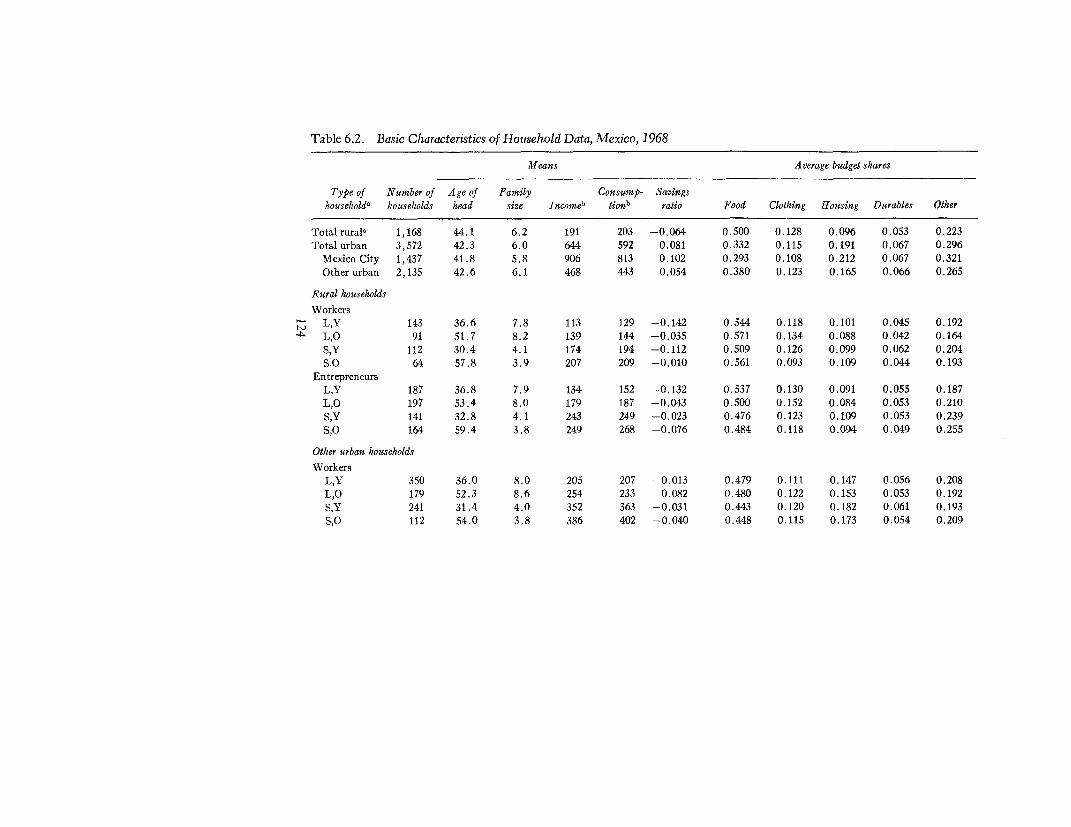
Table 6.2. Basic Characteristics of Household Data, Mexico, 1968

Means Average budget shares

Type of Number of Age of Family Consump- Savingshouseholds households head size Incomeb tionb ratio Food Clothing Housing Durables Other

Totalrural, 1,168 44.1 6.2 191 203 -0.064 0.500 0.128 0.096 0.053 0.223Totalurban 3,572 42.3 6.0 644 592 0.081 0.332 0.115 0.191 0.067 0.296

Mexico City 1,437 41.8 5.8 906 813 0.102 0.293 0.108 0.212 0.067 0.321Otherurban 2,135 42.6 6.1 468 443 0.054 0.380 0.123 0.165 0.066 0.265

Rural householdsWorkers

t L,Y 143 36.6 7.8 113 129 -0.142 0.544 0.118 0.101 0.045 0.1924 L,O 91 51.7 8.2 139 144 -0.035 0.571 0.134 0.088 0.042 0.164

S,Y 112 30.4 4.1 174 194 -0.112 0.509 0.126 0.099 0.062 0.204S.O 64 57.8 3.9 207 209 -0.010 0.561 0.093 0.109 0.044 0.193

EntrepreneursL,Y 187 36.8 7.9 134 152 -0.132 0.537 0.130 0.091 0.055 0.187L,O 197 53.4 8.0 179 187 -0.043 0.500 0.152 0.084 0.053 0.210S,Y 141 32.8 4.1 243 249 -0,023 0.476 0.123 0.109 0.053 0.239S,O 164 59.4 3.8 249 268 -0.076 0.484 0.118 0.094 0.049 0.255

Other urban householdsWorkers

L,Y 350 36.0 8.0 205 207 -0.013 0.479 0.111 0.147 0.056 0.208L,O 179 52.3 8.6 254 233 0.082 0.480 0.122 0.153 0.053 0.192S,Y 241 31.4 4.0 352 363 -0.031 0.443 0.120 0.182 0.061 0.193S,O 112 54.0 3.8 386 402 -0.040 0.448 0.115 0.173 0.054 0.209

EntrepreneursL,Y 144 37.0 7.9 324 322 0.006 0.399 0.109 0.150 0.071 0.271L,O 193 54.3 8.3 422 384 0.090 0.363 0.124 0.130 0.060 0.323S,Y 114 32.5 4.0 713 622 0.127 0.320 0.129 0.164 0.073 0.314S,O 172 60.2 3.5 723 669 0.075 0.336 0.107 0.191 0.063 0.303

TechnocratsL,Y 175 36.2 7.9 459 420 0.085 0.391 0.125 0.156 0.070 0.258L,O 108 51.6 8.2 565 505 0.107 0.356 0.138 0.147 0.066 0.293S,Y 234 31.2 3.9 756 731 0.032 0.350 0.140 0.170 0.078 0.262S,O 113 54.9 3.8 896 816 0.089 0.333 0.119 0.178 0.070 0.299

hlexico City households

WorkersL,Y 179 35.3 7.9 240 258 -0.074 0.472 0.122 0.173 0.051 0.182L,O 93 52.2 8.2 368 335 0.090 0.423 0.114 0.203 0.047 0.212

x S,Y 121 31.2 4.0 424 453 -0.069 0.420 0.114 0.182 0.061 0.222S,p 54 54.6 3.9 602 590 0.020 0.376 0.102 0.230 0.043 0.249

EntrepreneursL,Y 80 37.1 7.6 642 633 0.015 0.298 0.081 0.175 0.056 0.389L,O 86 53.1 8.0 948 795 0.161 0.300 0.132 0.225 0.055 0.288S,Y 60 34.1 4.0 1,115 982 0.120 0.283 0.115 0.211 0.082 0.309S,O 79 59.3 3.6 2,026 1,757 0.133 0.211 0.103 0.247 0.066 0.372

TechnocratsL,Y 163 36.6 7.5 738 705 0.045 0.292 0.104 O.A86 0.068 0.349L,O 116 52.8 7.7 999 870 0.129 0.283 0.129 0.211 0.053 0.325S,Y 282 31.4 3.9 1,146 1,056 0.079 0.277 0.115 0.209 0.077 0.321S,O 124 55.7 3.8 1,783 1,405 0.212 0.262 0.083 0.229 0.072 0.354

a. Households are divided by family size into large (L, more than 5) and small b. Income (disposable) and consumption are per capita in pesos a month.(S, 5 or less), and by age of head into young (Y, less than 45 years) and old (0, c. Includes 69 technocrats.45 and over).

126 Consumrption and Savings Behavior in Mexico

required and are all significant at the one percent level. Two-thirdsof the "t values" lie between 5 and 15.

An examination of the p estimates for rural households suggeststhat the marginal budget share for food declines with rising incomeand is higher for old households. Regressing the estimated valuesof ,B (food) on income and a dummy variable for old households(DO) yields the equation for the first line of table 6.5.5 Both effectsare significant at the 5 percent level. The point estimates imply thatamong rural households the marginal budget share for food falls by0.014 for every 10 peso increase in per capita income and, otherthings being equal, has a value that is 0.103 higher for old householdsthan for young. The income effect on the marginal share of otheris estimated to be equal in magnitude but opposite in sign to thatfor food, but the coefficient is significant only at the 10 percentlevel. Apart from some tendency for the marginal share of housing

Table 6.3. R2 Values, ELES, Mexico, 1968

Type of Consumptionhouseholda Food Clothing Housing Durables Other functiont

Rural houfseholds

WorkersL,Y 0.644 0.376 0.400 0.428 0.235 0.631L,O 0.571 0.132 0.466 0.305 0.347 0.672S,Y 0.540 0.358 0.436 0.207 0.344 0.646S,O 0.468 0.256 0.220 0.179 0.234 0.495

Entrepreneurs,,Y 0.576 0.412 0.514 0.349 0.322 0.694L,O 0.647 0.524 0.366 0.391 0.202 0.738S,Y 0.538 0.473 0.449 0.624 0.823 0.914S,O 0.787 0.420 0.661 0.602 0.687 0.860

Other urban households

WorkersL,Y 0.588 0.471 0.600 0.371 0.520 0.811L,O 0.518 0.408 0.486 0.340 0.516 0.752S,Y 0.514 0.471 0.058 0.220 0.351 0.589S,O 0.611 0.575 0.771 0.364 0.701 0.840

EntrepreneursL,Y 0.482 0.447 0.669 0.627 0.620 0.822L,O 0.450 0.431 0.539 0.377 0.621 0.731S,Y 0.311 0.496 0.743 0.462 0.797 0.864S,O 0.575 0.499 0.727 0.721 0.386 0.757

S. Other functional forms were tried, but for all rural p estimates the linearform performed best.

EMPIRICAL RESULTS 127

Table 6.3. (continued)

Type of Consumptionhousehold' Food Clothing Housing Durables Other function

Other urban households (continued)Technocrats

L,Y 0.534 0.218 0.574 0.566 0.723 0.823L,O 0.463 0.394 0.471 0.266 0.365 0.602S,Y 0.586 0.419 0.756 0.225 0.649 0.830S,0 0.545 0.667 0.626 0.560 0.625 0.854

Mexico City households

WorkersL,Y 0.478 0.158 0.342 0.159 0.252 0.552L,O 0.566 0.274 0.484 0.094 0.361 0.730S,Y 0.562 0.267 0.467 0.209 0.258 0.694S,0 0.309 0.166 0.436 0.280 0.202 0.494

EntrepreneursL,Y 0.539 0.502 0.705 0.696 0.536 0.694L,O 0.500 0.425 0.600 0.565 0.602 0.804S,Y 0.558 0.632 0.619 0.644 0.555 0.774S,0 0.515 0.374 0.746 0.626 0.634 0.819

TechnocratsL,Y 0.647 0.600 0.406 0.729 0.559 0.728L,O 0.629 0.269 0.612 0.588 0.621 0.747S,Y 0.480 0.353 0.650 0.387 0.643 0.785S,0 0.352 0.091 0.434 0.155 0.386 0.432

a. Household size is denoted by L (large, more than 5) and S (small, 5 or less). Age of household head isdenoted by Y (young, less than 45 years) and 0 (old, 45 and over).

to fall slightly with increased income, no other patterns are apparentin the rural p estimates.

With urban households a more systematic analysis of the 13 esti-mates is possible. The twenty-four estimates of each parameter wereused in the following regressions:

8i = ao + a, log 10 y + a2 DL + a3 DO + a4 DE + asDT + aeDMC(i = 1, ..., 5)

where y is per capita income, and DL, DO, DE, DT, and DMCare dummy variables representing family characteristics: large, old,entrepreneur, technocrat, and Mexico City respectively.6 In searchingfor the dominant influences greater weight is given to avoiding biasin the estimates of ai coefficients than to efficiency in estimation.

6. Linear and double-log equations were also used. The linear model gaveclearly inferior results; the semi-log was marginally preferred to the double-logformulation, but the differences were not great.

Table 6.4. Estimated Values of Marginal Budget Shares (pi) andMarginal Propensity to Consume (pu), ELES, Mexico, 1968

Type of Samplehouseholda size Incomeb Food Clothing Housing Durables Other I

Rural households

WorkersL,Y 143 113 0.364 0.122 0.084 0.055 0.375 1.038

(0.025) (0.015) (0.008) (0.006) (0.038) (0.067)oo L,O 91 139 0.490 0.098 0.110 0.040 0.262 0.656

(0.030) (0.023) (0.013) (0.006) (0.032) (0.049)S,Y 112 174 0.354 0.147 0.087 0.083 0.329 1.000

(0.023) (0.017) (0.009) (0.015) (0.030) (0.071)S,O 64 207 0.429 0.108 0.098 0.043 0.321 0.752

(0.043) (0.023) (0.018) (0.011) (0.048) (0.097)Entrepreneurs

L,Y 187 134 0.378 0.160 0.107 0.100 0.255 0.872(0.016) (0.013) (0.007) (0.010) (0.021) (0.043)

.,O 197 179 0.362 0.228 0.074 0.106 0.230 0.766(0.019) (0.014) (0.007) (0.009) (0.027) (0.033)

S,Y 141 234 0.212 0.104 0.090 0.058 0.536 0.846(0.014) (0.008) (0.008) (0.004) (0.021) (0.022)

S,p 164 249 0.286 0.113 0.065 0.084 0.452 1.198(0.010) (0.010) (0.004) (0.005) (0.014) (0.038)

Otlter urban households

WorkersL,Y 350 205 0.258 0.140 0.131 0.068 0.403 0.896

(0.010) (0.008) (0.006) (0.005) (0.015) (0.023)

L,O 179 254 0.344 0.155 0.143 0.070 0.290 0.672(0.017) (0.012) (0.010) (0.007) (0.018) (0.029)

S,Y 241 352 0.293 0.194 0.155 0.073 0.285 0.774(0.020) (0.014) (0.035) (0.008) (0.023) (0.042)

S,O 112 386 0.202 0.119 0.179 0.041 0.460 1.084(0.014) (0.009) (0.008) (0.005) (0.015) (0.045)

EntrepreneursL,Y 144 324 0.207 0.106 0.154 0.115 0.418 0.785

(0.014) (0.009) (0.008) (0.005) (0.015) (0.045)

L,O 193 422 0.176 0.116 0.115 0.076 0.518 0.585(0.011) (0.008) (0.007) (0.006) (0.017) (0.026)

S,Y 114 713 0.096 0.103 0.160 0.074 0.568 0.688(0.012) (0.008) (0.010) (0.006) (0.017) (0.026)

S,O 172 723 0.178 0.115 0.208 0.124 0.375 0.617(0.011) (0.008) (0.011) (0.008) (0.023) (0.027)

TechnocratsL,Y 175 459 0.236 0.098 0.142 0.112 0.411 0.677

(0.013) (0.013) (0.009) (0.008) (0.016) (0.024)L,O 108 565 0.201 0.140 0.143 0.077 0.439 0.586

(0.021) (0.016) (0.014) (0.010) (0.031) (0.046)

S,Y 234 756 0.207 0.154 0.179 0.069 0.391 0.850(0.010) (0.010) (0.008) (0.007) (0.014) (0.025)

S,O 113 896 0.148 0.199 0.137 0.086 0.429 0.842(0.012) (0.013) (0.010) (0.007) (0.019) (0.033)

(Table continues on the following page.)

Table 6.4. (continued)

Type of SamplehouseholdP size Incomeb Food Clothing Housing Durables Other

Mexico City houtseholds

WorkersL,Y 179 240 0.341 0.141 0.239 0.062 0.217 0.747

(0.020) (0.019) (0.024) (0.010) (0.020) (0.051)L,O 93 368 0.320 0.133 0.255 0.035 0.257 0.657

(0.027) (0.020) (0.026) (0.011) (0.028) (0.042)S,Y 121 424 0.308 0.155 0.183 0.100 0.254 0.835

(0.024) (0.021) (0.018) (0.016) (0.030) (0.051)S,O 54 602 0.214 0.111 0.250 0.062 0.363 0.556

(0.034) (0.032) (0.039) (0.014) (0.069) (0.078)Entrepreneurs

L,Y 80 642 0.105 0.053 0.130 0.060 0.652 0.846(0.011) (0.006) (0.012) (0.004) (0.028) (0.064)

L,O 86 948 0.138 0.156 0.209 0.067 0.430 0.612(0.013) (0.018) (0.0t7) (0.005) (0.029) (0.033)

S,Y 60 1,115 0.156 0.154 0.186 0.131 0.373 0.674(0.016) (0.015) (0.016) (0.011) (0.025) (0.048)

S,O 79 2,026 0.078 0.106 0.224 0.075 0.518 0.859(0.009) (0.016) (0.012) (0.007) (0.025) (0.046)

TechnocratsL,Y 163 738 0,091 0.077 0.095 0.079 0.659 1.071

(0.006) (0.004) (0.011) (0.003) (0.018) (0.052)

L,O 116 999 0.140 0.116 0.189 0.079 0.476 0.798

(0.010) (0.014) (0.015) (0.005) (0.018) (0.044)

S,Y 282 1,146 0.111 0.102 0.194 0.100 0.492 0.756

(0.006) (0.007) (0.009) (0.006) (0,014) (0.024)

S,p 124 1,783 0.098 0.031 0.190 0.068 0.613 0.507

(0.011) (0.008) (0.016) (0.009) (0.021) (0.053)

Note: Asymptotic standard errors in parentheses. b. Mean personal disposable income per capita in pesos a month. The t968 rate of

a. Iloutsehold size is denoted by L (large, more than 5) and S (small, S or less). exchange was 12.5 pesos = U.S. $1.00.

Age of household head is denoted by Y (young, less than 45 years) and 0 (old,

45 and over).

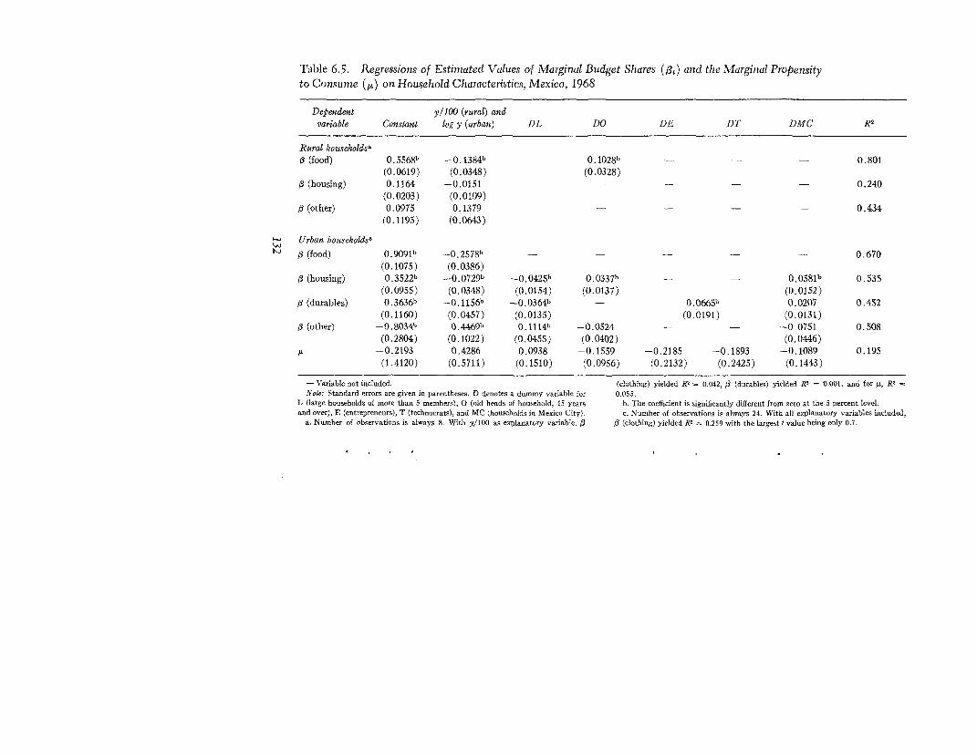
Table 6.5. Regressions of Estimated Values of Marginal Budget Shares (3) and the Marginal Propensity

to Consume (,,) on Household Characteristics, Mexico, 1968

Dependent y/lOO (rural) andvariable Constant log y (urban) DL DO DE DT DMC R2

Rural households'3 (food) 0.5568" -0.1384b 0.1028b 0.801

(0.0619) (0.0348) (0.0328)3 (housing) 0.1164 -0.0151 _ _ _ _ 0.240

(0.0203) (0.0109)( (other) 0.0975 0.1379 0.434

(0.1195) (0.0643)

Urban households,' (3 (food) 0.9091b -0.2578b - - 0 _ _ 0.670

(0.1075) (0.0386)fl (housing) 0.3522b --0.0729b -0.0425b 0.0337b 0.0581b 0.535

(0.0955) (0.0348) (0.0154) (0.0137) (0.0152)

13 (durables) 0.3636b -0.1156b -0.0364b - 0.0665b 0.0207 0.452

(0.1160) (0.0457) (0.0135) (0.0191) (0.0131)

3 (other) -0.8034" 0.4469" 0.1114b -0.0524 - - -0.0751 0.508

(0.2804) (0.1022) (0.0455) (0.0402) (0,0446)

p0 -0.2193 0.4286 0.0938 -0.1559 -0.2185 -0.1893 -0.1089 0.195

(1.4120) (0.5711) (0.1510) (0.0956) (0.2132) (0.2425) (0.1443)

-Variable not included. (clothing) yielded RI 0.042, ( (durables) yielded RI = 0.001, and for A, R2

Note: Standard errors are given in parentheses. D denotes a dummy variable for 0.055.

L (large households of more than 5 members), 0 (old heads of household, 45 years b. The coefficient is significantly different from zero at the 5 percent level.

and over), E (entrepreneurs), T (technocrats), and MC (households in Mexico City). c. Number of observations is always 24. With all explanatory variables included,

a. Number of observations is always 8. With y/iOO as explanatory variable, (3 ( (clothing) yielded RI 0.259 with the largest t value being only 0.7.

EMPIRICAL RESULTS 133

For this reason an explanatory variable is dropped only when itscoefficient is both small and exceeded in absolute value by its standarderror, so that the omission of variables has little effect on the pointestimates of the remaining ai.

The equations chosen in this manner yield the regression resultsfor urban households shown in table 6.5.7 The marginal budgetshares for food, housing, and durables decline significantly withincreased income, while that for other increases. The marginal budgetshares for housing and durables are significantly lower for largefamilies, suggesting economies of scale, whereas the marginal sharefor other is significantly higher for large families. Socioeconomic classhas no influence on the ,B values except for durables, where themarginal budget share is significantly lower for workers.8 The p valuefor housing is significantly higher for old households and householdsin Mexico City. Thus even after allowances are made for location,socioeconomic class, and household composition, the marginal budgetshares for urban households move significantly with income (exceptfor clothing). The only other regular influence is family size.

There is little overlap in mean incomes between the rural andurban cells: The largest mean per capita income for a rural cell is250 pesos a month; only two urban cells have a mean income belowthis. It is therefore difficult to isolate rural-urban effects from theeffects of income alone. Nevertheless, for food there is no evidenceof a specific rural effect on the marginal budget share. Evaluatingthe regression equations for food at an income level of 250 pesosper capita a month yields rural estimates of /8 which span the cor-responding urban estimate: rural ~, = .21 (young), .31 (old); urban

= .29. The estimated regression lines are drawn in figure 5.In the case of housing, however, evaluating the regression equation

of table 6.5 at an income of 250 pesos yields a rural estimate of 0.09,which is below the range of estimates for other urban households ofdiffering family composition at that income level (0.13-0.21). Forother expenditure, the comparable figures are rural, 0.44, and urban,0.22--0.38. The ,B estimates for clothing are irregular for both ruraland urban households. The mean values are 0.14 for rural and otherurban and 0.11 for Mexico City.

7. For a given commodity there is relatively little variation in the precisionof the p estimates. For this reason standards errors are ignored and estimationis by (unweighted) ordinary least squares (OLS).

8. The coefficients of DE and DT were the same to three decimal placesand the variables have been combined in the reported results.

Figure 5. Regression Lines for the Marginal Budget Shares (is) for Food

s (food)

O.5 -g Rural (old)

0.4 -

0.3-

0.2 - Rural o( youbg

0.1

0.0 I I I250 500 1,000 1,500

Income per capita in pesos a monzth

EMPIRICAL RESULTS 135

Marginal Propensity to Consume

In Lluch's (1973a) model the marginal propensity to consume isthe ratio of the subjective rate of discount (8) to the rate of interest(p). Thus a marginal propensity to consume of greater than oneimplies that 8 exceeds p and optimal consumption paths declinethrough (planning) time (see chapter 2, on ELES and saving). Heretwenty-seven of the thirty-two point estimates of M (table 6.4) are lessthan unity, and only one is significantly greater at the 5 percent level(rural entrepreneurs, S,O). All u estimates are significantly differentfrom zero at the one percent level.

The estimated values of It for rural households are irregular; therange is 0.66 to 1.20 and the mean value is 0.89. Similarly, littlepattern is evident for urban estimates of IL after regressing on theexplanatory variables used for the A estimates (see last row, table6.5). If differences in the relative importance of transitory incomeare taken into consideration [x would be expected to be lower forentrepreneurs, and although this occurs the effect is not particularlypronounced. There is some tendency for the (urban) marginalpropensity to consume to be lower for old households. The meanvalues are 0.75 for other urban and 0.74 for Mexico City, both wellbelow the rural mean.

It is interesting to note, however, that systematic influences aremore evident for the average propensity to save (APS). The pre-ferred equations are:

APS (rural) - 0.5253 + 0.1922 logy + 0.0468 DO,(0.2758) (0.1250) (0.0291)R2 = 0.594

APS (urban) =- 0.0678 + 0.0070 (y/100) + 0.0255 DL(0.0231) (0.0030) (0.0208)

+ 0.0520 DO+ 0.0607 DET, R2 = 0.727(0.0186) (0.0242)

where the dummy variables DO and DL are as defined in table 6.5,and DET is a dummy variable which is one for a household whosehead is an entrepreneur or a technocrat, but which otherwise is zero.In both areas the APS increases with income and age. For urbanhouseholds the coefficients for entrepreneurs and technocrats werevirtually identical when included separately.

Table 6.6. Estimated Values of Subsistence Parameters ( y*) andFrisch Parameters (X), ELES, Mexico, 1968

TotalType of consumption

household, expenditurell Food Clothing Housing Durables Other y* sum, W

Rural households

WorkersL,Y 129 -88 -38 -24 -18 -138 -306 -0.3

(279) (95) (64) (42) (270) (750)

L,O 144 87 20 14 6 26 154 15.5

(8) (3) (2) (1) (5) (15)

S,Yd 194S,O 209 120 20 23 10 42 215 35.1

(22) (6) (6) (3) (20) (54)

EntrepreneursL,Y 152 127 39 27 21 59 272 1.3

(22) (9) (6) (6) (16) (59)

L,O 187 102 34 18 13 45 212 7.4

(8) (6) (2) (3) (8) (25)

S,Y 249 125 34 30 15 76 279 8.2

(13) (6) (6) (3) (26) (52)

SO 268 97 19 18 3 16 153 -2.3

(19) (8) (5) (5) (26) (60)

Other urban households

WorkersL,Y 207 105 26 33 13 52 230 9.3

(10) (6) (5) (3) (17) (41)L,O 233 97 22 30 9 32 191 -5.5

(7) (3) (3) (1) (6) (18)S,Y 363 172 51 72 25 81 401 9.8

(14) (9) (14) (4) (15) (52)S,O 402 139 22 34 13 -9 200 -2.0

(47) (28) (42) (10) (102) (227)Entrepreneurs

L,Y 322 127 34 47 22 85 315 -49.3(13) (6) (8) (5) (24) (53)

L,O 384 130 41 44 19 96 331 -7.2(8) (5) (5) (4) (21) (37)

S,Y 622 180 60 70 30 82 421 -3.1(15) (13) (13) (10) (56) (96)

S,O 669 209 61 110 31 170 582 -7.7(15) (11) (15) (8) (45) (84)

TechnocratsL,Y 420 145 45 54 20 75 338 -5.1

(9) (6) (5) (4) (13) (33)L,O 505 163 58 62 27 111 420 -5.9

(11) (9) (8) (6) (31) (59)S,Y 731 227 81 100 48 138 592 -5.3

(23) (19) (17) (9) (44) (109)S,O 816 209 13 87 21 62 392 -1.9

(30) (38) (27) (17) (95) (200)

(Table continiues on the following page.)

Table 6.6. (continued)

TotalType of consumption

householda expenditureb Food Clothing Housing Durables Other Y* sumc co

Mexico City households

WorkersI,Y 258 140 39 57 17 58 311 4.9

(11) (6) (8) (2) (9) (34)L,O 335 122 30 52 14 55 272 -5.3

(10) (6) (8) (2) (10) (31)S,Y 453 235 75 109 43 138 600 3.1

(29) (17) (17) (11) (30) (100)S,O 590 218 59 132 24 141 574 -38.4

(18) (11) (17) (5) (37) (75)Entrepreneurs

L,Y 633 184 49 104 33 212 581 -12.3(38) (19) (46) (22) (267) (389)

L,O 795 206 68 129 28 125 554 -3.3(15) (19) (20) (7) (44) (91)

S,Y 982 235 70 156 45 201 707 -3.6(29) (25) (33) (23) (76) (173)

S,p 1,757 243 7 66 -8 -197 111 -1.1(71) (103) (214) (70) (535) (974)

TechnocratsL,Y 705 251 112 179 88 576 1,206 1.4

(74) (62) (83) (64) (502) (783)L,O 870 175 53 87 6 40 361 -1.7

(34) (38) (45) (20) (128) (258)S,Y 1,056 261 93 166 53 201 774 -3.8

(14) (15) (21) (14) (62) (120)S,O 1,405 330 104 248 74 259 1,015 -3.6

(24) (13) (45) (26) (165) (260)

Note: Asymptotic standard errors in parentheses. b. Mean total consumption expenditure per capita in pesos a month. (In 1968,a. Household size is denoted by L (large, more than 5), and S (small, 5 or less). 12.5 pesos = U.S. $1.00.)

Age of household head is denoted by Y (young, less than 45 years) and 0 (old, 45 c In pesos per capita a month. Sum may not add exactly due to rounding.and over). d. T* values unobtainable because I = 1.000. Estimates treated as nonsignificant.

Table 6.7. Weighted Regressions of Estimated Values of ye onHousehold Characteristics, Urban Mexico, 1968

Commodity Constant Log y DL DO DE DT DMC R2

Food 1.714 0.1899 -0.1342, - 0.0439 0.0764 0.0820. 0.935(0.190) (0.1140) (0.0297) (0.0437) (0.0488) (0.0306)

Clothing 1.634, - -0.2153a - 0.1666a 0.2600a 0.1319, 0.907(0.037) (0.0291) (0.0358) (0.0320) (0.0307)

Housing 0.778 0.3890a -0.1966a - 0.0907 0.2219a 0.948(0.441) (0.1731) (0.0469) (0.0656) (0.0453)

° Durables 1.350a - -0.2710, -0.0726a 0.2446a 0.3134a 0.1522a 0.904(0.037) (0.0336) (0.0335) (0.0419) (0.0409) (0.0344)

Other 1.888a -0.3005 - 0.3252a 0.1898a 0.874(0.043) (0.0379) (0.0400) (0.0395)

Total 2.558a - -0.2416a - 0.1931, 0.2272a 0.1705a 0.920(0.029) (0.0248) (0.0297) (0.0291) (0.0257)

- Variablc not included. and over), E (entrepreneurs), T (technocrats), and MC (households in Mexico City).Note: The dependent variable is loglvs*; coefficients of dummy variables, when Number of observations is always 24. RI is a weighted goodness of fit measure as

converted to natural logarithms, that .s, multiplied by 2.303, measure proportionate given, for example, in Buse (1973).effects on y'. Standard errors are given in parentheses. D denotes a dummy variable a. The coefficient is significantly different from zero at the 5 percent level.for L (large households of more than 5 members), 0 (old heads of household, 45 years

EMPIRICAL RESULTS 141

Subsistence Parameters

Estimated values of the "subsistence" parameters and their standarderrors are given in table 6.6. The estimates are determined with muchless precision than are the pt parameters. A problem arises when themarginal propensity to consume is close to unity for, as explained in

* chapter 2, if = I ELES collapses to LES and it is not possible toestimate the individual y*. Of the 160 y* estimates, 34 are not sig-nificantly different from zero at the 5 percent level, 17 of these beingassociated with L estimates close to one (table 6.6, rural workers,L,Y and S,Y; other urban workers, S,O; and Mexico City technocrats,L,Y). The y* estimates for food are determined with greatest pre-cision, being insignificant in only the two cases where j, =1.0 (ruralworkers, L,Y and S,Y). If these two cells are ignored, there are onlythree negative (but insignificant) values of y*; these occur fordurables and other (both are negative for Mexico City entrepreneurs,S,O, and other is negative also for urban workers, S,O). Thus the7* estimates are indeed behaving as subsistence parameters.

A necessary condition for the utility function to exist is that thesum of the subsistence expenditures, the y* sum, be less than totalconsumption expenditure. This condition tends to be violated forrural households and low-income urban households (see table 6.6),although in only one case (rural entrepreneurs, L,Y) is the estimateof the y* sum significantly greater than v at the 5 percent level.

There are insufficient usable y* estimates for rural households topermit detailed analysis. There is some tendency for y* (other) andthe y* sum to increase with income; the y* estimates for food arerelatively stable. Mean values in pesos per capita a month (excludingrural workers, L,Y and S,Y) are: 110 (food), 24 (clothing), 22(housing), 11 (durables), 44 (other), and 214 (total).

The y* estimates for urban households have been regressed onthe same set of explanatory variables that was used in analyzing the,a estimates. In this case, however, because the precision of theestimates varies substantially, weighted regressions were performed,the weights being the inverse of the standard error of the dependentvariable. A double-log specification proved marginally superior to asemi-log model, and the estimated regressions are given in table 6.7.9

9. The appropriate weighting factor in the double-log case is the parameterestimate divided by its standard error, that is, the "t value." The three negative^y/ values were put equal to unity, but in view of their very large standarderrors they have little influence on the regression coefficients. Total subsistenceexpenditure is calculated as the sum of positive y* estimates.

142 Consumption and Savings Behavior in Mexico

Except in the case of housing and, to a lesser extent, food, theinfluence of income is shown to be unimportant and highly insignifi-cant.10 Households living in Mexico City have significantly higherlevels of subsistence expenditure for all goods (ranging from 19percent for food to 51 percent for housing), partly because of higherprices there. The -y* estimates are always larger for those in the socio-economic classes of entrepreneur or technocrat."1 The results stronglysupport the notion that y* estimates are a measure of an acceptableminimum standard for households identifying with a given socio-economic group. The y* estimates also exhibit the effect of economies

Table 6.8. Total Expenditure Elasticities, ELES, Mexico, 1968

Type ofhousehold, Food Clothing Housing Durables Other Nb

Rural households

WorkersL,Y 0.67 1.03 0.83 1.21 1.95 0.91L,O 0.86 0.73 1.25 0.96 1.59 0.63S,Y 0.70 1.17 0.88 1.34 1.61 0.90S,0 0.77 1.16 0.90 0.98 1.67 0.99

EntrepreneursL,Y 0.70 1.23 1.18 1.83 1.36 0.77L,O 0.72 1.50 0.87 1.99 1.10 0.73S,Y 0.45 0.85 0.82 1.08 2.24 0.83S,0 0.59 0.96 0.69 1.74 1.77 1.11

Other urban households

WorkersL,Y 0.54 1.26 0.90 1.22 1.94 0.88L,O 0.72 1.27 0.93 1.31 1.51 0.73S,Y 0.66 1.61 0.85 1.19 1.48 0.75S,O 0.45 1.03 1.03 0.75 2.20 1.04

EntrepreneursL,Y 0.52 0.97 1.03 1.62 1.54 0.78L,O 0.48 0.94 0.89 1.25 1.60 0.64S,Y 0.30 0.80 0.97 1.10 1.81 0.79S,0 0.53 1.08 1.09 1.97 1.24 0.67

10. When log y is added back into the reported equations in table 6.7 it hasthe following coefficients and t values: clothing -0.05 (t = -0.25), durables0.05 (t = 0.13), other -0.10 (t =-0.38), and total 0.03 (t = 0.16).

11. The coefficients of DT always exceed those of DE, but the difference issignificant only for clothing, where it is 0.0934 with a t value of 2.73. Thecorresponding t values for food, durables, and total are 1.50, 1.45, and 1.06respectively.

EMPIRICAL RESULTS 143Table 6.8. (continued)

Type oflhouisehlolds Food Clotlhing Housing Durables Othser Bb

Other urban househiolds (conitinued)Technocrats

L,Y 0.61 0.78 0.91 1.61 1.60 0.74L,O 0.56 1.02 0.97 1.17 1.50 0.66S,Y 0.59 1.10 1.05 0.88 1.50 0.88S,0 0.45 1.67 0.77 1.22 1.44 0.92

Mexico City hiouseholds

WorkersL,Y 0.72 1.16 1.38 1.21 1.19 0.70L,O 0.76 1.17 1.25 0.75 1.21 0.72S,Y 0.73 1.36 1.00 1.62 1.14 0.78S,0 0.57 1.09 1.08 1.46 1.46 0.57

EntrepreneursL,Y 0.35 0.65 0.74 1.07 1.68 0.86L,O 0.46 1.18 0.93 1.22 1.50 0.73S,Y 0.55 1.34 0.88 1.59 1.21 0.77S,0 0.37 1.03 0.91 1.14 1.39 0.99

TechnocratsL,Y 0.31 0.73 0.51 1.17 1.89 1.12L,O 0.50 0.90 0.90 1.48 1.47 0.92S,Y 0.40 0.89 0.93 1.30 1.53 0.82S,0 0.37 0.38 0.83 0.95 1.73 0.64

a. Household size is denoted by L (large, more than 5) and S (small, 5 or less). Age of household head isdenoted by Y (young, less than 45 years) and 0 (old, 45 and over).

b. Elasticity of total consumption expenditure with respect to income. Total income elasticities are ob-tained by multiplying total expenditure elasticities by the row value of r).

of scale: Large households always have lower per capita subsistenceexpenditure than small households (for the total, 56 percent lower).The age of households is important only for durables, where it exertsa small but significant negative effect.

Frisch Parameter

Estimates of the expenditure elasticity of the marginal utility oftotal expenditure (-) are given in the last column of table 6.6. Itfollows from the definition of w (2.7) that estimates have the in-correct (positive) sign whenever estimates of total subsistenceexpenditure exceed actual consumption expenditure. Positive valuesof the Frisch parameter occur for those cells (predominantly ruralhouseholds) in which mean per capita income is less than 245 pesosa month; above this level all but three of the twenty-three eo esti-

Table 6.9. Regressions of Estimated Values of Total ExpenditureElasticities oni1lousehold Characteristics, Mexico, 1968

y/100 (rural)Comnmodity Constant and log y (urban) DL DO DET DilfC R2

Rural households,Food 0 95 9b -0.1991b _ 0.1608 b - _ 0.826

(0.084) (0.0475) (0.0450)Housing 1-351b -0.2348 0.394

(0.221) (0.1189)Other 1.232l' 0.2390 0.119

(0.493) (0.2650)

Urban households,

4I Food 1.817 b -0.4792b -0.0698 0.0539 0.0832 0.503

(0.312) (0.1138) (0.0505) (0.0448) (0.0497)Clothing 1.3 6 8 b -0.1110 _ -0.2773b -0.1385 0.310

(0.118) (0.1056) (0.1120) (0.1056)

Housing 3.789 - 1.113b -0.2726 0.1756 0.2575 0.2491 0.383

(1.268) (0.513) (0.1375) (0.0888) (0.2030) (0.1316)

Durables 5.891 -- 1.886 -0.4544 0.1686 0.8081 0.4075 0.195

(2.530) (1.023) (0,2743) (0.1771) (0.4050) (0.2624)

Other -1.967 1.439 0.3885 -0.2027 -0.5190 -0.4889b 0.235

(2.131) (0.862) (0.2310) (0.1492) (0.3411) (0.2210)

-Variable not included. a. Number of observationis is always 8. With y/lOO as explanatory variable, the

Note: Standard errors are given in parentheses. D denotes a dunimy variable for value of RI for clothing was 0.017 and for durables 0.001.

L (large households of more than S members), 0 (old heads of household, 45 years b. Coefficient is significantly different from zero at the 5 percent level.

and over), ET (entrepreneurs and technocrats), and MC (households in Mexico c. Number of observations is always 24.

City).

EMPIRICAL RESULTS 145

mates are negative. There is some tendency for the urban estimatesof the Frisch parameters to fall in absolute value as income rises,with a pronounced break at per capita incomes around 800 pesos amonth. Above this level the median value is -3.3, below this (butabove 245) the median value is -5.3. Since o-1 is a measure ofprice responsiveness (see chapter 2), the results imply that house-holds are more responsive to relative price changes at higher incomelevels.

Total Expenditure Elasticities

Estimates of total expenditure elasticities (?), calculated as in table2.2, are given in table 6.8. The elasticities for food are, as expected,the lowest. For rural households they range from 0.45 to 0.86; forurban households the values are lower, ranging from 0.30 to 0.76.The total expenditure elasticities for clothing are clustered aroundone: The means are 1.1 for rural and other urban, 1.0 for MexicoCity. All total expenditure elasticities for other exceed unity, as dothree-quarters of the values for durables.

The results of the regression equations corresponding to thoseestimated for the fli are reported in table 6.9. The regularities forrural households are few and similar to those observed for marginalbudget shares. The total expenditure elasticity for food decreasessignificantly with larger income and is higher for old families; thereis a tendency for the housing expenditure elasticity to decrease withlarger income (significant at the 10 percent level).

For urban households the total expenditure elasticity for clothingshows more systematic variation than the corresponding ,B estimate,but for all other commodities the R2 values are considerably lowerand the income effect weaker when elasticities are the dependentvariable. Socioeconomic effects, however, appear to be more im-portant. The Bi estimates for clothing and other are higher forworkers than for entrepreneurs and technocrats, those for housingand durables are lower.1 2 The strongest result obtained is the declinein the total expenditure elasticity for food as income rises. The pointestimates imply, for example, that for small, young households inMexico City the food expenditure elasticity falls with per capitamonthly income as follows: 0.65 at 400 pesos, 0.46 at 1,000 pesos,0.38 at 1,500 pesos.

12. For all commodities there was remarkably little difference between thecoefficients of DE and DT. In the results reported in table 6.9 a single dummyvariable, DET, has been used, where DET = DE + DT.

146 Consumption and Savings Behavior in Mexico

Price Elasticities

Own-price elasticities (,qij) are given in table 6.10. For urban house-holds 90 percent of the estimates are negative as required by theunderlying utility function. Mean values are given in table 6.15. Theresults are much less satisfactory for rural households. First, the twocells (rural workers, L,Y and S,Y) which give unacceptable estimatesof y* have to be excluded. Second, of the remaining thirty estimates,a third are positive. Only in the case of food are the reported ruralprice elasticities all negative-the mean value is -0.31. Since all piestimates are positive, own-price elasticities are positive only whereestimates of subsistence expenditure on a commodity exceed actualexpenditure (see formula for qi in table 2.2). Thus positive priceelasticities occur most frequently in those cells for which u is positivein table 6.6. The positive estimates of own-price elasticities amongthe urban results are concentrated in two cells for Mexico City(workers, S,Y, and technocrats, L,Y) where the y* estimates are

Table 6.10. Own-Price Elasticities, ELES, Mexico, 1968

Type ofhousehold'X Food Clothing Housing Durables Other

Rural householdsWorkers

L,Y - - - - -L,O -0.46 -0.06 -0.04 0.02 -0.19S,Y - - - - -

S,0 -0.42 -0.08 -0.08 -0.02 -0.29Entrepreneurs

L,Y -0.03 0.66 0.73 1.21 0.55L,O -0.30 -0.07 0.04 0.13 -0.12S,Y -0.17 -0.01 0.00 0.07 -0.41S,0 -0.47 -0.48 -0.34 -0.77 0.87

Other urban householdsWorkers

L,Y -0.22 -0.02 -0.05 0.05 -0.28L,O -0.43 -0.35 -0.29 -0.29 -0.49S,Y -0.25 -0.06 -0.08 0.04 -0.18S,0 -0.38 -0.57 -0.60 -0.40 -1.06

EntrepreneursL,Y -0.22 -0.12 -0.17 -0.14 -0.44L,O -0.23 -0.23 -0.23 -0.24 -0.63S,Y -0.18 -0.33 -0.42 -0.38 -0.82S,0 -0.23 -0.24 -0.32 -0.35 -0.48

EMPIRICAL RESULTS 147

Table 6.10. (continued)

Type ofhiousehiolds Food Clothing Housing Durables Other

Other urban households (continued)Technocrats

L,Y -0.33 -0.24 -0.29 -0.39 -0.59L,O -0.28 -0.29 -0.28 -0.26 -0.58S,Y -0.30 -0.33 -0.34 -0.23 -0.56S,O -0.35 -0.90 -0.48 -0.67 -0.86

Mexico City households

WorkersL,Y -0.24 0.06 -0.02 0.17 -0.03L,O -0.42 -0.32 -0.43 -0.17 -0.43S,Y -0.14 0.22 0.08 0.37 0.02S,O -0.23 -0.14 -0.27 -0.10 -0.39

EntrepreneursL,Y -0.13 -0.10 -0.18 -0.14 -0.70L,O -0.26 -0.46 -0.43 -0.41 -0.69S,Y -0.29 -0.47 -0.39 -0.52 -0.59S,O -0.40 -0.97 -0.88 -1.06 -1.15

TechnocratsL,Y 0.11 0.41 0.23 0.68 -0.20L,O -0.39 -0.58 -0.62 -0.88 -0.93S,Y -0.21 -0.32 -0.39 -0.41 -0.70S,O -0.19 -0.13 -0.38 -0.31 -0.80

- Model failed to yield meaningful estimates.a. Household size denoted by L (large, more than 5) and S (small, 5 or less). Age of household head is

denoted by Y (young, less than 45 years) and 0 (old, 45 and over).

"too high." Note, however, that positive values are not particularlyassociated with badly determined y* estimates.

Table 6.11 contains the results obtained from regressing the nega-tive own-price elasticities (for urban areas only) on the logarithmof income and dummy variables.13 A uniform pattem emerges: Own-price elasticities increase in absolute value with higher income andlarger family size; they are higher in absolute value for workers thanfor entrepreneurs and technocrats and lower for residents of MexicoCity than for other urban households.

Of the cross-price effects those for food tend to be most important.

13. These results are to be interpreted with due care because the 'y*estimates vary substantially in precision, and no allowance for this variation hasbeen attempted. Since qs depends on both p4 and 'yi*, precision will in generalbe higher than that for y,*.

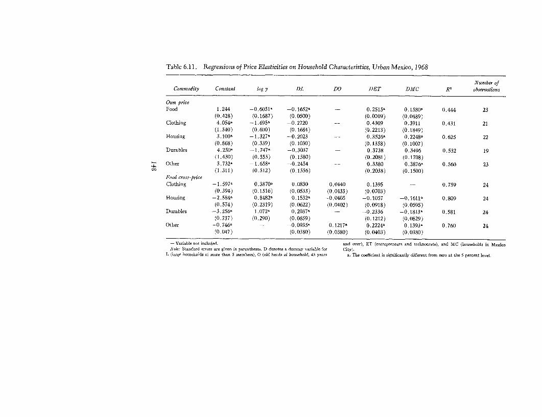
Table 6.11. Regressions of Price Elasticities onr Household Characteristics, Urban Mexico, 1968

Number ofCommodity Constant log y DL DO DET DMC R2 observations

Own priceFood 1.244 -0.6051, -0.1652 - 0.2515a 0.1580& 0.444 23

(0.428) (0.1687) (0.0500) (0.0709) (0.0489)Clothing 4.054* -1.695a -0.2720 - 0.4309 0.3911 0.431 21

(1.540) (0.600) (0.1684) (0.2213) (0.1849)Housing 3.100a -1.327a -0.2023 - 0.3526- 0.22489 0.625 22

(0.868) (0.339) (0.1030) (0.1358) (0.1007)Durables 4.250' -1.747, -0.3037 - 0.3738 0.3496 0.532 19

(1.430) (0.555) (0.1580) (0.2081) (0.1708)- Other 3.732a -1.658, -0.2454 - 0.3380 0.3876, 0.560 23oo (1.311) (0.512) (0.1556) (0.2038) (0.1500)

Food cross-priceClothing -1.597T 0.3870 0.0830 0.0440 0.1395 - 0.759 24

(0.394) (0.1516) (0.0533) (0.0433) (0.0703)Housing -2.584- 0.8482, 0.1532a -0.0405 -0.1057 -0.1611P 0.809 24

(0.574) (0.2319) (0.0622) (0.0402) (0.0918) (0.0595)Durables -3.256& 1.072a 0.2037% - -0.2336 -0.1813a 0.581 24

(0.737) (0.290) (0.0859) (0.1212) (0.0829)Other -0.746a -0.0935, 0.1217a 0.2224, 0.1393a 0.760 24

(0.047) (0.0380) (0.0380) (0.0403) (0.0380)

- Variable not included. and over), ET (entrepreneurs and technocrats), and MC (households in MexicoNote: Standard errors are given in parentheses. D denotes a dummy variable for City).

L (large households of more than 5 members), 0 (old heads of household, 45 years a. The coefficient is significantly different from zero at the S percent level.

AN OVERVIEW OF FINDINGS 149

The food cross-price elasticities (,7j,), calculated as in table 2.2, arelisted in table 6.12 and mean values in table 6.15. All estimates arenegative (again those for rural workers, L,Y and S,Y, are ignored),and the mean values for rural households are approximately doublethe mean urban estimates, for all commodities. The regressionequations for urban households in table 6.1114 show a strong tendencyfor the food cross-price elasticity to decline in absolute size as in-come increases. Family size and location are also important causalfactors. Patterns in the total cross-price effects of nonfood items canbe approximately obtained from the regression results for xi, 77., andyi (tables 6.9 and 6.11 ) by using both homogeneity ( + X qij = 0)

and the property of least squares regression that if dependent variablessum to zero then the estimated coefficients on each of the explanatoryvariables will do likewise across equations.1 5

Estimates of the elasticity of the average savings ratio with respectto the price of food are given in table 6.13 for urban areas (calculatedfrom equation 2.12). Five of the twenty-four estimates have anincorrect positive sign; in four of these cases mean saving is negative,in the fifth ,u exceeds one (Mexico City technocrats, L,Y). Ruralresults are not presented because mean saving is always negative. Aswith the Frisch parameter there is a break in the urban values at aper capita income level of 800 pesos a month. Above this level therange of values of e (food) is -0.70 to -0.13 with a median valueof -0.43, below this (but above 240 pesos) the median value is-1.26. Thus there is evidence that saving is more responsive to theprice of food at lower income levels.

An Overview of Findings

Fitting the extended linear expenditure system to data for homo-geneous groups of households in Mexico has uncovered important

14. Estimation is by OLS. In general the estimates of 0,l will be determinedreasonably precisely since they are functions only of Y1* and a (plus data),two well-determined parameters.

15. This is an exact property only if explanatory variables are identical ineach equation. Since explanatory variables are ornitted only when their influenceis both quantitatively small and statistically insignificant, the residual methodoutlined in the text will give a good approximation. The other departure fromexactness is that in some regressions we drop own-price elasticities with the"wrong" sign.

150 Consumption and Savings Behavior in Mexico

systematic variations in demand behavior. Key findings for urbanhouseholds are:

l. Marginal budget shares are influenced primarily by income andfamily size. Even after allowance is made for socioeconomicclass, the marginal budget shares for food, housing, and durablesfall significantly with higher income, and those for otherincrease.

2. Per capita subsistence expenditure (y* estimates) for all com-modities is significantly lower for large families, lower for thesocioeconomic group labeled workers, and higher for residentsof Mexico City. When these factors are allowed for, incomedifferences are an unimportant cause of variations in estimatesof subsistence expenditures except for housing and, to a lesserextent, food. Thus the -y* estimates may be interpreted asmeasuring an acceptable minimum standard as perceived byhouseholds in a given socioeconomic group.

Table 6.12. Food Cross-Price Elasticities, Mexico, 1968

Type ofhouseholds Clothing Housing Dorables Other

Rural householdsWorkers

L,Y - -

L,O -0.44 -0.75 -0.58 -0.96S,Y - - - -

S,0 -0.66 -0.52 -0.56 -0.95Entrepreneurs

L,Y -1.03 -0.99 -1.53 -1.14L,O -0.82 -0.48 -1.09 -0.60S,Y -0.43 -0.41 -0.54 -1.13S,0 -0.35 -0.25 -0.63 -0.64

Otlher urban households

WorkersL,Y -0.64 -0.45 -0.62 -0.98I,O -0.53 -0.39 -0.55 -0.63S,Y -0.76 -0.40 -0.56 -0.70S,0 -0.36 -0.36 -0.26 -0.76

EntrepreneursL,Y -0.38 -0.41 -0.64 -0.61L,O -0.32 -0.30 -0.42 -0.54S,Y -0.23 -0.28 -0.29 -0.52S,O -0.34 -0.34 -0.62 -0.39

AN OVERVIEW OF FINDINGS 151

Table 6.12. (continued)

Type ofhonsehlold, Clothing Housing Durables Other

Other zurban househiolds (continued)

TechnocratsL,Y -0.27 -0.31 -0.56 -0.55L,O -0.33 -0.31 -0.38 -0.48S,Y -0.34 -0.33 -0.27 -0.46S,O -0.43 -0.20 -0.31 -0.37

Mexico City lhouseholds

WorkersL,Y -0.63 -0.75 -0.66 -0.65L,O -0.42 -0.46 -0.27 -0.44S,Y -0.71 -0.52 -0.84 -0.59S,O -0.40 -0.40 -0.54 -0.54

EntrepreneursL,Y -0.19 -0.22 -0.31 -0.49L,O -0.31 -0.24 -0.32 -0.39S,Y -0.32 -0.21 -0.38 -0.29S,O -0.14 -0.13 -0.16 -0.19

TechnocratsL,Y -0.26 -0.18 -0.42 -0.67L,O -0.18 -0.18 -0.30 -0.30S,Y -0.22 -0.23 -0.32 -0.385,0 -0.09 -0.20 -0.22 -0.41

a. Household size is denoted by L (large, more than 5) and S (small, 5 or less). Age of householdhead is denoted by Y (young, less than 45 years) and 0 (old, 45 and over).

3. Total expenditure elasticities show less systematic variation thanthe corresponding p estimates, except for clothing. This earlierconclusion is reinforced by comparing the coefficients of variationpresented in table 6.14.

4. Own-price elasticities appear to increase in absolute value withhigher income, to be higher in absolute value for small familiesand workers, and lower for households in Mexico City.

5. The effect of a change in the price of food on the demand forother commodities is much stronger at low income levels.

6. The Frisch parameter and the elasticity of the average savingsratio Nwith respect to the price of food are both lower in absolutevalue for per capita incomes over about 800 pesos a month.

There is still some doubt, however, as to the precision with whichthe effects of socioeconomic class, location, and income have beenisolated in examining pattems in marginal budget shares and in

152 Consumption and Savings Behavior in Mexico

Table 6.13. Elasticity of Average Savings Ratio with Respectto Food Price, Urban Mexico, 1968

Type of household L,Y L,O S,Y S,O

Other urbanWorkers 4.37 -1.54 3.58 -0.75Entrepreneurs -15.31 -1.42 -0.62 -1.49Technocrats -1.20 -1.12 -1.39 -0.41

Mexico CityWorkers 1.99 -1.26 1.34 -7.90Entrepreneurs -3.01 -0.52 -0.57 -0.13Technocrats 0.54 -0.27 -0.70 -0.43

Nok: Household size is denoted by L (large, more than 5) and S (small, 5 or less). Age of householdhead is denoted by Y (young, less than 45 years) and 0 (old, 45 and over).

Table 6.14. Coefficient of Variation for Marginal Budget Shares (g3,)and Expenditure Elasticities (C,;), Mexico, 1968(Percent)

Parametersand

elasticities Food Clothing Housing Durables Other

Rural householdsgi 22 30 16 34 29:7s 17 21 19 27 20

Urban households

,Si 42 31 24 30 2877i 25 27 17 23 16

Note: The coefficient of variation is defined as the standard deviation of individual cell estimates as re-ported in tables 6.4 and 6.8 divided by mean value multiplied by 100.

expenditure and price elasticities. There is a strong tendency in theseregressions for the coefficients of the dummy variables for entre-preneur-technocrat and Mexico City to be opposite in sign to thatof the income variable. Since households with the highest incomesfall in these categories, any functional misspecification of the roleof income as a determinant of elasticities and marginal budget shareswould automatically be reflected in the estimated values of thelocation and socioeconomic dummies. Thus these estimated re-gressions might be expected to perform poorly for predicting theconsequences of any major changes in the distribution of incomeby location and socioeconomic class. Although experimentation withfunctional form was admittedly limited, it failed to diminish the

AN OVERVIEW OF FINDINGS 153

influence of the nonincome attributes. The reported results seemfairly robust as a description of the existing set of data, but the doubtabout their wider applicability remains. The regression coefficientsfor urban households in tables 6.5, 6.9, and 6.11 would seem torepresent upper bounds on the magnitude of responses.

For rural households the strongest results are obtained for food.Both the marginal budget share and total expenditure elasticity fallsignificantly with rising income and are significantly higher for oldhouseholds. There is no evidence of a specific rural effect, becausethe differences between these urban and rural results can be ex-plained by disparity of income. Similarly, the mean estimate ofsubsistence expenditure for food in rural areas lies within the rele-vant bounds implied by the urban estimates. Total expenditureelasticities again show less variation than the corresponding mar-ginal budget shares (see table 6.14).

Although we emphasize the importance of disaggregation andhave found significant differences in demand and savings behavioracross consumers, it is of some interest to collapse all our results intosimple average values of elasticities for rural and urban households.These are presented in table 6.15. Mean total expenditure elasticitiesfor rural and urban households are remarkably similar. The biggestdifference occurs for food (0.68 rural, 0.52 urban); overall averagesfor the other commodities are clothing 1.1, housing 0.95, durables1.3, other 1.6. The food cross-price elasticity in rural areas is aboutdouble that for urban households for all commodities. The modelfailed to yield reliable estimates of rural own-price elasticities exceptfor food, where the mean value is -0.31 (urban -0.27). For urbanhouseholds we can calculate total nonfood cross-price effects byusing the homogeneity property of the system, namely, that for eachgood the sum of all price elasticities is equal (apart from a changeof sign) to the total expenditure elasticity. At mean values, totalexpenditure elasticities break down evenly between own-price effect,food cross-price effect, and all other cross-price effects. For food, themean own-price elasticity is about half the total expenditure elasticitv.Again we emphasize that average values are only of limited interest.The relative importance of different price effects differs substantiallyacross groups of consumers.

Estimates of the demand parameters imply that, if disaggregateddata are to be pooled, the model must be modified to allow for theeffect of family size; a shift variable should be introduced to permitthe subsistence parameters to take different values for two socio-economic groups, workers and nonworkers; and the marginal budget

154 Consumption and Savings Behavior in Mexico

Table 6.1 5. Unweighted Mean Values of Elasticities, Mexico, 1968

Elasticity Food Clothing Housing Durables Other

Total expenditureRural 0.68 1.08 0.93 1.39 1.66Urban 0.52 1.06 0.95 1.26 1.53

Own price,Rural -0.31 - - - -

Urban -0.27 -0.34 -0.34 -0.39 -0.59Food price

Rural - -0.62 -0.57 -0.82 -0.90Urban - -0.37 -0.32 -0.43 -0.51

- Insufficient plausible values to average.Note: This table presents simple averages of values in tables 6.8, 6.10, and 6.12.a. Average of negative values only.

shares must be allowed to vary with income. Specific allowance forrural-urban differences has a lower priority. On the savings side nostrong intraregional regularities are apparent in estimates of themarginal propensity to consume. The mean value for rural house-holds is 0.89 and for urban households 0.75. This statistically signifi-cant interregional difference implies that if urban and rural data areto be pooled, ,c should be allowed to take two different values in ELES.

.7An Analysis of ECIEL HouseholdBudget Data for Bogota, Caracas,

* Guayaquil, and Lima

Howard Howe and Philip Musgrove

THIs CHAPTER INVESTIGATES PATTERNS of household consumptionamong different income classes in the principal city of four developingcountries: Colombia, Ecuador, Peru, and Venezuela. The ELES isestimated separately for each city and, within each city, by socio-economic stratum and by age of household head. The data consistof 4,117 observations from household budget surveys carried out inthese cities between 1966 and 1969 as part of the ECIEL program'sstudy of urban household income and consumption. 1 Estimation of

1. The authors wish to acknowledge their debt to their colleagues in theECIEL program (Estudios Conjuntos sobre Integraci6n Econ6mica Latinoamericana,joint studies on Latin American economic integration), who collaborated in thestudy from which this analysis is derived. The member institutes of the ECIELprogram whose data are used are: Centro de Estudios sobre Desarrollo Econ6mico,Universidad de los Andes, Bogota, Colombia; Banco Central de Venezuela,Caracas; Instituto Nacional de Estadistica, Quito, Ecuador; and PontificiaUniversidad Cat6lica del Penri, Lima.

The authors are also grateful to Constantino Lluch, Alan Powell, and RossWilliams for encouragement and help in specifying and estimating the model;to Jorge Spencer and Jorge Lamas of the ECIEL staff for organizing the data and

155

156 An Analysis of ECIEL Household Budget Data

ELES complements a variety of other analyses performed with thesedata and with those of six other Latin American cities surveyed atthe same time. This prior body of work was drawn on in specifyingthe models and interpreting the results presented here.2

Methodology

The estimating procedure conforms generally to that described inchapter 2 for cross-section estimation in the absence of price data.Maximum likelihood estimates of ), 3, and y* are obtained fromOLS reduced-form parameters as described by (2.29) and (2.30).Certain modifications should be noted, however:

1. Expenditures and income are totals for the household, not percapita values.

2. To compensate in part for this, subsistence expenditure (y*')is assumed to be different for small households (four members orfewer) and large ones (five members or more), but M and /,i areassumed not to differ by household size. The structural ELES equationcorresponding to (2.25) is written

2 2

(7.1) vTh. = E y7fZfh + 1L/3i(yh - X Y}'fZf7) + ej,f=l f_1 k

where Zfh are dummy variables representing the two household sizes.3. The error term is assumed, on the basis of tests for Bogota by

Howe (1974), to be heteroscedastic with a variance proportional tothe square of income. To restore homoscedasticity, the reduced-formequations are normalized on income for estimation. Equation (7.2)

performing the calculations; and to Robert Ferber and two anonymous refereesfor comments on a previous draft.

ECIEL acknowledges the financial support of the Development Research Centerof the World Bank for this study. The work was conducted at the BrookingsInstitution. The views expressed are those of the authors and not of theirrespective institutions.

2. Musgrove (1977) describes the surveys in detail, discusses the proceduresfor data cleaning and analysis, and presents a wide selection of empirical resultsfor ten cities in five countries. Another major investigation using ECIEL data isthe estimation of L'Es, ELEs, and QEs (quadratic expenditure system) by Howe(1974) for Bogoti and three other Colombian cities. Meyer (1973) estimatedlinear Engel curves for Bogoti, Lima, and Caracas. For studies of other house-hold budget data from South America see Belandria (1971) on Venezuela andBetancourt (1973 and chapter 8 of this volume) on Chile.

THE DATA 157

is the modification of (2.26) where the intercept differs betweenlarge and small households and the data are divided by incomebefore estimation:

2

(7.2) Vihlyh = Eif(zfhl/y) +- a + WiT.f=1

The resulting Engel curves pass through the means of vak/y7, so thevalue of vi corresponding to mean income y is not equal to V+.

4. Therefore uncompensated income elasticities (in) are evaluatedat mean income and mean household size (with the y* for each sizeclass weighted by the relative frequency of households of that size),whereas uncompensated price elasticities (gzi and j) are evaluatedat mean size and mean expenditure in the category vi.

5. The covariances across equations are ignored when deriving thevariances of the parameter estimates. As indicated in chapter 2, thisis equivalent to assuming a diagonal ,

Despite these methodological differences it is possible to comparethe results with those in other chapters, except of course that thesubsistence parameters cannot be compared with per capita valuesunless they are divided by mean household size. Estimates of y and ,8iare not affected, but their variances are computed differently becauseof points 3 and 5.

The Data

Household budget data for the largest city in each of the four coun-tries in the ECIEL study are analyzed: Bogota, Colombia; Guayaquil,Ecuador; Lima, Peru; Caracas, Venezuela. These four countries areat comparable levels of development and all are members of theAndean Pact. The four cities cover a fairly wide range of per capitaannual income (from $632 in Guayaquil to $1,112 in Caracas in1968 U.S. dollars) and of income concentration (Gini coefficientsfrom 0.429 in Caracas to 0.489 in Guayaquil).

Description

In the Caracas survey each family was interviewed in the course ofone month, whereas in the other three cities interviews were dis-tributed in four waves throughout twelve months or more. No familywas interviewved twice in Caracas or Lima, but in Bogota and

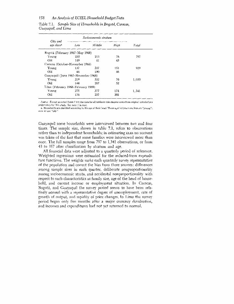
158 An Analysis of ECIEL Household Budget Data

Table 7.1. Sample Size of Households in Bogotd, Caracas,Guayaquil, and Lima

Socioeconomic stratum.City andage class, Low Middle High Total

Bogotg (February 1967-May 1968)Young 235 213 76 797Old 149 81 43

Caracas (October-Novenmber 1966)Young 137 357 153 929Old 46 190 46

Guayaquil (June 1967-November 1968)Young 219 352 76 1,050Old 144 207 52

Lima (February 1968-February 1969)Young 275 277 174 1.341Old 176 237 202

Ssarce: Except as noted (table 7.14) the data for all tables in this chapter come from original calculationsundertaken for this study. See note I in text.

a. Households are classified according to the age of their head. Those aged 45 years and less are "young";over 45 are "old."

Guavaquil some households were interviewed between two and fourtimes. The sample size, shown in table 7.1, refers to observationsrather than to independent households; in estimating ELES no accountwas taken of the fact that some families were interviewed more thanonce. The full samples range from 797 to 1,341 observations, or from43 to 357 after classification by stratum and age.

All financial data were adjusted to a quarterly period of reference.Weighted regressions were estimated for the reduced-form expendi-ture functions. The weights make each quarterly survey representativeof the population and correct the bias from three sources: differencesamong sample sizes in each quarter, deliberate nonproportionalitvamong socioeconomic strata, and accidental nonproportionality withrespect to such characteristics as family size, age of the head of house-hold, and current income or employment situation. In Caracas,Bogota, and Guayaquil the survey period seems to have been rela-tively normal with a representative degree of unemployment, rate ofgrowth of output, and rapidity of price changes. In Lima the surveyperiod began only five months after a major currency devaluation,and incomes and expenditures had not yet returned to normal.

THE DATA 159

Stratification

The six strata into which each sample was divided for estimationare defined by two independent criteria: the socioeconomic level ofthe household and the age of the head. Except in Caracas, the firststratification was part of the sample design, and the second wasadopted only after the data were collected. Inasmuch as the socio-economic strata are meant to separate households by their permanentincome rather than bv their tastes or needs or by the prices they face,the strata differ somewhat from the groupings used in chapters 6(Mexico) and 8 (Chile). The simultaneous classification of house-holds by age more nearly resembles the way families are classified inthe other chapters.

Neighborhoods were assigned to a high, middle, or low stratumon the basis of the extemal characteristics of dwellings, and samplingwas proportional within each stratum. The samples were nonpro-portional (the sampling fraction differed among strata) in Bogota,Guayaquil, and Lima. In Caracas the sample was proportional, butone stratum accounted for a very large share, and the strata correspondsomewhat less well to the levels of permanent income. The low-incomestratum was therefore defined as in the original sampling designaccording to place of residence (slums and marginal settlements),but the high and middle strata were separated according to theoccupation of the household head. Professional, technical, and ad-ministrative jobs constitute the high-income classification, and allothers are considered middle income.

The age of the household head appears to influence expenditureindependently of income level. Because this effect is nonlinear, it wasdecided to partition each sample at age 45.3 Households whose headis 45 or younger are called "young," and all others are "old." Theold households include some whose heads are retired and whosesaving behavior may differ from that of employed heads of the sameage.

Choice of Variables

Any variable which is presumed to affect expenditures can be usedto stratify the sample or included in the reduced-form equations.Two variables-current income and household size-are included inthe equations.

3. The results make it appear that three age classes would have been moresatisfactory, but some of the samples would then have been extremely small.

160 An Analysis of ECIEL Household Budget Data

Income. Total current income of all household members includesimputed rent of owned dwellings and income in kind received fromemployers or produced at home. It also includes transitory elementssuch as year-end bonuses, lottery winnings, and capital gains. Apartfrom the possibility of large errors in reporting current income, thechief drawback to using this variable is that the households havealready been stratified by a proxy for the level of permanent income.There may then be a great deal of transistory variation in the ob-served incomes, which may bias the expenditure-income relationsmore than the sample as a whole.

Household size. Because the smallest strata leave relatively fewdegrees of freedom, aiid because of the difficulty of specifying exactlyhow expenditures vary with household size at a given income level,a simple binary distinction was made. Households of four or fewermembers are "small" and all others are "large."4 No account wastaken of the age and sex of household members, so the size is notbased on the number of adult members only. For some house-holds, the number will include members who were absent for partof the period of reference and therefore contributed to determiningsome expenditures (shelter and durables, for example) but not others(such as food).5

Expenditures. The five expenditure categories are: (a) food,beverages, and tobacco, excluding food purchased in restaurants;(b) clothing and personal accessories; (c) housing and related ser-vices, including paid or imputed rent, but not mortgage payments;services such as fuel, water, and electricity; maintenance and repairs;insurance and taxes; paper products; washing and cleaning supplies;and garden supplies; (d) durable goods, including payments made

4. One-member households are included in Bogota and Guayaquil but notin Lima or Caracas. Except for the impossibility of estimating economies ofscale, the best approach would be to estimate a separate ya for members ofdifferent ages, as was done by Howe (1974).

5. The typical composition of households of a given size may vary amongcities, and among income levels and age classes in each city. In Bogota house-holds were defined as excluding supplementary members-those who sharepart but not all of their incomes and expenditures with the unit-whereas in theother cities the definition includes these members. Since supplementary membersare usually adults, households in Bogota will appear to contain a higher propor-tion of children and will, on the average, be smaller. In every city children aremore common, for a given household size, in young than in old households.Finally, high-income households, except in Bogota, will often include domesticservants.

EMPIRICAL RESULTS: ELES PARAMETER ESTIMATES 161

for vehicles as well as for furniture and household effects, and semi-durable goods such as household textiles (as in most householdsurvey data, expenditures may be a poor measure of the consumption-that is, depreciation-of durables); (e) all other expenditures, includ-ing education, transportation and communication, personal care,medical care, entertainment, direct taxes, gifts and transfers, and avariety of nonconsumption expenditures.

Mean income, expenditures, and household sizes. The mean valuesof income and of each of the expenditure classes, for each stratumand city, are shown in national currency in table 7.2. Annual incomeper capita is also shown in 1968 U.S. dollars. Average budget sharesand average income shares or spending propensities can be derivedfrom these means. Also shown are the mean household sizes, innumber of members, and the mean saving ratios.

Empirical Results: ELES Parameter Estimates

The parameters of the system (p., 3 and y*) are discussed in thissection, and subsistence expenditures are compared with observedmean income and total expenditure. Discussion of income elasticitiesand price elasticities derived from the parameters is left to the fol-lowing section.

The Marginal Propensity to Consume

The parameter pI should lie between zero and one, being fairly closeto one. It can be expected to stay constant or decline as income rises,but it is not clear bow , behaves with age, independently of income.The twenty-eight values of A are assembled in table 7.3 by incomestratum and age. The cities with the highest income (Caracas andLima) have the lowest overall marginal propensities, but these arebarely distinguishable from the estimate for Guayaquil, where incomeis at about the level of BogotA.6

When the A. are analyzed by stratum, the results are less satis-factory. Only in Bogota does A. decline with rising income in eachage group, and only there does p. (young) consistently exceed A (old),

6. For some categories the Caracas data have a shorter reference periodthan do those for other cities. The , for Caracas is therefore probably under-estimated to a slightly greater degree than in other cities since transitoryvariation is more important in the short run.

Table 7.2. Mean Quarterly Income and Expenditure, Mean Household Size,and Average Savings Ratio in Four South American Cities

Low Middle High

Item Young Old Young Old Young Old Total

Bogotd (tens of pesos)

Income 608.2 659.8 869.3 1,311.1 2,844.3 4,744.7 945.1Expenditure 647.2 650.2 867.1 1,134.7 2,483.7 4,199.0 911.6

Food 252.9 259.1 318.4 330.7 580.3 802.1 304.7Clothing 59.5 48.0 71.8 87.7 234.9 412.0 78.6

O Housing 160.6 197.8 249.4 321.0 737.6 1,233.5 256.5> Durables 26.7 7.9 26.1 26.2 138.4 t36.9 32. t

Other 147.6 137.5 191.5 369.2 792.5 1,614.5 239.8Size (persons) 6.02 5.55 6.70 6.53 5.81 6.92 6.13Average savings ratio -0.0641 0.0145 0.0025 0.1345 0.1268 0.1150 0.0354

Caracas (bolivars)

Income 2,764. 1 3,396.2 5,550.1 7,473.9 10,863.0 14,500.0 6,728.6Expenditure 2,359.6 3,119.9 5,581.9 6,494.6 9,951.9 12,532.0 6,219.6

Food 1,066.5 1,347.1 1,546.3 1,688.2 1,988.0 2,293.8 1,602.3Clothing 189.4 268.5 4t5.6 400.1 700.2 445.0 419.16Housing 502.4 736.3 1,753.2 2,270.8 3,349.5 4,936.4 2,038.4Durables 20.5 51.1 163.8 106.0 245.9 148.4 137.5Other 508.7 716.9 1,703.0 2,029.6 3,668.2 4,708.8 2,022.2

Size (persons) 6.30 6.98 4.88 5.24 5.33 5.63 5.38Averagesavingsratio 0.1463 0.0814 -0.0057 0.1310 0.0839 0.1357 0.0756

Guayaquil (sucres)

Income 7,880.8 9,125.2 9,359.9 13,901.0 28,183.0 32,912.0 10,631.0

Expenditure 6,364.1 7,841.7 9,553.4 12,119.0 25,368.0 29,768.0 9,261.9

Food 2,832.9 3,188.7 4,409.2 4,041.9 6,460.2 5,697.8 3,592.5

Clothing 599.4 643.8 576.2 669.6 1,568.5 1,809.4 635.4

Housing 1,407.5 2,065.9 2,153.8 4,199.8 9,392.5 12,698.7 2,652.5

Durables 487.6 183.9 327.0 538.4 1,081.1 666.1 369.2

Other 1,164.3 1,682.1 2,061.2 2,634.8 7,748.5 7,465.7 2,012.3

Size (persons) 6.03 6.42 5.81 5.57 5.82 5.41 6.01

Average savings ratio 0.1925 0.1407 -0.0014 0.1282 0.0999 0.0955 0.1288

Limna (tens of soles)

Income 2,005.6 2,342.6 4,025.8 5,224.6 14,743.0 13,786.0 3,252.8

Expenditure 1,952.5 1,986.6 4,202.3 4,545.4 10,381.0 10,027.0 2,968.9

Food 765.1 783.8 1,019.0 1,092.1 1,489.1 1,519.4 884.0

Clothing 148.1 189.1 350.5 377.4 766.7 1,083.2 249.9

Housing 330.2 424.1 1,160.5 1,382.7 3,892.0 3,907.4 754.0

Durables 181.8 125.8 494.1 477.8 917.1 593.7 282.9

Other 527.4 463.8 1,178.2 1,215.4 3,316.6 2,923.7 798.0

Size (persons) 6.56 6.99 5.80 6.02 7.03 7.70 6.47

Average savings ratio 0.0265 0.1520 -0.0438 0.1300 0.2959 0.2727 0.0873

Per capita income (1968 U.S.dollars a year)a

Bogota 431 507 554 857 2,089 2,925 658

Caracas 390 432 1,010 1,268 1,812 2,289 1,112

Guayaquil 467 508 576 892 1,730 2,173 632

Lima 433 475 983 1,229 2,970 2,535 712

a. Mean household income in national currency is divided by mean size, and then dates of the survey. The parities are 0.4800 (Colombia), 0.4019 (Ecuador), and 0.1593

converted to Venezuelan bolivars of equal purchasing power by parity rates calcu- (Peru); the bolivar-dollar free rate, used to convert to U.S. dollars, was 4.5.

lated for May 1968 and adjusted to account for inflation between that date and the

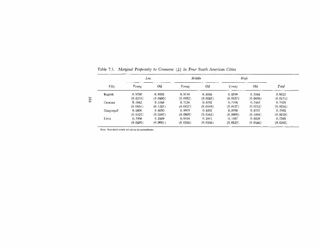
Table 7.3. Marginal Propensity to Consume (p) in Four South American Cities

Low Middle Ilig/s

City Young Old Young Old Young Old Total

Bogota 0.9700 0.9392 0.9144 0.8546 0.8599 0.5544 0.9313(0.0316) (0.0480) (0.0352) (0.0545) (0,0457) (0.0696) (0.0171)

Caracas 0.3882 0.3368 0.7136 0.6792 0.7106 0.7465 0.7429(0.0661) (0.1281) (0.0427) (0.0449) (0.0427) (0.0745) (0.0216)

Guayaquil 0.6808 0.8090 0.9979 0.8593 0.8598 0.8737 0.7992(0.0325) (0.0397) (0.0809) (0.0363) (0.0490) (0.1039) (0.0228)

Lima 0.7906 0.2889 0.9104 0.2441 0.1487 0.6539 0.7569(0.0495) (0.0907) (0.0536) (0.0568) (0.0829) (0.0446) (0.0260)

Note: Standard errors are given in parentheses.

EMPIRICAL RESULTS: ELES PARANIETER ESTINIATES 165

although the differences are not significant except at high incomes.In Caracas and Guayaquil the values for the middle and high strata,in both age groups, are not distinguishable with confidence, althoughthere is considerable variation in the point estimates. In Lima thereis no pattern to the propensities, and half of them are much toolow to be reasonable. (These are all cases in which one value of fiis negative.)

The standard errors of the estimates of st are often rather largebecause the strata are small, and in any case income is observed witherrors. A further difficulty is the substantial amount of transitoryincome and consumption. This factor explains why the very lowvalues of A are concentrated in Lima, where incomes were probablyabnormal in the survey period.7 'llTe variation in ,u among strata mayalso be explained by transitory income variation. Transitory incomeis likely to form a larger share of total income in the high and thelow strata than in the middle stratum because of high unemploymentin the low stratum and substantial capital receipts in the high stratum.

In summary, whenever all the estimates of / are reasonable, themarginal propensity to consume tends to decline or remain constantwith increasing income and also with increasing age. Transitoryincome variation in the high1 and-even more-in the low stratamakes it difficult to get reasonable results, however.

Marginal Budget Shares

The marginal budget shares derived from ELES should always bepositive. No inferior goods are allowed, which should not be asignificant limitation for the aggregated categories analyzed here, Ofthe 140 values of Si obtained, five are negative, and four of theseare distinct from zero. In each of the five cases the income elasticity(Ti) is also negative at the point of means, although the standarderrors on the elasticities are so large that none can be distinguishedfrom zero. In three cases (Bogota low-old, Lima low-old, and Caracaslow-young), 4i < 0 for expenditure on durables and vehicles. This

7. If the linear form of the permanent income hypothesis is correct (Fried-man, 1957, pp. 31-37), then ,a can be expressed as K var(yv)/var(y), whereK is the propensity to consume permanent income y,. Estimates with thelogaiithmic form of the hypothesis (Musgrove, 1977, chapter 2), suggest thatfor Lima, var(yp) is only about 70 percent of var(y), leading to low values of,a for a given K. In contrast, for Colombia (Bogota plus three smaller cities),var(yp) appears to exceed 90 percent of var(y). The same is true for Guayaquil(together with Quito).

166 An Analysis of ECIEL Household Budget Data

category may be expected to have a very large transitory variance,and the marginal budget share is negative only in the low stratum,where transitory variation in income may also be especially large.The other two cases, expenditures on food in Lima (high-young andmiddle-old), seem to imply that at high enough incomes food be-comes an inferior good, which is scarcely possible.

Tables 7.4 through 7.7 display the estimates of fh and y.* by city.

When all strata are analyzed together, the marginal share for food isinversely related to the income level, and the share for "other" isdirectly related. Housing takes a relatively constant share of marginalspending, ranging from 27 to 33 percent. Clothing shows only slightlygreater variation; its share is highest in Bogota and Lima, wherepersonal effects are most likely to be bought as saving substitutes.'The greatest variation is in durables, with a share ranging between3 and 5 percent except in Lima where it reaches 10 percent. Thisis almost certainly a consequence of accelerated inflation coupledwith large transitory variation in income and total expenditure.8

When the ,j are compared for young and old households in eachstratum, it is evident that voung families are more apt to devotethe marginal budget to durables and less apt to spend on housingand "other" than are older households.9 If the middle and high strataare considered together, young families also give higher marginalbudget shares to food and clothing except in Lima; at low incomesthis is true only in Bogota and Guayaquil.10 For necessities, themarginal budget share should fall as income rises, while it shouldrise for luxuries." The comparison is complicated by the occasionalnegative estimates of /3, since these raise the other marginal sharesin the same stratum and age group, but the effect on the ranking ofthe estimates across strata seems to be slight.

8. Differences in prices among cities are probably also important in explain-ing marginal spending shares, but are not considered here. The explanationin terms of inflation is discussed at more length later.

9. The comparison is not reliable for Lima because a negative value ofoccurs for food in the high-young and middle-old strata, and for durables in

low-old. Negative ,3 for durables in Bogota (low-old) and Caracas (low-young)have much smaller effects.

10. If those cases are excluded in which the two estimates cannot be dis-tinguished, then ,i (clothing) is always higher for young than for old families,and 13 (durables) is higher in all but one case.

11. No account is taken of differences in mean household size betweenyoung and old households, but, as table 7.1 indicates, these differences areusually slight.

EMPIRICAL RESULTS: ELES PARAMETER ESTIMATES 167

The most consistent pattern occurs for food expenditures, wherej8 (low) > , (middle) > S (high) six out of eight times. Forclothing, , (low) is always highest among young households, butthis pattern is less clear for older households. There is no consistentranking of , (middle) and , (high) for either age group. Fordurables, the pattern j§ (high) > (middle) > , (low) occursmost frequently, but in two cases j8 (low) is actually the highestestimate. There is no regular ranking for housing or for other goodsand services.

Subsistence Expenditures

The Stone-Geary utility function requires that v. > y* for eachhousehold in the sample. Since the estimate y* obtained is an averageover the sample, it can only be compared with an average level ofexpenditure such as v. Since y* is estimated for two differentclasses of household size, an average y* = -y*Z + y 2z2 is usedinitially for comparisons, where zE, Z2 are the proportions of house-holds in the small and large classes respectively.12 (It is this value ofy* which enters the calculation of price elasticities, Wit, s},). Of the140 values of y8, 44 exceed the mean expenditure V: 20 instances inBogota, 6 in Caracas, 13 in Lima, and 5 in Guayaquil. Those inGuayaquil occur because the estimate of fi is almost unity; when

1 ELES collapses to LES and the y* parameters are not identified(see 2.29). In what follows this set of estimates is not considered,leaving 39 instances in which y* > v.

Except for luxuries, the value of y* may be expected to rise some-what with income, since it is affected by habit as well as by necessity.Nonetheless it should rise less rapidly than mean expenditure, be-cause as income rises a smaller share goes to "subsistence" expendi-ture. The likelihood that yW > v should therefore be highest for thelow-income stratum and should be essentially zero at high incomes.1 3

12. If 'y* > V < y* the calculation is unnecessary. An alternative is to

compare 'y* with mean expenditure by size class, V, = zv Z INrZ. Note that it

may still happen that -y* > v- for many households h; in that case the variablesused to estimate -y* do not account for all the variation in minimum expenditureamong households.

13. -y* estimates based on permanent or normal income often exceed thosebased on current income. This is a further reason for the use of current incomehere, since it reduces the likelihood of T* exceeding V. See Howe (1974), pp.201-05; Belandria (1971), pp. 90-101; and Betancourt (1973), pp. 22-23.

Table 7.4. ELES Parameter Estimates, Bogotd Households, 1967-68

Socio- Age of Marginaleconomic household Household propensity tostratum head size Food Clothing Housing Durables Other consurme (n) e sum

> Marginal budget share (4i)Total 0.3274 0.0956 0.3108 0.0322 0.2430 0.9313

(0.0064) (0.0018) (0.0058) (0.0058) (0.0066) (0.0048)Low Young 0.3473 0.1159 0.2679 0.0458 0.2231 0.9700

(0.0120) (0.0039) (0.0092) (0.0015) (0.0078) (0.0316)Old 0.3900 0.0775 0.3288 -0.0001 0.2038 0.9392

(0.0208) (0.0040) (0.0715) (0.0000) (0.0111) (0.0480)Middle Young 0.2713 0.0946 0.3190 0.0592 0.2559 0.9144

(0.0111) (0.0038) (0.0128) (0.0024) (0.0104) (0.0352)Old 0.2443 0.0830 0.2870 0.0318 0.3540 0.8456

(0.0167) (0.0055) (0.0192) 0.0021) (0.0243) (0.0545)High Young 0.1609 0.1083 0,2986 0.0748 0.3574 0.8599

(0.0089) (0.0059) (0.0167) (0.0042) (0.0200) (0.0457)Old 0.1480 0.0751 0.2537 0.0570 0.4662 0.5544

(0.0190) (0.0097) (0.0342) (0.0073) (0.0595) (0.0696)

Subsistence consutmption (a*)

Total Small 205.8 45.7 165.5 13.9 115.9 546.8(39.9) (11.5) (36.2) (4.9) (29.8)

Large 534.2 125.5 416.4 41.4 340.4 1,457.9(97.9) (28.3) (88.6) (12.0) (73.1)

Low Young Small 432.4 125.4 307.1 47.2 246.2 1,158.3(369.5) (121.9) (283.4) (49.2) (237.7)

Large 1,051.2 311.6 753.8 118.2 638.6 2,873.4(957.8) (315.9) (734.7) (127.5) (616.3)

Old Small 232.1 39.0 192.3 0.8 102.6 566.8(152.9) (29.9) (126.9) (8.0) (81.0)

Large 724.8 132.1 555.8 11.5 368.9 1,793.1(482.0) (94.3) (400.4) (25.4) (255.4)

Middle Young Small 104.8 8.8 44.5 -4.1 32.0 186.0(60.4) (22.3) (69.3) (15.1) (56.8)

CD" Large 416.9 97.8 352.1 50.6 260.6 1,223.0(84.5) (31.2) (97.0) (21.0) (79.4)

Old Small 215.2 32.2 237.5 27.8 170.0 682.7(61.1) (21.2) (67.5) (11.3) (91.4)

Large 306.0 64.6 244.1 29.9 217.9 862.5(51.6) (17.9) (56.9) (9.5) (77.1)

High Young Small 366.4 174.9 383.5 94.3 525.4 1,544.5(73.9) (50.4) (136.5) (44.0) (165.4)

Large 438.2 74.1 425.6 14.2 317.2 1,269.3(78.2) (53.3) (144.4) (46.4) (175.0)

Old Small 132.5 17.1 118.0 -2.7 182.6 447.5(30.5) (27.7) (67.5) (22.9) (102.9)

Large 833.7 407.4 1,270.8 125.6 1,534.8 4,172.3(63.9) (57.9) (140.7) (48.0) (215.4)

Note: Standard errors are given in parentheses.

Table 7.5. ELES Parameter Estimates, Caracas Households, October-Novemiber 1966

Socio- Age of Marginaleconomic household Household propensity tostratum head size Food Clothing Housing l)urables Other consume (a) - sum

N Marginal budget share (i)Total 0.1963 0.0741 0.3282 0.0284 0.3730 0.7429

(0.0060) (0.0022) (0.0100) (0.0008) (0.0115) (0.0216)Low Young 0.5481 0.1550 0.0581 -0.0113 0.2501 0.3882

(0.0922) (0,0273) (0.0108) (0.0019) (0.0468) (0.0660)Old 0.0803 0.1662 0.4706 0.0227 0.2601 0.3368

(0.0344) (0.0648) (0.1800) (0.0087) (0.1079) (0.1285)Middle Young 0.1932 0.0967 0.2768 0.0465 0.3869 0.7136

(0.0119) (0.0059) (0.0178) (0.0029) (0.0242) (0.0420)Old 0.1631 0.0194 0.3882 0.0152 0.4141 0.6792

(0.0112) (0.0113) (0.0262) (0.0010) (0.0288) (0.0440)High Young 0.0993 0.0854 0.3668 0.0450 0.4035 0.7106

(0.0075) (0.0064) (0.0278) (0.0034) (0.0313) (0.0522)Old 0.1053 0.0313 0.4283 0.0167 0.4183 0.7465

(0.0108) (0.0031) (0.0433) (0.0017) (0.0442) (0.0745)

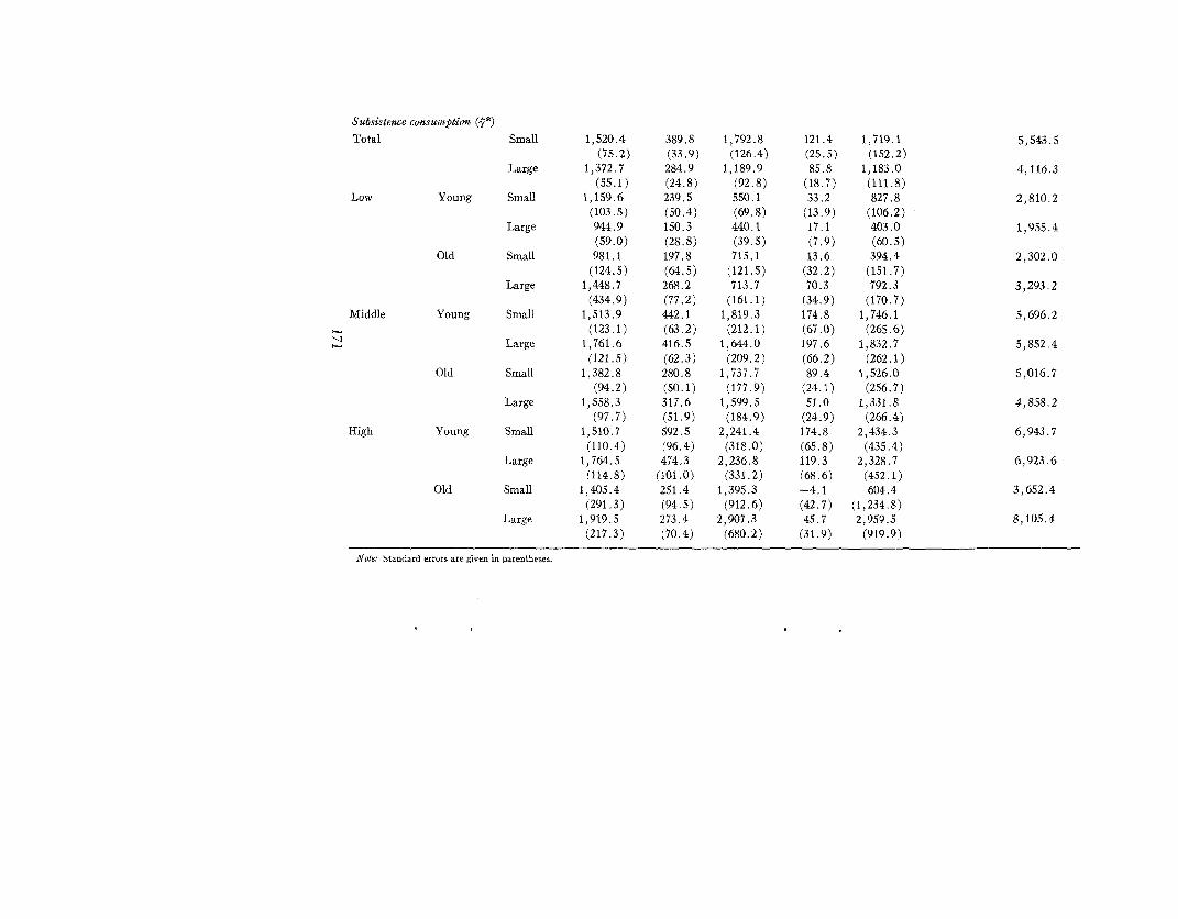
Subsistence consuniplion (.y*)

Total Small 1,520.4 389.8 1,792.8 121.4 1,719.1 5,543.5

(75.2) (33.9) (126.4) (25.5) (152.2)

Large 1,372.7 284.9 1,189.9 85.8 1,183.0 4,116.3

(55.1) (24.8) (92.8) (18.7) (111.8)

Low Young Small 1,159.6 239.5 550.1 33.2 827.8 2,810.2

(103.5) (50.4) (69.8) (13.9) (106.2)

Large 944.9 150.3 440.1 17.1 403.0 1,955.4

(59.0) (28.8) (39.5) (7.9) (60.5)

Old Small 981.1 197.8 715.1 13.6 394.4 2,302.0

(124.5) (64.5) (121.5) (32.2) (151.7)

Large 1,448.7 268.2 713.7 70.3 792.3 3,293.2

(434.9) (77.2) (161.1) (34.9) (170.7)

Middle Young Small 1,513.9 442.1 1,819.3 174.8 1,746.1 5,696.2

(123.1) (63.2) (212.1) (67.0) (265.6)

2 Large 1,761.6 416.5 1,644.0 197.6 1,832.7 5,852.4

(121.5) (62.3) (209.2) (66.2) (262.1)

Old Small 1,382.8 280.8 1,737.7 89.4 1,526.0 5,016.7

(94.2) (50.1) (177.9) (24.1) (256.7)

Large 1,558.3 317.6 1,599.5 51.0 1,331.8 4,858.2

(97.7) (51.9) (184.9) (24.9) (266.4)

High Young Small 1,510.7 592.5 2,241.4 174.8 2,434.3 6,943.7

(110.4) (96.4) (318.0) (65.8) (435.4)

Large 1,764.5 474.3 2,236.8 119.3 2,328.7 6,923.6

(114.8) (101.0) (331.2) (68.6) (452.1)

Old Small 1,405.4 251.4 1,395.3 -4.1 604.4 3,652.4

(291.3) (94.5) (912.6) (42.7) (1,234.8)

Large 1,919.5 273.4 2,907.3 45.7 2,959.5 8,105.4

(217.3) (70.4) (680.2) (31.9) (919.9)

Note: Standard errors are given in parentheses.

Table 7.6. ELES Parameter Estimates, Guayaquil Households, 1967-68

Socio- Age of Marginaleconomic household Household propensity tostratum head size Food Clothing Housing Durables Other consume (a) * sum

N Marginal budget share (,)Total 0.3840 0.0724 0.2875 0.0476 0.2083 0.7992

(0.0118) (0.0021) (0.0083) (0.0014) (0.0062) (0.0228)Low Young 0.3586 0.1008 0.2347 0.0738 0.2320 0.6808

(0.0181) (0.0049) (0.0116) (0.0038) (0.0117) (0.0325)Old 0.4033 0.0727 0.3100 0.0279 0,1861 0.8090

(0.0205) (0.0036) (0.0159) (0.0014) (0.0100) (0.0397)Middle Young 0.4434 0.0575 0.2318 0.0491 0.2182 0.9979

(0.0378) (0.0047) (0.0189) (0.0040) (0.0179) (0.0809)Old 0.3565 0.0611 0.3188 0.0506 0.2130 0.8593

(0.0156) (0.0026) (0.0139) (0.0023) (0.0100) (0.0363)High Young 0.2801 0.0739 0.3960 0.0486 0.2015 0.8598

(0.0167) (0.0043) (0.0229) (0.0229) (0.0132) (0.0040)Old 0.1112 0.0535 0.5379 0.0301 0.2673 0.8737

(0.0135) (0.0064) (0.0619) (0.0036) (0.0325) (0.1039)

Subsistence consutmption (.Z*)

Total Small 944.0 141.0 527.0 30.7 563.2 2,205.9(165.5) (23.7) (90.2) (23.2) (73.3)

Large 2,476.6 238.0 916.3 113.2 666.9 4,411.0(191.6) (27.4) (104.3) (26.8) (84.8)

Low Young Small 1,024.5 48.0 342.3 -29.0 191.6 1,577.4(142.6) (39.4) (82.0) (62.7) (93.0)

Large 2,4t9.4 238.5 698.0 132.9 575.2 3,864.1(115.3) (31.8) (66.1) (50.4) (74.8)

Old Small 974.4 195.4 646.3 36.7 655.0 2,507.8(218.4) (41.3) (165.1) (25.8) (125.6)

Large 2,135.6 216.6 837.7 43.4 641.5 3,874.8(316.9) (60.0) (239.7) (37.4) (182.0)

Middle Young Small -

Large - - - - _Old Small 981.5 121.2 862.3 46.2 927.3 2,938.5

(304.8) (52.0) (264.1) (69.7) (218.8)Large 1,839.5 126.2 898.5 114.2 468.7 3,447.1

(424.3) (72.3) (367.4) (96.9) (304.4)High Young Small 935.4 166.4 403.2 7.3 710.5 2,222.8

(739.9) (187.2) (973.7) (172.4) (685.1)Large 2,276.0 413.2 1,806.0 208.8 2,192.2 6,896.2

(680.0) (172.1) (895.4) (158.6) (629.8)Old Small 2,847.1 393.5 2,630.1 90.3 1,957.4 7,918.4

(718.2) (320.8) (3,625.3) (201.3) (1,618.4)Large 3,336.1 279.0 -429.1 -80.0 -22.7 3,083.3

(870.2) (348.1) (3,214.0) (254.9) (1,319.7)

- Estimated with very large standard errors because A is very close to one. Note: Standard errors are given in parentheses.

Table 7.7. ELES Parameter Estimates, Lima Households, 1968-69

Socio- Age of Marginaleconomic household Household propensity tostratum head size Food Clothing Housing Durables Other consumne (A) s* su

, Marginal budget share (,)Total 0.2237 0.1094 0.2730 0.0987 0.2952 0.7569

(0.0084) (0.0038) (0.0097) (0.0037) (0.0106) (0.0260)Low Young 0.2679 0.1205 0.1744 0.1442 0.2930 0.7906

(0.0186) (0.0076) (0.0112) (0.0098) (0.0189) (0.0495)Old 0.3115 0.1343 0.3328 -0.4015 0.6229 0.2889

(0.1023) (0.0445) (0.1078) (0.1547) (0.1927) (0.0907)Middle Young 0.2395 0.0875 0.3048 0.1676 0.2005 0.9104

(0.0145) (0.0052) (0.0184) (0.0106) (0.0134) (0.0536)Old -0.3617 0.1989 0.7132 0.2195 0.2302 0.2441

(0.1109) (0.0467) (0.1617) (0.0535) (0.0572) (0.0568)High Young -0.0142 0.0420 0.6394 0.2192 0.1137 0.1487

(0.0081) (0.0238) (0.3458) (0.1324) (0.0727) (0.0829)Old 0.1215 0.0814 0.4162 0.0880 0.2929 0.6539

(0.0086) (0.0057) (0.0297) (0.0063) (0.0207) (0.0446)

Subsistence consumption (e*)Total Small 694.5 204.6 591.6 196.1 668.0 2,354.8

(66.6) (27.2) (60.2) (37.8) (69.4)

Large 1,108.7 306.7 767.8 320.6 813.2 3,317.0

(82.4) (33.6) (74.5) (46.8) (85.8)

Low Young Small 544.5 168.1 329.2 205.7 498.4 1,745.9

(130.2) (42.8) (64.7) (73.0) (106.3)

Large 1,200.0 301.0 531.5 375.3 776.1 3,183.9

(209.2) (68.9) (104.0) (117.3) (171.0)

Old Small 527.1 50.1 229.8 -10.8 226.3 1,022.5

(56.9) (41.5) (51.5) (46.1) (47.9)

Large 860.0 245.5 431.2 124.2 545.1 2,206.8

(79.3) (57.9) (71.7) (64.1) (66.7)

Middle Young Small 2,881.9 1,029.9 3,555.9 1,765.8 2,772.5 12,011.0

(1,528.7) (562.8) (1,950.9) (1,179.2) (1,547.4)

Large 1,490.3 477.8 1,614.1 801.9 1,183.3 5,567.4

(636.8) (234.4) (812.5) (49t.2) (644.5)

Old Small 1,003.2 252.7 992.3 343.3 837.5 3,429.0

(104.1) (33.0) (85.2) (79.2) (97.5)

Large 861.3 263.5 1,089.0 316.4 862.3 3,392.5

(92.1) (29.1) (75.4) (70.0) (86.2)

High Young Small 1,010.6 1,204.1 1,427.3 589.4 2,477.3 6,708.7

(106.5) (109.1) (298.1) (330.6) (371.8)

Large 1,454.1 576.6 3,623.7 728.2 2,780.0 9,162.6

(98.2) (168.1) (274.5) (303.9) (340.9)

Old Small 1,073.5 515.7 2,817.9 345.3 1,470.7 6,223.1

(120.3) (85.5) (387.7) (113.7) (220.9)

Large 1,267.9 496.0 2,650.2 363.5 1,713.9 6,490.9

(94.3) (67.1) (303.8) (89.1) (172.6)

Note: Standard errors are given in parentheses.

176 An Analysis of ECIEL Household Budget Data

The results confirm this expectation. There are no instances of atoo high y* in the high-income stratum, 15 in the middle, and 16in the low stratum. (Eight instances occur when all strata areanalyzed together.)

It is less obvious a priori how the occurrence of y* > jv shouldbe distributed between young and old households, but the results arequite clear. In every city the mean expenditure for young householdsis closer to-or more frequently below-the minimum level. More-over, the occurrences for old households are, with only one exception,limited to the low-income stratum, while there are many instancesfor younger families at the middle level of income. This can occurbecause v is usually smaller for young households, or because y* ishigher. In the former case income is probably the most importantexplanatory variable. In the second case there may be importantdifferences in need determined by family size or age structure. Itmay simply be, however, that vounger households have differentexperiences and expectations, and envision a higher level of minimumacceptable consumption.

A comparison of v~ and y* between age groups reveals that bothinfluences are at work. Average expenditure is more often below y'for young households in the lower two strata, except in the case ofexpenditure for durables. At the same time, y* is higher for youngthan for old households 25 times out of 35 for small families and28 times out of 35 for large ones. Young households behave asthough they bad high levels of subs,istence expenditure even thoughthey usually have less money to spend than older households. Onlyon expenditure for durable goods does the stage in the life cyclehave a clear effect; for the other categories, "subsistence" levels seemto be determined by past consumption experience, income expecta-tions, or some other largely psychological influence.

The parameter y* should be positive for any category considereda necessity and negative only in the case of luxuries forgone at alow-income level. Of the 280 estimates of y* obtained, only eightare negative, and none differs significantly from zero. Six of thesevalues occur for durables, one for shelter, and one for other goodsand services. Small households are involved five times, at least oncein each city, and large households three times (all in Guayaquil,high-old). In general, durables are the only "unnecessary" category,and they become more necessary as household size increases. Whenall strata are analyzed together, y* (durables) always is significantlypositive for both sizes of household.

At a given income level it may be expected that y* (large) > y*

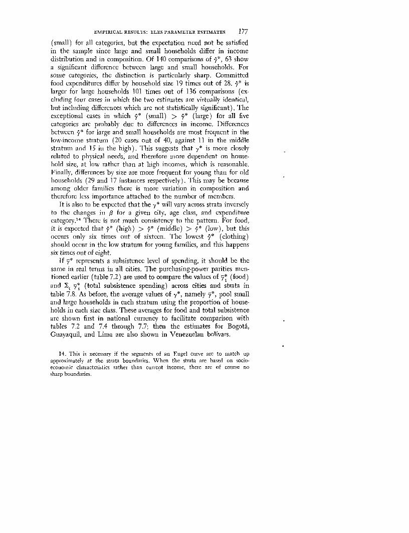
EMPIRICAL RESULTS: ELES PARAMETER ESTIMATES 177

(small) for all categories, but the expectation need not be satisfiedin the sample since large and small households differ in incomedistribution and in composition. Of 140 comparisons of y*, 63 showa significant difference between large and small households. Forsome categories, the distinction is particularly sharp. Committedfood expenditures differ by household size 19 times out of 28. y* islarger for large households 101 times out of 136 comparisons (ex-cluding four cases in which the two estimates are virtually identical,but including differences which are not statistically significant). Theexceptional cases in wbich 9* (small) > y* (large) for all fivecategories are probably due to differences in income. Differencesbetween y* for large and small households are most frequent in thelow-income stratum (20 cases out of 40, against 11 in the middlestratum and 15 in the high). This suggests that y* is more closelyrelated to physical needs, and therefore more dependent on house-hold size, at low rather than at high incomes, which is reasonable.Finally, differences by size are more frequent for young than for oldhouseholds (29 and 17 instances respectively). This may be becauseamong older families there is more variation in composition andtherefore less importance attached to the number of members.

It is also to be expected that the y* will vary across strata inverselyto the changes in pl for a given city, age class, and expenditurecategory.1 4 There is not much consistency to the pattern. For food,it is expected that y* (high) > y* (middle) > y* (low), but thisoccurs only six times out of sixteen. The lowest y* (clothing)should occur in the low stratum for young families, and this happenssix times out of eight.

If y* represents a subsistence level of spending, it should be thesame in real terms in all cities. The purchasing-power parities men-tioned earlier (table 7.2) are used to compare the values of * (food)and I * (total subsistence spending) across cities and strata intable 7.8. As before, the average values of -y*, namely y*, pool smalland large households in each stratum using the proportion of house-holds in each size class. These averages for food and total subsistenceare shown first in national currency to facilitate comparison withtables 7.2 and 7.4 through 7.7; then the estimates for Bogota,Guayaquil, and Lima are also showvn in Venezuelan bolivars.

14. This is necessary if the segments of an Engel curve are to match upapproximately at the strata boundaries. When the strata are based on socio-economic characteristics rather than current income, there are of course nosharp boundaries.

Table 7.8. Average Committed Expenditures on Food and in Total for Four South American Cities

Low Middle High

CommittedCity expenditure Total Young Old Young Old Young Old

National currency

Bogota. Food 437.3 850.3 546.2 359.6 277.8 414.5 728.7

Total 1,189.0 2,316.5 1,348.5 1,032.6 806.7 1,360.1 3,614.7

Caracas Food 1,437.0 1,004.8 1,324.5 1,630.7 1,470.4 1,673.3 1,741.1

Total 4,737.5 2,193.9 3,029.9 5,769.9 4,937.6 6,930.8 6,559.8

Guayaquil Food 1,999.5 2,043.0 1,773.0 - 1,497.8 1,939.5 3,100.5

Total 3,724.6 3,247.1 3,447.9 - 3,244.5. 5,723.1 5,412.9

9 Lima Food 1,002.8 1,055.2 772 1 1,889.6 905.1 1,385 .7 11,236.9

Total 3,071.0 2,866.2 1,894.0 7,416.4 3,403.8 8,784.3 6,448.2

Venezuelan bolivars%

Bogota Food 1,714.0 3,332.8 2,140.9 1,409.5 1,088.9 1,624.7 2,856.2

Total 5,707.2 11,119.2 6,472.8 4,956.5 3,872.2 6,528.5 17,350.6

Guayaquil Food 779.2 796.2 690.9 - 583.7 755.8 1,208.3

Total 1,497.0 1,305.0 1,385.7 - 1,304.0 2,300.1 2,175.4

Lima Food 1,622.7 1,707.5 1,249.4 3,057.8 1,464.6 2,242.3 2,001.6

Total 4,892.1 4,565.9 3,017.1 11,814.3 5,422.3 13,993.4 10,272.0

- Estimated with very large standard error because y is very close to one. are 0.39196, 0.3897, and 0.16182 respectively. No account is taken of the fact that

Note: For comparisons of y* (food), the purchasing-power parities are dividedl by rates of inflation for food prices differ from those for other consumption goods.

indexes of food prices relative to all prices. These indexes are 1.2246 for Colombia, a. As at the end of October 1966. The exchange rate was 4.5 bolivars to the U.S.

1.03142 for Ecuador, and 0.98445 for Peru, so the purchasing-power parities for food dollar.

ELASTICITY ESTIMATES 179

The definitions of strata differ sufficiently among cities and house-hold composition can differ so much within a given stratum that aclose correspondence cannot be expected. For y* (food) the esti-mates are fairly similar in real terms for Bogota, Caracas, and Lima;those for Guayaquil, however, are systematically much lower. Priceindexes based on the individual strata and with weights closer toconsumption patterns in these countries might remove much of thevariation. The correspondence is generally much less close for totalsubsistence expenditure, in part because this includes items such asdurables, which cannot be identified with needs, and because thetotal may be sensitive to the alternatives for saving which householdsface.

The values of y* might be expected to be most nearly equalamong cities in the low-income stratum, where households are closestto subsistence, but this expectation is not supported by the results.The closest correspondence occurs when all strata are pooled, perhapsbecause this diminishes the importance of transitory spending andof differences among definitions of the strata. The estimates are quiteclose for Caracas and Lima, the cities with the highest income.

Elasticity Estimates

The elasticities derived from ELES are, like the parameters, subjectto certain theoretical conditions. Each elasticity can be expressed asa function of those parameters and income (or total expenditure).

Expenditure Elasticity of the Marginal Utility of Expenditure

From (2.4) and (2.7), the Frisch parameter o can be expressed as

(7.3) v

Because actual spending should exceed subsistence expenditures,the parameter should be negative and should rise in absolute valueas income and total spending decline. As is evident from tables 7.2and 7.8, however, v is frequently less than X ?' leading to a positive

value for expression (7.3). This occurs in the lowest-income groupsfor Bogota and Lima, as well as for the entire sample in each city;it does not occur in Guayaquil owing to the notably low values of yobtained there.

180 An Analysis of ECIEL Household Budget Data

Table 7.9. Estimates of the Frisch Parameter at Mean Expenditurefor Four South American Cities

Socio- Age ofeconomic householdstratum head Bogotd Caracas Guayaquil Li;na

All households a -4.197 -1.673 _aLow Young -a -14.240 -2.042 -,

Old _ -34.666 -1.785 -21.454Middle Young ab _

Old - 3.460 -4.171 -1.366 -3.982High Young -2.211 -3.294 -1.291 -6.502

Old -7.186 -2.098 -1.222 -2.802

a. vC< YW

b. tji not calculated.

Table 7.9 presents estimates of w for those cases in which theparameter is negative. The most plausible estimates are those forCaracas, where in each age class the absolute value falls as incomerises. The overall value (--4.2) is also reasonable. The same patternis evident for Guayaquil but at lower absolute values, comparable tothose obtained for much richer countries (see table 4.4). Two of thethree values for Bogota are reasonable, but no pattern emerges.Reasonable estimates are derived for older households in the middleand high strata in Lima. It is not possible to estimate w for themiddle-young group in any city: this is the group that has consistentlyhigh subsistence expenditures relative to actual total spending, per-haps because of high expectations about future income.

After substituting for I`' = Ep.yi in (2.2), the Frisch parameter

can be written as a function of average and marginal saving pro-pensities (APs and MPS), that is,

- (1 -y)V -MPS (I - APS)( ) y~~~~I (y - V) (I - MPS) APS

from which it is evident that the parameter estimate is extremelysensitive to errors in estimating either the MPS or the APS. For smallgroups of households whose incomes and expenditures are reportedwith small errors and may in addition contain transitory components,the margin for error in the saving propensities is large, even if theELES parameters related to expenditures can be estimated satisfactorily.

ELASTICITY ESTIMATES 181

Income and Expenditure Elasticities

Tables 7.10 through 7.13 show income and expenditure elasticities(s7 and qj) by socioeconomic stratum in the four cities under study.The right-hand columns of the tables summarize the elasticitiesestimated by pooling the observations for all strata. These elasticitiesare highest in Bogota and Guayaquil, the cities with the lowestincome. They might have been uniformly highest in Caracas, exceptfor the larger transitory variation in income and spending; and theelasticities for durables might have been highest in Lima except forthe importance of inflation. Except for food, all the elasticities areclose to unity, but only five out of sixteen are indistinguishablefrom 1.0.

It may be of some interest to compare the estimates of 4j for thewhole sample (right-hand columns of tables 7.10-7.13) with someelasticities obtained with double-log Engel curves estimated usingtotal expenditure (see table 7.14). The latter elasticities refer to allthe cities surveyed in each country; only in Peru is the data base thesame. More importantly, these regressions are unweighted and thusoverrepresent the high stratum, except in Venezuela.

After allowance is made for all the data and procedural differencesbetween the two sets of estimates, it is notable that the ELES resultsare less widely dispersed than those obtained with double-log Engelcurves. Estimation within a system which guarantees the satisfactionof the budget constraint forces the elasticity estimates closer togetherand therefore closer to unity. In only two of the sixteen comparisonsis the ELES estimate farther from one in absolute value than are theestimates shown in table 7.14.

Own-Price Elasticities

One of the reasons for estimating ELES iS to obtain information abouthousehold responses to price changes.15 Estimates are given for eachstratum, since price elasticities are expected to be function ofincome and to differ as income rises.

Of 135 own-price elasticities presented in table 7.15 (not countingthe five estimates for Guayaquil, middle-young), 28 are positive,27 are negative but not significantly different from zero, and 80 areclearly negative. There are marked variations among cities and also

15. Information on prices paid by consumers was collected for some products(mostly foodstuffs) in some countries as part of the ECIEL survey, but thesedata have not been analyzed.

Table 7.10. Bogotd: Income and Expenditure Elasticities of Demand Evaluated at Point of Means

Low Middle High Total,

Income Expenditure Income Expenditure Income Expenditure Income ExpenditureCommodity elasticity elasticity elasticity elasticity elasticity elasticity elasticity elasticity

Young households

Food 0.74528 0.81760 0.65713 0.71683 0.63501 0.64485 0.79393 0.82228(0.02599) (0.03576) (0.05220) (0.01253)

Clothing 1.15693 1.26919 1.06713 1.16407 1.07862 1.09533 1.04892 1.08637(0.04244) (0.09491) (0.08537) (0.01948)

Housing 0.95849 1.05150 0.98001 1.06904 0.92115 0.93542 0.97018 1.00482(0.02988) (0.03717) (0.05133) (0.01141)

Durables 1.41000 1.54682 1.39510 1.52184 1.34408 1.36490 1.09236 1.13137co (0.10316) (0.16899) (0.19707) (0.06456)

Other 0.93033 1.02060 1.07614 1.17390 1.03811 1.05419 0.97689 1.0117(0.03599) (0.04963) (0.05377) (0.01501)

Old households

Food 0.82198 0.86426 0.70891 0.72556 0.47383 0.75637(0.03378) (0.05092) (0.07805)

Clothing 0.99551 1.04453 1.02282 1.04684 0.49887 0.79635(0.06134) (0.15187) (0.17509)

Housing 0.96429 1.00989 0.87307 0.89357 0.53094 0.84754(0.03332) (0.04012) (0.10736)

Durables -0.00609 -0.00639 0.82193 0.84123 1.05497 1.68405(1.41058) (0.17573) (0.31397)

Other 0.89856 0.94281 1.10867 1.3470 0.75501 1.20522(0.05167) (0.05137) (0.09258)

Note: Stanidard errors are given in parentheses. a. Includes both young and old households in all strata.

T'able 7.11. Caracas: Income and Expenditure Elasticities of Demand Evaluated at Point of Means

Low Middle High Totall

Income Expenditure Inconme Expenditure Income Expenditure Income ExpenditutreComnodity elasticity elasticity elasticity elasticity elasticity elasticity elasticity elasticity

Young households

Food 0.52219 1.14831 0.47801 0.67370 0.39294 0.50659 0.56802 0.70676(0.06238) (0.03647) (0.06736) (0.01985)

Clothing 0.79372 1.74541 0.92324 1.30119 0.87250 1.12485 0.84157 1.04712(0.18495) (0.06371) (0.12561) (0.03718)

Housing 0.12885 0.28334 0.64737 0.91239 0.86756 1.11849 0.84663 1.05342(0.16915) (0.05546) (0.05556) (0.01933)

Durables -0.63232 -1.39048 1,03280 1.45560 1.31131 1.69058 0.98928 1.23091°° (1.25711) (0.21795) (0.25555) (0.09870)

Other 0.46521 1.02301 0.88757 1.25092 0.82937 1.15047 0.94744 1.17885(0.16140) (0.04884) (0.08187) (0.02101)

Old households

Food 0.06884 0.18777 0.47270 0.60477 0.48178 0.55779(0.16697) (0.04736) (0.09480)

Clothing 0.70435 1.92116 0.29644 0.37927 0.75133 0.86987(0.32786) (0.23696) (0.16555)

Housing 0.69726 1.90182 0.84294 1.07846 0.92407 1.09070(0.18210) (0.03164) (0.04994)

Durables 0.44746 1.22048 0.80021 1.02379 1.41911 1.64300(0.93528) (0.25713) (0.19373)

Other 0.41408 1.12943 0.98116 1.25530 0.97974 1.13431(0.32072) (0.05566) (0.10626)

Note: Standard errors are given in parentheses. a. Includes both young and old households in all strata.

Table 7.12. Guayaquil: Income and Expenditure Elasticities of Demand Evaluated at Point of Means

Low Middle High Total,

Income Expenditure Income Expenditure Income Expenditure Income ExpenditureCommodity elasticity elasticity elasticity elasticity elasticity elasticity elasticity elasticity

Young households

Food 0.61299 0.72711 0.91084 0.91405 0.92362 0.96693 0.79213 0.86351(0.03177) (0.08244) (0.02353) (0.02328)

Clothing 1.09245 1.29583 1.02081 1.02441 1.00683 1.05404 1.01328 1.10459(0.04798) (0.04445) (0.02756) (0.01783)

IIousing 0.95471 1.13245 1.01328 1.01685 1.05439 1.10383 1.02555 1.11796(0.03238) (0.02135) (0.01275) (0.01003)

Durables 1.25880 1.49315 1.27614 1.28064 1.07367 1.12402 1.15446 1.25849co (0.14154) (0.09478) (0.07447) (0.04920)

Other 1.05435 1.25064 1.11097 1.11488 0.85486 0.89495 0.99191 1.08129(0.04208) (0.03333) (0.05432) (0.01789)

Old households

Food 0.82122 0.87233 0.89421 0.90723 0.55399 0.57350(0.02985) (0.01916) (0.08484)

Clothing 0.08693 1.04835 1.06748 1.08302 0.94978 0.98323(0.05849) (0.03151) (0.07730)

Housing 1.03926 1.10404 1.00123 1.01580 1.10732 1.14632(0.03335) (0.01653) (0.03146)

Durables 1.21610 1.29178 1.09791 1.11389 1.19348 1.23552(0.16752) (0.09531) (0.15738)

Other 0.91557 0.97255 0.97794 0.99217 1.04527 1.08209(0.06442) (0.03886) (0.03014)

Note: Standard errors are given in parentheses. a. Includes both young and old households in all strata.

Table 7.13. Lima: Income and Expenditure Elasticities of Demand Evaluated at Point of Means

Low Middle High Totala

Income Expenditure Incomne Expenditure Incomne Expenditure Income Expenditure

Commodity elasticity elasticity elasticity elasticity elasticity elasticity elasticitv elasticity

Young householdsFood 0.48677 0.59940 0.76320 0.87507 -0.02266 -0.10730 0.53280 0.64249

(0.05289) (0.03001) (0.16908) (0.02905)

Clothing 1.00762 1.24076 0.87605 1.00446 0.12960 0,61369 0.91121 1.09880

(0.03840) (0.04837) (0.28625) (0.02561)

Housing 0.75135 0.92519 0.90810 1.04121 0.36398 1.72353 0.88403 1.06602

(0.03887) (0.02885) (0.10841) (0.01530)

Durables 0.95343 1.17403 1.09450 1.25493 0.53336 2.52559 0.88403 0.96928

(0.08272) (0.06976) (0.47337) (0.05281)

'- Other 0.90139 1.10995 0.71943 0.82488 0.08793 0.41637 0.89006 1.07329

(0.03136) (0.07816) (0.25778) (0.01758)

Old householdsFood 0.25932 0.76120 -0.61965 -2.20850 0.60196 0.66956

(0.11054) (0.38075) (0.06046)

Clothing 0.43039 1.26336 0.72761 2.59328 0.82483 0.91746

(0.29553) (0.07345) (0.07171)

Housing 0.54388 1.57008 0.66092 2.35559 0.80273 0.89288

(0.15449) (0.04212) (0.04348)

Durables - 0.66291 2.36269 1.01315 1.12693

- (0.04212) (0.09020)

Other 0.77832 2.28467 0.30675 1.09329 0.85731 0.95358

(0.07493) (0.12327) (0.03412)

- Mean expenditure too close to subsistence to permit estimation. a. Includes both young and old households in all strata.

Note: Standard errors are given in parentheses.

186 An Analysis of ECIEL Household Budget Data

Table 7.14. Expenditure Elasticities from Double-Log Engel Curves

Colombia Venezuela Ecuador PeruCommodity (four cities) (two cities) (tSo cities) (Lima)

Food (excluding tobacco) 0.6624 0.6098 0.6696 0.4743(0.0057) (0.0116) (0.0082) (0.0139)

Clothing 1.2435 1.1852 1.1144 1.0495(0.0235) (0.0534) (0.0391) (0.0453)

Housing (excluding some 0.9239 0.7608 0.9614 0.9223services) (0.0149) (0.0166) (0.0240) (0.0316)

Durables (excluding vehicles) 1.4755 1.3082 1.3800 1.4958(0.0756) (0.0898) (0.0921) (0.1106)

Nole: Standard errors are given in parentheses.Source: Musgrove (1977), table 6-1.

among strata, but not between the two age groups. Out of 35 esti-mates for each city, 11 are significantly negative in Bogota, 16 inLima, 23 in Caracas, and 30 out of 30 in Guayaquil. Only 15 of 40estimates are significantly below zero in the low stratum, 18 of 35in the middle, and 35 of 40 in the high. The variation across strataand the very clear results obtained for high-income households com-pensate somewhat for the rather poor results obtained when allstrata are analyzed together (3 positive values, 12 negative, and 4negative but not distinct from zero).

The expected pattern of elasticities across strata is 4 ii (low) >27u (middle) > 7ii (high), with elasticities increasing in absolutevalue (becoming more negative) as income increases. The closer ahousehold is to subsistence, the less it can respond to changes inprices. This pattern is observed 19 times out of 40. In the 12 instancesin which r (middle) > 0, 1 (low) always exceeds ' (high).If these cases are excluded, the results are quite good. Finally, theexpected pattern is observed in 13 of 18 comparisons in which theelasticity is negative in all three strala.

Tlhe estimates for Bogota, Caracas, and Lima are usually of com-parable magnitude, while those for Guayaquil are almost uniformlylarger in absolute value. The smallest value in Guayaquil is -0.455for food in the low-young group, and the largest is -0.997 fordurables in high-old. This result is surprising in a low-income citylike Guayaquil. The explanation appears to lie in the low ratios ofy*:V found there, since the lower this ratio, the higher is jii. Intable 7.16 own-price elasticities aie averaged for both age groups,by stratum and commodity, for the first three cities together andfor Guayaquil alone. Only negative estimates are included in these

ELASTICITY ESTIMATES 187

averages.1 6 Differences between age classes are not systematic enoughto warrant separate calculations. Also shown is the average of thenegative elasticities calculated across all strata in each city. ForBogota, Caracas, and Lima together, all five elasticities rise in absolutevalue as income rises. The elasticities for clothing and durables risethe most, as indicated by rankings in each stratum. For Guayaquil,the elasticities for food and clothing fall slightly at high incomes,and the smallest in that city (-0.542) is still above the largestaverage in the other cities (-0.501). It seems likely that the resultsfor Guayaquil greatly overstate household response to price changes,but in the absence of direct estimation it is not certain that there isnot some marked difference in behavior.

Positive Own-Price Responses, Inflation, andthe Dynamic Interpretation of ELES

To satisfy the fundamental theorem of demand, the own-price elas-ticity iiii must be negative. Of the 28 positive estimates only one ofthese (durables in Caracas, low-young) is associated with a negativeestimate of p3i. The remainder are a subset of the 39 instances inwhich y* > v.

None of the positive own-price elasticities is distinguishable fromzero. Nonetheless, the point estimates suggest something aboutdynamic household responses to price changes. In three cases (Bogota,low-young, and Lima, low- and middle-young) all five elasticities arepositive. Of the remaining thirteen cases, six involve durables andfour involve clothing; food, housing, and other goods and serviceseach appear to have a positive elasticity only once. In all, durablesare affected nine times, clothing seven times, and each of the othercategories four times. Moreover, fourteen of the positive estimatesoccur for Bogota and eleven for Lima; there are three in Caracas (alldurables).

The rate of inflation was much higher in Bogota and in Lima inthe years immediately preceding the survey than it was in Caracas orGuayaquil.1 7 In the absence of capital-market adjustments to main-

16. The averages for all four cities are not shown, because the number ofpositive estimates varies and therefore the weight of Guayaquil would also vary.

17. The rate ranged from 9.4 percent annually (1966) to 19.1 percent(1968) in Lima and from 5.4 percent (1965) to 20.4 percent (1966) in Bogota(dropping to 9 percent or less in 1967-68). In Quito, Ecuador (no index isavailable for Guayaquil), the rate was 3.8 percent in 1967, 4.3 percent in 1968,and 6.3 percent in 1969. In Caracas the highest rate was 2.2 percent (1964).(Organization of American States [OAS], 1972.)

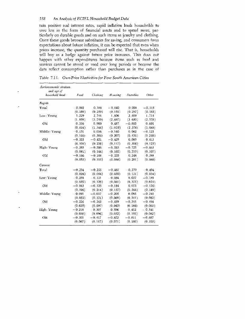
188 An Analysis of ECIEL Household Budget Data

tain positive real interest rates, rapid inflation leads households tosave less in the form of financial assets and to spend more, par-ticularly on durable goods and on such items as jewelry and clothing.Once these goods become substitutes for saving, and consumers formexpectations about future inflation, it can be expected that even whenprices increase, the quantity purchased will rise. That is, householdswill buy as a hedge against future price increases. This does nothappen with other expenditures because items such as food andservices cannot be stored or used over long periods or because thedata reflect consumption rather than purchases as in the case of

Table 7.15. Own-Price Elasticities for Four South American Cities

Socioeconomic stratumand age of

household head Food Clothing Housing Durables Other

Bogotd

Total -0.002 0.188 -0.040 0.008 -0.115(0.169) (0.259) (0.193) (0.287) (0.183)

Low: Young 1.229 2.744 1.806 2.409 1.714(1.959) (3.740) (2.667) (3.630) (2.578)

Old 0.336 0.900 0.487 -0.035 0.601(0.834) (1.344) (1.010) (2.378) (1.088)

Middle: Young -0.151 0.036 -0.160 0.062 -0.125(0.146) (0.306) (0.207) (0.426) (0.240)

Old -0.333 -0.421 -0.429 0.089 -0.615(0.104) (0.238) (0.117) (0.308) (0.123)

High: Young -0.385 -0.586 -0.585 -0.725 -0.663(0.081) (0.144) (0.102) (0.219) (0.107)

Old -0.166 -0.188 -0.235 -0.248 -0.388(0.055) (0.105) (0.068) (0.281) (0.068)

Caracas

Total -0.234 -0.255 -0.461 -0.279 -0.494(0.026) (0.054) (0.030) (0.131) (0.034)

Low: Young -0.258 -0.131 -0.084 0.057 -0.189(0.035) (0.128) (0.061) (0.375) (0.074)

Old -0.043 -0.123 -0.184 0.073 -0.126)(0.196) (0.214) (0.137) (0.568) (0.149)

Middle: Young -0.091 -0.037 -0.205 0.095 -0.240(0.053) (0.121) (0.069) (0.341) (0.082)

Old -0.226 -0.262 -0.459 -0.345 -0.494(0.035) (0.097) (0.043) (0.186) (0.063)

High: Young -0.218 -0.307 -0.506 -0.452 -0.541(0.038) (0.096) (0.052) (0.193) (0.062)

Old -0.301 -0.417 -0.672 -0.811 -0.687(0.067) (0.11'7) (0.071) (0.160) (0.103)

ELASTICITY ESTIMATES 189

Table 7.15. (continued)

Socioeconomic stratumand age of

houisehold head Food Clothing Housing Durables Other

Gnayaquil

Total -0.614 -0.692 -0.769 -0.771 -0.737(0.026) (0.030) (0.022) (0.052) (0.026)

Low: Young -0.455 -0.709 -0.641 -0.826 -0.659(0.024) (0.038) (0.030) (0.075) (0.041)

Old -0.625 -0.693 -0.718 -0.780 -0.674(0.048) (0.063) (0.063) (0.144) (0.066)

Middle: Young - - -Old -0.741 -0.824 -0.847 -0.845 -0.798

(0.049) (0.068) (0.042) (0.115) (0.063)High: Young -0.772 -0.790 -0.898 -0.860 -0.806

(0.061) (0.079) (0.048) (0.109) (0.050)Old -0.509 -0.824 -0.957 -0.997 -0.904

(0.098) (0.135) (0.107) (0.249) (0.118)

Lima

Total -0.058 0.029 -0.240 -0.056 -0.245(0.058) (0.109) (0.067) (0.131) (0.069)

Low: Young 0.087 0.660 0.271 0.646 0.041(0.154) (0.371) (0.233) (0.479) (0.210)

Old -0.103 -0.015 -0.194 -0.214 -0.185(0.047) (0.208) (0.097) (0.433) (0.077)

Middle: Young 0.450 0.670 0.352 0.850 0.138(0.661) (0.842) (0.681) (1.127) (0.574)

Old -0.098 -0.344 -0.367 -0.357 -0.336(0.064) (0.063) (0.033) (0.116) (0.048)

High: Young -0.067 -0.127 -0.236 -0.255 -0.190(0.051) (0.188) (0.040) (0.274) (0.066)

Old -0.251 -0.564 -0.501 -0.428 -0.537(0.048) (0.053) (0.043) (0.128) (0.041)

- Estimated with very large standard errors because ,i is very close to one.

housing. In short, under persistent but variable inflation, such itemsas durables and clothing may actually have positive price elasticitiespart of the time.18 This effect should be most pronounced among

18. This cannot occur all the time because eventually such items wouldabsorb the entire budget. The effect is probably strongest when prices accelerateafter an interval of stable prices or after a low and steady rate of inflation.This appears to have been the case in Lima following a devaluation in 1967,when inflation was more rapid than in most preceding years. This explanationis less certain for Bogota, although there was a sharp increase in inflation in theyear before the survey began.

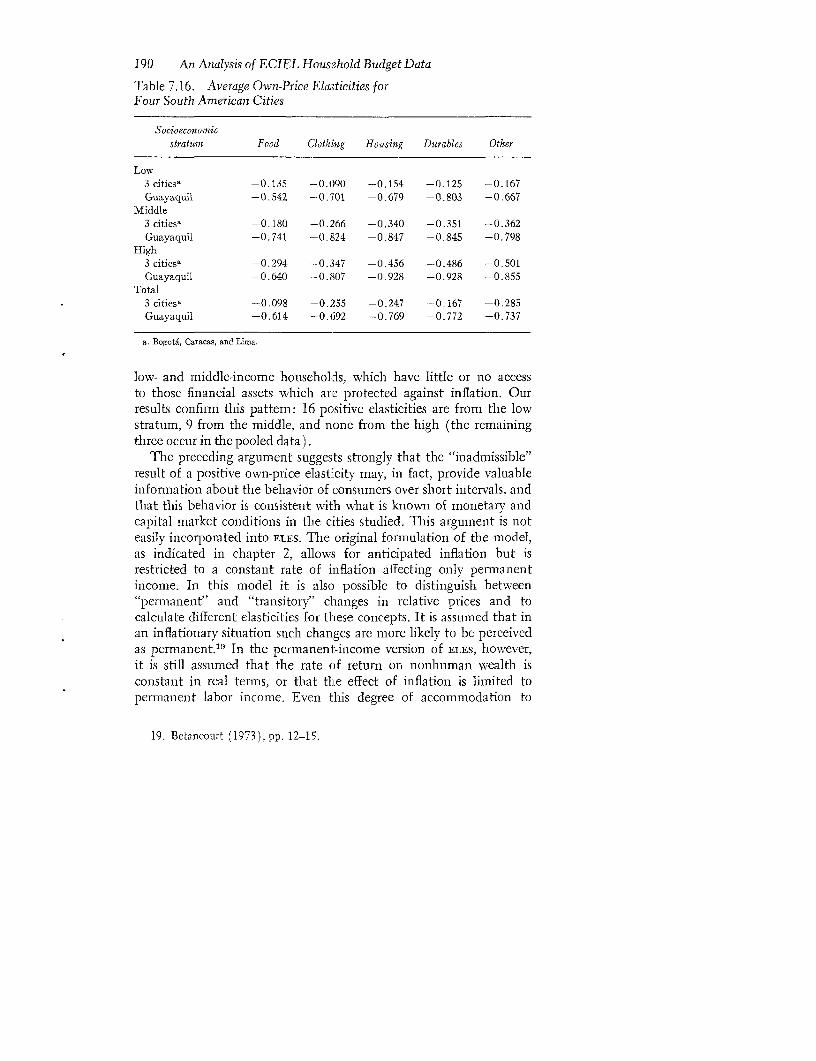
190 An Analysis of ECIEL Ilousehold Budget Data

Table 7.16. Average Own-Price Elasticities forFour South American Cities

Socwoecooromicstratum Food Clothing Housing Dutrables Other

Low3 cities, -0.135 -0.(90 -0.154 -0.125 -0.167Guayaquil -0.542 -0.701 -0.679 -0.803 -0.667

Middle3 cities, -0.180 -0.266 -0.340 -0.351 -0.362Guayaquil -0.741 -0.824 -0.847 -0.845 -0.798

High3 cities, -0.294 -0.347 -0.456 - 0.486 -0.501Guayaquil -0.640 -0.807 -0.928 -0.928 -0.855

Total3 cities, -0.098 -0.255 -0.247 -0.167 -0.285Guayaquil -0.614 -0.692 -0.769 -0.772 -0.737

a. Bogota, Caracas, and Lima.

low- and middle-income households, which have little or no accessto those financial assets which are protected against inflation. Ourresults confirm this pattern: 16 positive elasticities are from the lowstratum, 9 from the middle, and none from the high (the remainingthree occur in the pooled data).

The preceding argument suggests strongly that the "inadmissible"result of a positive own-price elasticity may, in fact, provide valuableinformation about the behavior of consumers over short intervals, andthat this behavior is consistent with what is known of monetary andcapital market conditions in the cities studied. This argument is noteasily incorporated into ELES. The original formulation of the model,as indicated in chapter 2, allows, for anticipated inflation but isrestricted to a constant rate of inflation affecting only permanentincome. In this model it is also possible to distinguish between"permanent" and "transitory" changes in relative prices and tocalculate different elasticities for these concepts. It is assumed that inan inflationary situation such changes are more likely to be perceivedas permanent. 19 In the permanent-income version of ELES, however,it is still assumed that the rate of return on nonhuman wealth isconstant in real terms, or that the effect of inflation is limited topermanent labor income. Even this degree of accommodation to

19. Betancourt (1973),pp. 12-15.

ELASTICITY ESTIMATES 191

the presence of inflation is lost when the model is estimated on thebasis of current rather than permanent income.

Despite these limitations, the ELES parameters can be interpretedin a way consistent with dynamic adjustments of expenditure tochanges in the rate of inflation. A positive y* is usually interpreted asa minimum level of expenditure determined either by physical needor by habits which are not easily changed. For a household with agiven income and composition, y'is assumed to be constant becausey is assumed constant and prices do not varv in a cross section.2 0

Since durable goods are not necessities on any reasonable definitionof subsistence, it is to be expected that y* (durables) will be smallor even negative. Nonetheless, y* (durables) < 0 only six times outof 56 estimates and is never significantly below zero, whereas y* >/(1 - ,43) for durables occurs eight times in 27 estimates.

If all forms of wealth have constant rates of return, variations inthe rate of saving depend primarily on variations in income. Inflation,unaccompanied by changes in nominal rates of return on some assets,reduces the total wealth of households owning those assets andprovokes a shift to other assets whose value is protected in real terms.Households will be seen to behave as if there were a relatively greatneed to accumulate the latter kind of assets. If these include durablegoods, estimation of ELES will yield high values of y* (durables).There will not necessarily be a high value of Pi because-as wasexplained earlier-the effect of inflation on wealth is concentratedamong low-income households.2 1

Cross-Elasticities with Respect to Food Price

Table 7.17 presents the cross-price elasticities nil with respect to foodprice. These elasticities can, in principle, be of either sign; but giventhe high level of aggregation and the fact that the own-price elas-ticities never exceed -1, the cross-elasticity for food is expected tobe less than zero. Of 112 cross-elasticities estimated, all but threeare negative. All these exceptions (in Bogota, low-old; Caracas, low-young; and Lima, low-old) reflect the purchase of durables in response

20. Although this assumption may be acceptable among bouseholds withina three-month period, it is less satisfactory for data gathered during twelve toeighteen months.

21. The reasoning here, relating flows to desired stocks, is similar to thatused to incorporate "consumption capital" into ELES, or to explain expenditure ondurables as consumption rather than as a form of saving. See Lluch (1974b)and Phlips (1972).

192 An Analysis of ECIEL Household Budget Data

to changes in the price of food. This accords with the evidencepresented earlier that purchase of durables is partly a form of savingand increases when inflation accelerates.

When all strata are analyzed together, the cross-elasticities withrespect to food prices are significantly negative. To facilitate inter-city comparisons, these are extracted from table 7.17 and repeatedin table 7.18. For each city, the four nonfood categories show verysimilar elasticities, although they (iffer appreciably among cities.

The food cross-elasticities are also usually significant (65 times out

Table 7.17. Cross-Elasticities and Elasticity of Average Savings Ratiowith Respect to Food Price (%) for Four South American Cities

Socioeconomic stratumand age of

household head Clothing Housing Durables Other {5 (food)

BogotaTotal -0.496 -0.479 -0.410 -0.413 -b

(0.123) (0.111) (0.127) (0.097)Low: Young -1.605 -1.376 -1.418 -1.247 -b

(1.654) (1.381) (1.497) (1.259)Old -0.828 -0.853 -0.005 -0.760 -b

(0.675) (0.661) (1.128) (0.606)Middle: Young -0.434 -0.421 -0.539 -0.439 _b

(0.174) (0. 145) (0.236) (0.154)Old -0.222 -0.210 -0.285 -0.225 -0.551

(0.084) (0.067) (0.157) (0.067)High: Young -0.164 -0.144 -0.193 -0.161 -0.279

(0.053) (0.0410) (0.075) (0.042)Old -0.073 -0.0083 -0.168 -0.117 -0.645

(0.036) (0.026) (0.091) (0.027)

Caracas

Total -0.189 -0.172 -0.220 -0.197 -0.722(0.022) (0.014) (0.056) (0.016)

Low: Young -0.319 -0.045 0.214 -0.168 -1.762(0.116) (0.064) (0.322) (0.077)

Old -0.276 -0.285 -0.198 -0.162 -3.616(0.188) (0. 126) (0.503) (0.156)

Middle: Young -0.271 -0.184 -0.330 0.264 -b

(0.047) (0.033) (0.141) (0.041)Old -0.049 -0.171 -0.143 -0.204 -0.580

(0.048) (0.020) (0.087) (0.032)High: Young -0.145 -0.130 -0.218 -0.131 -0.426

(0.035) (0.0'8) (0.076) (0.021)Old -0.092 -0.113 -0.147 -0.116 -0.219

(0.037) (0.023) (0.049) (0.028)

ELASTICITY ESTIMATES 193

Table 7.17. (continued)

Socioeconomic stratumnand age of

household head Clothing Housing Durables Other Ij (food)

Guaya quil

Total -0.182 -0.173 -0.206 -0.166 -0.290(0.019) (0.016) (0.034) (0.017)

Low: Young -0.234 -0.232 -0.211 -0.277 -0.441(0.030) (0.024) (0.065) (0.033)

Old -0.162 -0.215 -0.218 -0.159 -0.312(0.043) (0.047) (0.092) (0.040)

Middle: Young -_ -_a _a -

Old -0.117 -0.098 -0.121 -0.104 -0.141(0.041) (0.031) (0.054) (0.031)

High: Young -0.078 -0.070 -0.075 -0.043 -0.086(0.037) (0.031) (0.042) (0.092)

Old -0.080 -0.112 -0.122 -0.097 -0.113(0.025) (0.041) (0.035) (0.024)

Limoa

Total -0.332 -0.275 -0.265 -0.281 -5.516(0.041) (0.029) (0.055) (0.031)

Low: Young -0.679 -0.441 -0.661 -0.463 -b

(0.155) (0.103) (0.213) (0.104)Old -0.159 -0.175 -0.713 -0.300 -1.721

(0.148) (0.076) (0.296) (0.059)Middle: Young -0.430 -0.452 -0.584 -0.293 -b

(0.267) (0.273) (0.377) (0.196)Old -0.116 -0.114 -0.102 -0.042 -0.497

(0.025) (0.016) (0.045) (0.022)High: Young -0.011 -0.034 -0.049 -0.007 -0.233

(0.028) (0.014) (0.070) (0.022)Old -0.061 -0.086 -0.120 -0.081 -0.169

(0.014) (0.014) (0.034) (0.012)

Note: Standard errors are given in parentheses.a. Estimated with very large standard errors because,a is very close to one.

b. y < Et so 6 > O.

of 96) when the estimation is separated by stratum and age class.Table 7.19 presents the averages by stratum, across cities and agegroups. The estimates for Guavaquil, middle-voung, are not included.The averages obscure both the intercity variation and the fact thatyoung households usually respond more to price changes than doold households. Three conclusions emerge from table 7.19. The firstis that all the elasticitics except those for durables fall in absolute

194 An Analysis of ECIEL Household Budget Data

Table 7.18. Cross-Elasticity with Respect to Food Pricesfor Four South American Cities

Comnmodity Bogotd Caracas Guaya quil Limna

Clothing -0.4955 -- 0.1887 -0.1824 -0.3322(0.1228) (0.0219) (0.0192) (0.0413)

Housing -0.4793 -- 0.1719 -0.1732 -0.2748(0.1110) (0.0140) (0.0161) (0.0287)

Durables -0.4096 -- 0.2201 -0.2060 -0.2649(0.1272) (0.0563) (0.0336) (0.0552)

Other -0.4127 -- 0.1969 -0.1655 -0.2808(0.0968) (0.0164) (0.0165) (0.0308)

Note: Standard errors are given in parentheses.

Table 7.19. Food Cross-Elasticities: Average of Estimatesfor Four South American Cities

Socioeconomicstratum Clothing Hlousing Durables Other

Low -0.5328 --0.4528 -0.2218a -0.4420Middle -0.2381 -- 0.2327 -0.3004 -0.2245High -0.0882 -- 0.0967 -0.2364 -0.0940Total -0.2997 -- 0.2748 -0.2752 -0.2640

a. -0.5412 if only negative values are averaged.

value (rise toward zero) as incorne rises; typically, the elasticity isabout halved in passing from one stratum to another. Second, in eachstratum, all the elasticities except those for durables are about equal.Third, the purchase of durables depends on food prices in a way thatis very nearly independent of income.

Elasticity of the Average Savinigs Ratio with Respect to Food Price

Expression (2.12) makes the elasticity of the average savings ratiowith respect to food price (e,) ao function of the saving rate andmean subsistence food expenditure (n7*). The estimate of s, can beevaluated at mean income, mean total expenditure, or mean saving(because of the way the reduced form was estimated, these valuesdo not correspond to one another). Evaluation at mean income yleads to the saving rate s = (1- ) (y - Y,,y*) and therefore to

(7.5) _ -

CONCLUSIONS 195

(no standard errors are obtained). These values are shown in thelast column of table 7.17.

The results parallel those obtained for the Frisch parameter, withthe estimates for Caracas the most plausible and those for Guayaquilshowing similar relative values but low absolute values. (These arecomparable to the time-series estimates for high-income countriesreported in table 4.9 and to a few estimates for urban Mexico shownin table 6.14.) There is no pattern to the results for Bogota; thosefor old households in Lima are quite reasonable and agree ratherwell with those for Caracas. In Caracas, Guayaquil, and Lima allthree socioeconomic strata can be compared for old households:

Stratum Caracas Guayaquil LimaLow -3.616 -0.312 -1.721Middle -0.580 -0.141 -0.497High -0.219 -0.113 -0.169

The saving rate should be most responsive to food prices whenreal incomes are low, since food is then a larger share of the budget.This does not emerge from the comparison of Caracas and Lima,especially in the low stratum where income differences are greatest(incomes are appreciably less concentrated in Caracas than in Lima).The reason for this may be, again, that durables are a form of savingand that the saving rate is more sensitive to the price of durables.2 2

There does not appear to be any consistency to differences in thevalue of e, between age classes in any stratum. Estimates for all stratatogether (in Caracas, Guayaquil, and Lima) are very dispersed. Inthe low stratum the elasticity often exceeds one in absolute value,while among the rich it is never more than 0.43.

Conclusions

ELES was estimated twenty-eight separate times in the four citiesstudied, on the assumption that all its parameters depend on incomelevel and on age, and that in addition the subsistence expendituresvary with household size. Dividing the samples bv stratum and ageleads to some violations of the system restrictions on the signs and

22. 04, the saving elasticity with respect to the price of durables, is just-y*1/(y- A 7*); it can be seen from tables 7.5 and 7.7 that a* (durables)/a*(food) is systematically much greater in Lima than in Caracas, so that to islarger in absolute value than 6.

196 An Analysis of ECIEL Household Budget Data

sizes of parameters, but these failures are infrequent and may becompensated by the additional knowledge gained from piecewiselinear approximation of the demand functions.

ELES Parameters

The principal findings with respect to each of the three classifyingvariables may be briefly summarized.

Income. Both the marginal budget shares (,ai) and the subsistenceexpenditures (y.*) vary rather systematically with income level, asexpected, depending on whether the commodity is a necessity or aluxury. The sets of linear functions appear to capture the curvatureof expenditure relationships while retaining the advantages of theo-retically plausible local demand functions. Subsistence expendituresmay rise wvith income, but they decline relative to actual spending.This shows that they more nearly represent needs at low incomes,while habits and expectations become more important as incomerises. Income and expenditure elasticities also generally differ in theanticipated way. Thev are more nearlv equal to one another and to1.0 than elasticities estimated without the budget constraint.

Age. The effects of age are not entirely separated from those ofincome, since in most strata old households have higher mean in-comes than do young families. Tlhere is a clear life-cycle effect onlvin the case of durables, where marginal spending is nearly alwayshigher among the young; they tend to devote less of the marginalbudget to housing and to other expenditures than do older house-holds. Young households tend to lhave lower mean expenditures (vPi)but higher subsistence spending (y*). They behave as if their notionof a minimally acceptable standard of living, or their expectationsabout future income, were higher than those of older households.It cannot be determined whether this behavior merely reflects thestage in the life cycle or includes some demonstration effect or risingexpectations because of the different experiences of voung and oldfamilies.

Household size. This variable was not permitted to affect pi and j3 ibut only subsistence expenditures (y*). These generally differ betweenlarge and small households, being more often higher where there aremore members. It also appears that the difference betveen y* (large)and y* (small) is greater for young than for old families, perhapsbecause of greater differences in per capita income.

CONCLUSIONS 197

Price Elasticities and Inflation

Generally, the own-price elasticities (Yij) are negative and rise inabsolute value as income increases. The exceptions are concentratedin durables (and to a lesser extent in clothing) in the low- andmiddle-income strata, and in the cities of Bogota and Lima. Althoughthese results are not significant statistically, they are consistent withthe idea that durables and semidurable goods have positive priceelasticities under rapid or accelerated inflation, at least for thosehouseholds which do not have access to assets protected against in-flation. Durables are a form of saving for such households, whichrespond differently to dynamic price changes than they would tostatic changes in relative prices.

This hypothesis may be supported by the fact that the only positiveelasticities with respect to food prices are for durables and amonglow-income households. Generally, the cross-elasticities are negativeand decline in absolute value as income rises. Price elasticities alsoseem to rise in absolute value as the family is older. This rise isrelated to the fact that vW-, , uncommitted expenditure, is gen-erally larger for older households, but the effect is not very pronounced.

Consumption and Saving

Estimation of ELES yields information about the distribution ofhousehold expenditure among commodities; the results are usuallyreasonable and take account of differences in behavior due to differ-ences in income, age, and household size. The results concerning theallocation of income between consumption and saving are much lesssatisfactory. The elasticity of saving with respect to food prices (e,)is usually negative (except in the low stratum) and of reasonablemagnitude, but many of the values are rather low in absolute terms.Estimates of the marginal propensity to consume (/I) are extremelyvaried and often much too low. In particular, they do not alwaysdecline as income rises but are often low for very low incomes.Finally, estimates of the expenditure elasticity of the marginal ex-penditure utility (l)-which can be expressed in terms of averageand marginal saving rates-are satisfactory only for Caracas, withsome plausible relative or absolute values in the other cities.

Two problems make it hard to use ELES to study household savingwith cross-section data; both may be made worse when the sampleis stratified. One is that income and expenditure are reported witherrors, and some savings-related parameters (especially w) are ex-

198 An Analysis of ECIEL Household Budget Data

tremely sensitive to such errors. The other is that even if currentflows are accurately reported they contain transitory elements whichbias the estimates of , and, therefore, of the Frisch parameter (w).These problems arise more frequently for young households, whosespending may be related to expected income in the future and whomay currently dissave.

Despite these difficulties-whichi might be reduced or overcome bya more complex model based on good estimates of permanent in-come-estimation of ELES offers a valuable view of spending behaviorby consumers in developing countries. In particular, it offers a way toextract from rather limited household budget data information aboutspending as a function of income as well as about macroeconomicinfluences such as the level and rate of change of prices. Providedthese results are interpreted with care, they can help in understandingthe household sector's role in economic development.

8Household Behavior in Chile: AnAnalysis of Cross-Section Data

Roger Betancourt

THE WORK ON THE CHILEAN cross-section data was done before theanalysis of the other cross-section data used in this book. At thattime, a number of alternatives were tried in the formulation of themodel and in the empirical implementation, and the results providedguidance for subsequent research. In this chapter the alternativesconsidered initially are first summarized; those that were empiricallyimplemented are compared briefly with the one actually chosen andthe results that are comparable to those in the rest of the book arepresented in detail.

The data base is the Cost of Living Survey for Central Chile,which covers the month of January 1964.' The survey contains inde-pendent information on total expenditures, by thirteen expenditurecategories, and on disposable income for each household. It alsocontains the usual information on sociodemographic characteristicsof the households. Three of the expenditure categories are treatedas savings: direct saving as reported by the respondents, investmentin housing (other than imputed rent), and consumer durables. Theremaining expenditures are divided into three groups for ihe empiricalanalysis: rent, food, other.

1. Further characteristics of the survey are available in Betancourt (1971b).

199

200 Household Behavior in Chile

Modifications of the Model

In chapter 2 the model underlying this book (ELES) is formulated asintegrating the consumption-saving decision with decisions on theallocation of expenditures. The first modification considered was theintegration of these two aspects of household decisionmaking witha third aspect, the labor-leisure decision. This extension resulted ina more general model (labeled TELES for tw.ice extended linear ex-penditure system) which had ELES as a special case. The integration ofthe labor-leisure decision was accomplished at the theoretical level,2but the empirical implementation of TELES was not carried out for tworeasons. First, most bodies of cross-section data do not furnish theinformation necessary for the implementation of TELES, although theChilean data is an exception; consequently, it would have been im-possible to compare the results for this model across countries.Second, even when the information is available, estimation problemsarise that are considerably different from those involved in the esti-mation of ELES, for example, the errors in variables problem withrespect to the wage rate.3

Another modification to the model in chapter 2 was the formula-tion of ELES using discrete time and a finite horizon. As expected,this change gave rise to only minor alterations in the model. Morespecifically, the marginal propensity to consume out of income (tk) isno longer 8/p but becomes instead {/(1I + 8) [1 - 1/(1 ± S)71} (1+ p) [1 - 1/(l + p)T]/p where T is the distance from the planningperiod to the end of the horizon. Thus, as T -e oo, , e [8/(1 +8)]/[p/( 1 + p)]. In addition, it i, now possible, but not necessary,to allow the subsistence parameters (y) to vary over time. Theassumption that they are constant over time, together with theassumptions listed in chapter 2, lead to equations (2.1) and (2.2),except of course for the previously mentioned interpretation of U.The model embedding these assurnptions is referred to here as thecurrent income model. Another version of ELES which uses permanentincome as the appropriate income concept was also implementedempirically. As in Watts (1960) and Ramanathan (1968), a house-hold's permanent income was estimated from the income profile ofcomparable households. An extrapolative parameter, X, was intro-duced to project into the future the existing deviation of an indi-

2. See Betancourt (1973a) for elaboration.3. Aigner (1974) discusses the complications involved in solving this problem

within the context of estimating the labor supply function.

MODIFICATIONS OF THE MODEL 201

vidual family's income from the mean income of the group. In asimilar manner, families of above average size were assumed tomaintain their relative position with respect to this variable in sub-sequent stages of the life cycle. The model incorporating theseassumptions will be referred to as the permanent income model.This version of ELES also allows the identification of price elasticitiesin a cross-section context. In calculating the permanent effect ofrelative price changes it is assumed that changes in the initial periodare expected to last throughout the time horizon of the plan.4

Alternative formulations with respect to the life-cycle variableswere also considered. Because there is no clear-cut theoretical ra-tionale on how age should affect the parameters of the model, itsimpact was captured through the stratification of the sample intosix age groups (less than 25, 25-34, 35-44, 45-54, 55-64, 65 and over).With respect to family size, however, it seemed reasonable to postu-late that this variable would affect the subsistence parameters. Moreprecisely, a scheme suggested by Ando and Modigliani (1957) wasadapted as follows:

(8.1) yit = 4t[l + X(fAt - 1)]

where the bar indicates a subsistence parameter for a family of one,x, represents a parameter which captures economies of scale in con-sumption and is allowed to vary across commodities (i), and fht isthe family size of the hth household in the tth period.

This specification of the family size variable introduces a sub-stantive difference between the results for the Chilean data and thosein the rest of the book-the only substantive difference that is noteliminated in the section on current income results. Information isthus obtained on the desirability of capturing the effect of familvsize through stratification and the use of per capita income as theindependent variable, as is done elsewhere in the book, rather thandirectly as a determinant of the subsistence parameters. In the cur-rent income version of ELES, the main consequence of this specifi-cation of family size is to change the formulas for all the elasticitiesthat involve the subsistence parameters. For example, the uncom-

4. The assumptions used are discussed in detail in the appendix to thischapter. In the permanent income version of ELES the subsistence parameterscan be specified as growing over time at some constant growth rate, such asthe expected rate of growth of income. A justification for this hypothesis isprovided in Betancourt (1971a).

202 Household Behavior in Chile

pensated price elasticities for ELES become

(8.2) 4ij = (1- ) {pi 7i [l +Ai (k -1)] /vi} -1

and

(8.3) ij =-i {pj l7 [ +XAj(fA- 1)11/vs.

The rest of the formulas are similarly affected; that is, wherever 7y

appears it must be replaced by the right-hand side of (8.1). As forthe problem of estimation, there is an additional parameter to beestimated (xe) and an additional regressor in every expenditureequation (fh-1) of the current income version of ELES. In keepingwith the other assumptions of this model, it has been assumed thatthe consumer expects his family (size to remain unaltered over theplanning horizon. This assumption was relaxed in the empiricalimplementation of the permanent income version of ELES.5

Finally, urban-rural location and occupational status or socioeco-nomic class (workers, self-employed, employees) were used to controlfor differences among consumers in tastes and preferences as well asexpectations.6 The same models were also implemented withoutdisaggregating by occupational status in order to assess the impacton the estimates.

Permanent Income Compared with Current Income

Both permanent and current income versions of ELES were imple-mented with the Chilean data for households stratified by age, loca-tion, and occupational status. The estimating equation for the currentincome model differs slightly from the one presented in chapter 2because of the family size variable;' that is, for each household

(8.4) vik = [pi yi-p (Z p 1y)] - [xi pi y5 --

07 (1Xi pi YiMf,lt-1) + Bgyh +eih-

The regression results for the current income model are presented

5. Again see the appendix to this chapter for a detailed explanation.6. A more extended discussion of the roles of these variables in the Chilean

case, and possibly in other developing countries, is available in Betancourt(1973b).

7. Note that the estimation methods described in chapter 2 are still applicablein both (8.4) and (8.14).

PERMANENT INCOME COMPARED WITH CURRENT INCOME 203

in table 8.1 for the three expenditure functions.8 Table 8.2 presentsthe estimates of the derived parameters and elasticities. The cor-responding results for the permanent income model are availablein Betancourt (1973a) but are not presented here in detail. Instead,the main features of both sets of results are briefly compared toprovide the rationale for choosing the current income model afterempirical implementation.

With respect to the statistical significance of the regression co-efficients, the current income model performs better than thepermanent income model. For instance, in the current income modelall but one of the marginal propensities to consume ( ) have a tratio greater than two, as well as 38 of the 72 intercept coefficientsand 29 of the 72 family size coefficients. In the permanent incomemodel, although all but two of the regression coefficients for one ofthe income variables (gA3,) have t ratios greater than two, only 9 outof 72 intercepts and 7 out of the 72 coefficients for each of the twofamily size variables have t ratios greater than two; finally, the regres-sion coefficient of the other income variable [fj3 (1 - A)] has a t ratiogreater than two in only 11 out of 72 cases. The last result suggeststhat the appropriate value of the extrapolative tendencies parameter(X) is unity, which implies that the household expects to retain itsrelative income position over the life cycle.

Other striking features of the permanent income model relate toprice elasticities. T'he estimates of the temporary and the permanent(uncompensated) own-price elasticities are very close to each other,but the estimates for the (uncompensated) cross-price elasticities arevery far apart. More importantly, for the present discussion, 32 outof the 72 own-price elasticities (either temporary or permanent) arepositive. Furthermore, among the remaining 40, values smaller thanminus two occur frequently. In contrast only 5 out of the 72 own-price elasticities were positive in the current income model, andnone of the estimates took on values smaller than minus two. Thusthe empirical results for the current income version of ELES are moreconsistent with the underlying theoretical restrictions of the model.

It can be seen from the appendix to this chapter that the empiricalimplementation of the permanent income model requires the use of

8. The data were stratified into twelve subsamples (six age groups for urbanand rural location), and dummies on all variables were used for the three socio-economic status groups. The first and last age groups in both sectors weredropped from the analysis, however, because of the small number of observationsand the peculiarities of these stages of the life cycle.

Table 8.1. Regression Results for the Current Income Model: Expenditure Functionsof Urban and Rural Workers, Self-Employed, and Employees, Chile

Urban workers Rural workers

Agea and Coefficient Coefficientexpenditure Interceptb of fh' Interceptb i3' of fho

25-34

Rent 4.7500 0.1025* -0.4444 -2.3151 0.1617* -0.4560(4.2869) (0.0232) (0.6938) (1.5160) (0.0086) (0.2452)

Food 25.5248* 0.2789* 2.6969 10.0086* 0.4362* 1.4405*(9.4910) (0.0513) (1.5361) (3.4467) (0.0196) (0.5576)

Other -0.2537 0.2076* -0.4466 1.9782 0.1921* -0.5850

° (12.0020) (0.0648) (1.9425) (3.1454) (0.0179) (0.5088)35-44

Rent 6.7134 0.1007* -0.6672 3.6126 0.0792* -0.2476(4.2826) (0.0218) (0.5766) (2.1096) (0.0102) (0.2826)

Food 11.9768 0.4410* 2.4275* 36.4151* 0.2785* 1.2319*(8.0702) (0.0410) (1.0866) (4.3429) (0.0210) (0.5817)

Other -8.4985 0.3323* -1.1981 -2.9360 0.2775* 1.2555*(12.3524) (0.0628) (1.6632) (4.4855) (0.0217) (0.6008)

45-54

Rent 9.6359 0.0976 -0.9031 5.8498 0.0779 -0.5255(4,5096)* (0.0237)* (0.7051) (1.7786)* (0.0094)* (0.2376)*

Food 16.6903 0.4230 0.9771 9.8020 0.4474 1.1302

(8.8773) (0.0467)* (1.3885) (4.3749)* (0.0230)* (0.5845)Other -3.7978 0.2606 -0.6408 -1.7961 0.1937 -0.2282

(11.0617) (0.0582)* (1.7302) (3.8906) (0.0205)* (0.5198)

55-64

Rent 10.4694 0.1356 -2.2478 4.6796 0.0637 -0.3207

(7.0357) (0.0332)* (1.2077) (1.7241)* (0.0104)* (0.2617)

F'ood -6.4966 0.4703 4.5005 20.4261 0.3734 0.4105

(11.6584) (0.0551)* (2.0012)* (4.5242)* (0.0273)* (0.6868)

Other 9.2878 0.1942 -1.3837 -2.3791 0.2424 -0.6120

(13.5682) (0.0641)* (2.3290) (4.7106) (0.0285)* (0.7151)

Urban self-emnployed Rural self-employed

Age, and Coefficient Coefficient

expenditure Interceptb pi of fhc Intercepth ,* of fhc

25-34

Rent 6.5001 0.1039* -0.3068 2.4496 0.0855* -0.0802

(3.7670) (0.0101) (0.7209) (3.0962) (0.0160) (0.4836)

Food 9.2412 0.4124* 2.5191 14.5316* 0.5741* -1.5886

(8.3400) (0.0224) (1.5960) (7.0392) (0.036.3) (1.0034)

Other -17.3348 0.3268* 1.5812 2.6676 0.2505* -1.0168

(10.5466) (0.0283) (2.0183) (6.4239) (0.0331) (1.0034)

35-44

Rent 17.7557* 0.1058* -1.6808* 6.1127* 0.0730* -0.3601

(3.8568) (0.0083) (0.6173) (2.9816) (0.0111) (0.4569)

Food 27.6311* 0.2692* 4.4771* 31.9194* 0.2105* 1.5589

(7.2677) (0.0156) (1.1633) (6.1381) (0.0228) (0.9407)

Other -33.7060* 0.4912* -2.1092* -1.5476 0.2670* -0.5871

(11.1240) (0.0238) (1.7806) (6.3396) (0.0235) (0.9716)

(Table continues on the following page.)

Table 8.1. (continued)

Urban self-employed Rural self-em?ployed

Agea and Coefficient Coeficientexpenditure Interceptb 13 of f*C Interceptb 13. of A,,

45-54

Rent 15.5403* 0.0852* -0.3565 10.6427* 0.0442* -0.1959(3.6383) (0.0083) (0.6146) (2.2115) (0.0061) (0.3098)

Food 21.1537* 0.2234* 7.1265* 34.0246* 0.2029* 2.5955*(7.7621) (0.0164) (1.2099) (5.4399) (0.0151) (0.7620)

Other -13.2551 0.3867* -- 2.9936 -- 12.8761* 0.2423* 1.4539*(8.9243) (0.0204) (1.5076) (4.8378) (0.0134) (0.6777)

S S~~5-64

Rent 25.1850* 0.0695* -1.6217 8.8092* 0.0688* - 0.6819*(4.8709) (0.0076) (1.0853) (1.8481) (0.0076) (0.3028)

Food 22.4567* 0.2266* 6.1530 15.0866* 0.2601* 3.3730*(8.0713) (0.0126) (1.7983) (4.8494) (0.0200) (0.7940)

Other 25.9567* 0.2493* -6.1834 -2.2329 0.1972* 0.4835(9.3935) (0.0146) (2.0929) (5.0492) (0.0208) (0.8273)

Urban employees Rural emnployees

Agea and Coefficient Coefficientexpenditure Intercept" O3 of fhc Interceptb f3* of fh,'

25-34Rent 14.0860 0.0991* -1.0741 2.9208 0.1376* 1.6721*

(4.8568) (0.0102) (0.8560) (4.8947) (0.0122) (0.7424)

Food 20.8791 0.2789* 5.5476* 23.5504* 0.2432* 5.1460*

(10.7528) (0.0227) (1.8952) (11.1282) (0.0277) (1.6880)

Other -32.1870* 0.5346* -4.1149 34.4107 0.1820* -5.1969*

(13.5977) (0.0287) (2.3967) (10.1554) (0.0252) (1.5404)

35-44Rent 25.9330* 0.1013* -2.0235* -10.4740 0.1620* -0.4624

(4.4234) (0.0074) (0.6060) (6.2379) (0.0150) (0.9006)

Food 31.2502* 0.1920* 8.3240* 34.2140* 0.1822* 5.6510*

(8.3355) (0.0139) (1.1419) (12.8419) (0.0309) (1.8540)

Other -38.5125* 0,6308* -8.4086* 38.4081* 0.5055* -14.1485

(12.7585) (0.0212) (1.7479) (13.2635) (0.0320) (1.9149)

45-54Rent 22.0102* 0.0705* 0.3823 16.6120 0.0918* -1.8853

(6.8049) (0.0101) (0.9340) (10.2736) (0.0258) (0.9367)

Food 62.6384* 0.2422* -0.3436 47.6688 0.2264* 1.3445

(13.3950) (0.0199) (1.8386) (25.2710) (0.0634) (2.3041)

Other -3.7576 0.2156* 3.4600 36.4709 0.4302* -6.9564*

(16.6919) (0.0248) (2.2910) (22.4737) (0.0564) (2.0490)

55-64Rent 36.3305* 0.0962* -4.0924 8.9912 0.0133 1.2419

(12.3438) (0.0289) (2.4514) (10.2670) (0.0280) (1.1486)

Food 24.0356 0.1345* 14.0367* 45.1081 0.1951* 3.4332

(20.4542) (0.0479) (4.0621) (26.9408) (0.0735) (3.0139)

Other 7.9124 0.2854* -1.8900 63.6026* 0.3853* 12.5272*

(23.8049) (0.0558) (4.7275) (28.0508) (0.0765) (3.1380)

Source: Data for all tables in chapter 8 are derived from the Cost of Living Survey a. The age group is determined by the age of the household head.

for Central Chile, January 1964, conducted by the Instituto de Planificaci6n Econo- b. The intercept in equation (8.4) adjusted becausefh rather thanfh- 1 was used

mica, University of Chile. in the regression.

INote: Standard errors in parentheses. An asterisk next to a number indicates a c. The estinmate of the coefficient of fh - 1 in equation (8.4).

i ratio greater than two.

Table 8.2. Structural Estimates for Current Income Model: Urban and Rural Workers,Self-Employed, and Employees, Chile

1ijAgea and -- Mean Mean

expenditure Pi/l Xi j=rent j=food j = other 7i income family size

Urban workers25-34

1 Rent 12.2430 0.0005 -0.1992 -0.5471 -0.1355 0.8535Food 49.8191 0.0787 -0.0475 -0.3329 -0.0687 0.4433 114.4990 5.2887Other 15.3758 0.0303 -0.1192 -0.6556 -0.3559 1.112235-44Rent 14.6408 -0.0149 -0.3236 -0.4451 -0.1147 0.7287Food 52.0429 0.0845 -0.0705 -0.4971 -0.1074 0.6854 129.8434 6.2591Other 18.6647 0.0152 -0.1493 -0.8065 -0.5548 1.427045-54Rent 18.5292 -0.0624 -0.4093 -0.3014 -0.0772 0.7461Food 60.1252 -0.0020 -0.0592 -0.6049 -0.0704 0.7173 147.3986 6.1103Other 21.7186 -0.0606 -0.1018 -0.4796 -0.6572 1.187655-64Rent 17.8063 -0.0931 -0.5408 -0.3495 -0.1257 0.9603Food 31.2463 0.2095 -0.0849 -0.5004 -0.1509 1.1717 150.4861 4.9308Other 21.6308 -0.0249 -0.0803 -0.3822 -0.4425 1.0363

Rural workers

25-34

Rent 4.9837 -0.0298 -0.6555 -0.6960 -0.1453 1.4390Food 32.3684 0.0701 -0.0303 -0.5923 -0.0686 0.6828 92.9581 5.6552Other 10.6059 -0.0207 -0.0461 -0.5109 -0.5485 1.0412

35-44

Rent 9.7331 0.0245 0.0184 -0.5376 -0.3076 0.8286Food 50.0401 0.0588 -0.0488 -0.2472 -0.1757 0.4536 105.5723 6.9803Other 20.6319 0.1434 -0.1772 -1.0850 0.5691 1.6599

45-54

Rent 9.2699 -0.0454 -0.4437 -0.3018 -0.0547 0.7963Food 33.5926 0.0515 -0.0434 -0.6511 -0.0518 0.7538 116.1305 6.7362Other 7.7866 0.0041 -0.0716 -0.4303 -0.6647 1.1740

C 55-64Rent 8.7721 -0.0484 -0.4085 -0.2431 -0.0469 0.5595Food 46.7059 -0.0042 -0.0418 -0.5231 -0.0557 0.6531 105.2242 5.6448Other 13.8025 -0.0730 -0.1101 -0.7445 -0.5361 1.7116

(Table continues on the following page.)

Table 8.2. (continued)

,njAgea and Mean Mean

expenditure PMi Xi j= rent j=food j= other income famizily size

Urban self-employed

25-34

, Rent 7.6502 0.2883 -0.4294 -0.3113 -0.1331 0.7817s Food 17.5428 0.7120 -0.0746 -0.6153 -0.1322 0.7936 185.3818 4.6456

Other -11.1713 -0.8488 -0.1092 -0.4501 -0.7000 1.153735-44

Rent 25.8546 -0.0440 -0.4469 -0.2682 -0.0366 0.6262Food 56.9919 0.1028 -0.0510 -0.4177 -0.0298 0.5009 196.7757 5.6538Other 9.5892 0.0431 -0.2017 -0.8365 -0.8824 1.940545-54

Rent 22.7937 0.0307 -0.3856 -0.1982 -0.0574 0.4881Food 48.2339 0.2052 -0.0568 -0.3317 -0.0573 0.4803 217.9347 4.9409Other 18.2907 0.0984 -0.1627 -0.5501 -0.7429 1.391955-64

Rent 34.5626 -0.0542 -0.1002 -0.1899 -0.0855 0.5383Food 64.4721 0.0827 -0.0692 -0.3217 -0.0857 0.5678 230.8381 4.0632Other 59.2282 -0.1197 -0.1399 -0.3939 -0.4505 1.1229

Rural self-employed

25-34

Rent 18.5024 -0.1424 -0.1560 -0.1858 -0.0290 0.8703Food 121.2697 -0.1545 -0.0689 -0.6083 -0.1117 0.9832 95.8832 4.7235Other 48.9176 -0.1738 -0.1310 -0.7938 -0.3088 1.2827

35-44

Rent 11.7771 -0.0221 -0.2064 -0.3666 -0.1094 0.6823Food 50.8504 0.0363 -0.0388 -0.1759 -0.0696 0.4283 115.5592 5.5730Other 19.9002 -0.0112 -0.0921 -0.5194 -0.5478 1.0084

45-54

Rent 13.5324 0.0102 -0.0482 -0.2240 -0.0700 0.4345Food 50.7844 0.0813 -0.0390 -0.2410 -0.0617 0.3834 140.1342 5.8044Other 5.4926 0.5976 -0.1231 -0.6080 -0.4225 1.2171

2 55-64

Rent 11.7332 -0.0180 -0.2410 -0.2809 -0.0850 0.6641Food 32.0917 0.1594 -0.0416 -0.4223 -0.0635 0.4960 128.4644 5.0007Other 8.5860 0.2102 -0.0874 -0.4463 -0.4763 1.0447

(Table continutes on the following page.)

Table 8.2. (continued)

fi

Age, and Mean Mean

expenditure PiTi Xi j =rent j=food j other z. income family size

Urban employees

25-34t Rent 16.5685 -0.0403 -0.6200 -0.1488 0.0631 0.7511

, Food 36.4361 0.1637 -0.0293 -0.6145 0.0635 0.5603 245.7813 5.3280

Other -17.1156 0.1123 -0.0884 -0.4650 -1.1482 1.6446

35-44Rent 46.0148 -0.1051 -0.6239 -0.2023 0.1300 0.6639

Food 81.4717 0.0367 -0.0212 -0.4469 0.0973 0.4413 325.8828 6.2116

Other 90.7296 -0.2858 -0.1456 -0.6800 -1.1820 2.2829

45-54Rent 35.0053 0.0259 -0.3184 -0.1384 -0.0479 0.4549

Food 105.6257 0.0138 -0.0690 -0.3954 -0.1152 0.5935 345.3745 5.6903

Other 38.2744 0.1322 -0.0844 -0.2423 -0.5128 0.7459

55-64Rent 47.4128 -0.0526 -0.4259 -0.1084 -0.0834 0.5171

Food 59.2884 0,2745 -0.0292 -0.3779 -0.0536 0.2695 326.3501 4.5500

Other 51.0396 0.0560 -0.0827 -0.2805 -0.6592 0.7260

Rural emnployees

25-34

Rent 24.2645 0.0899 0.0280 -0.3996 -0.2074 1.1408

Food 63.4648 0.0953 -0.0805 -0.3856 -0.0688 0.5167 231.4566 5.1301

Other 55.2329 -0.3819 -0.1237 -0.3294 -0,4237 0.8118

35-44

Rent 46.3922 -0.2181 -1.2859 -0.5312 -1.0114 1.4319

Food 104.3420 -0.0499 0.0336 -0.4946 0.1467 0.4200 279.4000 6.6499

Other 203.1461 -0.2180 0.0934 -0.4221 -1.2690 1.6328

45-54

Rent 48.7520 -0.0948 -0.2582 -0.4196 -0.4236 0.9708

Food 132.9275 -0.0406 -0.0306 -0.3421 -0.0927 0.5033 259.7919 7.2085

v Other 188.9663 -0.1047 -0.1221 -0.4916 -0.5973 1.1934

55-64

Rent 14.6491 0.1232 -0.1721 -0.0846 -0.1721 0.0992

Food 113.3205 0.1032 -0.0726 1.1281 -1.0673 0.6304 205.1664 5.6668

Other 204.0513 0.1413 -0.1186 -0.8908 2.5892 1.3629

a. The age group is determined by the age of the household head.

Table 8.3. Estimated Values of Marginal Budget Shares (aji) and theMarginal Propensity to Consume (Es), ELES, Chile, 1964

Weight ofType of Sample youngest

household, size subgrostpb Income, Food Rent Other

RuralWorkers

Young 896 0.4788 100 0.499 0.168 0.330 0.709Old 574 0.6272 112 0.597 0.104 0.301 0.704

Self-employedYoung 237 0.3966 108 0.512 0.113 0.375 0.693Old 321 0.6044 136 0.448 0.107 0,444 0.504

EmployeesYounig 86 0.5349 254 0.309 0.214 0.477 0.696Old 36 0.6667 241 0.310 0.095 0.595 0.697

UrbanWorkers

Young 341 0.4575 123 0.493 0.137 0.370 0.744Old 190 0.6211 149 0.560 0.142 0.298 0.788

Self-employedYoung 266 0.4135 192 0.383 0.123 0.494 0.857Old 259 0.5907 223 0.355 0.125 0.521 0.634

EmployeesYoung 256 0.4648 289 0.252 0.109 0.638 0.919Old 91 0.7802 341 0.416 0.144 0.439 0.526

a. "Young" refers to young head of household, 25-44 years old; "Old" refers to weights for the other subgroups can be obtained by subtracting from one.old head of household, 45-64 years old. c. Mean monthly income per household in escudos (in 1964, 3.25 escudos

b. These weights are used for the youngest subgroup (25-34 for the "young" age US$1.00).group anid 45-54 for the "old" age group) in the aggregation of the results. The

CURRENT INCOME RESULTS 215

explicit assumptions about expectations. Undoubtedly, more exten-sive experimentation with alternative assumptions might eventuallylead to better results for the permanent income model. Nevertheless,this succinct summary of results indicates that the current incomeversion of ELES provides a more reliable basis for applied work, giventhe present state of knowledge about the formulation of expectations.

Current Income Results

In order to facilitate comparison with the results for other countries,the data presented in table 8.1 have been aggregated to obtain twoage groups, voung and old, within each socioeconomic status cellfor rural and urban households.9 Again it has to be stressed thathousehold income wvas the independent variable in the regressionsrather than household income per capita and that family size wasintroduced as an additional regressor. Thus, patterns in the estimateswhich are the same as for other countries should be regarded asimportant characteristics of household behavior.

Parameter Estimates

In table 8.3 the estimates of the marginal budget shares and themarginal propensity to consume are presented for each cell. Meanhousehold income for each cell is also included. This table as wellas the next two are ordered from lowest to highest household incomeby location and within each location by socioeconomic status. Thesame order would be obtained using household per capita income.It should be kept in mind that the self-employed are those whoemploy less than five persons; the employers group (those whoemploy more than five persons) had to be excluded from the analvsisbecause of the small number of observations.

In the case of rural households, the marginal propensity to con-sume is almost identical among young households regardless of in-come level. The marginal budget share for the category of otherexpenditure increases substantially with income for both young andold households, and the marginal budget share for food decreasessubstantialy with income for old households.

The urban results reveal a very different pattern in the marginalpropensitv to consume (,_) for young and old households. Amongyoung households there is a substantial increase in ,L as income in-

9. See table 8.3 for the relative sample size weights used in the aggregation.

216 Household Behavior in Chile

creases; among old households a substantial decrease in M as incomeincreases. Moreover, young urban households also exhibit a systematicvariation with income in the marginal budget shares. The marginalbudget share for food decreases substantially, the one for rent de-creases slightly, and the one for "other" increases substantially asincome increases. For old households there seems to be a break inany pattern of variation with income at the self-employed group.

Table 8.4 contains the estimates of the value of the subsistenceparameters for a familv of one (py), the familv size scale parameters(x,), and the household subsistence expenditures (py). Parentheti-cally, the latter can be converted into the same units as y* elsewherein the book through division by mean family size. Two features ofthe table stand out: in 11 out of 12 cells household subsistenceexpenditures are substantially larger for food than for the other twoexpenditure groups; and the scale parameters take on negative valuesquite frequently, particularly for rent and the category of otherexpenditure, which implies that as family size increases householdsubsistence expenditures decrease.

From an economic point of view, py is of greater interest thanpy. This discussion is thus restricted to the estimates of py and x1.In the urban area py tends to increase markedly with income for oldhouseholds in all three expenditure categories. In the rural area thesame pattem is also observed for both young and old householdswith respect to food and rent and for old households with respect toother expenditure. The scale parameters do not exhibit muchsystematic variation with income in either urban or rural areas,however.

The values of the sum of subsistence expenditures per householdand the Friscb parameter (w) for the household are also reportedin table 8.4 for convenience. Interestingly enough, the sum of sub-sistence expenditures per household increases as income increases foryoung and old households in botlh the urban and the rural areas.Frisch's conjecture that @ increases with income is consistent onlywith the pattern for young households in the urban area, and in therutral area two of the six estimates have the "wrong" sign.

Elasticity Estimates

The estimates for the various elasticities of interest are presented intable 8.5 as well as the aggregated average budget shares (w1).'1 Not

10. To facilitate comparison with estimnates in the rest of the book, table 8.5

CONSEQUENCES OF AGGREGATION 217

surprisingly, the estimates for the expenditure elasticities (1i and )exhibit the same pattem of variation with respect to income as themarginal budget shares (,8j) and the marginal propensity to consume(It). The only exception is in the category of other expenditure inthe rural area. Food has an expenditure elasticity less than unity,and other expenditure has an elasticity greater than unity in everycell. All but three of the rent expenditure elasticities are less thanunity, and the three exceptions are for young households.

As in the disaggregated results, most of the price responsivenessof the system is contained in the own-price elasticities and the foodcross-price elasticities. For the own-price elasticities, the only clearpattems of variation with income arise for expenditures on food andother in the rural area. The own-price elasticity of other expenditureincreases in absolute value with income for young households, andboth the food and the "other" own-price elasticities decrease inabsolute value with income for old households. Note that one of the36 own-price elasticities has the wrong (positive) sign. In both ruraland urban areas the food cross-price elasticities for both rent andother expenditure show some tendency to decrease as income in-creases among young households, but this is certainly not the case forold households.

The elasticity of the savings ratio with respect to food price (41)is also presented in table 8.5. For both young and old households inthe rural area and for young households in the urban area, thiselasticity decreases in absolute value as income increases, and thedecrease is quite large for young households. For old households inthe urban area, however, this elasticity increases in absolute value asincome increases.

Consequences of Aggregation

In the previous section discussion centered on patterns of systematicvariation with income arising from the point estimates for theparameters and the elasticities. However, the effect of income onthe point estimates seems to interact with the three household

contains values of 77 and i., rather than i, and i,j, that is, expenditure elasticitiesrather than income elasticities, and price elasticities are calculated on the assump-tion that total expenditure rather than income is held constant. Estimates of 5,and 1,£ are given in table 8.2 and form the basis of the discussion in thesecond section of this chapter.

Table 8.4. Estimated Values of Subsistence Parameters (piyi), Scale Parameters (Xi),Household Subsistence Expenditures (piyi), and the Frisch Parameter (w), ELES, Chile, 1964

Total con-sumption Mean Food Rent Other

Type of expendi- familyhousehold, turesb size pTy X py" py X pky Pf X py" Sumd we

RuralWorkers

Young 90 6.3 42 0.06 55 7 0.02 8 16 0.06 21 84 -15.0Old 95 6.3 38 0.03 44 9 -0.05 7 10 -0.02 9 60 -2.7

Self-employedYoung 94 5.2 79 -0.04 66 14 -0.07 10 31 -0.08 21 96 27.0Old 112 5.5 43 0.11 64 13 0.00 13 7 0.44 21 98 -8.0

Employeest2 Young 212 5.8 82 0.03 94 35 -0.05 27 124 -0.15 35 155 -3=7°° Old 206 6.7 126 0.01 133 37 -0.02 33 194 -0.02 172 338 1.6

UrbanWorkers

Young 120 5.8 51 0.08 71 14 -0.01 13 17 0.02 19 103 -7.1Old 128 5.7 49 0.08 67 18 -0.07 12 22 -0.05 17 96 -4.0

Self-employedYoung 182 5.2 41 0.35 101 18 0.09 25 1 -0.33 -0 126 -3.2Old 189 4.6 55 0.15 85 28 0.00 28 35 0.01 36 149 -4.5

EmployeesYoussg 260 5.8 61 0.11 93 32 -0.07 21 41 -0.10 21 136 -2.1Old 307 5.4 95 0.07 124 38 0.01 40 41 0.12 63 227 -3.8

a. "Young" refers to young head of household, 25-44 years old, and "Old" refers d. Sum of household subsistence expenditures; it may differ from sum of columnsto old head of household, 45-64 years old. because of rounding.

b. Average consumption expenditures a month per household in escudos. e. The Frisch parameter for the household. These estimates are obtained directlyc. Household subsistence expenditures calculated using (8.t) and the relevant esti- from the otlser estimates in this table using (2.7) and (2.4).

mates and sample statistics from this table.

Table 8.5. Estimates of the Price Elasticities (,"), Food Cross-Price Elasticities (sm), ExpenditureElasticities ( q,), and Elasticity of the Savings Ratio with Respect to Food Price (%), ELES, Chile, 1964

SJji Nlil 5)i

Tyspe ofhousehold, Food Rent Other Rent Other ,7b Food Rent Other 6,c Food Rent Other

RuralWorkers

Young -0.05 -0.36 -0.17 -0.93 -1.07 0.79 0.72 1.53 1.74 -1.61 0.69 0.11 0.19Old -0.73 -0.51 -0.65 -0.38 -0.73 0.83 0.87 0.80 1.58 -1.86 0.69 0.13 0.19

Self-employedYoung -0.43 -0.20 -0.5t -0.67 -0.95 0.80 0.85 0.94 1.34 -1.44 0.60 0.12 0.28Old -0.50 -0.17 -0.55 -0.49 -1.09 0.61 0.71 0.82 1.93 -1.33 0.63 0.13 0.23

EmployeesYoung -0.44 -0.30 -0.73 -0.67 -0.66 0.83 0.57 1.53 1.49 -0.68 0.54 0.14 0.32

X Old -0.07 0.14 -0.16 -0.49 -0.97 0.82 0.65 0.73 1.49 --1.15 0.48 0.13 0.40

UrbanWorkers

Young -0.54 -0.28 -0.55 -0.61 -- 1.00 0.76 0.76 1.05 1.68 -6.02 0.65 0. 3 0.22Old -0.62 -0.48 -0.62 -0.48 -0.65 0.92 0.93 0.89 1.24 -0.68 0.60 0.16 0.24

Self-employedYoung -0.39 -0.28 -1.00 -0.42 -0.98 0.90 0.68 0.77 1.76 -1.45 0.56 0.16 0.28Old -0.44 -0.30 -0.70 -0.30 -0.77 0.75 0.68 0.66 1.74 -0.91 0.52 0.19 0.30

EmployeesYoung -0.48 -0.55 -0.91 -0.24 -0.70 1.02 0.49 0.68 1.93 -0.26 0.51 0.16 0.33Old -0.50 -0.38 -0.67 -0.32 -0.51 0.58 0.87 0.80 1.25 -1.73 0.48 0,18 0.35

Note: The elasticity estimates are calculated using the formulas in table 2.2, with to old head of household, 45-64 years old.,yi as defined in (8.1), and the parameter estimates from the previous tables, unless b. Elasticity of total expenditures with respect to inicome.otherwise stated. In calculating price elasticities total expenditure (not income) c. Calculated usinig (2.12)is assumed to be constant. d. Average budget share obtained by aggregating the disaggregated average budget

a. "Young" refers to young head of household, 25-44 years old, and "Old" refers shares with the weights given in table 8.3.

220 Household Behavior in Chile

characteristics determining the cells. Although the focus was onpatterns across socioeconomic groups, given age and location, theeffect of income on the point estimates would interact with house-hold characteristics in the same waV even if the focus were on eitherof the other two alternatives. Furthermore, earlier tests on the dis-aggregated results for the marginal propensity to consume food (/3*)indicated that the point estimates were significantly different forhouseholds that differed in age, location, and socioeconomic status."1

Thlis section examines the consequences of ignoring these deter-minants of household behavior in the estimation.

The age group 35-44 years old in the rural sector is taken as anillustration, and the point estimates obtained by stratifying thesample by occupational status are compared with those obtained byfitting ELES without stratifying by this variable. Occupational statuswas chosen because it led to the largest number of differences in theearlier tests. This particular age and location was selected becausethe group contained almost exactly the same set of observations forthe aggregated results (657) as for the disaggregated (650).

Table 8.6 shows the two sets of point estimates for the parametersand elasticities of ELES as well a, the differences in sample char-acteristics owing to the seven observations missing from the dis-aggregated sample. The weight of these missing observations in theaggregation of the disaggregated results would have been about onepercent. The estimates for the marginal budget shares and themarginal propensity to consume differ less than 10 percent of thesize of the disaggregated estimates. The values of the subsistenceparameters for a family of one and the scale parameters sometimesdiffer much more, however, and in the case of the scale parameterfor the category of other expenditure the values have different signs.These differences also lead to large differences in household sub-sistence expenditures. A similar pattem appears in the elasticityestimates where the differences in the expenditure elasticities are lessthan 10 percent of the disaggregated results. All the other elasticityestimates differ by a considerable margin, however; in two cases theother elasticity estimates have opposite signs, and in all cases theother elasticity estimates differ more than 10 percent of the dis-aggregated results.

Disaggregation brings out the fact that the aggregated resultseliminate two violations of the theoretical restrictions of the model.

11. This was also true in the permanent income model. See Betancourt(1973b).

CONSEQUENCES OF AGGREGATION 221

Table 8.6. A Comparison of the Point Estimates Obtainedwith and without Disaggregating by Occupational Status,ELES, Chile, 1964

Expenditiure grouip estimiatesEstimation Othier Sampleprocedurea Food Rent Other estimates chlaracteristics

Meanf1 ,. income

Aggregated 0.37 0.14 0.50 0.69 122Disaggregated 0.41 0.13 0.46 0.63 118

MeanPt?i family size

Aggregated 46 11 22 6.51Disaggregated 53 12 31 6.65

Mean totalXi expenditure

Aggregated 0.04 -0.04 -0.10 107Disaggregated 0.05 0.00 0.10 103

p,yib Sum

Aggregated 56 9 10 75Disaggregated 68 12 49 129

Average budget

Y)n co shareAggregated -0.57 -0.43 -0.80 -3.3 0.12 (rent)Disaggregated -0.40 -0.08 0.11 4.0 0.11

77,1 01

Aggregated -0.61 -1.14 -1.16 0.65 (food)Disaggregated -0.78 -1.32 -1.68 0.66

Aggregated 0.57 1.17 2.17 0.79 0.23 (other)Disaggregated 0.62 1.18 2.0 0.72 0.23

iVote: All the symbols and definitions correspond exactly to those in the previous tables. These estimatesare for rural households having a head of household in the 35-44 years old group.

a. Aggregated results obtained by fitting ELES without stratifying by socioeconomic status. Disaggregatedresults obtained by fitting ELEs to each of the three socioeconomic status groups and then aggregating theestimates using the following weights: .72 for workers, .22 for self-employed, and .06 for employees.

b. All the estimates in subsequent rows of the table are based on sample characteristics and the relevantestimates from previous rows of this table.

These violations occur in the own-price elasticity for other expendi-ture and in the Frisch parameter; they stem from the disaggregatedestimates for workers, the group with the largest weight. These esti-

222 Household Behavior in Chile

mates contain violations that are not eliminated by aggregation ofthe disaggregated results.12

Summary

This chapter examines alternative formulations of ELES for theanalysis of Chilean cross-section data, and several features of theresults are worth emphasizing. Implementation of a permanentincome version of El-ES requires additional assumptions about ex-pectations, and a substantial amount of experimentation may berequired to find a form which yields results consistent with theunderlying restrictions of the model. The household is used as thebasic decisionmaking unit and familv size is introduced through thesubsistence parameters to provide a feasible formulation of the cur-rent income version of ELES. Moreover, the results indicate thathousehold characteristics such as age, location, and socioeconomicstatus of the head of household play a role in determining the valuesof the parameters and elasticities of ELES which cannot be explainedby income variations across these characteristics. The most systematicvariation with income among the estimates arises for the sum ofthe subsistence expenditures per household. Both for young and oldhouseholds in both urban and rtral areas, the values of this sumincrease steadily as income increases across socioeconomic statusgroups. Another significant regularitv is the variation of the elasticityof the savings ratio with respect to food price as income increasesacross socioeconomic groups. In the rural area there is a negativeassociation between the absolute value of this elasticity and incomefor both young and old households; in the urban area this associationinteracts with age, being negative for young households and positivefor old households. Finally, failure to control for socioeconomicstatus was shown to lead to differences of less than 10 percent inthe income-related estimates of ELES and substantially greater than10 percent in the price-related estimates of ELES.

12. The last four rows of disaggregated estimates could have been calculatedby direct aggregation of the corresponding disaggregated results. This altemativeincreases the number of calculations, however, and, more importantly, theresulting estimates tend to violate the restrictions of classical demand theory (asin Engel aggregation), even when these restrictions are satisfied in each of thedisaggregated estimates.

APPENDIX. IMPLEMENTATION OF PERMANENT INCOME MODEL 223

Appendix. The Empirical Implementationof the Permanent Income Model

Several assumptions about expectations had to be made in theempirical implementation of the permanent income model. Themodel was estimated for a representative consumer who was assumedto be in the middle of his age group. The planning horizon wasassumed to be twenty years for the first four age groups (less than 25years, 25-34, 35-44, and 45-54), and fifteen years and five years forthe last two age groups (55-64 and over 65) respectively. Thus, expec-tations span three stages of the life cycle for the first four age groups.Expectations were assumed to remain constant within a given agegroup or stage of the life cycle, but they were adjusted in a clearlyspecified manner to take account of a move from one age group toanother.

The expectations to be considered first are those concerning thevariation of the subsistence parameters over time. A family of oneis assumed to expect its subsistence parameters to grow at the samerate as its income is expected to grow over the planning horizon.Hence, the yit of equation (8.1) can be expressed as

(8.5) ? = 7io (I + r)I (t =0, ... T)

where u is the rate at which income is expected to grow.Specification of the permanent income variable has received the

greatest attention in the literature. The method used to estimatepermanent income is a variation of one first proposed by Watts(1960) and later used and modified by Ramanathan (1968). Itconsists of an attempt to estimate the household's permanent income(z) from the income profile of "comparable" households as follows:

(8.6) z= (1 - k A__ yp

where yhjO is the current income (both from work and other sources)of the hth household belonging to the jt ', comparable group in agiven age group; yj, is the mean current income of the jth comparablegroup in a given age group; X is a parameter (not to be confused withthe scale parameter Ai in the text) which reflects extrapolativetendencies; yP is the permanent income of a household of a given agebelonging to the jth comparable group which expects its income tofollow the same path as the mean income of the group, that is, the

224 Household Behavior in Chile

permanent income of a household for whom k 0. yl? was calculatedas follows:

(8.7) yX { [(1±a)] + (1± + P) t 1 + P)

+ Y,-i L'+ 0 )II 0

where af is the rate at which the household expects its income togrow.13 Equation (8.7) had to be adjusted for the fifth and sixthage groups by dropping the third term for the former, by droppingthe second and third term for the latter, and by using the appropriatedefinition of 6 for both.14 Finally, education was the main variableused to determine a comparable group.

In the empirical work equation (8.7) was estimated by assumingthat the household expected its income to grow at 3 percent overthe horizon (except for the last age group where ar wvas set at zero)and by using three educational groups (no education, at least someprimary education, and at least some education beyond primaryschool) for each cell in the three-way classification by location,occupational status, and age group.'5'

Implementation of the permanent income version with Chileandata makes it necessary to discuss price expectations. In countrieswith no inflationary experience, the expected rate of inflation islikely to be zero, and the usual assumption would be that the initialprice level is expected to prevail. In countries with inflationaryexperiences, however, the expected rate of inflation is not likely tobe zero. Expectations about the future thus seem to give inflation animportant role in this model. 'This is not necessarily true, however.If the consumer does not perceive a differential rate of inflation fordifferent commodities and if he does not perceive distributional

13. Different expectations for different socioeconomic status groups were alsotried but did not affect the results substantially. In addition, two rates of interest(0.3 and 0.1) were tried, and the higher one was chosen because it gave resultswhich tended to be more consistent with the theoretical restrictions of the model.

14. 6 is a correction factor which converts the stock fornulation into a flowformulation. It is a function of the rate of interest (p), and for the first fourage groups it con be expressed as

19

a /21( + p)t = p/ (I + p) [1-I/ (I+p)°.t=O

15. The model was also implemented with a two-way classification by loca-tion and age group.

APPENDIX. IMPLEMENTATION OF PERMANENT INCOME MODEL 225

effects through the expected behavior of wage rates, or exogenouslabor income, and interest rates, then inflation will have no effect(see Betancourt 1971a). This result must be interpreted cautiously;it does not mean that inflation can be left out of the analysis butthat under certain conditions it will not cloud results. In particular,it provides another incentive for stratifying the households intohomogeneous groups. No attempt is made here to discuss the possibledistributional effects of inflation. Instead a procedure is suggested,in the context of the permanent income version of ELES, for analyzingthe systematic changes in relative prices that usually accompany aninflationary experience.

The vector of forward prices in any time period can be expressed as

(8.8) P = p ( + -)'/(I + pNI + 7)t = N/ (I + p)t

where 7r is the expected general rate of inflation, which drops out ofthe analvsis unless distributional effects are assumed. Since the initialprice vector affects all subsequent price vectors, however, the con-sumer's response to a change in relative prices in an inflationarysituation is likely to be different from the response in a noninfla-tionary situation. With inflation changes in relative prices are likelyto be perceived as permanent, whereas without inflation these changesare likely to be perceived as temporarv. It is therefore necessary todistinguish betveen transitory and permanent changes in relativeprices. Such a distinction is analogous to that between transitory andpermanent changes in income, but it has been ignored in the previousliterature on ELES.

The transitory elasticities are:

(8.9) T9i i (1 - xj){(yb o[l +x (f,-l)]}/vi -1

(8.10) T -j = {- p O 1pjy°j[l + xj(f. - I)]}/vi.

These equations are for the uncompensated own- and cross-priceelasticities respectively. The corresponding permanent income elastici-ties are:

(8.11) P,i = (paio/tvi) { 1 + X(fo - 1)

2 2

- Zwk+Xi E wA(fk- 1) X W -f1h=O k=O

2 ~~~~~2(8.12) p4j - ( p(P-o0jv ) { E 2, + Xj[ W1k( f+ - 1

k-O A=O

where k refers to the stages in the life cycle. The formulas are

226 Household Behavior in Chile

exactly applicable to the first four age groups in each sector andneed a minor modification for the fifth age group, that is, k rangesover only two stages of the life cycle. These formulas (8.9 through8.12) also incorporate the expectational assumptions about familysize.

It was assumed that a household forms its expectations of familysize in the following manner. The family expects to retain its presentsize position relative to the comparable group over the life cycle.However, expectations of familv size in a given stage of thelife cycle will also be determined by the actual average family sizein that stage for the comparablc group to which the householdbelongs. For example, if in the first- stage of the life cycle a householdhas a family size greater than the average, then it will also expectto have a family size greater than the average, by the same proportion,in the next two stages of the life cycle. This formulation leads to

(8.13) (fk- 1)= (Afh1 - 1) (fj,-1) (k=O, 1,2)(fill- 1)(fk

where the subscript j refers to the group that is determined underthe same set of assumptions as in the case of permanent income,and the subscript k refers to the stages in the life cycle. Finally, theweights which apply to the family size variables presented in theprevious equations are:

w = E [ _ a WI = '-

19 [ ( + P Jt0

W2~= 6.'

Embedding all of these assumptions into the model leads to anestimating equation for each expenditure function (in the initialperiod):

(8.14) Vi, = Pijyjo - i (E E p-i,) 6 o + Xjpj-¾o( fhO - 1)t i

+ 3 1X) (yjP) + 3i A7j yT )

(E piXsi-'o) ai [E Wk ( fhk - 1) ] + eihi os

where the h subscript refers to the household.

9Consumption and Savings Behaviorof Farm Households in Yugoslavia

Tins CHAPTER EXAMINES the influences of income, location, and farmtype on saving and consumption expenditures of farm households inYugoslavia. The Institut za Ekonomika Poljoprivede in Belgradeconducts an extensive farm survey annually, and the data used hereare drawn from the 1972 survey. As in previous chapters householdsare partitioned into mutually exclusive groups of homogeneous con-sumers. In this case they are cross-classified by three regions (Serbia,Voyvodina, and Kosovo) and seven farm types. Since regions tendto specialize in types of farms, several cells have relatively few entries.Only three farm types are common to each region: livestock, crop,and mixed farming. We restrict our analysis to the twelve cells whichcontain over 100 observations. These are listed in table 9.1, togetherwith basic characteristics of the sample data. Again, ELES is fittedseparately for each cell.

A six-commodity breakdown is used: food, clothing, housing, fueland electricity, durables, and other. Housing is defined as repairs,additions, and improvements to houses; rent is not included. Withthis definition, expenditures on housing and durables are likely toexhibit similar patterns.

The definition of income is complicated for some groups of farmhouseholds by the importance of remittances from Yugoslaviansworking in neighboring countries. Preliminary analysis showed thatthe demand parameters made more sense when income included

227

Table 9.1. Basic Characteristics of Farm Household Survey, Yugoslavia, 1972

Average Average budget shares"propen- Average

Region and farmt Expendi- sity to Fetel and Sample familytype lncomea tu?re" save' Food Clothing Housing electricity Durables Other size size

Serbia 7,381 4,680 0.366 0.621 0.116 0.067 0.070 0.020 0.106 2,954 4.31.1 Livestock 7,557 5,044 0.333 0.611 0.104 0.089 0.067 0.020 0.109 659 4.01.2 Industrialcrop 5,789 3,755 0.649 0.525 0.178 0.054 0.093 0.021 0.129 136 7.71.3 Vegetable 8,997 4,678 0.480 0.593 0.133 0.070 0.056 0.021 0.127 194 4.31.4 Vinieyards 11,145 5,884 0.472 0.618 0.131 0.022 0.061 0.021 0.147 188 4.31,5 Crop 7,878 4,721 0.401 0.571 0.134 0.081 0.083 0.017 0.114 277 3.51.6 Mixed 6,676 4,446 0.334 0.648 0,109 0.061 0.070 0.020 0.092 1,500 4.2Voysodina 9,656 5,716 0.408 0.611 0.120 0.066 0.062 0.019 0.124 2,384 3.2

c 2.1 Livestock iO,077 6,133 0.391 0.593 0.120 0.081 0.061 0.027 0.119 382 3.22.5 Crop 6,575 5,137 0.219 0.606 0.106 0.087 0.065 0.015 0.121 517 3,02.6 Mixed 10,621 5,810 0.453 0.617 0.124 0.055 0.061 0.018 0.127 1,485 3.3Kosovo 5,440 3,500 0.357 0.627 0.129 0.050 0.057 0.023 0.113 1,606 7.53.1 Livestock 4,936 3,676 0.255 0.598 0.128 0.051 0.053 0.030 0.140 181 5.93.5 Crop 5,511 3,281 0.405 0.616 0.147 0.034 0.068 0.022 0.113 153 8.23.6 Mixed 5,503 3,501 0.364 0.633 0.127 0.052 0.057 0.022 0.109 1,272 7.6A verage

Livestock 7,957 5,182 0.349 0.603 0.113 0.082 0.063 0.024 0116 1,168 4.0Crop 6,784 4,715 0.305 0.597 0.119 0.079 0.071 0.016 0.118 947 4.0Mixed 7,702 4,639 0.398 0.631 0.120 0,056 0,063 0.021 0.111 4,257 4.9

Source: Data for all tables in chapter 9 are drawn from computer tapes of the b. Mean total contsumption expenditure per capita in dinars a year.1972 farm survey of the Institut za Ekonomrika Poljoprivede, Belgrade. c. Calculated as (Income - Expenditure)/Income.

a. Mean personal disposable income per capita in dinars a year (in 1972, 17 dinars d. Alcoholic beverages are included in food; cigarettes and tobacco in other. HousingUSS1.00). is defined as repairs and improvenments to houses.

ELES PARAMETER ESTIMATES 229

foreign remittances, and the wider definition is used in the reportedresults.

Price information was not available, it is assumed that all con-sumers in a given group face the same prices. This is likely to be avery close approximation of actuality for two reasons: First, thehouseholds included in each group live in the same geographic area,and, second, home-produced consumption, which is quantitativelyquite important here, is valued at common prices.

ELES Parameter Estimates

ELES estimates are obtained by fitting equation (2.26) to individualfarm household data on per capita expenditures and per capitapersonal disposable income for the year 1972. The method of esti-mation is ordinary least squares, and we ignore correlation in theerrors across equations (commodities), that is, we use error specifi-cation (2.32). Estimates of the basic ELES parameters (E< 8, y*) aregiven in tables 9.3 and 9.4, together with estimates of asymptoticstandard errors. In presenting results, cells are ranked in order ofincreasing per capita disposable income. The values of the coefficientof determination, R2 , for both the individual commodity equations(2.26) and the aggregate consumption function (2.27) are givenin table 9.2. The results exhibit the usual characteristics of analysesbased on individual household observations: relatively low R2 values,but high "t values" on parameters. The explanatory power of themodel is highest for the category of food, where the mean value of R2

is 0.34. Housing and durables exhibit the lowest R2 values. There issome tendency for the degree of fit to be lower at higher incomelevels.

Marginal Propensity to Consume

Although the estimates of the marginal propensity to consume (y)given in table 9.3 are all significantly larger than zero at the 5 percentlevel, they are numerically small, and there is a pronounced tendencyfor y to fall as income rises. At the lowest income level Z equals 0.40,falling to around 0.20 at high-income levels. The low values reflectthe failure to take account of permanent income, considerationswhich are likely to be important here because the economic activityis farming and because of foreign remittances to households. For onlyone group of farm households (cell 1.2), however, was the /A estimateraised substantially by the exclusion of foreign transfer income. In

Table 9.2. R2 Values, FLES, Farm Households, Yugoslavia, 1972

Region and farm Fuel and Consumpniontype, Food Clothing Housing electricity Duyrables Other function

3.1 0.507 0.294 0.104 0.280 0.111 0.047 0.5473.6 0.447 0.105 0.033 0.182 0.020 0.091 0.3953.5 0M549 0.123 0.138 0.20t) 0.070 0.1I6 0.5361.2 0.131 0.084 0.001 0.148 0.001 0.115 0.1302.5 0.417 0.137 0. 000 0.133 0.005 0.121 0.13i1.6 0.304 0.172 0.056 0.127 0.064 0.056 0.3821.1 0.353 0.227 0.033 0.158 0.034 0.154 0,3741.5 0.206 0.165 0.089 0.096 0.032 0.078 0.2761.3 0.359 0.345 0.000 0.306 0.022 0.076 0.2462.1 0.238 0.102 0.007 0.311 0.065 0.045 0.2052.6 0.260 0.126 0.006 0.092 0.006 0.053 0.1791,4 0.274 0.142 0.015 0,027 0.001 0.143 0.311

a See table 9.1 for code.

Table 9.3. Estimated Values of Marginal Budget Shares (p3j) and Marginal Propensity to Consume (,A),ELES, Farm Households, Yugoslavia, 1972

Region and Sample Fuel andfarm typea size Inco0neb Food Clothing Housing electricity Durables Other .u

3.1 181 4,936 0.539 0.124 0.137 0.058 0.076 0.066 0.404(0.030) (0.014) (0.027) (0.007) (0.015) (0.021) (0.024)

3.6 1,272 5,503 0.573 0.082 0.152 0.056 0.035 0.102 0.263(0.017) (0.007) (0.020) (0.004) (0.007) (0.009) (0.008)

3.5 153 5,511 0.495 0.084 0.184 0.073 0.057 0.107 0.346(0.032) (0.107) (0.032) (0.012) (0.016) (0.022) (0.022)

1.2 136 5,789 0.540 o0,19 -0.037 0.186 -0.020 0.213 0.143(0.104) (0.038) (0.145) (0.049) (0.047) (0.058) (0.029)

2.5 517 6,575 0.583 0.130 0.008 0.071 0.024 0.184 0.194(0.056) (0.018) (0.088) (0.010) (0.015) (0.025) (0.019)

1.6 1,500 6,676 0.499 0.098 0.212 0.056 0.068 0.067 0.310(0.016) (0.006) (0.018) (0.004) (0.007) (0.007) (0.010)

1.1 659 7,557 0.506 0.100 0.173 0.057 0.045 0.119 0.359(0.024) (0.008) (0.031) (0.006) (0.009) (0.011) (0.017)

1.5 277 7,878 0.372 0.106 0.347 0.049 0.038 0.087 0.238(0.039) (0.016) (0.047) (0.010) (0.013) (0.018) (0.020)

1.3 194 8,997 0.472 0.226 0.020 0.107 0.055 0.120 0.183(0.048) (0.028) (0.072) (0.015) (0.026) (0.029) (0.018)

2.1 382 10,077 0.436 0.115 0.119 0.115 0.120 0.095 o.A96(0.044) (0.019) (0.068) (0.013) (0.023) (0.022) (0.019)

2.6 1,485 10,621 0.507 0.156 0.121 0.057 0.028 0.131 0.183(0.026) (0.012) (0.037) (0.005) (0.009) (0.014) (0.009)

1.4 188 11,145 0.506 0.141 0.054 0.030 -0.010 0.278 0.219(0.046) (0.025) (0.031) (0.013) (0.022) (0.042) (0.020)

Note: Asymptotic standard errors in parentheses. b. Mean personal disposable income per capita in dinars a year (in 1972, 17 dinars =

a. See table 9.1 for code. USli1.O0).

232 Farm Households in Yugoslavia

this cell foreign remittances amounted to 31 percent of total dis-posable income, the highest for any cell.

Regressing estimates of p on the common logarithm of income,log y, and excluding cell 1.2, we obtain:

fib =2.065 - 0.465 log y R2 = 0.518 (unweighted)(0.580) (0.150)

= 1.632 - 0.356 logy (weighted)(0.496) (0.128)

where standard errors are given in parentheses, and the weights usedin the second regression are the standard errors of the p estimates intable 9.3. In both cases the income coefficients are significant at the5 percent level. The weighted results imply that as per capita dis-posable income rises from 5,000 to 10,000 dinars the marginalpropensity to consume falls from around 0.31 to around 0.21. Con-versely, the average propensity to save, s, increases significantly withrising income. Using data from table 9.1, and excluding cell 1.2, therelevant regression equation is:

s_-1.560 + 0.498 logy R2 = 0.475(0.677) (0.175)

The equation implies that as per capita income rises from 5,000 to10,000 dinars the average propensity to save increases, on average,from 0.28 to 0.43.

Marginal Budget Shares

The estimated values of ,8i given in table 9.3 are all positive, asrequired by the underlying utility function, except for three estimates.None of these negative values is significantly different from zero atthe 5 percent level (see housing and durables in cell 1.2, durables incell 1.4). Overall, 64 of the 72 estimates of pi are significantly dif-ferent from zero at the 5 percent level.

Strong pattems are not apparent in the I8 estimates, but the mar-ginal budget share for food tends to decline with increases in incomeand that for clothing increases. Regressing these p values on thecommon logarithm of income yields:

8 (food) = 1.366 - 0.224 logy R2 = 0.221(0.514) (0.133)

p (clothing) =-0.513 + 0.165 logy R2 = 0.262(0.338) (0.088)

ELES PARAMETER ESTIMATES 233

Neither relationship is significant at the 5 percent level. In each ofthese regressions, however, the varying precision of the p estimatesacross cells is ignored. Weighting variables by the standard errors ofthe /3i, that is, assuming that the error term on each equation hasvariance given by E(u2.) = o-2 var p.. (i = 1, 2; j 1, ..., 12), yields:

p (food) = 1.433 - 0.240 logy(0.458) (0.119)

p (clothing) =-0.562 + 0.174 logy(0.249) (0.065)

Correcting for heteroscedasticity has clearly improved the efficiencyof the estimation. The coefficient of income is now significant atthe 5 percent level for clothing and at the 10 percent level for food.The weighted results imply that at per capita income levels of 5,000dinars a year the marginal budget share for food is about 0.55, de-clining to around 0.47 at income levels of 10,000. The corresponding,B values for clothing are 0.082, increasing to 0.134.

Subsistence Expenditures

All y* estimates in table 9.4 are positive except one-housing in cell3.5-but the estimate is not significantly different from zero at the5 percent level. Only 13 of the 72 y* estimates are not significantlydifferent from zero, and these all occur for two commodities, housingand durables, which are nonessentials according to the definitionsgiven above. Estimates of "subsistence" expenditure on food areparticularly well determined.

Total subsistence expenditure (y* sum) is in each case significantlyless than actual mean expenditure. It follows that the Frisch param-eter (w) always has the "correct" sign. Estimates of the Frischparameter are concentrated around -4.0, except for the special case(cell 1.2) where foreign receipts are very important.

Estimates of subsistence expenditure on basic commodities in-crease with income. Double-log regressions were preferred here, andthe results are contained in table 9.5. For food and the total, thecoefficient of income is significantly different from zero but sig-nificantly less than one at the 5 percent level (for both weighted andunweighted regressions). This implies that food and total subsistenceexpenditures increase less than proportionally to increases in income.The weighted results imply that a one percent increase in incomeproduces an increase in both food and total subsistence expendituresof 0.74 percent. Coincidentally, exactly the same figure is obtained

Table 9.4. Estimated Values of Subsistence Parameters (y*) and Frisch Parameter (u),ELES, Farm Households, Yugoslavia, 1972

y*O

TotalRegion and consumption Fuel andfarm type' expenditure', Food Clotking Housing electricity Durables Other 7* sum c

3.1 3,676 1,736 366 71 146 46 458 2,821(85) (24) (50) (11) (26) (35) (149) -4.30

3.6 3,501 1,808 386 73 159 52 310 2,788(29) (9) (31) (4) (9) (12) (56) -4.91

3.5 3,281 1,564 387 -97 140 8 251 2,253(85) (34) (73) (22) (31) (45) (172) -3.19

1.2 3,755 1,789 627 215 287 84 414 3,415(75) (20) (79) (23) (26) (30) (135) -11.06

t'i 2.5 5,137 2,443 392 435 253 51 410 3,9844, (64) (26) (152) (14) (26) (40) (210) -4.46

1.6 4,446 2,380 388 58 255 18 342 3,441(42) (10) (42) (7) (12) (13) (80) -4,43

1.1 5,044 2,370 385 206 258 37 380 3,636(79) (18) (88) (12) (21) (26) (165) -3.58

1.5 4,721 2,330 526 43 344 41 453 3,737(95) (29) (142) (18) (25) (36) (212) -4.80

1.3 4,678 2,318 404 244 225 45 478 3,713(78) (37) (113) (19) (41) (48) (185) -4.85

2.1 6,133 3,216 626 383 261 47 637 5,171(83) (33) (145) (17) (44) (42) (215) -6.37

2.6 5,810 3,035 550 186 291 74 594 4,731(41) (18) (70) (8) (15) (24) (102) -5.38

1.4 5,884 2,889 561 49 315 140 455 4,409(133) (51) (63) (26) (41) (103) (225) -3.99

Note: Asymptotic standard errors in parentheses. b. Mean total consumption expenditure per capita in dinars a year.a. See table 9.1 for code. c In dinars per capita a year at 1972 prices (17 dinars = US$ 100).

TOTAL EXPENDITURE AND PRICE ELASTICITIES 235

Table 9.5. Double-Log Regressions of Subsistence Parameterson Income, Farm Households, Yugoslavia, 1972

Unweighted Weighteda

CommoTodity a b 2 b

Food 0.436 0.755 0.825 -0.508 0.741(0.426) (0.110) (0.339) (0.087)

Clothing 0.970 0.437 0.331 1.152 0.392(0.760) (0.196) (0.906) (0.236)

Fuelandelectricity -0.518 0.748 0.481 -0.492 0.742(0.950) (0.246) (0.784) (0.202)

Total subsistence 0.820 0.708 0.753 0.701 0.739expenditureb (0.495) (0.128) (0.329) (0.085)

Note: Equations are of the form log y = a + b log y. Twelve observations are used. Standard errorsare given in parentheses.

a. The appropriate weighting factor is now the inverse of the "t ratio."b. The negative (and insignificant) estimate of , (housing) in cell 3.5 has been placed equal to zero when

calculating total subsistence expenditure.

for fuel, although in this case the point estimate is not significantlyless than one. Subsistence expenditure on clothing shows sometendency to increase with income, but the relation is significant onlyin the unweighted regression. No relation was detected between in-come and subsistence expenditure on the remaining three goods-housing, durables, and other-and the regressions are not reported.

After allowance is made for income effects, the only regionalpattern apparent in estimates of subsistence expenditures is one ofrelatively high values for food and the total in Voyvodina. Theaverage propensity to consume also tends to be higher in this region,however.

Total Expenditure and Price Elasticities

Total expenditure elasticities (qi), calculated as in table 2.2, arepresented in table 9.6. In addition, average elasticities, weighted bysample sizes, are given for each region and for the three farm typescommon to each region. Patterns are similar to those observed forthe /3 estimates. Key features of the table are: (a) There is a fairlyconstant value for the total expenditure elasticity, for food at around0.8, with an income elasticity around 0.3. (b) The expenditureelasticity for clothing tends to increase with income, an effect that ismost pronounced in the average values for each region: 0.68 in the

T'able 9.6. Total Expenditure Elasticities, ELES, Farn Households, Yugoslavia, 1972

Total expenditure elasticities

Region and farm Income Fuel andtype, tevelb Food Clothing Houtsing electricity Durables Other 77

3.1 4,936 0.90 0.97 2.68 1.10 2.51 0.47 0.5423.6 5,503 0.91 0.65 2.92 0.99 1.59 0.93 0.4143.5 5,511 0.80 0.57 5.44 1.08 2.57 0.95 0.5821.2 5,789 1.03 0.67 -0.69 1.99 -0.99 1.64 0.2202.5 6,575 0.96 1.23 0.09 1.09 1.56 1.52 0.2481.6 6,676 0.77 0.90 3.47 0.80 3.51 0.73 0.4651.1 7,557 0.83 0.96 1.94 0.85 2.26 1.10 0.5381.5 7,878 0.65 0.80 4.26 0.59 2.29 0.77 0.3971.3 8,997 0.80 1.70 0.35 1.53 2.63 0.95 0.3522.1 10,077 0.74 0.96 1.46 1.90 4.52 0.80 0.3222.6 10,621 0.82 1.26 2.23 0.94 1.56 1.03 0.3351.4 11,145 0.82 1.08 2.47 0.50 -0.49 1.89 0.414A7)erage

Kosovo 5,440 0.90 0.68 3.13 1.01 1.78 0.88 0.444Serbia 7,381 0.79 0.96 2.74 0.88 2.60 0.95 0.453Voyvodiiia 9,656 0.84 1.21 1.64 1.13 2.03 1.10 0.314

Crop 6,784 0.84 1.00 2.17 0.94 1.94 1.21 0.346Mixed 7,702 0.83 0.95 2.87 0.91 2.26 0.89 0.404Livestock 7,957 0.81 0.96 1.90 1.22 3.00 0.91 0.471

a. See table 9.1 for code. c. sj elasticity of total consumption expenditure with respect to income. Totalb. Mean personal disposable income per capita in dinarsayear (in 1972, 17 dinars income elasticities are obtained by multiplying total expenditure elasticities by the

USS1.00). cell value of s7.

Table 9.7. Own-Price Elasticities and Elasticity of Average Savings Ratio

with Respect to Food Price, ELES, Farm IIouseholds, Yugoslavia, 1972

Own-price elasticities

Region and farm) Income Fuel and

type' levelb Food Clothing Housing electricity Durables Other t (food)

3.1 4,936 -0.64 -0.32 -0.67 -0.30 -0.62 -0.17 -0.82

3.6 5,503 -0.65 -0.20 -0.66 -0.25 -0.35 -0.27 -0.67

3.5 5,511 -0.61 -0.26 -1.71 -0.42 -0.89 -0.40 -0.46

1.2 5,789 -0.58 -0.17 0.10 -0.33 0.11 -0.33 -0.75

2.5 6,575 -0.67 -0.37 -0.03 -0.30 -0.36 -0.46 -1.37

1.6 6,676 -0.59 -0.28 -0.83 -0.23 -0.81 -0.22 -0.74

1.1 7,557 -0.62 -0.34 -0.62 -0.28 -0.65 -0.39 -0.60

1 .5 7,878 -0.46 -0.26 -0.93 -0.17 -0.50 -0.23 -0.56

1.3 8,997 -0.56 -0.50 -0.09 -0.39 -0.57 -0.29 -0.44

2.1 10,077 -0.50 -0.25 -0.32 -0.38 -0.74 -0.21 -0.66

2.6 10,621 -0.58 -0.35 -0.48 -0.22 -0.31 -0.30 -0.52

1.4 11,145 -0.61 -0.37 -0.64 -0.15 0.14 -0.62 -0.43

Average

Kosovo 5,440 -0.65 -0.22 -0.76 -0.27 -0.43 -0.27 -0.67

Serbia 7,381 -0.58 -0.31 -0.69 -0.25 -0.63 -0.29 -0.65

Voyvodina 9,656 -0.59 -0.34 -0.36 -0.26 -0.39 -0.32 -0.73

Crop 6,784 -0.60 -0.32 -0.56 -0.28 -0.49 -0.38 -0.99

Mixed 7,702 -0.60 -0.28 -0.66 -0.23 -0.50 -0.26 -0.64

Livestock 7,957 -0.59 -0.31 -0.53 -0.31 -0.67 -0.30 -0.65

a. See table 9.1 for code. b. Mean personal disposable income per capita in dinars a year (in 1972, 17 dinars

US$1.00).

Table 9.8. Elasticity with Respect to Food Price and Clothing Price,ELES, Farm Households, Yugoslavia, 1972

Food price Clothing price

Region and farm Income Fuel andtype, levelb Clothing Housing electricity Durable Other Ilousing Durables

3.1 4,936 -0.46 -1.27 -0.52 -1.19 -0.22 -0.27 -0.253.6 5,503 -0.33 -1.51 -0.51 -0.82 -0.48 -0.32 -0.183.5 5,511 -0.27 -2.60 -0.51 -1.23 -0.45 -0.64 -0.301.2 5,789 -0.32 0.33 -0.95 0.47 -0.78 -0.33 0,122.5 6,575 -0.59 -0.04 -0.52 -0.74 -0.72 -0.01 -0.121.6 6,676 -0.48 -1.86 -0.43 -1.88 -0.39 -0.30 -0.311.1 7,557 -0.45 -0.91 -0.40 -1.06 -0.52 -0.15 -0.17oo i .5 7,878 -0.39 -2.10 -0.29 -1.13 -0.38 -0.47 -0.261.3 8,997 -0.84 -0.17 -0.76 -1.31 -0.47 -0.03 -0.232.1 10,077 -0.50 -0.77 -0.99 -2.37 -0.42 -0.15 -0.462.6 10,621 -0.66 -1.16 -0.49 -0.82 -0.54 -0.21 -0.151.4 11,145 -0.53 -1.21 -0.24 0.24 -0.93 -0.24 0.05Average

Kosovo 5,440 -0.34 -1.59 -0.51 -0.90 -0.45 -0.35 -0.20Serbia 7,381 -0.48 -1.42 -0.44 -1.35 -0.48 -0.26 -0.23Voyvodina 9,656 -0.62 -0.85 -0.58 -1.05 -0.56 -0.16 -0.19Crop 6,784 -0.48 -1.06 -0.45 -0.93 -0.58 -0.25 -0.19Mixed 7,702 -0.50 -1.51 -0.47 -1.19 -0.47 -0.27 -0.22Livestock 7,957 -0.47 -0.92 -0.60 -1.49 -0.44 -0.17 -0.27

a. Sce table 9.1 for code. b. Mean personal disposable income per capita in dinars a year (in 1972, 17 dinars =US$1.00).

TOTAL EXPENDITURE AND PRICE ELASTICITIES 239

lowest income region, Kosovo; 0.96 in Serbia; increasing to 1.21 inthe highest income region, Voyvodina. (c) The elasticity of totalconsumption expenditure with respect to income is higher for high-income farm types: 0.35 for crops, 0.40 for mixed, and 0.47 forlivestock.

The price elasticities (B;j) given in tables 9.7 and 9.8 are calculatedusing the formulas in table 2.2 which assume total expenditureconstant. Table 9.7 also contains estimates of the elasticity of theaverage savings ratio with respect to food price (41) as defined inequation (2.12). Key features of table 9.7 are: (a) Of the 72 own-price elasticities (ri) only three have "incorrect" signs. The positivevalues occur for housing and durables in cell 1.2 and durables incell 1.4, and they are associated with the negative but insignificantestimates of 3j in table 9.3. (b) There is remarkable stability in theown-price elasticities for food (around -0.6) and clothing (around-0.3). (c) The elasticity of the average savings ratio with respectto food price is higher in absolute terms for crop farming (-1.0),where mean incomes are lower.

Of the cross-price effects, those for food dominate and the elas-ticities (,qij) are reported in full in table 9.8. In contrast to otherfindings in this book there is no tendency for the food cross-priceelasticities to decline in magnitude as income levels rise. Changesin the price of clothing appear to have considerable influence onthe demand for housing and durables (see last two columns of table9.8) but not on the demand for food and fuel, where numericalvalues were generally less than 0.1 in absolute value and are notreported.

When the numerical values of the three key elasticities (z, D,

and qij) are compared the food cross-price elasticity (,qi,) is alwaysclose to half the total expenditure elasticity for all commodities (otherthan food). This substantial cross-price effect is more importantthan the own-price effect for all commodities (other than food). Forthe nonfood categories the average results show that own-price elas-ticities tend to be around one-third of total expenditure elasticities;for food the ratio is about three-quarters.

The dominant feature of the results is the stability in elasticitiesacross groups of farm households, even though the mean income ofthe richest group is more than twice that of the poorest group. Sincethe ,B estimates also showed less than usual variation, it can be con-cluded that farm households in Yugoslavia are reasonably homo-geneous with respect to demand behavior. Savings behavior, however,is influenced by income levels.

10Summary and Conclusions

TIME-SERIES AND CROSS-SECTION data from a total of twenty-six coun-tries spanning the development spectrum have been used to investigatedemand and savings patterns. The aggregate time-series results providebroad measures of movements in demand and saving behavior as levelsof per capita GNP rise. The results obtained using disaggregatedcross-section data enable quantification of the effects of location,socioeconomic characteristics, and demographic features of house-holds. While controlling for these attributes it is also possible toexamine how demand and saving vary across households with percapita income levels and thus to establish a link with the aggregatetime-series results.' The key findings for each of the measures ofdemand and savings responsiveness are summarized and discussedbelow. In all reported results the use of a dollar sign ($) in front of avalue implies that the unit of measurement is 1970 U.S. dollars. Allvalues are expressed on an annual basis.

Savings Responses

The most pronounced characteristic of the marginal propensity tosave is that it is markedly larger for farmers. Estimates based on atime series of aggregate cross-section data for Korean farm house-

1. Aggregate time-series results for different countries may also be used toexamine the infiuence of demographic factors (see Parks and Barten, 1973).When aggregate data are used, however, these effects are likely to be muchmore difficult to pick up than when using disaggregated cross-section data.

240

SAVINGS RESPONSES 241

holds indicate a marginal propensity to save of 0.54. Similarly, dis-aggregated cross-section data for Yugoslavian farmers yield values ofaround 0.75. In contrast, rural households as a whole exhibit savingsresponses which are similar to those for urban households: Themarginal propensity to save averages 0.11 among rural households inMexico compared with 0.25 for urban households; for rural house-holds in Chile the values tend to be around 0.30, with slightly lowerlevels for comparable urban households.

It has been argued (especially in chapter 5) that the relativeinstability of farm income and the permanent income hypothesis ofconsumption behavior jointly imply that the marginal propensity tosave out of current income is likely to be higher for farmers than forother socioeconomic groups distinguished in this study. Within thecontext of ELES it was also noted in chapter 5 that if farmers facehigher interest rates than do other occupational groups this situationmight be expected to produce a higher marginal propensity to saveamong farmers. The Latin American cities analyzed in chapter 7offer the only other examples of a high marginal propensity to save be-ing associated with socioeconomic classes whose incomes are judgedlikely to have a high transitory component. There is no pronouncedtendency for the marginal propensity to save to be high for self-employed households in Mexico and Chile.

Some permanent income effects are noticeable in the aggregatetime-series results in chapter 3. Here the marginal propensity tosave is positively associated with the rate of growth of income. Re-placing current income by various measures of permanent incomein time-series analysis for Taiwan does not affect estimates of thelong-run savings response. It is an open question as to how generalthis result is, although it is an encouraging finding because both in-come growth and the estimated marginal propensity to save out ofcurrent income are high for Taiwan, and the estimate of the long-runsavings response might therefore be expected to be particularlysensitive to the income measures used.

Attempts (briefly referred to in chapters 7 and 8) at introducingmeasures of permanent income (other than those implicit in thesocioeconomic classifications adopted) into the cross-section workyielded results, for the model as a whole, inferior to those obtainedusing current income. Nevertheless, transitory influences affect thecross-section estimates of savings behavior; for this reason, andbecause of the simplicity of our treatment, the results should be usedcircumspectly in predicting over time.

Other pattems in estimates of savings responses are less marked.

242 Summary and Conclusions

There is some tendency in the cross-section results for the marginalpropensity to save to increase wit'h income and age, but interactioneffects are important here. In Chile, for example, it increases uni-formly with income for old households (as defined by age of house-hold head) but decreases uniformly for young households. In thefour Latin American studies in chapter 7 the marginal propensity tosave tends to increase with age in each socioeconomic stratum; onlyin Bogota does it rise with socioeconomic stratum within a givenage group.

A useful feature of ELES iS that it permits estimation of the re-sponsiveness of saving to changes in relative prices. Saving is foundto be sensitive to the price of food, although this effect declines withincome. The aggregate time-series results presented in chapter 4suggest that at levels of GNP a head of between $100 and $500 theelasticity of the average savings ratio (and of total saving) withrespect to the price of food (6) is around -1.8, declining to -0.3at per capita GNP levels around $3,000. A decline with income is alsoevident in the cross-section results, although irregularities occur. Inurban Mexico, for example, estimates of $& are centered around -1.3at low income levels and around -- 0.4 at high income levels. Broadlycomparable results are obtained for Yugoslavia, Chile, and the LatinAmerican cities studied in chaplter 7. Cross-section estimates forKorea range from -4.4 to -0.9, but these higher absolute valuesare to be expected given the lower income levels. There is thusbroad consistency between the time-series and cross-section results.This is of particular interest since the latter were calculated withoutusing price data.

Subsistence Expenditure

Estimates of the yi terms of ELES ate consistent with an interpretationof these parameters as measuring subsistence consumption, but onlyin the sense of perceived minimum requirements. At low incomelevels the estimates more closely represent "subsistence" in the senseof that which is necessary to survive. In both the time-series andcross-section work the key overall findings for estimates of the y

parameters are: (a) They are almost always positive for the basiccommodities of food, clothing, and shelter but are sometimes nega-tive for nonnecessities such as durables. (b) They increase withincome levels, but those for food and total subsistence decline rela-tive to actual spending. (c) Total subsistence expenditure for large

DEMAND RESPONSES TO INCOME CHANGES 243families is higher than for small, but on a per capita basis it tendsto be less, confirming the presence of some scale economies inhousehold consumption.

From the time-series results total subsistence or committed ex-penditure (y sum) is estimated to be around 62 percent of GNP atper capita GNP levels of $100 to $500, but this falls to around 25percent at levels of GNP per capita of about $2,500. Subsistenceexpenditure on food falls as a percentage of total subsistence ex-penditure from around 63 percent in the per capita GNP interval of$100 to $500, to 50 percent at higher levels.

Cross-section results suggest that the age of the household headis a relevant determinant of the y estimates. There is evidence thatin Mexico and the four South American cities studied in chapter 7subsistence expenditure on durables is higher for young households(after allowance is made for other factors). In the South Americancities young households also have a higher ratio of committed toactual expenditure than do older households.

The most detailed cross-section analysis of behavior of the yparameters was undertaken for Mexico. Here socioeconomic classappears to be the key determinant of the y estimates, and incomeadds nothing further to the explanation of their variation over house-hold groups. The y estimates appear to measure an acceptable mini-mum standard of consumption as perceived by households in a givensocioeconomic class. These estimates (and those for other countries)might therefore provide some guide to minimum levels of privateconsumption in prudent economic planning.

Demand Responses to Income Changes

In fitting our linear model to any given body of data, marginal budgetshares are assumed constant. By partitioning the data bodies intosubgroups, however, it is possible to estimate sets of marginal budgetshares (d)-in time-series analysis, for example, to arrive at separateestimates for countries at different income levels, or in cross-sectionanalysis separate estimates for different socioeconomic groups. Theempirical result that occurs with most frequency and strength is afall in the marginal budget share for food as income levels rise. Inthe time-series results the marginal budget share for food in high-income countries is only half that for low-income countries: 0.39 forper capita GNP less than $500, 0.18 for per capita GNP over $1,500.The same phenomenon occurs in the cross-section studies. In Korea,

244 Summary and Conclusions

which is typical, the marginal budget share for food declines fromabout 0.4 for low-income urban wage eamers (also the estimate forfarm households) to around 0.16 for high-income urban salary eamers(the values are lower for large families). Since mean per capitadisposable income for the high-income earners in Korea is alwaysless than $400, the estimates for this group are lower than would beexpected on the basis of the time-series results discussed above. Forlow-income rural households in Chile and Yugoslavia the food mar-ginal budget share sometimes exceeds 0.5. There is no evidence,however, of specific rural-urban effects over and above those due toincome differences.

The marginal budget share for clothing tends to be irregular,although in Korea and Yugoslavia there is some tendency for it toincrease with income. In the time-series results it is highest at middleincome levels, and in the cross-section studies there is some tendencyfor it to be higher for young households. When the time-series resultsare averaged for four income classes (table 3.11 ), the marginal budgetshare for clothing ranges from about 0.08 to 0.14. This spread en-compasses the majority of estimates in each of the cross-section studiesexcept Korea where the values are higher (up to 0.30 for younghouseholds in Seoul) and Guayaquil, Ecuador, where they tend tobe lower.

Estimates of the marginal budget share for housing based onnational accounts data increase with income, doubling from 0.12 atlow levels of per capita GNP to 0.21 at high levels. Comparison ofcross-section estimates is complicated by the different definitionsused in the surveys studied. The only strong patterns occur in urbanMexico where, interestingly, 80 percent of the values fall in the rangegiven above for the national accounts results (the definitions ofhousing are equivalent in both cases). In Mexico, the effect of in-come alone on housing's marginal budget share is negative, butestimates of this share are significantly higher in high-income MexicoCity, and for given per capita income the values are lower for largefamilies.

Only limited overall comparison of the results for durable goodsmay be made because of differences in definition and treatment. Inchapter 8 (Chile), for example, clurables are not included in con-sumption but are regarded as saving. In chapter 7 (South Americancities) they are included in consumption, but estimates of themarginal budget share differ substantially across cities in a mannerwhich is consistent with the purchase of durables as assets and ahedge against inflation. Both in the four South American cities and

DEMAND RESPONSES TO INCO-ME CHANGES 245

in Mexico those in high socioeconomic classes have a high propensityto spend on durables. In the four cities young families tend to spendmore on durables at the margin than do old families, but this is notevident in Mexico. The time-series results show that the marginalbudget share for household durables is lower for countries with percapita GNP below $500, but the marginal budget share for transport,which includes expenditure on motor vehicles, increases significantlywith income levels over the whole development spectrum (doublingin value from 0.10 to 0.20).

The elasticities of demand with respect to total expenditure orincome tend to be less dispersed than the corresponding estimatesof the marginal budget shares, but weaker versions of the patternsoutlined above for the / values are evident. In other words, sincethe expenditure elasticity is the ratio of the marginal to the averagebudget share, average budget shares tend to move in the same direc-tion as marginal budget shares but less strongly.2

The expenditure elasticity for food derived from national accountsdata declines with increases in per capita GNP, except that the meanvalue of 0.66 for the lowest income countries (GNP a head between$100 and $500) is less than the mean value of 0.82 obtained forcountries in the next highest income range ($500 to $1,000); theaverage value in the highest income group (over $1,500 per capitaGNP) is 0.50. In the Korean cross-section study the expenditureelasticity for food falls from about 0.90 to 0.45 as incomes rise;family size exerts a negative influence on the values. In Mexico theexpenditure elasticitv for food falls with income from about 0.85to 0.45 for rural households and from about 0.75 to 0.30 for urbanhouseholds, where incomes are above those in rural areas. For theSouth American cities studied in chapter 7, the values tend to varyinverselv with socioeconomic class; two-thirds of the estimates lie inthe range 0.6 to 1.0. Similar results are obtained for Chile. Thecross-section results for farmers in Yugoslavia show a fairlv constantvalue for the expenditure elasticitv for food of around 0.8. Inter-estingly, the cross-section estimates conform broadlv to those ob-tained by Clark (1957). Using mean data for different classes fromprewar familv budget studies in eleven countries, he fitted an averagerelationship which implies a decline in the value of the expenditureelasticity for food from 0.77 at per capita income levels of $100 to

2. The -major exception is the time-series results for transport. There theaverage budget share increases markedly with income, leading to a fall in thetotal expenditure elasticity even though the marginal budget share increaseswith CNP per capita.

246 Summary and Conclusions

0.41 and 0.26 at income levels of $500 and $1,000 respectively.3Time-series estimates of the expenditure elasticity for clothing

tend to be above unity at middle income levels and below unity atboth low and high income levels. However, if the low Korean figureof 0.66 in table 3.12 is replaced by the estimate of 1.42 obtainedusing a more recent time period4 (table 5.15), then there is more ofa tendency for the expenditure elasticity for clothing to fall uni-formly with income. The cross-section results for Latin Americaexhibit a remarkable tendency for vi values (clothing) near 1.1 tooccur. This is the estimate for average values in both rural and urbanMexico and in Bogota, Caracas, (Guayaquil, and Lima individuallywhen single estimates are obtained from nonpartitioned data. Koreancross-section estimates are higher--several estimates for urban house-holds are around 2.0. In Yugoslavia the cross-section estimates showthe expenditure elasticity for clothing increasing with income, aver-aging 0.7 in the low-income region and 1.2 in the high-income region.

Estimates of the expenditure elasticity of demand for housing tendto be centered on unity. The national accounts estimates average at1.0; they display a weak tendency to increase with levels of GNP percapita, which becomes stronger if the lowest income countries areexcluded. Estimates of the expencliture elasticity for housing in thefour South American cities tend to be a little above unity, those inMexico marginally below. In Chile nine of the twelve estimates liebelow unity; the three above unity all relate to young households. InMexico the estimates are higher in Mexico City and for those inthe higher socioeconomic classes, but within these groups incomeappears to have a negative impact on the expenditure elasticity forhousing.

The effects of income levels on estimates of the expenditureelasticities of demand for food, clothing, and housing are not aspronounced as those discerned by Russell (1967), who regressedHouthakker's (1957) cross-section estimates from different countrieson per capita consumption and relative price. For each of the threegoods Russell found that the expenditure elasticity declined signifi-cantly (at the one percent level) with increases in per capita con-sumption. The section of our formal analysis which is closest to that

3. These values are calculated from the equation reported in Clark (1957),p. 453, table V, using a conversion factor (kindly provided by Colin Clark) ofone International Unit to US $2.76 (1970).

4. A change of this magnitude occurring in estimates as a result of changesin the estimation period is very atypical. It may be partly explained by thesubstantial changes in the Korean economy over the 1955-72 period.

DEMAND RESPONSES TO INCOME CHANGES 247

of Russell is in chapter 3, where we regress time-series estimates ofexpenditure elasticities on per capita GNP. Although there are anumber of reasons whv these findings may differ from those ofRussell-the obvious one of cross-section as against time-series esti-mates, different methods of converting to a common currency,different explanatory variables 5 -a contributing factor would seem tobe that our values are estimated within the context of a demandsystem which satisfies the budget constraint, whereas the values usedby Russell were estimated using a double-log model which does notsatisfy such a constraint. In chapter 7 the expenditure elasticitiesderived from cross-section data for South America show less dispersionunder ELES and are closer to unity than is the case for estimatesobtained using a double-log formulation. Similarly, in Deaton's (1975)work using time-series data for the United Kingdom, there is atendency for the expenditure elasticities calculated using LES to becloser to unity than those calculated using a double-log model.6

If systems estimates of expenditure elasticities tend to under-estimate their variation, this is not evident for the remaining com-modity groups, which for convenience may be labeled "nonnecessi-ties." In the time-series results expenditure elasticities for durables,personal care, transport, recreation, and other services nearly alwaysexceed unity and for low-income countries are frequently around2.0. The estimates for durables, transport, and recreation declinesignificantly (at the 5 percent level) as GNP per capita increases.

The nonnecessities are subdivided into fewer commodity groups inthe cross-section work, but values of expenditure elasticities between1.0 and 2.0 predominate, with higher values for durables than forservices. In Mexico, estimates of the expenditure elasticities fordurables are higher in Mexico City and positively related to socio-economic class; in Yugoslavia they are particularly high for livestockfarmers, averaging 3.0.

Spending on durables and nonessential services may vary sub-stantially from country to country (as, for example, when motivesare affected by high rates of inflation in Latin America) and amongdifferent household types in a single country. More complicated

5. The price effect in Russell's analysis was never large and was significant(at the 5 percent level) only in his equation for clothing. It seems possible torule this out as an explanation of the difference. Our use of GNP rather thanconsumption as an explanatory variable should have the effect of moving ourfindings toward those of Russell since private consumption tends to fall as aproportion of GNP as income levels rise.

6. See, in particular, Deaton (1975), figure 5.4, p. 72.

248 Summary and Conclusions

models and richer data would therefore be required to analyze moreadequately the responsiveness of demand for nonnecessities to changesin income.

The Frisch Parameter and Overall Price Responsiveness

In his classic paper on demand analysis Frisch (1959) suggestedthat it would be extremely useful to construct a universal "atlas" ofthe values of the expenditure elasticity of the marginal utility ofexpenditure (d) for different countries and for different types ofpopulation. These values would then be used judiciously, in thecontext of an additive utility model, to calculate own- and cross-priceelasticities in situations where only expenditure elasticities wereknown. Frisch conjectured that the absolute value of . would declineas incomes rise. More recently, Sato (1972) has emphasized the roleof the inverse of the Friseb parameter, in directly additive models,as a measure of the overall elasticity of substitution and of theaverage price responsiveness of demand (as noted here in equation2.4), although he still recognizes the important role played by . orits inverse in linking price and expenditure responses. In keepingwith the analysis in the rest of the book, this overview of ourfindings concentrates on estimates of d rather than its inverse, whichin the context of ELES and LES is 4, the negative of the supemumeraryratio. Clearly, statements about o can be immediately transformedinto statements about its inverse.

Estimates of o from national accounts data have been discussedin some detail in chapter 4. There the relation between a) and GNP

per capita in 1970 U.S. dollars, denoted by X, is:

(10.1) o. _ -36 X

The implied values of (o at different levels of GNP per capita are:-7.5 at $100, -4 at $500, -3 at $1,000, and -2 at $3,000. Thusat low income levels estimates of the Frisch parameter are muchhigher in absolute terms than the value of -2.0 wNhich is frequentlyreported by others (and ourselves) for high-income countries.7

For cross-section results in Korea, the absolute values of . tendto fall as incomes rise. The range for urban households is from -13.5at the lowest level of per capita disposable income (around $140per year) to -5.3 at the highest income level (around $330). These

7. For a summary of estimated values see Brown and Deaton (1972) andSato (1972),p. 111.

THE FRISCH PARA1IMETER AND OVERALL PRICE RESPONSIVENESS 249

estimates are higher in absolute value than the -4.9 predicted fromequation (10.1). (Korean per capita GNP at the time of the house-hold survey was about $250.) 'Ihe results from using time series ofKorean aggregate survey data suggest a specific farm effect on esti-mates of C 4: = -5.3 for farm households and -6.8 for urbanwage and salary earners. Since incomes are higher for urban house-holds the obtained ranking is the reverse of that expected on thebasis of income alone.

In all the cross-section studies for Latin America (chapters 6-8),some difficulties were experienced in obtaining reliable estimates of, particularly at low income levels where values frequently have the"wrong" (positive) sign.8 Values of W for rural areas in Mexico andChile are unreliable, and a comparison of Latin American resultsmust be confined to those for urban households. In Guayaquil esti-mates of o,) decline in absolute value as incomes rise, but they arevery low, lying between -1.0 and -2.0, if the one positive value isexcluded, even though per capita GNP in Ecuador is only a little abovethe Korean figure. It should be borne in mind, however, that themean income of sample households in Guayaquil is above thenational average. In Bogotd and Lima the estimates straddle thevalues implied by equation (10.1) of -4.5 for Colombia and -4.0for Peru, but no strong patterns emerge. The time-series relationship(10.1) implies a value of (o of -3.5 for Mexico and Chile (per capitaGNPs around $620 and $650 respectively in the years of the samplesurveys). In urban Mexico the cross-section results yield a medianvalue of o of -5.2 for per capita disposable incomes below about$800 a year, and a median value of -3.3 for incomes above this. Inurban Chile values of X range from -7.1 at low incomes to -2.1at high; the income effect is most pronounced when young house-holds are considered separately. Thus the cross-section results forMexico and Chile are consistent with the value expected on thebasis of time-series estimates for other countries. The remaining setof Latin American estimates of w are those for Caracas. They show,for the two age classes considered separately, a decline in the absolutevalue of u as incomes rise. The overall estimate of -4.2 compareswith an implied value of -3.1 from equation (10.1) (per capitaGNP in vear of survey was around $890).

8. Note from the definition of w (equations 2.7 and 2.4) that as ZP, -happroaches v from below, a> becomes large negative, changing to large positivefor ip, -, > v. Thus in many cases positive values of w are not significantlydifferent from the (large) negative values of w expected at low-income levels.

250 Sumrnmary and Conclusions

From equation (10.1) the expected value of w for Yugoslavia is-3.5, the same as for Mexico a:nd Chile. Cross-section estimatesshow no marked patterns, but the median value of -4.6 is notinconsistent with the predicted value since the cross-section resultsrefer only to farm households. Unlike Korea, Yugoslavia offers noevidence of a specific farm effect on estimates of (v

Overall, then, the Frisch conjecture of a negative relation between-w and income is supported. In fact, the estimated relation is notonly negative but also relatively stable. The cross-section evidence isin general agreement with the relation between the expenditureelasticity of the marginal utility of expenditure and the level of incomewhich was established using national accounts data. The applicabilityof this result is enhanced by the fact that the countries included inthese two data sets are disjunct (except for Korea). The cross-sectionanalysis suggests that factors other than income are, in general, ofmuch less importance in influencing estimates of w. Finally, itfollows from considering estimates of the inverse of w that demand,both within and between countries, is much more responsive toprices at high income levels, where there is a wider latitude of choicein decisions to purchase.

Specific Price Effects

The underlying theoretical model requires that own-price elasticities(mi) be negative. In general our estimates satisfy this condition, withthe exception of cross-section values for lower income families inMexico and in Bogoti and Lima. IJ the time-series analysis only oneout of the 134 estimates of own-price elasticities is positive. Thisrepresents a major improvement on the results obtained by Weisskoff(1971) who, working outside a dlemand systems framework andusing a double-log model and data from sixteen low- and middle-income countries, obtained positive own-price elasticities in 28 per-cent of the cases. Within LES and ELEs, however, price effects dependvery heavily on model specification, on estimated income effects,and on the estimated Frisch parameter. Patterns perceived in priceelasticities, therefore, inevitably reflect to a substantial extent thepatterns already discussed in the previous two sections.

In our cross-section study of urban households in Korea no positivevalues of -ii occur; in Chile only one out of 36 7ij estimates arepositive, while in Yugoslavia three out of 72 are positive. For urbanMexico 90 percent of own-price elasticities are negative; but, with

SPECIFIC PRICE EFFECTS 251

the exception of own-price elasticities for food, rural estimates areunsatisfactory for two reasons. First, positive values occur becauseestimates of subsistence expenditure exceed mean actual expenditure;and, second, in two household groups the y parameters and own-priceelasticities are not identifiable because estimates of the marginalpropensity to consume are very close to one. The latter problem wasalso encountered in obtaining estimates for one household group inGuayaquil, but otherwise all qi estimates are negative in that city,as are all but three of the 35 estimates for Caracas. In both Bogotaand Lima about one-third of own-price elasticities are positive. Thepositive values are concentrated in the commodity groupings ofdurables and clothing (which includes personal effects), and noneoccur in the high socioeconomic stratum. It is argued in chapter 7that the positive values may reflect the high rates of inflation inBogota and Lima in the years immediately preceding the householdsurveys. Taken as a whole, however, the results of the cross-sectionstudies indicate that our model has been reasonably successful inproviding estimates of own-price elasticities with the correct signfrom data on income and expenditures only.

Consistent with the finding that overall price effects are moreimportant at high levels of income, the time-series results reportedin chapter 3 show that for most commodities own-price elasticitiesincrease in absolute value as per capita GNP rises. The increases aresignificant at the 5 percent level for housing, personal care, and trans-port, and at the 10 percent level for other services. The notableexception to this phenomenon is the own-price elasticity for food,which is relatively stable.

Among the cross-section estimates of own-price elasticities, thosefor urban Mexico and the four South American cities show a cleartendency for all own-price elasticities to increase in absolute valueas incomes rise (see, in particular, tables 6.11 and 7.16). Few clearpatterns are evident, however, in the other cross-section studies. InYugoslavia, for example, each set of own-price elasticities showsremarkable uniformity across types of farm households. In urbanKorea the own-price elasticity for fuel and light appears to increasein absolute size with household income, but the reverse is true for theown-price elasticity for food. The phenomenon of -- q,, (food)decreasing in value as incomes rise is also observed for rural familiesin Chile, particularly among old households.

The following summary of point estimates of own-price elasticitiesis limited to the important categories of food, clothing, and housing.The mean value of the own-price elasticity for food based on national

252 Summary and Conclusions

accounts data is -0.47. This compares, for example, with meanvalues of -0.32 for urban wage earners and -0.18 for urban salaryearners derived from Korean cross-section data, and -0.46 for Koreanfarm households from a time-series of aggregate survey data. Meanvalues of 7,, (food) from other cross-section studies are: -0.59 forYugoslavian farmers, -0.31 for rural and -0.27 for urban householdsin Mexico, and -0.45 and -0.50 for rural and urban households inChile. Averaging results for the cities of Bogota, Caracas, and Limayields a range of from -0.14 for the low socioeconomic class to-0.29 for the high socioeconomic class, but these values are notstrictly comparable with the other results. They are estimates of 8,,rather than y, that is, they are calculated on the assumption thatincome rather than total expenditure is held constant.

The national accounts estimates of the own-price elasticity ofdemand for clothing exhibit a marked jump at per capita GNP levelsof around $500. Below this income level the average is -0.30,whereas above this level the average is -0.52. Mean values of q22(clothing) from household survey data are: urban Korea, -0.37;Korean farmers, -0.32; urban Mexico, -0.37; and Yugoslavianfarmers, -0.31. These estimates show considerable uniformity andare consistent with the time-series results. The values of ,22 (clothing)for Latin American cities corresponding to those given above for 4,,(food) range from -0.09 for the low socioeconomic group to -0.35for the high socioeconomic group.

The regression equation developed in chapter 3 from nationalaccounts estimates of the own-price elasticity for housing (see table3.18) implies an increase in -33 (housing) from 0.29 at a per capitaGNP level of $200 a year to around 0.65 at $2,000. The cross-sectionstudies for Mexico and the four South American cities use a definitionof housing corresponding to that used in the national accounts. Inboth these cross-section studies the demand for housing becomesmore responsive to changes in its price as incomes rise, and the pointestimates are broadly comparable with those obtained using time-series data. In urban Mexico the mean value of q833 (housing) forthe poorest third of households (as measured by per capita dis-posable income) is -0.23, compared with -0.49 for the richestthird. Values of 3 (housing) for the cities of Bogota, Caracas, andLima, averaged by socioeconomic class, range from -0.15 for thelow stratum to -0.47 for the high stratum. In Chile the housingcategory includes only rent, but there are no clear patterns in esti-mates of the own-price elasticity; mean values are -0.23 for ruralhouseholds and -0.38 for urban households.

SPECIFIC PRICE EFFECTS 253

Cross-price effects can, in principle, be of either sign, but positivevalues rarely occur in our analyses. This is to be expected since weconsider only broad commodity groups-the income effect dominatesthe substitution effect. In both the time-series and cross-sectionresults the dominant cross-price effects are those related to the priceof food. Particularly at low levels of income the average budget sharefor food is relatively large and therefore the income effect of anychange in its relative price is also large.

The national accounts results show a clear tendency for cross-elasticities with respect to the price of food, qi,, to decline in absolutevalue as the level of per capita GNP rises. The falls are all significantat the 5 percent level except for housing. If housing is excluded,mean values at the highest income levels (per capita GNP over $1,500)range from one-half (personal care and other services) to one-quarter (durables and recreation) of the mean values at low incomelevels ($100 to $500). Average estimates of .9i, at these low levels ofper capita GNP range from a moderate -0.46 and -0.54 for clothingand housing respectively to a high -1.01 and -1.25 for durablesand transport.

In the cross-section study for Mexico the absolute values of 9decline significantly as incomes increase. Mean estimates for urbanhouseholds are -0.37 for clothing, -0.32 for housing, and -0.43for durables; values for rural households, where mean incomes aremuch lower, are nearly double those for urban consumers. Estimatesof qi, in urban Mexico also tend to be lower in absolute value forlarge families. Average values for the four South American citiesshow that each cross-elasticity with respect to food price, ail, declinesin magnitude by about half in moving from the low to the middlesocioeconomic stratum, and halves again in moving to the highsocioeconomic stratum (see table 7.19). The ranges for clothing,housing, and other are very similar-from about -0.5 to -0.1-whereas the values for durables are a little higher in absolute value.Mean values of Cj, for a given city are relatively constant acrosscommodities but differ across cities in a fairly consistent manner.Absolute values are much lower in high-income Caracas than inBogota and Lima, as expected, but the values for low-incomeGuayaquil are unexpectedly similar to those for Caracas. A non-income effect is also observed: Values of -4l tend to be larger foryoung households. In the cross-section results for Korea and Chilethere is only a weak tendency for estimates of -r7, to fall as incomesrise. Estimates for Yugoslavian farm households are irregular and noclear patterns emerge.

254 Sumrnury and Conclusions

Comparison of the Magnitudes ofExpenditure and Price Elasticities

It follows from the homogeneity property of the model that for agiven commodity the expenditure elasticity is equal in magnitudeto the sum of the price elasticities. Our empirical results show thatin comparing the relative magnitudes of elasticities it is useful topartition the consumption categories into food and nonfood. In thetime-series analysis of chapter 3, for example, the own-price elasticityfor food is relatively stable at around three-quarters of the expenditureelasticity at all levels of per capita GNP. For the nonfood categoriesown-price elasticities vary considerTably as a proportion of the ex-penditure elasticity, but the proportion has a tendency to be similarfor different commodities at a giveni level of per capita GNP, and thesum of the own-price and the food-price cross-elasticity is relativelystable at around three-quarters. Thus for all commodities the nonfoodcross-price elasticities tend to be about one-quarter the magnitude ofexpenditure elasticities, except at high levels of GNP per capita (over$1,500) wvhere they fall to around one-fifth. To facilitate comparisonwith cross-section results we note that own-price elasticities for com-modities other than food are around one-quarter of expenditureelasticities at per capita GNP levels of $100 to $500, rising to nearlyone-half at income levels of between $500 to $1,000. Conversely, theratio of the food-price cross-elasticities to the expenditure elasticities(our model forces them to be the same for each good) falls from 50to 27 percent over the same income range.

At the individual cell level in the cross-section studies the ratiosof price elasticities to expenditure elasticities are much more irregularthan was the case with the national accounts estimates. In a numberof cross-section studies, hoNvever, the food own-price elasticity isaround half the expenditure elasticity for food; this is the case forurban households in Mexico (at mean values) and Korea, and forfarm households in Yugoslavia. Fo:r Korean farmers the ratio is 60

* percent; values in both rural and urban Chile tend to be higher butthey exhibit substantial variation; estimates for Yugoslavian farmerstend to be around 75 percent and are therefore closest to the national

* accounts findings. For urban households in Korea the food-pricecross-elasticity tends to be about one-third of the correspondingexpenditure elasticity in the case of salary earners and 40 percent forwage earners; there is no pronounced tendency for the ratio of xii to7q to be constant across commodities. The Mexican results are irregu-lar at the individual cell level but at mean values for urban house-

CONSU-MER DISAGGREGATION 255

holds the own-price elasticity, the food-price cross-elasticity, and thesum of the remaining (nonfood) cross-price elasticities are each aboutone-third of the total expenditure elasticity for all commodities otherthan food. The estimates for Yugoslavian farm households showgreatest uniformity across cells; for each of the nonfood categoriesthe own-price elasticity tends to be around one-third of the expendi-ture elasticity, whereas the food-price cross-elasticity is always aboutone-half. These food cross-price effects are higher than those obtainedfor other cross-section studies and are similar to the national accountsestimates for lov-income countries.

At the disaggregate level the results for the four South Americancities tend to be irregular, but a few remarks can be made. InGuayaquil the ratio of the own-price to income elasticity for foodtends to be around 75 to 80 percent, but in the other cities itaverages around 50 percent. On the basis of aggregate data for eachcity, food cross-price effects are most pronounced in Bogota, wherethese elasticities approach 50 percent of the income elasticities; inGuavaquil and Caracas the ratio is only around 20 percent; in Limait is 36 percent. Again with aggregate data, Guayaquil is the onlycase in which own-price elasticities tend to be the same proportion(around 75 percent) of income elasticities for all goods-clearly allcross-price effects are small here.

In summary, the cross-section results tend to lie halfway betweenthose obtained for the two lowest income groups in the nationalaccounts analysis (per capita GNP $100 to $500 and $500 to $1,000 ayear), except that the own-price elasticity for food is a lower propor-tion of the expenditure elasticity. Thle only exception to this generalfinding is Yugoslavia, where the cross-section results correspond tothose obtained for the lowest income class. There is only limitedsupport for Deaton's (1974, 1975) claim that additive models ingeneral, and LES in particular, restrict the ratios of own-price to ex-penditure elasticities to be the same for all goods. It seems that thispotential limitation of the model is less important at the relativelyhigh levels of aggregation (three to eight commodities) considered inthis book. Certainly the restriction does not hold for a food-nonfoodbreakdown of consumption, the subdivision which we regard as mostcrucial at low and middle income levels.

Consumer Disaggregation

National accounts (time-series) data were used in chapters 3 and 4to provide estimates of demand and savings behavior on the basis

256 Summary and Conclusions

of a single representative consumer in each of the seventeen countriesstudied. In subsequent chapters the behavior of sets of representativeconsumers was studied by using household survey data for eight coun-tries with per capita GNP below $1,000, only one of which was in-cluded in the time-series analysis. Li previous sections of this chapterthe results obtained from the cross-section studies were noted to bein general conformityv with those obtained from the national accounts,at least after the characteristics of special groups such as farmersare taken into consideration. There seems to exist considerable uni-formity in demand and savings behavior.

Korea is the only country for wvhich estimates are derived fromboth national accounts and household survey data. Although thesample surveys do not cover the whole population, a time series ofaggregate survey data for urban wage and salarv earners was availabletogether with disaggregated data on individual urban households forone time period. In chapter 5 the results obtained for six representa-tive consumers in the detailed cross-section analysis are aggregatedand compared with those obtained using the time series of theaggregate survey data. Estimates of expenditure and own-price elas-ticites are similar in 60 percent of the cases. The exceptions are theexpenditure elasticities for food, fuel and light, and housing andthe own-price elasticity for housing; but in all four cases the resultsobtained by aggregating the estimates from the cross-section resultsare closer to the estimates obtained using national accounts datathan are results from the time series of aggregate cross sections.9 Theweakness of the cross-section analysis for Korea is that on aggregationit yields a comparatively low estimate for the marginal propensity toconsume.

Within countries with per capita GNP below $1,000 where do thegreatest differences in demand and savings behavior occur? It haslong been recognized that the savings behavior of farmers differssubstantially from that of other types of consumers, and the differenceis clearly confirmed here. There is also some evidence (from Korea)that consumption behavior of farrners differs from that of urbanconsumers. According to our results, however, nonfarm rural house-holds do not seem to differ appreciably from urban households in

9. In Korea the subgroups each yielded acceptable point estimates ofparameters and elasticities. Compare these results with those reported for Chilein chapter 8, where one rural subgroup contained a positive own-price elasticitywhich was carried through in aggregating over socioeconomic class, but whichwas not present when the model was fitted to less stratified cross-section data.

FUTURE RESEARCH 257

either savings or consumption behavior once income differences havebeen allowed for.

All our cross-section studies suggest that some classification bysocioeconomic class is very important, much more so than a classifi-cation by income. A comparison of results for Latin America(chapters 68 ) suggests that it is probably preferable to classifyaccording to the economic function of the family head (wage earner,salary earner, entrepreneur), as was done in Mexico and Chile, ratherthan by a proxy for permanent income (such as housing standards),as was done in the four Latin American cities, at least if currentincome is to be the explanatory variable in the model.

Age of household is also quite important: Demand and savingspatterns tend to become clearer when age is held constant. Through-out the book we have incorporated the age variable by a simpletwo-way classification of families into young and old. If enough data(and computer time!) are available, further disaggregation wouldseem to be desirable.

When cross-section estimates are obtained for families of differentsizes the greatest differences occur in the y parameters. Thus theeffects of family size may be conveniently incorporated directly intothe estimating equations as was done in chapters 7 and 8. Thisapproach seems called for once categorization goes beyond a simplesubdivision into small and large households. There is some evidencefrom Korea and Mexico of the effect of urban size as well: Demandpatterns in large metropolises seem to be different from those insmall urban concentrations, even after income differences are allowedfor.10 Because Seoul and Mexico City are two of the largest cities inthe less developed world, however, it would be rash to generalize.

Future Research

Directions for future research lie in three main areas: widening thedata base and estimation framework, extending the theoretical model,and incorporating the results into economywide models.

Although our national accounts data for low-income countrieswere confined to east Asia, this limitation was overcome to someextent by the cross-section analysis which included six Latin Americancountries and one from eastern Europe. The most noticeable remain-

10. Howe (1974), chapter 5, finds significant differences in LES estimatesfor cities of different sizes (Bogota, Barranquilla, and Medellin) in Colombia.

258 Summary and Conclusions

ing gap in the coverage is Africa, and the analysis should be extendedto countries from this continent as suitable national accounts andhousehold survey data become available. it would also be desirableto undertake cross-section work with data from developed countriesto see to what extent results are consistent with our time-seriesfindings.

In searching for demand and savings patterns we deliberatelyrefrained from pooling data from different countries. If demand andsavings responses vary substantially across countries, then simplepooling of data from different countries is likely to produce seriousspecification error, especially in the context of a model such as ELES,

which is only mildly nonlinear and is parsimonious in its use ofparameters. In addition, there are difficulties in converting incomesand prices to common units of measurement (which admittedlyapplies to the international comparison of incomes made in thisbook). NIow that estimates for individual countries have been ob-tained and certain pattems in demand and savings behavior noted,however, a judicious pooling of data (including time-series and cross-section data) would be possible which would provide statisticallymore efficient estimates. The recent work of Kravis and others (1975)on international price comparisons would facilitate conversion ofincome and price data.

The main theoretical weakness of our model appears to lie in itsfairly simple treatment of the allocation of consumption over time.Certainly the empirical results were poorest when they related to theconsumption-saving choice. The model proved inadequate to explaindemand and savings behavior of those household groups with negativemean saving; estimates of the marginal propensity to consume wereparticularly low in several cross-section studies; and estimates of own-price elasticities for durables in Latin American cities were frequentlypositive. Although the limited attempts to consider permanent in-come in the empirical work did not improve results, further workin this area is warranted. Also important for extending the rangeof the analytical framework would be explicit attention to the inte-gration of production and consumption decisions by the self-employed; in particular, the basis of the savings function should bebroadened to incorporate investment decisions. A promising attemptto extend the model to deal specifically with durable goods hasrecently been made by Dixon and Lluch (1975). Finally, a furtheruseful extension of the model not implemented in this monograph isLluch's (1974b) introduction of habit formation, with the conse-quent dynamization of the model.

FUTURE RESEARCH 259Although the assumption of direct additivity does not appear to

have been excessively restrictive at the level of aggregation used inthis book, extension of the empirical work to a more detailed break-down of commodities would require a more general utilitv specifi-cation. The task is a difficult one, however. Even in atemporalanalysis, much remains to be done in estimating at fine levels ofdisaggregation within a systems approach.1 '

Economywide development models require, for their closure, thedetailed specification of links between the input-output framework,the functional distribution of income, the personal distribution ofincome, and personal saving and consumption expenditures. A grow-ing concern in the literature of development economics is how toachieve growth and simultaneously improve the equity of incomedistribution in less developed countries (Chenery and others, 1974).Changes in the distribution of income must be expected to changethe consumption and savings patterns typical of consuming unitsin a developing country. It is hoped that the present work will giveguidance on the likely magnitude of these changes in demand andsaving and hence facilitate realistic modeling of the consumption-induced feedback from projected changes in the income distribution.Although work- on detailed economywide models is proceedingwithin the World Bank and elsewhere (Norton, 1975; Adelman andRobinson, 1975), only limited experience is available so far. In themeantime, experimentation with simple economywide models suchas those of Kelley, Williamson, and Cheetham (1972, 1974) andLluch's extension thereof (1974a) would seem to be warranted. Thesemodels are extremely highly aggregated with respect to both com-modity split-up (food-nonfood) and classes of households (rural-urban). Without sacrificing the simplicity of the two-way commoditysplit, our parameter estimates could be used for experimentation witha finer disaggregation of consumer types in order to put orders ofmagnitude on the potential importance of disaggregation by con-sumers for the behavior of quantitative development models.

11. For recent major advances in this area, see Brown and Heien (1972),Christensen and Manser (1975, 1977), and Manser (1975).

Bibliography

Adelman, I., and S. Robinson. 1975. A wage and price endogenousgeneral equilibrium model of a developing country: Factors affect-ing the distribution of income in the short run (restricted circula-tion document). Washington, D.C.: The World Bank. Forthcom-ing as Income distribution policy in developing countries (Stanford:Stanford University Press, 1977).

Aigner, D. 1974. An appropriate framework for estimating a laborsupply function from the SEO file. International economic review,15: 59-68.

Allen, R. G. D., and A. L. Bowley. 1935. Family expenditures.London: Staple Press.

Ando, A., and F. Modigliani. 1957. Test of the life cycle hypothesisof savings. Bulletin of the Oxford University Institute of Statistics,19: 99-124.

Balassa, B. 1973. Just how misleading are official exchange rateconversions? A comment. Economic journal, 83: 1258-67.

. 1974. The rule of four-ninths: A rejoinder. Economic journal,84: 609-14.

Bard, Y. 1967. Nonlinear parameter estimation and programming.IBM Contributed Program Library 360D-13.6.003.

Barten, A. P. 1964. Family composition, prices and expenditurepatterns. In Econometric analysis of national economic planning,ed. P. E. Hart and others. Proceedings of the 16th Symposium ofthe Colston Research Society. London: Butterworths.

261

262 Bibliography

. 1968. Estimating demand 'equations. Econometrica, 36: 213-51.

. 1969. Maximum likelihood estimation of a complete set ofdemand equations. European economic review, 1: 7-73.

.1974. Complete systems of demand equations: Some thoughtsabout aggregation and functional form. Recherches economiquesde Louvain, 40: 1-18.

1975. The systems of consumer demand approach: A review.Paper presented at Third World Congress of EconometricSociety, Toronto, Canada.

Belandria, F. 1971. An empirical study of consumer expenditurepatterns in Venezuelan cities. Ph.D. dissertation, NorthwestemUniversityv

Berndt, E. R., and N. E. Savin. 1975. Estimation and hypothesistesting in singular equation systems with autoregressive distur-bances. Econometrica, 43: 937-58.

Betancourt, R. R. 1971a. Interternporal allocation under additivepreferences: Implications for cross-section data. Southern economicjournal, 37: 458-68.

. 1971b. The normal income hypothesis in Chile. Journal ofthe American Statistical Association, 66: 258-63.

1973a. Household behaviour in a less developed country: Aneconometric analysis of Chilean cross-section data. College Park,Md.: Department of Economics, University of Maryland.

1973b. The analysis of patterns of consumption in under-developed countries. Paper presented to the ECIEL Conferenceon Consumption, Prices, and Economic Development, Hamburg,West Germany. In Consumption, prices, and economic develop-ment, ed. R. Ferber. Washington, D.C.: Brookings Institution,forthcoming.

Blitzer, C. R. 1975. Development and income distribution in a dualeconomy: A dynamic simulation model for Zambia (restrictedcirculation document). Washington, D.C.: Development ResearchCenter, The World Bank.

Blitzer, C. R., P. B. Clark, and L. Taylor, eds. 1975. Economy-widemodels and development planning. London: Oxford UniversityPress.

Bridge, J. L. 1971. Applied econometrics. Amsterdam: North-Holland.Brown, A., and A. Deaton. 1972. Surveys in applied economics:

Models of consumer behaviour. Economic journal, 82: 1145-1236.

BIBLIOGRAPHY 263

Brown, M., and D. Heien. 1972. The S-branch utility tree: Ageneralization of the linear expenditure system. Econometrica, 40:737-47.

Brown, T. M. 1952. Habit persistence and lags in consumer be-haviour. Econometrica, 20: 355-71.

Buse, A. 1973. Goodness of fit in generalized least squares estimation.The American statistician, 27: 106-08.

Byron, R. 1974. Empirical demand analysis: An informational ap-proach. Paper presented at the Fourth Conference of Economists,Canberra, Australia.

Carlevaro, F. 1971. Formulation et estimation des fonctions deconsommation semi-agr6gees. Canadian journal of economics, 4:441-70.

Carlevaro, F., and E. Rossier. 1970. Le Programme LINEX pourl'estimation des parametres du systeme lineaire de d6penses.Geneva: Centre d'econometrie, University of Geneva.

Cheetham, R. J., A. C. Kelley, and J. G. Williamson. 1974. Demand,structural change, and the process of economic growth. In Nationsand households in economic growth, ed. P. A. David and M. W.Reder. New York and London: Academic Press.

Chenery, H. B. 1960. Patterns of industrial growth. American eco-nomic review, 50: 624-54.th. 1965. The process of industrialization. Paper presented tothe First WVorld Congress of the Econometric Society, Rome.

ed. 1971. Studies in development planning. Cambridge:Harvard University Press.

-. 1975. The structuralist approach to development policy.American economic review, 65: 310-16.

Chenery, H. B., and W. J. Raduchel. 1971. Substitution in planningmodels. In Studies in development planning, ed. H. B. Chenery.Cambridge: Harvard University Press.

Chenery, H. B., and others. 1974. Redistribution with growth. Lon-don: Oxford University Press.

Chenery, H. B., and M. Syrquin. 1975. Patterns of development,1950-1970. London: Oxford University Press.

Christensen, L. R., and M. E. Manser. 1975. Cost of living indexesand price indexes for U.S. meat and produce, 1947-1971. InHousehold production and consumption, ed. N. E. Terleckyj.New York: National Bureau of Economic Research. Studies inincome and wealth, no. 40.

264 Bibliography

. 1977. Estimating U.S. consumer preferences for meat witha flexible utility function. Journal of econometrics, 5: 37-53.

Clark, C. 1940; 3d ed. 1957. The conditions of economic progress.London: Macmillan.

Clements, K., M. Evans, D. S. Ironmonger, and A. A. Powell. 1975.A linear expenditure system with adjustment costs. Paper presentedat Third World Congress of Econometric Society, Toronto.

Clower, R. 1965. The Keynesian counter-revolution: A theoreticalappraisal. In The theory of interest rates, ed. F. M. Hahn andF. P. R. Brechling. London: Macmillan.

David, P. A. 1972. Just how misleading are official exchange rateconversions? Economic journal, 82: 979-90.

1973. A reply to Professor Balassa. Economic journal, 83:1267-76.

Deaton, A. S. 1974. A reconsideration of the empirical implicationsof additive preferences. Economic journal, 84: 338-48.

. 1975. Models and projections of demand in post-war Britain.London: Chapman and Hall.

de Janvry, A., J. Bieri, and A. Nufez. 1972. Estimation of demandparameters under consumer budgeting: An application to Argen-tina. American journal of agricultural economics, 54: 422-30.

Dhrymes, P. J. 1970. Econometrics. New York: Harper and Row.

Dixon, P. B. 1975. The theory of ioint maximization. Amsterdam:North-Holland.

Dixon, P. B., and C. Lluch. 1975. Durable goods and the theory ofconsumer demand (restricted circulation document). Washington,D.C.: Development Research Center, The World Bank.

Duloy, J. H., and R. D. Norton. 1973. CHAC, a programming modelof Mexican agriculture. In Multi-level planning: Case studies inMexico, ed. L. M. Goreux and A. S. Manne. Amsterdam: North-Holland.

ECIEL. 1974. P. A. Musgrove, ed. Urban household income andconsumption patterns in Latin America. Washington, D.C.:Estudios Conjuntos sobre Integraci6n Econ6mica Latinoamericana,mimeographed.

Evans, M. 1969. Macroeconomic activity. New York: Harper andRow.

Fama, E. F., and M. H. Miller. 1972. The theory of finance. NewYork: Holt, Rinehart and Winston.

BIBLIOGRAPHY 265

Fisher, I. 1930. The theory of interest. New York: Macmillan.

Friedman, M. 1935. Professor Pigou's method for measuring elas-ticities of demand from budgetary data. Quarterly journal ofeconomics, 50: 151-63.

. 1957. A theory of the consumption function. Princeton:Princeton University Press.

Frisch, R. 1959. A complete scheme for computing all direct andcross price elasticities in a model with many sectors. Econometrica,27: 177-96.

Gamaletsos, T. 1973. Further analysis of cross country comparison ofconsumer expenditure patterns. European economic review, 4:1-20.

Geary, R. C. 1950-51. A note on "A constant utility index of thecost of living." Review of economic studies, 18: 65-66.

Goldberger, A. S. 1964. Econometric theory. New York: Wiley.

. 1967. Functional form and utility: A review of consumerdemand theorv. Systems Formulation, Methodology and PolicyWorkshop Paper 6703. Madison: Social Systems Research Insti-tute, University of Wisconsin.

Goldberger, A. S., and T. Gamaletsos. 1970. A cross-country com-parison of consumer expenditure pattems. European economicreview, 1: 357-400.

Green, H. A. J. 1964. Aggregation in economic analysis. Princeton:Princeton University Press.

Hicks, J. R. 1939; 2d ed. 1946. Value and capital. Oxford: ClarendonPress.

Hoel, M. 1975. A note on the estimation of the elasticitv of themarginal utility of consumption. European economic review, 6:411-15.

Houthakker, H. S. 1957. An international comparison of householdexpenditure patterns, commemorating the centenary of Engel'slaw. Econometrica, 25: 532-51.

1960. Additive preferences. Econometrica, 28: 244-57.1965. New evidence on demand elasticities. Econometrica,

33: 277-88.Houthakker, H. S., and L. D. Tavlor. 1970. Consumer demand in the

United States: Analyses and projections, 2d ed. Cambridge:Harvard University Press.

Howe, H. J. 1974. Estimation of the linear and quadratic expenditure

266 Bibliography

systems: A cross-section case for Colombia. Ph.D. dissertation,University of Pennsylvania.

1975. Development of the extended linear expenditure sys-tem from simple saving assumptions. European economic review,6: 305-10.

Howe, H. J., and R. Pollak. 1975. Time series estimation of thequadratic expenditure system. Paper presented at the Third WorldCongress of the Econometric Society, Toronto.

Iacono, J. 1976. Durables in the consumption function. M.Ec. thesis,Monash University.

Johansen, L. 1969. On the relationship between some svstems ofdemand functions. Liiketaloudellinen Aikakauskirja. Reprinted inReprint Series no. 47, Institute of Economics, University of Oslo.

1974. A multi-sectoral study of economic growth, 2d ed.Amsterdam: North-Holland.

Johnson, H. G. 1968. The transfer problem and exchange stability.In American Economic Association, Readings in internationaleconomics, ed. R. E. Caves a.nd H. G. Johnson. Homewood:Irwin.

Jorgenson, D. W., and L. J. Lau. 1975. The structure of consumerpreferences. Annals of economic and social measurement, vol. 4,no. 1, pp. 49-102.

Keiley, A. C. 1969. Demand patterns, demographic change, andeconomic growth. Quarterly journal of economics, 83: 110-26.

Kellev, A. C., J. G. Williamson, and R. J. Cheetham. 1972. Dualisticeconomic development. Chicago and London: University ofChicago Press.

. 1974. See under Cheetham.

Klein, L. R., and H. Rubin. 1947-48. A constant-utility index of thecost of living. Review of economic studies, 15: 84-87.

Klijn, N. 1974. The specification cf the extended linear expendituresystem: Some alternatives. Department of Economics, ResearchSchool of Social Sciences, Australian National University.

Kravis, I. B., and others. 1975. A system of international com-parisons of gross product and puirchasing power. Baltimore: JohnsHopkins University Press.

Kuznets, S. 1962. Quantitative aspects of the economic growth ofnations: VII. The share and stracture of consumption. Economicdevelopment and cultural change, vol. 10, no. 2, pt. 2, pp. 1-92.

BIBLIOGRAPHY 267

1966. Modern economic growth. New Haven, Conn.: YaleUniversity Press.

Lewis, W. A. 1954. Economic development with unlimited suppliesof labour. Manchester School of Economic and Social Studies,22: 139-91.

. 1955. The theory of economic growth. London: Allen andUnwin.

Liviatan, N. 1961. Errors in variables and Engel curve analysis.Econometrica. 29: 336-62.

. 1964. Consumption patterns in Israel. Jerusalem: JerusalemAcademic Press.

Lluch, C. 1971. Consumer demand functions, Spain, 1958-1964.European economic review, 2: 277-302.

. 1973a. The extended linear expenditure system. Europeaneconomic review, 4: 21-32.

. 1973b. Functional form for utility, demand systems, and theaggregate consumption function. IEEE transactions on automaticcontrol, 18: 385-87.

. 1974a. Development in segmented economies (restrictedcirculation document). Washington, D.C.: Development ResearchCenter, The World Bank.

. 1974b. Expenditure, savings and habit formation. Interna-tional economic review, 15: 786-97.

. 1974c. Some ELES estimates of the sublective rate of dis-counit (restricted circulation document). Washington, D.C.: De-velopment Research Center, The World Bank.

Lluch, C., and A. Powell. 1975. Intemational comparisons of ex-penditure patterns. European economic review, 6: 275-303.

Lluch, C., and-R. Williams. 1974. Household savings and demandpatterns in Korea: Some evidence from the national accounts.Bank of Korea, Quarterly economic review, pp. 19-25.

. 1975a. Consumer demand systems and aggregate consump--tion in the USA: An application of the extended linear expendi-ture system. Canadian journal of economics, 8: 49-66.f. 1975b. Dualism in demand and savings pattems: The case

of Korea. Economic record, 51: 40-51.

. 1975c. Cross country demand and savings pattems: Anapplication of the extended linear expenditure system. Review ofecononics and statistics, 57: 320-28.

268 Bibliography

Manser, M. E. 1975. Systems of demand equations and cost of livingindexes for U.S. food consumption, 1947-1973. Paper presented atThird World Congress of Econometric Society, Toronto.

Marschak, J., and W. H. Andrews. 1944. Random simultaneousequations and the theory of production. Econometrica, 12: 143-205.

Mattei, A. 1973. An intertemporal model of consumer behaviour.Institute for Economic Research, Swiss Federal Institute of Tech-nology.

McLaren, K. 1976. A dynamic model of the firm-household with animperfect capital market. Impact of Demographic Change onIndustry Structure in Australia, Preliminary Working Paper no.OP-06. Melboume: Industries Assistance Commission.

Meullbauer, J. 1974. Household composition, Engel curves andwelfare comparisons between households. European economic re-view, 5: 103-22.

1975. Identification and consumer unit scales. Econonetrica,43: 807-09.

Meyer, A. C. 1973. Intemational comparison of consumption pat-terns. Paper presented to the ECIEL Conference on Consumption,Prices and Economic Development, Hamburg, West Germany.

Mikesell, R. F., and J. E. Zinser. 1973. The nature of the savingsfunction in developing countries: A survey of the theoretical andempirical literature. Journal of economic literature, 11: 1-26.

Moore, H. L. 1914. Economic cycles: Their law and cause. NewYork: Macmillan.

Musgrove, P. A. 1977. Income and spending of urban families inLatin America: The ECIEL study. Washington, D.C.: BrookingsInstitution, forthcoming.

Norton, R. D. 1975. A computable general equilibrium frameworkfor structuralist models of economic development (restrictedcirculation document). Washington, D.C.: Development ResearchCenter, The World Bank.

Nurkse, R. 1959. Patterns of trade and development. The WicksellLectures. Stockholm: Almquist and Wiksell.

Oksanen, E. H., and B. G. Spencer. 1973. Intemational consumptionbehaviour: Tests of altemative consumption function hypothesesusing national accounting data for twelve countries. Internationalstatistical review, 41: 69-76.

BIBLIOGRAPHY 269

Organization of American States (OAS). 1972. Boletin estadistico,vol. 79.

Pak, K. H., and K. C. Han. 1969. An analysis of food consumptionin the Republic of Korea, 1964-67, with projected trends, 1968-71.Seoul: Yonsei University.

Parks, R. W. 1969. Systems of demand equations: An empiricalcomparison of alternative functional forms. Econometrica, 37:629-50.

. 1971. Maximum likelihood estimation of the linear expendi-ture system. Journal of the American Statistical Association, 66:900-03.

Parks, R. W., and A. P. Barten. 1973. A cross-country comparison ofthe effects of prices, income and population composition onconsumption pattems. Economic journal, 83: 834-52.

Pasinetti, L. 1962. Rate of profit and income distribution in relationto the rate of economic growth. Review of economic studies, 29:267-79.

. 1974. Growth and income distribution: Essays in economictheory. Cambridge: Cambridge University Press.

Phlips, L. 1972. A dynamic version of the linear expenditure model.Review of economics and statistics, 54: 450-58

Pigou, A. C. 1910. A method of determining the numerical value ofelasticities of demand. Economic journal, 20: 636-40.

Pollak, R. A. 1971. Additive utility functions and linear Engel curves.Review of economic studies, 38: 401-14.

Pollak, R. A., and T. J. Wales. 1969. Estimation of the linear ex-penditure system. Econometrica, 37: 611-28.

Powell, A. A. 1969. Aitken estimators as a tool in allocating pre-determined aggregates. Journal of the American Statistical Asso-ciation, 64: 913-22.

. 1973a. An ELES consumption function for the UnitedStates. Economic record, 49: 337-57.

. 1973b. Estimation of Lluch's extended linear expendituresystem from cross-sectional data. Australian journal of statistics,15: 111-17.

--. 1974. Empirical analytics of demand systems. Lexington,Mass.: D. C. Heath.

. 1975. The dynamics behind the linear expenditure system.Monash University.

Prais, S. J. 1959. A comment. Econometrica, 27: 127-29.

270 Bibliography

Prais, S. J., and H. S. Houthakker. 1955, 2d printing 1971. Theanalysis of family budgets. Cambridge: Cambridge UniversityPress.

Ramanathan, R. 1968. Estimating the permanent income of ahousehold: An application to Indian data. Review of economicsand statistics, 50: 383-87.

Rosenstein-Rodan, P. N. 1943. Problems of industrialization of east-em and southeastem EuLrope. Economic journal, 53: 202-11.

Russell, R. R. 1967. International disparities in income elasticities.Review of economics and statistics, 44: 579-82.

Saito, M. 1972. A general equilibrium analysis of prices and outputsin Japan, 1953-64. In The working of econometric models, ed.M. Morishima and others. Cambridge: Cambridge UniversityPress.

Samuelson, P. A. 1947-48. Some implications of "Linearity." Reviewof economic studies, 15: 88-90.

Sanderson, W. C. 1974. Does the theory of demand need the max-imum principle? In Nations and Households in Economic Growth,ed. P. A. David and M. W. Reder. NTew York and London:Academic Press.

Sato, K. 1972. Additive utility functions and double-log consumerdemand functions. Journal of political economy, 80: 102-24.

Saxonhouse, G. R. 1976. Estimated parameters as dependent variables.American economic review, 66: 178-83.

Schultz, H. 1938. The theory and measurement of demand. Chicago:University of Chicago Press.

Slutsky, E. 1952. Sulla teoria di bilancio del consomatore. Giornaledegli economisti, 51 (July 1915), 1-26. English trans. in Readingsin price theory, ed. G. Stigler and K. Boulding. London: Allenand Unwin.

Solari, L. 1969. Sur l'estimation du systeme lineaire de d6penses parla methode du maximum de vraisemblance. Centre d'econometrie,University of Geneva.

. 1971. The'orie des choix et fonctions de consommation semi-agregees, modees statistiques. Geneva: Dros.

Stone, R. 1954. Linear expenditure systems and demand analysis:An application to the pattem of British demand. Economicjournal, 64: 511-27.

. 1970. Mathematical models of the economy and otheressays. London: Chapman and Hall.

BIBLIOGRAPHY 271

Summers, R. 1959. A note on least squares bias in household ex-penditure analysis. Econometrica, 27: 121-26.

Taylor, L. 1969. Development patterns: A simulation study. Quar-terly journal of economics, 83: 220-41.

Taylor, L., and S. L. Black. 1974. Practical general equilibrium es-timation of resource pulls under trade liberalization. Journal ofinternational economics, 4: 37-58.

T'aylor, L. D., and D. Weiserbs. 1972. On the estimation of dynamicdemand functions. Review of economics and statistics, 54: 459-65.

Theil, H. 1954. Linear aggregation of economic relations. Amsterdam:North-Holland.

Thurow, L. 1969. The optimum lifetime distribution of consumptionexpenditures. American economic review, 59: 324-30.

Uzawa, H. 1968. Time preference, the consumption function, andoptimum asset holdings. In Value, capital, and growth, ed. J. N.Wolfe. Chicago: Aldine.

Watts, H. 1960. An objective permanent income concept for thehousehold. Cowles Foundation Discussion Paper no. 99.

Weisskoff, R. 1971. Demand elasticities for a developing economy.In Studies in development planning, ed. H. B. Chenery. Cam-bridge: Harvard University Press.

Yaari, MN. E. 1964. On the consumer's lifetime allocation process.International economic review, 5: 304-16.

Yang, C. Y. 1964. Intemational comparisons of consumption func-tions. Review of economics and statistics, 46: 279-86.

Zellner, A. 1962. An efficient method of estimating seemingly unre-lated regressions and tests for aggregation bias. Journal of theAmerican Statistical Association, 57: 348-68.

I

Author Index

Adelman, I., 259, 261 Clements, K. M., 14, 264Aigner, D., 200, 261 Clower, R., 15, 264Allen, R., 261Ando, A., 201, 261 David, P. A., 39, 74, 264Andrews, W. H., 6, 268 Deaton, A. S., 8, 21, 29, 57, 79,

247, 248, 255, 262, 264Balassa, B., 39, 74, 2 61 de janvry, A., 79, 264Bard, Y., 29, 261 Dbrymes, P. J., 29, 32, 264Barten, A. P., xxiii, 4, 7, 8,26, 29, 36, Dixon, P. B., 9, 14, 110, 258, 264

53, 59, 61, 71, 110, 240, 261, 269 Duloy, J. H., 2, 264Belandria, F., 31, 156, 167, 262Berndt, E. R., 26, 262 Evans, M., 14, 91, 264Betancourt, R, R., vii, 14, 31, 156,

167, 190, 199, 200, 201, 220, Fama, E. F., 24, 264225, 262 Fisher, I., 24, 265

Bieri, J., 79, 264 Friedman, M., xxx, 34, 93, 94, 96,Black, S. L., 2, 3, 271 165, 265Blitzer, C. R., 2, 3, 262 Frisch, R., 19, 21, 23, 25, 77, 79,Bowley, A. L., 261 85, 103, 107, 143, 145, 150, 248,Bridge, J. L., 91, 262 265Brown, A., 79, 248, 262Brown, M., 21, 259, 263 Gamaletsos, T., xxiii, 4, 21, 30, 36,Brown, T. M., 93, 94, 98, 263 53, 59, 61, 265Buse, A., 73, 263 Geary, R. C., 12, 20, 67, 76, 265

Byron, R., 7, 26, 263 Goldberger, A. S., xxiii, 4, 21, 30, 32,

Carlevaro, F., 29, 69, 263 36, 53, 59, 61, 110, 265Cheetham, R. J., 2, 3, 98, 263, 266 Green, H. A. J., 8, 265Chenerv, H. B., v, 2, 3, 4, 5, 259,

263 Han, K. C., 99, 269Christensen, L. R., 259, 263 Heien, D., 21, 259, 263Clark, C., v, xxiii, 2, 3, 4, 245, 246, Hicks, J. R., 6, 23, 68, 265

264 Hoel, M., 265

273

274 Author Index

Houthakker, H. S., xxiii, xxx, 2, 4, Phlips, L., 89, 191, 26921, 34, 36, 53, 61, 93, 246, 265, Pigou, A. C., xxx, 269270 Pollak, R. A., 21, 26, 89, 266, 269

Howe, H. J., vii, 14, 31, 155, 156, Powell, A. A., 14, 23, 27, 29, 31,160, 167, 257, 265, 266 34, 39, 61, 68, 90, 155, 264, 267

Prais, S. J., 34, 269Iacono, J., 27, 266Ironmonger, D. S., 14, 265 Raduchel, W. J., 2, 3, 263

Ramanathan, R., 200, 223, 270Johansen, L., 3, 21, 266 Robinson, S., 259, 261Johnson, H. G., 2, 25, 266 Rosenstein-Rodan, P. N., 2, 270Jorgenson, D. W., 266 Rossier, E., 29, 263

Rubini, H., 12, 266Kelley, A. C., 2, 3, 98, 259, 263, Russell, R. R., 246, 270

266Klein, L. R., 12, 266 Samuelson, P. A., 12, 20, 270Klijn, N., 14, 266 Sanderson, W. C., 7, 270Kravis, I. B., 78, 258, 266 Sato, K., 17, 21, 23, 248, 270Kuznets, S., v, xxiii, 2, 3, 4, 5, 266, Savin, N. E., 26, 262

267 Saxonhouse, G. R., 71, 270Schultz, 14., 5, 270

Lau, L. J., 266 Slutsky, E., 6, 270Lewis, W. A., 2, 267 Solari, L., 27, 29, 270Liviatan, N., 34, 267 Spencer, B. G., 4, 93, 268Liuch, C., vii, 2, 3, 9, 14, 21, 26, Stone, R., 12, 30, 67, 68, 74, 270

27, 29, 37, 39, 61, 86, 110, 118, Summers, R., 34, 271135, 155, 191, 258, 259, 267 Syrquin, M., v, 2, 3, 4, 5, 263

Manser, M. E., 259, 263, 268 Taylor, L., 2, 3, 271Marschak, J., 6, 268 Taylor, L. D., 89, 93, 265Mattei, A., 14, 268 Theil, H., 8, 271MeLaren, K., 102, 268 Thurow, L., 271Meullbauer, J., 268Mever, A. C., 156, 268 Uzawa, H., 24, 271Mikesell, R. F., 5, 268Miller, M. H., 24, 264 Wales, T. J., 26, 89, 269Modigliani, F., 201, 261 Watts, H., 200, 223, 271Moore, H. L., 5, 268 Weiserbs, D., 89, 271Musgrove, P. A., 31, 155, 156, 165, Weisskoff, R., xxiii, 4, 36, 53, 59,

268 61, 250, 271

Norton, R. D., 2, 3, 259, 264, 268 Williams, R., vii, 26, 39, 61, 86,Nufiez, A., 79 118, 155, 267Nurkse, R., 2, 268 Williamson, J. G., 2, 3, 98, 259,

263, 266

Oksanen, E. H., 4, 93, 268 Yaari, M. E., 24, 271

Pak, K. H., 99, 269 Yang, C. Y., 4, 271Parks, R. W., xxiii, 4, 29, 30, 36, 53,

59, 61, 71, 240, 269 Zellner, A., 32, 271Pasinetti, L., 2, 269 Zinser, J. E., 5, 268

Subject Index

Age of household head 203, 215-16, 232-33, 243-45;as classifier, 105, 122, 158-59, negative values, 51, 106, 165-

195, 201-02, 220, 257 66, 232, 239; theoretical prop-demand and, xxviii, 3, 113, 126, erties, xxiv, 12, 20, 22, 165

133, 143, 150, 166, 176-77,187, 196-97, 222, 243, 245, Caracas, 157-98, 246, 249, 251-251, 253 53, 255

saving and, xxviii, 107, 113, 135, Chile, xxvii-xxviii, 10, 39, 159,161, 165, 180, 195, 242, 249 199-226, 241-42, 244-46,

in permanent income model, 249-54, 257223-26 Clothing, 68, 99, 121, 160

Aggregation and disaggregation elasticities, 53, 59, 63-65, 145,over consumers, xxviii-xxix, 3, 5, 151, 235, 239, 246, 252-53

8-9, 86, 96-98, 107, 110, 113- ELES parameters, xxv, 51, 64, 67,19, 153, 220-22, 255-57 71, 74, 102-03, 106, 113, 141,

over commodities, xxiv, 8-9, 16, 166-67,177, 232-33, 242, 24468-69, 74-76, 79, 83, 86, 88, and inflation, 187-89, 197, 25199, 255, 259 Colombia, xxvii, 10, 155-76, 249,

Australia, 27n, 64 257n

Composite commodity theorem, 68Bogota, 157-98, 242, 246, 249-53, Consumption function

255 conventional, 91-93Budget constraint, 7, 14, 29, 181, cross-section estimates, 197, 229

196, 247 and ELES, 15, 16, 24, 68, 88-89,Budget shares 258

average, 16, 39, 64-65, 116-17, time-series estimates, 4, 84, 90,161, 195, 216, 245, 253 93-96

marginal: empirical estimates, 51, Cross-country patterns, xxviii, 3, 4,64-66, 90, 98-99, 102-03, 36, 59, 63-66, 75, 79, 240-57106, 113, 118-19, 123, 126, Cross-section versus time-series esti-133, 150-53, 165-67, 196, mates, 3, 116, 118-19, 240-57

275

276 Subject Index

Data. See also Income; Price indexes double-log, 4, 21n, 53, 181, 247,cross-section, xxvii-xxxi, 8, 10, 250

103-06, 113, 116, 121, 155, Engel'slaw,4, 20157-61, 199, 227, 256 Errors in variables, 34-35, 180, 197,

national accounts, xxiii-xxiv, 8, 20010, 36-39, 113 Expectations, 14, 23, 196, 201n,

time series of aggregate cross sec- 202, 223-26tions, xxvi-xxvii, 10, 98-99, Extended linear expenditure sys-113, 116 tem (ELES). See also Con-

Demand systems, xxiii-xxiv, 6-7, sumption function; Permanent15, 21n, 79, 247, 250, 259 income; Utility function

Discount, rate of, 14, 24, 27, 83, basicmodel, 11-15, 156-57102n, 200 complementaritv, 20, 253

Dualism, xxvi, xxvii, 1, 9, 98-103, direct utility function, 14

19., 59 dynamic versions, 88-90, 96,as classnfier, 97, 121-22, 202 187-91in demnand, xxviii, 97, 126, 133, elasticity formulas, 17-19

141, 145-46, 149, 153-54, estimation of, 29-35, 43, 111,216-17, 222, 251, 254, 256 123, 156, 202

in saving, xxviii, 135, 215-16, extensions, 21n, 102n, 200, 258220, 222, 241, 249, 256 indirect utility function, 22-23

Dummy variables, 126, 135, 141- likelihood function, 2842, 145, 147, 149, 156, 203n prie data unalal, 28

Durables, 14, 23, 68, 71, 229, 258 price data unavalabl, xxx, 301,defined, 37, 121, 160-61, 244 110, 117 119-20, 156, 201,elasticities, 63, 65, 145, 181, 2

193-94, 239, 247, 253, 258 stochastic specification, 15, 25-ELES parameters, 51, 65,133, 141, 33, 43, 157, 229

143, 165-67, 176, 179, 235, substitutability, 17, 20, 66, 69,242-45 79

inflation and, 187-92, 195, 197, versus linear expenditure system,199, 244, 251 15-16, 22-23, 27-28, 39n, 43,

life-cycle effect, 196 99n, 141Durbin-Watson statistic, 43, 86n,

90, 94, 106, 113 Family sizeaggregation and, 117, 158

Economic development, xxi-xxii, as classifier, xxviii, 11, 98, 105,1-4, 22, 98, 198, 259 122, 160

Economies of scale, xxviii, 133, 142, demand and, xxviii, 3, 106, 133,160n, 201, 216, 243 143, 145-53, 159, 197, 244-45

Economywide models, xxi, 3, 8, 97, expectations of, 226257, 259 saving and, 107, 135

Ecuador, xxvii, 10, 37, 155, 157, subsistence parameters and, xxviii,249 141-43, 156, 167, 176-77,

Engel curves 196, 201-03, 215-16, 222-24,linear, 33, 34, 156n, 157, 177n 257

SUBJECT INDEX 277Farm households, xxvii-xxix, 98- ELES parameters, xxv, 51, 64, 67,

103, 227, 240-41, 245, 249, 71, 74, 102, 106, 126, 133,252, 254-55. See also Dualism 141-42, 166-67, 176, 187,

compared with all rural, 121, 241, 216, 229, 242, 244256-57

Food, 68, 199, 229. See also Sav- Income. See also Data; Permanenting by households income; Transitory income

defined, 37, 121, 160, 229 as classifier, 105, 122, 257income effects on demand, xxv, distribution, xxii, 97, 157, 259

xxvii, xxix, 4, 51, 53, 63-64, farm, lOln, 123, 227, 24199, 106, 119, 126, 133, 145, foreign remittances, 227, 229153, 166-67, 215-17, 232-33, imputed, 102, 160, 199243-46, 256 personal disposable, xxiii, xxv, 12,

price effects on demand, xxv, 37, 39, 98, 105, 111, 117, 121-xxix, xxx, 57, 59, 63, 65, 79, 23, 133, 158-61146-53, 186-87, 192, 217, real, 93239, 251-55 Income and total expenditure elas-

role in development, xxii-xxiv, ticities, 4, 53, 59, 63-66, 99,20, 97-98, 259 110, 113, 119, 145, 150-53,

subsistence expenditure on, xxvi, 181, 196, 217, 235, 245-47,xxviii, xxx, 67, 71, 74, 119, 256141-42, 177, 179, 216, 233, formulas, 16-17, 157, 202, 217n242-43 Inflation, 93, 187-92, 197, 224-

Frisch parameter. See Marginal 25, 244, 247, 251utilitv of total expenditure Instrumental variables, 34

Fuel and light, 99 Interest rate, 14, 24, 27, 83, 101,elasticities, 110, 239, 251, 256 102n, 188, 200, 224n, 241ELES parameters, 106, 235 Ireland, 69

Israel, 43, 53, 59, 69Germany, West, 69, 74 Italy, 69Goodness of fit, 39n, 43, 76, 84, 90,

94, 103, 106, 113, 123, 145, Jamaica, 51, 53, 57, 69229

Greece, 69, 71 Korea, xxvii, 9, 10, 39, 43, 53, 69,Guayaquil, 157-98, 244, 246, 249- 81-86, 96-119, 122, 240, 242-

53, 255 46, 248-54, 256-57

Heteroscedasticitv, 43n, 156, 233 Lags, 16, 88-90, 93Household types, xxiii, xxviii, 16, Life cycle, 24, 196, 201, 203, 225-

97, 105, 110, 120, 159, 202, 26203n, 224-25, 227, 257 Lima, 157-98, 246, 249-53, 255

Housing Linearity assumption, 16, 22, 106,defined, 37, 68, 99, 121, 160, 122, 196, 258

199, 227 Linear expenditure system, 12, 15,elasticities, 53, 59, 63-65, 145, 17-18

217, 239, 246, 251-53, 256 complementaritv, 20

278 Subject Index

Linear expenditure system (cont.) 198, 200-03, 215, 223-26,dynamic versions, 89n 241, 258elasticity formulas, 17-19 Personal care, elasticities, 63, 65,empirical estimates, 39n, 43, 53 247, 251, 253estimation, 28-29,43 Peru, xxvii, 10, 37, 155, 157, 181,likelihood function, 29 249stochastic specification, 15, 27-28 Philippines, 37n, 43, 53, 63-64substitutability, 17, 20, 66, 79 Planning horizon, 14, 200-02

Marginal utility ofincomePooling, 31, 39, 153-54, 179, 181,Marginal utility of income, Income 258

elasticitv of, 23, 79-80Marginal utility of total expenditure, Present value, 14, 24, 37n, 89

expenditure elasticity of Price responsiveness, overall, 17, 20,estimates, 74-79, 91, 103, 107 79, 248, 250

113, 119, 145, 151, 195, 197, Priceelasticities216, 233, 248-50 development models and, xxii,

positive values, 74n, 143, 179- 2-580, 216, 221, 249 estimates, 59, 63, 65, 99, 110,

theoretical considerations, 23, 25, 113, 119, 146-51, 181, 186-179-80 87, 197, 217, 239, 250-53, 256

Mexico, xxvii-xxviii, 9-10, 120-54, formulas, 16-17, 167, 202, 217n,159, 195, 241-47, 249-54, 257 239

Mexico City, 122, 133, 142, 145- identification, xxvii, xxx, 16, 24,47, 150-52, 244, 246-47, 257 31, 141, 167, 201, 251

Multicollinearity, 5-6 permanent and transitory, 225positive values, 53, 146, 181,

Nonfood consumption, 4, 65, 98- 186-92, 197, 203, 217, 221,99, 102-03, 119, 192, 254-55, 239, 250-51, 253259 total expenditure elasticities com-

pared with, xxv, 57, 59, 65-66,Occupation of household head. 153, 239, 254-55

See Socioeconomic class Price indexes, 36-37, 68, 99n, 105,Other goods and services 110n, 179, 181n, 187

defined, 37, 68, 83n, 99, 121, 161 Production by households, 101-02,elasticities, 53, 63, 65, 217, 247, 229, 258

251, 253 Propensity to consumeELES parameters, xxv, 51, 103, average, 22, 117, 232, 235

141, 166-67, 176, 187, 215- marginal: estimates of, 43, 79, 83,16, 235 86, 88, 107, 113, 118, 135,

154, 161, 165, 197, 215-16,Panama, 39n, 43 229, 232, 240-42, 256; shortPermanent income, 24, 34, 37n, run versus long run, 90, 93-94;

93-94, 165n, 229, 241 theoretical considerations, 12,as a classifier, 105, 159-60, 257 14n, 15, 22-25, 27, 101-02ELES and, 86, 88-96, 167n, 190, Puerto Rico, 43, 51n

SUBJECT INDEX 279

Purchasing power parity, 39, 74, 16, 222, 243, 245-47, 251-52177, 258 saving and, 135, 194-95, 241

South Africa, 51, 59Quadratic expenditure system, 156n Spain, lIOn

Sri Lanka, 39Recreation, elasticities, 63, 65, 247, Subsistence expenditure

253 defined, xxiii-xxvi, 1, 12, 25, 67-Representative consumer, xxvi, 7-9, 68, 74, 151, 156, 167, 200,

36, 97, 223, 256 223, 242Rent. See Housing in economic development, 2, 98,Rural households. See Dualism; 101

Farm households empirical estimates, xxvii-xxix,15, 51, 69-74, 81, 83, 90, 99,

Saving by households 106, 119, 141-43, 150, 153,definition, 12, 192, 195, 199, 244 43, 251economic development and, xxii- and positive price elasticities,

xxiii, 1, 4-5, 98 146, 187, 251ELES and, 13-14, 23-25, 180 Substitution elasticity, 17, 79, 248farm, 5, 101-03, 119, 240-41 Supemumerarv income and ex-food-price effects, xxv, xxix, 5, 15, penditure, 12, 197

25, 81-82, 86, 94, 97, 103, Supernumerary ratio, 16, 22, 53,110-11, 113, 119, 149, 151, 74n,243,248194-95, 197, 217, 239, 242 Sweden, 69, 74

household savings ratio, xxv,xxvii-xxviii, 25, 81-86, 91, 94, Taiwan, 10, 37n, 59, 69, 88-96,96,135 241

income growth and, 5n, 43-45, Thailand, 39241 Total consumption expenditure

inflation and, 188, 191, 197 income elasticity of, 23, 59, 80,negative values, 39n, 149, 258 *239use in classification, 105, 122, price elasticity of, 59, 80

159 Transitory consumption, 165, 166,Seoul, 105, 111-13, 244, 257 179, 180-81, 198Serial correlation, 26n, 43, 71n, Transitory income, 122, 135, 160,

86n ,90_91 , 6, 43, 71, 165-66, 180-81, 198, 24186n 909 Transport

Socioeconomic class anspti 3 -, 24, 2A1,as a classifier, xxiv, 9, 105, 122, 253

158-59, 177n, 257 ELES parametes, XXV, 51, 64, 245defined, xxviii, 105, 122, 159,

202, 215 United Kingdom. 69, 71demand and, xxviii, 106, 113, United States, 27n, 39, 43n, 86n

133, 142, 145-46, 150-53, Urban households, xxviii, 103-13,176, 179, 181, 193, 197, 215- 155-98, 257. See also Dualism

280 Subject Index

Utility function, 7, 12, 22 Venezuela, xxvii, 10, 155-57, 177,additive, xxx, 4, 7-8, 16, 21, 24, 181

57n, 68, 120, 248, 255, 259atemporal, 14, 74, 259 Wealth, 14,191indirect, 22-23 WVeighted regression, 71, 74, 76,intertemporal, 14, 20-24 79, 141, 158, 232-33Klein-Rubin (Stone-Geary), 14,

20, 67, 74, 89n, 141, 167 Yugoslavia, xxvii-xxix, 10, 227-39,Utility functionals, 21, 23n 241-42, 244-47, 250-55

THE WORLD BANK

THE CHANGING STRUCTURE of consumer preferences is viewed .in this studyas it evolves in a developing economy. Broad patterns in household demandand saving are identified using national accounts data for seventeen countrieswvhich span the development spectrum; per capita GNP is used as a classi-fication index.

Economic development is multidimensional, accompanied by phenomenasuch as urbanization, structural shifts in the composition of output andemployment, and changes in the age structure and composition of the fam-ily. In order to take account of these aspects of economic development theauthors also examine how demand and savings parameters respond to changein a number of socioeconomic and demographic variables, using householdbudget data from eight developing countries.

The extended linear expenditure system is used as a model to estimatethe responsiveness of both demand and saving to the allocation of totalconsumption expenditure at the margin, that is, marginal budget shares;to price and total expenditure (or income) elasticities; to marginal andaverage propensities to save (and consumc); and to the elasticities ofhousehold saving with respect to changes in relative prices. Particularattention is paid to differences between rural and urban income andexpenditure, and the central role of food prices. The authors also estimateparameters which may be said to represent subsistence expenditures.

T'he parameter estimates will be particularly useful for builders ofdisaggregated economywide models, since ]hypotheses on household savingsbehavior occupy a central role in growth models. The analysis here facilitatesincorporation into economywide models by directly linking the choicebetween saving and consumption to the decision regarding allocation ofexpenditure.

Constantino Lluch is a senior economist in the Development ResearchCenter of the World Bank. Alan A. Powell recently left the DevelopmentResearch Center to become director of the Australian govemment's inter-agency IMPACT project; he is also professor of econometrics at MonashUniversity. Ross A. Williams is professor of econometrics at the Universityof Melboume.

Oxford University Press ISBN 0 19 920100 5Cover design by Carol Crosby Black Also available in hardback