Inequality and Mobility of Wealth in Sweden 1983/84-1992/93

Review of Income and Wealth Series 44, Number 4, December 1998

INEQUALITY AND MOBILITY O F WEALTH IN SWEDEN

1983184-1992193

Uppsala University

Using longitudinal data which include real estate wealth, financial assets as well as consumer durables, changes in the distribution of wealth in Sweden are related to major changes in asset prices and in incentives to hold various assets in the 1980s and the beginning of the 1990s. Our analysis of the mobility of wealth indicates that decile mobility is higher in Sweden than in the U.S., while the analysis of who is gaining and who is loosing shows results similar to those of previous studies.

Historical estimates of the inequality of wealth in Sweden show a decline in inequality from the beginning of this century to the middle of the 1970s. Accord- ing to the estimates in Spint (1987) the five percent richest households owned 77 percent of total net wealth at taxed values in 1920 but only 44 percent in 1975. Jansson and Johansson (1988) arrived at a somewhat lower estimate for total net wealth at market values in 1975, 38 percent and almost the same figure for 1985, 37 percent. The decline in the inequality of wealth thus came to a halt in the mid- 1970s. An international comparison shows that Swedish inequality in 1975 was comparatively low. In a table compiled in Kessler and Masson (1987) the five percent richest in most other countries included in their table held about 45 percent of total net wealth with the exception of U.K. for which the estimate was 57 percent.

PAlsson (1993) discussed the reasons why the inequality of wealth did not continue to decline. She suggested that this was the result of rather dramatic changes in asset prices. From a peak in 1979 the prices of owner-occupied houses returned in 1985 to their mid-1960s level. Listed shares on the other hand more than doubled in price in the first half of the 1980s. As wealthy households held a relatively large share of stocks and shares while the owner-occupied house was the major asset for most ordinary households, she concluded that these changes in asset prices could explain why the trend in the inequality of wealth no longer decreased.

After 1985 the Swedish economy has experienced a few major policy shocks. The financial markets became deregulated which resulted in a credit expansion and an increased demand for credit financed real estate and consumer durables. The real estate prices continued to increase until the beginning of the 1990s and so did the prices of stocks and shares. The stock market peaked a little before the real estate market. Real interest rates after tax for a person who wanted to borrow

Nore: Constructive comments from Peter Englund and anonymous referees are gratefully acknowledged.

money were negative until the beginning of the 1990s and increased sharply. Inflation averaged almost 7 percent 1985-1991 with a peak close to 11 percent in 1990. In 1992 inflation dropped to about 2 percent. In this year the exchange rate of the Swedish crown was unsuccessfully defended by increased interest rates and in November the crown was untied from the ECU and left floating. The financial crises also had a major impact on the real economy and the Swedish unemployment rate started to increase and reached a level never experienced before in the postwar period.

At the end of the 1980s and the beginning of the 1990s major changes in the tax system were likely to influence household portfolios. Cuts in the marginal tax rates and limitations in the possibilities to deduct interest paid had been introduced in the second half of the 1980s, but a major tax reform was decided and implemented in 1990191. This reform decreased the marginal income taxes, broadened the tax basis and included major changes in the taxation of the returns from financial assets and real estate. In summary, the expected effects on the distribution of wealth were a decrease in the shares of liabilities, real estate and consumer durables and an increase in the share of financial assets, in particular, bank deposits and bonds.

This paper offers an analysis of the changes in the Swedish distribution of wealth after 1980 and in particular in the years before and after the tax reform with the additional purpose of relating the observed changes to policy and market changes. In doing this we rely on rather unique panel data which not only permit an extension in time of previous studies but also for the first time allow for a study of wealth mobility in Sweden. Below follows a discussion of data issues and a comparison between two different data sources, then an analysis of total wealth and its components, the inequality of wealth, a multivariate analysis of changes in total wealth and finally the analysis of the mobility of wealth.

The HUS Surveys

The survey "Household Market and Nonmarket Activities" (HUS) is a panel survey of a random sample of Swedish households. Three waves include extensive wealth data, namely the 1984, 1986 and 1993 waves. In this study we will use all three but mostly concentrate on the last two. The sample size is rather small. The number of households included are 1505, 1772 and 1150 respectively.' In all three waves questions about the wealth of the household were administered to the household head in a written questionnaire. The fieldwork was done in the first half of the survey year and responses about assets applied to December 31 of the preceding year. In the sequel we will use the notation 1983184 to denote stocks of assets as of the end of 1983 and beginning of 1984 and analogously for other years. When personal interviews were used the questionnaire was handed over to

' For this study we were only able to use the 1993 panel. A new supplementary sample was not yet available for analysis. Preliminary comparisons of a few marginal distributions show no major differences. The supplementary sample has marginally higher estimates of wealth in owner-occupied homes and of mortgages and marginally smaller estimates of financial assets compared to the panel.

the head who was asked to write down his/her responses in privacy and return the questionnaire to the interviewer in a sealed envelope. When telephone interviews were used the same questionnaire was mailed to the head after the interview and the head was asked to return it by mail. Since the same instrument in col- lecting wealth data was used, we do not believe the choice of interview mode for the main interview (personal or telephone) much influenced the responses to the wealth questions.

Our wealth data are thus primarily based on the respondent's own evaluation and responses. Market values of owner-occupied houses, condominiums, secondary dwellings and other properties were estimated by the respondents. The same is true for consumer durables (except for the 1984 wave when a slightly more elaborate scheme was used). Financial assets are of four kinds: bank deposits; stocks, shares and bonds; private life insurance policies; and private pension policies. To protect the respondent's privacy and to avoid partial nonresponse, bonds were not separated from stocks and shares2 For the same reason responses were only asked for in relatively broad intervals. The questionnaires separated between mortgages on owner-occupied homes and other liabilities. In both cases we used the respondent's estimates.

The main principle of the household definition is that the household should constitute an economic unit. This means, among other things, that household members usually have the same residence, that they have some form of shared housekeeping and spend a certain amount of time together. This implies, for instance that parents and the adult children who live with them form one joint household. The wealth concept used throughout this study is the total household wealth and not per capita wealth or wealth per equivalent adult.

A disadvantage of the HUS-survey is that it does not cover the very old households. The sampling frame only included individuals below the age of 75. It is not evident how this will influence measures of the inequality of wealth. Among the very old are both poor households and households with large for- tunes. One might guess that the inequality of wealth would increase a little if these households had been included.

Nonresponse is almost always a problem with survey data and in particular when the survey includes such sensitive issues as the respondent's assets and liabilities. The HUS surveys are no exceptions. In all we have data for 2,305 households which participated in at least one survey wave. Data were missing and imputed for at least one variable and for at least one year in 59.2 percent of these cases, i.e. there are complete data for only 40.8 percent of all households. The share of imputations varied from 3.2 percent for Secondary dwellings and other real estate in 1983184 to 31.7 percent for Owner-occupied housing in 1992193. For most variables the share of imputations increased over time, perhaps indicating a little deterioration in data quality.3 To compensate for missing data the multiple imputation technique suggested by Rubin (1987) was used. (For additional details see Bager-Sjogren and Klevmarken, 1995.)

'Lottery bonds were not always declared for taxation and the authorities had no register which covered owners of these bonds.

For details see the Appendix table in Bager-Sjogren and Klevmarken (1995).

The HINK-surveys of Statistics Sweden

A second source of household wealth data is the HINK survey administered by Statistics Sweden. This is an annual survey which started in the mid-1970s and it is based on random samples from the population of all noninstitutionalized Swedish households. The sample sizes of the 1983, 1985 and 1992 waves were respectively as large as 9,584, 9,508 and 12,484 households. Most data were obtained from self-reported tax returns, which were supplemented with survey data covering socio-demographic information, labor market status etc. not included in the tax files. In each year stocks of assets were registered as of December 3 1.

The reliance on tax data has advantages as well as disadvantages. Some assets are very accurately reported, for instance listed shares and bank deposits. All banks and stock market brokers nowadays report all holdings and trans- actions of their customers directly to the tax authorities. This information net- work, however, does not cover so-called lottery bonds and the value of this asset is likely to be underreported in HINK. Data on liabilities are of relatively good quality because taxpayers have incentives to report them and claim deductions for interest paid.4

Ownership of real estate is well reported in HINK while the value of a property is obtained as the product of its tax assessed value multiplied by a regional estimate of the ratio of the average market value and the average tax assessed value. These estimates are likely to be good estimates of average market values but if house prices develop differently in different segments of the market then the tails of the distributions will become incorrectly estimated. Since large, expensive houses have increased less in value than small and medium sized houses the HINK estimates at the 90th percentile are thus probably exaggerated.

For condominiums and other types of cooperative forms of ownership the HINK data are not as good. The value of a condominium declared for taxation has usually very little relation to the corresponding market value. In many cases the mortgages on the whole apartment complex exceed the tax assessed value and then the value of a condominium is set to zero although its market value might be substantial. Further more, there are no regional coefficients which could be used to adjust the declared values to market values. The result is thus that the HINK surveys seriously underestimate this type of asset. About 10 percent of all households live in condominiums, most of them in the major cities.

The quality of data for consumer durables is also very poor. Taxpayers only have to declare certain items like cars, pleasure boats, jewelry, antiques, paintings and other arts, but there are problems with severe underreporting and other consumption capital goods like appliances, electronic equipment, furniture, sports equipment etc. are not reported for taxation at all.

Life insurance policies are included to the extent they are declared for wealth taxation, but private individual pension rights and future public and collective pension rights are not.

The HINK data, as well as any other data source including HUS, provide an incomplete picture of assets and inventories associated with unincorporated

One exception is students' loans, the interest of which is not deductible.

476

business. There are problems with their valuation and the determination of which assets should be part of household wealth and which should belong to the business sector.

A major disadvantage of the HINK data is the household definition used. Adults (18 years of age or older) who live in the same household without being married or cohabiting are registered as separate households. This implies, for instance that parents and adult children who live with their parents are considered separate households. This also holds, although much less common, if an old mother or father lives with a child. This is not unimportant. About 15 percent of all households are of this type.5 Compared to a more conventional household definition the definition used in the HINK survey is likely to increase the inequality of wealth. The survey will register an excessive number of households with no or very little wealth.

A Comparison between HUS and HZNK

The HUS and HINK estimates of wealth components were compared in Bager- Sjogren and Klevmarken (1993, 1995). These comparisons showed, for instance, that the share of households who own their home is estimated to 52-53 percent in HUS but only to 42-44 percent in HINK. The lower share in the HINK survey is at least partly a result of the difference in household definition. Adults who live with someone else without being married or cohabiting are in HlNK registered as separate nonowning households. Another possible partial explanation is that condominiums are underreported in the self-assessments. A taxpayer who should declare a value of zero for his condominium might as well not report it at all. A third explanation is the difference in population coverage. HUS does not include the very old households, of which relatively few live in owner-occupied houses.

The HUS estimates of the mean value of owner-occupied houses were a little higher than the HINK estimates for the first two years but in 1992/93 the estimate was much smaller. As explained above a HINK estimate towards the high side in 1992193 is likely to contribute to the latter difference. The direction of change in values is, however, the same in both data sources: a decrease in value between 1983/84 and 1985/86 and then an increase.

The share of owners of secondary dwellings and other real estate is also a little higher in HUS compared to HINK. The most likely explanation is again the difference in household definition. The mean value of this type of assets for those households who own it is much higher in HUS than in HINK for all three years. Since this group of assets includes both farm property and apartment complexes owned by households there are severe difficulties in getting reliable estimates in both surveys. For instance, if the sample would happen to include a family owning a few apartment complexes one year but not another year, then the difference in means might become severely influenced. The HINK surveys

In the HUS surveys 16 percent of all households had more than two adults in 1984. The corresponding estimates for 1986 and 1993 were respectively 20 percent and 14 percent. In the 1993 wave of HINK a new household concept similar to ours was introduced parallel to the old concept. A comparison showed that the number of households according to the old definition exceeded that of the new by 13.7 percent. (Statistiska Meddelanden Be21 SM 9501, Table 54).

also had special problems in estimating the market value of these two assets in the years 1990-92 due to the tax reform and changed data collection routine^.^ There is a relatively large increase in the HUS estimate 1985186-1992193 mostly due to one extreme value. If it is deleted the mean for 1992193 drops by 23 percent! Both data sources, however, show an increase in this wealth component.

The mean and the median values of bank deposits are very close for the first two years, but the HUS gives a higher estimate for 1992193. The differences are larger in the 90th percentile. For stocks and bonds there are also differences in estimates, which are hard to explain, in particular, the low estimate for 1992193 in HINK.

The share of households with liabilities is marginally higher in HINK which is as expected because taxpayers have incentives to report their debts to the tax authorities. There are also differences in value estimates. HUS suggests that the real value of the liabilities of Swedish households remained approximately constant between 1983184 and 1985186 and then declined. In particular households with large liabilities would have decreased them. The HINK data rather suggest an increase in liabilities and in particular in the right tail of the di~tribution!~

These comparisons thus show differences, which at least in part can be traced, to the differences in population coverage, household definition and in evaluation of values. The smaller size of HUS also makes this survey more vulner- able to single observations in the right tail of the wealth distribution. Each of the two data sets has its pros and cons and they will not give exactly the same picture of the distribution of wealth.

Using HINK data which give more frequent estimates than HUS data, the estimates of net wealth in constant prices show a decline from the end of the 1970s to the mid-1980s and then an increase until 1991 and after that again a decrease. For the periods at focus here 1983-92 and 1985-92, net wealth per household increased by 28 percent and 21 percent respectively. The shares of owner-occupied houses and secondary dwellings reached a peak in 1991 and then decreased marginally. The share of financial assets reached its peak already in 1988.~

Now turning to HUS data, with only three time-points we will not be able to distinguish the peak in net wealth in 1991, but only the net increase in the periods 1983-92 and 1985-92. Tables 1 and 2 use the full information in the HUS surveys, i.e. including condominiums, individual private life- and pension policies and consumer durables. The total wealth concept based on these components is called "extended wealth," as compared to the more limited definition of wealth used in the HINK. However, it does not include public and union related pension rights, or human capital. The first table gives estimates of gross and net extended wealth and its components in constant 1985 prices for all households and for

'Personal communication with Kjell Jansson, Statistics Sweden. 'Another source of comparisons is the aggregate national accounts statistics. The difference in

population coverage and evaluation principles is, however, even larger than in the comparison with HINK. For a discussion see Bager-Sjogren and Klevmarken (1995) footnote 5.

~ a b l e s 36, 39 and 40, Inkomstfordelningsundersokningen Be21 SM 9501, Statistics Sweden.

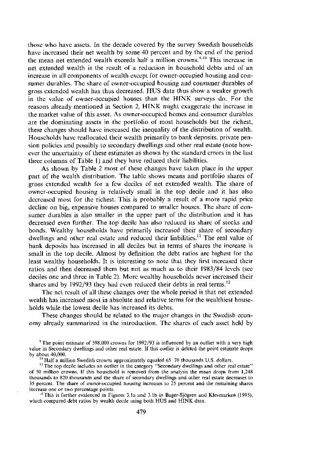
those who have assets. In the decade covered by the survey Swedish households have increased their net wealth by some 40 percent and by the end of the period the mean net extended wealth exceeds half a million crown^.^^'^ This increase in net extended wealth is the result of a reduction in household debts and of an increase in all components of wealth except for owner-occupied housing and consumer durables. The share of owner-occupied housing and consumer durables of gross extended wealth has thus decreased. HUS data thus show a weaker growth in the value of owner-occupied houses than the HINK surveys do. For the reasons already mentioned in Section 2, HINK might exaggerate the increase in the market value of this asset. As owner-occupied homes and consumer durables are the dominating assets in the portfolio of most households but the richest, these changes should have increased the inequality of the distribution of wealth. Households have reallocated their wealth primarily to bank deposits, private pension policies and possibly to secondary dwellings and other real estate (note however the uncertainty of these estimates as shown by the standard errors in the last three columns of Table 1) and they have reduced their liabilities.

As shown by Table 2 most of these changes have taken place in the upper part of the wealth distribution. The table shows means and portfolio shares of gross extended wealth for a few deciles of net extended wealth. The share of owner-occupied housing is relatively small in the top decile and it has also decreased most for the richest. This is probably a result of a more rapid price decline on big, expensive houses compared to smaller houses. The share of consumer durables is also smaller in the upper part of the distribution and it has decreased even further. The top decile has also reduced its share of stocks and bonds. Wealthy households have primarily increased their share of secondary dwellings and other real estate and reduced their liabilities." The real value of bank deposits has increased in all deciles but in terms of shares the increase is small in the top decile. Almost by definition the debt ratios are highest for the least wealthy households. It is interesting to note that they first increased their ratios and then decreased them but not as much as to their 1983184 levels (see deciles one and three in Table 2). More wealthy households never increased their shares and by 1992193 they had even reduced their debts in real terms.12

The net result of all these changes over the whole period is that net extended wealth has increased most in absolute and relative terms for the wealthiest households while the lowest decile has increased its debts.

These changes should be related to the major changes in the Swedish economy already summarized in the introduction. The shares of each asset held by

The point estimate of 598,000 crowns for 1992/93 is influenced by an outlier with a very high value in Secondary dwellings and other real estate. If this outlier is deleted the point estimate drops by about 40,000.

10 Half a million Swedish crowns approximately equaled 65-70 thousands U.S. dollars. I ' The top decile includes an outlier in the category "Secondary dwellings and other real estate"

of 50 million crowns. If this household is removed from the analysis the mean drops from 1,248 thousands to 820 thousands and the share of secondary dwellings and other real estate decreases to 35 percent. The share of owner-occupied housing increases to 25 percent and the remaining shares increase one or two percentage points.

12 This is further evidenced in Figures 3.la and 3.lb in Bager-Sjogren and Klevmarken (1995), which compared debt ratios by wealth decile using both HUS and HINK data.

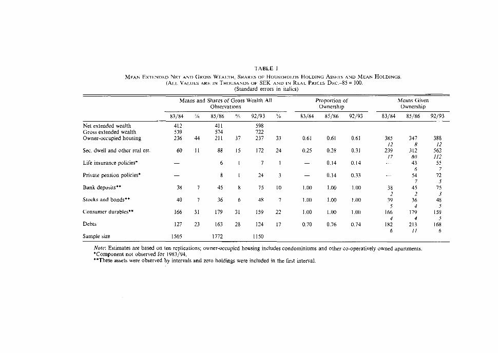
TABLE 1

MEAN EXTENDED NET AND GROSS WEALTH, SHARES OF HOUSEHOLDS HOLDING ASSETS AND MEAN HOLDINGS. (ALL VALUES ARE IN THOUSANDS OF SEK AND I N REAL PRICES D ~ c . 4 5 = 100.

(Standard errors in italics)

Means and Shares of Gross Wealth All Proportion of Means Given Observations Ownership Ownership

83/84 O h 85/86 % 92/93 % 83/84 85/86 92/93 83/84 85/86 92/93

Net extended wealth 412 41 1 598 Gross extended wealth 539 574 722 Owner-occupied housing 236 44 211 37 237 33 0.61 0.61 0.61 385 347 388

I2 8 I2 Sec. dwell and other real est. 60 1 1 88 15 172 24 0.25 0.28 0.31 239 312 562

17 60 112 Life insurance policies* - 6 1 7 1 - 0.14 0.14 - 43 55

6 7 Private pension policies* - 8 1 24 3 - 0.14 0.33 - 54 72

7 5 Bank deposits** 38 7 45 8 75 10 1 .OO 1.00 1.00 38 45 75

2 2 3 Stocks and bonds** 40 7 36 6 I S 7 1.00 1.00 1.00 39 36 48

5 4 5 Consumer durables** 166 31 179 31 159 22 1.00 1.00 1.00 166 179 159

4 4 5 Debts 127 23 163 28 124 17 0.70 0.76 0.74 182 213 168

6 I1 6 Sample size 1505 1772 1150

Note: Estimates are based on ten replications; owner-occupied housing includes condominiums and other co-operatively owned apartments. *Component not observed for 1983194. **These assets were observed by intervals and zero holdings were included in the first interval.

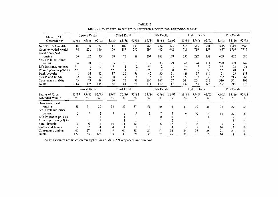
TABLE 2

MEANS A N D PORTFOLIO SHARES IN SELECTED DECILES FOR EXTENDED WEALTH

Lowest Decile Third Decile Fifth Decile Eighth Decile Top Decile Means of All Observations 83/84 85/86 92/93 83/84 85/86 92/93 83/84 85/86 92/93 83/84 85/86 92/93 83/84 85/86 92/93

Net extended wealth Gross extended wealth Owner-occupied

housing Sec. dwell and other

real est. Life insurance policies Private pension policies Bank deposits Stocks and bonds Consumer durables Debts

Lowest Decile Third Decile Fifth Decile Eighth Decile Top Decile

Shares of Gross 83/84 85/86 92/93 83/84 85/86 92/93 83/84 85/86 92/93 83/84 85/86 92/93 83/84 85/86 92/93 Extended Wealth % % YO O h % % % % % YO % % % Yu Yo

-

Owner-occupied housing 38 51 39 34 39 37 51 40 40 47 39 41 39 27

Sec. dwell and other real est. 5 8 2 3 5 5 9 7 7 9 10 13 18 29

Life insurance policies 1 1 1 1 0 0 1 1 2 Private pension policies 1 1 1 1 1 2 1 4 3 Bank deposits 9 6 11 10 11 15 10 8 12 7 8 13 6 7 Stocks and bonds 2 7 4 4 4 3 3 3 4 3 5 4 16 12 Consumer durables 46 27 43 49 40 38 26 41 36 34 36 25 21 20 Debts 120 185 128 37 43 39 33 29 26 21 21 15 14 12

Note: Estimates are based on ten replications of data. **Component not observed.

Swedish households were influenced by changing asset prices and by new incentives to hold assets given by the new tax system. Real estate prices peaked in the beginning of the 1990s and the subsequent fall was enforced by the new tax system. The decrease in marginal tax rates decreased the value of deductions, the most important being interest payments on mortgages, the old tax on imputed incomes from housing was replaced by a flat rate real estate tax with the tax assessed value of the property as a base. The tax on capital gains from owner- occupied houses also changed. In all the new tax system implied higher taxes on owner-occupied homes. More or less consistent with these changes is the observed no change 1985-92 in investments in owner-occupied homes. The old tax system combined with high inflation gave incentives to finance purchases of real estate and consumer durables by mortgages and loans and the debt ratio was relatively high in the middle of the 1980s. The new tax system made liabilities relatively more expensive and at the same time inflation started to decrease. Uncertainty about future incomes (increasing unemployment) and about the future pension system contributed to the observed decrease in household debts in the end of the period. Since consumption credits also became relatively more expensive the share of consumer durables was also decreased.

The new tax system made the taxation of bank deposits and bonds more equal to that of other assets. As a result the share of bank deposits and bonds have increased. Although the taxes on private investments in pension funds were increased this kind of asset still had a favor relative to alternatives. The increased uncertainty about the future of the public pension system also contributed to the increasing interest in private pension policies.

It is of course very difficult to separate out the effects of the tax reform from alternative explanations. Supplementary information from the HUS surveys on respondents' self-evaluated responses to the tax changes is suggestive. Almost 29 percent of all respondents believed that the tax reform made them decrease their debt while close to 13 percent thought that they had increased their debt as a result of the tax reform. The responses depended on the size of household net wealth in 1992. Among the 25 percent most wealthy 39 percent said they had decreased their debts and 7 percent that they had increased them. In the least wealthy quartile only about 25 percent said they had decreased their debts and 23 percent that they had increased them.

There were also questions about savings behavior. Almost 38 percent of the respondents said that the tax reform made them save more, men more than women and well-educated more than respondents with a shorter schooling. Sav- ings behavior is related to the size of disposable income and so were the responses to these questions. More than 52 percent of the respondents in the highest income quartile said that they saved more while only 26 percent in the lowest quartile gave this response. The decreased share of debts in the portfolio of households could thus be the combined effect of reallocations within the portfolio and increased net savings.

Table 3 compares three different inequality measures computed for both data sources.

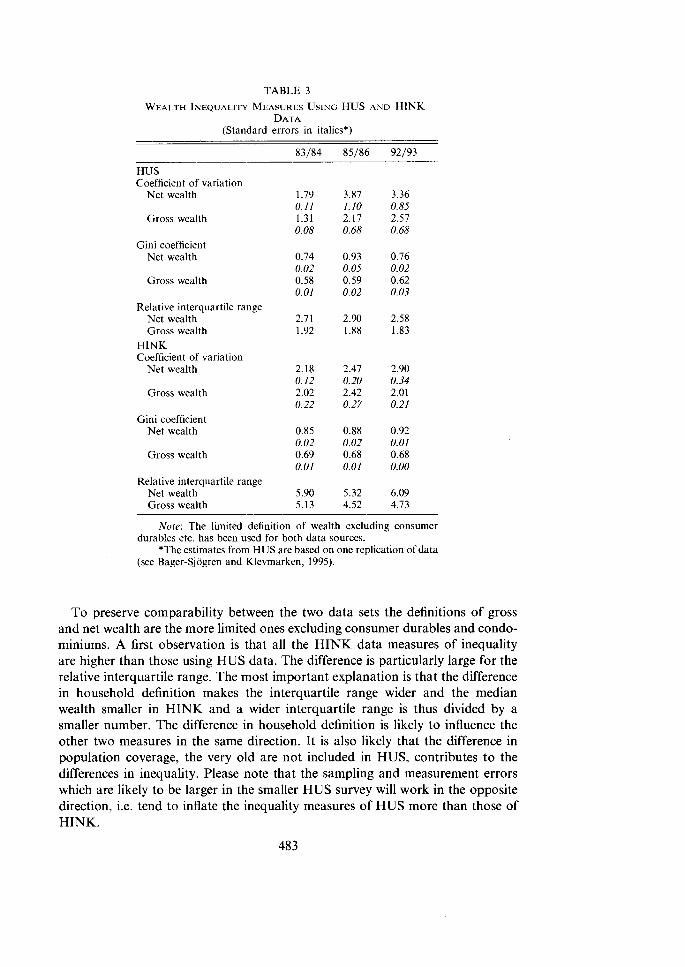
TABLE 3

WEALTH INEQUALITY MEASURES USING HUS AND HINK DATA

(Standard errors in italics*)

83/84 85/86 92/93

HUS Coefficient of variation

Net wealth

Gross wealth

Gini coefficient Net wealth

Gross wealth

Relative interquartile range Net wealth Gross wealth

HINK Coefficient of variation

Net wealth

Gross wealth


Gross wealth


Note: The limited definition of wealth excluding consumer durables etc. has been used for both data sources.

*The estimates from HUS are based on one replication of data (see Bager-Sjogren and Klevmarken, 1995).

To preserve comparability between the two data sets the definitions of gross and net wealth are the more limited ones excluding consumer durables and condominiums. A first observation is that all the HINK data measures of inequality are higher than those using HUS data. The difference is particularly large for the relative interquartile range. The most important explanation is that the difference in household definition makes the interquartile range wider and the median wealth smaller in HINK and a wider interquartile range is thus divided by a smaller number. The difference in household definition is likely to influence the other two measures in the same direction. It is also likely that the difference in population coverage, the very old are not included in HUS, contributes to the differences in inequality. Please note that the sampling and measurement errors which are likely to be larger in the smaller HUS survey will work in the opposite direction, i s . tend to inflate the inequality measures of HUS more than those of HINK.

One may also note both that the coefficient of variation is more sensitive to the tails of the distribution than the two other measures as evidenced by the relatively large standard errors and that the inequality of net wealth is higher than that of gross wealth. The very unequal distribution of liabilities explains the latter result.

The three measures do not give the same picture of changes in inequality during the period of observation. The measures more sensitive to the tails of the distribution, the coefficient of variation and the Gini coefficient indicate an increase in the inequality of net wealth, while the relative interquartile range shows no increase or even a decrease. Any increase in inequality should thus come from the extreme tails of the distribution." The standard errors of the estimates indicate, however that these changes are insignificant. Only the increase in the Gini coefficient for HINK data will pass a significance test. (The large value of the Gini coefficient for net wealth from HUS data in 1985186 is the result of an outlier with a large debt. The corresponding estimate for gross wealth does not give the same peak.) Both data sources show that the changes in inequality of gross wealth are smaller than those for net wealth. The relative interquartile range decreases while the other two measures either increase a little or remain approximately constant. Most of the changes in inequality of net wealth would thus seem to come from the changes in household debts. The same conclusion is reached if a longer and more frequent series of Gini coefficients from the HINK surveys are used. There is no trend in the inequality of gross wealth while the Gini coefficients for net wealth start to increase in the beginning of the 1990s. If wealthy households decreased their liabilities relatively more than poor households the inequality of net wealth should increase more than the inequality of gross wealth.

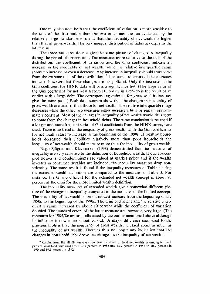
Bager-Sjogren and Klevmarken (1993) demonstrated that the measures of inequality are very sensitive to the definition of household wealth. If owner-occupied houses and condominiums are valued at market prices and if the wealth invested in consumer durables are included, the inequality measures drop con- siderably. The same result is found if the inequality measures of Table 4 using the extended wealth definition are compared to the measures of Table 3. For instance, the Gini coefficient for the extended net wealth concept is about 70 percent of the Gini for the more limited wealth definition.

The inequality measures of extended wealth give a somewhat different picture of the changes in inequality compared to the measures of the limited concept. The inequality of net wealth shows a modest increase from the beginning of the 1980s to the beginning of the 1990s. The Gini coefficient and the relative interquartile range increased by about 10 percent while the coefficient of variation doubled. The standard errors of the latter measure are, however, very large. (The measures for 1985186 are still influenced by the outlier mentioned above although its influence is now more smoothed out.) A major difference compared to the previous table is that the inequality of gross wealth increased about as much as the inequality of net wealth. There is thus no longer any indication that the changes in household debt drove the changes in the inequality of net wealth.

I3 Results from the HINK surveys show that the share of total net wealth belonging to the I percent wealthiest increased from 17.7 percent in 1983 and 15.7 percent in 1985 to 20.7 percent in 1990 and 19.5 percent in 1992.

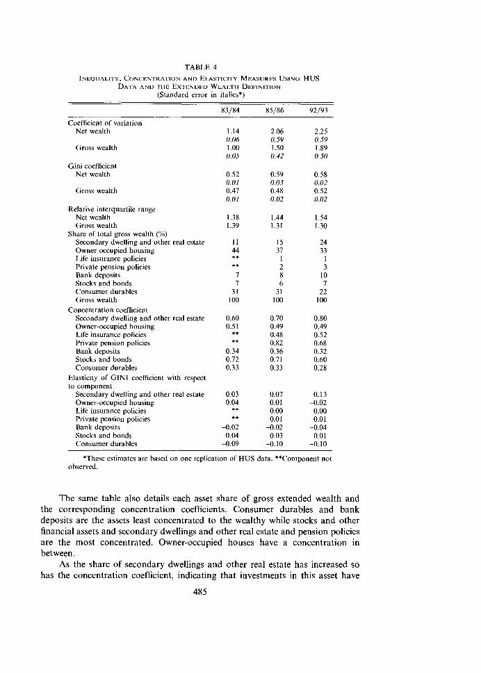
TABLE 4

INEQUALITY, CONCENTRATION AND ELASTICITY MEASURES USING HUS DATA AND THE EXTENDED WEALTH DEFINITION

(Standard error in italics*)

83/84 85/86 92/93

Coefficient of variation Net wealth

Gross wealth


Gross wealth


Share of total gross wealth (%) Secondary dwelling and other real estate Owner occupied housing Life insurance policies Private pension policies Bank deposits Stocks and bonds Consumer durables Gross wealth

Concentration coefficient Secondary dwelling and other real estate Owner-occupied housing Life insurance policies Private pension policies Bank deposits Stocks and bonds Consumer durables

Elasticity of GIN1 coefficient with respect to component

Secondary dwelling and other real estate Owner-occupied housing Life insurance policies Private pension policies Bank deposits Stocks and bonds Consumer durables

*These estimates are based on one replication of HUS data. **Component not observed.

The same table also details each asset share of gross extended wealth and the corresponding concentration coefficients. Consumer durables and bank deposits are the assets least concentrated to the wealthy while stocks and other financial assets and secondary dwellings and other real estate and pension policies are the most concentrated. Owner-occupied houses have a concentration in between.

As the share of secondary dwellings and other real estate has increased so has the concentration coefficient, indicating that investments in this asset have

primarily been made by the wealthy. As a contrast, investments in pension policies and stocks and bonds have become less concentrated to the wealthy.

Following Podder (1993) the last panel of Table 4 details the effects of changes in the components of wealth on the inequality of gross extended wealth by measures of elasticities of the Gini coefficient with respect to the components of gross wealth.I4 For instance, the elasticity of the Gini coefficient with respect to Secondary dwellings and other real estate was 0.13 in 1992193, i.e. a 10 percent proportional increase in this asset would increase the Gini with 1.3 percent.16 The results show that increases in the assets Secondary dwellings and other real estate and Stocks and bonds will increase the inequality in wealth, while increasing bank deposits and investments in consumer durables will decrease inequality. Changes in the latter asset, which is relatively evenly distributed among all households, have the strongest equalizing effect.

The estimated elasticities are not constant. For Secondary dwellings and other real estate the estimates increased more than four times in the period of observation. This is still another way to demonstrate that this asset has become more unevenly distributed. For Owner-occupied housing and for Stocks and bonds the changes in elasticities go in the opposite direction. In the beginning of the 1980s an increase in the wealth endowed in owner-occupied housing would have increased inequality while ten years later it would result in a decrease. Increased investments in Stocks and bonds still increase inequality but to a much lesser degree today than in the beginning of the 1980s. This is consistent with other information about a more widespread ownership of stocks and bonds, in particular through various types of investment funds.

We have already noted that HINK data show a cyclical pattern in mean net wealth with a trough in the mid-1980s and a peak in 1991. Using our more general definition of household wealth we have found that the mean net extended wealth in constant prices increased from the end of 1985 to the end of 1992 and that wealthy households have increased their wealth more than less wealthy. The mean increased by 238,000 crowns 1985186-1992193 in the 1985 price level (Rubin's standard error was 46,000) while the median only increased by 4,000 crowns. The percentiles demonstrate a considerable variability of the distribution of change. The 10th percentile decreased by 116,000 and the 90th percentile increased by 121,000. Behind these numbers thus lie very different experiences for Swedish households. Which households increased their wealth and which households decreased theirs? Guidance to an answer to this question is obtained from Table

14 The elasticity of the Gini coefficient with respect to the k:th component of wealth is defined by

where G is the Gini coefficient of total wealth, Ck the concentration index for wealth component k and pk/p the population share of component k.

15 It is assumed that the asset increases in value such that its concentration index is unchanged.

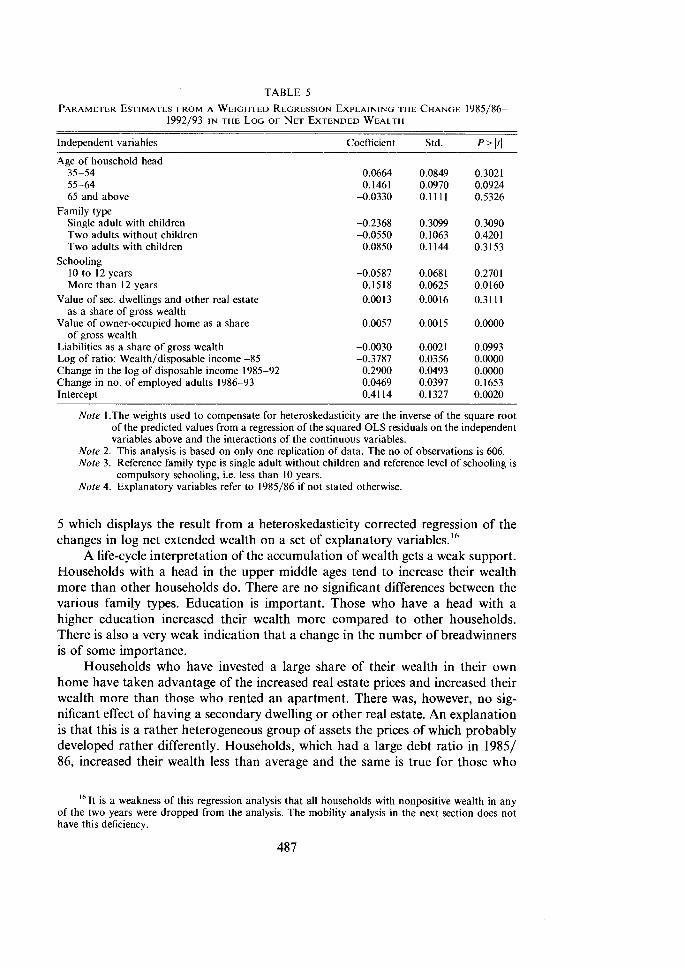
TABLE 5

PARAMETER ESTIMATES FROM A WEIGHTED REGRESSION EXPLAINING THE CHANGE 1985/86- 1992193 I N THE LOG OF NET EXTENDED WEAL.TH

Independent variables Coefficient Std. P > It1

Age of household head 35-54 55-64 65 and above

Family type Single adult with children Two adults without children Two adults with children

Schooling 10 to 12 years More than 12 years

Value of sec. dwellings and other real estate as a share of gross wealth

Value of owner-occupied home as a share of gross wealth

Liabilities as a share of gross wealth Log of ratio: Wealth/disposable income -85 Change in the log of disposable income 1985-92 Change in no. of employed adults 1986-93 Intercept

Note 1.The weights used to compensate for heteroskedasticity are the inverse of the square root of the predicted values from a regression of the squared OLS residuals on the independent variables above and the interactions of the continuous variables.

Note 2 . This analysis is based on only one replication of data. The no of observations is 606. Note 3. Reference family type is single adult without children and reference level of schooling is

compulsory schooling, i.e. less than 10 years. Note 4. Explanatory variables refer to 1985/86 if not stated otherwise.

5 which displays the result from a heteroskedasticity corrected regression of the changes in log net extended wealth on a set of explanatory variables.16

A life-cycle interpretation of the accumulation of wealth gets a weak support. Households with a head in the upper middle ages tend to increase their wealth more than other households do. There are no significant differences between the various family types. Education is important. Those who have a head with a higher education increased their wealth more compared to other households. There is also a very weak indication that a change in the number of breadwinners is of some importance.

Households who have invested a large share of their wealth in their own home have taken advantage of the increased real estate prices and increased their wealth more than those who rented an apartment. There was, however, no significant effect of having a secondary dwelling or other real estate. An explanation is that this is a rather heterogeneous group of assets the prices of which probably developed rather differently. Households, which had a large debt ratio in 19851 86, increased their wealth less than average and the same is true for those who

l6 It is a weakness of this regression analysis that all households with nonpositive wealth in any of the two years were dropped from the analysis. The mobility analysis in the next section does not have this deficiency.

started with a large wealth relative to their disposable income. Finally, we also note that the more a household increased its income the more wealth did it accumulate.

A Review of the Empirical Literature

There are relatively few studies of the mobility of wealth. Menchick (1979) analyzed the inter-generation wealth mobility among wealthy Connecticut resi- dents in the 1930s and 1940s. Steckel (1990) matched U.S census data on real estate data from 1850 and 1860 and found that mobility was relatively low in both ends of the wealth distribution compared to its middle, Shorrocks' measure of mobility was estimated to 0.605.'~

More recent U.S. studies are Steckel and Krishnan (1992) and Hurst et al., (1996). The former was based on a sub sample of older men and mature women of the NLS from the mid-1960s to the mid-1970s, while the latter used the PSID for the period 1984-94. The overall mobility as measured by Shorrocks' measure was almost the same, 0.77 and 0.80 respectively. There are also a few results from a European study, Bentzen and Schmidt-Sorensen (1994) using Danish data from the period 1983-90. Compared to the two modern time U.S. studies, the Danish distribution of wealth is more mobile at the bottom and less mobile at the top, while Shorrocks' overall mobility measure is about the same, 0.78.

Comparisons across these studies are not straightforward as they use data which have been collected in different ways for slightly different populations and time periods and do not use exactly the same definitions of net wealth. However, a few general observations can be made. Wealth mobility depends on the position in the life cycle. Except possibly for the very young, young and middle aged increase their wealth relatively rapidly. Those who have a higher education and obtain managerial and similar white-collar jobs also increase their relative wealth position. Marital status and changes in marital status are important. Singles have a disadvantage and becoming divorced or widowed decreases the ranking. Finally we might also note that the portfolio composition is important. The Danish study is an example of the importance of having assets which increase in value relative to other assets, in this case that of owning a home.

The Mobility of Wealth in Sweden

In this section we take advantage of the panel properties of the HUS data and analyze the mobility of wealth 1985186-1992193. First, a simple transition matrix is computed and compared to the studies reviewed above and then the mobility in decile ranks is analyzed in a multivariate approach.

17 Shorrock's measure of mobility (Shorrocks 1978) is defined as

where N is the number of groups (deciles) and tr(P) is the trace of the N*N transition matrix P. The range of S is [0, N/(N-I)] and a higher S indicates a higher degree of mobility.

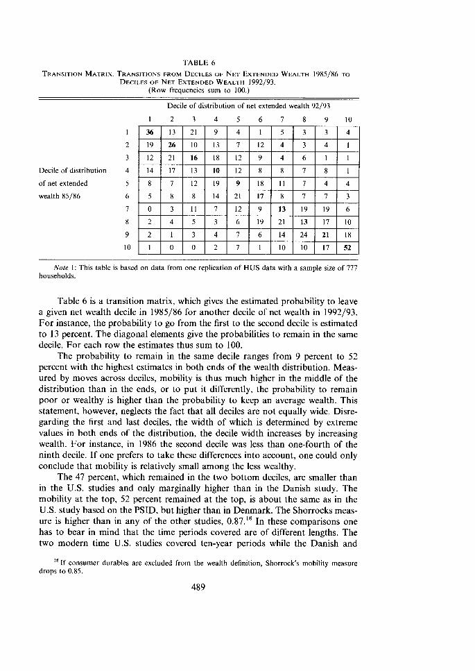
TABLE 6 TRANSITION MATRIX. TRANSITIONS FROM DECILES OF NET EXTENDED WEALTH 1985186 TO

DECILES OF NET EXTENDED WEALTH 1992193. (Row frequencies sum to 100.)

Decile of distribution of net extended wealth 92/93

Decile of distribution

of net extended

wealth 85/86

Note 1 : This table is based on data from one replication of HUS data with a sample size of 777 households.

Table 6 is a transition matrix, which gives the estimated probability to leave a given net wealth decile in 1985186 for another decile of net wealth in 1992193. For instance, the probability to go from the first to the second decile is estimated to 13 percent. The diagonal elements give the probabilities to remain in the same decile. For each row the estimates thus sum to 100.

The probability to remain in the same decile ranges from 9 percent to 52 percent with the highest estimates in both ends of the wealth distribution. Meas- ured by moves across deciles, mobility is thus much higher in the middle of the distribution than in the ends, or to put it differently, the probability to remain poor or wealthy is higher than the probability to keep an average wealth. This statement, however, neglects the fact that all deciles are not equally wide. Disre- garding the first and last deciles, the width of which is determined by extreme values in both ends of the distribution, the decile width increases by increasing wealth. For instance, in 1986 the second decile was less than one-fourth of the ninth decile. If one prefers to take these differences into account, one could only conclude that mobility is relatively small among the less wealthy.

The 47 percent, which remained in the two bottom deciles, are smaller than in the U.S. studies and only marginally higher than in the Danish study. The mobility at the top, 52 percent remained at the top, is about the same as in the U.S. study based on the PSID, but higher than in Denmark. The Shorrocks measure is higher than in any of the other studies, 0.87." In these comparisons one has to bear in mind that the time periods covered are of different lengths. The two modern time U S . studies covered ten-year periods while the Danish and

18 If consumer durables are excluded from the wealth definition, Shorrock's mobility measure drops to 0.85.

Swedish studies covered seven-year periods. If the Scandinavian studies had also covered ten years it is likely that they had shown an even higher mobility. With the reservation that the data sets are not fully comparable, we conclude that wealth mobility across deciles is higher in Sweden than in the two other countries.

To analyze who is gaining in decile rank and who is loosing, a multinomial model was estimated. The categorical dependent variable takes three values: decrease in decile ranks, no change and increase in decile ranks. The first group is the comparison group. The bottom and top deciles were dropped from the analysis because households in these two deciles can obviously only move in one direction. The mobility of these two deciles was analyzed in two separate logit analyses. The degree of mobility is obviously state dependent, cf. Table 6 and for this reason dummy variables for the deciles 2 4 and 6-9 were included in the model. Decile 5 is the decile of reference. Our sample includes both stable households and households which have experienced marriages, separations, the death of a spouse and other changes in their composition. Some of these changes may greatly influence the wealth of a household. With the current definition of a household, those who live jointly with a designated head, a separation may reduce the wealth of the head's household by half.19 The main rule at a separation is that the wealth of the household is split equally between the separating spouses. To control for these changes in the composition of the household a few dummy variables for family type and changes in marital status were introduced. In addition the model includes dummy variables for age group in 1986, the schooling of the head in 1986, if the household in 1986 had a secondary dwelling or other real estate, if it lived in an owner-occupied home and if it in 1986 had liabilities.

The parameter estimates are presented in Table 7 and predicted shares in Table 8. The model does a decent but not a very good job in predicting the observed outcome. The state dependencies come out clearly in the estimates. The probability to advance in rank or remain in the same decile is relatively higher in the bottom deciles and lower in the top deciles. Households, which experienced a separation or the death of a spouse, have a high probability of losing in rank. Those who persistently had single heads were also more likely to lose in rank than to gain and if these single heads had children their probability to lose was even higher. These results are consistent both with prior expectations and with previous results. The importance of separations to explain mobility and the relatively high separation rates in Sweden might contribute to the explanation of the difference in overall mobility between Sweden and the U.S.

Households in the age bracket 55-64 years have a relatively high probability to gain in decile rank or at least not to lose in rank. This is consistent with a decreasing obligation to provide for children in this age bracket, with both spouses working in the market and with amortized mortgages. Very young households and retirees are on the other hand not likely to gain in rank. Schooling significantly influences the relative probability to increase in decile rank. A household with a head who has a college or university education has a higher probability to increase in rank than households with less schooling.

19 Only if a head dies does the headship go to the surviving spouse.

490

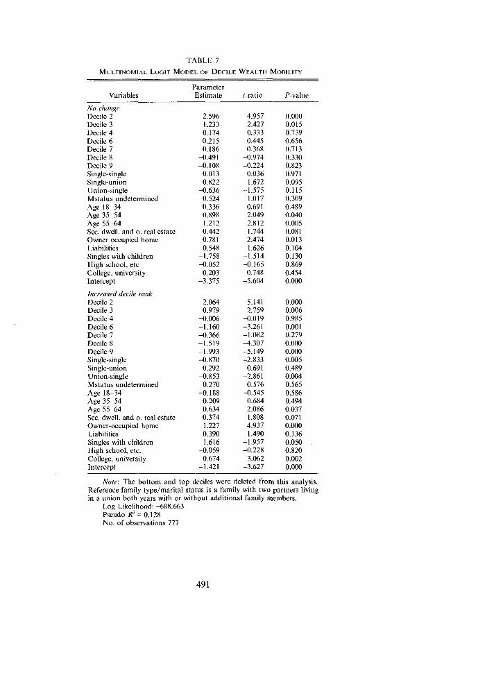
TABLE 7

Parameter Variables Estimate t-ratio P-value

No change Decile 2 Decile 3 Decile 4 Decile 6 Decile 7 Decile 8 Decile 9 Single-single Single-union Union-single Mstatus undetermined Age 18-34 Age 35-54 Age 55-64 Sec. dwell. and o. real estate Owner occupied home Liabilities Singles with children High school, etc College, university Intercept

Increased decile rank Decile 2 Decile 3 Decile 4 Decile 6 Decile 7 Decile 8 Decile 9 Single-single Single-union Union-single Mstatus undetermined Age 18-34 Age 35-54 Age 55-64 Sec. dwell. and o. real estate Owner-occupied home Liabilities Singles with children High school, etc. College, university Intercept

Note: The bottom and top deciles were deleted from this analysis. Reference family typelmarital status is a family with two partners living in a union both years with or without additional family members.

Log Likelihood: -688.663 Pseudo R' = 0.128 No. of observations 777

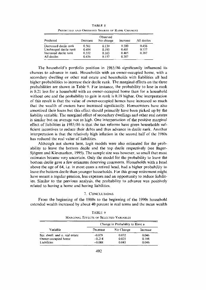
TABLE 8 PREDICTED A N D OBSERVED SI-IARES OF RANK CHANCES

Observed Predicted Decrease No change Increase All deciles

Decreased decile rank 0.561 0.139 0.300 0.456 Unchanged decile rank 0.404 0.195 0.401 0.157 Increased decile rank 0.352 0.163 0.485 0.387 All deciles 0.456 0.157 0.387

The household's portfolio position in 1985186 significantly influenced its chances to advance in rank. Households with an owner-occupied home, with a secondary dwelling or other real estate and households with liabilities all had higher probabilities to increase their decile rank. The marginal effects on the three probabilities are shown in Table 9. For instance, the probability to lose in rank is 0.21 less for a household with an owner-occupied home than for a household without one and the probability to gain in rank is 0.19 higher. One interpretation of this result is that the value of owner-occupied homes have increased so much that the wealth of owners have increased significantly. Homeowners have also amortized their loans but this effect should primarily have been picked up by the liability variable. The marginal effect of secondary dwellings and other real estates is similar but on average not as high. One interpretation of the positive marginal effect of liabilities in 1985186 is that the tax reforms have given households suf- ficient incentives to reduce their debts and thus advance in decile rank. Another interpretation is that the relatively high inflation in the second half of the 1980s has reduced the real value of liabilities.

Although not shown here, logit models were also estimated for the probability to leave the bottom decile and the top decile respectively (see Bager- Sjogren and Klevmarken, 1995). The sample size was however, so small that most estimates became very uncertain. Only the model for the probability to leave the bottom decile gave a few estimates deserving comments. Households with a head above the age of 64, i.e. in most cases a retired head, had a higher probability to leave the bottom decile than younger households. For this group retirement might have meant a regular pension, less expenses and an opportunity to reduce liabilities. Similar to the previous analysis, the probability to advance was positively related to having a home and having liabilities.

7. CONCLUSIONS From the beginning of the 1980s to the beginning of the 1990s household

extended wealth increased by about 40 percent in real terms and the mean wealth

TABLE 9 MARGINAL EFFECTS OF SELECTED VARIABLES

Change in Probabilitv to Have a

Variable Decrease No Change Increase

Sec. dwell. and o. real estate -0.078 0.032 0.046 Owner-occupied home -0.214 0.025 0.188 Liabilities -0.088 0.043 0.046

of a Swedish household exceeded half a million crowns at the end of the period. However, more recent data indicate a decline in average household wealth. Behind these figures we have found major changes both in the portfolio composition and in the inequality of wealth which can be related to market and policy changes which have taken place in this period.

Considering the whole period we have found that Swedish households increased their assets primarily in bank deposits, private pensions and secondary dwellings and other real estate. Their liabilities first increased and then decreased to reach a level in 1992193, which was a little smaller in real terms than in the beginning of the period. The wealth invested in owner-occupied homes decreased in value in the first half of the period and increased in the second. According to our estimates the mean real value of owner-occupied housing was about the same in the beginning and the end of the period. Other sources suggest that behind the average increase 1985186-1992193 lay a major increase in the house prices until 1991 and then a drop after the tax reform and in the subsequent recession.

These changes in the distribution of wealth are consistent with what we know about price changes on assets and the predicted consequences of the tax reform. As predicted, liabilities and the value of consumer durables have decreased and the holdings of bank deposits have increased. The value of real estate was predicted to decrease as a result of the tax reform. HINK-data also suggest that they have decreased after 1991, but the observed changes have also been influenced by the volatile price changes in the real estate markets unrelated to the tax reform and it is difficult to isolate the effects of the tax reform.

The largest changes in portfolio composition have occurred among the wealthiest and they have also increased their wealth relatively more than the less wealthy. As a result the inequality of the wealth distribution has increased. Inequality estimates are sensitive both to the definition of wealth and to the particular inequality index. Our data suggest that the Gini coefficient for extended wealth has increased by some 10 percent.

The increase in inequality is also a result of the change in portfolio composition. The increased investments in secondary dwellings and other real estate, private pension policies and in stocks and bonds, have increased inequality. The decreased investments in consumer durables worked in the same direction as well as the shift in the debt burden from the wealthy to the less wealthy. The only change, which decreased inequality, was the increase in bank deposits.

The decrease in the value of owner-occupied housing in the beginning of the period probably contributed, but only marginally, to an increase in inequality, but at the end of the period the same increase would have resulted in a small decrease in inequality. Taken over the whole period the changes in the value of owner-occupied houses probably did not effect inequality much, but the decrease in housing values which followed the tax reform should have contributed to the increase in inequality. Additional effects of the tax reform on the distribution of wealth are not so easy to distinguish. Pure portfolio reallocations should not immediately influence net wealth. Only differential changes in the return on assets will after some time change the distribution of net wealth.

The subjective responses to the tax reform summarized in Section 3 of this paper indicated that the reform had increased savings and reduced liabilities and

493

our analysis of changes in wealth showed that increases in incomes increased wealth. The increase in disposable income which was the combined effect of tax and transfer changes for many households could thus have contributed to a reduction in liabilities and an increased accumulation of wealth, changes which primarily took place in the upper half of the wealth distribution.

These results are supported and further detailed by our analysis of the mobility of wealth. Households who owned real estate and had liabilities in the middle of the 1980s had a higher chance than other households had to increase their rank in the wealth distribution.

Studies of mobility of wealth are rather few, but comparing our results with a few results from the U.S. and Denmark we found that decile mobility is relatively high in Sweden. This result might seem counter intuitive, because allegedly the U.S. is a country in which the self-made man can advance from nothing into wealth, while taxation would make this much more difficult in Sweden. However, mobility is measured relative to the inequality of wealth in each country. The greater inequality of wealth in the U.S. implies that a move of one decile in this country is a longer move than a decile in Sweden. If the distance of a move had been measured in absolute sense mobility might have turned out higher in the U.S. Another interpretation is that the nonwhite population in the United States have relatively little wealth and low mobility compared to the white population, while there is no such subpopulation in Sweden. A third explanation supported by our analysis but still somewhat speculative is that the relatively high separation rates in Sweden explain at least part of the differences in mobility between the two countries.

Additional results, which agree well with those of previous studies, are that mobility up the distribution primarily takes place among middle aged and among those with a university education.

REFERENCES Bager-Sjogren L. and N. A. Klevmarken, The Distribution of Wealth in Sweden 19841986, in

Research in Economic Inequality, Vol. 4. pp. 203-24, JAI Press, Greenwich, 1993. -, Inequality and Mobility of Wealth in Sweden 1983/841992/93, Tax Reform Evaluation

Report No. 21, November 1995, National institute of Economic Research, Stockholm, 1995. Bentzen J. and Schmidt-Sorensen, Wealth Distribution and Mobility in Denmark: A Longitudinal

Study, Working Paper 94-4, Centre for Labour Market and Social Research, University of Aarhus, Aarhus School of Business, 1994.

Flood, L., A. Klevmarken, and P. Olovsson, Household Market and Nonmarket Activities (HUS), Volume 111: The 1993 Panel Survey, Department of Economics, Uppsala University, 1997.

Hurst, E., Ming Ching Luoh, and F. P. Stafford, Wealth Dynamics of American Families, 1984- 1994, Working Paper, Department of Economics and ISR, University of Michigan, Ann Arbor, 1996.

Income Distribution Surveys (HINK), Statistiska meddelanden Series BE, Statistics Sweden, ~ r e b r o , annual.

Jansson, K. and S. Johansson, Formogenhetsfordelningen 1975-1987, Statistiska Centralbyrin, Stockholm, 1988.

Kessler, D. and A. Masson, Personal Wealth Distribution in France: Cross-sectional Evidence and Extensions, in E.N. Wolff (ed.) International Comparisons of Household Wealth, Clarendon, Oxford, 1987.

Klevmarken N. A. and P. Olovsson, Household Market and Nonmarket activities. Procedures and Codes 198&1991, Almquist and Wiksell International/IUI, Stockholm, 1993.

Little R. J. A. and D. B. Rubin, Statistical Analysis with Missing Data, J. Wiley, New York, 1987.

Menchik, P.L., Inter-generational Transmission of Inequality: An Empirical Study of Wealth Mobility, Economics, 46, 349-62, 1979.

Podder N., The Disaggregation of the Gini Coefficient by Factor Components and its Applications to Australia, Review of Income and Wealtlz, Series 39, No. 1, 1993.

Pilsson, A.-M., Household Risk Taking and Wealth: Does Risk Taking Matter?, Research in Econ- omic Inequalily, Vol. 4, pp. 225-61, JAI Press, Greenwich, 1993.

Rubin D. B., Multiple Imputations for Nonresponse Surveys, J. Wiley, New York, 1987. Shorrocks, A. F., The Measure of Mobility, Econometrics 46, 11 1-20, 1978. Spint, R., Den svenska fonnogenhetsfordelningens utveckling, Lontagarna och kapitaltillviixten 2,

SOU 1979:9, Allmanna Forlaget, 1979. -. , The Wealth Distribution in Sweden: 1920-1983, in E.N. Wolff (ed.), International Compari-

sions of the Distribution o f Household Wealth, Clarendon Press, Oxford, 1987. Steckel, R. H., Poverty and Prosperity: A Longitudinal Study of Wealth Accumulation, 1850-1860,

The Review of Economics and Slatistics, 72, 27585, 1990. Steckel, R. H. and J. Krishnan, Wealth Mobility in America: A View from the National Longitudinal

Survey, Working Paper No. 4137, National Bureau of Economic Research, Cambridge, MA, 1992.

Inequality and Mobility of Wealth in Sweden 1983/84-1992/93

Documents

Transcript of Inequality and Mobility of Wealth in Sweden 1983/84-1992/93