HAL Id: tel-03411094https://tel.archives-ouvertes.fr/tel-03411094

Submitted on 2 Nov 2021

HAL is a multi-disciplinary open accessarchive for the deposit and dissemination of sci-entific research documents, whether they are pub-lished or not. The documents may come fromteaching and research institutions in France orabroad, or from public or private research centers.

L’archive ouverte pluridisciplinaire HAL, estdestinée au dépôt et à la diffusion de documentsscientifiques de niveau recherche, publiés ou non,émanant des établissements d’enseignement et derecherche français ou étrangers, des laboratoirespublics ou privés.

In-Situ Investigation of Cavity Nucleation and Growthin Hydrogen-Exposed EPDM during Decompression

Mahak Fazal

To cite this version:Mahak Fazal. In-Situ Investigation of Cavity Nucleation and Growth in Hydrogen-ExposedEPDM during Decompression. Other. ISAE-ENSMA Ecole Nationale Supérieure de Mécanique etd’Aérotechique - Poitiers, 2019. English. �NNT : 2019ESMA0017�. �tel-03411094�

THESE

Pour l’obtention du Grade de

DOCTEUR DE L’ECOLE NATIONALE SUPERIEURE DE

MECANIQUE ET D’AEROTECHNIQUE (Diplôme National – Arrêté du 25 mai 2016)

Ecole Doctorale :

Sciences et Ingénierie en Matériaux, Mécanique, Energétique

Secteur de Recherche :

Mécanique des Solides, des Matériaux, des Structures et des Surfaces

Présentée par :

Mahak FAZAL

****************************

IN-SITU INVESTIGATION OF CAVITY NUCLEATION AND GROWTH IN

HYDROGEN-EXPOSED EPDM DURING DECOMPRESSION

****************************

Directrice de thèse : Sylvie CASTAGNET

Co-encadrant : Shin NISHIMURA

****************************

Soutenue le 04 Décembre 2019

devant la Commission d’Examen

****************************

JURY

Gerald PINTER, Full Professor, Leoben University

Lucien LAIARINANDRASANA Directeur de Recherche, Centre des Matériaux, Mines

ParisTech

Olivier LAME Professeur, laboratoire MATEIS, INSA de Lyon

Shin NISHIMURA Professor, Hydrogenius Laboratory, Kyushu University

Sylvie GIRAULT Ingénieur R&D, Arkema – ENSAM Paris

Azdine NAIT-ALI Maître de Conférences ISAE-ENSMA, Institut Pprime

Sylvie CASTAGNET Directrice de Recherche CNRS, Institut Pprime

Acknowledgements

This work, much like any other research project, is a result of hard work, guidance and support

of many people and I would be remiss to not express my gratitude here.

I am grateful for the help and guidance from my director, Sylvie Castagnet and for her

insistence that I pace myself while working and put down phone during writing. I am also

thankful to Azdine for being an irreverent guide who has in fact taught me the most important

lesson, that to have fun, to Mikael for his help with numerical simulations, to David and

Guillaume for the experimental work. I am also grateful to the Hydrogenius team at Kyushu

University for being such outstanding hosts during my stay at their lab.

To my friends in the lab (especially the B001 crew): thank you for the discussions both

scientific and otherwise; they have helped me be sane in the lonely quest that PhD is. A big

thank to Ravi for being my soundboard during the PhD and especially during thesis-writing, to

Sylvie Girault for her time during the discussions about the SAXS technique.

I would have not been here without the unconditional support from my family. Faza and Saud,

you are the source of my motivation for everything I undertake in life. Abu, Mom, thank you

for being my most ardent cheerleaders.

Table of Contents

Acknowledgements ................................................................................................................... iv

Table of Contents ....................................................................................................................... v

General introduction .................................................................................................................. 2

Chapter 1 Bibliography ........................................................................................................ 5

1.1 Molecular structure: .................................................................................................... 6

1.2 Mechanical properties: ................................................................................................ 9

1.2.1 Viscoelasticity: ................................................................................................... 11

1.2.2 Mullins effect: .................................................................................................... 11

1.2.3 Payne effect:....................................................................................................... 12

1.3 Cavitation in elastomers: a global view .................................................................... 12

1.4 Modelling approaches ............................................................................................... 15

1.4.1 Single cavity models .......................................................................................... 16

1.4.2 Cavity field models ............................................................................................ 19

1.5 Mechanisms of Diffusion in Polymers ...................................................................... 21

1.6 Cavitation induced by gas decompression ................................................................ 22

1.6.1 Effect of the nature of the gas ............................................................................ 23

1.6.2 Effect of saturation pressure .............................................................................. 26

1.6.3 Effect of rate of decompression ......................................................................... 27

1.7 Morphology of the damage ....................................................................................... 28

1.8 Origin of cavities- a molecular approach .................................................................. 31

1.9 Experimental tracking of cavitation .......................................................................... 34

1.9.1 Volume strain measurements ............................................................................. 35

1.9.2 Acoustic emission .............................................................................................. 35

1.9.3 Optical tracking .................................................................................................. 36

1.9.4 X-Ray computed tomography ............................................................................ 37

1.10 Synthesis of study...................................................................................................... 38

Chapter 2 Material Characterisation ................................................................................... 41

2.1. Chemical composition of EPDM .................................................................................. 42

2.1.1 Cross-link density .............................................................................................. 43

2.2 Hydrogen release profile and diffusivity ................................................................... 46

2.3 Hydrogen content and pressure ................................................................................. 47

2.4 Volume change coefficient due to hydrogen sorption .............................................. 48

2.5 Mechanical properties: .............................................................................................. 49

Chapter 3 Characterisation of EPDM at sub-micron scale using SAXS ............................ 51

3.1 Motivation ................................................................................................................. 52

3.2 Experimental set-up................................................................................................... 53

3.2.1 Ex-situ test ......................................................................................................... 55

3.2.2 In-situ test........................................................................................................... 56

3.3 Primary data processing ............................................................................................ 59

3.4 Scattering due to non-particulate systems ................................................................. 60

3.4.1 Two-Phase and Multiphase systems .................................................................. 60

3.4.2 Debye analysis ................................................................................................... 62

3.4.3 Porod analysis .................................................................................................... 65

3.5 X-Ray scattering for samples before exposure and at equilibrium ........................... 65

3.5.1 Effect of cross-link density on scattering intensity ............................................ 69

3.6 Scattering intensities for exposed samples ................................................................ 71

3.6.1 Scattering for longer q-range ............................................................................. 75

3.6.2 High-pressure exposure: scattering intensity during hydrogen desorption ........ 82

3.7 Conclusions ............................................................................................................... 85

Chapter 4 In-situ tracking of cavities at micron scale using 3D X-Ray Tomography ....... 87

4.1 Experimental set up ................................................................................................... 89

4.1.1 Samples .............................................................................................................. 89

4.1.2 Decompression conditions ................................................................................. 90

4.1.3 Hydrogen decompression tests .......................................................................... 90

4.1.4 In situ tomography set up ................................................................................... 91

4.2 Data treatment ........................................................................................................... 92

4.2.1 Image reconstruction .......................................................................................... 92

4.2.2 Image-processing and post-treatment ................................................................ 94

4.3 Classification of damage based on morphology ....................................................... 97

4.4 Inflation characteristics of isolated cavities .............................................................. 98

4.4.1 Rate of inflation ................................................................................................. 99

4.4.2 Evolution of anisotropy.................................................................................... 100

4.5 Factors influencing the growth kinetics of isolated cavities ................................... 103

4.5.1 Effect of distance from the free surface on rate of inflation ............................ 105

4.5.2 Effect of time of nucleation ............................................................................. 105

4.5.3 Effect of pressure conditions ........................................................................... 106

4.5.4 Effect of sample geometry ............................................................................... 107

4.5.5 Comparison with samples of different cross-link densities ............................. 108

4.6 Relationship of growth kinetics of cavities with macroscopic ................................ 110

desorption ........................................................................................................................... 110

4.7 Inflation characteristics of close cavities ................................................................ 117

4.7.1 Anisotropy........................................................................................................ 126

4.7.2 Qualitative observations of clustering ............................................................. 127

4.8 Conclusions ............................................................................................................. 130

Chapter 5 Investigation of interaction effects between close cavities using Finite Element

Simulations 135

5.1 Difficulties in simulation of cavity growth due to gas decompression ................... 136

5.2 Development of an alternate solution with the internal Finite Element Code

FOXTROT ......................................................................................................................... 139

5.3 Use of FOXTROT software in the context of present work ................................... 140

5.3.1 Main considerations ......................................................................................... 140

5.3.2 Limitations arising from the choice of realistic material parameters of EPDM

1.6 141

5.4 Simulation of the cavity growth using modified parameters .................................. 144

5.4.1 Model geometry and mesh ............................................................................... 144

5.4.2 Material and loading parameters ...................................................................... 145

5.4.3 Single-cavity model ......................................................................................... 146

5.4.4 Two-cavity models........................................................................................... 151

5.5 Conclusions ............................................................................................................. 154

General Conclusions and Perspectives .................................................................................. 155

Résumé étendu en français..................................................................................................... 161

List of Figures ......................................................................................................................... i

List of Tables ........................................................................................................................ xi

Bibliography ........................................................................................................................ xii

2 General introduction

General introduction

The depletion of fossil fuels and environmental issues arising from using them has long since

been a focus of studies leading to exploration of alternate sources of energy viable enough for

commercial and daily use. In particular, the conventional vehicles using fossil fuels contribute

much to the environmental pollution and therefore require an intensification in the

developments of transportation with zero-emissions.

Consequently, fuel cell vehicles (FCVs) using energy derived from hydrogen have attracted a

lot of attention recently as being an alternative means of transport and addressing the

environmental issues at the same time. However, to ensure the adequate cruising range of

FCVs, it is necessary to improve the volume energy density of hydrogen by storing the gas at

a high pressure of 70 MPa. With this pressure in the fuel cell vehicle tank systems, a range of

600 km can be attained.

These relatively high pressures combined with the safety measures required for the usage of

hydrogen itself pose serious challenges with respect to the seals in terms of material and design.

These seals are used in various places in the equipment used for storage and transport of

hydrogen as well as in the fuel recharging stations. The safety risk associated with hydrogen

leakage makes specific demands on the rubber materials used as seals in terms of durability

when exposed to repeated cycles of exposure to high-pressure hydrogen gas.

Figure i Illustration of various types of elastomers used as seals at various points of the hydrogen-FCV system

(Nishimura 2014)

Figure i illustrates the use of different elastomers as sealing materials at different parts of the

hydrogen production facility and the fueling station for the FCVs. Every sealing material has

been chosen for a specific set of pressure and temperature conditions that it will be subjected

to during usage.

EPDM, which is the material of focus in the present study, is used mainly in the form of O-

rings at connectors and receptacles for charging the tanks of the FCVs and as such undergoes

cyclic exposure to high pressure hydrogen leading to diffusion of the gas into the rubber

followed by a rapid decompression to atmospheric pressure. These conditions lead to the

formation of cavities and cracks in the rubber material, a damage that has previously been

termed an explosive decompression failure in the literature. However, this term can be

misleading since cavitation and blister fracture (see Figure ii) in elastomers is not limited to

high pressures and fast pressure release.

Figure ii. Blister fracture EPDM (Hs70) O-ring by exposure to hydrogen gas at 35 MPa and 100 °C for 15 hours

(Nishimura 2014)

This thesis addresses this phenomenon of cavitation due to hydrogen exposure and subsequent

decompression in EDPM. The rapid decompression results in multiple processes occurring

inside the rubber materials which leads to loss of material coherence in the form of appearance

of cavities. These cavities can appear as isolated ones in the bulk or within clusters depending

on the exposure pressure and pressure release rate. In the latter case, they have been suspected

to interact in the earlier studies, especially because cluster morphology evolves during cycling.

The present study aims to utilize the new state of the art experiments that can shed light on this

phenomenon of interaction of a cavity with another cavity and with a free surface, in a more

efficient way. The interaction between cavities is an important factor of study since it could

very well define the evolution of damage from cavitation to cracking. This is a first step towards

building a robust model for prediction of failure as well as development of new materials with

4 General introduction

optimized properties leading to better sealing materials for hydrogen fuel storage and delivery

system.

This document is divided into 5 chapters. The first chapter introduces the concepts associated

with the phenomenon of cavitation in elastomers and the corresponding studies in literature.

The second chapter describes the material of focus of the present study (Ethylene Propylene

Diene Monomer) and details the mechanical parameters of the said material as well as the

diffusion parameters of hydrogen in EPDM.

The third chapter is focused on the study of the heterogeneity of the EPDM-hydrogen system

at sub-micron scale using Small Angle X-ray scattering. A correlation between the network

heterogeneity of EPDM and nucleation of cavities is analysed with the help of novel in-situ

tests. In addition, the changes of the network structure after hydrogen exposure are examined

during and after complete desorption of hydrogen.

The fourth chapter describes the tracking of the cavitation so described at higher scales using

the new technique of time resolved 3D X-Ray computer tomography. The focus is mainly on

the effect of a free surface and on the interaction of cavities at the local scale; the parameters

describing this interaction in terms of spatial and temporal evolution are detailed.

Finally the fifth chapter depicts the attempts to simulate the growth of cavities (isolated or close

to another one) as a coupled problem of diffusion and mechanical pressure using the internal

numerical tool Foxtrot developed at Institut Pprime. Since the tool is still in its early

development stages, the simulation done here do not strictly adhere to the realistic experimental

conditions in which the tests for the EPDM samples were conducted.

The present work was funded by the French Government program “Investissements d’Avenir”

LABEX INTERACTIFS (reference ANR-11-LABX-0017-01). Additionally the tomography

bench used in this study was funded by EQUIPEX GAP (reference ANR-11-EQPX-0018).

Chapter 1 Bibliography

6 Bibliography

This chapter focuses on the studies available in literature carried out on cavitation in elastomers

to provide a background towards understanding the results obtained in the present thesis. In the

first part, a brief introduction about the structure and mechanical properties of elastomers is

given. Next, a global view on the studies of cavitation in literature is introduced and the later

part is focused on the specific study of cavitation due to gas exposure in elastomers and the

techniques to track this damage. Finally, the new ideas and experiments that will be addressed

in this work are summarized with focus on the spaces in existing studies.

1.1 Molecular structure:

Figure1.1 Schematic representation of a network of cross-linked carbon chains (represented with gray circles).

Structurally, rubber is a macromolecule consisting of long molecular chains which are

entangled and intertwined to form a network of non-uniform density. These entanglements act

as physical cross-links thereby imparting certain rigidity to the network which otherwise retains

freedom of movement between the long molecular chains, Figure 1.1. This relative mobility of

chains is responsible for the large deformation of rubber which may be up to several 100

percent of the original dimensions. As a result, chemical crosslinking called vulcanization is

introduced in order to enhance mechanical properties of rubber. This is done by creating

chemical bonds or crosslinks between the long chains that restrict their relative motion and

change the overall mechanical response of rubber. The magnitude of the modulus of elasticity

is directly proportional to the density of the crosslinks. Stress–strain curves for vulcanized and

un-vulcanized natural rubber are presented in Figure 1.2, and it can be seen that in the

vulcanized rubbers the larger strain is accompanied by a sudden increase in the stress.

Figure1.2 Stress–strain curves for unvulcanized and vulcanized natural rubber upto 600% elongation (Callister

and Rethwisch 2007)

The degree of crosslinking is expressed as “crosslink density". Conventionally, the crosslink

density of rubber is measured by methods like gel fraction measurements, swelling tests, or

shear modulus tests. As for the latter, the storage shear modulus (G') is related to the cross-link

density 𝑣𝑐 by the following equation

𝐺′ = 𝜈𝑐𝑅𝑇 𝑒𝑞𝑛 1.1

where R is the universal gas constant and T is the temperature. Plotting the storage modulus

against temperature, the value of cross-link density can be measured by measuring the

measuring the slope of the resulting curve (Jiang et al. 1999)

Crosslinking is also measured by swelling tests in which case the cross-linked samples are

placed into a solvent at a specific temperature. Subsequently, the either the change in mass or

the change in volume of the sample is measured. Thereafter, based on several parameters: the

Flory Interaction Parameter, and the density of the polymer and the solvent, the theoretical

degree of crosslinking can be calculated (Flory 1953).

As a consequence of cross-links, the movement of the long chains is restricted but molecular

segments between the cross-links remain flexible. As such, the crosslink density affects the

maximum extensibility of rubber. Only the rubber with relatively few and widely separated

crosslinks is capable of large extensions without rupture of the primary chain bonds.

8 Bibliography

Since, the rubber molecules consist of folded and convoluted chains in the relaxed state, the

molecular weight between the cross-links is an important parameter to characterise the cross-

link density via the equation

υ𝑐 =ρ

𝑀𝑐 𝑒𝑞𝑛 1.2

Where υ𝑐 is the cross-link density, 𝑀𝑐 is the average molecular weight between cross-links and

ρ is the bulk density of the dry rubber.

Moreover, since these crosslinking points are created in non-uniform fashion throughout the

network, there is an increase in the inhomogeneity of the structure microscopically, which is

well known in literature to influence permeability and diffusion and consequently the elastic

and swelling properties in polymer gels. Consequently, several studies consisting of X-ray

scattering experiments can be found in literature to analyse the concentration heterogeneities

in gels at submicron scales and their effects on their properties. The same techniques (SAXS,

SANS) could be extended to characterize cross-linked rubber network at submicron scales

which has been tackled in the later part of this chapter. Macroscopically, maximum

deformation of the rubber varies with change in cross-link density which is a quantification of

chemical cross-links in the rubber matrix. This is due to lower chain flexibility in rubbers with

low cross-link density. Network heterogeneity has also been linked to improved physical

properties in Poly-isoprene (Grobler and McGill 1994). Ono et al in their recent studies on

unfilled NBR exposed to high pressure hydrogen showed that the bulk expansion of NBR

samples due to hydrogen exposure varied linearly with the increase in the molecular weight

between crosslinks of the NBR chains, 𝑀𝑐; the higher value of 𝑀𝑐 corresponds to larger

distances between cross-links and therefore low cross-link density. This linear relationship was

true for both sulphur and peroxide cross-linked NBR (Ono, Fujiwara, and Nishimura 2018b).

1.2 Mechanical properties:

Figure 1.3 Effect of crosslink density on physical properties of vulcanized polymers (Thoguluva and Vijayaram

2019)

The mechanical properties of elastomers are not single valued functions of the chemical nature

of their corresponding macromolecules. They vary in accordance with other factors such as

degree of cross-linking, molecular weight, nature and amount of additives as well as

temperature. For our study, most of the variables were kept constant; only the degree of cross-

linking was varied, which in turn could affect the mechanical properties like hardness,

modulus, and fatigue of the samples under study, see Figure 1.3.

Generally, elastomers are highly deformable and nearly incompressible with the Poisson's ratio

ν close to 0.5. However, their properties depend more strongly on temperature and time of

testing in comparison with metallic materials. This is due to the fact that as the temperature is

sufficiently lowered, the elastomers become glassy and brittle and consequently lose the

property of rapid recovery. This temperature at which the elastomers transition from rubbery

to glassy state is called glass transition temperature. 𝑇𝑔 is practically important as it sets a

temperature range for the abrupt behavior changes due to local conformational changes leading

to relaxation in elastomers and hence set a practical lower temperature limit for rubbery

behavior of an elastomer. The transition of physical state of amorphous polymers with change

in temperature varies with molecular weight as shown in Figure 1.4.

10 Bibliography

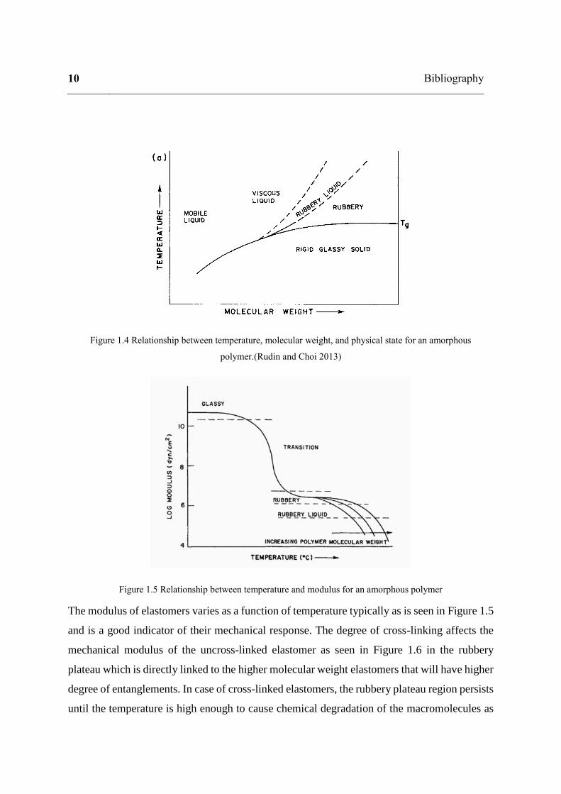
Figure 1.4 Relationship between temperature, molecular weight, and physical state for an amorphous

polymer.(Rudin and Choi 2013)

Figure 1.5 Relationship between temperature and modulus for an amorphous polymer

The modulus of elastomers varies as a function of temperature typically as is seen in Figure 1.5

and is a good indicator of their mechanical response. The degree of cross-linking affects the

mechanical modulus of the uncross-linked elastomer as seen in Figure 1.6 in the rubbery

plateau which is directly linked to the higher molecular weight elastomers that will have higher

degree of entanglements. In case of cross-linked elastomers, the rubbery plateau region persists

until the temperature is high enough to cause chemical degradation of the macromolecules as

seen in Figure 1.6. At very high cross-link densities, the mobility of chain segments is

eliminated so that the material in the glassy state at all practical usage temperatures for example

in some cases of phenolics (Rudin and Choi 2013).

Figure 1.6 Variation of modulus of an amorphous polymer with temperature with varying cross-link density

1.2.1 Viscoelasticity:

Elastomers show the mechanical properties intermediate between Hookean solids and

Newtonion liquids. The characteristic property of reversibility of elastomers on relaxation in

elastic region is time dependent and is reflective of the testing conditions. This is termed as

viscoelastic behavior. In fact, during cyclic tests this becomes evident in form of hysteresis

loops that appear during the unloading part of the cycle.

1.2.2 Mullins effect:

Another characteristic of rubbers, which is more commonly observed in filled rubbers, is the

Mullins effect which refers to the decrease in the stress, during cyclic loading, required to attain

deformation of the same value the first cycle during subsequent cycles,. Microscopically, it is

explained by the molecular structure of rubber with certain macromolecular chains having

different extensibility which broken in the first cycle causing a softening effect (Diani, Fayolle,

and Gilormini 2009).

12 Bibliography

1.2.3 Payne effect:

Similar to the Mullins effect at large deformation, Payne effect is observed for small

deformations, especially in carbon black filled rubbers. Payne effect is observed under cyclic

loading and refers to the decrease in storage modulus with increase in the strain amplitude.

This effect is dependent on the filler content and is not observed in unfilled elastomers. (Payne

1962; Lion, Kardelky, and Haupt 2003; Chazeau et al. 2000).

1.3 Cavitation in elastomers: a global view

Cavitation in elastomers refers to the appearance of damage corresponding to the growth of

defects present intrinsically in the rubber matrix. These intrinsic defects may either refer to the

pre-existing sub-micron voids present in the rubber matrix as a result of network

inhomogeneity or impurities that can cause local stress concentrations leading to nucleation of

cavities under external stresses in an otherwise void less matrix. Roughly, under the application

of sufficiently large external stresses, these defects grow elastically upto the maximum

extensibility of surrounding macromolecular chains.

Figure 1.7 Schematic representation of the "Poker Chip Test" test (Gent, 1959)

This kind of damage in rubbers was first observed by Busse, Yerzley in the 1930s in samples

under tension (Busse 1938; Yerzley 1939). In 1959, Gent conducted the poker chip test on

carbon black filled rubber. The test consisted of subjecting a rubber sample glued between two

metal cylinders to uniaxial tension to generate hydrostatic stress at the centre of the sample,

see Figure 1.7.

Analyzing the stress fields, the negative hydrostatic pressure was found to be maximum at the

centre of the sample (at A in Figure 1.7) and was connected to the tensile stress exerted by the

following relation:

𝐹

𝐴=

1

2𝑇𝑟(𝜎) (1 + 2

ℎ2

𝑟2) 𝑒𝑞𝑛 1.3

Where F is the force exerted on the surfaces A of the metal cylinders, r and h are the radius and

the height of the rubber sample respectively and 𝑇𝑟(�̿�) is the trace of the stress tensor at the

centre of the sample. The appearance of cavitation was accompanied by the change of the slope

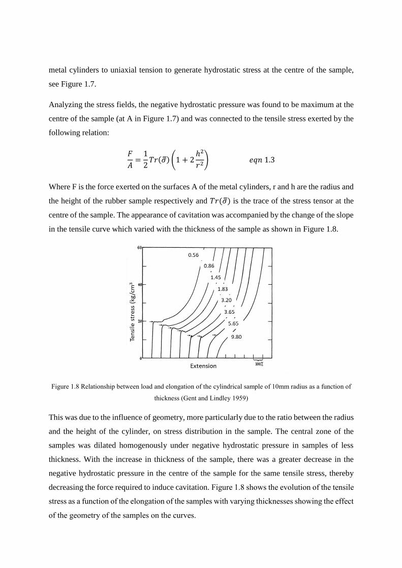
in the tensile curve which varied with the thickness of the sample as shown in Figure 1.8.

Figure 1.8 Relationship between load and elongation of the cylindrical sample of 10mm radius as a function of

thickness (Gent and Lindley 1959)

This was due to the influence of geometry, more particularly due to the ratio between the radius

and the height of the cylinder, on stress distribution in the sample. The central zone of the

samples was dilated homogenously under negative hydrostatic pressure in samples of less

thickness. With the increase in thickness of the sample, there was a greater decrease in the

negative hydrostatic pressure in the centre of the sample for the same tensile stress, thereby

decreasing the force required to induce cavitation. Figure 1.8 shows the evolution of the tensile

stress as a function of the elongation of the samples with varying thicknesses showing the effect

of the geometry of the samples on the curves.

14 Bibliography

They established a linear relationship between the elastic modulus and the hydrostatic pressure

required to induce cavitation from the simple elasticity theory as

𝑃𝑐 =5

6𝐸 𝑒𝑞𝑛 1.4

where 𝑃𝑐 is the critical stress for appearance of cavitation and E is the elastic modulus, see

Figure 1.9.

Figure1.9 Hydrostatic pressure required to have cavitation of the elastomer in function of the Young's modulus

of the material (Gent and Lindley 1959)

Figure 1.10 Fractured surfaces of styrene-butadiene rubber specimens of 100 mm diameter with varying

thicknesses, h, subjected to uniaxial tension. (Hocine et al. 2011)

The morphology of damage is also influenced by the geometry of the sample as seen by Hocine

et al in his study on carbon black-filled styrene-butadiene rubber (SBR) vulcanizate subjected

to uniaxial tension as shown in Figure 1.10.

1.4 Modelling approaches

In their study, Gent and Lindley considered the initiation cavitation as an elastic instability,

examining the problem as an elastic growth of an initial cavity of infinitesimal size embedded

at the centre of a Neo-Hookean rubber ball under uniform hydrostatic pressure.

At the critical value of applied pressure, the cavity became finite. As the theoretical results

agreed well with the experimental observations ones in their study, most of the work that

followed was based on the same approach. (Oberth and Bruenner 1965; Gent and Park 1984;

Lopez-pamies 2009; Nakamura and Lopez-Pamies 2012; Kabaria, Lew, and Cockburn 2015).

Williams and Schapery extended the radially symmetric calculation of Gent and Lindley

(1959a,b), to include the Griffith approach (Griffith 1921) taking into consideration that the

cavity surface stretches far more than the elastic values for rubber. They allowed for the cavity

embedded at the centre of a Neo-Hookean ball of finite size to deform not only plastically but

also by creation of new surfaces, treating cavitation as a fracture phenomenon. They also

accounted for the surface energy associated with the surface area increase from cavity

expansion (Williams and Schapery 1965). The relationship between the critical hydrostatic

pressure 𝑃𝑐𝑟 and surface energy was expressed as follows:

𝑃𝑐𝑟 = µ [52⁄ −

𝜆𝑎−4

2⁄ − 2𝜆𝑎

−1] 𝑒𝑞𝑛 1.5

Where 𝜆𝑎 is the solution of the equation 𝐶(𝜆𝑎) = 𝜇[2𝜆𝑎−1 − 𝜆𝑎

2 − 1] + 2𝛾 /𝑎0 = 0; µ

denotes the initial shear modulus of the Neo-Hookean medium and 𝛾 is the material constant

denoting the surface energy per unit undeformed area that is created. The analysis takes into

consideration the dependence of 𝑃𝑐𝑟 on the initial cavity size 𝑎0 through the parameter κ =

2γ/µ𝑎0. Assuming the range of values for parameters 𝜇 between 0.1 and 1 MPa, 𝛾 between 1

and 10 J/m2, 𝑎0 between 10-8 to 10-7 m and κ between 20 and 20,000 leading to 𝑃𝑐𝑟 between

2.045𝜇 and 2.486𝜇. These values were quite same as that of Gent and Lindley. Most of the

studies thereafter have followed the approach of Gent of treating cavitation as an elastic growth

16 Bibliography

of pre-existing defects. Lefevre et al carried out full field simulations of the Gent and Lindley,

and Gent and Park experiments under the assumption of nonlinear elasticity of rubber

specimens and the random and isotropic distribution of initial vacuous defects (Ravi-chandar

and Lopez-pamies 2014). Their findings have agreed with the theories of Williams and

Schapery (1965) the local stretches around the defects at which cavitation initiates far exceed

the elastic limit of the rubber making it obvious that cavitation in rubber is primarily a fracture

process. Moreover, their studies have indicated a need for more in depth experimental analysis

to understand the phenomenon of cavitation in rubber.

From a modelling point of view, two different approaches are possible with respect to the origin

of cavities: In the first approach cavitation is considered to be an expansion of pre-existing

voids in the rubber matrix whereas in the second approach the cavities are presumed to be

nucleated from an otherwise void-less material.

The second step in the classification is with respect to the scale of the modelling: i) at a local

scale for a single cavity or ii) at macroscopic scale for the global field of cavities, taking into

account both approaches of origin of cavities. In the first approach, a single cavity is assumed

to be representative of the whole phenomenon for which a cavitation criteria is defined. This

subsumes the cavities in the material to be far apart so as to not interact. The second approach

necessitates an introduction of statistical damage variable for the distribution of cavities and

implies a knowledge of the morphology of damage. In any case, it is necessary to predefine a

representative element volume (REV) of damage for the modelling.

1.4.1 Single cavity models

Looking at the theoretical description of cavitation, Ball was among the first people to develop

a robust mathematical representation of the cavitation phenomenon, taking into consideration

the nonlinear elastic solids in addition to Neo-Hookean ones (Ball 1982). He considered the

problem of a unit sphere with a spherical cavity embedded in it subjected to hydrostatic loading

on its outer surface, Figure 1.11.

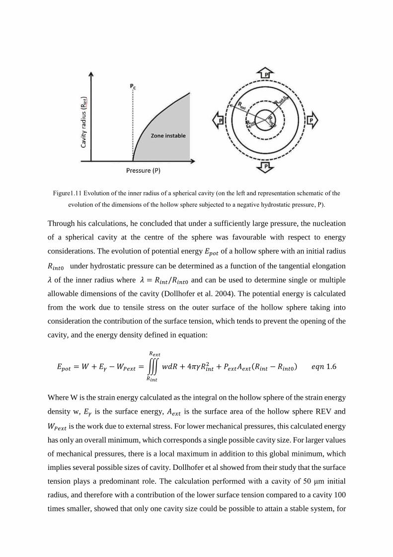
Figure1.11 Evolution of the inner radius of a spherical cavity (on the left and representation schematic of the

evolution of the dimensions of the hollow sphere subjected to a negative hydrostatic pressure, P).

Through his calculations, he concluded that under a sufficiently large pressure, the nucleation

of a spherical cavity at the centre of the sphere was favourable with respect to energy

considerations. The evolution of potential energy 𝐸𝑝𝑜𝑡 of a hollow sphere with an initial radius

𝑅𝑖𝑛𝑡0 under hydrostatic pressure can be determined as a function of the tangential elongation

𝜆 of the inner radius where 𝜆 = 𝑅𝑖𝑛𝑡/𝑅𝑖𝑛𝑡0 and can be used to determine single or multiple

allowable dimensions of the cavity (Dollhofer et al. 2004). The potential energy is calculated

from the work due to tensile stress on the outer surface of the hollow sphere taking into

consideration the contribution of the surface tension, which tends to prevent the opening of the

cavity, and the energy density defined in equation:

𝐸𝑝𝑜𝑡 = 𝑊 + 𝐸𝛾 − 𝑊𝑃𝑒𝑥𝑡 = ∭ 𝑤𝑑𝑅 + 4𝜋𝛾𝑅𝑖𝑛𝑡2

𝑅𝑒𝑥𝑡

𝑅𝑖𝑛𝑡

+ 𝑃𝑒𝑥𝑡𝐴𝑒𝑥𝑡(𝑅𝑖𝑛𝑡 − 𝑅𝑖𝑛𝑡0) 𝑒𝑞𝑛 1.6

Where W is the strain energy calculated as the integral on the hollow sphere of the strain energy

density w, 𝐸𝛾 is the surface energy, 𝐴𝑒𝑥𝑡 is the surface area of the hollow sphere REV and

𝑊𝑃𝑒𝑥𝑡 is the work due to external stress. For lower mechanical pressures, this calculated energy

has only an overall minimum, which corresponds a single possible cavity size. For larger values

of mechanical pressures, there is a local maximum in addition to this global minimum, which

implies several possible sizes of cavity. Dollhofer et al showed from their study that the surface

tension plays a predominant role. The calculation performed with a cavity of 50 μm initial

radius, and therefore with a contribution of the lower surface tension compared to a cavity 100

times smaller, showed that only one cavity size could be possible to attain a stable system, for

18 Bibliography

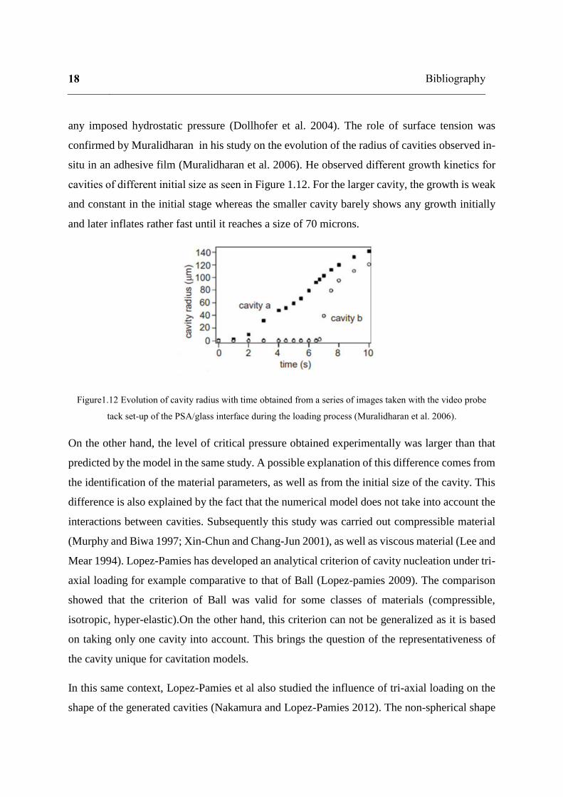
any imposed hydrostatic pressure (Dollhofer et al. 2004). The role of surface tension was

confirmed by Muralidharan in his study on the evolution of the radius of cavities observed in-

situ in an adhesive film (Muralidharan et al. 2006). He observed different growth kinetics for

cavities of different initial size as seen in Figure 1.12. For the larger cavity, the growth is weak

and constant in the initial stage whereas the smaller cavity barely shows any growth initially

and later inflates rather fast until it reaches a size of 70 microns.

Figure1.12 Evolution of cavity radius with time obtained from a series of images taken with the video probe

tack set-up of the PSA/glass interface during the loading process (Muralidharan et al. 2006).

On the other hand, the level of critical pressure obtained experimentally was larger than that

predicted by the model in the same study. A possible explanation of this difference comes from

the identification of the material parameters, as well as from the initial size of the cavity. This

difference is also explained by the fact that the numerical model does not take into account the

interactions between cavities. Subsequently this study was carried out compressible material

(Murphy and Biwa 1997; Xin-Chun and Chang-Jun 2001), as well as viscous material (Lee and

Mear 1994). Lopez-Pamies has developed an analytical criterion of cavity nucleation under tri-

axial loading for example comparative to that of Ball (Lopez-pamies 2009). The comparison

showed that the criterion of Ball was valid for some classes of materials (compressible,

isotropic, hyper-elastic).On the other hand, this criterion can not be generalized as it is based

on taking only one cavity into account. This brings the question of the representativeness of

the cavity unique for cavitation models.

In this same context, Lopez-Pamies et al also studied the influence of tri-axial loading on the

shape of the generated cavities (Nakamura and Lopez-Pamies 2012). The non-spherical shape

of the obtained cavities Figure 1.13, confirms that the appearance of cavities in nonlinear elastic

materials depends on applied tri-axial loading and not just the hydrostatic component.

Figure1.13 Cavity shapes obtained for different types of tri-axial loading satisfying cavitation conditions

(Nakamura and Lopez-Pamies 2012).

1.4.2 Cavity field models

Cavity field models involve generation of several same size cavities randomly distributed in a

cubic form REV, whose size depends on the number of cavities. One of the modelling strategies

used in the literature is the equivalent inclusion method (EIM): empty cavities are replaced by

equivalent inclusions. The method is described in detail in the literature (Moschovidis and

Mura 1975; Mura 2013).The main challenge for this method is to find the optimum properties

to be assigned to the inclusion and to quantify the interactions with close cavities. In fact,

replacing the empty cavities by inclusions with realistic properties makes it possible to

overcome the problems of computational convergence related the interfaces between cavities

and the matrix. The EIM provides the stress distribution around the cavities and gives an

estimate of the interactions between cavities.

All these models are based on a pre-existing cavity/cavities justified by the hypothesis that

defects are induced in the materials during the manufacturing process. Other models exist in

literature where the second approach of a nucleation of cavity from a healthy polymer is taken.

These models take into consideration the conditions of appearance and growth of the cavity.

Ball considered this problem as a hollow sphere problem by taking an infinitely small cavity

20 Bibliography

size that tends to zero. This yielded the same criteria of cavitation as proposed by Gent. A slight

difference in the criterion was observed by Dollhofer et al who considered the same calculation

by integrating the strain energy from 0 to 𝑅𝑒𝑥𝑡 in the eqn 1.6 and explained this difference by

the effect of surface tension which tends to close the small cavity (Dollhofer et al. 2004). In

other models, the appearance of the cavity is taken to occur as a result of instability in a healthy

material deduced from the balance of energy and for which analytical solutions have been

developed, for example by using the principle of virtual works (Hang-Sheng and Abeyaratne

1992). This method makes it possible to consider complex loads without taking into account

the position of instability. However, it is limited to cases of simple behavior laws for the

resolution to be analytical.

For modelling a cavity field that appears in a healthy polymer, a solution is to use molecular

dynamics. Sixou used this approach to study cavitation in a healthy amorphous polymer

subjected to hydrostatic loading and showed the change in the volume (ΔV) to be linear upto a

critical value of hydrostatic pressure after which the increase in volume was accompanied by

the decrease in stress (Sixou 2007). Highly localised and spherical cavities were observed for

the case of strong intermolecular interactions, whereas in case of weaker intermolecular

interactions or higher rigidity, the regions of cavities were more diffused. The authors assumed

the high mobility regions occurring before the peak stress to act as nucleation sites for the

cavitation process. The same technique was used by Morozinis et al to model a perfect

polyethylene network subjected to a tensile loading leading to the appearance of cavities in the

initially healthy material. They found the critical stress of cavitation to correlate with the

Young’s modulus of the material; this observation was in qualitative agreement with

macroscopic continuum mechanics analysis of Gent (Morozinis et al. 2013).

The models described above were mostly aimed at predicting the critical pressure required for

the appearance of cavitation in materials. However, these works did not take into account the

effects of loading rate on this criterion of cavitation. Again the coupled diffuso-mechanical

loading simulating the real loading conditions as the material is subjected to gas exposure has

not been reported. Jaravel developed a numerical 1D model to address the effect of both gas

diffusion and mechanics on volume change of a pre-existing cavity by considering a spherical

cavity at the centre of the sample as a hollow sphere problem with boundary conditions

calculated from the macroscopic conditions of the sample (Jaravel et al. 2013). In comparison

to the case of pure mechanical loading, where cavity growth is a consequence of instability, in

the case of coupled diffuso-mechanical loading, the cavity growth occurs as due to gas

diffusion between the cavity and the rubber matrix. A significant result of the study was a

temporal prediction of cavitation in real conditions that were seen experimentally including the

case of no cavitation for low values of decompression rates and saturation pressures.

Nevertheless, a robust 3D model for cavitation in elastomers taking into consideration the

coupled diffuso-mechanical loading has not so far been defined in literature.

1.5 Mechanisms of Diffusion in Polymers

In principle, the mechanism of diffusion in case of elastomers is the movement of diffusing

molecules into the vacant spaces inside the matrix created by the movement of the elastomer

molecules and the speed of these diffusing molecules depends on the testing temperature and

𝑇𝑔 of the elastomer. Silicone rubbers have a lower 𝑇𝑔 and this show high diffusivity for most

gases (Southern, 1985). Moreover, the diffusion of smaller molecules is easier than a larger

molecule since smaller spaces in the matrix occur more frequently than larger ones. The

vacancy in the elastomer matrix is related to the free volume of the rubber which can be related

to the compressibility of the rubber (Van Amerongen 1964). In soft and rubbery polymers, the

diffusion is generally Fickian. Deviations from Fickian behavior are in response to the sorption

or desorption of penetrant molecules causing time-dependent structure relaxations (Chen

2005). The diffusion process is thus time as well as concentration dependent. Mathematically

diffusion is characterized by the diffusion coefficient and permeability. The diffusivity or

diffusion coefficient is defined by Fick's first law which states that the flux of the diffusing gas

is proportional to the concentration gradient measured normal to the section.

𝐽 = −𝐷𝑑𝑐

𝑑𝑥 𝑒𝑞𝑛 1.7

Where J is the diffusion flux, measuring the amount of substance diffusing through a unit area

during a unit time interval, D is the diffusion coefficient or diffusivity, 𝑑𝑐/𝑑𝑥 is the

concentration gradient along x. This formula was proposed by Fick analogous to the equations

of heat transfer developed thirty years earlier (Fourier 1822). In the transitional regime, the

22 Bibliography

second law of Fick allows to calculate the change in the concentration of the diffusing species

with respect to time.

𝜕𝐶(𝑥, 𝑡)

𝜕𝑡= −

𝜕𝑗

𝜕𝑥=

𝜕𝐷

𝜕𝑥

𝜕𝐶

𝜕𝑥+ 𝐷

𝜕2𝑗

𝜕𝑥2𝐶 𝑒𝑞𝑛 1.8

The solution of this equation gives the concentration profile in the elastomeric membrane. The

gas content in the material after equilibrium is reached is defined as the solubility S which is

expressed in mol/Pa/m3. The solubility coefficient, defined by Henry's law relates the

equilibrium gas concentration,𝐶𝑒 and the solubility, S, in the elastomer to the pressure, P, of

the gas:

𝑃 =𝐶𝑒

𝑆 𝑒𝑞𝑛 1.9

Most gases follow Henry's law at low and moderate pressures, but significant deviations may

be encountered with easily condensable gases, especially at high pressures. Since H2 is well

known to be a non-condensable gas (Ramsey 1996), and the pressures under which the present

work is carried out is not very high, the diffusion is considered to obey Henry’s law. For

specific shapes of rubber specimens, the rate of the diffusing species as well as the amount can

be calculated as a function of specimen dimensions, the time t, the equilibrium concentration

and the diffusion coefficient D (Crank 1975). More often, the mathematical expression for

calculating the total amount of diffusing species is practically more useful than the calculation

of concentration gradients along the sample dimensions.

1.6 Cavitation induced by gas decompression

In additional to purely mechanical loading, cavitation of elastomers is also induced due to

decompression after gas saturation. This is due to the faster expansion of the dissolved gas in

the material than its desorption which generates nuclei of cavities. For conditions of extreme

loading, the damage is analogous to foaming. To describe the transient phase of gas diffusion

in the material as well as the final state characterized by the penetrated amount of gas, the two

main parameters are required: the diffusion coefficient D and the solubility S of the specific

gas into the specific material. This indicates that the cavitation damage in elastomers due to

gas decompression depends on the nature of the gas as well as that of the elastomer (Van

Amerongen 1964).

Figure1.14 Diffusion coefficient of different gases in different elastomers: (a) natural rubber, (b) NBR-20 and

(c) NBR-32, and (d) nitrile [Van Amerongen 1964].

Figure 1.14 illustrates the relationship between the rate of diffusion of the gas and its size; the

larger the size of the diffusing species the slower is the rate of diffusion resulting in a smaller

value of diffusion coefficient, D. In addition, this figure highlights the need to know D for the

material and gas studied, its value may vary by several decades when changing gas or

elastomer. Moreover, the decompression conditions are also dominant factors for the level and

nature of damage. This makes the studies for each gas pertinent in its own application field.

In addition to depending on the nature of the gas, the damage is also dependent on the nature

of the elastomer; the resistance to cavitation increases with the increase in stiffness of the

material (Peters 1990).

1.6.1 Effect of the nature of the gas

Damage induced during rapid gas decompression in elastomers has been studied

experimentally in different gases such as carbon dioxide (Briscoe and Liatsis 1992a; Briscoe,

Savvas, and Kelly 1994; Embury 2004; Zakaria 1990; Schrittesser et al. 2016), argon (Gent

and Tompkins 1969; Stewart 1971), methane (Stevenson and Morgan 1995), and more recently

24 Bibliography

hydrogen (Jaravel et al. 2011; Kane-Diallo et al. 2016; Ono et al. 2018; Ono, Fujiwara, and

Nishimura 2018a). Since, different gases have different coefficients of solubility and diffusivity

in the same sample, the induced damage is of different proportions and nature for each gas

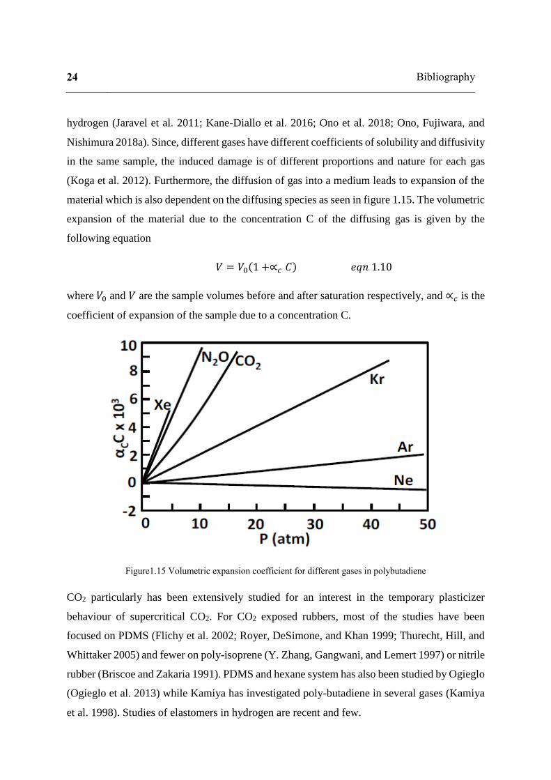
(Koga et al. 2012). Furthermore, the diffusion of gas into a medium leads to expansion of the

material which is also dependent on the diffusing species as seen in figure 1.15. The volumetric

expansion of the material due to the concentration C of the diffusing gas is given by the

following equation

𝑉 = 𝑉0(1 +∝𝑐 𝐶) 𝑒𝑞𝑛 1.10

where 𝑉0 and 𝑉 are the sample volumes before and after saturation respectively, and ∝𝑐 is the

coefficient of expansion of the sample due to a concentration C.

Figure1.15 Volumetric expansion coefficient for different gases in polybutadiene

CO2 particularly has been extensively studied for an interest in the temporary plasticizer

behaviour of supercritical CO2. For CO2 exposed rubbers, most of the studies have been

focused on PDMS (Flichy et al. 2002; Royer, DeSimone, and Khan 1999; Thurecht, Hill, and

Whittaker 2005) and fewer on poly-isoprene (Y. Zhang, Gangwani, and Lemert 1997) or nitrile

rubber (Briscoe and Zakaria 1991). PDMS and hexane system has also been studied by Ogieglo

(Ogieglo et al. 2013) while Kamiya has investigated poly-butadiene in several gases (Kamiya

et al. 1998). Studies of elastomers in hydrogen are recent and few.

Figure1.16 Effect of the nature of the gas on the development of the damage in EPDM O-rings saturated at a

pressure of 10 MPa at 25 ° C and decompressed at 33 MPa/min (Koga et al. 2012)

Figure 1.16 shows the top views of EPDM O-rings exposed to different gases at a pressure of

10 MPa: an example of the effect of the nature of the gas on the damage for elastomers. Since

EPDM is transparent, it allows a visual observation of the damage. As can be seen from the

figure, cavities appear earlier and are more numerous in case of helium. The size of the cavities

is also smaller and short lived, about 800 seconds. Nitrogen causes more detrimental damage

as compared to Helium and hydrogen. Cavities appear later but are larger in size and cracks

perpendicular to the joint axis are also visible. Moreover, the damage is visible even 1 hour

after the beginning of decompression. Koga has explained this difference in damage

morphology to the size of the different gas molecules.

Analogous to this, Colton in his study has observed difference in number of cells generated in

foams while using two different foaming agents; CO2 generates about 1000 times more cells

than nitrogen, an effect he attributes to the high solubility of CO2 as compared to

nitrogen.(Colton and Suh 1987)

26 Bibliography

1.6.2 Effect of saturation pressure

Figure1.17 Effect of saturation pressure on an SBR at 25 ° C and decompressed at 100 MPa / sec after exposure

to Argon (Stewart 1971)

The saturation pressure of the gas is an important parameter for characterization of the induced

damage. Studies show that at a fixed decompression rate, density of cavities decreases with the

decrease in saturation pressure (Figure 1.17) and at a sufficiently low pressure cavitation could

be prevented (Jaravel et al 2011, Stewart 1971). In addition, the study of the influence of the

saturation pressure made it possible to check the validity of the cavitation criterion under gas

decompression (Gent, 1969). For incompressible materials with simple geometries, the

saturation pressure level is equivalent and opposite of the hydrostatic stress in the sample,

which makes it possible to obtain the variation of hydrostatic stress in this sample subject to

gas decompression. Tests at different saturation pressure levels on the same materials have,

therefore, allowed to demonstrate that Gent’s criterion for mechanical cavitation was only valid

for weak saturation pressures (Jaravel et al, 2011). Indeed, cavitation under decompression of

gas is a coupled phenomenon of gas diffusion and mechanics, which was not taken into account

by Gent while defining the criterion for cavitation.

Park in his study with structural foam observed that the density of the cavities did not depend

on the pressure when using iso-pentane as the blowing agent (Park and Cheung 1997). In an

earlier study, Colton (1987) showed that in polystyrene foams with CO2 as the blowing agent,

the dependence of saturation pressure on the density of cavities was only seen in case of

homogenous nucleation and not heterogeneous nucleation rate and more number of

microcellular bubbles were produced by homogeneous nucleation.

Further study on cavitation in elastomers was done by Kane Diallo (2016) by optically tracking

and statistically analyzing the cavities in EPDM after exposure to hydrogen. The analysis was

enriched by the covariogram method and focused on the average size, size distribution as well

as spatial distribution of cavities. This informed the size and isotropy of a representative

element volume. His study could confirm the dependence of saturation pressure on the

phenomenon of cavitation; increase in saturation pressure led to an increase in the number and

average size of cavities and this dependence was nonlinear.

1.6.3 Effect of rate of decompression

Numerous studies in literature has examined the effect of saturation pressure on cavitation but

few exist analyzing the effect of decompression speed since the experiments require a remotely

controlled adjustable decompression valve. This makes it difficult to conduct the experiments

or check the repeatability of the tests conducted. It has been shown that an increase in the

decompression rate increases the number of cavities although the relationship is not linear

(Stewart, 1971; Stevenson and Morgan 1995). The authors explained this effect to be a possible

result of increase in amount of gas and the dimension of the sample which allowed for faster

desorption of the gas out of the samples. Later, Jaravel’s study shed more light on this

relationship. He showed that with low decompression rates of less than 0.3 MPa/min for

saturation at 9 MPa it was possible to avoid cavitation in 2 mm thick samples of silicone rubber.

(a)

28 Bibliography

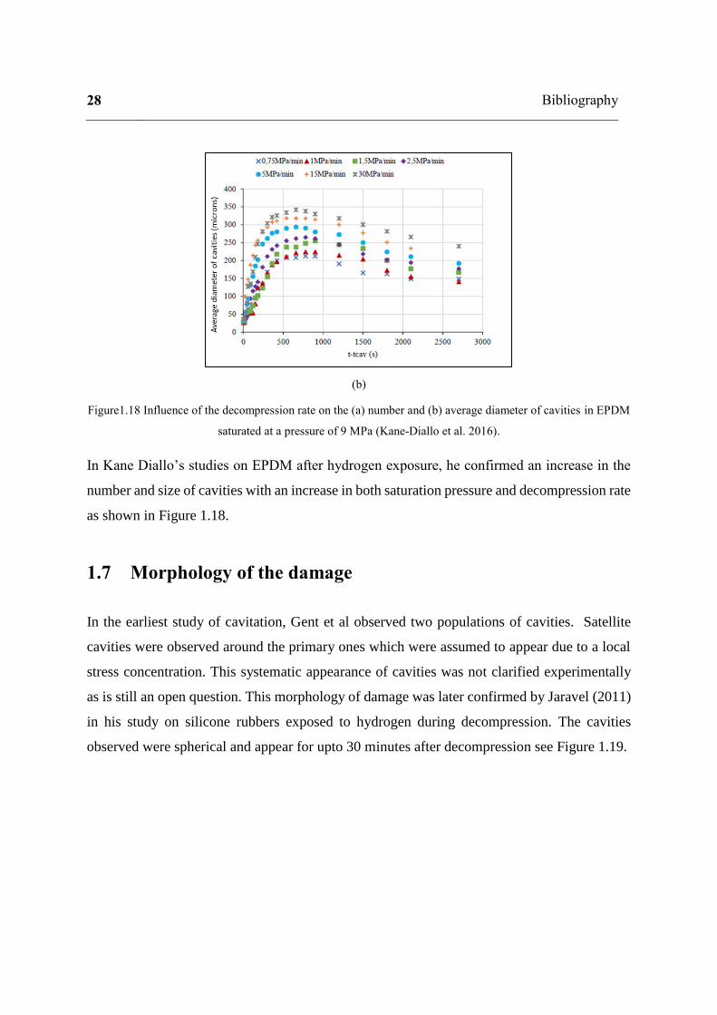
(b)

Figure1.18 Influence of the decompression rate on the (a) number and (b) average diameter of cavities in EPDM

saturated at a pressure of 9 MPa (Kane-Diallo et al. 2016).

In Kane Diallo’s studies on EPDM after hydrogen exposure, he confirmed an increase in the

number and size of cavities with an increase in both saturation pressure and decompression rate

as shown in Figure 1.18.

1.7 Morphology of the damage

In the earliest study of cavitation, Gent et al observed two populations of cavities. Satellite

cavities were observed around the primary ones which were assumed to appear due to a local

stress concentration. This systematic appearance of cavities was not clarified experimentally

as is still an open question. This morphology of damage was later confirmed by Jaravel (2011)

in his study on silicone rubbers exposed to hydrogen during decompression. The cavities

observed were spherical and appear for upto 30 minutes after decompression see Figure 1.19.

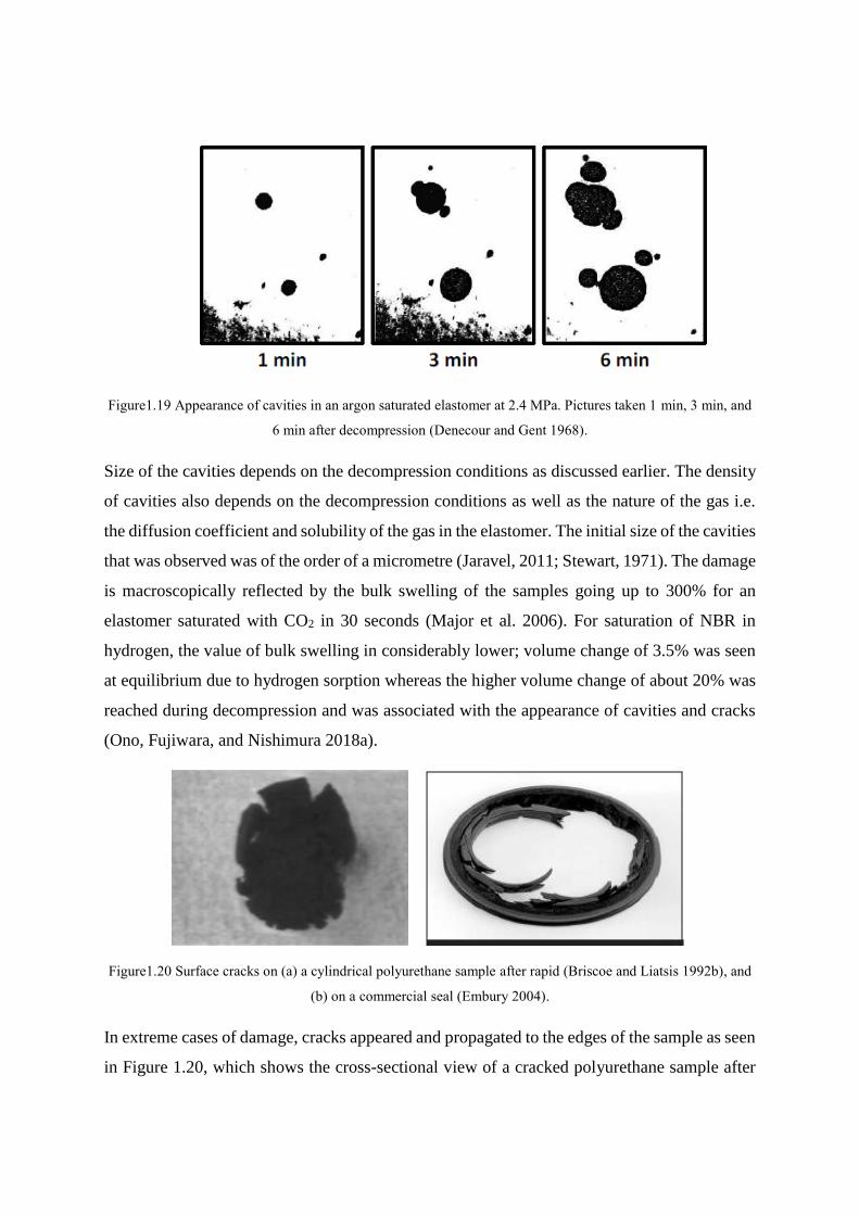
Figure1.19 Appearance of cavities in an argon saturated elastomer at 2.4 MPa. Pictures taken 1 min, 3 min, and

6 min after decompression (Denecour and Gent 1968).

Size of the cavities depends on the decompression conditions as discussed earlier. The density

of cavities also depends on the decompression conditions as well as the nature of the gas i.e.

the diffusion coefficient and solubility of the gas in the elastomer. The initial size of the cavities

that was observed was of the order of a micrometre (Jaravel, 2011; Stewart, 1971). The damage

is macroscopically reflected by the bulk swelling of the samples going up to 300% for an

elastomer saturated with CO2 in 30 seconds (Major et al. 2006). For saturation of NBR in

hydrogen, the value of bulk swelling in considerably lower; volume change of 3.5% was seen

at equilibrium due to hydrogen sorption whereas the higher volume change of about 20% was

reached during decompression and was associated with the appearance of cavities and cracks

(Ono, Fujiwara, and Nishimura 2018a).

Figure1.20 Surface cracks on (a) a cylindrical polyurethane sample after rapid (Briscoe and Liatsis 1992b), and

(b) on a commercial seal (Embury 2004).

In extreme cases of damage, cracks appeared and propagated to the edges of the sample as seen

in Figure 1.20, which shows the cross-sectional view of a cracked polyurethane sample after

30 Bibliography

rapid CO2 decompression and a commercial seal damaged due to explosive decompression

failure: a term used in the reference.

These cracks have been seen to be preferentially oriented (Diani, Brieu, and Gilormini 2006;

Mullins 1948); in the case of cylindrical sample, these cracks propagated perpendicularly to

the cylindrical axis. The surface damage is due to the propagation of cracks initiated in the

centre of the sample (Stevenson and Morgan 1995). However appearance of cavities close to

the edge of the sample have been seen in very thin samples (Campion 1990; Pugh and Goodson

1992). Except for these extreme damage scenarios where the cracking occurs, there remains an

undamaged layer at the edges of the sample: for silicone rubber exposed to hydrogen, this

thickness is of the order of 500 microns. This undamaged layer is attributed to the easier

desorption of gas around the edges and is dependent on the decompression conditions. In the

case of structural foam, the size of the cells or bubbles range between 0.1 and 10 μm with a

density varying between 109 and 1015 cells/cm3 (Colton and Suh 1987). Their size is controlled

by the concentration of the foaming agent in the polymer and the duration of the foaming

process (Figure 1.21).

Figure1.21 Representative images of bath foaming process on thermoplastic olefin containing 100 wt % linear

polypropylene saturated at 138 MPa nitrogen and decompressed at 33 MPa/sec (McCallum et al. 2008).

The damage morphology presented above, namely the number of cavities, their sizes and

undamaged thickness, depends on the nature of the gas and the elastomer but also pressure

conditions which have been discussed in the earlier section.

Kane Diallo (2016) addressed the cavity fields to highlight the spatial distribution of the two

populations of cavities. He concluded that the distribution of cavity diameter evolved with the

increase in saturation pressure or decompression rate and increased the tendency of delayed

nucleation resulting in two populations. Under severe decompression conditions, the

interactions were promoted between close cavities shown by the evolution of covariogram

shape and associated correlation lengths. For such damage, the REV size increased

significantly until it reached the size of the sample. Ono et al studied the evolution of cavitation

due gas decompression with cyclic exposure showing that damage evolution was not a

cumulative process of the systematic reappearance of cavities leading to coalescence. At local

scale, more complex coupled diffuso-mechanical processes govern damage evolution. This

study was carried out on EPDM rubber exposed to hydrogen at 9 and 15 MPa (Ono et al. 2018).

A more rigorous analysis of the cavitation at a local scale is required for a better understanding

of the morphology of damage and its temporal evolution based on the local boundary

conditions. The interactions between the close cavities and the possible topological constraints

arising from the primary population of cavities which could contribute towards the morphology

of the secondary population of cavities need to be addressed with a relevant framework of

damage in rubbers.

1.8 Origin of cavities- a molecular approach

A possibility of explaining gas cavitation in elastomers is by taking a molecular approach, that

is, taking the molecular structure of rubber into consideration. As mentioned in the earlier

section, rubber has vacant spaces or free volume which can be considered to be nano-voids or

cavities (Campion 1975). Due to variation in network density due to fluctuations of cross-

linking density as well as random distribution of cross-link points, the size of free volumes

ranges from 2 to 200 nm (Haward 1970). Stevenson et al., who observe cracks of several

millimeters in length for above 100 °C with NBR samples saturated at 17.2 MPa, assume that

there is a swelling of pre-existing cavities and cracking from areas of low density. To go in the

direction of an appearance of macroscopic cavities from already pre-cavities present whose

32 Bibliography

surface cracks under certain conditions, some photos of damage in transparent samples show

cavities that are not perfectly spherical with the presence of surface cracks as seen in Figure

1.22.

Figure1.22 Cavities obtained in EPDM after saturation with H2 at 3 MPa and 30 ° C for 65 hours (Yamabe and

Nishimura 2009).

Figure1.23 (a) dissolved hydrogen at the end of saturation, (b) formation of gas bubbles by agglomerations of

hydrogen molecules, (c) cavitation induced by stress concentrations induced by the bubbles (Yamabe and

Nishimura 2009)

Other sites of cavity nucleation include the defects and impurities occurring due to

manufacturing process of the material that cause local stress concentrations (Gent and

Tompkins 1969). Another possible cause of cavitation mentioned in the literature is

agglomeration of gas molecules during decompression leading to appearance of visible cavities

(Yamabe and Nishimura 2009) assuming that the gas agglomerates occur in the vacancies of

the network or areas of low network density (Figure 1.23). This is similar to the earlier

hypothesis in suggesting that the formation of cavities was due to free volume since that

indicates that the cavities form in the areas of lower network density.

The origin of the damage is correlated with the acceleration of the desorbing gas from the

sample inducing swelling of the sample (Lorge, Briscoe, and Dang 1999). Jarin noted

competing phenomenon during decompression of LDPE from saturation in CH4 in his study

using LVDT: an expansion of the sample due to decrease in hydrostatic pressure and

contraction due to desorption of the gas. This leads to a very quick desorption near the edge

prompting an undamaged thickness and surface contraction while retaining a high gas

concentration at the core of the samples (Jarrin, Dewimille, and Devaux 1994).

A recent study by Ono et al confirmed that the hydrogen content in unfilled NBR after high

pressure hydrogen exposure was proportional to its fractional free volume which is in

correlation with the effective cross-linking density taking the physical entanglements as well

as the chemical crosslinks into account (Ono, Fujiwara, and Nishimura 2018b).

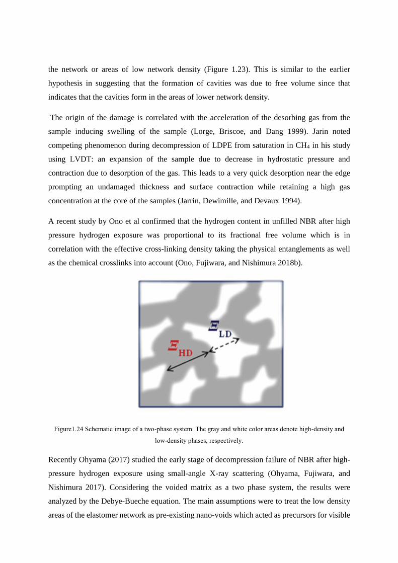
Figure1.24 Schematic image of a two-phase system. The gray and white color areas denote high-density and

low-density phases, respectively.

Recently Ohyama (2017) studied the early stage of decompression failure of NBR after high-

pressure hydrogen exposure using small-angle X-ray scattering (Ohyama, Fujiwara, and

Nishimura 2017). Considering the voided matrix as a two phase system, the results were

analyzed by the Debye-Bueche equation. The main assumptions were to treat the low density

areas of the elastomer network as pre-existing nano-voids which acted as precursors for visible

34 Bibliography

cavities to appear. The low density areas were as a result of local inhomogeneity due to cross-

link density which created a high density and a low density domain in the matrix denoted by

𝛯𝐻𝐷 and 𝛯𝐿𝐷 respectively, see Figure 1.24. The estimation of size of the precursors was

averaged spatially as well as temporally, which could be a good estimation of the general size

of heterogeneities. However, the estimation of local parameters with the global calculation

techniques are much estimated. She also correlated the global gas content with the evolution

of domain sizes, see Figure 1.25.

Figure1.25 Relationship between the remaining hydrogen content and the domain size of each phase (𝛯𝐻𝐷

and 𝛯𝐿𝐷)in NBR : (a) DCP ratio 0.15, (b) DCP ratio 0.5

These studies address these questions of origin of cavities in a polymer due to local

heterogeneities inherent in an amorphous structure due to entanglements and cross-links as

well as defects arising from manufacturing process, treating them as precursors for cavitation.

However, no experimental clarification is provided for these assumptions; in-situ studies at

sub-micron scale could be an important step towards clarifying this assumption of structural

heterogeneity of rubber matrix and localised appearance of cavitation being systematic.

1.9 Experimental tracking of cavitation

The earliest studies of cavitation in rubber were not supported with any visual tracking of the

damage that could prove the appearance of cavitation was systematic with the change of slope

in the tensile curves. Only later, in the work of Lindsey (1967) and Cristiano (2010, 2011),

with the visualization of damage in polyurethane samples, could these questions be cleared up

(Lindsey and Lindsey 2013; Cristiano et al. 2010, 2011). Some of the techniques used in

tracking damage are listed below rather briefly. The objective is to familiarize the reader with

the commonly used techniques and experimental devices and their background for justification

of the experimental technique chosen for the present study.

1.9.1 Volume strain measurements

In their review paper, Naqui and Robinson discussed the theory of tensile dilatometry which

has been used to enable the prediction of volumetric strain of a material associated with the

onset of cavitation (Naqui and Robinson 1993). However, this technique allows for the

quantification of volume fraction of cavities but provide no information on the spatial

distribution or morphology for damage. More recently, Castagnet et al used this technique to

characterise the volume inflation of NBR due to sorption of hydrogen as well as during

decompression stage, during which the volume change occurred due to hydrogen content as

well as due to damage processes activated during this phase (Castagnet, Ono, and Benoit 2017)

1.9.2 Acoustic emission

This is a non-destructive testing technique involving the detection of elastic waves in solids

that are a consequence of irreversible structural changes like plastic deformation or crack

formation (Takaoka et al. 2008). It allows for the analysis of a large sample in a time efficient

way which is of great important from an industrial point of view. For experimental purposes,

this technique is used to detect the onset of cavitation by comparison of the signal generated

by the damaged sample with that of an undamaged one (Yamabe and Nishimura 2011). In

addition, it allows a general idea about the location of damage in a larger sample due to which

it finds application in industries as a non-destructive technique (NDT) for providing valuable

information about discontinuities in the sample. Even if, it is useful for obtaining an estimation

of the beginning of cavitation, the size of the detectable cavities in the bulk of the sample is

much higher than those reported in literature which is a major limitation. Moreover, similar to

the technique of volume strain measurement, the technique provides no information about the

distribution or morphology of the detected cavities.

36 Bibliography

1.9.3 Optical tracking

Optical tracking concerns essentially with acquisition of images during the testing as well as

post mortem. The parameters of the acquisition depend on features that need to be temporally

tracked; the technique is adaptable to the material analyzed as well as the scale at which the

analysis has to be done. Moreover, in comparison to the two techniques mentioned above, this

technique allows for the morphological characterization as well as the quantitative

measurements of the cavitation phenomenon. The most commonly used tools in this case are

the optical microscope and the scanning electron microscope (for higher resolution). Another

technique is to use a CCD camera adapted to track the damage in situ with subsequent

processing of the acquired images to extract quantitative and qualitative data (Kane-Diallo et

al. 2016; Cristiano et al. 2010; Jaravel et al. 2011). The surface data so acquired can be

extrapolated to volumetric representations with an error bar corresponding to the thickness of

the sample (Russ and Dehoff 2012) limiting the technique to a samples of small dimensions.

Figure1.26 Optical tracking experimental set up (Kane Diallo 2016)

Furthermore, the 2D rendering of a 3D damage filed can introduce over or underestimation of

the parameters tracked due to assumptions about out of plane size and shape of cavity size.

Castagnet et al exemplified this in 2018 and were able to clarify this bias in calculation of REV

done previously with optical tracking technique (Kane-Diallo et al. 2016) through 3D in-situ

tomography see Figure 1.27. Another drawback is the limitation of this technique to

transparent samples.

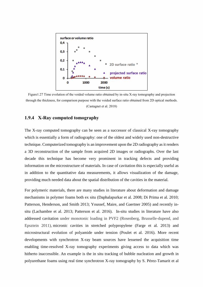
Figure1.27 Time evolution of the voided volume ratio obtained by in-situ X-ray tomography and projection

through the thickness, for comparison purpose with the voided surface ratio obtained from 2D optical methods.

(Castagnet et al. 2018)

1.9.4 X-Ray computed tomography

The X-ray computed tomography can be seen as a successor of classical X-ray tomography

which is essentially a form of radiography: one of the oldest and widely used non-destructive

technique. Computerized tomography is an improvement upon the 2D radiography as it renders

a 3D reconstruction of the sample from acquired 2D images or radiographs. Over the last

decade this technique has become very prominent in tracking defects and providing

information on the microstructure of materials. In case of cavitation this is especially useful as

in addition to the quantitative data measurements, it allows visualization of the damage,

providing much needed data about the spatial distribution of the cavities in the material.

For polymeric materials, there are many studies in literature about deformation and damage

mechanisms in polymer foams both ex situ (Daphalapurkar et al. 2008; Di Prima et al. 2010;

Patterson, Henderson, and Smith 2013; Youssef, Maire, and Gaertner 2005) and recently in-

situ (Lachambre et al. 2013; Patterson et al. 2016). In-situ studies in literature have also

addressed cavitation under monotonic loading in PVF2 (Rosenberg, Brusselle-dupend, and

Epsztein 2011), micronic cavities in stretched polypropylene (Farge et al. 2013) and

microstructural evolution of polyamide under tension (Poulet et al. 2016). More recent

developments with synchrotron X-ray beam sources have lessened the acquisition time

enabling time-resolved X-ray tomography experiments giving access to data which was

hitherto inaccessible. An example is the in situ tracking of bubble nucleation and growth in

polyurethane foams using real time synchrotron X-ray tomography by S. Pérez-Tamarit et al

38 Bibliography

(Pérez-tamarit et al. 2019). Synchrotron sources also have improved the resolution allowing

for the detection or quantification of very small cavities or defects, especially in semi-

crystalline polymers (Morgeneyer et al. 2014; Laiarinandrasana et al. 2010). Further

developments in equipment adapted to the synchrotron facilities enable high quality

mechanical tests to track damage in structural materials. For example recently Pelerine et al

2019 developed a versatile stage to perform in situ 3D imaging using synchrotron X-ray

tomography which made possible to test multiple sample geometries and load ranges upto 5KN

(Pelerin et al. 2019).

The main advantage of the 3D technique is that it provides additional data that can not be

accessed by 2D methods as in the study carried out by Castagnet et al (2018) who could clarify

the 3D shape of the cavities in EPDM exposed to hydrogen by providing information in out of

plane direction, thus providing reliable quantification of damage. This updated experimental

technique provides a new and improved way to track and quantify the damage and is well suited

to address the objectives of the current study.

1.10 Synthesis of study

The studies on cavitation in elastomers due to gas exposure carried so far have been focused

on qualitative analysis after the decompression has already taken place. This is due to the

complex experimental techniques that are required to access the phenomenon in-situ. Improved

experimental techniques have provided some insights into this phenomenon: for example

optical in-situ tracking and associated modelling. It also needs to be noted that damage occurs

as a result of coupling between the mechanical loading and the gas loading. As such the classic

criterion of cavitation due to critical hydrostatic pressure can no longer be considered solely

without taking into account the phenomenon of gas diffusion in the material. Even with the

improved experimental techniques, the direct access to the local gradients leading to nucleation

of cavities is not possible. Moreover the models describing it are limited to the growth of a

single cavity in a bulk with globally described boundary conditions. The data to access the

earliest stages of cavitation correlated with the molecular structure of unfilled rubber could

helpful as a means to predict the cavitation or in best cases, to avoid it altogether.

The second important factor to be analyzed is the interaction effects between cavities that could

exacerbate the damage and lead to cracking in the material. With respect to studies in hydrogen,

they remain few and limited to analysis at global damage field scale.

To sum up, the main focus of this thesis is the analysis of cavitation at a local scale and its

correlation with the network of rubber to understand how far they are systematic. This has been

done by a multi-scale experiment technique, the first step of which is to access the data of

rubber matrix at sub-micron scales through SAXS. This was done for virgin materials (before

hydrogen exposure) as well as after for exposed samples after decompression. Additional in-

situ tests were carried out using an experimental set up that was developed specifically for the

present work and is reported here for the first time. This experimental technique although in

nascent stage, is the first step of developing a robust tool for such complex in situ tests. At

higher scales, the damage was tracked in situ using 3D X-ray tomography which allowed for

the first time a proper 3D rendering of this damage and is a marked improvement on the 2d

tracking techniques used previously. Getting the data at both scales was important for the

simulations done in FOXTROT, a numerical tool developed at Institut P prime for coupled

problems which provided a realistic way of modelling the phenomenon of cavitation as a result

of coupling between hydrostatic pressure and gas diffusion.

40 Bibliography

Chapter 2 Material Characterisation

42 Material Characterisation

This chapter discusses briefly the characteristics of EPDM rubber which is the material of focus

of the present study. The practical usage of EPDM as seals in several industrial applications,

particularly in fuel cell vehicles make it a good candidate for the study. Additionally the

transparency of the unfilled EPDM selected here, and the morphology of damage when

exposed to hydrogen allows for the visual observation as well as quantification of cavitation in

terms of size and volume.

The chemical composition of EPDM is discussed briefly before detailing its diffusion

parameters in hydrogen. This study was focused on the damage of EPDM during the

decompression from an equilibrium state. Hence the hydrogen profile during desorption of the

tested samples was of particular interest and is discussed with respect to different pressures and

degrees of cross-linking.

The samples were provided by the HYDROGENIUS lab in Kyushu University, Japan. They

were manufactured in the form of sheets of 2 mm thickness by the process of compression

moulding. Sheets of 4 mm thickness were manufactured by heat compressing two sheets of 2

mm thickness. Cylindrical samples of diameter 29 mm and thickness 13 mm were also

provided. Moreover all the tests mentioned herein have been performed at the

HYDROGENIUS laboratory.

2.1. Chemical composition of EPDM

Ethylene propylene diene monomer rubber (EPDM rubber), is an M class synthetic rubber

which mostly finds applications in areas involving solvents, acids, and other aggressive

chemicals due to its properties of excellent chemical and thermal resistance. The M-class refers

to the classification in ASTM standard and comprises of elastomers with a polyethylene type

saturated chain. As the name suggests, EPDM comprises of ethylene, propylene and a diene

monomer (See Figure 2.1). The diene monomer is added to enable sulphur vulcanisation

although peroxide vulcanisation is used for better heat resistance. The percentage of the

comprising components affects the properties of the resulting compound; as ethylene content

approaches 50 weight percent and less, the resulting rubber is essentially amorphous. At higher

percentage of ethylene, EPDM is semi-crystalline. It should be noted that the present work is

focused on amorphous EPDM.

Consequently, the application dictates the formulation of the rubber compound. For example

in the recent application of EPDM relevant to present work, as O-rings in Fuel Cell Vehicles

(FCVs), the JIS B2401 and allied specifications lay down standards for the properties of the O-

ring materials. However, these specifications are for the final compound and do not lay any

constraint for the compounding or the additives. As a result, manufacturing companies use their

own specific compounding techniques and percentages of constituents, mostly undisclosed, to

obtain the specified standard for properties.

Figure 2.1 Ethylene-propylene-diene-monomer. The diene monomer in this case is ethylidene

norbornene (ENB) (Wang et al. 2018)

2.1.1 Cross-link density

For practical applications, as is the case with most rubbers, EPDM is cross-linked via

vulcanization and. compounded with fillers and plasticizers to attain suitable mechanical

properties. Crosslinking involves linking the polymers chains to each other and essentially

prevents the indefinite deformation of the material under the application of load. Increasing the

degree of cross-linking or cross-link density decreases the distance between cross-links

restricting the segmental motion and leading to a less flexible network (Brydson 1999).

As the rubber molecules consist of folded and convoluted chains in the relaxed state, this

distance between crosslinks is expressed as the molecular weight between the cross-links rather

than an actual distance. As a consequence, the molecular segments between the cross-links

remain flexible. As such, the crosslink density affects the maximum extensibility of rubber.

44 Material Characterisation

The relationship between the cross-link density and average molecular weight between cross-

links is expressed as

υ𝑐 =ρ

𝑀𝑐 𝑒𝑞𝑛 2.1

Where υ𝑐 is the cross-link density, 𝑀𝑐 is the average molecular weight between cross-links and

ρ is the bulk density of the dry EPDM. For the purposes of this study, the material of focus was

unfilled EPDM, with peroxide crosslinking (using dicumyl peroxide) which resulted in

transparent specimens allowing for the visual tracking of the damage in the samples. Specimens

of different cross-linking density were chosen while the rest of the composition remained

constant. The chemical composition of the samples including the concentration of crosslinking

agent with the corresponding cross-link density as well as 𝑀𝑐 for EPDM samples tested in the

present study is given in Table 2.1.

For calculation of 𝑀𝑐 (number average molecular weight between crosslinks) swelling tests

were carried out using toluene as the solvent. The values of Mc were estimated suing the

following Flory-Rehner equation (Flory Paul J, Rehner JR, John 1943). The value of cross-link

density was calculated using equation 2.2.

𝑀𝑐 =𝜌𝑉1 ( 𝑣2

13 − (𝑣2/2))

ln(1 − 𝑣2) + 𝑣2 + 𝜒𝑣2 𝑒𝑞𝑛 2.2

Where 𝑣2 is the volume fraction of EPDM in the EPDM-toulene mixture, ρ is the density of

dry EPDM, 𝑉1 is the molar volume of toluene and 𝜒 is the Flory solvent-polymer interaction

term (Ono, Fujiwara, and Nishimura 2018a).

As seen in the table, the calculated value of 𝑀𝑐 for EPDM with DCP 0.1 is 641766 g/mol which

exceeds average molecular weight of EPDM polymer: 324546 g/mol. This value was calculated

by size exclusion chromatography using a refractive index detector (RID). As such the swelling

method is not suitable to estimate the value of 𝑀𝑐 for rubbers of very low cross-link density.

There are several other methods of measuring cross-link density, the most popular one being

Nuclear Magnetic Resonance (NMR) method due to its speed and cost effectiveness. However,

in terms of precision, the two techniques are comparable as shown in the study by Dibbanti et

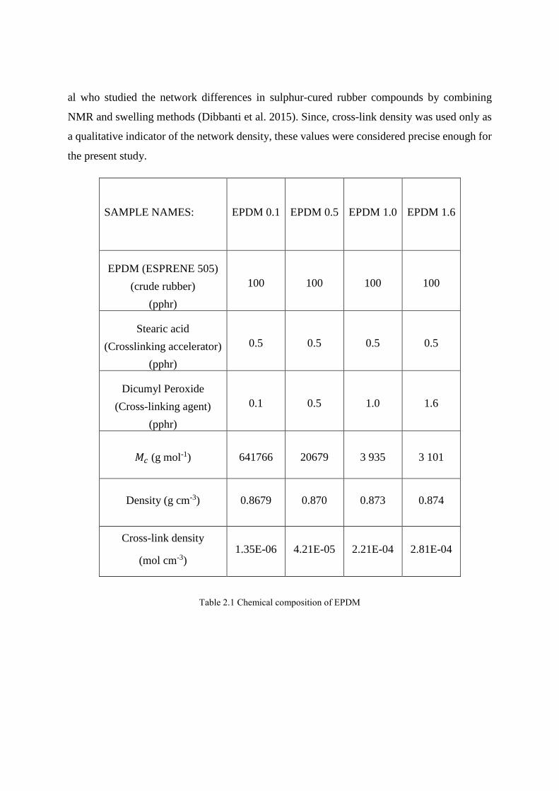
al who studied the network differences in sulphur-cured rubber compounds by combining

NMR and swelling methods (Dibbanti et al. 2015). Since, cross-link density was used only as

a qualitative indicator of the network density, these values were considered precise enough for

the present study.

SAMPLE NAMES:

EPDM 0.1 EPDM 0.5 EPDM 1.0 EPDM 1.6

EPDM (ESPRENE 505)

(crude rubber)

(pphr)

100 100 100 100

Stearic acid

(Crosslinking accelerator)

(pphr)

0.5 0.5 0.5 0.5

Dicumyl Peroxide

(Cross-linking agent)

(pphr)

0.1 0.5 1.0 1.6

𝑀𝑐 (g mol-1) 641766 20679 3 935 3 101

Density (g cm-3) 0.8679 0.870 0.873 0.874

Cross-link density

(mol cm-3) 1.35E-06 4.21E-05 2.21E-04 2.81E-04

Table 2.1 Chemical composition of EPDM

46 Material Characterisation

2.2 Hydrogen release profile and diffusivity

The hydrogen content diffused into the samples due to hydrogen exposure was measured by

Thermal Desorption analysis using a JSH-201 thermal desorption analyzer (J-Science Lab Co.,

Ltd.). Samples were cut in the form of 13 mm diameter and 2 mm thickness discs. The discs

were then kept in a pressure vessel filled with hydrogen at a prescribed pressure and

temperature till saturation after which the vessel was decompressed and the specimens were

removed from the vessel. Following decompression, the discs were kept in the tubular oven

with an Argon current, of the thermal desorption analyser that was kept at 30°C. The hydrogen

concentration in Argon was measured using gas chromatography and the residual hydrogen

content of the specimen was calculated. The calculation was done every 5 minutes to finally

obtain the hydrogen desorption profiles for specimens of varying cross-linking densities.

Thereafter, equation 2.3 was fitted to the remaining hydrogen content using least squares

method to estimate the equilibrium hydrogen content and diffusion coefficient (see Table 2.2);

the size of the specimen was assumed to be constant.

𝐶𝐻,𝑅(𝑡) =32

𝜋2 × 𝐶𝐻,𝐸 × {∑exp [−(2𝑛−1)2𝜋2𝐷𝑡

𝑙2⁄

(2𝑛−1)2∞𝑛=0 } × {∑

exp [−𝐷𝛽𝑛2𝑡

𝑟2⁄

𝛽𝑛2

∞𝑛=0 } 𝑒𝑞𝑛 2.3

where 𝐶𝐻,𝑅(𝑡) wt.ppm is the remaining hydrogen content in the specimen at the time t (s) after

decompression, 𝐶𝐻,𝐸 (wt.ppm) is the equilibrium hydrogen content of the specimen, D (𝑚2/𝑠)

is the diffusion coefficient, 𝛽𝑛 is the root of the zeroth-order Bessel function, and 𝑙 (𝑚) and

𝑟 (𝑚) are the thickness and radius of the specimen, respectively. The hydrogen content of the

samples at equilibrium can be calculated by extrapolation of the above equation, if required.

SAMPLE NAMES: EPDM 0.1 EPDM 0.5 EPDM 1.6

Diffusion coefficient (𝐷)

mm2/sec 1.66E-04 1.49E-04 1.89E-04

Table 2.2 Diffusion coefficients of EPDM with varying cross-link density calculated at a Psat of 30 MPa

2.3 Hydrogen content and pressure

(a)

(b)

Figure 2.2 Hydrogen release profiles for EPDM of varying cross-link density at saturation pressure of a) 0.6

MPa and b) 30MPa

Figures 2.2 (a) and (b) show the hydrogen desorption profiles for EPDM for various cross-link

densities at the saturation pressures of 0.6 and 30 MPa respectively. The relationship between

equilibrium hydrogen content and the saturation pressure has been studies by Yamabe et al. for

filled and unfilled rubbers including EPDM (Yamabe and Nishimura 2009). They could clarify

that the penetrated hydrogen content was proportional to the hydrogen pressure indicating that

48 Material Characterisation

the diffusion of hydrogen into rubber obeyed Henry’s law. Their study was done for saturation

pressures up to 10 MPa.

As seen from the figures the results seem to be consistent for higher pressure of 30 MPa as

well. It is also evident that the testing time for the SAXS experiments carried out here were

well estimated to take into account the hydrogen desorption from the sample. For the saturation

pressures of less than 1 MPa, the complete desorption has occurred by 1 hour after

decompression whereas for the higher saturation pressure of 30 MPa the complete desorption

occurs by 3 hours after decompression. These results are true for the samples of all crosslink

densities tested here.

2.4 Volume change coefficient due to hydrogen sorption

The volume change due to the sorption of hydrogen in EPDM 1.6 was estimated in the Hycomat

facility from a cubic sample (8 x 8 x 8 mm3) with four markers at each corner of the front face.

The sample was exposed at 20 MPa until saturation and pictures were taken with a CCD camera

through the chamber window all along the exposure. Correlation of these pictures provided a

linear swelling coefficients of 0.005 at equilibrium. Since the coefficient was found isotropic

along the horizontal and vertical direction, it could be converted into a volumetric swelling

coefficient of 0.015.

Figure 2.3 Picture of the 8x8x8 mm3 sample used for estimation of the volume change coefficient due to

hydrogen content in EPDM 1.6 with markers for image correlation.

Measurements were done for one exposure pressure only. For further Finite Element Method,

it will be linearly extrapolated over the pressure range: ∆𝑉/𝑉 × 1/𝑃 = 0.00075 MPa-1.

2.5 Mechanical properties:

In addition to the tests mentioned above, dynamic mechanical analysis (DMA) was conducted

on EPDM to characterise its mechanical properties. This method analyses simultaneously both

the elastic and viscous response of the material. The test is conducted by applying sinusoidal

strain or stress to the material (in tension, bending, or shear) using a motor and measuring the

resulting stress or strain with a force transducer or a position sensor respectively. The measured

stress is separated into an in-phase component called the elastic or storage modulus 𝐸’ and an

out-of-phase component called the loss modulus 𝐸”.

The storage modulus represents the elastic portion and defines the material’s ability to store

energy elastically whereas the loss modulus represents the viscous portion and is a measure of

the material’s ability to dissipate energy in form of heat. The complex modulus Ec of the

material if given by equation 2.4

𝐸𝑐 = 𝐸’ + 𝑖𝐸’’ 𝑒𝑞𝑛 2.4

In the present case, the tests were carried out by applying an oscillatory displacement on a

parallelepiped shaped sample placed in a thermally regulated chamber. The tests were carried

out in the temperature range of -120 °C to 200 °C with the rate of temperature change of 10

°C/min. the measurements were done for three different values of frequency: 2.5, 10 and 40

Hz to ensure the reproducibility of the resulting curves. The values of elastic modulus at room

temperature for samples of varying degrees of crosslinking were calculated from the curves

and are listed in Table 2.3. As can be seen form the table the values of storage modulus increase

with an increase in cross-linking density for EPDM 0.5 and EPDM 1.6. However, the value of

modulus for EPDM 0.1 is inconsistent. This is attributed to very high extensibility of the

material due to which the bending occurs during the test rendering the values less reliable for

this kind of material of low crosslink density. In addition, the difference is within the difference

range of the modulus tested of same material tested under different frequencies (see Figure 2.4)

which is consistent with the rheological properties of viscoelastic materials.

50 Material Characterisation

SAMPLE NAMES: EPDM 0.1 EPDM 0.5 EPDM 1.6

Storage modulus (𝐸’) 3 MPa 2.3 MPa 2.75 MPa

Table 2.3 Storage modulus for EDPM taken for the temperature of 30°C by taking the average of the values at

the frequencies of 2.5, 10 and 40 Hz

Figure 2.4 Storage modulus for EPDM 0.5 tested under different frequencies of applied deformation. The arrow

shows the variation of the modulus along different frequencies which is of the order of 0.5-0.8 MPa

This characterization was done mainly to provide a background on the properties of the

material of study and to furnish important data for correlation of the damage parameters to the

material and diffusion characteristics of the material itself. EPDM 1.6 data also provided the

set of parameters used for Finite Element Method in a first attempt for a more realistic

simulation before calibrating a set of parameters for better convergence.

Chapter 3 Characterisation of EPDM at

sub-micron scale using SAXS

52 Characterisation of EPDM at sub-micron scale using SAXS

Study of cavitation in polymers using SAXS is well established in literature for semi-crystalline

microstructures (Humbert et al. 2010; B Xiong et al. 2013; Bijin Xiong et al. 2014; Pawlak,

Galeski, and Rozanski 2014). However, most of analysis of this type of damage is under purely

mechanical conditions (Liu et al. 2003; H. Zhang et al. 2013). In comparison, fewer

publications exist for studies on polymer interactions with diffusing fluids. In-situ SAXS

experiments have been widely used to study the scattering properties of polymer gels and

several quantitative measurements of correlation length associated with both the thermal

fluctuations as well as frozen in topological constraints exist (Geissler et al. 1997; Suzuki et al.

2010). These studies are mostly limited to swelling of polymers in liquid. Polymer substances

are poly-disperse from a practical point of view, consisting of loose conformations in

amorphous state and random aggregates of lamellar layers for semi crystalline microstructures.

Therefore, SAXS studies for the characterisation of local heterogeneities for amorphous rubber

matrix are more challenging than studies of monodisperse systems and depend on appropriate

models for interpretation of the scattering patterns. In terms of in-situ SAXS experiments to

analyse cavitation, these are often focused on pure mechanical problems and often in semi

crystalline polymers(B Xiong et al. 2013; Defebvin et al. 2016). As has been already

established, the cavitation due to gases includes a non-negligible influence of diffusion; the

problem is as a result of the coupled influence of mechanical pressure and gas diffusion in the

rubber matrix and needs to be treated as such (Jaravel et al. 2011).

3.1 Motivation

In order to understand the changes in the rubber matrix due to saturation with hydrogen, as

well as during decompression phase which marks the beginning of cavitation, in-situ tests are

essential. This could be helpful towards building a multiscale approach towards understanding

of cavitation at the very beginning. The data from the sub-micron scale could be used to

highlight the transition from a heterogeneous hydrogen-rubber system at equilibrium towards

a voided state at the micro-scale with a spatial distribution that can be quantified from

tomography views. In this way, in-situ SAXS experiments could correlate the behaviour of

cavities at larger scales and also provide important information for the simulations to be carried

out later.

The main aim of the SAXS experiments in the present study was to characterise the

heterogeneities of the rubber matrix at submicron scale due to chemical cross-linking as well

as physical crosslinking that arise due to molecular entanglements. The characterisation could

give information about the nucleation of the cavities to track how far the heterogeneities of the

rubber matrix could be the precursors to cavities. The question of matrix heterogeneities and

the nucleation being systematic is a valid one due to the heterogeneous distribution of gas in

the matrix as well as local modulus of the rubber matrix. It should be addressed locally with

temporal evolution as a salient factor, keeping in mind that one intrinsic limitation of scattering

techniques remains that they provide average parameters of the distribution.

However, the in-situ tests are difficult to design owing to the practical difficulties of handling

hydrogen in lab conditions. The SAXS experimental set-up for the in-situ tests in hydrogen

was developed by HYDROGENIUS Laboratory at Kyushu University (Japan). Following the

Japanese regulations for gas use in laboratory settings and the constraints of associated safety

conditions, it was ensured that the tests were done at very low pressures of less than 1 MPa.

Another difficulty arising from using a laboratory X-Ray source is that the acquisition time is

usually long. It significantly reduces the number of valid data points, which is particularly

critical in the time just after decompression. For this reason, in the present study, both in-situ

and ex-situ SAXS tests were carried out at various facilities to get as much information possible

in different conditions of beam size and at various times of damage. SAXS tests were also

carried out at the Kyushu Synchrotron Light Research Centre in Japan.

3.2 Experimental set-up

Unfilled EPDM samples of varying cross-linking density were provided by the

HYDROGENIUS lab in Kyushu university Japan in the form of sheets of 2mm thickness

manufactured by the process of compression moulding. More details have been given in the

previous chapter.

54 Characterisation of EPDM at sub-micron scale using SAXS

Figure 3.1.EPDM sample used for SAXS experiments done in Japan

Figure 3.2: NanoStar SAXS device

All the specimens for measurement were cut from these sheets in the form of discs of 13 mm

diameter: see Figure 3.1. Similar to this, the disc specimens of 4 mm thickness were cut from

a 4 mm thick sheet of EPDM rubber manufactured by hot compression of two 2mm sheets.

The SAXS experiments with the lab source at the KYUSHU University were performed at

room temperature on the NanoSTAR device (see Figure 3.2) equipped with a Copper anode

and a 2D position sensitive proportional counter with the following conditions:

Size of the beam: 1.1 mm

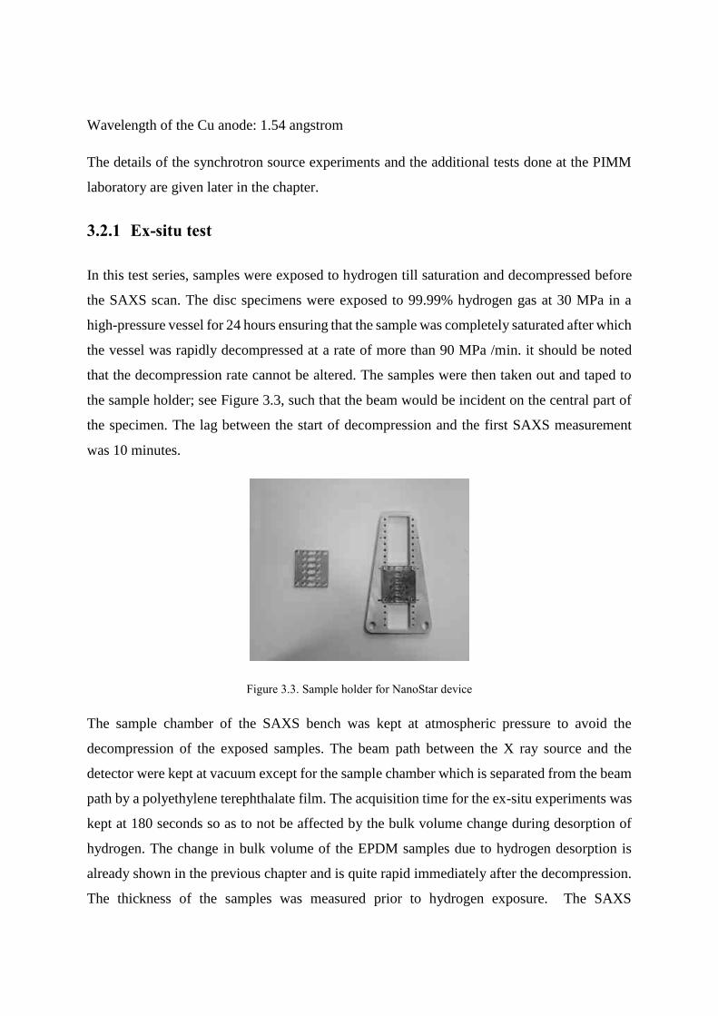
Wavelength of the Cu anode: 1.54 angstrom

The details of the synchrotron source experiments and the additional tests done at the PIMM

laboratory are given later in the chapter.

3.2.1 Ex-situ test

In this test series, samples were exposed to hydrogen till saturation and decompressed before

the SAXS scan. The disc specimens were exposed to 99.99% hydrogen gas at 30 MPa in a

high-pressure vessel for 24 hours ensuring that the sample was completely saturated after which

the vessel was rapidly decompressed at a rate of more than 90 MPa /min. it should be noted

that the decompression rate cannot be altered. The samples were then taken out and taped to

the sample holder; see Figure 3.3, such that the beam would be incident on the central part of

the specimen. The lag between the start of decompression and the first SAXS measurement

was 10 minutes.

Figure 3.3. Sample holder for NanoStar device

The sample chamber of the SAXS bench was kept at atmospheric pressure to avoid the

decompression of the exposed samples. The beam path between the X ray source and the

detector were kept at vacuum except for the sample chamber which is separated from the beam

path by a polyethylene terephthalate film. The acquisition time for the ex-situ experiments was

kept at 180 seconds so as to not be affected by the bulk volume change during desorption of

hydrogen. The change in bulk volume of the EPDM samples due to hydrogen desorption is

already shown in the previous chapter and is quite rapid immediately after the decompression.

The thickness of the samples was measured prior to hydrogen exposure. The SAXS

56 Characterisation of EPDM at sub-micron scale using SAXS

measurements were done after each 10 minute interval to see the evolution of the scattering

spectra after the decompression from saturation in hydrogen at 30 MPa.

3.2.2 In-situ test

For performing the in-situ experiments, a device was built at the Hydrogenius laboratory with

an internal chamber of 5 mm width and a diamond window on each side to allow the

transmission of the X-rays. The chamber was connected to an external hydrogen cylinder

through a thin metal hose equipped with a pressure gauge and valve that could be opened and

closed manually. Keeping the gas safety laws of Japan, the in-situ tests could only be carried

out at less than 1 MPa. The beam path between the X ray source and the detector was kept at

vacuum. The in-situ device itself was kept inside the sample chamber of the SAXS equipment

which was also kept in vacuum to avoid interference due to air. A schematic diagram of the set

up can be seen in Figure 3.4. The acquisition time in this case was 600 seconds as a compromise

between data quality and number of data points that could be attained during and immediately

after decompression. The increase in the acquisition time could reduce the noise in the gas-

saturated samples.

(a)

In-situ chamber

X-ray source

Sample

Hydrogen

Diamond windows Pressure gauge

(b)

Figure 3.4(a). Schematic of the in-situ chamber (b) Schematic of the set-up for in-situ tests

For both in-situ and ex situ experiments, the interest was to get data during saturation and

decompression or immediately after, hence only the central area of the sample was observed to

maximise the data points in time. SAXS acquisition was done for the samples prior to exposure

as well as for the vessel without samples to get the background data for correction later hereby

referred to as the “blank measurement”.

The in-situ tests were also carried at the KYUSHU Synchrotron Light Research Centre at

SAGA beamline for two samples of EPDM 0.1 of 2mm and 4 mm thickness respectively. The

in-situ chamber was connected to a manual valve which was connected to a remote

decompression valve. There was a lag between opening the manual valve and the remote valve

causing some initial drop of pressure (approximately 0.1-0.3MPa) from the saturation pressure

(𝑃𝑠𝑎𝑡) which was less than 1 MPa. The in-situ chamber was mounted between the ionizing

chambers of the SAXS bench, see Figure 3.5.

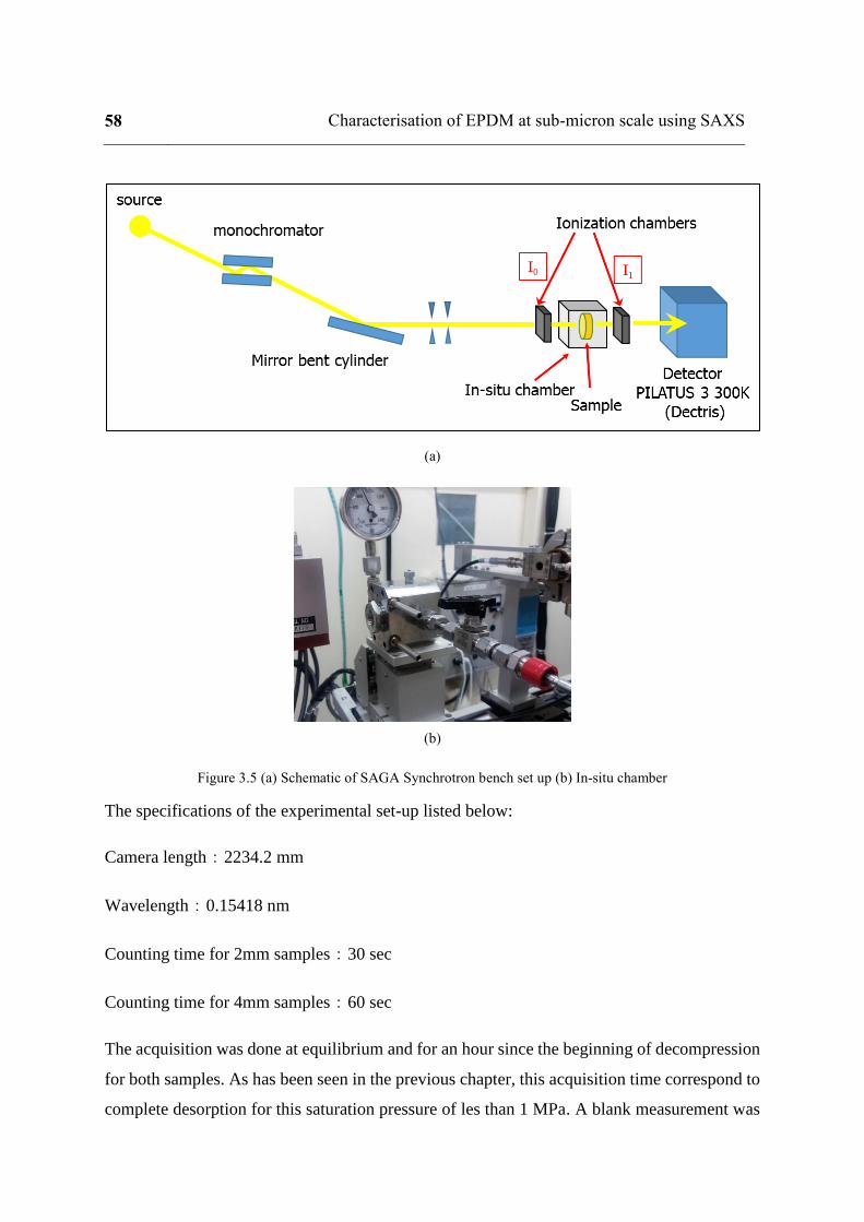
58 Characterisation of EPDM at sub-micron scale using SAXS

(a)

(b)

Figure 3.5 (a) Schematic of SAGA Synchrotron bench set up (b) In-situ chamber

The specifications of the experimental set-up listed below:

Camera length：2234.2 mm

Wavelength：0.15418 nm

Counting time for 2mm samples：30 sec

Counting time for 4mm samples：60 sec

The acquisition was done at equilibrium and for an hour since the beginning of decompression

for both samples. As has been seen in the previous chapter, this acquisition time correspond to

complete desorption for this saturation pressure of les than 1 MPa. A blank measurement was

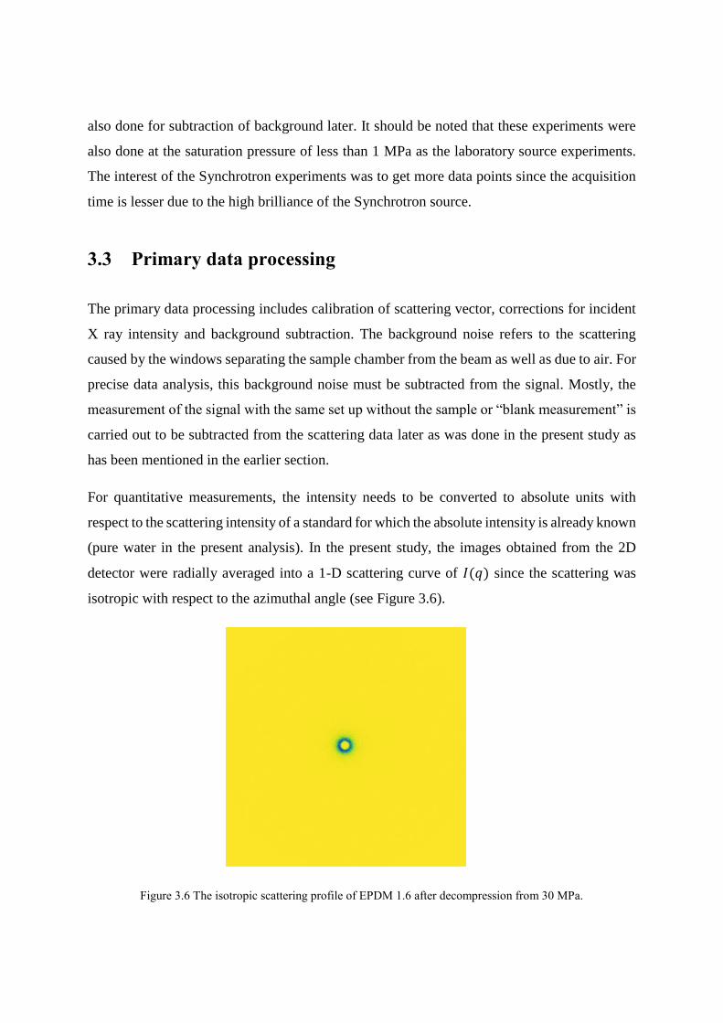
also done for subtraction of background later. It should be noted that these experiments were

also done at the saturation pressure of less than 1 MPa as the laboratory source experiments.

The interest of the Synchrotron experiments was to get more data points since the acquisition

time is lesser due to the high brilliance of the Synchrotron source.

3.3 Primary data processing

The primary data processing includes calibration of scattering vector, corrections for incident

X ray intensity and background subtraction. The background noise refers to the scattering

caused by the windows separating the sample chamber from the beam as well as due to air. For

precise data analysis, this background noise must be subtracted from the signal. Mostly, the

measurement of the signal with the same set up without the sample or “blank measurement” is

carried out to be subtracted from the scattering data later as was done in the present study as

has been mentioned in the earlier section.

For quantitative measurements, the intensity needs to be converted to absolute units with

respect to the scattering intensity of a standard for which the absolute intensity is already known

(pure water in the present analysis). In the present study, the images obtained from the 2D

detector were radially averaged into a 1-D scattering curve of 𝐼(𝑞) since the scattering was

isotropic with respect to the azimuthal angle (see Figure 3.6).

Figure 3.6 The isotropic scattering profile of EPDM 1.6 after decompression from 30 MPa.

60 Characterisation of EPDM at sub-micron scale using SAXS

The observed scattering profiles (𝐼𝑠(𝑞)) by SAXS measurements were corrected for air

scattering, absorption, sample thickness, and incident intensity of X-ray, and then converted to

absolute intensity using the following equation:

Iabs(q) = Is(q) ∙1

I0 ∙ ε ∙ 𝑇tr ⋅ 𝑉ir 𝑒𝑞𝑛 3.1

Where 𝐼𝑠(𝑞) is the raw scattering intensity of sample, 𝐼0 is the incident X-ray beam intensity,

𝜀 is the detector efficiency, 𝑇tr is the transmittance of X-ray through the sample and 𝑉ir is the

irradiated volume. Subsequently background was subtracted for carrying out further data

analysis.

3.4 Scattering due to non-particulate systems

Small angle X-ray scattering can be used to study non-particulate systems like liquids, glasses

and amorphous polymers where the heterogeneities arise from the difference of electron

densities of different phases in case of a multiphase system or from statistical fluctuations in

the single phase system. In general, heterogeneities of any kind in the colloidal range can be

studied using this technique.

3.4.1 Two-Phase and Multiphase systems

A multiphase system consists of two or more phases with different scattering densities

separated by an interface and in which case, the small-angle scattering is caused by the presence

of regions of colloidal size, occupied by different phases.

Ideally in a two-phase or a binary system, represented in Figure 3.7, the two phases have

constant electron densities and the contrast is represented by a mean square fluctuation in

comparison to a particulate disperse system where the contrast is represented by the difference

of mean particle and solvent densities. In addition, the contrast does not depend on the shape

of the heterogeneities but the volume fraction of each phase.

Figure 3.7. Schematic of an ideal binary system

In general, the basic expressions derived for the particle solutions still hold for a non-particulate

binary system but meaning of the structural parameters is less discerning. Hence, for a two-

phase system the generalized correlation function 𝛾0(𝑟), although containing an estimate of the

average dimensions and heterogeneities, has a probabilistic meaning. Simply put, it describes

the averaged surrounding as seen from a single reference point, marking the area with an excess

probability of having the same matter as the said reference point.

Additionally, in contrast to the case of scattering by a homogenous particle, the volume

calculated from the value of the invariant can only be regarded as an approximate estimate of

an average volume of the heterogeneities in non-particulate system. It should also be noted that

since no largest dimension (𝐷𝑚𝑎𝑥), calculated from the distance distribution function, can be

defined in a non-particulate system, the correlation function decreases asymptotically in the

higher q values rather than having a sharp drop to zero as is the case with a particulate system.

The loss of intuitiveness for the calculations is not too major in case of the correlation length

(Ξ), which might be considered a reasonably good measurement of the size of heterogeneities

in the multiphase non particulate system. Interestingly, the concept of shape could be a valuable

distinguishing parameter as in case of lamellar and globular systems and holds well as the

derivation does not take into account the particle system.

It is well known that only the scattering by an ideal two-phase system with constant but

different electron density in each phase separated by a sharp boundary obeys the Porod’s law

according to which the intensity decreases asymptotically in the high q region with a -4 slope:

𝐼(𝑞) ∝ 𝑆𝑞−4.

The formula is valid for a non-particulate system since only the surface structure is of importance

in this context, independent of large scale features. If the intensity is expressed in absolute units

62 Characterisation of EPDM at sub-micron scale using SAXS

and the electronic contrast is known, the formula can be used to calculate the specific surface S

(total surface per unit volume) of the particles via eqn. 3.2.

𝐼(𝑞) = (∆𝜌)2.2𝜋

𝑞4. 𝑆 𝑒𝑞𝑛 3.2

The above mentioned cases have been defined for an ideal binary system which consists of two

phases with constant electron density and separated by a clear interphase. The parameters,

however, deviate from ideality in case of a quasi-binary system with either no clear interface

between phases or fluctuations of electron density within one phase, which makes the quantitative

analysis of a heterogeneous system much more difficult. A suitable approach to evaluate the

diffraction pattern would be to calculate the correlation function and to interpret it with a proper

formalism. It has to be noted that, in this case, the correlation function would be different than of

the particle system due to the lack of a clear boundary. Consequently, the characteristic -4 slope

would not be observed in the high q regions.

The Debye-Bueche function has been used to characterise the inhomogeneity in swollen

polymer gels and more recently in hydrogen exposed NBR. In a similar way, Porod’s law is

important for characterising porous materials. These two methods of analysis pertain to the

results in the current study and are discussed in detail below:

3.4.2 Debye analysis

Geissler et al while investigating PDMS gels using SAXS and SANS spectra showed that the

scattering was dominated by the excess scattering of the frozen in elastic constraints in the

small q regions (Geissler et al. 1997). They showed that a 2 term expression (eqn 3.3) could be

used to describe the gel structure in the larger q range explored, where the first term is

mathematically of lorentzian form (eqn 3.4), and the second is a squared lorentzian term (eqn

3.5). Shibayama et al used a similar scattering function for inhomogeneous swollen gels to

analyse the SANS results for a series of cross-linked isoprene rubber having various network

chain densities (Shibayama 1998).

𝐼(𝑞) = 𝐼𝑠𝑜𝑙𝑛(𝑞) + 𝐼𝑒𝑥(𝑞) + 𝐼𝑖𝑛𝑐 𝑒𝑞𝑛 3.3

𝐼soln(𝑞) =𝐼soln(0)

(1 + 𝑞2𝜉2)

𝑒𝑞𝑛 3.4

𝐼ex(𝑞) =𝐼ex(0)

(1 + 𝑞2𝛯2)

2 𝑒𝑞𝑛 3.5

Where 𝐼𝑠𝑜𝑙𝑛 is the scattered intensity from the corresponding polymer solution corresponding

to the scattering at high q regions and the density correlation 𝜉 corresponds to the mesh size of

the network. However, the squared-Lorentz function, called the Debye-Bueche function, was

considered to be most suitable to represent the excess scattering term, 𝐼𝑒𝑥(𝑞) since this Debye-

Bueche term has been often used to represent the structural inhomogeneity in polymer gels and

describes the static fluctuations governed by the frozen-in elastic constraints, which act

between topologically connected cross-links. The same analysis can be extended to the present

study to characterize the polymer structure saturated in hydrogen by analyzing the scattering

in the low q region.

Figure 3.8 representation of the polymer matrix highlighting the local heterogeneity as represented by

correlation length 𝛯 (Ikeda et al. 2009)

In the present case, the Debye Bueche term corresponding to the scattering due to static

inhomogeneity in gels has been used to characterize the inhomogeneity in the rubber matrix

treated as an inhomogeneous non particulate system, see Figure 3.8. This function has

previously been used by Ohyama et al for characterization of inhomogeneity in NBR after

hydrogen exposure. This has already been mentioned in the bibliography chapter of this thesis.

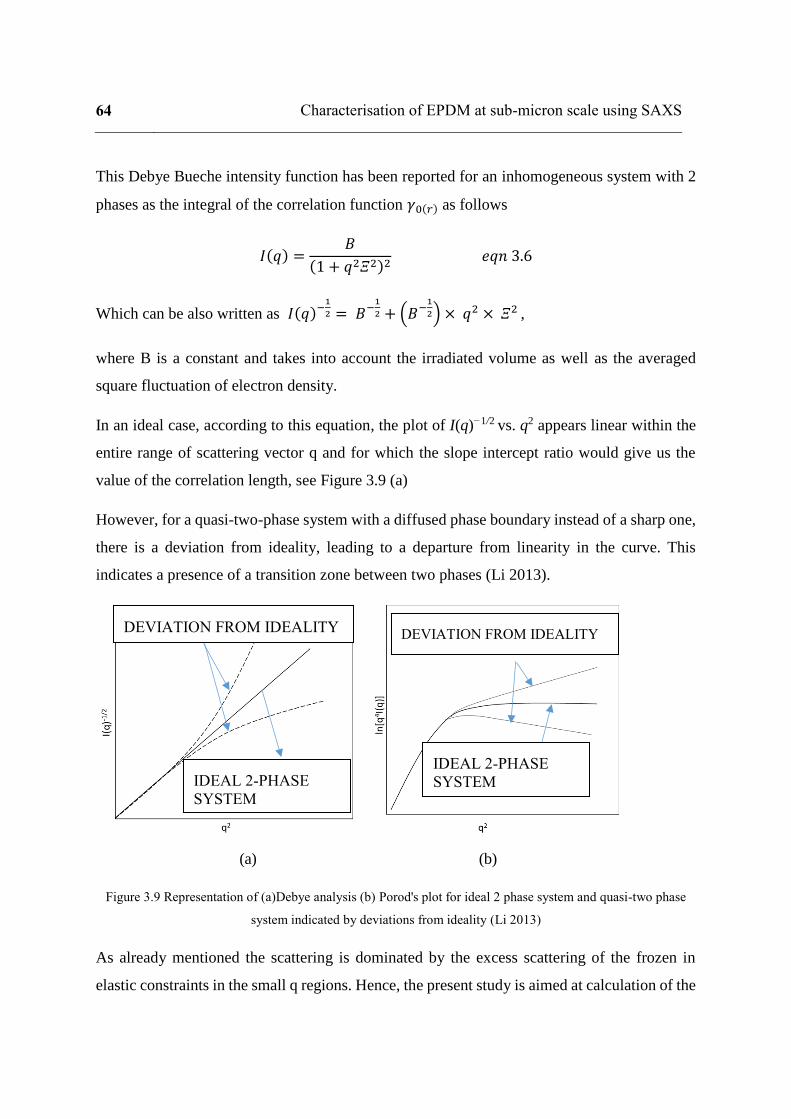
64 Characterisation of EPDM at sub-micron scale using SAXS

This Debye Bueche intensity function has been reported for an inhomogeneous system with 2

phases as the integral of the correlation function 𝛾0(𝑟) as follows

𝐼(𝑞) =𝐵

(1 + 𝑞2𝛯2)2 𝑒𝑞𝑛 3.6

Which can be also written as 𝐼(𝑞)−1

2 = 𝐵−1

2 + (𝐵−1

2) × 𝑞2 × 𝛯2 ,

where B is a constant and takes into account the irradiated volume as well as the averaged

square fluctuation of electron density.

In an ideal case, according to this equation, the plot of I(q)−1/2 vs. q2 appears linear within the

entire range of scattering vector q and for which the slope intercept ratio would give us the

value of the correlation length, see Figure 3.9 (a)

However, for a quasi-two-phase system with a diffused phase boundary instead of a sharp one,

there is a deviation from ideality, leading to a departure from linearity in the curve. This

indicates a presence of a transition zone between two phases (Li 2013).

(a) (b)

Figure 3.9 Representation of (a)Debye analysis (b) Porod's plot for ideal 2 phase system and quasi-two phase

system indicated by deviations from ideality (Li 2013)

As already mentioned the scattering is dominated by the excess scattering of the frozen in

elastic constraints in the small q regions. Hence, the present study is aimed at calculation of the

IDEAL 2-PHASE

SYSTEM

DEVIATION FROM IDEALITY

IDEAL 2-PHASE

SYSTEM

DEVIATION FROM IDEALITY

correlation length in lower values of q; the above equation is held valid and the fitting of the

curve in only the linear part of the curve is carried out.

3.4.3 Porod analysis

Theoretically, for an ideal two-phase system, the Porod’s plot or the plot of ln[𝑞4. 𝐼(𝑞)] vs 𝑞2

shows a plateau as shown in Figure 3.9(b). It has already been cleared that although this law

holds for the non-particulate system, a well-defined interface should be present to separate the

individual phases. However, for a quasi-two phase system without a sharply defined boundary

separating the two phases, the curve deviates from ideality similar to the Debye analysis. As

such specific volume cannot be quantified for such a system. However, the analysis is carried

out to ascertain the presence of a clear interface in the present study to understand whether the

phase separation is well defined in the rubber matrix and how it is affected by the exposure to

hydrogen. More precisely, Porod’s plot would indicate if cavitation occurs after decompression

from gas exposure at very low pressure.

3.5 X-Ray scattering for samples before exposure and at

equilibrium

Figure 3.10 (a) and (b) show the absolute scattering intensities 𝐼 (𝑞) for EPDM 0.1 and 0.5

respectively in unexposed state as well as at equilibrium (𝑃𝑠𝑎𝑡 < 1 MPa). In both cases, the

upturn can be clearly seen in the low q regions (q < 0.2) which indicates the existence of

inhomogeneity in the matrix structure. In polymer gels, this upturn is an indicator of existence

of localized clusters in solution (Suzuki et al. 2010). This cluster-like structure has also been

observed for such systems as graft copolymers and polyelectrolyte solution (Hourdet et al.

1998; Borsali, Nguyen, and Pecora 1998). As for the polyisoprene/toluene system, Geissler et

al. and Horkay et al. observed a similar upturn and clarified that this upturn originates from the

dense cluster of undissolved amorphous polymers (Horkay et al. 2000; Geissler et al. 1997).

In the similar vein, the small upturn in the low q regions seen in the graphs can be interpreted

as characteristic of network inhomogeneity in the form of dense clusters of rubber molecules

interspersed in the area of lower density. The spectra of the rubber-hydrogen system at 𝑃𝑠𝑎𝑡

66 Characterisation of EPDM at sub-micron scale using SAXS

show very little change in comparison with the unexposed one and this can be seen in the curves

for both EDPM 0.1 and EPDM 0.5.

(a)

(b)

Figure 3.10. Scattering curves for the samples at unexposed state and at equilibrium for (a) EPDM 0.1 and (b)

EPDM 0.5

1.0E-03

1.0E-02

1.0E-01

1.0E+00

1.0E-01 1.0E+00

Iab

s (1

/cm

)

q (1/nm)

unexposed Psat

1.0E-03

1.0E-02

1.0E-01

1.0E+00

1.0E-01 1.0E+00

Iab

s (1

/cm

)

q(1/nm)

unexp Psat

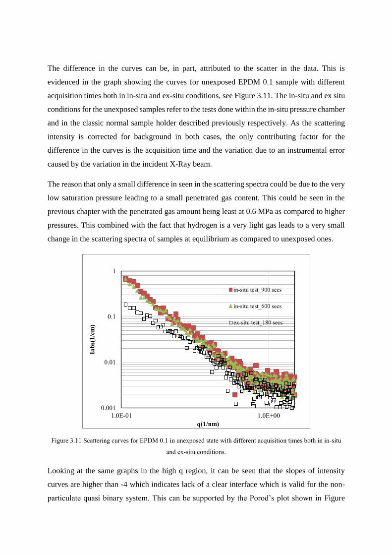
The difference in the curves can be, in part, attributed to the scatter in the data. This is

evidenced in the graph showing the curves for unexposed EPDM 0.1 sample with different

acquisition times both in in-situ and ex-situ conditions, see Figure 3.11. The in-situ and ex situ

conditions for the unexposed samples refer to the tests done within the in-situ pressure chamber

and in the classic normal sample holder described previously respectively. As the scattering

intensity is corrected for background in both cases, the only contributing factor for the

difference in the curves is the acquisition time and the variation due to an instrumental error

caused by the variation in the incident X-Ray beam.

The reason that only a small difference in seen in the scattering spectra could be due to the very

low saturation pressure leading to a small penetrated gas content. This could be seen in the

previous chapter with the penetrated gas amount being least at 0.6 MPa as compared to higher

pressures. This combined with the fact that hydrogen is a very light gas leads to a very small

change in the scattering spectra of samples at equilibrium as compared to unexposed ones.

Figure 3.11 Scattering curves for EPDM 0.1 in unexposed state with different acquisition times both in in-situ

and ex-situ conditions.

Looking at the same graphs in the high q region, it can be seen that the slopes of intensity

curves are higher than -4 which indicates lack of a clear interface which is valid for the non-

particulate quasi binary system. This can be supported by the Porod’s plot shown in Figure

0.001

0.01

0.1

1

1.0E-01 1.0E+00

Iab

s(1

/cm

)

q(1/nm)

in-situ test_900 secs

in-situ test_600 secs

ex-situ test_180 secs

68 Characterisation of EPDM at sub-micron scale using SAXS

3.12 which clearly indicates the lack of a plateau in the high q region for both EPDM 0.1 and

0.5. The lack of a clear interface is indicative of lack of cavitation which is consistent with

literature as already discussed in earlier chapters; no cavities are seen during the compression

phase. Clearly, since the Porod’s law does not apply in the present case, the size of the

heterogeneities is not calculable for virgin samples or samples at equilibrium.

(a)

(b)

Figure 3.12 Porod's plot for (a) EPDM 0.1 and (b) EPDM 0.5 at at unexposed state and at equilibrium.

-12

-10

-8

-6

-4

-2

0

0.01 0.51 1.01 1.51 2.01 2.51 3.01 3.51 4.01

ln[I

(q).

q^4

]

q^2

unexposed

Psat

-12

-10

-8

-6

-4

-2

0

0.01 0.51 1.01 1.51 2.01 2.51 3.01 3.51 4.01

ln[I

(q).

q^4

]

q^2

unexp

Psat

3.5.1 Effect of cross-link density on scattering intensity

It can be seen in Figure 3.13 that the spectra of EPDM 0.1 and 0.5 in the unexposed state are

almost superimposing on each other. These spectra were taken for samples inside the pressure

chamber with acquisition time of 600 seconds. Similar result is seen in the spectra for

unexposed samples taken without the pressure chamber as seen in Figure 3.14

Figure 3.13 shows the absolute scattering intensities 𝐼 (𝑞) for EPDM 0.1 to 0.5 in unexposed

state. The graph shows the same trend as could be observed for the samples in the in-situ

experiment: upturn in the low q regions (q < 0.2) indicating the existence of inhomogeneity in

the matrix structure. Furthermore, it is evident that an increase in the DCP ratio from 0.1 to 0.5

does not affect the scattering intensity values to a discernable degree.

Suzuki et al (2010) in her study on natural rubber noted that the difference in the 𝐼(𝑞) at the

very beginning was decreasing with increasing DCP content from 0 to 2 phr and noted that the

contribution from the DCP to the scattering was negligible and the change could be due to the

consequence of peroxide linking. In any case, the DCP ratio change from EPDM 0.1 to EPDM

0.5 is very small in comparison to Suzuki et al’s study and therefore, difference in the spectra

shown above results is not significant enough. This can be verified for EPDM samples of higher

cross-link densities in future experiments.

Figure 3.13 Absolute scattering intensities 𝐼 (𝑞) for EPDM 0.1 to 0.5 in unexposed state.

0.001

0.01

0.1

1

1.00E-01 1.00E+00

Iab

s (1

/cm

)

q (1/nm)

EPDM 0.5

EPDM 0.1

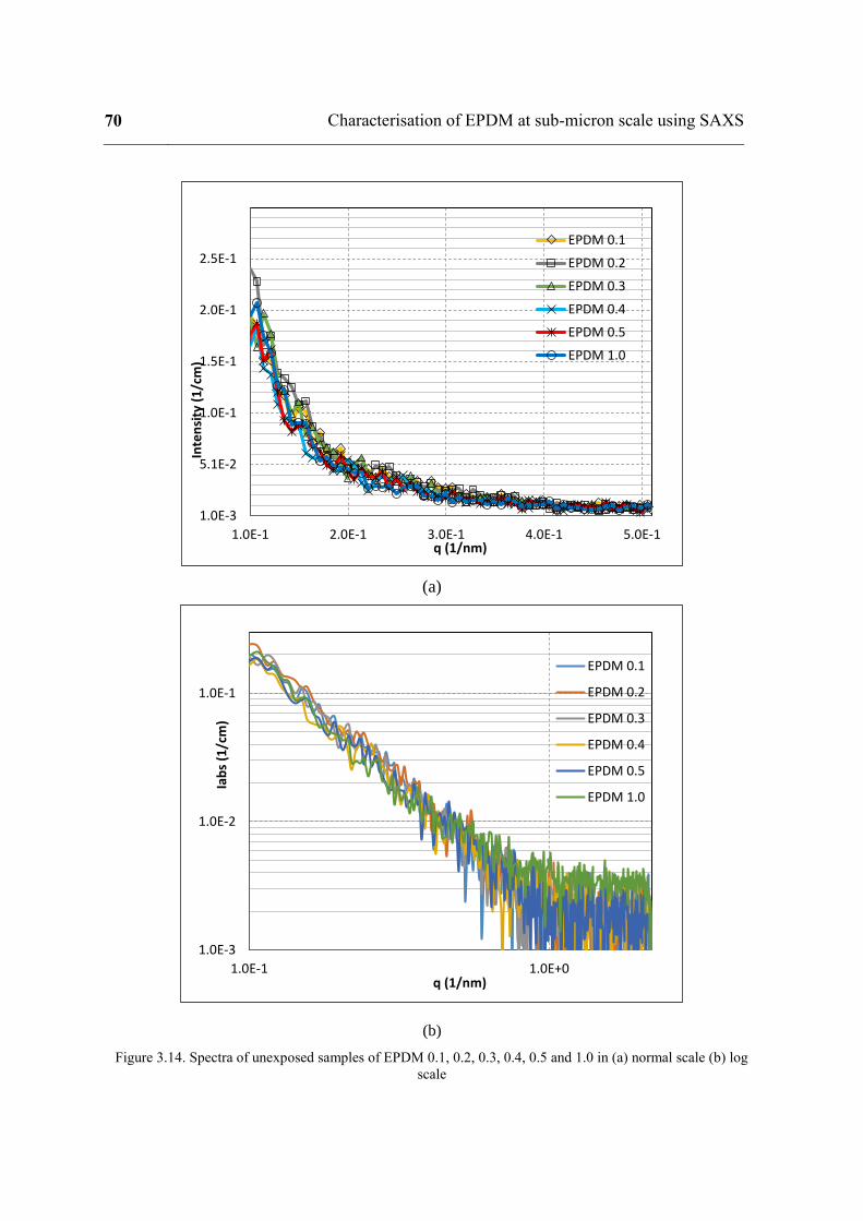
70 Characterisation of EPDM at sub-micron scale using SAXS

(a)

(b)

Figure 3.14. Spectra of unexposed samples of EPDM 0.1, 0.2, 0.3, 0.4, 0.5 and 1.0 in (a) normal scale (b) log

scale

1.0E-3

5.1E-2

1.0E-1

1.5E-1

2.0E-1

2.5E-1

1.0E-1 2.0E-1 3.0E-1 4.0E-1 5.0E-1

Inte

nsi

ty (

1/c

m)

q (1/nm)

EPDM 0.1

EPDM 0.2

EPDM 0.3

EPDM 0.4

EPDM 0.5

EPDM 1.0

1.0E-3

1.0E-2

1.0E-1

1.0E-1 1.0E+0

Iab

s (1

/cm

)

q (1/nm)

EPDM 0.1

EPDM 0.2

EPDM 0.3

EPDM 0.4

EPDM 0.5

EPDM 1.0

3.6 Scattering intensities for exposed samples

(a)

(b)

Figure 3.15. Spectra of (a) EPDM 0.1 and (b) EPDM 0.5 showing absolute intensity vs scattering vector q. I_10,

I_20, I_30 refer to intensities at 10, 20 and 30 min after the start of decompression

Figures 3.15 show the scattering curves for EPDM 0.1 and EPDM 0.5 samples for the in-situ

test. As can be seen form the curves, any qualitative assessment is not possible as the curves

1.0E-03

1.0E-02

1.0E-01

1.0E+00

1.0E-01 1.0E+00

I (1

/cm

)

q (1/nm)

unexposed

Psat

I_10mins

I_20mins

I_30mins

1.0E-03

1.0E-02

1.0E-01

1.0E+00

1.0E-01 1.0E+00

inte

nsi

ty (

1/c

m)

q(1/nm)

unexp

Psat

I_10mins

I_20mins

I_30mins

72 Characterisation of EPDM at sub-micron scale using SAXS

show very little change from unexposed to decompressed stages. This was the observed earlier

for unexposed and saturated samples for in-situ tests.

(a)

(b)

Figure 3.16 Porod's plot for (a) EPDM 0.1 and (b) EPDM 0.5 at 10, 20 and 30 minutes after the beginning of

decompression.

Again, it is clear that the Porod’s law is not followed by the current rubber gas system even

during decompression, this can be evidenced from Figure 3.16 which clearly shows lack of a

plateau in the higher q region. Therefore, the quantification of any possible change in the

inhomogeneity of the rubber matrix is done by Debye analysis in order to calculate the

-12

-10

-8

-6

-4

-2

0

0.01 0.51 1.01 1.51 2.01 2.51 3.01 3.51 4.01

ln[I

(q).

q^4

]

q^2

I_10mins

I_20mins

I_30mins

-12

-10

-8

-6

-4

-2

0

0.01 0.51 1.01 1.51 2.01 2.51 3.01 3.51 4.01

ln[I

(q).

q^4

]

q^2

I_10mins

I_20mins

I_30mins

correlation length at unexposed state as well as after exposure to hydrogen for both EPDM 0.1

and 0.5 by fitting the linear part of the curve of 𝐼(𝑞)−1

2 vs 𝑞2; see Figure 3.17.

Figure3.17. The Debye analysis for EPDM 0.1. The dotted line is the linear least squares fitting of the linear part

of the graph for the unexposed spectra. A similar fit was done for the rest of the curves.

It can be seen that after the initial linear part, the curve deviates from ideality of a binary two-

phase system, as explained earlier. However since, the interest was to calculate the correlation

length in the low q regions, it could be done by fitting the linear part of the curve with a

straight line using classic least squares method and calculating the value of by dividing the

slope and the intercept as has already been explained in the earlier section. The results of the

calculation are given in the Table 3.1.

Ξ (nm) UNEXPOSED AT Psat I_10 I_20 I_30

EPDM 0.5 4.5 3.9 4.2 4.1 4.1

EPDM 0.1 4.2 3.9 4.1 3.9 3.98

Table 3.1. Correlation length for unexposed as well as exposed samples. Psat, I_10, I_20, I_30 refer to the

values for samples at equilibrium and after 10, 20 and 30 min after decompression

-5

5

15

25

35

45

55

0.01 0.21 0.41 0.61 0.81 1.01 1.21 1.41 1.61 1.81

I(q

)-1/2

q2

unexposed

unexposed

at Psat

decomp1

decomp2

decomp3

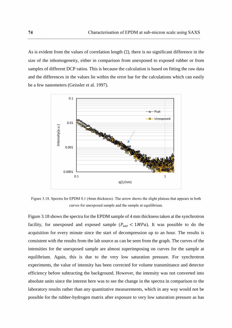
74 Characterisation of EPDM at sub-micron scale using SAXS

As is evident from the values of correlation length (Ξ), there is no significant difference in the

size of the inhomogeneity, either in comparison from unexposed to exposed rubber or from

samples of different DCP ratios. This is because the calculation is based on fitting the raw data

and the differences in the values lie within the error bar for the calculations which can easily

be a few nanometers (Geissler et al. 1997).

Figure 3.18. Spectra for EPDM 0.1 (4mm thickness). The arrow shows the slight plateau that appears in both

curves for unexposed sample and the sample at equilibrium.

Figure 3.18 shows the spectra for the EPDM sample of 4 mm thickness taken at the synchrotron

facility, for unexposed and exposed sample (𝑃𝑠𝑎𝑡 < 1𝑀𝑃𝑎). It was possible to do the

acquisition for every minute since the start of decompression up to an hour. The results is

consistent with the results from the lab source as can be seen from the graph. The curves of the

intensities for the unexposed sample are almost superimposing on curves for the sample at

equilibrium. Again, this is due to the very low saturation pressure. For synchrotron

experiments, the value of intensity has been corrected for volume transmittance and detector

efficiency before subtracting the background. However, the intensity was not converted into

absolute units since the interest here was to see the change in the spectra in comparison to the

laboratory results rather than any quantitative measurements, which in any way would not be

possible for the rubber-hydrogen matrix after exposure to very low saturation pressure as has

0.0001

0.001

0.01

0.1

0.1 1

Inte

nsi

ty(a

.u.)

q(1/nm)

Psat

Unexposed

been seen in the earlier results. However, the data is much less noisy in comparison to the lab

source data.

An interesting observation in the curve is an appearance of a plateau as shown by the arrow.

Since the graphs had a lot of scatter, and this phenomenon was not seen in any of the earlier

curves, additional tests were done with a smaller beam size to explore a larger q range with less

noisy data. These results are discussed in the section below and include scattering curves for

unexposed and exposed samples after decompression (ex-situ). This could help to evaluate the

possible permanent change in the rubber matrix due to high pressure hydrogen exposure after

the expulsion of hydrogen.

3.6.1 Scattering for longer q-range

These tests were carried out by S. Tencé-Girault at laboratory PIMM, Arts et Métiers

ParisTech.

Figure 3.19. Sample holder with the rectangular samples such that two areas of the samples could

be irradiated

Samples of 5×10 ×2mm were cut from the same 2 mm sheets as used for previous tests. The

samples were exposed to Hydrogen in HYCOMAT facility in a chamber for 24 hours after

which it was decompressed at 30 MPa per minute. The samples were then sent to the PIMM

laboratory where they were mounted on the sample holder as seen in Figure 3.19 and SAXS

76 Characterisation of EPDM at sub-micron scale using SAXS

experiments were carried out on them. The time of hydrogen exposure and the time of SAXS

experiment was set apart by a week to ensure the complete desorption of hydrogen from the

sample. For investigation of the broader q range the minimum wave vector was taken to be at

q = 0.005 Å-1 or 0.05 nm-1. In addition to samples of DCP ratio 0.1, 0.5, 1.0 samples of DCP

ratio 1.6 were also investigated.

Two areas of each sample were observed, with the following experimental conditions:

- The beam size is 200 µm

- Copper wavelength 1.54189 Å

- Counting time 600 seconds

Samples studied:

- EP 0.1 unexposed and EP 0.1 expo H

- EP 0.5 unexposed and EP 0.5 expo H

- EP 1.0 unexposed and EP 1.0 expo H

- EP 1.6 unexposed and EP 1.6 expo H

The spectra of the unexposed samples are reported in Figure 3.20. Regardless of the sample,

the two zones analyzed were identical, hence only one curve is shown in the graphs.

A small plateau can be seen in the graphs which becomes more prominent in the Lorentz

corrected intensity plot of 𝑞2𝑥𝐼 (𝑞) vs 𝑞 as shown in Figure 3.21. The change of scale from nm

to Å should be noted along the x-axis. The position of these maxima, which defines a

characteristic dimension over which the scattering occurs, is shown in Figure 3.21.

Figure 3.20. Spectra for unexposed samples done at PIMM. A small plateau cam be observed at approximately

between 0.2 to 0.3 nm

Figure 3.21 Lorentz corrected plot for unexposed samples done at PIMM

Although this maxima is not seen in the previous lab source results, it could be due to the

limited q-range explored as well as the large noise in the data. Although the polymers lack long

range order, the appearance of this maxima suggests a somewhat ordered distribution of the

high density and low density phases of the rubber matrix which is not directly proportional to

the cross-link density as is seen from the Table 3.2.

0.001

0.01

0.1

1

10

0.045 0.45

I(a.

u.)

q(1/nm)

EP 0.1 unexp

EP 0.5 unexpo

EP 1.0 unexp

EP 1.6 unexp

0

0.00002

0.00004

0.00006

0.00008

0.0001

0 0.01 0.02 0.03 0.04 0.05 0.06 0.07 0.08 0.09 0.1 0.11 0.12 0.13 0.14 0.15

I(q

) *

q2

q(1/Å)

EP 0.1 unexp

EP 0.5 unexpo

EP 1.0 unexp

EP 1.6 unexp

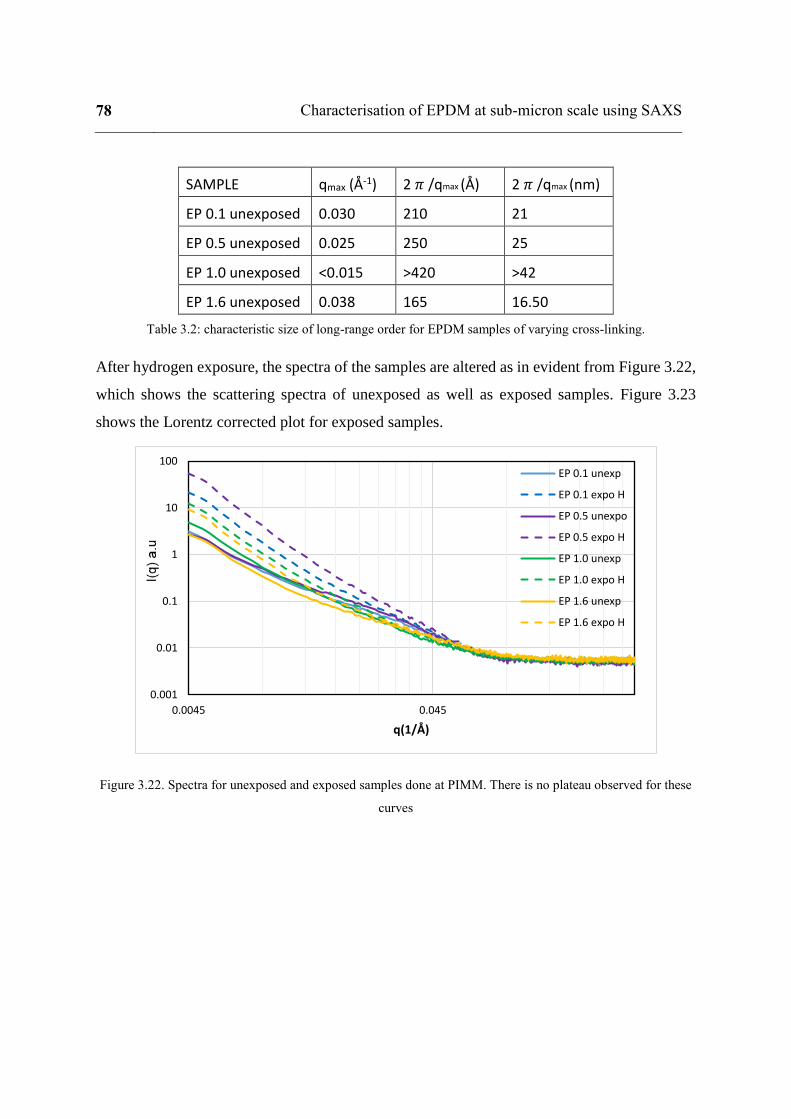
78 Characterisation of EPDM at sub-micron scale using SAXS

SAMPLE qmax (Å-1) 2 𝜋 /qmax (Å) 2 𝜋 /qmax (nm)

EP 0.1 unexposed 0.030 210 21

EP 0.5 unexposed 0.025 250 25

EP 1.0 unexposed <0.015 >420 >42

EP 1.6 unexposed 0.038 165 16.50

Table 3.2: characteristic size of long-range order for EPDM samples of varying cross-linking.

After hydrogen exposure, the spectra of the samples are altered as in evident from Figure 3.22,

which shows the scattering spectra of unexposed as well as exposed samples. Figure 3.23

shows the Lorentz corrected plot for exposed samples.

Figure 3.22. Spectra for unexposed and exposed samples done at PIMM. There is no plateau observed for these

curves

0.001

0.01

0.1

1

10

100

0.0045 0.045

q(1/Å)

EP 0.1 unexp

EP 0.1 expo H

EP 0.5 unexpo

EP 0.5 expo H

EP 1.0 unexp

EP 1.0 expo H

EP 1.6 unexp

EP 1.6 expo H

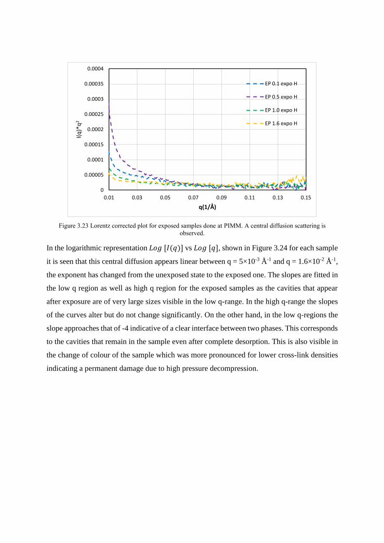
Figure 3.23 Lorentz corrected plot for exposed samples done at PIMM. A central diffusion scattering is

observed.

In the logarithmic representation 𝐿𝑜𝑔 [𝐼(𝑞)] vs 𝐿𝑜𝑔 [𝑞], shown in Figure 3.24 for each sample

it is seen that this central diffusion appears linear between q = 5×10-3 Å-1 and q = 1.6×10-2 Å-1,

the exponent has changed from the unexposed state to the exposed one. The slopes are fitted in

the low q region as well as high q region for the exposed samples as the cavities that appear

after exposure are of very large sizes visible in the low q-range. In the high q-range the slopes

of the curves alter but do not change significantly. On the other hand, in the low q-regions the

slope approaches that of -4 indicative of a clear interface between two phases. This corresponds

to the cavities that remain in the sample even after complete desorption. This is also visible in

the change of colour of the sample which was more pronounced for lower cross-link densities

indicating a permanent damage due to high pressure decompression.

0

0.00005

0.0001

0.00015

0.0002

0.00025

0.0003

0.00035

0.0004

0.01 0.03 0.05 0.07 0.09 0.11 0.13 0.15

I(q

)*q

2

q(1/Å)

EP 0.1 expo H

EP 0.5 expo H

EP 1.0 expo H

EP 1.6 expo H

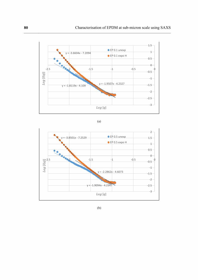
80 Characterisation of EPDM at sub-micron scale using SAXS

(a)

(b)

y = -1.8119x - 4.109

y = -3.6604x - 7.2094

y = -1.9507x - 4.2327

-3

-2.5

-2

-1.5

-1

-0.5

0

0.5

1

1.5

-2.5 -2 -1.5 -1 -0.5 0

𝐿𝑜𝑔

[𝐼(𝑞

)]

𝐿𝑜𝑔 [𝑞]

EP 0.1 unexp

EP 0.1 expo H

y = -1.9094x - 4.2347

y = -3.8501x - 7.2529

y = -2.2862x - 4.6073

-3

-2.5

-2

-1.5

-1

-0.5

0

0.5

1

1.5

2

-2.5 -2 -1.5 -1 -0.5 0

𝐿𝑜𝑔

[𝐼(𝑞

)]

𝐿𝑜𝑔 [𝑞]

EP 0.5 unexp

EP 0.5 expo H

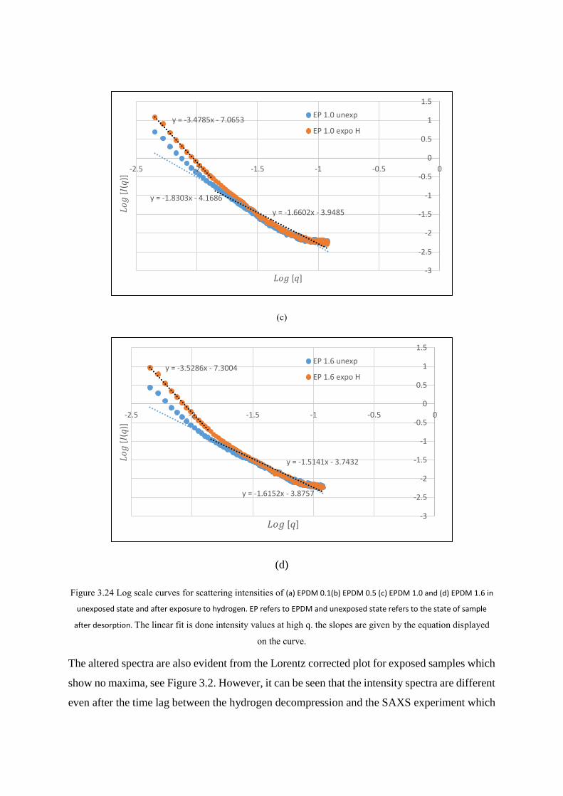
(c)

(d)

Figure 3.24 Log scale curves for scattering intensities of (a) EPDM 0.1(b) EPDM 0.5 (c) EPDM 1.0 and (d) EPDM 1.6 in

unexposed state and after exposure to hydrogen. EP refers to EPDM and unexposed state refers to the state of sample

after desorption. The linear fit is done intensity values at high q. the slopes are given by the equation displayed

on the curve.

The altered spectra are also evident from the Lorentz corrected plot for exposed samples which

show no maxima, see Figure 3.2. However, it can be seen that the intensity spectra are different

even after the time lag between the hydrogen decompression and the SAXS experiment which

y = -1.8303x - 4.1686

y = -3.4785x - 7.0653

y = -1.6602x - 3.9485

-3

-2.5

-2

-1.5

-1

-0.5

0

0.5

1

1.5

-2.5 -2 -1.5 -1 -0.5 0

𝐿𝑜𝑔

[𝐼(𝑞

)]

𝐿𝑜𝑔 [𝑞]

EP 1.0 unexp

EP 1.0 expo H

y = -1.6152x - 3.8757

y = -3.5286x - 7.3004

y = -1.5141x - 3.7432

-3

-2.5

-2

-1.5

-1

-0.5

0

0.5

1

1.5

-2.5 -2 -1.5 -1 -0.5 0

𝐿𝑜𝑔

[𝐼(𝑞

)]

𝐿𝑜𝑔 [𝑞]

EP 1.6 unexp

EP 1.6 expo H

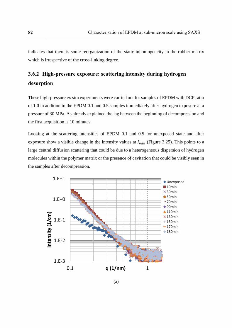
82 Characterisation of EPDM at sub-micron scale using SAXS

indicates that there is some reorganization of the static inhomogeneity in the rubber matrix

which is irrespective of the cross-linking degree.

3.6.2 High-pressure exposure: scattering intensity during hydrogen

desorption

These high-pressure ex situ experiments were carried out for samples of EPDM with DCP ratio

of 1.0 in addition to the EPDM 0.1 and 0.5 samples immediately after hydrogen exposure at a

pressure of 30 MPa. As already explained the lag between the beginning of decompression and

the first acquisition is 10 minutes.

Looking at the scattering intensities of EPDM 0.1 and 0.5 for unexposed state and after

exposure show a visible change in the intensity values at 𝐼𝑚𝑖𝑛 (Figure 3.25). This points to a

large central diffusion scattering that could be due to a heterogeneous dispersion of hydrogen

molecules within the polymer matrix or the presence of cavitation that could be visibly seen in

the samples after decompression.

(a)

1.E-3

1.E-2

1.E-1

1.E+0

1.E+1

0.1 1

Inte

nsi

ty (

1/c

m)

q (1/nm)

Unexposed

10min

30min

50min

70min

90min

110min

130min

150min

170min

180min

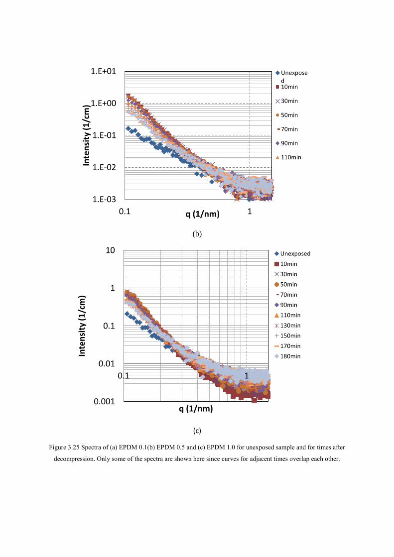
(b)

(c)

Figure 3.25 Spectra of (a) EPDM 0.1(b) EPDM 0.5 and (c) EPDM 1.0 for unexposed sample and for times after

decompression. Only some of the spectra are shown here since curves for adjacent times overlap each other.

1.E-03

1.E-02

1.E-01

1.E+00

1.E+01

0.1 1

Inte

nsi

ty (

1/c

m)

q (1/nm)

Unexposed10min

30min

50min

70min

90min

110min

0.001

0.01

0.1

1

10

0.1 1

Inte

nsi

ty (

1/c

m)

q (1/nm)

Unexposed

10min

30min

50min

70min

90min

110min

130min

150min

170min

180min

84 Characterisation of EPDM at sub-micron scale using SAXS

It can also be seen that the value of intensity increases after hydrogen exposure; see Figure

3.25, which indicates an increase in contrast. Again, this could be attributed to the increased

contrast between the voids and matrix, which is further supported by the increase in the slope

of the intensity at low q regions. The characteristic slope of q-4 is seen for EPDM 0.1 but does

not appear for samples other cross-link densities even after cavitation. The slope approaches

that of -4 in case of EPDM 0.5. Moreover, the characteristic slope is observed for the curves

immediately after decompression and decreases as desorption continues. The lack of the -4

slope for other samples could be due to the very close packing of the cavities along with the

diffusion on hydrogen in the rubber matrix, which makes it difficult to identify a clear interface.

Another contributing factor is the transient state of the voids which are evolving during the 180

seconds of acquisition time that could lead to a difficulty in detecting a sharp interface.

Moreover, the slope of the curves decreases in the subsequent data points which is consistent

with the deflation of cavities as desorption occurs, thereby decreasing the possibility of

observing an interface of the cavities in the rubber matrix. As such, the intensity values can

only be interpreted to signify either an increase the number of scattering objects or an increase

in the size of existing scattering objects.

As we can see, the curve at 180 minutes approaches the curve for the unexposed sample but

does not overlap on it. It can be concluded that the gas-matrix tends to come back to the state

of the unexposed rubber matrix but does not completely attain it. This is consistent with the

results discussed earlier for the samples tested after complete desorption of hydrogen.

To quantify the change in inhomogeneity, the Debye analysis was done in similar way to in-

situ experiments to calculate the correlation length. The change in correlation length with time

after decompression can be seen in Figure 3.26. The first plotted point in red at the axis

corresponds to the value of correlation length for the virgin material. It can be seen that after

decompression the value of correlation length increases since the heterogeneity is now a

function of cavities as well as the static fluctuations of the rubber matrix. Thereafter, the graph

shows a decreasing trend which could be correlated with the global desorption leading to a

gradual deflation of the cavities. However, the value does not reach the value of the unexposed

rubber matrix.

Figure 3.26 Temporal evolution of correlation length of EPDM 0.1, 0.5 and 1.0. The trend line is plotted for

each sample.

3.7 Conclusions

The main aim of this experimental campaign was to characterise EPDM at various stages of

gas exposure to understand if the microstructural heterogeneity of rubber induces cavitation

and if crosslink density could be used as an indicator of this heterogeneity. The in-situ tests

conducted on EPDM 0.1 and 0.5 do not show any change in the correlation length, which would

indicate a change in the size of heterogeneities in the rubber matrix due to the hydrogen

exposure. This is however due to the low saturation pressure and is supported by the results

from the ex situ experiments which clearly show an increase in the correlation length after

decompression from high-pressure exposure. However, the results from the synchrotron source

experiments showed a slight and diffused plateau that could be a possible indicator of a

correlated structure. To clarify this, additional scattering experiments were carried out

exploring a longer q-range which could enable the acquisition at a lower value of q that is

0.05nm-1. This plateau was observed again in case of unexposed samples which became clearer

in the Lorentz corrected plots. However, the position of these maxima were not directly

correlated with the cross-link density of the samples. After exposure, no maxima were detected

in the curves. This was as a result of large central scattering that was superimposed on the

initial spectra due to scattering by the cavities that appeared in the sample after decompression

0

10

20

30

40

50

60

70

80

90

100

110

120

130

140

150

0 10 20 30 40 50 60 70 80 90 100 110 120 130 140 150 160 170 180 190

Ξ (Å

)

time after decompression (mins)

EPDM 0.5

EPDM 0.1

EPDM 1.0

Linear (EPDM 0.5)

Linear (EPDM 0.1)

Linear (EPDM 1.0)

Unexposed samples

86 Characterisation of EPDM at sub-micron scale using SAXS

from high pressure. It is important to note that these experiments were carried out after the

complete desorption of hydrogen form the sample. Results from the scattering experiments

done immediately after decompression during the desorption of hydrogen indicate that the

spectra of the exposed samples taken immediately after decompression show a marked

difference from the spectra of the unexposed sample and these spectra tend to approach those

of the unexposed samples as the desorption progresses. However, the spectra of the exposed

samples do not superimpose those of the unexposed samples even after complete desorption of

the gas, indicating a permanent structural change in the rubber matrix after single hydrogen

exposure. As a general conclusion, it can be underlined that the hydrogen exposure leads to

microstructural change in the rubber matrix which is retained even when the gas is fully

desorbed. It was also seen that the heterogeneity of the rubber matrix at the sub-micron scale

is not directly correlated with the cross-link density. Additionally, the low pressure experiments

are not enough to calibrate the degree of heterogeneity in rubber matrix; the in-situ experiments

carried out in the present study showed that no change in the correlation length, corresponding

to the matrix heterogeneity, was observed after hydrogen exposure.

A better characterisation of these samples could be possible with high pressure in-situ tests in

future. Nevertheless, the tests performed in the present study offer a starting point for designing

such complex experiments for future studies. In the present case, the tests give an insight about

the size of heterogeneity in amorphous rubber matrix and highlight the effect of hydrogen on

the rubber matrix at very low scales.

Chapter 4 In-situ tracking of cavities at

micron scale using 3D X-Ray

Tomography

88 In-situ tracking of cavities at micron scale using 3D X-Ray Tomography

Introduction

The difficulties in observation and quantification of the phenomenon of cavitation in

elastomers due to gas decompression are limiting factors for the study of their cavity nucleation

and interactions. Typically, the techniques applied for detection of cavities due to gas

decompression are the same as those used for mechanically induced cavitation and their

applicability is restricted by the properties of the elastomer. Additionally, the properties of

hydrogen and the safety measures associated with it lead to strong limitations in conducting

experiments at the high pressure and require well developed and sophisticated experimental set

ups. This makes it more significant for the studies of cavitation to be specific to hydrogen

taking into consideration the practical applications and safety constraints. Recently, a 3D

analysis technique of micro-tomography, has been used to study cavitation providing an

efficient way to visualize the morphology of the damage in the sample by exploiting the change

in optical properties of the material due to the presence of voids (Masquelier and Marco 2013).

This provides an access to the quantitative data such as cavity size, number of cavities per unit

volume as well as their location in the sample volume. Recently, Castagnet et al (2018) used

this technique to evaluate the bias in calculation of Morphological RVE done previously using

2D techniques.

Considering the discussion above, the present study aims clarify the question of kinetics of

inflation of cavities at the scale of a single cavity or a group of very close ones. So far, the

cavitation in rubber due to high pressure hydrogen has been done only at global damage field

scale. Here, we have used the 3D in-situ tomography technique to track the cavitation in EPDM

rubber to better understand the local phenomenon of cavitation like growth kinetics with

emphasis on boundary conditions and interaction effects using the image analysis tool.

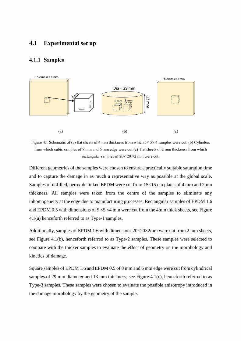
4.1 Experimental set up

4.1.1 Samples

(a) (b) (c)

Figure 4.1 Schematic of (a) flat sheets of 4 mm thickness from which 5× 5× 4 samples were cut. (b) Cylinders

from which cubic samples of 8 mm and 6 mm edge were cut (c) flat sheets of 2 mm thickness from which

rectangular samples of 20× 20 ×2 mm were cut.

Different geometries of the samples were chosen to ensure a practically suitable saturation time

and to capture the damage in as much a representative way as possible at the global scale.

Samples of unfilled, peroxide linked EPDM were cut from 15×15 cm plates of 4 mm and 2mm

thickness. All samples were taken from the centre of the samples to eliminate any

inhomogeneity at the edge due to manufacturing processes. Rectangular samples of EPDM 1.6

and EPDM 0.5 with dimensions of 5 ×5 ×4 mm were cut from the 4mm thick sheets, see Figure

4.1(a) henceforth referred to as Type-1 samples.

Additionally, samples of EPDM 1.6 with dimensions 20×20×2mm were cut from 2 mm sheets,

see Figure 4.1(b), henceforth referred to as Type-2 samples. These samples were selected to

compare with the thicker samples to evaluate the effect of geometry on the morphology and

kinetics of damage.

Square samples of EPDM 1.6 and EPDM 0.5 of 8 mm and 6 mm edge were cut from cylindrical

samples of 29 mm diameter and 13 mm thickness, see Figure 4.1(c), henceforth referred to as

Type-3 samples. These samples were chosen to evaluate the possible anisotropy introduced in

the damage morphology by the geometry of the sample.

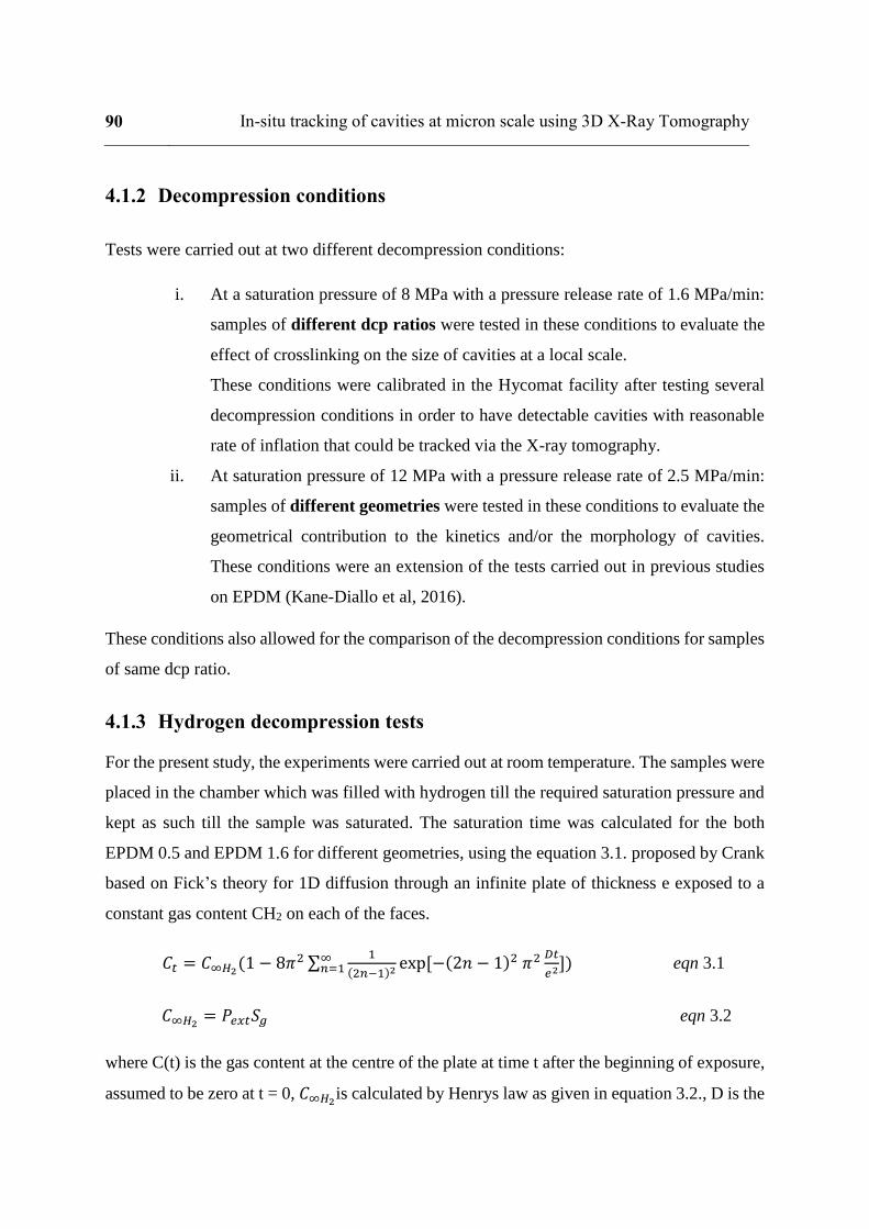
90 In-situ tracking of cavities at micron scale using 3D X-Ray Tomography

4.1.2 Decompression conditions

Tests were carried out at two different decompression conditions:

i. At a saturation pressure of 8 MPa with a pressure release rate of 1.6 MPa/min:

samples of different dcp ratios were tested in these conditions to evaluate the

effect of crosslinking on the size of cavities at a local scale.

These conditions were calibrated in the Hycomat facility after testing several

decompression conditions in order to have detectable cavities with reasonable

rate of inflation that could be tracked via the X-ray tomography.

ii. At saturation pressure of 12 MPa with a pressure release rate of 2.5 MPa/min:

samples of different geometries were tested in these conditions to evaluate the

geometrical contribution to the kinetics and/or the morphology of cavities.

These conditions were an extension of the tests carried out in previous studies

on EPDM (Kane-Diallo et al, 2016).

These conditions also allowed for the comparison of the decompression conditions for samples

of same dcp ratio.

4.1.3 Hydrogen decompression tests

For the present study, the experiments were carried out at room temperature. The samples were

placed in the chamber which was filled with hydrogen till the required saturation pressure and

kept as such till the sample was saturated. The saturation time was calculated for the both

EPDM 0.5 and EPDM 1.6 for different geometries, using the equation 3.1. proposed by Crank

based on Fick’s theory for 1D diffusion through an infinite plate of thickness e exposed to a

constant gas content CH2 on each of the faces.

𝐶𝑡 = 𝐶∞𝐻2(1 − 8𝜋2 ∑

1

(2𝑛−1)2 exp [−(2𝑛 − 1)2 𝜋2 𝐷𝑡

𝑒2])∞𝑛=1 eqn 3.1

𝐶∞𝐻2= 𝑃𝑒𝑥𝑡𝑆𝑔 eqn 3.2

where C(t) is the gas content at the centre of the plate at time t after the beginning of exposure,

assumed to be zero at t = 0, 𝐶∞𝐻2is calculated by Henrys law as given in equation 3.2., D is the

diffusion coefficient of hydrogen in EPDM, e is the thickness of the sample. Pext is the external

pressure of the gas and Sg is the solubility of the gas in EPDM. The summation was done for

250 terms. Coefficients Sg and D were deduced prior to the tomography test from permeation

tests and have been noted in Chapter 2.

In the last part of the experiment, a stage was 3D printed and used to place more than one

specimen in the XPRESS chamber. Consequently, the images so obtained for multiple samples

had more noise to data ratio as compared to the images obtained in case of a single specimen.

4.1.4 In situ tomography set up

The in situ X-ray micro-tomography was done using an Ultratom tomograph developed by RX

Solutions® (Figure 4.2(a)). The device essentially consists of three X-ray source tubes with

micro-focus, nano-focus and high voltage specifications, a sample mount on top of a rotation

stage, and two types of X-ray detectors: Varian detector for classical and CCD camera for high-

resolution acquisitions respectively.

For the present experiments, the tomograph was fitted with the cylindrical pressure chamber

(XPRESS chamber) as seen in Figure 4.2 (b), which allows the tests to be carried out in

different gaseous environments. Other details of the device are given in below

• Gases in which in-situ tests can be performed: N2, CO2 and H2

• Maximum operating pressure: 200 bars

• Maximum operating temperature : 150°C

• Remotely controlled

• Compression and decompression rate : regulated

The sample was centred on the rotation axis inside the chamber at a distance of 36-mm from

the X-ray source (voltage 80 kV, current 375 µA). The Varian X-ray detector was used which

consisted of an X-ray CsI scintillator screen settled on an amorphous silicon layer with

1920x1536 sensitive elements.

92 In-situ tracking of cavities at micron scale using 3D X-Ray Tomography

(a)

(b)

Figure 4.2 (a) Ultra Tomograph (b) XPRESS chamber for in-situ tracking of cavities in H2

4.2 Data treatment

4.2.1 Image reconstruction

During the tomography experiment, the model rotates in small steps about an axis of rotation

while taking a sequence of 2D radiographs which are later numerically reconstructed into a 3D

Rotating

stage

Detector

X-ray

source

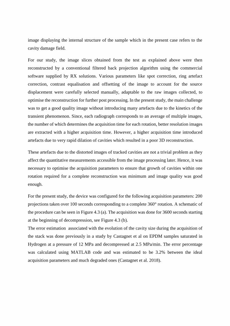
image displaying the internal structure of the sample which in the present case refers to the

cavity damage field.

For our study, the image slices obtained from the test as explained above were then

reconstructed by a conventional filtered back projection algorithm using the commercial

software supplied by RX solutions. Various parameters like spot correction, ring artefact

correction, contrast equalisation and offsetting of the image to account for the source

displacement were carefully selected manually, adaptable to the raw images collected, to

optimise the reconstruction for further post processing. In the present study, the main challenge

was to get a good quality image without introducing many artefacts due to the kinetics of the

transient phenomenon. Since, each radiograph corresponds to an average of multiple images,

the number of which determines the acquisition time for each rotation, better resolution images

are extracted with a higher acquisition time. However, a higher acquisition time introduced

artefacts due to very rapid dilation of cavities which resulted in a poor 3D reconstruction.

These artefacts due to the distorted images of tracked cavities are not a trivial problem as they

affect the quantitative measurements accessible from the image processing later. Hence, it was

necessary to optimise the acquisition parameters to ensure that growth of cavities within one

rotation required for a complete reconstruction was minimum and image quality was good

enough.

For the present study, the device was configured for the following acquisition parameters: 200

projections taken over 100 seconds corresponding to a complete 360° rotation. A schematic of

the procedure can be seen in Figure 4.3 (a). The acquisition was done for 3600 seconds starting

at the beginning of decompression, see Figure 4.3 (b).

The error estimation associated with the evolution of the cavity size during the acquisition of

the stack was done previously in a study by Castagnet et al on EPDM samples saturated in

Hydrogen at a pressure of 12 MPa and decompressed at 2.5 MPa/min. The error percentage

was calculated using MATLAB code and was estimated to be 3.2% between the ideal

acquisition parameters and much degraded ones (Castagnet et al. 2018).

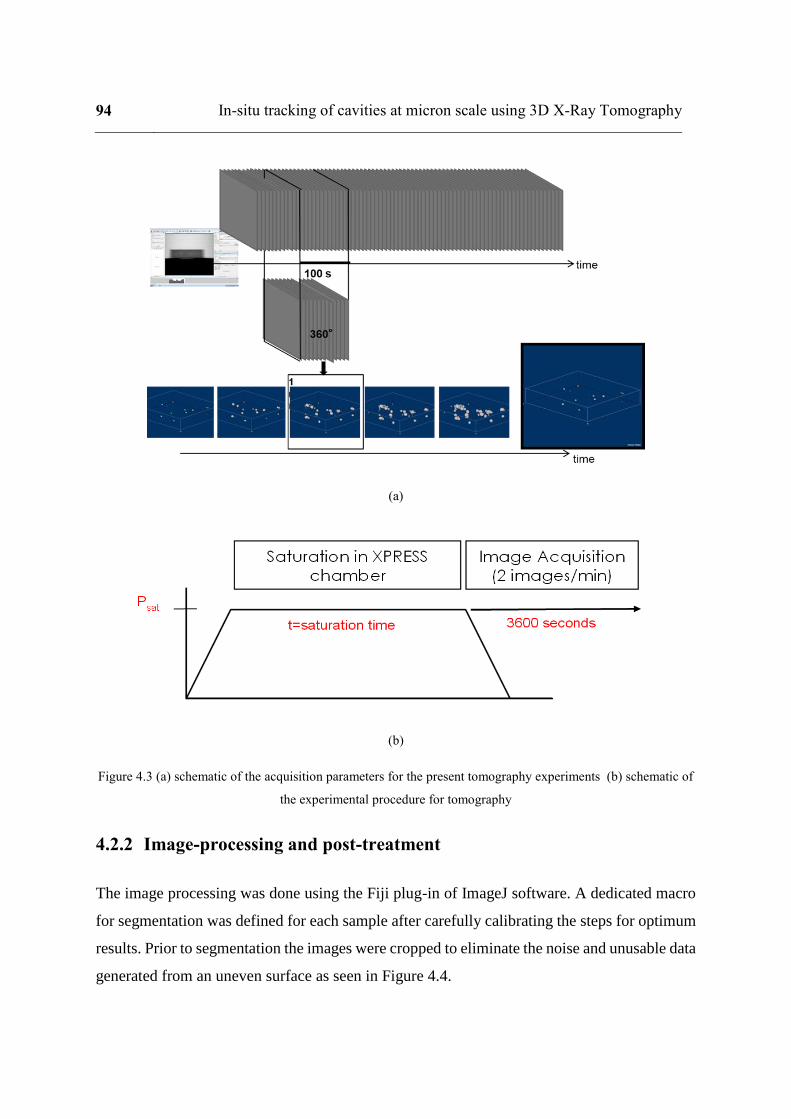
94 In-situ tracking of cavities at micron scale using 3D X-Ray Tomography

(a)

(b)

Figure 4.3 (a) schematic of the acquisition parameters for the present tomography experiments (b) schematic of

the experimental procedure for tomography

4.2.2 Image-processing and post-treatment

The image processing was done using the Fiji plug-in of ImageJ software. A dedicated macro

for segmentation was defined for each sample after carefully calibrating the steps for optimum

results. Prior to segmentation the images were cropped to eliminate the noise and unusable data

generated from an uneven surface as seen in Figure 4.4.

Figure 4.4 Type-1 sample of EPDM 1.6 exposed to hydrogen at 12 MPa and decompressed at 2.5 MPa/min at

the time step of 700-800 secs after decompression.

Figure 4.5 Various in-built thersholding filters applied on the same isolated cavity from Type-1 sample of

EPDM 0.5 at the time step of 350-450 seconds.

The segmentation was done in four major steps, the first being the application of various

mathematical operations in the form of filters to smooth the data: noise minimization and

contrast enhancement. In the second step, the thresholding was done to convert the greyscale

images into binary ones using an inbuilt binarisation algorithm to ensure consistency in data

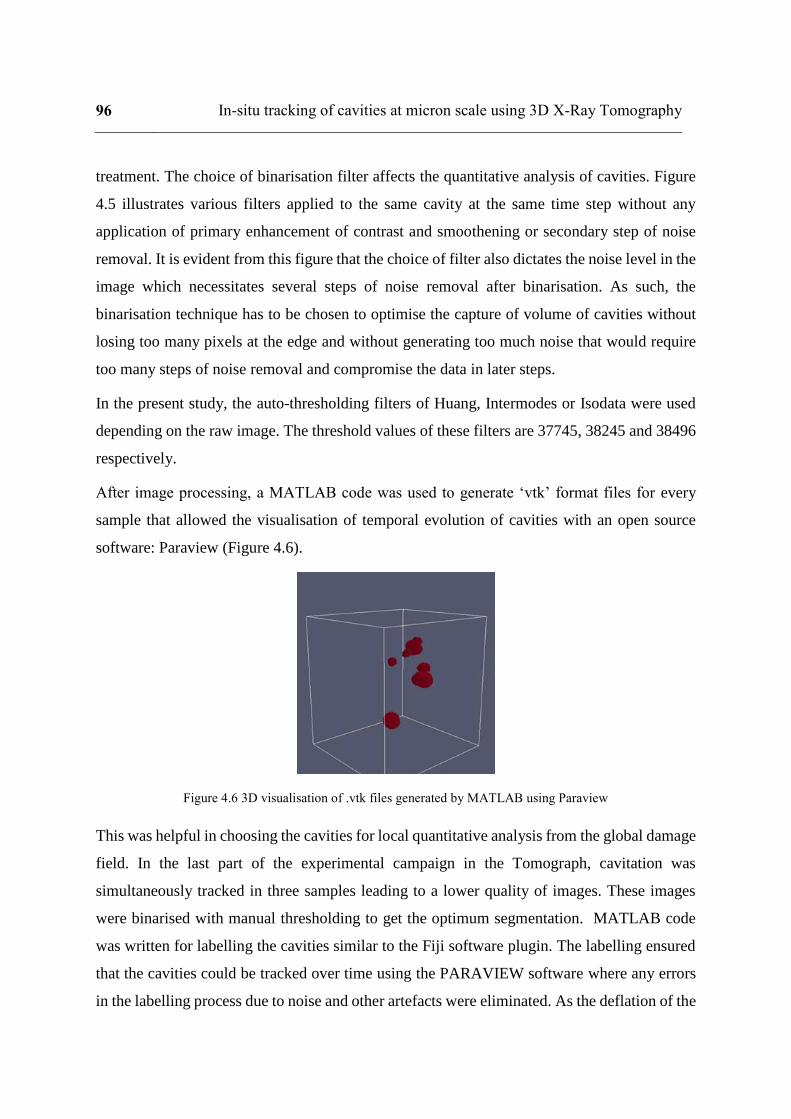
96 In-situ tracking of cavities at micron scale using 3D X-Ray Tomography

treatment. The choice of binarisation filter affects the quantitative analysis of cavities. Figure

4.5 illustrates various filters applied to the same cavity at the same time step without any

application of primary enhancement of contrast and smoothening or secondary step of noise

removal. It is evident from this figure that the choice of filter also dictates the noise level in the

image which necessitates several steps of noise removal after binarisation. As such, the

binarisation technique has to be chosen to optimise the capture of volume of cavities without

losing too many pixels at the edge and without generating too much noise that would require

too many steps of noise removal and compromise the data in later steps.

In the present study, the auto-thresholding filters of Huang, Intermodes or Isodata were used

depending on the raw image. The threshold values of these filters are 37745, 38245 and 38496

respectively.

After image processing, a MATLAB code was used to generate ‘vtk’ format files for every

sample that allowed the visualisation of temporal evolution of cavities with an open source

software: Paraview (Figure 4.6).

Figure 4.6 3D visualisation of .vtk files generated by MATLAB using Paraview

This was helpful in choosing the cavities for local quantitative analysis from the global damage

field. In the last part of the experimental campaign in the Tomograph, cavitation was

simultaneously tracked in three samples leading to a lower quality of images. These images

were binarised with manual thresholding to get the optimum segmentation. MATLAB code

was written for labelling the cavities similar to the Fiji software plugin. The labelling ensured

that the cavities could be tracked over time using the PARAVIEW software where any errors

in the labelling process due to noise and other artefacts were eliminated. As the deflation of the

cavities is very slow as compared to the inflation, only some reconstructed images were

segmented for the deflation stage of the cavities.

4.3 Classification of damage based on morphology

For local analysis, cavities were locally selected from a global damage field and classified into

separate groups based on spatial position in the sample. This classification was done by fitting

a box around the cavity with side equal to the maximum diameter attained by the cavity as

shown in Figure 4.7. The size of the box was taken such that it would contain the single cavity

throughout its evolution. In the cases that the cavities could be contained in the box without

any intrusion by other cavities all through their evolution, were termed as “isolated cavities”.

The cavities that couldn’t be contained in a single box without intrusion from other cavities

during the whole evolution were termed as close cavities.

Figure 4.7 (a) Isolated cavity (b) Close cavities

In most cases, however, the close cavities formed a cluster, consisting of a network of very

close cavities that were not visually distinguishable and could not be quantitatively analysed

by the image processing software. This was due to the low resolution of the Tomograph, which

allows the cavities to be distinctly identified with a minimum distance of 32 microns between

the cavity borders. As such, groups of 2 to 6 very close cavities that could be distinguished into

separate cavities were chosen from the global damage field for quantitative assessment of their

(a)

(b)

98 In-situ tracking of cavities at micron scale using 3D X-Ray Tomography

kinetics to clarify any interaction between these cavities. Large clusters of cavities that were

not accessible for quantitative analysis were nevertheless qualitatively analysed for providing

some insights into the evolution of the global damage field.

More than 50 cavities were manually selected from global damage fields of Type-1 samples of

EPDM 1.6, out of which 45 cavities were considered for this study as they did not transition to

cracking. In a similar way, 20 isolated cavities were picked from the Type-1 samples of EPDM

0.5. Additionally, 9 cavities were taken from Type-3 samples of EPDM 1.6. for analysing the

interaction between cavities, 9 groups of close cavities with the number ranging from 2-6

cavities were chosen from Type-1 and Type-3 samples of EPDM 1.6 for analysis. Clustering

was analysed using Type-2 samples of both EPDM 0.5 and EPDM 1.6.

4.4 Inflation characteristics of isolated cavities

As the first step in quantitative analysis, several parameters of the chosen cavities were

calculated using 3D manager plugin of Fiji software: size, anisotropy, location and distance

between cavities.

The volume of cavities was calculated at each time step by the method of counting voxels to

minimise the over or underestimation introduced due to fitting with an ellipse. However, this

method introduces certain artefacts when the size of the cavity is very small due to pixelisation.

The location refers to the centre of mass of the cavities.

The anisotropy was calculated by taking the ratio of diameters along x and y axes and defined

as sphericity in this document henceforth. For a perfectly spherical cavity the value of

sphericity is 1 indicating a completely isotropic cavity.

Distance to the free surface was calculated taking the cropped voxels into account for each

cavity manually, see Figure 4.8. It should be noted that due to the manual calculation, the error

bar in this case is in the range of 50-150 microns. Hence, the distance from the free surface

mentioned henceforth in the present document is the actual distance from the free surface of

the sample and not of the cropped image. Thereafter, these parameters were used to calculate

the inflation characteristics of these cavities which are detailed below. As the effect of these

(a

)

(b

)

parameters is convoluted, discussing them in rigorous steps is not possible. The sections below

tackle more than one parameter simultaneously at times, since the effect of parameters cannot

be detailed separately from one another.

Figure 4.8 distance to the free surface of the sample is calculated from the centre of mass of the cavity.

4.4.1 Rate of inflation

Figure 4.9 Volume evolution of cavities in type-1 samples of EPDM 0.5. Psat 8 MPa, decompression rate of 1.6

MPa/min

For calculating the rate of inflation as a first step, volume evolution of each cavity was plotted

against time as seen in Figure 4.9 which shows the evolution of cavities of Type-1 sample of

EPDM 0.5. exposed to hydrogen at 8 MPa and decompressed at a decompression rate of 1.6

MPa/min. Since the time step of 100 seconds corresponds to one data point for volume, the

mid-point of the time step has been considered for the corresponding value of volume in the

time axis of all the graphs henceforth, for example for the time step of 200-300 seconds, the

y = 38.404x - 11934R² = 0.9957

0

5000

10000

15000

20000

25000

30000

0 250 500 750 1000 1250 1500 1750 2000 2250 2500 2750 3000 3250 3500

volu

me

(vo

xels

)

time(s)

100 In-situ tracking of cavities at micron scale using 3D X-Ray Tomography

value of volume is plotted at time point of 250 seconds. As seen in the Figure 4.9 the volume

evolution curve of the cavities is generally parabolic.

The rate of inflation of the cavities was done by linearly fitting the first part of the curve

corresponding to the growth of the cavity. Usually, the first detected volume of the cavity is

prone to high error due to rapid inflation and biases introduced during image processing; this

effect is typical of first appearing cavities nucleated during the earliest stage of decompression

(within 200 seconds of decompression). Hence, the first data point was generally omitted

during the linear fitting of the curve to calculate the rate of inflation. However, for the cavities

nucleated later and detected at sufficiently high value so as not be severely affected by image

processing biases, the linear fitting included the first data point of calculated volume (Figure

4.9); smallest cavities with very few data points (less or equal to 3) in the range of inflation

were not fitted to analyse the rate.

4.4.2 Evolution of anisotropy

Figure 4.10 shows the evolution of anisotropy, characterised by sphericity, of the cavities in

Type-1 samples of EPDM 1.6 tested under the decompression conditions of Psat = 8MPa and

decompression rate of 1.6 MPa per min. It can be seen from the Figure 4.10 (a) that the

anisotropy is high at the beginning of the inflation and with time the cavities become more

spherical. This can be attributed to the artefacts due to the rapid volume increase at the very

beginning of decompression; deviation from perfect isotropy is expected due to the pixelisation

as a result of image processing and as a good estimate, 0.8 can be said to represent an almost

spherical cavity.

Figure 4.10 (b) shows the evolution of anisotropy of cavities with delayed nucleation. These

cavities nucleate at 350 to 500 seconds after decompression and are described in the later

section. As can be seen from the graph, they tend to have almost constant anisotropy ratio

throughout their evolution. This is due to their low rate of inflation at the time of nucleation

and as such the artefacts introduced due to rapid kinetics are lesser.

(a)

(b)

Figure 4.10: plots of temporal evolution of anisotropy during volume evolution of a) isolated primary cavities b)

isolated cavities with delayed nucleation in EPDM 1.6 samples of Type-1. Psat 8 MPa, Ṗ 1.6 MPa/min

Generally, anisotropy of isolated cavities can be attributed to the following factors: The first

factor is the geometry of the sample. This has already been addressed in the literature by

Castagnet et al who considered the EPDM sample of dimensions 10×10 with a thickness 2 mm,

saturated with hydrogen at 12 MPa and decompressed at 2.5 MPa/min. resulting in anisotropic

boundary conditions (Castagnet et al. 2018). However, the work was focused on the full cavity

field and only average anisotropy ratio was discussed. Having said that, it was seen in their

study that the average anisotropy ratio was maximum at the beginning of nucleation and at the

deflation stage. However, during the growth of the cavities, the cavities remained largely

0

0.1

0.2

0.3

0.4

0.5

0.6

0.7

0.8

0.9

1

0 250 500 750 1000 1250 1500 1750 2000 2250 2500 2750 3000 3250 3500

spher

icit

y

time after decompression (s)

EPDM 0,1

EPDM 0,5

EPDM 1.6

0

0.1

0.2

0.3

0.4

0.5

0.6

0.7

0.8

0.9

1

0 250 500 750 1000 1250 1500 1750 2000 2250 2500 2750 3000 3250 3500

spher

city

time after decompression (s)

EPDM 1.6

102 In-situ tracking of cavities at micron scale using 3D X-Ray Tomography

spherical. The anisotropy was assumed to be influenced by the shape of the sample that

contributed an anisotropic boundary conditions leading to flattening of cavities in the plane of

thickness of the sample. As the damage was reversible and no cracking was observed with their

samples, this assumption of anisotropy introduced by the geometry of the sample seems

reasonable.

The second factor contributing to the anisotropy is the transition of cavities to cracking: some

cavities become flattened during evolution showing a tendency to transition into a crack. This

is accompanied by a rapid shift (jump) in the normally parabolic volume evolution curve as a

result of a sudden increase in volume. An explanation of this could be the cracking of the cavity

walls that becomes more apparent during deflation. This is illustrated in Figure 4.11, which

shows the evolution of some of the isolated cavities of Type-1 sample of EPDM 1.6 at adjacent

time steps

Figure 4.11 Snapshots of cavities in the Type-1 sample of EPDM 1.6

Figure 4.12 shows the evolution of anisotropy of selected isolated cavities in EPDM 1.6 Type-

1 samples. The decrease in the sphericity seen in the graph corresponds to the flattening of the

cavity which becomes increasingly apparent during deflation. An illustration of this

phenomenon can be seen in Figure 4.11 where the evolution of cavities is clearly seen to be

anisotropic even during inflation. It can be observed that this “beginning” of cracking is not

due to coalescence but as a result of growth of a single cavity.

Figure 4.12 Evolution of anisotropy of selected isolated cavities from Type1 samples of EPDM 1.6 that flatten

during deflation. Psat 8 MPa, Ṗ 1.6 MPa/min

However, it must be considered that this assumption is strongly dependent on the resolution of

the technique. In the present study, this phenomenon was only observed in Type-1 samples of

EPDM 1.6. The generality of this phenomenon as well as possible geometrical influence of the

sample shape remains to be experimentally verified. Additionally, the possible coalescence of

cavities that might be observable at better resolutions as well as the non-reversibility of this

damage needs to be examined in further future studies.

In the present study, the focus is to access the kinetics of the cavities prior to cracking; hence,

the cavities which are considered to transition into cracking as discussed above have been

excluded from the analysis.

4.5 Factors influencing the growth kinetics of isolated cavities

This section discusses the various factors influencing the growth kinetics of isolated cavities

taken from Type 1 samples of EPDM 1.6. The same analysis is done for the samples of

EPDM 0.5 and is discussed in the later section.

Figure 4.13 shows the maximum volume (Vmax) attained by the isolated cavities versus the

distance from the free surface for the Type-1 EPDM 1.6 samples with the pressure conditions

of Psat 8 MPa and Ṗ 1.6 MPa/min.

0

0.1

0.2

0.3

0.4

0.5

0.6

0.7

0.8

0.9

1

0 250 500 750 1000 1250 1500 1750 2000 2250 2500 2750 3000 3250

spher

icit

y

time after decompression

104 In-situ tracking of cavities at micron scale using 3D X-Ray Tomography

Figure 4.13 Effect of distance to the free surface on the Vmax of cavities in Type-1 samples of EPDM 1.6

An increasing trend with a large scatter is observed in the first part of the graph indicating that

the maximum volume attained by the cavities is affected by the closeness to the free surface of

the sample. In the above graph the limiting value is observed in the range of 800-900 microns

after which the values corresponding to the maximum volume are random. This value is a

broadly estimated one and with more statistical analysis could be found to be a rather arbitrary

one. Nevertheless, it could be said that the proximity to the edge drives the maximum volume

of the cavities and is a first order factor for the inflation kinetics of cavities upto a limiting

distance. This might be attributed to the rapid desorption of the gas from the surface leading to

rapid deflation of the cavities. This assumption is an early one and will be tackled in the later

sections as well.

For cavities that occur in the bulk of the sample, i.e. cavities occurring at a distance of more

than 800-900 microns in the above graph can be taken to have isotropic boundary conditions

in terms of global boundary conditions. In such cases, the edge factor is no longer a dominant

one for the cavity evolution. For such cavities, the local boundary conditions such as proximity

to other cavities or nucleation of new cavities close to the existing one need to be analysed as

the major contributing factors in the temporal evolution of the cavity. These cavities were

tentatively termed as bulk cavities while the cavities with centroids at a distance of less than

0

5000

10000

15000

20000

25000

30000

35000

40000

45000

50000

0 200 400 600 800 1000 1200 1400 1600 1800 2000

Vm

ax(v

oxel

s)

distance to the free surface (microns)

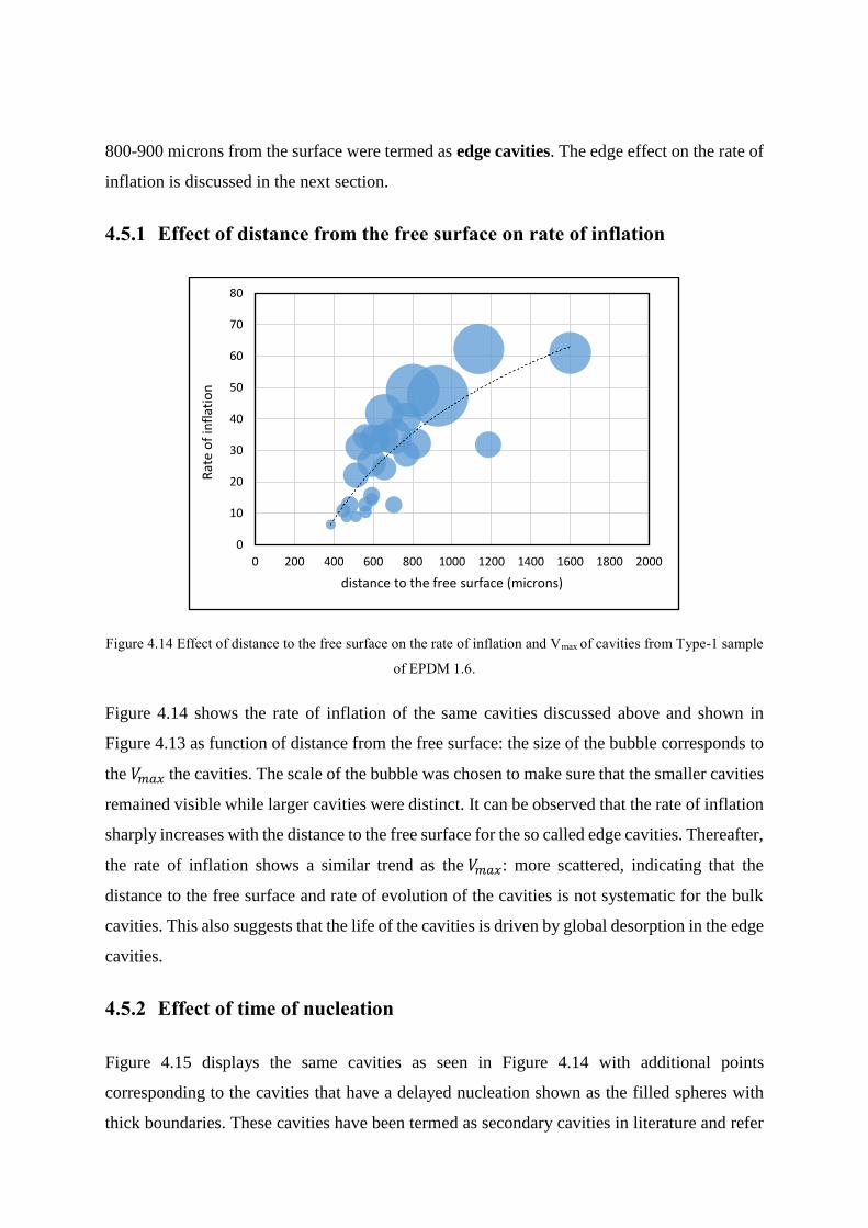
800-900 microns from the surface were termed as edge cavities. The edge effect on the rate of

inflation is discussed in the next section.

4.5.1 Effect of distance from the free surface on rate of inflation

Figure 4.14 Effect of distance to the free surface on the rate of inflation and Vmax of cavities from Type-1 sample

of EPDM 1.6.

Figure 4.14 shows the rate of inflation of the same cavities discussed above and shown in

Figure 4.13 as function of distance from the free surface: the size of the bubble corresponds to

the 𝑉𝑚𝑎𝑥 the cavities. The scale of the bubble was chosen to make sure that the smaller cavities

remained visible while larger cavities were distinct. It can be observed that the rate of inflation

sharply increases with the distance to the free surface for the so called edge cavities. Thereafter,

the rate of inflation shows a similar trend as the 𝑉𝑚𝑎𝑥: more scattered, indicating that the

distance to the free surface and rate of evolution of the cavities is not systematic for the bulk

cavities. This also suggests that the life of the cavities is driven by global desorption in the edge

cavities.

4.5.2 Effect of time of nucleation

Figure 4.15 displays the same cavities as seen in Figure 4.14 with additional points

corresponding to the cavities that have a delayed nucleation shown as the filled spheres with

thick boundaries. These cavities have been termed as secondary cavities in literature and refer

0

10

20

30

40

50

60

70

80

0 200 400 600 800 1000 1200 1400 1600 1800 2000

Rat

e o

f in

flat

ion

distance to the free surface (microns)

106 In-situ tracking of cavities at micron scale using 3D X-Ray Tomography

to a cluster of satellite cavities surrounding the primary ones (Gent 2011). However, it is seen

that although these secondary cavities do not necessarily nucleate closer to primary or initial

cavities, they nucleate a bit later than the initial ones. These cavities as seen in the graph show

slower kinetics than the primary cavities appearing in the same sample (Type-1) and exposed

to the same decompression conditions. The nucleation of these cavities was mostly seen at 350

to 500 seconds after decompression such that the mechanical pressure on the sample exerted

by the gas in the chamber is completely released.

Figure 4.15 Effect of delayed nucleation of rate of inflation and Vmax of cavities taken from Type-1 sample of

EPDM 1.6. Psat 8 MPa, Ṗ 1.6 MPa/min

The lack of mechanical pressure could be assumed to be a contributing factor in the slow

kinetics of these cavities. However, the earlier nucleating cavities are detected at 200 to 350

seconds after decompression where the gas pressure is either very low or completely zero

making this assumption rather broad. Another factor that could contribute to the slower kinetics

is the different iso-conditions due to global desorption leading to different local diffusion fields.

This question has been addressed in the later part of the chapter with simulations.

4.5.3 Effect of pressure conditions

Figure 4.16 shows the rate of inflation of isolated cavities in samples at two different pressure

conditions. The yellow spheres correspond to the sample with more drastic decompression

conditions: Psat 12 MPa and Ṗ 2.5 MPa/min as compared to the decompression conditions

0

10

20

30

40

50

60

70

80

0 200 400 600 800 1000 1200 1400 1600 1800 2000

Rat

e o

f in

flat

ion

distance to the free surface (microns)

analysed so far as represented by blue spheres: Psat 8 MPa and Ṗ 1.6 MPa/min. It should be

noted that the cavities with delayed nucleation have not been plotted in curve such that only

the effect of geometry can be clarified here.

Figure 4.16 Effect of decompression conditions of rate of inflation and Vmax of cavities. The yellow

spheres correspond to cavities in samples under more drastic decompression conditions

It can be seen that the cavities under more drastic decompression conditions have a faster

growth rate than the cavities under less intense decompression conditions even as they occur

at the same distance from the free surface. A shifting in the vertical direction can be seen in the

scatter graph of the yellow spheres indicative of general increase in the value of the rate of

inflation of the cavities as the pressure conditions are made more severe. It should be noted

that the cavities corresponding to the more drastic decompression conditions (shown here in

yellow) were picked up from samples with different dimensions which is compared in the next

section. The cavities corresponding to the blue spheres however have all been taken from the

Type-1 sample.

4.5.4 Effect of sample geometry

Figure 4.17 shows plots of the rates of inflation for cavities taken from two different geometries

for the same pressure conditions: Psat 12 MPa and Ṗ 2.5 MPa/min; the spheres with thick

boundaries correspond to cavities in Type-1 samples whereas the yellow filled spheres

correspond to cavities taken from Type-3 samples. It is evident that the rate of inflation or

maximum volume show no trend with respect to geometry indicating that the shape of the

sample does not affect the kinetics of the cavities at a local scale. Looking at the graph globally,

0

20

40

60

80

100

120

140

0 200 400 600 800 1000 1200 1400 1600 1800 2000

Rat

e o

f in

flat

ion

distance to the free surface (microns)

108 In-situ tracking of cavities at micron scale using 3D X-Ray Tomography

the initial section shows an increasing trend irrespective of the geometry of the sample whereas

the later part of the graph shows more random data points. This trend seen here with respect to

the distance from the free surface is consistent with the previous results. Tentatively this

reinstates the fact that the distance to the free surface remains the dominant limiting factor for

the growth of cavities irrespective of the geometry of the sample. Needless to say, the data

points for cavities taken from Type-1 sample are few and this assumption remains to be verified

in a more statistical manner.

Figure 4.17 Effect of geometry on rate of inflation and Vmax of cavities.

4.5.5 Comparison with samples of different cross-link densities

As a comparison to EPDM 1.6 the samples of EPDM 0.5 were tested in the same

decompression conditions: Psat = 8 MPa and Ṗ = 1.6 MPa/min with sample dimensions of

5×5×4 mm (Type-1). Similar to samples of EPDM 1.6, the volume evolution of cavities were

plotted against time and the maximum volume was calculated. Figure 4.18 shows the maximum

volume (Vmax) attained by the cavity as a function of distance from the free surface for EPDM

0.5. It can be seen that the maximum volume of the cavity shows a liner trend with the distance

from the free surface, and doesn’t show any normalisation at the distance of 800 microns.

However, since the number of data points are few, the same conclusion cannot be excluded for

EPDM 0.5.

0

20

40

60

80

100

120

140

0 200 400 600 800 1000 1200 1400 1600 1800 2000

Rat

e o

f in

flat

ion

distance to the free surface (microns)

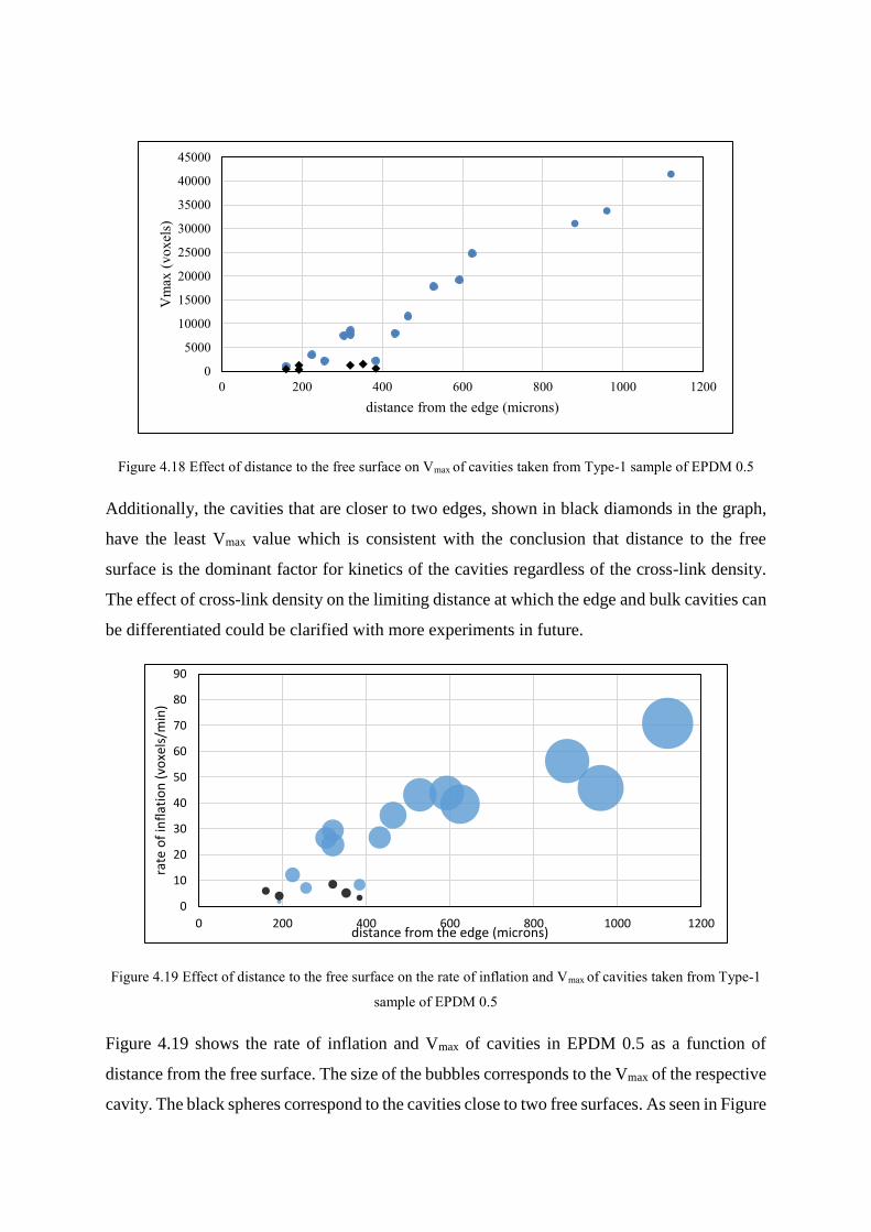
Figure 4.18 Effect of distance to the free surface on Vmax of cavities taken from Type-1 sample of EPDM 0.5

Additionally, the cavities that are closer to two edges, shown in black diamonds in the graph,

have the least Vmax value which is consistent with the conclusion that distance to the free

surface is the dominant factor for kinetics of the cavities regardless of the cross-link density.

The effect of cross-link density on the limiting distance at which the edge and bulk cavities can

be differentiated could be clarified with more experiments in future.

Figure 4.19 Effect of distance to the free surface on the rate of inflation and Vmax of cavities taken from Type-1

sample of EPDM 0.5

Figure 4.19 shows the rate of inflation and Vmax of cavities in EPDM 0.5 as a function of

distance from the free surface. The size of the bubbles corresponds to the Vmax of the respective

cavity. The black spheres correspond to the cavities close to two free surfaces. As seen in Figure

0

5000

10000

15000

20000

25000

30000

35000

40000

45000

0 200 400 600 800 1000 1200

Vm

ax (

vo

xel

s)

distance from the edge (microns)

0

10

20

30

40

50

60

70

80

90

0 200 400 600 800 1000 1200

rate

of

infl

atio

n (

voxe

ls/m

in)

distance from the edge (microns)

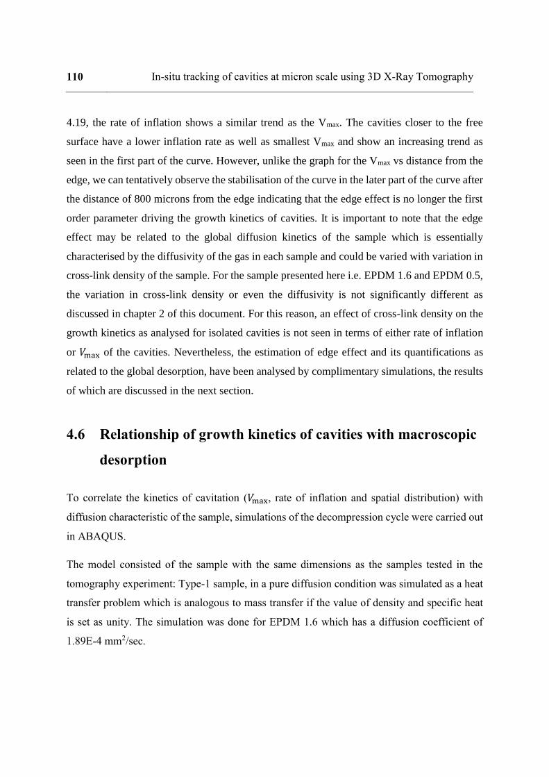
110 In-situ tracking of cavities at micron scale using 3D X-Ray Tomography

4.19, the rate of inflation shows a similar trend as the Vmax. The cavities closer to the free

surface have a lower inflation rate as well as smallest Vmax and show an increasing trend as

seen in the first part of the curve. However, unlike the graph for the Vmax vs distance from the

edge, we can tentatively observe the stabilisation of the curve in the later part of the curve after

the distance of 800 microns from the edge indicating that the edge effect is no longer the first

order parameter driving the growth kinetics of cavities. It is important to note that the edge

effect may be related to the global diffusion kinetics of the sample which is essentially

characterised by the diffusivity of the gas in each sample and could be varied with variation in

cross-link density of the sample. For the sample presented here i.e. EPDM 1.6 and EPDM 0.5,

the variation in cross-link density or even the diffusivity is not significantly different as

discussed in chapter 2 of this document. For this reason, an effect of cross-link density on the

growth kinetics as analysed for isolated cavities is not seen in terms of either rate of inflation

or 𝑉max of the cavities. Nevertheless, the estimation of edge effect and its quantifications as

related to the global desorption, have been analysed by complimentary simulations, the results

of which are discussed in the next section.

4.6 Relationship of growth kinetics of cavities with macroscopic

desorption

To correlate the kinetics of cavitation (𝑉max, rate of inflation and spatial distribution) with

diffusion characteristic of the sample, simulations of the decompression cycle were carried out

in ABAQUS.

The model consisted of the sample with the same dimensions as the samples tested in the

tomography experiment: Type-1 sample, in a pure diffusion condition was simulated as a heat

transfer problem which is analogous to mass transfer if the value of density and specific heat

is set as unity. The simulation was done for EPDM 1.6 which has a diffusion coefficient of

1.89E-4 mm2/sec.

(a) (b)

Figure 4.20 (a) Predefined field: constant concentration throughout the sample of magnitude 8 reflecting the

sample saturated at 8MPa (b) amplitude of boundary condition applied, reflecting the decompression stage

The model simulated the decompression stage of the hydrogen exposure, taking the initial state

of the sample at equilibrium which was defined by taking a predefined field of constant

concentration of 8 MPa through the sample defining the initial condition as that of a saturated

sample as seen in Figure 4.20 (a). The application of boundary conditions involved putting the

concentration of the sample edges at zero mimicking the decompression phase of the hydrogen

exposure for the conditions of Psat 8 MPa and Ṗ 1.6 MPa/min as seen in Figure 4.20 (b).

The sample was meshed with a standard linear heat transfer element of DC3D8 type. Prior to

actual simulations, the test for mesh sensitivity was carried out for a regular mesh with different

mesh sizes of 0.2, 0.1 and 0.05mm. The same simulation of a pure diffusion problem was

carried with different mesh sizes and the concentration gradients along the path from the centre

of the sample to the edge were plotted along different axes. Since the results were isotropic,

only the curves corresponding to concentration gradients of hydrogen in terms of partial

pressure along z-axis are shown in Figure 4.21. The sensitivity to mesh size is more pronounced

at the coarse mesh level of size 0.2 and decreases as the mesh size is reduced. However, the

curves for mesh size 0.1 and 0.05 are seen to almost superimpose. Consequently, the mesh size

of 0.1 was taken to be most suitable for regular meshing, illustrated in Figure 4.22.

112 In-situ tracking of cavities at micron scale using 3D X-Ray Tomography

Figure 4.21 Curves for comparison of different mesh sizes. The green, red and purple lines correspond to the

curves for 300, 500 and 1000 seconds after decompression respectively

Figure 4.22 Illustration of the mesh size 0.1 for Type-1 sample

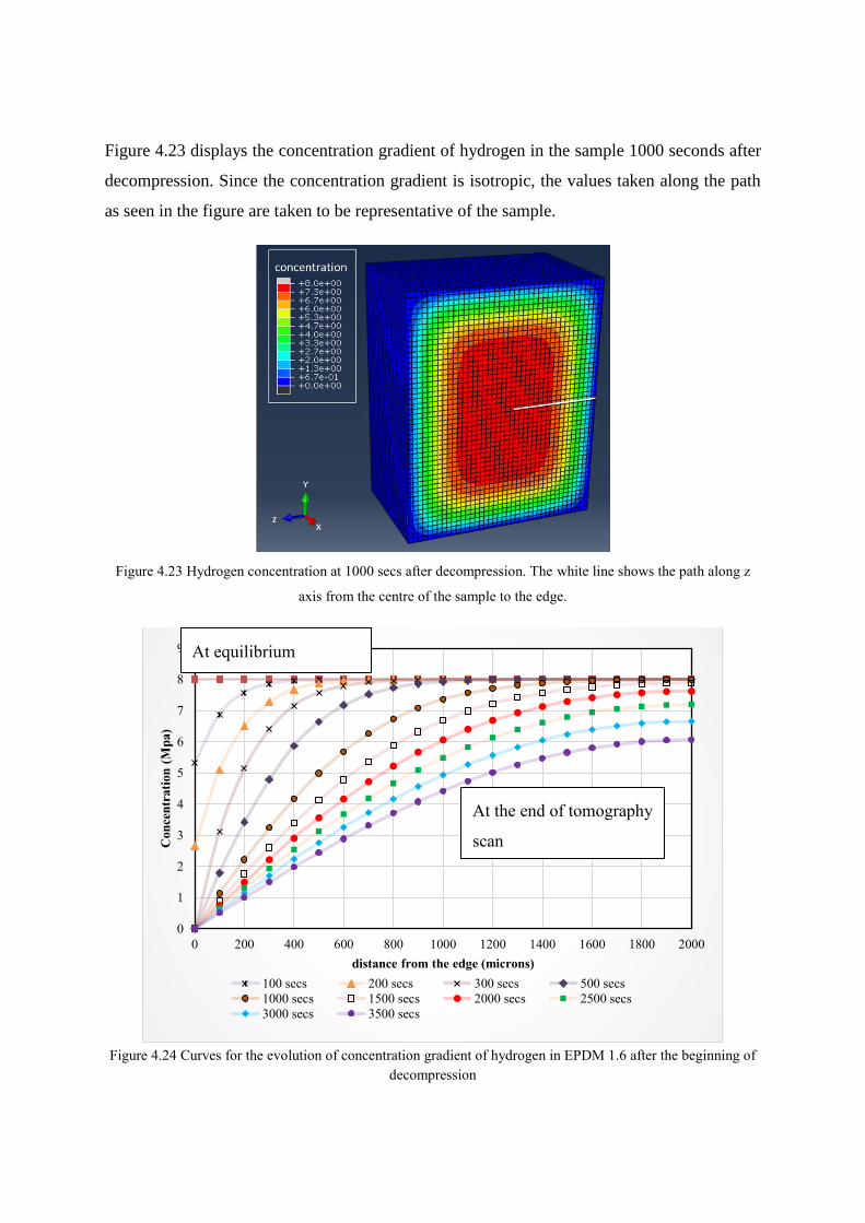
Figure 4.23 displays the concentration gradient of hydrogen in the sample 1000 seconds after

decompression. Since the concentration gradient is isotropic, the values taken along the path

as seen in the figure are taken to be representative of the sample.

Figure 4.23 Hydrogen concentration at 1000 secs after decompression. The white line shows the path along z

axis from the centre of the sample to the edge.

Figure 4.24 Curves for the evolution of concentration gradient of hydrogen in EPDM 1.6 after the beginning of

decompression

0

1

2

3

4

5

6

7

8

9

0 200 400 600 800 1000 1200 1400 1600 1800 2000

Con

cen

trati

on

(M

pa)

distance from the edge (microns)

100 secs 200 secs 300 secs 500 secs

1000 secs 1500 secs 2000 secs 2500 secs

3000 secs 3500 secs

At equilibrium

At the end of tomography

scan

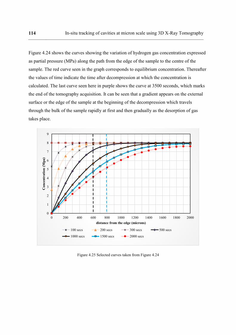
114 In-situ tracking of cavities at micron scale using 3D X-Ray Tomography

Figure 4.24 shows the curves showing the variation of hydrogen gas concentration expressed

as partial pressure (MPa) along the path from the edge of the sample to the centre of the

sample. The red curve seen in the graph corresponds to equilibrium concentration. Thereafter

the values of time indicate the time after decompression at which the concentration is

calculated. The last curve seen here in purple shows the curve at 3500 seconds, which marks

the end of the tomography acquisition. It can be seen that a gradient appears on the external

surface or the edge of the sample at the beginning of the decompression which travels

through the bulk of the sample rapidly at first and then gradually as the desorption of gas

takes place.

Figure 4.25 Selected curves taken from Figure 4.24

0

1

2

3

4

5

6

7

8

9

0 200 400 600 800 1000 1200 1400 1600 1800 2000

Con

cen

trati

on

(M

pa)

distance from the edge (microns)

100 secs 200 secs 300 secs 500 secs

1000 secs 1500 secs 2000 secs

Figure 4.26 Plots of time at Vmax of isolated cavities taken from Type-1 sample of EPDM 1.6. The size of the

bubbles correspond to the Vmax of the cavities

The edge effect described in the earlier sections can be analysed by looking at the selected

curves of global desorption shown in Figure 4.25 and comparing them with the graph shown

in Figure 4.26 which plots the time at which the cavities have attained the maximum volume

with the distance from the free surface. The size of the bubbles represent the size of the cavities.

Looking at the first section of both graphs demarcated by black dotted lines, it is seen that the

maximum volume of the cavities is reached by 850 seconds after decompression and not further

than that. There is a linear trend observed with respect to the distance from the free surface; the

more we move from the edge, the more time the cavity takes to attain its maximum volume.

Looking at the curves for the global desorption, this timeline is shown as the space between

two bold black lines corresponding to the concentration gradient of the gas at 500 and 1000

seconds after decompression. The black dotted line corresponds to the same distance of 600

microns from the free surface. The intersection of these lines show the curves for the

concentration gradients during the evolution of these cavities that have previously been termed

as edge cavities. The edge effect is corroborated here as the concentration varies rapidly during

this time at this distance from the free surface.

Looking at the second section marked by blue dotted lines in Figure 4.26 and corresponding to

the distance of 800 microns from the edge, the same effect is observed i.e. an increasing trend

towards the time taken to attain the maximum volume while moving away from the free

surface. Again, the global desorption gradients lie between the black and bold blue line in

250

450

650

850

1050

1250

1450

1650

1850

2050

2250

0 200 400 600 800 1000 1200 1400 1600 1800 2000

tim

e at

Vm

ax

distance from the edge (microns)

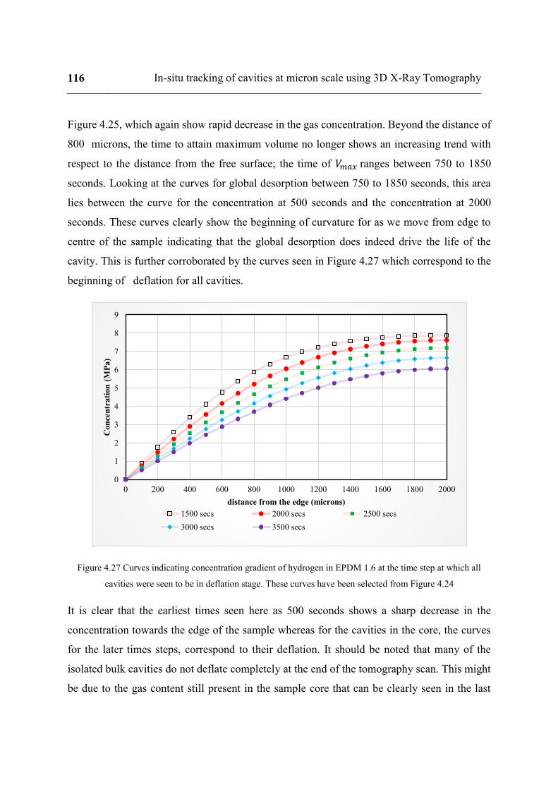
116 In-situ tracking of cavities at micron scale using 3D X-Ray Tomography

Figure 4.25, which again show rapid decrease in the gas concentration. Beyond the distance of

800 microns, the time to attain maximum volume no longer shows an increasing trend with

respect to the distance from the free surface; the time of 𝑉𝑚𝑎𝑥 ranges between 750 to 1850

seconds. Looking at the curves for global desorption between 750 to 1850 seconds, this area

lies between the curve for the concentration at 500 seconds and the concentration at 2000

seconds. These curves clearly show the beginning of curvature for as we move from edge to

centre of the sample indicating that the global desorption does indeed drive the life of the

cavity. This is further corroborated by the curves seen in Figure 4.27 which correspond to the

beginning of deflation for all cavities.

Figure 4.27 Curves indicating concentration gradient of hydrogen in EPDM 1.6 at the time step at which all

cavities were seen to be in deflation stage. These curves have been selected from Figure 4.24

It is clear that the earliest times seen here as 500 seconds shows a sharp decrease in the

concentration towards the edge of the sample whereas for the cavities in the core, the curves

for the later times steps, correspond to their deflation. It should be noted that many of the

isolated bulk cavities do not deflate completely at the end of the tomography scan. This might

be due to the gas content still present in the sample core that can be clearly seen in the last

0

1

2

3

4

5

6

7

8

9

0 200 400 600 800 1000 1200 1400 1600 1800 2000

Con

cen

trati

on

(M

Pa)

distance from the edge (microns)

1500 secs 2000 secs 2500 secs

3000 secs 3500 secs

curve corresponding to the concentration gradient in the sample at the end of the tomography

scan.

Interestingly, the idea of delayed nucleation being driven by different iso- conditions does not

seem to be correct as these cavities occur in the bulk, shown in Figure 4.26 as the spheres with

black borders, and nucleate at 350-500 seconds after decompression. At the distance of 1200

microns from the edge, the curves corresponding to the nucleation of these cavities takes place

at almost constant concentration of 8 MPa. This could raise the question of the delayed

nucleation being as a result of local stress concentration or interaction effects leading to the

nucleation of these cavities. While the question of nucleation cannot be accessed with the

present observation, the interaction effects between close cavities have been addressed in the

next section.

As mentioned earlier, this simulation is purely driven by diffusivity of the gas in the specific

material and the magnitude of the concentration at equilibrium. Since the diffusion coefficient

to EPDM does not vary significantly with respect to cross-link densities from 0.5 and 1.6, the

results from the above simulation can be interpreted for both these samples.

4.7 Inflation characteristics of close cavities

The sections details the characteristics of the close cavities and analyses them in comparison

with the isolated cavities. Groups of close cavities were taken from the global damage field of

Type-1 and Type-3 samples of EPDM 1.6 as described in the earlier section of the chapter.

Similar to isolated cavities, the volume evolution of these cavities was plotted against time and

the results were analysed taking isolated cavities as a reference for kinetics.

118 In-situ tracking of cavities at micron scale using 3D X-Ray Tomography

Figure 4.28: Volume evolution of close cavities at the edge of the sample as shown in the schematic to the right

from Type-1 EPDM 1.6 sample

Figure 4.28 shows the volume evolution of the first chosen pair of close cavities, illustrated by

the schematic, in EPDM 1.6 exposed at the pressure conditions of Psat 8 MPa and

decompression rate of 1.6 MPa/min. It should be noted that the schematic represents only

selected cavities and is not representative of the actual damage field of the sample.

It can be seen that the cavities show very low Vmax in comparison to the isolated cavities that

have been tackled in the previous section. However, since both these cavities are closer to the

edge, it is not clear whether this is due to the proximity to the edge or another cavity. The

comparison of these boundary conditions: proximity to the free surface and proximity to

another cavity needs to be addressed with another example of the close cavities in the bulk in

comparison to the cavities close to the free surface where the effect could be convoluted.

This is clarified in case close cavities in the bulk as shown in Figure 4.29 which shows the

evolution of three cavities in bulk for the same sample under the same decompression

conditions (Psat = 8 MPa, Ṗ = 1.6 MPa/min). The graph is important in illustrating the

interaction between cavities.

The larger cavity is termed as the primary cavity as it nucleates first. The second cavity in blue

nucleates closer to the primary cavity while the cavity in red nucleates farther but at the same

time. Comparing the two secondary cavities we can see that the kinetics are almost the same.

Both cavities have almost the same Vmax and rate of inflation. The lower volume and rate of

inflation is attributed to the delayed nucleation rather than different local boundary conditions.

0

500

1000

1500

2000

2500

3000

3500

4000

0 250 500 750 1000 1250 1500 1750 2000 2250 2500 2750 3000 3250 3500

VO

LUM

E (V

OX

ELS)

Time after decompression (secs)

Additionally, the evolution of the larger cavity remains unaffected by the nucleation of another

cavity close to it. In fact, the primary cavity shows similar kinetics to the isolated cavities.

Figure 4.29 Volume evolution of 3 selected cavities from the global damage field of Type-1 EPDM 1.6 sample.

This can also corroborated by the curves taken for same material albeit at more drastic

decompression conditions. Figure 4.30 shows the plots of two close cavities taken from Type-

3 samples of EPDM 1.6.

Figure 4.30 Volume evolution of 2 cavities of the selected group as shown by the raw image on the right. Cavity

1 is nucleated first while cavity 2 is nucleated later close to it.

0

10000

20000

30000

40000

50000

60000

70000

80000

90000

100000

0 250 500 750 1000 1250 1500 1750 2000 2250 2500 2750 3000 3250 3500

Vo

lum

e (v

ox)

Time (s)

0

10000

20000

30000

40000

50000

60000

70000

0 250 500 750 1000 1250 1500 1750 2000 2250 2500 2750 3000 3250 3500

Vo

lum

e (v

ox)

time after decompression (s)

cav 1 cav 2

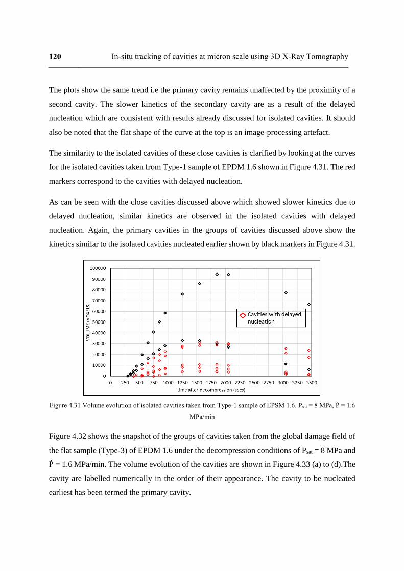
120 In-situ tracking of cavities at micron scale using 3D X-Ray Tomography

The plots show the same trend i.e the primary cavity remains unaffected by the proximity of a

second cavity. The slower kinetics of the secondary cavity are as a result of the delayed

nucleation which are consistent with results already discussed for isolated cavities. It should

also be noted that the flat shape of the curve at the top is an image-processing artefact.

The similarity to the isolated cavities of these close cavities is clarified by looking at the curves

for the isolated cavities taken from Type-1 sample of EPDM 1.6 shown in Figure 4.31. The red

markers correspond to the cavities with delayed nucleation.

As can be seen with the close cavities discussed above which showed slower kinetics due to

delayed nucleation, similar kinetics are observed in the isolated cavities with delayed

nucleation. Again, the primary cavities in the groups of cavities discussed above show the

kinetics similar to the isolated cavities nucleated earlier shown by black markers in Figure 4.31.

Figure 4.31 Volume evolution of isolated cavities taken from Type-1 sample of EPSM 1.6. Psat = 8 MPa, Ṗ = 1.6

MPa/min

Figure 4.32 shows the snapshot of the groups of cavities taken from the global damage field of

the flat sample (Type-3) of EPDM 1.6 under the decompression conditions of Psat = 8 MPa and

Ṗ = 1.6 MPa/min. The volume evolution of the cavities are shown in Figure 4.33 (a) to (d).The

cavity are labelled numerically in the order of their appearance. The cavity to be nucleated

earliest has been termed the primary cavity.

From the plots shown in Figure 4.33, it is clear that in all cases the primary cavity is the largest

cavity. In some cases, two close cavities in a group were detected at the same time step but do

not inflate to the same size; it should be noted that detection of the cavities in the same time

step does not preclude the fact of their simultaneous nucleation. In fact, due to the resolution

of the tomography, the time of nucleation is broadly used and signifies the time the cavity is

detected at the earliest possible step which in most cases is significantly later than the

nucleation time. Since the inflation is very quick in the earliest time steps, the first captured

volume of the cavity has a large error bar both in terms of quantitative value and the time step

where it is detected. It is highly probable that even when the cavities are detected at the same

time step, one of the cavities which grows to be the larger one should have nucleated earlier

than the cavity that inflates to a lower volume.

Figure 4.32 Snapshot of the global damage field of flat sample of 2 mm thickness of EPDM 1.6. 4 groups were

selected to be quantitatively analysed. The red orange, purple and green boxes enclose groups 1, 2, 3 and 4

respectively. Group 4 contains 6 cavities

122 In-situ tracking of cavities at micron scale using 3D X-Ray Tomography

(a)

(b)

(c)

0

2000

4000

6000

8000

10000

12000

14000

16000

18000

20000

0 250 500 750 1000 1250 1500 1750 2000 2250 2500 2750 3000 3250 3500

vo

lum

e (v

oxel

s)

time(s)

Cavity 1

Cavity 2

Cavity 3

0

5000

10000

15000

20000

25000

0 250 500 750 1000 1250 1500 1750 2000 2250 2500 2750 3000 3250 3500

vo

lum

e (v

oxel

s)

time(s)

Cavity 1

Cavity 2

Cavity 3

0

5000

10000

15000

20000

25000

30000

35000

0 250 500 750 1000 1250 1500 1750 2000 2250 2500 2750 3000 3250 3500

vo

lum

e (v

oxel

s)

time(s)

Cavity 1

Cavity 2

(d)

Figure 4.33 Volume evolutions of (a) group 1 (b) group 2 (c) group 3 and (d) group 4 shown in Figure 4.32. The

cavities are named in order of their appearance.

Figure 4.34 shows plots for groups of close cavities consisting of 3 cavities and 2 cavities

respectively, taken from another flat sample of EPDM 1.6 (Type-3) under the same

decompression conditions. The group with 3 cavities (Figure 4.34 (a)) consists entirely of

cavities with delayed nucleation. The graph is characteristic of secondary cavities with a less

steep slope for inflation as well as deflation.

(a)

0

5000

10000

15000

20000

25000

30000

35000

0 250 500 750 1000 1250 1500 1750 2000 2250 2500 2750 3000 3250 3500

vo

lum

e (v

oxel

s)

time(s)

Cavity 1 Cavity 2 Cavity 3

Cavity 4 Cavity 5 Cavity 6

0

2000

4000

6000

8000

10000

12000

14000

16000

18000

20000

22000

0 250 500 750 1000 1250 1500 1750 2000 2250 2500 2750 3000 3250 3500

Vo

lum

e (v

ox)

Time (s)

Cav 1

Cav 2

Cav 3

124 In-situ tracking of cavities at micron scale using 3D X-Ray Tomography

(b)

Figure 4.34 volume evolution of groups consisting of (a) 3 cavities and (b) 2 cavities.

In Figure 4.34 (b) it can be seen that the primary cavity does not inflate to be the largest cavity.

This is explained by the edge effect that has been explained in the earlier section. The distance

to the edge of the primary cavity is 516 μm; the cavities at this distance from the free surface

have been described as edge cavities in the previous sections already. Hence, this primary

cavity behaves as an edge cavity resulting in lower volume attributed to faster deflation due to

global desorption.

Figure 4.35 shows the plots of distances between the three cavities of group 1 as shown in

Figure 4.32 for Type-3 sample of EPDM 1.6. The blue and red markers correspond to the

distance of primary cavity to cavity 2 and cavity 3 respectively. In the groups of close cavities

examined, the distance between the centroids of the cavities which has been termed as core to

core distance (c-c), that is the between the centres of the primary and the secondary cavity is

never below 290 to 320 microns. Since we were able to pick only some of the groups owing to

the limitation of the image processing software in discretizing the very close cavities, it could

be possible that some cavities nucleate closer to each other than the above value. However, this

value of 290 to 320 microns could be taken as the upper limit for the distance between cavities

to form a group and thus be distinguished from the so called isolated cavities. For the distance

between the borders of the cavity (b-b), we were limited by the resolution to a minimum of 2

0

2000

4000

6000

8000

10000

12000

14000

16000

18000

20000

22000

0 250 500 750 1000 1250 1500 1750 2000 2250 2500 2750 3000 3250 3500

Vo

lum

e (v

ox)

Time (s)

cav 1

cav 2

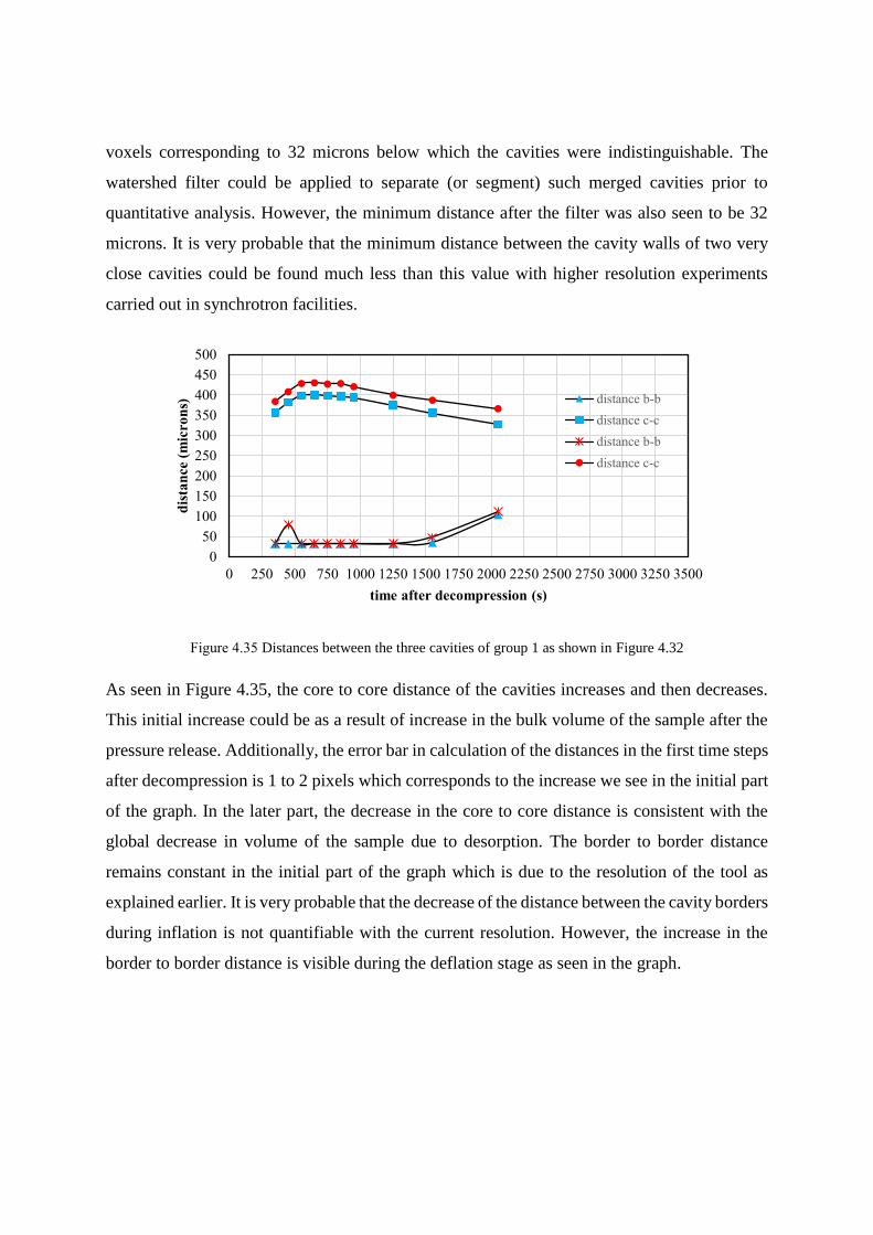
voxels corresponding to 32 microns below which the cavities were indistinguishable. The

watershed filter could be applied to separate (or segment) such merged cavities prior to

quantitative analysis. However, the minimum distance after the filter was also seen to be 32

microns. It is very probable that the minimum distance between the cavity walls of two very

close cavities could be found much less than this value with higher resolution experiments

carried out in synchrotron facilities.

Figure 4.35 Distances between the three cavities of group 1 as shown in Figure 4.32

As seen in Figure 4.35, the core to core distance of the cavities increases and then decreases.

This initial increase could be as a result of increase in the bulk volume of the sample after the

pressure release. Additionally, the error bar in calculation of the distances in the first time steps

after decompression is 1 to 2 pixels which corresponds to the increase we see in the initial part

of the graph. In the later part, the decrease in the core to core distance is consistent with the

global decrease in volume of the sample due to desorption. The border to border distance

remains constant in the initial part of the graph which is due to the resolution of the tool as

explained earlier. It is very probable that the decrease of the distance between the cavity borders

during inflation is not quantifiable with the current resolution. However, the increase in the

border to border distance is visible during the deflation stage as seen in the graph.

0

50

100

150

200

250

300

350

400

450

500

0 250 500 750 1000 1250 1500 1750 2000 2250 2500 2750 3000 3250 3500

dis

tan

ce (

mic

ron

s)

time after decompression (s)

distance b-b

distance c-c

distance b-b

distance c-c

126 In-situ tracking of cavities at micron scale using 3D X-Ray Tomography

4.7.1 Anisotropy

(a) (b)

Figure 4.36 (a) 3D picture of a group of 2 cavities b) raw image of a group of 3 cavities taken from Type-1

sample of EPDM 1.6

The main contributing factor to the anisotropy of close cavities is the topological effect created

by the proximity of cavities that could crowd the shape of the cavity, this is illustrated in Figure

4.36 (a) which shows a group of cavities taken from Type-1 sample of EPDM 1.6. This

topological effect is more pronounced when the cavity is sandwiched between two cavities as

is seen in Figure 4.36 (b) which shows another group of cavities taken from the same sample.

This is further collaborated by the plots of anisotropy for 3 groups of cavities taken from the

Type-3 EPDM 1.6 in Figure 4.37. The three groups of cavities refer to group 1, 2 and 4 as

shown in Figure 4,32. It can be seen that the anisotropy increases with time characterized by

the dip in the curve of sphericity as the cavities inflate. This is due to crowding of the cavities

leading to a topological anisotropy.

Figure 4.37: Plots for evolution of anisotropy for cavities in 3 clusters selected from the global damage filed of 2

mm flat samples of EPDM 1.6. Each color represents cavities in that cluster. The cavities appear spherical only

for a short time during inflation.

From these observations, it can be concluded that the interaction effects between close cavities

with borders at a minimum distance of 32 microns is rather trivial. The kinetics of close cavities

mimic those of isolated ones, with other factors like distance to the free surface and time of

nucleation being the first order parameters that drive the kinetics of inflation. The proximity to

other cavities remains a second order parameter mainly affecting the topological isotropy of

the cavities rather than growth kinetics. These conclusions are, however, valid for the minimum

distance measurable due to the Tomograph resolution. Furthers studies in using Synchrotron

sources with better resolution could help bring more clarity to these interaction effects at lesser

distances between borders of close cavities.

4.7.2 Qualitative observations of clustering

Clustering, as explained in earlier sections of the chapter refers to a group of cavities that

become indistinguishable visually and as such the quantitative assessment of these cavities is

not possible. However, these clusters have been observed qualitatively in this section.

Qualitatively, the flat samples of Type-3 show less clustering effect than the cubic ones. In the

cubic samples analysed (Type-1 and Type-2), it was observed that the growth of the clusters

0

0.1

0.2

0.3

0.4

0.5

0.6

0.7

0.8

0.9

1

0 250 500 750 1000 1250 1500 1750 2000 2250 2500 2750 3000 3250 3500

sph

eric

ity

time after decompression (s)

Cavité 1

Cavité 2

Cavité 3

Cavity 1

Cavity 2

Cavity 1

Cavity 2

Cavity 3

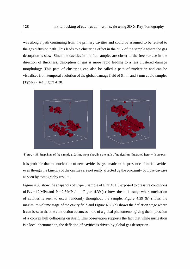
128 In-situ tracking of cavities at micron scale using 3D X-Ray Tomography

was along a path continuing from the primary cavities and could be assumed to be related to

the gas diffusion path. This leads to a clustering effect in the bulk of the sample where the gas

desorption is slow. Since the cavities in the flat samples are closer to the free surface in the

direction of thickness, desorption of gas is more rapid leading to a less clustered damage

morphology. This path of clustering can also be called a path of nucleation and can be

visualised from temporal evolution of the global damage field of 6 mm and 8 mm cubic samples

(Type-2), see Figure 4.38.

Figure 4.38 Snapshots of the sample at 2 time steps showing the path of nucleation illustrated here with arrows.

It is probable that the nucleation of new cavities is systematic to the presence of initial cavities

even though the kinetics of the cavities are not really affected by the proximity of close cavities

as seen by tomography results.

Figure 4.39 show the snapshots of Type 3 sample of EPDM 1.6 exposed to pressure conditions

of Psat = 12 MPa and Ṗ = 2.5 MPa/min. Figure 4.39 (a) shows the initial stage where nucleation

of cavities is seen to occur randomly throughout the sample. Figure 4.39 (b) shows the

maximum volume stage of the cavity field and Figure 4.39 (c) shows the deflation stage where

it can be seen that the contraction occurs as more of a global phenomenon giving the impression

of a convex hull collapsing on itself. This observation supports the fact that while nucleation

is a local phenomenon, the deflation of cavities is driven by global gas desorption.

(a) (b)

(c)

Figure 4.39 Global damage field of Tupe-2 sample of EPDM 1.6 exposed to pressure conditions of Psat = 12

MPa and Ṗ = 2.5 MPa/min

130 In-situ tracking of cavities at micron scale using 3D X-Ray Tomography

(a) (b)

Figure 4.40 Global damage fields of Type-3 samples of (a) EPDM 0.15 and (b) EPDM 1.6 exposed at the

presure coditons of Psat = 12 MPa and Ṗ = 2.5 MPa/min

Figure 4.40 shows the global damage fields of Type-3 samples of EPDM 0.15 and EPDM 1.6

exposed at the presure coditons of Psat = 12 MPa and Ṗ = 2.5 MPa/min. Looking at these

figures, it can be observed that the averge size of the cavities comprising the clusters decreases

with the increase in crosslink denisty. This is a qualitative observation at the global damage

scale. Locally, however, as discussed before, the size and kinetics of the cavities analysed in

the present study did not show any effect of the cross link density. Again, it must be noted that

the difference in crosslink densities of the samples shown in the above figures is markely higher

than the samples analysed in the present study.

4.8 Conclusions

The objective of the present study was to discriminate various factors affecting growth kinetics

of cavitation at a local scale and to clarify interaction between cavities through comparative

characterisation of isolated and close cavities. We also attempted to clarify the minimum

distance of this interaction and provide a qualitative insight into the inflation and deflation

characteristics of cavities. Since we were limited by the resolution of the tools, the very earliest

stages of nucleation were not accessible for robust quantitative analysis. Indeed the nucleation

time of the cavities described here refers to the first time step at which the cavity becomes

detectable. The volumes of the first detected cavities vary from very small (≈18 voxels) to very

large (≈1000 voxels). This variability occurs due to the conflict between the acquisition time

of the Tomograph and the very high rate of inflation at the beginning of cavity appearance. The

earliest cavities normally first appear at 150 to 300 seconds after decompression at which is

either towards the end of the decompression phase or completely after it. These cavities were

termed as primary cavities in the document. During the quantitative analysis the cavities

nucleating during the decompression phase and immediately after it show no difference in

kinetics. However, the kinetics are highly influenced by the proximity to the free surface. In

fact, by analysing the graphs for rate of inflation and the maximum volume attained by the

cavities, two sets of cavities could be distinguished based on their growth kinetics. These

cavities were termed as edge cavities and bulk cavities, a terminology that was based on the

first order parameters governing their growth. The growth of edge cavities was strongly limited

owing to the proximity to the free surface whereas the growth kinetics of bulk cavities were

more determined by other factors such as time of nucleation or other local boundary conditions.

The secondary cavities which refer to the isolated cavities that nucleate after the primary

cavities showed slower kinetics possibly due to the global desorption and changing iso

conditions. It should also be noted that the edge cavities do not appear as secondary cavities

supporting the argument that fast desorption at the free surface limits the maximum volume of

the edge cavities thereby, making the “cavity life” short.

The classification of edge and bulk cavities was supported by the simulations carried out to see

the temporal evolution of gradients of concentration along the sample geometry. There was

good agreement between the experimental results and the diffusion simulation which pointed

to this edge effect being directly related to the diffusion characteristics of the sample.

Isolated cavities were observed to be temporally isotropic during inflation and the flattening of

cavities was visible during deflation which suggests the transitioning of the cavity into a crack.

It should be noted that the formation of crack does not necessarily include coalescence. Isolated

cavities were seen to become cracks which is seen in the increase of anisotropy accompanied

by abrupt increase in volume deviating from the regular parabolic graph. As the study of

132 In-situ tracking of cavities at micron scale using 3D X-Ray Tomography

cracking was not the aim of the present study, these cavities were excluded from analysis.

However, the flattening of isolated cavities shown in the graphs above showed the beginning

of transition from cavity to crack. The reason for factors leading to the beginning of this

phenomenon are not clarified yet.

Groups of close cavities consisting of 2-6 cavities were also analysed with respect to the

distance between cavities and their respective evolution in comparison with the kinetics of

isolated cavities to see whether the interaction between cavities is a salient factor in their

growth kinetics. An attempt was made to clarify the distance between cavities at which the

interaction is perceptible. These groups of cavities were chosen from a global damage field.

Again, the limitation of the tool allowed for the quantification of characteristics of cavities with

a minimum distance of 2 voxels (32 microns). From our tests, the interaction between cavities

did not appear to be of a major consequence in terms of kinetics of the cavities. Other factors

like proximity to the edge and delayed nucleation were driving factors for kinetics in these

cavities also, much like isolated cavities. Since we were limited by the resolution, the minimum

distances between the cavities could not be accessed. However, the maximum distance between

the centres of the nucleating cavities to form a group was shown to be 290-320 microns.

Clustering of cavities i.e., number of cavities nucleating very close to each other, appeared in

all samples. However, thicker samples and cubic samples showed much more clustering than

the flat samples which is explained by the slow desorption of gas from the bulk of the samples

with more thickness. Consequently, the clustering was seen to occur along a path which could

also be seen as a path of nucleation for the secondary cavities and could be related to the gas

diffusion path or could be due to the local stress and diffusion conditions arising from the very

initial cavities. The nucleation of primary cavities was always random in all samples leading

to the important conclusion that nucleation is a localized phenomenon while the deflation of

the cavities seemed to be more driven by the global desorption. The fact that edge cavities have

a shorter life span supports this idea. Additionally, a qualitative observation of clusters in

samples of different cross-link densities showed that the average size of the cavities consisting

a cluster are larger for weakly cross linked samples. However, the parameters of cavity size

seem to be comparable for the samples of different cross-link densities analysed at the scale of

isolated cavities as well as groups of close cavities

Nevertheless, the data for local kinetics seen here is an important step for the simulations

carried out later to provide an experimental reference point for isolated or single cavity and

groups of close cavities.

134 In-situ tracking of cavities at micron scale using 3D X-Ray Tomography

Chapter 5 Investigation of interaction

effects between close cavities using Finite

Element Simulations

136 Investigation of interaction effects between close cavities using Finite Element

Simulations

One aim of the previous chapter of this document was to investigate the possible interaction of

close cavities from in-situ tomography views. Some characteristics of these cavities (growth

kinetics, shape, delayed nucleation time) was evaluated and compared to those of isolated

cavities. The analysis was based only on morphological considerations. Due to the full coupling

between diffusion and mechanics and the lack of direct tracking of the gas content field, the

discussion on mechanisms of cavity growth depending on their surrounding medium is not

trivial. Only fully-coupled microstructure simulations of the phenomenon can provide

complementary data about the diffusion problem and bring the additional material needed to

address this question. As explained in the following section, such fully coupled simulations

raise substantial numerical problems that the development of this new internal Finite Element

Code FOXTROT aims to overcome. This code has been developed at Institut Pprime by Mikaël

Gueguen and Jean-Claude Grandidier.

This chapter depicts the step forward that was attempted in a final perspective part of this study,

based on this tool.

5.1 Difficulties in simulation of cavity growth due to gas

decompression

As mentioned in Chapter 1, numerical studies for the modelling of cavity growth under purely

mechanical loading exist in literature (Lopez-pamies 2009; Ravi-chandar and Lopez-pamies

2014). However, only a few studies have been conducted at the cavity scale for decompression

failure in gas-exposed polymers at high pressure. The major difficulty of this simulation lies in

the calculation of the equilibrium volume of the cavity Vcav at each time step of the

computation, since it depends on the mechanical balance between applied external pressure,

surface tension and internal pressure inside the cavity (Pint). This internal pressure itself

depends on the number of gas molecules contained inside the cavity (updated from the gas flux

at the cavity wall) and the volume Vcav via the perfect gas law

𝑃𝑉 = 𝑛𝑅𝑇

where P is the pressure, V is the volume, n is the number of moles of the gas, R is the universal

gas constant and T is the temperature. Therefore, the solution to this fully-coupled problem at

the cavity wall must be calculated by iterating the two physical phenomenon simultaneously.

The problem is even more emphasized in rubbers, due to the application of high-pressure

loading to quasi-incompressible materials.

Figure 5.1 Hollow-sphere model developed by Jaravel et al. (2012) for the modelling of cavity growth under

decompression.

As a first step, Jaravel et al (Jaravel et al. 2013) had previously developed a hollow-sphere

model depicted in Figure 5.1. The cavity (smallest half-circle; several radii ranging from 50 up

to 500 nm) was located in the core of a rubber shell (second half-circle indexed ext). The

boundary conditions of pressure Pext and gas content cext applied to the spherical hollow-sphere

were deduced from a bulk diffusion problem through the thickness of the macroscopic sample

(with boundary conditions Pext,p and gas content cext,p ) but the problem was solved using

Matlab® along the radius of the hollow sphere, as plotted with white dots in Figure 5.1. The

evolution of the internal pressure and gas concentration inside the cavity (Pint and cint

respectively) could be computed in this way.

An interesting point was that both the surface tension at the cavity wall and finite strain

elasticity of the rubber matrix (quasi-incompressible neo-hookean constitutive law) were taken

into account. A strong limitation of this study was the 1D solving framework that prevented

simulation of close cavities. In addition, the diffusion and mechanical problems were

sequentially solved within the time step.

138 Investigation of interaction effects between close cavities using Finite Element

Simulations

In order to extend the possibility of this simulation to non-1D situations (e.g. several cavities

or non-hydrostatic mechanical loadings superimposed to the pressure release), the study of

Kane Diallo et al (2016) was carried out using Finite Element Method. This study was done by

modelling the cavity as a solid medium, in order to stabilize cavity wall problems from the

pressure continuity ensured by the mesh.

Figure 5.2 Finite Element simulation of the growth of one or two pre-existing cavities (radius 5 µm) in a bulk

elastic medium exposed to hydrogen diffusion and decompressed (Kane Diallo et al 2015). The cavity is

modelled as an “equivalent solid medium” not represented here.

The pressure dependence of the Young modulus of this “equivalent solid medium” (not

represented in Figure 5.2) was tabulated from an analogy between bulk modulus and perfect

gas law. The diffusion coefficient, solubility and volume change parameter were those of

hydrogen in air. The structure was meshed with C3D8HT elements and the problem was solved

using the heat transfer framework available in Abaqus®. The main interest of this proposal was

to make the simulation of 3D situations possible. However, the analogy with solid medium was

questionable and the simulation framework had to be restricted: the rubber matrix behavior was

linear elastic, surface tension was not taken into account finally, and convergence was obtained

by careful selection of material and loading parameters.

5.2 Development of an alternate solution with the internal Finite

Element Code FOXTROT

In order to solve these problems, an internal code has been in development for several years at

Institut Pprime, developed by Mikaël Gueguen and Jean-Claude Grandidier. The strategy is to

keep the Finite Element framework but to improve the solving of the diffuso-mechanical

problem and to take into account the surface tension.

As illustrated in Figure 5.3, the cavity is modelled as a void with continuity of the gas

concentration at the cavity wall. The cavity is viewed as a free surface with boundary conditions

that create a gas flux at the cavity wall. The problem is solved as a pressure one. The coupled

diffuso-mechanical aspect is imposed through the same pressure loading which has two

physical connotations: the mechanical hydrostatic pressure and a partial pressure

corresponding to the gas content at any point, by a factor equal to the solubility given by

Henry’s law.

Figure 5.3 Strategy of the internal Foxtrot software for diffuso-mechanical and cavity interaction modelling in

cavity growth context.

A first major improvement of this model is the calculation of the curvature of the cavity surface

at each node for each iteration of equilibrium search. No solid element was available in

iteration for mechanical equilibrium

Evaluation of the curvature at each node (Hv) of the cavity surface S

Calculation of the surface effort:

Evaluation of the number of gas moles n(t) from the fluxcavity viewed as a free surface (BC=continuity of concentration)summation of the flux integrated over all surface elements

Evaluation of the cavity volume V(t)

Updated value ofinternal pressure

diffusion problem(Henry’s law)

140 Investigation of interaction effects between close cavities using Finite Element

Simulations

Abaqus® to directly obtain the curvature of the cavity. Therefore, the load corresponding to

surface tension can be applied to each surface element and integrated into the search for

mechanical equilibrium.

Another major improvement is the ability to update the internal pressure from the perfect gas

law involving the current value of the cavity volume and the number of gas moles contained

inside the cavity, updated from the gas flux at the cavity wall integrated from the cavity surface

and the history of diffusion effect with an explicit scheme.

So far, a linear elastic constitutive law has been prescribed for the surrounding media.

Extension to finite strain elasticity is considered for future work but was beyond the scope of

this work.

5.3 Use of FOXTROT software in the context of present work

5.3.1 Main considerations

The simulations in the present work were conducted with the main following considerations:

- A pre-existing cavity, with a size of the order of those observed in the experiment by

in-situ tomography, was immersed into a cubic matrix of much larger size. The aim was

to simulate a bulk cavity, i.e. to apply similar boundary conditions at the surface of the

cubic model than those of the sample and to have vanishing gradient effects due to the

cavity when getting close to the free surface. The estimated size of morphological

Representative Volume Element of cavity fields evaluated from covariogram analysis

in Kane Diallo’s work (Kane-Diallo et al. 2016) was used as a guideline.

- The model was meshed with linear tetrahedron elements C3D4 in the bulk, and a

diffuso-mechanical coupling from finite element method was solved in the bulk. The

coupling solver use the equivalence between mass diffusion and heat transfer

equilibrium; therefore we have considered concentration as the degree of freedom of

the diffusion problem related to the heat transfer equilibrium. The gas diffusivity is

related to the thermal conductivity and an additional constant term is added to the speed

term of the mass balance of gas (the Cp constant).

- Diffuso-mechanical coupling and cavity interaction was treated at the interface using

the strategy depicted in Figure 5.3, and explained in the previous paragraph.

- The pressure loading was the same as applied in Tomography experimental campaigns,

with a saturation pressure of 8MPa and a decompression rate of 1.6 MPa/min. The

initial value was 0, indicating that the cavity is empty. As explained above, pressure

corresponds to both mechanical and diffusion loadings.

- Surface tension was not taken into account here, for several reasons. The first one was

to minimize the complexity level of the calculation. The second one was related to the

initial size of the cavity (200 µm), which exceeded the range of radii for which the

surface tension causes a considerable increase in the critical hydrostatic stress for

unstable cavity expansion (Fond 2001).

5.3.2 Limitations arising from the choice of realistic material parameters

of EPDM 1.6

As a first step, a series of calculations were conducted with parameters as close as possible to

ones used during the experiments carried out on EPDM 1.6. A cavity with an initial diameter

(8 µm) close to the tomography resolution was placed at the centre of a cube with edge of 20

microns which was then placed in the centre of another cube of edge 40 microns. This assembly

was finally placed in a cubic box of size comparable to the actual sample size (4x4x4 mm3) to

realistically simulate the conditions under which an isolated cavity exists in bulk of the sample

(illustrated in Figure 5.4). This strategy allowed for adaptable mesh size along the different

geometries. For the wall of the cavity very fine mesh was used which became coarser as we

moved away from the cavity Figure 5.4.

142 Investigation of interaction effects between close cavities using Finite Element

Simulations

(a)

(b)

Figure 5.4: Illustration of (a) 8µm-diameter cavity immersed in a boxes of different sizes (b) variable mesh size

around and far from the cavity.

The material parameters, listed in Table 5.1 were selected as close as possible to those of EPDM

1.6. The corresponding value of diffusivity D was 1.89e-04 mm²/s.

Material parameters inspired from EPDM 1.6

E = 2.75 MPa diffusivity D = 1.89e-04 mm2/s

= 0.49 Solubility S = 1

density = 1 Volume change = 2.5e-04 / MPa

“Specific heat” = 1

Table 5.1 Material parameters used as a first step to mimic EPDM 1.6

The reliability of these calculations is questionable, at least on two main points, illustrated in

Figure 5.5 which displays the time evolution of the applied pressure (green curve, left axis),

internal pressure of the cavity (red curve; left axis) and volume of the cavity (blue curve; right

axis).

Figure 5.5: Evolution of the internal pressure and volume of the cavity simulated in the model depicted in Figure

5.4, with material parameters inspired from EPDM 1.6

144 Investigation of interaction effects between close cavities using Finite Element

Simulations

The first problem is the sensitivity to the time step detectable from instabilities in the transient

stages like at the beginning of pressurization. The low elastic modulus, combined with quasi-

incompressibility and application of rather high pressure, may promote such instabilities. The

second problem is the meaningless residual volume observed at the end of the pressure cycle,

considering the fact that the matrix behavior is elastic and that the sample is fully desorbed.

It is important to underline that the same model under pure mechanical conditions (i.e. the

pressure loading only has the meaning of hydrostatic pressure) or weakly coupled diffuso-

mechanical loading (through volume change coefficient without any gas exchange at the cavity

wall) leads to stable and physically consistent solutions, returning to the initial configuration

at the end of the pressure cycle. The above depicted problems clearly originate from the full

coupling between diffusion and mechanics at the cavity wall.

5.4 Simulation of the cavity growth using modified parameters

The questions of the high dependency of these calculations on the mesh size, time step and

material parameters must be addressed for robust modelling with further studies but are beyond

the aim of the present work.

In the present study, the focus was shifted to reliable simulation of cavity growth, by using a

modified set of material parameters, mesh size and time step which had previously yielded

reliable results in a study conducted at Institut Pprime on simulation of the single cavity growth.

The focus was to compare these results to those obtained with simulation of growth of a pair

of close cavities, with all other parameters kept identical.

5.4.1 Model geometry and mesh

The model geometry and mesh used in this second simulation series for one cavity is presented

in Figure 5.6. The initial diameter of cavities was 0.2 mm and the size of the box in which the

cavity was placed was 20x20x20 mm3.

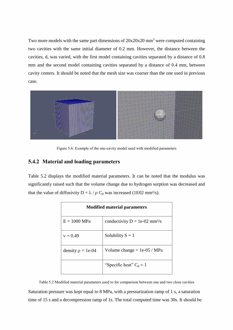
Two more models with the same part dimensions of 20x20x20 mm3 were computed containing

two cavities with the same initial diameter of 0.2 mm. However, the distance between the

cavities, d, was varied, with the first model containing cavities separated by a distance of 0.8

mm and the second model containing cavities separated by a distance of 0.4 mm, between

cavity centers. It should be noted that the mesh size was coarser than the one used in previous

case.

Figure 5.6: Example of the one-cavity model used with modified parameters

5.4.2 Material and loading parameters

Table 5.2 displays the modified material parameters. It can be noted that the modulus was

significantly raised such that the volume change due to hydrogen sorption was decreased and

that the value of diffusivity D = / Cp was increased (1E02 mm²/s).

Modified material parameters

E = 1000 MPa conductivity D = 1e-02 mm²/s

= 0.49 Solubility S = 1

density = 1e-04 Volume change = 1e-05 / MPa

“Specific heat” Cp = 1

Table 5.2 Modified material parameters used to for comparison between one and two close cavities

Saturation pressure was kept equal to 8 MPa, with a pressurization ramp of 1 s, a saturation

time of 15 s and a decompression ramp of 1s. The total computed time was 30s. It should be

146 Investigation of interaction effects between close cavities using Finite Element

Simulations

noted that the use of specific heat in this case has no physical meaning and is used as a

numerical damping factor to drive the calculation towards a reliable result.

5.4.3 Single-cavity model

Figure 5.7 displays the temporal evolution of the applied pressure (boundary condition) (green

curve; left axis), internal pressure in the cavity (red curve; left axis) and the volume of the

cavity (blue curve; right axis) during the pressure cycle.

Figure 5.7: Pressure and volume evolution of one central cavity (initial diameter 0.2mm) saturated at 8 MPa

During the saturation stage, the internal pressure increases and stabilizes rather fast, due to the

high diffusivity value. The cavity volume first decreases due to the mechanical pressure and

then increases as the gas penetrates into the cavity. Subsequently, the cavity volume stabilizes

to a value depending on both the equilibrium content of gas inside the cavity and the

surrounding swelling of the bulk matrix due to equilibrium hydrogen content.

As a comparison, Figure 5.8 shows the volume change of the cavity obtained from simulations

with (blue curve) and without (orange curve) gas exchange at the cavity. The latter case can be

compared to an adiabatic situation in the context of a heat transfer problem. Hence, the cavity

remains compacted all along the pressurization and saturation stages. In these simulations, the

expansion coefficient was ten times larger than in Figure 5.7. It can be noted that the stabilized

volume at saturation was only slightly smaller, suggesting that within this range of expansion

coefficient, the indirect effect of bulk swelling had minor effect. The internal pressure is seen

to decrease during decompression in a consistent way while the cavity volume is first seen to

increase as a result of the mechanical pressure release, and then decrease back to the initial

value.

All this phenomenology is consistent with the previous results obtained by Jaravel et al. and

Kane Diallo et al. in the different frameworks reported in section 5.1.

It can be noticed that the volume inflation of the cavity is very small. This is due to the stiffness

of the matrix and its linear elastic behavior which leads to an overestimated stress increase

during inflation and limits the growth in comparison with the one expected in real rubber.

Figure 5.8: Time evolution of the computed volume of the cavity with (blue curve) and without (orange) gas

exchange at the cavity wall (volume change parameter due to hydrogen sorption = 1e-04 MPa-1)

148 Investigation of interaction effects between close cavities using Finite Element

Simulations

Figure 5.9 illustrates a primary analysis of the response of the bulk in close proximity to the

cavity. These graphs show the evolution of the displacement magnitude and the gas content at

three different points around the cavity, i.e. at 0.1 mm from the cavity surface along the three

directions x, y and z. The gas content profile was identical whatever the direction. Small

differences were observed on the displacement magnitude, probably due to the discretization

error.

(a) (b)

Figure 5.9: Evolution of (a) displacements magnitude and (b) gas content at three different points close to the

cavity. Coordinates of the cavity centre were (10; 10; 10). Coordinates of probes labelled "x = 9.8", "y = 9.8"

and "z = 9.8" were respectively (9.8; 10; 10), (10; 9.8; 10) and (10; 10; 9.8).

Figure 5.10: View of the location of cavities (diameter 0.2mm) in the one-cavity model (green), two-cavity

model with a core-to-core distance d of 0.8mm (blue) or 0.4mm (yellow); white line shows the path for gas

concentration profile plot in Figure 5.11 (line between (10,10,0) and (10,10,20) points).

Figure 5.11 plots the gas concentration profile through the sample, along the path plotted in

white line in Figure 5.10, for different times of the pressure history.

Figure 5.11: Gas concentration profile through the sample along the direction plotted in white line in Figure

5.10.

150 Investigation of interaction effects between close cavities using Finite Element

Simulations

The red curve in Figure 5.11 (1.2s) was obtained just after the end of pressurization.

Concentration equals the applied partial pressure at the sample surface. A symmetrical gradient

is visible through the thickness. The cavity corresponds to the curve interruption since no

output from the Finite Element calculation is available in areas without material. It is clear that

the presence of the cavity creates a kind of “concentration well” with a spatial width around

0.2mm on each side when extrapolating the linear regimes observed from the cavity edges.

The flat orange curve (16s) was obtained at the end of saturation. The gas content is

homogeneous at any point of the matrix.

The green curve (16.8s) corresponds to the concentration profile during decompression. Value

at the free surface corresponds to the current value of the loading pressure ramp. A significantly

higher concentration is obtained close to the cavity which “traps” gas molecule for a while.

Figure 5.12 shows the gas pressure field (corresponding to the gas content one). Again, the

sharp gradient is observed over a shell about one diameter thick around the cavity.

The blue curve (18s) is obtained 1s after the end of decompression. It is almost flat to zero,

except around the cavity where an excess of gas can be observed. It can be assumed that the

full desorption of this residual gas could take a time significantly longer than the time scale of

bulk desorption.

Figure 5.12: Pressure fields (corresponding to the gas concentration one) in the full model and around the cavity

after 16.8s i.e. during decompression (80% of pressure release)

5.4.4 Two-cavity models

In order to discuss the possible interaction between close cavities, two two-cavity models were

simulated, with the same initial diameter of 0.2mm for all of them and a core-to-core distance

d of 0.8mm (blue cavities in Figure 5.10) and 0.4 (yellow cavities in Figure 5.10). In the initial

configuration, the edge-to-edge distance corresponded respectively to three and one diameter.

(a) (b)

Figure 5.13: Pressure and volume evolution of the two cavities (C_1 and C_2) compared to those of the single

one for a core-to-core distance d of (a) 0.8mm and (b) 0.4mm.

Figure 5.13 compares the time evolution of internal pressure and the volume change of the two

cavities (called C_1 and C_2 in the graphs) to those of the single one for the two core-to-core

distances d.

During saturation, the phenomenology was similar to that commented before for one single

cavity. The main difference was that the stabilized volume of the two cavities was significantly

smaller than that of the single cavity, like if the sorbed gas was distributed into the two cavities.

The pressure kinetics was almost the same. A small difference between C_1 and C_2 curves

was observed before saturation for d=0.8mm and a little bit more distinguishable for d=0.4mm.

152 Investigation of interaction effects between close cavities using Finite Element

Simulations

Again, the volume evolution was very small. Its evolution was a little bit different between

C_1 and C_2. There was no physical reason for this since the model was symmetrical to the

plotted axis and since the initial size of the two cavities was the same. The scatter was even

more important for d=0.4mm. Moreover, a residual value was observed at the end of the

pressure cycle. More simulations should be conducted to evaluate how far the spatial

discretization and subsequent cumulative effects could be responsible for these differences.

The possible interaction effect can be mainly discussed from the gas concentration profiles

plotted in Figure 5.14 at the same intermediate times as in Figure 5.11 for the single cavity.

Regarding the gradient in the bulk matrix around the cavity or the pair of cavities, the global

phenomenology is similar between the two two-cavity models and the one-cavity one. As a

complement, Figure 5.15 displays the concentration profiles during (16.8s) and after

decompression (18s) for the two models. The sharpness of concentration gradients seems

unchanged. Curves appear shifted by the difference of core-to-core distance.

(a) (b)

Figure 5.14: Gas concentration profiles at different times of the pressure cycle for the two-cavity models with

core-to-core distance d of (a) 0.8mm and (b) 0.4mm

Figure 5.15: Gas concentration profiles in the two two-cavity models during (16.8s) and after (18s)

decompression.

An interesting difference, confirmed by the concentration fields viewed in Figure 5.16, deals

with the significant residual gas concentration observed between the two cavities, especially

when they are close to each other by one diameter only. This residual value remains high even

when the bulk matrix around the pair of cavities is almost fully desorbed.

Figure 5.16: Pressure fields (corresponding to the gas concentration one) in the full model and around the cavity

after 16.8s i.e. during decompression (80% of pressure release) in the two-cavity model with core-to-core

distance d=0.4mm

154 Investigation of interaction effects between close cavities using Finite Element

Simulations

5.5 Conclusions

The simulation of cavity growth resulting from gas decompression using Finite Element

Method in a quasi-incompressible medium under high-pressure while considering the problem

as a fully coupled diffuso-mechanical one is a quite a huge challenge. Therefore, the

development of the internal code Foxtrot is an unprecedented attempt in literature. The aim of

developing this code was to use it in the present work to highlight the two physical fields

interacting during the inflation / deflation of close cavities.

Beyond the questionable fact that the above simulations are based on a pre-existing large

cavity, there are other numerical limitations such as sensitivity to the mesh size and time step,

as well as the limitation of the tool to linear elastic behaviour law characterizing the matrix.

Hence, only a few simulations could be possible which nevertheless provided a qualitative

comparison. Pairs of 0.2 mm-diameter cavities, separated by a distance of 0.6 mm (3 times the

diameter) and 0.2 mm (equal to the diameter) between their borders, were simulated and

compared to a single cavity under the same pressure cycle (saturation pressure 8 MPa).

In the latter case, a significant gas content gradient was observed around the cavity over a

distance of about one diameter. The growth was logically isotropic. In the former case, the

accuracy and spatial extension of gradients around cavities was almost similar to the ones in

the bulk direction. On the other hand, a residual gas content was observed in the ligament

between cavities. This “trapped” gas concentration was very close to the value at the cavity

surface when the ligament thickness equaled the diameter of the cavity.

These preliminary simulations indicate a rather local growth process and weak interaction

between cavities as soon as the thickness of the ligament separating them exceeds the value

equivalent to three times the cavity diameter, but at this stage any transition of these results to

interpret the “real rubber” investigated in Chapter 4 must be very careful, even based on

dimensionless considerations. Among other limitations, the sharpness of gradients and volume

change of cavities directly derives from the material parameters which were far from the ones

of real rubber.

General Conclusions and Perspectives

The work presented in this manuscript focused on the cavitation in unfilled EPDM rubber

induced after saturation in hydrogen during decompression. This experimental campaign was

possible thanks to collaboration between Hydrogenius laboratory at Kyushu University (Japan)

and Institut Pprime (France) funded by the French program “Investissements d’Avenir” Labex

Interactifs (reference ANR-11-LABX-0017-01).The main aim was to shed light on how far the

heterogeneity of the rubber matrix and cavitation were systematic. For this purpose,

experiments were carried out at two scales,

At sub-micron scale SAXS experiments were carried out for samples in equilibrium state as

well as immediately after decompression. For the in-situ tests, a novel pressure chamber was

designed with diamond windows which allowed the SAXS experiments to be carried out for

samples in saturated state to characterize the structural changes in EPDM rubber matrix if any

due to hydrogen exposure using the parameter of correlation length. These experiments were

also repeated using Synchrotron X-ray source (SAGA-LS) in Japan. Complementary ex-situ

tests were performed after exposure by S. Tencé-Girault (Arkema & PIMM laboratory at

ENSAM ParisTech).

The results from the in-situ test at low pressure do not indicate a change in the size of

heterogeneities in the rubber matrix due to the hydrogen exposure. This is contrary to the

calculations from the ex-situ test which clearly show increase in the correlation length after

decompression from high-pressure exposure (30 MPa). This could be pointed out that at low

saturation pressure, the penetrated hydrogen content is very small which is not enough to affect

any changes in the rubber matrix. However, the results from the synchrotron source

experiments showed a slight and diffused plateau that could be a possible indicator of a

correlated structure. To clarify this, additional scattering experiments were carried out

exploring a longer q-range which could enable the acquisition at a lower value of q that is

0.05nm-1. This plateau was observed again in case of unexposed samples which became clearer

in the Lorentz corrected plots. However, the position of these maxima were not directly

correlated with the cross-link density of the samples. After exposure, the maxima were no

longer detected. This was as a result of large central scattering that was superimposed on the

156 General Conclusions and Perspectives

initial spectra due to scattering by the cavities that appeared in the sample after decompression

from high pressure. It is important to note that these experiments were carried out after the

complete desorption of hydrogen form the sample. Results from the scattering experiments

done immediately after decompression during the desorption of hydrogen indicate that the

spectra of the exposed samples taken immediately after decompression show a marked

difference from the spectra of the unexposed sample and these spectra tend to approach those

of the unexposed samples as the desorption progresses. However, the spectra of the exposed

samples do not superimpose those of the unexposed samples even after complete desorption of

the gas, indicating a permanent structural change in the rubber matrix after single hydrogen

exposure. As a general conclusion, it can be underlined that the hydrogen exposure leads to

microstructural change in the rubber matrix which is retained even when the gas is fully

desorbed. It was also seen that the heterogeneity of the rubber matrix at the sub-micron scale

is not directly correlated with the cross-link density. Additionally, the low pressure experiments

are not enough to calibrate the degree of heterogeneity in rubber matrix; the in-situ experiments

carried out in the present study showed that no change in the correlation length, corresponding

to the matrix heterogeneity, was observed after hydrogen exposure.

At higher scales, tracking of cavitation in EPDM was carried out using time resolved 3D in-

situ tomography, the main aim of which was to clarify the interaction between cavities at a

local scale through comparative characterization of isolated and close cavities. An attempt was

also made to clarify the minimum distance of this interaction and provide a qualitative insight

into the inflation and deflation characteristics of cavities at the scale accessible due to the

resolution of the tool (30 microns). For this purpose two different cross-link densities of EPDM

were tested with different decompression conditions and sample geometries.

The earliest cavities were observed at 150 to 300 seconds after decompression at which is either

towards the end of the decompression phase or completely after it. These cavities were termed

as primary cavities in the document. During the quantitative analysis the cavities nucleating

during the decompression phase and immediately after it show no difference in kinetics.

However, the kinetics are highly influenced by the proximity to the free surface. In fact for

cavities with a distance of about 800-900 microns in case of EPDM 1.6 and 700-800 microns

for EPDM 0.5, this driving force superseded any other local boundary condition. These cavities

were termed as edge cavities distinguished from the bulk cavities which nucleated in the core

of the sample and whose kinetics were dependent on the local boundary conditions and time of

nucleation. The edge cavities were seen to have a short life driven by the global desorption.

The classification of edge and bulk cavities was supported by the simulations carried out to see

the temporal evolution of gradients of concentration along the sample geometry. There was

good agreement between the experimental results and the diffusion simulation which pointed

to this edge effect being directly related to the desorption field of the sample.

The secondary cavities which refer to the cavities that nucleate after the primary cavities

showed slower kinetics possibly due to the global desorption and changing iso-conditions. It

should also be noted that the edge cavities do not appear as secondary cavities supporting the

argument that fast desorption at the free surface limits the maximum volume of the edge

cavities thereby, making the “cavity life” short.

Isolated cavities were observed to be temporally isotropic during inflation and the flattening of

cavities was visible during deflation which suggests the transitioning of the cavity into a crack.

It should be noted that the formation of crack does not necessarily include coalescence. Isolated

cavities were seen to become cracks which is seen in the increase of anisotropy accompanied

by abrupt increase in volume deviating from the regular parabolic graph. As the study of

cracking was not the aim of the present study, these cavities were excluded from analysis.

However, the flattening of isolated cavities shown in the graphs above showed the beginning

of transition from cavity to crack.

Clustering of cavities i.e., number of cavities nucleating very close to each other, appeared in

all samples. However, thicker samples and cubic samples showed much more clustering than

the flat samples which is explained by the slow desorption of gas from the bulk of the samples

with more thickness. Additionally, the clustering was seen to occur along a path which could

also be seen as a path of nucleation for the secondary cavities and could be related to the gas

diffusion path or could be due to the local stress and diffusion conditions arising from the very

initial cavities. The nucleation of primary cavities was always random in all samples leading

to the important conclusion that nucleation is a localized phenomenon. The fact that edge

cavities have a shorter life span supports this idea.

Clustering was analysed quantitatively with respect to distance between cavities and their

respective evolution to compare with the kinetics of isolated cavities and to clarify the distance

158 General Conclusions and Perspectives

between cavities at which the interaction is perceptible. From our tests, the interaction between

cavities did not appear to be of a major consequence in terms of kinetics of the cavities. Other

factors like proximity to the edge and delayed nucleation were driving factors for kinetics in

these cavities also, much like isolated cavities. Since we were limited by the resolution, the

minimum distances between the cavities could not be accessed. However, the maximum

distance between the centres of the nucleating cavities to form a cluster was shown to be 290-

320 microns. A more qualitative analysis of clustering leads to a more global conclusion that

while nucleation seems to be a very localized process whereas deflation of cavities seems to be

driven by the macroscopic desorption field of the sample.

The results of 3D in-situ tomography campaign, while providing novel observations of the

phenomenon, do not make it possible to understand the nature of the diffuso-mechanical

characteristics which govern the growth, and possibly the interaction of cavities under gas

decompression. For this purpose, in the later part of the study, simulations of the growth of

cavities in strongly coupled diffuse-mechanical conditions were attempted using an internal

Finite Elements code (Foxtrot) developed by M. Gueguen and J.C. Grandidier. These

simulations are inherently very complex from a numerical point of view and the framework in

which these calculation can be successful in the present state is significantly different from the

real case of the elastomer (EPDM) studied here. The main assumptions that were made for

these simulations include the pre-existence of a cavity in the elastomer matrix in the initial state

are, the linear elastic behavior law governing the matrix and no introduction of a criterion of

rupture of the cavity wall accompanying its growth. Nevertheless, the novelty of the present

work in comparison to the studies in literature is the calculation of gas exchange at the cavity

wall at every step, such that the internal pressure and volume of the cavity take into account

the mechanical loading during the pressure cycle as well as the diffusion aspect.

The series of simulations carried out in the present work showed that the gas concentration

fields around the cavity have strong gradients over a range roughly equivalent to its diameter.

When the distance between two cavities is of this order, a significant gas concentration remains

in the ligament separating the cavities during desorption. The validity of this result in the more

realistic framework of the hyperelastic elastomer remains to be confirmed. However, this result

could explain the possibly influence of cavitation to the subsequent evolution of the damage in

general, and contribution to the nucleation of other peripheral cavities in particular.

Perspectives: Future work, as a continuation of the present project at a larger scale could be

proposed as follows.

As a first direct perspective of this study, it could be interesting to conduct more in-situ SAXS

experiments with a higher pressure which could provide much needed data about the rubber-

hydrogen matrix at equilibrium and at the very beginning of decompression. The tests

performed in the present study offer a starting point for designing such complex experiments

for future studies. It is also important to explore a broader q range by Ultra Small Angle X-Ray

Scattering (uSAXS) which could make the variation of the scattering accessible at very low

values of q.

Nevertheless, scattering methods provide average estimation of the diffusing entities and for

actual observable cavities, direct visual and optical tracking provides useful complementary

data. Still based on tomography experiments, the use of a synchrotron radiation source would

significantly improve the space and time resolution and make it possible to better detect earlier

stages of cavitation. The question of minimum distance for interaction of cavities could be

better addressed. Such experiments could also provide information about coalescence by

quantitatively analysing clusters which were not accessible with the present resolution.

However, the experimental tracking of this kind of damage has limitations even with very

advanced tools. The very beginning of cavity nucleation and the transition from a

heterogeneous gas-polymer equilibrium state to a damaged medium, cannot be observed from

the currently available experimental tools even by decreasing the space resolution down to the

micron. In addition, the diffusion field of the sample cannot be directly measured. For this

reason, the improvement of the Finite Element tool Foxtrot is of vital importance. The

immediate improvements include implementation of finite strain elasticity and clarifications as

well as corrections of numerical convergence / stability limitations.

In the more general context of this study, many open questions still exist. One of the current

issues being investigated is the evolution of damage upon pressure cycling which directly raises

questions on the interaction effect between close cavities. Factors that could influence the

global gas content and gas content heterogeneity in the rubber matrix before decompression is

160 General Conclusions and Perspectives

also worth being investigated. These include the saturation pressure (which changes the

solubility) and several microstructural parameters such as cross-link density and effect of

fillers. Finally, the present work was focused on rubbers exposed to hydrostatic pressure which

is far from the realistic conditions that rubber seals are subjected to in the hydrogen transport

and delivery system. Therefore, further work on these material should emphasize on including

the effect of mechanical loading in addition to the pressure induced due to gas exposure; many

practical limitations could be expected for carrying out these experiments.

Résumé étendu en français

IN-SITU INVESTIGATION OF CAVITY NUCLEATION AND GROWTH IN

HYDROGEN-EXPOSED EPDM DURING DECOMPRESSION

La thèse traite de l’endommagement par cavitation des élastomères exposés à de fortes

pressions de gaz diffusant. Ce phénomène résulte de l’expansion locale du gaz préalablement

absorbé, lorsque la désorption hors du polymère est trop lente par rapport au chargement

imposé. Elle vise à mieux comprendre le mécanisme élémentaire de formation, puis de

croissance et de coalescence des cavités, isolées ou en proche voisinage. Dans ce dernier cas,

une éventuelle interaction doit effectivement être caractérisée pour éclairer la coalescence et la

transition vers des fissures macroscopiques.

Le travail a été mené sur série d’Ethylène Propylène Diène Monomer (EPDM) non-renforcés,

avec une densité de points de réticulation variable, exposés à des pressions allant jusqu’à 30

MPa. Le volet expérimental s'appuie sur deux des techniques expérimentales in situ les plus

récentes : la diffusion des rayons X aux petits angles (SAXS) qui vise à caractériser les

hétérogénéités du système réseau élastomère – hydrogène à l'échelle submicronique (chapitre

3), et la tomographie X in-situ (sous des pressions allant jusqu’à 12 MPa) qui fournit des vues

3D résolues en temps des cavités, pendant et après décompression, et permet de préciser les

mécanismes (chapitre 4). Un second volet tente brièvement de discuter les effets d’interaction

entre cavités voisines à partir de simulations Eléments Finis en conditions diffuso-mécaniques

fortement couplées (chapitre 5).

Chapitre 1 - Bibliographie

Dans les élastomères, la cavitation d’origine purement mécanique fait référence à l'apparition

et à la croissance de défauts présents intrinsèquement dans la matrice de caoutchouc. Il s’agit

soit de vides sous-micrométriques préexistants dans la matrice de caoutchouc en raison de

l'inhomogénéité du réseau ou d'impuretés qui peuvent provoquer des concentrations de

contraintes locales conduisant à la nucléation de cavités. Sous l'application de contraintes

162 Résumé étendu en français

externes suffisamment importantes, ces défauts se développent élastiquement jusqu'à

l'extensibilité maximale des chaînes macromoléculaires environnantes et à la rupture du réseau.

Peu d’études existent sur la cavitation sous décompression de gaz. Jusqu'à présent, la littérature

sur le sujet s’est concentrée sur une analyse qualitative après que la décompression a déjà eu

lieu et n'ont été étayées que par de rares suivis visuels du dommage au cours de la

décompression. Cela est dû à la complexité des techniques expérimentales nécessaires pour

accéder au phénomène in situ. Des techniques expérimentales in-situ, notamment

tomographiques, ainsi que des modélisations diffuso-mécaniques fortement couplées, ont

récemment permis de mieux comprendre ce phénomène et d’accéder à une quantification fiable

de la morphologie et de la cinétique des champs de cavités. Leur sensibilité à plusieurs types

de facteurs extérieurs, dont les conditions d’exposition et de décompression, a également pu

être caractérisée.

Peu d'études abordent la question de l'origine des cavités, en raison des hétérogénéités locales

inhérentes à une structure amorphe (e.g. les enchevêtrements, les noeuds de réticulations ainsi

que des défauts résultant du processus de fabrication) qui agissent comme précurseurs de la

cavitation. Aucune clarification expérimentale n'est fournie pour ces hypothèses. Des études in

situ à une échelle submicronique pourraient être une étape importante vers la clarification de

cette hypothèse.

Le deuxième facteur important à analyser est l’effet d'interaction entre les cavités qui pourrait

aggraver les dommages et conduire à des fissures dans le matériau. Dans la première étude de

cavitation, Gent et al ont observé deux populations de cavités, à savoir des cavités satellites

supposées apparaître autour de cavités primaires en raison d'une concentration de contraintes

locales. Le caractère systématique ou non de cette initiation différée n'a pas été clarifié

expérimentalement et reste encore une question ouverte. Cette morphologie des dommages a

été confirmée par Jaravel (2011) dans son étude sur les caoutchoucs de silicone exposés à

l'hydrogène lors de la décompression. Kane Diallo (2016) a abordé les champs de cavités pour

mettre en évidence la distribution spatiale des deux populations de cavités. Il a conclu que la

distribution du diamètre de la cavité évoluait avec l'augmentation de la pression de saturation

ou du taux de décompression et augmentait la tendance à la nucléation différée et à la formation

de deux populations. Ono et al ont étudié l'évolution de la décompression due à la cavitation

due aux gaz avec une exposition cyclique montrant que l'évolution des dommages n'était pas

un processus cumulatif classique avec réapparition systématique des cavités conduisant à la

coalescence. À l'échelle locale, des processus diffuso-mécaniques couplés plus complexes

régissent l'évolution des dommages.

Dans ce contexte, l'objectif principal de cette thèse est l'analyse de la cavitation au niveau

local, avec une attention particulière portée sur la notion d’hétérogénéité de la distribution et

sa corrélation avec le réseau de caoutchouc pour comprendre dans quelle mesure elles sont

systématiques. Cela a été fait par une technique d'expérimentation à plusieurs échelles, dont la

première étape consiste à accéder aux données de la matrice de caoutchouc à des échelles sub-

microniques via SAXS. Cela a été fait pour les matériaux vierges (avant exposition à

l'hydrogène) ainsi qu'après décompression. Des tests in situ supplémentaires ont été effectués

en utilisant un montage expérimental qui a été développé spécifiquement pour le présent travail

et est rapporté ici pour la première fois. Cette technique expérimentale, bien qu'en phase

naissante, est la première étape du développement d'un outil robuste pour des tests in situ aussi

complexes. À des échelles plus élevées, les dommages ont été suivis in situ à l'aide d'une

tomographie à rayons X 3D qui a permis pour la première fois un rendu 3D correct de ces

dommages et constitue une nette amélioration par rapport aux techniques de suivi 2D utilisées

précédemment. L'obtention des données aux deux échelles était importante pour les simulations

effectuées dans FOXTROT, un outil numérique développé à l'Institut P prime pour les

problèmes couplés qui a fourni un moyen réaliste de modéliser le phénomène de cavitation

résultant du couplage entre la pression hydrostatique et la diffusion de gaz.

Chapitre 2 - Matériaux

Le matériau sur lequel porte la présente étude est le caoutchouc EPDM (Ethylene Propylene

Diene Monomer). L’EPDM est un caoutchouc synthétique qui trouve principalement des

applications dans les domaines impliquant des solvants, des acides et d'autres produits

chimiques agressifs en raison de ses propriétés d'excellente résistance chimique et thermique.

Il est notamment utilisé pour la fabrication de joints dans un certain nombre d’applications

industrielles, en particulier dans les véhicules à pile à combustible et d’infrastructures

associées. De plus, la morphologie et la cinétique de l’endommagement généré dans cet

élastomère est accessible par les différentes techniques mises en œuvre dans le travail.

164 Résumé étendu en français

Dans le cas présent, le pourcentage d’éthylène est tel que l’élastomère ne cristallise pas. Des

échantillons présentant trois densités volumiques de points de réticulation (qualifiés par la suite

d’EPDM 0.1, 0.5 et 1.6) ont été fournis par le laboratoire HYDROGENIUS de l'Université de

Kyushu, au Japon. Ils ont été découpés soit dans des feuilles de 2 mm d'épaisseur moulées par

compression, soit dans des feuilles de 4 mm d'épaisseur fabriquées par compression thermique

de deux feuilles de 2 mm d'épaisseur. Des échantillons cylindriques de diamètre 29 mm et

d'épaisseur 13 mm ont également été fournis.

Plusieurs tests ont été effectués pour caractériser les matériaux, principalement pour fournir

des données importantes pour la corrélation des paramètres d'endommagement avec le

matériau et les caractéristiques de diffusion du matériau lui-même. En effet, l’étude est centrée

sur les dommages de l'EPDM pendant la décompression à partir d'un état d'équilibre. Par

conséquent, le profil d'hydrogène pendant la désorption des échantillons testés est d'un intérêt

particulier et est discuté en fonction des différentes pressions et degrés de réticulation.

L’évolution de la teneur en hydrogène a été suivie par TDA (Thermal Desorption Analysis) au

sein de disques de 13 mm de diamètre et 2 mm d'épaisseur placés sous un balayage d’argon

après saturation sous pression d’hydrogène et décompression.

La concentration d'hydrogène dans l'Argon a été mesurée par chromatographie en phase

gazeuse et la teneur en hydrogène résiduel de l'échantillon a été calculée. Le coefficient de

diffusion de l’hydrogène dans l’EPDM et la solubilité sont déduits de la courbe obtenue.

Chapitre 3 – Caractérisation sub-micronique par diffusion des

rayons X aux petits angles

L’objectif de ce chapitre est de caractériser les hétérogénéités du mélange hydrogène – EPDM

dans différentes conditions : avant exposition, à l’équilibre sous pression de gaz, et pendant la

décompression puis la désorption.

L'étude de la cavitation dans les polymères utilisant la méthode des SAXS (Small-Angle X-ray

Scattering) est bien établie dans la littérature pour les microstructures semi-cristallines.

Cependant, la plupart des analyses de ce type de dommages se font dans des conditions

purement mécaniques. En comparaison, moins de publications existent pour les études sur les

interactions des polymères entre les polymères et les fluides diffusants. Les expériences SAXS

in situ ont été largement utilisées pour étudier les propriétés de diffusion des gels polymères et

il existe plusieurs mesures quantitatives de la longueur de corrélation associées à la fois aux

fluctuations thermiques et au gel des contraintes topologiques. Ces études se limitent

principalement au gonflement des polymères dans un liquide. D'un point de vue pratique, les

substances polymères sont poly-dispersées, consistant en des conformations lâches à l'état

amorphe et des agrégats aléatoires de couches lamellaires pour des microstructures semi-

cristallines. Par conséquent, les études SAXS pour la caractérisation des hétérogénéités locales

pour la matrice de caoutchouc amorphe sont plus difficiles que les études des systèmes

monodisperses et dépendent de modèles appropriés pour l'interprétation des modèles de

diffusion.

Afin de comprendre les changements dans la matrice de caoutchouc dus à la saturation en

hydrogène, ainsi que pendant la phase de décompression qui marque le début de la cavitation,

des tests in situ sont indispensables. Cependant, les tests in situ sont difficiles à concevoir en

raison des difficultés pratiques de manipulation de l'hydrogène en laboratoire. Un dispositif

expérimental SAXS pour les tests in situ dans l'hydrogène a été développé par le Laboratoire

HYDROGENIUS de l'Université de Kyushu (Japon). Conformément aux réglementations

japonaises relatives à l'utilisation du gaz en laboratoire et aux contraintes des conditions de

sécurité associées, il faut s'assurer que les tests sont effectués à des pressions très basses

inférieures à 1 MPa. Une autre difficulté résultant de l'utilisation d'une source de rayons X de

laboratoire est que le temps d'acquisition est généralement long. Il réduit considérablement le

nombre de points de données valides, ce qui est particulièrement critique juste après la

décompression. Pour cette raison, dans la présente étude, des tests SAXS in situ et ex situ ont

été effectués dans diverses installations afin d'obtenir le plus d'informations possible dans

différentes conditions de taille de faisceau et à différents moments de dommages. Des tests

SAXS ont également été effectués au Kyushu Synchrotron Light Research Center au Japon.

Ces campagnes ont été complétées par des mesures SAXS effectuées chez Arkema par S.

Tencé-Girault, avec un diamètre de faisceau incident plus faible, sur la même série d’EPDM

non-exposés et après décompression sous 30 MPa.

Les tests in situ effectués sur EPDM 0,1 et 0,5 ne montrent aucun changement dans la longueur

de corrélation, ce qui indiquerait un changement dans la taille des hétérogénéités dans la

matrice de caoutchouc en raison de l'exposition à l'hydrogène. Ceci est cependant dû à la faible

166 Résumé étendu en français

pression de saturation et est confirmé par les résultats des expériences ex situ qui montrent

clairement une augmentation de la longueur de corrélation après décompression à partir d'une

exposition à haute pression. Cependant, les résultats des expériences de source synchrotron ont

montré un plateau léger et diffus qui pourrait être un indicateur possible d'une structure

corrélée. Pour clarifier cela, des expériences de diffusion supplémentaires ont donc été menées

en explorant une plage de q plus longue qui pourrait permettre l'acquisition à une valeur

inférieure de q qui est de 0,05 nm-1. Ce plateau a été observé à nouveau en cas d'échantillons

non exposés. Cependant, les résultats ne sont pas directement corrélés à la densité de

réticulation des échantillons.

Après l'exposition, aucun maximum n’est détecté. Cela est dû à une diffusion centrale

importante qui se superpose aux spectres initiaux, en raison de la diffusion par les cavités

apparues dans l'échantillon après décompression à haute pression. Il est important de noter que

ces expériences ont été réalisées après la désorption complète de l'hydrogène de l'échantillon.

Les spectres des expériences de diffusion effectuées immédiatement après la décompression

pendant la désorption d'hydrogène montrent une différence marquée par rapport aux spectres

de l'échantillon non exposé. Ces spectres ont tendance à se rapprocher de ceux des échantillons

non exposés au fur et à mesure de la désorption, sans toutefois se superposer même après

désorption complète du gaz. Ceci indique un changement structurel résiduel dans la matrice de

caoutchouc après une seule exposition à l'hydrogène.

Les tests effectués dans la présente étude offrent un point de départ pour concevoir de telles

expériences complexes pour de futures études. Dans le cas présent, les tests donnent un aperçu

de la taille de l'hétérogénéité dans la matrice de caoutchouc amorphe et mettent en évidence

l'effet de l'hydrogène sur la matrice de caoutchouc à très faible échelle.

Chapitre 4 – Suivi des cavités à l’échelle micronique par

tomographie RX in-situ

L’approche par SAXS analyse les hétérogénéités en moyenne dans le volume à des échelles

fines. L’approche complémentaire qui fait l’objet de ce chapitre permet une visualisation

directe de l’endommagement en 3D résolue en temps des cavités, pendant et après

décompression, mais travaille à des échelles supérieures. Cette expérience de tomographie in-

situ sous décompression d’hydrogène est inédite dans la littérature. Les difficultés

d'observation et de quantification du phénomène de cavitation des élastomères dues à la

décompression des gaz sont des facteurs limitants pour l'étude de leur nucléation et de leurs

interactions. Typiquement, les techniques appliquées pour la détection des cavités dues à la

décompression des gaz sont les mêmes que celles utilisées pour la cavitation induite

mécaniquement et leur applicabilité est déjà limitée par les propriétés de l'élastomère. De plus,

les propriétés de l'hydrogène et les mesures de sécurité associées conduisent à de fortes

limitations dans la conduite d'expériences à haute pression et nécessitent des montages

expérimentaux bien développés et sophistiqués.

Ici, nous avons utilisé la technique de tomographie in situ 3D pour suivre l’endommagement à

l'échelle d'une seule cavité ou d'un groupe de cavités très proches, avec un intérêt particulier

porté aux effets de bord libre et aux effets d'interaction entre cavités. Différentes géométries

des échantillons ont été choisies de façon à capter l’endommagement de la manière la plus

représentative possible à l'échelle tout en limitant le temps de saturation. La micro-tomographie

à rayons X in situ a été réalisée à l'aide d'un tomographe Ultratom développé par RX

Solutions®, équipé de la chambre de pression cylindrique (chambre XPRESS) qui permet de

réaliser les tests dans différents environnements gazeux. Les essais ont été réalisés sous des

pressions d’hydrogène allant jusqu’à 12 MPa. Dans les conditions expérimentales optimisées,

la taille du voxel est de 16µm et l’acquisition d’une visualisation s’effectue en 100s à partir de

200 images acquises. Étant donné ces résolutions limitées, les toutes premières étapes de la

nucléation ne sont pas accessibles avec une précision robuste. Le temps de nucléation des

cavités décrit ici se réfère au premier pas de temps auquel la cavité devient détectable. Les

premières cavités apparaissent généralement entre 150 et 300 secondes après la décompression

(ces cavités sont appelées cavités primaires), soit vers la fin de la phase de décompression soit

complètement après. Les premiers volumes détectés pour les cavités primaires varient

fortement, de la vingtaine au millier de voxels.

Une procédure d’analyse d’images est appliquée de façon spécifique à une sélection de cavités

isolées ou en proche voisinage.

S’agissant des cavités isolées, deux familles (dites « de bord » ou « en volume ») sont

distingués à partir de leur cinétique de croissance et de leur volume maximal. La croissance

des cavités de bord est fortement limitée en raison de la proximité de la surface libre tandis que

168 Résumé étendu en français

la cinétique de croissance des cavités en volume est davantage déterminée par d'autres facteurs

tels que le temps de nucléation ou d'autres conditions aux limites locales. Les cavités primaires

nucléées en volume pendant la phase de décompression et immédiatement après celle-ci ne

montrent aucune différence de cinétique. Les cavités secondaires (qui se réfèrent aux cavités

isolées qui se sont nucléées après les cavités primaires) ont une cinétique de croissance plus

lente. Une simulation de la désorption globale de l’hydrogène à l’échelle de l’échantillon

montre que le comportement des cavités secondaires, ainsi que la moindre « durée de vie » des

cavités de bord se corrèle à l’évolution de la concentration en gaz au point matériel. Ceci

suggère que la quantité de gaz localement présente est une force motrice de la croissance des

cavités.

Les cavités isolées sont isotropes pendant la croissance tandis qu’un aplatissement est visible

pendant la déflation, ce qui suggère la transition de la cavité vers une fissure, avec une brusque

augmentation de l’anisotropie. Ce phénomène n’a pas été approfondi dans le cadre de la thèse.

En effet, la résolution de la tomographie in-situ ne permet pas de discriminer mécanisme de

fissuration et clusters de cavités dans une direction donnée.

Le second volet de l’analyse porte sur des groupes de quelques cavités (2 à 6) en proche

voisinage. L’objectif est de voir, par comparaison aux cavités isolées, dans quelle mesure la

présence d’une autre cavité modifie la cinétique de croissance. La distance entre cavités

voisines est également mesurée pour éventuellement déterminer une distance critique pour ce

phénomène d’interaction. La résolution spatiale de la tomographie borne la distance entre

cavités à une valeur minimale de 2 voxels (32 microns).

Dans la gamme de distance explorée (c’est-à-dire pour une distance maximale entre les centres

des cavités de 290 à 320 microns), les essais montrent que l'interaction entre les cavités

n’affecte pas leur cinétique de croissance. L’effet est en tous cas de second ordre

comparativement à d'autres facteurs comme la proximité du bord libre ou le caractère retardé

de la nucléation, tout comme pour les cavités isolées. Il n’y a pas non plus d’effet détectable

d’anisotropie induite.

L’analyse quantitative par cavité n’est pas possible avec la présente résolution spatiale dans le

cas de clusters très regroupés, tels que couramment observé dans les échantillons épais et/ou

les pressions de saturation / vitesses de décompressions élevées. Des observations qualitatives

suggèrent néanmoins une évolution de l’endommagement le long d'un chemin qui pourrait

également être considéré comme un chemin de nucléation pour les cavités secondaires. Il

pourrait être lié au chemin de diffusion du gaz ou pourrait être dû à la contrainte locale et aux

conditions de diffusion résultant de la toute première cavité.

Une conclusion importante du travail est que la nucléation est un phénomène localisé tandis

que la déflation des cavités semble être davantage due à la désorption globale.

Dans la gamme étroite de densités de réticulation étudiée, les paramètres de taille de cavité

semblent être comparables que ce soit à l'échelle de cavités isolées ou pour les cavités en proche

voisinage. La taille des clusters de cavités est en revanche plus élevée pour le matériau

faiblement réticulé.

Chapitre 5 – Simulation Eléments Finis de l’interaction entre

cavités voisines en conditions fortement couplées

Dans un contexte diffuso-mécanique fortement couplé, l’interprétation des mécanismes

observés au chapitre précédent se heurte à l’impossibilité d’accéder expérimentalement aux

champs mécaniques et de concentration de gaz. Les codes éléments finis existants rencontrent

des problèmes de convergence que le code interne Foxtrot développé à l’Institut Pprime tente

de surmonter. Dans une dernière partie exploratoire de la thèse, il a été mis à profit pour

comparer les gradients générés par une paire de cavités comparativement à une cavité isolée.

Des études numériques pour la modélisation de la croissance des cavités sous chargement

purement mécanique existent dans la littérature. Cependant, seules quelques études ont été

menées à l'échelle de la cavité dans le cas de la décompression dans les polymères exposés aux

gaz à haute pression. Les codes éléments finis existants rencontrent des problèmes de

convergence pour résoudre de problème. La difficulté majeure réside dans le calcul du volume

d'équilibre de la cavité Vcav à chaque pas de temps du calcul, car il dépend de l'équilibre

mécanique entre la pression externe appliquée, de la tension superficielle et de la pression

interne à l'intérieur de la cavité (Pint) qui dépend elle-même du nombre de molécules de gaz

contenues à l'intérieur de la cavité (mis à jour à partir du flux gazeux au niveau de la paroi de

la cavité) et du volume Vcav via la loi des gaz parfaits dans le cas présent :

PV = nRT

170 Résumé étendu en français

où P est la pression, V est le volume, n est le nombre de moles de gaz, R est la constante de

gaz universelle et T est la température. Par conséquent, la solution à ce problème entièrement

couplé au niveau de la paroi de la cavité doit être calculée en itérant simultanément les deux

phénomènes physiques. Le problème est même accentué dans les caoutchoucs, du fait de

l'application de charges haute pression sur des matériaux quasi incompressibles.

En raison du couplage complet entre diffusion et mécanique et de l'absence de suivi direct du

champ de contenu gazeux, la discussion sur les mécanismes de croissance des cavités en

fonction de leur milieu environnant n'est pas anodine. Seules les simulations de microstructure

entièrement couplées du phénomène peuvent fournir des données complémentaires sur le

problème de diffusion et apporter le matériel supplémentaire nécessaire pour répondre à cette

question. Cependant, de telles simulations entièrement couplées posent des problèmes

numériques importants que le développement de ce nouveau code interne d'éléments finis

FOXTROT vise à surmonter. La stratégie consiste à conserver le cadre des éléments finis mais

à améliorer la résolution du problème diffuso-mécanique.

La cavité est modélisée comme un vide avec continuité de la concentration de gaz au niveau

de la paroi de la cavité. La cavité est considérée comme une surface libre avec des conditions

aux limites qui créent un flux de gaz au niveau de la paroi de la cavité. Le problème est résolu

comme un problème de pression. L'aspect diffuso-mécanique couplé est imposé par la même

charge de pression qui a deux sens physiques: la pression hydrostatique mécanique et une

pression partielle correspondant à la teneur en gaz en tout point, à la solubilité près donnée par

la loi de Henry.

Dans un premier temps, une série de calculs a été réalisée avec des paramètres aussi proches

que possible de ceux utilisés lors des expériences menées sur EPDM 1.6. Cependant, plusieurs

problèmes ont été rencontrés qui proviennent clairement du couplage fort entre la diffusion et

la mécanique au niveau de la paroi de la cavité.

Dans un deuxième temps, les calculs ont été réalisés en utilisant un ensemble modifié de

paramètres matériau, de taille de maillage et de pas de temps qui avait précédemment donné

des résultats fiables pour la simulation de la croissance d'une seule cavité. Le module a été

significativement augmenté, la variation de volume due à la sorption d'hydrogène a été

diminuée et la diffusivité D = / Cp rendue beaucoup plus rapide.

L'objectif était de comparer ces résultats à ceux obtenus par simulation de croissance d'une

paire de cavités en proche voisinage, tous les autres paramètres restant identiques. Le diamètre

initial des cavités était de 0,2 mm et la taille de la boîte dans laquelle la cavité était placée était

de 20x20x20 mm3. Deux autres modèles avec les mêmes dimensions de pièce de 20x20x20

mm3 ont été calculés contenant deux cavités avec le même diamètre initial de 0,2 mm mais

séparées par deux distances différentes (0.8 et 0.4 mm entre les centres des cavités). La pression

de saturation était égale à 8 MPa.

Dans le cas d'une seule cavité, un gradient de teneur en gaz significatif a été observé autour de

la cavité sur une distance d'environ une fois le diamètre. La croissance était logiquement

isotrope. Dans le cas de deux cavités, la précision et l'extension spatiale des gradients autour

des cavités étaient presque similaires à celles de la direction globale. En revanche, une teneur

résiduelle en gaz a été observée dans le ligament entre les cavités. Cette concentration de gaz

«piégé» était très proche de la valeur à la surface de la cavité lorsque l'épaisseur du ligament

était égale au diamètre de la cavité.

Ces simulations préliminaires indiquent un processus de croissance plutôt localisé et une faible

interaction entre les cavités dès que l'épaisseur du ligament les séparant dépasse la valeur

équivalente à trois fois le diamètre de la cavité. Elles sont qualitativement cohérentes avec les

observations expérimentales du chapitre précédent. Néanmoins, toute transition directe au

caoutchouc réel doit être prudente à ce stade.

List of Figures

Figure i Illustration of various types of elastomers used as seals at various points

of the hydrogen-FCV system (Nishimura 2014) 2

Figure ii. Blister fracture EPDM (Hs70) O-ring by exposure to hydrogen gas at 35

MPa and 100 °C for 15 hours (Nishimura 2014) 3

Figure1.1 Schematic representation of a network of cross-linked carbon chains

(represented with gray circles). 5

Figure1.2 Stress–strain curves for unvulcanized and vulcanized natural rubber upto

600% elongation (Callister and Rethwisch 2007) 6

Figure 1.3 Effect of crosslink density on physical properties of vulcanized polymers

(Thoguluva and Vijayaram 2019) 8

Figure 1.4 Relationship between temperature, molecular weight, and physical state

for an amorphous polymer.(Rudin and Choi 2013) 9

Figure 1.5 Relationship between temperature and modulus for an amorphous

polymer 9

Figure 1.6 Variation of modulus of an amorphous polymer with temperature with

varying cross-link density 10

Figure 1.7 Schematic representation of the "Poker Chip Test" test (Gent, 1959) 11

Figure 1.8 Relationship between load and elongation of the cylindrical sample of

10mm radius as a function of thickness (Gent and Lindley 1959) 12

Figure1.9 Hydrostatic pressure required to have cavitation of the elastomer in

function of the Young's modulus of the material (Gent and Lindley 1959) 13

ii List of Figures

Figure 1.10 Fractured surfaces of styrene-butadiene rubber specimens of 100 mm

diameter with varying thicknesses, h, subjected to uniaxial tension. (Hocine et al.

2011)

13

Figure1.11 Evolution of the inner radius of a spherical cavity (on the left and

representation schematic of the evolution of the dimensions of the hollow sphere

subjected to a negative hydrostatic pressure, P).

16

Figure1.12 Evolution of cavity radius with time obtained from a series of images

taken with the video probe tack set-up of the PSA/glass interface during the loading

process (Muralidharan et al. 2006).

17

Figure1.13 Cavity shapes obtained for different types of tri-axial loading satisfying

cavitation conditions (Nakamura and Lopez-Pamies 2012). 18

Figure1.14 Diffusion coefficient of different gases in different elastomers: (a)

natural rubber, (b) NBR-20 and (c) NBR-32, and (d) nitrile [Van Amerongen 1964]. 22

Figure1.15 Volumetric expansion coefficient for different gases in polybutadiene 23

Figure1.16 Effect of the nature of the gas on the development of the damage in

EPDM O-rings saturated at a pressure of 10 MPa at 25 ° C and decompressed at 33

MPa/min (Koga et al. 2012)

24

Figure1.17 Effect of saturation pressure on an SBR at 25 ° C and decompressed at

100 MPa / sec after exposure to Argon (Stewart 1971) 25

Figure1.18 Influence of the decompression rate on the (a) number and (b) average

diameter of cavities in EPDM saturated at a pressure of 9 MPa (Kane-Diallo et al.

2016).

27

Figure1.19 Appearance of cavities in an argon saturated elastomer at 2.4 MPa.

Pictures taken 1 min, 3 min, and 6 min after decompression (Denecour and Gent

1968).

27

Figure1.20 Surface cracks on (a) a cylindrical polyurethane sample after rapid

(Briscoe and Liatsis 1992b), and (b) on a commercial seal (Embury 2004). 28

Figure1.21 Representative images of bath foaming process on thermoplastic olefin

containing 100 wt % linear polypropylene saturated at 138 MPa nitrogen and

decompressed at 33 MPa/sec (McCallum et al. 2008).

29

Figure1.22 Cavities obtained in EPDM after saturation with H2 at 3 MPa and 30 °

C for 65 hours (Yamabe and Nishimura 2009). 30

Figure1.23 (a) Dissolved hydrogen at the end of saturation, (b) Formation of gas

bubbles by agglomerations of hydrogen molecules, (c) Cavitation induced by stress

concentrations induced by the bubbles (Yamabe and Nishimura 2009)

31

Figure1.24 Schematic image of a two-phase system. The gray and white color areas

denote high-density and low-density phases, respectively. 32

Figure1.25 Relationship between the remaining hydrogen content and the domain

size of each phase (𝛯𝐻𝐷 and 𝛯𝐿𝐷)in NBR : (a) DCP ratio 0.15, (b) DCP ratio 0.5 33

Figure1.26 Optical tracking experimental set up (Kane Diallo 2016) 35

Figure1.27 Time evolution of the voided volume ratio obtained by in-situ X-ray

tomography and projection through the thickness, for comparison purpose with the

voided surface ratio obtained from 2D optical methods. (Castagnet et al. 2018)

35

Figure 2.1 Ethylene-propylene-diene-monomer.The diene monomer in this case

is (ENB) (Wang et al. 2018) 40

Figure 2.2 Hydrogen release profiles for EPDM of varying cross-link density at

saturation pressure of a) 0.6 MPa and b) 30MPa 44

Figure 2.3 Picture of the 8x8x8 mm3 sample used for estimation of the volume

change coefficient due to hydrogen content in EPDM 1.6 with markers for image

correlation.

45

Figure 2.4 Storage modulus for EPDM 0.5 tested under different frequencies of

applied deformation. The arrow shows the variation of the modulus along different

frequencies which is of the order of 0.5-0.8 MPa

47

Figure 3.1.EPDM sample used for SAXS experiments done in Japan 50

Figure 3.2: NanoStar SAXS device 50

Figure 3.3. Sample holder for NanoStar device 51

iv List of Figures

Figure 3.4(a). Schematic of the in-situ chamber (b) Schematic of the set-up for in-

situ tests 53

Figure 3.5 (a) Schematic of SAGA Synchrotron bench set up (b) In-situ chamber 54

Figure 3.6 The isotropic scattering profile of EPDM 1.6 after decompression from

30 MPa. 55

Figure 3.7. Schematic of an ideal binary system 57

Figure 3.8 representation of the polymer matrix highlighting the local heterogeneity

as represented by correlation length (Ikeda et al. 2009) 59

Figure 3.9 Representation of (a)Debye analysis (b) Porod's plot for ideal 2 phase

system and quasi-two phase system indicated by deviations from ideality (Li 2013) 60

Figure 3.10. Scattering curves for the samples at unexposed state and at equilibrium

for (a) EPDM 0.1 and (b) EPDM 0.5 62

Figure 3.11 Scattering curves for EPDM 0.1 in unexposed state with different

acquisition times both in in-situ and ex-situ conditions. 63

Figure 3.12 Porod's plot for (a) EPDM 0.1 and (b) EPDM 0.5 at at unexposed state

and at equilibrium. 64

Figure 3.13 Absolute scattering intensities for EPDM 0.1 to 0.5 in unexposed state. 65

Figure 3.14. Spectra of unexposed samples of EPDM 0.1, 0.2, 0.3, 0.4, 0.5 and 1.0

in (a) normal scale (b) log scale 66

Figure 3.15. Spectra of (a) EPDM 0.1 and (b) EPDM 0.5 showing absolute intensity

vs scattering vector q. I_10, I_20, I_30 refer to intensities at 10, 20 and 30 min after

the start of decompression

67

Figure 3.16 Porod's plot for (a) EPDM 0.1 and (b) EPDM 0.5 at 10, 20 and 30

minutes after the beginning of decompression. 68

Figure3.17. The Debye analysis for EPDM 0.1. The dotted line is the linear least

squares fitting of the linear part of the graph for the unexposed spectra. A similar

fit was done for the rest of the curves.

69

Figure 3.18. Spectra for EPDM 0.1 (4mm thickness). The arrow shows the slight

plateau that appears in both curves for unexposed sample and the sample at

equilibrium.

70

Figure 3.19. Sample holder with the rectangular samples such that two areas of the

samples could be irradiated 71

Figure 3.20. Spectra for unexposed samples done at PIMM. A small plateau cam

be observed at approximately between 0.2 to 0.3 nm 72

Figure 3.21 Lorentz corrected plot for unexposed samples done at PIMM 73

Figure 3.22. Spectra for unexposed and exposed samples done at PIMM. There is

no plateau observed for these curves 74

Figure 3.23 Lorentz corrected plot for exposed samples done at PIMM. A central

diffusion scattering is observed. 74

Figure 3.24 Log scale curves for scattering intensities of (a) EPDM 0.1(b) EPDM

0.5 (c) EPDM 1.0 and (d) EPDM 1.6 in unexposed state and after exposure to

hydrogen.

76

Figure 3.25 Spectra of (a) EPDM 0.1(b) EPDM 0.5 and (c) EPDM 1.0 for

unexposed sample and for times after decompression. 78

Figure 3.26 Temporal evolution of correlation length of EPDM 0.1, 0.5 and 1.0.

The trend line is plotted for each sample. 79

Figure 4.1 Schematic of (a) flat sheets of 4 mm thickness from which 5× 5× 4

samples were cut. (b) Cylinders from which cubic samples of 8 mm and 6 mm edge

were cut (c) flat sheets of 2 mm thickness from which rectangular samples of 20×

20 ×2 mm were cut.

83

Figure 4.2 (a) Ultra Tomograph (b) XPRESS chamber for in-situ tracking of

cavities in H2 86

Figure 4.3 (a) schematic of the acquisition parameters for the present tomography

experiments (b) schematic of the experimental procedure for tomography 88

Figure 4.4 Type-1 sample of EPDM 1.6 exposed to hydrogen at 12 MPa and

decompressed at 2.5 MPa/min at the time step of 700-800 secs after decompression. 89

vi List of Figures

Figure 4.5 Various in-built thersholding filters applied on the same isolated cavity

from Type-1 sample of EPDM 0.5 at the time step of 350-450 seconds. 89

Figure 4.6 3D visualisation of .vtk files generated by MATLAB using Paraview 90

Figure 4.7 (a) Isolated cavity (b) Close cavities 91

Figure 4.8 distance to the free surface of the sample is calculated from the centre of

mass of the cavity. 93

Figure 4.9 Volume evolution of cavities in type-1 samples of EPDM 0.5. Psat 8

MPa, decompression rate of 1.6 MPa/min 93

Figure 4.10: plots of temporal evolution of anisotropy during volume evolution of

a) isolated primary cavities b) isolated cavities with delayed nucleation in EPDM

1.6 samples of Type-1. Psat 8 MPa, Ṗ 1.6 MPa/min

95

Figure 4.11 Snapshots of cavities in the Type-1 sample of EPDM 1.6 96

Figure 4.12 Evolution of anisotropy of selected isolated cavities from Type1

samples of EPDM 1.6 that flatten during deflation. Psat 8 MPa, Ṗ 1.6 MPa/min 97

Figure 4.13 shows the maximum volume (Vmax) attained by the isolated cavities

versus the distance from the free surface for the Type-1 EPDM 1.6 samples with

the pressure conditions of Psat 8 MPa and Ṗ 1.6 MPa/min.

97

Figure 4.14 Effect of distance to the free surface on the rate of inflation and Vmax

of cavities from Type-1 sample of EPDM 1.6. 99

Figure 4.15 Effect of delayed nucleation of rate of inflation and Vmax of cavities

taken from Type-1 sample of EPDM 1.6. Psat 8 MPa, Ṗ 1.6 MPa/min 100

Figure 4.16 Effect of decompression conditions of rate of inflation and Vmax of

cavities. The yellow spheres correspond to cavities in samples under more drastic

decompression conditions

101

Figure 4.17 Effect of geometry on rate of inflation and Vmax of cavities. 102

Figure 4.18 Effect of distance to the free surface on Vmax of cavities taken from

Type-1 sample of EPDM 0.5 103

Figure 4.19 Effect of distance to the free surface on the rate of inflation and Vmax

of cavities taken from Type-1 sample of EPDM 0.5 103

Figure 4.20 (a) Predefined field: constant concentration throughout the sample of

magnitude 8 reflecting the sample saturated at 8MPa (b) amplitude of boundary

condition applied, reflecting the decompression stage

105

Figure 4.21 Curves for comparison of different mesh sizes. The green, red and

purple lines correspond to the curves for 300, 500 and 1000 seconds after

decompression respectively

106

Figure 4.22 Illustration of the mesh size 0.1 for Type-1 sample 106

Figure 4.23 Hydrogen concentration at 1000 secs after decompression. The white

line shows the path along z axis from the centre of the sample to the edge. 107

Figure 4.24 Curves for the evolution of concentration gradient of hydrogen in

EPDM 1.6 after the beginning of decompression 107

Figure 4.25 Selected curves taken from Figure 4.24 108

Figure 4.26 Plots of time at Vmax of isolated cavities taken from Type-1 sample of

EPDM 1.6. The size of the bubbles correspond to the Vmax of the cavities 109

Figure 4.27 Curves indicating concentration gradient of hydrogen in EPDM 1.6 at

the time step at which all cavities were seen to be in deflation stage. These curves

have been selected from Figure 4.24

110

Figure 4.28: Volume evolution of close cavities at the edge of the sample as shown

in the schematic to the right from Type-1 EPDM 1.6 sample 111

Figure 4.29 Volume evolution of 3 selected cavities from the global damage field

of Type-1 EPDM 1.6 sample. 112

Figure 4.30 Volume evolution of 2 cavities of the selected group as shown by the

raw image on the right. Cavity 1 is nucleated first while cavity 2 is nucleated later

close to it.

113

Figure 4.31 Volume evolution of isolated cavities taken from Type-1 sample of

EPSM 1.6. Psat = 8 MPa, Ṗ = 1.6 MPa/min 114

viii List of Figures

Figure 4.32 Snapshot of the global damage field of flat sample of 2 mm thickness

of EPDM 1.6. 4 groups were selected to be quantitatively analysed. The red orange,

purple and green boxes enclose groups 1, 2, 3 and 4 respectively. Group 4 contains

6 cavities

114

Figure 4.33 Volume evolutions of (a) group 1 (b) group 2 (c) group 3 and (d) group

4 shown in Figure 4.32. The cavities are named in order of their appearance. 116

Figure 4.34 volume evolution of groups consisting of (a) 3 cavities and (b) 2

cavities. 117

Figure 4.35 Distances between the three cavities of group 1 as shown in Figure 4.32 118

Figure 4.36 (a) 3D picture of a group of 2 cavities b) raw image of a group of 3

cavities taken from Type-1 sample of EPDM 1.6 119

Figure 4.37: Plots for evolution of anisotropy for cavities in 3 clusters selected from

the global damage filed of 2 mm flat samples of EPDM 1.6. Each color represents

cavities in that cluster. The cavities appear spherical only for a short time during

inflation.

120

Figure 4.38 Snapshots of the sample at 2 time steps showing the path of nucleation

illustrated here with arrows. 121

Figure 4.39 Global damage field of Tupe-2 sample of EPDM 1.6 exposed to

pressure conditions of Psat = 12 MPa and Ṗ = 2.5 MPa/min 122

Figure 4.40 Global damage fields of Type-3 samples of (a) EPDM 0.15 and (b)

EPDM 1.6 exposed at the pressure conditions of Psat = 12 MPa and Ṗ = 2.5

MPa/min

123

Figure 5.1 Hollow-sphere model developed by Jaravel et al. (2012) for the

modelling of cavity growth under decompression. 127

Figure 5.2 Finite Element simulation of the growth of one or two pre-existing

cavities (radius 5 µm) in a bulk elastic medium exposed to hydrogen diffusion and

decompressed (Kane Diallo et al 2015).

128

Figure 5.3 Strategy of the internal Foxtrot software for diffuso-mechanical and

cavity interaction modelling in cavity growth context. 129

Figure 5.4: Illustration of (a) 8µm-diameter cavity immersed in a boxes of different

sizes (b) variable mesh size around and far from the cavity. 132

Figure 5.5: Evolution of the internal pressure and volume of the cavity simulated in

the model depicted in Figure 5.4, with material parameters inspired from EPDM

1.6

133

Figure 5.6: Example of the one-cavity model used with modified parameters 135

Figure 5.7: Pressure and volume evolution of one central cavity (initial diameter

0.2mm) saturated at 8 MPa 136

Figure 5.8: Time evolution of the computed volume of the cavity with (blue curve)

and without (orange) gas exchange at the cavity wall (volume change parameter

due to hydrogen sorption = 1e-04 MPa-1)

137

Figure 5.9: Evolution of (a) displacements magnitude and (b) gas content at three

different points close to the cavity. Coordinates of the cavity center were (10; 10;

10). Coordinates of probes labelled "x = 9.8", "y = 9.8" and "z = 9.8" were

respectively (9.8; 10; 10), (10; 9.8; 10) and (10; 10; 9.8).

138

Figure 5.10: View of the location of cavities (diameter 0.2mm) in the one-cavity

model (green), two-cavity model with a core-to-core distance d of 0.8mm (blue) or

0.4mm (yellow); white line shows the path for gas concentration profile plot in

Figure 5.11 (line between (10,10,0) and (10,10,20) points).

139

Figure 5.11: Gas concentration profile through the sample along the direction

plotted in white line in Figure 5.10. 139

Figure 5.12: Pressure fields (corresponding to the gas concentration one) in the full

model and around the cavity after 16.8s i.e. during decompression (80% of pressure

release)

140

Figure 5.13: Pressure and volume evolution of the two cavities (C_1 and C_2)

compared to those of the single one for a core-to-core distance d of (a) 0.8mm and

(b) 0.4mm.

141

x List of Figures

Figure 5.14: Gas concentration profiles at different times of the pressure cycle for

the two-cavity models with core-to-core distance d of (a) 0.8mm and (b) 0.4mm 142

Figure 5.15: Gas concentration profiles in the two two-cavity models during (16.8s)

and after (18s) decompression. 143

Figure 5.16: Pressure fields (corresponding to the gas concentration one) in the full

model and around the cavity after 16.8s i.e. during decompression (80% of pressure

release) in the two-cavity model with core-to-core distance d=0.4mm

143

List of Tables

Table 2.1 Chemical composition of EPDM 42

Table 2.2 Diffusion coefficients of EPDM with varying cross link density

calculated at a saturation pressure of 30 MPa 43

Table 2.3 Storage modulus for EDPM taken for the temperature of 30°C by taking

the average of the values at the frequencies of 2.5, 10 and 40 Hz 47

Table 3.1. Correlation length for unexposed as well as exposed samples. Psat,

I_10, I_20, I_30 refer to the values for samples at equilibrium and after 10, 20

and 30 min after decompression

69

Table 3.2 Characteristic size of long-range order for EPDM samples of varying

cross-linking. 73

Table 5.1 Material parameters used as a first step to mimic EPDM 1.6 133

Table 5.2 Modified material parameters used to for comparison between one and

two close cavities 135

xii Bibliography

Bibliography

Amerongen, G J Van. 1964. “Diffusion in Elastomers.” Rubber Chemistry and Technology 37

(5): 1065–1152.

Ball, John Macleod. 1982. “Discontinuous Equilibrium Solutions and Cavitation in Nonlinear

Elasticity.” Philosophical Transactions of the Royal Society of London. Series A,

Mathematical and Physical Sciences 306 (1496): 557–611.

baron Fourier, Jean Baptiste Joseph. 1822. Théorie Analytique de La Chaleur. F. Didot.

Borsali, Redouane, Huy Nguyen, and R Pecora. 1998. “Small-Angle Neutron Scattering and

Dynamic Light Scattering from a Polyelectrolyte Solution: DNA.” Macromolecules 31

(5): 1548–55.

Briscoe, B.J, and D. Liatsis. 1992a. “Internal Crack Symmetry Phenomena during Gasinduced

Rupture of Elastomers.” Rubber Chemistry and Technology 65: 350–73.

Briscoe, B J, and D Liatsis. 1992b. “Internal Crack Symmetry Phenomena during Gas-Induced

Rupture of Elastomers.” Rubber Chemistry and Technology 65 (2): 350–73.

https://doi.org/10.5254/1.3538617.

Briscoe, B J, T Savvas, and C T Kelly. 1994. “‘Explosive Decompression Failure’ of Rubbers:

A Review of the Origins of Pneumatic Stress Induced Rupture in Elastomers.” Rubber

Chemistry and Technology 67 (3): 384–416.

Briscoe, B J, and S Zakaria. 1991. “Interaction of CO2 Gas with Silicone Elastomer at High

Ambient Pressures.” Journal of Polymer Science Part B: Polymer Physics 29 (8): 989–

99.

Brydson, John Andrew. 1999. Plastics Materials. Elsevier.

Busse, Warren F. 1938. “Physics of Rubber as Related to the Automobile.” Journal of Applied

Physics 9 (7): 438–51.

Callister, William D, and David G Rethwisch. 2007. Materials Science and Engineering: An

Introduction. Vol. 7. John wiley & sons New York.

Campion, R P. 1975. “The Influence of Structure on Autohesion (Self-Tack) and Other Forms

of Diffusion into Polymers.” The Journal of Adhesion 7 (1): 1–23.

Castagnet, Sylvie, David Mellier, Azdine Nait-Ali, and Guillaume Benoit. 2018. “In-Situ X-

Ray Computed Tomography of Decompression Failure in a Rubber Exposed to High-

Pressure Gas.” Polymer Testing 70 (September): 255–62.

https://doi.org/10.1016/J.POLYMERTESTING.2018.07.017.

Castagnet, Sylvie, Hiroaki Ono, and Guillaume Benoit. 2017. “ScienceDirect Swelling

Measurement during Sorption and Decompression in a NBR Exposed to High-Pressure

Hydrogen.” International Journal of Hydrogen Energy 42 (30): 19359–66.

https://doi.org/10.1016/j.ijhydene.2017.06.138.

Chazeau, Laurent, J D Brown, L C Yanyo, and S S Sternstein. 2000. “Modulus Recovery

Kinetics and Other Insights into the Payne Effect for Filled Elastomers.” Polymer

Composites 21 (2): 202–22.

Chen, Pu. 2005. Molecular Interfacial Phenomena of Polymers and Biopolymers. Taylor &

Francis US.

Colton, Jonathan S, and Nam P Suh. 1987. “Nucleation of Microcellular Foam: Theory and

Practice.” Polymer Engineering & Science 27 (7): 500–503.

Crank, John. 1975. The Mathematics of Diffusion. Clarendon Press.

Cristiano, Antonella, Alba Marcellan, Bert J Keestra, Paul Steeman, and Costantino Creton.

2011. “Fracture of Model Polyurethane Elastomeric Networks,” 355–67.

https://doi.org/10.1002/polb.22186.

Cristiano, Antonella, Alba Marcellan, Rong Long, Chung-yuen Hui, J A N Stolk, and

Costantino Creton. 2010. “An Experimental Investigation of Fracture by Cavitation of

Model Elastomeric Networks” 48: 1409–22. https://doi.org/10.1002/POLB.

Daphalapurkar, N P, J C Hanan, N B Phelps, H Bale, and H Lu. 2008. “Tomography and

Simulation of Microstructure Evolution of a Closed-Cell Polymer Foam in Compression.”

Mechanics of Advanced Materials and Structures 15 (8): 594–611.

Defebvin, Juliette, Sophie Barrau, Grégory Stoclet, Cyrille Rochas, and Jean-Marc Lefebvre.

2016. “In Situ SAXS/WAXS Investigation of the Structural Evolution of Poly (Vinylidene

Fluoride) upon Uniaxial Stretching.” Polymer 84: 148–57.

Denecour, R L, and A N Gent. 1968. “Bubble Formation in Vulcanized Rubbers.” Journal of

Polymer Science Part A-2: Polymer Physics 6 (11): 1853–61.

https://doi.org/doi:10.1002/pol.1968.160061103.

Diani, Julie, Mathias Brieu, and Pierre Gilormini. 2006. “Observation and Modeling of the

Anisotropic Visco-Hyperelastic Behavior of a Rubberlike Material.” International

Journal of Solids and Structures 43 (10): 3044–56.

Diani, Julie, Bruno Fayolle, and Pierre Gilormini. 2009. “A Review on the Mullins Effect.”

European Polymer Journal 45 (3): 601–12.

Dibbanti, Murali Krishna, Michele Mauri, Lucio Mauri, Gabriele Medaglia, and Roberto

Simonutti. 2015. “Probing Small Network Differences in Sulfur‐cured Rubber

Compounds by Combining Nuclear Magnetic Resonance and Swelling Methods.” Journal

of Applied Polymer Science 132 (43).

Dollhofer, J., A. Chiche, V. Muralidharan, C. Creton, and C. Y. Hui. 2004. “Surface Energy

Effects for Cavity Growth and Nucleation in an Incompressible Neo-Hookean Material -

Modeling and Experiment.” International Journal of Solids and Structures 41 (22–23):

xiv Bibliography

6111–27. https://doi.org/10.1016/j.ijsolstr.2004.04.041.

Embury, P. 2004. “High-Pressure Gas Testing of Elastomer Seals and a Practical Approach to

Designing for Explosive Decompression Service.” Sealing Technology, no. June: 6–11.

Farge, Laurent, Stéphane Andre, Andrzej Pawlak, Christophe Baravian, Sarah C Irvine, and

Adrian‐Marie Philippe. 2013. “A Study of the Deformation‐induced Whitening

Phenomenon for Cavitating and Non‐cavitating Semicrystalline Polymers.” Journal of

Polymer Science Part B: Polymer Physics 51 (10): 826–41.

Flichy, N M B, S G Kazarian, C J Lawrence, and B J Briscoe. 2002. “An ATR− IR Study of

Poly (Dimethylsiloxane) under High-Pressure Carbon Dioxide: Simultaneous

Measurement of Sorption and Swelling.” The Journal of Physical Chemistry B 106 (4):

754–59.

Flory, Paul J. 1953. Principles of Polymer Chemistry. Cornell University Press.

Fond, C. 2001. “Cavitation Criterion for Rubber Materials: A Review of Void‐growth Models.”

Journal of Polymer Science Part B: Polymer Physics 39 (17): 2081–96.

Geissler, Erik, Ferenc Horkay, Anne Marie Hecht, Cyrille Rochas, Peter Lindner, Claudie

Bourgaux, and Guy Couarraze. 1997. “Investigation of PDMS Gels and Solutions by

Small Angle Scattering.” Polymer 38 (1): 15–20. https://doi.org/10.1016/S0032-

3861(96)00490-9.

Gent, A. N. 2011. “Cavitation in Rubber: A Cautionary Tale.” Rubber Chemistry and

Technology. https://doi.org/10.5254/1.3538266.

Gent, A. N., and Byoungkyeu Park. 1984. “Failure Processes in Elastomers at or near a Rigid

Spherical Inclusion.” Journal of Materials Science 19 (6): 1947–56.

https://doi.org/10.1007/BF00550265.

Gent, A. N., and D. A. Tompkins. 1969. “Nucleation and Growth of Gas Bubbles in

Elastomers.” Journal of Applied Physics 40: 2520–25. https://doi.org/10.1063/1.1658026.

Gent, A N, and P B Lindley. 1959. “Internal Rupture of Bonded Rubber Cylinders in Tension.”

Proceedings of the Royal Society of London. Series A. Mathematical and Physical

Sciences 249 (1257): 195–205.

Griffith, Alan Arnold. 1921. “VI. The Phenomena of Rupture and Flow in Solids.”

Philosophical Transactions of the Royal Society of London. Series A, Containing Papers

of a Mathematical or Physical Character 221 (582–593): 163–98.

Grobler, J H A, and W J McGill. 1994. “Effect of Network Heterogeneity on Tensile and Tear

Strengths of Radiation, Peroxide, Efficient and Conventional Cured Polyisoprene.”

Journal of Polymer Science Part B: Polymer Physics 32 (2): 287–95.

Hang-Sheng, Hou, and Rohan Abeyaratne. 1992. “Cavitation in Elastic and Elastic-Plastic

Solids.” Journal of the Mechanics and Physics of Solids 40 (3): 571–92.

Haward, R N. 1970. “Occupied Volume of Liquids and Polymers.” Journal of Macromolecular

Science—Reviews in Macromolecular Chemistry 4 (2): 191–242.

Hocine, N Aït, A Hamdi, M Naït Abdelaziz, P Heuillet, and Fahmi Zaïri. 2011. “Experimental

and Finite Element Investigation of Void Nucleation in Rubber-like Materials.”

International Journal of Solids and Structures 48 (9): 1248–54.

Horkay, Ferenc, Peter J Basser, Anne-Marie Hecht, and Erik Geissler. 2000. “Osmotic and

SANS Observations on Sodium Polyacrylate Hydrogels in Physiological Salt Solutions.”

Macromolecules 33 (22): 8329–33.

Hourdet, D, F L’alloret, A Durand, F Lafuma, R Audebert, and J P Cotton. 1998. “Small-Angle

Neutron Scattering Study of Microphase Separation in Thermoassociative Copolymers.”

Macromolecules 31 (16): 5323–35.

Humbert, S, O Lame, J M Chenal, C Rochas, and G Vigier. 2010. “New Insight on Initiation

of Cavitation in Semicrystalline Polymers : In-Situ SAXS Measurements,” 7212–21.

https://doi.org/10.1021/ma101042d.

Ikeda, Yuko, Norihito Higashitani, Kensuke Hijikata, Yota Kokubo, Yuichi Morita, Mitsuhiro

Shibayama, Noboru Osaka, Takuya Suzuki, Hitoshi Endo, and Shinzo Kohjiya. 2009.

“Vulcanization: New Focus on a Traditional Technology by Small-Angle Neutron

Scattering.” Macromolecules 42 (7): 2741–48.

Jaravel, Julien, Sylvie Castagnet, Jean-claude Grandidier, and Guillaume Benoît. 2011. “On

Key Parameters in Fl Uencing Cavitation Damage upon Fast Decompression in a

Hydrogen Saturated Elastomer.” Polymer Testing 30 (8): 811–18.

https://doi.org/10.1016/j.polymertesting.2011.08.003.

Jaravel, Julien, Sylvie Castagnet, Jean-claude Grandidier, and Mikaël Gueguen. 2013.

“International Journal of Solids and Structures Experimental Real-Time Tracking and

Diffusion / Mechanics Numerical Simulation of Cavitation in Gas-Saturated Elastomers.”

International Journal of Solids and Structures 50 (9): 1314–24.

https://doi.org/10.1016/j.ijsolstr.2013.01.001.

Jarrin, Jacques, Bernard Dewimille, and Elizabeth Devaux. 1994. “Blistering of Thermoplastic

Materials Used in the Petroleum Industry.” In SPE Annual Technical Conference and

Exhibition. Society of Petroleum Engineers.

Jiang, H, W Su, P T Mather, and T J Bunning. 1999. “Rheology of Highly Swollen Chitosan /

Polyacrylate Hydrogels” 40: 4593–4602.

Kabaria, Hardik, Adrian J Lew, and Bernardo Cockburn. 2015. “A Hybridizable Discontinuous

Galerkin Formulation for Non-Linear Elasticity.” Computer Methods in Applied

Mechanics and Engineering 283: 303–29.

Kamiya, Yoshinori, Keishin Mizoguchi, Katsuhiko Terada, Yukihiko Fujiwara, and Jin-sheng

Wang. 1998. “CO 2 Sorption and Dilation of Poly ( Methyl Methacrylate )” 9297 (97):

472–78.

Kane-Diallo, Ousseynou, Sylvie Castagnet, Azdine Nait-Ali, Guillaume Benoit, and Jean

Claude Grandidier. 2016. “Time-Resolved Statistics of Cavity Fields Nucleated in a Gas-

xvi Bibliography

Exposed Rubber under Variable Decompression Conditions - Support to a Relevant

Modeling Framework.” Polymer Testing 51: 122–30.

https://doi.org/10.1016/j.polymertesting.2016.03.004.

KOGA, Atsushi, Tadahisa YAMABE, Hiroyuki SATO, Kenichi UCHIDA, Junichi

NAKAYAMA, Junichiro YAMABE, and Shin NISHIMURA. 2012. “A Visualizing

Study of Blister Fracture in Rubber O-Rings.” NIPPON GOMU KYOKAISHI 85 (5): 162–

67. https://doi.org/10.2324/gomu.85.162.

Lachambre, J, E Maire, J Adrien, and D Choqueuse. 2013. “In Situ Observation of Syntactic

Foams under Hydrostatic Pressure Using X-Ray Tomography.” Acta Materialia 61 (11):

4035–43.

Laiarinandrasana, Lucien, Thilo F Morgeneyer, Henry Proudhon, and Cédric Regrain. 2010.

“Damage of Semicrystalline Polyamide 6 Assessed by 3D X‐ray Tomography: From

Microstructural Evolution to Constitutive Modeling.” Journal of Polymer Science Part B:

Polymer Physics 48 (13): 1516–25.

Lee, B J, and M E Mear. 1994. “Studies of the Growth and Collapse of Voids in Viscous

Solids.” Journal of Engineering Materials and Technology 116 (3): 348–58.

Li, Zhi Hong. 2013. “A Program for SAXS Data Processing and Analysis.” Chinese Physics C

37 (10). https://doi.org/10.1088/1674-1137/37/10/108002.

Lindsey, Gerald H, and Gerald H Lindsey. 2013. “Triaxial Fracture Studies Modeling of Shear

Ductile Fracture Considering a Changeable Cut-off Value for Stress Triaxiality Internal

Fracture of Glass under Triaxial Tension Induced by Thermal Shock Triaxial Fracture

Studies *” 4843 (1967). https://doi.org/10.1063/1.1709232.

Lion, A, C Kardelky, and P Haupt. 2003. “On the Frequency and Amplitude Dependence of

the Payne Effect: Theory and Experiments.” Rubber Chemistry and Technology 76 (2):

533–47.

Liu, Li-Zhi, Benjamin S Hsiao, Bruce X Fu, Shaofeng Ran, Shigeyuki Toki, Benjamin Chu,

Andy H Tsou, and Pawan K Agarwal. 2003. “Structure Changes during Uniaxial

Deformation of Ethylene-Based Semicrystalline Ethylene− Propylene Copolymer. 1.

SAXS Study.” Macromolecules 36 (6): 1920–29.

Lopez-pamies, Oscar. 2009. “Onset of Cavitation in Compressible , Isotropic , Hyperelastic

Solids,” 115–45. https://doi.org/10.1007/s10659-008-9187-8.

Lorge, O, B J Briscoe, and P Dang. 1999. “Gas Induced Damage in Poly (Vinylidene Fluoride)

Exposed to Decompression.” Polymer 40 (11): 2981–91.

Major, Z, K Lederer, M Moitzi, M Mitterhuber, T Schwarz, and R W Lang. 2006. “Test and

Failure Analysis Methodology for Elastomeric Seals Exposed to Explosive

Decompression [Prüfungs- Und Versagensanalyse Für Die Explosive Dekompression

Elastomerer Dichtungen].” Gummi, Fasern, Kunststoffe.

Masquelier, I, and Y Marco. 2013. “Fatigue Damage in Carbon Black Filled Natural Rubber

Investigated by X-Ray Microtomography and Scanning Electron Microscopy.”

Constitutive Models for Rubber VIII, 393.

McCallum, Tara J, Marianna Kontopoulou, Chul B Park, Anson Wong, and Seong G Kim.

2008. “Effect of Branched PP Content on the Physical Properties and Cell Growth during

Foaming of TPOs.” Journal of Applied Polymer Science 110 (2): 817–24.

Morgeneyer, Thilo F, Henry Proudhon, Peter Cloetens, Wolfgang Ludwig, Quentin Roirand,

Lucien Laiarinandrasana, and Eric Maire. 2014. “Nanovoid Morphology and Distribution

in Deformed HDPE Studied by Magnified Synchrotron Radiation Holotomography.”

Polymer 55 (25): 6439–43.

Morozinis, Athanasios K, Christos Tzoumanekas, Stefanos D Anogiannakis, and Doros N

Theodorou. 2013. “Atomistic Simulations of Cavitation in a Model Polyethylene

Network.” Polymer Science Series C 55 (1): 212–18.

Moschovidis, Zissis Andrew, and T Mura. 1975. “Two-Ellipsoidal Inhomogeneities by the

Equivalent Inclusion Method.” Journal of Applied Mechanics 42 (4): 847–52.

Mullins, L. 1948. “Effect of Stretching on the Properties of Rubber.” Rubber Chemistry and

Technology 21 (2): 281–300.

Mura, Toshio. 2013. Micromechanics of Defects in Solids. Springer Science & Business Media.

Muralidharan, Vijayanand, C Y Hui, J Dollhofer, C Creton, and Y Y Lin. 2006. “Machine

Compliance and Hardening Effects on Cavity Growth in Soft Adhesives” 26: 117–24.

https://doi.org/10.1016/j.ijadhadh.2005.03.001.

Murphy, Jeremiah G, and Shiro Biwa. 1997. “Nonmonotonic Cavity Growth in Finite,

Compressible Elasticity.” International Journal of Solids and Structures 34 (29): 3859–

72.

Nakamura, Toshio, and Oscar Lopez-Pamies. 2012. “A Finite Element Approach to Study

Cavitation Instabilities in Non-Linear Elastic Solids under General Loading Conditions.”

International Journal of Non-Linear Mechanics 47 (2): 331–40.

Naqui, S I, and I M Robinson. 1993. “Tensile Dilatometric Studies of Deformation in

Polymeric Materials and Their Composites.” Journal of Materials Science 28 (6): 1421–

29.

Nishimura, S. 2014. “Fracture Behaviour of Ethylene Propylene Rubber for Hydrogen Gas

Sealing under High Pressure Hydrogen,” no. 12: 360–66.

Oberth, A. E., and R. S. Bruenner. 1965. “Tear Phenomena around Solid Inclusions in Castable

Elastomers.” Transactions of the Society of Rheology 9 (2): 165–85.

https://doi.org/10.1122/1.548997.

Ogieglo, Wojciech, Hans van der Werf, Kristianne Tempelman, Herbert Wormeester, Matthias

Wessling, Arian Nijmeijer, and Nieck E. Benes. 2013. “N-Hexane Induced Swelling of

Thin PDMS Films under Non-Equilibrium Nanofiltration Permeation Conditions,

Resolved by Spectroscopic Ellipsometry.” Journal of Membrane Science 437: 313–23.

xviii Bibliography

https://doi.org/10.1016/j.memsci.2013.04.039.

Ohyama, Keiko, Hirotada Fujiwara, and Shin Nishimura. 2017. “ScienceDirect Inhomogeneity

in Acrylonitrile Butadiene Rubber during Hydrogen Elimination Investigated by Small-

Angle X-Ray Scattering.” International Journal of Hydrogen Energy 43 (2): 1012–24.

https://doi.org/10.1016/j.ijhydene.2017.10.162.

Ono, Hiroaki, Hirotada Fujiwara, and Shin Nishimura. 2018a. “Penetrated Hydrogen Content

and Volume Inflation in Unfilled NBR Exposed to High-Pressure Hydrogen–What Are

the Characteristics of Unfilled-NBR Dominating Them?” International Journal of

Hydrogen Energy 43 (39): 18392–402. https://doi.org/10.1016/j.ijhydene.2018.08.031.

Ono, Hiroaki, Azdine Nait-ali Ousseynou, Kane Diallo, Guillaume Benoit, and Sylvie

Castagnet. 2018. “Influence of Pressure Cycling on Damage Evolution in an Unfilled

EPDM Exposed to High-Pressure Hydrogen.” International Journal of Fracture.

https://doi.org/10.1007/s10704-018-0266-y.

Park, Chul B, and Lewis K Cheung. 1997. “A Study of Cell Nucleation in the Extrusion of

Polypropylene Foams.” Polymer Engineering & Science 37 (1): 1–10.

Patterson, Brian M, Nikolaus L Cordes, Kevin Henderson, Jason J Williams, Tyler Stannard,

Sudhanshu S Singh, Angel Rodriguez Ovejero, Xianghui Xiao, Mathew Robinson, and

Nikhilesh Chawla. 2016. “In Situ X-Ray Synchrotron Tomographic Imaging during the

Compression of Hyper-Elastic Polymeric Materials.” Journal of Materials Science 51 (1):

171–87.

Patterson, Brian M, Kevin Henderson, and Zachary Smith. 2013. “Measure of Morphological

and Performance Properties in Polymeric Silicone Foams by X-Ray Tomography.”

Journal of Materials Science 48 (5): 1986–96.

Pawlak, Andrzej, Andrzej Galeski, and Artur Rozanski. 2014. “Cavitation during Deformation

of Semicrystalline Polymers.” Progress in Polymer Science 39 (5): 921–58.

Payne, Arthur R. 1962. “The Dynamic Properties of Carbon Black‐loaded Natural Rubber

Vulcanizates. Part I.” Journal of Applied Polymer Science 6 (19): 57–63.

Pelerin, Maxime, Andrew King, Lucien Laiarinandrasana, and Henry Proudhon. 2019.

“Development of a Versatile Mechanical Testing Device for In Situ Synchrotron

Tomography and Diffraction Experiments.”

Pérez-tamarit, S, E Solórzano, R Mokso, and M A Rodríguez-pérez. 2019. “In-Situ

Understanding of Pore Nucleation and Growth in Polyurethane Foams by Using Real-

Time Synchrotron X-Ray Tomography.” Polymer 166 (November 2018): 50–54.

https://doi.org/10.1016/j.polymer.2019.01.049.

Peters, L. 1990. “Silica Reinforcement of Oil Field Elastomers for Improved Decompression

Resistance.” Rubber World 203 (3): 30–35.

Poulet, Pierre-Alexis, Gilles Hochstetter, Andrew King, Henry Proudhon, Sébastien Joannès,

and Lucien Laiarinandrasana. 2016. “Observations by In-Situ X-Ray Synchrotron

Computed Tomography of the Microstructural Evolution of Semi-Crystalline Polyamide

11 during Deformation.” Polymer Testing 56: 245–60.

Prima, M A Di, K Gall, D L McDowell, R Guldberg, A Lin, T Sanderson, D Campbell, and S

C Arzberger. 2010. “Cyclic Compression Behavior of Epoxy Shape Memory Polymer

Foam.” Mechanics of Materials 42 (4): 405–16.

Pugh, T, and J Goodson. 1992. “Developing Elastomer Seals for Downhole Safety

Valves[Materials Must Withstand Explosive Decompression and Methyl Alcohol

Swell].” Offshore, Incorporating the Oilman 52: 39–40.

Ramsey, Norman F. 1996. “1 - Thermal Beam Sources.” In Atomic, Molecular, and Optical

Physics: Atoms and Molecules, edited by F B Dunning and Randall G B T - Experimental

Methods in the Physical Sciences Hulet, 29:1–20. Academic Press.

https://doi.org/https://doi.org/10.1016/S0076-695X(08)60783-8.

Ravi-chandar, Victor Lefèvre K, and Oscar Lopez-pamies. 2014. “Cavitation in Rubber : An

Elastic Instability or a Fracture Phenomenon ?” https://doi.org/10.1007/s10704-014-

9982-0.

Rosenberg, E, N Brusselle-dupend, and T Epsztein. 2011. “A Mesoscale Quantification

Method of Cavitation in Semicrystalline Polymers Using X-Ray Microtomography.”

Materials Science & Engineering A 528 (21): 6535–44.

https://doi.org/10.1016/j.msea.2011.04.091.

Royer, Joseph R, Joseph M DeSimone, and Saad A Khan. 1999. “Carbon Dioxide-Induced

Swelling of Poly (Dimethylsiloxane).” Macromolecules 32 (26): 8965–73.

Rudin, A, and P Choi. 2013. “Chapter 4-Mechanical Properties of Polymer Solids and

Liquids.” The Elements of Polymer Science & Engineering, 149–229.

Russ, John C, and Robert T Dehoff. 2012. Practical Stereology. Springer Science & Business

Media.

Schrittesser, B., G. Pinter, Th. Schwarz, Z. Kadar, and T. Nagy. 2016. “Rapid Gas

Decompression Performance of Elastomers – A Study of Influencing Testing

Parameters.” Procedia Structural Integrity 2: 1746–54.

https://doi.org/10.1016/j.prostr.2016.06.220.

Shibayama, Mitsuhiro. 1998. “Spatial Inhomogeneity and Dynamic Fluctuations of Polymer

Gels” 30: 1–30.

Sixou, B. 2007. “Molecular Dynamics Simulation of the First Stages of the Cavitation Process

in Amorphous Polymers.” Molecular Simulation 33 (12): 965–73.

https://doi.org/10.1080/08927020701502057.

Stevenson, A, and G Morgan. 1995. “Fracture of Elastomers by Gas Decompression.” Rubber

Chemistry and Technology 68: 197–211.

Stewart, Charles W. 1971. “Nucleation and Growth of Bubbles in Elastomers.” Rubber

Chemistry and Technology 44 (5): 1363–79. https://doi.org/10.5254/1.3544817.

xx Bibliography

Suzuki, Takuya, Noboru Osaka, Hitoshi Endo, Mitsuhiro Shibayama, Yuko Ikeda, Hanako

Asai, Norihito Higashitani, Yota Kokubo, and Shinzo Kohjiya. 2010. “Nonuniformity in

Cross-Linked Natural Rubber as Revealed by Contrast-Variation Small-Angle Neutron

Scattering.” Macromolecules 43 (3): 1556–63.

Takaoka, Masanori, Tatsuya Sakoda, Masahisa Otsubo, Shigeru Akaiwa, Masatoshi Iki, and

Shigeharu Nakano. 2008. “Studies of Elastic Waves in Ethylene Propylene Rubber Using

Acoustic Emission Sensor.” IEEJ Transactions on Fundamentals and Materials 128 (10):

641–46.

Thoguluva, Raghavan, and Dr Thoguluva Vijayaram. 2019. “A TECHNICAL REVIEW ON

RUBBER,” August.

Thurecht, Kristofer J, David J T Hill, and Andrew K Whittaker. 2005. “Equilibrium Swelling

Measurements of Network and Semicrystalline Polymers in Supercritical Carbon Dioxide

Using High-Pressure NMR.” Macromolecules 38 (9): 3731–37.

Wang, Weiwang, Yasuhiro Tanaka, Tatsuo Takada, Shinya Iwata, Hiroaki Uehara, and

Shengtao Li. 2018. “Influence of Oxidation on the Dynamics in Amorphous Ethylene-

Propylene-Diene-Monomer Copolymer: A Molecular Dynamics Simulation.” Polymer

Degradation and Stability 147: 187–96.

Williams, M L, and R A Schapery. 1965. “Spherical Flaw Instability in Hydrostatic Tension.”

International Journal of Fracture Mechanics 1 (1): 64–72.

Xin-Chun, Shang, and Cheng Chang-Jun. 2001. “Exact Solution for Cavitated Bifurcation for

Compressible Hyperelastic Materials.” International Journal of Engineering Science 39

(10): 1101–17.

Xiong, B, O Lame, J M Chenal, C Rochas, R Seguela, and G Vigier. 2013. “In-Situ SAXS

Study and Modeling of the Cavitation / Crystal-Shear Competition in Semi-Crystalline

Polymers : In Fl Uence of Temperature and Microstructure in Polyethylene.” Polymer 54

(20): 5408–18. https://doi.org/10.1016/j.polymer.2013.07.055.

Xiong, Bijin, Olivier Lame, Jean-Marc Chenal, Cyrille Rochas, Roland Seguela, and Gerard

Vigier. 2014. “In-Situ SAXS Study of the Mesoscale Deformation of Polyethylene in the

Pre-Yield Strain Domain: Influence of Microstructure and Temperature.” Polymer 55 (5):

1223–27.

Yamabe, Junichiro, and Shin Nishimura. 2009. “Influence of Fillers on Hydrogen Penetration

Properties and Blister Fracture of Rubber Composites for O-Ring Exposed to High-

Pressure Hydrogen Gas.” International Journal of Hydrogen Energy 34 (4): 1977–89.

https://doi.org/10.1016/j.ijhydene.2008.11.105.

Yerzley, Felix L. 1939. “Adhesion of Neoprene to Metal.” Industrial & Engineering Chemistry

31 (8): 950–56.

Youssef, Souhail, Eric Maire, and Roger Gaertner. 2005. “Finite Element Modelling of the

Actual Structure of Cellular Materials Determined by X-Ray Tomography.” Acta

Materialia 53 (3): 719–30.

Zakaria, S. 1990. “Why Rubber Explodes.” Chemtech 20 (8): 492–95.

Zhang, Huan, Arthur K Scholz, Yannick Merckel, Mathias Brieu, Daniel Berghezan, Edward

J Kramer, and Costantino Creton. 2013. “Strain Induced Nanocavitation and

Crystallization in Natural Rubber Probed by Real Time Small and Wide Angle X-Ray

Scattering,” 1125–38. https://doi.org/10.1002/polb.23313.

Zhang, Yi, Kishore K Gangwani, and Richard M Lemert. 1997. “Sorption and Swelling of

Block Copolymers in the Presence of Supercritical Fluid Carbon Dioxide.” The Journal

of Supercritical Fluids 11 (1): 115–34. https://doi.org/https://doi.org/10.1016/S0896-

8446(97)00031-4.

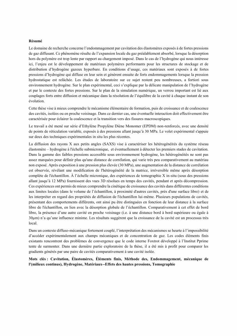
Résumé

Le domaine de recherche concerne l’endommagement par cavitation des élastomères exposés à de fortes pressions

de gaz diffusant. Ce phénomène résulte de l’expansion locale du gaz préalablement absorbé, lorsque la désorption

hors du polymère est trop lente par rapport au chargement imposé. Dans le cas de l’hydrogène qui nous intéresse

ici, l’enjeu est le développement de matériaux polymères performants pour les structures de stockage et de

distribution d’hydrogène gazeux hyperbare. En conditions d’usage, ces matériaux sont exposés à de fortes

pressions d’hydrogène qui diffuse en leur sein et génèrent ensuite de forts endommagements lorsque la pression

hydrostatique est relâchée. Les études de laboratoire sur ce sujet restent peu nombreuses, a fortiori sous

environnement hydrogène. Sur le plan expérimental, ceci s’explique par la délicate manipulation de l’hydrogène

et par le contexte des fortes pressions. Sur le plan de la simulation numérique, un verrou important est lié aux

couplages forts entre diffusion et mécanique dans la résolution de l’équilibre de la cavité à chaque instant de son

évolution.

Cette thèse vise à mieux comprendre le mécanisme élémentaire de formation, puis de croissance et de coalescence

des cavités, isolées ou en proche voisinage. Dans ce dernier cas, une éventuelle interaction doit effectivement être

caractérisée pour éclairer la coalescence et la transition vers des fissures macroscopiques.

Le travail a été mené sur série d’Ethylène Propylène Diène Monomer (EPDM) non-renforcés, avec une densité

de points de réticulation variable, exposés à des pressions allant jusqu’à 30 MPa. Le volet expérimental s'appuie

sur deux des techniques expérimentales in situ les plus récentes.

La diffusion des rayons X aux petits angles (SAXS) vise à caractériser les hétérogénéités du système réseau

élastomère – hydrogène à l'échelle submicronique, et éventuellement à détecter les premiers stades de cavitation.

Dans la gamme des faibles pressions accessible sous environnement hydrogène, les hétérogénéités ne sont pas

assez marquées pour définir plus qu'une distance de corrélation, qui varie très peu comparativement au matériau

non exposé. Après exposition à une pression plus élevée (30 MPa), une augmentation de la distance de corrélation

est observée, révélant une modification de l'hétérogénéité de la matrice, irréversible même après désorption

complète de l'échantillon. À l’échelle micronique, des expériences de tomographie X in-situ (sous des pressions

allant jusqu’à 12 MPa) fournissent des vues 3D résolues en temps des cavités, pendant et après décompression.

Ces expériences ont permis de mieux comprendre la cinétique de croissance des cavités dans différentes conditions

aux limites locales (dans le volume de l’échantillon, à proximité d'autres cavités, près d'une surface libre) et de

les interpréter en regard des propriétés de diffusion de l'échantillon lui-même. Plusieurs populations de cavités,

présentant des comportements différents, ont ainsi pu être distinguées en fonction de leur distance à la surface

libre de l'échantillon, en lien avec la désorption globale de l’échantillon. Comparativement à cet effet de bord

libre, la présence d’une autre cavité en proche voisinage (i.e. à une distance bord à bord supérieure ou égale à

30µm) n’a qu’une influence minime. Les résultats suggèrent que la croissance de la cavité est un processus très

local.

Dans un contexte diffuso-mécanique fortement couplé, l’interprétation des mécanismes se heurte à l’impossibilité

d’accéder expérimentalement aux champs mécaniques et de concentration de gaz. Les codes éléments finis

existants rencontrent des problèmes de convergence que le code interne Foxtrot développé à l’Institut Pprime

tente de surmonter. Dans une dernière partie exploratoire de la thèse, il a été mis à profit pour comparer les

gradients générés par une paire de cavités comparativement à une cavité isolée.

Mots clés : Cavitation, Élastomères, Éléments finis, Méthode des, Endommagement, mécanique de

l'(milieux continus), Hydrogène, Matériaux--Effets des hautes pressions, Tomographie

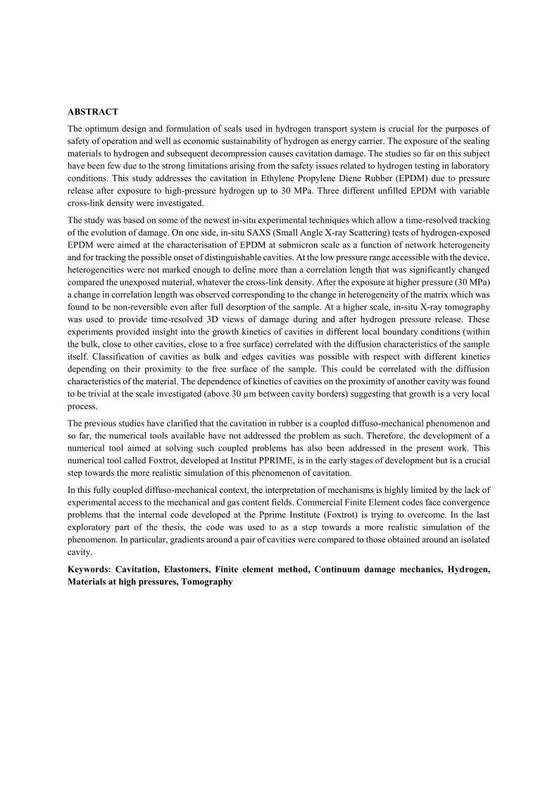
ABSTRACT

The optimum design and formulation of seals used in hydrogen transport system is crucial for the purposes of

safety of operation and well as economic sustainability of hydrogen as energy carrier. The exposure of the sealing

materials to hydrogen and subsequent decompression causes cavitation damage. The studies so far on this subject

have been few due to the strong limitations arising from the safety issues related to hydrogen testing in laboratory

conditions. This study addresses the cavitation in Ethylene Propylene Diene Rubber (EPDM) due to pressure

release after exposure to high-pressure hydrogen up to 30 MPa. Three different unfilled EPDM with variable

cross-link density were investigated.

The study was based on some of the newest in-situ experimental techniques which allow a time-resolved tracking

of the evolution of damage. On one side, in-situ SAXS (Small Angle X-ray Scattering) tests of hydrogen-exposed

EPDM were aimed at the characterisation of EPDM at submicron scale as a function of network heterogeneity

and for tracking the possible onset of distinguishable cavities. At the low pressure range accessible with the device,

heterogeneities were not marked enough to define more than a correlation length that was significantly changed

compared the unexposed material, whatever the cross-link density. After the exposure at higher pressure (30 MPa)

a change in correlation length was observed corresponding to the change in heterogeneity of the matrix which was

found to be non-reversible even after full desorption of the sample. At a higher scale, in-situ X-ray tomography

was used to provide time-resolved 3D views of damage during and after hydrogen pressure release. These

experiments provided insight into the growth kinetics of cavities in different local boundary conditions (within

the bulk, close to other cavities, close to a free surface) correlated with the diffusion characteristics of the sample

itself. Classification of cavities as bulk and edges cavities was possible with respect with different kinetics

depending on their proximity to the free surface of the sample. This could be correlated with the diffusion

characteristics of the material. The dependence of kinetics of cavities on the proximity of another cavity was found

to be trivial at the scale investigated (above 30 µm between cavity borders) suggesting that growth is a very local

process.

The previous studies have clarified that the cavitation in rubber is a coupled diffuso-mechanical phenomenon and

so far, the numerical tools available have not addressed the problem as such. Therefore, the development of a

numerical tool aimed at solving such coupled problems has also been addressed in the present work. This

numerical tool called Foxtrot, developed at Institut PPRIME, is in the early stages of development but is a crucial

step towards the more realistic simulation of this phenomenon of cavitation.

In this fully coupled diffuso-mechanical context, the interpretation of mechanisms is highly limited by the lack of

experimental access to the mechanical and gas content fields. Commercial Finite Element codes face convergence

problems that the internal code developed at the Pprime Institute (Foxtrot) is trying to overcome. In the last

exploratory part of the thesis, the code was used to as a step towards a more realistic simulation of the

phenomenon. In particular, gradients around a pair of cavities were compared to those obtained around an isolated

cavity.

Keywords: Cavitation, Elastomers, Finite element method, Continuum damage mechanics, Hydrogen,

Materials at high pressures, Tomography