Journal of Functional Analysis 255 (2008) 283–312

www.elsevier.com/locate/jfa

Gaussian bounds for degenerate parabolic equations

D. Cruz-Uribe a,∗, Cristian Rios b

a Department of Mathematics, Trinity College, Hartford, CT 06106-3100, USAb University of Calgary, Calgary, AB T2N1N4, Canada

Received 5 June 2007; accepted 29 January 2008

Available online 15 May 2008

Communicated by Daniel W. Stroock

Abstract

Let A be a real symmetric, degenerate elliptic matrix whose degeneracy is controlled by a weight w

in the A2 or QC class. We show that there is a heat kernel Wt(x, y) associated to the parabolic equationwut = div A∇u, and Wt satisfies classic Gaussian bounds:

∣∣Wt(x, y)∣∣ � C1

tn/2exp

(−C2

|x − y|2t

).

We then use this bound to derive a number of other properties of the kernel.© 2008 Published by Elsevier Inc.

Keywords: Kernel; Gaussian bounds; Degenerate elliptic; Degenerate parabolic

1. Introduction

1.1. Overview of the problem

In this paper we study the degenerate parabolic equation

div A∇u = w∂u

∂t. (1.1)

* Corresponding author.E-mail addresses: david.cruzuribe@trincoll.edu (D. Cruz-Uribe), crios@math.ucalgary.ca (C. Rios).

0022-1236/$ – see front matter © 2008 Published by Elsevier Inc.doi:10.1016/j.jfa.2008.01.017

284 D. Cruz-Uribe, C. Rios / Journal of Functional Analysis 255 (2008) 283–312

where A = (Aij (x))ni,j=1 is a matrix of complex-valued, measurable functions satisfying thedegenerate ellipticity condition

⎧⎪⎪⎨⎪⎪⎩

λw(x)|ξ |2 � Re〈Aξ, ξ 〉 = Ren∑

i,j=1

Aij (x)ξj ξi ,

∣∣〈Aξ, η〉∣∣ � Λw(x)|ξ ||η|,(1.2)

for some λ, Λ, 0 < λ � Λ < ∞, and all ξ, η ∈ Cn. The weight w that controls the degeneracy is

a non-negative, locally integrable function which we assume is either in the Muckenhoupt classA2 or in the class of QC weights, which arise in the study of quasi-conformal mappings. Forease of reference we make the following definition.

Definition 1.1. Let En(w,λ,Λ) denote the class of n×n matrices of complex-valued, measurablefunctions satisfying the degenerate ellipticity condition (1.2).

Remark 1.2. If A ∈ En(w,λ,Λ), then so is its adjoint, A∗.

Our goal is to show that if A is real symmetric, then there exists a heat kernel associated tothis equation: an L∞ function Wt(x, y) such that given a function f ∈ C∞

c ,

u(x, t) =∫Rn

Wt (x, y)f (y) dy (1.3)

is a solution of (1.1) satisfying the initial condition u(x,0) = f (x). Further, we will show thatthe heat kernel satisfies Gaussian bounds:

∣∣Wt(x, y)∣∣ � C1

tn/2exp

(−C2

|x − y|2t

). (1.4)

A central feature of our results is that the weight does not appear in (1.3) or in (1.4)—the kernelis defined with respect to Lebesgue measure.

When w ≡ 1 (that is, A is uniformly elliptic), these results are well known. For the existenceof the heat kernel, see Friedman [18]; Gaussian bounds are due to Aronson [1].

Solutions of Eq. (1.1) with A real symmetric were first treated by Chiarenza and Frasca [8].Chiarenza and Serapioni [11], showed that if n � 3 and w ∈ A2, then solutions of (1.1) satisfied aHarnack inequality on standard parabolic cylinders. Chiarenza and Franciosi [7] proved the sameresult for n � 2 and w a QC weight. (See Proposition 3.8 below.) More recently, Ishige [24] hasproved a Harnack inequality and continuity of the solution for a more general parabolic equationwith lower order terms, and for A any real matrix that satisfies (1.2) with w ∈ A2.

When A is a complex matrix, much less is known even when A is uniformly elliptic.Auscher [2] showed that Gaussian bounds hold for L∞ perturbations of real symmetric ma-trices. Auscher, McIntosh and Tchamitchian [5] showed that Gaussian bounds hold if A satisfies(1.2) and is Hölder continuous, and when n � 2 smoothness is not necessary. Ouhabaz [27]has shown that if A is a Lipschitz perturbation of a real, uniformly elliptic matrix, then (1.4)holds. (Note that neither of the last two results assumes that A is symmetric.) On the other hand,

D. Cruz-Uribe, C. Rios / Journal of Functional Analysis 255 (2008) 283–312 285

Auscher, Coulhon and Tchamitchian [4], building on an example in [26], showed that if n � 5,then Gaussian bounds for the heat kernel need not hold in general.

Given a degenerate elliptic matrix A, it might seem more natural to consider the usualparabolic equation

div A∇u = ∂u

∂t. (1.5)

When w ∈ A2 this equation has been studied by several authors; their results indicate that, sur-prisingly, (1.1) is the “right” generalization to consider. Chiarenza and Serapioni [9,10] showedthat the assumption w ∈ A2 did not imply local regularity of the solution. Local regularity re-quired higher integrability of the weight w−1; e.g., the stronger hypothesis w ∈ A1+2/n, n � 3.Further, they showed that in this case solutions to (1.5) satisfied a Harnack inequality on theweighted parabolic cylinders Qx,t (r) = B2r (x) × (t − hx(r), t), where

hx(r) =( ∫

Br (x)

w(y)−n/2 dy

)2/n

.

Gutiérrez and Nelson [22] showed that with the same assumption the heat kernel associatedwith Eq. (1.5), Wt (x, y), satisfied a weighted Gaussian estimate: there exist C1,C2, α > 0 suchthat

∣∣Wt (x, y)∣∣ � C1

h−1x (t)n

exp

(−C2

hx(|x − y|)t

)α

. (1.6)

A sharper but more complicated version of this inequality was later proved by Gutiérrez andWheeden [23].

1.2. Statement of the main results

Hereafter, let w be either an A2 weight or a QC weight. If w ∈ QC, then we will also assumen � 2; otherwise we can take n � 1. Define the differential operator Lw = −w−1 div A∇ , andlet e−tLw be the semigroup generated by Lw . Given any f in the domain of e−tLw , u(x, t) =e−tLwf (x) is a solution of the initial value problem

⎧⎨⎩

∂u

∂t= −Lwu,

u(x,0) = f (x).

(1.7)

Our main result is the following.

Theorem 1.3. If A ∈ En(w,λ,Λ) is real symmetric, then there exists a heat kernel Wt(x, y)

associated to the operator e−tLw such that for all f ∈ C∞c ,

e−tLwf (x) =∫n

Wt (x, y)f (y) dy. (1.8)

R

286 D. Cruz-Uribe, C. Rios / Journal of Functional Analysis 255 (2008) 283–312

Furthermore, for all t > 0 and x, y ∈ Rn, the kernel Wt satisfies the Gaussian bounds

∣∣Wt(x, y)∣∣ � C1

tn/2exp

(−C2

|x − y|2t

), (1.9)

and the Hölder continuity estimates

∣∣Wt(x + h,y) − Wt(x, y)∣∣ � C1

tn/2

( |h|t1/2 + |x − y|

)μ

exp

(−C2

|x − y|2t

), (1.10)

∣∣Wt(x, y + h) − Wt(x, y)∣∣ � C1

tn/2

( |h|t1/2 + |x − y|

)μ

exp

(−C2

|x − y|2t

), (1.11)

where h ∈ Rn is such that 2|h| � t1/2 + |x − y|. The constants C1, C2 and μ depend only on n,

w, λ, and Λ.

Remark 1.4. Perhaps the most outstanding aspect of our results is that they appear to be inde-pendent of the weight. Thus the kernel Wt(x, y) is integrated with respect to Lebesgue measureand the upper bounds (1.9) on Wt are the classic Gaussian bounds for the heat kernel [1]. Thisis in sharp contrast to the weighted inequalities (1.6) obtained in [22,23] for a related class ofdegenerate parabolic equations. The classical nature of our estimates will be very useful for theweighted Kato square root problem, among other applications.

Remark 1.5. We believe that Theorem 1.3 should hold for all real matrices (i.e., not necessar-ily symmetric) that satisfy (1.2). Towards proving this, we remark that the approach taken byOuhabaz [27] for uniformly elliptic matrices can be adapted to the case of degenerate matrices.However, this technique relies on the Sobolev embedding theorem, and in the weighted case thisresult is only true on bounded domains (see [17]).

Central to the proof of Theorem 1.3 is an estimate which is of independent interest. Whenw ≡ 1 this inequality appears in Auscher et al. [6], without proof; they note that in the specialcase of the Laplace–Beltrami operator the result is due to Gaffney [19] and that it can be provedby modifying an argument due to Davies [14].

Theorem 1.6. Given A ∈ En(w,λ,Λ), let E and F be two closed subsets of Rn and set d =

dist(E,F ). Then there exist constants c,C > 0 such that given any function f ∈ L2(w) withsupp(f ) ⊂ E,

∥∥e−tLwf∥∥

L2(w,F )� Ce−cd2/t‖f ‖L2(w,E).

The constants depend only n, λ, and Λ.

As a consequence of the Gaussian bounds we have the conservation property.

Theorem 1.7. Given a matrix A ∈ En(w,λ,Λ), suppose that the heat kernel of the associatedsemigroup e−tLw satisfies (1.4). Then e−tLw 1 = 1, where 1 denotes the function on R

n whichequals the constant 1.

D. Cruz-Uribe, C. Rios / Journal of Functional Analysis 255 (2008) 283–312 287

As another consequence we get bounds for the derivative of the semigroup.

Theorem 1.8. With the same hypotheses as Theorem 1.7, the semigroup Vt , t � 0, defined by

Vtf (x) = −(

∂

∂te−tLw

)f (x) = Lwe−tLwf (x),

is given by a heat kernel Vt(x, y): for all f ∈ C∞c ,

Vtf (x) =∫Rn

Vt (x, y)f (y) dy.

Furthermore, for all t > 0 and x, y ∈ Rn, Vt satisfies the Gaussian bounds

∣∣Vt(x, y)∣∣ � C1

tn/2+1exp

(−C2

|x − y|2t

),

and the Hölder continuity estimates

∣∣Vt (x + h,y) − Vt (x, y)∣∣ � C1

tn/2+1

( |h|t1/2 + |x − y|

)μ

exp

(−C2

|x − y|2t

),

∣∣Vt (x, y + h) − Vt (x, y)∣∣ � C1

tn/2+1

( |h|t1/2 + |x − y|

)μ

exp

(−C2

|x − y|2t

),

where h ∈ Rn is such that 2|h| � t1/2 + |x − y|. Finally, Vt has zero integral: for all x ∈ R

n,

Vt1 =∫Rn

Vt (x, y) dy = 0.

Remark 1.9. In both Theorems 1.7 and 1.8 we do not assume that A is real symmetric; we onlyassume that the associated heat kernel satisfies Gaussian bounds.

1.3. Organization

The remainder of this paper is organized as follows. In Sections 2 and 3 we gather some basicresult about weighted Sobolev spaces and semigroups. In Section 4 we prove the Gaffney-typeestimate in Theorem 1.6. In Section 5 we prove Theorems 1.3 and 1.8. In Section 6 we proveTheorem 1.7.

Throughout this paper, all notation will be standard or defined as needed. Λ and λ willalways denote the ellipticity constants in (1.2). Unless otherwise specified, C, c, etc., willdenote an arbitrary constant which may depend on the dimension n, λ and Λ, and the A2or QC constant associated with a weight w. Sometimes for clarity we will specify the de-pendence of the constant by writing C(n), C(n,w), etc. Given an angle θ , define the sectorΣ(θ) = {z ∈ C: z �= 0, |arg(z)| < θ}. Finally, given a bounded operator T on L2(w,Ω), let‖T ‖B(L2(w,Ω)) denote its operator norm.

288 D. Cruz-Uribe, C. Rios / Journal of Functional Analysis 255 (2008) 283–312

2. Weighted Sobolev spaces

The basic theory of weighted Sobolev spaces was developed by Fabes, Kenig and Serapi-oni [17] and we will follow their development. (See also Turesson [29].) One key difference,however, is that they only dealt with real-valued functions; complex-valued functions introducea number of minor technical complications.

2.1. Weights

By a weight we mean a non-negative, locally integrable function. Given a weight w and ameasurable set E, we let

w(E) =∫E

w(x)dx.

We are concerned with two weight classes: the Muckenhoupt class A2 and the quasi-conformal weights QC. The first class is straightforward to define; we give a slightly moregeneral definition which we will need below. Given p, 1 < p < ∞, and a weight w, we say thatw ∈ Ap if there exists a constant [w]Ap (referred to as the Ap constant of w) such that

supQ

(1

|Q|∫Q

w(x)dx

)(1

|Q|∫Q

w(x)1−p′dx

)p−1

= [w]Ap < ∞,

where the supremum is taken over all cubes Q in Rn. Note that if w ∈ Ap , then it follows by a

change of variables that for all a ∈ R, b ∈ Rn, wab(x) = w(ax + b) ∈ Ap , and [wab]Ap = [w]Ap .

Let A∞ denote the union of the Ap classes. The properties of these weights can be found in [16,20,21].

To define the class QC, fix n � 2 and let f : Rn → Rn be a bijection whose components fi

have distributional derivatives in LnLoc. Let f ′(x) denote the Jacobian of f and let |f ′| denote its

determinant. Then f is quasi-conformal if there exists a constant k such that

(n∑

i,j=1

∂fi

∂xj

(x)2

)1/2

� k∣∣f ′(x)

∣∣1/n.

Given such an f , the function w = |f ′|1−2/n is called a QC weight. We will denote the bestconstant k associated with f , and so with w, by [w]QC . As before we have that [wab]QC =[w]QC .

David and Semmes [12] showed that if w ∈ QC, then w ∈ A∞, but QC weights have muchmore structure than an arbitrary A∞ weight. The classes QC and A2 are different. Thus, a QC

weight need not be in A2: for example, w(x) = |x|α(n−2) ∈ QC for all α > −1, but w is not inA2 if α � n/(n − 2). Conversely, |x|β , −n < β � −(n − 2), is in A2 but not in QC. (See [17,p. 106].)

D. Cruz-Uribe, C. Rios / Journal of Functional Analysis 255 (2008) 283–312 289

2.2. Weighted Sobolev spaces

Given an open set Ω in Rn, and a weight w in either A2 or QC, let Lp(w,Ω), 1 � p < ∞,

be the Banach function space of complex-valued functions with norm

‖f ‖Lp(w,Ω) =( ∫

Rn

∣∣f (x)∣∣pw(x)dx

)1/p

.

L2(w,Ω) is a Hilbert space with inner product

〈f,g〉w =∫Ω

f (x)g(x)w(x)dx.

When p = ∞, L∞(w,Ω) consists of functions essentially bounded with respect to the measurew(x)dx; since w ∈ A∞, L∞(w,Ω) = L∞(Ω).

Define the Sobolev space H 10 (w,Ω) to be the closure of C∞

c (Ω) with respect to the norm

‖f ‖H 10 (w,Ω) = ‖f ‖L2(w,Ω) + ‖∇f ‖L2(w,Ω).

(If Ω = Rn, then we write simply L2(w) and H 1

0 (w).) That this closure is well defined is aconsequence of the following lemma [17, pp. 90, 106].

Lemma 2.1. Given a weight w in A2 or QC, suppose {gk} ⊂ C∞c (Ω) is such that

‖gk‖L2(w,Ω) → 0. If g is such that ‖∇gk − g‖L2(w,Ω) → 0, then g = 0.

Thus, if f ∈ H 10 (w,Ω), there exists a vector-valued function in L2(w,Ω), denoted ∇f , and

there exists {gk} ⊂ C∞c (Ω) such that in L2(w,Ω), {gk} converges to f and {∇gk} converges

to ∇f .If w ∈ A2, w−1 is locally integrable, so by Hölder’s inequality, f,∇f ∈ L1

Loc(Ω). Hence, wecan integrate by parts: for all φ ∈ C∞

c (Ω),∫Ω

∇f (x)φ(x) dx = −∫Ω

f (x)∇φ(x)dx.

However, if w ∈ QC, then f and ∇f need not be locally integrable, so this formula does notmake sense. This fact complicates the proof of some of the differentiation formulas given below.

To establish additional details about the structure of H 10 (w,Ω), note first that if f = u + iv ∈

H 10 (w,Ω), then by passing to the real and imaginary parts of an approximating sequence of C∞

cfunctions, we have that u,v ∈ H 1

0 (w,Ω).

Lemma 2.2. Let θ : R2 → C have continuous partial derivatives and be such that |∇θ | � M . Iff = u + iv ∈ H 1

0 (w,Ω), then the function θ(f ) = θ(u, v) ∈ H 10 (w,Ω) and almost everywhere

in Ω ,

∂θ(f )

∂xi

= ∂θ

∂s(u, v)

∂u

∂xi

+ ∂θ

∂t(u, v)

∂v

∂xi

, 1 � i � n. (2.1)

290 D. Cruz-Uribe, C. Rios / Journal of Functional Analysis 255 (2008) 283–312

Proof. Let {φk} ⊂ C∞c (Ω) be such that φk → f in H 1

0 (w,Ω). By passing to a subsequence,we may assume that it converges pointwise almost everywhere as well. For each k � 1, θ(φk)

is continuously differentiable and has compact support in Ω , and so is in H 10 (w,Ω). Let uk =

Re(φk), vk = Im(φk). By the chain rule, for 1 � i � n,

∂θ(φk)

∂xi

= ∂θ

∂s(uk, vk)

∂uk

∂xi

+ ∂θ

∂t(uk, vk)

∂vk

∂xi

.

By assumption, θ is Lipschitz, so |θ(φk)(x) − θ(f )(x)| � M|φk(x) − f (x)|. Hence,

(∫Ω

∣∣θ(φk)(x) − θ(f )(x)∣∣2

w(x)dx

)1/2

� M

(∫Ω

∣∣φk(x) − f (x)∣∣2

w(x)dx

)1/2

.

Since φk → f in L2(w,Ω), we have that θ(φk) → θ(f ) in L2(w,Ω).Since u,v ∈ L2(w,Ω) and ∇θ ∈ L∞, the right-hand side of (2.1) is in L2(w,Ω), 1 � i � n.

Temporarily denote it by Fi . Then∣∣∣∣∂θ(φk)

∂xi

− Fi

∣∣∣∣ �∣∣∣∣∂θ

∂s(uk, vk)

∂uk

∂xi

− ∂θ

∂s(u, v)

∂u

∂xi

∣∣∣∣ +∣∣∣∣∂θ

∂t(uk, vk)

∂uk

∂xi

− ∂θ

∂t(u, v)

∂u

∂xi

∣∣∣∣= Ak + Bk.

To complete the proof it will suffice to show that Ak,Bk → 0 in L2(w,Ω). For in that case, sinceH 1

0 (w,Ω) is complete we have that θ(f ) ∈ H 10 (w,Ω) and (2.1) holds.

We will show Ak converges to 0; the proof for Bk is identical. We have that

A �∣∣∣∣∂θ

∂s(uk, vk)

∂uk

∂xi

− ∂θ

∂s(uk, vk)

∂u

∂xi

∣∣∣∣ +∣∣∣∣∂θ

∂s(uk, vk)

∂u

∂xi

− ∂θ

∂s(u, v)

∂u

∂xi

∣∣∣∣� M

∣∣∣∣∂uk

∂xi

− ∂u

∂xi

∣∣∣∣ +∣∣∣∣∂θ

∂s(uk, vk) − ∂θ

∂s(u, v)

∣∣∣∣∣∣∣∣ ∂u

∂xi

∣∣∣∣.Since u ∈ H 1

0 (w,Ω), the first term tends to 0 in L2(w,Ω). The second term is dominated point-wise by 2M| ∂u

∂xi|. Further, since φk → f pointwise and θ has continuous partial derivatives, the

second term tends to 0 pointwise. Therefore, by the dominated convergence theorem it also tendsto 0 in L2(w,Ω), and we are done. �Lemma 2.3. Let f = u + iv ∈ H 1

0 (w,Ω). Then |f | ∈ H 10 (w,Ω) and for 1 � i � n and almost

every x ∈ Ω ,

∂|f |∂xi

(x) = u(x) ∂u∂xi

(x) + v(x) ∂v∂xi

(x)

|f (x)| χ{f (x) �=0}. (2.2)

Proof. For each ε > 0, define the function θε(s, t) = √s2 + t2 + ε2 −ε. Then θε has continuous,

bounded derivatives, and so by Lemma 2.2, θε(f ) ∈ H 10 (w,Ω) and for 1 � i � n,

∂θε(f )

∂x= u(x) ∂u

∂xi(x) + v(x) ∂v

∂xi(x)√

2 2 2

i u(x) + v(x) + ε

D. Cruz-Uribe, C. Rios / Journal of Functional Analysis 255 (2008) 283–312 291

almost everywhere. Since θε(f )(x) � |f (x)| and θε(f ) → |f | pointwise, by the dominated con-vergence theorem it converges in L2(w,Ω).

Denote the right-hand side of (2.2) by Fi . Then |Fi | � | ∂u∂xi

(x)| + | ∂u∂xi

(x)| ∈ L2(w,Ω). Fur-

ther, we have that | ∂θε(f )∂xi

| � |Fi | and | ∂θε(f )∂xi

| converges pointwise to Fi . So again by dominated

convergence it converges in L2(w,Ω). This yields the desired result. �Corollary 2.4. If f ∈ H 1

0 (w,Ω) is real-valued, then f + = max(f,0) and f − = min(f,0) areboth in H 1

0 (w,Ω), and for 1 � i � n,

∂f +

∂xi

= ∂f

∂xi

χ{f >0},∂f −

∂xi

= ∂f

∂xi

χ{f <0}.

Proof. It suffices to note that f + = (|f | + f )/2 and f − = (|f | − f )/2 and then applyLemma 2.3. �3. Semigroup theory

In this section we state some basic properties of semigroup theory and use these to constructa weak solution to (1.1). We follow the approach given by Ouhabaz [27] and we refer the readerto this work and to Kato [25] for further information. Throughout this section A ∈ En(w,λ,Λ)

and w is an A2 or QC weight.

3.1. Sesquilinear forms and the associated operators

Definition 3.1. For all f,g ∈ H 10 (w,Ω) define the sesquilinear form a(f, g) by

a(f, g) =∫Ω

A∇f (x) · ∇g(x)dx. (3.1)

Since C∞c (Ω) is dense in H 1

0 (w,Ω), the sesquilinear form a is densely defined on L2(w,Ω).We will sometimes denote H 1

0 (w,Ω), the domain of a, by D(a).

Proposition 3.2. The sesquilinear form a has the following properties:

(1) a is accretive: for all f ∈ D(a),

Rea(f,f ) � 0.

(2) a is continuous: |a(f, g)| � M‖f ‖a‖g‖a, where the norm is defined by ‖f ‖a =√Rea(f,f ) + ‖f ‖2

L2(w,Ω).

(3) a is closed: (D(a),‖ · ‖a) is a complete space.(4) a is sectorial: there exists ω ∈ (0, π

2 ) such that for all f ∈ D(a),

∣∣Ima(f,f )∣∣ � tan(ω)

∣∣Rea(f,f )∣∣.

292 D. Cruz-Uribe, C. Rios / Journal of Functional Analysis 255 (2008) 283–312

Proof. Properties (1), (2) and (4) are immediate consequences of the ellipticity condition (1.2):for all f,g ∈ D(a),

Rea(f,f ) � λ

∫Ω

∣∣∇f (x)∣∣2

w(x)dx � 0,

and

∣∣a(f, g)∣∣ � Λ

∫Ω

∣∣∇f (x)∣∣∣∣∇g(x)

∣∣w(x)dx

� Λ

(∫Ω

∣∣∇f (x)∣∣2

w(x)dx

)1/2(∫Ω

∣∣∇g(x)∣∣2

w(x)dx

)1/2

� Λ

λ

(Re

∫Ω

A∇f (x) · ∇f (x) dx

)1/2(Re

∫Ω

A∇g(x) · ∇g(x)dx

)1/2

� Λ

λ‖f ‖a‖g‖a.

Further,

∣∣Ima(f,f )∣∣ � Λ

∫Ω

∣∣∇f (x)∣∣2

w(x)dx

� Λ

λ

∫Ω

Re A∇f (x) · ∇f (x) dx = Λ

λ

∣∣Rea(f,f )∣∣.

This yields (4) with ω = arctan(Λ/λ).The proof of (3) follows from the fact that H 1

0 (w,Ω) is a complete space with respect to thenorm ‖ · ‖H 1

0 (w,Ω), and from the fact that ‖ · ‖a ≈ ‖ · ‖H 10 (w,Ω), since by the ellipticity condi-

tion (1.2), Rea(f,f ) ≈ ‖∇f ‖2L2(w,Ω)

. �The properties in Proposition 3.2 allow us to use the abstract theory of sesquilinear forms. This

immediately yields that there exists a densely defined operator Lw on L2(w,Ω) such that for allf ∈ D(Lw), g ∈ D(a), a(f, g) = 〈Lwf,g〉w . Furthermore, D(Lw) is dense in D(a) with respectto the norm ‖ · ‖a. (See [27, Proposition 1.22].) Note that if A and f,g are smooth functions,then by integration by parts we have that Lw = −w−1 div A∇ .

Define the adjoint form a∗ by

a∗(f, g) = a(g, f ) =∫Ω

A∗∇f (x) · ∇g(x)dx.

Since A∗ ∈ En(w,λ,Λ), everything we have said above holds for a∗. In particular, we have thedensely defined operator L∗ which is the adjoint of Lw .

w

D. Cruz-Uribe, C. Rios / Journal of Functional Analysis 255 (2008) 283–312 293

The classes En(w,λ,Λ) are preserved under (small) rotations. More precisely, we have thefollowing lemma.

Lemma 3.3. Let A ∈ En(w,λ,Λ), and let ω = arctan(Λ/λ), τ = arctan λ√Λ2−λ2

. If z ∈ Σ(τ),

then zA ∈ En(w,λz,Λz), where λz = λ|z|[cos(arg(z)) − sin(arg(z))/ tan(τ )] and Λz = Λ|z|.

Proof. First note that λz > 0:

cos(arg(z)

) − sin(arg(z)

)/ tan(τ ) = cos

(arg(z)

)[1 − tan

(arg(z)

)/ tan(τ )

]> cos

(arg(z)

)[1 − tan(τ )/ tan(τ )

] = 0.

Since A ∈ En(w,λ,Λ), for all ξ ∈ Cn,

(Re〈Aξ, ξ 〉)2 + (

Im〈Aξ, ξ 〉)2 = ∣∣〈Aξ, ξ 〉∣∣2 � Λ2w(x)2|ξ |4,(Re〈Aξ, ξ 〉)2 � λ2w(x)2|ξ |4.

Together, these imply that

∣∣Im〈Aξ, ξ 〉∣∣ �√

Λ2 − λ2w(x)|ξ |2,

and so

Re〈zAξ, ξ 〉 = |z|(cos(arg z)Re〈Aξ, ξ 〉 − sin(arg z) Im〈Aξ, ξ 〉)� |z|(cos(arg z)λw(x)|ξ |2 − ∣∣sin(arg z)

∣∣√Λ2 − λ2w(x)|ξ |2)

= λ|z|w(x)|ξ |2(

cos(arg z) − ∣∣sin(arg z)∣∣√

Λ2

λ2− 1

)

� λ|z|w(x)|ξ |2(cos(arg(z)

) − sin(arg(z)

)/ tan(τ )

).

On the other hand it is immediate that for all ξ , η, |〈zAξ, η〉| � Λ|z|w(x)|ξ ||η|. �3.2. Resolvents and semigroups

Though the operator Lw is not bounded, there are two closely related bounded operatorsassociated to it: the resolvent (λI +Lw)−1 and the semigroup e−tLw .

The operator Lw is the infinitesimal generator of a strongly continuous, contraction semi-group e−tLw . The range of e−tLw is D(Lw). Further, e−tLw is a holomorphic semigroup in thesector Σ(π/2 − ω), where ω = arctan(Λ/λ). (See [27, Theorem 1.52].)

Proposition 3.4. If the matrix A is real, then the semigroup e−tLw is real and positive: if f ∈L2(w,Ω) is real-valued, then so is e−tLwf ; if f is non-negative, then so is e−tLwf .

294 D. Cruz-Uribe, C. Rios / Journal of Functional Analysis 255 (2008) 283–312

Proof. By [27, Theorem 2.5], e−tLw is real if given any f = u + iv, a(u, v) ∈ R. This is im-mediate from the definition of a given that A is real. By [27, Theorem 2.6], e−tLw is positiveif, in addition, u+, u− ∈ H 1

0 (w,Ω), and a(u+, u−) � 0. The first condition is just Corol-lary 2.4. The second also follows from Corollary 2.4: ∇u+ and ∇u− have disjoint supports,so a(u+, u−) = 0. �

For every t > 0, tI +Lw is an invertible operator from D(Lw) into L2(w,Ω). Its inverse, theresolvent of Lw , (tI +Lw)−1, is a bounded operator on L2(w,Ω) satisfying

∥∥t (tI +Lw)−1∥∥B(L2(w,Ω))

� 1. (3.2)

An important consequence of the fact that e−tLw is a holomorphic semigroup is the fact that theresolvent is bounded on a sector of the complex plane larger than the half-plane {Re z > 0}. (See[27, Theorem 1.45].)

Proposition 3.5. Let ω = arctan(Λ/λ). Then for every θ ∈ (π/2,π − ω) there exists Mθ > 0such that

supz∈Σ(θ)

∥∥z(zI +Lw)−1∥∥B(L2(w,Ω))

� Mθ. (3.3)

The next proposition shows that e−tLw and (zI +Lw)−1 can be characterized in terms of oneanother. (See [25, pp. 482–489].)

Proposition 3.6. Let ω = arctan(Λ/λ). Then for f ∈ L2(w,Ω) and z ∈ Σ(π/2 − ω),

e−zLwf = 1

2πi

∫Γ

ezζ (ζ I +Lw)−1f dζ, (3.4)

where the path Γ is the union of the rays γ ± = {z ∈ C: z = re±iθ , r � R > 0} and the arcγ0 = {z ∈ C: z = Reiψ, |ψ | � θ}, going around the origin counter-clockwise, and π − ω > θ >

π/2 + |arg(z)|.Further, if Re(z) > 0,

(zI +Lw)−1 =∞∫

0

e−zt e−tLw dt. (3.5)

More generally, if z ∈ Σ(π − ω), then this identity remains true if we instead integrate over theray t = reiθ , r > 0, where θ is such that e−tLw is bounded and Re(zt) > 0.

Inequality (3.5) is referred to as the Laplace identity.Another consequence of the fact that e−tLw is a holomorphic semigroup is that the operator

(∂

e−tLw

)f = ∂ (

e−tLwf) = −Lwe−tLwf (3.6)

∂t ∂t

D. Cruz-Uribe, C. Rios / Journal of Functional Analysis 255 (2008) 283–312 295

is again a bounded operator on L2(w,Ω). More precisely, there exists C > 0 such that for allt > 0,

∥∥Lwe−tLw∥∥B(L2(w,Ω))

� C

t.

(See Yosida [30, p. 239].)Finally, we note that the operators e−zL∗

w and (zI + L∗w)−1 are the adjoints of e−zLw and

(zI +Lw)−1, respectively.

3.3. Solutions of the parabolic equation

Here we define a weak solution to the parabolic equation (1.7) and show that the semigroupe−tLw yields a solution. Our definition is the one given by Chiarenza and Frasca [8].

Fix T > 0; we say that u ∈ L2([0, T ],H 10 (w,Ω)) if for any t ∈ [0, T ] the function u(·, t) ∈

H 10 (w,Ω) and

T∫0

∥∥u(·, t)∥∥2H 1

0 (w,Ω)dt < ∞.

We define u ∈ L2([0, T ],L2(w,Ω)) in the same way, but with the H 10 norm replaced by

the L2 norm. We say that a function v ∈ W0([0, T ]) if v ∈ L2([0, T ],H 10 (w,Ω)), vt ∈

L2([0, T ],L2(w,Ω)), and v(x,0) = v(x,T ) = 0, x ∈ Ω .A function u is a weak solution of (1.1) if u ∈ L2([0, T ],H 1

0 (w,Ω)) and for all v ∈W0([0, T ]),

T∫0

∫Ω

(A∇u(x) · ∇v(x) − w(x)u(x)vt (x)

)dx dt = 0. (3.7)

Proposition 3.7. Given f ∈ L2(w,Ω), define the function u(x, t) = e−tLwf (x), t > 0. Thenu ∈ L2([0, T ],L2(w,Ω)) and (3.7) holds. Since u(x,0) = f (x), u is a solution of (1.7).

Proof. We first show that u ∈ L2([0, T ],L2(w,Ω)).

T∫0

∥∥u(·, t)∥∥2H 1

0 (w,Ω)dt � C

T∫0

∫Ω

∣∣u(x, t)∣∣2

w(x)dx dt + C

T∫0

∫Ω

∣∣∇u(x, t)∣∣2

w(x)dx dt.

We estimate each integral separately. The first is straightforward: since u = e−tLwf and thesemigroup is a contraction on L2(w,Ω),

T∫ ∫ ∣∣u(x, t)∣∣2

w(x)dx dt �T∫ ∫ ∣∣f (x)

∣∣2w(x)dx dt � T ‖f ‖2

L2(w,Ω)< ∞.

0 Ω 0 Ω

296 D. Cruz-Uribe, C. Rios / Journal of Functional Analysis 255 (2008) 283–312

To estimate the second integral, note that u(·, t) = e−tLwf (·) ∈ D(Lw), and so a(u,u) =〈Lwu,u〉w . Therefore, by the ellipticity conditions (1.2), again using the fact that e−tLw is acontraction,

T∫0

∫Ω

∣∣∇u(x, t)∣∣2

w(x)dx dt � 1

λ

T∫0

Rea(u(·, t), u(·, t))dt

= 1

λ

T∫0

Re∫Ω

Lwu(x, t)u(x, t)w(x)dx dt

= 1

λ

T∫0

Re∫Ω

Lwe−tLwf (x)e−tLwf (x)w(x)dx dt

= −1

2λRe

∫Ω

T∫0

∂

∂t

[(e−tLwf (x)

)2]w(x)dx dt

= 1

2λRe

∫Ω

f (x)2 − e−TLwf (x)2w(x)dx

� C‖f ‖2L2(w)

< ∞.

To show that u satisfies (3.7), first note that

ut = −Lwe−tLwf = −Lwu.

Now fix v ∈ W0([0, T ]). Then, since v(x,0) = v(x,T ) = 0, by Fubini’s theorem and integrationby parts in t ,

T∫0

∫Ω

w(x)u(x, t)vt (x, t) dx dt =∫Ω

(u(x, t)v(x, t)|T0 −

T∫0

ut (x, t)v(x, t) dt

)w(x)dx

=∫Ω

T∫0

Lwu(x, t)v(x, t) dt w(x)dx

=T∫

0

a(u(·, t), v(·, t))dt

=T∫

0

∫Ω

A∇u(x, t) · ∇v(x, t) dx dt.

Eq. (3.7) now follows immediately. �

D. Cruz-Uribe, C. Rios / Journal of Functional Analysis 255 (2008) 283–312 297

Finally, we give a precise statement of the Harnack inequality. Given a pair (x0, t0), x0 ∈ Ω ,t > 0, define the parabolic cylinders

Qρ(x0, t0) = {(x, t): |t − t0| < ρ2, |x − x0| < 2ρ

},

Q+ρ (x0, t0) =

{(x, t):

3

4ρ2 < t − t0 < ρ2, |x − x0| < ρ

2

},

Q−ρ (x0, t0) =

{(x, t): −3

4ρ2 < t − t0 < −1

4ρ2, |x − x0| < ρ

2

}.

Proposition 3.8. Let A ∈ En(w,λ,Λ) be real symmetric with w ∈ A2 (n � 1) or w ∈ QC

(n � 2). Then there exists γ = γ (n,λ,Λ,w) > 0 such that if u(x, t) is a non-negative solutionof (1.1) in Qρ(x0, t0), ρ > 0, then

supQ−

ρ (x0,t0)

u(x, t) � γ infQ+

ρ (x0,t0)

u(x, t).

Proof. When w ∈ QC and n � 2 this result is due to Chiarenza and Franciosi [7]. When w ∈ A2

and n � 3, it is due to Chiarenza and Serapioni [11]; the cases n = 1 and 2 for w ∈ A2 followfrom the higher-dimensional case via an argument shown to the second author by M. Safonov.Here we sketch the details for n = 2; the case n = 1 is treated in essentially the same way.

Let u(x, y, t) be a non-negative solution of (1.1) in Qρ(x0, y0, t0), ρ > 0, i.e.

div A∇u(x, y, t) = ∂tu(x, y, t),

where A ∈ E2(w,λ,Λ). For ρ � z � 3ρ define v(x, y, z, t) = zu(x, y, t) and let A(x, y, z) bethe 3 × 3 matrix

A(x, y, z) =(

A(x, y) 00 w(x,y)

).

Then a short calculation shows that v is a solution of the three-dimensional parabolic equationdiv(x,y,z) A∇(x,y,z)v = vt in the set Qρ(x0, y0,2ρ, t0) ⊂ Qρ(x0, y0, t0)×(ρ,3ρ). The matrix A isreal symmetric and A ∈ E3(w, λ,Λ), where w(x, y, z) = w(x,y) ∈ A2(R

3). Further, v is positivein Qρ(x0, y0,2ρ, t0). Therefore, by the Harnack inequality in dimension n = 3,

supQ−

ρ (x0,y0,2ρ,t0)

v(x, y, z, t) � γ infQ+

ρ (x0,y0,2ρ,t0)

v(x, y, z, t),

and so

supQ−

ρ (x0,y0,t0)

u(x, y, t) � 3γ infQ+

ρ (x0,y0,t0)

u(x, y, t). �

298 D. Cruz-Uribe, C. Rios / Journal of Functional Analysis 255 (2008) 283–312

4. Proof of Theorem 1.6

The proof of Theorem 1.6 is based on the following lemma. It is a generalization to degenerateelliptic operators and complex time of a result due to Auscher et al. [6, Lemma 2.1], and our proofis based on theirs. Throughout this section we assume that w ∈ A2 or QC and A ∈ En(w,λ,Λ).

Lemma 4.1. Let E and F be two closed sets in Rn and let d = dist(E,F ). Let τ = arctan λ√

Λ2−λ2

and fix ν, 0 < ν < π/2 + τ , and z ∈ Σ(ν). Then there exist positive constants C and c dependingon n,Λ,λ, ν such that for all f ∈ L2(w) with support in E,∫

F

∣∣z(zI +Lw)−1f (x)∣∣2

w(x)dx � Ce−cd√|z|

∫E

∣∣f (x)∣∣2

w(x)dx. (4.1)

Proof. We consider first the case where ν < π/2. Without loss of generality we may also assumeν > π/4, so tan(ν) > 1. Since z(zI + Lw)−1 = (I + z−1Lw)−1 and |z| > 0, if we make thechange of variables z �→ z−1, then to establish (4.1) it will suffice to prove∫

F

∣∣(I + zLw)−1f (x)∣∣2

w(x)dx � Ce−c d√|z|

∫E

∣∣f (x)∣∣2

w(x)dx. (4.2)

Define uz = (I + zLw)−1f ; then f = uz + zLwuz. By the definition of Lw , if v ∈ H 10 (w), then

〈Lwuz, v〉w = a(uz, v), so∫Rn

uz(x)v(x)w(x)dx + z

∫Rn

A∇uz(x) · ∇v(x) dx =∫Rn

f (x)v(x)w(x)dx.

Let v = η2ut , where η ∈ C∞0 is a non-negative function with supp(η) ∈ R

n \ E that will be fixedbelow. Since f and η have disjoint supports, the right-hand side is zero. Hence, if we rearrangeterms we get that

∫Rn

∣∣uz(x)∣∣2

η(x)2 w(x)dx + z

∫Rn

A∇uz(x) · ∇uz(x)η(x)2 dx

= −2z

∫Rn

η(x)uz(x)A∇uz(x) · ∇η(x)dx. (4.3)

Now take the absolute value of both sides of (4.3). Since A ∈ En(w,λ,Λ), we can apply (1.2)and Young’s inequality to get for any ε > 0 that

∣∣∣∣2z

∫Rn

η(x)uz(x)A∇uz(x) · ∇η(x)dx

∣∣∣∣� 2|z|

∫n

η(x)∣∣uz(x)

∣∣∣∣A∇uz(x) · ∇η∣∣dx

R

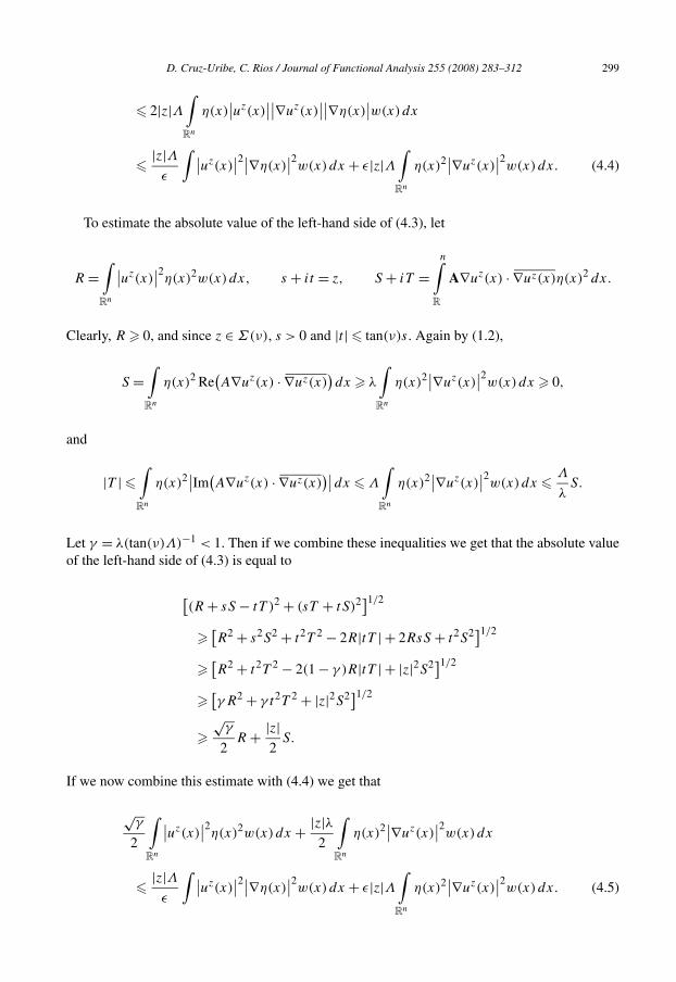
D. Cruz-Uribe, C. Rios / Journal of Functional Analysis 255 (2008) 283–312 299

� 2|z|Λ∫Rn

η(x)∣∣uz(x)

∣∣∣∣∇uz(x)∣∣∣∣∇η(x)

∣∣w(x)dx

� |z|Λε

∫ ∣∣uz(x)∣∣2∣∣∇η(x)

∣∣2w(x)dx + ε|z|Λ

∫Rn

η(x)2∣∣∇uz(x)

∣∣2w(x)dx. (4.4)

To estimate the absolute value of the left-hand side of (4.3), let

R =∫Rn

∣∣uz(x)∣∣2

η(x)2w(x)dx, s + it = z, S + iT =n∫

R

A∇uz(x) · ∇uz(x)η(x)2 dx.

Clearly, R � 0, and since z ∈ Σ(ν), s > 0 and |t | � tan(ν)s. Again by (1.2),

S =∫Rn

η(x)2 Re(A∇uz(x) · ∇uz(x)

)dx � λ

∫Rn

η(x)2∣∣∇uz(x)

∣∣2w(x)dx � 0,

and

|T | �∫Rn

η(x)2∣∣Im(

A∇uz(x) · ∇uz(x))∣∣dx � Λ

∫Rn

η(x)2∣∣∇uz(x)

∣∣2w(x)dx � Λ

λS.

Let γ = λ(tan(ν)Λ)−1 < 1. Then if we combine these inequalities we get that the absolute valueof the left-hand side of (4.3) is equal to

[(R + sS − tT )2 + (sT + tS)2]1/2

�[R2 + s2S2 + t2T 2 − 2R|tT | + 2RsS + t2S2]1/2

�[R2 + t2T 2 − 2(1 − γ )R|tT | + |z|2S2]1/2

�[γR2 + γ t2T 2 + |z|2S2]1/2

�√

γ

2R + |z|

2S.

If we now combine this estimate with (4.4) we get that

√γ

2

∫Rn

∣∣uz(x)∣∣2

η(x)2w(x)dx + |z|λ2

∫Rn

η(x)2∣∣∇uz(x)

∣∣2w(x)dx

� |z|Λε

∫ ∣∣uz(x)∣∣2∣∣∇η(x)

∣∣2w(x)dx + ε|z|Λ

∫n

η(x)2∣∣∇uz(x)

∣∣2w(x)dx. (4.5)

R

300 D. Cruz-Uribe, C. Rios / Journal of Functional Analysis 255 (2008) 283–312

Let ε = λ2Λ

; then the second term on each side of the inequality cancel. Now let η = eαθ − 1,where supp(θ) ⊂ R

n \ E, 0 � θ � 1, θ = 1 on F , ‖∇θ‖∞ � Kd

, and

α =[

λ√

γ

16Λ2K2

]1/2d√|z| .

Then (4.5) yields

√γ

2

∫Rn

(e2αθ(x) − 2eαθ(x) + 1

)∣∣uz(x)∣∣2

w(x)dx �√

γ

8

∫Rn

e2αθ(x)∣∣uz(x)

∣∣2w(x)dx.

If we discard the integral of |uz|2w on the left-hand side and rearrange terms, we get that∫Rn

e2αθ(x)∣∣uz(x)

∣∣2w(x)dx � 8

3

∫Rn

eαθ(x)∣∣uz(x)

∣∣2w(x)dx.

Since θ � 1 and θ = 1 on F , this yields∫F

∣∣uz(x)∣∣2

w(x)dx � 8

3e−α

∫Rn

∣∣uz(x)∣∣2

w(x)dx.

Since uz = (I + zLw)−1f and by Proposition 3.5 the resolvent is bounded on L2(w) with aconstant that depends on ν, inequality (4.2) follows immediately.

Now suppose that ν ∈ (π/2,π/2 + τ). In this case, we can find ν′ < π/2 and τ ′ < τ such thatz = z′ζ , where |ζ | = 1, | arg(ζ )| < τ ′, and z′ ∈ Σ(ν′). Then we can rewrite the left-hand side of(4.2) as ∫

F

∣∣(I + zLw)−1f (x)∣∣2

w(x)dx =∫F

∣∣(I + z′L′w

)−1f (x)2

∣∣w(x)dx,

where L′w = ζLw is the densely defined operator associated to the sesquilinear form generated by

the matrix ζA. By Lemma 3.3, there exist 0 < λζ < Λζ such that ζA ∈ En(w,λζ ,Λζ ). Therefore,L′

w and its resolvent have all the properties of Lw that we used in the above argument, so we canrepeat it to get the desired inequality. �Remark 4.2. Since A∗ ∈ En(w,λ,Λ), Lemma 4.1 holds for L∗

w with the same constants.

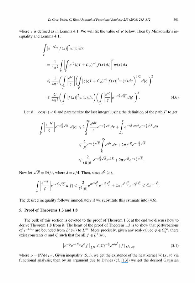
We will now prove Theorem 1.6. Fix t > 0; without loss of generality we may assume thatd2 � t . By Proposition 3.6,

e−tLwf = 1

2πi

∫Γ

etζ (ζ I +Lw)−1f dζ,

where Γ is the union of the rays γ ± = {z ∈ C: z = re±iν , r � R > 0} and the arc γ0 ={z ∈ C: z = Reiψ, |ψ | � ν}, going around the origin counter-clockwise, and ν ∈ (π/2,π/2+τ),

D. Cruz-Uribe, C. Rios / Journal of Functional Analysis 255 (2008) 283–312 301

where τ is defined as in Lemma 4.1. We will fix the value of R below. Then by Minkowski’s in-equality and Lemma 4.1,

∫F

∣∣e−tLwf (x)∣∣2

w(x)dx

= 1

4π2

∫F

∣∣∣∣∫Γ

etζ (ζ I +Lw)−1f (x)dζ

∣∣∣∣2

w(x)dx

� 1

4π2

(∫Γ

∣∣∣∣etζ

ζ

∣∣∣∣(∫

F

∣∣ζ(ζ I +Lw)−1f (x)∣∣2

w(x)dx

)1/2

d|ζ |)2

� C

4π2

(∫E

∣∣f (x)∣∣2

w(x)dx

)(∫Γ

∣∣∣∣etζ

ζ

∣∣∣∣e−c d2√|ζ | d|ζ |

)2

. (4.6)

Let β = cos(ν) < 0 and parametrize the last integral using the definition of the path Γ to get

∫Γ

∣∣∣∣e−tζ

ζ

∣∣∣∣e−c d2√|ζ | d|ζ | � 2

∞∫R

etβr

re−c d

2√

r dr +ν∫

−ν

e−tR cos θ e−c d2

√R dθ

� 2

Re−c d

2

√R

∞∫R

etβr dr + 2πetRe−c d2

√R

� 2

tR|β|e−c d

2

√RetβR + 2πetRe−c d

2

√R.

Now let√

R = δd/t , where δ = c/4. Then, since d2 � t ,

∫Γ

∣∣∣∣e−tζ

ζ

∣∣∣∣e−c d2√|ζ | d|ζ | � 2

δ2|β|eβδ2 d2

t e− cδ2

d2t + 2πeδ2 d2

t e− cδ2

d2t � Ce−c d2

t .

The desired inequality follows immediately if we substitute this estimate into (4.6).

5. Proof of Theorems 1.3 and 1.8

The bulk of this section is devoted to the proof of Theorem 1.3; at the end we discuss how toderive Theorem 1.8 from it. The heart of the proof of Theorem 1.3 is to show that perturbationsof e−tLw are bounded from L2(w) to L∞. More precisely, given any real-valued φ ∈ C∞

c , thereexist constants α and C such that for all f ∈ L2(w),

∥∥e−φe−tLweφf∥∥

L∞ � Ct−n4 eαtρ2‖f ‖L2(w), (5.1)

where ρ = ‖∇φ‖L∞ . Given inequality (5.1), we get the existence of the heat kernel Wt(x, y) viafunctional analysis; then by an argument due to Davies (cf. [13]) we get the desired Gaussian

302 D. Cruz-Uribe, C. Rios / Journal of Functional Analysis 255 (2008) 283–312

bounds. Hölder continuity estimates then follow from the Harnack inequality and a classicalargument.

5.1. The L2(w),L∞ estimates

To prove (5.1) it will suffice to prove it for non-negative functions f and for x = 0 and t = 1:

∣∣e−φe−Lweφf (0)∣∣ � Ceαρ2‖f ‖L2(w). (5.2)

To see that it suffices to consider non-negative functions, we use the fact that e−tLw is linear andthat given f = u + iv, we can decompose f as u+ − u− + iv+ − iv−, where g+ = max(g,0)

and g− = −min(g,0), ‖g‖L2(w) � ‖g−‖L2(w) + ‖g+‖L2(w) � 2‖g‖L2(w).The second reduction follows from homogeneity and the fact that if w is in A2 or QC, then

so is wab = w(a · +b) for all a ∈ R, b ∈ Rn. To show that we can take t = 1, suppose that(5.1) holds when t = 1 for all operators Lw . Define the functions u(x, t) = e−φe−tLweφf (x)

and v(y, s) = u(√

ty, ts). Then a straightforward computation shows that v = e−φte−sLt eφt

f t ,where f t (y) = f (

√ty), φt (y) = φ(

√ty), and Lt is the operator induced by the sesquilinear

form

at (f, g) =∫Rn

At∇f (x) · ∇g(x)dx,

where At (y) = A(√

ty). The matrix At satisfies (1.2) with w replaced by wt(y) = w(√

ty).Since w ∈ A2/QC, wt ∈ A2/QC with the same constant. Therefore, if (5.1) holds for s = 1 forthe operator Lt , then, with ρt = ‖∇φt‖L∞ = t1/2ρ,

∥∥u(·, t)∥∥L∞ = ∥∥v(·,1)

∥∥L∞ � Ceαρ2

t∥∥v(·,0)

∥∥L2(wt )

= Ceαtρ2( ∫

Rn

∣∣f (√

ty)∣∣2

w(√

ty) dy

) 12 = Ct−

n4 eαtρ2‖f ‖L2(w).

To show that it suffices to take x = 0, we can repeat the above argument, replacing f byf 0(x) = f (x + x0), w by w0(x) = w(x + x0), etc., for some fixed x0 ∈ R

n.We will now prove (5.2). Fix f ∈ L2(w). Let Q0 ⊂ R

n be the cube (with sides parallel to thecoordinate axes) centered at the origin with �(Q0) = 9, and let f 0 = f χQ0. For each integerk � 1, let Qk = 3kQ0 and define f k = f χQk\Qk−1 . Decompose Qk\Qk−1 into 3n − 1 disjointcubes Qk,j , 1 � j � 3n − 1, of side length 3k+1. For k � 1, let f k,j = f χQk,j . Then we havethat

∣∣e−φe−Lweφf (0)∣∣ � e−φ(0)

∞∑k=1

3n−1∑j=1

∣∣e−Lweφf k,j (0)∣∣ + e−φ(0)

∣∣e−Lweφf 0(0)∣∣. (5.3)

We first estimate the sum. Let uk,j (x, t) = e−tLweφf k,j (x); then by Proposition 3.4 uk,j isa non-negative solution of Lwu = ut in R

n+1+ . Define vk,j (y, s) = uk,j (3ky, s). Then vk,j is asolution to Lkv = vs in R

n+1+ , where Lk is the operator induced by the sesquilinear form defined

D. Cruz-Uribe, C. Rios / Journal of Functional Analysis 255 (2008) 283–312 303

as above with the matrix Ak(y) = A(3ky). The matrix Ak satisfies (1.2) with w replaced bywk(y) = w(3ky), which is again an A2/QC weight. Therefore, by Proposition 3.8 applied to theparabolic cylinder Q1(0, 13

8 ),

supQ−

1 (0, 138 )

vk,j (y, s) � γ infQ+

1 (0, 138 )

vk,j (y, s).

In particular, since (0,1) ∈ Q−1 (0, 13

8 ), |vk,j (0,1)| � γ infQ+1 (0, 13

8 )vk,j (y, s). Let Br = {x:

|x| < r}. Then

∣∣vk,j (0,1)∣∣ � C(n)γwk(B 1

2)−

12

( 218∫

198

∫|y|< 1

2

∣∣vk,j (y, s)∣∣2

wk(y)dy ds

) 12

.

By a change of variables this becomes

∣∣uk,j (0,1)∣∣ � C(n)γw(B 3k

2)−

12

( 218∫

198

∫|x|< 3k

2

∣∣uk,j (x, t)∣∣2

w(x)dx dt

) 12

.

Since eφf k,j (x) is supported in Qk,j and dist(Qk,j , {|x| < 3k

2 }) � dist(Qk,Qk−2) = 3k , by The-orem 1.6 we have

e−φ(0)∣∣e−Lweφf k,j (0)

∣∣= e−φ(0)

∣∣uk,j (0,1)∣∣

� C(n)γw(B 3k

2)−

12 e−c32k

( 218∫

198

∫Rn

e2(φ(x)−φ(0))∣∣f k,j (x)

∣∣2w(x)dx dt

) 12

� C(n)γw(B 3k

2)−

12 e−c32k∥∥eφ(·)−φ(0)

∥∥L∞(Qk,j )

∥∥f k,j∥∥

L2(w)

� C(n)γw(B 3k

2)−

12 e−c32k

e3k+1√

n2 ‖∇φ‖L∞ ∥∥f k,j

∥∥L2(w)

.

We estimate the last term on the right-hand side in (5.3) in a similar fashion, except thatinstead of Theorem 1.6 we use the fact that e−Lw is bounded on L2(w) to obtain

e−φ(0)∣∣e−Lweφf 0(0)

∣∣ � Ce9√

n2 ‖∇φ‖L∞ ∥∥f 0

∥∥L2(w)

.

Now substitute both these estimates in (5.3) and apply Hölder’s inequality twice to get

304 D. Cruz-Uribe, C. Rios / Journal of Functional Analysis 255 (2008) 283–312

e−φ(0)∣∣e−Lweφf (0)

∣∣� C(n)γ

∞∑k=1

3n−1∑j=1

w(B 3k

2)−

12 e−c32k

e3k+1√

n2 ‖∇φ‖L∞ ∥∥f k,j

∥∥L2(w)

+ Ce9√

n2 ‖∇φ‖L∞ ∥∥f 0

∥∥L2(w)

� C(n)γ(3n − 1

)1/2∞∑

k=1

w(B 3k

2)−

12 e−c32k

e3k+1√

n2 ‖∇φ‖L∞ ∥∥f k

∥∥L2(w)

+ Ce9√

n2 ‖∇φ‖L∞ ∥∥f 0

∥∥L2(w)

� C(n,γ )

∞∑k=0

w(B 3k

2)−

12 e−c32k

e3k+2√

n2 ‖∇φ‖L∞ ∥∥f k

∥∥L2(w)

� C(n,γ )

( ∞∑k=0

w(B 3k

2)−1

)1/2( ∞∑k=0

exp(−2c32k + 3k+2√n‖∇φ‖L∞

)∥∥f k∥∥2

L2(w)

)1/2

.

Since w ∈ A∞, it satisfies a reverse doubling condition: there exists β > 1 such that βw(Br) �w(B3r ). Thus,

∞∑k=0

w(B 3k

2)−1 �

∞∑k=0

β−kw(B 12)−1 < C(w) < ∞.

Therefore, we have shown that

e−φ(0)∣∣e−Lweφf (0)

∣∣� C(n,γ,w) exp

(81n

8c‖∇φ‖2

L∞

)( ∞∑k=0

∥∥f k∥∥2

L2(w)

)1/2

= C(n,γ,w)eαρ2‖f ‖L2(w),

where α = 81n8c

and ρ = ‖∇φ‖L∞ . This proves (5.2) and so (5.1).

5.2. Gaussian bounds

To find the heat kernel and show that it satisfies Gaussian bounds, first note that by duality,(5.1) implies that

∥∥e−φe−tLweφf∥∥

L2(w)� Ct−

n4 eαtρ2‖f ‖L1 .

Since e−φe−tLweφ is a semigroup, we can combine this inequality with (5.1) to get

∥∥e−φe−tLweφf∥∥ ∞ � Ct−n/2eαtρ2‖f ‖L1 . (5.4)

L

D. Cruz-Uribe, C. Rios / Journal of Functional Analysis 255 (2008) 283–312 305

By a classical result of Dunford and Pettis [15] (see also [3, p. 42]), this implies that for eachφ ∈ C∞

c , there exists a kernel Wφt (x, y) such that for all f ∈ L1,

e−φe−tLweφf (x) =∫Rn

Wφt (x, y)f (y) dy

and

∣∣Wφt (x, y)

∣∣ � Ct−n/2eαtρ2.

In particular, let φ ≡ 0 to get the kernel Wt(x, y) of e−tLw ; then it is immediate that Wt(x, y) =eφ(x)−φ(y)W

φt (x, y). Hence,

∣∣Wt(x, y)∣∣ � Ceαtρ2

eφ(x)−φ(y)t−n/2. (5.5)

Inequality (5.5) is true for every φ ∈ C∞c with ‖∇φ‖L∞ = ρ, ρ > 0. Therefore, by an ap-

proximation argument we may take φ to be a Lipschitz function that satisfies φ(x) − φ(y) =−ρ|x − y|. Then (5.5) becomes

∣∣Wt(x, y)∣∣ � Ct−n/2 exp

(αtρ2 − ρ|x − y|).

If we optimize the value of ρ, we get ρ = |x−y|2αt

, and thus

∣∣Wt(x, y)∣∣ � Ct−n/2 exp

(−|x − y|2

4αt

).

This is the desired inequality.

5.3. Hölder continuity

The proof of inequalities (1.10) and (1.11) follow by standard arguments from the classicaltheory of elliptic and parabolic operators. Therefore, here we will only briefly sketch the proof.First, since the heat kernel of L∗

w is Wt(y, x), (1.11) follows from (1.10) by duality.Given that Wt(x, y) satisfies Gaussian bounds, it is well known (see [3, p. 30]) that to prove

(1.10) it suffices to prove that there exist constants C and ν > 0 such that for all t > 0 and allx, y,h ∈ Rn,

∣∣Wt(x + h,y) − Wt(x, y)∣∣ � C|h|ν

tn/2+ν/2.

By a classical result (again see [3, p. 42]), this is equivalent to proving that e−tLw maps L1 intothe space of Hölder continuous functions Cν , with norm C|h|ν

n/2+ν/2 .

t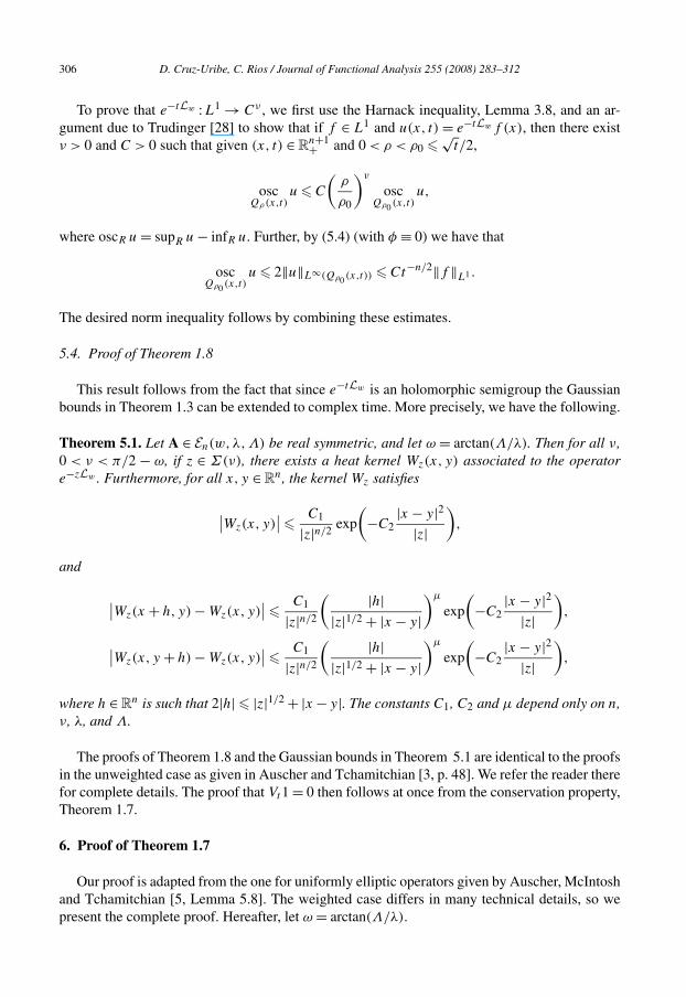

306 D. Cruz-Uribe, C. Rios / Journal of Functional Analysis 255 (2008) 283–312

To prove that e−tLw :L1 → Cν , we first use the Harnack inequality, Lemma 3.8, and an ar-gument due to Trudinger [28] to show that if f ∈ L1 and u(x, t) = e−tLwf (x), then there existν > 0 and C > 0 such that given (x, t) ∈ R

n+1+ and 0 < ρ < ρ0 �√

t/2,

oscQρ(x,t)

u � C

(ρ

ρ0

)ν

oscQρ0 (x,t)

u,

where oscR u = supR u − infR u. Further, by (5.4) (with φ ≡ 0) we have that

oscQρ0 (x,t)

u � 2‖u‖L∞(Qρ0 (x,t)) � Ct−n/2‖f ‖L1 .

The desired norm inequality follows by combining these estimates.

5.4. Proof of Theorem 1.8

This result follows from the fact that since e−tLw is an holomorphic semigroup the Gaussianbounds in Theorem 1.3 can be extended to complex time. More precisely, we have the following.

Theorem 5.1. Let A ∈ En(w,λ,Λ) be real symmetric, and let ω = arctan(Λ/λ). Then for all ν,0 < ν < π/2 − ω, if z ∈ Σ(ν), there exists a heat kernel Wz(x, y) associated to the operatore−zLw . Furthermore, for all x, y ∈ R

n, the kernel Wz satisfies

∣∣Wz(x, y)∣∣ � C1

|z|n/2exp

(−C2

|x − y|2|z|

),

and

∣∣Wz(x + h,y) − Wz(x, y)∣∣ � C1

|z|n/2

( |h||z|1/2 + |x − y|

)μ

exp

(−C2

|x − y|2|z|

),

∣∣Wz(x, y + h) − Wz(x, y)∣∣ � C1

|z|n/2

( |h||z|1/2 + |x − y|

)μ

exp

(−C2

|x − y|2|z|

),

where h ∈ Rn is such that 2|h| � |z|1/2 + |x − y|. The constants C1, C2 and μ depend only on n,

ν, λ, and Λ.

The proofs of Theorem 1.8 and the Gaussian bounds in Theorem 5.1 are identical to the proofsin the unweighted case as given in Auscher and Tchamitchian [3, p. 48]. We refer the reader therefor complete details. The proof that Vt1 = 0 then follows at once from the conservation property,Theorem 1.7.

6. Proof of Theorem 1.7

Our proof is adapted from the one for uniformly elliptic operators given by Auscher, McIntoshand Tchamitchian [5, Lemma 5.8]. The weighted case differs in many technical details, so wepresent the complete proof. Hereafter, let ω = arctan(Λ/λ).

D. Cruz-Uribe, C. Rios / Journal of Functional Analysis 255 (2008) 283–312 307

It is straightforward to show that since the kernel of e−zLw , z ∈ Σ(π/2−ω), satisfies Gaussianbounds, e−zLw :Lp → Lp , 1 � p � ∞, with a bound that depends only on arg(z). By the Laplaceidentity we get the same Lp estimates for (zI +Lw)−1. The same proof shows that the weightedversions of these inequalities are true if 2 � p < ∞; in the case 1 � p < 2 we need to assumew ∈ Ap . This need not be the case if w ∈ A2 or QC. However, the following weaker resultsuffices for our purposes.

Lemma 6.1. Let w ∈ A2 or QC, and let z ∈ Σ(π − ω). Then (zI +Lw)−1 is a densely definedoperator from L1(w) into itself with domain containing C∞

c . In fact, if φ ∈ C∞c , then

∣∣(zI +Lw)−1φ(x)∣∣ � Ce−c|x|, (6.1)

where the constants depend on n, Λ, λ, arg(z) and φ.

Proof. If inequality (6.1) holds, then it follows immediately that e−zLwφ ∈ L1(w): sincew ∈ A∞, there exists D > 1 such that for every r > 0, w(B2r (0)) � Dw(Br(0)) [21, p. 695].Hence,

∥∥(zI +Lw)−1φ∥∥

L1(w)� Cw

(B1(0)

) +∞∑

k=0

Ce−c2k

w(B2k+1(0) \ B2k (0)

)

� Cw(B1(0)

) ∞∑k=0

Dke−c2k

< ∞.

To prove (6.1), fix φ ∈ C∞c and suppose that supp(φ) ⊂ BR(0), R > 1. By Proposition 3.6,

(zI +Lw)−1φ(x) =∞∫

0

e−zνt e−νtLwφ(x) dt,

where we take ν ∈ Σ(π/2 − ω) such that |ν| = 1 and Re(zν) > 0. Since e−νtLwφ ∈ L∞ isuniformly bounded, assume without loss of generality that |x| > 2R, so if x ∈ supp(φ), |x −y| >|x|/2. Therefore, by Theorem 5.1,

∣∣(zI +Lw)−1φ(x)∣∣

� C

∞∫0

e−Re(zν)t

∫Rn

|νt |−n/2 exp

(−c

|x − y|2|νt |

)∣∣φ(y)∣∣dy dt

� C

∞∫0

e−Re(zν)t

n∫R

t−n/2 exp

(− c

4

|x|2t

)∣∣φ(y)∣∣dy dt

� C‖φ‖∞Rn

∞∫e−Re(zν)t t−n/2 exp

(− c

4

|x|2t

)dt

0

308 D. Cruz-Uribe, C. Rios / Journal of Functional Analysis 255 (2008) 283–312

� C‖φ‖∞Rn∞∑

j=−∞

2j+1|x|2∫2j |x|2

e−Re(zν)t t−n/2 exp

(− c

4

|x|2t

)dt

� C‖φ‖∞Rn∞∑

j=−∞2j |x|2e−2j |x|2 Re(zν)

(2j |x|2)−n/2 exp

(− c

82−j

)

� C‖φ‖∞|x|2∞∑

j=−∞exp

(−2j |x|2 Re(zν) − c

82−j − log(2)

(n

2− 1

)j

).

Since |x| > 2R � 2, there exists J > 0 such that 2J � |x| < 2J+1. We estimate the sum in thelast term by splitting it into three pieces depending on the size of j :

∞∑j=−∞

exp

(−2j |x|2 Re(zν) − c

82−j − log(2)

(n

2− 1

)j

)

=( ∞∑

j=0

+−1∑

j=−J

+−J−1∑j=−∞

)exp

(−2j |x|2 Re(zν) − c

82−j − log(2)

(n

2− 1

)j

)

�∞∑

j=0

exp(−2j |x|2 Re(zν)

)

+ exp(−|x|Re(zν)

) −1∑j=−J

exp

(− c

82−j − log(2)

(n

2− 1

)j

)

+ exp

(− c

8|x|

) ∞∑j=J+1

exp

(c

42J − c

82j + log(2)

(n

2− 1

)j

)

� Ce−c|x|.

Combining these two estimates we get that∣∣(zI +Lw)−1φ(x)∣∣ � C‖φ‖∞|x|2e−c|x| � C‖φ‖∞e−c|x|.

This completes the proof. �Proof of Theorem 1.7. Since the semigroup and the resolvent are bounded on L∞, by Proposi-tion 3.6 we have that

e−tLw 1 = 1

2πi

∫Γ

e−tζ (ζ I +Lw)−11dζ, (6.2)

where in the definition of Γ we take R = 1/t . Suppose for the moment that we could prove forall ζ ∈ Γ that

(ζ I +Lw)−11 = ζ−1. (6.3)

D. Cruz-Uribe, C. Rios / Journal of Functional Analysis 255 (2008) 283–312 309

Then (6.2) becomes

etLw 1 = 1

2πi

∫Γ

ζ−1e−tζ dζ = 1,

where the last equality follows from a standard contour integral argument.To prove (6.3) it suffices to show that for all φ ∈ C∞

c ,∫Rn

(ζ I +Lw)−11φ(x)w(x)dx = ζ−1∫Rn

φ(x)w(x)dx.

By duality, ∫Rn

(ζ I +Lw)−11φ(x)w(x)dx =∫Rn

(ζ I +L∗

w

)−1φ(x)w(x)dx.

Let h(x) = (ζ I +L∗w)−1φ(x); then by Lemma 6.1 we have that h ∈ L1(w). Furthermore, L∗

wh =−ζ h + φ, so L∗

wh ∈ L1(w). Therefore,∫Rn

(ζ I +Lw)−11φ(x)w(x)dx = ζ−1∫Rn

φ(x)w(x)dx − ζ−1∫Rn

L∗wh(x)w(x)dx.

To complete the proof we will show that the last integral equals zero. Let supp(φ) ⊂ BR(0),and for all r > 2R, let χr ∈ C∞

c be such that χr ≡ 1 on Br(0), supp(χr) ⊂ B2r (0), and |∇χr | �cr−1. Then∣∣∣∣∣

∫Rn

L∗wh(x)w(x)dx

∣∣∣∣∣ = limr→∞

∣∣∣∣n∫

R

L∗wh(x)χr(x)w(x)dx

∣∣∣∣= lim

r→∞

∣∣∣∣∫Rn

A∗∇h(x) · ∇χr(x) dx

∣∣∣∣� Λ lim

r→∞

∫Rn

∣∣∇h(x)∣∣∣∣∇χr(x)

∣∣w(x)dx

� limr→∞Cr−1w

(B2r (0)

)( ∫supp(∇χr )

∣∣∇h(x)∣∣2

w(x)dx

)1/2

.

To bound the last integral, we first make a preliminary estimate. let ψ ∈ C∞c be such that

supp(ψ) ∩ supp(φ) = ∅. Then for all δ > 0,∫Rn

∣∣∇h(x)∣∣2

ψ(x)2w(x)dx � λ−1 Re∫Rn

A∗∇h(x) · ∇h(x)ψ(x)2 dx

� λ−1∣∣∣∣∫n

A∗∇h(x) · ∇h(x)ψ(x)2 dx

∣∣∣∣

R

310 D. Cruz-Uribe, C. Rios / Journal of Functional Analysis 255 (2008) 283–312

� λ−1∣∣∣∣∫Rn

L∗wh(x)h(x)ψ(x)2w(x)dx

∣∣∣∣+ 2λ−1

∣∣∣∣∫Rn

ψ(x)h(x)A∗∇h(x) · ψ(x)dx

∣∣∣∣� λ−1

∣∣∣∣∫Rn

(−ζ h(x) + φ(x))h(x)ψ(x)2w(x)dx

∣∣∣∣+ δΛλ−1

∫Rn

∣∣∇h(x)∣∣2

ψ(x)2w(x)dx

+ δ−1Λλ−1∫Rn

∣∣h(x)∣∣2∣∣∇ψ(x)

∣∣2w(x)dx.

If we fix δ such that δΛλ−1 = 1/2, then we can rearrange terms to get

∫Rn

∣∣∇h(x)∣∣2

ψ(x)2w(x)dx � C|ζ |∫Rn

∣∣h(x)∣∣2(∣∣∇ψ(x)

∣∣2 + ψ(x)2)w(x)dx. (6.4)

Now for each r > 2R, fix ψr ∈ C∞c such that supp(ψ) ⊂ B3r (0) \ Br/2(0), ψ ≡ 1 on

supp(∇χr) and |∇ψr | � C. Then by (6.4) and Lemma 6.1 we have that

limr→∞Cr−1w

(B2r (0)

)( ∫supp(∇χr )

∣∣∇h(x)∣∣2

w(x)dx

)1/2

= limr→∞Cr−1w

(B2r (0)

)( ∫supp(∇χr )

∣∣∇h(x)∣∣2

ψr(x)2w(x)dx

)1/2

� limr→∞Cr−1w

(B2r (0)

)( ∫B3r (0)\Br/2(0)

∣∣h(x)∣∣2

w(x)dx

)1/2

� limr→∞Cr−1w

(B3r (0)

)3/2 exp(−cr)

= 0.

The last equality holds since w ∈ A∞: as in the proof of Lemma 6.1, there exists D > 1 such thatfor all r > 1, if 3N < r � 3N+1, then

w(B3r (0)

)3/2e−cr � D

32 (N+1)w

(B1(0)

)3/2e−c3N � C.

This completes the proof. �

D. Cruz-Uribe, C. Rios / Journal of Functional Analysis 255 (2008) 283–312 311

Acknowledgments

The authors would like to thank Steven Hofmann for suggesting this project to us and forhis help and guidance in completing it. Both authors gratefully acknowledge the support of theStewart-Dorwart faculty development fund at Trinity College.

References

[1] D.G. Aronson, Bounds for the fundamental solution of a parabolic equation, Bull. Amer. Math. Soc. 73 (1967)890–896.

[2] Pascal Auscher, Regularity theorems and heat kernel for elliptic operators, J. London Math. Soc. (2) 54 (2) (1996)284–296.

[3] Pascal Auscher, Philippe Tchamitchian, Square root problem for divergence operators and related topics,Astérisque 249 (1998), viii + 172.

[4] Pascal Auscher, Thierry Coulhon, Philippe Tchamitchian, Absence de principe du maximum pour certaines équa-tions paraboliques complexes, Colloq. Math. 71 (1) (1996) 87–95.

[5] Pascal Auscher, Alan McIntosh, Philippe Tchamitchian, Heat kernels of second order complex elliptic operatorsand applications, J. Funct. Anal. 152 (1) (1998) 22–73.

[6] Pascal Auscher, Steve Hofmann, Michael Lacey, Alan McIntosh, Ph. Tchamitchian, The solution of the Kato squareroot problem for second order elliptic operators on R

n, Ann. of Math. (2) 156 (2) (2002) 633–654.[7] Filippo Chiarenza, Michelangelo Franciosi, Quasiconformal mappings and degenerate elliptic and parabolic equa-

tions, Matematiche (Catania) 42 (1–2) (1987) 163–170.[8] Filippo Chiarenza, Michele Frasca, Boundedness for the solutions of a degenerate parabolic equation, Appl.

Anal. 17 (4) (1984) 243–261.[9] Filippo Chiarenza, Raul P. Serapioni, Degenerate parabolic equations and Harnack inequality, Ann. Mat. Pura Appl.

(4) 137 (1984) 139–162.[10] Filippo M. Chiarenza, Raul P. Serapioni, A Harnack inequality for degenerate parabolic equations, Comm. Partial

Differential Equations 9 (8) (1984) 719–749.[11] Filippo Chiarenza, Raul P. Serapioni, A remark on a Harnack inequality for degenerate parabolic equations, Rend.

Sem. Mat. Univ. Padova 73 (1985) 179–190.[12] Guy David, Stephen Semmes, Strong A∞ weights, Sobolev inequalities and quasiconformal mappings, in: Analysis

and Partial Differential Equations, in: Lecture Notes in Pure and Appl. Math., vol. 122, Dekker, New York, 1990,pp. 101–111.

[13] E.B. Davies, Heat Kernels and Spectral Theory, Cambridge Tracts in Math., vol. 92, Cambridge Univ. Press, Cam-bridge, 1990.

[14] E.B. Davies, Heat kernel bounds, conservation of probability and the Feller property, J. Anal. Math. 58 (1992)99–119, Festschrift on the occasion of the 70th birthday of Shmuel Agmon.

[15] Nelson Dunford, B.J. Pettis, Linear operations on summable functions, Trans. Amer. Math. Soc. 47 (1940) 323–392.[16] Javier Duoandikoetxea, Fourier Analysis, Grad. Stud. Math., vol. 29, Amer. Math. Soc., Providence, RI, 2001.[17] Eugene B. Fabes, Carlos E. Kenig, Raul P. Serapioni, The local regularity of solutions of degenerate elliptic equa-

tions, Comm. Partial Differential Equations 7 (1) (1982) 77–116.[18] Avner Friedman, Partial Differential Equations of Parabolic Type, Prentice Hall, Englewood Cliffs, NJ, 1964.[19] Matthew P. Gaffney, The conservation property of the heat equation on Riemannian manifolds, Comm. Pure Appl.

Math. 12 (1959) 1–11.[20] José García-Cuerva, José L. Rubio de Francia, Weighted Norm Inequalities and Related Topics, North-Holland

Math. Stud., vol. 116, North-Holland, Amsterdam, 1985.[21] Loukas Grafakos, Classical and Modern Fourier Analysis, Pearson/Prentice Hall, Upper Saddle River, NJ, 2004.[22] Cristian E. Gutiérrez, Gail S. Nelson, Bounds for the fundamental solution of degenerate parabolic equations,

Comm. Partial Differential Equations 13 (5) (1988) 635–649.[23] Cristian E. Gutiérrez, Richard L. Wheeden, Bounds for the fundamental solution of degenerate parabolic equations,

Comm. Partial Differential Equations 17 (7–8) (1992) 1287–1307.[24] Kazuhiro Ishige, On the behavior of the solutions of degenerate parabolic equations, Nagoya Math. J. 155 (1999)

1–26.[25] Tosio Kato, Perturbation Theory for Linear Operators, Grundlehren Math. Wiss., vol. 132, Springer-Verlag, New

York, 1966.

312 D. Cruz-Uribe, C. Rios / Journal of Functional Analysis 255 (2008) 283–312

[26] V.G. Maz’ya, S.A. Nazarov, B.A. Plamenevskiı, Absence of a de Giorgi-type theorem for strongly elliptic equationswith complex coefficients, Zap. Nauchn. Sem. Leningrad. Otdel. Mat. Inst. Steklov. (LOMI) 115 (309) (1982) 156–168, Boundary value problems of mathematical physics and related questions in the theory of functions, 14.

[27] El Maati Ouhabaz, Analysis of Heat Equations on Domains, London Math. Soc. Monogr. Ser., vol. 31, PrincetonUniv. Press, Princeton, NJ, 2005.

[28] Neil S. Trudinger, Pointwise estimates and quasilinear parabolic equations, Comm. Pure Appl. Math. 21 (1968)205–226.

[29] Bengt Ove Turesson, Nonlinear Potential Theory and Weighted Sobolev Spaces, Lecture Notes in Math., vol. 1736,Springer-Verlag, Berlin, 2000.

[30] Kôsaku Yosida, Functional Analysis, Grundlehren Math. Wiss., vol. 123, Academic Press, New York, 1965.