Improving the efficiency of parallel alternating directions algorithm for timedependent problemsMaria Ganzha, Nikola Kosturski, and Ivan Lirkov Citation: AIP Conf. Proc. 1487, 322 (2012); doi: 10.1063/1.4758974 View online: http://dx.doi.org/10.1063/1.4758974 View Table of Contents: http://proceedings.aip.org/dbt/dbt.jsp?KEY=APCPCS&Volume=1487&Issue=1 Published by the American Institute of Physics. Additional information on AIP Conf. Proc.Journal Homepage: http://proceedings.aip.org/ Journal Information: http://proceedings.aip.org/about/about_the_proceedings Top downloads: http://proceedings.aip.org/dbt/most_downloaded.jsp?KEY=APCPCS Information for Authors: http://proceedings.aip.org/authors/information_for_authors

Downloaded 09 Oct 2012 to 213.191.204.24. Redistribution subject to AIP license or copyright; see http://proceedings.aip.org/about/rights_permissions

Improving the efficiency of parallel alternating directionsalgorithm for time dependent problemsMaria Ganzha∗, Nikola Kosturski† and Ivan Lirkov†

∗Systems Research Institute, Polish Academy of Science, ul. Newelska 6, 01-447 Warsaw, Poland†Institute of Information and Communication Technologies, Bulgarian Academy of Sciences

Acad. G. Bonchev, bl. 25A, 1113 Sofia, Bulgaria

Abstract. We consider the time dependent Stokes equation on a finite time interval and on a uniform rectangular mesh, writtenin terms of velocity and pressure. A parallel algorithm based on a direction splitting approach is implemented. Our work ismotivated by the need to improve the parallel efficiency of our supercomputer implementation of the parallel algorithm.We are targeting the IBM Blue Gene/P massively parallel computer, which features a 3D torus interconnect. We study

the impact of the domain partitioning on the performance of the considered parallel algorithm for solving the time dependentStokes equation. Here, different parallel partitioning strategies are given special attention. The implementation is tested onthe IBM Blue Gene/P and the presented results from numerical tests confirm that decreasing the communication time betterparallel properties of the algorithm are obtained.Keywords: Navier-Stokes, time splitting, ADI, incompressible flows, pressure Poisson equation, parallel algorithmPACS: 02.60.Cb, 02.60.Lj, 02.70.Bf, 07.05.Tp, 47.10.ad, 47.11.Bc

INTRODUCTION

The objective of this article is to analyze the performance of the MPI and OpenMP parallel codes which use a newfractional time stepping technique, based on a direction splitting strategy, developed to solve the incompressibleNavier-Stokes equations.Projection schemes were first introduced in [1, 2] and they have been used in Computational Fluid Dynamics (CFD)

for the last forty years. During these years, these techniques have been evolving, but the main paradigm, consistingof decomposing vector fields into a divergence-free part and a gradient, has been preserved (see [3] for a reviewof projection methods). In terms of computational efficiency, projection algorithms are far superior to the methodsthat solve the coupled velocity-pressure system. This feature makes them the most popular techniques in the CFDcommunity for solving the unsteady Navier-Stokes equations. The computational complexity of each time step of theprojection methods is that of solving one vector-valued advection-diffusion equation, plus one scalar-valued Poissonequation with the Neumann boundary conditions. Note that, for large scale problems, and large Reynolds numbers,the cost of solving the Poisson equation becomes dominant.The alternating directions algorithm proposed in [4] reduces the computational complexity of the action of the

incompressibility constraint. The key idea is to modify the standard projection approach, in which the vector fieldsare decomposed into a divergence-free part plus a gradient part. In the new method the pressure equation is derivedfrom a perturbed form of the continuity equation, in which the incompressibility constraint is penalized in a negativenorm induced by the direction splitting. The standard Poisson problem for the pressure correction is replaced by seriesof one-dimensional second-order boundary value problems. This technique is proved to be stable and convergent [fordetails see 4]. Furthermore, the parallel performance of this technique is analyzed in [5, 6]. The aim of this paper isto study the impact of the domain partitioning on the performance of the algorithm for solving the 3D time dependentStokes equation.

STOKES EQUATION

Let us start by defining the problem to be solved. We consider the time-dependent Navier-Stokes equations on a finitetime interval [0,T ], and in a rectangular domain Ω. Since the nonlinear term in the Navier-Stokes equations does notinterfere with the incompressibility constraint, we focus our attention on the time-dependent Stokes equations, written

Application of Mathematics in Technical and Natural SciencesAIP Conf. Proc. 1487, 322-328 (2012); doi: 10.1063/1.4758974

© 2012 American Institute of Physics 978-0-7354-1099-2/$30.00

322

Downloaded 09 Oct 2012 to 213.191.204.24. Redistribution subject to AIP license or copyright; see http://proceedings.aip.org/about/rights_permissions

in terms of velocity u and pressure p:⎧⎪⎨⎪⎩ut −νΔu+ ∇p= f in Ω× (0,T)∇ ·u= 0 in Ω× (0,T)u|∂Ω = 0, ∂np|∂Ω = 0 in (0,T )u|t=0 = u0, p|t=0 = p0 in Ω

, (1)

where f is a smooth source term, ν is the kinematic viscosity, and u0 is a solenoidal initial velocity field with a zeronormal trace. In our work, we consider homogeneous Dirichlet boundary conditions on the velocity.To solve thus described problem, we discretize the time interval [0,T ] using a uniform mesh. Finally, let τ be the

time step used in the algorithm.

FORMULATION OF THE SCHEME

Let us describe the proposed parallel solution method. Authors of [4] introduced an innovative fractional time steppingtechnique for solving the incompressible Navier-Stokes equations, based on a direction splitting strategy. They used asingular perturbation of the Stokes equation with the perturbation parameter τ . The standard Poisson problem for thepressure correction was replaced by series of one-dimensional second-order boundary value problems.The scheme used in the algorithm is composed of the following parts: (i) pressure prediction, (ii) velocity update,

(iii) penalty step, and (iv) pressure correction. Let us now describe an algorithm that uses the direction splitting operator

A :=(1−

∂ 2

∂x2

)(1−

∂ 2

∂y2

)(1−

∂ 2

∂ z2

).

• Pressure predictor. The algorithm is initialized by setting p−12 = p−

32 = p0. Next, for all n ≥ 0, a pressure

predictor is computed as followsp∗,n+

12 = 2pn−

12 − pn−

32 . (2)

• Velocity update. The velocity field is initialized by setting u0 = u0, and for all n ≥ 0 the velocity update iscomputed by solving the following series of one-dimensional problems

ξξξ n+1−un

τ−νΔun+ ∇p∗,n+

12 = fn+

12 = f|t=(n+ 1

2 )τ , ξξξ n+1|∂Ω = 0

ηηηn+1−ξξξ n+1

τ−

ν2

∂ 2(ηηηn+1−un)∂x2

= 0, ηηηn+1|∂Ω = 0 (3)

ζζζ n+1−ηηηn+1

τ−

ν2

∂ 2(ζζζ n+1−un)∂y2

= 0, ζζζ n+1|∂Ω = 0 (4)

un+1−ζζζ n+1

τ−

ν2

∂ 2(un+1−un)∂ z2

= 0, un+1|∂Ω = 0. (5)

• Penalty step. The intermediate parameter φ is approximated by solving Aφ =− 1τ ∇ ·un+1. This is done by solving

the following series of one-dimensional problems:

θ −θxx = − 1τ ∇ ·un+1, θx|∂Ω = 0,

ψ−ψyy = θ , ψy|∂Ω = 0,φ −φzz = ψ , φz|∂Ω = 0,

(6)

• Pressure update. The pressure is updated using the parameter χ =∈ [0, 12 ].

pn+12 = pn−

12 + φ − χν∇ ·

un+1+un

2(7)

323

Downloaded 09 Oct 2012 to 213.191.204.24. Redistribution subject to AIP license or copyright; see http://proceedings.aip.org/about/rights_permissions

PARALLEL ALGORITHM

In the proposed algorithm, we use a rectangular uniform mesh combined with a central difference scheme for thesecond derivatives for solving equations (3)–(6). Thus the algorithm requires only the solution of tridiagonal linearsystems. The parallelization is based on a decomposition of the domain into rectangular sub-domains. Let us associatewith each such sub-domain a set of integer coordinates (ix, iy, iz), and identify it with a given processor. The linearsystems, generated by the one-dimensional problems that need to be solved in each direction, are divided into systemsfor each set of unknowns, corresponding to the internal nodes for each block that can be solved independently by adirect method. The corresponding Schur complement for the interface unknowns between the blocks that have an equalcoordinate ix, iy, or iz is also tridiagonal and can be therefore easily inverted directly. The overall algorithm requiresonly exchange of the interface data, which allows for a very efficient parallelization with an efficiency comparable tothat of an explicit schemes.

MPI implementation

To solve the problem, a portable parallel code was designed and implemented in C, while the parallelization hasbeen facilitated using the MPI library [7, 8]. In the code, we use the LAPACK subroutines DPTTRF and DPTTS2[see 9] for solving tridiagonal systems of equations resulting from equations (3), (4), (5), and (6) for the unknownscorresponding to the internal nodes of each sub-domain. The same subroutines are used to solve the tridiagonal systemswith the Schur complement.This version of the code uses MPI functions for the exchange of the data. For solving of one dimensional problems

new communicators were created usingMPI_Comm_split function.

Hybrid implementation

Our work presents perspectives of the parallelization based on the MPI and OpenMP standards. The work ismotivated by the need to improve the parallel efficiency of our implementation of the parallel algorithm. Essentialimprovements of the first version of the parallel algorithm are made by introducing two levels of parallelism: MPI andOpenMP.

Parallel code using MPI Cartesian topology functions

We study the impact of the domain partitioning on the performance of the considered parallel algorithm for solvingthe time dependent Stokes equation. Here, different parallel partitioning strategies are given special attention.Last version of the code uses MPI functions, OpenMP directives, and functions which process topologies and are

embedded in MPI standard. In order to obtain a better mapping of the processors to the physical interconnect topology,the functionMPI_Comm_split was replaced by the following sequence:

MPI_Dims_create /* Creates a division of processors in a Cartesian grid */MPI_Cart_create /* Makes a new communicator to which topology information has been attached */MPI_Cart_get /* Retrieves Cartesian topology information associated with a communicator */MPI_Cart_sub /* Partitions a communicator into subgroups which form lower-dimensional Cartesian

sub-grids */

First, a division of the processors in a 3D Cartesian grid is obtained viaMPI_Dims_create. After that a communicatorusing the Cartesian topology is created using the functionMPI_Cart_create. The MPI_Cart_get is used to retrievethe Cartesian topology information from the communicator and MPI_Cart_sub to partition the communicator intolower dimensional sub-grids.

324

Downloaded 09 Oct 2012 to 213.191.204.24. Redistribution subject to AIP license or copyright; see http://proceedings.aip.org/about/rights_permissions

TABLE 1. Execution time for solving of 3D problem on Galera.

nx ny nz nodes1 2 4 8 16 32 64 128 256

MPI code120 120 120 348.39 155.49 67.51 32.28 15.01 7.07 3.71 3.35 4.15120 120 240 733.36 348.81 150.16 71.35 32.85 14.92 7.09 3.65 1.99120 240 240 1605.20 769.83 351.08 163.61 74.00 32.97 15.79 7.53 3.95240 240 240 3358.13 1629.69 772.10 352.42 160.75 70.01 35.40 16.39 8.10240 240 480 6930.82 3368.49 1620.76 740.29 360.66 153.15 77.78 34.60 16.82240 480 480 14961.80 7246.11 3376.59 1597.62 792.48 357.68 175.76 77.33 35.69480 480 480 30064.50 15348.10 7472.27 3378.68 1652.82 772.97 378.36 175.28 76.66

hybrid version120 120 120 137.07 70.70 32.27 16.62 8.76 5.36 3.59 3.41 6.39120 120 240 281.44 142.45 66.43 34.16 16.77 8.79 5.48 3.51 2.62120 240 240 582.03 299.33 144.26 71.72 36.15 17.41 10.31 6.31 4.20240 240 240 1184.09 615.22 295.62 145.24 73.65 34.18 17.84 10.72 7.26240 240 480 2400.45 1234.29 606.84 295.88 147.28 71.36 36.47 19.24 11.67240 480 480 5026.87 2513.60 1242.79 610.62 311.91 152.58 76.43 41.41 21.77480 480 480 10239.10 5000.12 2503.64 1248.92 636.52 323.14 154.45 86.88 42.93

MPI + OpenMP + topology120 120 120 137.18 68.63 34.45 16.84 10.08 5.60 4.93 3.31 4.18120 120 240 281.57 139.53 70.26 34.50 19.46 10.05 5.38 3.60 2.66120 240 240 580.60 293.03 146.05 72.80 40.75 20.00 10.34 6.69 4.41240 240 240 1169.91 587.90 300.12 147.76 74.51 35.60 17.82 11.31 7.00240 240 480 2358.86 1177.95 605.26 302.16 154.11 74.19 36.53 23.39 13.19240 480 480 5005.15 2392.65 1264.05 629.31 324.81 154.27 76.05 52.20 26.36480 480 480 10028.60 5174.94 2571.37 1277.57 643.94 309.76 153.88 86.71 45.43

EXPERIMENTAL RESULTS

We have solved the problem (1) in the domain Ω = (0,1)3, for t ∈ [0,2] with Dirichlet boundary conditions. Thediscretization in time was done with time step 10−2. The parameter in the pressure update sub-step was χ = 1

2 , and thekinematic viscosity was ν = 10−3. The discretization in space used mesh sizes hx = 1

nx−1 , hy = 1ny−1 , and hz = 1

nz−1 .Thus, the equation (3) resulted in linear systems of size nx, the equation (4) resulted in linear systems of size ny, andthe equation (5) — in linear systems of size nz. The total number of unknowns in the discrete problem was 800nx ny nz.The parallel code has been tested on a cluster computer system Galera, located in the Polish Centrum Informatyczne

TASK and on the IBM Blue Gene/P machine at the Bulgarian Supercomputing Center. In our experiments, times havebeen collected using the MPI provided timer and we report the best results from multiple runs. In the following tables,we report the elapsed time Tk in seconds using k nodes, the parallel speed-up Sk = Ts/Tk where Ts is the execution timeusing sequential algorithm.Table 1 shows the results collected on the Galera. It is a Linux cluster with 336 nodes, and two Intel Xeon quad core

processors per node. Each processor runs at 2.33 GHz. Processors within each node share 8, 16, or 32 GB of memory,while nodes are interconnected with a high-speed InfiniBand network (see also http://www.task.gda.pl/kdm/sprzet/Galera). Here, we used an Intel C compiler, and compiled the code with the option “-O3”. Forsolving the tridiagonal systems of equations using LAPACK subroutines we linked our code to Intel Math KernelLibrary (see http://software.intel.com/en-us/articles/intel-mkl/).The execution time obtained on the cluster shows significant improvement of the efficiency of the algorithm using

OpenMP directives for shared memory multiprocessing. As it was expected, there is no significant improvement onthe performance usingMPI_Cart_create function on the cluster.Table 2 contains the speed-up obtained on the cluster. The discrete problem with nx = ny = nz = 480 requires

19 GB of memory. That is why we report the speed-up on Galera only for problems with nx,ny,nz = 120,240,480.Specifically, for larger problems we could not run the code on a single computational unit and thus the speed-up couldbe calculated.

325

Downloaded 09 Oct 2012 to 213.191.204.24. Redistribution subject to AIP license or copyright; see http://proceedings.aip.org/about/rights_permissions

TABLE 2. Speed-up on Galera.

nx ny nz nodes1 2 4 8 16 32 64 128 256

MPI code120 120 120 1.00 2.24 5.16 10.79 23.21 49.24 93.93 103.99 83.98120 120 240 1.00 2.10 4.88 10.28 22.71 49.16 103.49 200.68 368.00120 240 240 1.00 2.09 4.57 9.81 21.87 48.68 101.65 213.17 406.23240 240 240 1.00 2.06 4.35 9.53 20.96 47.97 94.86 204.91 414.53240 240 480 1.00 2.06 4.28 9.36 19.61 45.26 89.11 200.31 412.01240 480 480 1.00 2.06 4.43 9.37 19.14 41.83 85.13 193.49 419.26480 480 480 1.00 1.96 4.02 8.90 18.19 38.89 82.62 171.52 392.20

hybrid version120 120 120 2.54 4.93 10.80 20.97 39.77 65.00 96.93 102.09 54.50120 120 240 2.61 5.15 11.04 21.47 43.72 83.47 133.90 208.67 279.94120 240 240 2.76 5.36 11.13 22.38 44.40 92.22 155.73 254.36 381.81240 240 240 2.84 5.46 11.36 23.12 45.60 98.26 188.19 313.30 462.70240 240 480 2.89 5.62 11.42 23.42 47.06 97.12 190.06 360.23 593.66240 480 480 2.98 5.95 12.04 24.50 47.97 98.06 195.77 361.30 687.17480 480 480 2.90 6.01 12.01 24.07 47.23 93.04 194.65 346.05 700.27

MPI + OpenMP + topology120 120 120 2.54 5.08 10.11 20.69 34.55 62.26 70.63 105.22 83.37120 120 240 2.60 5.26 10.44 21.26 37.69 73.00 136.32 203.62 276.14120 240 240 2.76 5.48 10.99 22.05 39.40 80.27 155.19 240.03 363.61240 240 240 2.87 5.71 11.19 22.73 45.07 94.34 188.42 296.95 479.52240 240 480 2.94 5.88 11.45 22.94 44.97 93.42 189.75 296.26 525.59240 480 480 2.99 6.25 11.84 23.77 46.06 96.98 196.73 286.64 567.60480 480 480 3.00 5.81 11.69 23.53 46.69 97.06 195.37 346.71 661.74

Table 3 present execution time collected on the IBM Blue Gene/P machine at the Bulgarian SupercomputingCenter.It consists of 2048 compute nodes with quad core PowerPC 450 processors (running at 850 MHz). Each node has 2GB of RAM. For the point-to-point communications a 3.4 Gb 3D mesh network is used. Reduction operations areperformed on a 6.8 Gb tree network (for more details, see http://www.scc.acad.bg/).We have used the IBMXL C compiler and compiled the code with the following options: “-O5 -qstrict -qarch=450d -qtune=450”. For solvingthe tridiagonal systems of equations using LAPACK subroutines we linked our code to Engineering and ScientificSubroutine Library (ESSL) (see http://www-03.ibm.com/systems/software/essl/index.html).The memory of one node of IBM supercomputer is substantially smaller than on Galera and is not enough for

solving 3D problem with nx = ny = nz = 240. We solved these problems on two and more nodes. The execution timeobtained on the supercomputer shows improvement of the efficiency of the algorithm using OpenMP directives. Thelast version of the code is the fastest when we solve the problem on 64, 128, 256, and 512 nodes of the supercomputer.

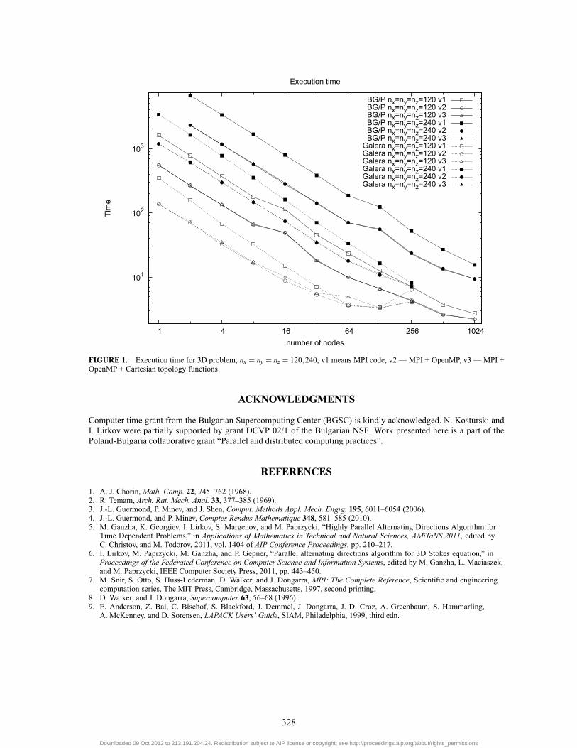
Table 4 shows the speed-up obtained on the supercomputer. Because of smaller memory on one node of the IBMBlue Gene/P we calculated the speed-up only for nx = 120 and ny,nz = 120,240.Finally, computing time on both parallel systems is shown in Fig. 1. Because of the slower processors, the execution

time obtained on the Blue Gene/P is substantially larger than that on the Galera. At the same time, the parallel efficiencyobtained on a large number of nodes on the supercomputer is better. The main reason of this can be related to thesuperior performance of the networking infrastructure of the Blue Gene.

CONCLUSIONS AND FUTURE WORK

We have studied parallel performance of the recently developed parallel algorithm based on a new direction splittingapproach for solving of the 3D time dependent Stokes equation on a finite time interval and on a uniform rectangularmesh. The performancewas evaluated on two different parallel architectures. In order to get better parallel performanceusing four cores per processor on the IBM Blue Gene/P (and future multi-core computers) we developed mixed

326

Downloaded 09 Oct 2012 to 213.191.204.24. Redistribution subject to AIP license or copyright; see http://proceedings.aip.org/about/rights_permissions

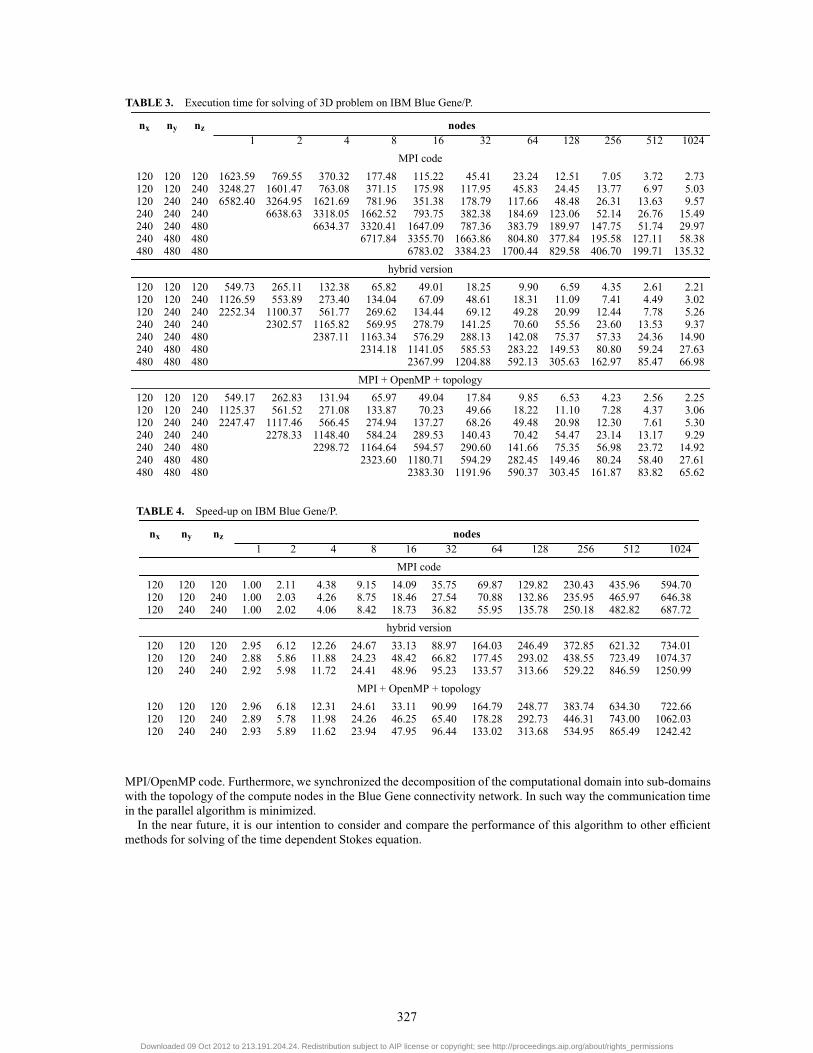
TABLE 3. Execution time for solving of 3D problem on IBM Blue Gene/P.

nx ny nz nodes1 2 4 8 16 32 64 128 256 512 1024

MPI code120 120 120 1623.59 769.55 370.32 177.48 115.22 45.41 23.24 12.51 7.05 3.72 2.73120 120 240 3248.27 1601.47 763.08 371.15 175.98 117.95 45.83 24.45 13.77 6.97 5.03120 240 240 6582.40 3264.95 1621.69 781.96 351.38 178.79 117.66 48.48 26.31 13.63 9.57240 240 240 6638.63 3318.05 1662.52 793.75 382.38 184.69 123.06 52.14 26.76 15.49240 240 480 6634.37 3320.41 1647.09 787.36 383.79 189.97 147.75 51.74 29.97240 480 480 6717.84 3355.70 1663.86 804.80 377.84 195.58 127.11 58.38480 480 480 6783.02 3384.23 1700.44 829.58 406.70 199.71 135.32

hybrid version120 120 120 549.73 265.11 132.38 65.82 49.01 18.25 9.90 6.59 4.35 2.61 2.21120 120 240 1126.59 553.89 273.40 134.04 67.09 48.61 18.31 11.09 7.41 4.49 3.02120 240 240 2252.34 1100.37 561.77 269.62 134.44 69.12 49.28 20.99 12.44 7.78 5.26240 240 240 2302.57 1165.82 569.95 278.79 141.25 70.60 55.56 23.60 13.53 9.37240 240 480 2387.11 1163.34 576.29 288.13 142.08 75.37 57.33 24.36 14.90240 480 480 2314.18 1141.05 585.53 283.22 149.53 80.80 59.24 27.63480 480 480 2367.99 1204.88 592.13 305.63 162.97 85.47 66.98

MPI + OpenMP + topology120 120 120 549.17 262.83 131.94 65.97 49.04 17.84 9.85 6.53 4.23 2.56 2.25120 120 240 1125.37 561.52 271.08 133.87 70.23 49.66 18.22 11.10 7.28 4.37 3.06120 240 240 2247.47 1117.46 566.45 274.94 137.27 68.26 49.48 20.98 12.30 7.61 5.30240 240 240 2278.33 1148.40 584.24 289.53 140.43 70.42 54.47 23.14 13.17 9.29240 240 480 2298.72 1164.64 594.57 290.60 141.66 75.35 56.98 23.72 14.92240 480 480 2323.60 1180.71 594.29 282.45 149.46 80.24 58.40 27.61480 480 480 2383.30 1191.96 590.37 303.45 161.87 83.82 65.62

TABLE 4. Speed-up on IBM Blue Gene/P.

nx ny nz nodes1 2 4 8 16 32 64 128 256 512 1024

MPI code120 120 120 1.00 2.11 4.38 9.15 14.09 35.75 69.87 129.82 230.43 435.96 594.70120 120 240 1.00 2.03 4.26 8.75 18.46 27.54 70.88 132.86 235.95 465.97 646.38120 240 240 1.00 2.02 4.06 8.42 18.73 36.82 55.95 135.78 250.18 482.82 687.72

hybrid version120 120 120 2.95 6.12 12.26 24.67 33.13 88.97 164.03 246.49 372.85 621.32 734.01120 120 240 2.88 5.86 11.88 24.23 48.42 66.82 177.45 293.02 438.55 723.49 1074.37120 240 240 2.92 5.98 11.72 24.41 48.96 95.23 133.57 313.66 529.22 846.59 1250.99

MPI + OpenMP + topology120 120 120 2.96 6.18 12.31 24.61 33.11 90.99 164.79 248.77 383.74 634.30 722.66120 120 240 2.89 5.78 11.98 24.26 46.25 65.40 178.28 292.73 446.31 743.00 1062.03120 240 240 2.93 5.89 11.62 23.94 47.95 96.44 133.02 313.68 534.95 865.49 1242.42

MPI/OpenMP code. Furthermore, we synchronized the decomposition of the computational domain into sub-domainswith the topology of the compute nodes in the Blue Gene connectivity network. In such way the communication timein the parallel algorithm is minimized.In the near future, it is our intention to consider and compare the performance of this algorithm to other efficient

methods for solving of the time dependent Stokes equation.

327

Downloaded 09 Oct 2012 to 213.191.204.24. Redistribution subject to AIP license or copyright; see http://proceedings.aip.org/about/rights_permissions

101

102

103

1 4 16 64 256 1024

Tim

e

number of nodes

Execution time

BG/P nx=ny=nz=120 v1BG/P nx=ny=nz=120 v2BG/P nx=ny=nz=120 v3BG/P nx=ny=nz=240 v1BG/P nx=ny=nz=240 v2BG/P nx=ny=nz=240 v3

Galera nx=ny=nz=120 v1Galera nx=ny=nz=120 v2Galera nx=ny=nz=120 v3Galera nx=ny=nz=240 v1Galera nx=ny=nz=240 v2Galera nx=ny=nz=240 v3

FIGURE 1. Execution time for 3D problem, nx = ny = nz = 120,240, v1 means MPI code, v2 — MPI + OpenMP, v3 — MPI +OpenMP + Cartesian topology functions

ACKNOWLEDGMENTS

Computer time grant from the Bulgarian Supercomputing Center (BGSC) is kindly acknowledged. N. Kosturski andI. Lirkov were partially supported by grant DCVP 02/1 of the Bulgarian NSF. Work presented here is a part of thePoland-Bulgaria collaborative grant “Parallel and distributed computing practices”.

REFERENCES

1. A. J. Chorin,Math. Comp. 22, 745–762 (1968).2. R. Temam, Arch. Rat. Mech. Anal. 33, 377–385 (1969).3. J.-L. Guermond, P. Minev, and J. Shen, Comput. Methods Appl. Mech. Engrg. 195, 6011–6054 (2006).4. J.-L. Guermond, and P. Minev, Comptes Rendus Mathematique 348, 581–585 (2010).5. M. Ganzha, K. Georgiev, I. Lirkov, S. Margenov, and M. Paprzycki, “Highly Parallel Alternating Directions Algorithm forTime Dependent Problems,” in Applications of Mathematics in Technical and Natural Sciences, AMiTaNS 2011, edited byC. Christov, and M. Todorov, 2011, vol. 1404 of AIP Conference Proceedings, pp. 210–217.

6. I. Lirkov, M. Paprzycki, M. Ganzha, and P. Gepner, “Parallel alternating directions algorithm for 3D Stokes equation,” inProceedings of the Federated Conference on Computer Science and Information Systems, edited by M. Ganzha, L. Maciaszek,and M. Paprzycki, IEEE Computer Society Press, 2011, pp. 443–450.

7. M. Snir, S. Otto, S. Huss-Lederman, D. Walker, and J. Dongarra, MPI: The Complete Reference, Scientific and engineeringcomputation series, The MIT Press, Cambridge, Massachusetts, 1997, second printing.

8. D. Walker, and J. Dongarra, Supercomputer 63, 56–68 (1996).9. E. Anderson, Z. Bai, C. Bischof, S. Blackford, J. Demmel, J. Dongarra, J. D. Croz, A. Greenbaum, S. Hammarling,A. McKenney, and D. Sorensen, LAPACK Users’ Guide, SIAM, Philadelphia, 1999, third edn.

328

Downloaded 09 Oct 2012 to 213.191.204.24. Redistribution subject to AIP license or copyright; see http://proceedings.aip.org/about/rights_permissions